lecture notes: introduction to condensed matter theory
TRANSCRIPT
Lecture Notes: Introduction to Condensed Matter Theory
Titus Neupert1
1Department of Physics, University of Zurich,
Winterthurerstrasse 190, CH-8057 Zurich, Switzerland
(Dated: May 28, 2018)
1

CONTENTS
Plan of the lectures 5
I. Introduction 6
II. From quantum statistical mechanics to condensed matter 9
A. Basic concepts 9
1. Second quantization 9
2. Hamiltonians and partition functions 12
3. Thermodynamic potentials 15
4. Spontaneous symmetry breaking 16
5. Mean-field approximation 19
6. Ginzburg-Landau theory for the Ising model 21
7. Critical exponents 23
B. Linear response 24
C. Symmetries in condensed matter 26
1. Non-local vs. local, unitary vs. antiunitary 26
2. Symmetries of a crystal 28
3. Reciprocal space 29
III. Noninteracting electron systems 32
A. Bloch’s theorem 32
B. Nearly free electron approximation 33
C. Tight-binding approximation 35
D. Wannier states 38
E. Interlude: Group representations and character tables 40
F. Symmetries in band structures 42
G. Obtaining information about band structures and symmetries 46
H. Filling of bands and density of states 47
I. Coupling to an external electro-magnetic field 48
1. Semiclassical equations of motion 49
2. The integer quantum Hall effect 51
2
3. Quantum oscillations 57
J. Phonons 59
1. Quantizing lattice vibrations 59
2. Peierls instability in 1D 61
IV. Interactions in itinerant systems 65
A. Particle-hole excitations 65
1. In semiconductors 65
2. In metals 68
B. Fermi liquid theory 73
1. Quasiparticles 74
2. Basics of Landau Fermi liquids 75
3. Specific heat – Density of states 77
4. Compressibility and susceptibility 78
5. Galilei invariance – effective mass and F s1 80
6. Stability of a Fermi liquid 82
7. Microscopic justification 83
8. Distribution function 86
9. Fermi liquid in one dimension? 87
C. Transport in metals 89
1. Linear response and complex analysis 89
2. Boltzmann transport theory 91
3. Conductivity 92
4. Optical properties 94
5. Computing the relaxation time 95
6. Kondo effect 98
7. Anderson localization in one dimension 100
D. Interacting instabilities 105
1. The fractional quantum Hall effect 105
2. Superconductivity 107
3. Density waves 118
4. Mott insulators 118
3
V. Magnetism in solids 125
A. Antiferromagnetism 125
1. Superexchange in the Hubbard model 125
2. Mean-field theory and its shortcomings 126
3. Spin-wave theory 128
B. Stoner magnetism 133
1. Mean-field theory 133
2. Susceptibility on the paramagnetic side 136
3. Magnons 137
VI. Advanced Topics 140
A. Relativistic effects in solids: spin-orbit coupling 140
B. Effective relativistic dispersions in band structures: Topological insulators and
Weyl semimetals 142
1. Topological insulators in three dimensions 143
2. Weyl semimetals 147
C. Density functional theory 148
1. Variational principle and Hartree-Fock approximation 148
2. Hohenberg-Kohn theorems 150
3. Kohn-Sham equation 152
4. Local density approximation and beyond 153
4
PLAN OF THE LECTURES
1. 22. Feb: I. Intro; II. Basic concepts
2. 23. Feb: II. Basic concepts
3. 1. Mar: II. Basic concepts, II. Linear response
4. 2. Mar: II. Symmetries in condensed matter
5. 8. Mar: III. Bloch theorem, III. Nearly free electrons
6. 9. Mar: III. Tight binding, III. Wannier states
7. 15. Mar: III. Group representations and character tables; III. Symmetries in band
structures; HANDS ON with ICSD, Materials project, Vesta and Bilbao server;
8. 16. Mar: III. Filling of bands and DOS, III. Coupling to EM field
9. 22. Mar: III. Coupling to EM field
10. 23. Mar: III. Coupling to EM field
11. 29. Mar: III. Phonons
12. 30. Mar– 6. Apr: (Easter break – no lecture)
13. 12. Apr: IV. Particle-hole excitations
14. 13. Apr: IV. Fermi liquid theory I
15. 19. Apr: IV. Fermi liquid theory II
16. 20. Apr: IV. Fermi liquid theory III
17. 26. Apr: IV. Transport I (lecture by Frank Schindler)
18. 27. Apr: IV. Transport II (lecture by Frank Schindler)
19. 3. May: IV. Transport III
20. 4. May: V. Interacting instabilities I: FQHE/supercondutivity
5
21. 10. May: (Auffahrt – no lecture)
22. 11. May: V. Interacting instabilities II: superconductivity
23. 17. May: V. Interacting instabilities III: Mott insulators
24. 18. May: VI. Antiferromagnetism
25. 24. May: VI. Stoner magnetism
26. 25. May: VI. Advanced topics: Spin-orbit coupling
27. 31. May: VI. Advanced topics: Topological insulators
28. 1. Jun: VI. Advanced topics: DFT
I. INTRODUCTION
The study of quantum condensed matter is a very hard problem. We consider in gen-
eral interacting many-body systems of 1024 degrees of freedom, typically represented by the
electrons in a solid. Since the Hilbert space is exponentially large in the number of degrees
of freedom, any ’brute force’ theoretical approach using the resources of classical computers
to this problem must fail. A quantum computer might help, but is not (yet) available. Nev-
ertheless, impressive progress has been made in the theoretical study of solid state systems,
thanks to two bold simplifications:
Separation of energy scales: In contrast to high-energy physics, where new physics
appears at ever higher energies, in condensed matter physics the phenomena of interest
typically appear at very low energies. To put it boldly, these two energy frontiers are where
we can expect new physics to appear. Everything in between is, at least on a fundamental
level, understood. Different physical phenomena can be separated by the energy scale at
which they appear, and their impact on the phenomena at smaller energy scales can often be
incorporated in some effective form. For example, it is in many cases sufficient to consider the
crystal as a rigid lattice of ions in which the electrons move or to only consider the coupling
between the electrons and the low-energy vibration (phonon) modes of the crystal. As
another example, the Coulomb interaction between electrons can in some cases be neglected
so that one solves only the problem of free electrons moving in the background potential
6
of the ions. A plethora of more sophisticated approximations has been developed, some of
which we will encounter in this course.
Use of symmetries: The formation of a crystal breaks (spontaneously) the Lorentz
symmetry of open space. At first sight, this appears to be problematic, as one cannot take
advantage of this symmetry group to describe the low-energy properties of electrons, in the
same way as one can identify allowed terms in a Lagrangian in high-energy physics, say.
However, the crystal breaks the symmetry not completely, but retains a discrete translation
symmetry and potentially other symmetries such as rotations, mirror reflections, inversion,
time-reversal symmetry and so on. In addition, at low energies effective symmetries can
emerge that are not shared by the whole crystal. For example, while a cubic crystal has
only four-fold rotational symmetry, the dispersion of electrons at low electron-density might
still be well described as parabolic, with an effective continuous rotation symmetry. This
renders the situation much better than, say, in bio-chemistry, where one cannot take much
advantage of constraining the problems by symmetries.
Thus, the ’master equation’ for solid state systems in equilibrium is given by the Hamil-
tonian
H =H0,e +H0,i +He−e +Hi−i +Hi−e,
H0,e =∑j
(α · pj + βme),
H0,i =∑j
P 2j
2Mj
,
He−e =∑j,l
e2
|rj − rl|, He−i =
∑j,l
e2Zl|rj −Rl|
, Hi−i =∑j,l
e2ZjZl|Rj −Rl|
,
(1)
where pj and rj are momentum and position operator of the j-th electron, me is the electron
mass, Pj and Rj are momentum and position operator of the j-th nucleus, Zj and Zj are
its charge and mass. The Dirac form of the electronic kinetic Hamiltonian was chosen to
include the physics of spin-orbit coupling, which is important to topics of recent interest
in solid state physics. Hamiltonian (1) is essentially impossible to solve without further
approximations. (What is not included in Hamiltonian (1) is the physics associated with
the nuclear spins.)
To make progress in understanding a specific phenomenon or system, one often works
7
with a toy model. While such models can be motivated using qualitative or quantitative
arguments, solid state theorists can become very creative in dreaming up new models. Some-
times, these models are still very hard to solve, like the paradigmatic Hubbard model, for
example. In other cases, the advantage of a specific model might be its exact solubility, as
is the case with the transverse-field Ising model, for example.
8
II. FROM QUANTUM STATISTICAL MECHANICS TO CONDENSED MATTER
A. Basic concepts
1. Second quantization
In first quantization, we denote the (non-degenerate) quantum state of a many-body
system of N identical particles by a wave function
Ψ(α1, α2, · · · , αN), (2)
where the αi, i = 1, · · · , N run over labels for a basis of the single-particle Hilbert space
H1 and each αi denotes the single-particle state that the i-th particle is in. For example, α
could label the position of a particle and in addition some internal degrees of freedom such as
spin. The Pauli principle, the axiom underlying many-body quantum mechanics, says that
equivalent particles are indistinguishable. Any observables, such as the probability density,
may thus not depend on the order in which the states αi of indistinguishable particles are
listed in the arguments of Ψ. For the exchange of only two particles, this amounts to impose
the equality
|Ψ(α1, · · · , αi, · · · , αj, · · · , αN)|2 = |Ψ(α1, · · · , αj, · · · , αi, · · · , αN)|2. (3)
Thus, upon exchange, Ψ could be multiplied by an arbitrary phase eiϕ(αi,αj). However,
exchanging the particles twice needs to bring the wave function back to itself, in order for
the wave function to be single valued, i.e., eiϕ(αi,αj) = ±1. (Non-degenerate wave functions
that are not single-valued are not permitted.) As a result, there are only tow possibilities
Ψ(α1, · · · , αi, · · · , αj, · · · , αN) = ±Ψ(α1, · · · , αj, · · · , αi, · · · , αN), (4)
which correspond to bosons (the + sign) and fermions (the − sign).
We recall that the N -particle Hilbert space HN is a direct product of N copies of the
single-particle Hilbert space, and the Fock space F is a direct sum over these
HN :=N⊗i=1
H1, F :=∞⊕N=1
HN , (5)
9
where H0 is a one-dimensional space spanned by the vacuum |0〉 alone. A basis for the
N -particle Hilbert space is then given by
Ψ(α1, α2, · · · , αN) =1√N !
∑p∈PN
(±1)σ(p)ψα1(p1)ψα2(p2) · · ·ψαN (pN), (6)
where the sum runs over all permutations p of the firstN integers, σ(p) denotes the sign of the
permutation, and the signs (+1) and (−1) apply to bosons and fermions, respectively. Here,
ψα are a set of basis functions of the single-particle Hilbert space H. The basis functions (6)
of HN are thus fully symmetrized (antisymmetrized) products of N single-particle basis
functions ψα in the case of bosons (fermions). The latter can be written in the form of a
determinant of the matrix with elements Mij = ψαi(j), i, j = 1, · · · , N , the so-called Slater
determinant. In bra-ket notation, the state corresponding to Eq. (6) is often written in
the occupation number representation by listing the number of particles that are occupying
a each single particle state α by nα. For fermions, nα = 0, 1, for the fully antisymmetric
wave function (6) vanishes if two or more particles occupy the same single-particle state. For
bosons, nα can be any nonnegative integer. For example, in a system with a five-dimensional
single-particle Hilbert space H1 (i.e., in which α can only take 5 different values), we would
denote the state with 3 particles, that occupy the first, third, and forth single particle state
by
Ψ(1, 3, 4) or |nα〉 = |1, 0, 1, 1, 0〉. (7)
The key object of the second-quantized formalism are particle creation operators c†α and
annihilation operators cα. For fermions, these operators act as
c†α|n1, · · · , nα, · · · 〉 = δnα,0(−1)n1+···+nα−1 |n1, · · · , nα + 1, · · · 〉,
cα|n1, · · · , nα, · · · 〉 = δnα,1(−1)n1+···+nα−1 |n1, · · · , nα − 1, · · · 〉,(8)
and obey the relations
cα, c†α′ = δα,α′ , cα, cα′ = c†α, c†α′ = 0, (9)
where A, B = AB + BA is the anticommutator. For bosons, they act as
c†α|n1, · · · , nα, · · · 〉 =√nα + 1|n1, · · · , nα + 1, · · · 〉,
cα|n1, · · · , nα, · · · 〉 =√nα|n1, · · · , nα − 1, · · · 〉,
(10)
10
and obey the relations
[cα, c†α′ ] = δα,α′ , [cα, cα′ ] = [c†α, c
†α′ ] = 0. (11)
For example, the occupation number of a state α can be measured with the operator c†αcα,
because c†αcα|n1, · · · , nα, · · · 〉 = nα|n1, · · · , nα, · · · 〉. Any state in the basis of F can be
generated by application of a product of c†α operators to the vacuum state |0〉, i.e.,
|nα〉 =∏α
(c†α)nα|0〉, (12)
where it is understood that (c†α)0 is the identity.
The second quantized operators transform natural under a basis change of the single
particle Hilbert space H1. Let uα,a = 〈α|a〉 be the matrix elements of the unitary operator
that encodes the change from a basis ψα of H1 to a different basis ψa. Then,
c†a =∑α
uα,ac†α, ca =
∑α
u∗α,acα. (13)
This transformation also applies if the label a is a continuous variable, such as the position
r of a particle, in wich case we obtain the field operators
φ†(r) =∑α
〈α|r〉c†α, φ(r) =∑α
〈r|α〉cα (14)
that obey in the case of fermions
φ(r), φ†(r′) = δ(r − r′), φ(r), φ(r′) = φ†(r), φ†(r′) = 0, (15)
and in the case of bosons
[φ(r), φ†(r′)] = δ(r − r′), [φ(r), φ(r′)] = [φ†(r), φ†(r′)] = 0. (16)
For example, a transformation of the form (14) is relevant to the case of a particle on a
ring of circumference L, i.e., r ∈ [0, L) with periodic boundary conditions. The momentum
k takes discrete values k = 2πl/L, l ∈ Z (like the index α), while r is continuous. The
coefficients 〈k|r〉 are nothing but the Fourier modes and we get
φ†(r) =1√L
∑k
eikrc†k, (17)
with the sum running over k = 2πl/L, l ∈ Z, as the transformation law between the operator
c†k that creates a particle with momentum k on the ring and the operator φ†(r) that creates
a particle at position r on the ring.
11
2. Hamiltonians and partition functions
Most of the time, we are interested in the properties of the unperturbed condensed matter
system, or in its repose to small perturbations. In the former case, we can treat the system
as closed, neither exchanging energy nor particles with the environment (corresponding to
the microcanonical ensemble of statistical mechanics). In the latter case, we can use the
isolated system as a good starting point for perturbative calculations within linear response
theory.
Within the Hamiltonian formalism, the energy conserving system is described by a Hamil-
tonian H that acts on the Hilbert or Fock space. Finding the eigenvalues and eigenstates of
this operator amounts to solving the problem, a task that is often too hard to be achieved
without further approximations. The Hamiltonian can be given either in first or second
quantization. For the free particle of mass m on the ring with periodic boundary conditions,
its first quantized version is
Hµ =p2
2m− µ, (18)
where p is the momentum operator that has the representation p = −i ddr
in the position
basis of the single particle Hilbert space. (Throughout these notes, we will set ~ = 1, and
only reinstate it in specific places to connect to well known-results in the right units.) The
real number µ is the chemical potential the meaning of which will be discussed below. In
the second quantized formulation, we can express Hµ either in the operators φ(r) or ck
Hµ =
∫ L
0
dr φ†(r)
(− 1
2m
d2
dr2− µ
)φ(r) =
∑k
(k2
2m− µ
)c†kck, (19)
where we used that ∫ L
0
dr
Lei(k−k′)r = δk,k′ . (20)
Notice that the term multiplying µ is nothing but the operator N :=∑
k c†kck that counts
the total number of particles in the system. From Eq. (19) we see that we have diagonalized
the Hamiltonian in momentum space, and its eigenvalues when acting on the single-particle
Hilbert space H1 are the energy levels of the system, given by εk = k2/(2m) − µ, with
k = 2πl/L, l ∈ Z. The 2π/L discretization is due to the finite size of the system. One
frequently encounters this splitting when considering small systems that can be solved (e.g.,
numerically), from which the behavior of the thermodynamically large system is to be ex-
trapolated.
12
An important difference between the two Hamiltonians (18) and (19) is that the former
always acts on a single-particle Hilbert space (as we only wrote the momentum operator
for one particle – for N particles we should have written the sum∑N
i=1 p2i over their N
momentum operators instead), while the latter can act on any HN or the Fock space F .
Let us understand the ground state of Hµ at zero temperature, when acting on F . When
µ < 0, it is just the vacuum |0〉, as occupying any state would cost energy. For µ > 0 we have
to separately consider the case of bosons from that of fermions: When considering bosons,
an infinite number of particles would occupy the single-particle eigenstate of lowest energy
ε0. In the case of fermions, every state can only be occupied once due to the Pauli exclusion
principle. At the same time, it is only energetically advantageous to occupy single-particle
eigenstate with negative energy εk < 0. (We don’t consider here the accidental case when
on of the εk equals 0, in which case the ground state would be degenerate.) The fermionic
zero-temperature ground state, the so-called Fermi sea (FS), is thus
|FS〉 =
( ∏k: εk<0
c†k
)|0〉. (21)
Finite-temperature properties of the system at inverse temperature β = 1/(kBT ) can be
computed from the partition function
Zβ,µ = TrFe−βHµ . (22)
Equation (22) can be rationalized by recalling that the partition function is a sum of the
unnormalized probablities e−βEs over all microstates s of the system, with associated energy
Es. Evaluating the trace TrF in the basis spanned by the eigenstates of Hµ readily yields
this connection. With Eq. (22) we compute the grand canonical partition function, i.e.,
the partition function for the grand canonical ensemble that is defined by not having a
fixed particle number. This is reflected by the fact that we take the trace over the Fock
space F instead of a Hilbert space HN of fixed particle number N , and by the fact that
the Hamiltonian contains the term −µN . We indicate it with the subscript µ to remind
us of the dependence on the chemical potential. The canonical partition function Zβ,N
for a system with fixed particle number N can be computed by dropping the latter term
in the Hamiltonian and by restricting the trace in Eq. (22) over HN . Equation. (22) is
a completely general formula that can be applied to any, possibly interacting, quantum
13
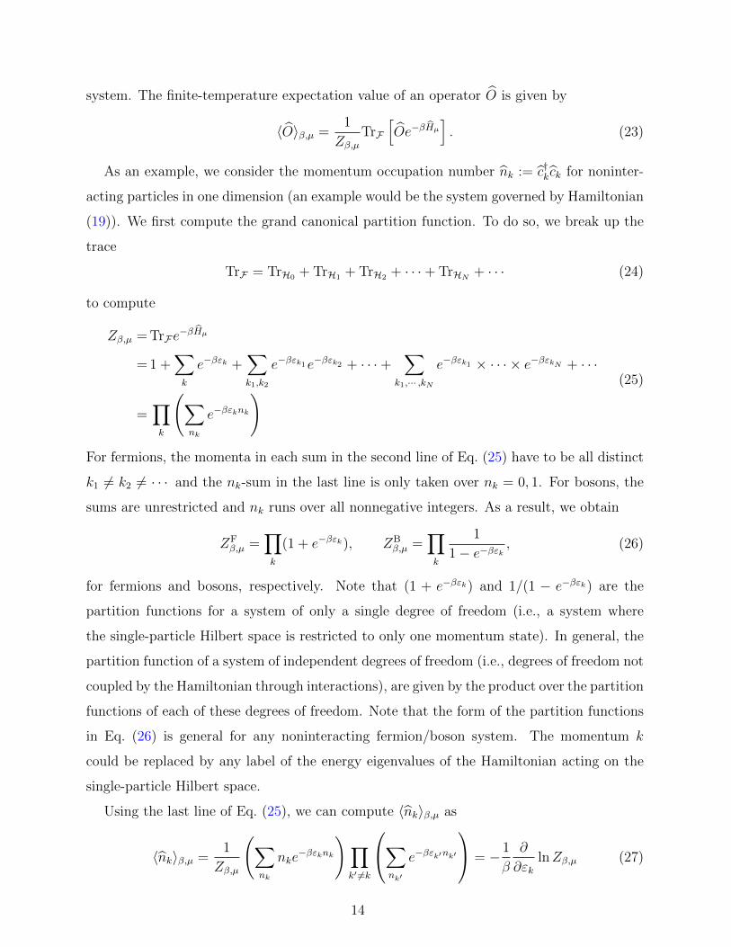
system. The finite-temperature expectation value of an operator O is given by
〈O〉β,µ =1
Zβ,µTrF
[Oe−βHµ
]. (23)
As an example, we consider the momentum occupation number nk := c†kck for noninter-
acting particles in one dimension (an example would be the system governed by Hamiltonian
(19)). We first compute the grand canonical partition function. To do so, we break up the
trace
TrF = TrH0 + TrH1 + TrH2 + · · ·+ TrHN + · · · (24)
to compute
Zβ,µ = TrFe−βHµ
= 1 +∑k
e−βεk +∑k1,k2
e−βεk1e−βεk2 + · · ·+∑
k1,··· ,kN
e−βεk1 × · · · × e−βεkN + · · ·
=∏k
(∑nk
e−βεknk
) (25)
For fermions, the momenta in each sum in the second line of Eq. (25) have to be all distinct
k1 6= k2 6= · · · and the nk-sum in the last line is only taken over nk = 0, 1. For bosons, the
sums are unrestricted and nk runs over all nonnegative integers. As a result, we obtain
ZFβ,µ =
∏k
(1 + e−βεk), ZBβ,µ =
∏k
1
1− e−βεk , (26)
for fermions and bosons, respectively. Note that (1 + e−βεk) and 1/(1 − e−βεk) are the
partition functions for a system of only a single degree of freedom (i.e., a system where
the single-particle Hilbert space is restricted to only one momentum state). In general, the
partition function of a system of independent degrees of freedom (i.e., degrees of freedom not
coupled by the Hamiltonian through interactions), are given by the product over the partition
functions of each of these degrees of freedom. Note that the form of the partition functions
in Eq. (26) is general for any noninteracting fermion/boson system. The momentum k
could be replaced by any label of the energy eigenvalues of the Hamiltonian acting on the
single-particle Hilbert space.
Using the last line of Eq. (25), we can compute 〈nk〉β,µ as
〈nk〉β,µ =1
Zβ,µ
(∑nk
nke−βεknk
)∏k′ 6=k
∑nk′
e−βεk′nk′
= − 1
β
∂
∂εklnZβ,µ (27)
14
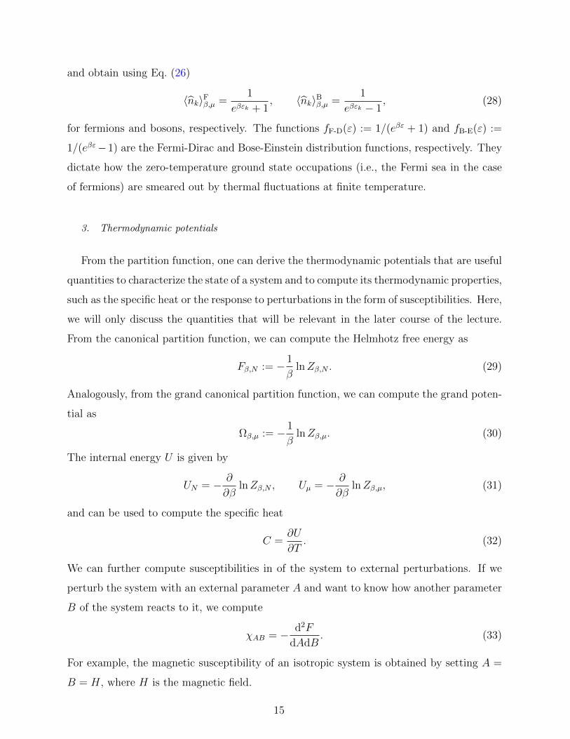
and obtain using Eq. (26)
〈nk〉Fβ,µ =1
eβεk + 1, 〈nk〉Bβ,µ =
1
eβεk − 1, (28)
for fermions and bosons, respectively. The functions fF-D(ε) := 1/(eβε + 1) and fB-E(ε) :=
1/(eβε−1) are the Fermi-Dirac and Bose-Einstein distribution functions, respectively. They
dictate how the zero-temperature ground state occupations (i.e., the Fermi sea in the case
of fermions) are smeared out by thermal fluctuations at finite temperature.
3. Thermodynamic potentials
From the partition function, one can derive the thermodynamic potentials that are useful
quantities to characterize the state of a system and to compute its thermodynamic properties,
such as the specific heat or the response to perturbations in the form of susceptibilities. Here,
we will only discuss the quantities that will be relevant in the later course of the lecture.
From the canonical partition function, we can compute the Helmhotz free energy as
Fβ,N := − 1
βlnZβ,N . (29)
Analogously, from the grand canonical partition function, we can compute the grand poten-
tial as
Ωβ,µ := − 1
βlnZβ,µ. (30)
The internal energy U is given by
UN = − ∂
∂βlnZβ,N , Uµ = − ∂
∂βlnZβ,µ, (31)
and can be used to compute the specific heat
C =∂U
∂T. (32)
We can further compute susceptibilities in of the system to external perturbations. If we
perturb the system with an external parameter A and want to know how another parameter
B of the system reacts to it, we compute
χAB = − d2F
dAdB. (33)
For example, the magnetic susceptibility of an isotropic system is obtained by setting A =
B = H, where H is the magnetic field.
15
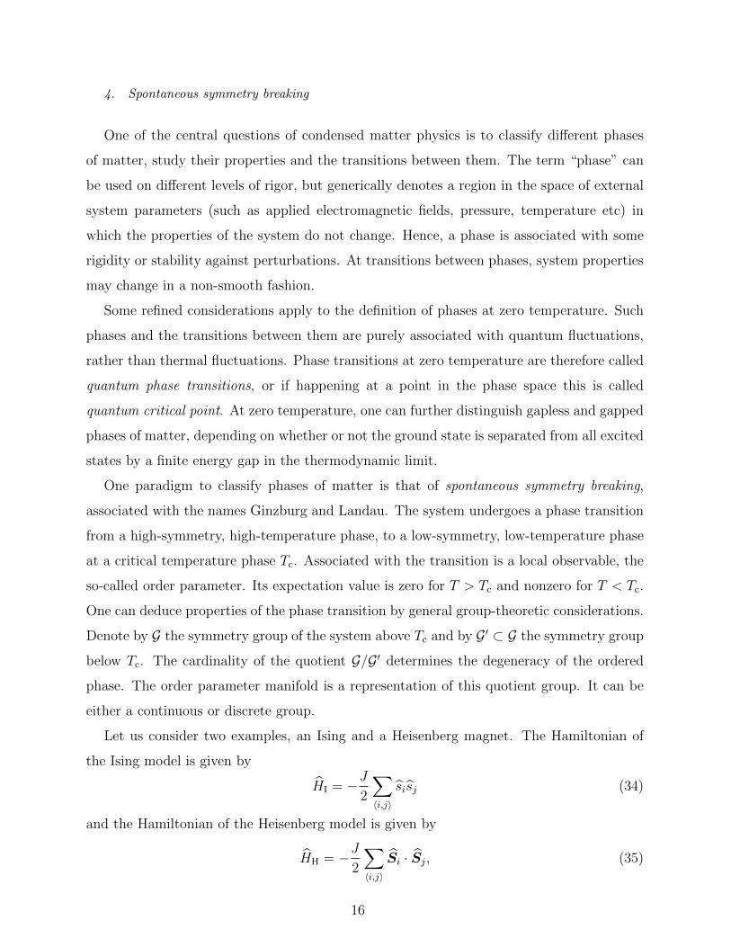
4. Spontaneous symmetry breaking
One of the central questions of condensed matter physics is to classify different phases
of matter, study their properties and the transitions between them. The term “phase” can
be used on different levels of rigor, but generically denotes a region in the space of external
system parameters (such as applied electromagnetic fields, pressure, temperature etc) in
which the properties of the system do not change. Hence, a phase is associated with some
rigidity or stability against perturbations. At transitions between phases, system properties
may change in a non-smooth fashion.
Some refined considerations apply to the definition of phases at zero temperature. Such
phases and the transitions between them are purely associated with quantum fluctuations,
rather than thermal fluctuations. Phase transitions at zero temperature are therefore called
quantum phase transitions, or if happening at a point in the phase space this is called
quantum critical point. At zero temperature, one can further distinguish gapless and gapped
phases of matter, depending on whether or not the ground state is separated from all excited
states by a finite energy gap in the thermodynamic limit.
One paradigm to classify phases of matter is that of spontaneous symmetry breaking,
associated with the names Ginzburg and Landau. The system undergoes a phase transition
from a high-symmetry, high-temperature phase, to a low-symmetry, low-temperature phase
at a critical temperature phase Tc. Associated with the transition is a local observable, the
so-called order parameter. Its expectation value is zero for T > Tc and nonzero for T < Tc.
One can deduce properties of the phase transition by general group-theoretic considerations.
Denote by G the symmetry group of the system above Tc and by G ′ ⊂ G the symmetry group
below Tc. The cardinality of the quotient G/G ′ determines the degeneracy of the ordered
phase. The order parameter manifold is a representation of this quotient group. It can be
either a continuous or discrete group.
Let us consider two examples, an Ising and a Heisenberg magnet. The Hamiltonian of
the Ising model is given by
HI = −J2
∑〈i,j〉
sisj (34)
and the Hamiltonian of the Heisenberg model is given by
HH = −J2
∑〈i,j〉
Si · Sj, (35)
16
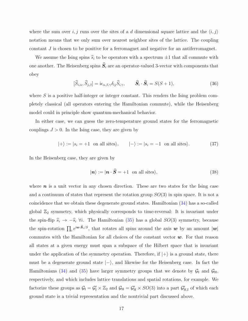
where the sum over i, j runs over the sites of a d dimensional square lattice and the 〈i, j〉notation means that we only sum over nearest neighbor sites of the lattice. The coupling
constant J is chosen to be positive for a ferromagnet and negative for an antiferromagnet.
We assume the Ising spins si to be operators with a spectrum ±1 that all commute with
one another. The Heisenberg spins Si are an operator-valued 3-vector with components that
obey
[Si,α, Sj,β] = iεα,β,γδijSi,γ, Si · Si = S(S + 1), (36)
where S is a positive half-integer or integer constant. This renders the Ising problem com-
pletely classical (all operators entering the Hamiltonian commute), while the Heisenberg
model could in principle show quantum-mechanical behavior.
In either case, we can guess the zero-temperature ground states for the ferromagnetic
couplings J > 0. In the Ising case, they are given by
|+〉 := |si = +1 on all sites〉, |−〉 := |si = −1 on all sites〉. (37)
In the Heisenberg case, they are given by
|n〉 := |n · S = +1 on all sites〉, (38)
where n is a unit vector in any chosen direction. These are two states for the Ising case
and a continuum of states that represent the rotation group SO(3) in spin space. It is not a
coincidence that we obtain these degenerate ground states. Hamiltonian (34) has a so-called
global Z2 symmetry, which physically corresponds to time-reversal: It is invariant under
the spin-flip si → −si ∀i. The Hamiltonian (35) has a global SO(3) symmetry, because
the spin-rotation∏
i eiw·Si/S, that rotates all spins around the axis w by an amount |w|
commutes with the Hamiltonian for all choices of the constant vector w. For that reason
all states at a given energy must span a subspace of the Hilbert space that is invariant
under the application of the symmetry operation. Therefore, if |+〉 is a ground state, there
must be a degenerate ground state |−〉, and likewise for the Heisenberg case. In fact the
Hamiltonians (34) and (35) have larger symmetry groups that we denote by GI and GH,
respectively, and which includes lattice translations and spatial rotations, for example. We
factorize these groups as GI = G ′I × Z2 and GH = G ′H × SO(3) into a part G ′H,I of which each
ground state is a trivial representation and the nontrivial part discussed above.
17
In a real system, the symmetries are never exactly present, but broken by small local
perturbations. (The emphasis on locality comes from the physical requirement that terms
in the Hamiltonian should not couple degrees of freedom that are far away, or if they do
so, then with a strength that decays sufficiently fast with their distance.) For example, the
spin-rotation symmetry can be broken by magnetic impurities, or even by coupling to the
earth’s magnetic field. As a result of these perturbations, the system will choose one of the
(almost) degenerate ground states. Once chosen, this ground state is robust, even if the
perturbation is removed or reversed, because changing between, say, |+〉 and |−〉 requires
reorganizing a macroscopic number of degrees of freedom. This constitutes a large energy
barrier as domain walls have to propagate through the system. In fact, this process has
vanishing probability if the system size is taken to infinity (the thermodynamic limit).
The process of spontaneous symmetry breaking can be cast in more rigorous terms as
follows. We define an order parameter, the magnetization
M =1
N
∑i
si, M =1
N
∑i
Si, (39)
where N is the number of lattice sites. We further add perturbations to the Hamiltonians
HI,h = HI +∑i
hsi, HH,H = HI +∑i
H · Si (40)
that break the symmetry subgroup GI,H/G ′I,H. Spontaneous symmetry breaking occurs if
0 6= limh→0
limN→∞
〈M〉β,HI,h, 0 6= lim
H→0limN→∞
〈M〉β,HH,H, (41)
while it is zero if the limits were taken in the reverse order. The expectation value at finite
inverse temperature β was defined in Eq. (23). Equation (41) holds for the ferromagnetic
case J > 0. For the antiferromagnet, we would need to use the staggered magnetization as
an order parameter and apply a staggered perturbation. To be able to define a staggered
magnetization, it is important that our square lattice is bipartite in any dimension, i.e.,
the sites can be divided into two sets A and B such that all nearest neighbors of a site
in A are in B. For instance, a triangular lattice in d = 2 is not bipartite and we say the
antiferromagnet is geometrically frustrated on this lattice. We will study these magnetic
orders in more detail in Chapter V.
An important distinction is made between spontaneous symmetry breaking of a discrete
and a continuous symmetry group. The latter are accompanied by Goldstone modes (one
18
mode per generator of a continuous symmetry), which are gapless excitations above the
symmetry-breaking ground state manifold. This implies that the ground state of the Ising
ferromagnet can have (and has in fact) a finite gap to all other excitations, while the ground
state of the Heisenberg ferromagnet has gapless excitations that are spin-wave deformations
of the ferromagnetic pattern.
A natural question is: Under which conditions can spontaneous symmetry breaking oc-
cur? This question is answered by the Mermin-Wagner theorem, stating that a continuous
symmetry cannot be spontaneously broken at any finite temperature in d ≤ 2 (with suffi-
ciently short-ranged interactions). In d = 2, a continuous symmetry can be spontaneously
broken at zero temperature. In d = 1, a continuous symmetry can never be broken sponta-
neously.
5. Mean-field approximation
States with spontaneously broken symmetry are often treated within the so-called mean-
field approximation. Above, we have seen that in a symmetry-broken ground state, observ-
ables that have a vanishing expectation value in any eigenspace of the Hamiltonian (which
is necessarily invariant under the symmetries of the system) acquire a non-vanishing expec-
tation value. For the example of the spin operator in the Ising model, we can relate it to
the classical magnetization M of the system
si = M + δsi. (42)
The mean-field approximation consists of dropping higher orders of the operators δsi from
the Hamiltonian, so that the system becomes soluble.
We will go though this mean-field calculation for the example of the Ising model, where
δsi = si −M for all lattice sites i. The Hamiltonian is rewritten as
H =− J
2
∑〈i,j〉
[M + (si −M)][M + (si −M)]− h∑i
si
=− J∑i
(zMsi − z
M2
2
)− h
∑i
si +O(δsiδsj),
(43)
where z is the coordination number of the nearest neighbors on the lattice (on a hypercubic
lattice z = 2d). Neglecting the last term is justified if 〈δsiδsj〉/(〈δsi〉〈δsj〉) = 〈δsiδsj〉/M2
19
1. The mean field Hamiltonian
Hmf =−∑i
siheff −NJz
2M2 +O(δsiδsj), (44)
which is the Hamiltonian for an ideal paramagnet (a collection of independent spins) in a
magnetic field heff = JzM + h. The partition function for this Hamiltonian is
ZN(β,M, h) = e−βJzM2N/2
∏i
∑si=±1
eβheffsi
= e−βJzM2N/2 [2 cosh (βheff)]N ,
(45)
from which we find the free energy
F (β,M, h) = −β−1 logZN = NJz
2M2 −Nβ−1 log [2 cosh (βheff)] . (46)
To find out whether a stable mean-field solution for M exists, we are looking for a minimum
of the free energy at finite M . Indeed
0 =∂F
∂M= NJzM −NJz tanh (βheff) (47)
has such a solution iff the self-consistency equation
M = tanh [β (JzM + h)] (48)
has one. We particularize on the case of zero magnetic field, and expand the tanh to linear
order in M in order to find the phase boundary. Solutions to Eq. (48) exist when the slope of
the function on the righthand side at M = 0 is larger than 1. This linearized self-consistency
equation
M = βJzM (49)
yields from this condition the critical temperature
Tc = Jz/kB. (50)
We can use this to expand the free energy as
F (T,M, h = 0) ≈ F0(T ) +NJz
[(1− Tc
T
)M2
2+
1
12s2
(Tc
T
)3
M4
]
≈ F0(T ) +NJz
[(T
Tc
− 1
)M2
2+
M4
12s2
] (51)
where for the last step we took into account that our expansion is only valid for T ≈ Tc.
Moreover, F0 = −NkBT log 2. This form of the free energy expansion is the famous Landau
theory of a continuous phase transition which we will analyze in more detail now.
20
6. Ginzburg-Landau theory for the Ising model
We have used the Landau expansion of the free energy above to discuss phase transitions
in the vicinity of the critical temperature where M was small. This can be extended to
a highly convenient method which allows us to discuss phase transition more generally, in
particular, those of second order. Landau’s concept of the disorder-to-order transition is
based on symmetry and spontaneous symmetry breaking.
A further important aspect emerges when long-length scale variations of the order pa-
rameter are taken into account. This can be easily incorporated in the Ginzburg-Landau
theory and allows to discuss spatial variations of the ordered phase as well as fluctuations.
For the Ising model of the previous section, we can identify M as the order parameter.
The order parameter M is not invariant under time reversal symmetry K ,
K M = −M . (52)
The two states with positive and negative M are degenerate. The relevant symmetry group
above the phase transition is
G = G×K (53)
with G as the space group of the lattice (simple cubic) and K, the group E, K (E
denotes the identity operation). As for the space group we consider the magnetic moment
here independent of the crystal lattice rotations such that G remains untouched through the
transition so that the corresponding subgroup is
G ′ = G ⊂ G (54)
The degeneracy of the ordered phase is given by the order of G/G ′ which is 2 in our case.
The Ginzburg-Landau free energy functional has in d dimensions the general form
F [M ;h, T ] = F0(h, T ) +
∫ddr
A
2M(r)2 +
B
4M(r)4 − h(r)M(r) +
κ
2[∇M(r)]2
= F0(h, T ) +
∫ddr f(M,∇M ;h, T )
(55)
where we choose the coefficients according to the expansion done in (51) as
A =Jz
ad
(T
Tc
− 1
)= −Jz
adτ and B =
Jz
3ad. (56)
21
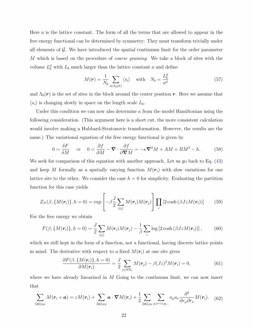
Here a is the lattice constant. The form of all the terms that are allowed to appear in the
free energy functional can be determined by symmetry: They must transform trivially under
all elements of G. We have introduced the spatial continuum limit for the order parameter
M which is based on the procedure of coarse graining. We take a block of sites with the
volume Ldb with Lb much larger than the lattice constant a and define
M(r) =1
Nb
∑i∈Λb(r)
〈si〉 with Nb =Ldbad
(57)
and Λb(r) is the set of sites in the block around the center position r. Here we assume that
〈si〉 is changing slowly in space on the length scale Lb.
Under this condition we can now also determine κ from the model Hamiltonian using the
following consideration. (This argument here is a short cut, the more consistent calculation
would involve making a Hubbard-Stratonovic transformation. However, the results are the
same.) The variational equation of the free energy functional is given by
0 =δF
δM⇒ 0 =
∂f
∂M−∇ · ∂f
∂∇M= −κ∇2M + AM +BM3 − h. (58)
We seek for comparison of this equation with another approach. Let us go back to Eq. (43)
and keep M formally as a spatially varying function M(ri) with slow variations for one
lattice site to the other. We consider the case h = 0 for simplicity. Evaluating the partition
function for this case yields
ZN(β, M(ri), h = 0) = exp
−βJ2
∑〈ij〉
M(ri)M(rj)
∏i
[2 cosh (βJzM(ri))] (59)
For the free energy we obtain
F (β, M(ri), h = 0) =J
2
∑〈ij〉
M(ri)M(rj)−1
β
∑i
log [2 cosh (βJzM(ri))] , (60)
which we still kept in the form of a function, not a functional, having discrete lattice points
in mind. The derivative with respect to a fixed M(ri) at one site gives
∂F (β, M(ri), h = 0)
∂M(ri)=J
2
∑j∈NNi
M(rj)− β(Jz)2M(ri) = 0, (61)
where we have already linearized in M Going to the continuum limit, we can now insert
that∑aNN
M(ri + a) = zM(ri) +∑aNN
a ·∇M(ri) +1
2
∑aNN
∑µ,ν=x,y...
aµaν∂2
∂rµ∂rνM(ri). (62)
22
The sum∑aNN
runs over nearest-neighbor sites. Note that the second term on the right-
hand side vanishes due to symmetry. We obtain
0 = Jz
(T
Tc
− 1
)M(r)− Ja2∇2M(r) , (63)
where factors of 1/2 are eaten up by accounting for double counting in the sums over nearest
neighbors. Comparison of coefficients leads to
κ = Ja2−d . (64)
We may rewrite the equation (63) as
0 = M − ξ2∇2M with ξ2 =a2kBTc
zkB(T − Tc)(65)
where we introduced the length ξ which is equal to the correlation length for T > Tc. It
diverges as the phase transition is approached.
7. Critical exponents
Close to the phase transition at Tc various quantities have a specific temperature or field
dependence which follows power laws in τ = 1 − T/Tc or h with characteristic exponents,
called critical exponents. We introduce here the exponents relevant for a magnetic system
like the Ising model. The heat capacity C and the susceptibility χ follow the behavior
C(T ) ∝ |τ |−α and χ(T ) ∝ |τ |−γ (66)
for both τ > 0 and τ < 0. Also the correlation length displays a powerlaw
ξ(T ) ∝ |τ |−ν . (67)
For τ > 0 (ordered phase) the magnetization grows as
M(T ) ∝ |τ |β . (68)
At T = Tc (τ = 0) the magnetization has the field dependence
M ∝ h1/δ. (69)
These exponents are not completely independent but are related by means of so-called scaling
laws:
23
• Rushbrooke scaling: α + 2β + γ = 2
• Widom scaling: γ = β(δ − 1)
• Josephson scaling: νd = 2− α
Let us now determine the exponents within mean field theory. The only one we have not
found so far is δ. Using the Ginzburg-Landau equations for τ = 0 leads to
BM3 = h ⇒ δ = 3 (70)
Thus the list of exponents is
α = 0 , β =1
2, γ = 1 δ = 3 , ν =
1
2(71)
These exponents satisfy the scaling relations apart from the Josephson scaling which depends
on the dimension d.
The critical exponents arise from the specific fluctuation (critical) behavior around a
second-order phase transition. They are determined by dimension, structure of order param-
eter and coupling topology, and are consequently identical for equivalent phase transitions.
Therefore, the critical exponents incorporate universal properties.
B. Linear response
Linear response studies the change in an observable A due to a small change H B (t) in
the static Hamiltonian H 0 of the system. The perturbation can be time-dependent with,
say, a single frequency ω and is adiabatically slowly switched on, i.e., the time-dependence
is taken to be H B (t) = B e−iωt+ηt with η a small positive real number. The Schroedinger
equation for the perturbation is then
id
dtA = [ A , H 0 + H B (t)]
= [ A , H 0] + [ A , B ]e−iωt+ηt.
(72)
Taking the thermal average of this equation 〈 A 〉 = Tr[ A e−β H 0 ]/Tr[e−β H 0 ] yields
(ω + iη)〈 A 〉 = 〈[ A , H 0]〉+ 〈[ A , B ]〉, (73)
24
which is subsequently solved to linear order in B . Here it was assumed that the expec-
tation values of A and its commutators acquire the same time dependence e−iωt+ηt as the
perturbation, and we are only probing this one Fourier component.
Consider the example of perturbing a free electrons gas (a metal in condensed matter
language) with a spatially and temporally varying potential (e.g., caused by an external
electric field). We are interested in the response of the electron density. The density operator
in momentum space is given by
ρ q =
∫dr φ †(r) φ (r)e−iq·r
=1
Ω
∑k
c †k c k+q
≡ 1
Ω
∑k
ρ k,q.
(74)
The setting corresponds to
H 0 =∑k
εk c†k c k, H B = ρ †qV (q, ω)e−iωt+ηt =
1
Ω
∑k
ρ †k,qV (q, ω)e−iωt+ηt (75)
and A = ρ q. Using [AB,BD] = AB,CD − A,CBD − CA,DB + CAB,D we
obtain the commutator
[ ρ k,q, ρ†k′,q] = δk,k′( c
†k c k − c †k+q c k+q) (76)
and
[ ρ k,q, ρ†k′,0] = (δk+q,k′ − δk,k′) ρ k,q (77)
we have
(ω + iη)〈 ρ k,q〉 = (εk+q − εk)〈 ρ k,q〉+ (〈nk+q〉F − 〈nk〉F)V (q, ω), (78)
where 〈nk〉F = 〈 c †k c k〉 is determined by the Fermi-Dirac distribution. Thus, summing over
k, we find the change in the electron density due to the external perturbation as
δρ(q, ω) =1
Ω
∑k
〈 ρ k,q〉 = χ0(q, ω)V (q, ω), (79)
where we defined the linear response function as
χ0(q, ω) =1
Ω
∑k
〈nk+q〉F − 〈nk〉Fεk+q − εk − ω − iη
, (80)
which is known as the Lindhard form.
25
C. Symmetries in condensed matter
1. Non-local vs. local, unitary vs. antiunitary
In particle physics, the fundamental symmetries are Lorentz symmetry, C (charge conjuga-
tion), P (parity or inversion), T (time-reversal symmetry), as well as the gauge symmetries
of the standard model. Of these symmetries, only T and P are important in condensed
matter physics. Wigner proved that any symmetry is either represented by antiuntiary or
unitary operators in quantum mechanics (i.e., by operators that contain complex conjuga-
tion or not). Time-reversal symmetry is of the antiuntary kind. To see this, consider the
Schrodinger equation: In order to flip ∂t to −∂t in general, the only option we have is to send
i → −i. The fundamental representation of time reversal on systems with bosonic degrees
of freedom or ‘spinless’ fermions is T = K. For spin-1/2 fermions, in contrast T = K(iσy),
where σy is the second Pauli matrix acting on each fermion’s spin degree of freedom. Most
other symmetries that we will be concerned with are unitary (another fundamental exception
is the charge conjugation symmetry C in high energy physics mentioned above).
A local unitary symmetry U can be written as U = U1U2 · · ·Un, where each U1 acts
only on a small region in space and the number of operators n grows proportional to the
system size if the latter is taken to infinity. As an example, consider the spin rotations
Rα =∏
spins i exp[iα · Si], that would rotate all spins in the Heisenberg model that we
discussed above by the same amount.
In contrast, a nonlocal unitary symmetry cannot be decomposed in the above way. Typ-
ical examples for such symmetries include spatial symmetries like reflections, rotations of
configuration space.
Such spatial symmetries shift the degrees of freedom (like lattice sites) around in space,
but also act on atomic orbitals and on the spin degree of freedom of an electron on each
site. For the latter part of their action, inversion (I), mirror M e , and rotations Rα act on
a spin-1/2 as
I = σ0, M e = i e · σ, Rα = exp[iα · σ/2]. (81)
As a side remark, time-reversal (and other anti-unitary symmetries) can be seen as a
non-local symmetry, since the complex conjugation acts non-locally. However, up to this
subtlety it is acting as a local symmetry. Time-reversal has to commute with all spatial
26
a1 a2
a1 a2
a) b) c)
b1b2
K
K 0M
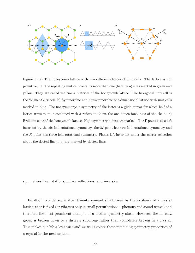
Figure 1. a) The honeycomb lattice with two different choices of unit cells. The lattice is not
primitive, i.e., the repeating unit cell contains more than one (here, two) sites marked in green and
yellow. They are called the two sublattices of the honeycomb lattice. The hexagonal unit cell is
the Wigner-Seitz cell. b) Symmorphic and nonsymmorphic one-dimensional lattice with unit cells
marked in blue. The nonsymmorphic symmetry of the latter is a glide mirror for which half of a
lattice translation is combined with a reflection about the one-dimensional axis of the chain. c)
Brillouin zone of the honeycomb lattice. High-symmetry points are marked. The Γ point is also left
invariant by the six-fold rotational symmetry, the M point has two-fold rotational symmetry and
the K point has three-fold rotational symmetry. Planes left invariant under the mirror reflection
about the dotted line in a) are marked by dotted lines.
symmetries like rotations, mirror reflections, and inversion.
Finally, in condensed matter Lorentz symmetry is broken by the existence of a crystal
lattice, that is fixed (or vibrates only in small perturbations – phonons and sound waves) and
therefore the most prominent example of a broken symmetry state. However, the Lorentz
group is broken down to a discrete subgroup rather than completely broken in a crystal.
This makes our life a lot easier and we will explore these remaining symmetry properties of
a crystal in the next section.
27
2. Symmetries of a crystal
A crystal is regular lattice of repeating structures (the unit cell) attached to all positions
Rn
Rn = n1a1 + n2a2 + n3a3, (82)
with linearly independent basis vectors ai, i = 1, 2, 3 and n ∈ Z3.
The space group of a crystal R is the group of all symmetry operations that leave the
crystal invariant: translations, rotations, inversion, reflections, and combinations thereof.
[Recall that a group G is a set of elements a, b, c, · · · ∈ G with a multiplication ? such that
it is: closed a ? b = c ∈ G; associative a ? (b ? c) = (a ? b) ? c; ∃ identity e, such that ∀a,
a ? e = e ? a = a; ∀a ∃ an inverse a−1 such that a ? a−1 = a−1 ? a = e. If a ? b = b ? a
the group is Abelian, otherwise it is non-Abelian; space groups are often non-Abelian, as
for example rotations do not commute.] In 2D there are 17 space groups (the so-called
wallpaper groups), in 3D there are 230 space groups. These counts apply to systems with
time-reversal symmetry, in magnetic systems the numbers are larger.
The unit cell of a lattice is not fixed uniquely. The Wigner-Seitz cell is a specific choice
that consists of the region of space that is closer to a given lattice point than to any other.
[See Fig. 1 a)]
Using the so-called Wigner notation, we can write a general spatial symmetry transfor-
mation of a crystal as a combination of a translation and another spatial symmetry
r′ = gr + a ≡ g|ar, (83)
where the elements g form the (smaller) point group P . It is tempting to think that all
allowed operations in a crystal are either translations E|a or rotations, mirror reflections,
inversions g|0 in which case R = P × trn, i.e., the space group is the direct product
of the point group elements and translations. This holds for so-called symmorphic space
groups (in 3D these are 73 of the 230). The remaining nonsymmorphic space groups also
contain screw rotations and glide mirror symmetries g|a, where a is a fractional lattice
translation. [See Fig. 1 b)] A screw rotation is a rotation combined with a translation a
along the rotation axis. A glide mirror is a mirror reflection combined with a translation
within the mirror plane. The associative multiplication rule for symmetry transformations
28
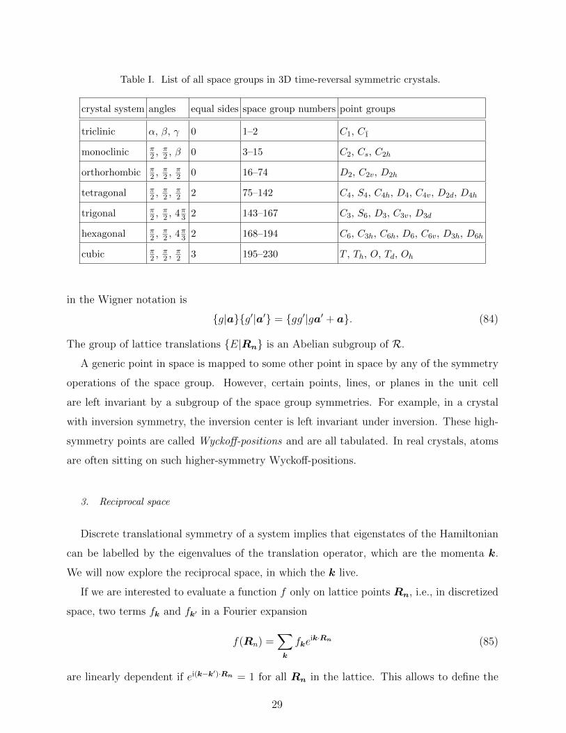
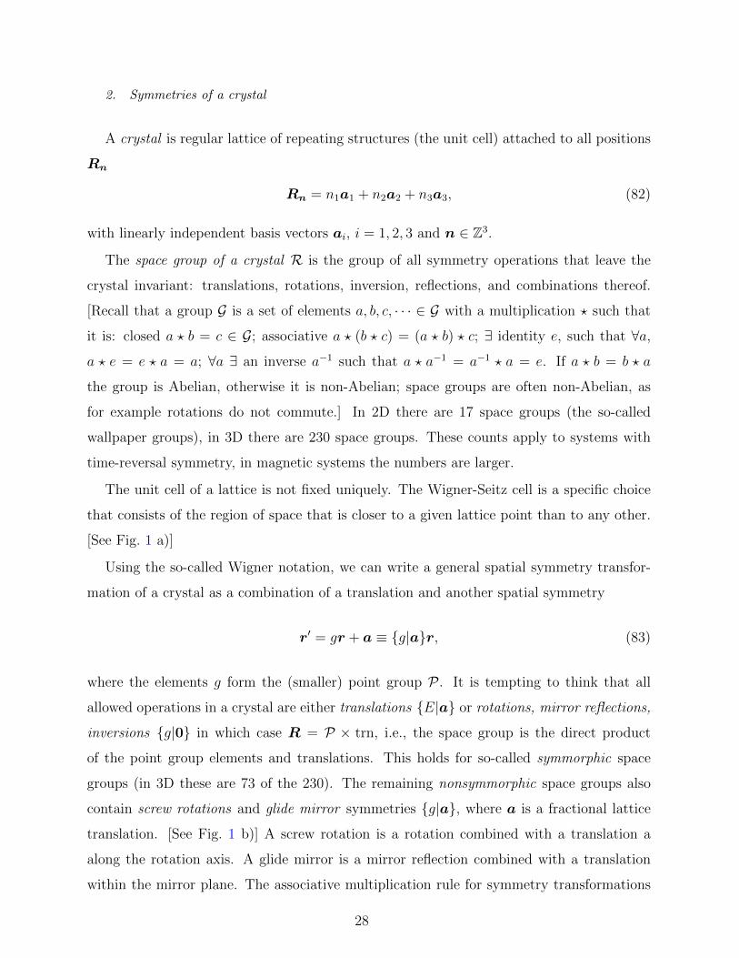
Table I. List of all space groups in 3D time-reversal symmetric crystals.
crystal system angles equal sides space group numbers point groups
triclinic α, β, γ 0 1–2 C1, C1
monoclinic π2 , π
2 , β 0 3–15 C2, Cs, C2h
orthorhombic π2 , π
2 , π2 0 16–74 D2, C2v, D2h
tetragonal π2 , π
2 , π2 2 75–142 C4, S4, C4h, D4, C4v, D2d, D4h
trigonal π2 , π
2 , 4π3 2 143–167 C3, S6, D3, C3v, D3d
hexagonal π2 , π
2 , 4π3 2 168–194 C6, C3h, C6h, D6, C6v, D3h, D6h
cubic π2 , π
2 , π2 3 195–230 T , Th, O, Td, Oh
in the Wigner notation is
g|ag′|a′ = gg′|ga′ + a. (84)
The group of lattice translations E|Rn is an Abelian subgroup of R.
A generic point in space is mapped to some other point in space by any of the symmetry
operations of the space group. However, certain points, lines, or planes in the unit cell
are left invariant by a subgroup of the space group symmetries. For example, in a crystal
with inversion symmetry, the inversion center is left invariant under inversion. These high-
symmetry points are called Wyckoff-positions and are all tabulated. In real crystals, atoms
are often sitting on such higher-symmetry Wyckoff-positions.
3. Reciprocal space
Discrete translational symmetry of a system implies that eigenstates of the Hamiltonian
can be labelled by the eigenvalues of the translation operator, which are the momenta k.
We will now explore the reciprocal space, in which the k live.
If we are interested to evaluate a function f only on lattice points Rn, i.e., in discretized
space, two terms fk and fk′ in a Fourier expansion
f(Rn) =∑k
fkeik·Rn (85)
are linearly dependent if ei(k−k′)·Rn = 1 for all Rn in the lattice. This allows to define the
29
reciprocal lattice as the collection of points G in momentum space with
1 = eiG·Rn , ∀Rn. (86)
The reciprocal lattice is spanned by bi, i = 1, 2, 3 with
bi = 2πaj × ak
ai · (aj × ak)(87)
for which ai · bj = 2πδij
Gm = m1b1 +m2b2 +m3b3. (88)
A function g that is expanded as
g(r) =∑G
gGeiG·r (89)
and evaluated at r in continuous real space will have the periodicity of the lattice. If we
have a chance to probe such a lattice-periodic function g(r) with a plane wave, say in a
scattering experiment, we are frequently compute
F [g] =
∫dreik·rg(r)
=∑R
∫unit cell
dxeik·(x+R)g(x+R)
=∑R
eik·RS(k),
(90)
where
S(k) =
∫unit cell
dxeik·xg(x) (91)
is called the structure factor.
The Brillouin zone (BZ) is the unit cell of the reciprocal lattice. Certain points, lines,
or planes in the BZ are left invariant under some of the point group symmetry operations.
By definition (since k are the eigenvalues of a translation operator), translations leave each
point in reciprocal space invariant. Mirror reflections leave the planes perpendicular to the
mirror normal invariant. Inversion leaves the so-called TRIM points (time-reversal invariant
momenta) k = 0 (the Γ point), k = b1/2, k = b2/2, k = b3/2, k = b1/2 + b2/2, k =
(b1 + b3)/2, k = (b2 + b3)/2, k = (b1 + b2 + b3)/2 invariant, because it maps k to −k,
but k ≡ k + G. The same points are left invariant by the time-reversal transformation.
30
Rotations leave the points along some lines parallel to the rotation axis invariant. [See
Fig. 1 c) for the honeycomb lattice as a 2D example.]
The group of symmetry operations that leave a point, line or plane in momentum space
invariant is called its little group.
31
III. NONINTERACTING ELECTRON SYSTEMS
A. Bloch’s theorem
We explore the consequences of the Abelian subgroup of translations of the point group
of a crystal. A Hamiltonian H that commutes with all translation operators T Rn , i.e,
[ H , T Rn ] = 0 is considered. The translation operator is defined through its action on
single-particle operators in the position basis
T Rn φ†(r) T −1
Rn= φ †(r +Rn), T Rn φ (r) T −1
Rn= φ (r +Rn), T −1
Rn= T −Rn .
(92)
We are, however, going to formulate things in first quantized language now. Consider the
single particle Hamiltonian
H =p 2
2m+ V ( r ), (93)
with the periodic potential V (r +Rn) = V (r) that could stem from a lattice of ions. H
and T Rn are all commuting and hence have a common eigenbasis. Bloch’s theorem says
that the eigenstates of T Rn have eigenvalues on the unit circle in the complex plane in order
not to blow up and to be extended. More precisely, the eigenstates of T ai are plane waves
T ai |k,m〉 = eik·ai|k,m〉, (94)
where m labels a possible degeneracy of the eigenspace.
A wave-function (notice the subtle distinction between wave function and state) of the
form
〈r|k,m〉 ≡ ψm,k =1√Ωeik·rum,k(r) ≡ 1√
Ωeik·r〈r|uk,m〉 (95)
satisfies this property if
um,k(r +Rn) = um,k(r) (96)
because then
ψm,k(r +Rn) = eik·Rnψm,k(r). (97)
We choose |k,m〉 to also diagonalize H
H |k,m〉 = εn,k|k,m〉, (98)
where m is the so-called band index, k is the pseudo-momentum, and um,k(r) the Bloch
wavefunction. Because eik·Rn = ei(k+Gm)·Rn , two momenta that differ by a reciprocal lattice
32
vector Gm are in the same eigenspace of the translation operator and we can restrict k to
the first BZ. Using
p |k,m〉 = p eik· r |uk,m〉 = eik· r ( p + k)|uk,m〉, (99)
we find the Bloch equation[( p + k)2
2m+ V ( r )
]|uk,m〉 = εm,k|uk,m〉, (100)
which has now to be solved for periodic states, i.e., TRn|uk,m〉 = |uk,m〉 only. (Notice that,
had we not set ~ = 1, the momentum shift would read ~k.) Taking the overlap with a
position eigenstate from the left, we obtain the alternate form in terms of wave functions[(−i∇r + k)2
2m+ V (r)
]uk,m(r) = εm,kuk,m(r). (101)
The fact that differential equations involving periodic functions have solutions that have the
same periodicity is a theorem named after Gaston Floquet (Floquet theory) in math. It was
rediscovered in the condensed matter context by Felix Bloch. In physics, Floquet’s name is
attached to the study of systems that are driven periodically in time.
We will now use two strategies to attack this problem, the nearly free electron approxi-
mation and the tight-binding approximation.
B. Nearly free electron approximation
In the nearly free electron approximation we consider electrons in a weak potential that
has the periodicity of the lattice
V (r) =∑G
VGeiGr. (102)
We want to solve the Bloch equation using perturbation theory in V (r). In configuration
space, the potential is a real function. If in addition V (r) = V (−r) (inversion symmetry),
then VG = V ∗G = V−G. Using the periodicity of the Bloch wave function, we can expand
uk,m(r) =∑G
cGe−iG·r (103)
to obtain [(k −G)2
2m− εm,k
]cG +
∑G′
VG′−G cG′ = 0, (104)
33
which presents an eigenvalue problem for the matrix VG′,G = VG′−G in infinite dimensions.
The zeroth order energy eigenvalues are given by the free electron parabolas
ε(0)G,k =
(k −G)2
2m, (105)
where we can use the reciprocal lattice vectors G as band labels. The first order result is
given by
ε(1)G,k = ε
(0)G,k +
∑G′ 6=G
|VG−G′|2
ε(0)G,k − ε
(0)G′,k
, (106)
valid if the bands are nondegenerate. If bands are degenerate, as it happens for example at
the zone boundary, we have to resort to degenerate perturbation theory (as we will exemplify
below).
1D example: Consider a 1D system perturbed by the potential with general coefficients
VG G2/(2m), where G = nb and b the unit vector spanning the reciprocal lattice. Let us
first compute the corrections to the lowest band for small k, i.e., near the zone center k b.
We obtain
ε(1)0,k =
k2
2m−∑G6=0
|VG|2[(k −G)2 − k2]/(2m)
≈ k2
2m?+ E0,
(107)
which we recast into a parabolic term with altered mass (the so-called effective mass) and
an overall energy shift
1
m?=
1
m
[1− 4
∑G 6=0
(2m|VG|G2
)2], E0 = −
∑G 6=0
2m|VG|2G2
. (108)
Next, let us consider what happens to the next-higher bands G = ±b at the zone center,
i.e., for k b. This problem has to be tackled with degenerate perturbation theory, for ε(0)b,k
and ε(0)−b,k are degenerate at k = 0. Degenerate perturbation theory amounts to diagonalizing
the Bloch equation in the degenerate subspace first (note that we cannot use the reciprocal
lattice vectors anymore as a label for the eigenstates, the perturbation is now really mixing
them) (k−b)2
2m− εk V−2b
V2b(k+b)2
2m− εk
cb
c−b
= 0. (109)
34
The characteristic equation of the above yields the eigenvalues
ε±,k =1
2
(k + b)2 + (k − b)2
2m±√[
(k + b)2 + (k − b)2
2m
]2
+ 4|V2b|2
=k2
2m?±± |V2b|+
b2
2m,
(110)
with the effective mass1
m?=
1
m
[1± b2
m|V2b|
], (111)
which due to |V2b| b2/(2m) have opposite sign. Thus the two bands obtain opposite
curvature. A band gap has opened. At k = 0, where the nontrivial part of the above matrix
is proportional to σ1, the eigenstates are given by cb = ±c−b yielding the real-space Bloch
wave functions
uk=0,+(x) = cos(bx), uk=0,−(x) = sin(bx), (112)
i.e., they are even and odd under the parity operation.
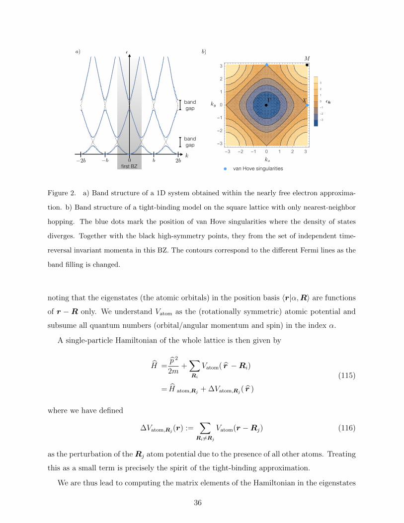
We can analyze the momenta at the zone boundary in a similar fashion using degenerate
perturbation theory, where we would likewise find the opening of a band gap. [See Fig. 2
a).]
C. Tight-binding approximation
We are now attempting to solve the Bloch equation in exactly the opposite limit, where
electrons are bound to a regular lattice of ionic potentials and the quantum mechanical
tunneling process of an electron between two atoms is seen as the perturbation. This so-
called tight-binding approximation is of much higher practical relevance than the nearly free
electron approximation.
Let us consider atoms positioned on sites Ri that could form a simple lattice or a lattice
with a basis. An isolated atom at R is described by a Hamiltonian
H atom,R =p 2
2m+ Vatom( r −R) (113)
which we can formally diagonalize
H atom,R|α,R〉 = εα|α,R〉, (114)
35
b 2bk
0b2bfirst BZ
band gap
band gap
a) b)
-3 -2 -1 0 1 2 3
-3
-2
-1
0
1
2
3
-3
-2
-1
0
1
2
3
kx
kyk X
M
van Hove singularities
Figure 2. a) Band structure of a 1D system obtained within the nearly free electron approxima-
tion. b) Band structure of a tight-binding model on the square lattice with only nearest-neighbor
hopping. The blue dots mark the position of van Hove singularities where the density of states
diverges. Together with the black high-symmetry points, they from the set of independent time-
reversal invariant momenta in this BZ. The contours correspond to the different Fermi lines as the
band filling is changed.
noting that the eigenstates (the atomic orbitals) in the position basis 〈r|α,R〉 are functions
of r −R only. We understand Vatom as the (rotationally symmetric) atomic potential and
subsume all quantum numbers (orbital/angular momentum and spin) in the index α.
A single-particle Hamiltonian of the whole lattice is then given by
H =p 2
2m+∑Ri
Vatom( r −Ri)
= H atom,Rj + ∆Vatom,Rj( r )
(115)
where we have defined
∆Vatom,Rj(r) :=∑Ri 6=Rj
Vatom(r −Rj) (116)
as the perturbation of theRj atom potential due to the presence of all other atoms. Treating
this as a small term is precisely the spirit of the tight-binding approximation.
We are thus lead to computing the matrix elements of the Hamiltonian in the eigenstates
36
of two atoms j and j in order to solve the perturbed problem
〈α,Rj| H |β,Rl〉 = εαδα,βδRj ,Rl + 〈α,Rj|∆ V atom,Rj |β,Rl〉. (117)
The last term describes the tunneling of an electron in orbital α of atom j to orbital β of
atom l. This is only likely to happen if Rj and Rl are close to one another.
In order to make progress, let us directly assume a form for these matrix elements. Let
us focus on atoms placed on a simple square lattice in 2D with lattice constant a, Nx ×Ny
sites and periodic boundary conditions. We consider only the lowest s orbital of each atom.
If we also neglect the electron spin degree of freedom (implicitly assuming that everything
is trivially spin-degenerate), we can drop the index α on each atom. Now, set
〈Rj|∆ V atom,Rj |Rl〉 =
−t if Rj and Rl are nearest neighbors
−t′ if Rj and Rl are next-nearest neighbors
0 else.
(118)
We also drop the irrelevant global shift of all onsite energies.
This is a great occasion to introduce second quantized notation, even though it is abso-
lutely not needed for this problem. However, the hopping processes are intuitively under-
stood in the second quantized language. We rewrite the tight-binding problem as
H tight−binding = −t∑〈Rj ,Rl〉
c†RjcRl − t′∑
〈〈Rj ,Rl〉〉
c†RjcRl , (119)
where c†Rj (cRj) is the creation (annihilation) operator for an electron on site Rj and the
summation subscripts 〈Rj,Rl〉 (〈〈Rj,Rl〉〉) are frequently used to indicate sums over nearest
(next-nearest) neighbors. Rewriting the second quantized operators using their Fourier
transform
c†Rj =1√NxNy
∑k
eik·Rjc†k, (120)
where the sum is taken over the first BZ k = 2π/a(n/Nx,m/Ny), n = 0, · · · , Nx − 1,
m = 0, · · · , Ny − 1, we obtain
H tight−binding = −∑k
2t[cos(kxa) + cos(kya)] + 4t′[cos(kxa) cos(kya)] c†kck. (121)
37
We observe that the Hamiltonian is readily diagonal in momentum space so that we can
read off the energy band dispersion
εk =− 2t[cos(kxa) + cos(kya)]− 4t′[cos(kxa) cos(kya)]
=− 4t− 4t′ − k2
2m?+O(k4),
(122)
where the effective mass m? = (2t + 8t′)−1 near k = 0. Expanding the Hamiltonian and
energy bands in small deviations p around a momentum point k is called a k · p approxi-
mation.
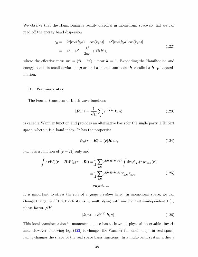
D. Wannier states
The Fourier transform of Bloch wave functions
|R, n〉 =1√Ω
∑k
e−ik·R|k, n〉 (123)
is called a Wannier function and provides an alternative basis for the single particle Hilbert
space, where n is a band index. It has the properties
Wn(r −R) ≡ 〈r|R, n〉, (124)
i.e., it is a function of (r −R) only and∫drW ∗
n(r −R)Wm(r −R′) =1
Ω
∑k,k′
ei(k·R−k′·R′)∫
drψ∗n,k′(r)ψm,k(r)
=1
Ω
∑k,k′
ei(k·R−k′·R′)δk,k′δn,m
=δR,R′δn,m.
(125)
It is important to stress the role of a gauge freedom here. In momentum space, we can
change the gauge of the Bloch states by multiplying with any momentum-dependent U(1)
phase factor ϕ(k)
|k, n〉 → eiϕ(k)|k, n〉. (126)
This local transformation in momentum space has to leave all physical observables invari-
ant. However, following Eq. (123) it changes the Wannier functions shape in real space,
i.e., it changes the shape of the real space basis functions. In a multi-band system either a
38
U(1)× · · ·×U(1) gauge transformation or, for N degenerate bands, a U(N) gauge transfor-
mation is allowed.
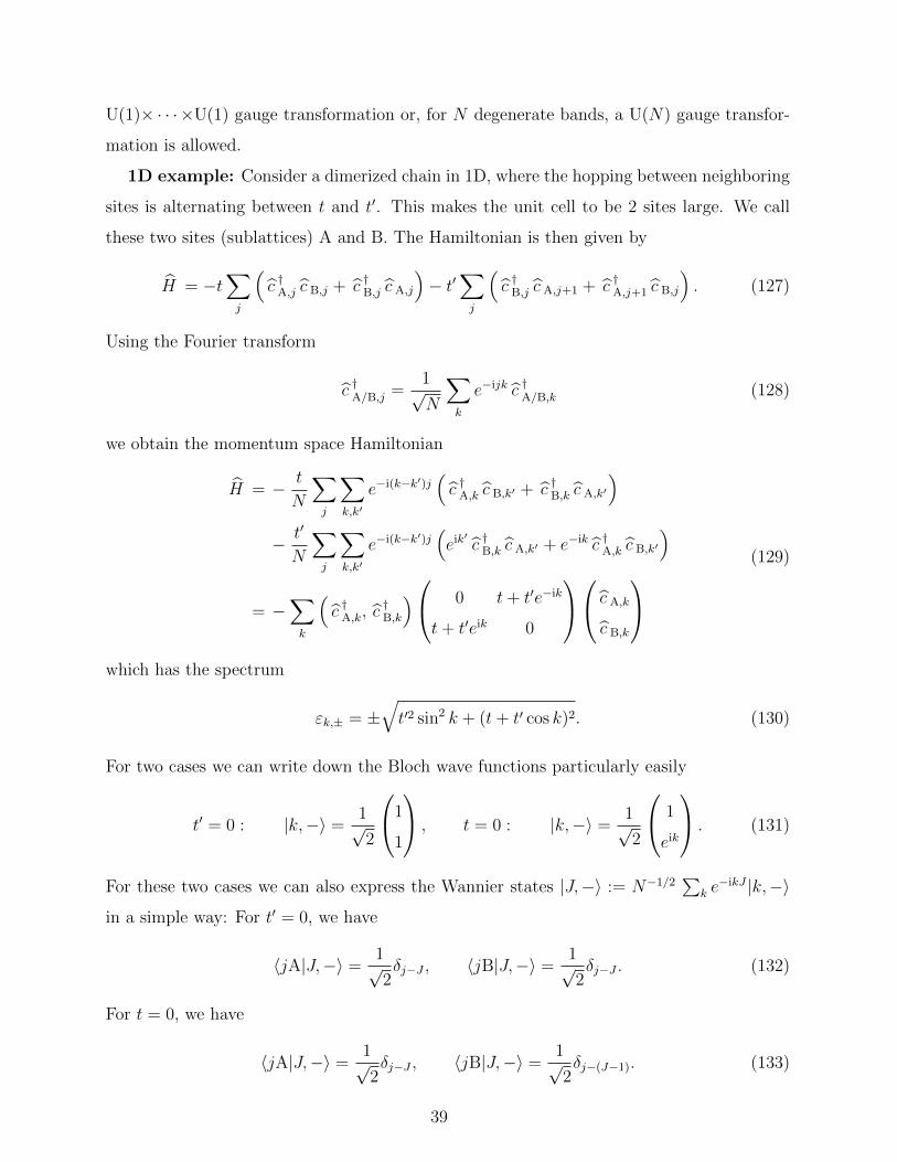
1D example: Consider a dimerized chain in 1D, where the hopping between neighboring
sites is alternating between t and t′. This makes the unit cell to be 2 sites large. We call
these two sites (sublattices) A and B. The Hamiltonian is then given by
H = −t∑j
(c †A,j c B,j + c †B,j c A,j
)− t′
∑j
(c †B,j c A,j+1 + c †A,j+1 c B,j
). (127)
Using the Fourier transform
c †A/B,j =1√N
∑k
e−ijk c †A/B,k (128)
we obtain the momentum space Hamiltonian
H = − t
N
∑j
∑k,k′
e−i(k−k′)j(c †A,k c B,k′ + c †B,k c A,k′
)− t′
N
∑j
∑k,k′
e−i(k−k′)j(eik′ c †B,k c A,k′ + e−ik c †A,k c B,k′
)
= −∑k
(c †A,k, c
†B,k
) 0 t+ t′e−ik
t+ t′eik 0
c A,k
c B,k
(129)
which has the spectrum
εk,± = ±√t′2 sin2 k + (t+ t′ cos k)2. (130)
For two cases we can write down the Bloch wave functions particularly easily
t′ = 0 : |k,−〉 =1√2
1
1
, t = 0 : |k,−〉 =1√2
1
eik
. (131)
For these two cases we can also express the Wannier states |J,−〉 := N−1/2∑
k e−ikJ |k,−〉
in a simple way: For t′ = 0, we have
〈jA|J,−〉 =1√2δj−J , 〈jB|J,−〉 =
1√2δj−J . (132)
For t = 0, we have
〈jA|J,−〉 =1√2δj−J , 〈jB|J,−〉 =
1√2δj−(J−1). (133)
39
We observe that the Wannier functions are not centered at a site of the lattice (in general
they can be centered at different Wyckoff positions than the atoms).The difference between
the two cases is that the Wannier functions are centered in the middle of the unit cell and at
the boundary of the unit cell, respectively. Since the model has inversion symmetry, these
are the only places where they could be located. For generic values of t and t′, the Wannier
functions would simply smear out over more lattice sites but keep their center.
E. Interlude: Group representations and character tables
The group of symmetry operations of a crystal constrains the electronic structure in
momentum space, as we shall see in the next section. To be prepared for this, we need to
quickly learn or recall some facts about the representation of groups.
A representation of a group over some vector space V is a collection of linear operators
on this vector space, which satisfy the same algebra as the group elements. As we are
only concerned with finite groups, we can always think of these operators as matrices. An
irreducible representation is a set of such matrix operators that is simultaneously block-
diagonalized and cannot be diagonalized into smaller blocks anymore.
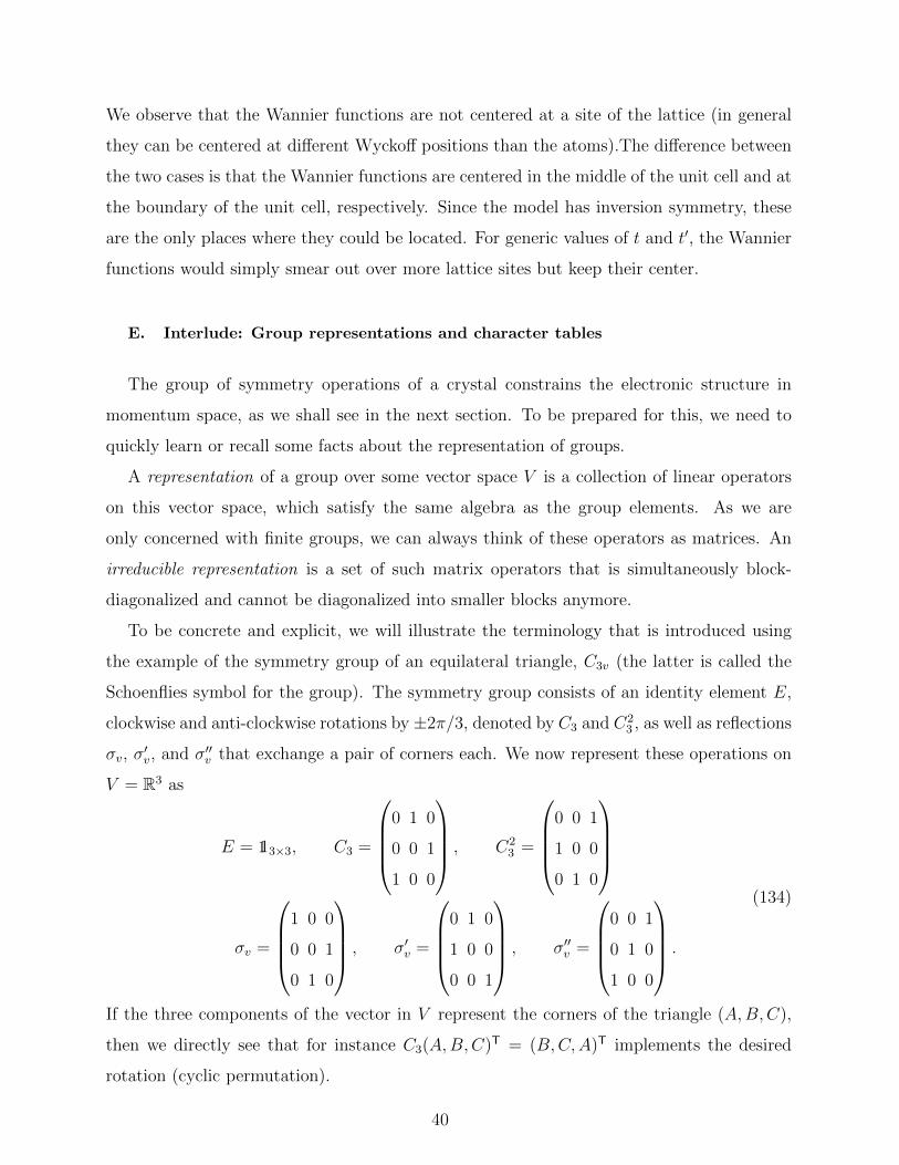
To be concrete and explicit, we will illustrate the terminology that is introduced using
the example of the symmetry group of an equilateral triangle, C3v (the latter is called the
Schoenflies symbol for the group). The symmetry group consists of an identity element E,
clockwise and anti-clockwise rotations by ±2π/3, denoted by C3 and C23 , as well as reflections
σv, σ′v, and σ′′v that exchange a pair of corners each. We now represent these operations on
V = R3 as
E = 113×3, C3 =
0 1 0
0 0 1
1 0 0
, C23 =
0 0 1
1 0 0
0 1 0
σv =
1 0 0
0 0 1
0 1 0
, σ′v =
0 1 0
1 0 0
0 0 1
, σ′′v =
0 0 1
0 1 0
1 0 0
.
(134)
If the three components of the vector in V represent the corners of the triangle (A,B,C),
then we directly see that for instance C3(A,B,C)T = (B,C,A)T implements the desired
rotation (cyclic permutation).
40
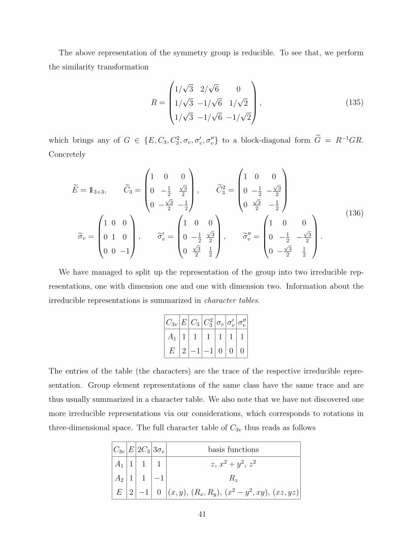
The above representation of the symmetry group is reducible. To see that, we perform
the similarity transformation
R =
1/√
3 2/√
6 0
1/√
3 −1/√
6 1/√
2
1/√
3 −1/√
6 −1/√
2
, (135)
which brings any of G ∈ E,C3, C23 , σv, σ
′v, σ
′′v to a block-diagonal form G = R−1GR.
Concretely
E = 113×3, C3 =
1 0 0
0 −12
√3
2
0 −√
32−1
2
, C23 =
1 0 0
0 −12−√
32
0√
32−1
2
σv =
1 0 0
0 1 0
0 0 −1
, σ′v =
1 0 0
0 −12
√3
2
0√
32
12
, σ′′v =
1 0 0
0 −12−√
32
0 −√
32
12
.
(136)
We have managed to split up the representation of the group into two irreducible rep-
resentations, one with dimension one and one with dimension two. Information about the
irreducible representations is summarized in character tables.
C3v E C3 C23 σv σ
′v σ′′v
A1 1 1 1 1 1 1
E 2 −1 −1 0 0 0
The entries of the table (the characters) are the trace of the respective irreducible repre-
sentation. Group element representations of the same class have the same trace and are
thus usually summarized in a character table. We also note that we have not discovered one
more irreducible representations via our considerations, which corresponds to rotations in
three-dimensional space. The full character table of C3v thus reads as follows
C3v E 2C3 3σv basis functions
A1 1 1 1 z, x2 + y2, z2
A2 1 1 −1 Rz
E 2 −1 0 (x, y), (Rx, Ry), (x2 − y2, xy), (xz, yz)
41
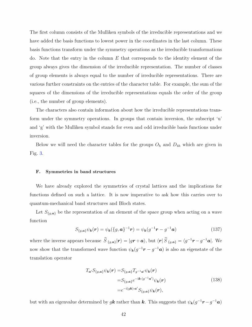
The first column consists of the Mulliken symbols of the irreducible representations and we
have added the basis functions to lowest power in the coordinates in the last column. These
basis functions transform under the symmetry operations as the irreducible transformations
do. Note that the entry in the column E that corresponds to the identity element of the
group always gives the dimension of the irreducible representation. The number of classes
of group elements is always equal to the number of irreducible representations. There are
various further constraints on the entries of the character table. For example, the sum of the
squares of the dimensions of the irreducible representations equals the order of the group
(i.e., the number of group elements).
The characters also contain information about how the irreducible representations trans-
form under the symmetry operations. In groups that contain inversion, the subscript ‘u’
and ‘g’ with the Mulliken symbol stands for even and odd irreducible basis functions under
inversion.
Below we will need the character tables for the groups Oh and D4h which are given in
Fig. 3.
F. Symmetries in band structures
We have already explored the symmetries of crystal lattices and the implications for
functions defined on such a lattice. It is now imperative to ask how this carries over to
quantum-mechanical band structures and Bloch states.
Let Sg,a be the representation of an element of the space group when acting on a wave
function
Sg,aψk(r) = ψk(g,a−1r) = ψk(g−1r − g−1a) (137)
where the inverse appears because S g,a|r〉 = |gr+a〉, but 〈r| S g,a = 〈g−1r−g−1a|. We
now show that the transformed wave function ψk(g−1r − g−1a) is also an eigenstate of the
translation operator
Ta′Sg,aψk(r) =Sg,aTg−1a′ψk(r)
=Sg,ae−ik·(g−1a′)ψk(r)
=e−i(gk)·a′Sg,aψk(r),
(138)
but with an eigenvalue determined by gk rather than k. This suggests that ψk(g−1r−g−1a)
42
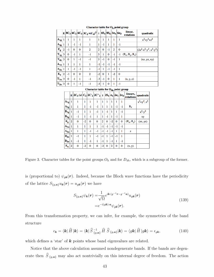
Figure 3. Character tables for the point groups Oh and for D4h, which is a subgroup of the former.
is (proportional to) ψgk(r). Indeed, because the Bloch wave functions have the periodicity
of the lattice Sg,auk(r) = ugk(r) we have
Sg,aψk(r) =1√Ωeik·(g−1r−g−1a)ugk(r)
=e−i(gk)·aψgk(r).
(139)
From this transformation property, we can infer, for example, the symmetries of the band
structure
εk = 〈k| H |k〉 = 〈k| S −1g,a H S g,a|k〉 = 〈gk| H |gk〉 = εgk, (140)
which defines a ‘star’ of k points whose band eigenvalues are related.
Notice that the above calculation assumed nondegenerate bands. If the bands are degen-
erate then S g,a may also act nontrivially on this internal degree of freedom. The action
43
that leaves k unchanged is the aforementioned little group symmetry of k. Assume that we
have a set of d degenerate states at some momentum
H |n,k〉 = εk|n,k〉, n = 1, · · · , d. (141)
For every element of the little group of k, S g|a we have a representation of the symmetry
S g|a|n,k〉 =∑n′
|n′,k〉Mn,n′;k, Mn,n′;k = 〈n′,k| S g|a|n,k〉. (142)
If the representation is irreducible, its dimension is that of the Bloch states at the momentum
k.
Example: Consider a tight-binding model for p-orbitals on a cubic lattice spanned by
the basis vectors ax, ay, and az. On each lattice site there are three atomic orbitals with
the from
〈r|x,R〉 =(R− r)xf(|R− r|),
〈r|y,R〉 =(R− r)yf(|R− r|),
〈r|z,R〉 =(R− r)zf(|R− r|),
(143)
which due to the symmetry of the simple cubic lattice remain degenerate in energy. For
nearest neighbors, the overlaps from Eq. (117) evaluate to
〈α,Rj|∆ V atom,Rj |β,Rj + aγ〉 =
tδα,β for γ = α σ-bonding
−tδα,β for γ 6= α π-bonding,(144)
with α, β, γ ∈ x, y, z. For next-nearest neighbors, the overlaps from Eq. (117) evaluate to
(for γ 6= ρ)
〈α,Rj|∆ V atom,Rj |β,Rj + aγ ± aρ〉 =
t′δα,β for γ = α
−t′δα,β for γ 6= α
−(±)˜t′δα,γδβ,ρ
(145)
with α, β, γ ∈ x, y, z. Notice that some hoppings are zero by symmetry, for example the
hopping along the x direction from an x to a y orbital.
Translating the above into a second quantized Hamiltonian in momentum space yields
44
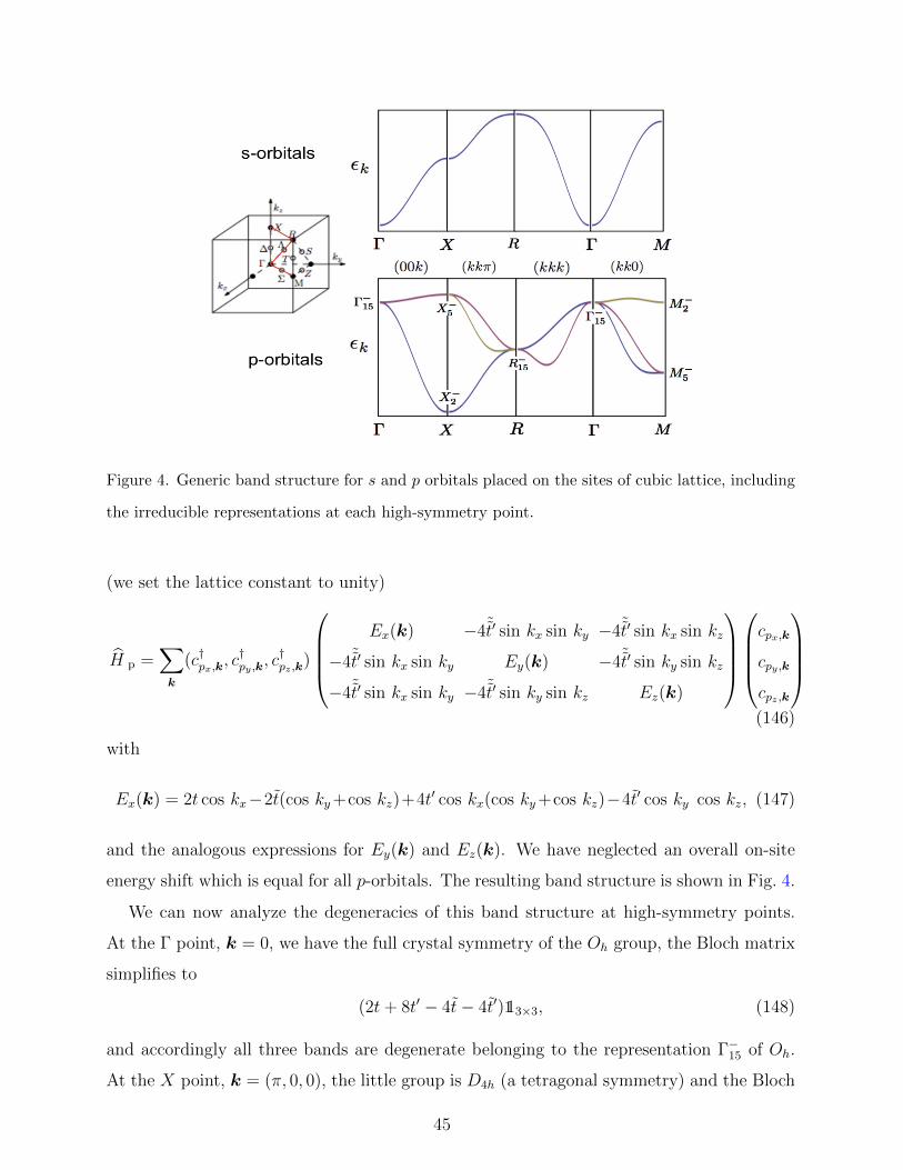
Figure 4. Generic band structure for s and p orbitals placed on the sites of cubic lattice, including
the irreducible representations at each high-symmetry point.
(we set the lattice constant to unity)
H p =∑k
(c†px,k, c†py ,k
, c†pz ,k)
Ex(k) −4˜t′ sin kx sin ky −4˜t′ sin kx sin kz
−4˜t′ sin kx sin ky Ey(k) −4˜t′ sin ky sin kz
−4˜t′ sin kx sin ky −4˜t′ sin ky sin kz Ez(k)
cpx,k
cpy ,k
cpz ,k
(146)
with
Ex(k) = 2t cos kx−2t(cos ky+cos kz)+4t′ cos kx(cos ky+cos kz)−4t′ cos ky cos kz, (147)
and the analogous expressions for Ey(k) and Ez(k). We have neglected an overall on-site
energy shift which is equal for all p-orbitals. The resulting band structure is shown in Fig. 4.
We can now analyze the degeneracies of this band structure at high-symmetry points.
At the Γ point, k = 0, we have the full crystal symmetry of the Oh group, the Bloch matrix
simplifies to
(2t+ 8t′ − 4t− 4t′)113×3, (148)
and accordingly all three bands are degenerate belonging to the representation Γ−15 of Oh.
At the X point, k = (π, 0, 0), the little group is D4h (a tetragonal symmetry) and the Bloch
45
matrix is given by
diag(−2t− 8t′ − 4t− 4t′, 2t+ 4t′, 2t+ 4t′), (149)
which is separated into a two-fold degenerate irreducible representation [X−5 , corresponding
to basis functions (x, y)] and a singly degenerate one [X−2 , corresponding to basis function
z]. In fact, the degeneracy between two bands persists for any momentum k = (kx, 0, 0)
that lies on the line connecting the Γ and the X point. The Bloch matrix is given by
diag(2(t+ 4t′) cos kx − 4(t+ t′),
2[t+ 2t′ − t+ (2t′ − t− 2t′) cos kx],
2[t+ 2t′ − t+ (2t′ − t− 2t′) cos kx]),
(150)
Such a degeneracy between two bands is called a nodal line. Depending on the space group
and irreducible representation, band structures can also posses nodal points, i.e., point-like
degeneracies, or (less common) nodal surfaces, i.e., degeneracies on a surface in momentum
space. Since these degeneracies are related to the irreducible representations of bands, they
are not an artifact of the type of tight-binding model that we have chosen, and could, e.g., not
be lifted by longer-range hoppings or other perturbations compatible with the point-group
symmetries.
G. Obtaining information about band structures and symmetries
Several big repositories and tables have recently emerged on the web which help to find
materials with a desired electronic structure or to help understand the electronic structure of
a given material. Here, we mention three repositories with different focus and functionality
• https://materialsproject.org: The Materials Project is a database with gives
rough information about the electronic structure of many materials. It is not the most
complete database, but it allows to take a quick look even at the band structure and
diffraction spectra. Exercise: Try to find the crystal and band structure of diamond
and (rock)salt. A list of the space groups is for example here: http://img.chem.ucl.
ac.uk/sgp/large/sgp.htm.
• https://icsd.fiz-karlsruhe.de/search/: The ICSD is a more complete and accu-
rate database of previously synthesized materials, but it requires institutional access.
46
One can search for a material and then find all relevant references in which the struc-
ture of the compound was experimentally determined. One can then download a
structure file (*.cif) which can be handled by programs computing band structures or
by the free VESTA software (http://jp-minerals.org/vesta/en/) to visualize the
structure.
• http://www.cryst.ehu.es/#retrievaltop: The Bilbao Crystallographic Server
contains very comprehensive information about the symmetry representations in band
structures. It does not contain any database related to materials.
Exercise: We want to understand the band structure of tungsten carbide (WC), a
material traditionally used for hardened tools and jewelry. Determine (maybe with the help
of google and Wikipedia) which space group WC is in and find the correct entry in the
Materials Project. Use the Bilbao Crystallographic Server to determine the labels of high-
symmetry points in the Brillouin zone for this space group. Along the Γ-A line two bands
cross in an X-like fashion above the Fermi energy. Why is this not an avoided crossing?
Use the Bilbao Crystallographic Server to find possible irreducible representations of the
bands along this line in momentum space and determine to which of them the two bands in
question belong. Picture the three-dimensional band structure around the degeneracy point
of the bands.
H. Filling of bands and density of states
So far we have only considered a single particle picture of electronic bands. In a many-
body Hilbert space, fermionic states can all be at most singly occupied. In the ground
state at zero temperature, all states below the Fermi level in a solid are singly occupied,
all states above are empty. The occupied states form the Fermi sea. If the Fermi level
is located such that it cuts though a band (or more generally, there are excited states ate
arbitrarily low energy available) one speaks of a metal. For a noninteracting system, the
locations in momentum space of these single-particle excitations with arbitrary low energy
and momentum transfer, form the Fermi surface. Materials with a finite excitation energy
above the ground state are called semiconductors (for small excitation energies) or insulators
(for large excitation energies). At finite temperature, the single-particle levels dictated by
47
the band structure are occupied according to the Fermi-Dirac distribution.
When counting the number of states available, it is always important to pay attention
whether spin-degeneracies have to be taken into account or not. If all bands are spin degen-
erate (as is the case in an electronic model which neglects spin-orbit and Zeeman couplings),
each state can be occupied by a spin-up and a spin-down electron.
To better understand the relation between the band dispersion and the number of occu-
pied states, we return to the example of the simple square lattice and restrict it to nearest
neighbor hopping only. The dispersion is εk = −2t cos kx − 2t cos ky. We want to compute
the density of states, i.e., dN/dε, where N is the number of occupied states. One interesting
point is the band bottom and the zero energy around which εk ≈ k2/(2m?). We have in 2D
dN = 2πkdk and k =√
2m?ε such that
dN
dε=
dN
dk
dk
dε= 2πk
√m?
2ε= 2πm?, (151)
i.e., it is a constant. The same calculation yields in 1D dN/dε ∝ 1/√ε and in 3D dN/dε ∝
√ε. The second interesting point to consider in 2D is near k = (π, 0) and symmetry
equivalent. The effective band dispersion is εk ≈ (k2y − k2
x)/(2m?), i.e., it is a saddle point.
The density of states is given by
dN
dε∝∫
dkxdkyδ[ε− (k2y − k2
x)/(2m?)]
∝∫
dkx1√
2m?ε+ k2x
∝ log[kx +
√k2x + 2m?ε
]∣∣∣Λ0
∝ (regular part)− log ε,
(152)
i.e., we find a log divergence as the energy approaches the saddle point in 2D. This is called
a van Hove singularity. [See Fig. 2 b).]
I. Coupling to an external electro-magnetic field
Electrons couple to a magnetic field in two ways which are considered distinct in the
realm of condensed matter physics (of course they are unified on the level of relativistic
quantum mechanics): For one due to their orbital motion to the electromagnetic gauge field
and on the other hand due to the Zeeman effect to the electronic spin. The former can be
48
accounted for by minimal coupling, i.e., the replacement
H ( p , r )→ H ( p − eA( r ), r ). (153)
The latter is an additive term
H ( p , r )→ H ( p , r ) + µB g? S ·B, (154)
where S is the spin operator and g? is the effective Lande g factor, which is g = 2 for the
free electron but can deviate substantially in the electronic environment of crystals, where
values of g? = 20 are easily possible. Depending on the physics one is interested in, often
only one of the two effects is considered at a time. Typically, the orbital coupling has the
more dramatic effect on the electronic structure and we will explore its consequences in the
following sections.
1. Semiclassical equations of motion
A minimal way to include quantum-mechanical phenomena in the description of electrons
in solids is to consider the dynamics of wave packets which are extended both in position
and momentum space. We write a wave function of the form
ψk(r, t) =∑k′
gk(k′)eik′·r−iεk′ t, (155)
where gk(k′) is a function centered around k with a characteristic width ∆k much smaller
than the size of the BZ. In turn, by the uncertainty principle the wave packet ψk(r, t) is
spread over many unit cells in position space. Assuming that the system is perturbed weakly
by electric and magnetic fields, E and B, such that no interband transitions are induced,
one can derive the following equations of motion
r ≡ vn(k) =∂εn,k∂k− k ×Ω(k)
k = −eE(r, t)− er ×B(r, t).
(156)
Notice that k is the pseudo momentum of the electron (i.e., related to the expectation value
of the translation operator), not the expectation value of the momentum operator. The
quantity Ωn(k) is a purely quantum-mechanical contribution known as the Berry curvature.
From the Bloch eigenstates of the bands, it is defined as
Ωn,α(k) = −εα,β,γi 〈∂kβun,k|∂kγun,k〉. (157)
49
From the form of Eq. (156) it is suggestive to interpret the Berry curvature as a ’magnetic
field in momentum space’, that has physical consequences for the electron motion in position
space.
Let us consider a 1D system with dispersion εk = −2 cos k in a static electric field E.
Equation (156) reads for this case
x = 2 sin k, k = −eE, ⇒ x = −2 sin (eEt) (158)
thus, the position of the wave packet oscillates according to
x(t) =2
eEcos (eEt) , (159)
which are called Bloch oscillations. They can be observed in very clean systems.
Now, consider a system which for simplicity is taken to have a quadratic band disper-
sion (such that ∂εn,k∂k = k/m) with applied homogeneous electric field E. We study
two situations (1) with an applied external homogeneous magnetic field B and (2) with a
nonvanishing intrinsic Berry curvature Ω.
For (1), the equations of motion reduce to
mv = −e(E + v ×B). (160)
We are interested in steady state solutions v = 0, i.e.,
v ×B = −E. (161)
The electric current is j = −en0v, where n0 is the carrier density. Comparing the above to
the definition of the conductivity jα = σα,βEβ, we find that the system has a non-vanishing
Hall response. Taking B = (0, 0, Bz) and E = (Ex, 0, 0), we have
σxy = jy/Ex = n0e/Bz = νe2/h, (162)
where ν = n0hc/(Be) is called the filling fraction and we have reinstated the appropriate
factors of c and h to obtain the well known form of the Hall conductivity. Measuring the Hall
response can thus determine both the carrier density and the electron or hole like nature of
the carriers.
For (2) we find
v =k
m+ eE ×Ω, (163)
50
i.e., the Berry connection induces a Hall response similar to an external magnetic field. For
a 2D system in the x-y plane with only one (partially) filled band the area of the Fermi sea
SFS is the density of carriers n0. Taking the latter to be (2π)2, we find
j =e2
h/(2π)SFS
[∫FS
d2k
(2π)2Ω(k)
]×E, (164)
where the integral is taken over the Fermi sea (FS). Thus, the Hall conductivity for such a
system is given by
σxy =e2
h2π
SFS
(2π)2
∫FS
d2kΩz(k). (165)
Notice that if the band is completely filled, i.e., the system is an insulator SFS = (2π)2 and
the Hall response can still be nonzero. In fact, it is then given by e2/h 2π∫
d2kΩz(k), which
for deep mathematical reasons is always an integer called the Chern number.
2. The integer quantum Hall effect
Quantum Hall effects are one of the driving thrusts of condensed matter research of the
past decades. Here, we will first consider the integer quantum Hall effect (IQHE) which can
be understood without considering electron-electron interactions. Later, we will mention
the fractional quantum Hall effect (FQHE), which needs interactions to exist.
The possibility of an IQHE was first noted in a theoretical paper by Ando et al. in 1975,
but the authors doubted that their result connects to the realm of experiments. The Nobel-
prize winning experimental discovery of the IQHE by von Klitzing et al. thus came as a
big surprise. In the experimental setup, electrons of charge e < 0 and effective mass m are
confined to a 2D plane in a high-quality GaAs heterojunction and a large magnetic field B is
applied perpendicular to that plane. In this situation, the electronic density of states consists
of discrete peaks, the so-called Landau levels. These Landau level bands are broadened
by disorder and equally spaced in energy with spacing given by the cyclotron frequency
ωc := eB/m. If the broadening is small enough such that there exist insulating regions
between the peaks, the transverse conductivity σH is quantized in units of the resistance
quantum e2/h whenever the chemical potential lies within such an insulating region. One
year after the experimental discovery, Laughlin gave a theoretical explanation for the high-
precision quantization of the conductivity. However, his description did not account for the
51
topological nature of the IQHE. The deep connection to topological quantum numbers was
made one year later by Thouless, Kohmoto, Nightingale, and den Nijs (TKKN).
The completion of the theoretical understanding of the IQHE coincided with the next
groundbreaking and Nobel-prize winning experimental discovery made by Stormer, Tsui and
coworkers in 1982. They observed that plateaus in the Hall resistance develop at fractional
fillings ν of the Landau level, accompanied by a dip or vanishing of the longitudinal resis-
tance. This FQHE turned out to have a much richer phenomenology than the integer effect
with more and more examples of stable filling fractions discovered as the sample quality
improved. As with the IQHE, it was Laughlin who gave a theoretical explanation for the
occurrence of the principal filling fractions ν = 1/n, n ∈ Z, based on the specific form
of the quantum state of the two-dimensional electron gas. However, he did not make the
connection to the topological character of the state which was later established by Wen and
Niu.
We consider a 2D electron gas in the x-y plane in a magnetic field B = (0, 0,−B) that is
orbitally coupled to the motion of the electrons. Such a situation can occur in heterostructure
interfaces. We have
H =1
2m
[( p x − eAx( r ))2 + ( p y − eAy( r ))2
], (166)
where m is not necessarily the bare electron mass, but an effective mass. We now introduce
the operators
a † =`√2
[( p x − eAx( r )) + i( p y − eAy( r ))] , a =`√2
[( p x − eAx( r ))− i( p y − eAy( r ))] ,
(167)
where `2 = (eB)−1 is the magnetic length. Their algebra
a a † − a † a = − i`2e
2([ p x, Ay( r )]− [ p y, Ax( r )]) +
i`2e
2([ p y, Ax( r )]− [ p x, Ay( r )])
=`2e
2(∂yAx(r)− ∂xAy(r))− `2e
2(∂xAy(r)− ∂yAx(r))
= `2eB
= 1
(168)
allows them to be interpreted as bosonic lowering and raising operators. We can define a
52
second set of operators
b =1√2`
r x − `2( p y − e A y) + i[ r y + `2( p x − e A x)]
,
b † =1√2`
r x − `2( p y − e A y)− i[ r y + `2( p x − e A x)]
,
(169)
which realize an independent bosonic algebra for
[ a , b ] = 0, [ a , b †] = 0, [ b , b †] = 1. (170)
The Hamiltonian rewritten in terms of these operators reads
H = ωc
(a † a +
1
2
). (171)
where again ωc = eB/m is the cyclotron frequency. The energy spectrum is that of a
harmonic oscillator, En = ωc(n + 1/2), n = 0, 1, 2, · · · . Each of these energy levels is called
Landau level. However, due to the commuting operator b, every level is highly degenerate, as
its single-particle eigenstates can be written |n,m〉 = (n!m!)−1/2 a †n b †m|0〉. To understand
this better, consider the eigenstates of the lowest Landau level in a symmetric gauge A =
(−Bry, Brx, 0)/2
〈r|0,m〉 =1√
2π2mm!`
(z`
)me−|z|
2/(4`)2
, m = 0, 1, 2, · · · , (172)
where z = rx − iry. We have 〈0,m| r 2|0,m〉 = 2(m + 1)`2. The amplitude of the wave
function 〈r|0,m〉 is peaked at a radius rm =√
2m`. This means that the area taken by
a “Hall droplet” with all states m < m0 filled, is proportional to m0 and the inverse field
strength. Thus the Landau level degeneracy m0 is given by the area S of the system divided
by the area taken by one magnetic flux quantum m0 ∼ S/(2π`2). (The magnetic flux
quantum is Φ0 = hc/e.)
To study the transport response, it is easier to use the Landau gauge A = (0, Brx, 0).
Then, ky is a good quantum number (instead of the angular momentum in the case of the
symmetric gauge) and
ψ0,ky =1√2π`
e−[rx−x0(ky)]2/(2`2)eikyry , (173)
with x0(ky) = `2ky, are the lowest Landau level wave functions. The energy is independent
of ky. We now apply an electric field Ex in x-direction, which enters the Hamiltonian as the
additive term −eEx r x. Clearly, this term can be absorbed by shifting the origin of the x
53
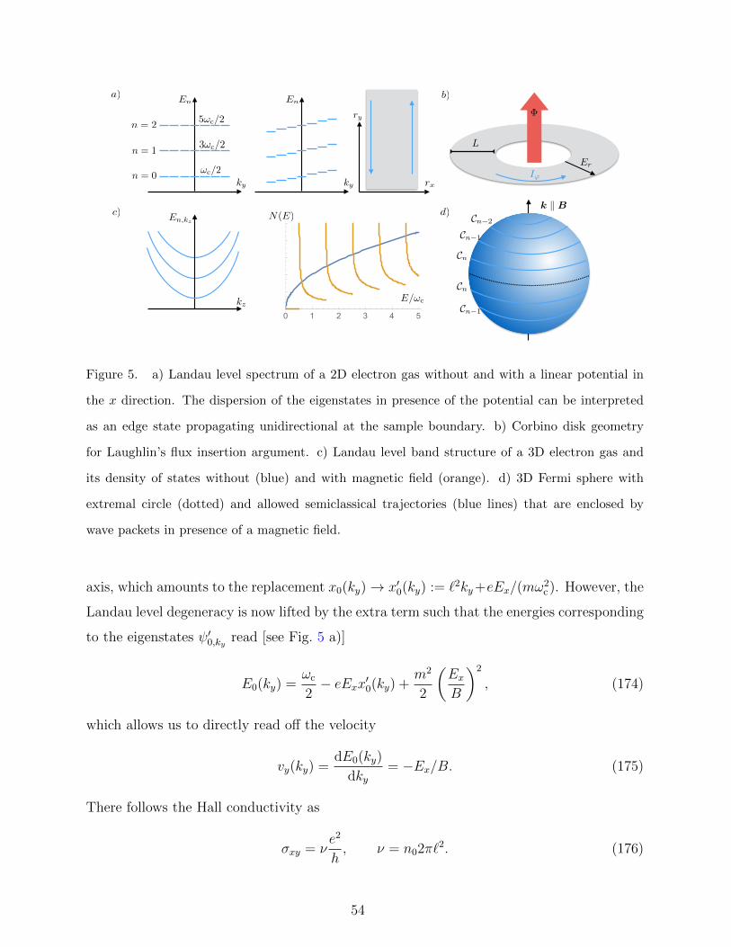
a)
ky
En
!c/2
3!c/2
5!c/2
n = 0
n = 1
n = 2
ky
En
rx
ry
b)
L
I'
Er
c)
kz
En,kz
0 1 2 3 4 5
2
4
6
8
10N(E)
E/!c
d)k k B
Cn
Cn1
Cn2
Cn
Cn1
Figure 5. a) Landau level spectrum of a 2D electron gas without and with a linear potential in
the x direction. The dispersion of the eigenstates in presence of the potential can be interpreted
as an edge state propagating unidirectional at the sample boundary. b) Corbino disk geometry
for Laughlin’s flux insertion argument. c) Landau level band structure of a 3D electron gas and
its density of states without (blue) and with magnetic field (orange). d) 3D Fermi sphere with
extremal circle (dotted) and allowed semiclassical trajectories (blue lines) that are enclosed by
wave packets in presence of a magnetic field.
axis, which amounts to the replacement x0(ky)→ x′0(ky) := `2ky+eEx/(mω2c ). However, the
Landau level degeneracy is now lifted by the extra term such that the energies corresponding
to the eigenstates ψ′0,ky read [see Fig. 5 a)]
E0(ky) =ωc
2− eExx′0(ky) +
m2
2
(ExB
)2
, (174)
which allows us to directly read off the velocity
vy(ky) =dE0(ky)
dky= −Ex/B. (175)
There follows the Hall conductivity as
σxy = νe2
h, ν = n02π`2. (176)
54
a. Hall plateaus and disorder Von Klitzing’s experimental observation was that the
longitudinal conductivity σyy vanished for certain ranges of the magnetic field, which pre-
cisely corresponded to integer fillings ν ∈ N. At the same time, the Hall conductivity is
quantized very precisely to the integer multiple of e2/h that corresponds to the number of
filled Landau levels. What was observed, however, is that the quantization forms stable
plateaus over a full range of magnetic fields, not only for the exact field value that corre-
sponds to a specific filling. This behavior can only be explained by considering the role of
disorder in the system. For simplicity, we return to the symmetric gauge and add a rotation-
ally symmetric disorder potential to the system of the form V (r) = Cr2. Its effect can be
absorbed in the wave function (172) by replacing ` with `′ = `(1 + 2mC)−1/4. The Landau
level degeneracy is now lifted to
E0,m =ωc
2
[m
(`2
`′2− 1
)+`2
`′2
], (177)
which for m 1 and a weak potential 2mC 1 can be recast as
E0,m ≈ωc
2+ Cr2
m, (178)
where rm =√
2m`′ is the wave function localization radius. The locking between the wave
function localization and the equipotential lines means that the quasiclassical trajectories
trace out equipotential lines. A weak electric field cannot induce a motion of these wave
packets in the orthogonal direction to the concentric rings. This picture can be elevated to
a completely disordered sample as follows: At a specific chemical potential, equipotential
lines that form a closed loop enclose states that do not contribute to bulk longitudinal
transport. Only at specific values of the chemical potential, where the equipotential lines
connect to form a delocalized channel that spans over the entire sample, connecting two leads,
bulk transport can happen. Thus, when slightly doping away from the chemical potential
corresponding to a filled Landau level, only small disconnected islands of equipotential lines
appear and no transport is possible. The sample remains insulating and we observe a plateau
in the Hall conductivity.
b. Edge states We now return to Eq. (174), namely the spectrum with an applied
electric field in the x direction. This mathematical result allows for a second very different
physical interpretation. For that, we reinterpret the source for the additional term in the
Hamiltonian as being a (linear) confining potential at the sample boundary [see Fig. 5 a)].
55
We are then lead to the conclusion that the sample boundary hosts a set of states ψ0,ky with
linear and unidirectional dispersion E0,ky ∝ ky that propagate along the boundary. The fact
that these modes can only move in one direction is very specific to the quantum Hall effect
and cannot be realized in a system confined to strictly one dimension (a 1D systems hosts
always as many right-moving modes as left-moving ones). While the velocity of these modes
is not universal, the number of them (each filled Landau level contributed one branch of
boundary modes) is in equal to the integer that determines the bulk Hall conductivity.
c. Laughlin’s argument Laughlin gave an argument as to why the Hall conductivity of
an insulator has to be quantized. The 2D insulator that is to be probed has the shape of a
so-called Corbino disk, that is, a disk with a hole [see Fig. 5 b)]. The magnetic flux Φ trough
the center of the disk is varied in time. This flux does not change the field distribution in
the disk and can therefore only be seen by states that extend fully around the disk. A
change in the flux by δΦ can be accounted for by a change in the ϕ component of the
vector potential Aϕ → Aϕ + δΦ/(2πr). The symmetric gauge wave function (172) changes
by ψ0,m → ψ0,meiϕ δΦ/Φ0 . This change can be absorbed by m → m − δΦ/Φ0. Hence, when
increasing Φ by one flux quantum, the index m has to be decreased by 1. This implies that
the wave functions are all continuously shifted in their localization radius during the flux
insertion. As a result, one electron is pumped from the outer to the inner edge of the system
after one flux quantum insertion.
When an electric field Er is applied radially, the charge transfer results in a potential
energy change −eErL, where L is the distance between the two edges of the disk, which we
assume to be much smaller than the inner radius. A second energy change IϕδΦ results from
the current Iϕ that is caused by the difference in angular momentum between the electronic
states that were filled and emptied, respectively. After insertion of a full flux quantum, the
energy of the system should remain unchanged, and hence these two energetic contributions
must add up to zero. This leads to the relation eErL = IϕΦ0. Returning to cartesian
coordinates and reinstating all constants we obtain the Hall conductivtiy
σxy =jyEx
=IyLEx
=e2
h. (179)
This argument is topological in nature and thus valid independently for any Landau level
and also for disordered systems.
56
3. Quantum oscillations
In studying the quantum Hall effect, we considered for simplicity a dispersion p2/(2m) and
introduced the magnetic field by minimal substitution. For other effective 2D dispersions, a
similar Landau level structure emerges, where the energies of the degenerate Landau levels
depend on the dispersion. For example, a linear dispersion as found around the K point in
graphene leads to Landau level energies ∝ √n.
Now, we want to extend the problem to a translationally invariant 3D systems in a homo-
geneous magnetic field, which we choose without loss of generality B = (0, 0, B). Working
again the Landau gaugeA = (0, Brx, 0), the system retains its translational invariance along
the z direction even in presence of the magnetic field. It can thus be seen as a collection of
2D Landau level problems parametrized by the good quantum number kz. The Hamiltonian
H =[ k − eA( r )]2
2m, (180)
has eigen wave functions
ψn,ky ,kz(r) =1√
2n n! 2π `2eikyryeikzrzHn[(rx − ky`2)/`]e−(rx−ky`2)2/(2`2) (181)
with energies
En,kz =k2z
2m+ ωc
(n+
1
2
). (182)
where n is the Landau level index [see Fig. 5 c)]. The spectrum thus takes a quasi one-
dimensional form of dispersing Landau levels – a general feature of 3D systems in a magnetic
field. We have to keep in mind that the Landau levels are still highly degenerate due to the
ky quantum number (this not being kx simply reflects an arbitrariness in the gauge choice).
Let us compute the density of states of a system of size L3
dN
dE(E) =
1
L3
∑n
L2
2π`2
∑kz
δ(E − En,kz)
=1
2π`2
∑n
∫dkz2π
δ
[E − k2
z
2m− ωc
(n+
1
2
)]=
(2m)3/2ωc
8π2
∑n
1√E − ωc(n+ 1/2)
.
(183)
Comparing this to the 3D system without magnetic field,
dN
dE(E) =
1
L3
∑k
δ[E − k2/(2m)] = (2m)3/2√E/(2π2), (184)
57
we observe that the magnetic field enforces a dramatic redistribution of states in the spec-
trum [see Fig. 5 c)]. The density of states develops a series of singularities located at the
bottom of each dispersing Landau level. This has profound implications for the magnetic
field dependence of all quantities that are sensitive to the density of states. If the Fermi
level is held fixed and B is increased, the bottom of Landau levels will pass the Fermi level
successively, each time providing a singular density of states. This leads to magnetic field
dependent oscillations of observables. Such oscillations measured in the magnetization of
the system go under the name de-Haas-van-Alphen effect. Oscillations in the conductivity
are called Shubnikov-de-Haas effect.
We return to semiclassics to get some analytical insight, neglecting both Berry and electric
fields
r =∂εn,k∂k
k = −er ×B ⇒ k = −e∂εn,k∂k×B. (185)
Since k is perpendicular to ∂kεn,k, the wave packet will stay on the Fermi surface and
encircle a closed path in a plane perpendicular to the applied magnetic field. Semiclassical
Bohr-Sommerfeld quantization yields the condition∮Cnp · dr = 2π(n+ γ), (186)
on allowed paths Cn for the wave function to be single valued. Here γ is an extra phase that
could be accumulated along the path (for example due to the here neglected Berry curvature
contributions). Replacing the momentum
p = k − eA = −e(r ×B +A), (187)
we obtain ∮Cnp · dr =− e
∮CnA · dr + eB
∮Cnr × dr
=− eΦn + 2eΦn
=2π(n+ γ),
(188)
where Φn = B⊥Sn is the magnetic flux through the area Sn in configuration space that is
enclosed by the path Cn. Thus,
Φn = (n+ γ)Φ0. (189)
The path Cn also encloses an area An in momentum space, which due to
dk = eB × dr ⇒ |dk| = eB⊥ |dr| (190)
58
is related as An = (eB⊥)2Sn, where B⊥ is the magnetic field component perpendicular to
the path in momentum space [see Fig. 5 d)]. Thus
An = e2B⊥Φn = 2πeB⊥(n+ γ) = 4π2B⊥Φ0
(n+ γ). (191)
Now, we change the mindset and keep the area A fixed, while changing the magnetic field.
Let combinations (n,Bn) and (n + 1, Bn+1) correspond to paths enclosing the same area.
Subtracting the two equations
1
Bn
=4π2
AΦ0
(n+ γ),1
Bn+1
=4π2
AΦ0
(n+ γ + 1) (192)
yields1
Bn+1
− 1
Bn
=4π2
AΦ0
. (193)
This means that the frequency of oscillations as a function of 1/B directly yields the area
in momentum space of the enclosed path. Since the largest (diverging) density of states
results from the bottom of Landau levels passing through the Fermi energy, which appear at
the extremal areas of the Fermi surface (minima and maxima in diameter perpendicular to
the applied field direction), the dominant contribution to the above frequency measures the
extremal area of the Fermi surface. Rotating the external field allows for a fairly complete
map of the Fermi surface shape, if it is of sufficiently simple form.
J. Phonons
1. Quantizing lattice vibrations
So far, we have considered the electrons as dynamical degrees of freedom that are moving
in a rigid background of the ionic lattice potential. However, these ion positions are not
necessarily as rigid and their motion can back-react on the electronic properties of the crystal.
The study of the dynamics of ionic positions around their equilibrium position (where the
displacements are small enough so that the crystalline order is not destroyed) is the physics
of phonons, i.e., coherent lattice vibrations.
Classically, and in a long-wavelength limit (comparing the wavelength of displacements
with the lattice spacing) we can consider a displacement field of a continuous medium
u(x) = x′(x)−x, where x is the absolute measure of space while x′(x) is the new position of
59
an infinitesimal part of the medium as a result of the displacement. For simplicity, are only
going to be concerned with the case of a 1D system here and only consider displacements
along this 1D directions (which will give rise to so-called acoustic phonons). Displacements
perpendicular to the direction of propagation, which are not captured by our continuous
medium approximation, are called optical phonons.
The classical displacement field u(x, t) has both elastic (or potential) and kinetic energy
Eel =λ
2
∫dx [∂xu(x, t)]2 , Ekin =
ρ0
2
∫dx [∂tu(x, t)]2 , (194)
where ρ0 is the mass density of the moving ions (i.e., the mass of an ion times their in-
verse distance). We now want to quantize this theory. To that end, we first expand the
displacement field in Fourier modes (such that the displacement is real)
u(x, t) =1√Ω
∑k
[qk(t)e
ikx + q∗k(t)e−ikx]
(195)
and re-express the Lagrangian L = Ekin−Eel using qk(t). Taking the derivative with respect
to q∗k(t) yields the equation of motion
∂2t qk(t) + ω2
k qk(t) = 0, qk(t) = qk,±e±iωkt (196)
where ωk = cs|k| is the acoustic phonon dispersion and cs =√λ/ρ0 is the speed of sound.
We us the equation of motion to substitute the time derivative in the expression of the
kinetic energy to obtain
E = Eel + Ekin =∑k
ρ0ω2k [qk(t)q
∗k(t) + q∗k(t)qk(t)] . (197)
To obtain a Hamiltonian description, we deduce the canonically conjugate variables
Qk ≡√ρ0(qk + q∗k), Pk ≡ ∂tQk = −iωk
√ρ0(qk − q∗k) (198)
in terms of which
E =1
2
∑k
[P 2k + ω2
kQ2k
]. (199)
Canonical quantization now amounts to elevating these quantities to (hermitian) operators
and imposing the commutation relation
[Qk, Pk′ ] = iδk,k′ . (200)
60
The problem is essentially a quantum Harmonic oscillator, and, as we just saw in the Landau
level eigenfunctions, it is convenient to rewrite the operators in a pair of bosonic creation
and annihilation operators
bk =1√2ωk
(ωkQk + iPk
), b†k =
1√2ωk
(ωkQk − iPk
)(201)
which satisfy [bk, b
†k′
]= δk,k′ ,
[bk, bk′
]= 0,
[b†k, b
†k′
]= 0. (202)
We thus obtain that the elementary excitations of the crystal, the phonons, are bosons
created by b†k with a dispersion ωk. They are governed by the Hamiltonian
H =∑k
ωk
(b†kbk +
1
2
). (203)
The displacement of ions is now endowed with the uncertainty principle, reflected by the
fact that their displacement becomes an operator
u(x) =1√Ω
∑k
1√2ρ0ωk
(bke
i kx + b†ke−i kx
). (204)
2. Peierls instability in 1D
Phonons couple to electrons by the deformation of the ionic background potential. This
coupling can have various effects on the electronic structure and on the lattice structure.
The electron-phonon coupling renormalizes various quantities such as the speed of sound in
the material. Here, we want to exemplify possible implications of electron-phonon coupling
by a very dramatic effect that appears preferably in (quasi-)1D systems, the so-called Peierls
instability. It consists of a static deformation of the crystal that goes along with a opening
of a gap in the electronic spectrum. The lattice distortion costs energy, but the opening of a
gap in the electronic spectrum yields energy so that the combination of the two effects can
be advantageous. A 1D electronic system with a simple k2/(2m) dispersion has two Fermi
points at k = ±kF. To open a gap, one needs to couple these two points, i.e., one needs to
provide a momentum difference of Q ≡ 2kF to scatter the electrons. The idea is that this
momentum is provided by the static lattice deformation, which thus needs to have the same
wave vector.
61
With our understanding that the phonons are bosons, a static lattice deformation requires
a state of the lattice with macroscopic occupation of the phonon state with momentum Q.
This is realized by a coherent state
|α,Q〉 = e−|α|2/2
∞∑n=0
(b†Q)n
n!αn|0〉 (205)
which has the properties
〈α,Q|b†QbQ|α,Q〉 = |α|2 (206)
and
〈α,Q|u(x)|α,Q〉 =1
2Lρ0ωQ
(αeiQx + α∗e−iQx
). (207)
The state can be thought of as a Bose condensate of momentum Q phonons. We will now
determine whether such a lattice deformation can be energetically favorable. Since the mode
occupation is macroscopic, it suffices to treat the distortion classically and assume
u(x) = u0 cos Qx, (208)
with an amplitude u0 that is to be determined.
The Hamiltonian describing phonons, electrons (which we take spinless for simplicity),
and their coupling reads in real space
H =∑k
k2
2mc†kck +
λ
2
∫dx [∂xu(x)]2 − n0
∫dxdx′ V (x− x′)[∂xu(x)]φ†(x′)φ(x′), (209)
where V is the Coulomb interaction. In momentum space, and particularizing on the single
phonon mode at momentum Q, we have
H =∑k
k2
2mc†kck +
Ωρ0
4ω2Qu
20 + iQVQn0u0
∑k
(c†k+Qck − c†k−Qck), (210)
where VQ is the respective Fourier component of the Coulomb interaction.
We now assume that u0 is small so that we only consider scattering between the phonon
states to first order in u0. The electronic part of the spectrum is then approximately deter-
mined by the eigenvalues of the matrix k2
2m∆
∆∗ (k−Q)2
2m
(211)
62
where ∆ ≡ −iQu0nVQ. They are given by
ε±k =(k −Q)2 + k2
4m±√[
(k −Q)2 − k2
4m
]2
+ |∆|2. (212)
The total energy of the Fermi sea and the deformed lattice is thus
E(u0) = 2∑
0≤k<Q
ε−k +λLQ2
4u2
0, (213)
where the factor of 2 arises from the changing the summation originally ranging from −Qto Q toward only positive k values. To find out whether a finite u0 is favored, we minimize
the energy with respect to u0
0 =1
L
dE(u0)
du0
=− 16Q2mn0V2Q u0
∫ Q
0
dk
2π
1√[(k −Q)2 − k2]2 + 16m2Q2n2
0V2Qu
20
+λ
2Q2u0
=(−)216Q2mn0V2Q u0
1
4πQlog
−Q3 +Q√Q4 + 16m2Q2n2
0V2Qu
20
+Q3 +Q√Q4 + 16m2Q2n2
0V2Qu
20
+λ
2Q2u0
≈u0
8Qmn20V
2Q
πlog
(mn0VQu0
kF
)+λ
2Q2u0.
(214)
The solution u0 = 0 is not of interest to us, but
u0 =kF
mn0VQexp
[− kFπλ
8mn20V
2Q
]=
2εF
kFn0VQe−1/ν(εF)g
(215)
is. Here, ν(εF) = 2m/πkF is the density of states at the Fermi level and g = 4n20V
2Q/λ
can be interpreted as a coupling constant that describes a phonon-induced electron-electron
interaction (hence the power 2 of VQ). The exponential dependence of the ‘order parameter’
u0 on the density of states and the coupling constant is a characteristic feature of such
weak-coupling instabilities of the Fermi sea, of which we will encounter more examples in
the next chapter. As promised, the Peierls instability will open a finite gap in the electronic
spectrum for
∆ε = ε+kF− ε−kF
= 2|∆| = 8εFe−1/N(εF)g. (216)
63
Thus, the 1D metal has turned into an insulator/semiconductor. As a result of this insta-
bility, the charge density of the electrons actually becomes modulated with a wave vector
Q. This is called a charge density wave. We will discuss density wave instabilities in more
detail in the next chapter.
64
IV. INTERACTIONS IN ITINERANT SYSTEMS
A. Particle-hole excitations
1. In semiconductors
What is a semiconductor? In theory, there is no sharp distinction between the notion of
an insulator and a semiconductor: both have a gapped band structure and hence (without
electron-electron interactions considered) a gapped zero temperature ground state. The
difference is quantitative, namely, the size of the gap in relation to the practically relevant
energy scale of thermal activation at room temperature (300 K ∼ 0.25 meV). Materials with
multi-eV band gaps (like diamond with ∆ = 5.5 eV) remain insulating at room temperature
as thermal activation is exponentially suppressed in ∆/(kBT ). Semiconductors with gaps of
up to 1 eV gain carrier densities of n ∼ 103–1011 cm−3 at room temperature, meaning that
they are not fully insulating.
A band structure is gapped if (at zero temperature) the minimum of the fully unoccupied
conduction band is above the maximum of the fully occupied valence band. We speak of a
direct gap if the minimum of the conduction band and the maximum of the valence band
coincide at the same momentum. Otherwise it is an indirect gap.
The obvious elementary excitations in semiconductors are electron-hole excitations. To
study what interactions do to these excitations, we take
H =∑k
(εk,v c
†v,k c v,k + εk,c c
†c,k c c,k
), (217)
as a spinless model of a semiconductor. Here c †v,k ( c †c,k) creates an electron in the va-
lence (conduction) band at momentum k and we take the dispersions of the two bands, for
simplicity, as a k · p approximation around a momentum with direct gap ∆
εk,v = − k2
2m, εk,c =
k2
2m+ ∆. (218)
In general there is no need for the two effective masses to be equal. The zero temperature
(many-body!) ground state is
|Ψ0〉 =∏k
c†v,k|0〉. (219)
Particle-hole excitations above it
|k, q〉 = c†c,k+qcv,k|Ψ0〉, (220)
65
carry a possibly nonzero momentum q and are eigenstates of the Hamiltonian with energy
Ek,q = E0 + εc,k+q − εv,k compared to the ground states energy E0. For a fixed q, due to
the freedom to choose k, such electron-hole excitations are possible for a range of energies.
The spectrum
I(q, E) =∑k
δ[E − (εc,k+q − εv,k)] (221)
forms the so-called electron-hole continuum above a q dependent energy threshold, which
for direct gap semiconductors has a minimum at q = 0 where it equals the gap ∆.
We now study how electron-electron interactions can alter the nature of the ground state
by favoring a coherent superposition of electron-hole pairs, so-called excitons, energetically.
We add the Coulomb interaction term
H int =
∫drdr′
∑α,β
e2
|r − r′| φ†β(r′) φ †α(r) φ α(r) φ β(r′), (222)
where α, β = 1, 2 are local degrees of freedom (like orbitals or sublattices) that gave rise to
the two bands of the semiconductor. Their Fourier transforms are unitarily rotated to the
band eigenstates by the Bloch vector un,α;k in momentum space
φ α(r) =1√Ω
∑n=c,v
∑k
un,α;k eik·r c n,k. (223)
We now consider a general trial wave function for an exciton state
|Ψq〉 =∑k
Aq(k)|k, q〉, (224)
parametrized by the function Aq(k). We can solve the eigenvalue problem ( H + H int)|Ψq〉 =
(E0 +Eq)|Ψq〉 in the space of two-particle excitations with momentum q above the ground
state ∑k′
〈k, q| H + H int|k′, q〉Aq(k′) = (E0 + Eq)Aq(k). (225)
The matrix elements are
〈k, q| H |k′, q〉 = δk,k′Ek,q (226)
66
and
〈k, q| H int|k′, q〉 =
∫drdr′
∑α,β
e2
|r − r′|〈k, q| φ†β(r′) φ †α(r) φ α(r) φ β(r′)|k′, q〉
=1
Ω2
∫drdr′
∑α,β
∑k1,k2,k3,k4
∑n,n′,m,m′=c,v
ei(k1−k2)·rei(k3−k4)·r′ e2
|r − r′|
× u∗n′,α;k2un,α;k1 u
∗m′,β;k4
um,β;k3 〈k, q| c †m′,k4c †n′,k2
c n,k1 cm,k3|k′, q〉.(227)
Since we are only interested in small momentum transfers (the main contributions come
from around k ∼ 0), we can approximate∑α
u∗m′,α;k1um,α;k2 ≈ δm,m′ (228)
yielding
〈k, q| H int|k′, q〉 =1
Ω2
∫drdr′
∑k1,k2,k3,k4
∑n,m=c,v
ei(k1−k2)·rei(k3−k4)·r′ e2
|r − r′|
× 〈k, q| c †m,k4c †n,k2
c n,k1 cm,k3|k′, q〉.(229)
The expectation value of the second quantized operators can, for k 6= k′ be replaced by
〈k, q| c †m,k4c †n,k2
c n,k1 cm,k3|k′, q〉 → − δm,vδn,cδk+q,k2δk,k3δk′,k4δk′+q,k1
− δn,vδm,cδk+q,k4δk,k1δk′,k2δk′+q,k3
(230)
resulting in
〈k, q| H int|k′, q〉 =− 2
Ω2
∫drdr′ei(k′−k)·(r−r′) e2
|r − r′|
=− 2 2π
Ω
e2
(k − k′)2.
(231)
We now include the electrostatic environment of the medium phenomenologically by in-
troducing the dielectric constant, replacing e2 → e2/ε in the interaction strength. The
eigenvalue equation for Aq(k) now reads
(Eq,k − E)Aq(k)− 1
Ω
∑k′
4πe2
ε(k − k′)2Aq(k
′) = 0. (232)
Returning to real space
Aq(r) =1√Ω
∑k
Aq(k)eik·r (233)
67
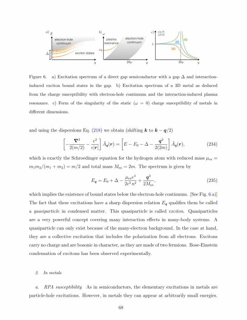
a)E
q
electron-hole continuum
exciton states
q
electron-hole continuum
plasma resonance
b) !
!p
2kF q2kF
c) (q, 0)
(0, 0)
1
1D
3D
2D
Figure 6. a) Excitation spectrum of a direct gap semiconductor with a gap ∆ and interaction-
induced exciton bound states in the gap. b) Excitation spectrum of a 3D metal as deduced
from the charge susceptibility with electron-hole continuum and the interaction-induced plasma
resonance. c) Form of the singularity of the static (ω = 0) charge susceptibility of metals in
different dimensions.
and using the dispersions Eq. (218) we obtain (shifting k to k − q/2)[− ∇2
2(m/2)− e2
ε|r|
]Aq(r) =
[E − E0 −∆− q2
2(2m)
]Aq(r), (234)
which is exactly the Schroedinger equation for the hydrogen atom with reduced mass µex =
m1m2/(m1 +m2) = m/2 and total mass Mex = 2m. The spectrum is given by
Eq = E0 + ∆− µexe4
2ε2 n2+
q2
2Mex
, (235)
which implies the existence of bound states below the electron-hole continuum. [See Fig. 6 a)]
The fact that these excitations have a sharp dispersion relation Eq qualifies them be called
a quasiparticle in condensed matter. This quasiparticle is called exciton. Quasiparticles
are a very powerful concept covering many interaction effects in many-body systems. A
quasiparticle can only exist because of the many-electron background. In the case at hand,
they are a collective excitation that includes the polarization from all electrons. Excitons
carry no charge and are bosonic in character, as they are made of two fermions. Bose-Einstein
condensation of excitons has been observed experimentally.
2. In metals
a. RPA susceptibility As in semiconductors, the elementary excitations in metals are
particle-hole excitations. However, in metals they can appear at arbitrarily small energies.
68
As a result, the effective Coulomb interaction is not only rescaled as is the case in semicon-
ductors due to the dipolar electric environment, but substantially modified taking the form
e−r/l/r, as we will derive below.
We recall that the noninteracting linear response of a metal to potential perturbation is
given by
δρ(q, ω) = χ0(q, ω)V (q, ω), (236)
with
χ0(q, ω) =1
Ω
∑k
nk+q − nkεk+q − εk − ω − iη
, (237)
where nk = 1/(eβεk + 1) is the occupation number of the band according to the Fermi-Dirac
distribution. We now want to see how the Coulomb interaction changes this response. The
redistribution of electron density δρ(q, ω) due to the external potential V (q, ω) sources an
additional Coulomb potential if interactions are considered. The latter is determined by the
Poisson equation
∇2VC(r, t) = −4πe2δρ(r, t), VC(q, ω) =4πe2
q2δρ(q, ω). (238)
The total potential felt by the electrons is thus the sum of the two contributions
Vtot(q, ω) =V (q, ω) + VC(q, ω)
=V (q, ω) +4πe2
q2δρ(q, ω),
(239)
which is a self-consistent equation for δρ(q, ω) when considered together with
δρ(q, ω) = χ0(q, ω)Vtot(q, ω). (240)
Solving for Vtot(q, ω), we can write
Vtot(q, ω) =1
ε(q, ω)V (q, ω), (241)
where
ε(q, ω) = 1− 4πe2
q2χ0(q, ω) (242)
is called the dynamical dielectric function that describes the renormalization of the external
potential due to the electrons in the metal.
Inserting this in the equation for δρ(q, ω), we find
δρ(q, ω) = χ(q, ω)V (q, ω), (243)
69
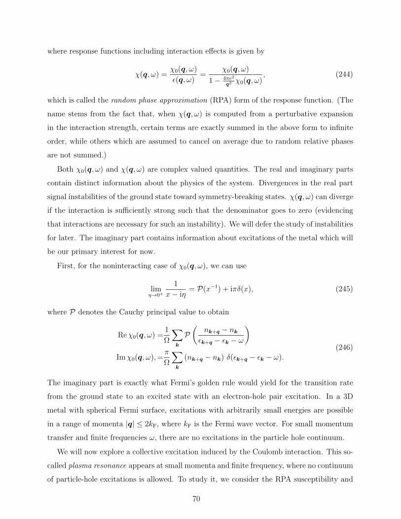
where response functions including interaction effects is given by
χ(q, ω) =χ0(q, ω)
ε(q, ω)=
χ0(q, ω)
1− 4πe2
q2 χ0(q, ω), (244)
which is called the random phase approximation (RPA) form of the response function. (The
name stems from the fact that, when χ(q, ω) is computed from a perturbative expansion
in the interaction strength, certain terms are exactly summed in the above form to infinite
order, while others which are assumed to cancel on average due to random relative phases
are not summed.)
Both χ0(q, ω) and χ(q, ω) are complex valued quantities. The real and imaginary parts
contain distinct information about the physics of the system. Divergences in the real part
signal instabilities of the ground state toward symmetry-breaking states. χ(q, ω) can diverge
if the interaction is sufficiently strong such that the denominator goes to zero (evidencing
that interactions are necessary for such an instability). We will defer the study of instabilities
for later. The imaginary part contains information about excitations of the metal which will
be our primary interest for now.
First, for the noninteracting case of χ0(q, ω), we can use
limη→0+
1
x− iη= P(x−1) + iπδ(x), (245)
where P denotes the Cauchy principal value to obtain
Reχ0(q, ω) =1
Ω
∑k
P(
nk+q − nkεk+q − εk − ω
)Imχ0(q, ω),=
π
Ω
∑k
(nk+q − nk) δ(εk+q − εk − ω).
(246)
The imaginary part is exactly what Fermi’s golden rule would yield for the transition rate
from the ground state to an excited state with an electron-hole pair excitation. In a 3D
metal with spherical Fermi surface, excitations with arbitrarily small energies are possible
in a range of momenta |q| ≤ 2kF, where kF is the Fermi wave vector. For small momentum
transfer and finite frequencies ω, there are no excitations in the particle hole continuum.
We will now explore a collective excitation induced by the Coulomb interaction. This so-
called plasma resonance appears at small momenta and finite frequency, where no continuum
of particle-hole excitations is allowed. To study it, we consider the RPA susceptibility and
70
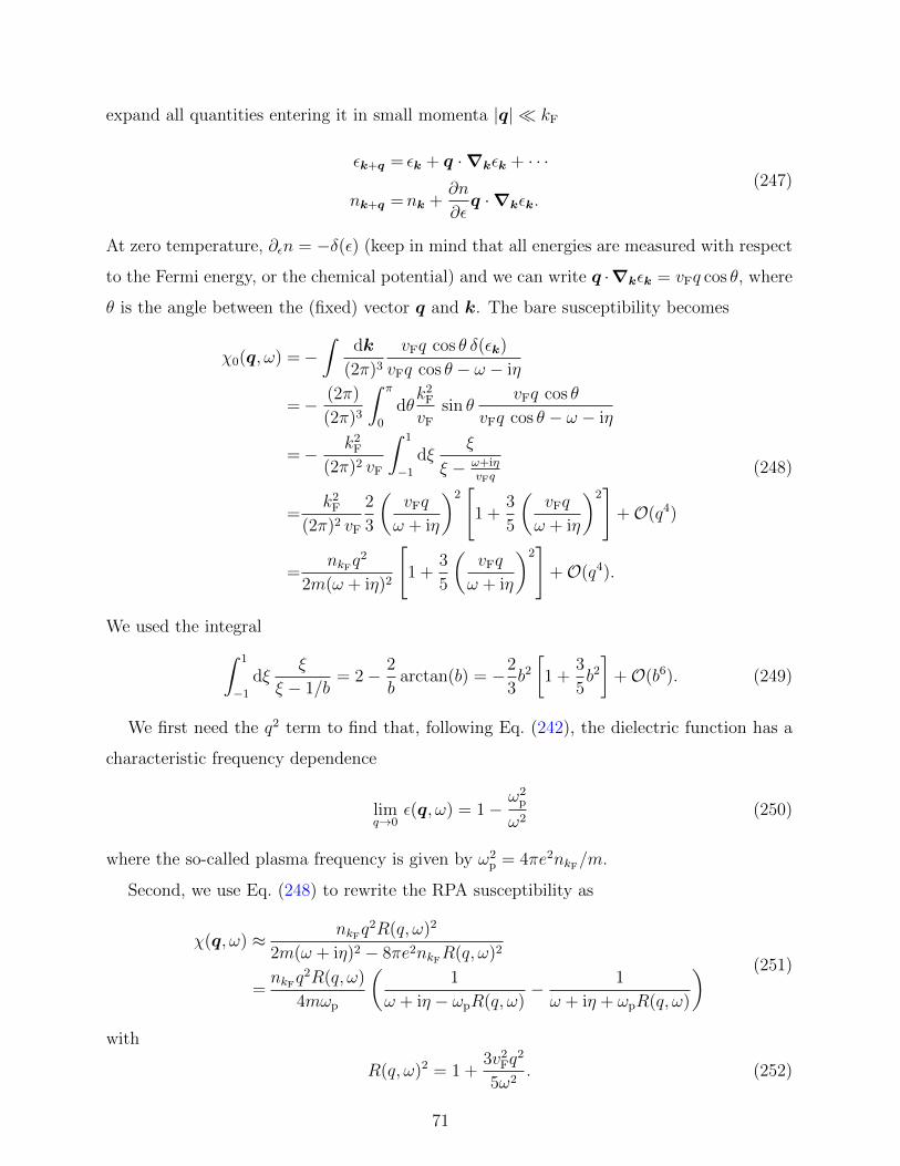
expand all quantities entering it in small momenta |q| kF
εk+q = εk + q ·∇kεk + · · ·
nk+q =nk +∂n
∂εq ·∇kεk.
(247)
At zero temperature, ∂εn = −δ(ε) (keep in mind that all energies are measured with respect
to the Fermi energy, or the chemical potential) and we can write q ·∇kεk = vFq cos θ, where
θ is the angle between the (fixed) vector q and k. The bare susceptibility becomes
χ0(q, ω) =−∫
dk
(2π)3
vFq cos θ δ(εk)
vFq cos θ − ω − iη
=− (2π)
(2π)3
∫ π
0
dθk2
F
vF
sin θvFq cos θ
vFq cos θ − ω − iη
=− k2F
(2π)2 vF
∫ 1
−1
dξξ
ξ − ω+iηvFq
=k2
F
(2π)2 vF
2
3
(vFq
ω + iη
)2[
1 +3
5
(vFq
ω + iη
)2]
+O(q4)
=nkF
q2
2m(ω + iη)2
[1 +
3
5
(vFq
ω + iη
)2]
+O(q4).
(248)
We used the integral∫ 1
−1
dξξ
ξ − 1/b= 2− 2
barctan(b) = −2
3b2
[1 +
3
5b2
]+O(b6). (249)
We first need the q2 term to find that, following Eq. (242), the dielectric function has a
characteristic frequency dependence
limq→0
ε(q, ω) = 1− ω2p
ω2(250)
where the so-called plasma frequency is given by ω2p = 4πe2nkF
/m.
Second, we use Eq. (248) to rewrite the RPA susceptibility as
χ(q, ω) ≈ nkFq2R(q, ω)2
2m(ω + iη)2 − 8πe2nkFR(q, ω)2
=nkF
q2R(q, ω)
4mωp
(1
ω + iη − ωpR(q, ω)− 1
ω + iη + ωpR(q, ω)
) (251)
with
R(q, ω)2 = 1 +3v2
Fq2
5ω2. (252)
71
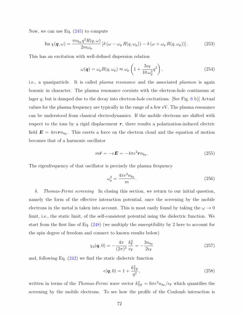
Now, we can use Eq. (245) to compute
Imχ(q, ω) =πnkF
q2R(q, ω)
2mωp
[δ (ω − ωpR(q, ωp))− δ (ω + ωpR(q, ωp))] . (253)
This has an excitation with well-defined dispersion relation
ω(q) = ωpR(q, ωp) ≈ ωp
(1 +
3vF
10ω2p
q2
), (254)
i.e., a quasiparticle. It is called plasma resonance and the associated plasmon is again
bosonic in character. The plasma resonance coexists with the electron-hole continuum at
lager q, but is damped due to the decay into electron-hole excitations. [See Fig. 6 b)] Actual
values for the plasma frequency are typically in the range of a few eV. The plasma resonance
can be understood from classical electrodynamics. If the mobile electrons are shifted with
respect to the ions by a rigid displacement r, there results a polarization-induced electric
field E = 4πernkF. This exerts a force on the electron cloud and the equation of motion
becomes that of a harmonic oscillator
mr = −eE = −4πe2rnkF. (255)
The eigenfrequency of that oscillator is precisely the plasma frequency
ω2p =
4πe2nkF
m. (256)
b. Thomas-Fermi screening In closing this section, we return to our initial question,
namely the form of the effective interaction potential, once the screening by the mobile
electrons in the metal is taken into account. This is most easily found by taking the ω → 0
limit, i.e., the static limit, of the self-consistent potential using the dielectric function. We
start from the first line of Eq. (248) (we multiply the susceptibility by 2 here to account for
the spin degree of freedom and connect to known results below)
χ0(q, 0) = − 4π
(2π)3
k2F
vF
= −3nkF
2εF(257)
and, following Eq. (242) we find the static dielectric function
ε(q, 0) = 1 +k2
TF
q2, (258)
written in terms of the Thomas-Fermi wave vector k2TF = 6πe2nkF
/εF which quantifies the
screening by the mobile electrons. To see how the profile of the Coulomb interaction is
72
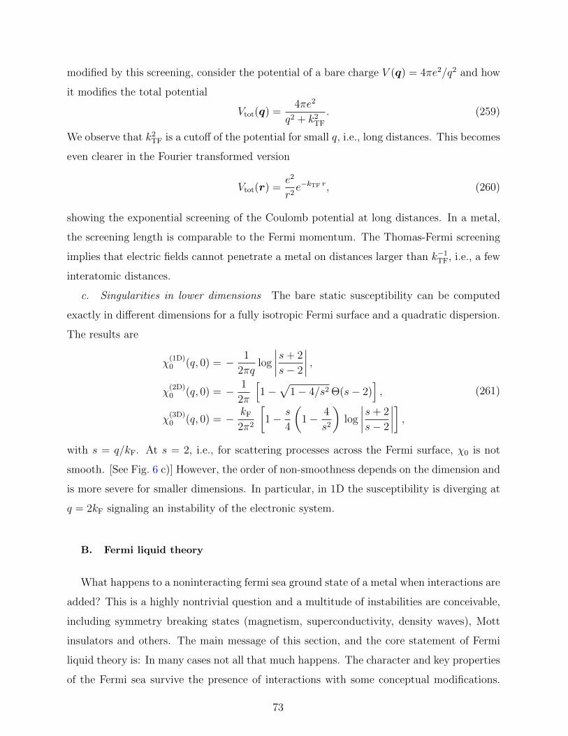
modified by this screening, consider the potential of a bare charge V (q) = 4πe2/q2 and how
it modifies the total potential
Vtot(q) =4πe2
q2 + k2TF
. (259)
We observe that k2TF is a cutoff of the potential for small q, i.e., long distances. This becomes
even clearer in the Fourier transformed version
Vtot(r) =e2
r2e−kTF r, (260)
showing the exponential screening of the Coulomb potential at long distances. In a metal,
the screening length is comparable to the Fermi momentum. The Thomas-Fermi screening
implies that electric fields cannot penetrate a metal on distances larger than k−1TF, i.e., a few
interatomic distances.
c. Singularities in lower dimensions The bare static susceptibility can be computed
exactly in different dimensions for a fully isotropic Fermi surface and a quadratic dispersion.
The results are
χ(1D)0 (q, 0) = − 1
2πqlog
∣∣∣∣s+ 2
s− 2
∣∣∣∣ ,χ
(2D)0 (q, 0) = − 1
2π
[1−
√1− 4/s2 Θ(s− 2)
],
χ(3D)0 (q, 0) = − kF
2π2
[1− s
4
(1− 4
s2
)log
∣∣∣∣s+ 2
s− 2
∣∣∣∣] ,(261)
with s = q/kF. At s = 2, i.e., for scattering processes across the Fermi surface, χ0 is not
smooth. [See Fig. 6 c)] However, the order of non-smoothness depends on the dimension and
is more severe for smaller dimensions. In particular, in 1D the susceptibility is diverging at
q = 2kF signaling an instability of the electronic system.
B. Fermi liquid theory
What happens to a noninteracting fermi sea ground state of a metal when interactions are
added? This is a highly nontrivial question and a multitude of instabilities are conceivable,
including symmetry breaking states (magnetism, superconductivity, density waves), Mott
insulators and others. The main message of this section, and the core statement of Fermi
liquid theory is: In many cases not all that much happens. The character and key properties
of the Fermi sea survive the presence of interactions with some conceptual modifications.
73
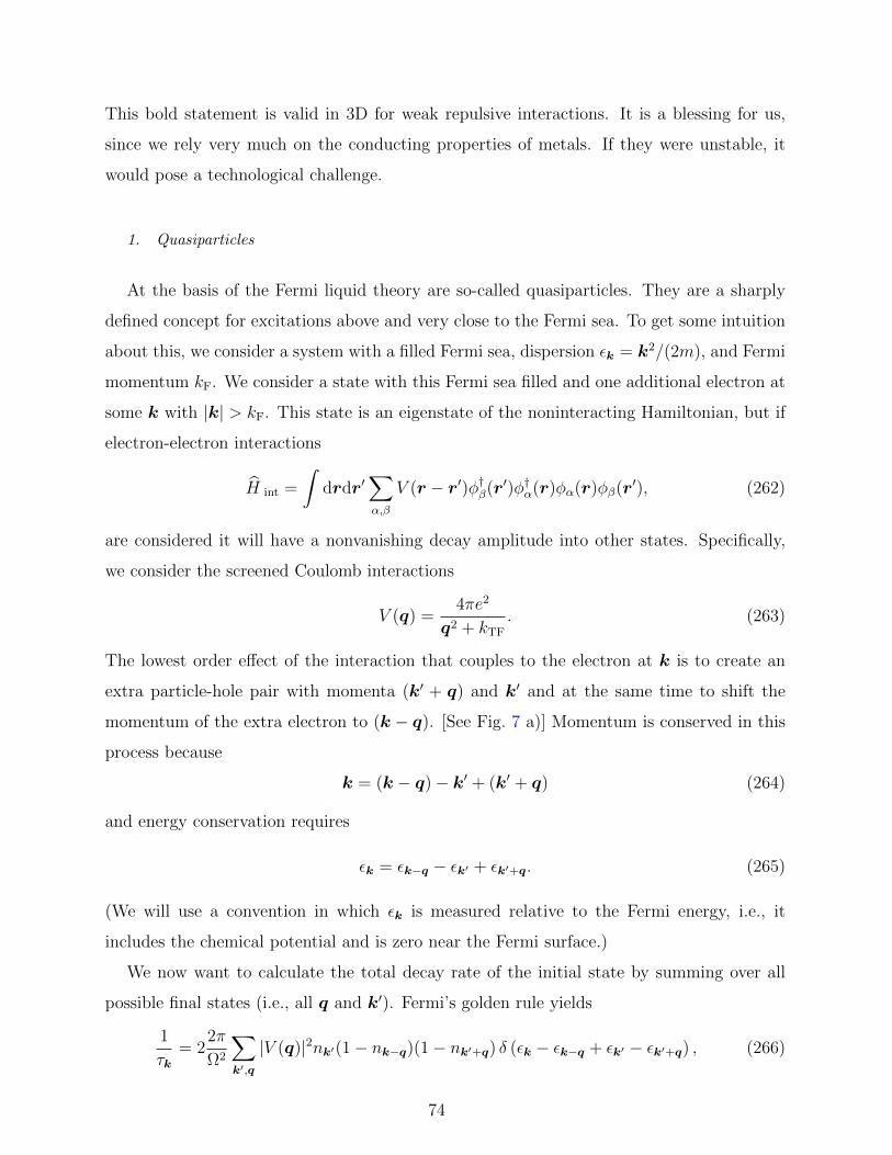
This bold statement is valid in 3D for weak repulsive interactions. It is a blessing for us,
since we rely very much on the conducting properties of metals. If they were unstable, it
would pose a technological challenge.
1. Quasiparticles
At the basis of the Fermi liquid theory are so-called quasiparticles. They are a sharply
defined concept for excitations above and very close to the Fermi sea. To get some intuition
about this, we consider a system with a filled Fermi sea, dispersion εk = k2/(2m), and Fermi
momentum kF. We consider a state with this Fermi sea filled and one additional electron at
some k with |k| > kF. This state is an eigenstate of the noninteracting Hamiltonian, but if
electron-electron interactions
H int =
∫drdr′
∑α,β
V (r − r′)φ†β(r′)φ†α(r)φα(r)φβ(r′), (262)
are considered it will have a nonvanishing decay amplitude into other states. Specifically,
we consider the screened Coulomb interactions
V (q) =4πe2
q2 + kTF
. (263)
The lowest order effect of the interaction that couples to the electron at k is to create an
extra particle-hole pair with momenta (k′ + q) and k′ and at the same time to shift the
momentum of the extra electron to (k − q). [See Fig. 7 a)] Momentum is conserved in this
process because
k = (k − q)− k′ + (k′ + q) (264)
and energy conservation requires
εk = εk−q − εk′ + εk′+q. (265)
(We will use a convention in which εk is measured relative to the Fermi energy, i.e., it
includes the chemical potential and is zero near the Fermi surface.)
We now want to calculate the total decay rate of the initial state by summing over all
possible final states (i.e., all q and k′). Fermi’s golden rule yields
1
τk= 2
2π
Ω2
∑k′,q
|V (q)|2nk′(1− nk−q)(1− nk′+q) δ (εk − εk−q + εk′ − εk′+q) , (266)
74
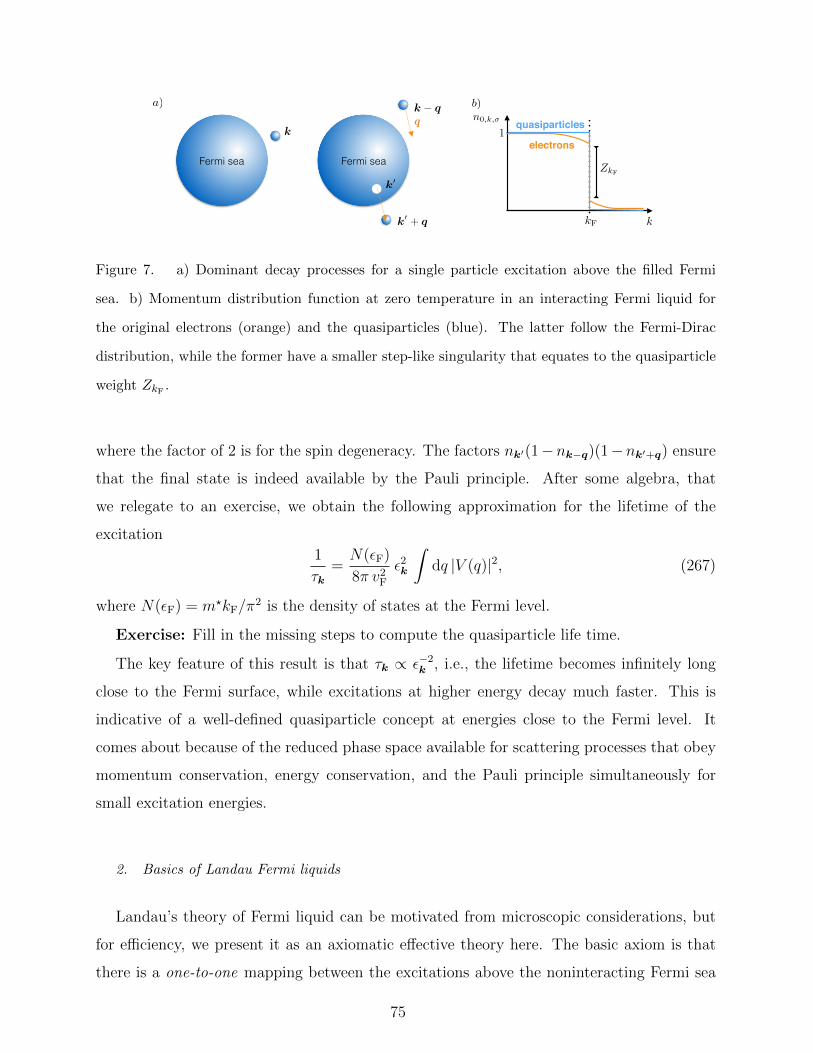
a)
Fermi sea
k
Fermi sea
k q
k0 + q
k0
q
b)
1electrons
quasiparticles
kF k
n0,k,
ZkF
Figure 7. a) Dominant decay processes for a single particle excitation above the filled Fermi
sea. b) Momentum distribution function at zero temperature in an interacting Fermi liquid for
the original electrons (orange) and the quasiparticles (blue). The latter follow the Fermi-Dirac
distribution, while the former have a smaller step-like singularity that equates to the quasiparticle
weight ZkF.
where the factor of 2 is for the spin degeneracy. The factors nk′(1−nk−q)(1−nk′+q) ensure
that the final state is indeed available by the Pauli principle. After some algebra, that
we relegate to an exercise, we obtain the following approximation for the lifetime of the
excitation
1
τk=N(εF)
8π v2F
ε2k
∫dq |V (q)|2, (267)
where N(εF) = m?kF/π2 is the density of states at the Fermi level.
Exercise: Fill in the missing steps to compute the quasiparticle life time.
The key feature of this result is that τk ∝ ε−2k , i.e., the lifetime becomes infinitely long
close to the Fermi surface, while excitations at higher energy decay much faster. This is
indicative of a well-defined quasiparticle concept at energies close to the Fermi level. It
comes about because of the reduced phase space available for scattering processes that obey
momentum conservation, energy conservation, and the Pauli principle simultaneously for
small excitation energies.
2. Basics of Landau Fermi liquids
Landau’s theory of Fermi liquid can be motivated from microscopic considerations, but
for efficiency, we present it as an axiomatic effective theory here. The basic axiom is that
there is a one-to-one mapping between the excitations above the noninteracting Fermi sea
75
(free electrons) and the excitations above the interacting many-body ground states (quasi-
particles). We denote the momentum distribution function of the quasiparticles by nk,σ and
that of the electrons by nk,σ, where σ = ± denotes the spin. The total number of electrons
equals the number of quasiparticles
N =∑k,σ
nk,σ =∑k,σ
nk,σ. (268)
One now postulates that the distribution function of the quasiparticles in equilibrium follows
the Fermi-Dirac distribution n0,k,σ. As a consequence, the electronic distribution function
becomes distorted. In particular, the jump at kF at T = 0 is reduced from 1 to a smaller
value (but there is still a jump). The jump height is called quasi-particle weight ZkF. [See
Fig. 7 b)]
The object of interest in the Fermi liquid theory are the deviations from the equilibrium
quasiparticle distribution function
δnk,σ = nk,σ − n0,k,σ, (269)
which is a small expansion parameter in the theory. Central is an expansion of the energy
as a functional of this parameter
E[δn] = E0 +∑k,σ
εσ,kδnk,σ +1
Ω
∑k,k′
∑σ,σ′
fk,k′;σ,σ′ δnk,σ δnk′,σ′ +O(δn3), (270)
where E0 is the ground state energy, and εσ,k as well as fk,k′;σ,σ′ are phenomenological param-
eters at this stage which can be determined from a microscopic derivation or experimental
input. The variational derivative with respect to δn yields a renormalized effective dispersion
of the quasiparticles due to the interaction with the perturbed background quasiparticles
εk,σ = εk,σ +1
Ω
∑k′,σ′
fk,k′;σ,σ′ δnk′,σ′ . (271)
To obtain a more practical set of parameters in a perturbative regime, one ignores the
radial dependence of fk,k′;σ,σ′ on k and k′ so that the only relevant variable is the angle θ
between k and k′, which are both assumed to lie on the Fermi surface. We can then expand
fk,k′;σ,σ′ in Legendre polynomials
fk,k′;σ,σ′ ≈ fθ;σ,σ′ =∞∑l=0
(f sl + σσ′f a
l )Pl(cos θ), (272)
76
where we have also split up each coefficient into a spin-symmetric f sl and a spin-asymmetric
part f al . When rescaled by the density of states at the Fermi level ν(εF), these parameters
are known as the Landau parameters of the theory
F sl = ν(εF) f s
l , F al = ν(εF) f a
l . (273)
The density of states at the Fermi surface is defined as
ν(εF) =2
Ω
∑k
δ(εk − εF) =k2
F
π2vF
=m?kF
π2(274)
and follows from the dispersion εk of the bare quasiparticle energy
∇εk|kF= vF =
kF
m?(275)
where for a fully rotation symmetric system we may write εk = k2/(2m?) with m? as an
“effective mass”, although we will be only interested at the spectrum in the immediate
vicinity of the Fermi energy.
3. Specific heat – Density of states
Since the quasiparticles are fermions, they obey Fermi-Dirac statistics fF−D(ε) = 1/(eβε+
1) which is their equilibrium distribution function
n0,k,σ(T ) =1
e(εk−µ)/(kBT ) + 1(276)
with the chemical potential µ. For low temperatures and an otherwise undisturbed system,
their deviation must obey
δnk,σ = n0,k,σ(T )− n0,k,σ(0) (277)
which, using Eq. (278) leads to εk,σ = εk,σ because here
0 =1
Ω
∑k′,σ′
fk,k′;σ,σ′ δnk′,σ′ , (278)
due to the fact that in δnk,σ there are as many particles (positive) as holes (negative)
such that they cancel in the correction term that measures the overall charge imbalance.
Therefore we rewrite the Fermi-Dirac distribution (276) as
n0,k,σ(T ) =1
e(εk−εF)/(kBT ) + 1. (279)
77
In doing so, we have also replaced the chemical potential µ by the Fermi energy εF which
is justified at low temperatures because µ = εF + O(T 2). We are interested in leading
corrections, which are usually of the order T 0 and T 1, and corrections of higher order may
therefore be neglected in the low-temperature regime. In order to discuss the specific heat,
we employ the expression for the entropy of a fermion gas. For each quasiparticle species
with a given spin there is one state labelled by k. The entropy density of independent
degrees of freedom may be computed from the distribution function
S = −kB
∑k,σ
nσ,kln(nσ,k) + (1− nσ,k) ln(1− nσ,k). (280)
Taking the derivative of the entropy S with respect to T , the specific heat is obtained as
C(T ) =T∂S
∂T
=− kBT
Ω
∑k,σ
eξk/(kBT )
(eξk/(kBT ) + 1)2
ξkkBT 2
ln
(nk,σ
1− nk,σ
)=− kBT
Ω
∑k,σ
1
4 cosh2 [ξk/(2kBT )]
ξkkBT 2
ξkkBT
,
(281)
where we introduced ξk = εk − εF. In the limit T → 0 we find
C(T )
T≈ ν(εF)
4kBT 3
∫dξ
ξ2
cosh2 [ξ/(2kBT )]
=k2
Bν(εF)
4
∫dy
y
cosh2 (y/2)
=π2k2
Bν(εF)
3
(282)
which is the well-known linear behavior C(T ) = γT for the specific heat at low temperatures,
with γ = π2k2Bν(εF)/3 the Sommerfeld coefficient. Since ν(εF) = m?kF/π
2, the effective mass
m? of the quasiparticles can directly determined by measuring the specific heat of the system.
4. Compressibility and susceptibility
As an application of the Fermi liquid theory, we compute its compressibility and magnetic
susceptibility. The former is defined by
κ = − 1
Ω
(∂Ω
∂p
)T,N
, (283)
78
where p is the uniform pressure exerted on the system. The quasiparticle energy levels are
affected by the pressure as
δεk,σ =∂εk,σ∂p
δp
=∂εk,σ∂k· ∂k∂Ω
∂Ω
∂pδp
=vk ·k
3κ(0)δp
≈ 2εF3κ(0)δp,
(284)
where we assumed to be close to the Fermi surface to obtain the last line and we used
k = n2π/Ω1/3. We are after the analogous equation for the renormalized quasiparticle
dispersion and the compressibility of the Fermi liquid κ
δεk,σ =2εF3κδp. (285)
To obtain it, we start with the definition of εk,σ and use Eq. (284) for the first term (here,
δεk,σ = εk,σ − εk,σ)
δεk,σ =2εF3κ(0)δp+
1
Ω
∑k′,σ′
fk,k′;σ,σ′δnk′,σ′
=2εF3κ(0)δp+
1
Ω
∑k′,σ′
fk,k′;σ,σ′∂nk′,σ′
∂pδp
=2εF3κ(0)δp+
1
Ω
∑k′,σ′
fk,k′;σ,σ′∂nk′,σ′
∂εk′,σ′δεk′,σ′
=2εF3κ(0)δp− 1
Ω
∑k′,σ′
fk,k′;σ,σ′δ(εk′,σ′ − εF)2εF3κδp.
(286)
Since εk′,σ′ is isotropic, this brings about exactly the l = 0 Landau parameter and we have
κ = κ(0) − κF s0 , κ =
κ(0)
1 + F s0
. (287)
Without derivation we also state the unperturbed compressibility of the Fermi liquid 1/κ(0) =
2nεF/3.
By similar considerations, we can compute the magnetic susceptibility of the Fermi liquid
χ =1
Ω
∂M
∂B
=µ2
Bν(εF)
1 + F a0
.(288)
79
Common to Eqs. (287) and (288) is that the Fermi liquid parameter appears in the denom-
inator, indicating the possibility of a divergence (when it reaches the value −1), i.e., an
instability of the system. However, for small Fa/s0 , i.e., weak interactions, the Fermi liquid is
stable, as promised. This proof can be extended to all angular momentum channels where
a similar form is found. A divergence of the magnetic susceptibility indicates a tendency
to (ferro-)magnetic order. This constitutes the so-called Stoner instability which we will
encounter again from a more microscopic viewpoint.
5. Galilei invariance – effective mass and F s1
We initially introduced by hand the effective mass of quasiparticles in εk,σ. In this section
we show, that overall consistency of the phenomenological theory requires a relation between
the effective mass and one Landau parameter, namely F s1 . The reason is, that the effective
mass is the result of the interactions among the electrons. This self-consistency is connected
with the Galilean invariance of the system.
To illustrate this, we consider a situation in which the momenta of all particles are shifted
by q as a perturbation to the Fermi liquid (|q| shall be very small compared to the Fermi
momentum kF in order to remain within the assumption-range of the Fermi liquid theory).
The distribution function is given by
δnσ,k = n(0)σ,k+q − n
(0)σ,k ≈ q ·∇kn
(0)σ,k. (289)
This function is strongly concentrated around the Fermi energy, as the derivative of n(0)σ,k
tends to zero far away from it.
The current density can now be calculated, using the distribution function nσ,k = n(0)σ,k +
δnσ,k. Within the Fermi liquid theory this yields,
jq =1
Ω
∑k,σ
vknσ,k (290)
with
vk =∇kεk,σ
=∇kεk,σ +1
Ω
∑k′,σ′
∇kfk,k′;σ,σ′ δnk′,σ′(291)
80
With this we obtain the current density
jq =1
Ω
∑k,σ
k
m?nσ,k +
1
Ω2
∑k,σ
∑k′,σ′
(n
(0)σ,k + δnσ,k
)∇kfk,k′;σ,σ′ δnσ′,k′
=1
Ω
∑k,σ
k
m?δnσ,k −
1
Ω2
∑k,σ
∑k′,σ′
(∇kn
(0)σ,k
)fk,k′;σ,σ′ δnσ′,k′ +O(q2)
=1
Ω
∑k,σ
k
m?δnσ,k +
1
Ω2
∑k,σ
∑k′,σ′
δ (εk′,σ − εF)k′
m?fk,k′;σ,σ′ δnσ,k +O(q2)
≡ j1 + j2,
(292)
where in the second line we integrated by parts and neglected terms quadratic in δn and to
reach the third line, we used fk,k′;σ,σ′ = fk′,k;σ′,σ as well as
∇kn(0)σ,k =
∂n(0)σ,k
∂εk,σ∇kεk,σ = −δ(εk,σ − εF)∇kεk,σ = −δ(εk,σ − εF)
k
m?. (293)
The current j1 denotes the quasiparticle current, while the second term j2 can be interpreted
as a drag-current, i.e., an induced motion (backflow) of the other particles due to interactions.
From a different viewpoint, we consider the system as being in the inertial frame with a
velocity |q|/m, as all particles received the same momentum. Here m is the bare electron
mass. The current density is then given by
jq =N
Ω
q
m=
1
Ω
∑k,σ
k
mnσ,k =
1
Ω
∑k,σ
k
mδnσ,k (294)
Since these two viewpoints have to be equivalent, the resulting currents should be the same.
Thus, we compare Eq. (292) and Eq. (294) and obtain the equation,
k
m=k
m?+
1
Ω
∑k′,σ′
fk,k′;σ,σ′δ(εk′,σ′ − εF)k′
m?(295)
which with k = k/kF then leads to
1
m=
1
m?+ ν(εF)
∫dΩ k ′
4π
∑l
f sl Pl(cos θ)
k · k ′m?
=1
m?+ ν(εF)
∫dΩ k ′
4π
∑l
f sl Pl(cos θ)
P1(cos θ)
m?
(296)
or by using the orthogonality of the Legendre polynomials,
m?
m= 1 +
1
3F s
1 , (297)
81
where 1/3 = 1/(2l + 1) for l = 1 originates from the orthogonality relation of Legendre-
polynomials. Therefore, the relation (297) has to couplem? to F s1 in order for Landaus theory
of Fermi liquids to be self-consistent. Generally, we find that F s1 > 0 so that quasiparticles
in a Fermi liquid are effectively heavier than bare electrons.
6. Stability of a Fermi liquid
Upon inspection of the renormalization of the quantities treated previously
γ
γ0
=m?
m,
κ
κ0
=m?
m
1
1 + F s0
,
χ
χ0
=m?
m
1
1 + F a0
,
(298)
withm?
m= 1 +
1
3F s
1 , (299)
and the the response functions of the non-interacting system are given by
γ0 =kBmkF
3, κ0 =
3m
nk2F
, χ0 = µ2B
mkF
π2, (300)
one notes that the compressibility κ (susceptibility χ) diverges for F s0 → −1 (F a
0 → −1),
indicating an instability of the system. A diverging spin susceptibility for example leads to
a ferromagnetic state with a split Fermi surface, one for each spin direction. On the other
hand, a diverging compressibility leads to a spontaneous contraction of the system. More
generally, the deformation of the quasiparticle distribution function may vary over the Fermi
surface, so that arbitrary deviations of the Fermi liquid ground state may be classified by
the deformation
δnσ, k =∞∑l=0
l∑m=−l
δnσ,l,mYl,m(θ k , φ k ). (301)
Note that we allow here formally for complex distribution functions. For pure charge density
deformations we have δn+,l,m = δn−,l,m, while pure spin density deformations are described
by δn+,l,m = −δn−,l,m. The general response function for a redistribution δnσ, k with the
anisotropy Yl,m(θ k , φ k ) is given by
χl,m =χ
(0)l,m
1 +F s,al
2l+1
(302)
82
Stability of the Fermi liquid against any of these deformations requires
1 +F s,al
2l + 1> 0 (303)
If for any deformation channel l this conditions is violated one talks about a “Pomeranchuck
instability”. Generally, the renormalization of the Fermi liquid leads to a change in the
Wilson ratio, defined as
R
R0
=χ
χ0
γ0
γ=
1
1 + F a0
(304)
where R0 = χ0/γ0 = 6µ2B/(π
2k2B). Note that the Wilson ratio does not depend on the
effective mass. A remarkable feature of the Fermi liquid theory is that even very strongly
interacting Fermions remain Fermi liquids, notably the quantum liquid 3He and so-called
heavy Fermion systems, which are compounds of transition metals and rare earths. Both
are strongly renormalized Fermi liquids. For 3He one observes that the higher the applied
pressure is, the denser the liquid becomes and the stronger the quasiparticles interact. As
a result, the Fermi liquid parameters and the effective mass increase with pressure. Ap-
proaching the solidification the compressibility is reduced, the quasiparticles become heavier
(slower) and the magnetic response increases drastically. Finally the heavy fermion systems
are characterized by the extraordinary enhancements of the effective mass which for many
of these compounds lies between 100 and 1000 times the bare electron mass (e.g., CeAl3,
UBe13). These large masses lead the notion of almost localized Fermi liquids, since the large
effective mass is induced by the hybridization of itinerant conduction electrons with strongly
interacting (localized) electron states in partially filled 4f - or 5f -orbitals of Lanthanide and
Actinide atoms, respectively.
7. Microscopic justification
A rigorous derivation of Landaus Fermi liquid theory requires methods of quantum
field theory and would go beyond the scope of these lectures. However, plain Rayleigh-
Schroedinger perturbation theory applied to a simple model allows to gain some insights
into the microscopic fundament of this phenomenologically based theory. In the follow-
ing, we consider a model of fermions with contact interaction Uδ(r − r′), described by the
83
Hamiltonian
H =∑k,σ
εk c†σ,k c σ,k +
∫d3rd3r′ φ †↑(r) φ †↓(r
′)Uδ(r − r′) φ ↓ φ ↑(r)
=∑k,σ
εk c†σ,k c σ,k +
U
Ω
∑k,k′,q
c †↑,k+q c†↓,k′−q c ↓,k′ c ↑,k
(305)
where εk = k2/2m is a parabolic dispersion of non-interacting electrons. We previously no-
ticed that, in order to find well-defined quasiparticles, the interaction between the Fermions
has to be short ranged. This specially holds for the contact interaction.
Starting form the Hamiltonian (305), we will determine Landau parameters for a cor-
responding Fermi liquid theory. For a given momentum distribution nσ,k = 〈 c †σ,k c σ,k〉 =
n(0)σ,k+δnσ,k, we can expand the energy resulting form equation (305) following the Rayleigh-
Schroedinger perturbation method,
E = E(0) + E(1) + E(2) + · · · (306)
with
E(0) =∑k,σ
εknσ,k
E(1) =U
Ω
∑k,k′
n↑,k′n↓,k
E(2) =U2
Ω2
∑k,k′,q
n↑,kn↓,k′(1− n↑,k+q)(1− n↓,k′−q)εk + εk′ − εk+q − εk′−q
(307)
The second order term E(2) describes virtual processes corresponding to a pair of particle-
hole excitations. The numerator of this term can be split into the corresponding four different
contributions. We first consider the term quadratic in nk and combine it with the first order
term E(1), which has the same structure,
E(1) = E(1) +U2
Ω2
∑k,k′,q
n↑,kn↓,kεk + εk′ − εk+q − εk′−q
≈ U
Ω
∑k,k′
n↑,kn↓,k′ (308)
In the last step, we defined the renormalized interaction U through
U = U +U2
Ω
∑q
1
εk + εk′ − εk+q − εk′−q(309)
In principle, U depends on the wave vectors k and k′. However, when the wave vectors
are restricted to the Fermi surface (|k| = |k′| = kF), and if the range of the interaction
84
` is small compared to the mean electron spacing, i.e., kF` 1, this dependency may be
neglected. (We should be careful with our choice of a contact interaction, since it would
lead to a divergence in the large-q range. A cutoff for q of order Qc ∼ `−1 would regularize
the integral which is dominated by the large-q part.)
Since the term quartic in nk vanishes due to symmetry, the remaining contribution to
E(2) is cubic in nk and reads
E(2) = − U2
Ω2
∑k,k′,q
n↑,kn↓,k(n↑,k+q + n↓,k′−q)
εk + εk′ − εk+q − εk′−q(310)
We replaced U2 by U2, which is admissible at this order of the perturbative expansion. The
variation of the energy E in Eq. (306) with respect to δn↑,k can easily be calculated
εk,↑ = εk +U
Ω
∑k′
n↓,k′ −U2
Ω2
∑k′,q
n↓,k′(n↑,k+q + n↓,k′−q)− n↑,k+qn↓,k′−qεk + εk′ − εk+q − εk′−q
, (311)
and an analogous expression is found for εk,↓. The coupling parameters fk,k′;σσ′ may be
determined using the definition (278). Starting with fkF,k′F;σσ′ with wave-vectors on the
Fermi surface (|kF| = |k′F| = kF), the terms contributing to the coupling can be written as
U2
Ω2
∑k′,q
n↑,k+qn↓,k′−q − n↓,k′
εk + εk′ − εk+q − εk′−qk+q→k′F→ 1
Ω
∑k′F
n↑,k′FU2
Ω
∑k′
n(0)↓,k′−q − n
(0)↓,k′
εk′ − εk′−q
∣∣∣∣∣q=k′F−kF
= − 1
Ω
∑k′F
n↑,k′FU2
2χ0(k′F − kF)
(312)
where we consider n↑,k′F = n(0)
↑,k′F+ δn↑,k′F . Note that the part in this term which depends on
n(0)
↑,k′Fwill contribute the ground state energy in Landaus energy functional. Here, χ0(q) is
the static spin susceptibility. With the help of Eq. (278), it follows immediately, that
fkF,k′F;↑↑ = fkF,k
′F;↓↓ =
U2
2χ0(kF − k′F) (313)
The other couplings are obtained in a similar way, resulting in
fkF,k′F;↑↓ = fkF,k
′F;↓↑ = U − U2
2[2χ0(kF + k′F)− χ0(kF − k′F)] (314)
where the function χ0(q) is defined as
χ0(q) =1
Ω
∑k′
n(0)↑,k′+q + n
(0)↓,k′
2εF − εk′+q − εk′(315)
85
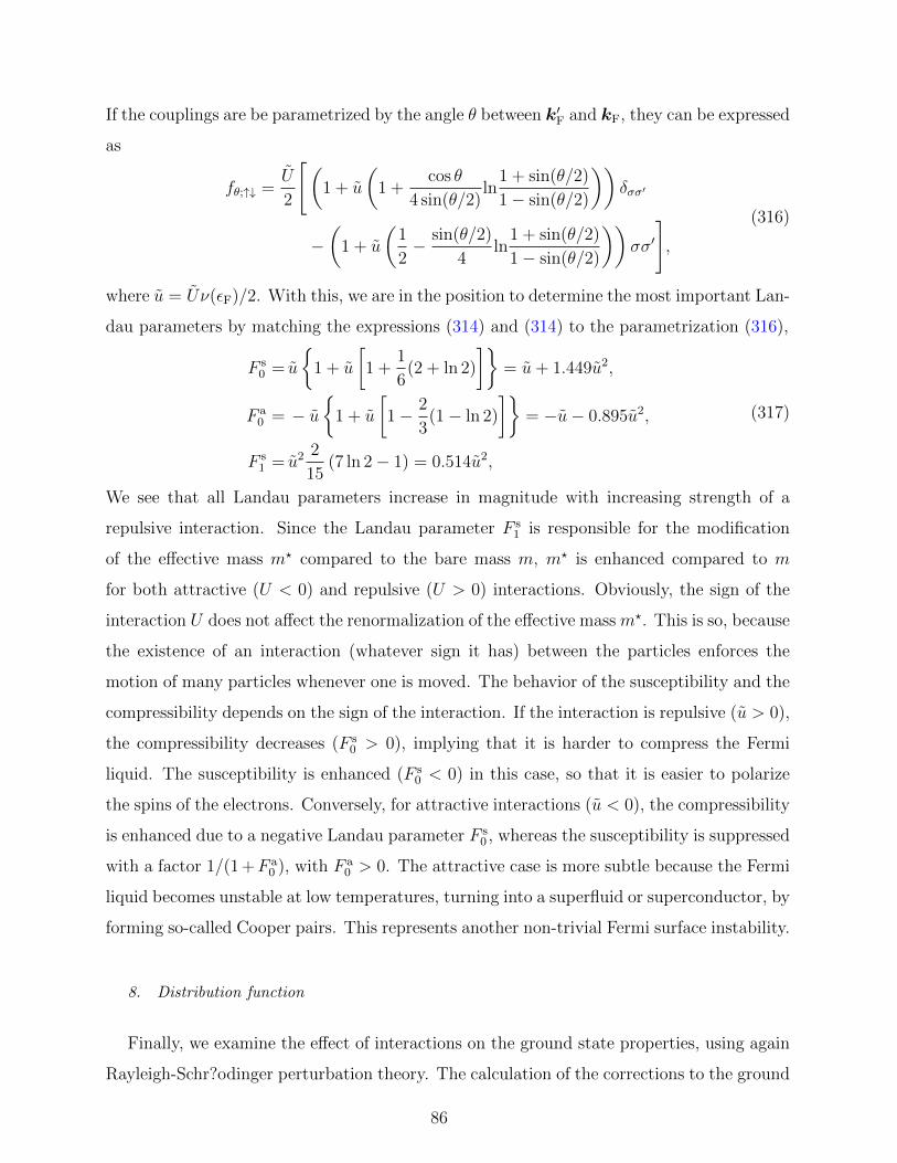
If the couplings are be parametrized by the angle θ between k′F and kF, they can be expressed
as
fθ;↑↓ =U
2
[(1 + u
(1 +
cos θ
4 sin(θ/2)ln
1 + sin(θ/2)
1− sin(θ/2)
))δσσ′
−(
1 + u
(1
2− sin(θ/2)
4ln
1 + sin(θ/2)
1− sin(θ/2)
))σσ′
],
(316)
where u = Uν(εF)/2. With this, we are in the position to determine the most important Lan-
dau parameters by matching the expressions (314) and (314) to the parametrization (316),
F s0 = u
1 + u
[1 +
1
6(2 + ln 2)
]= u+ 1.449u2,
F a0 = − u
1 + u
[1− 2
3(1− ln 2)
]= −u− 0.895u2,
F s1 = u2 2
15(7 ln 2− 1) = 0.514u2,
(317)
We see that all Landau parameters increase in magnitude with increasing strength of a
repulsive interaction. Since the Landau parameter F s1 is responsible for the modification
of the effective mass m? compared to the bare mass m, m? is enhanced compared to m
for both attractive (U < 0) and repulsive (U > 0) interactions. Obviously, the sign of the
interaction U does not affect the renormalization of the effective mass m?. This is so, because
the existence of an interaction (whatever sign it has) between the particles enforces the
motion of many particles whenever one is moved. The behavior of the susceptibility and the
compressibility depends on the sign of the interaction. If the interaction is repulsive (u > 0),
the compressibility decreases (F s0 > 0), implying that it is harder to compress the Fermi
liquid. The susceptibility is enhanced (F s0 < 0) in this case, so that it is easier to polarize
the spins of the electrons. Conversely, for attractive interactions (u < 0), the compressibility
is enhanced due to a negative Landau parameter F s0 , whereas the susceptibility is suppressed
with a factor 1/(1 +F a0 ), with F a
0 > 0. The attractive case is more subtle because the Fermi
liquid becomes unstable at low temperatures, turning into a superfluid or superconductor, by
forming so-called Cooper pairs. This represents another non-trivial Fermi surface instability.
8. Distribution function
Finally, we examine the effect of interactions on the ground state properties, using again
Rayleigh-Schr?odinger perturbation theory. The calculation of the corrections to the ground
86
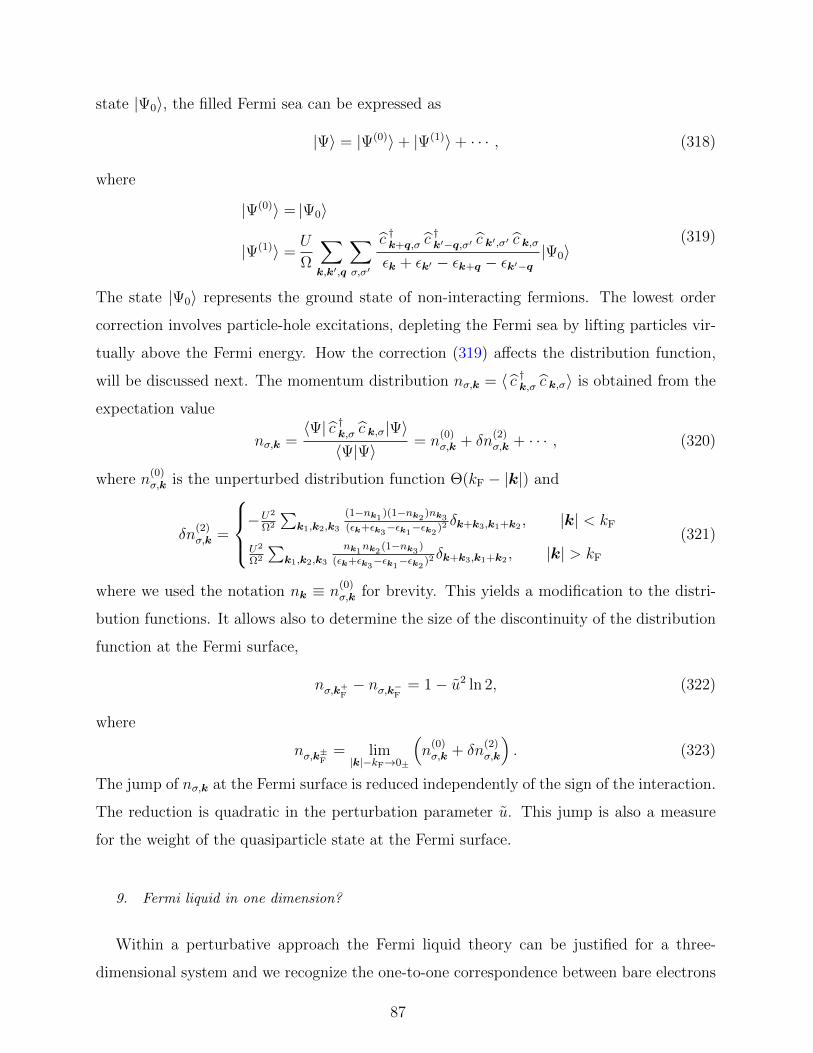
state |Ψ0〉, the filled Fermi sea can be expressed as
|Ψ〉 = |Ψ(0)〉+ |Ψ(1)〉+ · · · , (318)
where
|Ψ(0)〉 = |Ψ0〉
|Ψ(1)〉 =U
Ω
∑k,k′,q
∑σ,σ′
c †k+q,σ c†k′−q,σ′ c k′,σ′ c k,σ
εk + εk′ − εk+q − εk′−q|Ψ0〉
(319)
The state |Ψ0〉 represents the ground state of non-interacting fermions. The lowest order
correction involves particle-hole excitations, depleting the Fermi sea by lifting particles vir-
tually above the Fermi energy. How the correction (319) affects the distribution function,
will be discussed next. The momentum distribution nσ,k = 〈 c †k,σ c k,σ〉 is obtained from the
expectation value
nσ,k =〈Ψ| c †k,σ c k,σ|Ψ〉〈Ψ|Ψ〉 = n
(0)σ,k + δn
(2)σ,k + · · · , (320)
where n(0)σ,k is the unperturbed distribution function Θ(kF − |k|) and
δn(2)σ,k =
−U2
Ω2
∑k1,k2,k3
(1−nk1)(1−nk2
)nk3
(εk+εk3−εk1
−εk2)2 δk+k3,k1+k2 , |k| < kF
U2
Ω2
∑k1,k2,k3
nk1nk2
(1−nk3)
(εk+εk3−εk1
−εk2)2 δk+k3,k1+k2 , |k| > kF
(321)
where we used the notation nk ≡ n(0)σ,k for brevity. This yields a modification to the distri-
bution functions. It allows also to determine the size of the discontinuity of the distribution
function at the Fermi surface,
nσ,k+F− nσ,k−F = 1− u2 ln 2, (322)
where
nσ,k±F= lim|k|−kF→0±
(n
(0)σ,k + δn
(2)σ,k
). (323)
The jump of nσ,k at the Fermi surface is reduced independently of the sign of the interaction.
The reduction is quadratic in the perturbation parameter u. This jump is also a measure
for the weight of the quasiparticle state at the Fermi surface.
9. Fermi liquid in one dimension?
Within a perturbative approach the Fermi liquid theory can be justified for a three-
dimensional system and we recognize the one-to-one correspondence between bare electrons
87
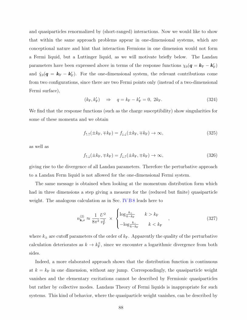
and quasiparticles renormalized by (short-ranged) interactions. Now we would like to show
that within the same approach problems appear in one-dimensional systems, which are
conceptional nature and hint that interaction Fermions in one dimension would not form
a Fermi liquid, but a Luttinger liquid, as we will motivate briefly below. The Landau
parameters have been expressed above in terms of the response functions χ0(q = kF − k′F)
and χ0(q = kF − k′F). For the one-dimensional system, the relevant contributions come
from two configurations, since there are two Fermi points only (instead of a two-dimensional
Fermi surface),
(kF, k′F) ⇒ q = kF − k′F = 0, 2kF. (324)
We find that the response functions (such as the charge susceptibility) show singularities for
some of these momenta and we obtain
f↑,↑(±kF,∓kF) = f↓,↓(±kF,∓kF)→∞, (325)
as well as
f↑,↓(±kF,∓kF) = f↓,↑(±kF,∓kF)→∞, (326)
giving rise to the divergence of all Landau parameters. Therefore the perturbative approach
to a Landau Ferm liquid is not allowed for the one-dimensional Fermi system.
The same message is obtained when looking at the momentum distribution form which
had in three dimensions a step giving a measure for the (reduced but finite) quasiparticle
weight. The analogous calculation as in Sec. IV B 8 leads here to
n(2)k,σ ≈
1
8π2
U2
v2F
×
log k+
k−kFk > kF
−log k−k−kF
k < kF
, (327)
where k± are cutoff parameters of the order of kF. Apparently the quality of the perturbative
calculation deteriorates as k → k±F , since we encounter a logarithmic divergence from both
sides.
Indeed, a more elaborated approach shows that the distribution function is continuous
at k = kF in one dimension, without any jump. Correspondingly, the quasiparticle weight
vanishes and the elementary excitations cannot be described by Fermionic quasiparticles
but rather by collective modes. Landaus Theory of Fermi liquids is inappropriate for such
systems. This kind of behavior, where the quasiparticle weight vanishes, can be described by
88
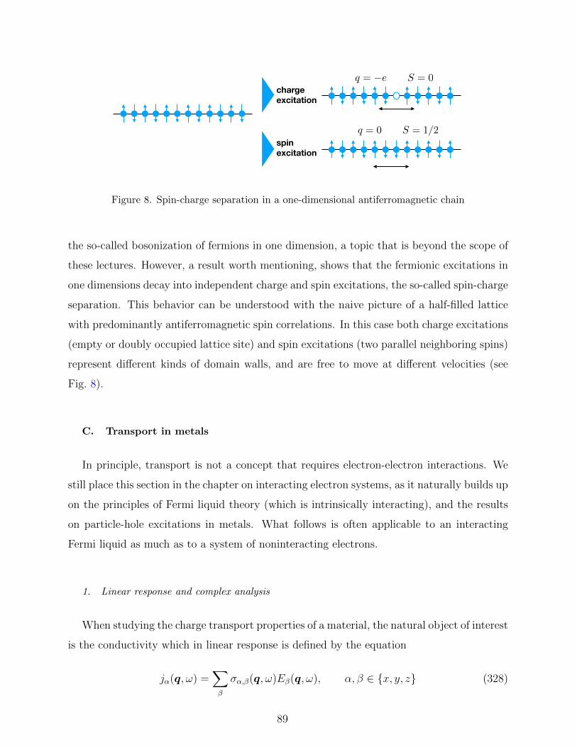
q = e S = 0
q = 0 S = 1/2
charge excitation
spin excitation
Figure 8. Spin-charge separation in a one-dimensional antiferromagnetic chain
the so-called bosonization of fermions in one dimension, a topic that is beyond the scope of
these lectures. However, a result worth mentioning, shows that the fermionic excitations in
one dimensions decay into independent charge and spin excitations, the so-called spin-charge
separation. This behavior can be understood with the naive picture of a half-filled lattice
with predominantly antiferromagnetic spin correlations. In this case both charge excitations
(empty or doubly occupied lattice site) and spin excitations (two parallel neighboring spins)
represent different kinds of domain walls, and are free to move at different velocities (see
Fig. 8).
C. Transport in metals
In principle, transport is not a concept that requires electron-electron interactions. We
still place this section in the chapter on interacting electron systems, as it naturally builds up
on the principles of Fermi liquid theory (which is intrinsically interacting), and the results
on particle-hole excitations in metals. What follows is often applicable to an interacting
Fermi liquid as much as to a system of noninteracting electrons.
1. Linear response and complex analysis
When studying the charge transport properties of a material, the natural object of interest
is the conductivity which in linear response is defined by the equation
jα(q, ω) =∑β
σα,β(q, ω)Eβ(q, ω), α, β ∈ x, y, z (328)
89
Here, we introduced σα,β(q, ω) in all generality as a tensorial quantity. However, in the
following discussion we specialize for simplicity on isotropic systems where σα,β is diagonal
with equal diagonal elements σ(q, ω).
We can relate σ(q, ω) to the susceptibility in the following. For this, we note that current
j(q, ω) and charge density ρ(q, ω) satisfy the continuity equation
ρ(r, t) + ∇ · j(r, t) = 0, (329)
which in reciprocal space reads
ωρ(q, ω)− q · j(q, ω) = 0. (330)
Inserting this into Eq. (240) (note that we divide ρ by (−e) to relate it to the number density
that was used as δρ in Eq. (240))
χ0(q, ω) =− ρ(q, ω)
eV (q, ω)
=− q · j(q, ω)
eωV (q, ω)
=− σ(q, ω) q ·E(q, ω)
eωV (q, ω)
=− σ(q, ω)
ω
iq2V (q, ω)
eV (q, ω),
(331)
where we used the first Maxwell equation eE(q, ω) = −iqV (q, ω). In summary
χ0(q, ω) = −iq2
e2ωσ(q, ω), ε(q, ω) = 1 + i
4π
ωσ(q, ω). (332)
From our discussion of the plasma resonance, we had deduced that for small q kF the
dielectric function takes the form ε(0, ω) = 1− ω2p/ω
2, which implies for the conductivity in
this limit
σ(ω) = iω2
p
4πω. (333)
Is the conductivity purely imaginary in the limit of small frequency and momenta? This is
not the case, as we can directly see from computing the Kramers-Kronig relation between
imaginary and real part
Reσ(ω) =− 1
πP[∫ ∞−∞
dω′Imσ(ω′)
ω − ω′]
Imσ(ω) = +1
πP[∫ ∞−∞
dω′Reσ(ω′)
ω − ω′].
(334)
90
Using the from of Eq. (333), we obtain for any finite ω that Reσ(ω) = 0 simply by shifting
the integration variable ω′ by ω/2. For ω = 0 we obtain a divergence which using the Cauchy
principal value yields
Reσ(ω) =ω2
p
4δ(ω), Imσ(ω) =
ω2p
4πω. (335)
This tells us that the metal is perfectly conducting (finite conductivity comes results from
disorder scattering, which will be considered below). Furthermore, the conductivity obeys
the so-called f sum rule following from complex analysis∫ ∞0
dω′Reσ(ω′) =1
2
∫ ∞−∞
dω′Reσ(ω′) =ω2
p
8=πe2n
2m, (336)
where n is the carrier density.
2. Boltzmann transport theory
To include the effect of impurity scattering, we utilize Boltzmann’s transport theory,
which is an efficient semiclassical tool to compute transport responses. The central object
of interest is the distribution function
f(k, r, t) (337)
in phase space which gives the number of (quasi-)particles residing in a phase space volume
d3rd3k/(2π)3 at a point (k, r) and at time t. For this semiclassical picture of phase space to
be applicable, we restrict ourselves to phenomena at small wave numbers and small energies
q kF, ω εF. (338)
From this definition there follows the total number of particles as
N = 2
∫d3k
(2π)3d3r f(k, r, t) (339)
and the equilibrium distribution function (i.e., in absence of perturbations to the system)
as the Fermi-Dirac distribution
f0(k, r, t) =1
eβ εk + 1. (340)
91
The key equation obeyed by f(k, r, t) is the Boltzmann equation which says that the total
time derivative of f(k, r, t) equals a functional called the collision integral which incorporates
the scattering processes
d
dtf(k, r, t) =
(∂t + r ·∇r + k ·∇k
)f(k, r, t) = (∂t f)coll (k, r, t). (341)
If scattering was absent (i.e., the right-hand side zero), the equation would simply be the
continuity equation for f(k, r, t) required by particle number conservation. Hence, all the
magic is in the collision integral. For scattering off static potentials, it can be written as
(∂t f)coll (k, r, t) = −∫
d3k′
(2π)3W (k,k′)f(k, r, t)[1− f(k′, r, t)]− (k↔ k′) . (342)
Here, W (k,k′) is the probability of a scattering process of a quasiparticle from momentum
k to k′. The factors f(k, r, t) and [1 − f(k′, r, t)] are the probability of there being a
quasiparticle at k that can be scattered in the first place and the probability of the state at
k′ being empty, respectively. The second term k↔ k′ describes scattering into (as opposed
to out of) the phase space volume near k from a state at k′ and therefore comes with a
negative sign. If a system has time-reversal symmetry, we have W (k,k′) = W (k′,k) and
thus
(∂t f)coll (k, r, t) = −∫
d3k′
(2π)3W (k,k′) [f(k, r, t)− f(k′, r, t)] . (343)
An important approximation to make progress is the so-called relaxation-time approxi-
mation. We assume that the system is close to an equilibrium distribution f0(k, r, t), which
is equal to the Fermi-Dirac distribution, but with a varying chemical potential µ(r, t) and
temperature β(r, t), which are the source of a position and time dependence in f0(k, r, t).
The collision integral is then written using the ansatz
(∂t f)coll = −f(k, r, t)− f0(k, r, t)
τ(εk), (344)
i.e., we replace the integral with a simple linear function of f(k, r, t) in the limit of small
deviations from equilibrium. The quantity τ(εk) is the relaxation time, quantifying the time
scale of scattering events.
3. Conductivity
As a simple application of the Boltzmann theory using the relaxation time approximation,
we compute the conductivity as a response to applying a small uniform electric field E(t).
92
Then f(k, r, t) = f(k, t) is independent of r. In absence of a magnetic field and for vanishing
Berry curvature, the semiclassical equations of motion
r =k
m, k = −eE, (345)
allow to introduce the electric field in the Boltzmann equation (341). The applied electric
field leads to a change δf(k, t) in the distribution f(k, t) = f0(k) + δf(k, t). We can thus
write the Boltzmann equation (341) to linear order in δf(k, t) and E(t) using their Fourier
transforms
f(k, t) =
∫ ∞−∞
dω
2πf(k, ω)e−iωt, E(t) =
∫ ∞−∞
dω
2πE(ω)e−iωt, (346)
as
− iω δf(k, ω)− eE(ω) ·∇k f0(k) = −δf(k, ω)
τ(εk). (347)
This is an algebraic equation for δf(k, ω) solved as
δf(k, ω) =eτ(εk)E(ω)
1− iωτ(εk)·∇kεk
∂f0(ε)
∂ε. (348)
Once we have obtained the distribution function, we can use it to calculate observables. For
example, the quasiparticle current is given by
j(ω) = −2e
∫d3k
(2π)3vkf(k, ω). (349)
As an aside, were we interested in the thermal response of a material, we could instead
compute the heat current
jh(ω) = −2e
∫d3k
(2π)3εkvkf(k, ω). (350)
For the case at hand, using vk = ∇kεk,
j(ω) = − e2
4π3
∫d3k
τ(εk)E(ω) · vk1− iωτ(εk)
∂f0(εk)
∂εkvk. (351)
Comparing to Eq. (328), we find the conductivity
σα,β(ω) = − e2
4π3
∫dε∂f0(ε)
∂ε
τ(ε)
1− iωτ(ε)
∫dΩk k
2vk;αvk;β
|vk|. (352)
We now discuss the result in different frequency regimes.
93
a. Limit of large frequencies If ωτ 1 and for temperatures small compared to the
Fermi energy, the energy integrand becomes a delta function multiplying i/ω. In the case of
an isotropic system of mass m, we have σα,β = δα,βσ with
σ(ω) =ie2
4π3 ω
∫dΩk
kF
mk2
F,x
=ie2
4π3 ω
k3F
m
4π
3
=ie2n
mω
=iω2
p
4πω,
(353)
where n = k3F/(3π
2) (spin degeneracy!). This agrees with our previous result Eq. (333).
b. Limit of small frequencies (dc limit) Before, our perfect conductor had a real delta
function conductivity at small frequencies. Using the Boltzmann theory, we can obtain a
more realistic result in this limit, namely
σ(ω) =e2 n
m
∫dε∂f0(ε)
∂ετ(ε)
=e2nτ
m
=ω2
pτ
4π,
(354)
where we simply defined the averaged relaxation time τ as the integral with the derivative
of the Fermi Dirac distribution, which is strongly peaked at the Fermi surface. This is
the Drude from of the conductivity, which can also be derived with much more elementary
means. Its important feature is that the conductivity is proportional to the relaxation time.
c. Limit of nearly constant relaxation times If the relaxation time depends only
weakly on energy, we can use the approximation used to derive the Drude from also at finite
frequencies to obtain
σ(ω) =ω2
p
4π
τ
1− iωτ
=ω2
p
4π
τ
1 + ω2τ 2+ i
ω2p
4π
τ 2ω
1 + ω2τ 2.
(355)
4. Optical properties
With the approximations above, there follows the dielectric function
ε(ω) = 1− ω2p
ω
τ
i + ωτ(356)
94
directly from the conductivity. It is related to the complex index of refraction n + iκ via
ε = (n + iκ)2, which determines how light propagates inside the metal. Light with vacuum
wave number k = ω/c has wave number k(n + iκ) in the material. Hence, the penetration
depth
δ = c/(ωκ) (357)
determines how far light can penetrate the metal.
Straight-forward evaluation yields in the regime of small frequencies ωτ 1 ωpτ that
δ(ω) ≈ c
ωp
√2
ωτ, (358)
yielding the dependence of the so-called skin depth of a metal δ ∝ ω−1/2.
For intermediate frequencies 1 ωτ ωpτ the penetration depth is only weakly de-
pendent on frequency as δ(ω) ≈ c/ωp, which is in the range of hundreds Angstrom. (This
regime does not include visible light.)
At ultraviolet frequencies ω ∼ ωp the imaginary part of ε is very small yielding a strong
increase in δ. The metal becomes transparent in the ultraviolet.
Note that we have only considered a single band model for a metal here. More dis-
criminating optical properties, like the shiny colors of some metals like gold in the visible
frequency range stem from interband transitions.
5. Computing the relaxation time
So far, we have introduced the relaxation time as a phenomenological function. We want
to improve on that by considering actual scattering mechanisms now. We consider time-
reversal invariant, isotropic, time-independent, and homogeneous systems, such that the
relevant equation from the collision integral is
f(k)− f0(k)
τ(εk)=
∫d3k′
(2π)3W (k,k′) [f(k)− f(k′)] . (359)
Let the only source of perturbation be an external electric field E, such that
f(k) = f0(k) + A(k)k ·E (360)
to lowest order by isotropy. Then
f(k)− f(k′) = A(k) (k − k′) ·E (361)
95
because elastic scattering implies that |k| = |k′|. Let θ and θ′ be the angles between E and k
as well as between k′ and k, respectively. Then k′ ·E = k′E(cos θ cos θ′+ sin θ sin θ′ cosφ′),
where φ′ is the polar angle between k and k′. The latter term drops out of the integral by
isotropy and
f(k)− f0(k)
τ(εk)=
1
(2π)3A(k) k E cos θ
∫dΩk′(1− cos θ′)W (k,k′)
=1
(2π)3[f(k)− f0(k)]
∫dΩk′(1− cos θ′)W (k,k′).
(362)
The relaxation time reduces to
1
τ(εk)=
∫d3k′
(2π)3(1− cos θ′)W (k,k′). (363)
The factor (1−cos θ′) gives more weight to the backscattering (θ′ = π) processes as compared
to forward scattering (θ′ = 0).
a. Impurity scattering If we get microscopic information about an impurity potential
V , we can compute W (k,k′) by applying Fermi’s golden rule
W (k,k′) = 2πnimp
∣∣∣⟨k ∣∣∣ V ∣∣∣k′⟩∣∣∣2 δ(εk − εk′), (364)
where nimp is the density of impurities, which is assumed to be small enough from them
to be considered as independent. Screened point charge scatterers of charge Ze have the
potential ⟨k∣∣∣ V ∣∣∣k′⟩ =
4πZe2
|k − k′|2 + k2TF
. (365)
In the limit of strong screening, kTF kF, we can drop the (k − k′) in the matrix element
and obtain
1
τ(εk)= 2πnimp
(4πZe2
k2TF
)2 ∫d3k′
(2π)3(1− cos θ′)δ(εk − εk′)
=π ν(εF)nimp
(4πZe2
k2TF
)2
.
(366)
This yields the temperature-independent residual resistivity of a metal
ρ =m
e2 n τ(εF), (367)
the ratio of which with the value of the resistivity at 300 K is the residual resistance ratio
RRR, which is a measure for the amount of impurities in the system and hence a measure
for sample quality. Typical values are in the tenths, clean materials reach RRR values in
the thousands.
96
b. Electron-electron scattering The scattering rate between electrons is suppressed for
energies close to the Fermi energy, because of the reduced phase space available for elastic
scattering there. The life-time (here interpreted as the relaxation time) takes the form
1
τ(ε)=
1
τe
(ε
εF
)2
, (368)
where τe is a constant and ε is measured with respect to the chemical potential, i.e., ε = 0
at the Fermi level. Inserting this in the first line of Eq. (354) to compute τ , we find
τ =
∫dε τ(ε)
∂f0
∂ε
=β
4
∫dε
τ(ε)
cosh2(βε/2).
(369)
The latter integral is divergent for small ε.
In order to regulate it, we also consider coexisting impurity scattering. To show how one
properly accounts for different scattering mechanisms we use Matthiessen’s rule. It states
that different independent scattering processes can be added at the level of the scattering
rates, i.e.,
W (k,k′) = W1(k,k′) +W2(k,k′). (370)
For the relaxation times and the resulting resistivity contributions this translates into
1
τ=
1
τ1
+1
τ2
, ρ = ρ1 + ρ2. (371)
It thus looks like we are coupling resistors in serial circuit. Matthiessen’s rule can be inap-
plicable for 1D systems and if the τ ’s are strongly k-dependent.
Returning to our integral (369), we replace 1/τ(ε) = ε2/(ε2F τe) + 1/τ0, where τ0 comes
from impurity scattering
τ ≈ β4
∫dε
1
cosh2(βε/2)
(τ0 −
τ 20
τe
ε2
ε2F
)= τ0 −
π2
3(βεF)2
τ 20
τe
.
(372)
The resistivity then becomes temperature dependent due to the electron-electron scattering
as
ρ(T ) = ρ0 +π2
3
m
ne2τE
(kBT
εF
)2
. (373)
The T 2 behavior is the main feature here which is often seen as an identification criterion
for a Fermi liquid.
97
c. Sources of momentum loss Devil’s advocate could argue at this point that if all
scattering processes conserve momentum, no resistance should occur. This line of argu-
mentation ignores the important role played by the lattice. In the case of electron-electron
scattering, it also allows for Umklapp processes in the scattering for which
k = k′ +G, (374)
where G is a reciprocal lattice vector. Such a process leads to a static deformation of the
lattice, which absorbs the momentum mismatch.
A second source of resistivity due to the lattice, which we have not touched upon is the
scattering between electrons and phonons, i.e., elementary lattice vibrations. The resulting
relaxation time has the characteristic temperature dependence
τ−1 ∝(T
ΘD
)5
, T ΘD,
τ−1 ∝ T
ΘD
, T ΘD,
(375)
where the Debye temperature kBΘD ≈ cs kF with cs the speed of sound.
6. Kondo effect
There are impurity atoms inducing so-called resonant scattering. If the resonance occurs
close to the Fermi energy, the scattering rate is strongly energy dependent, inducing a
more pronounced temperature dependence of the resistivity. An important example is the
scattering off magnetic impurities with a spin degree of freedom, yielding a dramatic energy
dependence of the scattering rate. This problem was first studied by Kondo in 1964 in order
to explain the peculiar minima in resistivity in some materials. The coupling between the
local spin impurities Si at Ri and the quasiparticle spin s(r) has the exchange form
V K =∑i
(V K
)i
= J∑i
S i · s (r) δ(r −Ri)
= J∑i
[S zi s
z(r) +1
2S +i s−(r) +
1
2S −i s
+(r)
]δ(r −Ri)
=J
2Ω
∑k,k′,i
[S zi
(c †k↑ c k′↑ − c †k↓ c k′↓
)+ S +
i c†k↓ c k′↑ + S −i c
†k↑ c k′↓
]e−i(k−k′)·Ri
(376)
98
Here, it becomes important that spin flip processes, which change the spin state of the
impurity and that of the scattered electron, are enabled. The results for the scattering rate
are presented here without derivation,
W (k,k′) ≈ J2S(S + 1)
[1 + 2Jν(εF) log
D
|εk − εF|
], (377)
where D is the bandwidth and we have assumed that Jν(εF) 1. The relaxation time is
found to be1
τ(εk)≈ J2S(S + 1)ν(εF)
[1 + 2Jν(εF)log
D
|εk − εF|
](378)
Note that W (k,k′) does not depend on angle, meaning that the process is described by
s-wave scattering. The energy dependence is singular at the Fermi energy, indicating that
we are not dealing with simple resonant potential scattering, but with a much more subtle
many-particle effect involving the electrons very near the Fermi surface. The fact that
the local spins Si can flip, makes the scattering center dynamical, because the scatterer
is constantly changing. The scattering process of an electron is influenced by previous
scattering events, leading to the singularity at εF . This cannot be described within the first
Born approximation, but requires at least the second approximation or the full solution. As
mentioned before, the resonant behavior induces a strong temperature dependence of the
conductivity. Indeed,
σ(T ) =e2k3
F
6π2m
∫dε
1
4kBT cosh2(ε− εF)/(2kBT )τ(ε)
≈ e2n
8mkBT
∫dεJ2S(S + 1)[1− 2Jν(εF) log(D/ε)]
cosh2(ε/2kBT ).
(379)
A simple substitution in the integral leads to
σ(T ) ≈ e2n
2mJS(S + 1)
[1− 2Jν(εF) log
D
kBT
](380)
Usual contributions to the resistance, like electron-phonon scattering, typically decrease
with temperature. The contribution (380) to the conductivity is strongly increasing, induc-
ing a minimum in the resistance, when we crossover from the decreasing behavior at high
temperatures to the low-temperature increase of ρ(T ). At even lower temperatures, the
conductivity would decrease and eventually even turn negative which is an artifact of our
approximation. In reality, the conductivity saturates at a finite value when the temperature
is lowered below a characteristic Kondo temperature TK,
kBTK = D e−1/[Jν(εF)], (381)
99
a characteristic energy scale of this system. The real behavior of the conductivity at tem-
peratures T TK is not accessible by simple perturbation theory. This regime, known
as the Kondo problem, represents one of the most interesting correlation phenomena of
many-particle physics.
7. Anderson localization in one dimension
Transport in one spatial dimension is very special, since there are only two different
directions to go: forward and backward. We introduce the transfer matrix formalism and
use it to express the conductivity through the Landauer formula. We will then investigate
the effects of multiple scattering at different obstacles, leading to the so-called Anderson
localization, which turns a metal into an insulator.
a. Landauer Formula for a single impurity The transmission and reflection at an ar-
bitrary potential with finite support in one dimension can be described by a transfer matrix
T [see Fig. 9 a) and b)]. A suitable choice for a basis of the electron states is the set of plane
waves e±ikx moving in the positive (negative) x-direction with wave vector +k (−k). Only
plane waves with the same |k| on the left (part I1) and right (part I2) side of the scatterer
are interconnected. Therefore, we write
ψ1(x) = a1+eikx + a1−e
−ikx,
ψ2(x) = a2+eikx + a2−e
−ikx,(382)
where ψ1 (ψ2) is defined in the area I1 (I2). The vectors ai = (ai+, ai−), i ∈ 1, 2 are
connected via the linear relation,
a2 = T a1 =
T11 T12
T21 T22
a1 (383)
with the 2× 2 transfer matrix T . The conservation of current (J1 = J2) requires that T is
unimodular, i.e., detT = 1. Here,
J =i
2m
(dψ∗(x)
dxψ(x)− ψ∗(x)
dψ(x)
dx
)(384)
such that, for a plane wave ψ(x) = (1/√L)eikx in a system of length L, the current results
in
J = v/L (385)
100
with the velocity v defined as v = k/m. Time reversal symmetry implies that, simultaneously
with ψ(x), the complex conjugate ψ∗(x) is a solution of the stationary Schroedinger equation.
From this, we find T11 = T ∗22 and T12 = T ∗21 ,such that
T =
T11 T12
T ∗12 T ∗11
. (386)
It is easily shown that a shift of the scattering potential by a distance x0 changes the coeffi-
cient T12 of T by a phase factor ei2kx0 . Meanwhile, the coefficient T11 remains unchanged.
With the ansatz for a right moving incoming wave (∝ eikx), producing a reflected (∝re−ikx) and transmitted part (∝ teikx) part, the wave functions on both sides of the scatterer
read
ψ1(x) =1√L
(eikx + re−ikx
), ψ2(x) =
1√Lteikx. (387)
The coefficients of T can be determined explicitly in this situation, resulting in
T =
1/t∗ −r∗/t∗
−r/t 1/t
. (388)
Here, the conservation of currents imposes the condition 1 = |r|2 + |t|2. Furthermore, we
can find a relation between the parameters (r, t) of the potential barrier and the electric
resistivity. For this, we notice that the incoming current density J0 is split into a reflected
Jr and transmitted Jt part, each given by
J0 = − 1
Lve = −n0ve,
Jr = − |r|2
Lve = −nrve,
Jt = − |t|2
Lve = −ntve,
(389)
with the electron charge −e, and the particle densities n0, nr, and nt corresponding to the
incoming, reflected and transmitted particles respectively. The electron density on the two
sides of the barrier is given by
n1 =n0 + nr =1 + |r|2L
,
n2 =nt =|t|2L.
(390)
From this consideration, a density difference δn = n1 − n2 = (1 + |r|2 − |t|2)/L = 2|r|2/Lresults between the left and the right side of the scatterer. The resistance R of the barrier
101
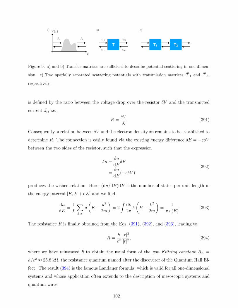
V (x)
x
I1 I2
Ta1+
a1 a2
a2+
T1 T2
a) b) c)
Figure 9. a) and b) Transfer matrices are sufficient to describe potential scattering in one dimen-
sion. c) Two spatially separated scattering potentials with transmission matrices T 1 and T 2,
respectively.
is defined by the ratio between the voltage drop over the resistor δV and the transmitted
current Jt, i.e.,
R =δV
Jt(391)
Consequently, a relation between δV and the electron density δn remains to be established to
determine R. The connection is easily found via the existing energy difference δE = −eδVbetween the two sides of the resistor, such that the expression
δn =dn
dEδE
=dn
dE(−eδV )
(392)
produces the wished relation. Here, (dn/dE)dE is the number of states per unit length in
the energy interval [E,E + dE] and we find
dn
dE=
1
L
∑k,σ
δ
(E − k2
2m
)= 2
∫dk
2πδ
(E − k2
2m
)=
1
π v(E)(393)
The resistance R is finally obtained from the Eqs. (391), (392), and (393), leading to
R =h
e2
|r|2|t|2 , (394)
where we have reinstated ~ to obtain the usual form of the von Klitzing constant RK =
h/e2 ≈ 25.8 kΩ, the resistance quantum named after the discoverer of the Quantum Hall Ef-
fect. The result (394) is the famous Landauer formula, which is valid for all one-dimensional
systems and whose application often extends to the description of mesoscopic systems and
quantum wires.
102
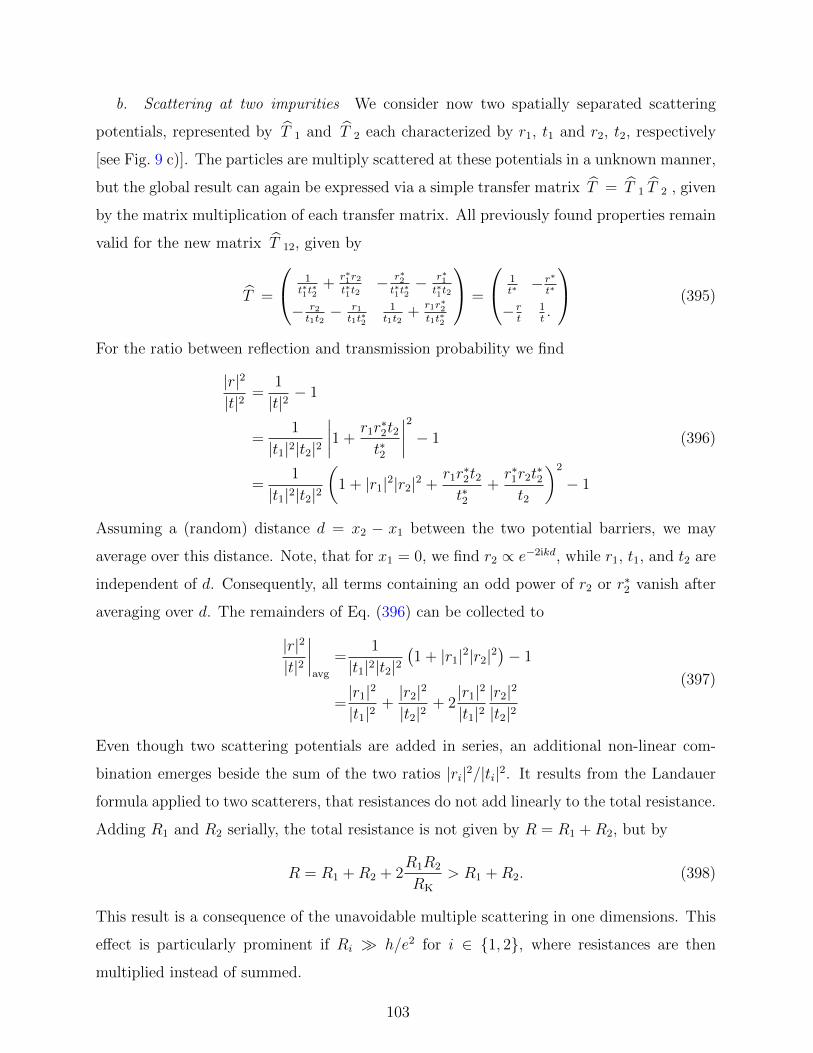
b. Scattering at two impurities We consider now two spatially separated scattering
potentials, represented by T 1 and T 2 each characterized by r1, t1 and r2, t2, respectively
[see Fig. 9 c)]. The particles are multiply scattered at these potentials in a unknown manner,
but the global result can again be expressed via a simple transfer matrix T = T 1 T 2 , given
by the matrix multiplication of each transfer matrix. All previously found properties remain
valid for the new matrix T 12, given by
T =
1t∗1t∗2
+r∗1r2t∗1t2
− r∗2t∗1t∗2− r∗1
t∗1t2
− r2t1t2− r1
t1t∗2
1t1t2
+r1r∗2t1t∗2
=
1t∗− r∗
t∗
− rt
1t.
(395)
For the ratio between reflection and transmission probability we find
|r|2|t|2 =
1
|t|2 − 1
=1
|t1|2|t2|2∣∣∣∣1 +
r1r∗2t2t∗2
∣∣∣∣2 − 1
=1
|t1|2|t2|2(
1 + |r1|2|r2|2 +r1r∗2t2t∗2
+r∗1r2t
∗2
t2
)2
− 1
(396)
Assuming a (random) distance d = x2 − x1 between the two potential barriers, we may
average over this distance. Note, that for x1 = 0, we find r2 ∝ e−2ikd, while r1, t1, and t2 are
independent of d. Consequently, all terms containing an odd power of r2 or r∗2 vanish after
averaging over d. The remainders of Eq. (396) can be collected to
|r|2|t|2∣∣∣∣avg
=1
|t1|2|t2|2(1 + |r1|2|r2|2
)− 1
=|r1|2|t1|2
+|r2|2|t2|2
+ 2|r1|2|t1|2|r2|2|t2|2
(397)
Even though two scattering potentials are added in series, an additional non-linear com-
bination emerges beside the sum of the two ratios |ri|2/|ti|2. It results from the Landauer
formula applied to two scatterers, that resistances do not add linearly to the total resistance.
Adding R1 and R2 serially, the total resistance is not given by R = R1 +R2, but by
R = R1 +R2 + 2R1R2
RK
> R1 +R2. (398)
This result is a consequence of the unavoidable multiple scattering in one dimensions. This
effect is particularly prominent if Ri h/e2 for i ∈ 1, 2, where resistances are then
multiplied instead of summed.
103
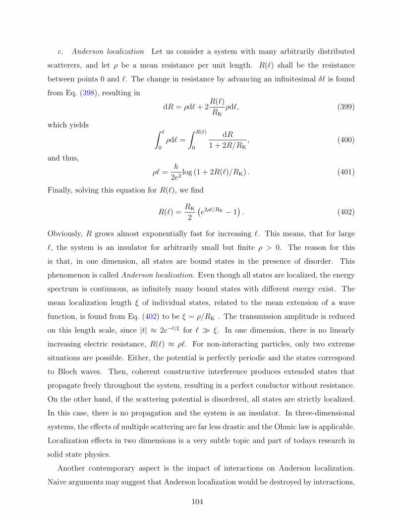
c. Anderson localization Let us consider a system with many arbitrarily distributed
scatterers, and let ρ be a mean resistance per unit length. R(`) shall be the resistance
between points 0 and `. The change in resistance by advancing an infinitesimal δ` is found
from Eq. (398), resulting in
dR = ρd`+ 2R(`)
RK
ρd`, (399)
which yields ∫ `
0
ρd` =
∫ R(`)
0
dR
1 + 2R/RK
, (400)
and thus,
ρ` =h
2e2log (1 + 2R(`)/RK) . (401)
Finally, solving this equation for R(`), we find
R(`) =RK
2
(e2ρ`/RK − 1
). (402)
Obviously, R grows almost exponentially fast for increasing `. This means, that for large
`, the system is an insulator for arbitrarily small but finite ρ > 0. The reason for this
is that, in one dimension, all states are bound states in the presence of disorder. This
phenomenon is called Anderson localization. Even though all states are localized, the energy
spectrum is continuous, as infinitely many bound states with different energy exist. The
mean localization length ξ of individual states, related to the mean extension of a wave
function, is found from Eq. (402) to be ξ = ρ/RK . The transmission amplitude is reduced
on this length scale, since |t| ≈ 2e−`/ξ for ` ξ. In one dimension, there is no linearly
increasing electric resistance, R(`) ≈ ρ`. For non-interacting particles, only two extreme
situations are possible. Either, the potential is perfectly periodic and the states correspond
to Bloch waves. Then, coherent constructive interference produces extended states that
propagate freely throughout the system, resulting in a perfect conductor without resistance.
On the other hand, if the scattering potential is disordered, all states are strictly localized.
In this case, there is no propagation and the system is an insulator. In three-dimensional
systems, the effects of multiple scattering are far less drastic and the Ohmic law is applicable.
Localization effects in two dimensions is a very subtle topic and part of todays research in
solid state physics.
Another contemporary aspect is the impact of interactions on Anderson localization.
Naive arguments may suggest that Anderson localization would be destroyed by interactions,
104
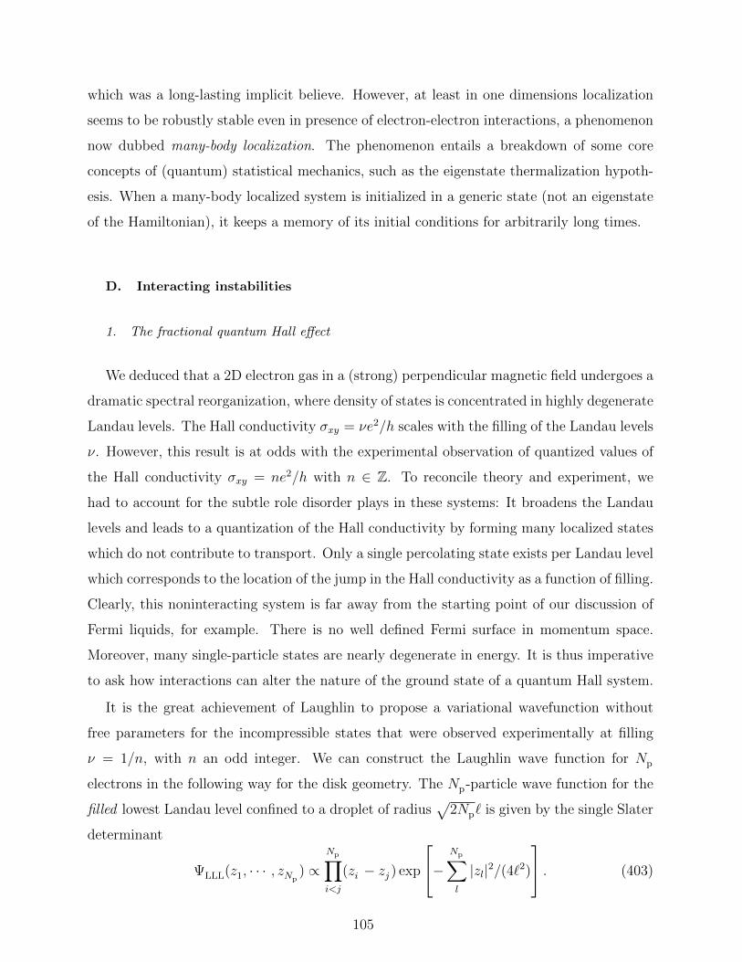
which was a long-lasting implicit believe. However, at least in one dimensions localization
seems to be robustly stable even in presence of electron-electron interactions, a phenomenon
now dubbed many-body localization. The phenomenon entails a breakdown of some core
concepts of (quantum) statistical mechanics, such as the eigenstate thermalization hypoth-
esis. When a many-body localized system is initialized in a generic state (not an eigenstate
of the Hamiltonian), it keeps a memory of its initial conditions for arbitrarily long times.
D. Interacting instabilities
1. The fractional quantum Hall effect
We deduced that a 2D electron gas in a (strong) perpendicular magnetic field undergoes a
dramatic spectral reorganization, where density of states is concentrated in highly degenerate
Landau levels. The Hall conductivity σxy = νe2/h scales with the filling of the Landau levels
ν. However, this result is at odds with the experimental observation of quantized values of
the Hall conductivity σxy = ne2/h with n ∈ Z. To reconcile theory and experiment, we
had to account for the subtle role disorder plays in these systems: It broadens the Landau
levels and leads to a quantization of the Hall conductivity by forming many localized states
which do not contribute to transport. Only a single percolating state exists per Landau level
which corresponds to the location of the jump in the Hall conductivity as a function of filling.
Clearly, this noninteracting system is far away from the starting point of our discussion of
Fermi liquids, for example. There is no well defined Fermi surface in momentum space.
Moreover, many single-particle states are nearly degenerate in energy. It is thus imperative
to ask how interactions can alter the nature of the ground state of a quantum Hall system.
It is the great achievement of Laughlin to propose a variational wavefunction without
free parameters for the incompressible states that were observed experimentally at filling
ν = 1/n, with n an odd integer. We can construct the Laughlin wave function for Np
electrons in the following way for the disk geometry. The Np-particle wave function for the
filled lowest Landau level confined to a droplet of radius√
2Np` is given by the single Slater
determinant
ΨLLL(z1, · · · , zNp) ∝
Np∏i<j
(zi − zj ) exp
− Np∑l
|zl|2/(4`2)
. (403)
105
The electron density per unit area inside the droplet is constant and given by 1/(2π`2). By
raising the holomorphic part of the wave function to the power n
Ψn(z1, · · · , zNp) ∝
Np∏i<j
(zi − zj )n exp
− Np∑l
|zl|2/(4`2)
, (404)
one obtains the Laughlin wave function describing a droplet that
• has all electrons in the lowest Landau level due to the holomorphic structure
• covers an n-times larger area of radius√
2nNp`,
• is a featureless liquid with electron density reduced by a factor 1/n,
• supports excitations of fractional charge e/n,
• includes strong correlations between the electrons.
By inspection of the Laughlin wavefunction, one can gain some intuition as to why it might
be an energetically favorable state for repulsively interacting electrons in the lowest Landau
level. As any two electrons approach each other, the wavefunction has a n-th order zero,
while the configurations with the electron positions well separated has the highest weight.
Further, any two electrons with coordinates z1 and z2 have a relative angular momentum of
mrel = n or higher. Here, the relative angular momentum of a two-particle state (z1−z2)m is
the exponent m. Remarkably, the elementary excitations are in some sense already contained
in the analytic form of the Laughlin wavefunction. For example, the wavefunction of a
quasihole with fractional charge −e/n localized at z0 is given by
Ψqhn (z1, · · · , zNp
|z0) ∝ Ψn(z1, · · · , zNp)
Np∏l
(z0 − zl ). (405)
As the Laughlin wave function is variational in nature, two immediate questions are: (i)
How close is it to the actual ground state of the partially filled Landau level, when electrons
are subject to Coulomb interactions? (ii) Does there exist a Hamiltonian for which Ψn is an
incompressible ground state? The answer to (i) is given by numerical exact diagonalization
studies of finite systems, which showed that the Laughlin state is in the same universality
class as the exact ground state, the so-called Coulomb ground state.
106
Trugman and Kievelson showed how to construct a Hamiltonian for which Ψn is an exact
and unique zero-energy ground state. Crucial to their derivation is the fact that any two
particles have relative angular momentum mrel = n or higher in the Laughlin wave function.
As an immediate consequence, Ψn is annihilated by the projector on states with angular
momentum mrel < n. This projector is precisely the so-called pseudopotential Hamiltonian
that they propose. In configuration space, its matrix elements are derivatives of delta-
functions. Physically, it corresponds to a highly local repulsive interaction.
2. Superconductivity
The theory of superconductivity is a very rich field, and as a result we can only give a
very short account of the theoretical description of superconductors. We will focus on the
derivation of the superconducting ground state and its elementary excitations.
Many materials turn superconducting at low temperatures (ironically, many nobel metals
and the excellent conductor copper don’t). The phenomenology of the superconducting state
is two-fold: (1) The resistivity of a superconductor vanishes exactly. (2) The magnetic field is
expelled from the bulk of a superconductor (or channelled in very thin flux tubes in so-called
type-II superconductors). The latter is called the Meissner-effect. Only the combination of
properties (1) and (2) yield a well-defined thermodynamic state. It also implies the existence
of persistent currents in a superconductor, which do not decay.
a. Cooper pairs The elementary building block of superconductors are Cooper pairs,
that is, coherent combinations of two-electron states. The formation of Cooper pairs results
from some effective attractive interaction between electrons, which overcomes their repulsive
Coulomb interaction. In so-called conventional superconductors, this attractive interactions
is mediated by phonons (lattice distortions). An electron passing through the crystal leaves
behind a slowly relaxing lattice distortion (the slowness is determined by the large mass
ration Mion/m of the ionic and electronic mass). This polarized crystal environment is seen
by the other electron of the Cooper pair as an attracting force.
Here, we do not detail the phononic origin of the interaction and simply assume that
there exists some attractive interaction between electrons. To understand the formation of
107
Cooper pairs more quantitatively, we consider the following wave function ansatz
|Ψ12(K)〉 =∑k,σ,σ′
ak,σ,σ′ c†k,σ c
†−k+K,σ′ |0〉, (406)
which describes two electrons (k, σ) and (K − k, σ′) added to the filled Fermi sea ground
state |0〉. Since we expect the system to remain translationally invariant, we have assigned
a well-defined momentum K to this state. Anticipating a minimization of the energy of
this state, we can further refine this ansatz. We assume that attractive interactions exist
between electrons only in a small energy range ω, which for the case of phonons can be
taken as the Debye frequency of the material, i.e., if |εk − εK−k| ≤ ω. Figure 10 a) suggests
that most electron pairs can take advantage of this interaction if K = 0. We furthermore
assume that the ground state in this two-electrons-above-the-Fermi-sea subspace has even
orbital character (as is usually the case for symmetric attractive potentials). To obtain a
valid fermionic two-body wave function (which is antisymmetric under particle exchange),
we thus have to make the spin part antisymmetric, i.e., the two electrons in our ansatz have
opposite spin, yielding
|Ψ12〉 =∑k
ak c†k,↑ c
†−k,↓|0〉. (407)
We want to study this family of states subject to the Hamiltonian
H =∑k,σ
εk c†k,σ c k,σ −
V
2
∑′
k,q,σ
c †k+q,σ c†−k−q,−σ c −k,−σ c k,σ (408)
where we take V 6= 0 only for |εk−εK−k| ≤ ω, which is indicated by the primed sum. Notice
also that we have already restricted the interaction to the so-called ‘Cooper channel’, i.e.,
we have dropped all terms of a generic translation symmetry preserving interaction that do
not connect states of the form (407). The energy is given by
E = 〈Ψ12| H |Ψ12〉
= 2∑k
εk|ak|2 − V∑′
k,q
a∗k+qak.(409)
We minimize it subject to the constraint∑k |ak|2 = 1,
∂
∂a∗k
(E − λ
∑k
|ak|2)
(410)
yielding
(2εk − λ)ak = V∑′
k′
ak′ . (411)
108
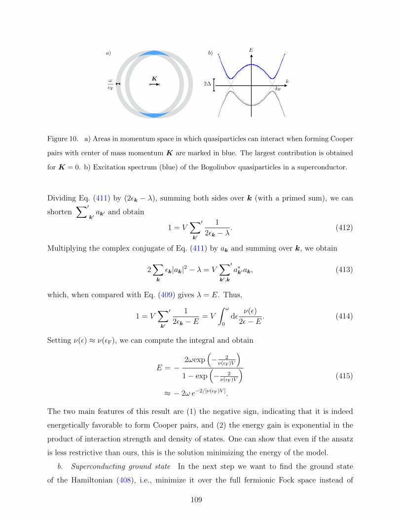
K!
vF
k
E
2kF
a) b)
Figure 10. a) Areas in momentum space in which quasiparticles can interact when forming Cooper
pairs with center of mass momentum K are marked in blue. The largest contribution is obtained
for K = 0. b) Excitation spectrum (blue) of the Bogoliubov quasiparticles in a superconductor.
Dividing Eq. (411) by (2εk − λ), summing both sides over k (with a primed sum), we can
shorten∑′
k′ak′ and obtain
1 = V∑′
k′
1
2εk − λ. (412)
Multiplying the complex conjugate of Eq. (411) by ak and summing over k, we obtain
2∑k
εk|ak|2 − λ = V∑′
k′,k
a∗k′ak, (413)
which, when compared with Eq. (409) gives λ = E. Thus,
1 = V∑′
k′
1
2εk − E= V
∫ ω
0
dεν(ε)
2ε− E . (414)
Setting ν(ε) ≈ ν(εF), we can compute the integral and obtain
E = −2ωexp
(− 2ν(εF)V
)1− exp
(− 2ν(εF)V
)≈ − 2ω e−2/[ν(εF)V ].
(415)
The two main features of this result are (1) the negative sign, indicating that it is indeed
energetically favorable to form Cooper pairs, and (2) the energy gain is exponential in the
product of interaction strength and density of states. One can show that even if the ansatz
is less restrictive than ours, this is the solution minimizing the energy of the model.
b. Superconducting ground state In the next step we want to find the ground state
of the Hamiltonian (408), i.e., minimize it over the full fermionic Fock space instead of
109
the two-particle excitation state considered so far. Implicitly, we will perform a mean-field
approximation for the case of small interaction V . We start out with a completely trivial
rewriting of the fermionic creation and annihilation operators into new linear combinations
as
αk =uk c k,↑ − vk c †−k,↓,
α−k =uk c −k,↓ + vk c†k,↑,
α†k =uk c†k,↑ − vk c −k,↓,
α†−k =uk c†−k,↓ + vk c k,↑,
(416)
where we have introduced the real (and k even) functions uk and vk. Their reality is merely
a gauge fixing. We have also explicitly locked the sign of k in α to the spin degree of freedom.
One verifies that the αk obey the usual fermionic anticommutation relations if
u2k + v2
k = 1, (417)
which shall be imposed from here on.
Let us rewrite the Hamiltonian in the new operators. We start with the noninteracting
part
H 0 =∑k,σ
εk c†k,σ c k,σ
=∑k
εk( c †k,↑ c k,↑ + c †−k,↓ c −k,↓)
=∑k
εk[2v2k + (u2
k − v2k)(α†kαk + α†−kα−k) + 2ukvk(α†kα
†−k + α−kαk)].
(418)
The interacting part gives
H int = − V
2
∑′
k,q,σ
c †k+q,σ c†−k−q,−σ c −k,−σ c k,σ
= − V∑′
k,k′
c †k′,↑ c†−k′,↓ c −k,↓ c k,↑
= − V∑′
k,k′
[ukvkuk′vk′(1− α†−k′α−k′ − α†k′αk′)(1− α†−kα−k − α†kαk)
+ (u2k − v2
k)uk′vk′(1− α†−k′α−k′ − α†k′αk′)(α−kαk + α†kα†−k)
+ (more forth-order terms in α)].
(419)
To proceed, we first neglect the residual terms of fourth order in α. This seems arbitrary
and highlights a general problem of mean-field approximations: If the ansatz (in this case
110
the expressions for the αs) is not a good description of the physics, we have no chance of
proceeding in a controlled way. The other problem are terms quadratic in the αs but of the
form α†α† or the hermitian conjugate. What our mean-field solution needs to achieve is that
all these terms (or better put, their prefectors) vanish. Notice that such terms appear both
in H 0 and in H int. The prefactor of terms of this form is
2εkukvk − V (u2k − v2
k)∑′
k′
uk′vk′ . (420)
To have it vanish, we sum over (the primed set of) k and set∑′
k′uk′vk′ = ∆/V (thereby
defining the constant ∆). This yields
2εkukvk = ∆(u2k − v2
k), (421)
which has the normalized solution
u2k =
1 + ξk2
, v2k =
1− ξk2
, ξk =εk√
ε2k + ∆2. (422)
The transformation from c operators to the α operators is called a Bogoliubov transforma-
tion. Finally, to calculate ∆ from this, we start from its definition
∆ =V∑′
k
ukvk
=V
2
∑′
k
√1− ξ2
k
=V
2
∑′
k
∆√ε2k + ∆2
.
(423)
Dividing it out and going to an integral representation
1 =V
4
∫ ω
−ωdε
ν(ε)√ε+ ∆2
≈ V ν(εF)
4
∫ ω
−ωdε
1√ε+ ∆2
,
(424)
yields a solvable integral that
∆ = 2ω e−2/[ν(εF)V ]. (425)
With the off-diagonal terms vanishing, the total Hamiltonian, omitting the fourth order
terms is of the from
H 0 + H int =∑k
εk2v2k − V
∑′
k,k′
ukvkuk′vk′
+∑k
√ε2k + ∆2 (α†−kα−k + α†kαk).
(426)
111
Let us first take a closer look at the constant terms, which encode the shift in ground state
energy. With the help of some more, less interesting integrals one can compute them in the
limit of small ∆ as
− ν(εF) ∆2/4. (427)
Again the main feature of this expression is its negative sign, signaling that our mean-field
state is indeed lower in energy than the noninteracting Fermi sea. It is the condensation
energy of the superconducting state.
The second line in Eq. (426) is the Hamiltonian for a noninteracting Fermi liquid with
only manifestly positive energies. The ground state is thus the state annihilated by all αk
and α−k operators. However, we should not forget that these operators are superpositions
of electron creation and annihilation operators. A first guess would be to write the ground
state as
|0〉 =∏k
αkα−k|vac〉
=∏k
(ukvk + v2k c†k c†−k)|vac〉.
(428)
This state is not normalized, though. The properly normalized state is
|0〉 =∏k
(uk + vk c†k c†−k)|vac〉. (429)
This many-body state has no definite particle number. The particle number conservation
is spontaneously broken in a superconductor: The condensate can absorb and emit Cooper
pairs.
c. Excitations The elementary excitations above this ground state can be directly read
off thanks to the noninteracting structure of the mean-field Hamiltonian. The quasiparti-
cles created by the α†k operators, called Bogoliubons, are fundamentally different from the
quasiparticles in a Fermi liquid in that they create a coherent superposition of a particle
and a hole. The uk gives the particle-like weight and the vk gives the hole-like weight. Far
away from the Fermi surface, they tend to vk → 1 and uk → 0 inside the Fermi sea, while
the opposite happens far outside the Fermi sea. Right at the Fermi surface they are an
equal amplitude superposition of electron and hole. The spectrum of these single-particle
like excitations √ε2k + ∆2 (430)
112
is gapped, i.e., the smallest excitation above the ground state has energy gap 2∆. [See
Fig. 10 b).]
From this observation, we can conclude that the superconductor must support persistent
currents. We can view a state which carries a current j in momentum space as displacing the
Fermi sea by an amount proportional to the current strength. After switching off the electric
field that drove the current, elastic scattering processes from one side of the displaced Fermi
sea to the opposite side (at impurities, phonons, etc.) lead to a relaxation of the Fermi
sea to its original form. If, however, there is an excitation gap 2∆ and the displacement of
the Fermi sea is small enough such that none of the states on the left end of the displaced
Fermi sea has an energy of 2∆ or more above the energy of any state on the right side of
the displaced Fermi sea, no such elastic scattering is possible. We can be more quantitative
by considering a displacement of the Fermi sphere
δk = −mδv =m
nej. (431)
Elastic scattering processes require
(kF + δk)2
2m− (kF − δk)2
2m≥ 2∆. (432)
From this, we can deduce the critical current density above which the superconductivity
breaks down as
jcrit =2en∆
kF
. (433)
Inserting typical values, we get jcrit ∼ 107 A/cm2, which is a pretty sizable value.
d. Unconventional superconductivity – gap function We have discussed the simplest
example of superconducting instabilities so far, where the order parameter is in the A1 irre-
ducible representation of the point group, as so-called s-wave superconductor (that is, the
gap ∆ does not depend on the value of the relative momentum k of the two electrons that
make up the Cooper pair). Historically these were also the first classes of superconductors
discovered and the first ones theoretically understood. However, in the search for materials
with higher transition temperatures, superconductors with generalized pairing order param-
eters were found. By now far more research is done on these unconventional superconductors
than on the conventional ones and they also become more important technologically.
The generalized BCS theory relies on an extended form of the microscopic interaction
where we consider again only the scattering of electron pairs with vanishing total momentum
113
which is attractive. The corresponding Hamiltonian can be written as
H =∑k,σ
εk c†k,σ c k,σ +
1
2
∑′
k,k′
∑σ1,σ2,σ3,σ4
Vk,k′;σ1,σ2,σ3,σ4 c†k,σ1
c †−k,σ2c −k′,−σ3 c k′,σ4 (434)
with the pair scattering matrix elements
Vk,k′;σ1,σ2,σ3,σ4 =⟨k, σ1;−k, σ2
∣∣∣ V ∣∣∣− k′, σ3;k′, σ4
⟩. (435)
Due to the Fermionic anticommutation rules it should have the following symmetries
Vk,k′;σ1,σ2,σ3,σ4 = −V−k,k′;σ2,σ1,σ3,σ4 = −Vk,−k′;σ1,σ2,σ4,σ3 = V−k,−k′;σ2,σ1,σ4,σ3 . (436)
We are again considering weak attractive interactions that only act in an energy range ω,
i.e., scattering matrix elements are only nonzero for −ω < εk, εk′ < ω, where εk is measured
relative to the Fermi energy εF while εF ω as measured from the band edge. We signify
this restriction by the primed sum. In analogy to the conventional case, we introduce the
off-diagonal mean-field
bk,σσ′ = 〈 c −k,σ c k,σ′〉 (437)
to rewrite the Hamiltonian as
H ′ =∑k,σ
εk c†k,σ c k,σ −
1
2
∑′
k
∑σ1,σ2
[∆k,σ1σ2 c
†k,σ1
c †−k,σ2+ ∆∗k,σ1σ2
c k,σ1 c −k,σ2
]+ K , (438)
where K subsumes constant terms (quadratic in bk,σσ′) and terms of fourth order in the
fermion operators which are considered small in our mean-field approximation. We will
neglect K from here on. The generalized gap function is defined as
∆k,σσ′ = −∑k′,σ3σ4
Vk,k′;σ,σ′,σ3,σ4bk,σ3σ4
∆∗k,σσ′ = −∑k′,σ1σ2
Vk′,k;σ1,σ2,σ′,σb∗k′,σ2σ1
(439)
We can rewrite the gap function as a complex 2× 2 matrix in spin space
∆k =
∆k,↑↑ ∆k,↑↓
∆k,↓↑ ∆k,↓↓
. (440)
The structure of the gap function is related to the wave function of the Cooper pairs bk,σσ′ .
Let us consider the case of no spin-orbit coupling and with inversion symmetry, in which we
can separate this wave function into an orbital and a spin part
bk,σσ′ = φkχσσ′ (441)
114
The parity of the orbital part and the spin configuration are linked due to the antisymmetry
condition of the many-Fermion wave functions as mentioned above:
Even parity φk = φ−k ⇔ χσσ′ = (| ↑↓〉 − | ↓↑〉)/√
2
Odd parity φk = −φ−k ⇔ χσσ′ =
| ↑↑〉
(| ↑↓〉+ | ↓↑〉)/√
2
| ↓↓〉
, (442)
which corresponds to spin-singlet and spin-triplet pairing, respectively. The gap function
obeys
∆k,σσ′ = −∆−k,σ′σ =
∆−k,σσ′ = −∆k,σ′σ even
−∆−k,σσ′ = ∆k,σ′σ odd(443)
or in matrix notation ∆k = −∆T−k. Following this, a spin-singlet gap function can always
be represented by a single function ψk = ψ−k as
∆k =
0 ψk
−ψk 0
= iσy ψk. (444)
A triplet gap function can be represented by a vector-valued function dk = −d−k as
∆k =
−dk,x + idk,y dk,z
dk,z dk,x + idk,y
= i (dk · σ)σy. (445)
Let us now discuss some examples of unconventional pairing. For that it is useful to also
consider the superconducting gap that appears in the spectrum and is related to many
measurable quantities. In general it is given by
|∆k|2 =1
2tr(
∆†k∆k
)=
|ψk|2 spin singlet
|dk|2 spin triplet.(446)
This result holds as long as we consider so-called unitary pairing states with d∗k ∧ dk = 0.
Non-unitary pairing states, in contrast, break time-reversal symmetry and show a net spin
polarization. As a result, the band structure of the BCS Hamiltonian becomes spin-split
and each band ± has a different gap
|∆k,±|2 = |dk|2 ± |d∗k ∧ dk|. (447)
Examples of paring states include
115
• The spin-singlet s-wave paring is what we discussed for conventional superconductors
and is in this scheme represented by a k-independent gap function
ψk = ∆, (448)
which yields an isotropic gap |∆| everywhere on the Fermi surface.
• There is also a simple spin-triplet gap function that gives an isotropic gap on a spherical
three-dimensional Fermi surface. It is called the Balian-Werthammer-state and given
by
dk =∆
kF
k, (449)
i.e., the d-vector is isotropically pointing outwards on the Fermi surface. The gap is
given by |dk|2 = |∆|2|k|2/k2F = |∆|2, as promised. This state appears as the superfluid
B-phase of 3-He at low temperatures (below about 2 K).
• One of the most studied unconventional pairing states appears in the cuprate high-
temperature superconductors. It is spin-singlet pairing with l = 2 relative angular
momentum, i.e., a gap function with d-wave symmetry
ψk =∆
k2F
(k2x − k2
y). (450)
This gap function has line nodes on the Fermi surface for (kx, ky) ‖ (1, 1) or (1,−1).
• Another spin-triplet state of great conceptual importance is a chiral (i.e., time-reversal
symmetry breaking) p-wave state
dk =∆
kF
z (kx ± iky) (451)
with
|∆k|2 = |∆|2k2x + k2
y
k2F
. (452)
This state has point nodes on the north and south pole of the Fermi surface and finite
(total, not relative) orbital angular momentum Lz = ±1 along the z-axis. The state
is realized in the superfluid A-phase of 3-He induced under pressure and may appear
in the quasi-two-dimensional metal Sr2RuO4.
116
e. Low-temperature properties The question arises how to experimentally distinguish
superconductors with these various pairing symmetries. The form of the gap function man-
ifests itself in various response functions (magnetic susceptibility, compressibility, specific
heat, ...) mainly through a characteristic behavior in the density of states at low tempera-
tures. It is defined as
ν(E) =2
Ω
∑k
δ(Ek − E), with Ek =√ε2k + |∆k|2. (453)
We decompose the k-integral into a radial energy part ξ and the angular part (average over
the Fermi surface):
ν(E) = ν(εF)
∫dΩk4π
∫dξ δ
(√ξ2 + |∆gk|2 − E
)= ν(εF)
∫dΩk4π
E√E2 + |∆gk|2
= ν(εF)
⟨E√
E2 + |∆gk|2
⟩|k|=kF
.
(454)
Here, ∆ is the maximal gap and gk is a function with gk ≤ 1. The density of states for an
isotropic gap gk = 1 is straight-forward
ν(E) = ν(εF)
0 |E| < |∆|
E√E2+|∆|2
|∆| < |E|.(455)
No state can be found with energies below ∆ and a characteristic square-root singularity
signals the onset of continuous spectrum above ∆. We are used to such a singularity from
one-dimensional systems. Here it appears in three dimensions because the bottom of the
Bogoliubov-quasiparticle band forms a sphere at nonzero momenta (with radius kF) as com-
pared to the usual case where the band bottom is a single point in momentum space. At
higher energies the density of states approaches the normal state value, so that the influence
of superconductivity is restricted to an energy range of several times the gap.
Turning to anisotropic gap functions we find an important change in the density of states,
since “subgap” states appear. First we consider a gap with line nodes. As a simple example
we take ∆k = ∆ cos θ which has a line node in the x-y-plane. We obtain
ν(E) = ν(εF)E
|∆|
∫ +1
−1
dxRe
(1√
(E/∆)2 − x2
)= ν(εF)
E
|∆|
π/2 |E| < |∆|
arcsin(|∆|E
)|∆| < |E|.
(456)
117
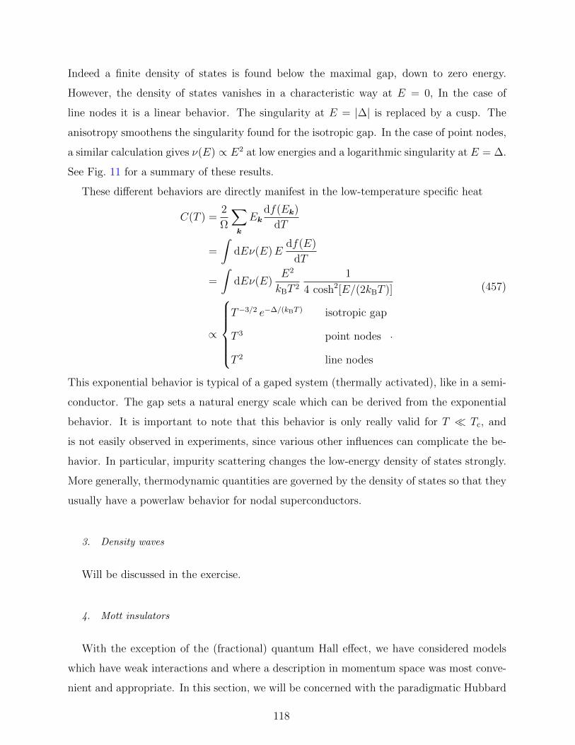
Indeed a finite density of states is found below the maximal gap, down to zero energy.
However, the density of states vanishes in a characteristic way at E = 0, In the case of
line nodes it is a linear behavior. The singularity at E = |∆| is replaced by a cusp. The
anisotropy smoothens the singularity found for the isotropic gap. In the case of point nodes,
a similar calculation gives ν(E) ∝ E2 at low energies and a logarithmic singularity at E = ∆.
See Fig. 11 for a summary of these results.
These different behaviors are directly manifest in the low-temperature specific heat
C(T ) =2
Ω
∑k
Ekdf(Ek)
dT
=
∫dEν(E)E
df(E)
dT
=
∫dEν(E)
E2
kBT 2
1
4 cosh2[E/(2kBT )]
∝
T−3/2 e−∆/(kBT ) isotropic gap
T 3 point nodes
T 2 line nodes
.
(457)
This exponential behavior is typical of a gaped system (thermally activated), like in a semi-
conductor. The gap sets a natural energy scale which can be derived from the exponential
behavior. It is important to note that this behavior is only really valid for T Tc, and
is not easily observed in experiments, since various other influences can complicate the be-
havior. In particular, impurity scattering changes the low-energy density of states strongly.
More generally, thermodynamic quantities are governed by the density of states so that they
usually have a powerlaw behavior for nodal superconductors.
3. Density waves
Will be discussed in the exercise.
4. Mott insulators
With the exception of the (fractional) quantum Hall effect, we have considered models
which have weak interactions and where a description in momentum space was most conve-
nient and appropriate. In this section, we will be concerned with the paradigmatic Hubbard
118
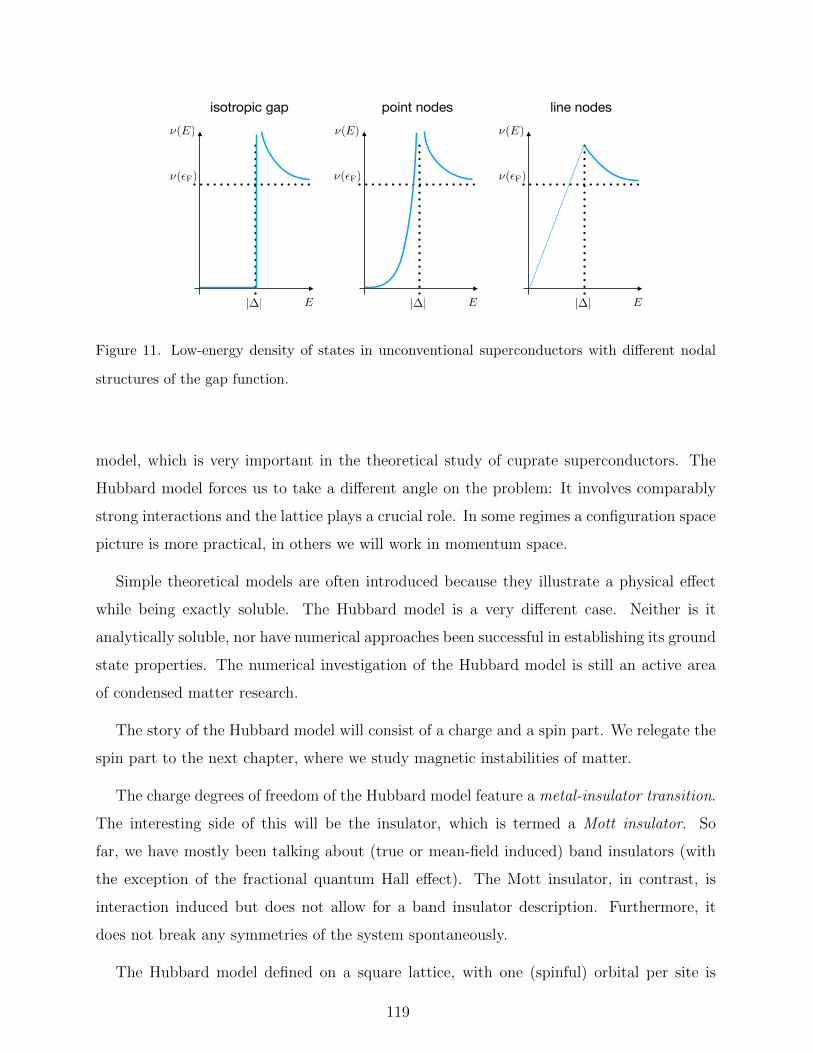
E||
(E)
(F)
E||
(E)
(F)
E||
(E)
(F)
isotropic gap point nodes line nodes
Figure 11. Low-energy density of states in unconventional superconductors with different nodal
structures of the gap function.
model, which is very important in the theoretical study of cuprate superconductors. The
Hubbard model forces us to take a different angle on the problem: It involves comparably
strong interactions and the lattice plays a crucial role. In some regimes a configuration space
picture is more practical, in others we will work in momentum space.
Simple theoretical models are often introduced because they illustrate a physical effect
while being exactly soluble. The Hubbard model is a very different case. Neither is it
analytically soluble, nor have numerical approaches been successful in establishing its ground
state properties. The numerical investigation of the Hubbard model is still an active area
of condensed matter research.
The story of the Hubbard model will consist of a charge and a spin part. We relegate the
spin part to the next chapter, where we study magnetic instabilities of matter.
The charge degrees of freedom of the Hubbard model feature a metal-insulator transition.
The interesting side of this will be the insulator, which is termed a Mott insulator. So
far, we have mostly been talking about (true or mean-field induced) band insulators (with
the exception of the fractional quantum Hall effect). The Mott insulator, in contrast, is
interaction induced but does not allow for a band insulator description. Furthermore, it
does not break any symmetries of the system spontaneously.
The Hubbard model defined on a square lattice, with one (spinful) orbital per site is
119
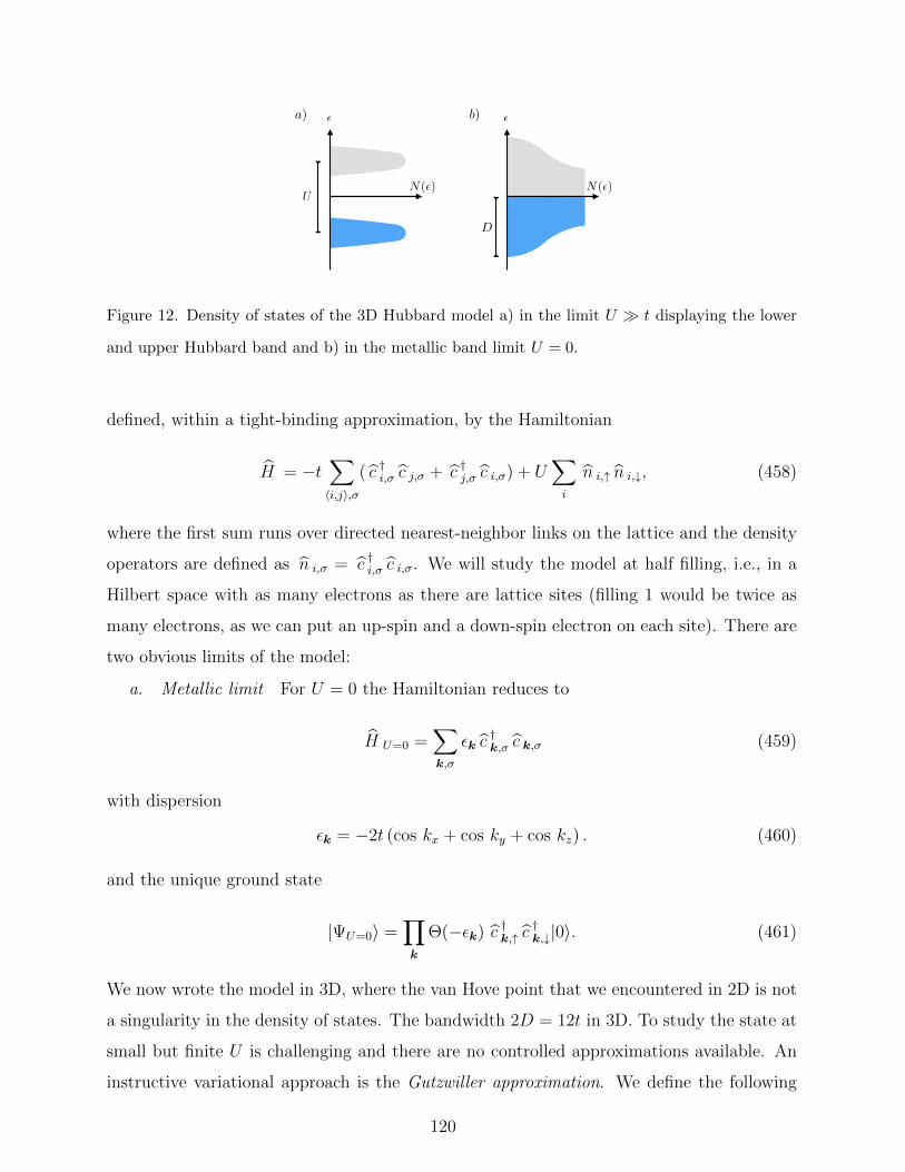
a) b)
N()U
N()
D
Figure 12. Density of states of the 3D Hubbard model a) in the limit U t displaying the lower
and upper Hubbard band and b) in the metallic band limit U = 0.
defined, within a tight-binding approximation, by the Hamiltonian
H = −t∑〈i,j〉,σ
( c †i,σ c j,σ + c †j,σ c i,σ) + U∑i
n i,↑ n i,↓, (458)
where the first sum runs over directed nearest-neighbor links on the lattice and the density
operators are defined as n i,σ = c †i,σ c i,σ. We will study the model at half filling, i.e., in a
Hilbert space with as many electrons as there are lattice sites (filling 1 would be twice as
many electrons, as we can put an up-spin and a down-spin electron on each site). There are
two obvious limits of the model:
a. Metallic limit For U = 0 the Hamiltonian reduces to
H U=0 =∑k,σ
εk c†k,σ c k,σ (459)
with dispersion
εk = −2t (cos kx + cos ky + cos kz) . (460)
and the unique ground state
|ΨU=0〉 =∏k
Θ(−εk) c †k,↑ c†k,↓|0〉. (461)
We now wrote the model in 3D, where the van Hove point that we encountered in 2D is not
a singularity in the density of states. The bandwidth 2D = 12t in 3D. To study the state at
small but finite U is challenging and there are no controlled approximations available. An
instructive variational approach is the Gutzwiller approximation. We define the following
120
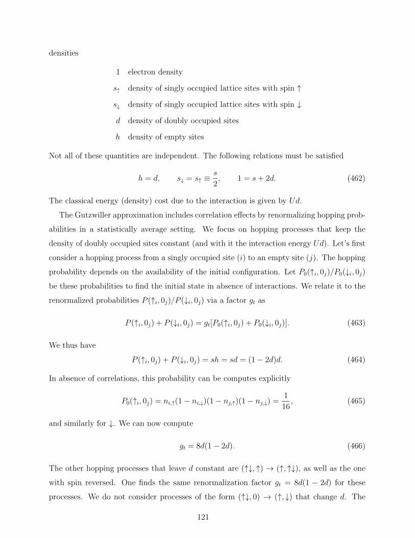
densities
1 electron density
s↑ density of singly occupied lattice sites with spin ↑
s↓ density of singly occupied lattice sites with spin ↓
d density of doubly occupied sites
h density of empty sites
Not all of these quantities are independent. The following relations must be satisfied
h = d, s↓ = s↑ ≡s
2, 1 = s+ 2d. (462)
The classical energy (density) cost due to the interaction is given by Ud.
The Gutzwiller approximation includes correlation effects by renormalizing hopping prob-
abilities in a statistically average setting. We focus on hopping processes that keep the
density of doubly occupied sites constant (and with it the interaction energy Ud). Let’s first
consider a hopping process from a singly occupied site (i) to an empty site (j). The hopping
probability depends on the availability of the initial configuration. Let P0(↑i, 0j)/P0(↓i, 0j)be these probabilities to find the initial state in absence of interactions. We relate it to the
renormalized probabilities P (↑i, 0j)/P (↓i, 0j) via a factor gt as
P (↑i, 0j) + P (↓i, 0j) = gt[P0(↑i, 0j) + P0(↓i, 0j)]. (463)
We thus have
P (↑i, 0j) + P (↓i, 0j) = sh = sd = (1− 2d)d. (464)
In absence of correlations, this probability can be computes explicitly
P0(↑i, 0j) = ni,↑(1− ni,↓)(1− nj,↑)(1− nj,↓) =1
16, (465)
and similarly for ↓. We can now compute
gt = 8d(1− 2d). (466)
The other hopping processes that leave d constant are (↑↓, ↑) → (↑, ↑↓), as well as the one
with spin reversed. One finds the same renormalization factor gt = 8d(1 − 2d) for these
processes. We do not consider processes of the form (↑↓, 0) → (↑, ↓) that change d. The
121
factor gt is used to renormalize the hopping probability, i.e., t → gtt. We thus find the
energy of a sector of constant d to be
E(d) = gtεkin + Ud, εkin =1
N
∫ 0
−Ddεν(ε) ε. (467)
Note that this is not a variational calculation in a strict sense, as E(d) is not guaranteed to
be an upper bound to the ground state energy. Nevertheless, we can minimize E(d) with
respect to d and obtain
d =1
4
(1− U
Uc
), gt = 1−
(U
Uc
)2
(468)
with
Uc = 8|εkin| ≈ 25t ≈ 4D. (469)
The theory thus naturally produces a critical interaction strength, and for U > Uc double
occupancy and with it any hopping is completely suppressed. This provides a qualitative
description for the metal-insulator transition in a Mott insulator. Obvious shortcomings are
that only local correlations are included to renormalize parameters, as opposed to corre-
lations between different lattice sites, and the spin degree of freedom plays no role in this
treatment.
We can argue more precisely why the system turns insulating by splitting up the con-
ductivity into two parts that correspond to different d sectors. Using the conductivity from
Eq. (335), we write
Reσ(ω) =ω?2p
4δ(ω) + Re σhigh energy(ω), (470)
where the first term is the conductivity associated with the Hamiltonian
H ren =∑k,σ
gt εk c†k,σ c k,σ + Ud (471)
while the second part corresponds to sectors with at least one more doubly occupied site.
Since ω2p ∝ 1/m, it renormalizes as ω?2p = gtω
2p. We can now make use of the f sum rule (336)∫ ∞
0
dωReσ(ω) =ω2
p
8gt + Ihigh energy =
ω2p
8. (472)
According to Eq. (468), the weight of the low energy contribution vanishes as U → Uc, and
the f sum rule dictates that it is sifted to the high-energy contribution (i.e., to large ω).
The system becomes insulating.
122
b. Insulating limit For t = 0, the ground state with zero energy has exactly one electron
per site. However, this ground state is not unique due to the spin degree of freedom. In
fact, any state of the from
|Ψσi〉 =∏i
c †i,σi |0〉 (473)
with any spin configuration σi is a ground state. The ground state degeneracy is 2N . It
is therefore a bit dangerous to call this an insulator, without knowing how this degeneracy
is lifted by small perturbations. However, since all these ground states do not differ in the
occupation numbers of each site, we can already anticipate that no electric transport will be
possible no matter how the degeneracy is lifted. The lifting of the ground state degeneracy
by small t will be the subject of the spin part of the Hubbard model story contained in
the next chapter. Excited states at energy U feature exactly one empty and one doubly
occupied site.
We now slightly depart from the limit t = 0 and consider the insulating state with
t U . The excitations of one site being doubly occupied and one site being empty are
called doublon and holon, respectively. When t is finite, these excitations can actually hop
and move through the lattice. This lifts some of the degeneracy of the “excited band” and
gives a dispersion
Ek,k′ = U + εk + εk′ > U − 12t. (474)
Upon increasing t, the two sectors (i.e., the ground state sector and this doublon-holon
band) start to overlap. When not overlapping, the two bands are called the lower and upper
Hubbard band. [See Fig. 12 a).] A holon is a hole in the lower Hubbard band and a doublon
is a particle in the upper Hubbard band. This density of states structure (there are no actual
energy bands here, the name is a complete abuse of language) is called a Mott insulator.
The gap is entirely due to the interaction, without the need for any mean-field treatment or
the like. It is therefore fundamentally different from the band insulators that we considered
before. We should keep in mind that we have neglected the role played by the spin.
c. The metallic state as a Fermi liquid In the uncorrelated case, we have
εkin =1
N
∑k∈FS
εk. (475)
Within the Gutzwiller we found εkin → gtεkin. One can furthermore show (we don’t give
a proof here) that within the same approximation a finite interaction strength induces a
123
nonzero and constant occupation number nout outside the Fermi surface while at the same
time the density inside the Fermi surface nin is reduced below 1 but remains constant. The
total must correspond to the filling, i.e.,
1
2=
1
N
∑k∈FS
nin +1
N
∑k 6∈FS
nout =nin + nout
2, (476)
where we used that the Fermi sea and its complement are equal in size. This gives the
constraint
gt εkin =1
N
∑k∈FS
ninεk +1
N
∑k 6∈FS
noutεk. (477)
We can furthermore use the particle-hole symmetry of the band structure
∑k∈FS
εk = −∑k 6∈FS
εk. (478)
Then we can determine from 1 = nin + nout and gt = nin − nout the densities
nin =1 + gt
2, nout =
1− gt2
. (479)
We thus find that there is a step in the distribution function (i.e., a quasiparticle picture
makes sense), as long as U < Uc. Without derivation, we give two Fermi liquid parameters
of the model
F a0 = −Uν(εF)
4
2Uc + U
(U + Uc)2Uc, F s
0 =Uν(εF)
4
2Uc − U(U − Uc)2
Uc. (480)
One interesting feature about them is the divergence of F s0 as U → Uc. We recall that F s
0
appears in the denominator of the compressibility
χ =µ2
B ν?(εF)
1 + F a0
, κ =ν?(εF)
n2(1 + F s0). (481)
The renormalized density of states at the Fermi level ν?(εF) = m?kF/π2 diverges due to
the diverging renormalized mass m? = m/gt ∝ (U − Uc)−1. However, the divergence in
F s0 is stronger so that, as expected for an insulator, the compressibility tends to zero. The
spin susceptibility does diverge at the metal-insulator transition, due to the formation of
completely independent local spins.
124
V. MAGNETISM IN SOLIDS
A. Antiferromagnetism
1. Superexchange in the Hubbard model
As discussed in the previous chapter, the Hubbard model has an extensive ground state
degeneracy in the limit t = 0. We now study how this degeneracy is lifted when a small
kinetic term t U is present. In order to derive an effective Hamiltonian, we consider
the hopping process between two neighboring sites in second order perturbation theory (to
get back to a ground state configuration, two hopping processes need to be involved). The
two neighboring sites have four degenerate ground state configurations | ↑, ↑〉, | ↑, ↓〉, | ↓, ↑〉,| ↓, ↓〉. Acting with the kinetic part of the Hamiltonian on each of them yields
H kin| ↑, ↑〉 = H kin| ↓, ↓〉 = 0,
H kin| ↑, ↓〉 = − H kin| ↓, ↑〉 = −t| ↑↓, 0〉 − t|0, ↑↓〉,(482)
where the relative minus sign in the last line is required by choosing a consistent ordering
of the second quantized operators.
This way we obtain the matrix elements
Mσ1,σ2;σ′1,σ′2
= − 〈σ1, σ2| H kin| ↑↓, 0〉〈↑↓, 0| H kin|σ′1, σ′2〉〈↑↓, 0| H U | ↑↓, 0〉
− 〈σ1, σ2| H kin|0, ↑↓〉〈0, ↑↓ | H kin|σ′1, σ′2〉〈0, ↑↓ | H U |0, ↑↓〉
,
(483)
where H U is the interaction part of the Hamiltonian. The denominator is U . The only
nonzero matrix elements are allocated in the blockM↑,↓;↑,↓ M↑,↓;↓,↑M↓,↑;↑,↓ M↓,↑;↓,↑
= −2t2/U
+1 −1
−1 +1
. (484)
which has the eigensystem
1√2
1
1
, E = 0;1√2
1
−1
, E = −4t2
U. (485)
The states | ↑, ↑〉 and | ↓, ↓〉 are two more eigenstates with zero energy. Together, the zero-
energy states for a degenerate triplet, as required by the SU(2) spin-rotation symmetry of
125
the Hamiltonian. The triplet | ↑, ↑〉, (| ↑, ↓〉+| ↓, ↑〉)/√
2, | ↓, ↓〉 furnishes the eigenspace with
eigenvalue S(S+1) for S = 1 of the operator (S1+S2)2. The singlet state (| ↑, ↓〉−| ↓, ↑〉)/√
2
corresponds to the S = 0 eigenvalue. Using that
(S1 + S2)2 = S21 + S2
2 + 2S1 · S2
=3
4+
3
4+ 2S1 · S2
(486)
we can thus recast the effective Hamiltonian as
H eff;1-2 = J
(S1 · S2 −
1
4
), J =
4t2
U> 0. (487)
This spin-spin coupling mediated by a pair of virtual hopping processes, that we derived
using second-order perturbation theory goes back to P.W. Anderson and is called superex-
change. It can be used to derive this coupling between any two nearest-neighbor sites in the
Hubbard model, yielding up to constant the effective Heisenberg Hamiltonian with antifer-
romagnetic coupling
HH = J∑〈i,j〉
Si · Sj. (488)
As mentioned above, the model has a global SU(2) spin rotation symmetry, represented by
Rα = exp
[−iα ·
∑i
Si
]. (489)
2. Mean-field theory and its shortcomings
We will now explore the ground state of the antiferromagnetic Heisenberg Hamilto-
nian (488). Surprisingly, there is a fundamental difference between the antiferromagnetic
and the ferromagnetic Heisenberg model, even though they are related by just a global sign
change in the Hamiltonian. The ferromagnetic problem essentially classical: the ground
state is of the form | ↑↑ · · · ↑〉, we can compute its energy exactly. For the antiferromag-
net, this is not true. The ground state deviates from | ↑↓ · · · ↑↓〉. The reason for this
striking difference lies in the fact that the order parameter commutes with the Hamiltonian
in the ferromagnetic case, while it does not commute in the antiferromagnet. If the order
parameter commutes with the Hamiltonian, both have common eigenstates, and the ground
state (necessarily an eigenstate of the Hamiltonian) can saturate the order parameter, as is
uniquely realized by the | ↑↑ · · · ↑〉 state in the ferromagnetic case. For the antiferromagnet,
126
by the lack of commutation such a ideal ground state cannot be found. We say quantum
fluctuations reduce the order parameter from the fully saturated value – the problem is
intrinsically quantum-mechanical.
Let us be a bit more explicit about the (missing) commutation and the order parameters.
The Heisenberg model is defined on a bipartite lattice, i.e., we can group the lattice sites in
two sublattices A and B with a checkerboard arrangement, such that each site in A has only
nearest neighbors in B and vice versa. The order parameters for ferro and antiferromagnet
are then defined as
Mfm =∑i∈A
Si +∑j∈B
Sj,
Mafm =∑i∈A
Si −∑j∈B
Sj
(490)
The lack of commutation can be seen from (for nearest neighbors i ∈ A and j ∈ B)
[Sx,iSx,j + Sy,iSy,j, Sz,i] = iSy,iSx,j − iSx,iSy,j,
[Sx,iSx,j + Sy,iSy,j, Sz,j] = iSx,iSy,j − iSy,iSx,j.(491)
If the two terms are summed up as in Mfm, the right-hand sides cancel, if we take their
differences, as in Mafm, they don’t.
While the symmetry is spontaneously broken in the antiferromagnetic ground state
〈Mafm〉 6= 0, mean-field theory is not going to deliver the exact ground state. Neverthe-
less, it is instructive to perform a mean-field calculation for the problem. We write
S i = M e z + ( S i −M e z), i ∈ A
S j = −M e z + ( S j +M e z), j ∈ B(492)
introducing the mean field M . The effective Hamiltonian is
Hmf = −JzM∑i∈A
Sz,i + JzM∑i∈A
Sz,i + Jz
2M2N, (493)
where we returned to a general case of coordination number z. The partition function
ZN(β,M) = tr eβHmf
= e−βJz2M2N
(eβJMz/2 + e−βJMz/2
)N (494)
is identical to the ferromagnetic case of Eq. (45), which shows again that the mean-field the-
ory is not capable of detecting the differences between antiferromagnetic and ferromagnetic
127
order. There follows the identical transition temperature, which for the antiferromagnet is
called Neel temperature
TN =Jz
4kB
. (495)
Clearly, the larger the coupling constant J and the more neighbors are present, the more
stable is the ordered state. Close to the transition, we can expand the free energy in M
F (M,T ) = F0 +Jz
2
[(1− TN
T
)M2 +
2
3
(TN
T
)3
M4
]. (496)
This effective free energy describes a second-order phase transition. Minimization of F
with respect to M yields the characteristic mean-field temperature dependence of the order
parameter
M(T ) =1
2
T
TN
√3
(1− T
TN
), T ≤ TN, (497)
while M(T ) vanishes for T > TN.
3. Spin-wave theory
We are going to study spin-wave excitations (magnons) on top of the ferromagnetically
and antiferromagnetically ordered state. We will treat this problem using the so-called
Holstein-Primakoff transformation, which allows to rewrite the spin operators at each lat-
tice site in terms of creation and annihilation operators of a boson. The virtue of this
transformation is that the algebra of bosons is much simpler than that of spins. However,
the price to pay is that the bosonic operators are acting on a larger local Hilbert space at
every lattice site than the spin operators. In this way, one might end up with solutions of the
bosonic problem, that do not map back to physical states in the spin variables. This problem
is avoided in the approximation by which spins only deviate slightly from the ferromagnetic
or antiferromagnetic orientation, as we shall see below.
Our goal is to derive the dispersion relations of spin waves and to understand their
connections to the symmetries of the problem. For small momenta k, the dispersions will
be quadratic in k in the ferromagnet and linear in k in the antiferromagnet. We will discuss
the general spin-S case and particularize on the spin-1/2 model discussed so far in the end.
On every lattice site i, the components Si,α with α = x, y, z of the spin operator act on the
128
(2S + 1)-dimensional local Hilbert space
Hsi = span| − S〉i, | − S + 1〉i, · · · , |S − 1〉i, |S〉i, (498)
which we have chosen to represent with the eigenbasis of Si,z,
Si,z|m〉i = m|m〉i, m = −S,−S + 1, · · · , S − 1, S. (499)
In order to perform the Holstein-Primakoff transformation, we consider introducing a
bosonic degree of freedom at every lattice site i with creation and annihilation operators a†i
and ai, respectively, that act on the local infinite-dimensional Hilbert space
Hbi = span
|n)i := (n!)−1/2 a†ni |0)i
∣∣∣ n = 0, 1, 2, · · · ; ai|0)i = 0, (500)
and obey
[ai, a†j] = δi,j, (501)
with all other commutators vanishing.
a. Ferromagnetic case The Holstein-Primakoff transformation is defined by introduc-
ing the following substitutes for the spin operators
S+i :=
√2S − a†i ai ai, S−i := a†i
√2S − a†i ai, Szi := S − a†i ai. (502)
One verifies that these spin wave operators obey the same algebra
[S+i , S−i ] = 2Szi , [S±i , Szi ] = ∓S±i (503)
on Hbi as the original spin operators do on Hs
i (where S±i := Si,x ± iSi,y). Now, the central
assumption that will allow us to simplify the theory when written in the bosonic variables
is that the fraction of reversed spins above the ferromagnetic ground state is small
〈a†i ai〉/S 1, ∀i. (504)
Within the range of validity of this assumption, it is justified to expand the square-roots
that enter Eq. (502) in a†i ai/(2S). Of course, this will be better justified, the larger S is,
i.e., the more “classical” the spin behaves.
It is furthermore useful to introduce the Fourier transforms of the bosonic operators
c†k =1√N
∑i
e−iri·ka†i , ck =1√N
∑i
eiri·kai. (505)
129
Using these together with Eq. (502), and expanding the square root to lowest order, the
Hamiltonian
Hfm = −J∑〈i,j〉
Si · Sj −B∑i
Si,z (506)
becomes
H ′fm = −JN z
2S2 −BNS − JzS
∑k
(γk + γ−k
2− 1
)c†kck +B
∑k
c†kck (507)
where
γk =2
z
∑δ
eik·δ, (508)
δ are the directed connection vectors to nearest neighbors and z is the coordination number.
Using γk = γ∗−k and dropping the constant terms in this Hamiltonian, we arrive at
H ′′fm =∑k
[JzS(1− Reγk) +B] c†kck. (509)
From this we can directly read off the dispersion of the ferromagnetic magnons as
ωk =JzS(1− Reγk) +B
≈B + JSa2k2,(510)
where we assumed a hypercubic lattice with lattice constant a to obtain the last line. This
is equivalent to the dispersion of a free massive particle with mass m? = 1/(2JSa2).
b. Antiferromagnetic case For the antiferromagnetic case, we have to account for the
two sublattices when performing the Holstein-Primakov transformation and we have to re-
place the source field B by a staggered one. We are thus interested in the Hamiltonian
Hafm = J∑〈i,j〉
Si · Sj −B∑i∈A
Si,z +B∑j∈B
Sj,z, (511)
and introduce on sublattice A the operators
S+i :=
√2S − a†i ai ai, S−i := a†i
√2S − a†i ai, Szi := S − a†i ai. (512)
while on sublattice B we use the operators
S+j := b†j
√2S − b†j bj, S−j :=
√2S − b†j bj bj, Szj := b†j bj − S. (513)
130
Both the a†j and b†j obey the usual bosonic algebra. It is again convenient to introduce
Fourier transforms of these bosonic operators
c†k =1√NA
∑i∈A
e−iri·ka†i , ck =1√NA
∑i∈A
eiri·kai,
d†k =1√NB
∑j∈B
e−irj ·kb†j, dk =1√NB
∑j∈B
eirj ·kbj,(514)
where NA = NB = N/2. Furthermore allowing for a linear transformation
αk = ukck − vkd†k, βk = ukdk − vkc†k, (515)
with 1 = u2k − v2
k, which ensures [αk, α†k] = [βk, β
†k] = 1, we can cast the Hamiltonian (511),
expanding in the bosonic operators, in the form
H ′afm = −JN z
2S(S + 1)− 1
2BN(2S + 1) +
∑k
ωk
(α†kαk + β†kβk + 1
). (516)
The antiferromagnetic magnon dispersion is given by
ωk =√
(JzS +B)2 − (JzS Re γk)2
≈ 2√
3JSa|k|,(517)
where we have expanded in small momenta a|k| 1 for the case of a hypercubic lattice for
B = 0 in the last line. Notice that in contrast to the ferromagnetic case, this is a gapless
dispersion.
This sharp difference between the ferro- and antiferromagnetic case is rooted in the prop-
erty that the order parameter commutes and does not commute with the Hamiltonian in
the two cases, respectively.
We can expand on this observation by considering the symmetries of Hamiltonians (506)
and (511) in the limit B = 0. The Hamiltonians, if the lattice Λ has the space group PΛ as
symmetry group, has the symmetry group
GΛ = SO(3)× Z2 × PΛ, (518)
where SO(3) are the proper rotations in spin space and Z2 is time-reversal. For the anti-
ferromagnetic order, we anticipate a reduction of the point group symmetry to PΛAof the
A sublattice only, where PΛ = Z2 × PΛA. Notice that all symmetries but time reversal are
unitary here.
131
For the ferromagnet, the order parameter M is actually one of the generators of the
continuous global symmetry group SO(3). This is the reason why it commutes with the
Hamiltonian. When aquiring a nonzero expectation value, M breaks SO(3) down to SO(2)
(rotations around the ferromagnetic axis) and at the same time breaks time-reversal sym-
metry. The symmetry-breaking pattern is thus
GΛ = SO(3)× Z2 × PΛ −→ HΛ,fm = SO(2)× PΛ. (519)
For the antiferromagnet, the order parameter similarly breaks SO(3) down to SO(2) and
breaks time-reversal. It does, however, preserve an ‘effective time-reversal symmetry’, that is
a composition of time-reversal symmetry and a translation that interchanges the sublattices
A and B. This yields the symmetry breaking pattern
GΛ = SO(3)× Z2 × PΛ −→ HΛ,afm = SO(2)× Z2 × PΛA. (520)
The fundamental difference between HΛ,fm and HΛ,afm is that the latter still contains an
antiunitary symmetry (the effective time reversal symmetry).
As stated before, the ferromagnetic ground state coincides with the quantum-mechanical
one, but this is not true for the antiferromagnet. To quantify this we compute the devia-
tion ∆M of the fully polarized classical sublattice magnetization NS/2 with the quantum
mechanical one within the approximation (504), i.e.,
∆M =NS
2−⟨∑i∈A
Si,z⟩, (521)
where the brackets stand for the ground state expectation value. With the form of Hamil-
tonian (516) this quantity can be computed as
∆M =1
2
∑k
(1√
1− (Reγk)2− 1
)
= − N
4+
1
2(2π)3
∫d3k
1√1− (Reγk)2
≈0.0784N
2,
(522)
meaning that we obtain a nearly 8 percent reduction from the fully polarized magnetization.
132
B. Stoner magnetism
In this section we are going to explore magnetism from a different angle, namely starting
from itinerant electrons. Magnetism arises here as an instability of a Fermi liquid, without
the need for a picture of localized moments and thus without the underlying lattice playing
an important role. Examples of magnets for which this mechanism is at work include
the ferromagnets iron, cobalt, and nickel, in all of which 3d-orbital electrons dominate the
states at the Fermi energy. The ferromagnetic order is a spontaneous symmetry breaking
phenomenon appearing at some finite Tc, the Curie temperature. The phase transition is of
second order in the Landau classification of phase transitions, thus featuring a discontinuity
in the specific heat but none in the entropy and volume.
Stoner magnetism is driven by repulsive (Coulomb) interactions. The energy gain can be
understood from Hunds rule: Alignment of the electronic spins in a favored direction allows
them to reduce the Coulomb energy. We recall that within Fermi liquid theory we have
found
χ =m?
m
χ0
1 + F a0
, (523)
for the magnetic susceptibility and concluded that a ferromagnetic instability would occur
if F a0 → −1. We will now use mean-field theory to derive this more microscopically.
1. Mean-field theory
We start from the Hamiltonian with a repulsive contact interaction
H =∑k,σ
εkc†k,σ ck,σ + U
∫d3rd3r′ ρ↑(r)δ(r − r′)ρ↓(r′), (524)
where ρσ(r) = φ†σ(r)φσ(r) is the density operator with φ†σ(r) the electron field operators.
We use this contact interaction as a simple model for screened Coulomb interaction. It is
clear that electrons of the same spin are not affected by the interaction, which gives rise to
the Hund’s rule mentioned above. We make the mean-field ansatz
ρσ(r) = nσ + [ρσ(r)− nσ], (525)
with nσ = 〈ρσ(r)〉 and the brackets represent the thermal average. To justify a mean-field
Hamiltonian, we assume
〈[ρ↓(r)− n↓][ρ↑(r)− n↑]〉 n↓n↑. (526)
133
Then
Hmf =∑k,σ
εkc†k,σ ck,σ + U
∫d3r [ρ↑(r)n↓ + ρ↓(r)n↑ − n↓n↑]
=∑k,σ
(εk + Un−σ) c†k,σ ck,σ − ΩUn↓n↑.(527)
This mean-field Hamiltonian describes electrons of one spin type σ moving in the background
of the opposite spin electrons −σ. We thus reduced the problem again to a single-particle
like problem. This is at the heart of the so-called Hartree-Fock approximation. To find a
self-consistent solution, we calculate the spin density
n↑ =1
Ω
∑k
〈c†k,↑ck,↑〉
=1
Ω
∑k
nεk+Un↓
=
∫dε
1
Ω
∑k
δ(ε− εk − Un↓)nε
=
∫dε
1
2ν(ε− Un↓)nε,
(528)
where nε is the Fermi Dirac distribution. The analogous equation holds for n↓. These
equations allow to self-consistently determine the mean densities nσ. Solutions must obey
particle number conservation. To implement this, it is convenient to split up the spin
densities in average particle densities n and magnetization m, the latter being related to the
measurable magnetization density M = µBm. That is
nσ =n+ σm
2. (529)
The self-consistency equations can then be cast in the form
n =1
2
∫dε [ν(ε− Un↓) + ν(ε− Un↑)]nε
m =1
2
∫dε [ν(ε− Un↓)− ν(ε− Un↑)]nε
(530)
or
n =1
2
∫dε∑σ
ν(ε− Un/2− σUm/2)nε
m =1
2
∫dε∑σ
σ ν(ε− Un/2− σUm/2)nε.
(531)
134
To make analytical progress from here, we assume that the magnetization is small, i.e.,
m n. We absorb the shift −Un/2 in the Fermi energy and expand (for the case of n,
where the m-odd term vanishes by the sum over σ
ν(ε− σUm/2) = ν(ε) +1
2
(Um
2
)2
ν ′′(ε) +O(m4). (532)
We furthermore use the so-called Sommerfeld expansion∫ ∞−∞
h(ε)1
eβ(ε−µ) + 1=
∫ µ
−∞h(ε)dε+
π2
6β2h′(µ) +O(βµ)−4. (533)
Lastly, we have to allow for a m-dependent shift in the chemical potential, i.e., µ(m, T ) =
εF + δµ(m, T ), such that δµ(0, T ) = 0. Together, when expanded to lowest order both in m
and in β−1, this yields
n =
∫ µ
−∞dεν(ε) +
1
2
(Um
2
)2
ν ′(εF) +π2
6β2ν ′(εF)
=
∫ εF
−∞dεν(ε) + δµν(εF) +
1
2
(Um
2
)2
ν ′(εF) +π2
6β2ν ′(εF)
= n+ δµν(εF) +1
2
(Um
2
)2
ν ′(εF) +π2
6β2ν ′(εF).
(534)
We can now solve for δµ as
δµ(m, T ) = −ν′(εF)
ν(εF)
[π2
6β2+
1
2
(Um
2
)2]. (535)
The analogous calculation for m reads
m =
∫dεnε
[ν ′(ε)
Um
2+
1
3!ν ′′′(ε)
(Um
2
)3]
=Um
2
[ν(εF) + δµν ′(εF) +
π2
6β2ν ′′(εF) +
1
3!
(Um
2
)2
ν ′′(εF)
]
=Um
2ν
[1− ν ′2
ν2
[π2
6β2+
1
2
(Um
2
)2]
+π2
6β2
ν ′′
ν+
1
3!
(Um
2
)2ν ′′
ν
]
= ν
[Um
2
(1− π2
6β2
ν ′2
ν2+
π2
6β2
ν ′′
ν
)+
(Um
2
)3(1
3!
ν ′′
ν− 1
2
ν ′2
ν2
)],
(536)
where we dropped the εF argument in the last line for notational compactness and inserted
δµ from Eq. (535).
135
The structure of this equation is m = am + bm3. If b is negative, we have two possible
solutions
m = 0, a < 1,
m =1− ab
, a ≥ 1.(537)
Obviously, the second solution is the one in the symmetry broken phase and hence a = 1
the critical value. Via the temperature dependence of a we can determine the critical
temperature (the Curie temperature)
1 =Uν
2
[1− π2
6β2
(ν ′2
ν2− ν ′′
ν
)](538)
yielding
kBTc =
√6
π√
ν′2
ν2 − ν′′
ν
√1− 2
Uν∝√
1− Uc
U, (539)
for U > Uc = 2/ν(εF). The latter condition
Uν(εF) > 2 (540)
on the minimal interaction strength is the instability condition for the paramagnetic Fermi
liquid to turn ferromagnetic at low temperatures, called the Stoner condition. For Uν(εF) <
2 there is no phase transition. In the symmetry-breaking phase (T < Tc), the magnetization
has the characteristic mean-field temperature-dependence
m(T ) ∝√Tc − T . (541)
This dependence is valid sufficiently close to the transition T −Tc Tc. Since the density of
states can also be changed by applying pressure, say, the phase transition can also be driven
a zero temperature if system parameters are changed such that the Uν(εF) = 2 is crossed.
A phase transition at zero temperature is called a quantum phase transition.
2. Susceptibility on the paramagnetic side
To compute the susceptibility, we apply a small symmetry-breaking field B along the
spin-quantization direction by adding the following Zeeman term to the Hamiltonian (527)
(setting the g-factor equal to 2)
HZ = −µB
∫d3rB [ρ↑(r)− ρ↓(r)] . (542)
136
The self-consistency equations (536) are now modified by replacing Um/2 with Um/2+µBB
on the right-hand side. We only keep the m-linear terms this time
m = ν
(Um
2+ µBB
)(1− π2
6β2
ν ′2
ν2+
π2
6β2
ν ′′
ν
)(543)
We can solve this equation for m and then compute the susceptibility χ via χ = M/B with
M = µBm. The result is given by
χ(T ) =M
B=
χ0(T )
1− Uχ0(T )
2µ2B
, (544)
where
χ0(T ) = µ2Bν
[1− π2
6β2
(ν ′2
ν2− ν ′′
ν
)]. (545)
Notice that the denominator of χ(T ) vanishes exactly when Eq. (538) is satisfied, i.e., at
the phase transition at finite temperature. From the paramagnetic side, the susceptibility
diverges as
χ(T ) ≈ χ0(Tc)T 2
c
T 2 − 1∝ |T − Tc|−1, (546)
which is the characteristic mean-field behavior with critical exponent 1. Notice also, that in
passing we have determined the Landau parameter
F a0 = −Uχ0
2µ2B
, (547)
which, as expected, is proportional to the interaction strength in the Fermi liquid.
3. Magnons
We have already encountered magnons as elementary excitations on top of the ferro-
magnetic ground state of the Heisenberg model using the spin-wave approximation. Here
we study how magnons arise in the itinerant ferromagnet that has undergone a Stoner-
instability. To that end, we consider particle-hole excitations with momentum q by making
the ansatz
|Ψq〉 =∑k
akc†k+q,↓ck,↑|0〉, (548)
where |0〉 is the (symmetry-broken) ground state and ak are coefficients. To find potential
eigenstates of this form, we solve the Schrodinger equation
H|Ψq〉 = (E0 + ωq)|Ψq〉, (549)
137
where H|0〉 = E0|0〉. We can recast this as
ωq|Ψq〉 =∑k
ak
[H, c†k+q,↓ck,↑
]|0〉 (550)
As before, we are going to employ a Hamiltonian with on-site interaction
H =∑k,σ
εkc†k,σ ck,σ +
U
Ω
∑k,k′,q
c†k+q,↑ck,↑c†k′−q,↓ck′,↓. (551)
with the help of which we can compute the commutator (550) as
ωq|Ψq〉 = (εk+q−εk)|Ψq〉+U
Ω
∑k
ak∑k′,q′
(c†k′+q′,↑ck′,↑c
†k+q−q′,↓ck,↑ − c†k+q,↓ck−q′,↑c
†k′−q′,↓ck′,↓
)|0〉.
(552)
We now make an approximation by which we replace pairs of c operators by their expectation
values nk,σ according to the Fermi-Dirac distribution
c†k′+q′,↑ck′,↑c†k+q−q′,↓ck,↑ → δq′,0nk′,↑c
†k+q,↓ck,↑ − δk,k′+q′nk,↑c†k+q−q′,↓ck−q′,↑,
−c†k+q,↓ck−q′,↑c†k′−q′,↓ck′,↓ → −δq′,0nk′,↓c†k+q,↓ck,↑ + nk+q,↓δk′,k+q c
†k−q′+q,↓ck−q′,↑,
(553)
which together give
c†k′+q′,↑ck′,↑c†k+q−q′,↓ck,↑ − c†k+q,↓ck−q′,↑c
†k′−q′,↓ck′,↓
→ δq′,0(nk′,↑ − nk′,↓)c†k+q,↓ck,↑ + (nk+q,↓δk′,k+q − nk,↑δk,k′+q′) c†k−q′+q,↓ck−q′,↑.(554)
This approximation yields an iteration of Eq. (552), that when projected on the state
〈0|c†k↑ck+q↓ reads
ak[ωq − εk+q,↓ + εk,↑
]=U
Ω
∑k
ak(nk+q,↓ − nk,↑) ≡ Rq, (555)
where we defined
εk,σ = εk + Un−σ (556)
in terms of the density of spin σ
nσ =1
Ω
∑k′
nk′,σ (557)
and
Rq =U
Ω
∑k
ak(nk+q,↓ − nk,↑). (558)
138
The goal is now to find the eigenvalues that solve Eq. (555) (we are not necessarily interested
in the eigenstates ak). To that end, we rewrite Eq. (555) as
ak =Rq
ωq − εk+q,↓ + εk,↑. (559)
Now, we use this expression for ak and insert it in Eq. (558) that defines Rq to obtain
Rq =U
ΩRq∑k
nk+q↓ − nk↑ωq − εk+q,↓ + εk,↑
. (560)
This equation has two types of solutions. One is Rq = 0, which yields ωq = εk+q,↓ − εk,↑ =
εk+q− εk+U(n↑−n↓) ≡ εk+q− εk+∆ and defines a particle-hole continuum at finite energy
(for small q). Aside from this solution, we have
1 =U
Ω
∑k
nk+q↓ − nk↑ωq − εk+q,↓ + εk,↑
. (561)
Setting q = 0 we find in addition zero energy excitations because
1 = Un↓ − n↑
ω0 − U(n↑ − n↓)(562)
is solved by ω0 = 0. This is the beginning of a magnon branch. We can follow it by
expanding Eq. (561) to quadratic order in q, assuming that ωq is small compared to the gap
∆
1 =U
Ω
∑k
nk+q↓ − nk↑ωq − εk+q,↓ + εk,↑
≈ − U
Ω
∑k
nk+q↓ − nk↑εk+q,↓ − εk,↑
− ωqU
Ω
∑k
nk+q↓ − nk↑(εk+q,↓ − εk,↑)2
≈ − U
Ω
∑k
nk+q↓ − nk↑εk+q − εk + ∆
− ωq(− 1
∆
)
≈ − U
Ω
∑k
nk+q↓ − nk↑∆
[1− εk+q − εk
∆+
(εk+q − εk
∆
)2]
+ωq∆
≈ 1− U
Ω
∑k
[nk↓ + nk↑
∆2
q2
2m− nk↓ − nk↑
∆2
(2k · q)2
2m2∆
]+ωq∆
≈ 1 +q2
2m∆2
(Un0 −
4εF3
)+ωq∆.
(563)
Solving for ωq, this gives the dispersion
ωq =q2
2m∆
4εF3
[UN(εF)− 2] +O(q4) (564)
139
which we can rewrite as
ωq ∝ q2
√U
Uc
− 1. (565)
This form shows how the magnon dispersion is related to the Stoner instability and the
dispersion becomes flat (the magnon heavy) near the transitions. That is, the magnons are
very ‘soft’ or easy to excite near right after the symmetry-breaking transition. We recall
that the magnon is the Goldstone mode of the continuously broken rotational symmetry.
VI. ADVANCED TOPICS
A. Relativistic effects in solids: spin-orbit coupling
When we considered noninteracting electronic band structures, we did not pay much
attention to the spin degree of freedom. It was always a mute variable the simply accounted
for a two-fold degeneracy of all energy bands, i.e., they could be occupied with a spin up and
a spin down electron. If however, we derive the Schroedinger equation from the relativistic
Dirac equation, we know that spin-orbit coupling appears and takes the form L · S in a
Lorentz invariant system. However, since Lorentz invariance is strongly broken in a crystal,
and crystal fields (which can be thought of as spatially varying electric fields) influence the
electron motion, we take a different route to understand spin-orbit coupling. We simply
assume that all terms in a Hamiltonian that are not forbidden by the lattice symmetry will
be present (with some material-specific coefficients).
Let us consider a two-dimensional electronic system k = (kx, ky) in a k ·p approximation.
The general Hamiltonian without any orbital degrees of freedom
H =∑k,σ,σ′
c †k,σhk,σσ′ c kσ′ (566)
is determined by the 2× 2 Bloch matrix hk,σσ′ . It is convenient to expand hk,σσ′ in terms of
the Pauli matrices
hk =∑
µ=0,x,y,z
dµ(k)σµ, (567)
where σ0 is the identity matrix. Time-reversal symmetry implies
T hkT −1 = h∗−k ⇒ d0(k) = d0(−k), di(k) = −di(−k), i = x, y, z (568)
140
with T = K iσy. Would we also also ask for inversion symmetry to be present, i.e., IhkI−1 =
h−k with I = σ0, then di(k) ≡ 0 and there would be no room for spin-orbit coupling terms
in this one-band model. In general multi-band models, spin-orbit coupling can appear also
with inversion symmetry. However, with I and T , all bands are always doubly degenerate,
because IT enforcers a Kramers degeneracy at every k due to (IT )2 = −1.
There are, however, enough crystals without inversion symmetry (so-called noncentrosym-
metric ones) and as far as two dimensional systems are concerned, we can also think of
interfaces or surfaces, where inversion is certainly broken. Let us instead impose mirror
symmetry in the x and y direction, respectively,
Mxhkx,kyM−1x = h−kx,ky ⇒ d0(kx, ky) = d0(−kx, ky),
dx(kx, ky) = dx(−kx, ky),
dy(kx, ky) = −dy(−kx, ky),
dz(kx, ky) = −dz(−kx, ky)
(569)
and similarly for My. We used Mx/y = iσx/y. Further, we want the system to be invariant
under (at least C4) rotations that are simulationsly carried out in momentum and spin space.
That is, for the case of C4, (kx, ky) → (ky,−kx) and (σx, σy, σz) → (σy,−σx, σz). Together,
these symmetries enforce, up to quadratic order in k the Hamiltonian to take the form
hk =
(k2
2m− µ
)σ0 + α(kxσy − kyσx). (570)
The second term is the relativistic Rashba spin-orbit coupling. Notice that we derived this
form solely from symmetries, but now we can give a physical interpretation to the result.
The coefficient α is proportional to the electric (crystal) field perpendicular to the plane
that breaks inversion symmetry. A relativistic electrons moving in the x direction (kx) in
an electric field in z direction experiences, in its rest frame, a magnetic field in y direction
(in both cases the Lorentz force should point in the z direction). This magnetic field can be
thought of coupling via the Zeeman effect and produces the term kxσy in the Hamiltonian.
The consequences of the Rashba term are nondegenerate electronic bands
ε±(k) =k2
2m− µ± α|k|, (571)
where the eigenstates of each band are such that the spin polarization at any given point in
141
k space is
〈±,k|σ|±,k〉 = ±
sin ϕ
− cos ϕ
0
, (572)
with ϕ = arctan(kx/ky). Thus, the Fermi surface splits up into two concentric rings. At
energy µ one of the Fermi surfaces shrinks to zero in a Dirac-like band touching at k =
0. Rashba spin-orbit coupling has a range of consequences when it comes to transport
properties, as well as superconductivity and other instabilities.
In multi-band systems, or in systems with even lower symmetries more general forms of
spin-orbit coupling are possible.
B. Effective relativistic dispersions in band structures: Topological insulators and
Weyl semimetals
We have seen that in some cases, the effective dispersion resulting from a k · p around
high-symmetry points in momentum space take the same form as the Dirac equation. This
is the case in graphene and at small momenta in the case of Rashba spin-orbit coupling.
But it can also appear in three-dimensional band structures. This fact motivates us to first
recall some basic aspects of the Dirac equation in a language useful for our purposes and
then apply this to a tight-binding simple model.
Dirac invented the equation named after him to link the dispersion relation E(k) =√k2 +m2 of relativistic particles with mass m (recall that the speed of light and ~ are set
to 1) with the theory of quantum mechanics. This led to a matrix-valued Hamiltonian that
is in general written in the form
H(k) =∑i
Γiki +mΓ0, (573)
where i can run over x, y, z (here for notational convenience also named 1, 2, 3) if we consider
particles in three dimensions or over x, y only if instead (quasi) two-dimensional space is
considered. The matrices Γµ, µ = 0, 1, 2, 3 are Hermitian and satisfy the algebra
Γµ,Γν = 2δµ,ν11. (574)
With this algebra, one verifies that H(k)2 = E(k)211, i.e., the desired dispersion is obtained.
There is, however, one caveat: The eigenvalues of H(k) are actually ±E(k). The negative
142
energy states essentially consisted the theoretical discovery of anti-particles. In three dimen-
sions, where µ, ν = 0, 1, 2, 3 the smallest matrix dimension that satisfies the algebra (574) is
4. In two dimensions, where µ, ν = 0, 1, 2, the smallest matrix size to satisfy this algebra is
2. The Pauli matrices
Γ0 ≡ σz =
1 0
0 −1
, Γ1 ≡ σx =
0 1
1 0
, Γ2 ≡ σy =
0 −i
i 0
(575)
do the job, for instance.
1. Topological insulators in three dimensions
We now turn to a tight-binding model which will display some interesting physics, related
to effective Dirac electron dispersions. It is defined on the cubic lattice. On each lattice
site we envision an atom with two orbitals, labelled a and b that are occupied by electrons.
This time, we are going to include the electron spin into the discussion. The Hamiltonian
contains two terms: H = H 1 + H 2. The first term models nearest neighbor hopping that
is the same for both spin orientations, but has the opposite sign for the two orbitals
H 1 =− t
2
∑〈Rj ,Rl〉
∑s=↑,↓
(c †Rj ,a,s cRl,a,s − c †Rj ,b,s cRl,b,s
)+M
∑Rj
∑s=↑,↓
(c †Rj ,a,s cRj ,a,s − c †Rj ,b,s cRj ,b,s
).
(576)
The parameter M quantifies a relativ on-site energy shift between the two orbitals. The
operator c †Rj ,α,s creates an electron on site Rj in orbital α ∈ a, b and with spin s ∈ ↑, ↓.The second term in the Hamiltonian
H 2 = −t′
2
∑Rj
∑i=x,y,z
∑s,s′=↑,↓
(iσi;s,s′ c
†Rj ,a,s
cRj+ai,b,s′ + h.c.)
(577)
is a spin-dependent hopping term (we accept that such a term should exist – it is a form
of spin-orbit coupling compatible with time-reversal symmetry). In momentum space, the
entire Hamiltonian reads
H =∑k
(c †k,a,↑, c
†k,a,↓, c
†k,b,↑, c
†k,b,↓
)H(k)
c k,a,↑
c k,a,↓
c k,b,↑
c k,b,↓
(578)
143
with
H(k) =
ξ(k) 0 t′ sin kz t′ sin kx − it′ sin ky
0 ξ(k) t′ sin kx + it′ sin ky −t′ sin kz
t′ sin kz t′ sin kx − it′ sin ky ξ(k) 0
t′ sin kx + it′ sin ky −t′ sin kz 0 ξ(k)
(579)
where ξ(k) = M + t (cos kx + cos ky + cos kz). It is now straight forward to derive a k · pHamiltonian around the Γ point yielding to linear order in k
HDirac(k) = (M + 3t)σ0 ⊗ σz + t′kxσx ⊗ σx + t′kyσy ⊗ σx + t′kzσz ⊗ σx (580)
where σ0 is the 2× 2 identity matrix and σµ⊗ σν stands for the direct product of two Pauli
matrices with index µ and ν, yielding a 4 × 4 matrix. One verifies that the four matrices
occurring in Eq. (580) satisfy the algebra (574) and hence we have a Dirac equation with
mass m = M + 3t. The eigenvalues of this effective Bloch Hamilton with energy bands
E±(k)
E±(k) = ±√m2 + k2, (581)
each of which is doubly degenerate. Clearly, the system is gapless (described by gapless
Dirac electrons) at the critical parameter value M = −3t. At other M 6= −3t the system is
an insulator (there might be gap closings at other momenta if M deviates much from −3t).
It turns out that this critical point actually discriminates two band structures which are
“topologically” distinct. For M < −3t we the Hamiltonian describes a normal insulator,
while for M > −3t, we speak of a topological insulator. While the study of topological band
structures is subject on its own, we want to point out the most important property of the
topological insulator, that is, its surface states. A topological insulator in three dimensional
crystals is characterized by gapless topological states on its surface, that are protected (i.e.,
gapless) as long as time-reversal symmetry is preserved.
Let’s solve explicitly for these states. To do so, we consider a geometry where the topo-
logical and trivial insulator are interfacing in the z = 0 plane. In this geometry, kx and ky
in Eq. (580) are still good quantum numbers, while kz has to be replaced by the momentum
operator, which is −i∂z in the position basis. The interface is then modeled by a z-dependent
mass term m(z) = m0sign(z). Let us first study the Hamiltonian at kx = ky = 0, which
144
reads
HDirac(kx = 0, ky = 0) =
m0sign(z) 0 −it′∂z 0
0 m0sign(z) 0 it′∂z
−it′∂z 0 −m0sign(z) 0
0 it′∂z 0 −m0sign(z)
(582)
We observe that it takes a form of two disconnected 2 × 2 blocks. We are interested in
eigenstates that are localized near the surface and energetically reside inside the energy gap
of the bulk material. As for the second property, a spectral symmetry of the problem we
are studying (which is not generic for topological insulators) allows to look for eigenstates
with exactly zero energy. One verifies that the following states are of this type
v± = e±m0|z|/t′
1
0
∓i
0
, u± = e±m0|z|/t′
0
1
0
±i
. (583)
Les us assume m0/t′ > 0. Then only v− and u− are localized at the boundary, i.e., admissible
normalizable solutions of our differential equation. (For m0/t′ < 0 only v+ and u+ would
be admissible.) Thus, we have two degenerate surface states at kx = ky = 0, both residing
at E = 0. Now, we would like to extend the dispersion of these states to finite momenta kx
and ky. For this, observe
Hsurf(kx, ky) =
〈v−|HDirac(kx, ky)|v−〉 〈v−|HDirac(kx, ky)|u−〉〈u−|HDirac(kx, ky)|v−〉 〈u−|HDirac(kx, ky)|u−〉
=
0 −i(kx − iky)
+i(kx + iky) 0
=kxσy − kyσx.
(584)
This again takes the form of a Dirac Hamiltonian, of the massless kind, with energy eigenval-
ues Esurf,± = ±√k2x + k2
y. Thus, the surface states of the topological insulator form a ’surface
Dirac cone’, a gapless two-dimensional state that lives at the intersection of a topological
insulator and a trivial insulator (which we can also call vacuum). As opposed to the bulk
states this Dirac cone has spin-polarized energy bands, i.e., they are not doubly degenerate
as the bulk bands. Note that the Hamiltonian looks similar to the Rashba Hamiltonian
145
studied before in purely two dimensions at first sight. There is, however, one important
difference: The Rashba Hamiltonian had two circles as Fermi surface, while this surface
Hamiltonian has only one such Fermi surface sheet. Fundamentally, with time-reversal sym-
metry, it is not possible to have only a single, non-spin degenerate Fermi surface in purely
two dimensions. The reason it is possible for the Dirac surface Hamiltonian lies in the fact
that it is ’secretly connected’ to a three-dimensional bulk band structure and that it has a
partner on the opposite side of the crystal.
In principle, we could imagine introducing a perturbation to the surface that gaps out
the Dirac cone degeneracy and makes also these surface states insulating. The unique term
that does this job in Hsurf(kx, ky) is given by msurfσz, because σz is the only non-commuting
anticommuting 2 × 2 matrix not already used in the surface Hamiltonian. However, this
perturbation breaks time-reversal symmetry. To understand that, we first have to find (or
define) the representation of the time-reversal transformation for the bulk Hamiltonian.
Noting that time-reversal reverts the momentum, we can define T = K iσy ⊗ σ0, which
squares to −1 as desired for spin-1/2 fermions. We check that
T HDirac(k)T −1 = HDirac(−k). (585)
Furthermore, T |u−〉 = −|v−〉 and T |v−〉 = +|u−〉, i.e., the two surface states degenerate at
kx = ky = 0 are Kramers partners. Kramers theorem then forbids any hybridization that
lifts their degeneracy (at kx = ky = 0), as long as time-reversal symmetry is obeyed. We
conclude that the gapless nature of the topological insulator surface states is protected by
time-reversal symmetry.
Finally, we note that the band representations can be used to determine whether an
insulator is topological, i.e., to predict whether it will have such a gapless Dirac surface
state. If the insulator has inversion symmetry, Fu and Kane found the formula (which we
just state without proof)
(−1)ν =∏
k∈TRIM
∏i∈occupied bands
ξi,k, (586)
where ξi,k is the inversion eigenvalue of the i-th band at momentum k. The product runs
only over the momenta in the three-dimensional Brillouin zone whose little group contains
inversion (i.e., which are invariant under inversion k→ −k up to a reciprocal lattice vector).
Since these are also the time-reversal invariant momenta (TRIM), bands are doubly degen-
erate by Kramers theorem at these points and only one eigenvalue per Kramers pair enters
146
the formula (586). The integer ν is defined modulo 2 and is called a topological invariant.
If ν = 0, the insulator is trivial, if ν = 1, the insulator is topological. We can check that for
the model at hand.
2. Weyl semimetals
Let us go back to the three-dimensional Dirac model (580) and introduce a time-reversal
breaking perturbation in the form of a Zeeman field
H(k) = (M + 3t)σ0 ⊗ σz + t′kxσx ⊗ σx + t′kyσy ⊗ σx + t′kzσz ⊗ σx +Bσz ⊗ σ0 (587)
If we tune the model to the formerly critical point M = −3t, we obtain the spectrum
Eλ,λ′ = λ√t′2(k2
x + k2y) + (B + λ′t′kz)2, λ, λ′ = ±. (588)
We observe that the fourfold degenerate gapless point at k = 0 (the touching of four bands)
has split into two gapless points at k = (0, 0,±B/t′) (each being the touching of two bands
only). We can derive an effective k · p Hamiltonian involving only the two touching bands
near k = (0, 0, B/t′), for instance: Only the σ0 ⊗ σx eigenstates with eigenvalue −1 will
play a role there, the other eigenstates are at high energy. We can thus replace in Eq. (587)
σµ ⊗ σx by −σµ while again setting M = −3t. This yields the effective Hamiltonian
HWeyl(k) = −t′(kxσx + kyσy + δkzσz), (589)
where δkz = kz−B/t′ and this expansion is valid for small δkz. The 2×2 Hamiltonian (589)
is what (in condensed matter) is called the Weyl Hamiltonian. Remarkably, while the
Dirac point that we started with was a degeneracy that required parameter fine-tuning
(M = −3t), the Weyl point degeneracy cannot be removed by a small perturbation or
parameter change: Any perturbation (i.e., any constant matrix W that can be added to
HWeyl(k) can be decomposed into W = w · σ resulting in
HWeyl(k) = −t′ [(kx − wx/t′)σx + (ky − wy/t′)σy + (δkz − wz/t′)σz] . (590)
This most general (small) perturbation simply moved the Weyl point to (kx, ky, δkz) = w/t′
but is not able to gap it out. The reason for this is that for a touching of two bands we have
exhausted the anticommuting 2× 2 matrices already for the kinetic part of the Hamiltonian
so that none are left to be added as masses.
147
Weyl semimetals also have topological surface states, so-called Fermi arcs, with rather
exotic properties. Together with topological insulators they are an active field of study in
contemporary condensed matter physics. Time-reversal symmetry breaking is not needed
to generate Weyl nodes in band structures, as long as inversion symmetry is broken.
C. Density functional theory
Density functional theory (DFT) has been introduced in the 1960s and has since become
the most successful and widely employed tool to compute the electronic structure of matter.
It has a high predictive power in its range of applicability. Here, we are most interested in the
computation of band structures of crystals, but the same concepts also apply to molecules.
DFT works best for weakly correlated materials that have s, p and at most d orbitals neat the
Fermi surface. It is by construction not able to describe strongly correlated states like Mott
insulators, fractional quantum Hall states and the like. More recently, extensions have been
developed to include superconducting instabilities, but with much less predictive power.
Routinely available are by now calculations that include spin-orbit coupling or magnetic
states.
1. Variational principle and Hartree-Fock approximation
Starting point for our considerations is the Born-Oppenheimer approximation to the
Hamiltonian (1) in our lecture notes, which assumes that the nuclei remain at their static
positions. We also reduce the problem here to the Schroedinger equation, noting that a
similar analysis would apply for a fully relativistic formulation. The many-body electronic
Hamiltonian is then written as
Hel = −1
2
N∑j=1
∇2j −
N∑j=1
M∑l=1
Zlrjl
+N∑j=1
N∑k>j
1
rjk, (591)
where rjl is the distance between nucleus l and electron j, while rlk is the distance between
electrons j and k.
The variational principle is based on the fact that a guessed wave function Ψ can be used
to compute the energy expectation value
E[Ψ] =〈Ψ|Hel|Ψ〉〈Ψ|Ψ〉 , (592)
148
and since the true ground state has the lowest energy E0, E[Ψ] will always be an upper bound
for E0. Here E[Ψ] should be viewed as a functional. Full minimization of the functional
E[Ψ] with respect to all allowed N -electron states will yield the true ground state Ψ0 and
its energy. This is, of course, an exponentially hard problem.
To make progress, the key simplification is to only use single Slater determinant wave
functions as an ansatz. This is the Hartree-Fock approximation. It greatly reduces the space
of wavefunctions (and therefore types of quantum states) that can be captured. Thus, with
Ψ0 ≈ ΨHF,N =1√N
∣∣∣∣∣∣∣∣∣ψ1(r1) · · · ψ1(rN)
......
ψN(r1) · · · ψN(rN)
∣∣∣∣∣∣∣∣∣ (593)
the problem reduces to finding an orthogonal basis of ψj that minimizes
EHF,N = minΨHF,NE[ΨHF,N ]. (594)
The energy can be written more explicitly as
EHF,N = 〈ΨHF,N |Hel|ΨHF,N〉
=N∑j=1
Hj +1
2
N∑j,k=1
(Jjk −Kjk)
Hj =
∫d3rψ∗j (r)
[−1
2∇2 − Vext(r)
]ψj(r)
Kjk =
∫d3r1
∫d3r2ψ
∗j (r1)ψk(r1)
1
r12
ψj(r2)ψ∗k(r2)
Jjk =
∫d3r1
∫d3r2ψj(r1)ψ∗j (r1)
1
r12
ψ∗k(r2)ψk(r2).
(595)
Here, Vext(r) is the potential felt by the electrons due to the nuclei, Jjk are the so-called
Coulomb integrals, and Kjk are the so-called exchange integrals. They obey Jjk ≥ Kjk ≥ 0
and Jjj = Kjj.
The Hartree-Fock equations are the equations resulting from varying EHF,N with respect
to the single electron wave functions ψj. They are non-linear and non-local (thanks to
Jjk and Kjk, and thus have to be solved self-consistently. Thus, albeit the Hartree-Fock
approximation has led us to simplify the interacting many-body problem to an effective one-
electron problem, it is still difficult to solve. It is important to stress that the problem we
want to solve is determined by only the external potential Vext(r) and the particle number
149
N . Everything else is the completely universal Schroedinger equation which does not contain
an further information specific to a particular problem.
2. Hohenberg-Kohn theorems
The key step that led to the development of density-functional theory is to not go down
the Hartree-Fock road and consider ψj but instead the electron density
ρ(r) = N
∫d3r2 · · ·
∫d3rN |Ψ(r, r2, · · · , rN)| (596)
as the central object of the theory. Physically, ρ(r) is the probability of finding an electrons
in the volume element d3r. Different from the wave functions, this is an experimentally
observable quantity (measurable, e.g., via X-ray diffraction). It satisfies
ρ(r) ≥ 0, limr→∞
ρ(r) = 0,
∫d3r ρ(r) = N. (597)
Further, at any position of an ion rl, the derivative of ρ(r) has a discontinuity determined
by the ion’s charge
limr→rl
(∂r + 2Zl) ρ(r) = 0, (598)
where ρ(r) is the angular average of ρ(r) with respect to the position of the ion. It is not
a priori obvious that considering the electron density instead of the wave function itself is
a sufficiently general way forward. However, the Hohenberg-Kohn theorems tell us exactly
that.
a. First Hohenberg-Kohn theorem The external potential Vext(r) is (up to a constant)
a unique functional of ρ(r). Since, in turn, Vext(r) fixes the Hamiltonian Hel, the full many-
particle ground state is a unique functional of ρ(r).
Proof : We prove this by contradiction. Assume there were two external potentials Vext(r)
and V ′ext(r) that differ by more than a constant, but have the same ρ(r) in the ground state.
Then, we have two corresponding Hamiltonians Hel and H ′el with different ground state wave
functions Ψ0 and Ψ′0 that have the same density. Take Ψ′0 as a variational wave function for
Hel
E0 < 〈Ψ′0|Hel|Ψ′0〉
= 〈Ψ′0|H ′el|Ψ′0〉+ 〈Ψ′0|Hel −H ′el|Ψ′0〉
=E ′0 +
∫d3rρ(r) [Vext(r)− V ′ext(r)] .
(599)
150
Exchanging the role of the primed and unprimed quantities we obtain
E ′0 <E0 +
∫d3rρ(r) [V ′ext(r)− Vext(r)] . (600)
Adding Eqs. (599) and (600) gives the contradiction E0 + E ′0 < E ′0 + E0. This means that
there cannot be two different Vext(r) with the same ground state density.
Thus, ρ(r) determines N and Vext(r) and with this all ground state properties. Thus,
we can formally write any ground state property as a functional of ρ(r). In particular, this
is true for the energy
E[ρ] =
∫d3rρ(r)Vext(r) + FHK[ρ],
FHK[ρ] =T [ρ] + J [ρ] + Encl[ρ]
J [ρ] =1
2
∫d3r1d3r2
ρ(r1)ρ(r2)
r12
.
(601)
The functional FHK[ρ] is here represented as a sum over the kinetic part T [ρ], the classical
electrostatic contribution and a quantum-mechanical contribution Encl[ρ] which contains
quantum mechanical corrections. Within Hartree-Fock, it contains the exchange and the
Coulomb correlations. The key advantage of this representation is that it separated the
energy in a problem-specific part involving Vext(r) that is know and easy to compute and a
completely universal part FHK[ρ]. The challenge is that FHK[ρ] is not known. Knowing it
amounts to solving the many-body Schroedinger equation exactly (not within Hartree-Fock).
Providing an explicit from of the functional FHK[ρ] that is in some sense a well-controlled
approximation is the central problem in density functional theory.
b. Second Hohenberg-Kohn theorem FHK[ρ], the functional that delivers the ground
state energy of the system, delivers the lowest energy if and only if the input density is the
true ground state density.
This basically guarantees uniqueness of the solution and allows us to employ the varia-
tional principle in the search for the ground state density and energy. Thus we can obtain
the ground state energy
E0 ≤ E[ρ] (602)
by minimizing the functional E[ρ] over all trial densities ρ.
Proof : We can use the variational principle for wave functions together with the first
Hohenberg-Kohn theorem. The latter states that there is a one-to-one connection between
151
a potential ρ and a Hamiltonian Hel for which this is the ground state density (in particular,
ρ determines a Vext(r) in this way). The Hamiltonian further has a unique ground state Ψ0.
We can use Ψ0 as a trial wave function for the Hamiltonian Hel generated from the true
external potential Vext(r)⟨ψ0|Hel|ψ0
⟩≡ E[ρ] ≥ E0 ≡ E[ρ] = 〈ψ0|Hel|ψ0〉 . (603)
We emphasize that this result is only true for the ground state, as association of the
Hamiltonian with a unique ground state is key. The approach cannot be used for excited
states.
3. Kohn-Sham equation
The Kohn-Sham equation provides an explicit approximate expression for T [ρ] and Encl[ρ]
and thereby defines a density functional theory. (Historically, the first relevant density
functional theory of relevance was the Thomas-Fermi theory which is still an important
subject of more mathematical research. For practical numerical computations it is however
not used anymore, because of the availability of better performing methods.)
Kohn and Sham suggested to calculate the exact kinetic energy of a non-interacting
reference system with the same density as the real, interacting one
TS = −1
2
N∑j=1
⟨ψj|∇2|ψj
⟩, ρS(r)
N∑j=1
|ψj(r)|2 != ρ(r), (604)
where ψj are the single-particle orbitals of the noninteracting system. Since TS will not be
equal to the actual kinetic energy T [ρ], one rewrites
FHK[ρ] = TS[ρ] + J [ρ] + EXC[ρ] (605)
where all the unknown functionals are subsumed in the exchange-correlation energy
EXC[ρ] = T [ρ]− TS[ρ] + Encl[ρ]. (606)
To go further with the approximation by a non-interacting system, we search for a potential
VS that provides as a solution a slater determinant that has the same density as the real
system that we are interested in. If we succeed in finding this, we have a single slater
determinant solution to a problem defined by TS and VS (i.e., a different problem) which
152
has the same solution in terms of electron density, as the problem we are interested in. We
recall the energy functional
E[ρ] =TS[ρ] +1
2
∫d3r1
∫d3r2
ρ(r1)ρ(r2)
r12
+ EXC[ρ] +
∫d3rVext(r)ρ(r). (607)
All terms except for EXC[ρ] can be straightforwardly written in terms of the ψj. We ignore
this issue for the moment and apply the variational principle, i.e., minimize with respect to
the ψj subject to 〈ψj|ψk〉 = δjk. This yields the Kohn-Sham equations−1
2∇2 +
[∫d3r2
ρ(r2)
r12
+ VXC(r1) + Vext(r1)
]ψj(r1) = εjψj(r1) (608)
with
VS(r1) =
∫d3r2
ρ(r2)
r12
+ VXC(r1) + Vext(r1). (609)
The problem is now to find VS. This only depends on the density, i.e., the Kohn-Sham
equations have to be solved iteratively/self-consistently. Up to this, the problem is reduced
to find VXC = δEXC/δρ. Would we succeed in that, we would have the exact ground state
energy of the interacting system. The orbitals ψj that we would find this way have – strictly
speaking – no physical meaning. Still, for weakly correlated systems, they provide a good
approximation to the true states of the system.
4. Local density approximation and beyond
The local density approximation (LDA) is the basis for all practically used approximations
to the exchange-correlation functional. The central idea is that of a uniform electron gas.
The form
ELDAXC [ρ] =
∫d3r ρ(r) εX(ρ(r)) + εC(ρ(r)) (610)
is postulated, where εX(ρ(r)) + εC(ρ(r)) is the exchange-correlation energy per particle of a
uniform electron gas of density ρ(r). This energy per particle is weighted with the probability
of finding an electron at this position. Of the two parts εX(ρ(r)) and εC(ρ(r)) the exchange
part is known exactly for the case of an electron in a uniform electron case of a particular
density
εX(ρ(r)) = −3
4
(3ρ(r)
π
)1/3
. (611)
153
The correlation part εC(ρ(r)) is only known from numerical simulations for the same case,
but with high accuracy.
For weakly correlated systems, LDA gives EXC[ρ] with an error of 10%–20%, but predicts
other ground state properties with much higher accuracy. LDA largely fails for systems
dominated by electron-electron interactions, such as heavy fermion compounds.
Several methods to go beyond LDA are known. One natural step to include more non-
local aspects of the electron density in EXC[ρ] is the generalized gradient approximation
(GGA)
EGGAXC [ρ] =
∫d3rf(ρ(r),∇ρ(r)). (612)
Besides the form of the exchange functional, another important property of a density
functional code is the basis set in which the ψj are expanded. One of many options is the
linear combination of atomic orbitals, i.e., orbitals of atoms in free space.
154