incremental map generation (img)
TRANSCRIPT
Incremental Map Generation (IMG)
Dawen Xie, Marco A. Morales A., Roger Pearce, Shawna Thomas, Jyh-MingLien, and Nancy M. Amato
Parasol Lab, Department of Computer Science,Texas A&M University, College Station, TX USA{dawenx, marcom, rap2317, sthomas, neilien, amato}@cs.tamu.edu
Abstract: Probabilistic roadmap methods (prms) have been highly successful insolving many high degree of freedom motion planning problems arising in diverseapplication domains such as traditional robotics, computer-aided design, and com-putational biology and chemistry. One important practical issue with prms is thatthey do not provide an automated mechanism to determine how large a roadmapis needed for a given problem. Instead, users typically determine this by trial anderror and as a consequence often construct larger roadmaps than are needed. In thispaper, we propose a new prm-based framework called Incremental Map Generation(img) to address this problem. Our strategy is to break the map generation intoseveral processes, each of which generates samples and connections, and to continueadding the next increment of samples and connections to the evolving roadmap un-til it stops improving. In particular, the process continues until a set of evaluationcriteria determine that the planning strategy is no longer effective at improving theroadmap. We propose some general evaluation criteria and show how to apply themto construct different types of roadmaps, e.g., roadmaps that coarsely or more finelymap the space. In addition, we show how img can be integrated with previouslyproposed adaptive strategies for selecting sampling methods. We provide resultsillustrating the power of img.
1 Introduction
Automatic motion planning has applications in many areas such as robotics,computer animation, computer-aided design (CAD), virtual prototyping, andcomputational biology and chemistry. Although many deterministic motionplanning methods have been proposed, most are not used in practice becausethey are computationally infeasible except for some restricted cases, e.g., whenthe robot has few degrees of freedom (dof) [16]. Indeed, there is strong evi-dence that any complete planner (one that is guaranteed to find a solution ordetermine that none exists) requires time exponential in the robot’s dof [23].
For this reason, attention has focused on randomized approaches that sam-ple and connect points in the robot’s configuration space (C-space). Such
2 D. Xie, M. Morales, R. Pearce, S. Thomas, J.-M. Lien and N. M. Amato
Pass
Fail
Build/ExpandRoadmap Evaluate
RoadmapQuery Roadmap
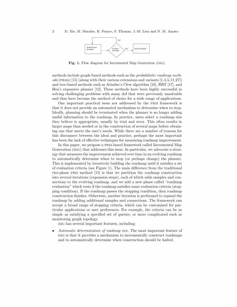
Fig. 1. Flow diagram for Incremental Map Generation (img).
methods include graph-based methods such as the probabilistic roadmap meth-
ods (prms) [15] (along with their various extensions and variants [1,4,5,11,27])and tree-based methods such as Ariadne’s Clew algorithm [18], RRT [17], andHsu’s expansive planner [12]. These methods have been highly successful insolving challenging problems with many dof that were previously unsolvableand thus have become the method of choice for a wide range of applications.
One important practical issue not addressed by the prm framework isthat it does not provide an automated mechanism to determine when to stop.Ideally, planning should be terminated when the planner is no longer addinguseful information to the roadmap. In practice, users select a roadmap sizethey believe is appropriate, usually by trial and error. This often results inlarger maps than needed or in the construction of several maps before obtain-ing one that meets the user’s needs. While there are a number of reasons forthis disconnect between the ideal and practice, perhaps the most importanthas been the lack of effective techniques for measuring roadmap improvement.
In this paper, we propose a prm-based framework called Incremental MapGeneration (img) that addresses this issue. In particular, we advocate a strat-egy that measures the improvement achieved over time in an evolving roadmapto automatically determine when to stop (or perhaps change) the planner.This is implemented by iteratively building the roadmap until it satisfies a setof evaluation criteria (see Figure 1). The main difference from the traditionaltwo-phase prm method [15] is that we partition the roadmap constructioninto several iterations (expansion steps), each of which adds samples and con-nections to the evolving roadmap, and we add a new phase called “roadmapevaluation” which tests if the roadmap satisfies some evaluation criteria (stop-ping condition). If the roadmap passes the stopping condition, then roadmapconstruction finishes. Otherwise, another iteration is performed to expand theroadmap by adding additional samples and connections. The framework canaccept a broad range of stopping criteria, which can be customized for par-ticular applications or user preferences. For example, the criteria can be assimple as satisfying a specified set of queries, or more complicated such asmonitoring graph topology.
img has several important features, including:
• Automatic determination of roadmap size. The most important feature ofimg is that it provides a mechanism to incrementally construct roadmapsand to automatically determine when construction should be halted.
Incremental Map Generation (IMG) 3
• Evaluation criteria. A key requirement for img is effective evaluation crite-ria that can be efficiently tested during roadmap construction. A contribu-tion of this work is to propose evaluation criteria for measuring roadmapquality (e.g., coverage and connectivity) that do not require prior knowl-edge about the solution (as do, e.g., test queries) and that do not rely onC-space discretization (so can be efficiently applied to high dof problems).
• Compatibility with existing sampling-based planners. img is not a new sam-pling method; instead, it is a general strategy that can be used with anysampling-based planner and, moreover, provides a natural mechanism foradaptive planning. For example, each img iteration can use any of theexisting adaptive strategies that utilize multiple planners (e.g., [13,19]) ordifferent strategies could be chosen for different img iterations.
2 Related work
The general prm methodology [15] consists of a preprocessing phase and aquery phase. Preprocessing, which is done once for a given environment, firstsamples points ‘randomly’ from the robot’s C-space, retaining those that sat-isfy certain feasibility requirements. Then, these points are connected to forma graph, or roadmap, containing representative paths in the free C-space. Thequery phase then connects any given start and goal to the same connectedcomponent of the roadmap, and if successful, returns a path connecting them.
The probability of failing to find a path in a probabilistic roadmap, whenone exists in C-free, decreases exponentially as the number of samples inthe roadmap increases [14]. However, it is difficult to decide beforehand theroadmap size required in practice.
The coverage and connectivity of an ideal prm roadmap should matchthat of its underlying C-space. In [9], coverage and maximal connectivityachieved by different sampling methods was compared to that of the C-spacebeing modeled. Coverage indicates how each query can be connected to theroadmap. If there exists a path in the free C-space between two query con-figurations, maximal connectivity ensures that a path between them can befound in the roadmap. The authors evaluate the time needed to adequatelycover and connect the free C-space for various techniques. This work relies ona discretization of C-space and so cannot be applied to high dof problems.
Since there is no principled mechanism to determine when to stop roadmapconstruction, a commonly used evaluation criterion is to predefine a set of rel-evant queries in each environment and continue building the roadmap untilthe query configurations can be connected to the same connected component.This is helpful in environments where the user knows beforehand such a rep-resentative query. However, in many situations defining such a query can beproblematic, e.g., in cluttered environments or in higher dof problems suchas the protein folding applications. The stopping criteria we propose can beapplied when it is hard or even impossible to define a representative query

4 D. Xie, M. Morales, R. Pearce, S. Thomas, J.-M. Lien and N. M. Amato
for a given problem. In the case when such a query is easy to define or whensolving a particular query is the user’s objective, then img can easily use itas a stopping criterion, i.e., img also supports the traditional query-basedcriterion.
A set of metrics are proposed in [20] to estimate how each new sampleimproves, or not, the representation of C-space achieved by the planner. Withthese metrics, the authors identify three phases common to all sampling-basedplanners: quick learning (a coarse roadmap is constructed), model enhance-ment (the roadmap is refined), and learning decay (most new samples do notprovide additional information). They also demonstrate that the traditionalscheme of testing a set of witness queries, which is commonly used in practiceas a stopping criteria, can be misleading.
Adaptive hybrid prm sampling [13] proposes using a mixture of samplers.They adapt the mixture of strategies based on each strategy’s past success. Inthis work, we incorporate hybrid prm sampling and apply our img frameworkto hybrid prm to decide when to stop building the roadmap.
3 Incremental Map Generation (IMG)
We propose a new prm-based framework called Incremental Map Generation(img) in which we iteratively build a roadmap until it satisfies a set of eval-uation criteria (see Figure 1). Most importantly, this framework provides asystematic way to automatically decide when to stop roadmap construction.Algorithm 3.1 describes img. This framework is simple and general. It can becustomized for a particular application domain or problem by simply varyingthe node generation and connection strategies used and the evaluation crite-ria. In the following sections we discuss two main aspects of our framework:incremental roadmap construction and roadmap evaluation.
Algorithm 3.1 Incremental Map Generation.
Input. An existing roadmap R, a roadmap evaluator E, the size of a node set, n.Output. A roadmap R that meets the criteria indicated by E.1: repeat
2: Initialization. Set parameters for this iteration.3: Sampling. Generate the new node set (n nodes) and add them to roadmap R.4: Connection. Perform connection.5: until R meets criteria in E
3.1 Incremental Roadmap Construction
To build the roadmap incrementally, we first divide roadmap construction into“sets” of size n; the size, or target number of nodes for each set, is specifiedby the user. Then, for each iteration, img performs the following steps.
Incremental Map Generation (IMG) 5
Initialization. In line 2, Algorithm 3.1, in order to ensure the independenceof each set, we seed the random number generator. The seed s is a polynomialfunction of the base seed of the program (e.g., the time execution starts), thetype of node generation method used, and the number of sets completed bythat node generation method so far. Calculating the seed in a deterministicway based on a (possibly random) base seed supports reproducibility giventhe same base seed.
Sampling. In line 3, Algorithm 3.1, the sampling strategy selected for thatiteration is applied. Recall that img is not a new sampling method, but ratheris a general strategy that can be applied to any sampling-based planner.
In addition, img provides a natural mechanism for adaptive planning. Forexample, each iteration of img could select a different sampling strategy or itmight use one of the recently proposed adaptive strategies that utilize multi-ple planners (e.g., [13, 19]). To illustrate this feature of img, we incorporatedhybrid prm [13] in our current implementation. In hybrid prm [13], the per-formance of component samplers is evaluated and the methods with goodperformance are chosen to run more frequently. We incorporated hybrid prm
in two different ways: (1) it is simply used as described in [13] as the samplingmethod in img, and (2) in each img iteration, an initial phase uses the hybridprm strategy to select a planner to use for the remainder of that iteration.
Connection. In line 4, Algorithm 3.1, the connection strategy chosen bythe user is applied to connect the new set of nodes to the existing roadmap.In the results presented here, we use a variant of the commonly used K-closest connection strategy. K-closest attempts to connect each node to itsk “nearby” neighbors, but it does not distinguish successful attempts fromfailed attempts. Nevertheless, identifying successes and failures in connectionattempts provides some information about the complexity of the local area.When a node can be connected to most of its neighbors, it indicates that thisnode is in an easy to connect area and we probably do not need to try manyconnection attempts; on the other hand, if a node fails to be connected tomost of its neighbors, it indicates that this node is in a difficult local areaand it could be useful to try to connect it to more neighbors. In order toadjust the connection effort based on a node’s local environment, we use amodified version of K-Closest connection method called L-Success-M-Failure.In L-Success-M-Failure, the local planner attempts to connect each node toits l + m “nearby” neighbors, stopping as soon as it has achieved l successfulattempts or m failed attempts.
3.2 Roadmap Evaluation
The other key component enabling automatic determination of roadmap sizeis the stopping or evaluation criteria. In this paper, we propose two classesof evaluation methods: roadmap progress evaluation and application-specific
evaluation. The following sections give examples of evaluators for both classes.
6 D. Xie, M. Morales, R. Pearce, S. Thomas, J.-M. Lien and N. M. Amato
Roadmap Progress Evaluation
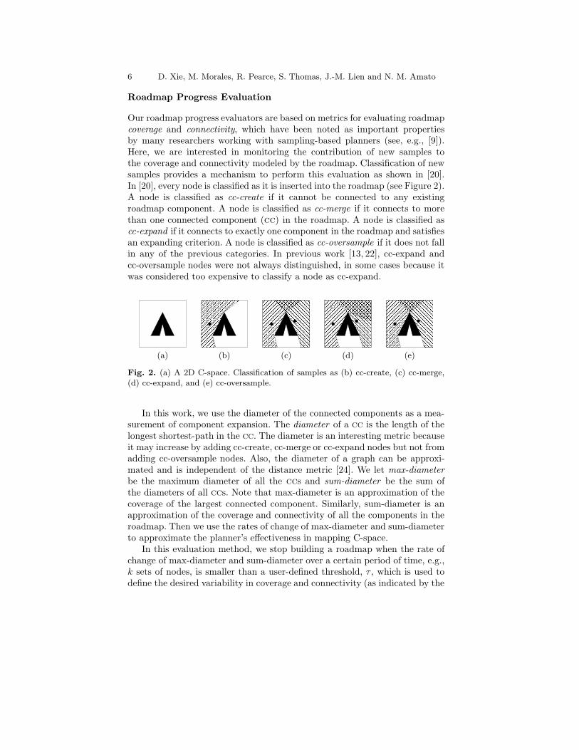
Our roadmap progress evaluators are based on metrics for evaluating roadmapcoverage and connectivity, which have been noted as important propertiesby many researchers working with sampling-based planners (see, e.g., [9]).Here, we are interested in monitoring the contribution of new samples tothe coverage and connectivity modeled by the roadmap. Classification of newsamples provides a mechanism to perform this evaluation as shown in [20].In [20], every node is classified as it is inserted into the roadmap (see Figure 2).A node is classified as cc-create if it cannot be connected to any existingroadmap component. A node is classified as cc-merge if it connects to morethan one connected component (cc) in the roadmap. A node is classified ascc-expand if it connects to exactly one component in the roadmap and satisfiesan expanding criterion. A node is classified as cc-oversample if it does not fallin any of the previous categories. In previous work [13, 22], cc-expand andcc-oversample nodes were not always distinguished, in some cases because itwas considered too expensive to classify a node as cc-expand.
(a)
��������������������������������������������������������������������������������������������������������������������������������������������������������������������������
��������������������������������������������������������������������������������������������������������������������������������������������������������������������������
(b)
��������������������������������������������������������������������������������������������������������������������������������������������������������������������������
������������������������������������������������������������������������������������������������������������������������������������������������������
��������������������������������������������������������������������������������������������������������������������������������������������������������������������������
��������������������������������������������������������������������������������������������������������������������������������������������������������������������������
���������������������������������������
���������������������������������
(c)
��������������������������������������������������������������������������������
��������������������������������������������������������������������������������
��������������������������������������������������������������������������������������������������������������������������������������������������������������������������
��������������������������������������������������������������������������������������������������������������������������������������������������������������������������
� � � � � � � � � � � � � � � � � � � � � � � � � � � � � � � � � � � � � � � �
�������������������������������������������������������������������������������������
(d)
��������������������������������������������������������������������������������������������������������������������������������������������������������������������������
������������������������������������������������������������������������������������������������������������������������������������������������������
��������������������������������������������������������������������������������������������������������������������������������������������������������������������������
��������������������������������������������������������������������������������������������������������������������������������������������������������������������������
���������������������������������������
���������������������������������
(e)
Fig. 2. (a) A 2D C-space. Classification of samples as (b) cc-create, (c) cc-merge,(d) cc-expand, and (e) cc-oversample.
In this work, we use the diameter of the connected components as a mea-surement of component expansion. The diameter of a cc is the length of thelongest shortest-path in the cc. The diameter is an interesting metric becauseit may increase by adding cc-create, cc-merge or cc-expand nodes but not fromadding cc-oversample nodes. Also, the diameter of a graph can be approxi-mated and is independent of the distance metric [24]. We let max-diameter
be the maximum diameter of all the ccs and sum-diameter be the sum ofthe diameters of all ccs. Note that max-diameter is an approximation of thecoverage of the largest connected component. Similarly, sum-diameter is anapproximation of the coverage and connectivity of all the components in theroadmap. Then we use the rates of change of max-diameter and sum-diameterto approximate the planner’s effectiveness in mapping C-space.
In this evaluation method, we stop building a roadmap when the rate ofchange of max-diameter and sum-diameter over a certain period of time, e.g.,k sets of nodes, is smaller than a user-defined threshold, τ , which is used todefine the desired variability in coverage and connectivity (as indicated by the
Incremental Map Generation (IMG) 7
components’ diameters). We compute the max-diameter among all ccs andthe sum-diameter of all the ccs at the end of each node set.
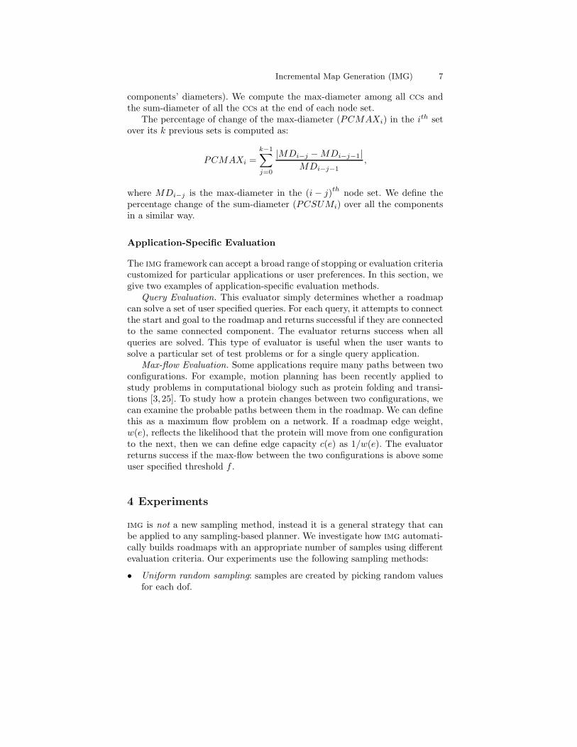
The percentage of change of the max-diameter (PCMAXi) in the ith setover its k previous sets is computed as:
PCMAXi =
k−1∑
j=0
|MDi−j − MDi−j−1|
MDi−j−1
,
where MDi−j is the max-diameter in the (i − j)th
node set. We define thepercentage change of the sum-diameter (PCSUMi) over all the componentsin a similar way.
Application-Specific Evaluation
The img framework can accept a broad range of stopping or evaluation criteriacustomized for particular applications or user preferences. In this section, wegive two examples of application-specific evaluation methods.
Query Evaluation. This evaluator simply determines whether a roadmapcan solve a set of user specified queries. For each query, it attempts to connectthe start and goal to the roadmap and returns successful if they are connectedto the same connected component. The evaluator returns success when allqueries are solved. This type of evaluator is useful when the user wants tosolve a particular set of test problems or for a single query application.
Max-flow Evaluation. Some applications require many paths between twoconfigurations. For example, motion planning has been recently applied tostudy problems in computational biology such as protein folding and transi-tions [3, 25]. To study how a protein changes between two configurations, wecan examine the probable paths between them in the roadmap. We can definethis as a maximum flow problem on a network. If a roadmap edge weight,w(e), reflects the likelihood that the protein will move from one configurationto the next, then we can define edge capacity c(e) as 1/w(e). The evaluatorreturns success if the max-flow between the two configurations is above someuser specified threshold f .
4 Experiments
img is not a new sampling method, instead it is a general strategy that canbe applied to any sampling-based planner. We investigate how img automati-cally builds roadmaps with an appropriate number of samples using differentevaluation criteria. Our experiments use the following sampling methods:
• Uniform random sampling: samples are created by picking random valuesfor each dof.
8 D. Xie, M. Morales, R. Pearce, S. Thomas, J.-M. Lien and N. M. Amato
• Gaussian-biased sampling [4]: sets of two samples are created, one uni-formly at random and the other a distance d away, where d has a Gaussiandistribution. A collision-free sample is added to the roadmap when one iscollision-free and the other is not.
• Bridge-test sampling [11]: similar to Gaussian sampling, it takes two ran-dom samples a distance d apart, where d has a Gaussian distribution, untilboth samples are in collision and their midpoint is not. The collision-freesample is added to the roadmap.
• Obstacle-based sampling (obprm) [1]: samples are generated near C-obstacle surfaces by first generating a random colliding (resp., collision-free) sample and searching along a random direction until the sample be-comes collision-free (resp., in collision).
We implemented all planners with the Parasol Lab motion planning librarydeveloped at Texas A&M University and performed collision detection withRAPID [10]. For each problem, we built two types of roadmaps: a tree anda graph. We use the L-Success-M-Failure connection strategy introduced inSection 3. In particular, we apply a 10-Success-20-Failure connection strategyfor building trees and 5-Success-20-Failure for building graphs. For rigid-bodymotion planning, we use two local planners: straight-line and rotate at 0.5 [2],which translates from the start to the midpoint, rotates to the orientation ofthe goal configuration and then translates to the goal configuration. For ar-ticulated linkage motion planning, we only use the straight-line local planner.All results were run on 700MHz Intel PIII Xeon processors.
In the following sections, we discuss the performance of img’s roadmapprogress evaluator, the overhead of the img framework, how img and hybridprm may be combined, and how img can be tailored to specific applicationssuch as protein folding.
4.1 Automatically Stopping Roadmap Construction
Here we investigate the performance of the roadmap progress evaluator (seeSection 3.2) in the four different environments shown in Figure 3. For theseexperiments, the node set size is 50 samples. After each set, we computePCMAXi and PCSUMi. Roadmap construction stops when both PCMAXi
and PCSUMi are below a threshold τ . τ represents the desired roadmap im-provement over a period of time, i.e., k sample sets. Note that in the beginningof roadmap construction (during the quick learning stage), there will be largechanges in PCMAX and PCSUM . These changes will drop when the en-hancement stage begins.
We studied the impact of τ and k on img’s performance for each samplingmethod in each environment by varying k with constant τ and alternativelyby varying τ with constant k. Due to space limitations, we only show a subsetof these results. A complete set of results can be found on our website.
Incremental Map Generation (IMG) 9
(a) (b)
(c) (d)
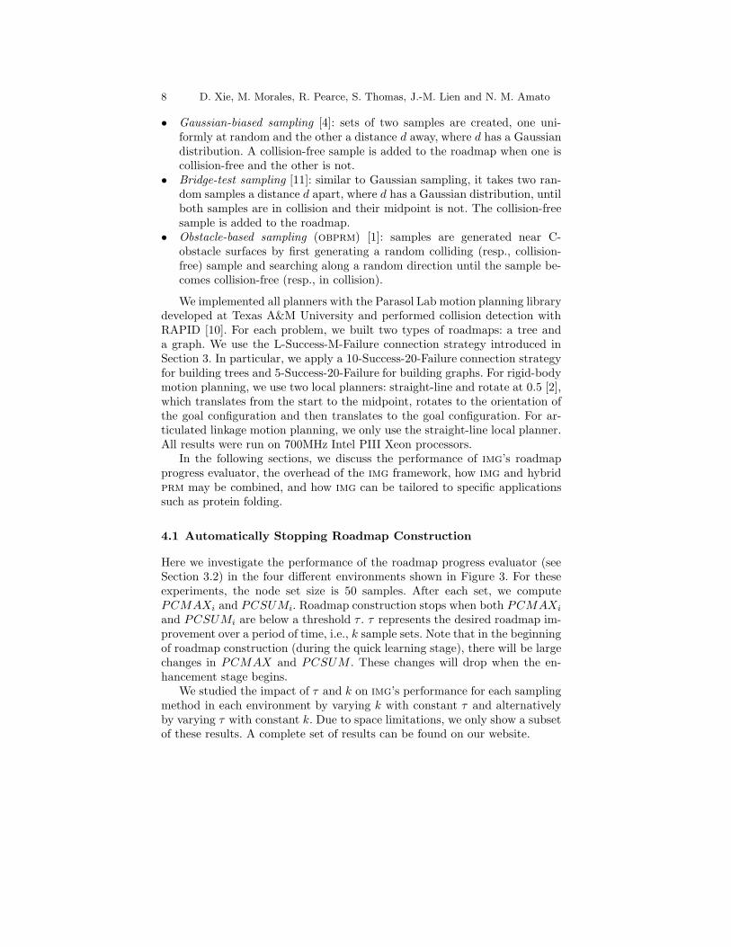
Fig. 3. Problems studied. (a) Maze environment (solid/wire frame): rigid bodyrobot must navigate the maze. (b) U shape environment: rigid body robot mustnavigate from one chamber to the other. (c) Hook environment: rigid body robotmust rotate to move from one side of the walls to the other. (d) Hook manipulatorenvironment: articulated linkage (10 dof) must move from one end to the other.
A Case Study: Varying k with Constant τ
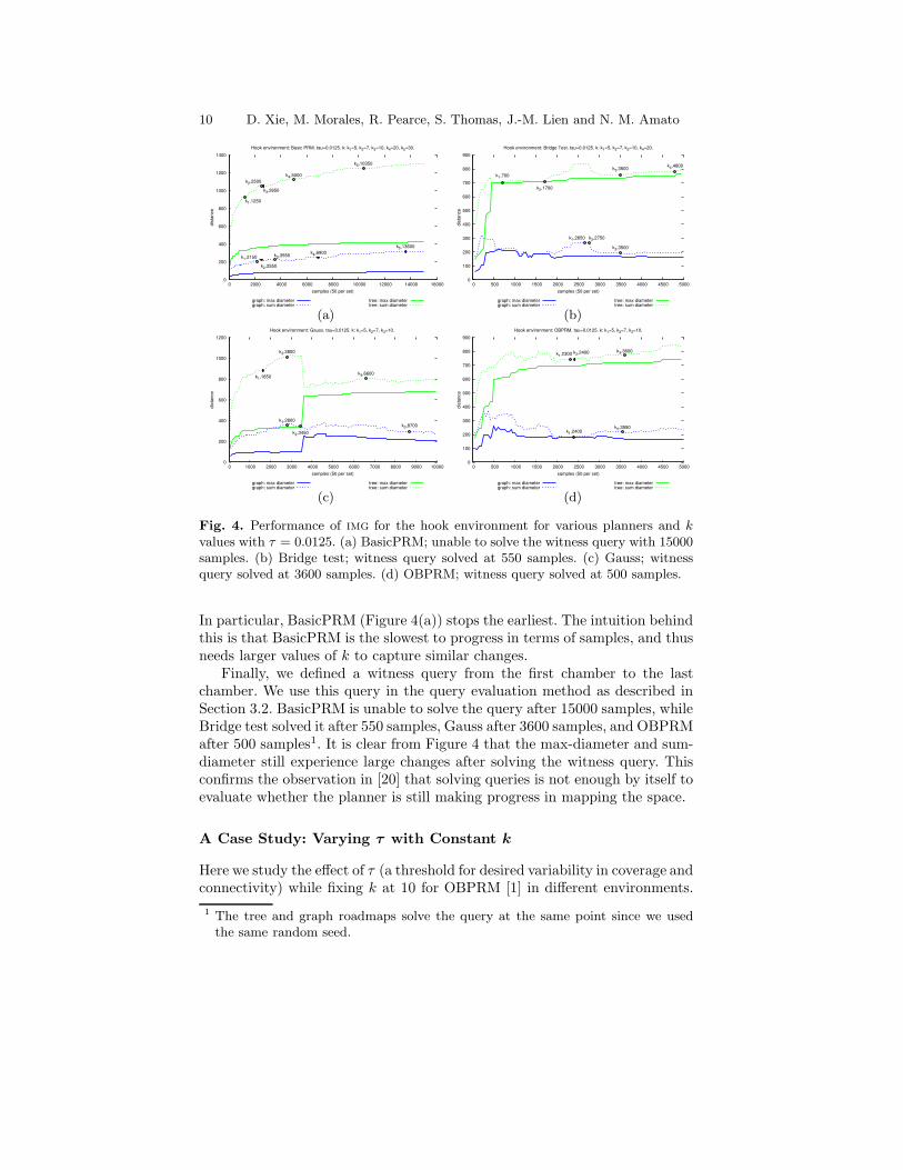
Figure 4 shows img’s performance at building both trees and graphs for eachplanner in the hook environment. Here we vary k (the number of sample setsover which the percentage change in diameter is computed) while keeping τconstant at 0.0125. In each plot, the upper two curves show the sum-diameterand max-diameter as a function of roadmap size for a tree, and the lower twocurves for a graph. The circles indicate where img would stop roadmap con-struction for various k. For example, the circle labeled k1, 1250 in Figure 4(a)shows that with k = k1 = 5, img would stop construction of the tree after1250 samples. Similarly, the circle labeled k1, 2150 indicates img would stopconstruction of the graph after 2150 samples with the same k value. All plotsuse the same random seed.
From the evolution of max-diameter and sum-diameter, it is clear that theroadmap grows rapidly in the beginning and then experiences a long period ofrefinement until both stabilize. As expected, the diameter in the tree roadmapis larger than the diameter in the graph roadmap. This corresponds to thegraph roadmap having shorter and smoother paths. An interesting observationfrom the graph roadmap is that the “path refinement” stage is clearly shownas the diameters drop.
Overall, we see that for a fixed τ , increasing k causes the planner to stoplater because larger k values allow img to capture changes over longer periods.This trend appears in all experiments we ran. This means that we can decidehow long we want to refine the roadmap by what value we choose for k. It isalso clear that for a given k value, different planners stop at different points.
10 D. Xie, M. Morales, R. Pearce, S. Thomas, J.-M. Lien and N. M. Amato
0
200
400
600
800
1000
1200
1400
0 2000 4000 6000 8000 10000 12000 14000 16000
dist
ance
samples (50 per set)
Hook environment: Basic PRM. tau=0.0125. k: k1=5, k2=7, k3=10, k4=20, k5=30.
graph: max diametergraph: sum diameter
tree: max diametertree: sum diameter
k1,2150
k2,2550
k3,3550 k4,6900k5,13600
k1,1250
k2,2500
k3,2650
k4,5000
k5,10350
(a)
0
100
200
300
400
500
600
700
800
900
0 500 1000 1500 2000 2500 3000 3500 4000 4500 5000
dist
ance
samples (50 per set)
Hook environment: Bridge Test. tau=0.0125. k: k1=5, k2=7, k3=10, k4=20.
graph: max diametergraph: sum diameter
tree: max diametertree: sum diameter
k1,2650 k2,2750
k3,3500
k1,700
k2,1700
k3,3500 k4,4800
(b)
0
200
400
600
800
1000
1200
0 1000 2000 3000 4000 5000 6000 7000 8000 9000 10000
dist
ance
samples (50 per set)
Hook environment: Gauss. tau=0.0125. k: k1=5, k2=7, k3=10.
graph: max diametergraph: sum diameter
tree: max diametertree: sum diameter
k1,2800
k2,3450k3,8700
k1,1650
k2,2800
k3,6600
(c)
0
100
200
300
400
500
600
700
800
900
0 500 1000 1500 2000 2500 3000 3500 4000 4500 5000di
stan
ce
samples (50 per set)
Hook environment: OBPRM. tau=0.0125. k: k1=5, k2=7, k3=10.
graph: max diametergraph: sum diameter
tree: max diametertree: sum diameter
k1,2400k2,3550
k1,2300 k2,2400 k3,3600
(d)
Fig. 4. Performance of img for the hook environment for various planners and k
values with τ = 0.0125. (a) BasicPRM; unable to solve the witness query with 15000samples. (b) Bridge test; witness query solved at 550 samples. (c) Gauss; witnessquery solved at 3600 samples. (d) OBPRM; witness query solved at 500 samples.
In particular, BasicPRM (Figure 4(a)) stops the earliest. The intuition behindthis is that BasicPRM is the slowest to progress in terms of samples, and thusneeds larger values of k to capture similar changes.
Finally, we defined a witness query from the first chamber to the lastchamber. We use this query in the query evaluation method as described inSection 3.2. BasicPRM is unable to solve the query after 15000 samples, whileBridge test solved it after 550 samples, Gauss after 3600 samples, and OBPRMafter 500 samples1. It is clear from Figure 4 that the max-diameter and sum-diameter still experience large changes after solving the witness query. Thisconfirms the observation in [20] that solving queries is not enough by itself toevaluate whether the planner is still making progress in mapping the space.
A Case Study: Varying τ with Constant k
Here we study the effect of τ (a threshold for desired variability in coverage andconnectivity) while fixing k at 10 for OBPRM [1] in different environments.
1 The tree and graph roadmaps solve the query at the same point since we usedthe same random seed.
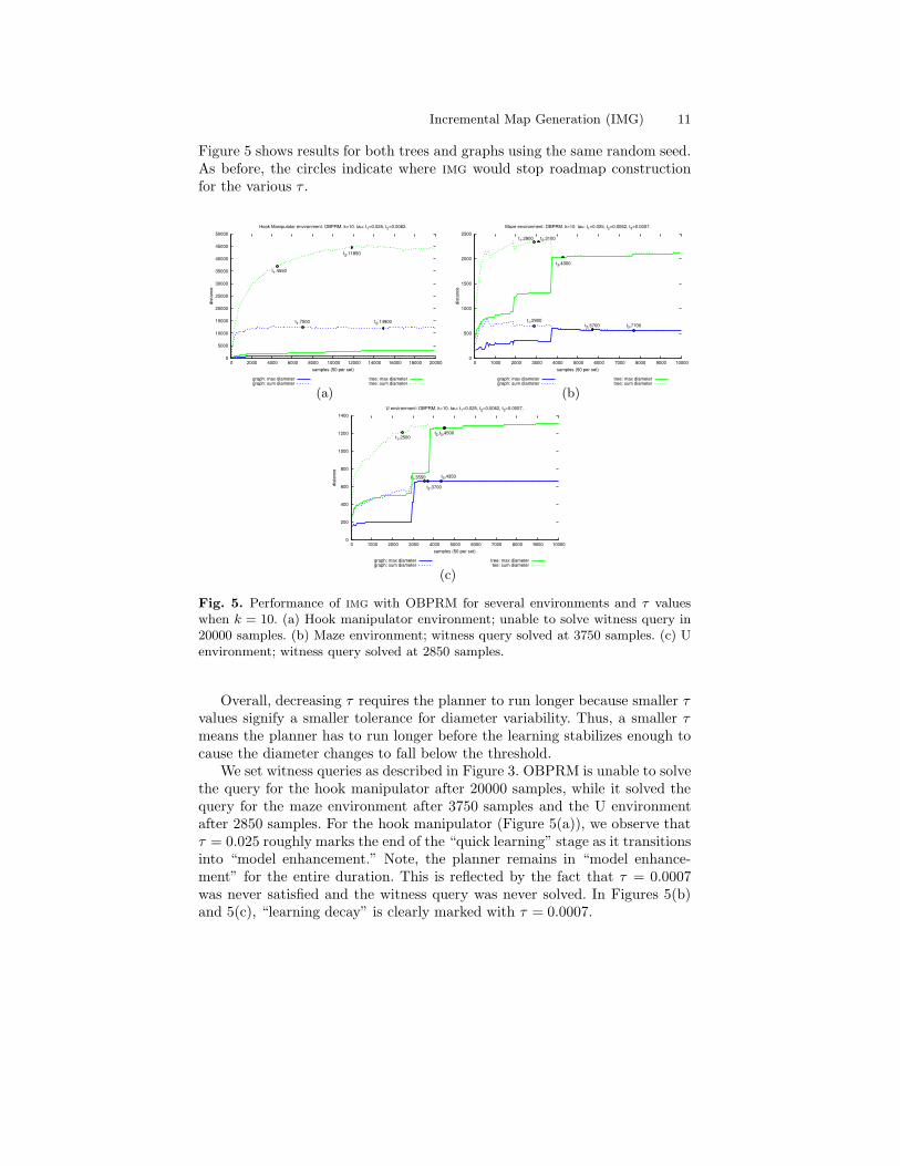
Incremental Map Generation (IMG) 11
Figure 5 shows results for both trees and graphs using the same random seed.As before, the circles indicate where img would stop roadmap constructionfor the various τ .
0
5000
10000
15000
20000
25000
30000
35000
40000
45000
50000
0 2000 4000 6000 8000 10000 12000 14000 16000 18000 20000
dist
ance
samples (50 per set)
Hook Manipulator environment: OBPRM. k=10. tau: t1=0.025, t2=0.0062.
graph: max diametergraph: sum diameter
tree: max diametertree: sum diameter
t1,7000 t2,14900
t1,4550
t2,11850
(a)
0
500
1000
1500
2000
2500
0 1000 2000 3000 4000 5000 6000 7000 8000 9000 10000
dist
ance
samples (50 per set)
Maze environment: OBPRM. k=10. tau: t1=0.025, t2=0.0062, t3=0.0007.
graph: max diametergraph: sum diameter
tree: max diametertree: sum diameter
t1,2900t2,5700 t3,7700
t1,2900 t2,3100
t3,4300
(b)
0
200
400
600
800
1000
1200
1400
0 1000 2000 3000 4000 5000 6000 7000 8000 9000 10000
dist
ance
samples (50 per set)
U environment: OBPRM. k=10. tau: t1=0.025, t2=0.0062, t3=0.0007.
graph: max diametergraph: sum diameter
tree: max diametertee: sum diameter
t1,3550
t2,3700
t3,4350
t1,2500t2,t3,4500
(c)
Fig. 5. Performance of img with OBPRM for several environments and τ valueswhen k = 10. (a) Hook manipulator environment; unable to solve witness query in20000 samples. (b) Maze environment; witness query solved at 3750 samples. (c) Uenvironment; witness query solved at 2850 samples.
Overall, decreasing τ requires the planner to run longer because smaller τvalues signify a smaller tolerance for diameter variability. Thus, a smaller τmeans the planner has to run longer before the learning stabilizes enough tocause the diameter changes to fall below the threshold.
We set witness queries as described in Figure 3. OBPRM is unable to solvethe query for the hook manipulator after 20000 samples, while it solved thequery for the maze environment after 3750 samples and the U environmentafter 2850 samples. For the hook manipulator (Figure 5(a)), we observe thatτ = 0.025 roughly marks the end of the “quick learning” stage as it transitionsinto “model enhancement.” Note, the planner remains in “model enhance-ment” for the entire duration. This is reflected by the fact that τ = 0.0007was never satisfied and the witness query was never solved. In Figures 5(b)and 5(c), “learning decay” is clearly marked with τ = 0.0007.
12 D. Xie, M. Morales, R. Pearce, S. Thomas, J.-M. Lien and N. M. Amato
Overhead
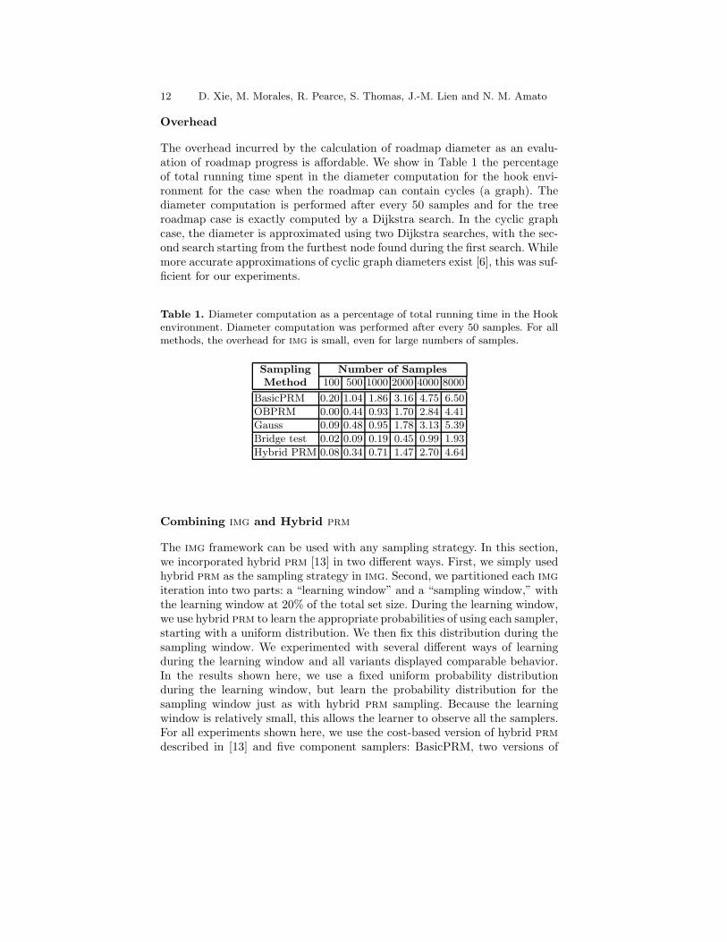
The overhead incurred by the calculation of roadmap diameter as an evalu-ation of roadmap progress is affordable. We show in Table 1 the percentageof total running time spent in the diameter computation for the hook envi-ronment for the case when the roadmap can contain cycles (a graph). Thediameter computation is performed after every 50 samples and for the treeroadmap case is exactly computed by a Dijkstra search. In the cyclic graphcase, the diameter is approximated using two Dijkstra searches, with the sec-ond search starting from the furthest node found during the first search. Whilemore accurate approximations of cyclic graph diameters exist [6], this was suf-ficient for our experiments.
Table 1. Diameter computation as a percentage of total running time in the Hookenvironment. Diameter computation was performed after every 50 samples. For allmethods, the overhead for img is small, even for large numbers of samples.
Sampling Number of Samples
Method 100 500 1000 2000 4000 8000
BasicPRM 0.20 1.04 1.86 3.16 4.75 6.50
OBPRM 0.00 0.44 0.93 1.70 2.84 4.41
Gauss 0.09 0.48 0.95 1.78 3.13 5.39
Bridge test 0.02 0.09 0.19 0.45 0.99 1.93
Hybrid PRM 0.08 0.34 0.71 1.47 2.70 4.64
Combining img and Hybrid prm
The img framework can be used with any sampling strategy. In this section,we incorporated hybrid prm [13] in two different ways. First, we simply usedhybrid prm as the sampling strategy in img. Second, we partitioned each img
iteration into two parts: a “learning window” and a “sampling window,” withthe learning window at 20% of the total set size. During the learning window,we use hybrid prm to learn the appropriate probabilities of using each sampler,starting with a uniform distribution. We then fix this distribution during thesampling window. We experimented with several different ways of learningduring the learning window and all variants displayed comparable behavior.In the results shown here, we use a fixed uniform probability distributionduring the learning window, but learn the probability distribution for thesampling window just as with hybrid prm sampling. Because the learningwindow is relatively small, this allows the learner to observe all the samplers.For all experiments shown here, we use the cost-based version of hybrid prm
described in [13] and five component samplers: BasicPRM, two versions of
Incremental Map Generation (IMG) 13
the Bridge test, and two versions of Gauss. The reward mechanism of theoriginal hybrid prm only rewards a planner when it generates cc-create and cc-
merge samples. However, a sample that expands a roadmap is also important.Therefore, when a planner generates a cc-expand sample we give it a rewardequal to the complement of the percentage of successful connections from thatsample to the roadmap.
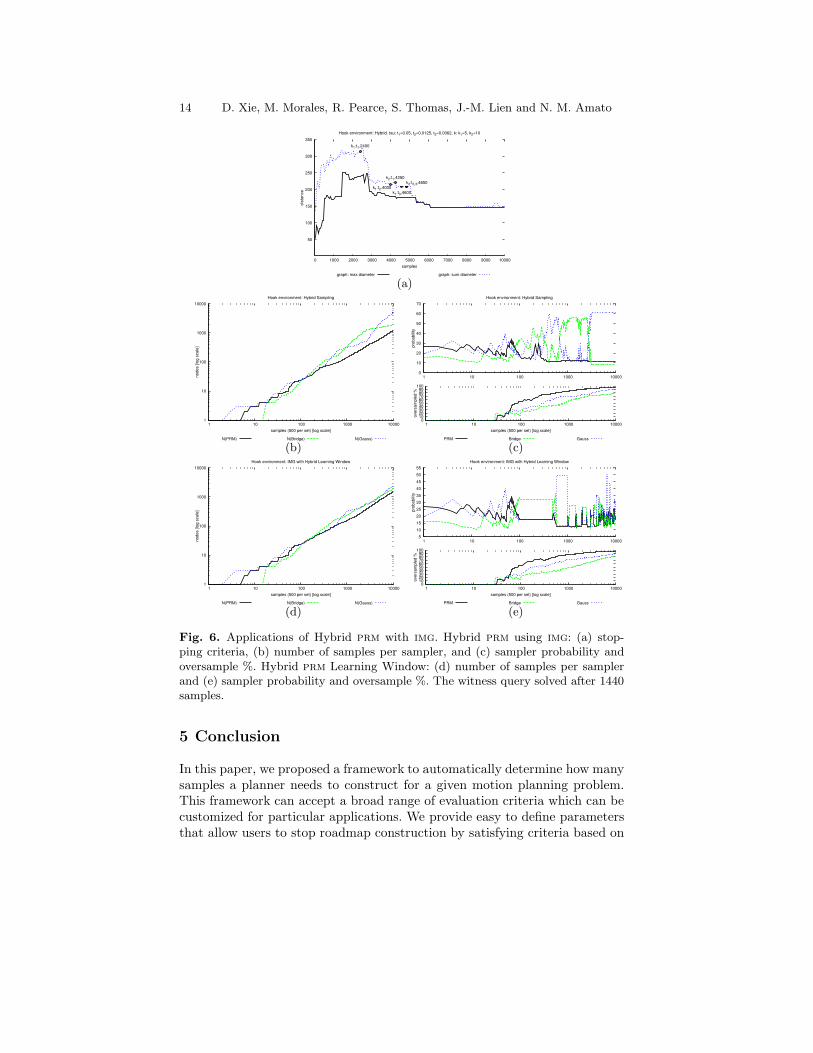
In Figure 6, we show hybrid prm in the img framework. For clarity, weonly show BasicPRM, and the version of Bridge test and Gauss that per-formed best. Figure 6(a) shows where img would stop roadmap constructionwith pure hybrid prm sampling for various values of k and τ . This showssimilar trends when varying k and τ as seen previously. Figure 6(b) shows thenumber of samples created by each sampler vs. the total number of samples.Figure 6(c) shows the probability of being selected along with the percentageof cc-oversample nodes for each sampler during roadmap construction. Ourresults here confirm the results found in [13]: BasicPRM is selected early onbecause it is a relatively inexpensive sampler but dies out quickly as other,more powerful and expensive samplers are selected. In the end, after the wit-ness query is solved, hybrid prm vacillates between a version of Gauss and aversion of Bridge test.
Figure 6(d) and 6(e) show similar plots as 6(b) and 6(c), respectively, forimg with a hybrid learning window. Unlike the previous plots (b and c), thisversion does not select a dominant sampler towards the end of roadmap con-struction, after the witness query is solved. We believe in fact that this is amore accurate evaluation because at this stage all samplers are equally “bad,”i.e., none are able to generate useful samples and should not necessarily be dis-tinguished. In particular, note that more than 80% of the nodes created by allsamplers are cc-oversample nodes in the later stages of roadmap construction.
4.2 Application-Specific Stopping Criteria
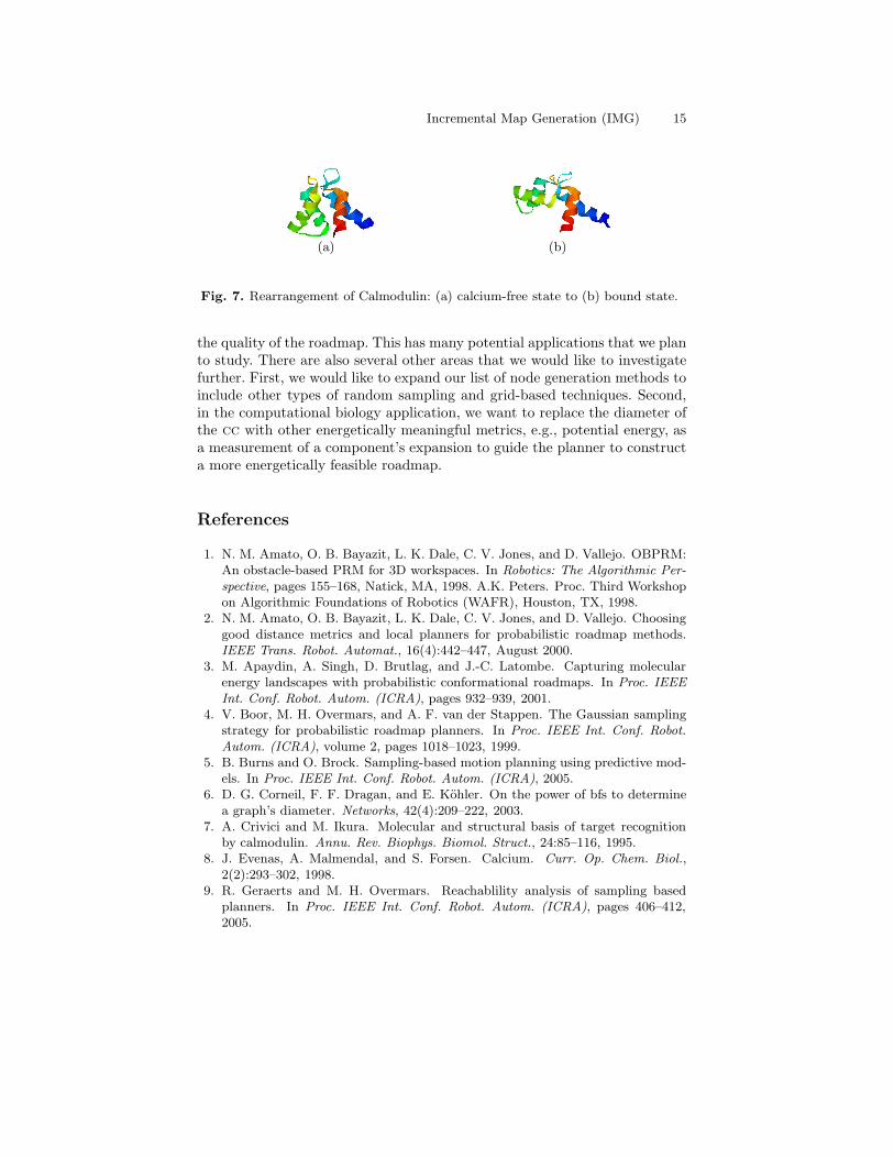
As discussed in Section 3.2, the img framework can accept a broad range ofstopping criteria that can be customized for particular applications or userpreferences. We can apply our framework to study computational biologyproblems such as protein folding and protein structure transitions. Here, weincrementally build a roadmap until the maximum flow between the two con-figurations of interest is above a threshold. We applied this approach to studycalmodulin, a signaling protein that binds to Ca2+ to regulate several pro-cesses in the cell [7, 8, 26]. When calmodulin binds to Ca2+, it undergoes alarge-scale rearrangement [21] shown in Figure 7.
Using img, we incrementally built a roadmap until it adequately describedthe C-space around both target configurations as well as the transition be-tween. We were able to build the smallest roadmap possible, given the incre-ment size, in 2 weeks of computation time. The traditional method of buildinga small roadmap, evaluating it, and rebuilding a larger one until it adequatelydescribes the C-space would take at least 4 weeks of computation time.
14 D. Xie, M. Morales, R. Pearce, S. Thomas, J.-M. Lien and N. M. Amato
50
100
150
200
250
300
350
0 1000 2000 3000 4000 5000 6000 7000 8000 9000 10000
dist
ance
samples
Hook environment: Hybrid. tau: t1=0.05, t2=0.0125, t3=0.0062, k: k1=5, k2=10
graph: max diameter graph: sum diameter
k1:t1,2400
k1:t2,4000k1:t3,4600
k2:t1,4250k2:t2,3,4850
(a)
1
10
100
1000
10000
1 10 100 1000 10000
node
s [lo
g sc
ale]
samples (500 per set) [log scale]
Hook environment: Hybrid Sampling
N(PRM) N(Bridge) N(Gauss)
(b)
0
10
20
30
40
50
60
70
1 10 100 1000 10000
prob
abilit
y
Hook environment: Hybrid Sampling
0 10 20 30 40 50 60 70 80 90
100
1 10 100 1000 10000
over
sam
pled
%
samples (500 per set) [log scale]
PRM Bridge Gauss
(c)
1
10
100
1000
10000
1 10 100 1000 10000
node
s [lo
g sc
ale]
samples (500 per set) [log scale]
Hook environment: IMG with Hybrid Learning Window
N(PRM) N(Bridge) N(Gauss)
(d)
5 10 15 20 25 30 35 40 45 50 55
1 10 100 1000 10000
prob
abilit
y
Hook environment: IMG with Hybrid Learning Window
0 10 20 30 40 50 60 70 80 90
100
1 10 100 1000 10000
over
sam
pled
%
samples (500 per set) [log scale]
PRM Bridge Gauss
(e)
Fig. 6. Applications of Hybrid prm with img. Hybrid prm using img: (a) stop-ping criteria, (b) number of samples per sampler, and (c) sampler probability andoversample %. Hybrid prm Learning Window: (d) number of samples per samplerand (e) sampler probability and oversample %. The witness query solved after 1440samples.
5 Conclusion
In this paper, we proposed a framework to automatically determine how manysamples a planner needs to construct for a given motion planning problem.This framework can accept a broad range of evaluation criteria which can becustomized for particular applications. We provide easy to define parametersthat allow users to stop roadmap construction by satisfying criteria based on
Incremental Map Generation (IMG) 15
(a) (b)
Fig. 7. Rearrangement of Calmodulin: (a) calcium-free state to (b) bound state.
the quality of the roadmap. This has many potential applications that we planto study. There are also several other areas that we would like to investigatefurther. First, we would like to expand our list of node generation methods toinclude other types of random sampling and grid-based techniques. Second,in the computational biology application, we want to replace the diameter ofthe cc with other energetically meaningful metrics, e.g., potential energy, asa measurement of a component’s expansion to guide the planner to constructa more energetically feasible roadmap.
References
1. N. M. Amato, O. B. Bayazit, L. K. Dale, C. V. Jones, and D. Vallejo. OBPRM:An obstacle-based PRM for 3D workspaces. In Robotics: The Algorithmic Per-spective, pages 155–168, Natick, MA, 1998. A.K. Peters. Proc. Third Workshopon Algorithmic Foundations of Robotics (WAFR), Houston, TX, 1998.
2. N. M. Amato, O. B. Bayazit, L. K. Dale, C. V. Jones, and D. Vallejo. Choosinggood distance metrics and local planners for probabilistic roadmap methods.IEEE Trans. Robot. Automat., 16(4):442–447, August 2000.
3. M. Apaydin, A. Singh, D. Brutlag, and J.-C. Latombe. Capturing molecularenergy landscapes with probabilistic conformational roadmaps. In Proc. IEEEInt. Conf. Robot. Autom. (ICRA), pages 932–939, 2001.
4. V. Boor, M. H. Overmars, and A. F. van der Stappen. The Gaussian samplingstrategy for probabilistic roadmap planners. In Proc. IEEE Int. Conf. Robot.Autom. (ICRA), volume 2, pages 1018–1023, 1999.
5. B. Burns and O. Brock. Sampling-based motion planning using predictive mod-els. In Proc. IEEE Int. Conf. Robot. Autom. (ICRA), 2005.
6. D. G. Corneil, F. F. Dragan, and E. Kohler. On the power of bfs to determinea graph’s diameter. Networks, 42(4):209–222, 2003.
7. A. Crivici and M. Ikura. Molecular and structural basis of target recognitionby calmodulin. Annu. Rev. Biophys. Biomol. Struct., 24:85–116, 1995.
8. J. Evenas, A. Malmendal, and S. Forsen. Calcium. Curr. Op. Chem. Biol.,2(2):293–302, 1998.
9. R. Geraerts and M. H. Overmars. Reachablility analysis of sampling basedplanners. In Proc. IEEE Int. Conf. Robot. Autom. (ICRA), pages 406–412,2005.

16 D. Xie, M. Morales, R. Pearce, S. Thomas, J.-M. Lien and N. M. Amato
10. S. Gottschalk, M. C. Lin, and D. Manocha. OBB-tree: A hierarchical struc-ture for rapid interference detection. Comput. Graph., 30:171–180, 1996. Proc.SIGGRAPH ’96.
11. D. Hsu, T. Jiang, J. Reif, and Z. Sun. Bridge test for sampling narrow passageswith proabilistic roadmap planners. In Proc. IEEE Int. Conf. Robot. Autom.(ICRA), pages 4420–4426, 2003.
12. D. Hsu, J.-C. Latombe, and R. Motwani. Path planning in expansive configura-tion spaces. In Proc. IEEE Int. Conf. Robot. Autom. (ICRA), pages 2719–2726,1997.
13. D. Hsu, G. Sanchez-Ante, and Z. Sun. Hybrid PRM sampling with a cost-sensitive adaptive strategy. In Proc. IEEE Int. Conf. Robot. Autom. (ICRA),pages 3885–3891, 2005.
14. L. E. Kavraki, J.-C. Latombe, R. Motwani, and P. Raghavan. Randomized queryprocessing in robot path planning. In Proc. ACM Symp. Theory of Computing(STOC), pages 353–362, May 1995.
15. L. E. Kavraki, P. Svestka, J. C. Latombe, and M. H. Overmars. Probabilisticroadmaps for path planning in high-dimensional configuration spaces. IEEETrans. Robot. Automat., 12(4):566–580, August 1996.
16. J.-C. Latombe. Robot Motion Planning. Kluwer Academic Publishers, Boston,MA, 1991.
17. S. M. LaValle and J. J. Kuffner. Randomized kinodynamic planning. In Proc.IEEE Int. Conf. Robot. Autom. (ICRA), pages 473–479, 1999.
18. E. Mazer, J. M. Ahuactzin, and P. Bessiere. The Ariadne’s clew algorithm. InJournal of Artificial Robotics Research (JAIR), volume 9, pages 295–316, 1998.
19. M. Morales, L. Tapia, R. Pearce, S. Rodriguez, and N. M. Amato. A machinelearning approach for feature-sensitive motion planning. In Proc. Int. Workshopon Algorithmic Foundations of Robotics (WAFR), pages 316–376, Utrecht/Zeist,The Netherlands, July 2004.
20. M. A. Morales A., R. Pearce, and N. M. Amato. Metrics for comparing C-Spaceroadmaps. In Proc. IEEE Int. Conf. Robot. Autom. (ICRA), 2006.
21. M. R. Nelson and W. J. Chazin. An interaction-based analysis of calcium-induced conformational changes in ca2+ sensor proteins. Protein Sci., 7:270–282, 1998.
22. C. Nissoux, T. Simeon, and J.-P. Laumond. Visibility based probabilisticroadmaps. In Proc. IEEE Int. Conf. Intel. Rob. Syst. (IROS), pages 1316–1321,1999.
23. J. H. Reif. Complexity of the mover’s problem and generalizations. In Proc.IEEE Symp. Foundations of Computer Science (FOCS), pages 421–427, SanJuan, Puerto Rico, October 1979.
24. R. Seidel. On the all-pairs-shortest-path problem. In Proc. 24th Annu. ACMSympos. Theory Comput., pages 745–749, 1992.
25. G. Song and N. M. Amato. Using motion planning to study protein foldingpathways. In Proc. Int. Conf. Comput. Molecular Biology (RECOMB), pages287–296, 2001.
26. H. Vogel. Calmodulin: a versatile calcium mediator protein. Biochem. CellBiol., 72(9-10):357–376, 1994.
27. S. A. Wilmarth, N. M. Amato, and P. F. Stiller. MAPRM: A probabilisticroadmap planner with sampling on the medial axis of the free space. In Proc.IEEE Int. Conf. Robot. Autom. (ICRA), volume 2, pages 1024–1031, 1999.