incremental lossless graph summarization - arxiv
TRANSCRIPT
Incremental Lossless Graph Summarization
Jihoon Ko∗KAIST AI
Yunbum Kook∗Dept. of Mathematical Science, KAIST
Kijung Shin†KAIST AI & EE
ABSTRACT
Given a fully dynamic graph, represented as a stream of edge inser-
tions and deletions, how can we obtain and incrementally update a
lossless summary of its current snapshot?
As large-scale graphs are prevalent, concisely representing themis inevitable for efficient storage and analysis. Lossless graph sum-marization is an effective graph-compression technique with manydesirable properties. It aims to compactly represent the input graphas (a) a summary graph consisting of supernodes (i.e., sets of nodes)and superedges (i.e., edges between supernodes), which provide arough description, and (b) edge corrections which fix errors inducedby the rough description. While a number of batch algorithms,suited for static graphs, have been developed for rapid and compactgraph summarization, they are highly inefficient in terms of timeand space for dynamic graphs, which are common in practice.
In this work, we proposeMoSSo, the first incremental algorithmfor lossless summarization of fully dynamic graphs. In response toeach change in the input graph,MoSSo updates the output repre-sentation by repeatedly moving nodes among supernodes. MoSSodecides nodes to be moved and their destinations carefully butrapidly based on several novel ideas. Through extensive experi-ments on 10 real graphs, we show MoSSo is (a) Fast and ‘any
time’: processing each change in near-constant time (less than 0.1millisecond), up to 7 orders of magnitude faster than runningstate-of-the-art batch methods, (b) Scalable: summarizing graphswith hundreds of millions of edges, requiring sub-linear memoryduring the process, and (c) Effective: achieving comparable com-pression ratios even to state-of-the-art batch methods.ACM Reference Format:
Jihoon Ko, Yunbum Kook, and Kijung Shin. 2020. Incremental LosslessGraph Summarization. In Proceedings of the 26th ACM SIGKDD Conference
on Knowledge Discovery and Data Mining (KDD ’20), August 23–27, 2020,
Virtual Event, USA. ACM, New York, NY, USA, 11 pages. https://doi.org/10.1145/3394486.3403074
1 INTRODUCTION
How can we extract a lossless summary from a dynamic graph andupdate the summary, reflecting changes in forms of edge additionsand deletions? Can we perform each update in near-constant timewhile maintaining a concise summary?∗Equal Contribution. †Corresponding author.
Permission to make digital or hard copies of all or part of this work for personal orclassroom use is granted without fee provided that copies are not made or distributedfor profit or commercial advantage and that copies bear this notice and the full citationon the first page. Copyrights for components of this work owned by others than ACMmust be honored. Abstracting with credit is permitted. To copy otherwise, or republish,to post on servers or to redistribute to lists, requires prior specific permission and/or afee. Request permissions from [email protected] ’20, August 23–27, 2020, Virtual Event, USA
© 2020 Association for Computing Machinery.ACM ISBN 978-1-4503-7998-4/20/08. . . $15.00https://doi.org/10.1145/3394486.3403074
Table 1: Comparison of lossless graph summarizationmeth-
ods.MoSSo is fast, space-efficient, and online.
[21] [13] [27] MoSSo (Proposed)
Takes near-linear time ✗ ✓ ✓ ✓
Requires sub-linear space ✗ ✗ ✗ ✓
Handles inserted edges (or nodes) ✗ ✗ ✗ ✓
Handles deleted edges (or nodes) ✗ ✗ ✗ ✓
Datasets representing relationships between objects are univer-sal in both academia and industry, and graphs are widely used asa simple but powerful representation of such data. For example,graphs naturally represent social networks, WWW, internet topolo-gies, citation networks, and even protein-protein interactions.
With the emergence of big data, real-world graphs have increaseddramatically in size, and many of them are still evolving over time.For example, the number of active users in Facebook (i.e., the num-ber of active nodes in the Facebook graph) has increased dramati-cally from 240 millions to 2.4 billions in the last decade. Such largedynamic graphs are naturally represented as a fully dynamic graph
stream, i.e., a stream of edge insertions and deletions over time.To manage large-scale graphs efficiently, compactly representing
graphs has become important. Moreover, compact representationsallow a larger portion to be stored in main memory or cache andthus can speed up computation on graphs [6, 28]. Thus, many graph-compression techniques have been proposed: relabeling nodes [4,7, 8], pattern mining [6], lossless graph summarization [13, 21, 27],lossy graph summarization [2, 16, 24], to name a few.
Lossless graph summarization is one of the most effective graphcompression techniques. Note that we use the term “lossless graphsummarization” to indicate this specific compression techniquethroughout this paper. Applying lossless graph summarization to agraph G = (V ,E) yields (a) a summary graph G∗ = (S, P), where Sis a partition ofV (i.e., each element of S is a subset ofV , and everynode in V belongs to exactly one element of S) and P is a set ofpairs of two elements in S , and (b) edge corrections C = (C+,C−).Let G be the graph where all pairs of nodes in each pair of subsetsin P are connected and the others are not. Then,C+ andC− are thesets of edges to be added to and removed from G, respectively, forrecovering the original graphG . In addition to yielding compact rep-resentations, lossless graph summarization stands out among manycompression techniques due to the following desirable properties:• Queryable: neighborhood queries (i.e., retrieving the neighbor-hood of a query node) can be answered rapidly from a summarygraph and edge corrections (Lemma 1 in Sect. 3.6). Neighborhoodqueries are the key building blocks repeatedly called in numerousgraph algorithms (DFS, Dijkstra’s algorithm, PageRank, etc).• Combinable: summary graphs and edges corrections, which arein the form of graphs, can be further compressed by any graph-compression methods. Combined with [4, 6–8], lossless graphsummarization achieves up to 3.4× additional compression [27].
arX
iv:2
006.
0993
5v1
[cs
.DB
] 1
7 Ju
n 20
20
1344
9192
x
100
102
104
106
108
1010
MoSSo SAGS SWeG
Algorithms
Exe
cutio
n T
ime
(mic
rose
ccon
ds)
(a) Speed
0.2
0.4
0.6
0.8
0.0 0.2 0.4 0.6 0.8 1.0Ratio of Processed Changes
Com
pres
sion
Rat
io MoSSo(Proposed)
SWeG(Best Batch)
(b) Compression
●
●
●
●
●
27
28
29
210
211
220 221 222 223 224
Number of Changes
A
ccum
ulat
ed
Ex
ecut
ion
Tim
e (s
ec) MoSSo
(Proposed)
Linear O(|E|)
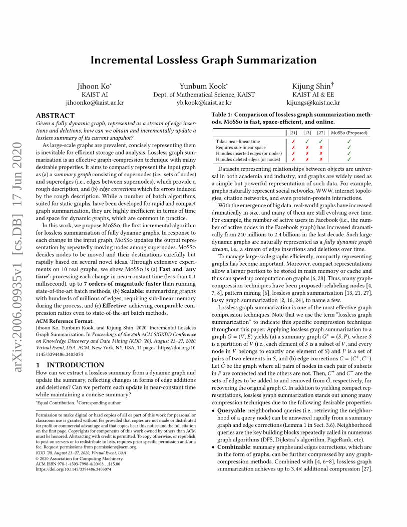
(c) ScalabilityFigure 1: MoSSo is fast, effective, and scalable. (a) Fast: pro-
cesses a change up to 7 orders of magnitude faster than the
fastest batch method. (b) Effective: gives comparable com-
pression rates to the best batchmethod. (c) Scalable: handles
each change in near-constant time, i.e., its total runtime is
near-linear in the number of changes. See Sect. 4 for details.
The lossless graph summarization problem [21], whose goal isto find the most concise representation in the form of a summarygraph and edge corrections, has been formulated only for staticgraphs. Thus, as shown in Table 1, all existing solutions [13, 21, 27]are prohibitively inefficient for dynamic graphs, represented as fullydynamic graph streams. Specifically, since these batch algorithmsare not designed to allow for incremental changes in the inputgraph, they should be rerun from scratch to reflect such changes.
In this work, we formulate a new problem, the goal of whichis lossless summarization of a fully dynamic graph. Then, we pro-pose the first incremental algorithmMoSSo (Move if Saved, Stayotherwise) for the problem. In response to each change in the inputgraph, MoSSo updates the summary graph and edge correctionsby moving nodes among supernodes. (a) Corrective Escape: in-jects randomness in order to escape a local optimum and to copewith changing optima, (b) Fast Random: performs neighborhoodsampling, which is repeatedly executed inMoSSo, in near-constanttime on the output representation without having to retrieve allneighbors,1 and (c) Careful Selection: when selecting a new su-pernode into which a node moves, selects it effectively using coarseclustering. Note that the coarse clustering is distinct from graphsummarization, which we refer to as fine clustering.
We evaluate MoSSo with respect to speed and compression rateon 10 real-world graphs with up to 0.3 billion edges. Specifically, wecompare MoSSo with state-of-the-art batch algorithms for losslessgraph summarization aswell as streaming baselines based on greedyand Markov chain Monte Carlo methods. Through theoretical andempirical analyses, we show the following merits of MoSSo:
• Fast and ‘any time’: It takes near-constant time to process eachchange (0.1 millisecond per change), and is up to 10 million timesfaster than state-of-the-art batch algorithms (Fig.s 1(a), 1(c)).• Scalable: It requires sub-linear memory (Thm. 4) while summa-rizing graph streams with up to hundreds of millions of edges.• Effective: It does not pale in comparison with state-of-the-artbatch algorithms in terms of compression rates (Fig. 1(b)).
Reproducibility: The code and datasets used in the paper areavailable at http://dmlab.kaist.ac.kr/mosso/.
In Sect. 2, we introduce some notations and concept, and weformally formulate a new problem whose goal is to incrementallysummarize graph streams. In Sect. 3, we presentMoSSo and analyzeit theoretically. In Sect. 4, we provide experimental results. Afterreviewing previous work in Sect. 5, we offer conclusions in Sect. 6.1Naively, we retrieve all neighbors of a query node from the output representation,which takes time proportional to its degree, and then uniformly sample some.
Table 2: Table of Symbols.
Symbol Meaning
Symbols for the problem definition (Sect. 2.1)
G=(V , E) a simple undirected graph with nodes V and edges EN (u) neighborhood of node udeg(u) degree of node u{et }∞t=0 a fully dynamic graph streamet ={u, v }+ edge insertion at time tet ={u, v }− edge deletion at time tGt G at time tG∗=(S, P ) a summary graph with supernodes S and superedges PC+ set of edges to be insertedC− set of edges to be deletedφ objective function that we aim to minimize
Symbols for the algorithm descriptions (Sect. 3.1)
y a testing nodeT P (u) testing pool related to node uT N (u) testing nodes related to node uz a candidateCP (y) candidate pool for testing node yEAB edges between supernodes A and BTAB all possible edges between supernodes A and BSv supernode in G∗ that contains node vN (Sv ) neighborhood of supernode Sv in a summary graph G∗C+(u) edges in C+ incident to node uC−(u) edges in C− incident to node u
𝑓𝑓
𝐴𝐴 = {𝑎𝑎}
𝐵𝐵 = {𝑏𝑏, 𝑐𝑐, 𝑑𝑑, 𝑒𝑒}
𝐶𝐶 = {𝑓𝑓,𝑔𝑔, ℎ, 𝑖𝑖}
𝑎𝑎
𝑏𝑏𝑐𝑐
𝑑𝑑
𝑒𝑒
𝑔𝑔
𝐶𝐶+ = 𝑎𝑎, 𝑓𝑓 , 𝐶𝐶− = { 𝑓𝑓, 𝑖𝑖 }
Summarization
Recoveryℎ
𝑖𝑖
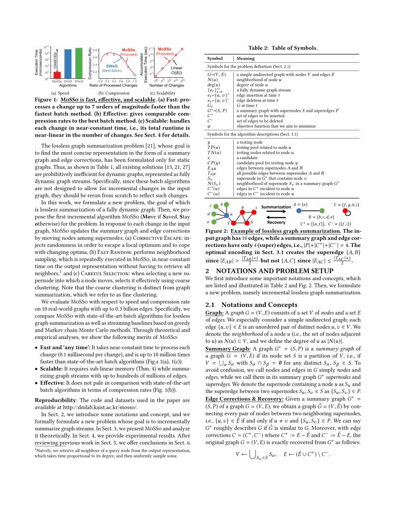
Figure 2: Example of lossless graph summarization. The in-
put graph has 10 edges, while a summary graph and edge cor-
rections have only 4 (super) edges, i.e., |P |+ |C+ |+ |C− | = 4. Theoptimal encoding in Sect. 3.1 creates the superedge {A,B}since |EAB | > |TAB |+12 but not {A,C} since |EAC | ≤ |TAC |+12 .
2 NOTATIONS AND PROBLEM SETUP
We first introduce some important notations and concepts, whichare listed and illustrated in Table 2 and Fig. 2. Then, we formulatea new problem, namely incremental lossless graph summarization.
2.1 Notations and Concepts
Graph: A graph G = (V ,E) consists of a set V of nodes and a set Eof edges. We especially consider a simple undirected graph; eachedge {u,v} ∈ E is an unordered pair of distinct nodes u,v ∈ V . Wedenote the neighborhood of a node u (i.e., the set of nodes adjacentto u) as N (u) ⊂ V , and we define the degree of u as |N (u)|.Summary Graph: A graph G∗ = (S, P) is a summary graph ofa graph G = (V ,E) if its node set S is a partition of V , i.e., ifV =
⋃α Sα with Sα ∩ Sβ = ∅ for any distinct Sα , Sβ ∈ S . To
avoid confusion, we call nodes and edges in G simply nodes andedges, while we call them in its summary graph G∗ supernodes andsuperedges. We denote the supernode containing a node u as Su andthe superedge between two supernodes Su , Sv ∈ S as {Su , Sv } ∈ P .Edge Corrections & Recovery: Given a summary graph G∗ =(S, P) of a graph G = (V ,E), we obtain a graph G = (V , E) by con-necting every pair of nodes between two neighboring supernodes,i.e., {u,v} ∈ E if and only if u , v and {Su , Sv } ∈ P . We can sayG∗ roughly describes G if G is similar to G. Moreover, with edge
corrections C = (C+,C−) where C+ := E − E and C− := E − E, theoriginal graph G = (V ,E) is exactly recovered from G∗ as follows:
V ←⋃
Sα ∈SSα , E ← (E ∪C+) \C−.
Step 0 Step 1 Step 2 Step 3 Step 4
a change arrives choose a testing node 𝑦𝑦 from the testing nodes 𝑇𝑇𝑁𝑁(𝑢𝑢)
choose a candidate 𝑧𝑧 from the candidate pool 𝐶𝐶𝐶𝐶(𝑦𝑦)
move 𝑦𝑦 to 𝑆𝑆𝑧𝑧(i.e., 𝑧𝑧’s supernode)
decide whether to accept or reject the change
𝑢𝑢 𝑣𝑣
Changededge 𝑒𝑒 = {𝑢𝑢,𝑣𝑣}
Candidate pool C𝐶𝐶(𝑦𝑦)
A testing node
𝑢𝑢 𝑣𝑣𝑦𝑦
zA candidate
nodeA testing
node
𝑢𝑢 𝑣𝑣𝑦𝑦
zA candidate
node 𝑢𝑢 𝑣𝑣𝑦𝑦
z 𝑢𝑢 𝑣𝑣𝑦𝑦
zOR
A trial related to a node 𝑢𝑢
Testing pool 𝑇𝑇𝐶𝐶(𝑢𝑢)
A testing node
𝑢𝑢 𝑣𝑣𝑦𝑦
Testing nodes 𝑇𝑇𝑁𝑁(𝑢𝑢)
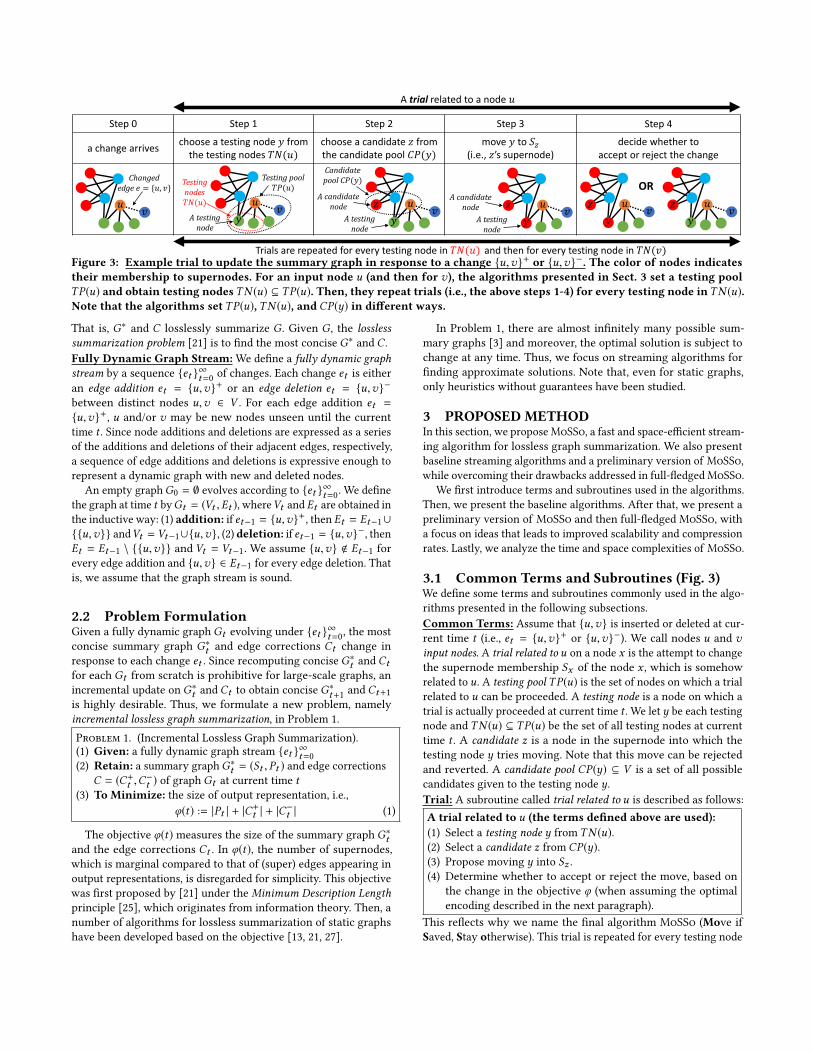
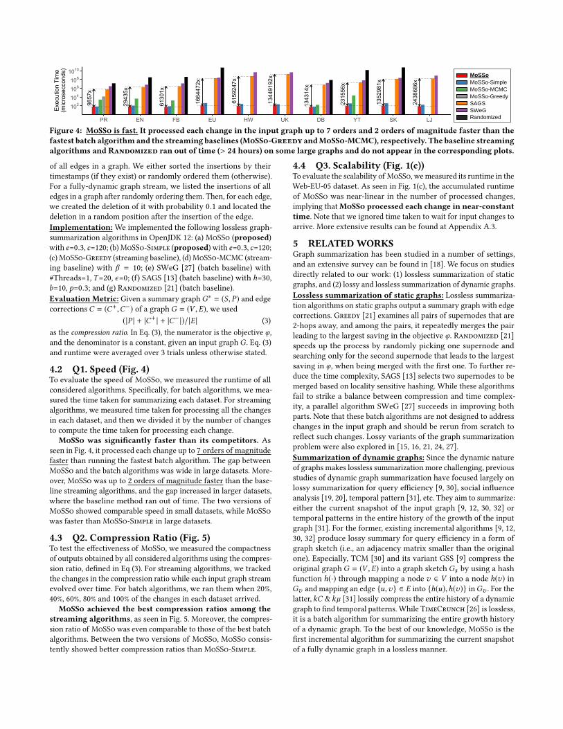
Trials are repeated for every testing node in 𝑇𝑇𝑁𝑁(𝑢𝑢) and then for every testing node in 𝑇𝑇𝑁𝑁(𝑣𝑣)Figure 3: Example trial to update the summary graph in response to a change {u,v}+ or {u,v}−. The color of nodes indicates
their membership to supernodes. For an input node u (and then for v), the algorithms presented in Sect. 3 set a testing pool
TP(u) and obtain testing nodesTN (u) ⊆ TP(u). Then, they repeat trials (i.e., the above steps 1-4) for every testing node inTN (u).Note that the algorithms set TP(u), TN (u), and CP(y) in different ways.
That is, G∗ and C losslessly summarize G. Given G, the lossless
summarization problem [21] is to find the most concise G∗ and C .Fully Dynamic Graph Stream: We define a fully dynamic graph
stream by a sequence {et }∞t=0 of changes. Each change et is eitheran edge addition et = {u,v}+ or an edge deletion et = {u,v}−between distinct nodes u,v ∈ V . For each edge addition et ={u,v}+, u and/or v may be new nodes unseen until the currenttime t . Since node additions and deletions are expressed as a seriesof the additions and deletions of their adjacent edges, respectively,a sequence of edge additions and deletions is expressive enough torepresent a dynamic graph with new and deleted nodes.
An empty graphG0 = ∅ evolves according to {et }∞t=0. We definethe graph at time t byGt = (Vt ,Et ), whereVt and Et are obtained inthe inductive way: (1) addition: if et−1 = {u,v}+, then Et = Et−1∪{{u,v}} andVt = Vt−1∪{u,v}, (2) deletion: if et−1 = {u,v}−, thenEt = Et−1 \ {{u,v}} and Vt = Vt−1. We assume {u,v} < Et−1 forevery edge addition and {u,v} ∈ Et−1 for every edge deletion. Thatis, we assume that the graph stream is sound.
2.2 Problem Formulation
Given a fully dynamic graph Gt evolving under {et }∞t=0, the mostconcise summary graph G∗t and edge corrections Ct change inresponse to each change et . Since recomputing concise G∗t and Ctfor each Gt from scratch is prohibitive for large-scale graphs, anincremental update on G∗t and Ct to obtain concise G∗t+1 and Ct+1is highly desirable. Thus, we formulate a new problem, namelyincremental lossless graph summarization, in Problem 1.Problem 1. (Incremental Lossless Graph Summarization).(1) Given: a fully dynamic graph stream {et }∞t=0(2) Retain: a summary graphG∗t = (St , Pt ) and edge corrections
C = (C+t ,C−t ) of graph Gt at current time t(3) To Minimize: the size of output representation, i.e.,
φ(t) := |Pt | + |C+t | + |C−t | (1)
The objective φ(t) measures the size of the summary graph G∗tand the edge corrections Ct . In φ(t), the number of supernodes,which is marginal compared to that of (super) edges appearing inoutput representations, is disregarded for simplicity. This objectivewas first proposed by [21] under the Minimum Description Length
principle [25], which originates from information theory. Then, anumber of algorithms for lossless summarization of static graphshave been developed based on the objective [13, 21, 27].
In Problem 1, there are almost infinitely many possible sum-mary graphs [3] and moreover, the optimal solution is subject tochange at any time. Thus, we focus on streaming algorithms forfinding approximate solutions. Note that, even for static graphs,only heuristics without guarantees have been studied.
3 PROPOSED METHOD
In this section, we proposeMoSSo, a fast and space-efficient stream-ing algorithm for lossless graph summarization. We also presentbaseline streaming algorithms and a preliminary version of MoSSo,while overcoming their drawbacks addressed in full-fledgedMoSSo.
We first introduce terms and subroutines used in the algorithms.Then, we present the baseline algorithms. After that, we present apreliminary version of MoSSo and then full-fledgedMoSSo, witha focus on ideas that leads to improved scalability and compressionrates. Lastly, we analyze the time and space complexities of MoSSo.
3.1 Common Terms and Subroutines (Fig. 3)
We define some terms and subroutines commonly used in the algo-rithms presented in the following subsections.Common Terms: Assume that {u,v} is inserted or deleted at cur-rent time t (i.e., et = {u,v}+ or {u,v}−). We call nodes u and vinput nodes. A trial related to u on a node x is the attempt to changethe supernode membership Sx of the node x , which is somehowrelated to u. A testing pool TP(u) is the set of nodes on which a trialrelated to u can be proceeded. A testing node is a node on which atrial is actually proceeded at current time t . We let y be each testingnode and TN (u) ⊆ TP(u) be the set of all testing nodes at currenttime t . A candidate z is a node in the supernode into which thetesting node y tries moving. Note that this move can be rejectedand reverted. A candidate pool CP(y) ⊆ V is a set of all possiblecandidates given to the testing node y.Trial: A subroutine called trial related to u is described as follows:A trial related to u (the terms defined above are used):
(1) Select a testing node y from TN (u).(2) Select a candidate z from CP(y).(3) Propose moving y into Sz .(4) Determine whether to accept or reject the move, based on
the change in the objective φ (when assuming the optimalencoding described in the next paragraph).
This reflects why we name the final algorithm MoSSo (Move ifSaved, Stay otherwise). This trial is repeated for every testing node
inTN (u). The algorithms presented in the following subsections aredistinguished by how they (1) set a testing pool TP(u), (2) extracttesting nodes TN (u) from TP(u), (3) set a candidate pool CP(y), (4)propose a candidate from CP(y), and (5) accept the proposal.Optimal Encoding:While finding the optimal set S of supernodes,which minimizes the objective φ, is challenging, finding optimalP and C for current S is straightforward. For each supernode pair{A,B}, let EAB := {{u,v} ∈ E |u ∈ A,v ∈ B,u , v} and TAB :={{u,v} ⊆ V |u ∈ A,v ∈ B,u , v} be the sets of existing andpotential edges between A and B, respectively. Then, the edgesbetween A and B (i.e., EAB ) are optimally encoded as follows:Optimal encoding for the edges in EAB :
(1) If |EAB | ≤ |TAB |+12 , then add all edges in EAB to C+.(2) If |EAB | > |TAB |+12 , then add the superedge {A,B} to P and
TAB \ EAB to C−.Note that adding all edges in EAB toC+ increases φ by |EAB |, whileadding the superedge {A,B} to P and TAB \ EAB to C− increasesφ by 1 + |TAB | − |EAB |. The above rules always choose an optionresulting in a smaller increase in φ.
3.2 MoSSo-Greedy: First Baseline
We present MoSSo-Greedy, a baseline streaming algorithm forProblem 1, and then we point out its limitations.Procedure: When an edge {u,v} is inserted or deleted, MoSSo-Greedy greedily moves u and then v , while fixing the other nodes,so that the objective φ is minimized. That is, in terms of the intro-duced notions, MoSSo-Greedy sets TP(u) = TN (u) = {u}, and acandidate is chosen from CP(y) = V so that φ is minimized.Limitation: While |TN (u)| is just 1, unlike the other algorithmsdescribed below, this approach is computationally expensive as ittakes all supernodes into account to find a locally best candidate. Itis also likely to get stuck in a local optimum, as described below.• Limitation 1 (Obstructive Obsession):MoSSo-Greedy lacks
exploration for reorganizing supernodes, and thus nodes tend tostay in supernodes that they move into in an early stage. Thisstagnation also prevents new nodes from moving into existingsupernodes. These lead to poor compression rates in the long run.
3.3 MoSSo-MCMC: Second Baseline
We presentMoSSo-MCMC, another streaming baseline algorithmbased on randomized search. It significantly reduces the compu-tational cost of each trial, compared to MoSSo-Greedy, since itdoes not have to find the best candidate, and thus makes moretrials affordable. Moreover, its randomness helps escaping fromlocal optima and smoothly coping with changing optima. However,this approach also suffers from two drawbacks, as described later.Motivation: Randomized searches based on Markov Chain MonteCarlo (MCMC) [10] have proved effective for the inference of sto-chastic block models (SBM) [11, 23]. We focus on an interestingrelation between communities in SBM and supernodes in graphsummarization. Since nodes belonging to the same community arelikely to have similar connectivity, grouping them into a supernodemay achieve significant reduction in φ. Hence, inspired by [11], weproposeMoSSo-MCMC for Problem 1.Procedure: In response to each change {u,v}+ or {u,v}− in theinput graph, MoSSo-MCMC performs the following steps for u(and then the exactly same steps for v):
Trials related to u byMoSSo-MCMC:
(1) Set TN (u) = TP(u) = N (u).(2) For each y in TN (u), select a candidate z from CP(y) = V
through sampling according to a predefined proposal proba-bility distribution [23].
(3) For each y, accept the proposal (i.e., move y into Sz ) with anacceptance probability, which depends on the change in φ.
In Step (1), the neighbors of u are used as testing nodes since theyare affected most by the input change. The deg(u) trials can beafforded since a trial in MoSSo-MCMC is computationally cheaperthan that in MoSSo-Greedy. The proposal probability distributionand the acceptance probability used in Steps (2) and (3) are describedin detail, with a pseudo code of MoSSo-MCMC, in Appendix C.Limitations:MoSSo-MCMC suffers from two limitations, whichare the bottlenecks of its speed and compression rates.
• Limitation 2 (Costly Neighborhood Retrievals): To processeach change {u,v}+ or {u,v}− in the input stream,MoSSo-MCMCretrieves the neighborhood of many nodes from current G∗ and C(see the proof of Lemma 1 for a detailed procedure of the retrieval).Specifically, it retrieves the neighborhood of u in Step (1), and foreach testing node y, it retrieves the neighborhood of at least onenode to select a candidate in Step (2). That is, at least 2 + |TN (u)| +|TN (v)| = 2+ deg(u)+ deg(v) neighborhood retrievals occur. Thus,the time complexity of MoSSo-MCMC is deadly affected by growthof graphs, which may lead to the appearance of high-degree nodesand the increase of average degree [17].• Limitation 3 (Redundant Tests): For proposals to be accepted,
promising candidates leading to reduction in φ need to be sampledfrom the proposal probability distribution. However, the probabilitydistribution [23], which proved successful for SBM, results inmostlyrejected proposals and thus a waste of computational time.
3.4 MoSSo-Simple: Simple Proposed Method
We present MoSSo-Simple, a preliminary version of MoSSo, withthree novel ideas for addressing the limitations that the baselinestreaming algorithms suffer from. Then, in order to look for furtherimprovement, we identify some limitations of MoSSo-Simple.Procedure: MoSSo-Simple is described in Alg. 1. In response toeach change {u,v}+ or {u,v}− in the input graph, MoSSo-Simple,equipped with the novel ideas described below, conducts the fol-lowing steps for u (and then exactly the same steps for v):Trials related to u byMoSSo-Simple:
(1) Sample a fixed number (denoted by c) of nodes from N (u)and use them as TP(u).
(2) Add eachw ∈ TP(u) to TN (u) with probability 1deg(w ) .
(3) For each y ∈ TN (u), with probability e of escape, proposecreating a singleton supernode {y}.
(4) Otherwise, randomly select a candidate z from CP(y) whereCP(y) = N (u) for every y ∈ TN (u).
(5) For each y, accept the proposal (i.e., move y to Sz ) if and onlyif it reduces φ.
Key Ideas: Contrary toMoSSo-MCMC, for each change {u,v}+ or{u,v}−, MoSSo-Simple (1) extracts TN (u) from TP(u) probabilisti-cally depending the degrees of nodes, (2) limits CP(y) to N (u) forevery testing node y ∈ TP(u), and (3) occasionally separates y fromSy and create a singleton supernode {y}. As shown in Sect. 4, these
ideas enable MoSSo-Simple to significantly outperform MoSSo-MCMC, as well as MoSSo-Greedy, in terms of speed and compres-sion rates. Below, we describe each idea in detail.• Careful Selection (1): When forming TN (u), MoSSo-
Simple first samples with replacement a fixed number of nodesfrom N (u) and construct TP(u) using them. Then, it adds eachsampled node w ∈ TP(u) to TN (u) with probability 1/deg(w). Inpractice, high-degree nodes tend to have unique connectivity, andthus they tend to form singleton supernodes. Therefore, movingthem rarely leads to the reduction ofφ. However, high-degree nodesare frequently contained in TP(u) since edge changes adjacent toany neighbor u put the high-degree nodes into TP(u). Moreover,once they are chosen as testing nodes, computing the change in φand updating the optimal encoding are computationally expensivesince they have many neighbors. By probabilistically filtering outhigh-degree nodes when forming TN (u), MoSSo-Simple signifi-cantly reduces redundant and computationally expensive trials andthus partially addresses Limitation 3 (i.e., Redundant Tests).• Corrective Escape: Instead of always finding a candidate
from CP(y), it separates y from Sy and creates a singleton supern-ode {y} with probability e ∈ [0, 1). By injecting flexibility to theformation of a summary graph, this idea, which we call CorrectiveEscape, helps supernodes to be reorganized in different and poten-tially better ways in the long run. Therefore, this idea addressesLimitation 1 and yields significant improvement in compression.• Fast Random (1): By limiting CP(y) to N (u) for every test-
ing node y ∈ TN (u), MoSSo-Simple reduces the number of re-quired neighborhood retrievals and thus partially addresses Lim-itation 2 (i.e., Costly Neighborhood Retrievals). For each in-put change, while MoSSo-MCMC repeats neighborhood retrievals2 + deg(u) + deg(v) times, MoSSo-Simple only retrieves N (u) andN (v). Moreover, since N (u) still contains promising candidates,limiting CP(y) to N (u) does not impair the compression rates asshown empirically in Sect. 4.Limitations: Although the above ideas successfully mitigate thelimitations, there remain issues to be resolved.• Limitation 2 (Costly Neighborhood Retrievals): While
MoSSo-Simple reduces the number of neighborhood retrievals totwo per each input change, the retrievals still remain as a scalabilitybottleneck. As analyzed in Lemma 1, retrieving the neighborhood ofa node from currentG∗ andC takesO(deд) time on average2, wheredeд = 2 |E |
|V | is the average degree in the input graph. However, it iswell known that lots of real-world graphs are densified over time[17]. Specifically, the number of edges increases super-linearly inthe number of nodes, leading to the growth of deд over time. Hence,full neighborhood retrievals pose a huge threat to scalability.• Limitation 3 (Redundant Tests): While MoSSo-Simple uses
the degree of nodes to reduce redundant trials, which lead to re-jected proposals, it does not fully make use of structural informationaround input nodes but simply draws a random candidate fromN (u). Careful selection of candidates based on the structural infor-mation can be desirable to further reduce the number of redundanttrials and thus to achieve concise summarization rapidly.2To retrieve the neighborhood N (y) of y , we need to collect all its neighbors in C+(i.e., {v ∈ V | {v, y } ∈ C+ }) and all nodes in the neighboring supernodes of Sy (i.e.{v ∈ V |v ∈ Su , Su ∈ N (Sy )} where N (Sy ) := {Su ∈ S | {Su , Sy } ∈ P }). Then,we need to filter out all its neighbors in {v ∈ V | {u, y } ∈ C− } (see Sect. 2.1).
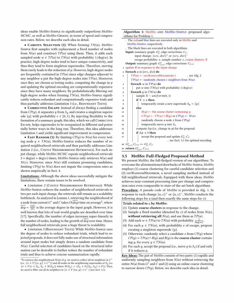
Algorithm 1: MoSSo and MoSSo-Simple: proposed algo-rithms for Problem 1.▷ The red and blue lines are executed only in MoSSo andMoSSo-Simple, respectively.
▷ The black lines are executed in both algorithms.Input: summary graph: G∗t , edge corrections: Ct ,
input change: {src, dst }+ or {src, dst }−escape probability: e , sample number: c , coarse clusters: R
Output: summary graph: G∗t+1, edge corrections: Ct+11 update R in response to the input change2 foreach u in {src, dst } do3 T P (u) ← getRandomNeighbor(c) ▷ see Alg. 2
T P (u) ← randomly chosen c neighbors from N (u)4 foreach w in T P (u) do5 put w into T N (u) with probability 1/deg(w )6 foreach y in T N (u) do7 sample X ∼ unif orm(0, 1)8 if X ≤ e then
9 temporarily create a new supernode Sy = {y }10 else
11 R(y) ← the coarse cluster containing y12 CP (y) ← T P (u) ∩ R(y) or CP (y) ← N (u)13 randomly choose a node z from CP (y)14 temporarily move y into Sz15 compute ∆φ (i.e., change in φ ) for the proposal16 if ∆φ ≤ 0 then17 accept the proposal and update G∗t , Ct
▷ see Sect. 3.1 for optimal encoding18 G∗t+1, Ct+1 ← G∗t , Ct19 return G∗t+1, Ct+1
3.5 MoSSo: Full-Fledged Proposed Method
We presentMoSSo, the full-fledged version of our algorithms. Toovercome the aforementioned drawbacks of MoSSo-Simple,MoSSoemploys (1) coarse clustering for careful candidate selection and(2) getRandomNeighbor, a novel sampling method instead offull neighborhood retrievals. Equipped with these ideas, MoSSoachieves near-constant processing time per change and compres-sion rates even comparable to state-of-the-art batch algorithms.Procedure: A pseudo code of MoSSo is provided in Alg. 1. Inresponse to each change {u,v}+ or {u,v}−, MoSSo conducts thefollowing steps for u (and then exactly the same steps for v):Trials related to u byMoSSo:
(1) Update coarse clusters in response to the change.(2) Sample a fixed number (denoted by c) of nodes from N (u),
without retrieving all N (u), and use them as TP(u).(3) Add eachw ∈ TP(u) to TN (u) with probability 1
deg(w ) .(4) For each y ∈ TN (u), with probability e of escape, propose
creating a singleton supernode {y}.(5) Otherwise, randomly select a candidate z from CP(y) where
CP(y) = TP(u) ∩R(y) and R(y) is the coarse cluster contain-ing y, for every y ∈ TN (u).
(6) For each y, accept the proposal (i.e., move y to Sz ) if and onlyif it reduces φ.
Key Ideas: The gist of MoSSo consists of two parts: (1) rapidly anduniformly sampling neighbors from N (u) without retrieving theentire N (u) fromG∗ andC and (2) using an online coarse clusteringto narrow down CP(y). Below, we describe each idea in detail.
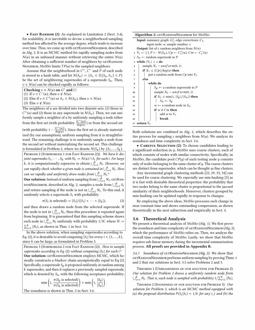
• Fast Random (2): As explained in Limitation 2 (Sect. 3.4),for scalability, it is inevitable to devise a neighborhood samplingmethod less affected by the average degree, which tends to increaseover time. Thus, we come up with getRandomNeighbor, describedin Alg. 2. It is an MCMC method for rapidly sampling nodes fromN (u) in an unbiased manner without retrieving the entire N (u).After obtaining a sufficient number of neighbors by getRandom-Neighbor,MoSSo limits TP(u) to the sampled neighbors.
Assume that the neighborhood in C+, C− and P of each nodeis stored in a hash table, and let N (Su ) := {Sv ∈ S |{Su , Sv } ∈ P}be the set of neighboring supernodes of a supernode Su . Then,v ∈ N (u) can be checked rapidly as follows:Checking v ∈ N (u) on G∗ and C:(1) If v ∈ C−(u), then v < N (u).(2) Else if v ∈ C+(u) or Sv ∈ N (Su ), then v ∈ N (u).(3) Else v < N (u).The neighbors of u are divided into two disjoint sets: (1) those inC+(u) and (2) those in any supernode in N (Su ). Then, we can uni-formly sample a neighbor of u by uniformly sampling a node eitherfrom the first set (with probability |C
+(u) |deg(u) ) or from the second set
(with probability 1 − |C+(u) |
deg(u) ). Since the first set is already material-ized (by our assumption), uniform sampling from it is straightfor-ward. The remaining challenge is to uniformly sample a node fromthe second set without materializing the second set. This challengeis formulated in Problem 2, where we denote N (Su ) by {S1, ..., Sk }.Problem 2 (Subproblem 1 for Fast Random (2)). We have k dis-
joint supernodes S1, · · · , Sk with Ni := N (u)∩Si for each i . For largek , it is computationally expensive to obtain
⋃ki=1 Ni . However, we
can rapidly check whether a given node is contained in
⋃ki=1 Ni . How
can we rapidly and uniformly draw nodes from
⋃ki=1 Ni ?
Our solution: Instead of uniform sampling from⋃ki=1 Ni , getRan-
domNeighbor, described in Alg. 2, samples a node from⋃ki=1 Si
and retries sampling if the node is not in⋃ki=1 Ni . To this end, it
randomly selects a supernode Si with probability
π (Si is selected) := |Si |/(|S1 | + · · · + |Sk |), (2)
and then draws a random node from the selected supernode. Ifthe node is not in
⋃ki=1 Ni , then this procedure is repeated again
from beginning. It is guaranteed that this sampling scheme drawseach node in
⋃ki=1 Ni uniformly with probability 1/N , where N :=∑k
i=1 |Ni |, as shown in Thm. 1 in Sect. 3.6.In the above solution, when sampling supernodes according to
Eq. (2), it is desirable to avoid computing |Si | for every i ∈ {1, ...,k},since k can be large, as formulated in Problem 3.Problem 3 (Subproblem 2 for Fast Random (2)). How to sample
supernodes according to Eq. (2) without computing |Si | for each i?Our solution: getRandomNeighbor employs MCMC, which ba-sically constructs a Markov chain asymptotically equal to Eq (2).Specifically, a supernode Sp is proposed uniformly at random amongk supernodes, and then it replaces a previously sampled supernode,which is denoted by Sn, with the following acceptance probability:
min(1,
π (Sp is selected)π (Sn is selected)
)= min
(1,|Sp ||Sn |
).
The soundness is shown in Thm. 2 in Sect. 3.6.
Algorithm 2: getRandomNeighbor for MoSSo.Input: summary graph: G∗t , edge corrections: Ct ,
input node: u , sample number: cOutput: list of c random neighbors from N (u)
1 Vr ← [ ], P ← N (Su ), Cp ← C+t (u), Cm ← C−t (u)2 Sn ← random supernode in P3 while |Vr | < c do
4 sample X1 ∼ unif orm(0, 1)5 if X1 ≤ |Cp |/deg(u) then6 put a random node from Cp into Vr7 else
8 while do
9 Sp ← a random supernode in P10 sample X2 ∼ unif orm(0, 1)11 if X2 ≤ min(1, |Sp |/ |Sn |) then12 Sn ← Sp13 w ← a random node in Sn14 if w < Cm then
15 add w to Vr16 break
17 return Vr
Both solutions are combined in Alg. 2, which describes the en-tire process for sampling c neighbors from N (u). We analyze itssoundness and time complexity in Sect. 3.6.• Careful Selection (2): To choose candidates leading to
a significant reduction in φ, MoSSo uses coarse clusters, each ofwhich consists of nodes with similar connectivity. Specifically, inMoSSo, the candidate pool CP(y) of each testing node y consistsonly of nodes belonging to the same cluster ofy. The coarse clustersare distinct from supernodes, which can be thought as fine clusters.
Any incremental graph clustering methods [22, 29, 33, 34] canbe used for coarse clustering. We especially use min-hashing [5] asit is fast with desirable theoretical properties: the probability thattwo nodes belong to the same cluster is proportional to the jaccardsimilarity of their neighborhoods. Moreover, clusters grouped bymin-hashing can be updated rapidly in response to changes.
By employing the above ideas, MoSSo processes each change innear-constant time and shows outstanding compression, as showntheoretically in the next subsection and empirically in Sect. 4.
3.6 Theoretical Analysis
We present a theoretical analysis of MoSSo (Alg. 1). We first provethe soundness and time complexity of getRandomNeighbor (Alg. 2),which the performance of MoSSo relies on. Then, we analyze theoverall time complexity of MoSSo. Lastly, we show that MoSSorequires sub-linear memory during the incremental summarizationprocess. All proofs are provided in Appendix B.
3.6.1 Soundness of getRandomNeighbor (Alg. 2). We show thatgetRandomNeighbor performs uniform sampling by proving Thms. 1and 2 that our solutions in Sect. 3.5 solve Problems 2 and 3.
Theorem 1 (Unbiasedness of our solution for Problem 2).Our solution for Problem 2 draws a uniformly random node from⋃ki=1 Ni . That is, each node is sampled with probability 1/∑k
i=1 |Ni |.Theorem 2 (Soundness of our solution for Problem 3). Our
solution for Problem 3, which is an MCMC method equipped with
(a) the proposal distribution P(Sj |Si ) = 1/k for any i, j and (b) the
acceptance probability A(Sj , Si ) = min(1, |Sj |/|Si |) for any move
from Si to Sj , asymptotically simulates π in Eq. (2).
3.6.2 Time Complexity of getRandomNeighbor (Alg. 2). Beforeproving the time complexity of getRandomNeighbor, which is acore building block of MoSSo, we first prove the time complexityof retrieving the neighborhood of an input node from the outputs(i.e., G∗ and C) in Lemma 1. We let C+(u) := {v ∈ V |{u,v} ∈ C+}and C−(u) := {v ∈ V |{u,v} ∈ C−} be the sets of neighbors of u inC+ and C−, respectively, and we let N (A) := {B ∈ S |{A,B} ∈ P} bethe set of neighboring supernodes of the supernode A.
Lemma 1 (Average time complexity of retrieving neighbor-hood). The average-case time complexity of retrieving the neighbor-
hood of a node is O(deд), where deд is the average degree.
As discussed in Limitation 2 in Sect. 3.4, Lemma 1 motivates us todesign getRandomNeighbor, which is much faster than retrievingthe entire neighborhood, as formulated in Thm. 3.
Theorem 3 (Average time complexity of getRandomNeigh-bor). Assume the neighborhood in C+, C− and P of each node is
stored in a hash table. The average-time complexity of Alg. 2 for each
node u is O(c · (1 + |C−(u)|/deд(u))).
The average time complexity of getRandomNeighbor called byMoSSo becomes constant, under a realistic assumption [1] that aninitial graph evolves under {et }∞t=0 where et takes place on a nodewith probability proportional to the degree of the node. That is,higher-degree nodes are more likely to go through changes in theirneighbors. This result is shown in Corollary 1 based on Lemma 2.
Lemma 2. Let X be a discrete random variable whose domain is
{ aubu }u ∈V , where au = |C−(u)| and bu = deд(u) for each node u and
the probability mass is proportional to deд(u). Then, E[X ] ≤ 1.
Collorary 1 (Average time complexity of getRandomNeigh-bor under preferential attachment [1]). The average-case time
complexity of getRandomNeighbor called by Alg. 1 is O(c) underthe assumption that each edge change et takes place on nodes with
probability proportional to the degree of the nodes.
3.6.3 Overall Time Complexity ofMoSSo (Alg. 1). In our analysisbelow, we let SN (A) := {B ∈ S : ∃(u,v) ∈ A× B, s.t. {u,v} ∈ E} bethe set of supernodes connected to A by at least one edge. We alsolet EAB := {{u,v} ∈ E |u ∈ A,v ∈ B,u , v} andTAB := {{u,v}|u ∈A,v ∈ B,u , v} be the sets of existing and potential edges betweensupernodes A and B, respectively.Computing Savings in the Objective φ (Eq. (1)): Suppose thatwe move a nodey from a supernode Sy to a supernode Sz . Then, theprevious optimal encoding (see Sect. 3.1) between Sy and each ofSN (Sy ) and between Sz and each of SN (Sz ) can be affected, whilethat between the other supernodes should remain the same. Hence,only SN (Sy ) and SN (Sz ) are of concern when computing the savingin the objective φ (i.e., Eq (1)) induced by the move of y. Thus, thetime complexity of this task is O(|SN (Sy )| + |SN (Sz )|).Updating Optimal Encoding: The computation of the saving de-termines whether a move is accepted or not. Once the move isaccepted, the previous optimal encoding should be updated in re-sponse to the move. As explained in Sect. 3.1, the edges betweentwo supernodes A and B are optimally encoded either as (1) |EAB |
Table 3: Real-world graph streams used in our experiments.
Name #Nodes #Insertions #Deletions Summary
Insertion-only (IO) graph streams
Protein (PR) 6, 229 146, 160 - Protein InteractionEmail-Enron (EN) 86, 977 297, 456 - EmailFacebook (FB) 61, 095 614, 797 - FriendshipWeb-EU-05 (EU) 862, 664 16, 138, 468 - HyperlinksHollywood (HW) 1, 985, 306 114, 492, 816 - CollaborationWeb-UK-02 (UK) 18, 483, 186 261, 787, 258 - Hyperlinks
Fully-dynamic (FD) graph streams
DBLP (DB) 317, 080 1, 049, 866 116, 042 CoauthorshipYouTube (YT) 1, 134, 890 2, 987, 624 331, 305 FriendshipSkitter (SK) 1, 696, 415 11, 095, 298 1, 233, 226 InternetLiveJournal (LJ) 3, 997, 962 34, 681, 189 3, 854, 423 Friendship
edges inC+ or as (2) the superedge {A,B} with |TAB | − |EAB | edgesin C−. In the latter case, |TAB | − |EAB | + 1 ≤ |EAB | holds in theoptimal encoding. Hence, in both cases, the number of referencesneeded to update the optimal encoding between each supernodepair {A,B} isO(|EAB |). Due to the reason discussed in the previousparagraph, the total worst-case time complexity is
O( ∑U ∈SN (Sy )
|ESyU |+∑
U ∈SN (Sz )|ESrU |
)= O
( ∑u ∈Sy
deд(u)+∑u ∈Sz
deд(u)).
Scalability in Practice: In practice, the above two subtasks do notharm the scalability of MoSSo, which proceeds to trials only withprobability 1
deд and updates the optimal encoding only if a moveis accepted. We show in Appendix. A.1 that the runtime of MoSSoin practice increases proportionally to the number of samples (i.e.,c) per input change, as expected from Corollary 1. For a fixed c ,MoSSo processes each change in near-constant time, regardlessof the growth of the input graph, as we show empirically in Sect. 4.4.
3.6.4 Space Complexity of MoSSo (Alg. 1). The sub-linear spacecomplexity of MoSSo proved in Thm. 4 implies that the entire inputgraph of sizeO(|V |+ |E |) does not have to be maintained in memoryduring the incremental summarization process.
Theorem 4 (Space complexity ofMoSSo). The space complexity
of Algorithm 1 is O(|V | + |P | + |C+ | + |C− |).
4 EXPERIMENTS
We review our experiments for answering the following questions:Q1. Speed: How fast isMoSSo, compared to the baseline streaming
algorithms and the best batch algorithms?Q2. Compression Ratio: How compact are the outputs of MoSSo,
compared to those obtained by the best competitors?Q3. Scalability:How does the runtime of MoSSo grow as the input
graph grows?Q4. Performance Analysis (Appendix A): How do graph prop-
erties and parameter values affect the performance of MoSSo?
4.1 Experimental Settings
Machine: We performed our experiments on a desktop with a3.7GHz Intel i5-9600k CPU and 64GB memory.Dataset: We used ten real-world graphs listed in Table 3. In everygraph, we ignored the direction of all edges and removed bothself-loops and multiple edges. From the graphs, we generate bothinsertion-only and fully dynamic graph streams with deletions. Wegenerated an insertion-only graph stream by listing the insertions
9857
x
2943
5x
6130
1x
1664
472x
6159
247x
1344
9192
x
1343
14x
2315
56x
1352
981x
2438
686x
102
104
106
108
1010
PR EN FB EU HW UK DB YT SK LJ
Exe
cutio
n T
ime
(mic
rose
ccon
ds)
MoSSo MoSSo-Simple MoSSo-MCMC MoSSo-Greedy SAGS SWeG Randomized
MoSSoMoSSo-SimpleMoSSo-MCMCMoSSo-GreedySAGSSWeGRandomized
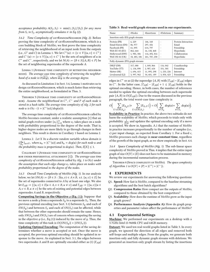
Figure 4: MoSSo is fast. It processed each change in the input graph up to 7 orders and 2 orders of magnitude faster than the
fastest batch algorithmand the streaming baselines (MoSSo-Greedy andMoSSo-MCMC), respectively. The baseline streaming
algorithms and Randomized ran out of time (> 24 hours) on some large graphs and do not appear in the corresponding plots.
of all edges in a graph. We either sorted the insertions by theirtimestamps (if they exist) or randomly ordered them (otherwise).For a fully-dynamic graph stream, we listed the insertions of alledges in a graph after randomly ordering them. Then, for each edge,we created the deletion of it with probability 0.1 and located thedeletion in a random position after the insertion of the edge.Implementation:We implemented the following lossless graph-summarization algorithms in OpenJDK 12: (a) MoSSo (proposed)with e=0.3, c=120; (b)MoSSo-Simple (proposed) with e=0.3, c=120;(c)MoSSo-Greedy (streaming baseline), (d)MoSSo-MCMC (stream-ing baseline) with β = 10; (e) SWeG [27] (batch baseline) with#Threads=1, T=20, ϵ=0; (f) SAGS [13] (batch baseline) with h=30,b=10, p=0.3; and (g) Randomized [21] (batch baseline).Evaluation Metric: Given a summary graphG∗ = (S, P) and edgecorrections C = (C+,C−) of a graph G = (V ,E), we used
(|P | + |C+ | + |C− |)/|E | (3)as the compression ratio. In Eq. (3), the numerator is the objective φ,and the denominator is a constant, given an input graph G. Eq. (3)and runtime were averaged over 3 trials unless otherwise stated.
4.2 Q1. Speed (Fig. 4)
To evaluate the speed of MoSSo, we measured the runtime of allconsidered algorithms. Specifically, for batch algorithms, we mea-sured the time taken for summarizing each dataset. For streamingalgorithms, we measured time taken for processing all the changesin each dataset, and then we divided it by the number of changesto compute the time taken for processing each change.
MoSSo was significantly faster than its competitors. Asseen in Fig. 4, it processed each change up to 7 orders of magnitudefaster than running the fastest batch algorithm. The gap betweenMoSSo and the batch algorithms was wide in large datasets. More-over, MoSSo was up to 2 orders of magnitude faster than the base-line streaming algorithms, and the gap increased in larger datasets,where the baseline method ran out of time. The two versions ofMoSSo showed comparable speed in small datasets, whileMoSSowas faster thanMoSSo-Simple in large datasets.
4.3 Q2. Compression Ratio (Fig. 5)
To test the effectiveness of MoSSo, we measured the compactnessof outputs obtained by all considered algorithms using the compres-sion ratio, defined in Eq (3). For streaming algorithms, we trackedthe changes in the compression ratio while each input graph streamevolved over time. For batch algorithms, we ran them when 20%,40%, 60%, 80% and 100% of the changes in each dataset arrived.
MoSSo achieved the best compression ratios among the
streaming algorithms, as seen in Fig. 5. Moreover, the compres-sion ratio of MoSSowas even comparable to those of the best batchalgorithms. Between the two versions of MoSSo, MoSSo consis-tently showed better compression ratios thanMoSSo-Simple.
4.4 Q3. Scalability (Fig. 1(c))
To evaluate the scalability of MoSSo, wemeasured its runtime in theWeb-EU-05 dataset. As seen in Fig. 1(c), the accumulated runtimeof MoSSo was near-linear in the number of processed changes,implying thatMoSSo processed each change in near-constant
time. Note that we ignored time taken to wait for input changes toarrive. More extensive results can be found at Appendix A.3.
5 RELATEDWORKS
Graph summarization has been studied in a number of settings,and an extensive survey can be found in [18]. We focus on studiesdirectly related to our work: (1) lossless summarization of staticgraphs, and (2) lossy and lossless summarization of dynamic graphs.Lossless summarization of static graphs: Lossless summariza-tion algorithms on static graphs output a summary graph with edgecorrections. Greedy [21] examines all pairs of supernodes that are2-hops away, and among the pairs, it repeatedly merges the pairleading to the largest saving in the objective φ. Randomized [21]speeds up the process by randomly picking one supernode andsearching only for the second supernode that leads to the largestsaving in φ, when being merged with the first one. To further re-duce the time complexity, SAGS [13] selects two supernodes to bemerged based on locality sensitive hashing. While these algorithmsfail to strike a balance between compression and time complex-ity, a parallel algorithm SWeG [27] succeeds in improving bothparts. Note that these batch algorithms are not designed to addresschanges in the input graph and should be rerun from scratch toreflect such changes. Lossy variants of the graph summarizationproblem were also explored in [15, 16, 21, 24, 27].Summarization of dynamic graphs: Since the dynamic natureof graphs makes lossless summarization more challenging, previousstudies of dynamic graph summarization have focused largely onlossy summarization for query efficiency [9, 30], social influenceanalysis [19, 20], temporal pattern [31], etc. They aim to summarize:either the current snapshot of the input graph [9, 12, 30, 32] ortemporal patterns in the entire history of the growth of the inputgraph [31]. For the former, existing incremental algorithms [9, 12,30, 32] produce lossy summary for query efficiency in a form ofgraph sketch (i.e., an adjacency matrix smaller than the originalone). Especially, TCM [30] and its variant GSS [9] compress theoriginal graph G = (V ,E) into a graph sketch Gs by using a hashfunction h(·) through mapping a node v ∈ V into a node h(v) inGv and mapping an edge {u,v} ∈ E into {h(u),h(v)} inGv . For thelatter, kC & kµ [31] lossily compress the entire history of a dynamicgraph to find temporal patterns. While TimeCrunch [26] is lossless,it is a batch algorithm for summarizing the entire growth historyof a dynamic graph. To the best of our knowledge, MoSSo is thefirst incremental algorithm for summarizing the current snapshotof a fully dynamic graph in a lossless manner.
0.00
0.25
0.50
0.75
1.00
0.0 0.2 0.4 0.6 0.8 1.0Ratio of Processed Changes
Com
pres
sion
Rat
io
(a) Protein (IO)
0.3
0.4
0.5
0.6
0.7
0.0 0.2 0.4 0.6 0.8 1.0Ratio of Processed Changes
Com
pres
sion
Rat
io
(b) Email-Enron (IO)
0.7
0.8
0.9
0.0 0.2 0.4 0.6 0.8 1.0Ratio of Processed Changes
Com
pres
sion
Rat
io
(c) Facebook (IO)
0.5
0.6
0.7
0.8
0.9
0.0 0.2 0.4 0.6 0.8 1.0Ratio of Processed Changes
Com
pres
sion
Rat
io
(d) DBLP (FD)
0.6
0.7
0.8
0.0 0.2 0.4 0.6 0.8 1.0Ratio of Processed Changes
Com
pres
sion
Rat
io
(e) YouTube (FD)
MoSSo MoSSo-Simple
MoSSo-MCMC
MoSSo-Greedy SAGS SWeG Randomized
MoSSoMoSSo-Simple
MoSSo-Greedy
SAGS
SWeG
Randomized
0.2
0.4
0.6
0.8
0.0 0.2 0.4 0.6 0.8 1.0Ratio of Processed Changes
Com
pres
sion
Rat
io
(f) Web-EU-05 (IO)
0.50.60.70.80.91.0
0.0 0.2 0.4 0.6 0.8 1.0Ratio of Processed Changes
Com
pres
sion
Rat
io
(g) Hollywood (IO)
0.2
0.4
0.6
0.8
0.0 0.2 0.4 0.6 0.8 1.0Ratio of Processed Changes
Com
pres
sion
Rat
io
(h) Web-UK-02 (IO)
0.5
0.6
0.7
0.8
0.0 0.2 0.4 0.6 0.8 1.0Ratio of Processed Changes
Com
pres
sion
Rat
io
(i) Skitter (FD)
0.7
0.8
0.9
0.0 0.2 0.4 0.6 0.8 1.0Ratio of Processed Changes
Com
pres
sion
Rat
io
(j) LiveJournal (FD)
MoSSoMoSSo-SimpleMoSSo-MCMCMoSSo-GreedySAGSSWeGRandomized
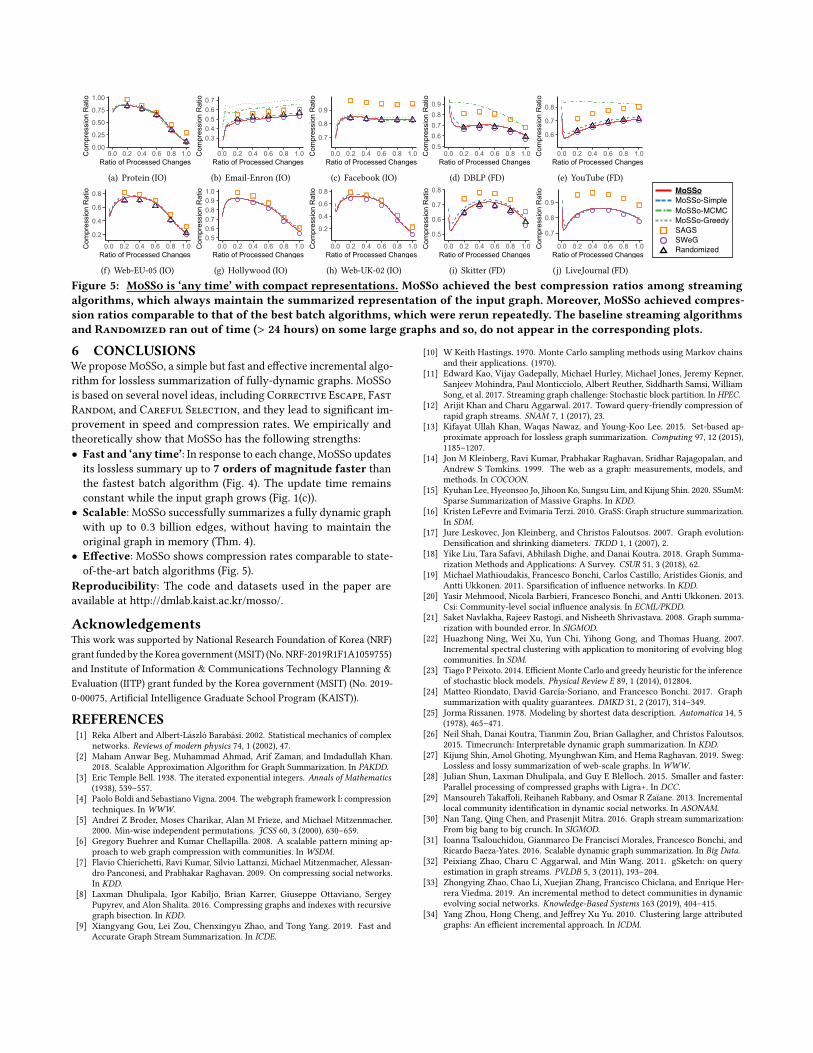
Figure 5: MoSSo is ‘any time’ with compact representations. MoSSo achieved the best compression ratios among streaming
algorithms, which always maintain the summarized representation of the input graph. Moreover, MoSSo achieved compres-
sion ratios comparable to that of the best batch algorithms, which were rerun repeatedly. The baseline streaming algorithms
and Randomized ran out of time (> 24 hours) on some large graphs and so, do not appear in the corresponding plots.
6 CONCLUSIONS
We proposeMoSSo, a simple but fast and effective incremental algo-rithm for lossless summarization of fully-dynamic graphs.MoSSois based on several novel ideas, including Corrective Escape, FastRandom, and Careful Selection, and they lead to significant im-provement in speed and compression rates. We empirically andtheoretically show thatMoSSo has the following strengths:• Fast and ‘any time’: In response to each change,MoSSo updatesits lossless summary up to 7 orders of magnitude faster thanthe fastest batch algorithm (Fig. 4). The update time remainsconstant while the input graph grows (Fig. 1(c)).• Scalable:MoSSo successfully summarizes a fully dynamic graphwith up to 0.3 billion edges, without having to maintain theoriginal graph in memory (Thm. 4).• Effective: MoSSo shows compression rates comparable to state-of-the-art batch algorithms (Fig. 5).
Reproducibility: The code and datasets used in the paper areavailable at http://dmlab.kaist.ac.kr/mosso/.
Acknowledgements
This work was supported by National Research Foundation of Korea (NRF)grant funded by the Korea government (MSIT) (No. NRF-2019R1F1A1059755)and Institute of Information & Communications Technology Planning &Evaluation (IITP) grant funded by the Korea government (MSIT) (No. 2019-0-00075, Artificial Intelligence Graduate School Program (KAIST)).
REFERENCES
[1] Réka Albert and Albert-László Barabási. 2002. Statistical mechanics of complexnetworks. Reviews of modern physics 74, 1 (2002), 47.
[2] Maham Anwar Beg, Muhammad Ahmad, Arif Zaman, and Imdadullah Khan.2018. Scalable Approximation Algorithm for Graph Summarization. In PAKDD.
[3] Eric Temple Bell. 1938. The iterated exponential integers. Annals of Mathematics
(1938), 539–557.[4] Paolo Boldi and Sebastiano Vigna. 2004. The webgraph framework I: compression
techniques. In WWW.[5] Andrei Z Broder, Moses Charikar, Alan M Frieze, and Michael Mitzenmacher.
2000. Min-wise independent permutations. JCSS 60, 3 (2000), 630–659.[6] Gregory Buehrer and Kumar Chellapilla. 2008. A scalable pattern mining ap-
proach to web graph compression with communities. In WSDM.[7] Flavio Chierichetti, Ravi Kumar, Silvio Lattanzi, Michael Mitzenmacher, Alessan-
dro Panconesi, and Prabhakar Raghavan. 2009. On compressing social networks.In KDD.
[8] Laxman Dhulipala, Igor Kabiljo, Brian Karrer, Giuseppe Ottaviano, SergeyPupyrev, and Alon Shalita. 2016. Compressing graphs and indexes with recursivegraph bisection. In KDD.
[9] Xiangyang Gou, Lei Zou, Chenxingyu Zhao, and Tong Yang. 2019. Fast andAccurate Graph Stream Summarization. In ICDE.
[10] W Keith Hastings. 1970. Monte Carlo sampling methods using Markov chainsand their applications. (1970).
[11] Edward Kao, Vijay Gadepally, Michael Hurley, Michael Jones, Jeremy Kepner,Sanjeev Mohindra, Paul Monticciolo, Albert Reuther, Siddharth Samsi, WilliamSong, et al. 2017. Streaming graph challenge: Stochastic block partition. In HPEC.
[12] Arijit Khan and Charu Aggarwal. 2017. Toward query-friendly compression ofrapid graph streams. SNAM 7, 1 (2017), 23.
[13] Kifayat Ullah Khan, Waqas Nawaz, and Young-Koo Lee. 2015. Set-based ap-proximate approach for lossless graph summarization. Computing 97, 12 (2015),1185–1207.
[14] Jon M Kleinberg, Ravi Kumar, Prabhakar Raghavan, Sridhar Rajagopalan, andAndrew S Tomkins. 1999. The web as a graph: measurements, models, andmethods. In COCOON.
[15] Kyuhan Lee, Hyeonsoo Jo, Jihoon Ko, Sungsu Lim, and Kijung Shin. 2020. SSumM:Sparse Summarization of Massive Graphs. In KDD.
[16] Kristen LeFevre and Evimaria Terzi. 2010. GraSS: Graph structure summarization.In SDM.
[17] Jure Leskovec, Jon Kleinberg, and Christos Faloutsos. 2007. Graph evolution:Densification and shrinking diameters. TKDD 1, 1 (2007), 2.
[18] Yike Liu, Tara Safavi, Abhilash Dighe, and Danai Koutra. 2018. Graph Summa-rization Methods and Applications: A Survey. CSUR 51, 3 (2018), 62.
[19] Michael Mathioudakis, Francesco Bonchi, Carlos Castillo, Aristides Gionis, andAntti Ukkonen. 2011. Sparsification of influence networks. In KDD.
[20] Yasir Mehmood, Nicola Barbieri, Francesco Bonchi, and Antti Ukkonen. 2013.Csi: Community-level social influence analysis. In ECML/PKDD.
[21] Saket Navlakha, Rajeev Rastogi, and Nisheeth Shrivastava. 2008. Graph summa-rization with bounded error. In SIGMOD.
[22] Huazhong Ning, Wei Xu, Yun Chi, Yihong Gong, and Thomas Huang. 2007.Incremental spectral clustering with application to monitoring of evolving blogcommunities. In SDM.
[23] Tiago P Peixoto. 2014. EfficientMonte Carlo and greedy heuristic for the inferenceof stochastic block models. Physical Review E 89, 1 (2014), 012804.
[24] Matteo Riondato, David García-Soriano, and Francesco Bonchi. 2017. Graphsummarization with quality guarantees. DMKD 31, 2 (2017), 314–349.
[25] Jorma Rissanen. 1978. Modeling by shortest data description. Automatica 14, 5(1978), 465–471.
[26] Neil Shah, Danai Koutra, Tianmin Zou, Brian Gallagher, and Christos Faloutsos.2015. Timecrunch: Interpretable dynamic graph summarization. In KDD.
[27] Kijung Shin, Amol Ghoting, Myunghwan Kim, and Hema Raghavan. 2019. Sweg:Lossless and lossy summarization of web-scale graphs. In WWW.
[28] Julian Shun, Laxman Dhulipala, and Guy E Blelloch. 2015. Smaller and faster:Parallel processing of compressed graphs with Ligra+. In DCC.
[29] Mansoureh Takaffoli, Reihaneh Rabbany, and Osmar R Zaïane. 2013. Incrementallocal community identification in dynamic social networks. In ASONAM.
[30] Nan Tang, Qing Chen, and Prasenjit Mitra. 2016. Graph stream summarization:From big bang to big crunch. In SIGMOD.
[31] Ioanna Tsalouchidou, Gianmarco De Francisci Morales, Francesco Bonchi, andRicardo Baeza-Yates. 2016. Scalable dynamic graph summarization. In Big Data.
[32] Peixiang Zhao, Charu C Aggarwal, and Min Wang. 2011. gSketch: on queryestimation in graph streams. PVLDB 5, 3 (2011), 193–204.
[33] Zhongying Zhao, Chao Li, Xuejian Zhang, Francisco Chiclana, and Enrique Her-rera Viedma. 2019. An incremental method to detect communities in dynamicevolving social networks. Knowledge-Based Systems 163 (2019), 404–415.
[34] Yang Zhou, Hong Cheng, and Jeffrey Xu Yu. 2010. Clustering large attributedgraphs: An efficient incremental approach. In ICDM.
0.55
0.60
0.65
0.70
0.75
0.0 0.2 0.4 0.6 0.8Escape Probability
Com
pres
sion
Rat
io
0
1000
2000
3000
0.0 0.2 0.4 0.6 0.8Escape Probability
A
ccum
ulat
ed
E
xecu
tion
Tim
e (s
ec)
𝑐𝑐 = 60𝑐𝑐 = 120𝑐𝑐 = 180𝑐𝑐 = 240
(a) Effects of the escape probability (i.e., e )
0.55
0.60
0.65
0.70
0.75
60 120 180 240Sample Number
Com
pres
sion
Rat
io
0
1000
2000
3000
60 120 180 240Sample Number
A
ccum
ulat
ed
E
xecu
tion
Tim
e (s
ec)
𝑒𝑒 = 0.8
𝑒𝑒 = 0𝑒𝑒 = 0.2𝑒𝑒 = 0.4𝑒𝑒 = 0.6
(b) Effects of the number of samples (i.e., c )
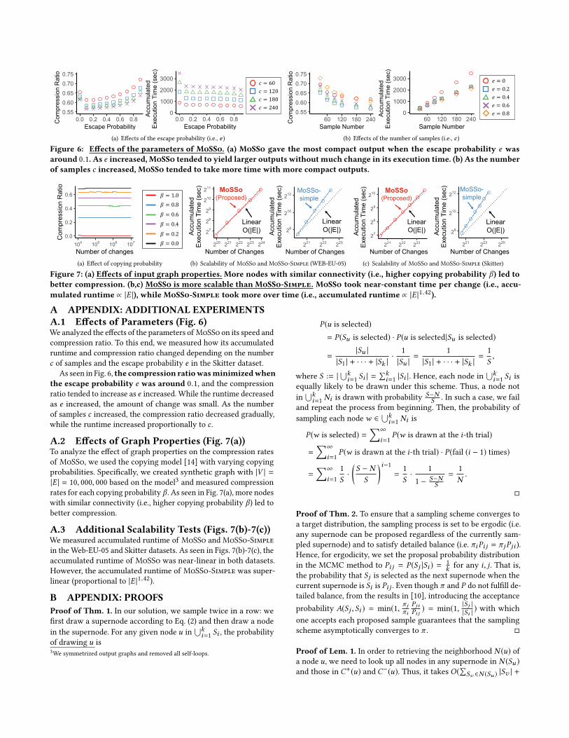
Figure 6: Effects of the parameters of MoSSo. (a) MoSSo gave the most compact output when the escape probability e was
around 0.1. As e increased,MoSSo tended to yield larger outputs without much change in its execution time. (b) As the number
of samples c increased,MoSSo tended to take more time with more compact outputs.
0.0
0.2
0.4
0.6
104 105 106 107
Number of changes
Com
pres
sion
Rat
io
𝛽 = 1.0𝛽 = 0.8
𝛽 = 0.6
𝛽 = 0.4
𝛽 = 0.2𝛽 = 0.0
(a) Effect of copying probability
27
28
29
210
211
220 221 222 223 224
Number of Changes
A
ccum
ulat
ed
E
xecu
tion
Tim
e (s
ec) MoSSo
(Proposed)
Linear O(|E|) 28
210
212
221 223 225
Number of Changes
Acc
umul
ated
E
xecu
tion
Tim
e (s
ec)
MoSSo-simple
Linear O(|E|)
(b) Scalability of MoSSo and MoSSo-Simple (WEB-EU-05)
27
28
29
210
221 222 223
Number of Changes
A
ccum
ulat
ed
E
xecu
tion
Tim
e (s
ec) MoSSo
(Proposed)
Linear O(|E|) 28
210
212
221 223 225
Number of Changes
A
ccum
ulat
ed
E
xecu
tion
Tim
e (s
ec) MoSSo-
simple
Linear O(|E|)
(c) Scalability of MoSSo and MoSSo-Simple (Skitter)
Figure 7: (a) Effects of input graph properties. More nodes with similar connectivity (i.e., higher copying probability β) led to
better compression. (b,c) MoSSo is more scalable thanMoSSo-Simple. MoSSo took near-constant time per change (i.e., accu-
mulated runtime ∝ |E |), while MoSSo-Simple took more over time (i.e., accumulated runtime ∝ |E |1.42).
A APPENDIX: ADDITIONAL EXPERIMENTS
A.1 Effects of Parameters (Fig. 6)
We analyzed the effects of the parameters of MoSSo on its speed andcompression ratio. To this end, we measured how its accumulatedruntime and compression ratio changed depending on the numberc of samples and the escape probability e in the Skitter dataset.
As seen in Fig. 6, the compression ratiowasminimizedwhen
the escape probability e was around 0.1, and the compressionratio tended to increase as e increased. While the runtime decreasedas e increased, the amount of change was small. As the numberof samples c increased, the compression ratio decreased gradually,while the runtime increased proportionally to c .
A.2 Effects of Graph Properties (Fig. 7(a))
To analyze the effect of graph properties on the compression ratesof MoSSo, we used the copying model [14] with varying copyingprobabilities. Specifically, we created synthetic graph with |V | =|E | = 10, 000, 000 based on the model3 and measured compressionrates for each copying probability β . As seen in Fig. 7(a), more nodeswith similar connectivity (i.e., higher copying probability β) led tobetter compression.
A.3 Additional Scalability Tests (Figs. 7(b)-7(c))
We measured accumulated runtime of MoSSo andMoSSo-Simplein the Web-EU-05 and Skitter datasets. As seen in Figs. 7(b)-7(c), theaccumulated runtime of MoSSo was near-linear in both datasets.However, the accumulated runtime of MoSSo-Simple was super-linear (proportional to |E |1.42).
B APPENDIX: PROOFS
Proof of Thm. 1. In our solution, we sample twice in a row: wefirst draw a supernode according to Eq. (2) and then draw a nodein the supernode. For any given node u in
⋃ki=1 Si , the probability
of drawing u is3We symmetrized output graphs and removed all self-loops.
P(u is selected)= P(Su is selected) · P(u is selected|Su is selected)
=|Su |
|S1 | + · · · + |Sk |· 1|Su |=
1|S1 | + · · · + |Sk |
=1S,
where S := |⋃ki=1 Si | =
∑ki=1 |Si |. Hence, each node in
⋃ki=1 Si is
equally likely to be drawn under this scheme. Thus, a node notin
⋃ki=1 Ni is drawn with probability S−N
S . In such a case, we failand repeat the process from beginning. Then, the probability ofsampling each nodew ∈ ⋃k
i=1 Ni is
P(w is selected) =∑∞
i=1P(w is drawn at the i-th trial)
=∑∞
i=1P(w is drawn at the i-th trial) · P(fail (i − 1) times)
=∑∞
i=11S·(S − NS
)i−1=
1S· 11 − S−N
S=
1N.
□
Proof of Thm. 2. To ensure that a sampling scheme converges toa target distribution, the sampling process is set to be ergodic (i.e.any supernode can be proposed regardless of the currently sam-pled supernode) and to satisfy detailed balance (i.e. πiPi j = πjPji ).Hence, for ergodicity, we set the proposal probability distributionin the MCMC method to Pi j = P(Sj |Si ) = 1
k for any i, j. That is,the probability that Sj is selected as the next supernode when thecurrent supernode is Si is Pi j . Even though π and P do not fulfill de-tailed balance, from the results in [10], introducing the acceptanceprobability A(Sj , Si ) = min(1, πjπi
PjiPi j ) = min(1, |Sj ||Si | ) with which
one accepts each proposed sample guarantees that the samplingscheme asymptotically converges to π . □
Proof of Lem. 1. In order to retrieving the neighborhood N (u) ofa node u, we need to look up all nodes in any supernode in N (Su )and those in C+(u) and C−(u). Thus, it takes O(∑Sv ∈N (Su ) |Sv | +
Algorithm 3:MoSSo-MCMC: a baseline algorithmInput: summary graph: G∗t , edge corrections: Ct ,
input change: {src, dst }+ or {src, dst }−Output: summary graph: G∗t+1, edge corrections: Ct+1
1 foreach u in {src, dst} do
2 T P (u) ← N (u), T N (u) ← N (u)3 foreach y in T N (u) do4 CP (y) ← Vt5 darw a uniformly random node x from N (y)6 draw a candidate z ∈ CP (y) using Eq. (4)7 temporarily move y into Sz8 compute ∆φ (i.e., change in φ ) for the proposal9 compute the acceptance probability p using Eq. (5)
10 sample X ∼ unif orm(0, 1)11 if X ≤ p then
12 accept the proposal and update G∗t , Ct▷ see Sect. 3.1 for optimal encoding
13 G∗t+1, Ct+1 ← G∗t , Ct14 return G∗t+1, Ct+1
|C−(u)| + |C+(u)|). Since ∑Sv ∈N (Su ) |Sv | + |C
+(u)| = deд(u) +|C−(u)|, the time complexity becomes O(deд(u) + 2|C−(u)|). Letau = |C−(u)| and bu = deд(u). Then, the average-case time com-plexity of retrieving the neighborhood of a node is:∑
u ∈V (2au + bu )|V | =
2∑u ∈V au +
∑u ∈V bu
|V | =4|C− | + 2|E ||V | ,
where the second equality comes from∑u ∈V |C−(u)| = 2|C− | and∑
u ∈V deд(u) = 2|E |. By the optimal encoding (Sect. 3.1), |P |+ |C+ |+|C− | ≤ |E | holds and thus, |C− | ≤ |E |. Using this inequality, theaverage-case time complexity is bounded by 3 · deд. □
Proof of Thm. 3. A node is drawn from C+(u) with probability|C+(u) |deд(u) and from
⋃ki=1 Si with probability deд(u)−|C+(u) |
deд(u) . The for-mer takes O(1), but the latter requires repeated sampling until anode in
⋃ki=1 Si is drawn. As in the proof of Thm. 1, a neighbor of
u in⋃ki=1 Ni is drawn with probability N
S in each trial. Thus, theexpected number of trials is simply S
N , and the average-case timecomplexity of getRandomNeighbor for sampling a node is
|C+(u)|deд(u) +
deд(u) − |C+(u)|deд(u) · S
N
=|C+(u)|deд(u) +
deд(u) − |C+(u)|deд(u) · deд(u) − |C
+(u)| + |C−(u)|deд(u) − |C+(u)|
=|C+(u)|deд(u) +
deд(u) − |C+(u)| + |C−(u)|deд(u) = 1 +
|C−(u)|deд(u) .
Hence, the average-case time complexity of getRandomNeighborfor c samples is O(c · (1 + |C
−(u) |deд(u) )). □
Proof of Lem. 2.
E[X ] =∑u ∈V(aubu
bu∑v ∈V bv
) =∑u ∈V
au∑v ∈V bv
=
∑u ∈V au∑u ∈V bu
.
As in the proof of Lemma 1, we can show∑u∈V au∑u∈V bu
=2 |C− |2 |E | ≤ 1
and thus E[X ] ≤ 1. □
Proof of Cor. 1. Due to the assumption, a node u is used as theinput of getRandomNeighbor with probability proportional todeд(u). By Lemma 2, |C
−(u) |deд(u) ≤ 1 in average case. Therefore, com-
bined with Thm. 3, the average-case time complexity of getRan-domNeighbor for c samples in Alg. 1 becomes O(c). □
Proof of Thm. 4. Alg. 1 maintains G∗ and C for the current snap-shot, and their size is O(|V | + |P | + |C+ | + |C− |) in total. More-over, additional O(|V |) space is required for storing coarse clustermemberships of nodes. Additionally, to rapidly estimate the savingin φ, our implementation maintains the counts of edges betweenpairs of supernodes, and the number of nonzero counts is upperbounded by O(|P | + |C+ |). Hence, the total space complexity isO(|V | + |P | + |C+ | + |C− |). □
C APPENDIX: DETAILS OF MOSSO-MCMC
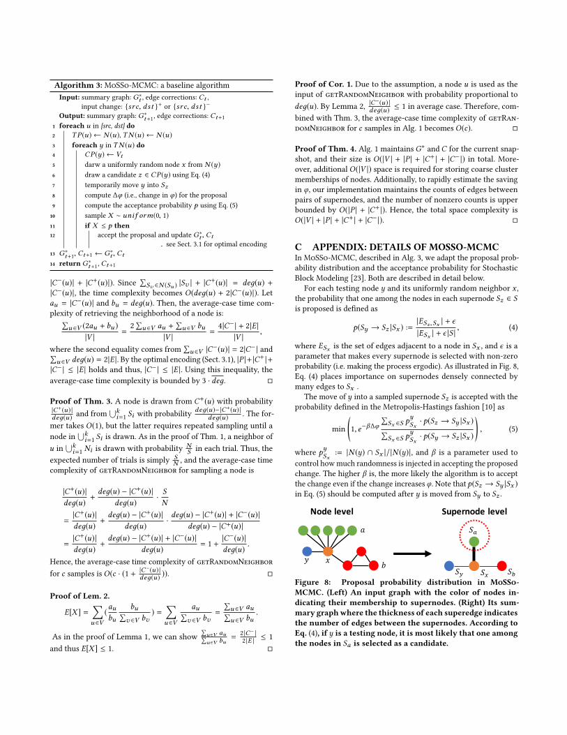
In MoSSo-MCMC, described in Alg. 3, we adapt the proposal prob-ability distribution and the acceptance probability for StochasticBlock Modeling [23]. Both are described in detail below.
For each testing node y and its uniformly random neighbor x ,the probability that one among the nodes in each supernode Sz ∈ Sis proposed is defined as
p(Sy → Sz |Sx ) :=|ESz,Sx | + ϵ|ESx | + ϵ |S |
, (4)
where ESx is the set of edges adjacent to a node in Sx , and ϵ is aparameter that makes every supernode is selected with non-zeroprobability (i.e. making the process ergodic). As illustrated in Fig. 8,Eq. (4) places importance on supernodes densely connected bymany edges to Sx .
The move of y into a sampled supernode Sz is accepted with theprobability defined in the Metropolis-Hastings fashion [10] as
min
(1, e−β∆φ
∑Sx ∈S p
ySx· p(Sz → Sy |Sx )∑
Sx ∈S pySx· p(Sy → Sz |Sx )
), (5)
where pySx := |N (y) ∩ Sx |/|N (y)|, and β is a parameter used tocontrol howmuch randomness is injected in accepting the proposedchange. The higher β is, the more likely the algorithm is to acceptthe change even if the change increases φ. Note that p(Sz → Sy |Sx )in Eq. (5) should be computed after y is moved from Sy to Sz .
Supernode level
𝑦𝑆# 𝑆$
𝑆%
𝑆&
Node level
𝑥
𝑎
𝑏
Figure 8: Proposal probability distribution in MoSSo-
MCMC. (Left) An input graph with the color of nodes in-
dicating their membership to supernodes. (Right) Its sum-
mary graphwhere the thickness of each superedge indicates
the number of edges between the supernodes. According to
Eq. (4), if y is a testing node, it is most likely that one among
the nodes in Sa is selected as a candidate.