accurate incremental voxelization in common
TRANSCRIPT
ACCURATE INCREMENTAL VOXELIZATION IN
COMMON SAMPLING LATTICES
by
Haris Widjaya
B.Sc., Simon Fraser University, 2002
a thesis submitted in partial fulfillment
of the requirements for the degree of
Master of Science
in the School
of
Computing Science
c© Haris Widjaya 2006
SIMON FRASER UNIVERSITY
Summer 2006
All rights reserved. This work may not be
reproduced in whole or in part, by photocopy
or other means, without the permission of the author.

APPROVAL
Name: Haris Widjaya
Degree: Master of Science
Title of thesis: Accurate Incremental Voxelization in Common Sampling Lat-
tices
Examining Committee: Dr. Greg Mori,
Assistant Professor, Computing Science
Simon Fraser University
Chair
Dr. Torsten Moller,
Associate Professor, Computing Science
Simon Fraser University
Senior Supervisor
Dr. Richard Zhang,
Assistant Professor, Computing Science
Simon Fraser University
Supervisor
Dr. Thomas C. Shermer,
Professor, Computing Science
Simon Fraser University
SFU Examiner
Date Approved:
ii

Abstract
Work on binary surface voxelization has previously focused on Cartesian lattices. In this
theses I present a generalized voxelization algorithm to any lattice structure in 2D space.
In 3D I extend the algorithm to include BCC lattices. Further, I prove the correctness of
our algorithm. An efficient implementation of the proposed algorithm has been achieved.
Thorough testing of our algorithm gives an experimental validation to our implementation.
Our results show that the efficient implementation of the proposed algorithm is (on average)
11% faster than a standard implementation.
iii

I dedicate this work to my parents,
who have supported me from the day I took my first breath
iv

For I know the plans I have for you declares the Lord, plans to prosper you and not to
harm you, plans to give you a hope and a future Jeremiah 29:11 (NIV)
v

Acknowledgments
To Dr Torsten Moller, my supervisor who constantly strives for excellence, and impresses
the same values upon me. One who guided me through tough times, and around numerous
dead ends that I can not foresee.
To Matt Olson, for all the open and honest discussion about many related topics to my
thesis.
To my friends in GrUVI lab for all the laughters, discussion, and arguments that helps
me get through the long days, and nights.
To my family in Jakarta who have always believed in my abilities and supported me
through my school years
To my second family at Brentwood Park Alliance Church who have been faithfully
praying for me during my time here.
vi

Contents
Approval ii
Abstract iii
Dedication iv
Quotation v
Acknowledgments vi
Contents vii
List of Tables ix
List of Figures x
1 Introduction 1
1.1 Boundary representation . . . . . . . . . . . . . . . . . . . . . . . . . . . . . . 2
1.2 Volumetric representation . . . . . . . . . . . . . . . . . . . . . . . . . . . . . 4
1.3 Voxelization . . . . . . . . . . . . . . . . . . . . . . . . . . . . . . . . . . . . . 11
1.3.1 Binary Voxelization . . . . . . . . . . . . . . . . . . . . . . . . . . . . 12
1.3.2 Multi valued voxelization . . . . . . . . . . . . . . . . . . . . . . . . . 13
1.4 Contributions . . . . . . . . . . . . . . . . . . . . . . . . . . . . . . . . . . . . 15
2 Background 17
2.1 Alternative lattice structure . . . . . . . . . . . . . . . . . . . . . . . . . . . . 17
2.2 Notations and Formalisms . . . . . . . . . . . . . . . . . . . . . . . . . . . . . 28
vii

3 Accurate voxelization 32
3.1 2D Lattices . . . . . . . . . . . . . . . . . . . . . . . . . . . . . . . . . . . . . 34
3.1.1 Theorem’s accuracy proof . . . . . . . . . . . . . . . . . . . . . . . . . 35
3.1.2 Cartesian Lattice . . . . . . . . . . . . . . . . . . . . . . . . . . . . . . 39
3.2 3D Lattices . . . . . . . . . . . . . . . . . . . . . . . . . . . . . . . . . . . . . 42
3.2.1 Cartesian Lattices . . . . . . . . . . . . . . . . . . . . . . . . . . . . . 44
4 Voxelization algorithms 48
4.1 Mesh Voxelization . . . . . . . . . . . . . . . . . . . . . . . . . . . . . . . . . 48
4.2 Brute Force Algorithm . . . . . . . . . . . . . . . . . . . . . . . . . . . . . . . 51
4.3 Fast incremental binary voxelization . . . . . . . . . . . . . . . . . . . . . . . 53
4.3.1 Region ∆(Lp) . . . . . . . . . . . . . . . . . . . . . . . . . . . . . . . . 54
4.4 Further optimization . . . . . . . . . . . . . . . . . . . . . . . . . . . . . . . . 62
4.5 Region ∆(Le) and∆(Lv) . . . . . . . . . . . . . . . . . . . . . . . . . . . . . . 64
4.6 Practicalities . . . . . . . . . . . . . . . . . . . . . . . . . . . . . . . . . . . . 65
5 Analysis of algorithm 67
5.1 Validation Techniques . . . . . . . . . . . . . . . . . . . . . . . . . . . . . . . 67
5.2 Testing Methodology . . . . . . . . . . . . . . . . . . . . . . . . . . . . . . . . 72
5.3 BCC vs Cartesian Lattice . . . . . . . . . . . . . . . . . . . . . . . . . . . . . 73
5.4 Results . . . . . . . . . . . . . . . . . . . . . . . . . . . . . . . . . . . . . . . . 74
6 Conclusions and future work 92
6.1 Future Work . . . . . . . . . . . . . . . . . . . . . . . . . . . . . . . . . . . . 93
Bibliography 95
viii

List of Tables
1.1 Comparison between surface representation and volume representation . . . . 8
4.1 Valid voxelization matrices M for 2-separating planes in a Cartesian lattice. . 57
4.2 Additional voxelization matrices M for Table 4.1. For a 1-separating planes
in a Cartesian lattice. . . . . . . . . . . . . . . . . . . . . . . . . . . . . . . . 58
4.3 Additional voxelization matrices M for Table 4.1 and Table 4.2. For a 0-
separating planes in a Cartesian lattice. . . . . . . . . . . . . . . . . . . . . . 59
4.4 Voxelization matrix M for 2-separating planes in a BCC lattice. . . . . . . . . 60
ix

List of Figures
1.1 Grid taxonomy in 2D . . . . . . . . . . . . . . . . . . . . . . . . . . . . . . . . 4
1.2 Direct Volume Rendering of the Industrial CT Images of a Tooth from Trans-
fer Function Bakeoff Panel at IEEE Visualization Conference [43]. The image
shows a transparent outer layer of the tooth as well as its inner structure.
This image is obtained using vuVolume2 splatter, with custom transfer function. 5
1.3 A slice of MRI data. The data set is obtained from UNC Chapel Hill Volume
Rendering test dataset [40] . . . . . . . . . . . . . . . . . . . . . . . . . . . . 6
1.4 Difference between binary and smooth pixelization . . . . . . . . . . . . . . . 11
2.1 Comb function pairs . . . . . . . . . . . . . . . . . . . . . . . . . . . . . . . . 18
2.2 The effect of sampling a band-limited continuous signal (a) by convolving a
comb function with a sampling distance W. When W is large we get aliasing
artifact shown in Figure (c). The dashed lines in (c) show the lost part of
the input spectrum. As W shrinks the replicated spectra are moving further
apart. At some point the replicated spectra will be perfectly separated from
each other as shown in Figure (d) . . . . . . . . . . . . . . . . . . . . . . . . . 19
2.3 Illustration of the reconstruction process. The left figure shows the original
continuous signal multiplied with the comb function, the dark dots on the
curve represent the sample value at that particular position. In the frequency
domain when W is chosen to be the Nyquist rates the spectrum of the sampled
signal will look like the figure on the right. To perfectly reconstruct the
original signal from the sampled signal, one must construct a box filter with
the same support as the signal’s frequency spectrum shown as dashed lines. . 19
x

2.4 Illustration of sampling in 2D space. Assuming that the sampled continuous
data has a frequency support shown in (a). Discrete sampling in 2D Cartesian
lattice replicates the primary spectrum over the plane, as shown in (b) . . . . 21
2.5 (a) Hexagonal lattice in the spatial domain. The shaded area shows the
fundamental parallelepiped in this lattice (b) The corresponding reciprocal
lattice showing frequency replicas . . . . . . . . . . . . . . . . . . . . . . . . . 23
2.6 Cartesian and BCC lattice packing, the images show the neighbours of the
voxel at the centre of the lattice. (a) The Cartesian lattice, and (b) the BCC
lattice with 14 neighbours. Because the packing in BCC lattice is the tightest
possible the centre voxel is completely occluded by its neighbour voxels as
shown in (b). In BCC there are two kinds of neighbour voxels. Neighbour
voxels of the first kind share a hexagonal face as shown in (c). Neighbour
voxels of the second kind share a square face as shown in (d). . . . . . . . . . 25
2.7 The left picture shows one possible 2D hexagonal indexing scheme. The
light shaded dots indicate points that can not be represented because in the
scheme they contain negative values. When the negative samples are required
a different indexing scheme shown on the right figure must be used with an
extra computation, see [51]. . . . . . . . . . . . . . . . . . . . . . . . . . . . 26
2.8 Two cases of continuous to discrete topology mapping problem . . . . . . . . 29
2.9 The set of neighboring pixels/voxels in a Cartesian lattice. . . . . . . . . . . . 30
2.10 Neighbouring Voronoi sets of hexagonal lattice (a) and BCC lattice (b) . . . . 31
3.1 The plane L, and two parallel planes LA and LB. Any voxels that lie in
between LA and LB are included in the voxelization of L . . . . . . . . . . . . 33
3.2 The two basis vectors v1 and v2 describe a lattice. (a) shows a regular Carte-
sian lattice (also called rectilinear grid, since the basis vectors are orthogonal),
while (b) shows a general 2D lattice. Note that in this lattice we have six
neighbourhood vectors of which half are depicted as q1, q2, and q3. The other
half can be obtained by rotating the vectors 180 degrees. From the picture
it is easy to see that the neighbourhood N0(z) and N1(z) in the general case
are identical . . . . . . . . . . . . . . . . . . . . . . . . . . . . . . . . . . . . 34
3.3 One cell of Figure 3.2b . . . . . . . . . . . . . . . . . . . . . . . . . . . . . . . 36
xi

3.4 G and H are the center of adjacent sample points on the lattice, Fk is the
edge/face shared between G and H. ‖ GH ‖= 2di. L is the continuous line
we voxelize . . . . . . . . . . . . . . . . . . . . . . . . . . . . . . . . . . . . . 38
3.5 Generalized Cartesian lattice case. There are two different neighbourhood
vectors available in this lattice. We denote ck as the set of neighbourhood
vectors with dk = W2 for k ∈ 1, 2. cj is the set of neighbourhood vectors with
dj =√
2W2 for k ∈ 3, 4. . . . . . . . . . . . . . . . . . . . . . . . . . . . . . . . 40
3.6 Because line L intersects pixel P and M the proof provided by Huang et al.
has shown that there can be no tunnel through P between pixel Q and R,
and between pixel K and N through M. However the proof did not cover a
case when the tunnel is composed of Q, P, M, and K. . . . . . . . . . . . . . . 41
3.7 The Voronoi cell of the BCC grid . . . . . . . . . . . . . . . . . . . . . . . . . 42
3.8 The two types of 2-arcs in a BCC lattice . . . . . . . . . . . . . . . . . . . . . 43
3.9 Principal directions in Cartesian lattice . . . . . . . . . . . . . . . . . . . . . 45
3.10 Spherical trigonometry . . . . . . . . . . . . . . . . . . . . . . . . . . . . . . . 46
4.1 This case shows the k-tunnel induced by the seam between two lines sharing
a single vertex. Point d is excluded because its projection on to line A or B is
outside of the line’s boundary point at C. When d is not part of the discrete
line the resulting line can permit a 0-tunnel. . . . . . . . . . . . . . . . . . . . 49
4.2 Three voxelization regions require careful attention to maintain k-separating
property of ∆(L) . . . . . . . . . . . . . . . . . . . . . . . . . . . . . . . . . . 50
4.3 By voxelizing each primitive separately we can construct a k-separating ∆(A)∪∆(B) however k-minimality can not be guaranteed at the point where ∆(A)
and ∆(B) meet. Pixel C, D, and E are all redundant because without them
we still have a k-separating ∆(A) ∪ ∆(B). . . . . . . . . . . . . . . . . . . . . 51
4.4 Two lines M and L meet at point p. The tight bounding box of line M is
marked with dotted fill. When we only use the pixel in the tight bounding
box we won’t include pixel b or c into consideration, which results in a 0-
tunnel between b and c. 2 extra pixels are added in X and Y direction which
adds the hatched pixels around the tight bounding box. By including these
extra pixels we can now guarantee that pixel b and c are considered. . . . . . 52
4.5 Worst case running complexity for brute force algorithm(O(kD3)) . . . . . . 53
xii

4.6 The algorithm’s main steps . . . . . . . . . . . . . . . . . . . . . . . . . . . . 55
4.7 For every point P’(i,j,0) we would like to compute its intersection P (i, j, k)
with the plane L. Mk is the chosen principal direction of L, P0 is a point on
L. The unit normal of L is NL . . . . . . . . . . . . . . . . . . . . . . . . . . . 60
4.8 Incremental voxelization algorithm . . . . . . . . . . . . . . . . . . . . . . . . 63
4.9 Two infinite lines A and B meets at a point in space. Point C,D,E,and F are
the nearest pixel around that intersection point. . . . . . . . . . . . . . . . . . 64
4.10 The effect of snapping triangle vertices to the nearest voxels. When two
triangle vertices snap into one voxel a triangle is transformed into one line
which can not be voxelized by our new algorithm (b). To handle this case
any suitable line voxelizer can be used to close the gap (c). Ant mesh taken
from the library of free meshes at www.3dcafe.com . . . . . . . . . . . . . . . 66
5.1 The tetrahedron used as input to the voxelization algorithm . . . . . . . . . . 69
5.2 Each dithered voxel belong in ∆(S). For each of the dithered voxels we check
its immediate neighbours along the principal direction shown as double ended
arrows. When the two neighbouring voxels belong in two different spaces we
mark the voxel as minimal. . . . . . . . . . . . . . . . . . . . . . . . . . . . . 70
5.3 The two boundary cases of minimality testing that need to be excluded from
testing. The two arrows point to the neighbours of the hatched voxel consid-
ered in the test. Case 1 happens at the intersection point of two lines/planes.
Case 2 happens when one of the neighbours of the surface voxel belongs to
another surface. . . . . . . . . . . . . . . . . . . . . . . . . . . . . . . . . . . . 71
5.4 The volume on the right has 2 extra voxels around the original volume. The
origin shifts as a result of the padding. The padding is added to remove
special cases of the minimality testing . . . . . . . . . . . . . . . . . . . . . . 71
5.5 Enlarging the bounding box of the triangle ensures that for all rotation angles
tested the tetrahedron will be fully enclosed within the bounding box. The
unit cube dimension is the same as the length of the triangle’s hypotenuse
which is of length√
2 . . . . . . . . . . . . . . . . . . . . . . . . . . . . . . . . 72
5.6 The left figure shows the standard Cartesian lattice indexing. The right
picture shows the BCC lattice as two inter-penetrating Cartesian lattices. In
the right figure the extra points add to the index length in the z dimension. . 74
xiii

5.7 This picture shows the stanford bunny voxelized in a 0-separating Cartesian
lattice. The lattice has 2563 discrete voxels in the lattice. There are 229,328
surface voxels on the bunny . . . . . . . . . . . . . . . . . . . . . . . . . . . . 75
5.8 This picture shows the stanford bunny voxelized in a 2-separating BCC lat-
tice. The lattice has 180x180x360 discrete voxels in the lattice. There are
85,699 surface voxels on the bunny . . . . . . . . . . . . . . . . . . . . . . . . 76
5.9 This picture shows the stanford bunny voxelized in a 2-separating BCC lat-
tice. The lattice has 203x203x406 discrete voxels in the lattice. There are
172,223 surface voxels on the bunny . . . . . . . . . . . . . . . . . . . . . . . 77
5.10 Results for the brute force algorithm. The graph shows the average result of
the ratio over 72 rotation angle cases. The straight line shows the ideal ratio
when we have a unit cube. . . . . . . . . . . . . . . . . . . . . . . . . . . . . 79
5.11 Results for the brute force algorithm. The graph shows the average result of
the ratio over 72 rotation angle cases.The straight line shows the ideal ratio
when we have a unit cube. . . . . . . . . . . . . . . . . . . . . . . . . . . . . . 80
5.12 Results for the incremental algorithm. The graph shows the average result
of the ratio over 72 rotation angle cases. . . . . . . . . . . . . . . . . . . . . . 81
5.13 Results for the incremental algorithm. The graph shows the average result
of the ratio over 72 rotation angle cases. . . . . . . . . . . . . . . . . . . . . . 82
5.14 Results for the optimized incremental algorithm. The graph shows the aver-
age result of the ratio over 72 rotation angle cases. . . . . . . . . . . . . . . . 83
5.15 Results for the optimized incremental algorithm. The graph shows the aver-
age result of the ratio over 72 rotation angle cases. . . . . . . . . . . . . . . . 84
5.16 Timing comparison between three algorithms. . . . . . . . . . . . . . . . . . . 85
5.17 Timing comparison between three algorithms. . . . . . . . . . . . . . . . . . . 86
5.18 Time ratio between standard and optimized incremental voxelization algorithm. 88
5.19 Time ratio between standard and optimized incremental voxlization algorithm. 89
5.20 Fill rate comparison between three algorithms. . . . . . . . . . . . . . . . . . 90
5.21 Fill rate comparison between three algorithms. . . . . . . . . . . . . . . . . . 91
xiv

6.1 The steps taking in the new integer algorithm. The algorithm starts with
a voxel A that intersects the line, then a step in the base-plane direction is
taken which leads us to pixel 1. Pixel 1 is chosen because its distance is
still less than t. At pixel 2 the algorithm moves along the principal direction
because its distance to the line L is bigger than t. . . . . . . . . . . . . . . . . 94
xv

Chapter 1
Introduction
In computer graphics there are two common ways of representing objects. We can describe
objects by their surface properties such as geometry, texture, colour, and reflectivity. This
surface description of an object is often called boundary representation (b-rep).
B-reps can be found in many computer graphics applications such as computer aided
design (CAD), visual effects, and computer games. In these applications the object’s surface
properties are the focus of attention, whereas the volumetric material properties such as
density and compressibility of the material do not concern the user.
Another way of representing objects in computer graphics is by storing the material’s
properties at discrete points in 3D space, an approach called volumetric representation (v-
rep). This type of representation uses the same approach as digital pictures, where pixels
make up a digital image. Each point in the object’s representation is called a volume element
or voxel for short. Just like a pixel holding a vector valued quantity called colour, a voxel
can hold a vector valued quantity representing physical measurement of the object.
Volumetric representation can be found in applications where both, surface information
and the object’s volumetric properties, are important. It is commonly found in the medical
imaging field, computational fluid dynamics, and weather simulations. V-rep is commonly
used among scientific communities to perform simulations of atmospheric conditions and
fluid flow around objects.
To put the two data representations in proper perspective we will discuss the benefits
and disadvantages of both in the next two sections.
1

CHAPTER 1. INTRODUCTION 2
1.1 Boundary representation
Boundary representations capture surface properties of opaque objects. Properties such as
colour, shape, and texture are object properties that our visual sensory system can acquire
upon inspecting an object. Our visual sensory system can adequately recreate an opaque
object from B-rep models. This is one reason why b-rep used in computer generated visual
effects for motion pictures can convince viewers of the reality shown on the screen. Motion
pictures such as the recent trilogies of Star Wars and the Lord of the Rings have succeeded
in creating a believable fantasy world on theatre screens. That achievement shows that
b-rep models can model realistic worlds.
There are many tools available to support the construction of b-rep models. Modeling
objects using b-rep started when computer aided design (CAD) programs were introduced
as a way of designing products without the cost of building a scaled down model/prototype.
CAD programs use sculpting metaphors to assist users in creating the product. The same
metaphors are improved and continually used in later generation modeling tools such as
Maya, 3D Studio Max, and XSI. The latest tools allow modelers to assign sophisticated
surface details, such as bi-directional reflectance functions, surface bump maps, and fur like
properties, to objects.
Computer gaming is another area where computer graphics play a key role. In computer
games b-rep is the most popular object representation, due to the availability of affordable
graphics hardware for personal computers and game consoles. Current consumer models of
graphic processing units (GPU) can display and manipulate points, edges and triangles in
the order of hundreds of millions of primitives per second. The availability of GPUs in the
hands of consumers makes b-rep a lucrative choice for the gaming industry.
B-rep is also popular in the computer game industry because it is well understood.
Over the years artists in the industry have built up expertise in building realistic b-rep
models. Along with the expertise of content builders, many improvements have been made
to increase the speed of rendering as well as the level of realism that is possible on GPUs.
Advanced rendering algorithms that exploit occlusions and level of details of objects enable
the creation of rich virtual worlds for gaming purposes. On the other side of the coin the
computer game industry is the main driving force behind advancement in affordable graphics
hardware. As long as demand for higher realism in computer games is strong, the quality
of images produced by graphics hardware will continue to increase.

CHAPTER 1. INTRODUCTION 3
Despite the popularity of boundary representations they have three major drawbacks:
1. B-reps are floating point representations of objects used in a finite precision environ-
ment.
2. B-reps can only express surface properties, not volumetric ones.
3. The storage space requirement depends on the complexity of the object being modeled.
The first weakness of b-rep is due to the finite precision of computers. B-rep is a contin-
uous representation which requires the use of floating point numbers in its representation.
The floating point numbers used in b-rep are problematic when they are stored and manip-
ulated in a finite precision computer. Consider computing the distance from a point to a
plane. We can easily derive an analytical solution to the problem with an exact answer1,
and determine on which side of the plane the point is positioned. When such a calculation
is performed by a computer, the result can be different from the correct analytical result
due to numerical inaccuracies. The point to plane distance calculation is the basis for the
b-rep collision detection algorithm, which explains why robustness for such an algorithm is
difficult to achieve. There are methods to ensure robustness of intersection tests, however
such algorithms tend to be expensive.
The second drawback of b-rep models lie in its expressive capacity. B-rep can only rep-
resent objects with salient boundaries. Natural phenomena such as fog, fire, smoke, fluid,
and clouds are volumetric in nature; they do not possess any clearly delineated surfaces.
We can approximate the appearance of such phenomena with b-rep, but the surface repre-
sentation is insufficient when the phenomena must interact with other objects. This is due
to the fact that there is no real well-defined boundary of said phenomena. Information on
the boundary as well as within the volume of the phenomena must be available to correctly
recreate the interaction between the phenomena and other objects.
The final problem with b-rep is that its storage space requirement depends on the com-
plexity of the object it is representing. This dependence on object complexity is undesirable
when the object we are trying to represent has a high degree of complexity such as biological
systems. The human body, for example, consists of over 12 major systems2. The nervous
1the same problem is illustrated in Section 4.22Source the “Atlas of the Body” from the American Medical Association http://www.ama-
assn.org/ama/pub/category/7140.html

CHAPTER 1. INTRODUCTION 4
Structured grid
Unstructured grid
CartesianGrid
RectilinearGrid
Curvi-LinearGrid
Hexagonal Grid
Hybrid grid
Figure 1.1: Grid taxonomy in 2D
system, for instance, starts from the brain which is connected directly to the spinal cord.
The spinal cord then branches off to all parts of the body, eventually connecting hundreds
of little nerve endings throughout the body to the brain. It would require an enormous
amount of storage space to store all the intricate details of the nervous system as a b-rep
model. Trying to represent all the systems that exist in a human body becomes an enormous
undertaking.
1.2 Volumetric representation
Volumetric representations (v-rep) are analogous to 2D raster representations of digital
images. Each unit volume is called a volume element (voxel). Often a voxel can be associated
with a shape which is understood as the Voronoi-cell formed by the underlying grid. Just as
grid structure determines the shape of a 2D pixel (see Figure 1.1), the shape of the voxel is
determined by the grid structure that we use to represent the data. The voxels can represent
a sampling of scalar or vector valued properties that make up the phenomena being studied.
For example in the medical field Magnetic Resonance Imaging (MRI) and Computed
Tomography (CT) scanners are indispensable tools for non-invasive diagnosis of patients.
MRI or CT scanners capture object information in a volumetric fashion. The output of such

CHAPTER 1. INTRODUCTION 5
Figure 1.2: Direct Volume Rendering of the Industrial CT Images of a Tooth from TransferFunction Bakeoff Panel at IEEE Visualization Conference [43]. The image shows a trans-parent outer layer of the tooth as well as its inner structure. This image is obtained usingvuVolume2 splatter, with custom transfer function.
scanners is a collection of structured voxels in 3D space. Each voxel contains information
on a particular material’s density, which helps physicians to detect structural abnormalities
within a patient’s body. Another feature of v-rep is its ability to display the outer surface of
the data transparently while displaying the internal structure of the object in context (see
Figure 1.2). Detail-in-context information helps surgeons to plan a path to the target area.
Pre-surgical planning can help to reduce the risk of complications and trauma inflicted upon
the patient.
The amount of storage space required for v-rep does not depend on the complexity of
the object we are capturing, instead the amount of storage space is solely determined by the
resolution of the volume. In Figure 1.3 we can see many complex surface folds that exist
in the human brain. Because v-rep model storage requirements only depend on the grid
chosen to represent the data, such a complex object can be captured with the same amount
of storage as other simpler objects using the same grid resolution.
V-rep is well suited to capture amorphous phenomena such as fog, fire, and cloud. Those
amorphous phenomena are volumetric in nature. Therefore, to accurately represent them

CHAPTER 1. INTRODUCTION 6
Figure 1.3: A slice of MRI data. The data set is obtained from UNC Chapel Hill VolumeRendering test dataset [40]
in the computer one must capture information at the edge as well as inside of such phe-
nomena. When volumetric information of the phenomena is available interactions between
the phenomena and other solid objects can be calculated by solving the relevant governing
partial differential equations (for example Navier-Stokes equations for fluid flow).
V-rep naturally supports block based operations. Boolean and morphological operators
can be easily applied to v-rep. Simple extension to popular 2D image operators can be ap-
plied directly to v-rep models without pre-processing. Lossless and lossy data compression,
which is available for 2D images is also available for volumetric data [9]. Because v-rep sup-
ports block based operators, CSG can be easily implemented. Because CSG is performed
at the discrete voxel unit, the error caused by finite precision arithmetic is non-existent.
There are three common drawbacks that v-rep faces:
1. The storage space requirement grows in a cubic fashion as the volume resolution grows.
2. There is limited hardware support for volume rendering.
3. There is a lack of volume modeling tools.
The first is the asymptotic storage space requirement of O(N3), where N is the resolution

CHAPTER 1. INTRODUCTION 7
of the volume along one dimension. The requirement for storage space and data transfer
bandwidth grows cubically larger for higher resolution volumes.
We shall illustrate the bandwidth problem for a computer system that renders volumetric
data. Assuming that we are running an unoptimized rendering algorithm that traverses a
volume of 5123 resolution, every 1/30th of a second, also assuming 1 byte of information per
voxel, this rendering algorithm roughly requires a bandwidth of 3.75 GB/s. This amount
of bandwidth is well within the capability of current mainstream computers. However,
interactive applications such as computer games use the CPU for other data processing
such as AI, sound, etc. With the assumption of 4.2GB3 front-side bus bandwidth, the 3.75
GB/s requirement represents 89% of the overall system bandwidth, which only leaves 11%
of the system bandwidth for the remaining tasks. If v-rep is to be a viable model for future
computer games, optimization in terms of data structure and algorithms is still needed to
reduce the asymptotic bandwidth requirement.
Specialized volume graphics rendering hardware that supports the high bandwidth re-
quirement of volumetric datasets has been introduced. The only commercially available
volume rendering hardware is VolumePro4 [42]. VolumePro uses a specialized processing
unit to deliver 30 frames/sec rendering of a 5123 dataset. This high-end volume rendering
board only serves a small niche market, such as medical visualization and geological survey
visualization. Wider adoption of volume rendering hardware is still hampered by the cost
of the solutions, and the limited number of software that use volume rendering as a mode
of display.
There is an encouraging trend to make v-rep more accessible to the general public. By
utilizing commodity GPUs some rendering algorithms [21, 58, 8] are able to render v-rep
models on a PC. There is still much work required to enable interactive v-rep rendering
on a consumer level hardware, however continued advancement in GPU volume rendering
algorithms can eventually make v-rep accessible to a wider audience.
Availability of tools to construct v-rep models is still limited to research labs. Volume
sculpting [24], Volume ablation [53], and Kizamu [41] are examples of some of the v-rep
modeling tools available today. These tools and others in research stages will require further
development to bring them to commercial use. When such tools are brought to the market
3The latest memory module can work at 533 Mhz clock speed with a peak transfer rate of 8 bytes perclock cycle
4http://www.terarecon.com/products/volumepro prod.html

CHAPTER 1. INTRODUCTION 8
Representation Type b-rep v-rep
Type of Representation Continuous Discrete
Size of Representation Depends on Depends oncomplexity of object size of volume grid
Modeling Tools are available Not many available
Dedicated Hardware Support Consumer level Specialized system
Table 1.1: Comparison between surface representation and volume representation
adoption of v-rep is still hampered by the learning curve that content creators have to
overcome.
We have discussed the benefits and drawbacks of both data representations. Table 1.1
summarizes the points presented so far.
Both v-rep and b-rep are useful in many areas of computer graphics. Some researchers
have taken advantage of both data representations to enable them to perform operations
that are difficult to do in one representation, in the other representation.
A number of applications fit into this category, one of which is volume visualization.
Volume visualization is slow because of the large data that needs to be traversed and dis-
played. In cases where only surface information is needed from the data, we can speed up
the visualization by extracting the relevant surface information and discarding the volume.
Because these surfaces usually represent a smaller portion of the overall volumetric data,
the end result is a net reduction in bandwidth requirement. In addition to the reduction of
bandwidth we can also utilize the power of the GPU in rendering surface polygons at an
interactive rate. Another gain in storage space is obtained when b-rep contours are stored in
lieu of the actual volumetric data. This example shows that b-rep can help to solve storage
and rendering problems found in v-rep.
Large geometric models obtained from remote sensing, laser scanners, and CAD can
contain errors such as cracks or holes. Because of the scale of the models, an automatic
repair tool is required to correctly repair these models. To perform such operations on the
b-rep model directly requires a complicated algorithm and does not scale well to higher
resolution b-rep models. The approach proposed in [32, 28] first converts the b-rep models
into the corresponding v-rep models. Then morphological operators are applied to the v-
rep to construct a closed and continuous surface. In this case v-rep representation provided

CHAPTER 1. INTRODUCTION 9
morphological operators that are unavailable in b-rep to close cracks or holes in the b-rep
model.
There have been many powerful image processing tools developed. Providing these tools
for 3D object representation can potentially provide content creators with powerful tools
to assist 3D model creation. Generalization of such tools to b-rep are difficult, because
these processing tools require spacing regularity of sample points not found in b-rep. The
same tools, however, can be applied directly to regularly sampled v-rep with minor changes.
Instead of directly applying image processing tools to b-rep, we can convert it into v-rep
first where generalization of the tools are straight forward, and then convert the v-rep back
to the b-rep domain. One such approach was proposed by Tasdizen et al. [50], where a
level set representation of the object’s surface is used to apply smoothing and sharpening
operations.
Volumetric display technology is starting to come to fruition. The development of vol-
umetric display devices is similar to the development of early 2D raster displays in the
80’s. Within one decade 2D raster devices completely replaced vector graphic systems com-
mon in that era. We can speculate that volumetric display technology has the potential to
completely replace our current 2D raster devices within the next two decades. The latest
volumetric display device is capable of displaying 100 million voxels [18], which can ap-
proximately display a volume with a resolution of 4653. The cost of such a device is still
prohibitively expensive, and the volume resolution of the device needs to increase before it
can gain wider acceptance. When such a device becomes affordable to the common con-
sumer, b-rep models that are common now need to be converted to v-rep models before they
can be displayed on such a device, which necessitates the mapping between the two models.
Applications that require interactions between b-rep and v-rep models require a bridge
between the two representations. One such possible application is in visual effects where
weather phenomena such as fog can be simulated volumetrically while the rest of the objects
are modeled using b-rep. Another possible application of b-rep and v-rep is in the area of
medical training/simulation tools, where real patient data obtained from MRI or CT can
be fed into a simulation engine. The simulation engine provides the user with a simulated
response from the patient as he/she is performing a surgery on the v-rep models using
surgical tools modeled with b-rep (CAD data). Such applications require a bridge between
the two data representations to facilitate interaction.
To summarize the mapping between the two data representations is important because

CHAPTER 1. INTRODUCTION 10
of the following reasons:
• Hybrid algorithms transform a hard problem from one domain to an easier one in the
other.
• Volumetric display technology requires a conversion from surface models to volumetric
models.
• Applications that use a mixture of volumetric and surface graphics require a bridge
to enable interaction between the two representations.
A v-rep to b-rep mapping is important in many algorithms. As noted earlier this mapping
is used as the last step of the hybrid mesh repair, the simplification algorithm, as well as
the volume rendering method. Because volumetric data can contain an arbitrary number
of boundaries between distinct material types, the mapping of v-rep into b-rep requires the
user to choose a particular boundary. A boundary is understood as a surface that cuts
through voxels with the same voxel value. This type of surface is also called an iso-surface,
and the mapping between the two representations is normally called iso-surface extraction.
There are several well known methods of constructing an iso-surface [5, 47, 27].
In this thesis we will be focusing our attention on the mapping from b-rep to v-rep which
is also called voxelization. The b-rep to v-rep mapping is used in the initial stages of hybrid
mesh repair explained above. It also serves as a bridge in applications requiring interactions
between b-rep and v-rep models.
We have discussed the benefits and disadvantages of each data representation. We will
focus our attention on voxelization in the remainder of the thesis. We will begin with an in
depth discussion on voxelization in the next chapter.

CHAPTER 1. INTRODUCTION 11
Regular Bresenham Smooth Line
Figure 1.4: Difference between binary and smooth pixelization
1.3 Voxelization
Voxelization can be classified into two major methods based on the resulting surface: binary
voxelization and smooth voxelization.
Binary voxelization is a voxelization that marks any voxel intersecting the surface as one,
and zero otherwise. Binary voxelization is similar to binary rasterization first applied to 2D
primitives. In 2D, Bresenham’s line algorithm is a well known binary line rasterization [20].
Bresenham’s line algorithm created an aliasing artifact also known as jaggies. This
aliasing artifact is visible on non-horizontal or vertical lines. Aliasing artifacts are caused
by lines which have an infinitely sharp edge. The infinite sharp edge represent infinite
frequency support, which is impossible to capture with finite devices such as a computer.
The solution to this is to dampen the high frequency content of the line by making it
wider and varying the pixel value smoothly across the wider line cross-section (see Figure
1.4). The pixel value varies according to a smooth function of distance from the actual line.
Voxelization that produces smooth boundaries/edges is also called multi-valued voxelization
or smooth voxelization.
The same jaggedness can be found in voxelization algorithms in 3D. Binary voxelization
creates a clear separation between surface voxels and non surface voxels. However, this
type of voxelization suffers from the same aliasing artifacts found in binary rasterized lines.
Smooth voxelization can alleviate the problem by introducing multi-valued voxels into the
surface to create fuzzy boundaries.

CHAPTER 1. INTRODUCTION 12
The next two sections will discuss the past advancements and recent discoveries in these
two different voxelization approaches.
1.3.1 Binary Voxelization
There have been numerous contributions to the topic of binary voxelization. We will start
our discussion on binary voxelization from the pioneering work of Bresenham. Because line
tracing is an important element in a fast ray-tracing algorithm, Bresenham’s algorithm has
been extended and refined for discrete ray traversal in 3D. The early improvements to 3D
Bresenham have been published by Amanatides and Woo [1]. Their algorithm constructs
discrete lines where adjacent voxels share one face (this neighbourhood is also known as
2-neighbourhood shown in Figure 2.9). The algorithm uses a parametric form of the line
equation to compute the next step in the algorithm. Assuming fixed point arithmetic the
algorithm uses four additions, two comparison operations, and one decrement operation for
every voxel chosen.
Cohen Or et al. presented an optimized algorithm called tripod [12] for a faster line
tracing in a 3D Cartesian grid. Their algorithm creates 6-connected lines using errors
derived from the projection of the line to three axis planes. The algorithm is faster than the
previous algorithm by Amanatides and Woo, because it eliminates the expensive floating
point initialization step found in the previous algorithm, and it reduces the number of
operations to six compared to seven found in the previous algorithm.
Recently a faster variant of the line tracing algorithm is presented by Liu et al. [35]. This
line algorithm maintains 6-connected lines and reduces the number of arithmetic operations
by changing the computed error. By calculating the distance of the line to the corner of the
voxel, this algorithm can detect whether two or more voxels need to be included in the line
with one test. Thus this algorithm is an improvement over the previous algorithms where
each individual voxel must be examined.
Ibanez et al. proposed an extension to the standard Bresenham algorithm to a general
lattice structure [26]. The authors generalized the notion of octant, and thus the error
computations of a line tracing to any lattice structure. This generalization enables the
standard Bresenham algorithm to work in any lattice structure without modification.
Binary surface voxelization started as early as the 80’s when the concept of spatial-
occupancy enumeration was introduced [20]. Furthermore, in the late 80’s Kaufman pre-
sented an incremental algorithm to voxelize lines, polygons, polyhedra, parametric curves,

CHAPTER 1. INTRODUCTION 13
and parametric surface patches [31]. In this work the author is concerned with fidelity, con-
nectivity and efficiency of the algorithm because of the limited amount of processing power
available at that time.
The following year, Kaufman presented a general algorithm to discretize continuous
analytical surfaces such as cubic parametric curves, bicubic parametric surfaces, and tricubic
parametric volumes [30]. The algorithm works by evaluating the analytic surface over a
parameter space, and rounding the evaluated result to the nearest grid point.
A novel idea to utilize hardware 2D rasterizers for voxelization was presented by Fang and
Chen [17]. The algorithm works by rendering slices of a mesh in z direction; the polygonal
silhouette on the screen simply becomes the voxels set in that particular z coordinate in the
final volume. Because of the support of hardware rasterization, this algorithm is able to
voxelize a filled polyhedron with negligible extra cost. This voxelization algorithm is highly
dependent on the fill rate of the GPU used, therefore as the algorithm’s fill rate increases we
can see a decrease in voxelization time. The algorithm’s current implementation is limited
to Cartesian grids, and the resolution of the generated volume is limited to the resolution
of the frame-buffer supported by the card.
In 1998 Huang et al. used the idea of minimal covers from [11]. He proposed a set of
prescriptive criteria for separable and minimal cover, as discussed in Section 3.1.2. The paper
details a brute force algorithm that uses the criterion he proposed. The proofs provided in
the paper are discussed and improved in chapter 3, to cover cases not considered by the
authors.
1.3.2 Multi valued voxelization
There are a number of approaches to smooth voxelization. The first smooth voxelization
algorithm was proposed by Wang and Kaufman [57]. The algorithm proposed is an extension
to the Gupta and Sproull algorithm for anti-aliased lines. This approach is often called pre-
filtering, because primitives are smoothed using a filter kernel before the discretization step.
One novel way of doing smooth voxelization proposed by Gibson [22] is called distance
map. In a distance map each voxel stores its signed distance to the nearest point on the
original surface. The distance map can provide volume renderers with accurate and smooth
normals, even at very low volume resolution. Gibson also proposes constrained elastic
surface nets as a method of estimating the distance map when a-priori knowledge of the
underlying surface is missing.

CHAPTER 1. INTRODUCTION 14
Sramek and Kaufman [55] presented quality comparison of different filter kernel uses in
smooth voxelization. The authors compared the quality of the reconstructed surface, as well
as the resulting normal estimated from the smooth volume.
Dachille and Kaufman [13] proposed a smooth incremental triangle voxelization algo-
rithm. By using a 1D filter oriented along the surface normal, the algorithm visits all the
voxels within an axis aligned bounding box around the triangle, and assigns a voxel density
value based on a function of its distance to the surface. The algorithm has a run time
complexity of O(N3), where N is the resolution of the volume in one dimension.
Bærentzen and Sramek [2] proposed smooth voxelization criteria for an accurate repre-
sentation of the input surface . The first criterion ties the overall curvature of the input mesh
to the volume grid resolution. The second criterion helps to find an optimal reconstruction
filter kernel size for a given input mesh.

CHAPTER 1. INTRODUCTION 15
1.4 Contributions
Both binary voxelization and multi-valued voxelization have their respective application
areas. Binary voxelization is useful in applications where binary decisions are needed, as
well as applications that require an accurate volume estimate of a polyhedron. Multi-valued
voxelization is useful in visual arts and illustration applications, where smooth surfaces are
preferred.
In this thesis we focus our work on binary voxelization. As noted earlier, for applications
requiring binary voxelized surfaces, we must ensure that the discrete surface is the closest
approximation possible to the real surface. We will develop some theories in the later
chapters that will quantify the closeness of a discrete surface to the original b-rep.
Binary voxelization in the traditional Cartesian grid (see Figure 1.1) has so far been
solved. Voxelization algorithms that preserve topological properties of the continuous sur-
face have also been discovered. In this thesis we present our work on voxelization theory
for a structured sampling grid called a lattice. A lattice is a special structure that can be
defined by a set of n basis vectors, where n is the number of spatial dimensions.
We present a theorem for voxelization in general 2D sampling lattices. Our theorems
treat the Cartesian lattice as a special case. In 3D there are exactly five distinct Voronoi
regions that a lattice point can generate. We chose to focus our effort on the traditional
Cartesian lattice and the Body Centred Cubic (BCC) lattice. The Cartesian lattice generates
a cubical Voronoi region, whereas the BCC lattice generates a truncated octahedron as its
Voronoi region.
The motivation for moving to a different lattice structure is discussed in Section 2.1.
Formal notations and notions necessary for further discussion of the voxelization theory are
detailed in Section 2.2.
Using the voxelization theorem we present in Chapter 3, we derive a new incremental
surface voxelization algorithm in Chapter 4. The incremental voxelization algorithm is an
extension of the algorithm by Kaufman [31] to a general lattice. Kaufman’s algorithm has
an optimum run-time complexity of O(N2), where N denotes the number of voxels along one
dimension. Issues relating to practical implementation of the algorithm are also discussed
in Chapter 4.
The theorems presented are built on the assumption of voxelizing an infinite plane,
however a practical implementation of the algorithm must work with a finite planar structure

CHAPTER 1. INTRODUCTION 16
such as triangles. To validate our new algorithms several important statistics regarding
separability and minimality of the surface are presented in Chapter 5. Timing measurements
are taken to show the predicted algorithmic run-time complexity of our new algorithm in
Chapter 5.
Lastly, Chapter 6 will summarize the results of this work, and discuss possible extensions
for future research.

Chapter 2
Background
2.1 Alternative lattice structure
As we have seen in the previous chapter, voxelization is a mapping from the continuous b-rep
to the discrete v-rep. In signal processing theory this mapping is also called discretization
or sampling.
A signal is usually represented as a function of time or space. Signals described this
way are called time or spatial domain signals. Signals can also be described as a function of
frequency and their mapping is known as a spectrum. The Fourier transform provides the
mapping between spatial and frequency domain representations.
From signal processing theory, sampling/discretization is viewed as multiplication of
a continuous signal with the comb function. The comb function is an infinite series of
equidistant Dirac’s delta functions described as follows:
∐∐(Wx) = W
∞∑
n=−∞δ(x − Wn) (2.1)
Let W be the distance between successive Dirac’s delta functions. The Fourier transform
of a comb function is another scaled comb function (see Figure 2.1) with the distance of 2πW
between successive peaks [23].
Because multiplication in the time domain translates to convolution in the frequency
domain; a sampling of a continuous input signal replicates the spectrum of the input signal
over the frequency domain with a distance of 2πW
as shown in Figure 2.2.
In section 1.3 we have discussed aliasing artifacts found on binary discretized lines. We
17

CHAPTER 2. BACKGROUND 18
W
Time Domain
X
f(X)
f(ω)
ω−2π/W
Frequency Domain
2π/W
Figure 2.1: Comb function pairs
can explain the aliasing phenomena with sampling theory. Aliasing occurs when the replicas
of the sampled signal overlap with one another, thus shadowing/aliasing part of the original
input spectrum as shown in Figure 2.2c. Because part of the spectrum is lost we can not
fully reconstruct the original signal. We denote the highest frequency of the spectrum as
B. The width of the input spectrum is also known as the bandwidth of the input signal. To
avoid aliasing we need to set the distance 2πW
≥ 2B. We can translate the frequency domain
distance into an equivalent spatial domain distance of W ≤ πB
. This condition on B is well
known as Shannon’s theorem, and the critical rate of W = πB
is known as the Nyquist rate.
In the frequency domain, to get the original signal back we need to isolate one frequency
spectrum from the replicas before we can perform the inverse Fourier transform. We can
isolate a particular spectrum by multiplying the spectrum of the sampled signal with a
function that has non-zero value within the width of one spectrum and zero otherwise. This
function is also known as a reconstruction filter. The perfect reconstruction filter is a box
filter, shown as a dashed box in Figure 2.3. With a box filter we can reconstruct the original
signal exactly. The width and value of the reconstruction filter affect the quality of the
reconstructed signal. A reconstruction filter with bigger support will create aliasing errors
because neighbouring frequency spectra will be included in the reconstruction, and a filter
with smaller support will remove important detail information from the original signal.
Up to this point we have only discussed 1D signals. In higher dimensional space the
position of samples in relation to other adjacent samples can also affect the quality of the

CHAPTER 2. BACKGROUND 19
(a) Signal’s Original Spectrum
f(ω)
ω
Convolve With
f(ω)
ω-2π/W 2π/W
(b) Comb function in frequency domain
ω-2π/W 2π/W
f(ω)
ω-2π/W 2π/W
(c) Overlapping spectrum due to undersampling (d) Spectrum of well sampled signal
B
Figure 2.2: The effect of sampling a band-limited continuous signal (a) by convolving a combfunction with a sampling distance W. When W is large we get aliasing artifact shown inFigure (c). The dashed lines in (c) show the lost part of the input spectrum. As W shrinksthe replicated spectra are moving further apart. At some point the replicated spectra willbe perfectly separated from each other as shown in Figure (d)
Time
Amplitude
Frequency
Amplitude
Spatial Domain Data Frequency Domain Data
2π/W 4π/WW
Figure 2.3: Illustration of the reconstruction process. The left figure shows the originalcontinuous signal multiplied with the comb function, the dark dots on the curve representthe sample value at that particular position. In the frequency domain when W is chosen tobe the Nyquist rates the spectrum of the sampled signal will look like the figure on the right.To perfectly reconstruct the original signal from the sampled signal, one must construct abox filter with the same support as the signal’s frequency spectrum shown as dashed lines.

CHAPTER 2. BACKGROUND 20
sampled signal [52]. Before we can discuss the 2D and 3D signals we need to introduce a
few definitions.
The set of all sample points in a lattice is denoted by
GV (z) = V z, z ∈ ZD, V ∈ RD×D (2.2)
The sample points defined in Equation 2.2 are also known as lattice points.
z = V −1GV (z), z ∈ ZD (2.3)
We shall call the set z integer lattice point and the set GV (z) to be real lattice
point.
V is called the sampling matrix and its columns consist of D-dimensional vectors that
span RD:
V = [v1 v2 · · · vD] (2.4)
To create a set of unique sample points the columns of matrix V must be linearly
independent which means that matrix V must be non-singular. The set GV (z) is an integer
linear combination of the vectors in V .
We can define a set of D-dimensional discrete signals as
x(z) = xa(V z) (2.5)
Equation 2.5 describes our discrete signal as a multiplication of the continuous signal
xa with our set of sample points GV (z) from Equation 2.2. This equation describing our
discrete signal is analogous to sampling in 1D as shown earlier.
We shall see the effect of 2D sampling in the frequency domain. Let xa(jω) be the
frequency spectrum of the input signal xa(t). The following equation is the generalized
Fourier transform of x(z) [52]:
X(ω) =1
|det V |∑
k∈ZDXa
(
j(V −1)T (ω − 2πk))
(2.6)
Equation 2.6 is illustrated in Figure 2.4.
In the frequency domain the sampling process replicates the input spectrum on a 2D
plane. To sample a 2D signal perfectly we need to place the replicas at a distance from

CHAPTER 2. BACKGROUND 21
(a) Frequency Support of Original Signal
ω0
ω1
(b) Frequency Support of a Signal Sampled
on a Cartesian Lattice
ω1
ω0
Figure 2.4: Illustration of sampling in 2D space. Assuming that the sampled continuous datahas a frequency support shown in (a). Discrete sampling in 2D Cartesian lattice replicatesthe primary spectrum over the plane, as shown in (b)
each other such that a 2D reconstruction filter can isolate one spectrum from the rest of the
replicas.
From the description we can see that the optimal sampling problem can also be seen as
a spectrum packing problem. The parameters of the packing problem are the shape and size
of the primary spectrum as well as its position relative to all adjacent spectra. The shape of
the input spectrum is determined by the frequency content of the input signal, whereas the
position of the replicas is directly determined by the reciprocal lattice described in Equation
2.7.
U = 2π(V −1)T . (2.7)
Each frequency spectrum can be completely enclosed within a uniform cell shown as
rectangles in Figure 2.4b. The value det|V | is known as the area of the fundamental par-
allelepiped (FPD) described by V (in the case of a Cartesian lattice the parallelepiped is a
square). Let us denote:
ρ =1
|detV | (2.8)
The value ρ describes the area that the FPD covers in relation to a unit area. The

CHAPTER 2. BACKGROUND 22
smaller this value the larger the area that an FPD covers. Smaller ρ means that sample
points are spread further apart from each other, which translates into a denser packing of
the spectrum in the frequency domain. We can use ρ as a measure of our lattice’s sampling
efficiency. Lower ρ values denote a more efficient lattice.
In the general case we would assume there is an equal likelihood for any direction around
the origin to be occupied by the spectrum. The shape of such spectrum is a disk in 2D or
a sphere in 3D.
We can now show that the Cartesian lattice in 2D is less efficient compared to a hexagonal
lattice. Let our isotropic input spectra have a radius R. For the Cartesian lattice we have
the following sampling lattice:
V =
[
W 0
0 W
]
(2.9)
with the corresponding reciprocal lattice points:
U = 2π(V −1)T = 2π
[
W−1 0
0 W−1
]
(2.10)
We can ensure non-overlapping spectrum when we ensure the following relation holds:
2π
W≥ 2R (2.11)
This translates into a time domain sampling distance of W ≤ πR
. Now we can compute
the sampling density of the lattice using Equation 2.8 as follows.
ρ =1
|detV | =1
W 2=
R2
π2(2.12)
The computed value is the minimum sampling density in the spatial domain to ensure
non-overlapping spectrum in the frequency domain.
The hexagonal lattice is illustrated in Figure 2.5. The shaded area in Figure 2.5a shows
the fundamental parallelepiped for this lattice. The hexagonal lattice is the most efficient
lattice known in 2D. In the frequency domain the spheres are packed in the reciprocal
lattice shown in Figure 2.5b. From the picture we can see that the disks are packed more
tightly than the Cartesian lattice packing. We begin with our ideal sampling lattice which
is described as follows:

CHAPTER 2. BACKGROUND 23
(a) Hexagonal Lattice (b) Frequency Support of Hexagonal
Lattice Samples
R
Figure 2.5: (a) Hexagonal lattice in the spatial domain. The shaded area shows the fun-damental parallelepiped in this lattice (b) The corresponding reciprocal lattice showingfrequency replicas
V =
[
W W2
0√
32 W
]
(2.13)
U = 2π(V −1)T = 2π
[
1W
0
−√
33W
2√
33W
]
(2.14)
To ensure non overlapping frequency spectrum in the frequency domain we need to
ensure that the following relation holds
2π
√
1
W 2+
1
3W 2≥ 2R
2π
W
√
4
3≥ 2R
4√
3π
3W≥ 2R
W ≤ 2√
3π
3R
Finally we get the following expression when computing |detV |

CHAPTER 2. BACKGROUND 24
|detV | =
√3
2W 2
=
√3
2
4π2
3R2
=2√
3π2
3R2
Which brings us to the following ρ value:
ρ =1
2√
3π2
3R2
=
√3R2
2π2= 0.86603
R2
π2
Considering, that ρ is the size of the fundamental parallelipiped of the lattice in the
frequency domain, we conclude that the spectra are packed more closely for hexagonal
sampling lattices compared to Cartesian sampling lattices.
The 3D case is analogous to the 2D case presented. The standard Cartesian lattice is
shown in Figure 2.6a. An efficient lattice in 3D is called the Body Centred Cubic (BCC)
lattice. In the BCC lattice a voxel has a total of 14 neighbours (neighbours are lattice points
whose Voronoi cell shares a point, line, or face with the current point’s Voronoi cell. Formal
definition of neighbours are discussed in the next section) as shown in Figure 2.6b. There
are two kinds of neighbours visible in that figure. There are 6 neighbouring voxels that
share square faces as shown in Figure 2.6d. The 8 remaining neighbours share hexagonal
faces as shown in Figure 2.6c.
By visual inspection of Figure 2.6 we can see a larger amount of empty space between
two adjacent spheres in the Cartesian case compared to BCC lattice packing. As shown
by Theußl and Moller [51], a BCC lattice needs approximately 29.3% less samples for the
preserving the same spherical frequency spectrum as the Cartesian lattice.
.
What the extra packing efficiency affords us depends on the input signal. When our
input spectrum has a finite radius R (bandwidth limited) a more efficient structure can
reduce the number of sample points we need to accurately represent the input signal. This
directly translates to reduced storage space for the sampled signal. When the radius of
our input signal is infinite (infinite bandwidth), a more efficient structure can capture more

CHAPTER 2. BACKGROUND 25
(a) Cartesian lattice packing of spheres (b) BCC lattice packing of spheres
(c) BCC lattice packing of spheres showing 8neighbours, each sharing a hexagonal face
(d) BCC lattice packing of spheres showing 6neighbours, each sharing a quad face
Figure 2.6: Cartesian and BCC lattice packing, the images show the neighbours of the voxelat the centre of the lattice. (a) The Cartesian lattice, and (b) the BCC lattice with 14neighbours. Because the packing in BCC lattice is the tightest possible the centre voxel iscompletely occluded by its neighbour voxels as shown in (b). In BCC there are two kindsof neighbour voxels. Neighbour voxels of the first kind share a hexagonal face as shown in(c). Neighbour voxels of the second kind share a square face as shown in (d).

CHAPTER 2. BACKGROUND 26
(0,0) (1,0) (2,0) (3,0) (4,0)
(0,1) (1,1) (2,1) (3,1) (4,1)
(0,2) (1,2) (2,2) (3,2) (4,2)
(0,3) (1,3) (2,3) (3,3) (4,3)(-1,3)
(-1,2)
(0,4) (1,4) (2,4) (3,4) (4,4)(-1,4)(-2,4)
(0,0) (1,0) (2,0) (3,0) (4,0)
(0,1) (1,1) (2,1) (3,1) (4,1)
(0,2) (1,2) (2,2) (3,2)
(0,3) (1,3) (2,3) (3,3)
(0,4) (1,4) (2,4) (3,4)
(4,2)
(4,3)
(4,4)
Figure 2.7: The left picture shows one possible 2D hexagonal indexing scheme. The lightshaded dots indicate points that can not be represented because in the scheme they containnegative values. When the negative samples are required a different indexing scheme shownon the right figure must be used with an extra computation, see [51].
detail information than the equivalent Cartesian lattice. This translates into higher qual-
ity sampling at the same storage cost as an equivalent Cartesian lattice. We will see an
illustration of the said advantages in Chapter 5.
We have discussed advantages of using non-Cartesian lattices in sampling. Voxelization
can also be seen as a sampling process for our input meshes. We can increase storage space
efficiency of our voxelization algorithm in the bandwidth limited case or increase the quality
of the result by switching to a non-Cartesian lattice.
This simple idea has a few challenges. For instance, storage of data sampled in a dif-
ferent lattice structure is more complex compared to a Cartesian lattice. For example the
hexagonal lattice in 2D can be viewed as a sheared Cartesian coordinate system, as shown
in Figure 2.7. The main problem with this indexing scheme is that the samples along the
Y axis have negative indices. When those samples are necessary, then a more complicated
indexing scheme on the right of Figure 2.7 is required.
Even after we manage to store our non-Cartesian lattices data, the visualization of
such data is non trivial. Available rendering algorithms assume Cartesian lattice structures,
which make data reconstruction/interpolation simpler. There have been many interpolation
schemes devised for the Cartesian lattice, however, there are few available for other classes

CHAPTER 2. BACKGROUND 27
of lattices. For BCC lattices some progress has been made in devising a higher order
interpolation filter to improve the reconstruction of BCC sampled data [14].
Before we can discuss voxelization in other sampling lattices we need to introduce some
notation required to explain our algorithms rigorously.

CHAPTER 2. BACKGROUND 28
2.2 Notations and Formalisms
Topological properties of continuous surfaces do not translate well into the discrete domain.
For example in Figure 2.8a, when we draw a continuous curve between the black dots it is
easy to see that the curve forms a closed continuous surface that partitions space into two
parts.
With the absence of a continuous curve between the black dots we are faced with a
question of which set of pixels are neighbours of a given pixel. We define the set of neighbour
pixels as a neighbourhood structure. In a 2D Cartesian lattice there are two different
neighbourhood structures. One is the set of neighbours that share an edge, which we
shall call 4-neighbourhood because there are 4 such neighbours to a pixel. If we include
pixels that share a corner point then we have 8 such pixels. We shall call this second set
8-neighbourhood.
When we assume an 8-neighbourhood structure, we can see that all the white space in
Figure 2.8a forms one connected component, but using a 4-neighbourhood structure we can
see two separate white regions. Another example of the continuous to discrete mapping
problem is illustrated by Figure 2.8b. The continuous line formed by creating line segments
between consecutive points intersect each other. However, the discrete version of the two
lines do not have a single common pixel.
At the core of these problems is the fact that the Cartesian lattice has two different
neighbourhood structures that we can consider. We can not define correspondence between
the continuous surface and discrete surface unless we define the neighbourhood structure
of the discrete surface. Therefore, any voxelization algorithm must pay attention to the
neighbourhood structure of the lattice to ensure correspondence between the discrete and
continuous surfaces.
We will start the discussion with some relevant set theory notions of digital surface.
We define distance d(p, p′) as the Euclidean distance between p, p′ ∈ RD. We define a
discrete object A to be a subset of ZD and the complementary set Ac = ZD/A is called
background.
We define the notion of Voronoi set V(V z) = VV (z) asVV (z) = p ∈ RD|d(p,GV (z)) ≤ d(p,GV (z′)),∀z′ ∈ ZD (2.15)
The Voronoi sets of 2D and 3D lattice points are known as pixel and voxel, respectively.

CHAPTER 2. BACKGROUND 29
(a) Does the black curve separate the two whiteregions ?
(b) Two continuous lines that crosses each other,when the discrete form does not.
Figure 2.8: Two cases of continuous to discrete topology mapping problem
Neighbouring D-dimensional Voronoi sets can share a point (0-dimensional), a straight line
segment (1-dimensional), and up to a (D-1) dimensional polyhedra.
Two lattice points z, z′ ∈ ZD are k-neighbours (0 ≤ k ≤ D − 1) if their Voronoi sets
share a point set of dimension k or higher, i.e. if dim(VV (z)⋂VV (z′)) ≥ k. Nk(z) is the
set of all the k-neighbours of the point z ∈ ZD. N(z) is a shorthand for N0(z).
A sequence (z0, · · · , zj) of points of an object A ⊂ ZD is a k-arc from z0 to zj in A,
when successive Voronoi sets between z0 and zj are k-neighbours. A ⊂ ZD is a simple
closed k-curve if each point of A has exactly two k-neighbours. Straight line segments
drawn between consecutive zi’s are called the continuous k-arc.
An object A ⊂ ZD is k-connected if there exists a k-arc in A from z to z’ for all points
z, z′ ∈ A. A k-component of A ⊂ ZD is defined as a maximal k-connected non-empty
subset of A.
An object A ⊂ ZD is k-separating when the background Ac consists of exactly two
k-components. A k-separating object A is called k-minimal if for any z ∈ A,A − z is not
k-separating.
The notion of a k-separating surface only applies to surfaces without boundaries, which
includes a closed manifold or an infinite surface. For finite extent surfaces such as triangles,

CHAPTER 2. BACKGROUND 30
0-Neighbourhood1-Neighbourhood
2-Neighbourhood 1-Neighbourhood 0-Neighbourhood
Figure 2.9: The set of neighboring pixels/voxels in a Cartesian lattice.
quadrilaterals and polygons the notion of a k-tunnel free surface as introduced in [11] is
more appropriate.
Let Bǫ(m) be a sphere of radius ǫ centered at m. A continuous k-arc C crosses the
surface S at p ∈ S if there exists an ǫ0 > 0 such that for any ǫ < ǫ0 the continuous path C
intersects two different components of Bǫ(p) − S.
A discretization (also known as voxelization or digitization) ∆V (S) of a continuous
surface S is a subset of GV (z) approximating the shape of S. For the sake of a simplified
notation, I will use ∆(S) ⊂ ZD if the underlying lattice V is unambiguous.
A digitization ∆(S) such that ∆(S) ⊂ ZD of a continuous surface S ⊂ RD is k-tunnel-
free if every continuous k-arc connecting points in (∆(S))C = ZD −∆(S) does not cross S.
A continuous k-arc connecting points in (∆(S))C that crosses S is called a k-tunnel.
The notion of k-minimal surfaces can be extended to finite extent surfaces using the
k-tunnel-free notion as follows: for any point p ∈ ∆(S), the digitization ∆(S) − p admits a
k-tunnel through p.
Using the k-neighbourhood notion we can classify connectivity within a lattice structure.
For example the Cartesian lattice in 2D permits 0 and 1 neighbourhood. In 3D, the Cartesian

CHAPTER 2. BACKGROUND 31
Y
X
(a) The 1 neighbours of the 2D hexagonal lattice
X
YZ
(b) Half of the 14, 2-neighbouring Voronoi setsin BCC lattice
Figure 2.10: Neighbouring Voronoi sets of hexagonal lattice (a) and BCC lattice (b)
lattice permits 0, 1, and 2 neighbourhood (see Figure 2.9). In 2D, the hexagonal lattice’s 0
and 1-neighbourhood are identical. In 3D the BCC lattice’s 0, 1, and 2-neighbourhood are
an identical set as shown in Figure 2.10.
The notations introduced here will be used throughout the rest of the thesis. We can now
start the discussion on accurate voxelization. The next chapter will discuss the theorems that
allow us to voxelize in general sampling lattices. Chapter 4 will discuss the algorithms we
build upon the results of Chapter 3. Chapter 5 will detail the validation technique we employ
to verify the correctness of our algorithm’s implementation, as well as performance results.
Chapter 6 will discuss the advantages and disadvantages of the voxelization algorithm and
suggestions for future improvements to the algorithm.

Chapter 3
Accurate voxelization
In Section 2.2 we have seen that discretizing a continuous plane requires us to define the
neighbourhood structure of the lattice used. We have introduced the notion of k-separating
and k-minimal discretization of continuous planes. For finite planes the more appropriate
notion of k-tunnel-free discretization is used instead of the k-separating.
We seek a binary voxelization algorithm that creates k-separating and k-minimal planes.
We call such an algorithm an accurate voxelization.
For now we will assume that the plane we are voxelizing is infinite. This relieves us from
thinking about boundary conditions. Implementation issues for finite planes are introduced
in detail in Chapter 4.
The ideas used in our algorithm were introduced by Huang et al. [25]. The proof of
Huang’s algorithm contains a flaw that we will correct in this thesis. We will extend their
ideas to the hexagonal lattice in 2D and the BCC lattice in 3D.
Huang et al. [25] noted that the k-separating property of discrete planes is a manifesta-
tion of their thickness. They also showed that an accurate voxelization of a discrete plane
can be obtained by “thickening” an infinitesimal thin plane to a proper thickness. Given
a plane L we can control the thickness of our voxelization by choosing pixels that lie in
between two parallel planes LA and LB (see Figure 3.1).
Given an equation of a plane L:
Ax + By + Cz + D = 0 (3.1)
32

CHAPTER 3. ACCURATE VOXELIZATION 33
LLA LB
t
Figure 3.1: The plane L, and two parallel planes LA and LB . Any voxels that lie in betweenLA and LB are included in the voxelization of L
the equation for LA and LB is:
Ax + By + Cz + D ± t = 0 (3.2)
assuming√
A2 + B2 + C2 = 1
Therefore a pixel centered at grid point (x, y, z) lies between the two planes LA and LB
when
−t ≤ Ax + By + Cz + D ≤ t (3.3)
Equation 3.3 can be compared to a convolution with a spherical box-filter of radius t/2. We
need to define some terms before we can launch into the derivation of the algorithm. Let
NL be the unit normal to a line or plane.
Definition 1 For any lattice point z ∈ ZD, zi ∈ N(z), we define di = ‖V (zi−z)‖2 to be the
interface distance.

CHAPTER 3. ACCURATE VOXELIZATION 34
v1v1
v2
q1
(a)
v2
(b)
q3 q2
q1
q2
Figure 3.2: The two basis vectors v1 and v2 describe a lattice. (a) shows a regular Cartesianlattice (also called rectilinear grid, since the basis vectors are orthogonal), while (b) showsa general 2D lattice. Note that in this lattice we have six neighbourhood vectors of whichhalf are depicted as q1, q2, and q3. The other half can be obtained by rotating the vectors180 degrees. From the picture it is easy to see that the neighbourhood N0(z) and N1(z) inthe general case are identical
Definition 2 Given a lattice point z ∈ ZD and an infinite plane given by the unit normal
NL, we define the principal direction C = V (zi − z) for that zi ∈ N(z) for which V (zi −z) · NL is a maximum.
Note that V (zi − z) ·NL = 2dicosαi, where di is the interface distance and αi the angle
between V (zi − z) and NL.
3.1 2D Lattices
Optimal algorithms for 2D Cartesian lattices have been studied. However, no generalizations
to other sampling lattices are known. In this section we introduce a new set of theorems
that extend the standard line scan-conversion algorithm to any sampling lattice in 2D (such
as the one depicted in Figure 3.2b).
A lattice can be described by the sampling matrix V shown in Equation 2.4. The set of
lattice points can be obtained using Equation 2.2. In 2 dimensions v1 and v2 of the sampling
matrix forms a pair of basis vector for the lattice, as shown in Figure 3.2.
The general Voronoi diagram of this sampling lattice is shown in Figure 3.2b. It is
easy to convince oneself of this fact by starting with an orthogonal set of basis vectors (see
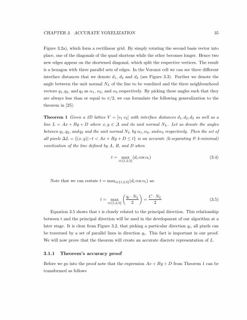
CHAPTER 3. ACCURATE VOXELIZATION 35
Figure 3.2a), which form a rectilinear grid. By simply rotating the second basis vector into
place, one of the diagonals of the quad shortens while the other becomes longer. Hence two
new edges appear on the shortened diagonal, which split the respective vertices. The result
is a hexagon with three parallel sets of edges. In the Voronoi cell we can see three different
interface distances that we denote d1, d2 and d3 (see Figure 3.3). Further we denote the
angle between the unit normal NL of the line to be voxelized and the three neighbourhood
vectors q1, q2, and q3 as α1, α2, and α3 respectively. By picking these angles such that they
are always less than or equal to π/2, we can formulate the following generalization to the
theorem in [25]:
Theorem 1 Given a 2D lattice V = [v1 v2] with interface distances d1, d2, d3 as well as a
line L = Ax + By + D where x, y ∈ R and its unit normal NL. Let us denote the angles
between q1, q2, and q3 and the unit normal NL by α1, α2, andα3 respectively. Then the set of
all pixels ∆L = (x, y)|−t < Ax + By + D ≤ t is an accurate (k-separating & k-minimal)
voxelization of the line defined by A, B, and D when
t = maxi∈1,2,3
(di cos αi) (3.4)
Note that we can restate t = maxi∈1,2,3(di cos αi) as:
t = maxi∈1,2,3
(
qi · NL
2
)
=C · NL
2(3.5)
Equation 3.5 shows that t is closely related to the principal direction. This relationship
between t and the principal direction will be used in the development of our algorithm at a
later stage. It is clear from Figure 3.2, that picking a particular direction qi, all pixels can
be traversed by a set of parallel lines in direction qi. This fact is important in our proof.
We will now prove that the theorem will create an accurate discrete representation of L.
3.1.1 Theorem’s accuracy proof
Before we go into the proof note that the expression Ax + By + D from Theorem 1 can be
transformed as follows

CHAPTER 3. ACCURATE VOXELIZATION 36
L
C
NL
α1
α2α3
d1
d2d3
Figure 3.3: One cell of Figure 3.2b
L = Ax + By + D = (x, y) · (A,B)T + D
We know that
NL = (A,B)T
If P = (x, y)
We have the following equation
L = P · NL + D
Using any point I on line L in the equation we should get
I · NL + D = 0
D = −I · NL
Therefore we can rewrite the expression
Ax + By + D
as
P · NL − I · NL = IP · NL

CHAPTER 3. ACCURATE VOXELIZATION 37
The inequality in Theorem 1 becomes
−t < IP · NL ≤ t
We will provide the k-separating proof by contradiction. First let us assume that ∆L
is not k-separating. By our definition we can conclude that a k-tunnel T exists in ∆L, as
shown in Figure 3.4. Let G, and H be two neighbouring pixel centers pierced by the tunnel
T , and NL be the unit normal vector to the line L. Let I be the intersection point between
L and the tunnel T in between G and H as shown in Figure 3.4.
We have two cases to consider for this proof. The first case is as follows:
On the first case let us assume without restriction of generality that ‖ GI ‖<‖ IH ‖, we
know that ‖ GH ‖= 2 · di for a particular direction qi. Because of our assumption we know
that ‖ GI ‖< di. The distance d from G to L, can be computed as
d
‖ GI ‖= cos αi
Which means
d = cos αi· ‖ GI ‖< di cos αi
Because t = max(di cos αi) we know that the following inequality hold
−t < GI · NL ≤ t
This means that G ∈ ∆L which is a contradiction to our assumption.
For the second case let us assume that
‖ GI ‖=‖ IH ‖= di
depending on the orientation of NL, either IG ·NL or IH ·NL will be positive. If we
assume that IG · NL > 0 then we have a distance of
d = GI · NL = di cos αi ≤ t = max(di cos αi)

CHAPTER 3. ACCURATE VOXELIZATION 38
G H
L
I
FK
TΝL
αi
Figure 3.4: G and H are the center of adjacent sample points on the lattice, Fk is theedge/face shared between G and H. ‖ GH ‖= 2di. L is the continuous line we voxelize
which means that G ∈ ∆L, which is a contradiction.
We have proved that Theorem 1 produces a k-separating voxelization ∆(L). Before we
can prove k-minimality of the theorem we need to introduce the following observation. For a
given line orientation the angles αi for i ∈ 1, 2, 3 are identical in each Voronoi cell. Hence
we can determine t and therefore the principal direction C globally. Hence dC cos(αC) is
the largest of all di cos(αi) for i ∈ 1, 2, 3. Another important observation is that we can
construct a k-arc along the principal direction C, which tiles the entire space (see Figure
3.2).
We will prove k-minimality of the theorem by contradiction, let us assume that ∆(L)
is not minimal. Let’s consider a k-tunnel in the principal direction C. Let the k-tunnel
intersect L at I. Because ∆(L) is not k-minimal there exist two or more pixels along T that
is part of ∆(L), we denote such pixel G and H (see Figure 3.4). Since G ∈ ∆(L) we have
−t < IG · NL ≤ t
‖ GI ‖ · cos αC ≤ t = dc · cos αc
‖ GI ‖≤ dc
Considering any other pixel H along the k-tunnel through G in it’s principal direction,

CHAPTER 3. ACCURATE VOXELIZATION 39
we know that ‖ HI ‖> dc, hence H /∈ ∆(L). We know from the k-separating proof that
either G or H will be included in ∆(L) when ‖ HI ‖=‖ GI ‖.If we remove G from ∆(L) we can construct a continuous 1-arc through G in it’s principal
direction, which intersects L, but none of its pixels are part of ∆(L) hence this would form
a 1-tunnel. Therefore we can conclude that ∆(L) is minimal. We can conclude, that for
every continuous 1-arc along the principal direction of the lattice, there exists exactly one
pixel in ∆(L).
3.1.2 Cartesian Lattice
The general theorem stated in the previous section will work for general 2D sampling lattices,
for which 0 and 1 neighbourhoods are identical. The 2D Cartesian lattice case presents a
challenge as its 1-neighbourhood is a non-trivial subset of its 0-neighbourhood. This means
that we can find two different types of neighbours at any given integer point z (see Figure 2.9)
Huang et al. [25] have proposed and proved the following two theorems for voxelization in
the Cartesian lattice.
Theorem 2 Let W be the length of the side of the square pixel in Figure 3.5. For a 1-
neighbourhood structure, let t1 = W2 cos αk. The set of pixels ∆(L) = (x, y) : −t1 <
Ax+ By + D ≤ t1 is a 1-separating and 1-minimal representation of the line defined by A,
B, and D.
Theorem 3 Let W be the length of the side of the square pixel in Figure 3.5. For t0 =√
22 W cos αk the set of pixels ∆(L) = (x, y) : −t0 ≤ Ax + By + D ≤ t0 is a 0-separating
and 0-minimal representation of the line defined by A, B, and D.
Note that Huang et al. uses the term 4-separable, and 8-separable planes which are
equivalent to our 1-separating and 0-separating planes defined in Section 2.2. Similarly the
symbol αk is equivalent to αC , which represent the angle between the line normal NL and
the principal direction C.
We note that, using our notation, W/2 = d1 = d2 (see Figure 3.5). The proof given by
Huang et al. [25] is incomplete, since they explicitly assume that a k-tunnel must be created
between a Voronoi cell that is intersected by the line L and two neighboring cells that are
not intersected by L. The proof fails to account the fact that line L can intersect more than

CHAPTER 3. ACCURATE VOXELIZATION 40
L
C1
C2
C3
C4
α1
α2
α3
α4
Figure 3.5: Generalized Cartesian lattice case. There are two different neighbourhoodvectors available in this lattice. We denote ck as the set of neighbourhood vectors with
dk = W2 for k ∈ 1, 2. cj is the set of neighbourhood vectors with dj =
√2W2 for k ∈ 3, 4.
one neighbouring pixel, thus any tunnel of the form inside-L-L-outside is never accounted
for in their proof (See Figure 3.6).
.
In this section we show how our new, more general, theorem covers the case of regular
Cartesian lattices as well. We also show that it covers rectilinear lattices which was never
considered by Huang et al.
We have already shown that for any general lattice in 2D we can derive a separating and
minimal voxelization using Theorem 1 (see Section 3.1.1). The 2D Cartesian lattice case is
a special case of our general theorem.
Refer to Figure 3.5 for the following proof.
For the 1-separating case in Cartesian lattices we have two vectors to consider, c1 and
c2, since these form the only allowable neighborhood structure. By Theorem 1 our line
thickness t is defined by max(d1 cos α1, d2 cos α2), however d1 = d2 = W/2. Hence, our
criteria is reduced to t = t1 of Theorem 2. Hence Theorem 2 is a special case of our general
Theorem 1.

CHAPTER 3. ACCURATE VOXELIZATION 41
d1
Q
P
R
L
K
M
N
Figure 3.6: Because line L intersects pixel P and M the proof provided by Huang et al. hasshown that there can be no tunnel through P between pixel Q and R, and between pixel Kand N through M. However the proof did not cover a case when the tunnel is composed ofQ, P, M, and K.
For 0-separating we consider two extra neighbourhood vectors c3, and c4, which add
neighbours that only share a vertex of the Voronoi cell. For the sake of the proof these
vertices can be seen as special zero-length edges between the appropriate Voronoi cells. By
Theorem 1 we can see that our criteria becomes max(dk cos αk, dj cos αj) for k ∈ 1, 2, j ∈3, 4 We also know that dk = W/2 while dj = W
√2
2 . Since the angles of the closest
neighboring directions ck and cj add up to 45 degrees, we can write αk = (45 − αj). Now
we seek to show that dkcos(αk) ≤ djcos(αj)
dkcos(45 − αj) ≤ djcos(αj)
dk(cos(45)cos(αj) + sin(45)sin(αj)) ≤ djcos(αj)
dk
√2
2(cos(αj) + sin(αj)) ≤ djcos(αj)
Because sin(αj) ≤ cos(αj) for αj ≤ 45 we can see that
dk
√2
2(cos(αj) + sin(αj)) ≤ dk
√2
2(cos(αj) + cos(αj)) = djcos(αj)

CHAPTER 3. ACCURATE VOXELIZATION 42
Figure 3.7: The Voronoi cell of the BCC grid
We can conclude that dkcos(αk) ≤ djcos(αj), thus our criteria simplifies to djcos(αj)
which is equivalent to Theorem 3.
We have shown that in both the 0, and 1 separating plane cases, our general voxelization
algorithm computes the same t parameter as the one that was suggested by Huang et al.
Therefore we can conclude that both cases are covered by our general voxelization theorem.
Because we have proved in Theorem 1 that ∆(L) to be both separating and minimal, we
can also conclude that Theorem 2 and 3 can both produce separating and minimal lines.
3.2 3D Lattices
The Voronoi cell of the BCC lattice is a truncated octahedron (see Figure 3.7). The trun-
cated octahedron have identical 0,1, and 2 neighbourhoods (N0(z) = N1(z) = N2(z)), which
means that all neighbouring voxels share a 2D face.
We can extend the idea used in Section 3.1 to the 3D case. The BCC Voronoi cell
is bounded by two types of faces as shown in Figure 3.7. There are 6 square faces and
8 hexagonal faces, which translates into 14 neighbourhood vectors. We can group the 14
vectors into two groups. Six neighbourhood vectors that are perpendicular to the square

CHAPTER 3. ACCURATE VOXELIZATION 43
Z
Y
X
(a) q3 neighbours on one sheet
X
Y
Z
(b) q4 neighbours on one sheet
Figure 3.8: The two types of 2-arcs in a BCC lattice
faces are called q3 with interface distance of d3. 8 neighbourhood vectors are perpendicular
to the hexagonal faces which we denote as q4 with interface distance d4. We also denote the
set of angles between the normal of the plane NL and q3 to be α3, while the angle between
NL and q4 is α4. We can construct two different types of 2-arc tilings in this lattice as shown
in Figure 3.8. We can now formulate the following theorem:
Theorem 4 Given a 3D lattice V = [v1 v2 v3] with interface distances d3 and d4 as well as
the plane L = Ax+By+Cz+D where x, y, z ∈ R and its unit normal NL. Let us denote the
angles between q3i and q4j and the unit normal NL by α3i and α4j respectively for i ∈ 1, 2, 3and j ∈ 1, 2, 3, 4. The set of all voxels ∆(L) = (x, y, z)|−t < Ax + By + Cz + D ≤ t is
an accurate voxelization of the plane defined by A, B, C, and D when
t = max(d3 cos α3i, d4 cos α4j) for i ∈ 1, 2, 3 and j ∈ 1, 2, 3, 4 (3.6)
The proof is identical to the proof of Theorem 1 and does not need to be repeated here.
The only difference is that the dot products in the proof is now in 3D space.

CHAPTER 3. ACCURATE VOXELIZATION 44
3.2.1 Cartesian Lattices
Following the ideas of Section 3.1.2 we can adapt Theorem 4 to the rectilinear case or the
Cartesian case as in Huang et al [25]. In 3D the Cartesian lattice has three possible k-tunnel
directions denoted by qf , qv, qe as shown in Figure 3.9. We define the corresponding interface
distance as df , dv , de and αf , αv, αe denote the corresponding angle to the plane normal NL.
Huang et al. stated the following two theorems for voxelization in a 3D Cartesian Lattice.
Theorem 5 The set of voxels: ∆(L) = (x, y, z)| − t0 < Ax + By + Cz + D ≤ t0 is a
0-separating and 0-minimal representation of the plane L defined by A,B,C, and D. Where
t0 = dvcos(αv).
Theorem 6 The set of voxels: ∆(L) = (x, y, z)| − t2 < Ax + By + Cz + D ≤ t2 is a
2-separating and 2-minimal representation of the plane L defined by A,B,C, and D. Where
t2 = df cos(αf ).
Note that Huang et al. uses 26-separable and 6-separable terms to denote 0-separating,
and 2-separating planes respectively.
We can show that for the 2-neighbourhood (see Figure 2.9), we would only have to
consider the 3 principal directions qf . In this case our criteria from Theorem 4 simplifies
to t = maxi∈1,2,3(df cos αf,i). Considering that df = W/2 our criterion simplifies to the
identical criterion for 2-separating planes stated in Theorem 6.
Considering 1-separating planes we have to include edge-connected cells besides all face-
connected cells. This means we have to take into consideration 6 new 1-arc directions qe,
which are formed by connecting the centre of the Voronoi cell to one of the 12 edge centres.
We find the distance to the edge centres to be de =√
22 W . We can now easily formulate the
criteria for 1-separating Cartesian plane voxelization - a new result that was not included
in the work by Huang et al [25].
Theorem 7 The set of all voxels ∆(L) = (x, y, z) : −t1 < Ax + By + Cz + D ≤ t1 where
t1 = max(df cos αf,i, de cos αe,k) for i ∈ 1, 2, 3 and k ∈ 1, 2, · · · , 6 is a 1-separating and
1-minimal representation of the plane L defined by A, B, C, and D.
Considering 0-separating planes, we will treat each corner as a special (degenerate)
hexagon and include the principal directions qv (in addition to qf , and qe). Hence our

CHAPTER 3. ACCURATE VOXELIZATION 45
qf,i
qe,k
qv,j
Figure 3.9: Principal directions in Cartesian lattice
adapted plane thickness t of theorem 4 is now: max(df cos αf,i, dv cos αv,j , de cos αe,k). Since
we have dv =√
32 W and df = W/2, we need to find under what circumstances dv cos αv,j >
df cos αf,i. This is certainly the case for all dv cos αv,j > df or cosαv,j > 1√3. However, this
holds for all angles since the largest angle away from any direction vector qv is the direction
vector qf . The cosine of the angle between these two principal directions is exactly 1√3
as
can be seen in Figure 3.9. Hence we conclude that our plane thickness t of theorem 4 can
be simplified to max(dv cos αv,j , de cos αf,k).
In order to verify that dv cos αv,j ≥ de cos αf,k we use cosine rules for sides in spherical
trigonometry (see [48]). Let γ be the angle between qv,j and qe,k, we can derive the value of
γ as follows:
qv,j · qe,k =‖ qv,j ‖‖ qe,k ‖ cos(γ)
cos(γ) =qv,j · qe,k
‖ qv,j ‖‖ qe,k ‖
cos(γ) =2√6
cos(γ) =
√2√3

CHAPTER 3. ACCURATE VOXELIZATION 46
A
B
C
ab
c
R
O
Figure 3.10: Spherical trigonometry
See Figure 3.10 for the remainder of this proof.
The cosine rules for sides state:
cos(a) = cos(b) cos(c) + sin(b) sin(c) cos(A) (3.7)
where A is the dihedral angle between the plane OAC and plane OAB. In our case we use
the following mapping, OC represents the plane normal NL, OB represents qv,j, and OA
represents qe,k. Therefore when we plug-in the appropriate variables we get the following
formula:
cos αj = cos αk cos γ + sin αk sin γ cos A (3.8)
By using our knowledge about cos γ and realizing that the second term of the right hand
side is positive we can conclude:
cos αj ≥√
2√3
cos αk (3.9)

CHAPTER 3. ACCURATE VOXELIZATION 47
from which we conclude dv cos αv,j ≥ de cos αe,k. We conclude that we can simplify our
criteria for regular Cartesian grids to t = t0 =√
22 W cos αj . Hence our theorem 4 can be
applied to the regular Cartesian case as well.
This general theorem for voxelization is based on maintaining proper thickness of the
resulting discrete plane. We have provided prescriptive theorems that gave us the proper
thickness parameter t. The simplest algorithm that one can derive from the theorems in
this section is a brute-force method shown in the next chapter. A incremental algorithm is
also explained in the next chapter.

Chapter 4
Voxelization algorithms
In the previous chapter we discussed necessary and sufficient conditions for a voxelization
algorithm to create k-separating and k-minimal planes. The discussion so far has excluded
necessary details that enable us to implement the algorithm. One assumption made through-
out the last chapter is that the input plane divides the volume into two half-spaces. In prac-
tical terms our input is a mesh-model, which is a b-rep model consisting of interconnected
polygons.
We will only consider triangles in our voxelization algorithm because we can guarantee
planarity of the triangle. Any n-gons found in our input mesh can be tessellated into triangles
first before they are voxelized. In the next section we will discuss the extra consideration
that we must make to ensure that an input mesh will produce a k-separating output.
We present a brute force algorithm derived directly from the conditions stated in the
previous chapter. The algorithm and our implementation details are discussed in Section
4.2. A new incremental algorithm is presented in Section 4.3. The last section in this chapter
explains further optimizations we made to the incremental algorithm.
4.1 Mesh Voxelization
Because the input mesh is a set of finite polygons, in addition to the distance threshold
discussed in Chapter 3 we must ensure that the voxels chosen are within the bounds of the
polygon.
When voxelizing piecewise polygons, we must pay special attention along shared edges
and vertices of two adjacent polygons. k-tunnels can be introduced when we only select
48

CHAPTER 4. VOXELIZATION ALGORITHMS 49
A
B
C
d
Figure 4.1: This case shows the k-tunnel induced by the seam between two lines sharing asingle vertex. Point d is excluded because its projection on to line A or B is outside of theline’s boundary point at C. When d is not part of the discrete line the resulting line canpermit a 0-tunnel.
voxels that are strictly within the bound of each primitive as illustrated in Figure 4.1.
In 3D the problem is extended to edges where two polygons meet. Therefore, to create
a k-separating voxelized piece-wise plane from finite polygons we need to voxelize edges and
vertices separately. To this end we introduce three boundary regions that we must consider
when voxelizing finite triangles. We define R to be the maximum interface distance for the
lattice (see Definition 3 on page 33).
1. The region ∆(Lv) is a sphere with radius R around a vertex of the polygon. Any voxel
whose centre lies within the sphere must be considered ∆(Lv).
2. The region ∆(Le) is a tube around the edge E with radius R. Any voxel whose centre
lies within this radius must be considered ∆(Le).
3. The region ∆(Lp) is a bounding volume defined by two planes PU and PL. For each
edge Ei(i=1..,n) we define a plane that is perpendicular to PU , PL, and P . The plane
PU and PL are t apart from the plane P . The set of planes form a closed volume as
shown in Figure 4.2c. Any voxel whose centre lies within this volume is included in
∆(Lp).

CHAPTER 4. VOXELIZATION ALGORITHMS 50
R
V
(a) For vertices, the∆(Lv) volume region
RE
(b) For edges, the ∆(Le) volume region
PU
PL
P
(c) For plane P, the ∆(Lp) volume region
Figure 4.2: Three voxelization regions require careful attention to maintain k-separatingproperty of ∆(L)

CHAPTER 4. VOXELIZATION ALGORITHMS 51
A
B C
D
E
Figure 4.3: By voxelizing each primitive separately we can construct a k-separating ∆(A)∪∆(B) however k-minimality can not be guaranteed at the point where ∆(A) and ∆(B)meet. Pixel C, D, and E are all redundant because without them we still have a k-separating∆(A) ∪ ∆(B).
We define our discrete representation of the finite triangle L to be ∆(L) = ∆(Lp) ∪∆(Le) ∪ ∆(Lv). The three cases discussed are graphically described in Figure 4.2. K-
minimality of ∆(L) can not be guaranteed because each triangle is voxelized separately.
This problem is demonstrated in Figure 4.3. In this case each triangle maintains a k-
separating and k-minimal surfaces by themselves, however the union of the two will create
a non minimal seam along shared edges and vertices.
The simplest voxelization algorithm that we can derive from these rules is a brute force
algorithm, as explained in the following section.
4.2 Brute Force Algorithm
For region ∆(Lp) we can construct a simple brute force algorithm using the threshold pa-
rameter t discussed in the previous chapter. The algorithm must begin by finding the ap-
propriate t for a given plane orientation. We can compute t for all the lattice neighbourhood
vectors, then we can choose the principal direction.

CHAPTER 4. VOXELIZATION ALGORITHMS 52
R
M
X
Y
a b
cL
p
Figure 4.4: Two lines M and L meet at point p. The tight bounding box of line M is markedwith dotted fill. When we only use the pixel in the tight bounding box we won’t includepixel b or c into consideration, which results in a 0-tunnel between b and c. 2 extra pixelsare added in X and Y direction which adds the hatched pixels around the tight boundingbox. By including these extra pixels we can now guarantee that pixel b and c are considered.
According to Theorem 1 and 4 we can use the computed threshold t against all the
voxels in the volume to check whether their distance is within t. This simple algorithm is
inefficient for small triangles, because most voxels considered will not lie in ∆(Lp). A better
strategy is to visit only those voxels within close proximity to the triangle, and adapt the
region to the size of the triangle. We can do this by creating an axis aligned bounding box
around the triangle, and performing the check for voxels within the bounding box.
To account for region ∆(Lv) and ∆(Le) each bounding box constructed must have 2
voxels margin around the edges. This margin will sufficiently cover the required radius of
R for the vertex sphere and edge tubes (see Figure 4.4). The voxels that lie within this
margin will be checked for their distance to the edge or vertex respectively. If this distance
is smaller than R, they will be included in the voxelization.
The adaptive bounding box method has a run-time complexity of Ω(kD2), and O(kD3),
where k is the number of input triangles, and D is the number of voxels along one axis.
When the input triangle is aligned with the bounding box, we can see that the algorithm
visits at most D2 number of voxels. The algorithm performs poorly when triangles are not
aligned with the bounding box as shown in Figure 4.5.

CHAPTER 4. VOXELIZATION ALGORITHMS 53
A
B
C
Figure 4.5: Worst case running complexity for brute force algorithm(O(kD3))
Because of its simplicity the brute force method is the quickest way to implement the
theorems presented in the previous chapter, however its performance will exponentially drop
as the lattice resolution increases.
4.3 Fast incremental binary voxelization
In deriving the incremental algorithm we view the voxelization in three separate regions as
shown in Figure 4.2. For region ∆(Lp), we can deduce that there exist an optimal algorithm
with O(kD2). It is easy to see that to arrive at this optimal algorithm we need a method
to walk along the plane we are voxelizing, and skip the voxels that will never be included
in the final representation ∆(Lp). On top of the asymptotic run-time requirement we also
want to ensure that the algorithm produces accurate planes for both BCC and Cartesian
lattices.
Our incremental voxelization algorithm is inspired by the paper on line voxelization by
Ibanez et al. [26]. They provided a framework where line voxelization can be done for any
lattice structure. By projecting the lines on to the lattice space, Ibanez et al. defined
error measures that adjust to any lattice structure. Using a generalized error measure the
original Bresenham algorithm can adapt to any lattice structure. The projection on to the
lattice space reduces the dimensionality of the problem. Our algorithm uses the same idea

CHAPTER 4. VOXELIZATION ALGORITHMS 54
to simplify our voxelization algorithm.
As we have discussed in section 4.1 we need to pay attention to regions ∆(Lv)and∆(Le).
These regions require special attention to ensure k-separating properties of the resulting
plane is still maintained. We devise a new way of ensuring that the correct voxels around
the edge and vertex regions of our input mesh are chosen.
4.3.1 Region ∆(Lp)
The new incremental voxelization is derived from the fact that a k-separating plane has no
k-tunnels. In the minimality proof of section 3.1.1 we have demonstrated that there must be
exactly one surface voxel on each continuous k-arc in the principal direction C, that crosses
L. With this knowledge we can construct an incremental algorithm as follows (see Figure
4.6):
• Step 1: The plane is projected along the principal direction on to a base plane. The
base plane is a 2 dimensional plane formed from 2 vectors of our lattice neighbourhood
vectors.
• Step 2: The projected plane is voxelized within this base-plane direction.
• Step 3: Project each voxel of the voxelized projected plane on to the original plane
using the principal direction.
The first two steps reduce our 3D voxelization problem into a 2D discretization. The
third step will put the voxels into the appropriate point in 3D space. Each step is discussed
in the following sections.
Step 1: Plane projection to intermediate plane
From Chapter 2, we defined a lattice by a set of basis vectors that spans the lattice space.
The set of basis vectors can be compactly represented with a sampling matrix V , with the
basis vectors arranged in the columns of V . Therefore any point in the lattice space can be
found by integer linear combination of the column vectors of V .
Using the same idea as finding an octant for line voxelization described in [26], we want
to describe possible directions that the voxelization algorithm can take from one voxel to the
next. For this purpose we define a matrix M as our voxelization matrix. This voxelization

CHAPTER 4. VOXELIZATION ALGORITHMS 55
Step 1 Step 2
X
Y
A
B
X
Y
A
B
Step 3
X
Y
A
B
Prin
cipa
l dir
ectio
n
base-plane direction
Sampling Matrix V
Figure 4.6: The algorithm’s main steps

CHAPTER 4. VOXELIZATION ALGORITHMS 56
matrix compactly describes the directions that the voxelization algorithm can take. We
restrict directions that the algorithm can take to integer combinations of the columns of M .
The following are the properties of M that we seek.
1. The vectors in M span the same lattice space as the original V
2. The last column of M is aligned with the principal direction
The first requirement translates into choosing a proper tiling of our lattice with a num-
ber of k-arcs constructed along the principal direction. The mathematical framework to
formulate this problem will be explained after the matrix M is fully explained.
The second required property of M is not readily apparent, because the connection
between alignment and thickness of the plane is not easily seen. This point provides the
theoretical underpinning of the validity of our algorithm. We defer discussion on the second
property until we have fully defined matrix M .
We define the voxelization matrix as follows M = [Mi Mj Mk]. Mk is the principal
direction that we choose for the plane we’re voxelizing, whereas Mi and Mj are two vectors
that describe the base-plane directions.
A direct corollary from the properties of M is non-singularity of M . This property
is important because the bijective mapping between integer points (i, j, k) ∈ Z3 and real
lattice points (x, y, z) ∈ R3 defined in Equation 2.2 is only possible with a non-singular M .
The following two equations expresses the bijective mapping between the two spaces that
directly follows from Equation 2.2.
x
y
z
= [Mi Mj Mk] ∗
i
j
k
(4.1)
i
j
k
= [Mi Mj Mk]−1 ∗
x
y
z
(4.2)
Construction of M begins by selecting the principal direction Mk (see Definition 3 on
page 34). We can derive an exhaustive algorithm that searches for the principal direction
among all lattice neighbourhood vectors.

CHAPTER 4. VOXELIZATION ALGORITHMS 57
After the proper Mk is selected we need to choose two vectors as our base-plane vectors
Mi and Mj. To choose these vectors we must observe the first requirement for M . Before
we can proceed we need to further discuss the properties of the sampling matrices.
For a given lattice structure, the sampling matrix V is not unique, therefore there are
many possible matrices that span the same lattice structure. Given a sampling matrix V a
well known result in point lattice theory states that for an integer matrix N we can derive
the matrix M that spans the same lattice space with the following equation M = V N if
and only if |detN | = 1 [15].
These constraints on N are not enough to uniquely determine Mi and Mj . Therefore we
use a table of precomputed values for Mi and Mj to determine the appropriate basis vectors
for a particular principal direction we choose.
We used an exhaustive search method to compute Mi andMj, with the following criteria
on the vectors det(V −1 · M) = 1.
For Cartesian lattices the matrix V that describes the lattice is given as follows
V =
1 0 0
0 1 0
0 0 1
Table 4.1 lists the principal direction and the corresponding matrix M that we use in the
implementation of the algorithm for 2-separating planes for Cartesian lattices. The table
only shows valid M’s for half of all the possible principal directions, the other half can be
easily obtained through symmetry.
Principal Direction Valid Matrix M Matrix N
(1,0,0)
0 0 10 -1 01 0 0
0 0 10 -1 01 0 0
(0,1,0)
-1 0 00 0 10 1 0
-1 0 00 0 10 1 0
(0,0,1)
1 0 00 1 00 0 1
1 0 00 1 00 0 1
Table 4.1: Valid voxelization matrices M for 2-separating planes in a Cartesian lattice.

CHAPTER 4. VOXELIZATION ALGORITHMS 58
Principal Direction Valid Matrix M Matrix N
(1,1,0)
0 0 10 1 1-1 0 0
0 0 10 1 1-1 0 0
(1,0,1)
0 0 10 -1 01 0 1
0 0 10 -1 01 0 1
(0,1,1)
1 0 00 1 10 0 1
1 0 00 1 10 0 1
(-1,1,0)
0 0 -10 1 11 0 0
0 0 -10 1 11 0 0
(-1,0,1)
0 0 -10 1 01 0 1
0 0 -10 1 01 0 1
(0,-1,1)
1 0 00 1 -10 0 1
1 0 00 1 -10 0 1
Table 4.2: Additional voxelization matrices M for Table 4.1. For a 1-separating planes in aCartesian lattice.
Table 4.2 lists 6 additional principal directions to table 4.1 that we need to consider
for 1-separating planes in a Cartesian lattice. The table only lists half of the 12 principal
directions. The other half can be obtained through symmetry.
Table 4.3 lists 4 additional principal direction to Table 4.2, and Table 4.1 that we need
to consider for 0-separating planes in a Cartesian lattice. Like previous tables the other 4
principal directions can be obtained through symmetry.
For a BCC lattice the sampling matrix V is as follows.
V =
2 0 1
0 2 1
0 0 1
(4.3)
In BCC lattice we have 14 principal directions. Half of them are listed on Table 4.4. The
other half can be obtained through symmetry.
The matrices shown in Tables 4.1-4.4 span the same space as the original lattice space
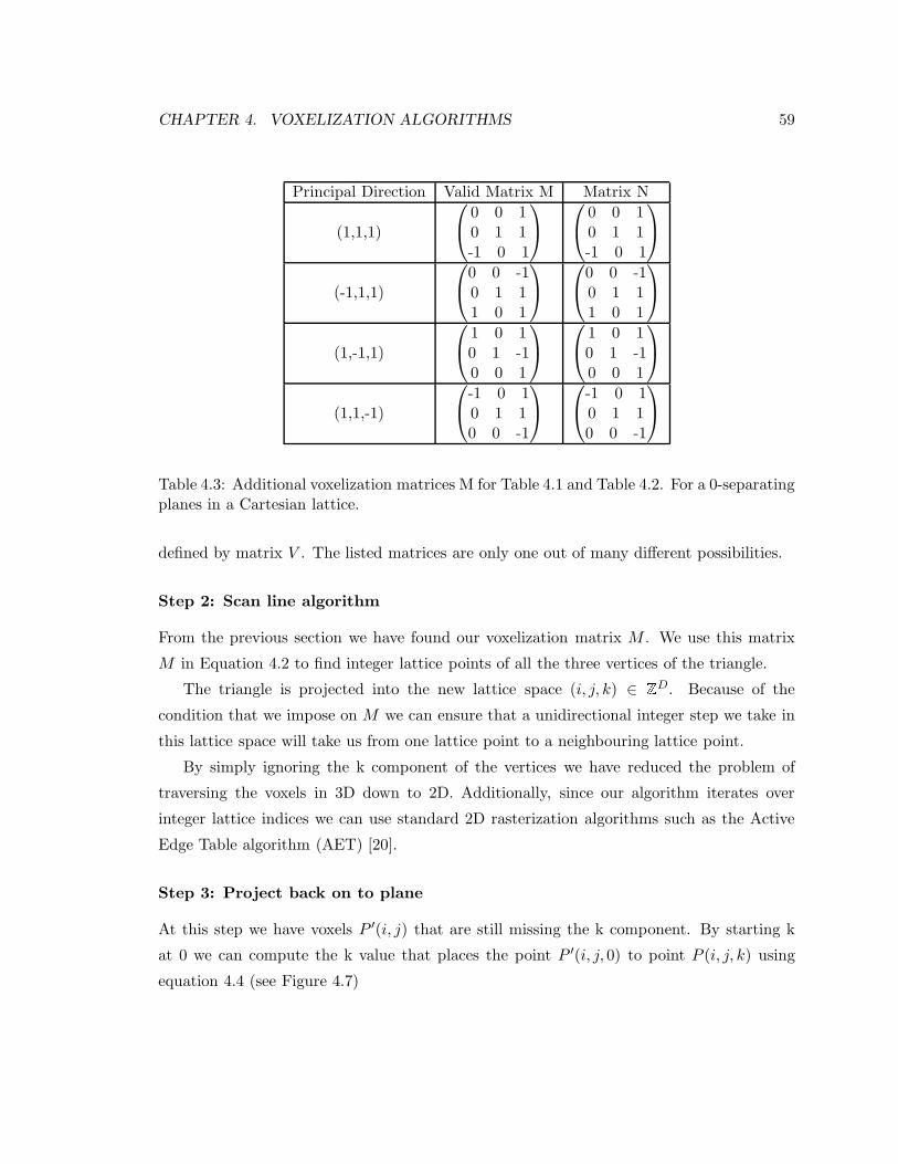
CHAPTER 4. VOXELIZATION ALGORITHMS 59
Principal Direction Valid Matrix M Matrix N
(1,1,1)
0 0 10 1 1-1 0 1
0 0 10 1 1-1 0 1
(-1,1,1)
0 0 -10 1 11 0 1
0 0 -10 1 11 0 1
(1,-1,1)
1 0 10 1 -10 0 1
1 0 10 1 -10 0 1
(1,1,-1)
-1 0 10 1 10 0 -1
-1 0 10 1 10 0 -1
Table 4.3: Additional voxelization matrices M for Table 4.1 and Table 4.2. For a 0-separatingplanes in a Cartesian lattice.
defined by matrix V . The listed matrices are only one out of many different possibilities.
Step 2: Scan line algorithm
From the previous section we have found our voxelization matrix M . We use this matrix
M in Equation 4.2 to find integer lattice points of all the three vertices of the triangle.
The triangle is projected into the new lattice space (i, j, k) ∈ ZD. Because of the
condition that we impose on M we can ensure that a unidirectional integer step we take in
this lattice space will take us from one lattice point to a neighbouring lattice point.
By simply ignoring the k component of the vertices we have reduced the problem of
traversing the voxels in 3D down to 2D. Additionally, since our algorithm iterates over
integer lattice indices we can use standard 2D rasterization algorithms such as the Active
Edge Table algorithm (AET) [20].
Step 3: Project back on to plane
At this step we have voxels P ′(i, j) that are still missing the k component. By starting k
at 0 we can compute the k value that places the point P ′(i, j, 0) to point P (i, j, k) using
equation 4.4 (see Figure 4.7)

CHAPTER 4. VOXELIZATION ALGORITHMS 60
Principal Direction Valid Matrix M Matrix N
(2,0,0)
1 0 21 -2 01 0 0
0.5 0 1.50.5 -1 0.50.5 0 -0.5
(0,2,0)
1 2 01 0 21 0 0
0.5 1.0 -1.50.5 0 1.50.5 0 -0.5
(0,0,2)
1 -2 01 0 01 0 2
0.5 -1.0 0.50.5 0.0 -0.50.5 0.0 1.5
(1,1,1)
2 0 10 2 10 0 1
1 0 00 1 00 0 1
(-1,1,1)
2 0 -10 2 10 0 1
1 0 -20 1 00 0 1
(1,-1,1)
2 0 10 2 -10 0 1
1 0 00 1 -20 0 1
(1,1,-1)
2 0 10 -2 10 0 -1
1 0 00 -1 20 0 -1
Table 4.4: Voxelization matrix M for 2-separating planes in a BCC lattice.
NL
P0
P’(i,j,0)
Mk
P(i,j,k)
L
Figure 4.7: For every point P’(i,j,0) we would like to compute its intersection P (i, j, k) withthe plane L. Mk is the chosen principal direction of L, P0 is a point on L. The unit normalof L is NL

CHAPTER 4. VOXELIZATION ALGORITHMS 61
P ′(i, j, 0) + kMk = P (i, j, k) (4.4)
We need to use the general plane equation in vector form such as follows: Let P0 be one
of the points on the plane L. Let NL the unit plane normal of plane L. Every point P that
belongs to L must fulfill:
P · NL − P0 · NL = 0 (4.5)
By plugging in Equation 4.4 into Equation 4.5 we can arrive at the following equation
for k
(P ′ + kMk) · NL − P0 · NL = 0
P ′ · NL + kMk · NL − P0 · NL = 0
kMk · NL = (P0 − P ′) · NL
k =(P0 − P ′) · NL
Mk · NL
(4.6)
To find the actual point P (i, j, k) we need to plug the k value from Equation 4.6 into
Equation 4.4 to get the following equation
P (i, j, k) = Mk
(P0 − P ′) · NL
Mk · NL+ P ′(i, j, 0) (4.7)
Using equation 4.7 we can compute the value of P for every P ′ that is generated by the
AET algorithm from the previous step.
One problem to note is that the k value we compute is a floating point quantity. Because
the lattice points are only defined as integer linear combination of the basis vectors in M ,
this floating point quantity means that the intersection point will not lie on a lattice point.
An extra rounding step is needed to get the point to the closest integer point. The rounding
must take into account the actual voxel center distance to the plane, and select one with
the least distance to the plane L.
The algorithm presented thus far already has O(D2) run-time complexity. Optimization
of the algorithm is still possible. To get the fastest algorithm possible, we can incremen-
tally update the offset k because we are taking constant steps in the i, j direction. This
optimization is explained in the next section.

CHAPTER 4. VOXELIZATION ALGORITHMS 62
4.4 Further optimization
The algorithm presented thus far computes the offset k of each voxel to the target plane, as
shown in equation 4.7. We can reduce the number of computations performed per voxel by
simply computing the delta value for k when we step in a particular i, or j direction within
the space.
The offset k is computed in equation 4.6. Point P ′ changes by (1,0,0) when we are
stepping in the i direction, and by (0,1,0) when we are stepping in the j direction. When
we substitute the incremental change to P ′ into the equation 4.6 we can find the amount
k is incremented at each step. Let δki be the k-offset increment when we step in the i
direction and δkj the k-offset increment in the j direction. We have the following equation
that determines the offset.
δki =(1, 0, 0) · NL
MTk · NL
(4.8)
δkj =(0, 1, 0) · NL
MTk · NL
(4.9)
Another simplification arises from the fact that NL can be transformed into (i, j, k) ∈ ZD
space which simplifies Equation 4.9 down to the following two equations:
δki =NL[1]
NL[3](4.10)
δkj =NL[2]
NL[3](4.11)
We use δki and δkj as the increment to the offset k when we are traversing each plane.
If the algorithm starts from a known point (a vertex of the triangle), we never have to
compute the voxel intersection. This incremental method minimizes the amount of floating
point operations to a single addition for every voxel visited, compared to 20 floating point
operations to evaluate Equation 4.7 for every voxel. The fully optimized version of the
algorithm in shown in Figure 4.8.
The discussion thus far has centred around the algorithm, however there are a number
of practical details that must be discussed. The next section discusses the fine details of the
algorithm that are required for robustness of the algorithm.

CHAPTER 4. VOXELIZATION ALGORITHMS 63
Input: Triangle vertices v ∈ ZD
Result: Voxelized triangleConstruct AET;currj = minimum j coordinate AET;istart = minimum i coordinate for the current scan-line;iprevious = istart;k = k coordinate that corresponds to istart and currj;compute δki and δkj ;while AET not empty do
istart = minimum i coordinate from the current scan-line;istop = maximum i coordinate of from the current scan-line;k+= (istart − iprevious) δki;iprevious = istart;currk = k;for i = istart to istop do
setvoxel at point (i,currj,currk);currk+= δki;
end
remove edge with j coordinate lower than currj from AET;currj++;k+= δkj ;
end
Figure 4.8: Incremental voxelization algorithm

CHAPTER 4. VOXELIZATION ALGORITHMS 64
A BInside
Outside
CD
E
F
A’B’
P
Figure 4.9: Two infinite lines A and B meets at a point in space. Point C,D,E,and F arethe nearest pixel around that intersection point.
4.5 Region ∆(Le) and∆(Lv)
To properly satisfy the constraints of region ∆(Le) and ∆(Lv), we propose the following
criteria.
Given two semi infinite lines A and B which have a common vertex P . We extend these
lines at P into A’ and B’ (see Figure 4.9). This creates four half-spaces, which we shall call
C, D, E, and F. A separating voxelization of A and B across P can now be formulated as:
∆(LA+B) = ∆(LA) ∪ ∆(LB) ∪ ∆(LA+A′) ∩ ∆(LB+B′)
This criteria can be proved as follows: Let us assume that there is a k-tunnel penetrating
∆(LA+B). There are three tunnel possibilities in this case. One tunnel connects region F
to D, another between region F to E, and the last one connects from F to C.
If there were a tunnel from F to D, this tunnel would have to cross A. According to
Theorem 1 this is not possible. On the same token a tunnel from region F to region C is
also impossible.
That leaves us with a k-tunnel connecting region F to E. We know that a tunnel between
F and D as well as F and C is impossible. We also eliminate any tunnels from E to C as
well as E to D when we voxelize A’ and B’. With the aggregate pixels, there could not exist

CHAPTER 4. VOXELIZATION ALGORITHMS 65
a tunnel between E and F because of Theorem 1. When we remove ∆(A′) and ∆(B′) and
keep the ∆(A′)∩∆(B′) voxels, a tunnel could not form along E and F because it would have
been covered by the remaining pixels from ∆(A′) and ∆(B′). This shows a contradiction
to our assumption, which means our criteria will create a k-separating arc of ∆(A)∪∆(B).
This same criteria can also be applied to two triangles that share a common edge or vertex.
4.6 Practicalities
The algorithm presented does not assume that the triangle vertices we started with are inZ3 space, in practice the algorithm implemented rounds triangle vertices to a nearest integer
lattice point, this is done to ensure that the voxelization algorithm starts at an integer lattice
point.
The vertex rounding produces one problem. When the voxel size is relatively large
compared to the plane area of the triangle, the rounding procedure can turn the triangle
vertices into one, two, or three unique vertices. This turns the plane into a point, a line or
a plane respectively. Our plane voxelizer can not handle lines and points, therefore extra
processing needs to be done. For the case of one unique vertex we can simply set the voxel
that includes the triangle vertex.
For the case of two unique vertices, hence a line, we use the voxelization algorithm
presented by Ibanez et al. [26] to voxelize the line. This case can be clearly seen in Figure
4.10.
The extra line tracing algorithm is required only when the size of the triangles are small
compared to the voxel sizes (a good example would be a mesh model with triangles that
only cover an area of one voxel).
We have shown that our algorithm will produce k-separating triangles. In section 4.5 we
have shown that our algorithm can still guarantee the k-separating property at the seam,
which means that we can create k-separating piece-wise discrete surfaces. The implication
is that we can voxelize any input mesh given that they are broken into smaller connected
triangles. Therefore this opens up an avenue to voxelize any input mesh.
We need a way to verify that our implementation performs as theoretically proved. The
next chapter will discuss some validation algorithm that we have developed to help verify
the correctness of our implementation.

CHAPTER 4. VOXELIZATION ALGORITHMS 66
(a) Original Mesh
(b) Resulting mesh without line (c) Resulting mesh with line voxelizer
Figure 4.10: The effect of snapping triangle vertices to the nearest voxels. When two trianglevertices snap into one voxel a triangle is transformed into one line which can not be voxelizedby our new algorithm (b). To handle this case any suitable line voxelizer can be used toclose the gap (c). Ant mesh taken from the library of free meshes at www.3dcafe.com

Chapter 5
Analysis of algorithm
We have stated the sufficient conditions for any voxelization algorithm to create k-separating
and k-minimal planes in Chapter 3. In Chapter 4 we have developed algorithms based on
these conditions. Here we verify that the algorithms presented are able to create accurate
planes, through a number of experiments. To enable verification of an algorithm’s accuracy
we need to develop validation algorithms that find k-tunnels and redundant voxels within a
voxelized plane.
5.1 Validation Techniques
Our validation algorithms follow from the definition of k-tunnel free and k-minimal in Section
2.2. The condition of k-tunnel free is stated in Section 2.2 as follows: a digitization ∆(S) ⊂ZD of a continuous surface S ⊂ RD is k-tunnel free if every continuous k-arc connecting
points in (∆(S))C = ZD − ∆(S) does not cross S.
We can perform validation by constructing all possible k-arcs in (∆(S))C . However this
exhaustive testing method will take too much time to perform over a large set of background
voxels. We will approach the problem from the perspective of measuring volumes.
A basic volume measurement technique is to measure the displacement of a liquid in a
container when an object that we are measuring is placed inside the liquid. The amount
of liquid that an object displaces is proportional to the volume of the empty space inside
it. A hollow permeable object would not displace the same volume of water as one that is
impermeable, thus the amount of liquid an object displaces also determines the permeability
of its surface. When the amount of liquid displaced is equal to the volume of the empty
67

CHAPTER 5. ANALYSIS OF ALGORITHM 68
space we know that the surfaces surrounding the object are impermeable. In the discrete
domain impermeable surfaces are called k-tunnel free. To test for k-tunnel free condition
of our discrete surface we can apply the same volume test towards the entire surface, given
that we define the corresponding properties of discrete water.
Because we are dealing with discrete surfaces, we define discrete water as a special voxel
value in the volume. The space filling property of water is simulated with a breadth first
search (BFS) algorithm. The BFS algorithm uses the lattice neighbourhood to traverse the
empty voxels in space and marks the voxels that it has visited with a special value.
With the property of water defined we can define the following metric to gauge whether
the output surface of a voxelization algorithm is k-tunnel free.
Let A be the total number of voxels occupied by the discrete water, and D be the total
number of voxels in the volume.
∆(V ) =D − ∆(S) − A
D(5.1)
∆(V ) is the normalized discrete volume contained by ∆(S). We expect this value to
approach the actual volume of S as the resolution of the lattice increases.
For our test we choose a hollow tetrahedron positioned inside a unit cube as shown in
Figure 5.1. The tetrahedron was chosen because the volume of its empty space is known,
and it has the minimum number of triangles over all possible input meshes that we can use
in the test. If the surface of the tetrahedron is water tight, it will displace 1/6 of the water
inside the unit cube when it is immersed in a unit cube filled with water.
We know the amount of water that the input tetrahedron will displace, we can expect the
same amount to be displaced in the discrete version of the tetrahedron when it is k-tunnel
free. We perform our tests starting with the tetrahedron sitting in an empty cube. Discrete
water is then poured into the empty space. If the surface of the discrete tetrahedron is
k-tunnel free then the unit cube will have 5/6 of its volume filled with water, if not the
entire volume is filled with water.
From that test we can not infer k-minimality of our discrete tetrahedron. We therefore
need to devise another validation test for minimality of the surface. If the surface ∆(S)
is k-separating, one way to test for k-minimality is by pouring discrete water into the unit
cube with one voxel in ∆(S) removed. If the cube is not filled with discrete water we know
that the voxel we removed from ∆(S) is redundant. By repeating the test for all voxels in

CHAPTER 5. ANALYSIS OF ALGORITHM 69
1Unit
1Unit
1Unit
Figure 5.1: The tetrahedron used as input to the voxelization algorithm
∆(S) we can assert the k-minimality of ∆(S). This test incurs a cubic run-time complexity
as the volume resolution increases. This test becomes infeasible for large volumes. We must
find another validation method that will give us the correct answer faster.
From the minimality proof in Section 3.1.1, we can see that a minimal surface only
contains one voxel p along the principal direction C. This fact leads us to the corollary that
the k-tunnel along the principal direction that passes through p is divided into two parts.
One part belongs to the inside space I and the other reside on the outside space O (see
Figure 5.2. From this corollary we can reformulate the minimality criterion such as follows:
Theorem 8 A k-separating discrete surface ∆(S) is minimal when ∀p ∈ ∆(S),∃q, r 6⊂∆(S) along the principal direction C such that q, r ∈ N(p) with q ∈ I and r ∈ O .
Using theorem 8, we can perform the minimality check by iterating through all the
surface voxels p ∈ ∆(S) and comparing its two immediate neighbours along the principal
direction, as shown in Figure 5.2. When the two immediate neighbours belong to two
different spaces then we mark the surface voxel as minimal.
Let ∆(S)′ be the number of minimal surface voxels. We define ratio R as follows:

CHAPTER 5. ANALYSIS OF ALGORITHM 70
X
YY
X
I
O
I
O
Figure 5.2: Each dithered voxel belong in ∆(S). For each of the dithered voxels we check itsimmediate neighbours along the principal direction shown as double ended arrows. Whenthe two neighbouring voxels belong in two different spaces we mark the voxel as minimal.
R = 1.0 − ∆(S)′
∆(S)
Using R we can now test that a surface is minimal when R is exactly 0. There are a few
problems using this metric in determining k-minimality properties of our input surface.
Because our input meshes are piecewise linear surfaces, there are two boundary cases
that we need to exclude from testing as shown in Figure 5.3. These two cases introduce
redundancy that is not created by the algorithm, thus they must be ignored to get the
correct measure of minimality for our discrete surface.
Other than the two exceptions listed, we consider other voxels that do not fit in Theorem
8 as non-minimal.
The minimality test we described will query regions outside of the volume when the
tetrahedron is placed exactly at the edge of the volume. We eliminated this special case at
the edges of the volume by padding the test volume with extra 4 voxels in each dimension.
The resulting voxelized surface is centred in this padded volume with a margin of 2, as
shown in Figure 5.4. We choose the voxel at the origin O(0,0,0) as the seed point for the
k-separating test.

CHAPTER 5. ANALYSIS OF ALGORITHM 71
I
O A
B
C
I
O A
B
C
Case 1 Case 2
Figure 5.3: The two boundary cases of minimality testing that need to be excluded fromtesting. The two arrows point to the neighbours of the hatched voxel considered in the test.Case 1 happens at the intersection point of two lines/planes. Case 2 happens when one ofthe neighbours of the surface voxel belongs to another surface.
Original Bounding Volume Padded Bounding Volume
O(0,0,0)
O(0,0,0)
Figure 5.4: The volume on the right has 2 extra voxels around the original volume. Theorigin shifts as a result of the padding. The padding is added to remove special cases of theminimality testing

CHAPTER 5. ANALYSIS OF ALGORITHM 72
(a) (b)
0 degrees rotation 45 degrees rotation
Figure 5.5: Enlarging the bounding box of the triangle ensures that for all rotation anglestested the tetrahedron will be fully enclosed within the bounding box. The unit cubedimension is the same as the length of the triangle’s hypotenuse which is of length
√2
5.2 Testing Methodology
We want to verify the correctness of our implemented algorithm as well as evaluate the
robustness of the method with regards to different plane orientations. To evaluate robustness
we tested the algorithm with rotated versions of input mesh.
The test was performed on the tetrahedron rotated around the X axis. Because of the
rotation there are parts of the tetrahedron that extend beyond the unit cube. To avoid
chopping the input tetrahedron, we voxelize in a bounding box large enough to enclose the
tetrahedron rotated to any angle. To ensure that all possible rotation of the tetrahedron
would fit in the bounding box we scaled each dimension of the box to fit the longest edge of
the tetrahedron, which is the hypotenuse of right triangle that forms three of the tetrahedron
faces (see Figure 5.5).
We rotated the tetrahedron with 5 degree increments, and performed the test from 0 to
355 degree. We introduce a random jitter that adds 0 to 4 degree to the rotational angle.
The tests were done in a lattice resolution of 10 to 200, for both BCC and Cartesian lattices.
For the Cartesian lattice we tested 0, 1, and 2 separating surfaces.
Due to a difference in structure, the BCC lattice can not be indexed in the same fashion

CHAPTER 5. ANALYSIS OF ALGORITHM 73
as Cartesian Lattices. The indexing scheme described in [51] views BCC lattices as two inter-
penetrating Cartesian lattices, which makes it possible to index BCC lattice as a standard
3D array. Because the BCC lattice packs voxels better, for a Cartesian lattice with D3
lattice resolution, if we use the same D for each dimension of BCC we will have 2D3 voxels
(see Figure 5.6). The lattice with more sample points can represent higher frequency spectra
than a lattice with less sample points, thus we can not draw a straight comparison between
a D3 Cartesian lattice and a 2D3 BCC lattice. To make the comparison across two different
lattice structure fair we generalize the notion of lattice resolution as the total number of
lattice points in space.
We use the following formula to compute the BCC lattice dimension
2D3BCC = D3
CC
DBCC =3
√
D3CC
2(5.2)
As an example a 1003 Cartesian lattice resolution by using Equation 5.2 we find that
DBCC ≈ 80 which means the BCC lattice resolution will be 80× 80× 160, which is roughly
the same number of sample points in space.
In the following section all of the results for BCC lattices will be quoted using DCC .
However, the actual tests were performed using a lattice of size 2D3BCC .
5.3 BCC vs Cartesian Lattice
As discussed in Section 2.1, the benefits of using a different lattice structure lies in the
lattice’s information carrying capacity. By using an optimal BCC lattice one can reduce
the lattice resolution by 30% compared to a Cartesian lattice to get the same amount of
information. Another way of looking at it is that we can capture 30% more information
when we use the same lattice resolution for the BCC lattice. This fact is illustrated in
Figures 5.7, 5.8, and 5.9.
Between Figure 5.7 and Figure 5.9, we can see the advantage of using a BCC lattice
over the corresponding Cartesian lattice. The BCC lattice captures the same surface detail
information as the Cartesian lattice with 25% less surface voxels. Between Figure 5.8 and
Figure 5.7 we can see that all the surface details visible in the latter can still be seen in
CHAPTER 5. ANALYSIS OF ALGORITHM 74
(0,0,0) (1,0,0)
(0,0,1) (1,0,1)
(0,1,1) (1,1,1)
(0,1,0)
(0,0,0) (1,0,0)
(0,0,1)
(1,0,2)
(0,1,2) (1,1,2)
(0,1,0)(1,1,0)
(0,0,2)
(1,0,1)
(0,1,1) (1,1,1)
Cartesian Lattice BCC Lattice
Figure 5.6: The left figure shows the standard Cartesian lattice indexing. The right pictureshows the BCC lattice as two inter-penetrating Cartesian lattices. In the right figure theextra points add to the index length in the z dimension.
the prior picture. with 73% less surface voxels, BCC volumes can capture the same amount
of surface detail information as the Cartesian lattice volume, which represents a significant
space saving.
5.4 Results
The tests are performed on an SGI Altix 3000. The machine has 64 1.5 Ghz Intel Itanium II
processor, with 64 Gibibyte (64X10243) of Global Shared Memory. The operating system
is SGI Advanced Linux Environment and ProPack 3/ Service Pack 2.
We perform the tests on three voxelization algorithms. The first algorithm is the brute
force algorithm described in Section 4.2, the second algorithm is described in Section 4.3,
and lastly the optimized incremental algorithm is described in Section 4.4.
As a result of enlarging the bounding box shown in Figure 5.5, the ∆(V ) defined in
equation 5.1 will not converge to 1/6, as explained above, instead it will approach a volume
of 1/(√
23 ∗ 6). This fact is shown in Figure 5.10, 5.11, 5.12, 5.13, 5.14, and 5.15. The
ideal ∆(V ) is shown as a black horizontal line across the graph. We can see that all the k-
separating ratios are converging to the ideal value. This tells us that the surfaces constructed

CHAPTER 5. ANALYSIS OF ALGORITHM 75
Figure 5.7: This picture shows the stanford bunny voxelized in a 0-separating Cartesianlattice. The lattice has 2563 discrete voxels in the lattice. There are 229,328 surface voxelson the bunny

CHAPTER 5. ANALYSIS OF ALGORITHM 76
Figure 5.8: This picture shows the stanford bunny voxelized in a 2-separating BCC lattice.The lattice has 180x180x360 discrete voxels in the lattice. There are 85,699 surface voxelson the bunny

CHAPTER 5. ANALYSIS OF ALGORITHM 77
Figure 5.9: This picture shows the stanford bunny voxelized in a 2-separating BCC lattice.The lattice has 203x203x406 discrete voxels in the lattice. There are 172,223 surface voxelson the bunny

CHAPTER 5. ANALYSIS OF ALGORITHM 78
are k-separating. The graphs show the average normalized tetrahedron volume (∆(V )) and
the average k-minimality (R) ratios over 72 rotation cases that we tested. We chose to show
only the average values because results for the different rotation angles show the same trend.
No outliers were found.
It is clear from Figure 5.12, 5.13, 5.14, and 5.15 that the new incremental algorithm
produces both k-minimal and k-separating surfaces, as ∆(V ) converges to the ideal ratio
shown by the black horizontal line, and R stays at zero.
The incremental method always produces k-minimal planes, whereas the brute force
method suffers from numerical precision problems. The condition in Theorem 4 only selects
one voxel along the principal direction. Because we are using a finite precision computer the
numerical error of a computer can include two adjacent voxel along the principal direction
in ∆(S). Thus adding redundant voxels. These cases are apparent in Figure 5.10 and 5.11.
The timing graphs (see Figure 5.16 and Figure 5.17) show the amount of time required
to voxelize the input tetrahedron. As discussed in Section 4.2, the brute-force algorithm’s
run time performance is dependent on the input triangle’s orientation. One of the triangles
in this tetrahedron straddles the entire volume forcing the brute-force algorithm to visit all
of the voxels in the volume. This explains why there is a large gap between the performance
of the brute force algorithm and the incremental algorithm.
The timing graphs for the algorithms are plotted in log scale to see the scaling trend
over different lattice resolution. Because the brute-force algorithm’s run time efficiency is
larger by an order of magnitude, the difference between the two incremental algorithms is
difficult to see. To show the difference between the optimized incremental algorithm and the
standard incremental algorithm, we plotted the run-time ratio between the two algorithms
as shown in Figure 5.18, and 5.19.
From Figure 5.18, and 5.19, it is clear that the new incremental algorithm runs one order
of magnitude faster than the brute-force algorithm. The optimized incremental algorithm
has a small lead over the standard version. The timing difference between the two incre-
mental algorithms is around 11% which only becomes significant when we move to higher
lattice resolutions. It is interesting to note that at low resolution the ratio swings between
0 and 20%. This swing is due to the dominant step 1 of the algorithm at low resolutions
(see Section 4.3.1). Because the setup time is the same for both algorithms, we expect the
ratio to be near 0 at lower resolution. As the resolution of the lattice increases more time
is spent on step 2 and 3 of the algorithm, and the optimization to the algorithm started to

CHAPTER 5. ANALYSIS OF ALGORITHM 79
Average Minimality and Separability Ratio for all angles
Lattice Resolution0 10 20 30 40 50 60 70 80 90 100 110 120 130 140 150 160 170 180 190 200
Rat
io(li
t/vol
ume)
−0.01
0.04
0.09
0.14
0.19 Separability RatioMinimality Ratio
(a) Cartesian lattice 2-separating and 2-minimal ratio graphs
Average Minimality and Separability Ratio for all angles
Lattice Resolution0 10 20 30 40 50 60 70 80 90 100 110 120 130 140 150 160 170 180 190 200
Rat
io(li
t/vol
ume)
−0.01
0.04
0.09
0.14
0.19 Separability RatioMinimality Ratio
(b) Cartesian lattice 1-separating and 1-minimal ratio graphs
Figure 5.10: Results for the brute force algorithm. The graph shows the average result ofthe ratio over 72 rotation angle cases. The straight line shows the ideal ratio when we havea unit cube.

CHAPTER 5. ANALYSIS OF ALGORITHM 80
Average Minimality and Separability Ratio for all angles
Lattice Resolution0 10 20 30 40 50 60 70 80 90 100 110 120 130 140 150 160 170 180 190 200
Rat
io(li
t/vol
ume)
−0.01
0.04
0.09
0.14
0.19 Separability RatioMinimality Ratio
(a) Cartesian lattice 0-separating and 0-minimal ratio graphs
Average Minimality and Separability Ratio for all angles
Lattice Resolution0 10 20 30 40 50 60 70 80 90 100 110 120 130 140 150 160 170 180 190 200
Rat
io(li
t/vol
ume)
−0.01
0.04
0.09
0.14
0.19 Separability RatioMinimality Ratio
(b) BCC lattice 0-separating and 0-minimal ratio graphs
Figure 5.11: Results for the brute force algorithm. The graph shows the average result ofthe ratio over 72 rotation angle cases.The straight line shows the ideal ratio when we havea unit cube.

CHAPTER 5. ANALYSIS OF ALGORITHM 81
Average Minimality and Separability Ratio for all angles
Lattice Resolution0 10 20 30 40 50 60 70 80 90 100 110 120 130 140 150 160 170 180 190 200
Rat
io(li
t/vol
ume)
−0.01
0.04
0.09
0.14
0.19 Separability RatioMinimality Ratio
(a) Cartesian lattice 2-separating and 2-minimal ratio graphs
Average Minimality and Separability Ratio for all angles
Lattice Resolution0 10 20 30 40 50 60 70 80 90 100 110 120 130 140 150 160 170 180 190 200
Rat
io(li
t/vol
ume)
−0.01
0.04
0.09
0.14
0.19 Separability RatioMinimality Ratio
(b) Cartesian lattice 1-separating and 1-minimal ratio graphs
Figure 5.12: Results for the incremental algorithm. The graph shows the average result ofthe ratio over 72 rotation angle cases.

CHAPTER 5. ANALYSIS OF ALGORITHM 82
Average Minimality and Separability Ratio for all angles
Lattice Resolution0 10 20 30 40 50 60 70 80 90 100 110 120 130 140 150 160 170 180 190 200
Rat
io(li
t/vol
ume)
−0.01
0.04
0.09
0.14
0.19 Separability RatioMinimality Ratio
(a) Cartesian lattice 0-separating and 0-minimal ratio graphs
Average Minimality and Separability Ratio for all angles
Lattice Resolution0 10 20 30 40 50 60 70 80 90 100 110 120 130 140 150 160 170 180 190 200
Rat
io(li
t/vol
ume)
−0.01
0.04
0.09
0.14
0.19 Separability RatioMinimality Ratio
(b) BCC Lattice 0-separating and 0-minimal ratio graphs
Figure 5.13: Results for the incremental algorithm. The graph shows the average result ofthe ratio over 72 rotation angle cases.

CHAPTER 5. ANALYSIS OF ALGORITHM 83
Average Minimality and Separability Ratio for all angles
Lattice Resolution0 10 20 30 40 50 60 70 80 90 100 110 120 130 140 150 160 170 180 190 200
Rat
io(li
t/vol
ume)
−0.01
0.04
0.09
0.14
0.19 Separability RatioMinimality Ratio
(a) Cartesian lattice 2-separating and 2-minimal ratio graphs
Average Minimality and Separability Ratio for all angles
Lattice Resolution0 10 20 30 40 50 60 70 80 90 100 110 120 130 140 150 160 170 180 190 200
Rat
io(li
t/vol
ume)
−0.01
0.04
0.09
0.14
0.19 Separability RatioMinimality Ratio
(b) Cartesian lattice 1-separating and 1-minimal ratio graphs
Figure 5.14: Results for the optimized incremental algorithm. The graph shows the averageresult of the ratio over 72 rotation angle cases.

CHAPTER 5. ANALYSIS OF ALGORITHM 84
Average Minimality and Separability Ratio for all angles
Lattice Resolution0 10 20 30 40 50 60 70 80 90 100 110 120 130 140 150 160 170 180 190 200
Rat
io(li
t/vol
ume)
−0.01
0.04
0.09
0.14
0.19 Separability RatioMinimality Ratio
(a) Cartesian lattice 0-separating and 0-minimal ratio graphs
Average Minimality and Separability Ratio for all angles
Lattice Resolution0 10 20 30 40 50 60 70 80 90 100 110 120 130 140 150 160 170 180 190 200
Rat
io(li
t/vol
ume)
−0.01
0.04
0.09
0.14
0.19 Separability RatioMinimality Ratio
(b) BCC lattice 0-separating and 0-minimal ratio graphs
Figure 5.15: Results for the optimized incremental algorithm. The graph shows the averageresult of the ratio over 72 rotation angle cases.

CHAPTER 5. ANALYSIS OF ALGORITHM 85
Timing comparison in 2−neighbourhood Cartesian lattice
Lattice Resolution0 10 20 30 40 50 60 70 80 90 100 110 120 130 140 150 160 170 180 190 200
Vox
eliz
atio
n tim
e (C
PU
usa
ge ti
me
in s
econ
ds)
10
20
30
40
50
60
Brute force algorithmIncremental algorithmOptimized incremental algorithm
(a) Timing graph between three algorithm for Cartesian lattice2-separating surfaces
Timing comparison in 1−neighbourhood Cartesian lattice
Lattice Resolution0 10 20 30 40 50 60 70 80 90 100 110 120 130 140 150 160 170 180 190 200
Vox
eliz
atio
n tim
e (C
PU
usa
ge ti
me
in s
econ
ds)
10
20
30
40
50
60
Brute force algorithmIncremental algorithmOptimized incremental algorithm
(b) Timing graph between three algorithm for Cartesian lattice1-separating surfaces
Figure 5.16: Timing comparison between three algorithms.

CHAPTER 5. ANALYSIS OF ALGORITHM 86
Timing comparison in 0−neighbourhood Cartesian lattice
Lattice Resolution0 10 20 30 40 50 60 70 80 90 100 110 120 130 140 150 160 170 180 190 200
Vox
eliz
atio
n tim
e (C
PU
usa
ge ti
me
in s
econ
ds)
10
20
30
40
50
60
Brute force algorithmIncremental algorithmOptimized incremental algorithm
(a) Timing graph between three algorithm for Cartesian lattice0-separating surfaces
Timing comparison in 0−neighbourhood BCC lattice
Lattice Resolution0 10 20 30 40 50 60 70 80 90 100 110 120 130 140 150 160 170 180 190 200
Vox
eliz
atio
n tim
e (C
PU
usa
ge ti
me
in s
econ
ds)
10
20
30
40
50
60
Brute force algorithmIncremental algorithmOptimized incremental algorithm
(b) Timing graph between three algorithm for BCC 2-separatingsurfaces
Figure 5.17: Timing comparison between three algorithms.

CHAPTER 5. ANALYSIS OF ALGORITHM 87
become noticeable.
From the timing graphs we can see that the new incremental algorithm performs an
order of magnitude faster than the traditional brute force method. This result verifies the
fact that our new algorithm is asymptotically faster than the brute-force algorithm. This
fact is further supported by the fill rate measure of each algorithm.
We define fill rate as the number of surface voxel divided by the total voxelization time.
Figure 5.20, 5.21 shows the fill-rate trend over different lattice resolutions.
From the fill-rate graphs we can see more clearly the advantage of the optimized in-
cremental algorithm over the other two algorithms. The low voxel fill-rate at low lattice
resolutions for the new algorithm is explained to a constant setup time that needs to be
done for each triangle. As the lattice resolution increases this setup time becomes a smaller
portion of the overall voxelization time, which explains the quick exponential fill-rate growth
at low lattice resolutions.
Another interesting conclusion from the timing graphs is the fact that the incremental
algorithm for the BCC performs just as efficiently as the normal Cartesian lattice algorithm.
This provides evidence that BCC lattice voxelization can be done as fast as a normal Carte-
sian lattice, which means the voxelization algorithm is not sensitive to the type of lattice
used for voxelization.

CHAPTER 5. ANALYSIS OF ALGORITHM 88
Timing ratio in 2−neighbourhood Cartesian lattice
Lattice Resolution
0 10 20 30 40 50 60 70 80 90 100
110
120
130
140
150
160
170
180
190
200
Rat
io 0.1
0.2
(a) 2-neighbourhood Cartesian lattice
Timing ratio in 1−neighbourhood Cartesian lattice
Lattice Resolution
0 10 20 30 40 50 60 70 80 90 100
110
120
130
140
150
160
170
180
190
200
Rat
io 0.1
0.2
(b) 1-neighbourhood Cartesian lattice
Figure 5.18: Time ratio between standard and optimized incremental voxelization algorithm.

CHAPTER 5. ANALYSIS OF ALGORITHM 89
Timing ratio in 0−neighbourhood Cartesian lattice
Lattice Resolution
0 10 20 30 40 50 60 70 80 90 100
110
120
130
140
150
160
170
180
190
200
Rat
io 0.1
0.2
(a) 0-neighbourhood Cartesian lattice
Timing ratio in 0−neighbourhood BCC lattice
Lattice Resolution
0 10 20 30 40 50 60 70 80 90 100
110
120
130
140
150
160
170
180
190
200
Rat
io 0.1
0.2
(b) BCC lattice
Figure 5.19: Time ratio between standard and optimized incremental voxlization algorithm.

CHAPTER 5. ANALYSIS OF ALGORITHM 90
Voxel fill rate in 2−neighbourhood Cartesian lattice
Lattice Resolution0 10 20 30 40 50 60 70 80 90 100 110 120 130 140 150 160 170 180 190 200
Vox
els
per
seco
nd
0
20000
40000
60000
80000
100000
120000
140000
160000
180000
200000
Brute force algorithmIncremental algorithmOptimized incremental algorithm
(a) 2-neighbourhood Cartesian lattice
Voxel fill rate in 1−neighbourhood Cartesian lattice
Lattice Resolution0 10 20 30 40 50 60 70 80 90 100 110 120 130 140 150 160 170 180 190 200
Vox
els
per
seco
nd
0
20000
40000
60000
80000
100000
120000
140000
160000
180000
200000
Brute force algorithmIncremental algorithmOptimized incremental algorithm
(b) 1-neighbourhood Cartesian lattice
Figure 5.20: Fill rate comparison between three algorithms.

CHAPTER 5. ANALYSIS OF ALGORITHM 91
Voxel fill rate in 0−neighbourhood Cartesian lattice
Lattice Resolution0 10 20 30 40 50 60 70 80 90 100 110 120 130 140 150 160 170 180 190 200
Vox
els
per
seco
nd
0
20000
40000
60000
80000
100000
120000
140000
160000
180000
200000
Brute force algorithmIncremental algorithmOptimized incremental algorithm
(a) 0-neighbourhood Cartesian lattice
Voxel fill rate in 2−neighbourhood BCC lattice
Lattice Resolution0 10 20 30 40 50 60 70 80 90 100 110 120 130 140 150 160 170 180 190 200
Vox
els
per
seco
nd
0
20000
40000
60000
80000
100000
120000
140000
160000
180000
200000
Brute force algorithmIncremental algorithmOptimized incremental algorithm
(b) BCC lattice
Figure 5.21: Fill rate comparison between three algorithms.

Chapter 6
Conclusions and future work
The conversion from a surface representation to a volumetric model is called voxelization,
and there are two types of voxelizations that we can perform on a model. One is called
multi-valued voxelization also known as smooth voxelization. This voxelization algorithm
constructs surfaces that tend to remove aliasing artifacts introduced by infinitely thin surface
boundaries. The surface constructed this way is useful when visual quality is important.
Binary voxelization is another kind of voxelization, where at the surface of the object
we turn the voxels either on or off depending on some criteria. Usually the criteria can be
as simple as voxels that intersect the boundary. In this thesis we focused our attention on
accurate binary voxelization algorithms.
The Cartesian lattice is traditionally used in sampling due to its simplicity. There are
efficient binary voxelization algorithms already available for this lattice. From a sampling
theory we know that the choice of lattice neighbourhood structure (geometry), can affect the
quality of the sampled data, as explained in Section 2.1. We have shown that the Cartesian
lattices are not the most efficient lattices available. This fact provides the main motivation
behind constructing sampling algorithms in more efficient lattices.
We presented a robust and incremental binary voxelization algorithm in common-sampling
lattices. We started with the construction of our incremental algorithm in 2D by proving
that our generalized voxelization theorems are both k-separating and k-minimal. From the
general case we have shown that any voxelization algorithm in 2D is a special case of the
generalized theorem we presented in 3.1.
The construction in 3D is analogous to the theorem presented in 2D. However the gen-
eralization to any lattice structure requires more research into possible lattice structures in
92

CHAPTER 6. CONCLUSIONS AND FUTURE WORK 93
3D. In this thesis we have chosen to limit the theorems to Cartesian, and BCC lattices.
We hypothesize that when the Voronoi cells of the lattice are known we can generalize the
theorem to general 3D lattices.
Using the proofs we presented in Chapter 3 we derived an incremental algorithm in
Chapter 4. We postulated that the new algorithm is superior in terms of run-time complexity
by an order of magnitude compared to the brute force algorithm. The incremental algorithm
is further optimized by arithmetic simplification in Section 4.4.
We validated the algorithms presented with validation algorithms that we developed and
implemented. The algorithms are explained in Section 5.1. The result of the test clearly
shows that our new incremental algorithm creates a k-separating and k-minimal planes,
over a range of lattice resolutions. The trends shown in Chapter 5 point towards separable
surfaces as lattice resolution increases.
The timing graphs showed that the predicted performance of our new algorithm matches
with the implementation. We noted that there is a small difference in run time efficiency
across different lattice structures. This means that the algorithm’s efficiency is not affected
by the lattice structure. We can argue that the traditional speed advantage that Cartesian
lattices have over BCC lattices is not justified. This provides a strong argument for using
BCC as our sampling lattice for voxelization.
6.1 Future Work
Further speed optimization to the current algorithm is possible, because part of the offset
computation is still done using floating point numbers. Further optimization towards integer
based offset is possible if we change the algorithm’s paradigm. To construct a fully integer
algorithm the first and second step of the algorithm needs to be combined. Voxelization
starts from the voxel that intersects the plane as shown in Figure 6.1. As the algorithm
moves along the base-plane direction, the decision to move along the principal direction
depends on the distance of the voxel center to the line L. When the distance is higher than
the the threshold t from Theorem 1 we should move along the principal direction.
This algorithm is the same as Bresenham’s incremental line discretization algorithm.
What is not known now is whether we can express t and the voxel distance to the plane as
an integer. This is a future direction that can be taken to speed up the algorithm further.
The algorithm can also be made to perform smooth voxelization over any plane in any

CHAPTER 6. CONCLUSIONS AND FUTURE WORK 94
X
Y
Pri
nci
pal
dir
ect
ion
base-plane direction
Sampling Matrix V
A
1
23
4
5
L
Figure 6.1: The steps taking in the new integer algorithm. The algorithm starts with a voxelA that intersects the line, then a step in the base-plane direction is taken which leads us topixel 1. Pixel 1 is chosen because its distance is still less than t. At pixel 2 the algorithmmoves along the principal direction because its distance to the line L is bigger than t.
lattice. By choosing more than one voxel along the principal direction, and weighting their
value according to some function of their distance to the plane. The incremental algorithm
can perform smooth voxelization in a fast and incremental fashion.
Currently the voxelization algorithm is limited to BCC and Cartesian lattice, a gener-
alization of voxelization algorithm is possible if we know the shape of the Voronoi cell of
other sampling lattices. A further research into Voronoi cell structure can reveal a more
general voxelization theorem in 3D that can be used to tailor the voxelization scheme to the
underlying information content.
GPU based voxelization has also been proposed by Fang and Chen [17], their algorithm
implementation can run on any GPU that performs standard triangle rasterization. The
algorithm proposed however is limited to the Cartesian lattice. Because our algorithm
performs the same scan line rasterization found in many GPUs, we can exploit the GPU to
rasterize the triangles and perform the simple offset calculation using programmable GPU.

Bibliography
[1] John Amanatides and Andrew Woo. A fast voxel traversal algorithm for ray tracing. InEurographics ’87, pages 3–10. Elsevier Science Publishers, Amsterdam, North-Holland,1987.
[2] J. A. Bærentzen, M. Sramek, and N. J. Christensen. A morphological approach to thevoxelization of solids. In Winter School of Computer Graphics (WSCG) 2000, volume 1,pages 44–51. University of West Bohemia, Plzen, Czech Republic, feb 2000.
[3] D.E. et a.l Breen. 3d scan conversion of csg models into distance volumes. In IEEESymposium on Volume Visualization, pages 7–14, 161, 1998.
[4] C.A. Wuthrich C. Lincke. Surface digitizations by dilations which are tunnel-free. InDiscrete Applied Mathematics, number 125, pages 81–91, 2003.
[5] Hamish Carr, Jack Snoeyink, and Ulrike Axen. Computing contour trees in all dimen-sions. In Symposium on Discrete Algorithms, pages 918–926, 2000.
[6] Hamish Carr, Thomas Theußl, and Torsten Moller. Isosurfaces on optimal regularsamples. Joint EUROGRAPHICS and IEEE TCVG Symposium on Visualization,17(10):939–954, May 2003.
[7] Hongsheng Chen and Shiaofen Fang. A volumetric approach to interactive csg modelingand rendering. In Proceedings of the fifth ACM symposium on Solid modeling andapplications, pages 318–319. ACM Press, 1999.
[8] Wei Chen, Liu Ren, Matthias Zwicker, and Hanspeter Pfister. Hardware-acceleratedadaptive ewa volume splatting. In Proceedings of the IEEE Visualization 2004 (VIS’04),pages 67–74. IEEE Computer Society, 2004.
[9] Tzi cker Chiueh, Chuan kai Yang, Taosong He, Hanspeter Pfister, and Arie Kaufman.Integrated volume compression and visualization. In Roni Yagel and Hans Hagen,editors, IEEE Visualization ’97, pages 329–336, 1997.
[10] J.C. Cleary and G. Wyvill. Analysis of an algorithm for fast ray tracing using uniformspace subdivision. The Visual Computer, 4(2):65–83, 1988.
95

BIBLIOGRAPHY 96
[11] Daniel Cohen-Or and Arie Kaufman. Fundamentals of surface voxelization. Graphicalmodels and image processing: GMIP, 57(6):453–461, November 1995.
[12] Daniel Cohen-Or and Arie Kaufman. 3D line voxelization and connectivity control.IEEE Computer Graphics and Applications, 17(6):80–87, /1997.
[13] Frank Dachille IX and Arie Kaufman. Incremental triangle voxelization. In GraphicsInterface, pages 205–212, 2000.
[14] Alireza Entezari, Ramsay Dyer, and Torsten Moller. Linear and cubic box splines forthe body centered cubic lattice. In Proceedings of IEEE Visualizations, pages 11–18,October 2004.
[15] Alireza Entezari, Torsten Moeller, and Jaques Vaisey. Subsampling matrices forwavelet decomposition on body centered cubic lattices. IEEE Signal Processing Letters,11(9):733–735, September 2004.
[16] Alireza Entezari, Niklas Rober, and Torsten Moller. Wavelets on optimal samplinglattices. Technical Report, School of Computing Science, Simon Fraser University,(SFU-CMPT-TR2003-01), April 2003.
[17] Shiaofen Fang and Hongsheng Chen. Hardware accelerated voxelization. Computersand Graphics, 24(3):433–442, 2000.
[18] Gregg E. Favalora, Joshua Napoli, Deirdre M. Hall, Rick K. Dorval, Michael Giovinco,Michael J. Richmond, and Won S. Chun. 100-million-voxel volumetric display. CockpitDisplays IX: Displays for Defense Applications, 4712(1):300–312, 2002.
[19] Ronald Fedkiw, Jos Stam, and Henrik Wann Jensen. Visual simulation of smoke.In Proceedings of the 28th annual conference on Computer graphics and interactivetechniques, pages 15–22. ACM Press, 2001.
[20] James D. Foley, Andries van Dam, Steven K. Feiner, and John F. Hughes. ComputerGraphics: Principles and Practice. The System Programming Series. Addison Wesley,second edition in c edition, 1996.
[21] Allen Van Gelder and Kwansik Kim. Direct volume rendering with shading via three-dimensional textures. In Proceedings of the 1996 symposium on Volume visualization,pages 23–ff. IEEE Press, 1996.
[22] Sarah F. F. Gibson. Using distance maps for accurate surface representation in sampledvolumes. In IEEE Symposium on Volume Visualization, pages 23–30, 1998.
[23] Andrew S. Glassner. Principles of Digital Image Synthesis, volume 1. Morgan Kauf-mann Publishers, Inc., 1995.

BIBLIOGRAPHY 97
[24] Jing Hua and Hong Qin. Haptics-based volumetric modeling using dynamic spline-based implicit functions. In VVS ’02: Proceedings of the 2002 IEEE symposium onVolume visualization and graphics, pages 55–64, Piscataway, NJ, USA, 2002. IEEEPress.
[25] Jian Huang, Roni Yagel, Vassily Filippov, and Yair Kurzion. An accurate methodfor voxelizing polygon meshes. In IEEE Symposium on Volume Visualization, pages119–126, 1998.
[26] Luis Ibanez, Chafiaa Hamitouche, and Christian Roux. A vectorial algorithm for tracingdiscrete straight lines in n-dimensional generalized grids. In IEEE Transactions onVisualization and Computer Graphics, volume 7, pages 97–108. IEEE, April-June 2001.
[27] T Itoh and K. Koyamada. Automatic isosurface propagation using an extrema graphand sorted boundary cell lists. IEEE Transactions on Visualization and ComputerGraphics, 1(4):319–327, December 1995.
[28] Tao Ju. Robust repair of polygonal models. ACM Trans. Graph., 23(3):888–895, 2004.
[29] A. Kaufman. Voxels as a computational representation of geometry. In SIGGRAPH’94 Course Notes., 1994.
[30] Arie Kaufman. Efficient algorithms for 3d scan-conversion of parametric curves, sur-faces, and volumes. Computer Graphics, 21(4):171–179, 1987.
[31] Arie Kaufman and Eyal Shimony. 3d scan-conversion algorithms for voxel-based graph-ics. In Interactive 3D Graphics, 1986.
[32] A. Kolb and L. John. Volumetric model repair for virtual reality applications. InProceedings of Eurographics 2001, Short presentations, 2001.
[33] Knut Langhans, Christian Guill, Elisabeth Rieper, Klaas Oltmann, and Detlef Bahr.Solid felix: a static volume 3d-laser display. Stereoscopic Displays and Virtual RealitySystems X, 5006(1):161–174, 2003.
[34] Orion Sky Lawlor and Laxmikant V. Kalée. A voxel-based parallel collisiondetection algorithm. In ICS ’02: Proceedings of the 16th international conference onSupercomputing, pages 285–293. ACM Press, 2002.
[35] Y.K. Liu, B. Zalik, and H. Yang. An integer one-pass algorithm for voxel traversal.Computer Graphics Forum, 23(2):167–172, June 2004.
[36] M. Meißner, J. Huang, D. Bartz, K. Mueller, and R. Crawfis. A practical comparisonof popular volume rendering algorithms. In Symposium on Volume Visualization andGraphics, pages 81–90, 2000.
[37] Chen Min and Kaufman A.E. Volume Graphics. Springer-Verlag, 2000.

BIBLIOGRAPHY 98
[38] N. Neophytou and K. Mueller. Space-time points splatting in 4d. Symposium on VolumeVisualization and Graphics 2002, 17(10):97–106, October 2002.
[39] F.S. Nooruddin and G. Turk. Simplification and repair of polygonal models using vol-umetric techniques. In IEEE Transactions on Visualizations and Computer Graphics,volume 9, pages 191–205, April-June 2003.
[40] University of North Carolina. Volume visualization data sets. http://www.siggraph.org/education/materials/vol-viz/volume_visualizatio%n_data_sets.htm.
[41] Ronald N. Perry and Sarah F. Frisken. Kizamu: a system for sculpting digital char-acters. In SIGGRAPH ’01: Proceedings of the 28th annual conference on Computergraphics and interactive techniques, pages 47–56, New York, NY, USA, 2001. ACMPress.
[42] Hanspeter Pfister, Jan Hardenbergh, Jim Knittel, Hugh Lauer, and Larry Seiler. Thevolumepro real-time ray-casting system. In Proceedings of the 26th annual conferenceon Computer graphics and interactive techniques, pages 251–260. ACM Press/Addison-Wesley Publishing Co., 1999.
[43] Hanspeter Pfister, Bill Lorensen, Will Schroeder, Chandrajit Bajaj, and Gordon Kindl-mann. The transfer function bake-off (panel session). In VIS ’00: Proceedings of theconference on Visualization ’00, pages 523–526. IEEE Computer Society Press, 2000.
[44] Hanspeter Pfister, Matthias Zwicker, Jeroen van Baar, and Markus Gross. Surfels:Surface elements as rendering primitives. In Proceedings of ACM SIGGRAPH 2000,Computer Graphics Proceedings, Annual Conference Series, pages 335–342, July 2000.
[45] Niklas Rober, Markus Hadwiger, Alireza Entezari, and Torsten Moller. Texture basedvolume rendering of hexagonal data sets. Technical Report, School of Computing Sci-ence, Simon Fraser University, (SFU-CMPT-TR2003-02), April 2003.
[46] Szymon Rusinkiewicz and Marc Levoy. Qsplat: A multiresolution point renderingsystem for large meshes. In Proceedings of ACM SIGGRAPH 2000, Computer GraphicsProceedings, Annual Conference Series, pages 343–352, July 2000.
[47] Han-Wei Shen, Charles D. Hansen, Yarden Livnat, and Christopher R. Johnson. Iso-surfacing in span space with utmost efficiency (ISSUE). In Roni Yagel and Gregory M.Nielson, editors, IEEE Visualization ’96, pages 287–294, 1996.
[48] W. M. Smart. Text-Book on Spherical Astronomy. Cambridge University Press, Cam-bridge, England, 6th edition, 1960.
[49] Jos Stam. Stable fluids. In Proceedings of the 26th annual conference on Computergraphics and interactive techniques, pages 121–128. ACM Press/Addison-Wesley Pub-lishing Co., 1999.

BIBLIOGRAPHY 99
[50] Tolga Tasdizen, Ross Whitaker, Paul Burchard, and Stanley Osher. Geometric surfaceprocessing via normal maps. ACM Trans. Graph., 22(4):1012–1033, 2003.
[51] Thomas Theußl, Torsten Moller, and Eduard Groller. Optimal regular volume render-ing. IEEE Visualization, 17(10):939–954, October 2001.
[52] P.P. Vaidyanathan. Multirate Systems and Filter Banks. Signal Processing Series. PTRPrentice Hall, Englewood Cliffs, New Jersey 07632, 1992.
[53] Hari Varadhan and Klaus Mueller. Volumetric ablation rendering. In VG ’03: Pro-ceedings of the 2003 Eurographics/IEEE TVCG Workshop on Volume graphics, pages53–60, New York, NY, USA, 2003. ACM Press.
[54] Klaus Voss. Discrete Images, Objects, and Functions in Zn. Algorithms and Combi-natorics 11. Springer-Verlag, 1993.
[55] A.E Sramek, M. Kaufman. Alias-free voxelization of geometric objects. In Visualizationand Computer Graphics, IEEE Transactions on, pages 251–267, 1999.
[56] Borut Zalik, Gordon Clapworthy, and Crtomir Oblonsek. An efficient code-based voxel-traversing algorithm. Computer Graphics Forum, 6(2):119–128, June 1997.
[57] S. Wang and A. Kaufman. Volume sampled voxelization of geometric primitives. InIEEE Visualization, pages 78–84, 1993.
[58] Daniel Weiskopf, Manfred Weiler, and Thomas Ertl. Maintaining constant frame ratesin 3d texture-based volume rendering. In Proceedings of the Computer Graphics Inter-national (CGI’04), pages 604–607. IEEE Computer Society, 2004.
[59] Haris Widjaya, Torsten Moller, and Alireza Entezari. Voxelization in common sam-pling lattices. In The 11th Pacific Graphics Conference on Computer Graphics andApplications, pages 497–501. IEEE, IEEE Computer Society, October 2003.