efficient incremental sensor network deployment algorithm
TRANSCRIPT
Efficient Incremental Sensor Network Deployment Algorithm
Luiz Filipe M. Vieira1, Marcos Augusto M. Vieira1, Linnyer Beatrys Ruiz13,Antonio A.F. Loureiro1, Diogenes Cecılio Silva2, Antonio Otavio Fernandes1
1Computer Science Department, Federal University of Minas GeraisAvenida Antonio Carlos, 6627 - Pampulha - Belo Horizonte-MG Brazil
2Department of Electrical Engineer, Federal University of Minas GeraisAvenida Antonio Carlos, 6627 - Pampulha - Belo Horizonte-MG Brazil
3Pontifıcia Universidade Catolica do ParanaR. Imaculada Conceicao, 1155 - CEP 80215-901 Curitiba-PR Brazil
{lfvieira, mmvieira, linnyer, loureiro, otavio}@dcc.ufmg.br
Abstract. We propose an efficient algorithm for incremental deployment ofnodes in a wireless sensor network. By examining the distribution of node den-sity, its energy level, and the sensing cover area, the algorithm indicates whichposition should have more nodes deployed and how many new nodes are nec-essary to cover the desired monitoring area. Our approach uses the largestempty circle problem, a well-known computational geometry problem which isΘ(n logn), to incrementally deploy sensors in a stressed wireless sensor net-work. Experiments show that our algorithm is very close to the upper limit andperformance 2.5 times better than the random insertion algorithm.
Resumo. Neste artigo e proposto um algoritmo eficiente para dispor nos in-crementais em uma rede de sensores sem fio. Examinando a distribuicao dedensidade dos nos, o nıvel de energia deles, e a area sendo sensoriada, o algo-ritmo indica quais posicoes devem ter mais nos dispostos e quantos nos seraonecessarios para cobrir a area que se deseja monitorar. A abordagem apre-sentada utiliza o problema do maior cırculo vazio, um problema de geometriacomputacional bem conhecido que possui complexidade Θ(n log n), para in-crementalmente dispor nos sensores em uma rede de sensores sem fio em uso.Experimentos mostram que o algoritmo e proximo do limite superior e que eletem uma performance 2,5 vezes melhor que um algoritmo incremental aleatorio.
1. Introduction
We propose an efficient algorithm for incremental deployment of nodes in a wirelesssensor network (WSN). By examining the distribution of node density, its energy level,and the sensing cover area, the algorithm indicates which position should have more nodesdeployed and how many new nodes are necessary to cover the desired monitoring area.Most work has been done in determining the sensor deployment of the initial network [5,7]. To our knowledge, this is the first to consider deterministic incremental deploymentafter the initial network has been used and considering the energy consumed. Anotheradvantage of the proposed algorithm is its computation time. Combining well-knownresults in computational geometry, the worst case to compute the position to add a nodeis Θ(n logn), where n is the total number of nodes in the network.
Recently, the idea of WSNs has attracted the researchers attention due to wide-ranged potential applications that will be enabled by WSNs, such as biological detection,home security, etc. [8, 14, 4, 13]. In addition to the new applications, wireless networksprovide a viable alternative to several existing technologies. A key challenge in WSNs isto determine a sensor field architecture that minimizes cost, provides high sensor cover-age, resilience to sensor failure, and appropriate computation and communication trade-off. Intelligent sensor deployment facilitates the unified design and operation of sensorsystems, and decreases the need for excessive network communication.
The deployment of sensor networks varies with the application considered. Insome environments, it can be predetermined and be strategically hand placed. The de-ployment can also be a priori undetermined: the sensors may be air-dropped or deployedby other means. The sensors can also be deterministically deployed by a robot, whichcan place them on the exact localization predetermined to optimize the use of networkresources. A number of problems with WSN can be solved or diminished by including amobile robot as part of the system [15]. Robot designed for WSN have already been built.Robomote [21] is a tiny mobile robot platform for ad-hoc Sensor Networks. Many otherssmall robots teams are available today [11]. In this study, the sensors are assumed to bedeterministically placed.
Determining the optimal placement - even in a greedy sense - is a fundamentallydifficult problem [12]; the deployment algorithm described in this paper therefore relieson a number of heuristics to guide the selection of deployment locations.
To evaluate our design, we perform simulation comparison. We compared theincremental deployment algorithm with a random insertion algorithm. To strengthen ourresult, we considered four different energy models. As predicted, our design can saveenergy without losing sensing area.
This scheme could be used in management architecture for WSN [19] or projectssuch as SensorWeb [1].
In this paper we preset a new framework to determine the sensor deployment in aused WSN, minimizing energy consumption, maximizing the lifetime of the network andminimizing the cost involved. It is organized as follows, in the next section we give anoverview of the WSN. In Section 3 we summarize the related work. Then, in Section 4,we present the algorithm based on the largest empty circle, a well-known problem in com-putational geometry. Section 5 contains a wide array of experimental results. Section 6 isa brief discussion of future works and the conclusion.
2. WSN Architecture
This section gives an overview of the WSN architecture used in this work. WSNs arenetworks composed of a great number of sensor nodes. The objective of these networksis to collect information.
WSNs usually do not have a previous infrastructure, like cellular or local wirelessnetworks. WSN is an ad hoc network, since its topology is dynamic, due to the fact thatsensor node can wake-up joining the network, or go to sleep, leaving the WSN.
Data sinks typically are sensor nodes that usually differ from others sensor nodes.Data sink purpose is to collect information from the network and send to an externalobserver. It connects the WSN to the outside world. This node has more energy, longerradio range and does not need sensors.
The major resource at WSN is energy. Each sensor node is composed of a small
battery, with a limit capacity. It is almost infeasible to recharge all battery since WSNcan be composed of thousands of sensor nodes. Therefore, the WSN project focus, fromhardware design to network protocols, is saving energy.
3. Related Work
Minimizing energy consumption, maximizing the lifetime of the network, minimizing thecost involved has been a major design goal for WSNs.
T. Clouquer et al. [6] realized a study in minimizing the cost of deployment sen-sors to achieve the desired detection performance for target detection. The minimum pathexposure is used as a measure of the goodness of deployment. They did not work withdeterministically placed sensors or considered the energy consumed by the network.
D. Tian et al. [22] propose an approach to prolong the system lifetime that pre-serves sensing covering. A node decides to turn it off when it discovers that its neighborscan help it to monitor its whole area. This works presents a scheduling scheme; nodestake turns in saving their energy without affect the service provided. This can also be usedwith our algorithm.
K. Chakrabarty et al. [5] present an integer linear programming (ILP) solution forminimizing the cost of sensor for complete coverage of the sensor field. Energy consumedby the network is not considered. The exact solution to the ILP takes an excessive amountof computation time. Our new approach reduces the computation time, taking advantageof known results in computational geometry [2].
In [7], it is proposed a sensor placement for grid coverage to construct the initialnetwork. Sensor behavior is modeled probabilistically, due to the uncertainty associatedwith sensor detection. Our approach is different, we consider the energy of each node,and our algorithm can be applied not just to grid placement.
Computational Geometry results have been applied in the study of WSNs.Meguerdichian et alal. [16] use the Delauney triangulation and the Voronoi diagram toidentify the path of maximal breach of surveillance.
To our knowledge this is the first time that computational geometry is combinedwith algorithm to incrementally deploy sensors in a used WSN and to reduce computationtime.
4. Incremental Deployment
Many nodes with communication, sensing and processing abilities compose a WSN.These nodes have restricted energy and the lifetime of the system is affect by the energyon the nodes. To increase the lifetime of the network, new nodes can be deployed. Sincethe local observations made by the sensors depend on their position, the performance ofthe network is a function of the deployment. The area where events, which the sensorsare sensing, can occur will be denominated ”desired monitor area”.
Sensor node may not be covering the desired monitor area. Some reasons are thenetwork density is low, nodes were not correctly deployed at the monitoring area, or sen-sor nodes lost their energy. Here we propose an algorithm to help incremental deploymentof sensors. We define a scheme that examining the distribution of node density, its energylevel, and sensing cover area, the algorithm indicates the quantity and which positionsshould have more node. The design utilizes ideas from the largest empty circle problem,which is explained next.
4.1. Largest Empty Circle
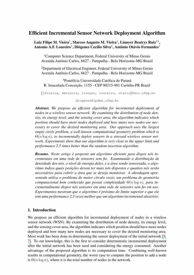
Following the definition in [18], the largest empty circle problem is: “Find the largestempty circle whose center is in the (closed) convex hull of a set of n sites S, empty inthat it contains no sites in its interior, and largest in that there is no other such circle withstrictly large radius”.
Figure 1: Largest Empty Circle Example.
Figure 1 shows an example of Largest Empty Circle. Given a set of points, calledsites, the answer is at the cross symbol, which represents the center of the wanted circled.Cross symbol represents the location whose distance to the nearest node is as large aspossible.
4.2. Assumptions
We work with homogenous [19] WSN distributed on a 2-D plane field. Our scheme doesnot loss generality because it can easily be extend to n-dimension. And it also can beextend to heterogeneous WSN. One way to do this is by adding fictitious sites. Each nodeis immobile, although the network topology could be dynamic, since nodes can becomeunavailable permanently or temporarily.
We assume that we have information about each node position. The position doesnot need to be global; it could be relative to the base station or to a known point. Aspoint out in [23], obtaining reliable node location has been studied in different contexts.Using Global Positioning System (GPS), we can determine geographical location withfair accuracy [9]. Others localization systems exist. One example is to use sensor nodescalled beacons, which know their coordinates in advance. Other nodes can approximatedistances to beacons and decide their locations by trilateration. For more informationsee [3, 10].
Another assumption is that we have the approximate energy level in each node.The energy map of the network can been obtained as shown in [23, 17]. Furthermore,there are components such as DS2438 that allows monitoring battery energy [20].
Applications of the algorithm assume that the sensors can be strategically placed,by any form. For example, the sensors could be deterministically deployed by a robot,which can place them on the exact localization predetermined to optimize the use of net-work resources. SensorWeb [1] is a NASA project that could be using such an application.
Sensor nodes are deployed through a desired monitor area, form a randomlyplaced network, wake-up, self-test, establish dynamic communication among them, com-posing an ad hoc network. The algorithm is used in those situations, which the networkis deployed, and not optimally configured, such as positioning each node to form a grid.In those cases, the new sensors can just replace old ones.

An advantage of the algorithm approach is the fact that it can be computed outsidethe WSN or at the data sink, saving the network energy and not requiring the algorithm tobe distributed.
4.3. The problem
Given the localization and the approximate energy level of each node in a WSN, what isthe minimum number of new nodes that should be added to the network so that it doesnot lose any covering area? Also, where should the new nodes be positioned?
The solution should be computed in reasonable time, considering that it may beapplied to networks with more than 50 nodes.
4.4. The algorithm
The input of the algorithm consists of the position and the energy map of the network.
First, we classify the operational state of each node using the parameters definedby the MANNA architecture [19], as shown in Table 1 classification.
Operational State Energy LevelActive >=30%Critical <30% and >15%Inactive <= 15%
Table 1: Operational State of sensor node.
Only nodes with active state will become sites. Nodes on other operational statewill be ignored. Others policies and others table values could be used instead. Using theset of sites, the algorithm calculates the largest empty circle. Regions with larger area arethe ones that need new nodes because the nodes are not healthy (active) or there are fewnodes at the region. The center of the circle indicates where is the best position to add anode. Repeating the process while the largest empty circle is larger than a threshold willindicate how many new nodes are necessary to guarantee that every circle area larger thanthe threshold is being covered and also where these new nodes should be placed.
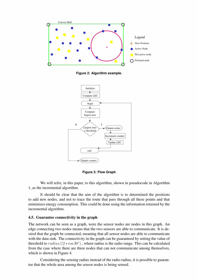
To calculate the largest empty circle is necessary to have a Convex Hull, otherwiseany point outside it could be the locale of the center of the circle. We choose four fictionalnodes to define the Convex Hull of the rectangle surveillance area. The number of fictionalnodes depends on the shape of the desired monitoring area. It does not affect the algorithmsince it keeps looking for the largest empty circle until the area of the circle is larger thana threshold. If the region near the border were uncovered, the algorithm would, anyway,indicate that region.
Figure 2 shows the structure of the network from the design vision. At the border,fictional nodes were created to delimit the Convex Hull. Nodes not active were discarded.The algorithm calculates the largest empty circle considering only active nodes. Thecenter of the circle indicates the best position to add a node. The worst-case complexity ofLargest Empty Circle is Θ(n logn). The algorithm can be extended to work with restrictedareas (areas where we don’t want to place sensors). Let’s consider a real applicationof WSN, an application of monitoring and sensing a volcano. When the sensors aredeployed, it is desirable that the sensors are not placed inside it or where the lava canreach them, otherwise, the sensors may be destroyed. Fictitious sites can be consideredon the restricted area, so that the algorithm does not consider adding a sensor on therestricted area.
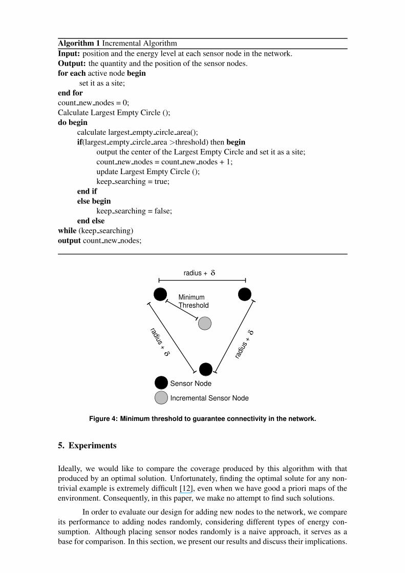
Figure 3 shows the flow graph of the incremental algorithm.
+••
•••
••
•
•
•• •
•
•• •
•
Convex Hull
New Position
Fictional node
Not active node• Active Node
+Legend
Figure 2: Algorithm example.
Initialize
Compute LEC
begin
Computelargest area
Largest area> threshold
Output center
Increment counter
Update LEC
N Y
end
Output counter
Figure 3: Flow Graph
We will refer, in this paper, to this algorithm, shown in pseudocode in Algorithm1, as the incremental algorithm.
It should be clear that the aim of the algorithm is to determined the positionsto add new nodes, and not to trace the route that pass through all these points and thatminimizes energy consumption. This could be done using the information returned by theincremental algorithm.
4.5. Guarantee connectivity in the graph
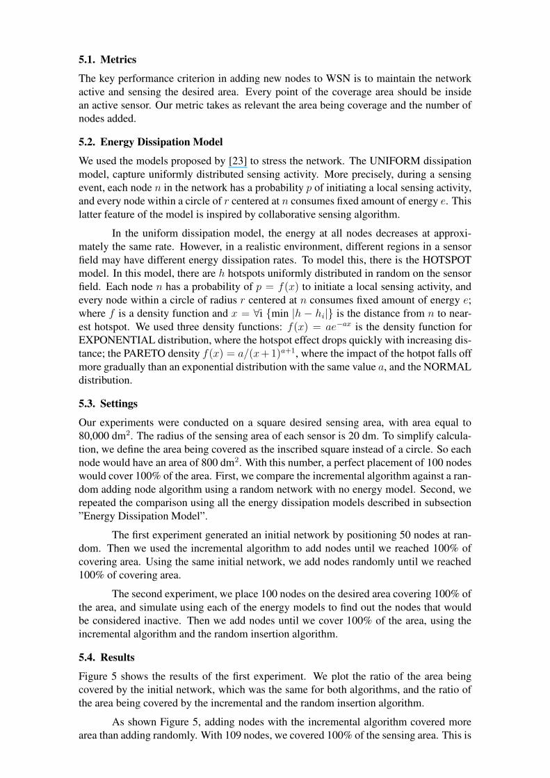
The network can be seen as a graph, were the sensor nodes are nodes in this graph. Anedge connecting two nodes means that the two sensors are able to communicate. It is de-sired that the graph be connected, meaning that all sensor nodes are able to communicatewith the data sink. The connectivity in the graph can be guaranteed by setting the value ofthreshold to radius/(2 ∗ cos 30◦) , where radius is the radio range. This can be calculatedfrom the case where there are three nodes that can not communicate among themselves,which is shown in Figure 4.
Considering the sensing radius instead of the radio radius, it is possible to guaran-tee that the whole area among the sensor nodes is being sensed.
Algorithm 1 Incremental AlgorithmInput: position and the energy level at each sensor node in the network.Output: the quantity and the position of the sensor nodes.for each active node begin
set it as a site;end forcount new nodes = 0;Calculate Largest Empty Circle ();do begin
calculate largest empty circle area();if(largest empty circle area >threshold) then begin
output the center of the Largest Empty Circle and set it as a site;count new nodes = count new nodes + 1;update Largest Empty Circle ();keep searching = true;
end ifelse begin
keep searching = false;end else
while (keep searching)output count new nodes;
Sensor Node
Incremental Sensor Node
MinimumThreshold
radius + d
radius +d
radi
us +
d
Figure 4: Minimum threshold to guarantee connectivity in the network.
5. Experiments
Ideally, we would like to compare the coverage produced by this algorithm with thatproduced by an optimal solution. Unfortunately, finding the optimal solute for any non-trivial example is extremely difficult [12], even when we have good a priori maps of theenvironment. Consequently, in this paper, we make no attempt to find such solutions.
In order to evaluate our design for adding new nodes to the network, we compareits performance to adding nodes randomly, considering different types of energy con-sumption. Although placing sensor nodes randomly is a naive approach, it serves as abase for comparison. In this section, we present our results and discuss their implications.
5.1. Metrics
The key performance criterion in adding new nodes to WSN is to maintain the networkactive and sensing the desired area. Every point of the coverage area should be insidean active sensor. Our metric takes as relevant the area being coverage and the number ofnodes added.
5.2. Energy Dissipation Model
We used the models proposed by [23] to stress the network. The UNIFORM dissipationmodel, capture uniformly distributed sensing activity. More precisely, during a sensingevent, each node n in the network has a probability p of initiating a local sensing activity,and every node within a circle of r centered at n consumes fixed amount of energy e. Thislatter feature of the model is inspired by collaborative sensing algorithm.
In the uniform dissipation model, the energy at all nodes decreases at approxi-mately the same rate. However, in a realistic environment, different regions in a sensorfield may have different energy dissipation rates. To model this, there is the HOTSPOTmodel. In this model, there are h hotspots uniformly distributed in random on the sensorfield. Each node n has a probability of p = f(x) to initiate a local sensing activity, andevery node within a circle of radius r centered at n consumes fixed amount of energy e;where f is a density function and x = ∀i {min |h − hi|} is the distance from n to near-est hotspot. We used three density functions: f(x) = ae−ax is the density function forEXPONENTIAL distribution, where the hotspot effect drops quickly with increasing dis-tance; the PARETO density f(x) = a/(x+ 1)a+1, where the impact of the hotpot falls offmore gradually than an exponential distribution with the same value a, and the NORMALdistribution.
5.3. Settings
Our experiments were conducted on a square desired sensing area, with area equal to80,000 dm2. The radius of the sensing area of each sensor is 20 dm. To simplify calcula-tion, we define the area being covered as the inscribed square instead of a circle. So eachnode would have an area of 800 dm2. With this number, a perfect placement of 100 nodeswould cover 100% of the area. First, we compare the incremental algorithm against a ran-dom adding node algorithm using a random network with no energy model. Second, werepeated the comparison using all the energy dissipation models described in subsection”Energy Dissipation Model”.
The first experiment generated an initial network by positioning 50 nodes at ran-dom. Then we used the incremental algorithm to add nodes until we reached 100% ofcovering area. Using the same initial network, we add nodes randomly until we reached100% of covering area.
The second experiment, we place 100 nodes on the desired area covering 100% ofthe area, and simulate using each of the energy models to find out the nodes that wouldbe considered inactive. Then we add nodes until we cover 100% of the area, using theincremental algorithm and the random insertion algorithm.
5.4. Results
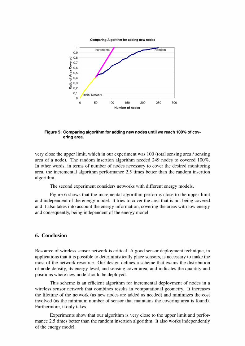
Figure 5 shows the results of the first experiment. We plot the ratio of the area beingcovered by the initial network, which was the same for both algorithms, and the ratio ofthe area being covered by the incremental and the random insertion algorithm.
As shown Figure 5, adding nodes with the incremental algorithm covered morearea than adding randomly. With 109 nodes, we covered 100% of the sensing area. This is
Comparing Algorithm for adding new nodes
0
0,1
0,2
0,3
0,4
0,5
0,6
0,7
0,8
0,9
1
0 50 100 150 200 250 300
Number of nodes
Initial Network
Incremental Random
Figure 5: Comparing algorithm for adding new nodes until we reach 100% of cov-ering area.
very close the upper limit, which in our experiment was 100 (total sensing area / sensingarea of a node). The random insertion algorithm needed 249 nodes to covered 100%.In other words, in terms of number of nodes necessary to cover the desired monitoringarea, the incremental algorithm performance 2.5 times better than the random insertionalgorithm.
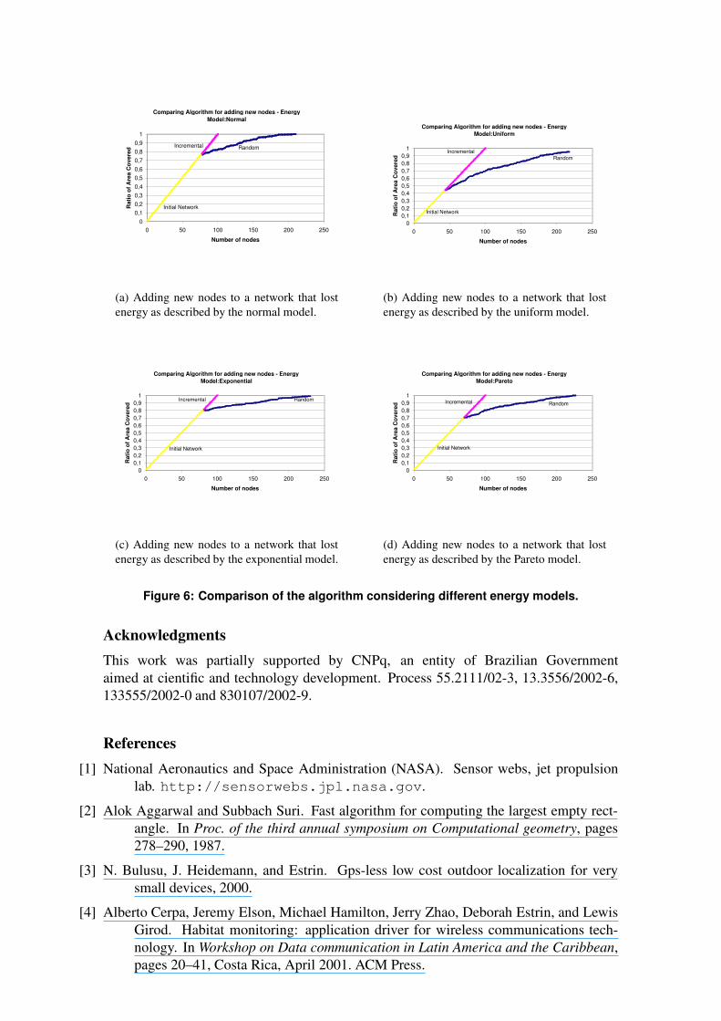
The second experiment considers networks with different energy models.
Figure 6 shows that the incremental algorithm performs close to the upper limitand independent of the energy model. It tries to cover the area that is not being coveredand it also takes into account the energy information, covering the areas with low energyand consequently, being independent of the energy model.
6. Conclusion
Resource of wireless sensor network is critical. A good sensor deployment technique, inapplications that it is possible to deterministically place sensors, is necessary to make themost of the network resource. Our design defines a scheme that exams the distributionof node density, its energy level, and sensing cover area, and indicates the quantity andpositions where new node should be deployed.
This scheme is an efficient algorithm for incremental deployment of nodes in awireless sensor network that combines results in computational geometry. It increasesthe lifetime of the network (as new nodes are added as needed) and minimizes the costinvolved (as the minimum number of sensor that maintains the covering area is found).Furthermore, it only takes
Experiments show that our algorithm is very close to the upper limit and perfor-mance 2.5 times better than the random insertion algorithm. It also works independentlyof the energy model.
Comparing Algorithm for adding new nodes - Energy Model:Normal
00,10,20,30,40,50,60,70,80,9
1
0 50 100 150 200 250
Number of nodes
Rat
io o
f Are
a C
over
ed
Initial Network
Incremental Random
(a) Adding new nodes to a network that lostenergy as described by the normal model.
Comparing Algorithm for adding new nodes - Energy Model:Uniform
00,10,20,30,40,50,60,70,80,9
1
0 50 100 150 200 250
Number of nodes
Rat
io o
f Are
a C
over
ed
Initial Network
IncrementalRandom
(b) Adding new nodes to a network that lostenergy as described by the uniform model.
Comparing Algorithm for adding new nodes - Energy Model:Exponential
00,10,20,30,40,50,60,70,80,9
1
0 50 100 150 200 250
Number of nodes
Rat
io o
f Are
a C
over
ed
Initial Network
Incremental Random
(c) Adding new nodes to a network that lostenergy as described by the exponential model.
Comparing Algorithm for adding new nodes - Energy Model:Pareto
00,10,20,30,40,50,60,70,80,9
1
0 50 100 150 200 250
Number of nodes
Rat
io o
f Are
a C
over
ed
Initial Network
Incremental Random
(d) Adding new nodes to a network that lostenergy as described by the Pareto model.
Figure 6: Comparison of the algorithm considering different energy models.
AcknowledgmentsThis work was partially supported by CNPq, an entity of Brazilian Governmentaimed at cientific and technology development. Process 55.2111/02-3, 13.3556/2002-6,133555/2002-0 and 830107/2002-9.
References[1] National Aeronautics and Space Administration (NASA). Sensor webs, jet propulsion
lab. http://sensorwebs.jpl.nasa.gov.
[2] Alok Aggarwal and Subbach Suri. Fast algorithm for computing the largest empty rect-angle. In Proc. of the third annual symposium on Computational geometry, pages278–290, 1987.
[3] N. Bulusu, J. Heidemann, and Estrin. Gps-less low cost outdoor localization for verysmall devices, 2000.
[4] Alberto Cerpa, Jeremy Elson, Michael Hamilton, Jerry Zhao, Deborah Estrin, and LewisGirod. Habitat monitoring: application driver for wireless communications tech-nology. In Workshop on Data communication in Latin America and the Caribbean,pages 20–41, Costa Rica, April 2001. ACM Press.
[5] K. Chakrabarty, S. S. Iyengar, H. Qi, and E. Cho. Grid coverage for surveillance andtarget location in distributed sensor networks. IEEE Transactions on Computers,51:1448–1453, December 2002.
[6] Thomas Clouquer, Veradej Phipatanasuphorn, Parmesh Ramanathan, and Kewal Saluja.Sensor deployment strategy for target detection. In Wireless Sensor Networks andApplications (WSNA), Atlanta,GA, 2002.
[7] S. S. Dhillon, K. Chakrabarty, and S. S. Iyengar. Sensor placement for grid coverage underimprecise detections. In Proc. International Conference on Information Fusion,pages 1581–1587, 2002.
[8] Deborah Estrin, Ramesh Govindan, John Heidemann, and Satish Kumar. Next centurychallenges: scalable coordination in sensor networks. In Proceedings of the 5thannual ACM/IEEE international conference on Mobile computing and networking,pages 263–270. ACM Press, 1999.
[9] B. R. Badrinath et al. Special issue on smart spaces and environments. IEEE Pers.Commun., October 2000.
[10] L. Girod. Development and characterization of an acoustic rangefinder, 2000.
[11] Bob Grabowski. Small robot survey. http://www.contrib.andrew.cmu.edu/˜rjg/webrobots/small_robot_survey.htm%l.
[12] Andrew Howard, Maja J Mataric, and Gaurav S. Sukhatme. An incremental deploymentalgorithm for mobile robot teams. Proceedings of the IEEE/RSJ International Con-ference on Intelligent Robots and Systems, 2002.
[13] I.F.Akyildiz, W.Su, Y.Sankarasubramaniam, and E. Cayirci. Wireless sensor networks: Asurvey. IEEE Communications Magazine, 40(8):102–14, August 2002.
[14] J. M. Kahn, R. H. Katz, and K. S. J. Pister. Next century challenges: mobile networkingfor smart dust. In Proceedings of the 5th annual ACM/IEEE international conferenceon Mobile computing and networking, pages 271–278. ACM Press, 1999.
[15] Anthony LaMarca, Waylon Brunette, David Koizumi, Matthew Lease, Stefan B. Sigurds-son, Kevin Sikorski, Dieter Fox, and Gaetano Boriello. Making sensor networkspractical with robots. International Conference on Pervasive Computing, 2002.
[16] Seapahn Meguerdichian, Farinaz Koushanfar, Miodrag Potkonjak, and Mani B. Srivas-tava. Coverage problems in wireless ad-hoc sensor networks. IEEE Infocom, pages1380–1387, 2001.
[17] Raquel A. F. Mini, Badri Nath, and Antonio A. F. Loureiro. Prediction-based approachesto construct the energy map for wireless sensor networks. XXI SBRC, May 2003.
[18] Joseph O’Rourke. Computational Geometry in C. Cambridge University Press, 1993.
[19] Linnyer Beatrys Ruiz, Jose Marcos Nogueira, and Antonio A. F. Loureiro. Manna: Amanagement architecture for wireless sensor networks. In IEEE CommunicationMagazine, volume 41, February 2003.
[20] Dallas Semiconductor. Ds2438 datasheet. http://pdfserv.maxim-ic.com/arpdf/DS2438.pdf.
[21] Gabriel T. Sibley, Mohammad H. Rahimi, and Gaurav S. Sukhatme. Robomote: A tinymobile robot platform for large-scale sensor networks. In Proceedings of the IEEEInternational Conference on Robotics and Automation (ICRA2002), volume 2, pages1143–1148, Washington, DC, May 2002.

[22] Di Tian and Nicolas D. Georganas. A coverage-preserving node scheduling scheme forlarge wireless sensor networks. In Proceedings of the 1st ACM international work-shop on Wireless sensor networks and applications, pages 32–41. ACM Press, 2002.
[23] Jerry Zhao, Ramesh Govindan, and Deborah Estrin. Residual energy scans for monitor-ing wireless sensor networks. In IEEE Wireless Communications and NetworkingConference (WCNC 02), Orlando, FL, March 2002.