Genetic Algorithm based Sensor Deployment with Area

Priority

Tahir Emre Kalaycı1, Aybars Uğur2

1Celal Bayar University, Dept. of Computer Engineering, Manisa, Türkiye

2Ege University, Dept. of Computer Engineering, Izmir, Türkiye

Abstract. We are introducing a new design goal called area priority for finding optimal

sensor node distribution. Environment that wireless sensor network (WSN) will be placed is

divided into parts and priorities are attached to these parts. Priorities make the deployment

problem adaptable to non-homogeneous environments such as forests having regions that

have different importance levels. Various tree/animal types and densities, residential in the

forest can be modeled by the area priority concept that we proposed. We also developed a

genetic algorithm based method to optimize the total importance in a fully connected WSN.

Experimental results obtained for different priorities are presented and discussed.

1 Introduction

With the proliferation in Micro-Electro-Mechanical Systems (MEMS) technology which has

facilitated the development of smart sensors, wireless sensor networks (WSNs) have gained

worldwide attention in recent years. Sensors that comprise these networks are small, with limited

processing and computing resources, and they are inexpensive compared to traditional sensors. Sensor

nodes can sense, measure, and gather information from the environment and, based on some local

1 Tahir Emre Kalayci is supported by the Ege University through DPT ÖYP (“Öğretim Üyesi Yetiştirme Programı”), ÖYP thesis project 05-DPT-003/05 and TÜBİTAK 2211 Yurt İçi Doktora scholarship.

1

decision processes, they can transmit the sensed data to the user (Yick, 2008). A WSN typically has

little or no infrastructure. It consists of a number of sensor nodes (few tens to thousands) working

together to monitor a region to obtain data about the environment. Careful and accurate node

positioning can be a very effective optimization means for achieving application requirements and

design goals (Younis, 2008). WSNs have great potential for many applications such as military target

tracking and surveillance, natural disaster relief, biomedical health monitoring, etc.

However, wireless sensors have several constraints such as restricted sensing and communication

range as well as limited battery capacity (Ghosh, 2008). These limitations bring issues such as

coverage, connectivity, network lifetime, scheduling and data aggregation (Nor, 2009). Coverage

characterizes the monitoring quality provided by a sensor network on a designated region and reflects

how well a sensor network is monitored or tracked by sensors (Huang, 2003). Some applications may

require that some areas in the network are more important than other areas and need to be covered by

more sensors, these important regions are called hot spots (Huang, 2003). Consequently, coverage can

be considered a measure of quality of the service of a sensor network (Yildirim, 2008). The coverage

requirement on hot spot regions also depends on the number of faults that must be tolerated.

Providing connectivity between sensor nodes is another important issue in wireless sensor networks.

Without connectivity, nodes may not be able to coordinate effectively or transmit data back to base

stations. Thus, combination of connectivity and coverage is an important concept in sensor networks

(Wang, 2003).

Genetic algorithms (GA), the most widely used form of evolutionary computation, has proven to be a

very successful meta-heuristic technique for many NP-complete optimization problems (Ugur, 2008).

GA are stochastic search methods that have been successfully applied in many search, timetabling,

scheduling, and machine learning problems and have been especially used in engineering, biology,

and medicine (Ugur, 2008). GA have also been used in a variety of hybrid intelligent systems (such as

evolutionary neural networks, fuzzy evolutionary systems, or genetic-neural architectures) to solve

2

many other real world applications (Ugur, 2008).

There are no examples of area priority based sensor deployment optimization research in the

literature. In this study, we are using GA with novel fitness function to obtain a good sensor

deployment based on priority of zones with preserving connectivity and covering some important

regions with at least k sensors. Area priority concept in sensor network deployment used to classify

the parts of the environment to be monitored. Environment that wireless sensor network placed may

not be homogeneous. We split environment into small fragments called cells, and we assign a value to

the every cell that indicates priority (importance) of the zone specified by that cell. For example, in a

forest there are many areas with different priorities. We can distinguish these areas based on tree

density and types, residential, animal types and density, etc. And we can give different priority values

based on these parameters. We can use “area priority” notion not only in forests, also transporter

parks to distinguish most valuable parts of it, national parks, residential areas, fish farms, historical

buildings, etc.

2 Related Work

Zorbas et al. (Zorbas, 2010) propose various coverage algorithms to achieve power efficient

monitoring of targets by sensor networks. They present a novel and efficient coverage algorithm that

can produce both disjoint cover sets as well as non-disjoint cover sets. Through simulations, they

show that the proposed algorithm outperforms similar heuristic algorithms found in the literature.

Nor et al. (Nor, 2009) aims to review the common strategies used in solving coverage problem in

WSN. The strategies studied are used during deployment phase where the coverage is calculated

based on the placement of the sensors on the region of interest (ROI). The strategies reviewed are

categorized into three groups based on the approaches used, namely; force based, grid based or

computational geometry based approach.

3

Yildirim et al. (Yildirim, 2008) are proposed a GA based solution to find an optimal sensor node

distribution to use as an initial deployment strategy that maximizes the coverage area of wireless

sensor network while preserving connectivity between nodes provided that all given hot spot regions

are covered by at least k sensors.

Wu et al. (Wu, 2007) propose a centralized and deterministic sensor deployment method, DT-Score

(Delaunay Triangulation-Score), aims to maximize the coverage of a given sensing area with

obstacles. According to the simulation results, DT-Score can reach higher coverage than grid-based

and random deployment methods with the increasing of deployable sensors.

Chen et al. (Chen, 2007) survey five recent research approaches on coverage of wireless sensor

networks and present in some detail the algorithms, assumptions, and results. A comprehensive

comparison among these approaches is given from the perspective of design objectives, assumptions,

algorithm attributes, and related results.

Xu et al. (Xu, 2006) identify two deployment errors, namely, misalignment and random errors. They

derive the minimum number of sensors required by a robust grid-based sensor deployment assuming

that the errors are bounded.

Bai et al. (Bai, 2006) propose an optimal deployment pattern to achieve both full coverage and 2-

connectivity, and prove its optimality for all values of r c÷r s (rc is the communication radius, rs is

the sensing radius). They also prove the optimality of a previously proposed deployment pattern for

achieving both full coverage and 1- connectivity, when r c÷r s < √3 .

Shen et al. (Shen, 2006) describe a basic coverage issue, and propose a scheme named Grid Scan that

is applied to calculate the basic coverage rate with arbitrary sensing radius of each node. The results

of simulation experiments support that Grid Scan based re-deployment is more effective to cover

monitored area than random spread.

4

Megerian et al. (Megerian, 2005) briefly discuss the definition of the coverage problem from several

points of view and formally define the worst and best-case coverage in a sensor network. They

establish the main highlight of the paper, an optimal polynomial time worst and average case

algorithm for coverage calculation for homogeneous isotropic sensors by combining computational

geometry and graph theoretic techniques, specifically the Voronoi diagram and graph search

algorithms.

For a comprehensive list of node placement strategies and techniques, Younis and Akkaya’s survey

(Younis, 2008), which report current state of the research, can be checked.

3 Problem Definition

Before giving the definition, we should introduce the parameters required for the problem. We are

working on a 2D area that is defined by A(width, height). Together with the dimensions of the area we

have sensor count N, sensing radius rs, communication radius - which is calculated using rc = 2 * rs

formula -, h hot spot areas and a k value for minimal sensor count needed for hot spot areas. In

addition to these parameters we need cell size cs, which will be used to divide area to cell fragments,

and priority value for every cell cpi = (rs, re, cs, ce) (s starting cell index, e ending cell index). These

cell parameters can also be entered using graphical user interface (GUI).

The problem we are struggling based on some assumptions listed in Lemma 1 and tries to fulfill

objectives presented in Proposition 2. And it is formalized as Problem 3.

Lemma 1. Area is obstacle free, the sensing and communication ranges of all sensors are identical,

sensors and hot spot areas are unit disk shaped and they all have identical radius.

Proposition 2. All sensors should communicate with each other (connectivity), h hot spot areas must

be covered by at least k sensors (k-covered), and total covered area priority of sensor network should

5

be maximized.

Problem 3. Using the given parameters A, N, rs, k, cs, cpi; try to increase covered area priority of the

sensor network satisfying that all hot spot areas are k-covered and all sensors are connected.

4 Solving Problem Using Genetic Algorithm

We are using a traditional GA with optimizations to solve the problems. Optimizations are based on

the problem and area information and serve for faster improvement of solutions. Developed GA uses

parameters that are required for every traditional GA: Pc, Pm, T, G2.

After loading the problem from a XML file and entering the parameters, before the GA loop, cells and

cell groups of the area are calculated based on the cell size, area dimensions and sensor radius. Cell

groups are an important part of our method which are used to improve sensor locations in the run

time. They are calculated using cell edge size and sensor radius.

After calculation cell groups, a random population is initialized. An important optimization when

initializing the population is connecting unconnected sensor blocks to achieve connectivity before GA

run. With this optimization, GA operates on already connected sensor network and this means that it

operates on feasible solutions in terms of the connectivity. Connecting unconnected sensor blocks is

one of the novel contributions of this study.

Finally, after population initialization, GA loop starts. It continues to improve population until

number of the iterations exceeds the predetermined termination criteria, generation count parameter

(G). At every iteration a new population are generated from the individuals (solutions, chromosomes,

individuals are used interchangeably in this paper) of the old population. Selected individuals are

crossed over and mutated based on GA parameters using GA operators. Outline of the GA follows:

2 crossover probability, mutation probability, population size, generation count

6

• Start: Initialize a random population

• Loop: Repeat until generation count is reached (G)

• Crossover selected results from population (T * Pc chromosomes are crossed over)

• Mutate selected results from population (T * Pm chromosomes are mutated)

• Select the best result as elite from generated population for this iteration

• End: Return elite (optimal) solution

At the end of the run, optimal solution of GA is returned to the invoker of the algorithm.

4.1 Chromosome Encoding

Choosing or designing suitable chromosomes for the problem are crucial for the success of the GA.

Our problem deals with placement of sensors, so we are using 2D coordinate representation for the

sensors that resides on a 2D plane ( A(width,height)) in the form:

S ( x,y ) : {0≤ x≤width,0≤ y≤height } (1)

Chromosomes has N genes and every gene (g) represents coordinates for every sensor. In the GA,

genes can be produced in four different ways: randomly, by crossover, by mutation or by

optimization. Population consist of T chromosomes. Formulations of population and chromosomes

(C) are listed in equations two and three respectively.

C i={ g ij :0<j<N } :0<i<T (2)

g= { x,y :0≤ x≤width, 0≤ y≤height } (3)

4.2 Genetic Algorithm Operators

Operators are the important components of the GA. As is in chromosome encoding, choosing right

operators for the problem improves the GA. Even though there are many generic operators that don't

depend on the problem, some problems require problem specific operators. On the other hand,

operators depend on the chromosome encoding. Still, GA developers can use already developed

operators that are suitable to the chromosome encoding and problem instead of developing new ones.

There are three types of operators in GA: crossover to generate offspring from parents, mutation for

7

small changes in the individual to maintain genetic diversity and selection for selecting suitable

individuals for crossover.

Crossover generates new offspring from the selected parents of the current population. We

implemented three different crossover schemes: one point crossover (OPC), two point crossover

(TPC) and uniform crossover (UC).

We use three different selection mechanisms to select individuals to crossover. Normal selection

mechanism selects individuals randomly. In rank selection mechanism every individual has the same

weight to be selected for crossover. Individual are selected if a random generated double is lower than

the crossover probability (Pc), and crossed over with the next individual in the following rank.

Geometric selection selects one low fittest chromosome and one high fittest chromosome for

crossover.

In OPC a random cut point is selected on parents and genes beyond this cut point is swapped between

parent chromosomes. In TPC two random cut point is selected. UC takes genes from first parent and

second parent following a sequence (sequence is 010101 - 0 for first parent and 1 for second parent).

The procured chromosomes after crossover are the children and replaced with the parents in the

current population to form a new and hopefully better population.

In GA loop, after finishing crossover operation, genes are randomly mutated based on mutation

probability (Pm). We developed three mutation schemes: random move mutation (RMM), coordinate

change mutation (CCM) and random coordinate mutation (RCM). In RMM, a randomly selected gene

moved randomly (upper limit of movement is sensor radius). CCM swaps x coordinate with y

coordinate of a randomly selected gene. RCM replaces a random gene with random generated

coordinates. In mutation the new chromosome changes are applied if only the result is better.

We use a simple elitism mechanism to save the best solution at the end of every iteration to use it in

the next iteration and to keep the best solution ever achieved.

8

4.3 Fitness Function

Fitness function is used to figure out the optimality of a solution in GA. Every chromosome is

compared against other chromosomes using the fitness value that is the result of the function. We

developed a novel fitness function to compare chromosomes. Developed function separates

chromosomes into three classes:

1. Connected, k-covered network - The optimal solutions that we seek. Fitness of this class is

equal to the total importance of the covered area by the network that is defined by the

chromosome. Total importance of chromosome is calculated by summing up the priority of

the cells that are covered by sensors defined by chromosome:

F=I t=∑s= 0

N

I s (4)

Even a cell is covered by more than one sensor we are not adding priority of this cell more

than one time to the fitness value:

I s=∑i=0

c

Pc ,Pc={ P i if cell priority is not added0 if cell priority is already added } (5)

Where Pi is priority of a cell covered by sensor s and c is the total count of covered cells by

sensor s.

2. Not connected, k-covered network - Non optimal solutions, but still it is close to the

solutions we seek. Fitness of this class is calculated by dividing total importance (It) by

unconnected component count (Cu).

F=I t

Cu (6)

3. Not connected, non k-covered network - Worst solutions. Fitness of non k-covered

solutions is equal to zero (0).

Fitness calculation algorithm for these three different classes is listed in algorithm 1.

9

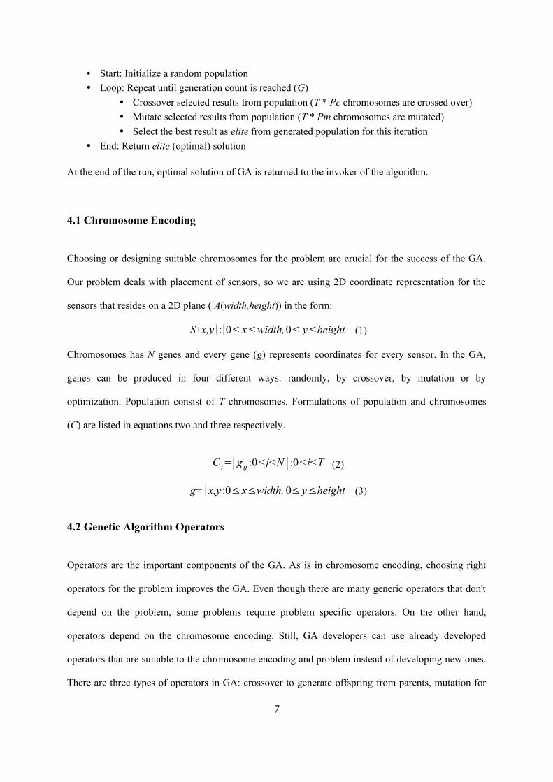
calculateFitness(Chromosome chr) calculateFitness(Chromosome chr)fitness = 0Reset Cell and Block Countsfor i =0 to GeneCount gene = chr.Gene(i) ti = calculateSensorImportance(gene) if (ti == 0)

ci = CellAnalysisTool.getNextBest()chr.setGene(i, ci.coords.clone())importance = ci.totalImportance

save worst sensor fitness += timove sensor with least importance to a high priority locationcc = countConnectedComponents(chr.getGenes())if cc > 1 fitness = fitness / ccif isKCovered(chr.Genes) fitness = 0return fitness

calculateSensorImportance(Sensor s)totalImportance = 0for i=0 to cellCount c = cells[i] if contains(s,c) if c.howManyTimesCovered == 0 totalImportance += c.importance c.howManyTimesCovered +=1

CellAnalysisTool.removeCell(c)return totalImportance

Algorithm 1: Fitness algorithm

When calculating total importance of a sensor, we are using euclidean distance calculation to find the

cells that are covered by this sensor. And importance of these covered cells are added only once to the

total importance of this sensor to get a better divergence. We are also saving the count of the sensors

that covers the cell to use it when moving sensors with zero importance.

10

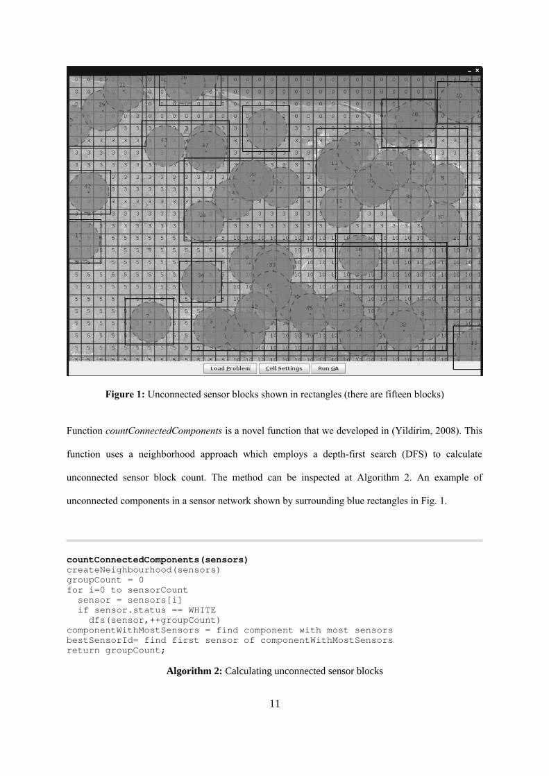
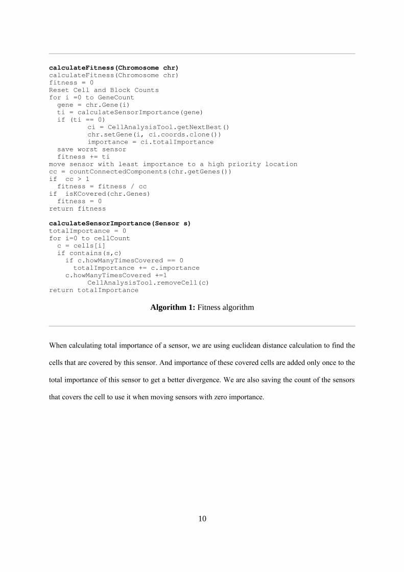
Figure 1: Unconnected sensor blocks shown in rectangles (there are fifteen blocks)

Function countConnectedComponents is a novel function that we developed in (Yildirim, 2008). This

function uses a neighborhood approach which employs a depth-first search (DFS) to calculate

unconnected sensor block count. The method can be inspected at Algorithm 2. An example of

unconnected components in a sensor network shown by surrounding blue rectangles in Fig. 1.

countConnectedComponents(sensors)createNeighbourhood(sensors)groupCount = 0for i=0 to sensorCount sensor = sensors[i] if sensor.status == WHITE dfs(sensor,++groupCount)componentWithMostSensors = find component with most sensorsbestSensorId= find first sensor of componentWithMostSensorsreturn groupCount;

Algorithm 2: Calculating unconnected sensor blocks

11

Checking if every hot spot is covered by at least k sensors is carried out by isKCovered function.

Algorithm of this function has a O(N * H) (H: hot spot count) complexity because it checks every hot

spot if it is covered by a sensor. Coverage check is using a simple euclidean distance calculation if the

sensor contains the center of the hot spot. All these calculations, algorithms, and functions form our

novel fitness approach.

4.4 Optimizations

Analyzing problem information and using the results of the analysis can help GA to converge

solutions faster. Therefore, we are analyzing problem information before starting GA loop and using

the results to optimize solutions. Developed two optimizations are explained in the following

subsections.

4.4.1 Cell Analysis and relocating zero importance sensors

Cell analysis is an important approach to know more about cells and locations that require more

attention. Results of this analysis are used to relocate sensors with zero importance (or the worst

importance) to a better (high priority) location.

First of all, every cell are visited and cells inside a square with edge size equals to sensor diameter are

grouped together to form a cell block. During grouping total importance of every cell group is

calculated by summing importance of the cells that it contains.

After calculation of cell groups and their total importance, groups are sorted based on their total

importance (in priority queue techniques sorting has been accomplished internally). Later this sorted

list is used to relocate zero or lowest importance sensors to a center of one of the groups. For this

optimization three different techniques has been developed. First technique (caV) uses vector to keep

12

generated groups and next coordinate taken from this vector in sequence (using a position index). If

index reaches to the end of the vector, it is reset to zero (head of the vector). Also if the center cell of

the received group is covered already, next group coordinate is asked from the vector.

Second technique (caPQ) uses a priority queue. The only difference with the first technique is that it

uses a priority queue and when queue is emptied, cell analysis is invoked again.

Third technique (caPQU) also uses a priority queue to keep analysis results. But this technique

updates priority queue when cell coverage condition changes. When a cell is covered, it is removed

from all of the groups contains it. So this removal changes the priority queue (order of the groups). As

second technique when queue is emptied, cell analysis is invoked again.

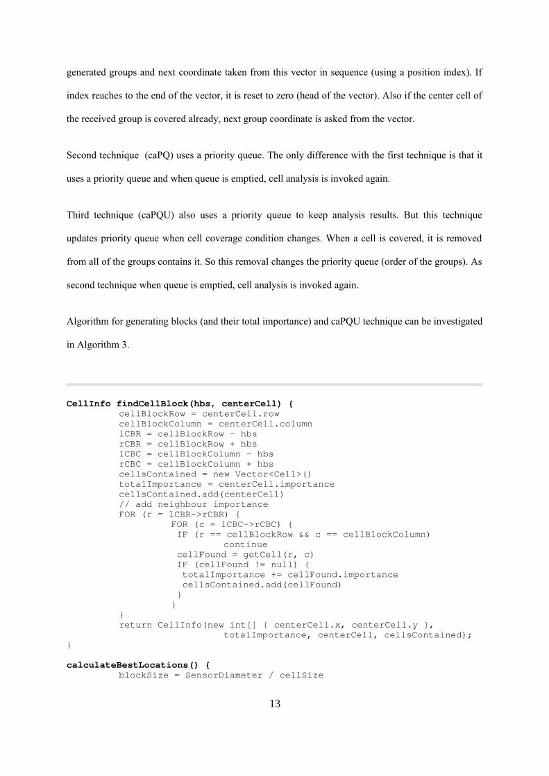
Algorithm for generating blocks (and their total importance) and caPQU technique can be investigated

in Algorithm 3.

CellInfo findCellBlock(hbs, centerCell) {cellBlockRow = centerCell.rowcellBlockColumn = centerCell.columnlCBR = cellBlockRow - hbsrCBR = cellBlockRow + hbslCBC = cellBlockColumn - hbsrCBC = cellBlockColumn + hbscellsContained = new Vector<Cell>()totalImportance = centerCell.importancecellsContained.add(centerCell)// add neighbour importanceFOR (r = lCBR->rCBR) {

FOR (c = lCBC->rCBC) { IF (r == cellBlockRow && c == cellBlockColumn)

continue cellFound = getCell(r, c) IF (cellFound != null) { totalImportance += cellFound.importance cellsContained.add(cellFound) }}

}return CellInfo(new int[] { centerCell.x, centerCell.y },

totalImportance, centerCell, cellsContained);}

calculateBestLocations() {blockSize = SensorDiameter / cellSize

13

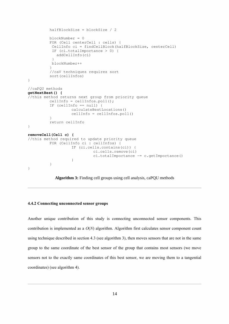
halfBlockSize = blockSize / 2

blockNumber = 0FOR (Cell centerCell : cells) { CellInfo ci = findCellBlock(halfBlockSize, centerCell) IF (ci.totalImportance > 0) { addCellInfo(ci) } blockNumber++}//caV techniques requires sortsort(cellInfos)

}

//caPQU methodsgetNextBest() {//this method returns next group from priority queue

cellInfo = cellInfos.poll();IF (cellInfo == null) {

calculateBestLocations()cellInfo = cellInfos.poll()

}return cellInfo

}

removeCell(Cell c) {//this method required to update priority queue

FOR (CellInfo ci : cellInfos) {IF (ci.cells.contains(ci)) {

ci.cells.remove(ci)ci.totalImportance -= c.getImportance()

}}

}

Algorithm 3: Finding cell groups using cell analysis, caPQU methods

4.4.2 Connecting unconnected sensor groups

Another unique contribution of this study is connecting unconnected sensor components. This

contribution is implemented as a O(N) algorithm. Algorithm first calculates sensor component count

using technique described in section 4.3 (see algorithm 3), then moves sensors that are not in the same

group to the same coordinate of the best sensor of the group that contains most sensors (we move

sensors not to the exactly same coordinates of this best sensor, we are moving them to a tangential

coordinates) (see algorithm 4).

14

connectDisjointComponents(sensors,bestSensor) componentCount = countUnconnectedComponents(sensors)if componentCount > 1 for i=0 to sensorCount sensor = sensors[i] if sensor.groupNumber != componentWithMostSensors sensor.coords = coords[bestSensorId]+diameter

Algorithm 4: Pseudo code for connecting unconnected sensor groups

5 Experimental Results

We have performed different experiments to analyze the developed technique. In these experiments

we used default parameters as follows: 100 for population size and generation limit, 0.9 for crossover

probability, 0.2 for mutation probability, one point crossover, random coordinate mutation and rank

selection. We run the algorithm for 50 times.

Our first experiment examines different selection, mutation and crossover types. Results can be

examined in table 1. This experiment shows that most reasonable choice is normal selection with two

point crossover and random coordinates mutation.

Table 1: Fitness results for different selection, mutation and crossover types

Normal Selection Rank selection Geometric selection

RCM CCM RMM RCM CCM RMM RCM CCM RMM

OPC 1911 1758 1717 945 288 369 1036 263 363

TPC 2011 1790 1855 1043 252 401 1020 286 354

UC 1343 392 582 1044 269 385 1011 269 383

15

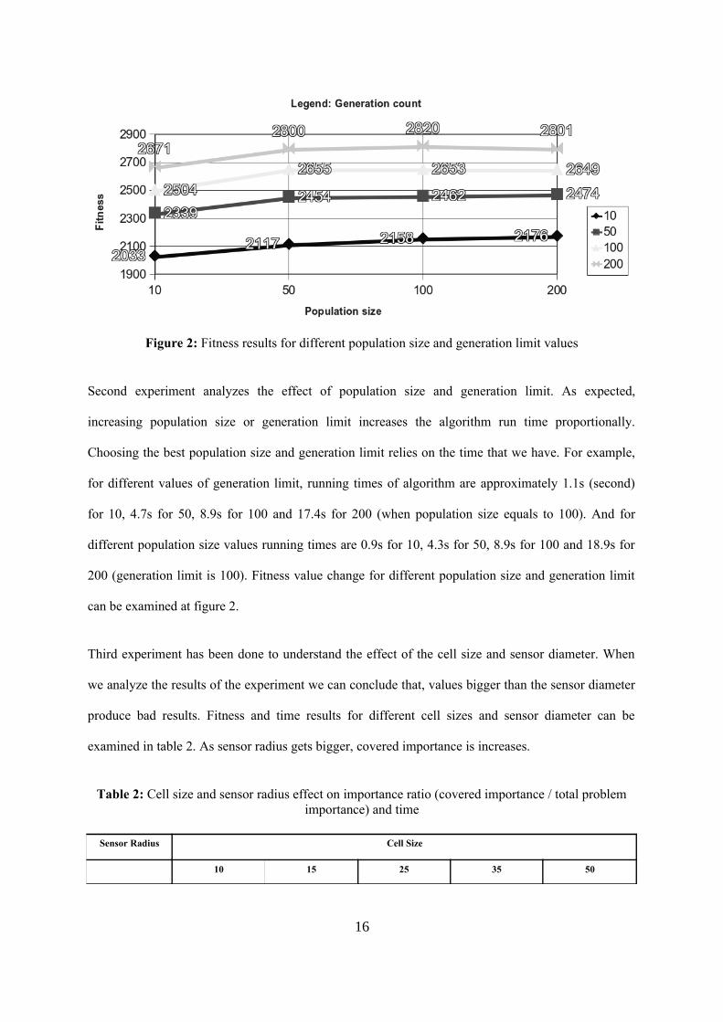
Figure 2: Fitness results for different population size and generation limit values

Second experiment analyzes the effect of population size and generation limit. As expected,

increasing population size or generation limit increases the algorithm run time proportionally.

Choosing the best population size and generation limit relies on the time that we have. For example,

for different values of generation limit, running times of algorithm are approximately 1.1s (second)

for 10, 4.7s for 50, 8.9s for 100 and 17.4s for 200 (when population size equals to 100). And for

different population size values running times are 0.9s for 10, 4.3s for 50, 8.9s for 100 and 18.9s for

200 (generation limit is 100). Fitness value change for different population size and generation limit

can be examined at figure 2.

Third experiment has been done to understand the effect of the cell size and sensor diameter. When

we analyze the results of the experiment we can conclude that, values bigger than the sensor diameter

produce bad results. Fitness and time results for different cell sizes and sensor diameter can be

examined in table 2. As sensor radius gets bigger, covered importance is increases.

Table 2: Cell size and sensor radius effect on importance ratio (covered importance / total problem importance) and time

Sensor Radius Cell Size

10 15 25 35 50

16

25 %77.49 (160.67s) %77.92 (74.05s) %79.68 (27s) %78.37 (14.27s) %82.22 (7.38s)

50 %77.08 (161.13s) %77.67 (74.16s) %79.23 (26.71s) %78.72 (14.30s) %82.59 (7.38s)

75 %76.37 (161.04s) %78.38 (73.96s) %79.08 (27.07s) %78.37 (14.30s) %81.93 (7.37s)

100 %76.67 (160.79s) %77.76 (74.02s) %79.46 (27.38s) %79.03 (14.28s) %81.85 (7.38s)

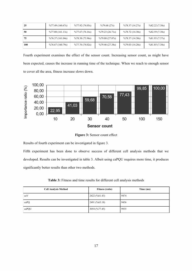
Fourth experiment examines the effect of the sensor count. Increasing sensor count, as might have

been expected, causes the increase in running time of the technique. When we reach to enough sensor

to cover all the area, fitness increase slows down.

Figure 3: Sensor count effect

Results of fourth experiment can be investigated in figure 3.

Fifth experiment has been done to observe success of different cell analysis methods that we

developed. Results can be investigated in table 3. Albeit using caPQU requires more time, it produces

significantly better results than other two methods.

Table 3: Fitness and time results for different cell analysis methods

Cell Analysis Method Fitness (ratio) Time (ms)

caV 2422 (%61.43) 9474

caPQ 2491 (%63.18) 9456

caPQU 3054 (%77.45) 9935

17

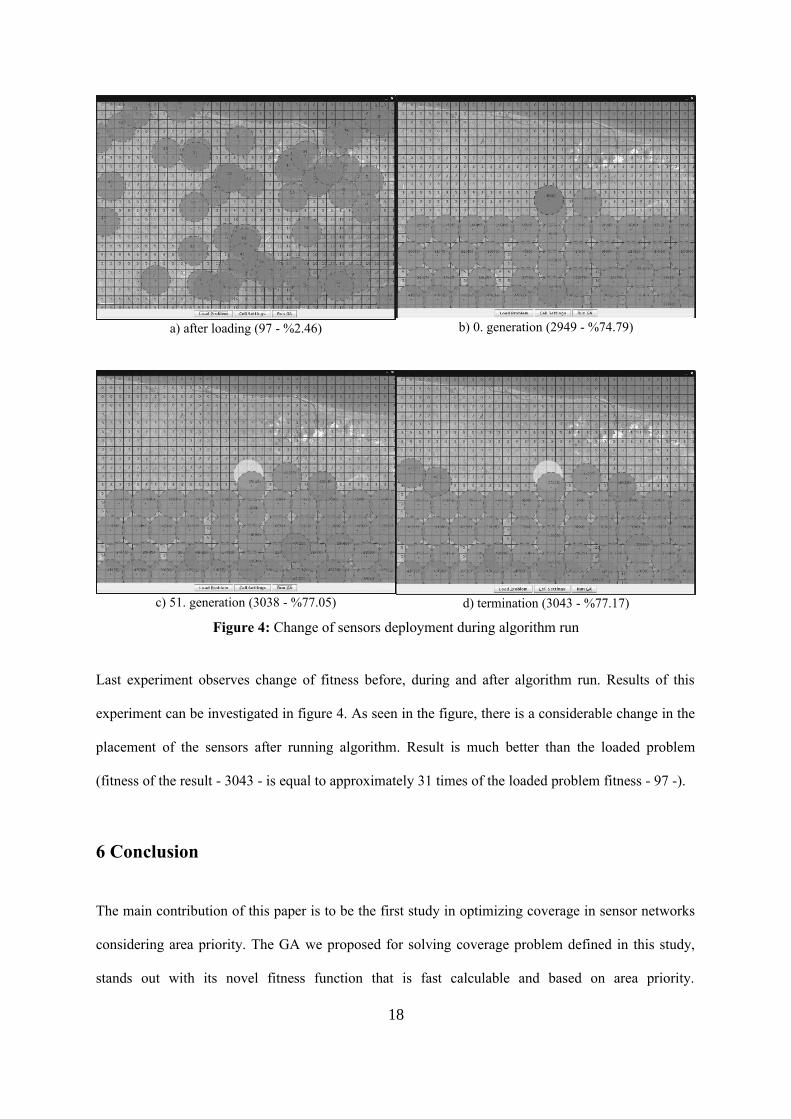
a) after loading (97 - %2.46) b) 0. generation (2949 - %74.79)

c) 51. generation (3038 - %77.05) d) termination (3043 - %77.17)

Figure 4: Change of sensors deployment during algorithm run

Last experiment observes change of fitness before, during and after algorithm run. Results of this

experiment can be investigated in figure 4. As seen in the figure, there is a considerable change in the

placement of the sensors after running algorithm. Result is much better than the loaded problem

(fitness of the result - 3043 - is equal to approximately 31 times of the loaded problem fitness - 97 -).

6 Conclusion

The main contribution of this paper is to be the first study in optimizing coverage in sensor networks

considering area priority. The GA we proposed for solving coverage problem defined in this study,

stands out with its novel fitness function that is fast calculable and based on area priority.

18

Additionally the proposed optimizations are other novel approaches that we introduced in this study

which helps for a faster convergence of the solutions.

Our solution can be used in many different application areas which contain different zones with

different degree of traceability. One of the examples, which also is used in our experiments, is the

monitoring forests against fires. Preserving forests is an important task that requires many resources

and attention. Using wireless sensor networks can ease and help this task. But deployment of a WSN

to a forest can be compelling work, analysis before deployment will help to decrease this challenging

task. Our solution will help to address this difficult task and be useful to find a deployment scheme

based on zone priorities.

The solution proposed can also be extended with different ideas and criteria. Even though proposed

solution is an example of a solution to a problem with multiple objectives, it can be improved using

multi-objective techniques.

References

M. Younis and K. Akkaya. Strategies and techniques for node placement in wireless sensor networks: A survey.

Ad Hoc Netw., 6(4):621 — 655, 2008.

Nor Azlina Ab. Aziz, Kamarulzaman Ab. Aziz, and Wan Zakiah Wan Ismail. Coverage strategies for wireless

sensor networks. WASET 50, 2009.

X. Bai, S. Kumar, D. Xuan, Z. Yun, and T. H. Lai. Deploying wireless sensors to achieve both coverage and

connectivity. MobiHoc'06, 2006.

J. Chen and X. Koutsoukos. Survey on coverage problems in wireless ad hoc sensor networks. IEEE

SouthEastCon 2007, 2007.

A. Ghosh and S. K. Das. Coverage and connectivity issues in wireless sensor networks: A survey. Pervasive

19

and Mobile Computing, 4(3):303 — 334, 2008.

C.F. Huang and Y.C. Tseng. The coverage problem in a wireless sensor network. WSNA’03, pp. 115-121, 2003.

S. Megerian, F. Koushanfar, M. Potkonjak, and M.B. Srivastava. Worst and best-case coverage in sensor

networks. IEEE T. Mobile Comput., 4(1):84 — 92, 2005.

X. Shen, J. Chen, and Y. Sun. Grid scan: A simple and effective approach for coverage issue in wireless sensor

networks. IEEE ICC’06 , v. 8, pp 3480 —3484, 2006.

A. Ugur. Path planning on a cuboid using genetic algorithms. Inform. Sciences, 178 (16) :3275 — 3287, 2008.

K. Xu, G. Takahara, and H. Hassanein. On the robustness of grid-based deployment in wireless sensor

networks. IWCMC'06, pp 1183—1188, 2006.

X. Wang, G. Xing, Y. Zhang, C. Lu, R. Pless, and C. Gill. Integrated coverage and connectivity configuration

in wireless sensor networks. SenSys'03, 28—39, 2003.

C.H. Wu, K.C. Lee, and Y.C. Chung. A delaunay triangulation based method for wireless sensor network

deployment. Comput. Commun., 30(14-15):2744—2752, 2007.

J. Yick and B. Mukherjee and D. Ghosal, Wireless sensor network survey, Computer Networks, 52(12):2292–

2330, 2008.

K. S. Yildirim, T. E. Kalayci, and A. Ugur. Optimizing coverage in a k-covered and connected sensor network

using genetic algorithms. 9th WSEAS Int. Conf. on Evolutionary Computing, 21—26pp, 2008.

D. Zorbas, D. Glynos, P. Kotzanikolaou, and C. Douligeris. Solving coverage problems in wireless sensor

networks using cover sets. Ad Hoc Netw., 8(4):400 — 415, 2010.

20