remote sensing

Article

Improving Ship Detection in Clutter-Edge and Multi-TargetScenarios for High-Frequency Radar

Zhiqing Yang 1, Hao Zhou 1,* , Yingwei Tian 1 , Weimin Huang 2 and Wei Shen 3

�����������������

Citation: Yang, Z.; Zhou, H.; Tian, Y.;

Huang, W.; Shen, W. Improving Ship

Detection in Clutter-Edge and

Multi-Target Scenarios for

High-Frequency Radar. Remote Sens.

2021, 13, 4305. https://doi.org/

10.3390/rs13214305

Academic Editor: Silvia Piedracoba

Received: 7 September 2021

Accepted: 23 October 2021

Published: 26 October 2021

Publisher’s Note: MDPI stays neutral

with regard to jurisdictional claims in

published maps and institutional affil-

iations.

Copyright: © 2021 by the authors.

Licensee MDPI, Basel, Switzerland.

This article is an open access article

distributed under the terms and

conditions of the Creative Commons

Attribution (CC BY) license (https://

creativecommons.org/licenses/by/

4.0/).

1 The School of Electronic Information, Wuhan University, Wuhan 430072, China; yangzq@whu.edu.cn (Z.Y.);tianyw@whu.edu.cn (Y.T.)

2 Faculty of Engineering and Applied Science, Memorial University of Newfoundland,St. John’s, NL A1B 3X5, Canada; weimin@mun.ca

3 The School of Computer Science and Engineering, Nanjing University of Science and Technology,Nanjing 210094, China; weishen@njust.edu.cn

* Correspondence: zhou.h@whu.edu.cn

Abstract: As one of the main sensors for continuous maritime measurements of sea state parameters,high-frequency surface wave radar (HFSWR) also plays an important role in ship detection andtracking. Compact HFSWR often suffers from missing targets, especially when the target appears nearthe Doppler region with heavy sea clutter or near another target in a multi-target scenario. To addressthis problem, an automatic ship detection method based on time–frequency (TF) analysis is presentedin this paper. The TF target ridge areas are extracted in the TF image via the eigenvalues of theHessian matrix, image edge detection, and local maximum search. Then, whether ship signals existin the TF ridges or not is decided by a decision threshold that is calculated by fitting the probabilitydistribution function (PDF) of sea clutter in the TF domain. The proposed TF method can separateTF ridges of similar Doppler frequency and performs constant false alarm rate (CFAR) detection forTF targets, which facilitates detecting these targets that are masked by sea clutter and other largetargets. Experimental results show that the number of detected ships that match with the automaticidentification system (AIS) records is four times more than that obtained by the conventional constantfalse alarm rate (CFAR) detectors and 1.3 times more than that by the state-of-the-art TF method inconsideration of approximately the same number of detected targets.

Keywords: hessian matrix; HFSWR; image edge detection; multi-target; sea clutter;time–frequency analysis

1. Introduction

High-frequency surface wave radar (HFSWR) has the advantages of long detectionrange, real-time, and continuous operation in all weathers compared with microwaveradar [1,2], and has been used in most coastal countries for sustained observations ofthe ocean surface. Thus far, there are more than 400 HF radar stations around the worldfor ocean observations [3,4]. By processing the echo data, HFSWRs are used to servevarious societal applications such as ocean current and wave monitoring [5], oil spillpollution trajectory forecasting [6], and tsunami warning [7,8], and so on. At the sametime, it also plays an important role in ship detection for monitoring the 200-nautical-mileexclusive economic zone. It should be noted that the maximum radar detection rangedepends on its frequency, bandwidth, and power. With a typical bandwidth of 100 kHz,an operating frequency of 8 MHz, and 30 watts of transmitting power, the WEllen RAdar(WERA) achieves ship detection ranges up to 200 km [9]. With a frequency of 4.55 MHz, abandwidth of 25 kHz, and an average radiated power of 40 watts, a long-range SeaSondehigh-frequency radar can “see” ships to a range of approximately 120 km [10]. Accordingto the antenna type, HFSWR can be classified into two main families [11]. One class isthe phased array system. An example of a phased array system is the WERA with a

Remote Sens. 2021, 13, 4305. https://doi.org/10.3390/rs13214305 https://www.mdpi.com/journal/remotesensing

Remote Sens. 2021, 13, 4305 2 of 26

linear receiving antenna array developed by the University of Hamburg [12,13]. WERAwas designed to allow for a wide range of working frequencies, spatial resolutions, andantenna configurations. In addition to measuring ocean currents and wave mapping,WERA can also be used for ship target detection and tracking [14,15]. The other class is thecrossed-loop/monopole (CLM) antenna system [3]. These radar systems mostly consistof the SeaSonde radar system developed by Coastal Ocean Dynamics Applications Radar(CODAR) Ocean Sensors, Ltd. [16,17]. SeaSonde radars are also used to detect and trackships entering and leaving ports, which achieves multi-use of HF radar [18,19]. Now, real-time vessel detections for the approaches to New York Harbor and the Delaware Bay areprovided by SeaSonde radar systems. These detections are supplied to the Naval ResearchLab’s (NRL) Open Mongoose data fusion engine where they are turned into vessel tracksusing a combination of data from different sensors [20]. Another example is the OceanState Monitoring and Analyzing Radar (OSMAR) developed by Wuhan University, whichis available in both a phased array [21] and compact CLM system [22]. The advantage ofa compact CLM radar system is that it can save valuable coastal resources and facilitateinstallation and maintenance, but its small antenna aperture also means a low spatialgain, which makes the target echoes become more easily submerged by the sea clutter.Meanwhile, the CLM antenna may be distorted due to the surrounding obstacles within adistance of 1–2 wavelengths from the antenna [23]. The surrounding objects may introducean error of up to 10◦–15◦ to the estimation of the direction of arrival (DOA) [23]. Therefore,for the compact HF radar systems deployed to detect ship targets, some cooperative ornon-cooperative signal sources are usually used to calibrate the measured CLM antennapattern [24,25]. As we know, the ship detection threshold depends on the target radar crosssection (RCS). In the HF band, the ship RCS fluctuates within a confined range with radarwavelength [26,27]. Emery et al. [28] found that the ships’ radial velocities and spectralamplitudes can vary significantly as they move within the radar coverage area, and thatlarger ships are likely to provide stronger backscatter. Small ships tend to have lower RCSsince the height of a ship has an important significance on the ship’s RCS [29]. Echoesfrom small ships are often masked by those from other large ships. Therefore, HFSWR shipdetection is a challenging problem.

According to the Bragg scattering mechanism, the first-order echoes appear as twostrong spectral peaks symmetrically located on both sides of the zero Doppler frequency,while the surrounding second-order spectral components are lower than their first-ordercounterparts [30,31]. When the radial velocities of the target and the Bragg wave areapproximately the same, the target echo usually falls into the Bragg region so that targetmasking occurs. In addition, when multiple targets of different sizes at the same distanceand direction from the radar have similar radial velocities, the Doppler spectral peaks oflarge targets tend to mask those of small targets, which can also cause the missed detectionof small targets. The detection of small ships is more challenging, and it depends on manyfactors such as radar frequency, integration time, target cross section, and sea state condi-tions. The clutter level can be reduced by lowering the radar operating frequency [32,33].A higher bandwidth and antenna directivity are recommended to reduce the clutter area. Adifferent length of echo data will result in a different signal-to-noise ratio (SNR) of the targetand the corresponding detection threshold is also different. Roarty et al. [34] analyzed therelationship between detection threshold and data length, and they found that a coherentintegration time (CIT) of 1–2 min had the highest detection probability. Compared withlarge targets, small targets with a low RCS are more difficult to be detected. The constantfalse alarm rate (CFAR) algorithm [35,36] has been widely used for radar target detection.For the case of a homogeneous environment, a cell average CFAR (CA-CFAR) [37] is opti-mal for target detection. However, a homogeneous sea environment is rarely seen in reality.To address the non-homogeneous environments, the smallest of CFAR (SO-CFAR) [38]and the greatest of CFAR (GO-CFAR) [39] were proposed, but the performance of thesetwo detectors drops significantly for targets in the clutter-edge and multi-target scenario,respectively. The ordered statistics CFAR (OS-CFAR) [40] and its variants such as automatic

Remote Sens. 2021, 13, 4305 3 of 26

censored mean level CFAR (ACMLD-CFAR) [41], generalized OS-CFAR (GOS-CFAR) [42],and so on were developed, and this type of CFAR processor exhibits a good performancein multi-target and clutter transition situations. The limitation of these methods is thatthey make assumptions about the nature or composition of the background, but once theassumptions are not valid, as in a real fluctuating environment, their performance dropsdramatically. The trimmed-mean CFAR [43] and the variably trimmed-mean CFAR [44] areother types of CFAR detectors, which have a robust performance in a non-homogeneousenvironment but suffer performance losses in a homogeneous case. In addition, it is dif-ficult to apply a single CFAR detector to work satisfactorily in both homogeneous andnon-homogeneous environments, which may occur alternately in practice. To addressthis problem, composite CFAR detectors were developed for accommodating a variety ofenvironments. For example, the adaptive order statistic (AOS) CFAR [45] and the selectionand estimation (SE) test processor [46], and variability index CFAR (VI-CFAR) [47] havethe ability to select the appropriate CFAR detector for the current operational environ-ment. The VI-CFAR detector consists of three CFAR detectors: CA-CFAR, GO-CFAR, andSO-CFAR. It selects the most appropriate of these by utilizing the variability index (VI)and mean ratio (MR) statistics. However, the performance of VI-CFAR degrades severelyif there are interfering targets distributed on either side of the test cell. Recently, for thescenario with multi-target and targets at the clutter edge, several new CFAR detectors suchas cell under test inclusive CFAR [48], first-order difference CFAR (FOD-CFAR) [49], andsecond-order difference CFAR (SOD-CFAR) [50,51] have been developed. When the statis-tical distribution characteristics of the clutter do not satisfy the hypothesized distribution,the above CFAR detectors may fail. For SOD-CFAR, the number of interfering targets isestimated based on the minimum of the second-order difference of the ordered samples inthe reference window. By using the Shapiro–Wilk (S–W) test [52,53] method, SOD-CFARimplements the uniformity test on the remaining samples after removing interfering targets.However, the S–W test assumes a Gaussian distribution, and it is not suitable for caseswith a uniform distribution [54]. In other words, when the distribution characteristic of theclutter located in reference units is not Gaussian, the SOD-CFAR detector may not work. Inpractical application, the target number and distribution property of reference units areoften unknown. Therefore, the decision threshold of the cell under test (CUT) could beeasily raised by interference, clutter, and other larger ship targets located in the referenceunits. As a result, these CFAR detectors generally have a poor detection performance whenthe target appears at the Bragg peaks’ edge or for cases with multiple targets. To addressthis problem, the time–frequency constant false alarm rate (TF-CFAR) method is proposed,which can directly extract target ridges and will not be significantly affected by sea clutterand other ship’s signals.

TF representation [55–58] provides an effective way to analyze multi-componentsignals and has been applied in radar target detection [59–61]. Panagopoulos and Sor-aghan [62] presented a method for weak target detection by X-band radar using a setof three signal processing techniques (i.e., signal averaging, time–frequency representa-tion, and morphological filtering) to suppress unwanted sea clutter radar echo. However,sea echoes of an X-band radar are quite different from those of an HF radar in terms oftime–frequency characteristics [59,63], which limits the application of the method in [62]to only X-band radar. Moreover, it may be inaccurate if the target detection in the TF planeis only based on the duration of TF ridges because such a duration is sometimes shorterthan that of sea clutter and interference. For targets at the HFSWR clutter edge, Stankovicet al. proposed a decomposition method based on S transform [64] to separate a targetsignal from heavy sea clutter. When the target signal approaches the first-order sea clutterin the TF plane, it is very difficult to distinguish the target and clutter decompositioncomponents [65], thus, the S method will fail. To overcome the above disadvantages,Zuo et al. [66] proposed a method based on TF iteration decomposition to detect slow-moving weak targets in sea clutter. Two criteria, i.e., signal duration and time–frequencyconcentration, are applied to determine the presence of weak target signal components, but

Remote Sens. 2021, 13, 4305 4 of 26

they may also be easily affected by sea clutter and interference. In addition, the numberof iterations needs to be adjusted manually to obtain the best detection performance forweak targets. Besides the above methods, the combination of TF representation and imagesegmentation has also been studied and applied in HF radar target detection. Li et al. useddiscrete wavelet transform to reconstruct ship target signals from the range-Doppler (RD)image contaminated by sea clutter [67]. After the removal of sea clutter and interference,the Ostu algorithm [68] is used for the adaptive segmentation of the RD grayscale imagesand identification of ship targets. Likewise, the detection threshold also needs to be ad-justed adaptively according to clutter intensity, and weak target components may be easilymistaken as background noise. Cai et al. used synchro-extracting transform (SET) to repre-sent radar signals and the Ostu algorithm to extract the TF ridges of ships [69]. Althoughtheir method detected weak ship signals successfully, its disadvantages remain the sameas [68]. For HFSWR, Yang et al. [70] proposed a TF domain binary integration methodto improve the detection of weak target signals, and they reported that the combinationof CFAR and TF-CFAR can lead to a further improvement. Although the time–frequencybinary integration CFAR (TF-BI-CFAR) in [70] improves the performance of weak targets’detection, the method still suffers from the masking problem due to strong clutter and largetargets, so that the detection performance in the scenarios of multi-target and clutter edgeis poor. Later, Yang et al. [71] found that the log-normal distribution was optimal to modelsea clutter in the TF domain, and with this model they achieved a better performance forweak and non-stationary target detection than other conventional CFAR detectors.

The above target detection methods involving the TF domain analysis mainly focus onsignal representations or weak signal detection, and have not given enough considerationto the case of multi-target and targets at the Bragg edge, where target masking oftenhappens. In this paper, a TF-CFAR method is developed to improve the performanceof clutter-edge targets and multi-target detection. Multi-synchrosqueezing transform(MSST) [72] is used to represent the radar signal in a TF image and the Hessian matrixis adopted to identify TF ridge candidates. Whether a single TF ridge belongs to a shipor not is determined by a detection threshold. Before target detection, the relationshipbetween the detection threshold and the false alarm probability (Pfa) is calculated by fittinga probability distribution model of sea clutter. The advantage of combining MSST and theHessian matrix is that the TF ridges of multi-targets can be separated easily. The detectionof TF ridges without using reference units can avoid targets from being missed in strongclutter and multi-target scenarios. To validate the proposed method, a dataset collectedby the Ocean State Monitoring and Analyzing Radar, type SD (OSMAR-SD) on 5 October2015 is used along with the ship records from an automatic identification system (AIS) asthe ground truth. Results show that the method proposed in this paper outperforms theconventional CFAR and TF-BI-CFAR methods for HFSWR.

The remaining sections of this paper are organized as follows. Section 2 describesthe target signal representation, extraction, and detection in the TF domain. Experimentalresults are illustrated in Section 3. Section 4 gives some discussions. Section 5 contains abrief conclusion.

2. Method

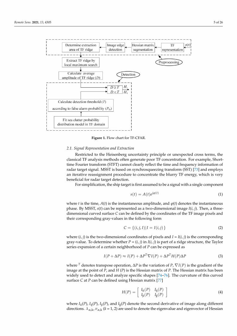
Figure 1 gives a flow chart of signal processing for TF-CFAR, which mainly includessignal representation, ridge extraction, and target detection. The preprocessing part inFigure 1 is to extract the boundary of TF ridge, including TF representation, Hessian matrixsegmentation, and image edge detection. The detection part includes fitting the probabilitydistribution model of sea clutter in the TF plane and calculating the detection threshold Tby Pfa, after which the average energy D of the extracted TF ridge is compared with T todetermine whether a target exists.

Remote Sens. 2021, 13, 4305 5 of 26

Remote Sens. 2021, 13, x FOR PEER REVIEW 5 of 26

tection threshold T by Pfa, after which the average energy D of the extracted TF ridge is compared with T to determine whether a target exists.

Figure 1. Flow chart for TF-CFAR.

2.1. Signal Representation and Extraction Restricted to the Heisenberg uncertainty principle or unexpected cross terms, the

classical TF analysis methods often generate poor TF concentration. For example, Short-time Fourier transform (STFT) cannot clearly reflect the time and frequency in-formation of radar target signal. MSST is based on synchrosqueezing transform (SST) [73] and employs an iterative reassignment procedure to concentrate the blurry TF energy, which is very beneficial for radar target detection.

For simplification, the ship target is first assumed to be a signal with a single com-ponent

)()()( tjetAts ϕ= (1)

where t is the time, A(t) is the instantaneous amplitude, and φ(t) denotes the instanta-neous phase. By MSST, s(t) can be represented as a two-dimensional image I(i, j). Then, a three-dimensional curved surface C can be defined by the coordinates of the TF image pixels and their corresponding gray-values in the following form

}),(,,{ jiIIIjiC == ）（ (2)

where (i, j) is the two-dimensional coordinates of pixels and I = I(i, j) is the corresponding gray-value. To determine whether P = (i, j) in I(i, j) is part of a ridge structure, the Taylor series expansion of a certain neighborhood of P can be expressed as

PPHPPIPPIPPI TT ΔΔ+∇Δ+≈Δ+ )()()()( (3)

where T denotes transpose operation, ΔP is the variation of P, )(PI∇ is the gradient of the image at the point of P, and H (P) is the Hessian matrix of P. The Hessian matrix has been widely used to detect and analyze specific shapes [74–76]. The curvature of this curved surface C at P can be defined using Hessian matrix [77]

= )()(

)()()( PIPIPIPIPH

jjji

ijii (4)

Figure 1. Flow chart for TF-CFAR.

2.1. Signal Representation and Extraction

Restricted to the Heisenberg uncertainty principle or unexpected cross terms, theclassical TF analysis methods often generate poor TF concentration. For example, Short-time Fourier transform (STFT) cannot clearly reflect the time and frequency information ofradar target signal. MSST is based on synchrosqueezing transform (SST) [73] and employsan iterative reassignment procedure to concentrate the blurry TF energy, which is verybeneficial for radar target detection.

For simplification, the ship target is first assumed to be a signal with a single component

s(t) = A(t)ejϕ(t) (1)

where t is the time, A(t) is the instantaneous amplitude, and ϕ(t) denotes the instantaneousphase. By MSST, s(t) can be represented as a two-dimensional image I(i, j). Then, a three-dimensional curved surface C can be defined by the coordinates of the TF image pixels andtheir corresponding gray-values in the following form

C = {(i, j, I)|I = I(i, j)} (2)

where (i, j) is the two-dimensional coordinates of pixels and I = I(i, j) is the correspondinggray-value. To determine whether P = (i, j) in I(i, j) is part of a ridge structure, the Taylorseries expansion of a certain neighborhood of P can be expressed as

I(P + ∆P) ≈ I(P) + ∆PT∇I(P) + ∆PT H(P)∆P (3)

where T denotes transpose operation, ∆P is the variation of P, ∇I(P) is the gradient of theimage at the point of P, and H (P) is the Hessian matrix of P. The Hessian matrix has beenwidely used to detect and analyze specific shapes [74–76]. The curvature of this curvedsurface C at P can be defined using Hessian matrix [77]

H(P) =[

Iii(P) Iij(P)Iji(P) Ijj(P)

](4)

where Iii(P), Iij(P), Iji(P), and Ijj(P) denote the second derivative of image along differentdirections. λα,k, vα,k (k = 1, 2) are used to denote the eigenvalue and eigenvector of Hessian

Remote Sens. 2021, 13, 4305 6 of 26

matrix at scale α, respectively. Assuming |λ1| < |λ2|, from the definition of eigenvalue,we have

vTα,kH(P)vα,k = λα,k (5)

The eigenvalue decomposition of Hessian matrix yields two orthogonal vectors, v1and v2 that are parallel and perpendicular to the TF ridge [78], respectively. In order toreduce noise and smooth the original TF image, a 4-by-4 Gaussian filter g(P, α) with a scaleα = 0.5 is used in this study and its first and second derivatives are denoted as gi, gj, gii,gij, gji and gjj, respectively. Then, these derivatives of the Gaussian filter are convolutedwith each pixel of the TF image to obtain the derivatives of each pixel of the TF image,denoted as Ii(P), Ij(P), Iii (P), Iij (P), Iji (P), and Ijj (P), respectively. The eigenvalue of theHessian matrix with a larger absolute value λ2 and corresponding eigenvector v2 indicatesthe normal direction of TF ridge, denoted as (ni, nj). The gray level of the adjacent pixels ofP can be expressed as

I[(mni + i), (mnj + j)] = I(i, j) + mni Ii(i, j)+mnj Ij(P) + 1

2 m2n2i Ii(P) + 1

2 m2n2j Ij(P)+ ,

m2ninj Iij(P)(6)

Let ∂∂m I[(mni + i), (mnj + j)] = 0, we can obtain

m = −ni Ii + nj Ij

n2i Iii + 2ninj Iij + n2

j Ijj(7)

where the variable m is computed for determining whether the directional derivativevanishes at this pixel or not. If the product of m and v2 is smaller than a threshold p(here, p = 0.5), then the pixel is considered as part of the ridge, otherwise, it is not. Bychecking each pixel, the regions of ridges on a TF image can be identified and marked bythe Hessian matrix.

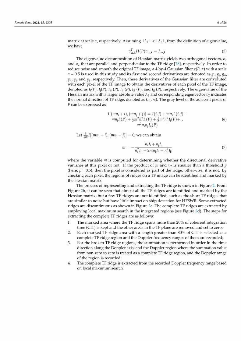
The process of representing and extracting the TF ridge is shown in Figure 2. FromFigure 2b, it can be seen that almost all the TF ridges are identified and marked by theHessian matrix, but a few TF ridges are not identified, such as the short TF ridges thatare similar to noise but have little impact on ship detection for HFSWR. Some extractedridges are discontinuous as shown in Figure 2c. The complete TF ridges are extracted byemploying local maximum search in the integrated regions (see Figure 2d). The steps forextracting the complete TF ridges are as follows:

1. The marked area where the TF ridge spans more than 20% of coherent integrationtime (CIT) is kept and the other areas in the TF plane are removed and set to zero;

2. Each marked TF ridge area with a length greater than 80% of CIT is selected as acomplete TF ridge region and the Doppler frequency ranges of them are recorded;

3. For the broken TF ridge regions, the summation is performed in order in the timedirection along the Doppler axis, and the Doppler region where the summation valuefrom non-zero to zero is treated as a complete TF ridge region, and the Doppler rangeof the region is recorded;

4. The complete TF ridge is extracted from the recorded Doppler frequency range basedon local maximum search.

Remote Sens. 2021, 13, 4305 7 of 26Remote Sens. 2021, 13, x FOR PEER REVIEW 7 of 26

(a) (b)

(c) (d)

Figure 2. Power spectrum, TF image, and ridge extraction of radar signal at 18th range bin at 01:11 on 5 October 2015. (a) power spectrum; (b) the regions of ridges marked by Hessian matrix; (c) the extracted discontinuous TF ridges; (d) the extracted continuous TF ridges.

2.2. Target Detection How to perform CFAR detection based on the extracted TF ridges is important. The

CFAR detectors usually assume a probability distribution model (PDF) of sea clutter for target detection. The amplitude of sea clutter in the TF plane is found to coincide well with a log-normal distribution, which is given by

0 ,21)( 2

2

2)(ln

≥=−−

xex

xfux

σπσ

(8)

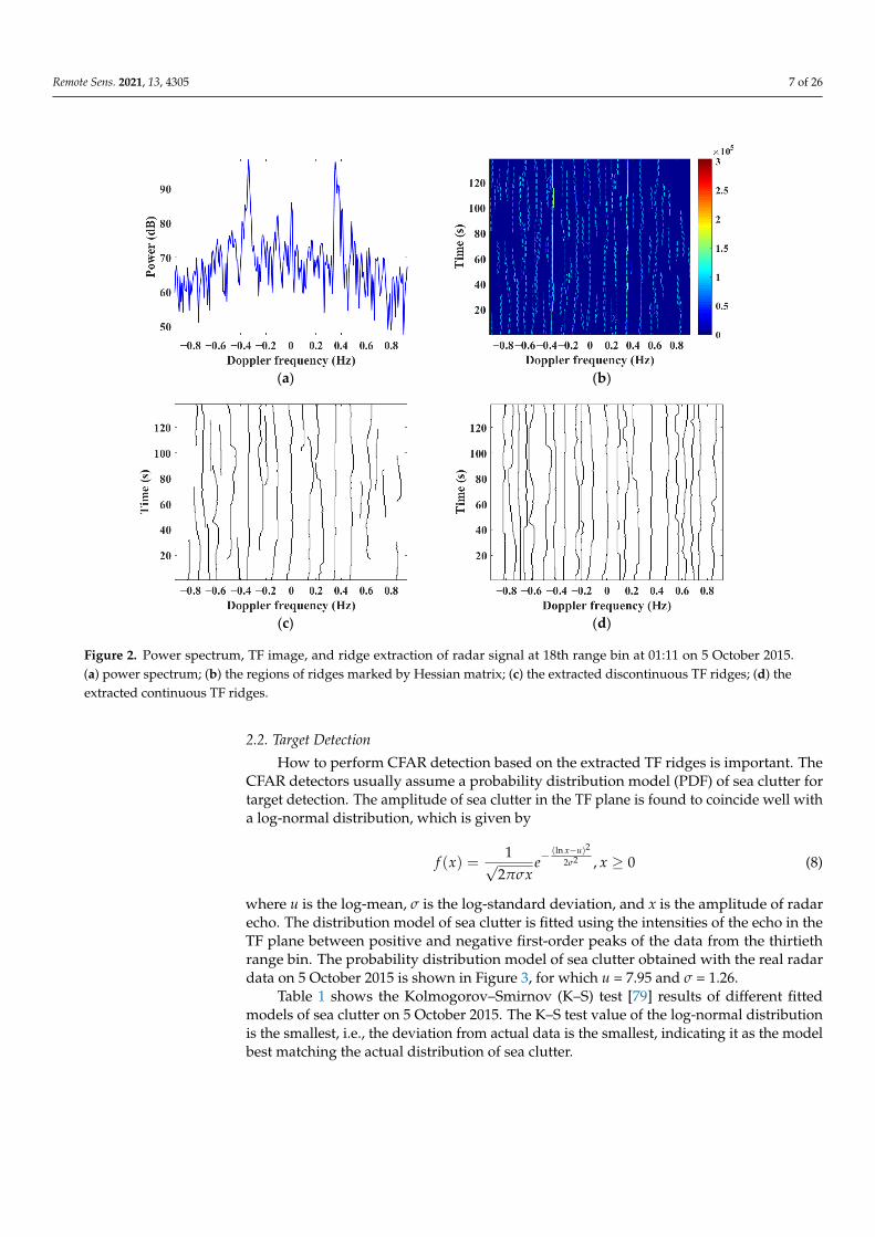
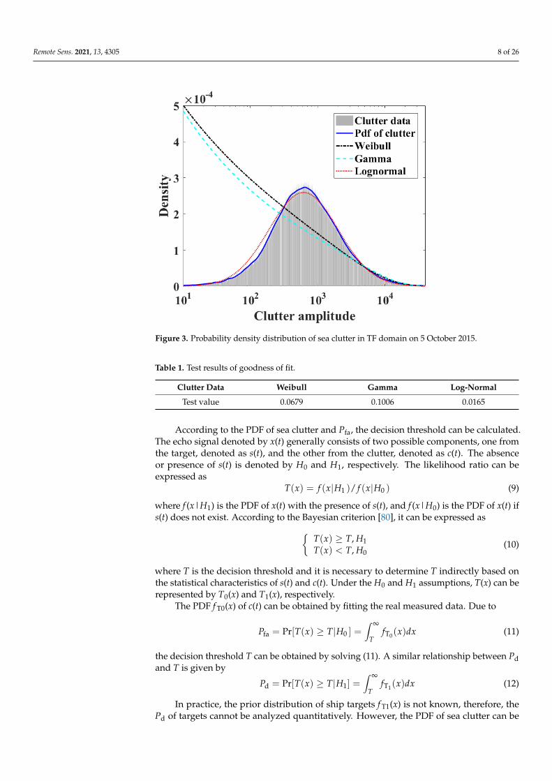
where u is the log-mean, σ is the log-standard deviation, and x is the amplitude of radar echo. The distribution model of sea clutter is fitted using the intensities of the echo in the TF plane between positive and negative first-order peaks of the data from the thirtieth range bin. The probability distribution model of sea clutter obtained with the real radar data on 5 October 2015 is shown in Figure 3, for which u = 7.95 and σ = 1.26.

Figure 2. Power spectrum, TF image, and ridge extraction of radar signal at 18th range bin at 01:11 on 5 October 2015.(a) power spectrum; (b) the regions of ridges marked by Hessian matrix; (c) the extracted discontinuous TF ridges; (d) theextracted continuous TF ridges.

2.2. Target Detection

How to perform CFAR detection based on the extracted TF ridges is important. TheCFAR detectors usually assume a probability distribution model (PDF) of sea clutter fortarget detection. The amplitude of sea clutter in the TF plane is found to coincide well witha log-normal distribution, which is given by

f (x) =1√

2πσxe−

(ln x−u)2

2σ2 , x ≥ 0 (8)

where u is the log-mean, σ is the log-standard deviation, and x is the amplitude of radarecho. The distribution model of sea clutter is fitted using the intensities of the echo in theTF plane between positive and negative first-order peaks of the data from the thirtiethrange bin. The probability distribution model of sea clutter obtained with the real radardata on 5 October 2015 is shown in Figure 3, for which u = 7.95 and σ = 1.26.

Table 1 shows the Kolmogorov–Smirnov (K–S) test [79] results of different fittedmodels of sea clutter on 5 October 2015. The K–S test value of the log-normal distributionis the smallest, i.e., the deviation from actual data is the smallest, indicating it as the modelbest matching the actual distribution of sea clutter.

Remote Sens. 2021, 13, 4305 8 of 26Remote Sens. 2021, 13, x FOR PEER REVIEW 8 of 26

Figure 3. Probability density distribution of sea clutter in TF domain on 5 October 2015.

Table 1 shows the Kolmogorov–Smirnov (K–S) test [79] results of different fitted models of sea clutter on 5 October 2015. The K–S test value of the log-normal distribution is the smallest, i.e., the deviation from actual data is the smallest, indicating it as the model best matching the actual distribution of sea clutter.

Table 1. Test results of goodness of fit.

Clutter Data Weibull Gamma Log-Normal Test value 0.0679 0.1006 0.0165

According to the PDF of sea clutter and Pfa, the decision threshold can be calculated. The echo signal denoted by x(t) generally consists of two possible components, one from the target, denoted as s(t), and the other from the clutter, denoted as c(t). The absence or presence of s(t) is denoted by H0 and H1, respectively. The likelihood ratio can be ex-pressed as

)()()( 01 HxfHxfxT = (9)

where f(x|H1) is the PDF of x(t) with the presence of s(t), and f(x|H0) is the PDF of x(t) if s(t) does not exist. According to the Bayesian criterion [80], it can be expressed as

<≥

01

,)( ,)(HTxTHTxT (10)

where T is the decision threshold and it is necessary to determine T indirectly based on the statistical characteristics of s(t) and c(t). Under the H0 and H1 assumptions, T(x) can be represented by T0(x) and T1(x), respectively.

The PDF fT0(x) of c(t) can be obtained by fitting the real measured data. Due to

dxxfHTxTPT

Tfa ∞

=≥= )(])(Pr[ 00 (11)

the decision threshold T can be obtained by solving (11). A similar relationship between Pd and T is given by

Figure 3. Probability density distribution of sea clutter in TF domain on 5 October 2015.

Table 1. Test results of goodness of fit.

Clutter Data Weibull Gamma Log-Normal

Test value 0.0679 0.1006 0.0165

According to the PDF of sea clutter and Pfa, the decision threshold can be calculated.The echo signal denoted by x(t) generally consists of two possible components, one fromthe target, denoted as s(t), and the other from the clutter, denoted as c(t). The absenceor presence of s(t) is denoted by H0 and H1, respectively. The likelihood ratio can beexpressed as

T(x) = f (x|H1 )/ f (x|H0 ) (9)

where f (x|H1) is the PDF of x(t) with the presence of s(t), and f (x|H0) is the PDF of x(t) ifs(t) does not exist. According to the Bayesian criterion [80], it can be expressed as{

T(x) ≥ T, H1T(x) < T, H0

(10)

where T is the decision threshold and it is necessary to determine T indirectly based onthe statistical characteristics of s(t) and c(t). Under the H0 and H1 assumptions, T(x) can berepresented by T0(x) and T1(x), respectively.

The PDF f T0(x) of c(t) can be obtained by fitting the real measured data. Due to

Pfa = Pr[T(x) ≥ T|H0 ] =∫ ∞

TfT0(x)dx (11)

the decision threshold T can be obtained by solving (11). A similar relationship between Pdand T is given by

Pd = Pr[T(x) ≥ T|H1] =∫ ∞

TfT1(x)dx (12)

In practice, the prior distribution of ship targets f T1(x) is not known, therefore, thePd of targets cannot be analyzed quantitatively. However, the PDF of sea clutter can be

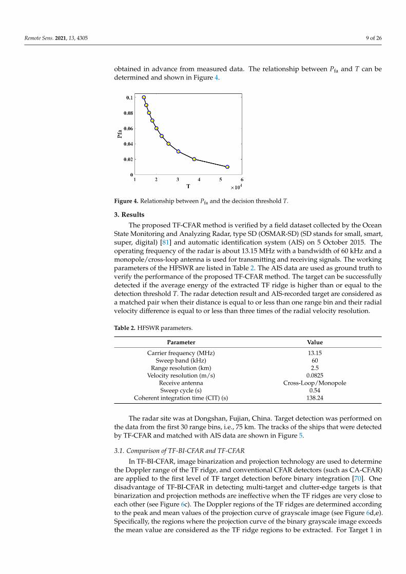
Remote Sens. 2021, 13, 4305 9 of 26

obtained in advance from measured data. The relationship between Pfa and T can bedetermined and shown in Figure 4.

Remote Sens. 2021, 13, x FOR PEER REVIEW 9 of 26

[ ] dxxfHTxTPT

Td ∞

=≥= )(|)(Pr 11 (12)

In practice, the prior distribution of ship targets fT1(x) is not known, therefore, the Pd of targets cannot be analyzed quantitatively. However, the PDF of sea clutter can be ob-tained in advance from measured data. The relationship between Pfa and T can be de-termined and shown in Figure 4.

Figure 4. Relationship between Pfa and the decision threshold T.

3. Results The proposed TF-CFAR method is verified by a field dataset collected by the Ocean

State Monitoring and Analyzing Radar, type SD (OSMAR-SD) (SD stands for small, smart, super, digital) [81] and automatic identification system (AIS) on 5 October 2015. The operating frequency of the radar is about 13.15 MHz with a bandwidth of 60 kHz and a monopole/cross-loop antenna is used for transmitting and receiving signals. The working parameters of the HFSWR are listed in Table 2. The AIS data are used as ground truth to verify the performance of the proposed TF-CFAR method. The target can be successfully detected if the average energy of the extracted TF ridge is higher than or equal to the detection threshold T. The radar detection result and AIS-recorded target are considered as a matched pair when their distance is equal to or less than one range bin and their radial velocity difference is equal to or less than three times of the radial veloc-ity resolution.

Table 2. HFSWR parameters.

Parameter Value Carrier frequency (MHz) 13.15

Sweep band (kHz) 60 Range resolution (km) 2.5

Velocity resolution (m/s) 0.0825 Receive antenna Cross-Loop/Monopole Sweep cycle (s) 0.54

Coherent integration time (CIT) (s) 138.24

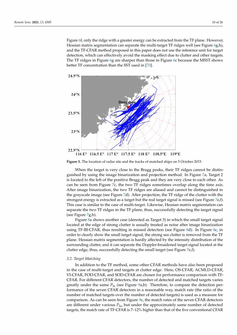
The radar site was at Dongshan, Fujian, China. Target detection was performed on the data from the first 30 range bins, i.e., 75 Km. The tracks of the ships that were detected by TF-CFAR and matched with AIS data are shown in Figure 5.

Figure 4. Relationship between Pfa and the decision threshold T.

3. Results

The proposed TF-CFAR method is verified by a field dataset collected by the OceanState Monitoring and Analyzing Radar, type SD (OSMAR-SD) (SD stands for small, smart,super, digital) [81] and automatic identification system (AIS) on 5 October 2015. Theoperating frequency of the radar is about 13.15 MHz with a bandwidth of 60 kHz and amonopole/cross-loop antenna is used for transmitting and receiving signals. The workingparameters of the HFSWR are listed in Table 2. The AIS data are used as ground truth toverify the performance of the proposed TF-CFAR method. The target can be successfullydetected if the average energy of the extracted TF ridge is higher than or equal to thedetection threshold T. The radar detection result and AIS-recorded target are considered asa matched pair when their distance is equal to or less than one range bin and their radialvelocity difference is equal to or less than three times of the radial velocity resolution.

Table 2. HFSWR parameters.

Parameter Value

Carrier frequency (MHz) 13.15Sweep band (kHz) 60

Range resolution (km) 2.5Velocity resolution (m/s) 0.0825

Receive antenna Cross-Loop/MonopoleSweep cycle (s) 0.54

Coherent integration time (CIT) (s) 138.24

The radar site was at Dongshan, Fujian, China. Target detection was performed onthe data from the first 30 range bins, i.e., 75 km. The tracks of the ships that were detectedby TF-CFAR and matched with AIS data are shown in Figure 5.

3.1. Comparison of TF-BI-CFAR and TF-CFAR

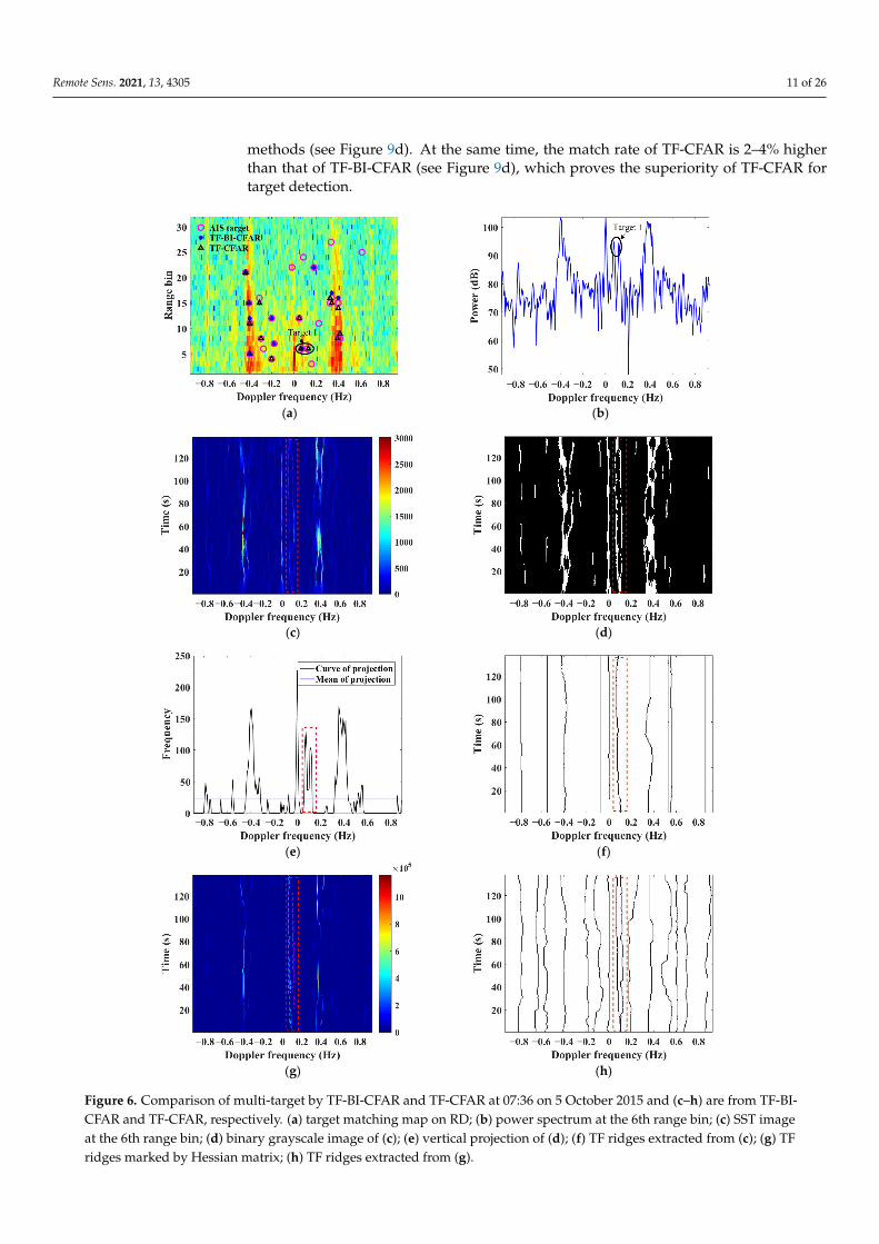
In TF-BI-CFAR, image binarization and projection technology are used to determinethe Doppler range of the TF ridge, and conventional CFAR detectors (such as CA-CFAR)are applied to the first level of TF target detection before binary integration [70]. Onedisadvantage of TF-BI-CFAR in detecting multi-target and clutter-edge targets is thatbinarization and projection methods are ineffective when the TF ridges are very close toeach other (see Figure 6c). The Doppler regions of the TF ridges are determined accordingto the peak and mean values of the projection curve of grayscale image (see Figure 6d,e).Specifically, the regions where the projection curve of the binary grayscale image exceedsthe mean value are considered as the TF ridge regions to be extracted. For Target 1 in

Remote Sens. 2021, 13, 4305 10 of 26

Figure 6f, only the ridge with a greater energy can be extracted from the TF plane. However,Hessian matrix segmentation can separate the multi-target TF ridges well (see Figure 6g,h),and the TF-CFAR method proposed in this paper does not use the reference unit for targetdetection, which can effectively avoid the masking effect due to clutter and other targets.The TF ridges in Figure 6g are sharper than those in Figure 6c because the MSST showsbetter TF concentration than the SST used in [70].

Remote Sens. 2021, 13, x FOR PEER REVIEW 10 of 26

Figure 5. The location of radar site and the tracks of matched ships on 5 October 2015.

3.1. Comparison of TF-BI-CFAR and TF-CFAR In TF-BI-CFAR, image binarization and projection technology are used to determine

the Doppler range of the TF ridge, and conventional CFAR detectors (such as CA-CFAR) are applied to the first level of TF target detection before binary integration [70]. One disadvantage of TF-BI-CFAR in detecting multi-target and clutter-edge targets is that binarization and projection methods are ineffective when the TF ridges are very close to each other (see Figure 6c). The Doppler regions of the TF ridges are determined according to the peak and mean values of the projection curve of grayscale image (see Figure 6d,e). Specifically, the regions where the projection curve of the binary grayscale image exceeds the mean value are considered as the TF ridge regions to be extracted. For Target 1 in Figure 6f, only the ridge with a greater energy can be extracted from the TF plane. However, Hessian matrix segmentation can separate the multi-target TF ridges well (see Figure 6g,h), and the TF-CFAR method proposed in this paper does not use the reference unit for target detection, which can effectively avoid the masking effect due to clutter and other targets. The TF ridges in Figure 6g are sharper than those in Figure 6c because the MSST shows better TF concentration than the SST used in [70].

(a) (b)

Figure 5. The location of radar site and the tracks of matched ships on 5 October 2015.

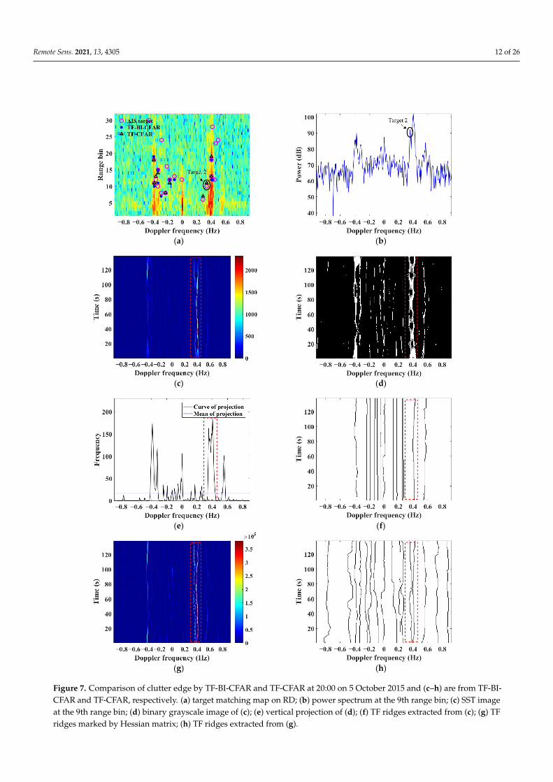
When the target is very close to the Bragg peaks, their TF ridges cannot be distin-guished by using the image binarization and projection method. In Figure 7a, Target 2is located to the left of the positive Bragg peak and they are very close to each other. Ascan be seen from Figure 7c, the two TF ridges sometimes overlap along the time axis.After image binarization, the two TF ridges are aliased and cannot be distinguished inthe grayscale image (see Figure 7d). After projection, the TF ridge of the clutter with thestrongest energy is extracted as a target but the real target signal is missed (see Figure 7e,f).This case is similar to the case of multi-target. Likewise, Hessian matrix segmentation canseparate the two TF ridges in the TF plane, thus, successfully detecting the target signal(see Figure 7g,h).

Figure 8a shows another case (denoted as Target 3) in which the small target signallocated at the edge of strong clutter is usually treated as noise after image binarizationusing TF-BI-CFAR, thus resulting in missed detection (see Figure 8d). In Figure 8c, inorder to clearly show the small target signal, the strong sea clutter is removed from the TFplane. Hessian matrix segmentation is hardly affected by the intensity distribution of thesurrounding clutter, and it can separate the Doppler-broadened target signal located at theclutter edge, thus, successfully detecting the small target (see Figure 7e,f).

3.2. Target Matching

In addition to the TF method, some other CFAR methods have also been proposedin the case of multi-target and targets at clutter edge. Here, OS-CFAR, ACMLD-CFAR,VI-CFAR, FOD-CFAR, and SOD-CFAR are chosen for performance comparison with TF-CFAR. For different CFAR detectors, the number of detected and matched targets variesgreatly under the same Pfa (see Figure 9a,b). Therefore, to compare the detection per-formance of the seven CFAR detectors in a reasonable way, match rate (the ratio of thenumber of matched targets over the number of detected targets) is used as a measure forcomparison. As can be seen from Figure 9c, the match rates of the seven CFAR detectorsare different under various Pfa, but under the approximately same number of detectedtargets, the match rate of TF-CFAR is 7–12% higher than that of the five conventional CFAR

Remote Sens. 2021, 13, 4305 11 of 26

methods (see Figure 9d). At the same time, the match rate of TF-CFAR is 2–4% higherthan that of TF-BI-CFAR (see Figure 9d), which proves the superiority of TF-CFAR fortarget detection.

Remote Sens. 2021, 13, x FOR PEER REVIEW 10 of 26

Figure 5. The location of radar site and the tracks of matched ships on 5 October 2015.

3.1. Comparison of TF-BI-CFAR and TF-CFAR In TF-BI-CFAR, image binarization and projection technology are used to determine

the Doppler range of the TF ridge, and conventional CFAR detectors (such as CA-CFAR) are applied to the first level of TF target detection before binary integration [70]. One disadvantage of TF-BI-CFAR in detecting multi-target and clutter-edge targets is that binarization and projection methods are ineffective when the TF ridges are very close to each other (see Figure 6c). The Doppler regions of the TF ridges are determined according to the peak and mean values of the projection curve of grayscale image (see Figure 6d,e). Specifically, the regions where the projection curve of the binary grayscale image exceeds the mean value are considered as the TF ridge regions to be extracted. For Target 1 in Figure 6f, only the ridge with a greater energy can be extracted from the TF plane. However, Hessian matrix segmentation can separate the multi-target TF ridges well (see Figure 6g,h), and the TF-CFAR method proposed in this paper does not use the reference unit for target detection, which can effectively avoid the masking effect due to clutter and other targets. The TF ridges in Figure 6g are sharper than those in Figure 6c because the MSST shows better TF concentration than the SST used in [70].

(a) (b)

Remote Sens. 2021, 13, x FOR PEER REVIEW 11 of 26

(c) (d)

(e) (f)

(g) (h)

Figure 6. Comparison of multi-target by TF-BI-CFAR and TF-CFAR at 07:36 on 5 October 2015 and (c–h) are from TF-BI-CFAR and TF-CFAR, respectively. (a) target matching map on RD; (b) power spectrum at the 6th range bin; (c) SST image at the 6th range bin; (d) binary grayscale image of (c); (e) vertical projection of (d); (f) TF ridges extracted from (c); (g) TF ridges marked by Hessian matrix; (h) TF ridges extracted from (g).

When the target is very close to the Bragg peaks, their TF ridges cannot be distin-guished by using the image binarization and projection method. In Figure 7a, Target 2 is located to the left of the positive Bragg peak and they are very close to each other. As can be seen from Figure 7c, the two TF ridges sometimes overlap along the time axis. After image binarization, the two TF ridges are aliased and cannot be distinguished in the grayscale image (see Figure 7d). After projection, the TF ridge of the clutter with the strongest energy is extracted as a target but the real target signal is missed (see Figure 7e,f). This case is similar to the case of multi-target. Likewise, Hessian matrix segmenta-tion can separate the two TF ridges in the TF plane, thus, successfully detecting the target signal (see Figure 7g,h).

Figure 6. Comparison of multi-target by TF-BI-CFAR and TF-CFAR at 07:36 on 5 October 2015 and (c–h) are from TF-BI-CFAR and TF-CFAR, respectively. (a) target matching map on RD; (b) power spectrum at the 6th range bin; (c) SST imageat the 6th range bin; (d) binary grayscale image of (c); (e) vertical projection of (d); (f) TF ridges extracted from (c); (g) TFridges marked by Hessian matrix; (h) TF ridges extracted from (g).

Remote Sens. 2021, 13, 4305 12 of 26

Remote Sens. 2021, 13, x FOR PEER REVIEW 12 of 26

(a) (b)

(c) (d)

(e) (f)

(g) (h)

Figure 7. Comparison of clutter edge by TF-BI-CFAR and TF-CFAR at 20:00 on 5 October 2015 and (c–h) are from TF-BI-CFAR and TF-CFAR, respectively. (a) target matching map on RD; (b) power spectrum at the 9th range bin; (c)

Figure 7. Comparison of clutter edge by TF-BI-CFAR and TF-CFAR at 20:00 on 5 October 2015 and (c–h) are from TF-BI-CFAR and TF-CFAR, respectively. (a) target matching map on RD; (b) power spectrum at the 9th range bin; (c) SST imageat the 9th range bin; (d) binary grayscale image of (c); (e) vertical projection of (d); (f) TF ridges extracted from (c); (g) TFridges marked by Hessian matrix; (h) TF ridges extracted from (g).

Remote Sens. 2021, 13, 4305 13 of 26

Remote Sens. 2021, 13, x FOR PEER REVIEW 13 of 26

SST image at the 9th range bin; (d) binary grayscale image of (c); (e) vertical projection of (d); (f) TF ridges extracted from (c); (g) TF ridges marked by Hessian matrix; (h) TF ridges extracted from (g).

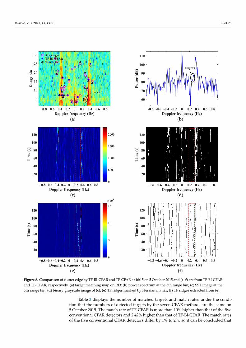
Figure 8a shows another case (denoted as Target 3) in which the small target signal located at the edge of strong clutter is usually treated as noise after image binarization using TF-BI-CFAR, thus resulting in missed detection (see Figure 8d). In Figure 8c, in order to clearly show the small target signal, the strong sea clutter is removed from the TF plane. Hessian matrix segmentation is hardly affected by the intensity distribution of the surrounding clutter, and it can separate the Doppler-broadened target signal located at the clutter edge, thus, successfully detecting the small target (see Figure 7e,f).

(a) (b)

(c) (d)

(e) (f)

Figure 8. Comparison of clutter edge by TF-BI-CFAR and TF-CFAR at 16:15 on 5 October 2015 and (c–f) are from TF-BI-CFAR and TF-CFAR, respectively. (a) target matching map on RD; (b) power spectrum at the 5th range bin; (c) SST image at the 5th range bin; (d) binary grayscale image of (c); (e) TF ridges marked by Hessian matrix; (f) TF ridges extracted from (e).

Figure 8. Comparison of clutter edge by TF-BI-CFAR and TF-CFAR at 16:15 on 5 October 2015 and (c–f) are from TF-BI-CFARand TF-CFAR, respectively. (a) target matching map on RD; (b) power spectrum at the 5th range bin; (c) SST image at the5th range bin; (d) binary grayscale image of (c); (e) TF ridges marked by Hessian matrix; (f) TF ridges extracted from (e).

Table 3 displays the number of matched targets and match rates under the condi-tion that the numbers of detected targets by the seven CFAR methods are the same on5 October 2015. The match rate of TF-CFAR is more than 10% higher than that of the fiveconventional CFAR detectors and 2.42% higher than that of TF-BI-CFAR. The match ratesof the five conventional CFAR detectors differ by 1% to 2%, so it can be concluded that

Remote Sens. 2021, 13, 4305 14 of 26

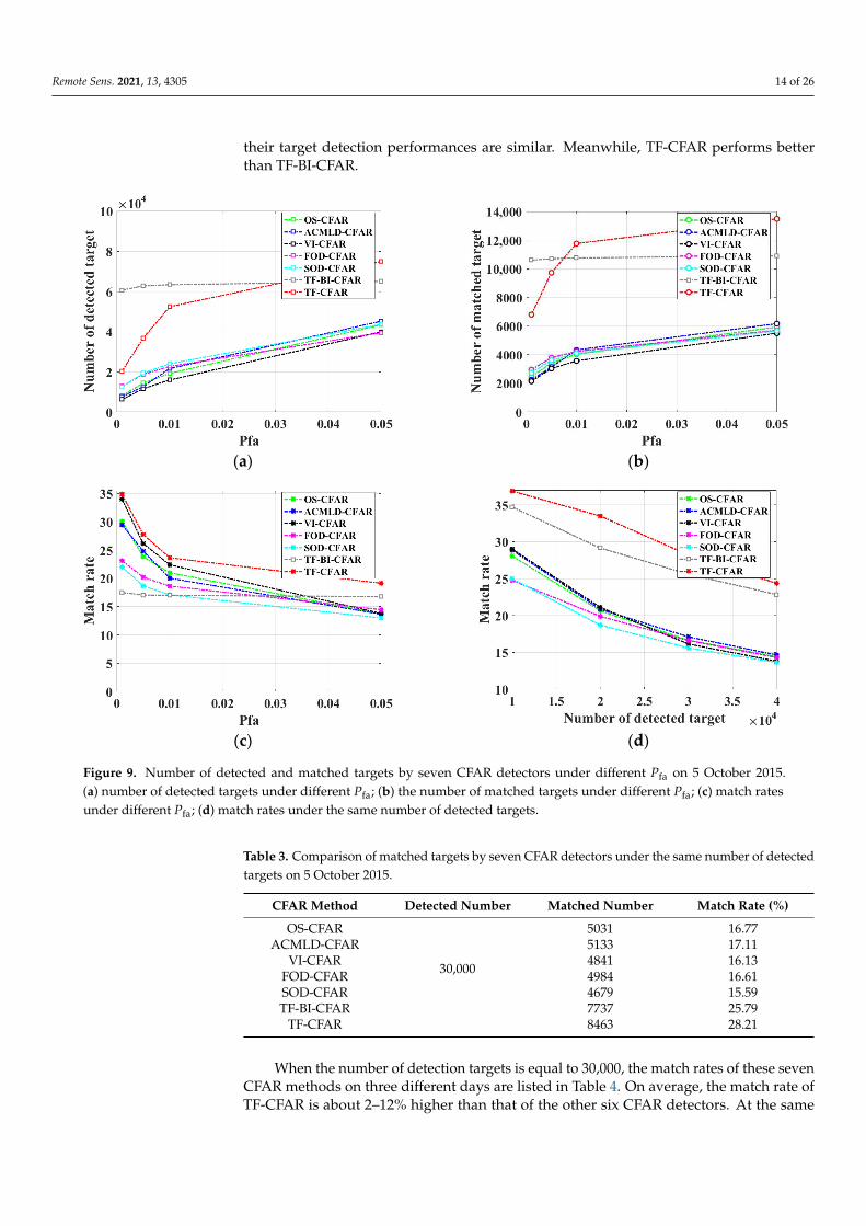
their target detection performances are similar. Meanwhile, TF-CFAR performs betterthan TF-BI-CFAR.

Remote Sens. 2021, 13, x FOR PEER REVIEW 14 of 26

3.2. Target Matching In addition to the TF method, some other CFAR methods have also been proposed

in the case of multi-target and targets at clutter edge. Here, OS-CFAR, ACMLD-CFAR, VI-CFAR, FOD-CFAR, and SOD-CFAR are chosen for performance comparison with TF-CFAR. For different CFAR detectors, the number of detected and matched targets varies greatly under the same Pfa (see Figure 9a,b). Therefore, to compare the detection performance of the seven CFAR detectors in a reasonable way, match rate (the ratio of the number of matched targets over the number of detected targets) is used as a measure for comparison. As can be seen from Figure 9c, the match rates of the seven CFAR detectors are different under various Pfa, but under the approximately same number of detected targets, the match rate of TF-CFAR is 7–12% higher than that of the five conventional CFAR methods (see Figure 9d). At the same time, the match rate of TF-CFAR is 2–4% higher than that of TF-BI-CFAR (see Figure 9d), which proves the superiority of TF-CFAR for target detection.

Table 3 displays the number of matched targets and match rates under the condition that the numbers of detected targets by the seven CFAR methods are the same on 5 Oc-tober 2015. The match rate of TF-CFAR is more than 10% higher than that of the five conventional CFAR detectors and 2.42% higher than that of TF-BI-CFAR. The match rates of the five conventional CFAR detectors differ by 1% to 2%, so it can be concluded that their target detection performances are similar. Meanwhile, TF-CFAR performs better than TF-BI-CFAR.

(a) (b)

(c) (d)

Figure 9. Number of detected and matched targets by seven CFAR detectors under different Pfa on 5 October 2015. (a) number of detected targets under different Pfa; (b) the number of matched targets under different Pfa; (c) match rates under different Pfa; (d) match rates under the same number of detected targets.

Figure 9. Number of detected and matched targets by seven CFAR detectors under different Pfa on 5 October 2015.(a) number of detected targets under different Pfa; (b) the number of matched targets under different Pfa; (c) match ratesunder different Pfa; (d) match rates under the same number of detected targets.

Table 3. Comparison of matched targets by seven CFAR detectors under the same number of detectedtargets on 5 October 2015.

CFAR Method Detected Number Matched Number Match Rate (%)

OS-CFAR

30,000

5031 16.77ACMLD-CFAR 5133 17.11

VI-CFAR 4841 16.13FOD-CFAR 4984 16.61SOD-CFAR 4679 15.59TF-BI-CFAR 7737 25.79

TF-CFAR 8463 28.21

When the number of detection targets is equal to 30,000, the match rates of these sevenCFAR methods on three different days are listed in Table 4. On average, the match rate ofTF-CFAR is about 2–12% higher than that of the other six CFAR detectors. At the same

Remote Sens. 2021, 13, 4305 15 of 26

time, it can be seen that the match rate on 29 September is 3–7% higher than that of theother two days because the radar data on October 4 and 5 were seriously contaminated.

Table 4. Comparison of match rates by seven CFAR detectors under the same number of detectedtargets in three days.

Time (Month/Day) 09/29 10/04 10/05

CFAR Method Detected Number Match Rate (%)

OS-CFAR

30,000

22.39 18.07 16.77ACMLD-CFAR 22.71 18.21 17.11

VI-CFAR 21.28 17.68 16.13FOD-CFAR 21.95 17.40 16.61SOD-CFAR 20.88 16.67 15.59TF-BI-CFAR 33.67 29.55 25.79

TF-CFAR 35.55 32.47 28.21

3.3. Comparison of Conventional CFAR and TF-CFAR

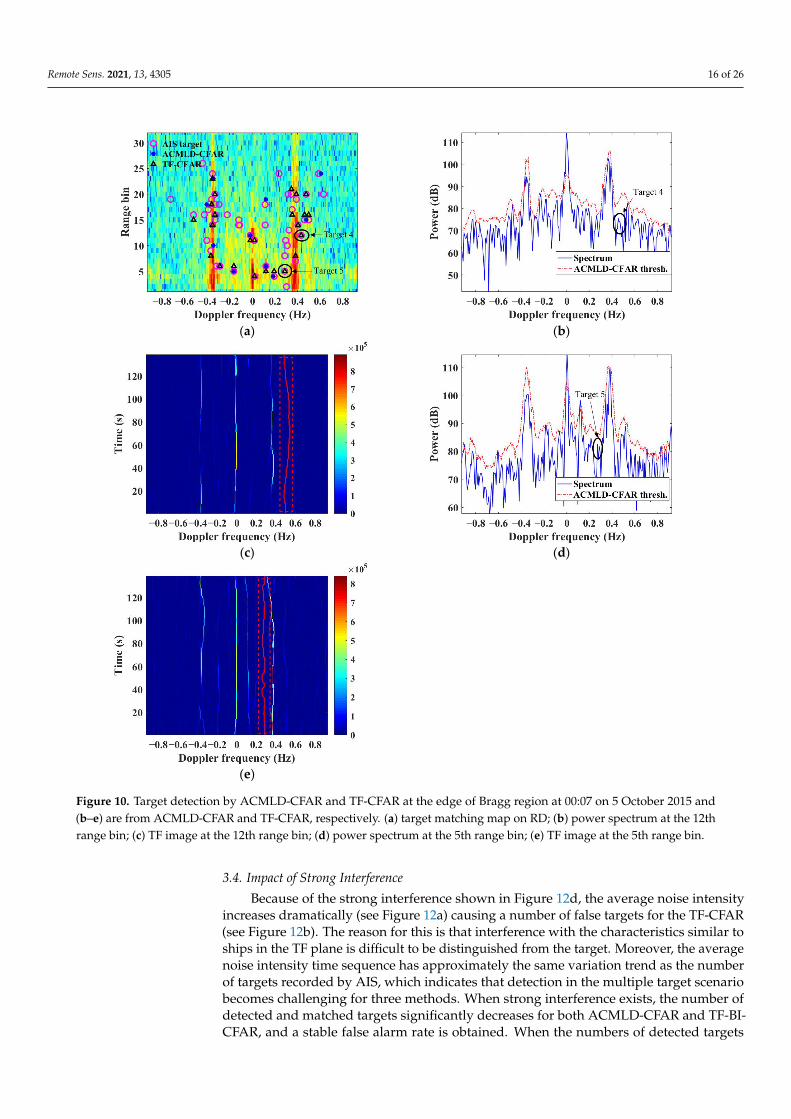
When the number of detected targets was 30,000, ACMLD-CFAR and TF-CFAR wereused to demonstrate the detection performance difference for clutter-edge and multi-targetscenarios. As mentioned earlier, the masking phenomenon occurs when the target fallsin the Doppler region around the Bragg peaks (see Figure 10a), thus, missed detectionhappens. In Figure 10a, the echo of Target 4 appears between two relatively strongerclutters causing it to be masked by sea clutter and interference (see Figure 10b). In this case,it is quite difficult to detect the target on a single range-Doppler bin, while the TF ridgeof the target is extracted successfully (as shown in Figure 10c). Target 5 is on the left tothe positive first-order peak, and its power intensity is lower than the sea clutter aroundit (see Figure 10d). TF-CFAR successfully detects Target 5 (see Figure 10e) but ACMLD-CFAR fails. When the background clutter or interference becomes stronger, ACMLD-CFARtends to miss the target due to the increased detection threshold. However, the use of TFcharacteristics helps TF-CFAR reduce the clutter or interference to some extent, which is anadvantage of TF-CFAR.

In the case of multi-target scenarios, when the large and small targets appear onadjacent Doppler bins at the same time (see Figure 11a,d), the large target whose spectralintensity is strong as clutter or interference tends to mask the small target and cause misseddetection (see Figure 11b,e). Figure 11b displays an example of two targets’ (Target 6)detection. From the power spectrum, it can be seen that the large target on the right sideraises the detection threshold for the small target on the left side, resulting in misseddetection of the small target. However, the TF-CFAR method can successfully separateand detect the large target and the small target even though their Doppler frequenciesare similar (see Figure 11c). Figure 11d shows another example of a multi-target case thatinvolves three targets’ (Target 7) detection. It can be found that the spectral intensity ofthe left target is the highest, the right target is the lowest, and the middle target is thesecond highest in Figure 11e. Only the target with the strongest energy is detected byACMLD-CFAR, and the other two small targets are missed. However, the TF-CFAR methodcan successfully distinguish the Doppler frequencies of the three targets (see Figure 11f) torecognize them.

Remote Sens. 2021, 13, 4305 16 of 26Remote Sens. 2021, 13, x FOR PEER REVIEW 16 of 26

(a) (b)

(c) (d)

(e)

Figure 10. Target detection by ACMLD-CFAR and TF-CFAR at the edge of Bragg region at 00:07 on 5 October 2015 and (b–e) are from ACMLD-CFAR and TF-CFAR, respectively. (a) target matching map on RD; (b) power spectrum at the 12th range bin; (c) TF image at the 12th range bin; (d) power spectrum at the 5th range bin; (e) TF image at the 5th range bin.

In the case of multi-target scenarios, when the large and small targets appear on adjacent Doppler bins at the same time (see Figure 11a,d), the large target whose spectral intensity is strong as clutter or interference tends to mask the small target and cause missed detection (see Figure 11b,e). Figure 11b displays an example of two targets’ (Target 6) detection. From the power spectrum, it can be seen that the large target on the right side raises the detection threshold for the small target on the left side, resulting in missed detection of the small target. However, the TF-CFAR method can successfully separate and detect the large target and the small target even though their Doppler fre-quencies are similar (see Figure 11c). Figure 11d shows another example of a multi-target case that involves three targets’ (Target 7) detection. It can be found that the spectral in-

Figure 10. Target detection by ACMLD-CFAR and TF-CFAR at the edge of Bragg region at 00:07 on 5 October 2015 and(b–e) are from ACMLD-CFAR and TF-CFAR, respectively. (a) target matching map on RD; (b) power spectrum at the 12thrange bin; (c) TF image at the 12th range bin; (d) power spectrum at the 5th range bin; (e) TF image at the 5th range bin.

3.4. Impact of Strong Interference

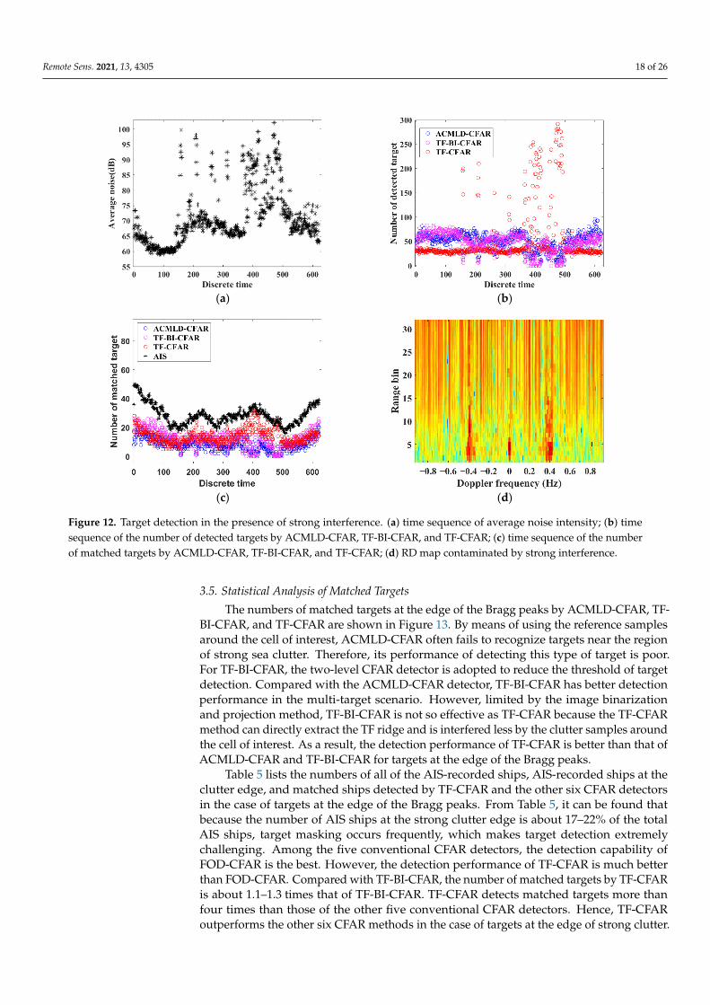
Because of the strong interference shown in Figure 12d, the average noise intensityincreases dramatically (see Figure 12a) causing a number of false targets for the TF-CFAR(see Figure 12b). The reason for this is that interference with the characteristics similar toships in the TF plane is difficult to be distinguished from the target. Moreover, the averagenoise intensity time sequence has approximately the same variation trend as the numberof targets recorded by AIS, which indicates that detection in the multiple target scenariobecomes challenging for three methods. When strong interference exists, the number ofdetected and matched targets significantly decreases for both ACMLD-CFAR and TF-BI-CFAR, and a stable false alarm rate is obtained. When the numbers of detected targets

Remote Sens. 2021, 13, 4305 17 of 26

by ACMLD-CFAR, TF-BI-CFAR, and TF-CFAR are all 30,000, the number of matchedtargets is 8463, 7737, and 5133, respectively. The number of matched targets detectedby TF-CFAR is 1.64 and 1.09 times more than that by ACMLD-CFAR and TF-BI-CFAR,respectively. When TF-CFAR is applied to target detection under strong interference, manyinterferences are identified as target signals because they appear as TF ridges with energyabove the detection thresholds. This scenario should be avoided for three detectors wherea preprocessing of interference suppression is required.

Remote Sens. 2021, 13, x FOR PEER REVIEW 17 of 26

tensity of the left target is the highest, the right target is the lowest, and the middle target is the second highest in Figure 11e. Only the target with the strongest energy is detected by ACMLD-CFAR, and the other two small targets are missed. However, the TF-CFAR method can successfully distinguish the Doppler frequencies of the three targets (see Figure 11f) to recognize them.

(a) (b)

(c) (d)

(e) (f)

Figure 11. Multi-target detection by ACMLD-CFAR and TF-CFAR at 04:02 and 02:32 on 5 October 2015 and (b,c,e,f) are from ACMLD-CFAR and TF-CFAR, respectively. (a) target matching map on RD; (b) power spectrum at the 5th range bin; (c) TF image at the 5th range bin; (d) target matching map on RD; (e) power spectrum at the 6th range bin; (f) TF image at the 6th range bin.

3.4. Impact of Strong Interference Because of the strong interference shown in Figure 12d, the average noise intensity

increases dramatically (see Figure 12a) causing a number of false targets for the TF-CFAR (see Figure 12b). The reason for this is that interference with the characteristics similar to

Figure 11. Multi-target detection by ACMLD-CFAR and TF-CFAR at 04:02 and 02:32 on 5 October 2015 and (b,c,e,f) arefrom ACMLD-CFAR and TF-CFAR, respectively. (a) target matching map on RD; (b) power spectrum at the 5th range bin;(c) TF image at the 5th range bin; (d) target matching map on RD; (e) power spectrum at the 6th range bin; (f) TF image atthe 6th range bin.

Remote Sens. 2021, 13, 4305 18 of 26

Remote Sens. 2021, 13, x FOR PEER REVIEW 18 of 26

ships in the TF plane is difficult to be distinguished from the target. Moreover, the aver-age noise intensity time sequence has approximately the same variation trend as the number of targets recorded by AIS, which indicates that detection in the multiple target scenario becomes challenging for three methods. When strong interference exists, the number of detected and matched targets significantly decreases for both ACMLD-CFAR and TF-BI-CFAR, and a stable false alarm rate is obtained. When the numbers of detected targets by ACMLD-CFAR, TF-BI-CFAR, and TF-CFAR are all 30,000, the number of matched targets is 8463, 7737, and 5133, respectively. The number of matched targets detected by TF-CFAR is 1.64 and 1.09 times more than that by ACMLD-CFAR and TF-BI-CFAR, respectively. When TF-CFAR is applied to target detection under strong interference, many interferences are identified as target signals because they appear as TF ridges with energy above the detection thresholds. This scenario should be avoided for three detectors where a preprocessing of interference suppression is required.

(a) (b)

(c) (d)

Figure 12. Target detection in the presence of strong interference. (a) time sequence of average noise intensity; (b) time sequence of the number of detected targets by ACMLD-CFAR, TF-BI-CFAR, and TF-CFAR; (c) time sequence of the number of matched targets by ACMLD-CFAR, TF-BI-CFAR, and TF-CFAR; (d) RD map contaminated by strong inter-ference.

3.5. Statistical Analysis of Matched Targets The numbers of matched targets at the edge of the Bragg peaks by ACMLD-CFAR,

TF-BI-CFAR, and TF-CFAR are shown in Figure 13. By means of using the reference samples around the cell of interest, ACMLD-CFAR often fails to recognize targets near the region of strong sea clutter. Therefore, its performance of detecting this type of target is poor. For TF-BI-CFAR, the two-level CFAR detector is adopted to reduce the threshold of target detection. Compared with the ACMLD-CFAR detector, TF-BI-CFAR has better detection performance in the multi-target scenario. However, limited by the image bina-rization and projection method, TF-BI-CFAR is not so effective as TF-CFAR because the

Figure 12. Target detection in the presence of strong interference. (a) time sequence of average noise intensity; (b) timesequence of the number of detected targets by ACMLD-CFAR, TF-BI-CFAR, and TF-CFAR; (c) time sequence of the numberof matched targets by ACMLD-CFAR, TF-BI-CFAR, and TF-CFAR; (d) RD map contaminated by strong interference.

3.5. Statistical Analysis of Matched Targets

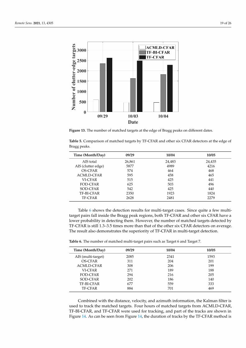
The numbers of matched targets at the edge of the Bragg peaks by ACMLD-CFAR, TF-BI-CFAR, and TF-CFAR are shown in Figure 13. By means of using the reference samplesaround the cell of interest, ACMLD-CFAR often fails to recognize targets near the regionof strong sea clutter. Therefore, its performance of detecting this type of target is poor.For TF-BI-CFAR, the two-level CFAR detector is adopted to reduce the threshold of targetdetection. Compared with the ACMLD-CFAR detector, TF-BI-CFAR has better detectionperformance in the multi-target scenario. However, limited by the image binarizationand projection method, TF-BI-CFAR is not so effective as TF-CFAR because the TF-CFARmethod can directly extract the TF ridge and is interfered less by the clutter samples aroundthe cell of interest. As a result, the detection performance of TF-CFAR is better than that ofACMLD-CFAR and TF-BI-CFAR for targets at the edge of the Bragg peaks.

Table 5 lists the numbers of all of the AIS-recorded ships, AIS-recorded ships at theclutter edge, and matched ships detected by TF-CFAR and the other six CFAR detectorsin the case of targets at the edge of the Bragg peaks. From Table 5, it can be found thatbecause the number of AIS ships at the strong clutter edge is about 17–22% of the totalAIS ships, target masking occurs frequently, which makes target detection extremelychallenging. Among the five conventional CFAR detectors, the detection capability ofFOD-CFAR is the best. However, the detection performance of TF-CFAR is much betterthan FOD-CFAR. Compared with TF-BI-CFAR, the number of matched targets by TF-CFARis about 1.1–1.3 times that of TF-BI-CFAR. TF-CFAR detects matched targets more thanfour times than those of the other five conventional CFAR detectors. Hence, TF-CFARoutperforms the other six CFAR methods in the case of targets at the edge of strong clutter.

Remote Sens. 2021, 13, 4305 19 of 26

Remote Sens. 2021, 13, x FOR PEER REVIEW 19 of 26

TF-CFAR method can directly extract the TF ridge and is interfered less by the clutter samples around the cell of interest. As a result, the detection performance of TF-CFAR is better than that of ACMLD-CFAR and TF-BI-CFAR for targets at the edge of the Bragg peaks.

Figure 13. The number of matched targets at the edge of Bragg peaks on different dates.

Table 5 lists the numbers of all of the AIS-recorded ships, AIS-recorded ships at the clutter edge, and matched ships detected by TF-CFAR and the other six CFAR detectors in the case of targets at the edge of the Bragg peaks. From Table 5, it can be found that because the number of AIS ships at the strong clutter edge is about 17–22% of the total AIS ships, target masking occurs frequently, which makes target detection extremely challenging. Among the five conventional CFAR detectors, the detection capability of FOD-CFAR is the best. However, the detection performance of TF-CFAR is much better than FOD-CFAR. Compared with TF-BI-CFAR, the number of matched targets by TF-CFAR is about 1.1–1.3 times that of TF-BI-CFAR. TF-CFAR detects matched targets more than four times than those of the other five conventional CFAR detectors. Hence, TF-CFAR outperforms the other six CFAR methods in the case of targets at the edge of strong clutter.

Table 5. Comparison of matched targets by TF-CFAR and other six CFAR detectors at the edge of Bragg peaks.

Time (Month/Day) 09/29 10/04 10/05 AIS total 26,861 24,483 24,435

AIS (clutter edge) 5877 4989 4216 OS-CFAR 574 464 468

ACMLD-CFAR 595 458 465 VI-CFAR 515 425 441

FOD-CFAR 625 503 496 SOD-CFAR 542 425 440 TF-BI-CFAR 2350 1923 1824

TF-CFAR 2628 2481 2279

Table 6 shows the detection results for multi-target cases. Since quite a few mul-ti-target pairs fall inside the Bragg peak regions, both TF-CFAR and other six CFAR have a lower probability in detecting them. However, the number of matched targets detected

Figure 13. The number of matched targets at the edge of Bragg peaks on different dates.

Table 5. Comparison of matched targets by TF-CFAR and other six CFAR detectors at the edge ofBragg peaks.

Time (Month/Day) 09/29 10/04 10/05

AIS total 26,861 24,483 24,435AIS (clutter edge) 5877 4989 4216

OS-CFAR 574 464 468ACMLD-CFAR 595 458 465

VI-CFAR 515 425 441FOD-CFAR 625 503 496SOD-CFAR 542 425 440TF-BI-CFAR 2350 1923 1824

TF-CFAR 2628 2481 2279

Table 6 shows the detection results for multi-target cases. Since quite a few multi-target pairs fall inside the Bragg peak regions, both TF-CFAR and other six CFAR have alower probability in detecting them. However, the number of matched targets detected byTF-CFAR is still 1.3–3.5 times more than that of the other six CFAR detectors on average.The result also demonstrates the superiority of TF-CFAR in multi-target detection.

Table 6. The number of matched multi-target pairs such as Target 6 and Target 7.

Time (Month/Day) 09/29 10/04 10/05

AIS (multi-target) 2085 2341 1593OS-CFAR 311 204 201

ACMLD-CFAR 308 206 199VI-CFAR 271 189 188

FOD-CFAR 294 216 205SOD-CFAR 202 186 140TF-BI-CFAR 677 559 333

TF-CFAR 884 701 469

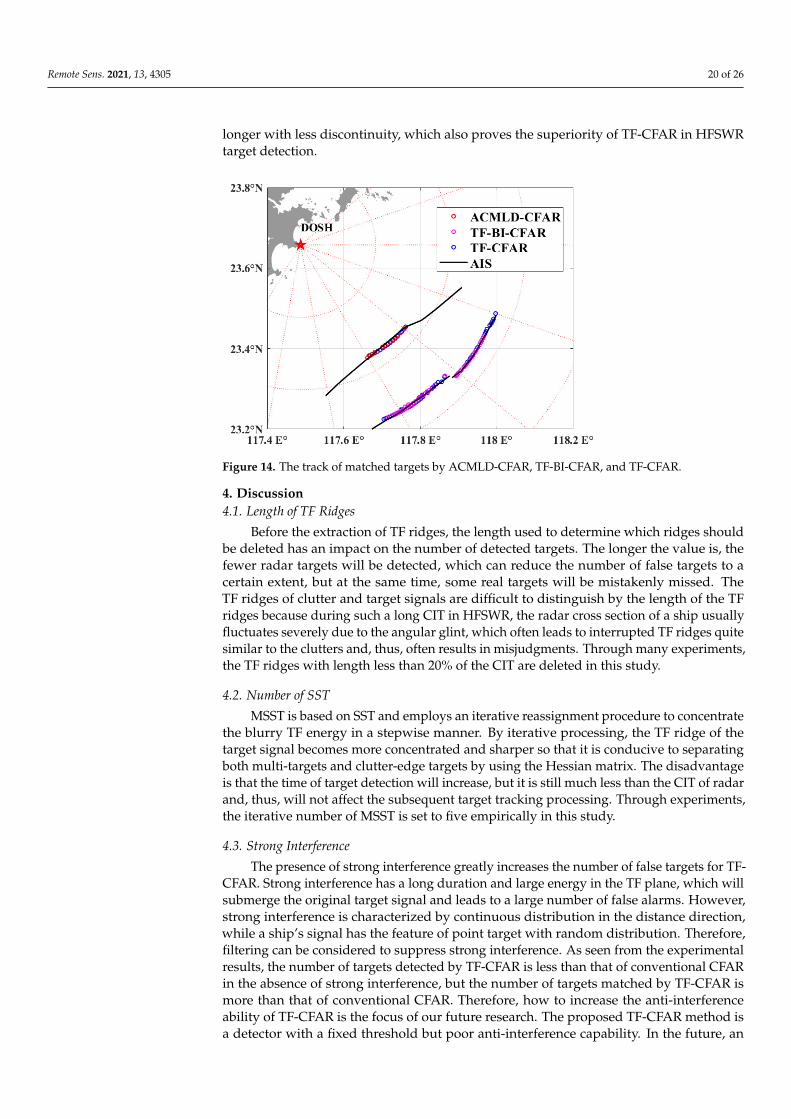
Combined with the distance, velocity, and azimuth information, the Kalman filter isused to track the matched targets. Four hours of matched targets from ACMLD-CFAR,TF-BI-CFAR, and TF-CFAR were used for tracking, and part of the tracks are shown inFigure 14. As can be seen from Figure 14, the duration of tracks by the TF-CFAR method is

Remote Sens. 2021, 13, 4305 20 of 26

longer with less discontinuity, which also proves the superiority of TF-CFAR in HFSWRtarget detection.

Remote Sens. 2021, 13, x FOR PEER REVIEW 20 of 26

by TF-CFAR is still 1.3–3.5 times more than that of the other six CFAR detectors on av-erage. The result also demonstrates the superiority of TF-CFAR in multi-target detection.

Table 6. The number of matched multi-target pairs such as Target 6 and Target 7.

Time (Month/Day) 09/29 10/04 10/05 AIS (multi-target) 2085 2341 1593

OS-CFAR 311 204 201 ACMLD-CFAR 308 206 199

VI-CFAR 271 189 188 FOD-CFAR 294 216 205 SOD-CFAR 202 186 140 TF-BI-CFAR 677 559 333

TF-CFAR 884 701 469

Combined with the distance, velocity, and azimuth information, the Kalman filter is used to track the matched targets. Four hours of matched targets from ACMLD-CFAR, TF-BI-CFAR, and TF-CFAR were used for tracking, and part of the tracks are shown in Figure 14. As can be seen from Figure 14, the duration of tracks by the TF-CFAR method is longer with less discontinuity, which also proves the superiority of TF-CFAR in HFSWR target detection.

Figure 14. The track of matched targets by ACMLD-CFAR, TF-BI-CFAR, and TF-CFAR.

4. Discussion 4.1. Length of TF Ridges

Before the extraction of TF ridges, the length used to determine which ridges should be deleted has an impact on the number of detected targets. The longer the value is, the fewer radar targets will be detected, which can reduce the number of false targets to a certain extent, but at the same time, some real targets will be mistakenly missed. The TF ridges of clutter and target signals are difficult to distinguish by the length of the TF ridges because during such a long CIT in HFSWR, the radar cross section of a ship usu-ally fluctuates severely due to the angular glint, which often leads to interrupted TF ridges quite similar to the clutters and, thus, often results in misjudgments. Through many experiments, the TF ridges with length less than 20% of the CIT are deleted in this study.

Figure 14. The track of matched targets by ACMLD-CFAR, TF-BI-CFAR, and TF-CFAR.

4. Discussion4.1. Length of TF Ridges

Before the extraction of TF ridges, the length used to determine which ridges shouldbe deleted has an impact on the number of detected targets. The longer the value is, thefewer radar targets will be detected, which can reduce the number of false targets to acertain extent, but at the same time, some real targets will be mistakenly missed. TheTF ridges of clutter and target signals are difficult to distinguish by the length of the TFridges because during such a long CIT in HFSWR, the radar cross section of a ship usuallyfluctuates severely due to the angular glint, which often leads to interrupted TF ridges quitesimilar to the clutters and, thus, often results in misjudgments. Through many experiments,the TF ridges with length less than 20% of the CIT are deleted in this study.

4.2. Number of SST

MSST is based on SST and employs an iterative reassignment procedure to concentratethe blurry TF energy in a stepwise manner. By iterative processing, the TF ridge of thetarget signal becomes more concentrated and sharper so that it is conducive to separatingboth multi-targets and clutter-edge targets by using the Hessian matrix. The disadvantageis that the time of target detection will increase, but it is still much less than the CIT of radarand, thus, will not affect the subsequent target tracking processing. Through experiments,the iterative number of MSST is set to five empirically in this study.

4.3. Strong Interference

The presence of strong interference greatly increases the number of false targets for TF-CFAR. Strong interference has a long duration and large energy in the TF plane, which willsubmerge the original target signal and leads to a large number of false alarms. However,strong interference is characterized by continuous distribution in the distance direction,while a ship’s signal has the feature of point target with random distribution. Therefore,filtering can be considered to suppress strong interference. As seen from the experimentalresults, the number of targets detected by TF-CFAR is less than that of conventional CFARin the absence of strong interference, but the number of targets matched by TF-CFAR ismore than that of conventional CFAR. Therefore, how to increase the anti-interferenceability of TF-CFAR is the focus of our future research. The proposed TF-CFAR method isa detector with a fixed threshold but poor anti-interference capability. In the future, an

Remote Sens. 2021, 13, 4305 21 of 26

adaptive threshold and interference suppression should be introduced into TF-CFAR tofurther improve the detection performance.

4.4. Target Detection Strategies

For CLM antennas, there are three receive channels available at the same time, namelyan omnidirectional monopole and two directional crossed loops. In order to reduce falsealarm and improve the detection probability, TF methods and traditional CFAR methodsuse some target detection strategies. For the TF method, if the average energy of theextracted TF ridge from the monopole is greater than the target detection threshold T, bothof the crossed-loop channels will also extract a TF ridge, respectively, in the correspondingcandidate target regions. Then, the intersection of the Doppler ranges of the three TF ridgesis used for a possible target, which equivalently combines the three TF ridges into one TFridge. For the traditional CFAR methods, a signal with two of the three receiving channelsgreater than the detection threshold T is considered as a possible ship target [34]. Such useof multiple channels in the detection process mainly aims at the reduction of false numbers.

4.5. The Pros and Cons of Different Methods

In the experimental results section, it can be seen from the target matching maps thatfor the traditional CFAR method and the TF method, as well as the different traditionalCFAR methods and the different TF methods, they do not match exactly with the sametargets. The main reason for the differences in performance of the different methods isthe influence of clutter, interference, and noise. By processing the samples in the refer-ence window, the detection threshold of the conventional CFAR method increases withthe increase in the clutter intensity (and vice versa), thus maintaining the constant falsealarm ability. However, the reference window may also bring adverse effects, making thedetection of multiple targets and clutter-edge targets less effective. The proposed TF-CFARdoes not utilize a reference window where the TF signals above a detection threshold aredetermined as “true” targets. TF-CFAR brings a certain false alarm when interferenceexists, while the advantage is that the effect of the clutter background around targets is notconsidered so that frequently occurring multi-target and clutter-edge targets can be betterdetected. At the same time, the TF method uses two-dimensional images to represent theradar signals, which can identify some weak targets and non-stationary targets better. Forthe Doppler-spread and some low-SNR target signals, the traditional CFAR method alsohas poor performance due to the limitation of the reference window.

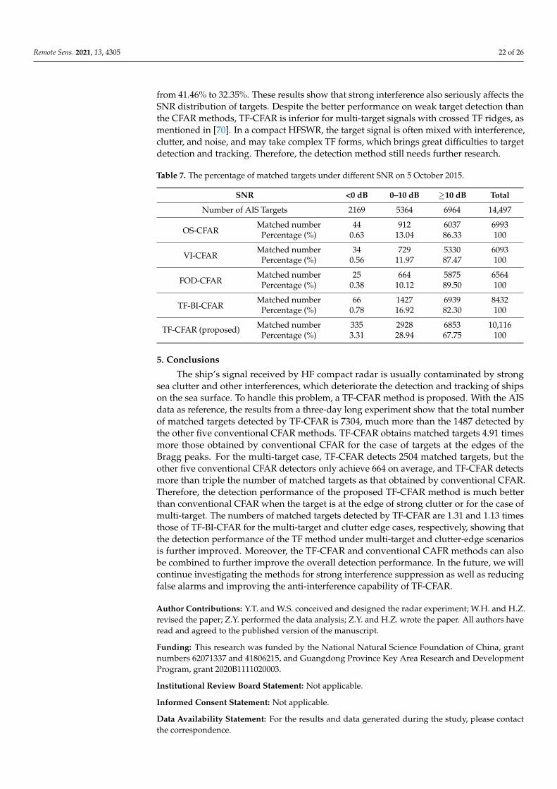
Reference [70] focused on an analysis of weak target detection performance andresults by TF-BI-CFAR. Here, we compared and analyzed the weak target detection perfor-mances of TF-CFAR, OS-CFAR [40], VI-CFAR [47], FOD-CFAR [49], and TF-BI-CFAR [70].In [70], TF-BI-CFAR occupied more than 40% of the matched targets below 10 dB on25 September 2015. In order to be consistent with [70], the number of detected targets herewas set to approximately 70,000 for the data on 25 October 2015. TF-BI-CFAR matched10,316 targets, and 3368 targets were less than 10 dB. Out of the total number matched byTF-BI-CFAR, the number below 10 dB occupied 32.64%. The analysis in Section 3.4 showsthat the interference can severely affect the performance on weak target detection. Table 7shows the match rates of the mentioned CFAR methods under different SNR with anapproximately same number of detected targets (i.e., 70,000) on 5 October 2015. Because theexistence of strong interference also changes the SNR of the original targets, the matchedtargets with strong interferences are excluded in Table 7.

It can be seen from Table 7 that the TF-CFAR method still has better detection per-formance than OS-CFAR, VI-CFAR, and FOD-CFAR in the case of low SNR. Below 10 dB,TF-CFAR performs the best and captures 14% more targets than TF-BI-CFAR. When theradar data with strong interference are not considered, the proportion of matched targets ofless than 10 dB occupied by TF-BI-CFAR decreased from 32.6% to 17.7%, and the number ofmatched targets decreased from 10,316 to 8432. For TF-CFAR, the number of matched tar-gets decreased from 13,109 to 10,116, and the proportion of targets below 10 dB decreased

Remote Sens. 2021, 13, 4305 22 of 26

from 41.46% to 32.35%. These results show that strong interference also seriously affects theSNR distribution of targets. Despite the better performance on weak target detection thanthe CFAR methods, TF-CFAR is inferior for multi-target signals with crossed TF ridges, asmentioned in [70]. In a compact HFSWR, the target signal is often mixed with interference,clutter, and noise, and may take complex TF forms, which brings great difficulties to targetdetection and tracking. Therefore, the detection method still needs further research.

Table 7. The percentage of matched targets under different SNR on 5 October 2015.

SNR <0 dB 0–10 dB ≥10 dB Total

Number of AIS Targets 2169 5364 6964 14,497

OS-CFARMatched number 44 912 6037 6993

Percentage (%) 0.63 13.04 86.33 100

VI-CFARMatched number 34 729 5330 6093

Percentage (%) 0.56 11.97 87.47 100

FOD-CFARMatched number 25 664 5875 6564

Percentage (%) 0.38 10.12 89.50 100

TF-BI-CFARMatched number 66 1427 6939 8432

Percentage (%) 0.78 16.92 82.30 100

TF-CFAR (proposed) Matched number 335 2928 6853 10,116Percentage (%) 3.31 28.94 67.75 100

5. Conclusions

The ship’s signal received by HF compact radar is usually contaminated by strongsea clutter and other interferences, which deteriorate the detection and tracking of shipson the sea surface. To handle this problem, a TF-CFAR method is proposed. With the AISdata as reference, the results from a three-day long experiment show that the total numberof matched targets detected by TF-CFAR is 7304, much more than the 1487 detected bythe other five conventional CFAR methods. TF-CFAR obtains matched targets 4.91 timesmore those obtained by conventional CFAR for the case of targets at the edges of theBragg peaks. For the multi-target case, TF-CFAR detects 2504 matched targets, but theother five conventional CFAR detectors only achieve 664 on average, and TF-CFAR detectsmore than triple the number of matched targets as that obtained by conventional CFAR.Therefore, the detection performance of the proposed TF-CFAR method is much betterthan conventional CFAR when the target is at the edge of strong clutter or for the case ofmulti-target. The numbers of matched targets detected by TF-CFAR are 1.31 and 1.13 timesthose of TF-BI-CFAR for the multi-target and clutter edge cases, respectively, showing thatthe detection performance of the TF method under multi-target and clutter-edge scenariosis further improved. Moreover, the TF-CFAR and conventional CAFR methods can alsobe combined to further improve the overall detection performance. In the future, we willcontinue investigating the methods for strong interference suppression as well as reducingfalse alarms and improving the anti-interference capability of TF-CFAR.

Author Contributions: Y.T. and W.S. conceived and designed the radar experiment; W.H. and H.Z.revised the paper; Z.Y. performed the data analysis; Z.Y. and H.Z. wrote the paper. All authors haveread and agreed to the published version of the manuscript.

Funding: This research was funded by the National Natural Science Foundation of China, grantnumbers 62071337 and 41806215, and Guangdong Province Key Area Research and DevelopmentProgram, grant 2020B1111020003.

Institutional Review Board Statement: Not applicable.

Informed Consent Statement: Not applicable.

Data Availability Statement: For the results and data generated during the study, please contactthe correspondence.

Remote Sens. 2021, 13, 4305 23 of 26

Acknowledgments: We sincerely thank the Academic Editor and reviewers for their helpful com-ments, which greatly improved this paper.

Conflicts of Interest: The authors declare no conflict of interest.

References1. Wang, Y.; Mao, X.; Zhang, J.; Ji, Y. Detection of Vessel Targets in Sea Clutter Using in Situ Sea State Measurements with HFSWR.

IEEE Geosci. Remote Sens. Lett. 2018, 15, 302–306. [CrossRef]2. Sun, W.; Huang, W.; Ji, Y.; Dai, Y.; Ren, P.; Hao, X. A Vessel Azimuth and Course Joint Re-Estimation Method for Compact HFSWR.

IEEE Trans. Geosci. Remote Sens. 2020, 58, 1041–1051. [CrossRef]3. Fujii, S.; Heron, M.; Kim, K.; Lai, J.; Lee, S.; Wu, X.; Wu, X.; Wyatt, L.; Yang, W. An Overview of Developments and Applications

of Oceanographic Radar Networks in Asia and Oceania Countries. Ocean Sci. J. 2013, 48, 69–97. [CrossRef]4. Barrick, D. After 40 years, how are HF radar currents now being used? In Proceedings of the 2011 IEEE/OES 10th Current, Waves

and Turbulence Measurements (CWTM), Monterey, CA, USA, 20–23 March 2011; p. 3. [CrossRef]5. Lai, Y.; Zhou, H.; Zeng, Y.; Wen, B. Quantifying and Reducing the DOA Estimation Error Resulting from Antenna Pattern

Deviation for Direction-Finding HF Radar. Remote Sens. 2017, 9, 1285. [CrossRef]6. Abascal, A.J.; Sanchez, J.; Chiri, H.; Ferrer, M.I.; Cárdenas, M.; Gallego, A.; Castanedo, S.; Medina, R.; Alonso-Martirena, A.; Berx,

B.; et al. Operational oil spill trajectory modelling using HF radar currents: A northwest European continental shelf case study.Mar. Pollut. Bull. 2017, 119, 336–350. [CrossRef]

7. Lipa, B.; Barrick, D.; Diposaptono, S.; Isaacson, J.; Jena, B.K.; Nyden, B.; Rajesh, K.; Kumar, T.S. High Frequency (HF) RadarDetection of the Weak 2012 Indonesian Tsunamis. Remote Sens. 2012, 4, 2944–2956. [CrossRef]

8. Lipa, B.; Barrick, D.; Saitoh, S.-I.; Ishikawa, Y.; Awaji, T.; Largier, J.; Garfield, N. Japan Tsunami Current Flows Observed by HFRadars on Two Continents. Remote Sens. 2011, 3, 1663–1679. [CrossRef]

9. Dzvonkovskaya, A.; Rohling, H. Cargo ship RCS estimation based on HF radar measurements. In Proceedings of the 11thInternational Radar Symposium, Vilnius, Lithuania, 16–18 June 2010; pp. 1–4.

10. Roarty, H.; Barrick, D.; Kohut, J.; Glenn, S. Dual-use of compact HF radars for the detection of mid- and large-size vessels. Turk. J.Electr. Eng. Comput. Sci. 2014, 18, 373–388.

11. Barrick, D. History, present status, and future directions of HF surfacewave radars in the U.S. In Proceedings of the InternationalConference on Radar, Adelaide, SA, Australia, 3–5 September 2003; pp. 652–655. [CrossRef]

12. Gurgel, K.; Antonischki, G. Remote sensing of surface currents and waves by the HF radar WERA. In Proceedings of the 7thInternational Conference Electronic Engineer in Oceanography, Southampton, UK, 23–25 June 1997; pp. 211–217. [CrossRef]

13. Dzvonkovskaya, A.; Gurgel, K.; Rohling, H.; Schlick, T. Low power High Frequency Surface Wave Radar application for ship de-tection and tracking. In Proceedings of the 2008 International Conference on Radar, Adelaide, SA, Australia, 2–5 September 2008;pp. 627–632. [CrossRef]

14. Dzvonkovskaya, A.; Rohling, H. HF radar performance analysis based on AIS ship information. In Proceedings of the 2010 IEEERadar Conference, Arlington, VA, USA, 10–14 May 2010; pp. 1239–1244. [CrossRef]

15. Gurgel, K.; Schlick, T.; Horstmann, J.; Maresca, S. Evaluation of an HF-radar ship detection and tracking algorithm by comparisonto AIS and SAR data. In Proceedings of the 2010 International WaterSide Security Conference, Carrara, Italy, 3–5 November 2010;pp. 1–6. [CrossRef]

16. Martin, R.J.; Kearney, M.J. Remote sea current sensing using HF radar: An autoregressive approach. IEEE J. Ocean. Eng. 1997, 22,151–155. [CrossRef]

17. Gurgel, K.W.; Schlick, T. HF radar wave measurements in the presence of ship echoes–Problems and solutions. In Proceedings ofthe Europe Oceans, Brest, France, 20–23 June 2005; pp. 937–941. [CrossRef]

18. Dobson, C.; Holenstein, K.; Smith, M.; Roarty, H.; Glenn, S.; Welan, C.; Barrick, D.; Isaacson, J. Monostatic vessel detectionstatistics from the CODAR SeaSonde. In Proceedings of the 2013 OCEANS, San Diego, CA, USA, 23–27 September 2013; pp. 1–4.[CrossRef]

19. Holenstein, K.; Dobson, C.; Smith, M.; Roarty, H.; Glenn, S.; Barrick, D.E. Bistatic vessel detection from the CODAR SeaSonde. InProceedings of the 2013 OCEANS, San Diego, CA, USA, 23–27 September 2013; pp. 1–5. [CrossRef]

20. Smith, M.; Roarty, H.; Glenn, S.; Whelan, C.; Barrick, D.; Isaacson, J. Methods of associating CODAR seasonde vessel detectiondata into unique tracks. In Proceedings of the 2013 OCEANS, San Diego, CA, USA, 23–27 September 2013; pp. 1–5. [CrossRef]

21. Huang, X.J.; Wen, B.Y.; Ding, F. Ship detection and tracking using multi-frequency HFSWR. IEICE Electron. Express 2010, 7,410–415. [CrossRef]

22. Zhou, H.; Roarty, H.; Wen, B. Wave extraction with portable high-frequency surface wave radar OSMAR-S. J. Ocean Univ. China2014, 13, 957–963. [CrossRef]

23. Barrick, D.; Lipa, B. Using antenna patterns to improve the quality of SeaSonde HF radar surface current maps. In Proceedings ofthe IEEE Sixth Working Conference on Current Measurement, San Diego, CA, USA, 13 March 1999; pp. 5–8. [CrossRef]

24. Evans, C.; Roarty, H.; Handel, E.; Glenn, S. Evaluation of three antenna pattern measurements for a 25 MHz seasonde. InProceedings of the 2015 IEEE/OES Eleveth Current, Waves and Turbulence Measurement (CWTM), St. Petersburg, FL, USA,2–6 March 2015; pp. 1–5. [CrossRef]

Remote Sens. 2021, 13, 4305 24 of 26

25. Emery, B.; Washburn, L.; Whelan, C.; Barrick, D.; Harlan, J. Measuring Antenna Patterns for Ocean Surface Current HF Radarswith Ships of Opportunity. J. Atmos. Ocean. Technol. 2014, 31, 1564–1582. [CrossRef]

26. Wilson, H.; Leong, H. An estimation and verification of vessel radar-cross-sections for HF surface wave radar. In Proceedings ofthe 2003 International Conference on Radar, Adelaide, SA, Australia, 3–5 September 2003; pp. 711–716. [CrossRef]

27. Leong, H.; Wilson, H. An estimation and verification of vessel radar cross sections for high-frequency surface-wave radar. IEEEAntennas Propag. Mag. 2006, 48, 11–16. [CrossRef]

28. Emery, B.; Whelan, C.; Barrick, D.; Washbum, L. Ocean Current Radar Calibration with Ships of Opportunity and the AutomaticIdentification System Phase I Final Report. Available online: https://www.researchgate.net/publication/268256027 (accessed on21 October 2021).

29. Leong, H. An estimation of radar cross sections of small vessels at HF. In Proceedings of the 2007 IET International Conference onRadar Systems, Edinburgh, UK, 15–18 October 2007; pp. 1–4. [CrossRef]

30. Chen, Z.; He, C.; Zhao, C.; Xie, F. Using SVD-FRFT Filtering to Suppress First-Order Sea Clutter in HFSWR. IEEE Geosci. RemoteSens. Lett. 2017, 14, 1076–1080. [CrossRef]

31. Chen, S.; Gill, E.W.; Huang, W. A High-Frequency Surface Wave Radar Ionospheric Clutter Model for Mixed-Path Propagationwith the Second-Order Sea Scattering. IEEE Trans. Antennas Propag. 2016, 64, 5373–5381. [CrossRef]

32. Guinvarc’h, R.; Lesturgie, M.; Durand, R.; Cheraly, A. On the Use of HF Surface Wave Radar in Congested Waters: Influence ofMasking Effect on Detection of Small Ships. IEEE J. Ocean. Eng. 2006, 31, 894–903. [CrossRef]

33. Frazer, G.; Williams, C. HF RCS of Small Boat Displacement in the Ocean. In Proceedings of the 2020 IEEE Radar Conference,Florence, Italy, 21–25 September 2020; pp. 1–6. [CrossRef]

34. Roarty, H.; Rivera Lemus, E.; Handel, E.; Glenn, S.; Barrick, D.; Isaacson, J. Performance Evaluation of SeaSonde High-FrequencyRadar for Vessel Detection. Mar. Technol. Soc. J. 2011, 45, 14–24. [CrossRef]

35. Blake, S. OS-CFAR theory for multiple targets and nonuniform clutter. IEEE Trans. Aerosp. Electron. Syst. 1988, 24, 785–790.[CrossRef]

36. Kuang, C.; Wang, C.; Wen, B.; Hou, Y.; Lai, Y. An Improved CA-CFAR Method for Ship Target Detection in Strong Clutter UsingUHF Radar. IEEE Signal Process. Lett. 2020, 27, 1445–1449. [CrossRef]

37. Finn, H.M.; Johnson, R.S. Adaptive detection mode with threshold control as a function of spatially sampled clutter level estimates.RCA Rev. 1968, 29, 414–464.

38. Trunk, G.V. Range Resolution of Targets Using Automatic Detectors. IEEE Trans. Aerosp. Electron. Syst. 1978, 14, 750–755.[CrossRef]

39. Hansen, V.G.; Sawyers, J.H. Detectability Loss Due to “Greatest Of” Selection in a Cell-Averaging CFAR. IEEE Trans. Aerosp.Electron. Syst. 1980, 16, 115–118. [CrossRef]

40. Rohling, H. Radar CFAR Thresholding in Clutter and Multiple Target Situations. IEEE Trans. Aerosp. Electron. Syst. 1983, 19,608–621. [CrossRef]

41. Himonas, S.D.; Barkat, M. Automatic censored CFAR detection for non-homogeneous environments. IEEE Trans. Aerosp. Electron.Syst. 1992, 28, 286–304. [CrossRef]

42. Kim, C.J.; Han, D.S.; Lee, H.S. Generalized OS CFAR detector with noncoherent integration. Signal Process. 1993, 31, 43–56.[CrossRef]

43. Gandhi, P.P.; Kassam, S.A. Analysis of CFAR processors in nonhomogeneous background. IEEE Trans. Aerosp. Electron. Syst. 1988,24, 427–445. [CrossRef]

44. Ozgunes, I.; Gandhi, P.P.; Kassam, S.A. A variably trimmed mean CFAR radar detector. IEEE Trans. Aerosp. Electron. Syst. 1992,28, 1002–1014. [CrossRef]

45. Gandhi, P.P.; Kassam, S.A. An adaptive order statistic constant false alarm rate detector. In Proceedings of the InternationalConference on Systems Engineering, Fairborn, OH, USA, 24–26 August 1989; pp. 85–88. [CrossRef]

46. Viswanathan, R.; Eftekhari, A. A selection and estimation test for multiple target detection. IEEE Trans. Aerosp. Electron. Syst.1992, 28, 509–519. [CrossRef]

47. Smith, M.E.; Varshney, P.K. Intelligent CFAR processor based on data variability. IEEE Trans. Aerosp. Electron. Syst. 2000, 36,837–847. [CrossRef]

48. Kim, J.H.; Bell, M.R. A computationally efficient CFAR algorithm based on a goodness-of-fit test for piecewise homogeneousenvironments. IEEE Trans. Aerosp. Electron. Syst. 2013, 49, 1519–1535. [CrossRef]

49. Jiang, W.; Huang, Y.; Yang, J. Automatic censoring CFAR detector based on ordered data difference for low-flying helicoptersafety. Sensors 2016, 16, 1055. [CrossRef] [PubMed]

50. Abbadi, A.; Abbane, A.; Bencheikh, M.L.; Soltani, F. A new adaptive CFAR processor in multiple target situations. In Proceedingsof the 2017 Seminar on Detection Systems Architectures and Technologies (DAT), Algiers, Algeria, 20–22 February 2017; pp. 1–5.[CrossRef]

51. Abbadi, A.; Bouhedjeur, H.; Bellabas, A.; Menni, T.; Soltani, F. Generalized Closed-Form Expressions for CFAR Detection inHeterogeneous Environment. IEEE Geosci. Remote Sens. Lett. 2018, 15, 1011–1015. [CrossRef]

52. Shapiro, S.S.; Wilk, M.B. An analysis of variance test for normality (complete samples). Biometrika 1965, 52, 591–611. [CrossRef]53. Ascher, S. A survey of tests for exponentiality. Commun. Stat.-Theory Methods 1990, 19, 1811–1825. [CrossRef]

Remote Sens. 2021, 13, 4305 25 of 26

54. Liu, Y.; Zhang, S.; Suo, J.; Zhang, J.; Yao, T. Research on a New Comprehensive CFAR (Comp-CFAR) Processing Method. IEEEAccess 2019, 7, 19401–19413. [CrossRef]

55. Beklaouz, H.L.; Hamadouch, M.; Mimi, M.; Ahmed, A.T. Study and analysis of a new detector of radar targets using CFAR withGabor transform. In Proceedings of the 2008 15th International Conference on Systems, Signals and Image Processing, Bratislava,Slovakia, 25–28 June 2008; pp. 437–440. [CrossRef]

56. Lei, Z.; Huang, Y. Time-frequency analysis based image processing for maneuvering target detection in HF OTH radar. InProceedings of the 2009 IET International Radar Conference, Guilin, China, 20–22 April 2009; pp. 1–6. [CrossRef]

57. Boashash, B. Time–Frequency Signal Analysis and Processing, 2nd ed.; Elsevier: New York, NY, USA, 2015; pp. 256–280.58. Chen, V.C.; Ling, H. Joint time-frequency analysis for radar signal and image processing. IEEE Signal Process. Mag. 1999, 16,

81–93. [CrossRef]59. Greco, M.; Bordoni, F.; Gini, F. X-band sea-clutter nonstationarity: Influence of long waves. IEEE J. Ocean. Eng. 2004, 29, 269–283.

[CrossRef]60. Herselman, P.L.; Baker, C.J. Analysis of calibrated sea clutter and boat reflectivity data at C- and X-band in South African coastal

waters. In Proceedings of the 2007 IET International Conference on Radar Systems, Edinburgh, UK, 15–18 October 2007; pp. 1–5.[CrossRef]

61. Herselman, P.L.; Baker, C.J.; Wind, H.J.D. An analysis of X-band calibrated sea clutter and small boat reflectivity at medium-to-lowgrazing angles. Int. J. Navig. Observ. 2008, 2, 1–14. [CrossRef]

62. Panagopoulos, S.; Soraghan, J.J. Small-target detection in sea clutter. IEEE Trans. Geosci. Remote Sens. 2004, 42, 1355–1361.[CrossRef]

63. Grosdidier, S.; Baussard, A.; Khenchaf, A. HFSW radar model simulation and measurement. IEEE Trans. Geosci. Remote Sens.2010, 48, 3539–3549. [CrossRef]

64. Stankovic, L.J.; Thayaparan, T.; Dakovic, M. Signal decomposition by using the S-method with application to the analysis of HFradar signals in sea-clutter. IEEE Trans. Signal Process. 2006, 54, 4332–4342. [CrossRef]

65. Stankovic, L.J.; Bohme, J.F. Time-frequency analysis of multiple resonances in combustion engine signals. Signal Process. 1999, 9,15–28. [CrossRef]

66. Zuo, L.; Li, M.; Zhang, X.; Wang, Y.; Wu, Y. An Efficient Method for Detecting Slow-Moving Weak Targets in Sea Clutter Based onTime–Frequency Iteration Decomposition. IEEE Trans Geosci. Remote Sens. 2013, 51, 3659–3672. [CrossRef]

67. Li, Q.; Zhang, W.; Li, M.; Niu, J.; Jonathan Wu, Q.M. Automatic Detection of Ship Targets Based on Wavelet Transform for HFSurface Wavelet Radar. IEEE Geosci. Remote Sens. Lett. 2017, 14, 714–718. [CrossRef]

68. Jiao, S.; Li, X.; Lu, X. An improved Ostu method for image segmentation. In Proceedings of the 2006 8th International Conferenceon Signal Processing, Guilin, China, 16–20 November 2006; pp. 164–166. [CrossRef]

69. Cai, J.; Zhou, H.; Huang, W.; Wen, B. Ship Detection and Direction Finding Based on Time-Frequency Analysis for Compact HFRadar. IEEE Geosci. Remote Sens. Lett. 2021, 18, 72–76. [CrossRef]

70. Yang, Z.; Tang, J.; Zhou, H.; Xu, X.; Tian, Y.; Wen, B. Joint Ship Detection Based on Time-Frequency Domain and CFAR Methodswith HF Radar. Remote Sens. 2021, 13, 1548. [CrossRef]

71. Yang, Z.; Zhou, H.; Tian, Y.; Zhao, J. Improved CFAR Detection and Direction Finding on Time-Frequency Plane With High-Frequency Radar. IEEE Geosci. Remote Sens. Lett. 2021. [CrossRef]

72. Yu, G.; Wang, Z.; Zhao, P. Multisynchrosqueezing Transform. IEEE Trans. Ind. Electron. 2019, 66, 5441–5455. [CrossRef]73. Meignen, S.; Pham, D.; McLaughlin, S. On Demodulation, Ridge Detection, and Synchrosqueezing for Multicomponent Signals.

IEEE Trans. Signal Process. 2017, 65, 2093–2103. [CrossRef]74. Xiao, B.; Ou, G.; Tang, H.; Bi, X.; Li, W. Multi-Focus Image Fusion by Hessian Matrix Based Decomposition. IEEE Trans. Multimedia

2020, 22, 285–297. [CrossRef]75. Chahine, C.; Vachier-Lagorre, C.; Chenoune, Y.; Berbari, R.E.; Fawal, Z.E.; Petit, E. Information fusion for unsupervised image

segmentation using stochastic watershed and Hessian matrix. IET Image Process. 2018, 12, 525–531. [CrossRef]76. Anupama, P.; Nandyal, S. Blood vessel segmentation using Hessian matrix for diabetic retinopathy detection. In Proceedings of

the 2017 Second International Conference on Electrical, Computer and Communication Technologies (ICECCT), Coimbatore,India, 22–24 February 2017; pp. 1–5. [CrossRef]

77. Li, Y.; Gong, H.; Wu, W.; Liu, G.; Chen, G. An automated method using Hessian matrix and random walks for retinal blood vesselsegmentation. In Proceedings of the 2015 8th International Congress on Image and Signal Processing (CISP), Shenyang, China,14–16 October 2015; pp. 423–427. [CrossRef]

78. Xia, S.; Zhu, H.; Liu, X.; Gong, M.; Huang, X.; Xu, L.; Zhang, H.; Guo, J. Vessel Segmentation of X-ray Coronary AngiographicImage Sequence. IEEE Trans. Biomed. Eng. 2020, 67, 1338–1348. [CrossRef] [PubMed]

79. Zhou, Y.H.; Gao, J.B.; White, K.D.; Merk, I.; Yao, K. Perceptual dominance time distributions in multistable visual perception. Biol.Cybern. 2004, 90, 256–263. [CrossRef]

Remote Sens. 2021, 13, 4305 26 of 26

80. Liu, J.; Han, J.; Zhang, Z.; Li, J. Bayesian Detection for MIMO Radar in Gaussian Clutter. IEEE Trans. Signal Process. 2018, 66,6549–6559. [CrossRef]

81. Tian, Y.; Wen, B.; Tan, J.; Li, K.; Yan, Z.; Yang, J. A new fully-digital HF radar system for oceanographical remote sensing. IEICEElectron. Express 2013, 14, 1–6. [CrossRef]