Airborne Radar STAP using Sparse Recovery of

Clutter Spectrum Ke Sun, Hao Zhang, Gang Li, Huadong Meng, Xiqin Wang

(Department of Electronic Engineering, Tsinghua University, Beijing 100084, China)

Abstract: Space-time adaptive processing (STAP) is an effective tool for detecting a moving

target in spaceborne or airborne radar systems. Statistical-based STAP methods generally need

sufficient statistically independent and identically distributed (IID) training data to estimate the

clutter characteristics. However, most actual clutter scenarios appear only locally stationary and

lack sufficient IID training data. In this paper, by exploiting the intrinsic sparsity of the clutter

distribution in the angle-Doppler domain, a new STAP algorithm called SR-STAP is proposed,

which uses the technique of sparse recovery to estimate the clutter space-time spectrum. Joint

sparse recovery with several training samples is also used to improve the estimation performance.

Finally, an effective clutter covariance matrix (CCM) estimate and the corresponding STAP filter

are designed based on the estimated clutter spectrum. Both the Mountaintop data and simulated

experiments have illustrated the fast convergence rate of this approach. Moreover, SR-STAP is

less dependent on prior knowledge, so it is more robust to the mismatch in the prior knowledge

than knowledge-based STAP methods. Due to these advantages, SR-STAP has great potential for

application in actual clutter scenarios.

Key words: STAP, sparse recovery, fast convergence rate, robustness, space-time spectrum

1. Introduction

An airborne/spaceborne (A/S) space time adaptive processor (STAP) attempts to detect a

moving target in the presence of a Doppler/angle spread clutter environment [1-2]. Due to the

motion of the radar platform, one dimensional processing in neither angle nor Doppler domain can

effectively distinguish the moving target from the surrounding clutter environment. Therefore, it is

necessary to carry out joint angle-Doppler processing. The fundamental component of STAP is the

effective estimation of the clutter covariance matrix (CCM), which is used to construct the optimal

linear weighting of the adaptive matched filter such that the output signal-to-clutter ratio is

maximized [1]. The adaptive processor requires a certain quantity of independent identically

distributed (IID) training samples to effectively estimate CCM due to lack of knowledge about the

external clutter environment [3-4]. The number of IID samples required to produce an output

signal-to-clutter power ratio (SCR) performance that is close to the optimum (nominally, within 3

dB) is called the convergence rate of the processor. Reducing the convergence rate is quite

meaningful because the clutter is locally stationary in the actual scenario and the CCM estimation

with slow convergence rate will cause a significant SCR loss between the adaptive

implementation and the optimum design [5].

The foundational work by Reed, called sample matrix inversion (SMI) [3], provides a way to

estimate the CCM. This method uses data samples directly and the convergence rate is twice the

problem dimensionality. However, in actual clutter scenarios, this quantity of IID samples is often

unavailable due to the nonstationarity of the reflectivity properties, strong discrete scatters, and so

forth [5-6]. Thus, faster-converging methods, such as loaded sample matrix inversion (LSMI) and

principal component (PC), are proposed in [6-7]. These methods avoid the use of eigenvectors

associated with small eigenvalues that are difficult to estimate. In this way, the convergence rate is

reduced to twice the number of significant eigenvalues (referred to as the ‘effective clutter rank’)

of the CCM. However, the convergence rate can hardly be improved beyond the clutter rank

because these methods do not assume any prior knowledge in the CCM estimation.

Recently, a class of algorithms called KB-STAP (knowledge-based STAP) [8-12] was

proposed to solve the problem of lacking IID training samples. These methods use prior

knowledge of the spectral characteristics in the underlying clutter scenario to pre-whiten the CCM

and enhance the convergence rate. This prior knowledge includes the radar parameters and

anticipated structure of the clutter return, which could be obtained from a digital terrain and

elevation data map, synthetic aperture radar (SAR) imagery, and some other sensors [8]. Two

important KB-STAP algorithms are colored loading (CL) [9] and fast maximum likelihood with

assumed clutter covariance (FMLACC) [10]. It has been proved that both approaches are

equivalent to a kind of pre-whitening process and the convergence rate is twice the rank of the

pre-whitened CCM. However, it should also be noted that accurate prior knowledge is hard to

acquire due to the limited computational resources, insufficient resolution, inadequate array

calibration and so forth [9-10]. Therefore, the mismatch between the assumed and the actual CCM

will impact the performance of the KB-STAP methods.

Focusing on the problem of slow convergence rate in the conventional STAP and sensitivity

to the prior knowledge in the KB-STAP methods, a new STAP algorithm is proposed in this paper.

Similar to the idea in KB-STAP, this method also utilizes prior knowledge to obtain the clutter

spectral characteristics. However, this spectrum estimation is obtained via sparse recovery, which

has evolved very rapidly in the last decade [13-18]. In its most basic form, the problem of sparse

recovery attempts to find the sparsest signal α to satisfy x Ψα= , where m nCΨ ×∈ is an

overcomplete basis, i.e., m ≤ n. Without prior knowledge that α is sparse, the equation x Ψα=

is ill-posed and has many solutions. Additional information that α should be sufficiently sparse

allows one to eliminate this ill-posedness [13-14]. Solving the ill-posed problem involving

sparsity typically requires combinatorial optimization, which is intractable even for modest data

size. A number of practical algorithms such as convex optimization (including 1L norm

minimization) [15-16] and greedy algorithms [17-18] have been proposed to approximate the

solution to this problem. Convex optimization provides a guarantee of uniformity and is also very

stable. However, this method is based on linear programming and has a quite high computational

complexity, ( )3O n . On the other hand, greedy methods make a sequence of locally optimal

choices in an effort to obtain a globally optimal solution. The computational load is quite small,

but it lacks the strong guarantee of convergence that convex optimization provides. Prior research

has proved sparse recovery as a valuable tool for spectrum estimation, but its application has been

mainly focused in the field of source localization, where the sparsity condition is obviously

satisfied [19-21].

In this paper, we exploit the prior knowledge of the sparsity of the clutter distribution in the

angle-Doppler domain and obtain the space-time spectrum via sparse recovery. This method can

obtain the clutter spectral characteristics with many fewer IID samples, such that the convergence

rate of the CCM is significantly enhanced. The remainder of this paper is organized as follows.

Section 2 describes the basic model of the STAP received data. In section 3, the SR-STAP (STAP

via sparse recovery) approach is proposed to estimate the clutter space-time spectrum from both

single and multiple snapshots. Then, the CCM estimation based on this spectrum is given to

effectively suppress the clutter. Section 4 analyzes the convergence rate and robustness for

simulated data. The Mountaintop data [22] provided by Lincoln Laboratories is also used to verify

the effectiveness of SR-STAP in an actual clutter scenario. Section 5 presents concluding remarks

about the proposed algorithm and points out directions for future work.

2. STAP MODEL

When a radar platform is moving, stationary clutter has an angle-Doppler dependence given

by

2 sin ,d svf θλ

= (1)

where sθ and df stand for the spatial angle and Doppler frequency of the clutter scatter,

respectively; v is the moving velocity of the radar platform; λ denotes the radar wavelength.

Suppose that N is the number of array channels and M is the number of pulses in a coherent

process interval (CPI). The target-free snapshot CNMx∈ for a given range cell can be expressed

as [1]

, ,1

( , ) ,cN

i s i d ii

fx φ nγ θ=

= ⋅ +∑ (2)

where , ,( , )s i d ifφ θ is the 1NM × space-time steering vector of the ith clutter scatter, given

by

( )

( )

, ,, ,

, ,

( , ) 1, exp 2 ,..., exp 2 1PRF PRF

1, exp 2 sin ,..., exp 2 1 sin ,

Td i d i

s i d i

T

s i s i

f ff j j M

d dj j N

φ θ π π

π θ π θλ λ

⎡ ⎤⎛ ⎞ ⎛ ⎞= −⎢ ⎥⎜ ⎟ ⎜ ⎟

⎝ ⎠ ⎝ ⎠⎣ ⎦

⎡ ⎤⎛ ⎞ ⎛ ⎞⊗ −⎜ ⎟ ⎜ ⎟⎢ ⎥⎝ ⎠ ⎝ ⎠⎣ ⎦

(3)

, ,,s i d ifθ denote the space angle and Doppler frequency of the ith clutter scatter, ⊗ denotes

the Kronecker product, PRF is the radar pulse repetition frequency, d is the inter-sensor

spacing of the uniform linear array. cN is the total number of the uncorrelated clutter scatters,

( )2,CNn 0 Iδ∼ is the complex gauss noise ( I is the NM NM× identity matrix), and iγ

is the complex amplitude of the ith clutter scatter satisfying

{ } 0, 1 ,i cE i Nγ = ∀ ≤ ≤ (4)

The optimal STAP is to design the 1NM × space-time filter to maximize the output SCR and

the corresponding optimal space-time filter is given as [1-2]

1 ,optw R sμ −= (5)

where μ is a non-zero constant, matrix { }HER xx= represents the actual CCM, and s is

the space-time steering vector of the moving target. In practice, the CCM is unknown and should

be estimated using IID snapshots. In the SMI approach [3], the CCM estimation is given via the

direct data approach:

1

1ˆ ,L

HSMI i i

iLR x x

=

= ∑ (6)

where ,1i i Lx ≤ ≤ denote the IID snapshots. This approach can achieve nearly optimal

performance when the number of IID snapshots satisfies 2L MN≥ . However, this quantity of

stationary samples is often unavailable in an actual clutter scenario [5]. One great improvement to

this method is called LSMI (Loaded SMI), which adds a small diagonal loading factor into the

SMI estimation:

ˆ ˆLSMI SMI LR R Iβ= + (7)

where Lβ is a small loading factor. It has been proved that this approach can achieve nearly

optimal performance using twice as many IID samples as the effective clutter rank [6]. However,

the convergence rate can hardly be improved beyond the effective clutter rank because it does not

use any prior knowledge in the CCM estimation. At the same time, substituting (2) into the CCM

definition, the CCM can also be expressed as [1]

, , , ,1 1

( , ) ( , ) .c c

HN NH

i s i d i j s j d ji j

E E f fR xx φ n φ nγ θ γ θ= =

⎧ ⎫⎛ ⎞⎛ ⎞⎪ ⎪⎡ ⎤= = + +⎨ ⎬⎜ ⎟⎜ ⎟⎣ ⎦⎝ ⎠⎝ ⎠⎪ ⎪⎩ ⎭∑ ∑ (8)

The clutter scatters are uncorrelated with each other, that is

{ } { } { } 0, , : .i j i jE E E i j i jγ γ γ γ∗ ∗= = ∀ ≠ (9)

Moreover, the noise is uncorrelated with these clutter scatters. In this case, the CCM could be

further simplified as

{ }2 2, , , ,

1( , ) ( , ) ,

cNH

i s i d i s i d ii

E f fR φ φ Iγ θ θ δ=

= +∑ (10)

where { }2 ,1i cE i Nγ ≤ ≤ denotes the power distribution of the clutter scatters in the

angle-Doppler domain, that is, the space-time spectrum. In this way, the relationship between the

CCM and the clutter spectral characteristics is built up. The assumed CCM can be used as an

approximation for the actual one, effectively accelerating the convergence rate, as long as the prior

knowledge of the clutter distribution is obtained accurately. The recently-developed

knowledge-based STAP methods are based on this idea [8-12]. By incorporating the prior

knowledge into the estimation process, these methods show a strong capability to reduce the

number of required data samples. One important knowledge-based STAP algorithm is called CL

[9], which provides the following estimate for the CCM:

ˆ ˆCL SMI d c LR R R Iβ β= + + (11)

where ˆSMIR is the SMI part standing for the contribution of the data samples, cR is the

assumed CCM using the prior knowledge in (10), dβ and Lβ denote the colored loading and

diagonal loading factors respectively. The CL method utilizes the prior knowledge of the clutter

distribution to force the nulls in the angle-Doppler domain and effectively suppress the

corresponding clutter. In this way, the convergence rate improves to twice the effective rank of the

pre-whitened clutter residual, which is not contained in the prior knowledge. However, accurate

prior knowledge is hard to acquire due to various real-world effects, such that there will be some

performance degradation in KB-STAP due to the mismatch between the prior knowledge and the

real-world scenario [9-10].

3. Spectrum Estimation and Clutter Suppression

As stated above, the CCM estimation could be obtained with high performance as long as the

clutter spectral characteristics are accurately acquired. Based on this idea, a new STAP algorithm

is developed via sparse recovery to obtain the clutter spectrum and estimate the CCM with much

less IID snapshots [23]. The space angle and Doppler frequency axes are discretized into

,s s d dN N N Mρ ρ= = grids in the angle-Doppler domain to obtain the clutter spectrum with

high resolution. The parameters ,s dρ ρ are the resolution scales along the angle and Doppler

axes, respectively. In this way, the received data in (2) can be written in matrix form as

1

,s dN N

i ii

x Ψ n Ψα + nα=

= ⋅ + =∑ (12)

where s dNM N N× matrix Ψ is the basis made up with the space-time steering vectors and

can be expressed as

( ) ( ) ( ) ( ),1 ,1 , ,1 ,1 , , ,, , , , , , , , , , .s d s ds d s N d s d N s N d Nf f f fΨ φ φ φ φθ θ θ θ⎡ ⎤= ⎣ ⎦ (13)

The vector α stands for the clutter distribution in the basis Ψ , that is, the clutter space-time

spectrum. Equation (12) is the fundamental equation in this paper and has two characteristics that

we should pay attention to. First, estimating the space-time spectrum α is equivalent to solving

the linear equation (12) with the data x . Second, the basis matrix Ψ is overcomplete and the

problem is ill-posed because the resolution scales ,s dρ ρ are greater than the one used to obtain

the high-resolution spectrum. However, according to the theory of sparse recovery [13-16], when

the actual clutter spectral distribution 0α is sparse, this ill-posed problem can be solved via

sparse recovery. Next, some discussion is given to verify the sparse characteristic of the

space-time clutter in the discretized angle-Doppler plane.

3.1 The sparsity of the space-time clutter

As stated above, the angle-Doppler domain is discretized into ,s dN N cells along the angle

and Doppler axes, respectively. Each cell in this discretized plane corresponds to a certain

space-time steering vector and all these vectors make up the overcomplete basis Ψ . Because the

noise does not correspond to a certain space-time steering vector, its distribution is reflected as a

small noise floor in the angle-Doppler plane. As shown in Fig. 1, the angle-Doppler dependence in

(1) focuses the clutter distribution only along the clutter ridge, whose slope is determined by the

radar parameters. The STAP clutter scenario usually has a high CNR [1-2], therefore the

distribution of the training data in the angle-Doppler plane is mainly determined by the clutter

component. Moreover, the clutter scatters from the sidelobe are much smaller (more than 10dB

lower) than that from the mainlobe due to the effect of antenna azimuth weighting. In this way, the

significant clutter scatters only exist along the clutter ridge within the mainlobe [ ]min max,θ θ .

Conventionally, the significant elements of the actual solution are used to express the degree of

sparsity in the sparse recovery [13-14]. In our problem of spectrum estimation, the sparsity of the

space-time clutter is equal to the number of cells occupied by the clutter ridge in the discretized

angle-Doppler plane, which is marked by the slash cells in Fig. 1.

minθ maxθAngle axis

Ideal clutter ridge

Main lobe

Fig. 1 Clutter distribution in the discretized angle-Doppler plane

In an actual clutter scenario, the sparsity of the actual clutter distribution is unknown and

need to be estimated. Similar to the knowledge-based methods, the assumed sparsity could be

similarly given by the number of cells occupied by the assumed clutter ridge based on the prior

knowledge. Generally, the sparsity is related to both the actual clutter distribution and the number

of the discretized cells in the angle-Doppler plane. Due to the effect of the discretization, the

sparsity estimation in the angle-Doppler plane may differ from that in the continuous case. An

effective estimation method is given to obtain the sparsity as follows.

1. Determine the azimuth angle cells occupied by the clutter distribution as

( )min max ,

180 sN Nθ θ

α−⎡ ⎤

Δ = ⋅⎢ ⎥⎢ ⎥

(14)

where [ ]min max,θ θ stands for the mainlobe angle extent and ⋅⎡ ⎤⎢ ⎥ is the ceiling

operation (rounding up).

2. Calculate the corresponding Doppler cells due to the clutter spreading as

( )max min2 sin sin

.PRF d

vM M

θ θα

λ−⎡ ⎤

Δ = ⋅⎢ ⎥⋅⎢ ⎥ (15)

3. Theoretically, sparsity estimation has a range value [ ] ˆmax ,M N s M NΔ Δ ≤ ≤ Δ + Δ .

However, when the resolution scales ,s dρ ρ are much greater than the one, we can

calculate it directly as

2 2ˆ .s M N⎡ ⎤= Δ + Δ⎢ ⎥ (16)

This estimation clearly illustrates the relationship between the radar parameters and the sparsity.

Although it is simple and may be not very accurate, the simulation in the next section will show

that SR-STAP is robust to this sparsity estimation. Some other practical factors, such as crab angle,

also affect the assumed sparsity and will be discussed in detail later.

3.2 Space-time spectrum estimation via sparse recovery

A. Single snapshot case

Once the actual clutter spectrum 0α is sparse, the ill-posed problem in (12) can be solved

using the 1L norm minimization, constructed as

1 2

ˆ arg min ,subject toα α x Ψα ε= − ≤ (17)

where p

⋅ stands for the pL norm and ε is the error allowance in sparse recovery. In this

way, the 2L norm constraint by ε guarantees the residual 2

x Ψα− to be small, whereas the

1L norm enforces the sparsity of the estimated spectrum. The sparse recovery via the 1L norm

minimization can be efficiently carried out via convex optimization. Great achievements in sparse

recovery [13] have also proved that even in the scenario with small noise, the 1L norm recovery

can approximate the actual solution as 2

ˆ ,0α α ε− ≤ Λ ⋅ where Λ is the stability coefficient

and related to the maximal mutual coherence in the matrix Ψ .

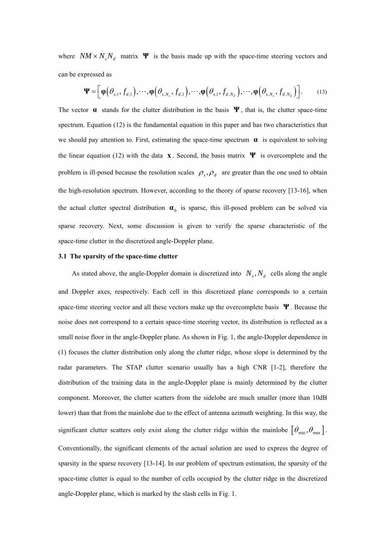
Next, the Mountaintop data [22] is used to verify the effectiveness of the spectrum estimation

in SR-STAP. The Mountaintop program consists of 14 array sensors and 16 pulses in each CPI. As

for the clutter scenario, the dominant clutter is located at about azimuth -15 degrees and

normalized Doppler frequency 0.25. The clutter in other directions is small due to shadowing by

nearer-range mountains [24]. The resolution scales are set as 4, 4s dρ ρ= = to obtain the

high-resolution spectrum. The Capon estimator [25] is introduced here as a reference to verify the

performance of the SR-STAP spectrum. The number of snapshots is set to 40 (range cells 80-120).

In SR-STAP, only one snapshot (range cell 120) is used to estimate the clutter spectrum. Here, cvx,

the most popular convex optimization package, is employed as the 1L norm optimization tool

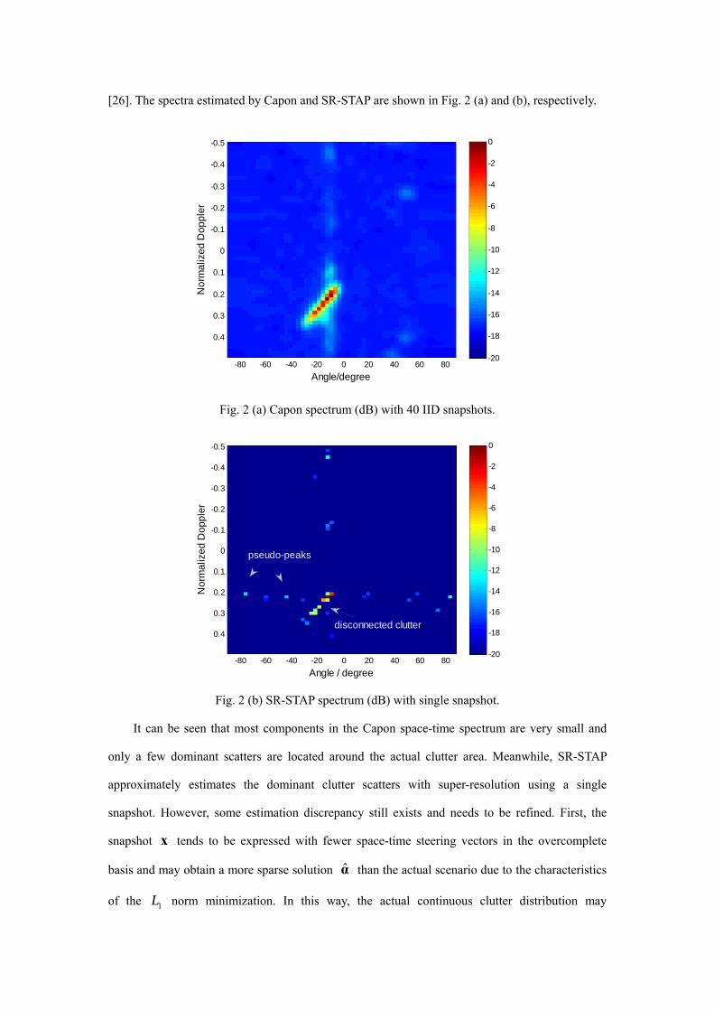
[26]. The spectra estimated by Capon and SR-STAP are shown in Fig. 2 (a) and (b), respectively.

Nor

mal

ized

Dop

pler

Angle/degree

-80 -60 -40 -20 0 20 40 60 80

-0.5

-0.4

-0.3

-0.2

-0.1

0

0.1

0.2

0.3

0.4

-20

-18

-16

-14

-12

-10

-8

-6

-4

-2

0

Fig. 2 (a) Capon spectrum (dB) with 40 IID snapshots.

Angle / degree

Nor

mal

ized

Dop

pler

-80 -60 -40 -20 0 20 40 60 80

-0.5

-0.4

-0.3

-0.2

-0.1

0

0.1

0.2

0.3

0.4

-20

-18

-16

-14

-12

-10

-8

-6

-4

-2

0

pseudo-peaks

disconnected clutter

Fig. 2 (b) SR-STAP spectrum (dB) with single snapshot.

It can be seen that most components in the Capon space-time spectrum are very small and

only a few dominant scatters are located around the actual clutter area. Meanwhile, SR-STAP

approximately estimates the dominant clutter scatters with super-resolution using a single

snapshot. However, some estimation discrepancy still exists and needs to be refined. First, the

snapshot x tends to be expressed with fewer space-time steering vectors in the overcomplete

basis and may obtain a more sparse solution α̂ than the actual scenario due to the characteristics

of the 1L norm minimization. In this way, the actual continuous clutter distribution may

converge into several disconnected clutter scatters, marked by the ellipse in Fig. 2 (b). This

phenomenon is quite common in the field of sparse recovery [19-21]. Second, some estimation

error, called ‘pseudo-peaks,’ exists. These are marked by the arrow in the SR-STAP spectrum.

This is caused by the noise and ill-posedness in (12). Normally, these pseudo-peaks appear

randomly in the angle-Doppler domain among different snapshots and their amplitudes are much

smaller (-10dB) than the actual clutter scatters. The following work will focus on how to eliminate

these pseudo-peaks, as well as obtain the connected clutter spectrum with multiple snapshots.

B. Multiple snapshots case：simple average

In the actual clutter scenario, although sufficient training samples are hard to guarantee, there

are still a few training samples that we can exploit. Therefore, we extend this work to the multiple

snapshots case [27-28] to improve the estimation performance as

,X ΨS N= + (18)

where NM L× matrix ( ) ( )1 , LX x x⎡ ⎤= ⎣ ⎦ denotes the multiple training snapshots, NM L×

matrix ( ) ( )1 , LN n n⎡ ⎤= ⎣ ⎦ is the observation noise, and s dN N L× matrix

( ) ( )1 , LS α α⎡ ⎤= ⎣ ⎦ is the clutter spectrum of multiple snapshots. A simple method is to separate

this joint problem into a series of independent subproblems as

( ) ( ) ( ) , 1 .k k k k Lx Ψα n= + ≤ ≤ (19)

Each subproblem can be solved via the 1L norm minimization in (17) to obtain the sparse

spectrum estimation. Then, the average of these estimated spectra ( )ˆ , 1k k Lα ≤ ≤ , can be taken

as

( )

1

1ˆ ˆ .L

k

kLα α

=

= ∑ (20)

This method is simple and the computing effort is linearly proportional to the number of snapshots.

The estimation result via simple average is shown in Fig. 3 for Mountaintop data range cells

80-120. It is shown that this approach can improve the disconnected spectrum estimation to some

extent, compared to the single snapshot method. However, some pseudo-peaks still exist after

simple averaging because this method does not make use of the stationary characteristic of the

clutter distribution in the IID snapshots. In fact, the position is more important than the amplitude

information in the clutter distribution.

Nor

mal

ized

Dop

pler

Angle/degree

-80 -60 -40 -20 0 20 40 60 80

-0.5

-0.4

-0.3

-0.2

-0.1

0

0.1

0.2

0.3

0.4

-20

-18

-16

-14

-12

-10

-8

-6

-4

-2

0

connected clutter

pseudo-peaks

Fig. 3 SR-STAP spectrum (dB) with simple average

C. Multiple snapshots case：joint sparse recovery

To improve the spectrum performance of the simple average approach, a more reasonable

approach called joint sparse recovery [29-30] is proposed to treat these snapshots in conjunction.

This assumes that the sparse structure of a stationary process remains the same across different

snapshots and the only difference is reflected in the amplitude variation. In this case, the sparsity

s in each spectrum ( ) , 1k k Lα ≤ ≤ is identical, which means that the actual clutter scatters are

located at the same cells in the angle-Doppler domain in these spectra ( ) , 1k k Lα ≤ ≤ as

( ) ( )1 ,kΓ Γ= (21)

where the position set ( )kΓ in the kth snapshot is defined as

( ) ( )( )sarg max , 1 ,k k k LΓ α= ≤ ≤ (22)

where operation ( )sarg max ⋅ denotes obtaining the positions of the maximal s elements in a

vector. Prior research on joint sparse recovery achieved great recovery performance with the

assumptions of accurate knowledge of the sparsity and small maximal mutual coherence in the

overcomplete matrix Ψ . However, these assumptions are not valid in the problem of spectrum

estimation in the actual clutter scenario because the sparsity of the actual clutter scenario is

unknown and the maximal mutual coherence in the overcomplete matrix Ψ increases with the

resolution scales ,s dρ ρ . For example, when , 1s dρ ρ , the maximal mutual coherence may

become large, such that the clutter spectrum estimation via the current joint sparse recovery

method is not very effective. Therefore, some practical improvements should also be considered to

enhance the current methods of joint sparse recovery.

As stated above, the spectrum estimation with the single snapshot is discontinuous along the

actual clutter area and may have some pseudo-peaks. Because these snapshots are joint sparse, the

combing result with position sets ( )ˆ , 1k k LΓ ≤ ≤ is more close to the continuous distribution of

the actual clutter. Moreover, the pseudo-peaks could be effectively suppressed using this

combining operation because they appear randomly in the spectrum estimation of the different

snapshots. Thus, the joint problem with multiple snapshots could be effectively solved via the

least squares (LS) method as soon as the actual position set is accurately obtained [33]. The

procedure for this method is elaborated as follows.

1. Decompose the joint problem into a series of subproblems and solve each subproblem

independently as

( ) ( ) ( ) ( )1 2

ˆ arg min , 1 .k k k ksubject to k Lα α x Ψα ε= − ≤ ≤ ≤ (23)

2. Estimate the position set of the clutter distribution in each space-time spectrum as

( ) ( )( )sˆ ˆarg max , 1 .k k k LΓ α= ≤ ≤ (24)

3. Define a series of 1s dN N × vectors ( ) ( )1 , Lc c as

( )( ) ( )

( )

ˆ , 1, 1 , 1 .

, 0

k kk i

s dki

if i ci N N k L

else c

Γc

⎧ ∈ =⎪= ≤ ≤ ≤ ≤⎨=⎪⎩

(25)

4. Combine these vectors as ( ) ( )1 LP c c= + + , with the element iP standing for the

occurrence number on the ith space-time cell after the combining process.

5. Obtain the joint position set with the position sets of multiple snapshots as

( )sˆ arg max .Γ P= (26)

6. Once the joint position set Γ̂ is recovered, the joint problem can be expressed as [24]

ˆ

2ˆ ˆ 2

min ,Γ

Γ ΓSΨ S X− (27)

where NM s× matrix Γ̂

Ψ stands for the corresponding Γ̂ columns in the

overcomplete basis Ψ , then the LS minimization can be effectively implemented to solve

the problem as

( )ˆ ˆ ˆ ˆ ,-1H H

Γ Γ Γ ΓS Ψ Ψ Ψ X= (28)

the s L× matrix Γ̂

S stands for the corresponding Γ̂ rows in the matrix S and all other

elements of the matrix are set to zero.

7. Calculate the average spectrum of joint sparse recovery as

1

1ˆ , 1 .L

kk

k LL

α S=

= ≤ ≤∑ (29)

where kS stands for the kth column of the matrix S and α̂ represents the final

spectrum estimation with multiple snapshots.

Until now, we have introduced the SR-STAP spectrum based on joint sparse recovery. The

result in Fig. 4 shows that most of the pseudo-peaks are effectively suppressed, which can be

explained as follows. There are fewer false positions induced by the pseudo-peaks in the joint

position set Γ̂ because the position information is more reliable than the amplitude information.

Moreover, even though some false positions are contained in the final position set Γ̂ , the

projection coefficients onto them are quite small because LS has projected most of the

measurement X onto the actual subspace ΓS to minimize the 2L norm distance. Therefore,

the final spectrum estimate is not sensitive to the impact of the pseudo-peaks. It can be concluded

that joint sparse recovery could reduce the impact of the pseudo-peaks and obtain a connected

spectrum estimate in the actual clutter area.

Nor

mal

ized

Dop

pler

Angle / degree

-80 -60 -40 -20 0 20 40 60 80

-0.5

-0.4

-0.3

-0.2

-0.1

0

0.1

0.2

0.3

0.4

-20

-18

-16

-14

-12

-10

-8

-6

-4

-2

0

connected clutter

Fig. 4 SR-STAP spectrum (dB) with the joint sparse recovery

3.2 Covariance matrix estimation

Once SR-STAP can estimate the clutter distribution in the angle-Doppler domain accurately,

the CCM estimation can be given as

( ) ( )2, , , ,

ˆ ˆ , , , H

SR i s i d i s i d i Li

f fR φ φ Iα θ θ β= +∑ (30)

where 2ˆiα is the space-time power spectrum for the ith clutter scatter and Lβ is a small

loading factor. Most elements in 2α̂ are quite small and there are only few significant elements

standing for the influence of the actual clutter scatters { }2 ,1i cE i Nγ ≤ ≤ . Finally, the

space-time adaptive filter in SR-STAP can be given as

1ˆ .SR SRw R sμ −= (31)

4. Experimental Results

In this section, the target detection performance is first shown for Mountaintop data to

confirm the effectiveness of SR-STAP. Next, some simulations are presented to test the

convergence rate and robustness of different STAP approaches.

4.1 Target detection performance

In the Mountaintop program [24], a synthetic target is introduced at the location of range cell

146, azimuth 15 degrees and normalized Doppler 0.25. As shown by the ‘Non’ line in Fig. 5 (a),

the target is completely obscured by the sidelobe leakage from the dominant clutter area without

adaptive beamformer processing because the dominant clutter and the target have the same

Doppler frequency. Fig. 5 (a) gives the output power along the range cell with 6 training samples

for both LSMI and SR-STAP (the nearest 4 cells around the test cell are guard cells and not

included in the training samples). It is shown that SR-STAP can effectively suppress the dominant

clutter and make the maximum clutter residual 8 dB below the actual target. For comparison,

LSMI with the same amount of samples can hardly obtain a sufficient estimate of the actual clutter

distribution. Thus, there is still strong residual clutter after the adaptive processing and the target is

still submerged in the surrounding clutter environment. Fig. 5 (b) gives the corresponding results

with 12 training samples, where the performance of both SR-STAP and LSMI improves to some

extent. However, this quantity of training samples is still not enough for LSMI to cover all the

clutter rank and it can only make the maximum clutter residual 2 dB below the actual target.

However, the performance for SR-STAP with the same training samples yields a 10 dB clutter

suppression. Finally, Fig. 5 (c) shows the corresponding results with 40 training samples, in which

both LSMI and SR-STAP could effectively suppress the clutter (the maximum clutter residual is

about 12 dB below the actual target) and make the target visible from the surrounding clutter

environment.

100 110 120 130 140 150 160 170 180 190 20060

70

80

90

100

110

120

Range cell

Out

put p

ower

/dB

LSMINonSR-STAPtarget

Fig. 5 (a) Range plot of Mountaintop data with 6 training samples

100 110 120 130 140 150 160 170 180 190 20060

70

80

90

100

110

120

Range cell

Out

put p

ower

/dB

LSMINonSR-STAPtarget

Fig. 5 (b) Range plot of Mountaintop data with 12 training samples

100 110 120 130 140 150 160 170 180 190 20060

70

80

90

100

110

120

Range cell

Out

put p

ower

/dB

LSMINonSR-STAP

target

Fig. 5 (c) Range plot of Mountaintop data with 40 training samples

4.2 Simulation experiments

In the actual clutter scenario, where the clutter is only locally stationary, the CCM estimation

with fast convergence rate has a great advantage because it can avoid the problem of the

heterogeneity in the training samples [2, 5]. Therefore, the simulations in this subsection are

presented to evaluate the convergence rate for CCM estimation. In addition, the influence of the

mismatch in the prior knowledge is also considered because both the SR-STAP and KB-STAP

approaches utilize this information in some form. Normally, the prior knowledge includes both the

radar parameters and the scattering properties of the actual clutter scenario [9-10]. For simplicity,

we focus only on the mismatch of the radar parameters by assuming that the scattering power is

uniform, { }2 1,1i cE i Nγ = ≤ ≤ . The simulated scenario employs an airborne radar system

incorporating a side-looking uniform linear array. The azimuthal extent of the clutter distribution

is between 30 50∼ , the desired target is located at azimuth 10 with a radial velocity

45 /m s , and other parameters are given in Table I. All the convergence plots are based on 100

Monte Carlo simulations.

Table I Simulated parameters

Parameter Symbol Value

Number of sensors N 8

Number of pulses M 8

Platform velocity v 300 m/s

Pulse repetition interval PRI 0.25 ms

Radar wavelength λ 0.3 m

Inter-sensor spacing d 0.15 m

Input clutter-to-noise ratio CNR 35 dB

Conventionally, the efficiency of the STAP filter is evaluated by the improvement factor (IF),

which is defined as the ratio of the SCR between the output and input:

( )

2

,out

in

SCRIFSCR tr

H H

H

w s w Rws s R

= = (32)

where the adaptive filter is given as 1ˆ -w R sμ= , R̂ is the CCM estimation using a given

technique (such as LSMI, CL or SR-STAP), s denotes the steering vector of the moving target,

R is the actual CCM, and ( )tr R is the input clutter power. The IF performance is compared to

the optimum value to evaluate the convergence rate as

2

1

H

Loss H Hopt

IFIFIF

w sw Rw s R s−= =

⋅ (33)

where optIF is the performance given by the optimal filter 1-w R sμ= . The number of IID

snapshots required to yield LossIF within -3 dB is called the convergence rate of the processor

[2].

Next, the convergence performance of different STAP approaches is evaluated in the various

clutter scenarios. The colored loading factor dβ in CL is set to one, and Lβ is set to match the

actual noise floor for all these STAP approaches. In SR-STAP, the noise allowance ε is set to

410− and the sparsity s is unknown, but can be estimated from the prior knowledge using

(14)-(16). Therefore, any mismatch in the prior knowledge will cause a performance loss because

both the SR-STAP and KB-STAP approaches utilize prior knowledge implicitly or explicitly. Next,

we will analyze the influence of the mismatch in these parameters on both the SR-STAP and

KB-STAP algorithms.

A. Velocity mismatch

In the first scenario, the velocity mismatch is considered and other radar parameters are kept

in accordance with the actual scenario. Figure 6 gives the LossIF performance versus the number

of IID snapshots. The convergence rate of LSMI is slow at about 12 (twice the clutter rank)

because it does not use any prior knowledge. For the CL algorithm, when the assumed velocity

assv coincides with the actual scenario 300 /assv m s= , the assumed CCM in (11) is identical to

the actual one, so the convergence rate is exactly one. However, when there is some velocity

mismatch, such as 285 /assv m s= , which is common airborne radar systems, the assumed

clutter ridge will deviate from the actual one such that the assumed CCM could hardly contain all

the actual clutter scatters along the actual clutter ridge. As a consequence, the convergence rate in

CL will decrease to about 6. This indicates that the convergence rate of KB-STAP is sensitive to

the velocity mismatch. On the other hand, SR-STAP could effectively accelerate the convergence

rate in the ideal case where 300 /assv m s= because it has the capacity of obtaining the spectral

characteristics even with a few snapshots. Furthermore, the slope deviation of the clutter ridge

causes little sparsity variation in the discretized angle-Doppler plane. For example, velocity

deviations as great as 50 /m s only cause a sparsity variation as ˆ 1sΔ = , according to (14)-(16).

Hence, SR-STAP still has enough sparsity to cover the actual clutter distribution and the spectrum

estimation fits with the actual clutter scenario, per 2

x Ψα ε− ≤ , in the case of velocity

mismatch. More details are given to analyze the reason for this robustness.

5 10 15 20 25 30-25

-20

-15

-10

-5

0

IF L

oss/

dB

Number of IID snapshots

LSMICL, vass=300

CL, vass=280

SR-STAP, vass=285

SR-STAP, vass=300

Fig. 6 LossIF versus number of IID snapshots with velocity mismatch

Figure 7 gives the LossIF result versus the assumed velocity with 3 IID snapshots. It is

shown that CL could achieve the optimal performance when the assumed velocity assv matches

with the actual value, 300 /assv m s= . Any velocity mismatch will make the assumed clutter

ridge deviate from the actual one because the velocity determines the slope of the clutter ridge.

Therefore, any estimation error will cause a sharp decrease in the corresponding performance,

whether it is an overestimation or underestimation. On the other hand, SR-STAP can achieve good

performance at nearly all assumed velocities because little sparsity change is introduced by the

velocity variation. The estimated spectrum can still fit with the actual clutter distribution as long

as the sparsity is enough to cover the actual clutter distribution. In other words, although SR-STAP

is influenced by the velocity variation implicitly, its spectrum estimation is mainly determined by

the data samples and the algorithm is robust to the velocity mismatch.

250 260 270 280 290 300 310 320 330 340 350-7

-6

-5

-4

-3

-2

-1

0

IF L

oss/

dB

the assumed velocity

SR-STAPCL

Fig. 7 LossIF versus the assumed velocity

B. Azimuth angle mismatch

In the second scenario, the clutter azimuth center is set as 40 to match the actual scenario

and the width mismatch is considered. Other simulated parameters are kept the same as those

specified in Table I. The LossIF performance versus the number of IID snapshots is given in Fig.

8 with width mismatch. LSMI does not need any prior knowledge and the convergence rate is the

same as the rate shown in Fig. 6. The assumed CCM in CL is identical to the actual one when the

assumed azimuth width asswidth coincides with the actual value, 20asswidth = , such that

the convergence rate is one sample. However, when the width is overestimated, for example

40asswidth = , CL will make extra clutter in the vicinity of the desired moving target, which is

located at azimuth 10 with the radial velocity 45 /m s . Therefore, the adaptive filter will force

the nulls near the target and cause an LossIF degradation. Furthermore, the performance

improves more slowly as the number of snapshots increases because the moving target is still

submerged in the extra clutter. However, SR-STAP can achieve very good performance in this

case, as explained in the following section. The sparsity estimation in (14)-(16) increases in the

case of width overestimation. Therefore, the joint position set Γ̂ contains nearly all the positions

along the actual clutter ridge, as well as some false positions, which are caused by the

pseudo-peaks. The projection amplitude of the measurement X onto the false positions is quite

small because LS minimizes the distance between the measurement X and the subspace Γ̂Ψ .

In this way, SR-STAP does not make extra clutter near the moving target and the clutter spectrum

still fits with the actual distribution.

5 10 15 20 25 30-25

-20

-15

-10

-5

0IF

Los

s/dB

Number of IID snapshots

LSMICL, widthass=20

CL, widthass=40

SR-STAP, widthass=20

SR-STAP, widthass=40

Fig. 8 LossIF versus number of IID snapshots with azimuth width mismatch

Figure 9 gives the LossIF versus the assumed azimuth width with 3 IID snapshots. It is

shown that CL can achieve the optimal performance when the assumed width matches the actual

value, 20asswidth = . However, this performance will degrade to some extent in the case of

underestimation because the assumed distribution is not wide enough and there is still some clutter

residual after adaptive processing. At the same time, CL will make extra false clutter near the

moving target in the case of overestimation and the corresponding LossIF will degrade. SR-STAP

obtains similar results in the case of underestimation because the sparsity is not enough to cover

the actual clutter distribution. However, it can achieve very good performance in the case of

overestimation because the amplitudes on the false positions are effectively suppressed by LS.

Therefore, the CCM estimation in SR-STAP maintains the merit of fast convergence rate in the

case of azimuth overestimation.

5 10 15 20 25 30 35 40 45-16

-14

-12

-10

-8

-6

-4

-2

0

IF L

oss/

dB

the assumed azimuth width

SR-STAPCL

Fig. 9 LossIF versus the assumed azimuth width

C. Crab angle mismatch

In an actual airborne radar system, due to the effect of aircraft deviation, the angle-Doppler

dependence of the clutter is changed into [10]

( )2 sin ,d s avf θ φλ

= + (34)

where aφ stands for the crab angle, i.e., the angle between the directions of the moving platform

and the linear array. Therefore, the sparsity estimate in SR-STAP should be reconsidered because

the Doppler spreading is related with both the azimuth angle sθ and crab angle aφ . Here we

simply recalculate the Doppler cells to consider this effect as

( ) ( )( )2 sin sin

,high a low a

d

vM M

PRF

θ φ θ φα

λ

⎡ ⎤⋅ + − +⎢ ⎥Δ = ⋅

⋅⎢ ⎥⎢ ⎥

(35)

so the sparsity estimation can be carried out similarly to (16). The actual crab angle is set as

2aφ = and the effect of mismatch is considered. Other radar parameters are kept in accordance

with the actual scenario in Table I. Fig. 10 gives the LossIF performance versus the number of

IID snapshots for crab angle mismatch. LSMI does not need any prior knowledge and the

performance remains the same. For CL, the assumed CCM is identical to the actual one and the

convergence rate is one sample when the assumed crab angle ,a assφ coincides with the actual

value, , 2a assφ = . The assumed clutter ridge will deviate from the actual scenario when the

assumed crab angle mismatches with the actual value, for example, , 0a assφ = . In this case, the

convergence rate declines to about 4. However, similar to the velocity mismatch, the crab angle

mismatch only impacts the slope of the assumed clutter ridge and has little influence on the

corresponding sparsity. Therefore, the spectrum estimation in SR-STAP can still fit with the actual

scenario even in the case of crab angle mismatch.

5 10 15 20 25 30-20

-18

-16

-14

-12

-10

-8

-6

-4

-2

0

IF L

oss/

dB

Number of IID snapshots

LSMICL, φa,ass=0

CL, φa,ass=2

SR-STAP, φa,ass=0

SR-STAP, φa,ass=2

Fig. 10 LossIF versus number of IID snapshots with crab angle mismatch

Fig. 11 gives the LossIF versus the assumed crab angle with 3 IID snapshots. It is shown

that CL can achieve optimal performance in the ideal case. Nevertheless, any estimation error will

cause a sharp decrease in the corresponding performance, whether it is an overestimation or

underestimation. On the other hand, although the crab mismatch makes the assumed clutter ridge

deviate from the actual one, the occupied cells by the assumed clutter ridge remain nearly the

same. Therefore, SR-STAP still has enough sparsity to cover the actual clutter ridge and achieves

quite good performance even in the case of crab angle mismatch.

-2 -1 0 1 2 3 4 5 6-6

-5

-4

-3

-2

-1

0

IF L

oss/

dB

the assumed crab angle

SR-STAPCL

Fig. 11 LossIF versus the assumed crab angle

Finally, some concluding remarks are presented for the different STAP approaches discussed

above. Conventional statistical-based STAP like LSMI is directly data-based; thus it is robust, but

converges slowly. At the same time, KB-STAP methods like CL can effectively accelerate the

convergence rate by incorporating the prior knowledge explicitly, but these methods lack

robustness. The reason for this is that CL contains both the assumed cR and data-based ˆSMIR

parts in the CCM estimation. When the prior knowledge mismatches the actual clutter scenario,

there will be some clutter residual which must be estimated by the SMI part. As a result, the

convergence rate of CL will be slowed down. However, SR-STAP can obtain an accurate clutter

space-time spectrum to estimate the CCM with a fast convergence rate. Moreover, SR-STAP

depends less on the prior-knowledge than KB-STAP methods, so it is more robust to any

mismatch between the prior knowledge and the actual clutter environment. In this way, SR-STAP

can still preserve the benefits of fast convergence, even in the case of prior knowledge mismatch.

5. Conclusions

In this paper, we have analyzed the sparsity of the clutter distribution in the angle-Doppler

domain and proposed a new SR-STAP algorithm to estimate the clutter space-time spectrum via

sparse recovery. The CCM estimate as well as the STAP filter can be obtained with a fast

convergence rate based on this estimated spectrum. The Mountaintop results have shown that

SR-STAP can obtain an accurate clutter space-time spectrum and the corresponding filter is quite

effective, such that it can suppress the maximum clutter residual to 8-12 dB below the actual target

using only a few training samples. The quantitative analysis in the simulated experiments

illustrated that SR-STAP can obtain the CCM estimate with a convergence rate of about 3-4

training samples, which is much faster than the conventional statistical-based STAP techniques

like LSMI. Furthermore, the simulation has also shown that SR-STAP depends less on the prior

knowledge, making it more robust to the mismatch of the prior knowledge than knowledge-based

STAP techniques. Therefore, SR-STAP has the advantages of fast convergence rate and robustness,

and therefore has great potential in actual clutter scenarios.

Some considerations for further research are given as follows. First, sparse recovery, as

described in this paper, is currently based on convex optimization. This approach is stable but has

a very high computational load. Therefore, it would be valuable to study the performance of the

greedy methods [17-18], which are suitable for real-time processing. Second, it is also essential to

consider practical nonideal factors, such as clutter internal motion or channel mismatch, in the

process of sparse recovery. Consideration of these factors can improve the spectrum estimation in

actual clutter scenarios.

6. References

[1] J. R. Guerci, Space-Time Adaptive Processing for Radar. Norwood, MA: Artech House, 2003.

[2] R. Klemm, Space-time adaptive processing. In Principles and Applications, IEE, London, 1999.

[3] I. S. Reed, J. D. Mallett, and L. E. Brennan, “Rapid convergence rate in adaptive arrays,” IEEE Transactions

on Aerospace and Electronic Systems, vol.10, no.6, pp.853-863, Nov.1974.

[4] M. C. Wicks, M. Rangaswamy, R. Adve, and T. B. Hale, “Space-time adaptive processing,” IEEE Signal

Processing Magazine, vol.23, no.1, pp.51—65, 2006.

[5] W. L. Melvin, “Space-time adaptive radar performance in heterogeneous clutter,” IEEE Transactions on

Aerospace and Electronic Systems, vol.36, no.1, pp. 621-633, Apr.2000.

[6] B. D. Carlson, “Covariance matrix estimation errors and diagonal loading in adaptive arrays,” IEEE

Transactions on Aerospace and Electronic Systems, vol.24, no.4, pp.397-401, July 1988.

[7] C. H. Gierull, B. Balaji, “Minimal sample support space-time adaptive processing with fast subspace

techniques,” IEE Proceedings, Radar, Sonar and Navigation, vol.149, no.5, pp. 209 - 220, 2002.

[8] C.T. Capraro, G.T. Capraro, A.D. Maio, A. Farina, M. Wicks, “Demonstration of knowledge-aided

space-time adaptive processing using measured airborne data,” IEE Proceedings, Radar, Sonar and

Navigation, vol.153, no.6, pp. 487 - 494, 2006.

[9] J. S. Bergin, C. M. Teixeira, P. M. Techau, and J. R. Guerci, “Improved clutter mitigation performance using

knowledge-aided space-time adaptive processing,” IEEE Transactions on Aerospace and Electronic Systems,

vol. 42, no. 3, pp. 997-1009, July 2006.

[10] K. Gerlach, and M. L. Picciolo, “Airborne/spacebased radar STAP using a structured covariance matrix,”

IEEE Transactions on Aerospace and Electronic Systems, vol.39, no.1, pp.269-281, Jan.2003.

[11] P. R. Gurram, N. A. Goodman, “Spectral-domain covariance estimation with a priori knowledge,” IEEE

Transactions on Aerospace and Electronic Systems, vol. 42, no. 3, pp. 1010-1020, July 2006.

[12] W.L. Melvin, “A STAP overview,” IEEE Aerospace and Electronic Systems Magazine, vol.19, no.1,

pp.19-35, 2004.

[13] D. L. Donoho, M. Elad, and V. N. Temlyakov, “Stable recovery of sparse overcomplete representations in the

presence of noise,” IEEE Transactions on Information Theory, vol.52, no.1, pp.6–18, Jan.2006.

[14] E. Candes, J. Romberg, T. Tao, “Stable signal recovery from incomplete and inaccurate measurements.”

Communications on Pure and Applied Mathematics; vol. 59:pp. 1207–1223, 2006.

[15] J. A. Tropp, “Just Relax: Convex Programming Methods for Identifying Sparse Signals in Noise,” IEEE

Transactions on Information Theory, vol.1, no.1, pp.6–18, Jan.2006.

[16] D.L. Donoho, & M. Eladar, “Optimally sparse representation in general (non-orthogonal) dictionaries via L1

minimization,” Proc. Nat. Aca. Sci. 100 2197-2202, 2003.

[17] J. A. Tropp, “Greed is Good: Algorithmic Results for Sparse Approximation,” Univ. Texas at Austin, ICES

Rep. 03-04, Feb. 2003.

[18] J. A. Tropp, “Topics in sparse approximation,” Ph.D. dissertation, Computational and Applied Mathematics,

The University of Texas at Austin, August 2004.

[19] B. D. Jeffs, “Sparse inverse solution methods for signal and image processing applications,” in Proc. IEEE

Int. Conf. Acoust., Speech, Signal Process., vol. 3, 1998, pp. 1885–1888.

[20] D. Malioutov, M. Cetin, A.S. Willsky, “A sparse signal reconstruction perspective for source localization

with sensor arrays,” IEEE Transactions on Signal Processing, vol. 53, pp. 3010 – 3022, 2005.

[21] J. J. Fuchs, “Linear programming in spectral estimation. Application to array processing,” in Proc. IEEE Int.

Conf. Acoust., Speech, Signal Process., vol. 6, 1996, pp. 3161–3164.

[22] http://spib.rice.edu/spib/mtn_top

[23] Ke Sun, Hao Zhang, Gang Li, Huadong Meng Xiqin Wang “A Novel STAP Algorithm Using Sparse

Recovery Technique,” IEEE International Conference on Geoscience & Remote Sensing Symposium, 2009.

[24] G. W. Titi and D. F. Marshall. “The ARPA/NAVY Mountaintop Program: Adaptive Signal Processing for

Airborne Early Warning Radar,” IEEE International Conference on Acoustics, Speech and Signal Processing,

Atlanta, Georgia, vol.2, no.7, pp: 1165 – 1168, May 7-10, 1996.

[25] J. Capon, “Super-resolution frequency-wavenumber spectrum analysis” Proceedings of the IEEE, vol.57,

no.8, 1969.

[26] http://www.stanford.edu/~boyd/cvx

[27] S. Cotter, B. Rao, K. Engan, and K. Kreutz-Delgado, “Sparse solutions to linear inverse problems with

multiple measurement vectors,” IEEE Transactions on Signal Processing, vol.53, no.7, pp.2477–2488,

Jul.2005.

[28] J. Chen and X. Huo, “Sparse representations for multiple measurement vectors (MMV) in an over-complete

dictionary,” in Proc. IEEE Int. Conf. Acoustics, Speech and Signal Processing (ICASSP 2005), Philadelphia,

PA, vol.4, no.18, pp.257–260, Mar. 2005.

[29] E. van den Berg and M. P. Freidelander, “Joint-sparse recovery from multiple measurements,” Technical

report from Department of Computer Science, University of British Columbia, 2009.

[30] M. Mishali and Y. C. Eldar, “Reduce and boost: recovering arbitrary sets of jointly sparse vectors,” IEEE

Transactions on Signal Processing, vol. 56, no. 10, pp. 4692–4702, Oct. 2008.