Computational Statistics & Data Analysis 40 (2002) 801–824www.elsevier.com/locate/csda

Improved estimation of clutter properties inspeckled imagery

Francisco Cribari-Netoa ;∗, Alejandro C. Freryb , Michel F. SilvacaDepartamento de Estat �stica, Universidade Federal de Pernambuco, Cidade Universit aria, Recife, PE

50740-540, BrazilbCentro de Inform atica, Universidade Federal de Pernambuco, Cidade Universit aria, Recife, PE

50732-970, BrazilcDepartamento de Estat �stica, Universidade de Sao Paulo, Caixa Postal 66281, Sao Paulo, SP

05315-970, Brazil

Received 1 March 2001; received in revised form 1 February 2002

Abstract

This paper’s aim is to evaluate the e1ectiveness of bootstrap methods in improving estima-tion of clutter properties in speckled imagery. Estimation is performed by standard maximumlikelihood methods. We show that estimators obtained this way can be quite biased in 6nitesamples, and develop bias correction schemes using bootstrap resampling. In particular, we pro-pose a bootstrapping scheme which is an adaptation of that proposed by Efron (J. Amer. Statist.Assoc. 85 (1990) 79). The proposed bootstrap does not require the quantity of interest to haveclosed form, as does Efron’s original proposal. The adaptation we suggest is particularly im-portant since the maximum likelihood estimator of interest does not have a closed form. Weshow that this particular bootstrapping scheme outperforms alternative forms of bias reductionmechanisms, thus delivering more accurate inference. We also consider interval estimation usingbootstrap methods, and show that a particular parametric bootstrap-based con6dence interval istypically more reliable than both the asymptotic con6dence interval and other bootstrap-basedcon6dence intervals. An application to real data is presented and discussed. c© 2002 ElsevierScience B.V. All rights reserved.

Keywords: Bias; Bootstrap; Maximum likelihood estimation; Speckle; Synthetic aperture radar

1. Introduction

Speckle noise appears in images obtained with coherent illumination, e.g., B-scanultrasound, sonar and synthetic aperture radar (SAR) imagery. This noise deviates

∗ Corresponding author.E-mail addresses: cribari@de.ufpe.br (F. Cribari-Neto), frery@cin.ufpe.br (A.C. Frery).

0167-9473/02/$ - see front matter c© 2002 Elsevier Science B.V. All rights reserved.PII: S0167 -9473(02)00102 -0

802 F. Cribari-Neto et al. / Computational Statistics & Data Analysis 40 (2002) 801–824

from the classical model, which assumes that the corruption is a Gaussian noise, in-dependent of the signal, that adds to the true value. The speckle noise enters thedata in a multiplicative fashion, and in the amplitude and intensity formats it doesnot obey the Gaussian law. Speckle noise is known to make image analysis dif-6cult, since its ‘salt-and-pepper e1ect’ tends to corrupt the information or groundtruth.There are a number of di1erent approaches for extracting the information contained

in speckled imagery, the statistical framework being the one that has provided userswith the best models and tools for image processing and analysis.We focus on a particular distribution which is useful for modeling speckled imagery,

namely the G0A(�; �; n) law, and consider the estimation of the parameters that index

such a distribution. In particular, we evaluate the performance of maximum likelihoodpoint estimation and of asymptotic con6dence intervals based on maximum likelihoodestimates. We also consider di1erent schemes of 6nite-sample bias correction of pointestimates based on the bootstrap and bootstrap-based con6dence intervals. The boot-strap is a computer-intensive method which avoids the need for analytical expansionswhen designing estimation approaches with superior 6nite-sample performance. This isa clear advantage of the bootstrap approach since these expansions can be quite cum-bersome. (See Ferrari and Cribari-Neto, 1998, for a comparison of computer-intensiveand analytical bias reduction methods.)Our results suggest that a particular approach we propose for numerically bias-

correcting the maximum likelihood point estimates can deliver substantial 6nite-sampleimprovement over the original maximum likelihood parameter estimates and over otherbootstrap-based bias-corrected estimation procedures. Our proposal is based on thebootstrapping scheme designed by Efron (1990), but unlike the original proposal ourmethod does not requite the estimator of interest to have a closed-form expression.The results also reveal that BCa bootstrap con6dence intervals typically display betterparameter probability coverage than asymptotic intervals when the sample size is small.Therefore, image processing and analysis based on maximum likelihood methods canbe substantially improved by using bootstrap methods when speckle noise degrades thedata.The paper unfolds as follows. In Section 2 the model of interest is presented and

it is applied to real data in Section 3. Section 4 discusses likelihood inference for theconsidered model whereas Section 5 presents bootstrap methods for point and intervalinference with the proposal of a new bootstrapping scheme that is developed as anadaptation of the scheme proposed by Efron (1990). Section 6 presents and discussesthe main numerical results. These results are applied in Section 7 to real SAR imageanalysis. Finally, Section 8 concludes the paper.

2. The model

The speckle noise is always associated with coherent-illuminated scenes, such asthose obtained by microwaves, laser, B-scan ultrasound, etc. This type of noise appearsdue to interference phenomena between the reGected signals.

F. Cribari-Neto et al. / Computational Statistics & Data Analysis 40 (2002) 801–824 803

The multiplicative model is a common framework used to explain the stochasticbehavior of data obtained with coherent illumination. It assumes that the observationsfor these kind of images are the outcome of the product of two independent randomvariables, X and Y , representing the terrain backscatter and the speckle noise, respec-tively (Goodman, 1985). The former is frequently assumed real and positive, while thelatter can be complex (if the considered image is in complex format) or positive real(amplitude or intensity formats). Only the amplitude format will be considered here,since the other two are seldom used in practice.Complex speckle, YC, is usually assumed to follow a bivariate normal distribution,

with independent and identically distributed components having zero mean and variance12 . Multilook amplitude speckle is obtained by taking the square root of the average ofn independent samples of ‖YC‖2. That is, the multilook amplitude speckle is given byY=

√n−1(‖YC‖21 + · · ·+ ‖YC‖2n). It follows the square root of the gamma distribution,

denoted here as Y ∼ �1=2(n; n), thus having density function

fY (y) =nn

�(n)y2n−1 exp{−ny2}; n¿ 1; y¿ 0;

where �(·) is the gamma function. It is possible to show that the variance, the skewnessand the excess kurtosis of this distribution converge to zero when n → ∞. The imageprocessing unit has, to some extent, control over this parameter, and techniques thatincrease n, known as multilook processing, can be used to reduce the inGuence ofspeckle noise in the image at the expense of poorer spatial resolution.The backscatter (or clutter) that describes the ground truth (X ) may exhibit di1erent

degrees of homogeneity, and di1erent models can be used to encompass this charac-teristic. Three main models have proved useful in modeling amplitude backscatter: aconstant (whenever the area is homogeneous to the sensor), the square root of gammadistributed random variable (for heterogeneous areas) and, more recently, the squareroot of the reciprocal of a gamma distributed random variable (for extremely hetero-geneous areas). These three situations, whose adequacy to real data will be shown inSection 3, are uni6ed by the square root of the generalized inverse Gaussian distribu-tion, whose density function is given by

fX (x) =(�=�)�=2

K�(2√

��)x2�−1 exp

{− �

x2− �x2

}; x¿ 0; (1)

where K� denotes the modi6ed Bessel function of the third kind and order �, with theparameter space given by: (i) �¿ 0; �¿ 0 if �¡ 0; (ii) �¿ 0; �¿ 0 if � = 0; (iii)�¿ 0; �¿ 0 if �¿ 0.The distribution induced by the density given in Eq. (1) is denoted here as

X∼N−1=2(�; �; �). For detailed properties and applications of the square of theN−1=2(�; �; �) distribution (known as the generalized inverse Gaussian distribution), thereader is referred to Barndor1-Nielsen and Blaesild (1981) and JHrgensen (1982).The square root of the generalized inverse Gaussian distribution can be reduced to

several important particular cases, but the following three are of special interest for

804 F. Cribari-Neto et al. / Computational Statistics & Data Analysis 40 (2002) 801–824

modeling the backscatter in speckled images:

(i) the square root of the gamma distribution, when �=0, denoted here as �1=2(�; �);(ii) the distribution of the reciprocal of the square root of a gamma distributed random

variable when �= 0, denoted here as �−1=2(�; �);(iii) a constant value �.

Assuming that the speckle noise obeys the square root of gamma law, these threetypes of backscatter lead to the following three distributions for the return Z (Frery etal., 1997):

(i) The amplitude K distribution, whose density function is

fZ(z) =4�nz

�(�)�(n)(�nz2)(�+n)=2−1K�−n(2z

√�n); n¿ 1; �; �; z¿ 0:

This distribution is often seen in heterogeneous areas, such as forests, and isdenoted KA.

(ii) The model that will be discussed here, whose distribution is given in Eq. (2)below.

(iii) A scaled square root of gamma distribution, with density given by

fZ(z) = 2nn

�(n)�2n z2n−1 exp{−n(z=�)2}:

This distribution is characteristic of homogeneous areas, such as crops, deforestedspots etc.

If X ∼ N−1=2(�; �; �) and Y ∼ �1=2(n; n) are independent random variables, then theproduct Z = XY has a distribution which is called amplitude G. This distribution willbe denoted here by GA(�; �; �; n). Its density function is

fZ(z) =2nn(�=�)�=2

�(n)K�(2√

��)z2n−1

(�+ nz2

�

)(�−n)=2

K�−n(2√

�(�+ nz2)); z ¿ 0

with n¿ 1. The parameter space for (�; �; �) is the same as that for the generalizedinverse Gaussian distribution.This distribution for the amplitude response is quite general. However, estimators

for its parameters are diKcult to obtain by maximum likelihood methods. Frery et al.(1997) have shown that a particular case, namely when X ∼ �−1=2(�; �), leads to aspecial distribution for Z , denoted here as G0

A(�; �; n). This distribution has the followingattractive properties:

(i) its density only involves simple functions, since it is given by

fZ(z) =2nn�(n− �)z2n−1

���(n)L(−�)(�+ nz2)n−� (2)

with n¿ 1 and −�; �; z¿ 0;

F. Cribari-Neto et al. / Computational Statistics & Data Analysis 40 (2002) 801–824 805

(ii) it allows the modeling of homogeneous, heterogeneous and very heterogeneousclutter; speci6cally, data from deforested areas, from primary forest and fromurban areas are very well 6tted by this distribution;

(iii) its cumulative distribution function is easily obtained, since the G0A(�; �; n) dis-

tribution is readily seen to be proportional to the square root of the well-knownSnedecor F2n;−2� distribution (see Vasconcellos and Frery, 1996); it can be eval-uated using the relation

FZ(t) = M2n;−2�(−�t2=�); (3)

where M�;� is the cumulative distribution function of an F�;� distributed randomvariable. Since the F distribution arises in many important statistical problems,its cumulative distribution function M is obtainable in a wide variety of statisticaltables and systems.

The parameter � in Eq. (2) describes the degree of roughness, with small values(say, �¡ − 15) usually associated with homogeneous targets, like pasture, values inthe [−15;−5] interval usually observed in heterogeneous clutter, like forests, and largevalues (−5¡�¡ 0, for instance) commonly seen when extremely heterogeneous areasare imaged. The � parameter is related to the scale of the distribution, in the sense thatif Z ′ is G0

A(�; 1; n) distributed then Z =√�Z ′ follows a G0

A(�; �; n) distribution.The rth moment of the G0

A(�; �; n) distribution is given by

E(Zr) =( �n

)r=2 �(−�− r=2)�(n+ r=2)�(−�)�(n)

; �¡− r=2; n¿ 1; (4)

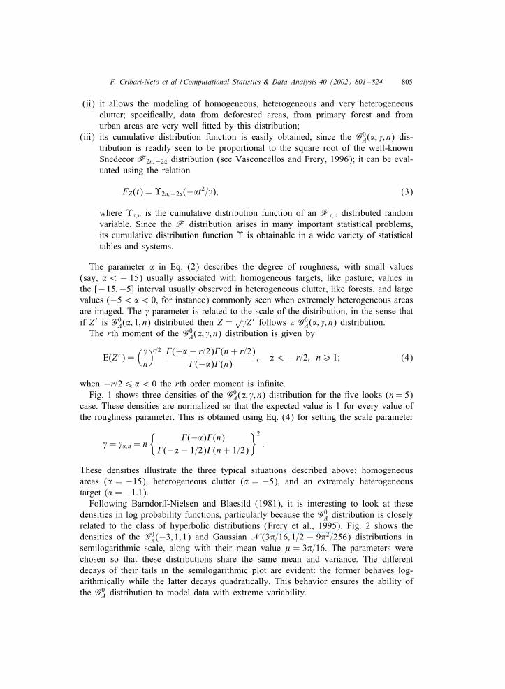
when −r=26 �¡ 0 the rth order moment is in6nite.Fig. 1 shows three densities of the G0

A(�; �; n) distribution for the 6ve looks (n= 5)case. These densities are normalized so that the expected value is 1 for every value ofthe roughness parameter. This is obtained using Eq. (4) for setting the scale parameter

�= ��;n = n{

�(−�)�(n)�(−�− 1=2)�(n+ 1=2)

}2

:

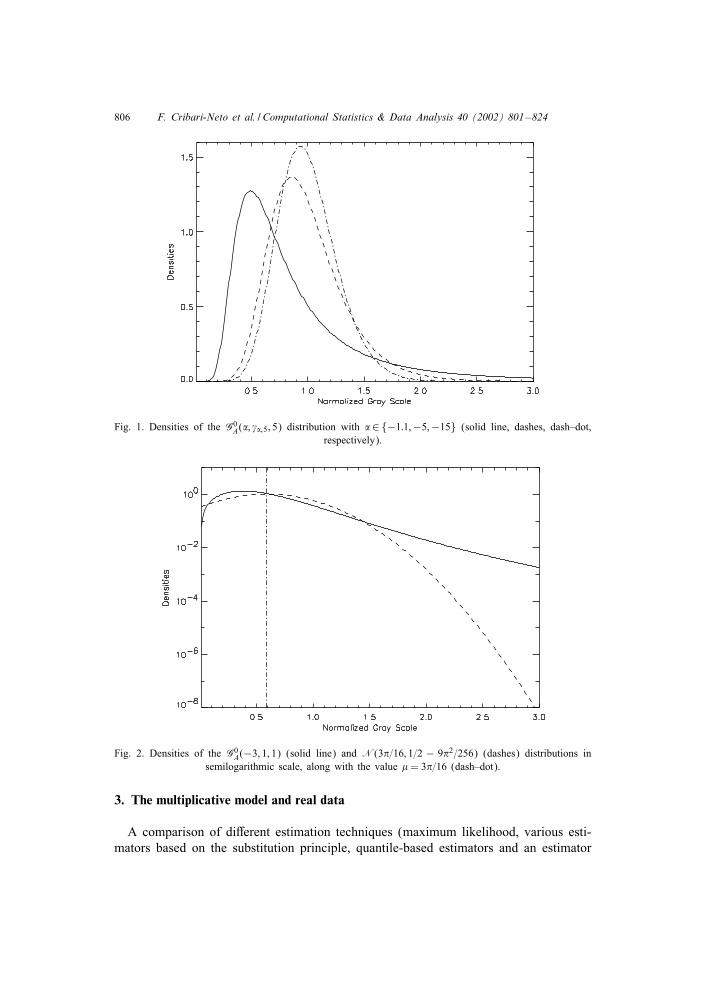
These densities illustrate the three typical situations described above: homogeneousareas (� = −15), heterogeneous clutter (� = −5), and an extremely heterogeneoustarget (�=−1:1).Following Barndor1-Nielsen and Blaesild (1981), it is interesting to look at these

densities in log probability functions, particularly because the G0A distribution is closely

related to the class of hyperbolic distributions (Frery et al., 1995). Fig. 2 shows thedensities of the G0

A(−3; 1; 1) and Gaussian N(3�=16; 1=2 − 9�2=256) distributions insemilogarithmic scale, along with their mean value � = 3�=16. The parameters werechosen so that these distributions share the same mean and variance. The di1erentdecays of their tails in the semilogarithmic plot are evident: the former behaves log-arithmically while the latter decays quadratically. This behavior ensures the ability ofthe G0

A distribution to model data with extreme variability.

806 F. Cribari-Neto et al. / Computational Statistics & Data Analysis 40 (2002) 801–824

Fig. 1. Densities of the G0A(�; ��;5; 5) distribution with �∈{−1:1;−5;−15} (solid line, dashes, dash–dot,

respectively).

Fig. 2. Densities of the G0A(−3; 1; 1) (solid line) and N(3�=16; 1=2 − 9�2=256) (dashes) distributions in

semilogarithmic scale, along with the value � = 3�=16 (dash–dot).

3. The multiplicative model and real data

A comparison of di1erent estimation techniques (maximum likelihood, various esti-mators based on the substitution principle, quantile-based estimators and an estimator

F. Cribari-Neto et al. / Computational Statistics & Data Analysis 40 (2002) 801–824 807

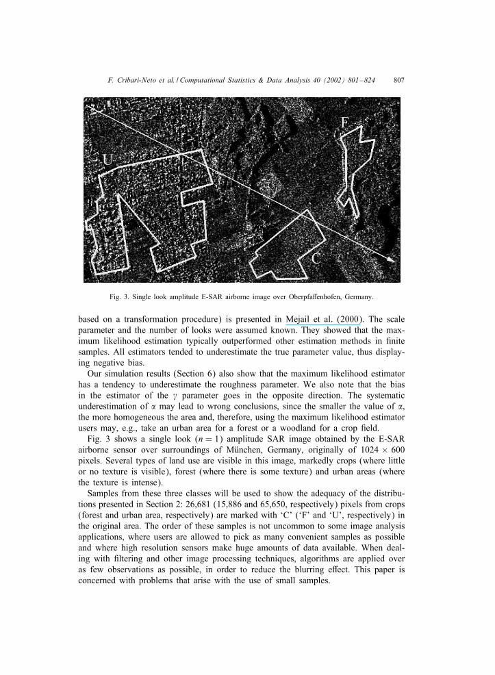
Fig. 3. Single look amplitude E-SAR airborne image over Oberpfa1enhofen, Germany.

based on a transformation procedure) is presented in Mejail et al. (2000). The scaleparameter and the number of looks were assumed known. They showed that the max-imum likelihood estimation typically outperformed other estimation methods in 6nitesamples. All estimators tended to underestimate the true parameter value, thus display-ing negative bias.Our simulation results (Section 6) also show that the maximum likelihood estimator

has a tendency to underestimate the roughness parameter. We also note that the biasin the estimator of the � parameter goes in the opposite direction. The systematicunderestimation of � may lead to wrong conclusions, since the smaller the value of �,the more homogeneous the area and, therefore, using the maximum likelihood estimatorusers may, e.g., take an urban area for a forest or a woodland for a crop 6eld.Fig. 3 shows a single look (n = 1) amplitude SAR image obtained by the E-SAR

airborne sensor over surroundings of MPunchen, Germany, originally of 1024 × 600pixels. Several types of land use are visible in this image, markedly crops (where littleor no texture is visible), forest (where there is some texture) and urban areas (wherethe texture is intense).Samples from these three classes will be used to show the adequacy of the distribu-

tions presented in Section 2: 26,681 (15,886 and 65,650, respectively) pixels from crops(forest and urban area, respectively) are marked with ‘C’ (‘F’ and ‘U’, respectively) inthe original area. The order of these samples is not uncommon to some image analysisapplications, where users are allowed to pick as many convenient samples as possibleand where high resolution sensors make huge amounts of data available. When deal-ing with 6ltering and other image processing techniques, algorithms are applied overas few observations as possible, in order to reduce the blurring e1ect. This paper isconcerned with problems that arise with the use of small samples.

808 F. Cribari-Neto et al. / Computational Statistics & Data Analysis 40 (2002) 801–824

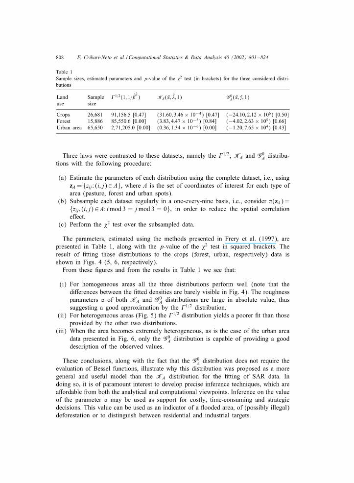
Table 1Sample sizes, estimated parameters and p-value of the �2 test (in brackets) for the three considered distri-butions

Land Sample �1=2(1; 1=�2) KA(�; �; 1) G0

A(�; �; 1)use size

Crops 26,681 91,156.5 [0.47] (31:60; 3:46× 10−4) [0.47] (−24:10; 2:12× 106) [0.50]Forest 15,886 85,550.6 [0.00] (3:83; 4:47× 10−5) [0.84] (−4:02; 2:63× 105) [0.66]Urban area 65,650 2,71,205.0 [0.00] (0:36; 1:34× 10−6) [0.00] (−1:20; 7:65× 104) [0.43]

Three laws were contrasted to these datasets, namely the �1=2, KA and G0A distribu-

tions with the following procedure:

(a) Estimate the parameters of each distribution using the complete dataset, i.e., usingzA = {zij: (i; j)∈A}, where A is the set of coordinates of interest for each type ofarea (pasture, forest and urban spots).

(b) Subsample each dataset regularly in a one-every-nine basis, i.e., consider �(zA)={zij; (i; j)∈A: imod 3 = jmod 3 = 0}, in order to reduce the spatial correlatione1ect.

(c) Perform the �2 test over the subsampled data.

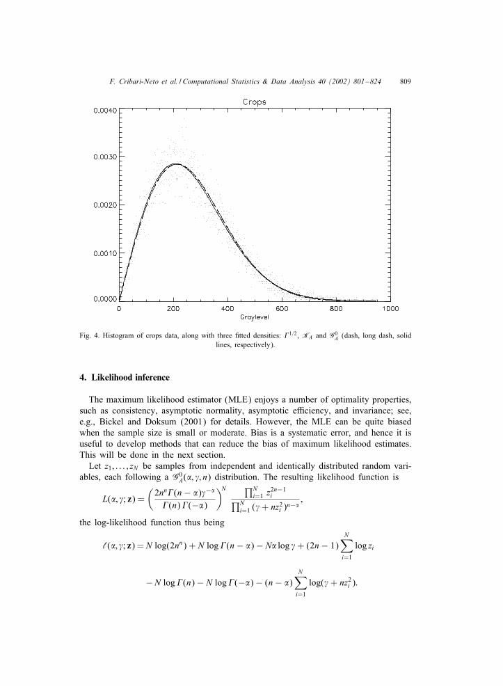
The parameters, estimated using the methods presented in Frery et al. (1997), arepresented in Table 1, along with the p-value of the �2 test in squared brackets. Theresult of 6tting those distributions to the crops (forest, urban, respectively) data isshown in Figs. 4 (5, 6, respectively).From these 6gures and from the results in Table 1 we see that:

(i) For homogeneous areas all the three distributions perform well (note that thedi1erences between the 6tted densities are barely visible in Fig. 4). The roughnessparameters � of both KA and G0

A distributions are large in absolute value, thussuggesting a good approximation by the �1=2 distribution.

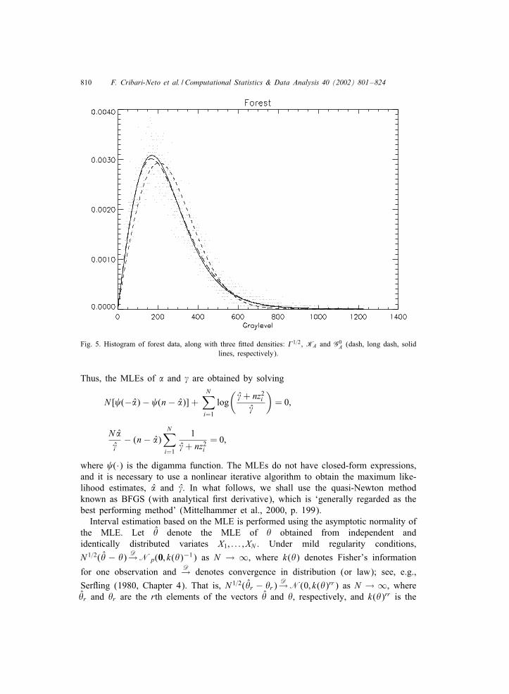
(ii) For heterogeneous areas (Fig. 5) the �1=2 distribution yields a poorer 6t than thoseprovided by the other two distributions.

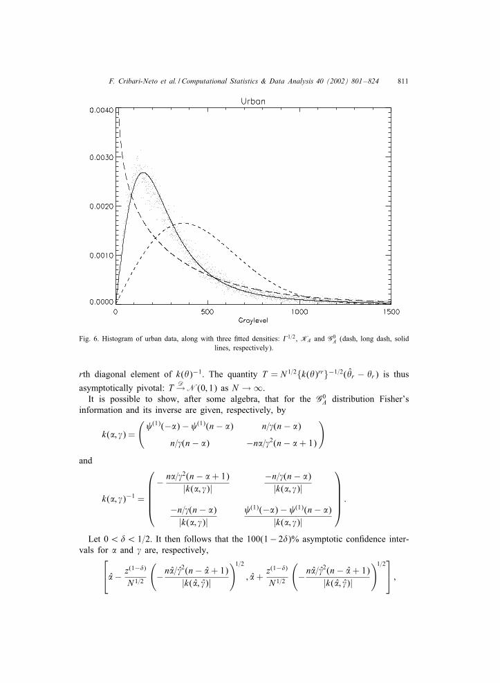
(iii) When the area becomes extremely heterogeneous, as is the case of the urban areadata presented in Fig. 6, only the G0

A distribution is capable of providing a gooddescription of the observed values.

These conclusions, along with the fact that the G0A distribution does not require the

evaluation of Bessel functions, illustrate why this distribution was proposed as a moregeneral and useful model than the KA distribution for the 6tting of SAR data. Indoing so, it is of paramount interest to develop precise inference techniques, which area1ordable from both the analytical and computational viewpoints. Inference on the valueof the parameter � may be used as support for costly, time-consuming and strategicdecisions. This value can be used as an indicator of a Gooded area, of (possibly illegal)deforestation or to distinguish between residential and industrial targets.

F. Cribari-Neto et al. / Computational Statistics & Data Analysis 40 (2002) 801–824 809

Fig. 4. Histogram of crops data, along with three 6tted densities: �1=2, KA and G0A (dash, long dash, solid

lines, respectively).

4. Likelihood inference

The maximum likelihood estimator (MLE) enjoys a number of optimality properties,such as consistency, asymptotic normality, asymptotic eKciency, and invariance; see,e.g., Bickel and Doksum (2001) for details. However, the MLE can be quite biasedwhen the sample size is small or moderate. Bias is a systematic error, and hence it isuseful to develop methods that can reduce the bias of maximum likelihood estimates.This will be done in the next section.Let z1; : : : ; zN be samples from independent and identically distributed random vari-

ables, each following a G0A(�; �; n) distribution. The resulting likelihood function is

L(�; �; z) =(2nn�(n− �)�−�

�(n)�(−�)

)N ∏Ni=1 z2n−1

i∏Ni=1 (�+ nz2i )n−�

;

the log-likelihood function thus being

‘(�; �; z) =N log(2nn) + N log�(n− �)− N� log �+ (2n− 1)N∑i=1

log zi

−N log�(n)− N log�(−�)− (n− �)N∑i=1

log(�+ nz2i ):

810 F. Cribari-Neto et al. / Computational Statistics & Data Analysis 40 (2002) 801–824

Fig. 5. Histogram of forest data, along with three 6tted densities: �1=2, KA and G0A (dash, long dash, solid

lines, respectively).

Thus, the MLEs of � and � are obtained by solving

N [ (−�)− (n− �)] +N∑i=1

log(�+ nz2i

�

)= 0;

N ��

− (n− �)N∑i=1

1�+ nz2i

= 0;

where (·) is the digamma function. The MLEs do not have closed-form expressions,and it is necessary to use a nonlinear iterative algorithm to obtain the maximum like-lihood estimates, � and �. In what follows, we shall use the quasi-Newton methodknown as BFGS (with analytical 6rst derivative), which is ‘generally regarded as thebest performing method’ (Mittelhammer et al., 2000, p. 199).Interval estimation based on the MLE is performed using the asymptotic normality of

the MLE. Let & denote the MLE of & obtained from independent andidentically distributed variates X1; : : : ; XN . Under mild regularity conditions,

N 1=2(& − &) D→Np(0; k(&)−1) as N → ∞, where k(&) denotes Fisher’s information

for one observation and D→ denotes convergence in distribution (or law); see, e.g.,

SerGing (1980, Chapter 4). That is, N 1=2(&r − &r)D→N(0; k(&)rr) as N → ∞, where

&r and &r are the rth elements of the vectors & and &, respectively, and k(&)rr is the

F. Cribari-Neto et al. / Computational Statistics & Data Analysis 40 (2002) 801–824 811

Fig. 6. Histogram of urban data, along with three 6tted densities: �1=2, KA and G0A (dash, long dash, solid

lines, respectively).

rth diagonal element of k(&)−1. The quantity T = N 1=2{k(&)rr}−1=2(&r − &r) is thus

asymptotically pivotal: T D→N(0; 1) as N → ∞.It is possible to show, after some algebra, that for the G0

A distribution Fisher’sinformation and its inverse are given, respectively, by

k(�; �) =

( (1)(−�)− (1)(n− �) n=�(n− �)

n=�(n− �) −n�=�2(n− �+ 1)

)

and

k(�; �)−1 =

− n�=�2(n− �+ 1)|k(�; �)|

−n=�(n− �)|k(�; �)|

−n=�(n− �)|k(�; �)|

(1)(−�)− (1)(n− �)|k(�; �)|

:

Let 0¡)¡ 1=2. It then follows that the 100(1− 2))% asymptotic con6dence inter-vals for � and � are, respectively,

�− z(1−))

N 1=2

(−n�=�2(n− �+ 1)

|k(�; �)|

)1=2; �+

z(1−))

N 1=2

(−n�=�2(n− �+ 1)

|k(�; �)|

)1=2 ;

812 F. Cribari-Neto et al. / Computational Statistics & Data Analysis 40 (2002) 801–824

[�− z(1−))

N 1=2

( (1)(−�)− (1)(n− �)

|k(�; �)|)1=2

;

�+z(1−))

N 1=2

( (1)(−�)− (1)(n− �)

|k(�; �)|)1=2]

;

where z(1−)) is the 1− ) upper point from the standard normal distribution.

5. Bootstrap methods

This section presents di1erent bootstrapping schemes that can be used to reduce thebias of the MLE. Let X be a random sample of size N where each entry representsa random draw from the random variable X that has distribution function F = F(&).Here, & is the parameter that indexes the distribution and is viewed as a functional ofF , i.e., &= t(F). Let & be an estimator of & obtained using the random sample above,&= s(X).

The idea behind the bootstrap method proposed by Efron (1979) is to use resam-pling to obtain additional pseudo-samples, and then to extract information from thesesamples to improve inference. We can broadly classify bootstrap methods into twoclasses, depending on how the sampling is performed: parametric and nonparametric.In the parametric version, the bootstrap samples are obtained from F(&) whereas inthe nonparametric version they are obtained from the empirical distribution function(F) through sampling with replacement. Note that the nonparametric bootstrap doesnot entail parametric assumptions.Suppose we have R bootstrap samples x∗ = (x∗1 ; : : : ; x

∗N ), and hence R estimates

s(x∗). We then have R bootstrap estimates of &, denoted &∗i, i = 1; : : : ; R. The R

bootstrap replications of & are then used to estimate the distribution function of & andits associated features and moments. Our interest lies in obtaining an estimate for thebias of the MLE, so that we can use it to de6ne a bias-corrected estimator. Let BF(&; &)denote the bias of an estimator &= s(X), that is,

BF(&; &) = EF [&− &] = EF [s(X)]− &= EF [s(X)]− t(F);

where the statistic s(X) is a function of independent and identically distributed ran-dom variables, each having distribution function F . The parametric and nonparametricbootstrap bias estimates are obtained replacing F in the expression above by F& andF , respectively, thus yielding

BF&(&; &) = EF&

[s(X∗)]− t(F&) and BF(&; &) = EF [s(X∗)]− t(F):

The idea is then to approximate EF&[s(X∗)] and EF [s(X

∗)] using &∗(·)=R−1 ∑R

i=1 &∗i.

Therefore, the parametric and nonparametric bootstrap estimates for the bias of & are,

F. Cribari-Neto et al. / Computational Statistics & Data Analysis 40 (2002) 801–824 813

respectively,

BF&(&; &) = &

∗(·)− s(x) and BF(&; &) = &

∗(·)− s(x);

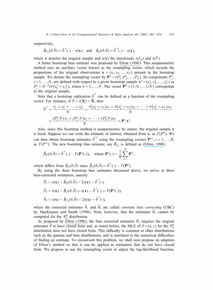
where x denotes the original sample and s(x) the functionals t(F&) and t(F).A better bootstrap bias estimate was proposed by Efron (1990). This nonparametric

method uses an auxiliary vector known as the resampling vector, which records theproportions of the original observations x = (x1; x2; : : : ; xN ) present in the bootstrapsample. We denote the resampling vector by P∗=(P∗

1 ; P∗2 ; : : : ; P

∗N ). Its components P∗

j ,j=1; : : : ; N , are de6ned with respect to a given bootstrap sample x∗=(x∗1 ; x

∗2 ; : : : ; x

∗N ) as

P∗j =N−1(#{x∗k = xj}), where k =1; : : : ; N . The vector P0 = (1=N; : : : ; 1=N ) corresponds

to the original sample.Note that a bootstrap replication &

∗can be de6ned as a function of the resampling

vector. For instance, if &= s(X) = VX, then

&∗=

x∗1 + x∗2 + · · ·+ x∗NN

=#{x∗k = x1}x1 + #{x∗k = x2}x2 + · · ·+ #{x∗k = xN}xN

N

=(P∗

1 N ) x1 + (P∗2 N )x2 + · · ·+ (P∗

NN )xNN

= P∗ x′:

Also, since this bootstrap method is nonparametric by nature, the original sample xis 6xed. Suppose we can write the estimate of interest, obtained from x, as T (P0). We

can then obtain bootstrap estimates &∗i

using the resampling vectors P∗i, i = 1; : : : ; R,as T (P∗i). The new bootstrap bias estimate, say VBF , is de6ned as (Efron, 1990)

VBF(&; &) = &∗(·)− T (P∗(·)); where P∗(·) = 1

R

R∑i=1

P∗i ;

which di1ers from BF(&; &) since BF(&; &) = &∗(·)− T (P0).

By using the three bootstrap bias estimates discussed above, we arrive at threebias-corrected estimators, namely:

V&1 = s(x)− BF(&; &) = 2s(x)− &∗(·);

V&2 = s(x)− VBF(&; &) = s(x)− &∗(·) + T (P∗(·));

V&3 = s(x)− BF&(&; &) = 2s(x)− &

∗(·);

where the corrected estimates V&1 and V&3 are called constant bias correcting (CBC)by MacKinnon and Smith (1998). Note, however, that the estimator V&2 cannot becomputed for the G0

A distribution.As proposed by Efron (1990), the bias corrected estimator V&2 requires the original

estimator & to have closed form and, as noted before, the MLE of &=(�; �) for the G0A

distribution does not have closed form. This diKculty is common to other distributionssuch as the gamma and beta distributions, and is unrelated to the numerical diKcultiesof 6nding an estimate. To circumvent this problem, we shall now propose an adaptionof Efron’s method so that it can be applied to estimators that do not have closedform. We propose to use the resampling vector to adjust the log-likelihood function,

814 F. Cribari-Neto et al. / Computational Statistics & Data Analysis 40 (2002) 801–824

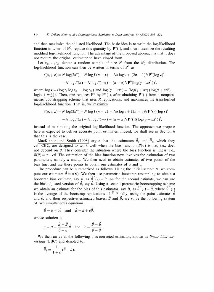
and then maximize the adjusted likelihood. The basic idea is to write the log-likelihoodfunction in terms of P0, replace this quantity by P∗(·), and then maximize the resultingmodi6ed log-likelihood function. The advantage of the proposed approach is that it doesnot require the original estimator to have closed form.Let zn; : : : ; zN denote a random sample of size N from the G0

A distribution. Thelog-likelihood function can then be written in terms of P0 as

‘(�; �; z) =N log(2nn) + N log�(n− �) − N� log �+ (2n− 1)NP0(log z)′

−N log�(n)− N log�(−�)− (n− �)NP0(log(�+ nz2))′;

where log z = (log z1 log z2 : : : log zN ) and log (�+ nz2) = {log(�+ nz21) log(�+ nz22) : : :log(�+ nz2N )}. Then, one replaces P0 by P∗(·), after obtaining P∗(·) from a nonpara-metric bootstrapping scheme that uses R replications, and maximizes the transformedlog-likelihood function. That is, we maximize

‘(�; �; z) =N log(2nn) + N log�(n− �) − N� log �+ (2n− 1)NP∗(·)(log z)′

−N log�(n)− N log�(−�)− (n− �)NP∗(·)(log (�+ nz2))′;

instead of maximizing the original log-likelihood function. The approach we proposehere is expected to deliver accurate point estimates. Indeed, we shall see in Section 6that this is the case.MacKinnon and Smith (1998) argue that the estimators V&1 and V&3, which they

call CBC, are designed to work well when the bias function B(&) is Gat, i.e., doesnot depend on &. They consider the situation where the bias function is linear, i.e.,B(&) = a+ c&. The estimation of the bias function now involves the estimation of twoparameters, namely a and c. We then need to obtain estimates of two points of thebias line, and use these points to obtain our estimates of a and c.The procedure can be summarized as follows. Using the initial sample x, we com-

pute our estimate: & = s(x). We then use parametric bootstrap resampling to obtain abootstrap bias estimate, say B, as &

∗(·) − &. As for the second estimate, we can use

the bias-adjusted version of &, say &. Using a second parametric bootstrapping schemewe obtain an estimate for the bias of this estimator, say B, as &

∗(·)− &, where &

∗(·)

is the average of the bootstrap replications of &. Finally, using the point estimates &and &, and their respective estimated biases, B and B, we solve the following systemof two simultaneous equations:

B= a+ c& and B= a+ c&;

whose solution is

a= B− B− B

&− && and c =

B− B

&− &:

We then arrive at the following bias-corrected estimator, known as linear bias cor-recting (LBC) and denoted V&4:

V&4 =1

1 + c(&− a):

F. Cribari-Neto et al. / Computational Statistics & Data Analysis 40 (2002) 801–824 815

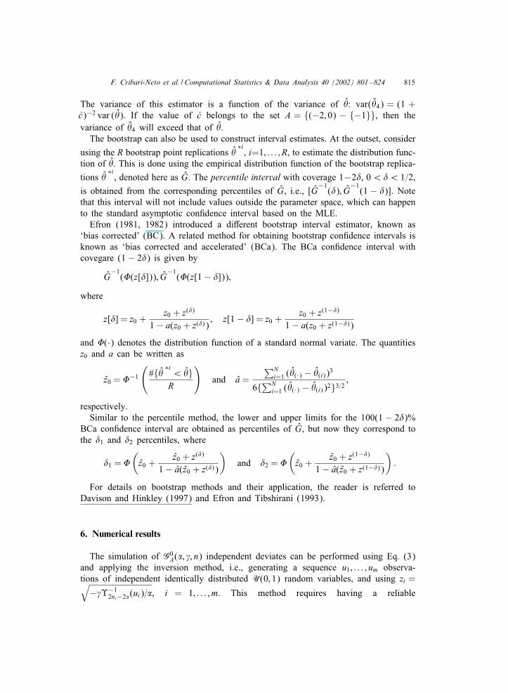
The variance of this estimator is a function of the variance of &: var( V&4) = (1 +c)−2 var (&). If the value of c belongs to the set A = {(−2; 0) − {−1}}, then thevariance of V&4 will exceed that of &.

The bootstrap can also be used to construct interval estimates. At the outset, consider

using the R bootstrap point replications &∗i, i=1; : : : ; R, to estimate the distribution func-

tion of &. This is done using the empirical distribution function of the bootstrap replica-

tions &∗i, denoted here as G. The percentile interval with coverage 1−2), 0¡)¡ 1=2,

is obtained from the corresponding percentiles of G, i.e., [G−1

()); G−1

(1 − ))]. Notethat this interval will not include values outside the parameter space, which can happento the standard asymptotic con6dence interval based on the MLE.Efron (1981, 1982) introduced a di1erent bootstrap interval estimator, known as

‘bias corrected’ (BC). A related method for obtaining bootstrap con6dence intervals isknown as ‘bias corrected and accelerated’ (BCa). The BCa con6dence interval withcovegare (1− 2)) is given by

G−1

(1(z[)])); G−1

(1(z[1− )]));

where

z[)] = z0 +z0 + z())

1− a(z0 + z())); z[1− )] = z0 +

z0 + z(1−))

1− a(z0 + z(1−)))

and 1(·) denotes the distribution function of a standard normal variate. The quantitiesz0 and a can be written as

z0 = 1−1

(#{& ∗i

¡ &}R

)and a=

∑Ni=1 (&(·) − &(i))3

6{∑Ni=1 (&(·) − &(i))2}3=2

;

respectively.Similar to the percentile method, the lower and upper limits for the 100(1 − 2))%

BCa con6dence interval are obtained as percentiles of G, but now they correspond tothe )1 and )2 percentiles, where

)1 = 1(z0 +

z0 + z())

1− a(z0 + z()))

)and )2 = 1

(z0 +

z0 + z(1−))

1− a(z0 + z(1−)))

):

For details on bootstrap methods and their application, the reader is referred toDavison and Hinkley (1997) and Efron and Tibshirani (1993).

6. Numerical results

The simulation of G0A(�; �; n) independent deviates can be performed using Eq. (3)

and applying the inversion method, i.e., generating a sequence u1; : : : ; um observa-tions of independent identically distributed U(0; 1) random variables, and using zi =√−�M−1

2n;−2�(ui)=�, i = 1; : : : ; m. This method requires having a reliable

816 F. Cribari-Neto et al. / Computational Statistics & Data Analysis 40 (2002) 801–824

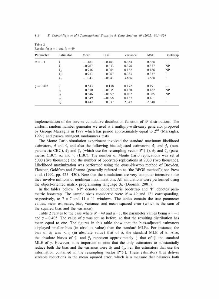
Table 2Results for n = 1 and N = 49

Parameter Estimator Mean Bias Variance MSE Bootstrap

�=−1 � −1:183 −0:183 0.334 0.368 —V�1 −0:967 0.033 0.376 0.377 NPV�2 −0:936 0.064 0.182 0.186 NPV�3 −0:933 0.067 0.333 0.337 PV�4 −1:043 −0:043 3.866 3.868 P

�= 0:405 � 0.543 0.138 0.172 0.191 —V�1 0.370 −0:035 0.180 0.182 NPV�2 0.346 −0:059 0.082 0.085 NPV�3 0.349 −0:056 0.157 0.161 PV�4 0.442 0.037 2.347 2.348 P

implementation of the inverse cumulative distribution function of F distributions. Theuniform random number generator we used is a multiply-with-carry generator proposedby George Marsaglia in 1997 which has period approximately equal to 260 (Marsaglia,1997) and passes stringent randomness tests.The Monte Carlo simulation experiment involved the standard maximum likelihood

estimators, � and �, and also the following bias-adjusted estimators: V�1 and V�1 (non-parametric CBC), V�2 and V�2 (which use the resampling vector P∗(·)), V�3 and V�3 (para-metric CBC), V�4 and V�4 (LBC). The number of Monte Carlo replications was set at5000 (6ve thousand) and the number of bootstrap replications at 2000 (two thousand).Likelihood maximization was performed using the quasi-Newton method of Broyden,Fletcher, Goldfarb and Shanno (generally referred to as ‘the BFGS method’); see Presset al. (1992, pp. 425–430). Note that the simulations are very computer-intensive sincethey involve millions of nonlinear maximizations. All simulations were performed usingthe object-oriented matrix programming language Ox (Doornik, 2001).In the tables bellow ‘NP’ denotes nonparametric bootstrap and ‘P’ denotes para-

metric bootstrap. The sample sizes considered were N = 49 and 121 corresponding,respectively, to 7 × 7 and 11 × 11 windows. The tables contain the true parametervalues, mean estimates, bias, variance, and mean squared error (which is the sum ofthe squared bias and the variance).Table 2 relates to the case where N=49 and n=1, the parameter values being �=−1

and �= 0:405. The value of � was set, as before, so that the resulting distribution hasmean equal to one. The 6gures in this table show that the bias-adjusted estimatorsdisplayed smaller bias (in absolute value) than the standard MLEs. For instance, thebias of V�1 was ¡ 1

5 (in absolute value) that of �, the standard MLE of �. Also,the absolute biases of V�1 and V�4 represent approximately 1

4 that of �, the standardMLE of �. However, it is important to note that the only estimators to substantiallyreduce both the bias and the variance were V�2 and V�2, i.e., the estimators that use theinformation contained in the resampling vector P∗(·). These estimators thus deliversizeable reductions in the mean squared error, which is a measure that balances both

F. Cribari-Neto et al. / Computational Statistics & Data Analysis 40 (2002) 801–824 817

Table 3Results for n = 3 and N = 49

Parameter Estimator Mean Bias Variance MSE Bootstrap

�=−1 � −1:082 −0:082 0.077 0.084 —V�1 −0:985 0.015 0.054 0.054 NPV�2 −0:983 0.017 0.054 0.054 NPV�3 −0:982 0.018 0.051 0.051 PV�4 −0:997 0.003 0.057 0.057 P

�= 0:346 � 0.392 0.046 0.022 0.024 —V�1 0.337 −0:009 0.014 0.015 NPV�2 0.336 −0:010 0.014 0.015 NPV�3 0.336 −0:010 0.014 0.014 PV�4 0.344 −0:002 0.016 0.016 P

Table 4Results for n = 1 and N = 49

Parameter Estimator Mean Bias Variance MSE Bootstrap

�=−3 � −3:522 −0:522 3.419 3.692 —V�1 −3:546 −0:546 7.358 7.656 NPV�2 −2:742 0.258 2.611 2.677 NPV�3 −3:523 0.523 8.138 8.412 PV�4 −7:125 4.125 377.469 394.481 P

�= 2:882 � 3.528 0.646 5.193 5.610 —V�1 3.557 0.675 11.180 11.635 NPV�2 2.555 −0:327 3.908 4.015 NPV�3 3.535 0.653 12.229 12.656 PV�4 8.145 5.263 699.150 726.844 P

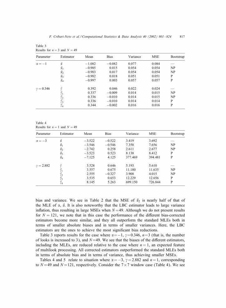
bias and variance. We see in Table 2 that the MSE of V�2 is nearly half of that ofthe MLE of �, �. It is also noteworthy that the LBC estimator leads to large varianceinGation, thus resulting in large MSEs when N=49. Although we do not present resultsfor N = 121, we note that in this case the performance of the di1erent bias-correctedestimators become more similar, and they all outperform the standard MLEs both interms of smaller absolute biases and in terms of smaller variances. Here, the LBCestimators are the ones to achieve the most signi6cant bias reductions.Table 3 reports results for the case where �=−1, �=0:346, n=3 (that is, the number

of looks is increased to 3), and N=49. We see that the biases of the di1erent estimators,including the MLEs, are reduced relative to the case where n= 1, an expected featureof multilook processing. All corrected estimators outperformed the standard MLEs bothin terms of absolute bias and in terms of variance, thus achieving smaller MSEs.Tables 4 and 5 relate to situation where �=−3, �=2:882 and n=1, corresponding

to N=49 and N=121, respectively. Consider the 7×7 window case (Table 4). We see

818 F. Cribari-Neto et al. / Computational Statistics & Data Analysis 40 (2002) 801–824

Table 5Results for n = 1 and N = 121

Parameter Estimator Mean Bias Variance MSE Bootstrap

�=−3 � −3:488 −0:488 2.257 2.495 —V�1 −3:329 −0:329 4.035 4.143 NPV�2 −2:949 0.051 1.809 1.811 NPV�3 −3:283 −0:283 4.091 4.171 PV�4 −4:071 −1:071 36.938 38.086 P

�= 2:882 � 3.489 0.607 3.527 3.896 —V�1 3.296 0.414 6.370 6.541 NPV�2 2.818 −0:064 2.805 2.809 NPV�3 3.243 0.361 6.416 6.546 PV�4 4.371 1.489 76.794 79.010 P

Table 6Results for n = 3 and N = 49

Parameter Estimator Mean Bias Variance MSE Bootstrap

�=−3 � −3:609 −0:609 2.971 3.341 —V�1 −3:073 −0:073 3.716 3.721 NPV�2 −2:860 0.140 1.850 1.869 NPV�3 −3:031 −0:031 4.003 4.004 PV�4 −3:416 −0:416 25.899 26.071 P

�= 2:459 � 3.079 0.620 3.109 3.493 —V�1 2.539 0.080 3.904 3.910 NPV�2 2.319 −0:140 1.893 1.913 NPV�3 2.498 0.039 4.200 4.202 PV�4 2.919 0.460 32.434 32.645 P

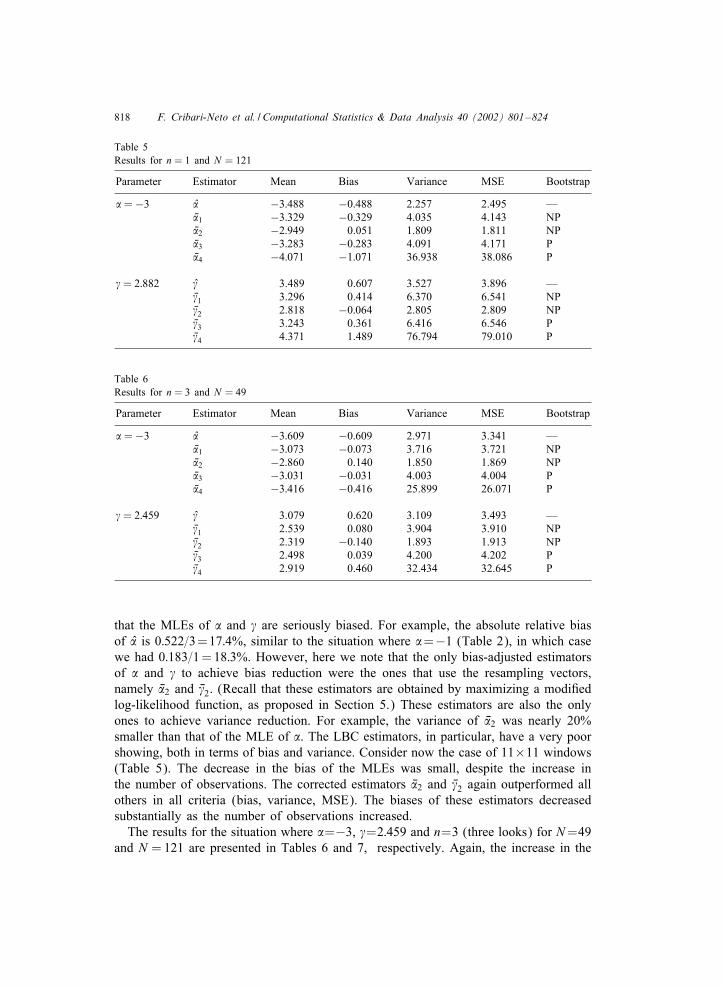
that the MLEs of � and � are seriously biased. For example, the absolute relative biasof � is 0:522=3=17:4%, similar to the situation where �=−1 (Table 2), in which casewe had 0:183=1=18:3%. However, here we note that the only bias-adjusted estimatorsof � and � to achieve bias reduction were the ones that use the resampling vectors,namely V�2 and V�2. (Recall that these estimators are obtained by maximizing a modi6edlog-likelihood function, as proposed in Section 5.) These estimators are also the onlyones to achieve variance reduction. For example, the variance of V�2 was nearly 20%smaller than that of the MLE of �. The LBC estimators, in particular, have a very poorshowing, both in terms of bias and variance. Consider now the case of 11×11 windows(Table 5). The decrease in the bias of the MLEs was small, despite the increase inthe number of observations. The corrected estimators V�2 and V�2 again outperformed allothers in all criteria (bias, variance, MSE). The biases of these estimators decreasedsubstantially as the number of observations increased.The results for the situation where �=−3, �=2:459 and n=3 (three looks) for N=49

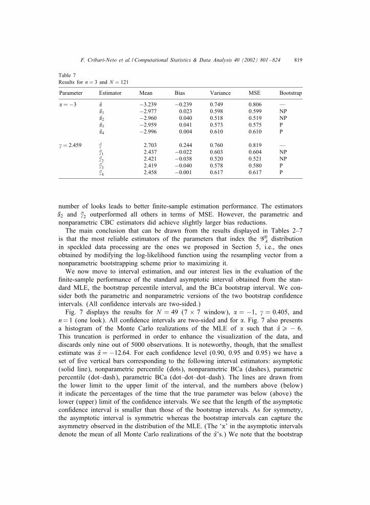
and N =121 are presented in Tables 6 and 7, respectively. Again, the increase in the

F. Cribari-Neto et al. / Computational Statistics & Data Analysis 40 (2002) 801–824 819

Table 7Results for n = 3 and N = 121

Parameter Estimator Mean Bias Variance MSE Bootstrap

�=−3 � −3:239 −0:239 0.749 0.806 —V�1 −2:977 0.023 0.598 0.599 NPV�2 −2:960 0.040 0.518 0.519 NPV�3 −2:959 0.041 0.573 0.575 PV�4 −2:996 0.004 0.610 0.610 P

�= 2:459 � 2.703 0.244 0.760 0.819 —V�1 2.437 −0:022 0.603 0.604 NPV�2 2.421 −0:038 0.520 0.521 NPV�3 2.419 −0:040 0.578 0.580 PV�4 2.458 −0:001 0.617 0.617 P

number of looks leads to better 6nite-sample estimation performance. The estimatorsV�2 and V�2 outperformed all others in terms of MSE. However, the parametric andnonparametric CBC estimators did achieve slightly larger bias reductions.The main conclusion that can be drawn from the results displayed in Tables 2–7

is that the most reliable estimators of the parameters that index the G0A distribution

in speckled data processing are the ones we proposed in Section 5, i.e., the onesobtained by modifying the log-likelihood function using the resampling vector from anonparametric bootstrapping scheme prior to maximizing it.We now move to interval estimation, and our interest lies in the evaluation of the

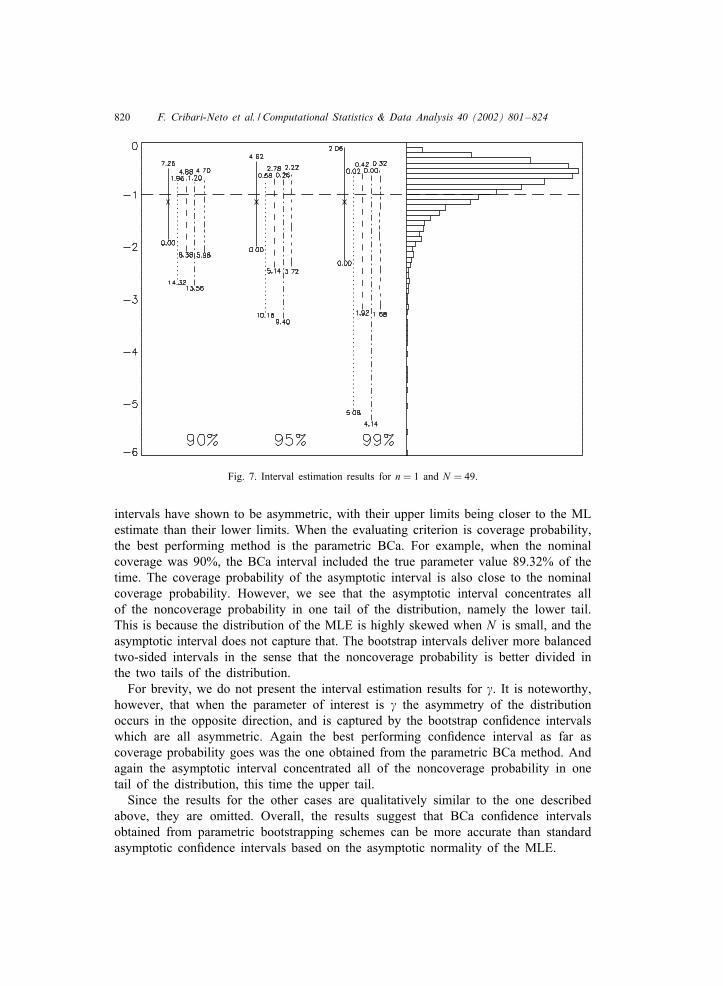
6nite-sample performance of the standard asymptotic interval obtained from the stan-dard MLE, the bootstrap percentile interval, and the BCa bootstrap interval. We con-sider both the parametric and nonparametric versions of the two bootstrap con6denceintervals. (All con6dence intervals are two-sided.)Fig. 7 displays the results for N = 49 (7 × 7 window), � = −1, � = 0:405, and

n=1 (one look). All con6dence intervals are two-sided and for �. Fig. 7 also presentsa histogram of the Monte Carlo realizations of the MLE of � such that �¿ − 6.This truncation is performed in order to enhance the visualization of the data, anddiscards only nine out of 5000 observations. It is noteworthy, though, that the smallestestimate was � =−12:64. For each con6dence level (0.90, 0.95 and 0.95) we have aset of 6ve vertical bars corresponding to the following interval estimators: asymptotic(solid line), nonparametric percentile (dots), nonparametric BCa (dashes), parametricpercentile (dot–dash), parametric BCa (dot–dot–dot–dash). The lines are drawn fromthe lower limit to the upper limit of the interval, and the numbers above (below)it indicate the percentages of the time that the true parameter was below (above) thelower (upper) limit of the con6dence intervals. We see that the length of the asymptoticcon6dence interval is smaller than those of the bootstrap intervals. As for symmetry,the asymptotic interval is symmetric whereas the bootstrap intervals can capture theasymmetry observed in the distribution of the MLE. (The ‘x’ in the asymptotic intervalsdenote the mean of all Monte Carlo realizations of the �’s.) We note that the bootstrap

820 F. Cribari-Neto et al. / Computational Statistics & Data Analysis 40 (2002) 801–824

Fig. 7. Interval estimation results for n = 1 and N = 49.

intervals have shown to be asymmetric, with their upper limits being closer to the MLestimate than their lower limits. When the evaluating criterion is coverage probability,the best performing method is the parametric BCa. For example, when the nominalcoverage was 90%, the BCa interval included the true parameter value 89.32% of thetime. The coverage probability of the asymptotic interval is also close to the nominalcoverage probability. However, we see that the asymptotic interval concentrates allof the noncoverage probability in one tail of the distribution, namely the lower tail.This is because the distribution of the MLE is highly skewed when N is small, and theasymptotic interval does not capture that. The bootstrap intervals deliver more balancedtwo-sided intervals in the sense that the noncoverage probability is better divided inthe two tails of the distribution.For brevity, we do not present the interval estimation results for �. It is noteworthy,

however, that when the parameter of interest is � the asymmetry of the distributionoccurs in the opposite direction, and is captured by the bootstrap con6dence intervalswhich are all asymmetric. Again the best performing con6dence interval as far ascoverage probability goes was the one obtained from the parametric BCa method. Andagain the asymptotic interval concentrated all of the noncoverage probability in onetail of the distribution, this time the upper tail.Since the results for the other cases are qualitatively similar to the one described

above, they are omitted. Overall, the results suggest that BCa con6dence intervalsobtained from parametric bootstrapping schemes can be more accurate than standardasymptotic con6dence intervals based on the asymptotic normality of the MLE.

F. Cribari-Neto et al. / Computational Statistics & Data Analysis 40 (2002) 801–824 821

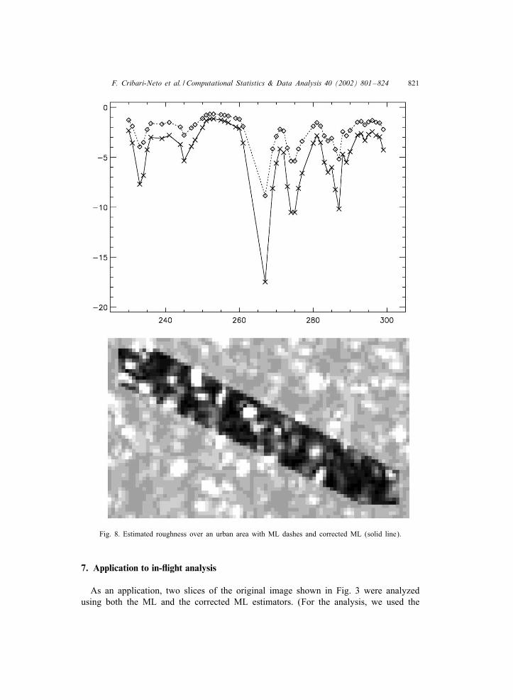
Fig. 8. Estimated roughness over an urban area with ML dashes and corrected ML (solid line).

7. Application to in-)ight analysis

As an application, two slices of the original image shown in Fig. 3 were analyzedusing both the ML and the corrected ML estimators. (For the analysis, we used the

822 F. Cribari-Neto et al. / Computational Statistics & Data Analysis 40 (2002) 801–824

simplest corrected estimator, namely the nonparametric CBC estimator.) These sliceswere taken from in-Gight data, presented as the white arrow in Fig. 3, and they corre-spond to an urban area and to a forest region. The results of the estimated roughnessfor these slices, using a sliding window of 11×11 pixels, are presented in Figs. 8 and9, respectively.If only ML estimation were used (dashes in Fig. 8), the analysis of the urban data

would lead to the conclusion that amongst the extremely heterogeneous targets (withvalues ranging in the [− 1;−5] interval, approximately) there is a heterogeneous spot,the one corresponding to the value −9. The corrected estimator, on the other hand,suggests the existence of several heterogeneous spots and of a very homogeneous area.The ground truth suggests that the latter analysis is the correct one, since the datacorrespond to small houses separated by gardens with trees (heterogeneous targets)and grass (homogeneous targets). These 6gures show both the analysis of the data(top) and the data themselves (bottom), as a dark strip over a light background. Eachpixel corresponds to, approximately, 1 m2 on the ground.

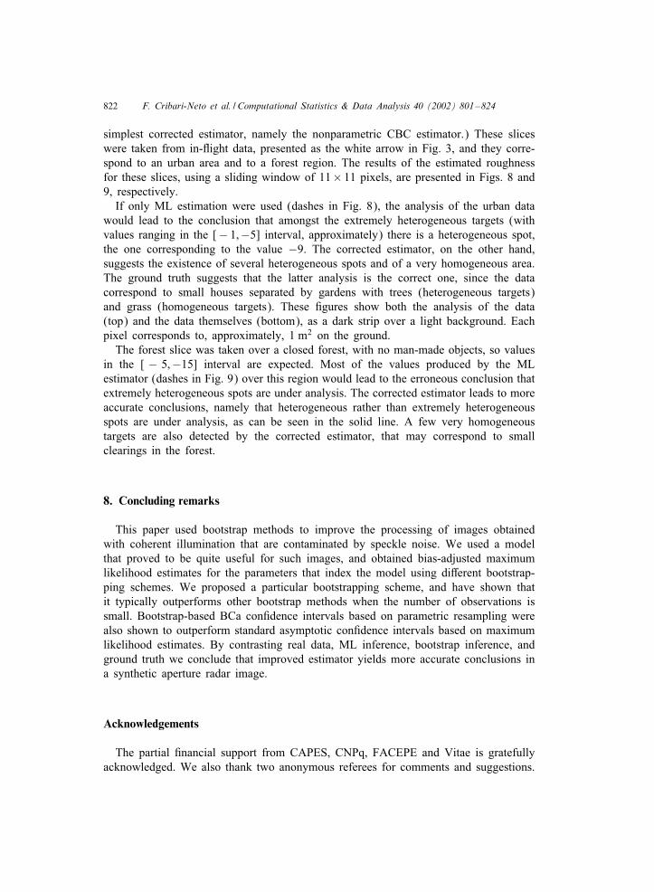
The forest slice was taken over a closed forest, with no man-made objects, so valuesin the [ − 5;−15] interval are expected. Most of the values produced by the MLestimator (dashes in Fig. 9) over this region would lead to the erroneous conclusion thatextremely heterogeneous spots are under analysis. The corrected estimator leads to moreaccurate conclusions, namely that heterogeneous rather than extremely heterogeneousspots are under analysis, as can be seen in the solid line. A few very homogeneoustargets are also detected by the corrected estimator, that may correspond to smallclearings in the forest.

8. Concluding remarks

This paper used bootstrap methods to improve the processing of images obtainedwith coherent illumination that are contaminated by speckle noise. We used a modelthat proved to be quite useful for such images, and obtained bias-adjusted maximumlikelihood estimates for the parameters that index the model using di1erent bootstrap-ping schemes. We proposed a particular bootstrapping scheme, and have shown thatit typically outperforms other bootstrap methods when the number of observations issmall. Bootstrap-based BCa con6dence intervals based on parametric resampling werealso shown to outperform standard asymptotic con6dence intervals based on maximumlikelihood estimates. By contrasting real data, ML inference, bootstrap inference, andground truth we conclude that improved estimator yields more accurate conclusions ina synthetic aperture radar image.

Acknowledgements

The partial 6nancial support from CAPES, CNPq, FACEPE and Vitae is gratefullyacknowledged. We also thank two anonymous referees for comments and suggestions.

F. Cribari-Neto et al. / Computational Statistics & Data Analysis 40 (2002) 801–824 823

Fig. 9. Estimated roughness over a forested region with ML (dashes) and corrected ML (solid line).

References

Barndor1-Nielsen, O.E., Blaesild, P., 1981. Hyperbolic distributions and rami6cations: contributions to theoryand applications. In: Taillie, C., Baldessari, B.A. (Eds.), Statistical Distributions in Scienti6c Work. Reidel,Dordrecht, pp. 19–44.

824 F. Cribari-Neto et al. / Computational Statistics & Data Analysis 40 (2002) 801–824

Bickel, P.J., Doksum, K.A., 2001. Mathematical Statistics: Basic Ideas and Selected Topics, Vol. 1, 2ndEdition. Prentice-Hall, Upper Saddle River.

Davison, A.C., Hinkley, D.V., 1997. Bootstrap Methods and their Application. Cambridge University Press,New York.

Doornik, J.A., 2001. Ox: an Object-oriented Matrix Programming Language, 4th Edition. TimberlakeConsultants, London, & http://www.nuff.ox.ac.uk/Users/Doornik, Oxford.

Efron, B., 1979. Bootstrap methods: another look at the jackknife. Ann. Statist. 7, 1–26.Efron, B., 1981. Nonparametric standard errors and con6dence intervals. Canad. J. Statist. 9, 139–172.Efron, B., 1982. The Jackknife, the Bootstrap and Other Resampling Plans. Society for Industrial and Applied

Mathematics, Philadelphia.Efron, B., 1990. More eKcient bootstrap computations. J. Amer. Statist. Assoc. 85, 79–89.Efron, B., Tibshirani, R.J., 1993. An Introduction to the Bootstrap. Chapman and Hall, New York.Ferrari, S.L.P., Cribari-Neto, F., 1998. On bootstrap and analytical bias corrections. Econom. Lett. 58, 761–

782.Frery, A.C., Yanasse, C.C.F., Sant’Anna, S.J.S., 1995. Alternative distributions for the multiplicative model

in SAR images. In: Quantitative Remote Sensing for Science and Applications, GARSS’95 Proc., IEEE,Florence, pp. 169–171.

Frery, A.C., MPuller, H.-J., Yanasse, C.C.F., Sant’Anna, S.J.S., 1997. A model for extremely heterogeneousclutter. IEEE Trans. Geosci. Remote Sensing 35, 648–659.

Goodman, J.W., 1985. Statistical Optics. Wiley, New York.JHrgensen, B., 1982. Statistical Properties of the Generalized Inverse Gaussian Distribution. Springer, Berlin,

New York.MacKinnon, J.G., Smith Jr., A.A., 1998. Approximate bias correction in econometrics. J. Econometrics 85,

205–230.Marsaglia, G., 1997. A random number generator for C. Discussion Paper, posting on usenet newsgroup

sci.stat.math.Mejail, M., Jacobo-Berlles, J., Frery, A.C., Bustos, O.H., 2000. Parametric roughness estimation in amplitude

SAR images under the multiplicative model. Rev. de Teledet. 13, 37–49.Mittelhammer, R.C., Judge, G.G., Miller, D.J., 2000. Econometric Foundations. Cambridge University Press,

New York.Press, W.H., Teukolsky, S.A., Vetterling, W.T., Flannery, B.P., 1992. Numerical Recipes in C: The Art of

Scienti6c Computing, 2nd Edition. Cambridge University Press, New York.SerGing, R.J., 1980. Approximation Theorems of Mathematical Statistics. Wiley, New York.Vasconcellos, K.L.P., Frery, A.C., 1996. Maximum likelihood 6tting of extremely heterogeneous radar

clutter. In: First Latin-American Seminar on Radar Remote Sensing: Image Processing Techniques, FirstLatino-American Seminar on Radar Remote Sensing: Image Processing Techniques (SP 407 Fev. 1997),Noordwijk, The Netherlands, ESA, pp. 97–101.