site specific radar coverage and land clutter modelling
TRANSCRIPT

Univers
ity of
Cap
e Tow
n
Site Specific Radar Coverage and Land
Clutter Modelling
Prepared by:
Sulayman Salie
SLXSUL003
Prepared for:
Professor Michael Raymond Inggs
Department of Electrical Engineering
University of Cape Town
April 2016
A minor dissertation submitted to the Department of Electrical Engineering,
University of Cape Town, in partial fulfilment of the requirements
for the degree of
Master of Engineering Specialising in Radar and Electronic Defence
The copyright of this thesis vests in the author. No quotation from it or information derived from it is to be published without full acknowledgement of the source. The thesis is to be used for private study or non-commercial research purposes only.
Published by the University of Cape Town (UCT) in terms of the non-exclusive license granted to UCT by the author.
Univers
ity of
Cap
e Tow
n

Declaration
I know the meaning of plagiarism and declare that all the work in the document, save for
that which is properly acknowledged, is my own. It is being submitted for the degree of
Master of Engineering Specialising in Radar and Electronic Defence in the University of
Cape Town. It has not been submitted before for any degree or examination in any other
university.
Signature of Author .
Cape Town
April 2016
Abstract
The objectives of this minor dissertation were to investigate relevant theory, models and
processes required for the development of a site specific radar coverage and land clutter
modelling tool.
Various sources of digital elevation model (DEM) and land cover (LC) data were investig-
ated. It was found that the ASTER GDEM and SRTM 30 m DEM datasets can be used to
characterise land topography for all intended areas of interest. It was also found that two
LC datasets, namely the National Land Cover 2009, and GlobeLand30 m data sources
can be used to characterise land cover for all intended areas of interest. For each terrain
type found in the GlobeLand30 or NLC 2009 datasets, a decision was made as to which
of the terrain types for each land clutter model matches the land cover data terrain type
the closest. These classifications were presented in the form of tables. It was concluded
that the SRTM 30 m DEM dataset and the GlobeLand30 LC dataset should be used as
they are currently the highest quality DEM and LC datasets that are freely available that
covers all intended areas of interest.
Numerous monostatic land clutter models exist in literature that address specific cases of
clutter types and behaviours. Nine such land clutter models were investigated. Measured
land clutter data collected over various terrain types in the Western Cape region of South
Africa are compared to simulated backscatter data from these land clutter models. From
insights gained from the literature study as well as the analysis of these comparisons, a
classification was made on each model’s compatibility and validity for different grazing
angles and frequency ranges. A classification table was presented indicating the appro-
priate land clutter models to use in order of their validity, with respect to different grazing
angle regions and frequency ranges. It was found that out of the nine models investigated,
only the land clutter models developed by Billingsley, Ulaby and Dobson and Mediavalli
ii

can be classified and used as a high validity model. This investigation identified that for
many grazing angle and frequency ranges of interest, only lower validity models exist,
and in some cases no appropriate model exists.
It was concluded that the validity of such a tool is highly dependent on the validity of the
data and specific elements of the land clutter model used.
iii

Acknowledgements
First of all, I thank Allah S.W.T for giving me the strength and ability to complete this
research study.
I would like to thank ARMSCOR for funding the larger part of this research study.
CSIR for providing me with the time to work on my research and use of their resources.
My supervisor and co-supervisor Professor Michael Inggs and Johan Smit for their excel-
lent assistance and guidance throughout my research.
My wonderful wife Ameera Gangat, family, and friends for their belief in me, encourage-
ment and support.
iv
Contents
Declaration i
Abstract ii
Acknowledgements iv
List of Symbols xv
Nomenclature xviii
1 Introduction 1
1.1 Subject and Motivation . . . . . . . . . . . . . . . . . . . . . . . . . . . 1
1.2 Background to the Study . . . . . . . . . . . . . . . . . . . . . . . . . . 2
1.3 Objectives and Aim . . . . . . . . . . . . . . . . . . . . . . . . . . . . . 4
1.4 Scope and Limitations . . . . . . . . . . . . . . . . . . . . . . . . . . . 5
1.5 Document Outline and Overview . . . . . . . . . . . . . . . . . . . . . . 5
2 Theoretical Overview 8
2.1 Radar Propagation . . . . . . . . . . . . . . . . . . . . . . . . . . . . . 8
2.1.1 Wave Propagation Through the Earth’s Atmosphere and Atmo-
spheric Propagation Effects . . . . . . . . . . . . . . . . . . . . 8
2.1.2 Refraction . . . . . . . . . . . . . . . . . . . . . . . . . . . . . . 10
v
2.1.2.1 Refractive Conditions . . . . . . . . . . . . . . . . . . 11
2.1.2.2 Standard and Normal Conditions . . . . . . . . . . . . 12
2.1.2.3 Subrefractive Conditions . . . . . . . . . . . . . . . . 12
2.1.2.4 Superrefractive Conditions . . . . . . . . . . . . . . . 12
2.1.2.5 Trapping Conditions . . . . . . . . . . . . . . . . . . . 12
2.1.2.6 Diffraction . . . . . . . . . . . . . . . . . . . . . . . . 13
2.1.3 Radar Horizon and Earth Curvature Effects . . . . . . . . . . . . 13
2.2 Radar Coverage . . . . . . . . . . . . . . . . . . . . . . . . . . . . . . . 16
2.2.1 Flat Earth and Spherical Earth . . . . . . . . . . . . . . . . . . . 16
2.2.2 Shadowing Effects by Land Terrain and Cover . . . . . . . . . . 17
2.2.3 Optimisation of Radar Deployment Sites . . . . . . . . . . . . . 17
2.3 Pattern Propagation Factor, F . . . . . . . . . . . . . . . . . . . . . . . . 18
2.4 Radar Clutter . . . . . . . . . . . . . . . . . . . . . . . . . . . . . . . . 19
2.4.1 Radar Land Clutter . . . . . . . . . . . . . . . . . . . . . . . . . 19
2.4.2 Backscatter Coefficient σ◦ . . . . . . . . . . . . . . . . . . . . . 20
2.4.3 Backscatter Coefficient σ◦ Dependencies . . . . . . . . . . . . . 21
2.4.3.1 Frequency / Wavelength . . . . . . . . . . . . . . . . . 22
2.4.3.2 Incident, Depression and Grazing Angle . . . . . . . . 22
2.4.3.3 Polarisation . . . . . . . . . . . . . . . . . . . . . . . 24
2.4.3.4 Resolution . . . . . . . . . . . . . . . . . . . . . . . . 25
2.4.3.5 Surface Roughness and Moisture Content . . . . . . . 26
2.4.3.6 Land Topography and Relief . . . . . . . . . . . . . . 26
2.4.3.7 Complex Dielectric Constant . . . . . . . . . . . . . . 27
2.4.3.8 Type of Terrain / Land Cover . . . . . . . . . . . . . . 27
vi
2.4.3.9 Spatial and Temporal Statistics . . . . . . . . . . . . . 27
2.4.4 Land Clutter Modeling . . . . . . . . . . . . . . . . . . . . . . . 29
2.4.4.1 Standard PDF’s Used to Model Land Clutter Variation . 29
2.4.4.2 Empirically Derived Land Clutter Models . . . . . . . 32
2.4.4.3 Mathematically Derived Land Clutter Models . . . . . 33
2.5 GIS Data . . . . . . . . . . . . . . . . . . . . . . . . . . . . . . . . . . 33
2.5.1 Digital Elevation Model Data . . . . . . . . . . . . . . . . . . . 33
2.5.2 Earth References, Geoids and Ellipsoids . . . . . . . . . . . . . . 34
2.5.2.1 WGS84 Reference Ellipsoid Model . . . . . . . . . . . 35
2.5.2.2 EGM96 Reference Geoid Model . . . . . . . . . . . . 35
2.5.2.3 Mean Sea Level (MSL) and Height Above Mean Sea
Level (AMSL) . . . . . . . . . . . . . . . . . . . . . . 35
2.5.3 Land Cover Data . . . . . . . . . . . . . . . . . . . . . . . . . . 36
2.6 Chapter Summary . . . . . . . . . . . . . . . . . . . . . . . . . . . . . . 37
3 System Models, Processes and Data 40
3.1 Land Clutter / Backscatter Coefficient Models . . . . . . . . . . . . . . . 40
3.1.1 Constant Gamma Land Clutter Model . . . . . . . . . . . . . . . 42
3.1.2 Morchin Land Clutter Model . . . . . . . . . . . . . . . . . . . . 44
3.1.3 Kulemin Land Clutter Model . . . . . . . . . . . . . . . . . . . . 46
3.1.4 Nathanson Land Clutter Model Tables . . . . . . . . . . . . . . . 47
3.1.5 Georgia Tech Research Institute (GTRI) Land Clutter Model . . . 49
3.1.6 Ulaby and Dobson Land Clutter Model . . . . . . . . . . . . . . 50
3.1.7 σ◦ Generating Function Land Clutter Model . . . . . . . . . . . 55
3.1.8 Adapted GTRI Sea Clutter Model . . . . . . . . . . . . . . . . . 58
vii
3.1.9 Billingsley Land Clutter Model . . . . . . . . . . . . . . . . . . 61
3.1.10 Land Clutter Models Discussion and Summary . . . . . . . . . . 66
3.2 GIS Data . . . . . . . . . . . . . . . . . . . . . . . . . . . . . . . . . . 71
3.2.1 Digital Elevation Model Data . . . . . . . . . . . . . . . . . . . 71
3.2.1.1 Shuttle Radar Topography Mission (SRTM) Digital El-
evation Model Data . . . . . . . . . . . . . . . . . . . 71
3.2.1.2 Advanced Spaceborne Thermal Emission and Reflec-
tion Radiometer (ASTER) Global Digital Elevation Model
(GDEM) Data . . . . . . . . . . . . . . . . . . . . . . 74
3.2.1.3 Digital Terrain Elevation Data (DTED) . . . . . . . . . 75
3.2.1.4 Astrium Data . . . . . . . . . . . . . . . . . . . . . . 76
3.2.2 Land Cover Data . . . . . . . . . . . . . . . . . . . . . . . . . . 77
3.2.2.1 Global Land Cover Data (GlobeLand30) . . . . . . . . 78
3.2.2.2 South African National Land Cover 1994 (NLC 1994) . 80
3.2.2.3 South African National Land Cover 2000 (NLC 2000) . 80
3.2.2.4 South African National Land Cover 2005 (NLC 2005) . 81
3.2.2.5 South African National Land Cover 2009 (NLC 2009) . 81
3.2.2.6 Global Land Cover (GLC) 2000 . . . . . . . . . . . . . 83
3.2.2.7 Global Land Cover by National Mapping Organisations
(GLCNMO) . . . . . . . . . . . . . . . . . . . . . . . 84
3.2.2.8 Global Land Cover Share (GLC-Share) . . . . . . . . . 85
3.2.3 GIS Data Discussion and Summary . . . . . . . . . . . . . . . . 86
3.3 Simulating the Clutter Scene . . . . . . . . . . . . . . . . . . . . . . . . 87
3.3.1 Clutter Patch Grid Method . . . . . . . . . . . . . . . . . . . . . 87
3.3.2 Radar Coverage . . . . . . . . . . . . . . . . . . . . . . . . . . . 91
viii
3.3.3 Clutter Cell Size, DEM Resolution, and DEM Height Accuracy . 91
3.3.4 Simulating Coherent Radar Returns . . . . . . . . . . . . . . . . 94
3.4 Chapter Summary . . . . . . . . . . . . . . . . . . . . . . . . . . . . . . 95
4 Analysis and Results 97
4.1 Analysis of Land Clutter Models . . . . . . . . . . . . . . . . . . . . . . 97
4.1.1 Low Grazing Angle Region . . . . . . . . . . . . . . . . . . . . 98
4.1.2 Plateau and High Grazing Angle Region . . . . . . . . . . . . . . 99
4.1.3 Discussion and Summary . . . . . . . . . . . . . . . . . . . . . 104
4.2 Grazing Angle and Frequency Ranges Considered by Land Clutter Models 105
4.2.1 Low Grazing Angle Region . . . . . . . . . . . . . . . . . . . . 106
4.2.2 Plateau Grazing Angle Region . . . . . . . . . . . . . . . . . . . 109
4.2.3 High Grazing Angle Region . . . . . . . . . . . . . . . . . . . . 109
4.2.4 Discussion and Summary . . . . . . . . . . . . . . . . . . . . . . 109
4.3 Linking Land Clutter Models to Land Cover Data . . . . . . . . . . . . . 110
4.4 Proposed Site Specific Radar Coverage and Land Clutter Modelling Tool
Program Flow . . . . . . . . . . . . . . . . . . . . . . . . . . . . . . . 110
4.5 Chapter Summary . . . . . . . . . . . . . . . . . . . . . . . . . . . . . . 114
5 Conclusions, Recommendations and Future Work 116
5.1 Conclusions and Recommendations . . . . . . . . . . . . . . . . . . . . 116
5.2 Future Work . . . . . . . . . . . . . . . . . . . . . . . . . . . . . . . . . 122
A Source Code 124
Bibliography 125
ix
List of Figures
2.1 Geometry of the earth’s atmosphere. . . . . . . . . . . . . . . . . . . . . 9
2.2 Atmospheric attenuation due to water vapor and gaseous content of the air. 10
2.3 Depiction of the four different types of refractive conditions. . . . . . . . 11
2.4 Radar horizon and dead zone. . . . . . . . . . . . . . . . . . . . . . . . . 14
2.5 Grazing angle as a function of range near the horizon for two different
effective earth radii values. . . . . . . . . . . . . . . . . . . . . . . . . . 15
2.6 Radar horizon for different tower heights, and target heights. . . . . . . . 16
2.7 Shadowing effects by land terrain. . . . . . . . . . . . . . . . . . . . . . 17
2.8 Spatial resolution cell for a radar looking at the surface of the earth. . . . 21
2.9 Diagram of : incident, local incident, depression and grazing angle. . . . . 23
2.10 General behaviour of σ◦ as a function of grazing angle. . . . . . . . . . . 23
2.11 Theoretical polarisation dependence of the backscatter coefficient for dif-
ferent changing grazing angles. . . . . . . . . . . . . . . . . . . . . . . . 25
2.12 Forms of surface roughness . . . . . . . . . . . . . . . . . . . . . . . . . 26
2.13 Land clutter measurements showing varying values. . . . . . . . . . . . . 28
2.14 Digital elevation model for Setif region in Algeria. . . . . . . . . . . . . 34
2.15 EGM geoid height for earth in metres. . . . . . . . . . . . . . . . . . . . 35
2.16 Reference geoid and ellipsoid earth model. . . . . . . . . . . . . . . . . . 36
2.17 Land cover dataset for Africa developed in the year 2000. . . . . . . . . . 37
x
3.1 Backscatter coefficient at 10 GHz using the constant gamma land clutter
model. . . . . . . . . . . . . . . . . . . . . . . . . . . . . . . . . . . . 43
3.2 Backscatter coefficient in dB for the various terrain types at 13.8 GHz
using the Morchin land clutter model. . . . . . . . . . . . . . . . . . . . 45
3.3 Backscatter coefficient at 10 GHz using the Kulemin land clutter model. . 47
3.4 Backscatter coefficient at 10 GHz using the GTRI land clutter model. . . 51
3.5 Backscatter coefficient in dBs for the various terrain types at 10 GHz
using the Ulaby and Dobson land clutter model. . . . . . . . . . . . . . . 54
3.6 Mean reflected energy σ0 in dBs for the various terrain types at 10 GHz,
polarisation HH, using the generating function. . . . . . . . . . . . . . . 57
3.7 Backscatter at X-band, Polarisation HH, Using the Adapted GTRI Sea
Clutter Model. . . . . . . . . . . . . . . . . . . . . . . . . . . . . . . . . 60
3.8 Spatial resolution cell area, A, from the geometry of land clutter for a
surface radar: (a) elevation view, (b) plan view. . . . . . . . . . . . . . . 63
3.9 Reflected energy σ0F4 in dBs for the various terrain types at 10 GHz
using the Billingsley angle specific land clutter model. . . . . . . . . . . 65
3.10 Mean clutter strength versus frequency for all measured terrain types. . . 66
3.11 Interferometric process from the SRTM space shuttle. . . . . . . . . . . . 72
3.12 NLC 1994 five terrain class land cover map. . . . . . . . . . . . . . . . . 80
3.13 NLC 2000 five terrain class land cover map. . . . . . . . . . . . . . . . . 81
3.14 NLC 2005 five terrain class land cover map. . . . . . . . . . . . . . . . . 82
3.15 NLC 2009 five terrain class land cover map. . . . . . . . . . . . . . . . . 83
3.16 GLCNMO land cover map. . . . . . . . . . . . . . . . . . . . . . . . . . 85
3.17 GLC-Share land cover map. . . . . . . . . . . . . . . . . . . . . . . . . 86
3.18 DEM for simulated mountainous terrain. . . . . . . . . . . . . . . . . . . 90
3.19 Triangulation process. . . . . . . . . . . . . . . . . . . . . . . . . . . . . 90
xi
3.20 Radar coverage using ray tracing process. . . . . . . . . . . . . . . . . . 92
4.1 Comparison of measured and simulated land clutter map at Brazeau, Al-
berta Canada. . . . . . . . . . . . . . . . . . . . . . . . . . . . . . . . . 99
4.2 Average backscatter coefficient σ◦F4 for various terrain types. . . . . . . 100
4.3 Average backscatter coefficient σ◦F4 for terrain types farmland and fyn-
bos compared to land clutter models. . . . . . . . . . . . . . . . . . . . . 101
4.4 Average backscatter coefficient σ◦F4 for all urban terrain types compared
to land clutter models. . . . . . . . . . . . . . . . . . . . . . . . . . . . . 102
4.5 RMSE of the measured average backscatter σ◦F4 for and simulated data
from land clutter models. . . . . . . . . . . . . . . . . . . . . . . . . . . 103
4.6 Radar land clutter models frequency and grazing angle ranges and validity. 107
4.7 Radar land clutter models frequency and grazing angle ranges and validity
(log scale). . . . . . . . . . . . . . . . . . . . . . . . . . . . . . . . . . 108
xii
List of Tables
2.1 Refractive gradients for the different types of refractive conditions. . . . . 13
2.2 Backscatter coefficient σ◦ dependencies. . . . . . . . . . . . . . . . . . . 22
2.3 Radar frequency bands. . . . . . . . . . . . . . . . . . . . . . . . . . . . 22
3.1 The value of γ for various terrain types. . . . . . . . . . . . . . . . . . . 43
3.2 Morchin land clutter model constant values for various terrains. . . . . . . 45
3.3 Terrain types and constants values for Kulemin land clutter model. . . . . 46
3.4 Nathanson land clutter model tables. . . . . . . . . . . . . . . . . . . . . 48
3.5 Constant values for GTRI Land Clutter model for various terrain types
and frequencies. . . . . . . . . . . . . . . . . . . . . . . . . . . . . . . . 50
3.6 Valid grazing angle ranges of each terrain type category, for the various
frequency bands and polarisations. . . . . . . . . . . . . . . . . . . . . . 55
3.7 GTRI sea state for wind speed and wave height descriptor values. . . . . . 60
3.8 Billingsley’s angle specific land clutter model. . . . . . . . . . . . . . . . 64
3.9 Land clutter models summary. . . . . . . . . . . . . . . . . . . . . . . . 69
3.10 SRTM dataset characteristics. . . . . . . . . . . . . . . . . . . . . . . . . 73
3.11 Format information for ASTER GDEM DEM and QA files. . . . . . . . . 74
3.12 DTED levels description. . . . . . . . . . . . . . . . . . . . . . . . . . . 75
3.13 Elevation datasets currently available from Astrium. . . . . . . . . . . . . 77
xiii
3.14 Digital Elevation Model summary. . . . . . . . . . . . . . . . . . . . . . 88
3.15 Land Cover data summary. . . . . . . . . . . . . . . . . . . . . . . . . . 89
3.16 Clutter cell sizes and computation times for different DEM data resolu-
tions for 9 km radius coverage area. . . . . . . . . . . . . . . . . . . . . 93
3.17 Statistics of the calculated grazing angle for each DEM set of different
RMSE values. . . . . . . . . . . . . . . . . . . . . . . . . . . . . . . . . 93
4.1 Land clutter models to use for low, plateau and high grazing angle regions
in order of model compatibility and validity. . . . . . . . . . . . . . . . . 106
4.2 Linking GlobeLand30 terrain types to Land Clutter model terrain types. . 111
4.3 Linking NLC 2009 terrain types to Land Clutter model terrain types. . . . 112
xiv
List of Symbols
A — Spatial resolution cell area; Morchin land clutter model constant 1;
GTRI land clutter model constant 1
A1 −A3 — Kulemin land clutter model constant 1 to 3
Ai — Interference factor
Au — Upwind-downwind factor
aw — Weibull shape parameter
Aw — Wind speed factor
b — Scale parameter for Weibull PDF
B — Morchin land clutter model constant 2; GTRI land clutter model
constant 2
c — Speed of light
C — GTRI land clutter model constant 3
D — GTRI land clutter model constant 4
D0 — Distance from reference point
es — Partial pressure of water vapor
f — Frequency
f◦ — Base frequency
F — Pattern propagation factor
G — Antenna gain
h — Height above sea level
hav — Average wave height
hr — Tower height
ht — Target height
HH — Horizontal-Horizontal polarisation
H2O — Water vapour
xv
HV — Horizontal-Vertical polarisation
k — Effective earth radius constant; Shape parameter for Weibull PDF
LC — Left-hand circular polarisation
Ls — System losses
M — Modified refractivity; Number of columns
M1 −M3 — Ulaby and Dobson land clutter model resultant coefficients for SD
function
n — Index of refraction
N — Refractivity index; Number of samples; Vector length; North; Number
of rows
N′′( f ) — Imaginary part of the frequency dependent complex refractivity
O2 — Oxygen
p — Atmosphere’s barometric pressure
P1 −P6 — Ulaby and Dobson land clutter model constants 1 to 6
Pt — Transmit power
Pr — Receive power
qw — Power factor
re,Re — Earth radius
R — Target range
Re f f — Effective earth radius
Rh — Distance to radar horizon
RC — Right-hand circular polarisation
s — Scale parameter for Rayleigh and Log-normal PDF’s
S — Nathanson land clutter model statistics variable; South
SD — Standard deviation
T — Absolute temperature
V H — Vertical-Horizontal polarisation
v — Velocity
VV — Vertical-Vertical polarisation
Vw — Wind velocity
x — longitude; General vector of variables
y — latitude
α — One way attenuation coefficient; Skewness parameter
xvi
β — Amplitude term
β0 — Morchin land clutter model constant 3
γ — Gamma constant for CG specific terrain types; Distribution adjustment
term
δ — Grazing angle
δc — Critical grazing angle
δR,△r — Range resolution
△θ , Θ3dB — 3 dB azimuth beamwidth
△E — Elevation drop
θ , Θ — Incidence angle
ΘL — Local incident angle
κ — Two-way signal attenuation
κo — Specific attenuation constant for oxygen
κw — Specific attenuation constant for water
λ — Wavelength
µ — Shape parameter for Log-normal PDF; Morchin land clutter model
surface roughness
σ — Radar cross section
σ◦ — Backscatter coefficient
σc — Critical angle
σh — RMS height of surface irregularities; RMS surface roughness
σ◦W — Weibull mean clutter strength
σ◦φ — Calculated backscatter
τ — Pulsewidth
Φ3dB — 3 dB elevation beamwidth
ψ — Depression angle
xvii
Nomenclature and Abbreviations
1-D—One dimensional
2-D—Two dimensional
3-D—Three dimensional
AD—Air Defence
AMSL—Above Mean Sea Level
AREPS—Advanced Refractive Effects Prediction System
ARMSCOR—Armaments Corporation of South Africa
ASTER—Advanced Spaceborne Thermal Emission and Reflection Radiometer
ATC—Air Traffic Control
Azimuth—Angle in a horizontal plane, relative to a fixed reference, usually north or the
longitudinal reference axis of an aircraft or satellite.
Beamwidth—The angular width of a slice through the mainlobe of the radiation pattern
of an antenna in the horizontal, vertical or other plane.
BIL—Band Interleaved by Line
CARPET—Computer Aided Radar Prediction and Evaluation Tool
CG—Constant Gamma
CLT—Central Limit Theorem
cm—Centimetre
CSIR—Council of Scientific and Industrial Research
xviii
dB—Decibel
DEM—Digital Elevation Model
DLR—Deutsches Zentrum für Luft- und Raumfahrt (German Aerospace Centre)
DOD—Department of Defence
DTED—Digital Terrain Elevation Data
EGM96—Earth Gravitational Model 1996
EM—Electromagnetic
EOS—Earth Observing System
FAO—Food and Agriculture Organisation
GDEM—Global Digital Elevation Model
GeoTIFF—Georeferenced Tagged Image File Format
GHz—Gigahertz
GIS—Geographic Information System
GLC—Global Land Cover
GLCD—Global Land Cover Data
GLCNMO—Global Land Cover by National Mapping Organisations
GPS—Global Positioning System
GSFC—Goddard Space Flight Centre
GTRI—Georgia Tech Research Institute
HDF—Hierarchical Data Format
Hz—Hertz (cycles per second)
IES—Institute of Environment and Sustainability
IfSAR—Interferometric Synthetic Aperture Radar
JPL—Jet Propulsion Laboratory
xix

km—Kilometre
Kw—Kilo-Watt
LC—Land Cover
LiDAR—Light Detection and Ranging
LOS—Line of Sight
m—Meter
METI—Ministry of Economy Trade and Industry
MHz—Megahertz
MIT/LL—Massachusetts Institute of Technology/Lincoln Labs
MODIS—Moderate Resolution Imaging Spectroradiometer
MSL—Mean Sea Level
NASA—National Aeronautics and Space Administration
NASU—National Academy of Sciences of Ukraine
NIMA—National Imagery and Mapping Agency
PDF’s—Probability Density / Distribution Functions
PRF—Pulse Repetition Frequency
QA—Quality Assessment
Radar—Radio Detection and Ranging
RCS—Radar Cross Section
RMSE—Root Mean Squared Error
RMS—Root Mean Square
RSA—Republic of South Africa
s—Second
SADC—Southern African Development Community
xx

SANBI—South African National Biodiversity Institute
SAR—Synthetic Aperture Radar
SPOT—Satellite Pour l’Observation de la Terre, (Earth-Observing Satellite)
SRTM—Shuttle Radar Topography Mission
TIN—Triangular Irregular Networks
UHF—Ultra High Frequency
US—United States
VHF—Very High Frequency
W—Watt
WGS84—World Geodetic System 1984
WGS—World Geodetic System
X-SAR—X-band Synthetic Aperture Radar
xxi
Chapter 1
Introduction
1.1 Subject and Motivation
This minor dissertation describes the related theoretical information, models and pro-
cesses required for the development of a site specific radar coverage and land clutter
modelling tool. The scope of the investigation involved a theoretical overview and in-
vestigation of radar propagation, radar coverage, geographic information systems (GIS)
related data and radar land clutter models.
Due to the complex nature of clutter, radar land clutter models are difficult to characterise
with consistency and accuracy. No land clutter model will therefore represent the exact
clutter returns from a specific site. However these models can be used to predict typical
conditions. The nature of land clutter models can be determined from how they were
derived, and their relationship with clutter returns seen on specific sites or trials.
Different land clutter models can be used for different clutter conditions and scenarios,
thus existing land clutter model’s validity are based on different underlying assumptions
and dependencies. In the context of this dissertation, land clutter model validity will
be defined as the extent to which the model corresponds to different simulated clutter
conditions and characteristics. Some of the different land clutter simulation conditions
can be summarised as the dependence that the model has on:
1. Grazing, incidence or depression angle of the simulated clutter patch area.
1
2. Surface roughness of the simulated clutter patch area.
3. Surface moisture of the simulated clutter patch area.
4. Radar waveform transmitted and received frequencies.
5. Radar waveform transmitted and received polarisation.
6. Type of terrain (land cover) of the simulated clutter patch area.
7. Topography and relief of the simulated clutter patch area.
8. Spatial and temporal statistics of the simulated clutter patch area.
These are therefore some of the significant characteristics that affect clutter returns. Given
the review of some of the existing monostatic radar land clutter models, the purpose of
the investigation is to determine the most appropriate land clutter models and processes
to use for different clutter conditions which significantly affect the clutter returns, such as
those listed above, in order to aid clutter model decisions required for the development of
a site specific radar coverage and land clutter modelling tool.
1.2 Background to the Study
Radio Detection and Ranging (radar), is a remote sensing device that uses electromag-
netic waveforms for the purpose of detecting, ranging and tracking of targets of interest.
It can also be used for imaging and remote sensing purposes [1]. A radar operates by
transmitting an electromagnetic wave, and the echo that is reflected back to the radar
is used to determine the target’s range. In addition to target range, a radar can also be
used to determine target location, direction, and speed. The return signal is comprised of
the direct return path as well as other artefacts such as, multipath returns, echoes from
other targets, thermal noise and jammers if present [2]. Clutter can thus be defined as
unwanted radar return echoes, typically from the ground, sea, rain or other precipitation,
chaff, birds, insects, meteors, and aurora [3]. Specifically, all echoes besides that of the
target of interest, noise and jammer can be considered to be radar clutter [2].
The determination of a radar’s direct line of sight (LOS) coverage and clutter performance
in a specific area of interest is required for optimal radar placement, optimisation and
2
performance analysis. The ability to be able to model the radar observed environment,
coverage and clutter contributions, in site specific areas of interest, are of value to the
effective development, placement and deployment of medium to long range surveillance
radar systems. This capability is required for air traffic control (ATC), as well as air
defence (AD) radar purposes.
As part of the design or acquisition of radar systems, modelling and simulation of the
radar system performances can be used to facilitate project planning, development, system
engineering processes, and to reduce project risk and costs.
There have been a number of studies and investigations into characterising the spatial and
temporal statistics of radar land clutter over various sites [4, 5, 6, 7, 8, 9, 10, 11]. These
types of models accurately reproduce the patchiness of land clutter, but the modelling
results are not relevant to the specific geographic region, terrain topography, terrain type,
and radar position. In the case of determining the radar coverage and clutter performance
in a complex environment, a more site specific approach is required in order to effectively
characterise the radar observed terrain and target visibility, as well as the terrain clutter.
This characterisation is important for modelling purposes due to the complications that
terrain and terrain clutter pose to the radars performance. These complications include
terrain shadowing over the land and the effects of clutter returns from the terrain [12].
Terrain shadowing results in decreased coverage performance due to masking or ghost
areas within the operating range of the radar. Terrain clutter returns result in dynamic
range and radar receiver saturation issues. In order to accurately model the performance of
a radar system in a specific radar deployment site, terrain obscuration’s and environment
effects (clutter contributions) need to be taken into account [13].
This requirement would necessitate accurate and relevant (GIS) data as well. The increas-
ing quality and availability of digital terrain elevation data and advancements in computer
technology have led to a significant increase in the need to effectively model the coverage
capabilities and clutter performance of a radar system in a complex environment.
In order to develop such a tool, related theoretical information, relevant clutter model’s
and processes required for the development of a site specific radar coverage and land
clutter modelling tool needs to be investigated. The validity of such a modelling tool is
greatly dependent on the clutter modelling approach used.
3
For successful modelling of site specific radar coverage, the terrain topography properties
of the intended simulated area of interest needs to be known. Similarly for successful
characterisation of the clutter performance, land cover data of the intended simulated area
needs to be taken into account. The clutter performance can be modelled by implementing
an appropriate land clutter model for the particular area of interest. Numerous land clutter
models exist in literature that address specific cases of clutter types and behaviors [14, 15,
9, 16, 7, 17, 18, 19, 6]. Land clutter models in most cases are described in terms of
the backscattering coefficient (σ◦), which is the normalised measure of electromagnetic
energy return from a distributed target [3]. For a radar site specific case, appropriate land
clutter models need to be identified and chosen to cater for the varying types of clutter that
can exist in particular areas of interest. The purpose is thus to investigate and examine
existing monostatic land clutter models in order to identify the appropriate models to
use for the varying land clutter simulation cases that can arise which significantly affects
clutter returns.
1.3 Objectives and Aim
The aim of this project is to bring together the models and processes needed to start
the development of a site specific radar coverage and land clutter modelling tool. The
objectives of this project are therefore to investigate the related theoretical information
and intended models and processes required for the development of a site specific radar
coverage and land clutter modelling tool. These include:
1. Review of radar propagation, land clutter, coverage and GIS related information.
2. Investigation and review of appropriate land clutter models, and related digital el-
evation and land cover data.
3. Investigation of which are the most appropriate land clutter models to use for vary-
ing terrain types, range of frequencies and significant characteristics which affect
clutter returns. This will include a comparison of measured backscatter data with
simulated backscatter data calculated from these land clutter models.
4. To provide a classification table in terms of each model’s validity for different graz-
ing angles and frequency ranges.
4
5. Highlight grazing angle and frequency ranges where low validity or no land clutter
models are available, such that recommendations can be made on where future
studies on land clutter modelling can be focused on.
1.4 Scope and Limitations
The scope of this investigation is limited to the review, description and analysis of radar
propagation, radar coverage, GIS related data and existing monostatic radar land clutter
models appropriate for modelling the clutter behaviour and strength from any specified
site specific areas within the Southern African Development Community (SADC) region.
A review and description of the processes, models and data required for a simulation of
this nature will be conducted. The main focus of this investigation will be to determine
the most appropriate monostatic land clutter models to use for the varying land clutter
simulation cases that can arise. The development and implementation of a site specific
radar coverage and clutter simulation modelling tool is not within the scope of this invest-
igation. The development of new land clutter models is also not within the scope of this
investigation and the focus will remain on the use of existing models, data and processes.
The author notes that all measures of clutter strength, or measures of backscatter coef-
ficient σ◦ in this dissertation , both in the representation of measured data as well as in
predictive modelling of σ◦, do not attempt to separate the effects of propagation (in terms
of F4), over the terrain between the radar and the clutter cell from the intrinsic terrain
backscatter σ◦from the clutter cell itself. Thus terms such as the clutter strength, σ or σ◦
as used in this dissertation is defined as the product of the backscatter coefficient σ◦ and
the patter propagation factor to the fourth power, F4, where F is assumed to include all
propagation effects, including multipath and diffraction, between the radar and the clutter
cell.
1.5 Document Outline and Overview
The structure and layout of this dissertation mirrors the approach taken during the course
of research. Chapter 2 gives an overview of some of the relevant theory from literature
5
that provides context to the investigation. Although much of this chapter is derived from
standard text book material, it highlights important information and considerations re-
quired for the development of a site specific radar coverage and land clutter modelling
tool. It describes relevant topics of radar propagation, radar coverage, radar clutter and
GIS related information.
Due to the nature of the objectives and scope of this dissertation, much of the literature
review of current land clutter models, GIS data / sources and other topics required for the
development of a site specific radar coverage and land clutter modelling tool is given in
Chapter 3.
In Chapter 3, a description of the models and processes of the different topics covered in
the Chapter 2 is given. Firstly it describes appropriate existing statistical and empirical
monostatic radar land clutter models. Several clutter (backscatter coefficient) models are
discussed in this section in order to determine the appropriate clutter models to use for a
particular clutter scene and radar setup. Based on the information gathered, the models
investigated will be classified as either a weak, strong, or excellent land clutter model
to use for site specific radar land clutter modelling purposes. The classification will be
based upon the model’s validity, parameters taken into account, terrain types, angular
and frequency ranges. It should be noted that a particular model can be considered valid
and classified as an excellent model to use when restricted to certain grazing angle or
frequency range, however the aim is to base the classification not only on specific ranges
but as a general classification which takes into account all ranges of grazing angle and
radar related frequencies of interests as well. This concept of results will be illustrated as
well as tabulated in aid of developing algorithms for use in a site specific radar coverage
and land clutter modelling tool. It follows on by providing a description and overview of
relevant digital elevation and land cover data sources that can be considered in simulation
for areas within the SADC region. It then ends by describing the methods and processes
used to simulate the clutter scene as well as a discussion on the required simulated clutter
cell size, DEM resolution, and DEM height accuracy. This includes the description of
proposed creation of clutter patches using meshing and grid methods, radar coverage
using LOS ray tracing algorithms, and a method of simulating coherent clutter returns.
Chapter 4 provides a discussion of the land clutter models in the context of use in a site
specific radar clutter modelling tool. It aims to determine which of the existing models
6
are the most appropriate to use for the varying simulation cases, as well as to identify
categories of land clutter models where little or insufficient models are available, such
that recommendations can be made on where future studies on land clutter modelling can
be focused on. The aim is to determine how well simulated site specific clutter using
the land clutter models agree with measured data, and which models are best suited to
use for the various grazing angle and frequency ranges. The process will be based on in-
formation gathered from literature for low grazing angles, and from comparing simulated
clutter using the land clutter models with measured data for angles in the plateau and high
grazing angle region. It also aims to provide the link between the different terrain classes
described in land cover data compared to those in land clutter models. As with the land
clutter models, link results for land cover data will be illustrated and tabulated in aid of
developing algorithms for use in a site specific radar coverage and land clutter modelling
tool. It ends by proposing a guide on the process to follow for the development of a site
specific radar coverage and land clutter modelling tool.
Chapter 5 provides a discussion of the information and results obtained during this re-
search. It then provides conclusions based on the foregoing information in the report, and
then ends by providing recommendations and discussions for future work.
7
Chapter 2
Theoretical Overview
This chapter gives an overview of some of the relevant theory from literature that provides
context to the investigation. It describes radar propagation, radar coverage, radar clutter
and GIS related information considered necessary for the development of a site specific
radar coverage and land clutter modelling tool.
2.1 Radar Propagation
The atmosphere of the earth and the surrounding environment has a considerable effect
on propagating electromagnetic waves. In order to predict the performance of the radar
system, the signal distortions due to the earth’s surface and the atmosphere needs to be
taken into account. These effects include diffraction of electromagnetic waves, refraction
of radar waves caused by the atmosphere, and the absorption or attenuation of radar wave
energy due to the gases in the atmosphere [20].
2.1.1 Wave Propagation Through the Earth’s Atmosphere and At-
mospheric Propagation Effects
The earth’s atmosphere constitutes several different layers, as shown in Figure 2.1. The
first layer up to an altitude of about 20 km is known as the troposphere. The layer between
20 km and 50 km is known as the interference zone and the layer between altitudes 50 km
and 600 km is known as the ionosphere. The section below the troposphere and horizon,
8
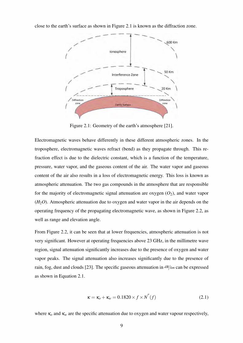
close to the earth’s surface as shown in Figure 2.1 is known as the diffraction zone.
Figure 2.1: Geometry of the earth’s atmosphere [21].
Electromagnetic waves behave differently in these different atmospheric zones. In the
troposphere, electromagnetic waves refract (bend) as they propagate through. This re-
fraction effect is due to the dielectric constant, which is a function of the temperature,
pressure, water vapor, and the gaseous content of the air. The water vapor and gaseous
content of the air also results in a loss of electromagnetic energy. This loss is known as
atmospheric attenuation. The two gas compounds in the atmosphere that are responsible
for the majority of electromagnetic signal attenuation are oxygen (O2), and water vapor
(H2O). Atmospheric attenuation due to oxygen and water vapor in the air depends on the
operating frequency of the propagating electromagnetic wave, as shown in Figure 2.2, as
well as range and elevation angle.
From Figure 2.2, it can be seen that at lower frequencies, atmospheric attenuation is not
very significant. However at operating frequencies above 23 GHz, in the millimetre wave
region, signal attenuation significantly increases due to the presence of oxygen and water
vapor peaks. The signal attenuation also increases significantly due to the presence of
rain, fog, dust and clouds [23]. The specific gaseous attenuation in dB/km can be expressed
as shown in Equation 2.1.
κ = κo +κw = 0.1820× f ×N′′( f ) (2.1)
where κo and κw are the specific attenuation due to oxygen and water vapour respectively,
9
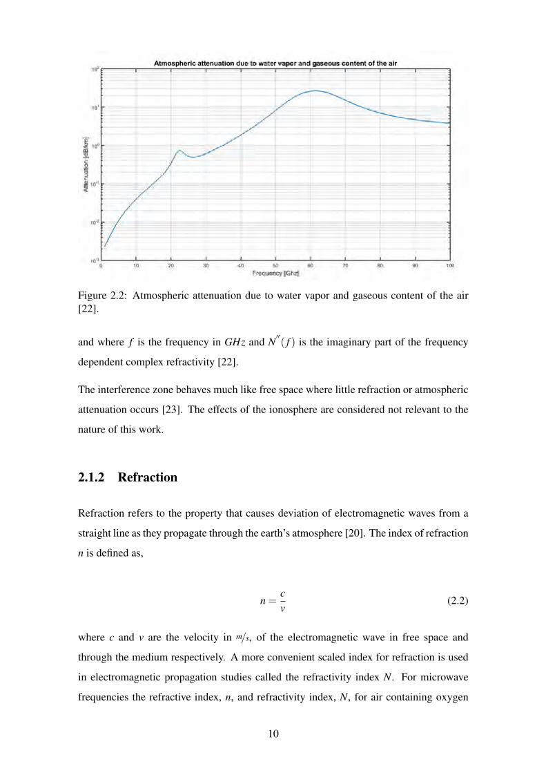
Figure 2.2: Atmospheric attenuation due to water vapor and gaseous content of the air
[22].
and where f is the frequency in GHz and N′′( f ) is the imaginary part of the frequency
dependent complex refractivity [22].
The interference zone behaves much like free space where little refraction or atmospheric
attenuation occurs [23]. The effects of the ionosphere are considered not relevant to the
nature of this work.
2.1.2 Refraction
Refraction refers to the property that causes deviation of electromagnetic waves from a
straight line as they propagate through the earth’s atmosphere [20]. The index of refraction
n is defined as,
n =c
v(2.2)
where c and v are the velocity in m/s, of the electromagnetic wave in free space and
through the medium respectively. A more convenient scaled index for refraction is used
in electromagnetic propagation studies called the refractivity index N. For microwave
frequencies the refractive index, n, and refractivity index, N, for air containing oxygen
10
and water vapor is given by,
N = (n−1)×106 =77.6p
T+
es ×3.73×10⁵
T 2(2.3)
where es is the partial pressure of water vapor in millibars, p is the atmosphere’s baro-
metric pressure in millibars and T is the absolute temperature in Kelvin. For practical
purposes in propagation modelling, a modified refractivity that includes the effects of the
earth’s curvature is used. The modified refractivity M is given by,
M = N +h
re ×10−6= N +0.157h. (2.4)
Where re is the radius of the earth in metres and h is the height above sea level in metres.
2.1.2.1 Refractive Conditions
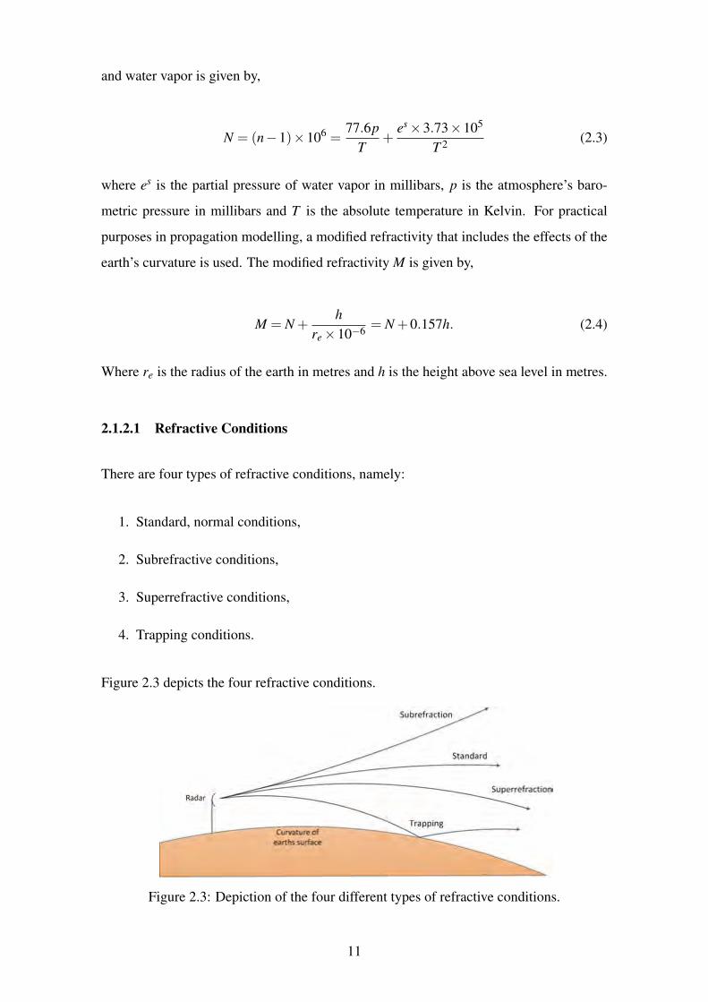
There are four types of refractive conditions, namely:
1. Standard, normal conditions,
2. Subrefractive conditions,
3. Superrefractive conditions,
4. Trapping conditions.
Figure 2.3 depicts the four refractive conditions.
Figure 2.3: Depiction of the four different types of refractive conditions.
11
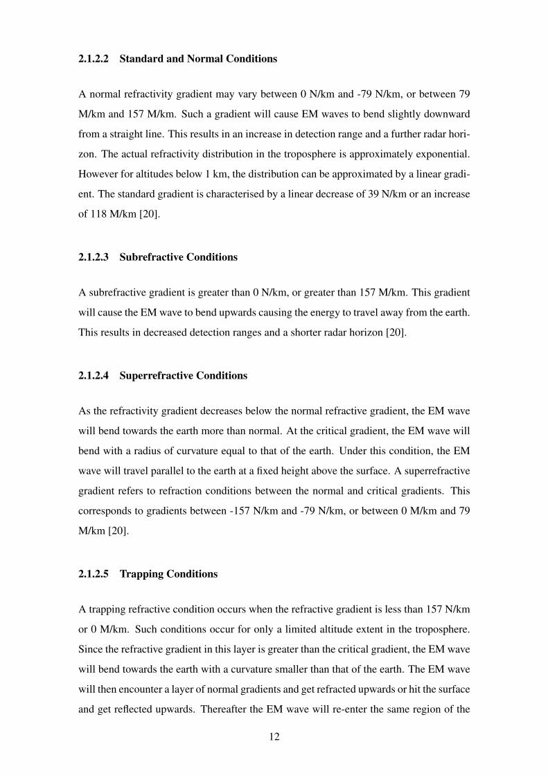
2.1.2.2 Standard and Normal Conditions
A normal refractivity gradient may vary between 0 N/km and -79 N/km, or between 79
M/km and 157 M/km. Such a gradient will cause EM waves to bend slightly downward
from a straight line. This results in an increase in detection range and a further radar hori-
zon. The actual refractivity distribution in the troposphere is approximately exponential.
However for altitudes below 1 km, the distribution can be approximated by a linear gradi-
ent. The standard gradient is characterised by a linear decrease of 39 N/km or an increase
of 118 M/km [20].
2.1.2.3 Subrefractive Conditions
A subrefractive gradient is greater than 0 N/km, or greater than 157 M/km. This gradient
will cause the EM wave to bend upwards causing the energy to travel away from the earth.
This results in decreased detection ranges and a shorter radar horizon [20].
2.1.2.4 Superrefractive Conditions
As the refractivity gradient decreases below the normal refractive gradient, the EM wave
will bend towards the earth more than normal. At the critical gradient, the EM wave will
bend with a radius of curvature equal to that of the earth. Under this condition, the EM
wave will travel parallel to the earth at a fixed height above the surface. A superrefractive
gradient refers to refraction conditions between the normal and critical gradients. This
corresponds to gradients between -157 N/km and -79 N/km, or between 0 M/km and 79
M/km [20].
2.1.2.5 Trapping Conditions
A trapping refractive condition occurs when the refractive gradient is less than 157 N/km
or 0 M/km. Such conditions occur for only a limited altitude extent in the troposphere.
Since the refractive gradient in this layer is greater than the critical gradient, the EM wave
will bend towards the earth with a curvature smaller than that of the earth. The EM wave
will then encounter a layer of normal gradients and get refracted upwards or hit the surface
and get reflected upwards. Thereafter the EM wave will re-enter the same region of the
12
atmosphere causing a downward refraction again. Hence this condition is called trapping,
as the EM wave tends to be confined in a narrow region of the troposphere [20].
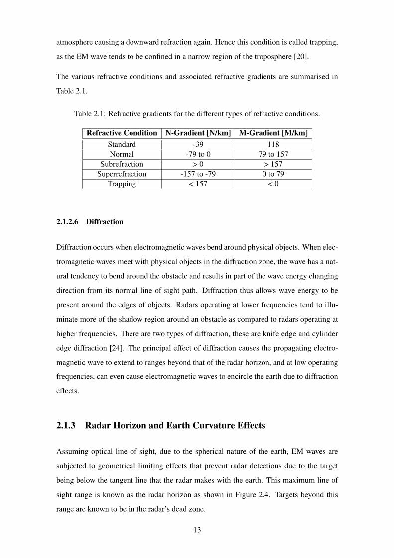
The various refractive conditions and associated refractive gradients are summarised in
Table 2.1.
Table 2.1: Refractive gradients for the different types of refractive conditions.
Refractive Condition N-Gradient [N/km] M-Gradient [M/km]
Standard -39 118
Normal -79 to 0 79 to 157
Subrefraction > 0 > 157
Superrefraction -157 to -79 0 to 79
Trapping < 157 < 0
2.1.2.6 Diffraction
Diffraction occurs when electromagnetic waves bend around physical objects. When elec-
tromagnetic waves meet with physical objects in the diffraction zone, the wave has a nat-
ural tendency to bend around the obstacle and results in part of the wave energy changing
direction from its normal line of sight path. Diffraction thus allows wave energy to be
present around the edges of objects. Radars operating at lower frequencies tend to illu-
minate more of the shadow region around an obstacle as compared to radars operating at
higher frequencies. There are two types of diffraction, these are knife edge and cylinder
edge diffraction [24]. The principal effect of diffraction causes the propagating electro-
magnetic wave to extend to ranges beyond that of the radar horizon, and at low operating
frequencies, can even cause electromagnetic waves to encircle the earth due to diffraction
effects.
2.1.3 Radar Horizon and Earth Curvature Effects
Assuming optical line of sight, due to the spherical nature of the earth, EM waves are
subjected to geometrical limiting effects that prevent radar detections due to the target
being below the tangent line that the radar makes with the earth. This maximum line of
sight range is known as the radar horizon as shown in Figure 2.4. Targets beyond this
range are known to be in the radar’s dead zone.
13
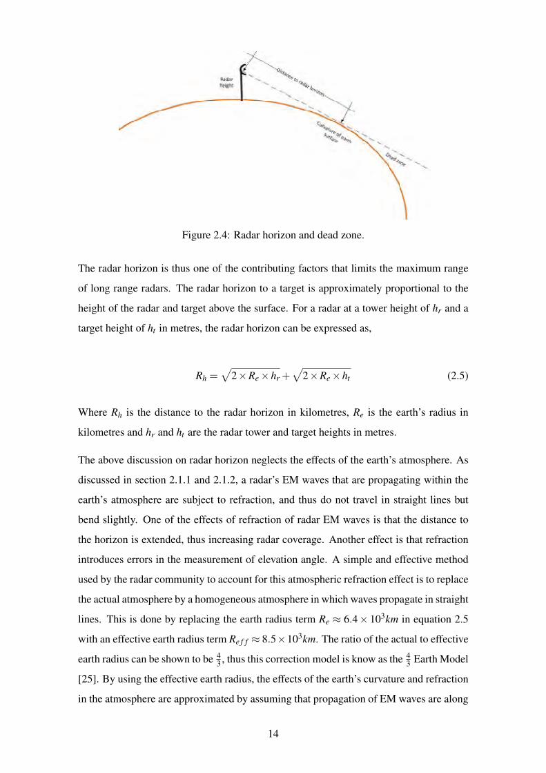
Figure 2.4: Radar horizon and dead zone.
The radar horizon is thus one of the contributing factors that limits the maximum range
of long range radars. The radar horizon to a target is approximately proportional to the
height of the radar and target above the surface. For a radar at a tower height of hr and a
target height of ht in metres, the radar horizon can be expressed as,
Rh =√
2×Re ×hr +√
2×Re ×ht (2.5)
Where Rh is the distance to the radar horizon in kilometres, Re is the earth’s radius in
kilometres and hr and ht are the radar tower and target heights in metres.
The above discussion on radar horizon neglects the effects of the earth’s atmosphere. As
discussed in section 2.1.1 and 2.1.2, a radar’s EM waves that are propagating within the
earth’s atmosphere are subject to refraction, and thus do not travel in straight lines but
bend slightly. One of the effects of refraction of radar EM waves is that the distance to
the horizon is extended, thus increasing radar coverage. Another effect is that refraction
introduces errors in the measurement of elevation angle. A simple and effective method
used by the radar community to account for this atmospheric refraction effect is to replace
the actual atmosphere by a homogeneous atmosphere in which waves propagate in straight
lines. This is done by replacing the earth radius term Re ≈ 6.4× 10³km in equation 2.5
with an effective earth radius term Re f f ≈ 8.5×10³km. The ratio of the actual to effective
earth radius can be shown to be 43, thus this correction model is know as the 4
3Earth Model
[25]. By using the effective earth radius, the effects of the earth’s curvature and refraction
in the atmosphere are approximated by assuming that propagation of EM waves are along
14
straight lines.
Because of it’s simplicity and convenience, the 43
earth model has been a trusted model
to use to account for the effects of atmospheric refraction. The model does however have
limitations. The model assumes standard atmospheric conditions throughout altitudes and
uses a constant value for k = 43. In reality, the value for k will change as a function of alti-
tude, atmospheric conditions, frequency, etc [1]. Atmospheric refraction not only causes
bending of EM waves, but produces errors in radar measurements of range and elevation
as well. These errors decrease with elevation angle, and are generally independent for fre-
quencies below ∼20 GHz [10, 26]. By assuming standard atmospheric conditions, these
measurement errors can be corrected to an accuracy of approximately 15% by using error
curves as those found in [26] (Figure 4.9, and Figure 4.10, p75).
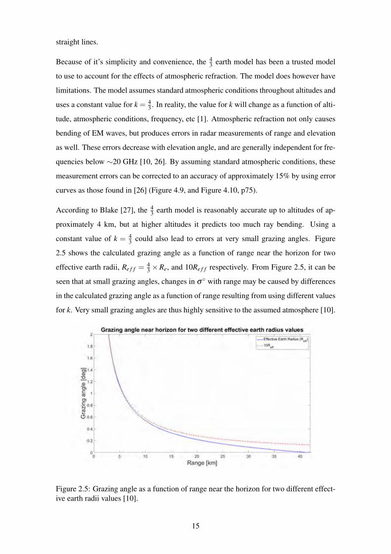
According to Blake [27], the 43
earth model is reasonably accurate up to altitudes of ap-
proximately 4 km, but at higher altitudes it predicts too much ray bending. Using a
constant value of k = 43
could also lead to errors at very small grazing angles. Figure
2.5 shows the calculated grazing angle as a function of range near the horizon for two
effective earth radii, Re f f =43×Re, and 10Re f f respectively. From Figure 2.5, it can be
seen that at small grazing angles, changes in σ◦ with range may be caused by differences
in the calculated grazing angle as a function of range resulting from using different values
for k. Very small grazing angles are thus highly sensitive to the assumed atmosphere [10].
Figure 2.5: Grazing angle as a function of range near the horizon for two different effect-
ive earth radii values [10].
15
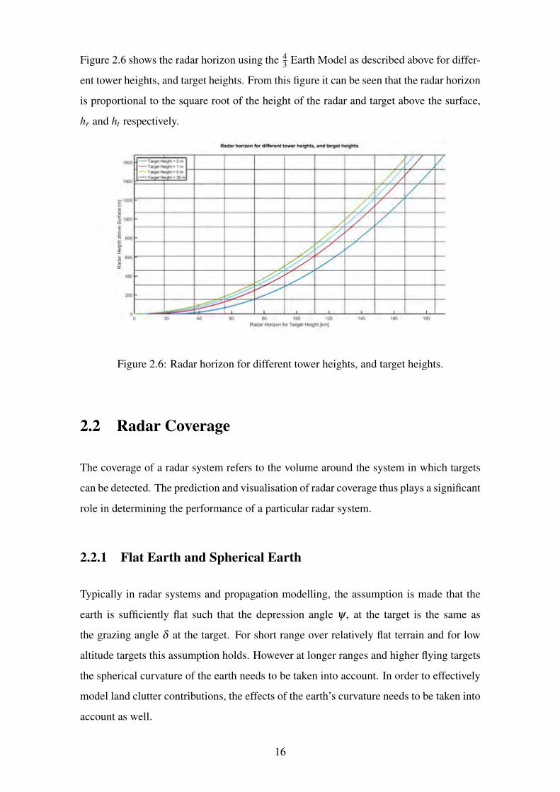
Figure 2.6 shows the radar horizon using the 43
Earth Model as described above for differ-
ent tower heights, and target heights. From this figure it can be seen that the radar horizon
is proportional to the square root of the height of the radar and target above the surface,
hr and ht respectively.
Figure 2.6: Radar horizon for different tower heights, and target heights.
2.2 Radar Coverage
The coverage of a radar system refers to the volume around the system in which targets
can be detected. The prediction and visualisation of radar coverage thus plays a significant
role in determining the performance of a particular radar system.
2.2.1 Flat Earth and Spherical Earth
Typically in radar systems and propagation modelling, the assumption is made that the
earth is sufficiently flat such that the depression angle ψ , at the target is the same as
the grazing angle δ at the target. For short range over relatively flat terrain and for low
altitude targets this assumption holds. However at longer ranges and higher flying targets
the spherical curvature of the earth needs to be taken into account. In order to effectively
model land clutter contributions, the effects of the earth’s curvature needs to be taken into
account as well.
16
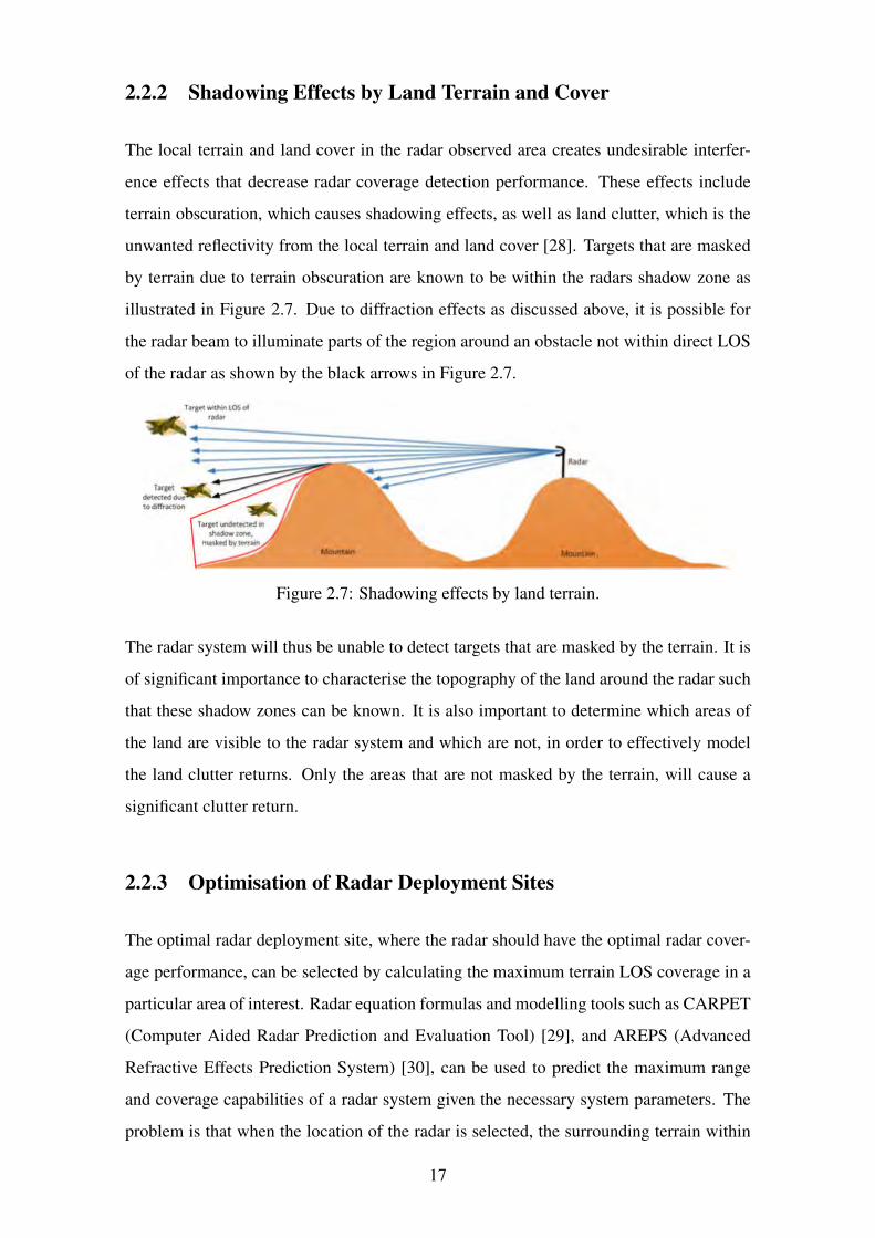
2.2.2 Shadowing Effects by Land Terrain and Cover
The local terrain and land cover in the radar observed area creates undesirable interfer-
ence effects that decrease radar coverage detection performance. These effects include
terrain obscuration, which causes shadowing effects, as well as land clutter, which is the
unwanted reflectivity from the local terrain and land cover [28]. Targets that are masked
by terrain due to terrain obscuration are known to be within the radars shadow zone as
illustrated in Figure 2.7. Due to diffraction effects as discussed above, it is possible for
the radar beam to illuminate parts of the region around an obstacle not within direct LOS
of the radar as shown by the black arrows in Figure 2.7.
Figure 2.7: Shadowing effects by land terrain.
The radar system will thus be unable to detect targets that are masked by the terrain. It is
of significant importance to characterise the topography of the land around the radar such
that these shadow zones can be known. It is also important to determine which areas of
the land are visible to the radar system and which are not, in order to effectively model
the land clutter returns. Only the areas that are not masked by the terrain, will cause a
significant clutter return.
2.2.3 Optimisation of Radar Deployment Sites
The optimal radar deployment site, where the radar should have the optimal radar cover-
age performance, can be selected by calculating the maximum terrain LOS coverage in a
particular area of interest. Radar equation formulas and modelling tools such as CARPET
(Computer Aided Radar Prediction and Evaluation Tool) [29], and AREPS (Advanced
Refractive Effects Prediction System) [30], can be used to predict the maximum range
and coverage capabilities of a radar system given the necessary system parameters. The
problem is that when the location of the radar is selected, the surrounding terrain within
17
the proposed coverage of the radar could potentially reduce the coverage performance of
the radar due to effects such as shadowing by the topography and masking by clutter. It
is thus important to determine which parts of the surrounding observed terrain is within
the radar’s LOS and which areas are blinded, as well as to be able to determine the clutter
contributions from the area of interest.
2.3 Pattern Propagation Factor, F
The pattern propagation factor (F), is defined in [3], as the ratio of the field strength that
is actually present at a point in space to that which would have been present if free-space
propagation had occurred with the antenna beam directed toward the point in question.
This factor is used in the radar equation to modify the strength of the transmitted or re-
ceived signal to account for the changes in field strength caused by multipath propagation,
diffraction, refraction, and the antenna beam pattern..
The effects of the environment are included in the radar equation via means of the pattern
propagation factor F . As a consequence of the definition of F , the power at a point is F2
times its value if the propagation medium is a vacuum, for one-way propagation. Thus
for monostatic radars, the received power is proportional to F4 [10].
For a fixed resolution cell with area A, the echo strength is thus proportional to σ◦F4. For
measurement data, the effects of F4 are due to environmental factors and are therefore
necessarily included in the measurement. Determining F4 accurately is extremely com-
plex and in most cases cannot be separated from the echo strength measurement. Thus
from measurement data reflecting the echo strength, the investigator can determine σF4
or σ◦F4, and not σ or σ◦. The effects of F4 are thus inherently included in the meas-
urement [10]. Existing empirically derived land clutter / backscatter coefficient models
may express backscatter data in terms of σ or σ◦, but it should be noted that the pattern
propagation factor to the fourth power F4 is inherently included [10]. This is especially
true for low grazing angles less than 10◦where the effect of F is generally different in
each resolution cell and thus impractical to determine. For microwave and millimetre
wave frequencies, and for grazing angles greater than 10◦, it is found that F4 can often be
approximated by unity and therefore σF4 or σ◦F4 might be reasonably represented by
σ or σ◦ [6]. This is found to be the case for most land clutter models which focuses on
18
grazing angles in the plateau or high grazing angle regions.
For the purposes of the models and work presented in this dissertation, it is assumed that
the effects of the propagation factor are necessarily included in RCS (σ) or backscatter
coefficient (σ◦) values. If they are expressed without F4, it is assumed to be inherently
included and are in fact, averages of either σF4 or σ◦F4 [10].
2.4 Radar Clutter
The term radar clutter is used to describe echoes that are of no interest to the radar. Radar
clutter takes on different forms depending on the type of radar system. For ground based
radars in which targets of interest are man made objects such as aircraft, ships or ground
targets, clutter would then be all unwanted returns from naturally occurring objects such
as echo reflections from land terrain and the sea. However for earth imaging radars for
remote sensing purposes, reflections from natural land objects and terrain are of interest,
and man made objects are considered clutter. The primary focus of this dissertation will
be radar land clutter.
2.4.1 Radar Land Clutter
Radar land clutter can be caused by terrain, vegetation and man made structures. All
natural and man made objects on the ground that are of no interest to the function or
role of a radar system constitute radar land clutter. This section focuses on radar land
clutter and discusses the most important characteristics of land clutter necessary for the
development of a site specific radar coverage and land clutter modelling tool. Due to
many distributed scatterers found over land terrain, land clutter is generally described and
modelled by the RCS per unit area of the clutter surface, called the backscatter coefficient,
σ◦ [1, 31]. The backscatter coefficient is described and discussed further in the section to
follow.
19
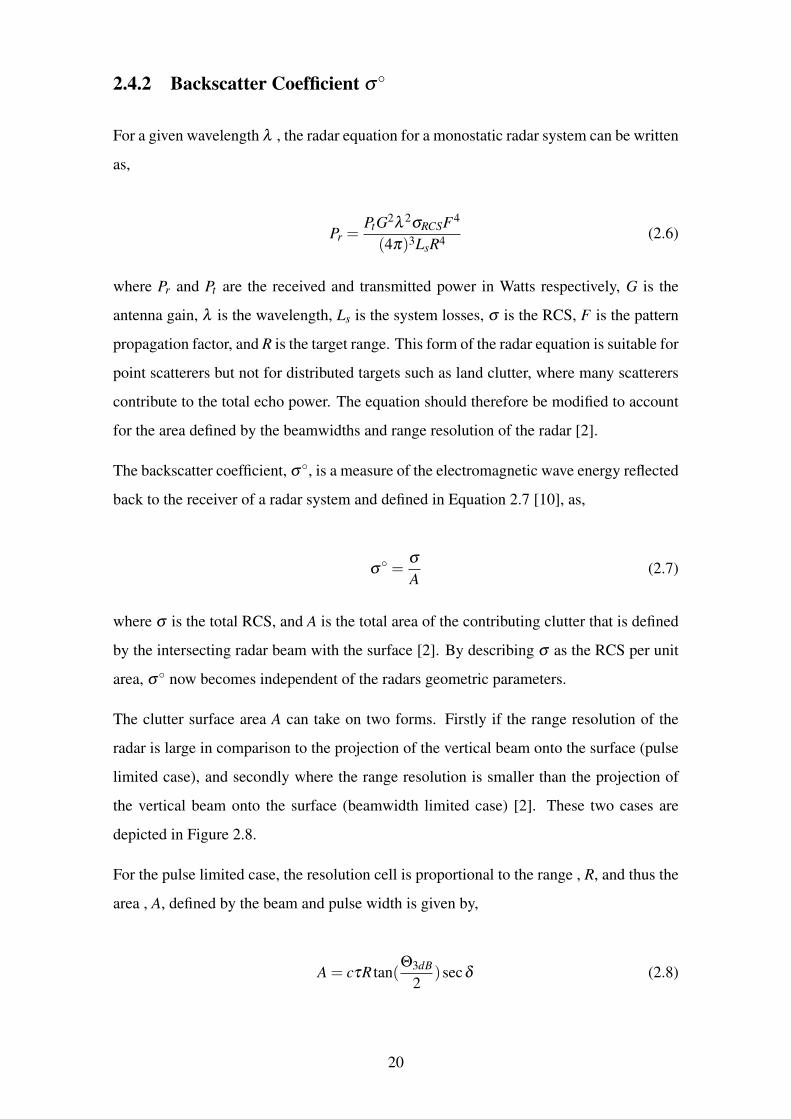
2.4.2 Backscatter Coefficient σ◦
For a given wavelength λ , the radar equation for a monostatic radar system can be written
as,
Pr =PtG
2λ 2σRCSF4
(4π)3LsR4(2.6)
where Pr and Pt are the received and transmitted power in Watts respectively, G is the
antenna gain, λ is the wavelength, Ls is the system losses, σ is the RCS, F is the pattern
propagation factor, and R is the target range. This form of the radar equation is suitable for
point scatterers but not for distributed targets such as land clutter, where many scatterers
contribute to the total echo power. The equation should therefore be modified to account
for the area defined by the beamwidths and range resolution of the radar [2].
The backscatter coefficient, σ◦, is a measure of the electromagnetic wave energy reflected
back to the receiver of a radar system and defined in Equation 2.7 [10], as,
σ◦ =σ
A(2.7)
where σ is the total RCS, and A is the total area of the contributing clutter that is defined
by the intersecting radar beam with the surface [2]. By describing σ as the RCS per unit
area, σ◦ now becomes independent of the radars geometric parameters.
The clutter surface area A can take on two forms. Firstly if the range resolution of the
radar is large in comparison to the projection of the vertical beam onto the surface (pulse
limited case), and secondly where the range resolution is smaller than the projection of
the vertical beam onto the surface (beamwidth limited case) [2]. These two cases are
depicted in Figure 2.8.
For the pulse limited case, the resolution cell is proportional to the range , R, and thus the
area , A, defined by the beam and pulse width is given by,
A = cτR tan(Θ3dB
2)secδ (2.8)
20
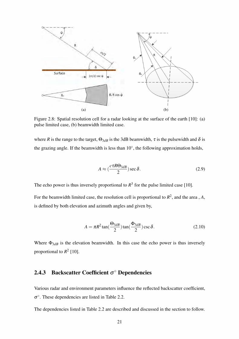
(a) (b)
Figure 2.8: Spatial resolution cell for a radar looking at the surface of the earth [10]: (a)
pulse limited case, (b) beamwidth limited case.
where R is the range to the target, Θ3dB is the 3dB beamwidth, τ is the pulsewidth and δ is
the grazing angle. If the beamwidth is less than 10◦, the following approximation holds,
A ≈ (cτRΘ3dB
2)secδ . (2.9)
The echo power is thus inversely proportional to R3 for the pulse limited case [10].
For the beamwidth limited case, the resolution cell is proportional to R2, and the area , A,
is defined by both elevation and azimuth angles and given by,
A = πR2 tan(Θ3dB
2) tan(
Φ3dB
2)cscδ . (2.10)
Where Φ3dB is the elevation beamwidth. In this case the echo power is thus inversely
proportional to R2 [10].
2.4.3 Backscatter Coefficient σ◦ Dependencies
Various radar and environment parameters influence the reflected backscatter coefficient,
σ◦. These dependencies are listed in Table 2.2.
The dependencies listed in Table 2.2 are described and discussed in the section to follow.
21
Table 2.2: Backscatter coefficient σ◦ dependencies.
Radar Parameters Environment Parameters
Incident / Grazing / Depression Angle Surface Roughness and Moisture Content
Frequency / Wavelength Land Topography and Relief
Polarisation Complex Dielectric Constant
Resolution Type of Terrain / Land Cover
- Spatial and Temporal Statistics
2.4.3.1 Frequency / Wavelength
Radar operating frequencies are divided into different frequency / wavelength bands as
shown in Table 2.3.
Table 2.3: Radar frequency bands.
Radar Band Frequency Wavelength
UHF 300-1000 MHz 100-30 cm
L 1-2 GHz 30-15 cm
S 2-4 GHz 7.5-15 cm
C 4-8 GHz 7.5-3.75 cm
X 8-12 GHz 3.75-2.4 cm
Ku 12-18 GHz 2.4-1.7 cm
K 18-27 GHz 1.7-1.1 cm
Ka 27-40 GHz 1.1-0.75 cm
V 40-75 GHz 0.75-0.4 cm
W 75-110 GHz 0.4-0.27 cm
The wavelength of radar systems has a strong influence on the backscattered energy that
is received at the receiver. Longer wavelengths have greater penetration depths through
land objects that are small in comparison to the length of the wave as compared to shorter
wavelengths. Different wavelengths will therefore reflect different properties of the land
and thus significantly influences the backscattered energy received [2, 32].
2.4.3.2 Incident, Depression and Grazing Angle
The incident angle, θ , is described as the angle between the radar line of sight and the
vertical with respect to the earth geoid. The incident angle does not take into account the
terrain slope. The angle with respect to the slope is known as the local incident angle
θL. The local incident angle accounts for the variation in the slope of the terrain at the
point of illumination. The look or elevation angle is defined as the angle between the
22
antenna and the vertical, and the depression angle, ψ , is defined as the angle between the
horizontal line of the antenna and the radar line of sight [33]. The grazing angle, δ , is
defined as the angle between the horizontal line relative to the slope and the radar line of
sight (compliment of the local incident angle). The depression angle and grazing angle are
closely related and are identical for flat horizontal surfaces [2]. These angles are depicted
in Figure 2.9.
Figure 2.9: Diagram of : incident, local incident, depression and grazing angle.
There is a strong backscatter coefficient dependency to the radar viewing geometry. The
grazing angle is the most important viewing angle that explains scattering mechanisms
and will be used throughout this dissertation unless otherwise stated. Some backscatter
datasets and models are published as a function of depression or incident angle because
the grazing angle could not be precisely known [2].
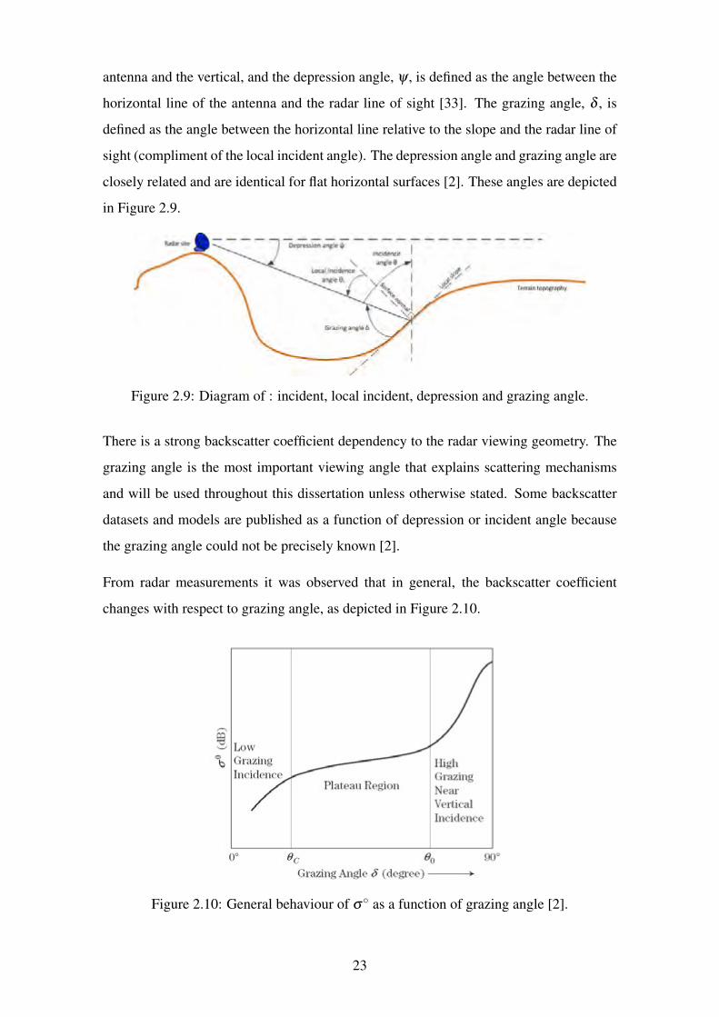
From radar measurements it was observed that in general, the backscatter coefficient
changes with respect to grazing angle, as depicted in Figure 2.10.
Figure 2.10: General behaviour of σ◦ as a function of grazing angle [2].
23
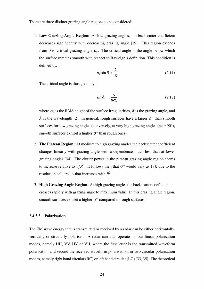
There are three distinct grazing angle regions to be considered:
1. Low Grazing Angle Region: At low grazing angles, the backscatter coefficient
decreases significantly with decreasing grazing angle [19]. This region extends
from 0 to critical grazing angle σc. The critical angle is the angle below which
the surface remains smooth with respect to Rayleigh’s definition. This condition is
defined by,
σh sinδ <λ
8(2.11)
The critical angle is thus given by,
sinδc =λ
8σh
(2.12)
where σh is the RMS height of the surface irregularities, δ is the grazing angle, and
λ is the wavelength [2]. In general, rough surfaces have a larger σ◦ than smooth
surfaces for low grazing angles (conversely, at very high grazing angles (near 90◦),
smooth surfaces exhibit a higher σ◦ than rough ones).
2. The Plateau Region: At medium to high grazing angles the backscatter coefficient
changes linearly with grazing angle with a dependence much less than at lower
grazing angles [34]. The clutter power in the plateau grazing angle region seems
to increase relative to 1/R3. It follows then that σ◦ would vary as 1/R due to the
resolution cell area A that increases with R2.
3. High Grazing Angle Region: At high grazing angles the backscatter coefficient in-
creases rapidly with grazing angle to maximum value. In this grazing angle region,
smooth surfaces exhibit a higher σ◦ compared to rough surfaces.
2.4.3.3 Polarisation
The EM wave energy that is transmitted or received by a radar can be either horizontally,
vertically or circularly polarised. A radar can thus operate in four linear polarisation
modes, namely HH, VV, HV or VH, where the first letter is the transmitted waveform
polarisation and second the received waveform polarisation, or two circular polarisation
modes, namely right hand circular (RC) or left hand circular (LC) [33, 35]. The theoretical
24
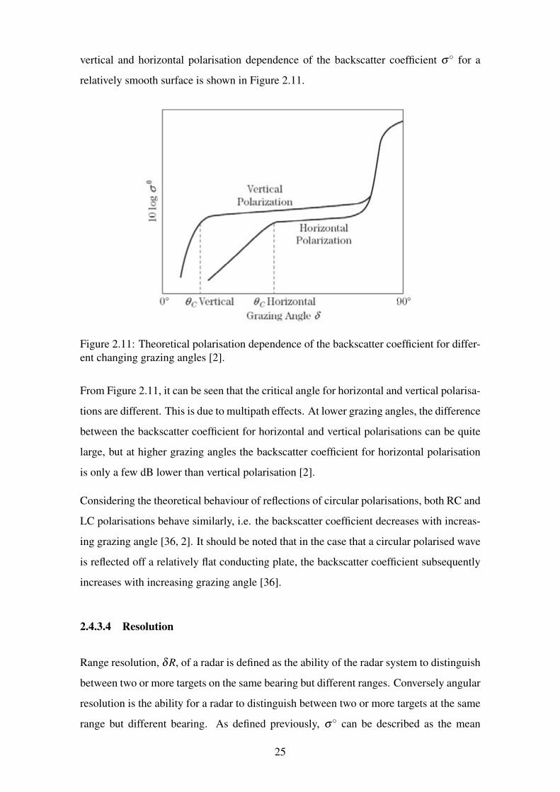
vertical and horizontal polarisation dependence of the backscatter coefficient σ◦ for a
relatively smooth surface is shown in Figure 2.11.
Figure 2.11: Theoretical polarisation dependence of the backscatter coefficient for differ-
ent changing grazing angles [2].
From Figure 2.11, it can be seen that the critical angle for horizontal and vertical polarisa-
tions are different. This is due to multipath effects. At lower grazing angles, the difference
between the backscatter coefficient for horizontal and vertical polarisations can be quite
large, but at higher grazing angles the backscatter coefficient for horizontal polarisation
is only a few dB lower than vertical polarisation [2].
Considering the theoretical behaviour of reflections of circular polarisations, both RC and
LC polarisations behave similarly, i.e. the backscatter coefficient decreases with increas-
ing grazing angle [36, 2]. It should be noted that in the case that a circular polarised wave
is reflected off a relatively flat conducting plate, the backscatter coefficient subsequently
increases with increasing grazing angle [36].
2.4.3.4 Resolution
Range resolution, δR, of a radar is defined as the ability of the radar system to distinguish
between two or more targets on the same bearing but different ranges. Conversely angular
resolution is the ability for a radar to distinguish between two or more targets at the same
range but different bearing. As defined previously, σ◦ can be described as the mean
25
clutter strength over the illuminated scene with area A. Resolution therefore does not
directly affect σ◦, but both resolutions would therefore affect the amplitude statistics or
fluctuations about the mean defined by σ◦ [2].
2.4.3.5 Surface Roughness and Moisture Content
The size of the land particles on a micro composition scale relative to the radar wavelength
determines the surface roughness. Rough terrain will reflect stronger backscatter energy
as compared to smooth terrain surfaces [33]. Rayleigh’s condition’s to determine sur-
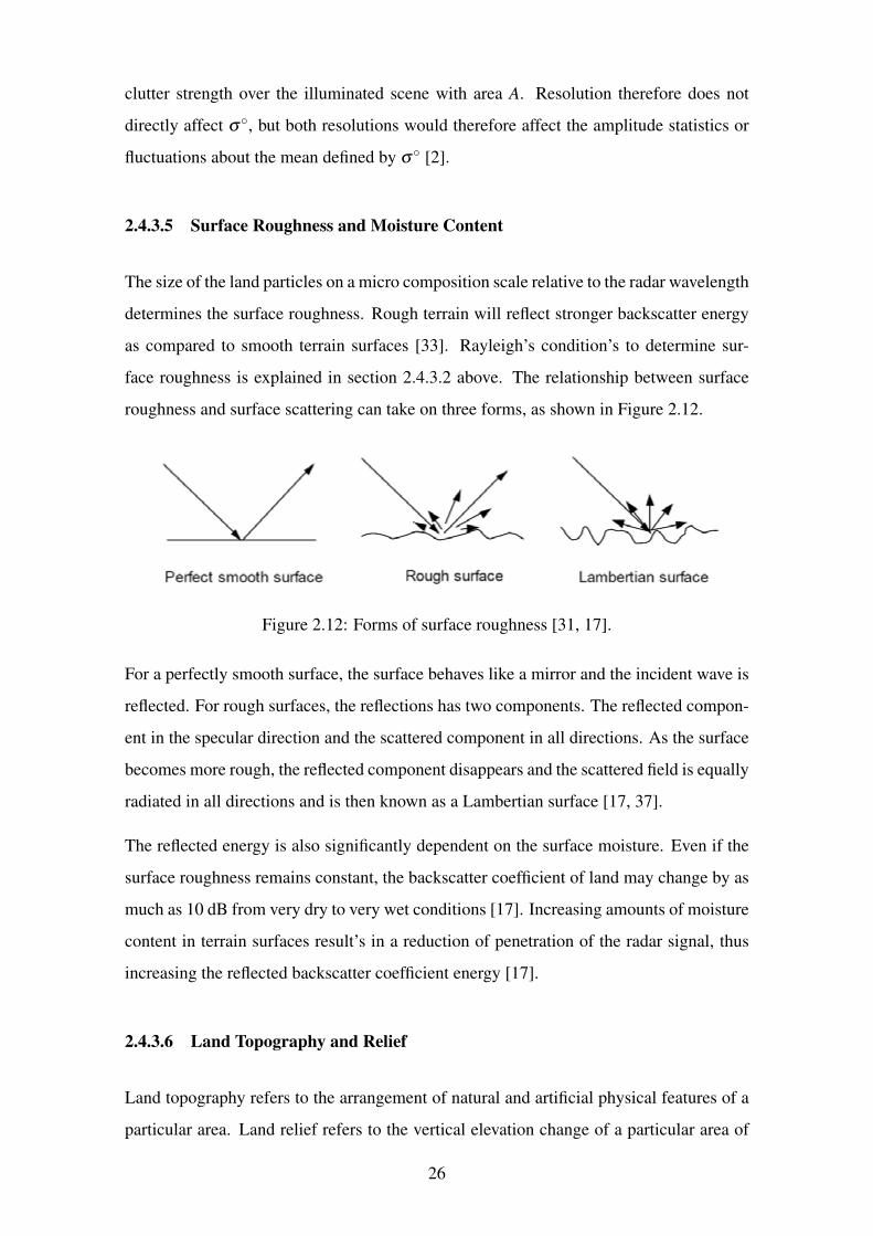
face roughness is explained in section 2.4.3.2 above. The relationship between surface
roughness and surface scattering can take on three forms, as shown in Figure 2.12.
Figure 2.12: Forms of surface roughness [31, 17].
For a perfectly smooth surface, the surface behaves like a mirror and the incident wave is
reflected. For rough surfaces, the reflections has two components. The reflected compon-
ent in the specular direction and the scattered component in all directions. As the surface
becomes more rough, the reflected component disappears and the scattered field is equally
radiated in all directions and is then known as a Lambertian surface [17, 37].
The reflected energy is also significantly dependent on the surface moisture. Even if the
surface roughness remains constant, the backscatter coefficient of land may change by as
much as 10 dB from very dry to very wet conditions [17]. Increasing amounts of moisture
content in terrain surfaces result’s in a reduction of penetration of the radar signal, thus
increasing the reflected backscatter coefficient energy [17].
2.4.3.6 Land Topography and Relief
Land topography refers to the arrangement of natural and artificial physical features of a
particular area. Land relief refers to the vertical elevation change of a particular area of
26
interest (related to the slopes / gradients of surfaces). Relative to the area that radar energy
is illuminating, both land topography and land relief influence the backscatter coefficient.
The differences and dependence that backscatter energy has on land topography and relief
will be investigated further in subsequent sections of this dissertation.
2.4.3.7 Complex Dielectric Constant
The electric characteristics of terrain surfaces influences the reflected backscatter energy
of the returned radar signal. These characteristics are denoted by the complex dielectric
constant which is the ratio of the permittivity of a substance to the permittivity of free
space. The complex dielectric constant is an indicator of the intrinsic ability of a sub-
stance / terrain surface to store charge and transmit energy [38, 32]. Dry surface areas
will contain low dielectric constant, and wet surfaces a high dielectric constant (typically
>80), due to the presence of water [39]. Surface areas with a low dielectric constant that
are illuminated by radar energy will reflect less backscatter energy than surface areas with
a high dielectric constant [40]. Thus with constant surface roughness, the reflected backs-
catter coefficient energy increases with increasing dielectric constant (surface moisture)
[17].
2.4.3.8 Type of Terrain / Land Cover
The type of terrain being illuminated vastly influences the reflected backscatter energy.
Different types of terrain will present different backscatter coefficients due to its partic-
ular surface properties. The differences and dependence that backscatter energy has on
different types of terrain will be investigated further in subsequent sections of this disser-
tation.
2.4.3.9 Spatial and Temporal Statistics
The reflected backscatter energy as seen by the radar system varies from one region to an-
other. Given a certain land type, the reflected energy is not a constant value over time and
space. This is shown in Figure 2.13, which represents the mean backscatter coefficient
as a function of various radar frequencies and range resolutions, as measured at 35 sites
27
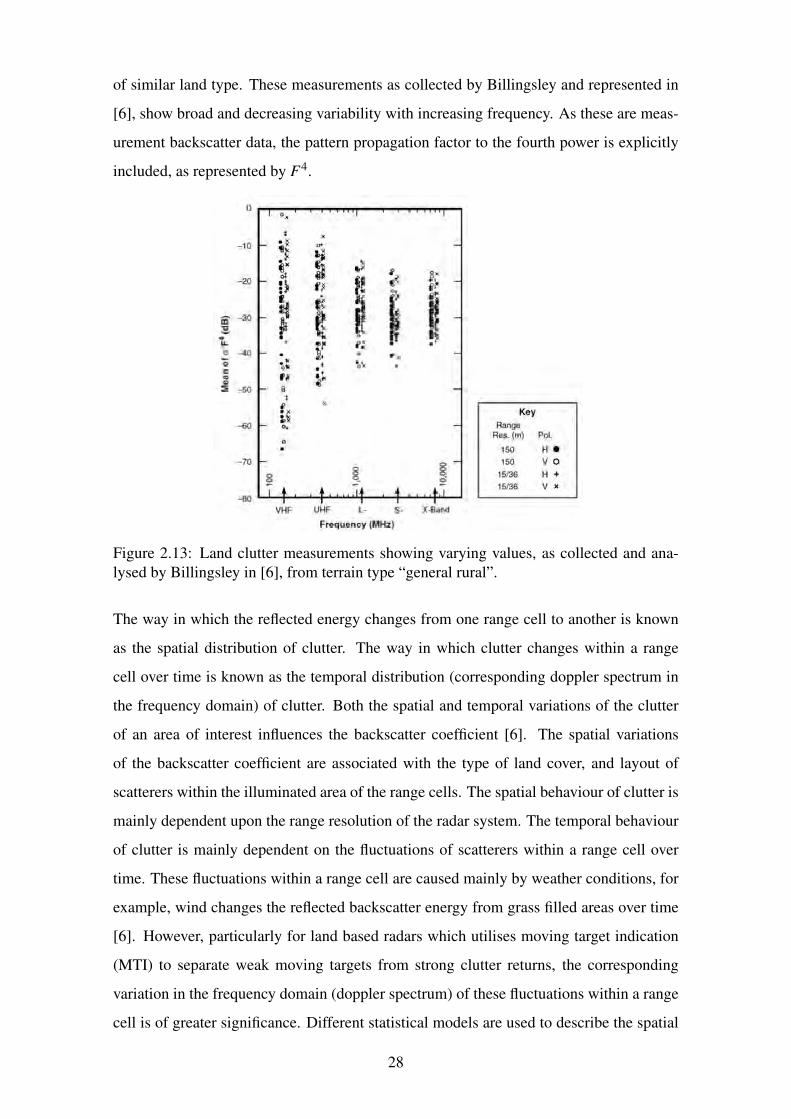
of similar land type. These measurements as collected by Billingsley and represented in
[6], show broad and decreasing variability with increasing frequency. As these are meas-
urement backscatter data, the pattern propagation factor to the fourth power is explicitly
included, as represented by F4.
Figure 2.13: Land clutter measurements showing varying values, as collected and ana-
lysed by Billingsley in [6], from terrain type “general rural”.
The way in which the reflected energy changes from one range cell to another is known
as the spatial distribution of clutter. The way in which clutter changes within a range
cell over time is known as the temporal distribution (corresponding doppler spectrum in
the frequency domain) of clutter. Both the spatial and temporal variations of the clutter
of an area of interest influences the backscatter coefficient [6]. The spatial variations
of the backscatter coefficient are associated with the type of land cover, and layout of
scatterers within the illuminated area of the range cells. The spatial behaviour of clutter is
mainly dependent upon the range resolution of the radar system. The temporal behaviour
of clutter is mainly dependent on the fluctuations of scatterers within a range cell over
time. These fluctuations within a range cell are caused mainly by weather conditions, for
example, wind changes the reflected backscatter energy from grass filled areas over time
[6]. However, particularly for land based radars which utilises moving target indication
(MTI) to separate weak moving targets from strong clutter returns, the corresponding
variation in the frequency domain (doppler spectrum) of these fluctuations within a range
cell is of greater significance. Different statistical models are used to describe the spatial
28
and temporal statistics of land clutter. These models are described in the section to follow.
2.4.4 Land Clutter Modeling
In order to estimate radar system performance in land clutter, clutter models are required.
Standard probability density functions (PDF’s) models can be used to describe the vari-
ation of different types of land clutter. From measurement data, statistical parameters
required by these PDF models for different types of land clutter can be defined empiric-
ally. Empirical models that describe the mean backscatter reflectivity σ◦ for various types
of land terrain as a function of frequency, grazing angle and polarisation can also be de-
veloped from measurement data. The type of existing land clutter models that can be used
to characterise σ◦ for use in a site specific radar coverage and land clutter modelling tool
is dependent on the nature of how the model was developed. Mathematical models can
also be developed that provide an estimation to the the general shape of the backscatter
coefficient.
2.4.4.1 Standard PDF’s Used to Model Land Clutter Variation
PDF’s are used to describe and characterise the statistics of land clutter in space and time.
In the past, most radars operated with inherently low range resolution capabilities such
that reflected clutter echoes were thought to be comprised of a sum of responses from a
very large number of individual scatterers. From the central limit theorem (CLT), it was
concluded that the appropriate statistical model to describe the in-phase and quadrature
components of reflected backscatter energy was the Gaussian PDF [41]. The amplitude
of the clutter is thus Rayleigh distributed. The theoretical PDF for Rayleigh distribution
is defined by Equation 2.13,
PDFRayleigh =x
s2exp(
−x2
2s2) (2.13)
where x is the amplitude of the return signals, and s is the scale parameter of the distribu-
tion which determines the statistical dispersion of the distribution.
As the range resolution improves, the CLT begins to fail and the subsequent in-phase and
29
quadrature components of clutter can no longer be considered Gaussian distributed. This
is due to the number of scatterers in a resolution cell becoming finite or due to individual
dominating scatterers. The improved range resolution results in the radar being more
sensitive to spatial variations in the clutter which makes the distribution more spiky [42,
43]. The amplitude statistics thus deviates from Rayleigh as well. The spiky characteristic
of high range resolution clutter causes the tail of the amplitude distribution to rise. The
amplitude distributions considered to best fit this situation for land clutter are the Log-
normal and Weibull PDF’s [16, 10, 42]. The theoretical PDF for Log-normal distribution
is defined by two parameters (shape and scale), and shown in Equation 2.14,
PDFLog−normal =1
xs√
2πexp(
−(lnx−µ)2
2s2) (2.14)
where µ is the shape parameter, and s is the scale parameter. The shape and scale para-
meters µ and s represents the mean and standard deviation, respectively, of the clutter
intensity expressed in dB having a Gaussian PDF.
In some cases the tail of the Log-normal PDF is too long for the clutter amplitude data
to fit. In this case, the Weibull PDF is considered as it’s tail is shorter than that of the
Log-normal PDF but still longer than that of the Rayleigh PDF [44]. The Weibull PDF is
also defined by two parameters (shape and scale), and shown in equation 2.15.
PDFWeibull =k
b(
x
b)k−1 exp(−(
x
b)k) (2.15)
where k is the shape parameter, and b is the scale parameter. For k = 2, the Weibull PDF
is identical to that of the Rayleigh PDF.
The above distributions describe the spatial behaviour of land clutter, i.e., the variation of
land clutter from one range cell to another. These spatial variations are associated with
the layout of the backscatterers in the range cells that are illuminated. Thus the spatial
behaviour of land clutter is related to the land cover and the radar range resolution.
For temporal variations in land clutter, the return from scatterers within a range cell can
be classified as either a steady component, or diffuse component. The steady component
is a result of return from fixed discrete scatterers that do not change in time, such as
30
buildings. Diffuse components is a result of discrete scatterers that can move and change
in time, such as wind-blown foliage due to weather conditions. The temporal variations of
land clutter mainly depends on the fluctuations of backscatterers within a range cell over
time, however it is important to note the indirect effect land cover and range resolution
plays on the temporal variations of clutter as well. For example, clutter within a range
cell that is dominated by a strong stationary scatterer, such as a building, exhibits little
or no fluctuation in time, whereas clutter within a range cell that is dominated by foliage
would exhibit more fluctuations in time. The radar range resolution therefore affects the
temporal statistics of land clutter by changing the contents within range cells [45].
The Ricean PDF was derived from the analysis of the statistical properties of a sine wave
in additive noise, as described and discussed in [46]. H.C Chan describes in [45] that
through the analyses of radar land clutter, it was found that the coherent component of
land clutter can be considered a constant or slow varying signal, and thus can be modelled
as a sine wave with zero frequency. It was further found that if the corresponding diffuse
components is describable by complex Gaussian distributions. Thus for a case where a
range cell consists of both a strong steady component as well as a diffuse component,
the distribution that can be used to model this situation is the Ricean PDF. The diffuse
component can be modelled using the Rayleigh PDF, which is a special case of the Ricean
PDF [47, 45, 46].
For clutter that changes both in space and in time, a compound clutter model is required.
A compound clutter model that is widely used is the K-Distribution. This distribution
enables both spatial and temporal correlation properties to be taken into account [48, 49].
The K-Distribution is a widely used model for sea clutter, but can be applied to other
types of clutter as well. The K-Distribution is also a two parameter (shape and scale)
PDF. Further information of the K-Distribution as used for radar clutter can be found in
[50, 51, 8].
The different grazing angle regions as discussed in section 2.4.3.2 affect the amplitude
statistics of land clutter as well. Clutter at low grazing angles are characterised by patchi-
ness / lack of uniformity in spatial extent, due to shadowing, and / or extreme resolution
dependencies leading to large resolution cell-to-cell variability. Clutter amplitude stat-
istics in the low-grazing angle region are characterised by distributions with long tails
(spiky clutter), making Weibull and Log-Normal distributions suitable choices to model
31
their probability density functions (PDF’s). The long tails of the distributions are due to
the prevalence of terrain shadowing and multipath at these low grazing angles. The amp-
litude statistics for clutter in the plateau grazing angle region tend to be more consistent
and less spiky than those at lower grazing angles, since terrain shadowing and multipath
effects are of less concern. In general, the Rayleigh PDF is a good distribution to use to
fit the clutter amplitude statistics observed in the plateau grazing angle region.
2.4.4.2 Empirically Derived Land Clutter Models
Empirical and semi-empirical land clutter models are developed by using radar measure-
ment data. Measurement trials are performed over different terrain surfaces, at varying
grazing angles and frequencies. The measurement data collected from these trials are
then used to develop empirical land clutter models that describe the average or statistical
behaviour of the backscatter coefficient. These models provide an estimation of the backs-
catter coefficient of different terrain surfaces, at varying grazing angles and frequencies.
These models are dependent upon the type of terrain, frequency of operation and grazing
angle. To describe the statistical behaviour, the measurement data is fit to common PDF
models. The PDF parameters are then empirically derived. These types of models would
require large amounts of computer resources for use in a site specific radar coverage and
land clutter modelling tool described in this study.
The measurement data can also be used to develop semi-empirical models. Instead of
describing the statistical behaviour of the clutter, these models often describe the aver-
age backscatter coefficient given by simple formulas containing several parameters (e.g.
grazing angle, frequency, polarisation, terrain type, etc). These provide a quick and simple
estimation of the backscatter coefficient. It is important to remember that these models are
based upon experimental data and include a pattern propagation factor F to the 4th power.
Other influences of the environment may also be included that is not taken into account
by these models. Some of these models may also only be valid for certain terrain types,
grazing angles and frequencies. Despite the limitations, the simplicity and lower com-
putational resources required to simulate these models make semi-empirical land clutter
models more suited to be used for developing a site specific radar coverage and land clut-
ter modelling tool. The limitations and validity of some of these models will be discussed
and compared to each other in this dissertation in order to determine the appropriate land
32
clutter / backscatter coefficient models to use for the varying land clutter simulation cases
that can arise.
2.4.4.3 Mathematically Derived Land Clutter Models
Rather than using empirical models which are based on observations, mathematical mod-
els can be derived which mathematically describe relationships of land clutter. Simple
mathematical formulas are thus developed that provide an estimation to the the general
shape of the backscatter coefficient for different terrain types and frequencies. Mathemat-
ical models are usually evaluated by validating the model against experimental measure-
ments or other empirical data.
2.5 GIS Data
In order to develop a site specific radar coverage and land clutter modelling tool, models
of real world terrain surfaces, terrain classification and terrain characteristics are required.
The GIS data products that are considered are real world digital elevation model (DEM)
data, and land cover (LC) data.
2.5.1 Digital Elevation Model Data
DEM data is defined as a digital model, or 3-D representation of a terrain’s surface that
is created from terrain elevation data. An example of DEM data is shown in Figure 2.14.
The figure represents a digital elevation model for Setif region in Algeria.
Available DEM data products vary in quality, arc spacing (resolution), accuracy, availab-
ility and cost. The DEM data can either be represented by digital raster / height maps, or
by vector based triangular irregular networks (TIN). The TIN dataset can be considered
the primary raw measured dataset whereas the digital raster / height map dataset con-
sidered being the secondary computed DEM dataset. Early digital elevation model data
were a product of photogrammetric data capture. These relied on interpretation of aer-
ial photographs or satellite imagery. This can also be done by digitising contour lines
on topographic maps. Present DEM data is acquired and produced by mappers and na-
33
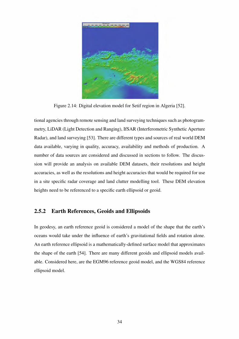
Figure 2.14: Digital elevation model for Setif region in Algeria [52].
tional agencies through remote sensing and land surveying techniques such as photogram-
metry, LiDAR (Light Detection and Ranging), IfSAR (Interferometric Synthetic Aperture
Radar), and land surveying [53]. There are different types and sources of real world DEM
data available, varying in quality, accuracy, availability and methods of production. A
number of data sources are considered and discussed in sections to follow. The discus-
sion will provide an analysis on available DEM datasets, their resolutions and height
accuracies, as well as the resolutions and height accuracies that would be required for use
in a site specific radar coverage and land clutter modelling tool. These DEM elevation
heights need to be referenced to a specific earth ellipsoid or geoid.
2.5.2 Earth References, Geoids and Ellipsoids
In geodesy, an earth reference geoid is considered a model of the shape that the earth’s
oceans would take under the influence of earth’s gravitational fields and rotation alone.
An earth reference ellipsoid is a mathematically-defined surface model that approximates
the shape of the earth [54]. There are many different geoids and ellipsoid models avail-
able. Considered here, are the EGM96 reference geoid model, and the WGS84 reference
ellipsoid model.
34
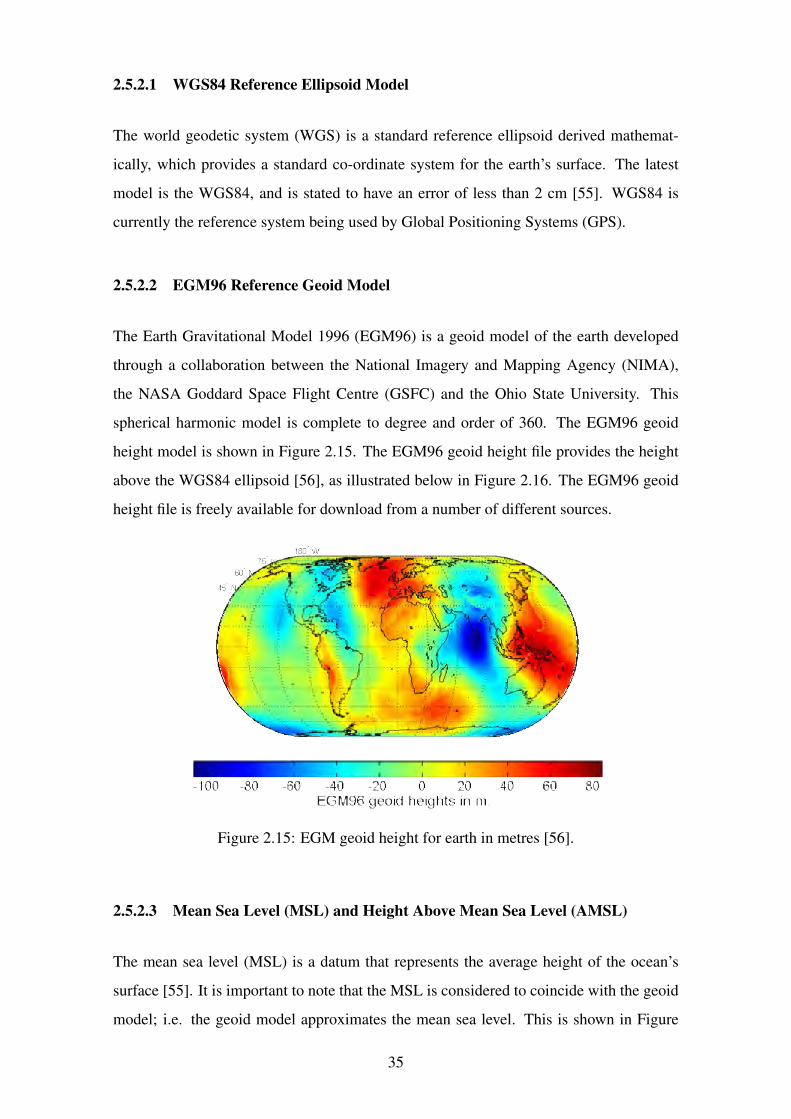
2.5.2.1 WGS84 Reference Ellipsoid Model
The world geodetic system (WGS) is a standard reference ellipsoid derived mathemat-
ically, which provides a standard co-ordinate system for the earth’s surface. The latest
model is the WGS84, and is stated to have an error of less than 2 cm [55]. WGS84 is
currently the reference system being used by Global Positioning Systems (GPS).
2.5.2.2 EGM96 Reference Geoid Model
The Earth Gravitational Model 1996 (EGM96) is a geoid model of the earth developed
through a collaboration between the National Imagery and Mapping Agency (NIMA),
the NASA Goddard Space Flight Centre (GSFC) and the Ohio State University. This
spherical harmonic model is complete to degree and order of 360. The EGM96 geoid
height model is shown in Figure 2.15. The EGM96 geoid height file provides the height
above the WGS84 ellipsoid [56], as illustrated below in Figure 2.16. The EGM96 geoid
height file is freely available for download from a number of different sources.
Figure 2.15: EGM geoid height for earth in metres [56].
2.5.2.3 Mean Sea Level (MSL) and Height Above Mean Sea Level (AMSL)
The mean sea level (MSL) is a datum that represents the average height of the ocean’s
surface [55]. It is important to note that the MSL is considered to coincide with the geoid
model; i.e. the geoid model approximates the mean sea level. This is shown in Figure
35
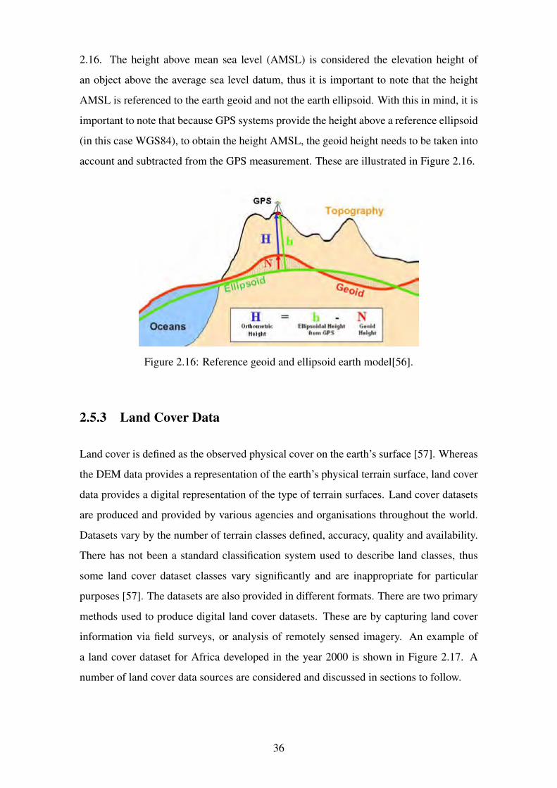
2.16. The height above mean sea level (AMSL) is considered the elevation height of
an object above the average sea level datum, thus it is important to note that the height
AMSL is referenced to the earth geoid and not the earth ellipsoid. With this in mind, it is
important to note that because GPS systems provide the height above a reference ellipsoid
(in this case WGS84), to obtain the height AMSL, the geoid height needs to be taken into
account and subtracted from the GPS measurement. These are illustrated in Figure 2.16.
Figure 2.16: Reference geoid and ellipsoid earth model[56].
2.5.3 Land Cover Data
Land cover is defined as the observed physical cover on the earth’s surface [57]. Whereas
the DEM data provides a representation of the earth’s physical terrain surface, land cover
data provides a digital representation of the type of terrain surfaces. Land cover datasets
are produced and provided by various agencies and organisations throughout the world.
Datasets vary by the number of terrain classes defined, accuracy, quality and availability.
There has not been a standard classification system used to describe land classes, thus
some land cover dataset classes vary significantly and are inappropriate for particular
purposes [57]. The datasets are also provided in different formats. There are two primary
methods used to produce digital land cover datasets. These are by capturing land cover
information via field surveys, or analysis of remotely sensed imagery. An example of
a land cover dataset for Africa developed in the year 2000 is shown in Figure 2.17. A
number of land cover data sources are considered and discussed in sections to follow.
36
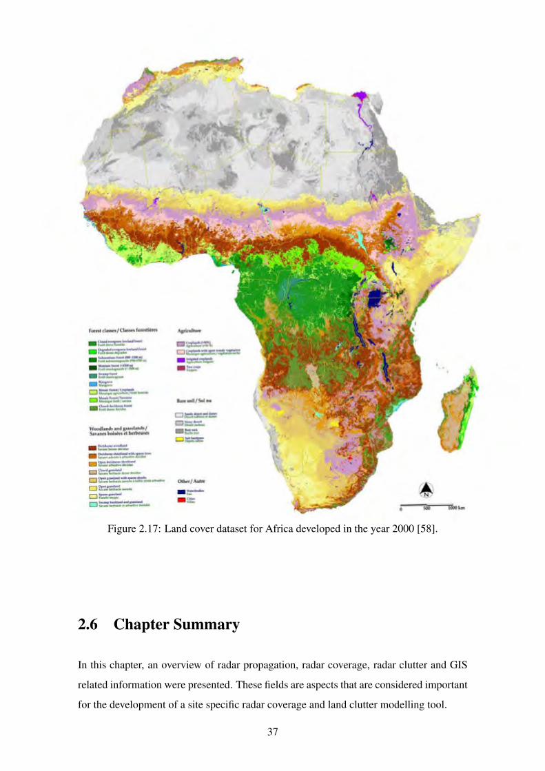
Figure 2.17: Land cover dataset for Africa developed in the year 2000 [58].
2.6 Chapter Summary
In this chapter, an overview of radar propagation, radar coverage, radar clutter and GIS
related information were presented. These fields are aspects that are considered important
for the development of a site specific radar coverage and land clutter modelling tool.
37
fo1tSI classes/ Cl assn fortstlhn
- f!:".:::C:"'1-11-4 C ::a:!:~:Undl-9 a :=«=:~ ... - =:--=:.::,~ .. • :::~.--= D ~~~,fl"_ .. D ::::;.~r--: • =-'.::=.. .....
Woodludt and gm sb.ndJ/ SoJnna boiffff ft hf"rbtUHI -~::.--~ - ~~...::=-.,,.. c:::1~=.=~ c::J=t::' ............ Cl~--====-........ D ~r.::.:!---o :..i:;:-' (=>t::=:-~~---
Ag,icultutt
D ~~-~l, D~~=i~!".: -=--=• :~~
lb~ IOU/ Sol nu
D~~=~= o:::r.::"' ..... •::-.. -.!. t=l r:.•,:::~r.:
Othtr/ ""'"
• r. ........ • r.::
iii- ~km
An overview of radar propagation is presented in section 2.1. Radar waves propagating
through the atmosphere are subjected to signal distortions. These distortions need to be
taken into account in a site specific radar coverage and land clutter modelling tool. These
effects include diffraction of electromagnetic waves, refraction of electromagnetic waves
caused by the atmosphere, the absorption or attenuation of radar wave energy due to the
gases in the atmosphere, and earth curvature effects.
An overview of radar coverage is presented in section 2.2. It was found that for short range
propagation modelling, the flat earth approximation holds. However for longer ranges and
higher flying targets the spherical curvature of the earth needs to be taken into account.
The radar horizon is a geometrical limiting effect that prevent radar detection’s due to the
target being below the tangent line that the radar makes with the earth. The radar horizon
is thus one of the contributing factors that limits the maximum range of long range radars.
Terrain obscuration, causes shadowing effects, as well as land clutter. Optimisation of
radar deployment sites requires knowledge of which parts of the surrounding observed
terrain is within the LOS and which areas are blinded, as well as to be able to determine
the clutter contributions from the area of interest. It is important to model the terrain to
determine shadow regions, and to characterise the land cover for land clutter modelling
purposes.
An overview of the pattern propagation factor, F , is presented in section 2.3. The effects
of the environment are included in the radar equation via means of the pattern propagation
factor F . For monostatic radars, the received power is proportional to F4. It has been
noted that F4 is inherently included in the measurement and modelling of the backscatter
coefficient and attempts to separate it is not within the scope of this dissertation. F is
assumed to include all propagation effects, including multipath and diffraction, between
the radar and the clutter cell.
An overview of radar clutter is presented in section 2.4. Radar land clutter can be caused
by terrain, vegetation and man made structures. Due to many distributed scatterers found
over land terrain, land clutter is generally described and modelled by the radar cross sec-
tion (RCS) per unit area of the clutter surface, called the backscatter coefficient, σ◦. It was
found that the backscatter coefficient is dependent on a number of factors, these include
both radar and environment parameters. One of the most important factors that influences
σ◦ is the grazing angle. Three grazing angle regions exist and reflectivity behave differ-
38
ently in these three regions. Standard probability density functions (PDF’s) models can be
used to describe the variation of different types of land clutter. From measurement data,
statistical parameters required by these PDF models for different types of land clutter
can be defined empirically. Empirical and semi-empirical models that describe the mean
backscatter reflectivity σ◦ for various types of land terrain as a function of frequency,
grazing angle and polarisation can also be developed from measurement data. Empir-
ically derived PDF models would require large amounts of computer resources for use
in a site specific radar coverage and land clutter modelling tool described in this study.
Semi-empirical models describe the average backscatter coefficient given by simple for-
mulas containing several parameters. These provide a quick and simple estimation of
the backscatter coefficient and considered more suited to be used for developing a site
specific radar coverage and land clutter modelling tool. Mathematical models can also
be developed that provide an estimation to the the general shape of the backscatter coef-
ficient. The nature of how a land clutter model was derived is thus an important factor
to consider when determining the appropriate model to use for particular cases. Several
existing land clutter models are investigated in sections to follow.
An overview of GIS data is presented in section 2.5. The types of GIS data considered
important for site specific radar coverage and land clutter modelling are DEM and LC
data. DEM data is required for determining land topography and LC data is required for
characterising land cover. Several DEM and LC data sources are investigated in sections
to follow.
39
Chapter 3
System Models, Processes and Data
This chapter provides a description of the models and processes of the different topics
covered in the literature review. First it describes appropriate existing statistical and em-
pirical monostatic radar land clutter / backscatter coefficient models, which is considered
the main focus of this minor dissertation. It follows on by providing a description and
overview of relevant digital elevation and land cover data sources that can be considered
in simulation for areas within the SADC region. It then ends by describing the methods
and processes used to simulate the clutter scene as well as a discussion on the required
simulated clutter cell size, DEM resolution, and DEM height accuracy. This includes the
description of proposed creation of clutter patches using meshing and grid methods, radar
coverage using LOS ray tracing algorithms, and methods of simulating coherent clutter
returns. As discussed in section 2.3, for the purposes of the land clutter / backscatter
coefficient models and work presented below, it is assumed that the effects of propagation
are necessarily included in RCS (σ) or backscatter coefficient (σ◦) values by the pattern
propagation factor F4. If they are expressed without F4, it is assumed to be inherently
included and are in fact, averages of either σF4 or σ◦F4.
3.1 Land Clutter / Backscatter Coefficient Models
One of the fundamental procedures in developing a site specific radar land clutter mod-
elling simulation, is to estimate the clutter strength from the area of interest. The land
clutter strength can be characterised by a land clutter map. In order to estimate the clutter
40
strength from a particular area of interest, an appropriate land clutter model is required.
Different clutter models are used for different clutter scenes, depending on the scene char-
acteristics. The clutter strength received is determined by the backscatter coefficient from
the land surface. Several clutter (backscatter coefficient) models are discussed in this sec-
tion in order to determine the appropriate clutter models to use for a particular clutter
scene and radar setup.
The reflectivity strength from land is a difficult phenomenon to document due to the wide
variety of land types, surface roughness’s, and describing area with specificity [10]. The
backscatter coefficient is a useful parameter to use to for describing extended areas of
various terrain types. There are hundreds of papers and texts on land clutter modelling in
literature today. For the evaluation of clutter models for the purpose of site specific radar
land clutter modelling, it was decided to only consider those models which appeared to
the author as being well referenced and documented, and those that consider the varying
grazing angles, terrain types, and frequencies of interest. Nine land clutter models are
considered, namely:
1. Constant Gamma Land Clutter Model [14].
2. Morchin Land Clutter Model [15].
3. Kulemin Land Clutter Model [9].
4. Nathanson Land Clutter Model Tables [16].
5. Georgia Tech Research Institute (GTRI) Land Clutter Model [7].
6. Ulaby and Dobson Land Clutter Model [17].
7. σ◦ Generating Function Land Clutter Model [18].
8. Adapted Georgia Tech Research Institute (GTRI) Sea Clutter Model [19].
9. Billingsley Land Clutter Model [6].
Based on the information gathered, the above models will be classified as either a weak,
strong, or excellent land clutter model to use for site specific radar land clutter modelling
purposes. The classification will be based upon the model’s validity, parameters taken into
account, terrain types, angular and frequency ranges. This classification aims to represent
41
the extent to which a model agrees to real world land clutter situations, such that the most
appropriate available model can be used for particular simulation and radar characterist-
ics. It should be noted that a particular model can be considered valid and classified as
an excellent model to use when restricted to certain grazing angle or frequency ranges,
however the aim is to base the classification not only on specific ranges but as a general
classification which takes into account all ranges of grazing angles and radar related fre-
quencies of interests as well. This concept of results will be illustrated as well as tabulated
in aid of developing algorithms for use in a site specific radar coverage and land clutter
modelling tool.
3.1.1 Constant Gamma Land Clutter Model
Based on land clutter measurement data, Clapp [14], developed a simple model to char-
acterise the backscatter from rough surfaces known as the constant gamma model, shown
in Equation 3.1.
σ◦ = γ sinδ (3.1)
where δ is the grazing angle, and γ is a constant for specific terrain types. This model was
found to be a reasonably good fit for uniformly, electromagnetically rough surfaces in the
plateau region of grazing angles, approximately between 20◦ and 60◦ [16]. To account
for different operating frequencies, a correction to the constant γ is performed, as shown
in Equation 3.2 [16]. For a given terrain type, γ will vary with frequency. This is valid for
operating frequencies from 1-10 GHz [10].
γcorrected = γ +5log(f
f0) (3.2)
where f is the operating frequency and f0 is the base frequency of 10 GHz. Eight terrain
classes are associated with the constant gamma land clutter model. The types of terrain
classes and their associated γ value is shown in Table 3.1. The γ value is almost con-
stant with different frequencies for rough terrain and increases slightly with frequency for
smooth terrain.
42
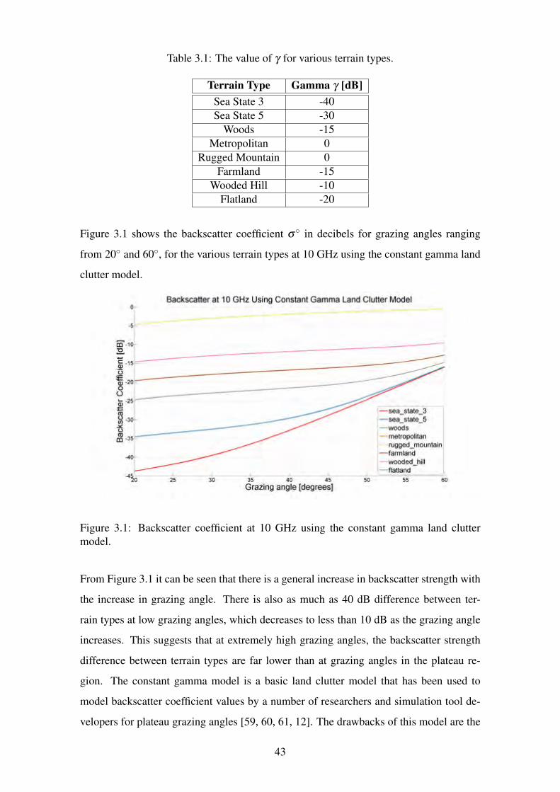
Table 3.1: The value of γ for various terrain types.
Terrain Type Gamma γ [dB]
Sea State 3 -40
Sea State 5 -30
Woods -15
Metropolitan 0
Rugged Mountain 0
Farmland -15
Wooded Hill -10
Flatland -20
Figure 3.1 shows the backscatter coefficient σ◦ in decibels for grazing angles ranging
from 20◦ and 60◦, for the various terrain types at 10 GHz using the constant gamma land
clutter model.
Figure 3.1: Backscatter coefficient at 10 GHz using the constant gamma land clutter
model.
From Figure 3.1 it can be seen that there is a general increase in backscatter strength with
the increase in grazing angle. There is also as much as 40 dB difference between ter-
rain types at low grazing angles, which decreases to less than 10 dB as the grazing angle
increases. This suggests that at extremely high grazing angles, the backscatter strength
difference between terrain types are far lower than at grazing angles in the plateau re-
gion. The constant gamma model is a basic land clutter model that has been used to
model backscatter coefficient values by a number of researchers and simulation tool de-
velopers for plateau grazing angles [59, 60, 61, 12]. The drawbacks of this model are the
43
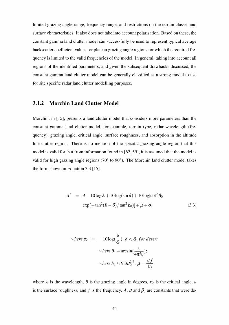
limited grazing angle range, frequency range, and restrictions on the terrain classes and
surface characteristics. It also does not take into account polarisation. Based on these, the
constant gamma land clutter model can successfully be used to represent typical average
backscatter coefficient values for plateau grazing angle regions for which the required fre-
quency is limited to the valid frequencies of the model. In general, taking into account all
regions of the identified parameters, and given the subsequent drawbacks discussed, the
constant gamma land clutter model can be generally classified as a strong model to use
for site specific radar land clutter modelling purposes.
3.1.2 Morchin Land Clutter Model
Morchin, in [15], presents a land clutter model that considers more parameters than the
constant gamma land clutter model, for example, terrain type, radar wavelength (fre-
quency), grazing angle, critical angle, surface roughness, and absorption in the altitude
line clutter region. There is no mention of the specific grazing angle region that this
model is valid for, but from information found in [62, 59], it is assumed that the model is
valid for high grazing angle regions (70◦ to 90◦). The Morchin land clutter model takes
the form shown in Equation 3.3 [15].
σ◦ = A−10logλ +10log(sinδ )+10log[cot2 β0
exp(− tan2(B−δ )/ tan2 β0)]+µ +σc (3.3)
where σc = −10log(δ
δc), δ < δc f or desert
where δc = arcsin(λ
4πhe);
where he ≈ 9.3B2.20 , µ =
√f
4.7
where λ is the wavelength, δ is the grazing angle in degrees, σc is the critical angle, u
is the surface roughness, and f is the frequency. A, B and β0 are constants that were de-
44
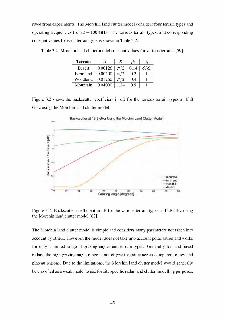
rived from experiments. The Morchin land clutter model considers four terrain types and
operating frequencies from 3− 100 GHz. The various terrain types, and corresponding
constant values for each terrain type is shown in Table 3.2.
Table 3.2: Morchin land clutter model constant values for various terrains [59].
Terrain A B β0 σc
Desert 0.00126 π/2 0.14 δ/δc
Farmland 0.00400 π/2 0.2 1
Woodland 0.01260 π/2 0.4 1
Mountain 0.04000 1.24 0.5 1
Figure 3.2 shows the backscatter coefficient in dB for the various terrain types at 13.8
GHz using the Morchin land clutter model.
Figure 3.2: Backscatter coefficient in dB for the various terrain types at 13.8 GHz using
the Morchin land clutter model [62].
The Morchin land clutter model is simple and considers many parameters not taken into
account by others. However, the model does not take into account polarisation and works
for only a limited range of grazing angles and terrain types. Generally for land based
radars, the high grazing angle range is not of great significance as compared to low and
plateau regions. Due to the limitations, the Morchin land clutter model would generally
be classified as a weak model to use for site specific radar land clutter modelling purposes.
45
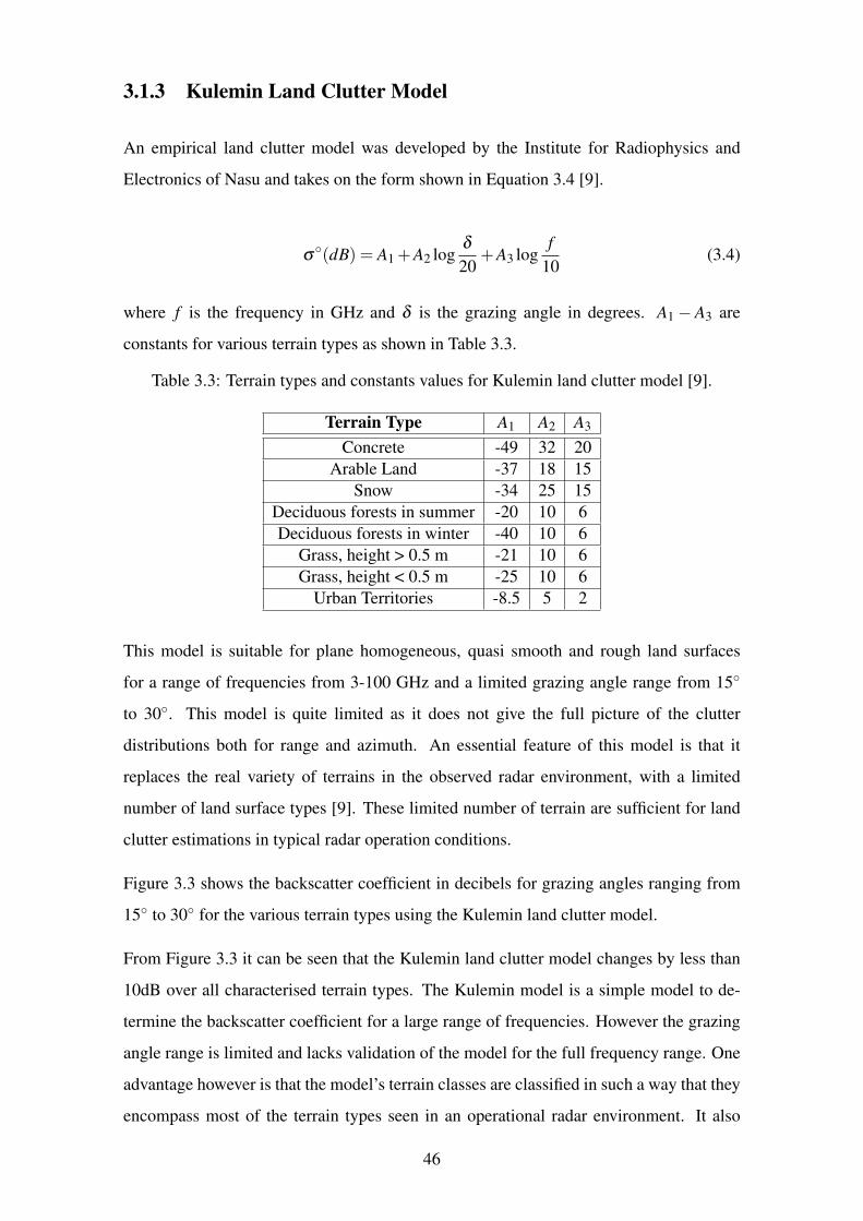
3.1.3 Kulemin Land Clutter Model
An empirical land clutter model was developed by the Institute for Radiophysics and
Electronics of Nasu and takes on the form shown in Equation 3.4 [9].
σ◦(dB) = A1 +A2 logδ
20+A3 log
f
10(3.4)
where f is the frequency in GHz and δ is the grazing angle in degrees. A1 − A3 are
constants for various terrain types as shown in Table 3.3.
Table 3.3: Terrain types and constants values for Kulemin land clutter model [9].
Terrain Type A1 A2 A3
Concrete -49 32 20
Arable Land -37 18 15
Snow -34 25 15
Deciduous forests in summer -20 10 6
Deciduous forests in winter -40 10 6
Grass, height > 0.5 m -21 10 6
Grass, height < 0.5 m -25 10 6
Urban Territories -8.5 5 2
This model is suitable for plane homogeneous, quasi smooth and rough land surfaces
for a range of frequencies from 3-100 GHz and a limited grazing angle range from 15◦
to 30◦. This model is quite limited as it does not give the full picture of the clutter
distributions both for range and azimuth. An essential feature of this model is that it
replaces the real variety of terrains in the observed radar environment, with a limited
number of land surface types [9]. These limited number of terrain are sufficient for land
clutter estimations in typical radar operation conditions.
Figure 3.3 shows the backscatter coefficient in decibels for grazing angles ranging from
15◦ to 30◦ for the various terrain types using the Kulemin land clutter model.
From Figure 3.3 it can be seen that the Kulemin land clutter model changes by less than
10dB over all characterised terrain types. The Kulemin model is a simple model to de-
termine the backscatter coefficient for a large range of frequencies. However the grazing
angle range is limited and lacks validation of the model for the full frequency range. One
advantage however is that the model’s terrain classes are classified in such a way that they
encompass most of the terrain types seen in an operational radar environment. It also
46
Figure 3.3: Backscatter coefficient at 10 GHz using the Kulemin land clutter model.
does not take into account polarisation effects. Based on the models limitations, and lack
of validations, this model in general would be classified as a weak model to use for site
specific radar land clutter modelling purposes.
3.1.4 Nathanson Land Clutter Model Tables
Nathanson, [16], provides a summary of the backscatter coefficient values from more than
50 investigators for various terrains and frequencies, at discrete grazing angles, namely
0◦−1.5◦, 3◦, 10◦, 30◦and 60◦. The tables provide the mean σ◦ value, which is the aver-
age of horizontal and vertical polarisations. In some cases, it also attempts to define the
statistics of the backscatter coefficient by S, which is the dB difference between the me-
dian value and 84th percentile. This provides an indication of whether the distribution can
be approximated by a Rayleigh distribution or not, but no further statistical information
is provided [16]. The terrain types covered are deserts, farmlands, heavy woods / jungle
and urban. The frequency bands covered are L, S,C, X , Ku and Ka bands. The Nathanson
land clutter model tables are shown in Table 3.4.
47
-5 Backscatter at 10 GHz Using the Kulemin Land Clutter Model
-10
~-15 Cl'.l "O '::' -20 C Ql
~ -25 Ql
8-30 <ii := -35 ro u <fl
.:£ -40 u ro
Cl'.l -45
-50
-
~ -55
15 I
20
Grazing angle [degrees]
- concrete - arable_land - snow - forests_summer - forests_winter
grass_more_than_0.5m grass_less_than_0.5m urban
-
I I
25 30
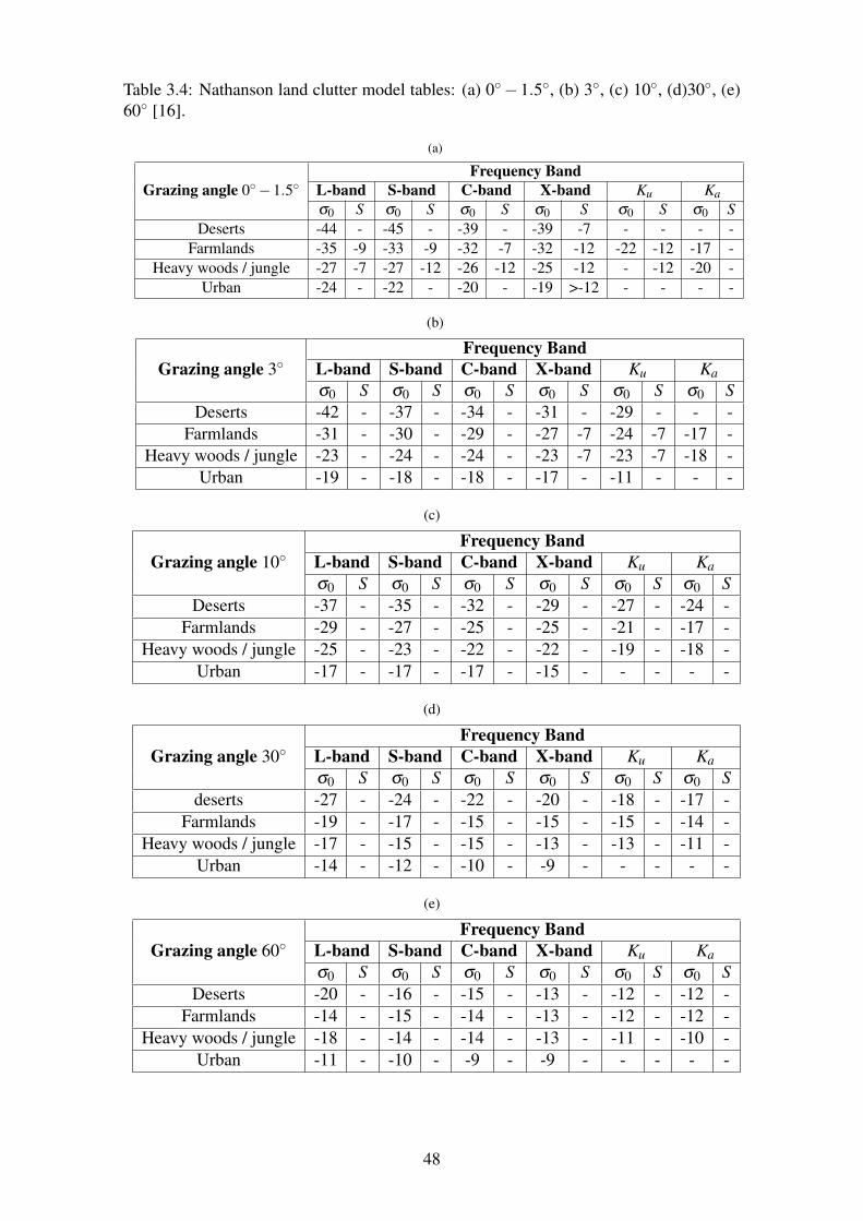
Table 3.4: Nathanson land clutter model tables: (a) 0◦−1.5◦, (b) 3◦, (c) 10◦, (d)30◦, (e)
60◦ [16].
(a)
Grazing angle 0◦−1.5◦Frequency Band
L-band S-band C-band X-band Ku Ka
σ0 S σ0 S σ0 S σ0 S σ0 S σ0 S
Deserts -44 - -45 - -39 - -39 -7 - - - -
Farmlands -35 -9 -33 -9 -32 -7 -32 -12 -22 -12 -17 -
Heavy woods / jungle -27 -7 -27 -12 -26 -12 -25 -12 - -12 -20 -
Urban -24 - -22 - -20 - -19 >-12 - - - -
(b)
Grazing angle 3◦Frequency Band
L-band S-band C-band X-band Ku Ka
σ0 S σ0 S σ0 S σ0 S σ0 S σ0 S
Deserts -42 - -37 - -34 - -31 - -29 - - -
Farmlands -31 - -30 - -29 - -27 -7 -24 -7 -17 -
Heavy woods / jungle -23 - -24 - -24 - -23 -7 -23 -7 -18 -
Urban -19 - -18 - -18 - -17 - -11 - - -
(c)
Grazing angle 10◦Frequency Band
L-band S-band C-band X-band Ku Ka
σ0 S σ0 S σ0 S σ0 S σ0 S σ0 S
Deserts -37 - -35 - -32 - -29 - -27 - -24 -
Farmlands -29 - -27 - -25 - -25 - -21 - -17 -
Heavy woods / jungle -25 - -23 - -22 - -22 - -19 - -18 -
Urban -17 - -17 - -17 - -15 - - - - -
(d)
Grazing angle 30◦Frequency Band
L-band S-band C-band X-band Ku Ka
σ0 S σ0 S σ0 S σ0 S σ0 S σ0 S
deserts -27 - -24 - -22 - -20 - -18 - -17 -
Farmlands -19 - -17 - -15 - -15 - -15 - -14 -
Heavy woods / jungle -17 - -15 - -15 - -13 - -13 - -11 -
Urban -14 - -12 - -10 - -9 - - - - -
(e)
Grazing angle 60◦Frequency Band
L-band S-band C-band X-band Ku Ka
σ0 S σ0 S σ0 S σ0 S σ0 S σ0 S
Deserts -20 - -16 - -15 - -13 - -12 - -12 -
Farmlands -14 - -15 - -14 - -13 - -12 - -12 -
Heavy woods / jungle -18 - -14 - -14 - -13 - -11 - -10 -
Urban -11 - -10 - -9 - -9 - - - - -
48
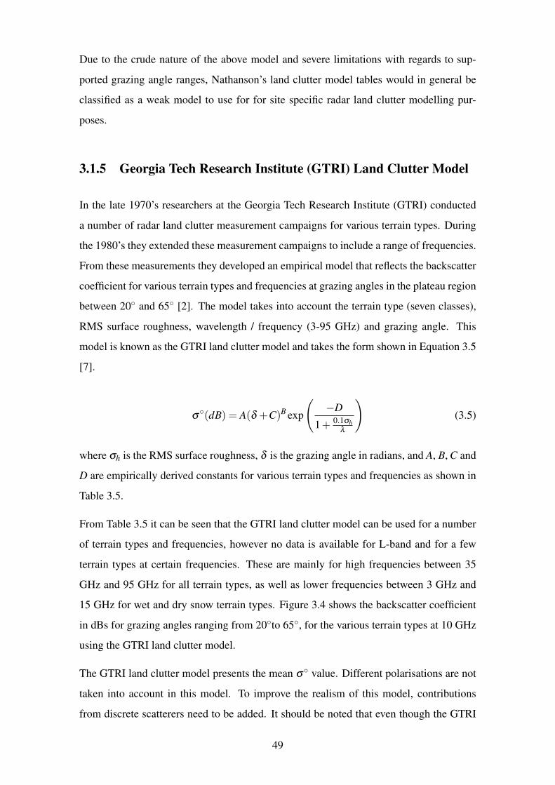
Due to the crude nature of the above model and severe limitations with regards to sup-
ported grazing angle ranges, Nathanson’s land clutter model tables would in general be
classified as a weak model to use for for site specific radar land clutter modelling pur-
poses.
3.1.5 Georgia Tech Research Institute (GTRI) Land Clutter Model
In the late 1970’s researchers at the Georgia Tech Research Institute (GTRI) conducted
a number of radar land clutter measurement campaigns for various terrain types. During
the 1980’s they extended these measurement campaigns to include a range of frequencies.
From these measurements they developed an empirical model that reflects the backscatter
coefficient for various terrain types and frequencies at grazing angles in the plateau region
between 20◦ and 65◦ [2]. The model takes into account the terrain type (seven classes),
RMS surface roughness, wavelength / frequency (3-95 GHz) and grazing angle. This
model is known as the GTRI land clutter model and takes the form shown in Equation 3.5
[7].
σ◦(dB) = A(δ +C)B exp
(
−D
1+ 0.1σh
λ
)
(3.5)
where σh is the RMS surface roughness, δ is the grazing angle in radians, and A, B, C and
D are empirically derived constants for various terrain types and frequencies as shown in
Table 3.5.
From Table 3.5 it can be seen that the GTRI land clutter model can be used for a number
of terrain types and frequencies, however no data is available for L-band and for a few
terrain types at certain frequencies. These are mainly for high frequencies between 35
GHz and 95 GHz for all terrain types, as well as lower frequencies between 3 GHz and
15 GHz for wet and dry snow terrain types. Figure 3.4 shows the backscatter coefficient
in dBs for grazing angles ranging from 20◦to 65◦, for the various terrain types at 10 GHz
using the GTRI land clutter model.
The GTRI land clutter model presents the mean σ◦ value. Different polarisations are not
taken into account in this model. To improve the realism of this model, contributions
from discrete scatterers need to be added. It should be noted that even though the GTRI
49
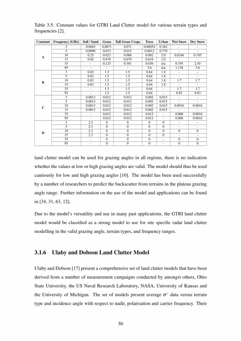
Table 3.5: Constant values for GTRI Land Clutter model for various terrain types and
frequencies [2].
Constant Frequency [GHz] Soil / Sand Grass Tall Grass Crops Trees Urban Wet Snow Dry Snow
A
3 0.0045 0.0071 0.071 0.00054 0.362 - -
5 0.0096 0.015 0.015 0.0012 0.779 - -
10 0.25 0.023 0.006 0.002 2.0 0.0246 0.195
15 0.05 0.079 0.079 0.019 2.0 - -
35 - 0.125 0.301 0.036 n/a 0.195 2.45
95 - - - 3.6 n/a 1.138 3.6
B
3 0.83 1.5 1.5 0.64 1.8 - -
5 0.83 1.5 1.5 0.64 1.8 - -
10 0.83 1.5 1.5 0.64 1.8 1.7 1.7
15 0.83 1.5 1.5 0.64 1.8 - -
35 - 1.5 1.5 0.64 - 1.7 1.7
95 - 1.5 1.5 0.64 - 0.83 0.83
C
3 0.0013 0.012 0.012 0.002 0.015 - -
5 0.0013 0.012 0.012 0.002 0.015 - -
10 0.0013 0.012 0.012 0.002 0.015 0.0016 0.0016
15 0.0013 0.012 0.012 0.002 0.015 - -
35 - 0.012 0.012 0.012 - 0.008 0.0016
95 - 0.012 0.012 0.012 - 0.008 0.0016
D
3 2.3 0 0 0 0 - -
5 2.3 0 0 0 0 - -
10 2.3 0 0 0 0 0 0
15 2.3 0 0 0 0 - -
35 - 0 0 0 - 0 0
95 - 0 0 0 - 0 0
land clutter model can be used for grazing angles in all regions, there is no indication
whether the values at low or high grazing angles are valid. The model should thus be used
cautiously for low and high grazing angles [10]. The model has been used successfully
by a number of researchers to predict the backscatter from terrains in the plateau grazing
angle range. Further information on the use of the model and applications can be found
in [34, 31, 63, 12].
Due to the model’s versatility and use in many past applications, the GTRI land clutter
model would be classified as a strong model to use for site specific radar land clutter
modelling in the valid grazing angle, terrain types, and frequency ranges.
3.1.6 Ulaby and Dobson Land Clutter Model
Ulaby and Dobson [17] present a comprehensive set of land clutter models that have been
derived from a number of measurement campaigns conducted by amongst others, Ohio
State University, the US Naval Research Laboratory, NASA, University of Kansas and
the University of Michigan. The set of models present average σ◦ data versus terrain
type and incidence angle with respect to nadir, polarisation and carrier frequency. Their
50
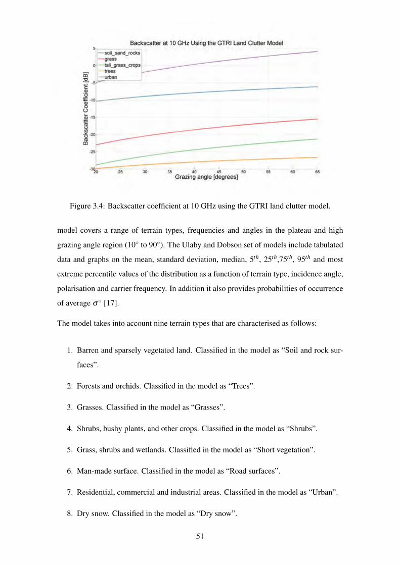
Figure 3.4: Backscatter coefficient at 10 GHz using the GTRI land clutter model.
model covers a range of terrain types, frequencies and angles in the plateau and high
grazing angle region (10◦ to 90◦). The Ulaby and Dobson set of models include tabulated
data and graphs on the mean, standard deviation, median, 5th, 25th,75th, 95th and most
extreme percentile values of the distribution as a function of terrain type, incidence angle,
polarisation and carrier frequency. In addition it also provides probabilities of occurrence
of average σ◦ [17].
The model takes into account nine terrain types that are characterised as follows:
1. Barren and sparsely vegetated land. Classified in the model as “Soil and rock sur-
faces”.
2. Forests and orchids. Classified in the model as “Trees”.
3. Grasses. Classified in the model as “Grasses”.
4. Shrubs, bushy plants, and other crops. Classified in the model as “Shrubs”.
5. Grass, shrubs and wetlands. Classified in the model as “Short vegetation”.
6. Man-made surface. Classified in the model as “Road surfaces”.
7. Residential, commercial and industrial areas. Classified in the model as “Urban”.
8. Dry snow. Classified in the model as “Dry snow”.
51
Backscatter at 10 GHz Using the GTRI Land Clutter Model 5,~-----~
- soil_sand_rocks - grass
co o - tall_grass_crops
- trees
"'O ~ -5 c (I) ·o ti= -10 (I) 0 (.)
ci3 -15
~ rn
1'.5 -20 ro
CD
- urban
25 30 35 40 45 50 55
Grazing angle [degrees] 60 65
9. Wet snow. Classified in the model as “Wet snow”.
The data for the nine terrain types are grouped to their corresponding frequency bands.
The range of frequencies included in this model are L, S,C, X , Ku, Ka and W bands. Then
for each terrain category and frequency band, the data are arranged by polarisation and
valid incidence angles. Three polarisation types are included, namely HH, VV , and HV
[10]. The data for each category can be found in the appendix section of [17]. It should be
noted that the validity of the data provided is not the same for all categories. They differ
by the valid incidence angle ranges and number of observations taken. Some categories
can be classified as having insufficient data due to the low number of observations taken.
An overview of the source data in terms of number of observations and the range of valid
incidence angles is given in Tables 6.6 through to 6.8, from [17].
From the datasets provided, Ulaby and Dobson derived an empirical model for the mean
value as a function of incidence angle, for each terrain category, frequency band and
polarisation. The model takes the form shown in Equation 3.6. This relationship between
the mean value of σ◦ was calculated by a least squares curve fitting process for each
terrain type [10].
σ◦mean(dB) = P1 +P2 exp(−P3θ)+P4 cos(P5θ +P6) (3.6)
where θ is the incidence angle expressed in radians and P1 through to P6 are empirically
derived constants which differ for each category type. This model is only valid for the
categories with sufficient data. Expressions to compute the standard deviation SD is also
given, as shown in equation 3.7.
SD(dB) = M1 +M2 exp(−M3θ) (3.7)
where M1through to M3 are resultant coefficients used for the standard deviation function.
For instances where the sample space is small, (i.e. N<6), the values for M are statistically
insignificant and are therefore not included [17]. From computed values for the σ◦mean and
SD, the 5th and 95th percentile values are then given as shown in Equation 3.8 and 3.9.
These are based upon the assumption of Gaussian distributions.
52
σ◦5%(dB) = σ◦
mean +1.645×SD (3.8)
and
σ◦95%(dB) = σ◦
mean −1.645×SD (3.9)
By taking the compliment of the incidence angle, the above models can easily be ex-
pressed in terms of the grazing angle instead. The values for P and M can be found in
the appendix section of [17] for each category. Table 3.6 provides a summary of the valid
grazing angle ranges of each terrain type category, for the various frequency bands and
polarisations. The categories with a null, indicates insufficient data where equations 3.6
to 3.9 can not be used. Ulaby and Dobson do however provide mean values for a limited
range of discrete grazing angles for categories that are classified as having insufficient
data. These values should be used with caution. As shown in Table 3.6, the urban terrain
type has no sufficient data for all frequency ranges and polarisations.
Figure 3.5 shows the backscatter coefficient in dBs for the various terrain types at 10 GHz
using the Ulaby and Dobson land clutter model for polarisations HH, HV and VV .
These plots agree with the valid grazing angle ranges and terrain types as shown in Table
3.6. Snow terrain types were purposefully excluded from the plot as snow rarely falls
within the SADC region. It is assumed that a Log-normal distribution is generally accep-
ted to provide a good fit to the measured data [17].
The Ulaby and Dobson land clutter model provides valid data for a range of terrain types,
frequencies and polarisations at grazing angles in the plateau and high region. Caution
should be taken when using the Ulaby and Dobson model for categories which has in-
sufficient data, especially for urban terrain which has no sufficient data for all categories.
Caution should also be taken when using the model for certain grazing angle ranges, as
many of the categories valid range differs from the assumed 10◦ to 90◦ as shown in Table
3.6. Due to the many advantages and extra information given for the Ulaby and Dobson
model as compared to others, this model would in general be classified as an excellent
model to use for site specific radar land clutter modelling for grazing angles ranging in
53
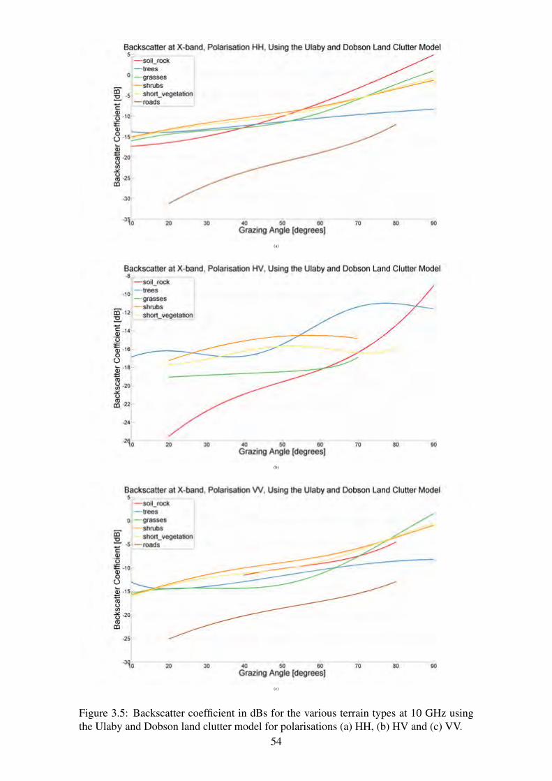
(a)
(b)
(c)
Figure 3.5: Backscatter coefficient in dBs for the various terrain types at 10 GHz using
the Ulaby and Dobson land clutter model for polarisations (a) HH, (b) HV and (c) VV.
54
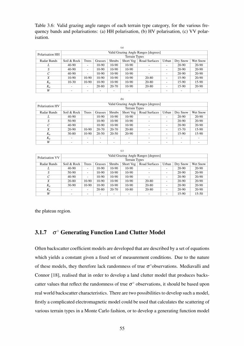
Table 3.6: Valid grazing angle ranges of each terrain type category, for the various fre-
quency bands and polarisations: (a) HH polarisation, (b) HV polarisation, (c) VV polar-
isation.
(a)
Polarisation HHValid Grazing Angle Ranges [degrees]
Terrain Types
Radar Bands Soil & Rock Trees Grasses Shrubs Short Veg Road Surfaces Urban Dry Snow Wet Snow
L 40-90 - 10-90 10-90 10-90 - - 20-90 20-90
S 40-90 - 10-90 10-90 10-90 - - 20-90 20-90
C 40-90 - 10-90 10-90 10-90 - - 20-90 20-90
X 10-90 10-90 10-90 10-90 10-90 20-80 - 15-90 20-90
Ku 10-30 10-90 10-90 10-90 10-90 20-80 - 15-90 15-90
Ka - - 20-80 20-70 10-90 20-80 - 15-90 20-90
W - - - - - - - - -
(b)
Polarisation HVValid Grazing Angle Ranges [degrees]
Terrain Types
Radar Bands Soil & Rock Trees Grasses Shrubs Short Veg Road Surfaces Urban Dry Snow Wet Snow
L 40-90 10-90 10-90 10-90 - - 20-90 20-90
S 50-90 10-90 10-90 10-90 - - 20-90 20-90
C 40-90 10-90 10-90 10-90 - - 20-90 20-90
X 20-90 10-90 20-70 20-70 20-80 - - 15-70 15-90
Ku 30-80 10-90 20-50 20-50 20-90 - - 15-90 15-90
Ka - - - - - - - - -
W - - - - - - - - -
(c)
Polarisation VVValid Grazing Angle Ranges [degrees]
Terrain Types
Radar Bands Soil & Rock Trees Grasses Shrubs Short Veg Road Surfaces Urban Dry Snow Wet Snow
L 40-90 - 10-90 10-90 10-90 - - 20-90 20-90
S 50-90 - 10-90 10-90 10-90 - - 20-90 20-90
C 40-90 - 10-90 10-90 10-90 - - 20-90 20-90
X 20-80 10-90 10-90 10-90 10-90 20-80 - 20-90 20-90
Ku 30-90 10-90 10-90 10-90 10-90 20-80 - 20-90 20-90
Ka - - 20-80 20-70 10-80 20-80 - 20-90 20-90
W - - - - - - - 15-90 15-50
the plateau region.
3.1.7 σ◦ Generating Function Land Clutter Model
Often backscatter coefficient models are developed that are described by a set of equations
which yields a constant given a fixed set of measurement conditions. Due to the nature
of these models, they therefore lack randomness of true σ◦observations. Mediavalli and
Connor [18], realised that in order to develop a land clutter model that produces backs-
catter values that reflect the randomness of true σ◦ observations, it should be based upon
real world backscatter characteristics. There are two possibilities to develop such a model,
firstly a complicated electromagnetic model could be used that calculates the scattering of
various terrain types in a Monte Carlo fashion, or to develop a generating function model
55
that returns values similar to those of measured terrain reflection coefficients. They argued
that all the previous models would be generally unacceptable to use for model validation
as they were deterministic in nature and repeatedly produced identical backscatter values,
for a given category [64].
The data that they decided to base their model on was the Ulaby and Dobson set of radar
scattering statistics for terrain. The data presented by Ulaby and Dobson does not rep-
resent the actual backscatter numbers, but rather data of the statistical properties of the
backscatter numbers and their frequency of occurrence in histogram form. The data re-
flects the reality in which σ◦ from different terrain types is determined by the actual
properties of the terrain.
The requirements for the generator were that the attributes of the coefficients in this gen-
erator need to behave in a certain way. The mean and standard deviation of the generated
distributions of σ◦ need to approach those of the measured data, and the frequency of
occurrence must be similar to the original data. The generator was thus designed such
that it returns values that are similar to the observed measurement terrain scattering data
found in [17]. The generator should output values for all terrain types, polarisations, and
radar bands associated with the Ulaby and Dobson datasets.
They developed a probabilistic land clutter model (i.e. a model that does not repeatedly
produce identical backscatter values for a given category setup, but produces results of
varying values that conform to the statistical nature of real world measurements for a
given category setup), that returns the σ◦ for any combination of terrain type, frequency
band, polarisation and grazing angle that would be similar to, and have similar statistical
properties as the observed data by Ulaby and Dobson. Thus instead of using Ulaby and
Dobson’s empirical model that only provides a deterministic answer, use the statistical
data gathered by Ulaby and Dobson to develop a probabilistic σ◦ generating land clutter
model. Thus being able to obtain any percentile statistic and statistical properties rather
than only the mean values.
The generating function is defined by Equation 3.10 [18].
σ◦ = β (− ln(U)α)+ γ (3.10)
56
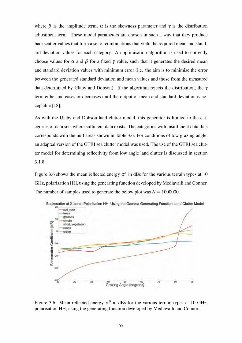
where β is the amplitude term, α is the skewness parameter and γ is the distribution
adjustment term. These model parameters are chosen in such a way that they produce
backscatter values that form a set of combinations that yield the required mean and stand-
ard deviation values for each category. An optimisation algorithm is used to correctly
choose values for α and β for a fixed γ value, such that it generates the desired mean
and standard deviation values with minimum error (i.e. the aim is to minimise the error
between the generated standard deviation and mean values and those from the measured
data determined by Ulaby and Dobson). If the algorithm rejects the distribution, the γ
term either increases or decreases until the output of mean and standard deviation is ac-
ceptable [18].
As with the Ulaby and Dobson land clutter model, this generator is limited to the cat-
egories of data sets where sufficient data exists. The categories with insufficient data thus
corresponds with the null areas shown in Table 3.6. For conditions of low grazing angle,
an adapted version of the GTRI sea clutter model was used. The use of the GTRI sea clut-
ter model for determining reflectivity from low angle land clutter is discussed in section
3.1.8.
Figure 3.6 shows the mean reflected energy σ◦ in dBs for the various terrain types at 10
GHz, polarisation HH, using the generating function developed by Mediavalli and Conner.
The number of samples used to generate the below plot was N = 1000000.
Figure 3.6: Mean reflected energy σ0 in dBs for the various terrain types at 10 GHz,
polarisation HH, using the generating function developed by Mediavalli and Connor.
57
Due to the fact that this model is based upon datasets by Ulaby and Dobson, it repres-
ents the same advantages as well as disadvantages and limitations. However the gamma
generating function generates a probabilistic output instead of deterministic at a better an-
gular resolution than the standard Ulaby and Dobson model [18]. The probabilistic nature
makes it suitable for validation purposes. This is an excellent model to use to simulate
any percentile statistic and backscatter characteristics that behaves in a similar way to real
world observed data. The model does however use more computing resources than the
Ulaby and Dobson model due to its probabilistic nature. The σ◦ generating function land
clutter model would in general be classified as an excellent model to use for site specific
radar land clutter modelling for grazing angles ranging in the plateau region.
3.1.8 Adapted GTRI Sea Clutter Model
The GTRI sea state clutter model provides mean clutter strength predictions for land clut-
ter in low grazing angle range, or where no available measurements are given for a par-
ticular angular extent of the generating function model by Mediavalli and Conner. This
model is used due to the scarcity of measured data in the low grazing angle range (0◦to
15◦) .
Mediavalli and Connor decided that for cases of low grazing angle regions (0◦to 15◦),
where there is a scarcity of measured data, they would adapt and use the GTRI sea clutter
model. The adaptation to the model allows the surface roughness to be changed from very
smooth to very high by changing certain descriptors of the GTRI model. They argued
that the shapes of different sea states in the low grazing angle region is similar to different
surface roughness terrain types producing different shapes for σ◦. The adaptation uses the
different sea state models to relate to different terrain types of different surface roughness
[19]. The GTRI sea state model equations are shown below [2].
For 1 to 10 GHz
σ◦HH = 10log[3.9×10⁻⁶λδ 0.4AiAuAw] (3.11)
58
For 1 to 3 GHz
σ◦VV = σ◦
HH −1.73ln(hav +0.015)+3.76ln(λ )+2.46ln(δ +0.0001)+222 (3.12)
σφ = (14.5λ +5.5)δhav/λ (3.13)
Ai = σ4φ/(1+σ4
φ ) (3.14)
Au = exp[0.2cosφ(1−2.8δ )(λ +0.015)−0.4 (3.15)
qw = 1.1(λ +0.015)0.4 (3.16)
Vw = 8.67h0.4av (3.17)
Aw = [1.94Vw/(1+Vw/15.4]qw (3.18)
where λ is the radar wavelength, δ is the grazing angle, φ is the angle between antenna
boresight and wind direction, hav is the average wave height, Ai is the interference factor,
Au is the upwind-downwind factor, Aw is the wind speed factor, Vw is the velocity of
the wind, qw is the power factor and σ◦φ is the calculated backscatter. These sea state
descriptor values are shown in Table 3.7.
The decisions made as to which sea state to assign to a particular terrain type is as follows.
Firstly it compares the number of facets available, and the average slope of the facets. In
the cases where there is data available, the sea state to use is experimentally determined
by matching the roughness of the terrain type with the roughness of the equivalent sea
state model. In the cases where no data is available, terrain types with smooth surfaces
such as snow is given smaller sea states, and terrain types with rough surfaces such as
trees is given larger sea state values [19].
59
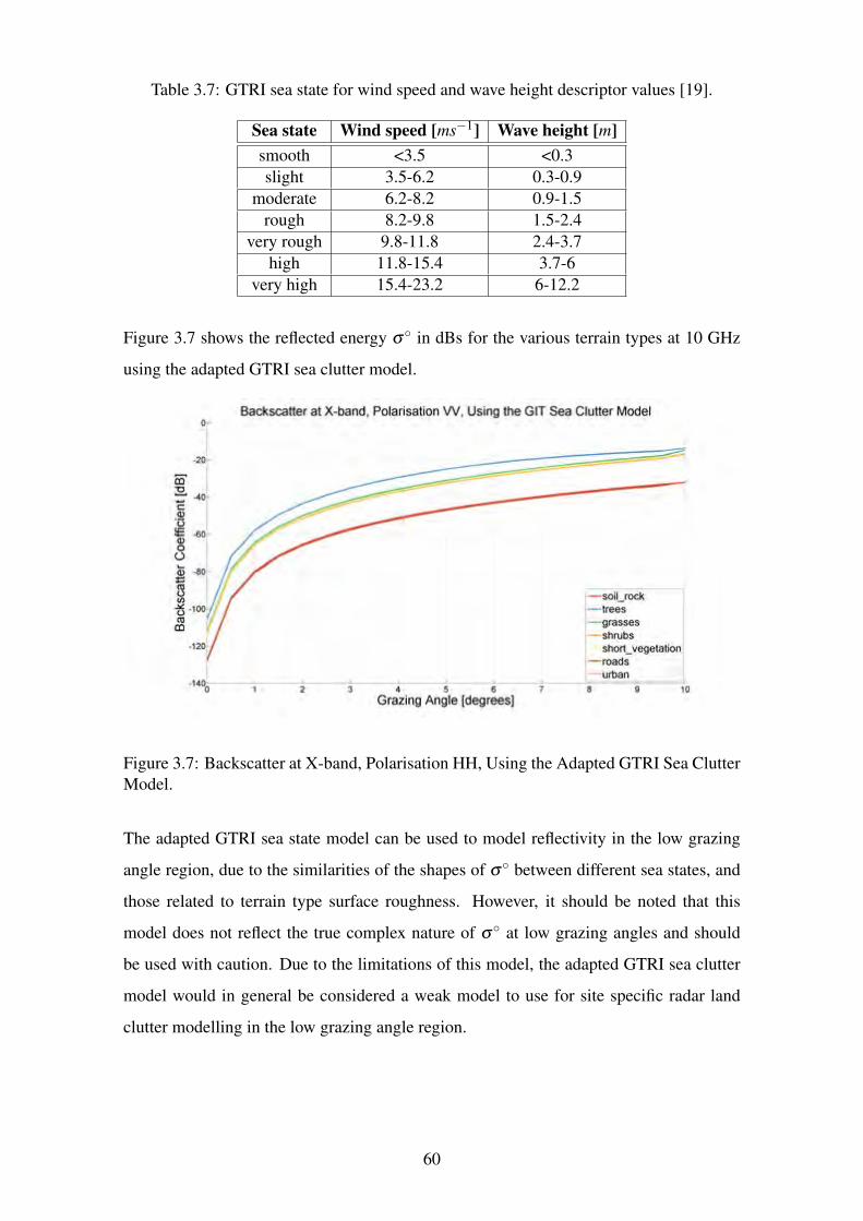
Table 3.7: GTRI sea state for wind speed and wave height descriptor values [19].
Sea state Wind speed [ms−1] Wave height [m]
smooth <3.5 <0.3
slight 3.5-6.2 0.3-0.9
moderate 6.2-8.2 0.9-1.5
rough 8.2-9.8 1.5-2.4
very rough 9.8-11.8 2.4-3.7
high 11.8-15.4 3.7-6
very high 15.4-23.2 6-12.2
Figure 3.7 shows the reflected energy σ◦ in dBs for the various terrain types at 10 GHz
using the adapted GTRI sea clutter model.
Figure 3.7: Backscatter at X-band, Polarisation HH, Using the Adapted GTRI Sea Clutter
Model.
The adapted GTRI sea state model can be used to model reflectivity in the low grazing
angle region, due to the similarities of the shapes of σ◦ between different sea states, and
those related to terrain type surface roughness. However, it should be noted that this
model does not reflect the true complex nature of σ◦ at low grazing angles and should
be used with caution. Due to the limitations of this model, the adapted GTRI sea clutter
model would in general be considered a weak model to use for site specific radar land
clutter modelling in the low grazing angle region.
60
3.1.9 Billingsley Land Clutter Model
The text by Billingsley [6], provides an extremely comprehensive set of models that spe-
cifically focuses on low grazing angle land clutter. Most of these models and current in-
formation available on low angle land clutter characteristics was uncovered by Billingsley
during his time at Massachusetts Institute of technology/Lincoln Labs (MIT/LL). Some
of the important conclusions made by Billingsley on low angle clutter are:
1. Land clutter at low grazing angles are characterised by patchiness / lack of uniform-
ity in spatial extent, due to shadowing and due to extreme resolution dependencies
leading to large resolution cell-to-cell variability.
(a) Higher radar spatial resolution leads to less averaging and therefore more vari-
ability.
(b) Note that resolution changes the shape of the whole spatial amplitude distri-
bution (PDF), not just the tails.
2. Clutter amplitude statistics in the low-grazing angle region are characterised by
distributions with long tails (spiky clutter), making Weibull and Log-Normal distri-
butions suitable choices to model their probability density functions (PDFs).
3. The long tails of the distributions are due to the prevalence of terrain shadowing
and multipath at these low grazing angles.
4. In general, rough surfaces have a larger σ◦ than smooth surfaces for low grazing
angles (conversely, at very high grazing angles (near 90◦), smooth surfaces exhibit
a higher σ◦ than rough ones).
Billingsley’s land clutter models are unconventional compared to other models that fo-
cus on clutter in the plateau and high grazing angle region. Firstly, Billingsley notes that
at low-grazing angles, it is not practical to take grazing angle into consideration in the
conventional sense on a micro facet grazing angle level. He reasons that digital eleva-
tion model (DEM) data is just not at a high enough resolution to sensibly incorporate
into low-angle clutter models. In addition he mentions that DEM data also does not
take into account the discrete elements that dominate scintillation of land clutter at low
angles. He mentions that all attempts to this extent have failed. Thus instead of grazing
61
angle, Billingsley classifies his models in terms of the depression angle, which is relat-
ively simple and unambiguous quantity to determine. The differences between depression
angle, and grazing angle are shown in section 2.4.3.2.
Secondly, Billingsley notes that at low depression angles, the effective F4 term is different
in each resolution cell and thus can significantly affect the clutter strength measurement
(i.e. greater significance as compared to those from higher grazing angles). The effect of
F4 is thus much more of a concern at low depression / grazing angles. Billingsley also
uses the standard 43
Earth Model to account for effects of earth curvature and atmospheric
refraction. Thus at short range where effects of refraction are negligible, grazing angle
and depression angle are assumed to be equal.
For smaller depression angles, the standard deviations from measurements are much lar-
ger than for a Rayleigh distribution. For decreasing depression angles, the ratio of the
average to median σ◦ values increase substantially. This indicates that there is a large
increase in the standard deviation with decreasing depression angles. At low angles, F
increases rapidly and thus backscatter strength from scatterers increase rapidly as well
with height above the ground. Land objects, even at small heights can cause considerable
shadowing effects. Thus changes in F4 are exaggerated at smaller depression angles. Ac-
cording to Billingsley, for farmlands at low depression angles, there is a large increase in
spread when the resolution cell size is decreased, this is due to strong dominating discrete
scatterers. However, for forests at low depression angles, less spread occurs when the
resolution cell size is decreased, because the forest is a more homogeneous surface. For
forests at high depression angles, even less spread is seen as a result of improved illumin-
ation. Urban terrain also show decreasing spread with increasing angle, but with a much
stronger average backscatter than for corresponding rural / low relief terrain distributions
[10].
Thirdly, due to the nature of F at low depression angles, Billingsley places a strong de-
pendence of the spread of land clutter distributions on spatial resolution.The spatial res-
olution or cell size A in m2 is defined by Equation 3.19,
A = r×△r×△θ (3.19)
where r is the range, △r is the range resolution, and △θ is the beamwidth. The spatial
62
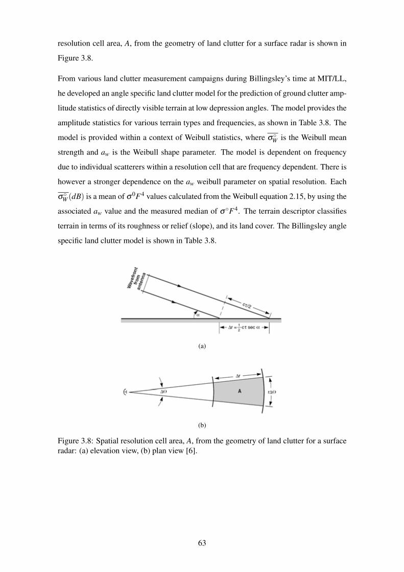
resolution cell area, A, from the geometry of land clutter for a surface radar is shown in
Figure 3.8.
From various land clutter measurement campaigns during Billingsley’s time at MIT/LL,
he developed an angle specific land clutter model for the prediction of ground clutter amp-
litude statistics of directly visible terrain at low depression angles. The model provides the
amplitude statistics for various terrain types and frequencies, as shown in Table 3.8. The
model is provided within a context of Weibull statistics, where σ◦W is the Weibull mean
strength and aw is the Weibull shape parameter. The model is dependent on frequency
due to individual scatterers within a resolution cell that are frequency dependent. There is
however a stronger dependence on the aw weibull parameter on spatial resolution. Each
σ◦W (dB) is a mean of σ0F4 values calculated from the Weibull equation 2.15, by using the
associated aw value and the measured median of σ◦F4. The terrain descriptor classifies
terrain in terms of its roughness or relief (slope), and its land cover. The Billingsley angle
specific land clutter model is shown in Table 3.8.
(a)
(b)
Figure 3.8: Spatial resolution cell area, A, from the geometry of land clutter for a surface
radar: (a) elevation view, (b) plan view [6].
63
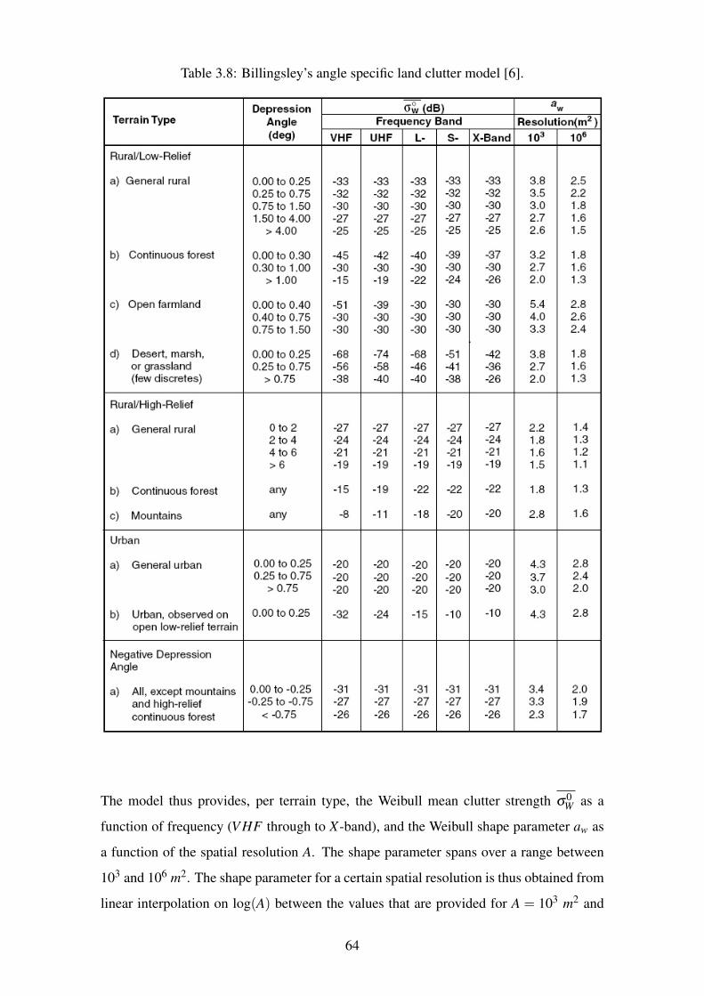
Table 3.8: Billingsley’s angle specific land clutter model [6].
The model thus provides, per terrain type, the Weibull mean clutter strength σ0W as a
function of frequency (V HF through to X-band), and the Weibull shape parameter aw as
a function of the spatial resolution A. The shape parameter spans over a range between
103 and 106 m2. The shape parameter for a certain spatial resolution is thus obtained from
linear interpolation on log(A) between the values that are provided for A = 103 m2 and
64
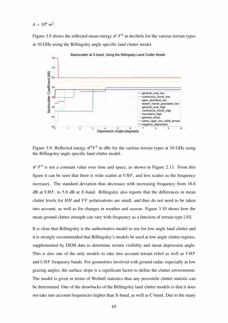
A = 106 m2.
Figure 3.9 shows the reflected mean energy σ◦F4 in decibels for the various terrain types
at 10 GHz using the Billingsley angle specific land clutter model.
Figure 3.9: Reflected energy σ0F4 in dBs for the various terrain types at 10 GHz using
the Billingsley angle specific land clutter model.
σ◦F4 is not a constant value over time and space, as shown in Figure 2.13. From this
figure it can be seen that there is wide scatter at V HF , and less scatter as the frequency
increases. The standard deviation thus decreases with increasing frequency from 16.6
dB at V HF , to 5.8 dB at X-band. Billingsley also reports that the differences in mean
clutter levels for HH and VV polarisations are small, and thus do not need to be taken
into account, as well as for changes in weather and season. Figure 3.10 shows how the
mean ground clutter strength can vary with frequency as a function of terrain type [10].
It is clear that Billingsley is the authoritative model to use for low angle land clutter and
it is strongly recommended that Billingsley’s models be used at low angle clutter regions,
supplemented by DEM data to determine terrain visibility and mean depression angle.
This is also one of the only models to take into account terrain relief as well as V HF
and UHF frequency bands. For geometries involved with ground radar, especially at low
grazing angles, the surface slope is a significant factor to define the clutter environment.
The model is given in terms of Weibull statistics thus any percentile clutter statistic can
be determined. One of the drawbacks of the Billingsley land clutter models is that it does
not take into account frequencies higher than X-band, as well as C-band. Due to the many
65
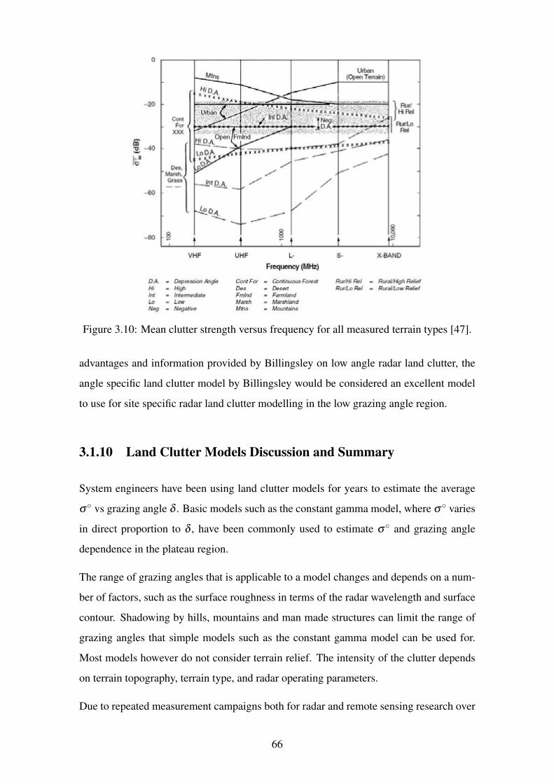
Figure 3.10: Mean clutter strength versus frequency for all measured terrain types [47].
advantages and information provided by Billingsley on low angle radar land clutter, the
angle specific land clutter model by Billingsley would be considered an excellent model
to use for site specific radar land clutter modelling in the low grazing angle region.
3.1.10 Land Clutter Models Discussion and Summary
System engineers have been using land clutter models for years to estimate the average
σ◦ vs grazing angle δ . Basic models such as the constant gamma model, where σ◦ varies
in direct proportion to δ , have been commonly used to estimate σ◦ and grazing angle
dependence in the plateau region.
The range of grazing angles that is applicable to a model changes and depends on a num-
ber of factors, such as the surface roughness in terms of the radar wavelength and surface
contour. Shadowing by hills, mountains and man made structures can limit the range of
grazing angles that simple models such as the constant gamma model can be used for.
Most models however do not consider terrain relief. The intensity of the clutter depends
on terrain topography, terrain type, and radar operating parameters.
Due to repeated measurement campaigns both for radar and remote sensing research over
66
0
- 20
Cont For
XXX
co ~ -40
It! Des,
Marsh, Grass lntQA_
- 60
l.0 0.,4 -...:._
- 80 §
VHF
DA. Depression Angle Hi High Int lntem,ediate Lo Low Neg Negative
/
/
----UHF
Cont For Des Fmlnd Marsh Mins
§
L
Frequency (MHz)
Continuous Fores/ Desett Farmland Marshland Mountains
/
Urban (Open Terrain)
S-
Rur/Hi Rel Rur/Lo Rel
1 Rur/ J Hi Rel
I Rur/Lo Rel
X-BAND
Rural/High Relief Rural/Low Relief
the years, there is a considerable amount of knowledge available for σ◦ from L through
to Ka bands for the plateau and high grazing angle regions. There is also a comprehensive
set of average σ◦ data as a function of radar frequency and terrain type in these grazing
angle regions. Empirical land clutter models were developed from measured data us-
ing regression methods to estimate model parameters. There is however few sources of
data available for low grazing angle regions. The only source that has comprehensively
studied reflectivity from land in the low grazing angle region is Billingsley, whom has
provided datasets for VHF through to X-band frequencies for low grazing angle regions.
Generally for the plateau and high grazing angle regions, σ◦ decreases with decreasing
grazing angle, but Billingsley has shown that at very low grazing angles this is untrue.
He found that the median of average values of σ◦F4 over the five considered radar bands
was roughly the same (≈ -30 dB for terrain type “general rural”), also that the spread
of σ◦F4 increases with decreasing frequencies. Thus σ◦F4 can either be much larger or
much smaller at lower frequency bands than at higher ones. However for smoother land
surfaces with a few discretes, it was found that the median of average values for σ◦F4
generally decreases with decreasing frequency.
In terms of polarisations, most of the available data are for HH and VV polarisations, or an
average of the two. Few data sources are available for HV and VH polarisations and none
for circular polarisation in terms of terrain backscatter [10]. Currently only the Ulaby and
Dobson and Generating Function Land Clutter models take into account polarisation.
The types of clutter models that were presented were, basic and simple mathematical land
clutter models, semi-empirical land clutter models, and empirical land clutter models
which describe statistical behaviour. The simple models are based upon mathematical
formulas that provide an estimation to the the general shape of the backscatter coefficient
for different terrain types and frequencies, at grazing angles in the plateau region.
Semi-empirical models are based upon fitting model equations to observed data using
the polynomial fit algorithms such as the least squares. These models thus output the
backscatter coefficient that has the same mean value as the observed data, for different
terrain types and frequencies at different grazing angles. Most semi-empirical models
average out HH and VV polarisations, however there are a few that take polarisation into
account as well. It is important to note that these models are deterministic in nature and
do not represent the true statistical nature of σ0 for different terrains.
67
The empirical models presented are based upon using observed terrain datasets as a refer-
ence to develop a probabilistic model that can be used to generate σ◦ values that behave
in the same statistical nature as the statistics of the observed data. They use typical PDF
models in which the corresponding PDF parameters are empirically derived. Any percent-
ile statistic can be determined and not only a deterministic average value. These models
inherently require more computer resources.
These empirical land clutter models are good for providing non-site specific clutter maps
that describe the statistical properties of the clutter strength for different radars. These are
thus mostly used to model the patchiness of clutter and not relevant for specific regions,
terrain features and radar position. Site specific clutter models however represent the
clutter intensity over a particular radar operation site of interest [63]. These models are
dependent upon detailed information about the site.
A summary of the land clutter models discussed in this dissertation is shown in Table
3.9. Further analysis and comparisons of the listed land clutter models are investigated in
section 4.1. Results obtained from this investigation further justifies the ‘Model Validity /
Compatibility’ parameter seen in Table 3.9.
68
Table 3.9: Land clutter models summary.
69
70
------ --------~------------------- ---------- ------ ------ ~-------- - - - - - - - - - ·- ---- - - -Ulabyand Sem i -Em iprica l • So il a nd r ock • Shrubs • Fr e-q u e-ncy • 2 - 1 8 GHz 102- 9 0 2 • HH • Determ in i s t i c • H igh v a lid ity
Dobson s urfa ces • Sh o rt v eget a t i o n • I n c i den ce a n g le • 2 7 - 40 G Hz • HV o u tput b etween 20 2 a nd
• Trees • U r ban a r ea.s (G r azi ng a n g le ) • 75 - 100 G Hz • W • M ean (a v er age) 702
• Gr ass.es • Sn o w d ry • Po la r isat i o n b a cks.catte r • low v a lid ity
• Sno w wet • T erra i n type (based coeffi c i en t (d B) e l s ewh er e on m o de l con st a n ts) • Sta n d a r dev iati o n • Excellen t mode l
• 5 th per cen t ile
b a cks.catte r
coeffi c i en t (d B)
• 9 5 th p e r cen t ile
b ackscatte r
coeffi c i en t (d B)
Ga.mma Em per ica l / • So il a nd r ock • Sho rt v eget a t i o n • Fr e-q u e-ncy • 2 - 1 8 GH z 102-90 2 • HH • Proba b ilis t i c • H igh v a lid ity Gene r-ating Probab a lis t i c s urfa ces • Urba n a r eas • I n c i den ce a n g l e • 2 7 - 40 G Hz • HV o u tput b etween 20 2 a nd
Function • Trees • Sn o w d ry (G r azi ng a n g le ) • 75 - 100 G Hz • W • M ean (a v erage) 702 • Gr a.ss.es • Sn o w wet • Po la r isat i o n b ackscatte r • Lo w v a lid ity • Shrub s • Terra i n type (ba.sed coeffi c i en t (d B) e l s ewh er e
on m o de l constan ts) • Sta n d a r d • Excellen t mode l
d ev i a t ion
• Any per centi l e
b ackscatte r coeffi c i en t (d B)
Adapted GTRI Sem i -Empir ica l Fo r a ny t e r r a in type. • Fr e-q u e-ncy 3- l OO G Hz 0 2 - 102 N/A • Determ in i s t i c • Lo w v a lid i ty
Sea Clutter Bas.ed on the s u rface •Gr azin g a ng l e o u tput • W eak m o de l
Model r o ug h ness of the • Po la r isat i o n • M ean (a v erage) terr-a in. • Terra i n type (ba.sed b ackscatte r
on m o de l constan ts) coeffi c i en t a• (d B)
Billingsley Em p er ica l / • H igh o r Low Re l i ef : • H igh o r Low Relief : • Fr e-q u e-ncy • 0.0 3 - 4 G Hz • 0 2 - 1 0 2 N/A • Prob a b ilis t i c • H igh v a lid ity
Probab a listi c Gen er a l Ru ra l G r assla nd • D-eperes.s i o n a ng l e • 8 - 1 2 GH z • Negat iv e o utput • Excellen t mode l
• H igh o r low Re l i e f : • H igh o r low Relief : • Terra i n type d epres.si on • M ean (a v er-age)
Cont i n u o u s f o rest Open f a rml a n d • W e ib u ll s hape a n g les b ackscatte r
• H igh o r low Re l i e f : • H igh or Low Relief : p a r a m et er (d ep en d ent coeffi c i en t (d B)
D-esert U r ban on s p .a t i a l r e-sol u tion ). • Sta n d a r d • H igh o r low Relie f : • Lo w r elief n e-gat i v e • W e ib u ll sca l e d ev i a t ion
M a r s h depr essio n a n g le p a r a m eter (d ep endent • Any per centile
on m ean v a l ues ). b ackscatte r
coeffi c i en t (d B)
3.2 GIS Data
A fundamental procedure required in developing a site specific radar coverage and land
clutter modelling tool, is the creation of the radar observed environment. Inputs that are
required are DEM data, as well as land cover data for particular areas of interest. For the
purpose of this dissertation, the focus of the simulation area will be the SADC region. Site
specific clutter models are thus dependent upon detailed information of the radar observed
environment. This information can be provided by DEM and Land Cover data [63].
3.2.1 Digital Elevation Model Data
DEM data is required to model the topography of the land for the simulated area of in-
terest. The data is also required in a site specific radar coverage and land clutter modelling
tool to determine facets, surface contours (slopes) and terrain shadowing regions. Several
sources of DEM data are proposed and discussed. These are:
1. Shuttle Radar Topography Mission (SRTM) Digital Elevation Model Data.
2. Advanced Spaceborne Thermal Emission and Reflection Radiometer (ASTER) Global
Digital Elevation Model (GDEM) Data.
3. Digital Terrain Elevation Data (DTED).
4. Astrium Digital Elevation Model Data.
Based on the information gathered, the above DEM’s will be classified as either a weak,
strong, or excellent DEM dataset to use for site specific radar coverage and land clutter
modelling purposes. The classification will be based upon the model’s validity, availabil-
ity, resolution, accuracy, parameters taken into account, terrain classes covered and cover
over SADC region.
3.2.1.1 Shuttle Radar Topography Mission (SRTM) Digital Elevation Model Data
SRTM datasets are remote sensed data that were obtained during an eleven day flight of
the space shuttle endeavour and operated by NASA, DLR, and others in the U.S. The
71
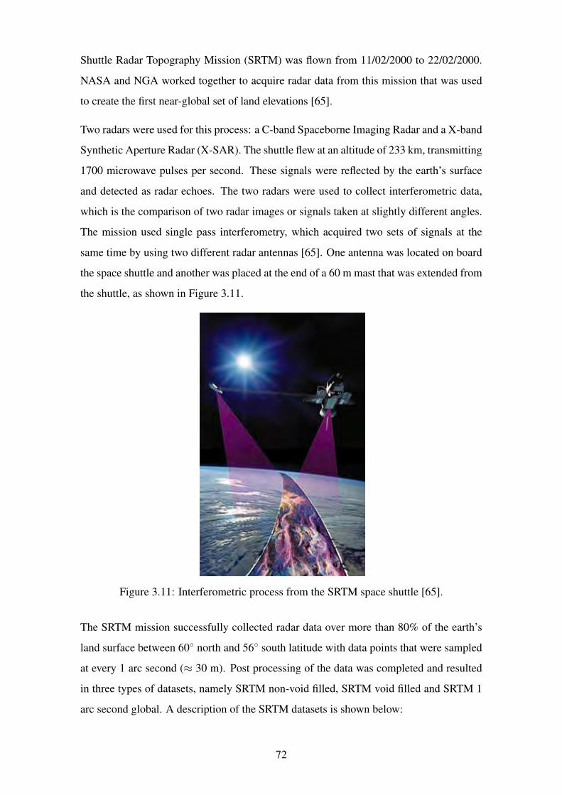
Shuttle Radar Topography Mission (SRTM) was flown from 11/02/2000 to 22/02/2000.
NASA and NGA worked together to acquire radar data from this mission that was used
to create the first near-global set of land elevations [65].
Two radars were used for this process: a C-band Spaceborne Imaging Radar and a X-band
Synthetic Aperture Radar (X-SAR). The shuttle flew at an altitude of 233 km, transmitting
1700 microwave pulses per second. These signals were reflected by the earth’s surface
and detected as radar echoes. The two radars were used to collect interferometric data,
which is the comparison of two radar images or signals taken at slightly different angles.
The mission used single pass interferometry, which acquired two sets of signals at the
same time by using two different radar antennas [65]. One antenna was located on board
the space shuttle and another was placed at the end of a 60 m mast that was extended from
the shuttle, as shown in Figure 3.11.
Figure 3.11: Interferometric process from the SRTM space shuttle [65].
The SRTM mission successfully collected radar data over more than 80% of the earth’s
land surface between 60◦ north and 56◦ south latitude with data points that were sampled
at every 1 arc second (≈ 30 m). Post processing of the data was completed and resulted
in three types of datasets, namely SRTM non-void filled, SRTM void filled and SRTM 1
arc second global. A description of the SRTM datasets is shown below:
72
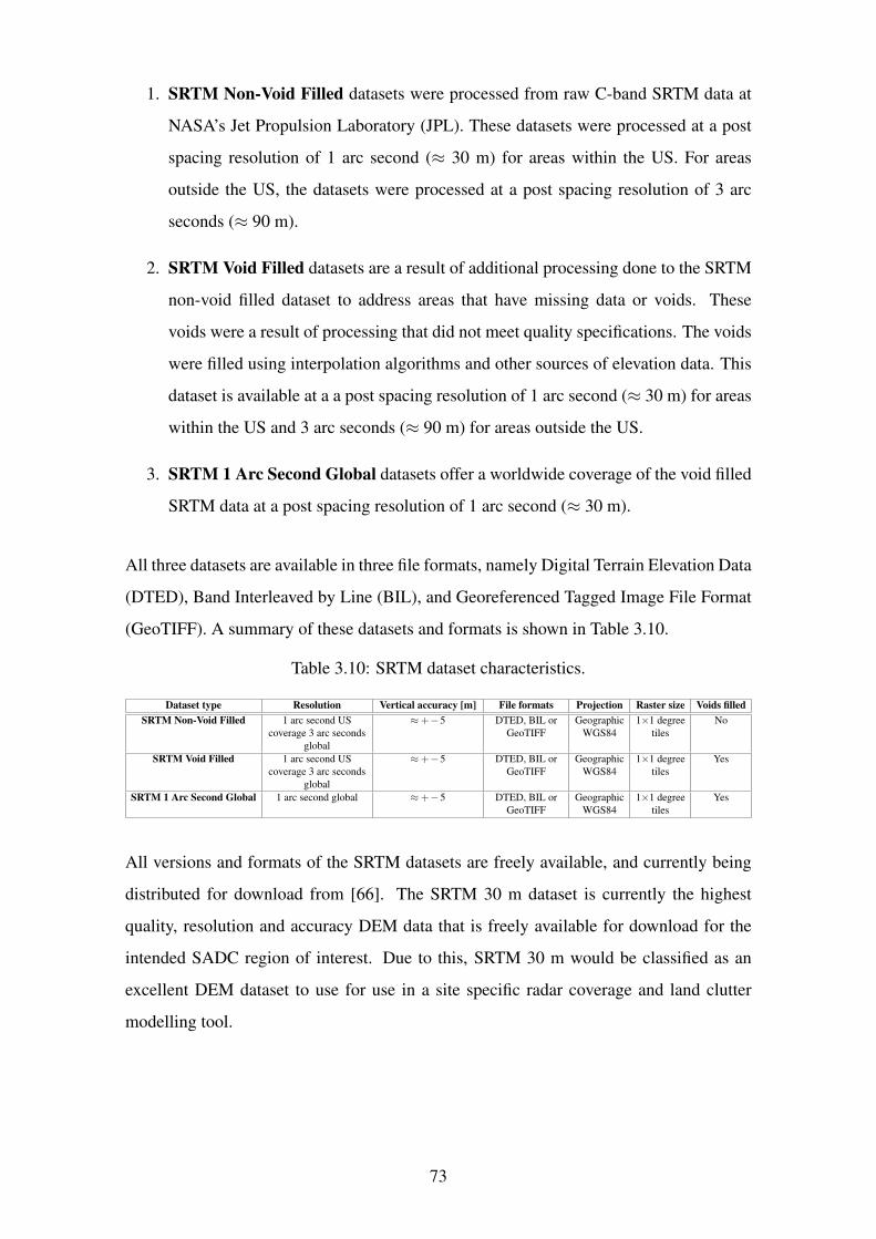
1. SRTM Non-Void Filled datasets were processed from raw C-band SRTM data at
NASA’s Jet Propulsion Laboratory (JPL). These datasets were processed at a post
spacing resolution of 1 arc second (≈ 30 m) for areas within the US. For areas
outside the US, the datasets were processed at a post spacing resolution of 3 arc
seconds (≈ 90 m).
2. SRTM Void Filled datasets are a result of additional processing done to the SRTM
non-void filled dataset to address areas that have missing data or voids. These
voids were a result of processing that did not meet quality specifications. The voids
were filled using interpolation algorithms and other sources of elevation data. This
dataset is available at a a post spacing resolution of 1 arc second (≈ 30 m) for areas
within the US and 3 arc seconds (≈ 90 m) for areas outside the US.
3. SRTM 1 Arc Second Global datasets offer a worldwide coverage of the void filled
SRTM data at a post spacing resolution of 1 arc second (≈ 30 m).
All three datasets are available in three file formats, namely Digital Terrain Elevation Data
(DTED), Band Interleaved by Line (BIL), and Georeferenced Tagged Image File Format
(GeoTIFF). A summary of these datasets and formats is shown in Table 3.10.
Table 3.10: SRTM dataset characteristics.
Dataset type Resolution Vertical accuracy [m] File formats Projection Raster size Voids filled
SRTM Non-Void Filled 1 arc second US
coverage 3 arc seconds
global
≈+−5 DTED, BIL or
GeoTIFF
Geographic
WGS84
1×1 degree
tiles
No
SRTM Void Filled 1 arc second US
coverage 3 arc seconds
global
≈+−5 DTED, BIL or
GeoTIFF
Geographic
WGS84
1×1 degree
tiles
Yes
SRTM 1 Arc Second Global 1 arc second global ≈+−5 DTED, BIL or
GeoTIFF
Geographic
WGS84
1×1 degree
tiles
Yes
All versions and formats of the SRTM datasets are freely available, and currently being
distributed for download from [66]. The SRTM 30 m dataset is currently the highest
quality, resolution and accuracy DEM data that is freely available for download for the
intended SADC region of interest. Due to this, SRTM 30 m would be classified as an
excellent DEM dataset to use for use in a site specific radar coverage and land clutter
modelling tool.
73
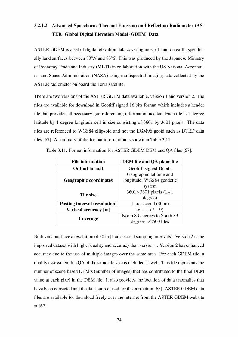
3.2.1.2 Advanced Spaceborne Thermal Emission and Reflection Radiometer (AS-
TER) Global Digital Elevation Model (GDEM) Data
ASTER GDEM is a set of digital elevation data covering most of land on earth, specific-
ally land surfaces between 83◦N and 83◦S. This was produced by the Japanese Ministry
of Economy Trade and Industry (METI) in collaboration with the US National Aeronaut-
ics and Space Administration (NASA) using multispectral imaging data collected by the
ASTER radiometer on board the Terra satellite.
There are two versions of the ASTER GDEM data available, version 1 and version 2. The
files are available for download in Geotiff signed 16 bits format which includes a header
file that provides all necessary geo-referencing information needed. Each tile is 1 degree
latitude by 1 degree longitude cell in size consisting of 3601 by 3601 pixels. The data
files are referenced to WGS84 ellipsoid and not the EGM96 geoid such as DTED data
files [67]. A summary of the format information is shown in Table 3.11.
Table 3.11: Format information for ASTER GDEM DEM and QA files [67].
File information DEM file and QA plane file
Output format Geotiff, signed 16 bits
Geographic coordinates
Geographic latitude and
longitude. WGS84 geodetic
system
Tile size3601×3601 pixels (1×1
degree)
Posting interval (resolution) 1 arc second (30 m)
Vertical accuracy [m] ≈+− (7−9)
CoverageNorth 83 degrees to South 83
degrees, 22600 tiles
Both versions have a resolution of 30 m (1 arc second sampling intervals). Version 2 is the
improved dataset with higher quality and accuracy than version 1. Version 2 has enhanced
accuracy due to the use of multiple images over the same area. For each GDEM tile, a
quality assessment file QA of the same tile size is included as well. This file represents the
number of scene based DEM’s (number of images) that has contributed to the final DEM
value at each pixel in the DEM file. It also provides the location of data anomalies that
have been corrected and the data source used for the correction [68]. ASTER GDEM data
files are available for download freely over the internet from the ASTER GDEM website
at [67].
74
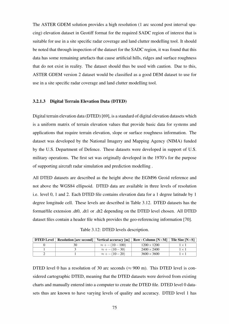
The ASTER GDEM solution provides a high resolution (1 arc second post interval spa-
cing) elevation dataset in Geotiff format for the required SADC region of interest that is
suitable for use in a site specific radar coverage and land clutter modelling tool. It should
be noted that through inspection of the dataset for the SADC region, it was found that this
data has some remaining artefacts that cause artificial hills, ridges and surface roughness
that do not exist in reality. The dataset should thus be used with caution. Due to this,
ASTER GDEM version 2 dataset would be classified as a good DEM dataset to use for
use in a site specific radar coverage and land clutter modelling tool.
3.2.1.3 Digital Terrain Elevation Data (DTED)
Digital terrain elevation data (DTED) [69], is a standard of digital elevation datasets which
is a uniform matrix of terrain elevation values that provide basic data for systems and
applications that require terrain elevation, slope or surface roughness information. The
dataset was developed by the National Imagery and Mapping Agency (NIMA) funded
by the U.S. Department of Defence. These datasets were developed in support of U.S.
military operations. The first set was originally developed in the 1970’s for the purpose
of supporting aircraft radar simulation and prediction modelling .
All DTED datasets are described as the height above the EGM96 Geoid reference and
not above the WGS84 ellipsoid. DTED data are available in three levels of resolution
i.e. level 0, 1 and 2. Each DTED file contains elevation data for a 1 degree latitude by 1
degree longitude cell. These levels are described in Table 3.12. DTED datasets has the
format/file extension .dt0, .dt1 or .dt2 depending on the DTED level chosen. All DTED
dataset files contain a header file which provides the geo-referencing information [70].
Table 3.12: DTED levels description.
DTED Level Resolution [arc second] Vertical accuracy [m] Row×Column [N×M] Tile Size [N×S]
0 30 ≈+− (10−100) 1200×1200 1×1
1 3 ≈+− (10−30) 2400×2400 1×1
2 1 ≈+− (10−20) 3600×3600 1×1
DTED level 0 has a resolution of 30 arc seconds (≈ 900 m). This DTED level is con-
sidered cartographic DTED, meaning that the DTED datasets were derived from existing
charts and manually entered into a computer to create the DTED file. DTED level 0 data-
sets thus are known to have varying levels of quality and accuracy. DTED level 1 has
75
a resolution of 3 arc seconds (≈ 90 m), and considered to be a basic medium resolution
dataset. DTED level 1 has a resolution of 1 arc second (≈ 30 m), and considered to be
a basic high resolution dataset. DTED level 1 datasets has a quality measurement of less
than 90% confidence of a linear error of less than 30 m, and a horizontal error of less than
50 m. DTED level 2 datasets has a 90% confidence of less than 18 m and a horizontal
error of less than 23 m. This means that 9 out of 10 measurements should be less than the
spacing value listed but potentially the tenth value could have an error greater than that
spacing value [70].
The distribution and availability of DTED products is authorised by the U.S Department
of Defence. DTED level 0 is freely available for download through the internet within
copyright restrictions, however level 1 and 2 DTED datasets are not freely available for
download. DTED level 1 and 2 are specifically suited for military activities.
The DTED solution provides a high to low resolution (1-30 arc second post interval spa-
cing) elevation dataset in Geotiff format for the required SADC region of interest. How-
ever only the low level dataset is freely available for download. The low level dataset can
be used to provide a rough idea of terrain shadowing effects but would not be sufficient
to use in a site specific radar coverage and land clutter modelling tool. DTED 30 m (level
2) would be classified as an excellent dataset for use in a site specific radar coverage and
land clutter modelling tool.
3.2.1.4 Astrium Data
Astrium Geo-Information Services is a European company generating one of the best
digital elevation data sets currently available. They provide a dataset for any land area
in the world with various resolutions ranging from 30 m down to 1 m. The dataset has a
vertical accuracy of 2 m relative and 4 m absolute, which is significantly better than any
DTED, ASTER GDEM or STRM datasets. All datasets are based upon optical and radar
technologies. The quality and accuracy is achieved from extensive post processing of the
data to conform to the true nature of the land. Astrium offers a solution of highest data
quality and accuracy compared to DTED or ASTER GDEM sources, however this data is
not freely available. Astrium’s standard offerings and prices are available on their website
at [71]. A summary of the features of the available Astrium datasets are shown below in
76
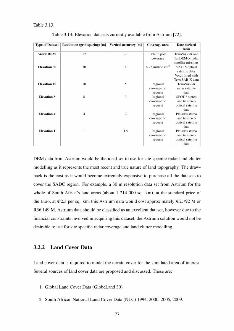
Table 3.13.
Table 3.13: Elevation datasets currently available from Astrium [72].
Type of Dataset Resolution (grid spacing) [m] Vertical accuracy [m] Coverage area Date derived
from
WorldDEM 12 2 Pole to pole
coverage
TerraSAR-X and
TanDEM-X radar
satellite missions
Elevation 30 30 8 > 75 million km2 SPOT 5 optical
satellite data.
Voids filled with
TerraSAR-X data
Elevation 10 10 5 Regional
coverage on
request
TerraSAR-X
radar satellite
data
Elevation 8 8 3 Regional
coverage on
request
SPOT 6 stereo
and tri stereo
optical satellite
data
Elevation 4 4 2 Regional
coverage on
request
Pleiades stereo
and tri stereo
optical satellite
data
Elevation 1 1 1.5 Regional
coverage on
request
Pleiades stereo
and tri stereo
optical satellite
data
DEM data from Astrium would be the ideal set to use for site specific radar land clutter
modelling as it represents the most recent and true nature of land topography. The draw-
back is the cost as it would become extremely expensive to purchase all the datasets to
cover the SADC region. For example, a 30 m resolution data set from Astrium for the
whole of South Africa’s land areas (about 1 214 000 sq. km), at the standard price of
the Euro, at C2.3 per sq. km, this Astrium data would cost approximately C2.792 M or
R36.149 M. Astrium data should be classified as an excellent dataset, however due to the
financial constraints involved in acquiring this dataset, the Astrium solution would not be
desirable to use for site specific radar coverage and land clutter modelling.
3.2.2 Land Cover Data
Land cover data is required to model the terrain cover for the simulated area of interest.
Several sources of land cover data are proposed and discussed. These are:
1. Global Land Cover Data (GlobeLand 30).
2. South African National Land Cover Data (NLC) 1994, 2000, 2005, 2009.
77
3. Global Land Cover (GLC) 2000 Data.
4. Global Land Cover by National Mapping Organisations (GLCNMO)
5. Global Land Cover Share (GLC-Share)
Based on the information gathered, the above land cover datasets will be classified as
either a weak, strong, or excellent land cover dataset to use for site specific radar land
clutter modelling purposes. The classification will be based upon the model’s validity,
resolution, parameters taken into account, terrain classes covered and cover over SADC
region.
3.2.2.1 Global Land Cover Data (GlobeLand30)
With the demand for improved global land cover data at higher spatial resolutions and
accuracy, China embarked upon a global land cover mapping project in 2010. This project
produced the first 30 m resolution global land cover dataset with 10 classes of terrain
types. This dataset covers land cover of the earth between 80◦ N to 80◦ S longitude.
The data and images that were used for the development of GlobeLand30 were multispec-
tral images from the US land resources satellite (Landsat), as well as multispectral images
from China’s Environmental Disaster Alleviation Satellite (HJ-1). Auxiliary data from ex-
isting land cover datasets and online resources were also used during the processing and
development of GlobeLand 30.
GlobeLand30 includes 10 land cover types, namely, cultivated land, forest, grassland,
shrubland, wetland, water bodies, tundra, artificial surfaces, bareland, permanent snow
and ice. A description for each of these land types is shown below.
1. Cultivated Land includes land types that are used for agriculture, horticulture,
gardens, paddy fields, irrigated and dry farmland, vegetation and fruit gardens, etc.
2. Forest includes land types that are covered with trees, with vegetation cover of
more than 30%, as well as deciduous and coniferous forests and sparse woodland
with cover of between 10 - 30%, etc.
3. Grassland include land types that are covered by natural grass with cover of more
than 10 %.
78
4. Shrubland includes land types that are covered with shrubs with cover more than
30%, including deciduous and evergreen shrubs and desert steppe with cover more
than 10%, etc.
5. Water Bodies includes land types that have water bodies in the area, including
rivers, lakes, reservoirs, fish ponds, etc.
6. Wetland includes land types that are covered with wetland plants and water bodies,
including inland marsh, lake marsh, river floodplain wetland, forest / shrub wetland,
peat bogs, mangrove and salt marsh, etc.
7. Tundra includes land types that are covered by lichen, moss, hardy perennial herb
and shrubs in the polar regions, including shrub tundra, herbaceous tundra, wet
tundra and barren tundra, etc.
8. Artificial Surfaces includes land types that are modified by human activities, in-
cluding all kinds of habitation, industrial and mining area, transportation facilities,
and interior urban green zones and water bodies, etc.
9. Barelands includes land types that are covered with vegetation cover lower than
10%, including desert, sandy fields, Gobi, bare rocks, saline and alkaline lands, etc.
10. Permanent Snow and Ice includes land types that are covered by permanent snow,
glacier and icecap.
GlobeLand30 adopts the geographic WGS84 coordinate system. The data is available in
GeoTIFF file format and consists of five parts, namely, classification result file, coordinate
information file, map setting file of classification image, metadata file and illustrative
file. The overall accuracy of GlobeLand30 is approximately 80.33%. The dataset can be
downloaded freely over the internet from the GlobeLand30 website at [73].
GlobeLand30 is currently the latest and most up to date freely available land cover dataset
available for the SADC region. It takes into account terrain classes which can be related
to land clutter models. It is also of a high resolution that can easily be integrated with
current DEM data sources. GlobeLand30 would thus be classified as an excellent dataset
to use for site specific radar coverage and land clutter modelling purposes.
79
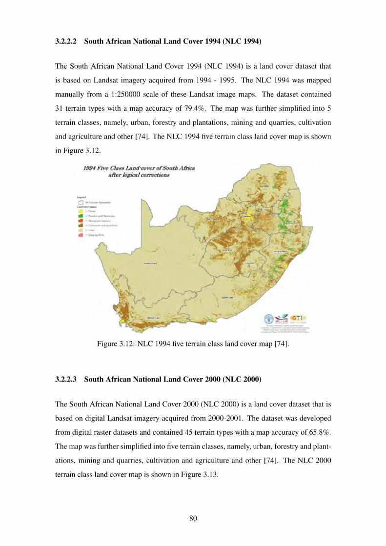
3.2.2.2 South African National Land Cover 1994 (NLC 1994)
The South African National Land Cover 1994 (NLC 1994) is a land cover dataset that
is based on Landsat imagery acquired from 1994 - 1995. The NLC 1994 was mapped
manually from a 1:250000 scale of these Landsat image maps. The dataset contained
31 terrain types with a map accuracy of 79.4%. The map was further simplified into 5
terrain classes, namely, urban, forestry and plantations, mining and quarries, cultivation
and agriculture and other [74]. The NLC 1994 five terrain class land cover map is shown
in Figure 3.12.
Figure 3.12: NLC 1994 five terrain class land cover map [74].
3.2.2.3 South African National Land Cover 2000 (NLC 2000)
The South African National Land Cover 2000 (NLC 2000) is a land cover dataset that is
based on digital Landsat imagery acquired from 2000-2001. The dataset was developed
from digital raster datasets and contained 45 terrain types with a map accuracy of 65.8%.
The map was further simplified into five terrain classes, namely, urban, forestry and plant-
ations, mining and quarries, cultivation and agriculture and other [74]. The NLC 2000
terrain class land cover map is shown in Figure 3.13.
80
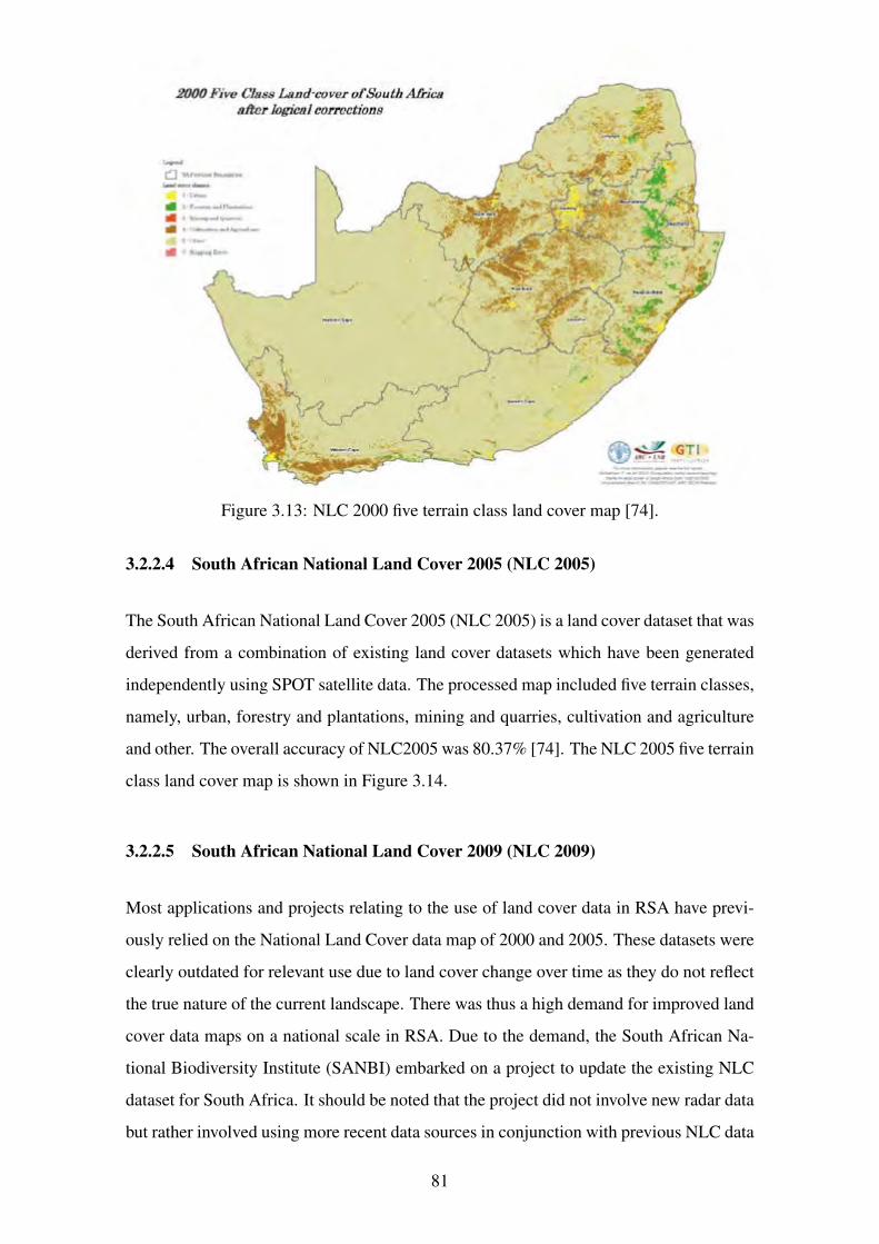
Figure 3.13: NLC 2000 five terrain class land cover map [74].
3.2.2.4 South African National Land Cover 2005 (NLC 2005)
The South African National Land Cover 2005 (NLC 2005) is a land cover dataset that was
derived from a combination of existing land cover datasets which have been generated
independently using SPOT satellite data. The processed map included five terrain classes,
namely, urban, forestry and plantations, mining and quarries, cultivation and agriculture
and other. The overall accuracy of NLC2005 was 80.37% [74]. The NLC 2005 five terrain
class land cover map is shown in Figure 3.14.
3.2.2.5 South African National Land Cover 2009 (NLC 2009)
Most applications and projects relating to the use of land cover data in RSA have previ-
ously relied on the National Land Cover data map of 2000 and 2005. These datasets were
clearly outdated for relevant use due to land cover change over time as they do not reflect
the true nature of the current landscape. There was thus a high demand for improved land
cover data maps on a national scale in RSA. Due to the demand, the South African Na-
tional Biodiversity Institute (SANBI) embarked on a project to update the existing NLC
dataset for South Africa. It should be noted that the project did not involve new radar data
but rather involved using more recent data sources in conjunction with previous NLC data
81
2000 Five Class Land-cover of South Africa after logical corrections
...... h.,,..,,, ...._ I ·t'ri»•
1111 :l-FoNetryanct l'J..,u,1,on11
II a Mm, .... nd Q....-n ...
1111 l · C,\,ltnnhon...,clAtJno•ll." r"
6·C.llcr
• 0-Mltff'ui'!'E, rw
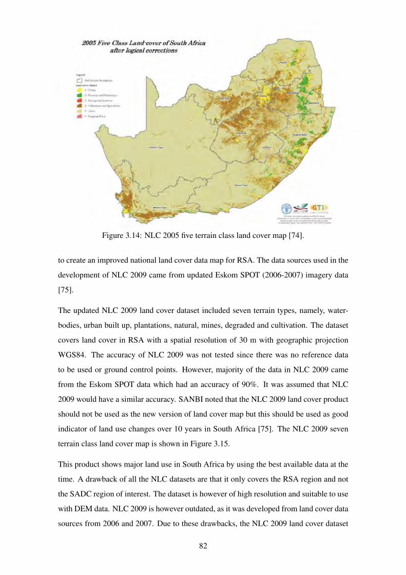
Figure 3.14: NLC 2005 five terrain class land cover map [74].
to create an improved national land cover data map for RSA. The data sources used in the
development of NLC 2009 came from updated Eskom SPOT (2006-2007) imagery data
[75].
The updated NLC 2009 land cover dataset included seven terrain types, namely, water-
bodies, urban built up, plantations, natural, mines, degraded and cultivation. The dataset
covers land cover in RSA with a spatial resolution of 30 m with geographic projection
WGS84. The accuracy of NLC 2009 was not tested since there was no reference data
to be used or ground control points. However, majority of the data in NLC 2009 came
from the Eskom SPOT data which had an accuracy of 90%. It was assumed that NLC
2009 would have a similar accuracy. SANBI noted that the NLC 2009 land cover product
should not be used as the new version of land cover map but this should be used as good
indicator of land use changes over 10 years in South Africa [75]. The NLC 2009 seven
terrain class land cover map is shown in Figure 3.15.
This product shows major land use in South Africa by using the best available data at the
time. A drawback of all the NLC datasets are that it only covers the RSA region and not
the SADC region of interest. The dataset is however of high resolution and suitable to use
with DEM data. NLC 2009 is however outdated, as it was developed from land cover data
sources from 2006 and 2007. Due to these drawbacks, the NLC 2009 land cover dataset
82
2005 Five Class Land-cover of South Africa after logical corrections
1-l'l"b,i,Q
.. 2·FoNc411ry-dPl•11u.110N1
Ill 4 · M,n,,.and(t""'"',..
Ill l · C\.Jti,·,n ..... _il~ll.11,.,.
~ ·Ot.hoi-r
• O · M•I-Vl•'t!'E' r'"
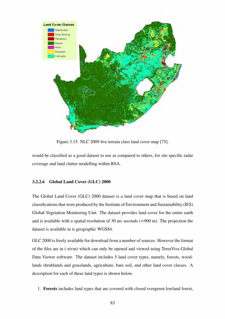
Figure 3.15: NLC 2009 five terrain class land cover map [75].
would be classified as a good dataset to use as compared to others, for site specific radar
coverage and land clutter modelling within RSA.
3.2.2.6 Global Land Cover (GLC) 2000
The Global Land Cover (GLC) 2000 dataset is a land cover map that is based on land
classifications that were produced by the Institute of Environment and Sustainability (IES)
Global Vegetation Monitoring Unit. The dataset provides land cover for the entire earth
and is available with a spatial resolution of 30 arc seconds (≈900 m). The projection the
dataset is available in is geographic WGS84.
GLC 2000 is freely available for download from a number of sources. However the format
of the files are in (.xtvm) which can only be opened and viewed using TerraViva Global
Data Viewer software. The dataset includes 5 land cover types, namely, forests, wood-
lands shrublands and grasslands, agriculture, bare soil, and other land cover classes. A
description for each of these land types is shown below.
1. Forests includes land types that are covered with closed evergreen lowland forest,
83
Land Cover Cl asses
- Wate,bod,es
- Urban Buol~up
- Plantahon s
- Natur~I
.. Minee
C"°' Dog,aded
- Cutwa11on
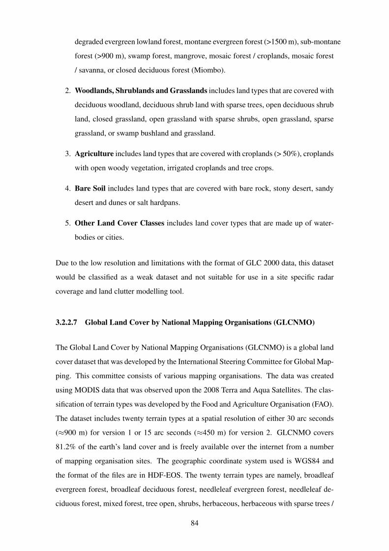
degraded evergreen lowland forest, montane evergreen forest (>1500 m), sub-montane
forest (>900 m), swamp forest, mangrove, mosaic forest / croplands, mosaic forest
/ savanna, or closed deciduous forest (Miombo).
2. Woodlands, Shrublands and Grasslands includes land types that are covered with
deciduous woodland, deciduous shrub land with sparse trees, open deciduous shrub
land, closed grassland, open grassland with sparse shrubs, open grassland, sparse
grassland, or swamp bushland and grassland.
3. Agriculture includes land types that are covered with croplands (> 50%), croplands
with open woody vegetation, irrigated croplands and tree crops.
4. Bare Soil includes land types that are covered with bare rock, stony desert, sandy
desert and dunes or salt hardpans.
5. Other Land Cover Classes includes land cover types that are made up of water-
bodies or cities.
Due to the low resolution and limitations with the format of GLC 2000 data, this dataset
would be classified as a weak dataset and not suitable for use in a site specific radar
coverage and land clutter modelling tool.
3.2.2.7 Global Land Cover by National Mapping Organisations (GLCNMO)
The Global Land Cover by National Mapping Organisations (GLCNMO) is a global land
cover dataset that was developed by the International Steering Committee for Global Map-
ping. This committee consists of various mapping organisations. The data was created
using MODIS data that was observed upon the 2008 Terra and Aqua Satellites. The clas-
sification of terrain types was developed by the Food and Agriculture Organisation (FAO).
The dataset includes twenty terrain types at a spatial resolution of either 30 arc seconds
(≈900 m) for version 1 or 15 arc seconds (≈450 m) for version 2. GLCNMO covers
81.2% of the earth’s land cover and is freely available over the internet from a number
of mapping organisation sites. The geographic coordinate system used is WGS84 and
the format of the files are in HDF-EOS. The twenty terrain types are namely, broadleaf
evergreen forest, broadleaf deciduous forest, needleleaf evergreen forest, needleleaf de-
ciduous forest, mixed forest, tree open, shrubs, herbaceous, herbaceous with sparse trees /
84
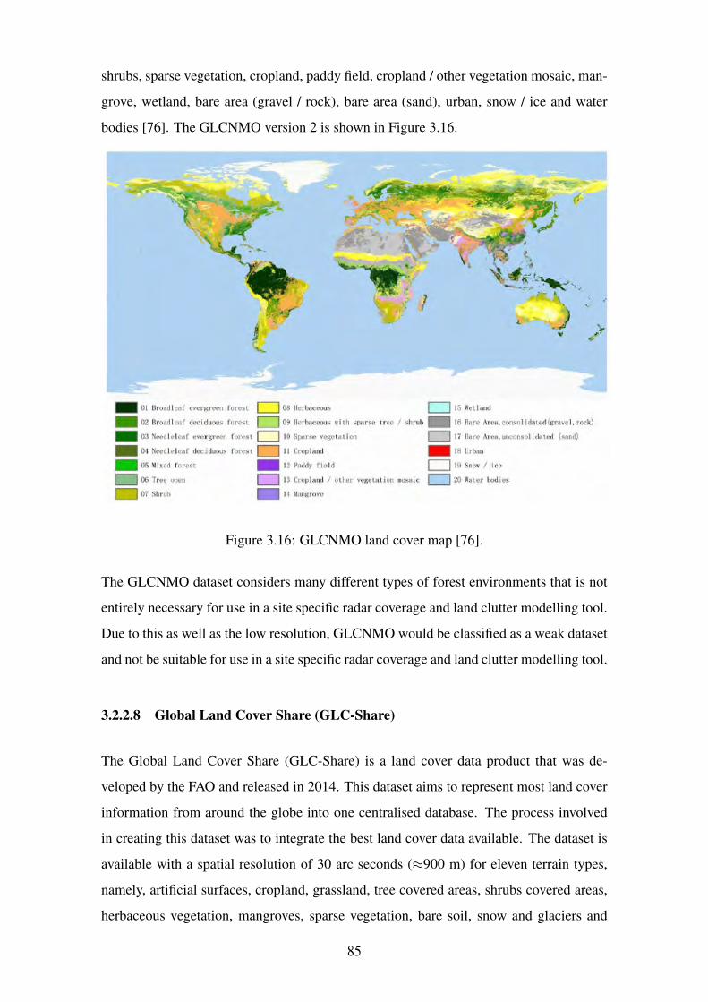
shrubs, sparse vegetation, cropland, paddy field, cropland / other vegetation mosaic, man-
grove, wetland, bare area (gravel / rock), bare area (sand), urban, snow / ice and water
bodies [76]. The GLCNMO version 2 is shown in Figure 3.16.
Figure 3.16: GLCNMO land cover map [76].
The GLCNMO dataset considers many different types of forest environments that is not
entirely necessary for use in a site specific radar coverage and land clutter modelling tool.
Due to this as well as the low resolution, GLCNMO would be classified as a weak dataset
and not be suitable for use in a site specific radar coverage and land clutter modelling tool.
3.2.2.8 Global Land Cover Share (GLC-Share)
The Global Land Cover Share (GLC-Share) is a land cover data product that was de-
veloped by the FAO and released in 2014. This dataset aims to represent most land cover
information from around the globe into one centralised database. The process involved
in creating this dataset was to integrate the best land cover data available. The dataset is
available with a spatial resolution of 30 arc seconds (≈900 m) for eleven terrain types,
namely, artificial surfaces, cropland, grassland, tree covered areas, shrubs covered areas,
herbaceous vegetation, mangroves, sparse vegetation, bare soil, snow and glaciers and
85
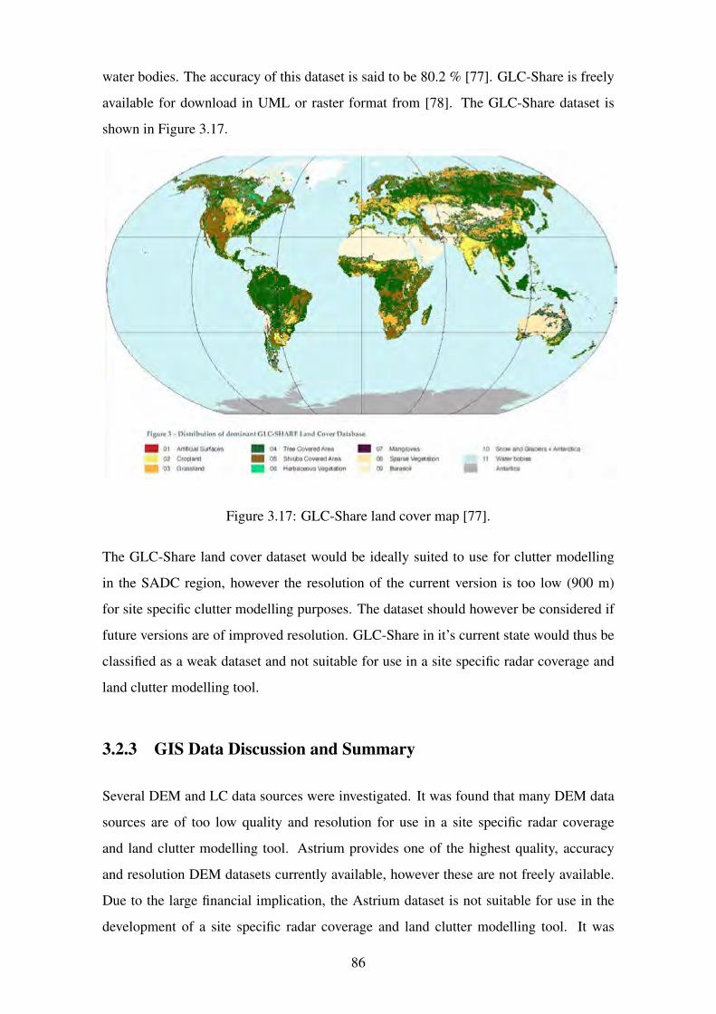
water bodies. The accuracy of this dataset is said to be 80.2 % [77]. GLC-Share is freely
available for download in UML or raster format from [78]. The GLC-Share dataset is
shown in Figure 3.17.
Figure 3.17: GLC-Share land cover map [77].
The GLC-Share land cover dataset would be ideally suited to use for clutter modelling
in the SADC region, however the resolution of the current version is too low (900 m)
for site specific clutter modelling purposes. The dataset should however be considered if
future versions are of improved resolution. GLC-Share in it’s current state would thus be
classified as a weak dataset and not suitable for use in a site specific radar coverage and
land clutter modelling tool.
3.2.3 GIS Data Discussion and Summary
Several DEM and LC data sources were investigated. It was found that many DEM data
sources are of too low quality and resolution for use in a site specific radar coverage
and land clutter modelling tool. Astrium provides one of the highest quality, accuracy
and resolution DEM datasets currently available, however these are not freely available.
Due to the large financial implication, the Astrium dataset is not suitable for use in the
development of a site specific radar coverage and land clutter modelling tool. It was
86
found that the ASTER GDEM and SRTM 30 m DEM sources are currently the highest
resolution datasets that are freely available and covers all the intended areas of interest.
Even though these two datasets both have a resolution of 30 m, it was found that the
ASTER GDEM data contained some remaining artefacts that cause artificial hills, ridges
and surface roughness that do not exist in reality. The SRTM datasets therefore are more
accurate. It is thus recommended that the SRTM 30 m DEM dataset be used in a site
specific radar coverage and land clutter modelling tool.
Similarly, it was found that many LC data sources are either of too low quality, resolution
or outdated for use in a site specific radar coverage and land clutter modelling tool. Two
LC data sources can be considered, namely the NLC 2009 or GlobeLand30 m LC datasets.
These are both at a high resolution of 30 m. The NLC 2009 dataset however only covers
the RSA region, whereas the GlobeLand30 m covers the entire SADC region of interest.
The GlobeLand30 m source is also a more current LC model than the NLC 2009 data
source. The GlobeLand30 m dataset is therefore recommended for use in a site specific
radar coverage and land clutter modelling tool.
Linking the appropriate land classes of these LC datasets to use with the various land
clutter models is discussed in section 4.3.
A summary of the DEM and Land Cover data sources discussed above is shown in Table
3.14 and Table 3.15 respectively.
3.3 Simulating the Clutter Scene
3.3.1 Clutter Patch Grid Method
Once a DEM of the radar observed environment is loaded, it produces a N ×M matrix
model equally spaced in the x (longitude) and y (latitude) dimension. Each point repres-
ents a value corresponding to the terrain height information at the specified location. The
effects of the earth’s curvature and atmospheric refraction should be accounted for when
simulating a radar observed environment covering large areas. The former will cause a
blind area or dead zone as shown in Figure 2.4, and latter will curve the LOS of the radar,
as seen in Figure 2.3. A close approximation to account for the effects of earth curvature
87
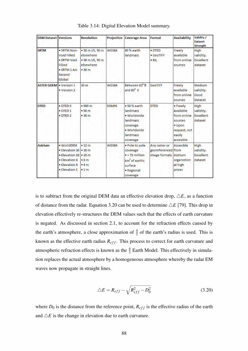
Table 3.14: Digital Elevation Model summary.
is to subtract from the original DEM data an effective elevation drop, △E, as a function
of distance from the radar. Equation 3.20 can be used to determine △E [79]. This drop in
elevation effectively re-structures the DEM values such that the effects of earth curvature
is negated. As discussed in section 2.1, to account for the refraction effects caused by
the earth’s atmosphere, a close approximation of 43
of the earth’s radius is used. This is
known as the effective earth radius Re f f . This process to correct for earth curvature and
atmospheric refraction effects is known as the 43
Earth Model. This effectively in simula-
tion replaces the actual atmosphere by a homogeneous atmosphere whereby the radar EM
waves now propagate in straight lines.
△E = Re f f −√
R2e f f −D2
0 (3.20)
where D0 is the distance from the reference point, Re f f is the effective radius of the earth
and △E is the change in elevation due to earth curvature.
88
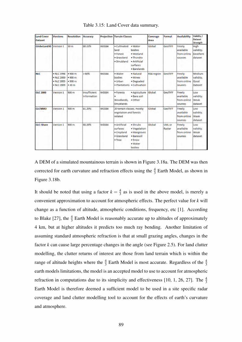
Table 3.15: Land Cover data summary.
A DEM of a simulated mountainous terrain is shown in Figure 3.18a. The DEM was then
corrected for earth curvature and refraction effects using the 43
Earth Model, as shown in
Figure 3.18b.
It should be noted that using a factor k = 43
as is used in the above model, is merely a
convenient approximation to account for atmospheric effects. The perfect value for k will
change as a function of altitude, atmospheric conditions, frequency, etc [1]. According
to Blake [27], the 43
Earth Model is reasonably accurate up to altitudes of approximately
4 km, but at higher altitudes it predicts too much ray bending. Another limitation of
assuming standard atmospheric refraction is that at small grazing angles, changes in the
factor k can cause large percentage changes in the angle (see Figure 2.5). For land clutter
modelling, the clutter returns of interest are those from land terrain which is within the
range of altitude heights where the 43
Earth Model is most accurate. Regardless of the 43
earth models limitations, the model is an accepted model to use to account for atmospheric
refraction in computations due to its simplicity and effectiveness [10, 1, 26, 27]. The 43
Earth Model is therefore deemed a sufficient model to be used in a site specific radar
coverage and land clutter modelling tool to account for the effects of earth’s curvature
and atmosphere.
89
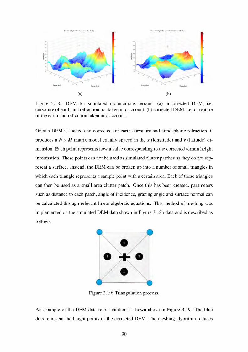
(a) (b)
Figure 3.18: DEM for simulated mountainous terrain: (a) uncorrected DEM, i.e.
curvature of earth and refraction not taken into account, (b) corrected DEM, i.e. curvature
of the earth and refraction taken into account.
Once a DEM is loaded and corrected for earth curvature and atmospheric refraction, it
produces a N ×M matrix model equally spaced in the x (longitude) and y (latitude) di-
mension. Each point represents now a value corresponding to the corrected terrain height
information. These points can not be used as simulated clutter patches as they do not rep-
resent a surface. Instead, the DEM can be broken up into a number of small triangles in
which each triangle represents a sample point with a certain area. Each of these triangles
can then be used as a small area clutter patch. Once this has been created, parameters
such as distance to each patch, angle of incidence, grazing angle and surface normal can
be calculated through relevant linear algebraic equations. This method of meshing was
implemented on the simulated DEM data shown in Figure 3.18b data and is described as
follows.
Figure 3.19: Triangulation process.
An example of the DEM data representation is shown above in Figure 3.19. The blue
dots represent the height points of the corrected DEM. The meshing algorithm reduces
90
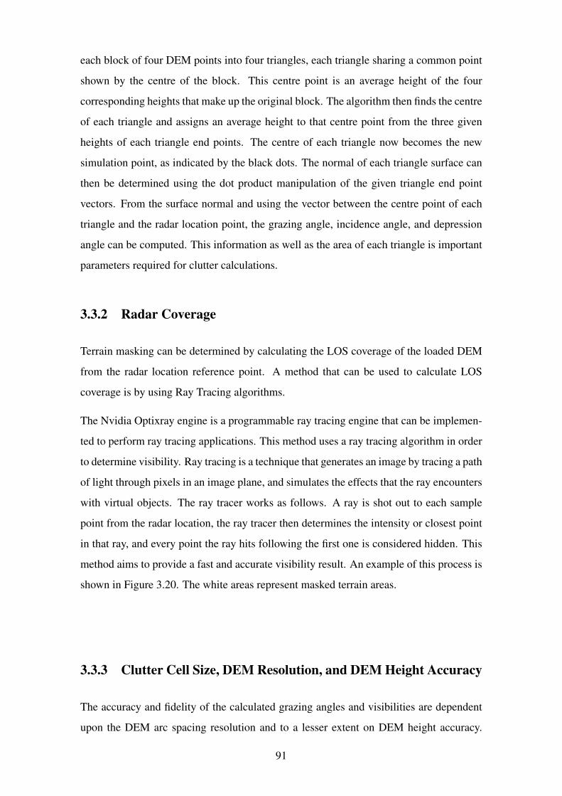
each block of four DEM points into four triangles, each triangle sharing a common point
shown by the centre of the block. This centre point is an average height of the four
corresponding heights that make up the original block. The algorithm then finds the centre
of each triangle and assigns an average height to that centre point from the three given
heights of each triangle end points. The centre of each triangle now becomes the new
simulation point, as indicated by the black dots. The normal of each triangle surface can
then be determined using the dot product manipulation of the given triangle end point
vectors. From the surface normal and using the vector between the centre point of each
triangle and the radar location point, the grazing angle, incidence angle, and depression
angle can be computed. This information as well as the area of each triangle is important
parameters required for clutter calculations.
3.3.2 Radar Coverage
Terrain masking can be determined by calculating the LOS coverage of the loaded DEM
from the radar location reference point. A method that can be used to calculate LOS
coverage is by using Ray Tracing algorithms.
The Nvidia Optixray engine is a programmable ray tracing engine that can be implemen-
ted to perform ray tracing applications. This method uses a ray tracing algorithm in order
to determine visibility. Ray tracing is a technique that generates an image by tracing a path
of light through pixels in an image plane, and simulates the effects that the ray encounters
with virtual objects. The ray tracer works as follows. A ray is shot out to each sample
point from the radar location, the ray tracer then determines the intensity or closest point
in that ray, and every point the ray hits following the first one is considered hidden. This
method aims to provide a fast and accurate visibility result. An example of this process is
shown in Figure 3.20. The white areas represent masked terrain areas.
3.3.3 Clutter Cell Size, DEM Resolution, and DEM Height Accuracy
The accuracy and fidelity of the calculated grazing angles and visibilities are dependent
upon the DEM arc spacing resolution and to a lesser extent on DEM height accuracy.
91
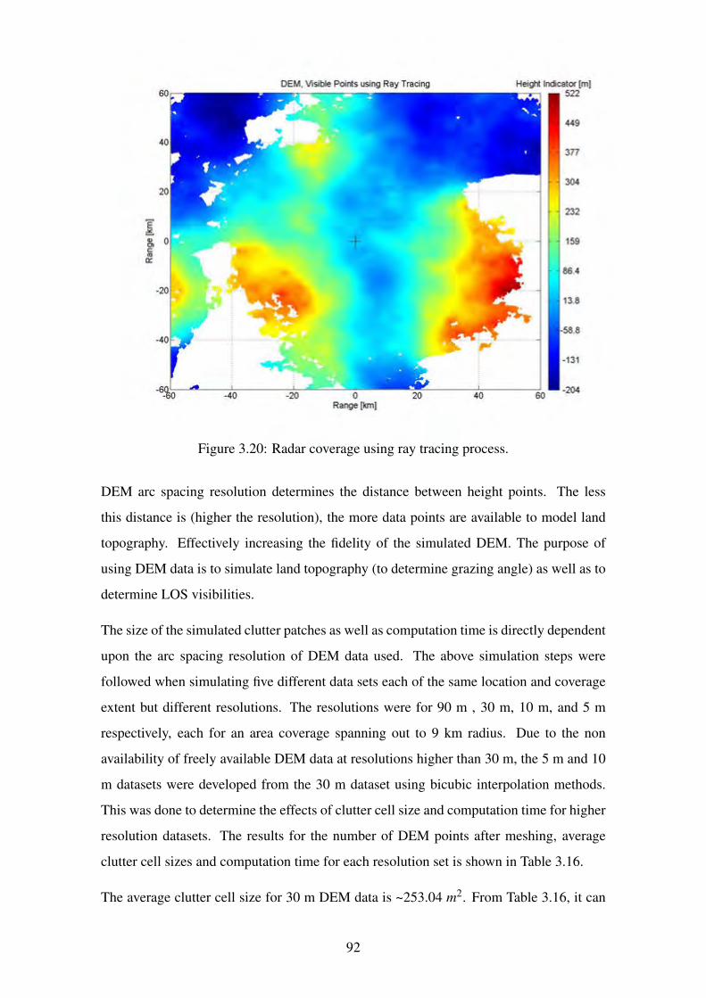
Figure 3.20: Radar coverage using ray tracing process.
DEM arc spacing resolution determines the distance between height points. The less
this distance is (higher the resolution), the more data points are available to model land
topography. Effectively increasing the fidelity of the simulated DEM. The purpose of
using DEM data is to simulate land topography (to determine grazing angle) as well as to
determine LOS visibilities.
The size of the simulated clutter patches as well as computation time is directly dependent
upon the arc spacing resolution of DEM data used. The above simulation steps were
followed when simulating five different data sets each of the same location and coverage
extent but different resolutions. The resolutions were for 90 m , 30 m, 10 m, and 5 m
respectively, each for an area coverage spanning out to 9 km radius. Due to the non
availability of freely available DEM data at resolutions higher than 30 m, the 5 m and 10
m datasets were developed from the 30 m dataset using bicubic interpolation methods.
This was done to determine the effects of clutter cell size and computation time for higher
resolution datasets. The results for the number of DEM points after meshing, average
clutter cell sizes and computation time for each resolution set is shown in Table 3.16.
The average clutter cell size for 30 m DEM data is ~253.04 m2. From Table 3.16, it can
92
DEM, Visible Points using Ray Tracing Height Indicator [m] 60 522
449
40 377
304 20
232
E ~ + Cl) 0 159 Cl C
"' 0:::
86.4
-20 13.8
-58.8 -40
-131
-6i - 0 -40 -20 0 20 40 60 -204
Range [km]
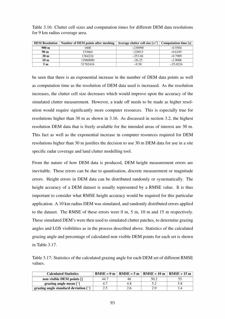
Table 3.16: Clutter cell sizes and computation times for different DEM data resolutions
for 9 km radius coverage area.
DEM Resolution Number of DEM points after meshing Average clutter cell size [m2] Computation time [s]
900 m 1600 ~238990 ~0.5504
90 m 153664 ~2269.5 ~0.6185
30 m 1364224 ~253.04 ~0.7909
10 m 12960000 ~26.25 ~2.9006
5 m 51782416 ~9.58 ~25.0224
be seen that there is an exponential increase in the number of DEM data points as well
as computation time as the resolution of DEM data used is increased. As the resolution
increases, the clutter cell size decreases which would improve upon the accuracy of the
simulated clutter measurement. However, a trade off needs to be made as higher resol-
ution would require significantly more computer resources. This is especially true for
resolutions higher than 30 m as shown in 3.16. As discussed in section 3.2, the highest
resolution DEM data that is freely available for the intended areas of interest are 30 m.
This fact as well as the exponential increase in computer resources required for DEM
resolutions higher than 30 m justifies the decision to use 30 m DEM data for use in a site
specific radar coverage and land clutter modelling tool.
From the nature of how DEM data is produced, DEM height measurement errors are
inevitable. These errors can be due to quantisation, discrete measurement or magnitude
errors. Height errors in DEM data can be distributed randomly or systematically. The
height accuracy of a DEM dataset is usually represented by a RMSE value. It is thus
important to consider what RMSE height accuracy would be required for this particular
application. A 10 km radius DEM was simulated, and randomly distributed errors applied
to the dataset. The RMSE of these errors were 0 m, 5 m, 10 m and 15 m respectively.
These simulated DEM’s were then used to simulated clutter patches, to determine grazing
angles and LOS visibilities as in the process described above. Statistics of the calculated
grazing angle and percentage of calculated non visible DEM points for each set is shown
in Table 3.17.
Table 3.17: Statistics of the calculated grazing angle for each DEM set of different RMSE
values.
Calculated Statistics RMSE = 0 m RMSE = 5 m RMSE = 10 m RMSE = 15 m
non visible DEM points [] 44.7 46 50.2 55
grazing angle mean [◦] 4.7 4.8 5.2 5.8
grazing angle standard deviation [◦] 2.5 2.6 2.9 3.4
93
From Table 3.17, it is shown that with an increase in RMSE, there is a general increase
in the percentage of non visible DEM points, as well as an increase in the mean grazing
angle, and grazing angle standard deviation. The grazing angle mean only changes by
0.1◦ with an injected RMSE of 5 m, and by 0.5◦ and 1.1◦ with an injected RMSE of 10
m and 15 m. These changes are fairly insignificant given that in most cases a change of
1◦ in grazing angle, changes the calculated backscatter coefficient value by less than 0.1
dBs for the plateau grazing angle region. This increases for low and high grazing angle
regions. A more significant effect that increasing RMSE has is the percentage change
in calculation of DEM visibilities. The percentage of non visible DEM points changes
by 1.3% with an injected RMSE of 5 m, but increases to to 5.5% and 10.3% with an
injected RMSE of 10 m and 15 m. The change in visibilities with RMSE of 5 m is fairly
insignificant and considered acceptable in terms of the purpose of using DEM data for
site specific radar coverage and land clutter modelling.
The above discussion on DEM resolution and height accuracy further justifies the recom-
mendation to use the SRTM 30 m DEM dataset in a site specific radar coverage and land
clutter modelling tool, which has a arc spacing resolution of 30 m, and an associated
height accuracy RMSE of ~5 m.
3.3.4 Simulating Coherent Radar Returns
The above steps are necessary to obtain a clutter scene relative to the position of a radar
system. The data is thus representative of the radar observed environment information
(environment model) which includes the clutter patches, each with an associated LOS
visibility from the radar, height, area, distance from the radar, grazing angle (including
incidence and depression angles), and the terrain class that the patch matches to the closest
(based on the Land Cover data chosen). Using environment model information, land
clutter models can be used to provide a backscatter coefficient value for each visible
clutter patch. The reflectivity (including the inherent pattern propagation factor F4) for
each clutter patch can be determined to create the land clutter model characteristics of the
scene.
This only represents the radar observed environment, LOS coverage, and the reflectivity.
The objective of simulating site specific radar land clutter returns can not be achieved
94
without the application of a radar sensor model, including the antenna beam pattern. The
radar sensor contains information about the radar characteristics including but not lim-
ited to, radar operating frequency, waveform, radar resolution and range limits, antenna
pattern, transmit and receive gains, radar position, height, and orientation, radar system
losses etc. The mapping of the radar antenna beam pattern onto the scene and coherent
addition of returns from the clutter patches would be the next step.
The modelling of coherent radar returns would firstly require the radar observed envir-
onment and land clutter model that was developed. The radar antenna beam pattern is
modelled in both azimuth and elevation. The visible terrain data that is within the radar
antenna beamwidth would be computed. Range traces are then formed at closely spaced
azimuth angles which is based on the radar antenna beamwidth, scan rate, and pulse re-
petition frequency (PRF). The azimuth spacing needs to be chosen such that it provides
adequate fidelity. The range samples are then calculated and spaced according the radar
range resolution. Area sampling is performed for each range trace. For each range trace,
all samples within the radar range bin is summed to simulate coherent radar return. The
returns are modified by the attenuation relative to the antenna peak gain at boresight as a
function of the off boresight sample angle. The land clutter power at the receiver for each
range bin is then calculated using the radar equation.
3.4 Chapter Summary
In this chapter, several existing land clutter models, DEM and LC data sources were
investigated.
A description and analysis of several existing land clutter models are presented in section
3.1. A summary of these land clutter models are presented in Table 3.9 above. Further
analysis and comparisons of these land clutter models are investigated in section 4.1.
A description and analysis of several DEM and LC data sources are presented in section
3.2. It is recommended that the SRTM 30 m DEM dataset and the GlobeLand30 LC
dataset should be used in a site specific radar coverage and land clutter modelling tool as
they are currently the highest quality DEM and LC datasets that are freely available that
covers all intended areas of interest. A summary of these DEM and LC data sources are
95
presented in Table 3.14 and Table 3.15 respectively.
Section 3.3 presents a meshing technique that can be used to simulate clutter patches
in a site specific radar coverage and land clutter modelling tool. The process involves
breaking up the DEM height points into triangular surface areas, each representing a
clutter patch from which various calculations can be performed. Earth curvature and
atmospheric refraction effects can be reduced by using the 43
Earth Model. Section 3.3.2
presents a terrain LOS visualisation technique known as ray tracing that can be used in a
site specific radar coverage and land clutter modelling tool to determine masked areas.
A discussion and brief analysis on the required simulated clutter cell size, DEM resolu-
tion, and DEM height accuracy. is given in section 3.3.3. This analysis further justified
the recommendation to use the SRTM 30 m DEM dataset in a site specific radar coverage
and land clutter modelling tool.
Furthermore, a process for simulating coherent radar clutter returns is given in section
3.3.4.
96
Chapter 4
Analysis and Results
This chapter provides a discussion of the land clutter / backscatter coefficient models in
the context for use in a site specific radar coverage and land clutter modelling tool. It
aims to determine which of the existing models are the most appropriate to use for the
varying simulation cases, as well as to identify categories of land clutter models where
little or insufficient models are available. It also aims to provide the link between the
different terrain classes described in land cover data compared to those in land clutter /
backscatter coefficient models. Land clutter and land cover link results will be illustrated
and tabulated in aid of developing algorithms for use in a site specific radar coverage and
land clutter modelling tool. It ends by proposing a guide on the process to follow for the
development of a site specific radar coverage and land clutter modelling tool.
4.1 Analysis of Land Clutter Models
This section provides an analysis of the various land clutter models discussed in this
dissertation. The aim is to determine how well site specific simulated clutter using the
land clutter models agree with measured data, and which models are best suited to use
for the various grazing angle regions. The process will be based on information gathered
from literature for low grazing angles, and from comparing simulated clutter using the
land clutter models with measured data for angles in the plateau and high grazing angle
region. This information does not aim to fully validate the various land clutter models
considered in this dissertation for all cases, but rather aims to determine whether the
97
assumptions made in section 3.1 about the compatibility (strength) and validity of these
models are valid for a few cases.
4.1.1 Low Grazing Angle Region
As stated in previous sections, the text by Billingsley in [6], analyses low grazing angle
clutter regions extensively. The analysis of results for low angle clutter modelling will be
based upon Billingsley’s finding’s on simulated low angle land clutter using the land clut-
ter model as described in section 3.1.9. It should be noted that the clutter map comparison
described below are between a measured scene, and a simulated scene where the paramet-
ers that were used in the simulated land clutter model were derived from the scene. They
are therefore likely to be similar, however the purpose for including this analysis was to
identify important findings made by Billingsley with regard to the way in which he based
his validation of the model, as well as the performance of LOS coverage obtained using
90 m DTED data.
In [6], Billingsley aims to validate his land clutter model with measured data. The process
involved simulating the spatial variation of land clutter at Brazeau, a forested wilderness
area in Alberta Canada using his proposed model. Firstly 90 m DEM data was used
to determine the LOS terrain visibility, and surface slopes. Land cover data was then
integrated to identify the different land cover types within the area of interest. The clutter
strength for each visible cell was then calculated using Billingsley’s land clutter model.
An example of the outcome of this process is shown in Figure 4.1.
Figure 4.1 compares the simulated and measured clutter maps. The black regions in the
simulated map represent the masked terrain regions. This corresponds reasonably well
with the masked regions as shown in the measured data. The coloured regions represent
the backscatter coefficient σ◦F4 values for the measured and simulated maps. There is
generally a good correlation between σ◦F4 for the measured and simulated clutter maps.
Billingsley however noted that the cell to cell spatial correlation of the measured map is
not precisely followed by the simulated map.
Billingsley bases his validation on how the particular radar system performance measure
computed from simulated clutter compares to the performance measure using measured
clutter and not on how closely the simulated and measured clutter maps compare. By
98
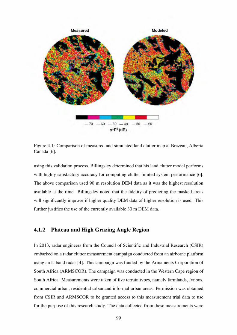
Figure 4.1: Comparison of measured and simulated land clutter map at Brazeau, Alberta
Canada [6].
using this validation process, Billingsley determined that his land clutter model performs
with highly satisfactory accuracy for computing clutter limited system performance [6].
The above comparison used 90 m resolution DEM data as it was the highest resolution
available at the time. Billingsley noted that the fidelity of predicting the masked areas
will significantly improve if higher quality DEM data of higher resolution is used. This
further justifies the use of the currently available 30 m DEM data.
4.1.2 Plateau and High Grazing Angle Region
In 2013, radar engineers from the Council of Scientific and Industrial Research (CSIR)
embarked on a radar clutter measurement campaign conducted from an airborne platform
using an L-band radar [4]. This campaign was funded by the Armaments Corporation of
South Africa (ARMSCOR). The campaign was conducted in the Western Cape region of
South Africa. Measurements were taken of five terrain types, namely farmlands, fynbos,
commercial urban, residential urban and informal urban areas. Permission was obtained
from CSIR and ARMSCOR to be granted access to this measurement trial data to use
for the purpose of this research study. The data collected from these measurements were
99
Measured Modeled
- 70 - 60 - 50 - 40 - 30 - 20
cr°F4 (dB)
processed to determine the backscatter coefficient σ◦ in dBs as a function of grazing
angle δ for the five terrain types. The range of measured angles are in the plateau and
high grazing region. This is shown in Figure 4.2.
Figure 4.2: Average backscatter coefficient σ◦F4 for various terrain types.
From Figure 4.2 it can be seen that there is general dependence of σ◦ on grazing angle in
the plateau and high grazing region that agrees with literature. It also shows that urban
terrains produce σ◦ values that are of an order of magnitude higher than farmlands or
shrub like plantation terrain types. This is in agreement with the the list of given land
clutter models, as shown in Figures 3.1, 3.2, 3.3, 3.4, 3.6 and 3.5.
Figures 4.3, and 4.4 show a comparison of the measured σ◦ values for different terrain
types with σ◦ values simulated using the various land clutter models described in chapter
3 for plateau and high grazing angles. The measured data is compared to land clutter
models terrain types that are the same or similar. Measured farmland and fynbos data
is compared with land clutter model, Constant Gamma with terrain type ‘farmland’ and
‘flatland’, Morchin with terrain type ‘farmland’ and ‘desert’, Kulemin with terrain type
‘arable land’, GTRI with terrain type ‘tall grass crops’ and ‘soil, sand and rocks’, and
Ulaby and Dobson or Generating Function with terrain type ‘shrubs’. Similarly measured
commercial urban, residential urban, and informal urban data is compared with land clut-
ter model, Constant Gamma with terrain type ‘metropolitan’, Kulemin with terrain type
‘urban territories’, GTRI with terrain type ‘urban’ and ‘soil’ and Ulaby and Dobson or
Generating Function with terrain type ‘urban’.
100
The root mean squared error (RMSE) between the measured and simulated average backs-
catter (σ◦F4) data for plateau and high grazing angle regions is shown in Figure 4.5.
Figure 4.3: Average backscatter coefficient σ◦F4 for terrain types farmland and fynbos
compared to land clutter models.
From Figures 4.3 it can be seen that the measured data for farmlands is for most grazing
angles larger than the simulated data from land clutter models. It is believed that this is
due to discrete scatterers such as tree trunks interspersed in the homogeneous terrain. As
expected, the land clutter model that closely agrees with the measured farmland data in
the plateau grazing angle region is the Ulaby and Dobson and Generating Function land
clutter models with terrain type (shrubs), with an associated RMSE of 1.4 dBs, and 2
dBs respectively. The backscatter from the measured fynbos data is significantly larger
than the measured farmland data for the plateau grazing angle region and decreases in
difference as the grazing angle moves towards the high grazing angle region. As with the
farmland data, the land clutter model that is closest to the the measured fynbos data is the
Ulaby and Dobson and Generating Function land clutter models with terrain type (shrubs).
Even though fynbos is considered shrub-like terrain type, it produces a RMSE that is as
much as 9.9 dBs, and 10.5 dBs for the simulated Ulaby and Dobson and Generating
Function land clutter models respectively. This is again believed to be as a result of
discrete scatterers. The land clutter model that produced the largest RMSE (larger than
34 dBs) relative to the measured data was for all cases the Kulemin land clutter model.
This agrees with the assumption that Kulemin is a considered a weak and low validity
101
Figure 4.4: Average backscatter coefficient σ◦F4 for all urban terrain types compared to
land clutter models.
land clutter model. From literature it was believed that the GTRI land clutter model
would be a more valid model to use for farmlands than the Constant Gamma land clutter
model. However from these figures it is seen that the Constant Gamma land clutter model
produces less of an RMSE (11.5 dBs against measured farmlands, and 20.3 dBs against
measured fynbos) relative to the measured data than the GTRI land clutter model (RMSE
of 15.8 dBs against measured farmlands, and a RMSE of 24.6 dBs against measured
fynbos) for grazing angles in the plateau region. For high grazing angles, the Ulaby and
Dobson and Generating Function land clutter models produces values that are closest to
the measured data (RMSE of 7.8 dBs and 8.1 dBs against measured farmlands, and a
RMSE of 10.4 dBs and 10.6 dBs against measured fynbos), followed by the Morchin
land clutter model (RMSE of 8.9 dBs against measured farmlands, and a RMSE of 10.5
dBs against measured fynbos). However, for the limited grazing angle range between 70◦
and 90◦, the Morchin land clutter model has the lowest RMSE (8.9 dBs against measured
farmlands, and 10.5 dBs against measured fynbos) as compared to the Ulaby and Dobson
and Generating Function land clutter models (RMSE of 11.1 dBs and 12.1 dBs against
measured farmlands, and a RMSE of 11.8 dBs and 12.9 dBs against measured fynbos).
From Figure 4.4 it is seen that commercial urban terrains produces larger backscatter
coefficient values than that of residential and informal urban terrains. This is due to the the
large scattering sources such as tall buildings in commercial urban areas. The measured
102
Average Backscatter Coefficient 1,.0F4 for Terrain Type Urban Compared to Land Clutter Models 20 ,;=================;-------,-------,---~---~---,
---e-Measured Commercial Urban ---..- Measured Residential Urban co
~ 15 ---e- Measured Informal Urban
- Simulated Constant Gamma (metropolitan) - Simulated Kulemin (urban)
c - Simulated GTRI (u rban ) OJ 10 - Simulated Ulaby et.al and Generating Fune (urban) ·u :i= OJ 0 u ._ Jg Cll u Cl)
..lo:: u
5
0
Cll -5 co OJ Cl ~ -10 OJ >
<( -15 ~---~----~---~----~---~----~---~----~---~
0 10 20 30 40 50 60 70 80 90
Grazing angle o [degrees]
(a) (b)
(c) (d)
Figure 4.5: RMSE of the measured average backscatter σ◦F4 for and simulated data
from land clutter models : (a) RMSE error between measured and simulated land clutter
for plateau grazing angle region , (b) RMSE error between measured and simulated land
clutter for high grazing angle region , (c) RMSE error between measured urban terrains
and simulated land clutter for plateau grazing angle region , (c) RMSE error between
measured urban terrains and simulated land clutter for high grazing angle region.
urban data is as much as 10 dBs larger than that of the closest land clutter model. The
land clutter model that produces values that are closest to the measured Urban terrain
data is the Constant Gamma land clutter model for grazing angles in the plateau region,
with an associated RMSE of 10 dBs, 5.5 dBs, and 5.3 dBs for commercial, residential
and informal urban respectively). This is followed by GTRI, Ulaby and Dobson and
Generating function, and Kulemin (limited grazing angle range for Kulemin model) land
clutter models respectively. As with the measured farmland and fynbos data, the Constant
Gamma land clutter model performs better than the GTRI land clutter model. The land
clutter model that produced the largest RMSE relative to the measured urban data was
the Ulaby and Dobson and Generating function land clutter model for grazing angles in
the plateau region. This is due to the lack of sufficient data available for urban terrain
in the Ulaby and Dobson and Generating Function land clutter models. Only the Ulaby
and Dobson and Generating Function is valid for the high grazing angle region for urban
103
terrain. Care should be taken when modelling for urban terrain in the high grazing angle
region as the RMSE is large (15.5 dBs, 10.4 dBs and 11.4 dBs for commercial, residential
and informal urban respectively).
4.1.3 Discussion and Summary
As seen in chapter 3, it was found that only Billingsley’s land clutter model and the adap-
ted GTRI sea clutter model is valid for the entire low grazing angle region. Nathanson’s
land clutter model tables can be used as well but for only a few limited discrete grazing
angles.
The adapted GTRI sea clutter model is based on linking sea states with various surface
roughness of different terrain types. This provides the general and not true behaviour
of σ◦ for varying terrains at low grazing angles. The adapted GTRI sea clutter model
should thus be used with caution and thus classified as a weak and low validity model.
It is clear that Billingsley is the authoritative land clutter model to use for low grazing
angle regions specifically for the terrain classes that he has used to derive his model.
Billingsley’s validation process as discussed above further justifies the assumption that
his model is considered an excellent and high validity model to use for low grazing angle
regions specific to the terrain classes defined in the model.
For grazing angles in the plateau region, Ulaby and Dobson or Gamma Generating Func-
tion should be considered first as they produced backscatter values that produced the low-
est RMSE to measured data as compared to the others. The Constant Gamma land clutter
model performed better than the GTRI land clutter model for all cases. The Kulemin land
clutter model produced the largest error and thus justifies the assumption made to classify
it as a weak and low validity model.
For general high grazing angles, the Ulaby and Dobson and Generating Function land
clutter models should be considered first, as they produced backscatter values that pro-
duced the lowest RMSE to measured data as compared to the others. Following these
will be the Morchin and GTRI land clutter models respectively. However, for the lim-
ited grazing angle range between 70◦ and 90◦, the Morchin land clutter model should be
considered first as it produced the lowest RMSE in this region of angles.
104
As shown in the cases of urban terrain comparisons, it is further justified that the Ulaby
and Dobson or Gamma Generating Function should be used with caution for cases where
the model is based on insufficient data. Specifically for urban terrain, the Constant
Gamma model should be considered first, followed by the GTRI and Kulemin land clutter
models for plateau grazing angle regions respectively. For urban terrain at high grazing
angles, only the Ulaby and Dobson or Gamma Generating Function is valid and can be
considered, however this should be used with caution as the model for urban terrain is
based on insufficient data. It should be noted that for urban areas, the land clutter can in
most cases only be modelled in a general way as urban terrain is far too complex to be
accurately statistically modelled.
Nathanson’s tables provides average values for σ◦ for only a few discrete grazing angles
and thus not suitable for use in site specific land clutter modelling where the dependence
of σ◦ for a range of grazing angles would be required.
In general, and in order of models validity classification (weak, strong or excellent), Table
4.1a provides a list of land clutter models that can be used to simulate σ◦ for low, plateau
and high grazing angle regions. Based on the foregoing results, Table 4.1b provides a list
in order of preference of land clutter models to use specifically for urban terrains. The
models in brackets are models that are not valid for the particular grazing angle region,
but if required is able to produce σ◦ values for that region. It should be noted that models
other than the top listed models should be used only if a higher listed model does not
support a certain model dependent that is of interest to the researcher. Measured data of
other terrain types and frequencies are required to properly compare and validate land
clutter models for all terrain types and model dependencies. This is recommended for
future work.
4.2 Grazing Angle and Frequency Ranges Considered by
Land Clutter Models
A summary of the land clutter models discussed in this dissertation is shown in Figure
4.6. This figure shows the range of frequencies, and grazing angles that each model
encompasses as a bounding box. Each model is represented by a different colour as
105
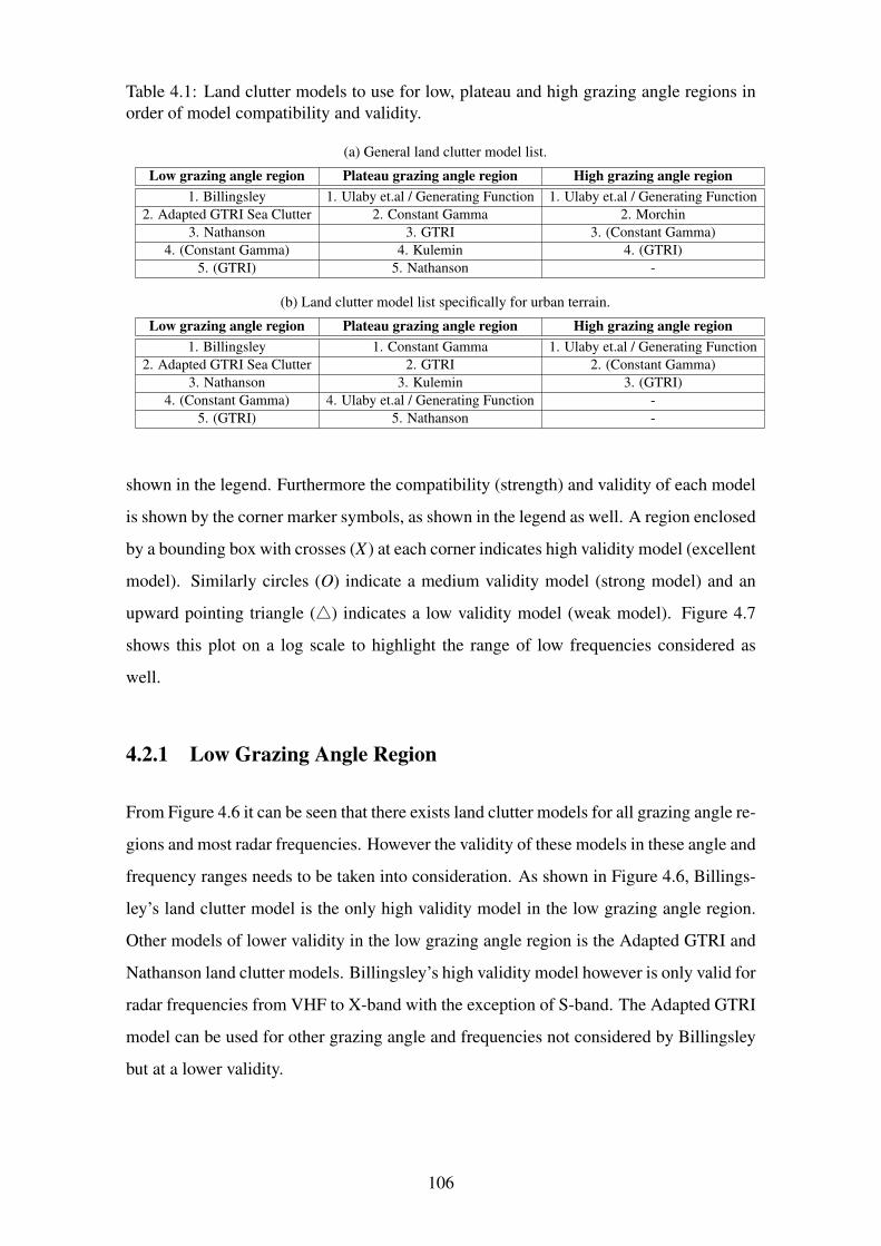
Table 4.1: Land clutter models to use for low, plateau and high grazing angle regions in
order of model compatibility and validity.
(a) General land clutter model list.
Low grazing angle region Plateau grazing angle region High grazing angle region
1. Billingsley 1. Ulaby et.al / Generating Function 1. Ulaby et.al / Generating Function
2. Adapted GTRI Sea Clutter 2. Constant Gamma 2. Morchin
3. Nathanson 3. GTRI 3. (Constant Gamma)
4. (Constant Gamma) 4. Kulemin 4. (GTRI)
5. (GTRI) 5. Nathanson -
(b) Land clutter model list specifically for urban terrain.
Low grazing angle region Plateau grazing angle region High grazing angle region
1. Billingsley 1. Constant Gamma 1. Ulaby et.al / Generating Function
2. Adapted GTRI Sea Clutter 2. GTRI 2. (Constant Gamma)
3. Nathanson 3. Kulemin 3. (GTRI)
4. (Constant Gamma) 4. Ulaby et.al / Generating Function -
5. (GTRI) 5. Nathanson -
shown in the legend. Furthermore the compatibility (strength) and validity of each model
is shown by the corner marker symbols, as shown in the legend as well. A region enclosed
by a bounding box with crosses (X) at each corner indicates high validity model (excellent
model). Similarly circles (O) indicate a medium validity model (strong model) and an
upward pointing triangle (△) indicates a low validity model (weak model). Figure 4.7
shows this plot on a log scale to highlight the range of low frequencies considered as
well.
4.2.1 Low Grazing Angle Region
From Figure 4.6 it can be seen that there exists land clutter models for all grazing angle re-
gions and most radar frequencies. However the validity of these models in these angle and
frequency ranges needs to be taken into consideration. As shown in Figure 4.6, Billings-
ley’s land clutter model is the only high validity model in the low grazing angle region.
Other models of lower validity in the low grazing angle region is the Adapted GTRI and
Nathanson land clutter models. Billingsley’s high validity model however is only valid for
radar frequencies from VHF to X-band with the exception of S-band. The Adapted GTRI
model can be used for other grazing angle and frequencies not considered by Billingsley
but at a lower validity.
106
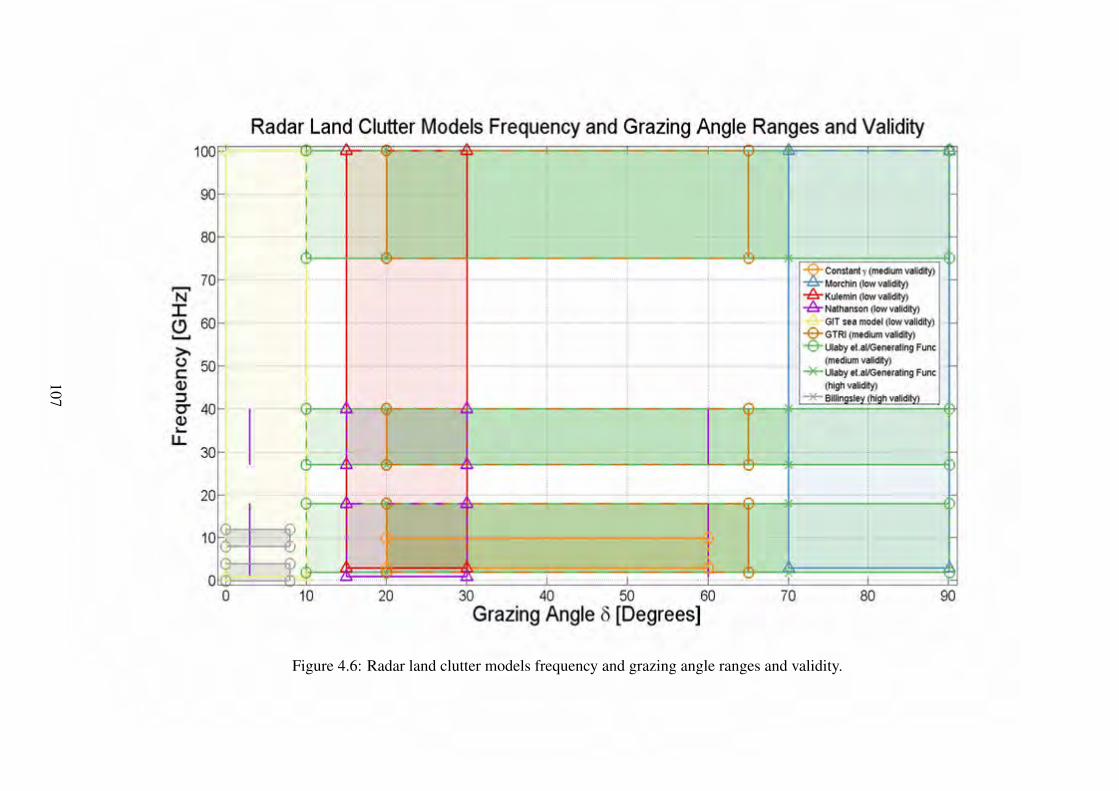
Figure 4.6: Radar land clutter models frequency and grazing angle ranges and validity.
107
100·-
90
80
70 l""""'I
N I C., 60 ........ > u 50 C Q) :::J O"' 40 Q) I... u.
30
20
10
0 0
Radar Land Clutter Models Frequency and Grazing Angle Ranges and Validity
10 20 30 40 50 60 Grazing Angle 8 [Degrees]
. , -9- Constant y (medium validity) , . -A- Morehin (low validity) -b- Kulemin (low validity) -b- Nathanson (low validity)
GIT sea model (low validity) -9- GTRI (medium validity) -6-Ulaby et.al/Generating Fune
(medium validity) · ' *'" Ulaby et.al/Generating Fune ,. (high validity) *'" Billingsley (high validit
70 80 90
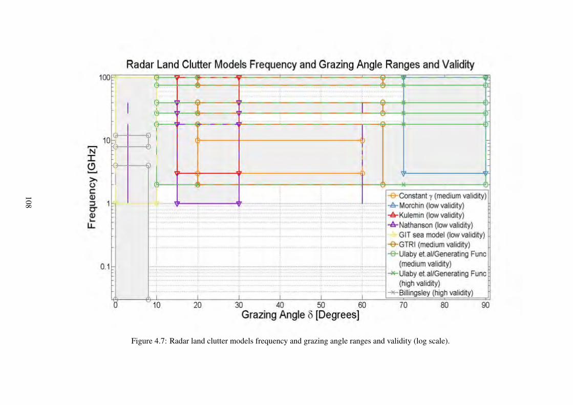
Figure 4.7: Radar land clutter models frequency and grazing angle ranges and validity (log scale).
108
,......, N I C) ......... >, (.) C: Q) :::I 1 ~.· C" Q) ~
u.
0.1
Radar Land Clutter Models Frequency and Grazing Angle Ranges and Validity
30 40 50 60 Grazing Angle 8 [Degrees]
-e-constant y (medium validity) -A- Morehin (low validity) -A-Kulemin (low validity) -A-Nathanson (low validity)
GIT sea model (low validity) -e-GTRI (medium validity) -e-Ulaby et.al/Generating Fune
(medium validity) """*-Ulaby et.al/Generating Fune
(high validity) """*-Billingsley (high validity)
70 80 90
4.2.2 Plateau Grazing Angle Region
For the plateau grazing angle region, the Ulaby and Dobson and Generating Function
land clutter model is the only high validity models. Other models of lower validity in
the plateau grazing angle region are the Constant Gamma and GTRI land clutter models
(medium validity), followed by the Kulemin and Nathanson land clutter models (low
validity). Ulaby and Dobson and the Generating Function model is valid for frequency
bands from L to W, with the exception of K and V band. The Kulemin model can be used
for other grazing angle and frequencies not considered by Ulaby and Dobson / Generating
Function land clutter model, but at a lower validity.
4.2.3 High Grazing Angle Region
For high grazing angle regions, the Ulaby and Dobson and Generating Function model can
be used, however it should be noted that for high grazing angles this model is considered
medium validity. This is followed by the Morchin land clutter model. Thus no high
validity model exists for high grazing angle region. The valid frequency bands range
from L to W band.
4.2.4 Discussion and Summary
It is shown that high validity land clutter models only exist for a limited range of grazing
angles and frequencies. Furthermore, no land clutter model exists for K and V frequency
band in the plateau grazing angle region. This may be due to a lack of radars in the K
and V frequency bands. This is believed to be due to the high attenuation that occurs in
these regions as discussed in section 2.1.1, making these frequency bands unsuitable for
general radar use. There also does not exist any land clutter models currently for low
frequencies in the plateau and high grazing angle regions, as shown in Figure 4.7. Land
clutter models other than high validity models should be used with caution for cases where
no high validity model exists. As shown in section 4.1, these lower validity models can
at times produce simulated values that are orders of magnitude different from measured
data.
It is thus recommended that future research in land clutter modelling focus on developing
109
high validity models for all non-existing and lower validity regions that has been identified
above.
4.3 Linking Land Clutter Models to Land Cover Data
Land cover data is required to determine the type of terrain cover of the simulated clutter
patches. For all different simulated clutter patch terrain types, an appropriate land clutter
model terrain type should be used that closely matches the clutter patch terrain type. The
GlobeLand30 or NLC 2009 land cover datasets were identified as appropriate models to
use to classify land cover within the SADC and RSA region of interest. Thus for each
terrain type found in the GlobeLand30 or NLC 2009 datasets, a decision was made as
to which of the terrain types for each land clutter model matches to the land cover data
terrain type the closest. Either the land clutter model does or does not have a terrain type
that matches with the land cover data terrain type. The decision can be classified in three
ways, either the land clutter model with chosen terrain type fully agrees and matches
with the land cover data terrain type, closely agrees and matches with it, or only partially
agrees and matches with the land cover data terrain type. In some cases no land clutter
model terrain type matches with the land cover data terrain type.
The process of linking the land cover data terrain types to land clutter model terrain types
is shown in Table 4.2 for GlobeLand30 dataset and in Table 4.3 for NLC 2009 dataset.
4.4 Proposed Site Specific Radar Coverage and Land Clut-
ter Modelling Tool Program Flow
As proposed, the site specific radar coverage and land clutter modelling tool can be ex-
ecuted according to the following steps.
1. Load latitude and longitude location of site of interest. This point will serve as
the reference point where the simulated radar is located. All calculations are based
on this reference point.
2. Load simulated radar specific parameters. Radar parameters required are the
110
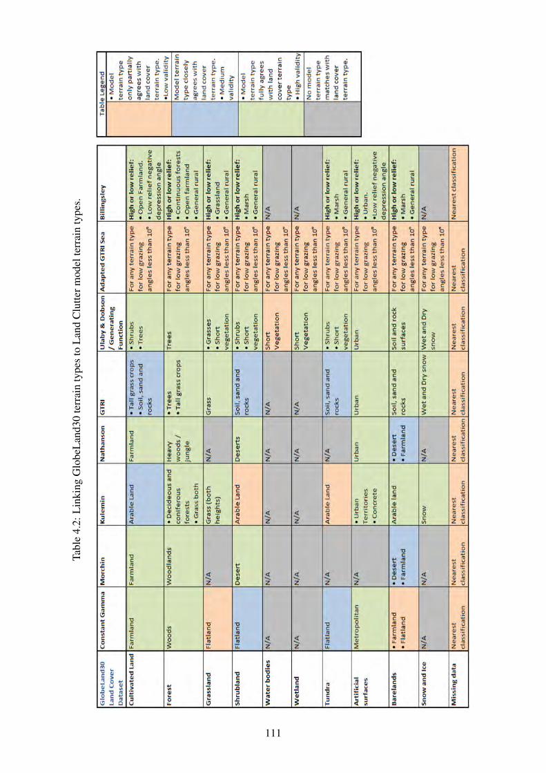
Tab
le4.2
:L
inkin
gG
lobeL
and30
terr
ain
types
toL
and
Clu
tter
model
terr
ain
types
.
111
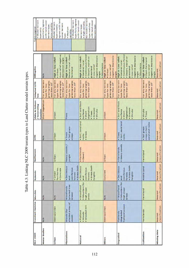
Tab
le4.3
:L
inkin
gN
LC
2009
terr
ain
types
toL
and
Clu
tter
model
terr
ain
types
.
112
radar tower height, radar operating frequency, range resolution, polarisation etc.
3. Load DEM and Land Cover data for area of interest. The DEM data will be used
to identify masked areas within the radar observed environment and to determine
the land topography and slopes. The land cover data will be used to determine the
type of terrain cover for each simulated clutter patch.
4. Account for earth curvature and atmospheric refraction. The 43
earth model
will be used to distort the loaded DEM and Land Cover data in order to account for
earth curvature and atmospheric refraction effects.
5. Create simulated clutter patches. Clutter patches will be created by breaking the
DEM data up into triangular surfaces. A suitable meshing process will be used for
this process. Each triangular surface will be a separate clutter patch.
6. Determine masked areas. By using Ray Tracing algorithms, the LOS from the
reference point to each centre point of each clutter patch will be determined. All
clutter patches that are not within LOS will be disregarded and not used further in
the simulation. These will show the masked areas within the terrain.
7. Determine data for each visible clutter patch. For all visible clutter patches, the
range to the clutter patch from reference point, clutter patch surface normal and
area, grazing, incidence and depression angles, and type of terrain cover will be
determined.
8. Determine backscatter coefficient σ◦ for each visible clutter patch. Based on
each visible clutter patches grazing angle / incidence angle / depression angle, ter-
rain type, terrain relief and slope, as well as the radar operating frequency, an ap-
propriate land clutter model will be chosen to simulate a backscatter coefficient σ◦
value for the clutter patch. The land clutter model chosen will be based on the
highest validity model that can be used that is valid for all the necessary input data.
This decision should correspond with the proposed land clutter model to use for
different situations as discussed in this dissertation.
9. Determine RCS for each clutter patch. Once σ◦ is calculated for each visible
clutter patch, the RCS can be calculated by multiplying σ◦ with the area of the
113
clutter patch. At this point the radar observed environment model, LOS coverage
and land clutter model of the scene is complete.
10. Develop the radar sensor model. As discussed in section 3.3.4, the radar sensor
model needs to be developed. This shows the characteristics of the radar system
and antenna beam pattern.
11. Develop radar range traces. As discussed in section 3.3.4, range traces are then
formed at closely spaced azimuth angles which is based on the radar antenna beam-
width, scan rate, and pulse repetition frequency (PRF). The azimuth spacing needs
to be chosen such that it provides adequate fidelity. The range samples are then
calculated and spaced according the radar range resolution. Area sampling is per-
formed for each range trace.
12. Simulate coherent radar returns. As discussed in section 3.3.4, for each range
trace, all samples within the radar range bin is summed to simulate coherent radar
return. The returns are modified by the attenuation relative to the antenna peak gain
at boresight as a function of the off boresight sample angle. The land clutter power
at the receiver for each range bin is calculated using the radar equation.
4.5 Chapter Summary
In this chapter, an analysis of the land clutter models, as well as the linking of land cover
terrain classes with land clutter models terrain types were presented.
Section 4.1 presents a comparison of existing land clutter models with measured data.
These comparisons justify the validity and compatibility for land clutter models in the
low, plateau and high grazing angle regions. Conclusions drawn and recommendations
made based on these comparisons are given in section 4.1.3 above.
Section 4.2 presents a view of the range of grazing angles, frequencies and validity for
the existing land clutter models. Ranges that lack high validity land clutter models were
identified. It is recommended that future land clutter model research be conducted in
these identified ranges. Further conclusions and recommendations based on this analysis
are given in section 4.2 above.
114

Linking of land cover terrain classes with the appropriate land clutter terrain types are
presented in section 4.3. Recommendations made for this linking process is given in
Table 4.2 for GlobeLand30 dataset and in Table 4.3 for NLC 2009 dataset.
A proposed program flow for a site specific radar coverage and land clutter modelling tool
is presented in section 4.4.
115
Chapter 5
Conclusions, Recommendations and
Future Work
This chapter provides conclusions and recommendations based on the foregoing inform-
ation in the report and then ends by highlighting areas for future work.
5.1 Conclusions and Recommendations
The aim of this project was to bring together the models and processes required to start
the development of a site specific radar coverage and land clutter modelling tool. The
objectives were therefore to investigate the related theoretical information and intended
models and processes required for the development of a site specific radar coverage and
land clutter modelling tool. In order to complete this objective, a theoretical study with
regards to elements that would influence the development of such a tool was done. These
included topics covering radar propagation, radar coverage, geographic information sys-
tems (GIS) related data and radar land clutter / backscatter coefficient models. Different
land clutter models can be used for different simulation and radar characteristics, thus
existing land clutter model’s validity are based on different underlying model assump-
tions and dependencies. The main focus of this investigation was thus to determine the
most appropriate land clutter models to use for varying terrain types, range of frequencies
and significant characteristics which affect clutter returns. This included a comparison of
measured backscatter data with simulated backscatter data calculated from these land clut-
116
ter models. Furthermore to provide classification tables in terms of each model’s validity
for different grazing angles and frequency ranges. The purpose being to aid clutter model
decisions required for the development of a site specific radar coverage and land clutter
modelling tool, and to highlight grazing angle and frequency ranges where low validity
or no land clutter models are available, such that recommendations can be made on where
future studies on land clutter modelling can be focussed on.
Chapter 2 highlighted a number of important considerations with regards to developing a
site specific radar coverage and land clutter modelling tool. It was shown that it is import-
ant to consider the effects that propagation, the atmosphere and curvature of the earth has
on a propagating EM wave. The make up and concentration levels of water and oxygen
in the different zones of the atmosphere can introduce signal attenuation and refraction
effects. The curvature of the earth can limit the radar horizon. A simple method that
was proposed that takes into account earth curvature and atmospheric refraction was the
43
Earth Model. The model does however have limitations. The model assumes standard
atmospheric conditions throughout altitudes and assumes constant ratio of actual to ef-
fective earth radius. In reality, this ratio will change as a function of altitude, atmospheric
conditions and frequency. Because of it’s simplicity and convenience, the 43
Earth Model
has been a trusted model to use to account for the effects of atmospheric refraction in
simulation by various radar analysts and researchers.
It was found that the effects of the pattern propagation factor, F , should be noted when
simulating or measuring radar land clutter. In all instances the author notes that F to
the fourth power would be inherently included in the measurement and modelling of the
backscatter coefficient, σ◦. For the purposes of this research, no attempts are made to
separate the effects of propagation (in terms of F4), over the terrain, between the radar
and the clutter cell from the intrinsic terrain backscatter σ◦, from the clutter cell itself.
This being for all measures of clutter strength, or measures of backscatter coefficient σ◦,
both in the representation of measured data as well as in predictive modelling of σ◦. This
separation is a complex task and in some cases not realisable, especially at lower grazing
angles. Thus terms such as the clutter strength, σ or σ◦, as used in this dissertation is
defined as the product of the backscatter coefficient σ◦ and the pattern propagation factor
to the fourth power, F4 , where F is assumed to include all propagation effects, including
multipath and diffraction, between the radar and the clutter cell.
117
In order to model the radar observed environment effectively, high quality digital eleva-
tion model (DEM) and land cover data is required. DEM data is used to model the terrain
topography such that masked areas and terrain relief can be determined. Similarly for
successful characterisation of the clutter performance, land cover data of the intended
simulated area needs to be taken into account. Various sources of DEM and land cover
data were investigated in this dissertation. It was found that the SRTM 30 m DEM data
is currently the highest quality elevation dataset that is freely available and covers all in-
tended areas of interest. Two land cover data sources can be considered, namely the NLC
2009 or GlobeLand30 m LC datasets. These are both at a high resolution of 30 m. The
NLC 2009 dataset however only covers the RSA region, whereas the GlobeLand30 m
covers the entire SADC region of interest. The GlobeLand30 m source is also a more cur-
rent LC model than the NLC 2009 data source. The GlobeLand30 m dataset is therefore
recommended for use in a site specific radar coverage and land clutter modelling tool.
The method proposed to create simulated clutter patches was by meshing processes. The
method proposed to determine masked terrain and LOS radar coverage was by using ray
tracing algorithms.
In order to estimate radar system performance in land clutter, clutter models are required.
These land clutter models are generally described by the backscatter coefficient σ◦. It was
found that there are many radar and environment parameters that influence σ◦. These are
shown in Table 2.2. One of the factors that influences σ◦ and that was of interest in this
dissertation was the grazing angle. It was found that σ◦ behaves differently in different
grazing angle regions, namely the low, plateau, and high grazing angle regions. Standard
probability density functions (PDF’s) models can be used to describe the variation of
different types of land clutter. From measurement data, statistical parameters required by
these PDF models for different types of land clutter can be defined empirically. Empirical
and semi-empirical models that describe the mean backscatter reflectivity σ◦ for various
types of land terrain as a function of frequency, grazing angle and polarisation can also
be developed from measurement data. Empirically derived PDF models would require
large amounts of computer resources for use in a site specific radar coverage and land
clutter modelling tool described in this study. Semi-empirical models describe the average
backscatter coefficient given by simple formulas containing several parameters. These
provide a quick and simple estimation of the backscatter coefficient and considered more
118
suited to be used for developing a site specific radar coverage and land clutter modelling
tool. Mathematical models can also be developed that provide an estimation to the the
general shape of the backscatter coefficient. Radar land clutter models are difficult to
characterize with consistency and accuracy. This is due to the complex nature of clutter.
No land clutter model will therefore represent the exact clutter returns from a specific
site. However these models can be used to predict typical conditions. The nature of land
clutter models can be determined from how they were derived, and their relationship with
clutter returns seen on specific sites or trials. The nature of how a land clutter model was
derived is thus an important factor to consider when determining the appropriate model
to use for particular cases.
One of the main objectives was thus to identify and investigate existing land clutter mod-
els that can be used in a site specific radar coverage and land clutter modelling tool to
predict typical conditions. The author notes that specific scene measurements will not
coincide with modelling predictions exactly, however the purpose of this analysis was
to identify which models would be best suited (or be the best fit model to use for spe-
cific scenes). Where a first order analysis of the simulated radar coverage and clutter
performance would aid in the design and deployment of radar systems (especially where
measurement data in the concept design phase is not possible or not feasible). The ana-
lysis as well as the comparison to measured data thus aims to identify not only the best
fit models, but if the approach of using models is valid, and to what extent, which design
consideration questions or trade-offs could it add value to.
Several mathematical, empirical, and semi-empirical land clutter models were considered.
These land clutter models were:
1. Constant Gamma Land Clutter Model.
2. Morchin Land Clutter Model.
3. Kulemin Land Clutter Model.
4. Nathanson Land Clutter Model Tables.
5. Georgia Tech Research Institute (GTRI) Land Clutter Model.
6. Ulaby and Dobson Land Clutter Model.
119
7. σ◦ Generating Function Land Clutter Model.
8. Adapted Georgia Tech Research Institute (GTRI) Sea Clutter Model.
9. Billingsley Land Clutter Model.
It was found that only Billingsley’s land clutter model and the adapted GTRI sea clutter
model is valid for the entire low grazing angle region. Nathanson’s land clutter model
tables can be used as well but only for a few limited discrete grazing angles. It is clear
that Billingsley is the authoritative land clutter model to use for low grazing angle regions.
Billingsley’s successful validation process further justifies the assumption that his model
is considered an excellent and high validity model to use for low grazing angle regions.
For grazing angles in the plateau region, the Ulaby and Dobson or Gamma Generating
Function model should be considered first as they produced backscatter values that were
the closest and lowest RMSE relative to measured data as compared to the others. The
Constant Gamma land clutter model performed better than the GTRI land clutter model
for all cases. The Kulemin land clutter model produced the largest RMSE and thus justi-
fies the assumption made to classify it as a weak and low validity model.
For general high grazing angles, the Ulaby and Dobson and Generating Function land
clutter models should be considered first, as they produced backscatter values that pro-
duced the lowest RMSE to measured data as compared to the others. Following these
will be the Morchin and GTRI land clutter models respectively. However, for the lim-
ited grazing angle range between 70◦ and 90◦, the Morchin land clutter model should be
considered first as it produced the lowest RMSE in this region of angles.
As shown in the cases of urban terrain comparisons, it is further justified that the Ulaby
and Dobson or Gamma Generating Function should be used with caution for cases where
the model is based on insufficient data. Specifically for urban terrain, the Constant
Gamma model should be considered first, followed by GTRI and Kulemin land clutter
models for plateau grazing angle regions respectively. For urban terrain at high grazing
angles, only the Ulaby and Dobson or Gamma Generating Function is valid and can be
considered, however this should be used with caution as the model for urban terrain is
based on insufficient data. It should be noted that for urban areas, the land clutter can in
most cases only be modelled in a general way as urban terrain is far too complex to be
accurately statistically modelled.
120
Nathanson’s tables provide average values for σ◦ for only a few discrete grazing angles
and are therefore not suitable for use in site specific radar land clutter modelling where
the dependence of σ0 on a range of grazing angles would be required.
As it was shown when comparing simulated data to measured data, the presence of dis-
crete scatterers interspersed can significantly increase the reflectivity measurement from
homogeneous terrain. It is thus important to remove any sources of discrete scatterers
when developing future land clutter models. These discrete scatterers are also important
to consider when developing a site specific radar land clutter modelling tool to determine
radar dynamic ranges, as their contribution can be orders of magnitude larger than the
average backscatter values of the homogeneous terrain.
A classification table was presented indicating the appropriate land clutter models to use
in order of validity (weak,strong or excellent) for different grazing angle regions. This
table should be followed when developing algorithms for the site specific radar coverage
and land clutter modelling tool. It was found that only Billingsley and Ulaby and Dobson
/ Generating Function land clutter model can be classified and used as a high validity
model. It was also shown that for many grazing angle and frequency ranges of interest,
only lower validity models exist, and in some cases no models exist. These were identified
specifically for high frequencies in the low grazing angle region, low frequencies in the
plateau grazing angle region, and the high grazing angle region for all frequencies.
For each terrain type found in the GlobeLand30 and NLC 2009 datasets, a decision was
made as to which of the terrain types for each land clutter model matches to the land cover
data terrain type the closest. This classification was presented in the form of a table. It
was found that for some land cover classes, either none or low validity match is found
with a land clutter model. This is also dependent on the grazing angle and frequency. It
is thus recommended that future land clutter modelling work should be done in not only
the missing grazing angle and frequency ranges identified, but for certain terrain classes
identified by land cover data as well.
A proposed program flow for a site specific radar coverage and land clutter modelling
tool was presented. The proposed classification tables (Tables 4.1a, 4.1b, 4.2 and 4.3)
that show the appropriate models to use for different cases should be followed when
developing algorithms for a site specific radar coverage and land clutter modelling tool.
121
This will ensure that an existing land clutter model with the highest validity available will
be used to simulate σ◦ values.
It was concluded that the validity of the such a tool is highly dependent on the validity of
the data and specifics of the land clutter model used. In some cases for specific frequencies
and terrain types, the result from the land clutter model closely matches measured data,
and in some cases it does not. A land clutter model may be classified as a high validity
model in general, but for certain cases where insufficient data exists, the validity of the
model can decrease significantly.
It was shown that high validity land clutter models only exist for a limited range of grazing
angles and frequencies. Furthermore, no land clutter model exists for K and V frequency
band in the plateau grazing angle region. This may be due to a lack of radars in the K
and V frequency bands. This is believed to be due to the high attenuation that occurs in
these regions, making these frequency bands unsuitable for general radar use. There also
does not exist any land clutter models for low frequencies in the plateau and high grazing
angle regions. Land clutter models other than high validity models should be used with
caution for cases where no high validity model exists. Lower validity models can at times
produce simulated values that are orders of magnitude different from measured data.
It is thus recommended that future research in land clutter modelling focus on developing
high validity models for all non-existing and lower validity regions that have been iden-
tified. It is also recommended that measured data for all terrain types considered in the
land cover data sources be conducted such that a full comparison and validation process
can be performed for all land clutter models terrain types of interest.
5.2 Future Work
Based on the insights gained during this research study, the following proposed future
works aims to extend and improve on the development of a site specific radar coverage
and land clutter modelling tool:
1. This dissertation only focused on the spatial statistics and average values. Future
work can aim to investigate simulating the temporal statistics of clutter as well.
122
2. Future studies can be conducted into implementing the insights gained into the
development, testing and validation of such a tool.
3. Future studies can be conducted to develop new high validity land clutter models for
grazing angles, frequencies and terrain types not represented by existing models.
4. All existing empirical land clutter models are based upon measured data from areas
not within the SADC region. Future studies can be conducted to develop land clutter
models that are based upon terrain and measurements taken from within the SADC
region.
123
Appendix A
Source Code
All source code that the author has developed and used to generate simulations and ana-
lysis results as seen in this report has been included as an attachment to the submission.
Subsequently it can also be obtained via the following link: ❤tt♣s✿ ✴✴ ✇✇✇✳ ❞r♦♣❜♦①✳
❝♦♠✴ s❤✴ ♦♦♣✉❛✈✵❣❛✉✵✐✼❜①✴ ❆❆❈❩❙✈❈●❲✼✽t✉❩❑❨♣♣❛▼✲q❚✺❛❄ ❞❧❂ ✵
124
Bibliography
[1] M. Skolnik. Introduction to Radar Systems. McGraw-Hill Education, 2002.
[2] M A Richards et al. Principles of modern radar. Number v. 1 in Principles of
Modern Radar. SciTech Publishing, Incorporated, 2010.
[3] The Institute of Electrical and Electronics Engineers. IEEE standard radar defin-
itions. IEEE Std 686-2008 (Revision of IEEE Std 686-1997), pages c1–41, May
2008.
[4] J.J. de Witt and J.J. Strydom. Analysis of measured l-band airborne land clutter
from the western cape region of south africa. In Radar Conference (Radar), 2014
International, pages 1–6, Oct 2014.
[5] Juan Pablo Ardila Lopez. Assessment and modeling of angular backscattering
variation in alos scansar images over tropical forest areas. 2008.
[6] J.B. Billingsley. Low-angle Radar Land Clutter: Measurements and Empirical
Models. Radar, Sonar, Navigation and Avionics Bks. William Andrew Pub., 2002.
[7] N C Currie. Radar reflectivity measurement: techniques & applications. Artech
house radar library. Artech House, 1989.
[8] S H Yueh. K-distribution and polarimetric terrain radar clutter. Electromagnetic
Waves and Applications, 3:747–768, April 1989.
[9] GP Kulemin, EA Goroshko, and EV Tarnavsky. Land backscattering model for
millimeter wave radar. In Modern Problems of Radio Engineering, Telecommunic-
ations and Computer Science, 2004. Proceedings of the International Conference,
pages 138–141. IEEE, 2004.
125
[10] M Long. Radar Reflectivity of Land and Sea. Artech House radar library. Artech
House, 2001.
[11] William Connor. Low grazing angle terrain backscattering coefficient generator.
Masters thesis, Air Force Institute of Technology USA, Airforce Institute of Tech-
nology, 2950 P Street WPAFB, OH 45433-7765, March 1999.
[12] Christopher C Lin and J Patrick Reilly. A site-specific model of radar terrain backs-
catter and shadowing. Johns Hopkins APL Technical Digest, 18(3):433, 1997.
[13] G Rode. Radar clutter backscattering simulation for specific sites. Frequenz, 62(1-
2):7–11, 2008.
[14] Roger E Clapp. A theoretical and experimental study of radar ground return. Ra-
diation Laboratory, Massachusetts Institute of Technology, 1946.
[15] W.C. Morchin. Airborne Early Warning Radar. Artech House radar library. Artech
House, 1990.
[16] Fred E Nathanson et al. Radar Design Principles, chapter 9, pages 247–282.
SciTech Publishing, 1999.
[17] F.T. Ulaby and M.C. Dobson. Handbook of Radar Scattering Statistics for Terrain.
Artech House remote sensing library. Artech House, 1989.
[18] R. Mediavilla, W. O’Connor, V. Pyati, and K. Wilson. Terrain backscattering coef-
ficient generator. In Geoscience and Remote Sensing Symposium, 1999. IGARSS
’99 Proceedings. IEEE 1999 International, volume 2, pages 1429–1431 vol.2,
1999.
[19] Kelce Wilson, Dale Patrick, and James Blair. Radar scattering statistics for digital
terrain models, 2005.
[20] Donald E Kerr. Propagation of short radio waves, volume 24. IET, 1951.
[21] Khan Major Mohammad Ali, Rahman Afia Binte, Popy Jannatul Fardous, et al. Ef-
fects of changing RCS and Antenna Array pattern Radar performance. PhD thesis,
Department of Electrical, Electronics and Communication Engineering (EECE),
2011.
126
[22] F.T. Ulaby, D.G. Long, W.J. Blackwell, C. Elachi, and K. Sarabandi. Microwave
Radar and Radiometric Remote Sensing. University of Michigan Press, 2014.
[23] B.R. Mahafza. Radar Systems Analysis and Design Using MATLAB. CRC Press,
2002.
[24] Leslie W Barclay. Propagation of radiowaves, volume 502. Iet, 2003.
[25] D.K. Barton. Modern Radar System Analysis. Artech House Radar Library. Artech
House, 1988.
[26] G.R. Curry. Radar Essentials: A Concise Handbook for Radar Design and Per-
formance. Electromagnetics and Radar Series. Institution of Engineering and Tech-
nology, 2012.
[27] L.V. Blake. Radar range-performance analysis. LexingtonBooks, 1980.
[28] K.R. Noth. Modeling and simulation of a ground based sense and avoid archi-
tecture for unmanned aircraft system operations. In Integrated Communications,
Navigation and Surveilance Conference (ICNS), 2011, pages O7–1–O7–9, May
2011.
[29] A.G. Huizing and A. Theil. CARPET (Computer-aided Radar Performance Eval-
uation Tool): Radar Performance Analysis Software and User’s Manual, Version
1.0: Buch. Artech House, 1993.
[30] Wayne L Patterson. Advanced Refractive Effects Prediction System. Space and
Naval Warfare Systems Center, Defense Technical Information Center 8725 John
J. Kingman Road Ft. Belvoir, VA 22060-6218, 1 edition, April 1998.
[31] Yunhan Dong. Models of land clutter vs grazing angle, spatial distribution and
temporal distribution-l-band vv polarisation perspective. Technical report, DTIC
Document, 2004.
[32] Daniel Sabel, Marcela Doubkova, Wolfgang Wagner, Paul Snoeij, and Evert At-
tema. A global backscatter model for c-band sar. In Proceedings of the ESA Living
Planet Symposium, Bergen, Norway, volume 28, 2010.
[33] Floyd M Henderson, Anthony J Lewis, et al. Principles and applications of ima-
ging radar. Manual of remote sensing, volume 2. John Wiley and sons, 1998.
127
[34] E. V. Tarnavsky and G. P. Kulemin. Modeling of radar land clutter map for small
grazing angles. In R. S. Romaniuk, editor, Photonics Applications in Astronomy,
Communications, Industry, and High-Energy Physics Experiments II, volume 5484
of Society of Photo-Optical Instrumentation Engineers (SPIE) Conference Series,
pages 702–706, July 2004.
[35] Abdenasser Djafri and Boualem Haddad. Mapping of weather radar ground clutter
using the digital elevation model (srtm). Signal & Image Processing: An Interna-
tional Journal (SIPIJ), 3:135–151, 2012.
[36] RA Kropfli, I Katz, TG Konrad, and EB Dobson. Simultaneous radar reflectivity
measurements and refractive index spectra in the clear atmosphere. Radio Science,
3(10):991–994, 1968.
[37] Klett, Eberhard Witwe, Detleffsen, Christoph Peter, et al. Photometria. sumptibus
viduae Eberhardi Klett, 1760.
[38] Benjamin Crowell. 2 simple nature an introduction to physics for engineering and
physical science students. 2007.
[39] William M Haynes. CRC handbook of chemistry and physics. CRC press, 2014.
[40] Thomas Lillesand, Ralph W Kiefer, and Jonathan Chipman. Remote sensing and
image interpretation. John Wiley & Sons, 2014.
[41] Kevin J Sangston and Kari R Gerlach. Coherent detection of radar targets in a
non-gaussian background. Aerospace and Electronic Systems, IEEE Transactions
on, 30(2):330–340, 1994.
[42] J.B. Billingsley, A. Farina, F. Gini, M.V. Greco, and L. Verrazzani. Statistical
analyses of measured radar ground clutter data. Aerospace and Electronic Systems,
IEEE Transactions on, 35(2):579–593, Apr 1999.
[43] Ulku Cilek Doyuran and Yalcin Tanik. Detection in range-heterogeneous weibull
clutter. In Radar Conference, 2007 IEEE, pages 343–347. IEEE, 2007.
[44] M. Sekine and Y. Mao. Weibull Radar Clutter. Electromagnetics and Radar Series.
P. Peregrinus Limited, 1990.
128
[45] HC Chan. Temporal statistics of low-angle ground clutter. Technical report, DTIC
Document, 1989.
[46] Stephen O Rice. Mathematical analysis of random noise. Bell System Technical
Journal, 23(3):282–332, 1944.
[47] J Barrie Billingsley and John F Larrabee. Multifrequency measurements of radar
ground clutter at 42 sites. Massachusetts Institute of Technology, Lincoln Labor-
atory, 1991.
[48] KD Ward et al. Sea clutter: Scattering, the k distribution and radar performance.
IET Radar, Sonar and Navigation Series 20, 22(1), January 2006.
[49] T.J. Nohara and S. Haykin. Canadian east coast radar trials and the k-distribution.
Radar and Signal Processing, IEE Proceedings F, 138(2):80–88, Apr 1991.
[50] Eo Jakeman. On the statistics of k-distributed noise. Journal of Physics A: Math-
ematical and General, 13(1):31, 1980.
[51] Eo Jakeman and PN Pusey. A model for non-rayleigh sea echo. Antennas and
Propagation, IEEE Transactions on, 24(6):806–814, 1976.
[52] G Sun et al. Terrain effect on forest radar backscatter: Modelling and correction.
Number 01-074 in CEOS-SAR, 1 Department of Geography, University of Mary-
land, College Park, MD 20742 USA, 2001. Department of Geography, University
of Maryland.
[53] J P Wilson et al. Terrain Analysis: Principles and Applications. New York: Wiley,
2000.
[54] Christine Mary Rutherford Fowler. The solid earth: an introduction to global
geophysics. Cambridge University Press, 1990.
[55] Witold Fraczek. Mean sea level, gps, and the geoid. [Online] at: ❤tt♣✿✴✴✇✇✇✳
❡sr✐✳❝♦♠✴♥❡✇s✴❛r❝✉s❡r✴✵✼✵✸✴❣❡♦✐❞✶♦❢✸✳❤t♠❧, July 2003.
[56] Raytheon STX Williamson and RH Rapp. The development of the joint nasa
gsfc and the national imagery and mapping agency (nima) geopotential model
egm96. NASA Technical Paper NASA/TP-1998-206861, Goddard Space Flight
Center, Greenbelt, 1998.
129
[57] Antonio Di Gregorio and Louisa JM Jansen. Land cover classification system
(lccs): classification concepts and user manual. FAO, Rome, 1998.
[58] P Mayaux, E Bartholome, M Massart, C Van Cutsem, A Cabral, A Nonguierma,
O Diallo, C Pretorius, M Thompson, M Cherlet, et al. A land cover map of africa.
carte de occupation du sol de lafrique. European Commission, Joint Research
Center, EUR, 20665, 2003.
[59] S Feng and J Chen. Low-angle reflectivity modeling of land clutter. Geoscience
and Remote Sensing Letters, IEEE, 3(2):254–258, 2006.
[60] Frank Hanssen, Roel May, Yngve Steinheim, Roald Vang, et al. Gis-modeling
of radar detection coverage and ground clutter within the complex environment of
smøla wind-power plant. 2011.
[61] C Lin et al. Radar terrain clutter model with consideration of propagation effects.
In Microwave Conference, 1993. 23rd European, pages 478–482, Sept 1993.
[62] Ramesh Nepal et al. A simulation study of the impact of surface clutter and space-
borne precipitation radar sensor. 36th Conference on Radar Meteorology, Septem-
ber 2013.
[63] Andriy Kurekin, Lik-Kwan Shark, Kenneth Lever, Darren Radford, and Dave Mar-
shall. Site-specific land clutter modelling based on radar remote sensing images
and digital terrain data. In Remote Sensing, pages 783013–783013. International
Society for Optics and Photonics, 2010.
[64] Michael A Temple and Kelce S Wilson. Probabilistic backscatter coefficient gen-
erating function. In AeroSense’99, pages 644–649. International Society for Optics
and Photonics, 1999.
[65] Digital Geography. Release of world-wide high resolution srtm
data. [Online] at: ❤tt♣✿✴✴✇✇✇✳❞✐❣✐t❛❧✲❣❡♦❣r❛♣❤②✳❝♦♠✴
❛♥♥♦✉♥❝❡♠❡♥t✲r❡❛❧❡❛s❡✲✇♦r❧❞✇✐❞❡✲❤✐❣❤✲r❡s✉❧t✐♦♥✲srt♠✲❞❛t❛✲✸✵♠✴★✳
❱▼❏❳❛❊❡❯❡P❛, September 2014.
[66] United States Department of the Interior. Shuttle radar topography mission (srtm) 1
arc-second global. [Online] at: ❤tt♣s✿✴✴❧t❛✳❝r✳✉s❣s✳❣♦✈✴❙❘❚▼✶❆r❝, January
2012.
130
[67] Jspace Systems. Aster global digital elevation model (gdem). [Online] at: ❤tt♣s✿
✴✴✇✇✇✳❥s♣❛❝❡s②st❡♠s✳♦r✳❥♣✴❡rs❞❛❝✴●❉❊▼✴❊✴✹✳❤t♠❧, October 2012.
[68] GDEM ASTER. Aster global dem validation summary report. [On-
line] at: ❤tt♣✿✴✴✇✇✇✳❡rs❞❛❝✳♦r✳❥♣✴●❉❊▼✴❊✴✐♠❛❣❡✴❆❙❚❊❘●❉❊▼❭
❴❱❛❧✐❞❛t✐♦♥❙✉♠♠❛r②❘❡♣♦rt❭❴❱❡r✶✳♣❞❢, 2009.
[69] Nicolas H. Durland. Defining mean sea level in military simulations with dted.
In Proceedings of the 2009 Spring Simulation Multiconference, SpringSim ’09,
pages 115:1–115:3, San Diego, CA, USA, 2009. Society for Computer Simulation
International.
[70] John Pike. Digital terrain elevation data [dted]. [Online] at: ❤tt♣✿✴✴✇✇✇✳❢❛s✳
♦r❣✴✐r♣✴♣r♦❣r❛♠✴❝♦r❡✴❞t❡❞✳❤t♠, January 2009.
[71] Airbus Defence and Space. World dem from astrium. [Online]
at: ❤tt♣✿✴✴✇✇✇✳❣❡♦✲❛✐r❜✉s❞s✳❝♦♠✴❢✐❧❡s✴♣♠❡❞✐❛✴♣✉❜❧✐❝✴r✺✹✸✹❴✾❴❣❡♦❴
✵✷✷❴✇♦r❧❞❞❡♠❴❡♥❴❧♦✇✳♣❞❢, 2014.
[72] Airbus Defence and Space:Geo-Intelligence. Terrain data - global to local. [On-
line] at: ❤tt♣✿✴✴✇✇✇✳❣❡♦✲❛✐r❜✉s❞s✳❝♦♠✴❢✐❧❡s✴♣♠❡❞✐❛✴♣✉❜❧✐❝✴r✸✶✽✶❴✾❴
❣❡♦❴✵✷✻❴❣❡♦❡❧❡✈❛t✐♦♥❴❡♥❴❧♦✇✳♣❞❢, 2013.
[73] Open Land Service. Global land cover 2013. [Online] at: ❤tt♣✿✴✴✇✇✇✳
❣❧♦❜❛❧❧❛♥❞❝♦✈❡r✳❝♦♠✴❤♦♠❡✴❊♥❜❛❝❦❣r♦✉♥❞✳❛s♣①, 2014.
[74] Fritz Schoeman, TS Newby, MW Thompson, and Elzie Catharina Van den Berg.
South african national land-cover change map. South African Journal of Geomat-
ics, 2(2):94–105, 2014.
[75] SANBI. Updating national land cover. Technical report, SANBI (South African
National Biodiversity Institute), 2 Pretoria St, Pretoria, 0184 South Africa, October
2009.
[76] Ryutaro Tateishi et al. Global map-global land cover (glcnmo). Technical report,
Chiba University, Center for Environmental Remote Sensing, Chiba University,
Center for Environmental Remote Sensing, 1-33 Yayoi-cho, Inage-ku Chiba, 263-
8522 Japan, November 2008.
131
[77] John Latham et al. Global land cover share. Technical report, Food and Agricultural
Organisation of the United Nations (FAO), FAO, Viale delle Terme di Caracalla,
00100, Rome, Italy, 2014.
[78] Global Land Cover Network. Glc-share. [Online] at: ❤tt♣✿✴✴✇✇✇✳❣❧❝♥✳♦r❣✴
❞❛t❛❜❛s❡s✴❧❝❴❣❧❝s❤❛r❡❴❡♥✳❥s♣, 2014.
[79] Lin-San Yang, Jia Xu, Xiao Gao, Xiu-Tan Wang, and Ying-Ning Peng. A novel
three-dimensional coverage visualization system of netted radars based on arcob-
jects. In Radar Conference, 2009 IET International, pages 1–5, April 2009.
[80] George L Bair. Airborne radar simulation. Camber Corporation, Dallas, Texas,
1996.
[81] Jody L Kirtner and Harry R Anderson. The application of land use/land
cover data to wireless communication system design. EDX Engineering, Inc.,
http://proceedings. esri. com/library/userconf/proc98/PROCEED/TO550/PAP525
P, 525:1–16.
[82] Sagi Katz, Ayellet Tal, and Ronen Basri. Direct visibility of point sets. ACM Trans.
Graph., 26(3), July 2007.
[83] W S Ament. Forward and backscattering by certain rough surfaces. Antennas and
Propagation, 4:369–373, July 1956.
[84] Wm Randolph Franklin, Clark K Ray, and Shashank Mehta. Geometric algorithms
for siting of air defense missile batteries. A], Research Project for Battle, (2756),
1994.
[85] Christelle Vancutsem, Eduardo Marinho, François Kayitakire, Linda See, and
Steffen Fritz. Harmonizing and combining existing land cover/land use datasets
for cropland area monitoring at the african continental scale. Remote Sensing,
5(1):19, 2012.
[86] D Barton. Land clutter models for radar design and analysis. Proceedings of the
IEEE, 73(2):198–204, Feb 1985.
[87] J P Reilly et al. A radar land clutter model and its verification. In Geoscience and
Remote Sensing Symposium, 1994. IGARSS ’94. Surface and Atmospheric Remote
132
Sensing: Technologies, Data Analysis and Interpretation., International, volume 4,
pages 2319–2321, Aug 1994.
[88] Li Zhang et al. Airship radar system modeling and simulation. Progress In Elec-
tromagnetics Research Symposium, August 2012.
[89] Mark Thompson. Development of a new south african land cover dataset using
automated mapping techniques. Pretoria South Africa, August 2013. GeoTerraIm-
age Pty Ltd.
[90] Mike Hensel and Erik P Blasch. Fusion of distributions for radar clutter modeling.
In Fusion 2004: Seventh International Conference on Information Fusion, 2004.
[91] G. Davidson, H.D. Griffiths, and S. Ablett. Statistical analysis of high resolution
land clutter. In RADAR 2002, pages 434–438, Oct 2002.
[92] G. Davidson, H.D. Griffiths, and S. Ablett. Statistical analysis of high resolution
land clutter. In RADAR 2002, pages 434–438, Oct 2002.
[93] Andrew J Gatesman, Thomas M Goyette, Jason C Dickinson, Jerry Waldman,
Jim Neilson, and William E Nixon. Physical scale modeling the millimeter-wave
backscattering behavior of ground clutter. In Aerospace/Defense Sensing, Simula-
tion, and Controls, pages 141–151. International Society for Optics and Photonics,
2001.
[94] Antonio Di Gregorio et al. Land Cover Classification System. Food and Agriculture
Organization of the United Nations, FAO Viale delle Terme di Caracalla 00100
Rome Italy, 2 edition, 2005.
[95] Ricardo Mediavilla. Terrain backscattering coefficient generator. Master’s thesis,
Air Force Institute of Technology USA, 2950 Hobson Way, Wright Ptrsn Afb, OH
45433, United States, 1999.
[96] Iulian Rosu. Basics of radio wave propagation. [Online] at: ❤tt♣✿✴✴✇✇✇✳qs❧✳
♥❡t✴✈❛✸✐✉❧✴.
[97] Tom Mahood. Radar ranges of the mojave desert. [Online] at: ❤tt♣✿✴✴✇✇✇✳
t❤❡❤♦✇❧❛♥❞❝♦♠♣❛♥②✳❝♦♠✴r❛❞❛r❴st❡❛❧t❤✴❇❧✉❡❢✐r❡✳❤t♠, June 2012.
133
[98] Canan OZGEN. Spectral and Statistical Analyses of Experimental Radar Clutter
Data. PhD thesis, Middle East Technical University, 2010.
[99] Maria S Greco and Fulvio Gini. Radar clutter modelling, 2013.
[100] H Laur, P Bally, P Meadows, J SANCHEz, B Schaettler, and E Lopinto. Derivation
of the backscatter coefficient sigma0 in esa ers sar pri products. esa document no.
Technical report, ES-TN-RS-PM-HL09, 1997.
[101] GLCN Secretariat and Land Cover Topic Centre. Land cover activities in the sadc
region. Technical report, Food and Agriculture Organization of the United Nations,
NRC, Food and Agriculture Organization of the United Nations (FAO) Viale delle
Terme di Caracalla Rome 00100, Italy, 2008.
[102] T Fawwaz et al. Millimeter wave measurement and modelling of terrain scattering.
Technical Report 07040188, Radiation Laboratory, University of Michigan, Ann
Arbor, Michigan 48109, February 1992.
[103] SANBI. Gis metadata : Detailed report. Technical report, South African National
Biodiversity Institute, 2 Pretoria St, Pretoria, 0184, South Africa, January 2009.
134

EBE Faculty: Assessment of Ethics in Research Projects
Any person planning to undertake research in the Faculty of Engineering and the Built Environment at the University of Cape Town is required to complete this form before collecting or analysing data. When completed it should be submitted to the supervisor (where applicable) and from there to the Head of Department. If any of the questions below have been answered YES, and the applicant is NOT a fourth year student, the Head
should forward this form for approval by the Faculty EIR committee: submit to Ms Zulpha Geyer [email protected]; Chemical Engineering Building, Upper Campus, UCT, (Ph 021 650 4791 ). NB: A copy of this completed form must be included with the thesis/dissertation/report when it Is submitted for examination.
Name of Principal Researcher/Student: Sulayman Salie
Preferred email address of applicant: [email protected]
Department: Electrical Engineering
If a Student: Degree: MEng Electrical Engineering Supervisor: Professor Michael Raymond lnggs
If a Research Contract indicate source of funding/sponsorship: Council of Scientific and Industrial Research
Research Project Title: Site Specific Radar Coverage and Land Clutter Modelling
Overview of ethics issues In your research project:
Question 1: Is there a possibility that your research could cause harm to a third party (i.e. YES a erson not involved In our ro·ect? Question 2: Is your research making use of human subjects as sources of data? YES If our answer is YES, lease com lete Addendum 2. Question 3: Does your research involve the participation of or provision of services to YES communities? If our answer is YES lease com lete Addendum 3. Question 4: If your research Is sponsored, is there any potential for conflicts of interest? YES If our answer is YES lease com lete Addendum 4. If you have answered YES to any of the above questions, please append a copy of your research proposal, as well as any interview schedules or questionnaires (Addendum 1) and please complete further addenda as appropriate.
I hereby undertake to carry out my research In such a way that • there is no apparent legal objection to the nature or the method of research; and • the research will not compromise staff or students or the other responsibilities of the University; • the stated objective will be achieved, and the findings will have a high degree of validity; • limitations and alternative interpretations will be considered; • the findings could be subject to peer review and publicly available; and • I will comply with the conventions of copyright and avoid any practice that would constitute plagiarism.
Signed by:
Principal Researcher/Student:
HOD ( or delegated nominee): Final authority for all assessments with NO to all questions and for all undergraduate research. Chair : Faculty EIR Committee For applicants other than undergraduate students who have answered YES to any of the above uestions.
Full name and signature Date