Coverage Adjusted Entropy Estimation

Vincent Q. Vu∗, Bin Yu∗, Robert E. Kass†

{vqv, binyu}@stat.berkeley.edu, kass@stat.cmu.edu

∗Department of Statistics, University of California, Berkeley

†Department of Statistics and Center for the Neural Basis of Cognition, Carnegie Mellon University

March 23, 2007

Abstract

Data on “neural coding” have frequently been analyzed using information-theoretic mea-

sures. These formulations involve the fundamental, and generally difficult statistical problem of

estimating entropy. In this paper we review briefly several methods that have been advanced to

estimate entropy, and highlight a method due to Chao and Shen that appeared recently in the

environmental statistics literature. This method begins with the elementary Horvitz-Thompson

estimator, developed for sampling from a finite population and adjusts for the potential new

species that have not yet been observed in the sample—these become the new patterns or

“words” in a spike train that have not yet been observed. The adjustment is due to I.J. Good,

and is called the Good-Turing coverage estimate. We provide a new empirical regularization

derivation of the coverage-adjusted probability estimator, which shrinks the MLE (the naive

or “direct” plug-in estimate) toward zero. We prove that the coverage adjusted estimator, due

to Chao and Shen, is consistent and first-order optimal, with rate OP (1/ log n), in the class of

distributions with finite entropy variance and that within the class of distributions with finite

qth moment of the log-likelihood, the Good-Turing coverage estimate and the total probability

of unobserved words converge at rate OP (1/(log n)q). We then provide a simulation study of the

estimator with standard distributions and examples from neuronal data, where observations are

dependent. The results show that, with a minor modification, the coverage adjusted estimator

performs much better than the MLE and is better than the Best Upper Bound estimator, due

to Paninski, when the number of possible words m is unknown or infinite.

1 Introduction

The problem of “neural coding” is to elucidate the representation and transformation of information

in the nervous system. [17] An appealing way to attack neural coding is to take the otherwise

vague notion of “information” to be defined in Shannon’s sense, in terms of entropy. [20] This

project began in the early days of cybernetics [24] [11], received considerable impetus from work

summarized in the book Spikes: Exploring the Neural Code [18], and continues to be advanced by

many investigators. In most of this research, the findings concern the mutual information between

a stimulus and a neuronal spike train response. For a succinct overview see [4]. The mutual

information, however, is the difference of marginal and expected conditional entropies; to compute

it from data one is faced with the basic statistical problem of estimating the entropy1

H := −∑x∈X

P (x) logP (x) (1)

of an unknown discrete probability distribution P over a possibly infinite space X , the data being

conceived as random variables X1, . . . , Xn with Xi distributed according to P . An apparent method

of estimating the entropy is to apply the formula after estimating P (x) for all x ∈ X , but estimating

a discrete probability distribution is, in general, a difficult nonparametric problem. Here, we point

out the potential use of a method, the coverage adjusted estimator, due to Chao and Shen [5], which

views estimation of entropy as analogous to estimation of the total of some variable distributed

across a population, which in turn may be estimated by a simple device introduced by Horvitz

and Thompson [8]. We provide an alternative derivation of this estimator, establish optimality

of its rate of convergence, and provide simulation results indicating it can perform very well in

finite samples–even when the observations are mildly dependent. The simulation results for data

generated to resemble neuronal spike trains are given in Figure 1, where the estimator is labeled

CAE. In Section 2 we provide background material. Section 3 contains our derivation of the

estimator and the convergence result, and Section 4 the description of the simulation study and

additional simulation results.1Unless otherwise stated, we take all logarithms to be base 2 and define 0 log 0 = 0.

1

●

●●

●●

●●●●●●●●●●●●●●●●

●●

●●

●

●

●●

●● ●●●●

●● ● ●

100 200 500 2000 5000 20000

0.0

0.2

0.4

0.6

0.8

1.0

sample size (n)

RM

SE

V1 VLMC (T=6)

●● ●●●●●●●●●●●●●●●●●●●

● ●●●●

●● ● ● ● ●●●● ● ● ● ●

100 200 500 2000 5000 20000

0.00

0.05

0.10

0.15

0.20

sample size (n)

RM

SE

● MLEBUB−

BUB+CAE

Field L VLMC (T=15)

Figure 1: Comparison of entropy estimators in terms of root mean squared error, as a function ofsample size, for word lengths T = 6 from V1 data (left) and T = 15 from Field L data (right).Full definitions are given in Section 4. The samples of size n are drawn from a stationary variablelength Markov chain (VLMC) [10] used to model neuronal data from visual (V1) and auditory(Field L) systems. We followed the “direct method” and divided each sample sequence into words,which are blocks of length T . The plots display the root mean squared error (RMSE) of theestimates of H/T . The RMSE was estimated by averaging 1000 independent realizations. MLEis the “naive” empirical plug-in estimate. CAE is the coverage adjusted estimator. BUB+ is theBUB estimator [16] with its m parameter set to the maximum possible number of words (V1: 6T

= 46,656, Field L: 2T = 32,768). BUB- is the BUB estimator with m set, naively, to the observednumber of words. The actual values of H/T are V1: 1.66 and Field L: 0.151. The BUB+ estimatorhas a very large RMSE resulting from specifying m as the maximum number of words. The CAEestimator performs relatively well, especially for sample sizes as small as several hundred words.

2 Background

In linguistic applications, X could be the set of words in a language, with P specifying their

frequency of occurrence. For neuronal data, Xi often represents the number of spikes (action

potentials) occurring during the ith time bin. Alternatively, when a fine resolution of time is used

(such as ∆t = 1 millisecond), the occurrence of spikes is indicated by a binary sequence, and Xi

becomes the pattern, or “word,” made up of 0-1 words or “letters,” for the ith word. This is

described in Figure 2, and it is the basis for the widely-used “direct method” proposed by Strong

et al. [21]. The number of possible words m := |{x ∈ X : P (x) > 0}| is usually unknown and

possibly infinite. In the example in Figure 2, the maximum number of words is the total number

2

0 1 0 0 0 0 1 0 1 0 0 0 1 0 0 0 1 0 1 0 0 0 0 1 0 0 0 0 0 00 0 0 0 1 0 0 1 0 0

0 1 0 0 0 0 1 0 1 0 0 0 1 0 0 0 1 0 1 0 0 0 0 0 1 0 0 1 0 0 0 0 0 1 0 0 0 0 0 0 0 0 0 1 0time

X1 X2 X3 X4

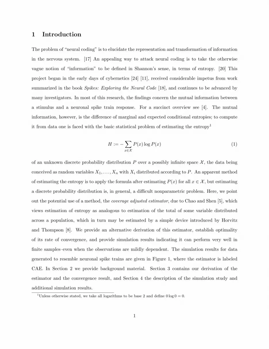
Figure 2: The top row depicts 45 milliseconds of a hypothetical spike train. The ticks on the timeaxis demarcate ∆t = 1 millisecond bins (intervals). The spike train is discretized into a sequenceof counts. Each count is the number of spikes that fall within a single time bin. Subdividingthis sequence into words of length T = 10 leads to the words shown at the bottom. The wordsX1, X2, . . . take values in the space X = {0, 1}10 consisting of all 0-1 strings of length 10.

of 0-1 strings of length T . For T = 10 this number is 1024; for T = 20 it is well over one million,

and in general there is an exponential explosion with increasing T . Furthermore, the phenomenon

under investigation will often involve fine time resolution, necessitating a small bin size ∆t and

thus a large T . For large T , the estimation of P (x) is likely to be challenging.

We note that Strong et al. [21] calculated the entropy rate. Let {Wt : t = 1, 2, . . .} be a

discretized (according to ∆t) spike train as in the example in Figure 2. If {Wt} is a stationary

process, the entropy of a word, say X1 = (W1, . . . ,WT ), divided by its length T is non-increasing

in T and has a limit as T →∞, i.e.

limT→∞

1TH(X1) = lim

T→∞

1TH(W1, . . . ,WT ) =: H ′ (2)

exists [6]. This is the entropy rate of {Wt}. The word entropy is used to estimate the entropy

rate. If {Wt} has finite range dependence, then the above entropy factors into a sum of conditional

entropies and a single marginal entropy. Generally, the word length is chosen to be large enough so

that H(W1, . . . ,WT )/T is a close approximation to H ′, but not so large that there are not enough

words to estimate H(W1, . . . ,WT ). Strong et al. [21] proposed that the entropy rate estimate be

extrapolated from estimates of the word entropy over a range of word lengths. We do not address

3

this extrapolation, but rather focus on the problem of estimating the entropy of a word.

In the most basic case the observations X1, . . . , Xn are assumed to be independent and identi-

cally distributed (i.i.d.). Without loss of generality, we assume that X ⊆ N and that the words 2

are labeled 1, 2, . . .. The seemingly most natural estimate is the empirical plug-in estimator

H := −∑

x

P (x) log P (x), (3)

which replaces the unknown probabilities in (1) with the empirical probabilities P (x) := nx/n,

that is the observed proportion nx/n of occurrences of the word x in X1, . . . , Xn. The empirical

plug-in estimator is often called the “naive” estimate or the “MLE”–after the fact that P is the

maximum likelihood estimate of P . We will use “MLE” and “empirical plug-in” interchangeably.

From Jensen’s Inequality it is readily seen that the MLE is negatively biased unless P is trivial. In

fact no unbiased estimate of entropy exists, see [16] for an easy proof.

In the finite m case, Basharin [3] showed that the MLE is biased, consistent, and asymptotically

normal with variance equal to the entropy variance Var[logP (X1)]. Miller [13] previously studied

the bias independently and provided the formula

EH −H = −m− 12n

+O(1/n2). (4)

The bias dominates the mean squared error of the estimator [1], and has been the focus of recent

studies [23, 16].

The original “direct method” advocated an ad-hoc strategy of bias reduction based on a sub-

sampling extrapolation [21]. A more principled correction based on the jackknife technique was

proposed earlier by Zahl [27]. The formula (4) suggests a bias correction of adding (m − 1)/(2n)

to the MLE. This is known as the Miller-Maddow correction. Unfortunately, it is an asymptotic

correction that depends on the unknown parameter m. Paninski [16] observed that both the MLE

and Miller-Maddow estimates fall into a class of estimators that are linear in the frequencies of ob-2The information theory literature traditionally refers to X as an alphabet and its elements as symbols. It is

natural to call a tuple of symbols a word, but the problem of estimating the entropy of the T -tuple word reduces tothat of estimating the entropy in an enlarged space (of T -tuples).

4

served word counts fj = |{nx : nx = j}|. He proposed an estimate, “Best Upper Bounds” (BUB),

based on numerically minimizing an upper-bound on the bias and variance of such estimates when

m is assumed finite and known. We note that in the case that m is unknown, it can be replaced

by an upper-bound, but the performance of the estimator is degraded.

Bayesian estimators have also been proposed for the finite m case by Wolpert and Wolf [25].

Their approach is to compute the posterior distribution of entropy based on a symmetric Dirichlet

prior on P . Nemenman et al. [14] found that the Dirichlet prior on P induces a highly concentrated

prior on entropy. They argued that this property is undesirable and proposed an estimator based

on a Dirichlet mixture prior with the goal of flattening the induced prior distribution on entropy.

Their estimate requires a numerical integration and also the unknown parameter m, or at least

an upper-bound. The estimation of m is even more difficult than the estimation of entropy [1],

because it corresponds to estimating lima↓0∑

x[P (x)]a.

In the infinite m case, Antos and Kontoyiannis [1] proved consistency of the empirical plug-in

estimator and showed that there is no universal rate of convergence for any estimator. However,

Wyner and Foster [26] have shown that the best rate (to first order) for the class of distributions

with with finite entropy variance or equivalently finite log-likelihood second moment

∑x

P (x)(logP (x))2 <∞ (5)

is OP (1/ log n). This rate is achieved by the empirical plug-in estimate as well as an estimator

based on match lengths. Despite the fact that the empirical plug-in estimator is asymptotically

optimal, its finite sample performance leaves much to be desired.

Chao and Shen [5] proposed a coverage adjusted entropy estimator intended for the case when

there are potentially unseen words in the sample. This is always the case when m is relatively large

or infinite. Intuitively, low probability words are typically absent from most sequences, i.e. the

expected sample coverage is < 1, but in total, the missing words can have a large contribution to

H. The estimator is based on plug-in of a coverage adjusted version of the empirical probability

into the Horvitz-Thompson [8] estimator of a population total. They presented simulation results

showing that the estimator seemed to perform quite well, especially in the small sample size regime,

5

when compared to the usual empirical plug-in and several bias corrected variants. The estimator

does not require knowledge of m, but they assumed a finite m. We prove here (Theorem 1) that

the coverage adjusted estimator also works in the infinite m case. Chao and Shen also provided

approximate confidence intervals for the coverage adjusted estimate, however they are asymptotic

and depend on the assumption of finite m.

The problems of entropy estimation and estimation of the distribution P are distinct. Entropy

estimation should be no harder than estimation of P , since H is a functional of P . However, several

of the entropy estimators considered here depend either implicitly or explicitly on estimating P .

BUB is linear in the frequency of observed word counts fj , and those are 1-to-1 with the empirical

distribution P up to labeling. In general, any symmetric estimator is a function of P . The only

estimators mentioned above that does not depend on P is the match length estimator. For the

coverage adjusted estimator, the dependence on estimating P is only through estimating P (k) for

observed words k.

3 Theory

Unobserved words—those that do not appear in the sample, but have non-zero probability–can

have a great impact on entropy estimation. However, these effects can be mitigated with two types

of corrections: Horvitz-Thompson adjustment and coverage adjustment of the probability estimate.

Section 3.1 contains an exposition of some of these effects. The adjustments are described in Section

3.2 along with the definition of the resulting coverage adjusted entropy estimator. A key ingredient

of the estimator is a coverage adjusted probability estimate. We provide a novel derivation from

the viewpoint of regularization in Section 3.3. Lastly, Section 3.4 concludes the theoretical study

with our rate of convergence results.

Throughout this section we assume that X1, . . . , Xn is an i.i.d. sequence from the distribution

P on the countable set X . Without loss of generality, we assume that the P (k) > 0 for all k ∈ X

6

and write pk for P (k) = P(Xi = k). As before, m := |X | and possibly m = ∞. Let

nk :=n∑

i=1

1{Xi = k} (6)

be the number of times that the word k appears in the sequence X1, . . . , Xn, with 1{·} denoting

the indicator of the event {·}.

3.1 The Unobserved Word Problem

The set of observed words S is the set of words that appear at least once in the sequence X1, . . . , Xn,

i.e.

S := {k : nk > 0}. (7)

The complement of S, i.e. X\S, is the set of unobserved words. There is always a non-zero

probability of unobserved words, and if m > n or m = ∞ then there are always unobserved words.

In this section we describe two effects of the unobserved words pertaining to entropy estimation.

Given the set of observed words S, the entropy of P can be written as the sum of two parts:

H = −∑k∈S

pk log pk −∑k/∈S

pk log pk. (8)

One part is the contribution of observed words; the other is the contribution of unobserved words.

Suppose for a moment that pk is known exactly for k ∈ S, but unknown for k /∈ S. Then we could

try to estimate the entropy by

−∑k∈S

pk log pk, (9)

but there would be an error in the estimate unless the sample coverage

C :=∑k∈S

pk (10)

is identically 1. The error is due to the contribution of unobserved words and thus the unobserved

7

summands:

−∑k/∈S

pk log pk. (11)

This error could be far from negligible, and its size depends on the pk for k /∈ S. However, there is

an adjustment that can be made so that the adjusted version of (9) is an unbiased estimate of H.

This adjustment comes from the Horvitz-Thompson [8] estimate of a population total, and we will

review it in Section 3.2.

Unfortunately, pk is unknown for both k ∈ S and k /∈ S. A common estimate for pk is the

MLE/empirical pk := nk/n. Plugging this estimate into (9) gives the MLE/empirical plug-in

estimate of entropy:

H := −∑

k

pk log pk = −∑k∈S

pk log pk, (12)

because pk = 0 for all k /∈ S. If the sample coverage C is < 1, then this is a degenerate estimate

because∑

k∈S pk = 1 and so pk = 0 for all k /∈ S. Thus, we could shrink the estimate of pk on

S toward zero so that its sum over S is < 1. This is the main idea behind the coverage adjusted

probability estimate, however we will derive it from the viewpoint of regularization in Section 3.3.

We have just seen that unobserved words can have two negative effects on entropy estima-

tion: unobserved summands and error-contaminated summands. The average “size” of the set of

unobserved words can be measured by 1 minus the sample coverage:

1− C =∑k/∈S

pk = P(Xn+1 /∈ S|S). (13)

Thus, it is also the conditional probability that a future observation Xn+1 is not a previously

observed word. So

E(1− C) = P(Xn+1 /∈ S) =∑

k

pk(1− pk)n. (14)

and in general E(1−C) > 0. Its rate of convergence to 0, as n→∞, depends on P and can be very

slow. (See the corollary to Theorem 2 below). So it is necessary to understand how to mitigate the

effects of unobserved words on entropy estimation.

8

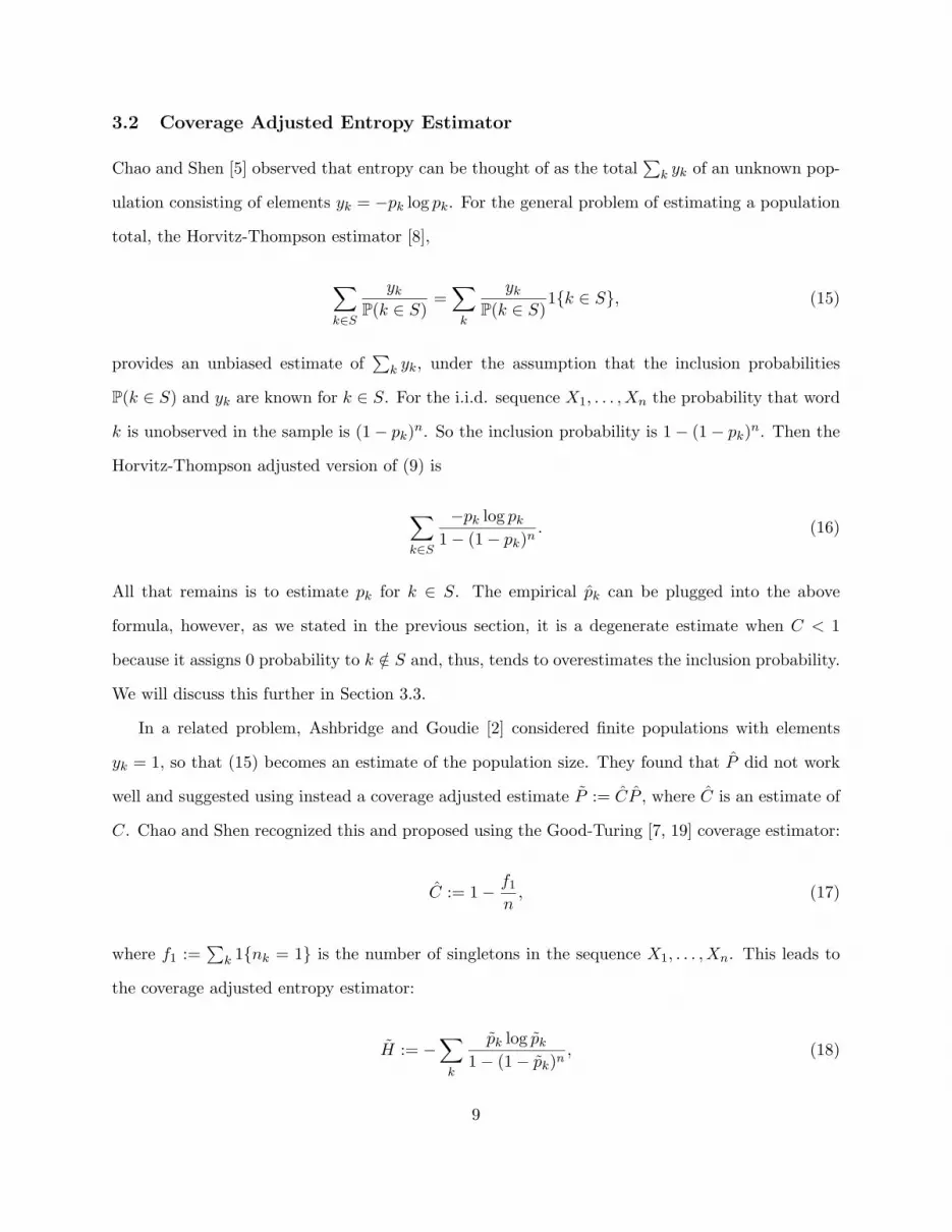
3.2 Coverage Adjusted Entropy Estimator

Chao and Shen [5] observed that entropy can be thought of as the total∑

k yk of an unknown pop-

ulation consisting of elements yk = −pk log pk. For the general problem of estimating a population

total, the Horvitz-Thompson estimator [8],

∑k∈S

yk

P(k ∈ S)=

∑k

yk

P(k ∈ S)1{k ∈ S}, (15)

provides an unbiased estimate of∑

k yk, under the assumption that the inclusion probabilities

P(k ∈ S) and yk are known for k ∈ S. For the i.i.d. sequence X1, . . . , Xn the probability that word

k is unobserved in the sample is (1− pk)n. So the inclusion probability is 1− (1− pk)n. Then the

Horvitz-Thompson adjusted version of (9) is

∑k∈S

−pk log pk

1− (1− pk)n. (16)

All that remains is to estimate pk for k ∈ S. The empirical pk can be plugged into the above

formula, however, as we stated in the previous section, it is a degenerate estimate when C < 1

because it assigns 0 probability to k /∈ S and, thus, tends to overestimates the inclusion probability.

We will discuss this further in Section 3.3.

In a related problem, Ashbridge and Goudie [2] considered finite populations with elements

yk = 1, so that (15) becomes an estimate of the population size. They found that P did not work

well and suggested using instead a coverage adjusted estimate P := CP , where C is an estimate of

C. Chao and Shen recognized this and proposed using the Good-Turing [7, 19] coverage estimator:

C := 1− f1

n, (17)

where f1 :=∑

k 1{nk = 1} is the number of singletons in the sequence X1, . . . , Xn. This leads to

the coverage adjusted entropy estimator:

H := −∑

k

pk log pk

1− (1− pk)n, (18)

9

where pk := Cpk. Chao and Shen gave an argument for CP based on a conditioning property of

the multinomial distribution. In the next section we give a different derivation from the perspective

of regularization of an empirical risk, and state why C works well.

3.3 Regularized Probability Estimation

Consider the problem of estimating P under the entropy loss L(q, x) = − logQ(x), for Q satisfying

Q(k) = qk ≥ 0 and∑qk = 1. This loss function is closely aligned with the problem of entropy

estimation because the risk, i.e. the expected loss on a future observation,

R(Q) := −E logQ(Xn+1) (19)

is uniquely minimized by Q = P and its optimal value is the entropy of P . The MLE P minimizes

the empirical version of the risk

R(Q) := − 1n

n∑i=1

logQ(Xi). (20)

As stated previously in Section 3.1, this is a degenerate estimate when there are unobserved words.

More precisely, if the expected coverage EC < 1 (which is true in general), then R(P ) = ∞.

Analogously to (8), the expectation in (19) can be split into two parts by conditioning on

whether Xn+1 is a previously observed word or not:

R(Q) =− E[logQ(Xn+1)|Xn+1 ∈ S] P(Xn+1 ∈ S)+

− E[logQ(Xn+1)|Xn+1 /∈ S] P(Xn+1 /∈ S).(21)

Since P(Xn+1 ∈ S) does not depend on Q, minimizing (21) with respect to Q is equivalent to

minimizing

−E[logQ(Xn+1)|Xn+1 ∈ S]− λ∗E[logQ(Xn+1)|Xn+1 /∈ S], (22)

where λ∗ = P(Xn+1 /∈ S)/P(Xn+1 ∈ S). We cannot distinguish the probabilities of the unobserved

words on the basis of the sample. So consider estimates Q which place constant probability on

10

x /∈ S. Equivalently, these estimates treat the unobserved words as a single class and so the risk

reduces to the equivalent form:

−E[logQ(Xn+1)|Xn+1 ∈ S]− λ∗E log

[1−

∑k∈S

Q(k)

]. (23)

The above expectations only involve evaluating Q at observed words. Thus, (20) is more natural as

an estimate of −E[logQ(Xn+1)|Xn+1 ∈ S], than as an estimate of R(Q). If we let λ be any estimate

of the odds ratio λ∗ = P(Xn+1 /∈ S)/P(Xn+1 ∈ S), then we arrive at the regularized empirical risk.

R(q;λ) := − 1n

∑i

logQ(Xi)− λ log

[1−

∑i

Q(Xi)

]. (24)

This is the usual empirical risk with an additional penalty on the total mass assigned to observed

words. It can be verified that the minimizer, up to an equivalence, is (1 + λ)−1P . This estimate

shrinks the MLE towards 0 by the amount (1+λ)−1. Any Q which agrees with (1+λ)−1P on S is a

minimizer of (24). Note that (1+λ∗)−1 = P(Xn+1 ∈ S) = EC is the expected coverage, rather than

the sample coverage C. C can be used to estimate both EC and C, however it is actually better as

an estimate of EC because McAllester and Schapire [12] have shown that C = C +OP (log n/√n),

whereas we prove in the appendix:

Proposition 1. 0 ≥ E(C−C) = −∑

k p2k(1−pk)n−1 ≥ (1−1/n)n−1/n ∼ −e−1/n and Var C ≤ 4/n.

So C is a 1/√n consistent estimate of EC. Using C to estimate EC = (1 + λ∗)−1, we obtain

the coverage adjusted probability estimate P = CP .

3.4 Convergence Rates

In the infinite m case, Antos and Kontoyiannis [1] proved that the MLE is universally consistent

almost surely and in L2, provided that the entropy exists. However, they also showed that there

can be no universal rate of convergence for entropy estimation. Some additional restriction must

be made beyond the existence of entropy in order to obtain a rate of convergence. Wyner and

Foster [26] found that for the weakest natural restriction,∑

k pk(log pk)2 < ∞, the best rate of

11

convergence, to first order, is OP (1/ log n). They proved that the MLE and an estimator based

on match lengths achieves this rate. Our main theoretical result is that the coverage adjusted

estimator also achieves this rate.

Theorem 1. Suppose that∑

k pk(log pk)2 <∞. Then as n→∞,

H = H +OP (1/ log n). (25)

In the previous section we employed C = 1 − f1/n, in the regularized empirical risk (24). As

for the observed sample coverage, C = P(Xn+1 ∈ S|S), McAllester and Schapire [12] proved that

C = P(Xn+1 ∈ S|S)+OP (log n/√n), regardless of the underlying distribution. Our theorem below

together with McAllester and Schapire’s implies a rate of convergence on the total probability of

unobserved words.

Theorem 2. Suppose that∑

k pk| log pk|q <∞. Then as n→∞, almost surely,

C = 1−O(1/(log n)q). (26)

Corollary. Suppose that∑

k pk| log pk|q <∞. Then as n→∞,

1− C = P(Xn+1 /∈ S|S) = OP (1/(log n)q). (27)

Proof. This follows from the above theorem and Theorem 3 of [12] which implies |C − P(Xn+1 ∈

S|S)| ≤ oP (1/(log n)q) because

0 ≤ P(Xn+1 /∈ S|S) ≤ |1− C|+ |C − P(Xn+1 ∈ S|S)| (28)

and OP (1/(log n)q) + oP (1/(log n)q) = OP (1/(log n)q).

We defer the proofs of Theorems 1 and 2 to Appendix A. At the time of writing, the only other

entropy estimators proved to be consistent and asymptotically first-order optimal in the finite

entropy variance case that we are aware of are the MLE and Wyner and Foster’s modified match

12

length estimator. However, the OP (1/ log n) rate, despite being optimal, is somewhat discouraging.

It says that in the worst case we will need an exponential number of samples to estimate the entropy.

Furthermore, the asymptotics are unable to distinguish the coverage adjusted estimator from the

MLE, which has been observed to be severely biased. In the next section we use simulations to

study the small-sample performance of the coverage adjusted estimator and the MLE, along with

other estimators. The results suggest that in this regime their performances are quite different.

4 Simulation Study

We conducted a large number of simulations under varying conditions to investigate the performance

of the coverage adjusted estimator (CAE) and compare with four other estimators:

• Empirical Plug-in (MLE): defined in (3).

• Miller-Maddow corrected MLE (MM): based on the asymptotic bias formula provided by

Miller [13] and Basharin [3]. It is derived from equation (4) by estimating m by the number

of distinct words observed m =∑

k 1{nk ≥ 1} and adding (m− 1)/(2n) to the MLE.

• Jackknife (JK): proposed by Zahl [27]. It is a bias corrected version of the MLE obtained by

averaging all n leave-one-out estimates.

• Best Upper Bounds (BUB): proposed by Paninski [16]. It is obtained by numerically mini-

mizing a worst case error bound for a certain class of linear estimators for a distribution with

known support size m.

The NSB estimator proposed by [14] was not included in our simulation comparison because of

problems with the software and its computational cost. We also tried their asymptotic formula for

their estimator in the “infinite (or unknown)” m case:

ψ(1)/ ln(2)− 1 + 2 log n− ψ(n− m), (29)

where ψ(z) = Γ′(z)/Γ(z) is the digamma function. However, we were also unable to get it to work

because it seemed to increase unboundedly with the sample size, even for m = ∞ cases.

13

There are two sets of experiments consisting of multiple trials. The first set of experiments

concern some simple, but popular model distributions. The second set of experiments deal with

neuronal data recorded from primate visual and avian auditory systems. It departs from the

theoretical assumptions of Section 3 in that the observations are dependent.

Chao and Shen [5] also conducted a simulation study of the coverage adjusted estimator for

distributions with small m and showed that it performs reasonably well even when there is a

relatively large fraction of unobserved words. Their article also contains examples from real data

sets concerning diversity of species. The experiments presented here are intended to complement

their results and expand the scope.

Practical Considerations

We encountered a few practical hurdles when performing these experiments. The first is that the

coverage adjusted estimator is undefined when the sample consists entirely of singletons. In this

case C = 0 and p = 0. The probability of this event decays exponentially fast with the sample

size, so it is only an issue for relatively small samples. To deal with this matter we replaced the

n denominator in the definition of C with n + 1. This minor modification does not affect the

asymptotic behavior of the estimator, and allows it to be defined for all cases.3

The BUB estimator assumes that the number of words m is finite and requires that it be

specified. m is usually unknown, but sometimes an upper-bound on m may be assumed. To

understand the effect of this choice we tried three different variants on the BUB estimator’s m

parameter:

• Understimate (BUB-): The naive m as defined above for the Miller-Maddow corrected MLE.

• Oracle value (BUB.o): The true m in the finite case and d2He in the infinite case.

• Overestimate (BUB+): Twice the oracle value for the first set of experiments and the maxi-

mum number of words |X | for the second set of neuronal data experiments.3Another variation is to add .5 to the numerator and 1 to the denominator.

14

support (k =) pk H Var[log p(X)]Uniform 1, . . . , 1024 1/1024 10 0

Zipf 1, . . . , 1024 k−1/∑

k k−1 7.51 9.59

Poisson 1, . . . ,∞ 1024k/(k!e1024) 7.05 1.04Geometric 1, . . . ,∞ (1023/1024)k−1/1024 11.4 2.08

Table 1: Standard models considered in the first set of experiments.

Although the BUB estimator is undefined for the m infinite case, we still tried using it, defining the

m parameter of the oracle estimator to be d2He. This is motivated by the Asymptotic Equipartition

Property (AEP) [6], which roughly says that, asymptotically, 2H is the effective support size of the

distribution. There are no theoretical guarantees for this heuristic use of the BUB estimator, but

it did seem to work in the simulation cases below. Again, this is an oracle value and not actually

known in practice. The implementation of estimator was adapted from software provided by the

author of [16] and its numerical tuning parameters were left as default.

Experimental Setup

In each trial we sample from a single distribution and compute each estimator’s estimate of the

entropy. Trials are repeated, with 1,000 independent realizations.

Standard Models We consider the four discrete distributions shown in Table 1. The uniform

and truncated Zipf distributions have finite support (m = 1, 024), while the Poisson and geometric

have infinite support. The Zipf distribution is very popular and often used to model linguistic data.

It is sometimes referred to as a “power law.” We generated i.i.d. samples of varying sample size (n)

from each distribution and computed the respective estimates. We also considered the distribution

of distinct words in James Joyce’s novel Ulysses. We found that results were very similar to that

of the Zipf distribution and did not include them in this article.

Neuronal Data Here we consider two real neuronal data sets obtained from the Neural Prediction

Challenge (http://neuralprediction.berkeley.edu/), first presented in [22]. We fit a variable

length Markov chain (VLMC) to subsets of each data set and treated the fitted models as the

15

depth (msec) X word length T |X | H H/T

Field L VLMC 232 (232) {0, 1}10 10 1,024 1.51 0.151232 (232) {0, 1}15 15 32,768 2.26 0.150

V1 VLMC 3 (48) {0, 1, . . . , 5}5 5 7,776 8.32 1.663 (48) {0, 1, . . . , 5}6 6 46,656 9.95 1.66

Table 2: Fitted VLMC models. Entropy (H) was computed by Monte Carlo with 106 samples fromthe stationary distribution. H/T is the entropy of the word divided by its length.

truth. Our goal was not to model the neuronal data exactly, but to construct an example which

reflects real neuronal data, including any inherent dependence. This experiment departs from the

assumption of independence for the theoretical results. See [10] for a general overview of the VLMC

methodology.

From the first data set, we extracted 10 repeated trials, recorded from a single neuron in the Field

L area of avian auditory system during natural song stimulation. The recordings were discretized

into ∆t = 1 millisecond bins and consist of sequences of 0’s and 1’s indicating the absence or

presence of a spike. We concatenated the ten recordings before fitting the VLMC (with state space

{0, 1}). A complete description of the physiology and other information theoretic calculations from

the data can be found in [9].

The other data set contained several separate single neuron recording sequences from the V1

area of primate visual system, during a dynamic natural image stimulation. We used the longest

contiguous sequence from one particular trial. This consisted of 3,449 spike counts, ranging from 0

to 5. The counts are number of spikes occurring during consecutive ∆t = 16 millisecond periods.

(For the V1 data, the state space of the VLMC is {0, 1, 2, 3, 4, 5}). The resulting fits for both data

sets are shown in Table 2. Note that for each VLMC, H/T is nearly the same for both choices of

word length (cf. the remarks under equation (2) in Section 2).

The (maximum) depth of the VLMC is a measure of time dependence in the data. For the Field

L data, the dependence is long, with the VLMC looking 232 time periods (232 msec) into the past.

This may reflect the nature of the stimulus in the Field L case. For the V1 data, the dependence

is short with the fitted VLMC looking only 3 time periods (48 msec) into the past.

Samples of length n were generated from the stationary distribution of the fitted VLMCs. We

16

subdivided each sample into non-overlapping words of length T . Figure 2 shows this for the Field

L model with T = 10. We tried two different word lengths for each model. The word lengths and

entropies are shown in Table 2. We then computed each estimator’s estimate of entropy on the

words and divided by the word length to get an estimate of the entropy rate of the word.

We treat m as unknown in this example and did not include the oracle BUB.o in the experiment.

We used the maximum possible value of m, i.e. |X | for BUB+. In the case of Field L with T = 10,

this is 1,024. The other values are shown in Table 2.

Results

Standard Models The results are plotted in Figures 3, 4. It is surprising that good estimates

can be obtained with just a few observations. Estimating m from its empirical value marginally

improves MM over the MLE. The naive BUB-, which also uses the empirical value of m, performs

about the same as JK.

Bias apparently dominates the error of most estimators. The CAE estimator trades away bias

for a moderate amount of variance. The RMSE results for the four distributions are very similar.

The CAE estimator performs consistently well, even for smaller sample sizes, and is competitive

with the oracle BUB.o estimator. The Zipf distribution example seems to be the toughest case for

the CAE estimator, but it still performs relatively well for sample sizes of at least 1,000.

Neuronal Data The results are presented in Figures 5 and 6. The effect of the dependence in

the sample sequences is not clear, but all the estimators seem to be converging to the truth. CAE

consistently performs well for both V1 and Field L, and really shines in the V1 example. However,

for Field L there is not much difference between the estimators, except for BUB+.

BUB+ uses m equal to the maximum number of words |X | and performs terribly because the

data are so sparse. The maximum entropy corresponding to |X | is much larger than the actual

entropy. In the Field L case, the maximum entropies are 10 and 15, while the actual entropies are

1.51 and 2.26. In the V1 case, the maximum entropies are 12.9 and 15.5, while the actual entropies

are 8.32 and 9.95. This may be the reason that the BUB+ estimator has such a large positive

bias in both cases, because the estimator is designed to approximately minimize a balance between

17

●

●

●●

●●

●●

●●

●●

●●●

●●

●●●●●●●●●●●

●●●●●●

● ●●●●

●● ● ●

10 20 50 100 200 500 2000 5000

68

1012

14

Uniform Distribution

sample size (n)

Est

imat

e

●

●

●

●●

●●●● ● ●●●● ● ●●●●●●●●●●●●●●●●●●● ● ●●●● ● ● ● ●

−−

−−−−−−−

−−−−−−−−−−−

−−−−−−−−−

−−−−−−−−−−

− − − −

−−

−−−−−−−

−−−−−−−−−−−

−−−−−−−−−

−−−−−−−−−−

− − − −

−−

−−−−−−−

−−−−−−−−−−−

−−−−−−−−−−−−−

−−−−−− − − − −

−−

−−

−−−−−−−−−−

−−−−−−−−−−−

−−−−−−−−−−−−−− − − − −

−

−

−−

−−−−−−−−−−−−−−−−−−−−−−−−−−−−−−−−−−− − − − −

−

−

−−−−−

−−−−−−−−−−−−−−−−−−−−−−−−−−−−−− − − − −

−

−

−−

−−−−−−−−−−−−−−−−−−−−−−−−−−−−−−−−−−− − − − −

−−

−−−−−−−

−−−−−−−−−−−

−−−−−−−−−

−−−−−−−−−−

− − − −

−−

−−−−−−−

−−−−−−−−−−−

−−−−−−−−−

−−−−−−−−−−

− − − −

−−

−−−−−−−

−−−−−−−−−−−

−−−−−−−−−−−

−−−−−−−− − − − −

−−

−−

−−−−−−−−−−

−−−−−−−−−−−

−−−−−−−−−−−−−− − − − −

−

−

−−

−−−−−−−−−−−−−−−−−−−−−−−−−−−−−−−−−−− − − − −

−

−

−−−−−

−−−−−−−−−−−−−−−−−−−−−−−−−−−−−− − − − −

−

−−

−−−−−−−−−−−−−−−−−−−−−−−−−−−−−−−−−−−− − − − −

● ●MLEMMJKBUB−

BUB.oBUB+CAE

●

●

●

●●

●

●

●

●●

●

●

●●

●●

●●●●●●●●●●●●●●●

●●

●●

●

●● ● ●

10 20 50 100 200 500 2000 5000

01

23

4

sample size (n)

RM

SE

●

●

●

●

●

●●●● ● ●●●● ● ●●●●●●●●●●●●●●●●●●● ● ●●●● ● ● ● ●

●

●●

●●

●●●●● ●●●●

● ●●●●●●●●●●●●●●●●●●●

● ●●●●● ● ● ●

10 20 50 100 200 500 2000 5000

46

810

Zipf Distribution

sample size (n)

Est

imat

e

●

●

●

●

●●

●●●

● ●●●● ● ●●●●●●●●●●●●●●●●●●● ● ●●●● ● ● ● ●

−−

− −−−−−−−−−−−−−−−−−−−−−−−−−−−−−−−

−−−−− − − − −

−−

− −−−−−−−−−−−−−−−−−−−−−−−−−−−−−−−

−−−−− − − − −

−−

− −−−−−−−−−−−−−−−−−−−−−−−−−−−−−−−−−−−− − − − −

−−

− −−−−−−−−−−−−−−−−−−−−−−−−−−−−−−−−−−−− − − − −

−

−

−−

−−−−−−−−−−−−−−−−−−−−−−−−−−−−−−−−−− − − − −

−

−−−−−

−−−−−−−−−−−−−−−−−−−−−−−−−−−−−− − − − −

− − − −−−−−−−−−−−−−−−−−−−−−−−−−−−−−−−−−−−− − − − −

−−

− −−−−−−−−−−−−−−−−−−−

−−−−−−−−−−−−−−−−−

− − − −

−−

− −−−−−−−−−−−−−−−−−−−−−−−−−−−−

−−−−−−−− − − − −

−−

− −−−−−−−−−−−−−−−−−−−−−−−−−−−−−−−

−−−−− − − − −

−−

− −−−−−−−−−−−−−−−−−−−−−−−−−−−−−−−

−−−−− − − − −

−

−

−−

−−−−−−−−−−−−−−−−−−−−−−−−−−−−−−−−−−− − − − −

−

−

−−−−−

−−−−−−−−−−−−−−−−−−−−−−−−−−−−−− − − − −

− − − −−−−−−−−−−−−−−−−−−−−−−−−−−−−−−−−−−−− − − − −

● ●MLEMMJKBUB−

BUB.oBUB+CAE

●

●

●

●

●●

●●

●●

●●

●●

●●

●●

●●●●●●●●●●●●●●●●● ●●●●

●● ● ●

10 20 50 100 200 500 2000 5000

01

23

4

sample size (n)

RM

SE

●

●

●

●

●

●●

●

●●

●●● ● ●●●●●●●●●●●●●●●●●●● ● ●●●● ● ● ● ●

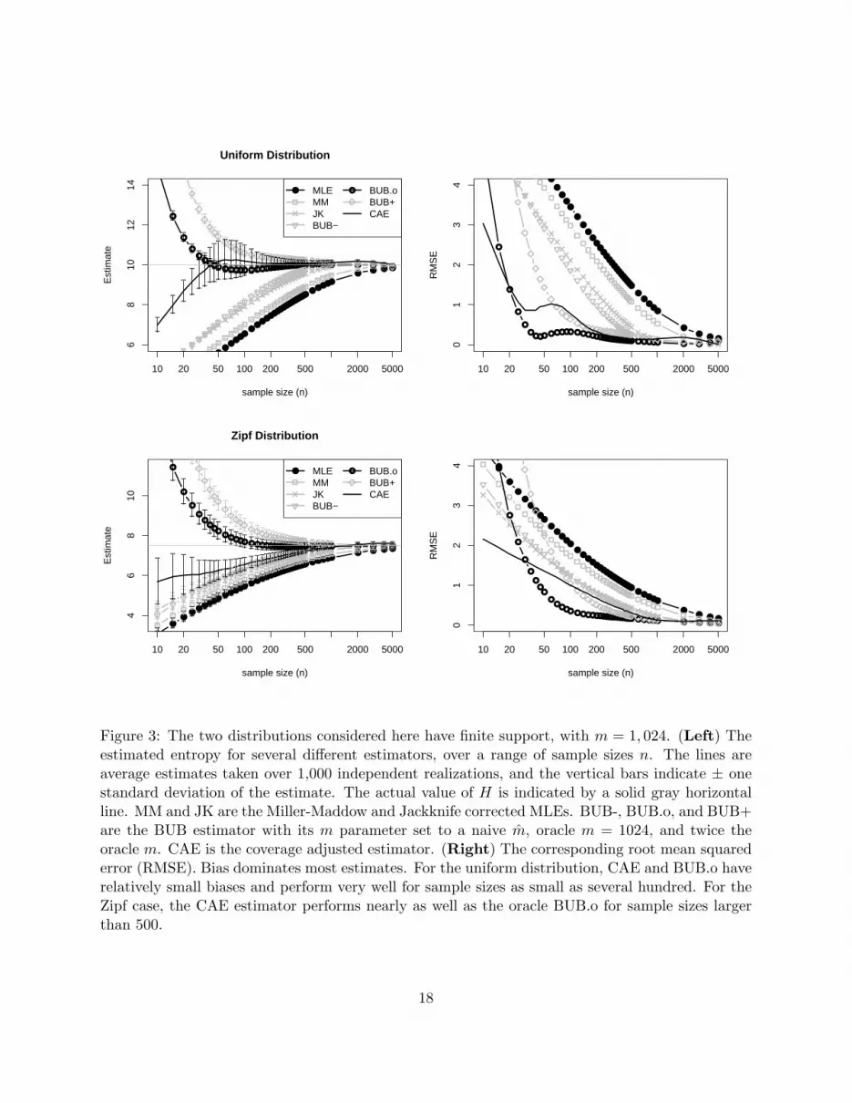
Figure 3: The two distributions considered here have finite support, with m = 1, 024. (Left) Theestimated entropy for several different estimators, over a range of sample sizes n. The lines areaverage estimates taken over 1,000 independent realizations, and the vertical bars indicate ± onestandard deviation of the estimate. The actual value of H is indicated by a solid gray horizontalline. MM and JK are the Miller-Maddow and Jackknife corrected MLEs. BUB-, BUB.o, and BUB+are the BUB estimator with its m parameter set to a naive m, oracle m = 1024, and twice theoracle m. CAE is the coverage adjusted estimator. (Right) The corresponding root mean squarederror (RMSE). Bias dominates most estimates. For the uniform distribution, CAE and BUB.o haverelatively small biases and perform very well for sample sizes as small as several hundred. For theZipf case, the CAE estimator performs nearly as well as the oracle BUB.o for sample sizes largerthan 500.

18

●

●

●●

●●

●●●●

●●●● ● ●●●●●●●●●●●●●●●●●●● ● ●●●● ● ● ● ●

10 20 50 100 200 500 2000 5000

46

810

Poisson Distribution

sample size (n)

Est

imat

e

● ● ● ● ● ●●●● ● ●●●● ● ●●●●●●●●●●●●●●●●●●● ● ●●●● ● ● ● ●

−−

− −−−−−−−−−−−−−−−−−−−−−−

−−−−−−−−−−−−−− − − − −

−−

− −−−−−−−−−−−−−−−−−−−−−−−−−−−−−−−−−−−− − − − −

−−

− −−−−−−−−−−−−−−−−−−−−−−−−−−−−−−−−−−−− − − − −

−−

−−−−−−−−−−−−−−−−−−−−−−−−−−−−−−−−−−−−− − − − −

− − − −−−−−−−−−−−−−−−−−−−−−−−−−−−−−−−−−−−− − − − −

−− − −−−−−−−−−−−−−−−−−−−−−−−−−−−−−−−−−−−− − − − −

−− − −−−−−−−−−−−−−−−−−−−−−−−−−−−−−−−−−−−− − − − −

−−

−−−−−−−

−−−−−−−−−−−−−−−−−−−−−−−−−−−−−− − − − −

−−

− −−−−−−−−−−−−−−−−−−−−−−−−−

−−−−−−−−−−− − − − −

−−

− −−−−−−−−−−−−−−−−−−−−−−−−−−−−−−−−−−−− − − − −

−−

−−−−−−−−−−−−−−−−−−−−−−−−−−−−−−−−−−−−− − − − −

− − − −−−−−−−−−−−−−−−−−−−−−−−−−−−−−−−−−−−− − − − −

−− − −−−−−−−−−−−−−−−−−−−−−−−−−−−−−−−−−−−− − − − −

−− − −−−−−−−−−−−−−−−−−−−−−−−−−−−−−−−−−−−− − − − −

● ●MLEMMJKBUB−

BUB.oBUB+CAE

●

●

●

●

●

●●

●●

●●

●●

●●

●●

●●●●●●●●●●●●●●●●● ● ●●●● ● ● ● ●

10 20 50 100 200 500 2000 5000

01

23

4

sample size (n)

RM

SE

● ● ● ● ● ●●●● ● ●●●● ● ●●●●●●●●●●●●●●●●●●● ● ●●●●● ● ● ●

●●

●●

●●

●●

●●

●●

●●

●●●●●●●●●

●●●●●●

●●●●

●●●●

●●

● ●

10 20 50 100 200 500 2000 5000

810

1214

Geometric Distribution

sample size (n)

Est

imat

e

●

●

●

●

●

●●

●●

●●● ● ●●●●●●●●●●●●●●●●●●● ● ●●●● ● ● ● ●

−−

−−−−−−−−−−−

−−−−−−−−−

−−−−−−−−−

−−−−−−−−

− − −

−−

−−−−−−−−−−−

−−−−−−−−−

−−−−−−−−−

−−−−−−−− − − −

−−

−−−−−−−

−−−−−−−−−−−

−−−−−−−−−

−−−−−−−−−−

− − − −

−−

−−

−−−−−−−−−−

−−−−−−−−−−

−−−−−−−−−−

−−−−−− − − −

−

−

−

−−−−

−−−−−−−−−−−−−−−−−−−−−−−−−−−−−− − − − −

−

−−

−−−−−

−−−−−−−−−−−−−−−−−−−−−−−−− − − − −

−

−

−−

−−−−−

−−−−−−−−−−−−−−−−−−−−−−−−−−−−−− − − − −

−−−−−−−

−−−−−−−−−−−

−−−−−−−

−−−−−−−−−−−−

−− − −

−−

−−−−−−−−−−−

−−−−−−−−−

−−−−−−−−−

−−−−−−−− − − −

−−

−−−−−−−

−−−−−−−−−−−

−−−−−−−−−

−−−−−−−−−−

− − − −

−−

−−

−−−−−−−−−−

−−−−−−−−−−

−−−−−−−−−−

−−−−−− − − −

−

−

−

−−−−

−−−−−−−−−−−−−−−−−−−−−−−−−−−−−− − − − −

−

−

−−

−−−−−

−−−−−−−−−−−−−−−−−−−−−−−−− − − − −

−

−−

−−−−−−

−−−−−−−−−−−−−−−−−−−−−−−−−−−−−− − − − −

● ●MLEMMJKBUB−

BUB.oBUB+CAE

●

●●

●

●

●

●●

●●●●●●●●●●●●●●●●

●●

●●

●

●

●●

●

10 20 50 100 200 500 2000 5000

01

23

4

sample size (n)

RM

SE

●

●

●

●

●

●

●

●●●●

● ●●●●●●●●●●●●●●●●●●● ● ●●●●● ● ● ●

Figure 4: The two distributions considered here have infinite support, with m = ∞. (Left) Theestimated entropy for several different estimators, over a range of sample sizes n. The lines areaverage estimates taken over 1,000 independent realizations, and the vertical bars indicate ± onestandard deviation of the estimate. The actual value of H is indicated by a solid gray horizontalline. MM and JK are the Miller-Maddow and Jackknife corrected MLEs. BUB-, BUB.o, andBUB+ are the BUB estimator with its m parameter set to a naive m, oracle m = d2He, and twicethe oracle m. CAE is the coverage adjusted estimator. (Right) The corresponding root meansquared error (RMSE). Results are very similar to those in the previous figure, the CAE estimatorperforms nearly as well as the oracle BUB.o.

19

● ● ●●●●●●●●●●●●●●●●●●● ● ●●●● ● ● ● ● ● ●●●● ● ● ● ●

100 200 500 2000 5000 20000

0.00

0.10

0.20

0.30

Field L VLMC (T=10)

sample size (n)

Est

imat

e

−−−−−−−−−−−−−−−−−−−−−−−−−− − − − −−−−−− − − − −−−−−−−−−−−−−−−−−−−−−−−−−−− − − − −−−−−− − − − −−−−−−−−−−−−−−−−−−−−−−−−−−− − − − −−−−−− − − − −−−−−−−−−−−−−−−−−−−−−−−−−−− − − − −−−−−− − − − −

−−−−−−−−−

−−−−−

−− − −−−−−− − − − −

−−−−−−−−−−−−−−−−−−−−−−−−−−− − − −−−−−− − − − −

−−−−−−−−−−−−−−

−−−−−−−−−−−−

− − − −−−−−− − − − −

−−−−−−−−−−−−−−

−−−−−−−−−−−−

− − − −−−−−− − − − −

−−−−−−−−−−−−−

−−−−−−−−−−−−− − − − −−−−−− − − − −

−−−−−−−−−−−−

−−−−−−−−−−−−−− − − − −−−−−− − − − −

−−−−−−−−−−−−−−

−−−−−

−− − −−−−−− − − − −

−−−−−−−−−−−−

−−−−−−−−−−−−−− − − − −−−−−− − − − −

● MLEMMJK

BUB−BUB+CAE

● ●●●●●●●●●●●●●●●●●●●● ● ●●●●

●● ● ● ● ●●●● ● ● ● ●

100 200 500 2000 5000 20000

0.00

0.05

0.10

0.15

0.20

sample size (n)

RM

SE

●● ●●●●●●●●●●●●●●

●●●●●● ●●●●

● ● ● ● ● ●●●● ● ● ● ●

100 200 500 2000 5000 20000

0.00

0.10

0.20

0.30

Field L VLMC (T=15)

sample size (n)

Est

imat

e

−−−−−−−−−−−−−−−−−−−−−−−−−− − − − −−−−−− − − − −

−−−−−−−−−−−−−−−−−−−−−−−−−− − − − −−−−−− − − − −−−−−−−−−−−−−−−−−−−−−−−−−−− − − − −−−−−− − − − −

−−−−−−−−−−−−−−−−−−−−−−−−−− − − − −−−−−− − − − −

−

−−−−

−

−− −

−−−−−−−−−−−−−−−−−−−−−−−−−− − − − −−−−−− − − − −

−−−−−−−−−−−−−−−−−−

−−−−−−−−− − − −−−−−− − − − −

−−−−−−−−−−−−−−−−

−−−−−−−−−−− − − −−−−−− − − − −

−−−−−−−−−−−−−−−−

−−−−−−−−−−− − − −−−−−− − − − −

−−−−−−−−−−−−−−−−−

−−−−−−−−−− − − −−−−−− − − − −

−

−−−−

−−

− −

−−−−−−−−

−−−−−−−−−−−−−

−−−−− − − − −−−−−− − − − −

● MLEMMJK

BUB−BUB+CAE

●● ●●●●●●●●●●●●●●●●●●●

● ●●●●

●● ● ● ● ●●●● ● ● ● ●

100 200 500 2000 5000 20000

0.00

0.05

0.10

0.15

0.20

sample size (n)

RM

SE

Figure 5: (Left) The estimated entropy rate for several different estimators. Samples of size n aredrawn from a stationary VLMC used to model neuronal data from Field L of avian auditory system.A single sample corresponds to 1 millisecond of recording time. We followed the “direct method”and divided each sample sequence into words of length T . In the top row the word length is T = 10and the maximum number of words |X | is 1,024. In the bottom row T = 15 and |X | = 32, 768. Thelines are average estimates taken over 1,000 independent realizations, and the vertical bars indicate± one standard deviation of the estimate. The actual value of H/T is indicated by a solid grayhorizontal line. MM and JK are the Miller-Maddow and Jackknife corrected MLEs. BUB- andBUB+ are the BUB estimator with its m parameter set to a naive m and the maximum possiblenumber of words |X |: 1,024 for the top row and 32,768 for the bottom. CAE is the coverage adjustedestimator. (Right) The corresponding root mean squared error (RMSE). The BUB+ estimatorhas a considerably large bias in both cases. The CAE estimator has a moderate balance of biasand variance and shows a visible improvement over all other estimators in the larger (T = 15) wordcase.

20

●●

●●●●●●●●●●●●●●●

●●●●● ●●●●

●● ● ● ● ●●●● ● ● ● ●

100 200 500 2000 5000 20000

1.0

1.5

2.0

2.5

V1 VLMC (T=5)

sample size (n)

Est

imat

e

−−−−−−−−−−−−−−

−−−−−−−−−−−−

− − − −−−−−− − − − −

−−−−−−−−−−−−−−

−−−−−−−−−−−−

− − − −−−−−− − − − −

−−−−−−−−−−−−−−−−−

−−−−−−−−− − − − −−−−−− − − − −

−−−−−−−−−−−−−−

−−−−−−−−−−−− − − − −−−−−− − − − −

−−−−−−−−−−−−

−−−−−

−− − −−−−−− − − − −−−−−−−−−−−−−−−−−−−−−−−−−−− − − − −−−−−− − − − −

−−−−−−−−−−−−−

−−−−−−−−−−−−−

− − − −−−−−− − − − −

−−−−−−−−−−−−−−

−−−−−−−−−−−−

− − − −−−−−− − − − −

−−−−−−−−−−−−−−

−−−−−−−−−−−−

− − − −−−−−− − − − −

−−−−−−−−−−−−−−

−−−−−−−−−−−−

− − − −−−−−− − − − −

−−−−−−−−−−−−−−

−−−−−

− − − −−−−−− − − − −

−−−−−−−−−−−−−−−−−−−−−

−−−−− − − − −−−−−− − − − −

● MLEMMJK

BUB−BUB+CAE

●●

●●

●●

●●●●●●●●●●●●●●●

●●

●●●

●

●●

● ● ●●●●● ● ● ●

100 200 500 2000 5000 20000

0.0

0.2

0.4

0.6

0.8

1.0

sample size (n)

RM

SE

●● ●●●●●●●●●●●

●●●●●●●●

● ●●●●

●●

● ● ● ●●●●● ● ● ●

100 200 500 2000 5000 20000

1.0

1.5

2.0

2.5

V1 VLMC (T=6)

sample size (n)

Est

imat

e

−−−−−−−−−−−−−−

−−−−−−−−−−−−

− − − −−−−−− − − − −

−−−−−−−−−−−−−−

−−−−−−−−−−−−

− − − −−−−−− − − − −

−−−−−−−−−−−−−−

−−−−−−−−−−−−

− − − −−−−−− − − − −

−−−−−−−−−−−−−

−−−−−−−−−−−−−

− − − −−−−−− − − − −

−

−

−−

−−−−−− − − −

−−−−−−−−−−−−−−−−−−−−−−−−−− − − − −−−−−− − − − −

−−−−−−−−−−−−−

−−−−−−−−−−−−−

− − − −−−−−−− − − −

−−−−−−−−−−−−−−

−−−−−−−−−−−−

− − − −−−−−− − − − −

−−−−−−−−−−−−−−

−−−−−−−−−−−−

− − − −−−−−− − − − −

−−−−−−−−−−−−−

−−−−−−−−−−−−−

− − − −−−−−− − − − −

−

−−

−−−−−−− − − −

−−−−−−−−−−−−−−−−−−−−−−−−−−

− − − −−−−−− − − − −

● MLEMMJK

BUB−BUB+CAE

●

●●

●●

●●●●●●●●●●●●●●●●

●●

●●

●

●

●●

●● ●●●●

●● ● ●

100 200 500 2000 5000 20000

0.0

0.2

0.4

0.6

0.8

1.0

sample size (n)

RM

SE

Figure 6: (Left) The estimated entropy rate for several different estimators. The samples of size nare drawn from a stationary VLMC used to model neuronal data from V1 of primate visual system.A single sample corresponds to 16 milliseconds of recording time. We followed the “direct method”and divided each sample sequence into words of length T . In the top row the word length is T = 5and the maximum number of words |X | is 7,776. In the bottom row T = 6 and |X | = 46, 656. Thelines are average estimates taken over 1,000 independent realizations, and the vertical bars indicate± one standard deviation of the estimate. The actual value of H/T is indicated by a solid grayhorizontal line. MM and JK are the Miller-Maddow and Jackknife corrected MLEs. BUB- andBUB+ are the BUB estimator with its m parameter set to a naive m and the maximum possiblenumber of words: 7,776 for the top row and 46,656 for the bottom. CAE is the coverage adjustedestimator. (Right) The corresponding root mean squared error (RMSE). The CAE estimator hasthe smallest bias and performs much better than the other estimators across all sample sizes.

21

upper-bounds on worst case bias and variance.

Summary

The coverage adjusted estimator is a good choice for situations where m is unknown and/or infinite.

In these situations, the use of an estimator which requires specification of m is disadvantageous

because a poor estimate (or upper-bound) of m, or the “effective” m in the infinite case, leads

to further error in the estimate. BUB.o, which used the oracle m, performed well in most cases.

However, it is typically not available in practice, because m is usually unknown.

The Miller-Maddow corrected MLE, which used the empirical value of m, improved on the

MLE only marginally. BUB-, which is BUB with the empirical value of m, performed better than

the MLE. It appeared to work in some cases, but not others. For BUB+, where we overestimated

or upper-bounded m (by doubling the oracle m, or using the maximal |X |), the bias and RMSE

increased significantly over BUB.o for small sample sizes. It appeared to work in some cases, but not

others–always alternating with BUB-. In the case of the neuronal data models, BUB+ performed

very poorly. In situations like this, even though an upper-bound on m is known, it can be much

larger than the “effective” m, and result in a gross error.

5 Conclusions

Our study has emphasized the value of viewing entropy estimation as a problem of sampling from

a population, here a population of words made up of spike train sequence patterns. The coverage

adjusted estimator performed very well in our simulation study, and it is very easy to compute.

When the word length m is known, the BUB estimator can perform better. In practice, however,

m is usually unknown and, as seen in V1 and Field L examples, assuming an upper bound on it

can result in a large error. The coverage-adjusted estimator therefore appears to us to be a safer

choice.

Other estimates of the probabilities of observed words, such as the profile-based estimator

proposed by Orlitsky et al. [15], might be used in place of P in the coverage adjusted entropy

estimator but that is beyond the scope of this article.

22

The V1 and Field L examples have substantial dependence structure, yet methods derived

under the i.i.d. assumption continue to perform well. It may be shown that both the direct method

and the coverage-adjusted estimator remain consistent under the relatively weak assumption of

stationarity and ergodicity, but the rate of convergence will depend on mixing conditions. On

the other hand, in the non-stationary case these methods become inconsistent. Stationarity is,

therefore, a very important assumption. We intend to discuss these issue at greater length in a

separate paper.

As is clear from our simulation study, the dominant source of error in estimating entropy is

often bias, rather than variance, which is typically not captured from computed standard errors.

An important problem for future investigation would therefore involve data-driven estimation of

bias in the case of unknown or infinite m.

Acknowledgements

The authors thank both the Theunissen Lab and Gallant Lab at the University of California,

Berkeley for providing the data sets. They also thank J. Victor and L. Paninski for helpful comments

and discussions on an earlier version of this work presented at the SAND3 poster session. V. Q. Vu

would like to gratefully acknowledge support from a NSF VIGRE Graduate Fellowship and from

NIDCD grant DC 007293. B. Yu would like to gratefully acknowledge support from NSF grant

DMS-03036508 and ARO grant W911NF-05-1-0104. This work began while Kass was a Miller

Institute Visiting Research Professor at the University of California, Berkeley. Support from the

Miller Institute is greatly appreciated. Kass’s work was also supported in part by NIMH grant

RO1-MH064537-04.

23

A Proofs

We first prove Theorem 2. The proof builds on the following application of a standard concentration

technique.

Lemma 1. C → 1 almost surely.

Proof. Consider the number of singletons f1 as a function of xn1 = (x1, . . . , xn). Modifying a single

coordinate of xn1 changes the number of singletons by at most 2 because the number of words

affected by such a change is at most 2. Hence C = 1 − f1/n changes by at most 2/n. Using

McDiarmid’s method of bounded differences, i.e. the Hoeffding-Azuma Inequality, gives

P(|C − EC| > ε) ≤ 2e−12nε2 (30)

and by consequence of the Borel-Cantelli Lemma, |C − EC| → 0 almost surely. To show that

EC → 1, we note that 1 ≥ (1− pk)n−1 → 0 for all pk > 0 and

|1− EC| = E1n

∑k

1{nk = 1} (31)

=∑

k

pk(1− pk)n−1 → 0 (32)

as n→∞ by the Bounded Convergence Theorem.

Proof of Proposition 1. The bias is

EC − P(Xn+1 ∈ S) = P(Xn+1 /∈ S)− E(1− C) (33)

=∑

k

pk(1− pk)n −∑

k

pk(1− pk)n−1 (34)

= −∑

k

p2k(1− pk)n−1. (35)

This quantity is trivially non-positive, and a little bit of calculus shows that the bias is maximized

24

by the uniform distribution pk = 1/n:

∑k

p2k(1− pk)n−1 ≤

∑k

pk max0≤x≤1

x(1− x)n−1 (36)

= max0≤x≤1

x(1− x)n−1 (37)

= (1− 1/n)n−1/n (38)

The variance bound can be deduced from equation (30), because Var C =∫∞0 P(|C − EC|2 > x)dx

and (30) implies ∫ ∞

0P(|C − EC|2 > x)dx ≤

∫ ∞

02e−

12nxdx = 4/n. (39)

Proof of Theorem 2. From (30) we conclude that C = EC +OP (n−1/2). So it suffices to show that

EC = 1 +O(1/(log n)q). Let εn = 1/√n. We split the summation in (32):

|1− EC| =∑

k:pk≤εn

pk(1− pk)n−1 +∑

k:pk>εn

pk(1− pk)n−1 (40)

Using Lemma 2 below, the first term on the right side is

∑k:pk≤εn

pk(1− pk)n−1 ≤∑

k:pk≤εn

pk = O(1/(log n)q) (41)

The second term is

∑k:pk>εn

pk(1− pk)n−1 ≤ (1− εn)n−1∑

k:pk>εn

pk (42)

≤ (1− εn)n−1 (43)

≤ exp(−(n− 1)/√n) (44)

by the well-known inequality 1 + x ≤ ex.

25

Lemma 2 (Wyner and Foster [26]).

∑k:pk≤ε

pk ≤∑

k pk| log pk|q

log(1/ε)q

Proof. Since log(1/x) is a decreasing function,

∑k:pk≤ε

pk

∣∣∣∣log1pk

∣∣∣∣q ≥ ∑k:pk≤ε

pk

∣∣∣∣log1ε

∣∣∣∣q (45)

and then we collect the log(1/ε)q term to the left side to derive the claim.

Proof of Theorem 1. Using the result of Wyner and Foster that under the above assumptions,

H = H +OP (1/ log n), it suffices to show |H − H| = OP (1/ log n). All summations below will only

be over k such that pk > 0 or pk > 0. It is easily verified that

H − H = −∑

k

pk log pk

1− (1− pk)n− pk log pk (46)

= −∑

k

[C

1− (1− pk)n− 1

]pk log pk︸ ︷︷ ︸

Dn

(47)

−∑

k

Cpk log C1− (1− pk)n︸ ︷︷ ︸

Rn

(48)

To bound Rn we will use the OP (1/(log n)2) rate of C from Theorem 2. Note that C/n ≤ Cpk =

pk ≤ 1 and by the decreasing nature of 1/[1− (1− pk)n]

|Rn| ≤| log C|

1− (1− C/n)n

∑k

pk =| log C|

1− (1− C/n)n(49)

By Lemma 1, C → 1 almost surely and since xn → 1 implies (1− xn/n)n → e−1, the right side is

∼ | log C|/(1− e−1) = OP (1/(log n)2). As for Dn,

|Dn| ≤ −∑

k

|C − 1|+ (1− pk)n

1− (1− pk)npk log pk (50)

26

and since pk ≥ C/n whenever pk > 0,

−∑

k

|C − 1|1− (1− pk)n

pk log pk ≤|C − 1|

1− (1− C/n)nH (51)

∼ |C − 1|1− e−1

H (52)

= OP (1/(log n)2) (53)

because H is consistent. The remaining part of Dn will require a bit more work and we will split

it according to the size of pk. Let εn = log n/n. Then

−∑

k

(1− pk)n

1− (1− pk)npk log pk =−

∑k:pk≤εn

(1− pk)n

1− (1− pk)npk log pk

−∑

k:pk>εn

(1− pk)n

1− (1− pk)npk log pk

(54)

Similarly to our previous argument, (1−pk)n

1−(1−pk)n is decreasing in pk. So the second summation on the

right side is

−∑

k:pk>εn

(1− pk)n

1− (1− pk)npk log pk ≤

(1− εn)n

1− (1− εn)nH (55)

= OP (1/n) (56)

For the remaining summation, we use the fact that pk ≥ C/n and the monotonicity argument once

more.

−∑

k:pk≤εn

(1− pk)n

1− (1− pk)npk log pk ≤ − (1− C/n)n

1− (1− C/n)n

∑k:pk≤εn

pk log pk (57)

By the consistency of C, the leading term converges to the constant e−1/(1 − e−1) and can be

ignored. Since − log pk ≤ log n,

−∑

k:pk≤εn

pk log pk ≤ log n∑

k:pk≤εn

pk (58)

27

We split the summation once last time, but according to the size of pk.

log n∑

k:pk≤εn

pk ≤ log n

∑k:pk>1/

√n

εn +∑

k:pk≤1/√

n

pk

(59)

≤ (log n)2√n

+ log n∑

k:pk≤1/√

n

pk, (60)

where we have used the fact that |{k : pk > 1/√n}| ≤

√n. Taking expectation, applying Lemma 2

and Markov’s Inequality shows that

= log n∑

k:pk≤1/√

n

pk = OP (1/ log n) (61)

The proof is complete because (log n)2/√n is also O(1/ log n).

References

[1] A. Antos and I. Kontoyiannis. Convergence properties of functional estimates for discrete

distributions. Random Structures and Algorithms, 19:163–193, 2001.

[2] J. Ashbridge and I. B. J. Goudie. Coverage-adjusted estimators for mark-recapture in hetero-

geneous populations. Communications in Statistics-Simulation, 29:1215–1237, 2000.

[3] G. P. Basharin. On a statistical estimate for the entropy of a sequence of independent random

variables. Theory of Probability and its Applications, 4:333–336, 1959.

[4] A. Borst and F. E. Theunissen. Information theory and neural coding. Nature Neuroscience,

2(11):947–957, 1999.

[5] A. Chao and T.-J. Shen. Nonparametric estimation of shannon’s index of diversity when there

are unseen species in sample. Environmental and Ecological Statistics, 10:429–443, 2003.

[6] T. Cover and J. Thomas. Elements of Information Theory. Wiley, 1991.

28

[7] I. J. Good. The population frequencies of species and the estimation of population parameters.

Biometrika, 40(3/4):237–264, 1953.

[8] D. G. Horvitz and D. J. Thompson. A generalization of sampling without replacement from a

finite universe. Journal of the American Statistical Association, 47(260):663–685, 1952.

[9] A. Hsu, S. M. N. Woolley, T. E. Fremouw, and F. E. Theunissen. Modulation power and phase

spectrum of natural sounds enhance neural encoding performed by single auditory neurons.

The Journal of Neurosccience, 24(41):9201–9211, 2004.

[10] M. Machler and P. Buhlmann. Variable length markov chains: Methodology, computing and

software. Technical Report 104, ETH Zurich, 2002.

[11] D. M. MacKay and W. S. McCulloch. The limiting information capacity of a neuronal link.

Bulletin of Mathematical Biophysics, 14:127–135, 1952.

[12] D. McAllester and R. E. Schapire. On the convergence rate of good-turing estimators. In

Proc. 13th Annu. Conference on Comput. Learning Theory, pages 1–6. Morgan Kaufmann,

San Francisco, 2000.

[13] G. Miller. Note on the bias of information estimates. In H. Quastler, editor, Information

Theory in Psychology: Problems and Methods II-B, pages 95–100. Free Press, Glencoe, IL,

1955.

[14] I. Nemenman, W. Bialek, and R. de Ruyter van Steveninck. Entropy and information in neural

spike trains: Progress on the sampling problem. Physical Review E, 69, 2004.

[15] A. Orlitsky, N. P. Santhanam, K. Viswanathan, and J. Zhang. On modeling profiles instead

of values. In Conference on Uncertainty in Artificial Intelligence, pages 426–435, 2004.

[16] L. Paninski. Estimation of entropy and mutual information. Neural Computation, 15:1191–

1253, 2003.

[17] D. H. Perkel and T. H. Bullock. Neural coding: A report based on an nrp work session.

Neurosciences Research Program Bulletin, 6:219–349, 1968.

29

[18] F. Rieke, R. de Ruyter van Steveninck, and W. Bialek. Spikes: Exploring the Neural Code.

MIT Press, 1997.

[19] H. E. Robbins. Estimating the total probability of the unobserved outcomes of an experiment.

The Annals of Mathematical Statistics, 39(1):256–257, 1968.

[20] C. E. Shannon. The mathematical theory of communication. Bell System Technical Journal,

27:379–423, 1948.

[21] S. P. Strong, R. Koberle, R. de Ruyter van Steveninck, and W. Bialek. Entropy and information

in neural spike trains. Physical Review Letters, 80(1):197–200, 1998.

[22] F. E. Theunissen, S. V. David, N. C. Singh, A. Hsu, W. E. Vinje, and J. L. Gallant. Estimating

spatio-temporal receptive fields of auditory and visual neurons from their responses to natural

stimuli. Network, 12(3):289–316, 2001.

[23] J. D. Victor. Asymptotic bias in information estimates and the exponential (bell) polynomials.

Neural Computation, 12:2797–2804, 2000.

[24] N. Wiener. Cybernetics: or Control and Communication in the Animal and the Machine. John

Wiley & Sons, 1948.

[25] D. Wolpert and D. Wolf. Estimating functions of probability distributions from a finite set of

samples. Physical Review E, 52(6):6841–6853, 1995.

[26] A. J. Wyner and D. Foster. On the lower limits of entropy estimation. IEEE Transactions on

Information Theory, submitted for publication, 2003.

[27] S. Zahl. Jackknifing an index of diversity. Ecology, 58:907–913, 1977.

30