Applied Mathematical Modelling 38 (2014) 5767–5780

Contents lists available at ScienceDirect

Applied Mathematical Modelling

journal homepage: www.elsevier .com/locate /apm

Hybrid flexible flowshop problems: Models and solutionmethods

http://dx.doi.org/10.1016/j.apm.2014.04.0120307-904X/� 2014 Elsevier Inc. All rights reserved.

⇑ Corresponding author. Tel.: +98 281 3665275x4243.E-mail address: m_yazdani@qiau.ac.ir (M. Yazdani).

B. Naderi a, Sheida Gohari b, M. Yazdani b,⇑a Department of Industrial Engineering, Faculty of Engineering, University of Kharazmi, Karaj, Iranb Department of Industrial Engineering, Faculty of Industrial and Mechanical Engineering, Qazvin Islamic Azad University, Qazvin, Iran

a r t i c l e i n f o a b s t r a c t

Article history:Received 24 October 2012Received in revised form 7 January 2014Accepted 4 April 2014Available online 21 April 2014

Keywords:Hybrid flowshop schedulingMixed integer linear programming modelHybrid particle swarm optimizationalgorithms

This paper considers the problem of hybrid flowshop scheduling. First, we review theshortcoming of the available model in the literature. Then, four different mathematicalmodels are developed in form of mixed integer linear programming models. A completeexperiment is conducted to compare the models for performance based on the size andcomputational complexities. Besides the models, the paper proposes a novel hybridparticle swarm optimization algorithm equipped with an acceptance criterion and a localsearch heuristic. The features provide a fine balance of diversification and intensificationcapabilities for the algorithm. Using Taguchi method, the algorithm is fine tuned. Then,two numerical experiments are performed to evaluate the performance of the proposedalgorithm with three particle swarm optimization algorithms available in the schedulingliterature and one well-known iterated local search algorithm in the hybrid flowshopliterature. All the results show the high performance of the proposed algorithm.

� 2014 Elsevier Inc. All rights reserved.

1. Introduction

Among the different complex combinatorial optimization problems, shop scheduling problems are uttermost active fieldof research. Their applications could be found in wide variety of situations, from information services to manufacturing sys-tems [1]. Among different shop scheduling systems, a flowshop problem is a multi-stage manufacturing process in whicheach stage has a single processor. The flowshop occurs when manufacturing products (or performing jobs) with the samegeneric recipe.

In real world cases, we rarely encounter a shop with a single processor at each stage. Commonly, processors areduplicated in parallel at stages. The purpose is to balance the capacity of stages, increase the overall shop floor capacity,reduce, if not eliminate, the impact of bottleneck stages and so on [2], Behnamian and Fatemi Ghomi [3]. The shop with multiprocessors at its stages (or at least one stage with more than one processor) is called a hybrid flowshop. A classicalassumption in flowshop related problems is that all jobs need to visit all stages. Yet in many applications, each job mightskip some stages. Considering stage skipping results in a shop called hybrid flexible flowshop (HFF). One can find applica-tions of HFF in food processing industry, ceramic tile manufacturing, the processing of wood and the manufacture offurniture.

5768 B. Naderi et al. / Applied Mathematical Modelling 38 (2014) 5767–5780

Commonly, mathematical programming models, in form of mixed integer linear programming (MILP), have been pro-posed and evaluated for finding optimal solutions for scheduling problems Naderi and Ruiz [2]. Apart from MILP modeldevelopment, many papers review and evaluate the available MILP models for regular flowshops [4–6], job shops [4], openshops [7]. However, as we explain next, there is very limited available literature on this important topic of MILP developmentfor HFF or relevant problems, let alone comparative studies. Even, this sporadic literature suffers from several critical short-comings that this paper aims to address. The purposes of this paper are three-fold. First, the shortcomings of available MILPmodels for HFF are described in summary fashion. Second, four different MILP models are developed. Third, all four modelsare compared for performance.

Moreover, to solve larger sizes of the problems, we propose a novel particle swarm optimization (PSO). To evaluate theproposed algorithm, we compare it with four available algorithms. They are three available versions of particle swarm opti-mization (combinatorial, discrete, and hybrid PSOs) and one iterated local search algorithm.

The rest of the paper is organized as follows. Section 2 formally defines the problem and its existing literature. Section 3develops four different MILP models for the problem under consideration. Section 4 compares the models for performance.

2. Problem definition and available literature

A hybrid flexible flowshop problem could be described as follows. There is a set N of n jobs and a set M of m stages whereat stage i (i = {1, 2, . . ., m}) there are a set of mi identical machines. Every job j (j = {1, 2, . . ., n}) is required to follow the exactsame processing sequence across all stages, starting from stage 1, then stage 2 until stage m. Each job might skip some stages.Therefore, each stage i processes a set Ei of ei jobs where Ei # N. Each job is processed by exactly one machine l(l = {1, 2, . . ., mi}) among machine available at each stage where pj,i denotes the processing time of job j at stage i. Sincemachines inside each stage are identical, the processing time is only job-stage dependent.

Each machine can process no more than one job simultaneously while each job can be processed by no more than onemachine at a time. The setup and transportation are negligible or included into processing times. There is no machine failure;hence, machines are continuously available for processing. Finally, All jobs are available at time 0 and the process of a job ona machine can be never interrupted; therefore, once the process starts, it continues until it finishes. The objective is to bothassign jobs to one machine at each stage and then sequence jobs on machines so as to minimize the maximum completiontime of jobs, called makespan.

The problem of HFF with separated setup time is formulated by Kurz and Askin [8]. The model does not consider theassignment since its variables only find the sequence. In this model, the constraint set (5) specifies that completion timeof two consecutive jobs at each stage. Therefore, it is not extendable for the case of hybrid flow shop with non-identicalmachines. The problem of HFF with transportation time is formulated by Naderi et al. [9]. This model is also based on themodel of Kurz and Askin [8] and suffers from the same flaw.

Another attempt to formulate HFF is done by Paternina-Arboleda et al. [10]. In this model, although the assignment ofjobs to machines at each stage is determined by constraint set (4), yet it never uses it in constraint sets (6) and (7) to preventfrom making relation between completion times of two jobs if they are assigned to two different machines at one stage.Therefore, it suffers the same flaw as the other models do. Behnamian and Zandieh (2011) present another model which suf-fers from several mistakes.

Kis and Pesch [11] propose a MILP model for hybrid flowshops with no flexibility. Another model with the same concept isproposed for HFF with some additional assumptions by Ruiz et al. [12]. Unfortunately, although this model works correctly, itis not effective due to its large complexity size. This issue will be discussed later in next two sections. As reviewed, one cansee the available models suffer from serious flaws and shortcomings. This lack makes a research on MILP formulation of HFFmore and more interesting.

3. Mixed integer linear programming models

This paper proposes three different novel models for HFF. The application of integer programming models in solvingscheduling problems starts with the pioneer model of Wagner [13]. Yet, regarding the limitation of computer capacityand the lack of specified software, the progress of research on this field is not as active as the other solution approaches.Due to recent advances obtained in computer capacity and advent of efficient specialized software, the MILP model devel-opment is each time becoming more and more interesting. Even if we accept this idea that mathematical models cannot beefficient solution algorithms, they are the first natural way to approach scheduling problems by Pan [4]. They can explicitlydescribe all the characteristics of a scheduling problem. Furthermore, mathematical models are used in many solution meth-ods such as branch and bound, dynamic programming and branch and price. More efficient MILP models would result inmore effective solution methods.

The models presented here are on three different bases that are separately discussed in the following. Apart from thethree proposed model, the only available model is also adapted to problem under study. The parameters and indexes usedin these models are:

B. Naderi et al. / Applied Mathematical Modelling 38 (2014) 5767–5780 5769

n

number of jobs m number of stages j, k index for jobs where {1,2, . . .,n} i index for stages where {1,2, . . .,m} Ei the set of jobs to be processed in stage i where |Ei| = ei

mi

number of machines at stage i l index for machines at stage i where {1,2, . . .,mi} pj,i processing time of job j at stage i.

3.1. Model 1

The first model is adaptation of the MILP model proposed by Kis and Pisch [11] and Ruiz et al. [12] for HFF. It specifies ifone job is an immediate predecessor of another one or not. In this model, we define a dummy job 0 that precedes the first jobon each machine. The model include the restriction that every stage must be visited by at least as many jobs as there aremachines in that stage. The variables used in this model are as follows:

Xj,i,k,l

Binary variable taking value 1 if job j is processed immediately after job k at stage i on machine l, and 0 otherwise. Cj,i Continuous variable for the completion time of job j at stage i .

Model 1 is as follows.

Minimize Cmax

Subject to :

Xk2f0[Eig;k–j

Xmi

l¼1

Xj;i;k;l ¼ 1 8i;j2Eið1Þ

Xj2Ei ;k–j

Xmi

l¼1

Xj;i;k;l 6 1 8i;k2Eið2Þ

Xj2Ei

Xj;i;0;l ¼ 1 8i;l ð3Þ

Xj2Ei ;k–j

Xj;i;k;l 6X

j2f0[Eig;k–j

Xk;i;j;l 8i;l;k2Eið4Þ

Xmi

l¼1

ðXj;i;k;l þ Xk;i;j;lÞ 6 1 8i;ðj;kÞ2Eið5Þ

Cj;1 P pj;1 8j2E1 ð6Þ

Cj;i P Cj;i�1 þ pj;i 8j;i>l ð7Þ

Cj;i P Ck;i þ pj;i �M � 1�Xmi

l¼1

Xj;i;k;l

!8i;j;k2Ei ;k–j ð8Þ

Cmax P Cj;m 8j ð9Þ

Cj;i P 0 8j;i ð10Þ

Xj;i;k;l 2 f0;1g 8i;l;j2Ei ;k2f0[Eig;k–j ð11Þ

In this model, Constraint set (1) assures that every job has exactly one preceding job at each stage. Constraint set (2)specifies that each job has at most one succeeding job (since there is no job after the last job on each machine). Constraintset (3) ensures that dummy job 0 has exactly one succeeding job. Constraint set (4) assures that for each job at each stagethere is one and only one machine satisfying the previous three conditions. Constraint set (6) controls that the completiontime of job at each stage is greater than its processing time. Similarity, constraint set (7) gives the completion time in sub-sequence stages. The value of processing time of jobs skipping one stage is set to 0. Constraint set (8) implies the relationbetween any consecutive jobs at each stage respect the sequence. Constraint set (9) calculates makespan. Finally, constraintsets (10) and (11) define the decision variables.

5770 B. Naderi et al. / Applied Mathematical Modelling 38 (2014) 5767–5780

3.2. Model 2

This model only shows if one job is processed after another job or not. In this case, for each pair of job, only one binaryvariable is required. Another binary variable is also defined to specify job assignment at each stage.

Xj,i,k,l

binary variable taking value 1 if job j is processed after job k on machine l of stage i, and 0 otherwise. Yj,i,l binary variable taking value 1 if job j is processed at stage i on machine l, and 0 otherwise. Cj,i,l continuous variable for the completion time of job j at stage i on machine l Sj,i,l continuous variable for the starting time of job j at stage i on machine l

Model 2 formulates the problem of HFF as follows.

Minimize Cmax

Subject to :

Xmi

l¼1

Yj;i;l ¼ 1 8i;j2Eið1Þ

Sj;i;l þ Cj;i;l 6 MðYj;i;lÞ 8i;l;j2Eið2Þ

Cj;i;1 P Sj;i;1 8i;j2fN�Eig ð3Þ

Cj;i;l P Sj;i;l þ pj;i �Mð1� Yj;i;lÞ 8i;l;j2Eið4Þ

Xmi

l¼1

Sj;i;l PXmi�1

l¼1

Cj;i�1;l 8i>l;j ð5Þ

Sj;i;l P Ck;i;l �Mð1� Xj;i;k;lÞ 8i;l;ðj;kÞ2Eið6Þ

Sk;i;l P Cj;i;l �MðXj;i;k;lÞ 8i;l;ðj;kÞ2Eið7Þ

Cmax PXmm

l¼1

Cj;m;l 8j ð8Þ

Sj;i;l;Cj;i;l P 0 8j;i;l ð9Þ

Xj;i;k;l 2 f0;1g 8i;l;ðj;kÞ2Eið10Þ

Yj;i;l 2 f0;1g 8i;l;j2Eið11Þ

In this model, Constraint set (1) specifies job assignment to machines at each stage. Constraint set (2) forces that thecompletion time of each job on machines that do not process the job becomes 0. Constraint set (3) controls the completionof jobs at stages that the job skips. While constraint set (4) guarantees that the difference between the starting and thecompletion times of each job at each stage is equal in the least to the corresponding processing time. Constraint set (5)ensures that the process of each job on one stage starts once its process completes at previous stage. Constraint sets (6)and (7) both controls the completion time of each pair jobs if they are processed by the same machine at each stage.Constraint set (8) calculates makespan. Finally, constraint sets (9), (10) and (11) define the decision variables.

3.3. Model 3

This model determines job position in the job sequence of each stage. The job assignment is done by another variabletype. In this model, index k refers to positions and its range is {1, 2, . . ., ei}. The variables used in this model are

Xj,i,k

binary variable taking value 1 if job j occupies position k at stage i, and 0 otherwise. Yi,k,l binary variable taking value 1 if the job in position k of stage i is processed on machine l, and 0 otherwise. Si,k continuous variable for the starting time of the job in position k at stage i Tj,i Continuous variable for the starting time of the job j at stage i

B. Naderi et al. / Applied Mathematical Modelling 38 (2014) 5767–5780 5771

Model 3 model HFF problems as such.

Minimize Cmax

Subject to :

Xei

k¼1

Xj;i;k ¼ 1 8i;j2Eið1Þ

Xj2Ei

Xj;i;k ¼ 1 8i;k ð2Þ

Xmi

l¼1

Yi;k;l ¼ 1 8i;k ð3Þ

Tj;iþ1 P Tj;i þ pj;i 8i<m;j ð4Þ

Si;k � Si;t þXj2Ei

Xj;i;t � pj;i �Mð2� Yi;k;l � Yi;t;lÞ 8i;l;k>l;t<k ð5Þ

Si;k P Tj;i �Mð1� Xj;i;kÞ 8i;j2Ei ;k ð6Þ

Si;k 6 Tj;i þMð1� Xj;i;kÞ 8i;j2Ei ;k ð7Þ

Cmax � Tj;m þXn

k¼1

Xj;m;k � pj;i 8j ð8Þ

Si;k P 0 8i;k ð9Þ

Tj;i P 0 8i;j ð10Þ

Xj;i;k 2 f0;1g 8i;j2Ei ;k ð11Þ

Yj;i;l 2 f0;1g 8i;j2Ei ;l ð12Þ

In this model, Constraint set (1) ensures that each job at each stage occupies one position. While constraint set (2)specifies that each position is occupied once. Constraint set (3) assigns the job in each position to one machine at each stage.Constraint set (4) forces that each job go though stages in the specified sequence. Constraint set (5) enforces each machine toprocess at most one operation at a time. Constraint sets (6) and (7) ensure that the process of each job at each stage can startafter the assigned machine is idle and the process of the job at previous stage is completed. Constraint set (8) calculatesmakespan. Finally, constraint sets (9), (10), (11) and (12) define the decision variables.

3.4. Model 4

This model determines the relative precedence of jobs in pairs. It formulates the problem with two sets of three-indexbinary variables, one for job sequencing and the other for job assigning. The following variables are defined.

Xj,i,k

binary variable taking value 1 if job j is processed after job k at stage i, and 0 otherwise.7 Yj,i,l binary variable taking value 1 if job j is processed at stage i on machine l, and 0 otherwise. Cj,i continuous variable for the completion time of job j at stage i

Minimize Cmax

Subject to :Xmi

l¼1

Yj;i;l ¼ 1 8i;j2Eið1Þ

Cj;i P Cj;i�1 þ pj;i 8j;i ð2ÞCj;i � Ck;i þ pj;i �M � ð3� Xj;i;k � Yj;i;l � Yk;i;lÞ 8i;l;ðj;kÞ2Ei

ð3ÞCk;i � Cj;i þ pk;i �M � Xj;i;k �M � ð2� Yj;i;l � Yk;i;lÞ 8i;l;ðj;kÞ2Ei

ð4ÞCmax P Cj;m 8j ð5ÞCj;i P 0 8j;i ð6ÞXj;i;k 2 f0;1g 8i;ðj;kÞ2Ei

ð7ÞYj;i;l 2 f0;1g 8i;l;j2Ei

ð8Þ

5772 B. Naderi et al. / Applied Mathematical Modelling 38 (2014) 5767–5780

In this model, Constraint set (1) specifies the job assignment of jobs to one machine among the machines available at eachstage. Constraint set (2) determines the minimum completion of each job at each stage regarding the completion time of thejob in last stage. Constraint sets (3) and (4) determines the minimum completion time of each job at each stage regarding thecompletion time of jobs processed before the job at the same machine. Constraint set (5) calculates makespan. Finally,constraint sets (6), (7) and (8) define the decision variables.

4. Particle swarm optimization algorithm

Since the problem under consideration is NP-hard, a metaheuristic algorithm based on particle swarm optimization (PSO)is developed to find the optimal or near optimal job sequence. The reason of considering PSO in this research is that PSOsproposed for flowshop problems show the high performance comparing with other algorithms. One can refer the readerto papers by Liao et al. [14], Tseng and Liao [5] and Hajinejad et al. [15].

4.1. Background of PSO

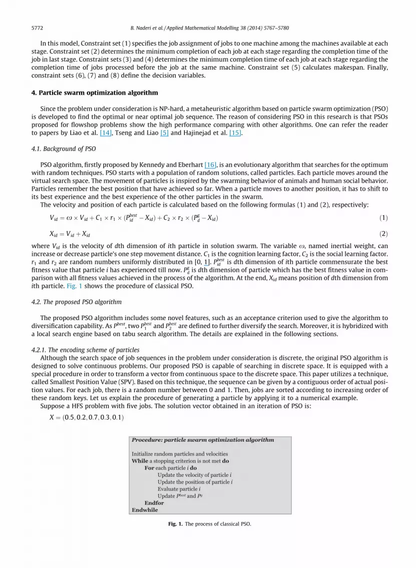
PSO algorithm, firstly proposed by Kennedy and Eberhart [16], is an evolutionary algorithm that searches for the optimumwith random techniques. PSO starts with a population of random solutions, called particles. Each particle moves around thevirtual search space. The movement of particles is inspired by the swarming behavior of animals and human social behavior.Particles remember the best position that have achieved so far. When a particle moves to another position, it has to shift toits best experience and the best experience of the other particles in the swarm.

The velocity and position of each particle is calculated based on the following formulas (1) and (2), respectively:

Vid ¼ x� Vid þ C1 � r1 � ðPbestid � XidÞ þ C2 � r2 � ðPg

d � XidÞ ð1Þ

Xid ¼ Vid þ Xid ð2Þ

where Vid is the velocity of dth dimension of ith particle in solution swarm. The variable x, named inertial weight, canincrease or decrease particle’s one step movement distance. C1 is the cognition learning factor, C2 is the social learning factor.r1 and r2 are random numbers uniformly distributed in [0, 1]. Pbest

id is dth dimension of ith particle commensurate the bestfitness value that particle i has experienced till now. Pg

d is dth dimension of particle which has the best fitness value in com-parison with all fitness values achieved in the process of the algorithm. At the end, Xid means position of dth dimension fromith particle. Fig. 1 shows the procedure of classical PSO.

4.2. The proposed PSO algorithm

The proposed PSO algorithm includes some novel features, such as an acceptance criterion used to give the algorithm todiversification capability. As Pbest, two Pbest

1 and Pbest2 are defined to further diversify the search. Moreover, it is hybridized with

a local search engine based on tabu search algorithm. The details are explained in the following sections.

4.2.1. The encoding scheme of particlesAlthough the search space of job sequences in the problem under consideration is discrete, the original PSO algorithm is

designed to solve continuous problems. Our proposed PSO is capable of searching in discrete space. It is equipped with aspecial procedure in order to transform a vector from continuous space to the discrete space. This paper utilizes a technique,called Smallest Position Value (SPV). Based on this technique, the sequence can be given by a contiguous order of actual posi-tion values. For each job, there is a random number between 0 and 1. Then, jobs are sorted according to increasing order ofthese random keys. Let us explain the procedure of generating a particle by applying it to a numerical example.

Suppose a HFS problem with five jobs. The solution vector obtained in an iteration of PSO is:

X ¼ ð0:5;0:2;0:7;0:3;0:1Þ

Fig. 1. The process of classical PSO.

B. Naderi et al. / Applied Mathematical Modelling 38 (2014) 5767–5780 5773

The corresponding sequence with this solution by SPV rule is:

Y ¼ ð5;2;4;1;3Þ:

The smallest value in X is 0.1 which is located at the fifth position in vector X and so, the first value in Y should be five. Thesecond smallest value in X is 0.2 and is placed in the second position. Then, the second member of Y would be two. Othervalues in Y are calculated by using the similar procedure. One of initial solution is generated by NEHH heuristic [9]. The othersolutions are randomly generated from feasible solutions.

4.2.2. Particles movement and acceptance criterionIn the first step, the velocity of the particle i is updated regarding current Pg

i and Pbest. In the proposed PSO, there are twodifferent Pbest. The first, called Pbest

1 , is the best ever visited solution by all particles and the second, called Pbest2 , is the best

solution among the current Pgi for all the particles. As a result, for each particle, two velocities are produced, one obtained

by Pbest1 and the other by Pbest

2 (using Formula (1)). The regarding each of two available velocities, the particle’s position isrevised and two new particles are generated (using Formula (2)). Then, the better particle is selected.

In classical PSO, the best particle for ith member of swarm (i.e., Pgi ) is replaced with the new produced particle only if it

improves Pgi . We tested the proposed PSO with this classical procedure and found out that the PSO can easily get stuck in

local optima. Several different mechanisms, from easy to complicated ones, have been tested. Finally, it turned out that asimulated annealing-like mechanism performs well. The acceptance criterion can be described as follows. The ith particleis accepted to replace Pg

i with probability of e�DX=T where DX is the fitness of the ith particle minus the fitness of Pgi and T

is a control factor. It decreases when the algorithms proceeds. Note that when the ith particle improves Pgi , then we have

DX < 0 ) e�DX=T > 1

In this case, the new particle is surely accepted for substitution. When the ith particle deteriorates Pgi , then we have

DX > 0 ) 0 < e�DX=T < 1

Therefore, the new particle might be accepted. The probability of acceptance depends on the deterioration size (DX). Ahigher deterioration size reduces the probability. The other factor is the control factor of T where high T means higher chanceof being accepted. During the search, the control factor of T deceases by 1 � a percent after each iteration of PSO. Its bestvalue is determined in the parameter tuning section.

4.2.3. Local search mechanismAlthough PSO is known to be robust with a well global exploration capability, it is often trapped in local minima. This

shortcoming results in the slow convergence. In order to improve the performance, many studies have been carried outin the literature with hybrid PSO algorithms. Poli et al. [17], give a review different variations and hybrids of PSO on the algo-rithm, current and ongoing research, applications and open problems. In light of this, we have been thinking of utilizing alocal search mechanism to enhance the algorithm’s performance.

The proposed local search is based on tabu search (TS) algorithm. In PSOs, the particle Pbest is used to produce a new pop-ulation of particles for the next generation. Therefore, it plays a vital role in both intensification and diversification capabil-ities of the algorithm. If it is defined as the best ever visited particle (like classical PSOs), the algorithm increases itsintensification capability by searching particles around the best and pays less attention to its diversification capability. Toavoid such a shortcoming, as earlier stated, the proposed PSO has two different particles as Pbest. The first, called Pbest

1 , isthe best ever visited solution by all particles and the second, called Pbest

2 , is the best solution among the current Pgi of the

all particles. The particle Pbest1 is to intensify the search and the particle Pbest

2 is to diversify the search.At each iteration of the proposed PSO, the particle Pbest

2 is further improved by the proposed local search mechanismwhich can be described as follows. There is a tabu set of solutions which performs like the well-know tabu list of TS. But,in the tabu list of TS, last moves used to produce new solutions are saved, and the same moves are prohibited for a numberof subsequent iterations; while, in the proposed PSO, the complete particles themselves are put in the tabu set. More pre-cisely, the particle Pbest

2 at each iteration is first checked to find out that if it is in the tabu set or not. If it is not in the tabuset, we use it as the particle Pbest

2 of next iteration and save it the tabu set. Otherwise (i.e., it is in the tabu set), a movingoperator generates new particles from the current Pbest

2 by changing the positions of two jobs. If this new particle improvesthe current tabu Pbest

2 and it is not in the tabu set, it is accepted to be Pbest2 ; otherwise, another new particle is generated from

the current tabu Pbest2 . This procedure iterates NL times. This parameter is tuned in parameter tuning section. When a particle

is put into the tabu set, it is banned to be Pbest2 for five next iterations. The general structure of the proposed hybrid PSO is

shown in Fig. 2.

4.2.4. Computing fitness value (Cmax)To decode a particle and convert it into a schedule, we use the method proposed by Xia and Wu [18]. To have a schedule

in HFS problems, two decisions have to be taken, the assignment of jobs to machines at each stage and job sequencing oneach machine. In the proposed PSO, each particle merely expresses the job sequence at the first stage. No job assignmentand job sequence at subsequent stages are determined by the encoded solution.

Fig. 2. The general procedure of the proposed PSO.

5774 B. Naderi et al. / Applied Mathematical Modelling 38 (2014) 5767–5780

To assign jobs to machines at the first stage, each job, according to the sequence, is processed by the first availablemachine; that is, whenever a machine is idle, the first unscheduled job is assigned to that machine. At subsequent stages,the job sequence is determined by the earliest completion time of jobs at the previous stage. The fitness value of a particleis then measured with the maximum completion time of all jobs.

5. Experimental evaluation

This section evaluates the models and algorithms for performance. This experimental evaluation includes three differentparts: models evaluation, parameter tuning and algorithms evaluation. Later on, we present these three parts.

5.1. Models evaluation

This subsection evaluates and compares the proposed models. In the literature, MILP models are commonly compared forperformance in terms of the model size complexity, computational complexity or both. In the size complexity evaluation,models are contrasted on the basis of the numbers of binary variables, continuous variables and constraints generated bythe nature of the models. In the computational complexity, models are used to solve a common set of problems in orderto adjudicate conflicting results and conclusions found in the literature regarding the relative solution powers of models.For example, Pan [4] compare the available MILP models for regular flowshop based on complexity sizes while Staffordand Tseng [19] evaluates the model on basis of computational time required to solve some instances.

5.1.1. Size complexity comparisonThe four models are compared by the number of binary variables (NBV), the number of continuous variables (NCV), and

the number of constraints (NC) required formulating a same problem size with n jobs and m stages where there are mi iden-tical machines at stage i. We assume that all jobs visit all machines. Table 1 shows the NBV, NCV and NC of each model. Allthree novel proposed models for HFF have less NBV than the adaptation of available model has. These differences becomemore significant when the problem size grows up. Model 4 needs the least NBV. The second rank is for Model 3. Models1 and 4 need the least NCV, while Model 2 needs the most. Model 1 needs the least NC, while Model 2 has the most.

Table 1Model’s comparison on the size complexity.

Factors Factors

NBV NCV NC

Model 1 nm nP

mi

� �nm nm 2þ

Pmi þ n�1

2 þ n� �

þ nP

mi þ n

Model 2 nm n�12

Pmi þ

Pmi

� �2nm

Pmi nm 2þ ðnþ 1Þ

Pmi þm

� �� n

Model 3 nm nþP

mi

� �2nm nm 4þ n�1

2

Pmi þ 2n

� �Model 4 nm ðn�1Þ

2 þP

mi

� �nm nm 2þ ðn� 1Þ

Pmi

� �þ n

B. Naderi et al. / Applied Mathematical Modelling 38 (2014) 5767–5780 5775

To have a better view of the size complexity of the models, Tables 2–4 presents NBV, NCV and NC for some illustrativeinstances, respectively. In these instances, we have mi = 2 for all i = 1, 2, . . ., m. For example, in a problem with n = 10 andm = 5, NBV of Model 1 is 5000, while Model 4 consists of 725 binary variables.

5.1.2. Computational complexity comparisonIn order to compare the computational complexity of the models, the performance of the four MILP models is evaluated to

solve different problem sizes. A set of 24 instances is generated as follows.

n ¼ f6;8;10;12g; m ¼ f2;3;4g

For each combination of n and m, two instances are generated, one with mi = 2 and one with mi = U[1, 3] for stages. Theprocessing times are pj,i = U[2, 15]. The probability for a job to skip each stage is 0.2. Using CPLEX 12, all the 24 instances aresolved by the four MILP models on a notepad with 2.40 GHz Intel Core i3 Duo and 4 GB of RAM memory.

Table 5 shows the results obtained by the models. In this table, for each model, there are two columns. The column ‘‘time’’shows the average computational time of the model elapsed to optimally solve the instances in the corresponding sizes. Thevalue in parenthesis shows the number of instances out of two that the model solves them to optimality. Mark ‘‘�‘‘ meansthat the corresponding model is not able to solve the any of instances within 600 s. The column ‘‘gap’’ shows the averageoptimality gap of each model for those unsolved instances. The value inside the parenthesis shows the number of unsolvedinstances in that corresponding size. For example, both two instances with n = 8 and m = 4 are optimally solved by Model 2 in24.27 s.

Table 2NBV required by models in some illustrative instances.

Instances Models

n m Model 1 Model 2 Model 3 Model 4

5 2 200 120 90 6010 2 800 440 280 17015 2 1800 960 570 33020 2 3200 1680 960 540

5 5 1250 750 375 30010 5 5000 2750 1000 72515 5 11250 6000 1875 127520 5 20000 10500 3000 1950

Table 3NCV required by models in some illustrative instances.

Instances Models

n m Model 1 Model 2 Model 3 Model 4

5 2 10 80 20 1010 2 20 160 40 2015 2 30 240 60 3020 2 40 320 80 40

5 5 25 500 50 2510 5 50 1000 100 5015 5 75 1500 150 7520 5 100 2000 200 100

Table 4NC required by models in some illustrative instances.

Instances Models

n m Model 1 Model 2 Model 3 Model 4

5 2 155 275 220 18510 2 460 950 840 77015 2 915 2025 1860 175520 2 1520 3500 3280 3140

5 5 530 1670 850 105510 5 1435 5840 3450 461015 5 2715 12510 7800 1066520 5 4370 21680 13900 19220

Table 5The results of the models on small-sized instances.

n m Model

1 2 3 4

%gap Time %gap Time %gap Time %gap Time

6 2 _ 0.10(2) _ 0.15(2) _ 0.63(2) _ 0.13(2)3 _ 0.45(2) _ 0.42(2) _ 0.44(2) _ 0.12(2)4 _ 0.44(2) _ 5.13(2) 1.02(1) 0.16(1) _ 4.59(2)

8 2 _ 12.98(2) _ 0.69(2) _ 29.62 (2) _ 6.08(2)3 _ 16.405(2) _ 82.26(2) 5.98(2) _ 2.925(2) _4 _ 110.23(2) _ 24.27(2) 12.54(2) _ 2.57(2) _

10 2 49.16(2) _ _ 1.56(2) _ 1.5(2) _ 7.17(2)3 10(2) _ _ 156.9(2) 20.25(2) _ 7.69(1) 34.51(1)4 35.79(2) _ _ 113.15(2) 1.85(1) 301.99(1) _ 5.65(2)

12 2 63.98(2) _ 28.57(1) 214.83(1) _ 6.43 (2) 24.18(1) 167.36(1)3 60.52(2) _ 6.73(2) _ _ 6.77(2) _ 245.51(2)4 50.87(2) _ 17.41(2) _ _ 6.95(2) _ 330.77(2)

5776 B. Naderi et al. / Applied Mathematical Modelling 38 (2014) 5767–5780

The results demonstrate that Model 1 is significantly outperformed by the others. Comparing the models, Model 1 has themost binary variables. This low performance shows that the number of binary variables is the most influential factor in com-putational complexity of models. None of the models are able to solve the instances with n = 14. Model 1 tackles theinstances up to n = 8 and m = 4 while Model 2 goes up to n = 12 and m = 2 by solving one of two instances in this size. Models2, 3 and 4 solve the 76%, 67% and 75% of 24 instances, respectively. Model 3 is faster in larger sizes.

5.2. Algorithm evaluation

The section proceeds with the numerical comparison of the proposed PSO against other available solution algorithms inthe literature. We bring four algorithms into the experiment. The reason is to compare the proposed PSO with three highperforming available PSOs and one state-of-the-art algorithm. The tested algorithms are:

– The combinatorial particle swarm optimization (PSO1): proposed by for the permutation flowshop and compared withPSO of Tasgetiren et al. [20].

– The discrete particle swarm optimization (PSO2): proposed by Liao et al. [14] for the flowshop and is compared with con-tinuous PSO algorithm of Tasgetiren et al. [21].

– The hybrid particle swarm optimization (PSO3): proposed by Kuo et al. [22] for the flowshop and compared with thegenetic algorithm and PSO of Lian et al. [23].

– The state-of-art iterated local search (ILS): proposed by Naderi et al. [9] for the hybrid flowshop and compared withgenetic algorithm of Ruiz and Maroto [24], artificial immune algorithm of Zandieh et al. [25] and random key geneticalgorithm of Kurz and Askin [8].

The four algorithms brought from the literature are compared with six other algorithms. Therefore, we actually compareour proposed PSO with 10 algorithms, four directly and six indirectly. All five above-mentioned algorithms and our proposedPSO are coded into MATLAB. The stopping criterion for the metaheuristics is set to n2m milliseconds elapsed CPU time. Usinga time limit as the stopping criterion is commonly used by researchers [27]. We use the relative percentage deviation (RPD)as the performance measure. RPD is calculated as follows.

RPD ¼ Sol� LBLB

where Sol and LB are makespan of solution found by the algorithm and the lowest makespan found by any of algorithms foran instance.

5.2.1. Parameter tuningBy the great choice of algorithm’s parameter, its performance can be improved [28]. Therefore, we first conduct an exper-

iment to tune the parameters of the proposed PSO. The algorithm includes 6 parameters of Np, C1, W, TL, T0 and alpha. Tocarry out the experiment, we have different statistical designs. Among different alternatives, Taguchi design is known to bethe most effective one when dealing with several factors [26]. Besides determining the optimal levels, Taguchi establishesthe relative significance of individual factors in terms of their main effects on the objective function.

In the Taguchi method, the results are transformed into a measure called signal-to-noise (S/N) ratio indicating both meanand variation presented in the response variable. The objective is to maximize the S/N ratio. For minimization objectives, theS/N ratio is

S=N ratio ¼ �10log10ðRPDÞ2Þ:

B. Naderi et al. / Applied Mathematical Modelling 38 (2014) 5767–5780 5777

As mentioned, the proposed PSO’s controllable factors are: 6, 3, 3, 3, 3 and 3. After initial tests, we consider the levels,presented in Table 6, for these parameters. The L18 is selected as the fittest orthogonal array design that meets all therequirements.

We generate a set of 45 instances with the following sizes.

n ¼ f6;8;10;12g; m ¼ f2;3;4g

After obtaining the results of Taguchi experiment, RPDs are transformed into S/N ratio. Fig. 3 presents the average S/Nratio obtained at different levels of each factor. The results show that Np(3), C1(2), W(2), TL(2), To(2) and Alpha(2) arethe best levels.

To explore the relative significance of individual factors in terms of their main effects on the objective function, Delta sta-tistic, the highest minus the lowest average S/N ratio for each factor, is computed. Table 7 presents the results of analysis. Nphas the greatest effect on the quality of the algorithm with Delta of 11.8; while alpha obtains the 6th rank with Delta of 2.1.

5.2.2. The computational experimentsWe first evaluate the general performance of the six algorithms. To this end, we use the small-sized instances previously

generated for model’s evaluation. We compare the results against the optimal solution. The proposed PSO and ILS optimallysolve all 24 instances; therefore, they both provide the optimality gap of 0. The worst performing algorithm is PSO3 withaverage optimality gap of 1.57% and solving only 10 out of 24 instances (42%). PSO1 and PSO2 obtain the gap of 0.27%and 0.65%, respectively. They also solve 20 and 16 out of 24 instances, respectively. That is, PSO1 and PSO2 optimally solve83% and 67% of the instances (see Table 8).

We now further evaluate the performance of algorithms using a set of 480 large-sized instances with the following sizes:

n ¼ f20;50;80;120g; m ¼ f2;4;8g; mi ¼ f2;U½1;4�g;

Table 6Factors and their levels.

Factor Level Values

Np 6 (1) �50, (2) �100, (3) �150, 4)� 200, 5)� 250, 6)�300C1 3 (1) �1, (2) �1.5, (3) �2W 3 (1) �0.5, (2) �1, (3) �1.5TL 3 �4, (2) �8, (3) �12T0 3 (1) �1000, (2) �1500, (3) �2000Alpha 3 (1) �0.7, (2) �0.8, (3) �0.9

Fig. 3. The S/N of controlled factors.

Table 7Response table for signal to noise ratios smaller is better.

Level Np C1 W TL T0 Alpha

1 �11.3051 �5.7628 �4.4500 �7.7284 �7.0969 �4.74752 �8.2164 �2.7114 �1.8086 �2.0128 �2.8191 �3.96393 0.4719 �6.3068 �8.5225 �5.0399 �4.8650 �6.06974 �0.99985 �1.90716 �7.6057Delta 11.777 3.5954 6.7139 5.7156 4.2778 2.1058Rank 1 5 2 3 4 6

Table 8The optimality gap of the tested algorithms.

n m Algorithms

PSO1 PSO2 PSO3 PSO ILS

6 2 0.0 0.0 0.0 0.0 0.03 0.0 0.0 0.0 0.0 0.04 0.0 0.0 0.0 0.0 0.0

8 2 0.0 0.0 0.0 0.0 0.03 0.0 0.0 0.0 0.0 0.04 0.0 0.0 2.49 0.0 0.0

10 2 0.0 0.0 0.0 0.0 0.03 1.19 1.19 6.22 0.0 0.04 0.0 3.35 4.60 0.0 0.0

12 2 0.0 1.19 2.38 0.0 0.03 0.0 0.0 0.0 0.0 0.04 2.08 2.08 3.12 0.0 0.0

Ave. 0.27 0.65 1.57 0.0 0.0

Table 9The average RPD of the tested algorithms.

n m Algorithms

PSO1 PSO2 PSO3 PSO ILS

20 2 0.26 2.19 2.38 0.06 0.074 1.55 6.02 7.74 0.56 0.098 2.76 7.65 9.05 0.51 0.32

50 2 0.04 0.81 1.17 0.01 0.044 1.24 4.10 4.46 0.08 0.738 2.32 5.75 6.03 0.38 1.02

80 2 0.06 0.86 1.00 0.02 0.344 0.75 2.42 2.80 0.07 0.718 1.37 3.50 4.20 0.45 0.80

120 2 0.06 0.57 0.78 0.01 0.444 0.40 1.31 1.64 0.05 0.878 0.87 2.02 2.67 0.09 1.11

Ave. 0.97 3.10 3.66 0.19 0.54

5778 B. Naderi et al. / Applied Mathematical Modelling 38 (2014) 5767–5780

Table 9 shows the results of the comparison, averaged for each combination of n and m (40 data per average). As it can beseen, the proposed PSO outperforms the other algorithms with average RPD of 0.19%. The second best is ILS with RPD of0.54%. Among the remaining algorithms, PSO1 provide the best results with RPD of 0.97%. The two worst performing algo-rithms are PSO2 and PSO3 with RPD of 3.10% and 3.66%, respectively.

We conduct an ANOVA on the results where the algorithm type is the single controlled factor. The results indicate thatthere are statistically significant differences between various algorithms with a p-value very close to zero. Fig. 4 shows themeans plot with least significant difference (LSD) intervals at the 95% confidence level for the different algorithms. As can beseen, the proposed PSO provides statistically better results among the tested algorithms.

To further evaluate the algorithms, we analyze the relation between the performance of the algorithms and the problemsizes. We first start with the influence of n over the different algorithms. Fig. 5 presents the average RPD obtained by any ofalgorithms in different sizes of n. In instances with n = 20, ILS outperforms the others; yet, with more jobs the proposed PSOperforms better. More precisely, for more than 50 jobs, PSO clearly and statistically outperforms the others.

Fig. 4. Means plot with LSD intervals for the different algorithms.

Fig. 5. Means plot of algorithms versus the number of jobs.

Fig. 6. Means plot of algorithms versus the number of stages.

B. Naderi et al. / Applied Mathematical Modelling 38 (2014) 5767–5780 5779

It is also interesting to evaluate the influence of m over the different algorithms. Fig. 6 presents the means plot resultingfrom such analysis. There is a clear interaction between PSO, m and the remaining algorithms. Albeit ILS and the proposedPSO yield the same results when m = 2, with more stages, the performance of PSO improves comparatively. PSO is statisti-cally the best algorithm from the comparison.

6. Conclusion and future research

This paper investigated the hybrid flowshop scheduling and studied the shortcoming of the available mathematicalmodels in the literature. Three different mixed integer programming models were built. First, the models were comparedbased on the size complexity and then computational complexity. By the mathematical models and CPLEX software, the

5780 B. Naderi et al. / Applied Mathematical Modelling 38 (2014) 5767–5780

small-sized instances (up to 12 jobs) were solved to optimality. The paper proposed a novel algorithm based on the hybrid-ization of particle swarm optimization algorithm with an acceptance criterion and local search heuristic. This algorithmenjoyed a fine balance of diversification and intensification capability. The proposed algorithm is well tuned using Taguchimethod. To evaluate the performance of the proposed algorithm, two numerical experiments were done and four particleswarm optimization algorithms available in the scheduling literature and one well-known iterated local search algorithmin the hybrid flowshop literature were brought into the experiments. The proposed metaheuristic significantly outperformedthe other algorithms.

It is interesting to mathematically formulate some extensions of the problem with additional realistic assumptions. Onecan analyze the problem and models to find out some preprocessing rules. In this case, the solution space is reduced signif-icantly. Another future research line is to enhance the solution methods by hybridizing with some advanced features.

References

[1] M. Pinedo, Scheduling Theory, Algorithms, and Systems, third ed., Springer, LLC, New York, 2008.[2] B. Naderi, R. Ruiz, The distributed permutation flowshop scheduling problem, Comput. Oper. Res. 37 (2010) 754–768.[3] J. Behnamian, S.M.T. Fatemi Ghomi, Hybrid flowshop scheduling with machine and resource-dependent processing times, Appl. Math. Model. 35

(2011) 1107–1112.[4] C.H. Pan, A study of integer programming formulations for scheduling problems, Int. J. Syst. Sci. 28 (1997) 33–41.[5] C.T. Tseng, C.J. Liao, A particle swarm optimization algorithm for hybrid flowshop scheduling with multiprocessor tasks, Int. J. Prod. Res. 46 (17) (2008)

4655–4670.[6] E.F. Stafford, F.T. Tseng, J.N.D. Gupta, Comparative evaluation of MILP flowshop models, J. Oper. Res. Soc. 56 (2005) 88–101.[7] B. Naderi, S.M.T. Fatemi Ghomi, M. Aminnayeri, M. Zandieh, Scheduling open shops with parallel machines to minimize total completion time, J.

Comput. Appl. Math. 235 (2011) 1275–1287.[8] M.E. Kurz, R.G. Askin, Scheduling flexible flow lines with sequence-dependent setup times, Eur. J. Oper. Res. 159 (2004) 66–82.[9] B. Naderi, R. Ruiz, M. Zandieh, Algorithms for a realistic variant of flowshop scheduling, Comput. Oper. Res. 37 (2010) 236–246.

[10] C. Paternina-Arboleda, J. Montoya-Torres, M. Acero-Dominguez, M. Herrera-Hernandez, Scheduling jobs on a k-stage flexible flow-shop, Ann. Oper.Res. 164 (2007) 29–40.

[11] T. Kis, E. Pesch, A review of exact solution methods for the non-preemptive multiprocessor flowshop problem, Eur. J. Oper. Res. 164 (2005) 592–608.[12] R. Ruiz, Serifoglu F. Sivrikaya, T. Urlings, Modeling realistic hybrid flexible flowshop scheduling problems, Comput. Oper. Res. 35 (4) (2008) 1151–1175.[13] H.M. Wagner, An integer linear-programming model for machine scheduling, Nav. Res. Logist. Q. 6 (1959) 131–140.[14] C.J. Liao, C.T. Tseng, P. Luarn, A discrete version of particle swarm optimization for flowshop scheduling problems, Comput. Oper. Res. 34 (2007) 3099–

3111.[15] D. Hajinejad, N. Salmasi, R. Mokhtari, A fast hybrid particle swarm optimization Algorithm for flow shop sequence dependent group scheduling

problem, Scientia Iranica 18 (3) (2011) 759–764.[16] J. Kennedy, R.C. Eberhart. Particle swarm optimization, in: Proceedings of IEEE International Conference on Neural Network, Piscataway: IEEE 4, (1995)

1942–1948.[17] R. Poli, J. Kennedy, T. Blackwell, Particle Swarm Optimization, 1, Springer Science Business Media, 2007. 33-57.[18] W. Xia, Z. Wu, An effective hybrid optimization approach for multi-objective flexible job-shop scheduling problems, Comput. Ind. Eng. 48 (2005) 409–

425.[19] E.F. Stafford, F.T. Tseng, Two models for a family of flowshop sequencing problems, Eur. J. Oper. Res. 142 (2002) 282–293.[20] M.F. Tasgetiren, Y.C. Liang, M. Sevkli, G. Gencyilmaz, A particle swarm optimization algorithm for makespan and total flowtime minimization in the

permutation flowshop sequencing problem, Eur. J. Oper. Res. 177 (2007) 1930–1947.[21] M.F. Tasgetiren, Y.C. Liang, M. Sevkli, G. Gencyilmaz, Particle swarm optimization algorithm for makespan and maximum lateness minimization in

permutation flowshop sequencing problem, in: Proceedings of the Fourth International Symposium on Intelligent Manufacturing Systems, Turkey,Sakarya, 2004, pp. 431–441.

[22] H. Kuo, S.J. Horng, T.W. Kao, T.L. Lin, C.L. Lee, T. Terano, Y. Pan, An efficient flow-shop scheduling algorithm based on a hybrid particle swarmoptimization model, Expert Syst. Appl. 36 (2009) 7027–7032.

[23] Z. Lian, X. Gu, B. Jiao, A novel particle swarm optimization algorithm for permutation flow-shop scheduling to minimize makespan, Chaos, SolitonsFractals 35 (2008) 851–861.

[24] R. Ruiz, C.A. Maroto, Genetic algorithm for hybrid flowshops with sequence dependent setup times and machine eligibility, Eur. J. Oper. Res. 169 (3)(2006) 781–800.

[25] M. Zandieh, S.M.T. Fatemi Ghomi, S.M. Moattar Husseini, An immune algorithm approach to hybrid flowshops scheduling with sequence-dependentsetup times, Appl. Math. Comput. 180 (2006) 111–127.

[26] Phadke S.B. (1996). Comments on Sliding mode control of linear systems with mismatched uncertainties. Automatica, February, 285–286.[27] E. Vallada, R. Ruiz, G. Minella, Minimising total tardiness in the m-machine flowshop problem: a review and evaluation of heuristics and

metaheuristics, Comput. Oper. Res. 35 (4) (2008) 1350–1373.[28] B. Naderi, M. Zandieh, V. Roshanaei, Scheduling hybrid flowshops with sequence dependent setup times to minimize makespan and maximum

tardiness, Int. J. Adv. Manuf. Technol. 41 (2009) 1186–1198.