quanser flexible link workbook
TRANSCRIPT

Rotary Flexible Link
WorkbookFLEXGAGE
Instructor Version
Quanser Inc.2011

c⃝ 2011 Quanser Inc., All rights reserved.
Quanser Inc.119 Spy CourtMarkham, OntarioL3R [email protected]: 1-905-940-3575Fax: 1-905-940-3576
Printed in Markham, Ontario.
For more information on the solutions Quanser Inc. offers, please visit the web site at:http://www.quanser.com
This document and the software described in it are provided subject to a license agreement. Neither the software nor this document may beused or copied except as specified under the terms of that license agreement. All rights are reserved and no part may be reproduced, stored ina retrieval system or transmitted in any form or by any means, electronic, mechanical, photocopying, recording, or otherwise, without the priorwritten permission of Quanser Inc.
ACKNOWLEDGEMENTSQuanser, Inc. would like to thank Dr. Hakan Gurocak, Washington State University Vancouver, USA, for his help to include embedded out-comes assessment.
FLEXGAGE Workbook - Instructor Version 2
CONTENTS1 Introduction 4
2 Modeling 52.1 Background 52.2 Pre-Lab Questions 102.3 Lab Experiments 142.4 Results 22
3 Control Design 233.1 Specifications 233.2 Background 233.3 Pre-Lab Questions 253.4 Lab Experiments 273.5 Results 36
4 System Requirements 374.1 Overview of Files 384.2 Setup for Finding Stiffness 404.3 Setup for Model Validation 404.4 Setup for Flexible Link Control Simulation 414.5 Setup for Flexible Link Control Implementation 42
5 Lab Report 435.1 Template for Content (Modeling) 435.2 Template for Content (Control) 445.3 Tips for Report Format 45
6 Scoring Sheet for Pre-Lab Modeling Questions 46
7 Scoring Sheet for Lab Report (Modeling) 47
8 Scoring Sheet for Pre-Lab Control Questions 48
9 Scoring Sheet for Lab Report (Control) 49
A Instructor's Guide 50
FLEXGAGE Workbook - Instructor Version v 1.0
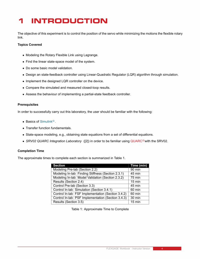
1 INTRODUCTIONThe objective of this experiment is to control the position of the servo while minimizing the motions the flexible rotarylink.
Topics Covered
• Modeling the Rotary Flexible Link using Lagrange.
• Find the linear state-space model of the system.
• Do some basic model validation.
• Design an state-feedback controller using Linear-Quadratic Regulator (LQR) algorithm through simulation.
• Implement the designed LQR controller on the device.
• Compare the simulated and measured closed-loop results.
• Assess the behaviour of implementing a partial-state feedback controller.
Prerequisites
In order to successfully carry out this laboratory, the user should be familiar with the following:
• Basics of Simulinkr.
• Transfer function fundamentals.
• State-space modeling, e.g., obtaining state equations from a set of differential equations.
• SRV02 QUARC Integration Laboratory ([2]) in order to be familiar using QUARCrwith the SRV02.
Completion Time
The approximate times to complete each section is summarized in Table 1.
Section Time (min)Modeling Pre-lab (Section 2.2) 90 minModeling In-lab: Finding Stiffness (Section 2.3.1) 45 minModeling In-lab: Model Validation (Section 2.3.2) 75 minResults (Section 2.4) 15 minControl Pre-lab (Section 3.3) 45 minControl In-lab: Simulation (Section 3.4.1) 60 minControl In-lab: FSF Implementation (Section 3.4.2) 60 minControl In-lab: PSF Implementation (Section 3.4.3) 30 minResults (Section 3.5) 15 min
Table 1: Approximate Time to Complete
FLEXGAGE Workbook - Instructor Version 4
2 MODELING
2.1 Background
2.1.1 Model
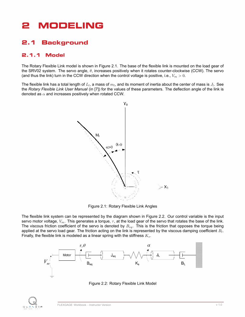
The Rotary Flexible Link model is shown in Figure 2.1. The base of the flexible link is mounted on the load gear ofthe SRV02 system. The servo angle, θ, increases positively when it rotates counter-clockwise (CCW). The servo(and thus the link) turn in the CCW direction when the control voltage is positive, i.e., Vm > 0.
The flexible link has a total length of Ll, a mass of ml, and its moment of inertia about the center of mass is Jl. Seethe Rotary Flexible Link User Manual (in [7]) for the values of these parameters. The deflection angle of the link isdenoted as α and increases positively when rotated CCW.
Figure 2.1: Rotary Flexible Link Angles
The flexible link system can be represented by the diagram shown in Figure 2.2. Our control variable is the inputservo motor voltage, Vm. This generates a torque, τ , at the load gear of the servo that rotates the base of the link.The viscous friction coefficient of the servo is denoted by Beq. This is the friction that opposes the torque beingapplied at the servo load gear. The friction acting on the link is represented by the viscous damping coefficient Bl.Finally, the flexible link is modeled as a linear spring with the stiffness Ks.
Figure 2.2: Rotary Flexible Link Model
FLEXGAGE Workbook - Instructor Version v 1.0

2.1.2 Finding the Equations of Motion
Instead of using classical mechanics, the Lagrange method is used to find the equations of motion of the system.This systematic method is often used for more complicated systems such as robot manipulators with multiple joints.
More specifically, the equations that describe the motions of the servo and the link with respect to the servo motorvoltage, i.e. the dynamics, will be obtained using the Euler-Lagrange equation:
∂2L
∂t∂qi− ∂L
∂qi= Qi (2.1)
The variables qi are called generalized coordinates. For this system let
q(t)⊤ = [θ(t) α(t)] (2.2)
where, as shown in Figure 2.2, θ(t) is the servo angle and α(t) is the flexible link angle. The corresponding velocitiesare
q(t)⊤ =
[∂θ(t)
∂t
∂α(t)
∂t
](2.3)
Note: The dot convention for the time derivative will be used throughout this document, i.e., θ = dθdt and α = dα
dt .The time variable t will also be dropped from θ and α, i.e., θ := θ(t) and α := α(t).
With the generalized coordinates defined, the Euler-Lagrange equations for the rotary flexible link system are
∂2L
∂t∂θ− ∂L
∂θ= Q1 (2.4)
and∂2L
∂t∂α− ∂L
∂α= Q2 (2.5)
The Lagrangian of a system is definedL = T − V (2.6)
where T is the total kinetic energy of the system and V is the total potential energy of the system. Thus the Lagrangianis the difference between a system's kinetic and potential energies.
The generalized forces Qi are used to describe the non-conservative forces (e.g., friction) applied to a system withrespect to the generalized coordinates. In this case, the generalized force acting on the rotary arm is
Q1 = τ −Beq θ (2.7)
and acting on the link isQ2 = −Blα. (2.8)
The torque applied at the base of the rotary arm (i.e., at the load gear) is generated by the servo motor as describedby the equation
τ =ηgKgηmkt(Vm −Kgkmθ)
Rm. (2.9)
See [4] for a description of the corresponding SRV02 parameters (e.g. such as the back-emf constant, km). Theservo damping (i.e. friction), Beq, opposes the applied torque. The flexible link is not actuated, the only force actingon the link is the damping, Bl.
Again, the Euler-Lagrange equations is a systematic method of finding the equations of motion (EOMs) of a system.Once the kinetic and potential energy are obtained and the Lagrangian is found, then the task is to compute variousderivatives to get the EOMs.
FLEXGAGE Workbook - Instructor Version 6

2.1.3 Potential and Kinetic Energy
Kinetic EnergyTranslational kinetic equation is defined as
T =1
2mv2, (2.10)
where m is the mass of the object and v is the linear velocity.
Rotational kinetic energy is described asT =
1
2Jω2 (2.11)
where J is the moment of inertia of the object and ω is its angular rate.
Potential EnergyPotential energy comes in different forms. Typically in mechanical system we deal with gravitational and elasticpotential energy. The relative gravitational potential energy of an object is
Vg = mg∆h, (2.12)
where m is the object mass and ∆h is the change in altitude of the object (from a reference point). The potentialenergy of an object that rises from the table surface (i.e., the reference) up to 0.25 meter is ∆h = 0.25 − 0 = 0.25and the energy stored is Vg = 0.25mg.
The equation for elastic potential energy, i.e., the energy stored in a spring, is
Ve =1
2K∆x2 (2.13)
where K is the spring stiffness and ∆x is the linear or angular change in position. If an object that is connected toa spring moves from in its initial reference position to 0.1 m, then the change in displacement is ∆x = 0.1− 0 = 0.1and the energy stored equals Ve = 0.005K.
2.1.4 Linear State-Space Model
The linear state-space equations arex = Ax+Bu (2.14)
andy = Cx+Du (2.15)
where x is the state, u is the control input, A, B, C, and D are state-space matrices. For the Rotary Flexible Linksystem, the state and output are defined
x⊤ = [θ α θ α] (2.16)
andy⊤ = [x1 x2]. (2.17)
In the output equation, only the position of the servo and link angles are being measured. Based on this, the C andD matrices in the output equation are
C =
[1 0 0 00 1 0 0
](2.18)
andD =
[00
]. (2.19)
The velocities of the servo and link angles can be computed in the digital controller, e.g., by taking the derivativeand filtering the result though a high-pass filter.
FLEXGAGE Workbook - Instructor Version v 1.0
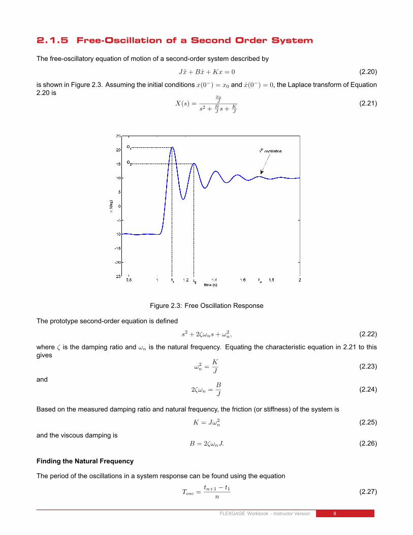
2.1.5 Free-Oscillation of a Second Order System
The free-oscillatory equation of motion of a second-order system described by
Jx+Bx+Kx = 0 (2.20)
is shown in Figure 2.3. Assuming the initial conditions x(0−) = x0 and x(0−) = 0, the Laplace transform of Equation2.20 is
X(s) =x0
J
s2 + BJ s+
KJ
(2.21)
Figure 2.3: Free Oscillation Response
The prototype second-order equation is defined
s2 + 2ζωns+ ω2n, (2.22)
where ζ is the damping ratio and ωn is the natural frequency. Equating the characteristic equation in 2.21 to thisgives
ω2n =
K
J(2.23)
and2ζωn =
B
J(2.24)
Based on the measured damping ratio and natural frequency, the friction (or stiffness) of the system is
K = Jω2n (2.25)
and the viscous damping isB = 2ζωnJ. (2.26)
Finding the Natural Frequency
The period of the oscillations in a system response can be found using the equation
Tosc =tn+1 − t1
n(2.27)
FLEXGAGE Workbook - Instructor Version 8
where tn is the time of the nth oscillation, t1 is the time of the first peak, and n is the number of oscillations considered.From this, the damped natural frequency (in radians per second) is
ωd =2π
Tosc(2.28)
and the undamped natural frequency isωn =
ωd√1− ζ2
. (2.29)
Finding the Damping Ratio
The damping ratio of a second-order system can be found from its response. For a typical second-order under-damped system, the subsidence ratio (i.e., decrement ratio) is defined as
δ =1
nln
O1
On(2.30)
where O1 is the peak of the first oscillation and On is the peak of the nth oscillation. Note that O1 > On, as this is adecaying response.
The damping ratio is definedζ =
1√1 + 2π
δ
2(2.31)
FLEXGAGE Workbook - Instructor Version v 1.0

2.2 Pre-Lab Questions
1. A-2 Energy is stored in the flexible link, i.e., the "spring", as it flexes by an angle of α (see Figure 2.1). Findthe potential energy of the flexible link. Use the parameters shown in Figure 2.2.
Answer 2.1
Outcome SolutionA-2 Using Equation 2.13, the elastic energy stored in the spring equals
V =1
2Ksα
2 (Ans.2.1)
This is the total potential energy that is store in the system.
2. A-2 Find the total kinetic energy of the system contributed by the rotary servo, θ, and the deflection in thelink, α. Use the parameters shown in Figure 2.2.
Answer 2.2
Outcome SolutionA-2 Using the Equation 2.11, the total kinetic energy from the SRV02 rotating
and the deflection of the link is
T =1
2Jeq θ
2 +1
2Jl(θ + α)2. (Ans.2.2)
3. A-2 Compute the Lagrangian of the system.
Answer 2.3
Outcome SolutionA-2 Using Equation 2.6, the total kinetic energy from the SRV02 rotating and
the deflection of the link is
L =1
2Jeq θ
2 +1
2Jl(θ + α)2 − 1
2Ksα
2. (Ans.2.3)
4. A-1, A-2 Find the first Euler-Lagrange equation given in 2.4. Keep the equations in terms of applied torque, τ(i.e., not in terms of DCmotor voltage). Also make sure your equations follow the general form: Jx+Bx+Kx =u.
FLEXGAGE Workbook - Instructor Version 10

Answer 2.4
Outcome SolutionA-1 Compute the derivatives required by Equation 2.4 and substitute the
generalized force, Q1, given in Equation 2.7.A-2 The derivatives are
∂L
∂θ= Jeq θ + Jl(θ + α)
∂2L
∂t∂θ= Jeq θ + Jl(θ + α)
∂L
∂θ= 0.
Substituting the above answers and Equation 2.7 into Equation 2.4 givesthe first equation of motion
(Jeq + Jl)θ + Jlα+Beq θ = τ (Ans.2.4)
5. A-1, A-2 Find the second Euler-Lagrange Equation 2.5.
Answer 2.5
Outcome SolutionA-1 Compute the derivatives required by Equation 2.5 and substitute the
generalized force, Q2, given in Equation 2.8.A-2 The derivatives are
∂L
∂α= Jl(θ + α)
∂2L
∂t∂α= Jl(θ + α)
∂L
∂α= Ksα.
Substituting the above derivative and Equation 2.8 into Equation 2.5gives the second equation of motion
Jlθ + Jlα+Blθ +Ksα = 0 (Ans.2.5)
6. A-1, A-2 Find the equations of motion: θ = f1(θ, θ, α, α, τ) and α = f2(θ, θ, α, α, τ). Assume the viscousdamping of the link is negligible, i.e., Bl = 0.
FLEXGAGE Workbook - Instructor Version v 1.0
Answer 2.6
Outcome SolutionA-1 Solve for θ and α in Ans.2.4 and Ans.2.5.A-2 Subtract equation Ans.2.4 from Ans.2.5 and set Bl = 0 to obtain the first
equation of motion
θ = −Beq
Jeqθ +
Ks
Jeqα+
1
Jeqτ. (Ans.2.6)
Substitute this into Equation Ans.2.5
Jl
(−Beq
Jeqθ +
Ks
Jeqα+
1
Jeqτ
)+ Jlα+Ksα = 0
−JlBeq
Jeqθ + Jlα+Ks
(JlJeq
+ 1
)α = − Jl
Jeqτ
Solve for α to obtain the second equation of motion
α =Beq
Jeqθ −Ks
(Jl + JeqJlJeq
)α− 1
Jeqτ (Ans.2.7)
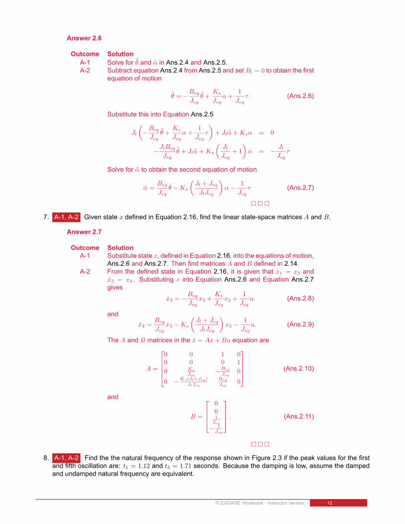
7. A-1, A-2 Given state x defined in Equation 2.16, find the linear state-space matrices A and B.
Answer 2.7
Outcome SolutionA-1 Substitute state x, defined in Equation 2.16, into the equations of motion,
Ans.2.6 and Ans.2.7. Then find matrices A and B defined in 2.14.A-2 From the defined state in Equation 2.16, it is given that x1 = x3 and
x2 = x4. Substituting x into Equation Ans.2.6 and Equation Ans.2.7gives
x3 = −Beq
Jeqx3 +
Ks
Jeqx2 +
1
Jequ. (Ans.2.8)
andx4 =
Beq
Jeqx3 −Ks
(Jl + JeqJlJeq
)x2 −
1
Jequ. (Ans.2.9)
The A and B matrices in the x = Ax+Bu equation are
A =
0 0 1 00 0 0 1
0 Ks
Jeq−Beq
Jeq0
0 −Ks(Jl+Jeq)JlJeq
Beq
Jeq0
(Ans.2.10)
and
B =
001
Jeq
− 1Jeq
. (Ans.2.11)
8. A-1, A-2 Find the the natural frequency of the response shown in Figure 2.3 if the peak values for the firstand fifth oscillation are: t1 = 1.12 and t5 = 1.71 seconds. Because the damping is low, assume the dampedand undamped natural frequency are equivalent.
FLEXGAGE Workbook - Instructor Version 12
Answer 2.8
Outcome SolutionA-1 Since ζ is small, assume that ωn = ωd and find the natural frequency
using Equation 2.28A-2 Using Equation 2.27, the period is
Tosc =t5 − t1
4
=1.71− 1.12
4= 0.148
From Equation 2.28, the natural frequency is
ωn =2π
0.0148= 42.6 rad/s (Ans.2.12)
or 6.76 Hz.
FLEXGAGE Workbook - Instructor Version v 1.0
2.3 Lab Experiments
In the first part of this laboratory, the stiffness of the flexible link is determined by measuring its natural frequency. Inthe second part, the state-space model is finalized and validated against actual measurements.
2.3.1 Finding Stiffness
In Section 2.1.5 we found an equation describing the free-oscillation response of a second-order system. This canalso be used to describe the response of the flexible link when initially perturbed and left to decay.
Physical Parameters for the Lab
In order to do some of the laboratory exercises, you will need these values:
Beq = 0.004 N · m / (rad/s)Jeq = 2.08× 10⁻³ kg · m2
ml = 0.065 kgLl = 0.419 m
Note: The equivalent viscous damping, Beq, and moment of inertia, Jeq, parameters are for the SRV02 when thereis no load (i.e., the parameter found in the SRV02 Modeling Laboratory was for servo with the disc load).
Experimental Setup
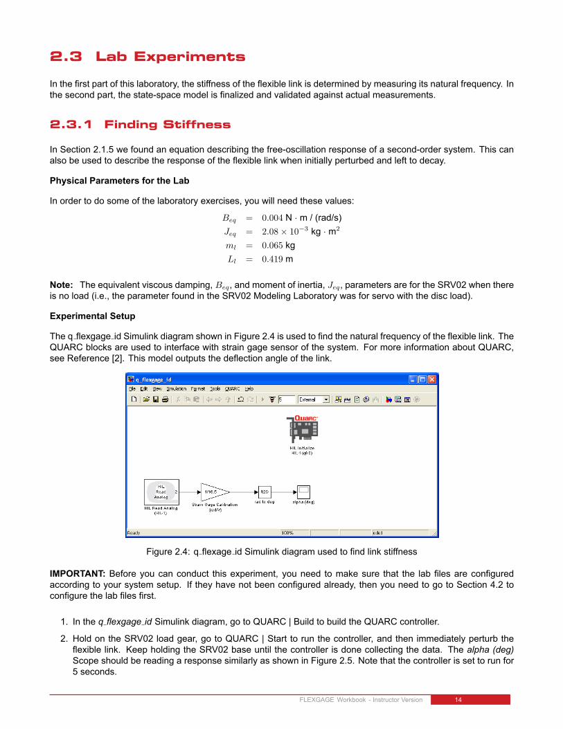
The q flexgage id Simulink diagram shown in Figure 2.4 is used to find the natural frequency of the flexible link. TheQUARC blocks are used to interface with strain gage sensor of the system. For more information about QUARC,see Reference [2]. This model outputs the deflection angle of the link.
Figure 2.4: q flexage id Simulink diagram used to find link stiffness
IMPORTANT: Before you can conduct this experiment, you need to make sure that the lab files are configuredaccording to your system setup. If they have not been configured already, then you need to go to Section 4.2 toconfigure the lab files first.
1. In the q flexgage id Simulink diagram, go to QUARC | Build to build the QUARC controller.
2. Hold on the SRV02 load gear, go to QUARC | Start to run the controller, and then immediately perturb theflexible link. Keep holding the SRV02 base until the controller is done collecting the data. The alpha (deg)Scope should be reading a response similarly as shown in Figure 2.5. Note that the controller is set to run for5 seconds.
FLEXGAGE Workbook - Instructor Version 14
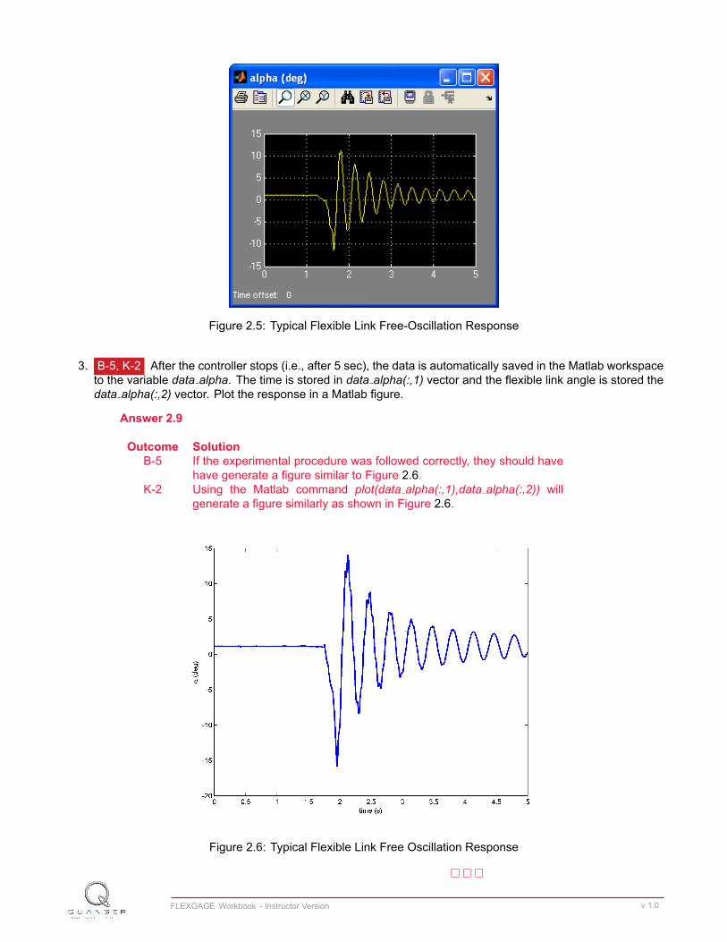
Figure 2.5: Typical Flexible Link Free-Oscillation Response
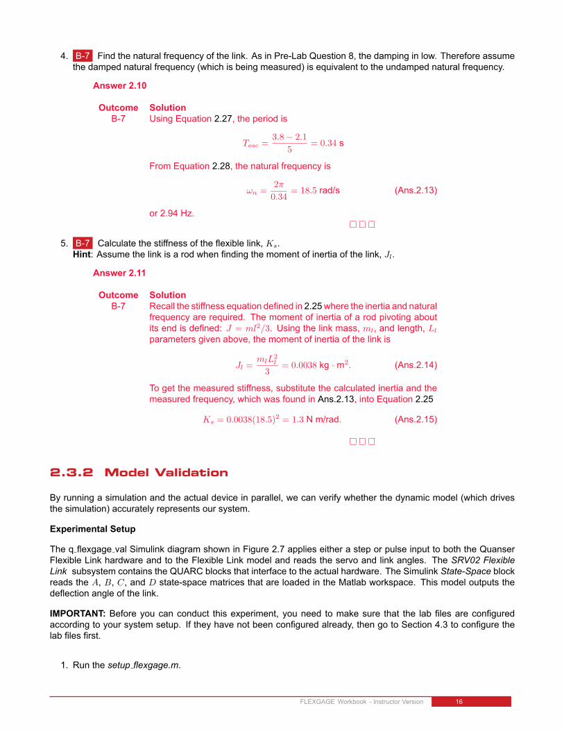
3. B-5, K-2 After the controller stops (i.e., after 5 sec), the data is automatically saved in the Matlab workspaceto the variable data alpha. The time is stored in data alpha(:,1) vector and the flexible link angle is stored thedata alpha(:,2) vector. Plot the response in a Matlab figure.
Answer 2.9
Outcome SolutionB-5 If the experimental procedure was followed correctly, they should have
have generate a figure similar to Figure 2.6.K-2 Using the Matlab command plot(data alpha(:,1),data alpha(:,2)) will
generate a figure similarly as shown in Figure 2.6.
Figure 2.6: Typical Flexible Link Free Oscillation Response
FLEXGAGE Workbook - Instructor Version v 1.0
4. B-7 Find the natural frequency of the link. As in Pre-Lab Question 8, the damping in low. Therefore assumethe damped natural frequency (which is being measured) is equivalent to the undamped natural frequency.
Answer 2.10
Outcome SolutionB-7 Using Equation 2.27, the period is
Tosc =3.8− 2.1
5= 0.34 s
From Equation 2.28, the natural frequency is
ωn =2π
0.34= 18.5 rad/s (Ans.2.13)
or 2.94 Hz.
5. B-7 Calculate the stiffness of the flexible link, Ks.Hint: Assume the link is a rod when finding the moment of inertia of the link, Jl.
Answer 2.11
Outcome SolutionB-7 Recall the stiffness equation defined in 2.25 where the inertia and natural
frequency are required. The moment of inertia of a rod pivoting aboutits end is defined: J = ml2/3. Using the link mass, ml, and length, Ll
parameters given above, the moment of inertia of the link is
Jl =mlL
2l
3= 0.0038 kg · m2. (Ans.2.14)
To get the measured stiffness, substitute the calculated inertia and themeasured frequency, which was found in Ans.2.13, into Equation 2.25
Ks = 0.0038(18.5)2 = 1.3 N m/rad. (Ans.2.15)
2.3.2 Model Validation
By running a simulation and the actual device in parallel, we can verify whether the dynamic model (which drivesthe simulation) accurately represents our system.
Experimental Setup
The q flexgage val Simulink diagram shown in Figure 2.7 applies either a step or pulse input to both the QuanserFlexible Link hardware and to the Flexible Link model and reads the servo and link angles. The SRV02 FlexibleLink subsystem contains the QUARC blocks that interface to the actual hardware. The Simulink State-Space blockreads the A, B, C, and D state-space matrices that are loaded in the Matlab workspace. This model outputs thedeflection angle of the link.
IMPORTANT: Before you can conduct this experiment, you need to make sure that the lab files are configuredaccording to your system setup. If they have not been configured already, then go to Section 4.3 to configure thelab files first.
1. Run the setup flexgage.m.
FLEXGAGE Workbook - Instructor Version 16
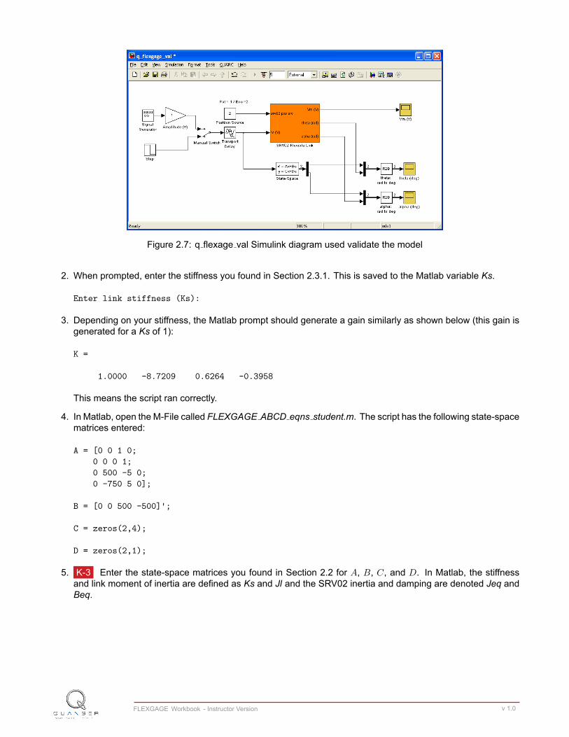
Figure 2.7: q flexage val Simulink diagram used validate the model
2. When prompted, enter the stiffness you found in Section 2.3.1. This is saved to the Matlab variable Ks.
Enter link stiffness (Ks):
3. Depending on your stiffness, the Matlab prompt should generate a gain similarly as shown below (this gain isgenerated for a Ks of 1):
K =
1.0000 -8.7209 0.6264 -0.3958
This means the script ran correctly.
4. In Matlab, open the M-File called FLEXGAGE ABCD eqns student.m. The script has the following state-spacematrices entered:
A = [0 0 1 0;0 0 0 1;0 500 -5 0;0 -750 5 0];
B = [0 0 500 -500]';
C = zeros(2,4);
D = zeros(2,1);
5. K-3 Enter the state-space matrices you found in Section 2.2 for A, B, C, and D. In Matlab, the stiffnessand link moment of inertia are defined as Ks and Jl and the SRV02 inertia and damping are denoted Jeq andBeq.
FLEXGAGE Workbook - Instructor Version v 1.0
Answer 2.12
Outcome SolutionK-3 In the script, enter the A and B matrices in Ans.2.10 and Ans.2.11 and
the C and D matrices in 2.18 and 2.19 that were found in Section 2.2:A = [0 0 1 0;
0 0 0 1;0 Ks/Jeq -Beq/Jeq 0;0 -Ks*(Jeq+Jl)/Jeq/Jl Beq/Jeq 0];
B = [0 0 1/Jeq -1/Jeq]';
C = eye(2,4);
D = zeros(4,2);The solution is given in FLEXGAGE ABCD eqns.m.
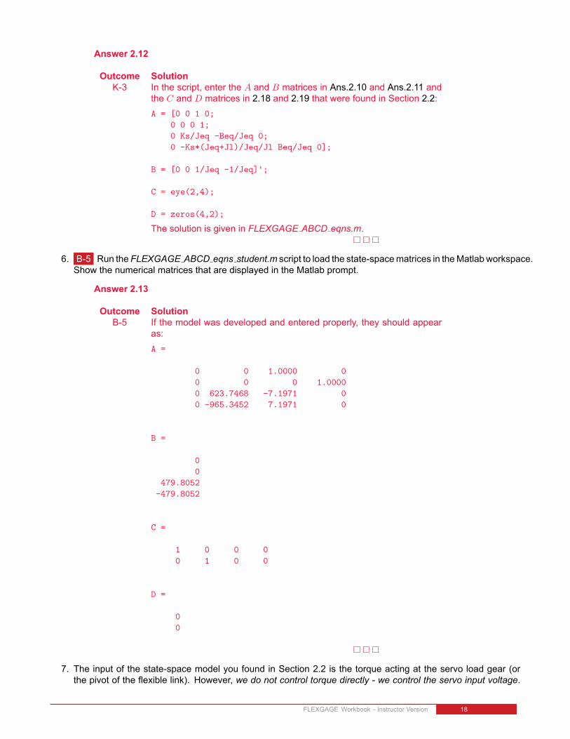
6. B-5 Run the FLEXGAGE ABCD eqns student.m script to load the state-spacematrices in theMatlab workspace.Show the numerical matrices that are displayed in the Matlab prompt.
Answer 2.13
Outcome SolutionB-5 If the model was developed and entered properly, they should appear
as:A =
0 0 1.0000 00 0 0 1.00000 623.7468 -7.1971 00 -965.3452 7.1971 0
B =
00
479.8052-479.8052
C =
1 0 0 00 1 0 0
D =
00
7. The input of the state-space model you found in Section 2.2 is the torque acting at the servo load gear (orthe pivot of the flexible link). However, we do not control torque directly - we control the servo input voltage.
FLEXGAGE Workbook - Instructor Version 18
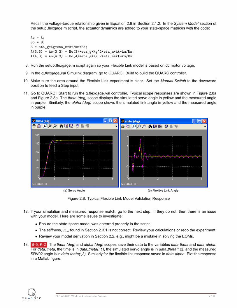
Recall the voltage-torque relationship given in Equation 2.9 in Section 2.1.2. In the System Model section ofthe setup flexgage.m script, the actuator dynamics are added to your state-space matrices with the code:
Ao = A;Bo = B;B = eta_g*Kg*eta_m*kt/Rm*Bo;A(3,3) = Ao(3,3) - Bo(3)*eta_g*Kg^2*eta_m*kt*km/Rm;A(4,3) = Ao(4,3) - Bo(4)*eta_g*Kg^2*eta_m*kt*km/Rm;
8. Run the setup flexgage.m script again so your Flexible Link model is based on dc motor voltage.
9. In the q flexgage val Simulink diagram, go to QUARC | Build to build the QUARC controller.
10. Make sure the area around the Flexible Link experiment is clear. Set the Manual Switch to the downwardposition to feed a Step input.
11. Go to QUARC | Start to run the q flexgage val controller. Typical scope responses are shown in Figure 2.8aand Figure 2.8b. The theta (deg) scope displays the simulated servo angle in yellow and the measured anglein purple. Similarly, the alpha (deg) scope shows the simulated link angle in yellow and the measured anglein purple.
(a) Servo Angle (b) Flexible Link Angle
Figure 2.8: Typical Flexible Link Model Validation Response
12. If your simulation and measured response match, go to the next step. If they do not, then there is an issuewith your model. Here are some issues to investigate:
• Ensure the state-space model was enterred properly in the script.• The stiffness, Ks, found in Section 2.3.1 is not correct. Review your calculations or redo the experiment.• Review your model derivation in Section 2.2, e.g., might be a mistake in solving the EOMs.
13. B-5, K-2 The theta (deg) and alpha (deg) scopes save their data to the variables data theta and data alpha.For data theta, the time is in data theta(:,1), the simulated servo angle is in data theta(:,2), and the measuredSRV02 angle is in data theta(:,3). Similarly for the flexible link response saved in data alpha. Plot the responsein a Matlab figure.
FLEXGAGE Workbook - Instructor Version v 1.0
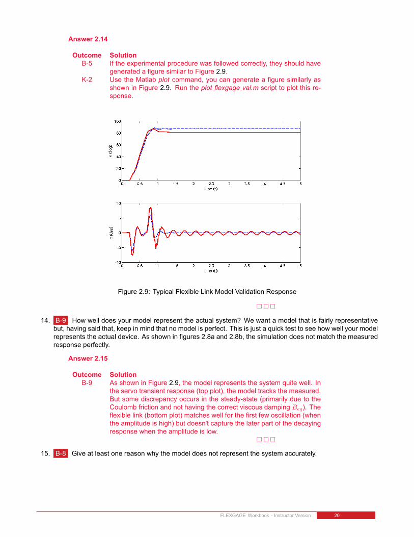
Answer 2.14
Outcome SolutionB-5 If the experimental procedure was followed correctly, they should have
generated a figure similar to Figure 2.9.K-2 Use the Matlab plot command, you can generate a figure similarly as
shown in Figure 2.9. Run the plot flexgage val.m script to plot this re-sponse.
Figure 2.9: Typical Flexible Link Model Validation Response
14. B-9 How well does your model represent the actual system? We want a model that is fairly representativebut, having said that, keep in mind that no model is perfect. This is just a quick test to see how well your modelrepresents the actual device. As shown in figures 2.8a and 2.8b, the simulation does not match the measuredresponse perfectly.
Answer 2.15
Outcome SolutionB-9 As shown in Figure 2.9, the model represents the system quite well. In
the servo transient response (top plot), the model tracks the measured.But some discrepancy occurs in the steady-state (primarily due to theCoulomb friction and not having the correct viscous damping Beq). Theflexible link (bottom plot) matches well for the first few oscillation (whenthe amplitude is high) but doesn't capture the later part of the decayingresponse when the amplitude is low.
15. B-8 Give at least one reason why the model does not represent the system accurately.
FLEXGAGE Workbook - Instructor Version 20
Answer 2.16
Outcome SolutionB-8 Here are some reasons:
• Themodel does not take Coulomb friction, i.e., stiction, into account.• Flexible link is modeled as a linear spring. Actual link is nonlinear(e.g., has high-frequency models that are unmodeled).
• Servo viscous damping, Beq, different for that servo.• Neglecting the flexible link damping, Bl.
16. K-1 In Matlab, find the open-loop poles (i.e., eigenvalues) of the system using the state-space matrix A thatis loaded.Note: These will be required for a pre-lab question in Section 3.3.
Answer 2.17
Outcome SolutionK-1 Using the Matlab command eig(A), the open-loop poles of the system
are: -24, −8.16 + j22.5, −8.16− j22.5, and 0.
FLEXGAGE Workbook - Instructor Version v 1.0
2.4 Results
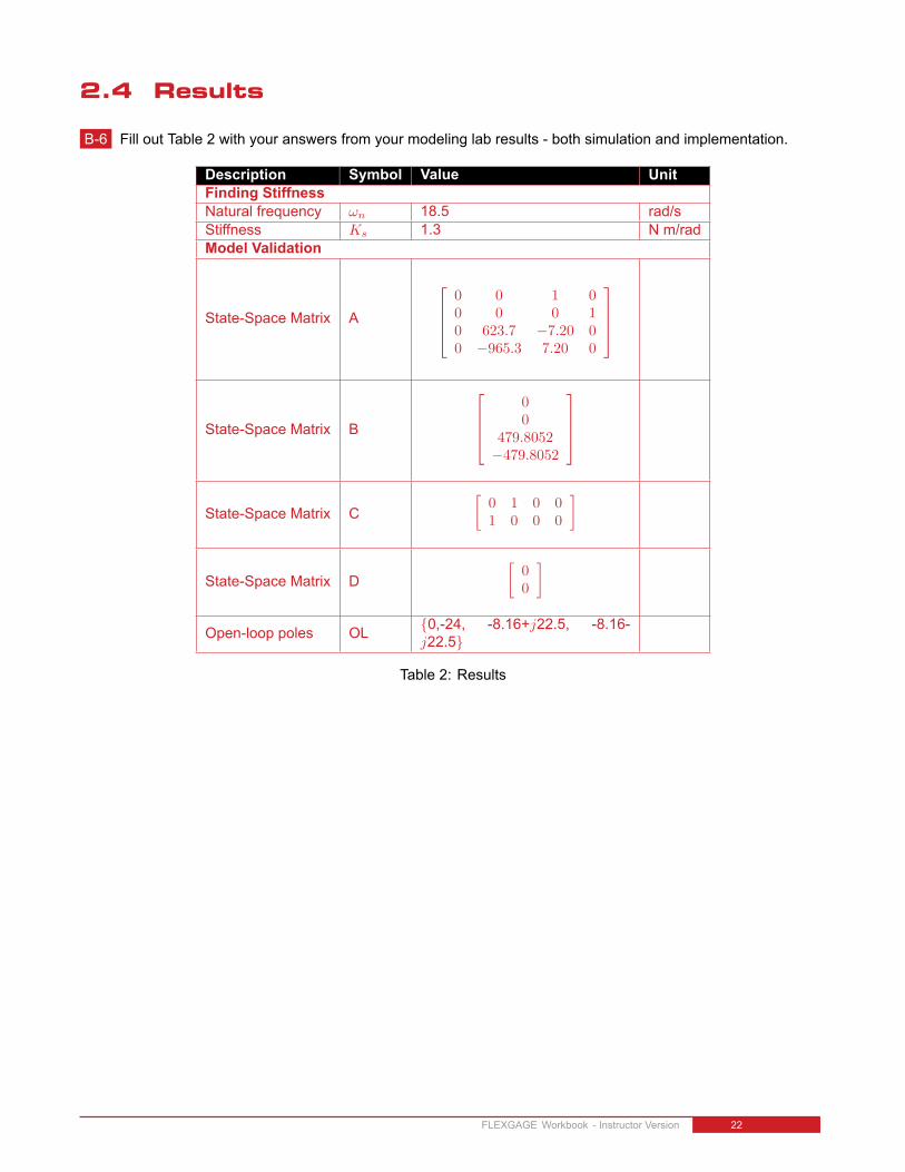
B-6 Fill out Table 2 with your answers from your modeling lab results - both simulation and implementation.
Description Symbol Value UnitFinding StiffnessNatural frequency ωn 18.5 rad/sStiffness Ks 1.3 N m/radModel Validation
State-Space Matrix A
0 0 1 00 0 0 10 623.7 −7.20 00 −965.3 7.20 0
State-Space Matrix B
00
479.8052−479.8052
State-Space Matrix C[
0 1 0 01 0 0 0
]
State-Space Matrix D[
00
]
Open-loop poles OL {0,-24, -8.16+j22.5, -8.16-j22.5}
Table 2: Results
FLEXGAGE Workbook - Instructor Version 22
3 CONTROL DESIGN
3.1 Specifications
The time-domain requirements are:
Specification 1: Servo angle settling time: ts <= 0.5 s.
Specification 2: Servo angle percentage overshoot: PO <= 7.5 %.
Specification 3: Maximum link angle deflection: |α| <= 10 deg.
Specification 4: Maximum control effort / voltage: |Vm| <= 10 V.
These specifications are to be satisfied when the rotary arm is tracking a ±30 degree angle square wave.
3.2 Background
In Section 2.2, we found a linear state-state space model that represents the Rotary Flexible Link system. Thismodel is used to investigate the stability properties of the Flexible Link system in Section 3.2.1. In Section 3.2.2,the notion of controllability is introduced. Using the Linear Quadratic Regular algorithm, or LQR, is a common wayto find the control gain and is discussed in Section 3.2.3. Lastly, Section 3.2.4 describes the state-feedback controlused to control the servo position while minimizing link deflection.
3.2.1 Stability
The stability of a system can be determined from its poles ([8]):
• Stable systems have poles only in the left-hand plane.
• Unstable systems have at least one pole in the right-hand plane and/or poles of multiplicity greater than 1 onthe imaginary axis.
• Marginally stable systems have one pole on the imaginary axis and the other poles in the left-hand plane.
The poles are the roots of the system's characteristic equation. From the state-space, the characteristic equation ofthe system can be found using
det (sI −A) = 0 (3.1)
where det() is the determinant function, s is the Laplace operator, and I the identity matrix. These are the eigenvaluesof the state-space matrix A.
3.2.2 Controllability
If the control input, u, of a system can take each state variable, xi where i = 1 . . . n, from an initial state to a finalstate then the system is controllable, otherwise it is uncontrollable ([8]).
Rank Test The system is controllable if the rank of its controllability matrix
T =[B AB A2B . . . AnB
](3.2)
equals the number of states in the system,rank(T ) = n. (3.3)
FLEXGAGE Workbook - Instructor Version v 1.0
3.2.3 Linear Quadratic Regular (LQR)
If (A,B) are controllable, then the Linear Quadratic Regular optimization method can be used to find a feedbackcontrol gain. Given the plant model in Equation 2.14, find a control input u that minimizes the cost function
J =
∫ ∞
0
x(t)′Qx(t) + u(t)′Ru(t) dt, (3.4)
where Q and R are the weighting matrices. The weighting matrices affect how LQR minimizes the function and are,essentially, tuning variables.
Given the control law u = −Kx, the state-space in Equation 2.14 becomes
x = Ax+B(−Kx)
= (A−BK)x
3.2.4 Feedback Control
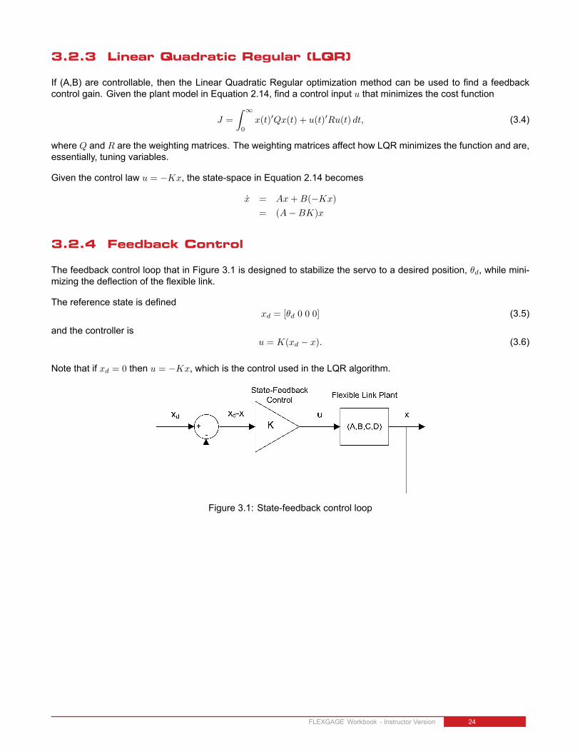
The feedback control loop that in Figure 3.1 is designed to stabilize the servo to a desired position, θd, while mini-mizing the deflection of the flexible link.
The reference state is definedxd = [θd 0 0 0] (3.5)
and the controller isu = K(xd − x). (3.6)
Note that if xd = 0 then u = −Kx, which is the control used in the LQR algorithm.
Figure 3.1: State-feedback control loop
FLEXGAGE Workbook - Instructor Version 24

3.3 Pre-Lab Questions
1. A-1, A-3 Based on your analysis of the system in the Modeling Laboratory (Section 2.3), is the systemstable, marginally stable, or unstable? From your experience in Section 2.3, does the stability you determinedanalyically match how the actual system behaves?
Answer 3.1
Outcome SolutionA-1 Recall from Step 16 in Section 2.3 the open-loop poles are -24, -
8.16+j22.5, -8.16-j22.5, and 0. Because one pole is on the imagi-nary axis (and all the others are in the left-hand plane), the system ismarginally stable. This is based on the definitions outlined in Section3.2.1.
A-3 From the Modeling laboratory, rotating the servo back and forth does notcause the system to go unstable but it does make the link vibrate andintroduces oscillations in the response. Due to these oscillations, thesystem cannot be categorized as stable but rather is marginally stable.
2. A-1, A-2 Designing a controller with the Linear Quadratic Regular (LQR) technique is an iterative process.In software, you have to tune the Q and R matrices, generate the gain K using LQR, and either simulate thesystem or implement the control to see if you have the desired response. The relationship between changingQ and R and the closed-loop response is not evident. However, we can have a better idea on how changingthe different elements in Q and R will effect the response. We will only be changing the diagonal elements inQ, thus let
Q =
q1 0 0 00 q2 0 00 0 q3 00 0 0 q4
. (3.7)
Since we are dealing with a single-input system, R is a scalar value. Using the Q and R defined, expand thecost function given in Equation 3.4.
Answer 3.2
Outcome SolutionA-1 Substitute Q given in Equation 3.7 above into Equation 3.4 and expand
the equation.A-2 The cost function becomes
J =
∫ ∞
0
x′Qx+Ru2 dt
=
∫ ∞
0
[x1 x2 x3 x4]
q1 0 0 00 q2 0 00 0 q3 00 0 0 q4
x1
x2
x3
x4
+Ru2 dt
=
∫ ∞
0
q1x21 + q2x
22 + q3x
23 + q4x
24 +Ru2 dt (Ans.3.1)
3. A-3 For the feedback control u = −Kx, the Linear-Quadratic Regular algorithm finds a gainK that minimizesthe cost function J . Matrix Q sets the weight on the states and determines how u will minimize J (and hencehow it generates gain K). From your solution in Question 2, explain how increasing the diagonal elements, qi,effects the generated gain K = [k1 k2 k3 k4].
FLEXGAGE Workbook - Instructor Version v 1.0
Answer 3.3
Outcome SolutionA-3 Looking at Equation Ans.3.1, increasing qi causes control input u to work
harder to minimize state xi, which will predominately increase ki. If q1is increased then k1 will increase to compensate for the larger weightplaced on state x1. Depending on the model, changing a single qi caneffect multiple ki gains because each state is not independent.
4. A-3 Explain the effect of increasing R has on the generated gain, K.
Answer 3.4
Outcome SolutionA-3 Looking at Equation Ans.3.1, if R is increased then control input u has
to work less to minimize J . In that case, LQR would generate a loweroverall gain of K.
FLEXGAGE Workbook - Instructor Version 26
3.4 Lab Experiments
The control gain is designed using LQR through simulation first. Once a gain that satisfies the requirements is found,it is implemented on the actual Quanser Flexible Link system.
3.4.1 Control Simulation
Using the linear state-space model of the system and the designed control gain, the closed-loop response can besimulated. This way, we can test the controller and see if it satisfies the given specifications before running it on thehardware platform.
Experiment Setup
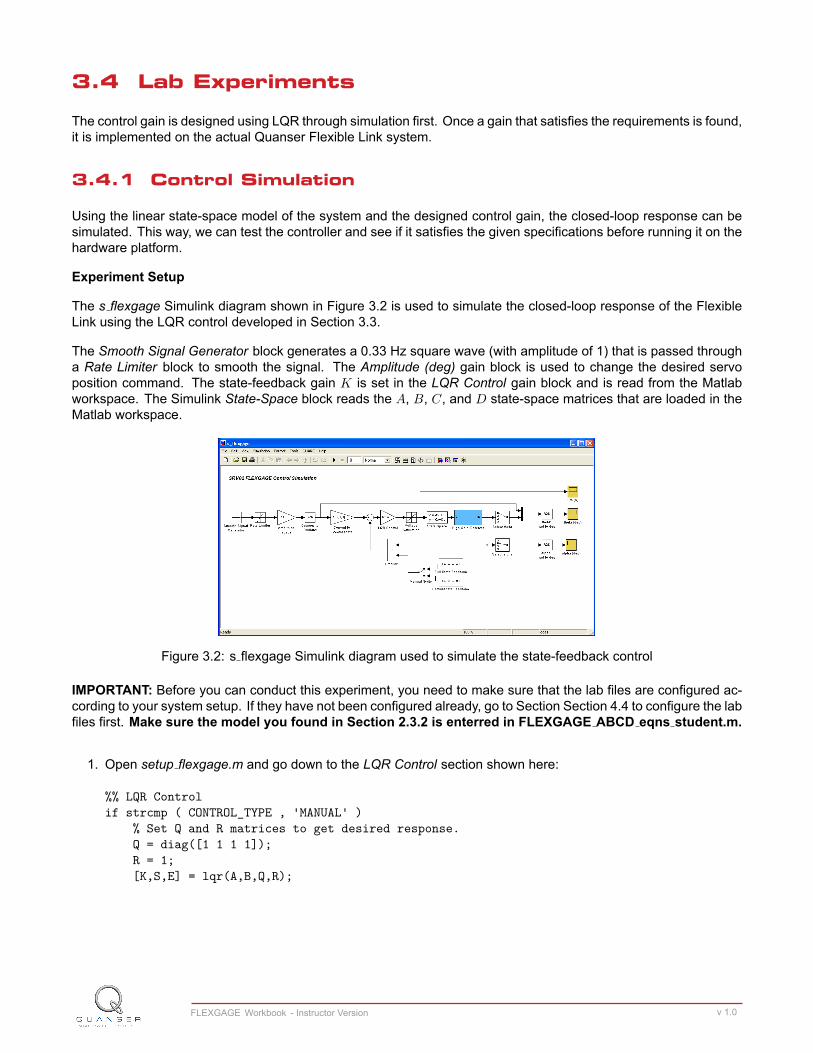
The s flexgage Simulink diagram shown in Figure 3.2 is used to simulate the closed-loop response of the FlexibleLink using the LQR control developed in Section 3.3.
The Smooth Signal Generator block generates a 0.33 Hz square wave (with amplitude of 1) that is passed througha Rate Limiter block to smooth the signal. The Amplitude (deg) gain block is used to change the desired servoposition command. The state-feedback gain K is set in the LQR Control gain block and is read from the Matlabworkspace. The Simulink State-Space block reads the A, B, C, and D state-space matrices that are loaded in theMatlab workspace.
Figure 3.2: s flexgage Simulink diagram used to simulate the state-feedback control
IMPORTANT: Before you can conduct this experiment, you need to make sure that the lab files are configured ac-cording to your system setup. If they have not been configured already, go to Section Section 4.4 to configure the labfiles first. Make sure the model you found in Section 2.3.2 is enterred in FLEXGAGE ABCD eqns student.m.
1. Open setup flexgage.m and go down to the LQR Control section shown here:
%% LQR Controlif strcmp ( CONTROL_TYPE , 'MANUAL' )
% Set Q and R matrices to get desired response.Q = diag([1 1 1 1]);R = 1;[K,S,E] = lqr(A,B,Q,R);
FLEXGAGE Workbook - Instructor Version v 1.0
The Q and R are initially set to the default values of:
Q =
1 0 0 00 1 0 00 0 1 00 0 0 1
and
R = 1.
2. These will not give you the desired response, but run the script to generate the default gain K. Enter thestiffness you found in Section 2.3.1 when prompted.
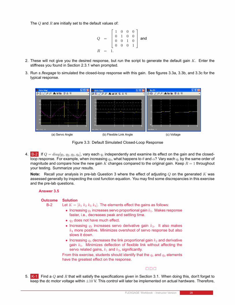
3. Run s flexgage to simulated the closed-loop response with this gain. See figures 3.3a, 3.3b, and 3.3c for thetypical response.
(a) Servo Angle (b) Flexible Link Angle (c) Voltage
Figure 3.3: Default Simulated Closed-Loop Response
4. B-2 If Q = diag[q1, q2, q3, q4], vary each qi independently and examine its effect on the gain and the closed-loop response. For example, when increasing q3, what happens to θ and α? Vary each qi by the same order ofmagnitude and compare how the new gain K changes compared to the original gain. Keep R = 1 throughoutyour testing. Summarize your results.Note: Recall your analysis in pre-lab Question 3 where the effect of adjusting Q on the generated K wasassessed generally by inspecting the cost function equation. You may find some discrepancies in this exerciseand the pre-lab questions.
Answer 3.5
Outcome SolutionB-2 Let K = [k1 k2 k3 k4]. The elements effect the gains as follows:
• Increasing q1 increases servo proportional gain k1. Makes responsefaster, i.e., decreases peak and settling time.
• q2 does not have much effect.• Increasing q3 increases servo derivative gain k3. It also makes
k4 more positive. Minimizes overshoot of servo response but alsoslows it down.
• Increasing q4 decreases the link proportional gain k2 and derivativegain k4. Minimizes deflection of flexible link without affecting theservo related gains, k1 and k3, significantly.
From this exercise, students should identify that the q1 and q4 elementshave the greatest effect on the response.
5. K-1 Find a Q and R that will satisfy the specifications given in Section 3.1. When doing this, don't forget tokeep the dc motor voltage within ±10 V. This control will later be implemented on actual hardware. Therefore,
FLEXGAGE Workbook - Instructor Version 28

make sure the actuator is not being saturated. Enter the weighting matrices, Q and R, used and the resultinggain, K.
Answer 3.6
Outcome SolutionK-1 One set of weighting matrices that yields adequate results are
Q =
150 0 0 00 1 0 00 0 1 00 0 0 3
(Ans.3.2)
andR = 1 (Ans.3.3)
which generates the gain
K = [12.2 − 23.0 1.39 − 0.311]. (Ans.3.4)
6. B-5, K-3 Plot the responses from the theta (deg), alpha (deg), and Vm (V) scopes in a Matlab figure. Whenthe QUARC controller is stopped, these scopes automatically save the last 5 seconds of their response datato the variables data theta, data alpha, and data vm. For data theta, the time is in data theta(:,1), the setpoint(i.e., desired SRV02 angle) is in data theta(:,2), and the simulated SRV02 angle is in data theta(:,3). In thedata alpha and data vm variables, the (:,1) holds the time vector and the (:,2) holds the actual measureddata.
Answer 3.7
Outcome SolutionB-5 If the experimental procedure was followed correctly, they should have
generated a figure similar to Figure 3.4.K-3 Use the Matlab plot command, you can generate a figure similarly as
shown in Figure 3.4. Run the meas flexgage specs.m script after run-ning the s flexgage.mdl to plot this response.
7. K-1, B-9 Measure the settling time and percent overshoot of the simulated servo response and the maximumlink deflection. Does the response satisfy the specifications given in Section 3.1?
Answer 3.8
Outcome SolutionK-1 The settling time and overshoot measured from the top plot in Figure
3.4 arets = 0.42 s
andPO = 2.8
The maximum deflection of the link is
|α|max = 9.5 deg
B-9 The specifications in Section 3.1 are satisfied while the input voltage iskept between ±10 V. Use the meas flexgage spec.m script to find thespecifications automatically after running s flexgage.
FLEXGAGE Workbook - Instructor Version v 1.0
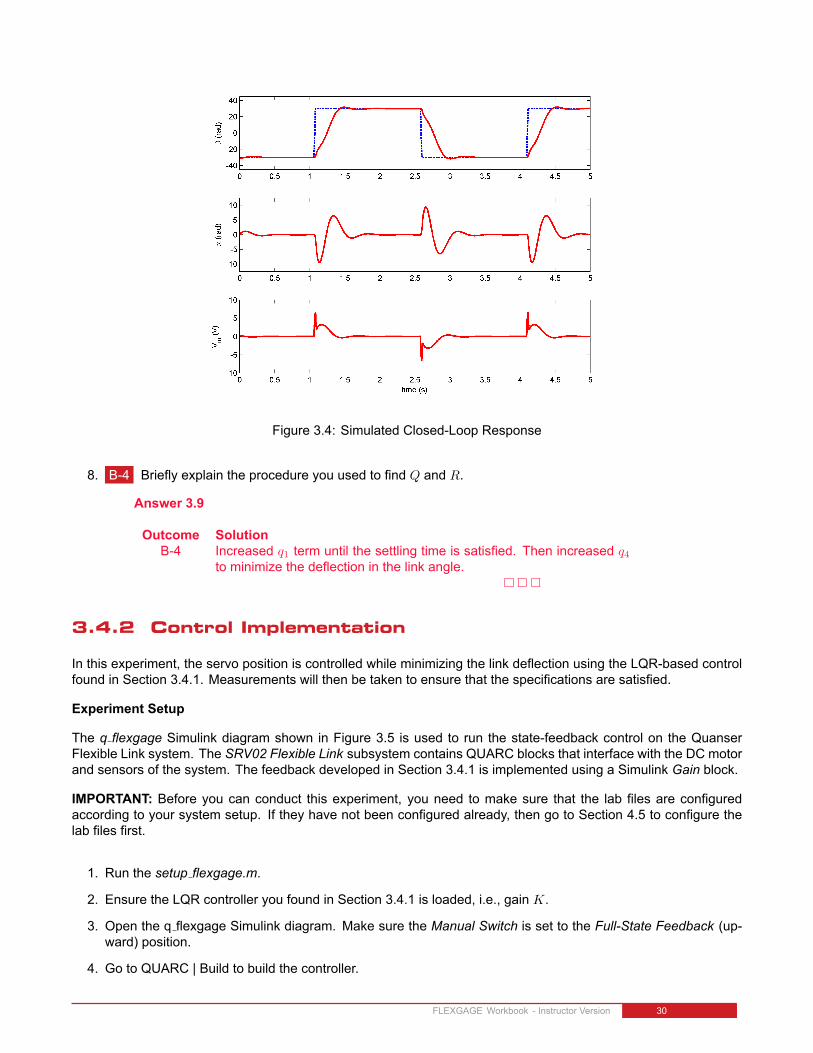
Figure 3.4: Simulated Closed-Loop Response
8. B-4 Briefly explain the procedure you used to find Q and R.
Answer 3.9
Outcome SolutionB-4 Increased q1 term until the settling time is satisfied. Then increased q4
to minimize the deflection in the link angle.
3.4.2 Control Implementation
In this experiment, the servo position is controlled while minimizing the link deflection using the LQR-based controlfound in Section 3.4.1. Measurements will then be taken to ensure that the specifications are satisfied.
Experiment Setup
The q flexgage Simulink diagram shown in Figure 3.5 is used to run the state-feedback control on the QuanserFlexible Link system. The SRV02 Flexible Link subsystem contains QUARC blocks that interface with the DC motorand sensors of the system. The feedback developed in Section 3.4.1 is implemented using a Simulink Gain block.
IMPORTANT: Before you can conduct this experiment, you need to make sure that the lab files are configuredaccording to your system setup. If they have not been configured already, then go to Section 4.5 to configure thelab files first.
1. Run the setup flexgage.m.
2. Ensure the LQR controller you found in Section 3.4.1 is loaded, i.e., gain K.
3. Open the q flexgage Simulink diagram. Make sure the Manual Switch is set to the Full-State Feedback (up-ward) position.
4. Go to QUARC | Build to build the controller.
FLEXGAGE Workbook - Instructor Version 30
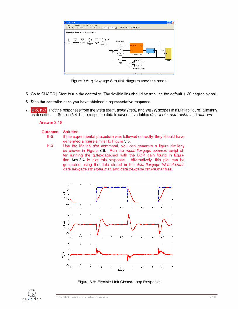
Figure 3.5: q flexgage Simulink diagram used the model
5. Go to QUARC | Start to run the controller. The flexible link should be tracking the default ± 30 degree signal.
6. Stop the controller once you have obtained a representative response.
7. B-5, K-3 Plot the responses from the theta (deg), alpha (deg), and Vm (V) scopes in a Matlab figure. Similarlyas described in Section 3.4.1, the response data is saved in variables data theta, data alpha, and data vm.
Answer 3.10
Outcome SolutionB-5 If the experimental procedure was followed correctly, they should have
generated a figure similar to Figure 3.6.K-3 Use the Matlab plot command, you can generate a figure similarly
as shown in Figure 3.6. Run the meas flexgage specs.m script af-ter running the q flexgage.mdl with the LQR gain found in Equa-tion Ans.3.4 to plot this response. Alternatively, this plot can begenerated using the data stored in the data flexgage fsf theta.mat,data flexgage fsf alpha.mat, and data flexgage fsf vm.mat files.
Figure 3.6: Flexible Link Closed-Loop Response
FLEXGAGE Workbook - Instructor Version v 1.0
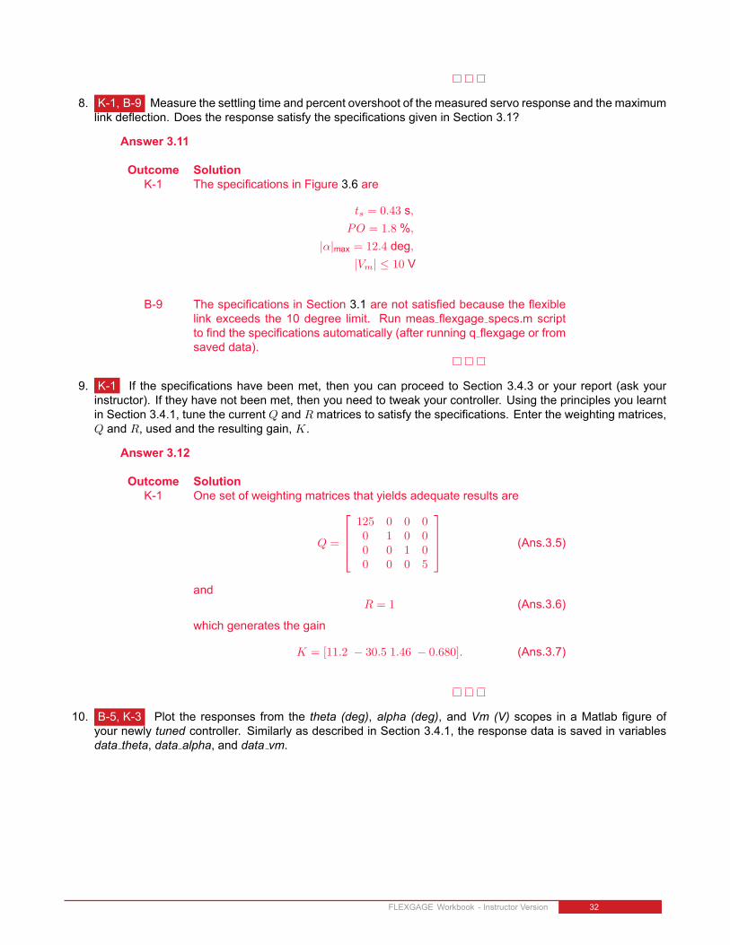
8. K-1, B-9 Measure the settling time and percent overshoot of the measured servo response and the maximumlink deflection. Does the response satisfy the specifications given in Section 3.1?
Answer 3.11
Outcome SolutionK-1 The specifications in Figure 3.6 are
ts = 0.43 s,PO = 1.8 %,
|α|max = 12.4 deg,|Vm| ≤ 10 V
B-9 The specifications in Section 3.1 are not satisfied because the flexiblelink exceeds the 10 degree limit. Run meas flexgage specs.m scriptto find the specifications automatically (after running q flexgage or fromsaved data).
9. K-1 If the specifications have been met, then you can proceed to Section 3.4.3 or your report (ask yourinstructor). If they have not been met, then you need to tweak your controller. Using the principles you learntin Section 3.4.1, tune the current Q and R matrices to satisfy the specifications. Enter the weighting matrices,Q and R, used and the resulting gain, K.
Answer 3.12
Outcome SolutionK-1 One set of weighting matrices that yields adequate results are
Q =
125 0 0 00 1 0 00 0 1 00 0 0 5
(Ans.3.5)
andR = 1 (Ans.3.6)
which generates the gain
K = [11.2 − 30.5 1.46 − 0.680]. (Ans.3.7)
10. B-5, K-3 Plot the responses from the theta (deg), alpha (deg), and Vm (V) scopes in a Matlab figure ofyour newly tuned controller. Similarly as described in Section 3.4.1, the response data is saved in variablesdata theta, data alpha, and data vm.
FLEXGAGE Workbook - Instructor Version 32
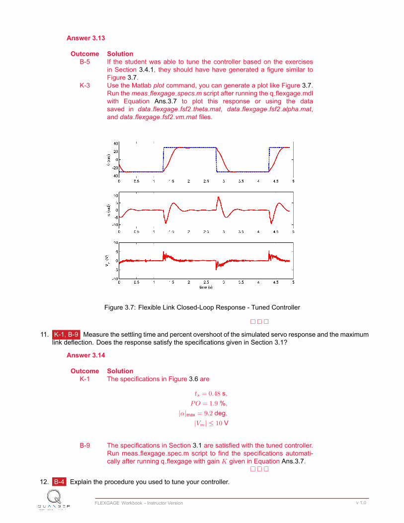
Answer 3.13
Outcome SolutionB-5 If the student was able to tune the controller based on the exercises
in Section 3.4.1, they should have have generated a figure similar toFigure 3.7.
K-3 Use the Matlab plot command, you can generate a plot like Figure 3.7.Run themeas flexgage specs.m script after running the q flexgage.mdlwith Equation Ans.3.7 to plot this response or using the datasaved in data flexgage fsf2 theta.mat, data flexgage fsf2 alpha.mat,and data flexgage fsf2 vm.mat files.
Figure 3.7: Flexible Link Closed-Loop Response - Tuned Controller
11. K-1, B-9 Measure the settling time and percent overshoot of the simulated servo response and the maximumlink deflection. Does the response satisfy the specifications given in Section 3.1?
Answer 3.14
Outcome SolutionK-1 The specifications in Figure 3.6 are
ts = 0.48 s,PO = 1.9 %,
|α|max = 9.2 deg,|Vm| ≤ 10 V
B-9 The specifications in Section 3.1 are satisfied with the tuned controller.Run meas flexgage spec.m script to find the specifications automati-cally after running q flexgage with gain K given in Equation Ans.3.7.
12. B-4 Explain the procedure you used to tune your controller.
FLEXGAGE Workbook - Instructor Version v 1.0
Answer 3.15
Outcome SolutionB-4 Increasing parameter q4 from 3 to 5 dampens the link deflection but it
also increases the speed of the servo response, i.e., resulting in a largersettling time. By decreasing q1 from 150 down to 125, the servo re-sponse settling time is decreased within specification.
3.4.3 Implementing Partial-State Feedback Control
In this section, the partial-state feedback response of the system is assessed and compared with the full-statefeedback control in Section 3.4.2.
1. Run the setup flexgage.m.
2. Ensure the LQR control gain you settled on in Section 3.4.2 is loaded, i.e., gain K.
3. Open the q flexgage Simulink diagram. Make sure the Manual Switch is set to the Partial-State Feedback(downward) position.
4. Go to QUARC | Start to run the controller. The flexible link should be tracking the default ±30 degree signal.
5. Stop the controller once you have obtained a representative response.
6. B-5, K-3 As in Section 3.4.2, attach a Matlab figure representing the SRV02 angle and flexible link angleresponse, as well as the input voltage.
Answer 3.16
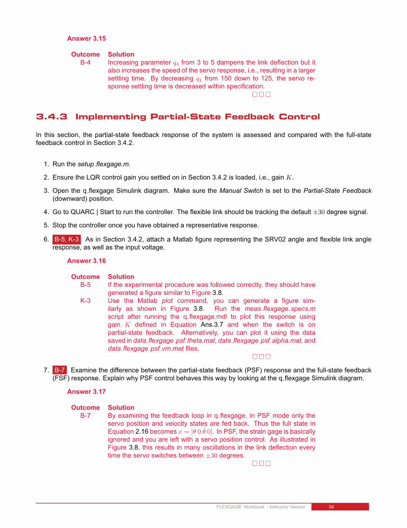
Outcome SolutionB-5 If the experimental procedure was followed correctly, they should have
generated a figure similar to Figure 3.8.K-3 Use the Matlab plot command, you can generate a figure sim-
ilarly as shown in Figure 3.8. Run the meas flexgage specs.mscript after running the q flexgage.mdl to plot this response usinggain K defined in Equation Ans.3.7 and when the switch is onpartial-state feedback. Alternatively, you can plot it using the datasaved in data flexgage psf theta.mat, data flexgage psf alpha.mat, anddata flexgage psf vm.mat files.
7. B-7 Examine the difference between the partial-state feedback (PSF) response and the full-state feedback(FSF) response. Explain why PSF control behaves this way by looking at the q flexgage Simulink diagram.
Answer 3.17
Outcome SolutionB-7 By examining the feedback loop in q flexgage, in PSF mode only the
servo position and velocity states are fed back. Thus the full state inEquation 2.16 becomes x = [θ 0 θ 0]. In PSF, the strain gage is basicallyignored and you are left with a servo position control. As illustrated inFigure 3.8, this results in many oscillations in the link deflection everytime the servo switches between ±30 degrees.
FLEXGAGE Workbook - Instructor Version 34
Figure 3.8: Partial-State Closed-Loop Response
FLEXGAGE Workbook - Instructor Version v 1.0
3.5 Results
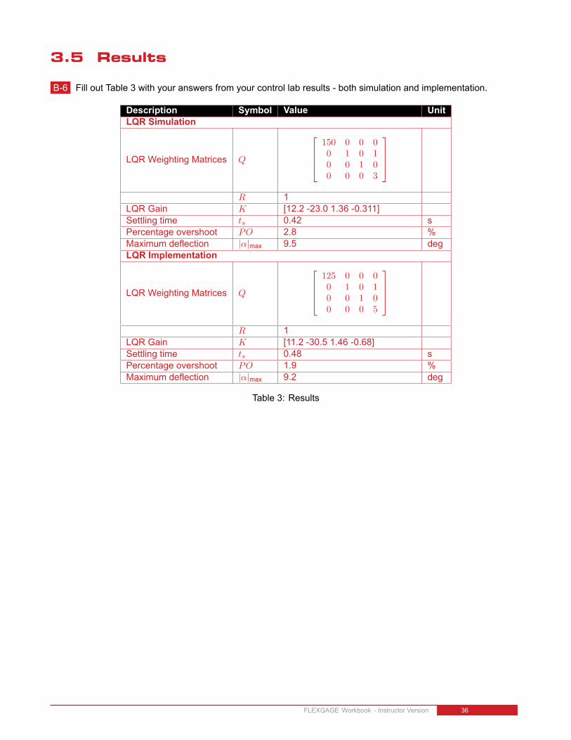
B-6 Fill out Table 3 with your answers from your control lab results - both simulation and implementation.
Description Symbol Value UnitLQR Simulation
LQR Weighting Matrices Q
150 0 0 00 1 0 10 0 1 00 0 0 3
R 1
LQR Gain K [12.2 -23.0 1.36 -0.311]Settling time ts 0.42 sPercentage overshoot PO 2.8 %Maximum deflection |α|max 9.5 degLQR Implementation
LQR Weighting Matrices Q
125 0 0 00 1 0 10 0 1 00 0 0 5
R 1
LQR Gain K [11.2 -30.5 1.46 -0.68]Settling time ts 0.48 sPercentage overshoot PO 1.9 %Maximum deflection |α|max 9.2 deg
Table 3: Results
FLEXGAGE Workbook - Instructor Version 36
4 SYSTEM REQUIREMENTSRequired Software
• Microsoft Visual Studio
• Matlabrwith Simulinkr, Real-Time Workshop, and the Control System Toolbox.
• QUARCr2.1, or later.
See the QUARCrsoftware compatibility chart at [5] to see what versions of MS VS and Matlab are compatible withyour version of QUARC and for what OS.
Required Hardware
• Data-acquisition (DAQ) card that is compatible with QUARC. This includes Quanser Hardware-in-the-loop(HIL) boards such as:
– Q2-USB– Q8-USB– QPID– QPIDe
and some National Instruments DAQ devices (e.g., NI USB-6251, NI PCIe-6259). For a full listing of compliantDAQ cards, see Reference [1].
• Quanser SRV02-ET rotary servo.
• Quanser Rotary Flexible Joint (attached to SRV02).
• Quanser VoltPAQ-X1 power amplifier, or equivalent.
Before Starting Lab
Before you begin this laboratory make sure:
• QUARCris installed on your PC, as described in [3].
• The QUARC Analog Loopback Demo has been ran successfully.
• SRV02 Rotary Flexible Joint and amplifier are connected to your DAQ board as described Reference [7].
FLEXGAGE Workbook - Instructor Version v 1.0

4.1 Overview of Files
File Name DescriptionFlexible Link User Manual.pdf This manual describes the hardware of the Rotary Flexi-
ble Link system and explains how to setup and wire thesystem for the experiments.
Flexible Link Workbook (Student).pdf This laboratory guide contains pre-lab questions and labexperiments demonstrating how to design and implementa position controller on the Quanser SRV02 Flexible Linkplant using QUARCr .
setup flexgage.m The main Matlab script that sets the SRV02 motor andsensor parameters, the SRV02 configuration-dependentmodel parameters, and the Flexible Link (i.e., flexgage)sensor parameters. Run this file only to setup the labora-tory.
config srv02.m Returns the configuration-based SRV02 model specifica-tions Rm, kt, km, Kg, eta g, Beq, Jeq, and eta m, thesensor calibration constants K POT, K ENC, and K TACH,and the amplifier limits VMAX AMP and IMAX AMP.
config flexgage.m Returns the Flexible Link model inertial, Jl, viscous damp-ing, Bl, and sensor calibration constant K GAGE.
d model param.m Calculates the SRV02 model parameters K and tau basedon the device specifications Rm, kt, km, Kg, eta g, Beq,Jeq, and eta m.
FLEXGAGE ABCD eqns student.m Contains the incomplete state-space A, B, C, and D matri-ces. These are used to represent the Flexible Link system.
calc conversion constants.m Returns various conversions factors.s flexgage.mdl Simulink file that simulates the Flexible Link system when
using a full or partial state-feedback control.q flexgage id.mdl When ran with QUARCr, this Simulink model measures
the Flexible Link angle. The measured response can thenbe used to find the stiffness of the link.
q flexgage val.mdl This Simulink model is used with QUARCrto comparethe Flexible Link state-space model with the measured re-sponse from the actual system.
q flexgage.mdl Simulink file that implements a closed-loop state-feedbackcontroller on the actual FLEXGAGE system usingQUARCr .
Table 4: Files supplied with the SRV02 Flexible Link Control Laboratory.
FLEXGAGE Workbook - Instructor Version 38
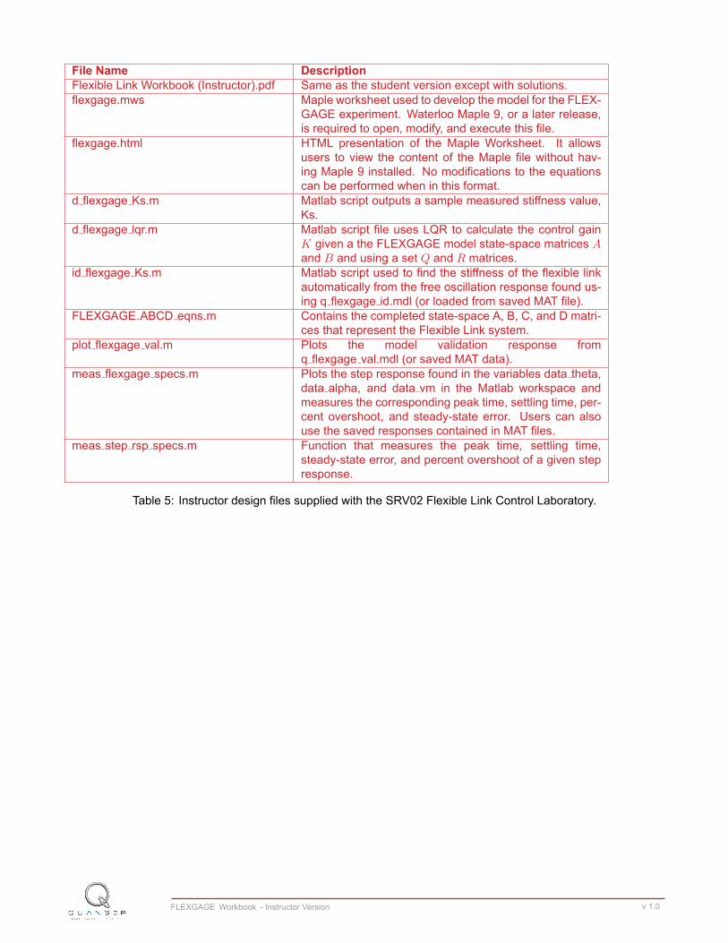
File Name DescriptionFlexible Link Workbook (Instructor).pdf Same as the student version except with solutions.flexgage.mws Maple worksheet used to develop the model for the FLEX-
GAGE experiment. Waterloo Maple 9, or a later release,is required to open, modify, and execute this file.
flexgage.html HTML presentation of the Maple Worksheet. It allowsusers to view the content of the Maple file without hav-ing Maple 9 installed. No modifications to the equationscan be performed when in this format.
d flexgage Ks.m Matlab script outputs a sample measured stiffness value,Ks.
d flexgage lqr.m Matlab script file uses LQR to calculate the control gainK given a the FLEXGAGE model state-space matrices Aand B and using a set Q and R matrices.
id flexgage Ks.m Matlab script used to find the stiffness of the flexible linkautomatically from the free oscillation response found us-ing q flexgage id.mdl (or loaded from saved MAT file).
FLEXGAGE ABCD eqns.m Contains the completed state-space A, B, C, and D matri-ces that represent the Flexible Link system.
plot flexgage val.m Plots the model validation response fromq flexgage val.mdl (or saved MAT data).
meas flexgage specs.m Plots the step response found in the variables data theta,data alpha, and data vm in the Matlab workspace andmeasures the corresponding peak time, settling time, per-cent overshoot, and steady-state error. Users can alsouse the saved responses contained in MAT files.
meas step rsp specs.m Function that measures the peak time, settling time,steady-state error, and percent overshoot of a given stepresponse.
Table 5: Instructor design files supplied with the SRV02 Flexible Link Control Laboratory.
FLEXGAGE Workbook - Instructor Version v 1.0
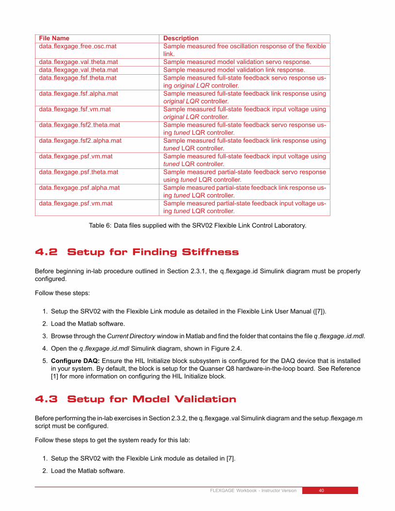
File Name Descriptiondata flexgage free osc.mat Sample measured free oscillation response of the flexible
link.data flexgage val theta.mat Sample measured model validation servo response.data flexgage val theta.mat Sample measured model validation link response.data flexgage fsf theta.mat Sample measured full-state feedback servo response us-
ing original LQR controller.data flexgage fsf alpha.mat Sample measured full-state feedback link response using
original LQR controller.data flexgage fsf vm.mat Sample measured full-state feedback input voltage using
original LQR controller.data flexgage fsf2 theta.mat Sample measured full-state feedback servo response us-
ing tuned LQR controller.data flexgage fsf2 alpha.mat Sample measured full-state feedback link response using
tuned LQR controller.data flexgage psf vm.mat Sample measured full-state feedback input voltage using
tuned LQR controller.data flexgage psf theta.mat Sample measured partial-state feedback servo response
using tuned LQR controller.data flexgage psf alpha.mat Samplemeasured partial-state feedback link response us-
ing tuned LQR controller.data flexgage psf vm.mat Sample measured partial-state feedback input voltage us-
ing tuned LQR controller.
Table 6: Data files supplied with the SRV02 Flexible Link Control Laboratory.
4.2 Setup for Finding Stiffness
Before beginning in-lab procedure outlined in Section 2.3.1, the q flexgage id Simulink diagram must be properlyconfigured.
Follow these steps:
1. Setup the SRV02 with the Flexible Link module as detailed in the Flexible Link User Manual ([7]).
2. Load the Matlab software.
3. Browse through theCurrent Directory window inMatlab and find the folder that contains the file q flexgage id.mdl.
4. Open the q flexgage id.mdl Simulink diagram, shown in Figure 2.4.
5. Configure DAQ: Ensure the HIL Initialize block subsystem is configured for the DAQ device that is installedin your system. By default, the block is setup for the Quanser Q8 hardware-in-the-loop board. See Reference[1] for more information on configuring the HIL Initialize block.
4.3 Setup for Model Validation
Before performing the in-lab exercises in Section 2.3.2, the q flexgage val Simulink diagram and the setup flexgage.mscript must be configured.
Follow these steps to get the system ready for this lab:
1. Setup the SRV02 with the Flexible Link module as detailed in [7].
2. Load the Matlab software.
FLEXGAGE Workbook - Instructor Version 40
3. Browse through the Current Directory window in Matlab and find the folder that contains the QUARC FLEX-GAGE file q flexgage val.mdl.
4. Open the q flexgage val.mdl Simulink diagram, shown in Figure 2.7.
5. Configure DAQ: Ensure the HIL Initialize block in the SRV02 Flexible Link subsystem is configured for theDAQ device that is installed in your system. By default, the block is setup for the Quanser Q8 hardware-in-the-loop board. See Reference [1] for more information on configuring the HIL Initialize block.
6. Configure Sensor: The position of the SRV02 load shaft can be measured using either the potentiometer orthe encoder. Set the Pos Src Source block in q flexgage val, as shown in Figure 2.7, as follows:
• 1 to use the potentiometer• 2 to use to the encoder
Note that when using the potentiometer, there will be a discontinuity.
7. Configure Input: Set theManual Switch to the DOWN position for a step input or the UP position for a squaresignal.
8. Open the setup flexgage.m file. This is the setup script used for the FLEXGAGE Simulink models.
9. Configure setup script: When used with the Flexible Link, the SRV02 has no load (i.e., no disc or bar) andhas to be in the high-gear configuration. Make sure the script is setup to match this setup:
• EXT GEAR CONFIG to 'HIGH'• LOAD TYPE to 'NONE'• Ensure ENCODER TYPE, TACH OPTION, K CABLE, AMP TYPE, and VMAX DAC parameters are setaccording to the SRV02 system that is to be used in the laboratory.
• CONTROL TYPE to 'MANUAL'.
For Instructors: Set CONTROL TYPE = 'AUTO' to automatically set the link stiffness, Ks, load the model,and find the LQR gain.The students should not have access to the files given in Table 5 and Table 6. However, exactly what shouldbe given to the students is at the discretion of the instructor.
4.4 Setup for Flexible Link Control Simulation
Before going through the control simulation in Section 3.4.1, the s flexgage Simulink diagram and the setup flexgage.mscript must be configured.
Follow these steps to configure the lab properly:
1. Load the Matlab software.
2. IMPORTANT: Make sure the model you found in Section 2.3.2 is enterred in FLEXGAGE ABCD eqnsstudent.m.For Instructors: Set CONTROL TYPE = 'AUTO' as explained in Section 4.3 to load the model from the FLEX-GAGE ABCD eqns.m files and then find the LQR gain, K, automatically.
3. Browse through the Current Directory window in Matlab and find the folder that contains the s flexgage.mdlfile.
4. Open s flexgage.mdl Simulink diagram shown in Figure 3.2.
5. Configure the setup flexgage.m script according to your hardware. See Section 4.3 for more information.
6. Run the setup flexgage.m script.
7. Enter the stiffness (Ks) you found in Section 2.3.1.
FLEXGAGE Workbook - Instructor Version v 1.0

4.5 Setup for Flexible Link Control Implementation
Before beginning the in-lab exercises given in Section 3.4.2 (or Section 3.4.3), the q flexgage Simulink diagram andthe setup flexgage.m script must be setup.
Follow these steps to get the system ready for this lab:
1. Setup the SRV02 with the Flexible Link module as detailed in [7] .
2. Load the Matlab software.
3. Browse through the Current Directory window in Matlab and find the folder that contains the q flexgage.mdlfile.
4. Open the q flexgage.mdl Simulink diagram shown in Figure 3.5.
5. Configure DAQ: Ensure the HIL Initialize block in the SRV02 Flexible Link subsystem is configured for theDAQ device that is installed in your system. By default, the block is setup for the Quanser Q8 hardware-in-the-loop board. See Reference [1] for more information on configuring the HIL Initialize block.
6. Configure Sensor: The position of the SRV02 load shaft can be measured using the potentiometer or theencoder. Set the Pos Src Source block in q flexgage, as shown in Figure 3.5, as follows:
• 1 to use the potentiometer• 2 to use to the encoder
Note that when using the potentiometer, there will be a discontinuity.
7. Configure setup script: Set the parameters in the setup flexgage.m script according to your system setup.See Section 4.3 for more details.
8. Run the setup flexgage.m script.
FLEXGAGE Workbook - Instructor Version 42

5 LAB REPORTThis laboratory contains two groups of experiments, namely,
1. Modeling the Quanser Rotary Flexible Link system, and
2. State-feedback control using LQR.
For each experiment, follow the outline corresponding to that experiment to build the content of your report. Also,in Section 5.3 you can find some basic tips for the format of your report.
5.1 Template for Content (Modeling)
I. PROCEDURE
1. Finding Stiffness
• Briefly describe the main goal of the experiment.• Briefly describe the experiment procedure (Section 2.3.1)
2. Model Validation
• Briefly describe the main goal of the experiment.• Briefly describe the experiment procedure (Section 2.3.2)
II. RESULTSDo not interpret or analyze the data in this section. Just provide the results.
1. Free-oscillation plot from step 3 in Section 2.3.1.
2. Model validation plot from step 13 in Section 2.3.2.
3. Provide applicable data collected in this laboratory (from Table 2).
III. ANALYSISProvide details of your calculations (methods used) for analysis for each of the following:
1. Measured link stiffness in step 5 in Section 2.3.1.
2. Model discrepancies given in step 15 in Section 2.3.2.
IV. CONCLUSIONSInterpret your results to arrive at logical conclusions for the following:
1. How does the model compare with the actual system in step 14 of Section 2.3.2, State-space model validation.
FLEXGAGE Workbook - Instructor Version v 1.0

5.2 Template for Content (Control)
I. PROCEDURE
1. Simulation
• Briefly describe the main goal of the simulation.• Briefly describe the simulation procedure (Section 3.4.1).• Briefly describe the procedure in step 4 of Section 3.4.1 to examine the effect of variables on the gain andclosed-loop response.
• Briefly explain the procedure used to find Q and R in step 8 of Section 3.4.1).
2. Full-State Feedback Implementation
• Briefly describe the main goal of this experiment.• Briefly describe the experimental procedure (Section 3.4.2).• Briefly explain the procedure used to tune the controller in step 12 of Section 3.4.3.
3. Partial-State Feedback Implementation
• Briefly describe the main goal of this experiment.• Briefly describe the experimental procedure (Section 3.4.3).
II. RESULTSDo not interpret or analyze the data in this section. Just provide the results.
1. Response plot from step 6 in Section 3.4.1, Full-state feedback LQR controller simulation.
2. Response plot from step 7 in Section 3.4.2, for Full-state feedback LQR controller implementation.
3. Response plot from step 10 in Section 3.4.2, for Tuned LQR full-state feedback controller implementation.
4. Response plot from step 6 in Section 3.4.3, for Partial-state feedback LQR controller implementation.
5. Provide applicable data collected in this laboratory (from Table 3).
III. ANALYSISProvide details of your calculations (methods used) for analysis for each of the following:
1. Settling time and percent overshoot in step 7 in Section 3.4.1, Full-state feedback LQR controller simulation.
2. Settling time and percent overshoot in step 8 in Section 3.4.2, for Full-state feedback LQR controller imple-mentation.
3. Settling time and percent overshoot in step 11 in Section 3.4.2, for Tuned LQR full-state feedback controllerimplementation.
4. Comparison between partial-state and full-state feedback in step 7 in Section 3.4.3.
IV. CONCLUSIONSInterpret your results to arrive at logical conclusions for the following:
1. Whether the controller meets the specifications in step 7 in Section 3.4.1, Full-state feedback LQR controllersimulation.
2. Whether the controller meets the specifications in step 8 in Section 3.4.2, for Full-state feedback LQR controllerimplementation.
3. Whether the controller meets the specifications in step 11 in Section 3.4.2, for Tuned LQR full-state feedbackcontroller implementation.
FLEXGAGE Workbook - Instructor Version 44

5.3 Tips for Report Format
PROFESSIONAL APPEARANCE
• Has cover page with all necessary details (title, course, student name(s), etc.)
• Each of the required sections is completed (Procedure, Results, Analysis and Conclusions).
• Typed.
• All grammar/spelling correct.
• Report layout is neat.
• Does not exceed specified maximum page limit, if any.
• Pages are numbered.
• Equations are consecutively numbered.
• Figures are numbered, axes have labels, each figure has a descriptive caption.
• Tables are numbered, they include labels, each table has a descriptive caption.
• Data are presented in a useful format (graphs, numerical, table, charts, diagrams).
• No hand drawn sketches/diagrams.
• References are cited using correct format.
FLEXGAGE Workbook - Instructor Version v 1.0

6 SCORING SHEET FOR PRE-LABMODELING QUESTIONS
Student Name :
Question1 A-1 A-2 A-312345678
Total
1This scoring sheet is for the Modeling Pre-Lab questions in Section 2.2.
FLEXGAGE Workbook - Instructor Version 46
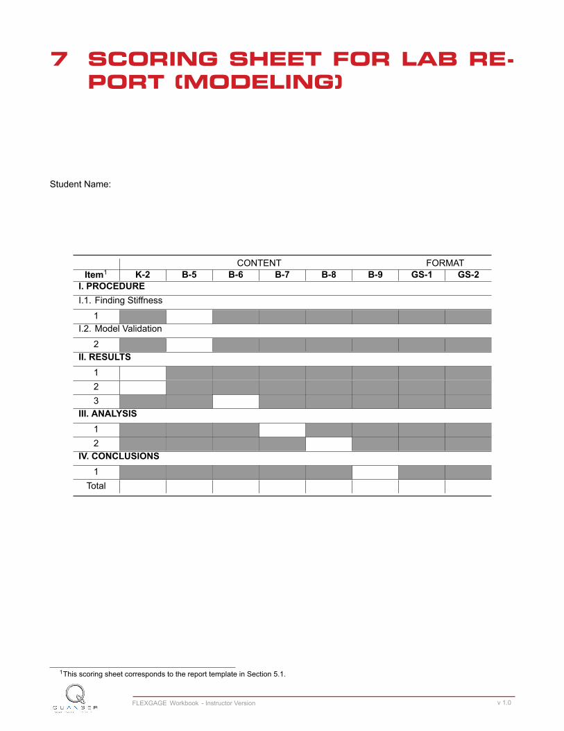
7 SCORING SHEET FOR LAB RE-PORT (MODELING)
Student Name:
CONTENT FORMATItem1 K-2 B-5 B-6 B-7 B-8 B-9 GS-1 GS-2
I. PROCEDUREI.1. Finding Stiffness
1I.2. Model Validation
2II. RESULTS
123
III. ANALYSIS12
IV. CONCLUSIONS1
Total
1This scoring sheet corresponds to the report template in Section 5.1.
FLEXGAGE Workbook - Instructor Version v 1.0

8 SCORING SHEET FOR PRE-LABCONTROL QUESTIONS
Student Name :
Question1 A-1 A-2 A-31234
Total
.
1This scoring sheet is for the Control Pre-Lab questions in Section 3.3
FLEXGAGE Workbook - Instructor Version 48
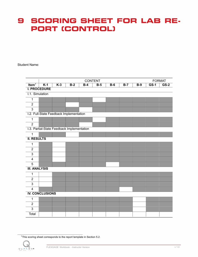
9 SCORING SHEET FOR LAB RE-PORT (CONTROL)
Student Name:
CONTENT FORMATItem1 K-1 K-3 B-2 B-4 B-5 B-6 B-7 B-9 GS-1 GS-2I. PROCEDUREI.1. Simulation
123
I.2. Full-State Feedback Implementation
12
I.3. Partial-State Feedback Implementation
1II. RESULTS
12345
III. ANALYSIS1234
IV. CONCLUSIONS123
Total
1This scoring sheet corresponds to the report template in Section 5.2.
FLEXGAGE Workbook - Instructor Version v 1.0
APPENDIX A
INSTRUCTOR'S GUIDEEvery laboratory in this manual is organized into four sections.
Background section provides all the necessary theoretical background for the experiments. Students should readthis section first to prepare for the Pre-Lab questions and for the actual lab experiments.
Pre-Lab Questions section is not meant to be a comprehensive list of questions to examine understanding of theentire background material. Rather, it provides targeted questions for preliminary calculations that need to be doneprior to the lab experiments.
Lab Experiments section provides step-by-step instructions to conduct the lab experiments and to record the col-lected data.
System Requirements section describes all the details of how to configure the hardware and software to conductthe experiments. It is assumed that the hardware and software configuration have been completed by the instructoror the teaching assistant prior to the lab sessions. However, if the instructor chooses to, the students can alsoconfigure the systems by following the instructions given in this section.
Assessment of ABET outcomes is incorporated into this manual as shown by indicators such as A-1, A-2 . Theseindicators correspond to specific performance criteria for an outcome. The SRV02 Instructor Lab Manual (Reference[6] for Appendix A) provides extensive explanations on how to incorporate outcomes assessment into your courseand how to use the indicators built into the curriculum.
FLEXGAGE Workbook - Instructor Version 50
REFERENCES[1] Quanser Inc. QUARC User Manual.
[2] Quanser Inc. SRV02 QUARC Integration, 2008.
[3] Quanser Inc. QUARC Installation Guide, 2009.
[4] Quanser Inc. SRV02 User Manual, 2009.
[5] Quanser Inc. QUARC Compatibility Table, 2010.
[6] Quanser Inc. SRV02 lab manual. 2011.
[7] Quanser Inc. SRV02 Rotary Flexible Link User Manual, 2011.
[8] Norman S. Nise. Control Systems Engineering. John Wiley & Sons, Inc., 2008.
FLEXGAGE Workbook - Instructor Version v 1.0