J Intell Robot SystDOI 10.1007/s10846-011-9547-7

A HIL simulator of Flexible-link Mechanisms

Paolo Boscariol · Alessandro Gasparetto ·Vanni Zanotto

Received: 7 June 2010 / Accepted: 18 January 2011© Springer Science+Business Media B.V. 2011

Abstract The aim of this paper is to develop a Hardware-In-the-Loop (HIL) sim-ulator of flexible-link mechanisms. The core of the simulator is a highly accurateFEM nonlinear dynamic model of planar mechanisms. The accuracy of the proposedsimulator is proved by comparing the response of the virtual model with the responseof the real mechanism by using the same real controller. Results are provided by theuse of classical controllers real-time capability of the dynamic model is guaranteedby a symbolic manipulation of the equations that describe the mechanism, in orderto avoid the numerical inversion of the large mass matrix of the system. This HILsimulator is a valuable tool for the tuning of closed-loop control strategies for thisclass of mechanisms, since it allows to reduce the safety risks and the time needed tofine tune the real-time controller parameters.

Keywords Mechanical vibrations · Hardware-In-the-Loop ·Flexible-link mechanism

1 Introduction

Flexible-link robot manipulators show many advantages over their rigid counter-parts: they are lighter in weight, have faster manipulation speed, lower powerconsumption and need smaller actuators. Moreover, they are safer to work, have aless overall cost and higher payload with respect to the robot weight ratio. However,the control of flexible-link manipulators is quite challenging, especially in case of highoperative speed. The resulting vibration can lead to poor positioning performance,to instability and mechanical breakage. For this reason from the 70’s a great deal of

P. Boscariol · A. Gasparetto · V. Zanotto (B)DIEGM, University of Udine, Via delle Scienze 208, 33100 Udine, Italye-mail: vanni.zanotto@uniud.it

J Intell Robot Syst

work has been done on modeling and control of such mechanisms. A comprehensivereview of the work done in this area can be found in [1].

On the other hand, the experimental tests of control strategies for vibrationreduction in flexible-link mechanisms (FLMs) give rise to some technical problems.FLMs are quite prone to mechanical failure, which occurs, for example, if strongtorques warp the links as a consequence of an unsuitable control strategy. This alsorepresents a potential safety risk for the operator. Replacing a broken link is a time-consuming task, since it is needed to attach a new strain gauge bridge to the beam,and to calibrate the strain gauge amplifier. Moreover the small differences oftenencountered between two links can reduce the reproducibility of the experiments.

One way to solve the problem can be found in Hardware-In-the-Loop (HIL)simulation. This technology allows the complete and right interaction of a real device(the controller) with a simulated one (the FLM).

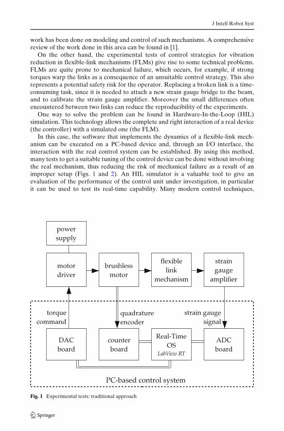
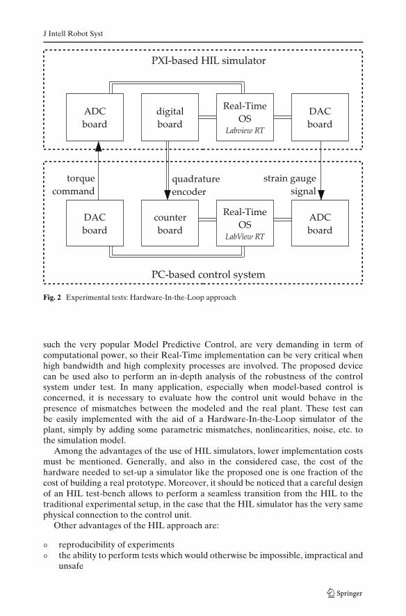
In this case, the software that implements the dynamics of a flexible-link mech-anism can be executed on a PC-based device and, through an I/O interface, theinteraction with the real control system can be established. By using this method,many tests to get a suitable tuning of the control device can be done without involvingthe real mechanism, thus reducing the risk of mechanical failure as a result of animproper setup (Figs. 1 and 2). An HIL simulator is a valuable tool to give anevaluation of the performance of the control unit under investigation, in particularit can be used to test its real-time capability. Many modern control techniques,

Fig. 1 Experimental tests: traditional approach

J Intell Robot Syst

Fig. 2 Experimental tests: Hardware-In-the-Loop approach

such the very popular Model Predictive Control, are very demanding in term ofcomputational power, so their Real-Time implementation can be very critical whenhigh bandwidth and high complexity processes are involved. The proposed devicecan be used also to perform an in-depth analysis of the robustness of the controlsystem under test. In many application, especially when model-based control isconcerned, it is necessary to evaluate how the control unit would behave in thepresence of mismatches between the modeled and the real plant. These test canbe easily implemented with the aid of a Hardware-In-the-Loop simulator of theplant, simply by adding some parametric mismatches, nonlinearities, noise, etc. tothe simulation model.

Among the advantages of the use of HIL simulators, lower implementation costsmust be mentioned. Generally, and also in the considered case, the cost of thehardware needed to set-up a simulator like the proposed one is one fraction of thecost of building a real prototype. Moreover, it should be noticed that a careful designof an HIL test-bench allows to perform a seamless transition from the HIL to thetraditional experimental setup, in the case that the HIL simulator has the very samephysical connection to the control unit.

Other advantages of the HIL approach are:

◦ reproducibility of experiments◦ the ability to perform tests which would otherwise be impossible, impractical and

unsafe

J Intell Robot Syst

◦ a shorter time required for experimental testing◦ testing the effects of component faults◦ long-term durability testing

Hardware-In-the-Loop technology is experiencing a wide diffusion in many indus-trial fields, in the wake of its early but successful introduction in the aerospace [2] andautomotive [3] research areas. More recently many papers have been written on thesubject of HIL simulator for mechatronic systems, such as [4, 5] on the use of HILin machine tool design, [6] on the design of mobile robots and [7–9] on the analysisand synthesis of robotic systems. However, to the authors’ best knowledge, there areno papers available in literature on the development or the use of Hardware-In-the-Loop simulators for mechanisms with link flexibility.

One requirement of the dynamic model used for the HIL simulation is the Real-Time capability, since it is necessary to make it interact with real-world signals, asthe input and outputs of the control system are used in the feedback loop. This isa challenging problem, since the FLM dynamic model is both non-linear and highorder. It involves large and badly conditioned matrices whose computation requiresa large amount of resources [10]. Moreover, the structure of the model and itsparameters make the dynamic equation ill-conditioned.

The proposed simulation can also be used for Real-Time SIL (Software-In-the-Loop) simulations [11, 12]. This strategy involves the interaction of two softwaredevices, that in this case would simulate the mechanism and the control unit,respectively. This approach, while certainly valid, is less useful for our purposesthan the HIL approach, since our target is to provide a full validation of thehardware implementation of the control system. In fact, unlike the SIL, the HILtechnology allows to test the control unit as a whole system, composed by itshardware components (processor, memory ,I/O devices) and its firmware.

Next section provides a brief explanation of the FLM dynamic model, while themain characteristics of the test bench are exposed in detail. In Section 3, some detailsof the Real-Time implementation will be introduced. In Section 4, the experimentalresults are presented. Here the validity of this approach is investigated by comparingthe response of the HIL simulator with the response of the FLM to the same realcontroller. Two classical control strategy are tested: a usual PI controller and anOptimal LQY regulator.

Here two well-known control strategies are applied to the simplest flexible-linkmechanism, namely the 1-link FLM, but the authors’ aim is to address their futurework to extending the capabilities of the proposed simulator to the 4-link FLMalready analyzed in [13] and to use such a simulator to test the capabilities of theModel-Predictive Control proposed in [14, 15].

2 Dynamic Model of a Planar Flexible-link Mechanism

In this section the dynamic model of a flexible-link mechanism proposed byGiovagnoni [16] will be briefly outlined. This introduction is meant to give aninsight of the model, which can be useful to better understand the complexity ofthe software implementation of the Hardware-In-the-Loop simulator. The choice ofthis formulation among the several proposed in the last 40 years has been motivated

J Intell Robot Syst

mainly by the high grade of accuracy provided by this model, which has been provedseveral times: for example in [17–19].

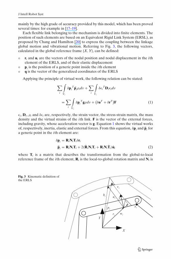
Each flexible link belonging to the mechanism is divided into finite elements. Theposition of such elements are based on an Equivalent Rigid Link System (ERSL), asproposed by Chang and Hamilton [20] to express the coupling between the linkageglobal motion and vibrational motion. Referring to Fig. 3, the following vectors,calculated in the global reference frame {X, Y}, can be defined:

◦ ri and ui are the vectors of the nodal position and nodal displacement in the i thelement of the ERLS, and of their elastic displacement

◦ pi is the position of a generic point inside the i th element◦ q is the vector of the generalized coordinates of the ERLS

Applying the principle of virtual work, the following relation can be stated:

∑

i

∫

Vi

δpiT piρidν +

∑

i

∫

Vi

δεiTDiεidν

=∑

i

∫

Vi

δpiTgρdν + (

δuT + δrT)F (1)

εi, Di, ρi and δεi are, respectively, the strain vector, the stress-strain matrix, the massdensity and the virtual strains of the i th link. F is the vector of the external forces,including gravity, whose acceleration vector is g. Equation 1 shows the virtual worksof, respectively, inertia, elastic and external forces. From this equation, δpi and pi fora generic point in the i th element are:

δpi = RiNiTiδri

pi = RiNiTi + 2(RiNiTi + RiNiTi)ui (2)

where Ti is a matrix that describes the transformation from the global-to-localreference frame of the i th element, Ri is the local-to-global rotation matrix and Ni is

Fig. 3 Kinematic definition ofthe ERLS

J Intell Robot Syst

the shape function matrix. Taking Bi(xi, yi, zi) as the strain-displacement matrix, thefollowing relation holds:

δεi = BiδTiui + BiTiδui (3)

Since the nodal elastic virtual displacements (δu) and nodal virtual displacementsof the ERLS (δr) are independent from each other, the resulting equation describingthe motion of the system is:

[M MS

STM STMS

] [uq

]=

[f

ST f

](4)

M is the mass matrix of the whole system and S is the sensitivity matrix for all thenodes. Vector F = F(u, u, q, q) takes into account all the forces affecting the system,including the force of gravity and the friction. The friction acting on the shaft of themotor is modeled as Coulomb friction. The coefficient of friction has been evaluatedexperimentally, and has been implemented as in [21] in order to avoid numericalproblems during the solution of the ODE that describe the system dynamics. Thedamping of elastic vibration is modeled using Rayleigh damping, introducing it tothe right-hand side of Eq. 4 yields:

[f

ST f

]=

[−2MG − αM − βK −MS −KST(−2MG − αM) −STMS 0

]⎡

⎣uqu

⎤

⎦

+[

M ISTM ST

] [gF

](5)

Matrix MG accounts for the Coriolis contribution, while K is the stiffness matrixof the whole system. α and β are the two Rayleigh damping coefficients. The systemin Eqs. 4 and 5 can be made solvable by forcing to zero as many elastic displacementsas there are generalized coordinates, and in this way the ERLS position is definedunivocally [16]. Finally, after removing the displacement forced to zero from Eqs. 4and 5 one obtains:

[Min (MS)in

(STM)in STMS

] [uin

q

]=

[fin

ST fin

](6)

2.1 Reference Mechanism

The mechanism for the HIL simulation is a flexible-link manipulator. The link isa square-section metal rod actuated by a brushless AC motor. It can swing in thevertical plane and its rigid configuration depends on the angular position q.

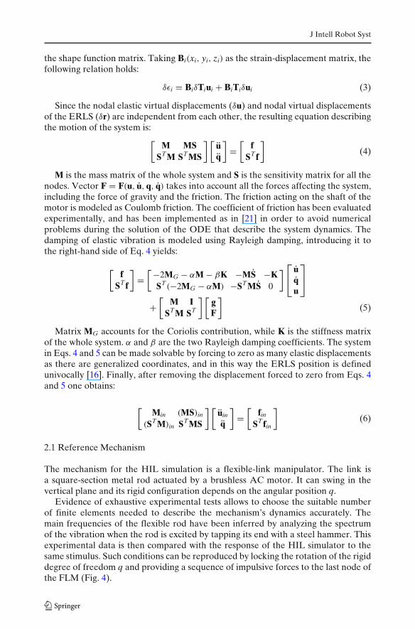
Evidence of exhaustive experimental tests allows to choose the suitable numberof finite elements needed to describe the mechanism’s dynamics accurately. Themain frequencies of the flexible rod have been inferred by analyzing the spectrumof the vibration when the rod is excited by tapping its end with a steel hammer. Thisexperimental data is then compared with the response of the HIL simulator to thesame stimulus. Such conditions can be reproduced by locking the rotation of the rigiddegree of freedom q and providing a sequence of impulsive forces to the last node ofthe FLM (Fig. 4).

J Intell Robot Syst

Fig. 4 The mechanisms usedfor experimental tests

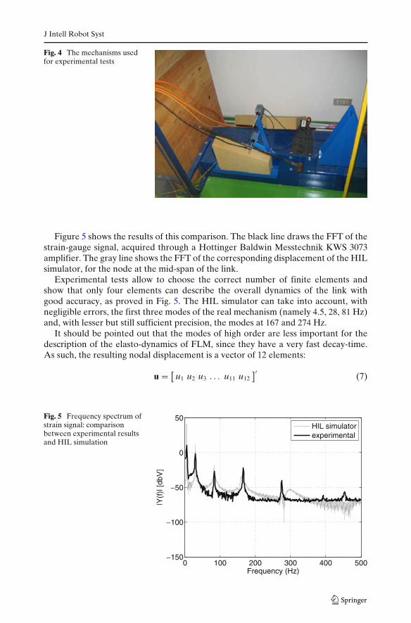
Figure 5 shows the results of this comparison. The black line draws the FFT of thestrain-gauge signal, acquired through a Hottinger Baldwin Messtechnik KWS 3073amplifier. The gray line shows the FFT of the corresponding displacement of the HILsimulator, for the node at the mid-span of the link.

Experimental tests allow to choose the correct number of finite elements andshow that only four elements can describe the overall dynamics of the link withgood accuracy, as proved in Fig. 5. The HIL simulator can take into account, withnegligible errors, the first three modes of the real mechanism (namely 4.5, 28, 81 Hz)and, with lesser but still sufficient precision, the modes at 167 and 274 Hz.

It should be pointed out that the modes of high order are less important for thedescription of the elasto-dynamics of FLM, since they have a very fast decay-time.As such, the resulting nodal displacement is a vector of 12 elements:

u = [u1 u2 u3 . . . u11 u12

]′ (7)

Fig. 5 Frequency spectrum ofstrain signal: comparisonbetween experimental resultsand HIL simulation

0 100 200 300 400 500−150

−100

−50

0

50

Frequency (Hz)

|Y(f

)| [d

bV]

HIL simulatorexperimental

J Intell Robot Syst

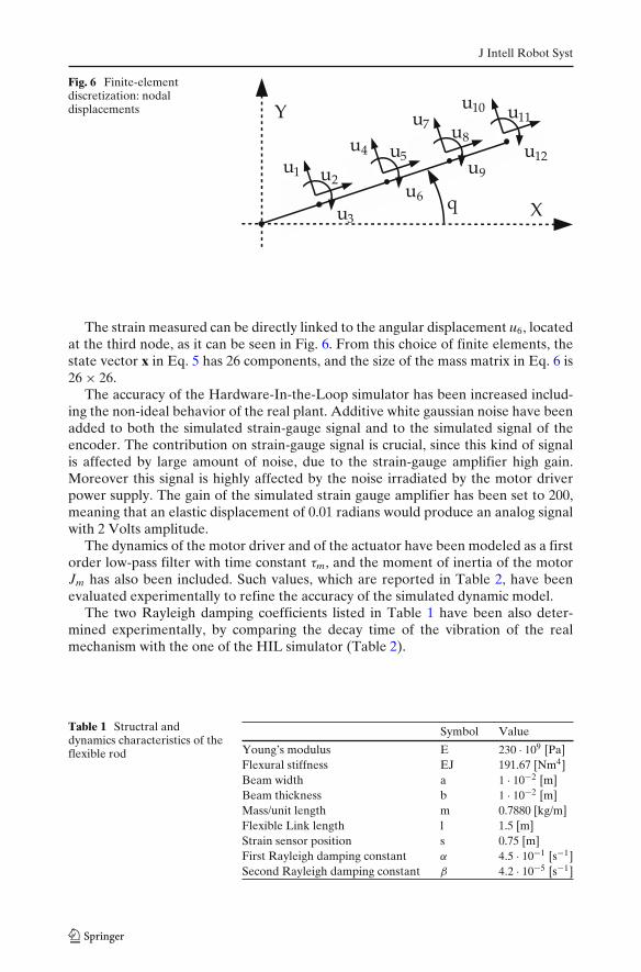
Fig. 6 Finite-elementdiscretization: nodaldisplacements

The strain measured can be directly linked to the angular displacement u6, locatedat the third node, as it can be seen in Fig. 6. From this choice of finite elements, thestate vector x in Eq. 5 has 26 components, and the size of the mass matrix in Eq. 6 is26 × 26.

The accuracy of the Hardware-In-the-Loop simulator has been increased includ-ing the non-ideal behavior of the real plant. Additive white gaussian noise have beenadded to both the simulated strain-gauge signal and to the simulated signal of theencoder. The contribution on strain-gauge signal is crucial, since this kind of signalis affected by large amount of noise, due to the strain-gauge amplifier high gain.Moreover this signal is highly affected by the noise irradiated by the motor driverpower supply. The gain of the simulated strain gauge amplifier has been set to 200,meaning that an elastic displacement of 0.01 radians would produce an analog signalwith 2 Volts amplitude.

The dynamics of the motor driver and of the actuator have been modeled as a firstorder low-pass filter with time constant τm, and the moment of inertia of the motorJm has also been included. Such values, which are reported in Table 2, have beenevaluated experimentally to refine the accuracy of the simulated dynamic model.

The two Rayleigh damping coefficients listed in Table 1 have been also deter-mined experimentally, by comparing the decay time of the vibration of the realmechanism with the one of the HIL simulator (Table 2).

Table 1 Structral anddynamics characteristics of theflexible rod

Symbol Value

Young’s modulus E 230 · 109 [Pa]Flexural stiffness EJ 191.67 [Nm4]Beam width a 1 · 10−2 [m]Beam thickness b 1 · 10−2 [m]Mass/unit length m 0.7880 [kg/m]Flexible Link length l 1.5 [m]Strain sensor position s 0.75 [m]First Rayleigh damping constant α 4.5 · 10−1 [s−1]Second Rayleigh damping constant β 4.2 · 10−5 [s−1]

J Intell Robot Syst

Table 2 Dynamiccharacteristics of the actuator

Symbol Value

Motor time constant τm 3 [ms]Motor shaft inertia Jm 0.0021 [kg m2]Coulomb friction coefficient μ 0.1Driver torque analog command gain Gd 0.4 [Nm]/[V]

3 HIL Implementation

The goal of the Hardware-In-the-Loop simulator is to make the real controller andthe simulated model interact with each other, without any need of change on thestructure and/or the tuning of the controller. As such, the dynamic model must meettwo main requirements: (a) high accuracy (b) real-time (RT) capability.

The accuracy allows to mask the virtual model to the controller and, undoubtedly,allows to make the experiments consistent. The dynamic model described abovehas been investigated by the same authors and its accuracy has been demonstratedin recent papers by comparing the results of several experimental tests with thecorresponding simulation’s results [22].

The need for the RT capacity arises from the mentioned interaction between realand simulated signals. This requires the dynamic model running on the RT targetmust have a constant updating frequency to allow the correct synchronization amongthe signals. These constraints ask for some algebraic manipulations on the dynamicmodel (Fig. 7).

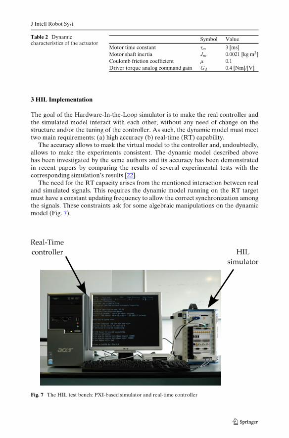
Fig. 7 The HIL test bench: PXI-based simulator and real-time controller

J Intell Robot Syst

Equation 6 can be rewritten as:

⎡

⎢⎢⎣

M MS 0 0STM STMS 0 0

0 0 I 00 0 0 I

⎤

⎥⎥⎦

⎡

⎢⎢⎣

uquq

⎤

⎥⎥⎦ =

⎡

⎢⎢⎣

M ISTM ST

0 00 0

⎤

⎥⎥⎦

[gF

]

+

⎡

⎢⎢⎣

−2MG − αM − βK −MS −K 0ST(−2MG − αM) −STMS 0 0

I 0 0 00 I 0 0

⎤

⎥⎥⎦

⎡

⎢⎢⎣

uquq

⎤

⎥⎥⎦

or, in a more compact form:

M(x, t)x = (x, F, t) (8)

where:

x = [u, q, u, q]T

and

(x, F, t) =

⎡

⎢⎢⎣

M ISTM ST

0 00 0

⎤

⎥⎥⎦

[gF

]+

⎡

⎢⎢⎣

−2MG − αM − βK −MS −K 0ST(−2MG − αM) −STMS 0 0

I 0 0 00 I 0 0

⎤

⎥⎥⎦ x

M(x, t) =

⎡

⎢⎢⎣

M MS 0 0STM STMS 0 0

0 0 I 00 0 0 I

⎤

⎥⎥⎦

From Eq. 8, it can be seen that the updating equation of the dynamic systeminvolves a large, non-linear and time-dependent matrix, M(x, t), which needs to beinverted at every iteration.

x = M(x, t)−1(x, F, t) (9)

It should be point out that, owing to the specific choice of the constraints on theflexible displacements u, the matrix M is always nonsingular.

To speed up the computation of x and improve the updating time, it is necessaryto make explicit the vector x, by computing its components algebraically. Thisoperation can be done off-line and improves the updating time drastically, since thecomputation of Eq. 9 becomes a mere numerical substitution during the run-timeoperations. The main drawback of this approach is that a large amount of memory isrequired to memorize all the components of the vector.

An optimized C-code routine corresponding to Eq. 9 further improves the real-time (or even faster-than-real-time) capacity.

The RT simulation of the whole system, including sensors, actuators and driversruns on a National Instruments PXI device. It integrates a standard PC-basedCPU with a high performance I/O board, so it is well suited for both control andmeasurement applications.

J Intell Robot Syst

In particular, the HIL simulator has been implemented on a 1042Q PXI chassiswith a PXI-8110 controller, a PXI-6259 analog I/O board and a PXI-6602 counterboard, all made by National Instruments®.

The dynamic equation, originally written in C language, can be easily included ina LabVIEW RT project.

In order to evaluate the maximum refresh frequency of the HIL simulator, a largenumber of tests has been done. The aim was at evaluation of the maximum timerequired for the computation of Eq. 9.

The results show that the mean time required is T = 0.61831428 ms, evaluatedwith the precision of 4 × 10−8 s. As a consequence, the model’s refresh frequency forall the experimental tests presented in this paper has been set to 1 kHz. This samplingfrequency is sufficient to describe with a good accuracy all the first seven modes ofvibration of the flexible link.

4 Experimental Validation of the HIL Simulator

A set of experimental tests has been conducted to prove the effectiveness of theHIL simulator. In particular, the simulator has been validated by using classicalcontrollers while the comparison between the open-loop responses of the real andthe simulated plant is necessary missing. This depends on the gravity force that makesunstable the plant.

It must be pointed out that, for each experimental test, the same (real) controllerhas been used both for the real mechanism and the simulated one, without anychange on its setup.

In Section 4.1 the simulator is validated by comparing the step response of the realand the simulated mechanism, when the controller implements a simple PI regulator.In Section 4.2 the same comparison is done by using a LQY regulator.

4.1 Validation with PI Closed-loop Position Control

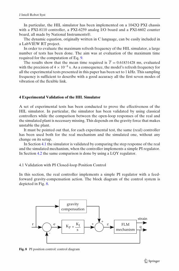
In this section, the real controller implements a simple PI regulator with a feed-forward gravity-compensation action. The block diagram of the control system isdepicted in Fig. 8.

Fig. 8 PI position control: control diagram

J Intell Robot Syst

0 5 10 15 2084

85

86

87

88

89

90

91

time [s]

angu

lar

posi

tion

[deg

]referenceexperimentalHIL

Fig. 9 PI position control: experimental validation of the angular position closed-loop response

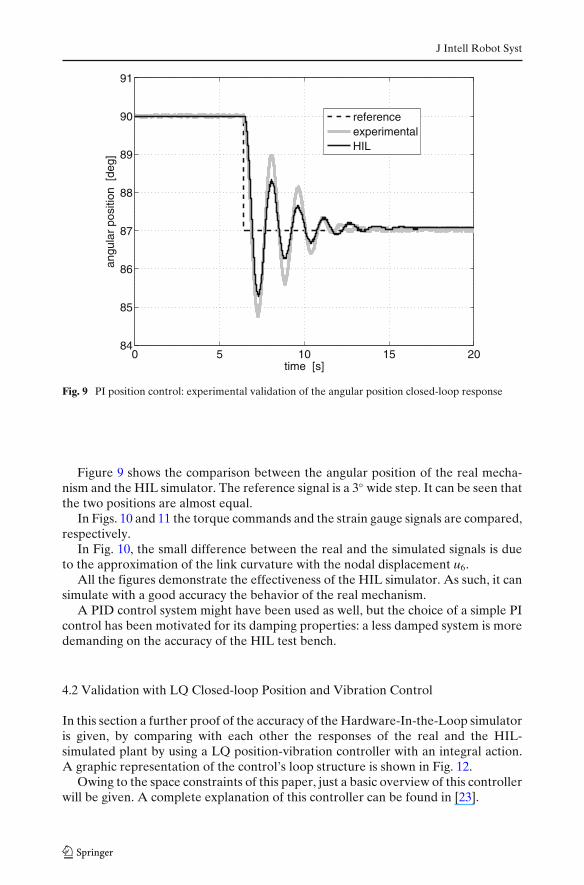
Figure 9 shows the comparison between the angular position of the real mecha-nism and the HIL simulator. The reference signal is a 3◦ wide step. It can be seen thatthe two positions are almost equal.

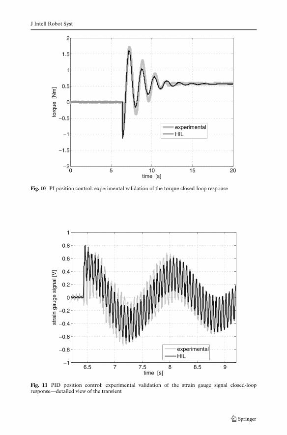
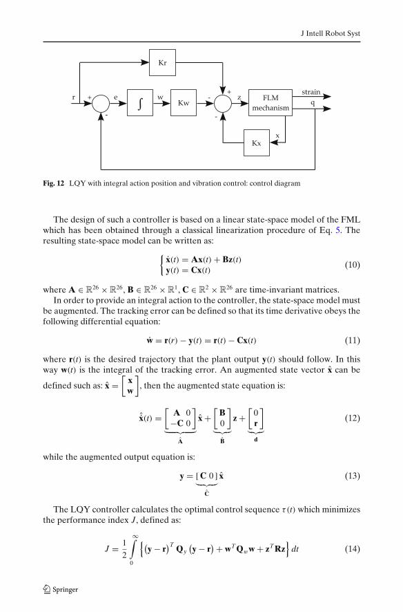
In Figs. 10 and 11 the torque commands and the strain gauge signals are compared,respectively.

In Fig. 10, the small difference between the real and the simulated signals is dueto the approximation of the link curvature with the nodal displacement u6.

All the figures demonstrate the effectiveness of the HIL simulator. As such, it cansimulate with a good accuracy the behavior of the real mechanism.

A PID control system might have been used as well, but the choice of a simple PIcontrol has been motivated for its damping properties: a less damped system is moredemanding on the accuracy of the HIL test bench.

4.2 Validation with LQ Closed-loop Position and Vibration Control

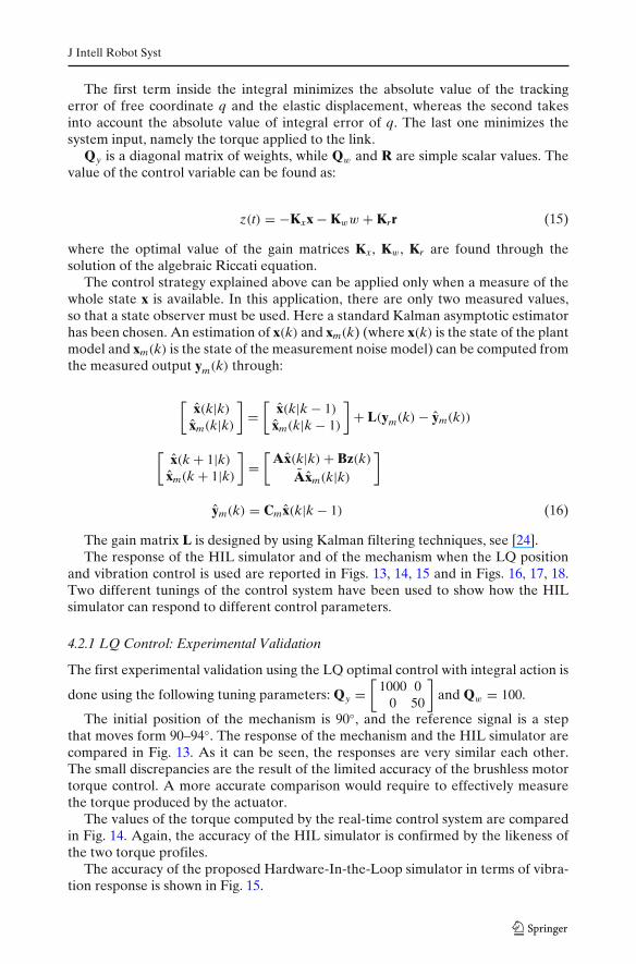
In this section a further proof of the accuracy of the Hardware-In-the-Loop simulatoris given, by comparing with each other the responses of the real and the HIL-simulated plant by using a LQ position-vibration controller with an integral action.A graphic representation of the control’s loop structure is shown in Fig. 12.

Owing to the space constraints of this paper, just a basic overview of this controllerwill be given. A complete explanation of this controller can be found in [23].

J Intell Robot Syst

0 5 10 15 20−2

−1.5

−1

−0.5

0

0.5

1

1.5

2

time [s]

torq

ue [

Nm

]

experimentalHIL

Fig. 10 PI position control: experimental validation of the torque closed-loop response

6.5 7 7.5 8 8.5 9−1

−0.8

−0.6

−0.4

−0.2

0

0.2

0.4

0.6

0.8

1

time [s]

stra

in g

auge

sig

nal [

V]

experimentalHIL

Fig. 11 PID position control: experimental validation of the strain gauge signal closed-loopresponse—detailed view of the transient

J Intell Robot Syst

Fig. 12 LQY with integral action position and vibration control: control diagram

The design of such a controller is based on a linear state-space model of the FMLwhich has been obtained through a classical linearization procedure of Eq. 5. Theresulting state-space model can be written as:

{x(t) = Ax(t) + Bz(t)y(t) = Cx(t)

(10)

where A ∈ R26 × R

26, B ∈ R26 × R

1, C ∈ R2 × R

26 are time-invariant matrices.In order to provide an integral action to the controller, the state-space model must

be augmented. The tracking error can be defined so that its time derivative obeys thefollowing differential equation:

w = r(r) − y(t) = r(t) − Cx(t) (11)

where r(t) is the desired trajectory that the plant output y(t) should follow. In thisway w(t) is the integral of the tracking error. An augmented state vector x can be

defined such as: x =[

xw

], then the augmented state equation is:

ˆx(t) =[

A 0−C 0

]

︸ ︷︷ ︸A

x +[

B0

]

︸ ︷︷ ︸B

z +[

0r

]

︸︷︷︸d

(12)

while the augmented output equation is:

y = [ C 0 ]︸ ︷︷ ︸

C

x (13)

The LQY controller calculates the optimal control sequence τ(t) which minimizesthe performance index J, defined as:

J = 1

2

∞∫

0

{(y − r

)T Qy(y − r

) + wTQww + zTRz}

dt (14)

J Intell Robot Syst

The first term inside the integral minimizes the absolute value of the trackingerror of free coordinate q and the elastic displacement, whereas the second takesinto account the absolute value of integral error of q. The last one minimizes thesystem input, namely the torque applied to the link.

Qy is a diagonal matrix of weights, while Qw and R are simple scalar values. Thevalue of the control variable can be found as:

z(t) = −Kxx − Kww + Krr (15)

where the optimal value of the gain matrices Kx, Kw, Kr are found through thesolution of the algebraic Riccati equation.

The control strategy explained above can be applied only when a measure of thewhole state x is available. In this application, there are only two measured values,so that a state observer must be used. Here a standard Kalman asymptotic estimatorhas been chosen. An estimation of x(k) and xm(k) (where x(k) is the state of the plantmodel and xm(k) is the state of the measurement noise model) can be computed fromthe measured output ym(k) through:

[x(k|k)

xm(k|k)

]=

[x(k|k − 1)

xm(k|k − 1)

]+ L(ym(k) − ym(k))

[x(k + 1|k)

xm(k + 1|k)

]=

[Ax(k|k) + Bz(k)

Axm(k|k)

]

ym(k) = Cmx(k|k − 1) (16)

The gain matrix L is designed by using Kalman filtering techniques, see [24].The response of the HIL simulator and of the mechanism when the LQ position

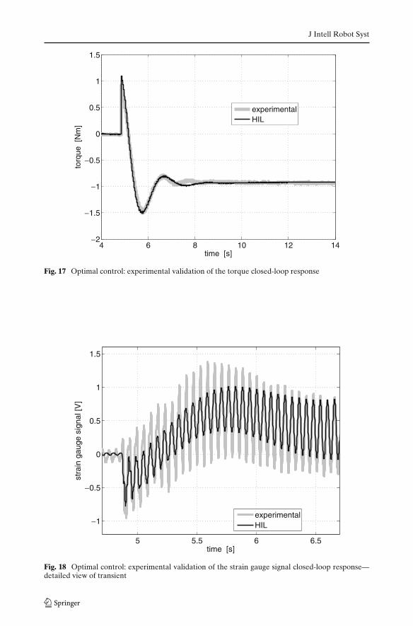
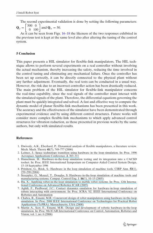
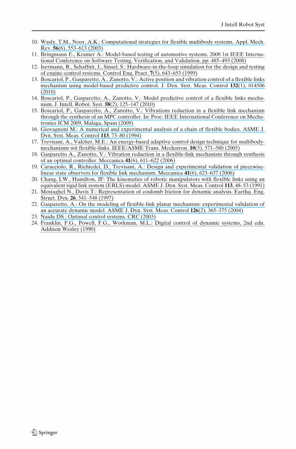
and vibration control is used are reported in Figs. 13, 14, 15 and in Figs. 16, 17, 18.Two different tunings of the control system have been used to show how the HILsimulator can respond to different control parameters.

4.2.1 LQ Control: Experimental Validation

The first experimental validation using the LQ optimal control with integral action is

done using the following tuning parameters: Qy =[

1000 00 50

]and Qw = 100.

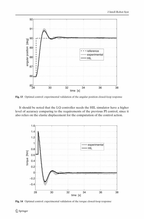
The initial position of the mechanism is 90◦, and the reference signal is a stepthat moves form 90–94◦. The response of the mechanism and the HIL simulator arecompared in Fig. 13. As it can be seen, the responses are very similar each other.The small discrepancies are the result of the limited accuracy of the brushless motortorque control. A more accurate comparison would require to effectively measurethe torque produced by the actuator.

The values of the torque computed by the real-time control system are comparedin Fig. 14. Again, the accuracy of the HIL simulator is confirmed by the likeness ofthe two torque profiles.

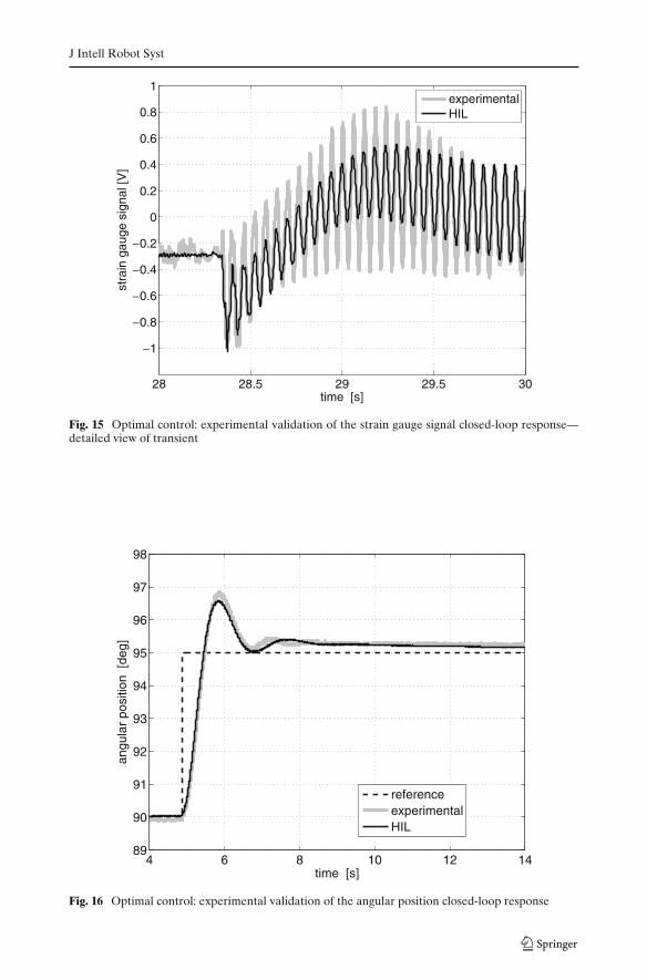
The accuracy of the proposed Hardware-In-the-Loop simulator in terms of vibra-tion response is shown in Fig. 15.

J Intell Robot Syst

28 30 32 34 36 3885

86

87

88

89

90

91

92

time [s]

angu

lar

posi

tion

[deg

]

referenceexperimentalHIL

Fig. 13 Optimal control: experimental validation of the angular position closed-loop response

It should be noted that the LQ controller needs the HIL simulator have a higherlevel of accuracy comparing to the requirements of the previous PI control, since italso relies on the elastic displacement for the computation of the control action.

28 30 32 34 36 38

−0.4

−0.2

0

0.2

0.4

0.6

0.8

1

1.2

1.4

1.6

time [s]

torq

ue [

Nm

]

experimentalHIL

Fig. 14 Optimal control: experimental validation of the torque closed-loop response

J Intell Robot Syst

28 28.5 29 29.5 30

−1

−0.8

−0.6

−0.4

−0.2

0

0.2

0.4

0.6

0.8

1

time [s]

stra

in g

auge

sig

nal [

V]

experimentalHIL

Fig. 15 Optimal control: experimental validation of the strain gauge signal closed-loop response—detailed view of transient

4 6 8 10 12 1489

90

91

92

93

94

95

96

97

98

time [s]

angu

lar

posi

tion

[deg

]

referenceexperimentalHIL

Fig. 16 Optimal control: experimental validation of the angular position closed-loop response

J Intell Robot Syst

4 6 8 10 12 14−2

−1.5

−1

−0.5

0

0.5

1

1.5

time [s]

torq

ue [

Nm

]

experimentalHIL

Fig. 17 Optimal control: experimental validation of the torque closed-loop response

5 5.5 6 6.5

−1

−0.5

0

0.5

1

1.5

time [s]

stra

in g

auge

sig

nal [

V]

experimentalHIL

Fig. 18 Optimal control: experimental validation of the strain gauge signal closed-loop response—detailed view of transient

J Intell Robot Syst

The second experimental validation is done by setting the following parameters:

Qy =[

500 00 100

]and Qw = 50.

As it can be seen from Figs. 16–18 the likeness of the two responses exhibited inthe previous test is kept at the same level also after altering the tuning of the controlsystem.

5 Conclusion

This paper presents a HIL simulator for flexible-link manipulators. The HIL tech-nique allows to perform several experiments on a real controller without involvingthe actual mechanism, thereby increasing the safety, reducing the time involved inthe control tuning and eliminating any mechanical failure. Once the controller hasbeen set up correctly, it can be directly connected to the physical plant withoutany further adjustment. Eventually, the real tests can be conducted in a usual way.However, the risk due to an incorrect controller action has been drastically reduced.The main problem of the HIL simulator for flexible-link manipulator concernsthe real-time capability, since the real signals of the controller must interact withthe simulated signals of the plant. Therefore, the differential equations governing theplant must be quickly integrated and solved. A fast and effective way to compute thedynamic model of planar flexible-link mechanisms has been presented in this work.The accuracy and the effectiveness of the simulator have been demonstrated throughexperimental evidence and by using different control structures. Future works willconsider more complex flexible-link mechanisms to which apply advanced controlstructures for vibration reduction, as those presented in previous works by the sameauthors, but only with simulated results.

References

1. Dwivedy, A.K., Eberhard, P.: Dynamical analysis of flexible manipulators, a literature review.Mech. Mach. Theory 41(7), 749–777 (2006)

2. Leitner, J.: Space technology transition using hardware in the loop simulation. In: Proc. 1996Aerospace Applications Conference. 2, 303–311

3. Hanselman, H.: Hardware-in-the-loop simulation testing and its integration into a CACSDtoolset. In: Proc. IEEE International Symposium on Computer-Aided Control System Design,15–18 September 1996

4. Pritshow, G., Röck, S.: Hardware in the loop simulation of machine tools. CIRP Ann. 53(1),259–298 (2004)

5. Stoeppler, G., Menzel, T., Douglas, S: Hardware-in-the-loop simulation of machine tools andmanufacturing systems. Comput. Control Eng. J. 16(1), 10–15 (2005)

6. Hu, X.: Applying robot-in-the-loop simulation to mobile robot systems. In: Proc. 12th Interna-tional Conference on Advanced Robotics ICAR (2005)

7. Aghili, F., Piedboeuf, J.C.: Contact dynamics emulation for hardware-in-loop simulation ofrobots interacting with environment. In: Proc. ICRA ’02. IEEE International Conference onRobotics and Automation

8. Chabra, R., Emami, M.R.: Concurrent design of robot manipulators using hardware-in-the-loopsimulation. In: Proc. 2008 IEEE International Conference on Technologies for Practical RobotApplications (TePRA). Massachusetts, USA (2008)

9. Martin A., Scot, E., Emami, M.R.: Design and development of robotic hardware-in-the-loopsimulation. In: Proc. 9th ICAR International Conference on Control, Automation, Robotics andVision, vol. 1, no. 6 (2006)

J Intell Robot Syst

10. Wasfy, T.M., Noor, A.K.: Computational strategies for flexible multibody systems. Appl. Mech.Rev. 56(6), 553–613 (2003)

11. Bringmann E., Kramer A.: Model-based testing of automotive systems. 2008 1st IEEE Interna-tional Conference on Software Testing, Verification, and Validation, pp. 485–493 (2008)

12. Isermann, R., Schaffnit, J., Sinsel, S.: Hardware-in-the-loop simulation for the design and testingof engine-control systems. Control Eng. Pract. 7(5), 643–653 (1999)

13. Boscariol, P., Gasparetto, A., Zanotto, V.: Active position and vibration control of a flexible linksmechanism using model-based predictive control. J. Dyn. Syst. Meas. Control 132(1), 014506(2010)

14. Boscariol, P., Gasparetto, A., Zanotto, V.: Model predictive control of a flexible links mecha-nism. J. Intell. Robot. Syst. 58(2), 125–147 (2010)

15. Boscariol, P., Gasparetto, A., Zanotto, V.: Vibrations reduction in a flexible link mechanismthrough the synthesis of an MPC controller. In: Proc: IEEE International Conference on Mecha-tronics ICM 2009, Malaga, Spain (2009)

16. Giovagnoni M.: A numerical and experimental analysis of a chain of flexible bodies. ASME J.Dyn. Syst. Meas. Control 113, 73–80 (1994)

17. Trevisani, A., Valcher, M.E.: An energy-based adaptive control design technique for multibody-mechanisms wit flexible-links. IEEE/ASME Trans. Mechatron. 10(5), 571–580 (2005)

18. Gasparetto A., Zanotto, V.: Vibration reduction in a flexible-link mechanism through synthesisof an optimal controller. Meccanica 41(6), 611–622 (2006)

19. Caracciolo, R., Richiedei, D., Trevisani, A.: Design and experimental validation of piecewise-linear state observers for flexible link mechanism. Meccanica 41(6), 623–637 (2006)

20. Chang, LW., Hamilton, JF: The kinematics of robotic manipulators with flexible links using anequivalent rigid link system (ERLS) model. ASME J. Dyn. Syst. Meas. Control 113, 48–53 (1991)

21. Mostaghel N., Davis T.: Representation of coulomb friction for dynamic analysis. Earthq. Eng.Struct. Dyn. 26, 541–548 (1997)

22. Gasparetto, A.: On the modeling of flexible-link planar mechanism: experimental validation ofan accurate dynamic model. ASME J. Dyn. Syst. Meas. Control 126(2), 365–375 (2004)

23. Naidu DS.: Optimal control systems. CRC (2003)24. Franklin, F.G., Powell, F.G., Workman, M.L.: Digital control of dynamic systems, 2nd edn.

Addison Wesley (1990)