applied sciences

Article

Development of a Power and Communication Bus Using HILand Computational Intelligence

Marek Sznura * and Piotr Przystałka

Citation: Sznura, M.; Przystałka, P.

Development of a Power and

Communication Bus Using HIL and

Computational Intelligence. Appl. Sci.

2021, 11, 8709. https://doi.org/

10.3390/app11188709

Academic Editor: Alessandro

Gasparetto

Received: 21 July 2021

Accepted: 13 September 2021

Published: 18 September 2021

Publisher’s Note: MDPI stays neutral

with regard to jurisdictional claims in

published maps and institutional affil-

iations.

Copyright: © 2021 by the authors.

Licensee MDPI, Basel, Switzerland.

This article is an open access article

distributed under the terms and

conditions of the Creative Commons

Attribution (CC BY) license (https://

creativecommons.org/licenses/by/

4.0/).

Department of Fundamentals of Machinery Design , Silesian University of Technology, 18A Konarskiego Street,44-100 Gliwice, Poland; piotr.przystalka@polsl.pl* Correspondence: marek.sznura@gmail.com

Abstract: This paper deals with the development of a power and communication bus named DLN(Device Lightweight Network) that can be seen as a new interface with auto-addressing functionalityto transfer power and data by means of two wires in modern cars. The main research goal of thispaper is to elaborate a new method based on a hardware in the loop technique aided by computationalintelligence algorithms in order to search for the optimal structure of the communication modules,as well as optimal features of hardware parts and the values of software parameters. The desiredproperties of communication modules, which have a strong influence on the performance of thebus, cannot be found using a classical engineering approach due to the large number of possiblecombinations of configuration of the hardware and software parts of the whole system. Therefore,an HIL-based optimization method for bus prototyping is proposed, in which the optimization taskis formulated as a multi-criteria optimization problem. Several criterion functions are proposed,corresponding to the automotive objectives and requirements. Different soft computing optimizationalgorithms, such as a single-objective/multi-objectives evolutionary algorithm and a particle swarmoptimization algorithm, are applied to searching for the optimal solution. The verification study wascarried out in order to show the merits and limitations of the proposed approach. Attention wasalso paid to the problem of the selection of the behavioural parameters of the heuristic algorithms.The overall results proved the high practical potential of the DLN, which was developed using theproposed optimization method.

Keywords: computational intelligence; soft computing optimization; automotive bus; wire harness;hardware-in-the-loop; multi-objectives optimization

1. Introduction

The first car design by Benz in 1885 [1] had an elementary harness, which merelyinvolved high voltage cables to spark plugs. In 1915 [2], the Ford Motor Company imple-mented electric headlamps and horns, soon followed by turn signals, electric wipers, andother equipment. In the 1980s, Bosch proposed the first data interface, called the ControllerArea Network (CAN) [3], for reducing the number of wire harnesses. Nowadays, cars areequipped more and more with electronic systems [4], Electronic Control Units (ECU) andinterfaces. The typical low-speed CAN is limited to 125 kpbs, a classic CAN is limitedto 1 Mbps, and CAN FD is limited to 3–5 Mbps depending on the environment. A LocalInterconnect Network (LIN) is commonly used in communication with comfort devicesor non-safety sensors, due to the lack of hardware redundancy and low speed (typically20 kbps). FlexRay, which was developed to be faster and more reliable than other protocols,is used for safety critical applications and allows the transferring of data up to 10 Mbps [5].Ethernet is used for high-speed-requiring devices, such as cameras in autonomous driving,and a typical baud rate is 100 Mbps or 1000 Mbps [6]. Autonomous driving raises com-munication techniques to a higher level, using the newest and the fastest technology ofwireless techniques such as 5G for V2X communication [7–9]. Unfortunately, point-to-pointwiring is still being used.

Appl. Sci. 2021, 11, 8709. https://doi.org/10.3390/app11188709 https://www.mdpi.com/journal/applsci

Appl. Sci. 2021, 11, 8709 2 of 25

As can be read in papers [10,11], a harness can weigh from 15 kg in a combustionengine car, to about 20 kg in a small EV, to 91 kg in luxury vehicles [12]. The mass of thevehicle has a significant influence on energy consumption [13], but nowadays, EVs partlysolve this problem by using recuperation [14]. Based on [10] it can be stated that a harnesscan cost up to 1000 USD. The harness’ simplicity can significantly reduce weight, cost andrisk of failure during operation.

When it comes to small devices, of which many are used in a car (e.g., ambient light,sensors, actuators), Original Equipment Manufacturers (OEMs) have three solutions—using a separate wire for each device (this increases cost, weight and geometrical sizes ofthe harness), the same hardware but different software, where the address is programmed(this increases effort during production, and the risk of mixing devices which have thesame shape), or auto-addressed modules on the line. There are a few solutions for auto-addressing available on the market; one of them from Melexis [15], another from TexasInstruments [16] named “Automatic slave node detection”, and a patent describing auto-addressing [17] is available for RS485 [18]. All solutions require wires, commonly oneadditional, which gives four lines including power supply. Focusing on reducing thenumber of wires in the automotive industry, there is only one solution that uses thesame wires for transferring power and data, but not command. The company Yamar [19]proposed special chips to “inject” multiple interfaces to a power line. Depending on thechip used, one can achieve a data speed from 9.6 Kbps to 500 kbps. This solution has afew disadvantages: cost (7EUR for CAN chip) and size (mainly peripheral components,coils, capacitors, and one crystal resonator). For a hardware engineer who designs a newdevice, one of the goals is to use as few components as possible, due to three reasons: moreelements generate higher production costs (single component, assembly, maintenance),potential issues (hidden defects, production issues, supply chain issues), size (each elementrequires more space on the PCB (Printed Circuit Board). Researchers [20] attempted to senddata using Yamar SIG60 (the oldest solutions from Yamar) with unsatisfactory results—theinterface was working, but it was relatively slow at only 57.6 kbps and the researchers gotno transmission error. Unfortunately, there are no more studies with the newest solutionsfrom Yamar. In the industry, we can find the AS-I [21] interface, where data and powerare sent on the same line. Voltage on the line is 12 V, and baud rate is low. Transfer is notexpressed in bits per second. AS-I can check the status of 62 nodes in 20 ms. One of theoldest commonly used interfaces that uses only ground and one wire to deliver power anddata is “1 wire”, introduced by Dallas Semiconductor, now known as Maxim.

The authors developed an interface to transfer power and data on the same line. Theidea of this solution is to determine time frames for power transmission and another onefor data transmission. The prototype of the proposed solution was built, and it was used inorder to carry out several tests in a laboratory environment as well as in real conditions(Figure 1). It was possible to achieve a data link up to 2 Mbps, a power link up to 48 Vand 10 A, hence the possibility of transmitting 480 W of power was accomplished. Theseexperiments showed the high potential of the proposed solution. The next step presentedin this study deals with solving the auto-addressing problem. The next step of this solutionis to design auto-addressing.

Appl. Sci. 2021, 11, 8709 3 of 25

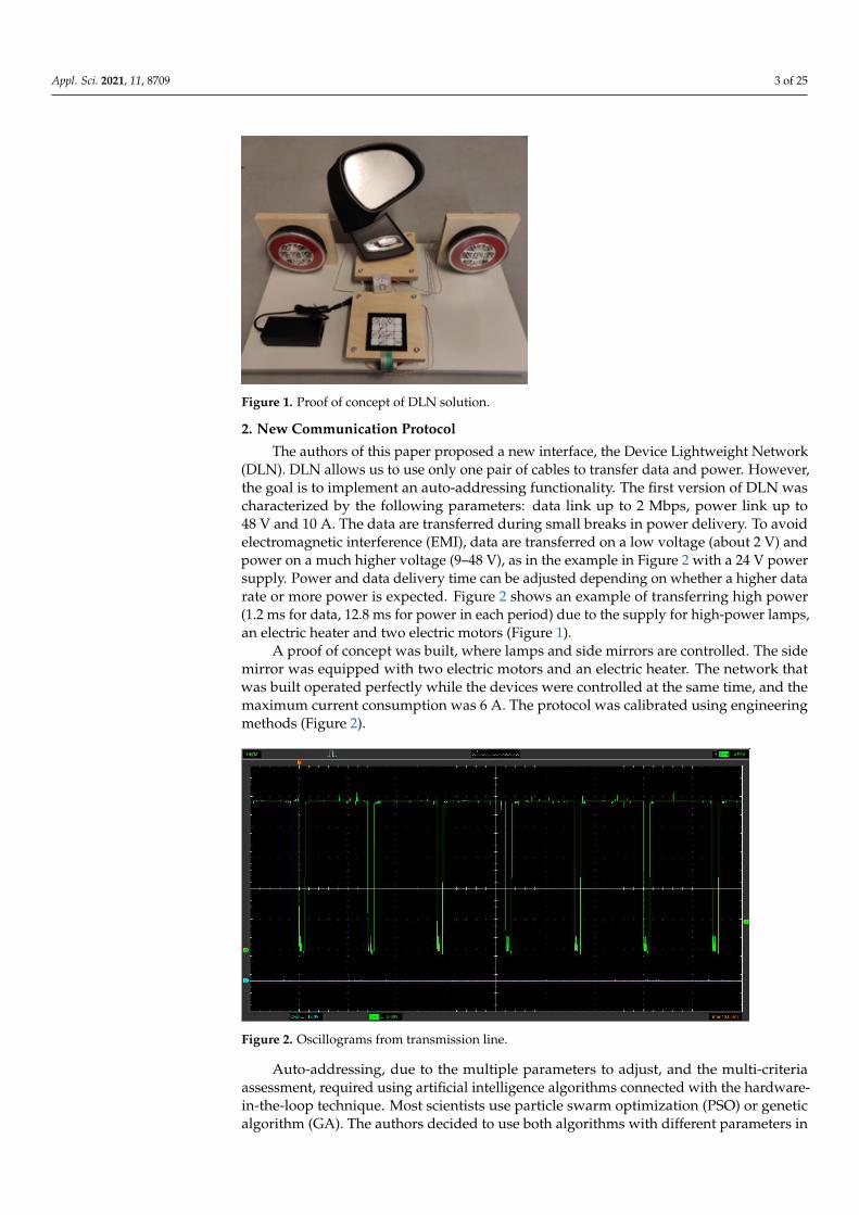
Figure 1. Proof of concept of DLN solution.

2. New Communication Protocol

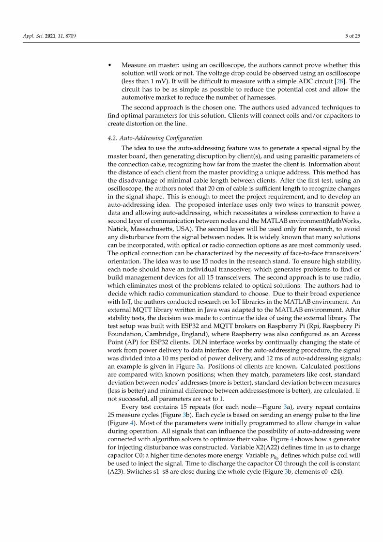
The authors of this paper proposed a new interface, the Device Lightweight Network(DLN). DLN allows us to use only one pair of cables to transfer data and power. However,the goal is to implement an auto-addressing functionality. The first version of DLN wascharacterized by the following parameters: data link up to 2 Mbps, power link up to48 V and 10 A. The data are transferred during small breaks in power delivery. To avoidelectromagnetic interference (EMI), data are transferred on a low voltage (about 2 V) andpower on a much higher voltage (9–48 V), as in the example in Figure 2 with a 24 V powersupply. Power and data delivery time can be adjusted depending on whether a higher datarate or more power is expected. Figure 2 shows an example of transferring high power(1.2 ms for data, 12.8 ms for power in each period) due to the supply for high-power lamps,an electric heater and two electric motors (Figure 1).

A proof of concept was built, where lamps and side mirrors are controlled. The sidemirror was equipped with two electric motors and an electric heater. The network thatwas built operated perfectly while the devices were controlled at the same time, and themaximum current consumption was 6 A. The protocol was calibrated using engineeringmethods (Figure 2).

Figure 2. Oscillograms from transmission line.

Auto-addressing, due to the multiple parameters to adjust, and the multi-criteriaassessment, required using artificial intelligence algorithms connected with the hardware-in-the-loop technique. Most scientists use particle swarm optimization (PSO) or geneticalgorithm (GA). The authors decided to use both algorithms with different parameters in

Appl. Sci. 2021, 11, 8709 4 of 25

order to compare the results of the optimization. To avoid unnecessary effort of simulations,the authors decided to find the optimal solutions using easier methods such as planningthe experiment. For comparison purposes, the authors decided to find the best solution byapplying an easier method based on a Latin hypercube sampling (LHS) approach to avoidunnecessary effort of simulations.

3. Motivation

Regarding multiple of the same devices on the line, for example, 25 lighting/sensor/actuator modules which are in one element in the car, for example, door side/cockpit/middle console, the possibility of auto-addressing can radically reduce cost, materials andtime for production. Nowadays, a 4-line solution is commonly used in the case of auto-addressing, one pair of power supplies, and one pair of LIN_in, and LIN_out signals [16].In this paper, the authors propose a solution for how to use only two wires, for power,transmitting data and auto-addressing. While auto-addressing is the ability to give a uniqueID to each slave node on the line, ID defines the position on the line. Data transmissionwas designed and tuned using engineering methods with promising results, neverthelesstuning the auto-addressing features required to use artificial intelligence algorithms suchas genetic algorithms [22] and particle swarm optimization, due to the number of possiblecombinations.

β =7

∑i=0

(max(phi

)−min(phi)) + (max(psi )−min(psi )

)= 5.58× 1013. (1)

Due to the goal of finding a global optimum and a nonlinear function with discretevalues, gradient methods cannot be used, mainly due to the stochastic nature of theobjectives and because there are continuous and discrete decision variables in the vector p(more details can be seen in Section 3). The authors decided to use an experiment planningmethod, genetic algorithm and particle swarm optimization to compare results and checkif given results can be treated as a global optimum.

The idea for solving the auto-addressing task was to inject by master a disruptionwhich will be reflected and modified by the client, and at the end the master signal willbe sampled. Such a solution is very difficult to test in a virtual environment. The authorsdecided to connect the whole system to hardware-in-the-loop instead of trying to builda mathematical model according to the Jaguar Land Rover approach, which connectsthe windscreen wiper for the hardware-in-the-loop setup [23] and other non-automotiveresearchers who optimized the buck converter [22], and validated PID using HIL [24].

4. Auto Addressing Method

There are several methods of auto-addressing. In the beginning, it auto-addressinghas to be defined. Nowadays, almost every device has a unique number or address. In thispaper, the authors focus on addressing defined as assigning the next unique number to thenext device. Such a solution is used by Texas Instruments [16] and Melexis [15] for the LINinterface, as well as the RS485 interface [17].

4.1. The Method of Auto Addressing

Due to the target of using only one pair of cables, the use of some kind of reflectometeridea was needed, which is used in optics [25], echo location/ultrasounds [26] and alsoin detecting damages in electric cables [27] and will be used in the proposed approach.However, it has to be simplified to a maximum, and the system has to be able to changethe characteristics of the nodes on the line, or measure the signal directly on the clients.

• Measure on clients: this solution was the easiest. Using a simple pulse generator,the authors measured up to 400 mV deferments on each node. The voltage dropwas lower at a greater distance from the master. This solution required a separatemeasurement circuit on each node which in the end will give the result but will be tooexpensive to implement.

Appl. Sci. 2021, 11, 8709 5 of 25

• Measure on master: using an oscilloscope, the authors cannot prove whether thissolution will work or not. The voltage drop could be observed using an oscilloscope(less than 1 mV). It will be difficult to measure with a simple ADC circuit [28]. Thecircuit has to be as simple as possible to reduce the potential cost and allow theautomotive market to reduce the number of harnesses.

The second approach is the chosen one. The authors used advanced techniques tofind optimal parameters for this solution. Clients will connect coils and/or capacitors tocreate distortion on the line.

4.2. Auto-Addressing Configuration

The idea to use the auto-addressing feature was to generate a special signal by themaster board, then generating disruption by client(s), and using parasitic parameters ofthe connection cable, recognizing how far from the master the client is. Information aboutthe distance of each client from the master providing a unique address. This method hasthe disadvantage of minimal cable length between clients. After the first test, using anoscilloscope, the authors noted that 20 cm of cable is sufficient length to recognize changesin the signal shape. This is enough to meet the project requirement, and to develop anauto-addressing idea. The proposed interface uses only two wires to transmit power,data and allowing auto-addressing, which necessitates a wireless connection to have asecond layer of communication between nodes and the MATLAB environment(MathWorks,Natick, Massachusetts, USA). The second layer will be used only for research, to avoidany disturbance from the signal between nodes. It is widely known that many solutionscan be incorporated, with optical or radio connection options as are most commonly used.The optical connection can be characterized by the necessity of face-to-face transceivers’orientation. The idea was to use 15 nodes in the research stand. To ensure high stability,each node should have an individual transceiver, which generates problems to find orbuild management devices for all 15 transceivers. The second approach is to use radio,which eliminates most of the problems related to optical solutions. The authors had todecide which radio communication standard to choose. Due to their broad experiencewith IoT, the authors conducted research on IoT libraries in the MATLAB environment. Anexternal MQTT library written in Java was adapted to the MATLAB environment. Afterstability tests, the decision was made to continue the idea of using the external library. Thetest setup was built with ESP32 and MQTT brokers on Raspberry Pi (Rpi, Raspberry PiFoundation, Cambridge, England), where Raspberry was also configured as an AccessPoint (AP) for ESP32 clients. DLN interface works by continually changing the state ofwork from power delivery to data interface. For the auto-addressing procedure, the signalwas divided into a 10 ms period of power delivery, and 12 ms of auto-addressing signals;an example is given in Figure 3a. Positions of clients are known. Calculated positionsare compared with known positions; when they match, parameters like cost, standarddeviation between nodes’ addresses (more is better), standard deviation between measures(less is better) and minimal difference between addresses(more is better), are calculated. Ifnot successful, all parameters are set to 1.

Every test contains 15 repeats (for each node—Figure 3a), every repeat contains25 measure cycles (Figure 3b). Each cycle is based on sending an energy pulse to the line(Figure 4). Most of the parameters were initially programmed to allow change in valueduring operation. All signals that can influence the possibility of auto-addressing wereconnected with algorithm solvers to optimize their value. Figure 4 shows how a generatorfor injecting disturbance was constructed. Variable X2(A22) defines time in µs to chargecapacitor C0; a higher time denotes more energy. Variable ph5 defines which pulse coil willbe used to inject the signal. Time to discharge the capacitor C0 through the coil is constant(A23). Switches s1–s8 are close during the whole cycle (Figure 3b, elements c0–c24).

Appl. Sci. 2021, 11, 8709 6 of 25

Figure 3. Auto-addressing signal. (a) Standard signal (b) Zoom to auto-addressing pulse (c) Zoom forpreparationline to the first pulse (d) Zoom to pulse generation and sampling the answer on the line.

Figure 4. schematic of pulse generator.

Using a dedicated circuit with an RC filter, an active peak detector and an analogueto digital converter (ADC), the microcontroller can capture the numerical value of theresponse from the line. Based on Andreas Spiess tests [29], the authors anticipated that theinternal ADC from the ESP32 microcontroller would not be precise enough to measuresignals. The PCB was equipped with an external, precise ADC, but the analogue signalwas also connected to integrated ADC from ESP32. During the final test, the authorsrecognized that internal ADC was precise enough, and was much cheaper. Therefore, theauthors decided to use only the internal one. During the first tests, using an oscilloscope,the authors observed a response from a line. Depending on additional elements on the line,the response signal is characterized by different parameters, such as amplitude or length ofthe wave form. Due to the usage of active peak detector, it is essential when the analoguevalue will be taken. Variable ps2 defined the delay between generating pulse and first ADCsample, Variable ps3 defined the delay between four measures.

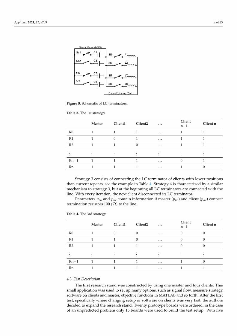
To generate disturbance on the line, a coil, or capacitor, was connected to the line. Theschematic on Figure 5 shows the idea of connection. For switches, the authors chose transis-tors with high peak current and fast opening time. To provide many configuration options,components as shown in Table 1 were chosen. Later in the article, these components willbe named LC terminators.

Four auto-addressing strategies have been developed. Algorithms chose a strategyusing parameter ps4 [see Table 2]. In the case of 15 nodes (1 master + 14 clients), measure-ments have to be repeated 15 times (R0-R14 in Figure 3a). Strategies define which clients

Appl. Sci. 2021, 11, 8709 7 of 25

have to connect the LC terminator parallel with the signal line. Table 3 shows the firststrategy. In all variants, LC terminators are always used by the master board. Parametersph2 and ph3 can be set to not use the LC terminator—it allows us to reduce the quantity ofstrategy from eight variants to four variants giving the same effect. Strategy 2 is similar tothe first one, but all LC terminators are, as a default, disconnected from the line, and withevery next repeat (R0-R14) the proper client connected his LC terminator.

Table 1. The components of the LC terminator.

Inductor Capacitor

1 330 nH 330 pF

2 1 µH 1 nF

3 3.3 µH 3.3 nF

4 10 µH 10 nF

5 33 µH 33 nF

6 100 µH 100 nF

7 330 µH 330 nF

8 1 mH 1 µF

Table 2. A list of decision variables with descriptions.

Indicator Range Description

ps1 1–150 [µs] (Signal A22)—Pulse generator charging time. See Figure 3

ph11–9 Selection capacitor on Master (see Table 1).

ph2 1–9 Selection coil on Master. See Table 1

ph3 1–9 Selection capacitor on Client. See Table 1

ph41–9 Selection coil on Client. See Table 1

ps2 1–999 [µs] (Signal A31)—delay before first ADC measure. See Figure 3

ps3 1–40 [µs] (Signal A32)—delay between ADC measure. See Figure 3

ps4 1–4 Strategy of using coils and capacitors—see Table 3, & Table 4

ps5 0–7 Method of data analysing0—median; 1—mean; 2—max; 3—min; 4—mode;5—sum-max/size; 6—value of C0—See Figure 3b;7—max-min ;

ps6 0–3 Source of data for analysing0—S0—See Figure 3d—ADC1—S1—See Figure 3d—ADC2—S2—See Figure 3d—ADC3—S3—See Figure 3d—ADC

ps7 1–4 Define addresses trend1—rising trend2—falling trend3—rising trend + replace last address4—falling trend + replace last address

ph5 2–8 Coil selection to pulse generator—Master only—Figure 4

ph6 0–1 1—use termination resistor on Master board0—do not use

ph7 0–1 1—use termination resistor on Client board0—do not use

Appl. Sci. 2021, 11, 8709 8 of 25

Figure 5. Schematic of LC terminators.

Table 3. The 1st strategy.

Master Client1 Client2 . . . Clientn−1 Client n

R0 1 1 1 . . . 1 1

R1 1 0 1 . . . 1 1

R2 1 1 0 . . . 1 1

......

......

......

...

Rn−1 1 1 1 . . . 0 1

Rn 1 1 1 . . . 1 0

Strategy 3 consists of connecting the LC terminator of clients with lower positionsthan current repeats, see the example in Table 4. Strategy 4 is characterized by a similarmechanism to strategy 3, but at the beginning all LC terminators are connected with theline. With every iteration, the next client disconnected its LC terminator.

Parameters ph6 and ph7 contain information if master (ph6) and client (ph7) connecttermination resistors 100 (Ω) to the line.

Table 4. The 3rd strategy.

Master Client1 Client2 . . . Clientn−1 Client n

R0 1 0 0 . . . 0 0

R1 1 1 0 . . . 0 0

R2 1 1 1 . . . 0 0

......

......

......

...

Rn−1 1 1 1 . . . 1 0

Rn 1 1 1 . . . 1 1

4.3. Test Description

The first research stand was constructed by using one master and four clients. Thissmall application was used to set up many options, such as signal flow, measure strategy,software on clients and master, objective functions in MATLAB and so forth. After the firsttest, specifically where changing setup or software on clients was very fast, the authorsdecided to expand the research stand. Twenty prototype boards were ordered, in the caseof an unpredicted problem only 15 boards were used to build the test setup. With five

Appl. Sci. 2021, 11, 8709 9 of 25

boards, everything works correctly using Rpi as the MQTT server and AP. With this setup,the authors adjusted all parameters to optimize communication between nodes, where 2Mbps was achieved. All parameters of communication were adjusted using well-knownlaboratory equipment and engineering knowledge.

The next step was to build up a research stand for 15 boards and find parameters ofauto-addressing, which finally was even more difficult than the authors expected. Unfortu-nately, the stability of AP on Rpi was unsatisfactory when all 15 nodes sent the report afterthe test (exactly at the same time). The report contains 1500 measured parameters. Thebehaviour was diagnosed by MQTT.fx—external tool. It necessitated the use of additionalAP, where the Mikrotik RouterBoard was selected, then all frames could be received by thecomputer with the MQTT.fx and MATLAB environment installed in it. The last issue theauthors had to tackle was the MQTT library written in Java for the MATLAB environmentbecause it lacked speed to process all frames from MQTT. The standard solution is toincrease Quality Of Service (QOS) in MQTT frames. The disadvantage of this solutionis, however, the extended time of sending each measurement. Therefore, in the case ofplanned 500 k–1 mln tests, another solution was selected. A two-thread script was writtenin Python, and ran on Rpi. One thread handled receiving and decoding MQTT frames fromthe JSON format, the other one analysed data, and after the finished test, it collected alldata into one frame which was then sent to Matlab. This configuration made the researchstand and data flow concept more complicated, but significantly reduced the time of asingle measurement, and guaranteed almost 100% data correctness. The only programmeddelay (Figure 6, p. 4) was to synchronize all nodes.

Figure 6. A data flow between research stand modules.

The authors prepared a special program in the MATLAB environment, which receivedinput data of 15 variables, where artificial algorithms (AA) try to find optimal values andmany static values, such as strictly hardware dependent parameters, or the component costof LC terminators. The communication between all components of the stand is shown in

Appl. Sci. 2021, 11, 8709 10 of 25

Figure 6. The MATLAB environment code is responsible for building up MQTT frames. Allframes are sent to boards and Rpi. Client boards after receiving frames with an individualconfiguration (Figure 6 frame 3) are set to wait for a trigger from the master. To avoid anyproblems with synchronization, the software waits 200 ms (Figure 6 p. 4) before the datapublish the start of the test frame (Figure 6 frame 5). After the test, the boards publishthe measured data, which are collected by Rpi to one frame (Figure 6 frame 9), which ispublished by Rpi, and subscribed by the MATLAB environment (Figure 6 frame 10).

4.4. Research Stand

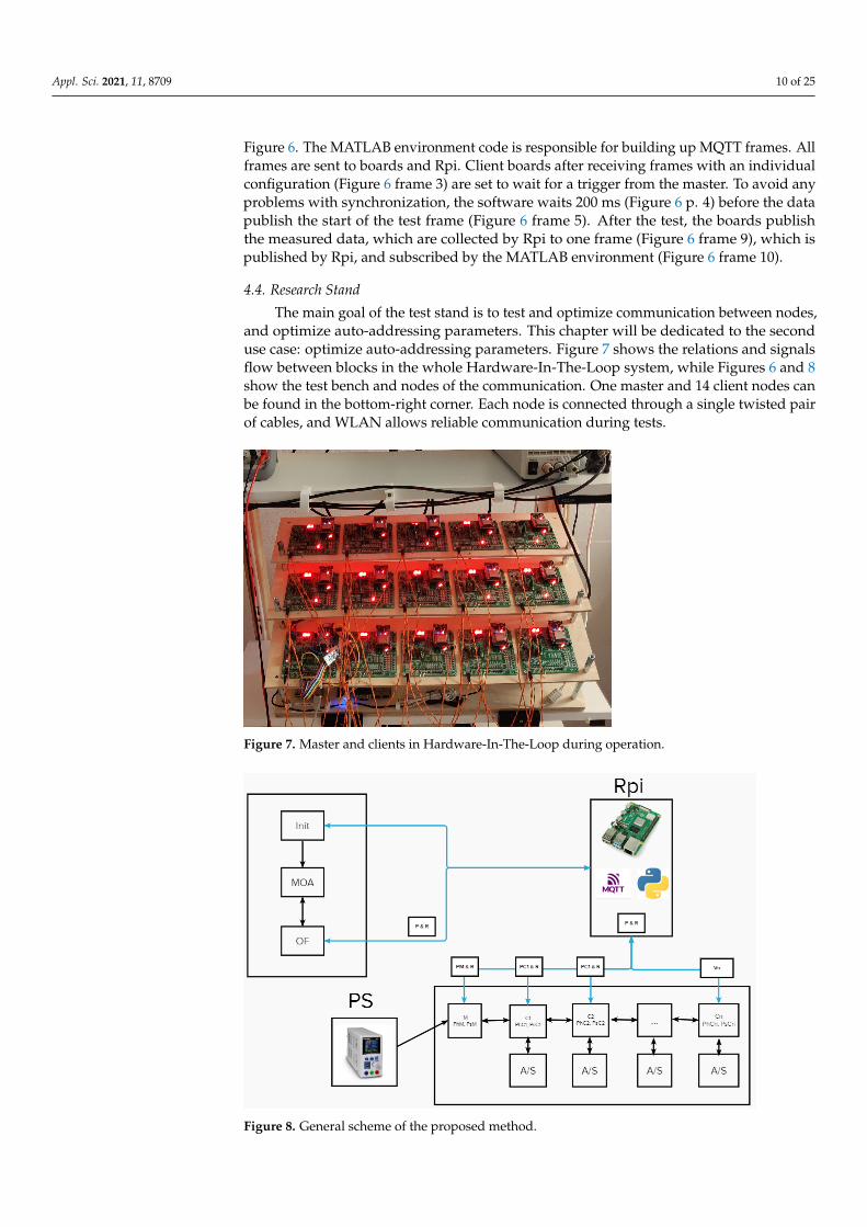
The main goal of the test stand is to test and optimize communication between nodes,and optimize auto-addressing parameters. This chapter will be dedicated to the seconduse case: optimize auto-addressing parameters. Figure 7 shows the relations and signalsflow between blocks in the whole Hardware-In-The-Loop system, while Figures 6 and 8show the test bench and nodes of the communication. One master and 14 client nodes canbe found in the bottom-right corner. Each node is connected through a single twisted pairof cables, and WLAN allows reliable communication during tests.

Figure 7. Master and clients in Hardware-In-The-Loop during operation.

Figure 8. General scheme of the proposed method.

Appl. Sci. 2021, 11, 8709 11 of 25

5. HIL-Based Optimization Method for Bus Prototyping

The effectiveness of the power supply and communication bus strongly depends on itsHardware-In-The-Loop structure S as well as on the hardware components and softwareparameters of the proposed solution. These factors have a great influence on addressables,and therefore they must be adjusted correctly.

The main purpose of the optimization process is to search for the optimal structureof the bus and the optimal values of hardware parameters ph and software parametersps, to obtain the highest performance of the whole system. This issue is viewed as amulti-objective optimization problem and hence it can be stated as the following equation:

Minimize C(S , ph, ps) =[c1(S , ph, ps) c2(S , ph, ps) . . . cn(S , ph, ps)

]subject to Ω(S , ph, ps, C),

(2)

where S , ph and ps represent decision variables, ci is the i-th criterion function that is beingused to express the desirable features and performance of the research version of the bus(it should be stressed that criterion functions represent objectives which are not conflicted),Ω is related to constraints and boundaries, which should be chosen to consider differentvariants of hardware and software parameters. To reduce the complexity of the problem, itis noted that in some cases the structure S can be determined using a part of the decisionvariables corresponding to the values of hardware features included in ph.

The hardware and software features of the bus for the given number of the modules ncan be written using the general formula as follows:

p = [phM phC psM psC ], (3)

where phM and phC denote the hardware parameters of a master and clients, whereas psM

and psC describe their software parameters.In this paper, it is assumed that phM is composed of four values of parameters

as follows:phM = [ph1 , ph2 , ph6 , ph5 ], (4)

and phC is composed ofphC = [ph3 , ph4 , ph7 ], (5)

where ph2 is the number corresponding to the selected capacitor on master (see Table 1), ph2is the number corresponding to the selected inductor on master (see Table 1), ph6 is usedto decide whether a termination resistor on master is necessary or not, ph5 is applied todescribe the inductor in the pulse generator (see Figure 4), ph3 is used to select a capacitoron client (see Table 1) and (Figure 5), ph4 is used to select an inductor on client (see Table 1and Figure 5), ph7 is used to decide whether a termination resistor on client is needed ornot. Except for hardware parameters, software decision variables can be divided to auto-addressing configurations such as ps2 and ps3 , where the delay before the first ADC sampleand the gap between samples can be chosen, ps1 is the time to charge pulse generator(A22 in Figure 3d), and ps4 is a discrete variable defined strategy of auto-addressing,especially managing the use of coils and capacitors on master and clients (Tables 3 and 4).The second group of software decision variables are data processing methods, like ps5

where mathematical operations of the input data are chosen, ps6 , where the source of datafor analysis is chosen, and ps7 , where the target manner for addressing is chosen. Priorresearch has thoroughly investigated how the following addresses will look; two obvioustrends ware noticed—following addresses will rise or fall—as well as another two not soobvious trends—in the rising trend the lower value is the last one, and in the falling trend,the higher avlue is the last one. An example is shown in Figure 9.

Appl. Sci. 2021, 11, 8709 12 of 25

Figure 9. One of the characteristic trends of the addresses value.

Generally, multi-objective functions very often have an infinite number of local aswell as global extrema and therefore one should investigate a set of points, each of whichsatisfies the objectives. Because of this, the predominant Pareto optimality concept isadopted. The Pareto-optimal solution is often considered the same as a non-dominatedsolution; it exists if there is no solution that improves at least one objective function withoutworsening the others. In this research, it is sufficient to apply the following fundamentalmeasures as objectives:

• c1, which is based on addressable factor:

c1(ph, ps) =

1

n−1∑

i=2(

1 if ai>ai+10 other )

if ps7 = 2 or 4

1n−1∑

i=2(

1 if ai<ai+10 other )

other ,(6)

where elements of the vector a are computed using the proposed rule in the formas follows:

an(a) =

an = max(a) + 1 if an = min(a) and ps7 = 3an = min(a)− 1 if an = max(a) and ps7 = 4no change in other,

(7)

and n represents the number of nodes, ps7 defines the addresses trend (see Table 2),and ai measures address value of the i-th node.

• c2 is based on the minimal difference between addresses:

c2(ph, ps) =1

∆max + 1, (8)

where ∆max describes the difference in addresses between neighbour nodes.

• c3 is used to show the overall cost of the system:

c3(ph) = ν(phM , phC , n), (9)

where ν is the function which calculates a cost of each element used in the cur-rent approach.

Appl. Sci. 2021, 11, 8709 13 of 25

On the other hand, the global criterion method can be successfully applied to transforma multiple objective function into a single objective one. This way, an indirect utilityfunction can be expressed in its simplest form as the weighted sum of objectives:

C(ph, ps) =wCT(p)

1wT =

5c1 if c1 ≥ 1

n − 1w1c2 + w2c3 other,

(10)

where w is a row vector with weights indicating the relative significance of the objec-tive functions; in this study, w1 and w2 indicate the weights for the second and thirdcriteria, respectively.

The optimal solution is found if the criterion function C has a relative minimum valueat p*, that means if:

p∗ = [p∗h p∗s ] = argmin︸ ︷︷ ︸p∈Ω

C(ph, ps). (11)

It has been decided to apply intelligent computing and hardware in the loop tech-niques due to several difficulties in bus prototyping discussed in Section 2. The proposedscheme of the optimization method is present in Figure 8. The HIL part of the systemis composed of n modules (one master unit and n − 1 clients), where all modules areconnected with one twisted pair of cables and a wireless network to remove the influ-ence of auto-addressing signals. The optimization process is managed by the softwarecreated employing MATLAB and Raspberry Pi platforms.The authors decided to use theGlobal Optimization Toolbox for the implementation of evolutionary and particle swarmalgorithms. More details are given and described in Section 5.2.

Different optimization algorithms can be utilized for solving the problem, whichhas been declared in the form of (2) or (10). Hard computing optimization methods, forexample, gradient-based approaches, cannot be adopted in this paper, mainly due to thestochastic nature of the objectives and because there are continuous and discrete decisionvariables in the vector p. On the other hand, pure stochastic optimization methods, forexample, Monte Carlo techniques, will not be able to find an accurate solution, in thiscase guaranteeing polynomial-time convergence. Instead, soft computing optimizationmethods may be used to find the global minimum of the function. In this study, heuristicalgorithms are applied such as SOAE, MOAE (Single or Multi-Objective EvolutionaryAlgorithm) and PSO (Particle Swarm Optimization).

5.1. Single or Multi-Objective Evolutionary Algorithm

Evolutionary algorithms are based on the natural selection process that mimics bio-logical evolution. In order to apply such an optimization technique for finding a solutionof the problem it is necessary to define the following properties of the algorithm [30]: therepresentation of the individuals, the fitness function, selection and succession methods,crossover and mutation operators. It is assumed that the number of individuals in thepopulation is fixed at each epoch of the evolutionary process and that individuals arecomposed of genes representing real numeric and integer values of adjustable hardwareand software parameters of the bus. The length of the chromosome is dependent on thenumber of these parameters and equals the length of the vector p:

chr = p = [p1 p2 . . . pd]. (12)

The initial population is generated using the normal distribution. The fitness value ofan individual is computed using the objective function (2) or (10). The best fitness value fora population is the smallest fitness value for every individual in the population. Stochasticuniform is applied to choose parents for the next generation, whereas succession operationsare realized by defining the reproduction rules characterized by two parameters: elite count(δs) and crossover fraction (pc). The first parameter is the number of individuals with thebest fitness values in the current generation that are guaranteed to survive to the next

Appl. Sci. 2021, 11, 8709 14 of 25

generation. The second one is the fraction of individuals in the next generation, other thanelite children, that are created by crossover. It is decided to use a simple heuristic crossoveroperator. On the basis of two individuals, p1 and p2, in the case of C(p1) < C(p2), thenthe new one p3 is created according to the formula mentioned below

p3 = p2 + λh(p1 − p2), (13)

where λh is a fraction pointing at the better adapted individual.A mutation operator is responsible for generating heterogeneous individuals. This

operator is based on an adaptive feasible method, and it randomly generates directionswith respect to the last successful or unsuccessful generation. The mutation operator findsa direction and step length satisfying bounds and linear constraints. The algorithm is alsodescribed by two important parameters such as the population size and the number ofgenerations. The values of these parameters are arbitrarily selected during optimizationexperiments. In this study, it is decided that the total number of evaluation of the fitnessfunction is constant, and it is equal to Ψ. Hence, the number of individuals in a populationis calculated using the following formula:

Population =Ψ

Generations. (14)

5.2. Particle Swarm Optimization

The particle swarm optimization is a population-based stochastic optimization tech-nique [31,32], which is inspired by simulation of the social behaviour reflected in flocks ofbirds, bees and fish that adapt their movements in order to seek the best food sources aswell as to avoid predators [31,33]. This type of optimization approach is also viewed as aparallel evolutionary computation technique.

Numerically, the basic PSO algorithm can be formulated in vector notation, as isproposed in [34]. The velocity vk is updated using its current value and a term whichattracts the particle towards its own previous best position p∗1 and globally the best positionp∗2 in the whole swarm:

vk+1 = avk + b1r1 ⊗ (p∗1 − pk) + b2r2 ⊗ (p∗2 − pk), (15)

while the particle position pk is dynamically actualized using its current value and thenewly computed velocity vk+1:

pk+1 = cpk + dvk+1, (16)

where the symbol ⊗ denotes element-by-element vector multiplication, a is the momentumfactor, also known as the inertia weight, coefficients b1 and b2 are used to describe thestrength of attraction (cognitive and social attraction coefficients, respectively), c and d areblack-box tuning parameters, vectors of random numbers r1 and r2 that are useful for goodstate space exploration (they are usually obtained using the generator of pseudo-randomnumbers with uniform distribution in the range of 0 to 1).

In this algorithm, the cost function in the form of (10) was used. The PSO algorithmcharacterizes three main parameters—population size, self-adjustment weight and minimalneighbours’ fraction. To have a reliable comparison between algorithms, the same totalnumber of cost function evaluations is necessary (Ψ), hence the max iteration is calculatedusing the simple equation:

SwarmSize =

[Ψ

MaxIter + 1

]. (17)

The self-adjustment weight parameter can be in the range from 0.5 to 3.5 with step 1.0,where a default value is 1.49. Considering a stability analysis provided by Brest et al. [35],

Appl. Sci. 2021, 11, 8709 15 of 25

Clerc and Kennedy [36] or Katunin and Przystałka [37], it is decided to relate the self-adjustment weight (b1) and social adjustment weight (b2) as follows:

b2 = 4.05− b1. (18)

This technique was chosen to test the parameters of the algorithm with differentconfigurations; some researchers use PSO with fixed parameters where self-adjustmentweight (b1) and social adjustment weight (b2) are set to 2 [33,38]. The adopted methodologyused close values at b1 = 2.5 and at b1 = 2.5, where b2 is calculated to 1.55 and 2.55.Interpolating results from Section 6, the authors conclude that the decision was the rightone. The interpolated quality parameters of PSO also suggest that the default value of b1 iscloser to optimal than 2.

6. Verification and Validation

Verification was divided into a few sections, where initially the authors comparedresults from GA with different parameters. There will be quantitative and qualitativecomparisons. The same approach will be used for PSO. All results will also be comparedwith LSH.

6.1. LHS Results

Finding solutions using artificial algorithms always provides the risk of not findingthe best-fit result, especially in a noisy environment. The authors decided to start withthe LHS algorithm to have sample coverage. The results, shown in Figure 10 will alsobe beneficial for comparison with other algorithms, to prove AI algorithms can alwaysbe better. The authors generated Ψ = 10, 000 unique elements using LHS and checkedthe results. Seven input samples allowed HIL to correct addressing. The LHS algorithmworked with a success factor 0.07%.

To have reliable addressing, c2 should be at a minimum level of 0.5. LSH gives us onlythree such results, which is 0.03% of the selected data. LHS does not deliver any informationabout which optimization variable we can reduce, as we can find many parameters in eachdecision variable in all seven results.

Figure 10. LHS result .

6.2. Results of GA

The results of Multi objective Optimization using Genetic Algorithm were dividedinto two parts; one is quantitative, where the authors checked how many results warefound from each algorithm configuration, and the second is a qualitative comparison,where the authors checked how close to optimal all the algorithms were.

Appl. Sci. 2021, 11, 8709 16 of 25

6.2.1. Quantitative Results of GA

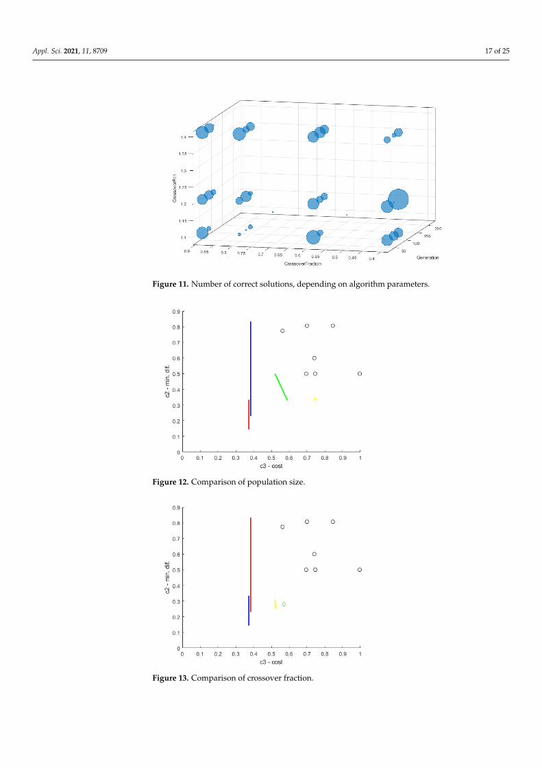
The authors carried out 48 optimizations with different parameters (Table 2). Thebest one finds 50 results in 100 individuals (crossover fraction 0.4 and crossover heuristicparameter 1.2), which is remarkable in correlation with LSH. The worst one could not findeven one result—all cases with 200 generations, where the population is characterized byonly 50 individuals. Figure 11 and Table 5 present a number of correct solutions, dependingon algorithm parameters.

Table 5. Sum of correct results using specific GA parameters. Colour code: Green → the best; lightgreen → better than 70% of best; orange → better than 40% of best; red → worst than 40% of best.

PopulationSize Sum Coefficient

Fraction Sum CrossoverHeuristic Sum

200 172 0.4 125 1.1 94

125 86 0.6 97 1.2 148

100 106 0.8 66 1.4 124

50 2 0.9 78

As can be seen in Table 5, the highest number of results can be found using the largestpopulations (in this test 200 individuals), the crossover fraction set to 0.4 and crossoverheuristic parameter set to 1.2. During testing different parameters, test with the aboveparameters found the largest amount of correct results.

6.2.2. Qualitative results of GA

Due to multi objective optimization used in GA, quality features were compared onthe Pareto front. For the first, the check width was most of the results, all points wereprinted on a diagram with the cost (c3) of the solution on the X-axis and minimal differencebetween address (c2) on the Y-axis (Figures 12–14). Decision variable c2 was calculatedfrom Equation (8). The colour code informs about the type of optimization (see Table 6). Itis worth noticing that GA parameters, which generate a higher number of results, did notgenerate the best results.

Table 6. Colour codes for figures.

Gen

erat

ion

(Pop

ulat

ion)

Cro

ssov

erFr

acti

on

Cro

ssov

erH

euri

stic

Col

orC

ode

inFi

gure

s12

–14

valu

e

50 (200) 0.4 1.1 red

80 (125) 0.6 1.2 blue

100 (100) 0.8 1.4 green

200 (50) 0.9 yellow

Appl. Sci. 2021, 11, 8709 17 of 25

Figure 11. Number of correct solutions, depending on algorithm parameters.

Figure 12. Comparison of population size.

Figure 13. Comparison of crossover fraction.

Appl. Sci. 2021, 11, 8709 18 of 25

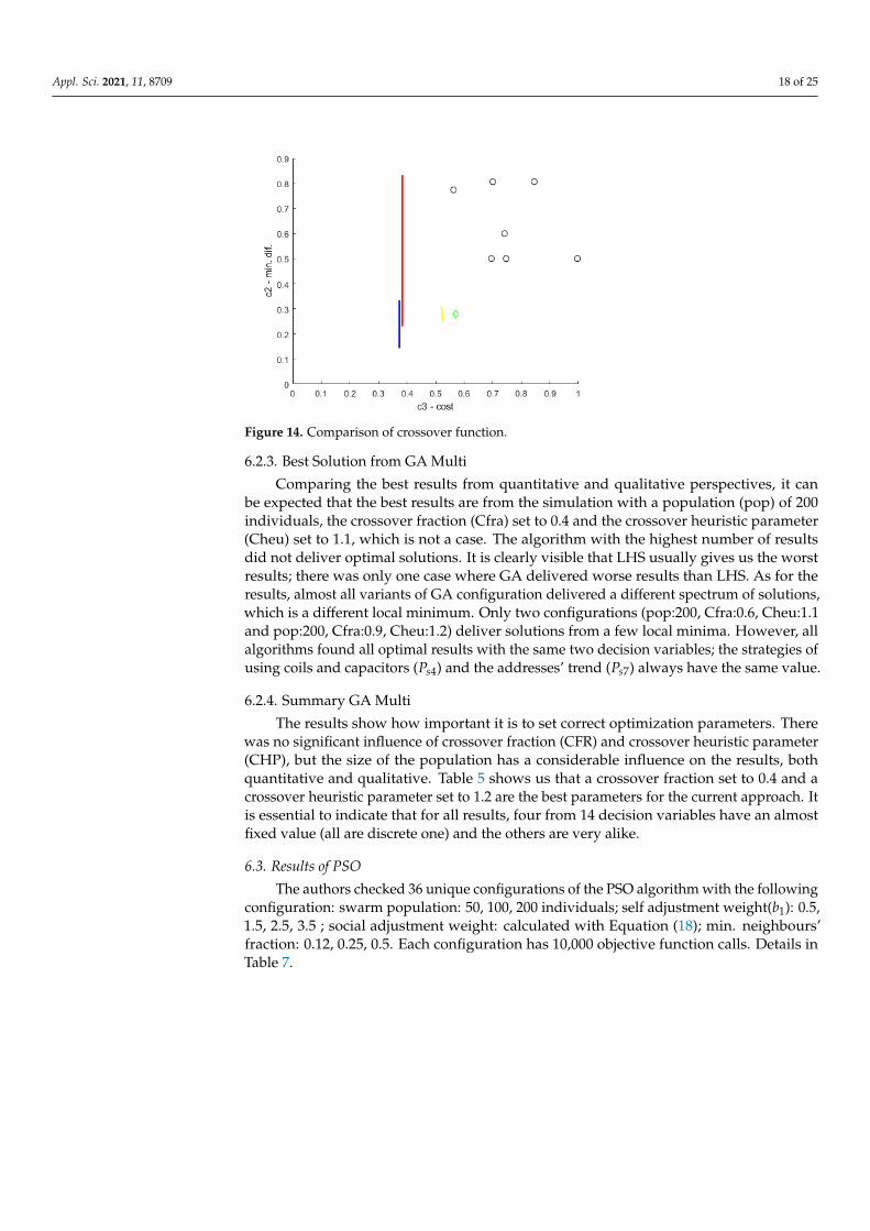
Figure 14. Comparison of crossover function.

6.2.3. Best Solution from GA Multi

Comparing the best results from quantitative and qualitative perspectives, it canbe expected that the best results are from the simulation with a population (pop) of 200individuals, the crossover fraction (Cfra) set to 0.4 and the crossover heuristic parameter(Cheu) set to 1.1, which is not a case. The algorithm with the highest number of resultsdid not deliver optimal solutions. It is clearly visible that LHS usually gives us the worstresults; there was only one case where GA delivered worse results than LHS. As for theresults, almost all variants of GA configuration delivered a different spectrum of solutions,which is a different local minimum. Only two configurations (pop:200, Cfra:0.6, Cheu:1.1and pop:200, Cfra:0.9, Cheu:1.2) deliver solutions from a few local minima. However, allalgorithms found all optimal results with the same two decision variables; the strategies ofusing coils and capacitors (Ps4) and the addresses’ trend (Ps7) always have the same value.

6.2.4. Summary GA Multi

The results show how important it is to set correct optimization parameters. Therewas no significant influence of crossover fraction (CFR) and crossover heuristic parameter(CHP), but the size of the population has a considerable influence on the results, bothquantitative and qualitative. Table 5 shows us that a crossover fraction set to 0.4 and acrossover heuristic parameter set to 1.2 are the best parameters for the current approach. Itis essential to indicate that for all results, four from 14 decision variables have an almostfixed value (all are discrete one) and the others are very alike.

6.3. Results of PSO

The authors checked 36 unique configurations of the PSO algorithm with the followingconfiguration: swarm population: 50, 100, 200 individuals; self adjustment weight(b1): 0.5,1.5, 2.5, 3.5 ; social adjustment weight: calculated with Equation (18); min. neighbours’fraction: 0.12, 0.25, 0.5. Each configuration has 10,000 objective function calls. Details inTable 7.

Appl. Sci. 2021, 11, 8709 19 of 25

Table 7. PSO parameters and colour/shape codes for figures.

Swarm Size b1Colour Code inFigures 15–17 MNF

SymbolColour in

Figures 15–17

valu

e

50 0.5 red 0.12 +

100 1.5 blue 0.25 x

200 2.5 green 0.5 ♦

3.5 yellow

Figure 15. Particle Swarm Optimization. Swarm size: 50. Black ball—LHS. Others, see Table above.

Figure 16. Particle Swarm Optimization. Swarm size: 100. Black ball—LHS. Others, see Table above.

Appl. Sci. 2021, 11, 8709 20 of 25

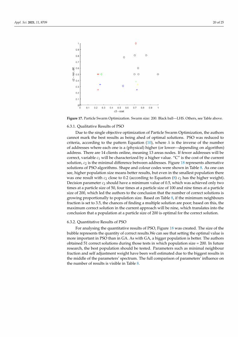
Figure 17. Particle Swarm Optimization. Swarm size: 200. Black ball—LHS. Others, see Table above.

6.3.1. Qualitative Results of PSO

Due to the single objective optimization of Particle Swarm Optimization, the authorscannot mark the best results as being ahed of optimal solutions. PSO was reduced tocriteria, according to the pattern Equation (10), where λ is the inverse of the numberof addresses where each one is a (physical) higher (or lower—depending on algorithm)address. There are 14 clients online, meaning 13 areas nodes. If fewer addresses will becorrect, variable c1 will be characterized by a higher value. “C” is the cost of the currentsolution, c2 is the minimal difference between addresses. Figure 18 represents alternativesolutions of PSO algorithms. Shape and colour codes were shown in Table 8. As one cansee, higher population size means better results, but even in the smallest population therewas one result with c2 close to 0.2 (according to Equation (8) c2 has the higher weight).Decision parameter c2 should have a minimum value of 0.5, which was achieved only twotimes at a particle size of 50, four times at a particle size of 100 and nine times at a particlesize of 200, which led the authors to the conclusion that the number of correct solutions isgrowing proportionally to population size. Based on Table 8, if the minimum neighboursfraction is set to 3.5, the chances of finding a multiple solution are poor; based on this, themaximum correct solution in the current approach will be nine, which translates into theconclusion that a population at a particle size of 200 is optimal for the correct solution.

6.3.2. Quantitative Results of PSO

For analysing the quantitative results of PSO, Figure 18 was created. The size of thebubble represents the quantity of correct results.We can see that setting the optimal value ismore important in PSO than in GA. As with GA, a bigger population is better. The authorsobtained 51 correct solutions during those tests in which population size = 200. In futureresearch, the best population should be tested. Parameters such as minimal neighbourfraction and self adjustment weight have been well estimated due to the biggest results inthe middle of the parameters’ spectrum. The full comparison of parameters’ influence onthe number of results is visible in Table 8.

Appl. Sci. 2021, 11, 8709 21 of 25

Figure 18. Bubble visualization of quantitative results of different PSO configurations.

Table 8. Sum of correct results using specific PSO parameters. Colour code: green→ the best; lightgreen→ better than 70% of best; orange→ better than 40% of best; red→ worst than 40% of best.

Swarm Size Sum b1 Sum MNF Sum

50 14 0.5 29 0.12 20

100 28 1.5 43 0.25 45

200 51 2.5 20 0.5 28

3.5 1

6.3.3. Summary of PSO

It is clearly visible that LHS usually gives us the worst results, but in the case of usingbad algorithm configurations, LHS can deliver better results. As for the results, on theupper diagrams, the authors mark 19 results—the best from each algorithm configuration.In Figures 16 and 17, “x” can be found in the bottom-left corner and two solutions arevisible; they are the best results from all tests that the authors conducted. Comparing thesetwo points and all other points (not shown in the figures) from these two configurations,the authors noted that only one decision variable was not the same in all cases.

6.4. Summary

To summarize, the best results ware achieved by PSO (Size: 200, MNF: 0.5 SAW:0.25),confirmed by Equation (10). The best GA solution was 59%, and the best LHS solution was245%, which was more expensive compared to PSO, the comparison is shown on Figure 19.However, the best GA solution was characterized by a three times better MDA than PSO(in this particular case the costs are 3.23 times higher than in the best result), and the bestLHS is characterized as two times worse c2 compared to PSO.

Appl. Sci. 2021, 11, 8709 22 of 25

Figure 19. Results from all algorithms. Black ball—LHS. Red fronts and diamonds—GA, Bluex—PSO.

7. Conclusions

The goal of this research was to develop and test a power and communication bus,with a focus on developing and finding the best parameters for auto-addressing. All goalswere achieved. The bus was developed with better parameters than were expected; it is upto four times faster (up to 2 Mbps, where 512 kbps was the target) and can transfer up to480 W (48 V and 10 A). DLN is cutting-edge technology, which can significantly reducethe number of cables in cars, which at the end reduce CO2 footprint, the weight of a carand also reduce costs by reducing production time and used materials. The authors areconfident that the proposed solution can be used in all non-safety applications in a car. Thecost of the example of usage is much lower than the current solution.

The authors, using the HIL setup, artificial intelligence computing in a particulargenetic algorithm, swarm optimization and planning an experimental method, checkedmultiple parameters of DLN and chose the best one to ensure the proper operation of theauto-addressing function. The best results were achieved by using artificial intelligencealgorithms, in both cases of the solution and the difference between module addresses. Outof the two used algorithms, both have better results in the highest number of individuals ina population. Particle swarm optimization delivered the best results in the tested approach.However, in future, the use of PSO algorithms with more variants of minimal neighbourfraction parameters have to be tested, especially 0.2 and 0.3.

The proposed bus DLN can be implemented in new cars after real life tests andadmission tests. DLN can be commonly used in QM solutions and not in safety systemsdue to the lack of redundancy. The proposed Hardware-In-The-Loop system connected toartificial intelligence proved to be a perfect method for adjusting physical hardware. Thisapproach can be used in the future for solving similar problems.

Author Contributions: Conceptualization, M.S. and P.P.; methodology, M.S. and P.P.; software, M.S.;validation, M.S. and P.P.; formal analysis, M.S.; investigation, M.S.; resources, M.S.; data curation,M.S.; writing—original draft preparation, M.S.; writing—review and editing, P.P.; visualization, M.S.;supervision, P.P.; project administration, M.S.; funding acquisition, P.P. All authors have read andagreed to the published version of the manuscript.

Appl. Sci. 2021, 11, 8709 23 of 25

Funding: Paid from the funds of the Ministry of Education and Science 12/DW/2017/01/1 fromday of 7th of November 2017 r.

Institutional Review Board Statement: Not applicable.

Informed Consent Statement: Not applicable.

Data Availability Statement: Data available in a publicly accessible repository that does not issueDOIs. Publicly available data sets were analyzed in this study. Data can be shared on request.

Conflicts of Interest: The authors declare no conflict of interest.

AbbreviationsThe following abbreviations are used in this manuscript:

LIN Local Interface NetworkS Hardware-In-The-Loop structurep Parameters—Decision variablesR Measure ResultsC criteriaci i-th criterion functionph hardware parametersps software parametersΩ boundaries of ph and psRpi Raspberry PIAP Access PointMQTT Message Queuing Telemetry TransportIOT Internet Of ThingsPS Power SupplyM Master boardC Client BoardMOA Multi Objective AlgorithmA/S Actuator or Sensorcn i-th of Client BoardMDA (c2) minimal difference between addressLHS Latin Hypercube SampleDLN Device Lightweight NetworkEMI Electromagnetic InterferenceOEM Original Equipment ManufacturerPCB Printed Circuit Board

References1. CO, Benz. Fahrzeug Mit Gasmotorenbetrieb; Technical Report; Patent Office: Munich, Germany, 1886.2. Ford. Exterior Lighting History; Technical Report; Ford: Dearborn, MI, USA, 2021.3. Li, R.; Liu, C.; Luo, F. A design for automotive CAN bus monitoring system. In Proceedings of the 2008 IEEE Vehicle Power and

Propulsion Conference, Harbin, China, 3–5 September 2008; pp. 1–5. doi:10.1109/VPPC.2008.4677544.4. Ploss, R.; Mueller, A.; Leteinturier, P. Solving automotive challenges with Electronics. In Proceedings of the 2008 Interna-

tional Symposium on VLSI Technology, Systems and Applications (VLSI-TSA), Hsinchu, Taiwan, 21–23 April 2008; pp. 1–2.doi:10.1109/VTSA.2008.4530772.

5. Zalewski, J.; Trawczynski, D.; Sosnowski, J.; Kornecki, A.; Sniezek, M. Safety Issues in Avionics and Automotive Databuses. IFACProc. Vol. 2005, 38, 26–31. doi:10.3182/20050703-6-CZ-1902.01183.

6. Keysight. From Standard Ethernet To Automotive Ethernet; Technical Report; Keysight: Santa Rosa, CA, USA, 2019.7. Zadobrischi, E.; Dimian, M. Vehicular Communications Utility in Road Safety Applications: A Step toward Self-Aware Intelligent

Traffic Systems. Symmetry 2021, 13. doi:10.3390/sym13030438.8. Ahangar, M.N.; Ahmed, Q.Z.; Khan, F.A.; Hafeez, M. A Survey of Autonomous Vehicles: Enabling Communication Technologies

and Challenges. Sensors 2021, 21, 706. doi:10.3390/s21030706.9. Alparslan, O.; Arakawa, S.; Murata, M. Next Generation Intra-Vehicle Backbone Network Architectures. In Proceedings of the

2021 IEEE 22nd International Conference on High Performance Switching and Routing (HPSR), Paris, France, 7–10 June 2021;pp. 1–7. doi:10.1109/HPSR52026.2021.9481803.

Appl. Sci. 2021, 11, 8709 24 of 25

10. Palanivel, N.; Chen, T. Wiring harness reduction in automotive using Li-Fi technology. In Proceedings of the 2017 InternationalConference on Wireless Communications, Signal Processing and Networking (WiSPNET), Chennai, India, 22–24 March 2017;pp. 1778–1783. doi:10.1109/WiSPNET.2017.8300067.

11. Munro, S. BMW I3 REPORTS; Technical Report; MunroLive: Auburn Hills, MI, USA, 2013.12. Sparks, D.; Noll, T.; Agrotis, D.; Betzner, T.; Gschwend, K. Multi-Sensor Modules with Data Bus Communication Capability;

International Congress & Exposition; SAE International: Warrendale, PA, USA, 1999. doi:10.4271/1999-01-1277.13. Kivekäs, K.; Lajunen, A.; Baldi, F.; Vepsäläinen, J.; Tammi, K. Reducing the Energy Consumption of Electric Buses With Design

Choices and Predictive Driving. IEEE Trans. Veh. Technol. 2019, 68, 11409–11419. doi:10.1109/TVT.2019.2936772.14. Koehler, S.; Viehl, A.; Bringmann, O.; Rosenstiel, W. Optimized recuperation strategy for (Hybrid) Electric Vehicles based on

intelligent sensors. In Proceedings of the 2012 12th International Conference on Control, Automation and Systems, Jeju, Korea,17–21 October 2012; pp. 218–223.

15. Melexis. MLX81112 Datascheet; Technical Report; Melexis: Ypres, Belgium, 2013.16. Anand Gopalan, A.W. Automatic Slave Node Position Detection ; Technical Report; TexasInstruments: Dallas, TX, USA, 2015.17. Westrick, R.L.; Zulim, D. Automatic Self-Addressing Method for Wired Network Nodes; Technical Report; Patent Office: Washington,

DC, USA, 2010.18. Bhojwani, H.; Sain, G.K.; Sharma, G.P. Computerized Fuse Auto Changeover System with RS485 Bus Reporting Multiple

IOT Cloud Connectivity Avenues. In Proceedings of the 2018 3rd Technology Innovation Management and EngineeringScience International Conference (TIMES-iCON), Bangkok, Thailand, 12–14 December 2018; pp. 1–5. doi:10.1109/TIMES-iCON.2018.8621681.

19. Yamar. Automatic Slave Node Position Detection; Technical Report; Yamar: Tel Aviv, Israel, 2015.20. Strobl, M.; Waas, T.; Moehne, S.; Kucera, M.; Rath, A.; Balbierer, N.; Schingale, A. Using Ethernet over powerline communication

in automotive networks. In Proceedings of the 10th International Workshop on Intelligent Solutions in Embedded Systems,Klagenfurt, Austria, 5–6 July 2012; pp. 39–44.

21. Commission, I.E. Low-Voltage Switchgear and Controlgear—Controller-Device Interfaces; Technical Report; International Electrotech-nical Commission: Geneva, Switzerland, 2008.

22. Wilkie, K.; Foster, M.; Stone, D.; Bingham, C. Hardware-in-the-loop tuning of a feedback controller for a buck converter using aGA. In Proceedings of the 2008 International Symposium on Power Electronics, Electrical Drives, Automation and Motion, Ischia,Italy, 11–13 June 2008; pp. 680–684. doi:10.1109/SPEEDHAM.2008.4581265.

23. Wei, J.; Mouzakitis, A.; Wang, J.; Sun, H. Vehicle windscreen wiper mathematical model development and optimisation for modelbased hardware-in-the-loop simulation and control. In Proceedings of the 17th International Conference on Automation andComputing, Huddersfield, UK, 10 September 2011; pp. 207–212.

24. Angel, L.; Viola, J.; Vega, M. Hardware in the loop experimental validation of PID controllers tuned by genetic algorithms. InProceedings of the 2019 IEEE 4th Colombian Conference on Automatic Control (CCAC), Medellin, Colombia, 15–18 October 2019;pp. 1–6. doi:10.1109/CCAC.2019.8921229.

25. Stopinski, S.; Anders, K.; Szostak, S.; Piramidowicz, R. Optical Time Domain Reflectometer Based on Application SpecificPhotonic Integrated Circuit. In Proceedings of the 2019 Conference on Lasers and Electro-Optics Europe European QuantumElectronics Conference (CLEO/Europe-EQEC), Munich Germany, 23–27 June 2019; p. 1. doi:10.1109/CLEOE-EQEC.2019.8872144.

26. McClements, D.; Fairley, P. Frequency scanning ultrasonic pulse echo reflectometer. Ultrasonics 1992, 30, 403–405.doi:10.1016/0041-624X(92)90097-6.

27. Tsai, P.; Lo, C.; Chung, Y.C.; Furse, C. Mixed-signal reflectometer for location of faults on aging wiring. IEEE Sens. J. 2005,5, 1479–1482. doi:10.1109/JSEN.2005.858894.

28. Alluhaibi, O.; Ahmed, Q.Z.; Kampert, E.; Higgins, M.D.; Wang, J. Revisiting the Energy-Efficient Hybrid D-A Precoding andCombining Design for mm-Wave Systems. IEEE Trans. Green Commun. Netw. 2020, 4, 340–354. doi:10.1109/TGCN.2020.2972267.

29. Spiess, A. How Good are the ADCs Inside Arduinos, ESP8266, and ESP32? And Extenal ADCs (ADS1115); Technical Report; Andreas:Basel, Switzerland, 2020.

30. Deb, M. Multi-Objective Optimization Using Evolutionary Algorithms; Wiley: Hoboken, NJ, USA, 2009.31. Kennedy, J.; Eberhart, R.C.; Shi, Y. Preface. In Swarm Intelligence ; The Morgan Kaufmann Series in Artificial Intelligence; Morgan

Kaufmann: San Francisco, CA, USA, 2001; pp. xiii–xxvii. doi:10.1016/B978-155860595-4/50000-0.32. Ahmed, Q.Z.; Ahmed, S.; Alouini, M.S.; Aïssa, S. Minimizing the Symbol-Error-Rate for Amplify-and-Forward Relaying Systems

Using Evolutionary Algorithms. IEEE Trans. Commun. 2015, 63, 390–400. doi:10.1109/TCOMM.2014.2375255.33. Soo, K.K.; Siu, Y.M.; Chan, W.S.; Yang, L.; Chen, R.S. Particle-Swarm-Optimization-Based Multiuser Detector for CDMA

Communications. IEEE Trans. Veh. Technol. 2007, 56, 3006–3013. doi:10.1109/TVT.2007.900383.34. Trelea, I.C. The particle swarm optimization algorithm: convergence analysis and parameter selection. Inf. Process. Lett. 2003,

85, 317–325. doi:10.1016/S0020-0190(02)00447-7.35. Brest, J.; Greiner, S.; Boskovic, B.; Mernik, M.; Zumer, V. Self-Adapting Control Parameters in Differential Evolution: A Compara-

tive Study on Numerical Benchmark Problems. IEEE Trans. Evol. Comput. 2006, 10, 646–657. doi:10.1109/TEVC.2006.872133.36. Clerc, M.; Kennedy, J. The particle swarm—Explosion, stability, and convergence in a multidimensional complex space. IEEE

Trans. Evol. Comput. 2002, 6, 58–73. doi:10.1109/4235.985692.

Appl. Sci. 2021, 11, 8709 25 of 25

37. Katunin, A.; Przystałka, P. Damage assessment in composite plates using fractional wavelet transform of modal shapes withoptimized selection of spatial wavelets. Eng. Appl. Artif. Intell. 2014, 30, 73–85. doi:10.1016/j.engappai.2014.01.003.

38. Zhao, Y.; Zheng, J. Particle swarm optimization algorithm in signal detection and blind extraction. In Proceedings of the 7thInternational Symposium on Parallel Architectures, Algorithms and Networks, Hong Kong, China, 10–12 May 2004; pp. 37–41.doi:10.1109/ISPAN.2004.1300454.