the flexible phenotype
TRANSCRIPT

The Flexible Phenotype

‘This text is a must for anybody who has remained curious about the ways animals, including humans, deal with their environment. It’s scientifi cally sound and at the same time it’s a gripping story.’
Dr Hans Hoppeler , Institute of Anatomy, University of Bern, Switzerland and Editor-in-Chief of Journal of Experimental Biology
‘Written with zest, a sense of fun, and a deep love of nature, The Flexible Phenotype offers biologists a real synthesis of ecology, physiology, and behaviour, based on in-depth empirical research. The adventures of the subject of many of these studies, the red knot, a migrant shorebird, captivate the imagination, show us how physiology and morphology express ecology, and make this book not only an important and truly integrated study in biology, but also a pleasure to read.’
Professor Eva Jablonka , Cohn Institute, Tel-Aviv University, Israel
‘Even amongst mammals and birds, animals are diverse. Biologists have long sought the evolutionary pressures that have led to particular body designs and lifestyles. I believe that to do so requires an approach that considers the interaction of body design and behaviour in an ecological context. Too often these components are considered in relative isolation. In contrast, this book is wonderfully broad and holistic, integrating across levels. Even though the book is written in an accessible style that will entertain anyone who is interested in nature, it is serious science.’
Professor John McNamara , University of Bristol, UK
‘Change rules every individual’s world, whether imposed by temporal variation in the environment or by movement through variable surroundings, and survival and reproductive success depend on adaptive responses to this change. Drawing on experience in fi eld and laboratory research, and integrating modern ideas about acclimatization and the optimizing of individual behavior, physiology, and morphology, the authors have produced an accessible, highly readable, and stimulating synthesis of the fl exible phenotype. Using examples drawn from their own work on migrating shorebirds, as well as myriad other organisms, the authors show how individuals respond to change by altering their structure and function through a variety of behavioral and physiological mechanisms. Long-standing traditions of research in physiological, behavioral, and evolutionary ecology are brought completely up-to-date in this timely treatment of organisms in their changeable worlds. The ways in which mechanisms of individual response promote survival and productivity are keys to understanding how organisms will adjust, or fail to do so, in the face of habitat alteration and global climate change.’
Professor Robert E. Ricklefs , University of Missouri - St. Louis, USA
‘In their book Piersma and van Gils provide a timely summary of the reawakening in our knowledge of phenotypic fl exibility in the context of comparative biology. They convincingly remind us of how it is a key component of the whole process by which an organism interacts with its environment. Written in an engaging style which draws the reader into the salient issues of the day with everyday examples this book is not only a landmark in the fi eld, but an entertaining read as well. It will therefore appeal to readers across the spectrum, from interested amateur naturalists, via students of physiological and behavioural ecology to established professional researchers.’
Professor John Speakman , University of Aberdeen, UK
The Flexible PhenotypeA body-centred integration of ecology, physiology,and behaviour
Theunis Piersma & Jan A. van Gils
1
1Great Clarendon Street, Oxford ox2 6dpOxford University Press is a department of the University of Oxford. It furthers the University’s objective of excellence in research, scholarship, and education by publishing worldwide in Oxford New York Auckland Cape Town Dar es Salaam Hong Kong Karachi Kuala Lumpur Madrid Melbourne Mexico City Nairobi New Delhi Shanghai Taipei Toronto With offi ces inArgentina Austria Brazil Chile Czech Republic France Greece Guatemala Hungary Italy Japan Poland Portugal Singapore South Korea Switzerland Thailand Turkey Ukraine Vietnam
Oxford is a registered trade mark of Oxford University Press in the UK and in certain other countries
Published in the United States by Oxford University Press Inc., New York
© Theunis Piersma and Jan A. van Gils 2011
The moral rights of the authors have been asserted Database right Oxford University Press (maker)
First published 2011
All rights reserved. No part of this publication may be reproduced, stored in a retrieval system, or transmitted, in any form or by any means, without the prior permission in writing of Oxford University Press, or as expressly permitted by law, or under terms agreed with the appropriate reprographics rights organization. Enquiries concerning reproduction outside the scope of the above should be sent to the Rights Department, Oxford University Press, at the address above
You must not circulate this book in any other binding or cover and you must impose the same condition on any acquirer
British Library Cataloguing in Publication Data Data available
Library of Congress Cataloging in Publication Data Data available
Typeset by SPI Publisher Services, Pondicherry, India Printed in Great Britainon acid-free paper byCPI Antony Rowe, Chippenham, Wiltshire
ISBN 978–0–19–923372–4 (Hbk.)978–0–19–959724–6 (Pbk.)
10 9 8 7 6 5 4 3 2 1

dedicated to
Rudi Drent (1937–2008)
ethologist-extraordinaire who never lost sight of ecological context

This page intentionally left blank
1. Introduction 1 The migrant shorebird story . . . . . . . . . . . . . . . . . . . . . . . . . . . . . . . . . . . . . . . . . . . . . . . . . . 1 Bodies express ecology . . . . . . . . . . . . . . . . . . . . . . . . . . . . . . . . . . . . . . . . . . . . . . . . . . . . . . 2 What is an organism anyway? . . . . . . . . . . . . . . . . . . . . . . . . . . . . . . . . . . . . . . . . . . . . . . . . 4 Organization of the book . . . . . . . . . . . . . . . . . . . . . . . . . . . . . . . . . . . . . . . . . . . . . . . . . . . . 5 Scope and readership . . . . . . . . . . . . . . . . . . . . . . . . . . . . . . . . . . . . . . . . . . . . . . . . . . . . . . . 7 Acknowledgements . . . . . . . . . . . . . . . . . . . . . . . . . . . . . . . . . . . . . . . . . . . . . . . . . . . . . . . . 8
Part I Basics of organismal design
2. Maintaining the balance of heat, water, nutrients, and energy 15 Dutch dreamcows do not exist . . . . . . . . . . . . . . . . . . . . . . . . . . . . . . . . . . . . . . . . . . . . . . . 15
Hot bodies in the cold . . . . . . . . . . . . . . . . . . . . . . . . . . . . . . . . . . . . . . . . . . . . . . . . . . . . . 16 Thermometers do not measure feelings . . . . . . . . . . . . . . . . . . . . . . . . . . . . . . . . . . . . . . . . 20 Balancing water . . . . . . . . . . . . . . . . . . . . . . . . . . . . . . . . . . . . . . . . . . . . . . . . . . . . . . . . . . 23 Elements of a body . . . . . . . . . . . . . . . . . . . . . . . . . . . . . . . . . . . . . . . . . . . . . . . . . . . . . . . . 26 Birds are not airplanes . . . . . . . . . . . . . . . . . . . . . . . . . . . . . . . . . . . . . . . . . . . . . . . . . . . . . 28 Shorebird insurance strategies . . . . . . . . . . . . . . . . . . . . . . . . . . . . . . . . . . . . . . . . . . . . . . . 30 Dying strategically . . . . . . . . . . . . . . . . . . . . . . . . . . . . . . . . . . . . . . . . . . . . . . . . . . . . . . . . 31 Synopsis . . . . . . . . . . . . . . . . . . . . . . . . . . . . . . . . . . . . . . . . . . . . . . . . . . . . . . . . . . . . . . . . 32
3. Symmorphosis: principle and limitations of economic design 33 A well-trained man, a frog, and a hummingbird . . . . . . . . . . . . . . . . . . . . . . . . . . . . . . . . . 33
Economy of design . . . . . . . . . . . . . . . . . . . . . . . . . . . . . . . . . . . . . . . . . . . . . . . . . . . . . . . . 34 Symmorphosis: the principle and the test . . . . . . . . . . . . . . . . . . . . . . . . . . . . . . . . . . . . . . . 36 Safety factors . . . . . . . . . . . . . . . . . . . . . . . . . . . . . . . . . . . . . . . . . . . . . . . . . . . . . . . . . . . . 40 Multiple design criteria . . . . . . . . . . . . . . . . . . . . . . . . . . . . . . . . . . . . . . . . . . . . . . . . . . . . 43 One more problem: the climbing of adaptive peaks . . . . . . . . . . . . . . . . . . . . . . . . . . . . . . . 44 In addition to oxygen, fi res need fuel too . . . . . . . . . . . . . . . . . . . . . . . . . . . . . . . . . . . . . . . 46 Testing symmorphosis in shorebird food-processing systems . . . . . . . . . . . . . . . . . . . . . . . . 47 Synopsis . . . . . . . . . . . . . . . . . . . . . . . . . . . . . . . . . . . . . . . . . . . . . . . . . . . . . . . . . . . . . . . . 49
Part II Adding environment
4. Metabolic ceilings: the ecology of physiological restraint 55 Captain Robert Falcon Scott, sled dogs, and limits to hard work . . . . . . . . . . . . . . . . . . . . . 55 The need for a yardstick . . . . . . . . . . . . . . . . . . . . . . . . . . . . . . . . . . . . . . . . . . . . . . . . . . . . 57 Peaks and plateaus: what is true endurance? . . . . . . . . . . . . . . . . . . . . . . . . . . . . . . . . . . . . . 60
Contents
v i i i C O N T E N T S
Regulation of maximal performance: central, peripheral, or external? . . . . . . . . . . . . . . . . . 61 Temperature and the allometric scaling constant . . . . . . . . . . . . . . . . . . . . . . . . . . . . . . . . . 65 Protecting long-term fi tness assets: factorial scopes and optimal working capacity revisited . . . . . . . . . . . . . . . . . . . . . . . . . . . . . . . . . . . . . . . . . . . . . . . . . . . . . . . . . . 66 The evolution of laziness . . . . . . . . . . . . . . . . . . . . . . . . . . . . . . . . . . . . . . . . . . . . . . . . . . . 68 Evolutionary wisdom of physiological constraints . . . . . . . . . . . . . . . . . . . . . . . . . . . . . . . . 69 Beyond Rubner’s legacy: why birds can burn their candle at both ends . . . . . . . . . . . . . . . . 70 Hard-working shorebirds . . . . . . . . . . . . . . . . . . . . . . . . . . . . . . . . . . . . . . . . . . . . . . . . . . . 72 Synopsis . . . . . . . . . . . . . . . . . . . . . . . . . . . . . . . . . . . . . . . . . . . . . . . . . . . . . . . . . . . . . . . . 75
5. Phenotypic plasticity: matching phenotypes to environmental demands 79 Adaptive arm-waving, and more . . . . . . . . . . . . . . . . . . . . . . . . . . . . . . . . . . . . . . . . . . . . . . 79 Use it or lose it . . . . . . . . . . . . . . . . . . . . . . . . . . . . . . . . . . . . . . . . . . . . . . . . . . . . . . . . . . . 81 The dynamic gut . . . . . . . . . . . . . . . . . . . . . . . . . . . . . . . . . . . . . . . . . . . . . . . . . . . . . . . . . 84 ‘Classical’ phenotypic plasticity: developmental reaction norms . . . . . . . . . . . . . . . . . . . . . . 85 Seasonal phenotype changes in ptarmigan, deer, and butterfl ies . . . . . . . . . . . . . . . . . . . . . . 90 Environmental variability and predictability, and the kinds of phenotypic adjustments that make sense . . . . . . . . . . . . . . . . . . . . . . . . . . . . . . . . . . . . . . . . . . . . . . . . . 93 Degrees of fl exibility . . . . . . . . . . . . . . . . . . . . . . . . . . . . . . . . . . . . . . . . . . . . . . . . . . . . . . . 95 Direct costs and benefi ts, their trade-offs, and other layers of constraint . . . . . . . . . . . . . . . 96 Phenotypes of fear . . . . . . . . . . . . . . . . . . . . . . . . . . . . . . . . . . . . . . . . . . . . . . . . . . . . . . . . 98 Plasticity: the tinkerer’s accomplishment? . . . . . . . . . . . . . . . . . . . . . . . . . . . . . . . . . . . . . 101 Phenotypic fl exibility in birds . . . . . . . . . . . . . . . . . . . . . . . . . . . . . . . . . . . . . . . . . . . . . . . 102 Synopsis . . . . . . . . . . . . . . . . . . . . . . . . . . . . . . . . . . . . . . . . . . . . . . . . . . . . . . . . . . . . . . . 106
Part III Adding behaviour
6. Optimal behaviour: currencies and constraints 109 When the going gets tough, the tough get going . . . . . . . . . . . . . . . . . . . . . . . . . . . . . . . . 109 Loading leatherjackets . . . . . . . . . . . . . . . . . . . . . . . . . . . . . . . . . . . . . . . . . . . . . . . . . . . . 110 Better lazy than tired . . . . . . . . . . . . . . . . . . . . . . . . . . . . . . . . . . . . . . . . . . . . . . . . . . . . . 114 More haste less speed . . . . . . . . . . . . . . . . . . . . . . . . . . . . . . . . . . . . . . . . . . . . . . . . . . . . . 115 Oystercatchers pressed for time . . . . . . . . . . . . . . . . . . . . . . . . . . . . . . . . . . . . . . . . . . . . . 117 Informational constraints: getting to know your environment . . . . . . . . . . . . . . . . . . . . . . 119 Informational constraints: getting to know your patch . . . . . . . . . . . . . . . . . . . . . . . . . . . . 121 Do updating animals really exist? . . . . . . . . . . . . . . . . . . . . . . . . . . . . . . . . . . . . . . . . . . . . 122 The psychology of decision-making . . . . . . . . . . . . . . . . . . . . . . . . . . . . . . . . . . . . . . . . . . 125 Ideal birds sleep together . . . . . . . . . . . . . . . . . . . . . . . . . . . . . . . . . . . . . . . . . . . . . . . . . . 128 Synopsis . . . . . . . . . . . . . . . . . . . . . . . . . . . . . . . . . . . . . . . . . . . . . . . . . . . . . . . . . . . . . . . 130
7. Optimal foraging: the dynamic choice between diets, feeding patches, and gut sizes 131
Eating more by ignoring food . . . . . . . . . . . . . . . . . . . . . . . . . . . . . . . . . . . . . . . . . . . . . . 131 A hard nut to crack . . . . . . . . . . . . . . . . . . . . . . . . . . . . . . . . . . . . . . . . . . . . . . . . . . . . . . . 133 It takes guts to eat shellfi sh . . . . . . . . . . . . . . . . . . . . . . . . . . . . . . . . . . . . . . . . . . . . . . . . . 135 Optimal gizzards . . . . . . . . . . . . . . . . . . . . . . . . . . . . . . . . . . . . . . . . . . . . . . . . . . . . . . . . 140 Synopsis . . . . . . . . . . . . . . . . . . . . . . . . . . . . . . . . . . . . . . . . . . . . . . . . . . . . . . . . . . . . . . . 144
C O N T E N T S i x
Part IV Towards a fully integrated view
8. Beyond the physical balance: disease and predation 147 Running with the Red Queen . . . . . . . . . . . . . . . . . . . . . . . . . . . . . . . . . . . . . . . . . . . . . . 147 The responsive nature of ‘constitutive’ innate immunity . . . . . . . . . . . . . . . . . . . . . . . . . . . 149 Body-building to defy death . . . . . . . . . . . . . . . . . . . . . . . . . . . . . . . . . . . . . . . . . . . . . . . . 151 Coping with danger . . . . . . . . . . . . . . . . . . . . . . . . . . . . . . . . . . . . . . . . . . . . . . . . . . . . . . 155 Predicting carrying capacity in the light of fear . . . . . . . . . . . . . . . . . . . . . . . . . . . . . . . . . 158 Synopsis . . . . . . . . . . . . . . . . . . . . . . . . . . . . . . . . . . . . . . . . . . . . . . . . . . . . . . . . . . . . . . . 159
9. Population consequences: conservation and management of fl exible phenotypes 161
The Holy Grail of population biology . . . . . . . . . . . . . . . . . . . . . . . . . . . . . . . . . . . . . . . . 161 Dredging out bivalve-rich intertidal fl ats: a case study on red knots . . . . . . . . . . . . . . . . . 161 Population consequences for the molluscivores . . . . . . . . . . . . . . . . . . . . . . . . . . . . . . . . . 162 Which individual red knots made it through? . . . . . . . . . . . . . . . . . . . . . . . . . . . . . . . . . . 165 Migrant fl exibility and speed of migration . . . . . . . . . . . . . . . . . . . . . . . . . . . . . . . . . . . . . 166 Global change and phenotypic change: plasticity prevails . . . . . . . . . . . . . . . . . . . . . . . . . 167 How fl exible phenotypes cope with advancing springs . . . . . . . . . . . . . . . . . . . . . . . . . . . . 169 When organisms can cope no more: limits to phenotypic change . . . . . . . . . . . . . . . . . . . 172 Synopsis . . . . . . . . . . . . . . . . . . . . . . . . . . . . . . . . . . . . . . . . . . . . . . . . . . . . . . . . . . . . . . . 173
10. Evolution in fi ve dimensions: phenotypes fi rst! 174 Flexible phenotypes and the study of adaptation . . . . . . . . . . . . . . . . . . . . . . . . . . . . . . . . 174 Separating the environment from the organism . . . . . . . . . . . . . . . . . . . . . . . . . . . . . . . . . 175 . . . and putting them back together: phenotypes fi rst! . . . . . . . . . . . . . . . . . . . . . . . . . . . . . 176 Genotypes accommodating environmental information? . . . . . . . . . . . . . . . . . . . . . . . . . . 176 Enter the tarbutniks, and niche construction . . . . . . . . . . . . . . . . . . . . . . . . . . . . . . . . . . . 179 Evolution in four or fi ve dimensions? . . . . . . . . . . . . . . . . . . . . . . . . . . . . . . . . . . . . . . . . . 180 Context, please! An orchestra in need of a theatre . . . . . . . . . . . . . . . . . . . . . . . . . . . . . . . 182 Synopsis . . . . . . . . . . . . . . . . . . . . . . . . . . . . . . . . . . . . . . . . . . . . . . . . . . . . . . . . . . . . . . . 184
References 185 Name Index 219 Subject Index 222

This page intentionally left blank
1
CHAPTER 1
Introduction Since an organism is inseparable from its environment, any person who attempts to understand an organ-ism’s distribution must keep constantly in mind that the item being studied is neither a stuffed skin, a pickled specimen, nor a dot on a map. It is not even the live organism held in the hand, caged in the laboratory, or seen in the fi eld. It is a complex interaction between a self-sustaining physico-chemical system and the environment.
G.A. Bartholomew (1958 : p. 83)
George Bartholomew was not the only one to struggle with phenotypes. We all do—whether on a personal level, because our bodies and performances change with age for better or for worse, or professionally, because we are farm-ers, veterinarians, nurses, medical doctors, ath-letes, physiotherapists, ecologists, evolutionary biologists or students of these matters. Our bodies, and those of the organisms that com-mand our attention, never stay the same, and, as we will discover in this book, neither are they quite what they seem to be at fi rst sight.
The migrant shorebird story
Although encompassing the whole living world, this book was inspired by, and fi nds a focus in, the spectacle of seasonal migration, the way that birds and other animals travel the world. Migration would appear a natural fascination for anyone with a burning desire to explore and discover. How do animals fi nd their way? How do birds cope with the radically different condi-tions that they encounter on their northern breeding grounds compared with their tropical wintering areas? Why do they carry out their extensive seasonal movements in the fi rst place? Are they as free as they appear to be?
Born and raised as we were in the water-rich Netherlands, our youthful fascination with the biology of migration would soon fi nd a focus in
waterbirds, and especially the shorebirds that bred in the meadows around our villages to then disappear for the winter, or migrated through in great numbers in spring and in autumn. In the late 1980s, as budding profes-sional scientists, we quite naturally chose a coastal shorebird known to use contrasting migration routes, the red knot Calidris canutus , as the focal species in which to evaluate the energetic consequences of this fascinating intercontinental migration behaviour. In The Netherlands, red knots come in two types. One population, breeding on the tundra of north-central Siberia, passes by in autumn to spend the winter in tropical West Africa and makes a brief touchdown during the return migration in late spring. Another population, from northern Greenland and the far north-eastern Arctic of Canada, comes to us in early autumn, only to leave in spring, thus having to endure the wet and windy, and sometimes frosty, conditions typical of winters in north-western Europe.
Field studies in both West Africa and the Dutch Wadden Sea are revealing. We can look at the birds’ behaviour, assess their diet, which consists mostly of molluscs, study their move-ments and foraging activity over the intertidal fl ats in relation to tide and time of day, and look at changes in body mass—and the size of body stores—in the course of the winter. However, for a full evaluation of the distinct
2 T H E F L E X I B L E P H E N OT Y P E
energetic balances of the tropical- and the tem-perate-winterers, we had to bring birds into captivity, so that we could measure digestive effi ciencies as a function of prey type, and met-abolic rates as a function of thermal conditions. Rather than feeding them the small bivalves that red knots typically eat and ingest whole in the fi eld, we fed them the only thing we could afford to give them: protein-rich fi sh food-pel-lets, prey that did not need crushing in their muscular gizzards, as was their wont. When, after some time, we compared the bodies of free-living and long-term captive red knots, we were in for the shock that eventually trig-gered this book: wild and captive birds could not have been more different! At similar body masses, the captive red knots were fatter, with much smaller digestive organs than their wild counterparts. Rather than the expected 8–10-g gizzard, the captives eating soft food pellets had a 1–3-g gizzard. All of a sudden, the long-term captives no longer seemed a particularly good model for birds in the fi eld.
But of course, and this insight came obligingly fast, the drastic changes in body composition in general, and in gizzard size in particular, of birds brought from one (outdoor) environment into a very different (indoor) environment, provided us with the key to the natural ways in which red knots cope with the environmental variations encountered in the course of their seasonal migrations. Our little revelation, that organis-mal structure tends to change in concert with the ambient environment in fully adaptive ways, was not new. George A. Bartholomew, for one, had the insight almost half a century earlier. However, it did make it clear that, in order to understand migrant birds, we needed a much tighter integration of ecological, physiological, and behavioural approaches than was usual at the time. And there seems no reason why this should not be true for any other organism.
Since then, we have tried to elaborate on this insight, studying problems of behaviour
and distribution from various directions, including, simultaneously, the ecological, the behavioural, and the physiological angles. To be sure, a jack of all trades runs the risk of being master of none, which may explain why, at a time when the term ‘integrative’ has become part of the name of highly cited jour-nals and university departments, truly inte-grative studies of organisms, with due attention to physiology, behaviour, and ecol-ogy, and their inter-relationships, are still thin on the ground. This understanding, together with our conviction that ecological studies of organisms that ignore the key elements of their physiology, physiological studies that disregard the organisms’ ecology and behav-ioural studies carried out in ignorance of the environmental context, might all be a waste of time, were all factors that inspired the writing of this book.
Bodies express ecology
By developing empirical arguments to describe the intimate connections between (animal) bodies and their environments, we have tried to formulate a true synthesis of physiology, behaviour, and ecology. We shall review the principles guiding current research in eco-physiology, behaviour, and ecology, and illus-trate these using as wide a range of examples as possible. The results of our long-term research programme on migrant shorebirds—and the foods they eat—will provide the uni-fying narrative. Chapters in the fi rst half of the book all end with sections showing relevant examples from the shorebird world. As shore-birds travel from environment to environment, the changing natures of their bodies refl ect the changing selection pressures in these different environments. The book and its examples will be incremental. Each successive chapter will build on the previous ones and add another level of explanation to the fascinating
I N T R O D U C T I O N 3
complexity of integrative organismal biology, illustrating how changes in an individual’s shape, size, and capacity are a direct function of the ecological demands placed upon it. In essence, the book is about the ways in which bodies express ecology .
Bodies can ‘express ecology’ by being suffi -ciently plastic, by taking on different structure, form or composition in different environments. Part of the phenotypic variation between organ-isms, especially differences between isolated populations and unrelated individuals, may be fi xed and refl ect differences in genetic make-up ( Mayr 1963 ). Some of the variation develops in interaction with the particularities of the envi-ronment in which an organism fi nds itself. This part, indicated by the term phenotypic plasticity , can be further subcategorized on the basis of whether phenotypic changes are reversible and occur within a single individual, and whether the changes occur, or do not occur, in seasonally predictable, cyclical ways ( Table 1 ). The non- reversible phenotypic variation between geneti-cally similar organisms that originates during development, developmental plasticity , has attrac-ted much empirical and theoretical attention, including the publication of several monographs ( Rollo 1995 , Schlichting and Pigliucci 1998 , Pigliucci 2001a ). In contrast, the subcategory of phenotypic plasticity that is expressed by single
reproductively mature organisms throughout their life, phenotypic fl exibility —reversible with-in-individual variation—has remained little explored and exploited in biology ( Piersma and Drent 2003 ). This is surprising, because, as we shall discover, intra-individual variation most readily provides insights into the links between phenotypic design, ecological demand func-tions (performance) and fi tness ( Feder and Watt 1992 ).
The subtitle of our book contains the words ‘ecology’, ‘physiology’, and ‘behaviour’, but not the word ‘evolution’. This is not because we have neglected evolution in any way. Indeed, we fully subscribe to Theodosius Dobzhansky’s classic dictum that ‘nothing in biology makes sense except in the light of evo-lution’ ( Dobzhansky 1973 ). Evolution is not in our title because it is somewhat on the periph-ery of what we want to reveal concerning the intimate connections between environment and phenotype. Rather than discussing evolu-tion explicitly, such as the exciting but poorly understood relationships between phenotypic plasticity and evolutionary change or innova-tion (as examined in the impressive treatise by West-Eberhard 2003 ), we shall assign evolu-tionary thinking to a back-seat, as we discuss, on the basis of reversible phenotypic traits, the many ecological aspects of organismal design.
Table 1. Mutually exclusive defi nitions of the four historically most commonly used categories of phenotypic plasticity (after Piersma and Drent 2003 ; note that previous workers used less restrictive defi nitions). Phenotypic plasticity itself indicates the general capacity for change or transformation within genotypes in response to different environmental conditions.
Plasticity category Phenotypic change is reversible
Variability occurs within a single individual
Phenotypic change is seasonally cyclic
Developmental plasticity No No No Polyphenism 1 No No Yes Phenotypic fl exibility Yes Yes No Life-cycle staging 2 Yes Yes Yes
1 Can be regarded as a subcategory of developmental plasticity. 2 Life-cycle staging is a subcategory of phenotypic fl exibility.
4 T H E F L E X I B L E P H E N OT Y P E
Even current authors who do explicitly dis-cuss the role of phenotypic plasticity in micro-evolutionary adaptation to new environments (e.g. Price et al . 2003 , Ghalambor et al . 2007 ), while they may incorporate developmental plas-ticity into their arguments, tend not to mention the existence of the reversible plasticity categories ( Table 1 ). Does this indicate ignorance or over-sight, or is it the case that understanding the role of phenotypic fl exibility in evolutionary change still lies beyond grasp? In the fi nal chapter of this book we shall provide our views on this subject and conclude that ‘nothing in evolution makes sense except in the light of ecology’.
What is an organism anyway?
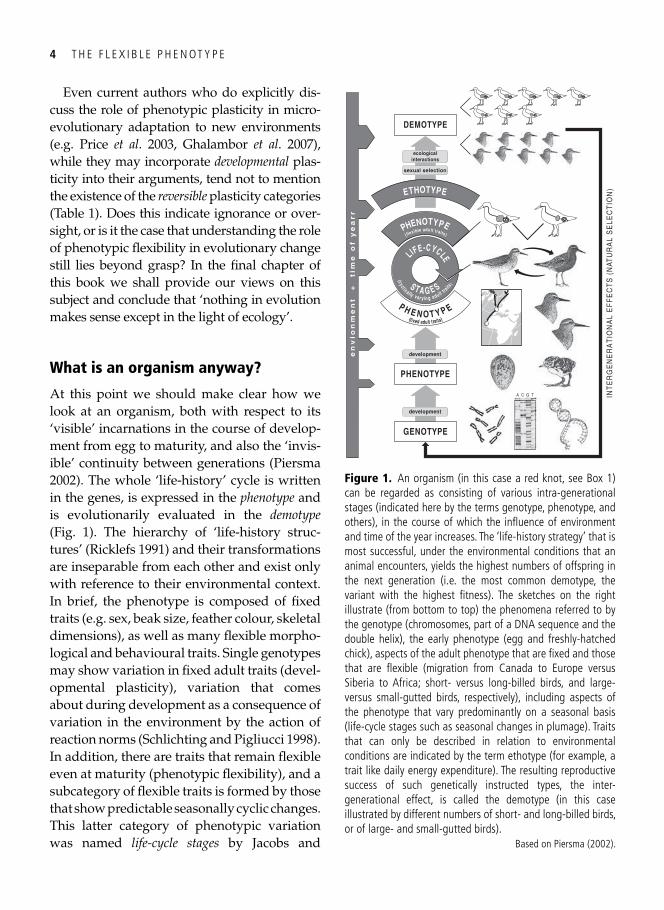
At this point we should make clear how we look at an organism, both with respect to its ‘visible’ incarnations in the course of develop-ment from egg to maturity, and also the ‘invis-ible’ continuity between generations ( Piersma 2002 ). The whole ‘life-history’ cycle is written in the genes, is expressed in the phenotype and is evolutionarily evaluated in the demotype ( Fig. 1 ). The hierarchy of ‘life-history struc-tures’ ( Ricklefs 1991 ) and their transformations are inseparable from each other and exist only with reference to their environmental context. In brief, the phenotype is composed of fi xed traits (e.g. sex, beak size, feather colour, skeletal dimensions), as well as many fl exible morpho-logical and behavioural traits. Single genotypes may show variation in fi xed adult traits (devel-opmental plasticity), variation that comes about during development as a consequence of variation in the environment by the action of reaction norms ( Schlichting and Pigliucci 1998 ). In addition, there are traits that remain fl exible even at maturity (phenotypic fl exibility), and a subcategory of fl exible traits is formed by those that show predictable seasonally cyclic changes. This latter category of phenotypic variation was named life-cycle stages by Jacobs and
DEMOTYPE
PHENOTYPE
GENOTYPE
INT
ER
GE
NE
RA
TIO
NA
L E
FF
EC
TS
(N
ATU
RA
L S
ELE
CT
ION
)
A C G T
S T A G E S
(cycl i c a lly v ar yi n g adult tra
its)
LIFE-CYCLE
ecologicalinteractions
PHENOTYPE
ETHOTYPE
P H E N O T Y P E
en
vio
nm
en
t +
ti
me
of
ye
ar
r
( f lexible adult traits)
(fixed adult traits)
development
development
sexual selection
Figure 1. An organism (in this case a red knot, see Box 1 ) can be regarded as consisting of various intra-generational stages (indicated here by the terms genotype, phenotype, and others), in the course of which the infl uence of environment and time of the year increases. The ‘life-history strategy’ that is most successful, under the environmental conditions that an animal encounters, yields the highest numbers of offspring in the next generation (i.e. the most common demotype, the variant with the highest fi tness). The sketches on the right illustrate (from bottom to top) the phenomena referred to by the genotype (chromosomes, part of a DNA sequence and the double helix), the early phenotype (egg and freshly-hatched chick), aspects of the adult phenotype that are fi xed and those that are fl exible (migration from Canada to Europe versus Siberia to Africa; short- versus long-billed birds, and large- versus small-gutted birds, respectively), including aspects of the phenotype that vary predominantly on a seasonal basis (life-cycle stages such as seasonal changes in plumage). Traits that can only be described in relation to environmental conditions are indicated by the term ethotype (for example, a trait like daily energy expenditure). The resulting reproductive success of such genetically instructed types, the inter-generational effect, is called the demotype (in this case illustrated by different numbers of short- and long-billed birds, or of large- and small-gutted birds).
Based on Piersma ( 2002 ).
I N T R O D U C T I O N 5
Wingfi eld ( 2000 ). Life-cycle staging specifi cally refers to the occurrence of seasonally-struc-tured sequences of ‘unique’ phenotypes with respect to state (e.g. reproductive or not; moult-ing or not) and appearance (e.g. nuptial plum-age or not). Similarly, a subcategory of developmental plasticity called polyphenism refers to season-specifi c occurrences of particu-lar phenotypes. The best-known examples are those butterfl ies in which the phenotypes of successive generations, during any given year, will depend on the season of hatching ( Shapiro 1976 , Brakefi eld and Reitsma 1991 , Nijhout 1999 ). Both life-cycle staging and polyphenism may be under the infl uence of endogenous programmes, especially such as that of the cir-cannual clock system ( Gwinner 1986 ).
Phenotype , as classically understood, is something that one can measure in an organ-ism independently of its environment, whereas the ethotype has no meaning except when set in an environmental context ( Ricklefs 1991 ). The ethotype (derived from the now outdated label for the study of animal behaviour: ethology) encompasses the behavioural dimension of phenotypes, and includes factors such as the energy requirements of an individual as a measure of its performance in its environment. In principle, the fi tness values of all these pheno- and ethotypic variants could be quan-tifi ed (Nager et al . 2000 ), and in Ricklefs’ (1991) terminology one would call this entity the demotype . The demotype, or fi tness of an organ-ism, is a function of both ecological interac-tions and sexual selection processes. Fitness determines which of the competing ‘units of sequenced structures and transformations’ (i.e. organisms) will survive in nature’s never-ending struggle ( Fig. 1 ).
Organization of the book
This book is built around a logically arranged constellation of fi rst principles in energetics,
ecology, physiology, and behaviour. Let us call them ‘rules of organismal design’ (including constraints on design). In Chapter 2 we start off from two relevant physical laws: (1) organ-isms cannot escape the fi rst law of thermody-namics (the law of conservation of energy) and (2) they are bound by the second law of ther-modynamics (the law of spontaneous ‘spread-ing-out’ of energy and matter). In order to reduce the amount of entropy in their bodies, organisms have actively to maintain a balance in terms of their gains and losses of water, nutrients and energy, and solutes (micronutri-ents). Depending on what needs to be kept in balance, and the size and nature of the body involved, accounting takes place over varying time-scales. In Chapter 3 we introduce the background of the cost–benefi t analyses of functional capacities that recur throughout the book. Organs are always part of chains of processing units within bodies. For this reason there is no point in spending the energy and nutrients that would be required to build organs with excess capacity relative to that of the other organs in the chain. This is the prin-ciple of symmorphosis that predicts close quantitative coupling of different performance measures within single organisms. As com-mon sense as this may seem, there are never-theless several issues that need to be discussed. These have to do with multiple functions, reserve capacities of specifi c organs under extreme and dangerous conditions, and the problematic climbing of ‘adaptive peaks’ ( Dawkins 1996 ). Some of the empirical argu-ments build around the technique of ‘allomet-ric scaling’, a concept that is briefl y introduced in that chapter.
In Chapter 4 we make our fi rst excursion from physiology to ecology, moving away from physical boundary factors and design principles to the real world. In this chapter we examine the extremes of adaptiveness as we discuss peak-performance rates, also
6 T H E F L E X I B L E P H E N OT Y P E
known as ‘metabolic ceilings’. The idea that the working capacity of organisms would have some sort of maximum level dictated by size and other design constraints (known as maximum sustained metabolic rates), has inspired a large body of ecophysiological research, including the search for allometric constants. We shall review the fi eld and illus-trate the (conditional) presence and workings of such ceilings by examining shorebirds working hard, both under cold conditions (during breeding in the High Arctic and under harsh climatic conditions in the non-breeding season) and also during trans-oceanic non-stop migration fl ights. We conclude that met-abolic ceilings are functional solutions to (1) the environmental conditions in which an organism lives and (2) the precise ways in which hard work precipitates death, a con-clusion that reverberates through much of what we will repeatedly encounter in the rest of the book.
Expanding on our introductory Table 1 , we illustrate in Chapter 5 how phenotypes, at several different levels and over several dif-ferent time- and developmental scales, suc-ceed in matching their environments. This chapter is not simply a lengthy review of odd organismal phenomena. By describing the great variation of ways in which organisms adjust to variable environmental demands, we emphasize the immense ‘creativity’ of the evolutionary process in response to ecologi-cal challenges. After a discussion on the pos-sible costs of a capacity to change, we raise questions about the extent to which pheno-typic adjustments are fully genetically instructed or self-organized on the basis of organism–environment feedback loops. The reversibility of some such changes is illus-trated by the way in which the organs of birds are continuously adjusted to changes in energy expenditure, food quality, and other environmental factors.
The cost–benefi t approach introduced in Chapter 3 is incomplete because it is limited to physical responses. After all, the behavioural dimension of phenotypes (the ethotypes) can respond even more rapidly to changing envi-ronments than bodies can. The behaviour of real animals at particular times and places is not only infl uenced by locally achievable ener-getic costs and benefi ts, but also by the fi tness currency that the animal has been naturally selected to optimize. In Chapter 6 we discuss how currencies and design constraints infl u-ence optimal behavioural strategies, especially with respect to time and place allocations. In the process we review the use of the word ‘optimal’ in evolutionary ecology. Having introduced this additional layer of complexity, in Chapter 7 we focus on a particular class of behaviour: the choice of diets and feeding patches. Foraging must guarantee a steady income at the lowest possible price. We intro-duce the elegant theories of optimal diet choice and the use of feeding patches. Until now such theories have assumed rather constant envi-ronments and bodies. Here, based on our own work on shorebirds, we extend the story to include the dynamics of organ size, energy expenditure, and prey quality. These observa-tions accord with new versions of foraging models that allow for fl exible adjustments of food-processing capacities.
From here onwards, building on the basics laid out in the previous chapters, the book becomes increasingly ‘integrative’. There is more to nature than nutrients and energy equivalents: only organisms that successfully escape predation and resist disease long enough will leave offspring. In Chapter 8 we bring these factors into context by introducing the ways in which animals cope with the threats of disease and predation. The immune system is not only amazingly complex, but it is shown to be highly fl exible as well. In addition to simple behavioural measures to avoid being
I N T R O D U C T I O N 7
killed by predators, birds also appear to have physiological adjustments in store. We intro-duce ways in which the fi elds of predation, disease, and foraging can be merged under the single equation of ‘common currencies’.
In Chapter 9 we come close to fi nding the Holy Grail of population biology by reaching an understanding of how environmental con-ditions and organismal strategies translate into individual fi tness (the demotype), and hence into changes in the size (and the distri-bution) of populations. We illustrate how the relationships between variable features of the environment (i.e. prey quality) and of the organism living in that environment (i.e. giz-zard size or processing capacity) combine to affect subsequent survival and population sizes of red knots. We also examine how organ-isms cope with various kinds of global change. Do the adjustments shown refl ect changes at the level of the genome, or do they refl ect phe-notypic plasticity?
In Chapter 10 we try to bring everything together under an evolutionary spotlight. In his masterful book-length essay on the basics of evolutionary organismal biology, Denis Noble ( 2006 ) stopped short of using the term ‘ecology’ with a discussion of organs and sys-tems, which he described as the ‘orchestra’. Here we provide a venue in which that ‘orches-tra’ can be located, a proper ‘theatre’ composed of the ever-stringent ecological context. Indeed, many of the riddles in understanding the dis-tribution of red knots, other shorebirds, and many other organisms, could not have been explained without insights into their energet-ics (and those of their prey), organ capacities, and phenotypic fl exibility. What we provide here is a discussion of the degree in which fl ex-ibility of phenotype is relevant to the evolu-tionary process. For example, do genes take the lead during evolutionary adaptive change, or is there merit in the suggestion that genetic changes actually follow phenotypic adjust-
ments ( West-Eberhard 2003 )? The writing of this fi nal chapter on evolutionary implications was diffi cult. It most clearly represents this book’s attempt to ‘grope publicly for solutions to recalcitrant conceptual issues of the day’ ( Gottlieb 1992 ).
Scope and readership
We trust that this book will encourage a fur-ther integration of ecology, physiology, and behaviour, and will in turn foster collaborative research agendas between various kinds of organismal scientists, beyond early proposals such as those of Bill Karasov ( 1986 ). Although migrant shorebirds are the principal characters in some parts of our story, the arguments developed here are of much broader relevance. We hope that this book will be read by a wide audience of professionals (obviously includ-ing advanced students) who work with organ-isms, whether they have medical, veterinarian or biological backgrounds. It should attract readership among active researchers and scholars from a wide range of taxonomic spe-cializations. Given our own background, our approaches will be most easily recognized and appreciated by those working at the interface of physiology, behavioural ecology, and evolu-tionary biology, but we also hope to heighten the interest of both hard-core evolutionary and molecular biologists and practising pheno-type-specialists, including those in the medi-cal and veterinary professions.
Although aimed at a diverse audience, this is still a ‘scientifi c’ book that offers in places complicated, but fundamentally instructive, drawings and diagrams, uses technical terms (that we have tried to explain as we encoun-ter them in the course of the story) and refer-ences to the primary literature. At the same time, we have tried hard to engage our readers by developing narratives of excitement and discovery.
8 T H E F L E X I B L E P H E N OT Y P E
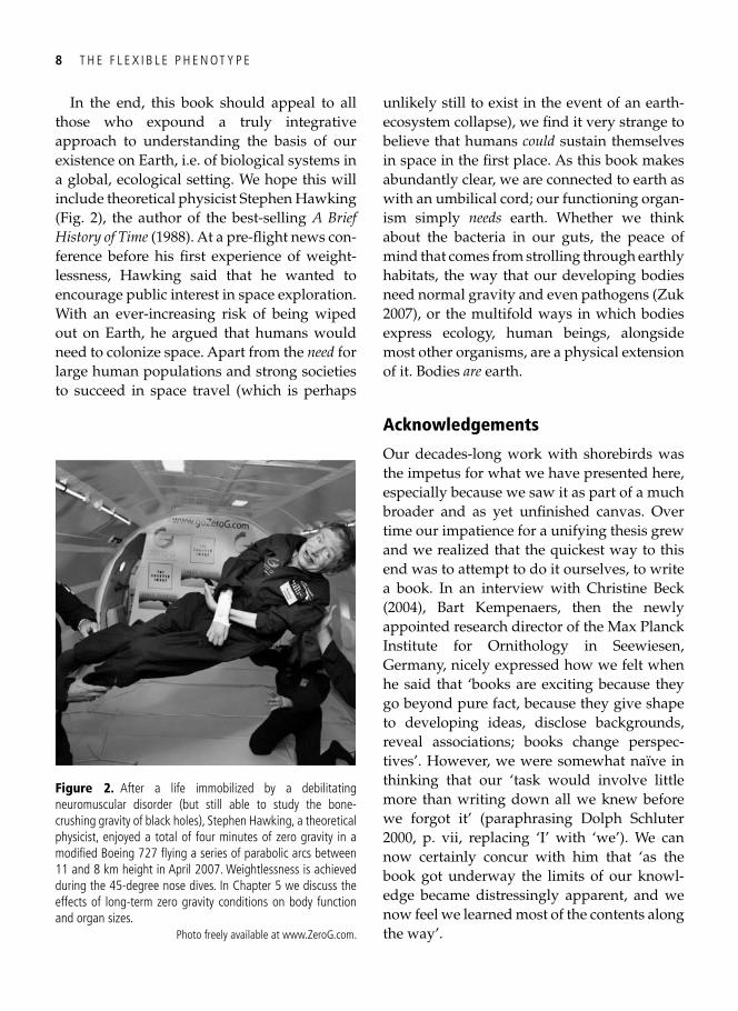
In the end, this book should appeal to all those who expound a truly integrative approach to understanding the basis of our existence on Earth, i.e. of biological systems in a global, ecological setting. We hope this will include theoretical physicist Stephen Hawking ( Fig. 2 ), the author of the best-selling A Brief History of Time (1988). At a pre-fl ight news con-ference before his fi rst experience of weight-lessness, Hawking said that he wanted to encourage public interest in space exploration. With an ever-increasing risk of being wiped out on Earth, he argued that humans would need to colonize space. Apart from the need for large human populations and strong societies to succeed in space travel (which is perhaps
unlikely still to exist in the event of an earth-ecosystem collapse), we fi nd it very strange to believe that humans could sustain themselves in space in the fi rst place. As this book makes abundantly clear, we are connected to earth as with an umbilical cord; our functioning organ-ism simply needs earth. Whether we think about the bacteria in our guts, the peace of mind that comes from strolling through earthly habitats, the way that our developing bodies need normal gravity and even pathogens ( Zuk 2007 ), or the multifold ways in which bodies express ecology, human beings, alongside most other organisms, are a physical extension of it. Bodies are earth.
Acknowledgements
Our decades-long work with shorebirds was the impetus for what we have presented here, especially because we saw it as part of a much broader and as yet unfi nished canvas. Over time our impatience for a unifying thesis grew and we realized that the quickest way to this end was to attempt to do it ourselves, to write a book. In an interview with Christine Beck ( 2004 ), Bart Kempenaers, then the newly appointed research director of the Max Planck Institute for Ornithology in Seewiesen, Germany, nicely expressed how we felt when he said that ‘books are exciting because they go beyond pure fact, because they give shape to developing ideas, disclose backgrounds, reveal associations; books change perspec-tives’. However, we were somewhat naïve in thinking that our ‘task would involve little more than writing down all we knew before we forgot it’ (paraphrasing Dolph Schluter 2000 , p. vii, replacing ‘I’ with ‘we’). We can now certainly concur with him that ‘as the book got underway the limits of our knowl-edge became distressingly apparent, and we now feel we learned most of the contents along the way’.
Figure 2. After a life immobilized by a debilitating neuromuscular disorder (but still able to study the bone-crushing gravity of black holes), Stephen Hawking, a theoretical physicist, enjoyed a total of four minutes of zero gravity in a modifi ed Boeing 727 fl ying a series of parabolic arcs between 11 and 8 km height in April 2007. Weightlessness is achieved during the 45-degree nose dives. In Chapter 5 we discuss the effects of long-term zero gravity conditions on body function and organ sizes.
Photo freely available at www.ZeroG.com .
I N T R O D U C T I O N 9
Box 1 Brief description of the book’s empirical backbone: a molluscivore migrating bird interacting with its buried prey
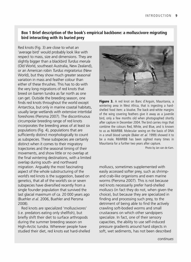
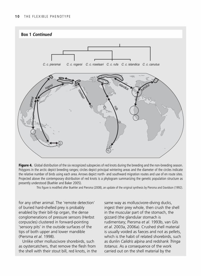
Red knots ( Fig. 3 ) are close to what an ‘average bird’ would probably look like with respect to mass, size and dimensions. They are slightly bigger than a blackbird Turdus merula (Old World, southeast Australia, New Zealand), or an American robin Turdus migratorius (New World), but they show much greater seasonal variation in mass and feather colour than either of these thrushes. This has to do with the very long migrations of red knots that breed on barren tundra as far north as one can get. Outside the breeding season, one fi nds red knots throughout the world except Antarctica, but only in marine coastal habitats, usually large wetlands with extensive intertidal foreshores ( Piersma 2007 ). The discontinuous circumpolar breeding range of red knots incorporates the breeding areas of at least six populations ( Fig. 4 ), populations that are suffi ciently distinct morphologically to count as subspecies. These subspecies are certainly distinct when it comes to their migratory trajectories and the seasonal timing of their movements, and show little or no overlap at the fi nal wintering destinations, with a limited overlap during south- and northward migration. Arguably the most fascinating aspect of the whole substructuring of the world’s red knots is the suggestion, based on genetics, that all of the world’s six or seven subspecies have diversifi ed recently from a single founder population that survived the last glacial maximum of ca. 20 000 years ago ( Buehler et al . 2006 , Buehler and Piersma 2008 ).
Red knots are specialized ‘molluscivores’ (i.e. predators eating only shellfi sh), but briefl y shift their diet to surface arthropods during the summer breeding season on High-Arctic tundra. Wherever people have studied their diet, red knots eat hard-shelled
molluscs, sometimes supplemented with easily accessed softer prey, such as shrimp- and crab-like organisms and even marine worms ( Piersma 2007 ). This is not because red knots necessarily prefer hard-shelled molluscs (in fact they do not, when given the choice), but because they are specialized in fi nding and processing such prey, to the detriment of being able to fi nd the actively crawling soft-bodied worms and small crustaceans on which other sandpipers specialize. In fact, one of their sensory capacities, the ability to use self-induced pressure gradients around hard objects in soft, wet sediments, has not been described
continues
Figure 3. A red knot on Banc d’Arguin, Mauritania, a wintering area in West Africa, that is ingesting a hard-shelled food item: a bivalve. The back-and-white margins of the wing covering feathers give it away as a juvenile bird, only a few months old when photographed shortly after capture in December 2004. The bird carries rings that combine the colours Red, White, and Blue, and is known to us as R6WRBB. Molecular sexing on the basis of DNA in a small blood sample ( Baker et al . 1999 ) showed it to be a male. R6WRBB has been sighted many times in Mauritania for a further two years after capture.
Photo by Jan van de Kam.
1 0 T H E F L E X I B L E P H E N OT Y P E
Box 1 Continued
for any other animal. The ‘remote detection’ of buried hard-shelled prey is probably enabled by their bill-tip organ, the dense conglomerations of pressure sensors (Herbst corpuscles) clustered in forward-pointing ‘sensory pits’ in the outside surfaces of the tips of both upper and lower mandible ( Piersma et al . 1998 ).
Unlike other molluscivore shorebirds, such as oystercatchers, that remove the fl esh from the shell with their stout bill, red knots, in the
same way as molluscivore-diving ducks, ingest their prey whole, then crush the shell in the muscular part of the stomach, the gizzard (the glandular stomach is rudimentary; Piersma et al . 1993b , van Gils et al . 2003a , 2006a ). Crushed shell material is usually voided as faeces and not as pellets, which is the habit of related shorebirds, such as dunlin Calidris alpina and redshank Tringa totanus . As a consequence of the work carried out on the shell material by the
islandica canutus
rufa
roselaari
C. c. piersmai C. c. rogersi C. c. roselaari C. c. rufa C. c. islandica C. c. canutus
pier
smai
rogersi
Figure 4. Global distribution of the six recognized subspecies of red knots during the breeding and the non-breeding season. Polygons in the arctic depict breeding ranges; circles depict principal wintering areas and the diameter of the circles indicate the relative number of birds using each area. Arrows depict north- and southward migration routes and use of en route sites. Projected above the contemporary distribution of red knots is a phylogram summarizing the genetic population structure as presently understood ( Buehler and Baker 2005 ).
This fi gure is modifi ed after Buehler and Piersma ( 2008 ), an update of the original synthesis by Piersma and Davidson ( 1992 ).
I N T R O D U C T I O N 1 1
gizzard and intestine, and in order, perhaps, to prevent the wear and tear infl icted by shell fragments on the sensitive intestinal wall, both gizzard and intestine are relatively heavy in shorebirds that eat hard-shelled-prey. In an allometric comparison among 41 shorebird species, the red knot came out as the one with the largest gizzard for its body mass ( Battley and Piersma 2005 ).
Although red knots are able to crush and process reasonably heavily built molluscs, they rather prefer, as we shall see, thin-shelled prey. It also helps their food-fi nding if the shellfi sh live close to the sediment surface, or on top of it, and if they are not attached to any hard surface, such as a piece of rock, a mussel- or oyster-bank, or mangrove roots. The state of traits that red knots, indeed most predators, prefer, obviously precisely mirrors the state of traits that molluscs use to avoid being eaten. As prey they can develop heavy or extravagant armature, they can attach themselves to a hard substrate, they can sit deep in the sediment beyond the length of a probing bill, or, upon discovery by a predator, they can try
to move away fast ( Vermeij 1987 , 1993 ). Red knots do eat gastropod molluscs (snails, usually protected by a heavy or profusely ornamented shell), but most of their diet consists of bivalves, and these bivalves employ all the different strategies just listed ( Stanley 1970 , Piersma et al . 1993a ). All bivalves are protected by hard valves, but shallowly buried species, such as edible cockles Cerastoderma edule , are much more heavily armoured than deep-buried bivalves, such as the Baltic tellin Macoma balthica and the other relatively thin-shelled tellinids. There are no examples of intertidal bivalves exhibiting ridges or spines, although the heavily ridged venerid Placamen gravescens from north Australia comes close. Mussels of the family Mytilidae come in heavily armoured forms, or may secure themselves to rocks or conglomerates of conspecifi cs with so-called ‘byssal threads’. A few bivalves of intertidal fl ats, such as the very thin-shelled Siliqua pulchella that lives in the soft muds of Australasia, are fast burrowers and swimmers and still have a chance to get away when detected by a probing shorebird.
We dedicate this book to our mentor and teacher, Rudi Drent. We are sad that he did not live to be part of the entire writing process. Sharing thoughts with him and entertaining ideas about our science were among the most formative and fantastic experiences in our pro-fessional lives. Rudi infl uenced this book in many more ways than by introducing us early on to the concepts of optimal working capaci-ties, also known as ‘metabolic ceilings’ ( Chapter 4 ). As an ethologist, Rudi certainly never lost sight of ecological context. As pro-fessor in animal ecology at the University of Groningen he created a great ambiance for budding ecologists. He was forever stimulat-
ing ambitious, if not daring, programmes of fi eld research, whilst still attending to the physiological nuts and bolts that are better studied in laboratory settings. We appreciate, and cherish, his many fi ghts for the institu-tional embedding of our endeavours, the very force that gave our generation a chance in science.
Yes, fi nishing this book has been a long jour-ney. We would like to acknowledge the trust, patience, encouragement, help and tolerance of the people that have to live with us in their daily lives—both our colleagues at work and our family members. TP is grateful to Petra de Goeij for creating great ambiances for book
1 2 T H E F L E X I B L E P H E N OT Y P E
writing. JAvG admires the patience of his wife, Ilse Veltman, and their children, Lieke and Jort, which they expressed so many times dur-ing the writing process. We are also grateful to the artists who helped make this book what it is. Dick Visser prepared all the new artwork and, as usual, it was both exciting and a great pleasure to work with him. We thank Barbara Jonkers for her smart cover design, Jan van de Kam for providing stunning pho-tos, and Ysbrand Galama for the dreamcow of Chapter 2 . TP thanks David Winkler and the Cornell Laboratory of Ornithology for gener-ous hospitality during a minisabbatical in Ithaca—laying the ground for Chapter 10 . We are very grateful to our contacts at Oxford University Press, especially editors Ian Sherman and Helen Eaton, for their guidance, encouragement, patience, and general good faith in the enterprise. Marie-Anne Martin provided the index, was a great text editor and a constant source of encouragement during the fi nal phases.
Two long-time friends from Canada, Hugh Boyd and Jerry Hogan, read all chapters. Apart from giving us confi dence, they kept us honest in the use of English, the terminology of proxi-mate and ultimate causes, and helped us with context. We are very grateful for their endur-ing support. Bob Gill provided a refreshing review of the introductory chapter. Irene Tieleman shined her bright light on Chapter 2 .
Hans Hoppeler, Ewald Weibel, Maurine Dietz and Rob Bijlsma provided helpful comments on Chapter 3 . We enjoyed interacting with Tim Noakes with respect to Chapter 4 , and appre-ciated the constructive comments by John Speakman, Bob Gill, Bob Ricklefs, Kristin Schubert (who additionally provided material for an entire paragraph), Bernd Heinrich, Irene Tieleman, Joost Tinbergen, John McNamara, Maurine Dietz, Klaas Westerterp, and Dan Mulcahy. For comments on Chapter 5 we thank Matthias Starck, Paul Brakefi eld, Chris Neufeld, Rick Relyea, and Massimo Pigliucci. Ola Olsson commented on Chapter 6 , John McNamara on Chapter 7 , Piet van den Hout on Chapter 8 and Christiaan Both helped with Chapter 9 . Ritsert Jansen tinkered with the fi rst and the last chapters, but what we may really need is a new book! Eva Jablonka, Massimo Pigliucci, and Bob Gill helped with the fi nal chapter, as did the 2009/2010 cohort of the University of Groningen TopProgramme in Evolution and Ecology: Adriana Alzate-Vallejo, Lotte van Boheemen, Rienk Fokkema, Jordi van Gestel, Oleksandr Ivanov, Hernan Morales, Froukje Postma, Andrés Quinones, and Michiel Veldhuis. Finally, we thank those who either supplied or helped us fi nd original photos or artwork: John Speakman, Colleen Handel and Bob Gill, Chris Neufeld, Mike Stroud, Duncan Irschick and Maria Ramos, Ola Olsson, and Alexander Badyaev.

Part I
Basics of organismal design

This page intentionally left blank
15
CHAPTER 2
Maintaining the balance of heat, water, nutrients, and energy
Dutch dreamcows do not exist
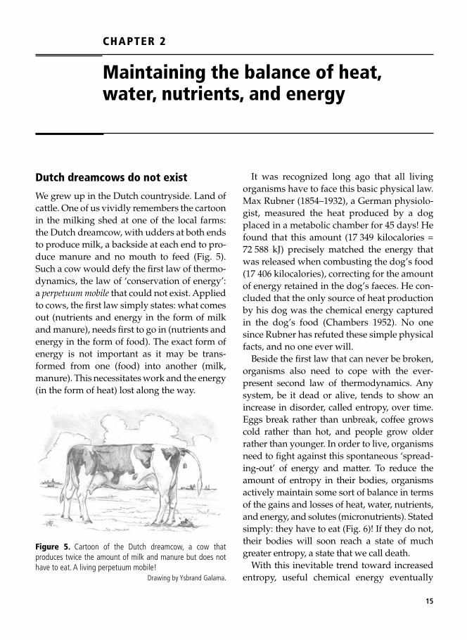
We grew up in the Dutch countryside. Land of cattle. One of us vividly remembers the cartoon in the milking shed at one of the local farms: the Dutch dreamcow, with udders at both ends to produce milk, a backside at each end to pro-duce manure and no mouth to feed ( Fig. 5 ). Such a cow would defy the fi rst law of thermo-dynamics, the law of ‘conservation of energy’: a perpetuum mobile that could not exist. Applied to cows, the fi rst law simply states: what comes out (nutrients and energy in the form of milk and manure), needs fi rst to go in (nutrients and energy in the form of food). The exact form of energy is not important as it may be trans-formed from one (food) into another (milk, manure). This necessitates work and the energy (in the form of heat) lost along the way.
It was recognized long ago that all living organisms have to face this basic physical law. Max Rubner (1854–1932), a German physiolo-gist, measured the heat produced by a dog placed in a metabolic chamber for 45 days! He found that this amount (17 349 kilocalories = 72 588 kJ) precisely matched the energy that was released when combusting the dog’s food (17 406 kilocalories), correcting for the amount of energy retained in the dog’s faeces. He con-cluded that the only source of heat production by his dog was the chemical energy captured in the dog’s food ( Chambers 1952 ). No one since Rubner has refuted these simple physical facts, and no one ever will.
Beside the fi rst law that can never be broken, organisms also need to cope with the ever-present second law of thermodynamics. Any system, be it dead or alive, tends to show an increase in disorder, called entropy, over time. Eggs break rather than unbreak, coffee grows cold rather than hot, and people grow older rather than younger. In order to live, organisms need to fi ght against this spontaneous ‘spread-ing-out’ of energy and matter. To reduce the amount of entropy in their bodies, organisms actively maintain some sort of balance in terms of the gains and losses of heat, water, nutrients, and energy, and solutes (micronutrients). Stated simply: they have to eat ( Fig. 6 )! If they do not, their bodies will soon reach a state of much greater entropy, a state that we call death.
With this inevitable trend toward increased entropy, useful chemical energy eventually
Figure 5. Cartoon of the Dutch dreamcow, a cow that produces twice the amount of milk and manure but does not have to eat. A living perpetuum mobile!
Drawing by Ysbrand Galama.
1 6 B A S I C S O F O R G A N I S M A L D E S I G N
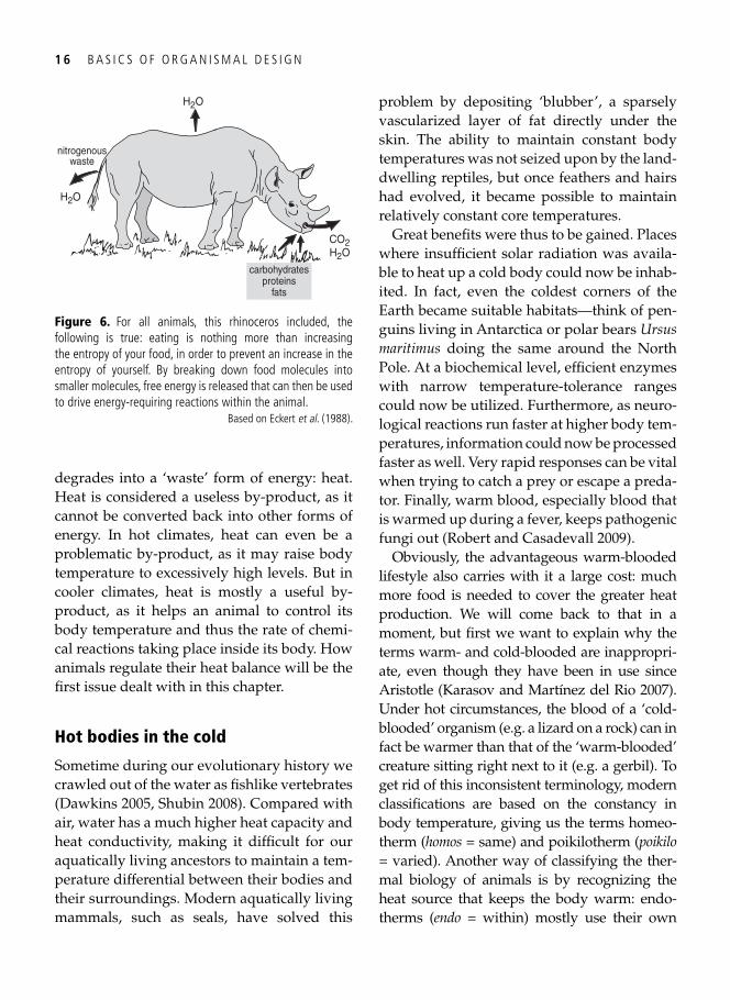
degrades into a ‘waste’ form of energy: heat. Heat is considered a useless by-product, as it cannot be converted back into other forms of energy. In hot climates, heat can even be a problematic by-product, as it may raise body temperature to excessively high levels. But in cooler climates, heat is mostly a useful by-product, as it helps an animal to control its body temperature and thus the rate of chemi-cal reactions taking place inside its body. How animals regulate their heat balance will be the fi rst issue dealt with in this chapter.
Hot bodies in the cold
Sometime during our evolutionary history we crawled out of the water as fi shlike vertebrates ( Dawkins 2005 , Shubin 2008 ). Compared with air, water has a much higher heat capacity and heat conductivity, making it diffi cult for our aquatically living ancestors to maintain a tem-perature differential between their bodies and their surroundings. Modern aquatically living mammals, such as seals, have solved this
problem by depositing ‘blubber’, a sparsely vascularized layer of fat directly under the skin. The ability to maintain constant body temperatures was not seized upon by the land-dwelling reptiles, but once feathers and hairs had evolved, it became possible to maintain relatively constant core temperatures.
Great benefi ts were thus to be gained. Places where insuffi cient solar radiation was availa-ble to heat up a cold body could now be inhab-ited. In fact, even the coldest corners of the Earth became suitable habitats—think of pen-guins living in Antarctica or polar bears Ursus maritimus doing the same around the North Pole. At a biochemical level, effi cient enzymes with narrow temperature-tolerance ranges could now be utilized. Furthermore, as neuro-logical reactions run faster at higher body tem-peratures, information could now be processed faster as well. Very rapid responses can be vital when trying to catch a prey or escape a preda-tor. Finally, warm blood, especially blood that is warmed up during a fever, keeps pathogenic fungi out ( Robert and Casadevall 2009 ).
Obviously, the advantageous warm-blooded lifestyle also carries with it a large cost: much more food is needed to cover the greater heat production. We will come back to that in a moment, but fi rst we want to explain why the terms warm- and cold-blooded are inappropri-ate, even though they have been in use since Aristotle ( Karasov and Martínez del Rio 2007 ). Under hot circumstances, the blood of a ‘cold-blooded’ organism (e.g. a lizard on a rock) can in fact be warmer than that of the ‘warm-blooded’ creature sitting right next to it (e.g. a gerbil). To get rid of this inconsistent terminology, modern classifi cations are based on the constancy in body temperature, giving us the terms homeo-therm ( homos = same) and poikilotherm ( poikilo = varied). Another way of classifying the ther-mal biology of animals is by recognizing the heat source that keeps the body warm: endo-therms ( endo = within) mostly use their own
nitrogenouswaste
H2O
carbohydratesproteins
fats
H2O
H2OCO2
Figure 6. For all animals, this rhinoceros included, the following is true: eating is nothing more than increasing the entropy of your food, in order to prevent an increase in the entropy of yourself. By breaking down food molecules into smaller molecules, free energy is released that can then be used to drive energy-requiring reactions within the animal.
Based on Eckert et al . ( 1988 ).
M A I N TA I N I N G T H E B A L A N C E O F H E AT, W AT E R , N U T R I E N T S , A N D E N E R G Y 1 7
metabolism for this, while ectotherms ( ecto = outside) use external heat. Most endotherms are homeotherms (e.g. the gerbil) and most ecto-therms are poikilotherms (e.g. the lizard), but there are exceptions (e.g. parasites living inside a bird or a mammal are typical homeothermic ectotherms). In this chapter we shall mostly deal with homeothermic endotherms.
Let us now return to the costs of being a homeo-therm . Much of what we now know about tem-perature regulation in homeotherms is due to the pioneering work of Per Scholander ( Scholander et al . 1950a ). This man, who moved to the United States after growing up and being trained as a botanist in Norway, had a lifelong fascination with the physiological responses to extreme conditions of both plants and animals. His adventurous mind, together with the need to take measurements along an ‘extreme condi-tion axis’, brought him around the world at a time when not so many could do so ( Scholander 1990 ). For his work on thermoregulation, his original plan was to build a mobile laboratory in a huge military troop glider (an engineless aircraft), which could then be brought to remote places (e.g. the inaccessible and practically unknown Prince Patrick Island in the Canadian Arctic Archipelago was on his mind). His boss thought this idea was insane, but at the same time suggested building a more permanent lab-oratory at an alternative location, Point Barrow on Alaska’s North Slope. And this he did.
In Alaska, Scholander measured the costs of homeothermy by placing individual animals in small metabolic chambers. During trials lasting eight to twelve hours, an individual’s O 2 -consumption and CO 2 -production were quantifi ed across a wide range of temperatures (from the lowest Alaskan winter temperatures of –40 °C up to over +30 °C generated by an electric heater). The animals were of various
kinds: snow buntings Plectrophenax nivalis , jays Perisoreus canadensis , arctic gulls Larus hyper-boreus , weasels Mustela rixosa , lemmings Dicrostonyx groenlandicus rubricatus , ground squirrels Citellus parryii , arctic foxes Alopex lagopus , Eskimo dogs Canis familiaris , and polar bear cubs Thalarctos maritimus . With this diver-sity of animals locked up in out- and indoor cages, there were times when the Point Barrow laboratory must have looked like a small zoo.
Scholander and his colleagues predicted that simple Newtonian cooling laws governed the heat loss of an animal, i.e. that the heat loss (and thus heat production under a constant core temperature) would be proportional to the temperature gradient between the animal and its surroundings ( Newton 1701 , Mitchell 1901 ). They were right. Cooling down the met-abolic chamber, such that the gradient between body temperature and environmental temper-ature doubled, did indeed double an animal’s metabolic rate. However, this simple and ele-gant result was found only when the environ-mental temperature was below a certain value. Above this threshold, the so-called lower criti-cal temperature, metabolic rate remained remarkably stable; in this region, heat as a ‘waste product’ of resting metabolism could be used to maintain constant body tempera-ture. As shown later (e.g. King 1964 ), an upper critical temperature also exists. Above this threshold additional costs come into play in order to prevent overheating.
The lower critical temperature differed enor-mously between their study animals: lem-mings and weasels reached this threshold between 10 and 20 °C, while arctic foxes could go down to –30 °C or more before they elevated their metabolic rate. 1 In general, Scholander et al . found that the lower critical temperature was lower in larger animals than in smaller
1 Note that a recent study on arctic foxes found much higher values ( Fuglesteg et al . 2006 ). It was argued that Scholander’s foxes were not at rest during the measurements.
1 8 B A S I C S O F O R G A N I S M A L D E S I G N
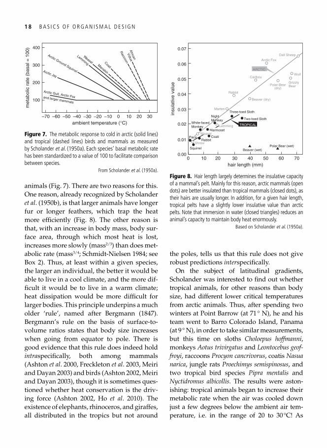
animals ( Fig. 7 ). There are two reasons for this. One reason, already recognized by Scholander et al . ( 1950b ), is that larger animals have longer fur or longer feathers, which trap the heat more effi ciently ( Fig. 8 ). The other reason is that, with an increase in body mass, body sur-face area, through which most heat is lost, increases more slowly (mass 2/3 ) than does met-abolic rate (mass 3/4 ; Schmidt-Nielsen 1984 ; see Box 2). Thus, at least within a given species, the larger an individual, the better it would be able to live in a cool climate, and the more dif-fi cult it would be to live in a warm climate; heat dissipation would be more diffi cult for larger bodies. This principle underpins a much older ‘rule’, named after Bergmann ( 1847 ). Bergmann’s rule on the basis of surface-to- volume ratios states that body size increases when going from equator to pole. There is good evidence that this rule does indeed hold intra specifi cally, both among mammals ( Ashton et al . 2000 , Freckleton et al . 2003 , Meiri and Dayan 2003 ) and birds ( Ashton 2002 , Meiri and Dayan 2003 ), though it is sometimes ques-tioned whether heat conservation is the driv-ing force ( Ashton 2002 , Ho et al . 2010 ). The existence of elephants, rhinoceros, and giraffes, all distributed in the tropics but not around
the poles, tells us that this rule does not give robust predictions inter specifi cally.
On the subject of latitudinal gradients, Scholander was interested to fi nd out whether tropical animals, for other reasons than body size, had different lower critical temperatures from arctic animals. Thus, after spending two winters at Point Barrow (at 71 ° N), he and his team went to Barro Colorado Island, Panama (at 9 ° N), in order to take similar measurements, but this time on sloths Choloepus hoffmanni , monkeys Aotus trivirgatus and Leontocebus geof-froyi , raccoons Procyon cancrivorus , coatis Nasua narica , jungle rats Proechimys semispinosus , and two tropical bird species Pipra mentalis and Nyctidromus albicollis . The results were aston-ishing: tropical animals began to increase their metabolic rate when the air was cooled down just a few degrees below the ambient air tem-perature, i.e. in the range of 20 to 30 °C! As
–60
100
200
300
400
met
abol
ic r
ate
(bas
al =
100
)
–40 –20 0 20ambient temperature (°C)
Coati
Weasel
Lemming
–70 –50 –30 –10 10 30
Arctic Ground SquirrelArctic Jay
Arctic Gull, Arctic Fox and larger mammals
Manakin
Raccoon
African
Vidua
Figure 7. The metabolic response to cold in arctic (solid lines) and tropical (dashed lines) birds and mammals as measured by Scholander et al . ( 1950a ). Each species’ basal metabolic rate has been standardized to a value of 100 to facilitate comparison between species.
From Scholander et al . ( 1950a ).
00.00
0.01
0.02
0.03
0.04
0.05
0.06
0.07
insu
lativ
e va
lue
10 20 30 40 50 60 70hair length (mm)
Squirrel
Shrew
PacaRabbit
Coati
White-facedMonkey
NightMonkey
Three-toed Sloth
Two-toed Sloth
Marten
Beaver (wet)Polar Bear (wet)
Beaver (dry)
Rabbit
Caribou
Arctic Fox
Wolf
GrizzlyBearPolar Bear
(dry)
Dall Sheep
MarmosetWeasel
Lemming TROPICAL
ARCTIC
Figure 8. Hair length largely determines the insulative capacity of a mammal’s pelt. Mainly for this reason, arctic mammals (open dots) are better insulated than tropical mammals (closed dots), as their hairs are usually longer. In addition, for a given hair length, tropical pelts have a slightly lower insulative value than arctic pelts. Note that immersion in water (closed triangles) reduces an animal’s capacity to maintain body heat enormously.
Based on Scholander et al . ( 1950a ).
M A I N TA I N I N G T H E B A L A N C E O F H E AT, W AT E R , N U T R I E N T S , A N D E N E R G Y 1 9
raccoons and jungle rats are not smaller than weasels and lemmings, this difference could not be explained by body size. Scholander et al. skinned several of their study animals and found that a piece of tropical pelt had a lower insulative capacity than an equally sized piece of arctic pelt; this result could be partly explained by the fact that tropical fur is generally sparser and shorter ( Fig. 8 ). As human beings, we are a good example of how the low insulative value of our ‘pelt’ over-rules the effect of a relatively large body size. Our lower critical temperature lies between 27 and 29 °C ( Du Bois 1936 , Winslow and Herrington 1949 ). Needless to say, this is with our clothes off. Scholander et al . ( 1950a ) concluded: ‘Man is indeed a tropical animal, carrying his tropical environment with him.’ Note that better insulation in northern arctic/temperate species is not a general rule. For example, Tieleman et al . ( 2002 ) found ‘desert larks’ (exposed to cold nights) were better insu-lated than equally sized larks living in the tem-perate zone.
Apart from body size and the insulative value of fur, there may be another reason why arctic homeotherms can better withstand the cold than their tropical equivalents: they have a bigger ‘engine’, a higher basal metabolic rate (BMR). This would have the effect of low-ering an animal’s lower critical temperature. Is there evidence for higher BMRs in arctic mam-mals and birds? Scholander et al. ( 1950c ) con-cluded that there were no general BMR differences between ‘their’ tropical and arctic animals, notwithstanding a few exceptions (the ‘lazy-acting’ sloths had relatively low metabolic rates, unsurprisingly). This was consistent with a study on fi ve tropical bird species by Vleck and Vleck ( 1979 ). However, later studies, both on birds ( Weathers 1979 , Hails 1983 , Kersten et al. 1998 , Wiersma et al. 2007 ) and mammals ( Lovegrove 2000 ), consistently found BMRs that were 20–40% lower in the tropics than in the temperate and
arctic zones. This difference is now widely accepted ( Wiersma et al. 2007 ).
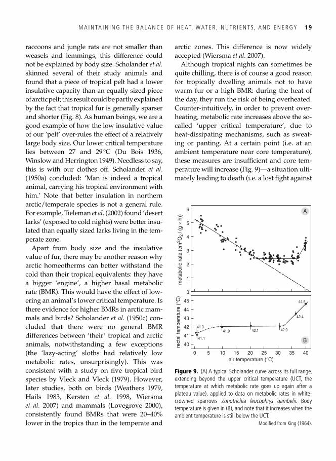
Although tropical nights can sometimes be quite chilling, there is of course a good reason for tropically dwelling animals not to have warm fur or a high BMR: during the heat of the day, they run the risk of being overheated. Counter-intuitively, in order to prevent over-heating, metabolic rate increases above the so-called ‘upper critical temperature’, due to heat-dissipating mechanisms, such as sweat-ing or panting. At a certain point (i.e. at an ambient temperature near core temperature), these measures are insuffi cient and core tem-perature will increase ( Fig. 9 )—a situation ulti-mately leading to death (i.e. a lost fi ght against
0
1
2
3
4
5
A
B
6
met
abol
ic r
ate
(cm
3 O2
/(g
× h)
)
40
41
42
43
44
45
rect
al te
mpe
ratu
re (°
C)
41.1
41.341.9 42.1 42.0
42.4
44.5
0 1510 20 30 405 25 35air temperature (°C)
Figure 9. (A) A typical Scholander curve across its full range, extending beyond the upper critical temperature (UCT, the temperature at which metabolic rate goes up again after a plateau value), applied to data on metabolic rates in white-crowned sparrows Zonotrichia leucophrys gambelii . Body temperature is given in (B), and note that it increases when the ambient temperature is still below the UCT.
Modifi ed from King ( 1964 ).
2 0 B A S I C S O F O R G A N I S M A L D E S I G N
Nature’s second law, occurring at core temper-atures of 46–47 °C; The Guinness Book of Records reports a lethal core temperature of 46.5 °C in humans; McWhirter 1980 ). Scholander et al. did not ‘heat up’ their study animals enough to reach upper critical tem-peratures, but with experimental temperatures approaching +35 °C they must have brought them very close. In fact, the existence of the upper critical temperature was established later in studies on birds, such as the one by King ( 1964 ).
With lower critical temperatures being lower in arctic animals as an adaptation to the cold, we may expect upper critical temperatures to be higher in tropical animals as an adaptation to the heat. This has never been thoroughly sur-veyed along the arctic–tropics gradient, but there is some sparse evidence from a compari-son between birds living in hot deserts and related species from the temperate zone. Tieleman et al. ( 2002 ) contrasted two temperate-living larks (skylarks Alauda arvensis and wood-larks Lullula arborea ) with two desert-dwelling larks (hoopoe larks Alaemon alaudipes and Dunn’s lark Eremalauda dunni ), and did indeed fi nd that the desert birds had higher upper criti-cal temperatures (38–44 °C vs. 35–40 °C). However, this effect was not found in a general analysis containing more desert and non-desert species ( Tieleman and Williams 1999 ). Three mechanisms may underlie this possible adapta-tion of tropical/desert homeotherms: not only do they produce less heat (because of a lower BMR) and are better able to get rid of this heat (because of thinner fur or sparser plumage—except for the better insulated desert larks just discussed), but they may also be able to tolerate higher core temperatures. For example, variable seedeaters Sporophila aurita , small passerines that live in humid lowland tropics and thus have diffi culty in cooling off via evaporation, are able to tolerate core temperatures approach-ing 47 °C ( Weathers 1997 )!
So far we have seen very signifi cant differ-ences between arctic and tropical animals in terms of their thermoregulation. Red knots, key players in this book, breed in the High Arctic and some winter in the tropics. They thus need to tolerate both cold and heat stress within their same small bodies. No wonder that fl exibility became a way of life for these impressive globetrotters. And the differences between arctic and tropical environments can get even greater when we consider more than just air temperature alone.
Thermometers do not measure feelings
‘It feels cold’ is an expression we often hear. It captures the notion that air temperature alone does not always describe our sense of heat loss. Strong winds on a sunny, seemingly warm day, make us reluctant to take off our sweaters and we would certainly leave them on if a cloud moved in front of the sun, taking away the pleas-ant warmth of the sunlight. The way to encap-sulate all the factors that affect an animal’s heat balance is to talk in terms of ‘environmental temperature’ or ‘operative temperature’. In Dutch, we literally use the term gevoelstempera-tuur , ‘feelings temperature’, when we speak about environmental temperature.
Thus, in addition to air temperature, envi-ronmental temperature is affected by convec-tion through wind, different forms of radiation and conductance ( Fig. 10 ). Furthermore, ani-mal properties such as size, shape, and colour infl uence the thermoregulatory signifi cance of given levels of wind and radiation ( Porter and Gates 1969 ). Therefore, under specifi ed weather conditions, environmental temperature is dif-ferent for different animals! The early labora-tory measurements on thermoregulation by Scholander and others had ignored these com-plexities, and it was only after George Bakken had published an infl uential theoretical paper
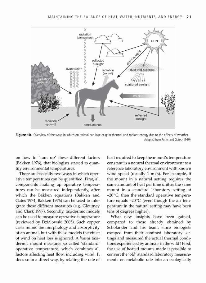
M A I N TA I N I N G T H E B A L A N C E O F H E AT, W AT E R , N U T R I E N T S , A N D E N E R G Y 2 1
on how to ‘sum up’ these different factors ( Bakken 1976 ), that biologists started to quan-tify environmental temperatures.
There are basically two ways in which oper-ative temperatures can be quantifi ed. First, all components making up operative tempera-tures can be measured independently, after which the Bakken equations ( Bakken and Gates 1974 , Bakken 1976 ) can be used to inte-grate these different measures (e.g. Gloutney and Clark 1997 ). Secondly, taxidermic models can be used to measure operative temperature (reviewed by Dzialowski 2005 ). Such copper casts mimic the morphology and absorptivity of an animal, but with these models the effect of wind on heat loss is ignored. A heated taxi-dermic mount measures so called ‘standard’ operative temperature, which combines all factors affecting heat fl ow, including wind. It does so in a direct way, by relating the rate of
heat required to keep the mount’s temperature constant in a natural thermal environment to a reference laboratory environment with known wind speed (usually 1 m/s). For example, if the mount in a natural setting requires the same amount of heat per time unit as the same mount in a standard laboratory setting at –20 °C, then the standard operative tempera-ture equals –20 °C (even though the air tem-perature in the natural setting may have been tens of degrees higher).
What new insights have been gained, compared to those already obtained by Scholander and his team, since biologists escaped from their confi ned laboratory set-tings and measured the actual thermal condi-tions experienced by animals in the wild? First, the use of heated mounts made it possible to convert the ‘old’ standard laboratory measure-ments on metabolic rate into an ecologically
dust and particles
scattered sunlight
radiation(vegetation)
radiation(atmosphere)
radiation(ground)
evaporation
reflectedsunlight
W I N D
direc
t sun
light
reflectedsunlight
radiation(animal)
conductance
SUN
Figure 10. Overview of the ways in which an animal can lose or gain thermal and radiant energy due to the effects of weather. Adapted from Porter and Gates ( 1969 ).
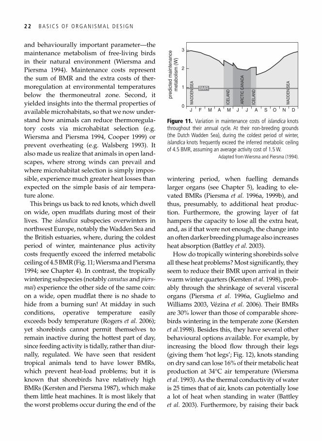
2 2 B A S I C S O F O R G A N I S M A L D E S I G N
and behaviourally important parameter—the maintenance metabolism of free-living birds in their natural environment ( Wiersma and Piersma 1994 ). Maintenance costs represent the sum of BMR and the extra costs of ther-moregulation at environmental temperatures below the thermoneutral zone. Second, it yielded insights into the thermal properties of available microhabitats, so that we now under-stand how animals can reduce thermoregula-tory costs via microhabitat selection (e.g. Wiersma and Piersma 1994 , Cooper 1999 ) or prevent overheating (e.g. Walsberg 1993 ). It also made us realize that animals in open land-scapes, where strong winds can prevail and where microhabitat selection is simply impos-sible, experience much greater heat losses than expected on the simple basis of air tempera-ture alone.
This brings us back to red knots, which dwell on wide, open mudfl ats during most of their lives. The islandica subspecies overwinters in northwest Europe, notably the Wadden Sea and the British estuaries, where, during the coldest period of winter, maintenance plus activity costs frequently exceed the inferred metabolic ceiling of 4.5 BMR ( Fig. 11 ; Wiersma and Piersma 1994 ; see Chapter 4 ). In contrast, the tropically wintering subspecies (notably canutus and piers-mai ) experience the other side of the same coin: on a wide, open mudfl at there is no shade to hide from a burning sun! At midday in such conditions, operative temperature easily exceeds body temperature ( Rogers et al. 2006 ); yet shorebirds cannot permit themselves to remain inactive during the hottest part of day, since feeding activity is tidally, rather than diur-nally, regulated. We have seen that resident tropical animals tend to have lower BMRs, which prevent heat-load problems; but it is known that shorebirds have relatively high BMRs ( Kersten and Piersma 1987 ), which make them little heat machines. It is most likely that the worst problems occur during the end of the
wintering period, when fuelling demands larger organs (see Chapter 5 ), leading to ele-vated BMRs ( Piersma et al. 1996a , 1999b ), and thus, presumably, to additional heat produc-tion. Furthermore, the growing layer of fat hampers the capacity to lose all the extra heat, and, as if that were not enough, the change into an often darker breeding plumage also increases heat absorption ( Battley et al. 2003 ).
How do tropically wintering shorebirds solve all these heat problems? Most signifi cantly, they seem to reduce their BMR upon arrival in their warm winter quarters ( Kersten et al. 1998 ), prob-ably through the shrinkage of several visceral organs ( Piersma et al . 1996a , Guglielmo and Williams 2003 , Vézina et al. 2006 ). Their BMRs are 30% lower than those of comparable shore-birds wintering in the temperate zone ( Kersten et al. 1998 ). Besides this, they have several other behavioural options available. For example, by increasing the blood fl ow through their legs (giving them ‘hot legs’; Fig. 12 ), knots standing on dry sand can lose 16% of their metabolic heat production at 34°C air temperature ( Wiersma et al . 1993 ). As the thermal conductivity of water is 25 times that of air, knots can potentially lose a lot of heat when standing in water ( Battley et al. 2003 ). Furthermore, by raising their back
pred
icte
d m
aint
enan
cem
etab
olis
m (W
)
0
1
2
3
OJ F M A M J J A S N D
BMR
WAD
DEN
SEA
ICEL
AND
ARC
TIC
CAN
ADA
ICEL
AND
WAD
DEN
SEA
Figure 11. Variation in maintenance costs of islandica knots throughout their annual cycle. At their non-breeding grounds (the Dutch Wadden Sea), during the coldest period of winter, islandica knots frequently exceed the inferred metabolic ceiling of 4.5 BMR, assuming an average activity cost of 1.5 W.
Adapted from Wiersma and Piersma ( 1994 ).
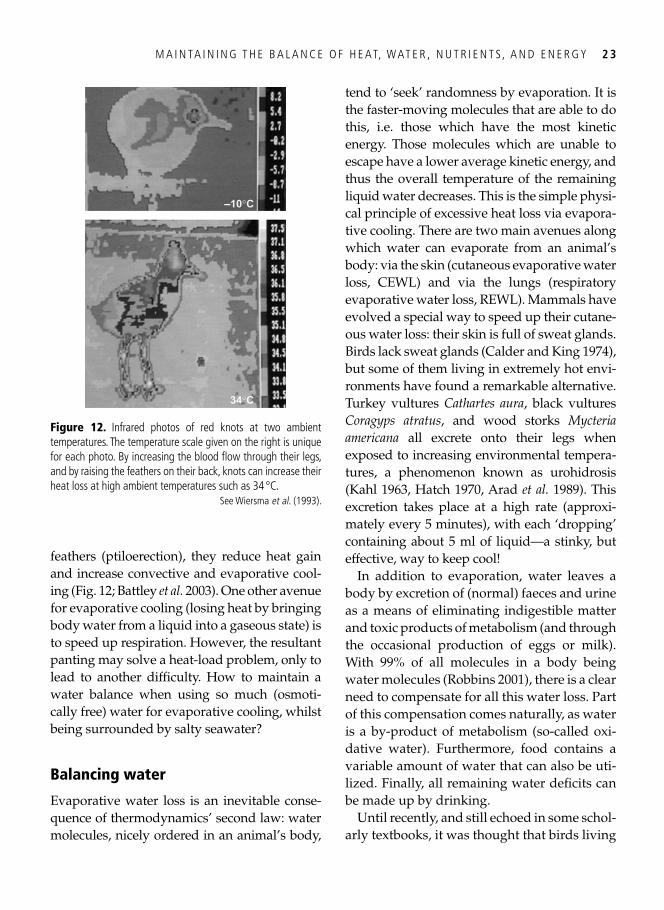
M A I N TA I N I N G T H E B A L A N C E O F H E AT, W AT E R , N U T R I E N T S , A N D E N E R G Y 2 3
feathers (ptiloerection), they reduce heat gain and increase convective and evaporative cool-ing ( Fig. 12 ; Battley et al. 2003 ). One other avenue for evaporative cooling (losing heat by bringing body water from a liquid into a gaseous state) is to speed up respiration. However, the resultant panting may solve a heat-load problem, only to lead to another diffi culty. How to maintain a water balance when using so much (osmoti-cally free) water for evaporative cooling, whilst being surrounded by salty seawater?
Balancing water
Evaporative water loss is an inevitable conse-quence of thermodynamics’ second law: water molecules, nicely ordered in an animal’s body,
tend to ‘seek’ randomness by evaporation. It is the faster-moving molecules that are able to do this, i.e. those which have the most kinetic energy. Those molecules which are unable to escape have a lower average kinetic energy, and thus the overall temperature of the remaining liquid water decreases. This is the simple physi-cal principle of excessive heat loss via evapora-tive cooling. There are two main avenues along which water can evaporate from an animal’s body: via the skin (cutaneous evaporative water loss, CEWL) and via the lungs (respiratory evaporative water loss, REWL). Mammals have evolved a special way to speed up their cutane-ous water loss: their skin is full of sweat glands. Birds lack sweat glands ( Calder and King 1974 ), but some of them living in extremely hot envi-ronments have found a remarkable alternative. Turkey vultures Cathartes aura , black vultures Coragyps atratus , and wood storks Mycteria americana all excrete onto their legs when exposed to increasing environmental tempera-tures, a phenomenon known as urohidrosis ( Kahl 1963 , Hatch 1970 , Arad et al. 1989 ). This excretion takes place at a high rate (approxi-mately every 5 minutes), with each ‘dropping’ containing about 5 ml of liquid—a stinky, but effective, way to keep cool!
In addition to evaporation, water leaves a body by excretion of (normal) faeces and urine as a means of eliminating indigestible matter and toxic products of metabolism (and through the occasional production of eggs or milk). With 99% of all molecules in a body being water molecules ( Robbins 2001 ), there is a clear need to compensate for all this water loss. Part of this compensation comes naturally, as water is a by-product of metabolism (so-called oxi-dative water). Furthermore, food contains a variable amount of water that can also be uti-lized. Finally, all remaining water defi cits can be made up by drinking.
Until recently, and still echoed in some schol-arly textbooks, it was thought that birds living
Figure 12. Infrared photos of red knots at two ambient temperatures. The temperature scale given on the right is unique for each photo. By increasing the blood fl ow through their legs, and by raising the feathers on their back, knots can increase their heat loss at high ambient temperatures such as 34 °C.
See Wiersma et al . ( 1993 ).
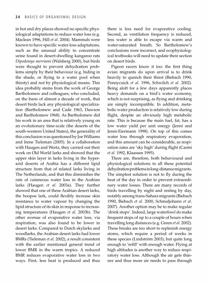
2 4 B A S I C S O F O R G A N I S M A L D E S I G N
in hot and dry places showed no specifi c phys-iological adaptations to reduce water loss (e.g. Maclean 1996 , Hill et al. 2004 ). Mammals were known to have specifi c water-loss adaptations, such as the unusual ability to concentrate urine found in desert-dwelling kangaroo rats Dipodomys merriami ( Walsberg 2000 ), but birds were thought to prevent dehydration prob-lems simply by their behaviour (e.g. hiding in the shade, or fl ying to a water pool when thirsty) and not by physiological means. This idea probably stems from the work of George Bartholomew and colleagues, who concluded, on the basis of almost a decade of work, that desert birds lack any physiological specializa-tion ( Bartholomew and Cade 1963 , Dawson and Bartholomew 1968 ). As Bartholomew did his work in an area that is relatively young on an evolutionary time-scale (the deserts of the south-western United States), the generality of this conclusion was questioned by Joe Williams and Irene Tieleman (2005). In a collaboration with Haugen and Wertz, they carried out their work on Old World larks and showed that the upper skin layer in larks living in the hyper-arid deserts of Arabia has a different lipid structure from that of related larks living in The Netherlands, and that this diminishes the rate of cutaneous water loss in the Arabian larks ( Haugen et al. 2003a ). They further showed that one of these Arabian desert larks, the hoopoe lark, could fl exibly increase skin resistance to water vapour by changing the lipid structure of its skin in response to increas-ing temperatures ( Haugen et al. 2003b ). The other avenue of evaporative water loss, via respiration, was also found to be lower in desert larks. Compared to Dutch skylarks and woodlarks, the Arabian desert larks had lower BMRs ( Tieleman et al. 2002 ), a result consistent with the earlier mentioned general trend of lower BMR in the warm tropics. A reduced BMR reduces evaporative water loss in two ways. First, less heat is produced and thus
there is less need for evaporative cooling. Second, as ventilation frequency is reduced, less water is able to escape via warm and water-saturated breath. So Bartholomew’s conclusions were incorrect, and ecophysiolog-ical textbooks will need to update their section on desert birds.
Pigeon racers know it too: the fi rst thing avian migrants do upon arrival is to drink heavily to quench their thirst ( Biebach 1990 , Pennycuick et al. 1996 , Schwilch et al . 2002 ). Being aloft for a few days apparently places heavy demands on a bird’s water economy, which is not surprising, as fl ying and drinking are simply incompatible. In addition, meta-bolic water production is relatively low during fl ight, despite an obviously high metabolic rate. This is because the main fuel, fat, has a low water yield per unit energy ( Jenni and Jenni-Eiermann 1998 ). On top of this comes water loss through respiratory evaporation, and this amount can be considerable, as respi-ration rates are ‘sky high’ during fl ight ( Carmi et al. 1992 , Klaassen 1995 ).
There are, therefore, both behavioural and physiological solutions to all these potential dehydration problems in long-distance migrants. The simplest solution is not to fl y during the heat of the day in order to prevent extraordi-nary water losses. There are many records of birds travelling by night and resting by day, notably among trans-Sahara migrants ( Biebach 1990 , Biebach et al. 2000 , Schmaljohann et al . 2007 ). Another option may be to make regular ‘drink stops’. Indeed, large waterfowl do make frequent stops of up to a couple of hours when travelling long distances (e.g. Green et al. 2002 ). These breaks are too short to replenish energy stores, which require a period of weeks in these species ( Lindström 2003 ), but quite long enough to ‘refi ll’ with enough water. Flying at high altitudes is another way to reduce respi-ratory water loss. Although the air gets thin-ner and thus more air needs to pass through
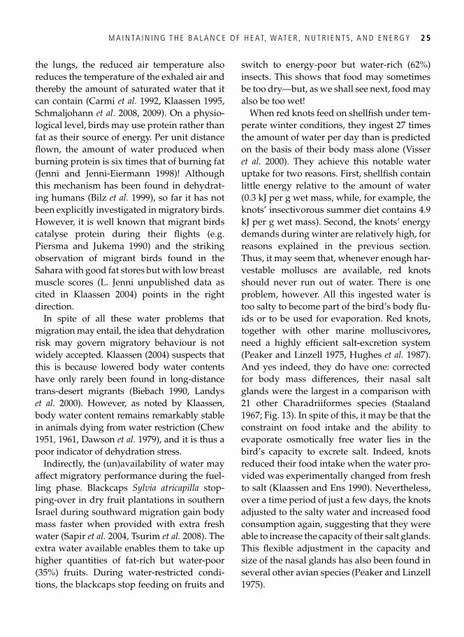
M A I N TA I N I N G T H E B A L A N C E O F H E AT, W AT E R , N U T R I E N T S , A N D E N E R G Y 2 5
the lungs, the reduced air temperature also reduces the temperature of the exhaled air and thereby the amount of saturated water that it can contain ( Carmi et al. 1992 , Klaassen 1995 , Schmaljohann et al . 2008 , 2009 ). On a physio-logical level, birds may use protein rather than fat as their source of energy. Per unit distance fl own, the amount of water produced when burning protein is six times that of burning fat ( Jenni and Jenni-Eiermann 1998 )! Although this mechanism has been found in dehydrat-ing humans ( Bilz et al. 1999 ), so far it has not been explicitly investigated in migratory birds. However, it is well known that migrant birds catalyse protein during their fl ights (e.g. Piersma and Jukema 1990 ) and the striking observation of migrant birds found in the Sahara with good fat stores but with low breast muscle scores (L. Jenni unpublished data as cited in Klaassen 2004 ) points in the right direction.
In spite of all these water problems that migration may entail, the idea that dehydration risk may govern migratory behaviour is not widely accepted. Klaassen ( 2004 ) suspects that this is because lowered body water contents have only rarely been found in long-distance trans-desert migrants ( Biebach 1990 , Landys et al. 2000 ). However, as noted by Klaassen, body water content remains remarkably stable in animals dying from water restriction ( Chew 1951 , 1961 , Dawson et al. 1979 ), and it is thus a poor indicator of dehydration stress.
Indirectly, the (un)availability of water may affect migratory performance during the fuel-ling phase. Blackcaps Sylvia atricapilla stop-ping-over in dry fruit plantations in southern Israel during southward migration gain body mass faster when provided with extra fresh water ( Sapir et al. 2004 , Tsurim et al. 2008 ). The extra water available enables them to take up higher quantities of fat-rich but water-poor (35%) fruits. During water-restricted condi-tions, the blackcaps stop feeding on fruits and
switch to energy-poor but water-rich (62%) insects. This shows that food may sometimes be too dry—but, as we shall see next, food may also be too wet!
When red knots feed on shellfi sh under tem-perate winter conditions, they ingest 27 times the amount of water per day than is predicted on the basis of their body mass alone ( Visser et al. 2000 ). They achieve this notable water uptake for two reasons. First, shellfi sh contain little energy relative to the amount of water (0.3 kJ per g wet mass, while, for example, the knots’ insectivorous summer diet contains 4.9 kJ per g wet mass). Second, the knots’ energy demands during winter are relatively high, for reasons explained in the previous section. Thus, it may seem that, whenever enough har-vestable molluscs are available, red knots should never run out of water. There is one problem, however. All this ingested water is too salty to become part of the bird’s body fl u-ids or to be used for evaporation. Red knots, together with other marine molluscivores, need a highly effi cient salt-excretion system ( Peaker and Linzell 1975 , Hughes et al. 1987 ). And yes indeed, they do have one: corrected for body mass differences, their nasal salt glands were the largest in a comparison with 21 other Charadriiformes species ( Staaland 1967 ; Fig. 13 ). In spite of this, it may be that the constraint on food intake and the ability to evaporate osmotically free water lies in the bird’s capacity to excrete salt. Indeed, knots reduced their food intake when the water pro-vided was experimentally changed from fresh to salt ( Klaassen and Ens 1990 ). Nevertheless, over a time period of just a few days, the knots adjusted to the salty water and increased food consumption again, suggesting that they were able to increase the capacity of their salt glands. This fl exible adjustment in the capacity and size of the nasal glands has also been found in several other avian species ( Peaker and Linzell 1975 ).
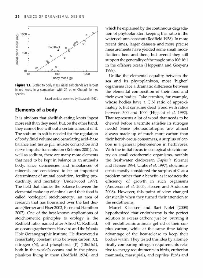
2 6 B A S I C S O F O R G A N I S M A L D E S I G N
Elements of a body
It is obvious that shellfi sh-eating knots ingest more salt than they need, but, on the other hand, they cannot live without a certain amount of it. The sodium in salt is needed for the regulation of body fl uid volume and osmolarity, acid–base balance and tissue pH, muscle contraction and nerve impulse transmission ( Robbins 2001 ). As well as sodium, there are many more elements that need to be kept in balance in an animal’s body, since defi ciencies and imbalances of minerals are considered to be an important determinant of animal condition, fertility, pro-ductivity, and mortality ( Underwood 1977 ). The fi eld that studies the balance between the elemental make-up of animals and their food is called ‘ecological stoichiometry’, an area of research that has fl ourished over the last dec-ade ( Sterner and Elser 2002 , Elser and Hamilton 2007 ). One of the best-known applications of stoichiometric principles to ecology is the Redfi eld ratio, named after Alfred C. Redfi eld, an oceanographer from Harvard and the Woods Hole Oceanographic Institute. He discovered a remarkably constant ratio between carbon (C), nitrogen (N), and phosphorus (P) (106:16:1), both in the world’s oceans and in the phyto-plankton living in them ( Redfi eld 1934 ), and
which he explained by the continuous degrada-tion of phytoplankton keeping this ratio in the water column constant ( Redfi eld 1958 ). In more recent times, larger datasets and more precise measurements have yielded some small modi-fi cations here and there, but overall they still support the generality of the magic ratio 106:16:1 in the offshore ocean ( Hoppema and Goeyens 1999 ).
Unlike the elemental equality between the sea and its phytoplankton, most ‘higher’ organisms face a dramatic difference between the elemental composition of their food and their own bodies. Take termites, for example, whose bodies have a C:N ratio of approxi-mately 5, but consume dead wood with ratios between 300 and 1000 ( Higashi et al. 1992 ). That represents a lot of wood that needs to be chewed before a termite satisfi es its nitrogen needs! Since photoautotrophs are almost always made up of much more carbon than their herbivorous consumers, a surplus of car-bon is a general phenomenon in herbivores. With the initial focus in ecological stoichiome-try on small ectothermic organisms, notably the freshwater cladoceran Daphnia ( Sterner and Hessen 1994 , Urabe et al. 1997 ), stoichiom-etrists mostly considered the surplus of C as a problem rather than a benefi t, as it reduces the effi ciency of growth in such organisms ( Anderson et al. 2005 , Hessen and Anderson 2008 ). However, this point of view changed drastically when they turned their attention to the endotherms.
Marcel Klaassen and Bart Nolet (2008) hypothesized that endothermy is the perfect solution to excess carbon: just by ‘burning it off’ endothermic animals get rid of their sur-plus carbon, while at the same time taking advantage of the heat-release to keep their bodies warm. They tested this idea by allomet-rically comparing nitrogen requirements rela-tive to energy requirements in birds, eutherian mammals, marsupials, and reptiles. Birds and
10
100
nasa
l gla
nd m
ass
(mg)
10010body mass (g)
1000
1000
Red Knot
Figure 13. Scaled to body mass, nasal salt glands are largest in red knots in a comparison with 21 other Charadriiformes species.
Based on data presented by Staaland ( 1967 ).
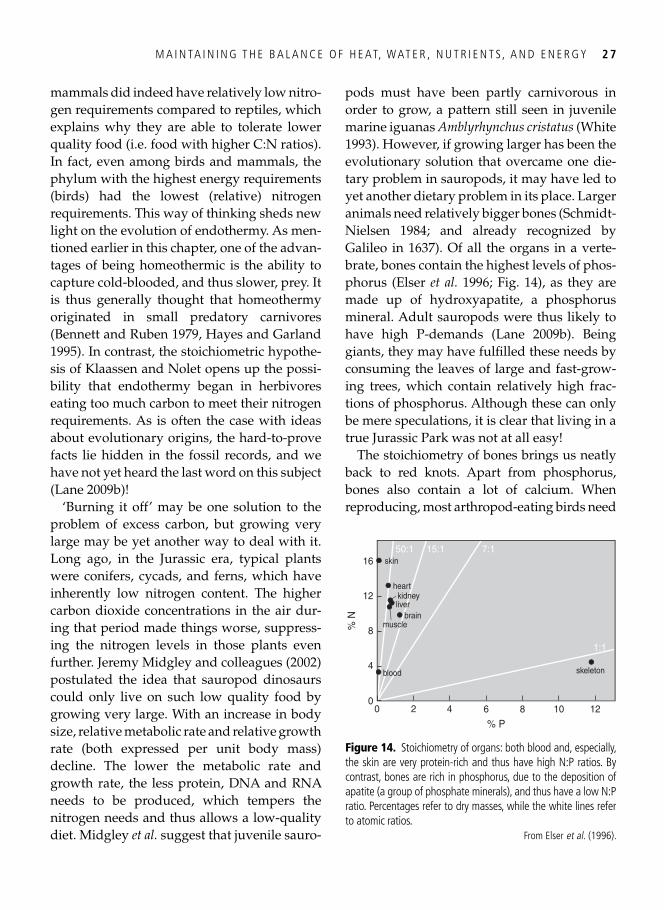
M A I N TA I N I N G T H E B A L A N C E O F H E AT, W AT E R , N U T R I E N T S , A N D E N E R G Y 2 7
mammals did indeed have relatively low nitro-gen requirements compared to reptiles, which explains why they are able to tolerate lower quality food (i.e. food with higher C:N ratios). In fact, even among birds and mammals, the phylum with the highest energy requirements (birds) had the lowest (relative) nitrogen requirements. This way of thinking sheds new light on the evolution of endothermy. As men-tioned earlier in this chapter, one of the advan-tages of being homeothermic is the ability to capture cold-blooded, and thus slower, prey. It is thus generally thought that homeothermy originated in small predatory carnivores ( Bennett and Ruben 1979 , Hayes and Garland 1995 ). In contrast, the stoichiometric hypothe-sis of Klaassen and Nolet opens up the possi-bility that endothermy began in herbivores eating too much carbon to meet their nitrogen requirements. As is often the case with ideas about evolutionary origins, the hard-to-prove facts lie hidden in the fossil records, and we have not yet heard the last word on this subject ( Lane 2009b )!
‘Burning it off’ may be one solution to the problem of excess carbon, but growing very large may be yet another way to deal with it. Long ago, in the Jurassic era, typical plants were conifers, cycads, and ferns, which have inherently low nitrogen content. The higher carbon dioxide concentrations in the air dur-ing that period made things worse, suppress-ing the nitrogen levels in those plants even further. Jeremy Midgley and colleagues ( 2002 ) postulated the idea that sauropod dinosaurs could only live on such low quality food by growing very large. With an increase in body size, relative metabolic rate and relative growth rate (both expressed per unit body mass) decline. The lower the metabolic rate and growth rate, the less protein, DNA and RNA needs to be produced, which tempers the nitrogen needs and thus allows a low-quality diet. Midgley et al. suggest that juvenile sauro-
pods must have been partly carnivorous in order to grow, a pattern still seen in juvenile marine iguanas Amblyrhynchus cristatus ( White 1993 ). However, if growing larger has been the evolutionary solution that overcame one die-tary problem in sauropods, it may have led to yet another dietary problem in its place. Larger animals need relatively bigger bones ( Schmidt-Nielsen 1984 ; and already recognized by Galileo in 1637). Of all the organs in a verte-brate, bones contain the highest levels of phos-phorus ( Elser et al. 1996 ; Fig. 14 ), as they are made up of hydroxyapatite, a phosphorus mineral. Adult sauropods were thus likely to have high P-demands ( Lane 2009b ). Being giants, they may have fulfi lled these needs by consuming the leaves of large and fast-grow-ing trees, which contain relatively high frac-tions of phosphorus. Although these can only be mere speculations, it is clear that living in a true Jurassic Park was not at all easy!
The stoichiometry of bones brings us neatly back to red knots. Apart from phosphorus, bones also contain a lot of calcium. When reproducing, most arthropod-eating birds need
% N
16
0
8
4
4 8
% P
0 2 6 1210
12
musclebrain
blood
heart
skin
kidneyliver
skeleton
50:1 15:1 7:1
1:1
Figure 14. Stoichiometry of organs: both blood and, especially, the skin are very protein-rich and thus have high N:P ratios. By contrast, bones are rich in phosphorus, due to the deposition of apatite (a group of phosphate minerals), and thus have a low N:P ratio. Percentages refer to dry masses, while the white lines refer to atomic ratios.
From Elser et al. ( 1996 ).
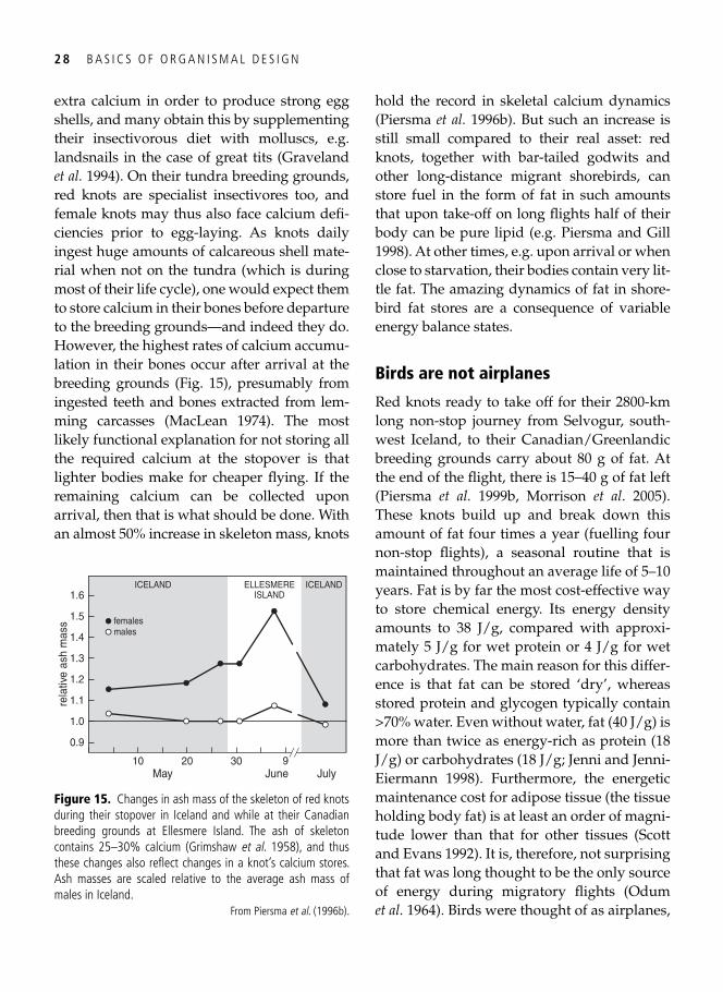
2 8 B A S I C S O F O R G A N I S M A L D E S I G N
extra calcium in order to produce strong egg shells, and many obtain this by supplementing their insectivorous diet with molluscs, e.g. landsnails in the case of great tits ( Graveland et al. 1994 ). On their tundra breeding grounds, red knots are specialist insectivores too, and female knots may thus also face calcium defi -ciencies prior to egg-laying. As knots daily ingest huge amounts of calcareous shell mate-rial when not on the tundra (which is during most of their life cycle), one would expect them to store calcium in their bones before departure to the breeding grounds—and indeed they do. However, the highest rates of calcium accumu-lation in their bones occur after arrival at the breeding grounds ( Fig. 15 ), presumably from ingested teeth and bones extracted from lem-ming carcasses ( MacLean 1974 ). The most likely functional explanation for not storing all the required calcium at the stopover is that lighter bodies make for cheaper fl ying. If the remaining calcium can be collected upon arrival, then that is what should be done. With an almost 50% increase in skeleton mass, knots
hold the record in skeletal calcium dynamics ( Piersma et al. 1996b ). But such an increase is still small compared to their real asset: red knots, together with bar-tailed godwits and other long-distance migrant shorebirds, can store fuel in the form of fat in such amounts that upon take-off on long fl ights half of their body can be pure lipid (e.g. Piersma and Gill 1998 ). At other times, e.g. upon arrival or when close to starvation, their bodies contain very lit-tle fat. The amazing dynamics of fat in shore-bird fat stores are a consequence of variable energy balance states.
Birds are not airplanes
Red knots ready to take off for their 2800-km long non-stop journey from Selvogur, south-west Iceland, to their Canadian/Greenlandic breeding grounds carry about 80 g of fat. At the end of the fl ight, there is 15–40 g of fat left ( Piersma et al. 1999b , Morrison et al . 2005 ). These knots build up and break down this amount of fat four times a year (fuelling four non-stop fl ights), a seasonal routine that is maintained throughout an average life of 5–10 years. Fat is by far the most cost-effective way to store chemical energy. Its energy density amounts to 38 J/g, compared with approxi-mately 5 J/g for wet protein or 4 J/g for wet carbohydrates. The main reason for this differ-ence is that fat can be stored ‘dry’, whereas stored protein and glycogen typically contain >70% water. Even without water, fat (40 J/g) is more than twice as energy-rich as protein (18 J/g) or carbohydrates (18 J/g; Jenni and Jenni-Eiermann 1998 ). Furthermore, the energetic maintenance cost for adipose tissue (the tissue holding body fat) is at least an order of magni-tude lower than that for other tissues ( Scott and Evans 1992 ). It is, therefore, not surprising that fat was long thought to be the only source of energy during migratory fl ights ( Odum et al. 1964 ). Birds were thought of as airplanes,
0.9
1.0
1.1
1.2
1.3
1.4
1.5
1.6
rela
tive
ash
mas
s
10 20 30 9May
females
June July
males
ICELAND ELLESMEREISLAND
ICELAND
Figure 15. Changes in ash mass of the skeleton of red knots during their stopover in Iceland and while at their Canadian breeding grounds at Ellesmere Island. The ash of skeleton contains 25–30% calcium ( Grimshaw et al . 1958 ), and thus these changes also refl ect changes in a knot’s calcium stores. Ash masses are scaled relative to the average ash mass of males in Iceland.
From Piersma et al . ( 1996b ).
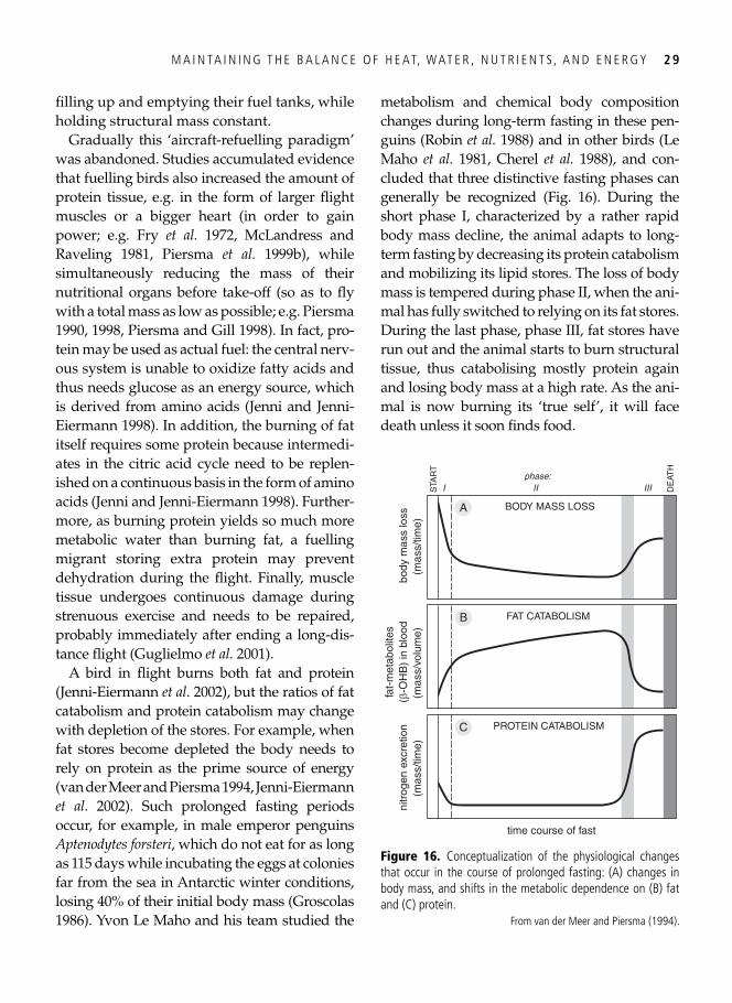
M A I N TA I N I N G T H E B A L A N C E O F H E AT, W AT E R , N U T R I E N T S , A N D E N E R G Y 2 9
fi lling up and emptying their fuel tanks, while holding structural mass constant.
Gradually this ‘aircraft-refuelling paradigm’ was abandoned. Studies accumulated evidence that fuelling birds also increased the amount of protein tissue, e.g. in the form of larger fl ight muscles or a bigger heart (in order to gain power; e.g. Fry et al. 1972 , McLandress and Raveling 1981 , Piersma et al. 1999b ), while simultaneously reducing the mass of their nutritional organs before take-off (so as to fl y with a total mass as low as possible; e.g. Piersma 1990 , 1998 , Piersma and Gill 1998 ). In fact, pro-tein may be used as actual fuel: the central nerv-ous system is unable to oxidize fatty acids and thus needs glucose as an energy source, which is derived from amino acids ( Jenni and Jenni-Eiermann 1998 ). In addition, the burning of fat itself requires some protein because intermedi-ates in the citric acid cycle need to be replen-ished on a continuous basis in the form of amino acids ( Jenni and Jenni-Eiermann 1998 ). Further-more, as burning protein yields so much more metabolic water than burning fat, a fuelling migrant storing extra protein may prevent dehydration during the fl ight. Finally, muscle tissue undergoes continuous damage during strenuous exercise and needs to be repaired, probably immediately after ending a long-dis-tance fl ight ( Guglielmo et al. 2001 ).
A bird in fl ight burns both fat and protein ( Jenni-Eiermann et al . 2002 ), but the ratios of fat catabolism and protein catabolism may change with depletion of the stores. For example, when fat stores become depleted the body needs to rely on protein as the prime source of energy ( van der Meer and Piersma 1994 , Jenni-Eiermann et al . 2002 ). Such prolonged fasting periods occur, for example, in male emperor penguins Aptenodytes forsteri , which do not eat for as long as 115 days while incubating the eggs at colonies far from the sea in Antarctic winter conditions, losing 40% of their initial body mass ( Groscolas 1986 ). Yvon Le Maho and his team studied the
metabolism and chemical body composition changes during long-term fasting in these pen-guins ( Robin et al. 1988 ) and in other birds (Le Maho et al. 1981 , Cherel et al. 1988 ), and con-cluded that three distinctive fasting phases can generally be recognized ( Fig. 16 ). During the short phase I, characterized by a rather rapid body mass decline, the animal adapts to long-term fasting by decreasing its protein catabolism and mobilizing its lipid stores. The loss of body mass is tempered during phase II, when the ani-mal has fully switched to relying on its fat stores. During the last phase, phase III, fat stores have run out and the animal starts to burn structural tissue, thus catabolising mostly protein again and losing body mass at a high rate. As the ani-mal is now burning its ‘true self’, it will face death unless it soon fi nds food.
PROTEIN CATABOLISM
FAT CATABOLISM
BODY MASS LOSSA
B
C
nitr
ogen
exc
retio
n(m
ass/
time)
time course of fast
II
fat-
met
abol
ites
(β-O
HB
) in
blo
od(m
ass/
volu
me)
body
mas
s lo
ss(m
ass/
time)
IIISTA
RT
DE
ATH
Iphase:
Figure 16. Conceptualization of the physiological changes that occur in the course of prolonged fasting: (A) changes in body mass, and shifts in the metabolic dependence on (B) fat and (C) protein.
From van der Meer and Piersma ( 1994 ).
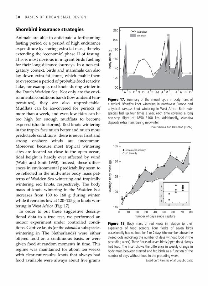
3 0 B A S I C S O F O R G A N I S M A L D E S I G N
Shorebird insurance strategies
Animals are able to anticipate a forthcoming fasting period or a period of high endurance expenditure by storing extra fat mass, thereby extending the ‘economic’ phase II of fasting. This is most obvious in migrant birds fuelling for their long-distance journeys. In a non-mi-gratory context, birds and mammals can also lay down extra fat stores, which enable them to overcome a period of probable food scarcity. Take, for example, red knots during winter in the Dutch Wadden Sea. Not only are the envi-ronmental conditions harsh (low ambient tem-peratures), they are also unpredictable. Mudfl ats can be ice-covered for periods of more than a week, and even low tides can be too high for enough mudfl ats to become exposed (due to storms). Red knots wintering in the tropics face much better and much more predictable conditions: there is never frost and strong onshore winds are uncommon. Moreover, because most tropical wintering sites are located so close to the open ocean, tidal height is hardly ever affected by wind ( Wolff and Smit 1990 ). Indeed, these differ-ences in environmental predictability seem to be refl ected in the midwinter body mass pat-terns of Wadden Sea wintering and tropically wintering red knots, respectively. The body mass of knots wintering in the Wadden Sea increases from 130 to 160 g during winter, while it remains low at 120–125 g in knots win-tering in West Africa ( Fig. 17 ).
In order to put these suggestive descrip-tional data to a true test, we performed an indoor experiment under controlled condi-tions. Captive knots (of the islandica subspecies wintering in The Netherlands) were either offered food on a continuous basis, or were given food at random moments in time. This regime was maintained for about ten weeks with clear-cut results: knots that always had food available were always about fi ve grams
body
mas
s (g
)
100
200
220 islandicacanutus
120
140
160
180
OJ F M A M J J A SN DOA S
Figure 17. Summary of the annual cycle in body mass of a typical islandica knot wintering in northwest Europe and a typical canutus knot wintering in West Africa. Both sub- species fuel up four times a year, each time covering a long non-stop fl ight of 1850–5100 km. Additionally, islandica deposits extra mass during midwinter.
From Piersma and Davidson ( 1992 ).
0
120
135
aver
age
body
mas
s (g
)
10 20 30 40 50 60 70 80number of days since capture
115
125
130
0
0
1
2
1
0
2 1
2
0
2
2occasional scarcityno scarcity
0 1
–4
–2
0
2
2
Figure 18. Body mass of red knots in relation to their experience of food scarcity. Four fl ocks of seven birds occasionally had no food for 1 or 2 days (the number above the closed dots indicating the number of days without food in the preceding week). Three fl ocks of seven birds (open dots) always had food. The inset shows the difference in weekly change in body mass between starved and fed birds as a function of the number of days without food in the preceding week.
Based on T. Piersma et al . unpubl. data.
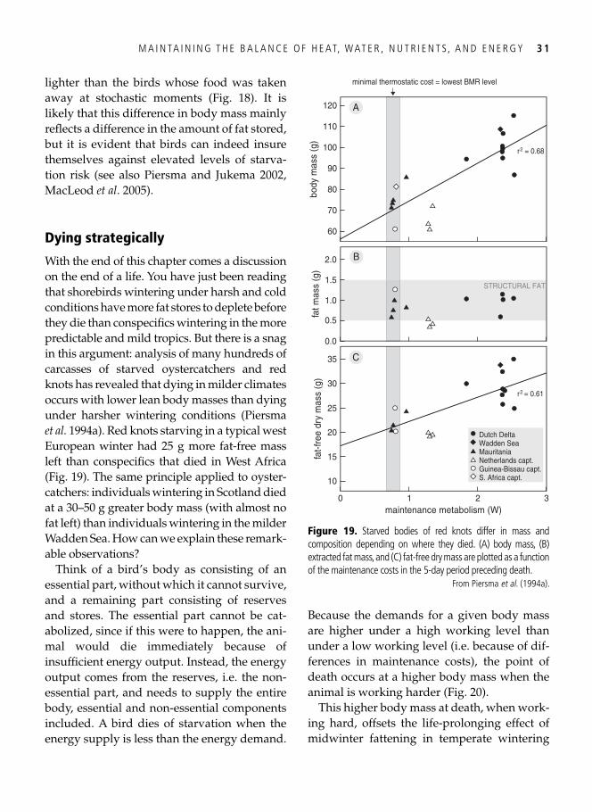
M A I N TA I N I N G T H E B A L A N C E O F H E AT, W AT E R , N U T R I E N T S , A N D E N E R G Y 3 1
lighter than the birds whose food was taken away at stochastic moments ( Fig. 18 ). It is likely that this difference in body mass mainly refl ects a difference in the amount of fat stored, but it is evident that birds can indeed insure themselves against elevated levels of starva-tion risk (see also Piersma and Jukema 2002 , MacLeod et al . 2005 ).
Dying strategically
With the end of this chapter comes a discussion on the end of a life. You have just been reading that shorebirds wintering under harsh and cold conditions have more fat stores to deplete before they die than conspecifi cs wintering in the more predictable and mild tropics. But there is a snag in this argument: analysis of many hundreds of carcasses of starved oystercatchers and red knots has revealed that dying in milder climates occurs with lower lean body masses than dying under harsher wintering conditions ( Piersma et al. 1994a ). Red knots starving in a typical west European winter had 25 g more fat-free mass left than conspecifi cs that died in West Africa ( Fig. 19 ). The same principle applied to oyster-catchers: individuals wintering in Scotland died at a 30–50 g greater body mass (with almost no fat left) than individuals wintering in the milder Wadden Sea. How can we explain these remark-able observations?
Think of a bird’s body as consisting of an essential part, without which it cannot survive, and a remaining part consisting of reserves and stores. The essential part cannot be cat-abolized, since if this were to happen, the ani-mal would die immediately because of insuffi cient energy output. Instead, the energy output comes from the reserves, i.e. the non-essential part, and needs to supply the entire body, essential and non-essential components included. A bird dies of starvation when the energy supply is less than the energy demand.
Because the demands for a given body mass are higher under a high working level than under a low working level (i.e. because of dif-ferences in maintenance costs), the point of death occurs at a higher body mass when the animal is working harder ( Fig. 20 ).
This higher body mass at death, when work-ing hard, offsets the life-prolonging effect of midwinter fattening in temperate wintering
0
10
20
30
25
35
15fat-
free
dry
mas
s (g
)
1 2 3maintenance metabolism (W)
Dutch Delta
0.0
0.5
1.0
1.5
2.0
fat m
ass
(g)
110
60
70
80
90
120 A
B
C
body
mas
s (g
)
Wadden SeaMauritaniaNetherlands capt.Guinea-Bissau capt.S. Africa capt.
100
r2 = 0.61
r2 = 0.68
STRUCTURAL FAT
minimal thermostatic cost = lowest BMR level
Figure 19. Starved bodies of red knots differ in mass and composition depending on where they died. (A) body mass, (B) extracted fat mass, and (C) fat-free dry mass are plotted as a function of the maintenance costs in the 5-day period preceding death.
From Piersma et al . ( 1994a ).
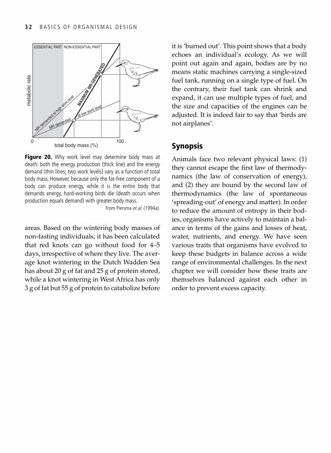
3 2 B A S I C S O F O R G A N I S M A L D E S I G N
areas. Based on the wintering body masses of non-fasting individuals, it has been calculated that red knots can go without food for 4–5 days, irrespective of where they live. The aver-age knot wintering in the Dutch Wadden Sea has about 20 g of fat and 25 g of protein stored, while a knot wintering in West Africa has only 3 g of fat but 55 g of protein to catabolize before
it is ‘burned out’. This point shows that a body echoes an individual’s ecology. As we will point out again and again, bodies are by no means static machines carrying a single-sized fuel tank, running on a single type of fuel. On the contrary, their fuel tank can shrink and expand, it can use multiple types of fuel, and the size and capacities of the engines can be adjusted. It is indeed fair to say that ‘birds are not airplanes’.
Synopsis
Animals face two relevant physical laws: (1) they cannot escape the fi rst law of thermody-namics (the law of conservation of energy), and (2) they are bound by the second law of thermodynamics (the law of spontaneous ‘spreading-out’ of energy and matter). In order to reduce the amount of entropy in their bod-ies, organisms have actively to maintain a bal-ance in terms of the gains and losses of heat, water, nutrients, and energy. We have seen various traits that organisms have evolved to keep these budgets in balance across a wide range of environmental challenges. In the next chapter we will consider how these traits are themselves balanced against each other in order to prevent excess capacity.
0
met
abol
ic ra
te
100total body mass (%)
MR deman
ded a
t high
work le
vel
MR demanded at low work level
ESSENTIAL PART
MAX
IMUM
MR-
GENE
RATE
D
NON-ESSENTIAL PART
Figure 20. Why work level may determine body mass at death: both the energy production (thick line) and the energy demand (thin lines; two work levels) vary as a function of total body mass. However, because only the fat-free component of a body can produce energy, while it is the entire body that demands energy, hard-working birds die (death occurs when production equals demand) with greater body mass.
From Piersma et al . ( 1994a ).
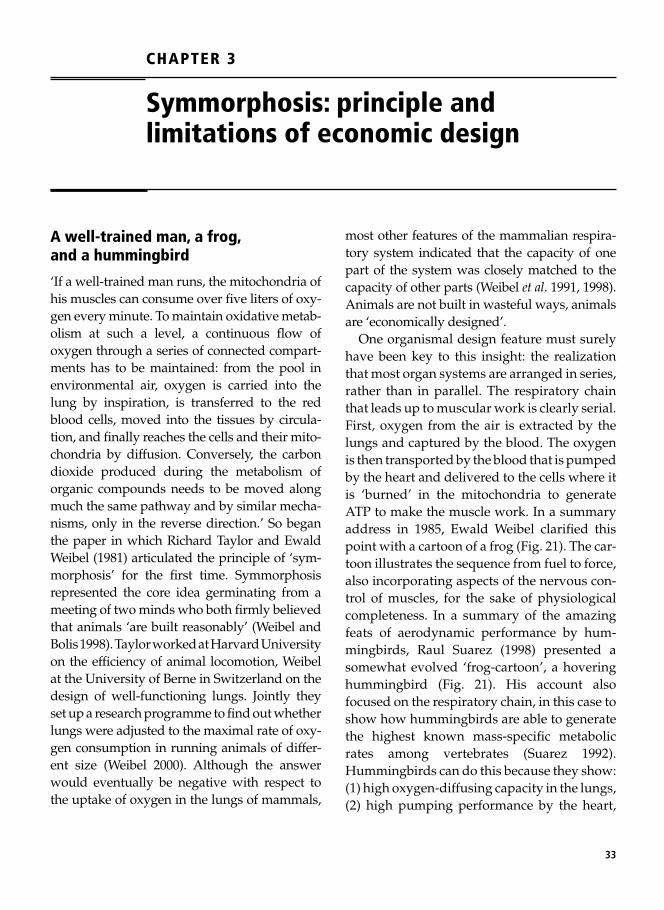
33
CHAPTER 3
Symmorphosis: principle and limitations of economic design
A well-trained man, a frog, and a hummingbird
‘If a well-trained man runs, the mitochondria of his muscles can consume over fi ve liters of oxy-gen every minute. To maintain oxidative metab-olism at such a level, a continuous fl ow of oxygen through a series of connected compart-ments has to be maintained: from the pool in environmental air, oxygen is carried into the lung by inspiration, is transferred to the red blood cells, moved into the tissues by circula-tion, and fi nally reaches the cells and their mito-chondria by diffusion. Conversely, the carbon dioxide produced during the metabolism of organic compounds needs to be moved along much the same pathway and by similar mecha-nisms, only in the reverse direction.’ So began the paper in which Richard Taylor and Ewald Weibel (1981) articulated the principle of ‘sym-morphosis’ for the fi rst time. Symmorphosis represented the core idea germinating from a meeting of two minds who both fi rmly believed that animals ‘are built reasonably’ ( Weibel and Bolis 1998 ). Taylor worked at Harvard University on the effi ciency of animal locomotion, Weibel at the University of Berne in Switzerland on the design of well-functioning lungs. Jointly they set up a research programme to fi nd out whether lungs were adjusted to the maximal rate of oxy-gen consumption in running animals of differ-ent size ( Weibel 2000 ). Although the answer would eventually be negative with respect to the uptake of oxygen in the lungs of mammals,
most other features of the mammalian respira-tory system indicated that the capacity of one part of the system was closely matched to the capacity of other parts ( Weibel et al . 1991 , 1998 ). Animals are not built in wasteful ways, animals are ‘economically designed’.
One organismal design feature must surely have been key to this insight: the realization that most organ systems are arranged in series, rather than in parallel. The respiratory chain that leads up to muscular work is clearly serial. First, oxygen from the air is extracted by the lungs and captured by the blood. The oxygen is then transported by the blood that is pumped by the heart and delivered to the cells where it is ‘burned’ in the mitochondria to generate ATP to make the muscle work. In a summary address in 1985, Ewald Weibel clarifi ed this point with a cartoon of a frog ( Fig. 21 ). The car-toon illustrates the sequence from fuel to force, also incorporating aspects of the nervous con-trol of muscles, for the sake of physiological completeness. In a summary of the amazing feats of aerodynamic performance by hum-mingbirds, Raul Suarez ( 1998 ) presented a somewhat evolved ‘frog-cartoon’, a hovering hummingbird ( Fig. 21 ). His account also focused on the respiratory chain, in this case to show how hummingbirds are able to generate the highest known mass-specifi c metabolic rates among vertebrates ( Suarez 1992 ). Hummingbirds can do this because they show: (1) high oxygen-diffusing capacity in the lungs, (2) high pumping performance by the heart,
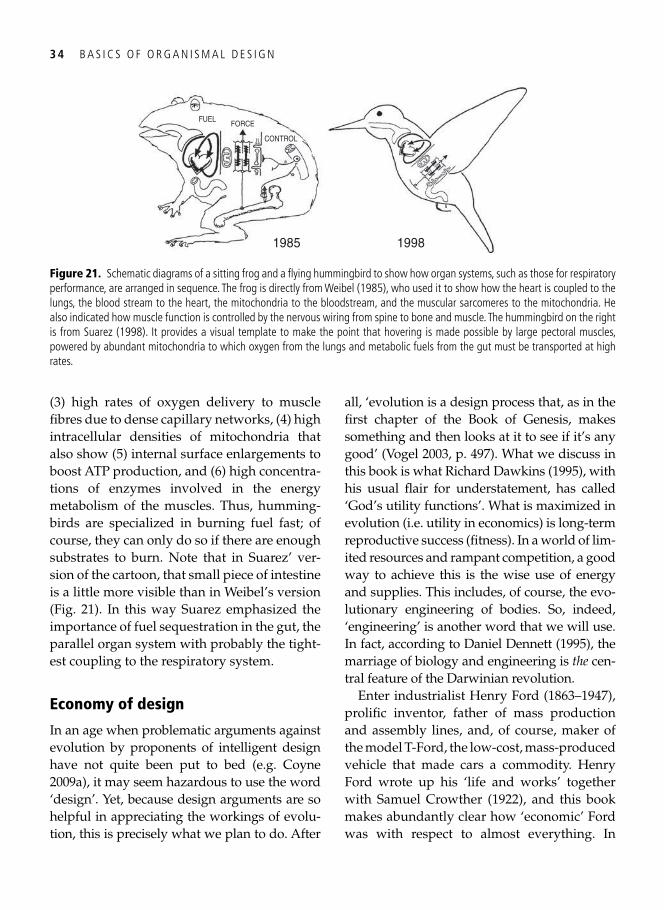
3 4 B A S I C S O F O R G A N I S M A L D E S I G N
(3) high rates of oxygen delivery to muscle fi bres due to dense capillary networks, (4) high intracellular densities of mitochondria that also show (5) internal surface enlargements to boost ATP production, and (6) high concentra-tions of enzymes involved in the energy metabolism of the muscles. Thus, humming-birds are specialized in burning fuel fast; of course, they can only do so if there are enough substrates to burn. Note that in Suarez’ ver-sion of the cartoon, that small piece of intestine is a little more visible than in Weibel’s version ( Fig. 21 ). In this way Suarez emphasized the importance of fuel sequestration in the gut, the parallel organ system with probably the tight-est coupling to the respiratory system.
Economy of design
In an age when problematic arguments against evolution by proponents of intelligent design have not quite been put to bed (e.g. Coyne 2009a ), it may seem hazardous to use the word ‘design’. Yet, because design arguments are so helpful in appreciating the workings of evolu-tion, this is precisely what we plan to do. After
all, ‘evolution is a design process that, as in the fi rst chapter of the Book of Genesis, makes something and then looks at it to see if it’s any good’ ( Vogel 2003 , p. 497). What we discuss in this book is what Richard Dawkins ( 1995 ), with his usual fl air for understatement, has called ‘God’s utility functions’. What is maximized in evolution (i.e. utility in economics) is long-term reproductive success (fi tness). In a world of lim-ited resources and rampant competition, a good way to achieve this is the wise use of energy and supplies. This includes, of course, the evo-lutionary engineering of bodies. So, indeed, ‘engineering’ is another word that we will use. In fact, according to Daniel Dennett ( 1995 ), the marriage of biology and engineering is the cen-tral feature of the Darwinian revolution.
Enter industrialist Henry Ford (1863–1947), prolifi c inventor, father of mass production and assembly lines, and, of course, maker of the model T-Ford, the low-cost, mass-produced vehicle that made cars a commodity. Henry Ford wrote up his ‘life and works’ together with Samuel Crowther (1922), and this book makes abundantly clear how ‘economic’ Ford was with respect to almost everything. In
FUEL
1985
FORCE
CONTROL
1998
Figure 21. Schematic diagrams of a sitting frog and a fl ying hummingbird to show how organ systems, such as those for respiratory performance, are arranged in sequence. The frog is directly from Weibel ( 1985 ), who used it to show how the heart is coupled to the lungs, the blood stream to the heart, the mitochondria to the bloodstream, and the muscular sarcomeres to the mitochondria. He also indicated how muscle function is controlled by the nervous wiring from spine to bone and muscle. The hummingbird on the right is from Suarez ( 1998 ). It provides a visual template to make the point that hovering is made possible by large pectoral muscles, powered by abundant mitochondria to which oxygen from the lungs and metabolic fuels from the gut must be transported at high rates.
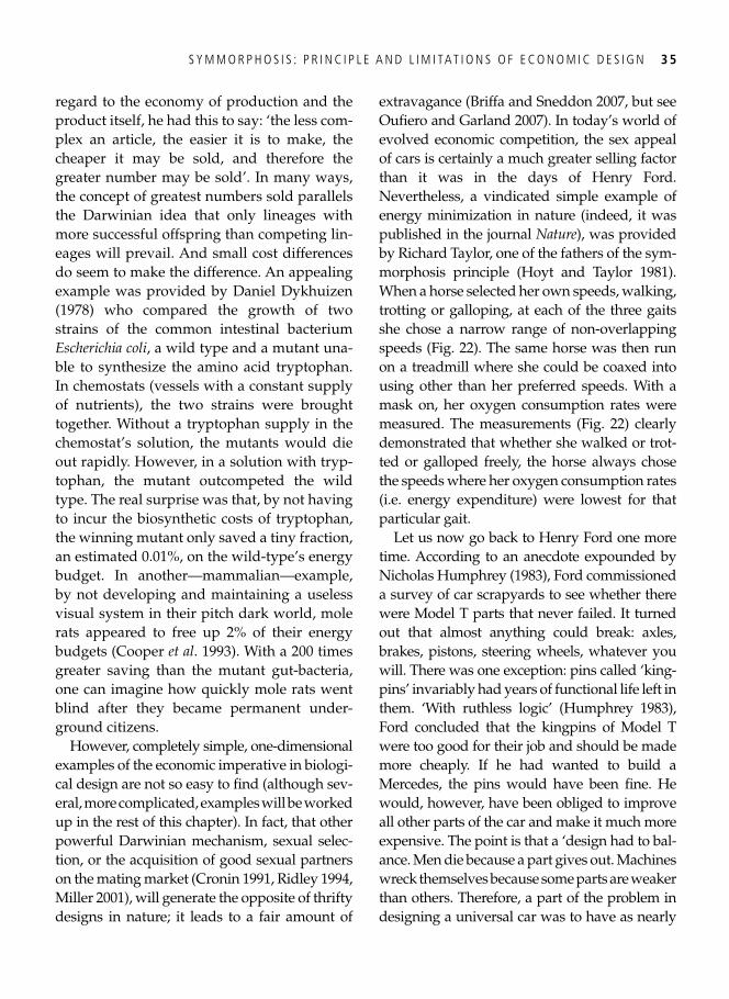
S Y M M O R P H O S I S : P R I N C I P L E A N D L I M I TAT I O N S O F E C O N O M I C D E S I G N 3 5
regard to the economy of production and the product itself, he had this to say: ‘the less com-plex an article, the easier it is to make, the cheaper it may be sold, and therefore the greater number may be sold’. In many ways, the concept of greatest numbers sold parallels the Darwinian idea that only lineages with more successful offspring than competing lin-eages will prevail. And small cost differences do seem to make the difference. An appealing example was provided by Daniel Dykhuizen ( 1978 ) who compared the growth of two strains of the common intestinal bacterium Escherichia coli , a wild type and a mutant una-ble to synthesize the amino acid tryptophan. In chemostats (vessels with a constant supply of nutrients), the two strains were brought together. Without a tryptophan supply in the chemostat’s solution, the mutants would die out rapidly. However, in a solution with tryp-tophan, the mutant outcompeted the wild type. The real surprise was that, by not having to incur the biosynthetic costs of tryptophan, the winning mutant only saved a tiny fraction, an estimated 0.01%, on the wild-type’s energy budget. In another—mammalian—example, by not developing and maintaining a useless visual system in their pitch dark world, mole rats appeared to free up 2% of their energy budgets ( Cooper et al . 1993 ). With a 200 times greater saving than the mutant gut-bacteria, one can imagine how quickly mole rats went blind after they became permanent under-ground citizens.
However, completely simple, one- dimensional examples of the economic imperative in biologi-cal design are not so easy to fi nd (although sev-eral, more complicated, examples will be worked up in the rest of this chapter). In fact, that other powerful Darwinian mechanism, sexual selec-tion, or the acquisition of good sexual partners on the mating market ( Cronin 1991 , Ridley 1994 , Miller 2001 ), will generate the opposite of thrifty designs in nature; it leads to a fair amount of
extravagance ( Briffa and Sneddon 2007 , but see Oufi ero and Garland 2007 ). In today’s world of evolved economic competition, the sex appeal of cars is certainly a much greater selling factor than it was in the days of Henry Ford. Nevertheless, a vindicated simple example of energy minimization in nature (indeed, it was published in the journal Nature ), was provided by Richard Taylor, one of the fathers of the sym-morphosis principle ( Hoyt and Taylor 1981 ). When a horse selected her own speeds, walking, trotting or galloping, at each of the three gaits she chose a narrow range of non-overlapping speeds ( Fig. 22 ). The same horse was then run on a treadmill where she could be coaxed into using other than her preferred speeds. With a mask on, her oxygen consumption rates were measured. The measurements ( Fig. 22 ) clearly demonstrated that whether she walked or trot-ted or galloped freely, the horse always chose the speeds where her oxygen consumption rates (i.e. energy expenditure) were lowest for that particular gait.
Let us now go back to Henry Ford one more time. According to an anecdote expounded by Nicholas Humphrey ( 1983 ), Ford commissioned a survey of car scrapyards to see whether there were Model T parts that never failed. It turned out that almost anything could break: axles, brakes, pistons, steering wheels, whatever you will. There was one exception: pins called ‘king-pins’ invariably had years of functional life left in them. ‘With ruthless logic’ ( Humphrey 1983 ), Ford concluded that the kingpins of Model T were too good for their job and should be made more cheaply. If he had wanted to build a Mercedes, the pins would have been fi ne. He would, however, have been obliged to improve all other parts of the car and make it much more expensive. The point is that a ‘design had to bal-ance. Men die because a part gives out. Machines wreck themselves because some parts are weaker than others. Therefore, a part of the problem in designing a universal car was to have as nearly
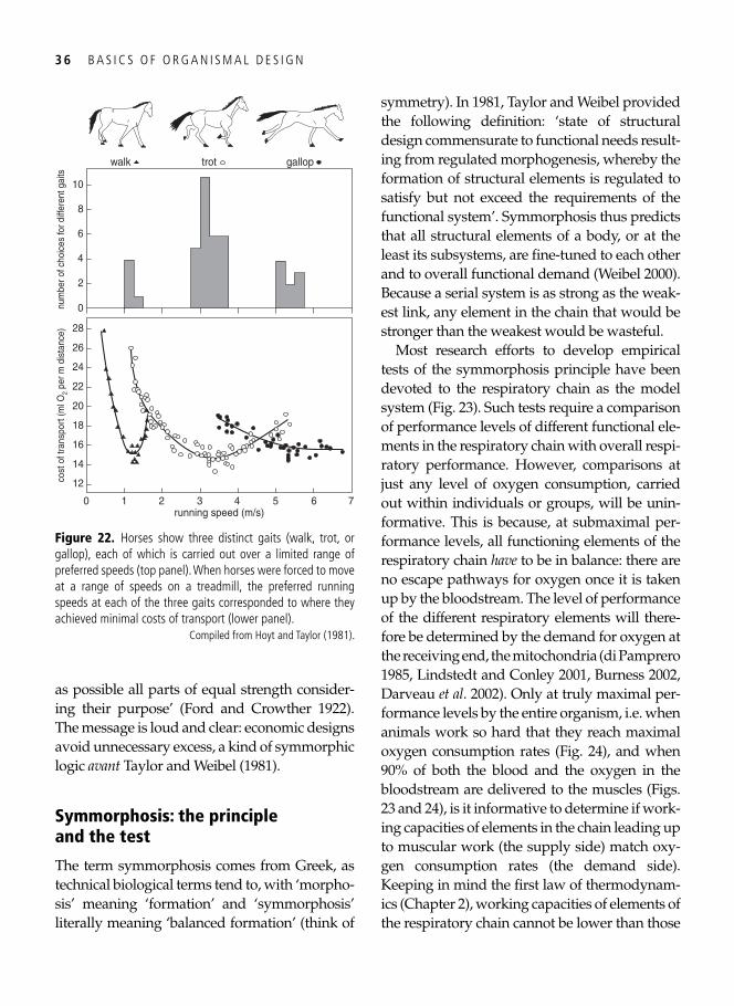
3 6 B A S I C S O F O R G A N I S M A L D E S I G N
as possible all parts of equal strength consider-ing their purpose’ ( Ford and Crowther 1922 ). The message is loud and clear: economic designs avoid unnecessary excess, a kind of symmorphic logic avant Taylor and Weibel ( 1981 ).
Symmorphosis: the principle and the test
The term symmorphosis comes from Greek, as technical biological terms tend to, with ‘morpho-sis’ meaning ‘formation’ and ‘symmorphosis’ literally meaning ‘balanced formation’ (think of
symmetry). In 1981, Taylor and Weibel provided the following defi nition: ‘state of structural design commensurate to functional needs result-ing from regulated morphogenesis, whereby the formation of structural elements is regulated to satisfy but not exceed the requirements of the functional system’. Symmorphosis thus predicts that all structural elements of a body, or at the least its subsystems, are fi ne-tuned to each other and to overall functional demand ( Weibel 2000 ). Because a serial system is as strong as the weak-est link, any element in the chain that would be stronger than the weakest would be wasteful.
Most research efforts to develop empirical tests of the symmorphosis principle have been devoted to the respiratory chain as the model system ( Fig. 23 ). Such tests require a comparison of performance levels of different functional ele-ments in the respiratory chain with overall respi-ratory performance. However, comparisons at just any level of oxygen consumption, carried out within individuals or groups, will be unin-formative. This is because, at submaximal per-formance levels, all functioning elements of the respiratory chain have to be in balance: there are no escape pathways for oxygen once it is taken up by the bloodstream. The level of performance of the different respiratory elements will there-fore be determined by the demand for oxygen at the receiving end, the mitochondria ( di Pamprero 1985 , Lindstedt and Conley 2001 , Burness 2002 , Darveau et al . 2002 ). Only at truly maximal per-formance levels by the entire organism, i.e. when animals work so hard that they reach maximal oxygen consumption rates ( Fig. 24 ), and when 90% of both the blood and the oxygen in the bloodstream are delivered to the muscles ( Figs. 23 and 24 ), is it informative to determine if work-ing capacities of elements in the chain leading up to muscular work (the supply side) match oxy-gen consumption rates (the demand side). Keeping in mind the fi rst law of thermodynam-ics ( Chapter 2 ) , working capacities of elements of the respiratory chain cannot be lower than those
0
12
20
24
28
22
26
16
cost
of t
rans
port
(ml O
2 pe
r m d
ista
nce)
1 2 3 4 5 6 7running speed (m/s)
walk trot gallop
14
18
0
6
8
2
4
10
num
ber o
f cho
ices
for d
iffer
ent g
aits
Figure 22. Horses show three distinct gaits (walk, trot, or gallop), each of which is carried out over a limited range of preferred speeds (top panel). When horses were forced to move at a range of speeds on a treadmill, the preferred running speeds at each of the three gaits corresponded to where they achieved minimal costs of transport (lower panel).
Compiled from Hoyt and Taylor ( 1981 ).
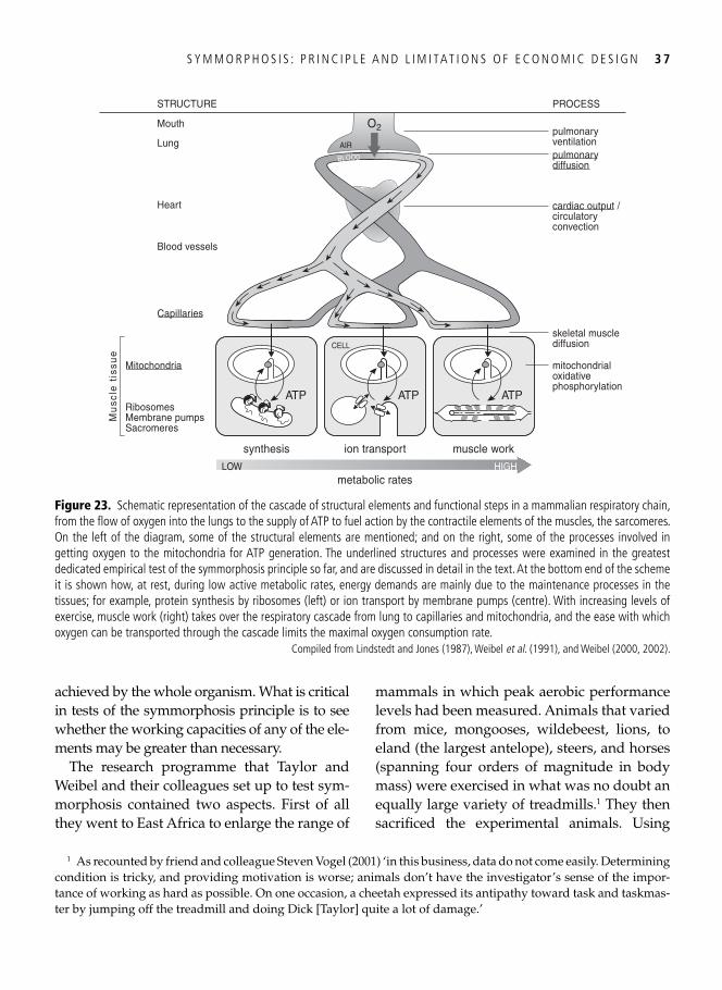
S Y M M O R P H O S I S : P R I N C I P L E A N D L I M I TAT I O N S O F E C O N O M I C D E S I G N 3 7
1 As recounted by friend and colleague Steven Vogel ( 2001 ) ‘in this business, data do not come easily. Determining condition is tricky, and providing motivation is worse; animals don’t have the investigator’s sense of the impor-tance of working as hard as possible. On one occasion, a cheetah expressed its antipathy toward task and taskmas-ter by jumping off the treadmill and doing Dick [Taylor] quite a lot of damage.’
achieved by the whole organism. What is critical in tests of the symmorphosis principle is to see whether the working capacities of any of the ele-ments may be greater than necessary.
The research programme that Taylor and Weibel and their colleagues set up to test sym-morphosis contained two aspects. First of all they went to East Africa to enlarge the range of
mammals in which peak aerobic performance levels had been measured. Animals that varied from mice, mongooses, wildebeest, lions, to eland (the largest antelope), steers, and horses (spanning four orders of magnitude in body mass) were exercised in what was no doubt an equally large variety of treadmills. 1 They then sacrifi ced the experimental animals. Using
synthesis
ATP ATP ATP
ion transport muscle work
metabolic rates
Heart
Blood vessels
Capillaries
Mitochondria
RibosomesMembrane pumpsSacromeres
Mouth
Lung
STRUCTURE
skeletal musclediffusion
mitochondrialoxidativephosphorylation
PROCESS
pulmonaryventilationpulmonarydiffusion
cardiac output /circulatoryconvection
O2
LOW HIGH
AIR
CELL
Mu
scle
tis
sue
BLOOD
Figure 23. Schematic representation of the cascade of structural elements and functional steps in a mammalian respiratory chain, from the fl ow of oxygen into the lungs to the supply of ATP to fuel action by the contractile elements of the muscles, the sarcomeres. On the left of the diagram, some of the structural elements are mentioned; and on the right, some of the processes involved in getting oxygen to the mitochondria for ATP generation. The underlined structures and processes were examined in the greatest dedicated empirical test of the symmorphosis principle so far, and are discussed in detail in the text. At the bottom end of the scheme it is shown how, at rest, during low active metabolic rates, energy demands are mainly due to the maintenance processes in the tissues; for example, protein synthesis by ribosomes (left) or ion transport by membrane pumps (centre). With increasing levels of exercise, muscle work (right) takes over the respiratory cascade from lung to capillaries and mitochondria, and the ease with which oxygen can be transported through the cascade limits the maximal oxygen consumption rate.
Compiled from Lindstedt and Jones ( 1987 ), Weibel et al . ( 1991 ), and Weibel ( 2000 , 2002 ).
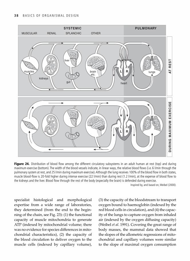
3 8 B A S I C S O F O R G A N I S M A L D E S I G N
specialist histological and morphological expertise from a wide range of laboratories, they determined (from the end to the begin-ning of the chain, see Fig. 23 ): (1) the functional capacity of muscle mitochondria to generate ATP (indexed by mitochondrial volume; there was no evidence for species differences in mito-chondrial characteristics), (2) the capacity of the blood circulation to deliver oxygen to the muscle cells (indexed by capillary volume),
(3) the capacity of the bloodstream to transport oxygen bound to haemoglobin (indexed by the red blood cells in circulation), and (4) the capac-ity of the lungs to capture oxygen from inhaled air (indexed by the oxygen diffusing capacity) ( Weibel et al . 1991 ). Covering the great range of body masses, the mammal data showed that the slopes of the allometric regressions of mito-chondrial and capillary volumes were similar to the slope of maximal oxygen consumption
muscles
kidneysgut
brainetc.
liver
heart
lungs
MUSCULAR RENAL SPLANCHIC OTHER
SYSTEMIC PULMONARY
DU
RIN
G M
AX
IMU
M E
XE
RC
ISE
AT
RE
ST
L R
L R
Figure 24. Distribution of blood fl ow among the different circulatory subsystems in an adult human at rest (top) and during maximum exercise (bottom). The width of the blood vessels indicate, in linear ways, the relative blood fl ows (i.e. 6 l/min through the pulmonary system at rest, and 25 l/min during maximum exercise). Although the lung receives 100% of the blood fl ow in both states, muscle blood-fl ow is 20-fold higher during intense exercise (22 l/min) than during rest (1.2 l/min), at the expense of blood fl ow to the kidneys and the liver. Blood fl ow through the rest of the body (especially the brain) is defended during exercise.
Inspired by, and based on, Weibel ( 2000 ).
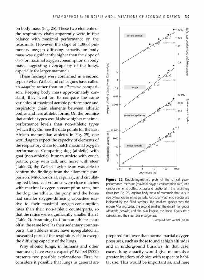
S Y M M O R P H O S I S : P R I N C I P L E A N D L I M I TAT I O N S O F E C O N O M I C D E S I G N 3 9
on body mass ( Fig. 25 ). These two elements of the respiratory chain apparently were in fi ne balance with maximal performance on the treadmills. However, the slope of 1.08 of pul-monary oxygen diffusing capacity on body mass was signifi cantly higher than the slope of 0.86 for maximal oxygen consumption on body mass, suggesting overcapacity of the lungs, especially for larger mammals.
These fi ndings were confi rmed in a second type of what Weibel and colleagues have called an adaptive rather than an allometric compari-son. Keeping body mass approximately con-stant, they went on to compare the same variables of maximal aerobic performance and respiratory chain elements between athletic bodies and less athletic forms. On the premise that athletic types would show higher maximal performance levels than non-athletic types (which they did, see the data points for the East African mammalian athletes in Fig. 25 ), one would again expect the capacity of elements of the respiratory chain to match maximal oxygen performance. Comparing dog (athletic) with goat (non-athletic), human athlete with couch potato, pony with calf, and horse with steer ( Table 2 ), the Weibel–Taylor team was able to confi rm the fi ndings from the allometric com-parison. Mitochondrial, capillary, and circulat-ing red blood cell volumes were close matches with maximal oxygen-consumption rates, but the dog, the athlete, the pony, and the horse had smaller oxygen-diffusing capacities rela-tive to their maximal oxygen-consumption rates than their non-athletic counterparts, so that the ratios were signifi cantly smaller than 1 ( Table 2 ). Assuming that human athletes start off at the same level as their sedentary counter-parts, the athletes must have upregulated all measured parts of the respiratory chain except the diffusing capacity of the lungs.
Why should lungs, in humans and other mammals, have excess capacity? Weibel ( 2000 ) presents two possible explanations. First, he considers it possible that lungs in general are
prepared for lower than normal partial oxygen pressures, such as those found at high altitudes and in underground burrows. In that case, excess lung capacity would give mammals a greater freedom of choice with respect to habi-tat use. This would be important as, and here
1
10
100
mito
chon
dria
l vol
ume
(ml)
100100.01 10.1
body mass (kg)1000
1000
10,0001
10
100
1000
10,000
0.001
0.01
0.1
1
10
0.1
1
10
100
1000
oxyg
en d
iffus
ing
capa
city
(m
l O2/
mm
Hg/
s)
capi
lary
vol
ume
(ml)
max
imal
oxy
gen
cons
umpt
ion
(ml O
2/s)
slope = 0.87
slope = 0.89
slope = 1.08
slope = 0.86
mitochondria
muscle capillaries
lungs
whole animal
Figure 25. Double-logarithmic plots of the critical peak-performance measure (maximal oxygen consumption rate) and various elements, both structural and functional, in the respiratory chain (see Fig. 23 ) against body mass of mammals that vary in size by four orders of magnitude. Particularly ‘athletic’ species are indicated by the fi lled symbols. The smallest species was the mouse Mus musculus , the second smallest the dwarf mongoose Melogale pervula , and the two largest, the horse Equus ferus caballus and the steer Bos primigenius .
Compiled from Weibel ( 2000 ).
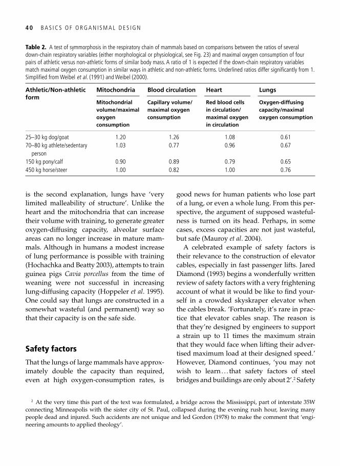
4 0 B A S I C S O F O R G A N I S M A L D E S I G N
2 At the very time this part of the text was formulated, a bridge across the Mississippi, part of interstate 35W connecting Minneapolis with the sister city of St. Paul, collapsed during the evening rush hour, leaving many people dead and injured. Such accidents are not unique and led Gordon ( 1978 ) to make the comment that ‘engi-neering amounts to applied theology’.
is the second explanation, lungs have ‘very limited malleability of structure’. Unlike the heart and the mitochondria that can increase their volume with training, to generate greater oxygen-diffusing capacity, alveolar surface areas can no longer increase in mature mam-mals. Although in humans a modest increase of lung performance is possible with training ( Hochachka and Beatty 2003 ), attempts to train guinea pigs Cavia porcellus from the time of weaning were not successful in increasing lung-diffusing capacity ( Hoppeler et al . 1995 ). One could say that lungs are constructed in a somewhat wasteful (and permanent) way so that their capacity is on the safe side.
Safety factors
That the lungs of large mammals have approx-imately double the capacity than required, even at high oxygen-consumption rates, is
good news for human patients who lose part of a lung, or even a whole lung. From this per-spective, the argument of supposed wasteful-ness is turned on its head. Perhaps, in some cases, excess capacities are not just wasteful, but safe ( Mauroy et al . 2004 ).
A celebrated example of safety factors is their relevance to the construction of elevator cables, especially in fast passenger lifts. Jared Diamond ( 1993 ) begins a wonderfully written review of safety factors with a very frightening account of what it would be like to fi nd your-self in a crowded skyskraper elevator when the cables break. ‘Fortunately, it’s rare in prac-tice that elevator cables snap. The reason is that they’re designed by engineers to support a strain up to 11 times the maximum strain that they would face when lifting their adver-tised maximum load at their designed speed.’ However, Diamond continues, ‘you may not wish to learn . . . that safety factors of steel bridges and buildings are only about 2’. 2 Safety
Table 2. A test of symmorphosis in the respiratory chain of mammals based on comparisons between the ratios of several down-chain respiratory variables (either morphological or physiological, see Fig. 23 ) and maximal oxygen consumption of four pairs of athletic versus non-athletic forms of similar body mass. A ratio of 1 is expected if the down-chain respiratory variables match maximal oxygen consumption in similar ways in athletic and non-athletic forms. Underlined ratios differ signifi cantly from 1. Simplifi ed from Weibel et al . ( 1991 ) and Weibel ( 2000 ).
Athletic/Non-athletic form
Mitochondria Blood circulation Heart Lungs
Mitochondrial volume/maximal oxygen consumption
Capillary volume/maximal oxygen consumption
Red blood cells in circulation/maximal oxygen in circulation
Oxygen-diffusing capacity/maximal oxygen consumption
25–30 kg dog/goat 1.20 1.26 1.08 0.61 70–80 kg athlete/sedentary
person 1.03 0.77 0.96 0.67
150 kg pony/calf 0.90 0.89 0.79 0.65 450 kg horse/steer 1.00 0.82 1.00 0.76
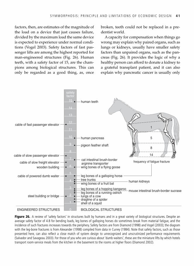
S Y M M O R P H O S I S : P R I N C I P L E A N D L I M I TAT I O N S O F E C O N O M I C D E S I G N 4 1
factors, then, are estimates of the magnitude of the load on a device that just causes failure, divided by the maximum load the same device is expected to experience under normal condi-tions ( Vogel 2003 ). Safety factors of fast pas-senger lifts are among the highest reported for man-engineered structures ( Fig. 26 ). Human teeth, with a safety factor of 15, are the cham-pions among biological structures. This can only be regarded as a good thing, as, once
broken, teeth could not be replaced in a pre- dentist world.
A capacity for compensation when things go wrong may explain why paired organs, such as lungs or kidneys, usually have smaller safety factors than unpaired organs, such as the pan-creas ( Fig. 26 ). It provides the logic of why a healthy person can afford to donate a kidney to a grateful transplant patient, and it can also explain why pancreatic cancer is usually only
0
1
2
3
4
5
6
7
8
9
10
11
12
13
14
15
safetyfactor
human teeth
cable of fast passenger elevator
human pancreas
wing bones of a flying goose
leg bones of a galloping horsetree trunkswing bones of a fruit bat
pigeon feather shaft
leg bones of a hopping kangarooleg bones of a running ostrichlungs of a cowdragline of a spidershell of a squid
cable of slow passenger elevator
cable of slow freight elevatorwooden building
cable of powered dumb waiter
steel building or bridge
human kidneys
mouse intestinal brush-border sucrase
ENGINEERED STRUCTURES BIOLOGICAL STRUCTURES
cat intestinal brush-borderarginine transporter frequency of fatigue fracture
14
8
5
1
Figure 26. A review of ‘safety factors’ in structures built by humans and in a great variety of biological structures. Despite an average safety factor of 4.8 for bending loads, leg bones of galloping horses do sometimes break from material fatigue, and the incidence of such fractures increases towards the periphery. Safety factors are from Diamond ( 1998 ) and Vogel ( 2003 ); the diagram with the leg-bone fractures is from Alexander ( 1998 ) compiled from data in Currey ( 1984 ). Note that safety factors, such as those presented here, can also refl ect a close match of system design to unrecognized and unscrutinized performance requirements ( Salvador and Savageau 2003 ). For those of you who are curious about ‘dumb waiters’, these are the miniature lifts by which hotels transport room-service meals from the kitchen in the basement to the rooms at higher fl oors ( Diamond 2002 ).
4 2 B A S I C S O F O R G A N I S M A L D E S I G N
detected when pancreatic enzyme outputs have dropped to only 10% of normal peak val-ues (DiMagno et al . 1973, Diamond 2002 ). That the wing bones of birds have a safety factor of approximately 6, whereas their feather shafts have a safety factor of 9 ( Fig. 26 ), probably has to do with the higher variability of the over-load on structures, such as fl ight feathers, when compared with wing bones ( Corning and Biewener 1998 ). It is not diffi cult to imagine that the wing bones of fast-fl ying animals, such as birds and bats, face greater overloads (e.g. when hitting or avoiding obstacles in mid-air) than the leg bones of hopping kangaroos, which in turn may face greater stresses than the leg bones of ostriches running on fl at ground. These examples clearly suggest some of the general engineering considerations sum-marized in Table 3 : with an increase in the coef-fi cients of variation of load or capacity, and with an increase in the costs of failure (high for fast elevators, lower for slow elevators and negligible for dumb waiters), safety factors should go up. This is also true if the capacity of structures to withstand overloads deteriorates with time; an example would be the keratin
used by birds to build their feathers ( Bonser 1996 , Weber et al . 2005 ). While wear and tear on feathers may well explain their relatively high safety factor, it certainly explains their regular replacement during moult.
At the low end of safety factors higher than one (remember that 1 indicates symmorphosis as originally understood) are structures such as the spider’s dragline. Draglines just have to carry the spider’s own weight, and some of its prey. In cases when local failure actually gives a fi tness advantage, safety factors can thus better be lower than 1 and do not quite deserve the term any more ( Vogel 2003 ). In the summer of 1999, during an icebreaker-based expedition organ-ized by the Swedish Polar Secretariat, we vis-ited a series of tundra sites across the Canadian Arctic. We were interested in the spatial varia-tion of predation pressure by shorebirds on insects. Research partner Jens Rydell then pro-posed to count, as a measure of predation pres-sure, the number of legs remaining on mature cranefl ies (Tipulidae; they start off with six). With too few cranefl ies captured per site, the plan did not quite work, but the story makes the point that giving up a leg grabbed by a bird can be a good thing for a cranefl y, if it prevents it from being eaten. There are other examples where places of weak construction in a struc-ture pay off: self-amputations occur in spiders (eight legs to lose) and lizards (one tail to spare, but the tail will grow back). Nicely obeying the evolutionary engineering principles advocated in this book, lacertid lizards Podarcis spp. that live in places with high predation pressure, release their tails more readily when receiving the proper prompting than similar lizards that have less to fear ( Cooper et al . 2004 ). Birds adap-tively drop their tail feathers when pursued or grabbed by raptors for exactly the same reason ( Lindström and Nilsson 1988 , de Nie 2002 , Møller et al . 2006 ). Trees may survive a storm if some weaker branches snap and streamline the remaining structure ( Heinrich 1997 ). At this
Table 3. Nine considerations that would either increase (+) or decrease (−) the setting of safety factors in design processes. Modifi ed from Diamond ( 2002 ).
Consideration Increase or decrease of setpoint value
Coeffi cient of variation of load + Coeffi cient of variation of
capacity +
Deterioration of capacity with time
+
Cost of failure + Cost of initial construction – Cost of maintenance – Cost of operation – Opportunity cost of occupied
space –
Cost of rebuilding –
S Y M M O R P H O S I S : P R I N C I P L E A N D L I M I TAT I O N S O F E C O N O M I C D E S I G N 4 3
point you may want to go to the garden shed to verify whether those long-legged spiders, the harvestmen (order Opiliones), do indeed move around well with only 5, 6 or 7 legs!
For spiders, the combined costs of losing a leg and rebuilding it, or losing a silky dragline and renewing it, are relatively cheap. As listed in Table 3 , with increasing costs of construc-tion, maintenance, and operation, safety fac-tors should go down. Cost considerations may explain why, despite safety factors close to 5, race horses nevertheless break leg bones, and, particularly, why the frequencies of fatigue fractures during or prior to falling increase in the bones at the extremities ( Fig. 26 ); these bones are made of the same material as those closer to the core of the horse. The costs of transport during running (which, as we have seen, Hoyt and Taylor’s horse wanted to mini-mize, Fig. 22 ), will go up a great deal if the lower leg bones are given extra strength and weight ( Alexander 1984 , 1998 ). After all, these parts have to be powered with the greatest momentum. Incidentally, the lack of weight in the extremities explains why long- and thin-legged birds, like shorebirds, have relatively low costs when they run ( Bruinzeel et al . 1999 ).
This brings us back to previous considera-tions about weaker than average links in serial constructions such as the respiratory chain, or indeed, the legs of a horse. As explained by Alexander ( 1997 , 1998 ), if elements in a chain differ in the coeffi cients of variation with respect to load, capacity, and/or cost ( Table 3 ), the performance of the system is optimized by devoting resources to extra capacity for the more variable or the cheaper element. Quite literally, in a chain made partly of expensive gold links and partly of cheap iron links, mak-ing the gold links very slightly weaker and the iron links much stronger would result in a stronger chain for the same price. This is some-what counter-intuitive, but means, as poin-ted out by Alexander ( 1998 ), that because the
metabolic rate of lungs is smaller than the met-abolic rate of the skeletal musculature, the oxygen-diffusing surface of the lungs is the relatively cheap link in the respiratory chain. Therefore, he predicted, lungs would be designed for higher capacities than the rela-tively expensive mitochondria!
Multiple design criteria
Since their grand summary in 1991 of tests of the symmorphosis principle, by detailed stud-ies on serial capacities in the respiratory chains of mammals, and in the face of serious con-structive criticism (e.g. Garland and Huey 1987 , Lindstedt and Jones 1987 , Dudley and Gans 1991 , Garland 1998 , Gordon 1998 , Bacigalupe and Bozinovic 2002 ), Weibel and associates have regularly updated their analy-ses ( Weibel et al . 1992 , 2004 , Weibel and Hoppeler 2005 ). They clearly stand by their conclusion that respiratory chain elements such as the vascular supply network and the energy needs of the cells active during maxi-mal work are quantitatively coupled to maximal metabolic rates; these elements thus have safety factors close to 1. Although sym-morphosis is no longer a hotly debated issue ( Suarez and Darveau 2005 ), the previous dis-cussion illustrates that the principle of elegant economic design needs qualifi cation.
Let us get back to lungs. Although we have not acknowledged this yet, they do more than catch oxygen for the circulation of blood and eventual delivery to the mitochondrial power-houses. Lungs also service the body by remov-ing carbon dioxide, one of the products of metabolism, from the bloodstream. The remo-val of carbon dioxide and the regulation of blood pH (a delicate function of carbon diox-ide level in the body circulation) may put dif-ferent design constraints on the lungs ( Lindstedt and Jones 1987 , Dudley and Gans
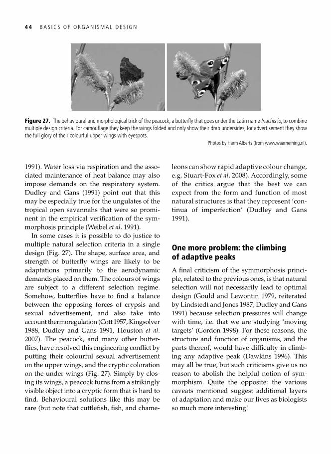
4 4 B A S I C S O F O R G A N I S M A L D E S I G N
1991 ). Water loss via respiration and the asso-ciated maintenance of heat balance may also impose demands on the respiratory system. Dudley and Gans ( 1991 ) point out that this may be especially true for the ungulates of the tropical open savannahs that were so promi-nent in the empirical verifi cation of the sym-morphosis principle ( Weibel et al . 1991 ).
In some cases it is possible to do justice to multiple natural selection criteria in a single design ( Fig. 27 ). The shape, surface area, and strength of butterfl y wings are likely to be adaptations primarily to the aerodynamic demands placed on them. The colours of wings are subject to a different selection regime. Somehow, butterfl ies have to fi nd a balance between the opposing forces of crypsis and sexual advertisement, and also take into account thermoregulation ( Cott 1957 , Kingsolver 1988 , Dudley and Gans 1991 , Houston et al . 2007 ). The peacock, and many other butter-fl ies, have resolved this engineering confl ict by putting their colourful sexual advertisement on the upper wings, and the cryptic coloration on the under wings ( Fig. 27 ). Simply by clos-ing its wings, a peacock turns from a strikingly visible object into a cryptic form that is hard to fi nd. Behavioural solutions like this may be rare (but note that cuttlefi sh, fi sh, and chame-
leons can show rapid adaptive colour change, e.g. Stuart-Fox et al . 2008 ). Accordingly, some of the critics argue that the best we can expect from the form and function of most natural structures is that they represent ‘con-tinua of imperfection’ ( Dudley and Gans 1991 ).
One more problem: the climbing of adaptive peaks
A fi nal criticism of the symmorphosis princi-ple, related to the previous ones, is that natural selection will not necessarily lead to optimal design ( Gould and Lewontin 1979 , reiterated by Lindstedt and Jones 1987 , Dudley and Gans 1991 ) because selection pressures will change with time, i.e. that we are studying ‘moving targets’ ( Gordon 1998 ). For these reasons, the structure and function of organisms, and the parts thereof, would have diffi culty in climb-ing any adaptive peak ( Dawkins 1996 ). This may all be true, but such criticisms give us no reason to abolish the helpful notion of sym-morphism. Quite the opposite: the various caveats mentioned suggest additional layers of adaptation and make our lives as biologists so much more interesting!
Figure 27. The behavioural and morphological trick of the peacock, a butterfl y that goes under the Latin name Inachis io , to combine multiple design criteria. For camoufl age they keep the wings folded and only show their drab undersides; for advertisement they show the full glory of their colourful upper wings with eyespots.
Photos by Harm Alberts (from www.waarneming.nl ).
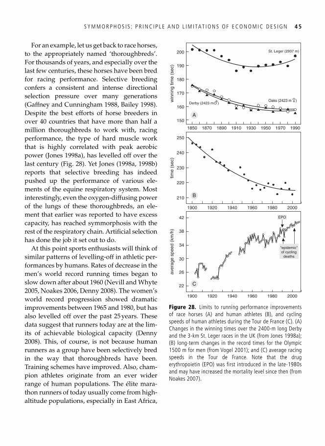
S Y M M O R P H O S I S : P R I N C I P L E A N D L I M I TAT I O N S O F E C O N O M I C D E S I G N 4 5
For an example, let us get back to race horses, to the appropriately named ‘thoroughbreds’. For thousands of years, and especially over the last few centuries, these horses have been bred for racing performance. Selective breeding confers a consistent and intense directional selection pressure over many generations ( Gaffney and Cunningham 1988 , Bailey 1998 ). Despite the best efforts of horse breeders in over 40 countries that have more than half a million thoroughbreds to work with, racing performance, the type of hard muscle work that is highly correlated with peak aerobic power ( Jones 1998a ), has levelled off over the last century ( Fig. 28 ). Yet Jones ( 1998a , 1998b ) reports that selective breeding has indeed pushed up the performance of various ele-ments of the equine respiratory system. Most interestingly, even the oxygen-diffusing power of the lungs of these thoroughbreds, an ele-ment that earlier was reported to have excess capacity, has reached symmorphosis with the rest of the respiratory chain. Artifi cial selection has done the job it set out to do.
At this point sports enthusiasts will think of similar patterns of levelling-off in athletic per-formances by humans. Rates of decrease in the men’s world record running times began to slow down after about 1960 ( Nevill and Whyte 2005 , Noakes 2006 , Denny 2008 ). The women’s world record progression showed dramatic improvements between 1965 and 1980, but has also levelled off over the past 25 years. These data suggest that runners today are at the lim-its of achievable biological capacity ( Denny 2008 ). This, of course, is not because human runners as a group have been selectively bred in the way that thoroughbreds have been. Training schemes have improved. Also, cham-pion athletes originate from an ever wider range of human populations. The élite mara-thon runners of today usually come from high-altitude populations, especially in East Africa,
22
30
26
34
38
42
aver
age
spee
d (k
m/h
)
St. Leger (2937 m)
210
230
220
240
250
time
(sec
)
150
190
170
160
A
B
C
180
win
ning
tim
e (s
ec)
1850
200
Oaks (2423 m )
EPO
Derby (2423 m )
"epidemic"of cycling
deaths
1870 1890 1910 1930 1950 1970 1990
1900 1920 1940 1960 1980 2000
1900 1920 1940 1960 1980 2000
Figure 28. Limits to running performance improvements of race horses (A) and human athletes (B), and cycling speeds of human athletes during the Tour de France (C). (A) Changes in the winning times over the 2400-m long Derby and the 3-km St. Leger races in the UK (from Jones 1998a ); (B) long-term changes in the record times for the Olympic 1500 m for men (from Vogel 2001 ); and (C) average racing speeds in the Tour de France. Note that the drug erythropoietin (EPO) was first introduced in the late-1980s and may have increased the mortality level since then (from Noakes 2007 ).
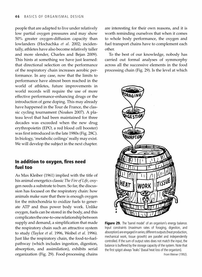
4 6 B A S I C S O F O R G A N I S M A L D E S I G N
people that are adapted to live under relatively low partial oxygen pressures and may show 50% greater oxygen-diffusion capacity than lowlanders ( Hochachka et al . 2002 ; inciden-tally, athletes have also become relatively taller and more slender, Charles and Bejan 2009 ). This hints at something we have just learned: that directional selection on the performance of the respiratory chain increases aerobic per-formance. In any case, now that the limits to performance have almost been reached in the world of athletes, future improvements in world records will require the use of more effective performance-enhancing drugs or the introduction of gene doping. This may already have happened in the Tour de France, the clas-sic cycling tournament ( Noakes 2007 ). A pla-teau level that had been maintained for three decades was exceeded when the new drug erythropoietin (EPO, a red blood cell booster) was fi rst introduced in the late 1980s ( Fig. 28C ). In biology, ‘metabolic ceilings’ really may exist. We will develop the subject in the next chapter.
In addition to oxygen, fi res need fuel too
As Max Kleiber ( 1961 ) implied with the title of his animal energetics classic The Fire of Life , oxy-gen needs a substrate to burn. So far, the discus-sion has focused on the respiratory chain: how animals make sure that there is enough oxygen for the mitochondria to oxidize fuels to gener-ate ATP and thus power body work. Unlike oxygen, fuels can be stored in the body, and this complicates the one-to-one relationship between supply and demand, a simplifi cation that made the respiratory chain such an attractive system to study ( Taylor et al . 1996 , Weibel et al . 1996 ). Just like the respiratory chain, the food-to-fuel-pathway (which includes ingestion, digestion, absorption, and assimilation), exhibits serial organization ( Fig. 29 ). Food-processing chains
are interesting for their own reasons, and it is worth reminding ourselves that when it comes to whole body performance, the oxygen and fuel transport chains have to complement each other.
To the best of our knowledge, nobody has carried out formal analyses of symmorphy across all the successive elements in the food processing chain ( Fig. 29 ). Is the level at which
Figure 29. The ‘barrel model’ of an organism’s energy balance. Input constraints (maximum rates of foraging, digestion, and absorption) are engaged in series; different outputs (heat production, mechanical work, tissue growth) are parallel and independently controlled. If the sum of output rates does not match the input, the balance is buffered by the storage capacity of the system. Note that the fi rst spigot always ‘leaks’ (basal heat loss of the organism).
From Weiner ( 1992 ).
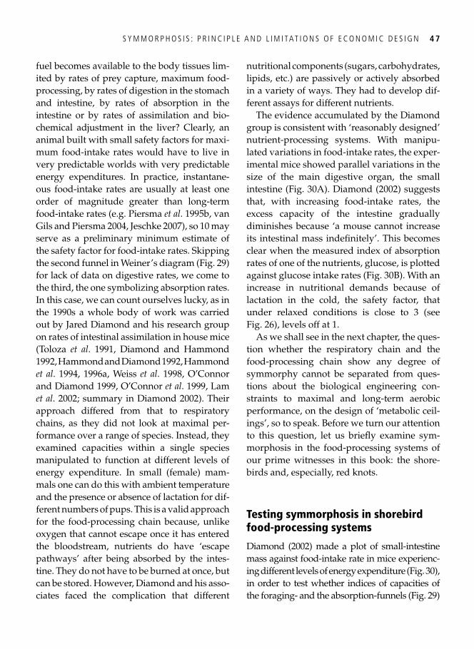
S Y M M O R P H O S I S : P R I N C I P L E A N D L I M I TAT I O N S O F E C O N O M I C D E S I G N 4 7
fuel becomes available to the body tissues lim-ited by rates of prey capture, maximum food-processing, by rates of digestion in the stomach and intestine, by rates of absorption in the intestine or by rates of assimilation and bio-chemical adjustment in the liver? Clearly, an animal built with small safety factors for maxi-mum food-intake rates would have to live in very predictable worlds with very predictable energy expenditures. In practice, instantane-ous food-intake rates are usually at least one order of magnitude greater than long-term food-intake rates (e.g. Piersma et al . 1995b , van Gils and Piersma 2004 , Jeschke 2007 ), so 10 may serve as a preliminary minimum estimate of the safety factor for food-intake rates. Skipping the second funnel in Weiner’s diagram ( Fig. 29 ) for lack of data on digestive rates, we come to the third, the one symbolizing absorption rates. In this case, we can count ourselves lucky, as in the 1990s a whole body of work was carried out by Jared Diamond and his research group on rates of intestinal assimilation in house mice ( Toloza et al . 1991 , Diamond and Hammond 1992 , Hammond and Diamond 1992 , Hammond et al . 1994 , 1996a , Weiss et al . 1998 , O’Connor and Diamond 1999 , O’Connor et al . 1999 , Lam et al . 2002 ; summary in Diamond 2002 ). Their approach differed from that to respiratory chains, as they did not look at maximal per-formance over a range of species. Instead, they examined capacities within a single species manipulated to function at different levels of energy expenditure. In small (female) mam-mals one can do this with ambient temperature and the presence or absence of lactation for dif-ferent numbers of pups. This is a valid approach for the food-processing chain because, unlike oxygen that cannot escape once it has entered the bloodstream, nutrients do have ‘escape pathways’ after being absorbed by the intes-tine. They do not have to be burned at once, but can be stored. However, Diamond and his asso-ciates faced the complication that different
nutritional components (sugars, carbohydrates, lipids, etc.) are passively or actively absorbed in a variety of ways. They had to develop dif-ferent assays for different nutrients.
The evidence accumulated by the Diamond group is consistent with ‘reasonably designed’ nutrient-processing systems. With manipu-lated variations in food-intake rates, the exper-imental mice showed parallel variations in the size of the main digestive organ, the small intestine ( Fig. 30A ). Diamond ( 2002 ) suggests that, with increasing food-intake rates, the excess capacity of the intestine gradually diminishes because ‘a mouse cannot increase its intestinal mass indefi nitely’. This becomes clear when the measured index of absorption rates of one of the nutrients, glucose, is plotted against glucose intake rates ( Fig. 30B ). With an increase in nutritional demands because of lactation in the cold, the safety factor, that under relaxed conditions is close to 3 (see Fig. 26 ), levels off at 1.
As we shall see in the next chapter, the ques-tion whether the respiratory chain and the food-processing chain show any degree of symmorphy cannot be separated from ques-tions about the biological engineering con-straints to maximal and long-term aerobic performance, on the design of ‘metabolic ceil-ings’, so to speak. Before we turn our attention to this question, let us briefl y examine sym-morphosis in the food-processing systems of our prime witnesses in this book: the shore-birds and, especially, red knots.
Testing symmorphosis in shorebird food-processing systems
Diamond ( 2002 ) made a plot of small-intestine mass against food-intake rate in mice experienc-ing different levels of energy expenditure ( Fig. 30 ), in order to test whether indices of capacities of the foraging- and the absorption-funnels ( Fig. 29 )
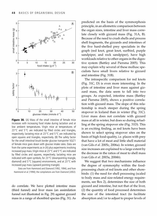
4 8 B A S I C S O F O R G A N I S M A L D E S I G N
do correlate. We have plotted intestine mass (third funnel) and liver mass (an assimilation funnel not illustrated in Fig. 29 ) against gizzard mass in a range of shorebird species ( Fig. 31 ). As
predicted on the basis of the symmorphosis principle, in an allometric comparison between the organ sizes, intestine and liver mass corre-late closely with gizzard mass ( Fig. 31A , B). Because of the need to crush shells and process shell fragments, the gizzards and intestines of the fi ve hard-shelled prey specialists in the graph (red knot, great knot, surfbird, purple sandpiper, and rock sandpiper), have high workloads relative to other organs in the diges-tive system ( Battley and Piersma 2005 ). This may explain why several of these mollusc spe-cialists have small livers relative to gizzard and intestine ( Fig. 31B ).
The intraspecifi c comparison for red knots ( Fig. 31C , D) is even more interesting. In the plots of intestine and liver mass against giz-zard mass, the data seem to fall into two groups. As expected, intestine mass ( Battley and Piersma 2005 ), shows a positive correla-tion with gizzard mass. The slope of this rela-tionship is much steeper during the spring stopover in Iceland than in winter ( Fig. 31C ). Liver mass does not correlate with gizzard mass at all in winter, but does so during refuel-ling at the spring stopover site ( Fig. 31D ). This is an exciting fi nding, as red knots have been shown to select spring stopover sites on the basis of high food-quality, i.e. places with prey that have a lot of meat and little shell material ( van Gils et al . 2005c , 2006a ). In winter, gizzard size increases are explained to a large extent by the decrease in the ratios of meat to shell mass ( van Gils et al . 2003a , 2006b ).
We suggest that two mechanisms infl uence the degree of symmorphy within the food-processing chain of red knots and other shore-birds: (1) the need for shell processing (scaled to body mass and size-related energy require-ments, see Box 2 ), determines the size of both gizzard and intestine, but not that of the liver, (2) the quantity of food processed determines the size of the intestinal tract (to facilitate absorption and/or to adjust to proper levels of
00
1
2
3
safe
ty fa
ctor
10 20 30 40 50glucose intake (mmole d–1)
food intake (g d–1)0
0
1
2
3
4
5 A
B
smal
l int
estin
e m
ass
(g)
10 205 25 3015
Figure 30. (A) Mass of the small intestine of female mice increases with increasing food intake during lactation and at low ambient temperatures. Virgin mice at temperatures of 23 °C and 5 °C are indicated by fi lled circles and triangles, respectively; lactating mice at 23 °C and 5 °C are indicated by open squares and triangles, respectively. (B) The safety factor for the small intestinal brush border glucose transporter SGLT1 of female mice goes down with glucose intake rates. Data are from the same experiments as in (A) plus experiments involving increased pup mass. Virgin mice at 23 °C and 5 °C are indicated by fi lled circles and squares, respectively; lactating mice are indicated with open symbols, for 23 °C (downpointing triangle, diamond) and 5 °C (squares) environments, and at 23 °C with increased pup mass (upward pointing triangle).
Data are from Hammond and Diamond ( 1992 , 1994 ), and from Hammond et al. ( 1994 ); the compilations are from Diamond ( 2002 ).
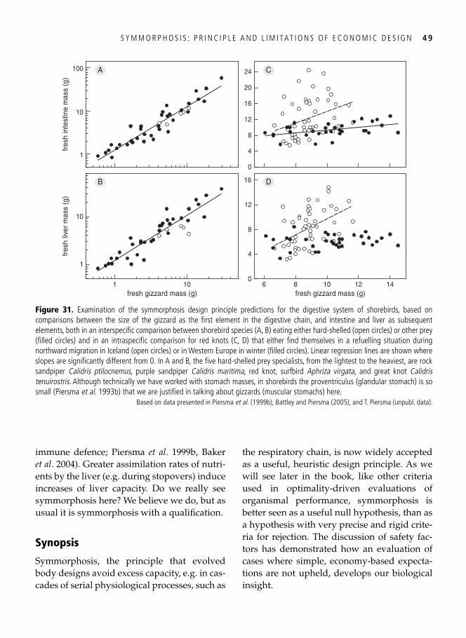
S Y M M O R P H O S I S : P R I N C I P L E A N D L I M I TAT I O N S O F E C O N O M I C D E S I G N 4 9
immune defence; Piersma et al . 1999b , Baker et al . 2004 ). Greater assimilation rates of nutri-ents by the liver (e.g. during stopovers) induce increases of liver capacity. Do we really see symmorphosis here? We believe we do, but as usual it is symmorphosis with a qualifi cation.
Synopsis
Symmorphosis, the principle that evolved body designs avoid excess capacity, e.g. in cas-cades of serial physiological processes, such as
the respiratory chain, is now widely accepted as a useful, heuristic design principle. As we will see later in the book, like other criteria used in optimality-driven evaluations of organismal performance, symmorphosis is better seen as a useful null hypothesis, than as a hypothesis with very precise and rigid crite-ria for rejection. The discussion of safety fac-tors has demonstrated how an evaluation of cases where simple, economy-based expecta-tions are not upheld, develops our biological insight.
10
1
fres
h liv
er m
ass
(g)
101fresh gizzard mass (g)
0
12
4
8
16
12106 8fresh gizzard mass (g)
14
10
1
100 A C
DB
fres
h in
test
ine
mas
s (g
)
0
12
4
8
16
20
24
Figure 31. Examination of the symmorphosis design principle predictions for the digestive system of shorebirds, based on comparisons between the size of the gizzard as the fi rst element in the digestive chain, and intestine and liver as subsequent elements, both in an interspecifi c comparison between shorebird species (A, B) eating either hard-shelled (open circles) or other prey (fi lled circles) and in an intraspecifi c comparison for red knots (C, D) that either fi nd themselves in a refuelling situation during northward migration in Iceland (open circles) or in Western Europe in winter (fi lled circles). Linear regression lines are shown where slopes are signifi cantly different from 0. In A and B, the fi ve hard-shelled prey specialists, from the lightest to the heaviest, are rock sandpiper Calidris ptilocnemus , purple sandpiper Calidris maritima , red knot, surfbird Aphriza virgata , and great knot Calidris tenuirostris . Although technically we have worked with stomach masses, in shorebirds the proventriculus (glandular stomach) is so small ( Piersma et al . 1993b ) that we are justifi ed in talking about gizzards (muscular stomachs) here.
Based on data presented in Piersma et al . ( 1999b ), Battley and Piersma ( 2005 ), and T. Piersma (unpubl. data).
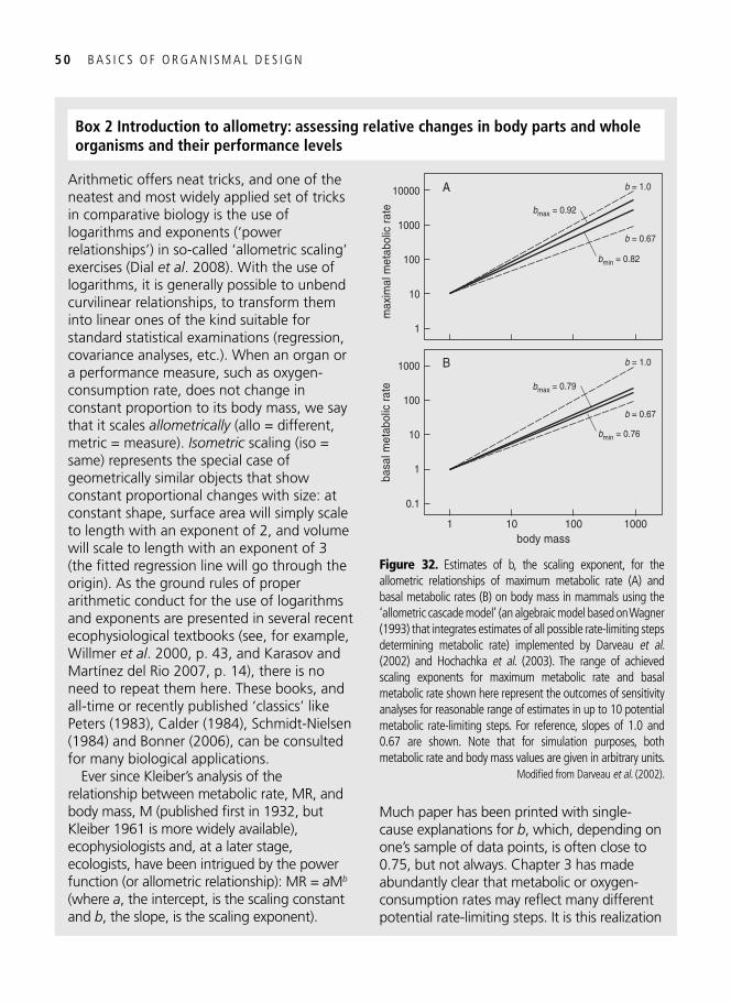
5 0 B A S I C S O F O R G A N I S M A L D E S I G N
Box 2 Introduction to allometry: assessing relative changes in body parts and wholeorganisms and their performance levels
Arithmetic offers neat tricks, and one of the neatest and most widely applied set of tricks in comparative biology is the use of logarithms and exponents (‘power relationships’) in so-called ‘allometric scaling’ exercises ( Dial et al . 2008 ). With the use of logarithms, it is generally possible to unbend curvilinear relationships, to transform them into linear ones of the kind suitable for standard statistical examinations (regression, covariance analyses, etc.). When an organ or a performance measure, such as oxygen-consumption rate, does not change in constant proportion to its body mass, we say that it scales allometrically (allo = different, metric = measure). Isometric scaling (iso = same) represents the special case of geometrically similar objects that show constant proportional changes with size: at constant shape, surface area will simply scale to length with an exponent of 2, and volume will scale to length with an exponent of 3 (the fi tted regression line will go through the origin). As the ground rules of proper arithmetic conduct for the use of logarithms and exponents are presented in several recent ecophysiological textbooks (see, for example, Willmer et al . 2000 , p. 43, and Karasov and Martínez del Rio 2007 , p. 14), there is no need to repeat them here. These books, and all-time or recently published ‘classics’ like Peters ( 1983 ), Calder ( 1984 ), Schmidt-Nielsen ( 1984 ) and Bonner ( 2006 ), can be consulted for many biological applications.
Ever since Kleiber’s analysis of the relationship between metabolic rate, MR, and body mass, M (published fi rst in 1932, but Kleiber 1961 is more widely available), ecophysiologists and, at a later stage, ecologists, have been intrigued by the power function (or allometric relationship): MR = a M b (where a , the intercept, is the scaling constant and b , the slope, is the scaling exponent).
Much paper has been printed with single-cause explanations for b , which, depending on one’s sample of data points, is often close to 0.75, but not always. Chapter 3 has made abundantly clear that metabolic or oxygen-consumption rates may refl ect many different potential rate-limiting steps. It is this realization
1
0.1
basa
l met
abol
ic ra
te
101body mass
10
100 1000
100
1000 b = 1.0
b = 0.67
10
1
max
imal
met
abol
ic r
ate
100
1000
10000 A
B
bmax = 0.92
b = 1.0
b = 0.67
bmin = 0.82
bmax = 0.79
bmin = 0.76
Figure 32. Estimates of b, the scaling exponent, for the allometric relationships of maximum metabolic rate (A) and basal metabolic rates (B) on body mass in mammals using the ‘allometric cascade model’ (an algebraic model based on Wagner ( 1993 ) that integrates estimates of all possible rate-limiting steps determining metabolic rate) implemented by Darveau et al . ( 2002 ) and Hochachka et al . ( 2003 ). The range of achieved scaling exponents for maximum metabolic rate and basal metabolic rate shown here represent the outcomes of sensitivity analyses for reasonable range of estimates in up to 10 potential metabolic rate-limiting steps. For reference, slopes of 1.0 and 0.67 are shown. Note that for simulation purposes, both metabolic rate and body mass values are given in arbitrary units.
Modifi ed from Darveau et al . ( 2002 ).
S Y M M O R P H O S I S : P R I N C I P L E A N D L I M I TAT I O N S O F E C O N O M I C D E S I G N 5 1
that caused Charles Darveau, his supervisor Peter Hochachka and their associates, to try and operationalize b not to refl ect a single rate-limiting process, but to refl ect the whole cascade of key steps in the complex pathways of energy demand and energy supply ( Darveau et al . 2002 , 2003 , Hochachka et al . 2003 , Suarez et al . 2004 ; the immediate criticisms by Banavar et al . 2003 , West et al . 2003 are also instructive to read and to get a feel for this enormous literature).
The team of Hochachka and Darveau comes to the conclusion that the generally
lower scaling exponent b for basal metabolic rate compared with maximum metabolic rate ( Fig. 32 ), can be explained by different rate-limiting steps being most important in the two exercise conditions. For basal metabolic rate, oxygen-delivery steps of the kind discussed in the symmorphosis literature and in this chapter (relatively low exponents), contribute almost nothing to the overall scaling exponent b . In contrast, for maximum metabolic rates, b is controlled entirely by the oxygen delivery steps (relatively high exponents).

This page intentionally left blank
Part II
Adding environment

This page intentionally left blank
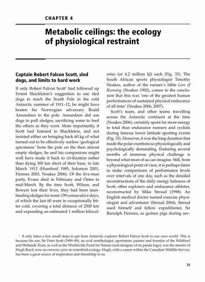
55
CHAPTER 4
Metabolic ceilings: the ecology of physiological restraint
Captain Robert Falcon Scott, sled dogs, and limits to hard work
If only Robert Falcon Scott 1 had followed up Ernest Shackleton’s suggestion to use sled dogs to reach the South Pole in the cold Antarctic summer of 1911–12, he might have beaten his Norwegian adversary Roald Amundsen to the pole. Amundsen did use dogs to pull sledges, sacrifi cing some to feed the others as they went. More importantly, if Scott had listened to Shackleton, and not insisted either on bringing back 60 kg of what turned out to be effectively useless ‘geological specimens’ from the pole on the then almost empty sledges, he and his companions might well have made it back to civilization rather than dying 300 km short of their base, in late March 1912 ( Huntford 1985 , Solomon 2001 , Fiennes 2003 , Noakes 2006 ). Of the fi ve-man party, Evans died in February and Oates in mid-March. By the time Scott, Wilson, and Bowers lost their lives, they had been man-hauling sledges for some 159 consecutive days, of which the last 60 were in exceptionally bit-ter cold, covering a total distance of 2500 km and expending an estimated 1 million kilocal-
ories (or 4.2 million kJ) each ( Fig. 33 ). The South African sports physiologist Timothy Noakes, author of the runner’s bible Lore of Running ( Noakes 1992 ), comes to the conclu-sion that this was ‘one of the greatest human performances of sustained physical endurance of all time’ ( Noakes 2006 , 2007 ).
Scott’s team, and other teams travelling across the Antarctic continent at the time ( Noakes 2006 ), certainly spent far more energy in total than endurance runners and cyclists during famous lower latitude sporting events ( Fig. 33 ). However, it was the long duration that made the polar exertions so physiologically and psychologically demanding. Enduring several months of immense physical challenge is beyond what most of us can imagine. Still, from a physiological point of view, it is perhaps fairer to make comparisons of performance levels over intervals of one day, such as the detailed reconstructions of the daily energy balances of Scott, other explorers and endurance athletes, reconstructed by Mike Stroud ( 1998 ). An English medical doctor turned exercise physi-ologist and adventurer ( Stroud 2004 ), Stroud used himself and fellow expeditioner, Sir Ranulph Fiennes, as guinea pigs during sev-
1 It only takes a few small steps to get from Antarctic explorer Robert Falcon Scott to our own world. This is because his son, Sir Peter Scott (1909–89), an avid ornithologist, sportsman, painter and founder of the Wildfowl and Wetlands Trust, as well as the Worldwide Fund for Nature (and designer of its panda logo), was the mentor of Hugh Boyd, now an eminence grise in waterbird ecology. Hugh, with a career within the Canadian Wildlife Service, has been a great source of inspiration and friendship to us.
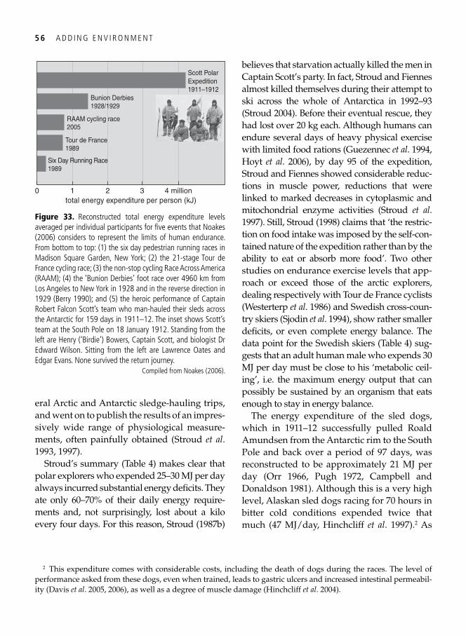
5 6 A D D I N G E N V I R O N M E N T
eral Arctic and Antarctic sledge-hauling trips, and went on to publish the results of an impres-sively wide range of physiological measure-ments, often painfully obtained ( Stroud et al . 1993 , 1997 ).
Stroud’s summary ( Table 4 ) makes clear that polar explorers who expended 25–30 MJ per day always incurred substantial energy defi cits. They ate only 60–70% of their daily energy require-ments and, not surprisingly, lost about a kilo every four days. For this reason, Stroud ( 1987b )
believes that starvation actually killed the men in Captain Scott’s party. In fact, Stroud and Fiennes almost killed themselves during their attempt to ski across the whole of Antarctica in 1992–93 ( Stroud 2004 ). Before their eventual rescue, they had lost over 20 kg each. Although humans can endure several days of heavy physical exercise with limited food rations ( Guezennec et al . 1994 , Hoyt et al . 2006 ), by day 95 of the expedition, Stroud and Fiennes showed considerable reduc-tions in muscle power, reductions that were linked to marked decreases in cytoplasmic and mitochondrial enzyme activities ( Stroud et al . 1997 ). Still, Stroud ( 1998 ) claims that ‘the restric-tion on food intake was imposed by the self-con-tained nature of the expedition rather than by the ability to eat or absorb more food’. Two other studies on endurance exercise levels that app-roach or exceed those of the arctic explorers, dealing respectively with Tour de France cyclists ( Westerterp et al . 1986 ) and Swedish cross-coun-try skiers ( Sjodin et al . 1994 ), show rather smaller defi cits, or even complete energy balance. The data point for the Swedish skiers ( Table 4 ) sug-gests that an adult human male who expends 30 MJ per day must be close to his ‘metabolic ceil-ing’, i.e. the maximum energy output that can possibly be sustained by an organism that eats enough to stay in energy balance.
The energy expenditure of the sled dogs, which in 1911–12 successfully pulled Roald Amundsen from the Antarctic rim to the South Pole and back over a period of 97 days, was reconstructed to be approximately 21 MJ per day ( Orr 1966 , Pugh 1972 , Campbell and Donaldson 1981 ). Although this is a very high level, Alaskan sled dogs racing for 70 hours in bitter cold conditions expended twice that much (47 MJ/day, Hinchcliff et al . 1997 ). 2 As
Scott PolarExpedition1911–1912
0 2 4 million
Bunion Derbies1928/1929
RAAM cycling race2005
Tour de France1989
Six Day Running Race1989
total energy expenditure per person (kJ)31
Figure 33. Reconstructed total energy expenditure levels averaged per individual participants for fi ve events that Noakes ( 2006 ) considers to represent the limits of human endurance. From bottom to top: (1) the six day pedestrian running races in Madison Square Garden, New York; (2) the 21-stage Tour de France cycling race; (3) the non-stop cycling Race Across America (RAAM); (4) the ‘Bunion Derbies’ foot race over 4960 km from Los Angeles to New York in 1928 and in the reverse direction in 1929 ( Berry 1990 ); and (5) the heroic performance of Captain Robert Falcon Scott’s team who man-hauled their sleds across the Antarctic for 159 days in 1911–12. The inset shows Scott’s team at the South Pole on 18 January 1912. Standing from the left are Henry (‘Birdie’) Bowers, Captain Scott, and biologist Dr Edward Wilson. Sitting from the left are Lawrence Oates and Edgar Evans. None survived the return journey.
Compiled from Noakes ( 2006 ).
2 This expenditure comes with considerable costs, including the death of dogs during the races. The level of performance asked from these dogs, even when trained, leads to gastric ulcers and increased intestinal permeabil-ity ( Davis et al . 2005 , 2006 ), as well as a degree of muscle damage ( Hinchcliff et al . 2004 ).
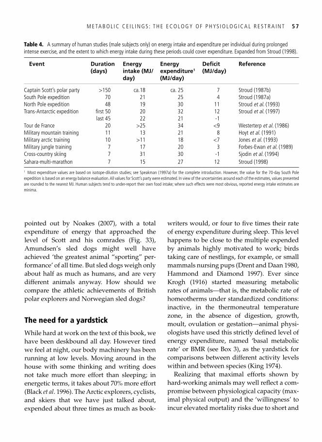
M E TA B O L I C C E I L I N G S : T H E E C O L O G Y O F P H YS I O L O G I C A L R E S T R A I N T 5 7
Table 4. A summary of human studies (male subjects only) on energy intake and expenditure per individual during prolonged intense exercise, and the extent to which energy intake during these periods could cover expenditure. Expanded from Stroud ( 1998 ).
Event Duration (days)
Energy intake (MJ/day)
Energy expenditure 1 (MJ/day)
Defi cit (MJ/day)
Reference
Captain Scott’s polar party >150 ca.18 ca. 25 7 Stroud (1987b) South Pole expedition 70 21 25 4 Stroud (1987a) North Pole expedition 48 19 30 11 Stroud et al . (1993) Trans-Antarctic expedition fi rst 50 20 32 12 Stroud et al . (1997) last 45 22 21 -1 Tour de France 20 >25 34 <9 Westerterp et al . (1986) Military mountain training 11 13 21 8 Hoyt et al . (1991) Military arctic training 10 >11 18 <7 Jones et al . (1993) Military jungle training 7 17 20 3 Forbes-Ewan et al . (1989) Cross-country skiing 7 31 30 -1 Sjodin et al . (1994) Sahara-multi-marathon 7 15 27 12 Stroud (1998)
1 Most expenditure values are based on isotope-dilution studies; see Speakman ( 1997a ) for the complete introduction. However, the value for the 70-day South Pole expedition is based on an energy balance evaluation. All values for Scott’s party were estimated. In view of the uncertainties around each of the estimates, values presented are rounded to the nearest MJ. Human subjects tend to under-report their own food intake; where such effects were most obvious, reported energy intake estimates are minima.
pointed out by Noakes ( 2007 ), with a total expenditure of energy that approached the level of Scott and his comrades ( Fig. 33 ), Amundsen’s sled dogs might well have achieved ‘the greatest animal “sporting” per-formance’ of all time. But sled dogs weigh only about half as much as humans, and are very different animals anyway. How should we compare the athletic achievements of British polar explorers and Norwegian sled dogs?
The need for a yardstick
While hard at work on the text of this book, we have been deskbound all day. However tired we feel at night, our body machinery has been running at low levels. Moving around in the house with some thinking and writing does not take much more effort than sleeping; in energetic terms, it takes about 70% more effort ( Black et al . 1996 ). The Arctic explorers, cyclists, and skiers that we have just talked about, expended about three times as much as book-
writers would, or four to fi ve times their rate of energy expenditure during sleep. This level happens to be close to the multiple expended by animals highly motivated to work; birds taking care of nestlings, for example, or small mammals nursing pups (Drent and Daan 1980, Hammond and Diamond 1997 ). Ever since Krogh ( 1916 ) started measuring metabolic rates of animals—that is, the metabolic rate of homeotherms under standardized conditions: inactive, in the thermoneutral temperature zone, in the absence of digestion, growth, moult, ovulation or gestation—animal physi-ologists have used this strictly defi ned level of energy expenditure, named ‘basal metabolic rate’ or BMR (see Box 3 ), as the yardstick for comparisons between different activity levels within and between species ( King 1974 ).
Realizing that maximal efforts shown by hard-working animals may well refl ect a com-promise between physiological capacity (max-imal physical output) and the ‘willingness’ to incur elevated mortality risks due to short and
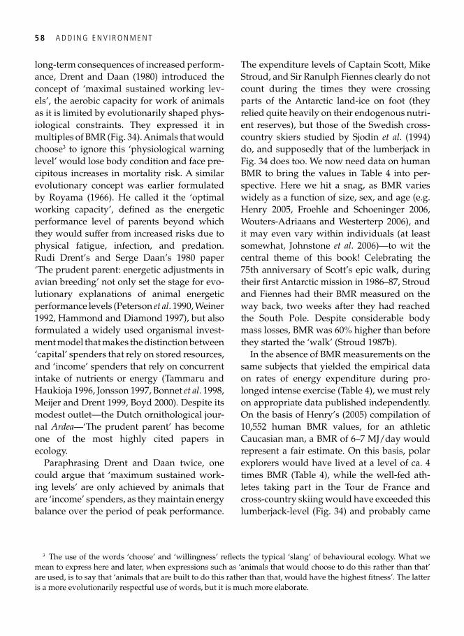
5 8 A D D I N G E N V I R O N M E N T
long-term consequences of increased perform-ance, Drent and Daan (1980) introduced the concept of ‘maximal sustained working lev-els’, the aerobic capacity for work of animals as it is limited by evolutionarily shaped phys-iological constraints. They expressed it in multiples of BMR ( Fig. 34 ). Animals that would choose 3 to ignore this ‘physiological warning level’ would lose body condition and face pre-cipitous increases in mortality risk. A similar evolutionary concept was earlier formulated by Royama ( 1966 ). He called it the ‘optimal working capacity’, defi ned as the energetic performance level of parents beyond which they would suffer from increased risks due to physical fatigue, infection, and predation. Rudi Drent’s and Serge Daan’s 1980 paper ‘The prudent parent: energetic adjustments in avian breeding’ not only set the stage for evo-lutionary explanations of animal energetic performance levels ( Peterson et al . 1990 , Weiner 1992 , Hammond and Diamond 1997 ), but also formulated a widely used organismal invest-ment model that makes the distinction between ‘capital’ spenders that rely on stored resources, and ‘income’ spenders that rely on concurrent intake of nutrients or energy ( Tammaru and Haukioja 1996 , Jonsson 1997 , Bonnet et al . 1998 , Meijer and Drent 1999 , Boyd 2000 ). Despite its modest outlet—the Dutch ornithological jour-nal Ardea —‘The prudent parent’ has become one of the most highly cited papers in ecology.
Paraphrasing Drent and Daan twice, one could argue that ‘maximum sustained work-ing levels’ are only achieved by animals that are ‘income’ spenders, as they maintain energy balance over the period of peak performance.
The expenditure levels of Captain Scott, Mike Stroud, and Sir Ranulph Fiennes clearly do not count during the times they were crossing parts of the Antarctic land-ice on foot (they relied quite heavily on their endogenous nutri-ent reserves), but those of the Swedish cross-country skiers studied by Sjodin et al . ( 1994 ) do, and supposedly that of the lumberjack in Fig. 34 does too. We now need data on human BMR to bring the values in Table 4 into per-spective. Here we hit a snag, as BMR varies widely as a function of size, sex, and age (e.g. Henry 2005 , Froehle and Schoeninger 2006 , Wouters-Adriaans and Westerterp 2006 ), and it may even vary within individuals (at least somewhat, Johnstone et al . 2006 )—to wit the central theme of this book! Celebrating the 75th anniversary of Scott’s epic walk, during their fi rst Antarctic mission in 1986–87, Stroud and Fiennes had their BMR measured on the way back, two weeks after they had reached the South Pole. Despite considerable body mass losses, BMR was 60% higher than before they started the ‘walk’ ( Stroud 1987b ).
In the absence of BMR measurements on the same subjects that yielded the empirical data on rates of energy expenditure during pro-longed intense exercise ( Table 4 ), we must rely on appropriate data published independently. On the basis of Henry’s (2005) compilation of 10,552 human BMR values, for an athletic Caucasian man, a BMR of 6–7 MJ/day would represent a fair estimate. On this basis, polar explorers would have lived at a level of ca. 4 times BMR ( Table 4 ), while the well-fed ath-letes taking part in the Tour de France and cross-country skiing would have exceeded this lumberjack-level ( Fig. 34 ) and probably came
3 The use of the words ‘choose’ and ‘willingness’ refl ects the typical ‘slang’ of behavioural ecology. What we mean to express here and later, when expressions such as ‘animals that would choose to do this rather than that’ are used, is to say that ‘animals that are built to do this rather than that, would have the highest fi tness’. The latter is a more evolutionarily respectful use of words, but it is much more elaborate.
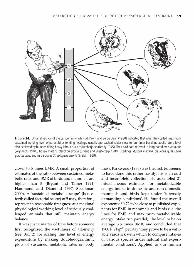
M E TA B O L I C C E I L I N G S : T H E E C O L O G Y O F P H YS I O L O G I C A L R E S T R A I N T 5 9
closer to 5 times BMR. A small proportion of estimates of the ratio between sustained meta-bolic rates and BMR of birds and mammals are higher than 5 ( Bryant and Tatner 1991 , Hammond and Diamond 1997 , Speakman 2000 ). A ‘sustained metabolic scope’ (hence-forth called factorial scope) of 5 may, therefore, represent a reasonable fi rst guess at a maximal physiological working level of seriously chal-lenged animals that still maintain energy balance.
It was just a matter of time before someone fi rst recognized the usefulness of allometry (see Box 2 ) for scaling this level of energy expenditure by making double-logarithmic plots of sustained metabolic rates on body
mass. Kirkwood ( 1983 ) was the fi rst, but seems to have done this rather hastily; his is an odd and incomplete collection. He assembled 21 miscellaneous estimates for metabolizable energy intake in domestic and non-domestic mammals and birds kept under ‘intensely demanding conditions’. He found the overall exponent of 0.72 to be close to published expo-nents for BMR in mammals and birds (i.e. the lines for BMR and maximum metabolizable energy intake run parallel), the level to be on average 3.6 times BMR, and concluded that 1700 kJ/kg 0.72 per day ‘may prove to be a valu-able yardstick with which to compare intakes of various species under natural and experi-mental conditions’. Applied to our human
1
2
3
4
Figure 34. Original version of the cartoon in which Rudi Drent and Serge Daan (1980) indicated that what they called ‘maximum sustained working level’ of parent birds tending nestlings, usually approached values close to four times basal metabolic rate, a level also achieved by humans doing heavy labour, such as lumberjacks ( Brody 1945 ). Their bird data referred to long-eared owls Asio otis ( Wijnandts 1984 ), house martins Delichon urbica ( Bryant and Westerterp 1980 ), starlings Sturnus vulgaris , glaucous gulls Larus glaucescens , and turtle doves Streptopelia risoria ( Brisbin 1969 ).
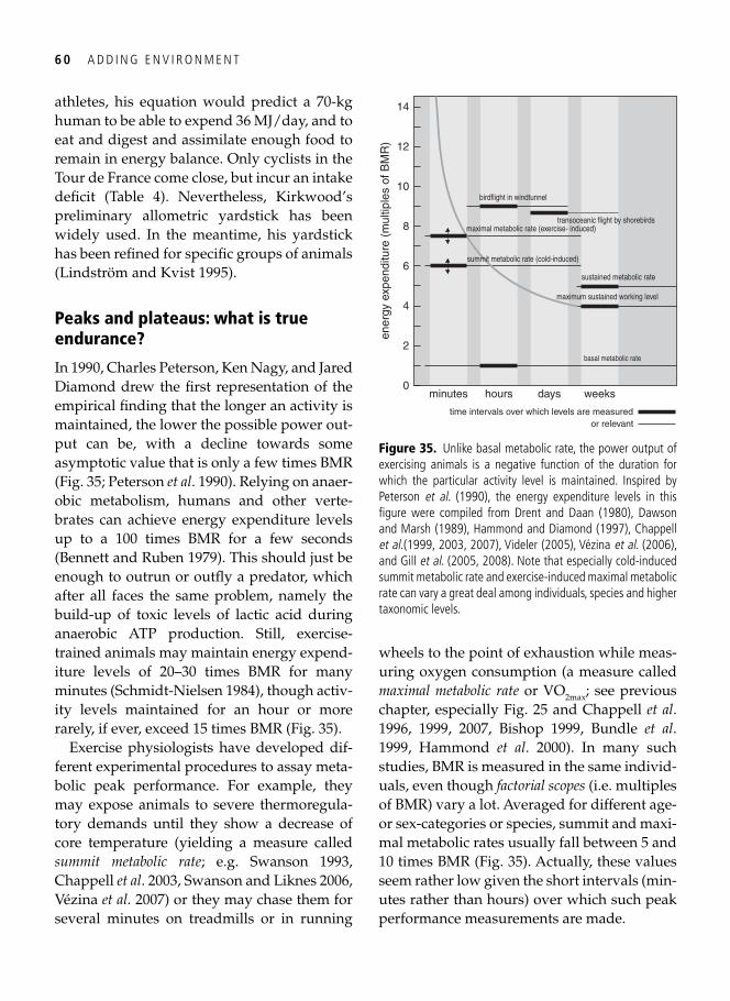
6 0 A D D I N G E N V I R O N M E N T
athletes, his equation would predict a 70-kg human to be able to expend 36 MJ/day, and to eat and digest and assimilate enough food to remain in energy balance. Only cyclists in the Tour de France come close, but incur an intake defi cit ( Table 4 ). Nevertheless, Kirkwood’s preliminary allometric yardstick has been widely used. In the meantime, his yardstick has been refi ned for specifi c groups of animals ( Lindström and Kvist 1995 ).
Peaks and plateaus: what is true endurance?
In 1990, Charles Peterson, Ken Nagy, and Jared Diamond drew the fi rst representation of the empirical fi nding that the longer an activity is maintained, the lower the possible power out-put can be, with a decline towards some asymptotic value that is only a few times BMR ( Fig. 35 ; Peterson et al . 1990 ). Relying on anaer-obic metabolism, humans and other verte-brates can achieve energy expenditure levels up to a 100 times BMR for a few seconds ( Bennett and Ruben 1979 ). This should just be enough to outrun or outfl y a predator, which after all faces the same problem, namely the build-up of toxic levels of lactic acid during anaerobic ATP production. Still, exercise-trained animals may maintain energy expend-iture levels of 20–30 times BMR for many minutes ( Schmidt-Nielsen 1984 ), though activ-ity levels maintained for an hour or more rarely, if ever, exceed 15 times BMR ( Fig. 35 ).
Exercise physiologists have developed dif-ferent experimental procedures to assay meta-bolic peak performance. For example, they may expose animals to severe thermoregula-tory demands until they show a decrease of core temperature (yielding a measure called summit metabolic rate ; e.g. Swanson 1993 , Chappell et al . 2003 , Swanson and Liknes 2006 , Vézina et al. 2007 ) or they may chase them for several minutes on treadmills or in running
wheels to the point of exhaustion while meas-uring oxygen consumption (a measure called maximal metabolic rate or VO 2max ; see previous chapter, especially Fig. 25 and Chappell et al . 1996 , 1999 , 2007 , Bishop 1999 , Bundle et al . 1999 , Hammond et al . 2000 ). In many such studies, BMR is measured in the same individ-uals, even though factorial scopes (i.e. multiples of BMR) vary a lot. Averaged for different age- or sex-categories or species, summit and maxi-mal metabolic rates usually fall between 5 and 10 times BMR ( Fig. 35 ). Actually, these values seem rather low given the short intervals (min-utes rather than hours) over which such peak performance measurements are made.
ener
gy e
xpen
ditu
re (
mul
tiple
s of
BM
R)
minutes0
2
4
6
8
10
12
14
hours days weeks
maximum sustained working level
sustained metabolic rate
summit metabolic rate (cold-induced)
maximal metabolic rate (exercise- induced)
basal metabolic rate
transoceanic flight by shorebirds
time intervals over which levels are measuredor relevant
birdflight in windtunnel
Figure 35. Unlike basal metabolic rate, the power output of exercising animals is a negative function of the duration for which the particular activity level is maintained. Inspired by Peterson et al . ( 1990 ), the energy expenditure levels in this fi gure were compiled from Drent and Daan (1980), Dawson and Marsh ( 1989 ), Hammond and Diamond ( 1997 ), Chappell et al . ( 1999 , 2003 , 2007 ), Videler ( 2005 ), Vézina et al . ( 2006 ), and Gill et al . ( 2005 , 2008). Note that especially cold-induced summit metabolic rate and exercise-induced maximal metabolic rate can vary a great deal among individuals, species and higher taxonomic levels.
M E TA B O L I C C E I L I N G S : T H E E C O L O G Y O F P H YS I O L O G I C A L R E S T R A I N T 6 1
Another interesting point is that, although both exercise- and cold-induced metabolic rates strongly involve skeletal muscle work (in running and shivering, respectively), animals tend to have higher factorial scopes for exer-cise-induced power output than for cold- induced power output ( Hinds et al . 1993 ). In birds, exercise-induced scopes are higher than cold-induced scopes ( Dawson and Marsh 1989 , Hinds et al . 1993 ), but in some small mammals, cold-induced factorial scope is higher than exercise-induced scope ( Chappell et al . 2003 ). These differences may be due to the fact that birds carry a relatively larger musculature for locomotion than mammals, i.e. the fl ight mus-cles, with the discrepancy between the sizes of great and small fl ight muscles negatively affecting shivering capacity ( Hinds et al . 1993 , and see Piersma and Dietz 2007 ). In addition, mammals, but not birds, can use ‘brown fat’ to generate heat for thermogenesis (i.e. ‘non-shivering thermogenesis’; see Cannon and Nedergaard 2004 , Morrison et al . 2008 ). With their two channels of heat generation, mam-mals achieve high cold-induced factorial scopes.
Experimental measurements of the cost of bird fl ight, carried out in wind-tunnels over many hours ( Pennycuick et al . 1997 , Kvist et al . 2001 , Ward et al . 2004 , Engel et al. 2006 , Schmidt-Wellenburg et al . 2006 , 2008 ) also vary widely, but gravitate towards values around 9 times BMR ( Videler 2005 ). During such long and intense exercise, it was not the thrush nightin-gale Luscinia luscinia called ‘Blue’ that fl ew continuously for 16 h that became exhausted, but the human experimentalists that needed to stand guard at the wind-tunnel from 7 a.m. the fi rst day to 1 a.m. the next ( Lindström et al . 1999 , Klaassen et al . 2000 , Å. Lindström pers. comm.).
Using the latest satellite-transmitter technol-ogy, it has now been demonstrated that bar-tailed godwits Limosa lapponica cross the entire
length of the Pacifi c from Alaska to New Zealand—a distance of 11,000 km—in single non-stop fl ights that may last nine days or even a few more ( Gill et al . 2009 ). On the basis of reconstructed fat and protein losses during such fl ights, the godwits would be fl ying at energy expenditure levels of about 9 times BMR ( Gill et al . 2005 ). This level is consistent with modern wind-tunnel data, but still curi-ously high compared to the trendline ( Fig. 35 ). It is almost double the long-term levels for sus-tained metabolic rate in hard-working mam-mals and non-fl ying birds, yet takes place over similar lengths of time.
A big difference, of course, is that long-dis-tance migrants are not in energy balance. They do not eat during the fl ight, but deplete the sizeable stores of fat and proteins that are accrued before they take off ( Piersma and Gill 1998 , Gill et al . 2005 ). Indeed, despite showing evidence of remarkable protein saving ( Jenni and Jenni-Eiermann 1998 ), such migrant shore-birds not only empty their abdominal and sub-cutaneous fat stores, but, with the exception of lungs and brain, also burn up belly organs and other proteinaceous tissues in fl ight ( Battley et al . 2000 ). This raises the possibility that sus-tained metabolic rates are constrained by the capacity of animals to digest and assimilate food, something that even active animals do not have to do as long as they rely on stores. Is there evidence that food processing and assim-ilation, i.e. the lower funnels that feed into Weiner’s (1992) ‘animal barrel’ (Fig. 29), could indeed determine plateau energy expenditure levels?
Regulation of maximal performance: central, peripheral, or external?
Here let us return to the topic of the design of metabolic ceilings left in the previous chapter, and the question of whether the food-process-ing chain and respiratory chains show any
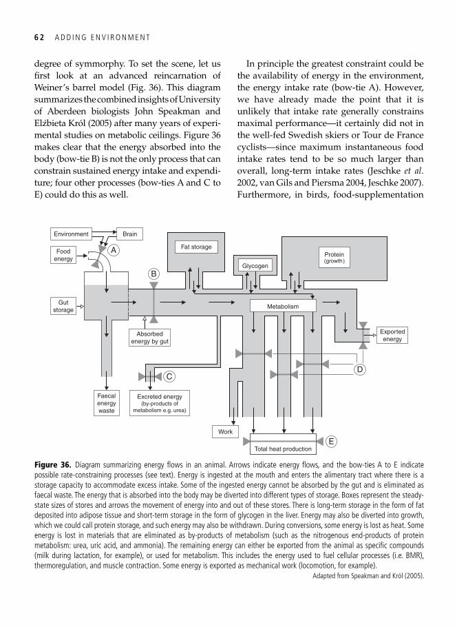
6 2 A D D I N G E N V I R O N M E N T
degree of symmorphy. To set the scene, let us fi rst look at an advanced reincarnation of Weiner’s barrel model ( Fig. 36 ). This diagram summarizes the combined insights of University of Aberdeen biologists John Speakman and Elzbieta Król (2005) after many years of experi-mental studies on metabolic ceilings. Figure 36 makes clear that the energy absorbed into the body (bow-tie B) is not the only process that can constrain sustained energy intake and expendi-ture; four other processes (bow-ties A and C to E) could do this as well.
In principle the greatest constraint could be the availability of energy in the environment, the energy intake rate (bow-tie A). However, we have already made the point that it is unlikely that intake rate generally constrains maximal performance—it certainly did not in the well-fed Swedish skiers or Tour de France cyclists—since maximum instantaneous food intake rates tend to be so much larger than overall, long-term intake rates ( Jeschke et al . 2002 , van Gils and Piersma 2004 , Jeschke 2007 ). Furthermore, in birds, food-supplementation
E
Foodenergy
Gutstorage
B
A
Metabolism
Brain
Absorbedenergy by gut
C
Fat storage
Glycogen
Protein(growth)
D
Total heat production
Work
Faecalenergywaste
Excreted energy(by-products of
metabolism e.g. urea)
Exportedenergy
Environment
Figure 36. Diagram summarizing energy fl ows in an animal. Arrows indicate energy fl ows, and the bow-ties A to E indicate possible rate-constraining processes (see text). Energy is ingested at the mouth and enters the alimentary tract where there is a storage capacity to accommodate excess intake. Some of the ingested energy cannot be absorbed by the gut and is eliminated as faecal waste. The energy that is absorbed into the body may be diverted into different types of storage. Boxes represent the steady-state sizes of stores and arrows the movement of energy into and out of these stores. There is long-term storage in the form of fat deposited into adipose tissue and short-term storage in the form of glycogen in the liver. Energy may also be diverted into growth, which we could call protein storage, and such energy may also be withdrawn. During conversions, some energy is lost as heat. Some energy is lost in materials that are eliminated as by-products of metabolism (such as the nitrogenous end-products of protein metabolism: urea, uric acid, and ammonia). The remaining energy can either be exported from the animal as specifi c compounds (milk during lactation, for example), or used for metabolism. This includes the energy used to fuel cellular processes (i.e. BMR), thermoregulation, and muscle contraction. Some energy is exported as mechanical work (locomotion, for example).
Adapted from Speakman and Król ( 2005 ).
M E TA B O L I C C E I L I N G S : T H E E C O L O G Y O F P H YS I O L O G I C A L R E S T R A I N T 6 3
experiments have rarely managed to increase measures of peak performance ( Meijer and Drent 1999 , Speakman and Król 2005 ). As was pointed out by John Speakman (pers. comm.), the very existence of storage organs at the entrance to the gut (crop, stomach; see Kersten and Visser 1996 ) suggests that the rate at which energy can be harvested often exceeds the rate at which it can be processed. In principle, it is also possible that metabolic ceilings are lim-ited by the capacity to excrete metabolic end-products, e.g. the capacity of the kidneys to excrete urea (bow-tie C). In lactating mice fed a high-protein diet, the latter may actually occur (J.R. Speakman pers. comm.).
For a long time there were two main hypoth-eses to explain the regulation of maximal per-formance. One, related to the capacity of the alimentary tract to absorb energy (the food-processing chain), is called the central limitation hypothesis (bow-tie B). The other, related to the capacity to expend energy at the different sites of utilization (the respiratory chain, with the muscles, testicles, ovaries, and, in mammals, brown adipose tissue and mammary glands as the sites of heat production) is called the periph-eral limitation hypothesis (bow-tie D) ( Ricklefs 1969 , Hammond and Diamond 1997 , Hammond et al . 2000 , Bacigalupe and Bozinovic 2002 , Speakman and Król 2005 ). Although the null hypothesis of symmorphosis predicts that nei-ther of them would be limiting on its own (Chapter 3 ) , these two alternatives have attracted a lot of elegant experimental testing, especially in small rodents. The rigour of the tests in this research programme, and the fact that they turned up an exciting new hypothe-sis, justifi es some elaboration.
Rodents breed fast, have fur, but can easily be exposed to temperatures that will elevate their metabolism, and have mammary glands that produce, and teats that deliver, milk. These characteristics make small mammals excellent models for experimental studies of
metabolic ceilings ( Table 5 ). Attention has focused on sustained energy intake rather than expenditure because during reproduction ‘con-siderable amounts of energy are exported as milk’ ( Speakman and Król 2005 ). In small mammals, pregnancy increases energy demand by about 60%, while during peak lactation, energy intake quadruples ( Johnson et al . 2001a ). To test whether this represents the metabolic ceiling, rodent mothers have been given more young ( Hammond and Diamond 1992 , Künkele 2000 , Johnson et al . 2001a ), young for a longer time ( Hammond and Diamond 1994 ), or more hungry young ( Laurien-Kehnen and Trillmich 2003 ). In none of these studies did food intake increase. Pup masses typically went down, which makes sense given that the same amount of food had to be shared by more pups. To test whether this apparent limit was centrally determined, diet quality was reduced ( Speakman et al . 2001 , Hacklander et al . 2002 , Valencak and Ruf 2009 ). Mice, and also European hares, responded by eating and assimilating more food, suggesting the ability of the digestive tract to upregulate capacity.
In order to increase selectively the demands of the peripheral systems, Perrigo ( 1987 ) forced lactating mice to run for their food, but found that, despite free access to food, neither of the two mouse species tested showed elevations of food intake. Furthermore, when Kristin Schubert and colleagues (2009) applied a simi-lar paradigm in laboratory mice, they found that minimum metabolic rate and daily energy expenditure (DEE) were both actually reduced (see below, ‘The evolution of laziness’). When peripheral demands were elevated, by making lactating rats and mice simultaneously preg-nant, food intake did not increase either ( Biggerstaff and Mann 1992 , Koiter et al . 1999 , Johnson et al . 2001c ). However, in all studies where rodents were exposed to cold ( Table 5 ), food intake did increase, especially during
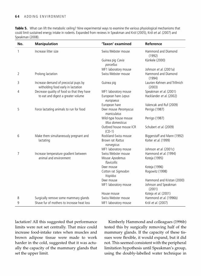
6 4 A D D I N G E N V I R O N M E N T
lactation! All this suggested that performance limits were not set centrally. That mice could increase food-intake rates when muscles and brown adipose tissue were made to work harder in the cold, suggested that it was actu-ally the capacity of the mammary glands that set the upper limit.
Kimberly Hammond and colleagues ( 1996b ) tested this by surgically removing half of the mammary glands. If the capacity of these tis-sues were fl exible, it would expand, but it did not. This seemed consistent with the peripheral limitation hypothesis until Speakman’s group, using the doubly-labelled water technique in
Table 5. What can lift the metabolic ceiling? Nine experimental ways to examine the various physiological mechanisms that could limit sustained energy intake in rodents. Expanded from reviews in Speakman and Król ( 2005 ), Król et al . ( 2007 ) and Speakman ( 2008 ).
No. Manipulation ‘Taxon’ examined Reference
1 Increase litter size Swiss Webster mouse Hammond and Diamond (1992)
Guinea pig Cavia porcellus
Künkele (2000)
MF1 laboratory mouse Johnson et al . (2001a) 2 Prolong lactation Swiss Webster mouse Hammond and Diamond
(1994) 3 Increase demand of precocial pups by
witholding food early in lactation Guinea pig Laurien-Kehnen and Trillmich
(2003) 4 Decrease quality of food so that they have
to eat and digest a greater volume MF1 laboratory mouse Speakman et al . (2001) European hare Lepus
europaeus Hacklander et al . (2002)
European hare Valencak and Ruf (2009) 5 Force lactating animals to run for food Deer mouse Peromyscus
maniculatus Perrigo (1987)
Wild-type house mouse Mus domesticus
Perrigo (1987)
Outbred house mouse ICR (CD-1)
Schubert et al . (2009)
6 Make them simultaneously pregnant and lactating
Rockland-Swiss mouse Biggerstaff and Mann (1992) Brown rat Rattus
norvegicus Koiter et al . (1999)
MF1 laboratory mouse Johnson et al . (2001c) 7 Increase temperature gradient between
animal and environment Swiss Webster mouse Hammond et al . (1994) Mouse Apodemus
fl avicollis Koteja (1995)
Deer mouse Koteja (1996) Cotton rat Sigmodon
hispidus Rogowitz (1998)
Deer mouse Hammond and Kristan (2000) MF1 laboratory mouse Johnson and Speakman
(2001) House mouse Koteja et al . (2001) 8 Surgically remove some mammary glands Swiss Webster mouse Hammond et al . (1996b) 9 Shave fur of mothers to increase heat loss MF1 laboratory mouse Król et al. (2007)
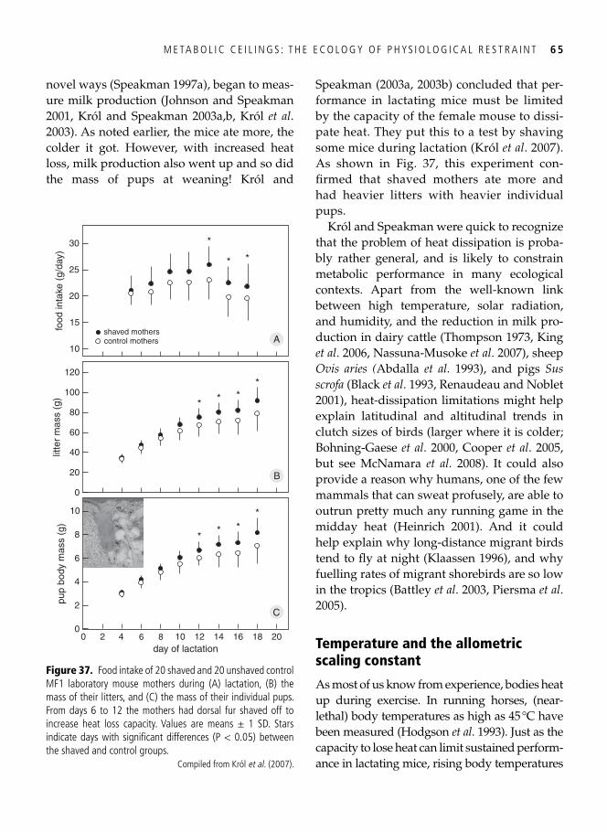
M E TA B O L I C C E I L I N G S : T H E E C O L O G Y O F P H YS I O L O G I C A L R E S T R A I N T 6 5
novel ways ( Speakman 1997a ), began to meas-ure milk production ( Johnson and Speakman 2001 , Król and Speakman 2003a , b , Król et al . 2003 ). As noted earlier, the mice ate more, the colder it got. However, with increased heat loss, milk production also went up and so did the mass of pups at weaning! Król and
Speakman ( 2003a , 2003b ) concluded that per-formance in lactating mice must be limited by the capacity of the female mouse to dissi-pate heat. They put this to a test by shaving some mice during lactation ( Król et al . 2007 ). As shown in Fig. 37 , this experiment con-fi rmed that shaved mothers ate more and had heavier litters with heavier individual pups.
Król and Speakman were quick to recognize that the problem of heat dissipation is proba-bly rather general, and is likely to constrain metabolic performance in many ecological contexts. Apart from the well-known link between high temperature, solar radiation, and humidity, and the reduction in milk pro-duction in dairy cattle ( Thompson 1973 , King et al . 2006 , Nassuna-Musoke et al . 2007 ), sheep Ovis aries ( Abdalla et al. 1993 ), and pigs Sus scrofa ( Black et al . 1993 , Renaudeau and Noblet 2001 ), heat-dissipation limitations might help explain latitudinal and altitudinal trends in clutch sizes of birds (larger where it is colder; Bohning-Gaese et al . 2000 , Cooper et al . 2005 , but see McNamara et al. 2008 ). It could also provide a reason why humans, one of the few mammals that can sweat profusely, are able to outrun pretty much any running game in the midday heat ( Heinrich 2001 ). And it could help explain why long-distance migrant birds tend to fl y at night ( Klaassen 1996 ), and why fuelling rates of migrant shorebirds are so low in the tropics ( Battley et al . 2003 , Piersma et al . 2005 ).
Temperature and the allometric scaling constant
As most of us know from experience, bodies heat up during exercise. In running horses, (near- lethal) body temperatures as high as 45 °C have been measured ( Hodgson et al . 1993 ). Just as the capacity to lose heat can limit sustained perform-ance in lactating mice, rising body temperatures
pup
body
mas
s (g
)
C
00
2
4
6
8
10
42day of lactation
106 8 12 14 16 18 20
****
litte
r m
ass
(g)
B
0
20
40
60
80
120*
***
food
inta
ke (
g/da
y)
A10
15
20
25
30
**
*
100
shaved motherscontrol mothers
Figure 37. Food intake of 20 shaved and 20 unshaved control MF1 laboratory mouse mothers during (A) lactation, (B) the mass of their litters, and (C) the mass of their individual pups. From days 6 to 12 the mothers had dorsal fur shaved off to increase heat loss capacity. Values are means ± 1 SD. Stars indicate days with signifi cant differences (P < 0.05) between the shaved and control groups.
Compiled from Król et al . ( 2007 ).
6 6 A D D I N G E N V I R O N M E N T
can put a limit to the duration or the level of intense exercise ( Weishaupt et al . 1996 , Fuller et al . 1998 , González-Alonso et al . 1999 , Arngrimsson et al . 2004 ). Noting that the allom-etric scaling constant for maximal metabolic rate in mammals (ca. 0.80) is consistently higher than that for BMR (0.70–0.75; Taylor et al . 1981 , Bishop 1999 , Savage et al . 2004 , Weibel et al . 2004 ), Gillooly and Allen ( 2007 ) proposed that the steeper size-dependence of maximal metabolic rate than of BMR may be explained by larger mammals achieving the highest muscle temper-atures at maximal activity. The larger the animal, the more unfavourable its surface–volume ratio when losing, rather than retaining, heat. In gen-eral, chemical reaction rates increase exponen-tially with temperature, as does metabolic rate ( Gillooly et al . 2001 ).
Gillooly and Allen ( 2007 ) suggest that the short-term maximal metabolic rate (technically called VO 2max ) is a function of body tempera-ture. This led them to the somewhat counter-intuitive prediction that mammals should be able to achieve higher maximal metabolic rates at higher ambient temperatures, because heat loss is more restricted, leading body tempera-tures to rise more. Craig White and colleagues ( 2008 ) tested this hypothesis on the basis of published maximum aerobic performance measurements in rodents, and rejected it. They found no relationship between VO 2max and test-ing temperature, which varied from –16 ° to +30 °C. Interestingly, they did fi nd that animals that were acclimated at lower temperatures achieved higher maximal metabolic rates. Cold necessitates shivering, and thus a more intense use of muscle tissue. This, as we shall see in the next chapter, usually leads to hypertrophy. In fact, within species, such chronic muscle-medi-ated thermogenesis can lead to greater increases in aerobic capacity, whether measured as maxi-mal or summit metabolic rate, than endurance training ( Schaeffer et al . 2001 , 2003 , 2005 , Vézina et al . 2006 ).
Protecting long-term fi tness assets: factorial scopes and optimal working capacity revisited
When one builds bigger bodies to ingest, absorb, excrete, and do work, the expand-ing machinery requires ever more energy for maintenance. Such increases in maintenance requirements will be refl ected by increasing BMR levels. A summary of the early studies on mice whose energy expenditure had been ele-vated in a variety of ways (see Table 5 ), shows BMR to go up with sustained metabolic rate ( Fig. 38A ). This effect comes with an increase in body mass, due to hypertrophy of the liver, digestive tract, and mammary glands ( Hammond et al . 1994 , Speakman and Johnson 2000 , Johnson et al . 2001b ). As a consequence of having put in place increasingly powerful machinery, factorial scope (the ratio between sustained energy expenditure and BMR) climbs to an asymptote of about 7 times BMR ( Fig. 38B ; Hammond and Diamond 1997 ).
We have come full circle. During our quest to establish whether maximal aerobic per-formance is limited centrally, by digestion and assimilation systems, or peripherally, by the power that can be generated by the receiving organs, experimental evidence has not been uniformly consistent with either alternative. In a sense, this celebrates the notion of symmor-phosis, the principle of logical, economic ani-mal design (Chapter 3 ) : symmorphic design would have negated evidence in favour of either hypothesis for a single site limiting aer-obic performance. That rates of heat loss best explain the limits to aerobic performance in lactating laboratory mice, which only push up their metabolic ceilings when it is cold enough or when insulation is poor enough, does not detract from the fact that mouse mothers can only do this by building a bigger body, a big-ger metabolic machine. Thus, they still face a maximum factorial scope of 7.
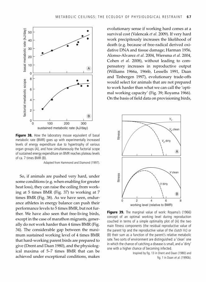
M E TA B O L I C C E I L I N G S : T H E E C O L O G Y O F P H YS I O L O G I C A L R E S T R A I N T 6 7
So, if animals are pushed very hard, under some conditions (e.g. when enabling for greater heat loss), they can raise the ceiling from work-ing at 5 times BMR ( Fig. 37 ) to working at 7 times BMR ( Fig. 38 ). As we have seen, endur-ance athletes in energy balance can push their performance levels to 5 times BMR, but not fur-ther. We have also seen that free-living birds, except in the case of marathon migrants, gener-ally do not work harder than 4 times BMR ( Fig. 34 ). The considerable gap between the maxi-mum sustained working level of 4 times BMR that hard-working parent birds are prepared to give (Drent and Daan 1980), and the physiolog-ical maxima of 5–7 times BMR that can be achieved under exceptional conditions, makes
evolutionary sense if working hard comes at a survival cost ( Valencak et al. 2009 ). If very hard work precipitously increases the likelihood of death (e.g. because of free-radical derived oxi-dative DNA and tissue damage; Harman 1956 , Alonso-Alvarez et al . 2004 , Wiersma et al . 2004 , Cohen et al . 2008 ), without leading to com-pensatory increases in reproductive output ( Williams 1966a , 1966b , Lessells 1991 , Daan and Tinbergen 1997 ), evolutionary trade-offs would select for animals that are not prepared to work harder than what we can call the ‘opti-mal working capacity’ ( Fig. 39 ; Royama 1966 ). On the basis of fi eld data on provisioning birds,
fact
oria
l met
abol
ic s
cope
00
2
4
6
8
sustained metabolic rate (kJ/day)100 200 300
basa
l met
abol
ic r
ate
(kJ/
day)
0
A
B
20
30
40
50
10
Figure 38. How the laboratory mouse equivalent of basal metabolic rate (BMR) goes up with experimentally increased levels of energy expenditure due to hypertrophy of various organ groups (A), and how simultaneously the factorial scope of sustained energy expenditure on BMR reaches plateau levels of ca. 7 times BMR (B).
Adapted from Hammond and Diamond ( 1997 ).
fitne
ss
0working level (relative to BMR)
2 4 6
A
B
8
fitne
ss
Vp dirty
V clean
V dirty
Vp clean
Vc
Figure 39. The marginal value of work: Royama’s (1966) concept of an optimal working level during reproduction couched in terms of a simple optimality plot of (A) the two main fi tness components (the residual reproductive value of the parent Vp and the reproductive value of the clutch Vc) or (B) their sum as a function of the parent’s relative metabolic rate. Two sorts of environment are distinguished: a ‘clean’ one in which the chance of catching a disease is small, and a ‘dirty’ one with a higher chance of becoming infected.
Inspired by fi g. 13 in Drent and Daan (1980) and fi g. 1 in Daan et al . ( 1990b ).
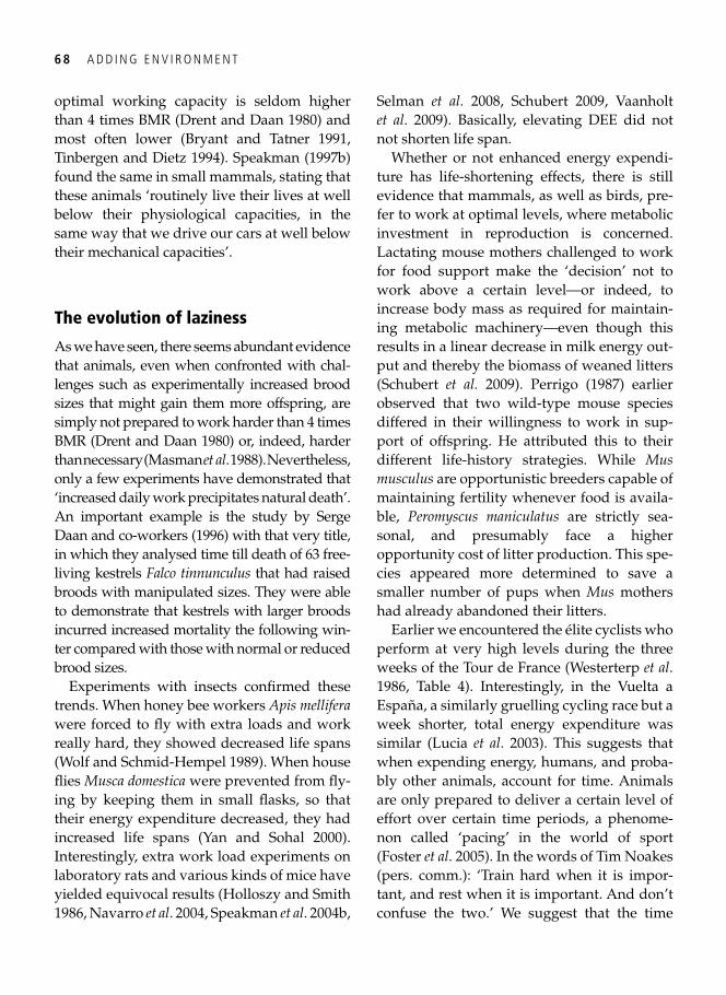
6 8 A D D I N G E N V I R O N M E N T
optimal working capacity is seldom higher than 4 times BMR (Drent and Daan 1980) and most often lower ( Bryant and Tatner 1991 , Tinbergen and Dietz 1994 ). Speakman ( 1997b ) found the same in small mammals, stating that these animals ‘routinely live their lives at well below their physiological capacities, in the same way that we drive our cars at well below their mechanical capacities’.
The evolution of laziness
As we have seen, there seems abundant evidence that animals, even when confronted with chal-lenges such as experimentally increased brood sizes that might gain them more offspring, are simply not prepared to work harder than 4 times BMR (Drent and Daan 1980) or, indeed, harder than necessary ( Masman et al . 1988 ). Nevertheless, only a few experiments have demonstrated that ‘increased daily work precipitates natural death’. An important example is the study by Serge Daan and co-workers (1996) with that very title, in which they analysed time till death of 63 free-living kestrels Falco tinnunculus that had raised broods with manipulated sizes. They were able to demonstrate that kestrels with larger broods incurred increased mortality the following win-ter compared with those with normal or reduced brood sizes.
Experiments with insects confi rmed these trends. When honey bee workers Apis mellifera were forced to fl y with extra loads and work really hard, they showed decreased life spans ( Wolf and Schmid-Hempel 1989 ). When house fl ies Musca domestica were prevented from fl y-ing by keeping them in small fl asks, so that their energy expenditure decreased, they had increased life spans ( Yan and Sohal 2000 ). Interestingly, extra work load experiments on laboratory rats and various kinds of mice have yielded equivocal results ( Holloszy and Smith 1986 , Navarro et al . 2004 , Speakman et al . 2004b ,
Selman et al . 2008 , Schubert 2009, Vaanholt et al . 2009 ). Basically, elevating DEE did not not shorten life span.
Whether or not enhanced energy expendi-ture has life-shortening effects, there is still evidence that mammals, as well as birds, pre-fer to work at optimal levels, where metabolic investment in reproduction is concerned. Lactating mouse mothers challenged to work for food support make the ‘decision’ not to work above a certain level—or indeed, to increase body mass as required for maintain-ing metabolic machinery—even though this results in a linear decrease in milk energy out-put and thereby the biomass of weaned litters (Schubert et al. 2009). Perrigo ( 1987 ) earlier observed that two wild-type mouse species differed in their willingness to work in sup-port of offspring. He attributed this to their different life-history strategies. While Mus musculus are opportunistic breeders capable of maintaining fertility whenever food is availa-ble, Peromyscus maniculatus are strictly sea-sonal, and presumably face a higher opportunity cost of litter production. This spe-cies appeared more determined to save a smaller number of pups when Mus mothers had already abandoned their litters.
Earlier we encountered the élite cyclists who perform at very high levels during the three weeks of the Tour de France ( Westerterp et al . 1986 , Table 4 ). Interestingly, in the Vuelta a España, a similarly gruelling cycling race but a week shorter, total energy expenditure was similar ( Lucia et al . 2003 ). This suggests that when expending energy, humans, and proba-bly other animals, account for time. Animals are only prepared to deliver a certain level of effort over certain time periods, a phenome-non called ‘pacing’ in the world of sport (Foster et al . 2005). In the words of Tim Noakes (pers. comm.): ‘Train hard when it is impor-tant, and rest when it is important. And don’t confuse the two.’ We suggest that the time
M E TA B O L I C C E I L I N G S : T H E E C O L O G Y O F P H YS I O L O G I C A L R E S T R A I N T 6 9
spans over which the accounting of metabolic performance takes place in different animals could be a rich area of experimental research.
Free-living animals are resistant to experi-mental manipulations to increase their instan-taneous work levels, for what we can now see are sound reasons. Unless some mechanistic shortcuts are found to the actual expenditure decision processes (e.g. Speakman and Król 2005 ), it will be impossible to verify experi-mentally the optimality model of Fig. 39 along the whole range of work levels. Nevertheless, it seems likely that within taxa the ‘death on working level curves’ would be determined by ecological conditions, e.g. the general envi-ronmental or social stress levels that have become known as ‘allostatic loads’ ( McEwen and Wingfi eld 2003 , Wingfi eld 2005 , Rubenstein 2007 ), or the levels of pathogens in the envi-ronment ( Piersma 1997 ).
Such variations suggest that there is scope for studies in which relationships between energy expenditure levels and survival are studied, either in a strict comparative context (comparing relationships in groups with dif-ferent environments) or in experimental con-texts (by additionally manipulating aspects of the environments in which the expenditure–survival relationships are studied). During such endeavours it remains important to pay attention to constraints other than work level, especially time limitations, that prevent ani-mals from keeping up with the hard work and from eating for very long (e.g. Kvist and Lindström 2000 , Tinbergen and Verhulst 2000 ). When interpretable aspects of the ecological context can be linked to maximal performance, or rather to the precise levels and relationships between experimentally manipulated work levels and both reproduction and survival ( Fig. 39 , and see Bouwhuis et al . 2009 for a pos-sible fi eld setting), we may achieve deeper lev-els of understanding of the selection factors driving the height of metabolic ceilings.
We believe that such insights need to come from adequate incorporation of ecology into what at fi rst sight may seem a purely physio-logical problem. The impressive portfolio of studies on highly inbred strains, or genetically modifi ed lab mice, will thus need expansion to a variety of free-living animals, with due atten-tion to ecological context for an appreciation of the evolutionary causes of metabolic ceilings.
Evolutionary wisdom of physiological constraints
Unlike bar-headed geese Anser indicus that have evolved particular muscle phenotypes to migrate over the Himalayas at heights of 9000 m ( Scott et al . 2009 ), humans clearly are a low- altitude species. When Reinhold Messner and his team were getting close to the summit at 8848 m of Mount Everest on 8 May 1978, expe-riencing an equivalent of 7% oxygen rather than the 21% at sea level, they found it increas-ingly hard to stay on their feet ( Messner 1979 ): ‘every 10–15 steps we collapsed into the snow to rest, then crawled on’. Their leg-muscle fatigue could not have been due to lactic acid poisoning because, paradoxically, observa-tions on human exercise at low partial oxygen pressures show that, whereas lactic acid levels should go up with increasing hypoxia at high altitudes, they actually go down ( Bigland-Ritchie and Vollestadt 1988 ). Also, paradoxi-cally, rather than going up to compensate for the decreasing partial oxygen pressures at great heights, heart rates actually go down with altitude ( Sutton et al . 1988 ). This change is related to blood being shunted away from the muscles (hence the fatigue experienced by Messner and his comrades; Amann et al . 2006 ) and towards the brain—the ‘selfi sh’ organ that controls oxygen delivery to the system ( Noakes et al . 2001 , 2004 ). Noting that, during impor-tant games, athletes can deliver an end spurt at the point where their muscles must show
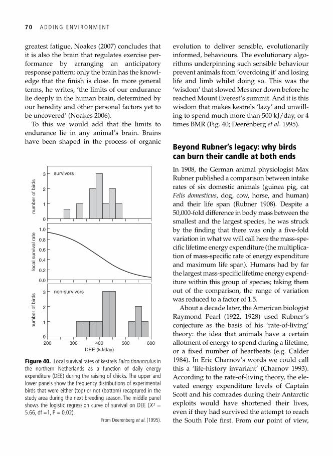
7 0 A D D I N G E N V I R O N M E N T
greatest fatigue, Noakes ( 2007 ) concludes that it is also the brain that regulates exercise per-formance by arranging an anticipatory response pattern: only the brain has the knowl-edge that the fi nish is close. In more general terms, he writes, ‘the limits of our endurance lie deeply in the human brain, determined by our heredity and other personal factors yet to be uncovered’ ( Noakes 2006 ).
To this we would add that the limits to endurance lie in any animal’s brain. Brains have been shaped in the process of organic
evolution to deliver sensible, evolutionarily informed, behaviours. The evolutionary algo-rithms underpinning such sensible behaviour prevent animals from ‘overdoing it’ and losing life and limb whilst doing so. This was the ‘wisdom’ that slowed Messner down before he reached Mount Everest’s summit. And it is this wisdom that makes kestrels ‘lazy’ and unwill-ing to spend much more than 500 kJ/day, or 4 times BMR ( Fig. 40 ; Deerenberg et al . 1995 ).
Beyond Rubner’s legacy: why birds can burn their candle at both ends
In 1908, the German animal physiologist Max Rubner published a comparison between intake rates of six domestic animals (guinea pig, cat Felis domesticus , dog, cow, horse, and human) and their life span ( Rubner 1908 ). Despite a 50,000-fold difference in body mass between the smallest and the largest species, he was struck by the fi nding that there was only a fi ve-fold variation in what we will call here the mass-spe-cifi c lifetime energy expenditure (the multiplica-tion of mass-specifi c rate of energy expenditure and maximum life span). Humans had by far the largest mass-specifi c lifetime energy expend-iture within this group of species; taking them out of the comparison, the range of variation was reduced to a factor of 1.5.
About a decade later, the American biologist Raymond Pearl ( 1922 , 1928 ) used Rubner’s conjecture as the basis of his ‘rate-of-living’ theory: the idea that animals have a certain allotment of energy to spend during a lifetime, or a fi xed number of heartbeats (e.g. Calder 1984 ). In Eric Charnov’s words we could call this a ‘life-history invariant’ ( Charnov 1993 ). According to the rate-of-living theory, the ele-vated energy expenditure levels of Captain Scott and his comrades during their Antarctic exploits would have shortened their lives, even if they had survived the attempt to reach the South Pole fi rst. From our point of view,
loca
l sur
viva
l rat
e
200
1
2
3
DEE (kJ/day)300 400 500
0.0
0.4
0.6
0.8
1.0
0.2
0600
survivors
non-survivors
num
ber
of b
irds
1
2
3
0
num
ber
of b
irds
Figure 40. Local survival rates of kestrels Falco tinnunculus in the northern Netherlands as a function of daily energy expenditure (DEE) during the raising of chicks. The upper and lower panels show the frequency distributions of experimental birds that were either (top) or not (bottom) recaptured in the study area during the next breeding season. The middle panel shows the logistic regression curve of survival on DEE ( X ² = 5.66, df =1, P = 0.02).
From Deerenberg et al . ( 1995 ) .
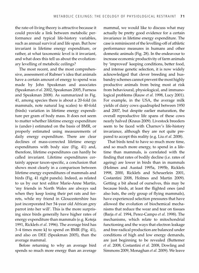
M E TA B O L I C C E I L I N G S : T H E E C O L O G Y O F P H YS I O L O G I C A L R E S T R A I N T 7 1
the rate-of-living theory is attractive because it could provide a link between metabolic per-formance and typical life-history variables, such as annual survival and life span. But how invariant is lifetime energy expenditure, or rather, at what taxonomic level is it invariant, and what does this tell us about the evolution-ary levelling of metabolic ceilings?
The most recent, and the most comprehen-sive, assessment of Rubner’s idea that animals have a certain amount of energy to spend was made by John Speakman and associates ( Speakman et al . 2002 , Speakman 2005 , Furness and Speakman 2008 ). As summarized in Fig. 41 , among species there is about a 20-fold (in mammals, note natural log scales) to 40-fold (birds) variation in lifetime energy expendi-ture per gram of body mass. It does not seem to matter whether lifetime energy expenditure is (under-) estimated on the basis of BMR, or properly estimated using measurements of daily energy expenditure. There are clear declines of mass-corrected lifetime energy expenditures with body size ( Fig. 41 ) and, therefore, lifetime expenditures can hardly be called invariant. Lifetime expenditures cer-tainly appear taxon-specifi c, a conclusion that shows most clearly in a comparison between lifetime energy expenditures of mammals and birds ( Fig. 41 right panels). Indeed, as related to us by our text editor Marie-Anne Martin, ‘my friends in North Wales are always sad when they keep losing their pet rats and fer-rets, while my friend in Gloucestershire has just incorporated her 54-year old African grey parrot into her will’. This is the more surpris-ing since birds generally have higher rates of energy expenditure than mammals (e.g. Koteja 1991 , Ricklefs et al . 1996 ). The average bird has 3–4 times more kJ to spend on BMR ( Fig. 41 ), and also on DEE ( Speakman 2005 ), than the average mammal.
Before returning to why an average bird spends so much more energy than an average
mammal, we would like to discuss what may actually be pretty good evidence for a certain invariance in lifetime energy expenditure. The case is reminiscent of the levelling-off of athletic performance measures in humans and other domestic animals (Fig. 28). In the endeavour to increase economic productivity of farm animals by ‘improved’ keeping conditions, better food, and intense genetic selection, it is now widely acknowledged that clever breeding and hus-bandry schemes cannot prevent the most highly productive animals from being most at risk from behavioural, physiological, and immuno-logical problems ( Rauw et al . 1998 , Lucy 2001 ). For example, in the USA, the average milk yields of dairy cows quadrupled between 1950 and 2007, but despite earlier maturation, the overall reproductive life spans of these cows nearly halved ( Knaus 2009 ). Livestock breeders seem to be faced with Charnov’s life-history invariance, although they are not quite pre-pared to accept this reality (e.g. Liu et al . 2008 ).
That birds tend to have so much more time, and so much more energy, to spend in a life-time than mammals, is correlated with the fi nding that rates of bodily decline (i.e. rates of ageing) are lower in birds than in mammals ( Holmes and Austad 1995a , 1995b , Ricklefs 1998 , 2000 , Ricklefs and Scheuerlein 2001 , Costantini 2008 , Holmes and Martin 2009 ). Getting a bit ahead of ourselves, this may be because birds, at least the fl ighted ones (and also bats, the only group of fl ying mammals), have experienced selection pressures that have allowed the evolution of biochemical mecha-nisms that reduce the wear and tear on tissues ( Barja et al. 1994 , Perez-Campo et al . 1998 ). The mechanisms, which relate to mitochondrial functioning and the ways that electron leakage and free-radical production are balanced under conditions of high and low energy demands, are just beginning to be revealed ( Buttemer et al . 2008 , Costantini et al . 2008 , Dowling and Simmons 2009 , Monaghan et al . 2009 ). We leave
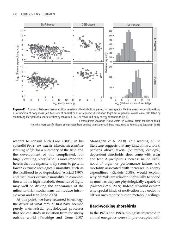
7 2 A D D I N G E N V I R O N M E N T
readers to consult Nick Lane ( 2005 ), in his splendid Power, sex, suicide: Mitochondria and the meaning of life , for a summary of the fi eld and the development of this complicated, but hugely exciting, story. What is most important here is that the capacity to fl y seems to go with lower extrinsic (ecological) mortality, such as the likelihood to be depredated ( Austad 1997 ), and that lower extrinsic mortality, in combina-tion with the high metabolic demands of fl ight, may well be driving the appearance of the mitochondrial mechanisms that reduce intrin-sic wear and tear ( Lane 2005 ).
At this point, we have returned to ecology, the driver of what may at fi rst have seemed purely mechanistic, physiological processes that one can study in isolation from the messy outside world ( Partridge and Gems 2007 ,
Monaghan et al . 2008 ). Our reading of the literature suggests that any kind of hard work, perhaps above taxon- (or rather, ecology-) dependent thresholds, does come with wear and tear. A precipitous increase in the likeli-hood of organ or performance failure, and mortality associated with increases in energy expenditure ( Ricklefs 2008 ), would explain why animals are reluctant habitually to spend as much as they are physiologically capable of ( Valencak et al . 2009 ). Indeed, it would explain why special kinds of motivation are needed to lift our own modest human metabolic ceilings.
Hard-working shorebirds
In the 1970s and 1980s, biologists interested in animal energetics were still pre-occupied with
log e
(lif
etim
e ex
pend
iture
, kJ/
g)
0
5
6
7
8
9
loge (body mass, g)10 122
10
11
4 6 8 0 2 4 6 8
abso
lute
frqu
ency
50
30
loge (lifetime expenditure, kJ/g)106
10
20
7 8 9
5
6
7
8
9
10
11
0
30
10
20
40
50
60
70
BIR
DS
MA
MM
ALS
BMR-based DEE-based BMR-based
Figure 41. Contrasts between mammals (top panels) and birds (bottom panels) in mass specifi c lifetime energy expenditure (kJ/g) as a function of body mass (left two sets of panels) or as a frequency distribution (right set of panels). Values were calculated by multiplying life span of a species either by measured BMR or measured daily energy expenditure (DEE).
Compiled from Speakman ( 2005 ), where the statistical details can also be found. Note that mass-specifi c lifetime energy expenditure declines signifi cantly with body mass (see also Furness and Speakman 2008 ).
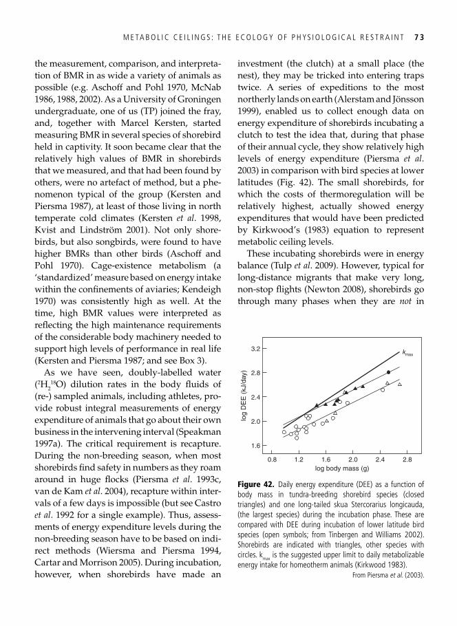
M E TA B O L I C C E I L I N G S : T H E E C O L O G Y O F P H YS I O L O G I C A L R E S T R A I N T 7 3
the measurement, comparison, and interpreta-tion of BMR in as wide a variety of animals as possible (e.g. Aschoff and Pohl 1970 , McNab 1986 , 1988 , 2002 ). As a University of Groningen undergraduate, one of us (TP) joined the fray, and, together with Marcel Kersten, started measuring BMR in several species of shorebird held in captivity. It soon became clear that the relatively high values of BMR in shorebirds that we measured, and that had been found by others, were no artefact of method, but a phe-nomenon typical of the group ( Kersten and Piersma 1987 ), at least of those living in north temperate cold climates ( Kersten et al . 1998 , Kvist and Lindström 2001 ). Not only shore-birds, but also songbirds, were found to have higher BMRs than other birds ( Aschoff and Pohl 1970 ). Cage-existence metabolism (a ‘standardized’ measure based on energy intake within the confi nements of aviaries; Kendeigh 1970 ) was consistently high as well. At the time, high BMR values were interpreted as refl ecting the high maintenance requirements of the considerable body machinery needed to support high levels of performance in real life ( Kersten and Piersma 1987 ; and see Box 3 ).
As we have seen, doubly-labelled water ( 2 H 2
18 O) dilution rates in the body fl uids of (re-) sampled animals, including athletes, pro-vide robust integral measurements of energy expenditure of animals that go about their own business in the intervening interval ( Speakman 1997a ). The critical requirement is recapture. During the non-breeding season, when most shorebirds fi nd safety in numbers as they roam around in huge fl ocks ( Piersma et al . 1993c , van de Kam et al . 2004 ), recapture within inter-vals of a few days is impossible (but see Castro et al . 1992 for a single example). Thus, assess-ments of energy expenditure levels during the non-breeding season have to be based on indi-rect methods ( Wiersma and Piersma 1994 , Cartar and Morrison 2005 ). During incubation, however, when shorebirds have made an
investment (the clutch) at a small place (the nest), they may be tricked into entering traps twice. A series of expeditions to the most northerly lands on earth ( Alerstam and Jönsson 1999 ), enabled us to collect enough data on energy expenditure of shorebirds incubating a clutch to test the idea that, during that phase of their annual cycle, they show relatively high levels of energy expenditure ( Piersma et al . 2003 ) in comparison with bird species at lower latitudes ( Fig. 42 ). The small shorebirds, for which the costs of thermoregulation will be relatively highest, actually showed energy expenditures that would have been predicted by Kirkwood’s (1983) equation to represent metabolic ceiling levels.
These incubating shorebirds were in energy balance ( Tulp et al . 2009 ). However, typical for long-distance migrants that make very long, non-stop fl ights ( Newton 2008 ), shorebirds go through many phases when they are not in
1.6
2.0
2.4
2.8
3.2
log
DE
E (
kJ/d
ay)
0.8 1.2 1.6 2.0 2.4 2.8log body mass (g)
kmax
Figure 42. Daily energy expenditure (DEE) as a function of body mass in tundra-breeding shorebird species (closed triangles) and one long-tailed skua Stercorarius longicauda, (the largest species) during the incubation phase. These are compared with DEE during incubation of lower latitude bird species (open symbols; from Tinbergen and Williams 2002 ). Shorebirds are indicated with triangles, other species with circles. k max is the suggested upper limit to daily metabolizable energy intake for homeotherm animals ( Kirkwood 1983 ).
From Piersma et al . ( 2003 ).
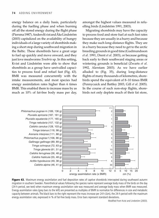
7 4 A D D I N G E N V I R O N M E N T
energy balance on a daily basis, particularly during the fuelling phase and when burning off all the stored energy during the fl ight phase ( Piersma 1987 ). Anders Kvist and Åke Lindström ( 2003 ) capitalized on the availability of hungry individuals of a large variety of shorebirds mak-ing a short stop during southward migration in the Baltic. These shorebirds have a great urge to fuel up quickly and move onward, and they just love mealworms Tenebrio sp. In this setting, Kvist and Lindström were able to show that shorebirds as a group have unrivalled capaci-ties to process food and refuel fast ( Fig. 43 ). BMR was measured concurrently with the intake measurements, and most species had energy assimilation rates higher than 6 times BMR. This enabled them to increase mass by as much as 10% of fat-free body mass per day,
amongst the highest values measured in refu-elling birds ( Lindström 1991 , 2003 ).
Migrating shorebirds may have the capacity to process food and store fuel at such fast rates because they are usually in a hurry and because they make such long-distance fl ights. They are in a hurry because they need to get to the arctic breeding grounds in good time ( Gudmundsson et al . 1991 , Drent et al . 2003 ), or because getting back early to their southward staging areas or wintering grounds is benefi cial ( Zwarts et al . 1992 , Alerstam 2003 ). As we have earlier alluded to ( Fig. 35 ), during long-distance fl ights of many thousands of kilometres, shore-birds spend the equivalent of 8–10 times BMR ( Pennycuick and Battley 2003 , Gill et al . 2005 ). In the course of such non-stop fl ights, shore-birds not only deplete much of their fat store,
0 12102 4 6 8energy assimilation rate (x BMR)
Calidris alpina (46, 41 g)
Actitis hypoleucos (49, 38 g)
Calidris hiaticula (55, 48 g)
Calidris ferruginea (56, 48 g)
Tringa glareola (61, 51 g)
Tringa ochropus (72, 63 g)
Gallinago gallinago (89, 89 g)
Philomachus pugnax f (106, 86 g)
Arenaria interpres (111, 88 g)
Tringa totanus (116, 98 g)
Calidris canutus (128, 103 g)
Tringa nebularia (157, 132 g)
Pluvialis squatarola (177, 165 g)
Pluvialis apricaria (187, 161 g)
Philomachus pugnax m (189, 136 g) 2
1
1
1
3
3
3
5
3
1
13
14
5
6
30
0 5 10 15Δm (%)
20
n =
Figure 43. Maximum energy assimilation and fuel deposition rates of captive shorebirds intercepted during southward autumn migration in southern Sweden. Parenthetical values following the species name represent average body mass of the birds on the day (24-h period, see text) when maximum energy assimilation rate was measured and average body mass when BMR was measured. Energy assimilation rates (grey bars to the left) are presented as multiples of BMR to normalize for differences in size and metabolic capacity between animals. The black bars to the right represent the mass increase per 24 h (∆m), the 24-h period with the maximum energy assimilation rate, expressed in % of fat-free body mass. Error bars represent standard deviations.
Modifi ed from Kvist and Lindström ( 2003 ).
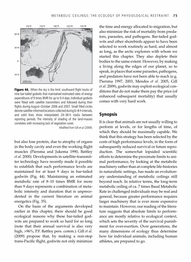
M E TA B O L I C C E I L I N G S : T H E E C O L O G Y O F P H YS I O L O G I C A L R E S T R A I N T 7 5
but also lose protein, due to atrophy of organs in the body cavity and even the working fl ight muscles ( Piersma and Jukema 1990 , Battley et al . 2000 ). Developments in satellite-transmit-ter technology have recently made it possible to establish that such performance levels are maintained for at least 9 days in bar-tailed godwits ( Fig. 44 ). Maintaining an estimated metabolic rate of 8–10 times BMR for more than 9 days represents a combination of meta-bolic intensity and duration that is unprece-dented in the current literature on animal energetics ( Fig. 35 ).
On the basis of the arguments developed earlier in this chapter, there should be good ecological reasons why these bar-tailed god-wits are prepared to work so hard for so long (note that their annual survival is also very high, >96%, P.F. Battley pers. comm.). Gill et al . ( 2009 ) propose that, by making a non-stop trans- Pacifi c fl ight, godwits not only minimize
the time and energy allocated to migration, but also minimize the risk of mortality from preda-tors, parasites, and pathogens. Bar-tailed god-wits and other shorebirds appear to have been selected to work routinely as hard, and almost as long, as the arctic explorers with whom we started this chapter. They also deplete their bodies to the same extent. However, by making a living along the edges of our planet, so to speak, in places that some parasites, pathogens, and predators have not been able to reach (e.g. Piersma 1997 , 2003 , Mendes et al . 2005 , Gill et al . 2009 ), godwits may exploit ecological con-ditions that do not make them pay the price (of enhanced subsequent mortality) that usually comes with very hard work.
Synopsis
It is clear that animals are not usually willing to perform at levels, or for lengths of time, of which they should be maximally capable. We think that this strategy has been selected by the costs of high performance levels, in the form of subsequently reduced survival or future repro-duction. The somewhat lopsided scientifi c efforts to determine the proximate limits to ani-mal performance, by looking at the metabolic machinery rather than at complete life-histories in naturalistic settings, has made an evolution-ary understanding of metabolic ceilings still beyond reach. In relative terms, the long-term metabolic ceiling of ca. 7 times Basal Metabolic Rate in challenged individuals may be real and general, because greater performance requires larger machinery that is ever more expensive to maintain. However, our reading of the litera-ture suggests that absolute limits to perform-ance are mostly relative to ecological context, which sets the severity of the survival punish-ment for over-exertion. Over generations, the many dimensions of ecology thus determine how far individual animals, including human athletes, are prepared to go.
2000 km
30°S
0°
30°N
60°N
120°E 150°E 180°E 150°W 120°W
Figure 44. When the sky is the limit: southward fl ight tracks of nine bar-tailed godwits that maintained estimated rates of energy expenditures of 9 times BMR for up to 9.4 days. Individual godwits were fi tted with satellite transmitters and followed during their fl ights during August–October 2006 and 2007. Small fi lled circles denote satellite-informed locations collected during 6–8-h intervals, and solid lines show interpolated 24–36-h tracks between reporting periods. The intensity of shading of the land-masses correlates with increasing lack of vegetation cover.
Modifi ed from Gill et al . (2009).
7 6 A D D I N G E N V I R O N M E N T
‘The most remarkable thing about the apteryx (the kiwi) was its small respiratory system, suggesting that in the wild this must be a shy, patient, creepy little bird, with little inclination to exert itself much and therefore little need to breathe heavily’. So wrote Charles Darwin in his early notebook ‘D’, according to David Quammen ( 2006 ). It is not unusual for Charles Darwin’s writings to encapsulate many later developments in biology. In the present case, reference to ‘little need to breathe heavily’ correctly anticipated the fi nding that the fl ightless kiwis of New Zealand have the lowest BMR-values reported in birds ( McNab 1994 , 1996 ); mention of ‘its small respiratory system’ refl ected the small size of fl ight muscles and other organs associated with respiration ( McNab 1996 ); and the observation that ‘in the wild this must be a shy, patient, creepy little bird’ anticipated the general tendency for high BMRs to be associated with high levels of energy expenditure under fi eld conditions ( Scholander et al . 1950c , Kersten and Piersma 1987 , Daan et al . 1990b , Speakman et al . 2004a ).
The rather strictly defi ned, standardized nature of BMR (the metabolism of inactive homeotherms that are not digesting, growing, moulting, ovulating or gestating under thermoneutral conditions) and the potential to correlate BMR with life-history and biogeographic variables in ever more sophisticated ways, have made BMR immensely popular with physiologists and ecologists alike; according to the ISI Web of Knowledge, well over 1000 published papers have BMR as their topic. See Lasiewski and Dawson ( 1967 ), Weathers ( 1979 ), McNab ( 1986 , 1988 ), Elgar and Harvey ( 1987 ), Lovegrove ( 2000 ), Tieleman and Williams ( 2000 ), White and Seymour ( 2004 , 2005 ), Anderson and Jetz ( 2005 ) and White et al . ( 2007 ) for examples.
Ricklefs et al. ( 1996 ) discussed whether metabolic ceilings should be seen as a direct function of BMR, or whether these quantities should be treated as energetic consequences of different aspects of an organism’s performance. They concluded that the relationship between BMR and energy expenditure in the fi eld ‘may be fortuitous rather than direct’. We propose that the relationship is indeed indirect, but certainly not fortuitous. In the most general interpretation BMR refl ects the size and maintenance cost of the metabolic machinery (much like the fuel usage of an idling motor), an idea fi rst explicitly formulated by our research associate Marcel Kersten in 1985 ( Kersten and Piersma 1987 ). Depending on the ecological context, the machinery may be necessary for animals to achieve high rates of energy expenditure during strenuous exercise (requiring large pectoral muscles and hearts and viscous blood) or to achieve the storage of large amounts of energy rich fuel each day (requiring large guts and livers). Thus, the graphical model presented by Piersma et al. ( 1996a ; Fig. 45A ) to show how BMR and fi eld metabolic rate would be functionally coupled is incomplete. In refl ecting the size and capacity of the metabolic machinery, BMR does not determine a general ceiling, but rather, by virtue of the size and capacity of particular organ groups, sets particular kinds of ceiling ( Fig. 45B ). Thus, similar levels of BMR can refl ect the maintenance requirements of widely varying machinery, not only between and within species, but even within individuals ( Piersma 2002 , Ksiazek et al . 2009 , Fig. 45B ). This led another research associate of ours, François Vézina, to refl ect with a sigh that ‘BMR is a package deal of so many different things’.
Although incomplete because of this compartmentalization, the rationale of using
Box 3 BMR: interesting baseline, epiphenomenon, or both?
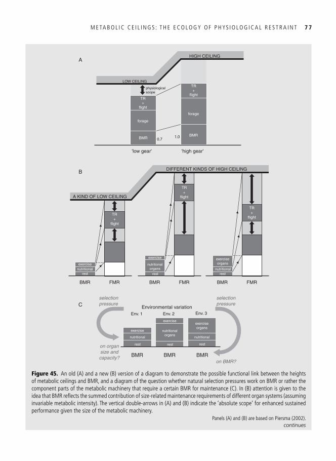
M E TA B O L I C C E I L I N G S : T H E E C O L O G Y O F P H YS I O L O G I C A L R E S T R A I N T 7 7
1.0 BMRBMR
forage
TR+
flight
HIGH CEILING
forage
TR+
flight
LOW CEILING
A
B
C
physiologicalscope
'low gear' 'high gear'
0.7
rest
nutritional
exercise
rest
nutritionalorgans
exercise
rest
nutritional
exerciseorgans
BMR BMR BMR
Env. 1 Env. 2 Env. 3Environmental variation
selectionpressure
selectionpressure
on organsize andcapacity?
on BMR?
DIFFERENT KINDS OF HIGH CEILING
A KIND OF LOW CEILING
FMRBMR
TR+
flight
FMRBMR
TR+
flight
FMRBMR
TR+
flight
rest
exercisenutritional nutritional
rest
nutritionalorgans
exercise
rest
exerciseorgans
Figure 45. An old (A) and a new (B) version of a diagram to demonstrate the possible functional link between the heights of metabolic ceilings and BMR, and a diagram of the question whether natural selection pressures work on BMR or rather the component parts of the metabolic machinery that require a certain BMR for maintenance (C). In (B) attention is given to the idea that BMR refl ects the summed contribution of size-related maintenance requirements of different organ systems (assuming invariable metabolic intensity). The vertical double-arrows in (A) and (B) indicate the ‘absolute scope’ for enhanced sustained performance given the size of the metabolic machinery.
Panels (A) and (B) are based on Piersma ( 2002 ). continues
7 8 A D D I N G E N V I R O N M E N T
BMR as a yardstick to evaluate or interspecifi cally scale maximal metabolic performances, seems nevertheless quite valid as long as the appropriate, context-specifi c, values for BMR are used ( McKechnie et al . 2006 ). However, even though BMR may (1) be repeatable within individuals ( Hayes et al . 1998 , Bech et al . 1999 , Horak et al . 2002 , Labocha et al . 2004 , Rønning et al . 2005 , Vézina and Williams 2005 ), (2) have a heritable component ( Konarzewski and
Diamond 1995 , Ksiazek et al . 2004 , 2009 ) and (3) be selected for in the wild ( Broggi et al . 2005 ), BMR may be too much of an epiphenomenon to be a good trait for natural selection to work on ( Fig. 45C ). We suggest that natural selection fi rst and foremost targets the size and capacity of different organs and organ groups, and that BMR will follow as a result (cf. Jackson and Diamond 1996 , Williams and Tieleman 2000 , Sadowska et al. 2008 ).
Box 3 Continued
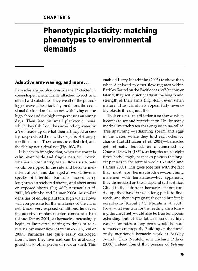
79
CHAPTER 5
Phenotypic plasticity: matching phenotypes to environmental demands
Adaptive arm-waving, and more . . .
Barnacles are peculiar crustaceans. Protected in cone-shaped shells, fi rmly attached to rock and other hard substrates, they weather the pound-ing of waves, the attacks by predators, the occa-sional desiccation that comes with living on the high shore and the high temperatures on sunny days. They feed on small planktonic items, which they fi sh from the surrounding water by a ‘net’ made up of what their arthropod ances-try has provided them with: six pairs of strongly modifi ed arms. These arms are called cirri, and the fi shing net a cirral net ( Fig. 46A , B ).
It is easy to imagine that, when the water is calm, even wide and fragile nets will work, whereas under strong water fl ows such nets would be ripped to the side and become inef-fi cient at best, and damaged at worst. Several species of intertidal barnacles indeed carry long arms on sheltered shores, and short arms on exposed shores ( Fig. 46C ; Arsenault et al . 2001 , Marchinko and Palmer 2003 ). At similar densities of edible plankton, high water fl ows will compensate for the smallness of the cirral net. Under very exposed conditions, however, the adaptive miniaturization comes to a halt ( Li and Denny 2004 ), as barnacles increasingly begin to limit cirral netting to times of rela-tively slow water fl ow ( Marchinko 2007 , Miller 2007 ). Barnacles are quite easily dislodged from where they live and can be artifi cially glued on to other pieces of rock or shell. This
enabled Kerry Marchinko ( 2003 ) to show that, when displaced to other fl ow regimes within Barkley Sound on the Pacifi c coast of Vancouver Island, they will quickly adjust the length and strength of their arms ( Fig. 46D ), even when mature. Thus, cirral nets appear fully reversi-bly plastic throughout life.
Their crustacean affi liation also shows when it comes to sex and reproduction. Unlike many marine invertebrates that engage in so-called ‘free spawning’—jettisoning sperm and eggs in the water, where they fi nd each other by chance ( Luttikhuizen et al. 2004 )—barnacles get intimate. Indeed, as documented by Charles Darwin ( 1854 ), at lengths up to eight times body length, barnacles possess the long-est penises in the animal world ( Neufeld and Palmer 2008 ). This goes together with the fact that most are hermaphrodites—combining maleness with femaleness—but apparently they do not do it on the cheap and self-fertilize. Glued to the substrate, barnacles cannot cud-dle up; they have to use a long penis to fi nd, reach, and then impregnate fastened but fertile neighbours ( Klepal 1990 , Murata et al . 2001 ). Now, what was true for the feeding arms form-ing the cirral net, would also be true for a penis extending out of the father’s cone: at high water-fl ow rates, a long penis would be hard to manoeuvre properly. Building on the previ-ously mentioned barnacle work at Barkley Sound, Chris Neufeld and Richard Palmer (2008) indeed found that penises of Balanus
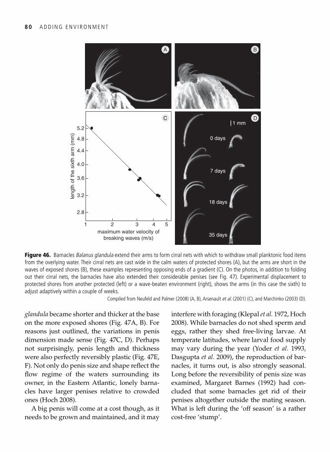
8 0 A D D I N G E N V I R O N M E N T
glandula became shorter and thicker at the base on the more exposed shores ( Fig. 47A , B ). For reasons just outlined, the variations in penis dimension made sense ( Fig. 47C , D). Perhaps not surprisingly, penis length and thickness were also perfectly reversibly plastic ( Fig. 47E , F). Not only do penis size and shape refl ect the fl ow regime of the waters surrounding its owner, in the Eastern Atlantic, lonely barna-cles have larger penises relative to crowded ones ( Hoch 2008 ).
A big penis will come at a cost though, as it needs to be grown and maintained, and it may
interfere with foraging ( Klepal et al. 1972 , Hoch 2008 ). While barnacles do not shed sperm and eggs, rather they shed free-living larvae. At temperate latitudes, where larval food supply may vary during the year ( Yoder et al . 1993 , Dasgupta et al . 2009 ), the reproduction of bar-nacles, it turns out, is also strongly seasonal. Long before the reversibility of penis size was examined, Margaret Barnes ( 1992 ) had con-cluded that some barnacles get rid of their penises altogether outside the mating season. What is left during the ‘off season’ is a rather cost-free ‘stump’.
1
2.8
3.2
4.0
5.2
leng
th o
f the
six
th a
rm (
mm
)
2 3 4 5maximum water velocity of
breaking waves (m/s)
3.6
4.4
4.8
A B
C
0 days
7 days
18 days
35 days
1 mmD
Figure 46. Barnacles Balanus glandula extend their arms to form cirral nets with which to withdraw small planktonic food items from the overlying water. Their cirral nets are cast wide in the calm waters of protected shores (A), but the arms are short in the waves of exposed shores (B), these examples representing opposing ends of a gradient (C). On the photos, in addition to folding out their cirral nets, the barnacles have also extended their considerable penises (see Fig. 47 ). Experimental displacement to protected shores from another protected (left) or a wave-beaten environment (right), shows the arms (in this case the sixth) to adjust adaptively within a couple of weeks.
Compiled from Neufeld and Palmer ( 2008 ) (A, B), Arsenault et al . ( 2001 ) (C), and Marchinko ( 2003 ) (D).
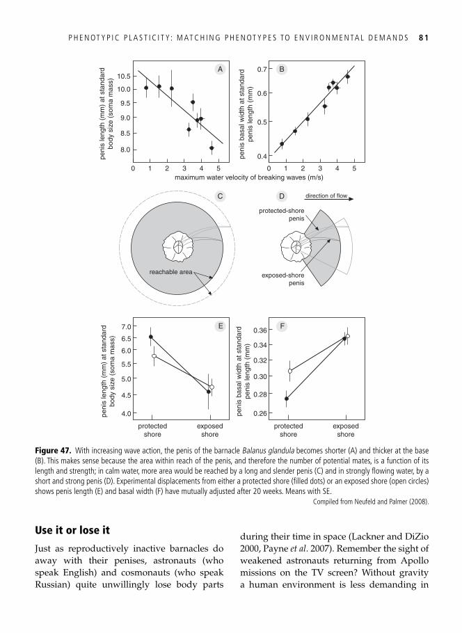
P H E N OT Y P I C P L A S T I C I T Y : M AT C H I N G P H E N OT Y P E S TO E N V I R O N M E N TA L D E M A N D S 8 1
Use it or lose it
Just as reproductively inactive barnacles do away with their penises, astronauts (who speak English) and cosmonauts (who speak Russian) quite unwillingly lose body parts
during their time in space ( Lackner and DiZio 2000 , Payne et al . 2007 ). Remember the sight of weakened astronauts returning from Apollo missions on the TV screen? Without gravity a human environment is less demanding in
0
8.0
8.5
9.0
9.5
10.0
peni
s le
ngth
(m
m)
at s
tand
ard
body
siz
e (s
oma
mas
s)
1 2 3 4 5maximum water velocity of breaking waves (m/s)
A10.5
0
0.4
0.5
0.6
peni
s ba
sal w
idth
at s
tand
ard
peni
s le
ngth
(m
m)
1 2 3 4 5
B0.7
4.0
4.5
5.0
5.5
6.0
peni
s le
ngth
(m
m)
at s
tand
ard
body
siz
e (s
oma
mas
s)
protectedshore
E
6.5
0.26
0.28
0.30
peni
s ba
sal w
idth
at s
tand
ard
peni
s le
ngth
(m
m)
F0.36
exposedshore
protectedshore
exposedshore
7.0
0.32
0.34
C D
reachable area exposed-shorepenis
protected-shorepenis
direction of flow
Figure 47. With increasing wave action, the penis of the barnacle Balanus glandula becomes shorter (A) and thicker at the base (B). This makes sense because the area within reach of the penis, and therefore the number of potential mates, is a function of its length and strength; in calm water, more area would be reached by a long and slender penis (C) and in strongly fl owing water, by a short and strong penis (D). Experimental displacements from either a protected shore (fi lled dots) or an exposed shore (open circles) shows penis length (E) and basal width (F) have mutually adjusted after 20 weeks. Means with SE.
Compiled from Neufeld and Palmer ( 2008 ).
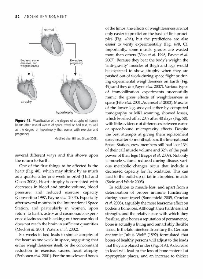
8 2 A D D I N G E N V I R O N M E N T
several different ways and this shows upon the return to Earth.
One of the fi rst things to be affected is the heart ( Fig. 48 ), which may shrink by as much as a quarter after one week in orbit ( Hill and Olson 2008 ). Heart atrophy is correlated with decreases in blood and stroke volume, blood pressure, and reduced exercise capacity ( Convertino 1997 , Payne et al . 2007 ). Especially after several months in the International Space Station, and particularly in women, upon return to Earth, astro- and cosmonauts experi-ence dizziness and blacking-out because blood does not reach the brain in suffi cient quantities ( Meck et al . 2001 , Waters et al . 2002 ).
Six weeks in bed leads to similar atrophy of the heart as one week in space, suggesting that either weightlessness itself, or the concomitant reduction in exercise, causes heart atrophy ( Perhonen et al . 2001 ). For the muscles and bones
of the limbs, the effects of weightlessness are not only easier to predict on the basis of fi rst princi-ples ( Fig. 49A ), but the predictions are also easier to verify experimentally ( Fig. 49B , C ). Importantly, some muscle groups are wasted more than others ( Vico et al . 1998 , Payne et al . 2007 ). Because they bear the body’s weight, the ‘anti-gravity’ muscles of thigh and legs would be expected to show atrophy when they are pushed out of work during space fl ight or dur-ing experimental weightlessness on Earth ( Fig. 49 ); and they do ( Payne et al . 2007 ). Various types of immobilization experiments successfully mimic the gross effects of weightlessness in space ( Fitts et al . 2001 , Adams et al . 2003 ). Muscles of the lower leg, assayed either by computed tomography or MRI scanning, showed losses, which levelled off at 20% after 40 days ( Fig. 50 ), with little evidence of differences between earth- or space-bound microgravity effects. Despite the best attempts at giving them replacement exercise, after six months aboard the International Space Station, crew members still had lost 13% of their calf muscle volume and 32% of the peak power of their legs ( Trappe et al . 2009 ). Not only is muscle volume reduced during disuse, vari-ous metabolic changes occur that include a decreased capacity for fat oxidation. This can lead to the build-up of fat in atrophied muscle ( Stein and Wade 2005 ).
In addition to muscle loss, and apart from a deterioration of proper immune functioning during space travel ( Sonnenfeld 2005 , Crucian et al . 2008), arguably the most fearsome effect on bodies is bone loss. Although their hardness and strength, and the relative ease with which they fossilize, give bones a reputation of permanence, bone is actually a living and remarkably fl exible tissue. In the late-nineteenth century, the German anatomist Julius Wolff ( 1892 ) formulated that bones of healthy persons will adjust to the loads that they are placed under ( Fig. 51A ). A decrease in load will lead to the loss of bone material at appropriate places, and an increase to thicker
normal
atrophy
hypertrophy
Bed rest, somediseases, andweightlessness
Excercise,pregnancy
Figure 48. Visualization of the degree of atrophy of human hearts after several weeks of space travel or bed rest, as well as the degree of hypertrophy that comes with exercise and pregnancy.
Modifi ed after Hill and Olson ( 2008 ).
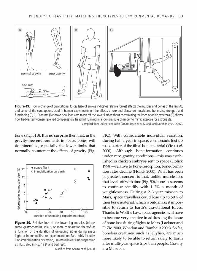
P H E N OT Y P I C P L A S T I C I T Y : M AT C H I N G P H E N OT Y P E S TO E N V I R O N M E N TA L D E M A N D S 8 3
bone ( Fig. 51B ). It is no surprise then that, in the gravity-free environments in space, bones will de-mineralize, especially the lower limbs that normally counteract the effects of gravity ( Fig.
51C ). With considerable individual variation, during half a year in space, cosmonauts lost up to a quarter of the tibial bone material ( Vico et al . 2000 ). Although bone-formation continues under zero gravity conditions—this was estab-lished in chicken embryos sent to space ( Holick 1998 )—relative to bone-resorption, bone-forma-tion rates decline ( Holick 2000 ). What has been of greatest concern is that, unlike muscle loss that levels off with time ( Fig. 50 ), bone loss seems to continue steadily with 1–2% a month of weightlessness. During a 2–3 year mission to Mars, space travellers could lose up to 50% of their bone material, which would make it impos-sible to return to Earth’s gravitational forces. Thanks to Wolff’s Law, space agencies will have to become very creative in addressing the issue of bone loss during fl ights to Mars ( Lackner and DiZio 2000 , Whedon and Rambaut 2006 ). So far, boneless creatures, such as jellyfi sh, are much more likely to be able to return safely to Earth after multi-year space trips than people. Gravity is a Mars bar.
normal gravity zero gravity
bed rest
A B C
Figure 49. How a change of gravitational forces (size of arrows indicates relative forces) affects the muscles and bones of the leg (A), and some of the contraptions used in human experiments on the effects of use and disuse on muscle and bone size, strength, and functioning (B, C). Diagram (B) shows how loads are taken off the lower limb without constraining the knee or ankle, whereas (C) shows how bed-rested women received compensatory treadmill running in a low-pressure chamber to mimic exercise for astronauts.
Compiled from Lackner and DiZio ( 2000 ), Tesch et al . ( 2004 ), and Dorfman et al . ( 2007 ).
decr
ease
in le
g m
uscl
e si
ze (
%)
00
5
10
20
25
duration of unloading experiment (days)10 20 30
15
40 100
space flightimmobilization on earth
Figure 50. Relative loss of the lower leg muscles (triceps surae, gastrocnemius, soleus, or some combination thereof) as a function of the duration of unloading either during space fl ight or in immobilization experiments on Earth (this includes limb immobilization by casting, unilateral lower limb suspension as illustrated in Fig. 49 B, and bed rest).
Modifi ed from Adams et al . ( 2003 ).
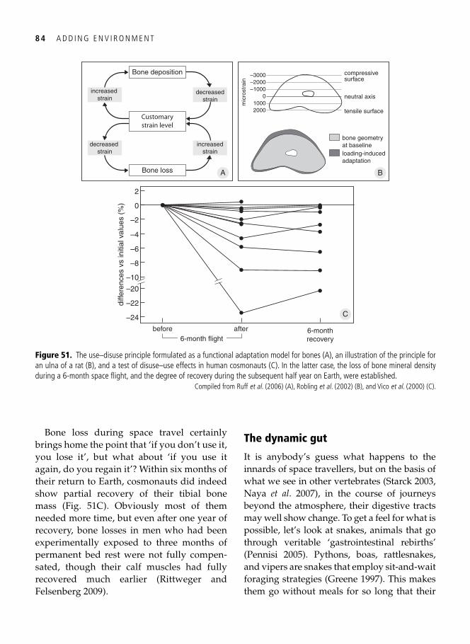
8 4 A D D I N G E N V I R O N M E N T
Bone loss during space travel certainly brings home the point that ‘if you don’t use it, you lose it’, but what about ‘if you use it again, do you regain it’? Within six months of their return to Earth, cosmonauts did indeed show partial recovery of their tibial bone mass ( Fig. 51C ). Obviously most of them needed more time, but even after one year of recovery, bone losses in men who had been experimentally exposed to three months of permanent bed rest were not fully compen-sated, though their calf muscles had fully recovered much earlier ( Rittweger and Felsenberg 2009 ).
The dynamic gut
It is anybody’s guess what happens to the innards of space travellers, but on the basis of what we see in other vertebrates ( Starck 2003 , Naya et al . 2007 ), in the course of journeys beyond the atmosphere, their digestive tracts may well show change. To get a feel for what is possible, let’s look at snakes, animals that go through veritable ‘gastrointestinal rebirths’ ( Pennisi 2005 ). Pythons, boas, rattlesnakes, and vipers are snakes that employ sit-and-wait foraging strategies ( Greene 1997 ). This makes them go without meals for so long that their
0 neutral axis
compressivesurface
tensile surface
mic
rost
rain
20001000
–1000–2000–3000
bone geometryat baselineloading-inducedadaptation
Bone deposition
Bone loss A B
decreasedstrain
increasedstrain
Customarystrain level
decreasedstrain
increasedstrain
diffe
renc
es v
s in
itial
val
ues
(%)
–24
–22
–10
–6
–4
before after
–8
C
–20
–2
0
2
6-monthrecovery6-month flight
Figure 51. The use–disuse principle formulated as a functional adaptation model for bones (A), an illustration of the principle for an ulna of a rat (B), and a test of disuse–use effects in human cosmonauts (C). In the latter case, the loss of bone mineral density during a 6-month space fl ight, and the degree of recovery during the subsequent half year on Earth, were established.
Compiled from Ruff et al . ( 2006 ) (A), Robling et al . ( 2002 ) (B), and Vico et al . ( 2000 ) (C).
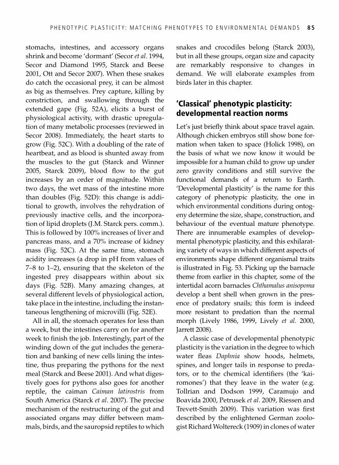
P H E N OT Y P I C P L A S T I C I T Y : M AT C H I N G P H E N OT Y P E S TO E N V I R O N M E N TA L D E M A N D S 8 5
stomachs, intestines, and accessory organs shrink and become ‘dormant’ ( Secor et al . 1994 , Secor and Diamond 1995 , Starck and Beese 2001 , Ott and Secor 2007 ). When these snakes do catch the occasional prey, it can be almost as big as themselves. Prey capture, killing by constriction, and swallowing through the extended gape ( Fig. 52A ), elicits a burst of physiological activity, with drastic upregula-tion of many metabolic processes (reviewed in Secor 2008 ). Immediately, the heart starts to grow ( Fig. 52C ). With a doubling of the rate of heartbeat, and as blood is shunted away from the muscles to the gut (Starck and Winner 2005, Starck 2009 ), blood fl ow to the gut increases by an order of magnitude. Within two days, the wet mass of the intestine more than doubles ( Fig. 52D ): this change is addi-tional to growth, involves the rehydration of previously inactive cells, and the incorpora-tion of lipid droplets (J.M. Starck pers. comm.). This is followed by 100% increases of liver and pancreas mass, and a 70% increase of kidney mass ( Fig. 52C ). At the same time, stomach acidity increases (a drop in pH from values of 7–8 to 1–2), ensuring that the skeleton of the ingested prey disappears within about six days ( Fig. 52B ). Many amazing changes, at several different levels of physiological action, take place in the intestine, including the instan-taneous lengthening of microvilli ( Fig. 52E ).
All in all, the stomach operates for less than a week, but the intestines carry on for another week to fi nish the job. Interestingly, part of the winding down of the gut includes the genera-tion and banking of new cells lining the intes-tine, thus preparing the pythons for the next meal ( Starck and Beese 2001 ). And what diges-tively goes for pythons also goes for another reptile, the caiman Caiman latirostris from South America ( Starck et al . 2007 ). The precise mechanism of the restructuring of the gut and associated organs may differ between mam-mals, birds, and the sauropsid reptiles to which
snakes and crocodiles belong ( Starck 2003 ), but in all these groups, organ size and capacity are remarkably responsive to changes in demand. We will elaborate examples from birds later in this chapter.
‘Classical’ phenotypic plasticity: developmental reaction norms
Let’s just briefl y think about space travel again. Although chicken embryos still show bone for-mation when taken to space ( Holick 1998 ), on the basis of what we now know it would be impossible for a human child to grow up under zero gravity conditions and still survive the functional demands of a return to Earth. ‘Developmental plasticity’ is the name for this category of phenotypic plasticity, the one in which environmental conditions during ontog-eny determine the size, shape, construction, and behaviour of the eventual mature phenotype. There are innumerable examples of develop-mental phenotypic plasticity, and this exhilarat-ing variety of ways in which different aspects of environments shape different organismal traits is illustrated in Fig. 53 . Picking up the barnacle theme from earlier in this chapter, some of the intertidal acorn barnacles Chthamalus anisopoma develop a bent shell when grown in the pres-ence of predatory snails; this form is indeed more resistant to predation than the normal morph ( Lively 1986 , 1999 , Lively et al . 2000 , Jarrett 2008 ).
A classic case of developmental phenotypic plasticity is the variation in the degree to which water fl eas Daphnia show hoods, helmets, spines, and longer tails in response to preda-tors, or to the chemical identifi ers (the ‘kai-romones’) that they leave in the water (e.g. Tollrian and Dodson 1999 , Caramujo and Boavida 2000 , Petrusek et al . 2009 , Riessen and Trevett-Smith 2009 ). This variation was fi rst described by the enlightened German zoolo-gist Richard Woltereck ( 1909 ) in clones of water
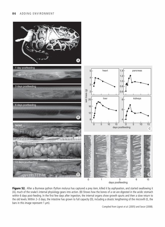
8 6 A D D I N G E N V I R O N M E N T
B
E
0 1 153days postfeeding
6
D
A
heart
0
8
wet
mas
s (g
)
10 155days postfeeding
12
16
20 liver
0 10 155
4
6
8 kidneys
2
3
4
5
0.6
0.8
1.0
pancreas
1.2
1.4
C
1 day postfeeding
3 days postfeeding
6 days postfeeding
fasted
2 days postfeeding
10 days postfeeding
Figure 52. After a Burmese python Python molurus has captured a prey item, killed it by asphyxation, and started swallowing it (A), much of the snake’s internal physiology gears into action. (B) Shows how the bones of a rat are digested in the acidic stomach within 6 days post-feeding. In the fi rst few days after ingestion, the internal organs show growth spurts and then a slow return to the old levels. Within 2–3 days, the intestine has grown to full capacity (D), including a drastic lengthening of the microvilli (E, the bars in this image represent 1 μm).
Compiled from Lignot et al . ( 2005 ) and Secor ( 2008 ).
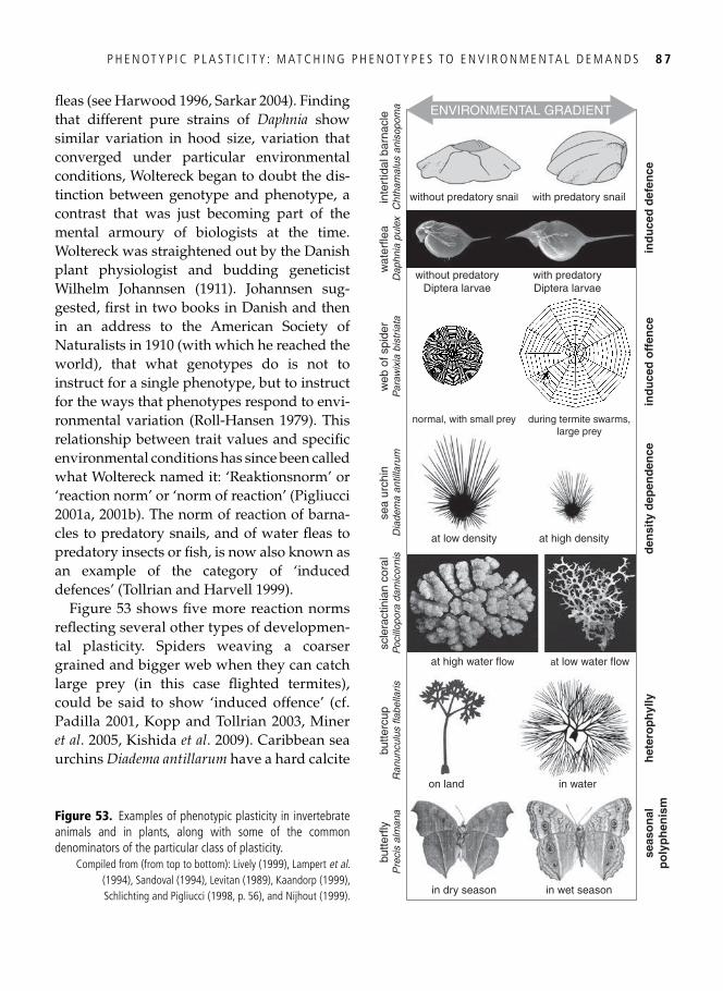
P H E N OT Y P I C P L A S T I C I T Y : M AT C H I N G P H E N OT Y P E S TO E N V I R O N M E N TA L D E M A N D S 8 7
fl eas (see Harwood 1996 , Sarkar 2004 ). Finding that different pure strains of Daphnia show similar variation in hood size, variation that converged under particular environmental conditions, Woltereck began to doubt the dis-tinction between genotype and phenotype, a contrast that was just becoming part of the mental armoury of biologists at the time. Woltereck was straightened out by the Danish plant physiologist and budding geneticist Wilhelm Johannsen ( 1911 ). Johannsen sug-gested, fi rst in two books in Danish and then in an address to the American Society of Naturalists in 1910 (with which he reached the world), that what genotypes do is not to instruct for a single phenotype, but to instruct for the ways that phenotypes respond to envi-ronmental variation ( Roll-Hansen 1979 ). This relationship between trait values and specifi c environmental conditions has since been called what Woltereck named it: ‘Reaktionsnorm’ or ‘reaction norm’ or ‘norm of reaction’ ( Pigliucci 2001a , 2001b ). The norm of reaction of barna-cles to predatory snails, and of water fl eas to predatory insects or fi sh, is now also known as an example of the category of ‘induced defences’ ( Tollrian and Harvell 1999 ).
Figure 53 shows fi ve more reaction norms refl ecting several other types of developmen-tal plasticity. Spiders weaving a coarser grained and bigger web when they can catch large prey (in this case fl ighted termites), could be said to show ‘induced offence’ (cf. Padilla 2001 , Kopp and Tollrian 2003 , Miner et al . 2005 , Kishida et al . 2009 ). Caribbean sea urchins Diadema antillarum have a hard calcite
butte
rfly
Pre
cis
alm
ana
without predatory snail with predatory snail
without predatoryDiptera larvae
with predatoryDiptera larvae
normal, with small prey during termite swarms,large prey
at low density at high density
at high water flow at low water flow
on land in water
in dry season in wet season
butte
rcup
Ran
uncu
lus
flabe
llaris
scle
ract
inia
n co
ral
Poc
illop
ora
dam
icor
nis
sea
urch
inD
iade
ma
antil
laru
mw
eb o
f spi
der
Par
awix
ia b
istr
iata
wat
erfle
aD
aphn
ia p
ulex
inte
rtid
al b
arna
cle
Cht
ham
alus
ani
sopo
ma
seas
on
alp
oly
ph
enis
mh
eter
op
hyl
lyd
ensi
ty d
epen
den
cein
du
ced
off
ence
ind
uce
d d
efen
ce
ENVIRONMENTAL GRADIENT
Figure 53. Examples of phenotypic plasticity in invertebrate animals and in plants, along with some of the common denominators of the particular class of plasticity.
Compiled from (from top to bottom): Lively ( 1999 ), Lampert et al . ( 1994 ), Sandoval ( 1994 ), Levitan ( 1989 ), Kaandorp ( 1999 ), Schlichting and Pigliucci ( 1998 , p. 56), and Nijhout ( 1999 ).
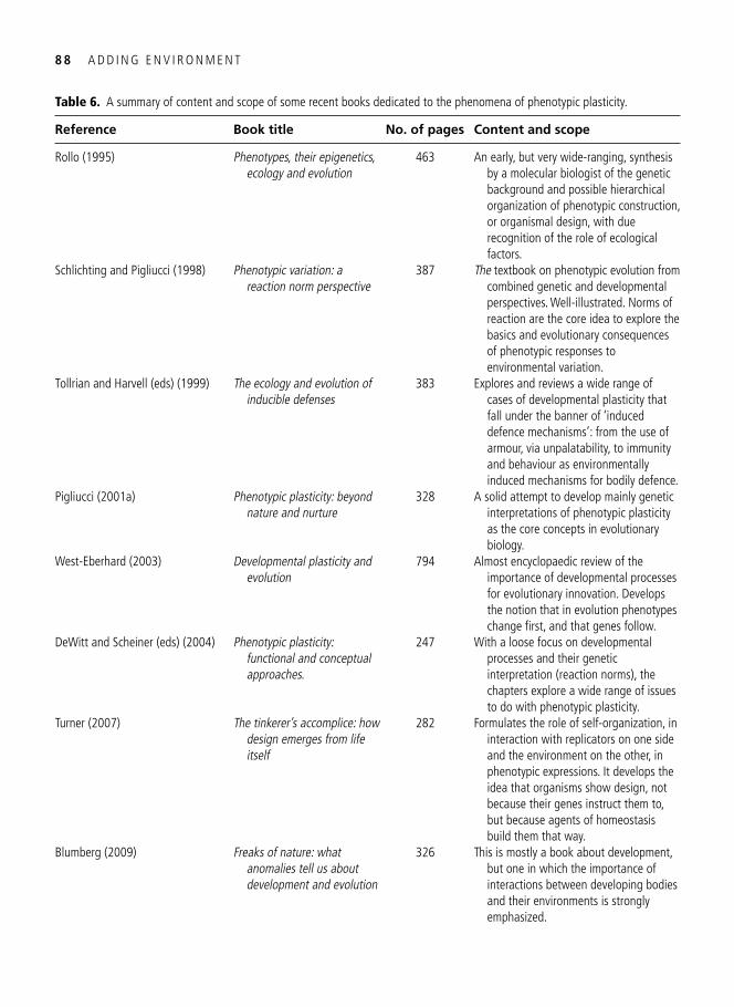
8 8 A D D I N G E N V I R O N M E N T
Table 6. A summary of content and scope of some recent books dedicated to the phenomena of phenotypic plasticity.
Reference Book title No. of pages Content and scope
Rollo (1995) Phenotypes, their epigenetics, ecology and evolution
463 An early, but very wide-ranging, synthesis by a molecular biologist of the genetic background and possible hierarchical organization of phenotypic construction, or organismal design, with due recognition of the role of ecological factors.
Schlichting and Pigliucci (1998) Phenotypic variation: a reaction norm perspective
387 The textbook on phenotypic evolution from combined genetic and developmental perspectives. Well-illustrated. Norms of reaction are the core idea to explore the basics and evolutionary consequences of phenotypic responses to environmental variation.
Tollrian and Harvell (eds) (1999) The ecology and evolution of inducible defenses
383 Explores and reviews a wide range of cases of developmental plasticity that fall under the banner of ‘induced defence mechanisms’: from the use of armour, via unpalatability, to immunity and behaviour as environmentally induced mechanisms for bodily defence.
Pigliucci (2001a) Phenotypic plasticity: beyond nature and nurture
328 A solid attempt to develop mainly genetic interpretations of phenotypic plasticity as the core concepts in evolutionary biology.
West-Eberhard (2003) Developmental plasticity and evolution
794 Almost encyclopaedic review of the importance of developmental processes for evolutionary innovation. Develops the notion that in evolution phenotypes change fi rst, and that genes follow.
DeWitt and Scheiner (eds) (2004) Phenotypic plasticity: functional and conceptual approaches.
247 With a loose focus on developmental processes and their genetic interpretation (reaction norms), the chapters explore a wide range of issues to do with phenotypic plasticity.
Turner (2007) The tinkerer’s accomplice: how design emerges from life itself
282 Formulates the role of self-organization, in interaction with replicators on one side and the environment on the other, in phenotypic expressions. It develops the idea that organisms show design, not because their genes instruct them to, but because agents of homeostasis build them that way.
Blumberg (2009) Freaks of nature: what anomalies tell us about development and evolution
326 This is mostly a book about development, but one in which the importance of interactions between developing bodies and their environments is strongly emphasized.
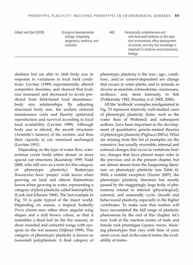
P H E N OT Y P I C P L A S T I C I T Y : M AT C H I N G P H E N OT Y P E S TO E N V I R O N M E N TA L D E M A N D S 8 9
skeleton but are able to shift body size in response to variations in local food condi-tions. Levitan ( 1989 ) experimentally altered competitor densities, and showed that body size increased and decreased to levels pre-dicted from fi eld-based food abundance–body size relationships. By adjusting structural body size, the urchins reduced maintenance costs and thereby optimized reproduction and survival according to local food availability ( Levitan 1989 ). Although body size is altered, the mouth structures (Aristotle’s lantern) of the urchins, and thus their capacity to eat, remained unchanged ( Levitan 1991 ).
Depending on the type of water fl ow, scler-actinian corals build either denser or more spaced out structures ( Kaandorp 1999 , Todd 2008 , who still owe us a term for this category of phenotypic plasticity). Buttercups Ranunculus have ‘proper’ wide leaves when growing on land and almost fi lamentous leaves when growing in water, representing a category of plant plasticity called heterophylly ( Cook and Johnson 1968 ). The last example in Fig. 53 is quite typical of the insect world. Depending on season, a tropical butterfl y Precis almana may either show angular wing shapes and a dull brown colour, so that it resembles a dead leaf (in the dry season), or show rounded and colourful wings with eye-spots (in the wet season) ( Nijhout 1999 ). This category of phenotypic plasticity is known as (seasonal) polyphenism. A fi nal category of
phenotypic plasticity is the size-, age-, condi-tion-, and/or context-dependent sex change that occurs in some plants, and in animals as diverse as annelids, echinoderms, crustaceans, molluscs, and, most famously, in fi sh ( Polikansky 1982 , Munday et al. 2005 , 2006 ).
All the ‘textbook’ examples amalgamated in Fig. 53 represent relatively well-studied cases of phenotypic plasticity. Some, such as the water fl eas of Woltereck and subsequent authors, have been important in the develop-ment of quantitative genetic-related theories of phenotypic plasticity ( Pigliucci 2001a ). What are missing from this list of examples are the extensive, but usually reversible, internal and external changes that occur in vertebrate bod-ies, changes that have played major roles in the previous and in the present chapter, but are almost absent from the burgeoning litera-ture on phenotypic plasticity (see Table 6 ). With a notable exception ( Turner 2007 ), the phenotypic plasticity literature has mostly passed by the staggeringly large body of phe-nomena related to internal (physiological), external, and seasonally cyclic (moult) and behavioural plasticity, especially in the higher vertebrates. To make sure that readers will have encountered the full range of plasticity phenomena by the end of this chapter, let’s now look at the reaction norms of male and female rock ptarmigan Lagopus mutus , show-ing phenotypes that vary with time of year, snow cover, and, in the case of males, the avail-ability of mates.
Gilbert and Epel (2009) Ecological developmental biology: integrating epigenetics, medicine, and evolution
480 Fantastically comprehensive and well-illustrated textbook on the ways that environments affect development of animals, and why this knowledge is important in medicine and evolutionary biology.
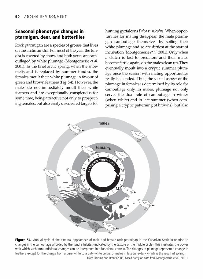
9 0 A D D I N G E N V I R O N M E N T
Seasonal phenotype changes in ptarmigan, deer, and butterfl ies
Rock ptarmigan are a species of grouse that lives on the arctic tundra. For most of the year the tun-dra is covered by snow, and both sexes are cam-oufl aged by white plumage ( Montgomerie et al . 2001 ). In the brief arctic spring, when the snow melts and is replaced by summer tundra, the females moult their white plumage in favour of green and brown feathers ( Fig. 54 ). However, the males do not immediately moult their white feathers and are exceptionally conspicuous for some time, being attractive not only to prospect-ing females, but also easily discovered targets for
hunting gyrfalcons Falco rusticolus . When oppor-tunities for mating disappear, the male ptarmi-gan camoufl age themselves by soiling their white plumage and so are dirtiest at the start of incubation ( Montgomerie et al . 2001 ). Only when a clutch is lost to predators and their mates become fertile again, do the males clean up. They eventually moult into a cryptic summer plum-age once the season with mating opportunities really has ended. Thus, the visual aspect of the plumage in females is determined by its role for camoufl age only. In males, plumage not only serves the dual role of camoufl age in winter (when white) and in late summer (when com-prising a cryptic patterning of browns), but also
D JF
M
A
M
JJA
S
O
N
aco
m
plete annual cycle
males
females
Figure 54. Annual cycle of the external appearance of male and female rock ptarmigan in the Canadian Arctic in relation to changes in the camoufl age afforded by the tundra habitat (indicated by the texture of the middle circle). This illustrates the power with which such intra-individual changes can be interpreted in a functional context. The changes in plumage represent a change in feathers, except for the change from a pure white to a dirty white colour of males in late June–July, which is the result of soiling.
From Piersma and Drent ( 2003 ) based partly on data from Montgomerie et al . ( 2001 ).
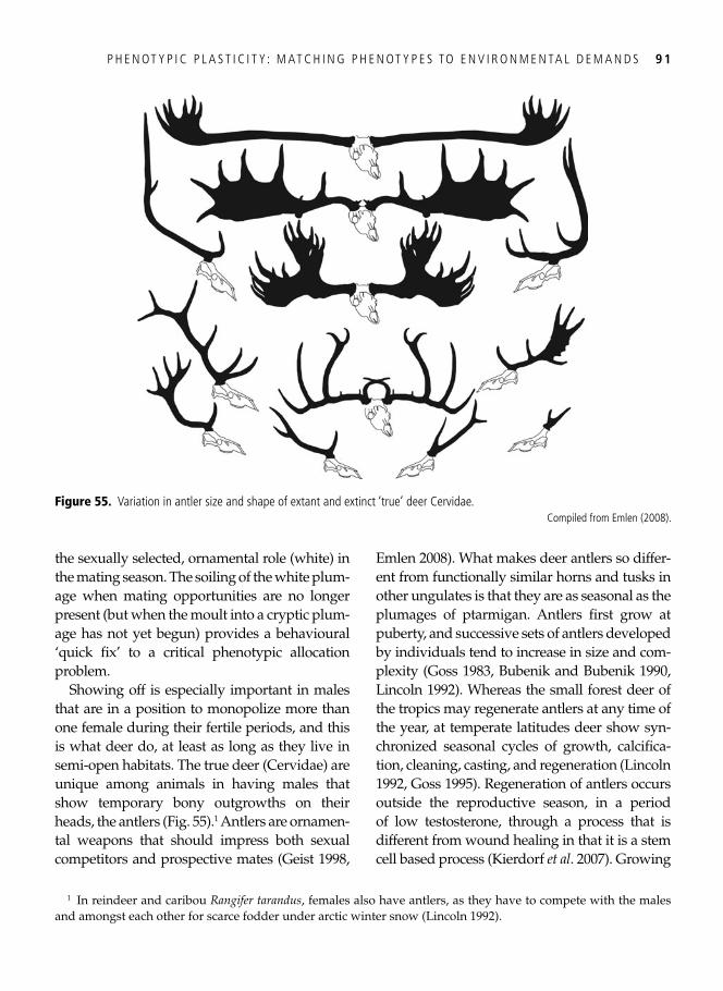
P H E N OT Y P I C P L A S T I C I T Y : M AT C H I N G P H E N OT Y P E S TO E N V I R O N M E N TA L D E M A N D S 9 1
the sexually selected, ornamental role (white) in the mating season. The soiling of the white plum-age when mating opportunities are no longer present (but when the moult into a cryptic plum-age has not yet begun) provides a behavioural ‘quick fi x’ to a critical phenotypic allocation problem.
Showing off is especially important in males that are in a position to monopolize more than one female during their fertile periods, and this is what deer do, at least as long as they live in semi-open habitats. The true deer (Cervidae) are unique among animals in having males that show temporary bony outgrowths on their heads, the antlers ( Fig. 55 ). 1 Antlers are ornamen-tal weapons that should impress both sexual competitors and prospective mates ( Geist 1998 ,
Emlen 2008 ). What makes deer antlers so differ-ent from functionally similar horns and tusks in other ungulates is that they are as seasonal as the plumages of ptarmigan. Antlers fi rst grow at puberty, and successive sets of antlers developed by individuals tend to increase in size and com-plexity ( Goss 1983 , Bubenik and Bubenik 1990 , Lincoln 1992 ). Whereas the small forest deer of the tropics may regenerate antlers at any time of the year, at temperate latitudes deer show syn-chronized seasonal cycles of growth, calcifi ca-tion, cleaning, casting, and regeneration ( Lincoln 1992 , Goss 1995 ). Regeneration of antlers occurs outside the reproductive season, in a period of low testosterone, through a process that is different from wound healing in that it is a stem cell based process ( Kierdorf et al . 2007 ). Growing
Figure 55. Variation in antler size and shape of extant and extinct ‘true’ deer Cervidae. Compiled from Emlen ( 2008 ).
1 In reindeer and caribou Rangifer tarandus , females also have antlers, as they have to compete with the males and amongst each other for scarce fodder under arctic winter snow ( Lincoln 1992 ).
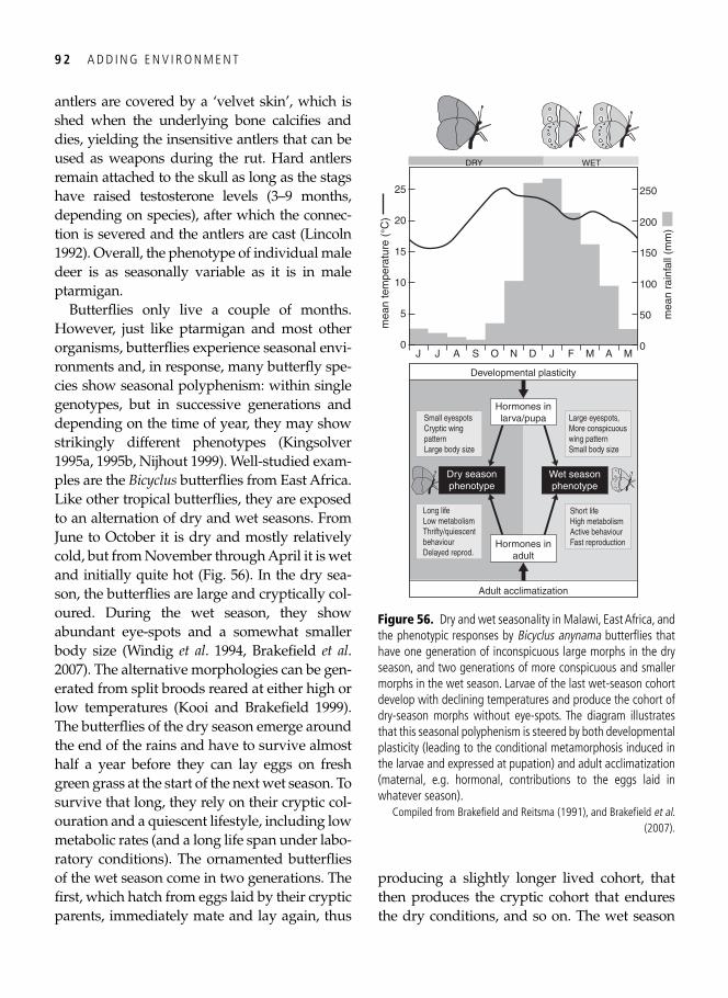
9 2 A D D I N G E N V I R O N M E N T
antlers are covered by a ‘velvet skin’, which is shed when the underlying bone calcifi es and dies, yielding the insensitive antlers that can be used as weapons during the rut. Hard antlers remain attached to the skull as long as the stags have raised testosterone levels (3–9 months, depending on species), after which the connec-tion is severed and the antlers are cast ( Lincoln 1992 ). Overall, the phenotype of individual male deer is as seasonally variable as it is in male ptarmigan.
Butterfl ies only live a couple of months. However, just like ptarmigan and most other organisms, butterfl ies experience seasonal envi-ronments and, in response, many butterfl y spe-cies show seasonal polyphenism: within single genotypes, but in successive generations and depending on the time of year, they may show strikingly different phenotypes ( Kingsolver 1995a , 1995b , Nijhout 1999 ). Well-studied exam-ples are the Bicyclus butterfl ies from East Africa. Like other tropical butterfl ies, they are exposed to an alternation of dry and wet seasons. From June to October it is dry and mostly relatively cold, but from November through April it is wet and initially quite hot ( Fig. 56 ). In the dry sea-son, the butterfl ies are large and cryptically col-oured. During the wet season, they show abundant eye-spots and a somewhat smaller body size ( Windig et al . 1994 , Brakefi eld et al . 2007 ). The alternative morphologies can be gen-erated from split broods reared at either high or low temperatures ( Kooi and Brakefi eld 1999 ). The butterfl ies of the dry season emerge around the end of the rains and have to survive almost half a year before they can lay eggs on fresh green grass at the start of the next wet season. To survive that long, they rely on their cryptic col-ouration and a quiescent lifestyle, including low metabolic rates (and a long life span under labo-ratory conditions). The ornamented butterfl ies of the wet season come in two generations. The fi rst, which hatch from eggs laid by their cryptic parents, immediately mate and lay again, thus
producing a slightly longer lived cohort, that then produces the cryptic cohort that endures the dry conditions, and so on. The wet season
J0
10
20
25
5
15
mea
n te
mpe
ratu
re (
°C)
AJ A S O N D J F M
mea
n ra
infa
ll (m
m)
M0
100
200
250
50
150
Hormones inlarva/pupa
Hormones inadult
Wet seasonphenotype
Large eyespots,More conspicuouswing patternSmall body size
Short lifeHigh metabolismActive behaviourFast reproduction
Dry seasonphenotype
Small eyespotsCryptic wingpatternLarge body size
Long lifeLow metabolismThrifty/quiescentbehaviourDelayed reprod.
Developmental plasticity
Adult acclimatization
DRY WET
Figure 56. Dry and wet seasonality in Malawi, East Africa, and the phenotypic responses by Bicyclus anynama butterfl ies that have one generation of inconspicuous large morphs in the dry season, and two generations of more conspicuous and smaller morphs in the wet season. Larvae of the last wet-season cohort develop with declining temperatures and produce the cohort of dry-season morphs without eye-spots. The diagram illustrates that this seasonal polyphenism is steered by both developmental plasticity (leading to the conditional metamorphosis induced in the larvae and expressed at pupation) and adult acclimatization (maternal, e.g. hormonal, contributions to the eggs laid in whatever season).
Compiled from Brakefi eld and Reitsma ( 1991 ), and Brakefi eld et al . ( 2007 ).
P H E N OT Y P I C P L A S T I C I T Y : M AT C H I N G P H E N OT Y P E S TO E N V I R O N M E N TA L D E M A N D S 9 3
butterfl ies show the distinct eye-spots; these may thwart attacking birds ( Kodandaramaiah et al . 2009 ) and are important during mate choice ( Constanzo and Monteiro 2007 , Oliver et al . 2009 ). The colourful wet season butterfl ies are also much more active, have a higher metabo-lism and a shorter life-span (even when not exposed to predation in the laboratory). A won-derful combination of fi eld and laboratory research enabled Paul Brakefi eld and co-work-ers (2007) to establish that the seasonal plasticity shown by Bicyclus butterfl ies represents aspects that are typical of both ‘classical’ developmental plasticity (hormonal effects in larva and pupa) and physiological acclimatization (induced in the reproductive adult stage and maternally contributed to the eggs) ( Fig. 56 ).
The extents of phenotypic change shown by ptarmigan and butterfl ies are rather similar, but their life spans (and life-cycle characteris-tics) are not. Individual ptarmigan may expe-rience many seasons, individual butterfl ies a single season at best. What is called seasonal polyphenism in insects is called life-cycle stag-ing in birds and mammals. And whereas the genetic-developmental architectures behind the phenotypic expressions are likely to be very different in birds and butterfl ies, in both groups seasonally varying ecological shaping factors to do with feeding, the avoidance of predation, and mating, can functionally explain their strikingly variable phenotypes.
Environmental variability and predictability, and the kinds of phenotypic adjustments that make sense
Different activities related to reproduction and survival (breeding, moult, migration, hiberna-tion, etc.) are usually separated in time within individuals, tend to occur at predictable times of the year in seasonal environments, and are accompanied by changes in the reproductively
active phenotype ( Murton and Westwood 1977 ). To perform optimally under a wide range of environmental conditions (variations that are often cyclic), a long-lived individual must track or anticipate the external changes by regulating gene expression to adjust its morphology, physiology, and behaviour ( Willmer et al . 2000 ). The cyclically varying phenotypic expressions of these adjustments within an individual rock ptarmigan, for example, are thus called ‘life-cycle stages’ ( Jacobs and Wingfi eld 2000 , Piersma 2002 , Ricklefs and Wikelski 2002 ). The seasonal template for such sequences might be pro-vided by the natural photoperiodic rhythm and/or by an endogenous circannual pace-maker ( Gwinner 1986 ). In addition, tempera-ture, rainfall, food, or densities of conspecifi cs might give supplementary information, which individuals could use to ‘fi ne-tune’ the timing of their phenotypic transformations ( Wingfi eld and Kenagy 1991 ). The polyphenisms of short-lived organisms, as in many insects, refl ect a similar strategy ( Shapiro 1976 , Danks 1999 ).
The accuracy with which future environ-mental conditions can be predicted would determine the kind of phenotypic plasticity that one might expect to evolve ( Levins 1968 , Moran 1992 , Padilla and Adolph 1996 ). In unpredictable environments, where there is insuffi cient environmental information, or if the wrong environmental information is used, an organism might end up with a phenotype that does not quite match its current environ-ment ( Hoffman 1978 ). Indeed, such mismatches are considered to be an important cost of devel-opmental plasticity (see Table 7 ). However, this potential cost would disappear for organisms that are capable of fast and reversible pheno-typic change. We will get back to this issue after we have addressed ‘trade-offs’.
Carrying on from our introductory classifi -cation in Chapter 1 ( Table 1 ), Fig. 57 represents the best attempt at present to place the different
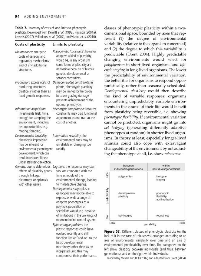
9 4 A D D I N G E N V I R O N M E N T
classes of phenotypic plasticity within a two-dimensional space, bounded by axes that rep-resent (1) the degree of environmental variability (relative to the organism concerned) and (2) the degree to which this variability is predictable (Drent 2004). Highly predictable changing environments would select for polyphenism in short-lived organisms and life-cycle staging in long-lived organisms. The lower the predictability of environmental variation, the better it is for organisms to respond oppor-tunistically, rather than seasonally scheduled. Developmental plasticity would then describe the kind of variable responses: organisms encountering unpredictably variable environ-ments in the course of their life would benefi t from plasticity being reversible, i.e. showing phenotypic fl exibility . If environmental variation cannot be predicted, organisms might go into bet hedging (generating differently adaptive phenotypes at random) in shorter-lived organ-isms. In theory at least, especially longer-lived animals could also cope with extravagant changeability of the environment by not adjust-ing the phenotype at all, i.e. show robustness .
Table 7. Inventory of costs of, and limits to, phenotypic plasticity. Developed from DeWitt et al . ( 1998 ), Pigliucci ( 2001a ), Lessells ( 2007 ), Valladares et al . ( 2007 ), and Vézina et al . ( 2010 ).
Costs of plasticity Limits to plasticity
Maintenance : energetic costs of sensory and regulatory mechanisms, and of any additional structures.
Phylogenetic ‘constraint’ : however adaptive a kind of plasticity would be, in any organism some forms of plasticity are impossible because of historic genetic, developmental or sensory constraints.
Production : excess costs of producing structures plastically rather than as fi xed genetic responses.
Damage-related constraints : in plants, phenotypic plasticity may be limited by herbivory because grazing damage prevents achievement of the optimal phenotype.
Information acquisition : investments (risk, time, energy) for sampling the environment, including lost opportunities (e.g. mating, foraging).
Phenotypic compromise : resource constraints may bias functional adjustment to one trait at the cost of another.
Developmental instability : phenotypic imprecision may be inherent for environmentally contingent development, which can result in reduced fi tness under stabilizing selection.
Information reliability : the environmental cues may be unreliable or changing too rapidly.
Genetic : due to deleterious effects of plasticity genes through linkage, pleiotropy, or epistasis with other genes.
Lag time : the response may start too late compared with the time schedule of the environmental change, leading to maladaptive change.
Developmental range : plastic genotypes may not be able to express as wide a range of adaptive phenotypes as a polytypic population of specialists would, e.g. because of limitations in the workings of neuroendocrine control system.
Epiphenotype problem : the plastic responses could have evolved recently and still function like an ‘add-on’ to the basic developmental machinery rather than as an integrated unit; this may compromise their performance.
variability HIGHLOW
HIG
HLO
Wpr
edic
tabi
lity
life-cyclestaging
phenotypicflexibility/acclimatization
robustness
polyphenism
developmentalplasticity
bet-hedging
betweenindividuals/generations
withinindividuals/generations
Figure 57. Different classes of phenotypic plasticity (or the lack of it in the case of robustness) arranged according to an axis of environmental variability over time and an axis of environmental predictability over time. The categories on the left show plasticity between individuals (and thus, between generations), and on the right within individuals.
Inspired by Meyers and Bull ( 2002 ) and adapted from Drent (2004).
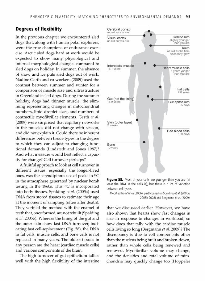
P H E N OT Y P I C P L A S T I C I T Y : M AT C H I N G P H E N OT Y P E S TO E N V I R O N M E N TA L D E M A N D S 9 5
Degrees of fl exibility
In the previous chapter we encountered sled dogs that, along with human polar explorers, were the true champions of endurance exer-cise. Arctic sled dogs hard at work would be expected to show many physiological and internal morphological changes compared to sled dogs on holiday. In summer, the absence of snow and ice puts sled dogs out of work. Nadine Gerth and co-workers (2009) used the contrast between summer and winter for a comparison of muscle size and ultrastructure in Greenlandic sled dogs. During the summer holiday, dogs had thinner muscle, the slim-ming representing changes in mitochondrial numbers, lipid droplet sizes, and numbers of contractile myofi brillar elements. Gerth et al . ( 2009 ) were surprised that capillary networks in the muscles did not change with season, and did not explain it. Could there be inherent differences between tissue types in the degree to which they can adjust to changing func-tional demands ( Lindstedt and Jones 1987 )? And what measure would best refl ect a capac-ity for change? Cell turnover perhaps?
A fruitful approach to look at cell turnover in different tissues, especially the longer-lived ones, was the serendipitous use of peaks in 14 C in the atmosphere generated by nuclear bomb testing in the 1960s. This 14 C is incorporated into body tissues. Spalding et al . ( 2005a ) used DNA from stored tissues to estimate their age at the moment of sampling (often after death). They verifi ed the method with the enamel of teeth that, once formed, are not rebuilt ( Spalding et al . 2005b ). Whereas the lining of the gut and the outer skin show fast DNA turnover, indi-cating fast cell-replacement ( Fig. 58 ), the DNA in fat cells, muscle cells, and bone cells is not replaced in many years. The oldest tissues in any person are the heart (cardiac muscle cells) and various components of the brain.
The high turnover of gut epithelium tallies well with the high fl exibility of the intestine
that we discussed earlier. However, we have also shown that hearts show fast changes in size in response to changes in workload, so how does that tally with the cardiac muscle cells living so long ( Bergmann et al . 2009 )? The discrepancy is due to cell components other than the nucleus being built and broken-down, rather than whole cells being renewed and removed. Myofi brillar volume may change, and the densities and total volume of mito-chondria may quickly change too ( Hoppeler
Cerebral cortexas old as you are
Visual cortexas old as you are
Cerebellumslightly younger
than you are
Intercostal muscle15.1 years
Gut (not the lining)15.9 years Gut epithelium
5 days
Skin (outer layer)2 weeks
Red blood cells120 days
Bone10 years
Teethas old as the time
since they grew
Heart muscle cells6 years yonger
than you are
Fat cells9.8 years
Figure 58. Most of your cells are younger than you are (at least the DNA in the cells is), but there is a lot of variation between cell types.
Modifi ed from Vince ( 2006 ), partly based on Spalding et al . ( 2005a , 2005b 2008 ) and Bergmann et al . ( 2009 ).
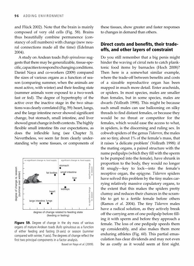
9 6 A D D I N G E N V I R O N M E N T
and Flück 2002 ). Note that the brain is mainly composed of very old cells ( Fig. 58 ). Brains thus beautifully combine permanence (con-stancy of cell numbers) with change (new neu-ral connections made all the time) ( Edelman 2004 ).
A study on Andean toads Bufo spinulosus sug-gests that there may be generalizable, tissue-spe-cifi c, capacities to respond to changing conditions. Daniel Naya and co-workers (2009) compared the sizes of various organs as a function of sea-son (comparing summer, when the animals are most active, with winter) and their feeding state (summer animals were exposed to a two-week fast or fed). The degree of hypertrophy of the active over the inactive stage in the two situa-tions was clearly correlated ( Fig. 59 ): heart, lungs, and the large intestine never showed signifi cant change, but stomach, small intestine, and liver showed great change in both contexts. The highly fl exible small intestine fi ts our expectations, as does the infl exible lung (see Chapter 3 ). Nevertheless, we seem far from clearly under-standing why some tissues, or components of
these tissues, show greater and faster responses to changes in demand than others.
Direct costs and benefi ts, their trade-offs, and other layers of constraint
Do you still remember that a big penis might hinder the waving of cirral nets to catch plank-tonic food items by barnacles ( Hoch 2008 )? Then here is a somewhat similar example, where the trade-off between benefi ts and costs of a sizeable reproductive organ has been mapped in much more detail. Enter arachnids, or spiders. In most species, males are smaller than females, but in some species, males are dwarfs ( Vollrath 1998 ). This might be because such small males can use ballooning on silky threads to fi nd distant females, or because they would be no threat or competitor for the females, which would ease the access to what, in spiders, is the discerning and ruling sex. In cobweb spiders of the genus Tidarren , the males are so tiny, about 1% of the female’s mass, that it raises ‘a delicate problem’ ( Vollrath 1998 ): if the mating organs, a paired structure with the name pedipalps (which they fi ll with the sperm to be pumped into the female), have shrunk in proportion to the body, they would no longer fi t snugly—key to lock—into the female’s receptive organ, the epigyne. Tidarren spiders have solved this problem by the tiny males car-rying relatively massive copulatory organs, to the extent that this makes the spiders pretty clumsy and reduces their chances in the scram-ble to get to a fertile female before others ( Ramos et al . 2004 ). The tiny Tidarren males have a radical solution, as they actively break off the carrying arm of one pedipalp before fi ll-ing it with sperm and before they approach a female. The loss of one pedipalp speeds them up considerably, and also makes them more enduring athletes ( Fig. 60 ). This partial emas-culation has clear dividends and may not even be as costly as it would seem at fi rst sight.
degr
ee o
f cha
nge
re. s
easo
n(s
umm
er o
ver
win
ter)
degree of change related to feeding state(feeding or fasting)
large intestine lungs
heartkidneys
liver
small intestinefat bodies
stomach
no significant change re. food supply significant change re. food supply
no s
igni
fican
t cha
nge
re. s
easo
nsi
gnifi
cant
cha
nge
re. s
easo
n
Figure 59. Degree of change in the dry mass of various organs of mature Andean toads Bufo spinulosus as a function of either feeding and fasting (X-axis) or season (summer compared with winter, Y-axis). The degrees of change refl ect the fi rst two principal components in a factor analysis.
Based on Naya et al . ( 2009 ).
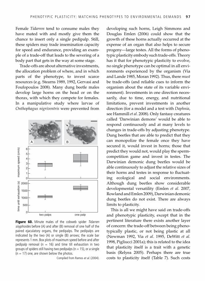
P H E N OT Y P I C P L A S T I C I T Y : M AT C H I N G P H E N OT Y P E S TO E N V I R O N M E N TA L D E M A N D S 9 7
Female Tidarren tend to consume males they have mated with and mostly give them the chance to insert only a single pedipalp. Still, these spiders may trade insemination capacity for speed and endurance, providing an exam-ple of a trade-off that leads to the severing of a body part that gets in the way at some stage.
Trade-offs are about alternative investments, the allocation problem of where, and in which parts of the phenotype, to invest scarce resources (e.g. Stearns 1989 , 1992 , Gervasi and Foufopoulos 2008 ). Many dung beetle males develop large horns on the head or on the thorax, with which they compete for females. In a manipulative study where larvae of Onthophagus nigriventris were prevented from
developing such horns, Leigh Simmons and Douglas Emlen (2006) could show that the growth of these horns actually occurred at the expense of an organ that also helps to secure progeny—large testes. All the forms of pheno-typic plasticity embody such trade-offs. Theory has it that for phenotypic plasticity to evolve, no single phenotype can be optimal in all envi-ronments experienced by the organism ( Via and Lande 1985 , Moran 1992 ). Thus, there must be trade-offs (and reliable cues to inform the organism about the state of its variable envi-ronment). Investments in one direction neces-sarily, due to time, energy, and nutritional limitations, prevent investments in another direction (for a model and a test with Daphnia , see Hammill et al . 2008 ). Only fantasy creatures called ‘Darwinian demons’ would be able to respond continuously and at many levels to changes in trade-offs by adjusting phenotype. Dung beetles that are able to predict that they can monopolize the female once they have secured it, would invest in horns; those that predict they would not, would play the sperm-competition game and invest in testes. The Darwinian demonic dung beetles would be able continuously to adjust the relative sizes of their horns and testes in response to fl uctuat-ing ecological and social environments. Although dung beetles show considerable developmental versatility ( Emlen et al . 2007 , Rowland and Emlen 2009 ), Darwinian demonic dung beetles do not exist. There are always limits to plasticity.
This is all we might have said on trade-offs and phenotypic plasticity, except that in the pertinent literature there exists another layer of concern: the trade-off between being pheno-typically plastic, or not being plastic at all ( Newman 1992 , Via et al . 1995 , DeWitt et al. 1998 , Pigliucci 2001a ); this is related to the idea that plasticity itself is a trait with a genetic basis ( Relyea 2005 ). Perhaps there are true costs to plasticity itself ( Table 7 ). Such costs
0
1500
2000
500
1000
time
until
exh
aust
ion
(s)
two palps one palp
0
3
4
1
2
max
imum
spe
ed (
cm/s
)
5
6
A B
Figure 60. Minute males of the cobweb spider Tidarren sisyphoides before (A) and after (B) removal of one half of the paired ejaculatory organs, the pedipalps. The pedipalps are indicated by the two (A) or single (B) arrows; the scale bar represents 1 mm. Box plots of maximum speed before and after pedipalp removal (n = 16) and time till exhaustion in two groups of spiders still having two pedipalps (n = 15), or a single (n = 17) one, are shown below the photos.
Compiled from Ramos et al . ( 2004 ).
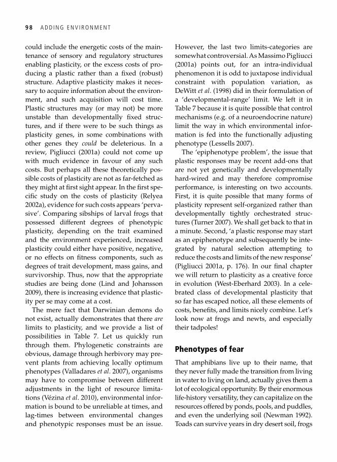
9 8 A D D I N G E N V I R O N M E N T
could include the energetic costs of the main-tenance of sensory and regulatory structures enabling plasticity, or the excess costs of pro-ducing a plastic rather than a fi xed (robust) structure. Adaptive plasticity makes it neces-sary to acquire information about the environ-ment, and such acquisition will cost time. Plastic structures may (or may not) be more unstable than developmentally fi xed struc-tures, and if there were to be such things as plasticity genes, in some combinations with other genes they could be deleterious. In a review, Pigliucci ( 2001a ) could not come up with much evidence in favour of any such costs. But perhaps all these theoretically pos-sible costs of plasticity are not as far-fetched as they might at fi rst sight appear. In the fi rst spe-cifi c study on the costs of plasticity ( Relyea 2002a ), evidence for such costs appears ‘perva-sive’. Comparing sibships of larval frogs that possessed different degrees of phenotypic plasticity, depending on the trait examined and the environment experienced, increased plasticity could either have positive, negative, or no effects on fi tness components, such as degrees of trait development, mass gains, and survivorship. Thus, now that the appropriate studies are being done ( Lind and Johansson 2009 ), there is increasing evidence that plastic-ity per se may come at a cost.
The mere fact that Darwinian demons do not exist, actually demonstrates that there are limits to plasticity, and we provide a list of possibilities in Table 7 . Let us quickly run through them. Phylogenetic constraints are obvious, damage through herbivory may pre-vent plants from achieving locally optimum phenotypes ( Valladares et al . 2007 ), organisms may have to compromise between different adjustments in the light of resource limita-tions ( Vézina et al . 2010 ), environmental infor-mation is bound to be unreliable at times, and lag-times between environmental changes and phenotypic responses must be an issue.
However, the last two limits-categories are somewhat controversial. As Massimo Pigliucci ( 2001a ) points out, for an intra-individual phenomenon it is odd to juxtapose individual constraint with population variation, as DeWitt et al . ( 1998 ) did in their formulation of a ‘developmental-range’ limit. We left it in Table 7 because it is quite possible that control mechanisms (e.g. of a neuroendocrine nature) limit the way in which environmental infor-mation is fed into the functionally adjusting phenotype ( Lessells 2007 ).
The ‘epiphenotype problem’, the issue that plastic responses may be recent add-ons that are not yet genetically and developmentally hard-wired and may therefore compromise performance, is interesting on two accounts. First, it is quite possible that many forms of plasticity represent self-organized rather than developmentally tightly orchestrated struc-tures ( Turner 2007 ). We shall get back to that in a minute. Second, ‘a plastic response may start as an epiphenotype and subsequently be inte-grated by natural selection attempting to reduce the costs and limits of the new response’ ( Pigliucci 2001a , p. 176). In our fi nal chapter we will return to plasticity as a creative force in evolution ( West-Eberhard 2003 ). In a cele-brated class of developmental plasticity that so far has escaped notice, all these elements of costs, benefi ts, and limits nicely combine. Let’s look now at frogs and newts, and especially their tadpoles!
Phenotypes of fear
That amphibians live up to their name, that they never fully made the transition from living in water to living on land, actually gives them a lot of ecological opportunity. By their enormous life-history versatility, they can capitalize on the resources offered by ponds, pools, and puddles, and even the underlying soil ( Newman 1992 ). Toads can survive years in dry desert soil, frogs
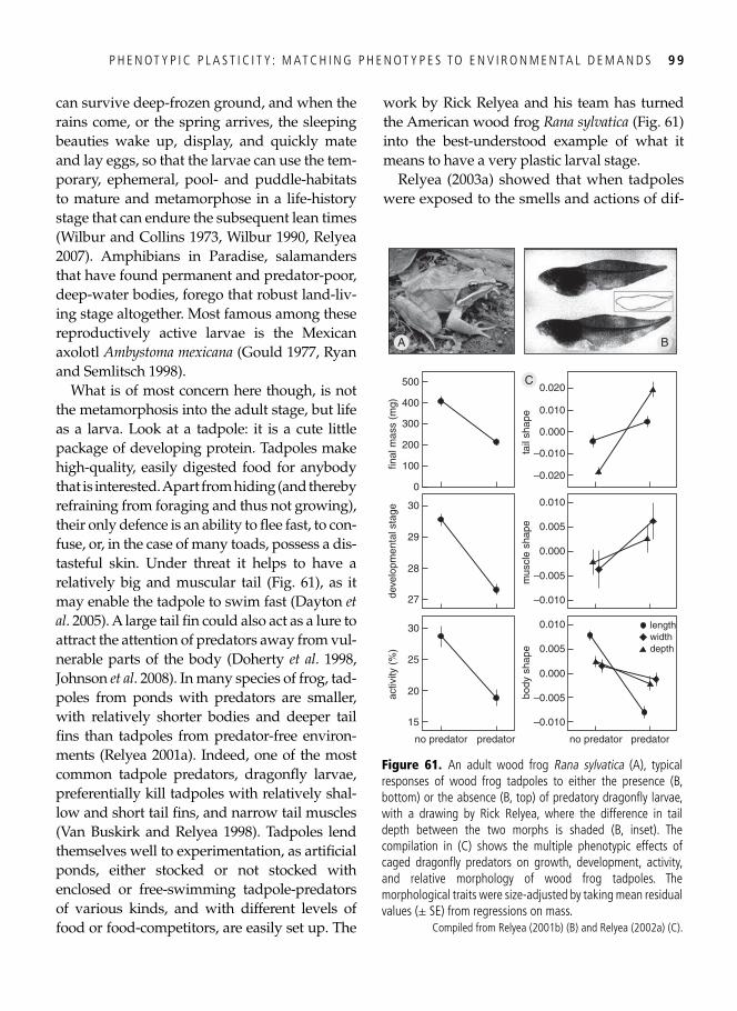
P H E N OT Y P I C P L A S T I C I T Y : M AT C H I N G P H E N OT Y P E S TO E N V I R O N M E N TA L D E M A N D S 9 9
can survive deep-frozen ground, and when the rains come, or the spring arrives, the sleeping beauties wake up, display, and quickly mate and lay eggs, so that the larvae can use the tem-porary, ephemeral, pool- and puddle-habitats to mature and metamorphose in a life-history stage that can endure the subsequent lean times ( Wilbur and Collins 1973 , Wilbur 1990 , Relyea 2007 ). Amphibians in Paradise, salamanders that have found permanent and predator-poor, deep-water bodies, forego that robust land-liv-ing stage altogether. Most famous among these reproductively active larvae is the Mexican axolotl Ambystoma mexicana ( Gould 1977 , Ryan and Semlitsch 1998 ).
What is of most concern here though, is not the metamorphosis into the adult stage, but life as a larva. Look at a tadpole: it is a cute little package of developing protein. Tadpoles make high-quality, easily digested food for anybody that is interested. Apart from hiding (and thereby refraining from foraging and thus not growing), their only defence is an ability to fl ee fast, to con-fuse, or, in the case of many toads, possess a dis-tasteful skin. Under threat it helps to have a relatively big and muscular tail ( Fig. 61 ), as it may enable the tadpole to swim fast ( Dayton et al . 2005 ). A large tail fi n could also act as a lure to attract the attention of predators away from vul-nerable parts of the body ( Doherty et al . 1998 , Johnson et al . 2008 ). In many species of frog, tad-poles from ponds with predators are smaller, with relatively shorter bodies and deeper tail fi ns than tadpoles from predator-free environ-ments ( Relyea 2001a ). Indeed, one of the most common tadpole predators, dragonfl y larvae, preferentially kill tadpoles with relatively shal-low and short tail fi ns, and narrow tail muscles ( Van Buskirk and Relyea 1998 ). Tadpoles lend themselves well to experimentation, as artifi cial ponds, either stocked or not stocked with enclosed or free-swimming tadpole-predators of various kinds, and with different levels of food or food-competitors, are easily set up. The
work by Rick Relyea and his team has turned the American wood frog Rana sylvatica ( Fig. 61 ) into the best-understood example of what it means to have a very plastic larval stage.
Relyea ( 2003a ) showed that when tadpoles were exposed to the smells and actions of dif-
15
30
20
25
activ
ity (
%)
no predator predator
deve
lopm
enta
l sta
ge
0
300
400
100
200
final
mas
s (m
g)500
–0.010
0.005
0.010
–0.005
0.000
body
sha
pe
no predator predator
mus
cle
shap
eta
il sh
ape
27
30
28
29
–0.010
0.005
0.010
–0.005
0.000
–0.020
0.010
0.020
–0.010
0.000
lengthwidthdepth
A B
C
B
Figure 61. An adult wood frog Rana sylvatica (A), typical responses of wood frog tadpoles to either the presence (B, bottom) or the absence (B, top) of predatory dragonfl y larvae, with a drawing by Rick Relyea, where the difference in tail depth between the two morphs is shaded (B, inset). The compilation in (C) shows the multiple phenotypic effects of caged dragonfl y predators on growth, development, activity, and relative morphology of wood frog tadpoles. The morphological traits were size-adjusted by taking mean residual values (± SE) from regressions on mass.
Compiled from Relyea ( 2001b ) (B) and Relyea ( 2002a ) (C).
1 0 0 A D D I N G E N V I R O N M E N T
ferent predators (there was a choice of four) or combinations thereof, they discriminated and produced predator-specifi c larval phenotypes. When predators were combined, tadpoles gen-erally developed phenotypes that were typical of the more risky type, suggesting that they perceived the risk of combined predators as the risk of the most dangerous one. Tadpoles not only have to survive, they also have to grow. Wood frogs that face high levels of com-petition from other tadpoles increase their for-aging activity and develop larger bodies. These larger bodies contain relatively larger scraping mouthparts and longer guts, which improve the animal’s ability to fi nd, consume, and digest food, but this ability comes at the cost of a large tail, which makes tadpoles more sus-ceptible to predators ( Relyea and Auld 2004 , 2005 ).
The extraordinary ability of tadpoles to sense changes in their environment and respond in precise and often appropriate ways, is illustrated, for example, by wood frog tad-poles in experimental ponds that appeared to respond differentially to variations in the per capita food levels and to changes in conspecifi c density alone ( Relyea 2002b ). When European common frog tadpoles Rana temporaria were exposed to non-lethal caged predators (drag-onfl y larvae) at low tadpole densities they showed morphological as well as behavioural defences. At high densities and with severe competition for food they remained active and only adjusted their morphology ( Teplitsky and Laurila 2007 ). Similarly, when tadpoles were exposed to fi sh (that pursue their prey), they built deeper and longer tails and bigger tail muscles. In the presence of dragonfl y larvae (sit-and-wait predators), they built only deeper tails ( Teplitsky et al . 2005a , Wilson et al . 2005 ), suggesting that tails as lures were the selective force behind oversized tail fi ns. Indeed, in a Neotropical tree frog Dendrosophus ebraccatus , the presence of dragonfl y larvae induced
highly visible, large, and colourful tail fi ns, whereas the presence of fi sh induced achro-matic tails ( Touchon and Warkentin 2008 ). Tadpoles of the tree frog Hyla versicolor altered their defences when 10 different prey (them-selves being one of the types) were either crushed by hand or consumed by dragonfl y larvae. Across all prey types, crushing induced only a subset of the defences that were induced by consumption, suggesting once more that tadpoles can assess quite precisely the degree and type of threat and respond accordingly ( Schoeppner and Relyea 2005 ).
Nevertheless, even the plasticity of tadpoles fi nds a limit. When Schoeppner and Relyea ( 2008 ) exposed wood frog tadpoles, and when Teplitsky et al . ( 2005b ) exposed tadpoles of a European frog Rana dalmatina , to a gradient of densities of a particular predator, all measured traits exhibited graded responses that levelled off with increased predation risk. This sug-gests that there is either an organizational limit to plasticity or a ‘functional limit’ that refl ects the high costs of the defensive phenotype. Part of these costs might be incurred later in life. Wood frog tadpoles reared with caged dragon-fl y larvae, rather than without, showed rela-tively large limbs and narrower bodies as fully grown frogs ( Relyea 2001b ); the survival value of these later adjustments was not established. However, four months after metamorphosis, common frogs that developed from predator-exposed, rather than predator-free, tadpoles swam more slowly with less endurance—the opposite of what happened in the larval stage ( Stamper et al . 2009 ). This suggests that the lar-val adjustments may come with a long-term fi tness cost.
We round up with the amazing story of two competing amphibian larvae studied in Japan- a frog Rana pirica and a salamander, or newt, called Hynobius retardatus . Tadpoles of many a salamander or toad have tendencies to become cannibalistic, but they only do so at high con-
P H E N OT Y P I C P L A S T I C I T Y : M AT C H I N G P H E N OT Y P E S TO E N V I R O N M E N TA L D E M A N D S 1 0 1
specifi c densities ( Pfennig 1992 , Michimae 2006 ), and, preferably, if these conspecifi cs are not closely related ( Pfennig and Frankino 1997 ). They then develop a broad head and gape large enough to swallow tasty nieces and nephews. They also turn predatory when there are many frog tadpoles around, as the mechan-ical vibrations of fl apping tadpole-tails are suf-fi cient for this transformation to take place ( Michimae et al . 2005 ). In a wonderful example of a phenotypic arms race, in response to sala-manders becoming broad-headed and danger-ous, frog tadpoles developed thicker bodies and a comb on their backs to prevent ingestion by the salamander larvae; to which salaman-ders responded by further enlarging gape size ( Kishida et al . 2009 )! Interestingly, frog tad-poles do not become bulky and high-bodied solely in the presence of salamander tadpoles, they only adjust when the salamander tad-poles become dangerous, i.e. express the pre-dacious phenotype ( Kishida et al . 2006 ). A fi nal subtlety is that when the threat of either preda-tory larval salamanders or dragonfl ies is taken away, the specifi c morphological defences are lost ( Kishida and Nishimura 2006 ). This reversal indicates once more that induced defences can come with serious costs ( Hoverman and Relyea 2007 ), and thus that fl exibility, or reversibility, pays if it is still an option developmentally ( Relyea 2003b ).
Plasticity: the tinkerer’s accomplishment?
With a few exceptions (e.g. Newman and Müller 2000 , Blumberg 2009 ), the literature on phenotypic plasticity is permeated with the idea that adaptive phenotypic responses, be they reversible or irreversible, cyclic or not, are instructed from the genome. Of course, they will be, at some level at least. In his eye-opening book The tinkerer’s accomplice , J. Scott Turner ( 2007 ) builds on early lines of reason-
ing, including the famous ‘spandrels’-paper by Stephen Jay Gould and Richard Lewontin (1979), and assembles many convincing argu-ments that good adaptive design is usually the result of the self-organization that logi-cally follows from growing structures inter-acting with their immediate physical environments. In his own words: ‘organisms are designed not so much because natural selection of particular genes has made them that way, but because agents of homeostasis build them that way’. Natural selection, the tinkerer, has an accomplice.
For an interesting exposition of this notion we go back to antlers. Unlike skeletal bones that are adaptively moulded because of the particular strains that they experience ( Fig. 51 ), antlers grow in the ‘assiduous avoidance of strain’ by virtue of a specialized, blood-rich, and highly innervated type of skin called vel-vet. Protected and nurtured by the velvet, car-tilage grows until specialized bone cells called osteoblasts, moving in from the blood, eventu-ally mineralize it. As long as the cartilage stays abreast of the osteoblasts, the antlers grow, but, as soon as the mineralizing osteoblasts have taken the upper hand, growth stops. The velvet then dies and, with its naked ossifi ed antlers, the stag is ready for the rut. The ratio between ossifi cation and cartilage growth determines the size and shape of the antlers. In small deer the ratio is high, so antlers stay small and pointed ( Fig. 62A ). In large deer the ratio between ossifi cation and cartilage growth is low, so antlers can grow as ‘expansive broad plates’ ( Turner 2007 ). After the rut, the antlers are shed. The new set usually resembles the old set except that, if a deer is well fed, it is a bit larger. That antlers grow larger with age is probably self-organized. Reproductive and stress hormones combine with direct diet cues to affect the relative rates of ossifi cation and cartilage growth, and thereby antler size and shape.
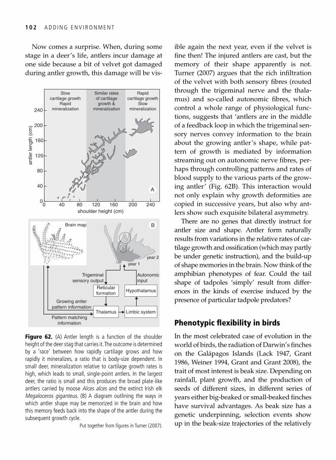
1 0 2 A D D I N G E N V I R O N M E N T
Now comes a surprise. When, during some stage in a deer’s life, antlers incur damage at one side because a bit of velvet got damaged during antler growth, this damage will be vis-
ible again the next year, even if the velvet is fi ne then! The injured antlers are cast, but the memory of their shape apparently is not. Turner ( 2007 ) argues that the rich infi ltration of the velvet with both sensory fi bres (routed through the trigeminal nerve and the thala-mus) and so-called autonomic fi bres, which control a whole range of physiological func-tions, suggests that ‘antlers are in the middle of a feedback loop in which the trigeminal sen-sory nerves convey information to the brain about the growing antler’s shape, while pat-tern of growth is mediated by information streaming out on autonomic nerve fi bres, per-haps through controlling patterns and rates of blood supply to the various parts of the grow-ing antler’ ( Fig. 62B ). This interaction would not only explain why growth deformities are copied in successive years, but also why ant-lers show such exquisite bilateral asymmetry.
There are no genes that directly instruct for antler size and shape. Antler form naturally results from variations in the relative rates of car-tilage growth and ossifi cation (which may partly be under genetic instruction), and the build-up of shape memories in the brain. Now think of the amphibian phenotypes of fear. Could the tail shape of tadpoles ‘simply’ result from differ-ences in the kinds of exercise induced by the presence of particular tadpole predators?
Phenotypic fl exibility in birds
In the most celebrated case of evolution in the world of birds, the radiation of Darwin’s fi nches on the Galápagos Islands ( Lack 1947 , Grant 1986 , Weiner 1994 , Grant and Grant 2008 ), the trait of most interest is beak size. Depending on rainfall, plant growth, and the production of seeds of different sizes, in different series of years either big-beaked or small-beaked fi nches have survival advantages. As beak size has a genetic underpinning, selection events show up in the beak-size trajectories of the relatively
00
120
200
240
40
80
160
antle
r le
ngth
(cm
)
160120 200 24040 80shoulder height (cm)
A
B
Slowcartilage growth
Rapidmineralization
Similar ratesof cartilagegrowth &
mineralization
Rapidcartilage growth
Slowmineralization
Reticularformation Hypothalamus
Thalamus Limbic system
Trigeminalsensory output
Brain map
Growing antlerpattern information
Pattern matchinginformation
Autonomicinput
year 1
year 2
Figure 62. (A) Antler length is a function of the shoulder height of the deer stag that carries it. The outcome is determined by a ‘race’ between how rapidly cartilage grows and how rapidly it mineralizes, a ratio that is body-size dependent. In small deer, mineralization relative to cartilage growth rates is high, which leads to small, single-point antlers. In the largest deer, the ratio is small and this produces the broad plate-like antlers carried by moose Alces alces and the extinct Irish elk Megaloceros giganteus. (B) A diagram outlining the ways in which antler shape may be memorized in the brain and how this memory feeds back into the shape of the antler during the subsequent growth cycle.
Put together from fi gures in Turner ( 2007 ).
P H E N OT Y P I C P L A S T I C I T Y : M AT C H I N G P H E N OT Y P E S TO E N V I R O N M E N TA L D E M A N D S 1 0 3
isolated island populations. Immersed, as we are here, in examples of phenotypic plasticity, one cannot help but wonder why small-beaked Darwin’s fi nches, living during times when bigger beaks would be advantageous, do not themselves build bigger bills?
Although oystercatchers Haematopus ostrale-gus can and do modify bill size and shape ( Hulscher 1985 , van de Pol et al . 2009 ), Darwin’s fi nches apparently cannot. In their very advanced synthesis of 34 years of work on nat-ural selection in action in Darwin’s fi nches, Peter and Rosemary Grant (2008) do not even use the word plasticity! Perhaps the material with which, and the way that, bills are built only allows for limited plasticity ( Gosler 1987 ). This contrasts with most other parts of bird bodies that do show plasticity, mostly in the categories of life-cycle staging ( Murton and Westwood 1977 , Wingfi eld 2008 ) and pheno-typic fl exibility (this book). In fact, one of the few examples of developmental plasticity in birds is the one for oystercatcher bills where, to an extent at least, youngsters learn from their parents to feed on a particular diet ( Sutherland 1987 , Sutherland et al . 1996 ). Depending on the prey types that they select, their bill is worn and strengthened in particu-lar ways (yes, self-organization!), even though there remains fl exibility later in life.
Rather than structural body size, what pre-dominantly varies in birds are body mass (an indicator of nutrient stores) and the size of most of the organs ( Table 8 ), with the excep-tion of the lungs ( Piersma et al . 1999b ). This is especially the case in those birds exposed to seasonally widely different conditions, either because they migrate from arctic or temperate to tropical climates, or precisely because they stay put at highly seasonal northern or south-ern latitudes. There is also considerable intra-individual variation in correlated metabolic attributes ( Vézina et al . 2006 , 2007 ) and aspects of the immune system ( Buehler et al . 2008a ).
Female red knots even show seasonal varia-tion in the mass of their skeleton: they store calcium before going to the trouble of laying a clutch of four eggs ( Piersma et al . 1996b ). A phenotypic aspect not studied in shorebirds, but carefully documented in songbirds, is the seasonal waxing and waning of song nuclei in the brain ( Nottebohm 1981 , Smith et al . 1997 , Tramontin et al . 2000 ; note that even modern humans leading domesticated lives show sea-sonal change in parts of the brain, Hofman and Swaab 1992 ). Within a week after shifting Gambel’s white-crowned Sparrows Zonotrichia leucophrys gambelii from short to long days, the number of neurons in a brain area called the High Vocal Centre increased by 50,000, or 70%, as did the volume of this nucleus ( Tramontin et al . 2000 ). Perhaps surprisingly, the morpho-logical changes were faster than the develop-ment of the song control circuitry and the degree of stereotypy of the songs themselves. These took some extra weeks to mature fully.
In view of the focus of much of the rest of this book on foraging, distributional decisions, and time-allocation problems, we round up by examining in greater detail the machinery for digestion and assimilation in birds, and their plasticity. The digestive system of birds can be divided into several main components ( Table 9 ). In any one taxon, each of these digestive organs will have morphological characteristics that functionally refl ect the evolutionary his-tory and contemporary ecology of the taxon ( Stevens and Hume 1995 ).
A large gut may provide the ability to use foods of low quality that are diffi cult to handle mechanically or chemically. The size of the digestive tract should, therefore, refl ect the ben-efi ts of having organs of that size, in balance with the costs of maintaining that system. Before assessing degrees of variation in organ size, it is worth considering some general fac-tors that may set upper bounds to the size of digestive systems. For example, it is obvious
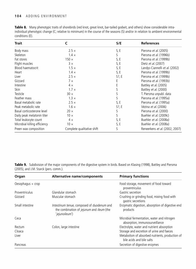
1 0 4 A D D I N G E N V I R O N M E N T
Table 8. Many phenotypic traits of shorebirds (red knot, great knot, bar-tailed godwit, and others) show considerable intra-individual phenotypic change (C; relative to minimum) in the course of the seasons (S) and/or in relation to ambient environmental conditions (E).
Trait C S/E References
Body mass 2.5 × S, E Piersma et al . (2005) Skeleton 1.4 × S Piersma et al . (1996b) Fat stores 150 × S, E Piersma et al . (1999b) Flight muscles 3 × S, E Dietz et al . (2007) Blood haematocrit 1.5 × S, E Landys-Ciannelli et al . (2002) Heart 1.4 × S, E Piersma et al . (1999b) Liver 2.5 × S?, E Piersma et al . (1999b) Gizzard 7 × E Piersma et al . (1993b) Intestine 4 × E Battley et al . (2005) Skin 1.7 × S Battley et al . (2000) Testicle 30 × S T. Piersma unpubl. data Feather mass 1.3 × S Piersma et al . (1995a) Basal metabolic rate 2.5 × S, E Piersma et al . (1995a) Peak metabolic rate 1.6 × S?, E Vézina et al . (2006) Basal corticosterone level 20 × S Piersma et al . (2000) Daily peak melatonin titer 10 × S Buehler et al . (2009c) Total leukocyte count 4 × S, E Buehler et al . (2008a) Microbial killing effi ciency 10 × S, E Buehler et al . (2008a) Preen wax composition Complete qualitative shift S Reneerkens et al . (2002, 2007)
Table 9. Subdivision of the major components of the digestive system in birds. Based on Klasing ( 1998 ), Battley and Piersma ( 2005 ), and J.M. Starck (pers. comm.).
Organ Alternative name/components Primary functions
Oesophagus + crop Food storage, movement of food toward proventriculus
Proventriculus Glandular stomach Gastric secretion Gizzard Muscular stomach Crushing or grinding food, mixing food with
gastric secretions Small intestine Intestinum tenue , composed of duodenum and
the combination of jejunum and ileum (the ‘ jejunoileum ’)
Enzymatic digestion, absorption of digestive end products
Ceca Microbial fermentation, water and nitrogen absorption, immunosurveillance
Rectum Colon, large intestine Electrolyte, water and nutrient absorption Cloaca Storage and excretion of urine and faeces Liver Metabolism of absorbed nutrients, production of
bile acids and bile salts Pancreas Secretion of digestive enzymes
P H E N OT Y P I C P L A S T I C I T Y : M AT C H I N G P H E N OT Y P E S TO E N V I R O N M E N TA L D E M A N D S 1 0 5
that there is a physical limit to the volume avail-able for organs within the abdominal cavity. Fat deposits will further reduce the abdominal space for the digestive tract. For example, migratory shorebirds deposit a thick layer of fat around the gizzard, covering the intestines and rectum, and pressing up against the tail end of the skeleton. In great knots Calidris tenuirostris about to depart on northward migration from Australia, fat in the abdominal cavity made up 38% of the total abdominal tissue mass ( Battley and Piersma 2005 ). At such times the profi le of the abdomen changes, with fat birds showing a ‘bulge’ behind the legs ( Owen 1981 , Wiersma and Piersma 1995 ). Confl icts for space between fuel stores and organs may limit the maximum size of the digestive organs.
Internal organ mass could directly affect fl ight costs and performance of birds. Because the costs of fl ight increase with body mass ( Kvist et al . 2001 ), and as manoeuvrability is impaired at higher masses ( Dietz et al . 2007 ), minimization of digestive organ mass will be an important consideration. In a comparative study of raptors, Hilton et al . ( 1999 ) showed that ‘pursuing’ species (that require fast and manoeuvrable fl ight) had shorter guts than ‘searching’ species, presumably refl ecting the pursuers’ need to minimize mass. The shorter retention time of these species would reduce the period of time they had food in their guts, also keeping body mass low, though at a cost of lowered digestive effi ciency. Sedinger ( 1997 ) showed that grouse have caeca 4–5 times longer than waterfowl feeding on the same diet, and suggested that the small caeca in waterfowl refl ect a balance between the costs of fl ight for waterfowl and the benefi ts of the caeca for nutrient balance. And even in animals at rest, mass-specifi c maintenance costs of the intes-tine and liver are greater than those of muscle and adipose tissue ( Krebs 1950 , Blaxter 1989 , Scott and Evans 1992 ). Reductions in metaboli-cally active tissues, therefore, dramatically
reduce basal energy requirements ( Battley et al . 2001 , Konarzewski and Diamond 1995 ).
Under the simplifying assumption that size (or mass) indicates functional capacity, Fig. 63 summarizes the magnitude of changes in three major gastrointestinal components, the gizzard, gut or small intestine, and liver. Data are separated into four taxonomic groups: galliformes (primarily grouse and quail), songbirds, shorebirds, and waterfowl. Even though only few of the studies in the review explicitly focused on documenting such changes, organ mass variations of 20–80% were common across a wide range of species; length changes of the intestine typically were lower, generally 10–20%. Earlier we discussed whether tissue-related differences in fl exibility could be due to dif-ferences in cell turnover, based on carbon-isotope signatures of historically spiked DNA ( Spalding et al . 2005a ). A method that informs about the whole cell content, rather than DNA only, may be more appropriate, and measurements of retention times of car-bon-isotopes supplied in food fulfi l this con-dition. In a study on zebra fi nches Taeniopygia guttata , Bauchinger and McWilliams ( 2009 ) found retention times varied between 8 days for small intestine, 10–13 days for stomach, kidney, liver,and pancreas, 17–21 days for heart, brain, blood, and fl ight muscle, and 26–28 days for leg muscle and skin. Thus, they found that tissues with a tendency to show large changes (notably the small intes-tine and liver) had fast turnover rates, whereas less dynamic tissues, such as the fl ight and leg muscles, had slower turnover rates. Tissue-specifi c turnover rate may thus partially determine the magnitude of organ fl exibility.
Clearly, if we keep an open mind and our eyes open, pretty much all parts of bodies appear to vary with time, age, demand, and environment. To ascertain the functionality of these changes
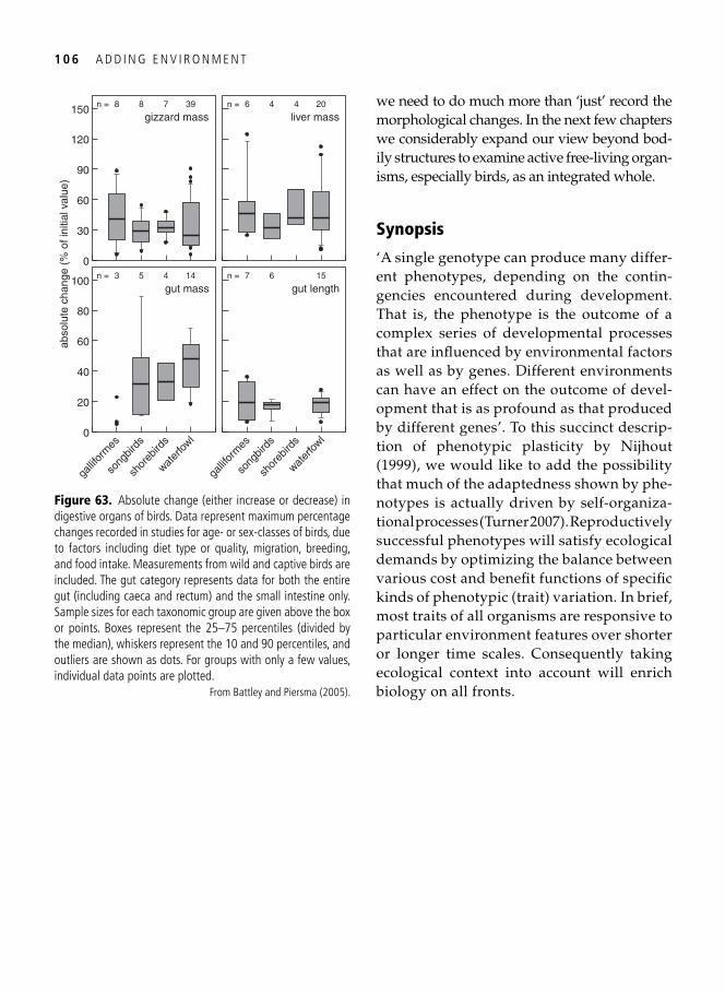
1 0 6 A D D I N G E N V I R O N M E N T
we need to do much more than ‘just’ record the morphological changes. In the next few chapters we considerably expand our view beyond bod-ily structures to examine active free-living organ-isms, especially birds, as an integrated whole.
Synopsis
‘A single genotype can produce many differ-ent phenotypes, depending on the contin-gencies encountered during development. That is, the phenotype is the outcome of a complex series of developmental processes that are infl uenced by environmental factors as well as by genes. Different environments can have an effect on the outcome of devel-opment that is as profound as that produced by different genes’. To this succinct descrip-tion of phenotypic plasticity by Nijhout ( 1999 ), we would like to add the possibility that much of the adaptedness shown by phe-notypes is actually driven by self-organiza-tional processes ( Turner 2007 ). Reproductively successful phenotypes will satisfy ecological demands by optimizing the balance between various cost and benefi t functions of specifi c kinds of phenotypic (trait) variation. In brief, most traits of all organisms are responsive to particular environment features over shorter or longer time scales. Consequently taking ecological context into account will enrich biology on all fronts.
0
20
40
60
80
100
abso
lute
cha
nge
(% o
f ini
tial v
alue
)
gallif
orm
es
3 5 4 14
song
birds
shor
ebird
s
water
fowl
gut mass
gallif
orm
es
7 6 15
song
birds
shor
ebird
s
water
fowl
gut length
0
30
60
90
120
150 8 8 7 39
gizzard mass6 4 4 20
liver mass
n = n =
n = n =
Figure 63. Absolute change (either increase or decrease) in digestive organs of birds. Data represent maximum percentage changes recorded in studies for age- or sex-classes of birds, due to factors including diet type or quality, migration, breeding, and food intake. Measurements from wild and captive birds are included. The gut category represents data for both the entire gut (including caeca and rectum) and the small intestine only. Sample sizes for each taxonomic group are given above the box or points. Boxes represent the 25–75 percentiles (divided by the median), whiskers represent the 10 and 90 percentiles, and outliers are shown as dots. For groups with only a few values, individual data points are plotted.
From Battley and Piersma ( 2005 ).

Part III
Adding behaviour

This page intentionally left blank
109
CHAPTER 6
Optimal behaviour: currencies and constraints
When the going gets tough, the tough get going
Rapidly rising concentrations of atmospheric carbon dioxide help to heat up our globe. Not only that, but the increase in carbon dioxide also means that the seas and oceans around us are becoming more acid. Compared to pre-industrial times, the pH of seawater has dropped by 0.1 units and is predicted to be 0.4 units lower by the end of this century ( Orr et al . 2005 ). The corresponding increases in dis-solved hydrogen ions (25% and 150%) will have a heavy impact on sea life, especially on those creatures that build a calcareous exoskel-eton or protective shell around themselves ( Vermeij 1987 ). Think of the python that we discussed earlier, which lowers the pH of its stomach fl uids in order to dissolve the bones of the ingested prey. Calcareous material sim-ply dissolves under acid conditions, and the current acidifi cation of our world seas is appar-ently enough to create problems for corals, molluscs, and some plankton (e.g. Riebesell et al . 2000 ). Not perhaps as serious as for a rat in a python’s stomach, but suffi cient to turn their daily lives upside down.
Enter periwinkles Littorina littorea , small gastropods living on rocky coasts. Just as in most other molluscs, their calcareous shell acts as a protective shield against predators. Although hard and seemingly unchangea-ble, their shell is actually quite plastic. Even when exposed to only the taste of shell-crushing crabs when they are reared in ‘crab
effl uent’, these snails adaptively increase the thickness of their shells ( Trussell and Smith 2000 ). However, as Bibby et al . ( 2007 ) discov-ered, this only occurs when the water is not acidifi ed. Periwinkles tasting crab-juice under normal pH conditions increased their shell thickness by 0.05 mm after 15 days, whereas those exposed in acidifi ed crab effl uent were unable to thicken their shells ( Fig. 64A ). This would bring unresponsive periwinkles into real danger if they were exposed to real crabs, rather than merely to crab effl uent, but in fact they have a simple way out of this potential problem. Snails may have a reputation of being slow and liv-ing virtually sedentary lives, but they do have behaviour as an option. The acidifi ed snails compensate for their lack of morpho-logical defence by increasing their avoidance behaviour, i.e. by crawling out of dangerous water ( Fig. 64B ).
This is exactly the point that we shall make repeatedly in this chapter: animals behave, and their behaviour is the most fl exible and fastest way to respond to environmental change. Think about the ptarmigan encoun-tered in the previous chapter ( Montgomerie et al . 2001 ), that soiled their snow-white feath-ers, thereby camoufl aging themselves: it takes weeks to moult into an inconspicuous tundra-like plumage, but only minutes to take a dirty mud bath. There are numerous examples where behaviour outruns morphological change as a way to cope with environmental change.
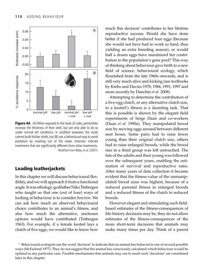
1 1 0 A D D I N G B E H AV I O U R
Loading leatherjackets
In this chapter we will discuss behavioural fl ex-ibility, and we will approach it from a functional angle. It was ethology-godfather Niko Tinbergen who taught us that one (out of four) ways of looking at behaviour is to consider function . We can ask how much an observed behavioural choice contributes to an animal’s fi tness, and also how much the alternative, unchosen options would have contributed ( Tinbergen 1963 ). For example, if a female kestrel lays a clutch of fi ve eggs, we would like to know how
much this decision 1 contributes to her lifetime reproductive success. Would she have done better if she had produced four eggs (because she would not have had to work so hard, thus yielding an extra breeding season), or would half a dozen eggs have maximized her contri-bution to the population’s gene pool? This way of thinking about behaviour gave birth to a new fi eld of science, behavioural ecology, which fl ourished from the late 1960s onwards, and is still very much alive and kicking (see textbooks by Krebs and Davies 1978 , 1984, 1991, 1997 and more recently by Danchin et al . 2008 ).
Attempting to determine the contribution of a fi ve-egg clutch, or any alternative clutch size, to a kestrel’s fi tness is a daunting task. That this is possible is shown by the elegant fi eld experiments of Serge Daan and co-workers ( Daan et al . 1990a ). They manipulated brood size by moving eggs around between different nest boxes. Some pairs had to raise fewer young than their original clutch size, others had to raise enlarged broods, while the brood size in a third group was left untouched. The fate of the adults and their young was followed over the subsequent years, enabling the esti-mation of survival and reproductive rates. After many years of data collection it became evident that the fi tness-value of the unmanip-ulated brood sizes was highest, because of a reduced parental fi tness in enlarged broods and a reduced fi tness of the clutch in reduced broods.
However elegant and stimulating such fi eld-based estimates of the fi tness-consequences of life-history decisions may be, they do not allow estimates of the fi tness-consequences of the more short-term decisions that animals may make many times per day. Think of a parent
0
5
10
20
% a
void
ance
res
pons
e
normal pH
B
15
low pH normal pH+ cue
low pH+ cue
–0.02
0.00
0.02
0.06
thic
knes
s in
crea
se (
mm
) A
0.04
*
*
*
Figure 64. (A) When exposed to the taste of crabs, periwinkles increase the thickness of their shell, but are only able to do so under normal pH conditions. In acidifi ed seawater, the snails cannot build thicker shells, but (B) use a behavioural way to avoid predation by crawling out of the water. Asterisks indicate treatments that are signifi cantly different from other treatments.
Modifi ed from Bibby et al . ( 2007 ).
1 Behavioural ecologists use the word ‘decision’ to indicate that an animal has behaved in one of several possible ways ( McFarland 1977 ). They do not suggest that the animal has consciously calculated which behaviour would be optimal in any particular case. Possible mechanisms that animals may use to reach such ‘decisions’ are considered later in this chapter.
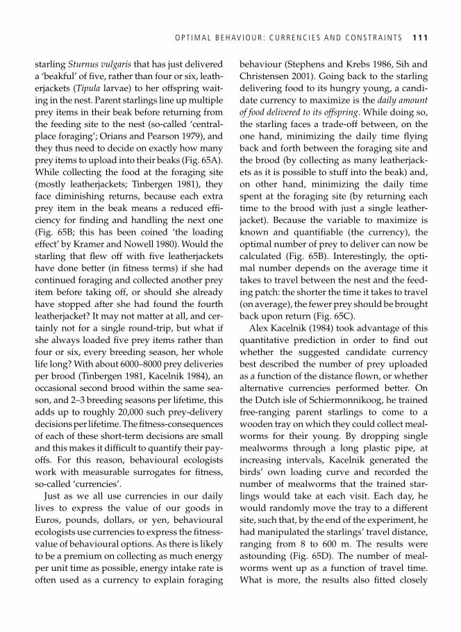
O P T I M A L B E H AV I O U R : C U R R E N C I E S A N D C O N S T R A I N T S 1 1 1
starling Sturnus vulgaris that has just delivered a ‘beakful’ of fi ve, rather than four or six, leath-erjackets ( Tipula larvae) to her offspring wait-ing in the nest. Parent starlings line up multiple prey items in their beak before returning from the feeding site to the nest (so-called ‘central-place foraging’; Orians and Pearson 1979 ), and they thus need to decide on exactly how many prey items to upload into their beaks ( Fig. 65A ). While collecting the food at the foraging site (mostly leatherjackets; Tinbergen 1981 ), they face diminishing returns, because each extra prey item in the beak means a reduced effi -ciency for fi nding and handling the next one ( Fig. 65B ; this has been coined ‘the loading effect’ by Kramer and Nowell 1980). Would the starling that fl ew off with fi ve leatherjackets have done better (in fi tness terms) if she had continued foraging and collected another prey item before taking off, or should she already have stopped after she had found the fourth leatherjacket? It may not matter at all, and cer-tainly not for a single round-trip, but what if she always loaded fi ve prey items rather than four or six, every breeding season, her whole life long? With about 6000–8000 prey deliveries per brood ( Tinbergen 1981 , Kacelnik 1984 ), an occasional second brood within the same sea-son, and 2–3 breeding seasons per lifetime, this adds up to roughly 20,000 such prey-delivery decisions per lifetime. The fi tness-consequences of each of these short-term decisions are small and this makes it diffi cult to quantify their pay-offs. For this reason, behavioural ecologists work with measurable surrogates for fi tness, so-called ‘currencies’.
Just as we all use currencies in our daily lives to express the value of our goods in Euros, pounds, dollars, or yen, behavioural ecologists use currencies to express the fi tness-value of behavioural options. As there is likely to be a premium on collecting as much energy per unit time as possible, energy intake rate is often used as a currency to explain foraging
behaviour ( Stephens and Krebs 1986 , Sih and Christensen 2001 ). Going back to the starling delivering food to its hungry young, a candi-date currency to maximize is the daily amount of food delivered to its offspring . While doing so, the starling faces a trade-off between, on the one hand, minimizing the daily time fl ying back and forth between the foraging site and the brood (by collecting as many leatherjack-ets as it is possible to stuff into the beak) and, on other hand, minimizing the daily time spent at the foraging site (by returning each time to the brood with just a single leather-jacket). Because the variable to maximize is known and quantifi able (the currency), the optimal number of prey to deliver can now be calculated ( Fig. 65B ). Interestingly, the opti-mal number depends on the average time it takes to travel between the nest and the feed-ing patch: the shorter the time it takes to travel (on average), the fewer prey should be brought back upon return ( Fig. 65C ).
Alex Kacelnik ( 1984 ) took advantage of this quantitative prediction in order to fi nd out whether the suggested candidate currency best described the number of prey uploaded as a function of the distance fl own, or whether alternative currencies performed better. On the Dutch isle of Schiermonnikoog, he trained free-ranging parent starlings to come to a wooden tray on which they could collect meal-worms for their young. By dropping single mealworms through a long plastic pipe, at increasing intervals, Kacelnik generated the birds’ own loading curve and recorded the number of mealworms that the trained star-lings would take at each visit. Each day, he would randomly move the tray to a different site, such that, by the end of the experiment, he had manipulated the starlings’ travel distance, ranging from 8 to 600 m. The results were astounding ( Fig. 65D ). The number of meal-worms went up as a function of travel time. What is more, the results also fi tted closely
1 1 2 A D D I N G B E H AV I O U R
with the prediction based on the maximization of the net amount of energy gained by the entire family as a whole , thus subtracting the metabolic rates of the parent and the chicks from the gross amount of energy collected. However, we should add that the predictions of the other three currencies were not too far off this mark either!
This example shows the use of decisions, currencies, constraints, and optimality in behavioural ecology. We must take into account that the starling needs to make many more decisions, which are not treated here (e.g. where to feed, how many prey items to con-
sume itself rather than to deliver to the young, etc.; see Tinbergen 1981 ), but the decision stud-ied here is: how many prey items to load before taking off? Then, after defi ning the currency , the unit in which the pay-offs of the taken deci-sion are expressed, it becomes clear what con-straints the parent starling faces: travel time, search time for each consecutive prey item, ‘loading time’ required to pick up each newly encountered prey item, and the metabolic rate in both the parent (in the feeding patch, in the air, and in the nest) and its offspring (while begging and while resting). If any of these con-straints could be alleviated (shortened in the
00
2
4
6
load
siz
e
10020 8040 60round trip travel time (s)
2
4
8
6
load
1
3
5
7
optimum
7 prey
8 prey
1 prey
optimumtravel time searching time
C
optimum (long)
shorttravel time searching time
optimum (short)
long
D
B A
Figure 65. (A) The complete foraging cycle of a central-place foraging parent starling, which alternates between collecting prey items at a feeding site and delivering them to its young in the nest. (B) The loading or gain curve at the feeding site describes the number of prey items loaded in the starling’s beak as a function of search time. As the beak-load increases, the effi ciency of fi nding and loading the next item decreases, resulting in a decelerating loading curve. The optimal number of items to load at the average site (seven in this example) depends on the average travel time between patches and can be found by the tangential solution shown. (C) The less time it takes to travel (on average), the fewer prey should be brought back upon return. (D) Kacelnik’s (1984) data (dots) fi tted best with the prediction based on net family gain rate maximization (line).
Compiled from Shettleworth ( 1998 ) (A) and Krebs and Davies (1991) (B–D).
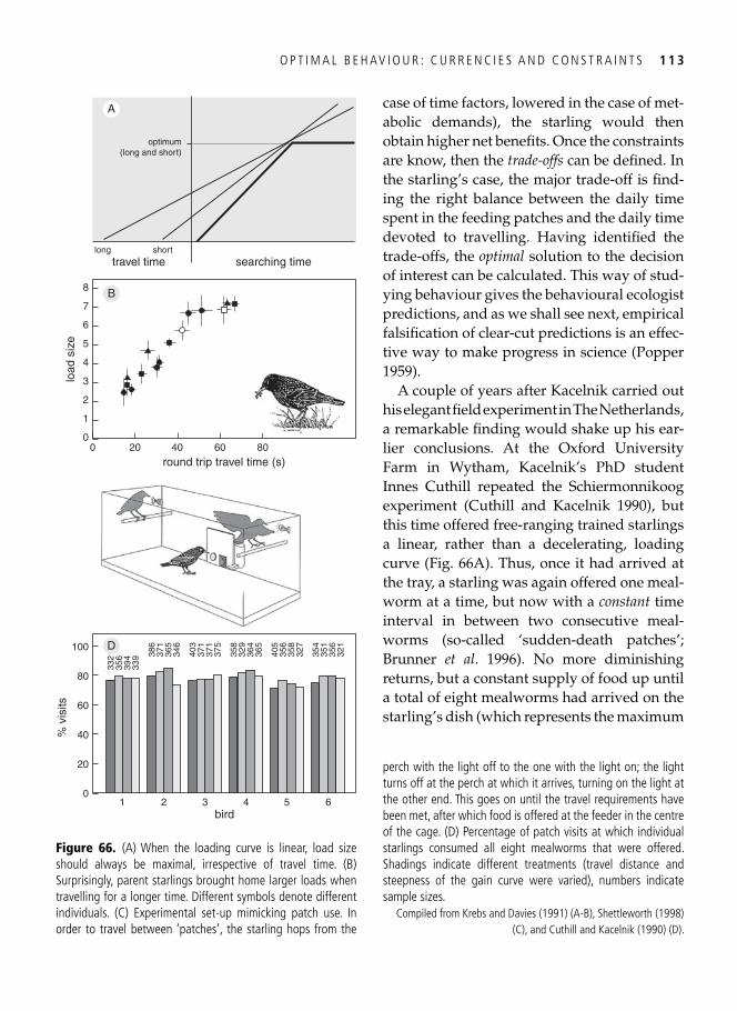
O P T I M A L B E H AV I O U R : C U R R E N C I E S A N D C O N S T R A I N T S 1 1 3
case of time factors, lowered in the case of met-abolic demands), the starling would then obtain higher net benefi ts. Once the constraints are know, then the trade-offs can be defi ned. In the starling’s case, the major trade-off is fi nd-ing the right balance between the daily time spent in the feeding patches and the daily time devoted to travelling. Having identifi ed the trade-offs, the optimal solution to the decision of interest can be calculated. This way of stud-ying behaviour gives the behavioural ecologist predictions, and as we shall see next, empirical falsifi cation of clear-cut predictions is an effec-tive way to make progress in science ( Popper 1959 ).
A couple of years after Kacelnik carried out his elegant fi eld experiment in The Netherlands, a remarkable fi nding would shake up his ear-lier conclusions. At the Oxford University Farm in Wytham, Kacelnik’s PhD student Innes Cuthill repeated the Schiermonnikoog experiment ( Cuthill and Kacelnik 1990 ), but this time offered free-ranging trained starlings a linear, rather than a decelerating, loading curve ( Fig. 66A ). Thus, once it had arrived at the tray, a starling was again offered one meal-worm at a time, but now with a constant time interval in between two consecutive meal-worms (so-called ‘sudden-death patches’; Brunner et al . 1996 ). No more diminishing returns, but a constant supply of food up until a total of eight mealworms had arrived on the starling’s dish (which represents the maximum
B
10
20
40
80
% v
isits
62 53 4bird
60
100
A
optimum(long and short)
332
356
394
339 38
637
136
534
6
403
371
371
375
358
329
364
365
405
356
358
327
354
351
356
321
00
2
4
6
load
siz
e
20 8040 60
round trip travel time (s)
1
3
5
8
short
searching timelong
travel time
7
D
C
Figure 66. (A) When the loading curve is linear, load size should always be maximal, irrespective of travel time. (B) Surprisingly, parent starlings brought home larger loads when travelling for a longer time. Different symbols denote different individuals. (C) Experimental set-up mimicking patch use. In order to travel between ‘patches’, the starling hops from the
perch with the light off to the one with the light on; the light turns off at the perch at which it arrives, turning on the light at the other end. This goes on until the travel requirements have been met, after which food is offered at the feeder in the centre of the cage. (D) Percentage of patch visits at which individual starlings consumed all eight mealworms that were offered. Shadings indicate different treatments (travel distance and steepness of the gain curve were varied), numbers indicate sample sizes.
Compiled from Krebs and Davies (1991) (A-B), Shettleworth ( 1998 ) (C), and Cuthill and Kacelnik ( 1990 ) (D).
1 1 4 A D D I N G B E H AV I O U R
number of mealworms that a starling can pos-sibly carry at any one time). The optimality model now predicts that the starling should always collect all eight prey items before tak-ing off, irrespective of travel distance ( Fig. 66A ). So what did the starlings actually do?
They ignored the theoretical prediction by bringing home more prey when travelling fur-ther ( Fig. 66B ). Imagine the amazement on the faces of Cuthill and Kacelnik! Yet, unabashed, they continued with another experiment that would eventually bring back light into the new darkness. The linear loading curves were now offered to self-feeding starlings that had no brood to care for, but still needed to travel to move between ‘patches’ ( Fig. 66C ). Guess what? Those self-feeding starlings did exactly what they were ‘supposed’ to do: they gave up virtually every food patch after collecting all eight mealworms, irrespective of the distance travelled ( Fig. 66D ). The only difference between these latter two experiments was the fact that chick-feeding starlings had to ‘upload’ and carry their prey items. Cuthill and Kacelnik, therefore, concluded that, with increasing load size, some cost function would increase, whether it was the energy expendi-ture while in the patch, or the energy expendi-ture while in fl ight, or the time it takes to return to the nest. Such costs had been overlooked when Kacelnik ( 1984 ) suggested that parent starlings should maximize net family gain . Even though this currency did account for parental energy expenditure, it did so in a load-size independent manner.
Such is the power of optimality models. As we have just demonstrated, a clash between theory and facts can lead to new ideas about the true constraints and currencies that under-lie the observed behaviour. Optimality models are by defi nition over-simplistic, but, when falsifi ed, they form a guide for further research. Just as in everyday life, making mistakes is the best way to learn! Having seen an example of
constraints that had to be redefi ned, the next scientifi c discovery story tells us how failing optimality models can inform us about alter-native currencies .
Better lazy than tired
For the most part, foraging theoreticians have included ‘time’ as the denominator in their favourite currency, meaning that something ought to be maximized per unit of time . For example, the number of leatherjackets col-lected per minute , or the net amount of Joules gained during the total day . This makes much sense, since foraging takes time, and animals also need to devote some of their daily time to activities such as fi nding a mate, building a nest, incubating eggs, and so on. It also makes sense when animals are in a hurry—when migrants need to fuel up to reach the breeding grounds in time, for example. In such cases, they devote all the time possible to foraging ( Piersma et al . 1994b ) and maximize the (net) energy income per day.
For this reason, it did not make sense when foragers were often observed feeding at a slower pace than was possible, even foragers that were trying to fuel up as quickly as they could, as you will see shortly. Dungeness crabs Cancer magister were eating smaller bivalves than expected from rate-maximizing princi-ples ( Juanes and Hartwick 1990 ), Lapland longspurs Calcarius lapponicus were not maxi-mizing the delivery rate to their offspring because they fl ew slower than they ‘should’ ( McLaughlin and Montgomerie 1990 ), as did black terns Chlidonias nigra ( Welham and Ydenberg 1993 ). Honey bee Apis mellifera workers only partially fi lled up their crops, whereas they should have fi lled them up com-pletely if they were to maximize the rate of delivering nectar to the hive ( Schmid-Hempel et al . 1985 ). This list could be extended further, but in all these examples it turned out that
O P T I M A L B E H AV I O U R : C U R R E N C I E S A N D C O N S T R A I N T S 1 1 5
another energetic currency was in fact being maximized, namely, the gross amount of energy gained per unit of energy expended, called ‘effi ciency’, and formally written as:
b / c ,
where b denotes gross energy intake rate and c denotes metabolic rate.
Initially, the reasons for this effi ciency max-imization were not understood. In fact, effi -ciency maximization was dismissed as a nonsensical currency by the fi rst foraging the-oreticians ( Stephens and Krebs 1986 ). They reasoned that, if 2 J can be gained for 1 J of expenditure, and the alternative would yield 5 J while expending 3 J, then the second option, the least effi cient option (5/3 < 2/1), should be preferred, simply because it yields a higher net gain (5–3 > 2–1). Only if expend-ing energy bears additional costs should it pay off to expend energy parsimoniously. We refer back to Chapter 4 for an in-depth treat-ment of non-energetic costs due to energy expenditure (such as shortened life span, increased risk of immediate death, hampered immune response). Although such non-ener-getic costs may explain effi cient and prudent behaviour, more recent foraging models have shown that there may nevertheless be purely energetic, rate-maximizing reasons for being an effi cient forager. Let us now examine this idea more closely.
More haste less speed
Even when in captivity, red knots fuel up rap-idly in spring and deposit the same amount of fat as do their free-ranging conspecifi cs ( Cadée et al . 1996 ). It was at this time of year that we performed an experiment with four red knots, which were allowed to exploit depletable patches in a large outdoor intertidal aviary ( van Gils et al . 2003b ). In the same way as the starlings we discussed earlier, the knots faced
diminishing returns when emptying their patches (because searching through the patches occurred in a non-systematic way, leading to longer time intervals between consecutive prey encounters). This gave rise to the critical question of this study: at what (diminishing) intake rate would knots give up a patch and switch to a new patch ( Fig. 67A )?
Given the time of year, we expected knots to give up their patches so that they maxi-mized their short-term net energy intake rate, i.e. their net intake calculated over total foraging time, taking into account the time and energy cost required to make brief fl ights between patches. This meant that, on the one hand, patches should not be exploited for too long, as the birds would lose too much time to increasingly long probing intervals, whereas, on the other hand, giving up the patches too soon would cost too much travel time, and especially travel energy, when moving between different patches ( Fig. 67B , C). To our initial surprise, the red knots probed much too long in their patches and were more reluctant to move on to a new patch than we had anticipated. Initially, we interpreted this as ‘lazy behaviour’, since the time devoted to the most costly activity, the short fl ights between patches, was less than half of what we expected.
Were the knots maximizing their effi ciency by obtaining every Joule of energy income as cheaply as possible, irrespective of the time it took? If so, would this increase their life-expectancy at a time of year when they actu-ally need to fuel up as quickly as possible? This could be the case, but it seemed more likely that it would be preferable to speed up the fuelling process, the more so because the birds weighed less than was normal for the last days of April.
The answer was provided by new the-oretical work from McNamara and Houston ( 1997 ), but also by Ydenberg and co-workers
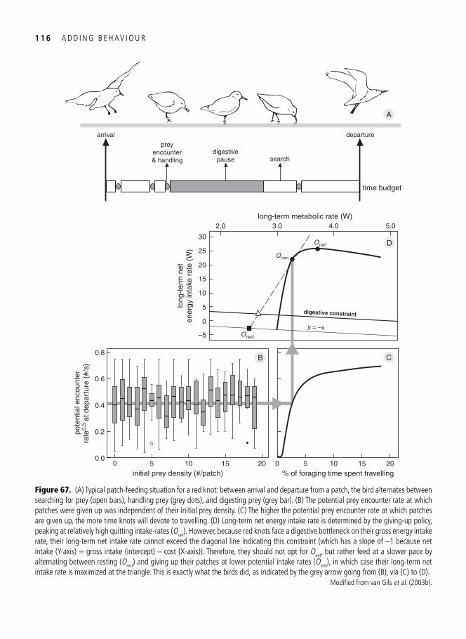
1 1 6 A D D I N G B E H AV I O U R
Orest
digestive constraint
Omin
Onet
y = –x
B C
D
A
00.0
0.2
0.4
0.6
0.8
pote
ntia
l enc
ount
erra
te0.
5at
dep
artu
re (
#/s)
105 15initial prey density (#/patch)
20 0 105 15% of foraging time spent travelling
20
2.0
–5
0
5
10
15
long
-ter
m n
eten
ergy
inta
ke r
ate
(W)
3.0long-term metabolic rate (W)
4.0 5.0
20
25
30
arrival
searchdigestive
pause
preyencounter& handling
departure
time budget
Figure 67. (A) Typical patch-feeding situation for a red knot: between arrival and departure from a patch, the bird alternates between searching for prey (open bars), handling prey (grey dots), and digesting prey (grey bar). (B) The potential prey encounter rate at which patches were given up was independent of their initial prey density. (C) The higher the potential prey encounter rate at which patches are given up, the more time knots will devote to travelling. (D) Long-term net energy intake rate is determined by the giving-up policy, peaking at relatively high quitting intake-rates (O net ). However, because red knots face a digestive bottleneck on their gross energy intake rate, their long-term net intake rate cannot exceed the diagonal line indicating this constraint (which has a slope of –1 because net intake (Y-axis) = gross intake (intercept) – cost (X-axis)). Therefore, they should not opt for O net , but rather feed at a slower pace by alternating between resting (O rest ) and giving up their patches at lower potential intake rates (O min ), in which case their long-term net intake rate is maximized at the triangle. This is exactly what the birds did, as indicated by the grey arrow going from (B), via (C) to (D).
Modifi ed from van Gils et al . ( 2003b ).
O P T I M A L B E H AV I O U R : C U R R E N C I E S A N D C O N S T R A I N T S 1 1 7
( Ydenberg et al . 1994 , Ydenberg and Hurd 1998 ), and Hedenström and Alerstam ( 1995 ). Energy-limited foragers, i.e. animals that face a constraint on the daily amount of energy that can be spent or assimilated, cannot feed dur-ing the entire day, as they need to ‘respect’ their energetic bottleneck (see Chapter 4 ). Such foragers, and this may sound counter-intui-tive, should actually maximize (a modifi ed form of) effi ciency while foraging , in order to maximize the net daily energy uptake across the entire day . The form of effi ciency that should be maximized has been coined the ‘foraging gain ratio’ ( Hedenström and Alerstam 1995 ) or simply the ‘modifi ed form of effi ciency’ ( Houston 1995 ), and takes account of the meta-bolic rate when not foraging, i.e. the resting metabolic rate r :
b / ( c – r ) .
This apparent paradox has a relatively simple explanation. If the gross amount of energy that can be assimilated cannot exceed a certain threshold, then it pays to gather this amount of energy as cheaply as possible, taking into account r , the metabolic rate while not feeding (the faster the threshold is reached, the more energy is lost to non-feeding behaviour). The less energy that is expended in total, the more energy remains. With respect to our knots, they were indeed energy-limited: the amount of energy they could assimilate during any one day was constrained by the rate at which they were able to process their shellfi sh prey. As knots ingest their prey whole, they must internally crush and process the bulky shell-material, which then needs to pass rapidly into the digestive system in order to make room for new food. The crushing of the shell takes place in the muscular stomach, called the gizzard ( Piersma et al . 1993b ), and it is especially the size of this part of the ‘gut’ that determines the daily amount of shell mass that the birds can process ( van Gils et al . 2003a ), and thus the
amount of fl esh that can be assimilated daily (about which we shall learn much more in the next chapter).
The intake rate at which our birds left their patches did indeed maximize the foraging gain ratio while they were feeding. To inves-tigate how this strategy would maximize overall net energy intake, we used the graphi-cal approach advocated by McNamara and Houston ( 1997 ) as shown in Fig. 67D . The tri-angle in that graph (the long-term net energy intake rate) cannot exceed the diagonal line indicating the digestive constraint. The more this point is located to the left on the diago-nal, the higher the long-term net energy intake rate (since the diagonal is going ‘down-hill’). This left-most location on the diagonal is achieved by alternating between resting (option O rest in the graph) and maximizing the foraging gain ratio while feeding (option O min , which is found by drawing a line from O rest —dashed in this case—that is tangental to the thick curve defi ning the continuous range of feeding options).
Of course, the argument for effi ciency maxi-mization only holds as long as there is enough time to reach the digestive bottleneck. When there is only a limited amount of foraging time, animals are said to be time constrained rather than energy constrained . When ‘heavily’ time constrained, the best thing such animals can do, when aiming to maximize net daily energy intake, is to maximize their net intake rate while feeding. It is as simple as that and means that animals may switch ‘tactics’, depending on whether they face a time constraint or an energy constraint, as exemplifi ed below.
Oystercatchers pressed for time
The aviaries in which we offered depletable patches to knots were used to study foraging oystercatchers Haematopus ostralegus 17 years earlier by Cees Swennen and others (1989).
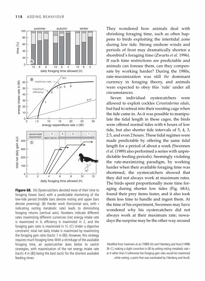
1 1 8 A D D I N G B E H AV I O U R
They wondered how animals deal with shrinking foraging time, such as often hap-pens to birds exploiting the intertidal zone during low tide. Strong onshore winds and periods of frost may dramatically shorten a shorebird’s foraging time ( Zwarts et al . 1996 ). If such time restrictions are predictable and animals can foresee them, can they compen-sate by working harder? During the 1980s, rate-maximization was still the dominant currency in foraging theory, and animals were expected to obey this ‘rule’ under all circumstances.
Seven individual oystercatchers were allowed to exploit cockles Cerastoderma edule , but had to retreat into their roosting cage when the tide came in. As it was possible to manipu-late the tidal length in these cages, the birds were offered normal tides with 6 hours of low tide, but also shorter tide intervals of 5, 4, 3, 2.5, and even 2 hours. These tidal regimes were made predictable by offering the same tidal length for a period of about a week (Swennen et al . ( 1989 ) also performed a series with unpre-dictable feeding periods). Seemingly violating the rate-maximizing paradigm, by working harder when their available foraging time was shortened, the oystercatchers showed that they did not always work at maximum rates. The birds spent proportionally more time for-aging during shorter low tides ( Fig. 68A ), found their prey items faster, and it also took them less time to handle and ingest them. At the time of his experiment, Swennen may have wondered why his oystercatchers did not always work at their maximum rate; nowa-days the surprise may be the other way around
b=c
C
4 3 2 1
B
A
summer autumn winter
00
200
400
tota
l net
dai
ly g
ain
(kJ)
102 84 6
daily foraging time allowed (h)
100
300
12
cannot meetrequirement
00
20
40
ener
gy in
take
rat
e b
(W)
255r 2010 15energy expenditure rate c (W)
10
30
30
BEST TACTIC
50
60
2
4
maximum rate
1
3 5 6
b /c
maximumefficiency
0
40
80
time
(%)
108 46
daily foraging time allowed (h)
20
60
12
100
6 8 512
Figure 68. (A) Oystercatchers devoted more of their time to foraging (lower bars) with a predictable shortening of the low-tide period (middle bars denote resting and upper bars denote preening). (B) Harder work (horizontal axis, with r indicating resting metabolic rate) leads to diminishing foraging returns (vertical axis). Numbers indicate different rates maximizing different currencies (net energy intake rate is maximized in 4, effi ciency is maximized in 2, and the foraging gain ratio is maximized in 1). (C) Under a digestive constraint, total net daily intake is maximized by maximizing the foraging gain ratio (tactic 1 in (B)). However, this strategy requires much foraging time. With a shrinkage of the available foraging time, an oystercatcher does better to switch strategies, with maximization of the net energy intake rate (tactic 4 in (B)) being the best tactic for the shortest available feeding times.
Modifi ed from Swennen et al . ( 1989 ) (A) and Ydenberg and Hurd ( 1998 ) (B–C), making a slight correction in (B) by setting resting metabolic rate r at 4 rather than 5 (otherwise the foraging gain ratio would be maximized
while resting, a point that was overlooked by Ydenberg and Hurd).
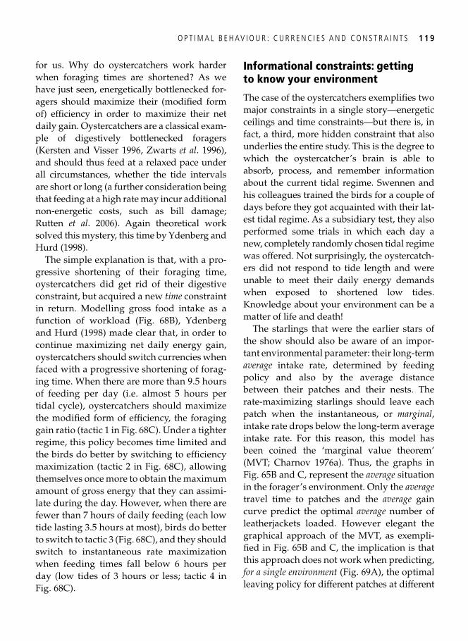
O P T I M A L B E H AV I O U R : C U R R E N C I E S A N D C O N S T R A I N T S 1 1 9
for us. Why do oystercatchers work harder when foraging times are shortened? As we have just seen, energetically bottlenecked for-agers should maximize their (modifi ed form of) effi ciency in order to maximize their net daily gain. Oystercatchers are a classical exam-ple of digestively bottlenecked foragers ( Kersten and Visser 1996 , Zwarts et al . 1996 ), and should thus feed at a relaxed pace under all circumstances, whether the tide intervals are short or long (a further consideration being that feeding at a high rate may incur additional non-energetic costs, such as bill damage; Rutten et al . 2006 ). Again theoretical work solved this mystery, this time by Ydenberg and Hurd ( 1998 ).
The simple explanation is that, with a pro-gressive shortening of their foraging time, oystercatchers did get rid of their digestive constraint, but acquired a new time constraint in return. Modelling gross food intake as a function of workload ( Fig. 68B ), Ydenberg and Hurd ( 1998 ) made clear that, in order to continue maximizing net daily energy gain, oystercatchers should switch currencies when faced with a progressive shortening of forag-ing time. When there are more than 9.5 hours of feeding per day (i.e. almost 5 hours per tidal cycle), oystercatchers should maximize the modifi ed form of effi ciency, the foraging gain ratio (tactic 1 in Fig. 68C ). Under a tighter regime, this policy becomes time limited and the birds do better by switching to effi ciency maximization (tactic 2 in Fig. 68C ), allowing themselves once more to obtain the maximum amount of gross energy that they can assimi-late during the day. However, when there are fewer than 7 hours of daily feeding (each low tide lasting 3.5 hours at most), birds do better to switch to tactic 3 ( Fig. 68C ), and they should switch to instantaneous rate maximization when feeding times fall below 6 hours per day (low tides of 3 hours or less; tactic 4 in Fig. 68C ).
Informational constraints: getting to know your environment
The case of the oystercatchers exemplifi es two major constraints in a single story—energetic ceilings and time constraints—but there is, in fact, a third, more hidden constraint that also underlies the entire study. This is the degree to which the oystercatcher’s brain is able to absorb, process, and remember information about the current tidal regime. Swennen and his colleagues trained the birds for a couple of days before they got acquainted with their lat-est tidal regime. As a subsidiary test, they also performed some trials in which each day a new, completely randomly chosen tidal regime was offered. Not surprisingly, the oystercatch-ers did not respond to tide length and were unable to meet their daily energy demands when exposed to shortened low tides. Knowledge about your environment can be a matter of life and death!
The starlings that were the earlier stars of the show should also be aware of an impor-tant environmental parameter: their long-term average intake rate, determined by feeding policy and also by the average distance between their patches and their nests. The rate-maximizing starlings should leave each patch when the instantaneous, or marginal , intake rate drops below the long-term average intake rate. For this reason, this model has been coined the ‘marginal value theorem’ (MVT; Charnov 1976a ). Thus, the graphs in Fig. 65B and C, represent the average situation in the forager’s environment. Only the average travel time to patches and the average gain curve predict the optimal average number of leatherjackets loaded. However elegant the graphical approach of the MVT, as exempli-fi ed in Fig. 65B and C, the implication is that this approach does not work when predicting, for a single environment ( Fig. 69A ), the optimal leaving policy for different patches at different
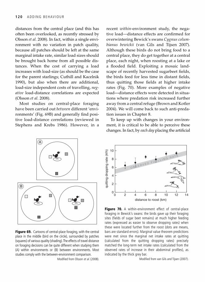
1 2 0 A D D I N G B E H AV I O U R
distances from the central place (and this has often been overlooked, as recently stressed by Olsson et al . 2008 ). In fact, within a single envi-ronment with no variation in patch quality, because all patches should be left at the same marginal intake rate, similar load sizes should be brought back home from all possible dis-tances. When the cost of carrying a load increases with load-size (as should be the case for the parent starlings; Cuthill and Kacelnik 1990 ), but also when there are additional, load-size independent costs of travelling, neg-ative load-distance correlations are expected ( Olsson et al . 2008 ).
Most studies on central-place foraging have been carried out between different ‘envi-ronments’ ( Fig. 69B ) and generally fi nd posi-tive load-distance correlations (reviewed in Stephens and Krebs 1986 ). However, in a
recent within -environment study, the nega-tive load—distance effects are confi rmed for overwintering Bewick’s swans Cygnus colum-bianus bewickii ( van Gils and Tijsen 2007 ). Although these birds do not bring food to a central place, they do get together at a central place, each night, when roosting at a lake or a fl ooded fi eld. Exploiting a mosaic land-scape of recently harvested sugarbeet fi elds, the birds feed for less time in distant fi elds, thus quitting those fi elds at higher intake rates ( Fig. 70 ). More examples of negative load—distance effects were detected in situa-tions where predation risk increased further away from a central refuge ( Brown and Kotler 2004 ). We will come back to such anti-preda-tion issues in Chapter 8 .
To keep up with changes in your environ-ment, it is critical to be able to perceive these changes. In fact, by each day placing the artifi cial
00
2
4
6
quitt
ing
drop
ping
rat
e (#
/h)
2 84 6
distance to roost (km)
8
10
10 12 14
O B S E R V E D F U E L L I N G R AT E
Figure 70. A within-environment effect of central-place foraging in Bewick’s swans: the birds gave up their foraging sites (fi elds of sugar beet remains) at much higher feeding rates (expressed as easier to observe dropping rates) when these were located further from the roost (dots are means, bars are standard errors). Marginal value theorem predictions were met since the marginal net intake rates at quitting (calculated from the quitting dropping rates) precisely matched the long-term net intake rates (calculated from the observed rates of increase in their abdominal profi les), as indicated by the thick grey bar.
Modifi ed from van Gils and Tijsen ( 2007 ).
A
B
Figure 69. Cartoons of central-place foraging, with the central place in the middle (bird on the circle), surrounded by patches (squares) of various quality (shading). The effects of travel distance on foraging decisions can be quite different when studying them (A) within environments or (B) between environments. Most studies comply with the between-environment comparison.
Modifi ed from Olsson et al . ( 2008 ).
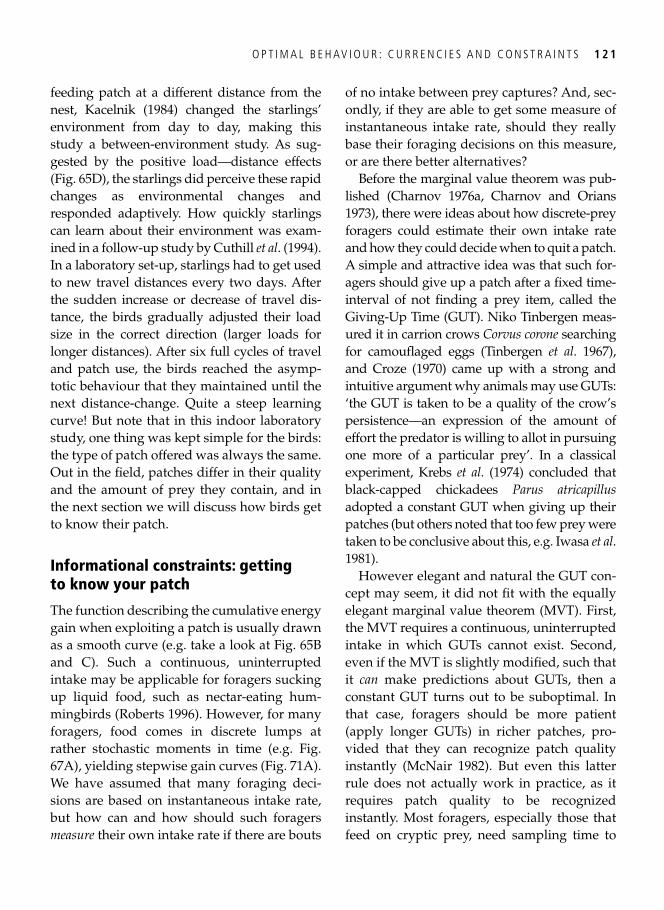
O P T I M A L B E H AV I O U R : C U R R E N C I E S A N D C O N S T R A I N T S 1 2 1
feeding patch at a different distance from the nest, Kacelnik ( 1984 ) changed the starlings’ environment from day to day, making this study a between-environment study. As sug-gested by the positive load—distance effects ( Fig. 65D ), the starlings did perceive these rapid changes as environmental changes and responded adaptively. How quickly starlings can learn about their environment was exam-ined in a follow-up study by Cuthill et al . ( 1994 ). In a laboratory set-up, starlings had to get used to new travel distances every two days. After the sudden increase or decrease of travel dis-tance, the birds gradually adjusted their load size in the correct direction (larger loads for longer distances). After six full cycles of travel and patch use, the birds reached the asymp-totic behaviour that they maintained until the next distance-change. Quite a steep learning curve! But note that in this indoor laboratory study, one thing was kept simple for the birds: the type of patch offered was always the same. Out in the fi eld, patches differ in their quality and the amount of prey they contain, and in the next section we will discuss how birds get to know their patch.
Informational constraints: getting to know your patch
The function describing the cumulative energy gain when exploiting a patch is usually drawn as a smooth curve (e.g. take a look at Fig. 65B and C). Such a continuous, uninterrupted intake may be applicable for foragers sucking up liquid food, such as nectar-eating hum-mingbirds ( Roberts 1996 ). However, for many foragers, food comes in discrete lumps at rather stochastic moments in time (e.g. Fig. 67A ), yielding stepwise gain curves ( Fig. 71A ). We have assumed that many foraging deci-sions are based on instantaneous intake rate, but how can and how should such foragers measure their own intake rate if there are bouts
of no intake between prey captures? And, sec-ondly, if they are able to get some measure of instantaneous intake rate, should they really base their foraging decisions on this measure, or are there better alternatives?
Before the marginal value theorem was pub-lished ( Charnov 1976a , Charnov and Orians 1973 ), there were ideas about how discrete-prey foragers could estimate their own intake rate and how they could decide when to quit a patch. A simple and attractive idea was that such for-agers should give up a patch after a fi xed time-interval of not fi nding a prey item, called the Giving-Up Time (GUT). Niko Tinbergen meas-ured it in carrion crows Corvus corone searching for camoufl aged eggs ( Tinbergen et al . 1967 ), and Croze (1970) came up with a strong and intuitive argument why animals may use GUTs: ‘the GUT is taken to be a quality of the crow’s persistence—an expression of the amount of effort the predator is willing to allot in pursuing one more of a particular prey’. In a classical experiment, Krebs et al . ( 1974 ) concluded that black-capped chickadees Parus atricapillus adopted a constant GUT when giving up their patches (but others noted that too few prey were taken to be conclusive about this, e.g. Iwasa et al . 1981 ).
However elegant and natural the GUT con-cept may seem, it did not fi t with the equally elegant marginal value theorem (MVT). First, the MVT requires a continuous, uninterrupted intake in which GUTs cannot exist. Second, even if the MVT is slightly modifi ed, such that it can make predictions about GUTs, then a constant GUT turns out to be suboptimal. In that case, foragers should be more patient (apply longer GUTs) in richer patches, pro-vided that they can recognize patch quality instantly ( McNair 1982 ). But even this latter rule does not actually work in practice, as it requires patch quality to be recognized instantly. Most foragers, especially those that feed on cryptic prey, need sampling time to
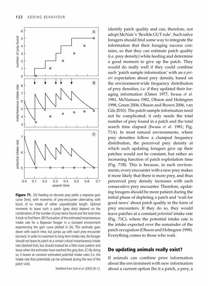
1 2 2 A D D I N G B E H AV I O U R
identify patch quality and can, therefore, not adopt McNair’s ‘fl exible GUT rule’. Such naïve foragers should fi nd some way to integrate the information that their foraging success con-tains, so that they can estimate patch quality (i.e. prey density) while feeding and determine a good moment to give up the patch. They would do really well if they could combine such ‘patch sample information’ with an a pri-ori expectation about prey density, based on the environment-wide frequency distribution of prey densities, i.e. if they updated their for-aging information ( Oaten 1977 , Iwasa et al . 1981 , McNamara 1982 , Olsson and Holmgren 1998 , Green 2006 , Olsson and Brown 2006 , van Gils 2010 ). The patch-sample information need not be complicated; it only needs the total number of prey found in a patch and the total search time elapsed ( Iwasa et al . 1981 ; Fig. 71A ). In most natural environments, where prey densities follow a clumped frequency distribution, the perceived prey density at which such updating foragers give up their patches would not be constant, but rather an increasing function of patch exploitation time ( Fig. 71B ). This is because, in such environ-ments, every encounter with a new prey makes it more likely that there is more prey, and thus perceived prey density increases with each consecutive prey encounter. Therefore, updat-ing foragers should be more patient during the initial phase of depleting a patch and ‘wait for good news’ about patch quality in the form of prey encounters. If they do so, they would leave patches at a constant potential intake rate ( Fig. 71C ), where the potential intake rate is the intake expected over the remainder of the patch occupation ( Olsson and Holmgren 1998 ). Everything comes to those who wait.
Do updating animals really exist?
If animals can combine prior information about the environment with new information about a current option (be it a patch, a prey, a
pote
ntia
l int
ake
rate
0.0
5
6
0.1 0.40.2 0.3search time
7
0.5 0.6 0.7
inst
anta
neou
s in
take
rat
e
3
4
5
6
7
8
num
ber
of p
rey
foun
d
0
4
5
6
3
2
1
A
B
C
Figure 71. (A) Feeding on discrete prey yields a stepwise gain curve (line), with moments of prey-encounter alternating with bouts of no intake of rather unpredictable length. Optimal moments to leave such a patch (grey dots) depend on the combination of the number of prey items found and the total time it took to fi nd them. (B) Fluctuation of the estimated instantaneous intake rate for a Bayesian forager in a clumped environment experiencing the gain curve plotted in (A). This estimate goes down with search time, but jumps up with each prey encounter (arrows). In order to maximize its long-term intake rate, the forager should not leave its patch at a certain critical instantaneous intake rate (dashed line), but should instead be a little more patient and leave when the estimates have reached the grey dots. (C) By doing so, it leaves at constant estimated potential intake rates (i.e. the intake rate that potentially can be achieved during the rest of the patch visit).
Modifi ed from Dall et al . ( 2005 ) (B–C).

O P T I M A L B E H AV I O U R : C U R R E N C I E S A N D C O N S T R A I N T S 1 2 3
mate, or whatever), they can markedly improve their assessment of the value of the current option, and thus improve fi tness ( Olsson and Brown 2010 ). This is the essence of ‘Bayesian’ updating, named after Thomas Bayes (1702–61), an Anglican priest inter-ested in probability theory. Just to give you a simple example of Bayesian updating in practice: imagine a patch in which a forager has found two prey items during the fi rst minute of search. Should it continue search-ing or should it leave this patch? If the envi-ronment is structured such that a patch can only contain two prey items at most, then the forager should defi nitely move on. By con-trast, if patches can contain many more than just two items, then the forager should stay, especially if it took little time to fi nd these two items. Thus, knowing your environment (in a statistical, probabilistic sense) greatly improves your assessment abilities; without knowledge about your environment, it is much harder to make the right choices. A popular example of Bayesian updating in humans is the so-called ‘Monty Hall prob-lem’ ( Selvin 1975 ), named after an American quizmaster. Imagine you are participating in a TV game in which you have to select one out of three closed doors ( Fig. 72 ). Behind one of these doors stands a car, behind each of the other two doors stands a goat. You will take home either a car or a goat, depending on which door you choose. Once you have selected your door, the friendly quizmaster, who knows what stands behind each door, helps you by opening one of the other two doors for you, with a goat behind it. Knowing this, or, in Bayesian terms, updating your prior expectation with new sampling information , should you switch to the other closed door? The answer is yes; by switching, your chance of winning the car increases from 1 in 3 to 2 in 3. The intuitive, but incorrect, answer is that there is no need to switch doors, since
your chances would only increase from 1 in 3 to 1 in 2, irrespective of whether you switch or not!
Since the seminal paper on Bayesian forag-ing by Oaten ( 1977 ), relatively few tests of this rapidly expanding family of models exist. Nevertheless, a recent review paper strongly suggests that animals are capable of Bayesian updating: in ten out of the eleven studies that were compared, behaviour was consistent with Bayesian-updating predictions ( Valone 2006 ). Most tests were performed on foraging animals, but there is also the case of female peacock wrasses Symphodus tinaca searching for males ( Luttbeg and Warner 1999 ). Even estuarine amphipods Gammarus lawrencianus use Bayesian updating when selecting their mates ( Hunte et al . 1985 ). As echoed by Valone ( 2006 ), the strongest support comes from stud-ies in which prior knowledge about the envi-ronment is experimentally manipulated, such as in the recently published work on Bayesian bumblebees Bombus impatiens ( Biernaskie et al . 2009 ). In this study, bees were each offered patches of 12 fl owers, of which fi ve fl owers contained nectar (a 30% sucrose solution). The bees were fooled by the other seven fl owers, as they contained only water, and no sugar. Optimal foraging in such a uniform environ-ment would indicate a greater tendency to leave the 12-fl ower patch with each successive encounter of a nectar fl ower ( Fig. 73A ), because each encounter means that the patch will har-bour one nectar fl ower less in the future, as the bee empties each encountered nectar fl ower. And that is indeed what they do ( Fig. 73B ).
Now comes the evidence that the bees were indeed Bayesian bees: when offered a differ-ent environment, with highly variable patches (in which the 12 fl owers contained either one or nine nectar fl owers), the bees switched pol-icies according to the theory. The tendency to stay in the patch should ( Fig. 73C ) and did ( Fig. 73D ) peak when encountering a second
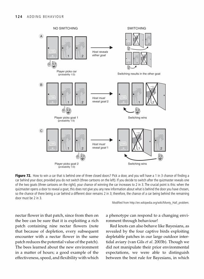
1 2 4 A D D I N G B E H AV I O U R
nectar fl ower in that patch, since from then on the bee can be sure that it is exploiting a rich patch containing nine nectar fl owers (note that because of depletion, every subsequent encounter with a nectar fl ower in the same patch reduces the potential value of the patch). The bees learned about the new environment in a matter of hours; a good example of the effectiveness, speed, and fl exibility with which
a phenotype can respond to a changing envi-ronment through behaviour!
Red knots can also behave like Bayesians, as revealed by the four captive birds exploiting depletable patches in our large outdoor inter-tidal aviary ( van Gils et al . 2003b ). Though we did not manipulate their prior environmental expectations, we were able to distinguish between the best rule for Bayesians, in which
A
Player picks car(probability 1/3)
Host revealseither goat1 2
B
Player picks goat 1(probability 1/3)
Host mustreveal goat 21 2
C
Player picks goat 2(probability 1/3)
Host mustreveal goat 11 2
NO SWITCHING
Switching results in the other goat
Switching wins
1 2
Switching wins
2
SWITCHING
1
1 2
21
Figure 72. How to win a car that is behind one of three closed doors? Pick a door, and you will have a 1 in 3 chance of fi nding a car behind your door, provided you do not switch (three cartoons on the left). If you decide to switch after the quizmaster reveals one of the two goats (three cartoons on the right), your chance of winning the car increases to 2 in 3. The crucial point is this: when the quizmaster opens a door to reveal a goat, this does not give you any new information about what is behind the door you have chosen, so the chance of there being a car behind a different door remains 2 in 3; therefore, the chance of a car being behind the remaining door must be 2 in 3.
Modifi ed from http://en.wikipedia.org/wiki/Monty_Hall_problem .
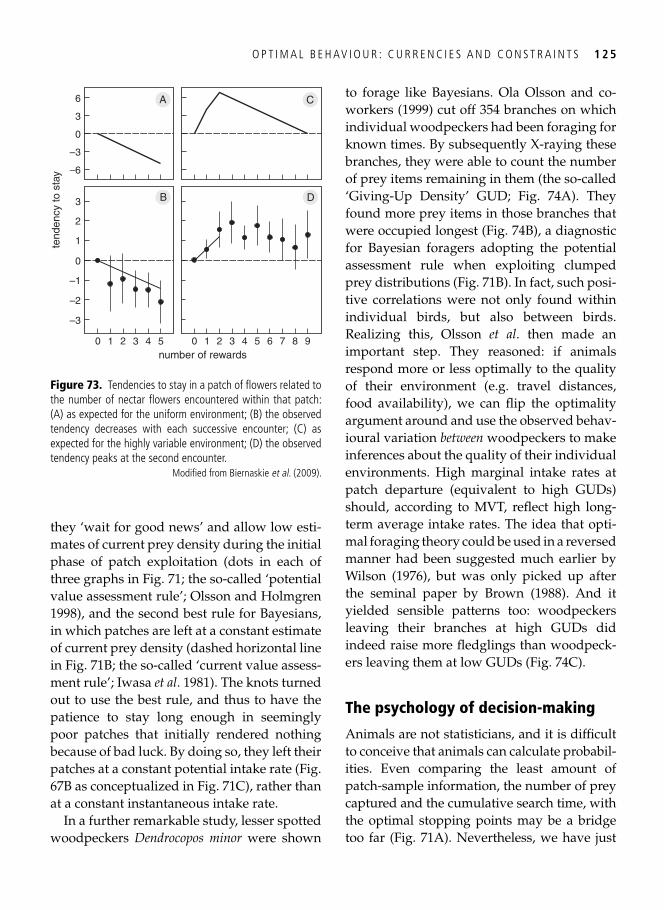
O P T I M A L B E H AV I O U R : C U R R E N C I E S A N D C O N S T R A I N T S 1 2 5
they ‘wait for good news’ and allow low esti-mates of current prey density during the initial phase of patch exploitation (dots in each of three graphs in Fig. 71 ; the so-called ‘potential value assessment rule’; Olsson and Holmgren 1998 ), and the second best rule for Bayesians, in which patches are left at a constant estimate of current prey density (dashed horizontal line in Fig. 71B ; the so-called ‘current value assess-ment rule’; Iwasa et al . 1981 ). The knots turned out to use the best rule, and thus to have the patience to stay long enough in seemingly poor patches that initially rendered nothing because of bad luck. By doing so, they left their patches at a constant potential intake rate ( Fig. 67B as conceptualized in Fig. 71C ), rather than at a constant instantaneous intake rate.
In a further remarkable study, lesser spotted woodpeckers Dendrocopos minor were shown
to forage like Bayesians. Ola Olsson and co-workers (1999) cut off 354 branches on which individual woodpeckers had been foraging for known times. By subsequently X-raying these branches, they were able to count the number of prey items remaining in them (the so-called ‘Giving-Up Density’ GUD; Fig. 74A ). They found more prey items in those branches that were occupied longest ( Fig. 74B ), a diagnostic for Bayesian foragers adopting the potential assessment rule when exploiting clumped prey distributions ( Fig. 71B ). In fact, such posi-tive correlations were not only found within individual birds, but also between birds. Realizing this, Olsson et al . then made an important step. They reasoned: if animals respond more or less optimally to the quality of their environment (e.g. travel distances, food availability), we can fl ip the optimality argument around and use the observed behav-ioural variation between woodpeckers to make inferences about the quality of their individual environments. High marginal intake rates at patch departure (equivalent to high GUDs) should, according to MVT, refl ect high long-term average intake rates. The idea that opti-mal foraging theory could be used in a reversed manner had been suggested much earlier by Wilson ( 1976 ), but was only picked up after the seminal paper by Brown ( 1988 ). And it yielded sensible patterns too: woodpeckers leaving their branches at high GUDs did indeed raise more fl edglings than woodpeck-ers leaving them at low GUDs ( Fig. 74C ).
The psychology of decision-making
Animals are not statisticians, and it is diffi cult to conceive that animals can calculate probabil-ities. Even comparing the least amount of patch-sample information, the number of prey captured and the cumulative search time, with the optimal stopping points may be a bridge too far ( Fig. 71A ). Nevertheless, we have just
0 1
tend
ency
to s
tay
A
B
0
–3
–2
–1
0
1
2
42number of rewards
3
1 53
–6
–3
0
3
6 C
D
4 82 65 93 7
Figure 73. Tendencies to stay in a patch of fl owers related to the number of nectar fl owers encountered within that patch: (A) as expected for the uniform environment; (B) the observed tendency decreases with each successive encounter; (C) as expected for the highly variable environment; (D) the observed tendency peaks at the second encounter.
Modifi ed from Biernaskie et al . ( 2009 ).
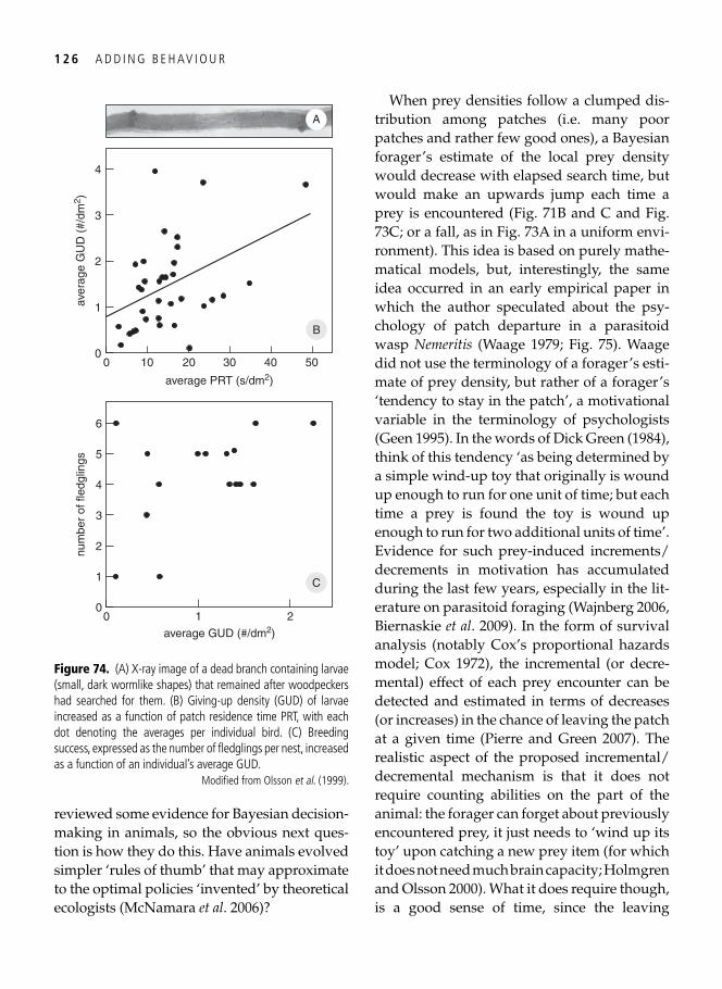
1 2 6 A D D I N G B E H AV I O U R
reviewed some evidence for Bayesian decision-making in animals, so the obvious next ques-tion is how they do this. Have animals evolved simpler ‘rules of thumb’ that may approximate to the optimal policies ‘invented’ by theoretical ecologists ( McNamara et al . 2006 )?
When prey densities follow a clumped dis-tribution among patches (i.e. many poor patches and rather few good ones), a Bayesian forager’s estimate of the local prey density would decrease with elapsed search time, but would make an upwards jump each time a prey is encountered ( Fig. 71B and C and Fig. 73C ; or a fall, as in Fig. 73A in a uniform envi-ronment). This idea is based on purely mathe-matical models, but, interestingly, the same idea occurred in an early empirical paper in which the author speculated about the psy-chology of patch departure in a parasitoid wasp Nemeritis ( Waage 1979 ; Fig. 75 ). Waage did not use the terminology of a forager’s esti-mate of prey density, but rather of a forager’s ‘tendency to stay in the patch’, a motivational variable in the terminology of psychologists ( Geen 1995 ). In the words of Dick Green ( 1984 ), think of this tendency ‘as being determined by a simple wind-up toy that originally is wound up enough to run for one unit of time; but each time a prey is found the toy is wound up enough to run for two additional units of time’. Evidence for such prey-induced increments/decrements in motivation has accumulated during the last few years, especially in the lit-erature on parasitoid foraging ( Wajnberg 2006 , Biernaskie et al . 2009 ). In the form of survival analysis (notably Cox’s proportional hazards model; Cox 1972 ), the incremental (or decre-mental) effect of each prey encounter can be detected and estimated in terms of decreases (or increases) in the chance of leaving the patch at a given time ( Pierre and Green 2007 ). The realistic aspect of the proposed incremental/decremental mechanism is that it does not require counting abilities on the part of the animal: the forager can forget about previously encountered prey, it just needs to ‘wind up its toy’ upon catching a new prey item (for which it does not need much brain capacity; Holmgren and Olsson 2000 ). What it does require though, is a good sense of time, since the leaving
00
2
4
aver
age
GU
D (
#/dm
2 )
10 20 5030 40
average PRT (s/dm2)
1
3
B
00
2
4
6
num
ber
of fl
edgl
ings
1 2
average GUD (#/dm2)
1
3
5
C
A
Figure 74. (A) X-ray image of a dead branch containing larvae (small, dark wormlike shapes) that remained after woodpeckers had searched for them. (B) Giving-up density (GUD) of larvae increased as a function of patch residence time PRT, with each dot denoting the averages per individual bird. (C) Breeding success, expressed as the number of fl edglings per nest, increased as a function of an individual’s average GUD.
Modifi ed from Olsson et al . ( 1999 ).
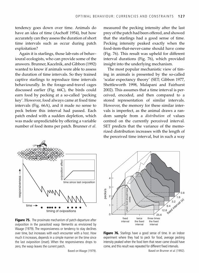
O P T I M A L B E H AV I O U R : C U R R E N C I E S A N D C O N S T R A I N T S 1 2 7
tendency goes down over time. Animals do have an idea of time ( Aschoff 1954 ), but how accurately can they assess the duration of short time intervals such as occur during patch exploitation?
Again it is starlings, those lab-rats of behav-ioural ecologists, who can provide some of the answers. Brunner, Kacelnik, and Gibbon ( 1992 ) wanted to know if animals were able to assess the duration of time intervals. So they trained captive starlings to reproduce time intervals behaviourally. In the forage-and-travel cages discussed earlier ( Fig. 66C ), the birds could earn food by pecking at a so-called ‘pecking key’. However, food always came at fi xed time intervals ( Fig. 66A ), and it made no sense to peck before this interval had passed. Each patch ended with a sudden depletion, which was made unpredictable by offering a variable number of food items per patch. Brunner et al .
measured the pecking intensity after the last prey of the patch had been offered, and showed that the starlings had a good sense of time. Pecking intensity peaked exactly when the food-item-that-never-came should have come ( Fig. 76 ). This result was upheld for different interval durations ( Fig. 76 ), which provided insight into the underlying mechanism.
The most popular mechanistic view of tim-ing in animals is presented by the so-called ‘scalar expectancy theory’ (SET; Gibbon 1977 , Shettleworth 1998 , Malapani and Fairhurst 2002 ). This assumes that a time interval is per-ceived, encoded, and then compared to a stored representation of similar intervals. However, the memory for these similar inter-vals is imperfect, as the animal draws a ran-dom sample from a distribution of values centred on the currently perceived interval. SET predicts that the variance of the memo-rized distribution increases with the length of the perceived time interval, but in such a way
peck
s/s
0
1
2
4
fixedinterval
3
twicethe fixedinterval
three timesthe fixedinterval
25.6
12.8
6.4
3.2
1.6
0.8
fixed
inter
val (s
)
whe
n fo
od s
houl
d ha
ve
com
e
Figure 76. Starlings have a good sense of time. In an indoor experiment where they had to peck for food, average pecking intensity peaked when the food item that never came should have come, and this result was repeated for different fi xed intervals.
Based on Brunner et al . ( 1992 ).
resp
onsi
vene
ss
timing of ovipositions
time
time since last oviposition
ovip
ositi
on e
ffect
Figure 75. The proximate mechanism of patch-departure after oviposition in the parasitoid wasp Nemeritis as envisioned by Waage ( 1979 ). The responsiveness or tendency to stay declines over time, but increases with each encounter with a host. How much it increases, depends in a simple manner on the time since the last oviposition (inset). When the responsiveness drops to zero, the wasp leaves the current patch.
Based on Waage ( 1979 ).
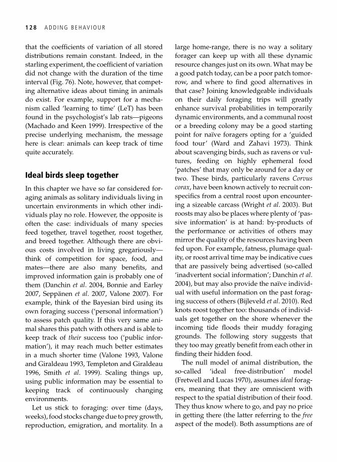
1 2 8 A D D I N G B E H AV I O U R
that the coeffi cients of variation of all stored distributions remain constant. Indeed, in the starling experiment, the coeffi cient of variation did not change with the duration of the time interval ( Fig. 76 ). Note, however, that compet-ing alternative ideas about timing in animals do exist. For example, support for a mecha-nism called ‘learning to time’ (LeT) has been found in the psychologist’s lab rats—pigeons ( Machado and Keen 1999 ). Irrespective of the precise underlying mechanism, the message here is clear: animals can keep track of time quite accurately.
Ideal birds sleep together
In this chapter we have so far considered for-aging animals as solitary individuals living in uncertain environments in which other indi-viduals play no role. However, the opposite is often the case: individuals of many species feed together, travel together, roost together, and breed together. Although there are obvi-ous costs involved in living gregariously—think of competition for space, food, and mates—there are also many benefi ts, and improved information gain is probably one of them ( Danchin et al . 2004 , Bonnie and Earley 2007 , Seppänen et al . 2007 , Valone 2007 ). For example, think of the Bayesian bird using its own foraging success (‘personal information’) to assess patch quality. If this very same ani-mal shares this patch with others and is able to keep track of their success too (‘public infor-mation’), it may reach much better estimates in a much shorter time ( Valone 1993 , Valone and Giraldeau 1993 , Templeton and Giraldeau 1996 , Smith et al . 1999 ). Scaling things up, using public information may be essential to keeping track of continuously changing environments.
Let us stick to foraging: over time (days, weeks), food stocks change due to prey growth, reproduction, emigration, and mortality. In a
large home-range, there is no way a solitary forager can keep up with all these dynamic resource changes just on its own. What may be a good patch today, can be a poor patch tomor-row, and where to fi nd good alternatives in that case? Joining knowledgeable individuals on their daily foraging trips will greatly enhance survival probabilities in temporarily dynamic environments, and a communal roost or a breeding colony may be a good starting point for naïve foragers opting for a ‘guided food tour’ ( Ward and Zahavi 1973 ). Think about scavenging birds, such as ravens or vul-tures, feeding on highly ephemeral food ‘patches’ that may only be around for a day or two. These birds, particularly ravens Corvus corax , have been known actively to recruit con-specifi cs from a central roost upon encounter-ing a sizeable carcass ( Wright et al . 2003 ). But roosts may also be places where plenty of ‘pas-sive information’ is at hand: by-products of the performance or activities of others may mirror the quality of the resources having been fed upon. For example, fatness, plumage qual-ity, or roost arrival time may be indicative cues that are passively being advertised (so-called ‘inadvertent social information’; Danchin et al . 2004 ), but may also provide the naïve individ-ual with useful information on the past forag-ing success of others ( Bijleveld et al . 2010 ). Red knots roost together too: thousands of individ-uals get together on the shore whenever the incoming tide fl oods their muddy foraging grounds. The following story suggests that they too may greatly benefi t from each other in fi nding their hidden food.
The null model of animal distribution, the so-called ‘ideal free-distribution’ model ( Fretwell and Lucas 1970 ), assumes ideal forag-ers, meaning that they are omniscient with respect to the spatial distribution of their food. They thus know where to go, and pay no price in getting there (the latter referring to the free aspect of the model). Both assumptions are of
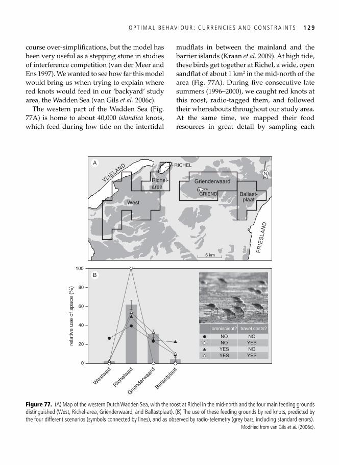
O P T I M A L B E H AV I O U R : C U R R E N C I E S A N D C O N S T R A I N T S 1 2 9
course over-simplifi cations, but the model has been very useful as a stepping stone in studies of interference competition ( van der Meer and Ens 1997 ). We wanted to see how far this model would bring us when trying to explain where red knots would feed in our ‘backyard’ study area, the Wadden Sea ( van Gils et al . 2006c ).
The western part of the Wadden Sea ( Fig. 77A ) is home to about 40,000 islandica knots, which feed during low tide on the intertidal
mudfl ats in between the mainland and the barrier islands ( Kraan et al . 2009 ). At high tide, these birds get together at Richel, a wide, open sandfl at of about 1 km 2 in the mid-north of the area ( Fig. 77A ). During fi ve consecutive late summers (1996–2000), we caught red knots at this roost, radio-tagged them, and followed their whereabouts throughout our study area. At the same time, we mapped their food resources in great detail by sampling each
NO NONO YESYES NOYES YES
omniscient? travel costs?
0
20
40
60
80
100
rela
tive
use
of s
pace
(%
)
Wes
twad
Richelw
ad
Griend
erwaa
rd
Ballas
tplaa
t
Grienderwaard
Ballast-plaat
5 km
VLIELAND
Richel-area
RICHEL
N
GRIEND
West
FR
IES
LAN
D
B
A
Figure 77. (A) Map of the western Dutch Wadden Sea, with the roost at Richel in the mid-north and the four main feeding grounds distinguished (West, Richel-area, Grienderwaard, and Ballastplaat). (B) The use of these feeding grounds by red knots, predicted by the four different scenarios (symbols connected by lines), and as observed by radio-telemetry (grey bars, including standard errors).
Modifi ed from van Gils et al . ( 2006c ).
1 3 0 A D D I N G B E H AV I O U R
year the macrozoobenthos at nearly 2000 sta-tions laid out in a grid at 250-m intervals. Combining measured tidal heights with fi ne-scaled elevation data, we could predict the daily exposure time for each station. Food densities and exposure time were the main input variables in a so-called ‘stochastic dynamic programming model’ in which we simulated red knot movements. We consid-ered four possible scenarios. If knots had no knowledge about their environment but were to travel for free, they would distribute them-selves randomly, only respecting the differen-tial availability of mudfl ats due to differences in elevation (fi lled dots in Fig. 77B ). If, instead, these naïve birds travelled at a cost, they would not get too far from the roost and all hang around near Richel during low tide (open dots in Fig. 77B ). If they ‘would know better’, have complete knowledge of their ‘foodscape’, and travelling was for free, they would go to the best feeding grounds (Ballastplaat), as much as the tide allowed them (this particular mudfl at lies relatively low and is therefore exposed relatively briefl y; closed triangles in Fig. 77B ). On the other hand, if such knowledgeable birds did not travel for free, they would get to Ballastplaat much less often, as this site is located furthest from the roost, and would instead spend more time feeding nearby (but skipping the food-poor area called ‘Westwad’; open triangles in Fig. 77B ).
The last prediction matched best with the movement data of our radio-tagged birds (bars in Fig. 77B ): knots seem to be ideal, but not free. It was no surprise to us that they were not free, since they have to pay a price for travel-ling, but we did not expect that the fi t with the ideal/omniscience prediction would be so
close. With a highly dynamic food supply that is consumed by many, grows fast, and hides in the mud, it is out of the question that only per-sonal sampling information can keep knots up-to-date. They must somehow exchange public information, be it actively or passively, and their central roost is likely to play an important role as an information centre ( Bijleveld et al . 2010 ).
With this report from the Wadden Sea, we have set the scene for the next chapter(s), in which ‘Wadden Sea knots’ will feature again. There will be one important difference, how-ever. So far we have assumed that all knots have similar bodies. In the next chapter, we will focus on these individual red knots, and we will see that different individuals do differ-ent things. Much of this behavioural variabil-ity can be explained by their fl exible bodies, bodies that we ‘looked into’ before releasing them once again into their wide open windy landscape.
Synopsis
Behaviour is a rapid way for animals to respond fl exibly to a changing environment. The study of behaviour has often been approached from a functional angle, which has allowed researchers to make clear-cut, fal-sifi able predictions about behaviour. Knowing the constraints faced by an animal (including informational constraints), and assuming a currency that approximates fi tness, research-ers can qualify decisions as optimal or subopti-mal . This chapter provides a stepping stone to the next chapter, where we adopt this success-ful optimality approach to interpret and pre-dict fl exible organ size changes within shorebirds.
131
CHAPTER 7
Optimal foraging: the dynamic choice between diets, feeding patches, and gut sizes
Eating more by ignoring food
In the previous chapter we demonstrated the intellectual elegance of behavioural optimality reasoning, a concept that enables ecologists to make stepwise scientifi c progression by means of Popperian falsifi cation of quantitative predic-tions. In this chapter we will show how our for-aging work on red knots was built on this approach, step by step. Initially we thought that the standard optimal-diet model of behavioural ecology would be suffi cient to explain the com-position of the menu of red knots functionally. However, this proved not to be the case, and only after including the process of digestion into the diet model were we able to explain diet selec-tion. This in turn led to a deeper understanding of the knots’ related selection criteria, notably of the habitats they made use of, and the strong dif-ferences between different phenotypes in these selection criteria. Not only could we then under-stand why different phenotypes responded dif-ferently to the different food patches on offer, but also how the idea worked in reverse—the food supply moulding the phenotypes. Elaborating these observations will be the aim of this chapter. But let us begin fi rst with a brief review of the standard diet model that we abandoned so soon after embracing it.
Back in 1966, Robert MacArthur and Eric Pianka developed a simple but effective model that showed how a forager, trying to maximize its long-term average food-intake rate, should
refrain from consuming every prey item that it encountered. A decade later, the model was refi ned by others (e.g. Pulliam 1974 , Werner and Hall 1974 , Charnov 1976b ), but the general structure and predictions remained unchanged. The basics are these: a forager can either search for prey, or handle an encountered prey item, but it cannot do both things at the same time. Therefore, handling a prey item carries a time cost, as searching has stopped for a moment. Sometimes it may be more fruitful to neglect an encountered prey item and to continue search-ing for a better one. This is the case when the ‘intake rate while handling the item’ is less than the maximum possible intake rate averaged over a long period of foraging. The ‘intake rate while handling’, usually referred to as ‘profi ta-bility’, is the key parameter in the model and equals the ratio between the energy content of a prey item and the required handling time. The main prediction of this simple diet model is thus clear cut and intuitively appealing: in rich envi-ronments, where high long-term average intake rates can be achieved, foragers should be more selective; in poor environments, diets should be broader. Its simple elegance also appealed to the godfather of ‘behavioural ecology’, Lord John R. Krebs, who tested this model in captive great tits Parus major .
Krebs et al . ( 1977 ) offered their tits segments of mealworms as prey. These came in two forms: long pieces (eight segments long) and short pieces (four segments). By adding a small
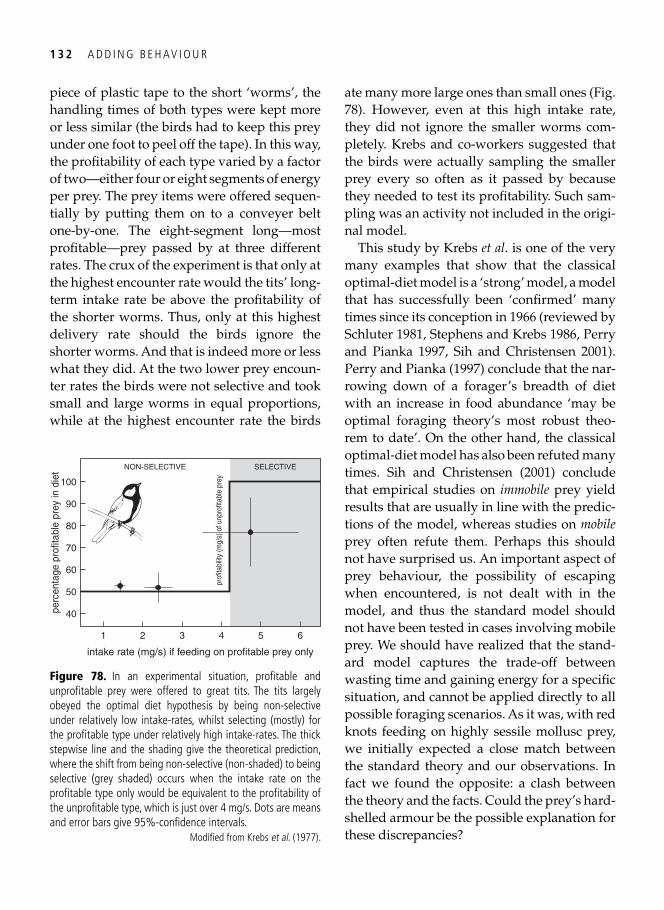
1 3 2 A D D I N G B E H AV I O U R
piece of plastic tape to the short ‘worms’, the handling times of both types were kept more or less similar (the birds had to keep this prey under one foot to peel off the tape). In this way, the profi tability of each type varied by a factor of two—either four or eight segments of energy per prey. The prey items were offered sequen-tially by putting them on to a conveyer belt one-by-one. The eight-segment long—most profi table—prey passed by at three different rates. The crux of the experiment is that only at the highest encounter rate would the tits’ long-term intake rate be above the profi tability of the shorter worms. Thus, only at this highest delivery rate should the birds ignore the shorter worms. And that is indeed more or less what they did. At the two lower prey encoun-ter rates the birds were not selective and took small and large worms in equal proportions, while at the highest encounter rate the birds
ate many more large ones than small ones ( Fig. 78 ). However, even at this high intake rate, they did not ignore the smaller worms com-pletely. Krebs and co-workers suggested that the birds were actually sampling the smaller prey every so often as it passed by because they needed to test its profi tability. Such sam-pling was an activity not included in the origi-nal model.
This study by Krebs et al . is one of the very many examples that show that the classical optimal-diet model is a ‘strong’ model, a model that has successfully been ‘confi rmed’ many times since its conception in 1966 (reviewed by Schluter 1981 , Stephens and Krebs 1986 , Perry and Pianka 1997 , Sih and Christensen 2001 ). Perry and Pianka ( 1997 ) conclude that the nar-rowing down of a forager’s breadth of diet with an increase in food abundance ‘may be optimal foraging theory’s most robust theo-rem to date’. On the other hand, the classical optimal-diet model has also been refuted many times. Sih and Christensen ( 2001 ) conclude that empirical studies on immobile prey yield results that are usually in line with the predic-tions of the model, whereas studies on mobile prey often refute them. Perhaps this should not have surprised us. An important aspect of prey behaviour, the possibility of escaping when encountered, is not dealt with in the model, and thus the standard model should not have been tested in cases involving mobile prey. We should have realized that the stand-ard model captures the trade-off between wasting time and gaining energy for a specifi c situation, and cannot be applied directly to all possible foraging scenarios. As it was, with red knots feeding on highly sessile mollusc prey, we initially expected a close match between the standard theory and our observations. In fact we found the opposite: a clash between the theory and the facts. Could the prey’s hard-shelled armour be the possible explanation for these discrepancies?
perc
enta
ge p
rofit
able
pre
y in
die
t
prof
itabi
lity
(mg/
s) o
f unp
rofit
able
pre
y
40
50
60
70
80
90
100
1 2 3 4 5 6
intake rate (mg/s) if feeding on profitable prey only
NON-SELECTIVE SELECTIVE
Figure 78. In an experimental situation, profi table and unprofi table prey were offered to great tits. The tits largely obeyed the optimal diet hypothesis by being non-selective under relatively low intake-rates, whilst selecting (mostly) for the profi table type under relatively high intake-rates. The thick stepwise line and the shading give the theoretical prediction, where the shift from being non-selective (non-shaded) to being selective (grey shaded) occurs when the intake rate on the profi table type only would be equivalent to the profi tability of the unprofi table type, which is just over 4 mg/s. Dots are means and error bars give 95%-confi dence intervals.
Modifi ed from Krebs et al . ( 1977 ).
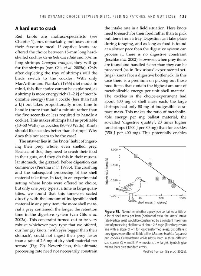
T H E DY N A M I C C H O I C E B E T W E E N D I E T S , F E E D I N G PAT C H E S , A N D G U T S I Z E S 1 3 3
A hard nut to crack
Red knots are mollusc-specialists (see Chapter 1 ), but, remarkably, molluscs are not their favourite meal. If captive knots are offered the choice between 15-mm long hard-shelled cockles Cerastoderma edule and 50-mm long shrimps Crangon crangon , they will go for the shrimps ( van Gils et al . 2005a ). Only after depleting the tray of shrimps will the birds switch to the cockles. With only MacArthur and Pianka’s (1966) diet model in mind, this diet choice cannot be explained, as a shrimp is more energy rich (1–2 kJ of metab-olizable energy) than a cockle (less than half a kJ) but takes proportionally more time to handle (more than half a minute rather than the fi ve seconds or less required to handle a cockle). This makes shrimps half as profi table (40–50 Watts) as cockles (80–90 Watts). Knots should like cockles better than shrimps! Why does this not seem to be the case?
The answer lies in the knots’ habit of ingest-ing their prey whole, even shelled prey. Because of this, they need to crush their food in their guts, and they do this in their muscu-lar stomach, the gizzard, before digestion can commence ( Piersma et al . 1993b ). The crushing and the subsequent processing of the shell material take time. In fact, in an experimental setting where knots were offered no choice, but only one prey type at a time in large quan-tities, we found that this time-cost scaled directly with the amount of indigestible shell material in any prey item: the more shell mate-rial a prey contained, the longer the retention time in the digestive system ( van Gils et al . 2003a ). This constraint turned out to be very robust: whichever prey type that we offered, our hungry knots, ‘with eyes bigger than their stomach’, could not ingest their prey faster than a rate of 2.6 mg of dry shell material per second ( Fig. 79 ). Nevertheless, this ultimate processing rate need not necessarily constrain
the intake rate in a fi eld situation. Here knots need to search for their food rather than to pick out items from a tray. Digestion can take place during foraging, and as long as food is found at a slower pace than the digestive system can process it, there is no digestive constraint ( Jeschke et al . 2002 ). However, when prey items are found and handled faster than they can be processed (as in ‘luxurious’ experimental set-tings), knots face a digestive bottleneck. In this case there is a premium on picking out those food items that contain the highest amount of metabolizable energy per unit shell material. The cockles in the choice-experiment had about 400 mg of shell mass each; the large shrimps had only 80 mg of indigestible cara-pace mass. This makes the ratio of metaboliz-able energy per mg ballast material, the so-called ‘digestive quality’, 20 times higher for shrimps (1500 J per 80 mg) than for cockles (350 J per 400 mg). This potentially enables
10.001
0.010
0.100
1.000
inta
ke r
ate
(pre
y/s)
100010
shell mass (mg/prey)
S
100
M
L
S
LM
Figure 79. No matter whether a prey type contained a little or a lot of shell mass per item (horizontal axis), the knots’ intake rate (vertical axis) would be constrained by a constant maximum rate of processing shell mass of about 2.6 mg/s (fi tted regression line with a slope of –1 for log-transformed axes). Six different prey-types were offered: Baltic tellins Macoma balthica (squares) and cockles Cerastoderma edule (dots), both in three different size classes (S = small; M = medium; L = large). Symbols give means, bars give standard errors.
Modifi ed from van Gils et al . ( 2003a ).
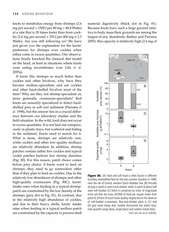
1 3 4 A D D I N G B E H AV I O U R
knots to metabolize energy from shrimps (2.6 mg per second × 1500 J per 80 mg = 48.8 Watts) at a rate that is 20 times faster than from cock-les (2.6 mg per second × 350 J per 400 mg = 2.3 Watts). Are you still following us? We have just given you the explanation for the knots’ preference for shrimps over cockles when either come in excess quantities. Our observa-tions fi nally knocked the classical diet model on the head, at least in situations where knots were eating invertebrates ( van Gils et al . 2005a ).
If knots like shrimps so much better than cockles and other bivalves, why have they become mollusc-specialists and eat cockles and other hard-shelled bivalves most of the time? Why are they not shrimp-specialists or, more generally, crustacean-specialists? Red knots are sensorily specialized to detect hard-shelled prey in soft wet sediment ( Piersma et al . 1998 ), but the answer lies in a crucial differ-ence between our laboratory studies and the fi eld situation. In the wild, food does not occur in excess quantities. It is not laid out conspicu-ously in plastic trays, but scattered and hiding in the sediment. Knots need to search for it. What is more, shrimps are relatively rare, while cockles and other low-quality molluscs are relatively abundant. In addition, shrimp patches contain rather few cockles and typical cockle patches harbour low shrimp densities ( Fig. 80 ). For this reason, patch choice comes before prey choice: if knots want to feed on shrimps, they need to go somewhere other than if they plan to feed on cockles. Due to the relatively low abundance of shrimps and other high-quality crustaceans ( Fig. 80C ), knots’ intake rates when feeding in a typical shrimp-patch are constrained by the low density of the shrimps (grey dot in Fig. 81 ). In contrast, due to the relatively high abundance of cockles, and due to their heavy shells, knots’ intake rates when feeding in a typical mollusc-patch are constrained by the capacity to process shell
material digestively (black dot in Fig. 81 ). Because knots have such a large gizzard (rela-tive to body mass their gizzards are among the largest of any shorebirds; Battley and Piersma 2005 ), this capacity is relatively high (2.6 mg of
Dig
estiv
e qu
ality
(J/m
g)A
vaila
ble
prey
bio
mas
s(g
AF
DM
/m2 )
Ava
ilabl
epr
ey d
ensi
ty (
%)
D
C
8
2
4
6
A BPatch
0.1
1
10
0
20
40
60
80B
100
hard
soft
patch B
GRIEND2 km
patch A
A
Figure 80. (A) Hard and soft food is often found in different localities, exemplifi ed here for the late-summer situation in 1998, near the isle of Griend, western Dutch Wadden Sea. (B) Virtually all prey in patch A were hard-shelled, while in patch B about half were soft bodied. (C) Patch A contained an order of magnitude more ash-free dry mass (AFDM) of food per square meter than patch B, (D) but of much lower quality, largely due to the absence of soft-bodied crustaceans. Box-and-whisker plots in (C) and (D) give mean (large dot), median (horizontal line within box), inter-quartile range (box), range (bars) and outliers (small dots).
From van Gils et al . ( 2005b ).
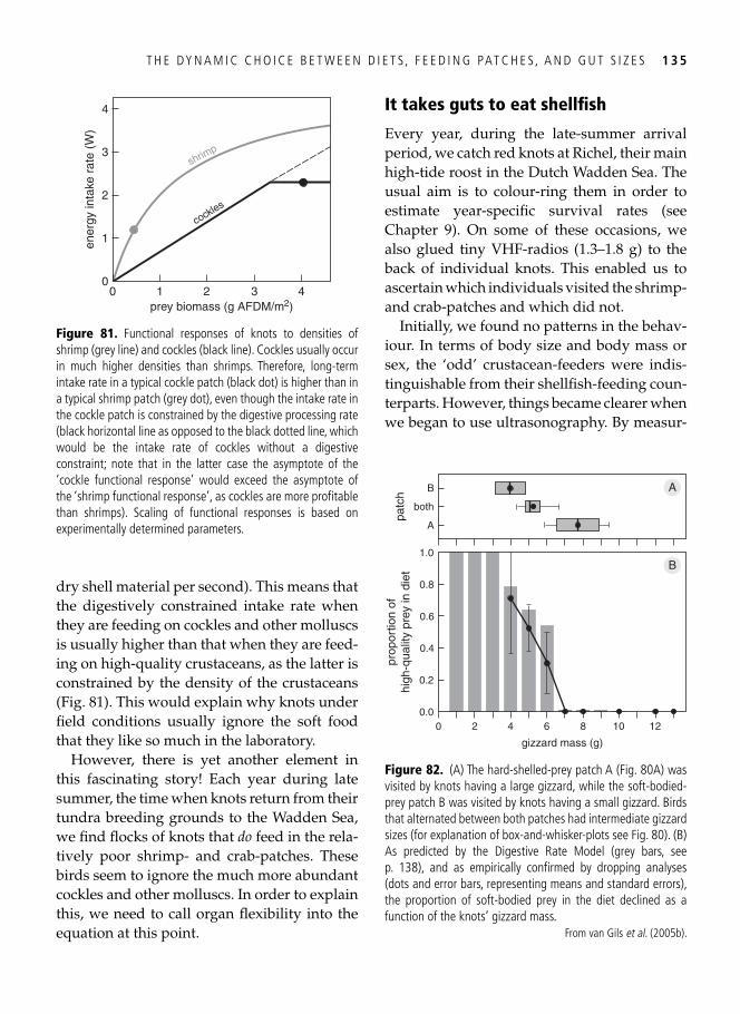
T H E DY N A M I C C H O I C E B E T W E E N D I E T S , F E E D I N G PAT C H E S , A N D G U T S I Z E S 1 3 5
dry shell material per second). This means that the digestively constrained intake rate when they are feeding on cockles and other molluscs is usually higher than that when they are feed-ing on high-quality crustaceans, as the latter is constrained by the density of the crustaceans ( Fig. 81 ). This would explain why knots under fi eld conditions usually ignore the soft food that they like so much in the laboratory.
However, there is yet another element in this fascinating story! Each year during late summer, the time when knots return from their tundra breeding grounds to the Wadden Sea, we fi nd fl ocks of knots that do feed in the rela-tively poor shrimp- and crab-patches. These birds seem to ignore the much more abundant cockles and other molluscs. In order to explain this, we need to call organ fl exibility into the equation at this point.
It takes guts to eat shellfi sh
Every year, during the late-summer arrival period, we catch red knots at Richel, their main high-tide roost in the Dutch Wadden Sea. The usual aim is to colour-ring them in order to estimate year-specifi c survival rates (see Chapter 9 ). On some of these occasions, we also glued tiny VHF-radios (1.3–1.8 g) to the back of individual knots. This enabled us to ascertain which individuals visited the shrimp- and crab-patches and which did not.
Initially, we found no patterns in the behav-iour. In terms of body size and body mass or sex, the ‘odd’ crustacean-feeders were indis-tinguishable from their shellfi sh-feeding coun-terparts. However, things became clearer when we began to use ultrasonography. By measur-
patc
hpr
opor
tion
ofhi
gh-q
ualit
y pr
ey in
die
t
A
A
both
B
0
gizzard mass (g)
10 122
0.4
4 6 8
B
0.2
0.8
1.0
0.0
0.6
Figure 82. (A) The hard-shelled-prey patch A ( Fig. 80A ) was visited by knots having a large gizzard, while the soft-bodied-prey patch B was visited by knots having a small gizzard. Birds that alternated between both patches had intermediate gizzard sizes (for explanation of box-and-whisker-plots see Fig. 80 ). (B) As predicted by the Digestive Rate Model (grey bars, see p. 138), and as empirically confi rmed by dropping analyses (dots and error bars, representing means and standard errors), the proportion of soft-bodied prey in the diet declined as a function of the knots’ gizzard mass.
From van Gils et al . ( 2005b ).
cockles
shrimp
00
1
2
3
ener
gy in
take
rat
e (W
)
1 2 3 4prey biomass (g AFDM/m2)
4
Figure 81. Functional responses of knots to densities of shrimp (grey line) and cockles (black line). Cockles usually occur in much higher densities than shrimps. Therefore, long-term intake rate in a typical cockle patch (black dot) is higher than in a typical shrimp patch (grey dot), even though the intake rate in the cockle patch is constrained by the digestive processing rate (black horizontal line as opposed to the black dotted line, which would be the intake rate of cockles without a digestive constraint; note that in the latter case the asymptote of the ‘cockle functional response’ would exceed the asymptote of the ‘shrimp functional response’, as cockles are more profi table than shrimps). Scaling of functional responses is based on experimentally determined parameters.
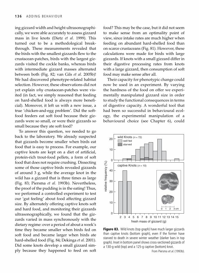
1 3 6 A D D I N G B E H AV I O U R
ing gizzard width and height ultrasonographi-cally, we were able accurately to assess gizzard mass in live knots ( Dietz et al . 1999 ). This turned out to be a methodological break-through. These measurements revealed that the birds with the smallest gizzards fl ew to the crustacean-patches, birds with the largest giz-zards visited the cockle banks, whereas birds with intermediate gizzard masses alternated between both ( Fig. 82 ; van Gils et al . 2005b )! We had discovered phenotype-related habitat selection. However, these observations did not yet explain why crustacean-patches were vis-ited (in fact, we simply reasoned that feeding on hard-shelled food is always more benefi -cial). Moreover, it left us with a new issue, a true ‘chicken-and-egg problem’. Did the soft-food feeders eat soft food because their giz-zards were so small, or were their gizzards so small because they ate soft food?
To answer this question, we needed to go back to the laboratory. We already suspected that gizzards become smaller when birds eat food that is easy to process. For example, our captive knots are kept on a diet of artifi cial, protein-rich trout-food pellets, a form of soft food that does not require crushing. Dissecting some of those captive birds revealed gizzards of around 3 g, while the average knot in the wild has a gizzard that is three times as large ( Fig. 83 ; Piersma et al . 1993b ). Nevertheless, the proof of the pudding is in the eating! Thus, we performed a controlled experiment to test our ‘gut feeling’ about food affecting gizzard size. By alternately offering captive knots soft and hard food, and monitoring their gizzards ultrasonographically, we found that the giz-zards varied in mass synchronously with the dietary regime: over a period of about a week’s time they became smaller when birds fed on soft food and became larger when birds ate hard-shelled food ( Fig. 84 ; Dekinga et al . 2001 ). Did some knots develop a small gizzard sim-ply because they happened to feed on soft
food? This may be the case, but it did not seem to make sense from an optimality point of view, since intake rates are much higher when feeding on abundant hard-shelled food than on scarce crustaceans ( Fig. 81 ). However, these calculations were made for birds with large gizzards. If knots with a small gizzard differ in their digestive processing rates from knots with a large gizzard, then consumption of soft food may make sense after all.
Their capacity for phenotypic change could now be used in an experiment. By varying the hardness of the food on offer we experi-mentally manipulated gizzard size in order to study the functional consequences in terms of digestive capacity. A wonderful tool that had been so successful in behavioural ecol-ogy, the experimental manipulation of a behavioural choice (see Chapter 6 ), could
0
10
20
30
40
rela
tive
freq
uenc
y (%
)
102 3 4 5 6 8 97
fresh mass of gizzard (g)
well fedstarved
11 12 13 14 15
captive Knots (n = 10)
0
10
20wild Knots (n = 72)
0 1 2 3 cm
Figure 83. Wild knots (top graph) have much larger gizzards than captive knots (bottom graph), even if the former have starved to death in severe winter weather (darker bars in top graph). Inset in bottom panel shows cross-sectioned gizzards of a 130-g wild (top) and a 125-g captive (bottom) knot.
From Piersma et al . ( 1993b ).
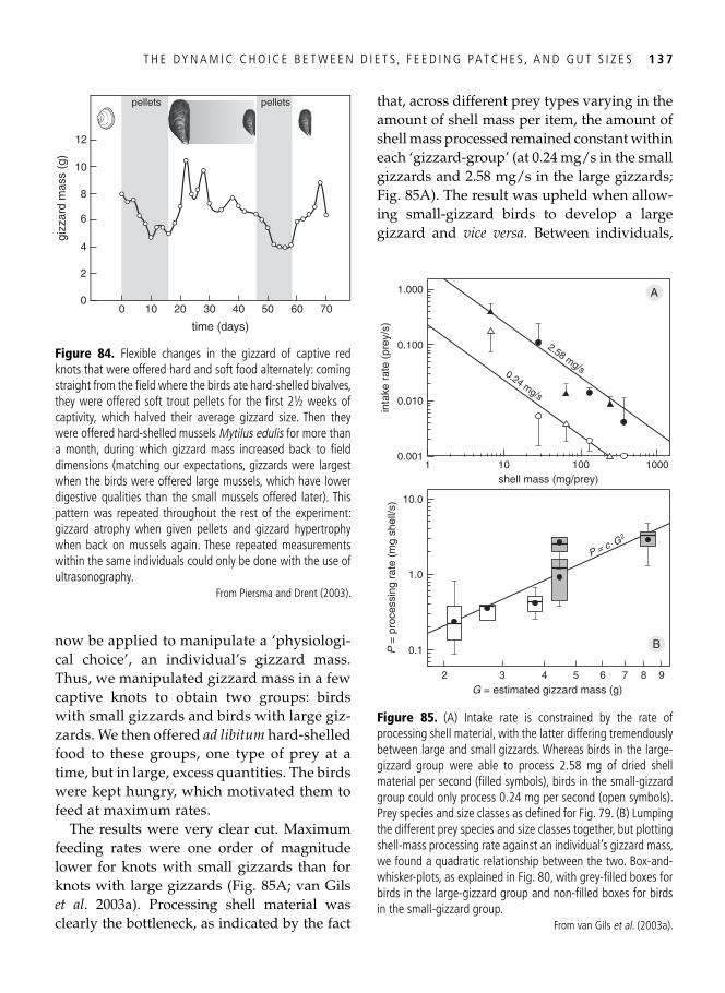
T H E DY N A M I C C H O I C E B E T W E E N D I E T S , F E E D I N G PAT C H E S , A N D G U T S I Z E S 1 3 7
now be applied to manipulate a ‘physiologi-cal choice’, an individual’s gizzard mass. Thus, we manipulated gizzard mass in a few captive knots to obtain two groups: birds with small gizzards and birds with large giz-zards. We then offered ad libitum hard-shelled food to these groups, one type of prey at a time, but in large, excess quantities. The birds were kept hungry, which motivated them to feed at maximum rates.
The results were very clear cut. Maximum feeding rates were one order of magnitude lower for knots with small gizzards than for knots with large gizzards ( Fig. 85A ; van Gils et al . 2003a ). Processing shell material was clearly the bottleneck, as indicated by the fact
that, across different prey types varying in the amount of shell mass per item, the amount of shell mass processed remained constant within each ‘gizzard-group’ (at 0.24 mg/s in the small gizzards and 2.58 mg/s in the large gizzards; Fig. 85A ). The result was upheld when allow-ing small-gizzard birds to develop a large gizzard and vice versa . Between individuals,
00
10
2
4
6
8
gizz
ard
mas
s (g
)
10 20 30 40 50 60 70
time (days)
12
pellets pellets
Figure 84. Flexible changes in the gizzard of captive red knots that were offered hard and soft food alternately: coming straight from the fi eld where the birds ate hard-shelled bivalves, they were offered soft trout pellets for the fi rst 2½ weeks of captivity, which halved their average gizzard size. Then they were offered hard-shelled mussels Mytilus edulis for more than a month, during which gizzard mass increased back to fi eld dimensions (matching our expectations, gizzards were largest when the birds were offered large mussels, which have lower digestive qualities than the small mussels offered later). This pattern was repeated throughout the rest of the experiment: gizzard atrophy when given pellets and gizzard hypertrophy when back on mussels again. These repeated measurements within the same individuals could only be done with the use of ultrasonography.
From Piersma and Drent ( 2003 ).
10.001
0.010
0.100
1.000 A
B
inta
ke r
ate
(pre
y/s)
100010shell mass (mg/prey)
100
2.58 mg/s
3G = estimated gizzard mass (g)
5 72 4 6 8
0.24 mg/s
0.1
1.0
P =
pro
cess
ing
rate
(m
g sh
ell/s
) 10.0
9
P = c. G2
Figure 85. (A) Intake rate is constrained by the rate of processing shell material, with the latter differing tremendously between large and small gizzards. Whereas birds in the large-gizzard group were able to process 2.58 mg of dried shell material per second (fi lled symbols), birds in the small-gizzard group could only process 0.24 mg per second (open symbols). Prey species and size classes as defi ned for Fig. 79 . (B) Lumping the different prey species and size classes together, but plotting shell-mass processing rate against an individual’s gizzard mass, we found a quadratic relationship between the two. Box-and-whisker-plots, as explained in Fig. 80 , with grey-fi lled boxes for birds in the large-gizzard group and non-fi lled boxes for birds in the small-gizzard group.
From van Gils et al . ( 2003a ).
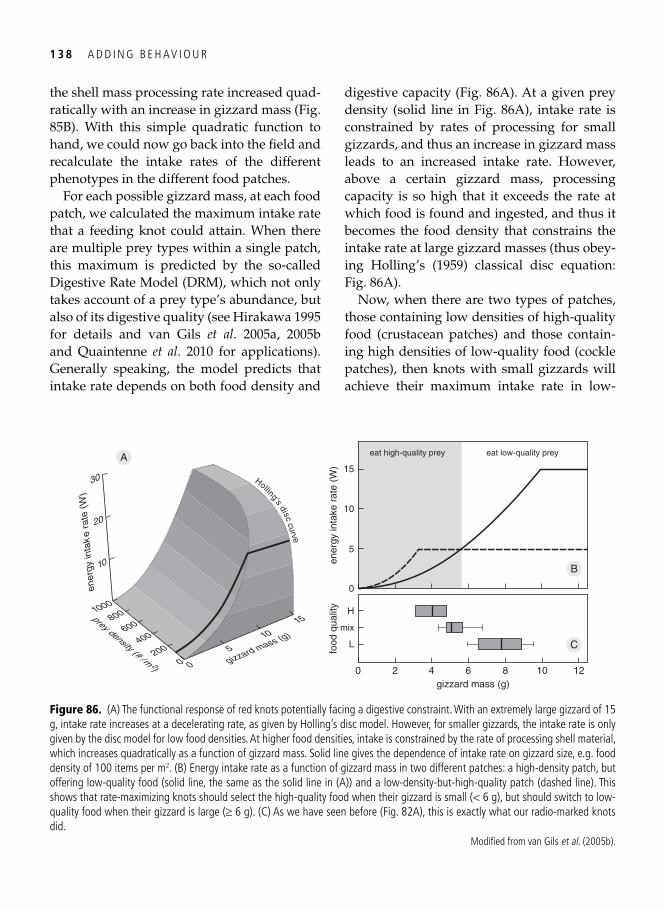
1 3 8 A D D I N G B E H AV I O U R
the shell mass processing rate increased quad-ratically with an increase in gizzard mass ( Fig. 85B ). With this simple quadratic function to hand, we could now go back into the fi eld and recalculate the intake rates of the different phenotypes in the different food patches.
For each possible gizzard mass, at each food patch, we calculated the maximum intake rate that a feeding knot could attain. When there are multiple prey types within a single patch, this maximum is predicted by the so-called Digestive Rate Model (DRM), which not only takes account of a prey type’s abundance, but also of its digestive quality (see Hirakawa 1995 for details and van Gils et al . 2005a , 2005b and Quaintenne et al . 2010 for applications). Generally speaking, the model predicts that intake rate depends on both food density and
digestive capacity ( Fig. 86A ). At a given prey density (solid line in Fig. 86A ), intake rate is constrained by rates of processing for small gizzards, and thus an increase in gizzard mass leads to an increased intake rate. However, above a certain gizzard mass, processing capacity is so high that it exceeds the rate at which food is found and ingested, and thus it becomes the food density that constrains the intake rate at large gizzard masses (thus obey-ing Holling’s (1959) classical disc equation: Fig. 86A ).
Now, when there are two types of patches, those containing low densities of high-quality food (crustacean patches) and those contain-ing high densities of low-quality food (cockle patches), then knots with small gizzards will achieve their maximum intake rate in low-
0
ener
gy in
take
rat
e (W
)
5
15A
B
C
10
eat high-quality prey eat low-quality prey
30
20
ener
gy in
tak
e ra
te (
W)
200400
6008001000
0
prey density (# /m 2)
10
0
5
15
gizzard mass (g)
Holling'sdisc curve
L
mix
H
food
qua
lity
0gizzard mass (g)
10 122 4 6 8
10
Figure 86. (A) The functional response of red knots potentially facing a digestive constraint. With an extremely large gizzard of 15 g, intake rate increases at a decelerating rate, as given by Holling’s disc model. However, for smaller gizzards, the intake rate is only given by the disc model for low food densities. At higher food densities, intake is constrained by the rate of processing shell material, which increases quadratically as a function of gizzard mass. Solid line gives the dependence of intake rate on gizzard size, e.g. food density of 100 items per m 2 . (B) Energy intake rate as a function of gizzard mass in two different patches: a high-density patch, but offering low-quality food (solid line, the same as the solid line in (A)) and a low-density-but-high-quality patch (dashed line). This shows that rate-maximizing knots should select the high-quality food when their gizzard is small (< 6 g), but should switch to low-quality food when their gizzard is large (³ 6 g). (C) As we have seen before ( Fig. 82A ), this is exactly what our radio-marked knots did.
Modifi ed from van Gils et al . ( 2005b ).
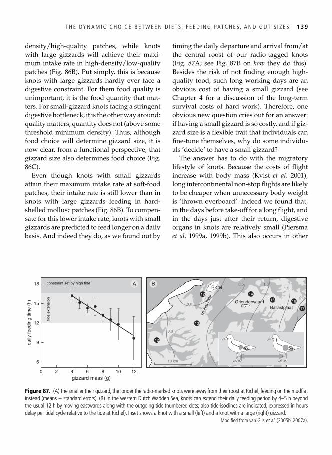
T H E DY N A M I C C H O I C E B E T W E E N D I E T S , F E E D I N G PAT C H E S , A N D G U T S I Z E S 1 3 9
density/high-quality patches, while knots with large gizzards will achieve their maxi-mum intake rate in high-density/low-quality patches ( Fig. 86B ). Put simply, this is because knots with large gizzards hardly ever face a digestive constraint. For them food quality is unimportant, it is the food quantity that mat-ters. For small-gizzard knots facing a stringent digestive bottleneck, it is the other way around: quality matters, quantity does not (above some threshold minimum density). Thus, although food choice will determine gizzard size, it is now clear, from a functional perspective, that gizzard size also determines food choice ( Fig. 86C ).
Even though knots with small gizzards attain their maximum intake rate at soft-food patches, their intake rate is still lower than in knots with large gizzards feeding in hard-shelled mollusc patches ( Fig. 86B ). To compen-sate for this lower intake rate, knots with small gizzards are predicted to feed longer on a daily basis. And indeed they do, as we found out by
timing the daily departure and arrival from/at the central roost of our radio-tagged knots ( Fig. 87A ; see Fig. 87B on how they do this). Besides the risk of not fi nding enough high-quality food, such long working days are an obvious cost of having a small gizzard (see Chapter 4 for a discussion of the long-term survival costs of hard work). Therefore, one obvious new question cries out for an answer: if having a small gizzard is so costly, and if giz-zard size is a fl exible trait that individuals can fi ne-tune themselves, why do some individu-als ‘decide’ to have a small gizzard?
The answer has to do with the migratory lifestyle of knots. Because the costs of fl ight increase with body mass ( Kvist et al . 2001 ), long intercontinental non-stop fl ights are likely to be cheaper when unnecessary body weight is ‘thrown overboard’. Indeed we found that, in the days before take-off for a long fl ight, and in the days just after their return, digestive organs in knots are relatively small ( Piersma et al . 1999a , 1999b ). This also occurs in other
17
1615
1412
13
12
2.0
1.51.00.5
0.0
0.0
GrienderwaardBallastplaat
Ric
hel-f
lats
Richel
10 km
0gizzard mass (g)
10 122
daily
feed
ing
time
(h)
15
18 A Bconstraint set by high tide
4 6 8
tide
exte
nsio
n
12
9
6
Figure 87. (A) The smaller their gizzard, the longer the radio-marked knots were away from their roost at Richel, feeding on the mudfl at instead (means ± standard errors). (B) In the western Dutch Wadden Sea, knots can extend their daily feeding period by 4–5 h beyond the usual 12 h by moving eastwards along with the outgoing tide (numbered dots; also tide-isoclines are indicated, expressed in hours delay per tidal cycle relative to the tide at Richel). Inset shows a knot with a small (left) and a knot with a large (right) gizzard.
Modifi ed from van Gils et al . ( 2005b , 2007a ).
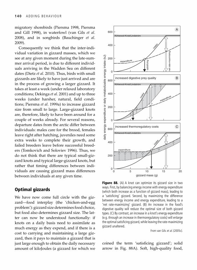
1 4 0 A D D I N G B E H AV I O U R
migratory shorebirds ( Piersma 1998 , Piersma and Gill 1998 ), in waterfowl ( van Gils et al . 2008 ), and in songbirds ( Bauchinger et al . 2009 ).
Consequently we think that the inter-indi-vidual variation in gizzard masses, which we see at any given moment during the late-sum-mer arrival period, is due to different individ-uals arriving in the Wadden Sea on different dates ( Dietz et al . 2010 ). Thus, birds with small gizzards are likely to have just arrived and are in the process of growing a larger gizzard. It takes at least a week (under relaxed laboratory conditions; Dekinga et al . 2001 ) and up to three weeks (under harsher, natural, fi eld condi-tions; Piersma et al . 1999a ) to increase gizzard size from small to large. Large-gizzard knots are, therefore, likely to have been around for a couple of weeks already. For several reasons, departure dates from the arctic differ between individuals: males care for the brood, females leave right after hatching, juveniles need some extra weeks to complete their growth, and failed breeders leave before successful breed-ers ( Tomkovich and Soloviev 1996 ). Thus, we do not think that there are typical small-giz-zard knots and typical large-gizzard knots, but rather that timing differences between indi-viduals are causing gizzard mass differences between individuals at any given time.
Optimal gizzards
We have now come full circle with the giz-zard—food interplay (the ‘chicken-and-egg problem’): gizzard size determines food choice, but food also determines gizzard size. The lat-ter can now be understood functionally: if knots on a daily basis need to assimilate as much energy as they expend, and if there is a cost to carrying and maintaining a large giz-zard, then it pays to maintain a gizzard that is just large enough to obtain the daily necessary amount of kiloJoules (a gizzard for which we
coined the term ‘satisfi cing gizzard’; solid arrow in Fig. 88A ). Soft, high-quality food,
increased thermoregulatory costs
daily
ene
rgy
expe
nditu
re o
r da
ily m
etab
oliz
able
ene
rgy
inta
ke (
kJ)
gizzard mass (g)
0
200
600Kirkwood-Kvist/Lindström
0 5 10 15 20
400
expenditure
inta
ke
increased digestive prey quality
0
200
600Kirkwood-Kvist/Lindström
400
inta
ke
0
200
600A
B
C
Kirkwood-Kvist/Lindström
400
inta
ke
expenditure
expenditure
netr
ate-
max
imis
ing
satis
ficin
g
Figure 88. (A) A knot can optimize its gizzard size in two ways. First, by balancing energy income with energy expenditure (which both increase as a function of gizzard mass), leading to a ‘satisfi cing’ gizzard. Second, by maximizing the difference between energy income and energy expenditure, leading to a ‘net rate-maximizing’ gizzard. (B) An increase in the food’s digestive quality will reduce the optimal size of both gizzard types. (C) By contrast, an increase in a knot’s energy expenditure (e.g. through an increase in thermoregulatory costs) will enlarge the optimal satisfi cing gizzard, while leaving the rate-maximizing gizzard unaltered.
From van Gils et al . ( 2005c ).
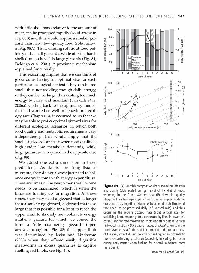
T H E DY N A M I C C H O I C E B E T W E E N D I E T S , F E E D I N G PAT C H E S , A N D G U T S I Z E S 1 4 1
with little shell mass relative to the amount of meat, can be processed rapidly (solid arrow in Fig. 88B ) and thus would require a smaller giz-zard than hard, low-quality food (solid arrow in Fig. 88A ). Thus, offering soft trout-food pel-lets yields small gizzards, while offering hard-shelled mussels yields large gizzards ( Fig. 84 ; Dekinga et al . 2001 ). A proximate mechanism explained functionally.
This reasoning implies that we can think of gizzards as having an optimal size for each particular ecological context. They can be too small, thus not yielding enough daily energy, or they can be too large, thus costing too much energy to carry and maintain ( van Gils et al . 2006a ). Getting back to the optimality models that had worked so well in behavioural ecol-ogy (see Chapter 6 ), it occurred to us that we may be able to predict optimal gizzard sizes for different ecological scenarios, in which both food quality and metabolic requirements vary independently. This would imply that the smallest gizzards are best when food quality is high under low metabolic demands, while large gizzards are required in the opposite case ( Fig. 88 ).
We added one extra dimension to these predictions. As knots are long-distance migrants, they do not always just need to bal-ance energy income with energy expenditure. There are times of the year, when (net) income needs to be maximized, which is when the birds are fuelling up for migration. At these times, they may need a gizzard that is larger than a satisfi cing gizzard, a gizzard that is so large that it is possible for a knot to reach the upper limit to its daily metabolizable energy intake, a gizzard for which we coined the term a ‘rate-maximizing gizzard’ (open arrows throughout Fig. 88 ; this upper limit was determined by Kvist and Lindström ( 2003 ) when they offered easily digestible mealworms in excess quantities to captive fuelling red knots; see Fig. 43).
prey
qua
lity
(kJ/
g sh
ell)
gizz
ard
mas
s (g
)
time of year
0
5
10
J M S D
daily
she
ll m
ass
inta
ke (g
)
daily energy requirement (kJ)
7
100
200
300
600300 400 500
6
7
8
9
10
requ
ired
gizz
ard
mas
s (g
)
F M A J J A O N
15
satisficer
net rate-maximizer
11
12
6
5
4
3
2 kJ/g shell
M
A
MF
JD
N
OS
A
J
1
Kir
kwoo
d-K
vist
diet
com
posi
tion
(%)
time of year
0
20
100A
B
C
J M S DF M A J J A O N
40
0
1
2
3
4
60
80
8 9
CrustaceaMyaHydrobiaCerastodermaMacoma
Figure 89. (A) Monthly composition (bars scaled on left axis) and quality (dots scaled on right axis) of the diet of knots wintering in the Dutch Wadden Sea. (B) How diet quality (diagonal lines, having a slope of 1) and daily energy expenditure (horizontal axis) together determine the amount of shell material that needs to be processed daily (left vertical axis), and thus determine the require gizzard mass (right vertical axis) for satisfi cing knots (monthly dots connected by lines in lower left corner) and for rate-maximizing knots (monthly dots in vertical Kirkwood-Kvist bar). (C) Gizzard masses of islandica knots in the Dutch Wadden Sea fi t the satisfi cer prediction throughout most of the year, except during periods of fuelling, when gizzards fi t the rate-maximizing prediction (especially in spring, but even during early winter when fuelling for a small midwinter body mass peak).
From van Gils et al . ( 2003a ).
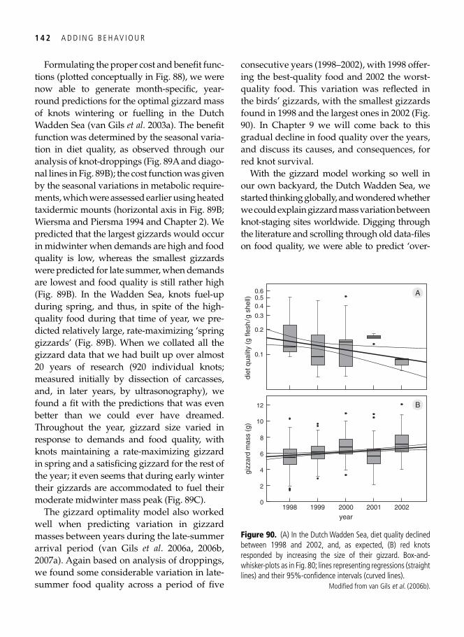
1 4 2 A D D I N G B E H AV I O U R
Formulating the proper cost and benefi t func-tions (plotted conceptually in Fig. 88 ), we were now able to generate month-specifi c, year-round predictions for the optimal gizzard mass of knots wintering or fuelling in the Dutch Wadden Sea ( van Gils et al . 2003a ). The benefi t function was determined by the seasonal varia-tion in diet quality, as observed through our analysis of knot-droppings ( Fig. 89A and diago-nal lines in Fig. 89B ); the cost function was given by the seasonal variations in metabolic require-ments, which were assessed earlier using heated taxidermic mounts (horizontal axis in Fig. 89B ; Wiersma and Piersma 1994 and Chapter 2 ). We predicted that the largest gizzards would occur in midwinter when demands are high and food quality is low, whereas the smallest gizzards were predicted for late summer, when demands are lowest and food quality is still rather high ( Fig. 89B ). In the Wadden Sea, knots fuel-up during spring, and thus, in spite of the high-quality food during that time of year, we pre-dicted relatively large, rate-maximizing ‘spring gizzards’ ( Fig. 89B ). When we collated all the gizzard data that we had built up over almost 20 years of research (920 individual knots; measured initially by dissection of carcasses, and, in later years, by ultrasonography), we found a fi t with the predictions that was even better than we could ever have dreamed. Throughout the year, gizzard size varied in response to demands and food quality, with knots maintaining a rate-maximizing gizzard in spring and a satisfi cing gizzard for the rest of the year; it even seems that during early winter their gizzards are accommodated to fuel their moderate midwinter mass peak ( Fig. 89C ).
The gizzard optimality model also worked well when predicting variation in gizzard masses between years during the late-summer arrival period ( van Gils et al . 2006a , 2006b , 2007a ). Again based on analysis of droppings, we found some considerable variation in late-summer food quality across a period of fi ve
consecutive years (1998–2002), with 1998 offer-ing the best-quality food and 2002 the worst-quality food. This variation was refl ected in the birds’ gizzards, with the smallest gizzards found in 1998 and the largest ones in 2002 ( Fig. 90 ). In Chapter 9 we will come back to this gradual decline in food quality over the years, and discuss its causes, and consequences, for red knot survival.
With the gizzard model working so well in our own backyard, the Dutch Wadden Sea, we started thinking globally, and wondered whether we could explain gizzard mass variation between knot-staging sites worldwide. Digging through the literature and scrolling through old data-fi les on food quality, we were able to predict ‘over-
diet
qua
lity
(g fl
esh
/g s
hell)
0
6
8
gizz
ard
mas
s (g
)
1998
year
12
1999 2000 2001 2002
0.1
0.3
10
4
2
0.2
0.40.50.6 A
B
Figure 90. (A) In the Dutch Wadden Sea, diet quality declined between 1998 and 2002, and, as expected, (B) red knots responded by increasing the size of their gizzard. Box-and-whisker-plots as in Fig. 80 ; lines representing regressions (straight lines) and their 95%-confi dence intervals (curved lines).
Modifi ed from van Gils et al . ( 2006b ).
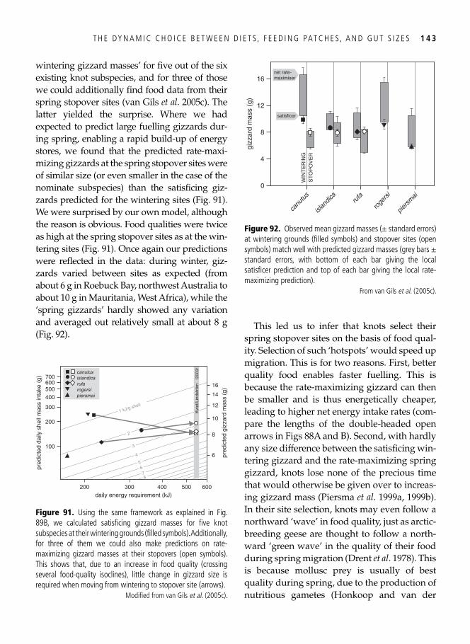
T H E DY N A M I C C H O I C E B E T W E E N D I E T S , F E E D I N G PAT C H E S , A N D G U T S I Z E S 1 4 3
wintering gizzard masses’ for fi ve out of the six existing knot subspecies, and for three of those we could additionally fi nd food data from their spring stopover sites ( van Gils et al . 2005c ). The latter yielded the surprise. Where we had expected to predict large fuelling gizzards dur-ing spring, enabling a rapid build-up of energy stores, we found that the predicted rate-maxi-mizing gizzards at the spring stopover sites were of similar size (or even smaller in the case of the nominate subspecies) than the satisfi cing giz-zards predicted for the wintering sites ( Fig. 91 ). We were surprised by our own model, although the reason is obvious. Food qualities were twice as high at the spring stopover sites as at the win-tering sites ( Fig. 91 ). Once again our predictions were refl ected in the data: during winter, giz-zards varied between sites as expected (from about 6 g in Roebuck Bay, northwest Australia to about 10 g in Mauritania, West Africa), while the ‘spring gizzards’ hardly showed any variation and averaged out relatively small at about 8 g ( Fig. 92 ).
This led us to infer that knots select their spring stopover sites on the basis of food qual-ity. Selection of such ‘hotspots’ would speed up migration. This is for two reasons. First, better quality food enables faster fuelling. This is because the rate-maximizing gizzard can then be smaller and is thus energetically cheaper, leading to higher net energy intake rates (com-pare the lengths of the double-headed open arrows in Figs 88A and B). Second, with hardly any size difference between the satisfi cing win-tering gizzard and the rate-maximizing spring gizzard, knots lose none of the precious time that would otherwise be given over to increas-ing gizzard mass ( Piersma et al . 1999a , 1999b ). In their site selection, knots may even follow a northward ‘wave’ in food quality, just as arctic-breeding geese are thought to follow a north-ward ‘green wave’ in the quality of their food during spring migration ( Drent et al . 1978 ). This is because mollusc prey is usually of best quality during spring, due to the production of nutritious gametes ( Honkoop and van der
pred
icte
d da
ily s
hell
mas
s in
take
(g)
daily energy requirement (kJ)
100
200
600300 400 500
6
8
10
pred
icte
d gi
zzar
d m
ass
(g)
14
12300
400500600700
16
200
3
2
76
8
5
4
1 kJ/g shell
Kvi
st/L
inds
tröm
( 200
3)canutusislandicarufarogersipiersmai
Figure 91. Using the same framework as explained in Fig. 89B , we calculated satisfi cing gizzard masses for fi ve knot subspecies at their wintering grounds (fi lled symbols). Additionally, for three of them we could also make predictions on rate-maximizing gizzard masses at their stopovers (open symbols). This shows that, due to an increase in food quality (crossing several food-quality isoclines), little change in gizzard size is required when moving from wintering to stopover site (arrows).
Modifi ed from van Gils et al . ( 2005c ).
gizz
ard
mas
s (g
)
0
4
12
8
16
canu
tus
islan
dica
rufa
roge
rsi
piers
mai
WIN
TE
RIN
GS
TO
PO
VE
R
net rate-maximiser
satisficer
Figure 92. Observed mean gizzard masses (± standard errors) at wintering grounds (fi lled symbols) and stopover sites (open symbols) match well with predicted gizzard masses (grey bars ± standard errors, with bottom of each bar giving the local satisfi cer prediction and top of each bar giving the local rate-maximizing prediction).
From van Gils et al . ( 2005c ).
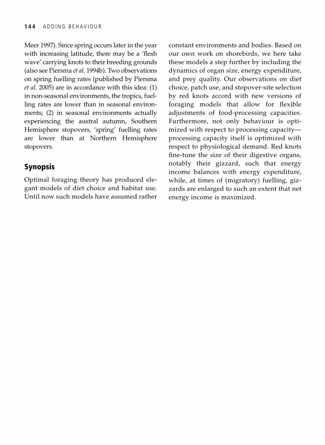
1 4 4 A D D I N G B E H AV I O U R
Meer 1997 ). Since spring occurs later in the year with increasing latitude, there may be a ‘fl esh wave’ carrying knots to their breeding grounds (also see Piersma et al . 1994b ). Two observations on spring fuelling rates (published by Piersma et al . 2005 ) are in accordance with this idea: (1) in non-seasonal environments, the tropics, fuel-ling rates are lower than in seasonal environ-ments; (2) in seasonal environments actually experiencing the austral autumn, Southern Hemisphere stopovers, ‘spring’ fuelling rates are lower than at Northern Hemisphere stopovers.
Synopsis
Optimal foraging theory has produced ele-gant models of diet choice and habitat use. Until now such models have assumed rather
constant environments and bodies. Based on our own work on shorebirds, we here take these models a step further by including the dynamics of organ size, energy expenditure, and prey quality. Our observations on diet choice, patch use, and stopover-site selection by red knots accord with new versions of foraging models that allow for fl exible adjustments of food-processing capacities. Furthermore, not only behaviour is opti-mized with respect to processing capacity—processing capacity itself is optimized with respect to physiological demand. Red knots fi ne-tune the size of their digestive organs, notably their gizzard, such that energy income balances with energy expenditure, while, at times of (migratory) fuelling, giz-zards are enlarged to such an extent that net energy income is maximized.

Towards a fully integrated view
Part IV

This page intentionally left blank
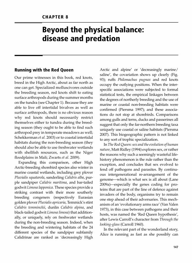
147
CHAPTER 8
Beyond the physical balance: disease and predation
Running with the Red Queen
Our prime witnesses in this book, red knots, breed in the High Arctic, about as far north as one can get. Specialized molluscivores outside the breeding season, red knots shift to eating surface arthropods during the summer months on the tundra (see Chapter 1 ). Because they are able to live off intertidal bivalves as well as surface arthropods, there is no obvious reason why red knots should necessarily restrict themselves either to tundra during the breed-ing season (they ought to be able to fi nd such arthropod prey in temperate meadows as well; Schekkerman et al . 2003 ) or to coastal intertidal habitats during the non-breeding season (they should also be able to use freshwater wetlands with shellfi sh resources, such as the Niger fl oodplains in Mali; Zwarts et al . 2009 ).
Expanding this comparison, other High Arctic-breeding shorebird species also winter in marine coastal wetlands, including grey plover Pluvialis squatarola , sanderling Calidris alba , pur-ple sandpiper Calidris maritima , and bar-tailed godwit Limosa lapponica . These species provide a striking contrast with their more southerly breeding congeners (respectively Eurasian golden plover Pluvialis apricaria , Temmick’s stint Calidris temminckii , dunlin Calidris alpina , and black-tailed godwit Limosa limosa ) that addition-ally, or uniquely, rely on freshwater wetlands during the non-breeding season. Indeed, when the breeding and wintering habitats of the 24 different species of the sandpiper subfamily Calidrinae are ranked as ‘decreasingly High
Arctic and alpine’ or ‘decreasingly marine/saline’, the covariation shows up clearly ( Fig. 93 ); ruffs Philomachus pugnax and red knots occupy the outlying positions. When the inter-specifi c associations were subjected to formal statistical tests, the empirical linkages between the degrees of northerly breeding and the use of marine or coastal non-breeding habitats were confi rmed ( Piersma 1997 ); and these associa-tions do not stop at shorebirds. Comparisons among gulls and terns, ducks and passerines all suggest that only the far-northern breeding taxa uniquely use coastal or saline habitats ( Piersma 2007 ). This biogeographic pattern is not linked to any sort of trophic specialization.
In The Red Queen: sex and the evolution of human nature , Matt Ridley ( 1994 ) explores sex, or rather the reasons why such a seemingly wasteful life-history phenomenon is the rule rather than the exception, and concludes that sex evolved to fend off pathogens and parasites. By continu-ous intergenerational re-arrangement of the genome—which is what sex is all about ( Lane 2009a )—especially the genes coding for pro-teins that are part of the line of defence against invaders of the body, organisms try to remain one step ahead of their adversaries. This mech-anism of an ‘evolutionary arms race’ ( Van Valen 1973 ), in this case between pathogens and their hosts, was named the ‘Red Queen hypothesis’, after Lewis Carroll’s character from Through the looking-glass ( Carroll 1960 ).
In the relevant part of the wonderland story, Alice is running as fast as she possibly can
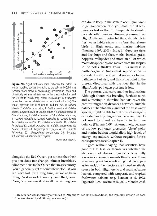
1 4 8 TO W A R D S A F U L LY I N T E G R AT E D V I E W
alongside the Red Queen, yet notices that their position does not change. Almost breathless, Alice mentions to the Queen that in her country ‘you’d generally get to somewhere else—if you ran very fast for a long time, as we’ve been doing’. ‘A slow sort of country!’ said the Queen. ‘Now, here, you see, it takes all the running you
can do, to keep in the same place. If you want to get somewhere else, you must run at least twice as fast as that!’ If temperate freshwater habitats offer greater disease pressure than High Arctic and marine habitats, shorebirds in freshwater habitats have to run faster than shore-birds in High Arctic and marine habitats ( Piersma 1997 , 2003 ). Indeed, ‘there are ticks and lice, bugs and fl ies, moths, beetles, grass-hoppers, millipedes and more, in all of which males disappear as one moves from the tropics to the poles’ ( Ridley 1994 ). 1 This increase in parthenogenetic (male-less) reproduction is consistent with the idea that sex exists to beat pathogens, but also, and this is the point in the present discourse, with the idea that in the High Arctic, pathogen pressure is low.
The patterns also carry another implication. Although shorebirds breeding furthest north and wintering in shoreline habitats cover the greatest migration distances between suitable patches of habitat, they, and not the freshwater species, might be able to pull off such energeti-cally demanding migrations because they do not need to invest as heavily in immune defence ( Piersma 1997 ). Alternatively, because of the low pathogen pressures, ‘clean’ polar and marine habitat would allow high levels of energy expenditure without negative fi tness consequences (see Chapter 4 ).
It goes without saying that scientists have gone out to test for themselves whether the abundance of disease organisms is actually lower in some environments than others. There is increasing evidence indicating that blood par-asites and/or their vectors are indeed relatively sparse in both High Arctic and marine/saline habitats compared with temperate and tropical freshwater habitats (e.g. Bennett et al . 1992 , Figuerola 1999 , Jovani et al . 2001 , Mendes et al .
1 This citation was incorrectly attributed to Daly and Wilson ( 1983 ). In addition, and ironically, it was cited back to front (confi rmed by M. Ridley pers. comm.).
10
20
25
5rank
ord
er w
inte
ring
habi
tat
10 15rank order breeding habitat
0
15
20 2550
13
24
1612
24
118
173
8
7
65
1410
15
21
19
20
119
2223
DECREASINGLY ARCTIC
DE
CR
EA
SIN
GLY
MA
RIN
E
Figure 93. Signifi cant correlation between the extent to which shorebird species belonging to the subfamily Calidrinae (Scolopacidae) breed in decreasingly arctic/alpine, open and climatically extreme habitats (rank order breeding habitat) and the extent to which they winter increasingly in freshwater rather than marine habitats (rank order wintering habitat). The linear regression line is shown to lead the eye. 1: Aphriza virgata ; 2: Calidris tenuirostris ; 3: Calidris canutus ; 4: Calidris alba ; 5: Calidris pusilla ; 6: Calidris mauri ; 7: Calidris rufi collis ; 8: Calidris minuta ; 9: Calidris temminckii ; 10: Calidris subminuta ; 11: Calidris minutilla ; 12: Calidris fuscicollis ; 13: Calidris bairdii ; 14: Calidris melanotos ; 15: Calidris acuminata ; 16: Calidris ferruginea ; 17: Calidris maritima ; 18: Calidris ptilocnemis ; 19: Calidris alpina ; 20: Eurynorhynchus pygmeus ; 21: Limicola falcinellus ; 22: Micropalama himantopus ; 23: Tryngites subrufi collis ; 24: Philomachus pugnax .
From Piersma ( 2003 ).
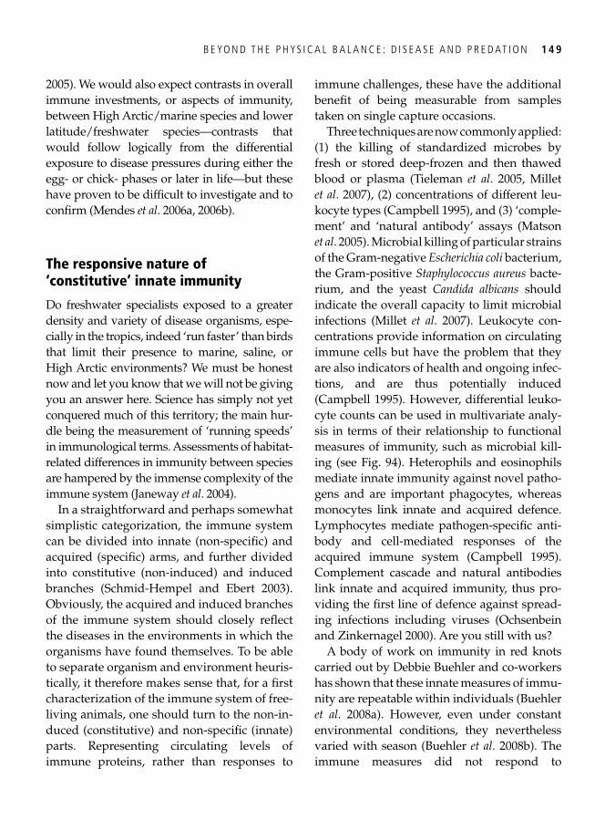
B E YO N D T H E P H YS I C A L B A L A N C E : D I S E A S E A N D P R E D AT I O N 1 4 9
2005 ). We would also expect contrasts in overall immune investments, or aspects of immunity, between High Arctic/marine species and lower latitude/freshwater species—contrasts that would follow logically from the differential exposure to disease pressures during either the egg- or chick- phases or later in life—but these have proven to be diffi cult to investigate and to confi rm ( Mendes et al . 2006a , 2006b ).
The responsive nature of ‘constitutive’ innate immunity
Do freshwater specialists exposed to a greater density and variety of disease organisms, espe-cially in the tropics, indeed ‘run faster’ than birds that limit their presence to marine, saline, or High Arctic environments? We must be honest now and let you know that we will not be giving you an answer here. Science has simply not yet conquered much of this territory; the main hur-dle being the measurement of ‘running speeds’ in immunological terms. Assessments of habitat-related differences in immunity between species are hampered by the immense complexity of the immune system ( Janeway et al . 2004 ).
In a straightforward and perhaps somewhat simplistic categorization, the immune system can be divided into innate (non-specifi c) and acquired (specifi c) arms, and further divided into constitutive (non-induced) and induced branches ( Schmid-Hempel and Ebert 2003 ). Obviously, the acquired and induced branches of the immune system should closely refl ect the diseases in the environments in which the organisms have found themselves. To be able to separate organism and environment heuris-tically, it therefore makes sense that, for a fi rst characterization of the immune system of free-living animals, one should turn to the non-in-duced (constitutive) and non-specifi c (innate) parts. Representing circulating levels of immune proteins, rather than responses to
immune challenges, these have the additional benefi t of being measurable from samples taken on single capture occasions.
Three techniques are now commonly applied: (1) the killing of standardized microbes by fresh or stored deep-frozen and then thawed blood or plasma ( Tieleman et al . 2005 , Millet et al . 2007 ), (2) concentrations of different leu-kocyte types ( Campbell 1995 ), and (3) ‘comple-ment’ and ‘natural antibody’ assays ( Matson et al . 2005 ). Microbial killing of particular strains of the Gram-negative Escherichia coli bacterium, the Gram-positive Staphylococcus aureus bacte-rium, and the yeast Candida albicans should indicate the overall capacity to limit microbial infections ( Millet et al . 2007 ). Leukocyte con-centrations provide information on circulating immune cells but have the problem that they are also indicators of health and ongoing infec-tions, and are thus potentially induced ( Campbell 1995 ). However, differential leuko-cyte counts can be used in multivariate analy-sis in terms of their relationship to functional measures of immunity, such as microbial kill-ing (see Fig. 94 ). Heterophils and eosinophils mediate innate immunity against novel patho-gens and are important phagocytes, whereas monocytes link innate and acquired defence. Lymphocytes mediate pathogen-specifi c anti-body and cell-mediated responses of the acquired immune system ( Campbell 1995 ). Complement cascade and natural antibodies link innate and acquired immunity, thus pro-viding the fi rst line of defence against spread-ing infections including viruses ( Ochsenbein and Zinkernagel 2000 ). Are you still with us?
A body of work on immunity in red knots carried out by Debbie Buehler and co-workers has shown that these innate measures of immu-nity are repeatable within individuals ( Buehler et al . 2008a ). However, even under constant environmental conditions, they nevertheless varied with season ( Buehler et al . 2008b ). The immune measures did not respond to
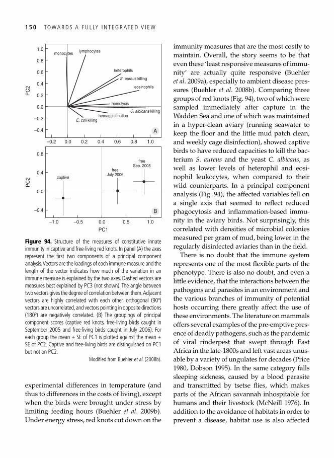
1 5 0 TO W A R D S A F U L LY I N T E G R AT E D V I E W
experimental differences in temperature (and thus to differences in the costs of living), except when the birds were brought under stress by limiting feeding hours ( Buehler et al . 2009b ). Under energy stress, red knots cut down on the
immunity measures that are the most costly to maintain. Overall, the story seems to be that even these ‘least responsive measures of immu-nity’ are actually quite responsive ( Buehler et al . 2009a ), especially to ambient disease pres-sures ( Buehler et al . 2008b ). Comparing three groups of red knots ( Fig. 94 ), two of which were sampled immediately after capture in the Wadden Sea and one of which was maintained in a hyper-clean aviary (running seawater to keep the fl oor and the little mud patch clean, and weekly cage disinfection), showed captive birds to have reduced capacities to kill the bac-terium S. aureus and the yeast C. albicans , as well as lower levels of heterophil and eosi-nophil leukocytes, when compared to their wild counterparts. In a principal component analysis ( Fig. 94 ), the affected variables fell on a single axis that seemed to refl ect reduced phagocytosis and infl ammation-based immu-nity in the aviary birds. Not surprisingly, this correlated with densities of microbial colonies measured per gram of mud, being lower in the regularly disinfected aviaries than in the fi eld.
There is no doubt that the immune system represents one of the most fl exible parts of the phenotype. There is also no doubt, and even a little evidence, that the interactions between the pathogens and parasites in an environment and the various branches of immunity of potential hosts occurring there greatly affect the use of these environments. The literature on mammals offers several examples of the pre-emptive pres-ence of deadly pathogens, such as the pandemic of viral rinderpest that swept through East Africa in the late-1800s and left vast areas unus-able by a variety of ungulates for decades ( Price 1980 , Dobson 1995 ). In the same category falls sleeping sickness, caused by a blood parasite and transmitted by tsetse fl ies, which makes parts of the African savannah inhospitable for humans and their livestock ( McNeill 1976 ). In addition to the avoidance of habitats in order to prevent a disease, habitat use is also affected
–0.4
0.0
0.4
0.8
PC
2
–1.0 –0.5 0.0 0.5 1.0
PC1
freeSep. 2005
freeJuly 2006
captive
–0.4
0.0
0.4
0.8
lymphocytes1.0
–0.2 0.20.0 0.4 1.00.6 0.8
A
B
0.2
0.6
–0.2
monocytes
heterophils
S. aureus killing
eosinophils
hemolysis
C. albicans killinghemagglutination
E. coli killing
PC
2
Figure 94. Structure of the measures of constitutive innate immunity in captive and free-living red knots. In panel (A) the axes represent the fi rst two components of a principal component analysis. Vectors are the loadings of each immune measure and the length of the vector indicates how much of the variation in an immune measure is explained by the two axes. Dashed vectors are measures best explained by PC3 (not shown). The angle between two vectors gives the degree of correlation between them. Adjacent vectors are highly correlated with each other, orthogonal (90º) vectors are uncorrelated, and vectors pointing in opposite directions (180º) are negatively correlated. (B) The groupings of principal component scores (captive red knots, free-living birds caught in September 2005 and free-living birds caught in July 2006). For each group the mean ± SE of PC1 is plotted against the mean ± SE of PC2. Captive and free-living birds are distinguished on PC1 but not on PC2.
Modifi ed from Buehler et al . ( 2008b ).
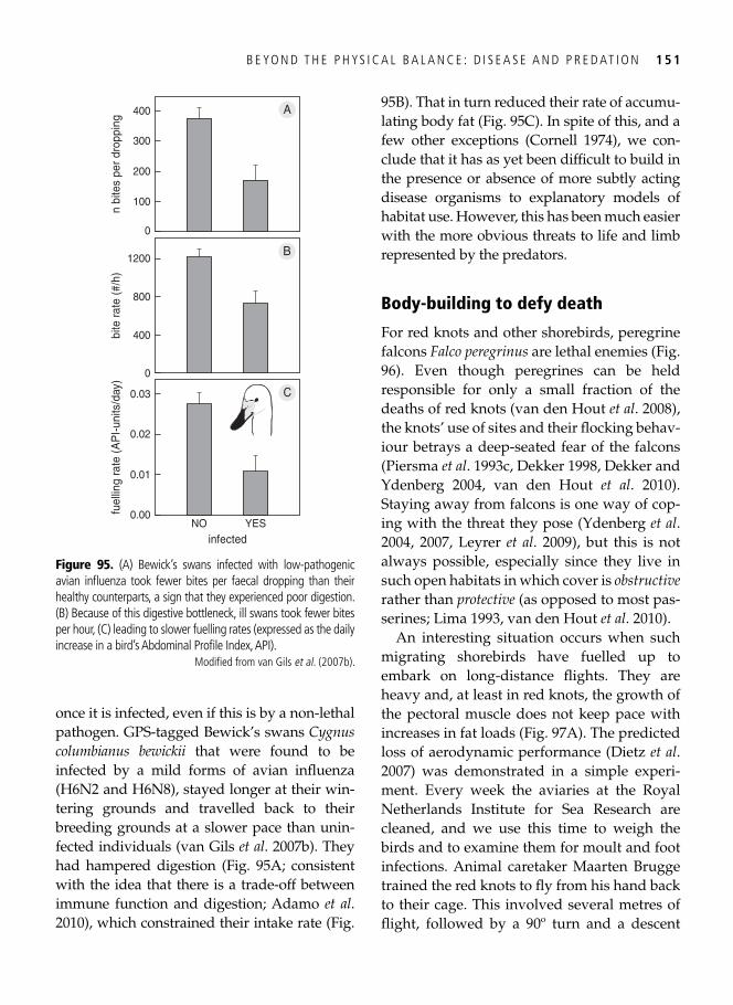
B E YO N D T H E P H YS I C A L B A L A N C E : D I S E A S E A N D P R E D AT I O N 1 5 1
once it is infected, even if this is by a non-lethal pathogen. GPS-tagged Bewick’s swans Cygnus columbianus bewickii that were found to be infected by a mild forms of avian infl uenza (H6N2 and H6N8), stayed longer at their win-tering grounds and travelled back to their breeding grounds at a slower pace than unin-fected individuals ( van Gils et al . 2007b ). They had hampered digestion ( Fig. 95A ; consistent with the idea that there is a trade-off between immune function and digestion; Adamo et al . 2010 ), which constrained their intake rate ( Fig.
95B ). That in turn reduced their rate of accumu-lating body fat ( Fig. 95C ). In spite of this, and a few other exceptions ( Cornell 1974 ), we con-clude that it has as yet been diffi cult to build in the presence or absence of more subtly acting disease organisms to explanatory models of habitat use. However, this has been much easier with the more obvious threats to life and limb represented by the predators.
Body-building to defy death
For red knots and other shorebirds, peregrine falcons Falco peregrinus are lethal enemies ( Fig. 96 ). Even though peregrines can be held responsible for only a small fraction of the deaths of red knots ( van den Hout et al . 2008 ), the knots’ use of sites and their fl ocking behav-iour betrays a deep-seated fear of the falcons ( Piersma et al . 1993c , Dekker 1998 , Dekker and Ydenberg 2004 , van den Hout et al . 2010 ). Staying away from falcons is one way of cop-ing with the threat they pose ( Ydenberg et al . 2004 , 2007 , Leyrer et al . 2009 ), but this is not always possible, especially since they live in such open habitats in which cover is obstructive rather than protective (as opposed to most pas-serines; Lima 1993 , van den Hout et al . 2010 ).
An interesting situation occurs when such migrating shorebirds have fuelled up to embark on long-distance fl ights. They are heavy and, at least in red knots, the growth of the pectoral muscle does not keep pace with increases in fat loads ( Fig. 97A ). The predicted loss of aerodynamic performance ( Dietz et al . 2007 ) was demonstrated in a simple experi-ment. Every week the aviaries at the Royal Netherlands Institute for Sea Research are cleaned, and we use this time to weigh the birds and to examine them for moult and foot infections. Animal caretaker Maarten Brugge trained the red knots to fl y from his hand back to their cage. This involved several metres of fl ight, followed by a 90º turn and a descent
0.00
0.01
0.02
0.03
fuel
ling
rate
(A
PI-
units
/day
)
NO YES
infected
0
400
800
1200
bite
rate
(#/
h)
0
100
200
400 A
B
C
300
n bi
tes
per
drop
ping
Figure 95. (A) Bewick’s swans infected with low-pathogenic avian infl uenza took fewer bites per faecal dropping than their healthy counterparts, a sign that they experienced poor digestion. (B) Because of this digestive bottleneck, ill swans took fewer bites per hour, (C) leading to slower fuelling rates (expressed as the daily increase in a bird’s Abdominal Profi le Index, API).
Modifi ed from van Gils et al . ( 2007b ).
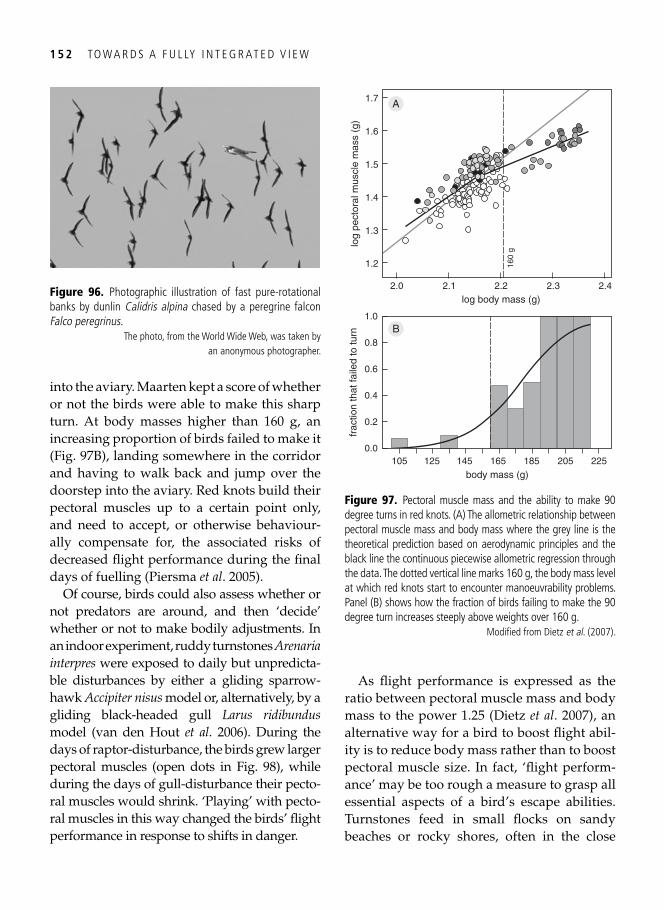
1 5 2 TO W A R D S A F U L LY I N T E G R AT E D V I E W
into the aviary. Maarten kept a score of whether or not the birds were able to make this sharp turn. At body masses higher than 160 g, an increasing proportion of birds failed to make it ( Fig. 97B ), landing somewhere in the corridor and having to walk back and jump over the doorstep into the aviary. Red knots build their pectoral muscles up to a certain point only, and need to accept, or otherwise behaviour-ally compensate for, the associated risks of decreased fl ight performance during the fi nal days of fuelling ( Piersma et al . 2005 ).
Of course, birds could also assess whether or not predators are around, and then ‘decide’ whether or not to make bodily adjustments. In an indoor experiment, ruddy turnstones Arenaria interpres were exposed to daily but unpredicta-ble disturbances by either a gliding sparrow-hawk Accipiter nisus model or, alternatively, by a gliding black-headed gull Larus ridibundus model ( van den Hout et al . 2006 ). During the days of raptor-disturbance, the birds grew larger pectoral muscles (open dots in Fig. 98 ), while during the days of gull-disturbance their pecto-ral muscles would shrink. ‘Playing’ with pecto-ral muscles in this way changed the birds’ fl ight performance in response to shifts in danger.
As fl ight performance is expressed as the ratio between pectoral muscle mass and body mass to the power 1.25 ( Dietz et al . 2007 ), an alternative way for a bird to boost fl ight abil-ity is to reduce body mass rather than to boost pectoral muscle size. In fact, ‘fl ight perform-ance’ may be too rough a measure to grasp all essential aspects of a bird’s escape abilities. Turnstones feed in small fl ocks on sandy beaches or rocky shores, often in the close
Figure 96. Photographic illustration of fast pure-rotational banks by dunlin Calidris alpina chased by a peregrine falcon Falco peregrinus .
The photo, from the World Wide Web, was taken by an anonymous photographer.
0.0
0.2
0.4
0.6
0.8
1.0
log
pect
oral
mus
cle
mas
s (g
)
105 125 145 165 185 205 225
body mass (g)
1.2
1.3
1.4
1.5
1.6
1.7 A
B
160
g
2.0 2.1 2.2 2.3 2.4
log body mass (g)
frac
tion
that
faile
d to
turn
Figure 97. Pectoral muscle mass and the ability to make 90 degree turns in red knots. (A) The allometric relationship between pectoral muscle mass and body mass where the grey line is the theoretical prediction based on aerodynamic principles and the black line the continuous piecewise allometric regression through the data. The dotted vertical line marks 160 g, the body mass level at which red knots start to encounter manoeuvrability problems. Panel (B) shows how the fraction of birds failing to make the 90 degree turn increases steeply above weights over 160 g.
Modifi ed from Dietz et al . ( 2007 ).
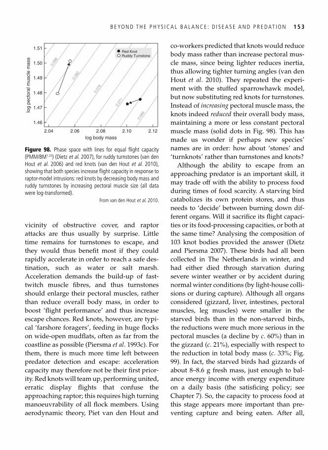
B E YO N D T H E P H YS I C A L B A L A N C E : D I S E A S E A N D P R E D AT I O N 1 5 3
vicinity of obstructive cover, and raptor attacks are thus usually by surprise. Little time remains for turnstones to escape, and they would thus benefi t most if they could rapidly accelerate in order to reach a safe des-tination, such as water or salt marsh. Acceleration demands the build-up of fast-twitch muscle fi bres, and thus turnstones should enlarge their pectoral muscles, rather than reduce overall body mass, in order to boost ‘fl ight performance’ and thus increase escape chances. Red knots, however, are typi-cal ‘farshore foragers’, feeding in huge fl ocks on wide-open mudfl ats, often as far from the coastline as possible ( Piersma et al . 1993c ). For them, there is much more time left between predator detection and escape: acceleration capacity may therefore not be their fi rst prior-ity. Red knots will team up, performing united, erratic display fl ights that confuse the approaching raptor; this requires high turning manoeuvrability of all fl ock members. Using aerodynamic theory, Piet van den Hout and
co-workers predicted that knots would reduce body mass rather than increase pectoral mus-cle mass, since being lighter reduces inertia, thus allowing tighter turning angles ( van den Hout et al . 2010 ). They repeated the experi-ment with the stuffed sparrowhawk model, but now substituting red knots for turnstones. Instead of increasing pectoral muscle mass, the knots indeed reduced their overall body mass, maintaining a more or less constant pectoral muscle mass (solid dots in Fig. 98 ). This has made us wonder if perhaps new species’ names are in order: how about ‘stones’ and ‘turnknots’ rather than turnstones and knots?
Although the ability to escape from an approaching predator is an important skill, it may trade off with the ability to process food during times of food scarcity. A starving bird catabolizes its own protein stores, and thus needs to ‘decide’ between burning down dif-ferent organs. Will it sacrifi ce its fl ight capaci-ties or its food-processing capacities, or both at the same time? Analysing the composition of 103 knot bodies provided the answer ( Dietz and Piersma 2007 ). These birds had all been collected in The Netherlands in winter, and had either died through starvation during severe winter weather or by accident during normal winter conditions (by light-house colli-sions or during capture). Although all organs considered (gizzard, liver, intestines, pectoral muscles, leg muscles) were smaller in the starved birds than in the non-starved birds, the reductions were much more serious in the pectoral muscles (a decline by c . 60%) than in the gizzard ( c . 21%), especially with respect to the reduction in total body mass ( c . 33%; Fig. 99 ). In fact, the starved birds had gizzards of about 8–8.6 g fresh mass, just enough to bal-ance energy income with energy expenditure on a daily basis (the satisfi cing policy; see Chapter 7 ). So, the capacity to process food at this stage appears more important than pre-venting capture and being eaten. After all,
1.46
1.47
1.48
1.49
1.50
1.51
log
pect
oral
mus
cle
mas
s
2.04 2.06 2.08 2.10 2.12log body mass
0.08
8
0.08
2
0.07
6
0.07
1
0.06
6
Red KnotRuddy Turnstone
Figure 98. Phase space with lines for equal fl ight capacity (PMM/BM 1.25 ) (Dietz et al . 2007 ), for ruddy turnstones (van den Hout et al . 2006 ) and red knots (van den Hout et al . 2010 ), showing that both species increase fl ight capacity in response to raptor-model intrusions: red knots by decreasing body mass and ruddy turnstones by increasing pectoral muscle size (all data were log-transformed).
From van den Hout et al . 2010 .
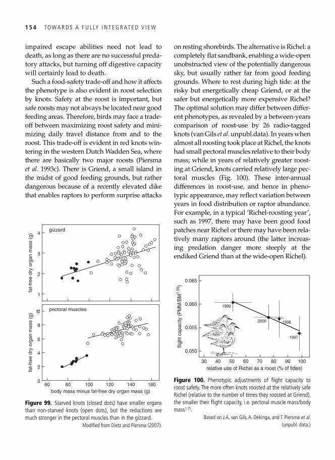
1 5 4 TO W A R D S A F U L LY I N T E G R AT E D V I E W
impaired escape abilities need not lead to death, as long as there are no successful preda-tory attacks, but turning off digestive capacity will certainly lead to death.
Such a food-safety trade-off and how it affects the phenotype is also evident in roost selection by knots. Safety at the roost is important, but safe roosts may not always be located near good feeding areas. Therefore, birds may face a trade-off between maximizing roost safety and mini-mizing daily travel distance from and to the roost. This trade-off is evident in red knots win-tering in the western Dutch Wadden Sea, where there are basically two major roosts ( Piersma et al . 1993c ). There is Griend, a small island in the midst of good feeding grounds, but rather dangerous because of a recently elevated dike that enables raptors to perform surprise attacks
on resting shorebirds. The alternative is Richel: a completely fl at sandbank, enabling a wide-open unobstructed view of the potentially dangerous sky, but usually rather far from good feeding grounds. Where to rest during high tide: at the risky but energetically cheap Griend, or at the safer but energetically more expensive Richel? The optimal solution may differ between differ-ent phenotypes, as revealed by a between-years comparison of roost-use by 26 radio-tagged knots (van Gils et al . unpubl.data). In years when almost all roosting took place at Richel, the knots had small pectoral muscles relative to their body mass; while in years of relatively greater roost-ing at Griend, knots carried relatively large pec-toral muscles ( Fig. 100 ). These inter-annual differences in roost-use, and hence in pheno-typic appearance, may refl ect variation between years in food distribution or raptor abundance. For example, in a typical ‘Richel-roosting year’, such as 1997, there may have been good food patches near Richel or there may have been rela-tively many raptors around (the latter increas-ing predation danger more steeply at the endiked Griend than at the wide-open Richel).
0
2
4
6
8
10
fat-
free
dry
org
an m
ass
(g)
100 12060 80body mass minus fat-free dry organ mass (g)
140 160
pectoral muscles
1
2
4
3
fat-
free
dry
org
an m
ass
(g)
gizzard
Figure 99. Starved knots (closed dots) have smaller organs than non-starved knots (open dots), but the reductions are much stronger in the pectoral muscles than in the gizzard.
Modifi ed from Dietz and Piersma ( 2007 ).
0.050
fligh
t cap
acity
(PM
M/B
M1.
25)
1005030 40relative use of Richel as a roost (% of tides)
60 70
0.055
0.060
0.065
80 90
1999
2000 1998
1997
Figure 100. Phenotypic adjustments of fl ight capacity to roost safety. The more often knots roosted at the relatively safe Richel (relative to the number of times they roosted at Griend), the smaller their fl ight capacity, i.e. pectoral muscle mass/body mass 1.25 .
Based on J.A. van Gils, A. Dekinga, and T. Piersma et al . (unpubl. data.)
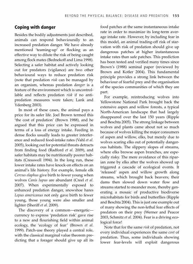
B E YO N D T H E P H YS I C A L B A L A N C E : D I S E A S E A N D P R E D AT I O N 1 5 5
Coping with danger
Besides the bodily adjustments just described, animals can respond behaviourally to an increased predation danger. We have already mentioned ‘teaming-up’ or fl ocking as an effective way to dilute the risk of being caught among fl ock mates ( Bednekoff and Lima 1998 ). Selecting a safer habitat and actively looking out for predators (vigilance) are two other behavioural ways to reduce predation risk (note that predation risk can be managed by an organism, whereas predation danger is a feature of the environment which is uncontrol-lable and refl ects predation risk if no anti- predation measures were taken; Lank and Ydenberg 2003 ).
In most of these cases, the animal pays a price for its safer life. Joel Brown termed this ‘the cost of predation’ ( Brown 1988 ), and he argued that this price can be expressed in terms of a loss of energy intake. Feeding in dense fl ocks usually leads to greater interfer-ence and reduced food-intake rates ( Vahl et al . 2005 ), looking out for potential threats detracts from fi nding food ( Radford et al . 2009 ), and safer habitats may be nutritionally poorer hab-itats ( Cresswell 1994 ). In the long run, these lower intake rates have knock-on effects on an animal’s life history. For example, female elk Cervus elaphus give birth to fewer young when wolves Canis lupus are abundant ( Creel et al . 2007 ). When experimentally exposed to enhanced predation danger, snowshoe hares Lepus americanus not only gave birth to fewer young, those young were also smaller and lighter ( Sheriff et al . 2009 ).
The discovery of a common—energetic—currency to express ‘predation risk’ gave rise to a new and fl ourishing fi eld within animal ecology, the ‘ecology of fear’ ( Brown et al . 1999 ). Patch-use theory played a central role, with the classical marginal value theorem pre-dicting that a forager should give up all its
food patches at the same instantaneous intake rate in order to maximize its long-term aver-age intake rate. However, by including fear in this model, an animal trading-off risk of star-vation with risk of predation should give up dangerous patches at higher instantaneous intake rates than safe patches. This prediction has been tested and verifi ed many times since Brown’s (1988) seminal paper (reviewed by Brown and Kotler 2004 ). This fundamental principle provides a strong link between the behaviour of fearful prey and the organisation of the species communities of which they are part.
For example, reintroducing wolves into Yellowstone National Park brought back the extensive aspen and willow forests, a typical North-American landscape that had largely disappeared over the last 150 years ( Ripple and Beschta 2005 ). The strong linkage between wolves and plants came about not so much because of wolves killing the major consumers of aspen and willow, elks, but merely due to wolves scaring elks out of potentially danger-ous habitats. The slippery slopes of streams, where elks browse aspen branches, are espe-cially risky. The mere avoidance of this ripar-ian zone by elks after the wolves showed up triggered a cascade of ecological events. It ‘released’ aspen and willow growth along streams, which brought back beavers; their dams then slowed down water fl ow and streams started to meander more, thereby gen-erating a mosaic of productive biodiverse microhabitats for birds and butterfl ies ( Ripple and Beschta 2004 ). This is just one example out of many showing the non-lethal fear effects of predators on their prey ( Werner and Peacor 2003 , Schmitz et al . 2004 ). Fear is a driving eco-logical force!
Note that for the same risk of predation, not every individual experiences the same cost of predation. Thus, some individuals showing lower fear-levels will exploit dangerous
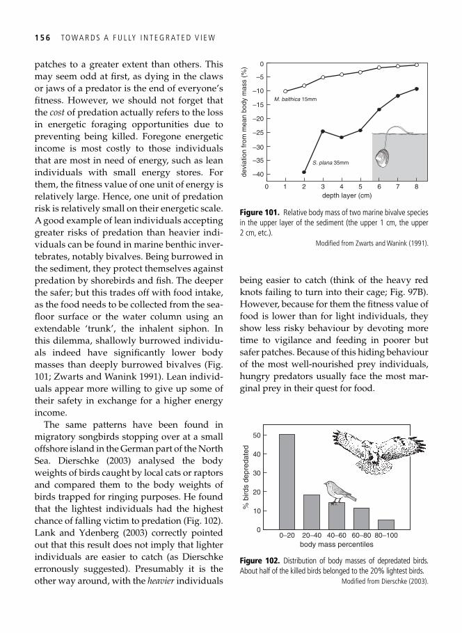
1 5 6 TO W A R D S A F U L LY I N T E G R AT E D V I E W
patches to a greater extent than others. This may seem odd at fi rst, as dying in the claws or jaws of a predator is the end of everyone’s fi tness. However, we should not forget that the cost of predation actually refers to the loss in energetic foraging opportunities due to preventing being killed. Foregone energetic income is most costly to those individuals that are most in need of energy, such as lean individuals with small energy stores. For them, the fi tness value of one unit of energy is relatively large. Hence, one unit of predation risk is relatively small on their energetic scale. A good example of lean individuals accepting greater risks of predation than heavier indi-viduals can be found in marine benthic inver-tebrates, notably bivalves. Being burrowed in the sediment, they protect themselves against predation by shorebirds and fi sh. The deeper the safer; but this trades off with food intake, as the food needs to be collected from the sea-fl oor surface or the water column using an extendable ‘trunk’, the inhalent siphon. In this dilemma, shallowly burrowed individu-als indeed have signifi cantly lower body masses than deeply burrowed bivalves ( Fig. 101 ; Zwarts and Wanink 1991 ). Lean individ-uals appear more willing to give up some of their safety in exchange for a higher energy income.
The same patterns have been found in migratory songbirds stopping over at a small offshore island in the German part of the North Sea. Dierschke ( 2003 ) analysed the body weights of birds caught by local cats or raptors and compared them to the body weights of birds trapped for ringing purposes. He found that the lightest individuals had the highest chance of falling victim to predation ( Fig. 102 ). Lank and Ydenberg ( 2003 ) correctly pointed out that this result does not imply that lighter individuals are easier to catch (as Dierschke erronously suggested). Presumably it is the other way around, with the heavier individuals
being easier to catch (think of the heavy red knots failing to turn into their cage; Fig. 97B ). However, because for them the fi tness value of food is lower than for light individuals, they show less risky behaviour by devoting more time to vigilance and feeding in poorer but safer patches. Because of this hiding behaviour of the most well-nourished prey individuals, hungry predators usually face the most mar-ginal prey in their quest for food.
0
10
20
30
40
50
% b
irds
depr
edat
ed
0–20body mass percentiles20–40 40–60 60–80 80–100
Figure 102. Distribution of body masses of depredated birds. About half of the killed birds belonged to the 20% lightest birds.
Modifi ed from Dierschke ( 2003 ).
0
0
–10
–20
–30
–40
–35
–25
–5
–15
devi
atio
n fr
om m
ean
body
mas
s (%
)
1 2 3 4 5 6 7 8depth layer (cm)
M. balthica 15mm
S. plana 35mm
Figure 101. Relative body mass of two marine bivalve species in the upper layer of the sediment (the upper 1 cm, the upper 2 cm, etc.).
Modifi ed from Zwarts and Wanink ( 1991 ).
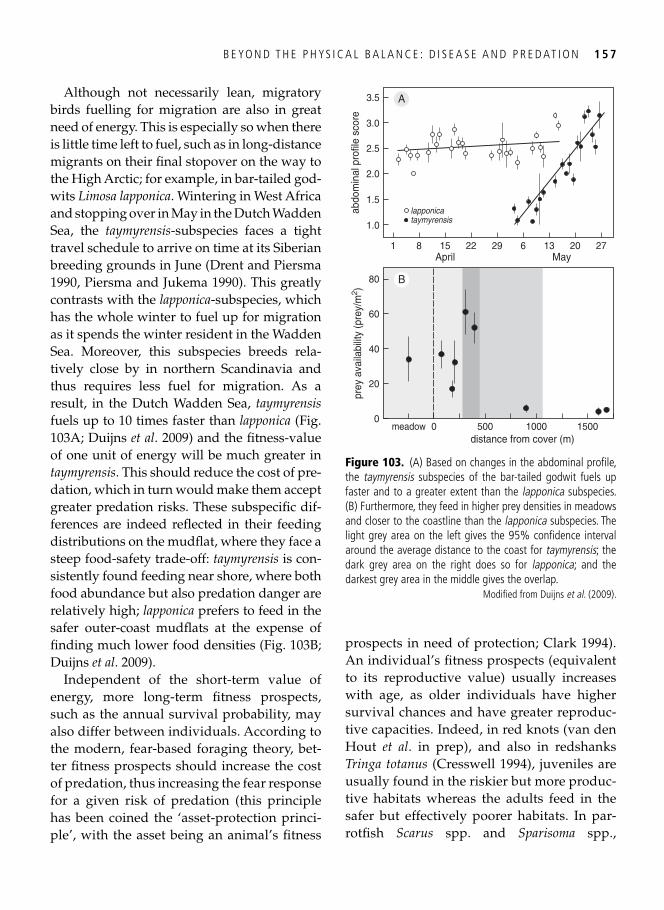
B E YO N D T H E P H YS I C A L B A L A N C E : D I S E A S E A N D P R E D AT I O N 1 5 7
Although not necessarily lean, migratory birds fuelling for migration are also in great need of energy. This is especially so when there is little time left to fuel, such as in long-distance migrants on their fi nal stopover on the way to the High Arctic; for example, in bar-tailed god-wits Limosa lapponica . Wintering in West Africa and stopping over in May in the Dutch Wadden Sea, the taymyrensis -subspecies faces a tight travel schedule to arrive on time at its Siberian breeding grounds in June ( Drent and Piersma 1990 , Piersma and Jukema 1990 ). This greatly contrasts with the lapponica -subspecies, which has the whole winter to fuel up for migration as it spends the winter resident in the Wadden Sea. Moreover, this subspecies breeds rela-tively close by in northern Scandinavia and thus requires less fuel for migration. As a result, in the Dutch Wadden Sea, taymyrensis fuels up to 10 times faster than lapponica ( Fig. 103A ; Duijns et al . 2009 ) and the fi tness-value of one unit of energy will be much greater in taymyrensis . This should reduce the cost of pre-dation, which in turn would make them accept greater predation risks. These subspecifi c dif-ferences are indeed refl ected in their feeding distributions on the mudfl at, where they face a steep food-safety trade-off: taymyrensis is con-sistently found feeding near shore, where both food abundance but also predation danger are relatively high; lapponica prefers to feed in the safer outer-coast mudfl ats at the expense of fi nding much lower food densities ( Fig. 103B ; Duijns et al . 2009 ).
Independent of the short-term value of energy, more long-term fi tness prospects, such as the annual survival probability, may also differ between individuals. According to the modern, fear-based foraging theory, bet-ter fi tness prospects should increase the cost of predation, thus increasing the fear response for a given risk of predation (this principle has been coined the ‘asset-protection princi-ple’, with the asset being an animal’s fi tness
prospects in need of protection; Clark 1994 ). An individual’s fi tness prospects (equivalent to its reproductive value) usually increases with age, as older individuals have higher survival chances and have greater reproduc-tive capacities. Indeed, in red knots (van den Hout et al . in prep), and also in redshanks Tringa totanus ( Cresswell 1994 ), juveniles are usually found in the riskier but more produc-tive habitats whereas the adults feed in the safer but effectively poorer habitats. In par-rotfi sh Scarus spp. and Sparisoma spp.,
00
20
40
60
80
prey
ava
ilabi
lity
(pre
y/m
2 )
1000 1500500distance from cover (m)
lapponica
meadow
taymyrensis
1
1.0
1.5
2.0
2.5
3.5 A
B
abdo
min
al p
rofil
e sc
ore
15April
8 22 29 6 20 2713May
3.0
Figure 103. (A) Based on changes in the abdominal profi le, the taymyrensis subspecies of the bar-tailed godwit fuels up faster and to a greater extent than the lapponica subspecies. (B) Furthermore, they feed in higher prey densities in meadows and closer to the coastline than the lapponica subspecies. The light grey area on the left gives the 95% confi dence interval around the average distance to the coast for taymyrensis ; the dark grey area on the right does so for lapponica ; and the darkest grey area in the middle gives the overlap.
Modifi ed from Duijns et al . ( 2009 ).
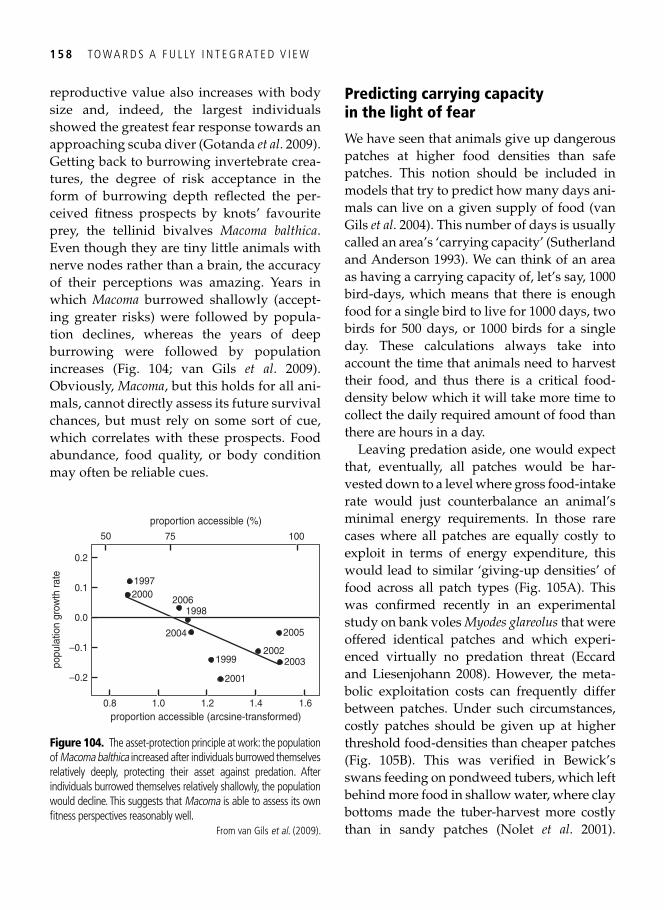
1 5 8 TO W A R D S A F U L LY I N T E G R AT E D V I E W
reproductive value also increases with body size and, indeed, the largest individuals showed the greatest fear response towards an approaching scuba diver ( Gotanda et al . 2009 ). Getting back to burrowing invertebrate crea-tures, the degree of risk acceptance in the form of burrowing depth refl ected the per-ceived fi tness prospects by knots’ favourite prey, the tellinid bivalves Macoma balthica . Even though they are tiny little animals with nerve nodes rather than a brain, the accuracy of their perceptions was amazing. Years in which Macoma burrowed shallowly (accept-ing greater risks) were followed by popula-tion declines, whereas the years of deep burrowing were followed by population increases ( Fig. 104 ; van Gils et al . 2009 ). Obviously, Macoma , but this holds for all ani-mals, cannot directly assess its future survival chances, but must rely on some sort of cue, which correlates with these prospects. Food abundance, food quality, or body condition may often be reliable cues.
Predicting carrying capacity in the light of fear
We have seen that animals give up dangerous patches at higher food densities than safe patches. This notion should be included in models that try to predict how many days ani-mals can live on a given supply of food ( van Gils et al . 2004 ). This number of days is usually called an area’s ‘carrying capacity’ ( Sutherland and Anderson 1993 ). We can think of an area as having a carrying capacity of, let’s say, 1000 bird-days, which means that there is enough food for a single bird to live for 1000 days, two birds for 500 days, or 1000 birds for a single day. These calculations always take into account the time that animals need to harvest their food, and thus there is a critical food-density below which it will take more time to collect the daily required amount of food than there are hours in a day.
Leaving predation aside, one would expect that, eventually, all patches would be har-vested down to a level where gross food-intake rate would just counterbalance an animal’s minimal energy requirements. In those rare cases where all patches are equally costly to exploit in terms of energy expenditure, this would lead to similar ‘giving-up densities’ of food across all patch types ( Fig. 105A ). This was confi rmed recently in an experimental study on bank voles Myodes glareolus that were offered identical patches and which experi-enced virtually no predation threat ( Eccard and Liesenjohann 2008 ). However, the meta-bolic exploitation costs can frequently differ between patches. Under such circumstances, costly patches should be given up at higher threshold food-densities than cheaper patches ( Fig. 105B ). This was verifi ed in Bewick’s swans feeding on pondweed tubers, which left behind more food in shallow water, where clay bottoms made the tuber-harvest more costly than in sandy patches ( Nolet et al . 2001 ).
0.2
–0.2
–0.1
0.0
0.1
popu
latio
n gr
owth
rate 1997
0.8 1.0 1.2 1.4 1.6proportion accessible (arcsine-transformed)
50 75 100
proportion accessible (%)
2000 20061998
2004
1999
2001
2002
2005
2003
Figure 104. The asset-protection principle at work: the population of Macoma balthica increased after individuals burrowed themselves relatively deeply, protecting their asset against predation. After individuals burrowed themselves relatively shallowly, the population would decline. This suggests that Macoma is able to assess its own fi tness perspectives reasonably well.
From van Gils et al . ( 2009 ).
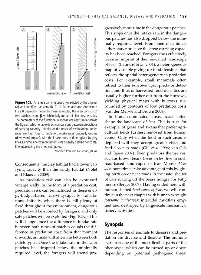
B E YO N D T H E P H YS I C A L B A L A N C E : D I S E A S E A N D P R E D AT I O N 1 5 9
Consequently, the clay habitat had a lower car-rying capacity than the sandy habitat ( Nolet and Klaassen 2009 ).
As predation risk can also be expressed ‘energetically’ in the form of a predation cost, predation risk can be included in these ener-gy-budget-based carrying-capacity calcula-tions. Initially, when there is still plenty of food throughout the environment, dangerous patches will be avoided by foragers, and only safe patches will be exploited ( Fig. 105C ). This will change once the difference in intake rate between both types of patches equals the dif-ference in predation cost: from that moment onwards, animals will alternate between both patch types. Once the intake rate in the safer patches has dropped below the minimally required level, the foragers will spend pro-
gressively more time in the dangerous patches. This stops once the intake rate in the danger-ous patches has also dropped below the mini-mally required level. From then on animals either starve or leave the area: carrying capac-ity has been reached. Foragers thus effectively leave an imprint of their so-called ‘landscape of fear’ ( Laundré et al . 2001 ), a heterogeneous map of variable giving-up food densities that refl ects the spatial heterogeneity in predation costs. For example, small mammals often retreat to their burrows upon predator detec-tion, and thus unharvested food densities are usually higher further out from the burrows, yielding physical maps with burrows sur-rounded by contours of low predation costs ( van der Merwe and Brown 2008 ).
In human-dominated areas, roads often shape the landscape of fear. This is true, for example, of geese and swans that prefer agri-cultural fi elds furthest removed from human access. Only when the food in such areas is depleted will they accept greater risks and feed closer to roads ( Gill et al . 1996 ; van Gils and Tijsen 2007 ). Even predators themselves, such as brown bears Ursus arctos , live in such road-based landscapes of fear. Moose Alces alces sometimes take advantage of this by giv-ing birth on or near roads in the ‘safe’ shelter of cars scaring off the bears hungry for baby moose ( Berger 2007 ). Having ended here with human-shaped landscapes of fear , we will con-tinue in the next chapter with human-wrought fearsome landscapes : intertidal mudfl ats emp-tied and destroyed by large-scale mechanical fi shery activities.
Synopsis
The responses of animals to diseases and pre-dation are diverse and fl exible. The immune system is one of the most fl exible parts of the phenotype, which can be turned up or down depending on potential pathogenic threat
0
gros
s in
take
rate
metabolic rate
A
α β α β α β
t=0123456789
10111213141516
B C
predation risk
y=x m
inim
al e
nerg
y re
quire
men
t
Figure 105. An area’s carrying capacity predicted by the original (A) and modifi ed versions (B–C) of Sutherland and Anderson’s (1993) depletion model. In these examples, the area consists of two patches, a and β, which initially contain similar prey densities. The parameters of the functional response are kept similar across the fi gures, which enable direct comparisons between predictions of carrying capacity. Initially, at the onset of exploitation, intake rates are high. Due to depletion, intake rates gradually decline (downward arrows), with the intake rates at time t given by grey lines. Minimal energy requirements are given by dashed horizontal line intersecting the three subfi gures.
Modifi ed from van Gils et al . ( 2004 ).
1 6 0 TO W A R D S A F U L LY I N T E G R AT E D V I E W
levels. Insightful knowledge on the fl exible immune system is still thin on the ground, as immunity is so amazingly complex. What we do know, however, is that shorebird species that breed in the relatively clean High Arctic, winter in relatively clean saline habitats; whereas species that breed at lower latitudes with higher pathogen pressures, winter in pathogen-rich freshwater environments. It is possible that High-Arctic breeders are the only ones able to make super long-distance migra-tions because they do not need to invest so much in immune defence. We understand much more about phenotypic responses to the
threat of predation. By fl exibly modifying body composition, prey can reduce their risk of predation. Birds ‘play’ with pectoral muscle mass and total body mass, depending on the need to escape through acceleration or through manoeuvrability. Obviously, the most immedi-ate response to predation threat is through behaviour: visually scanning the environment, coming together in fl ocks, or switching habi-tats. In such ways parasites and predators strongly affect an area’s carrying capacity for particular animals, something that is gradu-ally being realized and incorporated in applied contexts and conservation thinking.
161
CHAPTER 9
Population consequences: conservation and management of fl exible phenotypes
We are deep into the book now, and you have read much about phenotypes in interaction with their environments. We have come to understand diet choice and the distributions of animals because we took phenotypic change into account. That is all very interesting in its own right, but is it enough?
The Holy Grail of population biology
The population-oriented ecologists amongst us are usually after even ‘holier grails’: the understanding of changing numbers of organ-isms, and of variable population sizes ( Kingsland 1995 , Hilborn and Mangel 1997 , Vandermeer and Goldberg 2003 , Ranta et al. 2006 ). Building on what we have learned about specialized molluscivore shorebirds in the pre-vious two chapters, we now want to take the next step by disentangling the reasons behind their changing numbers. Can we understand population dynamics better if we include the notion of phenotypic fl exibility? In addition, given that the world’s ecology is in constant fl ux, we would like to establish what differ-ences fl exible rather than infl exible phenotypes could make to what animals can do or can tol-erate on this rapidly changing planet. This may allow us to predict population conse-quences somewhat outside the current range of environmental conditions. To set the scene, we will start with a case study on a bird that will not surprise you at all—the red knot.
Dredging out bivalve-rich intertidal fl ats: a case study on red knots
Tidal fl ats occur along shallow seas with soft sediment bottoms, in areas where the tidal range is at least a metre or so ( Eisma 1998 , Lenihan and Micheli 2001 , van de Kam et al. 2004 ). The lowest parts of intertidal areas are usually barren except for the occurrence of seagrass meadows and reefs formed by inver-tebrate ‘ecosystem engineers’, such as oysters Ostrea , mussels Mytilus , or tubeworms Sabellaria . Intertidal areas are inundated at least once a day. On the landside, fl ats may be bordered by salt marshes, or, in the warmer regions of the world, by mangrove forests.
The international Wadden Sea, a shared ter-ritory of The Netherlands, Germany, and Denmark, is reckoned to be one of the biggest intertidal areas in the world ( van de Kam et al . 2004 , Lotze et al . 2005 ), a distinction shared with the Yellow Sea (see below). Mostly 7 to 10 km wide, it stretches along 450 km of coast-line. During spring low tides a total of 490,000 ha of intertidal mud is exposed. Compared with other intertidal areas worldwide, the Wadden Sea harbours particularly large shell-fi sh populations ( Piersma et al . 1993a ). In 2009 it received recognition as a UNESCO World Heritage Site. The Netherlands’ 120,000 ha of the Wadden Sea are designated a State Nature Monument, and is protected under various other national and international conventions. Despite this high number of formal conservation
1 6 2 TO W A R D S A F U L LY I N T E G R AT E D V I E W
accolades, until 2004, three-quarters of the intertidal fl ats of the Dutch Wadden Sea were open to mechanical dredging for edible cock-les Cerastoderma edule ( Swart and van Andel 2008 , Piersma 2009 ). Most parts are still open to other forms of bottom disturbance with fi sh-ing gear of various severity ( Watling and Norse 1998 ).
Suction-dredging of cockles took place from big barges with a draft of only 80 cm ( Fig. 106E ). The dredges, suspended from either side of the barge, are about a metre wide and have water jets to loosen up the top layer of the sediment. This is then scraped off by a blade at a depth of approximately 5 cm. Within the dredge, a strong water fl ow ensures that small objects are pushed through a screen. The remaining items, such as large cockles, are sucked on board for further sorting and cleaning. After dredging, the intertidal fl ats look ‘scarred’ and can remain so for a whole year ( Fig. 106F ). In the case of mechanical cockle fi shing in the Wadden Sea, GPS loggers were installed to record the position and fi shing- activity of each barge ( Fig. 106A –D). On the basis of these records, an average 4.3% of the intertidal fl ats was affected by dredging each year ( Kamermans and Smaal 2002 ). Cumulatively, between 1992 and 2001, 19% of the intertidal area was affected by mechanical cockle-dredging at least once ( Kraan et al . 2007 ). If this still seems a small percentage to you, note that cockle-dredgers selected areas that red knots would select too, and that by far the greatest loss of feeding area ( Fig. 107C ) was accounted for by cockle-dredging ( van Gils et al. 2006b , Kraan et al . 2009 ).
A direct, immediate effect of dredging was the complete removal of all organisms larger than 19 mm in the top layer. As the dredged sites were usually the most biodiverse ( Kraan et al . 2007 ), dredging also affected smaller cockles, other bivalves such as blue mussels Mytilus edulis , Baltic tellins Macoma balthica ,
and sandgapers Mya arenaria , polychaetes, and crustaceans such as shorecrabs Carcinus mae-nas . More indirectly, and over longer time scales, sediments lost fi ne silts during dredg-ing events, and changing sediment character-istics may have led to long-term reductions in settlement rates by both cockles and Baltic tell-ins ( Piersma et al . 2001 , Hiddink 2003 ).
Population consequences for the molluscivores
Several decades of serious fi shing pressure not only led to a stark loss of the shellfi sh resources, but also resulted in a serious decline of many molluscivore birds in the Wadden Sea. The oystercatchers, most of which are resident in The Netherlands, showed a steep decline, incurring the greatest losses when high food demands coincided with restricted access to partially ice-covered mudfl ats during severe winters ( Camphuysen et al . 1996 , van Roomen et al . 2005 ). Eider ducks Somateria mollissima , consisting of local breeders and a much larger contingent migrating in from the Baltic, also showed food-scarcity related mass starvation and movements out of the Wadden Sea ( Camphuysen et al . 2002 ). Oystercatchers and eiders are large birds. Their actual death is eas-ily noticed. This is in marked contrast to the smallest dedicated molluscivore, the red knot, which shows rather cryptic mortality in the form of declining head counts. Following ear-lier losses ( Piersma et al . 1993c ), red knots declined by 42% between winters in the late-1990s and the early 2000s ( Fig. 107A ). A decrease in annual local survival from 89% to 82% per year could account for almost half of this decline ( Fig. 107B ). The remaining red knots moved elsewhere in Western Europe to winter ( Kraan et al . 2009 ). Red knots en route to winter-ing areas in West Africa must store fuel for fl ight and thus have greater energy demands. Their numbers in late summer showed an even
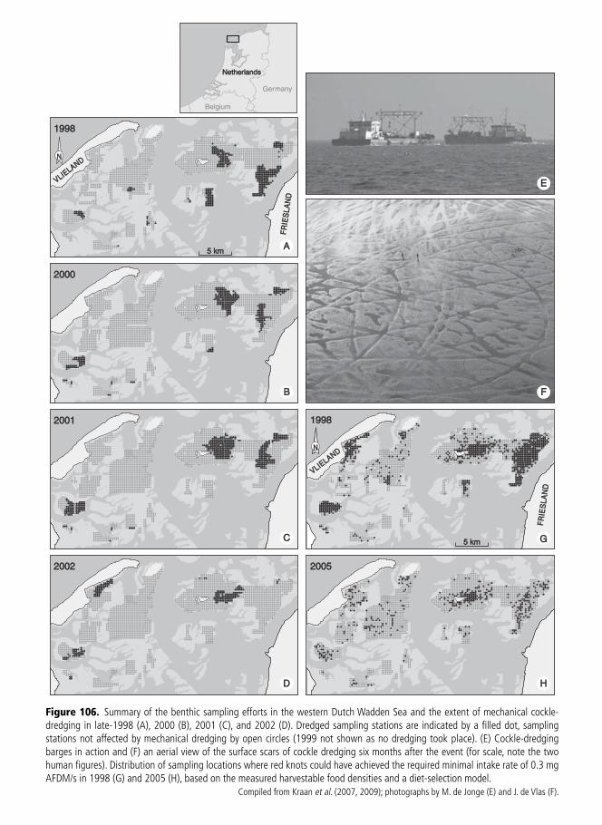
NN
5 km5 km
20052005
19981998
VLIELAN
VLIELANDD
FR
IES
LAN
FR
IES
LAN
DD
VVLILIEELLAANNDD
FR
IES
LAN
FR
IES
LAN
DD
20022002
20012001
20002000
19981998
AA
BB
CC
DD HH
GG
FF
EE
5 km5 km
Germany
Belgium
NetheNetherrlandslands
NN
Figure 106. Summary of the benthic sampling efforts in the western Dutch Wadden Sea and the extent of mechanical cockle-dredging in late-1998 (A), 2000 (B), 2001 (C), and 2002 (D). Dredged sampling stations are indicated by a fi lled dot, sampling stations not affected by mechanical dredging by open circles (1999 not shown as no dredging took place). (E) Cockle-dredging barges in action and (F) an aerial view of the surface scars of cockle dredging six months after the event (for scale, note the two human fi gures). Distribution of sampling locations where red knots could have achieved the required minimal intake rate of 0.3 mg AFDM/s in 1998 (G) and 2005 (H), based on the measured harvestable food densities and a diet-selection model.
Compiled from Kraan et al . ( 2007 , 2009 ); photographs by M. de Jonge (E) and J. de Vlas (F).
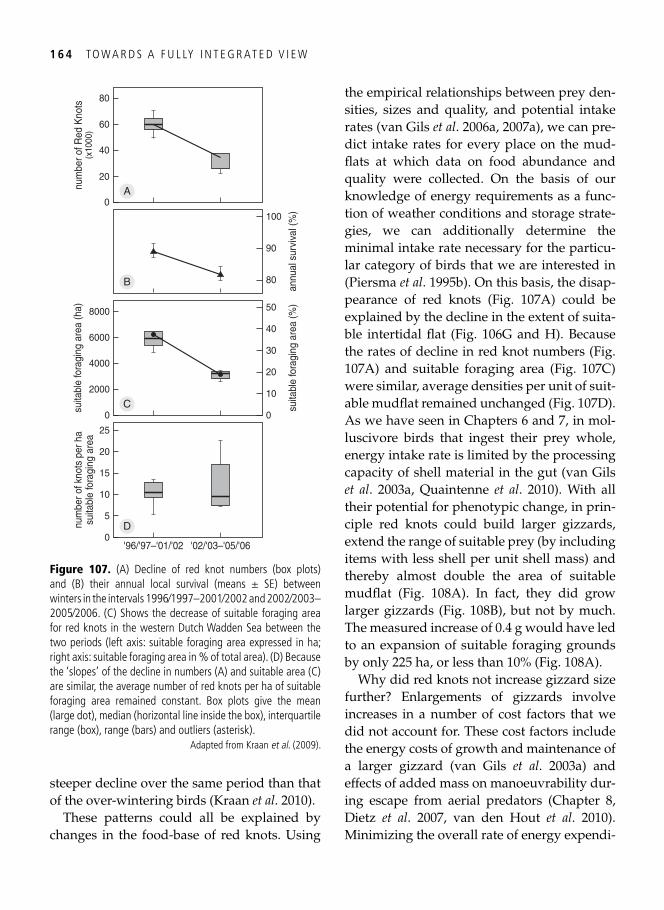
1 6 4 TO W A R D S A F U L LY I N T E G R AT E D V I E W
steeper decline over the same period than that of the over-wintering birds ( Kraan et al . 2010 ).
These patterns could all be explained by changes in the food-base of red knots. Using
the empirical relationships between prey den-sities, sizes and quality, and potential intake rates ( van Gils et al . 2006a , 2007a ), we can pre-dict intake rates for every place on the mud-fl ats at which data on food abundance and quality were collected. On the basis of our knowledge of energy requirements as a func-tion of weather conditions and storage strate-gies, we can additionally determine the minimal intake rate necessary for the particu-lar category of birds that we are interested in ( Piersma et al . 1995b ). On this basis, the disap-pearance of red knots ( Fig. 107A ) could be explained by the decline in the extent of suita-ble intertidal fl at ( Fig. 106G and H). Because the rates of decline in red knot numbers ( Fig. 107A ) and suitable foraging area ( Fig. 107C ) were similar, average densities per unit of suit-able mudfl at remained unchanged ( Fig. 107D ). As we have seen in Chapters 6 and 7 , in mol-luscivore birds that ingest their prey whole, energy intake rate is limited by the processing capacity of shell material in the gut ( van Gils et al . 2003a , Quaintenne et al . 2010 ). With all their potential for phenotypic change, in prin-ciple red knots could build larger gizzards, extend the range of suitable prey (by including items with less shell per unit shell mass) and thereby almost double the area of suitable mudfl at ( Fig. 108A ). In fact, they did grow larger gizzards ( Fig. 108B ), but not by much. The measured increase of 0.4 g would have led to an expansion of suitable foraging grounds by only 225 ha, or less than 10% ( Fig. 108A ).
Why did red knots not increase gizzard size further? Enlargements of gizzards involve increases in a number of cost factors that we did not account for. These cost factors include the energy costs of growth and maintenance of a larger gizzard ( van Gils et al . 2003a ) and effects of added mass on manoeuvrability dur-ing escape from aerial predators ( Chapter 8 , Dietz et al . 2007 , van den Hout et al . 2010 ). Minimizing the overall rate of energy expendi-
C
B
A
D0
num
ber o
f kno
ts p
er h
asu
itabl
e fo
ragi
ng a
rea
'96/'97–'01/'02
0
2000
4000
suita
ble
fora
ging
are
a (h
a)
suita
ble
fora
ging
are
a (%
)
0
20
40
80
num
ber o
f Red
Kno
ts(x
1000
)
'02/'03–'05/'06
8000
0
5
10
25
15
20
60
20
40
50
80
90
100
annu
al s
urvi
val (
%)
6000
10
30
Figure 107. (A) Decline of red knot numbers (box plots) and (B) their annual local survival (means ± SE) between winters in the intervals 1996⁄1997–2001⁄2002 and 2002⁄2003–2005⁄2006. (C) Shows the decrease of suitable foraging area for red knots in the western Dutch Wadden Sea between the two periods (left axis: suitable foraging area expressed in ha; right axis: suitable foraging area in % of total area). (D) Because the ‘slopes’ of the decline in numbers (A) and suitable area (C) are similar, the average number of red knots per ha of suitable foraging area remained constant. Box plots give the mean (large dot), median (horizontal line inside the box), interquartile range (box), range (bars) and outliers (asterisk).
Adapted from Kraan et al . ( 2009 ).
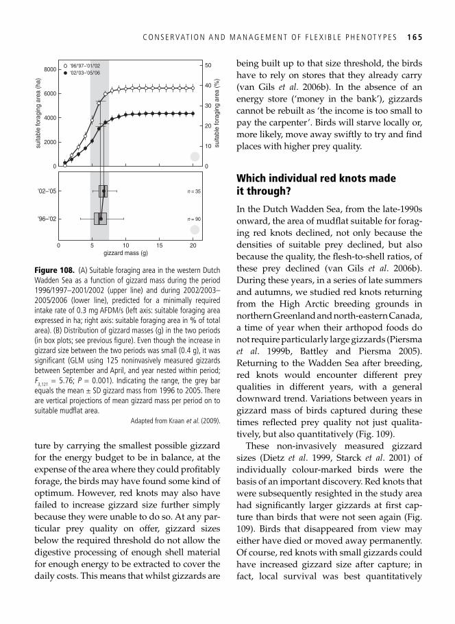
C O N S E R VAT I O N A N D M A N A G E M E N T O F F L E X I B L E P H E N OT Y P E S 1 6 5
ture by carrying the smallest possible gizzard for the energy budget to be in balance, at the expense of the area where they could profi tably forage, the birds may have found some kind of optimum. However, red knots may also have failed to increase gizzard size further simply because they were unable to do so. At any par-ticular prey quality on offer, gizzard sizes below the required threshold do not allow the digestive processing of enough shell material for enough energy to be extracted to cover the daily costs. This means that whilst gizzards are
being built up to that size threshold, the birds have to rely on stores that they already carry ( van Gils et al . 2006b ). In the absence of an energy store (‘money in the bank’), gizzards cannot be rebuilt as ‘the income is too small to pay the carpenter’. Birds will starve locally or, more likely, move away swiftly to try and fi nd places with higher prey quality.
Which individual red knots made it through?
In the Dutch Wadden Sea, from the late-1990s onward, the area of mudfl at suitable for forag-ing red knots declined, not only because the densities of suitable prey declined, but also because the quality, the fl esh-to-shell ratios, of these prey declined ( van Gils et al . 2006b ). During these years, in a series of late summers and autumns, we studied red knots returning from the High Arctic breeding grounds in northern Greenland and north-eastern Canada, a time of year when their arthopod foods do not require particularly large gizzards ( Piersma et al . 1999b , Battley and Piersma 2005 ). Returning to the Wadden Sea after breeding, red knots would encounter different prey qualities in different years, with a general downward trend. Variations between years in gizzard mass of birds captured during these times refl ected prey quality not just qualita-tively, but also quantitatively ( Fig. 109 ).
These non-invasively measured gizzard sizes ( Dietz et al . 1999 , Starck et al . 2001 ) of individually colour-marked birds were the basis of an important discovery. Red knots that were subsequently resighted in the study area had signifi cantly larger gizzards at fi rst cap-ture than birds that were not seen again ( Fig. 109 ). Birds that disappeared from view may either have died or moved away permanently. Of course, red knots with small gizzards could have increased gizzard size after capture; in fact, local survival was best quantitatively
0
2000
4000
6000
8000
suita
ble
fora
ging
are
a (h
a)
'96/'97–'01/'02'02/'03–'05/'06
0
20
50
30
10 suita
ble
fora
ging
are
a (%
)
0
'02–'05
205 10 15gizzard mass (g)
'96–'02
n = 35
n = 90
40
Figure 108. (A) Suitable foraging area in the western Dutch Wadden Sea as a function of gizzard mass during the period 1996⁄1997–2001⁄2002 (upper line) and during 2002⁄2003–2005⁄2006 (lower line), predicted for a minimally required intake rate of 0.3 mg AFDM/s (left axis: suitable foraging area expressed in ha; right axis: suitable foraging area in % of total area). (B) Distribution of gizzard masses (g) in the two periods (in box plots; see previous fi gure). Even though the increase in gizzard size between the two periods was small (0.4 g), it was signifi cant (GLM using 125 noninvasively measured gizzards between September and April, and year nested within period; F 3,121 = 5.76; P = 0.001). Indicating the range, the grey bar equals the mean ± SD gizzard mass from 1996 to 2005. There are vertical projections of mean gizzard mass per period on to suitable mudfl at area.
Adapted from Kraan et al . ( 2009 ).
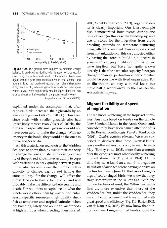
1 6 6 TO W A R D S A F U L LY I N T E G R AT E D V I E W
explained under the assumption that, after capture, birds increased their gizzards by an average 1 g ( van Gils et al . 2006b ). However, since birds with smaller gizzards also had lower body masses ( van Gils et al . 2006b ), the birds with especially small gizzards would not have been able to make the change. With no ‘money in the bank’, they would be the ones to move and/or to die.
All this material on red knots in the Wadden Sea goes to show that, by using their capacity to change the size and shell-processing capac-ity of the gut, red knots have an ability to cope with variations in prey quality between years. It has also become clear that limits to this capacity to change, e.g. by not having the stores to ‘pay’ for the change, will affect the birds’ decision to stay or to move on, and will probably make the difference between life and death. For red knots to capitalize on what the whole world offers them by way of particular, season-specifi c resources (high quality shell-fi sh at temperate and tropical latitudes when not breeding, safety and abundant arthropods at high latitudes when breeding; Piersma et al .
2005 , Schekkerman et al . 2003 ), organ fl exibil-ity is clearly important. Our latest example also demonstrated how events during one time of year (in this case the building up and use of stores for the migration from arctic breeding grounds to temperate wintering areas) affect the survival chances upon arrival from that migration (in this case affected either by having the stores to build up a gizzard in years with low prey quality, or not). What we have implied, but have not quite shown directly, is that the particular capacity for organ change enhances performance beyond what would be possible with fi xed organ sizes. For an illustration, we stay with red knots but move half a world away to the East-Asian–Australasian fl yway.
Migrant fl exibility and speed of migration
The red knots ‘wintering’ in the tropics of north-west Australia breed on tundra on the remote New Siberian Islands in the Arctic Ocean and, coincidentally, have been named after one of us by the Russian ornithologist Pavel S. Tomkovich ( 2001 )— Calidris canutus piersmai . We were sur-prised to discover that these ‘ piersmai -knots’ leave northwest Australia only in early to mid-May ( Battley et al . 2005 ), more than a month after the exodus of most other locally wintering migrant shorebirds ( Tulp et al . 1994 ). At this time they have less than a month to negotiate 10,400 km of airspace before having to arrive on the tundra in early June. On the basis of resight-ings of colour-ringed birds, we know that they stage somewhere in the Yellow Sea. With one million hectares of mud, the Yellow Sea mud-fl ats are more extensive than those of the Wadden Sea, but, unlike the Wadden Sea, they are still being reclaimed and transformed with great speed and effi ciency ( Fig. 110 ; Barter 2002 , van de Kam et al . 2008 ). We now know that dur-ing northward migration red knots choose the
4
6
8
(req
uire
d) g
izza
rd m
ass
(g)
prey quality (g flesh/g shell)
5
7
0.10
seen againnot seen again
0.12 0.14 0.16 0.18
Figure 109. The gizzard mass required to maintain energy balance is predicted to decline with function of prey quality (solid line). Gizzards of individually colour-marked birds seen again within a year after measurement in late summer and autumn fi tted the predicted quantitative relationship (grey dots; mean ± SE), whereas gizzards of birds not seen again within a year were signifi cantly smaller (open dots; the two groups almost entirely overlap in the poorest-quality year).
Adapted from van Gils et al . ( 2006b ).
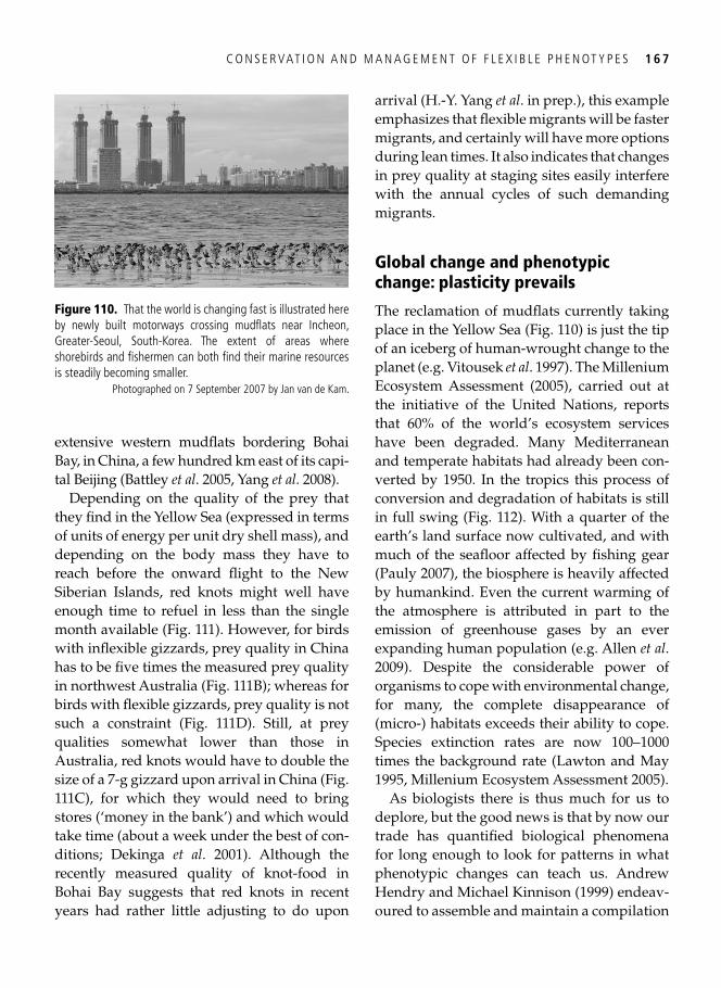
C O N S E R VAT I O N A N D M A N A G E M E N T O F F L E X I B L E P H E N OT Y P E S 1 6 7
extensive western mudfl ats bordering Bohai Bay, in China, a few hundred km east of its capi-tal Beijing ( Battley et al . 2005 , Yang et al . 2008 ).
Depending on the quality of the prey that they fi nd in the Yellow Sea (expressed in terms of units of energy per unit dry shell mass), and depending on the body mass they have to reach before the onward fl ight to the New Siberian Islands, red knots might well have enough time to refuel in less than the single month available ( Fig. 111 ). However, for birds with infl exible gizzards, prey quality in China has to be fi ve times the measured prey quality in northwest Australia ( Fig. 111B ); whereas for birds with fl exible gizzards, prey quality is not such a constraint ( Fig. 111D ). Still, at prey qualities somewhat lower than those in Australia, red knots would have to double the size of a 7-g gizzard upon arrival in China ( Fig. 111C ), for which they would need to bring stores (‘money in the bank’) and which would take time (about a week under the best of con-ditions; Dekinga et al . 2001 ). Although the recently measured quality of knot-food in Bohai Bay suggests that red knots in recent years had rather little adjusting to do upon
arrival (H.-Y. Yang et al . in prep.), this example emphasizes that fl exible migrants will be faster migrants, and certainly will have more options during lean times. It also indicates that changes in prey quality at staging sites easily interfere with the annual cycles of such demanding migrants.
Global change and phenotypic change: plasticity prevails
The reclamation of mudfl ats currently taking place in the Yellow Sea ( Fig. 110 ) is just the tip of an iceberg of human-wrought change to the planet (e.g. Vitousek et al . 1997 ). The Millenium Ecosystem Assessment ( 2005 ), carried out at the initiative of the United Nations, reports that 60% of the world’s ecosystem services have been degraded. Many Mediterranean and temperate habitats had already been con-verted by 1950. In the tropics this process of conversion and degradation of habitats is still in full swing ( Fig. 112 ). With a quarter of the earth’s land surface now cultivated, and with much of the seafl oor affected by fi shing gear ( Pauly 2007 ), the biosphere is heavily affected by humankind. Even the current warming of the atmosphere is attributed in part to the emission of greenhouse gases by an ever expanding human population (e.g. Allen et al . 2009 ). Despite the considerable power of organisms to cope with environmental change, for many, the complete disappearance of (micro-) habitats exceeds their ability to cope. Species extinction rates are now 100–1000 times the background rate ( Lawton and May 1995 , Millenium Ecosystem Assessment 2005 ).
As biologists there is thus much for us to deplore, but the good news is that by now our trade has quantifi ed biological phenomena for long enough to look for patterns in what phenotypic changes can teach us. Andrew Hendry and Michael Kinnison (1999) endeav-oured to assemble and maintain a compilation
Figure 110. That the world is changing fast is illustrated here by newly built motorways crossing mudfl ats near Incheon, Greater-Seoul, South-Korea. The extent of areas where shorebirds and fi shermen can both fi nd their marine resources is steadily becoming smaller.
Photographed on 7 September 2007 by Jan van de Kam.
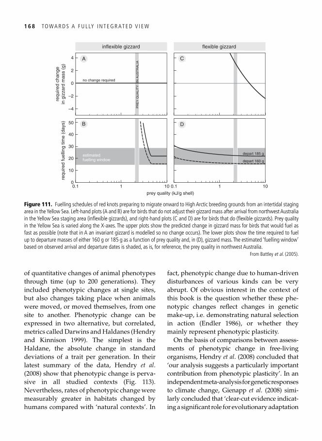
1 6 8 TO W A R D S A F U L LY I N T E G R AT E D V I E W
of quantitative changes of animal phenotypes through time (up to 200 generations). They included phenotypic changes at single sites, but also changes taking place when animals were moved, or moved themselves, from one site to another. Phenotypic change can be expressed in two alternative, but correlated, metrics called Darwins and Haldanes ( Hendry and Kinnison 1999 ). The simplest is the Haldane, the absolute change in standard deviations of a trait per generation. In their latest summary of the data, Hendry et al . ( 2008 ) show that phenotypic change is perva-sive in all studied contexts ( Fig. 113 ). Nevertheless, rates of phenotypic change were measurably greater in habitats changed by humans compared with ‘natural contexts’. In
fact, phenotypic change due to human-driven disturbances of various kinds can be very abrupt. Of obvious interest in the context of this book is the question whether these phe-notypic changes refl ect changes in genetic make-up, i.e. demonstrating natural selection in action ( Endler 1986 ), or whether they mainly represent phenotypic plasticity.
On the basis of comparisons between assess-ments of phenotypic change in free-living organisms, Hendry et al . ( 2008 ) concluded that ‘our analysis suggests a particularly important contribution from phenotypic plasticity’. In an independent meta-analysis for genetic responses to climate change, Gienapp et al . ( 2008 ) simi-larly concluded that ‘clear-cut evidence indicat-ing a signifi cant role for evolutionary adaptation
prey quality (kJ/g shell)
requ
ired
fuel
ling
time
(day
s)
10
20
40
0.1 10
estimatedfuelling window
50
10
30
10.1 10
depart 185 g
requ
ired
chan
gein
giz
zard
mas
s (g
)
–4
0
4
no change required
A
–2
2
depart 160 g
inflexible gizzard flexible gizzard
PR
EY
QU
ALI
TY
IN
AU
ST
RA
LIA
C
B D
Figure 111. Fuelling schedules of red knots preparing to migrate onward to High Arctic breeding grounds from an intertidal staging area in the Yellow Sea. Left-hand plots (A and B) are for birds that do not adjust their gizzard mass after arrival from northwest Australia in the Yellow Sea staging area (infl exible gizzards), and right-hand plots (C and D) are for birds that do (fl exible gizzards). Prey quality in the Yellow Sea is varied along the X-axes. The upper plots show the predicted change in gizzard mass for birds that would fuel as fast as possible (note that in A an invariant gizzard is modelled so no change occurs). The lower plots show the time required to fuel up to departure masses of either 160 g or 185 g as a function of prey quality and, in (D), gizzard mass. The estimated ‘fuelling window’ based on observed arrival and departure dates is shaded, as is, for reference, the prey quality in northwest Australia.
From Battley et al . ( 2005 ).
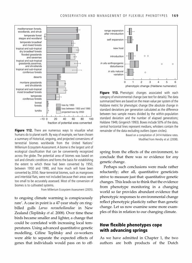
C O N S E R VAT I O N A N D M A N A G E M E N T O F F L E X I B L E P H E N OT Y P E S 1 6 9
to ongoing climate warming is conspicuously rare’. A case in point is a 47-year study on ring-billed gulls Larus novaehollandiae in New Zealand ( Teplitsky et al . 2008 ). Over time these birds became smaller and lighter, a change that could be correlated with increasing local tem-peratures. Using advanced quantitative genetic modelling, Céline Teplitsky and co-workers were able to separate the expected effects of genes that individuals would pass on to off-
spring from the effects of the environment, to conclude that there was no evidence for any genetic change.
Perhaps such conclusions were made rather reluctantly; after all, quantitative geneticists strive to measure just that: quantitative genetic changes. This leads us to think that the evidence from phenotype monitoring in a changing world so far provides abundant evidence that phenotypic responses to environmental change refl ect phenotypic plasticity rather than genetic change. Let us now examine some more exam-ples of this in relation to our changing climate.
How fl exible phenotypes cope with advancing springs
As we have admitted in Chapter 1 , the two authors are both products of the Dutch
0–10 10020 40 60 80fraction of potential area converted
tundra
borealforests
temperateconiferous forests
tropical and sub-tropicalmoist broadleaf forests
montane grasslandsand shrublands
deserts
tropical and sub-tropicalconiferous forests
tropical and sub-tropicalgrasslands,savannas,
and shrublands
flooded grasslandsand savannas
tropical and sub-tropicaldry broadleaf forests
temperate broadleafand mixed forests
temperate foreststeppe and woodland
mediterranean forests,woodlands, and shrub
loss by 1950loss between 1950 and 1990projected loss by 2050
Figure 112. There are numerous ways to visualize what humans do to planet earth. By way of example, we have chosen a summary of historical, ongoing, and projected conversions of terrestrial biomes worldwide from the United Nations’ Millenium Ecosystem Assessment. A biome is the largest unit of ecological classifi cation that can be conveniently recognized across the globe. The potential area of biomes was based on soil and climatic conditions and forms the basis for establishing the extent to which these had been converted by 1950, between 1950 and 1990, and how much will have been converted by 2050. Near-terrestrial biomes, such as mangroves and intertidal fl ats, were not included because their areas were too small to be accurately assessed. Most of the conversion of biomes is to cultivated systems.
From Millenium Ecosystem Assessment ( 2005 ).
0
range expansionafter introduction
1 2 3 4 5 6
phenotypic change (Haldane numerator)
self expansion
new host
introduction
in situ anthopogenicdisturbance
in situ naturalvariation
Figure 113. Phenotypic changes associated with each category of environmental change (see text for details). The data summarized here are based on the mean value per system of the Haldane metric for phenotypic change (the absolute change in standard deviations per generation calculated as the difference between two sample means divided by the within-population standard deviation and the number of elapsed generations; Haldane 1949 , Gingerich 1993 ). Boxes include 50% of the data, central horizontal lines represent medians, whiskers contain the remainder of the data excluding outliers (open circles).
Based on a compilation of 2414 Haldane rates. Modifi ed from Hendry et al . ( 2008 ).
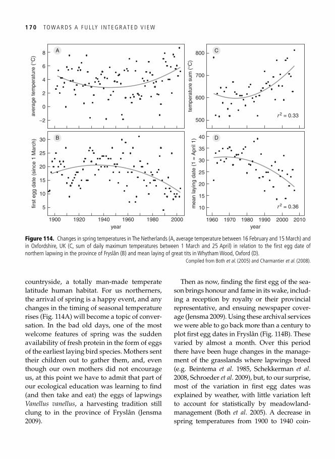
1 7 0 TO W A R D S A F U L LY I N T E G R AT E D V I E W
countryside, a totally man-made temperate latitude human habitat. For us northerners, the arrival of spring is a happy event, and any changes in the timing of seasonal temperature rises ( Fig. 114A ) will become a topic of conver-sation. In the bad old days, one of the most welcome features of spring was the sudden availability of fresh protein in the form of eggs of the earliest laying bird species. Mothers sent their children out to gather them, and, even though our own mothers did not encourage us, at this point we have to admit that part of our ecological education was learning to fi nd (and then take and eat) the eggs of lapwings Vanellus vanellus , a harvesting tradition still clung to in the province of Fryslân ( Jensma 2009 ).
Then as now, fi nding the fi rst egg of the sea-son brings honour and fame in its wake, includ-ing a reception by royalty or their provincial representative, and ensuing newspaper cover-age ( Jensma 2009 ). Using these archival services we were able to go back more than a century to plot fi rst egg dates in Fryslân ( Fig. 114B ). These varied by almost a month. Over this period there have been huge changes in the manage-ment of the grasslands where lapwings breed (e.g. Beintema et al. 1985 , Schekkerman et al . 2008 , Schroeder et al . 2009 ), but, to our surprise, most of the variation in fi rst egg dates was explained by weather, with little variation left to account for statistically by meadowland-management ( Both et al . 2005 ). A decrease in spring temperatures from 1900 to 1940 coin-
10
20
30
25
5
15
first
egg
dat
e (s
ince
1 M
arch
)
1900 1920 1940year
1960 1980 2000 1960 1970 1980year
1990 2000 2010
10
20
30
25
15m
ean
layi
ng d
ate
(1 =
Apr
il 1)
35
40
0
4
8 A
B D
C
6
−2
2
aver
age
tem
pera
ture
(°C
)
500
600
800
700
tem
pera
ture
sum
(°C
)
r 2 = 0.33
r 2 = 0.36
Figure 114. Changes in spring temperatures in The Netherlands (A, average temperature between 16 February and 15 March) and in Oxfordshire, UK (C, sum of daily maximum temperatures between 1 March and 25 April) in relation to the fi rst egg date of northern lapwing in the province of Fryslân (B) and mean laying of great tits in Whytham Wood, Oxford (D).
Compiled from Both et al . ( 2005 ) and Charmantier et al . ( 2008 ).
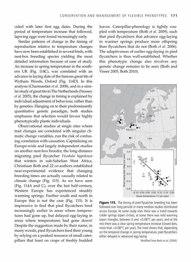
C O N S E R VAT I O N A N D M A N A G E M E N T O F F L E X I B L E P H E N OT Y P E S 1 7 1
cided with later fi rst egg dates. During the period of temperature increase that followed, lapwing eggs were found increasingly early.
Similar patterns of change in the timing of reproduction relative to temperature changes have now been established in several birds, with nest-box breeding species yielding the most detailed information because of ease of study. An increase in spring temperature in the south-ern UK ( Fig. 114C ), was correlated with an advance in laying date of the famous great tits of Wytham Woods, Oxford ( Fig. 114D ). In this analysis ( Charmantier et al . 2008 ), and in a simi-lar study of great tits in The Netherlands ( Nussey et al . 2005 ), the change in timing is explained by individual adjustment of behaviour, rather than by genetics. Hanging on to their predominantly quantitative genetic paradigm, both studies emphasize that selection would favour highly phenotypically plastic individuals.
Observational studies at single sites where trait changes are correlated with singular cli-matic change variables, run the risk of confus-ing correlation with causation. Capitalizing on Europe-wide and largely independent studies on another nest-box breeder, the long-distance migrating pied fl ycatcher Ficedula hypoleuca that winters in sub-Sahelian West Africa, Christiaan Both and 22 co-authors established near-experimental evidence that changing breeding times are actually causally related to climate change ( Fig. 115 ). As we have seen ( Fig. 114A and C), over the last half-century, Western Europe has experienced steadily warming springs. Further south and north in Europe this is not the case ( Fig. 115 ). It is impressive to fi nd that pied fl ycatchers bred increasingly earlier in areas where tempera-tures had gone up, but delayed egg-laying in areas where temperatures had gone down! Despite the suggestion made by their name, in many woods, pied fl ycatchers feed their young by relying on a peaked resource of small cater-pillars that feast on crops of freshly budded
leaves. Caterpillar-phenology is tightly cou-pled with temperature ( Both et al . 2009 ), such that pied fl ycatchers that advance egg-laying in warmer springs produce more offspring than fl ycatchers that do not ( Both et al . 2006 ). The adaptiveness of earlier egg-laying in pied fl ycatchers is thus well-established. Whether this phenotypic change also involves any genetic change remains to be seen ( Both and Visser 2005 , Both 2010 ).
1
2
7 24
1413
12
8,9,10,11
34 5
6
1516
17
18
19
25
21
20
23
22
–0.6
–0.4
–0.2
0.0
0.2
Slo
pe la
ying
dat
e (d
ays
per
year
)
0.10–0.10 –0.05 0.00 0.05 0.15
Slope temperature (°C per year)
0.20
2
1
221618 20
1917
23
2421
25
6
9
4
3
147
131012
118
5
15
0.4
Figure 115. The timing of pied fl ycatcher breeding has been followed over long periods in many nestbox studies distributed across Europe. At some study sites there was a trend towards colder springs (open circles), at some there was mild warming (open triangles, between 0 and +0.08°C per year), and at the rest there was a clear spring temperature increase (closed dots, more than +0.08°C per year). The inset shows that, depending on the temporal change in spring temperature, pied fl ycatchers either delayed or advanced egg laying.
Modifi ed from Both et al . ( 2004 ).
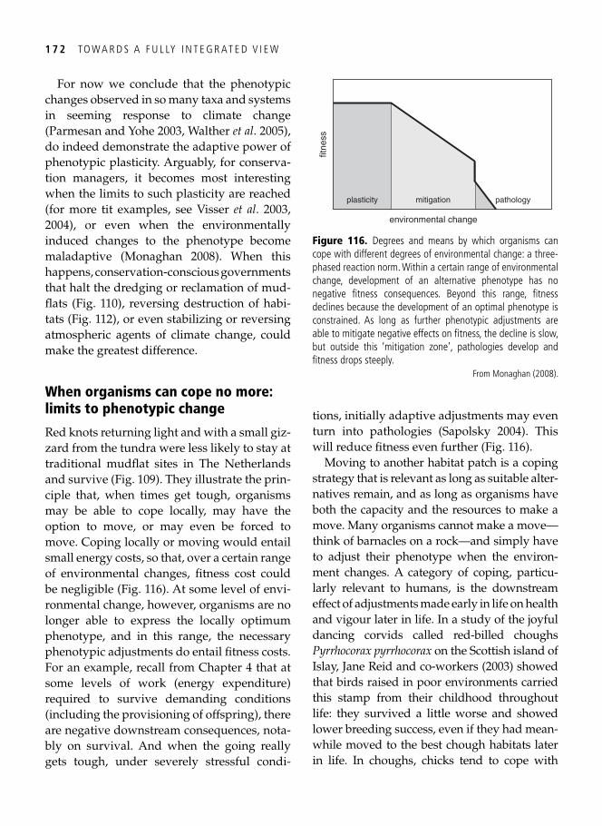
1 7 2 TO W A R D S A F U L LY I N T E G R AT E D V I E W
For now we conclude that the phenotypic changes observed in so many taxa and systems in seeming response to climate change ( Parmesan and Yohe 2003 , Walther et al . 2005 ), do indeed demonstrate the adaptive power of phenotypic plasticity. Arguably, for conserva-tion managers, it becomes most interesting when the limits to such plasticity are reached (for more tit examples, see Visser et al . 2003 , 2004 ), or even when the environmentally induced changes to the phenotype become maladaptive ( Monaghan 2008 ). When this happens, conservation-conscious governments that halt the dredging or reclamation of mud-fl ats ( Fig. 110 ), reversing destruction of habi-tats ( Fig. 112 ), or even stabilizing or reversing atmospheric agents of climate change, could make the greatest difference.
When organisms can cope no more: limits to phenotypic change
Red knots returning light and with a small giz-zard from the tundra were less likely to stay at traditional mudfl at sites in The Netherlands and survive ( Fig. 109 ). They illustrate the prin-ciple that, when times get tough, organisms may be able to cope locally, may have the option to move, or may even be forced to move. Coping locally or moving would entail small energy costs, so that, over a certain range of environmental changes, fi tness cost could be negligible ( Fig. 116 ). At some level of envi-ronmental change, however, organisms are no longer able to express the locally optimum phenotype, and in this range, the necessary phenotypic adjustments do entail fi tness costs. For an example, recall from Chapter 4 that at some levels of work (energy expenditure) required to survive demanding conditions (including the provisioning of offspring), there are negative downstream consequences, nota-bly on survival. And when the going really gets tough, under severely stressful condi-
tions, initially adaptive adjustments may even turn into pathologies ( Sapolsky 2004 ). This will reduce fi tness even further ( Fig. 116 ).
Moving to another habitat patch is a coping strategy that is relevant as long as suitable alter-natives remain, and as long as organisms have both the capacity and the resources to make a move. Many organisms cannot make a move—think of barnacles on a rock—and simply have to adjust their phenotype when the environ-ment changes. A category of coping, particu-larly relevant to humans, is the downstream effect of adjustments made early in life on health and vigour later in life. In a study of the joyful dancing corvids called red-billed choughs Pyrrhocorax pyrrhocorax on the Scottish island of Islay, Jane Reid and co-workers (2003) showed that birds raised in poor environments carried this stamp from their childhood throughout life: they survived a little worse and showed lower breeding success, even if they had mean-while moved to the best chough habitats later in life. In choughs, chicks tend to cope with
fitne
ss
environmental change
plasticity mitigation pathology
Figure 116. Degrees and means by which organisms can cope with different degrees of environmental change: a three-phased reaction norm. Within a certain range of environmental change, development of an alternative phenotype has no negative fi tness consequences. Beyond this range, fi tness declines because the development of an optimal phenotype is constrained. As long as further phenotypic adjustments are able to mitigate negative effects on fi tness, the decline is slow, but outside this ‘mitigation zone’, pathologies develop and fi tness drops steeply.
From Monaghan ( 2008 ).
C O N S E R VAT I O N A N D M A N A G E M E N T O F F L E X I B L E P H E N OT Y P E S 1 7 3
days of food shortage (and no growth), by faster compensatory growth as soon as the food sup-ply improves ( Schew and Ricklefs 1998 , Metcalfe and Monaghan 2001 ). That such growth accel-erations may actually come with costs later in life was shown in an elegant experiment with zebra fi nches. Here the degree of growth com-pensation was negatively correlated with the speed of learning a simple discriminatory task later in life ( Fisher et al . 2006 ).
Similar negative delayed effects of com-pensatory growth on cognition have been reported for small-born human infants (e.g. Estourgie-van Burk et al. 2009 ). It is the absence of a ‘silver spoon’ that tragically condemns some human groups to disease and poverty, partly because of the delayed detrimental effects of poor nutrition in early life ( Gluckman et al . 2009 ), or even during the pregnancy of the mother ( Roseboom et al . 2006 ). What is worse, longitudinal studies of children born in Amsterdam immediately after the Dutch winter famine at the end of the Second World War, showed that pre-natal famine may lead to poorer health, even in the offspring of these post-war children ( Painter et al . 2008 ). That health transcends genera-tions suggests that information other than
genes infl uences phenotypes. Whether there is more to phenotypic evolution than gene selection, and the very role of phenotypic plasticity in evolution, will be the subject of the next and fi nal chapter.
Synopsis
Humans modify habitats at a fast pace. With the disappearance of species-specifi c ‘good’ habitat there is no way to avoid individual dis-appearance and species extinctions. Species that persist tend to show considerable direc-tional phenotypic change across generations. Despite the best attempts to demonstrate that such changes refl ect genetic change, fi rm evi-dence for such micro-evolutionary processes in multicellular organisms is still quite limited. Instead, plants and animals have great pheno-typic plasticity, which, in several well-studied examples from the global ‘experiment’ of cli-mate change, helps these organisms to adjust and survive. Unless environmental conditions become so bad that coping strategies generate delayed negative effects, or even phenotypic breakdown, the various kinds of phenotypic plasticity certainly help organisms to survive in a world of change.
174
CHAPTER 10
Evolution in fi ve dimensions: phenotypes fi rst! . . . actually, if you say that genetics is relating variation in the genome to variation in phenotype, there is more accessible variation in expression than there is in sequence, and there is more variation in phenotype between cells and tissues and organs than between people.
P. Brown in an interview by J. Gitschier ( 2009 )
And the older identical twins become, the eas-ier it is to tell them apart! Not surprisingly, the shaping roles of development and environ-ment thus leave their marks on bodies that carry identical genomes. Bodies are fl exible, they change with age and with environment, but how does this relate to evolution? In this chapter we will elaborate, perhaps in a some-what partisan manner, the view that there is much more to evolution than selection of genes, which is the single axis of inheritance acknowledged in the ‘Modern Synthesis’ (e.g. Mayr 1982 , 2002 , Coyne 2009a ). As scientists we seem to be on the verge of a ‘post-Modern Synthesis’ in which the fl exible phenotype, in interaction with its environment, will take cen-tre stage.
Flexible phenotypes and the study of adaptation
This book has presented many examples of organisms responding to environmental chal-lenges, including humans during space-travel and competing in sports, and migrant birds conquering much of the globe in the course of their demanding annual itineraries. We hope to have succeeded in building an ever more pow-erful case that organisms and their particular environments are inseparable: changes in an
individual’s shape, size, and capacity will often be direct functions of the ecological demands placed upon them. Bodies express ecology.
What we have been talking about are adapta-tions, the functionally appropriate adjustment of phenotypes. In assembling our case, we have tried to foster the view that, for evolutionary insight, phenotype–environment interactions need to be studied functionally ( Feder and Watt 1992 , Watt 2000 ). Rather than emphasizing sim-ply that the capacity for phenotypic change is an adaptation (which it might well be; see Chapter 5 and Pigliucci 2001a , 2001b ), inter- and especially intra-individual trait variation can be used to evaluate the ‘goodness of design’ criterion for phenotypic adaptation. As argued by Piersma and Drent ( 2003 ), intra-individual phenotypic variations can demonstrate how alternative phenotypic representations of a single genotype represent adaptations. This is particularly appropriate when interspecifi c comparisons cannot be made. For example, to overcome the absence of matched food-specialists within the same taxon when studying digestive adapta-tions, Levey and Karasov ( 1989 ) compared the fl exible phenotypes of birds that were primarily frugivorous in autumn and insectivorous in spring.
Perhaps most importantly, reversible intra-individual phenotypic variation gives us a
E V O L U T I O N I N F I V E D I M E N S I O N S : P H E N OT Y P E S F I R S T ! 1 7 5
powerful tool to study phenotypic design experimentally ( Sinervo and Basolo 1996 , Sinervo 1999 ), almost in the same way that behavioural ecologists have so successfully unravelled the functions of behavioural traits ( Krebs and Davies 1987 ). In one tradition, such ‘phenotypic engineering’ has made use of hor-mone-implants, including the male sex hor-mone testosterone ( Sapolsky 1997 , Ketterson and Nolan 1999 ). In the dark-eyed juncos Junco hyemalis studied by the extended wife-and-husband team of Ellen D. Ketterson and Val Nolan ( Ketterson et al . 1991 , 1996 ), testosterone affected an array of phenotypic traits and life-history characteristics. This wide range of (interacting) effects actually limited the power of the hormonal implant approach. One of the examples of how natural and experimental variations of phenotype can enlighten issues of evolutionary adaptation, is spelled out in Chapters 6 and 7 . It is concerned with the vari-ably large muscular gizzards of birds eating hard-shelled prey ( Piersma et al . 1993b ). Our work with red knots showed that birds not only increased gizzard size when they shifted feeding from soft to hard food, but also increased their capacity to process that hard food, and vice versa ( van Gils et al . 2003a ). As we have seen in Chapter 9 , in an ecological context where large gizzards are necessary, individual red knots that managed to build up larger gizzards after returning from the Arctic tundra, were the ones who survived longest ( van Gils et al . 2006b ).
At this point in the argument, the study of appropriate phenotypic adjustment within generations meets the study of cross-genera-tional aspects of phenotypic adjustment— evolution proper. In evolutionary biology, a phenotypic trait can be considered an adapta-tion only if there is evidence that it has been moulded in specifi c ways during its evolution-ary history to make it more effective for its particular role ( Williams 1966b , West-Eberhard
1992 ). The question of whether this evolution-ary moulding is strictly a process of novel genetic instruction, or mostly one of the self-organized nature of pre-existing variations ( Newman and Müller 2000 , Camazine et al . 2001 , Turner 2007 ), cries out for much more investigation than we have the opportunity to indulge in here. Consequently we shall be obliged to leave it to one side and focus on the links between phenotypic plasticity and evolution.
Separating the environment from the organism . . .
In an insightful essay, Richard Lewontin and Richard Levins (2007) suggest that the most powerful contribution made by Charles Darwin to the development of modern biology was not his satisfactory evolutionary mecha-nism, but his ‘rigorous separation of internal and external forces that had, in previous theo-ries, been inseparable’. Before Charles Darwin, during the times of Lamarck and Charles’ grandfather Erasmus, many scientists enter-tained the thought of evolution involving modifi cation by descent. However, by allow-ing animals to propagate acquired characters in their offspring, they ‘totally confounded inner and outer forces in an unanalyzable whole’ ( Lewontin and Levins 2007 ). Charles Darwin separated a force (mutation) that was entirely internal to the organism and deter-mined the variation between individuals, from another force (natural selection) that was entirely external and determined which of the variations would survive and reproduce (survival of the fi ttest). Half a century after Darwin’s (1859) ‘ The origin of species ’, Johannsen ( 1911 ) proposed another distinction between the ‘internal and external forces’ when he considered the genotype to be the embellishment of a genome with its genetic instruction, and the phenotype to be the physi-
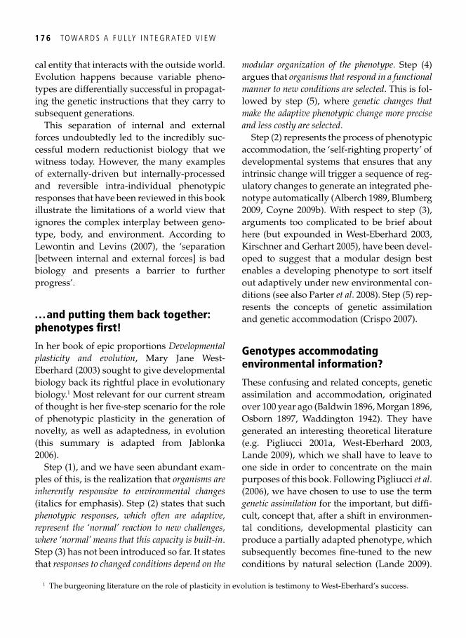
1 7 6 TO W A R D S A F U L LY I N T E G R AT E D V I E W
cal entity that interacts with the outside world. Evolution happens because variable pheno-types are differentially successful in propagat-ing the genetic instructions that they carry to subsequent generations.
This separation of internal and external forces undoubtedly led to the incredibly suc-cessful modern reductionist biology that we witness today. However, the many examples of externally-driven but internally-processed and reversible intra-individual phenotypic responses that have been reviewed in this book illustrate the limitations of a world view that ignores the complex interplay between geno-type, body, and environment. According to Lewontin and Levins ( 2007 ), the ‘separation [between internal and external forces] is bad biology and presents a barrier to further progress’.
. . . and putting them back together: phenotypes fi rst!
In her book of epic proportions Developmental plasticity and evolution , Mary Jane West-Eberhard ( 2003 ) sought to give developmental biology back its rightful place in evolutionary biology. 1 Most relevant for our current stream of thought is her fi ve-step scenario for the role of phenotypic plasticity in the generation of novelty, as well as adaptedness, in evolution (this summary is adapted from Jablonka 2006 ).
Step (1), and we have seen abundant exam-ples of this, is the realization that organisms are inherently responsive to environmental changes (italics for emphasis). Step (2) states that such phenotypic responses, which often are adaptive, represent the ‘normal’ reaction to new challenges, where ‘normal’ means that this capacity is built-in . Step (3) has not been introduced so far. It states that responses to changed conditions depend on the
modular organization of the phenotype . Step (4) argues that organisms that respond in a functional manner to new conditions are selected . This is fol-lowed by step (5), where genetic changes that make the adaptive phenotypic change more precise and less costly are selected .
Step (2) represents the process of phenotypic accommodation, the ‘self-righting property’ of developmental systems that ensures that any intrinsic change will trigger a sequence of reg-ulatory changes to generate an integrated phe-notype automatically ( Alberch 1989 , Blumberg 2009 , Coyne 2009b ). With respect to step (3), arguments too complicated to be brief about here (but expounded in West-Eberhard 2003 , Kirschner and Gerhart 2005 ), have been devel-oped to suggest that a modular design best enables a developing phenotype to sort itself out adaptively under new environmental con-ditions (see also Parter et al . 2008 ). Step (5) rep-resents the concepts of genetic assimilation and genetic accommodation ( Crispo 2007 ).
Genotypes accommodating environmental information?
These confusing and related concepts, genetic assimilation and accommodation, originated over 100 year ago ( Baldwin 1896 , Morgan 1896 , Osborn 1897 , Waddington 1942 ). They have generated an interesting theoretical literature (e.g. Pigliucci 2001a , West-Eberhard 2003 , Lande 2009 ), which we shall have to leave to one side in order to concentrate on the main purposes of this book. Following Pigliucci et al . ( 2006 ), we have chosen to use to use the term genetic assimilation for the important, but diffi -cult, concept that, after a shift in environmen-tal conditions, developmental plasticity can produce a partially adapted phenotype, which subsequently becomes fi ne-tuned to the new conditions by natural selection ( Lande 2009 ).
1 The burgeoning literature on the role of plasticity in evolution is testimony to West-Eberhard’s success.
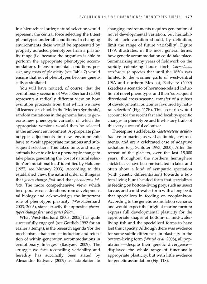
E V O L U T I O N I N F I V E D I M E N S I O N S : P H E N OT Y P E S F I R S T ! 1 7 7
In a hierarchical order, natural selection would represent the central force selecting the fi ttest phenotypes under all conditions. In changing environments these would be represented by properly adjusted phenotypes from a plastic-ity range (i.e. because the organism is able to perform the appropriate phenotypic accom-modation). If environmental conditions per-sist, any costs of plasticity (see Table 7 ) would ensure that novel phenotypes become geneti-cally assimilated.
You will have noticed, of course, that the evolutionary scenario of West-Eberhard ( 2003 ) represents a radically different view on how evolution proceeds from that which we have all learned at school. In the ‘Modern Synthesis’, random mutations in the genome have to gen-erate new phenotypic variants, of which the appropriate versions would then be selected in the ambient environment. Appropriate phe-notypic adjustments in new environments have to await appropriate mutations and sub-sequent selection. This takes time, and many animals have to die for a phenotypic change to take place, generating the ‘cost of natural selec-tion’ or ‘mutational load’ identifi ed by Haldane ( 1957 , see Nunney 2003 ). According to this established view, the natural order of things is that genes change fi rst and that phenotypes fol-low . The more comprehensive view, which incorporates considerations from developmen-tal biology and acknowledges the important role of phenotypic plasticity ( West-Eberhard 2003 , 2005 ), states exactly the opposite: pheno-types change fi rst and genes follow .
What West-Eberhard ( 2003 , 2005 ) has quite successfully engaged (see Gottlieb 1992 for an earlier attempt), is the research agenda ‘for the mechanisms that connect induction and reten-tion of within-generation accommodations in evolutionary lineages’ ( Badyaev 2009 ). The struggle we face reconciling variability and heredity has succinctly been stated by Alexander Badyaev ( 2009 ) as ‘adaptation to
changing environments requires generation of novel developmental variation, but heritabil-ity of such variation should, by defi nition, limit the range of future variability’. Figure 117A illustrates, in the most general terms, how genetic accommodation could take place. Summarizing many years of fi eldwork on the rapidly colonizing house fi nch Carpodacus mexicanus (a species that until the 1850s was limited to the warmer parts of west-central USA and northern Mexico), Badyaev ( 2009 ) sketches a scenario of hormone-related induc-tion of novel phenotypes and their ‘subsequent directional cross-seasonal transfer of a subset of developmental outcomes favoured by natu-ral selection’ ( Fig. 117B ). This scenario would account for the recent fast and locality-specifi c changes in phenotype and life-history traits of this very successful colonizer.
Threespine sticklebacks Gasterosteus aculea-tus live in marine, as well as limnic, environ-ments, and are a celebrated case of adaptive radiation (e.g. Schluter 1993 , 2000 ). After the retreat of the glaciers, over the last 15,000 years, throughout the northern hemisphere sticklebacks have become isolated in lakes and often show a kind of sympatric speciation (with genetic differentiation) towards a bot-tom-living blunt-headed form that specializes in feeding on bottom-living prey, such as insect larvae, and a mid-water form with a long beak that specializes in feeding on zooplankton. According to the genetic assimilation scenario, one would expect the original marine form to express full developmental plasticity for the appropriate shapes of bottom- or mid-water- living fi sh and the specialized forms to have lost this capacity. Although there was evidence for some subtle differences in plasticity in the bottom-living form ( Wund et al . 2008 ), all pop-ulations—despite their genetic divergence—displayed the whole range of functionally appropriate plasticity, but with little evidence for genetic assimilation ( Fig. 118 ).
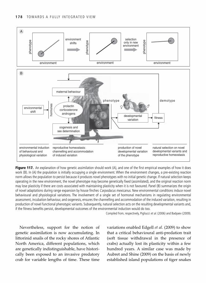
1 7 8 TO W A R D S A F U L LY I N T E G R AT E D V I E W
Nevertheless, support for the notion of genetic assimilation is now accumulating. In littorinid snails of the rocky shores of Atlantic North America, different populations, which are genetically indistinguishable, have histori-cally been exposed to an invasive predatory crab for variable lengths of time. These time
variations enabled Edgell et al . ( 2009 ) to show that a critical behavioural anti-predation trait (soft tissue withdrawal in the presence of crabs) actually lost its plasticity within a few hundred years. A similar case was made by Aubret and Shine ( 2009 ) on the basis of newly established island populations of tiger snakes
phen
otyp
eA
B
environmentshifts
phen
otyp
e selectiononly in newenvironment
phen
otyp
e
environment environment
maternal behaviour
oogenesis andsex determination
prolactincorticosterone
androgens
environmentalshift
horm
ones
environmental inductionof behavioural andphysiological variation
reproductive homeostasis:channelling and accommodationof induced variation
production of noveldevelopmental variationof the phenotype
developmentalvariation
fitness
natural selection on noveldevelopmental variants andreproductive homeostasis
demotypephenotype
environment
Figure 117. An explanation of how genetic assimilation should work (A), and one of the fi rst empirical examples of how it does work (B). In (A) the population is initially occupying a single environment. When the environment changes, a pre-existing reaction norm allows the population to persist because it produces novel phenotypes with no initial genetic change. If natural selection keeps operating in the new environment, the novel phenotype may become genetically fi xed (assimilated), and the original reaction norm may lose plasticity if there are costs associated with maintaining plasticity when it is not favoured. Panel (B) summarizes the origin of novel adaptations during range expansion by house fi nches Carpodacus mexicanus . New environmental conditions induce novel behavioural and physiological variations. The involvement of a single set of hormonal mechanisms in regulating environmental assessment, incubation behaviour, and oogenesis, ensures the channelling and accommodation of the induced variation, resulting in production of novel functional phenotypic variants. Subsequently, natural selection acts on the resulting developmental variants and, if the fi tness benefi ts persist, developmental outcomes of the environmental induction would do too.
Compiled from, respectively, Pigliucci et al . ( 2006 ) and Badyaev ( 2009 ).
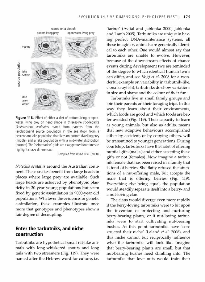
E V O L U T I O N I N F I V E D I M E N S I O N S : P H E N OT Y P E S F I R S T ! 1 7 9
Notechis scutatus around the Australian conti-nent. These snakes benefi t from large heads in places where large prey are available. Such large heads are achieved by phenotypic plas-ticity in 30-year young populations but seem fi xed by genetic assimilation in 9000-year old populations. Whatever the evidence for genetic assimilation, these examples illustrate once more that genotypes and phenotypes show a fair degree of decoupling.
Enter the tarbutniks, and niche construction
Tarbutniks are hypothetical small rat-like ani-mals with long-whiskered snouts and long tails with two streamers ( Fig. 119 ). They were named after the Hebrew word for culture, i.e.
‘tarbut’ ( Avital and Jablonka 2000 , Jablonka and Lamb 2005 ). Tarbutniks are unique in hav-ing perfect DNA-maintenance systems; all these imaginary animals are genetically identi-cal to each other. One would almost say that tarbutniks are unable to evolve. However, because of the downstream effects of chance events during development (we are reminded of the degree to which identical human twins can differ, and see Vogt et al . 2008 for a won-derful example on variability in tarbutnik-like, clonal crayfi sh), tarbutniks do show variations in size and shape and the colour of their fur.
Tarbutniks live in small family groups and join their parents on their foraging trips. In this way they learn about their environments, which foods are good and which foods are bet-ter avoided ( Fig. 119 ). Their capacity to learn as young animals, but also as adults, means that new adaptive behaviours accomplished either by accident, or by copying others, will be transmitted to younger generations. During courtship, tarbutniks have the habit of offering nuptial gifts (males) and either accepting these gifts or not (females). Now imagine a tarbut-nik female that has been raised in a family that is fond of berries. She fl atly refused the atten-tions of a nut-offering male, but accepts the male that is offering berries ( Fig. 119 ). Everything else being equal, the population would steadily separate itself into a berry- and a nut-loving clan.
The clans would diverge even more rapidly if the berry-loving tarbutniks were to hit upon the invention of protecting and nurturing berry-bearing plants; or if nut-loving tarbut-niks were to start cultivating nut-bearing bushes. At this point tarbutniks have ‘con-structed their niche’ ( Laland et al . 2008 ), and this niche cannot but reciprocally infl uence what the tarbutniks will look like. Imagine that berry-bearing plants are small, but that nut-bearing bushes need climbing into. The tarbutniks that love nuts would train their
bottom-living prey
marine
lakebottom
lakeopenwater
reared on a diet of:
sour
ce p
opul
atio
n
open water-living prey
Figure 118. Effect of either a diet of bottom-living or open-water living prey on head shape in threespine sticklebacks Gasterosteus aculeatus reared from parents from the (evolutionary) source population in the sea (top), from a descendant lake population that lives on bottom-dwelling prey (middle) and a lake population with a mid-water distribution (bottom). The ‘deformation’ grids are exaggerated four times to highlight shape differences.
Compiled from Wund et al . ( 2008 ).
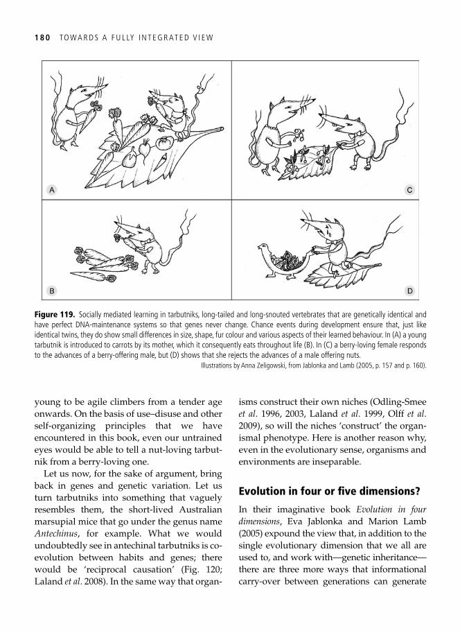
1 8 0 TO W A R D S A F U L LY I N T E G R AT E D V I E W
young to be agile climbers from a tender age onwards. On the basis of use–disuse and other self-organizing principles that we have encountered in this book, even our untrained eyes would be able to tell a nut-loving tarbut-nik from a berry-loving one.
Let us now, for the sake of argument, bring back in genes and genetic variation. Let us turn tarbutniks into something that vaguely resembles them, the short-lived Australian marsupial mice that go under the genus name Antechinus , for example. What we would undoubtedly see in antechinal tarbutniks is co-evolution between habits and genes; there would be ‘reciprocal causation’ ( Fig. 120 ; Laland et al . 2008 ). In the same way that organ-
isms construct their own niches ( Odling-Smee et al . 1996 , 2003 , Laland et al . 1999 , Olff et al . 2009 ), so will the niches ‘construct’ the organ-ismal phenotype. Here is another reason why, even in the evolutionary sense, organisms and environments are inseparable.
Evolution in four or fi ve dimensions?
In their imaginative book Evolution in four dimensions , Eva Jablonka and Marion Lamb (2005) expound the view that, in addition to the single evolutionary dimension that we all are used to, and work with—genetic inheritance—there are three more ways that informational carry-over between generations can generate
Figure 119. Socially mediated learning in tarbutniks, long-tailed and long-snouted vertebrates that are genetically identical and have perfect DNA-maintenance systems so that genes never change. Chance events during development ensure that, just like identical twins, they do show small differences in size, shape, fur colour and various aspects of their learned behaviour. In (A) a young tarbutnik is introduced to carrots by its mother, which it consequently eats throughout life (B). In (C) a berry-loving female responds to the advances of a berry-offering male, but (D) shows that she rejects the advances of a male offering nuts.
Illustrations by Anna Zeligowski, from Jablonka and Lamb ( 2005 , p. 157 and p. 160).
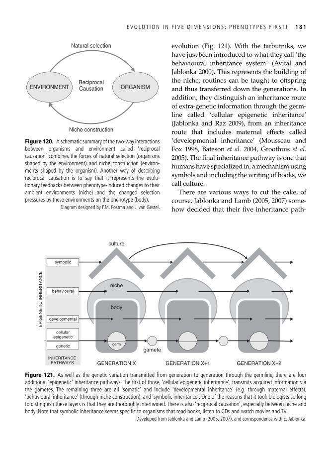
E V O L U T I O N I N F I V E D I M E N S I O N S : P H E N OT Y P E S F I R S T ! 1 8 1
evolution ( Fig. 121 ). With the tarbutniks, we have just been introduced to what they call ‘the behavioural inheritance system’ ( Avital and Jablonka 2000 ). This represents the building of the niche; routines can be taught to offspring and thus transferred down the generations. In addition, they distinguish an inheritance route of extra-genetic information through the germ-line called ‘cellular epigenetic inheritance’ ( Jablonka and Raz 2009 ), from an inheritance route that includes maternal effects called ‘developmental inheritance’ ( Mousseau and Fox 1998 , Bateson et al . 2004 , Groothuis et al . 2005 ). The fi nal inheritance pathway is one that humans have specialized in, a mechanism using symbols and including the writing of books, we call culture.
There are various ways to cut the cake, of course. Jablonka and Lamb ( 2005 , 2007 ) some-how decided that their fi ve inheritance path-
ENVIRONMENT ORGANISMReciprocalCausation
Natural selection
Niche construction
Figure 120. A schematic summary of the two-way interactions between organisms and environment called ‘reciprocal causation’ combines the forces of natural selection (organisms shaped by the environment) and niche construction (environ-ments shaped by the organism). Another way of describing reciprocal causation is to say that it represents the evolu-tionary feedbacks between phenotype-induced changes to their ambient environments (niche) and the changed selection pressures by these environments on the phenotype (body).
Diagram designed by F.M. Postma and J. van Gestel.
GENERATION X
niche
cellularepigenetic
behavioural
symbolic
INHERITANCEPATHWAYS
culture
body
EP
IGE
NE
TIC
INH
ER
ITA
NC
E
germ
gamete
GENERATION X+1 GENERATION X+2
developmental
genetic
Figure 121. As well as the genetic variation transmitted from generation to generation through the germline, there are four additional ‘epigenetic’ inheritance pathways. The fi rst of those, ‘cellular epigenetic inheritance’, transmits acquired information via the gametes. The remaining three are all ‘somatic’ and include ‘developmental inheritance’ (e.g. through maternal effects), ‘behavioural inheritance’ (through niche construction), and ‘symbolic inheritance’. One of the reasons that it took biologists so long to distinguish these layers is that they are thoroughly intertwined. There is also ‘reciprocal causation’, especially between niche and body. Note that symbolic inheritance seems specifi c to organisms that read books, listen to CDs and watch movies and TV.
Developed from Jablonka and Lamb ( 2005 , 2007 ), and correspondence with E. Jablonka.
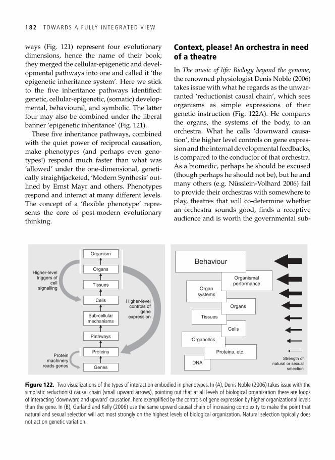
1 8 2 TO W A R D S A F U L LY I N T E G R AT E D V I E W
ways ( Fig. 121 ) represent four evolutionary dimensions, hence the name of their book; they merged the cellular-epigenetic and devel-opmental pathways into one and called it ‘the epigenetic inheritance system’. Here we stick to the fi ve inheritance pathways identifi ed: genetic, cellular-epigenetic, (somatic) develop-mental, behavioural, and symbolic. The latter four may also be combined under the liberal banner ‘epigenetic inheritance’ ( Fig. 121 ).
These fi ve inheritance pathways, combined with the quiet power of reciprocal causation, make phenotypes (and perhaps even geno-types!) respond much faster than what was ‘allowed’ under the one-dimensional, geneti-cally straightjacketed, ‘Modern Synthesis’ out-lined by Ernst Mayr and others. Phenotypes respond and interact at many different levels. The concept of a ‘fl exible phenotype’ repre-sents the core of post-modern evolutionary thinking.
Context, please! An orchestra in need of a theatre
In The music of life: Biology beyond the genome , the renowned physiologist Denis Noble ( 2006 ) takes issue with what he regards as the unwar-ranted ‘reductionist causal chain’, which sees organisms as simple expressions of their genetic instruction (Fig. 122A). He compares the organs, the systems of the body, to an orchestra. What he calls ‘downward causa-tion’, the higher level controls on gene expres-sion and the internal developmental feedbacks, is compared to the conductor of that orchestra. As a biomedic, perhaps he should be excused (though perhaps he should not be), but he and many others (e.g. Nüsslein-Volhard 2006 ) fail to provide their orchestras with somewhere to play, theatres that will co-determine whether an orchestra sounds good, fi nds a receptive audience and is worth the governmental sub-
Higher-levelcontrols of
geneexpression
Organism
Organs
Tissues
Cells
Sub-cellularmechanisms
Pathways
Proteins
Genes
Higher-leveltriggers of
cellsignalling
Proteinmachinery
reads genesDNA
Proteins, etc.
Organelles
Cells
Tissues
Organs
Organsystems
Organismalperformance
Behaviour
Strength ofnatural or sexual
selection
Figure 122. Two visualizations of the types of interaction embodied in phenotypes. In (A), Denis Noble ( 2006 ) takes issue with the simplistic reductionist causal chain (small upward arrows), pointing out that at all levels of biological organization there are loops of interacting ‘downward and upward’ causation, here exemplifi ed by the controls of gene expression by higher organizational levels than the gene. In (B), Garland and Kelly ( 2006 ) use the same upward causal chain of increasing complexity to make the point that natural and sexual selection will act most strongly on the highest levels of biological organization. Natural selection typically does not act on genetic variation.
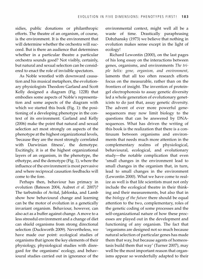
E V O L U T I O N I N F I V E D I M E N S I O N S : P H E N OT Y P E S F I R S T ! 1 8 3
sidies, public donations or philanthropic efforts. The theatre of an organism, of course, is the environment. It is the environment that will determine whether the orchestra will suc-ceed. But is there an audience that determines whether in a particular theatre a particular orchestra sounds good? Not visibly, certainly, but natural and sexual selection can be consid-ered to enact the role of invisible spectators.
As Noble wrestled with downward causa-tion and his musical metaphors, the evolution-ary physiologists Theodore Garland and Scott Kelly designed a diagram (Fig. 122B) that embodies some aspects of Noble’s representa-tion and some aspects of the diagram with which we started this book ( Fig. 1 ): the posi-tioning of a developing phenotype in the con-text of its environment. Garland and Kelly ( 2006 ) make the point that natural and sexual selection act most strongly on aspects of the phenotype at the highest organizational levels, ‘because they are the most strongly correlated with Darwinian fi tness’, the demotype. Excitingly, it is at the highest organizational layers of an organism, in the phenotype, the ethotype, and the demotype ( Fig. 1 ), where the infl uence of the environment is most pervasive and where reciprocal causation feedbacks will come to the fore.
Perhaps then, behaviour has primacy in evolution ( Bateson 2004 , Aubret et al . 2007 )? The tarbutniks of Avital, Jablonka, and Lamb show how behavioural change and learning can be the motor of evolution in a genetically invariant organism. Behaviour, however, can also act as a buffer against change. A move to a less stressful environment and a change of diet can shield organisms from strong directional selection ( Duckworth 2009 ). Nevertheless, we have made our point: ecological studies of organisms that ignore the key elements of their physiology, physiological studies with disre-gard for the organisms’ ecology, and behav-ioural studies carried out in ignorance of the
environmental context, might well all be a waste of time. Drastically paraphrasing Dobzhansky ( 1973 ) we believe that nothing in evolution makes sense except in the light of ecology!
Richard Lewontin ( 2000 ), on the last pages of his long essay on the interactions between genes, organisms, and environments The tri-ple helix: gene, organism, and environment , laments that all too often research efforts focus on the measurable, rather than on the frontiers of insight. The invention of protein-gel electrophoresis to assay genetic diversity led a whole generation of evolutionary genet-icists to do just that, assay genetic diversity. The advent of ever more powerful gene-sequencers may now limit biology to the questions that can be answered by DNA-sequences. What has driven the writing of this book is the realization that there is a con-tinuum between organisms and environ-ments that needs much more attention in the complementary realms of physiological, behavioural, ecological, and evolutionary study—the notable complication that even ‘small changes in the environment lead to small changes in the organism that, in turn, lead to small changes in the environment ( Lewontin 2000 ). What we have come to real-ize as well is that life scientists must not only include the ecological theatre in their think-ing and their measurements, but also that in the biology of the future there should be equal attention to the two, complementary, roles of the genetic coding of some processes and the self-organizational nature of how these proc-esses are played out in the development and functioning of any organism. The fact that ‘organisms are designed not so much because natural selection of particular genes has made them that way, but because agents of homeos-tasis build them that way’ ( Turner 2007 ), may well be the most important reason that organ-isms appear so wonderfully adapted to their
1 8 4 TO W A R D S A F U L LY I N T E G R AT E D V I E W
environments and their environments to them.
Synopsis
In this book we have offered a progression of ideas that support the view that, although bodies and environments are recognizable entities, they really are inseparable. In this fi nal chapter we extend this view to evolu-tion—the inheritance of, and selection for, ran-domly variable phenotypic traits across generations. What we fi nd is that evolutionary
change needs systems of inheritance, but we also fi nd that the genetic system that we all work with is just one of fi ve such possible inheritance systems. Since organisms not only provide the beginnings and nurture of their offspring, but also build the environments in which they and their offspring live, there are very tight feedbacks of reciprocal causation, both in the development of organisms and in the relationships between the developing organism and their environments. Bodies are earth, and we would do well to acknowledge that in the ways that we study them.
185
References
Abdalla, E.B., Kotby, E.A., and Johnson, H.D. (1993). Physiological responses to heat-induced hyperthermia of pregnant and lactating ewes. Small Ruminant Research 11 , 125–34.
Adamo, S.A., Barlett, A., Le, J., Spencer, N., and Sullivan, K. (2010). Illness-induced anorexia may reduce trade-offs between digestion and immune function. Animal Behaviour 79 , 3–10.
Adams, G.R., Caiozzo, V.J., and Baldwin, K.M. (2003). Skeletal unweighting: spacefl ight and ground-based models. Journal of Applied Physiology 95 , 2185–2201.
Alberch, P. (1989). The logic of monsters: Evidence for internal constraint in development and evolution. Geobios 19 , 21–57.
Alerstam, T. (2003). Bird migration speed. In Avian migra-tion , eds P. Berthold, E. Gwinner, and E. Sonnenschein, pp. 253–67. Springer-Verlag, Berlin.
Alerstam, T. and Jönsson, P.E. (1999). Ecology of tundra birds: Patterns of distribution, breeding and migration along the Northeast Passage. Ambio 28 , 212–24.
Alexander, R.McN. (1984). Optimum strengths for bones liable to fatigue and accidental fracture. Journal of Theoretical Biology 109 , 247–52.
Alexander, R.McN. (1997). A theory of mixed chains applied to safety factors in biological systems. Journal of Theoretical Biology 184 , 621–36.
Alexander, R.McN. (1998). Symmorphosis and safety factors. In Principles of animal design: The optimization and symmorphosis debate , eds E.R. Weibel, C.R. Taylor, and L. Bolis, pp. 28–35. Cambridge University Press, Cambridge.
Allen, M.R., Frame, D.J., Huntingford, C., Jones, C.D., Lowe, J.A., Meinshausen, M., and Meinshausen, N. (2009). Warming caused by cumulative carbon emis-sions towards the trillionth tonne. Nature 458 , 363–68.
Alonso-Alvarez, C., Bertrand, S., Devevey, G.L., Prost, J., Faivre, B., Sorci, G., and Loeschcke, V. (2004). Increased susceptibility to oxidative stress as a proximate cost of reproduction. Ecology Letters 7 , 363–68.
Amann, M., Eldridge, M.W., Lovering, A.T., Stickland, M.K., Pegelow, D.F., and Dempsey, J.A. (2006). Arterial oxygenation infl uences central motor output and exer-
cise performance via effects on peripheral locomotor muscle fatigue in humans. Journal of Physiology 575 , 937–52.
Anderson, K.J. and Jetz, W. (2005). The broad-scale ecol-ogy of energy expenditure of endotherms. Ecology Letters 8 , 310–18.
Anderson, T.R., Hessen, D.O., Elser, J.J., and Urabe, J. (2005). Metabolic stoichiometry and the fate of excess carbon and nutrients in consumers. American Naturalist 165 , 1–15.
Arad, Z., Midtgard, U., and Bernstein, M.H. (1989). Thermoregulation in Turkey vultures: Vascular anat-omy, arteriovenous heat exchange, and behaviour. Condor 91 , 505–14.
Arngrimsson, S.A., Petitt, D.S., Borrani, F., Skinner, K.A., and Cureton, K.J. (2004). Hyperthermia and maximal oxygen uptake in men and women. European Journal of Applied Physiology 92 , 524–32.
Arsenault, D.J., Marchinko, K.B., and Palmer, A.R. (2001). Precise tuning of barnacle leg length to coastal wave action. Proceedings of the Royal Society, London, B 268 , 2149–54.
Aschoff, J. (1954). Zeitgeber der tierischen Tagesperiodik. Naturwissenschaften 41 49–56.
Aschoff, J. and Pohl, H. (1970). Der Ruheumsatz von Vögeln als Funktion der Tageszeit und des Körpergrösse. Journal für Ornithologie 111 , 38–47.
Ashton, K.G. (2002). Patterns of within-species body size variation of birds: strong evidence for Bergmann’s rule. Global Ecology and Biogeography 11 , 505–23.
Ashton, K.G., Tracy, M.C., and de Queiroz, A. (2000). Is Bergmann’s rule valid for mammals? American Naturalist 156 , 390–415.
Aubret, F. and Shine, R. (2009). Genetic assimilation and the postcolonization erosion of phenotypic plasticity in island tiger snakes. Current Biology 19 , 1932–36.
Aubret, F., Bonnet, X., and Shine, R. (2007). The role of adaptive plasticity in a major evolutionary transition: Early aquatic experience affects locomotor performance of terrestrial snakes. Functional Ecology 21 , 1154–61.
Austad, S.N. (1997). Why we age: What science is discovering about the body’s journey through life . Wiley, New York.
1 8 6 R E F E R E N C E S
Avital, E. and Jablonka, E. (2000). Animal traditions: behav-ioural inheritance in evolution . Cambridge University Press, Cambridge.
Bacigalupe, L.D. and Bozinovic, F. (2002). Design limita-tions and sustained metabolic rate: Lessons from small mammals. Journal of Experimental Biology 205 , 2963–70.
Badyaev, A.V. (2009). Evolutionary signifi cance of pheno-typic accommodation in novel environments: An empir-ical test of the Baldwin effect. Philosophical Transactions of the Royal Society, London, B 364 , 1125–41.
Bailey, E. (1998). Odds on the FAST gene. Genome Research 8 , 569–71.
Baker, A.J., Piersma, T., and Greenslade, A.D. (1999). Molecular versus phenotypic sexing in red knots. Condor 101 , 887–93.
Baker, A.J., González, P.M., Piersma, T., Niles, L.J., de Lima Serrano do Nascimento, I., Atkinson, P.W., Clark, N.A., Minton, C.D.T., Peck, M.K., and Aarts, G. (2004). Rapid population decline in red knots: Fitness consequences of decreased refuelling rates and late arrival in Delaware Bay. Proceedings of the Royal Society, London, B 271 , 875–82.
Bakken, G.S. (1976). A heat transfer analysis of animals: Unifying concepts and the application of metabolism chamber data to fi eld ecology. Journal of Theoretical Biology 60 , 337–84.
Bakken, G.S. and Gates, D.M. (1974). Linearized heat transfer relations in biology. Science 183 , 976–77.
Baldwin, J.M. (1896). A new factor in evolution. American Naturalist 30 , 354–451.
Banavar, J.R., Damuth, J., Maritan, A., and Rinaldo, A. (2003). Allometric cascades. Nature 421 , 713–14.
Barja, G., Cadenas, S., Rojas, C., Perez-Campo, R., and López-Torres, M. (1994). Low mitochondrial free radical production per unit O 2 consumption can explain the simultaneous presence of high longevity and high aero-bic metabolic rate in birds. Free Radical Research 21 , 317–28.
Barnes, M. (1992). The reproductive periods and condition of the penis in several species of common Cirripedes. Oceanography and Marine Biology: an Annual Review , 30 483–525.
Barter, M. (2002). Shorebirds of the Yellow Sea: impor-tance, threats and conservation. International Wader Studies 12 , 1–104.
Bartholomew, G.A. (1958). The role of physiology in the distribution of terrestrial vertebrates. In Zoogeography , ed. C.L. Hubbs, pp. 81–95. Publ. No. 51, American Association for the Advancement of Science, Washington, DC.
Bartholomew, G.A. and Cade, T.J. (1963). The water econ-omy of land birds. Auk 80 , 504–39.
Bateson, P. (2004). The active role of behaviour in evolu-tion. Biology and Philosophy 19 , 283–98.
Bateson, P., Barker, D., Clutton-Brock, T., Deb, D., D’Udine, B., Foley, R.A., Gluckman, P., Godfrey, K., Kirkwood, T., Lahr, M.M., McNamara, J., Metcalfe, N.B., Monaghan, P., Spencer, H.G., and Sultan, S.E. (2004). Developmental plasticity and human health. Nature 430 , 419–21.
Battley, P.F. and Piersma, T. (2005). Adaptive interplay between feeding ecology and features of the digestive tract in birds. In Physiological and ecological adaptations to feeding in vertebrates , eds J.M. Starck and T. Wang, pp. 201–28. Science Publishers, Enfi eld.
Battley, P.F., Piersma, T., Dietz, M.W., Tang, S., Dekinga, A., and Hulsman, K. (2000). Empirical evidence for differ-ential organ reductions during trans-oceanic bird fl ight. Proceedings of the Royal Society, London, B 267 , 191–96.
Battley, P.F., Dietz, M.W., Piersma, T., Dekinga, A., Tang, S., and Hulsman, K. (2001). Is long-distance bird fl ight equivalent to a high-energy fast? Body composition changes in freely migrating and captive fasting great knots. Physiological and Biochemical Zoology 74 , 435–49.
Battley, P.F., Rogers, D.I., Piersma, T., and Koolhaas, A. (2003). Behavioural evidence for heat-load problems in great knots in tropical Australia fuelling for long-dis-tance fl ight. Emu 103 , 97–103.
Battley, P.F., Rogers, D.I., van Gils, J.A., Piersma, T., Hassell, C.J., Boyle, A., and Yang, H-Y. (2005). How do red knots Calidris canutus leave Northwest Australia in May and reach the breeding grounds in June? Predictions of stop-over times, fuelling rates, and prey quality in the Yellow Sea. Journal of Avian Biology 36 , 494–500.
Bauchinger, U. and McWilliams, S. (2009). Carbon turno-ver in tissues of a passerine bird: Allometry, isotopic clocks, and phenotypic fl exibility of organ size. Physiological and Biochemical Zoology 82 , 787–97.
Bauchinger, U., Kolb, H., Afi k, D., Pinshow, B., and Biebach, H. (2009). Blackcap warblers maintain diges-tive effi ciency by increasing digesta retention time on the fi rst day of migratory stopover. Physiological and Biochemical Zoology 82 , 541–48.
Bech, C., Langseth, I., and Gabrielsen, G.W. (1999). Repeatability of basal metabolism in breeding female kittiwakes Rissa tridactyla . Proceedings of the Royal Society, London, B 266 , 2161–67.
Beck, C. (2004). Personal portrait Bart Kempenaers—Ornithology. Max Planck Research 2 /2004, 64–67.
Bednekoff, P.A. and Lima, S.L. (1998). Re-examining safety in numbers: Interactions between risk dilution and col-lective detection depend upon predator targeting behaviour. Proceedings of the Royal Society, London, B 265 , 2021–26.
R E F E R E N C E S 1 8 7
Beintema, A.J., Beintema-Hietbrink, R.J., and Müskens, G.J.D.M. (1985). A shift in the timing of breeding in meadow birds. Ardea 73 , 83–89.
Bennett, A.F. and Ruben, J.A. (1979). Endothermy and activity in vertebrates. Science 206 , 649–54.
Bennett, G.F., Montgomerie, R., and Seutin, G. (1992). Scarcity of haematozoa in birds breeding on the arctic tundra of North America. Condor 94 , 289–92.
Berger, J. (2007). Fear, human shields and the redistribu-tion of prey and predators in protected areas. Biology Letters 3 , 620–23.
Bergmann, C. (1847). Über die Verhältnisse der Wärmeökonomie der Thiere zu ihrer Grösse. Göttinger Studien 3 , 595–708.
Bergmann, O., Bhardwaj, R.D., Bernard, S., Zdunek, S., Barnabé-Heider, F., Walsh, S., Zupinich, J., Alkass, K., Druid, H., Jivinge, S., and Frisén, J. (2009). Evidence for cariomycete renewal in humans. Science 325 , 98–102.
Berry, H. (1990). From LA to New York, from New York to LA . Self-published, Chorley, UK.
Bibby, R., Cleall-Harding, P., Rundle, S., Widdicombe, S., and Spicer, J. (2007). Ocean acidifi cation disrupts induced defences in the intertidal gastropod Littorina littorea . Biology Letters 3 , 699–701.
Biebach, H. (1990). Strategies of trans-Sahara migrants. In Bird migration , ed. E. Gwinner, pp. 352–67. Springer-Verlag, Berlin.
Biebach, H., Biebach, I., Friedrich, W., Heine, G., Partecke, J., and Schmidl, D. (2000). Strategies of passerine migra-tion across the Mediterranean Sea and the Sahara desert: a radar study. Ibis 142 , 623–34.
Biernaskie, J.M., Walker, S.C., and Gegear, R.J. (2009). Bumblebees learn to forage like Bayesians. American Naturalist 174 , 413–23.
Biggerstaff, S. and Mann, M. (1992). Consummatory behaviors and weight regulation in pregnant, lactating, and pregnant-lactating mice. Physiology and Behavior 52 , 485–91.
Bigland-Ritchie, B. and Vollestadt, N. (1988). Hypoxia and fatigue: how are they related? In Hypoxia: the tolerable limits , eds J.R. Sutton, C.S. Houston, and G. Coates, pp. 315–25. Benchmark, Indianapolis, Ill.
Bijleveld, A.I., Egas, M., van Gils, J.A., and Piersma, T. (2010). Beyond the information centre hypothesis: Communal roosting for information on food, predators, travel companions and mates? Oikos 119 , 277–85.
Bilz, S., Ninnis, R., and Keller, U. (1999). Effects of hypoos-molality on whole-body lipolysis in man. Metabolism - Clinical and Experimental 48 , 472–76.
Bishop, C.M. (1999). The maximum oxygen consumption and aerobic scope of birds and mammals: Getting to the
heart of the matter. Proceedings of the Royal Society, London, B 266 , 2275–81.
Black, A.E., Coward, W.A., Cole, T.J., and Prentice, A.M. (1996). Human energy expenditure in affl uent societies: An analysis of 574 doubly-labelled water measure-ments. European Journal of Clinical Nutrition 50 , 72–92.
Black, J.L., Mullan, B.P., Lorschy, M.L., and Giles, L.R. (1993). Lactation in the sow during heat-stress. Livestock Production Science 35 , 153–70.
Blaxter, K. (1989). Energy metabolism in animals and man. Cambridge University Press, Cambridge.
Blumberg, M.S. (2009). Freaks of nature: What anomalies tell us about development and evolution. Oxford University Press, New York.
Bohning-Gaese, K., Halbe, B., Lemoine, N., and Oberrath, R. (2000). Factors infl uencing clutch size, number of broods and annual fecundity of North American and European land birds. Evolutionary Ecology Research 2 , 8230839.
Bonner, J.T. (2006). Why size matters: From bacteria to blue whales . Princeton University Press, Princeton, NJ.
Bonnet, X., Bradshaw, A.D., and Shine, R. (1998). Capital versus income breeding: An ectothermic perspective. Oikos 83, 333–42.
Bonnie, K.E. and Earley, R.L. (2007). Expanding the scope for social information use. Animal Behaviour 74 , 171–81.
Bonser, R.H.C. (1996). The mechanical properties of feather keratins. Journal of Zoology 239 , 477–84.
Both, C. (2010). Flexibility of timing of avian migration to climate change masked by environmental conditions en route. Current Biology 20 , 243–48.
Both, C. and Visser, M.E. (2005). The effect of climate change on the correlation between life-history traits. Global Change Biology 11 , 1606–13.
Both, C., Artemyev, V.A., Blaauw, B., Cowie, R.J., Dekhuijzen, A.J., Eeva, T., Enemar, A., Gustafsson, L., Ivankina, E.V., Järvinen, A., Metcalfe, N.B., Nyholm, N.E.I., Potti, J., Ravussin, P-A., Sanz, J.J., Silverin, B., Slater, F.M., Sokolov, L.V., Török, J., Winkel, W., Wright, J., Zang, H., and Visser, M.E. (2004). Large-scale geo-graphical variation confi rms that climate change causes birds to lay earlier. Proceedings of the Royal Society, London, B 271 , 1657–62.
Both, C., Piersma, T., and Roodbergen, S. P. (2005). Climatic change explains much of the 20 th century advance in laying date of northern lapwing Vanellus vanellus in The Netherlands. Ardea 93 , 79–88.
Both, C., Bouwhuis, S., Lessells, C.M., and Visser, C.M. (2006). Climate change and population declines in a long-distance migratory bird. Nature 441 , 81–83.
Both, C., van Asch, M., Bijlsma, R.G., van den Burg, A.B., and Visser, M.E. (2009). Climate change and unequal pheno-
1 8 8 R E F E R E N C E S
logical changes across four trophic levels: Constraints or adaptations? Journal of Animal Ecology 78 , 73–83.
Bouwhuis, S., Sheldon, B.C., Verhulst, S., and Charmantier, A. (2009). Great tits growing old: Selective disappear-ance and the partitioning of senescence to stages within the breeding cycle. Proceedings of the Royal Society, London, B 276 , 2769–77.
Boyd, I.L. (2000). State-dependent fertility in pinnipeds: Contrasting capital and income breeders. Functional Ecology 14, 623–30.
Brakefi eld, P.M. and Reitsma, N. (1991). Phenotypic plas-ticity, seasonal climate and the population biology of Bicyclus butterfl ies (Satyridae) in Malawi. Ecological Entomology 16 , 291–303.
Brakefi eld, P.M., Pijpe, J., and Zwaan, B.J. (2007). Developmental plasticity and acclimation both contrib-ute to adaptive responses to alternating seasons of plenty and of stress in Bicyclus butterfl ies. Journal of Biosciences 32 , 465–75.
Briffa, M. and Sneddon, L.U. (2007). Physiological constraints on contest behaviour. Functional Ecology 21 , 627–37.
Brisbin, I.L. (1969). Bioenergetics of the breeding cycle of the ring dove. Auk 86 , 54–74.
Brody, S. (1945). Bioenergetics and growth . Reinhold (reprinted Hafner Publishing Company), New York.
Broggi, J., Hohtola, E., Orell, M., and Nilsson, J-Å. (2005). Local adaptation to winter conditions in a passerine spreading north: A common-garden approach. Evolution 59 , 1600–1603.
Brown, J.S. (1988). Patch use as an indicator of habitat preference, predation risk and competition. Behavioral Ecology and Sociobiology 22 , 37–48.
Brown, J.S. and Kotler, B.P. (2004). Hazardous duty pay and the foraging cost of predation. Ecology Letters 7 , 999–1014.
Brown, J.S., Laundré, J.W., and Gurung, M. (1999). The ecology of fear: Optimal foraging, game theory, and trophic interactions. Journal of Mammalogy 80 , 385–99.
Bruinzeel, L.W., Piersma, T., and Kersten, M. (1999). Low costs of terrestrial locomotion in waders. Ardea 87 , 199–205.
Brunner, D., Kacelnik, A., and Gibbon, J. (1992). Optimal foraging and timing processes in the starling, Sturnus vulgaris : Effect of inter-capture interval. Animal Behaviour 44 , 597–613.
Brunner, D., Kacelnik, A., and Gibbon, J. (1996). Memory for inter-reinforcement interval variability and patch departure decisions in the starling, Sturnus vulgaris . Animal Behaviour 51 , 1025–45.
Bryant, D.M. and Tatner, P. (1991). Intraspecies variation in energy expenditure: Correlates and constraints. Ibis 133 , 236–45.
Bryant, D.M. and Westerterp, K.R. (1980). The energy budget of the house martin ( Delichon urbica ). Ardea 68 , 91–102.
Bubenik, G.A. and Bubenik, A.B. eds (1990). Horns, prong-horns, and antlers: Evolution, morphology, physiology, and social signifi cance . Springer-Verlag, New York.
Buehler, D.M. and Baker, A.J. (2005). Population diver-gence times and historical demography in red knots and dunlins. Condor 107 , 497–513.
Buehler, D.M. and Piersma, T. (2008). Travelling on a budget: Predictions and ecological evidence for bottle-necks in the annual cycle of long-distance migrants. Philosophical Transactions of the Royal Society, London, B 363 , 247–66.
Buehler, D.M., Baker, A.J., and Piersma, T. (2006). Reconstructing palaeofl yways of the late Pleistocene and early Holocene red knot ( Calidris canutus ). Ardea 94 , 485–98.
Buehler, D.M., Matson, K.D., Piersma, T., and Tieleman, B.I. (2008a). Seasonal redistribution of immune function in a shorebird: Annual-cycle effects override adjustments to thermal regime. American Naturalist 172 , 783–96.
Buehler, D.M., Piersma, T., and Tieleman, B.I. (2008b). Captive and free-living red knots Calidris canutus exhibit differences in non-induced immunity that suggest dif-ferent immune strategies in different environments. Journal of Avian Biology 39 , 560–66.
Buehler, D.M., Tieleman, B.I., and Piersma, T. (2009a). Age and environment affect constitutive immune function in red knots ( Calidris canutus ). Journal of Ornithology 150 , 815–25.
Buehler, D.M., Encinas-Viso, F., Petit, M., Vézina, F., Tieleman, B.I., and Piersma T. (2009b). Limited access to food and physiological trade-offs in a long-distance migrant shorebird. II. Constitutive immune function and the acute-phase response. Physiological and Biochemical Zoology 82 , 561–71.
Buehler, D.M., Koolhaas, A., Van’t Hof, T.J., Schwabl, I., Dekinga, A., Piersma, T., and Tieleman, B.I. (2009c). No evidence for melatonin-linked immunoenhancement over the annual cycle of an avian species. Journal of Comparative Physiology A 195 , 445–51.
Bundle, M.W., Hoppeler, H., Vock, R., Tester, J.M., and Weyand, P.G. (1999). High metabolic rates in running birds. Nature 397 , 31–32.
Burness, G.P. (2002). Elephants, mice and red herrings. Science 296 , 1245–46.
Buttemer, W.A., Battam, H., and Hulbert, A.H. (2008). Fowl play and the price of petrel: Long-living Procellariiformes have peroxidation-resistant mem-brane composition compared with short-living Galliformes. Biology Letters 4 , 351–54.
R E F E R E N C E S 1 8 9
Cadée, N., Piersma, T., and Daan, S. (1996). Endogenous circannual rhythmicity in a non-passerine migrant, the knot Calidris canutus . Ardea 84 , 75–84.
Calder, W.A., III (1984). Size, function, and life history . Harvard University Press, Cambridge, Mass.
Calder, W.A., III and King, J.R. (1974). Thermal and caloric relations of birds. In Avian biology , eds D. S. Farner and J. R. King, Vol. 4 , pp. 260–415. Academic Press, New York.
Camazine, S., Deneubourg, J-L., Franks, N.R., Sneyd, J., Theraulaz, G., and Bonabeau, E. (2001). Self-organization in biological systems . Princeton University Press, Princeton, NJ.
Campbell, T.W. (1995). Avian hematology and cytology . Iowa State University Press, Ames.
Campbell, I.T. and Donaldson, J. (1981). Energy require-ments of Antarctic sledge dogs. British Journal of Nutrition 45 , 95–98.
Camphuysen, C.J., Ens, B.J., Heg, D., Hulscher, J.B., van der Meer, J., and Smit, C.J. (1996). Oystercatcher Haematopus ostralegus winter mortality in The Netherlands: the effect of severe weather and food sup-ply. Ardea 84A , 469–92.
Camphuysen, C.J., Berrevoets, C.M., Cremers, H.J.W.M., Dekinga, A., Dekker, R., Ens, B.J., van der Have, T.M., Kats, R.K.H., Kuiken, T., Leopold, M.F., van der Meer, J., and Piersma, T. (2002). Mass mortality of Common Eiders ( Somateria mollissima ) in the Dutch Wadden Sea, winter 1999/2000: starvation in a commercially exploited wetland of international importance. Biological Conservation 106 , 303–17.
Cannon, B. and Nedergaard, J. (2004). Brown adipose tis-sue: Function and physiological signifi cance. Physiological Reviews 84 , 277–359.
Caramujo, M-J. and Boavida, M.J. (2000). Induction and cost of tail spine elongation in Daphnia hyalina x galeata : Reduction of susceptibility to copepod predation. Freshwater Biology 45 , 413–23.
Carmi, N., Pinshow, B., Porter, W.P., and Jaeger, J. (1992). Water and energy limitations on fl ight duration in small migrating birds. Auk 109 , 268–76.
Carroll, L. (1960). The annotated Alice: Alice’s adventures in Wonderland and through the looking-glass . New American Library, New York.
Cartar, R.V. and Morrison, R.I.G. (2005). Metabolic corre-lates of leg length in breeding arctic shorebirds: The cost of getting high. Journal of Biogeography 32 , 377–82.
Castro, G., Myers, J.P., and Ricklefs, R.E. (1992). Ecology and energetics of sanderlings migrating to four lati-tudes. Ecology 73 , 833–44.
Chambers, W.H. (1952). Max Rubner (June 2, 1854–April 27, 1932). Journal of Nutrition 48 , 1–12.
Chappell, M.A., Zuk, M., and Johnsen, T.S. (1996). Repeatability of aerobic performance in red junglefowl: Effects of ontogeny and nematode infection. Functional Ecology 10 , 578–85.
Chappell, M.A., Bech, C., and Buttemer, W.A. (1999). The relationship of central and peripheral organ masses to aerobic performance variation in house sparrows. Journal of Experimental Biology 202 , 2269–79.
Chappell, M.A., Rezende, E.L., and Hammond, K.A. (2003). Age and aerobic performance of deer mice. Journal of Experimental Biology 206 , 1221–31.
Chappell, M.A., Garland, T.Jr, Robertson, G.F., and Saltzman, W. (2007). Relationships among running per-formance, aerobic physiology and organ mass in male Mongolian gerbils. Journal of Experimental Biology 210 , 4179–97.
Charles, J.D. and Bejan, A. (2009). The evolution of speed, size and shape in modern athletics. Journal of Experimental Biology 212 , 2419–25.
Charmantier, A., McCleery, R.H., Cole, L.R., Perrins, C., Kruuk, L.E.B., and Sheldon, B.C. (2008). Adaptive phe-notypic plasticity in response to climate change in a wild bird population. Science 320 , 800–803.
Charnov, E.L. (1976a). Optimal foraging: The marginal value theorem. Theoretical Population Biology 9 , 129–36.
Charnov, E.L. (1976b). Optimal foraging: attack strategy of a mantid. American Naturalist 110 , 141–51.
Charnov, E.L. (1993). Life history invariants: Some explora-tions of symmetry in evolutionary ecology . Oxford University Press, Oxford.
Charnov, E.L. and Orians, G.H. (1973). Optimal foraging: some theoretical explorations. Unpublished manuscript, http://hdl.handle.net/1928/1649 (last accessed 15 June 2010).
Cherel, Y., Robin, J-P., and Le Maho, Y. (1988). Physiology and biochemistry of long-term fasting in birds. Canadian Journal of Zoology 66 , 159–66.
Chew, R.M. (1951). The water exchange of some small mammals. Ecological Monographs 21 , 215–25.
Chew, R.M. (1961). Water metabolism of desert-inhabiting vertebrates. Biological Reviews 36 , 1–31.
Clark, C.W. (1994). Antipredation and behavior and the asset-protection principle. Behavioral Ecology 5 , 159–70.
Cohen, A.A., McGraw, K.J., Wiersma, P., Williams, J.B., Robinson, W.D., Robinson, T.R., Brawn, J.D., and Ricklefs, R.E. (2008). Interspecifi c associations between circulating antioxidant levels and life-history variation in birds. American Naturalist 172 , 178–93.
Constanzo, K. and Monteiro, A. (2007). The use of chemi-cal and visual cues in female choice in the butterfl y Bicyclus anyana . Proceedings of the Royal Society, London, B 274 , 845–51.
1 9 0 R E F E R E N C E S
Convertino, V.A. (1997). Cardiovascular consequences of bed rest: effect on maximal oxygen uptake. Medicine and Science in Sports and Exercise 29 , 191–96.
Cook, S.A. and Johnson, M.P. (1968). Adaptation to heter-ogenous environments. I. Variation in heterophylly in Ranunculus fl ammula L. Evolution 22 , 496–516.
Cooper, S.J. (1999). The thermal and energetic signifi cance of cavity roosting in mountain chickadees and juniper titmice. Condor 101 , 863–66.
Cooper, H.M., Herbin, M., and Nevo, E. (1993). Visual sys-tem of a naturally microphthalmic mammal: the blind mole rat, Spalax eherenbergi . Journal of Comparative Neurology 328 , 313–50.
Cooper, W.E., Perez-Mellado, V., and Vitt, L.J. (2004). Ease and effectiveness of costly autotomy vary with preda-tion intensity among lizard populations. Journal of Zoology 262 , 243–55.
Cooper, C.B., Hochachka, W.M., Butcher, G., and Dhondt, A.A. (2005). Seasonal and latitudinal trends in clutch size: thermal constraints during laying and incubation. Ecology 86 , 2018–31.
Cornell, H. (1974). Parasitism and distributional gaps between allopatric species. American Naturalist 108 , 880–83.
Corning, W.R. and Biewener, A.A. (1998). In vivo strains in pigeon fl ight feather shafts: Implications for structural design. Journal of Experimental Biology 201 , 3057–66.
Costantini, D. (2008). Oxidative stress in ecology and evo-lution: lessons from avian studies. Ecology Letters 11 , 1238–51.
Costantini, D., Dell’Ariccia, G., and Lipp, H-P. (2008). Long fl ights and age affect oxidative status of homing pigeons ( Columba livia ). Journal of Experimental Biology 211 , 377–81.
Cott, H.B. (1957). Adaptive coloration in animals . Methuen, London.
Cox, D.R. (1972). Regression models and life tables. Journal of the Royal Statistical Society, B 34 , 187–220.
Coyne, J.A. (2009a). Why evolution is true . Viking, New York.
Coyne, J.A. (2009b). Evolution’s challenge to genetics. Nature 457 , 382–83.
Creel, S., Christianson, D., Liley, S., and Winnie, J.A. (2007). Predation risk affects reproductive physiology and demography of elk. Science 315 , 960.
Cresswell, W. (1994). Age-dependent choice of redshank ( Tringa totanus ) feeding location: Profi tability or risk? Journal of Animal Ecology 63 , 589–600.
Crispo, E. (2007). The Baldwin effect and genetic assimila-tion: Revisiting two mechanisms of evolutionary change mediated by phenotypic plasticity. Evolution 61 , 2469–79.
Cronin, H. (1991). The ant and the peacock: Altruism and sexual selection from Darwin to today . Cambridge University Press, Cambridge.
Croze, H. (1970). Searching image in carrion crows: hunt-ing strategy in a predator and some anti-predator devices in camoufl aged prey. Zeitschrift für Tierpsychologie Suppl. 5, 1–86.
Crucian, B.E., Stowe, R.P., Pierson, D.L., and Sams, C.F. (2008). Immune system dysregulation following short- vs long-duration spacefl ight. Aviation Space and Environmental Medicine 79 , 835–43.
Currey, J.D. ed. (1984). The mechanical adaptations of bones . Princeton University Press, Princeton, NJ.
Cuthill, I. and Kacelnik, A. (1990). Central place foraging: a reappraisal of the ‘loading effect’. Animal Behaviour 40 , 1087–1101.
Cuthill, I.C., Haccou, P., and Kacelnik, A. (1994). Starlings ( Sturnus vulgaris ) exploiting patches: response to long-term changes in travel time. Behavioral Ecology 5 , 81–90.
Daan, S. and Tinbergen, J.M. (1997). Adaptation in life his-tories. In Behavioural ecology: An evolutionary approach , eds J.R. Krebs and N.B. Davies, 4th edition, pp. 311–33. Blackwell Science, Oxford.
Daan, S., Dijkstra, C., and Tinbergen, J.M. (1990a). Family planning in the kestrel ( Falco tinnunculus ): the ultimate control of covariation of laying date and clutch size. Behaviour 114 , 83–116.
Daan, S., Masman, D., and Groenewold, A. (1990b). Avian basal metabolic rates: their association with body com-position and energy expenditure in nature. American Journal of Physiology 259 , R333–40.
Daan, S., Deeerenberg, C., and Dijkstra, C. (1996). Increased daily work precipitates death in the kestrel. Journal of Animal Ecology 65 , 539–44.
Dall, S.R.X., Giraldeau, L-A., Olsson, O., McNamara, J.M., and Stephens, D.W. (2005). Information and its use by animals in evolutionary ecology. Trends in Ecology and Evolution 20 , 187–93.
Daly, M. and Wilson, M. (1983) . Sex, evolution and behavior , 2nd edition. Wadsworth, Belmont, CA.
Danchin, É., Giraldeau, L-A., Valone, T.J., and Wagner, R.H. (2004). Public information: From nosy neighbors to cultural evolution. Science 305 , 487–91.
Danchin, É., Giraldeau, L-A., and Cézilly, F. (2008). Behavioural ecology . Oxford University Press, Oxford.
Danks, H.V. (1999). Life cycles in polar arthropods - fl exi-ble or programmed? European Journal of Entomology 96 , 83–103.
Darveau, C-A., Suarez, R.K., Andrews, R.D., and Hochachka, P.W. (2002). Allometric cascade as a unify-ing principle of body mass effects on metabolism. Nature 417 , 166–70.
R E F E R E N C E S 1 9 1
Darveau, C-A., Suarez, R.K., Andrews, R.D., and Hochachka, P.W. (2003). Allometric cascades: reply to West et al ., and Banavar et al . Nature 421 , 714.
Darwin, C. (1854). The balanidae (or sessile cirripedes); the verrucidae, etc: A monograph of the sub-class cirripedia, with fi gures on all the species . The Ray Society, London.
Darwin, C. (1859). The origin of species . John Murray, London.
Dasgupta, S., Singh, R.P., and Kafatos, M. (2009). Comparison of global chlorophyll concentrations using MODIS data. Advances in Space Research 43 , 1090–1100.
Davis, M.S., Willard, M.D., Williamson, K.K., Steiner, J.M., and Williams, D.A. (2005). Sustained strenuous exercise increases intestinal permeability in racing Alaskan sled dogs. Journal of Veterinary Internal Medicine 19 , 34–39.
Davis, M.S., Willard, M.D., Williamson, K.K., Royer, C., Payton, M., Steiner, J.M., Hinchcliff, K., McKenzie, E., and Nelson, S. Jr (2006). Temporal relationship between gastrointestinal protein loss, gastric ulceration or ero-sion, and strenuous exercise in racing Alaskan sled dogs. Journal of Veterinary Internal Medicine 20 , 835–39.
Dawkins, R. (1995). River out of Eden: A Darwinian view of life . Weidenfeld and Nicolson, London.
Dawkins, R. (1996). Climbing Mount Improbable . Viking, London.
Dawkins, R. (2005). The ancestor’s tale: A pilgrimage to the dawn of evolution . Marine Books, New York.
Dawson, W.R. and Bartholomew, G.A. (1968). Temperature regulation and water economy of desert birds. In Desert biology , ed. G.W. Brown, pp. 357–94. Academic Press, New York.
Dawson, W.R. and Marsh, R.L. (1989). Metabolic adapta-tions to cold and season in birds. In Physiology of cold adaptation in birds , eds C. Bech and R.E. Reinertsen, pp. 83–94. Plenum Press, New York.
Dawson, W.R., Carey, C., Adkisson, C.S., and Ohmart, R.D. (1979). Responses of Brewer’s and chipping spar-rows to water restriction. Physiological Zoology 42 , 529–41.
Dayton, G.H., Saenz, D., Baum, K.A., Langerhans, R.B., and DeWitt, T.J. (2005). Body shape, burst speed and escape behavior of larval anurans. Oikos 111 , 582–91.
Deerenberg, C., Pen, I., Dijkstra, C., Arkies, B.J., Visser, G.H., and Daan, S. (1995). Parental energy expenditure in relation to manipulated brood size in the European kestrel Falco tinnunculus . Zoology 99 , 39–48.
Dekinga, A., Dietz, M.W., Koolhaas, A., and Piersma, T. (2001). Time course and reversibility of changes in the gizzards of red knots alternately eating hard and soft food. Journal of Experimental Biology 204 , 2167–73.
Dekker, D. (1998). Over-ocean fl ocking by dunlins, Calidris alpina , and the effect of raptor predation at Boundary
Bay, British Columbia. Canadian Field-Naturalist 112 , 694–97.
Dekker, D. and Ydenberg, R. (2004). Raptor predation on wintering dunlins in relation to the tidal cycle. Condor 106 , 415–19.
de Nie, G.J. (2002). Schrikrui bij wespendieven Pernis apivorus . De Takkeling 10 , 107–16.
Dennett, D.C. (1995). Darwin´s dangerous idea: Evolution and the meanings of life . Allen Lane/Penguin Press, London.
Denny, M.W. (2008). Limits to running speeds in dogs, horses and humans. Journal of Experimental Biology 211 , 3836–49.
DeWitt, T.J. and Scheiner, S.M. eds (2004) Phenotypic plas-ticity: Functional and conceptual approaches . Oxford University Press, New York.
DeWitt, T.J., Sih, A., and Wilson, D.S. (1998). Costs and limits of phenotypic fl exibility. Trends in Ecology and Evolution 13 , 77–81.
Dial, K.P., Greene, E., and Irschick, D.J. (2008). Allometry of behaviour. Trends in Ecology and Evolution 23 , 394–401.
Diamond, J.M.(1993). Evolutionary physiology. In The logic of life: The challenge of integrative physiology , eds C.A.R. Boyd and D. Noble, pp. 89–111. Oxford University Press, Oxford.
Diamond, J.M. (1998). Evolution of biological safety fac-tors: a cost/benefi t analysis. In Principles of animal design: The optimization and symmorphosis debate , eds E.R. Weibel, C.R. Taylor, and L. Bolis, pp. 21–27. Cambridge University Press, Cambridge.
Diamond, J.M. (2002). Quantitative evolutionary design. Journal of Physiology 542 , 337–45.
Diamond, J.M. and Hammond, K.A. (1992). The matches, achieved by natural selection, between biological capac-ities and their natural loads. Experientia 48 , 551–57.
Dierschke, V. (2003). Predation hazard during migratory stopover: are light or heavy birds under risk? Journal of Avian Biology 34 , 24–29.
Dietz, M.W. and Piersma, T. (2007). Red knots give up fl ight capacity and defend food processing capacity during winter starvation. Functional Ecology 21, 899–904.
Dietz, M.W., Dekinga, A., Piersma, T., and Verhulst, S. (1999). Estimating organ size in small migrating shore-birds with ultrasonography: an intercalibration exercise. Physiological and Biochemical Zoology 72 , 28–37.
Dietz, M.W., Piersma, T., Hedenström, A., and Brugge, M. (2007). Intraspecifi c variation in avian pectoral muscle mass: Constraints on maintaining manoeuvrability with increasing body mass. Functional Ecology 21, 317–26.
Dietz, M.W., Spaans, B., Dekinga, A., Klaassen, M., Korthals, H., van Leeuwen, C., and Piersma, T. (2010).
1 9 2 R E F E R E N C E S
Do red knots ( Calidris canutus islandica ) routinely skip Iceland during southward migration? Condor 112, 48–55.
DiMagno, E.P., Go, G.L.W., and Summerskill, W.H.J. (1973). Relations between pancreatic enzyme outputs and malabsorption in severe pancreatic insuffi ciency. New England Journal of Medicine 288 , 813–15.
di Pamprero, P.E. (1985). Metabolic and circulatory limita-tions to VO 2max at the whole animal level. Journal of Experimental Biology 115 , 319–31.
Dobson, A. (1995). The ecology and epidemiology of rind-erpest virus in Serengeti and Ngorongoro conservation area. In Serengeti II: dynamics, management, and conserva-tion of an ecosystem , eds A.R.E. Sinclair and P. Arcese, pp. 485–505. University of Chicago Press, Chicago.
Dobzhansky, T. (1973). Nothing in biology makes sense except in the light of evolution. American Biology Teacher 35 , 125–29.
Doherty, P.A., Wassersug, R.J., and Lee, J.M. (1998). Mechnical properties of the tadpole tail fi n. Journal of Experimental Biology 201 , 2691–99.
Dorfman, T.A., Levine, B.D., Tillery, T., Peschock, R.M., Hastings, J.L., Schneider, S.M., Macias, B.R., Biolo, G., and Hargens, A.R. (2007). Cardiac atrophy in women following bed rest. Journal of Applied Physiology 103 , 8–16.
Dowling, D.K. and Simmons, L.W. (2009). Reactive oxy-gen species as universal constraints in life-history evo-lution. Proceedings of the Royal Society, London, B 276 , 1737–45.
Drent, J. (2004). Life history variation of a marine bivalve ( Macoma balthica ) in a changing world . PhD thesis, University of Groningen, The Netherlands.
Drent, R.H. and Daan, S. (1980). The prudent parent: Energetic adjustments in avian breeding. Ardea 68 , 225–52.
Drent, R. and Piersma, T. (1990). An exploration of the energetics of leap-frog migration in arctic breeding waders. In Bird migration: Physiology and Ecophysiology, ed. E. Gwinner, pp. 399–412. Springer-Verlag, Berlin.
Drent, R., Ebbinge, B., and Weijand, B. (1978). Balancing the energy budgets of arctic-breeding geese throughout the annual cycle: a progress report. Verhandlungen der Ornithologischen Gesellschaft in Bayern 23 , 239–64.
Drent, R., Both, C., Green, M., Madsen, J., and Piersma, T. (2003). Pay-offs and penalties of competing migratory schedules. Oikos 103 , 274–92.
Du Bois, E.F. (1936). Basal metabolism in health and disease . Lea & Febiger, Philadelphia.
Duckworth, R.A. (2009). The role of behavior in evolution: a search for mechanism. Evolutionary Ecology 23 , 513–31.
Dudley, R. and Gans, C. (1991). A critique of symmorpho-sis and optimality models in physiology. Physiological Zoology 64 , 627–37.
Duijns, S., van Dijk, J.G.B., Spaans, B., Jukema, J., de Boer, W.F., and Piersma, T. (2009). Foraging site selection of two subspecies of bar-tailed godwit Limosa lapponica : Time minimizers accept greater predation danger than energy minimizers. Ardea 97 , 51–59.
Dykhuizen, D. (1978). Selection for tryptophan auxotrophs of Escherichia coli in glucose-limited chemostat as a test of the energy conservation hypothesis of evolution. Evolution 32 , 627–37.
Dzialowski, E.M. (2005). Use of operative temperature and standard operative temperature models in thermal biology. Journal of Thermal Biology 30 , 317–34.
Eccard, J.A. and Liesenjohann, T. (2008). Foraging deci-sions in risk-uniform landscapes. Public Library of Science One 3 , e3438.
Eckert, R., Randall, D., and Augustine, G. (1988). Animal physiology: Mechanisms and Adaptations . W.H. Freeman, New York.
Edelman, G.M. (2004). Wider than the sky. The phenomenal gift of consciousness . Yale University Press, Newhaven.
Edgell, T.C., Lynch, B.R., Trussell, G.C., and Palmer, A.R. (2009). Experimental evidence for the rapid evolution of behavioral canalization in natural populations. American Naturalist 174 , 434–40.
Eisma, D. (1998). Intertidal deposits: River mouths, tidal fl ats, and coastal lagoons . CRC Press, Boca Raton.
Elgar, M.A. and Harvey, P.H. (1987). Basal metabolic rates in mammals: allometry, phylogeny and ecology. Functional Ecology 1 , 25–36.
Elser, J.J. and Hamilton, A. (2007). Stoichiometry and the new biology: the future is now. Public Library of Science — Biology 5 , 1403–1405.
Elser, J.J., Dobberfuhl, D.R., MacKay, N.A., and Schampel, J.H. (1996). Organism size, life history, and N:P stoichi-ometry. Bioscience 46 , 674–84.
Emlen, D.J. (2008). The evolution of animal weapons. Annual Review of Ecology, Evolution, and Systematics 39 , 387–413.
Emlen, D.J., Lavine, L.C., and Ewen-Campen, B. (2007). On the origin and evolutionary diversifi cation of beetle horns. Proceedings of the National Academy of Sciences, USA 104 (Suppl. 1), 8661–68.
Endler, J.A. (1986). Natural selection in the wild . Princeton University Press, Princeton.
Engel, S., Biebach, H., and Visser, G.H. (2006). Metabolic costs of avian fl ight in relation to fl ight velocity: a study in rose coloured starlings ( Sturnus roseus , Linnaeus). Journal of Comparative Physiology B 176 , 415–27.
R E F E R E N C E S 1 9 3
Estourgie-van Burk, G.F., Bartels, M., Hoekstra, R.A., Polderman, T.J.C., Delemarre-van der Wal, H.A., and Boomsma, D.I. (2009). A twin study of cognitive costs of low birth weight and catch-up growth. Journal of Pediatrics 154 , 29–32.
Feder, M.E. and Watt, W.B. (1992). Functional biology of adaptation. In Genes in ecology , eds R.J. Berry, T.J. Crawford, and G.M. Hewitt, pp. 365–92. Blackwell Scientifi c Publications, Oxford.
Fiennes, R. (2003). Captain Scott . Hodder and Stoughton, London.
Figuerola, J. (1999). Effects of salinity on rates of infestation of waterbirds by haematozoa. Ecography 22 , 681–85.
Fisher, M.O., Nager, R.G., and Monaghan, P. (2006). Compensatory growth impairs adult cognitive function. Public Library of Science — Biology 4 , 1462–66.
Fitts, R.H., Riley, D.R., and Widrick, J.J. (2001) Functional and structural adaptations of skeletal muscle to micro-gravity. Journal of Experimental Biology 204 , 3201–3208.
Forbes-Ewan, C.H., Morrissey, B.L.L., Gregg, G.C., and Waters, D.R. (1989). Use of the doubly labelled water technique in soldiers training for jungle warfare. Journal of Applied Physiology 67 , 14–18.
Ford, H. and Crowther, S. (1922). My life and work . Electronic edition: www.gutenberg.org/etext/7213 (last accessed 16 June 2010).
Foster, C., Hoyos, J. Earnest, C., and Lucia, A. (2005). Regulation of energy expenditure during prolonged athletic competition. Medicine and Science in Sports and Exercise 37 , 670–75.
Freckleton, R.P., Harvey, P.H., and Pagel, M. (2003). Bergmann’s rule and body size in mammals. American Naturalist 161 , 821–25.
Fretwell, S.D. and Lucas, H.L. (1970). On territorial behav-iour and other factors infl uencing habitat distribution in birds. Acta Biotheoretica 19 , 16–36.
Froehle, A.W. and Schoeninger, M.J. (2006). Intraspecies variation in BMR does not affect estimates of early hom-inin total daily energy expenditure. American Journal of Physical Anthropology 131 , 552–59.
Fry, C.H., Ferguson, I.J., and Dowsett, R.J. (1972). Flight muscle hypertrophy and ecophysiological variation of yellow wagtail Motacilla fl ava races at Lake Chad. Journal of Zoology 167 , 293–306.
Fuglesteg, B.N, Haga, Ø.E., Folkow, L.P., Fuglei, E., and Schytte Blix, A. (2006). Seasonal variations in basal met-abolic rate, lower critical temperature and responses to temporary starvation in the arctic fox ( Alopex lagopus ) from Svalbard. Polar Biology 29 , 308–19.
Fuller, A., Carter, R.N., and Mitchell, D. (1998). Brain and abdominal temperatures at fatigue in rats exercising in the heat. Journal of Applied Physiology 84 , 877–83.
Furness, L.J. and Speakman, J.R. (2008). Energetics and longevity in birds. Age 30 , 75–87.
Gaffney, B. and Cunningham, E.P. (1988). Estimation of genetic trend in racing performance of thoroughbred horses. Nature 332 , 722–24.
Galilei, G. (1637). Dialogues concerning two new sciences (translated by H. Crew and A. De Salvio). Macmillan, New York, 1914.
Garland, T. Jr (1998). Conceptual and methodological issues in testing predictions of symmorphosis. In Principles of animal design: The optimization and symmor-phosis debate , eds E.R. Weibel, C.R. Taylor, and L. Bolis, pp. 40–47. Cambridge University Press, Cambridge.
Garland, T. Jr and Huey, R.B. (1987). Testing symmorpho-sis: does structure match functional requirements? Evolution 41 , 1404–1409.
Garland, T. Jr. and Kelly, S.A. (2006). Phenotypic plasticity and experimental evolution. Journal of Experimental Biology 209 , 2344–61.
Geen, R.G. (1995). Human motivation: A social psychological approach . Wadsworth Publishing, New York.
Geist, V. (1998). Deer of the world . Stackpole Books, Mechanicsburg, PA.
Gerth, N., Sum, S., Jackson, S., and Starck, J.M. (2009). Muscle plasticity of Inuit sled dogs in Greenland. Journal of Experimental Biology 212 , 1131–39.
Gervasi, S.S. and Foufopoulos, J. (2008). Costs of plasticity: responses to dessication decrease post-metamorphic immune function in a pond-breeding amphibian. Functional Ecology 22 , 100–108.
Ghalambor, C.K., McKay, C.K., Carroll, S.P., and Reznick, D.N. (2007). Adaptive versus non-adaptive plasticity and the potential for contemporary adaptation in new environments. Functional Ecology 21 , 394–407.
Gibbon, J. (1977). Scalar expectancy theory and Weber’s law in animal timing. Psychological Review 84 , 279–325.
Gienapp, P., Teplitsky, C., Alho, J.S., Mills, J.A., and Merilä, J. (2008). Climate change and evolution: disen-tangling environmental and genetic responses. Molecular Ecology 17 , 167–78.
Gilbert, S.F. and Epel, D. (2009). Ecological developmental biology: Integrating epigenetics, medicine, and ecolution . Sinauer, Sunderland, Mass.
Gill, J., Sutherland, W.J., Watkinson, A.R. (1996). A method to quantify the effects of human disturbance on animal populations. Journal of Applied Ecology 33 , 786–92.
Gill, R.E. Jr, Piersma, T., Hufford, G., Servranckx, R., and Riegen, A. (2005). Crossing the ultimate ecological bar-rier: evidence for an 11 000-km-long nonstop fl ight from Alaska to New Zealand and eastern Australia by bar-tailed godwits. Condor 107 , 1–20.
1 9 4 R E F E R E N C E S
Gill, R.E. Jr, Tibbitts, T.L., Douglas, D.C., Mulcahy, D.M., Handel, C.M., Gottschalck, J.C., Warnock, N., McCaffery, B.J., Battley, P.F., and Piersma, T. (2009). Extreme endur-ance fl ights by landbirds crossing the Pacifi c Ocean: Ecological corridor rather than barrier? Proceedings of the Royal Society, London, B 276 , 447–57.
Gillooly, J.F. and Allen, A.O. (2007). Changes in body tem-perature infl uence the scaling of VO 2max and aerobic scope in mammals. Biology Letters 3 , 99–102.
Gillooly, J.F., Brown, J.H., West, G.B., Savage, V.M., and Charnov, E.L. (2001). Effects of size and temperature on metabolic rate. Science 293 , 2248–51.
Gingerich, P.D. (1993). Quantifi cation and comparison of evolutionary rates. American Journal of Science 293A , 453–78.
Gitschier, J. (2009). You say you want a revolution: an interview with Pat Brown. Public Library of Science - Genetics 4 , e1000560.
Gloutney, M.L. and Clark, R.G. (1997). Nest site selection by mallards and blue winged teal in relation to microcli-mate. Auk 114 , 381–95.
Gluckman, P.D., Hanson, M.A., Bateson, P., Beedle, A.S., Law, C.M., Bhutta, Z.A., Anokhin, K.V., Bougnères, P., Chandak, G.T., Dasgupta, P., Davey Smith, G., Ellison, P.T., Forrester, T.E., Gilbert, S.F., Jablonka, E., Kaplan, H., Prentice, A.M., Simpson, S.J., Uauy, R., and West-Eberhard, M.J. (2009). Towards a new developmental synthesis: adaptive developmental plasticity and human disease. Lancet 373 , 1654–57.
González-Alonso, J., Teller, C., Amdersen, S.L., Jensen, F.B., Hyldig, T and Nielsen, B. (1999). Infl uence of body temperature on the development of fatigue during pro-longed exercise in the heat. Journal of Applied Physiology 86 , 1032–39.
Gordon, J.E. (1978). Structures, or why things don’t fall down . Plenum Press, New York.
Gordon, M.S. (1998). Evolution of optimal systems: overview. In Principles of animal design: The optimization and symmor-phosis debate , eds E.R. Weibel, C.R. Taylor, and L. Bolis, pp. 37–39. Cambridge University Press, Cambridge.
Gosler, A.G. (1987). Pattern and process in the bill mor-phology of the great tit Parus major . Ibis 129 , 451–76.
Goss, R.J. (1983). Deer antlers: Regeneration, function, and evolution . Academic Press, New York.
Goss, R.J. (1995). Future-directions in antler research. Anatomical Record 241 , 291–302.
Gotanda, K., Turgeon, K., and Kramer, D. (2009). Body size and reserve protection affect fl ight initiation distance in parrotfi sh. Behavioral Ecology and Sociobiology 63 , 1563–72.
Gottlieb, G. (1992). Individual development and evolution: The genesis of novel behavior. Oxford University Press, New York.
Gould, S.J. (1977). Ontogeny and phylogeny . Harvard University Press, Cambridge, Mass.
Gould, S.J. and Lewontin, R.C. (1979). The spandrels of San Marcos and the Panglossian paradigm: a critique of the adaptationist program. Proceedings of the Royal Society,London, B 205 , 581–98.
Grant, P.R. (1986). Ecology and evolution of Darwin’s fi nches . Princeton University Press, Princeton, NJ.
Grant, P.R. and Grant, B.R. (2008). How and why species multiply: The radiation of Darwin’s fi nches . Princeton University Press, Princeton, NJ.
Graveland, J., van der Wal, R., van Balen, J.H., and van Noordwijk, A.J. (1994). Poor reproduction in forest pas-serines from decline of snail abundance on acidifi ed soils. Nature 368 , 446–48.
Green, R.F. (1984). Stopping rules for optimal foragers. American Naturalist 123 , 30–43.
Green, R.F. (2006). A simpler, more general method of fi nding the optimal foraging strategy for Bayesian birds. Oikos 112 , 274–84.
Green, M., Alerstam, T., Clausen, P., Drent, R., and Ebbinge, B.S. (2002). Dark-bellied brent geese Branta bernicla ber-nicla , as recorded by satellite telemetry, do not minimize fl ight distance during spring migration. Ibis 144 , 106–21.
Greene, H.W. (1997). Snakes: The evolution of mystery in nature . University of California Press, Berkeley.
Grimshaw, H.M., Ovington, J.D., Betts, M.M., and Gibb, J.A. (1958). The mineral content of birds and insects in plantations of Pinus sylvestris L. Oikos 9 , 26–34.
Groothuis, T.G.G., Muller, W., von Engelhardt, N., Carere, C., and Eising, C. (2005). Maternal hormones as a tool to adjust offspring phenotype in avian species. Neuroscience and Biobehavioral Reviews 29 , 329–52.
Groscolas, R. (1986). Changes in body mass, body tem-perature and plasma fuel levels during the natural breeding fast in male and female emperor penguins Aptenodytes forsteri . Journal of Comparative Physiology B 156 , 521–27.
Gudmundsson, G.A., Lindström, Å., and Alerstam, T. (1991). Optimal fat loads and long-distance fl ights by migrating knots, Calidris canutus , sanderlings, C. alba , and turnstones, Arenaria interpres . Ibis 133 , 140–52.
Guezennec, C.Y., Satabin, P., Legrand, H., and Bigard, A.X. (1994). Physical performance and metabolic changes induced by combined prolonged exercise and different energy intakes in humans. European Journal of Applied Physiology 68 , 525–30.
Guglielmo, C.G. and Williams, T.D. (2003). Phenotypic fl exibility of body composition in relation to migratory state, age, and sex in the western sandpiper ( Calidris mauri ). Physiological and Biochemical Zoology 76 , 84–98.
R E F E R E N C E S 1 9 5
Guglielmo, C.G., Piersma, T., and Williams, T.D. (2001). A sport-physiological perspective on bird migration: Evidence for fl ight-induced muscle damage. Journal of Experimental Biology 204 , 2683–90.
Gwinner, E. (1986). Circannual rhythms: Endogenous annual clocks in the organization of seasonal processes . Springer-Verlag, Berlin.
Hacklander, K., Tataruch, F., and Ruf, T. (2002). The effect of dietary fat content on lactation energetics in the European hare ( Lepus europaeus ). Physiological and Biochemical Zoology 75 , 19–28.
Hails, C.J. (1983). The metabolic rate of tropical birds. Condor 85 , 61–65.
Haldane, J.B.S. (1949). Suggestions as to quantitative measurement of rates of evolution. Evolution 3 , 51–56.
Haldane, J.B.S. (1957). The cost of natural selection. Journal of Genetics 55 , 511–24.
Hammill, E., Rogers, A., and Beckerman, A.P. (2008). Costs, benefi ts and the evolution of inducible defences: a case study with Daphnia pulex . Journal of Evolutionary Biology 21 , 705–15.
Hammond, K.A. and Diamond, J.M. (1992). An experi-mental test for a ceiling on sustained metabolic rate in lactating mice. Physiological Zoology 65 , 952–77.
Hammond, K.A. and Diamond, J.M. (1994). Limits to die-tary nutrient intake and intestinal nutrient uptake in lactating mice. Physiological Zoology 67 , 282–303.
Hammond, K.A. and Diamond, J.M. (1997). Maximal sus-tained energy budgets in humans and animals. Nature 386 , 457–62.1
Hammond, K.A. and Kristan, D.M. (2000). Responses to lactation and cold exposure by deer mice ( Peromyscus maniculatus ). Physiological and Biochemical Zoology 73 , 547–56.
Hammond, K.A., Konarzewski, M., Torres, R., and Diamond, J.M. (1994). Metabolic ceilings under a combi-nation of peak energy demands. Physiological Zoology 67 , 1479–1506.
Hammond, K.A., Lam, M., Lloyd, K.C.K., and Diamond, J.M. (1996a). Simultaneous manipulation of intestinal capacities and nutrient loads in mice. American Journal of Physiology 271 , G969–79.
Hammond, K.A., Lloyd, K.C.K and Diamond, J.M. (1996b). Is mammary output capacity limiting to lactational per-formance in mice? Journal of Experimental Biology 199 , 337–49.
Hammond, K.A., Chappell, M.A., Cardullo, R.A., Lin, R-S., and Johnsen, T.S. (2000). The mechanistic basis of aerobic performance in red junglefowl. Journal of Experimental Biology 203 , 2053–64.
Harman, D. (1956). Aging: a theory based on free radical radiation chemistry. Journal of Gerontology 11 , 298–300.
Harwood, J. (1996). Weimar culture and biological theory: a study of Richard Woltereck (1877–1944). History of Science 34 , 347–77.
Hatch, D.E. (1970). Energy conserving and heat dissipat-ing mechanisms of Turkey vulture. Auk 87 , 111–24.
Haugen, M., Williams, J.B., Wertz, P., and Tieleman, B.I. (2003a). Lipids of the stratum corneum vary with cuta-neous water loss among larks along a temperature-moisture gradient. Physiological and Biochemical Zoology 76 , 907–17.
Haugen, M., Tieleman, B.I., and Williams, J.B. (2003b). Phenotypic fl exibility in cutaneous water loss and lipids of the stratum corneum. Journal of Experimental Biology 206 , 3581–88.
Hawking, S. (1988). A brief history of time: From the big bang to black holes . Bantam Books, London.
Hayes, J.P. and Garland, T. Jr. (1995). The evolution of endothermy: testing the aerobic capacity model. Evolution 49 , 836–47.
Hayes, J.P., Bible, C.A., and Boone, J.D. (1998). Repeatability of mammalian physiology: evaporative water loss and oxygen consumption of Dipodomys merriami . Journal of Mammalogy 79 , 475–85.
Hedenström, A. and Alerstam, T. (1995). Optimal fl ight speeds of birds. Philosophical Transactions of the Royal Society, London, B 348 , 471–87.
Heinrich, B. (1997). The trees in my forest . HarperCollins, New York.
Heinrich, B. (2001). Racing the antelope: What animals can teach us about running and life . HarperCollins, New York.
Hendry, A.P. and Kinnison, M.T. (1999). The pace of mod-ern life: measuring of contemporary microevolution. Evolution 53 , 1637–53.
Hendry, A.P., Farrugia, T.J., and Kinnison, M.T. (2008). Human infl uences on rates of phenotypic change in wild animal populations. Molecular Ecology 17 , 20–29.
Henry, C.J.K. (2005). Basal metabolic rate studies in humans: Measurement and development of new equa-tions. Public Health Nutrition 8 , 1133–52.
Hessen, D.O. and Anderson, T.R. (2008). Excess carbon in aquatic organisms and ecosystems: physiological, eco-logical and evolutionary implications. Limnology and Oceanography , 53 , 1685–96.
Hiddink, J.G. (2003). Effects of suction-dredging for cock-les on non-target fauna in the Wadden Sea. Journal of Sea Research 50 , 315–23.
Higashi, M., Abe, T., and Burns, T.P. (1992). Carbon-nitrogen balance and termite ecology. Proceedings of the Royal Society,London, B 249 , 303–308.
Hilborn, R. and Mangel, M. (1997). The ecological detective: Confronting models with data . Princeton University Press, Princeton, NJ.
1 9 6 R E F E R E N C E S
Hill, J.A. and Olson, E.N. (2008). Cardiac plasticity. New England Journal of Medicine 358 , 1370–80.
Hill, R.W., Wyse, G.A., and Anderson, M. (2004). Animal physiology . Sinauer Associates, Sunderland, MA.
Hilton, G.M., Houston, D.C., Barton, N.W.H., and Furness, R.W. (1999). Digestion strategies of meat- and fi sh-eat-ing birds. In Proceedings of the 22nd International Ornithological Congress, eds N. J. Adams and R.J. Slotow, pp. 2184–97. BirdLife South Africa, Johannesburg.
Hinchcliff, K.W., Reinhart, G.A., Burr, J.R., Schreier, C.J., and Swenson, R.A. (1997). Metabolizable energy intake and sustained energy expenditure of Alaskan sled dogs during heavy exertion in the cold. American Journal of Veterinary Research 58 , 1457–62.
Hinchcliff, K.W., Constable, P.D., and DiSilvestro, R.A. (2004). Muscle injury and antioxidant status in sled dogs competing in a long-distance sled dog race. Equine and Comparative Exercise Physiology 1 , 81–85.
Hinds, D.S., Baudinette, R.V., MacMillen, R.E., and Halpern, E.A. (1993). Maximum metabolism and the aerobic factorial scope of endotherms. Journal of Experimental Biology 182 , 41–56.
Hirakawa, H. (1995). Diet optimization with a nutrient or toxin constraint. Theoretical Population Biology 47 , 331–46.
Ho, C-K., Pennings, S.C., and Carefoot, T.H. (2010). Is diet quality an overlooked mechanism for Bergmann’s rule? American Naturalist 175 , 269–76.
Hoch, J.M. (2008). Variation in penis morphology and mat-ing ability in the acorn barnacle, Semibalanus balanoides . Journal of Experimental Marine Biology and Ecology 359 , 126–30.
Hochachka, P.W. and Beatty, C.L. (2003). Patterns of con-trol of maximum metabolic rate in humans. Comparative Biochemistry and Physiology A 136 , 215–25.
Hochachka, P.W., Beatty, C.L., Burelle, Y., Trump, M.E., McKenzie, D.C., and Matheson, G.O. (2002). The lactate paradox in human high altitude physiological perform-ance. News in Physiological Sciences 17 , 122–26.
Hochachka, P.W., Darveau, C-A., Andrews, R.D., and Suarez, R.K. (2003). Allometric cascade: A model for resolving body mass effects on metabolism. Comparative Biochemistry and Physiology A 134 , 675–91.
Hodgson, W.R., McCutcheon, J., Byrd, S.K., Brown, W.S., Bayly, W.M., Brengelmann, G.L., and Gollnick, P.D. (1993). Dissipation of metaboic heat in the horse during exercise. Journal of Applied Physiology 74 , 1161–70.
Hoffman, R.J. (1978). Environmental uncertainty and evo-lution of physiological adaptation in Colias butterfl ies. American Naturalist 112 , 999–1015.
Hofman, M.A. and Swaab, D.F. (1992). Seasonal changes in the suprachiasmatic nucleus of man. Neuroscience Letters 139 , 257–60.
Holick, M.F. (1998). Perspectives on the impact of weight-lessness on calcium and bone metabolism. Bone 22 , 105S–111S.
Holick, M.F. (2000). Microgravity–induced bone loss—will it limit human space exploration? Lancet 355 , 1569–70.
Holling, C.S. (1959). Some characteristics of simple types of predation and parasitism. Canadian Entomologist 91 , 385–98.
Holloszy, J.O. and Smith, E.K. (1986). Longevity of cold-exposed rats: A reevaluation of the ‘rate-of-living the-ory’. Journal of Applied Physiology 61 , 1656–60.
Holmes, D.J. and Austad, S.N. (1995a). Birds as animal models for the comparative biology of aging: A prospec-tus. Journal of Gerontology A 50 , B59–B66.
Holmes, D.J. and Austad, S.N. (1995b). The evolution of avian senescence patterns: Implications for understanding primary aging processes. American Zoologist 35 , 307–17.
Holmes, D.J. and Martin, K. (2009). A bird’s-eye view of aging: What’s in it for ornithologists? Auk 126 , 1–23.
Holmgren, N.M.A. and Olsson, O. (2000). A three-neuron model of information processing during Bayesian for-aging. In Artifi cial neural networks in medicine and biology: Proceedings of the ANNIMAB-1 conference, Göteborg, Sweden, 13 – 16 May 2000 , eds H. Malmgren, M. Borga, and L. Niklasson, pp. 265–70. Springer-Verlag, London.
Honkoop, P.J.C. and van der Meer, J. (1997). Reproductive output of Macoma balthica populations in relation to winter-temperature and intertidal-height mediated changes of body mass. Marine Ecology Progress Series 149 , 155–62.
Hoppeler, H. and Flück, M. (2002). Normal mammalian skeletal muscle and its phenotypic plasticity. Journal of Experimental Biology 205 , 2143–52.
Hoppeler, H., Altpeter, E., Wagner, M., Turner, D.L., Hokanson, J., König, M., Stalder-Navarro, V.P., and Weibel, E.R. (1995). Cold acclimation and endurance training in guinea pigs: changes in lung, muscle and brown fat tissue. Respiratory Physiology 101 , 189–98.
Hoppema, M. and Goeyens, L. (1999). Redfi eld behavior of carbon, nitrogen and phosphorus depletions in Antarctic surface water. Limnology and Oceanography 44 , 220–24.
Horak, P., Saks, L., Ots, I., and Kollist, H. (2002). Repeatability of condition indices in captive green-fi nches ( Carduelis chloris ). Canadian Journal of Zoology 80 , 636–43.
Houston, A.I. (1995). Energetic constraints and foraging effi ciency. Behavioral Ecology 6 , 393–96.
Houston, A.I., Stevens, M., and Cuthill, I.C. (2007). Animal camoufl age: compromise or specialize in a 2 patch-type environment? Behavioral Ecology 18, 769–75.
R E F E R E N C E S 1 9 7
Hoverman, J.T. and Relyea, R.A. (2007). How fl exible is phenotypic plasticity? Developmental windows for trait induction and reversal. Ecology 88 , 693–705.
Hoyt, D.F. and Taylor, C.R. (1981). Gait and the energetics of locomotion in horses. Nature 292 , 239–40.
Hoyt, R.W., Jones, T.E., Stein, T.P., McAnich, G.W., Lieberman, H.R., Askew, E.W., and Cymerman, A. (1991). Doubly labelled water measurement of human energy expenditure during strenuous exercise. Journal of Applied Physiology 71 , 16–22.
Hoyt, R.W., Opstad, P.K., Haugen, A–H., DeLany, J.P., Cymerman, A., and Friedl, K.E. (2006). Negative energy balance in male and female rangers: Effects of 7 days of sustained exercise and food deprivation. American Journal of Clinical Nutrition 83 , 1068–75.
Hughes, M.R., Roberts, J.R., and Thomas, B.R. (1987). Total body water and its turnover in free-living nestling glau-cous-winged gulls with a comparison of body water and water fl ux in avian species with and without salt glands. Physiological Zoology 60 , 481–91.
Hulscher, J.B. (1985). Growth and abrasion of the oyster-actcher bill in relation to dietary switches. Netherlands Journal of Zoology 35 , 124–54.
Humphrey, N.K. (1983). Consciousness regained . Oxford University Press, Oxford.
Hunte, W., Meyers, R.A., and Doyle, R.W. (1985). Bayesian mating decisions in an amphipod, Gammarus lawren-cianus Bousfi eld. Animal Behaviour 33 , 366–72.
Huntford, R. (1985). The last place on Earth . Pan Books, London.
Iwasa, Y., Highashi, M., and Yamamura, N. (1981). Prey distribution as a factor determining the choice of opti-mal foraging strategy. American Naturalist 117 , 710–23.
Jablonka, E. (2006). Genes as followers in evolution—a post-synthesis synthesis? Biology and Philosophy 21 , 143–54.
Jablonka, E. and Lamb, M.J. (2005). Evolution in four dimen-sions: Genetic, epigenetic, behavioral and symbolic variation in the history of life . MIT Press, Cambridge, Mass.
Jablonka, E. and Lamb, M.J. (2007). Precis of Evolution in four dimensions . Behavioral and Brain Sciences 30 , 353–65.
Jablonka, E. and Raz, G. (2009). Transgenerational epige-netic inheritance: prevalence, mechanisms, and implica-tions for the study of heredity and evolution. Quarterly Review of Biology 84 , 131–76.
Jackson, S. and Diamond, J.M. (1996). Metabolic and diges-tive responses to artifi cial selection in chickens. Evolution 50 , 1638–50.
Jacobs, J.D. and Wingfi eld, J.C. (2000). Endocrine control of lifecycle stages: a constraint on response to the envi-ronment? Condor 102 , 35–51.
Janeway, C.A., Travers, P., Walport, M., and Shlomchik, M. (2004). Immunobiology: The immune system in health and disease , 6th edition. Garland Publishing, New York.
Jarrett, J.N. (2008). Inter-population variation in shell mor-phology of the barnacle Chthamalus fi ssus . Journal of Crustacean Biology 28 , 16–20.
Jenni, L. and Jenni-Eiermann, S. (1998). Fuel supply and metabolic constraints in migrating birds. Journal of Avian Biology 29 , 521–28.
Jenni-Eiermann, S., Jenni, L., Kvist, A., Lindström, Å., Piersma, T., and Visser, G.H. (2002). Fuel use and meta-bolic response to endurance exercise: a wind tunnel study of a long-distance migrant shorebird. Journal of Experimental Biology 205 , 2453–60.
Jensma, G. (2009). Van professie naar traditie. Het ‘ljipaai-sykjen’ als uitgevonden traditie. In Friese sport: Tussen traditie en professie, eds G. Jensma and P. Breuker, pp. 18–62. Bornmeer, Gorredijk.
Jeschke, J.M. (2007). When carnivores are ‘full and lazy’. Oecologia 152 , 357–64.
Jeschke, J.M., Kopp, M., and Tollrian, R. (2002). Predator functional responses: discriminating between handling and digesting prey. Ecological Monographs 72 , 95–112.
Johannsen, W. (1911). The genotype conception of hered-ity. American Naturalist 45 , 129–59.
Johnson, M.S. and Speakman, J.R. (2001). Limits to sus-tained intake. V. Effect of cold-exposure during lactation in Mus musculus . Journal of Experimental Biology 204 , 1967–77.
Johnson, M.S., Thomson, S.C., and Speakman, J.R. (2001a). Limits to sustained intake. I. Lactation in the laboratory mouse Mus musculus . Journal of Experimental Biology 204 , 1925–35.
Johnson, M.S., Thomson, S.C., and Speakman, J.R. (2001b). Limits to sustained intake. II. Interrelationships between resting metabolic rate, life-history traits and morphol-ogy in Mus musculus . Journal of Experimental Biology 204 , 1937–46.
Johnson, M.S., Thomson, S.C., and Speakman, J.R. (2001c). Limits to sustained intake. III. Effects of concurrent pregnancy and lactation Mus musculus . Journal of Experimental Biology 204 , 1947–56.
Johnson, J.B., Burt, D.B., and DeWitt, T.J. (2008). Form, function, and fi tness: pathways to survival. Evolution 62 , 1243–51.
Johnstone, A.M., Rance, K.A., Murison, S.D., Duncan, J.S., and Speakman, J.R. (2006). Additional anthropometric measures may improve the predictability of basal meta-bolic rate in adult subjects. European Journal of Clinical Nutrition 60 , 1437–44.
Jones, J.H. (1998a). Symmorphosis and the mammalian res-piratory system: what is optimal design and does it exist?
1 9 8 R E F E R E N C E S
In Principles of animal design: The optimization and symmor-phosis debate , eds E.R. Weibel, C.R. Taylor, and L. Bolis, pp. 241–48. Cambridge University Press, Cambridge.
Jones, J.H. (1998b). Optimization of the mammalian respi-ratory system: symmorphosis versus single species adaptation. Comparative Biochemistry and Physiology B 120 , 125–38.
Jones, P.H., Jacobs, I., Morris, A., and Ducharme, M.B. (1993). Adequacy of food rations in soldiers during an arctic exercise measured by doubly labelled water. Journal of Applied Physiology 75 , 1790–97.
Jonsson, K.I. (1997). Capital and income breeding as alter-native tactics of resource use in reproduction. Oikos 78 , 57–66.
Jovani, R., Tella, J.L., Forero, M.G., Bertelotti, M., Blanco, G., Ceballos, O., and Donázar, J.A. (2001). Apparent absence of blood parasites in the Patagonian seabird community: is it related to the marine environment? Waterbirds 24 , 430–33.
Juanes, F. and Hartwick, E.B. (1990). Prey size selection in Dungeness crabs: the effect of claw damage. Ecology 71 , 744–58.
Kaandorp, J.A. (1999). Morphological analysis of growth forms of branching marine sessile organisms along environmental gradients. Marine Biology 134 , 295–306.
Kacelnik, A. (1984). Central-place foraging in starlings ( Sturnus vulgaris ). I. Patch residence time. Journal of Animal Ecology 53 , 283–99.
Kahl, P.M. Jr. (1963). Thermoregulation in the wood stork, with special reference to the role of the legs. Physiological Zoology 36 , 141–51.
Kamermans, P. and Smaal, A.C. (2002). Mussel culture and cockle fi sheries in The Netherlands: Finding a balance between economy and ecology. Journal of Shellfi sh Research 21 , 509–17.
Karasov, W.H. (1986). Energetics, physiology and vertebrate ecology. Trends in Ecology and Evolution 4 , 101–104.
Karasov, W.H. and Martínez del Rio, C. (2007). Physiological ecology: How animals process energy, nutrients, and toxins . Princeton University Press, Princeton, NJ.
Kendeigh, S.C. (1970). Energy requirements for existence in relation to size of bird. Condor 72 , 60–65.
Kersten, M. and Piersma, T. (1987). High levels of energy expenditure in shorebirds: Metabolic adaptations to an energetically expensive way of life. Ardea 75 , 175–87.
Kersten, M. and Visser, W. (1996). The rate of food provi-sioning in the oystercatcher: Food intake and energy expenditure constrained by a digestive bottleneck. Functional Ecology 10 , 440–48.
Kersten, M., Bruinzeel, L.W., Wiersma, P., and Piersma, T. (1998). Reduced basal metabolic rate of migratory wad-ers wintering in coastal Africa. Ardea 86 , 71–80.
Ketterson, E.D. and Nolan, V. Jr (1999). Adaptation, exap-tation, and constraint: A hormonal perspective. American Naturalist , 154 , S4–S25.
Ketterson, E.D., Nolan, V. Jr, Wolf, L., Ziegenfus, C., Dufty, A.M., Ball, G.F., and Johnsen, T.S. (1991). Testosterone and avian life histories: the effect of experimentally ele-vated testosterone on corticosterone and body-mass in dark-eyed juncos. Hormones and Behavior 25 , 489–503.
Ketterson, E.D., Nolan, V. Jr, Cawthorn, M.J., Parker, P.G., and Ziegenfus, C. (1996). Phenotypic engineering: using hormones to explore the mechanistic bases of pheno-type variation in nature. Ibis 138 , 70–86.
Kierdorf, U., Kierdorf, H., and Szuwart, T. (2007). Deer antler regeneration: cells, concepts and controversies. Journal of Morphology 268 , 726–38.
King, J.M., Parsons, D.J., Turnpenny, J.R., Nyangaga, J., Bakari, P., and Wathes, C.M. (2006). Modelling energy metabolism of Friesians in Kenya smallholdings shows how heat stress and energy defi cit constrain milk yield and cow replacement rate. Animal Science 82 , 705–16.
King, J.R. (1964). Oxygen consumption and body tempera-ture in relation to ambient temperature in the white-crowned sparrow. Comparative Biochemistry and Physiology 12 , 13–24.
King, J.R (1974). Seasonal allocation of time and energy resources in birds. In Avian energetics , ed. R.A. Paynter Jr, pp. 4–85. Nuttall Onithological Club, Cambridge, Mass.
Kingsland, S.E. (1995). Modeling nature: Episodes in the his-tory of population ecology , 2nd edition. University of Chicago Press, Chicago.
Kingsolver, J.G. (1988). Thermoregulation, fl ight and the evolution of wing pattern in pierid butterfl ies: the topography of adaptive landscapes. American Zoologist 28 , 899–912.
Kingsolver, J.G. (1995a). Viability selection on seasonally polyphenic traits: wing melanin patterns in western white butterfl ies. Evolution 49 , 932–41.
Kingsolver, J.G. (1995b). Fitness consequences of seasonal polyphenism in western white butterfl ies. Evolution 49 , 942–54.
Kirkwood, J.K. (1983). A limit to metabolisable energy intake in mammals and birds. Comparative Biochemistry and Physiology A 75 , 1–3.
Kirschner, M.W. and Gerhart, J.C. (2005). The plausibility of life: Resolving Darwin´s dilemma . Yale University Press, New Haven.
Kishida, O. and Nishimura, K. (2006). Flexible architecture of inducible morphological plasticity. Journal of Animal Ecology 75 , 705–12.
Kishida, O., Mizuta, Y., and Nishimura, K. (2006). Reciprocal phenotypic plasticity in predator-prey interaction between larval amphibians. Ecology 87 , 1599–1604.
R E F E R E N C E S 1 9 9
Kishida, O, Trussell, G.C., and Nishimura, K. (2009). Top-down effects on antagonistic inducible defense and offense. Ecology 90 , 1217–26.
Klaassen, M. (1995). Water and energy limitations on fl ight range. Auk 112 , 260–62.
Klaassen, M. (1996). Metabolic constraints on long-dis-tance migration in birds. Journal of Experimental Biology 199 , 57–64.
Klaassen, M. (2004). May dehydration risk govern long-distance migratory behaviour? Journal of Avian Biology 35 , 4–6.
Klaassen, M. and Ens, B.J. (1990). Is salt stress a problem for waders wintering on the Banc d’Arguin, Mauritania? Ardea 78 , 67–74.
Klaassen, M. and Nolet, B.A. (2008). Stoichiometry of endothermy: shifting the quest from nitrogen to carbon. Ecology Letters 11 , 785–92.
Klaassen, M., Kvist, A., and Lindström, Å. (2000). Flight costs and fuel composition of a bird migrating in a wind tunnel. Condor 102 , 444–51.
Klasing K.C. (1998). Comparative avian nutrition . CAB International, Wallingford.
Kleiber, M. (1961). The fi re of life . John Wiley, New York. Klepal, W. (1990). The fundamentals of insemination in
Cirripedes. Oceanography and Marine Biology: an Annual Review 28 , 353–79.
Klepal, W., Barnes, H., and Munn, E.A. (1972). The morphology and histology of the cirripede penis. Journal of Experimental Marine Biology and Ecology 10 , 243–65.
Knaus, W. (2009). Dairy cows trapped between perform-ance demands and adaptability. Journal of the Science of Food and Agriculture 89 , 1107–14.
Kodandaramaiah, U., Vallin, A., and Wiklund, C. (2009). Fixed eyespot display in a butterfl y thwarts attacking birds. Animal Behaviour 77 , 1415–19.
Koiter, T.R., Moes, H., Valkhof, N., and Wijkstra, S. (1999). Interaction of late pregnancy and lactation in rats. Journal of Reproduction and Fertility 115 , 341–47.
Konarzewski, M. and Diamond, J.M. (1995). Evolution of basal metabolic rate and organ masses in laboratory mice. Evolution 49 , 1239–48.
Kooi, R.E. and Brakefi eld, P.M. (1999). The critical period for wing pattern induction in the polyphenic tropical butterfl y Bicyclus anynana (Satyrinae). Journal of Insect Physiology 45 , 201–12.
Kopp, M. and Tollrian, R. (2003). Trophic size polyphen-ism in Lembadion bullinum : costs and benefi ts of an inducible offense. Ecology 84 , 641–51.
Koteja, P. (1991). On the relation between basal and fi eld metabolic rates in birds and mammals. Functional Ecology 5 , 56–64.
Koteja, P. (1995). Maximum cold-induced energy assimila-tion in a rodent, Apodemus fl avicollis . Comparative Biochemistry and Physiology A 112 , 479–85.
Koteja, P. (1996). Limits to the energy budget in a rodent, Peromyscus maniculatus : Does gut capacity set the limit? Physiological Zoology 69 , 994–1020.
Koteja, P., Swallow, J.G., Carter, P.A., and Garland, T. (2001). Maximum cold-induced food consumption in mice selected for high locomotor activity: implications for the evolution of endotherm energy budgets. Journal of Experimental Biology 204 , 1177–90.
Kraan, C., Piersma, T., Dekinga, A., Koolhaas, A., and Van der Meer, J. (2007). Dredging for edible cockles Cerastoderma edule on intertidal fl ats: short-term conse-quences of fi shermen’s patch-choice decisions for target and non-target benthic fauna. ICES Journal of Marine Science 64 , 1735–42.
Kraan, C., van Gils, J.A., Spaans, B., Dekinga, A., Bijleveld, A.I., van Roomen, M., Kleefstra, R., and Piersma, T. (2009). Landscape-scale experiment demonstrates that Wadden Sea intertidal fl ats are used to capacity by mol-luscivore migrant shorebirds. Journal of Animal Ecology 78 , 1259–68.
Kraan, C., van Gils, J.A., Spaans, B., Dekinga, A., and Piersma, T. (2010). Why Afro-Siberian red knots Calidris canutus canutus have stopped staging in the western Dutch Wadden Sea during southward migration. Ardea 97 , in press.
Kramer, D.L. and Nowell, W. (1980). Central place forag-ing in the eastern chipmunk, Tamias striatus . Animal Behaviour 28 , 772–78.
Krebs, H.A. (1950). Body size and tissue respiration. Biochimica et Biophysica Acta 4 , 249–69.
Krebs, J.R. and Davies, N.B. (1978, 1984, 1991, 1997). Behavioural ecology: An evolutionary approach . Blackwell Science, Oxford.
Krebs, J.R. and Davies, N.B. (1987). An introduction to behavioural ecology . Blackwell Science, Oxford.
Krebs, J.R., Ryan, J.C., and Charnov, E.L. (1974). Hunting by expectation or optimal foraging? A study of patch use by chickadees. Animal Behaviour 22 , 953–64.
Krebs, J.R., Erichsen, J.T., Webber, M.I., and Charnov, E.L. (1977). Optimal prey selection in the great tit ( Parus major ). Animal Behaviour 25 , 30–38.
Krogh, A. (1916). The respiratory exchange of animals and man . Longmans-Green, London.
Król, E. and Speakman, J.R. (2003a). Limits to sustained intake. VI. Energetics of lactation in laboratory mice at thermoneutrality. Journal of Experimental Biology 206 , 4255–66.
Król, E. and Speakman, J.R. (2003b). Limits to sustained intake. VII. Milk energy ouput in laboratory mice at
2 0 0 R E F E R E N C E S
thermoneutrality. Journal of Experimental Biology 206 , 4267–81.
Król, E., Johnson, M.S., and Speakman, J.R. (2003). Limits to sustained intake. VIII. Resting metabolic rate and organ morphology of laboratory mice lactating at ther-moneutrality. Journal of Experimental Biology 206 , 4283–91.
Król, E., Murphy, M., and Speakman, J.R. (2007). Limits to sustained intake. X. Effects of fur removal on reproduc-tive performance in laboratory mice. Journal of Experimental Biology 210 , 4233–43.
Książek, A., Konarzewski, M., and Łapo, I.B. (2004). Anatomic and energetic correlates of divergent selec-tion for basal metabolic rate in laboratory mice. Physiological and Biochemical Zoology 77 , 890–99.
Książek, A., Czerniecki, J., and Konarzewski, M. (2009). Phenotypic fl exibility of traits related to energy acquisi-tion in mice divergently selected for basal metabolic rate (BMR). Journal of Experimental Biology 212 , 808–14.
Künkele, J. (2000). Effects of litter size on the energetics of reproduction in a highly precocial rodent, the guinea pig. Journal of Mammalogy 81 , 691–700.
Kvist, A. and Lindström, Å. (2000). Maximum daily energy intake: It takes time to lift the metabolic ceiling. Physiological and Biochemical Zoology 73 , 30–36.
Kvist, A. and Lindström, Å. (2001). Basal metabolic rate in migratory waders: Intra-individual, intraspecifi c, inter-specifi c and seasonal variation. Functional Ecology 15 , 465–73.
Kvist, A. and Lindström, Å. (2003). Gluttony in migratory waders – unprecedented energy assimilation rates in vertebrates. Oikos 103 , 397–402.
Kvist, A., Lindström, Å., Green, M., Piersma, T., and Visser, G.H. (2001). Carrying large fuel loads during sustained bird fl ight is cheaper than expected. Nature 413 , 730–32.
Labocha, M.K., Sadowska, E.T., Baliga, K., Semer, A.K., and Koteja, P. (2004). Individual variation and repeata-bility of basal metabolism in the bank vole, Clethrionomys glareolus . Proceedings of the Royal Society,London, B 271 , 367–72.
Lack, D. (1947). Darwin’s fi nches . Cambridge University Press, Cambridge.
Lackner, J.R., and DiZio, P. (2000). Artifi cial gravity as a countermeasure in long-duration space fl ight. Journal of Neuroscience Research 62 , 169–76.
Laland, K.N., Odling-Smee, F.J., and Feldman, M.W. (1999). Evolutionary consequences of niche construc-tion and their implications for ecology. Proceedings of the National Academy of Sciences, USA 96 , 10242–47.
Laland, K.N., Odling-Smee, J., and Gilbert, S.F. (2008). EvoDevo and niche construction: Building bridges. Journal of Experimental Zoology B 310B , 549–66.
Lam, M., O’Connor, T.P., and Diamond, J.M. (2002). Loads, capacities, and safety factors of maltase and the glucose transporter SGLT1 in mouse intestinal brush border. Journal of Physiology 542 , 493–500.
Lampert, W., Tollrian, R., and Stibor, H. (1994). Chemische Induktion von Verteidigungsmechanismen bei Süßwassertieren. Naturwissenschaften 81 , 375–82.
Lande, R. (2009). Adaptation to an extraordinary environ-ment by evolution of phenotypic plasticity and genetic assimilation. Journal of Evolutionary Biology 22 , 1435–46.
Landys, M.M., Piersma, T., Visser, G.H., Jukema, J., and Wijker, A. (2000). Water balance during real and simu-lated long-distance migratory fl ight in the bar-tailed godwit. Condor 102 , 645–52.
Landys-Ciannelli, M.M., Jukema, J., and Piersma, T. (2002). Blood parameter changes during stopover in a long-distance migratory shorebird, the bar-tailed godwit Limosa lapponica taymyrensis . Journal of Avian Biology 33 , 451–55.
Lane, N. (2005). Power, sex, suicide: Mitochondria and the meaning of life . Oxford University Press, Oxford.
Lane, N. (2009a). Life ascending: the ten great inventions of evolution . Norton, New York.
Lane, N. (2009b). The furnace within. New Scientist 2694 , 42–45.
Lank, D.B. and Ydenberg, R.C. (2003). Death and danger at migratory stopovers: Problems with ‘predation risk’. Journal of Avian Biology 34 , 225–28.
Lasiewski, R.C. and Dawson, W.R. (1967). A re- examination of the relation between standard metabolic rate and body weight in birds. Condor 69 , 13–23.
Laundré, J.W., Hernández, L., and Altendorf, K.B. (2001). Wolves, elk, and bison: Reestablishing the ‘landscape of fear’ in Yellowstone National Park, USA. Canadian Journal of Zoology 79 , 1401–1409.
Laurien-Kehnen, C. and Trillmich, F. (2003). Lactation per-formance of guinea pigs ( Cavia porcellus ) does not respond to experimental manipulation of pup demands. Behavioral Ecology and Sociobiology 53 , 145–52.
Lawton, J.H. and May, R.M. eds (1995). Extinction rates . Oxford University Press, Oxford.
Le Maho, Y., Vu Van Kha, H., Koubi, H., Dewasmes, G., Girard, J., Ferre, P., and Cagnard, M. (1981). Body com-position, energy expenditure, and plasma metabolites in long-term fasting geese. American Journal of Physiology 241 , E342–54.
Lenihan, H.S. and Micheli, F. (2001). Soft-sediment com-munities. In, Marine community ecology , eds M.D. Bertness and S.D. Gaines, pp. 253–88. Sinauer Publishers, Sunderland.
Lessells, C.M. (1991). The evolution of life histories. In Behavioural ecology: An evolutionary approach , eds J.R.
R E F E R E N C E S 2 0 1
Krebs and N.B. Davies, 3rd edition, pp. 32–68. Blackwell Science, Oxford.
Lessells, C.M. (2007). Neuroendocrine control of life histo-ries: what do we need to know to understand the evolu-tion of phenotypic plasticity? Philosophical Transactions of the Royal Society, London, B 363 , 1589–98.
Levey, D.J. and Karasov, W.H. (1989). Digestive responses of temperate birds switched to fruit or insect diets. Auk 106 , 675–86.
Levins, R. (1968). Evolution in changing environments . Princeton University Press, Princeton, NJ.
Levitan, D.R. (1989). Density-dependent size regulation in Diadema antillarum : Effects on fecundity and survivor-ship. Ecology 70 , 1414–24.
Levitan, D.R. (1991). Skeletal changes in the test and jaws of the sea urchin Diadema antillarum in response to food limitation. Marine Biology 111 , 431–35.
Lewontin, R.C. (2000). The triple helix: Gene, organism, and environment . Harvard University Press, Cambridge, Mass.
Lewontin, R.C. and Levins, R. (2007). Biology under infl u-ence: Dialectical essays on ecology, agriculture, and health . Monthly Review Press, New York.
Leyrer J., Pruiksma S., and Piersma T. (2009). On 4 June 2008 Siberian red knots at Elbe Mouth kissed the canon-ical evening migration departure rule goodbye. Ardea 97 , 71–79.
Li, N.K. and Denny, M.W. (2004). Limits to phenotypic plasticity: fl ow effects on barnacle feeding appendages. Biological Bulletin 206 , 121–24.
Lignot, J-H., Helmstetter, C., and Secor, S.M. (2005). Postprandial morphological response of the epithelium of the Burmese python ( Python molurus ). Comparative Biochemsitry and Physiology A 141 , 280–91.
Lima, S.L. (1993). Ecological and evolutionary perspec-tives on escape from predatory attack – a survey of North-American birds. Wilson Bulletin 105 , 1–47.
Lincoln, G.A. (1992). Biology of antlers. Journal of Zoology 226 , 517–28.
Lind, M.I. and Johansson, F. (2009). Costs and limits of phenotypic plasticity in island populations of the com-mon frog Rana temporaria under divergent selection pressures. Evolution 63 , 1508–18.
Lindstedt, S.L. and Conley, K.E. (2001). Human aerobic performance: too much ado about limits to VO 2max . Journal of Experimental Biology 204 , 3195–99.
Lindstedt, S.L. and Jones, J.H. (1987). Symmorphosis and the concept of optimal design. In New directions in eco-logical physiology , eds M.E. Feder, A.F. Bennett, W.W. Burggren, and R.B. Huey, pp. 289–309. Cambridge University Press, Cambridge.
Lindström, Å. (1991). Maximum fat deposition rates in migrating birds. Ornis Scandinavica 22 , 12–19.
Lindström, Å. (2003). Fuel deposition rates in migrating birds: causes, constraints and consequences. In Avian migration , eds P. Berthold, E. Gwinner, and E. Sonnenschein, pp. 307–20. Springer-Verlag, Berlin.
Lindström, Å. and Kvist, A. (1995). Maximum energy intake rate is proportional to basal metabolic rate in pas-serine birds. Proceedings of the Royal Society, London, B 261 , 337–43.
Lindström, Å. and Nilsson, J.Å. (1988). Birds doing it the octopus way—fright moulting and distraction of preda-tors. Ornis Scandinavica 19 , 165–66.
Lindström, Å., Klaassen, M., and Kvist, A. (1999). Variation in energy intake and basal metabolic rate of a bird migrating in a wind-tunnel. Functional Ecology 13 , 352–59.
Liu, Z., Jaitner, J., Reinhardt, F., Pasman, E., Rensing, S., and Reents, R. (2008). Genetic evaluation of fertility traits of dairy cattle using a multiple-trait animal model. Journal of Dairy Science 91 , 4333–43.
Lively, C.M. (1986). Predator-induced shell dimorphism in the acorn barnacle Chthamalus fi ssus . Evolution 40 , 232–42.
Lively, C.M. (1999). Developmental strategies in spatially variable environments: Barnacle shell dimorphism and strategic models of selection. In The ecology and evolution of inducible defenses, eds R. Tollrian and C.D. Harvell, pp. 245–58. Princeton University Press, Princeton, NJ.
Lively, C.M., Hazel, W.N., Schellenberger, M.J., and Michelson, K.S. (2000). Predator-induced defense: Variation for inducibility in an intertidal barnacle. Ecology 81 , 1240–47.
Lotze, H.K., Reise, K., Worm, B., Van Beusekom, J., Busch, M., Ehlers, A., Heinrich, D., Hoffmann, R.C., Holm, P., Jensen, C., Knottnerus, O.S., Langhanki, N., Prummel, W., Vollmer, M., and Wolff, W.J. (2005) Human transfor-mations of the Wadden Sea ecosystem through time: a synthesis. Helgolander Marine Research 59 , 84–95.
Lovegrove, B.G. (2000). The zoogeography of mammalian basal metabolic rate. American Naturalist 156 , 201–19.
Lucia, A., Hoyos, J., Santalla, A., Earnest, C., and Chicharro, J.L. (2003). Tour de France versus Vuelta a España: which is harder? Medicine and Science in Sports and Exercise 35 , 872–78.
Lucy, M.C. (2001). Reproductive loss in high-producing dairy cattle: where will it end? Journal of Dairy Science 84 , 1277–93.
Luttbeg, B. and Warner, R.R. (1999). Reproductive deci-sion-making by female peacock wrasses: fl exible versus fi xed behavioural rules in a variable environment. Behavioral Ecology 10 , 666–74.
Luttikhuizen, P.C., Honkoop, P.J.C., Drent, J., and van der Meer, J. (2004). A general solution for optimal egg size
2 0 2 R E F E R E N C E S
during external fertilization, extended scope for inter-mediate optimal egg size and the introduction of Don Ottavio ‘tango’. Journal of Theoretical Biology 231 , 333–43.
MacArthur, R.H. and Pianka, E.R. (1966). On optimal use of a patchy environment. American Naturalist 100 , 603–609.
Machado, A. and Keen, R. (1999). Learning to time (LeT) or scalar expectancy theory (SET)? A critical test of two models of timing. Psychological Science 10 , 285–90.
MacLean, S.F. Jr. (1974). Lemming bones as a source of cal-cium for Arctic sandpipers ( Calidris spp.). Ibis 116 , 552–57.
Maclean, G. (1996). Ecophysiology of desert birds . Springer-Verlag, Berlin.
MacLeod, R., Barnett, P., Clark, J.A., and Cresswell, W. (2005). Body mass change strategies in blackbirds Turdus merula : the starvation–predation trade-off. Journal of Animal Ecology 74 , 292–302.
Malapani, C. and Fairhurst, S. (2002). Scalar timing in ani-mals and humans. Learning and Motivation 33 , 156–76.
Marchinko, K.B. (2003). Dramatic phenotypic plasticity in barnacle legs ( Balanus glandula Darwin): magnitude, age dependence, and speed of response. Evolution 57 , 1281–90.
Marchinko, K.B. (2007). Feeding behavior reveals the adaptive nature of plasticity in barnacle feeding limbs. Biological Bulletin , 213 , 12–15.
Marchinko, K.B. and Palmer, A.R. (2003). Feeding in fl ow extremes: dependence of cirrus form on wave-exposure in four barnacle species. Zoology 106 , 127–41.
Masman, D., Daan, S., and Dijkstra, C. (1988). Time alloca-tion in the kestrel ( Falco tinnunculus ), and the principle of energy minimization. Journal of Animal Ecology , 57 , 411–32.
Matson, K.D., Ricklefs, R.E., and Klasing, K.C. (2005). A hemolysis-hemagglutination assay for characterizing constitutive innate humoral immunity in wild and domestic birds. Developmental and Comparative Immunology 29 , 275–86.
Mauroy, B., Filoche, M., Weibel, E.R., and Sapoval, B. (2004). An optimal bronchial tree may be dangerous. Nature 427 , 633–36.
Mayr, E. (1963). Animal species and evolution . Belknap Press of Harvard University Press, Cambridge, Mass.
Mayr, E. (1982). The growth of biological thought: Diversity, evolution, and inheritance . Harvard University Press, Cambridge, Mass.
Mayr, E. (2002). What evolution is . Weidenfeld and Nicholson, London.
McEwen, B.S. and J.C. Wingfi eld (2003). The concept of allostasis in biology and biomedicine. Hormones and Behavior 43 , 2–15.
McFarland, D.J. (1977). Decision making in animals. Nature 269 , 15–21.
McKechnie, A.E., Freckleton, R.O., and Jetz, W. (2006). Phenotypic plasticity in the scaling of avian basal meta-bolic rate. Proceedings of the Royal Society, London, B 273 , 931–37.
McLandress, M.R. and Raveling, D.G. (1981). Changes in diet and body composition in Canada geese before spring migration. Auk 98 , 65–79.
McLaughlin, R.L. and Montgomerie, D.R. (1990). Flight speeds of parent birds feeding nestlings: maximization of foraging effi ciency or food delivery rate? Canadian Journal of Zoology 68 , 2269–74.
McNab, B.K. (1986). The infl uence of food habits on the energetics of eutherian mammals. Ecological Monographs 56 , 1–19.
McNab, B.K. (1988). Food habits and the basal rate of metabolism in birds. Oecologia 77 , 343–49.
McNab, B.K. (1994). Energy conservation and the evolu-tion of fl ightlessness in birds. American Naturalist 144 , 628–42.
McNab, B.K. (1996). Metabolism and temperature regula-tion of kiwis (Apterygidae). Auk 113 , 687–92.
McNab, B.K. (2002). The physiological ecology of vertebrates: A view from energetics . Cornell University Press, Ithaca.
McNair, J.N. (1982). Optimal giving-up times and the mar-ginal value theorem. American Naturalist 119 , 511–29.
McNamara, J.M. (1982). Optimal patch use in a stochastic environment. Theoretical Population Biology 21 , 269–88.
McNamara, J.M. and Houston, A.I. (1997). Currencies for foraging based on energetic gain. American Naturalist 150 , 603–17.
McNamara, J.M., Green, R.F., and Olsson, O. (2006). Bayes’ theorem and its application in animal behaviour. Oikos 112 , 243–51.
McNamara, J.M., Barta, Z., Wikelsi, M., and Houston, A.I. (2008). A theoretical investigation of the effect of lati-tude on avian life histories. American Naturalist 172 , 331–45.
McNeill, W.H. (1976). Plagues and people . Doubleday, New York.
McWhirter, N. (1980). Guinness book of world records , 41st edition. Sterling Publishing Co., New York.
Meck, J.V., Reyes, C.J., Perez, S.A., Goldberger, A.L., and Ziegler, M.G. (2001). Marked exacerbation of orthostatic intolerance after long- vs. short-duration spacefl ight in veteran astronauts. Psychosomatic Medicine 63 , 865–73.
Meijer, T. and Drent, R. (1999). Re-examination of the capi-tal and income dichotomy in breeding birds. Ibis 141, 399–414.
Meiri, S. and Dayan, T. (2003). On the validity of Bergmann’s rule. Journal of Biogeography 30 , 331–51.
R E F E R E N C E S 2 0 3
Mendes, L., Piersma, T., Lecoq, M., Spaans, B., and Ricklefs, R.E. (2005). Disease-limited distributions? Contrasts in the prevalence of avian malaria in shorebird species using marine and freshwater habitats. Oikos 109 , 396–404.
Mendes, L., Piersma, T., Hasselquist, D., Matson, K.D., and Ricklefs, R.E. (2006a). Variation in the innate and acquired arms of the immune system among fi ve shore-bird species. Journal of Experimental Biology 209 , 284–91.
Mendes, L., Piersma, T., and Hasselquist, D. (2006b). Two estimates of the metabolic costs of antibody production in migratory shorebirds: low costs, internal reallocation, or both? Journal of Ornithology 147 , 274–300.
Messner, R. (1979). Everest: Expedition to the ultimate . Kay and Ward, London.
Metcalfe, N.B. and Monaghan, P. (2001). Compensation for a bad start: grow now, pay later? Trends in Ecology and Evolution 16 , 254–60.
Meyers, L.A. and Bull, J.J. (2002). Fighting change with change: adaptive variation in an uncertain world. Trends in Ecology and Evolution 17 , 551–57.
Michimae, H. (2006). Differentiated phenotypic plasticity in larvae of the cannibalistic salamander Hynobius retardatus . Behavioral Ecology and Sociobiology 60 , 205–11.
Michimae, H., Nishimura, K., and Wakahara, M. (2005). Mechanical vibrations from tadpoles’ fl apping tails transform salamander’s carnivorous morphology. Biology Letters 1 , 75–77.
Midgley, J.J., Midgley, G., and Bond, W.J. (2002). Why were dinosaurs so large? A food quality hypothesis. Evolutionary Ecology Research 4 , 1093–95.
Millenium Ecosystem Assessment (2005). Ecosystems and human well-being: Synthesis . Island Press, Washington, DC.
Miller, G. (2001). The mating mind: How sexual choice shaped the evolution of human nature . Vintage, London.
Miller, L.P. (2007). Feeding in extreme fl ows: behavior compensates for mechanical constraints in barnacle cirri. Marine Ecology Progress Series 349 , 227–34.
Millet, S., Bennet, J., Lee, K.A., Hau, M., and Klasing, K.C. (2007). Quantifying and comparing constitutive immu-nity across avian species. Developmental and Comparative Immunology 31 , 188–201.
Miner, B.G., Sultan, S.E., Morgan, S.G., Padilla, D.K., and Relyea, R.A. (2005). Ecological consequences of pheno-typic plasticity. Trends in Ecology and Evolution 20 , 685–91.
Mitchell, A.C. (1901). On the convection of heat by air cur-rents. Transactions of the Royal Society of Edinburgh 40 , 39.
Møller, A.P., Nielsen, J.T., and Erritzoe, J. (2006). Losing the last feather: feather loss as an antipredator adapta-tion in birds. Behavioral Ecology 17 , 1046–56.
Monaghan, P. (2008). Early growth conditions, phenotypic development and environmental change. Philosophical Transactions of the Royal Society, London, B 363 , 1635–45.
Monaghan, P., Charmantier, A., Nussey, D.H., and Ricklefs, R.E. (2008). The evolutionary ecology of senescence. Functional Ecology 22 , 371–78.
Monaghan, P., Metcalfe, N.B., and Torres, R. (2009). Oxidative stress as a mediator of life history trade-offs: Mechanisms, measurements and interpretation. Ecology Letters 12 , 75–92.
Montgomerie, R., Lyon, B., and Holder, K. (2001). Dirty ptarmigan: behavioral modifi cation of conspicuous male plumage. Behavioral Ecology 12 , 429–38.
Moran, N.A. (1992). The evolutionary maintenance of alternative phenotypes. American Naturalist 139 , 971–89.
Morgan, C. (1896). Of modifi cation and variation. Science 4 , 733–40.
Morrison, R.I.G., Davidson, N.C., and Piersma, T. (2005). Transformation at high latitudes: Why do red knots bring body stores to the breeding grounds? Condor 107 , 449–57.
Morrison, S.F., Nakamura, K., and Madden, C.J. (2008). Central control of thermogenesis in mammals. Experimental Physiology 93 , 773–97.
Mousseau, T.A. and Fox, C.W. (1998). The adaptive signifi -cance of maternal effects. Trends in Ecology and Evolution 13 , 403–407.
Munday, P.L., Buston, P.M., and Warner, R.R. (2005). Diversity and fl exibility of sex-change strategies in ani-mals. Trends in Ecology and Evolution 21 , 89–95.
Munday, P.L., White, J.W., and Warner, R.R. (2006). A social basis for the development of primary males in a sex-changing fi sh. Proceedings of the Royal Society, London, B 283 , 2845–51.
Murata, A., Imafuku, M., and Abe, M. (2001). Copulation by the barnacle Tetraclita japonica under natural condi-tions. Journal of Zoology 253 , 275–80.
Murton, R.K. and Westwood, N.J. (1977). Avian breeding cycles . Clarendon Press, Oxford.
Nager, R.G., Keller, L.F., and van Noordwijk, A.J. (2000). Understanding natural selection on traits that are infl u-enced by environmental conditions. In Adaptive genetic variation in the wild , eds T.A. Mousseau, B. Sinervo, and J.A. Endler, pp. 95–115. Oxford University Press, New York.
Nassuna-Musoke, G.M., Kabasa, J.D., and King, M.J. (2007). Microclimate dynamics in smallholder Friesian dairies of the tropical warm-humid central Uganda. Journal of Animal and Veterinary Advances 6 , 907–11.
Navarro, A., Gomez, C., Lopez-Cepero, J.M., and Boveris, A. (2004). Benefi cial effects of moderate exercise on mice
2 0 4 R E F E R E N C E S
aging: Survival, behavior, oxidative stress, and mito-chondrial electron transfer. American Journal of Physiology 286 , R505–11.
Naya, D.E., Karasov, W.H., and Bozinovic, F. (2007). Phenotypic plasticity in laboratory mice and rats: a meta-analysis of current ideas on gut size fl exibility. Evolutionary Ecology Research 9 , 1363–74.
Naya, D.E., Veloso, C., Dabat, P., and Bozinovic, F. (2009). The effect of short- and long-term fasting on digestive and metabolic fl exibility in the Andean toad, Bufo spinu-losus . Journal of Experimental Biology 212 , 2167–75.
Neufeld, C.J. and Palmer, A.R. (2008). Precisely propor-tioned: Intertidal barnacles alter penis form to suit coastal wave action. Proceedings of the Royal Society, London, B 275 , 1081–87.
Nevill, A.M. and Whyte, G. (2005). Are there limits to run-ning world records? Medical Science Sports and Exercise 37 , 1785–88.
Newman, R.A. (1992). Adaptive plasticity in amphibian metamorphosis. BioScience 32 , 671–78.
Newman, S.A. and Müller, G.B. (2000). Epigenetic mecha-nisms of character origination. Journal of Experimental Zoology B , 288B , 304–17.
Newton, I. (1701). Scala graduum caloris: Calorum descriptiones & fi gna. Philosophical Transactions of the Royal Society , London 22 , 824–29.
Newton, I. (2008). The migration ecology of birds . Elsevier/Academic Press, London.
Nijhout, H.F. (1999). Control mechanisms of polyphenic development in insects. BioScience 49 , 181–92.
Noakes, T.D. (1992). Lore of running: Discover the science and the spirit of running . 3 rd Ed. Leisure Press, Champaign, Ill.
Noakes, T.D. (2006). The limits of endurance exercise. Basic Research in Cardiology 101 , 408–17.
Noakes, T.D. (2007). The limits of human endurance: what is the greatest endurance performance of all time? Which factors regulate performance at extreme altitude? In Hypoxia and the circulation , ed. R.C. Roach, pp. 259–80. Springer, New York.
Noakes, T.D., Peltonen, J.E., and Rusko, H.K. (2001). Evidence that a central governor regulates exercise per-formance during acute hypoxia and hyperoxia. Journal of Experimental Biology 201 , 3225–34.
Noakes, T.D., St Clair Gibson, A., and Lambert, E.V. (2004). From catastrophe to complexity: a novel model of integrative central neural regulation of effort and fatigue during exercise in humans: Summary and conclusions. British Journal of Sports Medicine 39 , 120–24.
Noble, D. (2006). The music of life: Biology beyond the genome . Oxford University Press, Oxford.
Nolet, B.A. and Klaassen, M. (2009). Retrodicting patch use by foraging swans in a heterogeneous environment using a set of functional responses. Oikos 118 , 431–39.
Nolet, B.A., Langevoord, O., Bevan, R.M., Engelaar, K.R., Klaassen, M., Mulder, R.J.W., and van Dijk, S. (2001). Spatial variation in tuber depletion by swans explained by differences in net intake rates. Ecology 82 , 1655–67.
Nottebohm, F. (1981). A brain for all seasons: cyclical ana-tomical changes in song control. Science 214 , 1368–70.
Nunney, L. (2003). The cost of natural selection revisited. Annales Zoologici Fennici 40 , 185–94.
Nussey, D.H., Postma, E., Gienapp, P., and Visser, M.E. (2005). Selection on heritable phenotypic plasticity in a wild bird population. Science 310 , 304–306.
Nüsslein-Volhard, C. (2006). Coming to life: How genes drive development . Kales Press, Carlsbad, CA.
Oaten, A. (1977). Optimal foraging in patches: a case for stochasticity. Theoretical Population Biology 12 , 263–85.
Ochsenbein, A.F. and Zinkernagel, R.M. (2000). Natural antibodies and complement link innate and acquired immunity. Immunology Today 21 , 624–30.
O’Connor, T. and Diamond, J.M. (1999). Ontogeny of intestinal safety factors: Lactase capacities and lactose loads. American Journal of Physiology 276 , R753–65.
O’Connor, T., Lam, M., and Diamond, J.M. (1999). The magnitude of functional adaptation after intestinal resection. American Journal of Physiology 276 , R1265–75.
Odling-Smee, F.J., Laland, K.N., and Feldman, M.W. (1996). Niche construction. American Naturalist 147 , 641–48.
Odling-Smee, F.J., Laland, K.N., and Feldman, M.W. (2003). Niche construction: The negelected process in evolu-tion . Princeton University Press, Princeton, NJ.
Odum, E.P., Rogers, D.T., and Hicks, D.L. (1964). Homeostasis of the non-fat components of migrating birds. Science 143 , 1037–39.
Olff, H., Alonso, D., Berg, M.P., Eriksson, B.K., Loreau, M., Piersma, T., and Rooney, N. (2009). Parallel ecological networks in ecosystems. Philosophical Transactions of the Royal Society, London, B 364 , 1755–79.
Oliver, J.C., Robertson, K.A., and Monteiro, A. (2009). Accomodating natural and sexual selection in butterfl y wing pattern evolution. Proceedings of the Royal Society, London, B 276 , 2369–75.
Olsson, O. and Brown, J.S. (2006). The foraging benefi ts of information and the penalty of ignorance. Oikos 112 , 260–73.
Olsson, O. and Brown, J.S. (2010). Smart, smarter, smart-est: foraging information states and coexistence. Oikos 119 , 292–303.
Olsson, O. and Holmgren, N.M.A. (1998). The survival-rate-maximizing policy for Bayesian foragers: wait for good news. Behavioral Ecology 9 , 345–53.
R E F E R E N C E S 2 0 5
Olsson, O., Wiktander, U., Holmgren, N.M.A., and Nilsson, S. (1999). Gaining ecological information about Bayesian foragers through their behaviour. II. A fi eld test with woodpeckers. Oikos 87 , 264–76.
Olsson, O., Brown, J.S., and Helf, K.L. (2008). A guide to central place effects in foraging. Theoretical Population Biology 74 , 22–33.
Orians, G.H. and Pearson, N.E. (1979). On the theory of central place foraging. In Analysis of ecological systems , eds D.J. Horn, R.D. Mitchell, and G.R. Stairs, pp. 154–77. Ohio State University Press, Columbus.
Orr, J.C., Fabry, V.J., Aumont, O., Bopp, L., Doney, S.C., Feely, R.A., Gnanadesikan, A., Gruber, N., Ishida, A., Joos, F., Key, R.M., Lindsay, K., Maier-Reimer, E., Matear, R., Monfray, P., Mouchet, A., Najjar, R.G., Plattner, G-K., Rodgers, K.B., Sabine, C.L., Sarmiento, J.L., Schlitzer, R., Slater, R.D., Totterdell, I.J., Weirig, M-F., Yamanaka, Y., and Yool, A. (2005). Anthropogenic ocean acidifi cation over the twenty-fi rst century and its impact on calcify-ing organisms. Nature 437 , 681–86.
Orr, N.W.M. (1966). The feeding of sledge dogs on Antarctic expeditions. British Journal of Nutrition 20 , 1–12.
Osborn, H.F. (1897). The limits of organic selection. American Naturalist 31 , 944–51.
Ott, B.D. and Secor, S.M. (2007). Adaptive regulation of digestive performance in the genus Python . Journal of Experimental Biology 210 , 340–56.
Oufi ero, C.E. and Garland, T. Jr (2007). Evaluating per-formance costs of sexually selected traits. Functional Ecology 21 , 676–89.
Owen, M. (1981). Abdominal profi le—a condition index for wild geese in the fi eld. Journal of Wildlife Management 45 , 227–30.
Padilla, D.K. (2001). Food and environmental cues trigger an inducible offense. Evolutionary Ecology Research 3 , 15–25.
Padilla, D.K. and Adolph, S.C. (1996). Plastic inducible morphologies are not always adaptive: the importance of time delays in a stochastic environment. Evolutionary Ecology 10 , 105–107.
Painter, R.C., Osmond, C., Gluckman, P., Hanson, M., Phillips, D.I.W., and Roseboom, T.J. (2008). Transgenerational effects of prenatal exposure to the Dutch famine on neona-tal adiposity and health in later life. British Journal of Obstetrics and Gynaecology 115 , 1243–49.
Parmesan, C. and Yohe, G (2003). A globally coherent fi n-gerprint of climate change impacts across natural sys-tems. Nature 421 , 37–42.
Parter, M., Kashtan, N., and Alon, U. (2008). Facilitated variation: how evolution learns from past environments to generalize to new environments. Public Library of Science — Computational Biology 4 , e1000206.
Partridge, L. and Gems, D. (2007). Benchmarks for ageing studies. Nature 450 , 165–67.
Pauly, D. (2007). The Sea Around Us Project: documenting and communicating global fi sheries impacts on marine ecosystems. Ambio 36 , 290–95.
Payne, W.M.C., Williams, D.R., and Trudel, G. (2007). Space fl ight rehabilitation. American Journal of Physical Medicine & Rehabilitation 86 , 583–91.
Peaker, M. and Linzell, J.L. (1975). Salt glands in birds and reptiles . Cambridge University Press, Cambridge.
Pearl, R. (1922). The biology of death . J.B. Lippincott, Philadelphia.
Pearl, R. (1928). The rate of living . Albert Knopf, New York. Pennisi, E. (2005). The inner tube of life—the dynamic gut.
Science 307 , 1896–99. Pennycuick, C.J. and Battley, P.F. (2003). Burning the
engine: A time-marching computation of fat and protein consumption in a 5420 km non-stop fl ight by great knots Calidris tenuirostris . Oikos 103 , 323–32.
Pennycuick, C.J., Einarsson, O., Bradbury, T.A.M., and Owen, M. (1996). Migrating whooper swans Cygnus cygnus : satellite tracks and fl ight performance calcula-tions. Journal of Avian Biology 27 , 118–34.
Pennycuick, C.J., Alerstam, T., and Hedenström, A. (1997). A new low turbulence wind tunnel for bird fl ight exper-iments at Lund University, Sweden. Journal of Experimental Biology 200 , 1441–49.
Perez-Campo, R., López-Torres, M., Cadenas, S., Rojas, C., and Barja, G. (1998). The rate of free radical production as a determinant of the rate of aging: evidence from the comparative approach. Journal of Comparative Physiology B 168 , 149–58.
Perhonen, M.A., Franco, F., Lane, L.D., Buckey, J.C., Blomqvist, C.G., Zerwekh, J.E., Peschock, R.M., Weatherall, P.T., and Levine, B.D. (2001). Cardiac atro-phy after bed rest and spacefl ight. Journal of Applied Physiology 91 , 645–53.
Perrigo, G. (1987). Breeding and feeding strategies in deer mice and house mice when females are chal-lenged to work for their food. Animal Behaviour 35 , 1298–316.
Perry, G. and Pianka, E.R. (1997). Animal foraging: past, present and future. Trends in Ecology and Evolution 12 , 360–64.
Peters, R.H. (1983). The ecological implications of body size . Cambridge University Press, Cambridge.
Peterson, C.C., Nagy, K.A., and Diamond, J.M.(1990). Sustained metabolic scope. Proceedings of the National Academy of Sciences, USA 87 , 2324–28.
Petrusek, A., Tollrian, R., Schwenk, K., Haas, A., and Laforsch, C. (2009). A ‘crown of thorns’ is an inducible defense that protects Daphnia against an ancient preda-
2 0 6 R E F E R E N C E S
tor. Proceedings of the National Academy of Sciences, USA 106 , 2248–52.
Pfennig, D.W. (1992). Polyphenism in spadefoot toad tad-poles as a locally adjusted evolutionarily stable strategy. Evolution 46, 1408–20.
Pfennig, D.W. and Frankino, W.A. (1997). Kind-mediated morphogenesis in facultatively cannibalistic tadpoles. Evolution 51 , 1993–99.
Pierre, J.S. and Green, R.F. (2007). A Bayesian approach to optimal foraging in parasitoids. In Behavioral ecology of insects parasitoids: From theoretical approaches to fi eld appli-cations , eds É. Wajnberg, C. Bernstein, and K. van Alphen, pp. 357–83. Wiley–Blackwell, Oxford.
Piersma, T. (1987). Hop, skip or jump? Constraints on migration of arctic waders by feeding, fattening, and fl ight speed. Limosa 60 , 185–94.
Piersma, T. (1990). Pre-migratory ‘fattening’ usually involves more than the deposition of fat alone. Ringing & Migration 11 , 113–15.
Piersma, T. (1997). Do global patterns of habitat use and migration strategies co-evolve with relative investments in immunocompetence due to spatial variation in para-site pressure? Oikos 80 , 623–31.
Piersma, T. (1998). Phenotypic fl exibility during migra-tion: optimization of organ size contingent on the risks and rewards of fueling and fl ight? Journal of Avian Biology , 29 511–20.
Piersma, T. (2002). Energetic bottlenecks and other design constraints in avian annual cycles. Integrative and Comparative Biology 42 , 51–67.
Piersma, T. (2003). ‘Coastal’ versus ‘inland’ shorebird spe-cies: Interlinked fundamental dichotomies between their life- and demographic histories? Wader Study Group Bulletin 100 , 5–9.
Piersma, T. (2007). Using the power of comparison to explain habitat use and migration strategies of shorebirds world-wide. Journal of Ornithology 148 (Suppl. 1), S45–S59.
Piersma, T. (2009). Threats to intertidal soft-sediment eco-systems. In Water policy in The Netherlands: Integrated management in a densely populated delta, eds S. Reinhard and H. Folmer, pp. 57–69. Resources for the Future, Washington, DC.
Piersma, T. and Davidson, N.C. (1992). The migrations and annual cycles of fi ve subspecies of knots in perspec-tive. Wader Study Group Bulletin , 64 (Suppl.), 187–97.
Piersma, T. and Dietz, M.W. (2007). Twofold seasonal vari-ation in the supposedly constant, species-specifi c, ratio of upstroke to downstroke fl ight muscles in red knots Calidris canutus . Journal of Avian Biology 38 , 536–40.
Piersma, T. and Drent, J. (2003). Phenotypic fl exibility and the evolution of organismal design. Trends in Ecology and Evolution 18 , 228–33.
Piersma, T. and Gill, R.E. Jr (1998). Guts don’t fl y: small digestive organs in obese bar-tailed godwits. Auk 115 , 196–203.
Piersma, T. and Jukema, J. (1990). Budgeting the fl ight of a long-distance migrant: changes in nutrient reserve lev-els of bar-tailed godwits at successive spring staging sites. Ardea 78 , 315–37.
Piersma, T. and Jukema, J. (2002). Contrast in adaptive mass gains: Eurasian golden plovers store fat before midwinter and protein before prebreeding fl ight. Proceedings of the Royal Society, London, B 269 , 1101–1105.
Piersma, T., de Goeij, P., and Tulp, I. (1993a). An evaluation of intertidal feeding habitats from a shorebird perspec-tive: towards relevant comparisons between temperate and tropical mudfl ats. Netherlands Journal of Sea Research 31, 503–12.
Piersma, T., Koolhaas, A., and Dekinga, A. (1993b). Interactions between stomach structure and diet choice in shorebirds. Auk 110 , 552–64.
Piersma, T., Hoekstra, R., Dekinga, A., Koolhaas, A., Wolf, P., Battley, P.F., and Wiersma, P. (1993c). Scale and inten-sity of intertidal habitat use by knots Calidris canutus in the western Wadden Sea in relation to food, friends and foes. Netherlands Journal of Sea Research 31 , 331–57.
Piersma, T., Tulp, I., and Schekkerman, H. (1994a). Final countdown of waders during starvation: Terminal use of nutrients in relation to structural size and concurrent energy expenditure. In Close to the edge: Energetic bottle-necks and the evolution of migratory pathways in knots , ed. T. Piersma, pp. 220–27. Uitgeverij Het Open Boek, Den Burg.
Piersma, T., Verkuil, Y., and Tulp, I. (1994b). Resources for long-distance migration of knots Calidris canutus island-ica and C. c. canutus : how broad is the temporal exploita-tion window of benthic prey in the western and the eastern Wadden Sea? Oikos 71 , 393–407.
Piersma, T., Cadée, N., and Daan, S. (1995a). Seasonality in basal metabolic rate and thermal conductance in a long-distance migrant shorebird, the knot ( Calidris canutus ). Journal of Comparative Physiology B 165 , 37–45.
Piersma, T., van Gils, J., de Goeij, P., and van der Meer, J. (1995b). Holling’s functional response model as a tool to link the food-fi nding mechanism of a probing shorebird with its spatial distribution. Journal of Animal Ecology 64 , 493–504.
Piersma, T., Bruinzeel, L., Drent, R., Kersten, M., van der Meer, J., and Wiersma, P. (1996a) . Variability in basal metabolic rate of a long-distance migrant shorebird (red knot, Calidris canutus ) refl ects shifts in organ sizes. Physiological Zoology 69 , 191–217.
Piersma, T., Gudmundsson, G.A., Davidson, N.C., and Morrison, R.I.G. (1996b). Do arctic-breeding Red Knots
R E F E R E N C E S 2 0 7
( Calidris canutus ) accumulate skeletal calcium before egg laying? Canadian Journal of Zoology 74 , 2257–61.
Piersma, T., van Aelst, R., Kurk, K., Berkhoudt, H., and Maas, L.R.M. (1998). A new pressure sensory mecha-nism for prey detection in birds: the use of principles of seabed dynamics? Proceedings of the Royal Society, London, B 265 , 1377–83.
Piersma, T., Dietz, M.W., Dekinga, A., Nebel, S., van Gils, J., Battley, P.F., and Spaans, B. (1999a). Reversible size-changes in stomachs of shorebirds: when, to what extent, and why? Acta Ornithologica 34 , 175–81.
Piersma, T., Gudmundsson, G.A., and Lilliendahl, K. (1999b). Rapid changes in the size of different functional organ and muscle groups during refueling in a long-distance migrating shorebird. Physiological and Biochemical Zoology 72 , 405–15.
Piersma, T., Reneerkens, J., and Ramenofsky, M. (2000). Baseline corticosterone peaks in shorebirds with maxi-mal energy stores for migration: a general preparatory mechanism for rapid behavioral and metabolic transi-tions? General and Comparative Endocrinology 120 , 118–26.
Piersma, T., Koolhaas, A., Dekinga, A., Beukema, J.J., Dekker, R., and Essink, K. (2001). Long-term indirect effects of mechanical cockle-dredging on intertidal bivalve stocks in the Wadden Sea. Journal of Applied Ecology 38 , 976–90.
Piersma, T., Lindström, Å., Drent, R., Tulp, I., Jukema, J., Morrison, R.I.G., Reneerkens, J., Schekkerman, H., and Visser, G.H. (2003). High daily energy expenditure of incubating shorebirds on High Arctic tundra: A cir-cumpolar study. Functional Ecology 17 , 356–62.
Piersma, T., Rogers, D.I., González, P.M., Zwarts, L., Niles, L.J., de Lima Serrano do Nascimento, I., Minton, C.D.T., and Baker, A.J. (2005). Fuel storage rates in red knots worldwide: Facing the severest ecological constraint in tropical intertidal conditions? In Birds of two worlds: The ecology and evolution of migratory birds , eds R. Greenberg and P.P. Marra, pp 262–74. Johns Hopkins University Press, Baltimore.
Pigliucci, M. (2001a). Phenotypic plasticity: Beyond nature and nurture . Johns Hopkins University Press, Baltimore.
Pigliucci, M. (2001b). Phenotypic plasticity. In Evolutionary ecology: Concepts and case studies, eds C.W. Fox, D.A. Roff, and D.J. Fairbairn, pp. 58–69. Oxford University Press, New York.
Pigliucci, M., Murren, C.J., and Schlichting, C.D. (2006). Phenotypic plasticity and evolution by genetic assimila-tion. Journal of Experimental Biology 209 , 2362–67.
Polikansky, D. (1982). Sex change in plants and animals. Annual Review of Ecology and Systematics 13 , 471–95.
Popper, K. (1959). The logic of scientifi c discovery . Basic Books, New York.
Porter, W.P. and Gates, D.M. (1969). Thermodynamic equi-libria of animals with environment. Ecological Monographs 39 , 227–44.
Price, P.W. (1980). Evolutionary biology of parasites . Princeton University Press, Princeton, NJ.
Price, T.D., Qvarnström, A., and Irwin, D.E. (2003). The role of phenotypic plasticity in driving genetic evolu-tion. Proceedings of the Royal Society, London , B 270 , 1433–40.
Pugh, L.G. (1972). The logistics of the polar journeys of Scott, Shackleton and Amundsen. Proceedings of the Royal Society of Medicine 65 , 42–47.
Pulliam, H.R. (1974). On the theory of optimal diets. American Naturalist 108 , 59–75.
Quaintenne, G., van Gils, J.A., Bocher, P., Dekinga, A., and Piersma, T. (2010). Diet selection in a molluscivore shorebird across Western Europe: does it show short- or long-term rate-maximization? Journal of Animal Ecology 79 , 53–62.
Quammen, D. (2006). The reluctant Mr. Darwin: An intimate portrait of Charles Darwin and the making of his theory of evolution . Norton, New York.
Radford, A.N., Hollén, L.I., and Bell, M.B.V. (2009). The higher the better: Sentinel height infl uences foraging success in a social bird. Proceeding of the Royal Society, London, B 276 , 2437–42.
Ramos, M., Irschick, D.J., and Christenson, T.E. (2004). Overcoming an evolutionary confl ict: Removal of a reproductive organ greatly increases locomotor per-formance. Proceedings of the National Academy of Sciences, USA 101 , 4883–87.
Ranta, E., Lundberg, P., and Kaitala, V. (2006). Ecology of populations . Cambridge University Press, Cambridge.
Rauw, W.M., Kanis, E., Noordhuizen-Stassen, E.N., and Grommers, F.J. (1998). Undesirable side effects of selec-tion for high production effi ciency in farm animals: a review. Lifestock Production Science 56 , 15–33.
Redfi eld, A.C. (1934). On the proportions of organic deri-vations in sea water and their relation to the composi-tion of plankton. In James Johnstone memorial volume , ed. R. J. Daniel, pp. 177–92. University Press of Liverpool, Liverpool.
Redfi eld, A.C. (1958). The biological control of chemical fac-tors in the environment. American Scientist 46 , 205–21.
Reid, J.M., Bignal, E.M., Bignal, S., McCracken, D.I., and Monaghan, P. (2003). Environmental variability, life-history covariation and cohort effects in the red-billed chough Pyrrhocorax pyrrhocorax . Journal of Animal Ecology 72 , 36–46.
Relyea, R.A. (2001a). Morphological and behavioral plas-ticity of larval anurans in response to different preda-tors. Ecology 82 , 523–40.
2 0 8 R E F E R E N C E S
Relyea, R.A. (2001b). The lasting effects of adaptive plas-ticity: Predator-induced tadpoles become long-legged frogs. Ecology 82 , 1947–55.
Relyea, R.A. (2002a). Costs of phenotypic plasticity. American Naturalist 159 , 272–82.
Relyea, R.A. (2002b). Competitor-induced plasticity in tad-poles: Consequences, cues, and connections to predator-induced plasticity. Ecological Monographs 72 , 523–40.
Relyea, R.A. (2003a). How prey respond to combined predators: a review and an empirical test. Ecology 84 , 1827–39.
Relyea, R.A. (2003b). Predators come and predators go: the reversibility of predator-induced traits. Ecology 84 , 1840–48.
Relyea, R.A. (2005). The heritability of inducible defenses in tadpoles. Journal of Evolutionary Biology 18 , 856–66.
Relyea, R.A. (2007). Getting out alive: how predators affect the decision to metamorphose. Oecologia 152 , 389–400.
Relyea, R.A. and Auld, J.R. (2004). Having the guts to com-pete: how intestinal plasticity explains the costs of inducible defences. Ecology Letters 7 , 869–75.
Relyea, R.A. and Auld, J.R. (2005). Predator- and competi-tor-induced plasticity: how changes in foraging morphol-ogy affect phenotypic trade-offs. Ecology 86 , 1723–29.
Renaudeau, D. and Noblet, J. (2001). Effects of exposure to high ambient temperature and dietary protein level on sow milk production and performance of piglets. Journal of Animal Science 79 , 1540–48.
Reneerkens, J., Piersma, T., and Sinninghe Damsté, J.S. (2002). Sandpipers (Scolopacidae) switch from mono to diester preen waxes during courtship and incubation, but why? Proceedings of the Royal Society, London , B 269 , 2135–39.
Reneerkens, J., Piersma, T., and Sinninghe Damste, J.S. (2007). Expression of annual cycles in preen wax com-position in red knots: Constraints on the changing phe-notype. Journal of Experimental Zoology A 307A, 127–39.
Ricklefs, R.E. (1969). Preliminary models for growth rates in altricial birds. Ecology 50 , 1031–39.
Ricklefs, R.E. (1991). Structures and transformations of life histories. Functional Ecology 5 , 174–83.
Ricklefs, R.E. (1998). Evolutionary theories of aging: con-fi rmation of a fundamental prediction, with implica-tions for the genetic basis and evolution of life span. American Naturalist 152 , 22–44.
Ricklefs, R.E. (2000). Intrinsic aging-related mortality in birds. Journal of Avian Biology 31 , 103–11.
Ricklefs, R.E. (2008). The evolution of senescence from a comparative perspective. Functional Ecology 22 , 379–92.
Ricklefs, R.E. and Scheuerlein, A. (2001). Comparison of aging-related mortality among birds and mammals. Experimental Gerontology 36 , 845–57.
Ricklefs, R.E. and Wikelski, M. (2002). The physiology–life history nexus. Trends in Ecology and Evolution 17 , 462–68.
Ricklefs, R.E., Konarzewski, M., and Daan, S. (1996). The relationship between basal metabolic rate and daily energy expenditure in birds and mammals. American Naturalist 147 , 1047–71.
Ridley, M. (1994). The Red Queen: Sex and the evolution of human nature. Penguin Books, London.
Riebesell, U., Zondervan, I., Rost, B., Tortell, P.D., Zeebe, R.E., and Morel, F.M.M. (2000). Reduced calcifi cation of marine plankton in response to increased atmospheric CO 2 . Nature 407 , 364–67.
Riessen, H.P. and Trevett-Smith, J.B. (2009). Turning induc-ible defenses on and off: Adaptive responses of Daphnia to a gape-limited predator. Ecology 90 , 3455–69.
Ripple, W.J. and Beschta, R.L. (2004). Wolves and the ecol-ogy of fear: can predation risk structure ecosystems? Bioscience 54 , 755–66.
Ripple, W.J. and Beschta, R.L. (2005). Linking wolves and plants: Aldo Leopold on trophic cascades. Bioscience 55 , 613–21.
Rittweger, J. and Felsenberg, D. (2009). Recovery of mus-cle atrophy and bone loss from 90 days bed rest: results from a one-year follow-up. Bone 44 , 214–24.
Robbins, C.T. (2001). Wildlife feeding and nutrition . Academic Press, San Diego.
Robert, V.A. and Casadevall, A. (2009). Vertebrate endo-thermy restricts most fungi as potential pathogens. Journal of Infectious Diseases 200 , 1623–26.
Roberts, W.M. (1996). Hummingbirds’ nectar concentra-tion preferences at low volume: the importance of time scale. Animal Behaviour 52 , 361–70.
Robin, J-P., Frain, M., Sardet, C., Groscolas, R., and Le Maho, Y. (1988). Protein and lipid utilization during long-term fasting in emperor penguins. American Journal of Physiology — Regulatory, Integrative and Comparative Physiology 254 , 61–68.
Robling, A.G., Hinant, F.M., Burr, D.B., and Turner, C.H. (2002). Improved bone structure and strength after long-term mechanical loading is greatest if loading is sepa-rated in short bouts. Journal of Bone and Mineral Research 17 , 1545–54.
Rogers, D.I., Battley, P.F., Piersma, T., van Gils, J.A., and Rogers, K.G. (2006). High tide habitat choice: Insights from modelling roost selection by shorebirds around a tropical bay. Animal Behaviour 72 , 563–75.
Rogowitz, G.L. (1998). Limits to milk fl ow and energy allo-cation during lactation of the hispid cotton rat ( Sigmodon hispidus ). Physiological Zoology 71 , 312–20.
Roll-Hansen, N. (1979). The genotype theory of Wilhelm Johannsen and its relation to plant breeding and the study of evolution. Centaurus 22 , 201–35.
R E F E R E N C E S 2 0 9
Rollo, C.D. (1995). Phenotypes: Their epigenetics, ecology and evolution . Chapman and Hall, London.
Rønning, B., Moe, B., and Bech, C. (2005). Long-term repeatability makes basal metabolic rate a likely herita-ble trait in the zebra fi nch Taeniopygia guttata . Journal of Experimental Biology 208 , 4663–69.
Roseboom, T., de Rooij, S., and Painter, R. (2006). The Dutch famine and its long-term consequences for adult health. Early Human Development 82 , 485–91.
Rowland, J.M. and Emlen, D.J. (2009). Two thresholds, three male forms result in facultative male trimorphism in beetles. Science 323 , 773–76.
Royama, T. (1966). Factors governing feeding rate, food requirement and brood size of nestling great tits Parus major . Ibis 108 , 313–47.
Rubenstein, D.M. (2007). Stress hormones and sociality: Integrating social and environmental stressors. Proceedings of the Royal Sciety, London, B 274 , 967–75.
Rubner, M. (1908). Das Problem der Lebensdauer und seine Beziehungen zum Wachstum und Ernahrung . Oldenburg, München.
Ruff, C., Holt, B., and Trinkaus, E. (2006). Who’s afraid of the big bad Wolff?: ‘Wolff’s Law’ and bone functional adaptation. American Journal of Physical Anthropology 129 , 484–98.
Rutten, A.L., Oosterbeek, K., Ens, B.J., and Verhulst, S. (2006). Optimal foraging on perilous prey: Risk of bill damage reduces optimal prey size in oystercatchers. Behavioral Ecology 17 , 297–302.
Ryan, R.T. and Semlitsch, R.D. (1998). Intraspecifi c hetero-chrony and life history evolution: Decoupling somatic and sexual development in a facultatively paedomor-phic salamander. Proceedings of the National Academy of Sciences, USA 95 , 5643–48.
Sadowska, E.T., Baliga-Klimczyk, K., Chrząścik, K.M., and Koteja, P. (2008). Laboratory model of adaptive radia-tion: a selection experiment in the bank vole. Physiological and Biochemical Zoology 81 , 627–40.
Salvador, A. and Savageau, M.A. (2003). Quantitative evo-lutionary design of glucose 6-phosphate dehydrogenase expression in human erythrocytes. Proceedings of the National Academy of Sciences, USA 100 , 14463–68.
Sandoval, C.P. (1994). Plasticity in web design in the spi-der Parawixia bistriata : a response to variable prey type. Functional Ecology 8 , 701–707.
Sapir, N., Tsurim, I., Gal, B., and Abramsky, Z. (2004). The effect of water availability on fuel deposition of two staging Sylvia warblers. Journal of Avian Biology 35 , 25–32.
Sapolsky, R.M. (1997). The trouble with testosterone, and other essays on the biology of the human predicament . Simon and Schuster, New York.
Sapolsky, R.M. (2004). Why zebras don´t get ulcers: The acclaimed guide to stress, stress/related diseases, and coping , 3rd edition. Owl Books, New York.
Sarkar, S. (2004). From the Reaktionsnorm to the evolution of adaptive plasticity. In Phenotypic plasticity: Functional and conceptual approaches, eds T.J. DeWitt and S.M. Scheiner, pp. 10–30. Oxford University Press, New York.
Savage, V.M., Gillooly, J.F., Woodruff, W.H., West, G.B., Allen, A.P., Enquist, B.J., and Brown, J.H. (2004). The predominance of quarter-power scaling in biology. Functional Ecology 18 , 257–82.
Schaeffer, P.J., Hokanson, J.F., Wells, D.J., and Lindstedt, S.L. (2001). Cold exposure increases running VO 2max and cost of transport in goats. American Journal of Physiology 280 , R42–R47.
Schaeffer, P.J., Villarin, J.J., and Lindstedt, S.L. (2003). Chronic cold exposure increases skeletal oxidative structure and function in Monodelphis domestica , a mar-supial lacking brown adipose tissue. Physiological and Biochemical Zoology 76 , 877–87.
Schaeffer, P.J., Villarin, J.J., Pierotti, D.J., Kelly, D.P., and Lindstedt, S.L. (2005). Cost of transport is increased after cold exposure in Monodelphis domestica : Training for ineffeiciency. Journal of Experimental Biology 208 , 3159–67.
Schekkerman, H., Tulp, I., Piersma, T., and Visser, G.H. (2003). Mechanisms promoting higher growth rates in arctic than temperate shorebirds. Oecologia 134 , 332–42.
Schekkerman, H., Teunissen, W., and Oosterveld, E. (2008). Mortality of black-tailed godwit Limosa limosa and northern lapwing Vanellus vanellus chicks in wet grass-lands: infl uence of predation and agriculture. Journal of Ornithology 150 , 133–45.
Schew, W.A. and Ricklefs, R.A. (1998). Developmental plas-ticity. In Avian growth and development: evolution within the altricial-precocial spectrum, eds J.M. Starck and R.E. Ricklefs, pp. 288–304. Oxford University Press, Oxford.
Schlichting, C.D. and Pigliucci, M. (1998). Phenotypic evolu-tion: A reaction norm perspective . Sinauer, Sunderland.
Schluter, D. (1981). Does the theory of optimal diets apply in complex environments? American Naturalist 118 , 139–47.
Schluter, D. (1993). Adaptive radiation in sticklebacks: size, shape and habitat use effi ciency. Ecology 74 , 699–709.
Schluter, D. (2000). The ecology of adaptive radiation . Oxford University Press, Oxford.
Schmaljohann, H., Liechti, F., and Bruderer, B. (2007). Songbird migration across the Sahara: The non-stop hypothesis rejected! Proceedings of the Royal Society, London, B 274 , 735–39.
2 1 0 R E F E R E N C E S
Schmaljohann, H., Bruderer, B., and Liechti, F. (2008). Sustained bird fl ights occur at temperatures beyond expected limits of water loss rates. Animal Behaviour 76 , 1133–38.
Schmaljohann, H., Liechti, F., and Bruderer, B. (2009). Trans-Sahara migrants select fl ight altitudes to mini-mize energy costs rather than water loss. Behavioral Ecology and Sociobiology 63 , 1609–19.
Schmid-Hempel, P. and Ebert, D. 2003. On the evolution-ary ecology of specifi c immune defence. Trends in Ecology and Evolution 18 , 27–32.
Schmid-Hempel, P., Kacelnik, A., and Houston, A.I. (1985). Honeybees maximize effi ciency by not fi lling their crop. Behavioral Ecology and Sociobiology 17 , 61–66.
Schmidt-Nielsen, K. (1984). Scaling: Why is animal size so important? Cambridge University Press, Cambridge.
Schmidt-Wellenburg, C.A., Biebach, H., Daan, S., and Visser, G.H. (2006). Energy expenditure and wing beat frequency in relation to body mass in free fl ying swal-lows ( Hirundo rustica ). Journal of Comparative Physiology B 177 , 327–37.
Schmidt-Wellenburg, C., Engel, S., and Visser, G.H. (2008). Energy expenditure during fl ight in relation to body mass: Effects of natural increases in mass and artifi cial load in rose coloured starlings. Journal of Comparative Physiology B 178 , 767–77.
Schmitz, O.J., Krivan, V., and Ovadia, O. (2004). Trophic cascades: The primacy of trait-mediated indirect inter-actions. Ecology Letters 7 , 153–63.
Schoeppner, N.M. and Relyea, R.A. (2005). Damage, diges-tion, and defence: the role of alarm cues and kairomones for inducing prey defences. Ecology Letters 8 , 505–12.
Schoeppner, N.M. and Relyea, R.A. (2008). Detecting small environmental differences: Risk-response curves for predator-induced behavior and morphology. Oecologia 154 , 743–54.
Scholander, P.F. (1990). Enjoying a life in science: The autobi-ography of P.F. Scholander . University of Alaska Press, Fairbanks.
Scholander, P.F., Hock, R., Walters, V., Johnson, F., and Irving, L. (1950a). Heat regulation in some Arctic and tropical mammals and birds. Biological Bulletin 99 , 237–58.
Scholander, P.F., Walters, V., Hock, R., and Irving, L. (1950b). Body insulation of some Arctic and tropical mammals and birds. Biological Bulletin 99 , 225–36.
Scholander, P.F., Hock, R., Walters, V., and Irving, L. (1950c). Adaptation to cold in arctic and tropical mam-mals and birds in relation to body temperature, insula-tion and basal metabolic rate. Biological Bulletin 99 , 259–71.
Schroeder, J., Lourenço, P.M., Hooijmeijer, J.C.E.W., Both, C., and Piersma, T. (2009). A possible case of contempo-
rary selection leading to a decrease in sexual plumage dimorphism in a grassland-breeding shorebird. Behavioral Ecology 20 , 797–807.
Schubert, K.A. (2009). Synthesis: environmental quality, energy allocation and the cost of reproduction. In Breeding on a budget: Fundamental links between energy metabolism and mammalian life history trade-offs , pp. 120–32. PhD thesis, University of Groningen, The Netherlands.
Schubert, K.A., de Vries, G., Vaanholt, L.M., Meijer, H., Daan, S., and Verhulst, S. (2009) . Maternal energy allo-cation to offspring increases with environmental quality in house mice. American Naturalist 173 , 831–40.
Schwilch, R., Piersma, T., Holmgren, N.M.A., and Jenni, L. (2002). Do migratory birds need a nap after a long non-stop fl ight? Ardea 90 , 149–54.
Scott, I. and Evans, P.R. (1992). The metabolic output of avian ( Sturnus vulgaris , Calidris alpina ) adipose tissue, liver and skeletal muscle: Implications for BMR/body mass relationships. Comparative Biochemistry and Physiology A 103 , 329–32.
Scott, G.R., Egginton, S., Richards, J.G., and Milsom, W.K. (2009). Evolution of muscle phenotype for extreme high altitude fl ight in the bar-headed goose. Proceedings of the Royal Society, London, B 276 , 3645–53.
Secor, S.M. (2008). Digestive physiology of the Burmese python: broad regulation of integrated performance. Journal of Experimental Biology 211 , 3767–74.
Secor, S.M. and Diamond, J.M. (1995). Adaptive responses to feeding in Burmese pythons: pay before pumping. Journal of Experimental Biology 198 , 1313–25.
Secor, S.M., Stein, E.D., and Diamond, J.M. (1994). Rapid up-regulation of snake intestine in response to feeding: a new model of intestinal adaptation. American Journal of Physiology 266 , G695–G705.
Sedinger, J.S. (1997). Adaptations to and consequences of an herbivorous diet in grouse and waterfowl. Condor 99, 314–26.
Selman, C., McLaren, J.S., Collins, A.R., Duthie, G.G., and Speakman, J.R. (2008). The impact of experimentally elevated energy expenditure on oxidative stress and lifespan in the short-tailed fi eld vole Microtus agrestis . Proceedings of the Royal Society, London , B 275 , 1907–16.
Selvin, S. (1975). On the Monty Hall problem. American Statistician 29 , 134.
Seppänen, J-T., Forsman, J.T., Mönkkönen, M., and Thomson, R.L. (2007). Social information use is a proc-ess across time, space, and ecology, reaching heterospe-cifi cs. Ecology 88 , 1622–33.
Shapiro, A.M. (1976). Seasonal polyphenism. Evolutionary Biology 9 , 259–333.
Sheriff, M.J., Krebs, C.J., and Boonstra, R. (2009). The sen-sitive hare: sublethal effects of predator stress on repro-
R E F E R E N C E S 2 1 1
duction in snowshoe hares. Journal of Animal Ecology 78 , 1249–58.
Shettleworth, S.J. (1998). Cognition, evolution and behaviour . Oxford University Press, Oxford.
Shubin, N. (2008). Your inner fi sh: A journey into the 3.5-bil-lion-year history of the human body . Vintage Books, New York.
Sih, A. and Christensen, B. (2001). Optimal diet theory: when does it work, and when and why does it fail? Animal Behaviour 61 , 379–90.
Simmons, L.W. and Emlen, D.J. (2006). Evolutionary trade-off between weapons and testes. Proceedings of the National Academy of Sciences, USA 103 , 16346–51.
Sinervo, B. (1999). Mechanistic analysis of natural selec-tion and a refi nement of Lack’s and Williams’s princi-ples. American Naturalist 154 , S26–S42.
Sinervo, B. and Basolo, A.L. (1996). Testing adaptation using phenotypic manipulations. In Adaptation, eds M.R. Rose and G.V. Lauder, pp. 149–85. Academic Press, San Diego.
Sjodin, A.M., Anderson, A.B., Hogberg, J.M., and Westerterp, K.R. (1994). Energy balance in cross-country skiers: a study using doubly labelled water. Medicine and Science in Sports and Exercise 26 , 720–24.
Smith, G.T., Brenowitz, E.A., and Wingfi eld, F.C. (1997). Roles of photoperiod and testosterone in seasonal plas-ticity of the avian song control system. Journal of Neurobiology 32 , 426–42.
Smith, J.W., Benkman, C.W., and Coffey, K. (1999). The use and misuse of public information by foraging red cross-bills. Behavioral Ecology 10 , 54–62.
Solomon, S. (2001). The coldest march: Scott’s fatal Antarctic expedition . Yale University Press, London.
Sonnenfeld, G. (2005). The immune system in space, including earth-based benefi ts of space-based research. Current Pharmaceutical Biotechnology 6 , 343–49.
Spalding, K.L., Bhardwaj, R.D., Buchholz, B.A., Druid, H., and Frisén, J. (2005a). Retrospective birth dating of cells in humans. Cell 122 , 133–43.
Spalding, K.L., Buchholz, B.A., Bergman, L-E., Druid, H., and Frisén, J. (2005b). Age written in teeth by nuclear tests. Nature 437 , 333–34.
Spalding, K.L., Arner, E., Westermark, P.O., Bernard, S., Buchholz, B.A., Bergmann, O., Blomqvist, L., Hoffstedt, J., Näslund, E., Britton, T., Concha, H., Hassan, M., Rydén, M., Frisén, J., and Arner, P. (2008). Dynamics of fat cell turnover in humans. Nature 453 , 783–87.
Speakman, J.R. (1997a). Doubly labelled water: Theory and practice . Chapman and Hall, London.
Speakman, J.R. (1997b). Factors infl uencing the daily energy expenditure of small mammals. Proceedings of the Nutrition Society 56 , 1119–36.
Speakman, J.R. (2000). The cost of living: fi eld metabolic rates of small mammals. Advances in Ecological Research 30 , 177–297.
Speakman, J.R. (2005). Body size, energy metabolism and lifespan. Journal of Experimental Biology 208 , 1717–30.
Speakman, J.R. (2008). The physiological costs of repro-duction in small mammals. Philosophical Transactions of the Royal Society, London, B 363 , 375–98.
Speakman, J.R. and Johnson, M.S. (2000). Relationships between resting metabolic rate and morphology in lactat-ing mice: what tissues are the major contributors to rest-ing metabolism? In Living in the cold , eds G. Heldmaier and M. Klingenspor, Vol 3, pp. 479–86. Springer, Berlin.
Speakman, J.R. and Król, E. (2005). Limits to sustained intake. IX. A review of hypotheses. Journal of Comparative Physiology B 175 , 375–94.
Speakman, J.R., Gidney, A., Bett, J., Mitchell, I.P., and Johnson, M.S. (2001). Limits to sustained intake. IV. Effect of variation in food quality on lactating mice Mus musculus . Journal of Experimental Biology 204 , 1957–65.
Speakman, J.R., Selman, C., McLaren, J., and Harper, E.J. (2002). Living fast, dying when? The link between aging and energetics. Journal of Nutrition 132 , 1583–97.
Speakman, J.R., Król, E., and Johnson, M.S. (2004a). The functional signifi cance of individual variation in basal metabolic rate. Physiological and Biochemical Zoology 77 , 900–15.
Speakman, J.R., Talbot, D.A., Selman, C., Snart, S., McLaren, J.S., Redman, P., Król, E., Jackson, D.M., Johnson, M.S., and Brand, M.D. (2004b). Uncoupling and surviving: Individual mice with higher metabolism have higher mitochondrial uncoupling and live longer. Aging Cell 3 , 87–95.
Staaland, H. (1967). Anatomical and physiological adapta-tions of nasal glands in Charadriiformes birds. Comparative Biochemistry and Physiology 23 , 933–44.
Stamper, C.E., Downie, J.T., Stevens, D.J., and Monaghan, P. (2009). The effects of perceived predation risk on pre- and post-metamorphic phenotypes in the common frog. Journal of Zoology 277 , 205–13.
Stanley, S.M. (1970). Relation of shell form to life habits of the Bivalvia (Mollusca). Geological Society of America emoirs 125 , 1–296.
Starck, J.M. (2003). Shaping up: how vertebrates adjust their digestive system to changing environmental con-ditions. Animal Biology 53 , 245–57.
Starck, J.M. (2009). Functional morphology and patterns of blood fl ow in the heart of Python regius . Journal of Morphology 270 , 673–87.
Starck, J.M. and Beese, K. (2001). Structural fl exibility of the intestine of Burmese python in response to feeding. Journal of Experimental Biology 201 , 325–35.
2 1 2 R E F E R E N C E S
Starck, J.M. and Wimmer, C. (2005). Patterns of blood fl ow during the postprandial response in ball pythons Python regius . Journal of Experimental Biology 208 , 881–89.
Starck, J.M., Dietz, M.W., and Piersma, T. (2001). The assessment of body composition and other parameters by ultrasound scanning. In Body composition analysis of animals: A handbook of non-destructive methods, ed. J.R. Speakman, pp. 188–210. Cambridge University Press, Cambridge.
Starck, J.M., Cruz-Neto, A.P., and Abe, A.S. (2007). Physiological and morphological responses to feeding in broad-nosed caiman ( Caiman latirostris ). Journal of Experimental Biology 210 , 2033–45.
Stearns, S.C. (1989). Trade-offs in life-history evolution. Functional Ecology 3 , 259–68.
Stearns, S.C. (1992). The evolution of life histories . Oxford University Press, New York.
Stein, T.P. and Wade, C.E. (2005). Metabolic consequences of muscle disuse atrophy. Journal of Nutrition 135 , 1824S–1828S.
Stephens, D.W. and Krebs, J.R. (1986). Foraging theory . Princeton University Press, Princeton, NJ.
Sterner, R.W. and Elser, J.J. (2002). Ecological stoichiometry: The biology of elements from molecules to the biosphere . Princeton University Press, Princeton, NJ.
Sterner, R.W. and Hessen, D.O. (1994). Algal nutrient limi-tation and the nutrition of aquatic herbivores. Annual Review of Ecology and Systematics 25 , 1–29.
Stevens, C.E. and Hume, I.D. (1995). Comparative physiol-ogy of the vertebrate digestive system , 2nd edition. Cambridge University Press, Cambridge.
Stroud, M.A. (1987a). Nutrition and energy balance on the ‘footsteps of Scott’ expedition 1984–86. Human Nutrition: Applied Nutrition 41A , 426–33.
Stroud, M.A. (1987b). Did Scott simply starve? Lessons from ‘The footsteps of the Scott Antarctic expedition’. Proceedings of the Nutrition Society 46 , A129.
Stroud, M. (1998). The nutritional demands of very pro-longed exercise in man. Proceedings of the Nutrition Society 57 , 55–61.
Stroud, M. (2004). Survival of the fi ttest: Anatomy of peak physical performance . Vintage, London.
Stroud, M.A., Coward, W.A., and Sawyer, M.B. (1993). Measurements of energy expenditure using isotope-la-belled water ( 2 H 2
18 O) during an Arctic expedition. European Journal of Applied Physiology 67 , 375–79.
Stroud, M.A., Ritz, P., Coward, W.A., Sawyer, M.B., Constantin-Teodosiu, D., Greenhaff, P.L. and Macdonald, I.A. (1997). Energy expenditure using isotope-labelled water ( 2 H 2
18 O), exercise performance, skeletal muscle enzyme activities and plasma biochemical parameters in humans during 95 days of endurance exercise with
inadequate energy intake. European Journal of Applied Physiology 76 , 243–52.
Stuart-Fox, D., Moussalli, A., and Whiting, M.J. (2008). Predator-specifi c camoufl age in chameleons. Biology Letters 4 , 326–29.
Suarez, R.K. (1992). Hummingbird fl ight: sustaining the highest mass-specifi c metabolic rates among verte-brates. Experientia 48 , 565–70.
Suarez, R.K. (1998). Oxygen and the upper limits to ani-mal design and performance. Journal of Experimental Biology 201 , 1065–72.
Suarez, R.K. and Darveau, C-A. (2005). Multi-level regula-tion and metabolic scaling. Journal of Experimental Biology 208 , 1627–34.
Suarez, R.K., Darveau, C-A., and Childress, J.J. (2004). Metabolic scaling: a many-splendoured thing. Comparative Biochemistry and Physiology B 139 , 531–41.
Sutherland, W.J. (1987). Why do animals specialize. Nature 325 , 483–84.
Sutherland, W.J. and Anderson, C.W. (1993). Predicting the distribution of individuals and the consequences of habitat loss: the role of prey depletion. Journal of Theoretical Biology 160 , 223–30.
Sutherland, W.J., Ens, B.J., Goss-Custard, J.D., and Hulscher, J.B. (1996). Specialization. In The oystercatcher: From individuals to populations, ed. J.D. Goss-Custard, pp. 56–76. Oxford University Press, Oxford.
Sutton, J.R., Reeves, J.T., Wagner, P.D., Groves, B.M., Cymerman, A., Malconian, M.K., Rock, P.B., Young, P.M., Walter, S.D., and Houston, C.S. (1988). Operation Everest II: Oxygen transport during exercise at extreme simu-lated altitude. Journal of Applied Physiology 64 , 1309–21.
Swanson, D.L. (1993). Cold tolerance and thermogenic capacity in dark-eyed juncos in winter: Geographic var-iation and comparison with American tree sparrows. Journal of Thermal Biology 18 , 275–81.
Swanson, D.L. and Liknes, E.T. (2006). A comparative analysis of thermogenic capacity and cold tolerance in small birds. Journal of Experimental Biology 209 , 466–74.
Swart, J.A.A. and van Andel, J. (2008). Rethinking the interface between ecology and society: the case of the cockle controversy in the Dutch Wadden Sea. Journal of Applied Ecology 45 , 82–90.
Swennen, C., Leopold, M.F., and de Bruijn, L.L.M. (1989). Time-stressed oystercatchers, Haematopus ostralegus , can increase their intake rate. Animal Behaviour 38 , 8–22.
Tammaru, T. and Haukioja, E. (1996). Capital breeders and income breeders among Lepidoptera—consequences to population dynamics. Oikos 77 , 561–64.
Taylor, C.R. and Weibel, E.R. (1981). Design of the mam-malian respiratory system. I. Problem and strategy. Respiratory Physiology 44 , 1–10.
R E F E R E N C E S 2 1 3
Taylor, C.R., Maloiy, G.M.O., Weibel, E.R., Langman, V.A., Kamau, J.M., Seeherman, H.J., and Heglund, N.C. (1981). Design of the mammalian respiratory system. III. Scaling maximum aerobic capacity to body mass: Wild and domestic animals. Respiratory Physiology 44 , 25–37.
Taylor, C.R., Weibel, E.R., Weber, J-M., Vock, R., Hoppeler, H., Roberts, T.J., and Bricon, G. (1996). Design of the oxygen and substrate pathways. I. Model and strategy to test symmorphosis in a network structure. Journal of Experimental Biology 199 , 1643–49.
Templeton, J.J. and Giraldeau, L-A. (1996). Vicarious sam-pling: the use of personal and public information by starlings foraging in a simple patchy environment. Behavioral Ecology and Sociobiology 38 , 105–14.
Teplitsky, C. and Laurila, A. (2007). Flexible defense strate-gies: competition modifi es investment in behavioral vs. morphological defenses. Ecology 88 , 1641–46.
Teplitsky, C., Plénet, S., Léna, J-P., Mermet, N., Malet, E., and Joly, P. (2005a). Escape behaviour and ultimate causes of specfi c induced defences in an anuran tadpole. Journal of Evolutionary Biology 18 , 180–90.
Teplitsky, C., Plénet, S., and Joly, P. (2005b). Costs and lim-its of dosage response to predation risk: To what extent can tadpoles invest in anti-predator morphology? Oecologia 145 , 364–70.
Teplitsky, C., Mills, J.A., Alho, J.S., Yarrall, J.W., and Merilä, J. (2008). Bergmann’s rule and climate change revisited: disentangling environmental and genetic responses in a wild bird population. Proceedings of the National Academy of Sciences, USA 105 , 13492–96.
Tesch, P.A., Trieschmann, J.T., and Ekberg, A. (2004). Hypertrophy of chronically unloaded muscle subjected to resistance exercise. Journal of Applied Physiology 96 , 1451–58.
Thompson, G.E. (1973). Review of the progress of dairy sciences: climatic physiology of cattle. Journal of Dairy Research 40 , 441–73.
Tieleman, B.I. and Williams, J.B. (1999). The role of hyper-thermia in the water economy of desert birds. Physiological and Biochemical Zoology 72 , 87–100.
Tieleman, B.I. and Williams, J.B. (2000). The adjustment of avian metabolic rates and water fl uxes to desert envi-ronments. Physiological and Biochemical Zoology 73 , 461–79.
Tieleman, B.I., Williams, J.B., and Buschur, M.E. (2002). Physiological adjustments to arid and mesic environ-ments in larks (Alaudidae). Physiological and Biochemical Zoology 75 , 305–13.
Tieleman, B.I., Williams, J.B., Ricklefs, R.E., and Klasing, K.C. (2005). Constitutive innate immunity is a compo-nent of the pace-of-life syndrome in tropical birds. Proceedings of the Royal Society, London, B 272 , 1715–20.
Tinbergen, N. (1963). On the aims and methods of ethol-ogy. Zeitschrift für Tierpsychologie 20 , 410–33.
Tinbergen, J.M. (1981). Foraging decisions in starlings ( Sturnus vulgaris L.). Ardea 69 , 1–67.
Tinbergen, J.M. and Dietz, M.W. (1994). Parental energy expenditure during brood rearing in the great tit ( Parus major ) in relation to body mass, temperature, food avail-ability and clutch size. Functional Ecology 8 , 563–72.
Tinbergen, J.M. and Verhulst, S. (2000). A fi xed energetic ceiling to parental effort in the great tit? Journal of Animal Ecology 69 , 323–34.
Tinbergen, J.M. and Williams, J.B. (2002). Energetics of incubation. In Avian incubation: Behaviour, environment and evolution , ed. D.C. Deeming, pp. 299–313. Oxford University Press, Oxford.
Tinbergen, N., Impekoven, M., and Franck, C.K. (1967). An experiment on spacing-out as a defence against pre-dation. Behaviour 28 , 307–20.
Todd, P.A. (2008). Morphological plasticity in scleractinian corals. Biological Reviews 83 , 315–37.
Tollrian, R. and Dodson, S.I. (1999). Inducible defenses in Cladocera: Constraints, costs, and multipredator envi-ronments. In The ecology and evolution of inducible defenses, eds R. Tollrian and C.D. Harvell, pp. 177–202. Princeton University Press, Princeton, NJ.
Tollrian, R. and Harvell, C.D. eds (1999). The ecology and evolution of inducible defenses . Princeton University Press, Princeton, NJ.
Toloza, E.M., Lam, M., and Diamond, J.M. (1991). Nutrient extraction by cold-exposed mice: A test of digestive safety margins. American Journal of Physiology 261 , G608–20.
Tomkovich, P.S. (2001). A new subspecies of red knot Calidris canutus from the New Siberian Islands. Bulletin British Ornithologists’ Club 121 , 257–63.
Tomkovich, P.S. and Soloviev, M.Y. (1996). Distribution, migrations and biometrics of knots Calidris canutus canutus on Taimyr, Siberia. Ardea 84 , 85–98.
Touchon, J.C. and Warkentin, K.M. (2008). Fish and drag-onfl y nymph predators induce opposite shifts in color and morphology of tadpoles. Oikos 117 , 634–40.
Tramontin, A.D., Hartman, V.N., and Brenowitz, E.A. (2000). Breeding conditions induce rapid and sequential growth in adult avian song control circuits: a model of seasonal plasticity in the brain. Journal of Neuroscience 20 , 854–61.
Trappe, S., Costill, D., Gallagher, P., Creer, A., Peters, J.R., Evans, H., Riley, D.A., and Fitts, R.H. (2009). Exercise in space: human skeletal muscle after 6 months aboard the International Space Station. Journal of Applied Physiology 106 , 1159–68.
Trussell, G.C. and Smith, L.D. (2000). Induced defenses in response to an invading crab predator: An explanation
2 1 4 R E F E R E N C E S
of historical and geographic phenotypic change. Proceedings of the National Academy of Sciences, USA 97 , 2123–27.
Tsurim, I., Sapir, N., Belmaker, J., Shanni, I., Izhaki, I., Wojciechowski, M.S., Karasov, W.H., and Pinshow, B. (2008). Drinking water boosts food intake rate, body mass increase and fat accumulation in migratory black-caps ( Sylvia atricapilla ). Oecologia 156 , 21–30.
Tulp, I., McChesney, S., and de Goeij, P. (1994). Migratory departures of waders from north-western Australia: behaviour, timing and possible migration routes. Ardea 82 , 201–21.
Tulp, I., Schekkerman, H., Bruinzeel, L.W., Jukema, J., Visser, G.H., and Piersma, T. (2009). Energetic demands during incubation and chick-rearing in a uniparental and a biparental arctic breeding shorebird. Auk 126 , 155–64.
Turner, J.S. (2007). The tinkerer’s accomplice: How design emerges from life itself . Harvard University Press, Cambridge, Mass.
Underwood, E.J. (1977). Trace elements in human and animal nutrition . Academic Press, New York.
Urabe, J., Clasen, J., and Sterner, R.W. (1997). Phosphorus limitation of Daphnia growth: Is it real? Limnology and Oceanography 42 , 1436–43.
Vaanholt, L.M., Daan, S., Schubert, K.A., and Visser, G.H. (2009). Metabolism and aging: effects of cold exposure on metabolic rate, body composition and longevity in mice. Physiological and Biochemical Zoology 82 , 314–24.
Vahl, W.K., van der Meer, J., Weissing, F.J., van Dullemen, D., and Piersma, T. (2005). The mechanisms of interfer-ence competition: two experiments on foraging waders. Behavioral Ecology 16 , 845–55.
Valencak, T.G. and Ruf, T. (2009). Energy turnover in European hares is centrally limited during early, but not during peak lactation. Journal of Comparative Physiology B 179 , 933–43.
Valencak, T.G., Tataruch, F., and Ruf, T. (2009). Peak energy turnover in lactating European hares: the role of fat reserves. Journal of Experimental Biology 212 , 231–37.
Valladares, F., Gianoli, E., and Gomez, J.M. (2007). Ecological limits to plant phenotypic plasticity. New Phytologist 176 , 749–63.
Valone, T.J. (1993). Patch information and estimation: a cost of group foraging. Oikos 68 , 258–66.
Valone, T.J. (2006). Are animals capable of Bayesian updat-ing? An empirical review. Oikos 112 , 252–59.
Valone, T.J. (2007). From eavesdropping on performance to copying the behaviour of others: A review of public infor-mation use. Behavioral Ecology and Sociobiology 62 , 1–14.
Valone, T.J. and Giraldeau, L-A. (1993). Patch estimation by group foragers: what information is used? Animal Behaviour 45 , 721–28.
Van Buskirk, J. and Relyea, R.A. (1998). Selection for phe-notypic plasticity in Rana sylvatica tadpoles. Biological Journal of the Linnean Society 65 , 301–28.
van de Kam, J., Ens, B. J., Piersma, T., and Zwarts, L. (2004). Shorebirds: An illustrated behavioural ecology . KNNV Publishers, Utrecht.
van de Kam, J., Battley, P.F., McCaffery, B.J., Rogers, D.I., Jae-Sang, Hong, Moores, N., Ju-Yong, Ki, Lewis, J., and Piersma, T. (2008). Invisible connections: Why migrating shorebirds need the Yellow Sea . Wetlands International, Wageningen.
van den Hout, P.J., Piersma, T., Dekinga, A., Lubbe, S.K., and Visser, G.H. (2006). Ruddy turnstones Arenaria interpres rapidly build pectoral muscle after raptor scares. Journal of Avian Biology 37 , 425–30.
van den Hout, P.J., Spaans, B., and Piersma, T. (2008). Differential mortality of wintering shorebirds on the Banc d’Arguin, Mauritania, due to predation by large falcons. Ibis 150 (Suppl. 1), 219–30.
van den Hout, P.J., Mathot, K.J., Maas, L.R.M., and Piersma, T. (2010). Predator escape tactics in birds: Linking ecology and aerodynamics. Behavioral Ecology 21 , 16–25.
van de Pol, M., Ens, B.J., Oosterbeek, K., Brouwer, L., Verhulst, S., Tinbergen, J.M., Rutten, A.L. and de Jong, M. (2009). Oystercatchers’ bill shapes as a proxy for diet specialization: More differentiation than meets the eye. Ardea 97 , 335–47.
van der Meer, J. and Ens, B.J. (1997). Models of interfer-ence and their consequences for the spatial distribution of ideal and free predators. Journal of Animal Ecology 66 , 846–58.
Vandermeer, J.H. and Goldberg, D.E. (2003). Population ecology: First principles . Princeton University Press, Princeton, NJ.
van der Meer, J. and Piersma, T. (1994). Physiologically inspired regression models for estimating and predict-ing nutrient stores and their composition in birds. Physiological Zoology 67 , 305–29.
van der Merwe, M. and Brown, J.S. (2008). Mapping the landscape of fear of the Cape ground squirrel. Journal of Mammalogy 89 , 1162–69.
van Gils, J.A. (2010). State-dependent Bayesian foraging on spatially autocorrelated food distributions. Oikos 119 , 237–44.
van Gils, J.A. and Piersma, T. (2004). Digestively con-strained predators evade the cost of interference compe-tition. Journal of Animal Ecology 73 , 386–98.
van Gils, J.A. and Tijsen, W. (2007). Short-term foraging costs and long-term fueling rates in central-place forag-ing swans revealed by giving-up exploitation times. American Naturalist 169 , 609–20.
R E F E R E N C E S 2 1 5
van Gils, J.A., Piersma, T., Dekinga, A., and Dietz, M.W. (2003a). Cost–benefi t analysis of mollusc-eating in a shorebird. II. Optimizing gizzard size in the face of sea-sonal demands. Journal of Experimental Biology 206 , 3369–80.
van Gils, J.A., Schenk, I.W., Bos, O., and Piersma, T. (2003b). Incompletely informed shorebirds that face a digestive constraint maximize net energy gain when exploiting patches. American Naturalist 161 , 777–93.
van Gils, J.A., Edelaar, P., Escudero, G., and Piersma, T. (2004). Carrying capacity models should not use fi xed prey density thresholds: a plea for using more tools of behavioural ecology. Oikos 104 , 197–204.
van Gils, J.A., de Rooij, S.R., van Belle, J., van der Meer, J., Dekinga, A., Piersma, T., and Drent, R. (2005a). Digestive bottleneck affects foraging decisions in red knots Calidris canutus . I. Prey choice. Journal of Animal Ecology 74 , 105–19.
van Gils, J.A., Dekinga, A., Spaans, B., Vahl, W.K., and Piersma, T. (2005b). Digestive bottleneck affects forag-ing decisions in red knots Calidris canutus . II. Patch choice and length of working day. Journal of Animal Ecology 74 , 120–30.
van Gils, J.A., Battley, P.F., Piersma, T., and Drent, R. (2005c). Reinterpretation of gizzard sizes of red knots world-wide emphasises overriding importance of prey quality at migratory stopover sites. Proceedings of the Royal Society, London , B 272 , 2609–18.
van Gils, J.A., Piersma, T., Dekinga, A., and Battley, P.F. (2006a). Modelling phenotypic fl exibility: An optimality analysis of gizzard size in red knots ( Calidris canutus ). Ardea 94, 409–20.
van Gils, J.A., Piersma, T., Dekinga, A., Spaans, B., and Kraan, C. (2006b). Shellfi sh-dredging pushes a fl exible avian top predator out of a protected marine ecosystem. Public Library of Science — Biology 4 , 2399–2404.
van Gils, J.A., Spaans, B., Dekinga, A., and Piersma, T. (2006c). Foraging in a tidally structured environment by red knots ( Calidris canutus ): Ideal, but not free. Ecology 87 , 1189–1202.
van Gils, J.A., Dekinga, A., van den Hout, P.J., Spaans, B., and Piersma, T. (2007a). Digestive organ size and behav-ior of red knots ( Calidris canutus ) indicate the quality of their benthic food stocks. Israel Journal of Ecology and Evolution 53 , 329–46.
van Gils, J.A., Munster, V.J., Radersma, R., Liefhebber, D., Fouchier, R.A.M., and Klaassen, M. (2007b). Hampered foraging and migratory performance in swans infected with low-pathogenic avian infl uenza A virus. Public Library of Science One 2 , e184.
van Gils, J.A., Beekman, J.H., Coehoorn, P., Corporaal, E., Dekkers, T., Klaassen, M., van Kraaij, R., de Leeuw, R.,
and de Vries, P.P. (2008). Longer guts and higher food quality increase energy intake in migratory swans. Journal of Animal Ecology 77 , 1234–41.
van Gils, J.A., Kraan, C., Dekinga, A., Koolhaas, A., Drent, J., de Goeij, P., and Piersma, T. (2009). Reversed optimality and predictive ecology: burrowing depth forecasts population change in a bivalve. Biology Letters 5 , 5–8.
van Roomen, M., van Turnhout, C., van Winden, E., Koks, B., Goedhart, P., Leopold, M., and Smit, C. (2005). Trends in benthivorous waterbirds in the Dutch Wadden Sea 1975-2002: large differences between shellfi sh-eaters and worm-eaters. Limosa 78 , 21–38.
Van Valen, L. (1973). A new evolutionary law. Evolutionary Theory 1 , 1–30.
Vermeij, G.J. (1987). Evolution and escalation: An ecological history of life . Princeton University Press, Princeton, NJ.
Vermeij, G.J. (1993). A natural history of shells . Princeton University Press, Princeton, NJ.
Vézina, F. and Williams, T.D. (2005). The metabolic cost of egg production is repeatable. Journal of Experimental Biology 208 , 2533–38.
Vézina, F., Jalvingh, K.M., Dekinga, A., and Piersma, T. (2006). Acclimation to different thermal conditions in a northerly wintering shorebird is driven by body mass-related changes in organ size. Journal of Experimental Biology 209 , 3141–54.
Vézina, F., Jalvingh, K.M., Dekinga, A., and Piersma, T. (2007). Thermogenic side-effects to migratory predispo-sition in shorebirds. American Journal of Physiology 292, R1287–97.
Vézina, F., Dekinga, A., and Piersma, T. (2010). Phenotypic compromise in the face of confl icting ecological demands: an example in red knots Calidris canutus . Journal of Avian Biology 41, 88–93.
Via, S. and Lande, R. (1985). Genotype-environment inter-action and the evolution of phenotypic plasticity. Evolution 39 , 505–22.
Via, S., Gomulkiewicz, R., de Jong, G., Scheiner, S.M., Schlichting, C.D., and van Tienderen, P.H. (1995). Adaptive phenotypic plasticity: concensus and contro-versy. Trends in Ecology and Evolution 10 , 212–17.
Vico, L., Lafage-Proust, M-H., and Alexandre, C. (1998). Effects of gravitational changes on the bone system in vitro and in vivo . Bone 22 , 95S–100S.
Vico, L., Collet, P., Guignandon, A., Lafage-Proust, M-H., Thomas, T., Rehailia, M., and Alexandre, C. (2000). Effects of long-term microgravity exposure on cancel-lous and cortical weight-bearing bones of cosmonauts. Lancet 355 , 1607–11.
Videler, J.J. (2005). Avian fl ight. Oxford University Press, Oxford.
2 1 6 R E F E R E N C E S
Vince, G. (2006). Your amazing regenerating body/The many ages of man. New Scientist 2556 , 15.
Visser, G.H., Dekinga, A., Achterkamp, B., and Piersma, T. (2000). Ingested water equilibrates isotopically with the body water pool of a shorebird with unrivaled water fl uxes. American Journal of Physiology — Regulatory, Integrative and Comparative Physiology 279 , R1795–1804.
Visser, M.E., Adriaensen, F., van Balen, J.H., Blondel, J., Dhondt, A.A., van Dongen, S., du Feau, C., Ivankina, E.V., Kerimov, A.B., De Laet, J., Matthysen, E., McCleery, R.H., Orell, M., and Thomson, D.L. (2003). Variable responses to large-scale climate change in European Parus populations. Proceedings of the Royal Society, London, B 270 , 367–72.
Visser, M.E., Both, C., and Lambrechts, M.M. (2004). Global climate change leads to mistimed avian reproduction. Advances in Ecological Research 35 , 89–110.
Vitousek, P.M., Mooney, H.A., Lubchenko, J., and Melillo, J.M. (1997). Human domination of earth’s ecosystems. Science 277 , 494–99.
Vleck, C.M. and Vleck, D. (1979). Metabolic rate in 5 bird species. Condor 81 , 89–91.
Vogel, S. (2001). Prime mover: A natural history of muscle . Norton, New York.
Vogel, S. (2003). Comparative biomechanics: Life’s physical world . Princeton University Press, Princeton, NJ.
Vogt, G., Huber, M., Thiemann, M., van den Boogaart, G., Schmitz, O.J., and Schubart, C.D. (2008). Production of different phenotypes from the same genotype in the same environment by developmental variation. Journal of Experimental Biology 211 , 510–23.
Vollrath, F. (1998). Dwarf males. Trends in Ecology and Evolution 13 , 159–63.
Waage, J.K. (1979). Foraging for patchily distributed hosts by the parasitoid, Nemeritis canescens . Journal of Animal Ecology 48 , 353–71.
Waddington, C.H. (1942). Canalization of development and the inheritance of acquired characters. Nature 150 , 563–65.
Wagner, P.D. (1993). Algebraic analysis of the determi-nants of VO 2 max. Respiratory Physiology 93 , 221–37.
Wajnberg, É. (2006). Time allocation strategies in insect parasitoids: from ultimate predictions to proximate behavioural mechanisms. Behavioral Ecology and Sociobiology 60 , 589–611.
Walsberg, G.E. (1993). Thermal consequences of diurnal microhabitat selection in a small bird. Ornis Scandinavica 24 , 174–82.
Walsberg, G.E. (2000). Small mammals in hot deserts: some generalizations revisited. Bioscience 50 , 109–20.
Walther, G.R., Berger, S., and Sykes, M.T. (2005). An eco-logical ‘footprint’ of climate change. Proceedings of the Royal Society, London , B 272 , 1427–32.
Ward, P. and Zahavi, A. (1973). The importance of certain assemblages of birds as ‘information centres’ for fi nding food. Ibis 115 , 517–34.
Ward, S., Moller, U., Rayner, J.M.V., Jackson, D.M., Nachtigall, W., and Speakman, J.R. (2004). Metabolic power of European starlings Sturnus vulgaris during fl ight in a wind tunnel, estimated from heat transfer modelling, doubly labelled water and mask respirome-try. Journal of Experimental Biology 207 , 4291–98.
Waters, W.W., Ziegler, M.G., and Meck, J.V. (2002). Postspacefl ight orthostatic hypotension occurs mostly in women and is predicted by low vascular resistance. Journal of Applied Physiology 92 , 586–94.
Watling, L. and Norse, E.A. (1998). Disturbance of the sea-bed by mobile fi shing gear: a comparison to forest clear-cutting. Conservation Biology 12 , 1180–97.
Watt, W.B. (2000). Avoiding paradigm-based limits to knowledge of evolution. Evolutionary Biology 32 , 73–96.
Weathers, W.W. (1979). Climatic adaptation in avian stand-ard metabolic rate. Oecologia 42 , 81–89.
Weathers, W.W. (1997). Energetics and thermoregulation by small passerines of the humid, lowland tropics. Auk 114 , 341–53.
Weber, T.P., Bergudd, J.J., Hedenström, A., Persson, K., and Sandberg, G. (2005). Resistance of fl ight feathers to mechanical fatigue covaries with moult strategy in two warbler species. Biology Letters 1 , 27–30.
Weibel, E.R. (1985). Design and performance of muscular systems: an overview. Journal of Experimental Biology 115 : 405–12.
Weibel, E.R. (2000). Symmorphosis: On form and function in shaping life . Harvard University Press, Cambridge, Mass.
Weibel, E.R. (2002). The pitfalls of power laws. Nature 417 , 131–32.
Weibel, E.R. and Bolis, L. (1998). In memory of Charles Richard Taylor (1939–1995). In Principles of animal design: The optimization and symmorphosis debate , eds E.R. Weibel, C.R. Taylor, and L. Bolis, pp. xv–xvii. Cambridge University Press, Cambridge.
Weibel, E.R. and Hoppeler, H. (2005). Exercise-induced maximal metabolic rates scales with muscle aerobic capacity. Journal of Experimental Biology 208 , 1635–44.
Weibel, E.R., Taylor, C.R., and Hoppeler, H. (1991). The concept of symmorphosis: a testable hypothesis of structure-function relationship. Proceedings of the National Academy of Sciences, USA , 88 , 10357–61.
Weibel, E.R., Taylor, C.R., and Hoppeler, H. (1992). Variations in function and design: testing symmorpho-sis in the respiratory system. Respiratory Physiology 87 , 325–48.
Weibel, E.R., Taylor, C.R., Weber, J-M., Vock, R., Roberts, T.J., and Hoppeler, H. (1996). Design of the oxygen and
R E F E R E N C E S 2 1 7
substrate pathways. VII. Different structural limits for oxygen and substrate supply to muscle mitochondria. Journal of Experimental Biology 199 , 1699–1709.
Weibel, E.R., Taylor, C.R., and Bolis, L. eds (1998). Principles of animal design: The optimization and symmorphosis debate . Cambridge University Press, Cambridge.
Weibel, E.R., Bacigalupe, L.D., Schmitt, B., and Hoppeler, H. (2004). Allometric scaling of maximal metabolic rate in mammals: muscle aerobic capacity as determinant factor. Respiratory Physiology and Neurobiology 140 , 115–52.
Weiner, J. (1992). Physiological limits to sustainable energy budgets in birds and mammals: Ecological implications. Trends in Ecology and Evolution 7 , 384–88.
Weiner, J. (1994). The beak of the fi nch: A story of evolution in our time . Jonathan Cape, London.
Weishaupt, M.A., Staernpfl i, H., Billeter, R., and Straub, R. (1996). Temperature changes during strenuous exercise in different body compartments of the horse. Pferdeheilkunde 12 , 450–54.
Weiss, S.L., Lee, E.A., and Diamond, J.M. (1998). Evolutionary matches of enzyme and transporter capac-ities to dietary substrate loads in the intestinal brush border. Proceedings of the National Academy of Sciences, USA 95 , 2117–21.
Welham, C.V.J. and Ydenberg, R.C. (1993). Effi ciency-maximizing fl ight speeds in parent black terns. Ecology 74 , 1893–1901.
Werner, E.E. and Hall, D.J. (1974). Optimal foraging and the size selection of prey by the bluegill sunfi sh ( Lepomis macrochirus ). Ecology 55 , 1042–52.
Werner, E.E. and Peacor, S.D. (2003). A review of trait-me-diated indirect interactions in ecological communities. Ecology 84 , 1083–1100.
West, G.B., Savage, V.M., Gillooly, J., Enquist, B.J., Woodruff, W.H., and Brown, J.H. (2003). Why does met-abolic rate scale with body size? Nature 421 , 713.
West-Eberhard, M.J. (1992). Adaptation: current usages. In Keywords in evolutionary biology, eds E.F. Keller and E.A. Lloyd, pp. 13–18. Harvard University Press, Cambridge, Mass.
West-Eberhard, M.J. (2003). Developmental plasticity and evolution . Oxford University Press, New York.
West-Eberhard, M.J. (2005). Developmental plasticity and the origin of species differences. Proceedings of the National Academy of Sciences , USA 102 , 6543–49.
Westerterp, K.R., Saris, W.H.M., van Es, M., and ten Hoor, F. (1986). Use of the doubly labeled water technique in humans during heavy sustained exercise. Journal of Applied Physiology 61 , 2162–67.
Whedon, G.D. and Rambaut, P.C. (2006). Effects of long-duration space fl ight on calcium metabolism: review of
human studies from Skylab to the present. Acta Astronautica 58 , 59–81.
White, C.R. and Seymour, R.S. (2004). Does basal meta-bolic rate contain a useful signal? Mammalian BMR allometry and correlations with a selection of physio-logical, ecological, and life-history variables. Physiological and Biochemical Zoology 77 , 929–41.
White, C.R. and Seymour, R.S. (2005). Allometric scaling of mammalian metabolism. Journal of Experimental Biology 208 , 1611–19.
White, C.R., Blackburn, T.M., Martin, G.R., and Butler, P.J. (2007). Basal metabolic rate of birds is associated with habitat temperature and precipitation, not primary pro-ductivity. Proceedings of the Royal Society, London, B 274 , 287–93.
White, C.R., Terblanche, J.S., Kabat, A.P., Blackburn, T.M., Chown, S.L., and Butler, P.J. (2008). Allometric scaling of maximum metabolic rate: the infl uence of temperature. Functional Ecology 22 , 616–23.
White, T.C.R. (1993). The inadequate environment: Nitrogen and the abundance of animals . Springer-Verlag, Berlin.
Wiersma, P. and Piersma, T. (1994). Effects of microhabitat, fl ocking, climate and migratory goal on energy expend-iture in the annual cycle of red knots. Condor 96 , 257–79.
Wiersma, P. and Piersma, T. (1995). Scoring abdominal profi les to characterize migratory cohorts of shorebirds: an example with red knots. Journal of Field Ornithology 66 , 88–98.
Wiersma, P., Bruinzeel, L., and Piersma, T. (1993). Energy savings in waders: studies on the insulation of knots. Limosa 66 , 41–52.
Wiersma, P., Selman, C., Speakman, J.R., and Verhulst, S. (2004). Birds sacrifi ce oxidative protection for reproduc-tion. Proceedings of the Royal Society, London, B 271 , S360–63.
Wiersma, P., Muñoz-Garcia, A., Walker, A., and Williams, J.B. (2007). Tropical birds have a slow pace of life. Proceedings of the National Academy of Sciences, USA 104 , 9340–45.
Wijnandts, H. (1984). Ecological energetics of the long-eared owl ( Asio otus ). Ardea 72 , 1–92.
Wilbur, H.M. (1990). Coping with chaos: toads in ephem-eral ponds. Trends in Ecology and Evolution 5 , 37.
Wilbur, H.M. and Collins, J.P. (1973). Ecological aspects of amphibian metamorphosis. Science 182 , 1305–14.
Williams, G.C. (1966a). Natural selection, the costs of reproduction, and a refi nement of Lack’s principle. American Naturalist 100 , 687–90.
Williams, G.C. (1966b). Adaptation and natural selection. Princeton University Press, Princeton, NJ.
Williams, J.B. and Tieleman, B.I. (2000). Flexibility in basal metabolic rate and evaporative water loss among
2 1 8 R E F E R E N C E S
hoopoe larks exposed to different environmental tem-peratures. Journal of Experimental Biology 203 , 3153–59.
Williams, J.B. and Tieleman, B.I. (2005). Physiological adaptation in desert birds. BioScience 55 , 416–25.
Willmer, P., Stone, G., and Johnston, I. (2000). Environmental physiology of animals . Blackwell Science, Oxford.
Wilson, D.S. (1976). Deducing the energy available in the environment: an application of optimal foraging theory. Biotropica 8 , 96–103.
Wilson, J.S., Kraft, P.G., and van Damme, R. (2005). Predator-specfi c changes in the morphology and swim-ming performance of larval Rana lessonae . Functional Ecology 19 , 238–44.
Windig, J.J., Brakefi eld, P.M., Reitsma, N., and Wilson, J.G.M. (1994). Seasonal polyphenism in the wild: Survey of wing patterns in fi ve species of Bicyclus butterfl ies in Malawi. Ecological Entomology 19 , 285–98.
Wingfi eld, J.C. (2005). The concept of allostasis: Coping with a capricious environment. Journal of Mammalogy 86 , 248–54.
Wingfi eld, J.C. (2008). Organziation of vertebrate annual cycles: implications for control mechanisms. Philosophical Transactions of the Royal Society, London, B 363 , 425–41.
Wingfi eld, J.C. and Kenagy, G.J. (1991). Natural regulation of reproductive cycles. In Vertebrate endocrinology: Fun-damentals and biomedical implications , eds M. Schreibman and R.E. Jones, Vol. 4B, pp. 181–241 . Academic Press, San Diego.
Winslow, C.E.A. and Herrington, L.P. (1949). Temperature and human life . Princeton University Press, Princeton, NJ.
Wolf, T.J. and Schmid-Hempel, P. (1989). Extra loads and foraging life span in honeybee workers. Journal of Animal Ecology 58 , 943–54.
Wolff, J. (1892). Das Gesetz der Transformation der Knochen . A. Hirchwild, Berlin (published in translation in 1986 as The law of bone remodelling . Springer-Verlag, Berlin).
Wolff, W.J. and Smit, C.J. (1990). The Banc d’Arguin, Mauritania, as an environment for coastal birds. Ardea 78 , 17–38.
Woltereck, R. (1909). Weitere experimentelle Untersuchungen über Artveränderung, speziell über das Wesen quantita-tiver Artunterschiede bei Daphniden. Versuche Deutsche Zoologisches Gesellschaft 19 , 110–72.
Wouters-Adriaans, M.P.E. and Westerterp, K.R. (2006). Basal metabolic rate as a proxy for overnight energy expenditure: the effect of age. British Journal of Nutrition 95 , 1166–70.
Wright, J., Stone, R.E., and Brown, N. (2003). Communal roosts as structured information centres in the raven, Corvus corax . Journal of Animal Ecology 72 , 1003–14.
Wund, M.A., Baker, J.A., Clancy, B., Golub, J.L., and Foster, S.A. (2008). A test of the ‘fl exible stem’ model of evolu-tion: ancestral plasticity, genetic accommodation, and morphological divergence in the threespine stickleback radiation. American Naturalist 172 , 449–62.
Yan, L.J. and Sohal, R.S.(2000). Prevention of fl ight activity prolongs the life span of the housefl y, Musca domestica , and attenuates the age-associated oxidative damage to specifi c mitochondrial proteins. Free Radical Biology and Medicine 29 , 1143–50.
Yang, H-Y., Chen, B., and Zhang, Z-W. (2008). Seasonal changes in numbers and species composition of migra-tory shorebirds in northern Bohai Bay, China. Wader Study Group Bulletin 115 , 133–39.
Ydenberg, R.C. and Hurd, P. (1998). Simple models of feeding with time and energy constraints. Behavioral Ecology 9 , 49–53.
Ydenberg, R.C., Welham, C.V.J., Schmid-Hempel, R., Schmid-Hempel, P., and Beauchamp, G. (1994). Time and energy constraints and the relationships between currencies in foraging theory. Behavioral Ecology 5 , 28–34.
Ydenberg, R.C., Butler, R.W., Lank, D.B., Smith, B.D., and Ireland, J. (2004). Western sandpipers have altered migration tactics as peregrine falcon populations have recovered. Proceedings of the Royal Society, London, B 271 , 1263–69.
Ydenberg, R.C., Butler, R.W., and Lank, D.B. (2007). Effects of predator landscapes on the evolutionary ecology of routing, timing and molt by long-distance migrants. Journal of Avian Biology 38 , 523–29.
Yoder, J.A., McClain, C.R., Feldman, G.C., and Esaias, W.E. (1993). Annual cycles of phytoplankton chlorophyll concentrations in the global ocean: a satellite view. Global Biochemical Cycles 7 , 181–93.
Zuk, M. (2007). Riddled with life: Friendly worms, ladybug sex, and the parasites that make us who we are . Harcourt, Orlando.
Zwarts, L. and Wanink, J.H. (1991). The macrobenthos fraction accessible to waders may represent marginal prey. Oecologia 87 , 581–87.
Zwarts, L., Blomert, A-M., and Wanink, J.H. (1992). Annual and seasonal variation in the food supply harvestable by knot Calidris canutus staging in the Wadden Sea in late summer. Marine Ecology Progress Series 83 , 129–39.
Zwarts, L., Ens, B.J., Goss-Custard, J.D., Hulscher, J.B., and Kersten, M. (1996). Why oystercatchers Haematopus ost-ralegus cannot meet their daily energy requirements in a single low water period. Ardea 84A , 269–90.
Zwarts, L., Bijlsma, R.G., van der Kamp, J., and Wymenga, E. (2009). Living on the edge: Wetlands and birds in a chang-ing Sahel . KNNV Publishing, Zeist.
219
Name index
Adams, G.R. 83 Alberts, H. 44 Alerstam, T. 117 Alexander, R.M. 41 , 43 Alice in Wonderland, 147–8 Allen, A.O. 66 Amundsen, R. 55–7 Anderson, C.W. 158–9 Arsenault, D.J. 80 Aubret, F. 178 Avital, E. 179 , 181 , 183
Badyaev, A.V. 12 , 177–8 Bakken, G. 20–1 Banavar, J.R. 51 Barnes, M. 80 Bartholomew, G.A. 1 , 2 , 24 Battley, P.F. 49 , 104 , 106 , 168 Bauchinger, U. 105 Bayes, T. 123 Bergmann, C. 18 Bergmann, O. 95 Bibby, R. 109–10 Biernaskie, J.M. 125 Bijlsma, R. 12 Blumberg, M.S. 88 Both, C. 12 , 170–1 Boyd, H. 12 , 55 Brakefi eld, P.M. 12 , 92–3 Brown, P. 174 Brown, J.S. 125 , 155 Brugge, M. 151–2 Brunner, D. 127 Buehler, D.M. 10 , 149–50 Bull, J.J. 94
Carroll, L. 147 Chappell, M.A. 60 Charmantier, A. 170 Charnov, E.L. 70 , 71 Christensen, B. 132
Crowther, S. 34 , 36 Croze, H. 121 Currey, J.D. 41 Cuthill, I. 113–14 , 121
Daan, S. 58–60 , 67–8 , 110 Dall, S.R.X. 122 Daly, M. 148 Darveau, C-A. 50–1 Darwin, C. 76 , 79 , 175 Darwin, E. 175 Davidson, N.C. 10 , 30 Davies, N.B. 112–13 Dawkins, R. 34 Dawson, W.R. 60 Deerenberg, C. 70 de Goeij, P. 11 de Jonge, M. 163 Dekinga, A. 154 Dennett, D. 34 de Vlas, J. 163 DeWitt, T.J. 88 , 94 , 98 Diamond, J.M. 40–2 , 47–8 ,
60 , 67 Dierschke, V. 156 Dietz, M.W. 12 , 152–4 DiZio, P. 83 Dobzhansky, T. 2 , 183 Dorfman, T.A. 83 Drent, R. v, 3 , 11 , 58–60 , 90 , 94 ,
137 , 174 Dudley, R. 44 Duijns, S. 157 Dykhuizen, D. 35
Eaton, H. 12 Eckert, R. 16 Edgell, T.C. 178 Elser, J.J. 27 Emlen, D.J. 91 , 97 Epel, D. 89
Fiennes, R. 55–6 , 58 Ford, H. 34–6
Galama, Y. 12 , 15 Gans, C. 44 Garland, T. 18 , 182–3 Gates, D.M. 21 Gerth, N. 95 Gibbon, J. 127 Gienapp, P. 168 Gilbert, S.F. 89 Gill, R.E. 12 , 60 , 75 Gillooly, J.F. 66 Gould, S.J. 101 Grant, B.R. 103 Grant, P.R. 103 Green, R.F. 126
Haldane, J.B.S. 177 Hall, M. 123–4 Hammond, K.A. 48 , 60 , 64 , 67 Handel, C. 12 Harvell, C.D. 88 Haugen, M. 24 Hawking, S. 8 Hedenström, A. 117 Heinrich, B. 12 Hendry, A.P. 167–9 Henry, C.J.K. 58 Hill, J.A. 82 Hilton, G.M. 105 Hochachka, P.W. 50–1 Hogan, J. 12 Holling, C.S. 138 Hoppeler, H. 12 Houston, A.I. 115 , 117 Hoyt, D.F. 36 Humphrey, N. 35 Hurd, P. 118–19
Irschick, D. 12
2 2 0 N A M E I N D E X
Jablonka, E. 12 , 176 , 179–81 , 183 Jacobs, J.D. 4 Jansen, R. 12 Johannsen, W. 87 , 175 Jones, J.H. 37 , 45 Jonkers, B. 12
Kaandorp, J.A. 87 Kacelnik, A. 111–14 , 121 , 127 Karasov, W.H. 7 , 174 Kelly, S.A. 182–3 Kempenaers, B. 8 Kersten, M. 73 , 76 Ketterson, E.D. 175 King, J.R. 19 Kinnison, M.T. 167–8 Kirkwood, J.K. 59–60 , 73 Klaassen, M. 25–7 Klasing, K.C. 104 Kleiber, M. 46 , 50 Kraan, C. 163–5 Krebs, J.R. 112–13 , 121 , 131–2 Krogh, A. 57 Król, E. 62–5 Kvist, A. 74
Lackner, J.R. 83 Lamarck, J-B. 175 Lamb, M.J. 179–81 , 183 Lampert, W. 87 Lane, N. 72 Lank, D.B. 156 Le Maho, Y. 29 Lessells, C.M. 94 Levey, D.J. 174 Levins, R. 175–6 Levitan, D.R. 87 , 89 Lewontin, R. C. 101 , 175–6 , 183 Lignot, J-H. 86 Lindstedt, S.L. 37 Lindström, Å. 74 Lively, C.M. 87
MacArthur, R.H. 131 , 133 Marchinko, K.B. 79–80 Marsh, R.L. 60 Martin, M-A. 12 , 71 Mayr, E. 182 McNair, J.N. 122 McNamara, J.M. 12 , 115 , 117 McWilliams, S. 105 Messner, R. 69–70
Meyers, L.A. 94 Midgley, J. 27 Monaghan, P. 172 Montgomerie, R. 90 Mulcahy, D. 12
Nagy, K.A. 60 Naya, D.E. 96 Neufeld, C.J. 12 , 79–81 Nijhout, H.F. 87 , 106 Noakes, T. 12 , 45 , 55–7 , 68 , 70 Noble, D. 7 , 182–3 Nolan, V. 175 Nolet, B. 26–7
Oaten, A. 123 Olson, E.N. 82 Olsson, O. 12 , 120 , 125–6
Palmer, A.R. 79–81 Pearl, R. 70 Perrigo, G. 63 , 68 Perry, G. 132 Peterson, C.C. 60 Pianka, E.R. 131–3 Piersma, T. passim Pigliucci, M. 12 , 87–8 , 94 , 98 ,
176 , 178 Porter, W.P. 21 Postma, F.M. 12 , 181
Quammen, D. 76
Ramos, M. 12 , 97 Redfi eld, A.C. 26 Reid, J.M. 172 Reitsma, N. 92 Relyea, R. 12 , 99–101 Ricklefs, R.E. 5 , 12 , 76 Ridley, M. 147–8 Robling, A.G. 84 Rollo, C.D. 88 Royama, T. 58 , 67 Rubner, M. 15 , 70–1 Ruff, C. 84 Rydell, J. 42
Sandoval, C.P. 87 Scheiner, S.M. 88 Schlichting, C.D. 87–8 Schluter, D. 8 Schoeppner, N.M. 100
Scholander, P. 17–21 Schubert, K.A. 12 , 63 Scott, P. 55 Scott, R.F. 55–8 , 70 Secor, S.M. 86 Sedinger, J.S. 105 Shackleton, E. 55 Sherman, I. 12 Shettleworth, S.J. 112–13 Shine, R. 178 Sih, A. 132 Simmons, L.W. 97 Sjodin, A.M. 58 Spalding, K.L. 95 Speakman, J.R. 12 , 62–5 , 68 , 71–2 Staaland, H. 26 Starck, J.M. 12 , 104 Stroud, M. 12 , 55–8 Suarez, R. 33–4 Sutherland, W.J. 158–9 Swennen, C. 117–19
Taylor, C.R. 33 , 35–7 , 39 Teplitsky, C. 100 , 169 Tesch, P.A. 83 Tieleman, B.I. 12 , 19 , 20 , 24 Tijsen, W. 120 Tinbergen, J.M. 12 Tinbergen, N. 110–11 , 121 Tollrian, R. 88 Tomkovich, P.S. 166 Turner, J.S. 88 , 89 , 101–2
Valladares, F. 94 Valone, T.J. 123 van de Kam, J. 9 , 12 , 167 van den Hout, P.J. 12 , 153 van der Meer, J. 29 van Gestel, J. 12 , 181 van Gils, J.A. passim Veltman, I. 12 Vézina, F. 60 , 76 , 94 Vico, L. 84 Videler, J.J. 60 Vince, G. 95 Visser, D. 12 Vogel, S. 37 , 41
Waage, J.K. 126–7 Wagner, P.D. 50 Wanink, J.H. 156 Weibel, E. 12 , 33–4 , 36–40 , 43

N A M E I N D E X 2 2 1
Weiner, J. 46–7 , 61–2 Wertz, P. 24 West, G.B. 51 West-Eberhard, M.J. 3 , 88 ,
176–7 Westerterp, K. 12 White, C.R. 66
Wiersma, P. 22 , 23 Williams, J. 24 Wilson, D.S. 125 Wilson, M. 148 Wingfi eld, J.C. 5 Winkler, D. 12 Wolff, J. 82–3
Woltereck, R. 85 , 87 , 89 Wund, M.A. 179
Ydenberg, R.C. 115 , 117–19 , 156
Zeligowski, A. 180 Zwarts, L. 156
222
Subject index
Abdominal Profi le Index 151 , 157 absorption
energy/food 46–8 , 56 , 62–3 , 66 , 104
heat 21–2 information 119 water 104
activity 93 , 114 butterfl ies 92–3 costs of 22 , 115 foraging 1 , 22 , 93 , 118–19 , 132 , 139 metabolic rates 37 , 57–61 , 66 , 78 organ size 96 red knot teams 153 , 155 and resources 128 tadpoles 99–100
see also exercise ; performance ; work
adaptation 2–5 , 174–5 , 183 adaptive behaviour 179–80 adaptive design 101 , 175 adaptive peaks 5 , 44–6 adaptive plasticity 97–8 adaptive radiation 177 arm-waving 79–81 bone functional adaptation
model 84 colour change 44 , 92 egg-laying dates 171 evolutionary 175–6 maladaptive phenotypic
change 94 partial 176 power of phenotypic
plasticity 172 random 94
symmorphosis 39 tarbutniks 179 to temperature 20 to water loss 24
see also phenotypic fl exibility ; phenotypic plasticity
adipose tissue 28 , 61–4 , 105 aerodynamic issues 44 , 151–3 Africa 4 , 71
East 37 , 39 , 45 , 92 , 150 South 31 , 55 West 1 , 9 , 30–2 , 143 , 157 , 162 , 171
age factors 71 , 105 , 157 , 174 airplanes 28–9 Alaska 17 , 56 , 61 allocation problems 96 , 103 allometry 11 , 38–9 , 50–1 , 59–60 ,
65–6 allostatic loads 69 altitudinal factors 24 , 65 , 69 amphibians 98–102 amphipods 123 amputation 42 , 96–7 annelids 89 Antarctica 9 , 16 , 29 , 55–8 , 70 antibodies 149 antlers 91–2 , 101–2 arctic zones
bar-tailed godwits 157 cold climates 6 , 16–20 , 55–6 , 60 ,
63–6 , 69 explorers 56–7 , 75 geese 143 mammals 17–20 polar 16–18 , 148 ptarmigan 90
red knots 1 , 9–10 , 20 , 22 , 140 , 147 , 165–8 , 175
shorebirds 6 , 42 , 74–5 , 147–9 , 160
sled dogs 95 temperature 19–20
see also Antarctica ; polar explorers ; tundra
Aristotle’s lantern 89 arthropods 147 , 165–6 asset protection principle 157–8 assimilation
energy/food 46–7 , 61 , 66 , 74 , 103 genetic 176–9
astronauts 81–3 athletes
arachnid 96 human 39–40 , 45–6 , 55 , 60 ,
67–9 , 75 see also running
ATP 33–4 , 37–8 , 46 , 60 Australia 9 , 11 , 105 , 143 , 166–8 ,
179–80 avian infl uenza 151 axolotl, Mexican 99
bacteria 35 , 149–50 balances, see physical balances Ballastplaat 129–30 , 139 bank voles 158 barnacles 79–81 , 85 , 87 , 96 , 172 bar-tailed godwits 28 , 61 , 75 , 104 ,
147 , 157 Barro Colorado Island, Panama 18 basal metabolic rate (BMR) 76–8
allometric relationships 50–1
In the hope that this index will be as fl exible as the subject matter on which it throws light, the page numbers in bold represent chapters or major sub-sections of text. Readers can therefore concentrate on these, for a speedy appraisal of a topic, or delve deeper into the sub-headings for further enlightenment. The extensive cross-referencing should guide you to any related ideas—phenotypes are variable, and so is the terminology used to describe them!
S U B J E C T I N D E X 2 2 3
birds 19 , 59 , 67 , 73 , 76 evaporative water loss 24 mammals 19 , 58–9 , 66 metabolic ceilings 61–2 ,
66–8 , 71–7 seasonal changes 104 thermoregulation 18–22 as yardstick for activity 57–60 ,
76–8 bats 41–2 , 71 Bayesian updating 117 , 122–6 , 128 bears 16–18 , 159 beavers 18 , 155 bees 68 , 114 , 123–5 behaviour 3–5 , 107–44
adaptive 179–80 avoidance 109–10 and brain evolution 70 as buffer against change 183 choice of, see choice and
decision-making constraints/currencies
109–30 , 133–5 cues 110 , 128 and dehydration 24–5 escape 132 , 152–4 , 164 and environment 6 , 109 , 120–4 ,
130 , 178 and evolution 70 , 182–3 farm animals 71 and fi tness 110–11 , 125–6 fl exible 109–10 , 124 , 130 , 159 fl ocking 153 , 155 , 160 and fl ight performance 152 foraging 111–30 , 131–44 , 153 and function 110 , 130–1 , 135–6 gene expression 93 hiding 156 inheritance system 181–2 lazy 19 , 68–9 , 70 , 114–15 migration 1 , 9–10 , 139–44 , 166–8 optimality 109–30 , 131 , 144 , 154 plasticity 89 , 91 , 100 and predation 151–2 , 155–6 ,
160 , 178 prey 132 , 155 risky 156 roost 128 , 154 sensible 70 spring temperature changes 171 thermoregulatory 22 time factors 109 , 124 , 130
vigilance 155–6 water balance 24
see also coping strategies ; ethotypes ; fear ; information ; integrative views ; learning ; performance ; psychology ; selection processes ; trade-offs
behavioural ecology 58 , 110–12 , 125–6 , 131 , 136
benefi ts and costs, see costs and benefi ts
bill-tip organ 10 biology of the future 183 biome conversions 169 biosphere 167 birds
acceleration 153 arctic, see arctic zones aviary, see captive animals Bayesian 117 , 124 , 128 beak/bill 4 , 10 , 102–3 , 112 BMR 19 , 59 , 67 , 73 , 76 body mass/size 18 , 103–5 candle burning at both ends 70–2 captive, see captive animals clutch sizes 65 dehydration 24–5 depredated 156 desert 19 , 20 , 24 , 169 digestive system 10 , 49 , 103–6 ecological cascade events 155 eggs in spring 170–1 escape abilities 152–4 , 164 factorial scopes 61 food supplementation 62–3 free-living, see wild versus captive
animals habitat preferences 149 immune system 103 , 148 lack of sweat glands 23 life-cycle staging 93 lifetime energy expenditure 70–2 manoeuvrability 105 , 152–4 , 164 nitrogen requirements 26–7 not airplanes 28–9 organ adjustment/size 6 , 103 parent 58–9 , 67 phenotypic fl exibility in 102–6 predation 7 scavenging 128 sleeping together 128–30 temperature changes 171
tropical 18–19 wild versus captive, see wild
versus captive animals wing bones 41–2
see also fl ight ; foraging ; gizzards ; migration ; molluscivores ; moult ; phenotypes ; plumage ; predation ; reproduction ; shorebirds ; songbirds ; waterbirds/fowl ; names of individual species/groups
bivalves 9–11 , 114 , 134 , 137 , 156–8 , 161–2
black-capped chickadees 121 blackcaps 25 black-tailed godwit 147 blood
carbon isotope retention 105 cell turnover 95 cold-blooded animals 16 , 27 during exercise 33 , 36 , 38 , 40 fl ow through the legs 22–3 fl ow to the brain 38 , 69 , 82 fl ow to the gut 85 haematocrit 104 parasites 148 , 150 pH regulation 43 proteins 27 stoichiometry 27 viscous 76 warm-blooded animals 16–20 , 26–7
see also leukocytes ; lymphocytes ; monocytes ; phagocytes
bodies 26–8 are earth 8 , 184 balanced, see physical balances 14 C in 95 changes in, see phenotypic
fl exibility ; phenotypic plasticity
constant 6 core temperature 19–20 , 22 , 60 design of, see design development of, see
developmental biology and ecology 2–4 , 32 , 174 enigma of 1 and environment, see environment evolutionary aspects, see evolution and exercise, see exercise fi ne-tuning of 36
2 2 4 S U B J E C T I N D E X
bodies (cont.) fl exible, see phenotypic fl exibility and genotype, see genetic factors and gravity 8 , 81–5 hot and cold 16–20 identical twins 174 , 179 insulation 18–19 , 66 life span 68 , 70–2 , 92–3 machinery of, see body machinery maintenance of, see body
maintenance mass, see body mass morphological features 92 , 100 ,
103 , 106 , 109 not static machines 32 parts and whole organisms 106 plasticity, see phenotypic plasticity size of, see body size starved, see starvation tired 58 , 114–15 weightless 8 , 81–5
see also death and dying ; digestive processes ; disease ; food and diet ; heat ; hormones ; immune system ; metabolism ; organisms ; organs ; phenotypes ; proteins ; respiration ; symmorphosis ; tissues ; water ; work
body composition 160 body condition 158 body fat, see fat body machinery 32
developmental 94 digestive 103 metabolic 66 , 68 , 75–7 protein 182
body maintenance and BMR 66 , 73 , 77 costs of 22 , 76 , 89 , 94 , 97 , 105 , 141
body mass and aerodynamic performance 152 birds 18 , 103–5 bivalves 156 and energy 66 , 70–4 and excess carbon 27 fasting 29 and feeding patch choice 135 and fl ight costs 139 and food availability 29–32 , 89 and functional capacity 105 , 136 and gizzard mass 11 , 166
metabolic ceilings 58–9 , 77 and migration 167 oxygen consumption 38–40 , 50 and pectoral muscle mass 152–3 and plasticity 98 and predation 154 , 156 spiders 96 starvation 30–1 , 153 tadpoles 100 thermoregulation 18–19 variability 70 , 103 and work 31–2
body parts, see organs body size 18 , 27 , 103 , 135
see also body mass body tissue, see tissues body weight, see weight Bohai Bay 167 bones
antlers 91–2 , 101–2 density 83–4 digestion by snakes 86 DNA turnover 95 leg 41–3 and space travel 82–4 stoichiometry 27–8 wing 41–2
book writers 57 brain
antler formation 102 and exercise 38 , 69–70 carbon isotope retention 105 energy fl ow 62 evolutionary behaviour 70 information processing 119 oldest tissue 95–6 seasonal changes 103 song nuclei 103 space travel 82 stoichiometry 27
see also behaviour breeding
bar-tailed godwits 157 Calidrinae 147–8 colonies 128 digestive organs 106 extra season 110 nest-box species 171 phenotypic changes 93 plumage 22 prey delivery 111 prudent parents 58
ranges 1 , 10 , 28 , 147–8 , 157 red knots 9–10 , 28 , 144 , 147 , 165–6 selective 45 , 71 success, see fi tness timing 171
see also arctic zones ; reproduction
buttercups 87 , 89 butterfl ies 5 , 44 , 87 , 89 , 90–93 , 155
caeca 104–6 caiman 85 calcium 27–8 , 103 camoufl age 44 , 90–1 Canada 12 , 17 , 55
ptarmigan 90 red knots 1 , 4 , 22 , 28 , 165 shorebirds 42
cannibalism 100 captive animals
Bayesian birds 117 , 124 body mass 30 cage-existence metabolism 73 diet 133–4 , 136 digestive organs 106 energetic balances 2 foraging 131 gizzard size 2 , 136–7 , 140–1 , 165–6 immunity 150 manoeuvrability 151–2 metabolic ceilings 63–9 , 73–4 as models for free-living animals 2 patch behaviour 115 , 121 , 127 thermoregulation 17 , 20–1
see also wild versus captive animals
carbohydrates 16 , 47 carbon 26–7
dioxide 33 , 43 , 109 14 C 95 isotopes 105
carrying capacity 158–9 cars 34–5 , 123–4 cats 41 , 70 , 156 cell turnover 95–6 , 105 cellular epigenetic inheritance 181–2 chameleons 44 cheetahs 37 chicken and egg problems 136 , 140 choice and decision-making 125–8 ,
131–44 Bayesian 126
S U B J E C T I N D E X 2 2 5
behavioural ecology 110–12 , 125–6 defi nitions 58 , 110 distributional 103 , 161 food/foraging 120–1 , 123 ,
131–44 , 161 gizzard size 139–40 habitat 39 , 131 , 136 , 147–9 , 155 , 166 life and death 119 , 166 manipulation of 136–7 optimal solutions 113 , 154 physiological 137 predation 152 selective breeding 45 , 71 short-term 110–11 starvation 153 stopover site 143–4 work levels 68–9
see also coping strategies ; learning ; trade-offs
circannual factors 5 , 93 cirral nets 79–80 , 96 climate
change 168–72 cold 6 , 16–20 , 55–6 , 60 , 63–6 , 69 dangerous/extreme 5 , 17 hot 16 , 20
see also arctic zones ; deserts and desert birds ; temperate zones ; tropical zones ; weather conditions
coastal habitats 147 coatis 18 cockles 11 , 118 , 133–6 , 138 , 162–3 conservation issues 160–2 , 172 coping strategies 172–3
danger 152 , 154–8 delayed negative effects 173 environmental variations 2 , 109 ,
167 , 172 predation threats 151 prey quality variations 166 thermodynamics 15
see also choice and decision-making
coral 87 , 89 cosmonauts 81–4 costs and benefi ts 96–8
activity 22 , 115 barnacle penis length 80 , 96 developmental plasticity 93 digestive system 103–5 compensatory growth 173
energetic 6 , 56 , 98 , 115 , 141 , 164 , 172
fi tness 100 , 172 , 178 fl ight 61 , 105 , 129–30 , 139 foraging 114–15 , 119–20 , 131 , 133 ,
139 , 158 genetic 94 , 98 gizzard size 139–42 , 164 gregarious living 128 immunity 149–50 induced defences 101 information 94 larval adjustments 100 maintenance 22 , 76 , 89 , 94 , 97 ,
105 , 141 metabolic exploitation 158 muscles 105 natural selection 177 phenotypic plasticity 6 , 94 , 176–8 physical 6 plasticity itself 97–8 predation 151 , 154–9 production 94 thermoregulatory 16 , 17 , 22 ,
73 , 140 time 115 , 131 , 133 transport 36 , 43 work 67–9 , 172
see also death and dying ; physical balances ; survival ; trade-offs
counting abilities 126 cows 15–16 , 41 , 65 , 70–1 Cox’s proportional hazards
model 126 crabs 109–10 , 114 , 135 , 162 , 178 cranefl ies 42 crustaceans 89 , 133–6 , 138 , 162 crypsis 44 , 90–2 , 121 current value assessment rule 125 cuttlefi sh 44 cyclists 45–6 , 55–8 , 60 , 62 , 68
danger 5 , 17 , 100 , 109 , 152 , 154–9 Daphnia 26 , 85 , 87 , 89 , 97 dark-eyed juncos 175 Darwinian demons 97–8 Darwin’s fi nches 102–3 Darwins 168 death and dying 31–2 , 151–4
cyclists 45 DNA mortality 67
fasting 29 , 31 , 136 , 153 and fl ight ability 72 , 75 hard work 6 , 56–8 , 67–9 life and death decisions 119 , 166 microbial 149–50 mortality risk factors 57–8 , 72 , 75 oystercatchers 162 predation 151 , 154 red knots 162 , 165–6 starvation 29 , 31 , 136 , 153 state of entropy 15 sudden-death feeding patches 113 thermoregulation 19–20 water restriction 25
see also life span ; survival decision-making, see choice and
decision-making deer 90–3 , 101–2 defi nitions, see terminology dehydration 24–5 demotype 4 , 5 , 7 , 178 , 183
see also fi tness density factors
bones 83–4 conspecifi cs 93 , 100–1 fl ocking behaviour 153 , 155 , 160 foraging 130 , 132 , 134–6 ,
138–9 Giving-Up Density (GUD) 125–6 ,
158–9 mitochondria 95 patch feeding 116 , 122 , 125–6 ,
157–9 pathogens 149–50 phenotypic plasticity 87 , 89 population issues 164–6
deserts and desert birds 19 , 20 , 24 , 169
design 13–51 , 174–5 adaptive 101 , 175 constraints 6 ecological aspects 3 economic 33–51 intelligent 34 modular 176 multiple criteria 43–4 rules of 5 safe, see safety factors and selection processes 44
see also symmorphosis developmental biology 89 ,
176–7 , 181–3
2 2 6 S U B J E C T I N D E X
developmental plasticity 3–5 , 85–8 , 92–4 , 98 , 103 , 176–7
see also reaction norms developmental-range limit 94 , 98 diet quality
coping with variations 166 feeding patches 121–2 , 133–4 ,
138–44 , 154 metabolic ceilings 63 nitrogen requirements 27 organ adjustment 6 , 103 and survival 158 , 164–8
see also food and diet digestive processes 2
in birds 10 , 49 , 103–6 bottlenecks/constraints 105 ,
116–17 , 119 , 133–9 , 151 digestive rate models 135 , 138 and disease 151 hypertrophy 66 , 137 and immune function 151 and metabolic rates 61–3 , 66 ,
74 , 77 plasticity 103–6 , 144 , 175 and predation 153 shellfi sh, see shells and shellfi sh snakes eating bones 86 in space 84 symmorphosis 46–9 time factors 74 , 114–15 , 141 , 157 ,
167–8 upregulating capacity 63
see also eating ; excretion ; food and diet ; gizzards ; guts ; intestines ; stomach
dinosaurs 27 disease 67 , 69 , 82 , 147–60 , 172–3
see also infection ; pathogens DNA
cell turnover 95 , 105 gene expression/sequencing
182–3 genotype 4 metabolic rates 27 mortality 67 red knots 9 tarbutniks 179–80
dogs 15 , 17 , 39–40 , 55–7 , 70 , 95 downward causation 182–3 dragonfl y larvae 99–101 dredging intertidal fl ats 161–2 ,
163 , 172
dreamcows 15–16 drinking 23 , 24 ducks 147 , 162 dumb waiters 41–2 dung beetles 97 dunlin 147 , 152
earth 8 , 82 , 85 , 167–9 , 184 see also global factors
eating 15–16 , 46 , 69 , 89 , 135–40 , 147 see also digestive processes ;
food and diet echinoderms 89 ecological stoichiometry 26–8 ecology 2–4 , 5–8 , 55–78
behavioural 58 , 110–12 , 125–6 , 131 , 136
cascading events 155 demand functions, see
performance and design 3 evolutionary 6–7 , 183 expressed in bodies 2–4 ,
32 , 174 extrinsic mortality 72 of fear 155 and gizzard size 141 global changes 161 integrative views 183
see also environment ; integrative views ; organisms ; seasonal factors
economic imperative 33–51 ecosystem services 167 , 169 ectotherms 17 , 26 egg dates 170–1 eland 37 electron leakage 71 elephants 18 elevator cables 40–2 elks 102 , 155 Ellesmere Island, Canada 28 endotherms 16–17 , 26–7 endurance 55–8 , 60–1 , 67 , 70 , 95 , 97 energetics 1–2 , 5 , 7 , 72 , 75 energy 5–6 , 15–32
absorption 46–8 , 56 , 62–3 , 66 , 104 assimilation 46–7 , 61 , 66 , 74 , 103 balance, see physical balances barrel model 46 , 61–2 basal requirements 105 and body mass 66 , 70–4
bottlenecks/ceilings 117 , 119 and carrying capacity 159 conservation of 15 constraints 117 costs and benefi ts 6 , 56 , 98 , 115 ,
141 , 164 , 172 currencies 115–19 , 155 daily expenditure (DEE) 63 , 68 ,
70–3 , 141 , 143 effi ciency 115–19 and endurance 55–7 expenditure, see physical balances fi tness value of one unit 156–7 fl ows 62 gains and losses 5 , 132 harvesting versus processing 65 intake, see physical balances lifetime expenditure 70–2 and metabolic rates 43 , 58 and migration 1–2 , 25 , 61 , 75 , 141 ,
148 , 157 plateau expenditure 60–1 and predation risk 156 of prey items 7 , 131–4 and resource investment 97 spreading out of 15 stored resources 58 , 62 , 164–7 stress 150 supply and demand 31 , 36 , 46 , 51 and survival 67 , 69–71 , 75 , 172 symmorphosis 34–5 trade-offs 153–4 , 156–7 and weather conditions 164
see also exercise ; food and diet ; foraging ; fuel and fuelling ; heat ; oxygen ; performance ; radiation ; respiration ; thermodynamics ; thermoregulation ; water ; work
engineering 34 , 40–1 , 44 , 175 see also cars
entropy 15–16 environment 2–7 , 53–106
and behaviour 6 , 109 , 120–4 , 130 , 178
clean/dirty 67 constant 6 coping with, see coping strategies cues 94 , 97 and development 85 , 183 disease pathogens in 69 , 148–9 dynamic, see variability
S U B J E C T I N D E X 2 2 7
ecological/social 97 energy in 62 and fi tness 172 fl uctuating, see variability and genotypes, see genetic factors gravity-free 8 , 81–5 information about 93 , 98 , 119–21 ,
123–4 , 128 integrative view 183 metabolic ceilings 6 , 77 mis-matched phenotypes 93 niche construction 179–80 , 181 and optimal phenotypes 97–8 and organisms 4 , 6–7 , 85 , 97 , 105 ,
167 , 174–6 , 180–4 parasites/pathogens in 150 phenotypic plasticity 5 , 79–106 ,
169 , 172 , 174–6 predation danger 155 predictability 30 , 93–4 quality of 125 , 131 seasonal, see seasonal factors tadpoles sensing changes in 100 as ‘theatre’ 183 variability 2–3 , 6–7 , 77 , 85 , 87 ,
93–4 , 97 , 109 , 128 , 167 , 172 , 178 visual scanning of 160
see also altitudinal factors ; climate ; earth ; ecology ; habitats ; latitudinal gradients ; temperature
enzymes 34 , 42 , 56 , 104 eosinophils 149–50 epigenetic inheritance 182 epiphenotype problem 94 , 98 erythropoietin (EPO) 45–6 ethotypes 4–6 , 183
see also behaviour evaporative cooling 21 , 23–4 evolution 174–84
arms race 101 , 147 behaviour 70 , 182–3 climate change 168–9 creativity of 6 and ecology 6–7 , 183 of endothermy 27 genetic factors 174–7 , 179 , 182 and inheritance 180–2 and intelligent design 34 of laziness 68–9 of metabolic ceilings 58 , 69–70 ,
71 , 75
micro-evolutionary processes 173 modifi cation by descent 175 phenotypic plasticity 3–4 , 88 ,
93–4 , 97 , 103 , 173 , 175–9 of sex 147
excretion faeces/urine 23 , 62–3 , 104 salt 25
exercise and blood 33 , 36 , 38 , 40 and brain 38 , 69–70 and heart 76 , 82 , 95 metabolic ceilings 56–61 , 64–6 , 70 ,
76–7 and muscles 33–4 , 36–8 , 43–4 ,
56 , 61 phenotypic plasticity 83 symmorphosis 37–8
see also activity ; endurance ; work extinction rates 167 eyes larger than stomachs 133
factorial scopes 59–61 , 66–8 fantasy creatures 15–16 , 97–8 ,
179–81 , 183 fasting 29–30 , 96 fat
in abdominal cavity 105 absorption 47 blubber 16 brown adipose 61 , 64 catabolism 29 , 32 and disease 151 DNA turnover 95 around gizzard 105 and migration 25 , 28–32 , 61 ,
105 , 151 oxidation in space 82 in skin 16 , 24 as social information 128 storage 28 , 62 , 74 , 104
see also body mass ; fuel and fuelling
fatigue 58 , 114–15 fear 98–101 , 151 , 155–7 , 158–9 feathers
colour 4 mass 104 ptarmigan 90 safety factors 41–2 thermoregulation 18 , 20 , 22–3
see also plumage
feeding patches 131–44 behaviour in 115–28 costly 158 dangerous 158–9 density factors 116 , 122 , 125–6 ,
157–9 and ecology of fear 155 Giving-Up Density (GUD) 125–6 ,
158–9 Giving-Up Time (GUT) 121–2 loss of 162 patch choice versus prey
choice 134 quality of 121–2 , 133–4 , 138–44 , 154 red knots 115–17 , 124–5 , 129 , 131 and roosts 154 safe 156 , 158–9 sudden-death 113 switching 115 , 160 , 162 , 165–6 ,
172 , 183 time factors 112–16 , 126–7
see also food and diet ; foraging feelings 20–3 ferrets 71 fi eld versus laboratory studies, see
wild versus captive animals fi sh 44 , 89 , 100 , 123 , 156–8 , 177 , 179 fi shing nets for barnacles,
see cirral nets fi shing pressure 162 , 167 fi tness 3–7 , 58
and behavioural choice 110–11 , 125–6
costs 100 , 172 , 178 currencies 6 , 109–30 and disease 148 , 172 and early life strategies 172–3 economy of design 34 environmental change 172 genetic assimilation 178 measurable surrogates for 111 and plasticity 98 and predation 156–8 protecting long-term assets 66–8 survival of the fi ttest 175 value of food 156 value of one unit of energy 156–7
see also demotype ; survival fl ies 68 , 150 fl ight
costs of 61 , 105 , 129–30 , 139 and drinking 24
2 2 8 S U B J E C T I N D E X
fl ight (cont.) erratic display 153 feathers 42 and foraging/travel time
111–14 , 116 metabolic ceiling 77 and mortality 72 , 75 muscles 29 , 61 , 75 , 104–5 non-stop 61 , 74 , 139 performance 44 , 105 , 151–4 , 164 and water production 24 , 29
see also migration ; space travel ; wings
food and diet 131–44 abundance, see density factors barnacles 80 and body mass 29–32 , 89 breadth of 132 captive animals 133–4 , 136 change of 128 , 164 , 183 choice 120–1 , 123 , 131–44 , 161 cues 101 , 158 in early life 173 elemental composition 26–7 and exercise 56 fi tness value 156 foodscape 130 food to fuel pathway 46 and gizzard mass, see gizzards guided tours 128 human intake reporting 57 ignoring 131–2 , 135 intake, see physical balances migrant birds, see migration models 131–4 , 144 optimal 6 , 132 , 136 phenotypic plasticity 6 , 93 ,
100 , 131 processing, see digestive processes quality, see diet quality quantity versus quality 139 , 165 seasonal factors 25 , 129 , 134–5 ,
140–4 , 147 soft/hard 2 , 9–11 , 48–9 , 134–141 ,
174–5 storage 28 , 62–5 , 74 , 76 , 104–5 , 166 supplementation 62–3 water content 23 , 25
see also absorption ; assimilation ; digestive processes ; eating ; energy ; fasting ; fat ; feeding patches ; foraging ; fuel and
fuelling ; nutrients ; prey ; starvation ; trade-offs
foraging activity 1 , 22 , 93 , 118–19 , 132 , 139 barrel model 46 Bayesian 123–6 behaviour 111–30 , 131–44 , 153 central-place 111–12 , 120 choice 120–1 , 123 , 131–44 , 161 costs 114–15 , 119–20 , 131 , 133 ,
139 , 158 decrease of suitable area 164 distributions 157 gain ratio 117–19 interference with 80 metabolic factors 77 , 112–13 , 115–17 optimal 123 , 125–6 , 131–44 parasitoid 126 past success 128 and predation 156 , 159 profi tability 131–3 , 135 sit-and-wait-strategies 84 solitary versus group 128 tadpoles 100 time factors 111–14 , 115–19 , 121–39 trade-offs 111 , 113 , 132 Wadden Sea 129–30 , 134–5 ,
139–42 , 164–6 wild versus captive animals 115 ,
121 , 134–8 see also density factors ; feeding
patches ; food and diet ; prey foxes 17–18 free-radical production 71 freshwater habitats/species 147–9 frogs 33–4 , 98–101 Fryslân 170 fuel and fuelling 46–7
deposition rates 74 from fuel to force 33–4 gizzard size 141–4 metabolic ceilings 65 , 74 , migration 28–32 , 48 , 65 , 114–15 ,
144 , 151–2 , 157 , 168 optimal working capacity 5 , 58 ,
66–8 , 69 storage 74 , 76 , 105 , 166 time factors 74 , 114–15 , 141 , 157 ,
167–8 see also energy ; fat ; food and
diet ; nutrients fur 18–20 , 63–5
galliformes 105–6 gastrointestinal organs 105
see also digestive processes geese 41 , 69 , 143 , 159 genetic factors 3–4 , 6–7
accommodation 176–7 antler size and shape 102 assimilation 176–9 butterfl ies 92 climate change 171 constraints/costs 94 , 98 disease defence 147 egg-laying dates 171 and environment 3 , 106 , 168–9 ,
176–9 and evolution 174–7 , 179 , 182 gene expression 93 , 182 mutation 175 , 177 parthenogenetic reproduction 148 plasticity 89 , 94 , 97–8 , 101 proteins 147 , 182 reaction norms 87 red-knot population structure 10 selection processes 101 , 174 tarbutniks 179–80 , 183 traits 93 , 97 variability 4 , 181–3
see also ATP ; DNA ; inheritance ; mitochondria
gevoelstemperatuur 20 giraffes 18 gizzards
captive birds 2 , 136–7 , 140–1 , 165–6
costs of enlarging 139–42 , 164 fat around 105 fl exibile 49 , 104–6 , 135–44 , 154 ,
164–8 , 175 infl exible 166–8 magnitude of change 105–6 mass and body mass 11 , 166 and migration staging-sites
142–3 , 165–7 optimal size 140–4 , 165 processing capacity 164 , 175 rate-mazimizing 140–3 red knots 10–11 , 48–9 , 117 , 133–5 ,
142–4 , 153–4 , 164–6 satisfi cing 140–3 , 153 seasonal factors 48–9 , 136 , 140–2 ,
166 starvation 136 , 165
S U B J E C T I N D E X 2 2 9
global factors 7–10 , 142 , 161 , 167–9 , 173
see also earth glucose 47–8 glycogen 62 goats 39 , 123–4 godwits 28 , 61 , 75 , 104 , 147 , 157 gravity 8 , 81–5 great knots 48–9 , 104–5 great tits 28 , 131–2 , 170–1 Greenland 1 , 28 , 95 , 165 grey plover 147 Griend 129 , 134 , 139 , 154 guinea pigs 40 , 64 , 70 gulls 17–18 , 59 , 147 , 152 , 169 guts 84–5 , 131–44
DNA/epithelium turnover 95 fuel processing 34 , 47 gut feelings 136 magnitude of change 105–6 and manoeuvrability 105 , 164 red knot 11 , 166 and shellfi sh 135–40 , 166 size/mass 103 , 105–6 , 131–44 , 166 in space 84 and storage organs 62 , 65
see also digestive processes ; gizzards ; intestines
gyrfalcons 90
habitats arctic, see arctic zones aviary, see captive animals coastal 147 dangerous/risky 155 , 157 degradation 167–70 , 172–3 desert, see desert and desert birds and disease/immunity 147–51 forest 91 , 155 , 161 , 169 freshwater 147–9 grassland 169–70 laboratory, see captive animals marine 27 , 109–10 , 147–9 , 177 , 179 models of habitat use 144 , 151 polar 16–18 , 148 safe 155 saline 147–9 savannah 44 , 150 , 169 selection of 39 , 131 , 136 , 147–9 ,
155 , 166 switching 115 , 160 , 162 , 165–6 ,
172 , 183
temperate, see temperate zones tropical, see tropical zones wetland 147
see also environment ; feeding patches ; microhabitats ; tundra
Haldanes 168–9 hard nuts 133–5 hard times 109–10 , 172 hard work, see work hares 63–4 , 155 health 173
see also disease heart
atrophy 82 carbon isotope retention 105 fi xed number of beats 70 hypertrophy 82 , 85 , 96 muscle 29 , 95 oldest tissue 95 oxygen 33 , 37 , 40 phenotypic change 104 rates at altitude 69 stoichiometry 27 strenuous exercise/workload
76 , 82 , 95 heat 15–32 , 44
absorption 21–2 dissipation 64–7 energy balance 46 , 62 generation in mammals 61 sense of loss 20
see also energy ; temperature heredity, see inheritance heterophyls 87 , 89 , 149–50 hibernation 93 Himalayas 69 Holy Grail 161 homeostasis 101 , 178 , 183 homeotherms 16–20 , 27 hormones 92–4 , 98 , 101 , 175 , 177–8 horses 21 , 35–7 , 39–41 , 43–5 , 65 , 70 house fi nches 177–8 house martins 59 humans
athletes 39–40 , 45–6 , 55 , 60 , 67–9 , 75
BMR 58 Bayesian updating 123 culture 181 disease 150 , 173 downstream effects of early
life 172–3
effort over time 68–9 endurance 55–8 exhaustion 61 food intake reporting 57 global change 167–9 , 173 and gravity 8 , 81–5 insulation 19 landscapes of fear 159 lifetime energy expenditure 70 low-altitude 69 motivation 72 pacing 68 performance levels 39–40 , 45 seasonal brain changes 103 sweating 65 teeth 41 , 95 temperature 19–20 trained 33–4 , 45
hummingbirds 33–4 , 121 hypothetical creatures 15–16 , 97–8 ,
179–81 , 183
Iceland 22 , 28 , 48–9 iguanas 27 immune system 149–51
birds 103 , 148 farm animals 71 fl exibility 6 , 149–51 , 159–60 space travel 82 symmorphosis 49
induced defences/offence 87 , 101 infection 58 , 67 , 149–51 infl ammation 150 information 119–22
carry-over between generations 180–1
costs of acquiring 94 environmental 93 , 98 , 119–21 ,
123–4 , 128 exchange at roosts 128 , 130 genotype accommodation 176–9 reliability of 94 sampling 125 , 130
see also learning ingestion, see eating inheritance 4 , 94 , 173–8 , 180–4
see also genetic factors insects 68 , 93
see also butterfl ies and names of other species
insulation 18–19 , 66 integrative views 2–3 , 6–8 , 106 , 145–84
2 3 0 S U B J E C T I N D E X
interference competition 128 intertidal mudfl ats 161–2 , 163 , 172
bivalves 11 China 167 foraging time 118 scarring 162–3 South Korea 167 thermoregulation 22 Wadden Sea 129 , 161–2 , 165 Yellow Sea 166
intestines fl exibility of 95 large 96 small 47–9 , 96 , 104–6 snake 85–6
see also guts isometric scaling 50
jays 17–18 Jurassic Park 27
kairomones 85 kangaroo 41–2 kestrels 68 , 70 , 110 kidneys 27 , 38 , 41 , 85 , 96 , 105 kiwis 76 knots, see great knots ; red knots
laboratory animals, see captive animals
lactation 48 , 63–6 , 68 , 71 lactic acid 60 , 69 Lapland longspurs 114 lapwings 170–1 larks 19 , 20 , 24 larvae 80 , 92–3 , 97–102 latitudinal gradients 18 , 20 , 65 , 73 ,
144 , 149 , 166 see also seasonal factors
laziness 19 , 68–9 , 70 , 114–15 learning
evolution/tarbutniks 179–80 , 183 by mistakes 114 speed of 121 , 124 , 173 to time (LeT) 128
see also information leatherjackets 110–14 legs
birds 22–3 , 43 bones 41–3 losing 42–3 muscles 69 , 82–3 , 105 , 153
lemmings 17–19 leukocytes 104 , 149–50 life and death 119 , 166
see also danger ; death and dying ; fear ; predation
life history characteristics 175 cycle staging 3–5 , 93–4 decisions 110 early life strategies 172–3 invariant 70–1 knock-on effects 155 lifetime energy expenditure 70–2 strategy/structure 4 versus metabolic machinery 75
life span 68 , 70–2 , 92–3 see also survival
lions 37 lipids, see fat liver
metabolism 62 , 66 , 104 plasticity 85 , 96 , 104–6 starvation 153 stoichiometry 27 symmorphosis 38 , 47–9
livestock 71 , 150 see also cows ; horses ; pigs ; sheep ;
steers lizards 16–17 , 42 load-distance correlations 120–1 loading effect 111 locomotion 61–2 long-eared owls 59 long-tailed skuas 73 lumberjacks 58–9 lungs 23 , 33 , 37–44 , 39 , 96 , 103 lymphocytes 149–50
Malawi 92 Mali 147 mammals
aquatic 16 arctic 17–20 BMR 19 , 58–9 , 66 body size increases 18 burrowing 159 as experimental models 63 factorial scopes 61 heat generation 61 life-cycle staging 93 lifetime energy expenditure 71–2 mammary glands 63–4 , 66
maximal metabolic rate 66 milk 48 , 63–6 , 68 , 71 nitrogen requirements 27 optimal work levels 68–9 pathogens in 150 pelt, see fur predation 159 pregnancy 63–4 , 82 , 173 respiration 33 , 37–40 , 43 sweat glands 23 tropical 18 , 20 water loss adaptations 24
see also humans ; names of individual mammals
marginal value theorem (MVT) 119–21 , 125 , 155
marine habitats/species 27 , 109–10 , 147–9 , 177 , 179
see also shells and shellfi sh ; Wadden Sea ; Yellow Sea ; names of individual species
Mars bar 83 mass/size factors, see body mass ;
body size ; feathers ; organs ; shells and shellfi sh
Mauritania 9 , 31 , 143 metabolic ceilings 6 , 22 , 45–6 , 55–78 metabolic rates
activity 37 , 57–61 , 66 , 78 allometric relationships 50–1 basal, see basal metabolic
rate (BMR) and body size 27 butterfl ies 92–3 cold-induced 55–6 , 60 constraints on 61–5 digestive processes 61–3 , 66 , 74 , 77 and energy 43 , 58 exercise-induced 56–60 foraging 77 , 112–13 , 115–17 and gizzard size 141 of lungs 43 maintenance processes 37 maximal 50 , 60 , 66 maximum sustained/peak, see
metabolic ceilings minimum 63 seasonal factors 142 summit 60 sustained metabolic scope, see
factorial scope thermal conditions 2 , 17–18
S U B J E C T I N D E X 2 3 1
variability of 60 , 76 see also performance
metabolism body machinery 66 , 68 , 75–7 by-products of 62 cage-existence 73 changes in space 82 limits of, see metabolic ceilings liver 62 , 66 , 104 maintenance 22 , 31 oxidative 33 rates of, see metabolic rates snakes 85 water production in fl ight 24 , 29
metamorphosis 92 , 99 methodological issues
Abdominal Profi le Index 151 , 157 allometry 11 , 38–9 , 50–1 ,
59–60 , 65–6 Bayesian updating 117 , 122–6 , 128 BMR as yardstick 76–8 causation/correlation 171 , 180–4 currencies 6–7 , 109–30 , 133–5 , 155 current value assessment rule 125 direct versus indirect methods 73 fl ight performance 152 immunity 149 isometric scaling 50 load-distance correlations 120–1 marginal value theorem
(MVT) 119–21 , 125 , 155 measurement versus insight 183 phenotypic design 174–5 reciprocal causation
feedbacks 180–4 rate-of-living theory 70–1 scalar expectancy theory (SET) 127 stoichiometry 26–8 ultrasonography 135–7 use-disuse principle 81–4 , 180 see also design ; models ; reaction
norms ; terminology ; variability ; wild versus captive animals
mice 37 , 39 , 41 , 47–8 , 63–8 , 180 microbes, see pathogens microhabitats 22 , 155 , 167 micronutrients 15 microvilli 85–6 migration 1–2 , 6–7 , 9–11
aerodynamic performance 151 dehydration/water 24–5 , 29
digestive organ size 140 distances 148 energy 1–2 , 25 , 61 , 75 , 141 , 148 , 157 and fat 25 , 28–32 , 61 , 105 , 151 fl exibility of 105 , 139–44 ,
166–7 , 168 fl ight phase, see fl ight food, see food and diet fuelling phase, see fuel and fuelling gizzards at staging-sites
142–3 , 165–7 at high altitude 24 hotspots 143 at night 24 , 65 and protein 25 , 29 , 32 , 61 , 75 speed of 166–7 stopover sites in N/S
hemispheres 144 survival 75 timing of 75 , 140 , 143
see also bar-tailed godwits ; red knots and names of other species ; seasonal factors ; shorebirds
Millennium Ecosystem Assessment 167 , 169
minerals 26 mitochondria 33–4 , 36–40 , 46 , 71–2 , 95 models
allometric cascade 50 barrel/energy balance 46 , 61–2 Bayesian foraging 123 bone functional adaptation 84 captive for wild birds 2 carrying capacity 158 Cox’s proportional hazards 126 diet/foraging 123 , 131–4 , 144 digestive rate 135 , 138 ecology of fear 155 genetic 169 gizzard optimality 142–3 habitat use 144 , 151 Holling’s disc 138 ideal free-distribution 128–9 mammals as experimental 63 optimality 67 , 69 , 114 , 131–2 , 142 sparrowhawk 153 stochastic dynamic
programming 130 symmorphosis 36 taxidermic 21 trade-off 97
Modern Synthesis 174 , 177 , 182 mole rats 35 molluscivores 9–11 , 161 , 162–5
see also red knots molluscs 11 , 28 , 89 , 132–5 , 139 , 143
see also names of individual species money in the bank 165–7 mongooses 37 , 39 monkeys 18 monocytes 149–50 Monty Hall problem 123–4 moose 102 , 159 more haste less speed 115–17 morphological features 92 , 100 , 103 ,
106 , 109 mortality, see death and dying motivation 57 , 72 , 126 moult 42 , 89–91 , 93 Mount Everest 69–70 mudfl ats, see intertidal mudfl ats mussels 11 , 137 , 141 , 161–2 muscles
atrophy 75 cardiac 95 in the cold 64 , 69 contraction 62 costs of 105 DNA turnover 95 during exercise 33–4 , 36–8 , 43–4 ,
56 , 61 fast-twitch fi bres 153 fatigue 68–70 fl ight 29 , 61 , 75 , 104–5 heart 29 , 95 intercostal 95 leg 69 , 82–3 , 105 , 153 muscular stomach, see gizzards pectoral 76 , 151–4 sled dogs 95 snakes 85 in space 82–4 stoichiometry 27 tadpole tail 99–102 thermogenesis 66
mutation 175 , 177
natural selection, see selection processes
Netherlands Ardea 58 Dutch dreamcows 15–16 Dutch postwar famine 173
2 3 2 S U B J E C T I N D E X
Netherlands (cont.) gevoelstemperatuur 20 infl uence on authors 1 , 169 kestrels 70 larks 24 oystercatchers 162 red knots 30–1 , 153 , 172 Royal Netherlands Institute for
Sea Research 151 Schiermonnikoog 111 , 113 spring temperatures 170–1 starling parents 113
see also Wadden Sea neuroendocrine control system 94 , 98 newts 98 , 100 New Zealand 9 , 61 , 76 , 169 niche construction 179–80 , 181 nitrogen 16 , 26–7 , 29 , 104 norm of reaction, see reaction norms nutrients 6 , 15–32 , 47
see also fat ; food and diet ; fuel and fuelling ; solutes
optimality 6 behaviour 109–30 , 131 , 144 , 154 foraging 111–12 , 123 , 125–6 , 131–44 gizzard size 140–4 , 165 models 67 , 69 , 114 , 131–2 , 142 phenotypes 97–8 , 109–30 , 131 , 144 working capacity 5 , 58 , 66–8 , 69
organisms and adversaries 147 assessing changes in 50–1 coping techniques, see coping
strategies defi nition of 4–5 design of, see design diseases, see pathogens distribution, see population issues and environment, see environment feedback loops 6 , 181–3 immobile 172 integrative studies of 2–3 , 6–8 ,
106 , 145–84 intra-generational stages 4 niche construction 179–80 , 181 phenotypic variation, see
phenotypes physical laws, see physical
balances ; physiology predated, see predation ‘theatre’ of 182–4
whole and body parts 106 see also behaviour ; birds ; bodies ;
ecology ; energy ; fi tness ; humans ; mammals ; morphological features ; performance ; reproduction ; sex ; survival ; traits
organs atrophy/shrinkage 22 , 29 , 75 ,
82 , 85 bill-tip 10 capacity 3 , 5–7 , 40–1 , 77–8 ,
164 , 174–5 digestive, see digestive processes failure 72 fl exibility 6 , 47 , 85–6 , 105 , 135 , 166 hypertrophy 66–7 , 96 miniaturization 79 nutritional, see digestive processes as orchestra 7 , 182–4 severing of 42 , 95–6 sex 79–81 , 96–7 size/mass 77–8 , 96 , 103–6 , 139 ,
144 , 153–4 stoichiometry 27 storage 62–3 , 65 systems in series 33
see also names of individual organs osteoblasts 101 ostriches 41–2l Oxford, UK 12 , 113 , 170–1 oxygen 33–40 , 43 , 46–7 , 50–1 , 60 , 69 oystercatchers 31 , 103 , 117–19 , 162
pancreas 41 , 85 , 104–5 parasites 17 , 75 , 147–8 , 150 parasitoid wasp 126–7 parrots 71 patches, see feeding patches pathogens 69 , 75 , 147–51
see also bacteria ; disease ; infection
pathologies 172 see also disease
paying the carpenter 165 pedipalps 96–7 penguins 16 , 29 penis length in barnacles 79–81 , 96 peregrine falcons 151–2 performance 3 , 5 , 61–5
aerodynamic/fl ight 44 , 105 , 151–4 , 164
assessing 50–1 endurance 55–8 , 60–1 , 67 , 70 ,
95 , 97 failure 72 genetic factors 182 and life history variables 71 limits to 45–6 , 58 , 63–6 , 75 maximal/peak 45 , 60–6 migrating shorebirds 75 and plastic responses 94 , 98 ,
105 , 166 race horses 45 regulation of 61–5 , 70 selection processes 46 symmorphosis 36–41 , 45 , 63
see also activity ; energy ; metabolic ceilings ; metabolic rates ; work
periwinkles 109–10 phagocytes 149–50 phenotypes
accommodation 176 adaptive, see adaptation adjustments 6–7 , 93–7 , 100 ,
154–5 , 172–7 see also phenotypic fl exibility ;
phenotypic plasticity behavioural dimension of,
see behaviour breakdown of 172–3 change, see phenotypic fl exibility ;
phenotypic plasticity defi nition of 4–5 developmental processes 6 ,
105 , 174 see also developmental plasticity
engineering 175 environmental factors,
see environment evolutionary factors, see evolution of fear 98–101 , 151 , 155–7 , 58–9 fi ttest, see fi tness fi xed traits/robustness 4 , 94 , 97 fl exible, see phenotypic fl exibility and genotype, see genetic factors larval 80 , 92–3 , 97–102 and life history cycles, see life
history maladaptive change 94 and niches 179–80 , 181 modular organization of 176 optimal 109–30 , 131 , 144
S U B J E C T I N D E X 2 3 3
partially adapted 176 and pathologies, see disease plastic, see phenotypic plasticity and predation, see predation reversible changes 3–6 , 79–80 , 89 ,
93–4 , 101 , 174 , 176 see also phenotypic fl exibility
seasonal changes, see seasonal factors
and selection, see selection processes
struggling with 1 time factors, see time and timing trade-offs, see trade-offs variable, see variability
see also bodies ; organisms ; organs
phenotypic fl exibility avian, see birds and climate change 169–72 core concept 7 , 182 developmental 101
see also developmental plasticity and evolution, see evolution immune system 6 , 149–51 , 159–60 and infl exibility 2–4 , 94–8 , 161 ,
166–8 population consequences, see
population issues reversible changes 3–6 , 79–80 , 89 ,
93–4 , 101 , 174 , 176 speed of 124 tissue-specifi c 96
see also phenotypic plasticity ; variability
phenotypic plasticity 79–106 behavioural, see behaviour books about 88–9 categories/defi nition of 3 , 85–9 classes/degrees of 94–6 classical 5 , 85–9 , 93 and environment 5 , 79–106 , 169 ,
172 , 174–6 and evolution 3–4 , 88 , 93–4 , 97 ,
103 , 173 , 175–9 generational factors 4 , 94 ,
173–8 , 180–4 genetic-related theories 89 , 94 ,
98 , 101 and global change 7–10 , 142 , 167–9 Haldane metric for 168–9 larval stages 80 , 92–3 , 97–102
limits to 94–8 , 100 , 103 , 105 , 166 , 172–3
patterns of 167–8 phylogenetic constraints 94 , 98 in plants 87 , 89 , 94 , 98 red knots 104 , 136 reproductive, see reproduction reversible, see phenotypic
fl exibility seasonal, see seasonal factors shells, see shells and shellfi sh and survival, see survival tadpoles 98–102 through time, see time and timing tinkerer’s accomplishment
88 , 101–2 versus no plasticity at all 97
see also adaptation ; developmental plasticity ; phenotypic fl exibility ; self-organization ; variability
phosphorus 26–7 physical balances 5–6 , 15–32
barrel model 46 disease 148 gizzard mass 11 , 166 metabolic ceilings 57–76 optimal behaviour/foraging
111–25 , 131 , 144 population consequences 164–5 predation 151 , 153 , 155–9 symmorphosis 36 , 48
physical challenge, see endurance ; work
physiology 3 , 5 , 7 , 55–78 acclimatization 93 dehydration 24–5 and environment 178 extreme conditions 17 farm animals 71 fasting 29 food-processing capacity 144 gene expression 93 integrative views 2–3 , 6–8 ,
106 , 145–84 manipulated `choices’ 137 metabolic ceilings 64 , 68–70 , 72 prey capture by snakes 85–6 sled dogs 95
see also integrative views ; metabolism ; physical balances
pied fl ycatchers 171 pigeons 24 , 41 pigs 65 plankton 26 , 80 , 96 plants 87 , 89 , 94 , 98 plasticity, see phenotypic plasticity plumage 22 , 90–1 , 128
see also feathers poikilotherms 16–17 Point Barrow, Alaska 17 , 18 polar explorers 55–8 , 75 polar habitats/species 16–18 , 148 polyphenism 3 , 5 , 87 , 89 , 92–3 population issues 7 , 9–10 , 161–73
bivalves 158 and individual constraint 98 and phenotypic fl exibility 161
see also survival potential value assessment rule 125 predation 147–60
aerial 164 and behaviour 151–2 , 155–6 ,
160 , 178 costs of 151 , 154–9 crabs 109–10 , 114 , 178 fear 98–101 , 151 , 155–7 , 158–9 metabolic ceilings 58 , 60 , 72 , 75 predatory snails 85 , 87 ptarmigan 90 risk factors 58 , 100 , 152 , 155–60 shorebirds/insects 42 , 151 , 156 tadpoles 99–100
see also molluscivores ; prey ; reaction norms ; snakes
pressure sensors 9–10 prey
behaviour 132 , 155 and bill shape 103 buried 9–11 , 134 , 156 , 158 changes in 128 cryptic 121 delivery decisions 111 density, see density factors digestion of, see digestive
processes distribution 125 , 128 , 134 , 154 dynamic 130 energetics 7 , 131–4 exposure time 130 handling 116 , 131–3 immobile/mobile 132 marginal 156
2 3 4 S U B J E C T I N D E X
prey (cont.) optimal number of 111 pecking intensity 127 preferences 133–4 quality, see diet quality rates of capture 47 remote detection of 9–10 sampling 121–2 , 132 searching for 112 , 116 , 125–6 ,
130–1 , 133–4 with shells, see shells and shellfi sh of snakes 85–6 of squid 41 whole ingestion 133
see also feeding patches ; food and diet ; foraging ; predation ; names of types of predators and prey
Prince Patrick Island 17 proteins
in blood 27 catabolism 29 , 32 , 153 energy release 16 genetic aspects 147 , 182 immune 149 during migration 25 , 29 , 32 , 61 , 75 storage 62
proventriculus 49 , 104 prudent parents 58 psychology 55 , 125–8 ptarmigan 89–93 , 109 ptiloerection 23 pythons 84–6
raccoons 18–19 radiation, thermal 20–1 rainfall 93 raptors 152–4 , 156 rate-of-living theory 70–1 rats 18–19 , 64 , 68 , 71 , 84 , 86 ravens 128 reaction norms Reaktionsnorm 4 ,
85–9 , 176 , 178 reciprocal causation
feedbacks 180–4 red-billed choughs 172 red knots passim
age factors 157 as Bayesians 124 breeding ranges 10 , 147 calcium dynamics 27–8 captive, see captive animals
diet, see food and diet digestive system, see digestive
processes DNA 9 farshore foragers 153 foraging behaviour, see foraging genetic population structure 10 gizzard size/mass, see gizzards ideal but not free 130 immunity in, see immune system life-cycle stages 4 migrant, see migration mortality 162 , 165–6 nasal salt glands 25–6 phenotypic change, see
phenotypic fl exibility ; phenotypic plasticity
population issues 10 , 161–2 , 164
predation, see predation ; prey roost behaviour 128 , 154 seasonal changes, see seasonal
factors shell-handling, see shells and
shellfi sh starvation 30–2 , 153–4 stopover site selection 143–4 subspecies 9–10 , 22 , 143
canutus 22 , 30 , 143 islandica 10 , 22 , 129 , 141 , 143 piersmai 10 , 22 , 143 , 166 rogersi 143 rufa 143
survival, see survival team activity 153 , 155 thermoregulation 20 , 22–3 water ingestion 25 wintering areas 10 , 30 , 147
Red Queen hypothesis 147–9 Redfi eld ratio 26 redshanks 157 reproduction
and ageing 157 barnacles 79 lactation 48 , 63–6 , 68 , 71 metabolic ceilings 67–9 , 71 parthenogenetic 148 phenotypic change 93 sea urchins 89 and temperature change 170–1
see also breeding ; prudent parents
reproductive success/value, see fi tness
reptiles 16 , 26–7 , 85 see also names of individual species
resources 58 , 62 , 94 , 97–8 , 128 see also energy ; food and diet ;
heat ; water respiration
evaporative water loss 23–4 metabolic ceilings 63 , 76 symmorphosis 33 , 36–40 ,
43–6 , 61–2 see also heart ; lungs
rhinoceros 16 , 18 Richel 129–30 , 135 , 139 , 154 rinderpest 150 risk and risk factors
behaviour 156 farm animals 71 fatigue 58 infection 58 mortality 57–8 , 72 , 75 organ failure 72 predation 58 , 100 , 152 , 155–60 starvation 31 , 155
see also danger ; safety factors roads 159 rodents 63–6 roosts 128 , 130 , 139 , 154 Rubner’s legacy 70–2 ruffs 147 running 33 , 36 , 43 , 45 , 55–6 , 64 ,
147–9 see also athletes
safety factors 40–3 in breeding areas 166 energy/safety trade-off
153–4 , 156–7 feathers 41–2 feeding patches 156 , 158–9 food intake rates 47 habitats 155 lung capacity 40 predation 154 , 156–7 at roosts 154
see also risk and risk factors salamanders 99–101 saline habitats 147–9
see also marine habitats/species salt 25 , 26 sanderling 147
S U B J E C T I N D E X 2 3 5
sandpipers 48–9 , 147 scalar expectancy theory (SET) 127 Schiermonnikoog 111 , 113 Scotland 31 Scott’s polar exploration 55–7 sealife, see marine habitats/species ;
Wadden Sea seals 16 sea urchins 87 , 89 seasonal factors
Antarctica 29 , 55 BMR 104 brain changes in humans 103 diet 25 , 129 , 134–5 , 140–4 , 147 disease 151 , 160 Dutch winter famine 173 European wintering 1 , 22 , 30–2 foraging time 118 fuelling rates 144 gizzard mass 48–9 , 136 , 140–2 , 166 habitat choice 147–8 homeothermy 17–18 immunity 149 lazy kestrels 68 metabolic requirements 142 organ size 96 phenotypic plasticity 3–5 , 87 ,
89–93 , 94 , 103–4 polyphenism 87 , 89 , 92–4 red knots 9–10 , 20 , 25 , 30 , 103 ,
147 , 154 , 162–6 shorebirds 22 , 31 , 74 , 147 sled dogs 95 song nuclei 103 spring, advancing 144 , 169–72 starvation 153 tropical wintering 1–2 , 22 , 30–2
see also breeding ; latitudinal gradients ; migration
sediment characteristics 162 selection criteria, see choice and
decision-making selection processes
artifi cial 45 , 71 as `audience/spectators’ 183 and BMR 77–8 and design processes 44 and functional responses 176 and genes 101 , 174 and metabolic ceilings 69 and mutation 177
natural/sexual 5 , 35 , 98 , 168 , 175–8 , 181–3
organ size/capacity 78 on performance 46 and phenotype plasticity 98 ,
171 , 184 tinkerer’s apprentice 101 and wear and tear on tissues 71–2
self-amputation 42 , 96–7 self-organization 6 , 98 , 101 , 106 , 175 ,
180 , 183 sex
appeal of cars 35 changes 89 evolution of 147 gender 4 , 96–7 , 135 , 148 hormones 175 organs 79–81 , 96–7 and pathogens 148 sexual advertisement 44 , 90–1 sexual selection 182–3
see also reproduction sheep 65 shells and shellfi sh 135–40
in acidifi ed seas 109–10 crushing 10 , 48 , 104 , 117 , 133 fl esh-to-shell ratio 165 hard/soft 2 , 9–11 , 48–9 , 134–141 ,
174–5 mass 133 , 137–8 , 141 , 143 , 164 processing 134 , 137–8 , 141 , 165–6 red knots 9–11 , 25 , 117 , 132–7 , 166 retention time 133 thickness 109–10 in Wadden Sea 161–2
see also names of individual species
shivering 61 , 66 shorebirds
basal metabolic rate 22 digestive organs/system 49 , 105–6 distribution 7 energy balance/expenditure 73–4 fat store dynamics 28 and fi shermen 167 food-processing 47–9 habitat preferences 147–8 hard-working 6 , 72–5 incubating 73 insect predation 42 insurance strategies 30–1 migrant, see migration
population issues 161 predators 151 , 156 running 43 tropically wintering 22 wetland wintering 147
see also names of individual species shrimps 133–5 skin
antler velvet 92 , 101 carbon isotope retention
times 105 distasteful toads 99 DNA turnover 95 fat/lipids 16 , 24 intra-individual change 104 stoichiometry 27 stuffed 1 sweating 23
sleeping sickness 150 sloths 18–19 snails 28 , 85 , 87 , 109 , 178
see also periwinkles snakes 84–6 , 178–9 snow buntings 17 sodium 26 solutes 15 songbirds 73 , 103 , 105–6 , 140 , 156 space travel 8 , 81–5 spandrels 101 sparrowhawks 152–3 spiders 41–3 , 87 , 96–7 sport, see athletes ; cyclists spring, advancing 144 , 169–72 squid shell 41 squirrels 17–18 starlings 59 , 111–14 , 119–21 , 127–8 starvation
body mass 30–1 , 153 fi shing pressure 162 gizzard size 136 , 165 mortality 29 , 31 , 136 , 153 polar explorers 56 protein catabolization 153 versus predation 155 , 159
steers 37 , 39 sticklebacks 177 , 179 stoichiometry 26–8 stomach 47 , 49 , 85–6 , 96 , 104–5
muscular, see gizzards storks 23 sugars 47 summer, see seasonal factors
2 3 6 S U B J E C T I N D E X
surfbird 48–9 survival
diet quality 158 , 164–8 and early life 172–3 and energy expenditure 67 ,
69–71 , 75 , 172 of the fi ttest 175 optimal behaviour 110 , 126 , 128 and phenotypic plasticity 89 , 93 ,
98 , 100 , 173 predation 157–8 red knots 162 , 165–6 , 172 and work 67–9 , 172
see also death and dying ; fi tness ; life span ; population issues
swans 120 , 151 , 158–9 symbolic inheritance 181–2 symmorphosis 33–51 , 66
defi nition of 33 , 36 food-processing chain 46–9 null hypothesis 49 , 63 performance limitation 36–41 ,
45 , 63 respiratory chain 33 , 36–40 ,
43–6 , 61–2 see also design
sympatric speciation 177
tadpoles 98–102 tarbutniks 179–81 , 183 tellinids 11 , 133 , 158 , 162 Temminck’s stint 147 temperate zones
disease pressure 148 energy factors 2 , 19 , 22 , 31–2 habitat loss 169 resource quality 166
temperature 20–3 air/ambient 20–2 , 25 , 66 and allometric scaling
constant 65–6 and butterfl y phenotypes 92 and caterpillar phenology 171 core body 19–20 , 22 , 60 and egg-laying dates 170 and exercise 64–6 feelings/ gevoelstemperatuur 20 and food-processing 48 and immunity 150 lower critical 17–20
metabolic rates 2 , 17–18 operative 20–2 phenotypic changes 93 regulation, see thermoregulation reproduction/spring
changes 170–1 upper critical 19–20
see also heat terminology
behavioural ecology slang 58 choice 58 , 110 cold-blooded 16 currencies 7 , 111 decision 110 ecology 7 evolution 3 inconsistent 16 metabolic ceiling 56 motivational variables 126 optimality 6 organism 4–5 phenotype 4–5 phenotypic plasticity 3 , 85–9 symmorphosis 33 , 36 tarbutniks 179 warm-blooded 16 willingness 58
termites 26 , 87 terns 114 , 147 testosterone 175 thermodynamics 5 , 15 , 23 thermogenesis 66 thermoregulation 16–23 , 44 , 60 , 62 ,
73 , 140 see also ectotherms ; endotherms ;
homeotherms ; poikilotherms threat detection 100
see also danger thrush nightingale 61 tidal factors 118–19 , 139 , 154 , 161
see also intertidal mudfl ats time and timing
allocation problems 103 animals’ assessment of 126–8 behavioural change 109 , 124 , 130 body changes 105 carbon isotope retention 105 , 133 costs and benefi ts 115 , 131 , 133 diet quality 142 duration of metabolic
intensity 75
and effort 68–9 energy balance 5 and evolutionary change 178 food processing/fuelling 74 ,
114–15 , 141 , 157 , 167–8 foraging 111–14 , 115–19 , 121–39 Giving–Up Time (GUT) 121 gizzard mass change 137 , 167 information acquisition 98 lagtime on phenotypic
response 94 , 98 learning to time (LeT) 128 lifetime energy expenditure 70–2 loss of plasticity 178 migration 75 , 140 , 143 mutational load 177 phenotypic plasticity 6 , 84 , 94 ,
168 , 178 predation 153 , 156 prey exposure 130 prey quality 165–6 reproduction 93 , 171 resource investments 97 roost arrival 128 and selection pressures 44 spring arrival 170 survival 93 , 175 time of year, see seasonal factors wasting time 132
see also endurance ; evolution tinkerer’s accomplishment 88 , 101–2 tiredness 58 , 114–15 tissues
adipose 28 , 61–4 , 105 burning up 29 , 61 cell turnover 95 , 105 damage and death 67 fl exibility differences 95–6 , 105 fuel availability 47 genetic factors 182 growth 46 maintenance processes 37 oldest 95–6 oxygen in 33 pH 26 protein 29 snails 178 specifi c plasticity 96 wear and tear 71–2
see also blood ; bones ; brain ; muscles ; skin
S U B J E C T I N D E X 2 3 7
toads 96 , 98–100 tough going 109–10 , 172 Tour de France 45–6 , 55–8 , 60 , 62 , 68 trade-offs 93 , 96–8
bivalve burying versus food intake 156
energy/food/safety 153–4 , 156–7 foraging 111 , 113 , 132 immune function and
digestion 151 insemination/speed and
endurance 97 predation/starvation 155 roost safety/travel distances 154 work/survival 67
see also choice and decision-making ; costs and benefi ts
traits BMR 78 butterfl ies 92 development 98 energy balance 32 and environmental conditions 87 fi xed versus fl exible/
reversible 3–4 , 94 , 97–8 genetic factors 93 , 97 inheritance 174–5 , 178 , 184 phenotypic compromise 94 red knots 11 shorebirds 104 sled dogs 95
treadmills 36–7 , 60 , 83 tropical zones
butterfl ies 92 disease 148 energy factors 1–2 , 18–20 , 22 ,
30–2 , 65 , 144 habitat degradation 166–7 , 169
tryptophan 35 tsetse fl ies 150 tundra
habitat loss 169 predation pressure 42 ptarmigan 90 , 109 red knots 1 , 9 , 28 , 135 , 147 , 166 ,
172 , 175 shorebirds 73
see also arctic zones turnstones 152–3 turtle doves 59
ultrasonography 135–7 updating animals 122–5 urohydrosis 23 use-disuse principle 81–4 , 180
Vancouver Island 79 variable seedeaters 20 variability
antler size 91 behavioural 125 , 130 , 159 , 178 body mass 70 , 103 bone loss in space 83 cell types 95 climate change 171 cost of fl ight 61 cyclic 93 energy balance/expenditure 28 , 70 environmental 2–3 , 6–7 , 77 , 85 , 87 ,
93–4 , 97 , 109 , 128 , 167 , 172 , 178 experimental/induced 175 , 178 fi rst egg dates 170–1 genetic 4 , 181–3 gizzard size 49 , 104–6 , 135–44 ,
154 , 164–8 , 175 and heredity 177 immunity 149 inter-individual 94 , 140 , 174–5 intra-individual 3 , 90 , 94 , 98 ,
103–4 , 174 , 176 life history 71 metabolic rates 60 , 76 motivational 126 organ size/mass 47 , 103–5 phenotypes 176–8 population sizes 161 predictable 93–4 prey quality 166 reversible 3 , 79–80 , 89 self-organized pre-existing 175 snail plasticity 178 and survival of the fi ttest 175 trait 174 water fl eas 85 , 87
see also phenotypic fl exibility ; phenotypic plasticity ; seasonal factors
viruses 149–50 vultures 23 , 128
waders, see shorebirds Wadden Sea 1 , 161–2
cockle-dredging 163 foraging areas 129–30 , 134–5 ,
139–42 , 164–6 intertidal mudfl ats 129 , 161–2 ,
165 predation 154 , 157 red knot immunity 150 wintering area 22 , 30–2
water 23–6 absorption 104 barnacle fi shing nets/penises
79–81 coral structure 87 , 89 doubly-labelled 64 , 73 fl eas 26 , 85 , 87 , 89 , 97 and fl ight 24 , 29 in food 23 , 25 loss 24–5 , 44 and migration 24–5 , 29 oxidative 23 periwinkles in dangerous 109 restriction and death 25 thermoregulation 22
see also freshwater habitats/species ; marine habitats/species ; wetlands
waterbirds/fowl 1 , 24 , 105–6 , 140 see also shorebirds
weasels 17–19 weather conditions 20–1 ,
164 , 170 see also climate ; radiation, thermal ;
rainfall ; wind weight
loss in polar explorers 56 and predation 156
see also body mass weightlessness 8 , 81–5 Westwad 129–30 wetlands 147 white-crowned sparrows 19 , 103 wild versus captive animals
digestive organs 106 energetic balances 1–2 foraging 115 , 121 , 134–8 gizzard size 2 , 136–7 , 140–1 ,
165–6 immunity 150 seasonal plasticity 92–3 thermal conditions 21
see also captive animals

2 3 8 S U B J E C T I N D E X
wildebeest 37 wind 20–2 , 61 , 118 wings 41–2 , 44 , 92
see also fl ight winter, see seasonal factors wolves 18 , 155 woodpeckers 125–6 work
and body mass 31–2 costs and benefi ts 67–9 , 172 deskbound 57 and energy 15 , 43 , 46 , 48 , 62
foraging 118–19 , 139 marginal value of 67 metabolic ceilings 55–7 , 58–9 mortality 6 , 56–8 , 67–9 motivation for 57 , 72 optimal working capacity 5 , 58 ,
66–8 , 69 resistance to 69 shorebirds 6 , 72–5 sled dogs 95 and survival 67–9 , 172 symmorphosis 36–7
wear and tear 42 , 72 willingness to 68
see also activity ; endurance ; energy ; exercise ; muscles ; performance ; running
yeasts 149–50 Yellow Sea 161 , 166–8 Yellowstone National Park 155
zebra fi nches 105 , 173