grape-6: massively-parallel special-purpose computer for
TRANSCRIPT
PASJ: Publ. Astron. Soc. Japan 55, 1163–1187, 2003 December 25c© 2003. Astronomical Society of Japan.
GRAPE-6: Massively-Parallel Special-Purpose Computerfor Astrophysical Particle Simulations
Junichiro MAKINODepartment of Astronomy, School of Science, The University of Tokyo, Tokyo 133-0033
[email protected] FUKUSHIGE and Masaki KOGA
Department of General System Studies, College of Arts and Sciences, The University of Tokyo, Tokyo [email protected]
andKen NAMURA
IBM Japan Industrial Solution Co., Ltd, Yamato, Kanagawa [email protected]
(Received 2003 June 10; accepted 2003 October 8)
Abstract
In this paper, we describe the architecture and performance of the GRAPE-6 system, a massively-parallel special-purpose computer for astrophysical N -body simulations. GRAPE-6 is the successor of GRAPE-4, which wascompleted in 1995 and achieved the theoretical peak speed of 1.08 Tflops. As was the case with GRAPE-4, theprimary application of GRAPE-6 is simulations of collisional systems, though it can also be used for collisionlesssystems. The main differences between GRAPE-4 and GRAPE-6 are (a) the processor chip of GRAPE-6 integrates6 force-calculation pipelines, compared to one pipeline of GRAPE-4 (which needed 3 clock cycles to calculate oneinteraction), (b) the clock speed is increased from 32 to 90 MHz, and (c) the total number of processor chips isincreased from 1728 to 2048. These improvements resulted in a peak speed of 64 Tflops. We also discuss the designof the successor of GRAPE-6.
Key words: celestial mechanics — methods: N -body simulations
1. Introduction
The N -body simulation technique, in which the equations ofmotion of N particles are integrated numerically, has been oneof the most powerful tools for studying astronomical objects,such as the solar system, star clusters, galaxies, clusters ofgalaxies, and large-scale structures of the universe.
Roughly speaking, the target systems for N -body simula-tions can be classified into two categories: collisional systemsand collisionless systems. In the case of collisional systems,the evolution of the system is driven by a two-body relax-ation process, in other words, by the microscopic exchangeof thermal energies between particles. In this case, thesimulation timescale tends to be long, since the relaxationtimescale measured by the dynamical timescale is proportionalto N/ logN , where N is the number of particles in the system.
The calculation cost of the simulation of collisional systemsincreases rapidly as we increase the number of particles, N ,for the following two reasons. First, as stated above, the relax-ation timescale increases roughly linearly as we increase N .This means that the number of timesteps also increases at leastlinearly (Makino, Hut 1988). The second reason is that it is noteasy to use fast and approximate algorithms, such as Barnes–Hut tree algorithm (Barnes, Hut 1986) or the fast multipolemethod (Greengard, Rokhlin 1987), to calculate the interactionbetween particles. These facts imply that the cost per timestepis O(N2), and that the total cost of the simulation is O(N3).
There are two reasons why the use of approximate
algorithms for the force calculation is difficult. The first reasonis the need for relatively high accuracy. Since the total numberof timesteps is very large, we need a rather high accuracy forthe force calculation. The other reason is the wide difference inthe orbital timescale of particles. A unique nature of the gravi-tational N -body problem is that particles interact only throughgravity, which is an attractive force. This means that two parti-cles can approach arbitrary close during a hyperbolic closeencounter. In addition, spatial inhomogeneity tends to develop,resulting in a high-density core and a low-density halo. Evenon average, particles in the core require much smaller timestepsthan do particles in the halo.
It is clearly very wasteful to apply the same timestep to allparticles in the system, and it is crucial to be able to applyan individual and adaptive timestep to each particle. Suchan “individual timestep” algorithm, first developed by Aarseth(1963, 1999), has been the core for practically any programthat handles the time integration of collisional N -body systems,such as star clusters and systems of planetesimals.
The basic idea of the individual timestep algorithm is toassign different times and timesteps to particles in the system.For particle i, its next time is ti + ∆ti , where ti is the currenttime and ∆ti is the current timestep. To integrate the system,we first choose a particle with minimum ti + ∆ti and set thecurrent system time t to be ti + ∆ti . Then, we predict thepositions of all particles at time t and calculate the force onparticle i. Finally, we correct the position of particle i usingthe calculated force, update ti and determine the new timestep
Dow
nloaded from https://academ
ic.oup.com/pasj/article/55/6/1163/2056223 by guest on 26 M
ay 2022
1164 J. Makino et al. [Vol. 55,
∆ti . In practice, we force the size of timesteps to be powers oftwo, so that the system time is quantized and multiple particleshave exactly the same time. In this way, we can use parallelor vector processors efficiently, since we can integrate multipleparticles in parallel (McMillan 1986; Makino 1991a).
It is necessary to use the linear multistep method (predictor–corrector method) with variable stepsize for the time integra-tion. Aarseth adopted an algorithm with third-order Newtoninterpolation. Recently, the method based on the third-orderHermite interpolation (Makino 1991b; Makino, Aarseth 1992)has become widely used, because of its simplicity.
In principle, it is not impossible to combine the individualtimestep algorithm and fast algorithms, such as the Barnes–Huttree algorithm or FMM. McMillan and Aarseth (1993) devel-oped such a combination, where the tree structure is dynam-ically updated according to the motion of the particles, andforce is calculated using multipole expansion up to octupole.They assigned predictor polynomials to each node of the treestructure so that they could calculate the force from nodes toparticles at arbitrary times.
A serious problem with such a combination is that thereis no known method to implement it on parallel computerswith distributed memory. It is not simple to achieve a goodparallel performance with the individual timestep algorithm,even without the tree algorithm. The reason is that simplemethods require fast and low-latency communication betweenprocessors. A recently proposed two-dimensional algorithm(Makino 2002) somewhat relaxes the requirement for thecommunication bandwidth, but it still requires low-latencycommunication. When combined with the tree algorithm,efficient parallelization becomes even more difficult.
Distributed-memory parallel computers have been used torun large-scale cosmological simulations, with or without theindividual timestep algorithm (Dubinski 1996; Springel et al.2001). In this case, we use simple spatial decomposition todistribute particles over the processors. This works fine withlarge-scale cosmological simulations, where the distribution ofparticles on the large scale is almost uniform. Many structuresform from initial density fluctuations, and many small high-density regions develop. Even so, we can still divide the entiresystem so that the calculation load is reasonably well balanced.In addition, the range of the timesteps is relatively small.
To parallelize the simulation of a single star cluster is muchmore difficult, because the calculation cost is dominated bya small number of particles in a single, small core (Makino,Hut 1988). Therefore, communication latency becomes thebottleneck, and it is difficult to parallelize the simple directsummation algorithm. As a result, no good parallel implemen-tation of the combination of the tree algorithm and individualtimestep algorithm exists. To really accelerate the calculationof a single cluster, we need an approach different from whathas been tried.
There are three different approaches to improve the speedof any simulation: a) to use a faster computer, b) to usealgorithms with a smaller calculation cost, and c) to improvethe efficiency of the algorithm used. Usually, option (a) meansto use commercially available fast computers, which at presentmeans distributed-memory parallel computers. An alterna-tive possibility is to develop a computer by ourselves. We
have been pursuing this direction, starting with GRAPE-1 (Itoet al. 1990).
The basic idea of the GRAPE (GRAvity piPE) architec-ture (Sugimoto et al. 1990) is to develop a fully pipelinedprocessor specialized for calculating the gravitational interac-tion between particles. In this way, a single force-calculationpipeline integrates more than 30 arithmetic units, which alloperate in parallel. In the case of an Hermite time integra-tion, we also need to calculate the first time derivative of theforce, resulting in nearly 60 arithmetic operations. This meansthat we can integrate a large number of arithmetic units into asingle hardware with a minimal amount of additional logic.
GRAPE-1 was an experimental hardware with a very shortword format (relative force accuracy of 5% or so), and was notreally suited for simulations of collisional systems. However,its exceptionally good cost–performance ratio made it usefulfor simulations of collisionless systems (Okumura et al. 1991;Funato et al. 1992). Also, we developed an algorithm to accel-erate the Barnes–Hut tree algorithm using GRAPE hardware(Makino 1991c), and developed GRAPE-1A (Fukushigeet al. 1991), which was designed to achieve good performancewith the tree code. Thus, the GRAPE approach turned outto be quite effective, not only for collisional simulations, butalso for collisionless simulations as well as SPH simulations(Umemura et al. 1993; Steinmetz 1996). GRAPE-1A and itssuccessors, GRAPE-3 (Okumura et al. 1993) and GRAPE-5(Kawai et al. 2000), have been used by researchers worldwidefor many different problems.
In this paper, we discuss GRAPE-6, our newest machinefor simulating collisional systems. We briefly summarize thehistory of the hardwares here.
GRAPE-2 (Ito et al. 1991) adopted the usual 64- and32-bit floating-point number format, and could be used withAarseth’s NBODY3 program. After GRAPE-2, we developedGRAPE-3 (Okumura et al. 1993), which was essentially anLSI implementation of GRAPE-1. In GRAPE-1, arithmeticoperations were realized by fixed-point ALU chips and ROMchips, and in GRAPE-2 by floating-point ALU chips. Thus,we needed several tens of LSIs to realize a single pipeline.With GRAPE-3, we implemented a single pipeline to a singlecustom LSI chip, and developed a board with 24 chips. In thisway, we achieved a speed of 9 Gflops per board (24 chips eachperforming 38 operations on 10 MHz clock cycle).
GRAPE-4 (Makino et al. 1997) was similarly a single-LSIimplementation of GRAPE-2, or actually that of HARP-1(Makino et al. 1993), which was designed to calculate forceand its time derivative. A single GRAPE-4 chip calculated oneinteraction in every three clock cycles, performing 19 opera-tions. Its clock frequency was 32 MHz and peak speed of achip was 608 Mflops.
A major difference between GRAPE-4 and previousmachines was its size. GRAPE-4 integrated 1728 pipelinechips, for a peak speed of 1.08 Tflops. The machine wascomposed of 4 clusters, each with 9 processor boards. A singleprocessor board housed 48 processor chips, all of which shareda single memory unit through another custom chip to handlepredictor polynomials. GRAPE-4 chip used two-way virtualmultiple pipeline, so that one chip looked like two chips withhalf the clock speed. Thus, one GRAPE-4 board calculated the
Dow
nloaded from https://academ
ic.oup.com/pasj/article/55/6/1163/2056223 by guest on 26 M
ay 2022
No. 6] GRAPE-6 1165
forces on 96 processors in parallel. Different boards calculatedthe forces from different particles, but to the same 96 parti-cles. Forces calculated in a single cluster were summed up byspecial hardware within the cluster.
In this paper, we describe the architecture and performanceof GRAPE-6, which is the direct successor of GRAPE-4.The main difference between GRAPE-4 and GRAPE-6 is inthe performance. The GRAPE-6 chip integrates 6 pipelinesoperating at 90 MHz, offering a speed of 30.8 Gflop, and theentire GRAPE-6 system with 2048 chips offers a speed of63.04 Tflop.
The plan of this paper is as follows. In section 2, we describethe overall architecture, and in sections 3 and 4 the detailsof implementation. In section 5, we discuss the differencebetween GRAPE-4 and GRAPE-6. In section 6 we discussthe performance. Section 7 is for discussions. Those whoare interested in how to use GRAPE-6, but not much in thedesign details, could skip subsection 2.1, most of section 3 andsection 5.
2. The Architecture of GRAPE-6
In this section, we give an overview of the architecture ofGRAPE-6. What GRAPE-6 calculates are the following. First,it calculates the gravitational force, its time derivative, andpotential, given by equations:
ai =∑
j
Gmj
r ij
(r2ij + ε2)3/2 , (1)
ai =∑
j
Gmj
[vij
(r2ij + ε2)3/2 −
3(vij · r ij )r ij
(r2ij + ε2)5/2
], (2)
φi =∑
j
Gmj
1(r2
ij + ε2)1/2 , (3)
where ai , ai , and φi are the gravitational acceleration, its firsttime derivative, and the potential of particle i; mi , xi , and vi
are the mass, position, and velocity of particle i, G is the gravi-tational constant, and ε is the softening parameter. GRAPE-6hardware assumes G = 1. If necessary, the host computer canmultiply the result calculated by GRAPE-6 by some constantto use a G other than one. Also note that the potential is calcu-lated without minus sign. The relative position, r ij , and relativevelocity, vij , are defined as
r ij = xj − xi , (4)
vij = vj − vi . (5)
While calculating the force, it also evaluates the distance to thenearest neighbor,
rmin = minj �=i
rij , (6)
and the value of index j , which gives the minimum distance.In addition, it constructs a list of neighboring particles, whosedistance squared (with softening, r2
ij + ε2) is smaller than a pre-specified value h2
i .The position xj and velocity vj of particles that exert forces
are “predicted” by the following predictor polynomial:
xj,p =∆t4
j
24a(2)
j,0 +∆t3
j
6aj,0 +
∆t2j
2aj,0 + ∆tjvj,0 + xj,0, (7)
vj,p =∆t3
j
6a(2)
j,0 +∆t2
j
2aj,0 + ∆tj aj,0 + vj,0, (8)
where xj,p and vj,p are the predicted position and velocity; xj,0,vj,0, aj,0, and aj,0 are the position, velocity, acceleration, andits time derivative of particle j at time tj,0; and ∆tj is the differ-ence between the current time tj of particle j and system time t ,i.e.,
∆tj = t − tj . (9)
2.1. Individual Timestep on GRAPE Hardware
Here, we briefly summarize how GRAPE-6 (and GRAPE-4)works with the individual timestep algorithm. For a moredetailed discussion, see Makino et al. (1997) or Makino andTaiji (1998).
The time integration proceeds in the following steps:
a) As the initialization procedure, the host sends all data(position, velocity, acceleration, its first time derivative,mass, and time) of all particles to the GRAPE memoryunit.
b) The host creates a list of particles to be integrated at thepresent timestep.
c) For each particle in the list, steps (d)–(g) are repeated.d) The host predicts the position and velocity of the particle,
and sends them to GRAPE. GRAPE stores them in theregisters of the force calculation pipeline. It also sets thecurrent time to a register in the predictor pipeline.
e) GRAPE calculates the force from all other particles. Thepositions and velocities of other particles at the currenttime are calculated in the predictor pipeline.
f) After the calculation is finished, the host retrieves theresult.
g) The host integrates the orbits of the particles and deter-mines new timesteps.
h) The present system time is updated and the processreturns to step (b).
Here, the key to achieving good performance is to sendonly particles updated in the current timestep to the GRAPEhardware. Thus, the GRAPE hardware needs to have a memoryunit large enough to keep all particles in the system. This isusually not a severe limitation, since even with fast GRAPEhardwares, the number of particles that we can handle with thedirect summation algorithm is not very large.
2.2. Top-Level Network Architecture
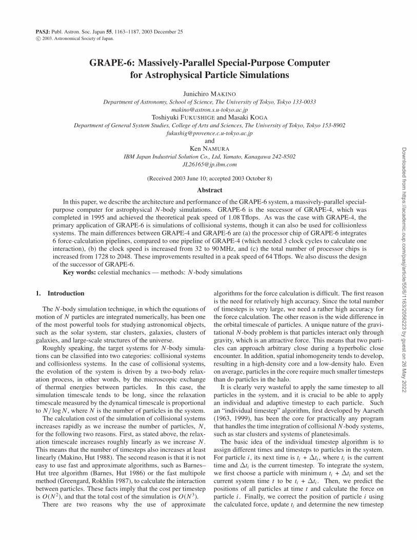
The top-level architecture of GRAPE-6 is shown in figure 1.It consists of 4 “clusters”, each of which comprises 16GRAPE-6 processor boards (PB), 4 host computers (H), andinterconnection networks. These 4 clusters are connected byGigabit Ethernet. For host computers, we currently use PCswith AMD Athlon XP 1800 + CPU and SiS 745 chipset.Ethernet cards are 1000 BT cards with NS 83820 single-chipEthernet controllers.
Dow
nloaded from https://academ
ic.oup.com/pasj/article/55/6/1163/2056223 by guest on 26 M
ay 2022
1166 J. Makino et al. [Vol. 55,
Fig. 1. Top level network structure of GRAPE-6. “H” indicates a hostcomputer and “PB” indicates a processor board.
In the following, we describe how we run parallel programson GRAPE-6. First, let us concentrate on parallelization withina cluster.
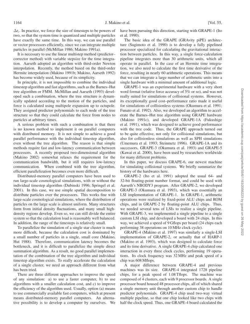
Figure 2 shows one cluster. Four processor boards areconnected to a host computer through a network board. Fournetwork boards are connected to each other, so that we can usea cluster as a single unit or as multiple units.
First consider the simplest case, where we just use 4 hoststo run independent calculations. In this case, 4 processorboards connected to a host through one network board calcu-late the forces on the same set of particles, but from a differentset of particles [what we called j -parallelism in Makinoet al. (1997)]. Each processor board stores different subsetsof particles in the particle memory, and calculates the forces onthe particles stored in the registers in the processor chips. Thepartial forces calculated in different boards are sent in parallelto the network board, where they are added together by anadder tree. The host computer receives the summed-up forces.As discussed later, multiple processor chips on one board alsohave their local memories to store particles. They calculate theforces on the same set of particles, but from different sets ofparticles. The partial forces are summed up by the adder treeon the processor board. From a logical point of view, there isno difference between a single-board system and multi-boardsystem, as long as we use a single host. We can regard theentire system as just a huge adder tree with processor chips atall leaves.
When all 16 boards and 4 hosts are used as a single unit,the particles are divided to 4 groups, and each group isassigned to one host. Conceptually, the j -th board connectedto host i calculates the force on particles in host i, fromparticles in host j . Summation of the partial forces isperformed in the same way as in the case of a single-hostcalculation. The only difference is that the data to be stored
Fig. 2. GRAPE-6 cluster. “NB” indicates a network board.
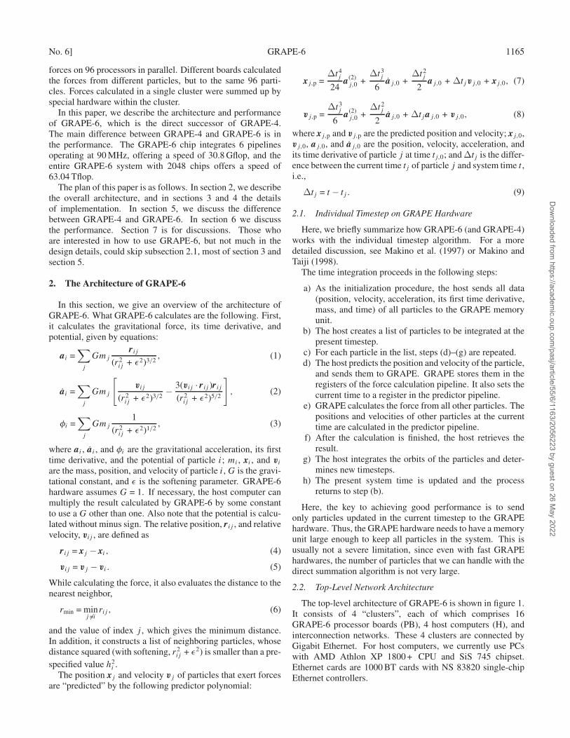
Fig. 3. A 4-input example of a switching network for parallelGRAPE.
in the memory come from other hosts.In order to allow both single-host and multi-host calcula-
tions, the network board must switch between the broadcastmode (for the single-host calculation) and the point-to-pointmode (for the multi-host calculation). It would also be usefulif we can use two hosts together. In this case, it is necessaryto accept two inputs, and to pass each of them to two boards.Thus, we need three operation modes for the network board.One simple way to implement these three modes is shown infigure 3. Here, nodes A and B simply output the inputs fromthe left-hand side ports to two output ports. Nodes C, D, andE can select one from two inputs. In the case of node C, theselected input is sent to two output ports.
Dow
nloaded from https://academ
ic.oup.com/pasj/article/55/6/1163/2056223 by guest on 26 M
ay 2022
No. 6] GRAPE-6 1167
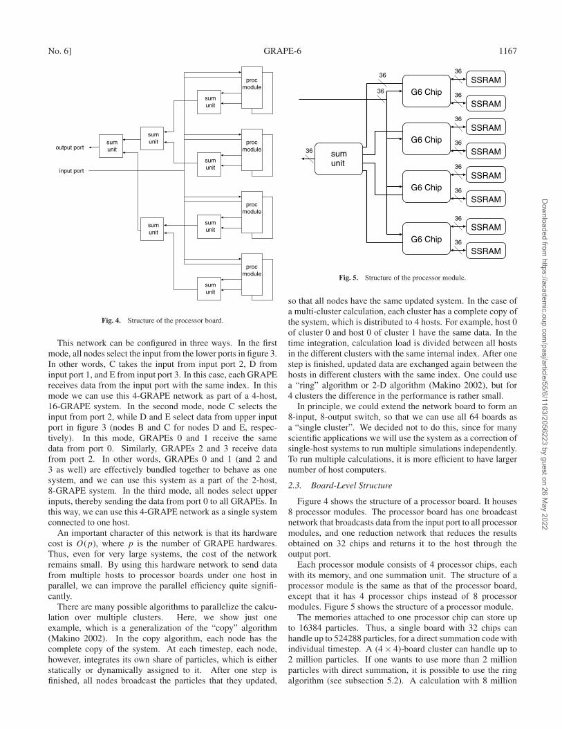
Fig. 4. Structure of the processor board.
This network can be configured in three ways. In the firstmode, all nodes select the input from the lower ports in figure 3.In other words, C takes the input from input port 2, D frominput port 1, and E from input port 3. In this case, each GRAPEreceives data from the input port with the same index. In thismode we can use this 4-GRAPE network as part of a 4-host,16-GRAPE system. In the second mode, node C selects theinput from port 2, while D and E select data from upper inputport in figure 3 (nodes B and C for nodes D and E, respec-tively). In this mode, GRAPEs 0 and 1 receive the samedata from port 0. Similarly, GRAPEs 2 and 3 receive datafrom port 2. In other words, GRAPEs 0 and 1 (and 2 and3 as well) are effectively bundled together to behave as onesystem, and we can use this system as a part of the 2-host,8-GRAPE system. In the third mode, all nodes select upperinputs, thereby sending the data from port 0 to all GRAPEs. Inthis way, we can use this 4-GRAPE network as a single systemconnected to one host.
An important character of this network is that its hardwarecost is O(p), where p is the number of GRAPE hardwares.Thus, even for very large systems, the cost of the networkremains small. By using this hardware network to send datafrom multiple hosts to processor boards under one host inparallel, we can improve the parallel efficiency quite signifi-cantly.
There are many possible algorithms to parallelize the calcu-lation over multiple clusters. Here, we show just oneexample, which is a generalization of the “copy” algorithm(Makino 2002). In the copy algorithm, each node has thecomplete copy of the system. At each timestep, each node,however, integrates its own share of particles, which is eitherstatically or dynamically assigned to it. After one step isfinished, all nodes broadcast the particles that they updated,
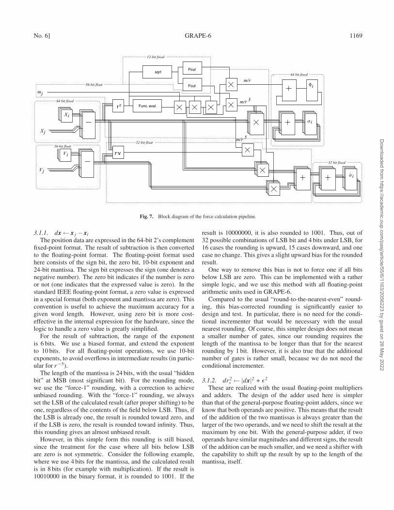
Fig. 5. Structure of the processor module.
so that all nodes have the same updated system. In the case ofa multi-cluster calculation, each cluster has a complete copy ofthe system, which is distributed to 4 hosts. For example, host 0of cluster 0 and host 0 of cluster 1 have the same data. In thetime integration, calculation load is divided between all hostsin the different clusters with the same internal index. After onestep is finished, updated data are exchanged again between thehosts in different clusters with the same index. One could usea “ring” algorithm or 2-D algorithm (Makino 2002), but for4 clusters the difference in the performance is rather small.
In principle, we could extend the network board to form an8-input, 8-output switch, so that we can use all 64 boards asa “single cluster”. We decided not to do this, since for manyscientific applications we will use the system as a correction ofsingle-host systems to run multiple simulations independently.To run multiple calculations, it is more efficient to have largernumber of host computers.
2.3. Board-Level Structure
Figure 4 shows the structure of a processor board. It houses8 processor modules. The processor board has one broadcastnetwork that broadcasts data from the input port to all processormodules, and one reduction network that reduces the resultsobtained on 32 chips and returns it to the host through theoutput port.
Each processor module consists of 4 processor chips, eachwith its memory, and one summation unit. The structure of aprocessor module is the same as that of the processor board,except that it has 4 processor chips instead of 8 processormodules. Figure 5 shows the structure of a processor module.
The memories attached to one processor chip can store upto 16384 particles. Thus, a single board with 32 chips canhandle up to 524288 particles, for a direct summation code withindividual timestep. A (4× 4)-board cluster can handle up to2 million particles. If one wants to use more than 2 millionparticles with direct summation, it is possible to use the ringalgorithm (see subsection 5.2). A calculation with 8 million
Dow
nloaded from https://academ
ic.oup.com/pasj/article/55/6/1163/2056223 by guest on 26 M
ay 2022

1168 J. Makino et al. [Vol. 55,
Fig. 6. Block diagram of the processor chip.
particles is theoretically possible on a single cluster with 16processor boards.
In the next two sections, we present a detailed descriptionof the hardware, in a bottom-up fashion. In section 3, wedescribe the processor chip and in section 4 the processorboard, network board, and interconnection.
3. The Processor Chip
The GRAPE-6 processor chip was fabricated using theToshiba TC-240 process (nominal design rule of 0.25 µm).The physical size of the chip is roughly 10 mm by 10 mm, andis packaged into 480-contact BGA package. It operates at a90 MHz clock cycle. The power supply voltage is 2.5 V. Heatdissipation is around 12 W at the maximum.
A processor chip consists of six force calculation pipelines,a predictor pipeline, a memory interface, a control unit, and I/Oports. Figure 6 shows an overview of the chip. In the following,we discuss each block in turn.
3.1. Force Calculation Pipeline
The task of the force calculation pipeline is to evaluateequations (1)–(3). It also determines the nearest neighborparticle and its distance. This function is rather convenientfor detecting close encounters or physical collisions betweenparticles that require special treatments. For this purpose, theindices of particles that exert forces are supplied to the pipeline.
The indices are also used to avoid self-interaction. The forcecalculation pipeline has the register for the index of the particlefor which the force is calculated, and avoids the accumulationof the result if two indices are the same. This capability is intro-duced to avoid the need to send particles twice to the memoryin the case of the individual timestep algorithm.
With the individual timestep algorithm and the hardwiredpredictor pipeline, the data of particles which exert forces areevaluated by the predictor pipeline on the chip, while the datafor the particle for which the force is calculated is evaluated onthe host computer and sent to the register of the force calcu-lation pipeline. These two values are not exactly the same,since the data format and accuracy of the hardware predictorare different from that of the host computer. The GRAPE-4pipeline does not have logic to use a particle index, and the onlyway to avoid the self interaction is to make the data exactly thesame. To achieve this, for the particles to be updated, we send
Table 1. Arithmetic operations in the force calculation pipeline.
# Operation Format Length Mantissa
1 dx← xj − xi fixed 64 · · ·2 dr2
s ← |dx|2 + ε2 float 36 243 calculation of r−α
s , float 36 24where α = 1,3,5
4 φij ←mjr−1s float 36 24
5 φi ← φi + φij fixed 64 · · ·6 aij ←mjr
−3s dx float 36 24
7 ai ← ai + aij fixed 64 · · ·8 dv← vj − vi float 36 249 s← dv · dx float 32 20
10 j1← dx · 3smjr−5s float 32 20
11 j2← dv ·mjr−5s float 32 20
12 aij ← j1 + j2 float 32 2013 ai ← ai + aij fixed 32 · · ·
the predicted data at the current time to the memory as wellas the registers. This means that we have to send j -particlestwice per timestep. With the index-based approach, we need tosend j -particles only once per timestep, resulting in a signifi-cant reduction in the total amount of communication.
For GRAPE-6 pipeline, have we adopted the 8-way VMP(virtual multiple pipeline, Makino et al. 1997), in which asingle physical pipeline serves as eight virtual pipelines, calcu-lating the forces on 8 different particles. In this way, we canreduce the requirement for memory bandwidth by a factor of 8,since all VMPs (and also physical multiple pipelines on a chip)calculate the forces from the same particle.
In the physical implementation of the pipeline, we haveadopted several different number representations, dependingon the required accuracy. For input position data, we use the64-bit fixed-point format. The reason that we used the fixed-point format here is to simplify the hardware. An additionaladvantage of using the fixed-point format is that the imple-mentation of the periodic boundary condition is simpler thanthat in the case of the floating-point data format (Fukushigeet al. 1996).
After first subtraction between two position vectors, theresult is converted to a floating-point format with a 24-bitmantissa. Here, the floating-point format is preferred, sinceotherwise we need very large multipliers.
For the final accumulation, we return to the 64-bit fixed-point format, again to simplify the hardware. Here, we specifythe scaling factor for each particle, so that we can calcu-late forces with very different magnitudes, without causing anoverflow or underflow.
The pipeline for the calculation of the time derivative isdesigned in a similar way, but with a 20-bit mantissa for inter-mediate data and the 32-bit fixed-point format for the finalaccumulation. Since the time derivative is one order higherthan the force, the required accuracy is lower.
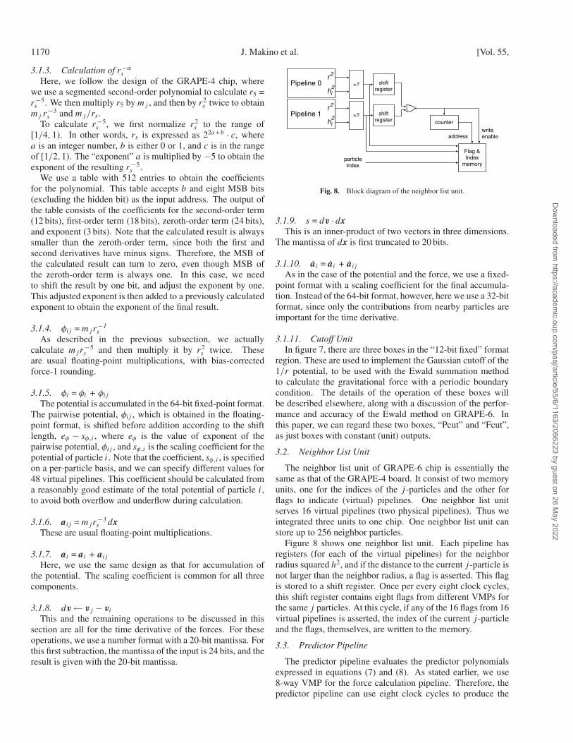
Figure 7 shows a block diagram of the pipeline. It consistsof arithmetic units to perform the operations listed in table 1.We briefly discuss each operations below.
Dow
nloaded from https://academ
ic.oup.com/pasj/article/55/6/1163/2056223 by guest on 26 M
ay 2022
No. 6] GRAPE-6 1169
Fig. 7. Block diagram of the force calculation pipeline.
3.1.1. dx← xj − xi
The position data are expressed in the 64-bit 2’s complementfixed-point format. The result of subtraction is then convertedto the floating-point format. The floating-point format usedhere consists of the sign bit, the zero bit, 10-bit exponent and24-bit mantissa. The sign bit expresses the sign (one denotes anegative number). The zero bit indicates if the number is zeroor not (one indicates that the expressed value is zero). In thestandard IEEE floating-point format, a zero value is expressedin a special format (both exponent and mantissa are zero). Thisconvention is useful to achieve the maximum accuracy for agiven word length. However, using zero bit is more cost-effective in the internal expression for the hardware, since thelogic to handle a zero value is greatly simplified.
For the result of subtraction, the range of the exponentis 6 bits. We use a biased format, and extend the exponentto 10 bits. For all floating-point operations, we use 10-bitexponents, to avoid overflows in intermediate results (in partic-ular for r−5).
The length of the mantissa is 24 bits, with the usual “hiddenbit” at MSB (most significant bit). For the rounding mode,we use the “force-1” rounding, with a correction to achieveunbiased rounding. With the “force-1” rounding, we alwaysset the LSB of the calculated result (after proper shifting) to beone, regardless of the contents of the field below LSB. Thus, ifthe LSB is already one, the result is rounded toward zero, andif the LSB is zero, the result is rounded toward infinity. Thus,this rounding gives an almost unbiased result.
However, in this simple form this rounding is still biased,since the treatment for the case where all bits below LSBare zero is not symmetric. Consider the following example,where we use 4 bits for the mantissa, and the calculated resultis in 8 bits (for example with multiplication). If the result is10010000 in the binary format, it is rounded to 1001. If the
result is 10000000, it is also rounded to 1001. Thus, out of32 possible combinations of LSB bit and 4 bits under LSB, for16 cases the rounding is upward, 15 cases downward, and onecase no change. This gives a slight upward bias for the roundedresult.
One way to remove this bias is not to force one if all bitsbelow LSB are zero. This can be implemented with a rathersimple logic, and we use this method with all floating-pointarithmetic units used in GRAPE-6.
Compared to the usual “round-to-the-nearest-even” round-ing, this bias-corrected rounding is significantly easier todesign and test. In particular, there is no need for the condi-tional incrementer that would be necessary with the usualnearest rounding. Of course, this simpler design does not meana smaller number of gates, since our rounding requires thelength of the mantissa to be longer than that for the nearestrounding by 1 bit. However, it is also true that the additionalnumber of gates is rather small, because we do not need theconditional incrementer.
3.1.2. dr2s ← |dx|2 + ε2
These are realized with the usual floating-point multipliersand adders. The design of the adder used here is simplerthan that of the general-purpose floating-point adders, since weknow that both operands are positive. This means that the resultof the addition of the two mantissas is always greater than thelarger of the two operands, and we need to shift the result at themaximum by one bit. With the general-purpose adder, if twooperands have similar magnitudes and different signs, the resultof the addition can be much smaller, and we need a shifter withthe capability to shift up the result by up to the length of themantissa, itself.
Dow
nloaded from https://academ
ic.oup.com/pasj/article/55/6/1163/2056223 by guest on 26 M
ay 2022
1170 J. Makino et al. [Vol. 55,
3.1.3. Calculation of r−αs
Here, we follow the design of the GRAPE-4 chip, wherewe use a segmented second-order polynomial to calculate r5 =r−5s . We then multiply r5 by mj , and then by r2
s twice to obtainmj r−3
s and mj/rs .To calculate r−5
s , we first normalize r2s to the range of
[1/4, 1). In other words, rs is expressed as 22a + b · c, wherea is an integer number, b is either 0 or 1, and c is in the rangeof [1/2,1). The “exponent” a is multiplied by −5 to obtain theexponent of the resulting r−5
s .We use a table with 512 entries to obtain the coefficients
for the polynomial. This table accepts b and eight MSB bits(excluding the hidden bit) as the input address. The output ofthe table consists of the coefficients for the second-order term(12 bits), first-order term (18 bits), zeroth-order term (24 bits),and exponent (3 bits). Note that the calculated result is alwayssmaller than the zeroth-order term, since both the first andsecond derivatives have minus signs. Therefore, the MSB ofthe calculated result can turn to zero, even though MSB ofthe zeroth-order term is always one. In this case, we needto shift the result by one bit, and adjust the exponent by one.This adjusted exponent is then added to a previously calculatedexponent to obtain the exponent of the final result.
3.1.4. φij = mjr−1s
As described in the previous subsection, we actuallycalculate mjr
−5s and then multiply it by r2
s twice. Theseare usual floating-point multiplications, with bias-correctedforce-1 rounding.
3.1.5. φi = φi + φij
The potential is accumulated in the 64-bit fixed-point format.The pairwise potential, φij , which is obtained in the floating-point format, is shifted before addition according to the shiftlength, eφ − sφ,i , where eφ is the value of exponent of thepairwise potential, φij , and sφ,i is the scaling coefficient for thepotential of particle i. Note that the coefficient, sφ,i , is specifiedon a per-particle basis, and we can specify different values for48 virtual pipelines. This coefficient should be calculated froma reasonably good estimate of the total potential of particle i,to avoid both overflow and underflow during calculation.
3.1.6. aij = mjr−3s dx
These are usual floating-point multiplications.
3.1.7. ai = ai + aij
Here, we use the same design as that for accumulation ofthe potential. The scaling coefficient is common for all threecomponents.
3.1.8. dv← vj − vi
This and the remaining operations to be discussed in thissection are all for the time derivative of the forces. For theseoperations, we use a number format with a 20-bit mantissa. Forthis first subtraction, the mantissa of the input is 24 bits, and theresult is given with the 20-bit mantissa.
Fig. 8. Block diagram of the neighbor list unit.
3.1.9. s = dv · dxThis is an inner-product of two vectors in three dimensions.
The mantissa of dx is first truncated to 20 bits.
3.1.10. ai = ai + aij
As in the case of the potential and the force, we use a fixed-point format with a scaling coefficient for the final accumula-tion. Instead of the 64-bit format, however, here we use a 32-bitformat, since only the contributions from nearby particles areimportant for the time derivative.
3.1.11. Cutoff UnitIn figure 7, there are three boxes in the “12-bit fixed” format
region. These are used to implement the Gaussian cutoff of the1/r potential, to be used with the Ewald summation methodto calculate the gravitational force with a periodic boundarycondition. The details of the operation of these boxes willbe described elsewhere, along with a discussion of the perfor-mance and accuracy of the Ewald method on GRAPE-6. Inthis paper, we can regard these two boxes, “Pcut” and “Fcut”,as just boxes with constant (unit) outputs.
3.2. Neighbor List Unit
The neighbor list unit of GRAPE-6 chip is essentially thesame as that of the GRAPE-4 board. It consist of two memoryunits, one for the indices of the j -particles and the other forflags to indicate (virtual) pipelines. One neighbor list unitserves 16 virtual pipelines (two physical pipelines). Thus weintegrated three units to one chip. One neighbor list unit canstore up to 256 neighbor particles.
Figure 8 shows one neighbor list unit. Each pipeline hasregisters (for each of the virtual pipelines) for the neighborradius squared h2, and if the distance to the current j -particle isnot larger than the neighbor radius, a flag is asserted. This flagis stored to a shift register. Once per every eight clock cycles,this shift register contains eight flags from different VMPs forthe same j particles. At this cycle, if any of the 16 flags from 16virtual pipelines is asserted, the index of the current j -particleand the flags, themselves, are written to the memory.
3.3. Predictor Pipeline
The predictor pipeline evaluates the predictor polynomialsexpressed in equations (7) and (8). As stated earlier, we use8-way VMP for the force calculation pipeline. Therefore, thepredictor pipeline can use eight clock cycles to produce the
Dow
nloaded from https://academ
ic.oup.com/pasj/article/55/6/1163/2056223 by guest on 26 M
ay 2022
No. 6] GRAPE-6 1171
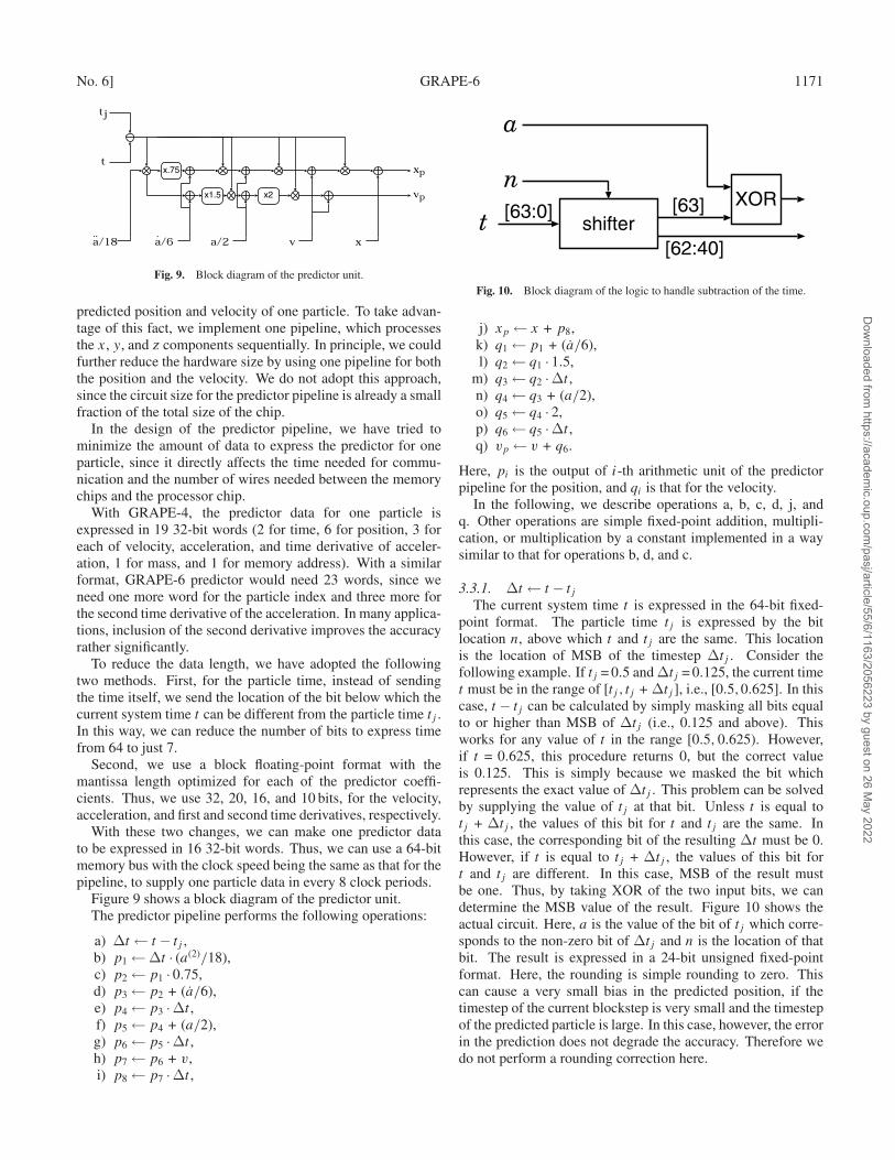
Fig. 9. Block diagram of the predictor unit.
predicted position and velocity of one particle. To take advan-tage of this fact, we implement one pipeline, which processesthe x, y, and z components sequentially. In principle, we couldfurther reduce the hardware size by using one pipeline for boththe position and the velocity. We do not adopt this approach,since the circuit size for the predictor pipeline is already a smallfraction of the total size of the chip.
In the design of the predictor pipeline, we have tried tominimize the amount of data to express the predictor for oneparticle, since it directly affects the time needed for commu-nication and the number of wires needed between the memorychips and the processor chip.
With GRAPE-4, the predictor data for one particle isexpressed in 19 32-bit words (2 for time, 6 for position, 3 foreach of velocity, acceleration, and time derivative of acceler-ation, 1 for mass, and 1 for memory address). With a similarformat, GRAPE-6 predictor would need 23 words, since weneed one more word for the particle index and three more forthe second time derivative of the acceleration. In many applica-tions, inclusion of the second derivative improves the accuracyrather significantly.
To reduce the data length, we have adopted the followingtwo methods. First, for the particle time, instead of sendingthe time itself, we send the location of the bit below which thecurrent system time t can be different from the particle time tj .In this way, we can reduce the number of bits to express timefrom 64 to just 7.
Second, we use a block floating-point format with themantissa length optimized for each of the predictor coeffi-cients. Thus, we use 32, 20, 16, and 10 bits, for the velocity,acceleration, and first and second time derivatives, respectively.
With these two changes, we can make one predictor datato be expressed in 16 32-bit words. Thus, we can use a 64-bitmemory bus with the clock speed being the same as that for thepipeline, to supply one particle data in every 8 clock periods.
Figure 9 shows a block diagram of the predictor unit.The predictor pipeline performs the following operations:
a) ∆t ← t − tj ,b) p1←∆t · (a(2)/18),c) p2← p1 · 0.75,d) p3← p2 + (a/6),e) p4← p3 ·∆t ,f) p5← p4 + (a/2),g) p6← p5 ·∆t ,h) p7← p6 + v,i) p8← p7 ·∆t ,
Fig. 10. Block diagram of the logic to handle subtraction of the time.
j) xp← x + p8,k) q1← p1 + (a/6),l) q2← q1 · 1.5,
m) q3← q2 ·∆t ,n) q4← q3 + (a/2),o) q5← q4 · 2,p) q6← q5 ·∆t ,q) vp← v + q6.
Here, pi is the output of i-th arithmetic unit of the predictorpipeline for the position, and qi is that for the velocity.
In the following, we describe operations a, b, c, d, j, andq. Other operations are simple fixed-point addition, multipli-cation, or multiplication by a constant implemented in a waysimilar to that for operations b, d, and c.
3.3.1. ∆t ← t − tjThe current system time t is expressed in the 64-bit fixed-
point format. The particle time tj is expressed by the bitlocation n, above which t and tj are the same. This locationis the location of MSB of the timestep ∆tj . Consider thefollowing example. If tj = 0.5 and ∆tj = 0.125, the current timet must be in the range of [tj , tj + ∆tj ], i.e., [0.5,0.625]. In thiscase, t − tj can be calculated by simply masking all bits equalto or higher than MSB of ∆tj (i.e., 0.125 and above). Thisworks for any value of t in the range [0.5,0.625). However,if t = 0.625, this procedure returns 0, but the correct valueis 0.125. This is simply because we masked the bit whichrepresents the exact value of ∆tj . This problem can be solvedby supplying the value of tj at that bit. Unless t is equal totj + ∆tj , the values of this bit for t and tj are the same. Inthis case, the corresponding bit of the resulting ∆t must be 0.However, if t is equal to tj + ∆tj , the values of this bit fort and tj are different. In this case, MSB of the result mustbe one. Thus, by taking XOR of the two input bits, we candetermine the MSB value of the result. Figure 10 shows theactual circuit. Here, a is the value of the bit of tj which corre-sponds to the non-zero bit of ∆tj and n is the location of thatbit. The result is expressed in a 24-bit unsigned fixed-pointformat. Here, the rounding is simple rounding to zero. Thiscan cause a very small bias in the predicted position, if thetimestep of the current blockstep is very small and the timestepof the predicted particle is large. In this case, however, the errorin the prediction does not degrade the accuracy. Therefore wedo not perform a rounding correction here.
Dow
nloaded from https://academ
ic.oup.com/pasj/article/55/6/1163/2056223 by guest on 26 M
ay 2022
1172 J. Makino et al. [Vol. 55,
3.3.2. p1←∆t · (a(2)/18)Both inputs are supplied in a 10-bit fixed-point format. Here,
we use the sign–magnitude format, instead of the usual 2’scomplement format, to simplify the design of the multiplier.Note that ∆t is supplied in the 24-bit format. Therefore, weneed to truncate it to the 10-bit format, using the bias-correctedforce-1 rounding discussed earlier. The result is also roundedto the 10-bit format.
3.3.3. p2← p1 · 0.75This multiplication by a constant is achieved by adding p1/2
and p1/4. These two values can be calculated by shifting themto the right by one bit and two bits, respectively. These shift-ings, in hardware, require just wiring and no logic. Thus, thismultiplication is actually implemented by a single adder. Here,we do not round the result, since the effect of the error in themultiplication in the predictor is usually very small.
3.3.4. p3← p2 + (a/6)Here, p2 is in the 10-bit sign-and-magnitude format, and
(a/6) is in a 16-bit format. Thus, we first extend p2 to 16 bits.If two inputs have different signs, we need to determine whichone is larger. We do this by calculating both a−b and b−a. Ifa−b does not cause an overflow, we can see that a≥b, and usea− b as the result. The sign of the result is the same as that ofa. This circuit is rather complicated and larger than that for the2’s complement format. However, the gate count is practicallynegligible.
3.3.5. Operations (e)–(i)All of these are the usual fixed-point addition or multiplica-
tion, implemented in the same way as operations (b) and (d).
3.3.6. xp← x + p8Here, we add two numbers in different formats. One is x in
the 64-bit 2’s complement fixed-point format. The other is p8in the floating-point format with a sign, exponent and mantissa.Since we do not perform any normalization during the calcula-tion of p8, the mantissa is not normalized. This means that wedo not use the hidden bit for p8. We first shift p8 according tothe value of the exponent of the velocity, and then add it to (orsubtract it from) x according to the sign bit.
3.3.7. Operations (k)–(p)These operations are implemented in the same way as
similar operations for the position predictor pipeline are imple-mented.
3.3.8. vp← v + q6This is essentially the same addition as used in other opera-
tions, but here we post-normalize the result. For the outputformat we use a mantissa with the hidden bit.
3.4. Memory Interface
The memory interface has two functions. The first one is towrite the data sent from the host, and the second one is to readthe memory during a calculation.
The data of one particle is packed into 16 32-bit words.A data packet sent from the host consists of two control
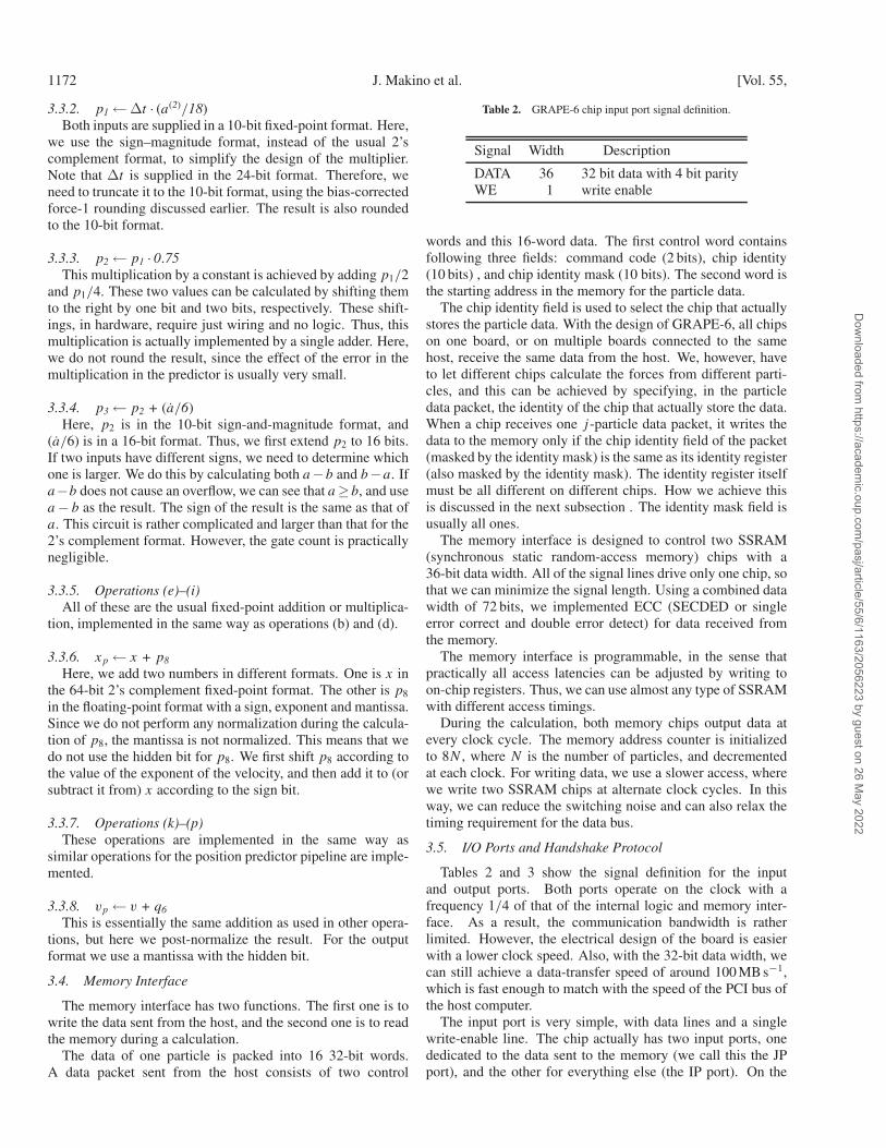
Table 2. GRAPE-6 chip input port signal definition.
Signal Width Description
DATA 36 32 bit data with 4 bit parityWE 1 write enable
words and this 16-word data. The first control word containsfollowing three fields: command code (2 bits), chip identity(10 bits) , and chip identity mask (10 bits). The second word isthe starting address in the memory for the particle data.
The chip identity field is used to select the chip that actuallystores the particle data. With the design of GRAPE-6, all chipson one board, or on multiple boards connected to the samehost, receive the same data from the host. We, however, haveto let different chips calculate the forces from different parti-cles, and this can be achieved by specifying, in the particledata packet, the identity of the chip that actually store the data.When a chip receives one j -particle data packet, it writes thedata to the memory only if the chip identity field of the packet(masked by the identity mask) is the same as its identity register(also masked by the identity mask). The identity register itselfmust be all different on different chips. How we achieve thisis discussed in the next subsection . The identity mask field isusually all ones.
The memory interface is designed to control two SSRAM(synchronous static random-access memory) chips with a36-bit data width. All of the signal lines drive only one chip, sothat we can minimize the signal length. Using a combined datawidth of 72 bits, we implemented ECC (SECDED or singleerror correct and double error detect) for data received fromthe memory.
The memory interface is programmable, in the sense thatpractically all access latencies can be adjusted by writing toon-chip registers. Thus, we can use almost any type of SSRAMwith different access timings.
During the calculation, both memory chips output data atevery clock cycle. The memory address counter is initializedto 8N , where N is the number of particles, and decrementedat each clock. For writing data, we use a slower access, wherewe write two SSRAM chips at alternate clock cycles. In thisway, we can reduce the switching noise and can also relax thetiming requirement for the data bus.
3.5. I/O Ports and Handshake Protocol
Tables 2 and 3 show the signal definition for the inputand output ports. Both ports operate on the clock with afrequency 1/4 of that of the internal logic and memory inter-face. As a result, the communication bandwidth is ratherlimited. However, the electrical design of the board is easierwith a lower clock speed. Also, with the 32-bit data width, wecan still achieve a data-transfer speed of around 100 MB s−1,which is fast enough to match with the speed of the PCI bus ofthe host computer.
The input port is very simple, with data lines and a singlewrite-enable line. The chip actually has two input ports, onededicated to the data sent to the memory (we call this the JPport), and the other for everything else (the IP port). On the
Dow
nloaded from https://academ
ic.oup.com/pasj/article/55/6/1163/2056223 by guest on 26 M
ay 2022
No. 6] GRAPE-6 1173
Table 3. FO port signal description.
Signal Direction (I/O) Description
D0-D35 O data (4 bits for parity)VD O valid dataND O new dataSTS O statusACTIVE O if 0, chip is unusedWD I wait data
JP port, the data of one particle consists of 18 32-bit words,and the control logic handles this 18-word packet. The IPport is a general-purpose port. It accepts variable-length datapackets. The first word of the packet is the starting address ofthe on-chip register. The second word is the number of datawords to follow, and the remaining words are all data.
The output port is more complicated, because we need toimplement flow control. The reason we need flow controlis that for some data, for example for the neighbor list, thehost must receive the data directly from all chips. In the caseof the force, all chips output the results synchronously andthe onboard reduction network reduces the data on the fly.However, the neighbor list data has to be transferred to the hostwithout any reduction.
It is possible to read the data of neighbor particles from eachchip without using hardware flow control by letting the hostcomputer send the commands to each chip sequentially untilit receives all data. In this case, the processor chip itself doesnot need any flow control. However, this procedure would berather slow, since the host has to set up the DMA transfer manytimes. Therefore, we chose to let the host send the command toall chips. The reduction network takes care of the flow control.In table 3, the WD signal is used for flow control.
When the WD signal is asserted, the chip stops sending newdata. When the chip sends new data, it asserts both VD andND signals. The VD signal is asserted as long as the data isvalid, but ND is asserted only when the data is actually updated.The STS line is a special signal which tells whether the forcecalculation pipeline is working or not. The ACTIVE signalis used to indicate defective chips. The output of this pin isprogrammable from the host, and if ACTIVE is negated, thereduction network ignores the output from the chip.
4. Processor Board and Network Hardware
4.1. Processor Module and Processor Board
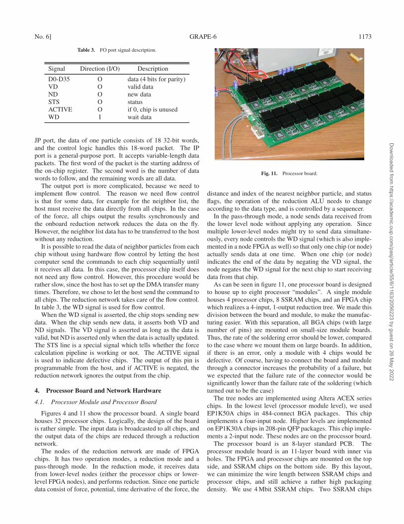
Figures 4 and 11 show the processor board. A single boardhouses 32 processor chips. Logically, the design of the boardis rather simple. The input data is broadcasted to all chips, andthe output data of the chips are reduced through a reductionnetwork.
The nodes of the reduction network are made of FPGAchips. It has two operation modes, a reduction mode and apass-through mode. In the reduction mode, it receives datafrom lower-level nodes (either the processor chips or lower-level FPGA nodes), and performs reduction. Since one particledata consist of force, potential, time derivative of the force, the
Fig. 11. Processor board.
distance and index of the nearest neighbor particle, and statusflags, the operation of the reduction ALU needs to changeaccording to the data type, and is controlled by a sequencer.
In the pass-through mode, a node sends data received fromthe lower level node without applying any operation. Sincemultiple lower-level nodes might try to send data simultane-ously, every node controls the WD signal (which is also imple-mented in a node FPGA as well) so that only one chip (or node)actually sends data at one time. When one chip (or node)indicates the end of the data by negating the VD signal, thenode negates the WD signal for the next chip to start receivingdata from that chip.
As can be seen in figure 11, one processor board is designedto house up to eight processor “modules”. A single modulehouses 4 processor chips, 8 SSRAM chips, and an FPGA chipwhich realizes a 4-input, 1-output reduction tree. We made thisdivision between the board and module, to make the manufac-turing easier. With this separation, all BGA chips (with largenumber of pins) are mounted on small-size module boards.Thus, the rate of the soldering error should be lower, comparedto the case where we mount them on large boards. In addition,if there is an error, only a module with 4 chips would bedefective. Of course, having to connect the board and modulethrough a connector increases the probability of a failure, butwe expected that the failure rate of the connector would besignificantly lower than the failure rate of the soldering (whichturned out to be the case)
The tree nodes are implemented using Altera ACEX serieschips. In the lowest level (processor module level), we usedEP1K50A chips in 484-connect BGA packages. This chipimplements a four-input node. Higher levels are implementedon EP1K30A chips in 208-pin QFP packages. This chip imple-ments a 2-input node. These nodes are on the processor board.
The processor board is an 8-layer standard PCB. Theprocessor module board is an 11-layer board with inner viaholes. The FPGA and processor chips are mounted on the topside, and SSRAM chips on the bottom side. By this layout,we can minimize the wire length between SSRAM chips andprocessor chips, and still achieve a rather high packagingdensity. We use 4 Mbit SSRAM chips. Two SSRAM chips
Dow
nloaded from https://academ
ic.oup.com/pasj/article/55/6/1163/2056223 by guest on 26 M
ay 2022
1174 J. Makino et al. [Vol. 55,
Fig. 12. Host interface board.
connected to a processor chip can store up to 16384 particles.One board can store up to 524288 particles.
The SSRAM chip we chose requires 2.5 V power supplyfor I/O and 3.3 V for the core. Both the processor board andthe module board have separate power planes for both 2.5 and3.3 V power supplies.
Though the chip has separate ports for j -particles and otherdata, for the board we decided to use a common data line tosimplify the design and reduce the manufacturing cost.
Currently, the core of the processor chip operates on a90 MHz clock, and the I/O part on a 22.5 MHz clock. Thereduction network and other logics of the control board alsooperate on a 22.5 MHz clock.
For the board–board connection, we use a semi-serial LVDSsignal. We use 4-wire (3 for signals and 1 for transmissionclock) chipset, which performs 7 : 1 parallel–serial conversion.Since our basic transfer unit is a 32-bit word, we use two cyclesof this chipset to transmit one data. Thus, the chipset operateson a 45 MHz clock, and the signal lines operate at a data rate of315 MHz. For conversion between the 22.5 MHz data rate ofthe board logic and the 45 MHz data rate of the LVDS chipset,we use additional FPGA chip.
With this LVDS chipset, the receiver chipset itself is drivenby the clock signal that comes with the data. In order to allowthe two boards connected to a link to operate on independentclocks, we add FIFO chips after the data rate is reduced to22.5 MHz.
The physical form factor of the card is that of an 8UEurocard (with the length of 400 mm). For the backplaneconnection, we use connectors designed for Compact PCIcards. The power supply is also from a backplane bus, throughspecial power connectors.
It is possible to connect a single processor board directlyto the host through the host interface card, without using thenetwork card. For this purpose, the processor board alsohas connectors for twisted-pair cables for the LVDS inter-face. These connectors are standard RJ-45 modular jackswidely used for 10/100/1000BT Ethernet connection. Standardcategory 5 (or enhanced 5) cables can be used for connections.
For LVDS interface chips, we use SN75LVD85 andSN75LVD86A chips from Texas Instruments.
4.2. Host Interface Card
Figure 12 shows a block diagram of the host interface card.It is a standard (32-bit, 33 MHz) PCI card. To transfer datafrom the host to GRAPE-6, the host sets up the data to betransferred in its memory and lets the PCI interface chip onthe interface card perform DMA transfer. The data received
Fig. 13. Network board.
by this DMA transfer is sent directly through the output link.In the design of the host interface card we implemented twooutput ports so that they can separately supply data to the JPand IP ports. As stated earlier, we decided to use only one portfor the processor board. Therefore, the second output port ofthe interface card is not used.
The input port is more complicated, with an FIFO memory tostore the received data. This FIFO memory is necessary, sincewe cannot guarantee the response time of the host operatingsystem to a DMA request from the interface card. We need tohave the memory large enough to avoid any possible overflow.
For the PCI interface, we use the 9080 chip from PLXtechnology.
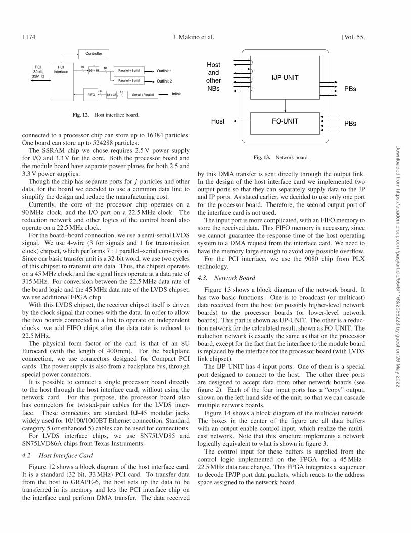
4.3. Network Board
Figure 13 shows a block diagram of the network board. Ithas two basic functions. One is to broadcast (or multicast)data received from the host (or possibly higher-level networkboards) to the processor boards (or lower-level networkboards). This part is shown as IJP-UNIT. The other is a reduc-tion network for the calculated result, shown as FO-UNIT. Thereduction network is exactly the same as that on the processorboard, except for the fact that the interface to the module boardis replaced by the interface for the processor board (with LVDSlink chipset).
The IJP-UNIT has 4 input ports. One of them is a specialport designed to connect to the host. The other three portsare designed to accept data from other network boards (seefigure 2). Each of the four input ports has a “copy” output,shown on the left-hand side of the unit, so that we can cascademultiple network boards.
Figure 14 shows a block diagram of the multicast network.The boxes in the center of the figure are all data bufferswith an output enable control input, which realize the multi-cast network. Note that this structure implements a networklogically equivalent to what is shown in figure 3.
The control input for these buffers is supplied from thecontrol logic implemented on the FPGA for a 45 MHz–22.5 MHz data rate change. This FPGA integrates a sequencerto decode IP/JP port data packets, which reacts to the addressspace assigned to the network board.
Dow
nloaded from https://academ
ic.oup.com/pasj/article/55/6/1163/2056223 by guest on 26 M
ay 2022
No. 6] GRAPE-6 1175
Fig. 14. Physical implementation of the multicast network.
4.4. Packaging and Power Distribution
In the standard configuration, eight processor boards andtwo network boards are installed in a card rack with a specialbackplane for the LVDS link. The network board is a single-height unit, but the processor board occupies a two-unit height,to allow sufficient airflow.
To both of the network boards and processor boards,electrical power is supplied through backplane connectors.However, in our present packaging, each processor board hasits own power supply unit. A power supply unit accepts DC330 V input, and supplies DC 2.5 V and 3.3 V. The DC 330 Vpower is generated by another power unit from a three-phaseAC power line. For all of these power units, we use productsfrom Vicor.
We chose Vicor product primarily to reduce the responsetime of the power supply to the change in power consump-tion by the boards. One advantage of the CMOS logic is thatit consumes power only when the logic state changes. Thismeans that even though we pay absolutely no effort to reducethe power consumption of the chip, its power consumptionalmost halves when the pipeline is not active.
This “feature” of the chip is rather good from the point ofview of the running cost of the machine, but pauses a ratherserious problem to the power supply. The typical responsetimescale of a switching power supply unit is on the orderof one millisecond. On the other hand, GRAPE-6 switchesbetween calculation and idle (or communication) states inabout one millisecond. This means that the response time ofthe power supply is too long to compensate for a change inthe load between the calculation state and the idle state, andthe supply voltage becomes rather unstable. Thus, we had tolook for power supplies with a relatively short response time.For switching power supplies, a short response time means ahigh operating frequency, and Vicor products had the highestfrequency among commercially available power units.
Even with high-frequency power supplies, the response time
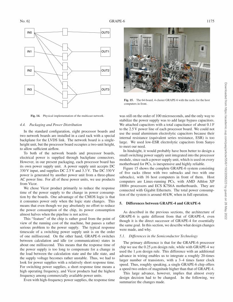
Fig. 15. The 64-board, 4-cluster GRAPE-6 with the racks for the hostcomputers in front.
was still on the order of 100 microseconds, and the only way tostabilize the power supply was to add large bypass capacitors.We attached capacitors with a total capacitance of about 0.1 Fto the 2.5 V power line of each processor board. We could notuse the usual aluminium electrolytic capacitors because theirinternal resistance (equivalent series resistance, ESR) is toolarge. We used low-ESR electrolytic capacitors from Sanyoto meet our need.
In hindsight, it would probably have been better to design asmall switching power supply unit integrated into the processormodule, since such a power supply unit, which is used on everymotherboard for PCs, is inexpensive and highly reliable.
Figure 15 shows the complete GRAPE-6 system consistingof five racks (three with two subracks and two with onesubracks), with 16 host computers in front of them. Hostcomputers are Linux-running PCs, with AMD Athlon XP1800+ processors and ECS K7S6A motherboards. They areconnected with Gigabit Ethernets. The total power consump-tion of the system is around 40 kW, when in full operation.
5. Differences between GRAPE-4 and GRAPE-6
As described in the previous sections, the architecture ofGRAPE-6 is quite different from that of GRAPE-4, eventhough it is the direct successor of GRAPE-4 for essentiallythe same goal. In this section, we describe what design changeswere made, and why.
5.1. Differences in the Semiconductor Technology
The primary difference is that for the GRAPE-6 processorchip we use the 0.25 µm design rule, while with GRAPE-4 weused the 1 µm design rule. This difference with an additionaladvance in wiring enables us to integrate a roughly 20-timeslarger number of transistors, with a 3–4 times faster clockspeed. Thus, roughly speaking, a single GRAPE-6 chip offersa speed two orders of magnitude higher than that of GRAPE-4.
This large advance, however, implies that almost everydesign decision had to be changed. In the following, wesummarize the changes made.
Dow
nloaded from https://academ
ic.oup.com/pasj/article/55/6/1163/2056223 by guest on 26 M
ay 2022

1176 J. Makino et al. [Vol. 55,
Fig. 16. A simple parallel-host, parallel-GRAPE system.
5.2. Host Computer and Overall Architecture
In GRAPE-4, 4 clusters were connected to a single host,sharing one I/O bus. For the peak speed of 1 Tflops, a singlehost was still okay for simulations with a large number ofparticles (105 and larger), and communication through a singleI/O bus was also okay.
With GRAPE-6, however, the peak speed is increased by afactor of 60. On the other hand, the speed of a single hostwould be improved only by a factor of 10 or so, if we assumethe standard Moore’s law (performance doubling time of 18months). Thus, if we want to achieve a reasonable speed for asimilar number of particles as that for GRAPE-4, we need touse around 10 host computers and the communication channelmust be 10–20 times faster than that used for GRAPE-4.
Around the time of the design, it was clear that a shared-memory multiprocessor system with 8–16 processors and asufficient I/O bandwidth would be prohibitingly expensive,with a price tag on the order of 1 M USD. On the other hand, acluster of 8–16 single-processor workstations or PCs would bemuch less expensive. As far as the cost is concerned, clearlya cluster of single-processor machines would be better than ashared-memory multiprocessor system.
One problem with the cluster is that the simplest configura-tion (see figure 16) does not work. The reason is as follows.
With this configuration, there are two different ways todistribute particle data over processors (Makino 2002). Oneis that each processor has a complete copy of the system (the“copy” algorithm). In this case, parallelization is performedas follows. At each blockstep, each processor determineswhich particles it updates. After all processors update theirshare of particles, they exchange the updated particles sothat all processors have an updated copy of the system.This algorithm has been used to implement the individualtimestep algorithm on distributed-memory parallel computers(Spurzem, Baumgardt 1999)
In this algorithm, at the end of the block timestep eachprocessor receives the particles updated on all other proces-sors. This means that the amount of communication is indepen-dent of (or, strictly speaking, is a slowly increasing function of)the number of processors, and the overall performance of thesystem is limited by the speed of communication.
The other possibility is to let each processor to have anon-overlapping subset of the system, so that one particle
resides only in one processor. In this case, with the block-step algorithm we need to pass around the particles in thecurrent blockstep, so that each processor can calculate theforces from its own particles to particles on other processors(the “ring” algorithm). The amount of communication (host–host and host–GRAPE) per blockstep is again independent ofthe number of processors. This algorithm is also implementedon distributed-memory parallel computers with direct summa-tion (Dorband et al. 2003) and even with the tree algorithm(Springel et al. 2001).
For general-purpose parallel computers, this simple algo-rithm actually works rather well, simply because the calcula-tion speed of a single node is so slow. Even a cluster withseveral hundred nodes is still slower than a single GRAPE-4.Thus, the communication speed of 10–100 MBs−1 is sufficient.However, with GRAPE-6 we do need a faster speed.
We now understand that it is possible to use a hybrid of theabove two algorithms to solve the bottleneck (Makino 2002).In this hybrid algorithm, we organize processors into a two-dimensional grid, and distribute the particles so that each row(and each column) has a complete copy of the system.
In the standard realization, this algorithm requires that thetotal number of processors is r2, where r is a positive integer.We divide N particles into r subsets, each with N/r particles.If we number processors from p11 to prr , processor pij hascopies of both the i-th and j -th subsets.
At the beginning of each blockstep, each processor selectsthe particles to be updated from subset i. Then, all of themcalculate the force on them from subset j . After that, thetotal forces can be calculated by taking a summation overthe columns. Here, we assume that the summed results areobtained on diagonal processors pii .
After particles in the current block are updated on pii , theyare broadcasted to all other processors in the same row (pxi)and also in the same column (pix), so that both subsets i and j
are updated on each processor.In this algorithm, the amount of communication for one
node is O(N/r). In other words, the effective communicationbandwidth (both host–host and host–GRAPE) is increased bya factor r . Thus, the communication speed is improved by afactor proportional to the square root of the number of proces-sors.
At present, this solution looks fine, since the price of thefastest single-processor frontend is now rather cheap. Thecost of the communication is also rather cheap, with GigabitEthernet adapters available for less than 100 USD per unit.
When we started the design of GRAPE-6 in 1996, we didnot expected such a drastic change in the price of fast frontendprocessors. At that time, RISC microprocessors were stillseveral-times faster than PCs with the IA-32 architecture, and100 Mbit Ethernet adapters were still expensive. Thus, we hadto come up with a design that did not need r2 processors or fasthost–host communication.
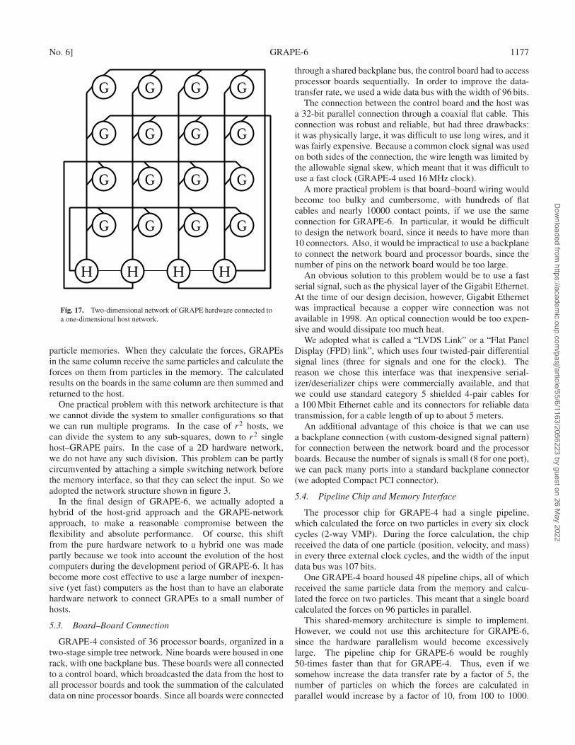
It was not really difficult to come up with such a design,since the only thing non-diagonal processors do is the forcecalculation. Instead of a two-dimensional grid of host proces-sors, we can construct a two-dimensional grid of GRAPEhardwares with orthogonal broadcast networks (figure 17). TheGRAPE hardware in the same row store the same data to their
Dow
nloaded from https://academ
ic.oup.com/pasj/article/55/6/1163/2056223 by guest on 26 M
ay 2022
No. 6] GRAPE-6 1177
Fig. 17. Two-dimensional network of GRAPE hardware connected toa one-dimensional host network.
particle memories. When they calculate the forces, GRAPEsin the same column receive the same particles and calculate theforces on them from particles in the memory. The calculatedresults on the boards in the same column are then summed andreturned to the host.
One practical problem with this network architecture is thatwe cannot divide the system to smaller configurations so thatwe can run multiple programs. In the case of r2 hosts, wecan divide the system to any sub-squares, down to r2 singlehost–GRAPE pairs. In the case of a 2D hardware network,we do not have any such division. This problem can be partlycircumvented by attaching a simple switching network beforethe memory interface, so that they can select the input. So weadopted the network structure shown in figure 3.
In the final design of GRAPE-6, we actually adopted ahybrid of the host-grid approach and the GRAPE-networkapproach, to make a reasonable compromise between theflexibility and absolute performance. Of course, this shiftfrom the pure hardware network to a hybrid one was madepartly because we took into account the evolution of the hostcomputers during the development period of GRAPE-6. It hasbecome more cost effective to use a large number of inexpen-sive (yet fast) computers as the host than to have an elaboratehardware network to connect GRAPEs to a small number ofhosts.
5.3. Board–Board Connection
GRAPE-4 consisted of 36 processor boards, organized in atwo-stage simple tree network. Nine boards were housed in onerack, with one backplane bus. These boards were all connectedto a control board, which broadcasted the data from the host toall processor boards and took the summation of the calculateddata on nine processor boards. Since all boards were connected
through a shared backplane bus, the control board had to accessprocessor boards sequentially. In order to improve the data-transfer rate, we used a wide data bus with the width of 96 bits.
The connection between the control board and the host wasa 32-bit parallel connection through a coaxial flat cable. Thisconnection was robust and reliable, but had three drawbacks:it was physically large, it was difficult to use long wires, and itwas fairly expensive. Because a common clock signal was usedon both sides of the connection, the wire length was limited bythe allowable signal skew, which meant that it was difficult touse a fast clock (GRAPE-4 used 16 MHz clock).
A more practical problem is that board–board wiring wouldbecome too bulky and cumbersome, with hundreds of flatcables and nearly 10000 contact points, if we use the sameconnection for GRAPE-6. In particular, it would be difficultto design the network board, since it needs to have more than10 connectors. Also, it would be impractical to use a backplaneto connect the network board and processor boards, since thenumber of pins on the network board would be too large.
An obvious solution to this problem would be to use a fastserial signal, such as the physical layer of the Gigabit Ethernet.At the time of our design decision, however, Gigabit Ethernetwas impractical because a copper wire connection was notavailable in 1998. An optical connection would be too expen-sive and would dissipate too much heat.
We adopted what is called a “LVDS Link” or a “Flat PanelDisplay (FPD) link”, which uses four twisted-pair differentialsignal lines (three for signals and one for the clock). Thereason we chose this interface was that inexpensive serial-izer/deserializer chips were commercially available, and thatwe could use standard category 5 shielded 4-pair cables fora 100 Mbit Ethernet cable and its connectors for reliable datatransmission, for a cable length of up to about 5 meters.
An additional advantage of this choice is that we can usea backplane connection (with custom-designed signal pattern)for connection between the network board and the processorboards. Because the number of signals is small (8 for one port),we can pack many ports into a standard backplane connector(we adopted Compact PCI connector).
5.4. Pipeline Chip and Memory Interface
The processor chip for GRAPE-4 had a single pipeline,which calculated the force on two particles in every six clockcycles (2-way VMP). During the force calculation, the chipreceived the data of one particle (position, velocity, and mass)in every three external clock cycles, and the width of the inputdata bus was 107 bits.
One GRAPE-4 board housed 48 pipeline chips, all of whichreceived the same particle data from the memory and calcu-lated the force on two particles. This meant that a single boardcalculated the forces on 96 particles in parallel.
This shared-memory architecture is simple to implement.However, we could not use this architecture for GRAPE-6,since the hardware parallelism would become excessivelylarge. The pipeline chip for GRAPE-6 would be roughly50-times faster than that for GRAPE-4. Thus, even if wesomehow increase the data transfer rate by a factor of 5, thenumber of particles on which the forces are calculated inparallel would increase by a factor of 10, from 100 to 1000.
Dow
nloaded from https://academ
ic.oup.com/pasj/article/55/6/1163/2056223 by guest on 26 M
ay 2022
1178 J. Makino et al. [Vol. 55,
This number is too large if we want to obtain a reasonableperformance for simulations of star clusters with small, high-density cores. Note that with multiple-board configurations,this number would become even larger. On an r × r two-dimensional system, the degree of parallelism becomes largerby a factor of r .
The data-transfer rate of GRAPE-4 chip was about200 MB s−1. To keep the degree of parallelism to be around100 or less, the GRAPE-6 chip would have to have a data-transfer rate of 5GBs−1, which was well beyond our capabilityof designing and manufacturing. At 100 MHz clock, the speedof 5GBs−1 requires 400 input pins. It is quite difficult to have400 signal lines, all with a 100 MHz data rate, to connect morethan a few chips.
Clearly, a different design was necessary. Excessive degreesof parallelism arose from our decision to let a large numberof chips share one memory unit. If we reduce the number ofchips to share the memory, we can thus solve the problem. Anextreme solution is to attach one memory unit to each pipelinechip, and let multiple pipelines calculate the force on the sameset of chips, but from different set of particles.
This extreme solution has one important practical advantage.The connection between the processor chip and its memoryis point-to-point, and physically short (since we can put aprocessor chip and its memory next to each other). This meansthat a high clock frequency, such as 100 MHz, is relatively easyto achieve.
To attach memory chips directly to the processor chips,we need to integrate the predictor pipeline and the memorycontroller unit (generation of address and other control signals)to the processor chip. These do not consume many transistors.Therefore, it does not have any effect to the performance of thechip.
With GRAPE-6, we adopted a 72-bit (with ECC) datawidth for transfer between the memory and the processorchip. A GRAPE-6 chip integrates six 8-way VMP pipelines.Therefore, it calculates the forces on 48 particles in parallel.All pipelines on board calculate the forces on the same set ofparticles. Thus, even with the largest configuration that wehave considered (an 8×8 system), the degree of the parallelismis still less than 400, not much different from that of the full-size GRAPE-4 (which was also 400).
This change from the shared memory design to the localmemory design implied that we had to take the summation of alarge number of partial forces obtained on chips on one board.With GRAPE-4, we also had to take the summation of forcesobtained on different boards, and we used commercially avail-able single-chip floating-point arithmetic units for this summa-tion. With GRAPE-6, we could not apply this solution simplybecause such chips no longer existed. Thus, we have to eitherintegrate this summation function into the processor chip, ordevelop another chip to take the summation.
We adopted the latter approach, but used FPGA (field-programmable gate array) chips to implement adders. It wasnot impossible to integrate floating-point adders into FPGAs,but such a design would require rather large, expensive FPGAchips and a complex design. In order to simplify the design,we chose to use a block floating-point format for the forceand the other calculated result. In this format, we specify the
exponent of the result before we start the calculation. Becausethe actual value of the exponent can be different for forceson different particles, we can calculate the forces with wildlydifferent magnitudes in parallel.
With this block floating-point method, we can greatlysimplify the design of the hardware to take the summation. Ofcourse, we have to supply the value of exponent, but its valueat the previous timestep is almost always okay. For the initialcalculation, we sometimes need to repeat the force calculationa few times until we have a good guess about the exponent.
A rather important advantage of using the block-floatingpoint format is that the calculated result is independent of thenumber of processor chips used to calculate one force. Sincethe actual summations, both within the chip and outside thechip, are done in the fixed-point format, no round-off error isgenerated during summation. Of course, a round-off error isgenerated when we shift the calculated force to meet the block-floating point format, but this error is independent of the orderin which the summation is performed. In the case of the usualfloating-point format used in GRAPE-4, the round-off errorgenerated in the summation depends on the order in which theforces from different particles are accumulated, and thereforethe calculated force is not exactly the same if the number ofboards in the system is different.
Of course, this difference does not have any effect on theaccuracy of the simulation, itself, since the word length itself ischosen as such. However, it is quite useful to be able to obtainexactly the same results on machines with different sizes, sinceit makes the validation of the result much simpler.
6. Performance
In this section, we discuss the performance of the GRAPE-6system, both for the direct summation algorithm with the indi-vidual timestep and the tree algorithm. For both algorithms,we discuss the performance of the single-host system and themulti-host system.
6.1. Direct Summation with Individual Timestep
Here, we discuss the performance of GRAPE-6 for theindividual timestep algorithm. As the benchmark runs, weintegrate the Plummer model with equal-mass particles for1 time unit [we use the “Heggie” unit, Heggie and Mathieu(1986), where the gravitational constant G and total mass ofthe system M are both unity and the total energy of the systemE is −1/4]. We use the standard Hermite integrator (Makino,Aarseth 1992) with the third-order predictor. The timestepcriterion is that of Aarseth (1999) with η = 0.01. For softeningparameter, we tried three different choices. The first one was aconstant softening, ε =1/64. We also tried ε =1/[8(2N )1/3] andε = 4/N to investigate the effect of the softening size. Note thatfor N = 256, all three choices of the softening gave the samevalue. In the following, we first describe the performance of asingle-host system (with 4 processor boards). We then discussthe performance of a single cluster with 2 or 4 hosts, and finallydiscuss the performance of multiple-cluster configurations.
Dow
nloaded from https://academ
ic.oup.com/pasj/article/55/6/1163/2056223 by guest on 26 M
ay 2022
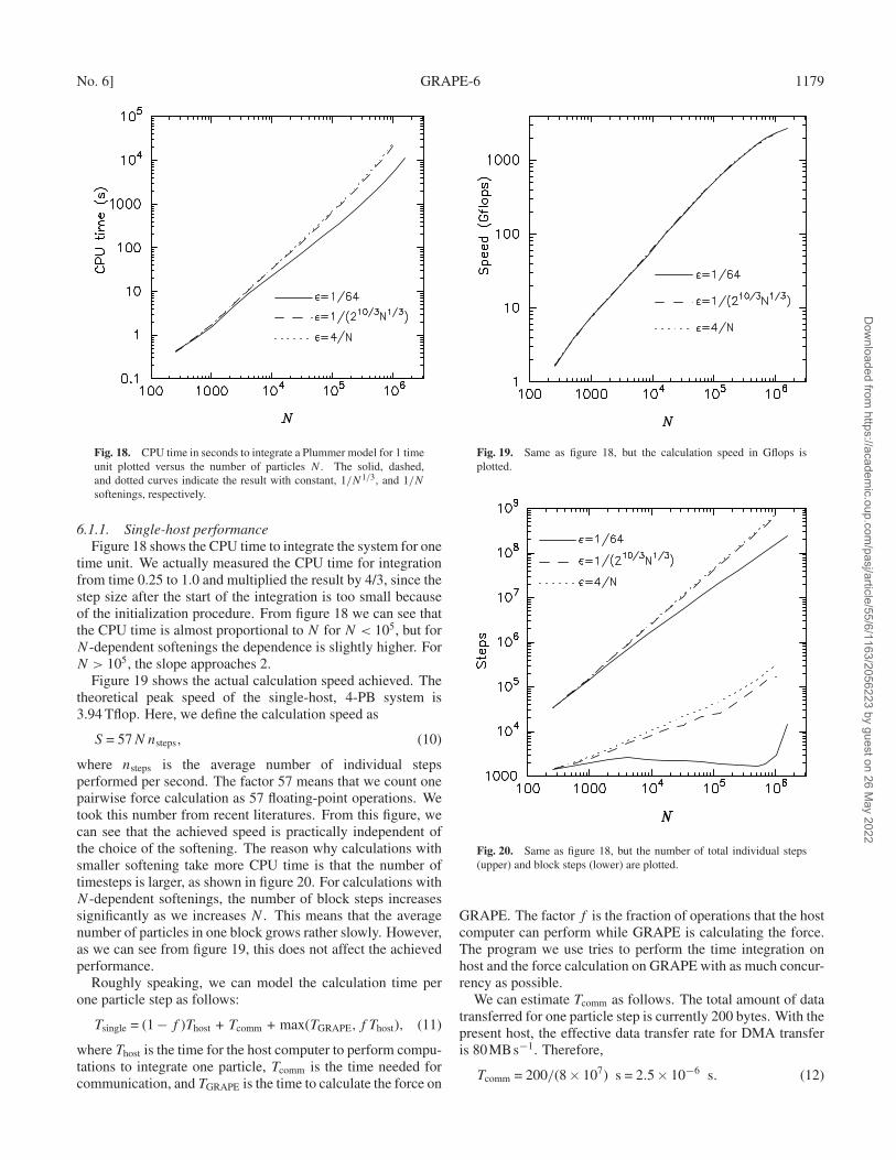
No. 6] GRAPE-6 1179
Fig. 18. CPU time in seconds to integrate a Plummer model for 1 timeunit plotted versus the number of particles N . The solid, dashed,and dotted curves indicate the result with constant, 1/N1/3, and 1/N
softenings, respectively.
6.1.1. Single-host performanceFigure 18 shows the CPU time to integrate the system for one
time unit. We actually measured the CPU time for integrationfrom time 0.25 to 1.0 and multiplied the result by 4/3, since thestep size after the start of the integration is too small becauseof the initialization procedure. From figure 18 we can see thatthe CPU time is almost proportional to N for N < 105, but forN -dependent softenings the dependence is slightly higher. ForN > 105, the slope approaches 2.
Figure 19 shows the actual calculation speed achieved. Thetheoretical peak speed of the single-host, 4-PB system is3.94 Tflop. Here, we define the calculation speed as
S = 57N nsteps, (10)
where nsteps is the average number of individual stepsperformed per second. The factor 57 means that we count onepairwise force calculation as 57 floating-point operations. Wetook this number from recent literatures. From this figure, wecan see that the achieved speed is practically independent ofthe choice of the softening. The reason why calculations withsmaller softening take more CPU time is that the number oftimesteps is larger, as shown in figure 20. For calculations withN -dependent softenings, the number of block steps increasessignificantly as we increases N . This means that the averagenumber of particles in one block grows rather slowly. However,as we can see from figure 19, this does not affect the achievedperformance.
Roughly speaking, we can model the calculation time perone particle step as follows:
Tsingle = (1− f )Thost + Tcomm + max(TGRAPE,f Thost), (11)
where Thost is the time for the host computer to perform compu-tations to integrate one particle, Tcomm is the time needed forcommunication, and TGRAPE is the time to calculate the force on
Fig. 19. Same as figure 18, but the calculation speed in Gflops isplotted.
Fig. 20. Same as figure 18, but the number of total individual steps(upper) and block steps (lower) are plotted.
GRAPE. The factor f is the fraction of operations that the hostcomputer can perform while GRAPE is calculating the force.The program we use tries to perform the time integration onhost and the force calculation on GRAPE with as much concur-rency as possible.
We can estimate Tcomm as follows. The total amount of datatransferred for one particle step is currently 200 bytes. With thepresent host, the effective data transfer rate for DMA transferis 80MBs−1. Therefore,
Tcomm = 200/(8× 107) s = 2.5× 10⁻⁶ s. (12)
Dow
nloaded from https://academ
ic.oup.com/pasj/article/55/6/1163/2056223 by guest on 26 M
ay 2022
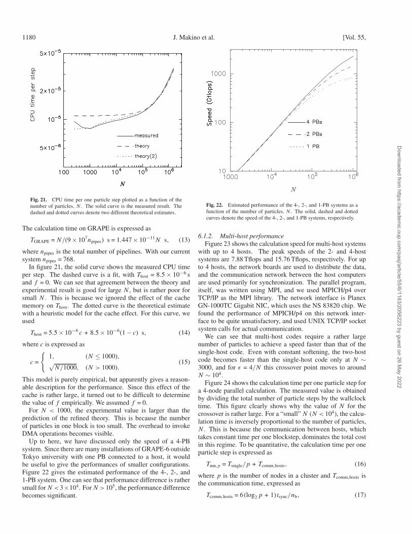
1180 J. Makino et al. [Vol. 55,
Fig. 21. CPU time per one particle step plotted as a function of thenumber of particles, N . The solid curve is the measured result. Thedashed and dotted curves denote two different theoretical estimates.
The calculation time on GRAPE is expressed as
TGRAPE = N/(9× 107npipes) s = 1.447× 10⁻¹¹N s, (13)
where npipes is the total number of pipelines. With our currentsystem npipes = 768.
In figure 21, the solid curve shows the measured CPU timeper step. The dashed curve is a fit, with Thost = 8.5× 10⁻⁶ sand f = 0. We can see that agreement between the theory andexperimental result is good for large N , but is rather poor forsmall N . This is because we ignored the effect of the cachememory on Thost. The dotted curve is the theoretical estimatewith a heuristic model for the cache effect. For this curve, weused
Thost = 5.5× 10⁻⁶ c + 8.5× 10⁻⁶(1− c) s, (14)
where c is expressed as
c =
{1, (N ≤ 1000),√
N/1000, (N > 1000).(15)
This model is purely empirical, but apparently gives a reason-able description for the performance. Since this effect of thecache is rather large, it turned out to be difficult to determinethe value of f empirically. We assumed f = 0.
For N < 1000, the experimental value is larger than theprediction of the refined theory. This is because the numberof particles in one block is too small. The overhead to invokeDMA operations becomes visible.
Up to here, we have discussed only the speed of a 4-PBsystem. Since there are many installations of GRAPE-6 outsideTokyo university with one PB connected to a host, it wouldbe useful to give the performances of smaller configurations.Figure 22 gives the estimated performance of the 4-, 2-, and1-PB system. One can see that performance difference is rathersmall for N <3×10⁴. For N >105, the performance differencebecomes significant.
Fig. 22. Estimated performance of the 4-, 2-, and 1-PB systems as afunction of the number of particles, N . The solid, dashed and dottedcurves denote the speed of the 4-, 2-, and 1-PB systems, respectively.
6.1.2. Multi-host performanceFigure 23 shows the calculation speed for multi-host systems
with up to 4 hosts. The peak speeds of the 2- and 4-hostsystems are 7.88 Tflops and 15.76 Tflops, respectively. For upto 4 hosts, the network boards are used to distribute the data,and the communication network between the host computersare used primarily for synchronization. The parallel program,itself, was written using MPI, and we used MPICH/p4 overTCP/IP as the MPI library. The network interface is PlanexGN-1000TC Gigabit NIC, which uses the NS 83820 chip. Wefound the performance of MPICH/p4 on this network inter-face to be quite unsatisfactory, and used UNIX TCP/IP socketsystem calls for actual communication.
We can see that multi-host codes require a rather largenumber of particles to achieve a speed faster than that of thesingle-host code. Even with constant softening, the two-hostcode becomes faster than the single-host code only at N ∼3000, and for ε = 4/N this crossover point moves to aroundN ∼ 104.
Figure 24 shows the calculation time per one particle step fora 4-node parallel calculation. The measured value is obtainedby dividing the total number of particle steps by the wallclocktime. This figure clearly shows why the value of N for thecrossover is rather large. For a “small” N (N < 104), the calcu-lation time is inversely proportional to the number of particles,N . This is because the communication between hosts, whichtakes constant time per one blockstep, dominates the total costin this regime. To be quantitative, the calculation time per oneparticle step is expressed as
Tmn,p = Tsingle/p + Tcomm,hosts, (16)
where p is the number of nodes in a cluster and Tcomm,hosts isthe communication time, expressed as
Tcomm,hosts = 6(log2 p + 1) tsync/nb, (17)
Dow
nloaded from https://academ
ic.oup.com/pasj/article/55/6/1163/2056223 by guest on 26 M
ay 2022
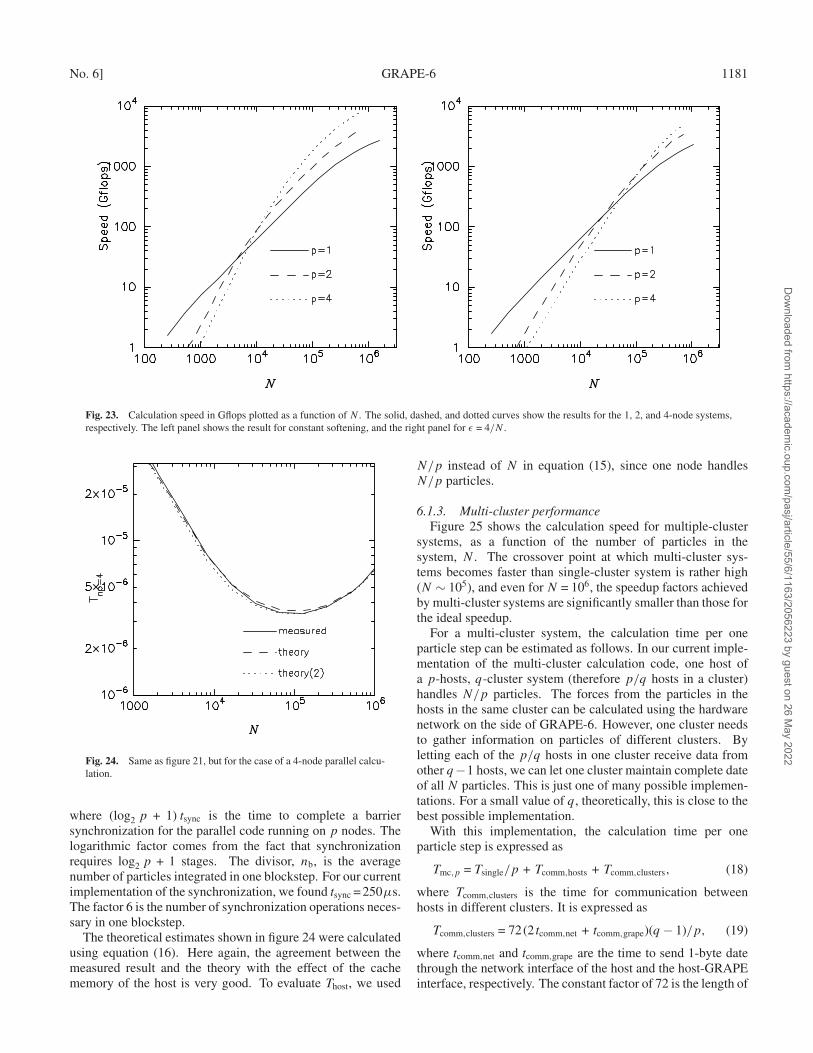
No. 6] GRAPE-6 1181
Fig. 23. Calculation speed in Gflops plotted as a function of N . The solid, dashed, and dotted curves show the results for the 1, 2, and 4-node systems,respectively. The left panel shows the result for constant softening, and the right panel for ε = 4/N .
Fig. 24. Same as figure 21, but for the case of a 4-node parallel calcu-lation.
where (log2 p + 1) tsync is the time to complete a barriersynchronization for the parallel code running on p nodes. Thelogarithmic factor comes from the fact that synchronizationrequires log2 p + 1 stages. The divisor, nb, is the averagenumber of particles integrated in one blockstep. For our currentimplementation of the synchronization, we found tsync = 250µs.The factor 6 is the number of synchronization operations neces-sary in one blockstep.
The theoretical estimates shown in figure 24 were calculatedusing equation (16). Here again, the agreement between themeasured result and the theory with the effect of the cachememory of the host is very good. To evaluate Thost, we used
N/p instead of N in equation (15), since one node handlesN/p particles.
6.1.3. Multi-cluster performanceFigure 25 shows the calculation speed for multiple-cluster
systems, as a function of the number of particles in thesystem, N . The crossover point at which multi-cluster sys-tems becomes faster than single-cluster system is rather high(N ∼ 105), and even for N = 106, the speedup factors achievedby multi-cluster systems are significantly smaller than those forthe ideal speedup.
For a multi-cluster system, the calculation time per oneparticle step can be estimated as follows. In our current imple-mentation of the multi-cluster calculation code, one host ofa p-hosts, q-cluster system (therefore p/q hosts in a cluster)handles N/p particles. The forces from the particles in thehosts in the same cluster can be calculated using the hardwarenetwork on the side of GRAPE-6. However, one cluster needsto gather information on particles of different clusters. Byletting each of the p/q hosts in one cluster receive data fromother q−1 hosts, we can let one cluster maintain complete dateof all N particles. This is just one of many possible implemen-tations. For a small value of q, theoretically, this is close to thebest possible implementation.
With this implementation, the calculation time per oneparticle step is expressed as
Tmc,p = Tsingle/p + Tcomm,hosts + Tcomm,clusters, (18)
where Tcomm,clusters is the time for communication betweenhosts in different clusters. It is expressed as
Tcomm,clusters = 72(2 tcomm,net + tcomm,grape)(q − 1)/p, (19)
where tcomm,net and tcomm,grape are the time to send 1-byte datethrough the network interface of the host and the host-GRAPEinterface, respectively. The constant factor of 72 is the length of
Dow
nloaded from https://academ
ic.oup.com/pasj/article/55/6/1163/2056223 by guest on 26 M
ay 2022

1182 J. Makino et al. [Vol. 55,
Fig. 25. Calculation speed in Tflops plotted as a function of N . Thesolid, dashed, and dotted curves show the results for the 4, 8, and16-host (1, 2, and 4-cluster) systems, respectively. Constant softeningis used for all runs.
data for one particle in bytes. The next factor of 2 comes fromthe fact that each node needs to both send and receive data. Thefactor q − 1 appears since one node receives data from q − 1other nodes. We used tcomm,net = 1.7× 10⁻⁸ s and tcomm,grape =1.25× 10⁻⁸ s. These values are based on separate measure-ments using small benchmark programs. Figure 26 shows thecalculation time per one particle step for a full-cluster calcula-tion (16 nodes, 4 clusters). The agreement between the theoret-ical estimate and the measured value is fairly good, but notideal. We probably have underestimated tcomm,net in the realprogram.
6.1.4. Summary for the direct summation codeIn this section we present the performance figures of
GRAPE-6 for a direct N -body simulation. As described inthe introduction, this kind of simulations is the main targetof GRAPE-6. This, we made a fairly detailed analysis of theperformance. What we have found is summarized as follows.
In the case of the single-host configuration, the calculationspeed of the present host computer is the largest bottleneck ofthe performance, and the communication speed is relativelyunimportant. This means that we can keep improving theoverall performance of the system just by replacing the hostcomputer, for the next several years.
For the multi-host configuration, the situation is ratherdifferent. In the case of a single cluster (no host–host datatransfer), the performance for small-N runs is determinedby the overhead of the barrier synchronization between hostcomputers. We currently use standard UNIX implementa-tion of the TCP/IP socket for the basic communication; theTCP/IP socket is certainly not the communication softwarewith the lowest possible latency. The use of communicationsoftware/hardware with a lower latency would significantlyimprove the performance.
Fig. 26. Same as figure 21, but for the case of a 16-host parallel calcu-lation.
Finally, for the case of the multi-cluster configuration, asexpected, the performance is limited by the bandwidth of thecommunication between the hosts. Currently, we use a GigabitEthernet card on a 32-bit, 33-MHz PCI bus. Clearly, by goingto a faster bus (PCI-66 or PCI-X) and a faster CPU, the commu-nication bandwidth will be significantly improved.
To summarize, at present the performance of GRAPE-6for small-N calculations is limited by the speed of the hostcomputer, and by the latency of the communication betweenthe hosts when multi-host or multi-cluster systems are used.Even so, GRAPE-6 can achieve a speed exceeding 100 Gflops,for relatively small number of particles, such as 16 k. In thecoming several years, improvements of the host computer willimprove the overall performance of the system.
6.2. Tree Algorithm
Here, we discuss the performance of GRAPE-6 for theBarnes–Hut tree algorithm. We use the modified algorithmintroduced by Barnes (1990). We discuss the performance ofa single-host code and a multi-host (parallel) code with up to12 host computers. The parallel algorithm is based on a spacedecomposition similar to the well-known orthogonal recursivebisection (ORB) method (Dubinski 1996). The details of theparallel algorithm will be discussed elsewhere.
6.2.1. Single-host performanceFigure 27 shows the CPU time per timestep as a function
of the number of particle, N . The distribution of particles is aPlummer model, with an outer cutoff radius of 22.8 in Heggieunits. We used ng = 20000 as the maximum group size for themodified algorithm.
We can see that the CPU time grows practically linearly aswe increase N . Also, the dependence on the opening angle, θ ,is rather weak. This weak dependence is the characteristic ofGRAPE implementation of the tree algorithm (Makino 1991c;
Dow
nloaded from https://academ
ic.oup.com/pasj/article/55/6/1163/2056223 by guest on 26 M
ay 2022
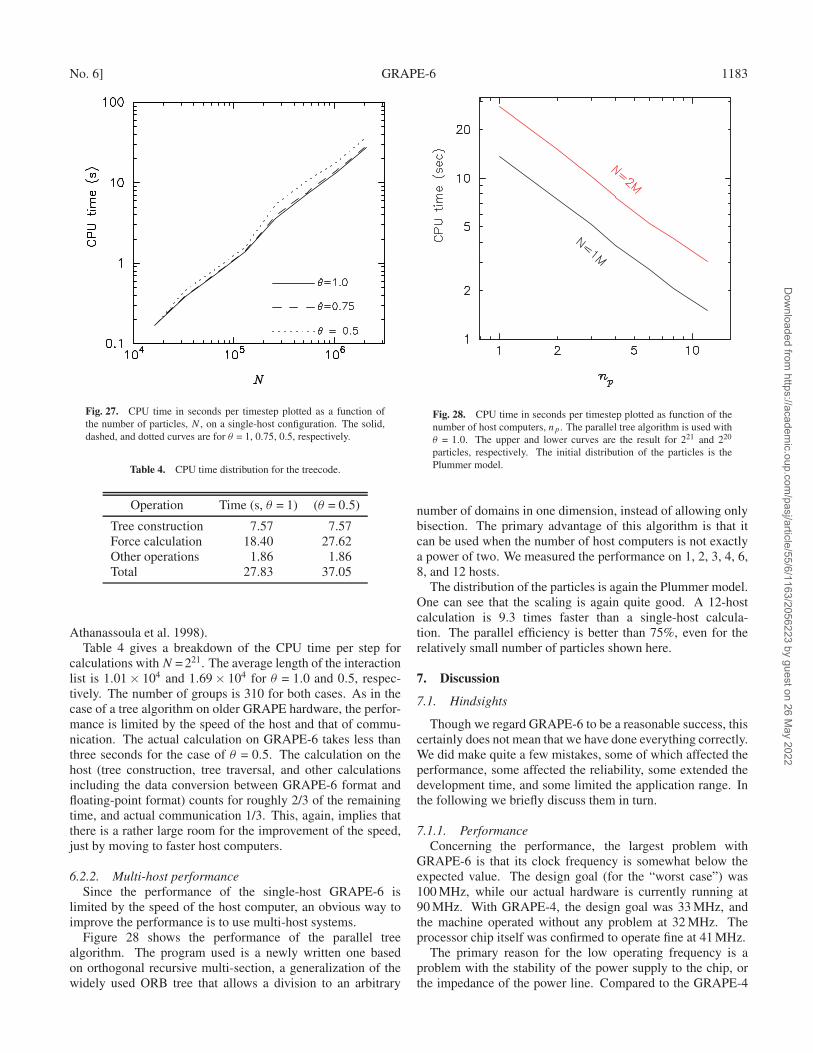
No. 6] GRAPE-6 1183
Fig. 27. CPU time in seconds per timestep plotted as a function ofthe number of particles, N , on a single-host configuration. The solid,dashed, and dotted curves are for θ = 1, 0.75, 0.5, respectively.
Table 4. CPU time distribution for the treecode.
Operation Time (s, θ = 1) (θ = 0.5)
Tree construction 7.57 7.57Force calculation 18.40 27.62Other operations 1.86 1.86Total 27.83 37.05
Athanassoula et al. 1998).Table 4 gives a breakdown of the CPU time per step for
calculations with N = 221. The average length of the interactionlist is 1.01× 10⁴ and 1.69× 10⁴ for θ = 1.0 and 0.5, respec-tively. The number of groups is 310 for both cases. As in thecase of a tree algorithm on older GRAPE hardware, the perfor-mance is limited by the speed of the host and that of commu-nication. The actual calculation on GRAPE-6 takes less thanthree seconds for the case of θ = 0.5. The calculation on thehost (tree construction, tree traversal, and other calculationsincluding the data conversion between GRAPE-6 format andfloating-point format) counts for roughly 2/3 of the remainingtime, and actual communication 1/3. This, again, implies thatthere is a rather large room for the improvement of the speed,just by moving to faster host computers.
6.2.2. Multi-host performanceSince the performance of the single-host GRAPE-6 is
limited by the speed of the host computer, an obvious way toimprove the performance is to use multi-host systems.
Figure 28 shows the performance of the parallel treealgorithm. The program used is a newly written one basedon orthogonal recursive multi-section, a generalization of thewidely used ORB tree that allows a division to an arbitrary
Fig. 28. CPU time in seconds per timestep plotted as function of thenumber of host computers, np . The parallel tree algorithm is used withθ = 1.0. The upper and lower curves are the result for 221 and 220
particles, respectively. The initial distribution of the particles is thePlummer model.
number of domains in one dimension, instead of allowing onlybisection. The primary advantage of this algorithm is that itcan be used when the number of host computers is not exactlya power of two. We measured the performance on 1, 2, 3, 4, 6,8, and 12 hosts.
The distribution of the particles is again the Plummer model.One can see that the scaling is again quite good. A 12-hostcalculation is 9.3 times faster than a single-host calcula-tion. The parallel efficiency is better than 75%, even for therelatively small number of particles shown here.
7. Discussion
7.1. Hindsights
Though we regard GRAPE-6 to be a reasonable success, thiscertainly does not mean that we have done everything correctly.We did make quite a few mistakes, some of which affected theperformance, some affected the reliability, some extended thedevelopment time, and some limited the application range. Inthe following we briefly discuss them in turn.
7.1.1. PerformanceConcerning the performance, the largest problem with
GRAPE-6 is that its clock frequency is somewhat below theexpected value. The design goal (for the “worst case”) was100 MHz, while our actual hardware is currently running at90 MHz. With GRAPE-4, the design goal was 33 MHz, andthe machine operated without any problem at 32 MHz. Theprocessor chip itself was confirmed to operate fine at 41 MHz.
The primary reason for the low operating frequency is aproblem with the stability of the power supply to the chip, orthe impedance of the power line. Compared to the GRAPE-4
Dow
nloaded from https://academ
ic.oup.com/pasj/article/55/6/1163/2056223 by guest on 26 M
ay 2022
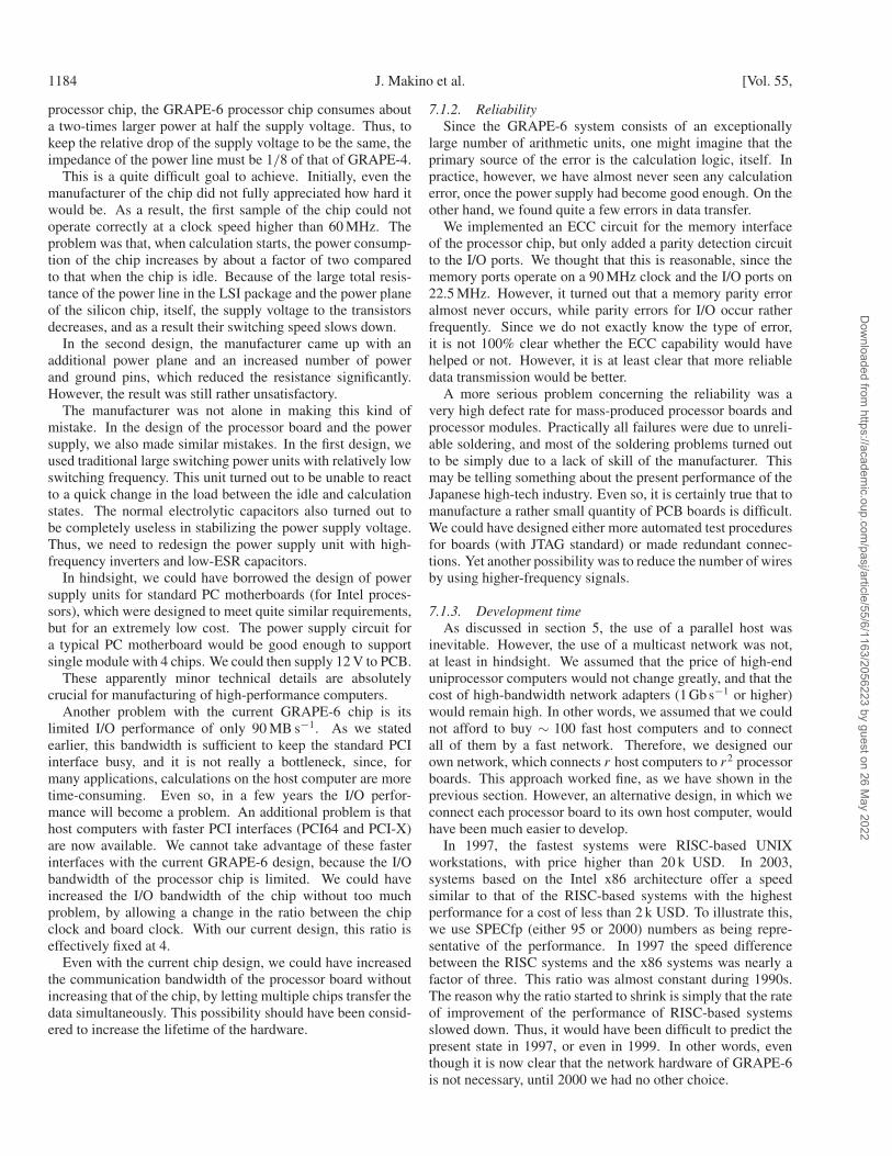
1184 J. Makino et al. [Vol. 55,
processor chip, the GRAPE-6 processor chip consumes abouta two-times larger power at half the supply voltage. Thus, tokeep the relative drop of the supply voltage to be the same, theimpedance of the power line must be 1/8 of that of GRAPE-4.
This is a quite difficult goal to achieve. Initially, even themanufacturer of the chip did not fully appreciated how hard itwould be. As a result, the first sample of the chip could notoperate correctly at a clock speed higher than 60 MHz. Theproblem was that, when calculation starts, the power consump-tion of the chip increases by about a factor of two comparedto that when the chip is idle. Because of the large total resis-tance of the power line in the LSI package and the power planeof the silicon chip, itself, the supply voltage to the transistorsdecreases, and as a result their switching speed slows down.
In the second design, the manufacturer came up with anadditional power plane and an increased number of powerand ground pins, which reduced the resistance significantly.However, the result was still rather unsatisfactory.
The manufacturer was not alone in making this kind ofmistake. In the design of the processor board and the powersupply, we also made similar mistakes. In the first design, weused traditional large switching power units with relatively lowswitching frequency. This unit turned out to be unable to reactto a quick change in the load between the idle and calculationstates. The normal electrolytic capacitors also turned out tobe completely useless in stabilizing the power supply voltage.Thus, we need to redesign the power supply unit with high-frequency inverters and low-ESR capacitors.
In hindsight, we could have borrowed the design of powersupply units for standard PC motherboards (for Intel proces-sors), which were designed to meet quite similar requirements,but for an extremely low cost. The power supply circuit fora typical PC motherboard would be good enough to supportsingle module with 4 chips. We could then supply 12 V to PCB.
These apparently minor technical details are absolutelycrucial for manufacturing of high-performance computers.
Another problem with the current GRAPE-6 chip is itslimited I/O performance of only 90 MB s−1. As we statedearlier, this bandwidth is sufficient to keep the standard PCIinterface busy, and it is not really a bottleneck, since, formany applications, calculations on the host computer are moretime-consuming. Even so, in a few years the I/O perfor-mance will become a problem. An additional problem is thathost computers with faster PCI interfaces (PCI64 and PCI-X)are now available. We cannot take advantage of these fasterinterfaces with the current GRAPE-6 design, because the I/Obandwidth of the processor chip is limited. We could haveincreased the I/O bandwidth of the chip without too muchproblem, by allowing a change in the ratio between the chipclock and board clock. With our current design, this ratio iseffectively fixed at 4.
Even with the current chip design, we could have increasedthe communication bandwidth of the processor board withoutincreasing that of the chip, by letting multiple chips transfer thedata simultaneously. This possibility should have been consid-ered to increase the lifetime of the hardware.
7.1.2. ReliabilitySince the GRAPE-6 system consists of an exceptionally
large number of arithmetic units, one might imagine that theprimary source of the error is the calculation logic, itself. Inpractice, however, we have almost never seen any calculationerror, once the power supply had become good enough. On theother hand, we found quite a few errors in data transfer.
We implemented an ECC circuit for the memory interfaceof the processor chip, but only added a parity detection circuitto the I/O ports. We thought that this is reasonable, since thememory ports operate on a 90 MHz clock and the I/O ports on22.5 MHz. However, it turned out that a memory parity erroralmost never occurs, while parity errors for I/O occur ratherfrequently. Since we do not exactly know the type of error,it is not 100% clear whether the ECC capability would havehelped or not. However, it is at least clear that more reliabledata transmission would be better.
A more serious problem concerning the reliability was avery high defect rate for mass-produced processor boards andprocessor modules. Practically all failures were due to unreli-able soldering, and most of the soldering problems turned outto be simply due to a lack of skill of the manufacturer. Thismay be telling something about the present performance of theJapanese high-tech industry. Even so, it is certainly true that tomanufacture a rather small quantity of PCB boards is difficult.We could have designed either more automated test proceduresfor boards (with JTAG standard) or made redundant connec-tions. Yet another possibility was to reduce the number of wiresby using higher-frequency signals.
7.1.3. Development timeAs discussed in section 5, the use of a parallel host was
inevitable. However, the use of a multicast network was not,at least in hindsight. We assumed that the price of high-enduniprocessor computers would not change greatly, and that thecost of high-bandwidth network adapters (1 Gb s−1 or higher)would remain high. In other words, we assumed that we couldnot afford to buy ∼ 100 fast host computers and to connectall of them by a fast network. Therefore, we designed ourown network, which connects r host computers to r2 processorboards. This approach worked fine, as we have shown in theprevious section. However, an alternative design, in which weconnect each processor board to its own host computer, wouldhave been much easier to develop.
In 1997, the fastest systems were RISC-based UNIXworkstations, with price higher than 20 k USD. In 2003,systems based on the Intel x86 architecture offer a speedsimilar to that of the RISC-based systems with the highestperformance for a cost of less than 2 k USD. To illustrate this,we use SPECfp (either 95 or 2000) numbers as being repre-sentative of the performance. In 1997 the speed differencebetween the RISC systems and the x86 systems was nearly afactor of three. This ratio was almost constant during 1990s.The reason why the ratio started to shrink is simply that the rateof improvement of the performance of RISC-based systemsslowed down. Thus, it would have been difficult to predict thepresent state in 1997, or even in 1999. In other words, eventhough it is now clear that the network hardware of GRAPE-6is not necessary, until 2000 we had no other choice.
Dow
nloaded from https://academ
ic.oup.com/pasj/article/55/6/1163/2056223 by guest on 26 M
ay 2022
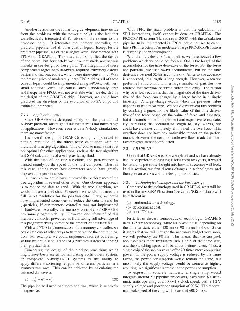
No. 6] GRAPE-6 1185
Another reason for the rather long development time (asidefrom the problems with the power supply) is the fact thatwe effectively integrated all functions of the system to theprocessor chip. It integrates the memory controller, thepredictor pipeline, and all other control logics. Except for thepredictor pipeline, all of these logics were implemented withFPGAs on GRAPE-4. This integration simplified the designof the board, but fortunately we have not made any seriousmistake in the design of these parts. The integration of thesecomplicated logics onto hardware required extremely carefuldesign and test procedures, which were time-consuming. Withthe present price of moderately large FPGA chips, all of thesecontrol logics could be implemented using FPGAs, with verysmall additional cost. Of course, such a moderately largeand inexpensive FPGA was not available when we decided onthe design of the GRAPE-6 chip. However, we could havepredicted the direction of the evolution of FPGA chips andestimated their price.
7.1.4. Application rangeSince GRAPE-6 is designed solely for the gravitational
N -body problem, one might think that there is not much rangeof applications. However, even within N -body simulations,there are many factors.
The overall design of GRAPE-6 is highly optimized toparallel execution of the direct force calculation with theindividual timestep algorithm. This of course means that it isnot optimal for other applications, such as the tree algorithmand SPH calculations of a self-gravitating fluid.
With the case of the tree algorithm, the performance islimited mainly by the speed of the host computer. Thus, inthis case, adding more host computers would have greatlyimproved the performance.
In principle, we could have improved the performance of thetree algorithm in several other ways. One obvious approachis to reduce the data to send. With the tree algorithm, wewould not use a predictor. Moreover, we would not need thefull 64-bit resolution for the position data. Thus, we couldhave implemented some way to reduce the data to send forj -particles, if our memory controller was not implementedin hardware. Actually, the memory controller of GRAPE-6has some programmability. However, one “feature” of thismemory controller prevented us from taking full advantage ofthis programmability to reduce the amount of data transfer.
With an FPGA implementation of the memory controller, wecould implement other ways to further reduce the communica-tion. For example, we could implement indirect addressing,so that we could send indices of j particles instead of sendingtheir physical data.
Concerning the design of the pipeline, one thing whichmight have been useful for simulating collisionless systemsor composite N -body + SPH systems is the ability toapply different softening lengths on different particles in asymmetrized way. This can be achieved by calculating thesoftened distance as
r2s = r2
ij + ε2i + ε2
j . (20)
The pipeline will need one more addition, which is relativelyinexpensive.
With SPH, the main problem is that the calculation ofSPH interactions, itself, cannot be done on GRAPE-6. ThePROGRAPE system (Hamada et al. 2000), with the calculationpipeline fully implemented in FPGA, could be used to calcu-late SPH interaction. An moderately large PROGRAPE systemis currently under development.
With the logic design of the pipeline, we have noticed a fewproblems which we could not foresee. One is the length of theaccumulator for the time derivative of the force. For the forceand potential, we used 64-bit accumulators, but for the timederivative we used 32-bit accumulators. As far as the accuracyis concerned, this length is long enough. However, when weperformed simulations with a large number of particles, werealized that overflow occurred rather frequently. The reasonwhy overflows occurs is that the magnitude of the time deriva-tive of the force can change by a large factor in a singletimestep. A large change occurs when the previous valuehappens to be almost zero. We could circumvent this problemby combing a guess for the likely value of the time deriva-tive of the force based on the value of force and timestep,but it is cumbersome to implement and expensive to evaluate.By increasing the accumulator length to, say, 40 bits, wecould have almost completely eliminated the overflow. Thisoverflow does not have any noticeable impact on the perfor-mance. However, the need to handle overflows made the inter-face program rather complicated.
7.2. GRAPE-7/8
Given that GRAPE-6 is now completed and we have alreadyhad the experience of running it for almost two years, it wouldbe natural to put some thought into how its successor will look.In this section, we first discuss changes in technologies, andthen give an overview of the design possibilities.
7.2.1. Technological changes and the basic designCompared to the technology used in GRAPE-6, what will be
used in the next GRAPE system (we call it NGS for short) willbe different in:
(a) semiconductor technology,(b) development cost,(c) host I/O bus.
First, let us discuss semiconductor technology. GRAPE-6uses 0.25µm technology, while NGS would use, depending onthe time to start, either 130 nm or 90 nm technology. Sinceit seems that we will not get the necessary budget very soon,we will probably use 90 nm. This means that we can packabout 8-times more transistors into a chip of the same size,and the switching speed will be about 3-times faster. Thus, asingle chip of the same size can offer 20-times more computingpower. If the power supply voltage is reduced by the samefactor, the power consumption would remain the same, butmost likely the supply voltage would be somewhat higher,resulting in a significant increase in the power consumption.
To express in concrete numbers, a single chip wouldintegrate around 50 pipeline processors, each with 60 arith-metic units operating at a 300 MHz clock speed, with a 1.2 Vsupply voltage and power consumption of 20 W. The theoret-ical peak speed of the chip will be around 600 Gflops.
Dow
nloaded from https://academ
ic.oup.com/pasj/article/55/6/1163/2056223 by guest on 26 M
ay 2022
1186 J. Makino et al. [Vol. 55,
Compared to the projected speed of general-purpose micro-processors in, say, 2007, this speed is quite attractive. In 2007,microprocessors will, at best, have a peak speed 10-times fasterthan they have now, or about 30 Gflops. The typical perfor-mance on real applications would be around 10 Gflops or less,for a power consumption of 100 W or more.
A necessary consideration is how to connect the pipelinesto memory. If we use the same memory system as we usedfor GRAPE-6, the total number of virtual pipelines per chipbecomes 1000, which is too large for a simulation of any colli-sional system. As is the case with GRAPE-6, it is necessaryto keep the number of i-particles calculated in parallel to bearound 500 or less for large systems with many chips. Thus,the number of virtual pipelines per chip must be less than200, or ideally less than 100. In other words, the memorybandwidth must be increased by at least a factor of five, toaround 3.5GBs−1.
This number, by itself, sounds relatively easy to achieve. Itis the same as what was used with the first Intel P4 processor(3.2GBs−1), using two DRDRAM channels each with a 16-bitdata width. The Intel P4 has been around for more than twoyears. We can now also use DDR 400 memory chips, whichhave 4-times more throughput than the SSRAM chips used inGRAPE-6. We could also use DDR SRAMs.
The choice of the memory interface has strong impact onthe range of applications. One major limitation of GRAPE-6is that, as discussed in the previous section, its memoryaddressing scheme is limited only to sequential access to a fullset of predictor data. Thus, it is not easy to use the tree orother sophisticated algorithms efficiently on GRAPE-6. Onepossibility to solve this problem is to implement the memorycontroller and other control logics in an FPGA chip. Theconnection between the FPGA chip and the pipeline chip mustbe quite fast, but this is relatively easy to achieve, since the datatransfer is unidirectional from the FPGA chip to the pipelinechip. The memory controller will be implemented in the FPGAchip. Thus, it will be possible to use different types of memory(DRDRAM, DDR DRAM/SRAM) without any need to changethe pipeline chip.
As we discussed earlier, parallelism will be achieved by atwo-dimensional network of host computers. Each of themwill have a relatively small GRAPE system. As an example,we consider a system with 256 host computers, each with twoGRAPE cards. Each card houses 4 processor chips with theirown memory control units and memories. All of them can bepackaged into a single card of the PCI form factor, though weneed to use special care for the power supply.
For the interface to the host, the easiest solution is to usePCI-X, which is now available with a data transfer speed of upto 1GBs−1. PCI-X gives us an order-of-magnitude increase inthe communication speed, which roughly balances the increasein the performance of a factor of 20. One problem is whetheror not PCI-X will be available around 5 years from now. Weneed to predict the market trend, or develop a design that canuse multiple interfaces.
Note that this factor-of-10 increase in the communicationimplies that the chip-to-chip communication must also befaster by the same factor. This is not easy, but since thephysical size of the board will be much smaller, it would not
be impossible to use fast clocks.Thus, the design of NGS seems to be simple, as long as we
set the parallel execution of the individual timestep algorithmwith direct summation as the primary design target.
The only, but quite serious, problem is that the predictedinitial cost for the custom chip will be very high. The initialcost for a custom chip has been increasing quite steeply.Roughly speaking, the initial cost has been proportional tothe inverse of the design rule. Thus, while the initial cost ofthe GRAPE-4 chip was around 200 k USD, that for GRAPE-6exceeded 1 M, and for NGS it will reach 3 M. Even thoughthis is “small” compared to the price of any massively-parallelsupercomputer or even PC clusters, to obtain a grant of thissize within the small community of theoretical astrophysics inJapan is not easy.
7.2.2. Combination with sophisticated algorithmsOne rather fundamental question concerning the next
GRAPE system is whether direct summation is really thebest solution or not. McMillan and Aarseth (1993) havedemonstrated that it is possible to implement a combinationof the Barnes–Hut tree algorithm and the individual timestepalgorithm that runs efficiently at least on a single-processorcomputer, and potentially also on shared-memory parallelcomputers. Even when we require very high accuracy, the gainby the tree algorithm is large for a large N . For example, thenumber of interactions per particle to achieve a relative forceaccuracy of 10−5 is around 8000 when the quadrupole momentis used, and around 2000 when the octupole moment is used,for around 106 particles. Thus, even if we assume that thecalculation cost of an octupole is 10-times higher than that ofa point-mass force, the calculation cost of the tree algorithmwould be a factor of 50 less than that of a direct calculation.
Even though the scaling is not as drastic as that of the treealgorithm, the Ahmad–Cohen scheme (1973, also known asthe neighbor scheme) offers a quite significant reduction of thecalculation cost over the simple direct summation. The theoret-ical gain in the calculation cost is O(N1/4) for the neighborscheme (Makino, Hut 1988; Makino, Aarseth 1992). However,the actual speedup is nearly a factor of 10 for only 1000 parti-cles. Thus, for 106 particles the gain can reach a factor of 50.
For 106 particles, both the tree algorithm and neighborscheme, at least theoretically, offer reduction in the calcula-tion cost of around a factor of 50. This factor is certainlystill smaller than the advantage of the GRAPE hardware overgeneral-purpose computers, since the difference in the price–performance ratio will exceed 103. However, if we can incor-porate either of these sophisticated algorithms, even with asignificant loss in the hardware efficiency, like a factor of 5 oreven more, we can still achieve a very significant improvementin the overall speed. We are currently investigating severalpossible ways to achieve this goal.
We would like to thank all of those who are and havebeen involved in the GRAPE project. In particular, we thankDaiichiro Sugimoto for his continuous support to the project,Atsushi Kawai for helping with the hardware design, YokoFunato, Eiichiro Kokubo, Simon Portegies Zwart, Piet Hut,Steve McMillan, Makoto Taiji, Sverre Aarseth, Takayuki Saito
Dow
nloaded from https://academ
ic.oup.com/pasj/article/55/6/1163/2056223 by guest on 26 M
ay 2022
No. 6] GRAPE-6 1187
and many others for discussions on their experience withGRAPE-4 and 5. We are grateful to Mary Inaba and JunichiroShitami for discussions on the network performance, andfor providing us with their software to measure the network
performance. This work is supported by the Research for theFuture Program of Japan Society for the Promotion of Science(JSPS-RFTF97P01102).
References
Aarseth, S. J. 1963, MNRAS, 126, 223Aarseth, S. J. 1999, Celest. Mech. Dyn. Astron., 73, 127Ahmad, A., & Cohen, L. 1973, J. Comput. Phys., 12, 389Athanassoula, E., Bosma, A., Lambert, J. C., & Makino, J. 1998,
MNRAS, 293, 369Barnes, J. E. 1990, J. Comput. Phys., 87, 161Barnes, J., & Hut, P. 1986, Nature, 324, 446Dorband, E. N., Hemsendorf, M., & Merritt, D. 2003, J. Comput.
Phys., 185, 484Dubinski, J. 1996, New Astron., 1, 133Fukushige, T., Ito, T., Makino, J., Ebisuzaki, T., Sugimoto, D., &
Umemura, M. 1991, PASJ, 43, 841Fukushige, T., Taiji, M., Makino, J., Ebisuzaki, T., & Sugimoto, D.
1996, ApJ, 468, 51Funato, Y., Makino, J., & Ebisuzaki, T. 1992, PASJ, 44, 613Greengard, L., & Rokhlin, V. 1987, J. Comput. Phys., 73, 325Hamada, T., Fukushige, T., Kawai, A., & Makino, J. 2000, PASJ, 52,
943Heggie, D. C., & Mathieu, R. D. 1986, in The Use of Supercomputers
in Stellar Dynamics, ed. P. Hut & S. McMillan (New York:Springer), 233
Ito, T., Ebisuzaki, T., Makino, J., & Sugimoto, D. 1991, PASJ, 43, 547Ito, T., Makino, J., Ebisuzaki, T., & Sugimoto, D. 1990, Comput.
Phys. Comm., 60, 187Kawai, A., Fukushige, T., Makino, J., & Taiji, M. 2000, PASJ, 52, 659
Makino, J. 1991a, PASJ, 43, 859Makino, J. 1991b, ApJ, 369, 200Makino, J. 1991c, PASJ, 43, 621Makino, J. 2002, New Astron., 7, 373Makino, J., & Aarseth, S. J. 1992, PASJ, 44, 141Makino, J., & Hut, P. 1988, ApJS, 68, 833Makino, J., Kokubo, E., & Taiji, M. 1993, PASJ, 45, 349Makino, J., & Taiji, M. 1998, Scientific Simulations with Special-
Purpose Computers — The GRAPE Systems (Chichester: JohnWiley and Sons)
Makino, J., Taiji, M., Ebisuzaki, T., & Sugimoto, D. 1997, ApJ, 480,432
McMillan, S. L. W. 1986, in The Use of Supercomputers in StellarDynamics, ed. P. Hut & S. McMillan (New York: Springer), 156
McMillan, S. L. W., & Aarseth, S. J. 1993, ApJ, 414, 200Okumura, S. K., et al. 1993, PASJ, 45, 329Okumura, S. K., Ebisuzaki, T., & Makino, J. 1991, PASJ, 43, 781Springel, V., Yoshida, N., & White, S. D. 2001, New Astron., 6, 79Spurzem, R., & Baumgardt, H. 1999, MNRAS submittedSteinmetz, M. 1996, MNRAS, 278, 1005Sugimoto, D., Chikada, Y., Makino, J., Ito, T., Ebisuzaki, T., &
Umemura, M. 1990, Nature, 345, 33Umemura, M., Fukushige, T., Makino, J., Ebisuzaki, T., Sugimoto,
D., Turner, E. L., & Loeb, A. 1993, PASJ, 45, 311
Dow
nloaded from https://academ
ic.oup.com/pasj/article/55/6/1163/2056223 by guest on 26 M
ay 2022