Fundamental Characteristics

of Feedback Mechanisms

DRAFT

Technical Report of the ISIS Groupat the University of Notre Dame

ISIS-09-006September, 2009

Panos J. AntsaklisDepartment of Electrical Engineering

University of Notre DameNotre Dame, IN 46556

Interdisciplinary Studies in Intelligent Systems

Fundamental Characteristics ofFeedback Mechanisms

1 Introduction and Summary of Results

Feedback is everywhere. Feedback is ubiquitous. Feedback is all around usand inside us.

It would be truly interesting to find out how old feedback is. How farback in time can we trace feedback mechanisms? Since the beginning oflife? Certainly even single cell creatures react to sensory inputs, they changedirection, are attracted to light. The purpose of having sensors is to use theinformation and act upon it to feed, to avoid danger, to find shelter. This isfeedback control. Single cell creatures in addition to using feedback to reactto external stimuli they also have feedback to regulate automatically internalfunctions. Is there life without feedback? In my opinion it is doubtful! Lifefunctions and feedback go hand in hand! But even before the beginning oflife, one could imagine feedback playing a central role in physical phenomenahelping settle processes to equilibrium points. But this discussion is probablyfor another time and place.

In the area of Systems and Control theory, the emphasis has been ondesigning feedback controllers given a model of the process to be controlled.Many powerful methodologies have been introduced in the past half centuryto design controllers, decision mechanisms, that stabilize and achieve desiredperformance in a robust way, being tolerant to certain class of plant param-eter variations and external disturbances. Feedback or closed loop controlis used, instead of feedforward or open loop control, because of uncertain-ties in the plant and its environment. Methods that optimize performance(LQR/LQG, Hinf) have also been used successfully for certain classes ofsystems. The models are typically ordinary differential or difference equa-tions mostly linear and time-invariant but also time-varying, and nonlinear.Less often the behavior of interest is described by partial differential equa-tions. Discrete event systems such as manufacturing systems are typicallydescribed by automata and Petri nets.

Significantly less effort has been spent in the past half century on un-derstanding exactly how and why feedback works so well not only in thecontrol of engineered systems, but in natural systems as well. What are thefundamental principles, the fundamental mechanisms which make feedbackcontrol so powerfully effective? These fundamental mechanisms should beindependent of the particular type of mathematical models used, that is the

1

system may be described by differential equations, by automata, by logic ex-pressions, by natural language since we do know that feedback is ubiquitousand works! What are these fundamental properties that are present every-where? Deeper understanding would make it possible to understand betterthe mechanisms at work in natural systems and would lead to designingbetter controllers.

So the question is whether there are intrinsic properties of feedback thattranscend particular applications and models and are present in electrical,mechanical, physical, biological, social, economic systems. Is there a funda-mental, ever-present, feedback property?

1.1 Feedback

Feedback is a mechanism, ubiquitous in nature that drastically and dramat-ically changes the behavior of the system (of the plant, the process to becontrolled). By behavior we mean the observed response of the system toexternal stimulus such as an input or initial condition. Examples of feed-back abound. Here a familiar situation every car driver has experienced isdescribed.

When driving and the slope of the road starts increasing, the car speedstarts decreasing. Typically the driver detects this by looking at thespeedometer and presses the gas pedal a bit more to increase the fuel rateand bring the speed up again to the previous level. The driver detects-viathe speedometer-the difference between the desired and actual speeds (theerror). When the error is positive-meaning that the actual speed is less thanthe desired-the driver increases the fuel to the engine; if negative-that is theactual speed is higher than the desired speed (going downhill for example)-the driver decreases the fuel input and the car slows down. Cruise (speed)controlers in cars do the same thing but automatically.

In what way does feedback alter the behavior of a system? Considerthe system consisting of the car and the control fuel input set at certainlevel corresponding to the desired speed (here the output) when the road ishorizontal. When there is a positive road incline and no corrective actionis applied the car normally will start slowing down, as its normal behaviordictates. Consider now having as input the desired speed with its corre-sponding fuel rate and adding to this an appropriate additional positive fuelrate when the incline is positive (and the error is positive). Now the systemcan be seen as having the same reference input (desired speed ) as beforebut with feedback it exhibits a different behavior since now the car doesnot slow down. So with the same desired speed as input, feedback makes it

2

possible for the car to have a different dynamic behavior!Can this be done without feedback? If we do know the details of the

incline and have an accurate model of the response of the car when thefuel rate is increased, then the driver, or a machine, can apply just the rightadditional fuel to do the job. However this implies knowledge we do not have.How for example can we have such accurate knowledge so to tell exactly-without using sensor information-when the incline starts and the car slowsdown? How do we know that there will not be a sudden gust of headwind,a disturbance, that will slow us down? In fact both such uncertainties inthe plant model and in disturbances are rather common in practice and soopen loop control typically does not work except in special cases.

The amazing thing is that with feedback the change of behavior is au-tomatic. When feedback information is available the driver maintains thedesired speed, without intimate knowledge of the slope of the incline or ofthe engine of the car, by just observing the speedometer and adding fuelwhen the error is positive, and reducing fuel when the error is negative.(Note that a more sophisticated controller may consider not only the errorin speed but also the rate of change of the actual speed so to react faster).

1.2 Feedback’s Fundamental Properties

In view of the above discusion, it appears that feedback is a way to changebehavior as if we were changing the plant itself but without actually doingso. How is feedback changing the plant behavior?

What are feedback’s most fundamental intrinsic properties? Is it itsability to reduce sensitivity of the behavior to uncertainties in the plant pa-rameters and external disturbances? This is appealing because the reasonsfor using feedback instead of open loop control are these uncertainties. Un-fortunately this is not so. Low sensitivity depends on the particular choicefor the controller and the choice may decrease or increase sensitivity.

For example the sensitivity S of a plant G = 1s+1 in a unity (negative)

feedback configuration with a static controller Gc = k is S = (1+GGc)−1 =s+1

s+1+k . Note that the plant is stable for 1+k > 0 or −1 < k. For −1 < k < 0the sensitivity to parameter variations is greater than 1 that is the sensitivityof the closed loop is worse than that of an open loop (see also Appendix).

So reducing sensitivity cannot be a property that is present independentlyof the particular controller used. Is then stabilization the most fundamen-tal feedback property? Similarly the choice of controller may stabilize ordestabilize the system and so stabilization cannot be an intrinsic feedbackproperty. So what is it?

3

Automatically Changing the DynamicsA key feedback property that transcends all applications and all choices

for the controller appears to be the ability of feedback to completely alter theplant dynamic behavior no matter what the particular plant dynamics are.This property is independent and distinct and separate from the ability toassign new dynamics by selecting the controller appropriately for stabiliza-tion or performance. Note that in the open loop non-feedback case we alsohave the ability to easily assign new dynamics, the problem being that tocancel existing dynamics is not always possible.

Even small feedback gains can change the dynamic behavior. Considerfor example the root-locus of a LTI SISO plant. As the gain k increasesfrom 0, even by a very small amount, the closed loop poles are not the openloop poles any longer-the open loop poles seem to vanish (similarly when kdecreases from 0).

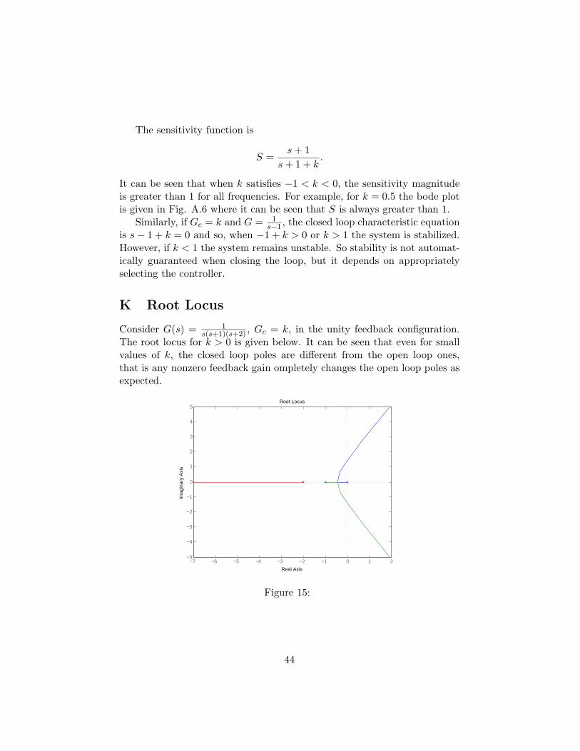
For example consider the plant G(s) = 1s(s+1)(s+2) and its root locus for

k ≥ 0 (see Appendix 11). For k = 0 the closed loop poles are at the openloop pole locations and for small positive k the closed loop poles are differentfrom the open loop pole locations.

As k goes towards infinity the closed loop poles move towards the finitezeros of the plant and to points at infinity along the asymptotes. For verylarge gains k the plant dynamics seem to cancel out completely. These arewell known phenomena in the controls literature and provide the clues forthe fundamental mechanisms of feedback.Automatically Changing the Gains

A second fundamental characteristic of feedback is change in gain. Itshould be noted however that in contrast to the previous property of chang-ing the dynamics, this property is dependent on the selection of the feedbackgain and strictly speaking it may not qualify as a fundamental property.Never the less, as it will be shown, it is directly related to a fundamentalproperty of feedback, namely the ability to reduce the sensitivity to param-eter variations in the plant. As it is discussed below, large gain variationsinside the loop typically can only cause small gain variations outside theloop and so the effect of uncertainties may be much reduced. The auto-matic change in the plant dynamics when closing the loop is essential in theresulting ability of appropriately changing the feedback gains to stabilize thesystem in a robust way. In an analogous fashion, the automatic change inthe gain is essential to the ability of appropriately choosing the feedback gainto reduce the dependence of the system to uncertainties. So, in feedback,the automatic change of the plant dynamics is related to stabilization, while

4

the automatic change in the plant gain is related to reduction of sensitivityto uncertainties.

Changing the dynamics is more complicated and so the next sectionswill be devoted to explaining the mechanisms involved. The mechanism ofchanging the gain can be easily seen from a simple feedback loop involvingonly static gains. Let the plant be an amplifier of gain A, i.e. G(s) = A,and consider a unity feedback control configuration with controller Gc = k,a static gain (see Fig. 1.6).

Here the output of the closed loop system is given by

Y =kA

1 + kAR = TR (1)

withU =

k

1 + kAR, E =

11 + kA

R (2)

while the open loop gain isY = AU. (3)

Sensitivity to plant parameter variations can be studied in detail usingthe sensitivity function S = 1

1+kA and the relation

∆TT≈ S∆G

G(4)

where G is the plant and T is the closed loop transfer function.The R to Y gain remains the same, equal to the plant’s gain A only

when k = 11−A ; in general the closed loop gain will be different from A. The

absolute value of the closed loop gain will be less than 1 for −12 < kA and

will be greater than 1 for kA < −12 . The sensitivity function S = 1

1+kA willhave absolute value |S| < 1 for kA > 0 and for kA < −2; it will have |S| > 1only for −2 < kA < 0. That is, the open loop gain kA maps the sensitivityS to −1...1 range and the closed loop gain T to 0...1 range for all kA > 0.A consequence of this is that variations in A (uncertainties) will not affectas much the overall R to Y gain, that is feedback reduces the sensitivityto parameter variations at the expense of reducing the gain. As a specificexample, consider k = 1 and A = 10000. In this case the R to Y gain is

A

1 +A=

100001 + 10000

≈ 1 (5)

which represents a great reduction in gain. The benefit is that if A changessay by 20% then

A+ .2A1 +A+ .2A

=1.2A

1 + 1.2A=

1.21A + 1.2

≈ 1. (6)

5

That is, the overall gain is insensitive to variations in the open loop gain A.Similar results may be seen in the more general case.Here

Y =GGc

1 +GGcR = TR (7)

withU =

Gc

1 +GGcR, E =

11 +GGc

R (8)

For specific frequencies, when GGc > −12 the closed loop gain has ab-

solute value less than 1. When GGc > 0 or GGc < −2, the absolute valueof the sensitivity S is less than 1. Feedback reduces automatically the sen-sitivity function to less than 1 (for a large class of feedback gains). Forexample, here for any GGc > 0 |S| < 1. Not that also |T | < 1. So thesensitivity function S maps all positive loop gains to the 0...1 range for |S|at the expense of reducing the closed loop gain |T | to the 0...1 range as well.This reduction of the overall R to Y gain of the compensated system is theprice to pay for low sensitivity.The Return Difference

The return difference in a feedback loop is the difference between thetransmitted (measured) and returned signals at the output of the plant; seesection 1.10. Both feedback fundamental characteristics, automatic changeof dynamcis (poles) and gains, are caused by the feedback interconnection,which can be expressed in terms of the return difference. Specifically, inthe unity feedback configuration, the output Y = −GGcY +GGcR or (1 +GGC)Y = GGcR where (1 +GGc) is the return difference; see Section 1.10.

Sidebar: The reason for not having a clear explanation of the feedbackmechanisms at work after many decades of impressive developments in themathematical theory of control may perhaps be due to the fact that modernsystems and control theories typically consider feedback to be already part ofthe setup and study the behavior of the whole system. So the actual feedbackmechanisms have not been explored nearly as well as the effects of feedbackon the compensated systems, where selection of appropriate feedback gainsare of importance and of main interest. In the earlier era of classical controlwhere control specialists typically were closer to applications, it was clearlyseen that the control law is there to manipulate the input u and produce thedesired effect. The plant dynamics cannot be changed. So understandingexactly how u acts on the plant would have been of great interest, but theunderstanding brought forth by internal system descriptions was not readilyavailable then. Today we can look at this problem having the benefit of the

6

insights developed over many years since the classical era of control in the1950s.

In the following sections the focus will be on simple LTI plants underopen and closed loop control. We focus on the automatic changes of dy-namics when closing the loop. Some basic concepts will be reviewed andpresented in a way that sheds light into the basic fundamental mechanismsof feedback control. The Appendix contain discussion on several related top-ics including pole/zero cancellations, sampled data, and nonlinear systems.The effect of high gains is discussed in Section 2, open loop control in Sec-tion 3, and closed loop control in Sections 4 and 5. In Section 6, state spacerepresentations are discussed, and the two degrees of freedom configurationsare discussed in Sections 7 and 8. In section 9, open and closed loop controlare compared and in Section 10 the role of the return difference is discussed.

2 High Gains in the Feedback Loop—A First Glimpseat the Feedback Mechanism

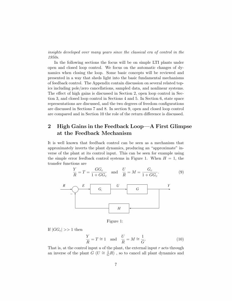
It is well known that feedback control can be seen as a mechanism thatapproximately inverts the plant dynamics, producing an “approximate” in-verse of the plant at its control input. This can be seen for example usingthe simple error feedback control systems in Figure 1. When H = 1, thetransfer functions are

Y

R= T =

GGc

1 +GGcand

U

R= M =

Gc

1 +GGc. (9)

–

YUEG

H

RGc

Figure 1:

If |GGc| >> 1 then

Y

R= T ∼= 1 and

U

R= M ∼=

1G. (10)

That is, at the control input u of the plant, the external input r acts throughan inverse of the plant G (U ∼= 1

GR) , so to cancel all plant dynamics and

7

produce an output y, which is approximately equal to the reference input r(Y = GU ∼= G 1

GR∼= R). In other words, the input to the plant u, generated

by the external input r, is such that when applied to the plant G causes theplant output y to be (approximately) equal to the externally applied inputr.

Note that in the case when Gc = k, a real gain, this effect can also beseen from the Root Locus where as the gain increases the closed-loop polesgo towards the open-loop finite and infinite zeros along the asymptotes andso for high gain, pole-zero cancellations do occur and the overall transferfunction is approximately 1.

If in addition there is a controller H ( 6= 1) in the feedback path, thenagain the plant and its inverse cancel, however the overall gain in this caseis (approximately) independent of the plant and equals 1

H :

Y

R= T ∼=

1H

andU

R= M ∼=

1GH

. (11)

H is selected to have a precise value (typically less than 1) so the compen-sated system has the desirable gain, while it remains robust to parametervariations in GcG.

Similar results can be shown in the nonlinear case (see for example [1]–pp. 29-36 and Appendix A.6). Again in this case, when high gains are appliedthe external input acts through an inverse of the plant on the plant’s input.

Remark: High gains of course can have undesirable effects such asamplification of measurement noise and even worse, can cause instability.The latter can be easily seen, for example, via the Root-Locus in the case ofnon-minimum phase plants where the closed-loop poles approach right-halfplane zeros for high gains and so the closed-loop system becomes unstable.

Discussion: Can it then be said that the feedback mechanism alwaysacts by generating a plant “inverse” and canceling somehow the plant dy-namics, as it was shown to be true in the case of high-loop gains?

Although our intuition based conjecture is basically correct, it is notvery exact. Explaining exactly how feedback acts on the plant is the goal ofthe present work. Clear understanding of the feedback mechanism is veryimportant especially today when feedback is identified and used to explainthe development of a variety of processes found in diverse areas from biology,to physics, to finance.

If we understand clearly how the feedback control produces all thesewonderful results, it will perhaps be easier to understand the cases when

8

feedback information is not readily available as it is the case, for example,in networked control systems, where the plant may have to operate often inan open-loop configuration.

In view of this, the closely related open-loop control versus closed-loopcontrol topic is discussed in detail in the folowing. Furthermore, as it wasdiscussed above, at the plant input u, for high gains the external inputr acts through an inverse of the plant that can be seen as an open-loop“equivalent” to feedback configuration, and these mechanisms will also bediscussed below. Note that in the Appendix A.1 a review of pole/zero can-cellation mechanisms (in both frequency and time domains) are given forcompleteness.

3 Open-loop Control (Feed-forward Control)—ASimple Example

We are interested in obtaining a desired transfer function (desired responseto any allowed input) from a given plant, the input of which is controlledby a controller in series with the plant. We shall start with a simple casewhich nevertheless contains the important salient features.

Consider a plant to be controlled described by the first-order differentialequation a(dy/dt) + y = u with initial condition y(0). If Y (s) and U(s) arethe Laplace transforms of the output and the input respectively, the transferfunction is

Y (s)/U(s) = G(s) =1

as+ 1. (12)

Let the output disturbance be d(t), so that

Y(s)U(s)G(s)

D(s)

Figure 2:

From the differential equation it is easy to see that a(sYp(s)−y(0))+Yp(s) =U(s) from which

Y (s) =a

as+ 1y(0) +

1as+ 1

U(s) +D(s). (13)

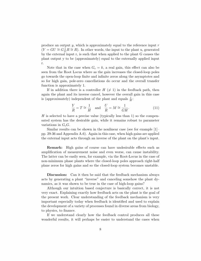
If we consider the open-loop controller in Figure 1.3,

9

U(s)R(s)G (s)c

Figure 3:

where

U(s)/R(s) = Gc(s) =bs+ 1cs+ 1

(c(du/dt) + u = b(dr/dt) + r), (14)

it can be shown that

U(s) =cu(0)− br(0)

cs+ 1+bs+ 1cs+ 1

R(s). (15)

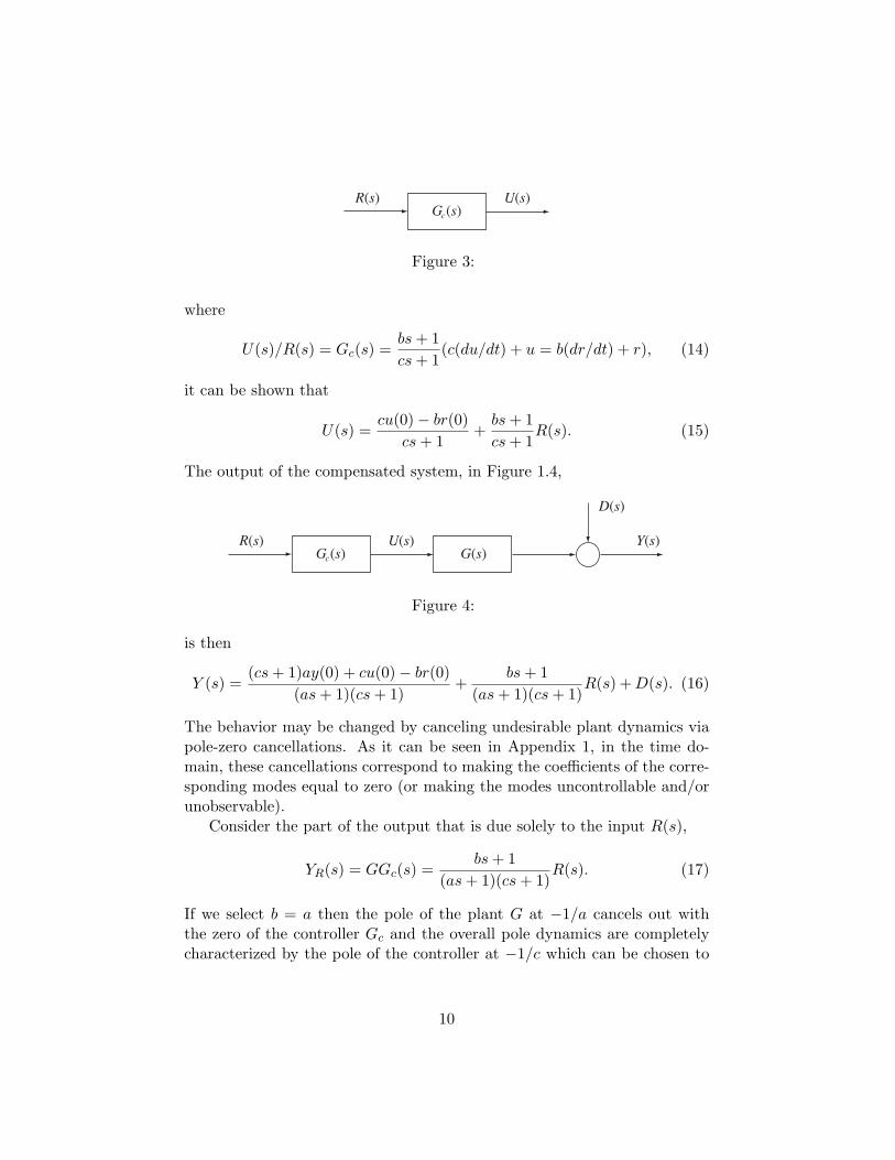
The output of the compensated system, in Figure 1.4,

Y(s)U(s)R(s)G(s)

D(s)

G (s)c

Figure 4:

is then

Y (s) =(cs+ 1)ay(0) + cu(0)− br(0)

(as+ 1)(cs+ 1)+

bs+ 1(as+ 1)(cs+ 1)

R(s) +D(s). (16)

The behavior may be changed by canceling undesirable plant dynamics viapole-zero cancellations. As it can be seen in Appendix 1, in the time do-main, these cancellations correspond to making the coefficients of the corre-sponding modes equal to zero (or making the modes uncontrollable and/orunobservable).

Consider the part of the output that is due solely to the input R(s),

YR(s) = GGc(s) =bs+ 1

(as+ 1)(cs+ 1)R(s). (17)

If we select b = a then the pole of the plant G at −1/a cancels out withthe zero of the controller Gc and the overall pole dynamics are completelycharacterized by the pole of the controller at −1/c which can be chosen to

10

our liking. To illustrate, let r(t) = 1(t) the unit step; then R(s) = 1s and

(let a 6= c for simplicity)

yR(t) = L−1{

bs+1(as+1)(cs+1)

1s

}= L−1

{−a a−b

a−c

as+1 +−c c−b

c−a

cs+1 + 1s

}=

[b−aa−ce

− ta + c−b

a−ce− t

c + 1]

1(t).

(18)

When b = a thenyR(t) =

[1− e−

tc

]1(t). (19)

If however, a is not known exactly (i.e. the exact location of the pole ofthe plant is not known exactly) and b is not taken to be exactly equal to a,but b = a+ ε, then

yR(t) =[

ε

a− ce−

ta +

[1−

(1 +

ε

a− c

)e−

tc

]]1(t) (20)

where it can be seen that the plant pole at −1/a has not been cancelled.If −1/a is positive (unstable pole) then the corresponding mode will growwith time and the system will be unstable.

The part of the response due to initial condition is YI(s), and in the timedomain is (let a 6= c for simplicity)

yI(t) = L−1

{a

as+ 1y(0) +

cu(0)− br(0)a− c

(a

as+ 1− c

cs+ 1

)}=

[[y(0) +

cu(0)− br(0)a− c

]e−

ta − cu(0)− br(0)

a− ce−

tc

]1(t).

(21)

When b, c, u(0), and r(0) are such that the coefficient of e−ta is zero, then

the plant dynamics are suppressed from the response. This happens when

(a− c)y(0) + cu(0)− br(0) = 0 (22)

which is exactly the condition in YI(s) for the factor as+1 in the denominatorto cancel with the numerator (the numerator should be zero for s = −1/awhich is the pole to be cancelled). Again, as in the yR(t) case above, if a andy(0) are not exactly known then the unstable mode will not be eliminatedfrom yI(t).

11

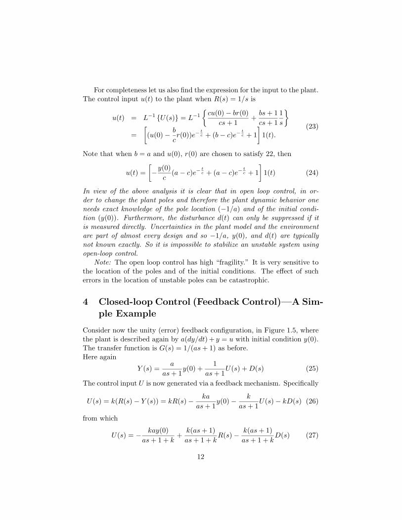
For completeness let us also find the expression for the input to the plant.The control input u(t) to the plant when R(s) = 1/s is

u(t) = L−1 {U(s)} = L−1

{cu(0)− br(0)

cs+ 1+bs+ 1cs+ 1

1s

}=

[(u(0)− b

cr(0))e−

tc + (b− c)e−

tc + 1

]1(t).

(23)

Note that when b = a and u(0), r(0) are chosen to satisfy 22, then

u(t) =[−y(0)

c(a− c)e−

tc + (a− c)e−

tc + 1

]1(t) (24)

In view of the above analysis it is clear that in open loop control, in or-der to change the plant poles and therefore the plant dynamic behavior oneneeds exact knowledge of the pole location (−1/a) and of the initial condi-tion (y(0)). Furthermore, the disturbance d(t) can only be suppressed if itis measured directly. Uncertainties in the plant model and the environmentare part of almost every design and so −1/a, y(0), and d(t) are typicallynot known exactly. So it is impossible to stabilize an unstable system usingopen-loop control.

Note: The open loop control has high “fragility.” It is very sensitive tothe location of the poles and of the initial conditions. The effect of sucherrors in the location of unstable poles can be catastrophic.

4 Closed-loop Control (Feedback Control)—A Sim-ple Example

Consider now the unity (error) feedback configuration, in Figure 1.5, wherethe plant is described again by a(dy/dt) + y = u with initial condition y(0).The transfer function is G(s) = 1/(as+ 1) as before.Here again

Y (s) =a

as+ 1y(0) +

1as+ 1

U(s) +D(s) (25)

The control input U is now generated via a feedback mechanism. Specifically

U(s) = k(R(s)− Y (s)) = kR(s)− ka

as+ 1y(0)− k

as+ 1U(s)− kD(s) (26)

from which

U(s) = − kay(0)as+ 1 + k

+k(as+ 1)as+ 1 + k

R(s)− k(as+ 1)as+ 1 + k

D(s) (27)

12

–

U(s)E(s)G(s)

R(s)K

Y(s)

D(s)

Figure 5:

When this input is applied to the plant

Y (s) =[

a

as+ 1y(0)− kay(0)

(as+ 1)(as+ 1 + k)

]+

k(as+ 1)(as+ 1)(as+ 1 + k)

R(s)

− k(as+ 1)(as+ 1)(as+ 1 + k)

D(s) +D(s)

=a(as+ 1)y(0)

(as+ 1)(as+ 1 + k)+

k(as+ 1)(as+ 1)(as+ 1 + k)

R(s)

(as+ 1)2

(as+ 1)(as+ 1 + k)D(s)

orY (s) =

ay(0)as+ 1 + k

+k

as+ 1 + kR(s) +

as+ 1as+ 1 + k

D(s) (28)

Observe that the factor (as+ 1) that corresponds to the undesirable open-loop dynamics was cancelled in all the terms. The denominator (as+ 1 + k)that represents the desirable dynamics appears in all the terms. Note thatthe system is stable for all k such that 1+k

a > 0. (When a > 0 (stableplant) for k > −1 the closed-loop is stable; when a < 0 (unstable plant) theclosed-loop is stable for k < −1.

The range of the acceptable values for the gain k for stability or thestability robustness of the system is remarkable and it is achieved withfeedback. In the case of the unstable plant for example, the gain k can beselected within a very wide range (−∞ < k < −1) and the system willbe stable even when the exact pole location (− 1

a) and the initial condition(y(0)) are not known. This is not the case when open-loop control is usedas it was shown above.

The above examples suggest that feedback acts in two distinct steps. Inthe first step the plant dynamics are cancelled automatically. In the sec-ond step new desirable dynamics are assigned by appropriately choosing the

13

feedback control law. In the following, these two fundamental feedback ac-tions are discussed at length with the cancellation of plant dynamics showninitially for a more general case and for the general two degrees of freedomcontrollers in the next section. The exact feedback mechanism that cancelsthe plant dynamics is shown.

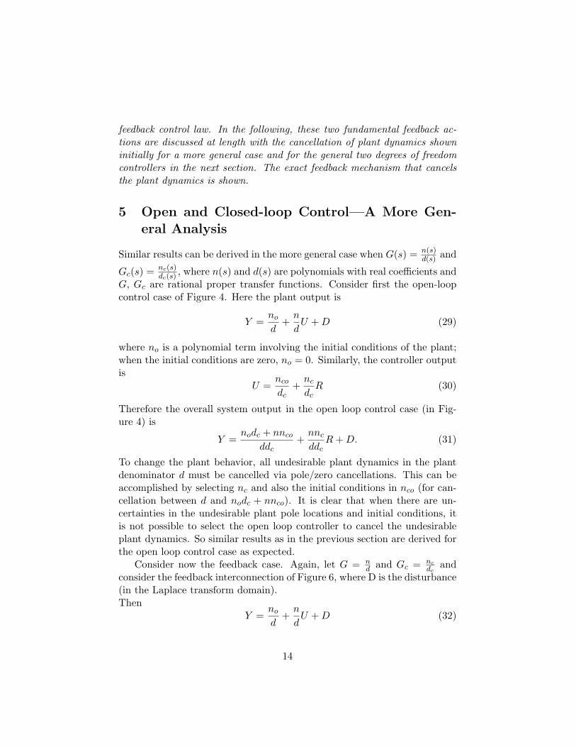
5 Open and Closed-loop Control—A More Gen-eral Analysis

Similar results can be derived in the more general case when G(s) = n(s)d(s) and

Gc(s) = nc(s)dc(s)

, where n(s) and d(s) are polynomials with real coefficients andG, Gc are rational proper transfer functions. Consider first the open-loopcontrol case of Figure 4. Here the plant output is

Y =no

d+n

dU +D (29)

where no is a polynomial term involving the initial conditions of the plant;when the initial conditions are zero, no = 0. Similarly, the controller outputis

U =nco

dc+nc

dcR (30)

Therefore the overall system output in the open loop control case (in Fig-ure 4) is

Y =nodc + nnco

ddc+nnc

ddcR+D. (31)

To change the plant behavior, all undesirable plant dynamics in the plantdenominator d must be cancelled via pole/zero cancellations. This can beaccomplished by selecting nc and also the initial conditions in nco (for can-cellation between d and nodc + nnco). It is clear that when there are un-certainties in the undesirable plant pole locations and initial conditions, itis not possible to select the open loop controller to cancel the undesirableplant dynamics. So similar results as in the previous section are derived forthe open loop control case as expected.

Consider now the feedback case. Again, let G = nd and Gc = nc

dcand

consider the feedback interconnection of Figure 6, where D is the disturbance(in the Laplace transform domain).Then

Y =no

d+n

dU +D (32)

14

–G

D

YUERGc

Figure 6:

and U = ncodc

+ Gc(R − Y ) = ncodc

+ ncdcR − nc

dc

(nod + n

dU +D)

from which(1 + ncn

dcd

)U = ncod−ncno

dcd + ncdcR− nc

dcD or

U =ncod− ncno

ddc + nnc+

ncd

ddc + nncR− ncd

ddc + nncD. (33)

Also

Y =[no

d+n(ncod− ncno)d(ddc + nnc)

]+

ncdn

d(ddc + nnc)R+

[1− ncdn

d(ddc + nnc)

]D

=d(nodc + nnco)d(ddc + nnc)

+dncn

d(ddc + nnc)R+

dddc

d(ddc + nnc)D

orY =

nodc + nnco

dk+ncn

dkR+

ddc

dkD (34)

wheredk ,= ddc + nnc. (35)

Here d, the denominator of the plant, was cancelled in all three terms. Notethat for internal stability dk must be a Hurwitz polynomial (all roots musthave strictly negative real parts). If d−1

k is stable, stability is guaranteedindependently of the initial conditions. Selecting nc and dc (with Gc = nc/dc

proper) to assign the closed-loop poles is straightforward. See the formulasthat characterize all solutions of the Diophantine equation (See for example[2] section 7.2E).

Again here it is seen that all the plant poles in d are automatically can-celled when the loop is closed. That is, when feedback is applied and the loopis closed, the input to the plant u is such that all the plant modes changeautomatically. The closed loop characteristic polynomial has roots (closedloop eigenvalues) that are different from the poles (eigenvalues) of the plant

15

G for almost any Gc (unless poles of G or Gc cancel in the loop gain GGc inwhich case there are uncontrollable and/or unobservable modes that cannotbe altered via output feedback.)

Remarks:

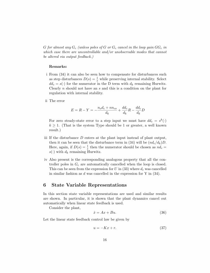
i From (34) it can also be seen how to compensate for disturbances suchas step disturbances D(s) = 1

s while preserving internal stability. Selectddc = s(·) for the numerator in the D term with dk remaining Hurwitz.Clearly n should not have an s and this is a condition on the plant forregulation with internal stability.

ii The error

E = R− Y = −nodc + nnco

dk+ddc

dkR− ddc

dkD

For zero steady-state error to a step input we must have ddc = sk(·)k ≥ 1. (That is the system Type should be 1 or greater, a well knownresult.)

iii If the disturbance D enters at the plant input instead of plant output,then it can be seen that the disturbance term in (34) will be (ndc/dk)D.Here, again, if D(s) = 1

s then the numerator should be chosen as ndc =s(·) with dk remaining Hurwitz.

iv Also present is the corresponding analogous property that all the con-troller poles in Gc are automatically cancelled when the loop is closed.This can be seen from the expression for U in (33) where dc was cancelledin similar fashion as d was cancelled in the expression for Y in (34).

6 State Variable Representations

In this section state variable representations are used and similar resultsare shown. In particular, it is shown that the plant dynamics cancel outautomatically when linear state feedback is used.

Consider the plant,x = Ax+Bu. (36)

Let the linear state feedback control law be given by

u = −Kx+ r. (37)

16

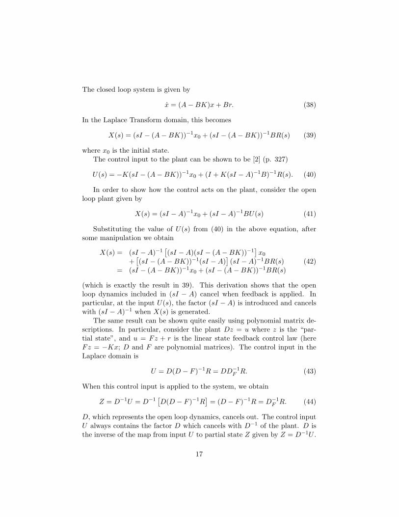
The closed loop system is given by

x = (A−BK)x+Br. (38)

In the Laplace Transform domain, this becomes

X(s) = (sI − (A−BK))−1x0 + (sI − (A−BK))−1BR(s) (39)

where x0 is the initial state.The control input to the plant can be shown to be [2] (p. 327)

U(s) = −K(sI − (A−BK))−1x0 + (I +K(sI −A)−1B)−1R(s). (40)

In order to show how the control acts on the plant, consider the openloop plant given by

X(s) = (sI −A)−1x0 + (sI −A)−1BU(s) (41)

Substituting the value of U(s) from (40) in the above equation, aftersome manipulation we obtain

X(s) = (sI −A)−1[(sI −A)(sI − (A−BK))−1

]x0

+[(sI − (A−BK))−1(sI −A)

](sI −A)−1BR(s)

= (sI − (A−BK))−1x0 + (sI − (A−BK))−1BR(s)(42)

(which is exactly the result in 39). This derivation shows that the openloop dynamics included in (sI − A) cancel when feedback is applied. Inparticular, at the input U(s), the factor (sI −A) is introduced and cancelswith (sI −A)−1 when X(s) is generated.

The same result can be shown quite easily using polynomial matrix de-scriptions. In particular, consider the plant Dz = u where z is the “par-tial state”, and u = Fz + r is the linear state feedback control law (hereFz = −Kx; D and F are polynomial matrices). The control input in theLaplace domain is

U = D(D − F )−1R = DD−1F R. (43)

When this control input is applied to the system, we obtain

Z = D−1U = D−1[D(D − F )−1R

]= (D − F )−1R = D−1

F R. (44)

D, which represents the open loop dynamics, cancels out. The control inputU always contains the factor D which cancels with D−1 of the plant. D isthe inverse of the map from input U to partial state Z given by Z = D−1U .

17

Remark: The linear state feedback gain may be chosen to satisfy addi-tional requirements beyond stabilization. Such requirements may impose therestrictions that certain open loop eigenvalues should become unobservable,by canceling them with zeros (as for example is the case in the disturbancedecoupling problem). In this case, some of the closed loop eigenvalues areequal to the open loop ones and so they are fixed.

Here, again, U is given by (43) and

Y = ND−1U = (ND−1)(DD−1F R) = ND−1

F R. (45)

Then if DF = DFNg where N = NNg,

Y = NNg(DFNg)−1R = NDF−1R. (46)

That is, the eigenvalues in Ng (in DF ) are unobservable and cancel out inthe transfer function.

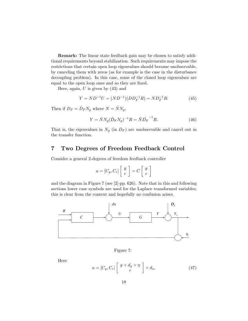
7 Two Degrees of Freedom Feedback Control

Consider a general 2-degrees of freedom feedback controller

u = [Cy, Cr][yr

]= C

[yr

]and the diagram in Figure 7 (see [2]-pp. 626). Note that in this and followingsections lower case symbols are used for the Laplace transformed variables;this is clear from the context and hopefully no confusion arises.

Dy

G

D

YURC

ydu

η

oY

Figure 7:

Here

u = [Cy, Cr][y + dy + η

r

]+ du. (47)

18

Then

y = G(I − CyG)−1 [Crr + Cydy + Cyη + du] (48)

u = (I − CyG)−1 [Crr + Cydy + Cyη + du] (49)

or

y = Tr + (So − I)dy +GQη +GSidu (50)u = Mr +Qdy +Qη + Sidu (51)

where, for G = ND−1

T = G(I − CyG)−1Cr = GM = NX

M = (I − CyG)−1Cr = DX

Q = (I − CyG)−1Cy = DL

So = (I −GCy)−1 = I +GQ

Si = (I − CyG)−1 = I +QG

(52)

Si and So are the input and output comparison sensitivity matrices. Si

is the transfer function between u and du, and So is the transfer functionbetween yo and dy as it can be seen from

yo = y + dy = Tr + Sody +GQη +GSidu. (53)

M is the transfer function between u and r; Q is the transfer functionbetween u and dy or η.

M and Q can be seen as design parameters. M is chosen primarilyto satisfy response requirements between r and y, while Q is selected tosatisfy feedback properties such as low sensitivity to parameter uncertainties,disturbance attenuation, etc. In the 2-degrees of freedom controller, M andQ maybe selected independently. This is not the case in more restrictedconfiguration (see [2]–pp. 629–632) when M and Q are related. For example,in the unity feedback configuration M = Q.

M andQ can always be written asM = DX andQ = DL, whereD is thedenominator of the plant (G = ND−1, where D, N are co-prime polynomialmatrices) and X, L are design parameters (stable rational functions forinternal stability). The part of u that is due to the external input r isur = Mr = DXr or D−1ur = Xr, and in view of the plant descriptionDz = u, y = Nz, zr = Xr. That is X determines the effect of r on theplant’s state z. Similarly, from ud = Qdy = DLdy, zdy = Ldy that is Ldetermines the effect of dy (or η) on z.

19

The expressions for u and y can be written as

u = D[Xr + Ldy + Lη + (I + LN)D−1du

](54)

y = N[Xr + Ldy + Lη + (I + LN)D−1du

]. (55)

This shows that no matter what r, dy, η, du, Cr, and Cy are, u can alwaysbe written as

u = D[X,L,L, (I + LN)D−1

] rdy

ηdu

= Dξ (56)

where ξ is a signal generated by filtered combination of r, dy, η, and du

(note that all the filters are stable for internal stability, see also AppendixA.2).

The feedback mechanism always generates a signal u the behavior ofwhich is modified by D, the inverse of the map D−1 which is the trans-fer function between z and u (z = D−1u) in the plant. D appears in thenumerator of the transfer function between u and r and it has the effect thatfor such u the behavior of the plant state z = D−1u = D−1DXr = Xr iscompletely freed from behavior determined by the plant modes.

So feedback does not really generate the inverse of the planty = Gu (or of the map between y and u)—which may or may notbe proper (causal) after all—but it generates the inverse of themap between z and u, namely of z = D−1u, which always exists.

More specifically, the expression (54) points out the fact that the po-tential is there for the feedback to generate the whole D at u. However,depending on the choices for X and L cancellations may take place betweenD and the denominators of X and L.

To illustrate, consider the case when r is the only external input (dy, du,and η are taken to be zero). If now Cy and Cr are chosen to stabilize thesystem (see [2], p. 623, Theorem 4.21 and Appendix A.2) then X is stableand can be chosen to cancel all stable poles of D. That is under stability,if D = DbDg where Db contains all the unstable (bad) dynamics and Dg

contains all the stable (good) dynamics, X = D−1g X will produce

u = Mr = DXr = DbDgD−1g Xr = DbXr (57)

i.e. only Db (the inverse of D−1b ) will need to appear in u.

20

On the other hand, if the system G = ND−1 is stable, for stability onecan select X = D−1X in which case

u = Mr = DXr = DD−1Xr = Xr (58)

and no inverse map of D need to be generated at u. So for stability u needcontain only all the bad poles of the plant as zeros.

Note that in the case when G−1 = DN−1 exists and is stable, then ifX = N−1X

u = Mr = DXr = DN−1Xr = G−1Xr (59)

that is the inverse of the plant is generated.So, the inverse of D−1 is generated in u as u = Dξ, as in (56),

always. In special cases G−1 is generated (assuming that the in-verse of G exists and is stable). When in addition specific goalsare to be satisfied, such as preserving the stable open loop polesin Dg, Db must be generated; see (57).

In Appendix A.2 the fundamental theorems for internal stability in the2-degrees of freedom case are given for completeness. It is also shown therethat in the most general LTI case u = Mr = DXr and y = Tr = NXrthat is control implies the cancellation of the plant dynamics (poles). Thisis done automatically via feedback when the loop is closed.

In summary, when the loop is closed, an inverse map is gen-erated automatically to cancel all the pole dynamics of the plant.The particular selection of Cy, Cr will determine properties suchas stability, and sensitivity, by generating new pole-zero dynamics(via X and L).

Feedback has the truly remarkable property of generating theinverse of the actual plant dynamics (of D−1) exactly. In LTI,this corresponds to generating zeros (in the map from R to U) atthe exact pole locations of the plant. The particular values of thefeedback gains will determine the new dynamics introduced (recallthat u = DXr and X is stable for stability but otherwise (almost)arbitrarily chosen; see Appendix a.2); DX = M must be proper.

8 Two Degree of Freedom Controllers—A Sum-mary of the Analysis

Given a model of the process dynamics y = Gu, where G is the transferfunction, and u = Mr is the control input, then y = G(Mr) = Tr where

21

T = GM is the desired input r-output y response map. We typically chooseT and M to be stable.

Let now G = ND−1 a coprime fractional polynomial matrix represen-tation that corresponds to the internal description Dz = u, y = Nz withz the partial state. It is known that to obtain the maps T and M withinternal stability, T = NX and M = DX where X is stable (see AppendixA.2). Note that the desired dynamics are introduced via X and the existingdynamics are cancelled via D.

The input u = Mr = DXr can certainly be implemented via open-loop.In fact the two-degrees of freedom controller formulation allows that. Theexamples in previous sections show the difficulties associated with open-loopcontrol when uncertainties in the process parameters and in the exogenousinfluences—initial conditions, external disturbances—are present. Note alsothe amount of dynamics in M = DX that are necessary to be generated,include all the plant dynamics in the denominator of M (D) in addition toall desired dynamics (in X).

The control action u = Mr can be generated via a combination of feed-forward and feedback actions. It corresponds to appropriately selecting thedesign parameters L and X, see Appendix A.2.

Now, the amazing fact is that feedback generates automatically abso-lutely exact models of the existing dynamics in D. This was shown usingthe two degree of freedom controller configuration above that contains dis-turbances and noise signals. Note that as it is well known internal stabilityin the closed-loop system may be guaranteed by requiring that certain mapsbetween appropriate signals be stable; in view of this we omit the initialconditions in the expressions without loss of generality.

In the expressions for u and y in (54) and (55), first notice that u = D(.),that is D−1u = z =(.) a function of the external inputs and disturbances. In(.), the stable design parameter X = D−1M contains the desired dynamicsof the r to y response as discussed above, while L = D−1Q and also (I +LN)D−1 must be stable for internal stability (in [2]–p. 625). Additional loopproperties such as sensitivity may be addressed by selecting L. Furthermoreby selecting L we can reduce the effect of the disturbances from the outputy and other signals in the loop.

It can be shown that Xr = z and so Tr = NXr = Nz = y andMr = DXr = Dz = u. A moment’s reflection reveals that the controlinput u = Dz(= Mr), implements the inverse of the u to z (in-put to state) map D−1 (z = D−1u). Certainly, there are cases whereu can insert an (exact or approximate) inverse of the plant that is of theu, y map G. To see this, assume G is invertible, and let X = N−1XN .

22

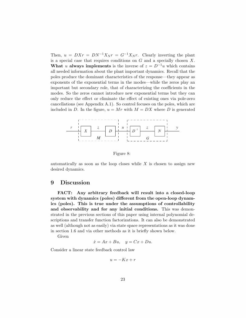
Then, u = DXr = DN−1XNr = G−1XNr. Clearly inverting the plantis a special case that requires conditions on G and a specially chosen X.What u always implements is the inverse of z = D−1u which containsall needed information about the plant important dynamics. Recall that thepoles produce the dominant characteristics of the response—they appear asexponents of the exponential terms in the modes—while the zeros play animportant but secondary role, that of characterizing the coefficients in themodes. So the zeros cannot introduce new exponential terms but they canonly reduce the effect or eliminate the effect of existing ones via pole-zerocancellations (see Appendix A.1). So control focuses on the poles, which areincluded in D. In the figure, u = Mr with M = DX where D is generated

Figure 8:

automatically as soon as the loop closes while X is chosen to assign newdesired dynamics.

9 Discussion

FACT: Any arbitrary feedback will result into a closed-loopsystem with dynamics (poles) different from the open-loop dynam-ics (poles). This is true under the assumptions of controllabilityand observability and for any initial conditions. This was demon-strated in the previous sections of this paper using internal polynomial de-scriptions and transfer function factorizations. It can also be demonstratedas well (although not as easily) via state space representations as it was donein section 1.6 and via other methods as it is briefly shown below.

Givenx = Ax+Bu, y = Cx+Du.

Consider a linear state feedback control law

u = −Kx+ r

23

or a constant output feedback control

u = −HCx+ r.

Then A−BK or A−BHC define the closed-loop dynamics.It is known that the eigenvalues of A−BHC will be different from the

eigenvalues of A for almost any H; in fact the set of gain H that preservethe eigenvalues of A in A − BHC has measure zero (they are roots of amultivariate polynomial in the gains in H). This is under the assumptionsthat (A,B) and (A,C) are controllable and observable respectively. If theyare not, it is known that the uncontrollable and/or unobservable eigenvaluesof the system cannot be altered and they will appear as eigenvalues of A−BHC. Corresponding results exist for A−BK where assuming that (A,B)is controllable its eigenvalues are different from the eigenvalues of A foralmost any K.

This fact can also be seen from the Root Locus where any feedback gainother than zero assigns the closed-loop poles at locations different from theopen-loop pole locations.

In the Diophantine equation under the assumptions of controllabilityand observability controllers will assign the closed-loop poles to differentlocations from the open-loop poles almost always. In fact, in the multi-inputmulti-output case, one can characterize all the controllers that will result toa closed-loop system with poles that contain all the open-loop poles. Thiscan be done for example using the methodology in (see [2]–Appendix) whichis based on Polynomial Matrix Interpolation.

So it is a fact that when the loop closes the dynamics are com-pletely reassigned for almost any feedback gains, that is the plantbehavior drastically changes.

Remark: It is worth mentioning at this point that when H has aspecial structure—for example some (block) diagonal structure as is the casein decentralized control even in the case of the system being controllable andobservable the characteristic polynomial of A−BHC may contain some fixedzeros which do not change with H.

9.1 Open vs Closed Loop Control

Summarizing, a comparison of open and closed loop control is given andtheir characteristics are briefly described.

24

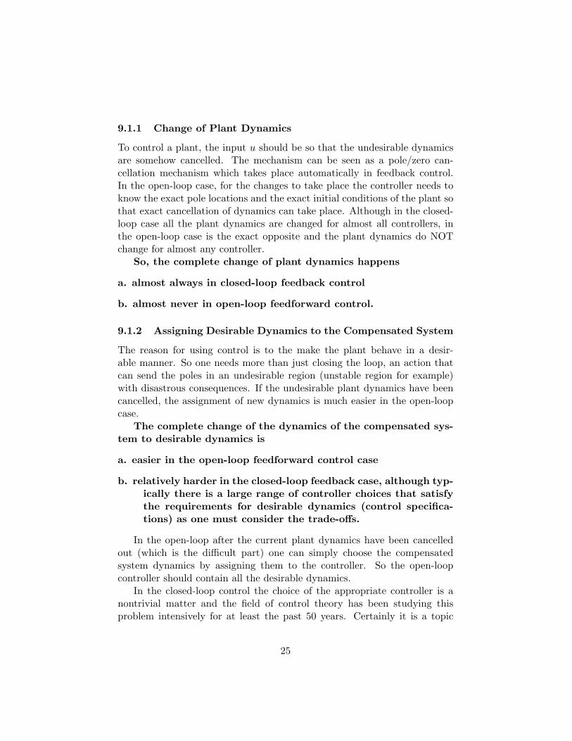
9.1.1 Change of Plant Dynamics

To control a plant, the input u should be so that the undesirable dynamicsare somehow cancelled. The mechanism can be seen as a pole/zero can-cellation mechanism which takes place automatically in feedback control.In the open-loop case, for the changes to take place the controller needs toknow the exact pole locations and the exact initial conditions of the plant sothat exact cancellation of dynamics can take place. Although in the closed-loop case all the plant dynamics are changed for almost all controllers, inthe open-loop case is the exact opposite and the plant dynamics do NOTchange for almost any controller.

So, the complete change of plant dynamics happens

a. almost always in closed-loop feedback control

b. almost never in open-loop feedforward control.

9.1.2 Assigning Desirable Dynamics to the Compensated System

The reason for using control is to the make the plant behave in a desir-able manner. So one needs more than just closing the loop, an action thatcan send the poles in an undesirable region (unstable region for example)with disastrous consequences. If the undesirable plant dynamics have beencancelled, the assignment of new dynamics is much easier in the open-loopcase.

The complete change of the dynamics of the compensated sys-tem to desirable dynamics is

a. easier in the open-loop feedforward control case

b. relatively harder in the closed-loop feedback case, although typ-ically there is a large range of controller choices that satisfythe requirements for desirable dynamics (control specifica-tions) as one must consider the trade-offs.

In the open-loop after the current plant dynamics have been cancelledout (which is the difficult part) one can simply choose the compensatedsystem dynamics by assigning them to the controller. So the open-loopcontroller should contain all the desirable dynamics.

In the closed-loop control the choice of the appropriate controller is anontrivial matter and the field of control theory has been studying thisproblem intensively for at least the past 50 years. Certainly it is a topic

25

that requires deep understanding. The following table summarizes the abovecomments.

Easier HarderOpen Loop Assign New Cancel Existing

Dynamics DynamicsClosed Loop Cancel Existing Assign New

Dynamics Dynamics

10 On the Role of the Return Difference

The return difference relation forces the cancellation of all plant (and con-troller) poles. It can be seen as the underlying cause of the fundamentalfeedback property of canceling automatically the open loop plant dynamics.

Consider the unity feedback configuration as discussed in the section,Open- and Closed-loop Control.

When the initial conditions and the external inputs are zero then, byconsidering the signals at the output of the plant, the return differencerelation is Y = −GGcY or (1 +GGc)Y = 0.

Considering initial conditions and the external input R, with Gc = ncdc

,G = n

d then:

Y =n0

d+GU,U =

nc0

dc+Gc(R− Y )

from which the return difference relation now becomes

Y =n0

d+G

[nc0

dc+Gc(R− Y )

]or

Y = −GGcY +GGcR+[n0

d+G

nc0

dc

]Then

(1 +GGc)Y =n0dc + nnc0

ddc+GGcR

Y =ddc

ddc + nnc

n0dc + nnc0

ddc+

ddcnnc

ddc(ddc + nnc)R

26

This last relation shows that ddc cancels throughout to obtain

Y =n0dc + nnc0

ddc + nnc+

nnc

ddc + nncR

That is, in order to satisfy the conditions on Y imposed by the feedbackinterconnection and expressed in terms of the return difference relations, ddc

must cancel and the new closed loop system has new dynamics imposed byddc + nnc (a Diophantine equation) instead of d (and dc).

Imposing the conditions of the return difference also causes an automaticchange in the gain as discussed in the introduction. Consider Fig. 1.5 withk = 1 and G(s) = A.

Here the return difference relations for the signals in the loop are

U = −AU +R, Y = −AY +AR

The term −AY in the Y equation represents the feedback signal. For anyinput R the signal Y in the output must equal the feedback signal −AY andthe signal R through the plant, AR. For large A this can only happen whenY ≈ R since the left hand side (Y ) is much smaller than AY . In general,from (1+A)Y = AR one can see that Y < R or the gain from R to Y is lessthan 1 (since A > 0, A

1+A < 1 always). So the conditions imposed by thereturn difference relations cause the overall gain to be less than 1. Similarly,they cause the sensitivity S = 1

1+A to be less than 1 as well for any A > 0.This automatic reduction in gain is the cause of lower sensitivity in the

feedback loop as opposed to the open loop. This is caused by the returndifference conditions imposed on the closed loop system by the feedbackinterconnection.

References

[1] G. Goodwin, S. Graebe, and M. Salgato, Control System Design, Pren-tice Hall, 2001.

[2] P.J. Antsaklis and A.N. Michel, Linear Systems, Birkhauser, 2005.

[3] G.F. Franklin, J.D. Powell and A. Emami-Naeini, Feedback Control ofDynamic Systems, 5/e, Pearson Prentice Hall, 2006.

[4] B.C. Kuo, Automatic Control Systems, 7th edition, Prentice-Hall,1995.

27

[5] K. Ogata, Modern Control Engineering, 3rd edition, Prentice-Hall,1997.

[6] R.C. Dorf and R.H. Bishop, Modern Control Systems, 10/e, PearsonPrentice-Hall, 2005.

[7] K.J. Astrom, R.M. Murray, Feedback Systems: An Introduction forScientists and Engineers, Princeton University Press, 2008.

[8] J. Truxal, Control System Synthesis, McGraw-Hill, 1955.

[9] G.C. Newton, L.A. Gould, J.F. Kaiser, Analytical Design of LinearFeedback Controls, Wiley, 1957.

[10] W.A. Wolovich, Linear Multivariable Systems, Springer-Verlag, 1974.

[11] T. Kailath, Linear Systems, Prentice-Hall, 1980.

[12] O. R. Gonzalez and P. J. Antsaklis, “Internal Models Over Rings,”Linear Circuits, Systems and Signal Processing: Theory and Applica-tion, C. I. Byrnes, C. F. Martin and R. E. Saeks, Eds., Chapter 1, pp.41-48, Elsevier Science Pubs. R. V., North Holland, 1988.

[13] O. R. Gonzalez and P. J. Antsaklis, “Internal Models in Regulation,Stabilization and Tracking,” Intern. Journal of Control, Vol 53, No 2,pp 411-430, 1991.

28

Appendix

A The Pole/Zero Cancellation Mechanism: A Re-view

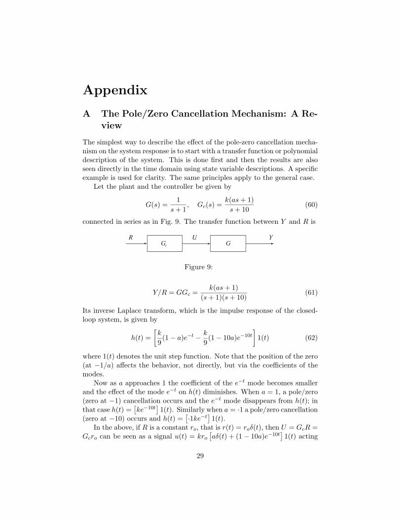
The simplest way to describe the effect of the pole-zero cancellation mecha-nism on the system response is to start with a transfer function or polynomialdescription of the system. This is done first and then the results are alsoseen directly in the time domain using state variable descriptions. A specificexample is used for clarity. The same principles apply to the general case.

Let the plant and the controller be given by

G(s) =1

s+ 1, Gc(s) =

k(as+ 1)s+ 10

(60)

connected in series as in Fig. 9. The transfer function between Y and R is

GYUR

Gc

Figure 9:

Y/R = GGc =k(as+ 1)

(s+ 1)(s+ 10)(61)

Its inverse Laplace transform, which is the impulse response of the closed-loop system, is given by

h(t) =[k

9(1− a)e−t − k

9(1− 10a)e−10t

]1(t) (62)

where 1(t) denotes the unit step function. Note that the position of the zero(at −1/a) affects the behavior, not directly, but via the coefficients of themodes.

Now as a approaches 1 the coefficient of the e−t mode becomes smallerand the effect of the mode e−t on h(t) diminishes. When a = 1, a pole/zero(zero at −1) cancellation occurs and the e−t mode disappears from h(t); inthat case h(t) =

[ke−10t

]1(t). Similarly when a = ·1 a pole/zero cancellation

(zero at −10) occurs and h(t) =[·1ke−t

]1(t).

In the above, if R is a constant ro, that is r(t) = roδ(t), then U = GcR =Gcro can be seen as a signal u(t) = kro

[aδ(t) + (1− 10a)e−10t

]1(t) acting

29

on the system G(s) and producing the pole/zero cancellation or the zeroingof the mode coefficient effects.

If R(s) = 1/s (for example), a unit step input r(t) = 1(t) then the plantoutput will be

y(t) =[−k(1− a)

9e−t +

k(1− 10a)90

e−10t +k

10

]1(t) (63)

and similar effects are observed when pole/zero cancellations occur, in thecases when a = 1 and a = ·1.

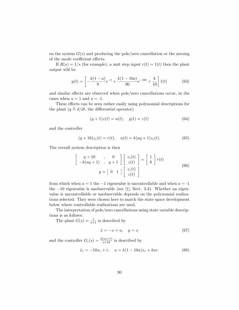
These effects can be seen rather easily using polynomial descriptions forthe plant (q , d/dt, the differential operator)

(q + 1)z(t) = u(t), y(t) = z(t) (64)

and the controller

(q + 10)zc(t) = r(t), u(t) = k(aq + 1)zc(t). (65)

The overall system description is then[q + 10 , 0

−k(aq + 1) , q + 1

] [zc(t)z(t)

]=[

10

]r(t)

y =[

0 1] [ zc(t)

z(t)

] (66)

from which when a = 1 the −1 eigenvalue is uncontrollable and when a = ·1the −10 eigenvalue is unobservable (see [1], Sect. 3.4). Whether an eigen-value is uncontrollable or unobservable depends on the polynomial realiza-tions selected. They were chosen here to match the state space developmentbelow where controllable realizations are used.

The interpretation of pole/zero cancellations using state variable descrip-tions is as follows:

The plant G(s) = 1s+1 is described by

x = −x+ u, y = x (67)

and the controller Gc(s) = k(as+1)s+10 is described by

xc = −10xc + r, u = k(1− 10a)xc + kar. (68)

30

The description of the overall system {A,B,C,D} is then[xc

x

]=[

−10 0k(1− 10a) −1

] [xc

x

]+[

1ka

]r

y = [0 1][xc

x

] (69)

From the controllability matrix

C = [B, AB] =[

1 −10ka k − 11ka

](70)

|C| = k(1−11a)+10ka = k(1−a). So for a = 1 the system is uncontrollable.In fact, the uncontrollable eigenvalue is at −1 (see [2]–Sect. 3.4). From theobservability matrix

O =[

CCA

]=[

0 1k(1− 10a) −1

](71)

|O| = −k(1 − 10a). So for a = ·1 the system is unobservable. In fact, theunobservable eigenvalue is at −10 (see [2]–Sect. 3.4). Again here in the statespace setting, pole/zero cancellations can be seen as cancellations betweeneigenvalues and input or output decoupling zeros see (see [2]–Sect. 3.4) whenthe cancelled eigenvalues (modes) become uncontrollable or unobservable.

In summary, what we conveniently describe as pole/zero cancellation (inthe frequency domain) is a fundamental mechanism of drastically alteringthe behavior of a system by zeroing the coefficient of the correspondingmode (in the time domain). The internal description interpretation is that apole/zero cancellation is making the mode (or the corresponding eigenvalue)uncontrollable from an input or unobservable from an output and so invisiblefrom an input/output point of view.

A.0.3 The Effects of Uncertainties in Pole Locations

If the pole of the plant is not exactly at −1 but at −(1 + ε) then the termin (63) that involves this pole of the plant becomes

y1(t) = − k(1− a+ aε)(9− ε)(1 + ε)

e−(1+ε)t. (72)

It is then clear that if a = 1 the coefficient will not become zero but willbe −k(aε)/(9− ε)(1 + ε). For ε very small the effect of this mode will still

31

be almost negligible. If, however, the pole of the plant were unstable, sayat +1 instead of −1, then the mode in this case would be (·)e(1+ε)t and nomatter how small the coefficient is, given enough time the term will growand so the system is unstable.

In summary, pole/zero cancellation of unstable poles will not work be-cause of the inherent uncertainties in the pole location of the system. Evenif the location of the unstable poles were known exactly pole/zero cancella-tion would not typically produce a stable system because of uncertainties inthe initial conditions since the cancelled unstable poles become uncontrol-lable/unobservable modes (they do not really disappear) and they can beexcited by initial conditions.

B Fundamental Theorems for Internal Stability

Let G = ND−1 be the proper transfer function of the plant; N and D areright coprime polynomial matrices. Let a desirable stable transfer funcion beT , y = Tr, obtained using control u = Mr, where M is also stable. Proofsfor the following theorems may be found in ([2]–Chapter 7 pp. 627-629).

Theorem 1. The stable rational function matrices T and M are realizablevia a two degrees of freedom control configuration with internal stability ifand only if there exists stable X so that[

TM

]=[ND

]X (73)

Theorem 2. T , M ∈ RH∞ are realizable with internal stability by meansof a two degrees of freedom control configuration if and only if there existsX ′ ∈ RH∞ so that [

TM

]=[N ′

D′

]X ′ (74)

Here RH∞ denotes the set of proper and stable rational function matri-ces. Let also S denote the desired stable sensitivity matrix (it is So in (1.52)in section 1.7).

Theorem 3. T , M , S ∈ RH∞ are realizable with internal stability by atwo degrees of freedom control configuration if and only if there exists X ′,L′ ∈ RH∞ so that T

MS

=

N ′ 0D′ 00 N ′

[ X ′L′

]+

00I

, (75)

32

where (I + L′N ′)D′−1 ∈ RH∞. Similarly, T , M , Q ∈ RH∞ (see section1.7) are realizable if and only if there exists X ′, L′ ∈ RH∞ so that T

MQ

=

N ′ 0D′ 00 D′

[ X ′L′

], (76)

where (I + L′N ′)D′−1 ∈ RH∞.D in u = DXr introduces zeros in the transfer function which cancel out

to produce a desired response as in:

T = GMR = ND−1DXr = NXr. (77)

The following two theorems are the basic internal stability theorems forfeedback control (see [2]–pp. 623-625). They give parameterizations of allstabilizing controllers and show that via two design parameters X,L (orM ,Q) the feedforward and feedback control actions can be appropriatelyassigned.

Theorem 4. Let the plant y = Gu have a proper transfer function and let

u = C

[yr

]= [Cy Cr]

[yr

](78)

be a proper 2-degrees of freedom controller. Let det(I − CyG) 6= 0. Theclosed-loop system in internally stable if and only if

1. u = Cyy internally stabilizes the system y = Gu,

2. Cr is such that the rational matrix M = (I − CyG)−1Cr satisfiesD−1M = X, a stable rational matrix, where Cy satisfies (1) andG = ND−1 is a right coprime polynomial matrix factorization.

Theorem 5. Given that the plant y = Gu is proper with G = ND−1 =D−1N doubly coprime polynomial MFDs, all internally stabilizing proper

controllers C in u = C

[yr

]are given by:

C = (I +QH)−1[Q,M ] = [(I + LN)D−1]−1[L,X], (79)

where Q = KD and M = DX are proper with L, X, and D−1(I + QH) =(I + LN)D−1 stable, so that (I +QH)−1 exists and is proper; or by

C = (X1 −KN)−1[−X2 +KD,X], (80)

33

where K and X are stable so that (X1 −KN)−1 exists and C is proper.Also X1 and X2 are determined from

UU−1 =[

X1 X2

−N D

] [D −X2

N X1

]=[I 00 I

]with U unimodular.If G = N ′D′−1 = D′−1N ′ are doubly coprime MFDs in RH∞, then all

stabilizing proper C are given by

C = (X ′1 −K ′N ′)−1[−X ′2 +K ′D′1), X ′], (81)

where K ′, X ′ ∈ RH∞ so that (X ′1 −K ′N ′)−1 exists and is proper. Also

U ′U ′−1 =[

X ′1 X ′2−N ′ D′

] [D′ −X ′2N ′ X ′1

]=[I 00 I

]with U ′, U ′−1 ∈ RH∞; or by

C = (I +QH)−1[Q,M ] = [(I + L′N ′)D′−1]−1[L′, X ′], (82)

where Q = D′L′, M = D′X ′ ∈ RH∞ with L′, X ′, and D′−1(I +QH) =(I +L′N ′)D′−1 ∈ RH∞ and so that (I +QH)−1 or (I +L′N ′)−1 exists andis proper.

C Comments on Stability Robustness

Given a plant G(s) there is an infinite number of controllers Gc(s) thatstabilize the system in a feedback configuration. They are all given by theYoula parameterization (see [2]–p. 615). To get a sense of how robust thestability of a system is, note that all plants G(s) that are stabilized by afixed constant gain controller Gc = k in a feedback configuration is given by

G = Q(1− kQ)−1 (83)

where Q is any proper and stable matrix, which is a large class of plants.The closed loop transfer function Y/R in Fig. 5 is then given by

Y/R = T =kG

1 + kG=

kQ

(1− kQ) + kQ= kQ (84)

andU/R = M =

k

1 + kG=

k(1− kQ)(1− kQ) + kQ

= k(1− kQ). (85)

34

Note that the sensitivity S to parameter variations is

S =1

1 + kG=

1− kQ(1− kQ) + kQ

= 1− kQ. (86)

The poles of Q are the closed-loop poles. If, for example, Q is selectedto be Q = 1/(as + 1 + k) then (83) becomes G = 1

as+1 which was usedabove, in sections 1.3 and 1.4. If Q is chosen to be stable (that is as+ 1 + kHurwitz or (1 + k)/a > 0) then the closed-loop is stable as before. (In thiscase S = as+1

as+1+k which for all k > 0 is less than 1 as desired.)

D DRAFT - Internal Models–Stability and Regu-lation

D.1 Review of Stability in Unity Feedback Configuration

Given a plant P and a controller C, a unity feedback control system isinternally stable if and only if (1+PC)−1, (1+PC)−1P and C(1+PC)−1 arestable (see [2]–p. 584). Having only (1 + PC)−1 stable does not guaranteethat cancellation of unstable P and C poles will not take place, and sowe need all conditions. If P and C are stable then internal stability isguaranteed iff (I + PC)−1 is stable.

The closed loop characteristic polynomial is d(1+PC)dc and so a systeminternally stable if and only if (d(1+PC)dc)−1 is stable. Going from internalpolynomial matrices descriptions is the best way to prove these results forthe MIMO case as well.

Internal Models: It can be shown that when (1 + PC)−1 is stable, (1 +PC)−1P is stable if and only if no bad poles of P cancel in 1 +PC. This inturn is true if and only if 1 + PC has an internal model of P .

We will say (not very precisely) that B has an internal model of A if allthe bad (undesirable) poles of A are poles of B. For a careful definition (see[13]). So if A = s+1

(s+2)(s−1) then B = 1(s−1)(s+4) has an internal model of A.

The system is internally stable iff the following 3 conditions hold:

1. (1 + PC)−1 is stable or the zeros of (1 + PC) are stable

2. (1 + PC)−1P is stable or no cancellations of unstable poles of P takeplace in (1+PC) , or (1 + PC) has an internal model of P

3. C(1 + PC)−1 is stable or no cancellations of unstable poles of C takeplace in (1 + PC) , or (1 + PC) has an internal model of C.

35

Remarks: In 1 above, (1 + PC)−1 stable is not difficult to satisfy. Usethe loop gain PC(jw) and Nyquist to stabilize the system. In 2 above, it iseasy to guarantee that no cancellations of bad poles of P occur in the loopgain PC. In 3 above, it is easy to guarantee that no cancellations of badpoles of C occur in the loop gain PC.

Note that u = Mr = C(1 + PC)−1r. When (1 + PC)−1 is stable and(1 + PC) has an internal model of P then M is has as zeros the unstablepoles of P and if (1 +PC) has an internal model of C then M is stable andPM is stable.

Regulation: Conditions are best shown using factorizations and internaldescriptions. Here Dw is an external disturbance (1 + PC)−1Dw must bestable. When (1+PC)−1 is stable (which it is when the system is internallystable) then regulation takes place iff (1+PC) has an internal model of Dw.

In [12],[13] it is made very clear that an internal model always exists inthe transfer function between the measured output and the plant output.In the unity feedback case this is the return difference (1 + PC)!

Open Loop: In open loop, we must have PM stable, that is D−1Mstable or M−1 should have an internal model of P (or PM does not havean internal model of P ). So stability iff M stable and M−1 has an internalmodel of P .

Remarks: M stable is easy to satisfy. M−1 having an internal modelof P is almost impossible to satisfy since the unstable poles of P are rarelyknown exactly.

The controller M has two roles to play. First it must cancel out allunstable (bad) poles of P in PM -by having these bad poles of P as itszeros, or having M−1 have an internal model of P ( when M comes forfeedback control this part is guaranteed from (1 + PC) having an internalmodel of P ). Secondly M must introduce the desirable dynamics (when Mcomes from feedback M is stable if (1 + PC) has an internal model of C-sono unstable poles of C appear in M−1 and (1 + PC)−1 is stable).

Open vs Closed Loop ControlWe cannot stabilize via open loop control because of our inability to

create an exact internal model of P in the open loop controller. This isvery easy to do in closed loop as it corresponds to simply not allowingcancellations of unstable poles of P in PC.

What about initial conditions? From (42) the expression

(sI −A)−1[(sI −A)(sI − (A−BK))−1

]x0

has an internal model of the plant, which is generated automatically.

36

E Connections to Internal Feedback of a GivenPlant (FIR and IIR) and to Recursive Relations

In this section, we examine feedback structures internal to given plants.Consider the system

x = Ax+Bu

1sB

A

MU X

Figure 10:

with initial conditions x0. From the figure, it is clear that

M = BU +AX = BU +A(1sM +

1sx0)

where U denotes the Laplace transform of u. This is so, because x = mfrom which sX − x0 = M and X = 1

sM + 1sx0. Then

(I −A1s

)M = BU +A1sx0.

Note that (I −A1s ) is the return difference. Then

M = (I−A1s

)−1BU + (I−A1s

)−1A1sx0 = s(sI−A)−1BU + (sI−A)−1Ax0

Substituting in X = 1sM + 1

sx0, we obtain

X =1s

[s(sI −A)−1BU + (sI −A)−1Ax0

]+

1sx0

=1s

[s(sI −A)−1BU

]+

1s

(sI −A)−1 [A+ sI −A]x0

= (sI −A)−1BU + (sI −A)−1x0.

So, sI, which is introduced in the last relation by the term that dependson U and the term that depends on x0, cancels with the pole of 1

sI as

37

expected (X = 1sM is the transfer function in the forward path). The new

eigenvalues (eigenvalues of A) are (almost always) completely different fromthe eigenvalues of x = m at zero. That is, in this internal feedback case, Aplays the role of feedback gain and similar results to the results derived forexternal feedback are obtained. Specifically, the input M to the open loopplant 1

sI is such that the open loop poles (at the origin) cancel automatically.

F Nonlinear Systems

The fundamental feedback property discussed above is applicable to moregeneral systems as well, for example to nonlinear systems: x = f(x, u).When feedback u = h(x, r) is applied, the closed loop system is x =f(x, h(x, r)) which almost always, for almost all h, has different behaviorfrom the open-loop system x = f(x, u) assuming the plant is controllable(see [1]–pp. 29-36).

G Sampled Data Systems

The plant poles also cancel in the case of sampled data systems as thefollowing example illustrates

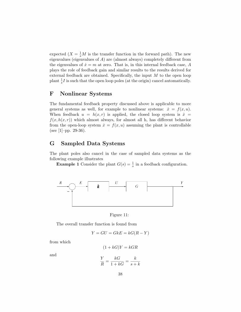
Example 1 Consider the plant G(s) = 1s in a feedback configuration.

k

Figure 11:

The overall transfer function is found from

Y = GU = GkE = kG(R− Y )

from which(1 + kG)Y = kGR

andY

R=

kG

1 + kG=

k

s+ k

38

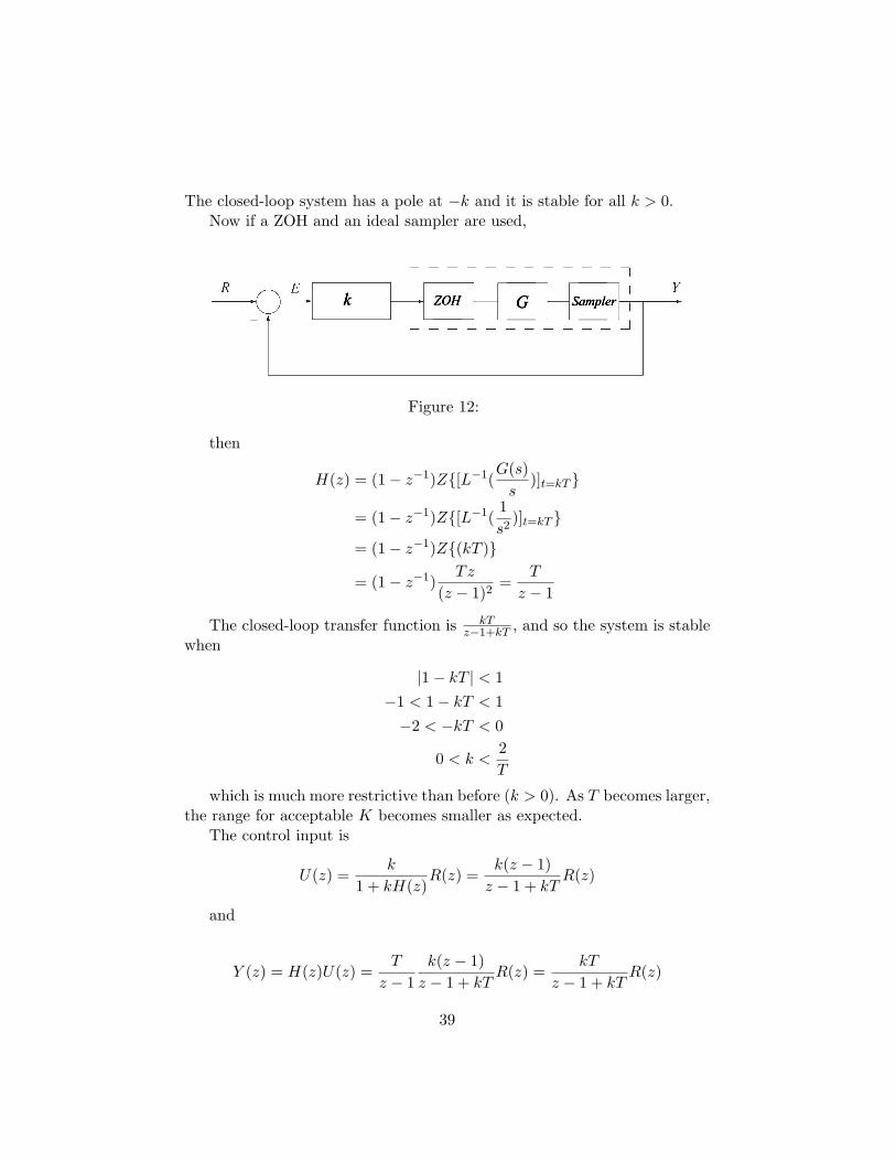
The closed-loop system has a pole at −k and it is stable for all k > 0.Now if a ZOH and an ideal sampler are used,

G Samplerk ZOH

Figure 12:

then

H(z) = (1− z−1)Z{[L−1(G(s)s

)]t=kT }

= (1− z−1)Z{[L−1(1s2

)]t=kT }

= (1− z−1)Z{(kT )}

= (1− z−1)Tz

(z − 1)2=

T

z − 1

The closed-loop transfer function is kTz−1+kT , and so the system is stable

when

|1− kT | < 1−1 < 1− kT < 1−2 < −kT < 0

0 < k <2T

which is much more restrictive than before (k > 0). As T becomes larger,the range for acceptable K becomes smaller as expected.

The control input is

U(z) =k

1 + kH(z)R(z) =

k(z − 1)z − 1 + kT

R(z)

and

Y (z) = H(z)U(z) =T

z − 1k(z − 1)z − 1 + kT

R(z) =kT

z − 1 + kTR(z)

39

Notice that U(z) as it acts on the plant H(z) cancels the plant dynamicsby the pole/zero cancellation of z − 1. The remarkable fact is that thiscancellation happens independently of the sampling period T . Even whenT is large, as long as T is finite, the feedback cancels the plant dynamics.

Example 2 considerG(s) =

a

s+ a

in a unity feedback configuration with gain k. For a > 0, the closed loopis stable when k > −1. When a < 0 (G(s) is unstable), the closed loop isstable for k < −1. The corresponding sampled data system with T as thesampling period is given by

H(z) =1− e−aT

z − e−aT.

The closed loop system is then stable for

−1 < k <1 + e−aT

1− e−aT

when a > 0 (case when open loop is stable). As T becomes larger the righthand side goes to 1. When a < 0 (open loop is unstable), the closed loopsystem is stable when k satisfies

1 + e−aT

1− e−aT≤ k < −1.

As T becomes larger, the left hand side goes to −1 and clearly the range ofk for stability is much reduced.

The examples illustrate what happens in the discrete time case withrespect to the effect of feeedback; they also show how the stability range fork is reduced in the sampled data case compared to the continuous case. Inthe discrete time case, every instant of time k, k + 1,K = 2, ... the input tothe plant is such that the plant dynamics cancel out automatically. This canalso be shown directly using the transfer function H(z) and the numeratorand denominator polynomials (polynomial matrices) N(z), D(z) or via thestate variable description x(k+1) = Ax(k)+Bu(k) in a manner completelyanalogous to the continuous case.

In the sampled data case, the cancelations happen every T units of time.In between time instants T, 2T, ... the continuous plant is running open loopand no plant pole cancelations are taking place. As T becomes larger, theplant is running open loop for longer time and so it is harder to stabilize itby applying feedback at such infrequent instants in time.

40

H Systems With Delays

Similar results can be shown for systems with delays. Note that the delay

e−Ts can be approximated by (first order approximations) 1−T2

s

1+T2

sand if this

is done it is clear that similar results regarding open loop pole cancelations,when feedback is used, can be derived. These results can be shown directly.

As an example, consider

G(s) =1

s+ 1(87)

in a unity feedback configuration with gain k. Without delay, if k satisfies−1 < k, the system is stable. With delay T , k must approximately satisfy−1 < k < 1 + 2

T for stability. As T becomes larger, the range of k becomessmaller.

I Discrete Event Systems

Discrete Event Systems (DES) are typically modeled using automata orPetri Nets (also logic, if-then statements, etc.). In the control literature,supervisory control is typically used to control the behavior of DES whichrestricts possible behaviors but it does not force a specific action. Although,similar results may be shown for automata, below the discussion focuses onsupervisory control of DES using Petri Nets.

In the supervisory control of DES described by Petri Nets, the feedbacksupervisory controller restricts the plant behavior so to satisfy desired con-straints. Specifically, appropriate place invariants are generated and a setof initial conditions are specified that restrict the dynamic behavior of theplant in such a way so to satisfy the control specifications which are givenhere in terms of inequalities on the markings.

Similar ideas apply when feedback is used and the process dynamicsare described by automata or Petri nets. In the Petri net case, specifica-tions described by linear inequalities are imposed by introducing new placeinvariants (new behaviors) and restricting the starting points (suppressingexisting behaviors)—place invariants restrict system behaviors, for exampleif the system starts with its state (markings) in an invariant set it staysthere. In standard Supervisory Control feedback information is used to re-strict the behavior and not to completely alter it. New dynamics are added(in the PN case via additional control places) and the class in initial con-ditions is restricted. The mechanism here corresponds to changing some ofthe modes of the LTI system but not all.

41

J Sensitivity Considerations

Reduction of uncertainties is the primary reason for using feedback. Thisis expressed very conveniently using the sensitivity function S(s) = (1 +GcG(s))−1. The percentage change in the total transfer function gain T (s)is determined by multiplying the percentage change of the loop gain GcG(s)by S(s) all evaluated at the frequencies of interest s = jω. Recall that

∆YY≈ S(

∆GG

).

So when the sensitivity of the loop is low, large variations in the plantgain, due to plant parameter variations, translate into small variations inthe overall gain of the compensated system.

Sensitivity reduction (and stability) are not automatic when closing theloop but they depend on the choice of the controller. If the controller is notselected appropriately, undesireable effects such as an increase in sensitivityor even destabilization may occur.

It is well known that that the main reason for using closed loop feedbackcontrol is the uncertainties in the plant and environment. Open loop controlcannot compensate for plant parameter variations or disturbances (unlessthey can be measured directly).

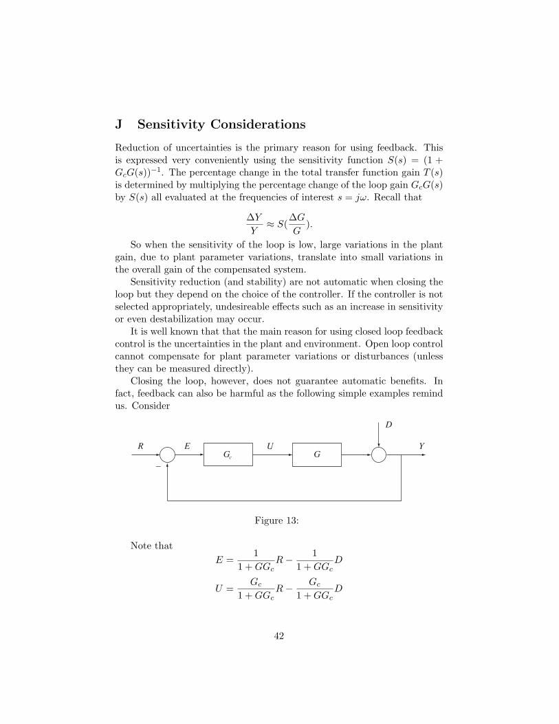
Closing the loop, however, does not guarantee automatic benefits. Infact, feedback can also be harmful as the following simple examples remindus. Consider

–G

D

YUERGc

Figure 13:

Note thatE =

11 +GGc

R− 11 +GGc

D

U =Gc

1 +GGcR− Gc

1 +GGcD

42

Y =GGc

1 +GGcR+

11 +GGc

D

The sensitivity function (to parameter variations) is

S =1

1 +GGc.

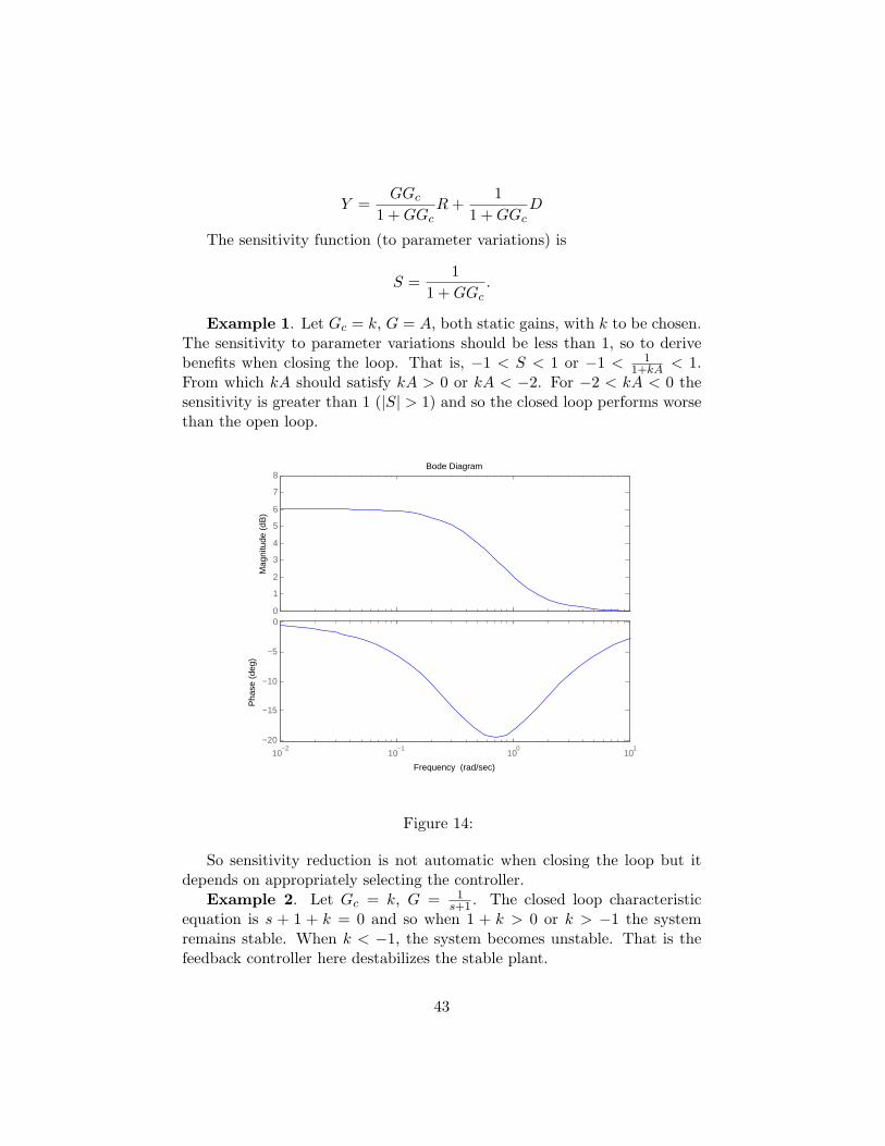
Example 1. Let Gc = k, G = A, both static gains, with k to be chosen.The sensitivity to parameter variations should be less than 1, so to derivebenefits when closing the loop. That is, −1 < S < 1 or −1 < 1

1+kA < 1.From which kA should satisfy kA > 0 or kA < −2. For −2 < kA < 0 thesensitivity is greater than 1 (|S| > 1) and so the closed loop performs worsethan the open loop.

0

1

2

3

4

5

6

7

8

Mag

nitu

de (

dB)

10−2

10−1

100

101

−20

−15

−10

−5

0

Pha

se (

deg)

Bode Diagram

Frequency (rad/sec)

Figure 14:

So sensitivity reduction is not automatic when closing the loop but itdepends on appropriately selecting the controller.

Example 2. Let Gc = k, G = 1s+1 . The closed loop characteristic

equation is s + 1 + k = 0 and so when 1 + k > 0 or k > −1 the systemremains stable. When k < −1, the system becomes unstable. That is thefeedback controller here destabilizes the stable plant.

43

The sensitivity function is

S =s+ 1

s+ 1 + k.

It can be seen that when k satisfies −1 < k < 0, the sensitivity magnitudeis greater than 1 for all frequencies. For example, for k = 0.5 the bode plotis given in Fig. A.6 where it can be seen that S is always greater than 1.

Similarly, if Gc = k and G = 1s−1 , the closed loop characteristic equation

is s− 1 + k = 0 and so, when −1 + k > 0 or k > 1 the system is stabilized.However, if k < 1 the system remains unstable. So stability is not automat-ically guaranteed when closing the loop, but it depends on appropriatelyselecting the controller.

K Root Locus

Consider G(s) = 1s(s+1)(s+2) , Gc = k, in the unity feedback configuration.

The root locus for k > 0 is given below. It can be seen that even for smallvalues of k, the closed loop poles are different from the open loop ones,that is any nonzero feedback gain ompletely changes the open loop poles asexpected.

−7 −6 −5 −4 −3 −2 −1 0 1 2−5

−4

−3

−2

−1

0

1

2

3

4

5Root Locus

Real Axis

Imag

inar

y A

xis

Figure 15:

44

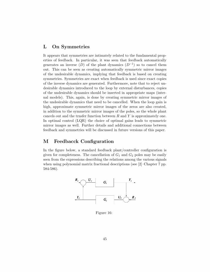
L On Symmetries

It appears that symmetries are intimately related to the fundamental prop-erties of feedback. In particular, it was seen that feedback automaticallygenerates an inverse (D) of the plant dynamics (D−1) so to cancel themout. This can be seen as creating automatically symmetric mirror imagesof the undesirable dynamics, implying that feedback is based on creatingsymmetries. Symmetries are exact when feedback is used since exact copiesof the inverse dynamics are generated. Furthermore, note that to reject un-desirable dynamics introduced to the loop by external disturbances, copiesof the undesirable dynamics should be inserted in appropriate maps (inter-nal models). This, again, is done by creating symmetric mirror images ofthe undesirable dynamics that need to be cancelled. When the loop gain ishigh, approximate symmetric mirror images of the zeros are also created,in addition to the symmetric mirror images of the poles, so the whole plantcancels out and the trnsfer function between R and Y is approximately one.In optimal control (LQR) the choice of optimal gains leads to symmetricmirror images as well. Further details and additional connections betweenfeedback and symmetries will be discussed in future versions of this paper.

M Feedbacck Configuration

In the figure below, a standard feedback plant/controller configuration isgiven for completeness. The cancellation of G1 and G2 poles may be easilyseen from the expressions describing the relations among the various signalswhen using polynomial matrix fractional descriptions (see [2]–Chapter 7 pp.584-586).

R Y

RY U

1 1 1

2 2 2

UG1

2G

Figure 16:

45