feedback systems
TRANSCRIPT
Feedback Systems
An Introduction for Scientists and Engineers
SECOND EDITION
Karl Johan AstromRichard M. Murray
Version v3.1.5 (2020-07-24)
This is the electronic edition of Feedback Systems and is available fromhttp://fbsbook.org. Hardcover editions may be purchased from Princeton
University Press, http://press.princeton.edu/titles/8701.html.
This manuscript is for personal use only and may not be reproduced, in whole orin part, without written consent from the publisher (see
http://press.princeton.edu/permissions.html).
Chapter 2
Feedback Principles
Feedback – it is the fundamental principle that underlies all self-regulatingsystems, not only machines but also the processes of life and the tidesof human a!airs.
A. Tustin, “Feedback”, Scientific American, 1952 [Tus52].
This chapter presents examples that illustrate fundamental properties of feed-back: disturbance attenuation, reference signal tracking, robustness to uncertainty,and shaping of behavior. The analysis is based on simple static and dynamical mod-els. After reading this chapter, readers should have some insight into the power offeedback, they should know about transfer functions and block diagrams, and theyshould be able to design simple feedback systems. The basic concepts describedin this chapter are explained in more detail in the remainder of the text, and thischapter can be skipped for readers who prefer to move directly to the more detailedanalysis and design techniques.
2.1 Nonlinear Static Models
We will start by capturing the behavior of a process and a controller using staticmodels. Although these models are very simple, they give significant insight aboutthe fundamental properties of feedback: negative feedback increases the range oflinearity, it improves reference signal tracking, and it reduces the gain and thee!ects of disturbances and parameter variations. Moderate positive feedback hasthe opposite properties: it shrinks the range of linearity and increases the gain ofthe system. At a critical value the gain becomes infinite and the system behaves likea relay; larger values of the gain give hysteretic behavior. Although static modelsgive some insight, they cannot capture dynamic phenomena like stability. Positivefeedback combined with dynamics often leads to instability and oscillations, as willbe discussed toward the end of the chapter.
Consider the closed loop system whose block diagram is shown in Figure 2.1.The closed loop system has a reference (or command) signal r that gives the desiredsystem output. The controller C has an input e that is the di!erence between thereference r and the process output y, and the output of the controller is the control
2-1
2-2 CHAPTER 2. FEEDBACK PRINCIPLES
y!
C P
k F (x)!
v
±1
r e u x
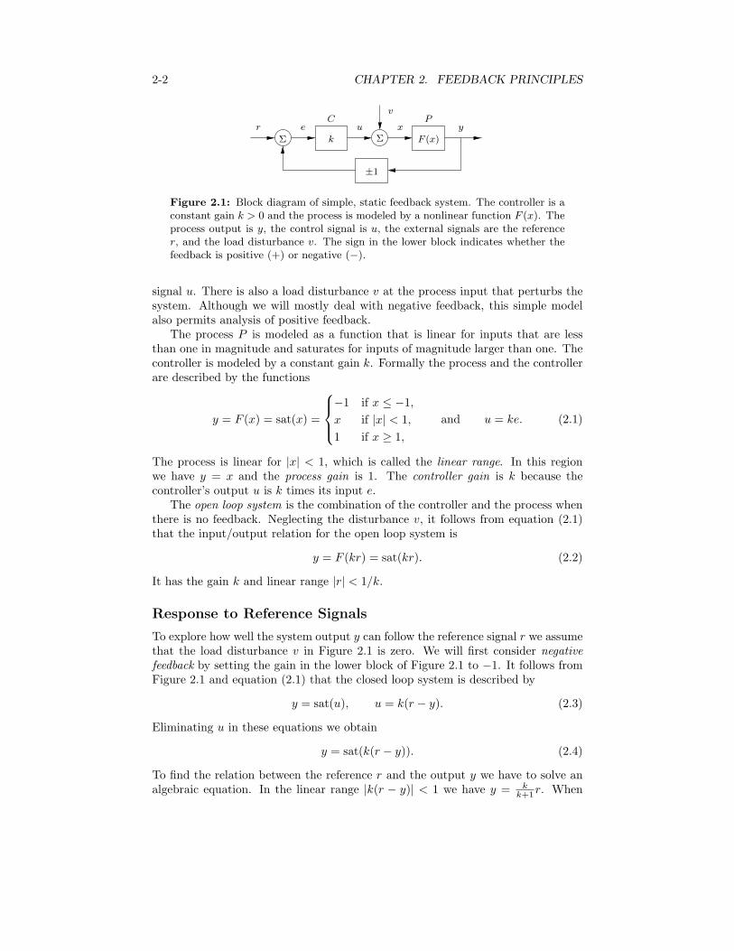
Figure 2.1: Block diagram of simple, static feedback system. The controller is aconstant gain k > 0 and the process is modeled by a nonlinear function F (x). Theprocess output is y, the control signal is u, the external signals are the referencer, and the load disturbance v. The sign in the lower block indicates whether thefeedback is positive (+) or negative (!).
signal u. There is also a load disturbance v at the process input that perturbs thesystem. Although we will mostly deal with negative feedback, this simple modelalso permits analysis of positive feedback.
The process P is modeled as a function that is linear for inputs that are lessthan one in magnitude and saturates for inputs of magnitude larger than one. Thecontroller is modeled by a constant gain k. Formally the process and the controllerare described by the functions
y = F (x) = sat(x) =
!"#
"$
!1 if x " !1,
x if |x| < 1,
1 if x # 1,
and u = ke. (2.1)
The process is linear for |x| < 1, which is called the linear range. In this regionwe have y = x and the process gain is 1. The controller gain is k because thecontroller’s output u is k times its input e.
The open loop system is the combination of the controller and the process whenthere is no feedback. Neglecting the disturbance v, it follows from equation (2.1)that the input/output relation for the open loop system is
y = F (kr) = sat(kr). (2.2)
It has the gain k and linear range |r| < 1/k.
Response to Reference Signals
To explore how well the system output y can follow the reference signal r we assumethat the load disturbance v in Figure 2.1 is zero. We will first consider negativefeedback by setting the gain in the lower block of Figure 2.1 to !1. It follows fromFigure 2.1 and equation (2.1) that the closed loop system is described by
y = sat(u), u = k(r ! y). (2.3)
Eliminating u in these equations we obtain
y = sat(k(r ! y)). (2.4)
To find the relation between the reference r and the output y we have to solve analgebraic equation. In the linear range |k(r ! y)| < 1 we have y = k
k+1r. When

2.1. NONLINEAR STATIC MODELS 2-3
Linearregion
r
y
(a) Negative feedback k > 1
r
y
(b) Positive feedback k < 1
Hysteresisregion r
y
(c) Positive feedback k > 1
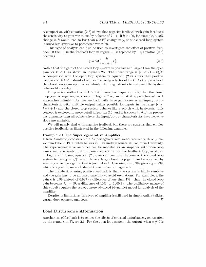
Figure 2.2: Input/output behavior of the system: (a) for large negative feedback(b) positive feedback k < 1 and (c) large positive feedback. The solid line is theresponse of the closed loop system and the dashed line is the response of the openloop system. Redrawn from [SDF18, Figure 20.5].
|k(r ! y)| # 1 the output saturates and we obtain y = ±1 (depending on the signof k(r ! y)). It can be shown that the overall input/output relationship satisfies
y = sat% k
k + 1r&=
!"#
"$
!1 if r " !k+1k ,
kk+1r if |r| < k+1
k ,
1 if r # k+1k .
(2.5)
The linear range for the closed loop system is |r| < k+1k . Comparing with equa-
tion (2.2) we find that negative feedback widens the linear range of the system by afactor of k+1 compared to the open loop system. This is illustrated in Figure 2.2a,which shows the input/output relations of the open loop system (dashed) and theclosed loop system (solid).
Robustness to Parameter Uncertainty
Next we will investigate the sensitivity of the closed loop system to gain variations.The sensitivity of a system describes how changes in the system parameters a!ectthe performance of the system. For the open loop system in the linear range wehave y = kr and it thus follows that
dy
dk= r =
y
k=$ dy
y=
dk
k. (2.6)
The relative change of the output is thus equal to the relative change of the param-eter and we say that the sensitivity is 1. Thus, for the open loop system, a changein k of 10% will lead to a change in the output of 10%.
For the closed loop system with an input in the linear range, it follows fromequation (2.5) that
dy
dk=
r
k + 1! kr
(k + 1)2=
r
(k + 1)2=
y
k(k + 1),
and hencedy
y=
1
k + 1
dk
k. (2.7)
2-4 CHAPTER 2. FEEDBACK PRINCIPLES
A comparison with equation (2.6) shows that negative feedback with gain k reducesthe sensitivity to gain variations by a factor of k+1. If k is 100, for example, a 10%change in k would lead to less than a 0.1% change in y, so the closed loop systemis much less sensitive to parameter variation.
This type of analysis can also be used to investigate the e!ect of positive feed-back. If the !1 in the feedback loop in Figure 2.1 is replaced by +1, equation (2.5)becomes
y = sat% k
!k + 1r&. (2.8)
Notice that the gain of the closed loop system is positive and larger than the opengain for k < 1, as shown in Figure 2.2b. The linear range is |r| < (1 ! k)/k.A comparison with the open loop system in equation (2.2) shows that positivefeedback with k < 1 shrinks the linear range by a factor of 1!k. As k approaches 1the closed loop gain approaches infinity, the range shrinks to zero, and the systembehaves like a relay.
For positive feedback with k > 1 it follows from equation (2.8) that the closedloop gain is negative, as shown in Figure 2.2c, and that it approaches !1 as kapproaches infinity. Positive feedback with large gains creates an input/outputcharacteristic with multiple output values possible for inputs in the range |r| <k/(k + 1) and the closed loop system behaves like a switch with hysteresis. Thisconcept is explored in more detail in Section 2.6, and it is shown that if the processhas dynamics then all points where the input/output characteristics have negativeslope are unstable.
We will mostly deal with negative feedback but there are systems that employpositive feedback, as illustrated in the following example.
Example 2.1 The Superregenerative AmplifierEdwin Armstrong constructed a “superregenerative” radio receiver with only onevacuum tube in 1914, when he was still an undergraduate at Columbia University.The superregenerative amplifier can be modeled as an amplifier with open loopgain k and a saturated output, combined with a positive feedback loop, as shownin Figure 2.1. Using equation (2.8), we can compute the gain of the closed loopsystem to be kcl = k/(1 ! k). A very large closed loop gain can be obtained byselecting a feedback gain k that is just below 1. Choosing k = 0.999 gives kcl = 999,which is a gain increase of almost three orders of magnitude.
The drawback of using positive feedback is that the system is highly sensitiveand the gain has to be adjusted carefully to avoid oscillations. For example, if thegain k is 0.99 instead of 0.999 (a di!erence of less than 1%), then the closed loopgain becomes kcl = 99, a di!erence of 10X (or 1000%). The oscillatory nature ofthis circuit requires the use of a more advanced (dynamic) model for analysis of theamplifier.
Despite its limitations, this type of amplifier is still used in simple walkie-talkies,garage door openers, and toys. %
Load Disturbance Attenuation
Another use of feedback is to reduce the e!ects of external disturbances, representedby the signal v in Figure 2.1. For the open loop system, the output when v &= 0 is
2.2. LINEAR DYNAMICAL MODELS 2-5
given byy = sat(kr + v).
In the linear region we thus have a gain of 1 between v and y, so that disturbancesare passed through with no attenuation.
To investigate the e!ect of feedback on load disturbances we consider the systemin Figure 2.1 with negative feedback and, for simplicity, we set the reference signalr to be zero. The relationship between the load disturbance v and the output y isgiven by y = sat(v ! ky), which is again an algebraic equation. In the linear rangewe get y = v/(k + 1) and more generally it can be shown that
y = sat% v
k + 1
&. (2.9)
In the linear region, negative feedback thus reduces the e!ect of load disturbancesby the factor k + 1.
Combining these three sets of analyses, we see that negative feedback increases therange of linearity of the system, decreases the sensitivity of the system to parameteruncertainty, and attenuates load disturbances. The trade-o! is that the closedloop gain is decreased. Positive feedback has the opposite e!ect: it can increasethe closed loop gain, but at the cost of increased sensitivity and amplification ofdisturbances.
2.2 Linear Dynamical Models
The analysis in the previous section was based on static models and the dynamicsof the process were neglected. We will now introduce a set of concepts and tools toanalyze the e!ects of dynamics. To do this we will introduce block diagrams, lineardi!erential equations, and transfer functions. The block diagram is an abstractionthat describes a system as an interconnection of blocks, whose input/output behav-ior is described by di!erential equations. The transfer function, which is a functionof complex variables, is a convenient representation of the di!erential equationsdescribing the dynamics of the system. Transfer functions make it possible for usto find the relations between the signals of a complex system represented by blockdiagrams using simple algebra. The values of the transfer function on the imagi-nary axis gives the steady-state response to sinusoidal signals, which means that thetransfer function can be determined experimentally from the steady-state responseto sinusoidal signals.
Linear Di!erential Equations and Transfer Functions
In many practical situations, the input/output behavior of a system can be modeledby a linear di!erential equation of the form
dny
dtn+ a1
dn!1y
dtn!1+ · · ·+ any = b0
dmu
dtm+ b1
dm!1u
dtm!1+ · · ·+ bmu, (2.10)
where u is the input, y is the output, and the coe"cients ak and bk are real numbers.The di!erential equation (2.10) is characterized by two polynomials
a(s) = sn + a1sn!1 + · · ·+ an, b(s) = b0s
m + b1sm!1 + · · ·+ bm, (2.11)
2-6 CHAPTER 2. FEEDBACK PRINCIPLES
where a(s) is the characteristic polynomial of the di!erential equation (2.10). Weassume that the polynomials a(s) and b(s) do not have common roots. (The con-sequences of having common roots is discussed in Section 8.3.)
Equation (2.10) represents a time-invariant system because if the pair u(t),y(t) satisfies the equation so does u(t + !), y(t + !). The equation is also linearbecause if u1(t), y1(t), and u2(t), y2(t) satisfy the equation so does "u1(t)+#u2(t),"y1(t) + #y2(t), where " and # are real numbers. Systems that are linear andtime-invariant are often called LTI systems. We can visualize these systems asbeing characterized by a huge table of corresponding input/output signal pairs. Aninteresting property of an LTI system is that it can be characterized by a singlecarefully chosen pair, for example the response of the system to a step input.
The solution to equation (2.10) is the sum of two terms: the general solution tothe homogeneous equation, which does not depend on the input, and a particularsolution, which depends on the input. The homogeneous equation associated withequation (2.10) is
dny
dtn+ a1
dn!1y
dtn!1+ · · ·+ any = 0. (2.12)
Letting sk represent the roots of the characteristic equation a(s) = 0, the solutionto equation (2.12) is of the form
y(t) =n'
k=1
Ckeskt (2.13)
if the characteristic polynomial does not have repeated roots. The coe"cientsC1, . . . , Cn can be determined from the initial conditions at t = 0.
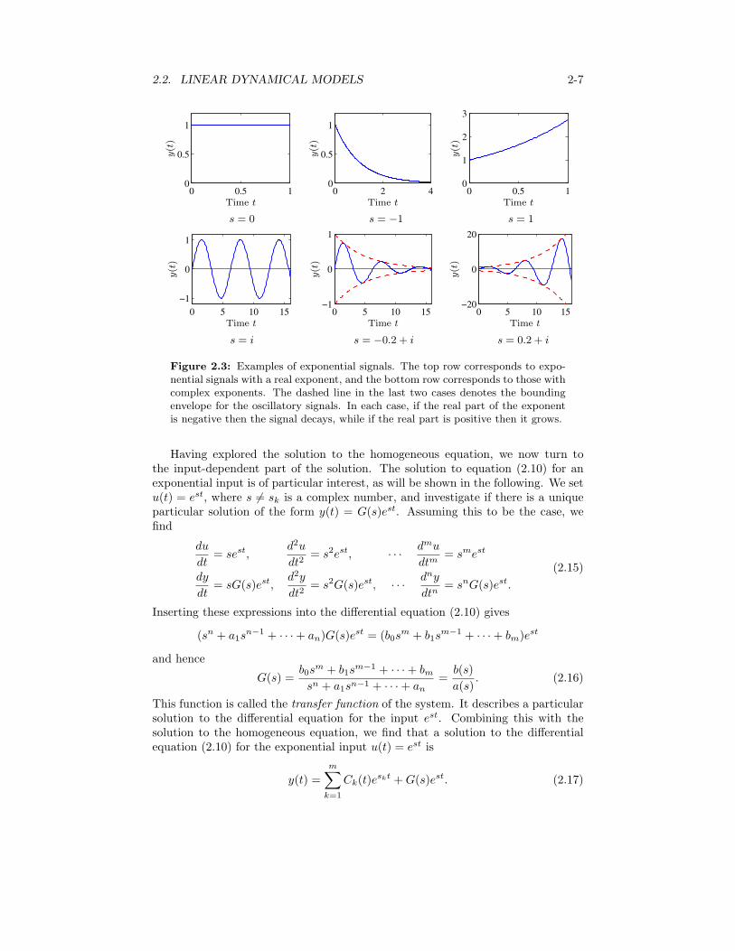
Since the coe"cients ak are real, the roots of the characteristic equation areeither real-valued or occur in complex conjugate pairs. A real root sk of the char-acteristic polynomial corresponds to the exponential function eskt. This functiondecreases over time if sk is negative, is constant if sk = 0, and increases if sk ispositive, as shown in the top row of Figure 2.3. For real roots sk the parameterT = 1/sk is called the time constant, because it describes how quickly the signaldecays.
A complex root sk = $ ± i% corresponds to the time functions
e!t sin (%t), e!t cos (%t),
which have oscillatory behavior, as illustrated in the bottom row of Figure 2.3. Thesine terms are shown as solid lines; they have zero crossings with the spacing &/%.The dashed lines show the envelopes, which correspond to the exponential function±e!t.
When the characteristic equation has repeated roots, the solutions to the ho-mogeneous equation (2.12) take the form
y(t) =m'
k=1
Ck(t)eskt, (2.14)
where Ck(t) is a polynomial with degree less than the multiplicity of the rootsk. The solution (2.14) has
(mk=1(degCk + 1) = n free parameters. This case is
considered in more detail in Section 6.2.
2.2. LINEAR DYNAMICAL MODELS 2-7
0 0.5 10
0.5
1
Time t
y(t)
s = 0
0 2 40
0.5
1
Time t
y(t)
s = !1
0 0.5 10
1
2
3
Time t
y(t)
s = 1
0 5 10 15
!1
0
1
Time t
y(t)
s = i
0 5 10 15!1
0
1
Time ty(t)
s = !0.2 + i
0 5 10 15!20
0
20
Time t
y(t)
s = 0.2 + i
Figure 2.3: Examples of exponential signals. The top row corresponds to expo-nential signals with a real exponent, and the bottom row corresponds to those withcomplex exponents. The dashed line in the last two cases denotes the boundingenvelope for the oscillatory signals. In each case, if the real part of the exponentis negative then the signal decays, while if the real part is positive then it grows.
Having explored the solution to the homogeneous equation, we now turn tothe input-dependent part of the solution. The solution to equation (2.10) for anexponential input is of particular interest, as will be shown in the following. We setu(t) = est, where s &= sk is a complex number, and investigate if there is a uniqueparticular solution of the form y(t) = G(s)est. Assuming this to be the case, wefind
du
dt= sest,
d2u
dt2= s2est, · · · dmu
dtm= smest
dy
dt= sG(s)est,
d2y
dt2= s2G(s)est, · · · dny
dtn= snG(s)est.
(2.15)
Inserting these expressions into the di!erential equation (2.10) gives
(sn + a1sn!1 + · · ·+ an)G(s)est = (b0s
m + b1sm!1 + · · ·+ bm)est
and hence
G(s) =b0sm + b1sm!1 + · · ·+ bmsn + a1sn!1 + · · ·+ an
=b(s)
a(s). (2.16)
This function is called the transfer function of the system. It describes a particularsolution to the di!erential equation for the input est. Combining this with thesolution to the homogeneous equation, we find that a solution to the di!erentialequation (2.10) for the exponential input u(t) = est is
y(t) =m'
k=1
Ck(t)eskt +G(s)est. (2.17)
2-8 CHAPTER 2. FEEDBACK PRINCIPLES
The relation between the transfer function (2.16) and the di!erential equa-tion (2.10) is clear: the transfer function (2.16) can be obtained by inspectionfrom the di!erential equation (2.10), and conversely the di!erential equation canbe obtained from the transfer function if the polynomials a(s) and b(s) do not havecommon factors. The transfer function G(s) can thus be regarded as a shorthandnotation for the di!erential equation (2.10). It is a complete characterization ofthe di!erential equation even if it was derived as the response to a specific inputu(t) = est. We note that the input and the initial conditions must both be given toobtain the full solution of the di!erential equation, given by equation (2.17), alsoreferred to as the response of the system.
To deal with oscillatory signals, like those shown in the bottom row of Figure 2.3,we allow s to be a complex number. The transfer function G is then a function thatmaps complex numbers to complex numbers. We let arg represent the argument(phase, angle) of a complex number and | · | the magnitude, and note that thecomplex response to an input u = ei"t = cos%t + i sin%t is given by G(i%)ei"t.Using just the imaginary parts of the signals, it follows that the particular solutionfor the input u = sin(%t) = Im ei"t is
y(t) = Im)G(i%) ei"t
*= Im
)|G(i%)| ei argG(i") ei"t
*
= |G(i%)| Im ei(argG(i")+"t) = |G(i%)| sin(%t+ argG(i%)).
The input is thus amplified by |G(i%)| and the phase shift between input and outputis argG(i%). The functions G(i%), |G(i%)|, and argG(i%) are called the frequencyresponse, gain, and phase. Gain and phase are also called magnitude and angle.
When the input and the output are constant, u(t) = u0 and y(t) = y0, thedi!erential equation (2.10) has the particular solution y(t) = (bm/an)u0 = G(0)u0,obtained by setting s = 0. The input is thus amplified by the factor G(0), whichis therefore called the zero frequency gain (or sometimes the static gain). If thedi!erential equation is stable then the solution will converge to G(0)u0 as t goes toinfinity.
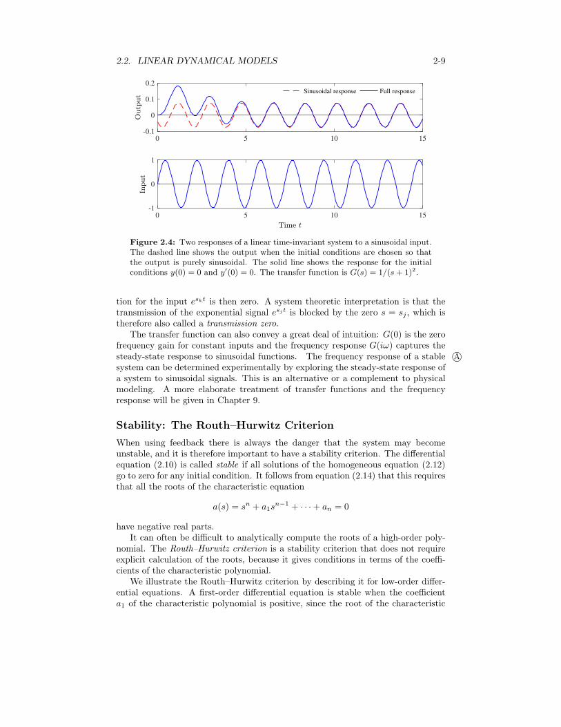
The full response to an exponential input is the sum of a particular solution anda solution to the homogeneous equation that is determined by the initial conditions,as given in equation (2.17). An illustration is given in Figure 2.4 for the transferfunction G(s) = 1/(s + 1)2. The dashed line, which is a pure sine wave, is thesolution obtained when all Ck in equation (2.17) are zero. The solid line shows theresponse obtained when the Ck are chosen so that y(0) and its derivatives y(k)(0),k = 1, . . . , n ! 1 are all zero. Since all roots of the characteristic polynomial havenegative real parts, the solution to the homogeneous equation (2.14) goes to zeroas t ' ( and the general solution converges to the particular solution.
The transfer function has many interpretations that can be exploited for insight,analysis, and design. The roots sk of the characteristic equation a(s) = 0 are calledpoles of the transfer function: the transfer function is infinite for s = sk. The polessk appear as exponents in the general solution to the homogeneous equation, asseen in equations (2.13) and (2.14). Systems with poles that are “lightly damped”(Re(sk) is negative but close to zero) can exhibit resonances when a sinusoidal inputis applied whose frequency is near the imaginary part of sk.
The roots sj of the polynomial b(s) are called zeros of the transfer function.The reason is that if b(sj) = 0 it follows that G(sj) = 0, and the particular solu-
2.2. LINEAR DYNAMICAL MODELS 2-9
0 5 10 15-0.1
0
0.1
0.2Sinusoidal response Full response
0 5 10 15-1
0
1
Outp
ut
Input
Time t
Figure 2.4: Two responses of a linear time-invariant system to a sinusoidal input.The dashed line shows the output when the initial conditions are chosen so thatthe output is purely sinusoidal. The solid line shows the response for the initialconditions y(0) = 0 and y!(0) = 0. The transfer function is G(s) = 1/(s+ 1)2.
tion for the input eskt is then zero. A system theoretic interpretation is that thetransmission of the exponential signal esjt is blocked by the zero s = sj , which istherefore also called a transmission zero.
The transfer function can also convey a great deal of intuition: G(0) is the zerofrequency gain for constant inputs and the frequency response G(i%) captures thesteady-state response to sinusoidal functions. The frequency response of a stable A!system can be determined experimentally by exploring the steady-state response ofa system to sinusoidal signals. This is an alternative or a complement to physicalmodeling. A more elaborate treatment of transfer functions and the frequencyresponse will be given in Chapter 9.
Stability: The Routh–Hurwitz Criterion
When using feedback there is always the danger that the system may becomeunstable, and it is therefore important to have a stability criterion. The di!erentialequation (2.10) is called stable if all solutions of the homogeneous equation (2.12)go to zero for any initial condition. It follows from equation (2.14) that this requiresthat all the roots of the characteristic equation
a(s) = sn + a1sn!1 + · · ·+ an = 0
have negative real parts.It can often be di"cult to analytically compute the roots of a high-order poly-
nomial. The Routh–Hurwitz criterion is a stability criterion that does not requireexplicit calculation of the roots, because it gives conditions in terms of the coe"-cients of the characteristic polynomial.
We illustrate the Routh–Hurwitz criterion by describing it for low-order di!er-ential equations. A first-order di!erential equation is stable when the coe"cienta1 of the characteristic polynomial is positive, since the root of the characteristic
2-10 CHAPTER 2. FEEDBACK PRINCIPLES
polynomial will be s = !a1 < 0. A second-order polynomial has the roots
s =1
2
%!a1 ±
+a21 ! 4a2
&,
and it is easy to verify that the real parts of the roots are both negative if and onlyif a1 > 0 and a2 > 0. A third order di!erential equation is more complicated, butthe roots can be shown to have negative real parts if and only if
a1, a2, a3 > 0, and a1a2 > a3. (2.18)
The corresponding conditions for a fourth order di!erential equation are
a1, a2, a3, a4 > 0, a1a2 > a3, and a1a2a3 > a21 a4 + a23. (2.19)
The Routh–Hurwitz criterion [Gan60] gives similar conditions for arbitrarily high H!order polynomials. Stability of a linear di!erential equation can thus be investi-gated just by analyzing the signs of various combinations of the coe"cients of thecharacteristic polynomial.
Block Diagrams and Transfer Functions
As we saw already in Chapter 1, control systems are often described using blockdiagrams, such as the ones shown in Figures 1.1 and 1.4. If the behavior of theblocks are represented by transfer functions, the transfer function of a system canbe obtained simply by algebraic manipulations. It follows from equation (2.17) thatthe transfer function can be derived from the particular solution for the input est.To derive the transfer function for a system composed of several blocks, we assumethat the input signal is an exponential u(t) = est and compute the correspondingparticular solutions for all blocks.
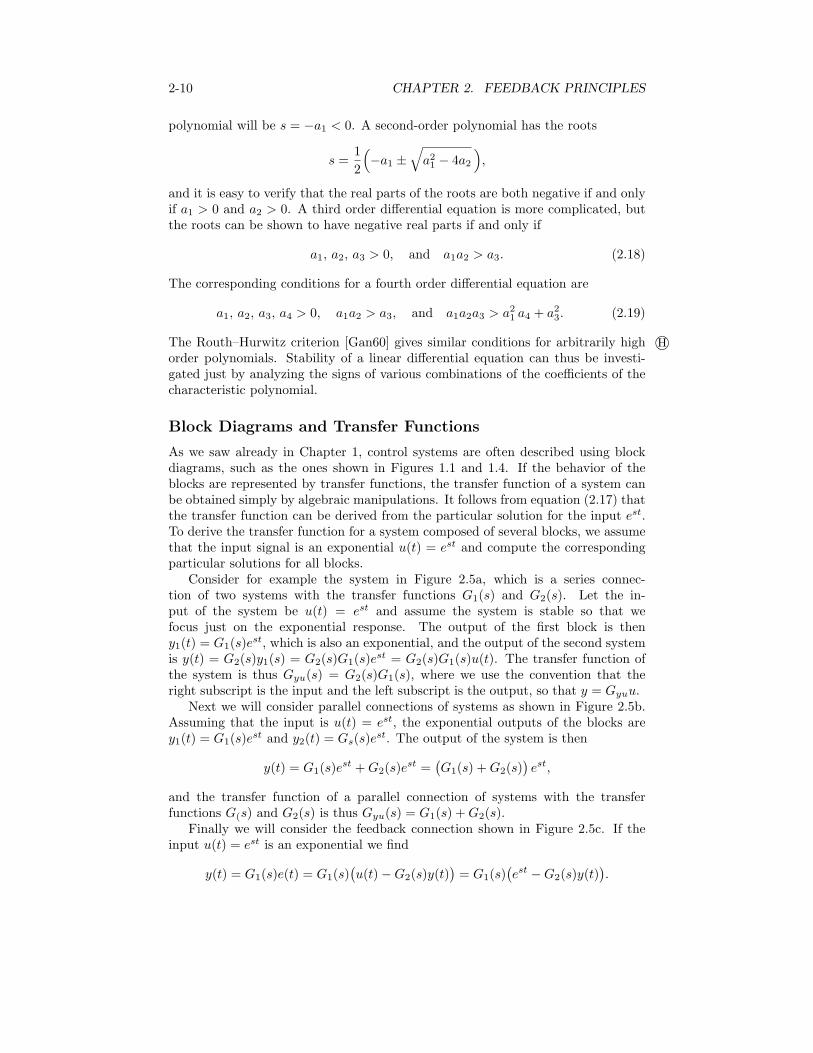
Consider for example the system in Figure 2.5a, which is a series connec-tion of two systems with the transfer functions G1(s) and G2(s). Let the in-put of the system be u(t) = est and assume the system is stable so that wefocus just on the exponential response. The output of the first block is theny1(t) = G1(s)est, which is also an exponential, and the output of the second systemis y(t) = G2(s)y1(s) = G2(s)G1(s)est = G2(s)G1(s)u(t). The transfer function ofthe system is thus Gyu(s) = G2(s)G1(s), where we use the convention that theright subscript is the input and the left subscript is the output, so that y = Gyuu.
Next we will consider parallel connections of systems as shown in Figure 2.5b.Assuming that the input is u(t) = est, the exponential outputs of the blocks arey1(t) = G1(s)est and y2(t) = Gs(s)est. The output of the system is then
y(t) = G1(s)est +G2(s)e
st =)G1(s) +G2(s)
*est,
and the transfer function of a parallel connection of systems with the transferfunctions G(s) and G2(s) is thus Gyu(s) = G1(s) +G2(s).
Finally we will consider the feedback connection shown in Figure 2.5c. If theinput u(t) = est is an exponential we find
y(t) = G1(s)e(t) = G1(s))u(t)!G2(s)y(t)
*= G1(s)
)est !G2(s)y(t)
*.
2.2. LINEAR DYNAMICAL MODELS 2-11
y1G2
u yG1
(a) Gyu(s) = G2(s)G1(s)
G2
!u y
G1
(b) Gyu(s) = G1(s) +G2(s)
!G2
!eu y
G1
(c) Gyu(s) =G1(s)
1 +G1(s)G2(s)
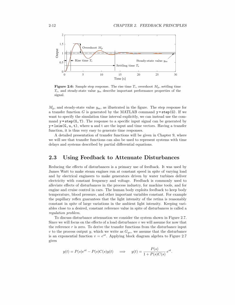
Figure 2.5: Interconnections of linear systems. Series (a), parallel (b) and feed-back (c) connections are shown. The transfer functions for the composite systemscan be derived by algebraic manipulations assuming exponential functions for allsignals.
Solving for y(t) gives
y(t) =G1(s)
1 +G1(s)G2(s)est.
The transfer function of a feedback connection of systems with the transfer functionsG1(s) and G2(s) is thus
Gyu(s) =G1(s)
1 +G1(s)G2(s). (2.20)
By using polynomials and transfer functions the relations between signals in afeedback system can thus be obtained by algebra. With some practice the transferfunctions can often be obtained by inspection, as we explore in more detail inChapter 9.
Computations Using Transfer Functions
Many software packages for control system analysis and design permit direct ma-nipulation of transfer functions. In MATLAB the transfer function
G(s) =s+ 1
(s2 + 5s+ 6)
can be created by the commands s = tf(’s’) and G = (s + 1)/(s^2 + 5*s + 6). Giventwo transfer functions G1 and G2, we can form series, parallel, and feedback inter-connections using the commands Gs = series(G1, G2), Gp = parallel(G1, G2), andGf = feedback(G1, G2) (by default, MATLAB’s feedback() command uses nega-tive feedback).
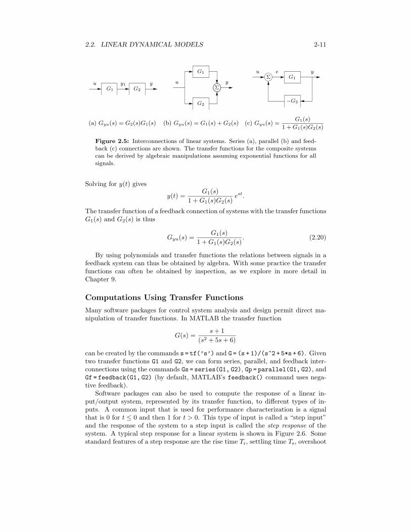
Software packages can also be used to compute the response of a linear in-put/output system, represented by its transfer function, to di!erent types of in-puts. A common input that is used for performance characterization is a signalthat is 0 for t " 0 and then 1 for t > 0. This type of input is called a “step input”and the response of the system to a step input is called the step response of thesystem. A typical step response for a linear system is shown in Figure 2.6. Somestandard features of a step response are the rise time Tr, settling time Ts, overshoot
2-12 CHAPTER 2. FEEDBACK PRINCIPLES
0 5 10 15 20 25 30
Time [s]
0
0.5
1
1.5
2
Out
put
Rise time Tr
Settling time Ts
Overshoot Mp
Steady-state value yss
Figure 2.6: Sample step response. The rise time Tr, overshoot Mp, settling timeTs, and steady-state value yss describe important performance properties of thesignal.
Mp, and steady-state value yss, as illustrated in the figure. The step response fora transfer function G is generated by the MATLAB command y = step(G). If wewant to specify the simulation time interval explicitly, we can instead use the com-mand y = step(G, T). The response to a specific input signal can be generated byy = lsim(G, u, t), where u and t are the input and time vectors. Having a transferfunction, it is thus very easy to generate time responses.
A detailed presentation of transfer functions will be given in Chapter 9, wherewe will see that transfer functions can also be used to represent systems with timedelays and systems described by partial di!erential equations.
2.3 Using Feedback to Attenuate Disturbances
Reducing the e!ects of disturbances is a primary use of feedback. It was used byJames Watt to make steam engines run at constant speed in spite of varying loadand by electrical engineers to make generators driven by water turbines deliverelectricity with constant frequency and voltage. Feedback is commonly used toalleviate e!ects of disturbances in the process industry, for machine tools, and forengine and cruise control in cars. The human body exploits feedback to keep bodytemperature, blood pressure, and other important variables constant. For examplethe pupillary reflex guarantees that the light intensity of the retina is reasonablyconstant in spite of large variations in the ambient light intensity. Keeping vari-ables close to a desired, constant reference value in spite of disturbances is called aregulation problem.
To discuss disturbance attenuation we consider the system shown in Figure 2.7.Since we will focus on the e!ects of a load disturbance v we will assume for now thatthe reference r is zero. To derive the transfer functions from the disturbance inputv to the process output y, which we write as Gyv, we assume that the disturbanceis an exponential function v = est. Applying block diagram algebra to Figure 2.7gives
y(t) = P (s)est ! P (s)C(s)y(t) =$ y(t) =P (s)
1 + P (s)C(s)est.
2.3. USING FEEDBACK TO ATTENUATE DISTURBANCES 2-13
y!!
v
!1
C Pr e u
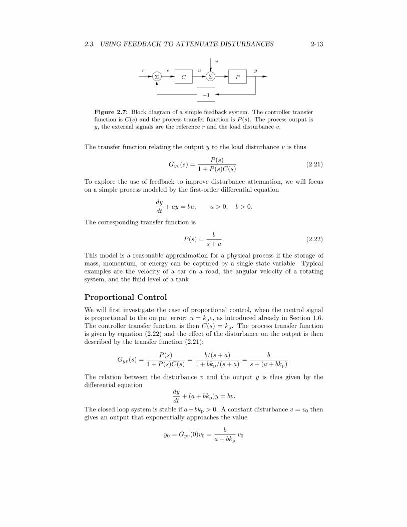
Figure 2.7: Block diagram of a simple feedback system. The controller transferfunction is C(s) and the process transfer function is P (s). The process output isy, the external signals are the reference r and the load disturbance v.
The transfer function relating the output y to the load disturbance v is thus
Gyv(s) =P (s)
1 + P (s)C(s). (2.21)
To explore the use of feedback to improve disturbance attenuation, we will focuson a simple process modeled by the first-order di!erential equation
dy
dt+ ay = bu, a > 0, b > 0.
The corresponding transfer function is
P (s) =b
s+ a. (2.22)
This model is a reasonable approximation for a physical process if the storage ofmass, momentum, or energy can be captured by a single state variable. Typicalexamples are the velocity of a car on a road, the angular velocity of a rotatingsystem, and the fluid level of a tank.
Proportional Control
We will first investigate the case of proportional control, when the control signalis proportional to the output error: u = kpe, as introduced already in Section 1.6.The controller transfer function is then C(s) = kp. The process transfer functionis given by equation (2.22) and the e!ect of the disturbance on the output is thendescribed by the transfer function (2.21):
Gyv(s) =P (s)
1 + P (s)C(s)=
b/(s+ a)
1 + bkp/(s+ a)=
b
s+ (a+ bkp).
The relation between the disturbance v and the output y is thus given by thedi!erential equation
dy
dt+ (a+ bkp)y = bv.
The closed loop system is stable if a+ bkp > 0. A constant disturbance v = v0 thengives an output that exponentially approaches the value
y0 = Gyv(0)v0 =b
a+ bkpv0
2-14 CHAPTER 2. FEEDBACK PRINCIPLES
0 2 4 6 80
1
2
0 2 4 6 8
!1
!0.5
0
Normalized time a t
Outp
uty
Inputu kp
kp
(a) Proportional control
0 2 4 6 80
1
2
0 2 4 6 8
!1
!0.5
0
Normalized time a t
Outp
uty
Inputu
!c
!c
(b) Proportional-integral (PI) control
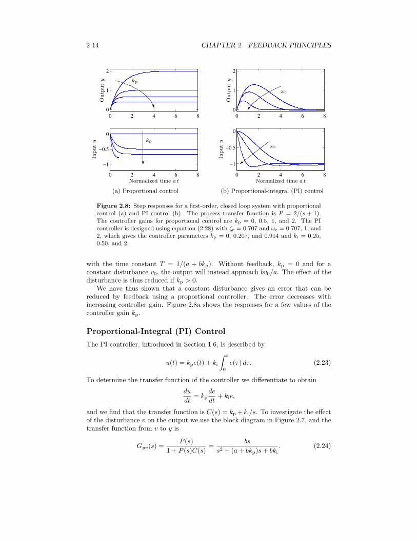
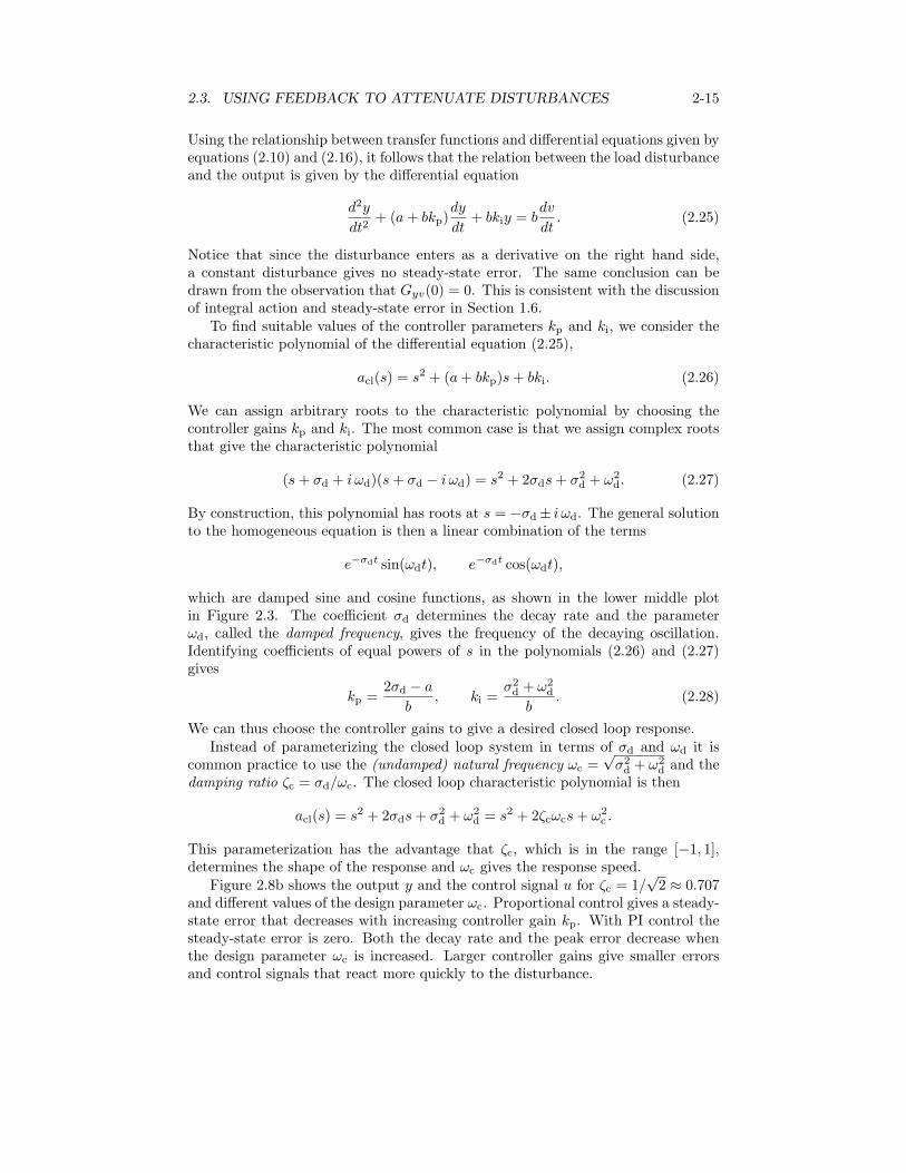
Figure 2.8: Step responses for a first-order, closed loop system with proportionalcontrol (a) and PI control (b). The process transfer function is P = 2/(s + 1).The controller gains for proportional control are kp = 0, 0.5, 1, and 2. The PIcontroller is designed using equation (2.28) with !c = 0.707 and "c = 0.707, 1, and2, which gives the controller parameters kp = 0, 0.207, and 0.914 and ki = 0.25,0.50, and 2.
with the time constant T = 1/(a + bkp). Without feedback, kp = 0 and for aconstant disturbance v0, the output will instead approach bv0/a. The e!ect of thedisturbance is thus reduced if kp > 0.
We have thus shown that a constant disturbance gives an error that can bereduced by feedback using a proportional controller. The error decreases withincreasing controller gain. Figure 2.8a shows the responses for a few values of thecontroller gain kp.
Proportional-Integral (PI) Control
The PI controller, introduced in Section 1.6, is described by
u(t) = kpe(t) + ki
, t
0e(!) d!. (2.23)
To determine the transfer function of the controller we di!erentiate to obtain
du
dt= kp
de
dt+ kie,
and we find that the transfer function is C(s) = kp+ ki/s. To investigate the e!ectof the disturbance v on the output we use the block diagram in Figure 2.7, and thetransfer function from v to y is
Gyv(s) =P (s)
1 + P (s)C(s)=
bs
s2 + (a+ bkp)s+ bki. (2.24)
2.3. USING FEEDBACK TO ATTENUATE DISTURBANCES 2-15
Using the relationship between transfer functions and di!erential equations given byequations (2.10) and (2.16), it follows that the relation between the load disturbanceand the output is given by the di!erential equation
d2y
dt2+ (a+ bkp)
dy
dt+ bkiy = b
dv
dt. (2.25)
Notice that since the disturbance enters as a derivative on the right hand side,a constant disturbance gives no steady-state error. The same conclusion can bedrawn from the observation that Gyv(0) = 0. This is consistent with the discussionof integral action and steady-state error in Section 1.6.
To find suitable values of the controller parameters kp and ki, we consider thecharacteristic polynomial of the di!erential equation (2.25),
acl(s) = s2 + (a+ bkp)s+ bki. (2.26)
We can assign arbitrary roots to the characteristic polynomial by choosing thecontroller gains kp and ki. The most common case is that we assign complex rootsthat give the characteristic polynomial
(s+ $d + i%d)(s+ $d ! i%d) = s2 + 2$ds+ $2d + %2
d. (2.27)
By construction, this polynomial has roots at s = !$d± i%d. The general solutionto the homogeneous equation is then a linear combination of the terms
e!!dt sin(%dt), e!!dt cos(%dt),
which are damped sine and cosine functions, as shown in the lower middle plotin Figure 2.3. The coe"cient $d determines the decay rate and the parameter%d, called the damped frequency, gives the frequency of the decaying oscillation.Identifying coe"cients of equal powers of s in the polynomials (2.26) and (2.27)gives
kp =2$d ! a
b, ki =
$2d + %2
d
b. (2.28)
We can thus choose the controller gains to give a desired closed loop response.Instead of parameterizing the closed loop system in terms of $d and %d it is
common practice to use the (undamped) natural frequency %c =)$2d + %2
d and thedamping ratio 'c = $d/%c. The closed loop characteristic polynomial is then
acl(s) = s2 + 2$ds+ $2d + %2
d = s2 + 2'c%cs+ %2c .
This parameterization has the advantage that 'c, which is in the range [!1, 1],determines the shape of the response and %c gives the response speed.
Figure 2.8b shows the output y and the control signal u for 'c = 1/)2 * 0.707
and di!erent values of the design parameter %c. Proportional control gives a steady-state error that decreases with increasing controller gain kp. With PI control thesteady-state error is zero. Both the decay rate and the peak error decrease whenthe design parameter %c is increased. Larger controller gains give smaller errorsand control signals that react more quickly to the disturbance.
2-16 CHAPTER 2. FEEDBACK PRINCIPLES
With the controller parameters (2.28), the transfer function (2.24) from distur-bance v to process output y becomes
Gyv(s) =P (s)
1 + P (s)C(s)=
bs
s2 + 2'c%cs+ %2c
.
For e"cient attenuation of disturbances, it is desirable that |Gyv(i%)| is small forall %. For small values of % we have |Gyv(i%)| * b%/%2
c , while for large % we have|Gyv(i%)| * b/%. The largest value of |Gyv(i%)| is b/(2'c%c) for % = %c. It thusfollows that a large value of %c gives good load disturbance attenuation.
In summary, we find that transfer function analysis gives a simple way to find theparameters of PI controllers for processes whose dynamics can be approximated bya first-order system. The technique can be generalized to more complicated systemsbut the controller will be more complex. To achieve the benefits of large controlgains the model must be accurate over wide frequency ranges, as will be discussednext.
Unmodeled Dynamics
The analysis we have made so far indicates that there are no limits to the perfor-mance that can be achieved. Figure 2.8b shows that arbitrarily fast response canbe obtained simply by making %c su"ciently large. In reality there are of courselimits on what is achievable. One reason is that the controller gains increase with%c: the proportional gain is kp = (2'c%c ! a)/b and the integral gain is ki = %2
c/b.A large value of %c thus gives large controller gains and the control signal maysaturate. Another reason is that the model (2.22) is a simplification: it is onlyvalid in a given frequency range. If the model is instead
P (s) =b
(s+ a)(1 + sT ), (2.29)
where the term 1 + sT represents the dynamics of sensors, actuators, or otherdynamics that were neglected when deriving equation (2.22)—so-called unmodeleddynamics—the closed loop characteristic polynomial for the closed loop systembecomes
acl = s(s+ a)(1 + sT ) + b(kps+ ki) = s3T + s2(1 + aT ) + 2'c%cs+ %2c .
It follows from the Routh–Hurwitz criterion (2.18) that the closed loop system isstable if %2
cT < 2'c%c(1 + aT ) or if
%cT < 2'c(1 + aT ).
The frequency %c and the achievable response time are thus limited by the unmod-eled dynamics represented by T , which typically is smaller than the time constant1/a of the process. When models are developed for control it is therefore importantto also consider the unmodeled dynamics.
The fact that unmodeled dynamics limit the performance of a feedback systemis an important property and must be considered during the system design. It iscommon to use simplified models when designing components of complex systems
2.4. USING FEEDBACK TO TRACK REFERENCE SIGNALS 2-17
and if the unmodeled dynamics of those components (or the other subsystems theyinteract with) are not properly taken into account, the implementation of the systemcan display poor behavior (of which instability is one extreme example). As we shallsee in later chapters, it is the ability to reason about the e!ects of uncertainty thatmakes control theory a particularly powerful mathematical tool for systems design.
2.4 Using Feedback to Track Reference Signals
Another major application of feedback is to make a system output follow a ref-erence value, which is called the servo problem. Cruise control, steering of a car,and tracking a satellite with an antenna or a star with a telescope are some exam-ples. Other examples are high performance audio amplifiers, machine tools, andindustrial robots.
To illustrate reference signal tracking we will consider the system in Figure 2.7where the process is a first-order system and the controller is a PI controller withproportional gain kp and integral gain ki. The transfer functions of the process andthe controller are
P (s) =b
s+ a, C(s) =
kps+ kis
. (2.30)
Since we will focus on following the reference signal r, we will neglect the loaddisturbance and set v = 0. Applying block diagram algebra to the system inFigure 2.7, we find that the transfer function from the reference signal r to theoutput y is
Gyr(s) =P (s)C(s)
1 + P (s)C(s)=
bkps+ bkis2 + (a+ bkp)s+ bki
. (2.31)
Since Gyr(0) = 1 it follows that r = y when r and y are constant, independent ofthe values of the parameters a and b, as long as the closed loop system is stable.The steady-state output is thus equal to the reference, a consequence of the integralaction in the controller.
To determine suitable values of the controller parameters kp and ki, we pro-ceed as in Section 2.3 by choosing controller parameters that make the closed loopcharacteristic polynomial
acl(s) = s2 + (a+ bkp)s+ bki (2.32)
equal to s2 + 2'c%cs+ %2c with 'c > 0 and %c > 0. Identifying coe"cients of equal
powers of s in these polynomials gives
kp =2'c%c ! a
b, ki =
%2c
b, (2.33)
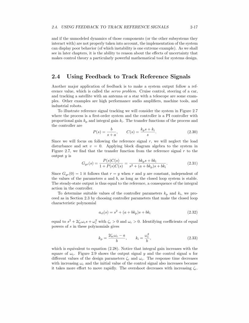
which is equivalent to equation (2.28). Notice that integral gain increases with thesquare of %c. Figure 2.9 shows the output signal y and the control signal u fordi!erent values of the design parameters 'c and %c. The response time decreaseswith increasing %c and the initial value of the control signal also increases becauseit takes more e!ort to move rapidly. The overshoot decreases with increasing 'c.
2-18 CHAPTER 2. FEEDBACK PRINCIPLES
0 2 4 60
0.5
1
1.5
0 2 4 60
2
4
6
Normalized time, !c t
Inputu
Outp
uty
!c
!c
0 2 4 60
0.5
1
1.5
0 2 4 60
1
2
3
Normalized time, !c t
Inputu
Outp
uty
"c
"c
Figure 2.9: Responses to a unit step change in the reference signal for di!erentvalues of the design parameters "c and !c. The left figure shows responses for fixed!c = 0.707 and "c = 1, 2, and 5. The right figure shows responses for "c = 2 and!c = 0.5, 0.707, and 1. The process parameters are a = b = 1. The initial value ofthe control signal is kp.
For %c = 2, the design choice 'c = 1 gives a short settling time and a responsewithout overshoot.
It is desirable that the output y will track the reference signal r for time-varyingreferences. This means that we would like the transfer function Gyr(s) to be closeto 1 for large frequency ranges. With the controller parameters (2.33), it followsfrom equation (2.31) that
Gyr(s) =P (s)C(s)
1 + P (s)C(s)=
(2'c%c ! a)s+ %2c
s2 + 2'c%cs+ %2c
.
Since Gyr(0) = 1, tracking of constant inputs is perfect. In addition, if s = i%is smaller in magnitude than %c, then using some approximations it can be shownthat Gyr(s) will be close to one. The frequency %c thus determines the upper boundof the frequency of reference signals that can be tracked with small error, and thisbound is referred to as the bandwidth of the closed loop system. The frequencyresponse of Gyr therefore provides a quantitative representation of the trackingabilities.
Controllers with Two Degrees of Freedom
The control law in Figure 2.7 has error feedback because the control signal u isgenerated from the error e = r ! y. With proportional control, a step in thereference signal r gives an immediate step change in the control signal u. Thisrapid reaction can be advantageous, but it may give large overshoot, which can beavoided by a replacing the PI controller in equation (2.23) with a controller of theform
u(t) = kp)#r(t)! y(t)
*+ ki
, t
0(r(!)! y(!)) d!. (2.34)
2.4. USING FEEDBACK TO TRACK REFERENCE SIGNALS 2-19
y
!1
!! ! P
v
ur
Controller
(1! #)kp
e#kp +
kis
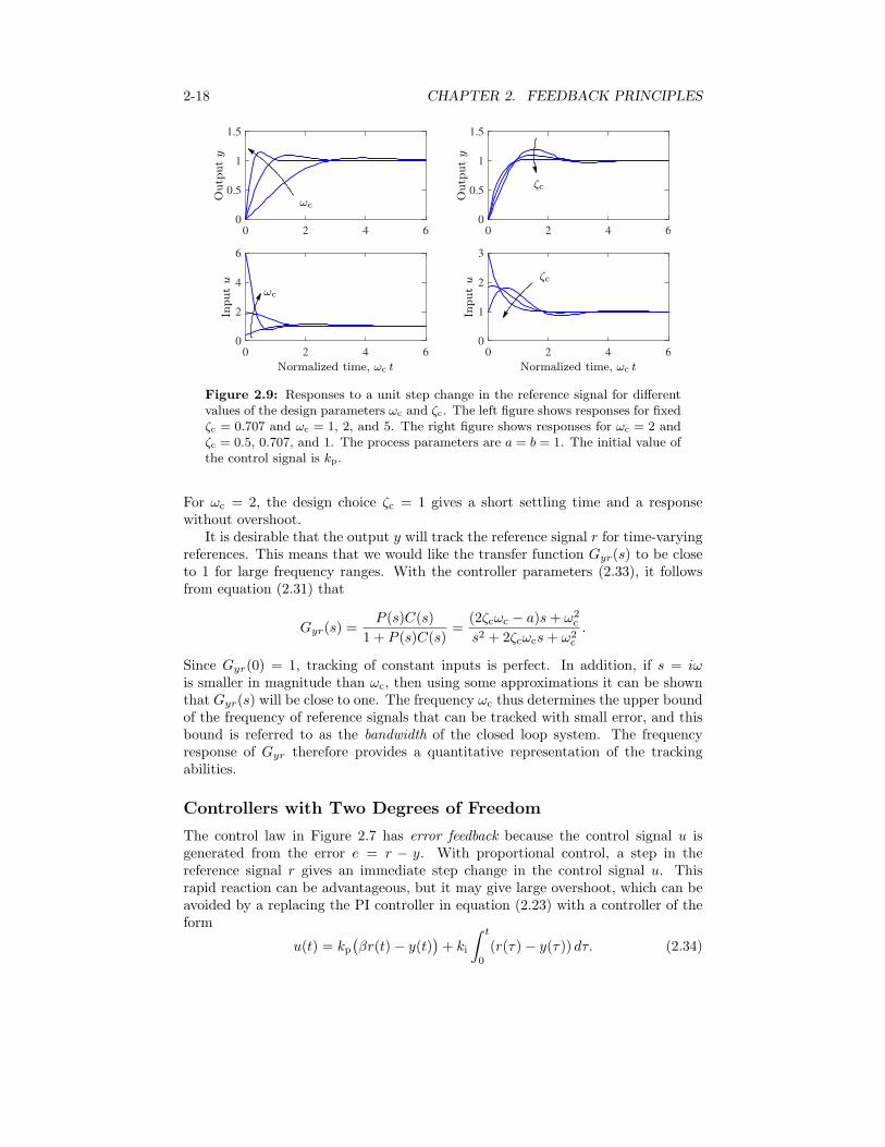
Figure 2.10: Block diagram of a closed loop system with a PI controller havingan architecture with two degrees of freedom.
In this modified PI algorithm, the proportional action only acts on the fraction #of the reference signal. The signal transmissions from reference r to u and fromoutput y to u can be represented by the (open loop) transfer functions
Cur(s) = #kp +kis, !Cuy(s) = kp +
kis
= C(s). (2.35)
The controller (2.34) is called a controller with two degrees of freedom since thetransfer functions Cur(s) and Cuy(s) are di!erent.
A block diagram of a closed loop system with a PI controller having two degreesof freedom is shown in Figure 2.10. Let the process transfer function be P (s) =b/(s + a). The transfer functions from reference r and disturbance v to output yare
Gyr(s) =b#kps+ bki
s2 + (a+ bkp)s+ bki, Gyv(s) =
bs
s2 + (a+ bkp)s+ bki. (2.36)
Comparing with the corresponding transfer function for a controller with errorfeedback in equations (2.24) and (2.31), we find that the response to the loaddisturbances is the same but the response to reference signals is di!erent.
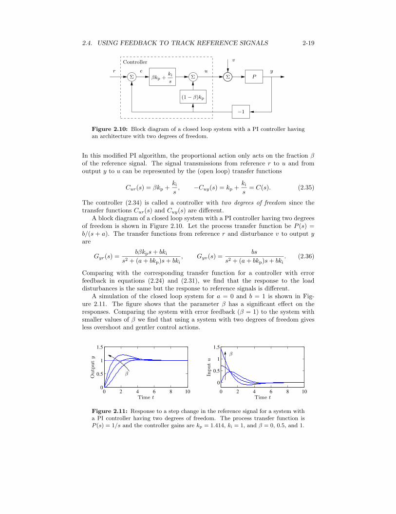
A simulation of the closed loop system for a = 0 and b = 1 is shown in Fig-ure 2.11. The figure shows that the parameter # has a significant e!ect on theresponses. Comparing the system with error feedback (# = 1) to the system withsmaller values of # we find that using a system with two degrees of freedom givesless overshoot and gentler control actions.
0 2 4 6 8 100
0.5
1
1.5
Time t
Outp
uty
#
0 2 4 6 8 10
0
0.5
1
1.5
Time t
Inputu
#
Figure 2.11: Response to a step change in the reference signal for a system witha PI controller having two degrees of freedom. The process transfer function isP (s) = 1/s and the controller gains are kp = 1.414, ki = 1, and # = 0, 0.5, and 1.
2-20 CHAPTER 2. FEEDBACK PRINCIPLES
The example shows that reference signal response can be improved by using acontroller architecture having two degrees of freedom. In Section 12.4 we will furthershow that the responses to reference signals and disturbances can be completelyseparated by using a more general system architecture. To use a system withtwo degrees of freedom both the reference signal r and the output signal y mustbe measured. There are situations where only the error signal e = r ! y canbe measured; typical examples are DVD players, optical memories, and atomicforce microscopes. In these cases, only single degree of freedom (error feedback)controllers can be used.
2.5 Using Feedback to Provide Robustness
Feedback can be used to make good systems from imprecise components. Black’sinvention of the feedback amplifier for the telephone network is an early exam-ple [Bla77]. Black used negative feedback to design extremely good amplifiers withlinear characteristics from components with nonlinear and time-varying properties.Since signals are transmitted over long distances they must be amplified. At thetime, the thermionic valve—a type of vacuum tube invented by Lee de Forest in1906—was the only available technology for amplifying electric signals until thetransistor was in invented in 1947. Vacuum tubes were the key to develop radio,telephony, and electronics in the first half of the 20th century. They are still usedby some hi-fi aficionados in high quality audio amplifiers.
Vacuum tubes can give high gain but they have nonlinear and time varyinginput/output characteristics that distort the transmitted signals. Bode [Bod60]expressed the problem as follows:
Most of you with hi-fi systems are no doubt proud of the quality of youramplifiers, but I doubt whether many of you would care to listen to thesound after the signal had gone in succession through several dozen orseveral hundred even of your fine amplifiers.
The e!ect is illustrated in Exercise 2.9.Black’s idea to develop a good amplifier was to close a loop with negative feed- H!
back around the tube amplifier. In this way he could obtain a closed loop systemwith a linear input/output relation having constant gain. The general recipe is tolocalize the nonlinearities and the source of process variations, and to close feedbackloops around them.
Reducing E!ects of Parameter Variations and Nonlinearities
Consider an amplifier with a static, nonlinear input/output relation with consider-able parameter variability, as illustrated in Figure 2.12a. The nominal input/outputcharacteristic is shown as a dashed bold line and examples of variations as thin lines.The nonlinearity in the figure is given by
y = F (u) = "(u+ #u3), !3 " u " 3. (2.37)
The nominal values corresponding to the dashed line are " = 0.2 and # = 1. Thevariations of the parameters " and # are in the ranges 0.1 " " " 0.5, 0 " # " 2.
2.5. USING FEEDBACK TO PROVIDE ROBUSTNESS 2-21
-2 0 2-3
-2
-1
0
1
2
3
Outp
uty
Input u
(a) I/O relationships
0 0.5 1 1.5 2-1
0
1
2
3
4
5
Time t
Outp
uty
(b) Output signals
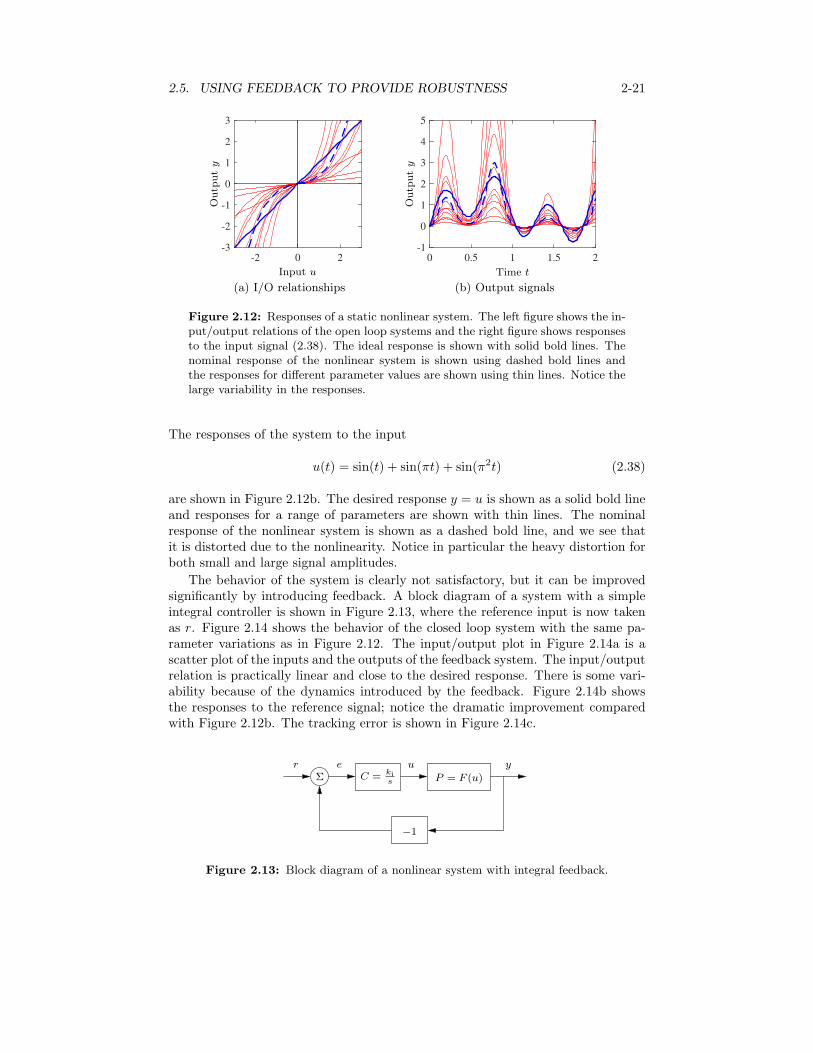
Figure 2.12: Responses of a static nonlinear system. The left figure shows the in-put/output relations of the open loop systems and the right figure shows responsesto the input signal (2.38). The ideal response is shown with solid bold lines. Thenominal response of the nonlinear system is shown using dashed bold lines andthe responses for di!erent parameter values are shown using thin lines. Notice thelarge variability in the responses.
The responses of the system to the input
u(t) = sin(t) + sin(&t) + sin(&2t) (2.38)
are shown in Figure 2.12b. The desired response y = u is shown as a solid bold lineand responses for a range of parameters are shown with thin lines. The nominalresponse of the nonlinear system is shown as a dashed bold line, and we see thatit is distorted due to the nonlinearity. Notice in particular the heavy distortion forboth small and large signal amplitudes.
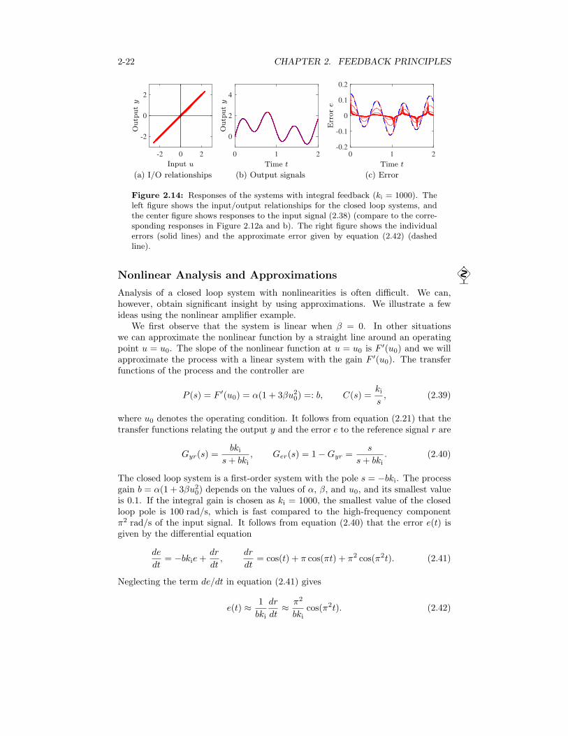
The behavior of the system is clearly not satisfactory, but it can be improvedsignificantly by introducing feedback. A block diagram of a system with a simpleintegral controller is shown in Figure 2.13, where the reference input is now takenas r. Figure 2.14 shows the behavior of the closed loop system with the same pa-rameter variations as in Figure 2.12. The input/output plot in Figure 2.14a is ascatter plot of the inputs and the outputs of the feedback system. The input/outputrelation is practically linear and close to the desired response. There is some vari-ability because of the dynamics introduced by the feedback. Figure 2.14b showsthe responses to the reference signal; notice the dramatic improvement comparedwith Figure 2.12b. The tracking error is shown in Figure 2.14c.
!1
u!
erC = ki
s
yP = F (u)
Figure 2.13: Block diagram of a nonlinear system with integral feedback.
2-22 CHAPTER 2. FEEDBACK PRINCIPLES
-2 0 2
-2
0
2
Outp
uty
Input u
(a) I/O relationships
0 1 2
0
2
4
Time t
Outp
uty
(b) Output signals
0 1 2-0.2
-0.1
0
0.1
0.2
Time t
Error
e
(c) Error
Figure 2.14: Responses of the systems with integral feedback (ki = 1000). Theleft figure shows the input/output relationships for the closed loop systems, andthe center figure shows responses to the input signal (2.38) (compare to the corre-sponding responses in Figure 2.12a and b). The right figure shows the individualerrors (solid lines) and the approximate error given by equation (2.42) (dashedline).
Nonlinear Analysis and Approximations !
Analysis of a closed loop system with nonlinearities is often di"cult. We can,however, obtain significant insight by using approximations. We illustrate a fewideas using the nonlinear amplifier example.
We first observe that the system is linear when # = 0. In other situationswe can approximate the nonlinear function by a straight line around an operatingpoint u = u0. The slope of the nonlinear function at u = u0 is F "(u0) and we willapproximate the process with a linear system with the gain F "(u0). The transferfunctions of the process and the controller are
P (s) = F "(u0) = "(1 + 3#u20) =: b, C(s) =
kis, (2.39)
where u0 denotes the operating condition. It follows from equation (2.21) that thetransfer functions relating the output y and the error e to the reference signal r are
Gyr(s) =bki
s+ bki, Ger(s) = 1!Gyr =
s
s+ bki. (2.40)
The closed loop system is a first-order system with the pole s = !bki. The processgain b = "(1 + 3#u2
0) depends on the values of ", #, and u0, and its smallest valueis 0.1. If the integral gain is chosen as ki = 1000, the smallest value of the closedloop pole is 100 rad/s, which is fast compared to the high-frequency component&2 rad/s of the input signal. It follows from equation (2.40) that the error e(t) isgiven by the di!erential equation
de
dt= !bkie+
dr
dt,
dr
dt= cos(t) + & cos(&t) + &2 cos(&2t). (2.41)
Neglecting the term de/dt in equation (2.41) gives
e(t) * 1
bki
dr
dt* &2
bkicos(&2t). (2.42)
2.6. POSITIVE FEEDBACK 2-23
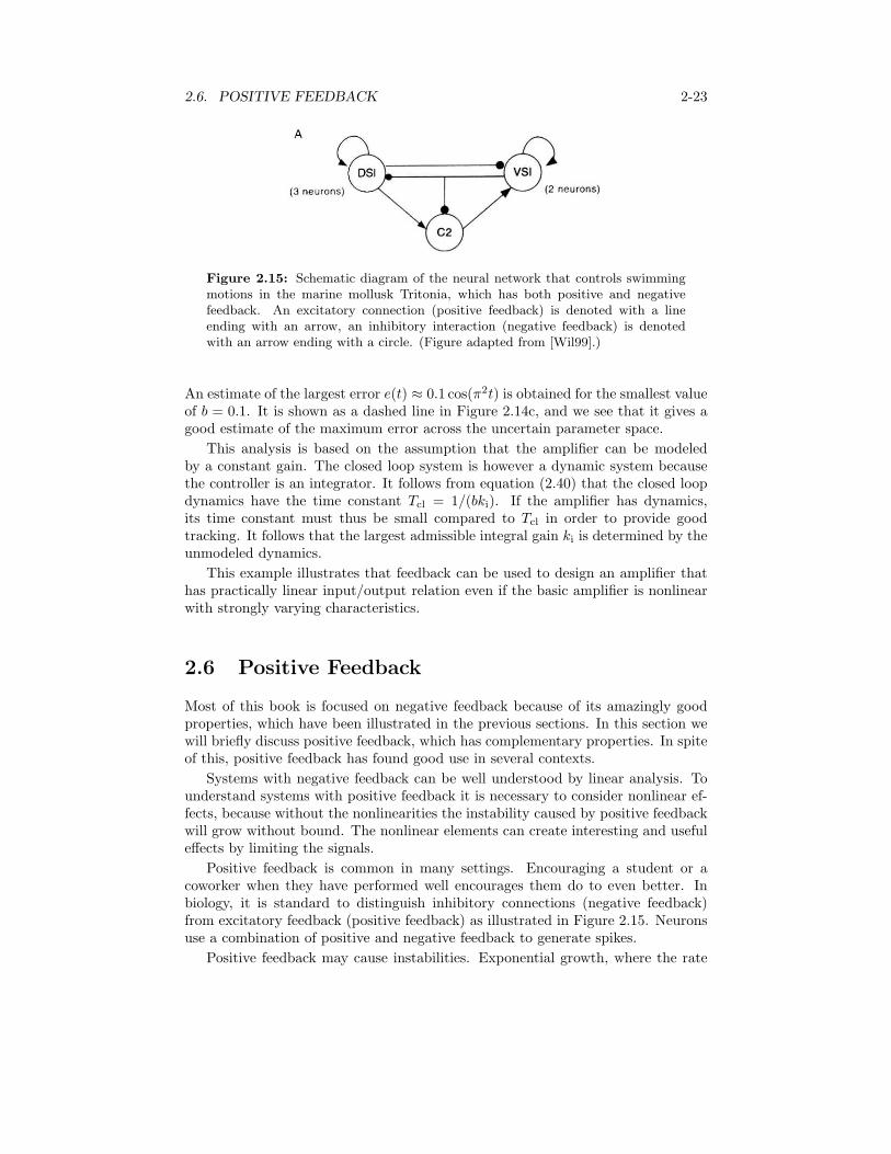
Figure 2.15: Schematic diagram of the neural network that controls swimmingmotions in the marine mollusk Tritonia, which has both positive and negativefeedback. An excitatory connection (positive feedback) is denoted with a lineending with an arrow, an inhibitory interaction (negative feedback) is denotedwith an arrow ending with a circle. (Figure adapted from [Wil99].)
An estimate of the largest error e(t) * 0.1 cos(&2t) is obtained for the smallest valueof b = 0.1. It is shown as a dashed line in Figure 2.14c, and we see that it gives agood estimate of the maximum error across the uncertain parameter space.
This analysis is based on the assumption that the amplifier can be modeledby a constant gain. The closed loop system is however a dynamic system becausethe controller is an integrator. It follows from equation (2.40) that the closed loopdynamics have the time constant Tcl = 1/(bki). If the amplifier has dynamics,its time constant must thus be small compared to Tcl in order to provide goodtracking. It follows that the largest admissible integral gain ki is determined by theunmodeled dynamics.
This example illustrates that feedback can be used to design an amplifier thathas practically linear input/output relation even if the basic amplifier is nonlinearwith strongly varying characteristics.
2.6 Positive Feedback
Most of this book is focused on negative feedback because of its amazingly goodproperties, which have been illustrated in the previous sections. In this section wewill briefly discuss positive feedback, which has complementary properties. In spiteof this, positive feedback has found good use in several contexts.
Systems with negative feedback can be well understood by linear analysis. Tounderstand systems with positive feedback it is necessary to consider nonlinear ef-fects, because without the nonlinearities the instability caused by positive feedbackwill grow without bound. The nonlinear elements can create interesting and usefule!ects by limiting the signals.
Positive feedback is common in many settings. Encouraging a student or acoworker when they have performed well encourages them do to even better. Inbiology, it is standard to distinguish inhibitory connections (negative feedback)from excitatory feedback (positive feedback) as illustrated in Figure 2.15. Neuronsuse a combination of positive and negative feedback to generate spikes.
Positive feedback may cause instabilities. Exponential growth, where the rate
2-24 CHAPTER 2. FEEDBACK PRINCIPLES
R2
C2
C1 R1
Rf
Rb
Vout
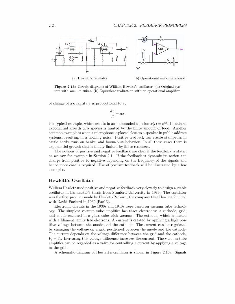
(a) Hewlett’s oscillator (b) Operational amplifier version
Figure 2.16: Circuit diagrams of William Hewlett’s oscillator. (a) Original sys-tem with vacuum tubes. (b) Equivalent realization with an operational amplifier.
of change of a quantity x is proportional to x,
dx
dt= "x,
is a typical example, which results in an unbounded solution x(t) = e#t. In nature,exponential growth of a species is limited by the finite amount of food. Anothercommon example is when a microphone is placed close to a speaker in public addresssystems, resulting in a howling noise. Positive feedback can create stampedes incattle herds, runs on banks, and boom-bust behavior. In all these cases there isexponential growth that is finally limited by finite resources.
The notions of positive and negative feedback are clear if the feedback is static,as we saw for example in Section 2.1. If the feedback is dynamic its action canchange from positive to negative depending on the frequency of the signals andhence more care is required. Use of positive feedback will be illustrated by a fewexamples.
Hewlett’s Oscillator
William Hewlett used positive and negative feedback very cleverly to design a stableoscillator in his master’s thesis from Stanford University in 1939. The oscillatorwas the first product made by Hewlett-Packard, the company that Hewlett foundedwith David Packard in 1939 [Pac13].
Electronic circuits in the 1930s and 1940s were based on vacuum tube technol-ogy. The simplest vacuum tube amplifier has three electrodes: a cathode, grid,and anode enclosed in a glass tube with vacuum. The cathode, which is heatedwith a filament, emits free electrons. A current is created by applying a high pos-itive voltage between the anode and the cathode. The current can be regulatedby changing the voltage on a grid positioned between the anode and the cathode.The current depends on the voltage di!erence between the grid and the cathode,Vg ! Vc. Increasing this voltage di!erence increases the current. The vacuum tubeamplifier can be regarded as a valve for controlling a current by applying a voltageto the grid.
A schematic diagram of Hewlett’s oscillator is shown in Figure 2.16a. Signals
2.6. POSITIVE FEEDBACK 2-25
1
1 + sTi
!kpe u
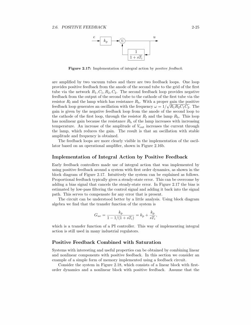
Figure 2.17: Implementation of integral action by positive feedback.
are amplified by two vacuum tubes and there are two feedback loops. One loopprovides positive feedback from the anode of the second tube to the grid of the firsttube via the network R1, C1, R2, C2. The second feedback loop provides negativefeedback from the output of the second tube to the cathode of the first tube via theresistor Rf and the lamp which has resistance Rb. With a proper gain the positivefeedback loop generates an oscillation with the frequency % = 1/
)R1R2C1C2. The
gain is given by the negative feedback loop from the anode of the second loop tothe cathode of the first loop, through the resistor Rf and the lamp Rb. This loophas nonlinear gain because the resistance Rb of the lamp increases with increasingtemperature. An increase of the amplitude of Vout increases the current throughthe lamp, which reduces the gain. The result is that an oscillation with stableamplitude and frequency is obtained.
The feedback loops are more clearly visible in the implementation of the oscil-lator based on an operational amplifier, shown in Figure 2.16b.
Implementation of Integral Action by Positive Feedback
Early feedback controllers made use of integral action that was implemented byusing positive feedback around a system with first order dynamics, as shown in theblock diagram of Figure 2.17. Intuitively the system can be explained as follows.Proportional feedback typically gives a steady-state error. This can be overcome byadding a bias signal that cancels the steady-state error. In Figure 2.17 the bias isestimated by low-pass filtering the control signal and adding it back into the signalpath. This serves to compensate for any error that is present.
The circuit can be understood better by a little analysis. Using block diagramalgebra we find that the transfer function of the system is
Gue =kp
1! 1/(1 + sTi)= kp +
kpsTi
,
which is a transfer function of a PI controller. This way of implementing integralaction is still used in many industrial regulators.
Positive Feedback Combined with Saturation
Systems with interesting and useful properties can be obtained by combining linearand nonlinear components with positive feedback. In this section we consider anexample of a simple form of memory implemented using a feedback circuit.
Consider the system in Figure 2.18, which consists of a linear block with first-order dynamics and a nonlinear block with positive feedback. Assume that the
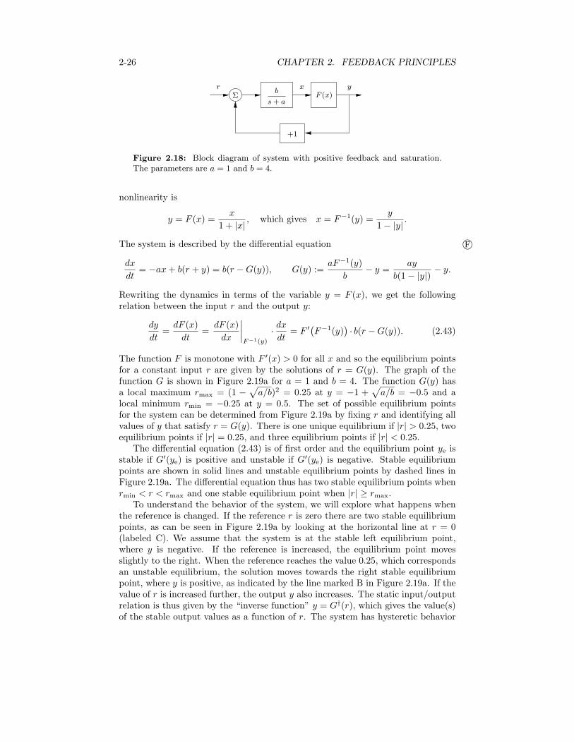
2-26 CHAPTER 2. FEEDBACK PRINCIPLES
F (x)y
!r
b
s+ a
+1
x
Figure 2.18: Block diagram of system with positive feedback and saturation.The parameters are a = 1 and b = 4.
nonlinearity is
y = F (x) =x
1 + |x| , which gives x = F!1(y) =y
1! |y| .
The system is described by the di!erential equation F!
dx
dt= !ax+ b(r + y) = b(r !G(y)), G(y) :=
aF!1(y)
b! y =
ay
b(1! |y|) ! y.
Rewriting the dynamics in terms of the variable y = F (x), we get the followingrelation between the input r and the output y:
dy
dt=
dF (x)
dt=
dF (x)
dx
----F!1(y)
·dx
dt= F ")F!1(y)
*· b(r !G(y)). (2.43)
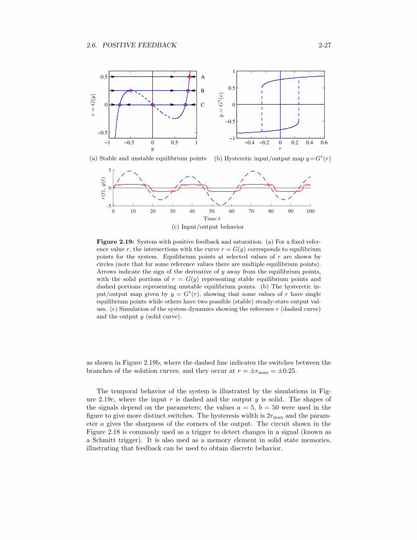
The function F is monotone with F "(x) > 0 for all x and so the equilibrium pointsfor a constant input r are given by the solutions of r = G(y). The graph of thefunction G is shown in Figure 2.19a for a = 1 and b = 4. The function G(y) hasa local maximum rmax = (1 !
.a/b)2 = 0.25 at y = !1 +
.a/b = !0.5 and a
local minimum rmin = !0.25 at y = 0.5. The set of possible equilibrium pointsfor the system can be determined from Figure 2.19a by fixing r and identifying allvalues of y that satisfy r = G(y). There is one unique equilibrium if |r| > 0.25, twoequilibrium points if |r| = 0.25, and three equilibrium points if |r| < 0.25.
The di!erential equation (2.43) is of first order and the equilibrium point ye isstable if G"(ye) is positive and unstable if G"(ye) is negative. Stable equilibriumpoints are shown in solid lines and unstable equilibrium points by dashed lines inFigure 2.19a. The di!erential equation thus has two stable equilibrium points whenrmin < r < rmax and one stable equilibrium point when |r| # rmax.
To understand the behavior of the system, we will explore what happens whenthe reference is changed. If the reference r is zero there are two stable equilibriumpoints, as can be seen in Figure 2.19a by looking at the horizontal line at r = 0(labeled C). We assume that the system is at the stable left equilibrium point,where y is negative. If the reference is increased, the equilibrium point movesslightly to the right. When the reference reaches the value 0.25, which correspondsan unstable equilibrium, the solution moves towards the right stable equilibriumpoint, where y is positive, as indicated by the line marked B in Figure 2.19a. If thevalue of r is increased further, the output y also increases. The static input/outputrelation is thus given by the “inverse function” y = G†(r), which gives the value(s)of the stable output values as a function of r. The system has hysteretic behavior
2.6. POSITIVE FEEDBACK 2-27
!1 !0.5 0 0.5 1
!0.5
0
0.5
C
B
A
y
r=
G(y)
(a) Stable and unstable equilibrium points
!0.4 !0.2 0 0.2 0.4 0.6!1
!0.5
0
0.5
1
r
y=
G†(r)
(b) Hysteretic input/output map y=G†(r)
0 10 20 30 40 50 60 70 80 90 100-5
0
5
Time t
r(t),y(t)
(c) Input/output behavior
Figure 2.19: System with positive feedback and saturation. (a) For a fixed refer-ence value r, the intersections with the curve r = G(y) corresponds to equilibriumpoints for the system. Equilibrium points at selected values of r are shown bycircles (note that for some reference values there are multiple equilibrium points).Arrows indicate the sign of the derivative of y away from the equilibrium points,with the solid portions of r = G(y) representing stable equilibrium points anddashed portions representing unstable equilibrium points. (b) The hysteretic in-put/output map given by y = G†(r), showing that some values of r have singleequilibrium points while others have two possible (stable) steady-state output val-ues. (c) Simulation of the system dynamics showing the reference r (dashed curve)and the output y (solid curve).
as shown in Figure 2.19b, where the dashed line indicates the switches between thebranches of the solution curves, and they occur at r = ±rmax = ±0.25.
The temporal behavior of the system is illustrated by the simulations in Fig-ure 2.19c, where the input r is dashed and the output y is solid. The shapes ofthe signals depend on the parameters; the values a = 5, b = 50 were used in thefigure to give more distinct switches. The hysteresis width is 2rmax and the param-eter a gives the sharpness of the corners of the output. The circuit shown in theFigure 2.18 is commonly used as a trigger to detect changes in a signal (known asa Schmitt trigger). It is also used as a memory element in solid state memories,illustrating that feedback can be used to obtain discrete behavior.
2-28 CHAPTER 2. FEEDBACK PRINCIPLES
2.7 Further Reading
The books by Bennett [Ben79, Ben93] and Mindel [Min02, Min08] give interestingperspective on the development of control. Much of the material touched upon inthis chapter is referred to as “classical control”; see [CM51], [JNP47], and [Tru55]for early texts on this material. A more thorough introduction to the principlesof feedback with minimal mathematical prerequisites is available in the textbookFeedback Control for Everyone [AM10]. The notion of controllers with two degreesof freedom was introduced by Horowitz [Hor63].
The analysis introduced here will be elaborated in the rest of the book. Transferfunctions and other descriptions of dynamics are discussed in Chapters 3 and 9,methods to investigate stability in Chapters 5 and 10. The simple method tofind parameters of controllers based on matching of coe"cients of the closed loopcharacteristic polynomial is developed further in Chapters 7, 8, and 13. Feedforwardcontrol is discussed in Sections 8.5 and 12.4.
Exercises
2.1 (Transfer functions and di!erential equations) Let y + R and u + R. Solve thedi!erential equations
dy
dt+ ay = bu,
d2y
dt2+ 2
dy
dt+ y = 2
du
dt+ u,
for t > 0. Determine the responses to a unit step u(t) = 1 and the exponentialsignal u(t) = est when the initial condition is zero. Derive the transfer functions ofthe systems.
2.2 (E!ect of zeros on time responses) Let y0(t) be the response of a system with thetransfer functionG0(s) to a given input. The transfer functionG(s) = (1+sT )G0(s)has the same zero frequency gain but it has an additional zero at z = !1/T . Lety(t) be the response of the system with the transfer function G(s) and show that
y(t) = y0(t) + Tdy0dt
. (2.44)
Next consider the system with the transfer function
G(s) =s+ a
a(s2 + 2s+ 1),
which has unit zero-frequency-gain (G(0) = 1). Use the result in equation (2.44)to explore the e!ect of a zero at s = !1/T on the step response of a system.
2.3 (PI control) Consider a closed loop system with process dynamics and a PIcontroller modeled by
dy
dt+ ay = bu, u = kp(r ! y) + ki
, t
0
)r(!)! y(!)) d!,
where r is the reference, u is the control variable, and y is the process output.
2.7. FURTHER READING 2-29
(a) Derive a di!erential equation relating the output y to the reference r by directmanipulation of the equations and compute the transfer function Hyr(s). Makethe derivations both by direct manipulation of the di!erential equations and bypolynomial algebra.
(b) Draw a block diagram of the system and derive the transfer functions of theprocess P (s) and the controller C(s).
(c) Use block diagram algebra to compute the transfer function from reference rto output y of the closed loop system and verify that your answer matches youranswer in part (a).
2.4 (Zero frequency gain) Consider the system described by the di!erential equa-tion (2.10) and the transfer function (2.16). Determine the zero frequency gain ofthe system by computing the particular solution of equation (2.10) for a constantinput u(t) = u0. Compare with the value of G(0).
2.5 (Pupil response) The dynamics of the pupillary reflex can be approximated bya linear system with the transfer function
P (s) =0.2(1! 0.1s)
(1 + 0.1s)3.
Assume that the nervous system that controls the pupil opening is modeled asa proportional controller with the gain k. Use the Routh–Hurwitz criterion todetermine the largest gain that gives a stable closed loop system.
2.6 (Parameter sensitivity) Consider the feedback system in Figure 2.7. Let thedisturbance v = 0, P (s) = 1 and C(s) = ki/s. Determine the transfer function Gyr
from reference r to output y. Also determine how much Gyr is changed when theprocess gain changes by 10%.
2.7 (PID control design) The calculations in Section 2.3 can be interpreted as adesign method for a PI controller for a first-order system. A similar calculation canbe made for PID control of a second-order system. Let the transfer functions of theprocess and the controller be
P (s) =b
s2 + a1s+ a2, C(s) = kp +
kis+ kds.
Show that the controller parameters
kp =(1 + 2"'c)%2
c ! a2b
, ki ="%3
c
b, kd =
("+ 2'c)%c ! a1b
give a closed loop system with the characteristic polynomial
(s2 + 2'c%cs+ %2c )(s+ "%c).
2-30 CHAPTER 2. FEEDBACK PRINCIPLES
2.8 (Linear behavior via feedback) Consider an open loop system with the nonlin-ear input/output relation y = F (u). Assume that the system is closed with theproportional controller u = k(r ! y). Show that the input/output relation of theclosed loop system is
y +1
kF!1(y) = r.
Estimate the largest deviation from ideal linear response y = r. Illustrate byplotting the input output responses for a) F (u) =
)u and b) F (u) = u2 with
0 " u " 1 and k = 5, 10, and 100.
2.9 (Nonlinear distortion) The following MATLAB commands will load and playHandel’s Messiah:
load handel % Load Handel’s Messiahsound(y, Fs); pause % Play the original music through speaker
Write a MATLAB function that implements a nonlinear amplifier with static gain
y = 2(z + az(1! z)! 0.5), z = (x+ 1)/2,
where x is the original signal (assumed to take values between !1 and 1) and ais the amplifier gain. Compare the sound that is obtained when the music is thensent through two amplifiers with the given nonlinearity and gain a = 1 versus whenthe music is sent through the same two amplifiers with feedback k = 10.
2.10 (Queing systems) Consider a queuing system modeled by
dx
dt= (! µmax
x
x+ 1,
where ( is the acceptance rate of jobs and x is the length of the queue. The modelis nonlinear and the dynamics of the system changes significantly with the queuinglength (see Example 3.15 for a more detailed discussion). Investigate the situationwhen a PI controller is used for admission control. Let r be the rate of arrival ofjob requests and model the (average) arrival intensity ( as
( = kp(r ! x) + ki
, t
(r(t)! x(t))dt.
The controller parameters are determined from the approximate model
dx
dt= (.
Find controller parameters that give the closed loop characteristic polynomial s2 +2s+ 1 for the approximate model. Investigate the behavior of the control strategyfor the full nonlinear model by simulation for the input r = 5 + 4 sin(0.1t).