feedback control and nonlinear controllability of nonholonomic systems
TRANSCRIPT
Feedback Control and Nonlinear Controllability of Nonholonomic Systems
Sabiha Amin Wadoo
Thesis submitted to the Faculty of the Virginia Polytechnic Institute and State University
in partial fulfillment of the requirements for the degree of
Masters of Science in
Electrical Engineering
Dr. Pushkin Kachroo, Chair Dr. A Lynn Abbott Dr. Daniel Stillwell
Jan 9, 2003 Blacksburg Virginia
Keywords: autonomous vehicle, controllability, nonholonomic, trajectory tracking, point stabilization, path following.
Copyright 2003, Sabiha Amin Wadoo
Feedback Control and Nonlinear Controllability of Nonholonomic Systems
Sabiha Amin Wadoo
(ABSTRACT)
In this thesis we study the methods for motion planning for nonholonomic
systems. These systems are characterized by nonholonomic constraints on their
generalized velocities. The motion planning problem with constraints on the velocities is
transformed into a control problem having fewer control inputs than the degrees of
freedom. The main focus of the thesis is on the study of motion planning and design of
the feedback control laws for an autonomous underwater vehicle: a nonholonomic
system. The nonlinear controllability issues for the system are also studied. For the
design of feedback cont rollers, the system is transformed into chained and power forms.
The methods of transforming a nonholonomic system into these forms are discussed. The
work presented in this thesis is a step towards the initial study concerning the
applicability of kinematic-based control on underwater vehicles.
iii
Acknowledgements
The author would like to extend thanks to Dr. Pushkin Kachroo for suggesting the
research topic, and for his help and guidance offered during the work. He encouraged the
author to study mathematics which helped the author not only in the research but also in
other fields of study.
Also, the author would like to thank Dr. Lynn Abbott and Dr. Daniel Stilwell for
participating in the advisory committee for the thesis.
iv
Contents 1. Introduction................................................................................................................... 1
1.1 Overview............................................................................................................. 1
1.2 Motivation........................................................................................................... 2
1.3 Thesis outline and organization of the chapters.................................................. 3
1.4 Previous research and contributions of the thesis ............................................... 4
2. Problem Formulation and Examples .......................................................................... 7
2.1 Motion planning of nonholonomic systems........................................................ 7
2.2 Nonholonomic constraints .................................................................................. 9
2.3 Problem description .......................................................................................... 11
2.4 Control model formulation ............................................................................... 13
2.5 Controllability issues ........................................................................................ 15
2.6 Stabilization ...................................................................................................... 16
2.6.1 Controllability and stabilization at a point ................................................ 17
2.6.2 Controllability and stabilization about trajectory ..................................... 18
2.6.3 Approximate linearization......................................................................... 18
2.6.4 Exact feedback linearization..................................................................... 19
2.6.5 Static feedback linearization..................................................................... 20
2.6.6 Dynamic feedback linearization................................................................ 20
2.7 Examples of nonholonomic systems................................................................. 22
3. Mathematical Modeling and Controllability Analysis of an Underwater Vehicle 26
3.1 Mathematical modeling..................................................................................... 26
v
3.1.1 Kinematic modeling and nonholonomic constraints................................. 27
3.1.2 Kinematic model with respect to global coordinates ................................ 28
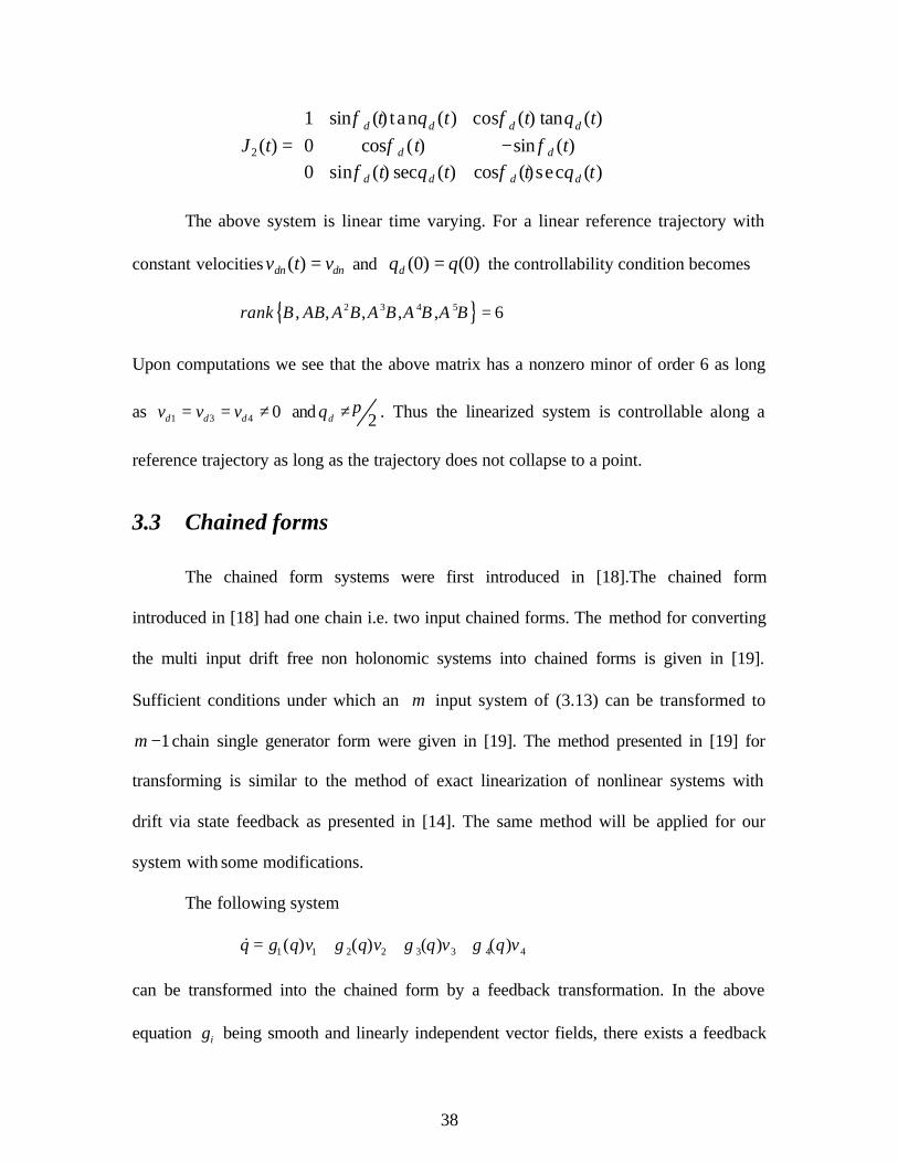
3.2 Controllability analysis ..................................................................................... 33
3.2.1 Controllability about a point .................................................................... 33
3.2.2 Controllability about a trajectory............................................................. 35
3.3 Chained forms ................................................................................................... 38
4. Control Design and Simulation Results .................................................................... 44
4.1 Trajectory tracking and controller design .......................................................... 44
4.2 Reference trajectory generation......................................................................... 45
4.3 Control using approximate linearization. ........................................................... 48
4.3.1 Simulation of the controller ...................................................................... 52
4.4 Control using exact feedback linearization........................................................ 60
4.4.1 Control using exact feedback linearization via static feedback ................ 61
4.4.2 Control using exact feedback linearization via dynamic feedback........... 62
4.4.3 Simulation of the controller ...................................................................... 65
4.5 Point to point stabilization ................................................................................ 73
4.5.1 Control with smooth time varying feedback............................................. 73
4.5.2 Power form................................................................................................ 73
4.5.3 Control law................................................................................................ 75
4.5.4 Simulation................................................................................................. 76
5. Conclusions .................................................................................................................. 82
5.1 Concluding remarks .......................................................................................... 82
5.2 Future work ....................................................................................................... 83
vi
References........................................................................................................................ 84
Vita ................................................................................................................................... 88
vii
List of Figures
2.1: Motion planning tasks for a car- like robot................................................................. 12
2.2: The nonholonomic constraints on a unicycle. ........................................................... 22
2.3: The nonholonomic constraints on a car- like robot. ................................................... 24
3.1: The coordinate systems of an under water vehicle .................................................... 28
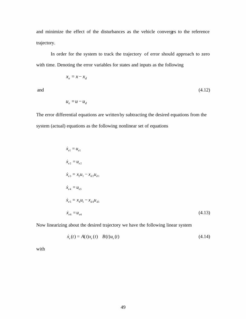
4. 1: The result of approximate linearization: tracking errors in chained form variables vs.
time (sec)................................................................................................................... 54
4. 2: The result of approximate linearization: tracking errors in chained form inputs vs.
time (sec)................................................................................................................... 54
4. 3: The result of approximate linearization: actual and desired chained form variables
vs. time (sec).. ........................................................................................................... 55
4. 4: The result of approximate linearization: actual and desired chained form inputs vs.
time (sec)................................................................................................................... 55
4. 5:The result of approximate linearization: tracking errors in variables x, y, z vs. time
(sec). .......................................................................................................................... 56
4. 6: The result of approximate linearization: tracking errors in variables ψ , θ , φ vs.
time (sec)................................................................................................................... 56
4. 7: The result of approximate linearization: actual and desired original variables x, y, z
vs. time (sec). ............................................................................................................ 57
4. 8: The result of approximate linearization: actual and desired original variables ψ , θ ,
φ vs. time (sec). ....................................................................................................... 57
4. 9: The result of approximate linearization: 1v (m/sec) vs. time (sec)........................... 58
viii
4. 10: The result of approximate linearization: 2v (rad/sec) vs. time (sec). ..................... 58
4. 11: The result of approximate linearization: 3v (rad/sec) vs. time (sec). ..................... 59
4. 12: The result of approximate linearization: 4v (rad/sec) vs. time (sec). ..................... 59
4. 13: The result of dynamic feedback: tracking errors in chained form variables vs. time
(sec). .......................................................................................................................... 67
4. 14: The result of dynamic feedback: tracking errors in chained form inputs vs. time
(sec). .......................................................................................................................... 67
4. 15: The result of dynamic feedback: actual and desired chained form variables vs. time
(sec). .......................................................................................................................... 68
4. 16: The result of dynamic feedback: actual and desired chained form inputs vs. time
(sec). .......................................................................................................................... 68
4. 17: The result of dynamic feedback: tracking errors in variables x, y, z vs. time (sec).
................................................................................................................................... 69
4. 18: The result of dynamic feedback: tracking errors in variables ψ , θ , φ vs. time
(sec). .......................................................................................................................... 69
4. 19: The result of dynamic feedback: actual and desired original variables x, y, z vs.
time............................................................................................................................ 70
4. 20: The result of dynamic feedback: actual and desired original variables ψ , θ , φ
vs. time...................................................................................................................... 70
4. 21: The result of dynamic feedback: 1v (m/sec) vs. time (sec)..................................... 71
4. 22: The result of dynamic feedback: 2v (rad/sec) vs. time (sec). ................................. 71
4. 23: The result of dynamic feedback: 3v (rad/sec) vs. time (sec). ................................. 72

ix
4. 24: The result of dynamic feedback: 4v (rad/sec) vs. time (sec). ................................. 72
4. 25: Point stabilization using time varying feedback: x (m) vs. time (sec). ................. 77
4. 26: Point stabilization using time varying feedback: y (rad) vs. time (sec). ............... 77
4. 27: Point stabilization using time varying feedback: z (m) vs. time (sec). ................. 78
4. 28: Point stabilization using time varying feedback: ψ (rad) vs. time (sec)................ 78
4. 29: Point stabilization using time varying feedback: θ (rad) vs. time (sec). ............... 79
4. 30: Point stabilization using time varying feedback: φ (rad) vs. time (sec). ............... 79
4. 31: Point stabilization using time varying feedback: 1v (m/sec) vs. time (sec)............ 80
4. 32: Point stabilization using time varying feedback: 2v (m/sec) vs. time (sec). .......... 80
4. 33: Point stabilization using time varying feedback: 3v (rad/sec) vs. time (sec). ........ 81
4. 34: Point stabilization using time varying feedback: 4v (rad/sec) vs. time (sec). ........ 81
Chapter 1
Introduction
This chapter gives the brief overview on the thesis topic and the motivation
behind the research work presented here. The chapter also gives a brief overview and the
organization of the chapters following in the text.
1.1 Overview
The purpose of this research is to study the issues related to motion planning,
nonlinear controllability and design of the feedback controllers for a specific class of
nonholonomically constrained mechanical systems. Specifically, differential geometric
control theory, nonlinear system analysis and control design techniques, and the results of
recent research in the motion planning of nonholonomic systems are used and presented
for the support of the current research work.
Finally, a mathematical model of an autonomous underwater vehicle is developed.
The kinematic modeling and the feedback controller design for the same are presented in
detail and simulation results are obtained. The methods for converting the system into
chained and power forms are also discussed. A brief mathematical analysis of the
concepts involved in the study of controllability, control design and modeling is
presented. The work presented in this thesis is a step towards the initial study concerning
the applicability of kinematic- based control on underwater vehicles.

2
1.2 Motivation
The initial motivation for the thesis came from the need of motion planning of
nonholonomic systems. These systems are characterized by the presence of
nonholonomic constraints on their generalized velocities. The control model for such
systems is drift free, nonlinear and under actuated, given by
1 1 2 2( ) ( ) ......... ( )m mq g q v g q v g q v= + + +& (1.1)
Here q M∈ is the state of the system, M is the state space and nM ⊂ ¡ . Thus q belongs
to a configuration space of dimension n . mv ∈¡ is the input or the control vector of
dimension m . ( ) nig q ∈¡ ; 1,2......,i m= are vector fields on M and are assumed to be
smooth and linear time invariant. The system is called drift free, because the system state
does not change under zero input conditions. Also the system is under actuated because
the dimension of the space spanned by the control vector is less than the dimension of the
configuration space.
A special case of (1.1) with two inputs was presented in [1]. In [1] the motion
planning tasks for a car- like robot were defined and the feedback control design was
studied. The control was achieved using various control strategies for each task. This
work is motivated by the desire to extend the similar work to an underwater vehicle. The
extended problem is higher dimensional with four inputs. In [1] the design is done using
the chained forms. In our work we will make use of chained and power forms to achieve
control.
The motivation also comes from the fact that the design of globally asymptotic
stabilizing controllers for nonholonomic systems is challenging. The design is difficult in

3
a sense that no time invariant smooth static stabilizing controller exists for such systems
[2]. Various control schemes have been adopted for this purpose. One way to deal with
this is to use time varying, smooth controllers. This approach has been extensively
studied in [3] [4]. In [3] it is shown that, time varying smooth, control laws for driftless
systems have necessarily algebraic (not exponential) convergence rates. Another
alternative is the use of the nonsmooth feedback controllers which can achieve
exponential convergence. These schemes have been proposed in [5], [6]. In our case we
will be adopting the former approach. The control design for stabilization used herein is
adopted from [7]. In this case global stabilization is achieved.
1.3 Thesis outline and organization of the chapters
Chapter 2 gives an introduction and general overview of the motion planning of
the autonomous vehicles. The concepts of nonholonomy, under actuated systems,
kinematic model of the nonholonomic systems and some examples are shown. Then the
general problem of motion planning and the related issues are formulated for a class of
the nonholonomic systems, with a review of some particular applications.
Chapter 3 presents an overview and detailed analysis of the related motion
planning tasks of an autonomous underwater vehicle. The chapter presents in detail the
derivation of the mathematical modeling of the system. For motion planning tasks, the
kinematic model of the system is obtained and the issues related to nonlinear
controllability of the system are studied in detail. Finally, for the purpose of control
design, the system is converted into chained form. The method of converting a multi
input nonholonomic system into a chained form is also discussed.

4
Chapter 4 presents the control design and the simulation results obtained for the
model of an underwater vehicle developed in chapter 3. The feedback control design is
developed using the kinematic model of the system. The performance of the controllers
using various techniques of control design is obtained and evaluated for different motion
planning tasks, such as trajectory tracking, point stabilization and path following. The
chapter also presents the simulation results obtained for different controllers. The
simulation results are used to compare and evaluate the performance of the various
controllers for different path following tasks.
Chapter 5 presents the conclusions of the work. The contributions of the presented
research work and the expansion or scope for the future work on the topic are also
discussed.
1.4 Previous research and contributions of the thesis
In this thesis we will be studying the motion planning for an example of
nonholonomic systems. Our example is the four- input nonholonomic system of an
underwater vehicle. The configuration of an underwater vehicle is given by six
dimensional special Euclidian group ( )3SE . If the velocity of the vehicle is constrained
so that only the forward velocity component can be non zero, the vehicle has four degrees
of freedom and two non holonomic constraints. The control inputs are the linear velocity
in x direction and three angular velocities along the x , y and z coordinate axes. The
controllability of the system is discussed and proved as related to motion planning. We
present feedback control laws which give global stabilization of the vehicle about a
desired trajectory and about a point. This is achieved by transforming the kinematic into a
5
canonical chained form. The thesis presents the method of converting the kinematic
model into the chained form via state feedback and coordinate transformation.
For trajectory tracking of underwater vehicles [23] proposed a stable tracking
control method based on a Lyapunov function. In [23] and [22] Lyapunov like function is
used to develop a nonlinear feedback control scheme. The control achieves global
stabilization about a desired trajectory. However the system is not point stablizable with
the use of the proposed controller. In our case first we will be making use of the full state
feedback (approximate linearization) scheme for trajectory tracking. This scheme results
in local asymptotic stabilization only. Exact nonlinear control (full state linearization)
design is used to achieve the global stabilization. In this case static state feedback fails to
achieve the goal. However the dynamic state feedback is used to serve the purpose. Here
the control design is done on the chained form system.
The kinematic model of underwater vehicle belongs to a class of systems which
cannot be stabilized by a pure state feedback law [2]. Thus to achieve point stabilization
different schemes have been implemented. Asymptotic stabilization for underwater
vehicles using time varying smooth feedback laws was achieved in [4]. In [25] a
discontinuous piecewise smooth control law was proposed and exponential convergence
to a constant desired configuration was achieved. In [15] a non smooth time invariant
controller was proposed to achieve the exponential convergence with stability to a
constant desired configuration. The controller was implemented using chained form. In
our case we will be making use of a time varying and smooth feedback. The controller
achieves global stabilization to a constant configuration for an underwater vehicle. To

6
this end, a transformation of the kinematic model into power form is derived and the
controller proposed in [7] is applied.
7
Chapter 2
Problem Formulation and Examples
This chapter gives an overview of motion planning and issues related to motion
planning tasks of autonomous vehicles. The control or the kinematic model obtained for
such vehicles involves the concepts of nonholonomy. It will be seen that the vehicles are
nonlinear and under actuated in nature because of nonholonomic constraints on their
generalized velocities. Finally some examples will be cited and motion planning problem
will be formulated for two specific examples of autonomous vehicles and issues related
to the various motion planning tasks and the feedback control design for these examples
will be discussed.
2.1 Motion planning of nonholonomic systems
The initial motivation for the work presented here comes from the research work
done in order to do the motion planning and control design for the nonholonomically
constrained systems. Motion planning for nonholonomic systems has been studied in
great detail and a lot of research is being done in this field. This problem has attracted
researchers because of its challenging theoretical nature and practical importance. The
nonholonomic constraints arise in a number of advanced robotic systems and the
application of such systems is numerous. The problem is also interesting because its
theoretical behavior presents a number of challenges. Firstly, such systems are under
actuated, i.e.; the number of control inputs is less than the number of the states or the
variables of the system to be controlled. Thus motion planning implies that the systems
8
can be completely controlled with a fewer number of actuators, thereby improving the
overall cost effectiveness of the system. Also under actuation can provide backup control
techniques for a fully actuated system. Secondly, both planning and control are more
difficult than for holonomic systems. Some of the motion control problems which have
been studied in detail are those of regulation (stabilization) and tracking.
The problem of stabilizing such systems is a big issue, as it has been proved by
Brockett [2], that the nonholonomic control systems with restricted mobility cannot be
stabilized to a desired configuration (equilibrium) using a smooth, time invariant state
feedback law. Because of this fact there has been extensive study of this problem. Some
authors have proposed non smooth or discontinuous control laws. Others have proposed
smooth but time-varying control laws for the purpose of regulation and some have
proposed the combination of both i.e. discontinuous time varying control laws [8], [9].
The method of transforming the kinematic model into the chained from model and doing
the control on the same was first proposed by [10] for the case of a car like robot. The
study of feedback control of a nonholonomic car like robot is done in [1]. Various motion
planning tasks such as tracking a time varying reference trajectory, path following and
point to point stabilization of a car like robot were presented in [1]. The work presented
in chapter 3 is along the same lines as [1], extended and modified for the application of
underwater vehicles. The design of feedback controllers will be used for different motion
tasks utilizing the kinematic model of the system. The kinematic model will be developed
using the definition of nonholonomic constraints. The work presented in this thesis is a
step towards the initial study concerning the applicability of kinematic- based control on
underwater vehicles.

9
2.2 Nonholonomic constraints
System constraints on the mechanical systems whose expression involves
generalized coordinates and velocities are known as kinematic constraints of the system.
These are of the following form
( ) 0, ,ia q q =& 1,2,........,i k n= < (2.1)
where q is the generalized coordinate vector or the state vector. nq M∈ ⊂ ¡ , where n is
the dimension of the configuration space M , to which the vector q belongs. These will
limit the admissible motions of the system by restricting the set of generalized velocities
that can be attained at a given configuration. Usually such constraints are in mechanics in
Pfaffian form
( ) 0Tia q q =& 1,2, ........,i k n= < (2.2)
or
( ) 0C q q =& (2.3)
which means they are linear in the generalized velocities. ( ) nia q ∈ ¡ , 1,2,...,i k= are
row vectors. The vectors : ni Ma a ¡ are assumed to be smooth and linearly
independent. The matrix ( ) n nC q ×∈¡ is a constraint matrix.
The kinematic constraints restrict the motion by limiting the set of generalized
velocities. The nonholonomic constraints cannot be integrated to the positions. Thus
while the instantaneous mobility that a system can perform is restricted to ( 1n − )
dimensional null space of the constraint matrix ( )C q , we can still say that it is possible
that any configuration in state space M can be reached. In general for a system with n

10
coordinates and k nonholonomic constraints, although the velocities are restricted to
n k− dimensional space, the global controllability in the configuration space is still
attainable.
These constraints mostly arise due to rolling of two surfaces against one another,
roll without the slip condition as in case of a wheel and the road. These can also arise due
to conservation laws, applicable to the system or from the nature of the control inputs
physically applied to the system [11]. Thus nonholonomic constraints allow the global
movement of the system in the configuration space while at the same time restricting or
reducing the degrees of freedom or motion performed locally by the system.
The concept of nonholonomy is related to controllability of the corresponding
control system. Redefining the constraint specification as the directions or degrees of
freedom in which the system can move rather than the direction in which it cannot move,
is equivalent to stating the controllability problem of the corresponding control system.
Thus we can safely say that if the system is maximally nonholonomic, the system is
controllable as any point in the configuration space can be reached. This way a motion
problem can be converted into a control problem.
Nonholonomic constraints arise in a number of ways and in various mechanical
systems and applications. These can arise because of the reasons already given in the
previous paragraph. For more detailed analysis, the reader is referred to [11] and [12].
Some of the typical examples of the nonholonomic systems can be summarized as
• Wheeled mobile robots.
• Space robots.
• Underwater vehicles.
11
• Satellites.
• Multifingered hands manipulators. • Hopping robots.
2.3 Problem description
The motion planning tasks for nonholonomic systems as pertaining to robots are
achieved through the use of the feedback controllers. The basic motion tasks considered
for a robot are as follows
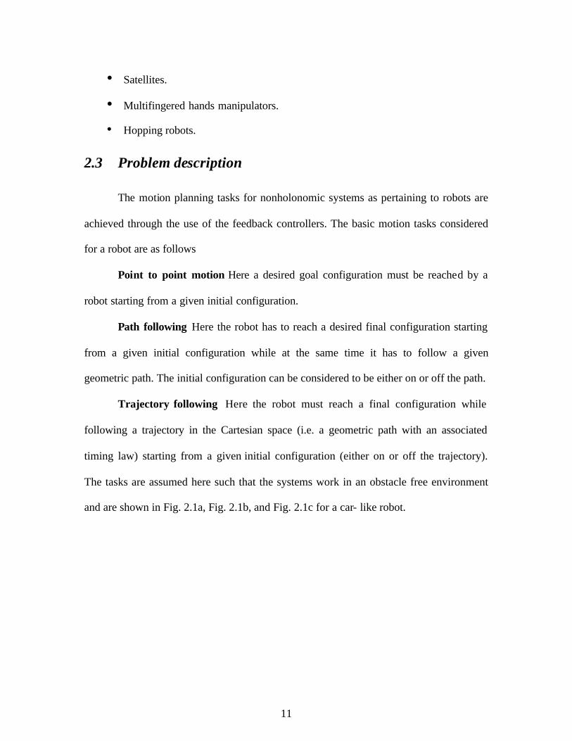
Point to point motion Here a desired goal configuration must be reached by a
robot starting from a given initial configuration.
Path following Here the robot has to reach a desired final configuration starting
from a given initial configuration while at the same time it has to follow a given
geometric path. The initial configuration can be considered to be either on or off the path.
Trajectory following Here the robot must reach a final configuration while
following a trajectory in the Cartesian space (i.e. a geometric path with an associated
timing law) starting from a given initial configuration (either on or off the trajectory).
The tasks are assumed here such that the systems work in an obstacle free environment
and are shown in Fig. 2.1a, Fig. 2.1b, and Fig. 2.1c for a car- like robot.
12
Figure2.1: Motion planning tasks for a car-like robot
The tasks can be obtained using either the feed forward (open loop) or feedback
(closed loop) control or a combination of the both. Since the feedback control is generally

13
robust and can work well in presence of disturbances, we will make use of feedback
control.
Thinking in terms of controls, point to point task can be thought of as a regulation
control problem or a posture stabilization problem for an equilibrium point in the state
space. Trajectory following is a tracking problem such that the error between the
reference and the desired trajectories asymptotically goes to zero.
For nonholonomic systems, tracking or path following or both is easier than
stabilization, whereas usually the reverse is true. This difference can be explained by
drawing a comparison between the numbers of inputs and outputs (or states) to be
controlled. In case of a regulation problem m inputs (two in case of a car like robot) are
required to regulate or control ‘ n ’ independent control variables or states (four in case of
a car like robot) with m less than n . Thus point to point stabilization is the most difficult
of all the three. In case of path following and trajectory tracking the output to be
controlled has the dimension (p ) equal to that of the input (m ). Thus these control
problems are square and their difficulty level is similar and less than the stabilization one.
For a car like robot, in case of path following m is one and p is one while for
trajectory tracking m is two and p is two, i.e. we have to stabilize to zero the two
dimensional error vector associated with the Cartesian trajectory[1].
2.4 Control model formulation
In this section we will be formulating the control model for the nonholonomic
systems. For developing the control model consider the first order kinematic constraints
on the system. As seen in section 2.2 such constraints are of the following form
14
( ) 0( ) ( )Tia q t q t =& 1,2, ........,i k n= <
or
( ) 0( ) ( )C q t q t =&
where q are the generalized coordinates and q& the first order derivative (velocities) of the
coordinates and ( )C q is the constraint matrix.
Let us denote the set of vector fields spanning the m dimensional distribution
∆ which is annihilated by the constraints as ' sjg ; 1,2,......j m= such that
{ }1 2, ,...., mspan g g g∆ =
The ' sjg are the basis for the ( )n k− right null space of the constraint matrix ( )C q so
that we have
( ) ( ) 0;Ti ja q g q = 1,2,........,i k n= < ( )1,2,......j n k m= − = (2.4)
or
( ) ( ) 0C q G q = (2.5)
The vector fields 'jg s are assumed to be smooth and linearly independent as a
consequence of the assumption on ( ) 'Ti sa q being smooth and independent. By
expressing all the feasible velocities as a linear combination of these basis vectors, we
obtain the first order kinematic model of the system as
1 1 2 2( ) ( ) ......... ( )m mq g q v g q v g q v= + + +& (2.6)
or
( )1
( )n k m
j jj
q g q v− =
== ∑& (2. 7)
15
where 'j sv known as psuedovelocities are taken as the control inputs and 'j sg are the
input vector fields. The model directly shows the presence of k nonholonomic constraints
on the system having n states or configuration variables and ( )n km −= control inputs.
The control model of equation (1) is known as the kinematic model of the system. The
model is a drift less (i.e. no motion takes place under zero input conditions), nonlinear
and under actuated (number of control inputs is less than the number of states to be
controlled) control system.
2.5 Controllability issues
Since the control model is driftless, the terms local accessibility and
controllability can be used interchangeably. Moreover, the controllability of the whole
configuration space is the (complete) nonholonomy of the kinematic constraints. The
controllability condition can be established using the Chows theorem. According to the
theorem, for the driftless control systems, if the accessibility rank condition
( )0dim c q n∆ = (2.8)
holds, then the control system is locally accessible (controllable) from 0q . c∆ is the
accessibility distribution of the kinematic model given by equation (2.6) and is defined as
the span of all the input vector fields
1{ }c ispan v v i∆ = ∈ ∆ ∀ ≥
with
{ }1 1 1 2, , ,i i ispan g v g v i− − ∆ = ∆ + ∈ ∆ ∈ ∆ ≥
{ }1 1 2, ,...., mspan g g g∆ = (2.9)
16
This implies that c∆ is the involutive closure under lie bracketing of the
distribution 1∆ associated with the input vector fields 'j sg . The term ,g v is the lie
bracket of the two vector fields g and v defined as
( ), ( ) ( )v gg v q g q v qq q
∂ ∂= −∂ ∂
(2.10)
The Chows theorem provides both necessary and sufficient condition for the
controllability [12]. Moreover if the system is controllable then its dynamic extension
given by
( )1
( )n k m
j jj
q g q v− =
== ∑&
and (2.11)
;j jv u=& 1,2, ........,j m=
is also controllable. In some cases the use of the nilpotent basis is made, that is the input
vector fields 'j sg are the nilpotent basis. This eliminates the need for cumbersome
computations as we will see that using this concept all higher order lie brackets above
some particular order are zero [12].
2.6 Stabilization
The stabilization problem for the control system of (2.7) can be defined as finding
the feedback control law of the form ( , )u q t in order to make the closed loop system
asymptotically stable about an equilibrium point or a reference (feasible) trajectory. In
the point stabilization problem we assume equilibrium point for the open loop system i.e.
( ) 0eq f q= =& .
17
2.6.1 Controllability and stabilization at a point
For the driftless control system of (2.7), any configuration ( eq ) is an open loop
equilibrium point under zero input conditions. For linear systems x Ax Bu= +& , it is a well
established fact that if the system satisfies the controllability rank condition given by 2 1...... nrank nB AB A B A B− = (2.12)
then the asymptotic (actually exponential) stabilization by a smooth, time invariant state
feedback is guaranteed. In other words we can say that if the controllability condition is
satisfied, there exists a feed back law ( )eu k x x= − such that the closed loop system is
asymptotically stable about the equilibrium point ex .
For the control model of (2.7) we would like to make a similar kind of analysis.
For this purpose we will look at the approximate linearization of the system at any
equilibrium point ( eq ).The approximate linearization given by
( )eq q G q vδ= =& & (2.13)
with eq q qδ = − is clearly not controllable as the rank of the controllability matrix
( )eG q is m (which is less thann ). Hence we can say that a linear controller can not
achieve stabilization, not even locally.
However the controllability of the nonlinear system can be established by using
the tools from the differential geometry, i.e. we can make use of the Lie algebra rank
condition to prove its controllability. However, even if the system can be proven to be
globally controllable (in a nonlinear sense) there is still a severe theoretical limitation on
point stabilization. The limitation is in a sense that Lyapunov (asymptotic) stability can
not be achieved by means of a smooth, time invariant feedback [13].
18
The above result can be established on the basis Brockett’s theorem [2] which
says that the stabilization of a driftless regular system by a smooth time invariant
feedback is not possible. For the driftless, under actuated control system (2.7) where
vector fields 'j sg are linearly independent (regular) at eq , the theorem implies the
number of inputs m is equal to the number of states n as both a necessary and sufficient
condition for smooth stabilization. Also it should be noted that if the system can not be
stabilized by a smooth feedback, the same negative result is true for its dynamic
extension and also the theorem is not applicable to time varying feedback laws.
Thus in order to design the feedback controllers for posture stabilization, it is
obligatory either to give up the continuity requirement, i.e. include the non smooth
feedback or to apply the time varying laws or apply a combination of both.
2.6.2 Controllability and stabilization about trajectory
In case of trajectory following, for stabilization about a trajectory it is ensured that
the reference trajectories are feasible for the system. In other words we should take or
generate only those state and input trajectories that satisfy the nonholonomic constraints
of the system, i.e. should satisfy (2.2)
2.6.3 Approximate linearization
For approximate linearization of the system (2.7) we take the desired state
trajectory as ( )dq t and the input trajectory as ( )dv t . It can be easily seen that the
linearization about a smooth trajectory results into a linear time varying system. The
system can easily be shown to satisfy the controllability condition i.e. the controllability
Grammian is nonsingular [21], as long as the input reference trajectory is persistent, i.e. it
does not come to a stop. Thus it implies that we can achieve stabilization about the
19
desired trajectory via a smooth, time invariant control law as long as the trajectories do
not come to a stop. One observation should be made here. As we know that the control
scheme presented here is based on the approximate linearization of the original system in
the neighborhood of a reference trajectory, the closed loop system is asymptotically
stable only locally. In order to achieve global stabilization for trajectory tracking error,
we have to make use of the nonlinear feedback design.
2.6.4 Exact feedback linearization
It is well known in robotics that if the number of generalized coordinates equals
the number of control inputs i.e. n m= , the system kinematics or dynamics can be
transformed into a linear system with the use of a nonlinear static state feedback [14].
The linearity is displayed by the system equations only after a coordinate transformation
in the state space.
For exact linearization of nonlinear systems outputs are chosen to which a desired
behavior is assigned. Two types of exact linearization are possible. The two schemes are
full state feedback linearization and input output linearization. In the first case the
feedback transformation is such that the whole set of system equations become linear
while as in the second case the transformation is such that the input and output response
of the closed loop system is linear. For MIMO systems this transformation results in
decoupling of the input and output vectors.
Both the transformations can be achieved through static feedback or the dynamic
feedback [14].
20
2.6.5 Static feedback linearization
For the nonholonomic kinematic model the full state feedback linearization
cannot be achieved using a static (time invariant) state feedback. The reason for this is the
violation of the necessary condition for the full state feedback linearization according to
[14]. The controllability condition for the system derived in section 2.6 requiring that the
distribution o∆ generated by jg s not be involutive violates the necessary condition for
static feedback transformation.
However, input output linearization is possible with the use of static feedback.
Here m equations are transformed via feedback into simple decoupled integrators.
However the choice of outputs which are linearized is not unique. Here it is worth
noticing that in the case of (2, n ) chained form transformation, the two variables are
indeed the examples of linearizing outputs with static feedback given by the input
transformation equation. Also it must be noted that in case of input output linearization
the internal dynamics may be left in the closed loop system. Thus for the exponential
(global) convergence of the trajectory error to go to zero, these internal dynamics should
be properly modeled, analyzed and their stability guaranteed.
2.6.6 Dynamic feedback linearization
For exact feedback linearization, if the static feedback design fails, we can make
use of dynamic feedback for nonholonomic systems. The use of dynamic feedback can
also result in full state feedback linearization. For model (2.7)
( ) ;q G q v=& ;n mq v∈ ∈¡ ¡ (2.14)
the dynamic feedback compensator is of the form
( , ) ( , )v a q b q rζ ζ= +
21
( , ) ( , )c q d q rζ ζ ζ= +& (2.15)
where ( ) vtζ ∈¡ is the compensator state vector of dimensions v and ( ) vr t ∈¡ (having
the same dimensions as the compensator state vector ( )tζ ) is the auxiliary input. (2.15) is
such that the closed loop system obtained from (2.14) and (2.15) is equivalent to a linear
system under a state transformation ( , )z q ζ= Τ . For the applications to nonholonomic
systems, the linearization process involves the following procedure.
Initially we define the output of the system (2.14) as ( )y h q= . To this output a
desired behavior is assigned (track a trajectory). Then the output y is successively
differentiated until the system inputs appear explicitly in a nonsingular way. The non
singularity is a must for the inversion of the differentiated equations to solve for the
inputs. If in a step involving differentiation of system outputs, the decoupling matrix
(differential map) of the system is singular (which means that some input is still not
appearing), integrators are added on some of the input channels and the process of
differentiation is continued. It is also necessary to avoid direct differentiation of the
system inputs in the next differentiation. This operation is known as dynamic extension
and converts a system input into a state of dynamic compensator. The dynamic
compensator has the new auxiliary input r as its input. The process of differentiation
continues until at some point the system is invertible (i.e. solution for new inputs can be
obtained) from the chosen output vector y and the process terminates. The number of
successive addition of integrators gives dimensions of the state ζ of the dynamic
compensator. Also, if the sum of the orders of the output differentiation is equal to the
dimensions of the extended state space system (original and dynamic compensator state)
22
which is n v+ , then the full state linearization of the system is obtained as there are no
internal dynamics left in the system.
2.7 Examples of nonholonomic systems
The simplest example of a nonholonomic system can be a wheel that rolls on
plane surface, such as a unicycle. The constraints here arise due to the roll without slip
condition. The configuration or the generalized coordinate vector is ( ), ,q x y θ= . The
coordinates x and y are the position coordinates of the wheel and θ is the angle which
the wheel makes with the x axis. The unicycle is shown in Fig. 2.2. The constraint here is
that the wheel cannot slip in the lateral direction.
Figure2.2: The nonholonomic constraints on a unicycle.
The generalized velocities are subject to the following kinematic constraint
sin cos 0x yθ θ− =& & (2.16)

23
In other words the velocity along the plane perpendicular to the point of contact between
the wheel and the ground is zero. The above equation is of the form ( ) 0C q q =& with
constraint matrix ( ) [ ]sin cos 0C q θ θ= − .
Expressing the feasible velocities as a linear combination of vector fields
spanning the null space of the matrix ( )C q , we get the following kinematic model
1 1 2 2( ) ( )q g q v g q v= +&
Or (2.17)
1 2
cos 0
sin 00 1
x
y v v
θ
θθ
= +
&&&
where 1v is the linear velocity of the wheel and 2v is its angular velocity around the
vertical axis. Here we observe that the number of states 3n = , number of control inputs
2m = and the number of nonholonomic constraints 1k = .
Another example is that of a car like robot shown in Fig.2.3. The robot has two
wheels and each wheel is subject to one nonholonomic constraint. The constraint is the
same as in the case of unicycle. The generalized coordinate vector is ( ), , ,q x y θ φ= , with
,x y and θ same as before. The angle φ is the steering angle.
24
Figure2.3: The nonholonomic constraints on a car- like robot.
The two nonholonomic constraints on the front and the rear wheels respectively
are
( ) ( )sin cos cos 0x y lθ φ θ φ θ φ+ − + − =&& &
sin cos 0x yθ θ− =& & (2.18)
Here l is the distance between the wheels. Again this is of the form ( ) 0C q q =& with
( ) ( ) ( )sin cos cos 0
sin cos 0 0
lC q
θ φ θ φ φ
θ θ
+ − + − = −
Choosing the rear wheel drive the kinematic model is obtained as
1 1 2 2( ) ( )q g q v g q v= +&
1 2
cos 0sin 0
tan 00 1
xy
v vl
θθ
θ φφ
= +
&&&&
(2.19)
25
Here 1v is the rear driving velocity input and 2v is the steering velocity input. The above
model is not defined at 2φ π= , where 1g is discontinuous. Physically this corresponds to
car becoming jammed because of its front wheel being normal to axis of the body.
The feedback control design, controllability analysis and the motion planning for all the
three motion tasks are done in [1]. Another example of nonholonomic systems is that of
an underwater vehicle which is discussed in next chapter. In next chapter we will be
studying the motion planning for the same and controllability of the system is discussed
and proved. We also present feedback control laws which give global stabilization of the
vehicle about a desired trajectory and about a point.
26
Chapter 3
Mathematical Modeling and Controllability Analysis of
an Underwater Vehicle
In this chapter an overview of an underwater vehicle is given and mathematical
model of the vehicle is derived. The chapter presents in detail the derivation of the
mathematical modeling of the system. For motion planning tasks, the kinematic model of
the system is obtained and the issues related to nonlinear controllability of the system are
studied in detail. Finally for the purpose of control design, the system is converted into
chained form.
3.1 Mathematical modeling
In this section the mathematical model of the under water vehicle is briefly
discussed. An underwater vehicle is generally defined as a six degree of freedom body. It
follows the laws of rigid body motion. The dynamics of the system are highly non linear
due to rigid body coupling and hydrodynamic forces on the vehicle. The mathematical
model of the underwater vehicle is obtained through the following two models.
Dynamic model This type of model allows for the actual forces, causing the
motion and the dynamic properties of the vehicle to be taken into account. The equations
of translation and rotation are obtained using Newton’s law [15].
Kinematic model The kinematic model of the system is the model where actual
forces causing the motion and the dynamic properties of the vehicle do not enter the
27
equations of motion. This type of model allows for the decoupling of the vehicle
dynamics from its movement. An autonomous underwater vehicle has nonholonomic
nature due to its nonlinear kinematic model [22]. In the following section the kinematic
model of the vehicle is derived. For the remaining chapter and the chapter following, the
kinematic model of the system will be used for analysis and control purposes.
3.1.1 Kinematic modeling and nonholonomic constraints
The kinematic model of the system is obtained by taking into consideration the
nonholonomic constraints on the linear velocity. The nonholonomic constraints restrict
the velocity of the system to be zero in certain directions but these restrictions do not
restrict the global movement of the system. For the development of the kinematic model
of the underwater vehicle model we assume two orthogonal coordinate systems [23].
Global coordinates The global or the inertial frame coordinates are denoted
by ( ), , ,P X Y Z . The frame remains fixed at the ocean surface with origin P .The unit
vector in the Z direction points up into the water while the unit vectors along X and Y
direction complete a right handed system.
Local coordinates The local or the body frame coordinates are denoted
by ( ), , ,p x y z . The frame remains fixed on the vehicle with origin surface with origin p .
The two coordinate systems are as shown below in Fig. 3.1[23].
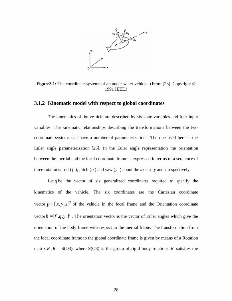
28
Figure3.1: The coordinate systems of an under water vehicle. (From [23]. Copyright © 1991 IEEE.)
3.1.2 Kinematic model with respect to global coordinates
The kinematics of the vehicle are described by six state variables and four input
variables. The kinematic relationships describing the transformations between the two
coordinate systems can have a number of parameterizations. The one used here is the
Euler angle parameterization [25]. In the Euler angle representation the orientation
between the inertial and the local coordinate frame is expressed in terms of a sequence of
three rotations: roll (φ ), pitch (θ ) and yaw (ψ ) about the axes x, y and z respectively.
Let q be the vector of six generalized coordinates required to specify the
kinematics of the vehicle. The six coordinates are the Cartesian coordinate
vector [ , , ]Tp x y z= of the vehicle in the local frame and the Orientation coordinate
vector [ , , ]Tη φ θ ψ= . The orientation vector is the vector of Euler angles which give the
orientation of the body frame with respect to the inertial frame. The transformation from
the local coordinate frame to the global coordinate frame is given by means of a Rotation
matrix R . R ∈ S(O3), where S(O3) is the group of rigid body rotations. R satisfies the
29
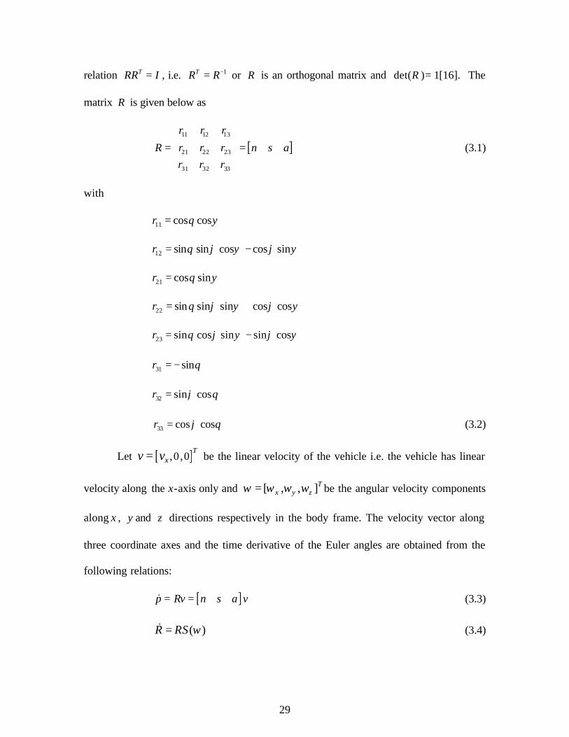
relation TRR I= , i.e. 1TR R−= or R is an orthogonal matrix and det( ) 1R = [16]. The
matrix R is given below as
[ ]11 12 13
21 22 23
31 32 33
r r r
R r r r n s ar r r
= =
(3.1)
with
11 cos cosr θ ψ=
12 sin sin cos cos sinr θ ϕ ψ ϕ ψ= −
21 cos sinr θ ψ=
22 sin sin sin cos cosr θ ϕ ψ ϕ ψ= +
23 sin cos sin sin cosr θ ϕ ψ ϕ ψ= −
31 sinr θ= −
32 sin cosr ϕ θ=
33 cos cosr ϕ θ= (3.2)
Let [ ],0 ,0T
xv v= be the linear velocity of the vehicle i.e. the vehicle has linear
velocity along the x-axis only and [ , , ]Tx y zω ω ω ω= be the angular velocity components
along x , y and z directions respectively in the body frame. The velocity vector along
three coordinate axes and the time derivative of the Euler angles are obtained from the
following relations:
[ ]p Rv n s a v= =& (3.3)
( )R RS ω=& (3.4)
30
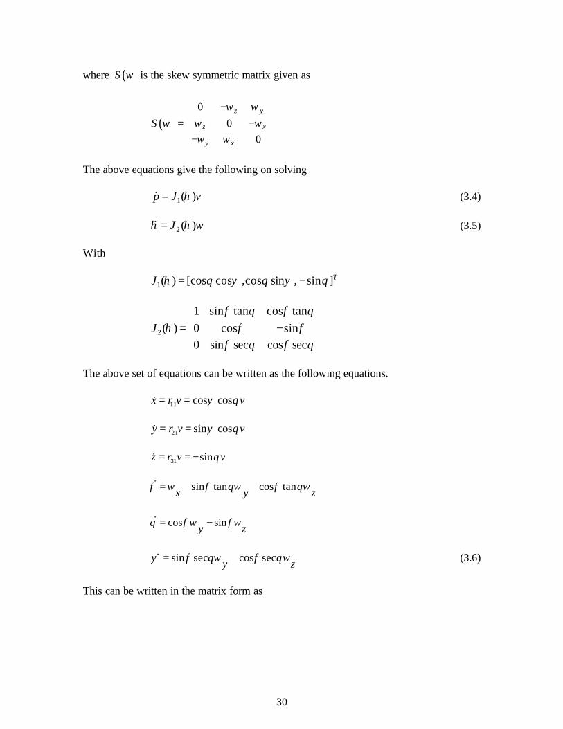
where ( )S ω is the skew symmetric matrix given as
( )0
00
z y
z x
y x
Sω ω
ω ω ωω ω
−
= − −
The above equations give the following on solving
1( )p J vη=& (3.4)
2( )Jη η ω=& (3.5)
With
1( ) [cos cos ,cos sin , sin ]TJ η θ ψ θ ψ θ= −
2
1 sin tan cos tan( ) 0 cos sin
0 sin sec cos secJ
φ θ φ θη φ φ
φ θ φ θ
= −
The above set of equations can be written as the following equations.
11 cos cosx r v vψ θ= =&
21 sin cosy r v vψ θ= =&
31 sinz r v vθ= = −&
sin tan cos tanx y zφ ω φ θω φ θω= + +&
cos siny zθ φω φω= −&
sin sec cos secy zψ φ θω φ θω= +& (3.6)
This can be written in the matrix form as
31
cos cos 0 0 0cos sin 0 0 0
sin 0 0 00 1 sin tan cos tan0 0 cos sin0 0 sin sec cos sec
xv
yxz
y
z
θ ψθ ψ
ωθ
ωφ φ θ φ θθ φ φ ωψ φ θ φ θ
−
= −
&&&&&&
(3.7)
The equations can be written in the generalized vector form as
cos cos 0 0 0cos sin 0 0 0
sin 0 0 00 1 sin tan cos tan0 0 cos sin0 0 sin sec cos sec
xyz
vx y z
θ ψθ ψ
θω ω ω
φ φ θ φ θθ φ φψ φ θ φ θ
−
= + + + −
&&&&&&
(3.8)
The system here is subject to two non holonomic constraints. The constraints are
on the linear velocities along y and z directions. The velocities along these directions are
zero. The two constraints are
0Ts p =&
0Ta p =& (3.8)
This can be written as
12 22 32 0r x r y r z+ + =& & &
13 23 33 0r x r y r z+ + =& & &
Or
(cos sin sin sin cos ) (sin sin sin cos cos ) (cos sin ) 0x y zψ θ φ ψ φ ψ θ φ ψ φ θ φ− + + + =& & &
(sin sin cos sin sin ) (sin sin cos cos sin ) (cos cos ) 0x y zψ θ φ ψ φ ψ θ φ ψ φ θ φ− + − + =& & & (3.9)
The above equation is of the form
( ) 0A q q =&
with

32
12 22 32
13 23 33
0 0 0( )
0 0 0r r r
A qr r r
=
(3.10)
Expressing the feasible velocities as the linear combination of vector
fields 1( )g q , 2( )g q , 3( )g q and 4( )g q spanning the null space of matrix ( )A q we have the
following kinematic model
1 1 2 2 3 3 4 4( ) ( ) ( ) ( )q g q v g q v g q v g q v= + + +&
[ ]1
21 2 3 4
3
4
( ) ( ) ( ) ( )
vv
q g q g q g q g qvv
=
& (3.11)
where
1
cos coscos sin
sin( )
000
g q
θ ψθ ψ
θ
−
= 2
000
( )100
g q
=
3
000
( )sin tan
cossin sec
g qφ θ
φφ θ
=
4
000
( )cos tan
sincos sec
g qφ θ
φφ θ
= −
(3.12)
and
1 2 3 4; ; ;x x y zv v v v v vω ω ω= = = = =
More generally we can write
33
( )q G q v=& (3.13)
The above equations are the kinematic model of the system. The system is
nonlinear and under actuated, which means that the number of inputs to the system is less
than its states. The generalized velocity vector q& cannot assume any independent value
unless it satisfies the nonholonomic constraints. The constraints are the examples of the
Pfaffian Constraints which are linear in velocities. The admissible generalized velocities
as given by (3.1) are contained in the null space of the constraint matrix ( )A q .
3.2 Controllability analysis
Consider the system ( )q G q v=& . The system is nonlinear, under actuated and
driftless. Thus, in order to establish the controllability of the vehicle we make use of the
mathematical concepts that are involved in Lie algebra rank condition.
3.2.1 Controllability about a point
Consider the linear approximation of the system (3.13) at equilibrium point
eq while setting the input ev equal to zero. Let the error associated with the equilibrium
point be given as
eq q q= −%
The time derivative of the error is given as
1 1 2 2 3 3 4 4( ) ( ) ( ) ( )e e e eq g q v g q v g q v g q v= + + +&%
( )eq G q v=&% (3.14)
Here ( )eG q is the controllability matrix at the equilibrium point. The rank of the
controllability matrix is four. Thus if we linearize the system about an equilibrium point
34
the linearized system is not controllable. Hence the linear controller will not work here.
To test the controllability of the above system we make use of the lie algebra rank
condition and nilpotent basis concepts.
Nilpotent basis The definition of nilpotent basis for a distribution is recalled here.
Given a set of generators or basis vector fields 1, 2,........., mg g g we define the length of a
Lie product recursively as
{ } 1;il g = 1,2,...............,i m=
[ ]( ) [ ] [ ],l A B l A l B= +
Where A and B are themselves Lie products. Alternatively, [ ]l A is the number of
generators in the expansion for A . A Lie algebra or basis is nilpotent if there exists an
integer k such that all Lie products of length greater than k are zero. The integer k is
called the order of nilpotency [17].The use of the nilpotent basis eliminates the need for
cumbersome computations as we see all higher order lie brackets above some particular
order are zero.
In the light of the above definition and conditions we see that the lie algebra
{ }1 2 3 4, , ,L g g g g is nilpotent algebra of order 2 ( )2k = i.e. the vector fields 1 2 3, ,g g g and
4g are the nilpotent basis. Thus all lie brackets of order more than two are zero. The only
independent Lie brackets computed from the four basis vector fields are[ ]1 3,g g
and [ ]1 4,g g . Thus for our system the lie algebra rank condition becomes
[ ] 6crank C =
1 2 3 4 1 3 1 4[ , , , ,[ , ][ , ]] 6rank g g g g g g g g = (3.15)
where 1 3,[ ]g g and 1 4[ , ]g g are the two independent lie brackets computed from the four
vector fields 1 2 3 4( , , , )g g g g as per the following definition.
[ ], ( )h g
g h x g hx x
∂ ∂∂ ∂
= − (3.16)
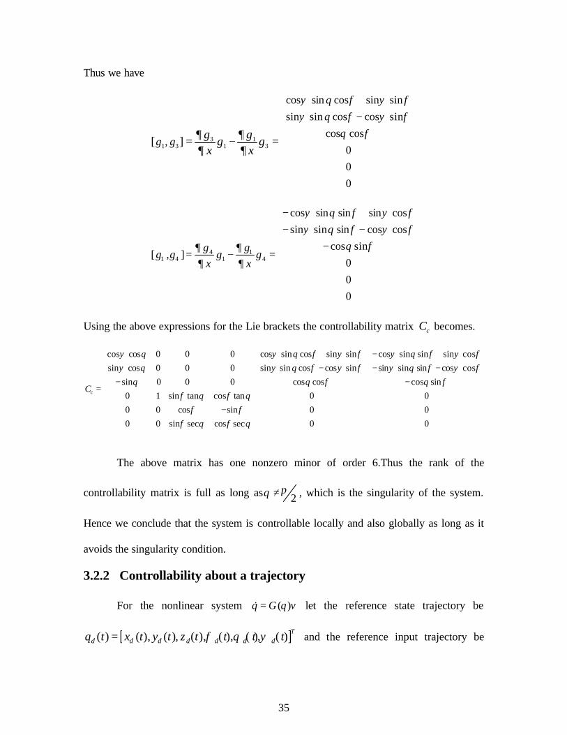
35
Thus we have
3 11 3 1 3
cos sin cos sin sinsin sin cos cos sin
cos cos,
000
[ ]g gg gg gx x
ψ θ φ ψ φψ θ φ ψ φ
θ φ∂ ∂∂ ∂
+ −
= − =
4 11 4 1 4
cos sin sin sin cossin sin sin cos cos
cos sin[ , ]
000
g gg g g g
x x
ψ θ φ ψ φψ θ φ ψ φ
θ φ∂ ∂∂ ∂
− + − − −
= − =
Using the above expressions for the Lie brackets the controllability matrix cC becomes.
cos cos 0 0 0 cos sin cos sin sin cos sin sin sin cossin cos 0 0 0 sin sin cos cos sin sin sin sin cos cos
sin 0 0 0 cos cos cos sin0 1 sin tan cos tan 0 00 0 cos sin 0 00 0 sin sec cos sec 0 0
cC
ψ θ ψ θ φ ψ φ ψ θ φ ψ φψ θ ψ θ φ ψ φ ψ θ φ ψ φ
θ θ φ θ φφ θ φ θ
φ φφ θ φ θ
+ − + − − − − −
= −
The above matrix has one nonzero minor of order 6.Thus the rank of the
controllability matrix is full as long as 2πθ ≠ , which is the singularity of the system.
Hence we conclude that the system is controllable locally and also globally as long as it
avoids the singularity condition.
3.2.2 Controllability about a trajectory
For the nonlinear system ( )q G q v=& let the reference state trajectory be
[ ]( ) ( ), ( ), ( ), ( ), ( ), ( ) T
d d d d d d dq t x t y t z t t t tφ θ ψ= and the reference input trajectory be
36
1 2 3 4( ) ( ), ( ), ( ), ( )d d d d dv t v t v t v t v t= . The reference trajectory should satisfy the
nonholonomic constraints on the system.
For the linear systems x Ax Bu= +& controllability implies asymptotic (actually
exponential) stabilization by smooth state feedback. Thus if the following accessibility
rank condition 2 1, , .............. nrank B AB A B A B n− = is satisfied, then there exists a
feedback gain so that the following control law
( )u k xd x= −
makes the desired trajectory xd asymptotically stable or in other words the error
associated with the desired solution goes to zero exponentially.
For nonlinear systems the condition does not apply as such. But for local
accessibility we may look at the approximate linearization of the system in the
neighborhood of xd . Thus in particular if the linearized system is controllable, the
nonlinear system can be stabilized locally at xd by a smooth feedback eu kx= . The
condition is sufficient but not necessary.
Let the errors associated with the desired state trajectory and input trajectory be
denoted as ( ) ( ) ( )e dq t q t q t= − and ( ) ( ) ( )e dv t v t v t= − respectively. Linearizing the
system about the desired trajectory we obtain the following system
( ) ( ) ( )d eq t q t q t= +& & &
{ }{ }( , ) ( ) ( )d e d eG q q t v t v t= + + (3.17)
The Taylor series expansion of ( , )G q t about the nominal solution ( )dq t is given as:
{ }( )( ) ( , ) ( ) . . ( ) ( )d e d e
d
G qq t G q t q t h o t v t v t
q q q
∂∂
= + + + =
&
37
Since the nominal solution satisfies (3.16) we have:
( )( ) ( ) ( ) ( , ) ( )e e d d e
d
G qq t q t v t G q t v
q q qt∂
∂
= + =
&
Or (3.17)
( ) ( ) ( ) ( ) ( )e e eq t A t q t B t v t= +&
With
4( ) ( )
1
ndn
d
gA t v t
qn q q
∂∂
= ∑= =
( ) ( , )dB t G q t= (3.18)
Upon computations we get
3 3 1
3 3 2
( )( )
( )O A t
A tO A t
×
×
=
1 1
1 1 1
1
0 cos ( ) s in ( ) ( ) sin ( )cos ( ) ( )
( ) 0 sin ( ) s in ( ) ( ) cos ( )cos ( ) ( )0 cos ( ) ( ) 0
d d d d d d
d d d d d d
d d
t t v t t t v t
A t t t v t t t v tt v t
ψ θ ψ θ
ψ θ ψ θθ
− − = − −
3 4 3 4
3 4
3 4
2
2 2cos ( ) t an ( ) ( ) sin ( ) t an ( ) ( ) sin ()sec ( ) ( ) cos ( )sec ( ) ( ) 0
( ) sin ( ) ( ) cos ( ) ( ) 0 0
cos ( ) sec ( ) ( ) sin ()sec ( ) ( ) sin ( ) sec ( ) t an ( )d
d d d d d d d d d d d d
d d d d
d d d d d d d d
t t v t t t v t t t v t t t v t
A t t v t t v t
t t v t t t v t t t t
φ θ φ θ φ θ φ θ
φ φ
φ θ φ θ φ θ θ
− +
= − −
− 3 4( ) cos ( )sec ( ) t an ( ) ( ) 0d d d d dv t t t t v tφ θ θ
+
1 3 3
3 1 2
( )( )
( )J t O
B tO J t
×
×
=
Here
1
cos ( )cos ( )( ) cos ()s in ( )
sin ( )
d d
d d
d
t tJ t t t
t
θ ψθ ψ
θ
=−
38
2
1 sin ( ) tan ( ) cos ( ) tan ( )( ) 0 cos ( ) sin ( )
0 sin ( ) sec ( ) cos ()sec ( )
d d d d
d d
d d d d
t t t tJ t t t
t t t t
φ θ φ θφ φ
φ θ φ θ
= −
The above system is linear time varying. For a linear reference trajectory with
constant velocities ( )dn dnv t v= and (0) (0)dq q= the controllability condition becomes
{ }2 3 4 5, , , , , 6rank B AB A B A B A B A B =
Upon computations we see that the above matrix has a nonzero minor of order 6 as long
as 1 3 4 0d d dv v v= = ≠ and 2dπθ ≠ . Thus the linearized system is controllable along a
reference trajectory as long as the trajectory does not collapse to a point.
3.3 Chained forms
The chained form systems were first introduced in [18].The chained form
introduced in [18] had one chain i.e. two input chained forms. The method for converting
the multi input drift free non holonomic systems into chained forms is given in [19].
Sufficient conditions under which an m input system of (3.13) can be transformed to
1m − chain single generator form were given in [19]. The method presented in [19] for
transforming is similar to the method of exact linearization of nonlinear systems with
drift via state feedback as presented in [14]. The same method will be applied for our
system with some modifications.
The following system
1 1 2 2 3 3 4 4( ) ( ) ( ) ( )q g q v g q v g q v g q v= + + +&
can be transformed into the chained form by a feedback transformation. In the above
equation ig being smooth and linearly independent vector fields, there exists a feedback
39
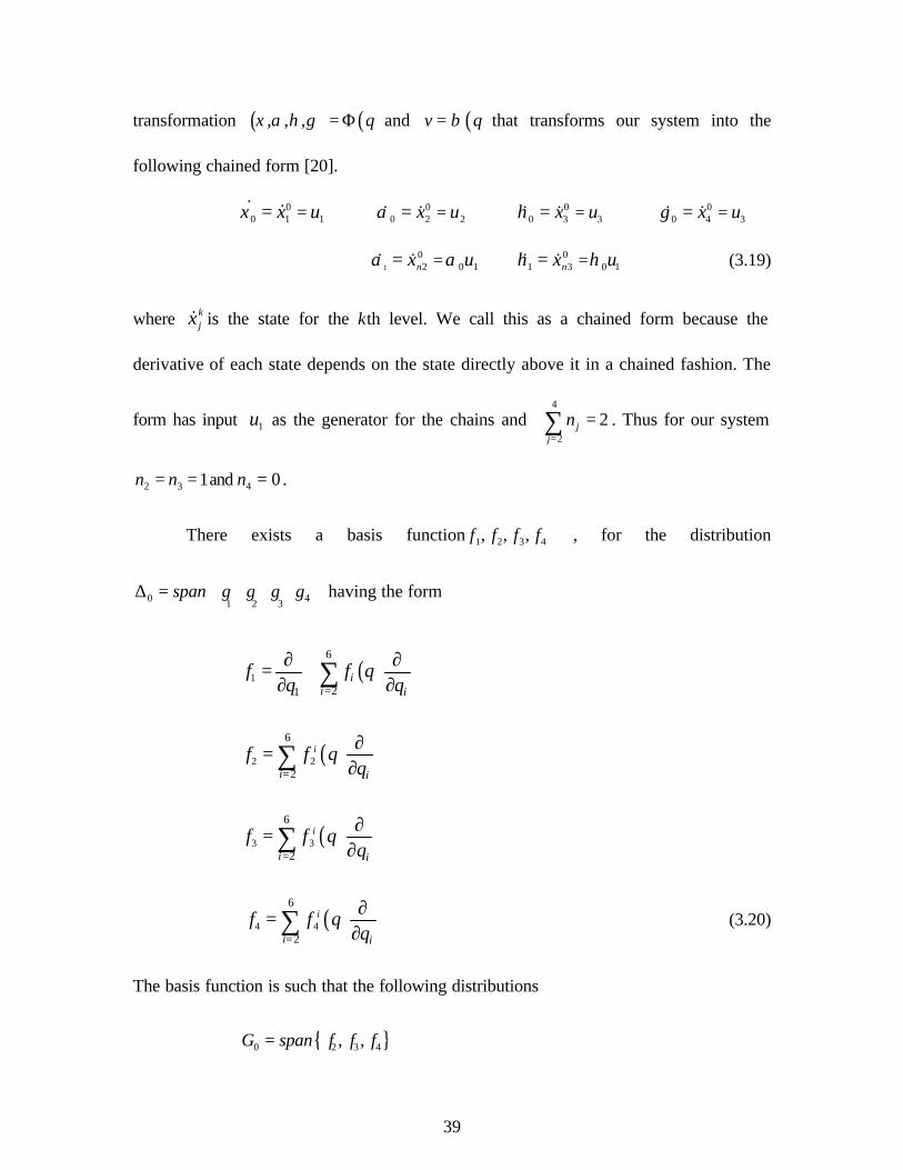
transformation ( ) ( ), , , qξ α η γ = Φ and ( )v qβ= that transforms our system into the
following chained form [20].
00 1 1x uξ ==& & 0
0 2 2x uα ==& & 00 3 3x uη ==& & 0
0 4 3x uγ ==& &
1
02 0 1nx uα α==& & 0
1 3 0 1nx uη η==& & (3.19)
where kjx& is the state for the kth level. We call this as a chained form because the
derivative of each state depends on the state directly above it in a chained fashion. The
form has input 1u as the generator for the chains and 4
2
2jj
n=
=∑ . Thus for our system
2 3 1n n= = and 4 0n = .
There exists a basis function 1 2 3 4, , ,f f f f , for the distribution
0 41 2 3span g g g g ∆ =
having the form
( )1
6
21i
i i
f f qq q=
∂ ∂= +∂ ∂∑
( )2 2
6
2
i
i i
f f qq=
∂=∂∑
( )3 3
6
2
i
i i
f f qq=
∂=∂∑
( )4 4
6
2
i
i i
f f qq=
∂=∂∑ (3.20)
The basis function is such that the following distributions
{ }0 2 3 4, ,G span f f f=
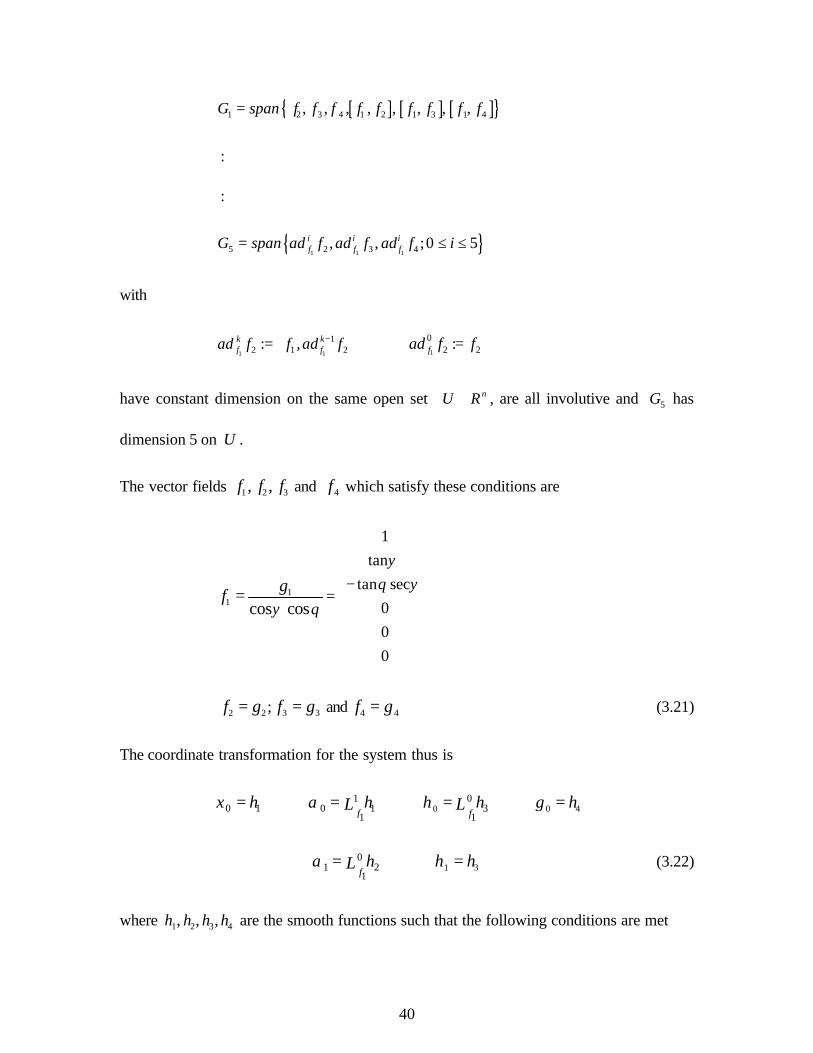
40
[ ] [ ] [ ]{ }1 2 3 4 1 2 1 3 1 4, , , , , , , ,G span f f f f f f f f f=
:
:
{ }1 1 15 2 3 4, , ;0 5i i if f fG span ad f ad f ad f i= ≤ ≤
with
1 1
12 1 2: ,k k
f fad f f ad f− = 1
02 2:fad f f=
have constant dimension on the same open set nU R∈ , are all involutive and 5G has
dimension 5 on U .
The vector fields 1 2 3, ,f f f and 4f which satisfy these conditions are
11
1tan
tan sec000
cos cosgf
ψθ ψ
ψ θ
−
=
=
2 2 3 3;f g f g= = and 4 4f g= (3.21)
The coordinate transformation for the system thus is
0 1hξ = 10 1
1fhLα = 0
03
1fhLη = 0 4hγ =
01 2
1fhLα = 1 3hη = (3.22)
where 1 2 3 4, , ,h h h h are the smooth functions such that the following conditions are met
41
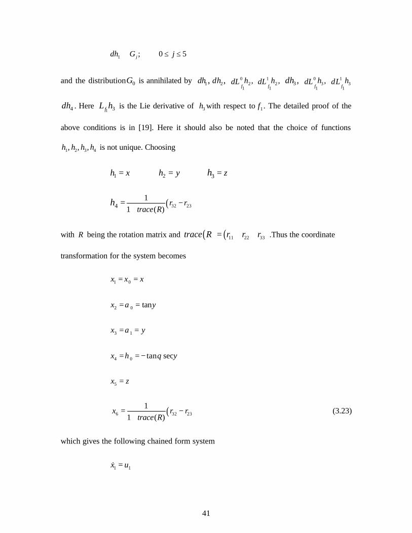
1 ;jdh G⊥ 0 5j≤ ≤
and the distribution 0G is annihilated by 1,dh 2,dh 02
1,
fhdL 1
21
,fhdL 3 ,dh 0
31
,fhdL 1
31fhdL
4dh . Here 1 3fL h is the Lie derivative of 3h with respect to 1f . The detailed proof of the
above conditions is in [19]. Here it should also be noted that the choice of functions
1 2 3 4, , ,h h h h is not unique. Choosing
1h x= 2h y= 3 zh =
( )32 2341
1 ( )r r
trace Rh −
+=
with R being the rotation matrix and ( ) ( )11 22 33trace R r r r= + + .Thus the coordinate
transformation for the system becomes
1 0x xξ= =
2 0 tanx α ψ= =
3 1x yα= =
4 0 tan secx η θ ψ= = −
5x z=
( )6 32 231
1 ( )x r r
trace R= −
+ (3.23)
which gives the following chained form system
1 1x u=&
42
2 2x u=&
3 2 1x x u=&
4 3x u=&
5 4 1x x u=&
6 4x u=& (3.24)
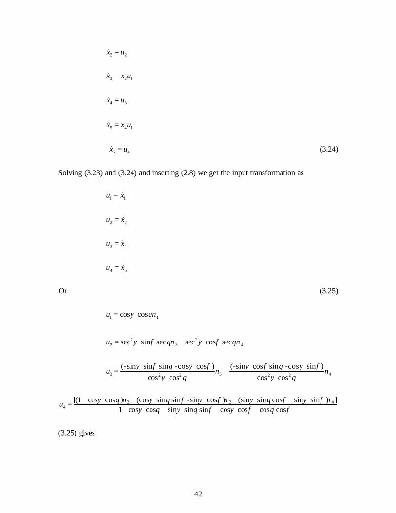
Solving (3.23) and (3.24) and inserting (2.8) we get the input transformation as
1 1u x= &
2 2u x= &
3 4u x= &
4 6u x= &
Or (3.25)
1 1cos cosu ψ θν=
2 22 3 4sec sin sec sec cos secu ψ φ θν ψ φ θν= +
3 3 42 2 2 2
(-sin sin sin -cos cos ) (-sin cos sin -cos sin )cos cos cos cos
uψ φ θ ψ φ ψ φ θ ψ φ
ν νψ θ ψ θ
= +
2 3 44
[(1 cos cos ) (cos sin sin -sin cos ) (sin sin cos sin sin ) ]1 cos cos sin sin sin cos cos cos cos
u ψ θ ν ψ θ φ ψ φ ν ψ θ φ ψ φ νψ θ ψ θ φ ψ φ θ φ
+ + + +=+ + + +
(3.25) gives

43
11 cos cosx
uv v
ψ θ= =
{ }3 2 3cos cos (cos sin sin sin cos ) (cos cos )y v u uω ψ θ ψ φ ψ θ φ φ θ= = − −
{ }4 2 3cos cos (sin sin sin cos cos ) (sin cos )z v u uω ψ θ ψ θ φ ψ φ φ θ= = + +
{2 41
(1 cos cos sin sin sin cos cos cos cos )cos cosx v uω ψ θ ψ θ φ ψ φ θ φ
ψ θ= = + + + +
}3 4(cos sin sin sin cos ) (sin sin cos sin sin )v vψ θ φ ψ φ ψ θ φ ψ φ− − − +
The inputs v1,v2 ,v3,v4 can be calculated from the above equations
provided cos cos 0ψ θ ≠ . Also here it should be noted that the chained form system is
completely controllable as the controllability is not affected by state feedback and
coordinate transformations i.e. they are invariant under the transformations.
44
Chapter 4
Control Design and Simulation Results
In this chapter controllers will be designed for the vehicle to track a desired
trajectory, follow a path and for point to point stabilization. The chapter presents the
control design and the simulation results obtained for the model of an underwater vehicle
developed in the previous chapter. The feedback control design is developed using the
kinematic model of the system. The performance of the controllers obtained using
various techniques of control design is evaluated for different motion planning tasks
mentioned above. The chapter also presents the simulation results obtained for different
controllers. The simulation results are used to compare and evaluate the performance of
the various controllers.
4.1 Trajectory tracking and controller design
The system is supposed to track a given (desired) Cartesian trajectory .The problem is
to regulate both the vehicles position and orientation with respect to that of a reference
system: the trajectory of which is parameterized by the variable ‘t ’. The goal will be
achieved using feedback control law with the following control schemes
• Full state feedback using approximate linearization
• Feedback linearization using input output linearization or full state linearization
Before going for the feedback design the problem of generating the desired output
trajectory is discussed both for original system and chained form system.
45
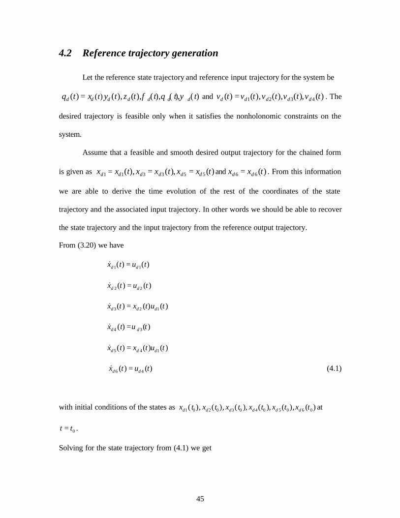
4.2 Reference trajectory generation
Let the reference state trajectory and reference input trajectory for the system be
( )( ) ( ), ( ), ( ), ( ), ( )d d d d d d dtq t x y t z t t t tφ θ ψ= and 1 2 3 4( ) ( ), ( ), ( ), ( )d d d d dv t v t v t v t v t= . The
desired trajectory is feasible only when it satisfies the nonholonomic constraints on the
system.
Assume that a feasible and smooth desired output trajectory for the chained form
is given as 1 1 3 3 5 5( ), ( ), ( )d d d d d dx x t x x t x x t= = = and 6 6( )d dx x t= . From this information
we are able to derive the time evolution of the rest of the coordinates of the state
trajectory and the associated input trajectory. In other words we should be able to recover
the state trajectory and the input trajectory from the reference output trajectory.
From (3.20) we have
1 1( ) ( )d dx t u t=&
2 2( ) ( )d dx t u t=&
3 2 1( ) ( ) ( )d d dx t x t u t=&
4 3( ) ( )d dx t u t=&
5 4 1( ) ( ) ( )d d dx t x t u t=&
6 4( ) ( )d dx t u t=& (4.1)
with initial conditions of the states as 1 0 2 0 3 0 4 0 5 0 6 0( ), ( ), ( ), ( ), ( ), ( )d d d d d dx t x t x t x t x t x t at
0t t= .
Solving for the state trajectory from (4.1) we get

46
2 3 1( ) ( ) ( )d d dx t x t x t= & &
4 5 1( ) ( ) ( )d d dx t x t x t= & & (4.2)
The corresponding input trajectory is given as
1 1( ) ( )d du t x t= &
22 2 1 3 3 1 1( ) ( ) ( ( ) ( ) ( ) ( )) ( )d d d d d d du t x t x t x t x t x t x t= = −& & && & && &
23 4 1 5 5 1 1( ) ( ) ( ( ) ( ) ( ) ( )) ( )d d d d d d du t x t x t x t x t x t x t= = −& & && & && &
4 6( ) ( )d du t x t= & (4.3)
(4.2.) and (4.3) gives the unique state and input trajectory, from which the desired output
trajectory can be reproduced or generated. As is seen, the values of the trajectories
depend upon the values of the output trajectory and its second order derivatives. Thus the
output trajectory should be differentiable everywhere. The derivation of the reference
input and state trajectory which generates a desired output trajectory can also be
performed on the original system. The original state and input trajectories can be derived
from the output trajectory as
1( ) ( )d dx t x t=
3( ) ( )d dy t x t=
5( ) ( )d dz t x t=
1 12tan ( ) tan ( )d d d dx y xψ − −= = & &
1 14tan ( cos ) tan ( cos )d d d d d dx z xθ ψ ψ− −= − = − &&
( )1cot cot sin tan sind d d d dφ θ ψ ψ θ−= + (4.4)
47
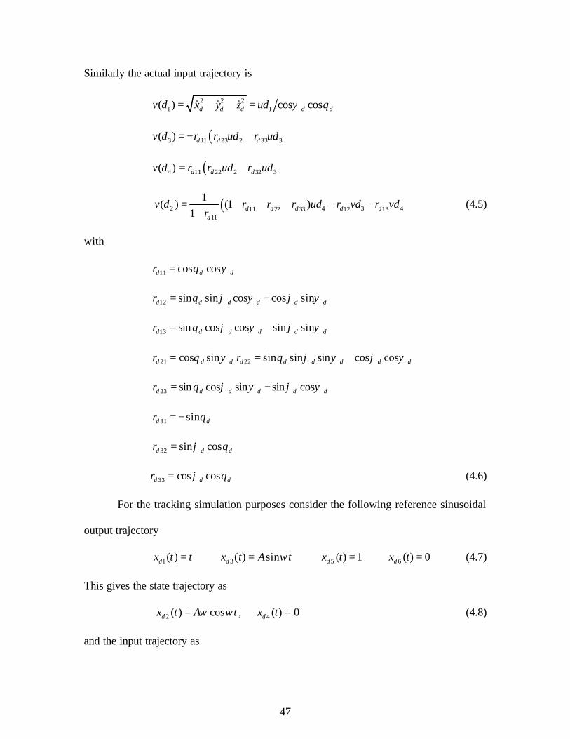
Similarly the actual input trajectory is
2 2 21 1( ) cos cosd d d d dv d x y z ud ψ θ= + + =& & &
( )3 2 311 23 33( ) d d dv d r r ud r ud= − +
( )4 2 311 22 32( ) d d dv d r r ud r ud= +
( )2 4 3 411 22 33 12 1311
1( ) (1 )
1 d d d d dd
v d r r r ud r vd r vdr
= + + + − −+
(4.5)
with
11 cos cosd d dr θ ψ=
12 sin sin cos cos sind d d d d dr θ ϕ ψ ϕ ψ= −
13 sin cos cos sin sind d d d d dr θ ϕ ψ ϕ ψ= +
21 cos sind d dr θ ψ= 22 sin sin sin cos cosd d d d d dr θ ϕ ψ ϕ ψ= +
23 sin cos sin sin cosd d d d d dr θ ϕ ψ ϕ ψ= −
31 sind dr θ= −
32 sin cosd d dr ϕ θ=
33 cos cosd d dr ϕ θ= (4.6)
For the tracking simulation purposes consider the following reference sinusoidal
output trajectory
1( )dx t t= 3( ) sindx t A tω= 5 ( ) 1dx t = 6 ( ) 0dx t = (4.7)
This gives the state trajectory as
2 ( ) cosdx t A tω ω= , 4 ( ) 0dx t = (4.8)
and the input trajectory as

48
1( ) 1du t = 22 ( ) sindu t A tω ω= −
3( ) 0du t = 4 ( ) 0du t = (4.9)
The initial states are
1(0) 0dx = 2(0)dx Aω= 3(0) 0dx =
4 (0) 0dx = 5(0) 1dx = 6 (0) 0dx = (4.10)
Here again it is to be noted that there is a singularity in the state and input trajectories at
1( ) 0dx t =& or 1( ) 0du t = as the state and input trajectories are not defined at that point.
4.3 Control using approximate linearization.
The feedback controller for trajectory tracking is based on standard linear control
theory. The design makes use of the approximate linearization of the system equations
about desired trajectory which leads to a time varying system as seen before. The method
here is illustrated for the chained form equations about the desired trajectory. The chained
form system is linear under piecewise constant inputs.
For the chained form system the desired state and input trajectory computed in
correspondence to the reference cartesian trajectory is
1 2 3 4 5 6( ) { ( ), ( ), ( ) , ( ), ( ), ( )}d d d d d d dx t x t x t x t x t x t x t=
and (4.11)
1 2 3 4( ) { ( ), ( ), ( ), ( )}d d d d du t u t u t u t u t=
An equivalent way to state the tracking problem is to require the difference
between the actual configuration and the desired configuration approach to zero. This
difference is denoted as the error. Since the vehicle will not necessarily share the same
initial conditions as the desired system, the tracking controller will drive the error to zero
49
and minimize the effect of the disturbances as the vehicle converges to the reference
trajectory.
In order for the system to track the trajectory of error should approach to zero
with time. Denoting the error variables for states and inputs as the following
e dx x x= −
and (4.12)
e du u u= −
The error differential equations are written by subtracting the desired equations from the
system (actual) equations as the following nonlinear set of equations
1 1e ex u=&
2 2e ex u=&
3 2 1 2 1e d dx x u x u= −&
4 3e ex u=&
5 4 1 4 1e d dx x u x u= −&
6 4e ex u=& (4.13)
Now linearizing about the desired trajectory we have the following linear system
( ) ( ) ( ) ( ) ( )e e ex t A t x t B t u t= +& (4.14)
with
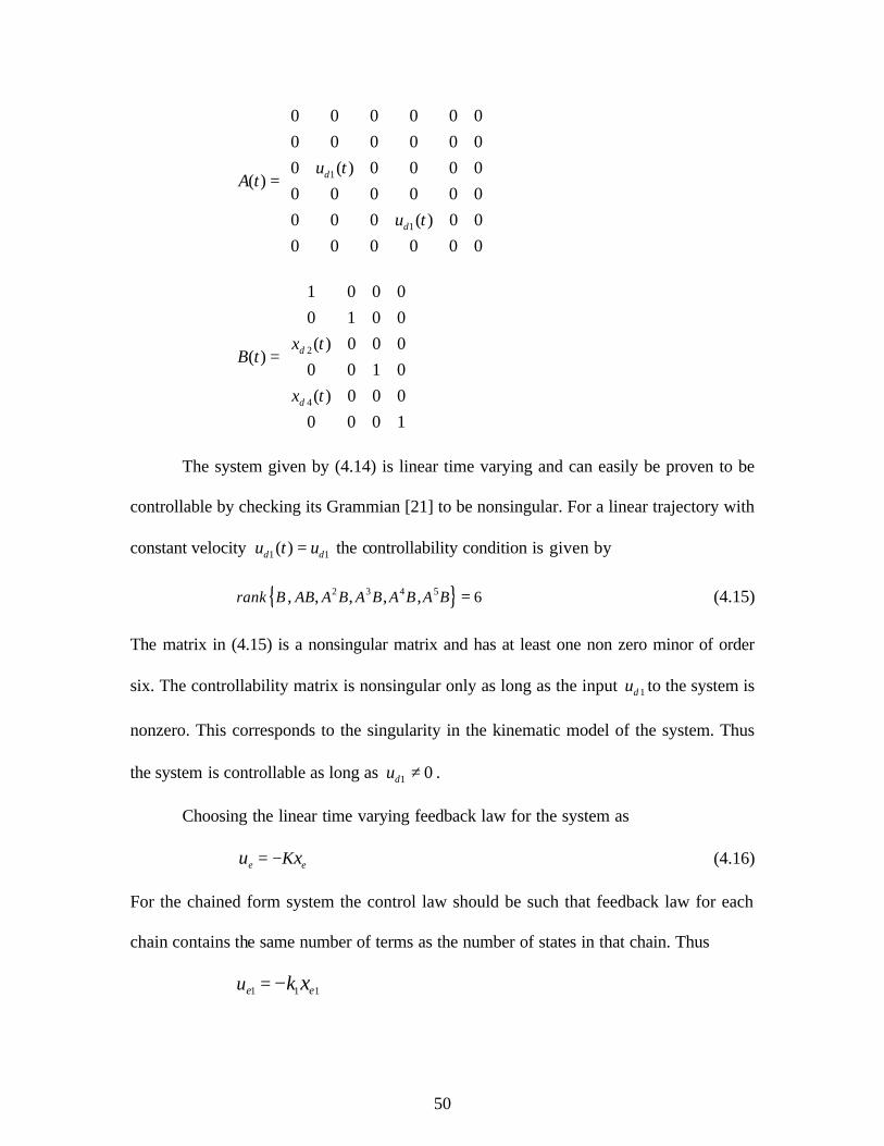
50
1
1
0 0 0 0 0 00 0 0 0 0 00 ( ) 0 0 0 0
( )0 0 0 0 0 00 0 0 ( ) 0 00 0 0 0 0 0
d
d
u tA t
u t
=
2
4
1 0 0 00 1 0 0( ) 0 0 0
( )0 0 1 0( ) 0 0 0
0 0 0 1
d
d
x tB t
x t
=
The system given by (4.14) is linear time varying and can easily be proven to be
controllable by checking its Grammian [21] to be nonsingular. For a linear trajectory with
constant velocity 1 1( )d du t u= the controllability condition is given by
{ }2 3 4 5 6, , , , ,rank B AB A B A B A B A B = (4.15)
The matrix in (4.15) is a nonsingular matrix and has at least one non zero minor of order
six. The controllability matrix is nonsingular only as long as the input 1du to the system is
nonzero. This corresponds to the singularity in the kinematic model of the system. Thus
the system is controllable as long as 1 0du ≠ .
Choosing the linear time varying feedback law for the system as
e eKu x= − (4.16)
For the chained form system the control law should be such that feedback law for each
chain contains the same number of terms as the number of states in that chain. Thus
1 1 1e eu k x= −

51
2 2 33
21
e e ed
uukk x x= − −
3 4 55
41
e e ed
uukk x x= − −
4 6 6e eu k x= − (4.17)
The feedback coefficients 3k and 5k are divided by 1du so that the characteristic equation
of the closed loop system matrix does not contain 1du , thus making the design global.
Thus the matrix K is given as
1
2 3 14
54 1
6
0 0 0 0 00 0 0 00 0 0 00 0 0 0 0
d
de
uu
u
kk k
k kk
= (4.18)
The 'sk are chosen such that 1k and 6k are positive, and 2k , 3k , 4k and 5k are such that
22 3k kλλ + + and 2
54k kλλ + + are Hurwitz. The closed loop sys tem matrix is thus
given as
clA A BK−=
( )( )
( )( )
1
2 3 1
2 1 1
4 5 1
4 1 1
6
0 0 0 0 0
0 0 0 00 0 0 0
0 0 0 00 0 0 0
0 0 0 0 0
d
d d
d
d d
k
k k u tx k u t
k k u tx k u t
k
− −
= − −
(4.19)
The closed- loop system matrix has constant eigenvalues with negative real parts.
This does not guarantee the asymptotic stability of the closed- loop time varying system
[26].However, for specific choices of ( )1du t , bounded away from zero and ( )2du t ,
52
( )3du t and ( )4du t , it is possible to use results on slowly –varying linear systems in order
to prove asymptotic stability. The feedback matrix is obtained by using pole placement
technique. Since for stability the eigen values of the closed loop matrix should have
negative real parts, the characteristic equation of the system should satisfy the following
( ) ( ) ( ) ( )( ) ( ) ( )1 2 3 4 5 6det clsI A s p s p s p s p s p s p− = − − − − − −
where ip ; 1,2,......,6i = are the eigen values of the system. The resulting closed loop
system (4.19) is controllable with the choice of feedback in (4.17).
4.3.1 Simulation of the controller
For simulation the following sinusoidal trajectory is chosen:
( )dx t t= ( ) sindy t a tω= ( ) 1dz t =
which gives the following desired values for the chained form states and inputs
1( )dx t t= 2( ) cosdx t a tω ω= 3( ) sindx t a tω= 4( ) 0dx t =
5( ) 1dx t = 6( ) 0dx t =
and
1( ) 1du t = 22 ( ) sindu t a tω ω= − 3( ) 0du t = 4( ) 0du t =
The initial conditions for the states are
1(0) 1dx = 2(0)dx aω= 3(0) 2dx = 4(0) 0dx =
5(0) 3dx = 6(0) 0dx =
Choosing the six coincident closed loop poles at -2, i.e.
51 2 3 4 6 2p p p p p p= = = = = = −
we get the feedback matrix coefficients as

53
1 6 2k k= = and 52 3 4 4k k k k= = = =
Choosing 1a = and ω π= we get the simulation results. The results show the tracking
errors for chained form states and inputs; and for actual states and inputs. Once the
tracking errors go to zero, the actual control inputs as obtained from the chained form
variables and inputs are same as the computed desired inputs. The desired inputs are
computed from actual system variables from (4.5). Since the control design is based on
the linearization of the system, the controller will make the controlled system locally
asymptotically stable.
54
Figure4. 1: The result of approximate linearization: tracking errors in chained form variables 1x (blue), 2x (green), 3x (red), 4x (cyan), 5x (magenta), 6x (yellow), vs. time (sec).
Figure4. 2: The result of approximate linearization: tracking errors (m/sec) in chained form inputs 1u (blue), 2u (green), 3u (red), 4u (cyan) vs. time (sec).
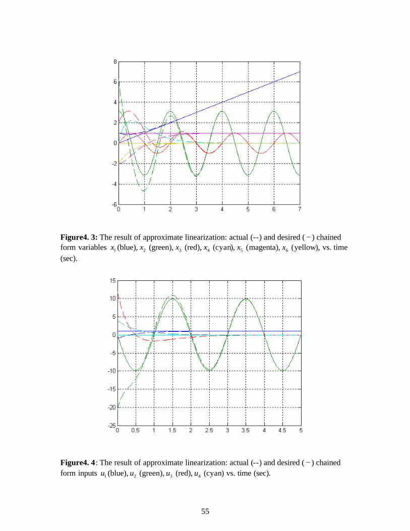
55
Figure4. 3: The result of approximate linearization: actual (--) and desired ( − ) chained form variables 1x (blue), 2x (green), 3x (red), 4x (cyan), 5x (magenta), 6x (yellow), vs. time (sec).
Figure4. 4: The result of approximate linearization: actual (--) and desired ( − ) chained form inputs 1u (blue), 2u (green), 3u (red), 4u (cyan) vs. time (sec).
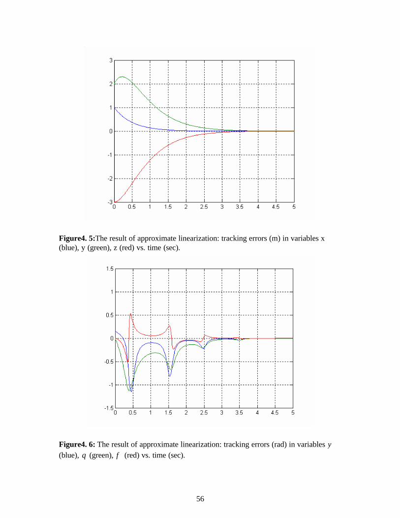
56
Figure4. 5:The result of approximate linearization: tracking errors (m) in variables x (blue), y (green), z (red) vs. time (sec).
Figure4. 6: The result of approximate linearization: tracking errors (rad) in variables ψ (blue), θ (green), φ (red) vs. time (sec).

57
Figure4. 7: The result of approximate linearization: actual (--) and desired ( − ) original variables x (blue), y (green), z (red) vs. time (sec).
Figure4. 8: The result of approximate linearization: actual (--) and desired ( − ) original variables ψ (blue), θ (green), φ (red) vs. time (sec).

58
Figure4. 9: The result of approximate linearization: 1v (m/sec) vs. time (sec).
Figure4. 10: The result of approximate linearization: 2v (rad/sec) vs. time (sec).

59
Figure4. 11: The result of approximate linearization: 3v (rad/sec) vs. time (sec).
Figure4. 12: The result of approximate linearization: 4v (rad/sec) vs. time (sec).
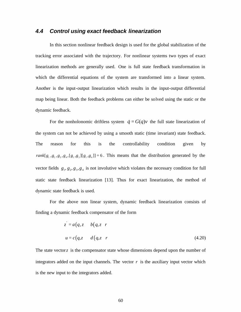
60
4.4 Control using exact feedback linearization
In this section nonlinear feedback design is used for the global stabilization of the
tracking error associated with the trajectory. For nonlinear systems two types of exact
linearization methods are generally used. One is full state feedback transformation in
which the differential equations of the system are transformed into a linear system.
Another is the input-output linearization which results in the input-output differential
map being linear. Both the feedback problems can either be solved using the static or the
dynamic feedback.
For the nonholonomic driftless system ( )q G q v=& the full state linearization of
the system can not be achieved by using a smooth static (time invariant) state feedback.
The reason for this is the controllability condition given by
1 2 3 4 1 3 1 4[ , , , , [ , ][ , ]] 6rank g g g g g g g g = . This means that the distribution generated by the
vector fields 1 2 3 4, , ,g g g g is not involutive which violates the necessary condition for full
static state feedback linearization [13]. Thus for exact linearization, the method of
dynamic state feedback is used.
For the above non linear system, dynamic feedback linearization consists of
finding a dynamic feedback compensator of the form
( ) ( ), ,a q b q rζ ζ ζ= +&
( ) ( ), ,u c q d q rζ ζ= + (4.20)
The state vectorζ is the compensator state whose dimensions depend upon the number of
integrators added on the input channels. The vector r is the auxiliary input vector which
is the new input to the integrators added.

61
The starting point of the dynamic extension for our problem is to define an m (4)
dimensional output ( )z h q= . A certain desired behavior is assigned to this output vector.
The output vector is then successively differentiated until each and every input in the
system appears and the invertible map (or matrix) is non singular. During the successive
differentiations of the output vector, it becomes necessary to add the chain of integrators
on inputs so as to avoid their direct differentiation. The number of integrators results in
the compensator state vector ζ . The inputs to these integrators become the new
auxiliary input vector r . The process continues and terminates after a finite number of
differentiations if the system is invertible from the chosen output vector z. If the sum of
the orders of the output differentiations is equal to the sum of the order of the original
system (n) and the dimensions of the compensator, then the full state linearization is
achieved in the sense that no internal dynamics are left in the system. The process also
results in the decoupling of the output vector from the new auxiliary input.
If at some point of differentiation of output in the algorithm the decoupling matrix
of the system is non singular without the addition of any compensator state, the process
results in the input output linearization of the system. The static feedback law of the form
( ) ( )u a q b q r= + (4.21)
is used to linearize the system.
4.4.1 Control using exact feedback linearization via static feedback
For our system let the output vector in the chained form be defined as
1
3
5
6
xx
zxx
=
(4.22)

62
The derivative of the output is given as
1 1
3 22
5 34
6 4
1 0 0 00 0 00 0 0
0 0 0 1
x ux ux
zx uxx u
= =
&&& &&
or (4.23)
( )z H q u=&
The inputs 2u and 3u do not appear after differentiation and also the decoupling matrix
( )H q is singular and not invertible. Hence the static feedback cannot be applied and the
system cannot be linearized by input output linearization. The same result follows if the
above procedure is repeated by choosing the actual state variable as the output vector.
4.4.2 Control using exact feedback linearization via dynamic feedback
Since the static feedback fails to solve the problem, we will be making use of
dynamic feedback extension. For the linearization via dynamic feedback let us again
define the linearizing output vector for the chained form as
1
3
5
6
xx
zxx
=
(4.24)
Differentiating w.r.t time we get
1 1
3 22
5 34
6 4
1 0 0 00 0 00 0 0
0 0 0 1
x ux ux
zx uxx u
= =
&&& &&
(4.25)
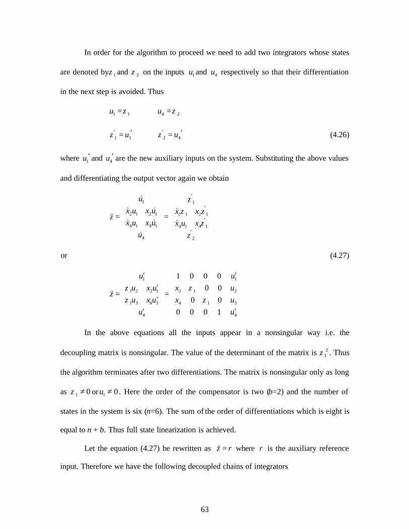
63
In order for the algorithm to proceed we need to add two integrators whose states
are denoted by 1ζ and 2ζ on the inputs 1u and 4u respectively so that their differentiation
in the next step is avoided. Thus
1 1u ζ= 4 2u ζ=
1 1uζ ′=& 2 4uζ ′=& (4.26)
where 1u ′ and 4u ′ are the new auxiliary inputs on the system. Substituting the above values
and differentiating the output vector again we obtain
1
2 1 2 1
4 1 4 1
4
ux u x u
zx u x u
u
+ = +
&& &&& & &
&
1
2 1 2 1
4 1 4 1
2
x xx u x
ζζ ζ
ζζ
+ = +
&&&&&
&
or (4.27)
1 1
1 2 2 1 22 1
1 3 4 1 34 1
4 4
1 0 0 00 0
0 00 0 0 1
u uu x u ux
zu x u ux
u u
ζ ζζ ζ
′ ′ ′+ = = ′+ ′ ′
&&
In the above equations all the inputs appear in a nonsingular way i.e. the
decoupling matrix is nonsingular. The value of the determinant of the matrix is 21ζ . Thus
the algorithm terminates after two differentiations. The matrix is nonsingular only as long
as 1 0ζ ≠ or 1 0u ≠ . Here the order of the compensator is two (b=2) and the number of
states in the system is six (n=6). The sum of the order of differentiations which is eight is
equal to n + b. Thus full state linearization is achieved.
Let the equation (4.27) be rewritten as z r=&& where r is the auxiliary reference
input. Therefore we have the following decoupled chains of integrators

64
1 1z r=&&
2 2z r=&&
3 3z r=&&
4 4z r=&& (4.28)
The resulting nonlinear dynamic feedback controller is
1 1u ζ=
( )2 2 2 1 1u r x r ζ= −
( )3 3 4 1 1u r x r ζ= −
4 2u ζ=
1 1 1u rζ ′= =&
2 4 4u rζ ′= =& (4.29)
Assuming the system follows a smooth desired reference trajectory in chained
form coordinates as ( )1 3 5 6( ) ( ), ( ), ( ), ( )d d d d dz t x t x t x t x t= , the exponentially stabilizing
feedback control law for the linear and decoupled system about this desired trajectory is
given as
( ) ( )( ) ( ) ( ) ( ) ( )i di vi di i pi di ir z t k z t z t k z t z t= + − + −&& & & ; 1,2...,4i = (4.30)
where vik and pik (the PD gains) are chosen such that they are positive and the
characteristic polynomials
2vi pis k s k+ + ; 1,2...,4i = (4.31)
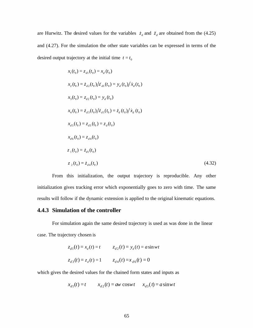
65
are Hurwitz. The desired values for the variables dz& and dz&& are obtained from the (4.25)
and (4.27). For the simulation the other state variables can be expressed in terms of the
desired output trajectory at the initial time 0t t=
1 0 1 0 0( ) ( ) ( )d dx t z t x t= =
2 0 2 0 1 0 0 0( ) ( ) ( ) ( ) ( )d d d dx t z t z t y t x t= = && &
3 0 2 0 0( ) ( ) ( )d dx t z t y t= =
4 0 3 0 1 0 0 0( ) ( ) ( ) ( ) ( )d d d dx t z t z t z t x t= = && & &
5 0 3 0 0( ) ( ) ( )d d dx t z t z t= =
6 0 4 0( ) ( )d dx t z t=
1 0 1 0( ) ( )dt z tζ = &
2 0 4 0( ) ( )dt z tζ = & (4.32)
From this initialization, the output trajectory is reproducible. Any other
initialization gives tracking error which exponentially goes to zero with time. The same
results will follow if the dynamic extension is applied to the original kinematic equations.
4.4.3 Simulation of the controller
For simulation again the same desired trajectory is used as was done in the linear
case. The trajectory chosen is
1 ( )( ) dd x t tz t == 2 ( ) sin( ) dd y t a tz t ω==
3 ( ) 1( ) dd z tz t == 4 6( ) ( ) 0d dz t x t= =
which gives the desired values for the chained form states and inputs as
1( )dx t t= 2( ) cosdx t a tω ω= 3( ) sindx t a tω=
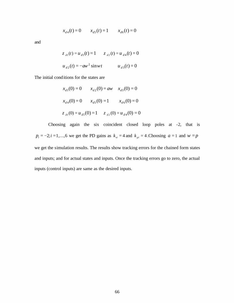
66
4( ) 0dx t = 5( ) 1dx t = 6( ) 0dx t =
and
1 1( ) ( ) 1d dt u tζ = = 2 4( ) ( ) 0d dt u tζ = =
22 ( ) sindu t a tω ω= − 3( ) 0du t =
The initial conditions for the states are
1(0) 0dx = 2(0)dx aω= 3(0) 0dx =
4(0) 0dx = 5(0) 1dx = 6(0) 0dx =
1 1(0) (0) 1d duζ = = 2 4(0) (0) 0d duζ = =
Choosing again the six coincident closed loop poles at -2, that is
2; 1,...,6i ip = − = we get the PD gains as 4vik = and 4pik = .Choosing 1a = and ω π=
we get the simulation results. The results show tracking errors for the chained form states
and inputs; and for actual states and inputs. Once the tracking errors go to zero, the actual
inputs (control inputs) are same as the desired inputs.

67
Figure4. 13: The result of dynamic feedback: tracking errors in chained form variables
1x (blue), 2x (green), 3x (red), 4x (cyan), 5x (magenta), 6x (yellow),vs. time (sec).
Figure4. 14: The result of dynamic feedback: tracking errors in chained form inputs 1u (blue), 2u (green), 3u (red), 4u (cyan) vs. time (sec).
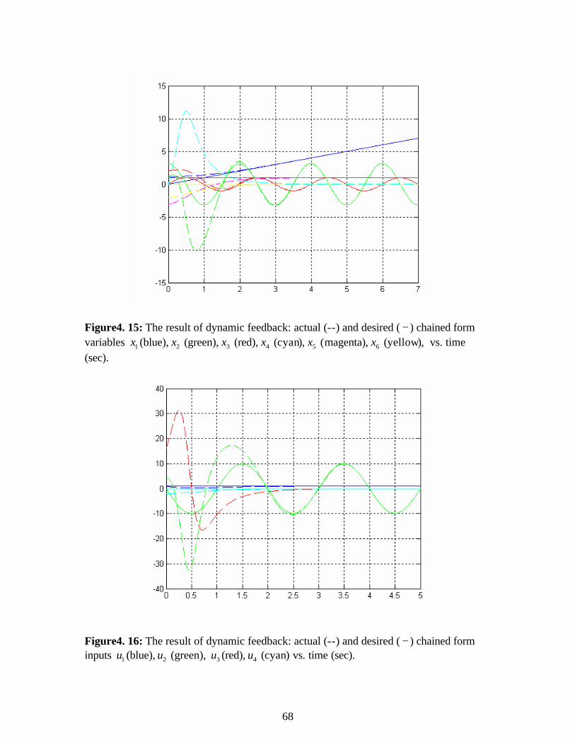
68
Figure4. 15: The result of dynamic feedback: actual (--) and desired ( − ) chained form variables 1x (blue), 2x (green), 3x (red), 4x (cyan), 5x (magenta), 6x (yellow), vs. time (sec).
Figure4. 16: The result of dynamic feedback: actual (--) and desired ( − ) chained form inputs 1u (blue), 2u (green), 3u (red), 4u (cyan) vs. time (sec).
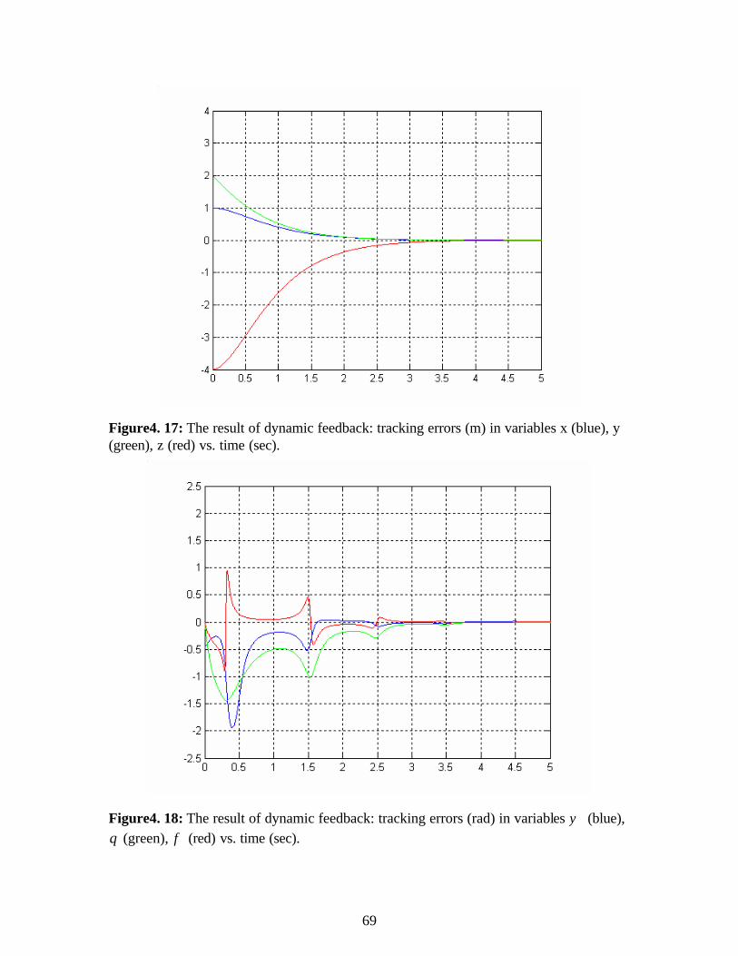
69
Figure4. 17: The result of dynamic feedback: tracking errors (m) in variables x (blue), y (green), z (red) vs. time (sec).
Figure4. 18: The result of dynamic feedback: tracking errors (rad) in variables ψ (blue), θ (green), φ (red) vs. time (sec).
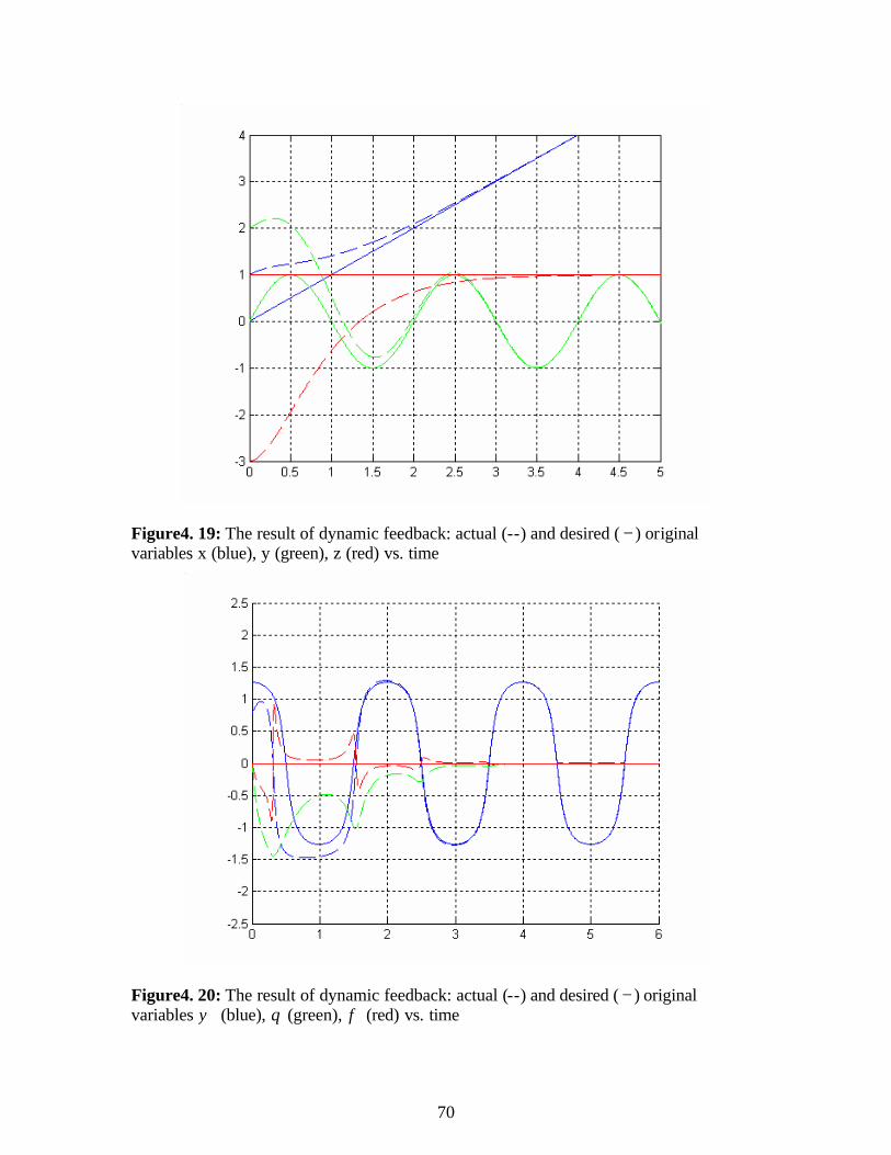
70
Figure4. 19: The result of dynamic feedback: actual (--) and desired ( − ) original variables x (blue), y (green), z (red) vs. time
Figure4. 20: The result of dynamic feedback: actual (--) and desired ( − ) original variables ψ (blue), θ (green), φ (red) vs. time
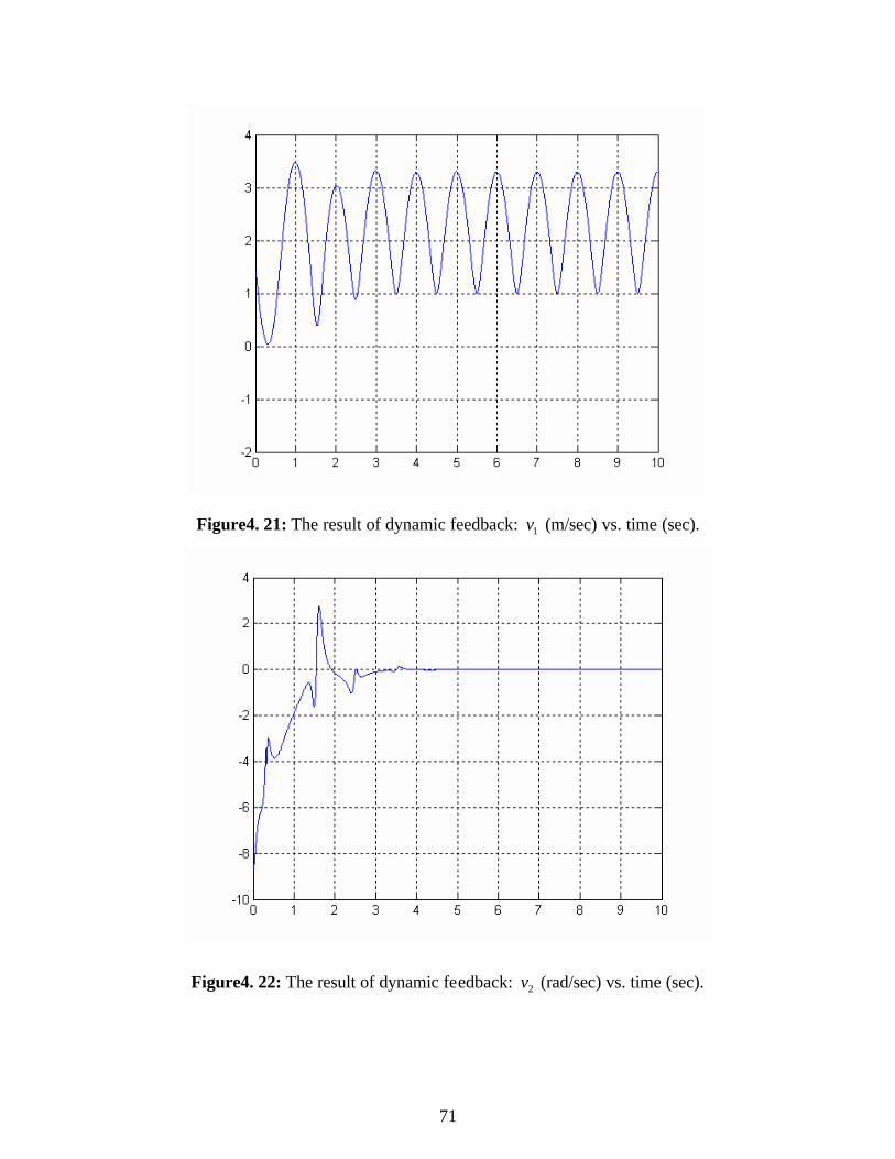
71
Figure4. 21: The result of dynamic feedback: 1v (m/sec) vs. time (sec).
Figure4. 22: The result of dynamic feedback: 2v (rad/sec) vs. time (sec).
72
Figure4. 23: The result of dynamic feedback: 3v (rad/sec) vs. time (sec).
Figure4. 24: The result of dynamic feedback: 4v (rad/sec) vs. time (sec).
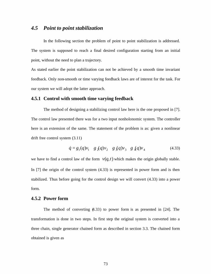
73
4.5 Point to point stabilization
In the following section the problem of point to point stabilization is addressed.
The system is supposed to reach a final desired configuration starting from an initial
point, without the need to plan a trajectory.
As stated earlier the point stabilization can not be achieved by a smooth time invariant
feedback. Only non-smooth or time varying feedback laws are of interest for the task. For
our system we will adopt the latter approach.
4.5.1 Control with smooth time varying feedback
The method of designing a stabilizing control law here is the one proposed in [7].
The control law presented there was for a two input nonholonomic system. The controller
here is an extension of the same. The statement of the problem is as: given a nonlinear
drift free control system (3.11)
1 1 2 2 3 3 4 4( ) ( ) ( ) ( )q g q v g q v g q v g q v= + + +& (4.33)
we have to find a control law of the form ( , )v q t which makes the origin globally stable.
In [7] the origin of the control system (4.33) is represented in power form and is then
stabilized. Thus before going for the control design we will convert (4.33) into a power
form.
4.5.2 Power form
The method of converting (4.33) to power form is as presented in [24]. The
transformation is done in two steps. In first step the original system is converted into a
three chain, single generator chained form as described in section 3.3. The chained form
obtained is given as
74
01 1 1xx u= =& 0
22 2xx u==& 034 3xx u==& 0
46 4xx u==&
0203 2 1xx x u==& 0
315 4 1xx x u==& (4.34)
In the second step the chained form system (4.34) is converted into power form.
For the three chain single generator chained form the global transformation to power
form is given below [24]:
0;j jy x= 1 4j≤ ≤
( ) ( ) ( ) ( )1
00 0 1 0
0
11 1
!
k k nk nk k nj j j
n
z x x xk n
− −
=
= − + −−∑ 2 4j≤ ≤ 1 jk n≤ ≤ (4.35)
which gives the power form as:
;j jy u=& 1 4j≤ ≤
( )0 1
1!
kkj jz y u
k= 2 4j≤ ≤ 1 jk n≤ ≤ (4.36)
Here we should recall from section 3.3 that 0 00j jx x= which are identified as the
top of the chains and 4
2
2jn
n=
=∑ . Thus we have 2 3 1n n= = and 4 0n = .Using (4.34) and
taking the above values, the transformation (4.35) becomes
1 1y x=
2 2y x=
3 4y x=
4 6y x=
11 20 3 1 2z z x x x= = − +
12 30 5 1 4z z x x x= = − +
75
03 40 6z z x= = (4.37)
and the corresponding power form is
1 1y u=&
2 2y u=&
3 3y u=&
4 4y u=&
120 1 2z y u=&
130 1 3z y u=&
040 4z u=& (4.38)
4.5.3 Control law
The control law for (4.38) from [7] is given here as
1 1 ( )(cos sin )u y z t tρ= − + −
2 2 1 1 cosu y c z t= − +
3 3 2 2 cosu y c z t= − +
4 4u y= − (4.39)
with 1c , 2c >0 and ( ) ( ) ( )2 2 2
1 2 3( )z z z zρ = + + The controls (4.39) asymptotically stabilize
the origin of (4.38).
For global stabilization the saturation functions are introduced in the control law.
These functions eliminate the destabilizing effects away from the origin. The control is
thus given as
1 1 ( ( ))(cos sin )u y z t tσ ρ= − + −
76
2 2 1 1( )cosu y c z tσ= − +
3 3 2 2( )cosu y c z tσ= − +
4 4u y= − (4.40)
where 0jc > and : R Rσ → is a non decreasing 3C saturation function with a magnitude
less than some 0δ > and is linear between ( , )δ δ− .For global stabilization δ should be
small enough. The saturation function then satisfies the following [7]:
1. ( )z zσ = when z ε≤
2. ( )zσ δ≤ for all z such that 0 ε δ< <
The closed loop dynamics are given as:
1 1 ( ( ))(cos sin )y y z t tσ ρ= − + −&
2 2 1 1( )cosy y c z tσ= − +&
3 3 2 2( )cosy y c z tσ= − +&
4 4y y= −& (4.41)
For some 0 ε δ< < , 0δ∃ such that if 0ε ε< , then the closed loop dynamics are globally
asymptotically stabilized to zero.
4.5.4 Simulation
For simulation the value of δ is chosen to be 0.001 and the saturation functions,
( ( ))zσ ρ , 1( )zσ and 2( )zσ are 0.26, 0.5 and 0.1. The constants 1c and 2c are both chosen
as 2. The initial values for 1y , 2y , 3y and 4y are chosen as -5, -2, -7 and -5 respectively.

77
Figure4. 25: Point stabilization using time varying feedback: x (m) vs. time (sec).
Figure4. 26: Point stabilization using time varying feedback: y (rad) vs. time (sec).
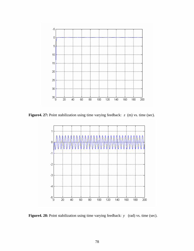
78
Figure4. 27: Point stabilization using time varying feedback: z (m) vs. time (sec).
Figure4. 28: Point stabilization using time varying feedback: ψ (rad) vs. time (sec).
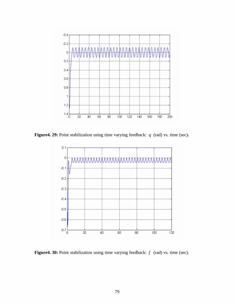
79
Figure4. 29: Point stabilization using time varying feedback: θ (rad) vs. time (sec).
Figure4. 30: Point stabilization using time varying feedback: φ (rad) vs. time (sec).
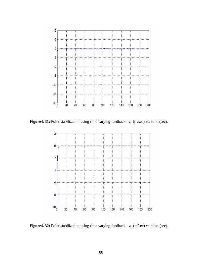
80
Figure4. 31: Point stabilization using time varying feedback: 1v (m/sec) vs. time (sec).
Figure4. 32: Point stabilization using time varying feedback: 2v (m/sec) vs. time (sec).
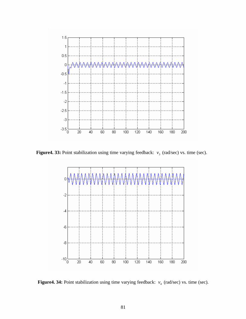
81
Figure4. 33: Point stabilization using time varying feedback: 3v (rad/sec) vs. time (sec).
Figure4. 34: Point stabilization using time varying feedback: 4v (rad/sec) vs. time (sec).
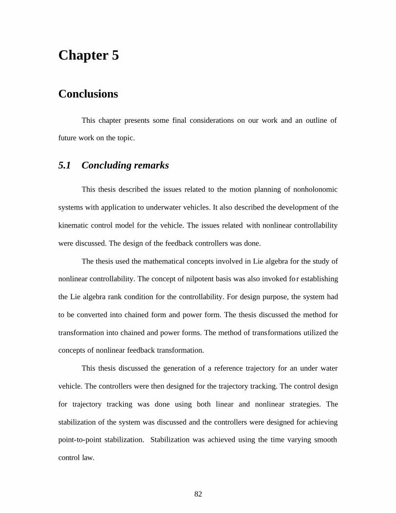
82
Chapter 5
Conclusions
This chapter presents some final considerations on our work and an outline of
future work on the topic.
5.1 Concluding remarks
This thesis described the issues related to the motion planning of nonholonomic
systems with application to underwater vehicles. It also described the development of the
kinematic control model for the vehicle. The issues related with nonlinear controllability
were discussed. The design of the feedback controllers was done.
The thesis used the mathematical concepts involved in Lie algebra for the study of
nonlinear controllability. The concept of nilpotent basis was also invoked fo r establishing
the Lie algebra rank condition for the controllability. For design purpose, the system had
to be converted into chained form and power form. The thesis discussed the method for
transformation into chained and power forms. The method of transformations utilized the
concepts of nonlinear feedback transformation.
This thesis discussed the generation of a reference trajectory for an under water
vehicle. The controllers were then designed for the trajectory tracking. The control design
for trajectory tracking was done using both linear and nonlinear strategies. The
stabilization of the system was discussed and the controllers were designed for achieving
point-to-point stabilization. Stabilization was achieved using the time varying smooth
control law.

83
5.2 Future work
For future work it is possible to extend similar analysis to a higher dimensional
nonholonomic problem. For the same problem as discussed here, the design of stabilizing
laws for path following can be done. For path following, the model can be transformed
into parametric form in order to apply the control schemes. The method of control with
input scaling can also be used.
The stabilization in both point-to-point and path following tasks can also be
achieved through other control methods. The use of nonsmooth control and open loop
control can be used. Also for underwater vehicle, motion planning can also be done while
taking the actual dynamics of the system into consideration.
84
References
[1] A. D. Luca, G. Orio lo, C. Samson, “Feedback control of a nonholonomic car- like
robot,” in J. P. Laumond (Ed), Robot motion planning and control, pp. 170-250,
Springer, 1998
[2] R.W. Brockett, “Asymptotic stability and feedback stabilization,” in R.W.
Brockett, R. S. Millman and H. J. Sussman (Eds), Differential geometric control
theory, pp. 181-208, Birkhauser, 1993
[3] C. Samson, “Control of chained systems application to path following and time
varying point stabilization of mobile robots,” IEEE transactions on automatic
control, vol. 40, no 1, pp. 64-77, Jan 1995
[4] J. B. Pomet, “Explicit design of time-varying stabilizing control laws for a class
of controllable systems without drift,” System and control letters, vol.18, pp. 147-
158, 1992
[5] A. Astolfi, “Discontinuous output feedback control of nonholonomic chained
systems,” in Proceedings of the 3rd European control conference, 1995
[6] C. Canudas de Wit and O. J. Sørdalen, “Exponential stabilization of mobile robots
with nonholonomic constraints,” IEEE transactions on automatic control, vol. 37,
no. 11, pp. 1791-1797, November 1992
[7] A. R. Teel, R. M. Murray, G. Walsh, “Nonholonomic control systems: from
steering to stabilization with sinusoids,” Proceedings of 31st conference on
decision and control, Tucson, pp. 1603-1609, Dec 1992.
85
[8] A. Tayebi and A. Rachid, “A time-varying-based robust control for the parking
problem of a wheeled mobile robot,” in Proceedings IEEE Int. conference on
robotics and automation, pp. 3099-3104, April 1996.
[9] O. Egeland and O. J. Sørdalen, “Exponential stabilization of nonholonomic
chained systems,” IEEE transactions on automatic control, vol. 1, pp.35-49, 1995
[10] R. M. Murray, S. Sastry, “Steering nonholonomic systems in chained form,” IEEE
proceedings of the 30th conference on decision and control, pp. 1121-1126,
December 1991
[11] R. M. Murray, S. Sastry, “Nonholonomic motion planning: steering using
sinusoids,” IEEE transactions on automatic control, vol. 38, no.5, pp. 700-716,
May 1993
[12] A. de. Luca, G. Oriolo, “Modeling and control of nonholonomic mechanical
systems,” in Nonholonomic mechanical systems
[13] G. Oriolo, A. D. Luca, M. Vendittelli, “WMR control via dynamic feedback
linearization: design, implementation and experimental validation,” IEEE
transactions on control systems technology, vol. 10, no.6, pp 835-852, Nov 2002.
[14] A. Isidori, Nonlinear control systems, 3rd Edition, Springer-Verlag, London, UK,
1995
[15] O. Egeland, E. Berglund and O. J. Sørdalen, “Exponential stabilization of a
nonholonomic underwater vehicle with constant desired configuration,”
Proceedings 1994 IEEE Int. conference on robotics and automation, pp.20-26,
1994

86
[16] M. W. Spong and M. Vidyasagar, Robot dynamics and control, John Wiley, New
York, 1989
[17] R. M. Murray, “Nilpotent bases for a class of non- integrable distributions with
applications to trajectory generation for nonholonomic systems,” Mathematics of
Controls, Signals, and Systems, 7(1):58-75, 1994
[18] R. M. Murray, S. Sastry, “Steering nonholonomic systems using sinusoids,” IEEE
proceedings of the 29th conference on decision and control, pp. 2097-2101,
December 1990
[19] L. G. Bushnell, D. M. Tilbury, S. S. Sastry, “Steering three input nonholonomic
systems: the fire truck example,” in European controls conference, pp. 1432-
1437, 1993
[20] D. Tilbury, O. Sørdalen, L. Bushnell, S. Sastry, “A multi-steering trailer system:
conversion into chained form using dynamic feedback,” IEEE transactions on
Robotics and Automation, vol.11, no.6, pp.807-818, December 1995
[21] T. Kailath, Linear systems, Prentice- Hall, Englewood Cliffs, N.J, 1980
[22] Y. Nakamura, S. Savant, “Nonlinear tracking control of autonomous underwater
vehicles,” Proceedings of the 1992 IEEE International conference on robotics
and automation, pp. A4-A9, May 1992
[23] Y. Nakamura, S. Savant, “Nonholonomic motion control of an autonomous
underwater vehicle,” IEEE International workshop on intelligent robots and
systems IROS ’91, pp. 1254-1259, Nov 3-5, 1991
87
[24] G. C. Walsh, L. G. Bushnell, “Stabilization of multiple input chained form control
systems,” IEEE proceedings of the 32nd conference on decision and control, pp.
959-964, Dec. 1993
[25] O. J. Sørdalen, M. Dalsmo and O. Egeland, “An exponentially convergent law for
a nonholonomic underwater vehicle,” 1993 IEEE Int. conference on robotics and
automation, pp. 790-795, May 2-7, 1993
[26] H. K. Khalil, Nonlinear systems, Macmillan, New York, NY, 1992
88
Vita
Sabiha Wadoo was born in Srinagar, Kashmir, India. She received her bachelor’s degree
in electrical engineering from the Regional Engineering College, Srinagar in June 2001.
In the spring of 2002, she joined the Bradley Department of Electrical Engineering at
Virginia Polytechnic Institute and State University, Blacksburg, Virginia as a masters
student. Her areas of research include nonlinear control, signal and image processing.