nonholonomic systems via moving frames: cartan equivalence and chaplygin hamiltonization
TRANSCRIPT
arX
iv:m
ath-
ph/0
4080
05v1
2 A
ug 2
004
Nonholonomic systems via moving frames:
Cartan equivalence and Chaplygin Hamiltonization
Kurt EhlersDepartment of Mathematics
Truckee Meadows Community College7000 Dandini Blvd Reno NV 89512-3999 USA
Jair KoillerFundacao Getulio Vargas
Praia de Botafogo 190,Rio de Janeiro, 22253-900 [email protected]
Richard MontgomeryMathematics Department
University of California at Santa CruzSanta Cruz CA 95064 USA
Pedro M. RiosDepartment of Mathematics
University of California at BerkeleyBerkeley CA 94720 USA.
submitted, October, 2003; revised version, April, 2004∗.
Dedicated to Alan Weinstein on his 60th Birthday
∗The authors thank the Brazilian funding agencies CNPq and FAPERJ: a CNPq research fellowship (JK), a CNPq post-doctoral fellowship at Berkeley (PMR), a FAPERJ visiting fellowship to Rio de Janeiro (KE). (JK) thanks the E. SchrodingerInstitute, Vienna, for financial support during Alanfest and the Poisson Geometry Program, August 2003.
1
CONTENTS 2
AbstractA nonholonomic system, for short “NH”, consists of a configuration space Qn, a Lagrangian L(q, q, t), a
nonintegrable constraint distributionH ⊂ TQ, with dynamics governed by Lagrange-d’Alembert’s principle.We present here two studies, both using adapted moving frames. In the first we explore the affine connectionviewpoint. For natural Lagrangians L = T − V , where we take V = 0 for simplicity, NH-trajectories aregeodesics of a (non metric) connection ∇NH which mimics Levi-Civita’s. Local geometric invariants areobtained by Cartan’s method of equivalence. As an example, we analyze Engel’s (2-4) distribution. Thisis the first such study for a distribution that is not strongly nonholonomic. In the second part we studyG-Chaplygin systems; for those, the constraints are given by a connection φ : TQ→ Lie(G) on a principalbundle G → Q→ S = Q/G and the Lagrangian L is G-equivariant. These systems compress to an almostHamiltonian system (T ∗S,Hφ,ΩNH), ΩNH = Ωcan + (J.K), with d(J.K) 6= 0 in general; the momentummap J : T ∗Q → Lie(G) and the curvature form K : TQ → Lie(G)∗ are matched via the Legendretransform. Under a s ∈ S dependent time reparametrization, a number of compressed systems becomeHamiltonian, i.e, ΩNH is sometimes conformally symplectic. A necessary condition is the existence of aninvariant volume for the original system. Its density produces a candidate for conformal factor. Assuming aninvariant volume, we describe the obstruction to Hamiltonization. An example of Hamiltonizable system isthe “rubber” Chaplygin’s sphere, which extends Veselova’s system in T ∗SO(3). This is a ball with unequalinertia coefficients rolling without slipping on the plane, with vertical rotations forbidden. Finally, wediscuss reduction of internal symmetries. Chaplygin’s “marble”, where vertical rotations are allowed, is notHamiltonizable at the compressed T ∗SO(3) level. We conjecture that it is also not Hamiltonizable whenreduced to T ∗S2.
Contents
1 Introduction and outline 31.1 Moving frames: Lagrangian and Hamiltonian mechanics . . . . . . . . . . . . . . . . . . . . 31.2 Nonholonomic systems . . . . . . . . . . . . . . . . . . . . . . . . . . . . . . . . . . . . . . . 61.3 Main results . . . . . . . . . . . . . . . . . . . . . . . . . . . . . . . . . . . . . . . . . . . . . 7
2 Nonholonomic geometry: Cartan equivalence 92.1 Nonholonomic geodesics: straightest paths . . . . . . . . . . . . . . . . . . . . . . . . . . . . 102.2 Equivalence problem of nonholonomic geometry . . . . . . . . . . . . . . . . . . . . . . . . . 122.3 A tutorial on the method of equivalence . . . . . . . . . . . . . . . . . . . . . . . . . . . . . 142.4 The nonholonomic geometry of an Engel manifold. . . . . . . . . . . . . . . . . . . . . . . . 16
3 Nonholonomic dynamics: Chaplygin Hamiltonization 213.1 Compression to T ∗S, S = Q/G; existence of invariant measures . . . . . . . . . . . . . . . . 213.2 Examples: Veselova’s system and Chaplygin spheres (marble or rubber) . . . . . . . . . . . 253.3 Chaplygin’s marble is not Hamiltonizable at the T ∗SO(3) level. . . . . . . . . . . . . . . . . 293.4 Chaplygin’s marble: reduction to T ∗S2 . . . . . . . . . . . . . . . . . . . . . . . . . . . . . 30
4 Recent developments and final comments 324.1 Invariant measures and integrability . . . . . . . . . . . . . . . . . . . . . . . . . . . . . . . 334.2 Nonholonomic reduction. . . . . . . . . . . . . . . . . . . . . . . . . . . . . . . . . . . . . . . 334.3 G-Chaplygin systems via affine connections . . . . . . . . . . . . . . . . . . . . . . . . . . . 34
1 Introduction and outline 3
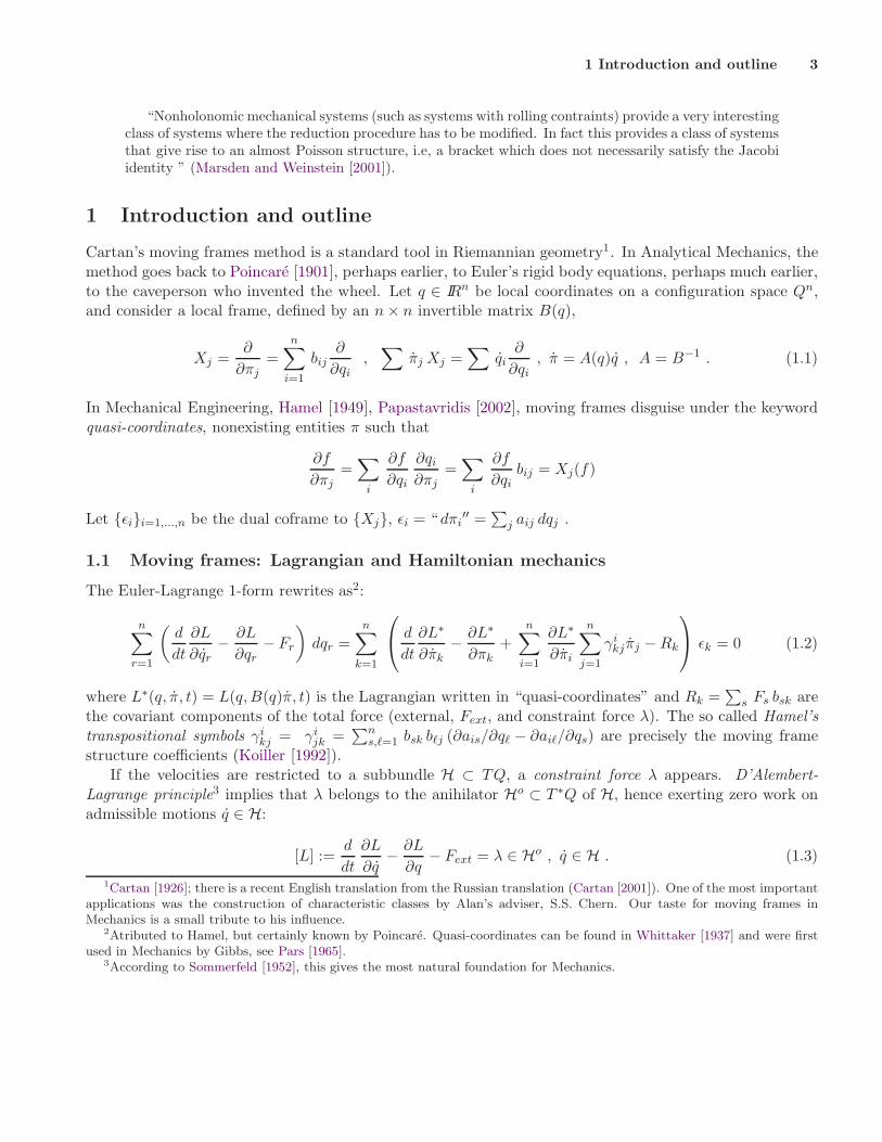
“Nonholonomic mechanical systems (such as systems with rolling contraints) provide a very interestingclass of systems where the reduction procedure has to be modified. In fact this provides a class of systemsthat give rise to an almost Poisson structure, i.e, a bracket which does not necessarily satisfy the Jacobiidentity ” (Marsden and Weinstein [2001]).
1 Introduction and outline
Cartan’s moving frames method is a standard tool in Riemannian geometry1. In Analytical Mechanics, themethod goes back to Poincare [1901], perhaps earlier, to Euler’s rigid body equations, perhaps much earlier,to the caveperson who invented the wheel. Let q ∈ IRn be local coordinates on a configuration space Qn,and consider a local frame, defined by an n× n invertible matrix B(q),
Xj =∂
∂πj=
n∑
i=1
bij∂
∂qi,
∑
πj Xj =∑
qi∂
∂qi, π = A(q)q , A = B−1 . (1.1)
In Mechanical Engineering, Hamel [1949], Papastavridis [2002], moving frames disguise under the keywordquasi-coordinates, nonexisting entities π such that
∂f
∂πj=
∑
i
∂f
∂qi
∂qi
∂πj=
∑
i
∂f
∂qibij = Xj(f)
Let ǫii=1,...,n be the dual coframe to Xj, ǫi = “ dπi′′ =
∑
j aij dqj .
1.1 Moving frames: Lagrangian and Hamiltonian mechanics
The Euler-Lagrange 1-form rewrites as2:
n∑
r=1
(
d
dt
∂L
∂qr− ∂L
∂qr− Fr
)
dqr =n
∑
k=1
d
dt
∂L∗
∂πk− ∂L∗
∂πk+
n∑
i=1
∂L∗
∂πi
n∑
j=1
γikjπj −Rk
ǫk = 0 (1.2)
where L∗(q, π, t) = L(q,B(q)π, t) is the Lagrangian written in “quasi-coordinates” and Rk =∑
s Fs bsk arethe covariant components of the total force (external, Fext, and constraint force λ). The so called Hamel’stranspositional symbols γi
kj = γijk =
∑ns,ℓ=1 bsk bℓj (∂ais/∂qℓ − ∂aiℓ/∂qs) are precisely the moving frame
structure coefficients (Koiller [1992]).If the velocities are restricted to a subbundle H ⊂ TQ, a constraint force λ appears. D’Alembert-
Lagrange principle3 implies that λ belongs to the anihilator Ho ⊂ T ∗Q of H, hence exerting zero work onadmissible motions q ∈ H:
[L] :=d
dt
∂L
∂q− ∂L
∂q− Fext = λ ∈ Ho , q ∈ H . (1.3)
1Cartan [1926]; there is a recent English translation from the Russian translation (Cartan [2001]). One of the most importantapplications was the construction of characteristic classes by Alan’s adviser, S.S. Chern. Our taste for moving frames inMechanics is a small tribute to his influence.
2Atributed to Hamel, but certainly known by Poincare. Quasi-coordinates can be found in Whittaker [1937] and were firstused in Mechanics by Gibbs, see Pars [1965].
3According to Sommerfeld [1952], this gives the most natural foundation for Mechanics.
1.1 Moving frames: Lagrangian and Hamiltonian mechanics 4
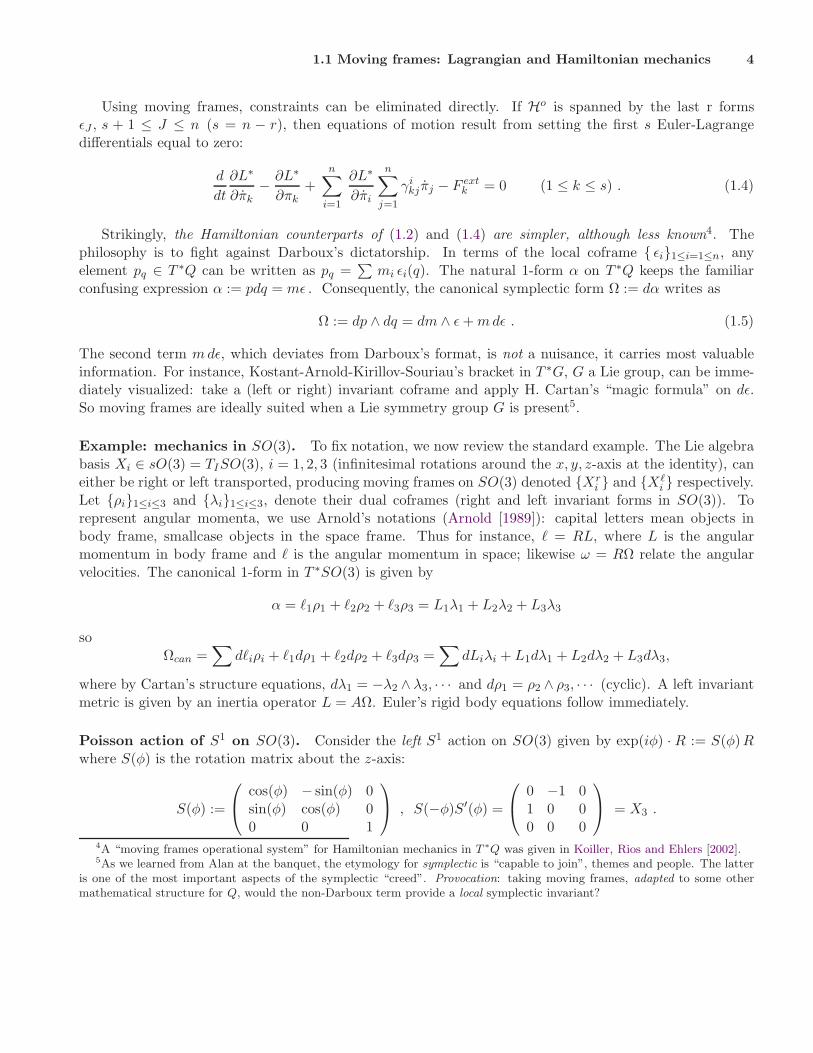
Using moving frames, constraints can be eliminated directly. If Ho is spanned by the last r formsǫJ , s + 1 ≤ J ≤ n (s = n − r), then equations of motion result from setting the first s Euler-Lagrangedifferentials equal to zero:
d
dt
∂L∗
∂πk− ∂L∗
∂πk+
n∑
i=1
∂L∗
∂πi
n∑
j=1
γikjπj − F ext
k = 0 (1 ≤ k ≤ s) . (1.4)
Strikingly, the Hamiltonian counterparts of (1.2) and (1.4) are simpler, although less known4. Thephilosophy is to fight against Darboux’s dictatorship. In terms of the local coframe ǫi1≤i=1≤n, anyelement pq ∈ T ∗Q can be written as pq =
∑
mi ǫi(q). The natural 1-form α on T ∗Q keeps the familiarconfusing expression α := pdq = mǫ . Consequently, the canonical symplectic form Ω := dα writes as
Ω := dp ∧ dq = dm ∧ ǫ + m dǫ . (1.5)
The second term m dǫ, which deviates from Darboux’s format, is not a nuisance, it carries most valuableinformation. For instance, Kostant-Arnold-Kirillov-Souriau’s bracket in T ∗G, G a Lie group, can be imme-diately visualized: take a (left or right) invariant coframe and apply H. Cartan’s “magic formula” on dǫ.So moving frames are ideally suited when a Lie symmetry group G is present5.
Example: mechanics in SO(3). To fix notation, we now review the standard example. The Lie algebrabasis Xi ∈ sO(3) = TISO(3), i = 1, 2, 3 (infinitesimal rotations around the x, y, z-axis at the identity), caneither be right or left transported, producing moving frames on SO(3) denoted Xr
i and Xℓi respectively.
Let ρi1≤i≤3 and λi1≤i≤3, denote their dual coframes (right and left invariant forms in SO(3)). Torepresent angular momenta, we use Arnold’s notations (Arnold [1989]): capital letters mean objects inbody frame, smallcase objects in the space frame. Thus for instance, ℓ = RL, where L is the angularmomentum in body frame and ℓ is the angular momentum in space; likewise ω = RΩ relate the angularvelocities. The canonical 1-form in T ∗SO(3) is given by
α = ℓ1ρ1 + ℓ2ρ2 + ℓ3ρ3 = L1λ1 + L2λ2 + L3λ3
soΩcan =
∑
dℓiρi + ℓ1dρ1 + ℓ2dρ2 + ℓ3dρ3 =∑
dLiλi + L1dλ1 + L2dλ2 + L3dλ3,
where by Cartan’s structure equations, dλ1 = −λ2 ∧ λ3, · · · and dρ1 = ρ2 ∧ ρ3, · · · (cyclic). A left invariantmetric is given by an inertia operator L = AΩ. Euler’s rigid body equations follow immediately.
Poisson action of S1 on SO(3). Consider the left S1 action on SO(3) given by exp(iφ) · R := S(φ)Rwhere S(φ) is the rotation matrix about the z-axis:
S(φ) :=
cos(φ) − sin(φ) 0sin(φ) cos(φ) 00 0 1
, S(−φ)S′(φ) =
0 −1 01 0 00 0 0
= X3 .
4A “moving frames operational system” for Hamiltonian mechanics in T ∗Q was given in Koiller, Rios and Ehlers [2002].5As we learned from Alan at the banquet, the etymology for symplectic is “capable to join”, themes and people. The latter
is one of the most important aspects of the symplectic “creed”. Provocation: taking moving frames, adapted to some othermathematical structure for Q, would the non-Darboux term provide a local symplectic invariant?
1.1 Moving frames: Lagrangian and Hamiltonian mechanics 5
Two matrices are in the same equivalence class iff their third rows, which we denote by γ, called the Poissonvector, are the same: R1 ∼ R2 ⇐⇒ R−1
1 k = R−12 k = γ ∈ S2 . So we have a principal bundle π : SO(3)→ S2,
γ = π(R) = R−1k = R† k. The derivative of π is
γ = π∗(R) = −(R−1RR−1)k = −(R−1R)(R−1)k = −[Ω]γ = −~Ω× γ = γ × ~Ω (1.6)
where we used the custumary identification6 [Ω] ∈ sO(3) ↔ ~Ω ∈ IR3, Arnold [1989]. The lifted action toT ∗SO(3) has momentum map J = ℓ3.
Connection on S1 → SO(3)→ S2. Take the usual bi-invariant metric << , >> on SO(3) so that bothXℓ
i and Xri are orthonormal moving frames. The tangent vectors to the fibers are (d/dφ)S(φ) · R =
Xright3 . Consider the mechanical connection associated to << , >>, namely, horizontal and vertical spaces
are orthogonal. The horizontal spaces are generated by Xright1 and Xright
2 . The connection form is φ = ρ3.The horizontal lift of γ to R is the tangent vector R such that
Ωhor = R−1R = [γ × γ] (1.7)
Note that Ωhor is the -90 degrees rotation of γ inside TγS2. The curvature of this connection κ = dρ3 isthe area form of the sphere.
Reduction of S1 symmetry. It is convenient for reduction to use (a, ℓ3), a ∈ IR3, a ⊥ γ ,
L := a× γ + ℓ3γ (1.8)
where a is a vector perpendicular to γ. The vector a has an intrinsic meaning: Consider a moving framee1, e2 in S2, with dual coframe θ1, θ2. Then vγ = v1e1+v2e2 parametrizes TS2, and pγ = a·dγ = p1θ1+p2θ2
parametrizes T ∗S2, a = p1 e1 + p2 e2. Here a · dγ ,∑
γidγi = 0 denotes both an element of T ∗S2 and thecanonical 1-form. Our parametrization for SO(3) is R(φ, γ) = S(φ) · R(γ), R(γ) = rows(e1, e2, γ). ThenL = p2 e1 − p1 e2 + ℓ3 γ corresponds to ℓ = (p2,−p1, ℓ3) along the section φ = 0. The right invariant formsare compactly represented as
ρ3 = dφ− (de1, e2) , ρ1 + iρ2 = −i exp(iφ)(θ1 + iθ2) . (1.9)
Lifting v ∈ TS2 to an horizontal vector in TSO(3) is simple:
Ωhor = [(v1 e1 + v2 e2)× γ] = [v2 e1 − v1 e2] or hor(v) = v2 Xr1 − v1 Xr
2 , (1.10)
Hence any vector R ∈ TSO(3) can be written as R = ω1 Xℓ1 + ω2 Xℓ
2 + ω3 Xℓ3 with ω1 = v2, ω2 = −v1. Any
covector pR ∈ T ∗SO(3) can be written as pR = p1 π∗(θ1) + p2 π∗(θ2) + ℓ3 ρ3.The reduced symplectic manifold J−1(ℓ3)/S
1 ≡ T ∗S2 can be explicitly constructed, taking the sectionφ = 0. Let i : T ∗S2 → T ∗SO(3),
i(γ, p1, p2) = (R(γ), ℓ) , ℓ = (p2,−p1, ℓ3) . (1.11)
6We will drop the [•] and ~• in the sequel, and mix all the notations, hoping no confusion will arise. Equation (1.6) is onehalf of every system of ODEs for S1-equivariant mechanics in SO(3). Of course, we also obtain γ = −Ω × γ by differentiatingRγ = k (we could use the notation γ = K, but we won’t).
1.2 Nonholonomic systems 6
Then from (1.9) we get i∗ ρ2 = −θ1 , i∗ ρ1 = θ2, and i∗d = di∗ yields
i∗ dρ1 = dθ2 , i∗ dρ2 = −dθ1 , i∗ dρ3 = i∗ρ1 ∧ i∗ρ2 = −θ2 θ1 = θ1 θ2.
We get immediately
ΩredT ∗S2 = i∗(ΩT ∗SO(3)) = d(p1 θ1 + p2 θ2) + ℓ3 area = Ωcan
T ∗S2 + ℓ3 areaS2. (1.12)
All references to the moving frame disappear, but the expression ΩcanT ∗S2 = d(p1 θ1 + p2 θ2), suggests that
whenever a natural mechanical system in T ∗SO(3) reduces to T ∗S2 ≡ TS2, there is a prefered choice for themoving frame e1, e2γ : namely, that one which diagonalizes the Legendre transform Tγ S2 → T ∗
γ S2 ≡ Tγ S2
of the reduced (Routh) Lagrangian.
1.2 Nonholonomic systems
A NH system (Q,L,H) consists of a configuration space Qn, a Lagrangian L : TQ× IR→ IR , and a totallynonholonomic constraint distribution H ⊂ TQ. The dynamics are governed by Lagrange-d’Alembert’sprinciple7. Usually L is natural, L = T −V where T is the kinetic energy associated to a Riemannian metric〈 , 〉, and V = V (q) is a potential. By totally nonholonomic we mean that the filtration H ⊂ H1 ⊂ H2 ⊂ ...ends in TQ. Each sub-bundle Hi+1 is obtained from the previous one by adding to Hi combinations ofall possible Lie brackets of vectorfields in Hi. To avoid interesting complications we assume that all haveconstant rank. Equivalently, let Ho ⊂ T ∗Q the co-distribution of “admissible constraints” anihilating H;dually, one has a decreasing filtration of derived ideals ending in zero.
Internal symmetries of NH systems: Noether’s theorem. An internal symmetry occurs whenevera vectorfield ξQ ∈ H preserves the Lagrangian. For natural systems ξQ is a Killing vectorfield for the metric.Noether’s theorem from unconstrained mechanics remains true. The argument (cf. Arnold, Kozlov, and Neishtadt[1988]) goes as follows: denote by φξ(s) the 1-parameter group generated by ξ and let φ(s, t) = φξ(s) · q(t),so φ′ = d
dsφ = ξQ(φ). where q(t) is chosen as a trajectory of the nonholonomic system. Differentiating
with respect to s the identitly L(φ(s, t), ddtφ(s, t)) = const., after a standard integration by parts we get
ddt(
∂L∂q φ′) = [L]φ′ . This vanishes precisely when φ′ = ξQ ∈ H so Iξ : = ∂L
∂q · ξ = const.
External symmetries: G-Chaplygin systems. External (or transversal) symmetries occur when groupG acts on Q, preserving the Lagrangian and the distribution H, this meaning that g∗Hq = Hgq. In themost favorable case one has a principal bundle action Gr → Qn → Sm, m + r = n, where H forms thehorizontal spaces of a connection with 1-form φ : TQ→ Lie(G). These systems are called G−Chaplygin8.
7“Vakonomic” mechanics uses the same ingredients, but the dynamics are governed by the variational principle with con-straints, and produce different equations, see e.g. Cortes, de Leon, de Diego and Martınez [2003]. The equations coincide ifand only if the distribution is integrable. In spite of many similarities, there are striking differences between NH and holonomicsystems. For instance, NH systems do not have (in general) a smooth invariant measure. Necessary and sufficient conditionsfor the existence of the invariant measure were first given (explicitly in coordinates) by Blackall [1941].
8A “historical” remark (by JK). Chaplygin considered the abelian case. During a post-doctoral year in Berkeley, wayback in 1982, I became interested in NH systems with symmetries. Alan directed me to two wonderful books: Hertz [1899]Foundation of Mechanics and Neimark and Fufaev [1972]. In the latter I learned about (abelian) Chaplygin systems, presentedin coordinates. I said to Alan that I would like to examine non-abelian group symmetries, and Alan immediately made adiagram on his blackboard, and told me: “well, then, the constraints are given by a connection on a pricipal bundle”. Thiswas the starting point of Koiller [1992].
1.3 Main results 7
Terminology. Since Bates and Sniatycki [1993], and Bloch, Krishnaprasad, Marsden and Murray [1996],several authors have called attention on these two types of symmetries. Reduction of internal symmetrieswas described already in Sniatycki [1998]. To stress the difference, reduction of external symmetries is calledhere compression. The word reduction will be used for internal symmetries.
LR systems. Veselov and Veselova [1986], Veselov and Veselova [1988] considered Lie groups Q = Gwith left invariant metrics, with constraint distributions given by right translation of D ⊂ Lie(G), i.e.,the constraints are given by right invariant forms. For a LR-Chaplygin system, in addition there is adecomposition Lie(G) = Lie(H) ⊕ D, where H is a Lie subgroup such that Adh−1D = h−1 D h = D.Therefore H → G → S = G/H is a H-Chaplygin system; the base S is the homogeneous space of cosetsHg. Fedorov and Jovanovic [2003] considered the case where G is compact and that Lie(H) is orthogonalto D with respect to the bi-invariant metric9.
Compression of G-Chaplygin systems. From symmetry, it is clear that the Lagrange-D’Alembertequations compress to the base TS10. In covariant form, the dynamics takes the form [Lφ] = F (s, s),where Lφ(s, s) = L(s, h(s)) is the compressed Lagrangian in TS; h(s) is the horizontal lift to any localsection and F is a pseudo-gyroscopic force11. In order to write F explicitly, take group-quasicoordinates(s, s, g, π). Write q = gσ(s), with g ∈ G and a local section σ(s) of Q → S. Fix a basis Xk for theLie algebra, [XK ,XL] =
∑
cJKL XJ , X(π) =
∑
πI XI . Any tangent vector q ∈ Tσ(s)Q can be written as
q = dσ(s) · s + X((π)) · σ(s). Horizontal vectors are represented by π = b(s) · s, where b(s) is an r ×mmatrix. The connection 1-form writes as φ(q) = π − b(s) · s. Then
[Lφ] = F (s, s) , F =r
∑
K=1
(
∂L
∂πk
)∗ m∑
j=1
bKi
∂qj− bKj
∂qi+
r∑
U,V =1
bUibV j cKUV
sj . (1.13)
1.3 Main results
Using the moving frames method we present results on two aspects of nonholonomic systems.
• Cartan’s equivalence, using Cartan’s geometric description of NH systems via affine connections(Cartan [1928]). The objective is to find all local invariants.
• Chaplygin systems: compression of external symmetries, reduction of internal symmetries. The ob-jective is to generalize Chaplygin’s “reducing factor” method (Chaplygin [1911]), namely, verify ifHamiltonization is possible (via conformally symplectic structures).
9These conditions are not met in the marble and rubber Chaplygin spheres, see section 3.2; however, the Veselov’s result(theorem 3.3 below) on invariant volume forms still holds.
10The full dynamics can be reconstructed from the compressed solutions, horizontal lifting the trajectories via φ, since theadmissible paths are horizontal relative to the connection. This last step is not “just” a quadrature; in the non-abelian case, apath-ordered integral is in order. For G = SO(3), see Levi [1996] found an interesting geometric construction.
11This nonholonomic force represents, philosophically, a conceiled force in the sense of Hertz [1899], having a geometric origin.This force vanishes in some special cases, not necessarily requiring the constraints being holonomic. Equivalently, the dynamicsin TS is the geodesic spray of a modified affine connection. One adds to the induced Levi-Civita connection in TS a certaintensor B(X, Y ). This NH connection in general is non-metric (Koiller [1992]).
1.3 Main results 8
Results on Cartan’s equivalence. In section 2 we analyze NH systems under the affine connectionperspective. We pursue the (local) classification programme proposed by Cartan [1928] using his equivalencemethod. See Koiller, Rodrigues and Pitanga [2001] and Tavares [2002], for a rewrite of Cartan’s paper inmodern language. Cartan’s method of equivalence is a powerful method for uncovering and interpretingall differential invariants and symmetries in a given geometric structure. In Ehlers [2002] NH systems ina 3-manifold with a contact distribution were classified. Here we go one step further, looking at Engel’sdistribution in 4-manifolds (see definition below). Our results are summarized in Theorem 2.3. The “rolemodel” here is the rolling penny example (no pun intended). This is the first such study for a distributionthat is not strongly nonholonomic. Next in line is studying the famous Cartan’s 2-3-5 distribution.
Results on G-Chaplygin systems. Instead of using (1.13) in TS, we may describe the compressedsystem in T ∗S as a almost Hamiltonian system12
iXΩNH = dH , H = Hφ : T ∗S → IR , ΩNH = ΩT ∗Scan + (J.K) , (1.14)
where Hφ is the Legendre transform of the compressed Lagrangian. (J.K) is a semi-basic 2-form on T ∗Swhich in general is not closed. As one may guess, J is the momentum map, and K is the curvature of theconnection. Ambiguities cancel, since J is Ad∗-equivariant while K is Ad-equivariant. The construction isindependent of the point q on the fiber over s.
Under an s ∈ S dependent time reparametrization, dτ = f(s) dt , several interesting compressed G-Chaplygin systems become Hamiltonian. A necessary condition is the existence of an invariant volume(Theorem 3.3), whose density F produces a candidate f = F 1/(m−1) , m = dim(S) for conformal factor.Chaplygin’s “rubber” ball (vertical rotations forbidden) is, as far we know, a new example, and generalizesthe well known Veselova system in SO(3) (Proposition 3.6). We describe the obstruction to Hamiltonizationas the 2-form iX d(fΩNH) (Theorem 3.4) and we discuss further reduction by internal symmetries. Anexample of the latter situation is Chaplygin’s “marble” (a hard ball with unequal inertia coefficients rollingwithout slipping on the plane). It is non Hamiltonizable in T ∗SO(3), and our calculations suggest that it isalso non-Hamiltonizable when reduced to T ∗S2 (heorem 3.8). Compare with Borisov and Mamaev [2001].
What does Hamiltonization accomplish. Why we focus so much on the question of Hamiltonizability?The example of the reduced equations for Chaplygins skate (after a 2- dimensional euclidean symmetry isremoved) shows that changing time scale in a nonholonomic systems can completely change its character.In this example (see e.g. Koiller [1992]) the fully reduced equations of motion are not Hamiltonian becauseevery solution is asymptotic in forward and backward time to a point, which depends on which solutionyou choose. However, after rescaling time the fully reduced equations become Hamiltonian, namely, theharmonic oscillator. However, this Hamiltonian vector field is incomplete because along one of the coordinateaxes the time rescaling is not defined13. In light of this example, why is time rescaling interesting? Theanswer is that it is interesting mostly in the context of integrability, where no singularities are removed inthe phase space. See section 3.
12For details, see Koiller, Rios and Ehlers [2002], Koiller and Rios [2001]. The Hamiltonian compression for Chaplyginsystems was first explored, in the abelian case, by Stanchenko [1985]. The non-closed term was described as a semi-basic2-form, depending linearly on the fiber coordinate in T ∗S, but its geometric content was not indicated there.
13We thank one of the referees for this observation.
2 Nonholonomic geometry: Cartan equivalence 9
2 Nonholonomic geometry: Cartan equivalence
A Cartan nonholonomic structure is a triple (Q,G = 〈 · , · 〉,H) where Q is an n-dimensional manifoldendowed with a Riemannian metric G and a rank r, totally nonholonomic distribution H. Our motivationfor studying such a structure is a free particle moving in Q, nonholonomically constrained to H, with kineticenergy T = 1
2〈 · , · 〉. The nonholonomic geodesic equations are obtained by computing accelerations usingthe Levi-Civita connection associated with G and orthogonally projecting the result onto H. The projectedconnection is called a nonholonomic connection (Lewis [1998]), and was introduced by Cartan [1928]. AdistributionH is strongly nonholonomic if any basis of vectorfields spanningH on U ⊂ Q, together with theirLie brackets, span the entire tangent space over U . The equivalence problem for nonholonomic geometrywas revisited in Koiller, Rodrigues and Pitanga [2001] and the generalization to arbitrary nonholonomicdistributions was discussed. Engel manifolds provide the simplest example involving distributions that arenot strongly nonholonomic14.
The main question we address is the following. Given two nonholonomic structures (Q,G,H) and(Q, G, H), is there a (local) diffeomorphism f : U ⊂ Q → U ⊂ Q carrying nonholonomic geodesics in Qto nonholonomic geodesics in Q? In Cartan’s approach, this question is recast as an equivalence problem.The nonholonomic structure is encoded into a subbundle of the frame bundle over Q, called a G-structure.The diffeomorphism f exists if the two corresponding G-structures are locally equivalent. Necessary andsufficient conditions for the G-structures to be equivalent are given in terms of differential invariants foundusing the method of equivalence.
Outline. Our main example is the equivalence problem for nonholonomic geometry on an Engel manifold.Let Q be a four-dimensional manifold and H be a rank two distribution. H is an Engel distribution if andonly if, for any vectorfields X and Y locally spanning H, and some functions a, b : Q→ IR, the vectorfieldsX, Y , Z = [X,Y ] , and W = a[X,Z] + b[Y,Z] form a local basis for TQ. By an Engel manifold, we mean afour-dimensional manifold endowed with an Engel distribution. We begin by describing the nonholonomicgeodesic equations. In the spirit of Cartan’s program, we express them in terms of connection one-formsand (co)frames adapted to the distribution. This formulation is particularly well suited to the problem athand; the nonholonomic geodesic equations are obtained by writing the ordinary geodesic equations in termsof the Levi-Civita connection one-form and crossing out terms corresponding to directions complementaryto H. We then set up the equivalence problem for nonholonomic geometry and give a brief descriptionof the equivalence method as it is applied to our main example. We conclude this section by applyingthe method of equivalence to the case of nonholonomic geometry on an Engel manifold. We derive alldifferential invariants associated with the nonholonomic structure and show that the symmetry group ofsuch a structure has dimension at most four.
14Historical remarks. Cartan [1928] introduced the equivalence problem for nonholonomic geometry and studied the case ofmanifolds endowed with strongly nonholonomic distributions. In his address, Cartan warned against attempts to study othercases because of the “plus compliques” computations involved. In the meantime strides have been made in the equivalencemethod by Robert Gardner and his students that allow computations to be made at the Lie algebra level rather than at thegroup level (Gardner [1989]). This together with symbolic computation packages such as Mathematica c© make equivalenceproblems tractable in many important cases. See Gardner [1989], Bryant [1994], Montgomery [2002], Grossman [2000], Ehlers[2002], Hughen [1995], and Moseley [2001] for some recent applications.
2.1 Nonholonomic geodesics: straightest paths 10
2.1 Nonholonomic geodesics: straightest paths
Totally nonholonomic distributions. A distribution H is a rank r vector subbundle of the tangentbundle T (Q) over Q. Let H1 = H+ [H,H] and Hi = [H,Hi], and consider the filtration
H ⊂ H1 ⊂ · · ·Hi ⊂ · · · ⊂ TQ.
H is totally nonholonomic if and only if, for some k, Hk = TQ at all points in Q. For the present discussionwe will assume that rank of each Hi have constant rank over Q. As a specific example, consider the Engeldistribution H on IR4 with coordinates (x, y, z, w), spanned by X1 = ∂
∂w ,X2 = ∂∂x + w ∂
∂y + y ∂∂z. There
are, in fact, local coordinates on any Engel manifold so that the distribution is given by this normal form,see Montgomery [2002]. Then X1,X2,X3 = [X1,X2] spans the three-dimensional distribution H1, andX1,X2,X3,X4 = [X2,X3] spans the entire TIR4.
A path c : IR → Q is horizontal if c(t) ∈ Hc(t) for all t. Chow’s theorem implies that if H is totallynonholonomic then any two points in Q can be joined by a horizontal path (see Montgomery [2002]). Atthe other extreme, the classical theorem of Frobenius implies that H is integrable, which is to say that Qis foliated by submanifolds whose tangent spaces coincide with H at each point, if and only if [Xi,Xj ] ∈ Hfor all i and j (Warner [1971]).
In what follows we will need a description of distributions in terms of differential ideals. Details canbe found in Warner [1971] or Montgomery [2002]. Let I = H⊥ be the ideal in Λ∗(Q) consisting of thedifferential forms annihilating H. If H is rank r, then I is generated by n− r independent one-forms. Thefirst derived ideal of I is the ideal
(I)′ := θ ∈ I | dθ ≡ 0 mod (I). (2.1)
If we set I(0) = I and I(n+1) = (I(n))′ we obtain a decreasing filtration
I = I(0) ⊃ I(1) ⊃ · · · ⊃ 0.
The filtration terminating with the 0 ideal is equivalent to the assumption that the distribution is completelynonholonomic. We note that I(j) = (Hj)⊥ for j = 1, but this is not true in general for j > 1 (seeMontgomery [2002]). At the other extreme, the differential ideal version of the Frobenius theorem impliesthat H is integrable if and only if (I)′ ⊂ I (Warner [1971]).
For the Engel example, the one forms η1 = dy − wdx and η2 = dz − ydx generate the ideal I. Noticethat dη2 = η1 ∧ dx so η2 ∈ I(1) but dη1 cannot be written in terms of η1 or η2 therefore η1 /∈ I(1).
The nonholonomic geodesic equations. There are two different geometries commonly defined on anonholonomic structure (Q,G = 〈 · , · 〉,H): subriemannian geometry and nonholonomic geometry. Insubriemannian geometry one is interested in shortest paths. The length of a path c : [a, b] → Q joiningpoints x and y is ℓ(c) =
∫ √
〈c, c〉dt. The distance from x to y is d(x, y) = inf(ℓ(c)) taken over all horizontalpaths joining x to y. In nonholonomic geometry one is interested in straightest paths, which are solutions tothe nonholonomic geodesic equations. Hertz [1899] was the first to notice that shortest 6= straightest unlessthe constraints are holonomic15.
The nonholonomic geodesic equations are obtained by computing the acceleration of a horizontal pathc : IR→ Q using the Levi-Civita connection associated with G and orthogonally projecting the result onto
15The terminology straightest path for a nonholonomic geodesic was in fact coined by Hertz himself.
2.1 Nonholonomic geodesics: straightest paths 11
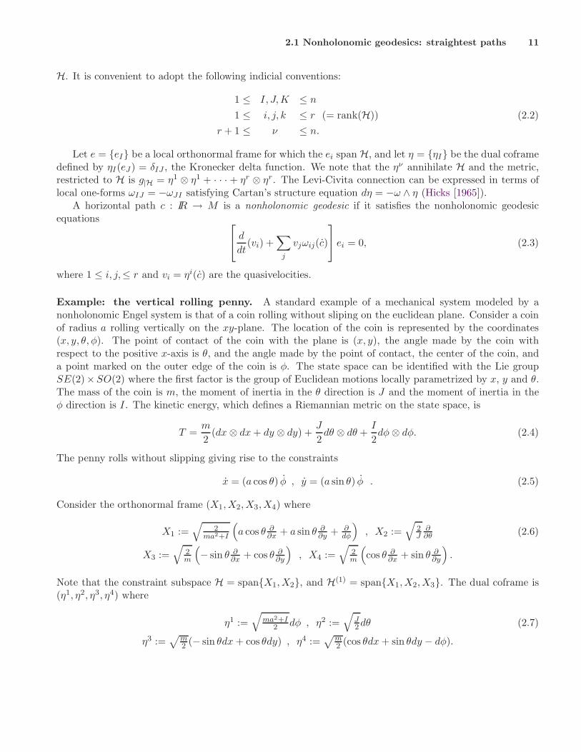
H. It is convenient to adopt the following indicial conventions:
1 ≤ I, J,K ≤ n
1 ≤ i, j, k ≤ r (= rank(H)) (2.2)
r + 1 ≤ ν ≤ n.
Let e = eI be a local orthonormal frame for which the ei span H, and let η = ηI be the dual coframedefined by ηI(eJ) = δIJ , the Kronecker delta function. We note that the ην annihilate H and the metric,restricted to H is g|H = η1 ⊗ η1 + · · · + ηr ⊗ ηr. The Levi-Civita connection can be expressed in terms oflocal one-forms ωIJ = −ωJI satisfying Cartan’s structure equation dη = −ω ∧ η (Hicks [1965]).
A horizontal path c : IR → M is a nonholonomic geodesic if it satisfies the nonholonomic geodesicequations
d
dt(vi) +
∑
j
vjωij(c)
ei = 0, (2.3)
where 1 ≤ i, j,≤ r and vi = ηi(c) are the quasivelocities.
Example: the vertical rolling penny. A standard example of a mechanical system modeled by anonholonomic Engel system is that of a coin rolling without sliping on the euclidean plane. Consider a coinof radius a rolling vertically on the xy-plane. The location of the coin is represented by the coordinates(x, y, θ, φ). The point of contact of the coin with the plane is (x, y), the angle made by the coin withrespect to the positive x-axis is θ, and the angle made by the point of contact, the center of the coin, anda point marked on the outer edge of the coin is φ. The state space can be identified with the Lie groupSE(2)×SO(2) where the first factor is the group of Euclidean motions locally parametrized by x, y and θ.The mass of the coin is m, the moment of inertia in the θ direction is J and the moment of inertia in theφ direction is I. The kinetic energy, which defines a Riemannian metric on the state space, is
T =m
2(dx⊗ dx + dy ⊗ dy) +
J
2dθ ⊗ dθ +
I
2dφ⊗ dφ. (2.4)
The penny rolls without slipping giving rise to the constraints
x = (a cos θ) φ , y = (a sin θ) φ . (2.5)
Consider the orthonormal frame (X1,X2,X3,X4) where
X1 :=√
2ma2+I
(
a cos θ ∂∂x + a sin θ ∂
∂y + ∂dφ
)
, X2 :=√
2J
∂∂θ (2.6)
X3 :=√
2m
(
− sin θ ∂∂x + cos θ ∂
∂y
)
, X4 :=√
2m
(
cos θ ∂∂x + sin θ ∂
∂y
)
.
Note that the constraint subspace H = spanX1,X2, and H(1) = spanX1,X2,X3. The dual coframe is(η1, η2, η3, η4) where
η1 :=√
ma2+I2 dφ , η2 :=
√
J2 dθ (2.7)
η3 :=√
m2 (− sin θdx + cos θdy) , η4 :=
√
m2 (cos θdx + sin θdy − dφ).
2.2 Equivalence problem of nonholonomic geometry 12
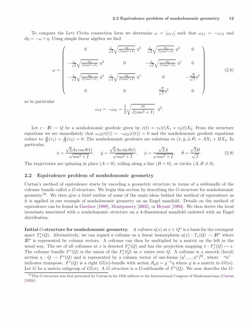
To compute the Levi Civita connection form we determine ω = [ωIJ ] such that ωIJ = −ωJI anddη = −ω ∧ η. Using simple linear algebra we find
ω =
0 1√2
√
mJ(ma2+I)
η3 1√2
√
mJ(ma2+I)
η2 0
− 1√2
√
mJ(ma2+I)
η3 0 − 1√2
√
mJ(ma2+I)
η1 0
− 1√2
√
mJ(ma2+I) η2 1√
2
√
mJ(ma2+I) η1 0 −
√2√Jη2
0 0√
2√Jη2 0
(2.8)
so in particular
ω12 = −ω21 =1
2
√
m
J(ma2 + I)η3.
Let c : IR → Q be a nonholonomic geodesic given by c(t) = v1(t)X1 + v2(t)X2. From the structureequations we see immediately that ω12(c(t)) = −ω21(c(t)) = 0 and the nonholonomic geodesic equationsreduce to d
dt(v1) = ddt(v2) = 0. The nonholonomic geodesics are solutions to (x, y, φ, θ) = AX1 + BX2. In
particular,
x =
√2Aa cos θ(t)√
ma2 + I, y =
√2Aa sin θ(t)√
ma2 + I, φ =
√2A√
ma2 + I, θ =
√2B√J
. (2.9)
The trajectories are spinning in place (A = 0), rolling along a line (B = 0), or circles (A,B 6= 0).
2.2 Equivalence problem of nonholonomic geometry
Cartan’s method of equivalence starts by encoding a geometric structure in terms of a subbundle of thecoframe bundle called a G-structure. We begin this section by describing the G-structure for nonholonomicgeometry16. We then give a brief outline of some of the main ideas behind the method of equivalence asit is applied in our example of nonholonomic geometry on an Engel manifold. Details on the method ofequivalence can be found in Gardner [1989], Montgomery [2002], or Bryant [1994]. We then derive the localinvariants associated with a nonholonomic structure on a 4-dimensional manifold endowed with an Engeldistribution.
Initial G-structure for nonholonomic geometry. A coframe η(x) at x ∈ Qn is a basis for the cotangentspace T ∗
x (Q). Alternatively, we can regard a coframe as a linear isomorphism η(x) : Tx(Q) → IRn whereIRn is represented by column vectors. A coframe can then be multiplied by a matrix on the left in theusual way. The set of all coframes at x is denoted F ∗
x (Q) and has the projection mapping π : F ∗x (Q) 7→ x.
The coframe bundle F ∗(Q) is the union of the F ∗x (Q) as x varies over Q. A coframe is a smooth (local)
section η : Q → F ∗(Q) and is represented by a column vector of one-forms (η1, ..., ηn)tr, where “tr”indicates transpose. F ∗(Q) is a right Gl(n)-bundle with action Rgη = g−1η where g is a matrix in Gl(n).Let G be a matrix subgroup of Gl(n). A G-structure is a G-subbundle of F ∗(Q). We now describe the G-
16This G-structure was first presented by Cartan in his 1928 address to the International Congress of Mathematicians (Cartan[1928])
2.2 Equivalence problem of nonholonomic geometry 13
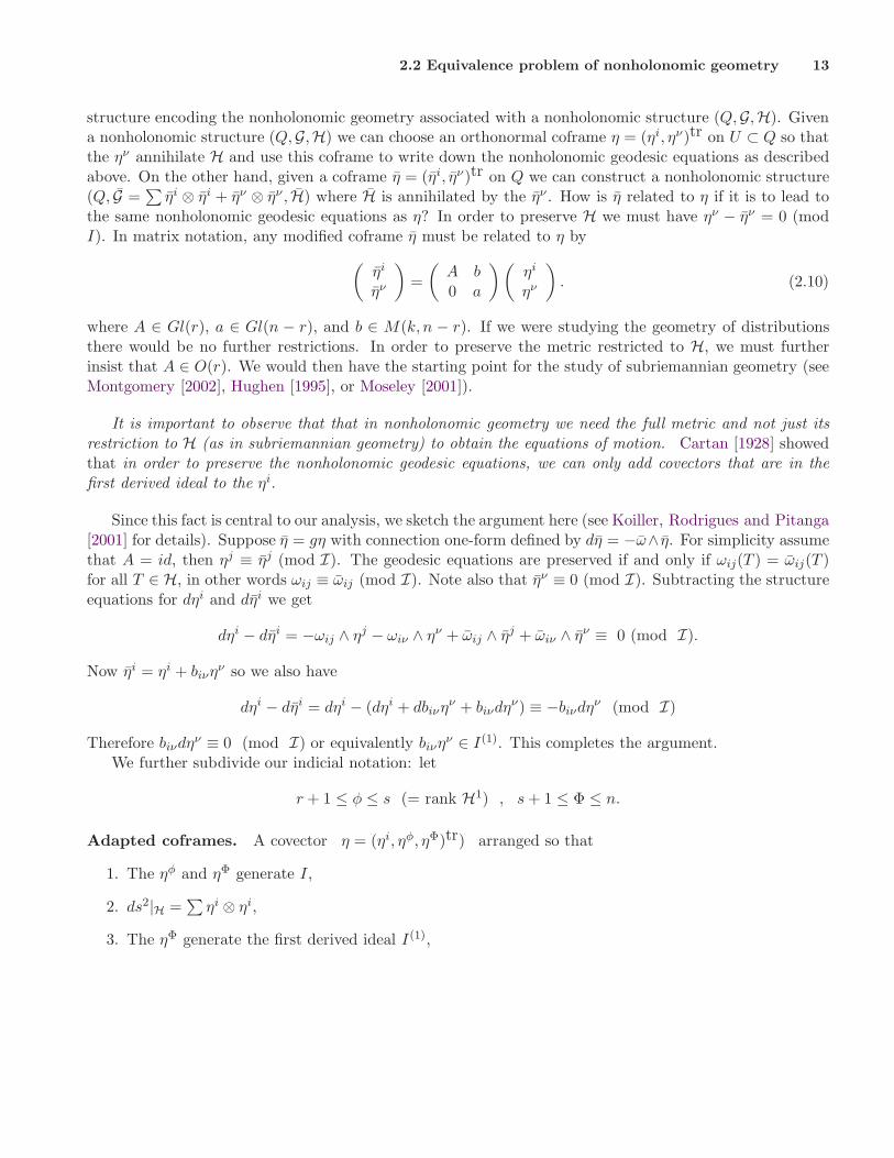
structure encoding the nonholonomic geometry associated with a nonholonomic structure (Q,G,H). Givena nonholonomic structure (Q,G,H) we can choose an orthonormal coframe η = (ηi, ην)tr on U ⊂ Q so thatthe ην annihilate H and use this coframe to write down the nonholonomic geodesic equations as describedabove. On the other hand, given a coframe η = (ηi, ην)tr on Q we can construct a nonholonomic structure(Q, G =
∑
ηi ⊗ ηi + ην ⊗ ην , H) where H is annihilated by the ην . How is η related to η if it is to lead tothe same nonholonomic geodesic equations as η? In order to preserve H we must have ην − ην = 0 (modI). In matrix notation, any modified coframe η must be related to η by
(
ηi
ην
)
=
(
A b0 a
)(
ηi
ην
)
. (2.10)
where A ∈ Gl(r), a ∈ Gl(n − r), and b ∈ M(k, n − r). If we were studying the geometry of distributionsthere would be no further restrictions. In order to preserve the metric restricted to H, we must furtherinsist that A ∈ O(r). We would then have the starting point for the study of subriemannian geometry (seeMontgomery [2002], Hughen [1995], or Moseley [2001]).
It is important to observe that that in nonholonomic geometry we need the full metric and not just itsrestriction to H (as in subriemannian geometry) to obtain the equations of motion. Cartan [1928] showedthat in order to preserve the nonholonomic geodesic equations, we can only add covectors that are in thefirst derived ideal to the ηi.
Since this fact is central to our analysis, we sketch the argument here (see Koiller, Rodrigues and Pitanga[2001] for details). Suppose η = gη with connection one-form defined by dη = −ω∧ η. For simplicity assumethat A = id, then ηj ≡ ηj (mod I). The geodesic equations are preserved if and only if ωij(T ) = ωij(T )for all T ∈ H, in other words ωij ≡ ωij (mod I). Note also that ην ≡ 0 (mod I). Subtracting the structureequations for dηi and dηi we get
dηi − dηi = −ωij ∧ ηj − ωiν ∧ ην + ωij ∧ ηj + ωiν ∧ ην ≡ 0 (mod I).
Now ηi = ηi + biνην so we also have
dηi − dηi = dηi − (dηi + dbiνην + biνdην) ≡ −biνdην (mod I)
Therefore biνdην ≡ 0 (mod I) or equivalently biνην ∈ I(1). This completes the argument.
We further subdivide our indicial notation: let
r + 1 ≤ φ ≤ s (= rank H1) , s + 1 ≤ Φ ≤ n.
Adapted coframes. A covector η = (ηi, ηφ, ηΦ)tr) arranged so that
1. The ηφ and ηΦ generate I,
2. ds2|H =∑
ηi ⊗ ηi,
3. The ηΦ generate the first derived ideal I(1),
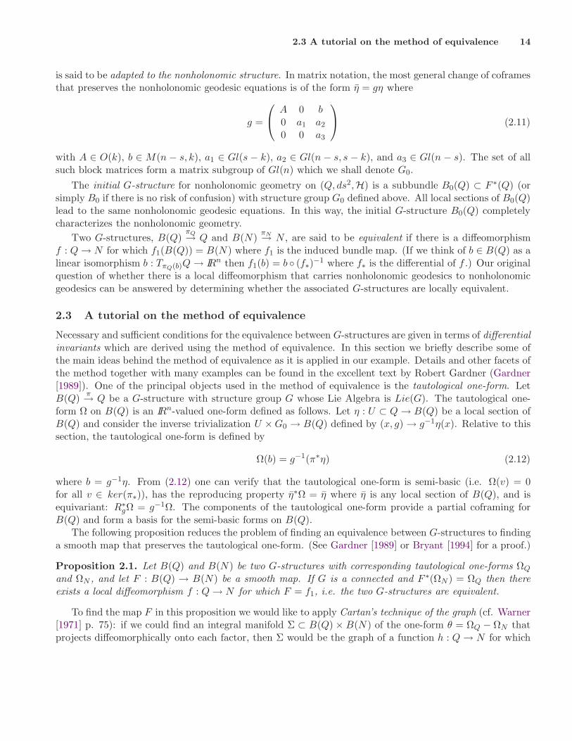
2.3 A tutorial on the method of equivalence 14
is said to be adapted to the nonholonomic structure. In matrix notation, the most general change of coframesthat preserves the nonholonomic geodesic equations is of the form η = gη where
g =
A 0 b0 a1 a2
0 0 a3
(2.11)
with A ∈ O(k), b ∈ M(n − s, k), a1 ∈ Gl(s − k), a2 ∈ Gl(n − s, s − k), and a3 ∈ Gl(n − s). The set of allsuch block matrices form a matrix subgroup of Gl(n) which we shall denote G0.
The initial G-structure for nonholonomic geometry on (Q, ds2,H) is a subbundle B0(Q) ⊂ F ∗(Q) (orsimply B0 if there is no risk of confusion) with structure group G0 defined above. All local sections of B0(Q)lead to the same nonholonomic geodesic equations. In this way, the initial G-structure B0(Q) completelycharacterizes the nonholonomic geometry.
Two G-structures, B(Q)πQ→ Q and B(N)
πN→ N , are said to be equivalent if there is a diffeomorphismf : Q→ N for which f1(B(Q)) = B(N) where f1 is the induced bundle map. (If we think of b ∈ B(Q) as alinear isomorphism b : TπQ(b)Q→ IRn then f1(b) = b (f∗)−1 where f∗ is the differential of f .) Our originalquestion of whether there is a local diffeomorphism that carries nonholonomic geodesics to nonholonomicgeodesics can be answered by determining whether the associated G-structures are locally equivalent.
2.3 A tutorial on the method of equivalence
Necessary and sufficient conditions for the equivalence between G-structures are given in terms of differentialinvariants which are derived using the method of equivalence. In this section we briefly describe some ofthe main ideas behind the method of equivalence as it is applied in our example. Details and other facets ofthe method together with many examples can be found in the excellent text by Robert Gardner (Gardner[1989]). One of the principal objects used in the method of equivalence is the tautological one-form. LetB(Q)
π→ Q be a G-structure with structure group G whose Lie Algebra is Lie(G). The tautological one-form Ω on B(Q) is an IRn-valued one-form defined as follows. Let η : U ⊂ Q→ B(Q) be a local section ofB(Q) and consider the inverse trivialization U ×G0 → B(Q) defined by (x, g)→ g−1η(x). Relative to thissection, the tautological one-form is defined by
Ω(b) = g−1(π∗η) (2.12)
where b = g−1η. From (2.12) one can verify that the tautological one-form is semi-basic (i.e. Ω(v) = 0for all v ∈ ker(π∗)), has the reproducing property η∗Ω = η where η is any local section of B(Q), and isequivariant: R∗
gΩ = g−1Ω. The components of the tautological one-form provide a partial coframing forB(Q) and form a basis for the semi-basic forms on B(Q).
The following proposition reduces the problem of finding an equivalence between G-structures to findinga smooth map that preserves the tautological one-form. (See Gardner [1989] or Bryant [1994] for a proof.)
Proposition 2.1. Let B(Q) and B(N) be two G-structures with corresponding tautological one-forms ΩQ
and ΩN , and let F : B(Q) → B(N) be a smooth map. If G is a connected and F ∗(ΩN ) = ΩQ then thereexists a local diffeomorphism f : Q→ N for which F = f1, i.e. the two G-structures are equivalent.
To find the map F in this proposition we would like to apply Cartan’s technique of the graph (cf. Warner[1971] p. 75): if we could find an integral manifold Σ ⊂ B(Q)× B(N) of the one-form θ = ΩQ − ΩN thatprojects diffeomorphically onto each factor, then Σ would be the graph of a function h : Q→ N for which
2.3 A tutorial on the method of equivalence 15
h∗1ΩN = ΩQ. By the above proposition the G-structures would then be equivalent. We generally cannot
apply this idea directly because ΩQ and ΩN do not provide full coframes on B(Q) and B(N) as is requiredin the technique of the graph. In the example of nonholonomic geometry on Engel manifolds, and indeed inmany important examples (see Gardner [1989], Hughen [1995], Moseley [2001], Montgomery [2002], Ehlers[2002]), application of the method of equivalence leads to a new G-structure called an e-structure. Ane-structure is a G-structure endowed with a canonical coframe.
Differentiating both sides of (2.12) one can verify that dΩ satisfies the structure equation
dΩ = −α ∧ Ω + T (2.13)
where T is a semi-basic two-form on B(Q) and α is a called a pseudoconnection: a Lie(G)-valued one-formon B(Q) that agrees with the Mauer-Cartan form on vertical vectorfields. Here, Lie(G) is the Lie Algebraof G. Summarizing,
Pseudoconnection : α = g−1dg + semibasic Lie(G)−valued one form. (2.14)
The components of the pseudoconnection together with the tautological one-form do provide a fullcoframe on the G-structure, but unlike the tautological one-form, the pseudoconnection is not canonicallydefined. Understanding how changes in the pseudoconnection affect the torsion is at the heart of the methodof equivalence.
For any G-structure, that part of the torsion that is left unchanged under all possible changes ofpseudoconnection is known as the intrinsic torsion. The intrinsic torsion is the only first order differentialinvariant of the G-structure (Gardner [1989]). As an example, the intrinsic torsion for the G-structure Bof a general distribution (equation 2.10) is the dual curvature of the distribution (Cartan [1910], see alsoMontgomery [2002]). In the case of a rank two distribution on a four dimensional manifold, the structureequations for the tautological one-form Ω are
d
Ω1
Ω2
Ω3
Ω4
= −
A11 A12 β13 β14
A21 A22 β23 β24
0 0 α33 α34
0 0 α34 α44
∧
Ω1
Ω2
Ω3
Ω4
+
T 1
T 2
T 3
T 4
(2.15)
where T I =∑
J<K T IJKΩJ ∧ΩK with T I
JK : B → IR. The intrinsic torsion consists of the terms T 312Ω
1 ∧Ω2
and T 412Ω
1 ∧ Ω2. Note that the distribution is integrable if and only if T 312 = T 4
12 = 0.
Reduction and prolongation. There are two major steps in the equivalence method: prolongation andreduction (see Gardner [1989] or Montgomery [2002]). In the case of nonholonomic geometry on an Engelmanifold a sequence of reductions lead to an e-structure. A brief outline of the reduction procedure isas follows. The first step involves writing out the structure equations for the tautological one-form Ω.A semi-basic Lie(G)-valued one-form is added to the pseudoconnection to make the torsion as simple aspossible. Gardner [1989] calls this step absorption of torsion. The action of G on the torsion is deducedby differentiating both sides of the identity R∗
g(Ω) = g−1Ω. The action of G is used to simplify part of thetorsion. The isotropy subgroup of that choice of simplified torsion is then the structure group of the reducedG-structure. In the case of nonholonomic geometry on an Engel manifold this procedure is repeated untilan e-structure is obtained.
2.4 The nonholonomic geometry of an Engel manifold. 16
Suppose that Ω is the canonical coframing on the resulting a manifold B. The Ωi form a basis for theone-forms on B so we can write
dΩI =∑
J<K
cIJKΩJ ∧ ΩK . (2.16)
Relationships between the cIJK are found by differentiating this equation. The resulting torsion functions
provide the “complete invariants” for the geometric structure (see Gardner [1989] p.59, Bryant [1994] pp.9-10, or Cartan [2001]).
Many important examples have integrable e-structures. An e-structure is integrable if the cIJK are
constant (Gardner [1989]). In this case we can apply the following result from Montgomery [2002]:
Lemma 2.2. Let B be an n-dimensional manifold endowed with a coframing Ω. Then the (local) group Gof diffeomorphisms of B that preserves this coframing is a finite-dimensional (local) Lie group of dimensionat most n. The bound n is achieved if and only if the e-structure is integrable. In this case the cI
JK are thestructure constants of G, G acts freely and transitively on B, and the coframe can be identified with the leftinvariant one-forms on G.
The Jacobi identities are found by differentiating dΩi =∑
J<K cIJKΩJ ∧ ΩK . Lie’s third fundamental
theorem then implies that we can, at least in principle, reconstruct the group G using the structure constants.In some circumstances one can also conclude that B itself is a Lie group (see Gardner [1989] p.72).
2.4 The nonholonomic geometry of an Engel manifold.
The initial G structure for nonholonomic geometry on Q,G,H where H is an Engel distribution on afour-dimensional manifold M is the subbundle B0 ⊂ F ∗(Q) with structure group G0 consisting of matricesof the form
A11 A12 0 B14
A21 A22 0 B24
0 0 a33 a34
0 0 0 a44
(2.17)
where A = [AIJ ] ∈ O(2), a33a44 6= 0, and B14 and B24 are arbitrary.Let Ω = (Ω1,Ω2,Ω3,Ω4)tr be the tautological one-form on B0. The structure equations are
d
Ω1
Ω2
Ω3
Ω4
= −
0 γ 0 β14
−γ 0 0 β24
0 0 α33 α34
0 0 0 α44
∧
Ω1
Ω2
Ω3
Ω4
+
T 113Ω
1 ∧ Ω3 + T 123Ω
2 ∧Ω3
T 213Ω
1 ∧ Ω3 + T 223Ω
2 ∧Ω3
T 312Ω
1 ∧Ω2
T 413Ω
1 ∧ Ω3 + T 423Ω
2 ∧Ω3
(2.18)
where we have chosen the pseudoconnection so that the remaining T ijk are zero. Ω4 ∈ I(1) so dΩ4 = 0 mod
(Ω3,Ω4) and we must therefore have T 412 = 0. Also, Ω3 /∈ I(1) so dΩ3 6= 0 mod (Ω3,Ω4) therefore the torsion
function T 312 cannot equal zero. The pseudo-connection for this choice of torsion is not unique. We can, for
instance, add arbitrary multiples of Ω4 to the βi4 and αi4.Following Cartan’s prescription, we investigate the induced action of G0 on the torsion. Let g ∈ G0.
To simplify notation, functions and forms pulled back by Rg will be indicated by a hat so, for instance,
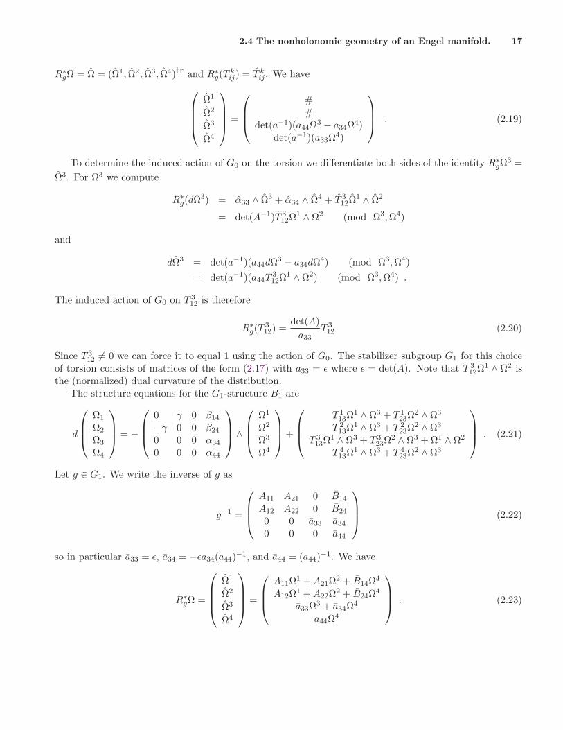
2.4 The nonholonomic geometry of an Engel manifold. 17
R∗gΩ = Ω = (Ω1, Ω2, Ω3, Ω4)tr and R∗
g(Tkij) = T k
ij . We have
Ω1
Ω2
Ω3
Ω4
=
##
det(a−1)(a44Ω3 − a34Ω
4)det(a−1)(a33Ω
4)
. (2.19)
To determine the induced action of G0 on the torsion we differentiate both sides of the identity R∗gΩ
3 =
Ω3. For Ω3 we compute
R∗g(dΩ3) = α33 ∧ Ω3 + α34 ∧ Ω4 + T 3
12Ω1 ∧ Ω2
= det(A−1)T 312Ω
1 ∧ Ω2 (mod Ω3,Ω4)
and
dΩ3 = det(a−1)(a44dΩ3 − a34dΩ4) (mod Ω3,Ω4)
= det(a−1)(a44T312Ω
1 ∧Ω2) (mod Ω3,Ω4) .
The induced action of G0 on T 312 is therefore
R∗g(T
312) =
det(A)
a33T 3
12 (2.20)
Since T 312 6= 0 we can force it to equal 1 using the action of G0. The stabilizer subgroup G1 for this choice
of torsion consists of matrices of the form (2.17) with a33 = ǫ where ǫ = det(A). Note that T 312Ω
1 ∧ Ω2 isthe (normalized) dual curvature of the distribution.
The structure equations for the G1-structure B1 are
d
Ω1
Ω2
Ω3
Ω4
= −
0 γ 0 β14
−γ 0 0 β24
0 0 0 α34
0 0 0 α44
∧
Ω1
Ω2
Ω3
Ω4
+
T 113Ω
1 ∧ Ω3 + T 123Ω
2 ∧Ω3
T 213Ω
1 ∧ Ω3 + T 223Ω
2 ∧Ω3
T 313Ω
1 ∧ Ω3 + T 323Ω
2 ∧ Ω3 + Ω1 ∧ Ω2
T 413Ω
1 ∧ Ω3 + T 423Ω
2 ∧Ω3
. (2.21)
Let g ∈ G1. We write the inverse of g as
g−1 =
A11 A21 0 B14
A12 A22 0 B24
0 0 a33 a34
0 0 0 a44
(2.22)
so in particular a33 = ǫ, a34 = −ǫa34(a44)−1, and a44 = (a44)
−1. We have
R∗gΩ =
Ω1
Ω2
Ω3
Ω4
=
A11Ω1 + A21Ω
2 + B14Ω4
A12Ω1 + A22Ω
2 + B24Ω4
a33Ω3 + a34Ω
4
a44Ω4
. (2.23)
2.4 The nonholonomic geometry of an Engel manifold. 18
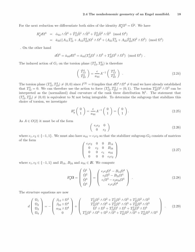
For the next reduction we differentiate both sides of the identity R∗gΩ
4 = Ω4. We have
R∗gdΩ4 = α44 ∧ Ω4 + T 4
13Ω1 ∧ Ω3 + T 4
23Ω2 ∧ Ω3 (mod Ω4)
= a33((A11T413 + A12T
423)Ω
1 ∧ Ω3 + (A21T413 + A22T
423)Ω
2 ∧Ω3) (mod Ω4)
. On the other hand
dΩ4 = a44dΩ4 = a44(T413Ω
1 ∧Ω3 + T 423Ω
2 ∧ Ω3) (mod Ω4) .
The induced action of G1 on the torsion plane (T 413, T
423) is therefore
(
T 413
T 423
)
=ǫ
a44A−1
(
T 413
T 423
)
. (2.24)
The torsion plane (T 413, T
423) 6= (0, 0) since I(2) = 0 implies that dΩ4∧Ω4 6= 0 and we have already established
that T 412 = 0. We can therefore use the action to force (T 4
13, T423) = (0, 1). The torsion T 4
23Ω2 ∧ Ω3 can be
interpreted as the (normalized) dual curvature of the rank three distribution H1. The statement that(T 4
13, T423) 6= (0, 0) is equivalent to H not being integrable. To determine the subgroup that stabilizes this
choice of torsion, we investigate
R∗g
(
01
)
=ǫ
a44A−1
(
01
)
=
(
01
)
. (2.25)
As A ∈ O(2) it must be of the form(
ǫ1ǫ2 00 ǫ2
)
(2.26)
where ǫ1, ǫ2 ∈ −1, 1. We must also have a44 = ǫ1ǫ2 so that the stabilizer subgroup G2 consists of matricesof the form
ǫ1ǫ2 0 0 B14
0 ǫ2 0 B24
0 0 ǫ1 a34
0 0 0 ǫ1ǫ2
(2.27)
where ǫ1, ǫ2 ∈ −1, 1 and B14, B24 and a34 ∈ IR. We compute
R∗gΩ =
Ω1
Ω2
Ω3
Ω4
=
ǫ1ǫ2Ω1 −B14Ω
4
ǫ2Ω2 −B24Ω
4
ǫ1Ω3 − ǫ2a34Ω
4
ǫ1ǫ2Ω4
. (2.28)
The structure equations are now
d
Ω1
Ω2
Ω3
Ω4
= −
β14 ∧ Ω4
β24 ∧ Ω4
α34 ∧Ω4
0
+
T 112Ω
1 ∧ Ω2 + T 113Ω
1 ∧ Ω3 + T 123Ω
2 ∧ Ω3
T 212Ω
1 ∧ Ω2 + T 213Ω
1 ∧ Ω3 + T 223Ω
2 ∧ Ω3
Ω1 ∧ Ω2 + T 313Ω
1 ∧ Ω3 + T 323Ω
2 ∧ Ω3
T 414Ω
1 ∧ Ω4 + Ω2 ∧ Ω3 + T 424Ω
2 ∧ Ω4 + T 434Ω
3 ∧ Ω4
. (2.29)
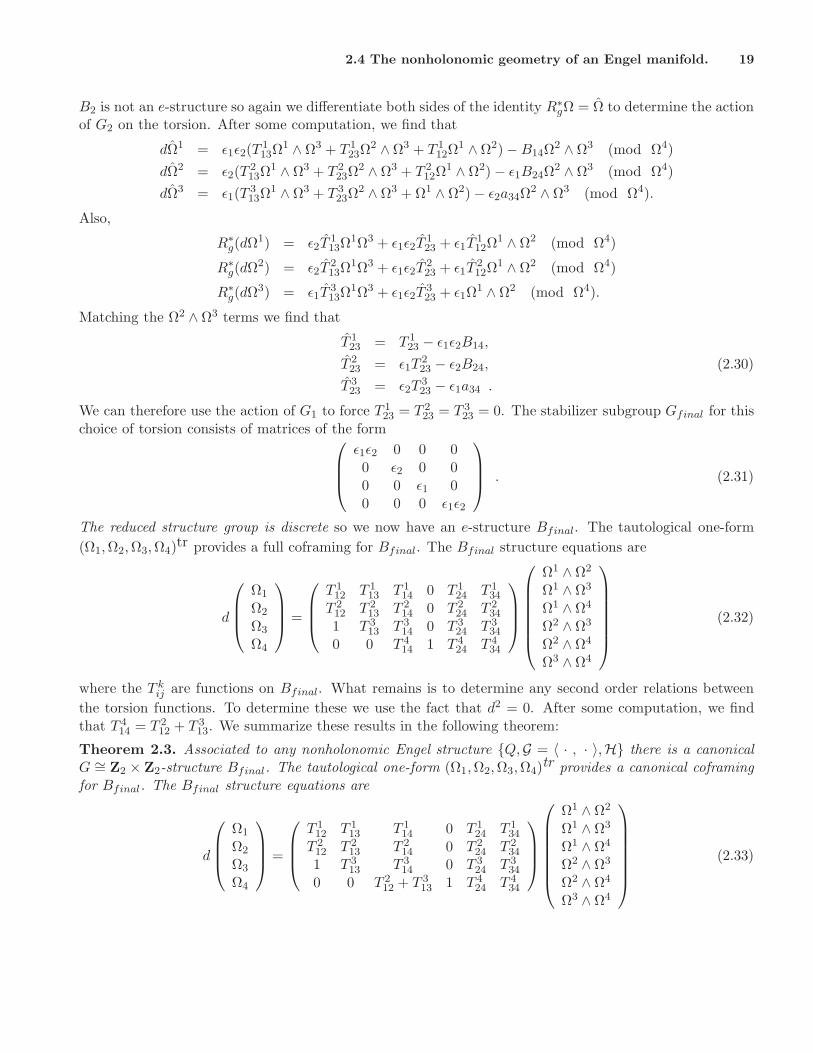
2.4 The nonholonomic geometry of an Engel manifold. 19
B2 is not an e-structure so again we differentiate both sides of the identity R∗gΩ = Ω to determine the action
of G2 on the torsion. After some computation, we find that
dΩ1 = ǫ1ǫ2(T113Ω
1 ∧ Ω3 + T 123Ω
2 ∧Ω3 + T 112Ω
1 ∧Ω2)−B14Ω2 ∧ Ω3 (mod Ω4)
dΩ2 = ǫ2(T213Ω
1 ∧ Ω3 + T 223Ω
2 ∧ Ω3 + T 212Ω
1 ∧ Ω2)− ǫ1B24Ω2 ∧ Ω3 (mod Ω4)
dΩ3 = ǫ1(T313Ω
1 ∧ Ω3 + T 323Ω
2 ∧ Ω3 + Ω1 ∧ Ω2)− ǫ2a34Ω2 ∧ Ω3 (mod Ω4).
Also,
R∗g(dΩ1) = ǫ2T
113Ω
1Ω3 + ǫ1ǫ2T123 + ǫ1T
112Ω
1 ∧ Ω2 (mod Ω4)
R∗g(dΩ2) = ǫ2T
213Ω
1Ω3 + ǫ1ǫ2T223 + ǫ1T
212Ω
1 ∧ Ω2 (mod Ω4)
R∗g(dΩ3) = ǫ1T
313Ω
1Ω3 + ǫ1ǫ2T323 + ǫ1Ω
1 ∧ Ω2 (mod Ω4).
Matching the Ω2 ∧ Ω3 terms we find that
T 123 = T 1
23 − ǫ1ǫ2B14,
T 223 = ǫ1T
223 − ǫ2B24, (2.30)
T 323 = ǫ2T
323 − ǫ1a34 .
We can therefore use the action of G1 to force T 123 = T 2
23 = T 323 = 0. The stabilizer subgroup Gfinal for this
choice of torsion consists of matrices of the form
ǫ1ǫ2 0 0 00 ǫ2 0 00 0 ǫ1 00 0 0 ǫ1ǫ2
. (2.31)
The reduced structure group is discrete so we now have an e-structure Bfinal. The tautological one-form
(Ω1,Ω2,Ω3,Ω4)tr provides a full coframing for Bfinal. The Bfinal structure equations are
d
Ω1
Ω2
Ω3
Ω4
=
T 112 T 1
13 T 114 0 T 1
24 T 134
T 212 T 2
13 T 214 0 T 2
24 T 234
1 T 313 T 3
14 0 T 324 T 3
34
0 0 T 414 1 T 4
24 T 434
Ω1 ∧Ω2
Ω1 ∧Ω3
Ω1 ∧Ω4
Ω2 ∧Ω3
Ω2 ∧Ω4
Ω3 ∧Ω4
(2.32)
where the T kij are functions on Bfinal. What remains is to determine any second order relations between
the torsion functions. To determine these we use the fact that d2 = 0. After some computation, we findthat T 4
14 = T 212 + T 3
13. We summarize these results in the following theorem:
Theorem 2.3. Associated to any nonholonomic Engel structure Q,G = 〈 · , · 〉,H there is a canonicalG ∼= Z2 × Z2-structure Bfinal. The tautological one-form (Ω1,Ω2,Ω3,Ω4)
tr provides a canonical coframingfor Bfinal. The Bfinal structure equations are
d
Ω1
Ω2
Ω3
Ω4
=
T 112 T 1
13 T 114 0 T 1
24 T 134
T 212 T 2
13 T 214 0 T 2
24 T 234
1 T 313 T 3
14 0 T 324 T 3
34
0 0 T 212 + T 3
13 1 T 424 T 4
34
Ω1 ∧ Ω2
Ω1 ∧ Ω3
Ω1 ∧ Ω4
Ω2 ∧ Ω3
Ω2 ∧ Ω4
Ω3 ∧ Ω4
(2.33)
2.4 The nonholonomic geometry of an Engel manifold. 20
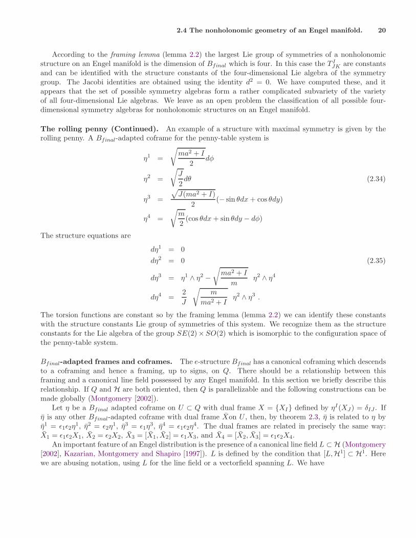
According to the framing lemma (lemma 2.2) the largest Lie group of symmetries of a nonholonomicstructure on an Engel manifold is the dimension of Bfinal which is four. In this case the T I
JK are constantsand can be identified with the structure constants of the four-dimensional Lie algebra of the symmetrygroup. The Jacobi identities are obtained using the identity d2 = 0. We have computed these, and itappears that the set of possible symmetry algebras form a rather complicated subvariety of the varietyof all four-dimensional Lie algebras. We leave as an open problem the classification of all possible four-dimensional symmetry algebras for nonholonomic structures on an Engel manifold.
The rolling penny (Continued). An example of a structure with maximal symmetry is given by therolling penny. A Bfinal-adapted coframe for the penny-table system is
η1 =
√
ma2 + I
2dφ
η2 =
√
J
2dθ (2.34)
η3 =
√
J(ma2 + I)
2(− sin θdx + cos θdy)
η4 =
√
m
2(cos θdx + sin θdy − dφ)
The structure equations are
dη1 = 0
dη2 = 0 (2.35)
dη3 = η1 ∧ η2 −√
ma2 + I
mη2 ∧ η4
dη4 =2
J
√
m
ma2 + Iη2 ∧ η3 .
The torsion functions are constant so by the framing lemma (lemma 2.2) we can identify these constantswith the structure constants Lie group of symmetries of this system. We recognize them as the structureconstants for the Lie algebra of the group SE(2)×SO(2) which is isomorphic to the configuration space ofthe penny-table system.
Bfinal-adapted frames and coframes. The e-structure Bfinal has a canonical coframing which descendsto a coframing and hence a framing, up to signs, on Q. There should be a relationship between thisframing and a canonical line field possessed by any Engel manifold. In this section we briefly describe thisrelationship. If Q and H are both oriented, then Q is parallelizable and the following constructions can bemade globally (Montgomery [2002]).
Let η be a Bfinal adapted coframe on U ⊂ Q with dual frame X = XI defined by ηI(XJ) = δIJ . Ifη is any other Bfinal-adapted coframe with dual frame Xon U , then, by theorem 2.3, η is related to η byη1 = ǫ1ǫ2η
1, η2 = ǫ2η1, η3 = ǫ1η
3, η4 = ǫ1ǫ2η4. The dual frames are related in precisely the same way:
X1 = ǫ1ǫ2X1, X2 = ǫ2X2, X3 = [X1, X2] = ǫ1X3, and X4 = [X2, X3] = ǫ1ǫ2X4.An important feature of an Engel distribution is the presence of a canonical line field L ⊂ H (Montgomery
[2002], Kazarian, Montgomery and Shapiro [1997]). L is defined by the condition that [L,H1] ⊂ H1. Herewe are abusing notation, using L for the line field or a vectorfield spanning L. We have
3 Nonholonomic dynamics: Chaplygin Hamiltonization 21
Corollary 2.4. Let η = ηI be a Bfinal-adapted coframe. Let X = XI be the dual frame defined byηI(XJ ) = δIJ , then L = span(X1).
Proof. Suppose L is spanned by the vectorfield Y = aX1 + bX2. Since η4 annihilates H1 we haveη4([X3, Y ]) = 0. Then
0 = η4([X3, Y ]) = X3η4(Y )− Y η4(X3)− dη4(X3, Y ) = −dη4(X3, Y ).
But dη4 ≡ η2 ∧ η3 mod (η4) so we must have
0 = η2 ∧ η3(X3, Y ) = η2(X3)η3(Y )− η3(X3)η2(Y )
= −η3(X3)η2(Y )
= −b.
L is therefore spanned by X1. This concludes the arguement.There is a natural metric, associated with Bfinal, on Q given by gnat = η1 ⊗ η1 + · · ·η4 ⊗ η4 where
η is any Bfinal-adapted coframe. Clearly all Bfinal-adapted coframes induce this same metric; using thesubriemannian metric gnat|H we form L⊥ within H so that H = L⊕ L⊥. By construction, X2 spans L⊥.
3 Nonholonomic dynamics: Chaplygin Hamiltonization
Historically, Hamiltonization of nonholonomic systems started with Chaplygin’s last multiplier method. Inthe new time, the dynamics obeys Euler-Lagrange equations without extra terms; the gyroscopic force (1.13)“magically” disappers! When after a time reparametrization the compressed system can be described as aHamiltonian system, symplectic techniques can be employed. A number of NH systems have been Hamil-tonized, and some interesting ones are Liouville-integrable, see Veselov and Veselova [1988], Kozlov [2002],Fedorov and Jovanovic [2003], Fedorov [1989], Dragovic, Gajic and Jovanovic [1998], Borisov and Mamaev[2002a], Borisov and Mamaev [2002b], Borisov, Mamaev and Kilin [2002], Borisov and Mamaev [2001], Jovanovic[2003].
3.1 Compression to T ∗S, S = Q/G; existence of invariant measures
We recall from the introduction that the compressed system has a concise almost Hamiltonian
dHφ = iXNHΩNH , ΩNH := ΩT ∗S
can + (J.K) , dΩNH 6= 0 (in general) ,
where ΩT ∗Scan is the canonical 2-form of T ∗S and the (J.K) term is a semi-basic two form, which in general is
non-closed. It combines the momentum J of the G-action on T ∗Q, and the curvature K of the connection.As this is important for the remaining, we outline the derivation (see Koiller, Rios and Ehlers [2002] fordetails). Given the coframe coordinates m, , ǫ(q) in T ∗Q (see 1.5) the Poisson bracket matrix relative toǫI , dmI is
[Λ] = [Ω]−1 =
(
0n In
−In E
)
(3.1)
withEJK = mIdǫI(eJ , eK) = −mIǫI [eJ , eK ] . (3.2)
3.1 Compression to T ∗S, S = Q/G; existence of invariant measures 22
Let us consider the case of a principal bundle π : Qn → Ss with Lie group Gr acting on the left, r = n− s.Recall our convention: capital roman letters I, J,K, etc., run from 1 to n. Lower case roman charactersi, j, k run from 1 to s. Greek characters α, β, γ, etc., run from s + 1 to n.
Fix a connection λ = λ(q) : TqQ→ Lie(G) defining a G-invariant distributionH of horizontal subspaces.Denote by K(q) = dλHor : TqQ×TqQ→ G the curvature 2-form (which is, as well known, Ad-equivariant).Choose a local frame ei on S. For simplicity, we may assume that
ei = ∂/∂si (3.3)
are the coordinate vectorfields of a chart s : S → IRs.Let ei = h(ei) their horizontal lift to Q. We complete to a moving frame of Q with vertical vectors eα
which we will specify in a moment. The dual basis will be denoted ǫi, ǫα and we write pq = miǫi + mαǫα.These are in a sense the “lesser moving” among all the moving frames adapted to this structure. We nowdescribe how the n× n matrix E = (EIJ) looks like in this setting.
i) The s× s block (Eij).
Decompose [ei, ej ] = h[ei, ej ] + V [ei, ej ] = V [ei, ej ] into vertical and horizontal parts. The choice (3.3)is convenient, since ei and ej commute: [ei, ej ] is vertical. Hence
Eij = −pq[ei, ej ] = −mαǫα[ei, ej ] . (3.4)
Now by Cartan’s rule,
K(ei, ej) = eiλ(ej)− ejλ(ei)− λ[ei, ej ] = −λ[ei, ej ] ∈ G
Thus we showed that[ei, ej ]q = −K(ei, ej) · q (3.5)
Moreover, let J : T ∗Q→ Lie(G)∗ the momentum mapping. We have
(J(pq),Kq(ei, ej)) = pq (K(ei, ej).q ) = −pq[ei, ej ] (= Eij)
Theorem 3.1. (The J.K formula)Eij = (J(pq),Kq(ei, ej)) (3.6)
This gives a nice description for this block, under the choice [ei, ej ] = 0. Notice that the functions Eij
depend on s and the components mα, but do not depend on g. This is because the Ad∗-ambiguity of themomentum mapping J is cancelled by the Ad-ambiguity of the curvature K. The other blocks are notneeded here, but we include for completeness.
ii) The r × r block (Eαβ).
Choose a basis Xα for Lie(G). We take eα(q) = Xα · q as the vertical distribution. Choosing a point qo
allows identifying the Lie group G with the fiber containing Gqo, so that id 7→ qo. Through the mappingg ∈ G 7→ gqo ∈ Gqo the vectorfied eα is identified to a right (not left!) invariant vectorfield in G. Thecommutation relations for the eα [eα, eβ ] = −cγ
αβ eγ appear with a minus sign. Therefore
Eαβ = mγcγαβ . (3.7)
3.1 Compression to T ∗S, S = Q/G; existence of invariant measures 23
iii) The s× n block (Eiα).
The vectors [ei, eα] are vertical, but their values depend on the specific principal bundle one is workingwith, and there are some noncanonical choices. Given a section σ : US → Q over the coordinate charts : US → IRm on S, we need to know the coefficients bγ
iα in the expansion
[ei, eα](σ(s)) = bγiα(s) eγ .
ThenEiα(σ(s)) = −mγ bγ
iα(s) . (3.8)
At another point on the fiber, we need the adjoint representation Adg : Lie(G) → Lie(G), X 7→ g−1∗ Xg,
described by a matrix (Aµα(g)) such that
Adg(Xα) = Aµα(g)Xµ . (3.9)
Then[ei, eα](g · σ(s)) = −mγb
γiµ(s)Aµα(g) . (3.10)
The clockwise diagram. Starting on ps ∈ T ∗S we go clockwise to Pq ∈ Leg(H) ⊂ T ∗Q, for some q onthe fiber π−1(s) of Q over s.
H ⊂ TQ −→ Leg(H) ⊂ T ∗QLeg
↑h|
TS ←− T ∗S(Legφ)−1
(3.11)
Taking differentials of all maps in (3.11) we obtain an induced principal connection φ in the bundle G →Leg(H) → T ∗S . Let v,w, z ∈ Tps(T
∗S), V,W,Z horizontal lifts at Pq ∈ Leg(H), and denote by K thecurvature of this induced connection. The following proposition is basically a rephrasing of a result inBates and Sniatycki [1993].
Proposition 3.2.d (J.K)(v,w, z) = cyclic(dJ(V ),K(W,Z)) . (3.12)
Densities of invariant measures and a dimension dependent exponent. A necessary and sufficientcondition for the existence of an invariant measure for compressed Chaplygin systems was obtained byCantrijn, Cortes, de Leon, and de Diego [2002] (Theorem 7.5). Since in T ∗S there is a natural Liouvillemeasure dvol = ds1...dsmdp1...dpm, where (s, p) are coordinates in T ∗S, the density function F produces aneducated guess for a time reparametrization which may Hamiltonize the compressed system. If dim(S) = mand f ΩNH is closed, the time-reparametrized vectorfield XNH/f has the invariant measure fm dvol. XNH
will have the invariant measure fm−1 ds1...dsmdp1...dpm. Working backwards, if a measure density F isknown so that F (s)dvol is an invariant measure for XNH , then the obvious candidate for conformal factoris
f = F (s)1
m−1 . (3.13)
This dimension dependent exponent will be relevant in the Chaplygin marble, see section 3.2.
3.1 Compression to T ∗S, S = Q/G; existence of invariant measures 24
Invariant measures for LR systems. Let Q = G a unimodular Lie group and identify TG ≡ T ∗Gvia the bi-invariant metric. Assume that H ⊂ G is a subgroup acting on the left and preserving thedistribution: Dhg = hDg = hDg (which boils down to Adh−1 D = h−1Dh = D). The Legendre transformLeg : Lie(G) → Lie(G) ≡ Lie∗(G) of a natural, left invariant Lagrangian, is represented by a positivesymmetric transformation A : Lie(G)→ Lie(G), the inertia operator.
For each g ∈ G, let P 1g and P 2
g be, respectively, the projections of Lie(G) relative to the decompositionLie(G) = Adg−1Lie(H) ⊕Adg−1D. We can also think of P 2
g as a map P 2g : Tg G→ D g, projection parallel
to the vertical spaces Lie(H)g. Let P 2g oLegg : Dg → Dg. This map descends to the compressed Legendre
transform Legφs : Ts S → Ts S ≡ T ∗
s S, where S = G/H is the homogeneous space whose metric is inducedby the bi-invariant metric on G. Consider the function
F (s) = detLegφs . (3.14)
The following result is a rephrasing of a theorem by Veselov and Veselova [1988], see also Fedorov and Jovanovic[2003] (Theorem 3.3)17.
Theorem 3.3. The reduced LR-Chaplygin system in the homogeneous space T ∗(G/H) always has theinvariant measure
ν = F (s)−1/2 ds1 · · · dsm dp1 · · · dpm , F (s) = det Legφs . (3.15)
The density can be also calculated by the “dual” formula
F (s) = det(A) det(
P 2g oA−1|g−1Lie(H)g
)
(3.16)
(P 1g is the projection over g−1Lie(H)g parallel to g−1Dg).
The second formula may be easier to use if there are few constraints.
Almost Hamiltonian systems. Let Ω be a non-degenerate (but in general, non-closed) 2-form on M2n,and H be a function on M . Denote (as usual) by X = XH the skew-gradient vectorfield defined byiXΩ = dH. We say XH is almost Hamiltonian. If α is a closed 1-form, the vectorfield X = Xα defined byiXΩ = α is called locally almost Hamiltonian. Distilling a construction in Stanchenko [1985], we formalizean extension of the notion of a conformally symplectic structure.
The 2-form Ω is called H (or α)- affine symplectic if there is a function f > 0 on M and a two form Ωo
such that i) iXΩo ≡ 0 ; ii) Ω− Ωo is non-degenerate, and iii) Ω = f(Ω− Ωo) is closed18.The first condition implies that X does not “see” Ωo. Together with the third, we get Ω(X/f, •) = dH
so the vectorfield X/f is (truly) Hamiltonian with respect to the symplectic form Ω.The closedness condition can be restated as
d(Ω − Ωo) = (Ω − Ωo) ∧ θ , where θ = df/f . (3.17)
When (3.17) holds with α a closed (but not necessarily exact) 1-form, we say that Ω is locally affinesymplectic. The following proposition describes the obstruction to Hamiltonization once f is given.
17We do not need to assume D and Lie(H) to be orthogonal with respect to the bi-invariant metric.18We must admit, however, that we found no example yet where the affine term is really needed. This notwithstanding, at
any point where X 6= 0, the contraction condition yields d = 2n equations on d(d−1)/2 unknowns (local coordinate coefficientsof Ωo). This allows additional freedom to Hamiltonize X rather than just requiring conformality of Ω.
3.2 Examples: Veselova’s system and Chaplygin spheres (marble or rubber) 25
Theorem 3.4. Given a locally almost hamiltonian system (Ω, α) and an educated guess f > 0, an affineterm Ωo exists with d(fΩ− Ωo) = 0 if and only if iX d(fΩ) = 0.
The proof is quite easy. The vectorfield X satisfies iXΩ = α. Since the same equation holds by replacingX by X/f and Ω by fΩ, to expedite notation we may assume f ≡ 1. Let us prove that Ωo exists if iXdΩ = 0.Since d(iX Ω) = dα = 0, we see that the Lie derivative LXΩ = 0. Consider a regular point of X. By theflow box theorem there are coordinates so that X = ∂/∂x1. Since LXΩ = 0, the coefficients of this 2-formdo not depend on the coordinate x1 (but there may exist terms with a dx1 factor). However, our hypothesisi∂/∂x1
dΩ = 0 ensures that there are no terms containing a dx1 factor in dΩ. Thus dΩ can be thought as a3-form in the space of the remaining coordinates. By Poincare’s theorem dΩ = dΩo, where Ωo is a 2-formin the space of the remaining coordinates. Hence iXΩo = 0 and d(Ω−Ωo) = 0, as desired. The converse iseven easier.
3.2 Examples: Veselova’s system and Chaplygin spheres (marble or rubber)
Veselov and Veselova [1986, 1988] considered one of the simplest nonholonomic LR-Chaplygin system, Q =SO(3) with a left invariant metric L = T = 1
2(AΩ,Ω), and subjected to a right invariant constraint which,without loss of generality, can be assumed to be ρ3 = 0. Hence the admissible motions satisfy ω3 = 0, whereω is the angular velocity viewed in the space frame. This is a LR Chaplygin system on S1 → SO(3)→ S2.
Chaplygin’s ball is a sphere of radius r and mass µ, whose center of mass is assumed to be at thegeometric center, but the inertia matrix A = diag(I1, I2, I3) may have unequal entries. Thus its Lagrangianis given by 2L = (AΩ,Ω) + µ(x2 + y2 + z2) . The configuration space is the euclidian group Q = SE(3).
In the case of the marble, the ball rolls without slipping on a horizontal plane, with rotations about the z-axis allowed19. Thus the distribution of admissible velocities is defined by D : z = 0 , x = rω1 , y = −rω2 .Both Lagrangian and constraints are preserved under the action of the euclidian motions in the plane,together with the vertical translations. G = SE(2) × IR acts on Q via
(φ, u, v, w).(R,x, y, z) = (S(φ)R, eiφ(u + iv), z + w) .
The dynamics could be be directly reduced to D/G, see e.g. Zenkov and Bloch [2003], but we will proceedin two stages. First, we Chaplygin-compress the dynamics from TQ to TSO(3) using the translationsubgroup of SE(3), regarding the constraint distribution as an abelian connection on Q with base spaceS = SO(3) and fiber IR3; the connection form is given by
αmarble := (dx− rρ2 , dy + rρ1, dz) . (3.18)
There is another S1 action on Q, this time acting on the first factor only: eiφ(R, z) = (S(φ)R, z). This
action preserves the Lagrangian but does not preserve the distribution: D(S(φ)R,z) 6= eiφ∗ D(R,z). However,
its infinitesimal action is given by the right vectorfield Xr3 ∈ D. Noether’s theorem applies, so pφ = ℓ3
is a constant of motion. Therefore Chaplygin’s marble equations can be reduced, on each level set ℓ3, toT (SO(3)/S1) = TS2.
19Chaplygin [2002] showed that the 3d problem is integrable using elliptic coordinates in the sphere; for n > 3 the problemis open. For basic informations, see Fedorov and Kozlov [1995], p. 147-149, on the 3-d case and p. 153-156 for the generaln-dimensional case. For a detailed account on the algebraic integrability of “Chaplygin’s Chaplygin sphere”, see Duistermaat[2000]. Schneider [2002] analyzed control theoretical aspects.
3.2 Examples: Veselova’s system and Chaplygin spheres (marble or rubber) 26
In the case of Chaplygin’s rubber ball20, rotations about the vertical axis are forbidden (since suchrotations would cause energy dissipation). Here the constraints are defined by a sub-distribution H ⊂ Dwith Cartan’s 2-3-5 growth numbers and in fact defining a connection on SE(2) × IR → Q → S2 with1-form
αrubber := (ρ3 k , dx− rρ2 , dy + rρ1 , dz) . (3.19)
The extrinsic viewpoint For clarity we present the classical, direct derivation of the equations of motion,following the “extrinsic viewpoint” advocated by the Russian Geometric Mechanics school (Borisov and Mamaev[2002a]).
• For the rubber Chaplygin ball (and Veselova’s): in the space frame one has ℓ = τ , where τ = λk isthe torque exerted by the constraint force. The torque is vertical because (τ, ω) = 0 for all ω with thirdcomponent equal to zero. Viewed in the body frame,
L + Ω× L = λγ , (3.20)
Together (1.6), one gets a closed system of ODEs in the space (L, γ) ∈ IR3 × IR3, provided the relationbetween Ω and L is obtained. In Veselova’s example, Ω = A−1L. The multiplier can be eliminated bydifferentiating the constraint equation (Ω, γ) = 0. After a simple computation, one gets
λ =(L,A−1γ ×A−1L)
(γ,A−1γ). (3.21)
Besides the standard integrals of motion 2H = (A−1L,L), (γ, γ) = 1, (A−1L, γ) = 0, Veselov and Veselova[1988] showed that there is a quartic polynomial integral
G = (L,L)− (L, γ)2 (3.22)
and an invariant measure21
µ = f(γ)dL1 ∧ dL2 ∧ dL3 ∧ dγ1 ∧ dγ2 ∧ dγ3 , f(γ) = (A−1γ, γ)−1/2 . (3.23)
• For Chaplygin’s marble: the angular momentum at the contact point, in the space frame ~ℓ is constant.An engineer would argue that both gravity and friction produce no torque at that point; a mathematicianwould use the fact that the admissible vectorfields Vi ∈ H given by
V1 := −r ∂/∂y + Xright1 , V2 := r ∂/∂x + Xright
2 , V3 := Xright3 (3.24)
preserve the Lagrangian, and would invoke NH-Noether’s theorem. Whichever explanation chosen, differ-entiating RL = ℓ = RL and Rγ = k one gets Chaplygin’s equations
L = −Ω× L , γ = −Ω× γ . (3.25)
20This problem was not studied by Chaplygin. For the physical justification, see Neimark and Fufaev [1972] andCendra, Ibort, de Leon, de Diego [2004]. As far as we know its integrability has not yet been established. Formally, Veselova’ssystem is the limit of Chaplygin’s rubber ball as r → 0.
21The level sets of the four integrals are 2-tori, since there are no fixed points in the dynamics. The existence of an invariantmeasure in the tori allows the explicit integration via Jacobi’s theorem. Veselov and Veselova [1988] found a rather unexpectedconnection with Neumann’s problem”.
3.2 Examples: Veselova’s system and Chaplygin spheres (marble or rubber) 27
These two form a coupled system, since again Ω is a linear function of L depending only on γ:
L = Lγ (Ω) = AΩ + µr2γ × (Ω× γ) = AΩ− µr2(γ,Ω)γ , A := A + µr2id (3.26)
A simple way to get this map is to look at the total energy
2T = (ω, ℓ) = (Ω, L) = (AΩ,Ω) + µ(x2 + y2) = (AΩ,Ω) + µr2(ω21 + ω2
2) (3.27)
which can be also written as
2T = (Ω, L) = (AΩ,Ω) + µr2(Ω , γ × (Ω× γ) ) = (Ω , AΩ + µr2γ × (Ω × γ) ) ) . (3.28)
The expression γ× (•× γ) represents the projection in the plane perpendicular to γ, and we get (3.26). Anansatz for the inverse of the map (3.26) is (Duistermaat [2000]),
Ω = Ω(L, γ) = (Lγ)−1(L) = A−1L + α(L)A−1(γ) (3.29)
and one gets the interesting expression for α(L) (which will be used in equation (3.48) and Proposition 3.8):
α(L) = µr2 (γ, A−1L)
1− µr2(γ, A−1 γ). (3.30)
The functionf(γ) := [1− µr2(γ, A−1γ)]−1/2 (3.31)
was found by Chaplygin to be the density of an invariant measure in IR6:
νIR6 = f(γ) dγ1dγ2dγ3dL1dL2dL3 (3.32)
This follows from Veselov’s theorem, as F (γ) = 1−µr2(γ, A−1γ) is (up to a constant factor) the determinantof the linear map Ω 7→ L = L(Ω; γ). For direct proofs of invariance of the measure, see Duistermaat [2000]or Fedorov and Kozlov [1995].
A system of ODE’s for the rubber ball can be derived in a similar fashion. For the angular momentumℓ at the contact point, we get the same equation (3.20) from Veselova’s system, but the relation betweenΩ and L is (3.26), the same as in Chaplygin’s marbe. Differentiating (Ω, γ) = 0 the multiplier can beeliminated.
Hamiltonization of Veselova’s system. The compressed Lagrangian is
Lcomp =1
2(A(γ × γ), γ × γ) , (3.33)
since Ω = γ × γ; the momentum map corresponding to the S1-action is J = ℓ3 = (L, γ). Thus (J.K) =ℓ3 dρ3 = (AΩ, γ) dρ3, where dρ3 is the area form of S2. The compressed Legendre transform is
γ 7→ a =∂L∗
∂γ= γ ×A(γ × γ) .
The nonholonomic 2-form in T ∗S2 is
ΩNH = da ∧ dγ + (A(γ × γ), γ) dρ3 (3.34)
3.2 Examples: Veselova’s system and Chaplygin spheres (marble or rubber) 28
Being a two-degrees of freedom system, a general result from Fedorov and Jovanovic [2003] (Theorem 3.5)garantees that this system is Hamiltonizable. In order to verify that ΩNH is conformally symplectic, it issimpler to use γ themselves as coordinates, that is, we pull back ΩNH to TS2 via Leg∗. We get
ΩNH = d(γ ×A(γ × γ))) ∧ dγ + (γ,A(γ × γ))dρ3 .
Proposition 3.5. Veselova’s system is conformally symplectic, d(fΩNH) = 0, with conformal factor
f = f(γ) = (A−1γ, γ)−1/2 . (3.35)
As expected, it is the density of the Veselovs invariant measure µ = f(γ)dLdγ obtained via Proposition3.3. The orthonormal frame in S2 diagonalizing (3.33) provides explicit coordinates for integration viaHamilton-Jacobi’s method.
Chaplygin’s rubber ball. The dynamics compress to T ∗S2, and by the same general result in Fedorov and Jovanovic[2003], we know in advance that the system is Hamiltonizable. Choose a moving frame e1, e2 in S2. Thehorizontal lift from γ = v1 e1 + v2 e2 to Hor(γ) ∈ T (SE(3)) is easily done via (1.10):
Hor(γ) = v2 (Xr1 − r∂/∂y)− v1 (Xr
2 + r∂/∂x)
Composing dαrubber = (ρ1 ∧ ρ2,−rρ3 ∧ ρ1, rρ2 ∧ ρ3, 0) with Hor, we get Krubber = (dSk, 0, 0, 0), where dS isthe S2 area form. Thus for the term (J.K) we need only the third component of the angular momentum,m3 = (M,γ) = (AΩ, γ), where we insert (1.10) Ω = γ × γ = v2 e1 − v1 e2. Therefore
ΩNH = ΩT ∗S2 + (A(γ × γ), γ) · dS . (3.36)
Here γ = v1 e1 + v2 e2 ∈ TS2 corresponds to pγ = p1θ1 + p2 θ2 via the Legendre map Legcomp of thecompressed Lagrangian
Lcomp =1
2A(v2 e1 − v1 e2, v2 e1 − v1 e2) +
1
2µr2(v2
1 + v22) . (3.37)
Clearly, this system becomes Veselova’s for r = 0. Using Proposition 3.3 and Fedorov’s result for twodegrees of system, we get:
Proposition 3.6. The compressed rubber ball system is Hamiltonizable. The conformal factor is
f = [det Legcomp]−1/2 = (I1I2I3)−1/2
(
(A−1γ, γ) + µ r2[γ22 + γ3
3
I2I3+
γ21 + γ3
3
I1I3+
γ21 + γ3
2
I1I2] +
µ2r4
I1I2I3
)−1/2
.
(3.38)
Proof.22 We checked using spherical coordinates and Mathematica c©.
22We can provide the (short) notebook under request. It should be investigated if the rubber ball problem is integrable.Does a (quartic) integral still exist?
3.3 Chaplygin’s marble is not Hamiltonizable at the T ∗SO(3) level. 29
3.3 Chaplygin’s marble is not Hamiltonizable at the T ∗SO(3) level.
The homogeneous sphere. In a nutshell: the dynamics in the homogeneous case is embarrassinglysimple. The angular velocity in space is constant, so the attitude matrix R evolves as a 1-parameter groupR = exp([ω]t), so Ω and ω are constant. The vector γ(t) describes a circle in the sphere perpendicularto ω, and L(t) the curve given by L(t) = (I + µr2)ω − ω3 γ(t). Provided ℓ is not vertical, L and γ arenever parallel. The invariant tori are always foliated by closed curves and the two frequencies coincide.From the constraint equations we see that the motion of the contact point in the plane is a straight line.Shooting pool with a perfect Chaplygin ball is very dull23. Let us use these simple results as template forour operational system. In terms of the right coframe, we have
ΩNH = dℓ1ρ1 + dℓ2ρ2 + dℓ3ρ3 + ℓ1ρ2ρ3 + ℓ2ρ3ρ1 + ℓ3ρ1ρ2 − µr2(ω2ρ3ρ1 + ω1ρ2ρ3) (3.39)
This formula holds in general. In the nonhomogeneous case one must write ω1 and ω2 in terms of ℓ andR ∈ SO(3): ω = RΩ = RΩγ(R
−1ℓ) which seems to be a quite involved expression, a haunting monsterwe will avoid, until a final confrontation in Proposition 3.8. In the homogeneous case, life is much easier:ω = R 1
κIR−1m = 1I m , so the dependence of ω on R disappears. The Hamiltonian is given by
H =1
2
(
ℓ21 + ℓ2
2
I + µr2
)
+ℓ23
I
where
ℓ1 = (1 +µr2
I)m1 , ℓ2 = (1 +
µr2
I)m2 , ℓ3 = m3 , ω1 =
m1
I, ω2 =
m2
I, ω3 =
m3
I.
To obtain the equations of motion we solve
ω1
ω2
ω3
ℓ1
ℓ2
ℓ3
=
0 0 0 1 0 00 0 0 0 1 00 0 0 0 0 1−1 0 0 0 ℓ3 −Iω2
0 −1 0 −ℓ3 0 −Iω1
0 0 −1 Iω2 −Iω1 0
·
000ω1
ω2
ω3
(3.40)
where we have used Hℓ1 = ℓ1/(I + µr2) = m1/I = ω1 , and similarly, Hℓ2 = ω2 ,Hℓ2 = ω2 . This gives, asexpected:
ℓ1 = (Iω3)Hℓ2 − Iω2Hℓ3 = 0 , ℓ2 = ... = 0 , ℓ3 = ... = 0 .
Thus ωi = mi/I = const , i = 1, 2, 3 and the vectorfield is simply X = ω1Xright1 + ω2X
right2 + ω3X
right3
(no components in the fiber directions ∂/∂mi). We now use Theorem 3.4. Using m as coordinates, thenonholonomic two form is given by
ΩNH = (1 +µr2
I) (dm1ρ1 + dm2ρ2) + dm3ρ3 + (m1ρ2ρ3 + m2ρ3ρ1 + m3ρ1ρ2)
23We found the following relevant information in www.ot.com/skew/five/myths.html (Top Ten Myths in Pool or the Lawsof Physics Do Apply): “4. If the cue is kept level, contacting the cueball purely left or right of its center will make it curveas it rolls. (No! The rolling cue ball can have two completely independent components to its angular momentum. Basically,this means that it can rotate in the manner of a top while rolling slowly forward along a straight line. In general, spin on acue ball is of two types; follow/draw is the spin like tires on a car, while English is the spin like a child’s toy ’top’. Seperately,neither one will make a ball curve! If they are combined - e.g., strike low-left giving left English and draw - then the spin iscalled masse (mass-ay), and the ball will curve as it travels.)”
3.4 Chaplygin’s marble: reduction to T ∗S2 30
so that dΩNH = −µr2
I (dm1ρ2ρ3 + dm2ρ3ρ1) . It is easy to see that the equation dΩNH = ΩNH ∧ α has nosolution whatsoever. Indeed, suppose α = A1dm1 + A2dm2 + A3dm3 + B1ρ1 + B2ρ2 + B3ρ3 . Taking theexterior product, and looking at terms like dm1dm2ρ2 we see that all the A’s must be zero. Examining thecoefficient of ρ1ρ2ρ3 we get B1m1 + B2m2 + B3m3 ≡ 0 so all the B’s are also zero.
Hence the homogeneous Chaplygin sphere, as simple at it can be, has no conformal symplectic structure!In fact, it does not have an affine symplectic structure either. A short calculation shows that
iXdΩNH =µr2
I2(−dm1m2ρ3 + dm1ρ2m3 − dm2m3ρ1 + dm2ρ3m1) 6= 0.
By continuity, for sufficiently close but different inertia coefficients the inequalities persists. We havealso done the calculation for the non homogeneous case and things only get worse. But, it still remains apossibility: is the reduced system to T ∗S2 Hamiltonizable? The impatient reader can go directly to Theorem3.8.
3.4 Chaplygin’s marble: reduction to T ∗S2
Using (1.8), L = a× γ + ℓ3 γ, Chaplygin’s marble equations in (L, γ)-space directly reduce to T ∗S2:
γ = γ ×Ω , a = −2H γ + (γ,Ω) · (a× γ + ℓ3 γ) (3.41)
with
Ω = Ω(a, γ; ℓ3) = A−1L + µr2 (γ, A−1L)
1− µr2(γ, A−1 γ)A−1(γ) .
S1 reduction of the homogeneous sphere to T ∗S2. The homogeneous Chaplygin sphere when reducedto T ∗S2 , produces a more interesting system. Equations (3.41) become
γ =1
I + µr2a , a = ω3 a× γ − 1
I + µr2|a|2γ (3.42)
One observes that (a, γ) = 0 and that |a|2 is conserved. So at each level set, we get an isotropic 3d-oscillatorwith a Lorentz force24.
Dimension count argument. In hindsight, we can give two simple arguments why the Chaplygin marblecould not be Hamiltonizable at the T ∗SO(3) level. First: if (T ∗SO(3),ΩNH ,H) were Hamiltonizable, thesystem would be Liouville integrable by “mere” symmetries, due to the existence of three independentfirst integrals H, ℓ3, ℓ
21 + ℓ2
2, ℓ23. But it is known that integrability of Chaplygin’s marble stems not from
symmetries, but from a special choice of separating coordinates (Duistermaat [2000]), namely, ellipticcoordinates of the sphere. Second: Stanchenko [1985] verified that Chaplygin’s density function F (3.31) ofthe system in IR6 also gives an invariant measure on T ∗SO(3) (see also Duistermaat [2000], section 7),
νT ∗SO(3) = F (γ)dλ1dλ2dλ3dL1dL2dL3 , F = [1− µr2(γ, A−1γ)]−1/2. (3.43)
Were the compressed system Hamiltonizable in T ∗SO(3), the conformal factor (time reparametrization)
should be F (γ)1
m−1 , with m = 3, see (3.13). But the correct time reparametrization holds with m = 2instead of m = 3. This strongly suggests that Hamiltonization should be attempted after reduction of theinternal S1 symmetry.
24Alan Weinstein commented in more than one occasion that “unreduction” sometimes is even nicer than reduction: unre-ducing a non-trivial system may lead to an trivial one. Alan credits this moto to Guillemin and Sternberg; one reference couldbe Guillemin and Sternberg [1980].
3.4 Chaplygin’s marble: reduction to T ∗S2 31
Phase locking. The fact that Chaplygin’s sphere is integrable implies an interesting phase locking prop-erty. For simplicity, consider a resonant torus and a periodic solution, γ(T ) = γ(0) , L(T ) = L(0). We mayassume that R(0) = identity so R(T ) preserves both k and ℓ. If we assume ℓ 6= ±k, then R(T ) must also bethe identity (there is only one orthogonal matrix with two different eigenvectors with equal eigenvalues 1).Since the rotational conditions are reproduced after time T , there is a “planar geometric phase” (meaninga translation), ∆z = (∆x,∆y). From Duistermaat [2000], section 11, one knows this direction:
Proposition 3.7. In average, ∆z moves in the direction of ℓ× k.
In the normal direction k×(ℓ×k) there is a “swaying motion”, with zero average, see Duistermaat [2000],(11.71), and remark 11.11. This result depends on the explicit solution in terms of elliptic coordinates, butthe zero average can be proved in a more elementary way, see Duistermaat, section 8.2. In the directionℓ× k one has
d
dt(z(t), ℓ × k) = r (ω × k , ℓ× k) = r (ω , ℓ− ℓ3 k) = r (2T − ℓ3ω3 ) > 0 .
Duistermaat [2000] shows (section 9.2) that by a suitable change of coordinates, one may assume thatℓ3 = 0, so in this equivalent problem, the velocity in this direction is simply 2rT .
Chaplygin’s marble via the almost Hamiltonian structure. After this detour, we hope the readerwill appreciate a concise way to describe this system. The clockwise map is
T (SO(3) × IR2) −→ T ∗(SO(3) × IR2) (Ω, x, y) 7→ (M = AΩ, Px = µx, Py = µy)Leg
↑ ↑h h| |
TSO(3) ←− T ∗SO(3) Ω ← L(Legφ)−1
(3.44)
where (x, y) = rω × k , and (Px, Py) = µrω × k . We now compute the “gyroscopic” 2-form:
(J.K) = r(−Pxdρ2 + Pydρ1) = µr(−xdρ2 + ydρ1) = −µr2(ω2dρ2 + ω1dρ1) (3.45)
To obtain ω1 and ω2 as functions in T ∗SO(3), we use the Legendre transformation: ω = RΩ = RA−1M so(J.K) is a combination of the basic forms ρ3 ∧ ρ1 , ρ2 ∧ ρ3 (coefficients linear in M and functions of R).
S1 invariance. We claim that ΩNH is S1-invariant (S1 acting only in the first factor of Q = SO(3)×IR3).For the canonical term this is a standard symplectic fact. The (J.K) term is invariant as well: (3.45), writtenin terms of the left-invariant forms, depends only on the Poisson vector γ:
(J.K) = µr2 (γ × (Ω(L, γ) × γ) , dλ) (3.46)
In fact, the S1 action generated by the right invariant vectorfield Xright3 maintains the projection γ fixed. We
know (general nonsense) that the right invariant vectorfields preserve the left invariant forms: R∗φ λi = λi .
(Proof: (R∗φ λi)(R) = λi(RφR[Ω]) = Ωi). Since under the left S1 action (actually under the left action of
SO(3) on SO(3)) the value of Ω remains unchanged, the (J.K) term is preserved.
4 Recent developments and final comments 32
The twisted action generator and S1 reduction. MW reduction method works fine, although Xr3 is
the Hamiltonian vectorfield of J = ℓ3, relative to the canonical symplectic form, but not relative to ΩNH .We just change to the twisted S1-action generator X3, defined by iX3
ΩNH = −dℓ3. A simple computation
gives X3 = Xr3 − m2
∂∂ℓ1
+ m1∂
∂ℓ2where m1 = ℓ1 − µr2ω1 , m2 = ℓ2 − µr2ω2. The reduced manifold is
the quotient of a level ℓ3 in T ∗SO(3), identifying the flow lines φ. A concrete realization is achieved using(1.11). Taking the pullback via i∗, the reduced form is then
Ωred = ΩcanT ∗S2 + ℓ3 areaS2 − µr2(ω1 dθ2 − ω2 dθ1) (3.47)
where we recall the parametrizations p1θ1 + p2θ2 ∈ T ∗S2 , R(γ) = rows(e1, e2, γ).In (3.47) we must write ω1, ω2 explicitly in terms of p1, p2, ℓ3. To write this explicitly, there is no other
option than to confront the monster (which actually is not that terrible): from Ω = R−1ω = ω1 e1 +ω2 e2 +ω3 γ and from (3.26) we get
ω = R(γ)Ωγ [R(γ)]† ℓ , ℓ = (p2,−p1, ℓ3) . (3.48)
where Ωγ is explicitly given by (3.30).
Theorem 3.8. iX d(fΩred) 6= 0 , f(γ) = [1− µr2(γ, A−1γ)]−1/2 .
Proof. We used spherical coordinates (faute de mieux) and a Mathematica c© notebook. It misses beingconformally symplectic by very little (even in the homogeneous case)25.
Our calculation suggests that Chaplygin’s sphere is not affine symplectic even at the T ∗S2 level, soChaplygin’s sphere integrability is due to a specific nonholonomic phenomenon. This observation is inaccordance with the opening statement in Duistermaat [2000]:
“Although the system is integrable in every sense of the word, it neither arises as a Hamiltoniansystem, nor is the integrability an immediate consequence of the symmetries”.
4 Recent developments and final comments
NH systems have a reputation of having peculiar (even rebellious) dynamic behaviour (Arnold, Kozlov, and Neishtadt[1988]). In spite of good progress, the general theory for NH systems is way behind the theory of Hamil-tonian systems. For instance, although the groundwork for an Hamilton-Jacobi theory for NH systems hasbeen set up in Weber [1986], not much has been achieved since then.
We have no intent (nor competence) to make a survey of recent developments in NH systems, speciallyregarding reduction of symmetries; nevertheless it may be worth registering the intense activity goingon. Recent books of interest are Cushman and Bates [1997], Cortes [2002], Oliva [2002], Bloch [2003] and atreatise in the Mechanical Engineering tradition is Papastavridis [2002]26. Reports on Mathematical Physicshas been publishing NH papers regularly, and Regular and Chaotic Dynamics devoted large parts of vols.1/2 (2002) to NH systems. For older eastern European literature see PMM USSR, J. Applied Math. andMechanics, which has strongly influenced Chinese mechanicists as well. For a historical account on NHsystems, from a somewhat “anti-reducionist” perspective, see Borisov and Mamaev [2002a].
25Borisov and Mamaev [2002] showed by a subtle numerical evidence that, in the original time, Chaplygin’s marble isnot Hamiltonizable at any level of reduction. The question whether Chaplygin’s marble is Hamiltonizable in the new timedt/dτ = f(γ) was addressed in Borisov and Mamaev [2001]. They provide a bracket structure in terms of the coordinates (L, γ)or the coordinates (L, γ), with L = L/f(γ). Using a computer algebra program we checked that the second brackets satisfythe Jacobi identity. However, we could not recover Chaplygin’s equations for the L coordinates, even in the homogenous case.
26Reviewed in Koiller [2003].
4.1 Invariant measures and integrability 33
4.1 Invariant measures and integrability
Kupka and Oliva [2001] and Kobayashi and Oliva [2003] find conditions insuring a special, but very inter-esting situation, where the Riemann measure in TQ induced by the metric in Q, is an invariant measurefor the NH system. Invariant measures for systems with distributional symmetries were characterized inZenkov and Bloch [2003].
Curiously, although a number of interesting NH systems have been solved using, say, Abelian functions,a precise definition for integrability of a NH system is still lacking (Bates and Cushman [1999]). Theseexamples suggest that the presence of an invariant measure must be imposed as a necessary (although notsufficient) condition for integrability (whatever it may be), see Kozlov [2002]. Most of them have enough in-tegrals of motion that the dynamics occurs on invariant 2-dimensional tori. Due to the invariant measure, theflow becomes linear in these tori after a time rescaling. This follows from Jacobi’s multiplier method and Kol-mogorov’s theorem (Arnold [1989]). Time reparametrization indicates the possibility of an affine symplecticstructure. We believe that characterizing NH systems possessing an affine symplectic structure (if needed,after some reduction stage) could be an interesting project. As a first step, one may examine the exisyingliterature to see which examples fit. We list a few papers for that purpose: Veselov and Veselova [1988],Veselov and Veselova [1986], Fedorov [1989], Cushman, Hermans and Kemppainen [1995], Zenkov [1995],Zenkov and Bloch [2000], Dragovic, Gajic and Jovanovic [1998], Jovanovic [2003], Fedorov and Jovanovic[2003]. One can hope that the manifestly geometric character of (1.14) can be instrumental to under-stand when, where and why Hamiltonization is possible. Moreover, a prior geometric understanding ofthe invariant volume form conditions is a more general question. It would be also interesting to tie the“Hamiltonizable” question with the invariants from the Cartan equivalence viewpoint, see below.
4.2 Nonholonomic reduction.
The difficulties in reduction for general NH systems are explained in Sniatycki [2002]. There are four currenttheories of reduction of symmety for nonholonomic systems27: i) projection methods, see Marle [1995],Dazord [1994]; ii) the distributional Hamiltonian approach, initiated by Bocharov and Vinogradov [1977]and developed in Bates and Sniatycki [1993], Cushman, Kemppainen, Sniatycki and Bates [1995], Sniatycki[1998], and Cushman and Sniatycki [2002]. iii) bracket methods, initiated by Mashke and van der Schaft[1994], and developed by Koon and Marsden [1998] and Sniatycki [2001]; iv) Lagrangian reduction, seeCendra, Marsden and Ratiu [2001].
A few other references in this rapidly developing theme, besides those already mentioned are: Bates[2002], Koon and Marsden [1997], Cantrijn, de Leon, Marrero and de Diego [1998], Cortes and de Leon [1999],Marle [1998], Marle [2003].
Almost Poisson, almost Dirac approaches. Mashke and van der Schaft [1994] were the first to de-scribe a NH system using an almost-Poisson structure28, xi = xi,HMS . This bracket, defined on the mani-fold P = Leg(H) ⊂ T ∗Q, where Leg : TQ→ T ∗Q is the Legendre transformation, in general does not satisfythe Jacobi identity. They proved that the Jacobi identity holds if and only if the constraints are integrable.In Koiller, Rios and Ehlers [2002] we gave a moving frames based derivation of the bracket structure. Forsome recent work on the MS-bracket and also Dirac estructures (the latter introduced in Courant [1990]),
27We thank one of the referees for this information.28Physicists are never shy to use the word “super” in their endeavours; on the other hand we, mathematicians, prefer to use
low key terminology, like “almost-quasi-twisted-(freakaz-)-‘oid’s”; this certainly does not help our image problem with appliedpeople, see Papastavridis [2002] and Koiller [2003].
4.3 G-Chaplygin systems via affine connections 34
see Cantrijn, de Leon, de Diego [1999], Koon and Marsden [1998], Ibort, de Leon, Marrero and de Diego[1999], Clemente-Gallardo, Maschke and van der Schaft [2001]. In spite of these advances, a complete un-derstanding of the NH bracket geometry is still in order29.
4.3 G-Chaplygin systems via affine connections
Trajectories of the compressed system can be described as geodesics of an affine connection ∇NH in S(Vershik and Fadeev [1981], Koiller [1992]). For background in this approach, see Lewis [1998] and referencestherein. Consider the parallel transport operator along closed curves; if the holonomy group is alwaysconjugate to a subgroup of S0(m), then the connection is metrizable. This means that there is a metricsuch that ∇NH is precisely the Levi-Civita connection of this metric. More generally, one may want toknow when the geodesics of ∇NH are, up to time reparametrization, the geodesics of a Riemannian metric.This is a traditional area in differential geometry, whose roots go back to the 19th century, and goes underthe name of projectively equivalent connections (Cartan [1937], Eisenhart [1925], Kobayashi and Nomizu[1963], Sharpe [1997]). Grossman [2000] studies integrability of geodesics equations via the equivalencemethod. Our problem, then, is to find conditions for the NH connection to be projectively equivalent to aRiemannian connection. It would be also interesting to tie the Hamiltonization question with the canonicalsystem and invariants of the Cartan equivalence method. When an internal symmetry group is present, itwould be desirable to construct a projected connection in S for each set of conserved momenta, and addressthese issues in the reduced level.
Acknowledgements. Thanks to Hans Duistermaat for informations on Chaplygin’s sphere and the refereesfor very good criticims and suggestions. This is also a special occasion to thank our mathematical family:Alan, of course; mathematical brothers and sisters from all continents (specially Yilmaz Akyildyz andHenrique Bursztyn) and cousins (specially Tudor Ratiu and Debra Lewis), “uncle” Jerry Marsden and, lastbut not least, “grandfather” Chern (with his gentle voice, commanding us to keep interested in Math, upto his age).
We shall toast in many more Alanfests: Madadayo!
References
Abraham, R., Marsden, J. [1994], Foundations of Mechanics, Perseus Publishing, 2nd revised edition, 1994.
Arnold, V. I. [1989], Mathematical Methods of Classical Mechanics, volume 60 of Graduate Texts in Math. Springer-Verlag,First Edition 1978, Second Edition, 1989.
Arnold, V. I., Kozlov, V.V., A. I. Neishtadt, A.I. [1988], Mathematical aspects of classical and celestial mechanics, in Arnold,V. I., editor, Dynamical Systems III. Springer-Verlag, 1988.
Bates, L. [2002], Problems and progress in nonholonomic reduction, Rep. Math. Phys. 49:2/3, 143–149.
Bates, L., Cushman, R. [1999], What is a completely integrable nonholonomic dynamical system?, Rep. Math. Phys. 44:1-2,29–35.
Bates, L., Sniatycki, J. [1993], Nonholonomic Reduction, Rep. Math. Phys. 32:1, 99–115.
29Observations by J. Marsden (joint work with H. Yoshimura), and by C.Marle, in their Alanfest talks, are important stepsin this direction.
REFERENCES 35
Blackall, C.J. [1941], On volume integral invariants of non-holonomic dynamical systems, Amer. J. Math. 63:1, 155–168.
Bloch, A.M. [2003], Nonholonomic mechanics and control, Springer-Verlag, 2003.
Bloch, A.M., Krishnaprasad, P.S., Marsden, J.E., Murray, R.M. [1996], Nonholonomic mechanical systems with symmetry,Arch. Ratl. Mech. Anal., 136, 21–99.
A.V. Bocharov, A.V., Vinogradov, A.M.[1977], The Hamiltonian form of mechanics with friction, nonholonomic mechanics,invariant mechanics, the theory of refraction and impact, appendix II in: “The structure of Hamiltonian mechanics”, B.A.Kuperschmidt and A.M. Vinogradov (authors), Russ. Math. Surv., 42:2, 177–243.
Borisov, A. V., Mamaev, I.S. [2001], Chaplygin’s ball rolling problem is Hamiltonian, Mathematical Notes (MatematicheskieZametki), 70:5, 793-795.
Borisov, A. V., Mamaev, I.S. [2002], Obstacle to the Reduction of Nonholonomic Systems to the Hamiltonian Form, DokladyPhysics USSR, 47:12, 892–894.
Borisov, A. V., Mamaev, I. S. [2002a], On the history of the development of the nonholonomic dynamics, Regular and ChaoticDyn. 7:1, 43–47.
Borisov, A. V., Mamaev, I. S. [2002a], The Rolling Body Motion Of a Rigid Body on a Plane and a Sphere. Hierarchy ofDynamics, Regular and Chaotic Dyn., 7:2, 177–200.
Borisov A.V., Mamaev I.S. and Kilin A.A.[2002], The rolling motion of a ball on a surface. New integrals and hierarchy ofdynamics, Regular and Chaotic Dyn., 7:2, 201-218.
Bryant, R. [1994], Lectures on the Geometry of Differential Equations, (The Fall 1994 Andr Aisenstadt Lectures givenat the Centre de Recherche Mathematique in Montreal), in preparation. See unpublished lecture notes, available athttp://www.cimat.mx/ gil
Cantrijn, F., de Leon, M., Marrero, J.C., de Diego, D. [1998], Reduction of nonholonomic mechanical systems with symmetries,Rep. Math. Phys. 42:1/2, 25–45.
Cantrijn, F., de Leon, M., de Diego, D. [1999], On almost-Poisson structures in nonholonomic mechanics, Nonlinearity 12,721–737.
Cantrijn, F., Cortes, J., de Leon, M., de Diego, D. [2002], On the geometry of generalized Chaplygin systems, Math. Proc.Camb. Phil. Soc. 132, 323–351.
Cartan, E. [1910], Le systemes de Pfaff a cinq variables et les equations aux derivees partielles du second ordre, Ann. Sci. EcoleNormale 27:(3), 109–192.
Cartan, E. [1926], La theorie des groupes finis et continus et la geometrie differentielle, traitees par la methode du repere mobile.Leons professees la Sorbonne (Redigees par Jean Leray), Gauthier-Villars, Paris, 1951.
Cartan, E. [1928], Sur la representation geometrique des systemes materiels non holonomes, Proc. Int. Congr. Math. Bologna4, 253–261.
Cartan, E [1937], Lecons sur la theorie des espaces a connexion projective, Gauthier-Villars, Paris, 1937.
Cartan, E. [2001], Riemannian geometry in an orthogonal frame. From lectures delivered by Elie Cartan at the Sorbonne in1926–27. With a preface to the Russian edition by S. P. Finikov. Translated from the 1960 Russian edition by Vladislav V.Goldberg and with a foreword by S. S. Chern, World Scientific Publishing Co., Inc., River Edge, NJ, 2001.
Cendra, H., Lacomba, E.A., Reartes, W. [2001], The Lagrange-d’Alembert-Poincare equations for the symmetric rolling sphere,Proc. Sixth Dr. Antonio A. R. Monteiro Congress of Math. (Bahıa Blanca, 2001), 19–32, Univ. Nac. Sur Dep. Mat. Inst.Mat., Bahıa Blanca, 2001. MR1919465 (2003g:70021)
Cendra, H., Marsden, J. E., Ratiu, T. S. [2001], Geometric mechanics, Lagrangian reduction and nonholonomic systems,Mathematics Unlimited-2001 and Beyond, (B. Enguist and W. Schmid, eds.), Springer-Verlag, New York, 221–273.
REFERENCES 36
Cendra, H., Ibort, A., de Leon, M., de Diego, D. [2004] A Generalization of Chetaevs Principle for a Class of Higher OrderNon-holonomic Constraints, submitted to J. Math. Phys.
Chaplygin, S.A. [1911], On the theory of the motion of nonholonomic systems. Theorem on the reducing factor, Mat. Sbornik,28, 303–314.
Chaplygin, S.A. [1981] Selected works on Mechanics and Mathematics Nauka, Moscow, 1981.
Chaplygin, S.A. [2002], On a ball’s rolling on a horizontal plane, Reg. Chaot. Dyn., 7:2, 131–148.Original paper in Math. Sbornik 24, 139–168, (1903).
Bryant, R.L., Chern, S.S., Gardner, R.B., Goldschmidt, H.L, and Griffiths, P.A. [1991], Exterior Differential Systems, volume18 of MSRI Publications, Springer-Verlag, 1991.
Clemente-Gallardo, J., Mashke, B., van der Schaft, A.J. [2001], Kinematical constraints and algebroids, Rep. Math. Phys. 47:3,413–429.
Cortes, J[2002], Geometric, Control and Numerical Aspects of Nonholonomic Systems, Springer-Verlag, 2002.
Cortes, J., de Leon, M.[1999], Reduction and reconstruction of the dynamics of nonholonomic systems, J. Phys. A: Math. Gen.32, 8615–8645.
Cortes, J., de Leon, M., de Diego, D., Martınez, S.[2003], Geometric description of vakonomic and nonholonomic dynamics;comparison of solutions, SIAM J. Control Optim. 41:5, 1389–1412.
Courant, T.J. [1990], Dirac Manifolds, Trans. Am. Math. Soc. 319:2, 631–661.
Cushman, R., Hermans, J., Kemppainen,D.[1995], The rolling disk, in Nonlinear dynamical systems and chaos (Groningen,1995), Prog. Nonlin. Diff. Eqs. Appl. 19, 21–60, Birkhauser, Basel.
Cushman, R., Kemppainen, D., Sniatycki, J., Bates, L. [1995], Geometry of nonholonomic constraints, Rep. Math. Phys. 36:2/3,275–286.
Cushman, R., Bates, L. [1997], Global aspects of Classical Integrable Systems, Birkhauser, Basel, 1997.
Cushman, R., Sniatycki, J. [2002], Nonholonomic reduction for free and proper actions, Reg. Chaotic Dyn., 7, 61–72.
Dazord, P. [1994], Mecanique hamiltonienne en presence de contraintes, Illinois J. Math., 38, 148-175.
Dragovic, V., Gajic, B., Jovanovic, B.[1998], Generalizations of classical integrable nonholonomic rigid body systems, J. Phys.A 31:49, 9861–9869.
Duistermaat, J.J. [2000], Chapygin’s sphere, in R. Cushman, J. J. Duistermaat and J. Sniatycki: Chaplygin and the Geometryof Nonholonomically Constrained Systems (in preparation).
Eisenhart, L.P. [1925], Riemannian Geometry, Princeton University Press, Princeton, fifth printing, 1964.
Ehlers, K. [2002], The geometry of nonholonomic three-manifolds, in Proc. Fourth Int. Conf. on Dynamical Systems andDifferential Equations Wilmington, NC, May 2002.
Fedorov, Yu. N.[1989], Two integrable nonholonomic systems in classical dynamics. (Russian), Vestnik Moskov. Univ. Ser. IMat. Mekh. 4, 38–41.
Fedorov, Yu. N., Kozlov, V.V. [1995], Various aspects of n-dimensional rigid body dynamics, in Kozlov, V.V. (editor) DynamicalSystems in Classical Mechanics, volume 168 of AMS Translations series 2, 1995.
Fedorov, Yu. N., Jovanovic, B. [2003], Nonholonomic LR systems as Generalized Chaplygin systems with an Invariant Measureand Geodesic Flows on Homogeneous Spaces, arxiv.org/abs/math-ph/0307016.
Flanders, H. [1963], Differential Forms with Applications to the Physical Sciences, Academic Press, 1963.
REFERENCES 37
Gardner, R. [1989], The Method of Equivalence and its Applications, SIAM, 1989.
Grossman, D.A. [2000], Torsion-free path geometries and integrable second order ODE systemsSel. math., New ser. 6, 399–442.
Guillemin, V., Sternberg, S. [1980], The moment map and collective motion, Ann. of Phys. 1278, 220–253.
Hamel, G. [1949], Theoretische Mechanik: Eine einheitliche Einfhrung in die gesamte Mechanik, volume 57 of Grundlehren derMathematischen Wissenschaften, revised edition, Springer-Verlag, Berlin-New York, 1978.
Haller, S., Rybicki, T. [1999] On the group of diffeomorphisms preserving a locally conformal symplectic structure Ann. GlobalAnal. Geom. 17, 475–502.
Haller, S., Rybicki, T. [2001] Symplectic reduction for locally conformal symplectic manifolds, J. Geom. Phys. 37 262–271.
Hertz, H. [1899], The principles of mechanics presented in a new form by Heinrich Hertz, with an introduction by H. vonHelmholtz, Macmillan, London, New York, 1899.
Hicks, N.J. [1965], Notes on Differential Geometry, Van Nostrand, 1965.
Hughen, K. [1995], The Geometry of SubRiemannian Three-Manifolds, Ph.D. Thesis, Duke University, 1995.
Ibort, A., de Leon, M., Marrero, J.C., de Diego, D. [1999], Dirac brackets in constraind dynamics, Fortschr. Phys. 47:5,459–492.
Iliyev, Il., On the conditions for the existence of the reducing Chaplygin factor, P.M.M. USSR 49:2, 295–301.
Jovanovic, B. [2003], Some multidimensional integrable cases of nonholonomic rigid body dynamics, Regular & Chaotic Dy-namics 8:1, 125–132.
Kazarian, M. R., Montgomery, R., Shapiro, B. [1997], Characteristic classes for the degenerations of two-plane fields in fourdimensions, Pacific J. Math. 179:2, 355–370.
Kobayashi, S., Nomizu, K. [1963] Foundations of Differential Geometry, vol. 1, J. Wiley, New York, London, 1963.
Kobayashi, M.H., Oliva, W.M. [2003], A note on the conservation of energy and volume in the setting of nonholonomicmechanical systems, Qual. Theory Dyn. Systems, to appear.
Koiller, J. [1992], Reduction of some classical non-holonomic systems with symmetry, Arch. Rational Mech. Anal. 118, 113–148.
Koiller, J., Rodrigues, P.R., Pitanga, P. [2001], Nonholonomic connections following Elie Cartan Anais Academia Brasileira deCiencias 73:2, 165–190.
Koiller, J., Rios, P.M. [2001], Non-holonomic systems with symmetry allowing a conformally symplectic reduction, Proc. IVInt. Symp. of Hamiltonian Systems and Celestial Mechanics (Mexico 2001), edited by J. Delgado, E. A. Lacomba, E.Perez-Chavela, to appear, Kluwer.
Koiller, J., Rios, P.M., Ehlers, K. [2002], Moving frames for cotangent bundles, Rep. Math. Phys. 49:2/3, 225–238.
Koiller, J. [2003], Analytical Mechanics, Bull. (new series) of the AMS, 40:3, 405–419.
Koon, W. S., Marsden, J.E. [1997], The Hamiltonian and Lagrangian approaches to the dynamics of nonholonomic systems,Rep. Math. Phys. 40, 21–62.
Koon, W. S., Marsden, J.E. [1998], Poisson reduction for nonholonomic mechanical systems with symmetry, Reports on Math.Phys., 42, 101–134.
Kozlov, V.V. [2002], On the integration theory of equations of nonholonomic mechanics, Reg. Chaot. Dyn., 7:2, 161–176.
Kummer, M. [1981], On the construction of the reduced phase space of a Hamiltonian system with symmetry, Indiana Univ.Math. J., 30, 281–291.
REFERENCES 38
Kupka, I., Oliva, W.M. [2001], The Non-Holonomic Mechanics, J. Diff. Equations 169, 169–189.
Levi, M.[1996], Composition of rotations and parallel transport, Nonlinearity 9, 413–419.
Lewis, A. D. [1998], Affine connections and distributions with applications to nonholonomic mechanics, Rep. Math. Phys.42:(1/2), 135–164.
Marle, C.M. [1995], Reduction of constrained mechanical systems and stability of relative equilibria, Commun. Math. Phys.174, 295-318.
Marle, C.M. [1998], Various approaches to conservative and nonconservative nonholonomic systems, Rep. Math. Phys. 42:1/2,211–229.
Marle, C.M. [2003], On symmetries and constants of motion in Hamiltonian systems with nonholonomic constraints, BanachCenter Publ., 59, 223–242.
Marsden, J.E., Weinstein, A. [2001], Reduction of symplectic manifolds with symmetry, Rep. Math. Phys. 5, 121–130.
Marsden, J.E., Weinstein, A. [2001], Some comments on the history, theory, and applications of symplectic reduction, inLandsman, N.P., Pflaum, M., eds., Quantization of singular symplectic quotients, Birkhauser, 2001.
Montgomery, R.[1991], How Much Does the Rigid Body Rotate? A Berry’s Phase from the 18th Century, Am. J. Physics,59:5, 394–398.
Montgomery, R. [2002] A tour of subRiemannian geometries, their geodesics, and applications, volume 91 of Mathematicalsurveys and monographs, Providence, R.I.: American Mathematical Society, 2002.
Moseley, K. [2001] The Geometry of SubRiemannian Engel Manifolds, Ph.D. Thesis, Duke University, 2001.
Neimark, J.I., N. A. Fufaev, N.A. [1972], Dynamics of nonholonomic systems volume 33 of AMS Translations of MathematicalMonographs, Providence, 1972.
Oliva, W.M. [2002], Geometric Mechanics, volume 1798 of Springer Lecture Notes in Mathematics Springer Verlag, 2002.
Papastavridis, J.G. [2002], Analytical Mechanics: a comprehensive treatise on the dynamics of constrained systems; for engi-neers, physicists and mathematicians, Oxford University Press, 2002. (Reviewed in Koiller [2003].)
Pars, L. A. [1965], A treatise on analytical dynamics John Wiley, New York, 1965.
Poincare, H. [1901], Sur une forme nouvelle des equations de la Mecanique, C. R. Acad. Sci. Paris 132, 369–371.
Ramos, A. [2004], Poisson structures for reduced non-holonomic systems, preprint, arXiv: math-ph/0401054 v1 .
Salamon, S. [1989], Riemannian geometry and holonomy groups, volume 201 of Pitman Research Notes in Mathematics, Long-man Scientific and Technical, Essex, 1989.
Schneider, D., Nonholonomic Euler-Poincare Equations and Stability in Chaplygin’s Sphere, Dyn. Syst.: an Intern. J., 17:2,87–130.
Sharpe, R.W. [1997] Differential Geometry: Cartan’s generalization of Klein’s Erlangen program, volume 166 of Graduate Textsin Math. Springer-Verlag, 1997.
Sniatycli, J.[1998], Nonholonomic Noether theorem and reduction of symmetries, Rep. Math. Phys. 42:1/2, 5–23.
Sniatycki, J.[2001], Almost Poisson spaces and nonholonomic singular reduction, Rep. Math. Phys. 48:1/2, 235–248.
Sniatycki, J.[2002], The momentum equation and the second order differential condition, Rep. Math. Phys. 213, 371–394.
Sommerfeld, A. [1952], Lectures on Theoretical Physics: Mechanics Academic Press, 1952.
REFERENCES 39
Stanchenko, S.V. [1985], Non-holonomic Chaplygin systems, P.M.M. USSR 53:1, 11–17.
Tavares, J.N. [2002], About Cartan geometrization of non holonomic mechanics, preprint, Centro de Matematica da Universi-dade do Porto, www.fc.up.pt/cmup .
van der Schaft, A., Mashke, B.M. [1994], On the hamiltonian formulation of nonholonomic mechanical systems, Rep. Math.Phys. 34, 225 – 233.
Vaisman, I., Locally conformal symplectic manifolds. Internat. J. Math. Math. Sci. 8:3, 521–536.
Vershik, A.M., Gerhskovich, V. [1994] Nonholonomic Dynamical Systems, Geometry of Distributions and Variational Problems,in Dynamical Systems VII ed. V.I. Arnol’d and S.P. Novikov, vol. 16 of the Encyclopedia of Mathematical Sciences series,Springer-Verlag, NY, 1994.
Vershik, A.M., Fadeev, L.D. [1981], Lagrangian mechanics in invariant form, Selecta Math. Sov. 1:4, 339–350.
Veselov, A. P., Veselova, L. E., Flows on Lie groups with a nonholonomic constraint and integrable non-Hamiltonian systems.(Russian), Funktsional. Anal. i Prilozhen. 20:4, 65–66. English translation: Functional Anal. Appl. 20:4,308–309.
Veselov, A. P., Veselova, L. E., Integrable nonholonomic systems on Lie groups. (Russian)Mat. Zametki 44:5 604–619, 701;translation in Math. Notes 44:5/6, 810–819 (1989).
Wade, A. [2000], Conformal Dirac structures, Lett. Math. Phys. 53, 331–348.
Warner, F. [1971] Foundations of Differentiable Manifolds and Lie Groups, Scott Foresman, 1971.
Weber, R.W.[1986], Hamiltonian systems with constraints and their meaning in mechanics, Arch. Ratl. Mech. Anal. 91, 309–335.
Whittaker, E. T. [1988], A treatise on the analytical dynamics of particles and rigid bodies. With an introduction to the problemof three bodies. Reprint of the 1937 edition Cambridge University Press, Cambridge, 1988.
Zenkov, D. V.[1995], The geometry of the Routh problem, J. Nonlinear Sci. 5:6, 503–519.
Zenkov, D.V., Bloch, A.M.[2000], Dynamics of the n-dimensional Suslov problem, J. Geom. Phys. 34:2, 121–136.
Zenkov, D.V., Bloch, A.M. [2003], Invariant measures of nonholonomic flows with internal degrees of freedom, Nonlinearity 16,1793–1807.