Evolutionary Learning of Neural Structures

for Visuo-Motor Control

Nils T Siebel1, Gerald Sommer1, and Yohannes Kassahun2

1 Cognitive Systems Group, Institute of Computer Science,Christian-Albrechts-University of Kiel, Germanynils@siebel-research.de, gs@ks.informatik.uni-kiel.de

2 Group for Robotics, DFKI Lab Bremen, University of Bremen, Germanykassahun@informatik.uni-bremen.de

1 Introduction

Artificial neural networks are computer constructs inspired by the neuralstructure of the brain. The aim is to approximate the vast learning and signalprocessing power of the human brain by mimicking its structure and mecha-nisms. In an artificial neural network (often simply called “neural network”),interconnected neural nodes allow the flow of signals from special input nodesto designated output nodes. With this very general concept neural networksare capable of modelling complex mappings between the inputs and outputsof a system up to an arbitrary precision [13, 21]. This allows neural net-works to be applied to problems in the sciences, engineering and even eco-nomics [4, 15, 25, 26, 30]. A further advantage of neural networks is the factthat learning strategies exist that enable them to adapt to a problem.

Neural networks are characterised by their structure (topology) and theirparameters (which includes the weights of connections) [27]. When a neuralnetwork is to be developed for a given problem, two aspects need therefore beconsidered:

1. What should be the structure (or, topology) of the network? More pre-cisely, how many neural nodes does the network need in order to fulfil thedemands of the given task, and what connections should be made betweenthese nodes?

2. Given the structure of the neural network, what are the optimal values forits parameters? This includes the weights of the connections and possiblyother parameters.

2 Nils T Siebel, Gerald Sommer, and Yohannes Kassahun

1.1 Current Practice

Traditionally the solution to aspect 1, the network’s structure, is found bytrial and error, or somehow determined beforehand using “intuition”. Findingthe solution to aspect 2, its parameters, is therefore the only aspect that isusually considered in the literature. It requires optimisation in a parameterspace that can have a very high dimensionality – for difficult tasks it can beup to several hundred. This so-called “curse of dimensionality” is a significantobstacle in machine learning problems [3, 22].3 Most approaches for determin-ing the parameters use the backpropagation algorithm [27, chap. 7] or similarmethods that are, in effect, simple stochastic gradient descent optimisationalgorithms [28, chap. 5].

1.2 Problems and Biology-inspired Solutions

The traditional methods described above have the following deficiencies:

1. The common approach to pre-design the network structure is difficult oreven infeasible for complicated tasks. It can also result in overly complexnetworks if the designer cannot find a small structure that solves the task.

2. Determining the network parameters by local optimisation algorithms likegradient descent-type methods is impracticable for large problems. It isknown from mathematical optimisation theory that these algorithms tendto get stuck in local minima [24]. They only work well with very simple(e.g., convex) target functions or if an approximate solution is knownbeforehand (ibid.).

In short, these methods lack generality and can therefore only be used todesign neural networks for a small class of tasks. They are engineering-typeapproaches; there is nothing wrong with that if one needs to solve only asingle, more or less constant problem4 but it makes them unsatisfactory froma scientific point of view.

In order to overcome these deficiencies the standard approaches can be re-placed by more general ones that are inspired by biology. Evolutionary theorytells us that the structure of the brain has been developed over a long periodof time, starting from simple structures and getting more complex over time.In contrast to that, the connections between biological neurons are modifiedby experience, i.e. learned and refined over a much shorter time span.

3 When training a network’s parameters by examples (e.g. supervised learning) itmeans that the number of training examples needed increases exponentially withthe dimension of the parameter space. When using other methods of determiningthe parameters (e.g. reinforcement learning, as it is done here) the effects aredifferent but equally detrimental.

4 The No Free Lunch Theorem states that solutions that are specifically designed fora particular task always perform better at this task than more general methods.However, they perform worse on most or all other tasks, or if the task changes.

Evolutionary Learning of Neural Structures for Visuo-Motor Control 3

In this chapter we will introduce such a method, called EANT, Evolution-ary Acquisition of Neural Topologies, that works in very much the same wayto create a neural network as a solution to a given task. It is a very generallearning algorithm that does not use any pre-defined knowledge of the taskor the required solution. Instead, EANT uses evolutionary search methods ontwo levels:

1. In an outer optimisation loop called structural exploration new neuralstructures are developed by gradually adding new structure to an initiallyminimal network that is used as a starting point.

2. In an inner optimisation loop called structural exploitation the parame-ters of all currently considered structures are adjusted to maximise theperformance of the networks on the given task.

To further develop and test this method, we have created a simulation ofa visuo-motor control problem, also known in robotics as visual servoing. Arobot arm with an attached hand is to be controlled by the neural networkto move to a position where an object can be picked up. The only sensorydata available to the network is visual data from a camera that overlooks thescene. EANT was used with a complete simulation of this visuo-motor controlscenario to learn networks by reinforcement learning.

The remainder of this chapter is organised as follows. In Section 2 webriefly describe the visuo-motor control scenario and review related work.Section 3 presents the main EANT approaches: genetic encoding of neuralnetworks and evolutionary methods for structural exploration and exploita-tion. In Section 4 we analyse a deficiency of EANT and introduce an improvedversion of EANT to overcome this problem. Section 5 details the results fromexperiments where a visuo-motor control has been learnt by both the originaland our new, improved version of EANT. Section 6 concludes the chapter.

2 Problem Formulation and Related Work

2.1 Visuo-Motor Control

Visuo-motor control (or visual servoing, as it is called in the robotics commu-nity) is the task of controlling the actuators of a manipulator (e.g. a humanor robot arm) by using visual feedback in order to achieve and maintain acertain goal configuration. The purpose of visuo-motor control is usually toapproach and manipulate an object, e.g. to pick it up.

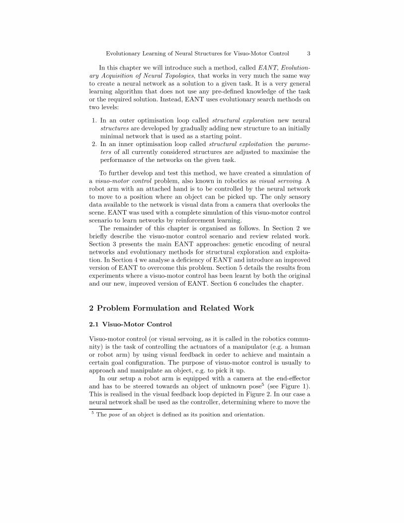
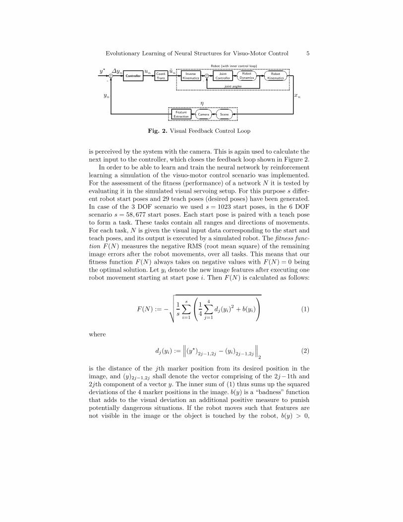
In our setup a robot arm is equipped with a camera at the end-effectorand has to be steered towards an object of unknown pose5 (see Figure 1).This is realised in the visual feedback loop depicted in Figure 2. In our case aneural network shall be used as the controller, determining where to move the

5 The pose of an object is defined as its position and orientation.

4 Nils T Siebel, Gerald Sommer, and Yohannes Kassahun

Fig. 1. Robot Arm with Camera and Object

robot on the basis of the object’s appearance in the image. Using the standardrobotics terminology defined by Weiss et al. [32] our visuo-motor controller isof the type “Static Image-based Look-and-Move”.

The object has 4 circular, identifiable markings. Its appearance in theimage is described by the image feature vector yn ∈ IR8 that contains the4 pairs of image coordinates of these markings. The desired pose relative tothe object is defined by the object’s appearance in that pose by measuringthe corresponding desired image features y⋆

∈ IR8 (“teaching by showing”).Object and robot are then moved so that no Euclidean position of the objector robot is known to the controller. The system has the task of moving the armsuch that the current image features resemble the desired image features. Thisis an iterative process. In some of our experiments the orientation of the robothand was fixed, allowing the robot to move in 3 degrees of freedom, DOFs.In others the orientation of the hand was also controllable, which means therobot could move in 6 DOFs.

The input to the controller is the image error ∆yn := y⋆− yn and ad-

ditionally image measurements which enable the neural network to make itsoutput dependent on the context. In some of the experiments this was simplyyn, resulting in a 16-dimensional input to the network. In other experimentsthe additional inputs were the 2 distances in the image of the diagonally op-posing markings, resulting in a 10-dimensional input vector. The output of thecontroller/neural network is a relative movement un of the robot in the cam-era coordinate system: un = (∆x, ∆y, ∆z) when moving the robot in 3 DOFs,un = (∆x, ∆y, ∆z, ∆yaw, ∆pitch, ∆roll) when moving in 6 DOFs. This out-put is given as an input to the robot’s internal controller which executes themovement. The new state xn+1 of the environment (i.e. the robot and scene)

Evolutionary Learning of Neural Structures for Visuo-Motor Control 5

y⋆

- e+∆yn- Controller -u

n Coord.

Trans.-u

n

Robot (with inner control loop)

Inverse

Kinematics- e+- Joint

Controller-

�

�

Robot

Dynamics--

joint angles6-

�

�

Robot

Kinematics

xn

��

�Scene�

�

�Camera�Feature

Extraction

η

6

yn

-

Fig. 2. Visual Feedback Control Loop

is perceived by the system with the camera. This is again used to calculate thenext input to the controller, which closes the feedback loop shown in Figure 2.

In order to be able to learn and train the neural network by reinforcementlearning a simulation of the visuo-motor control scenario was implemented.For the assessment of the fitness (performance) of a network N it is tested byevaluating it in the simulated visual servoing setup. For this purpose s differ-ent robot start poses and 29 teach poses (desired poses) have been generated.In case of the 3 DOF scenario we used s = 1023 start poses, in the 6 DOFscenario s = 58, 677 start poses. Each start pose is paired with a teach poseto form a task. These tasks contain all ranges and directions of movements.For each task, N is given the visual input data corresponding to the start andteach poses, and its output is executed by a simulated robot. The fitness func-tion F (N) measures the negative RMS (root mean square) of the remainingimage errors after the robot movements, over all tasks. This means that ourfitness function F (N) always takes on negative values with F (N) = 0 beingthe optimal solution. Let yi denote the new image features after executing onerobot movement starting at start pose i. Then F (N) is calculated as follows:

F (N) := −

√

√

√

√

√

1

s

s∑

i=1

1

4

4∑

j=1

dj(yi)2 + b(yi)

(1)

where

dj(yi) :=∥

∥

∥(y⋆)2j−1,2j

− (yi)2j−1,2j

∥

∥

∥

2

(2)

is the distance of the jth marker position from its desired position in theimage, and (y)2j−1,2j shall denote the vector comprising of the 2j−1th and2jth component of a vector y. The inner sum of (1) thus sums up the squareddeviations of the 4 marker positions in the image. b(y) is a “badness” functionthat adds to the visual deviation an additional positive measure to punishpotentially dangerous situations. If the robot moves such that features arenot visible in the image or the object is touched by the robot, b(y) > 0,

6 Nils T Siebel, Gerald Sommer, and Yohannes Kassahun

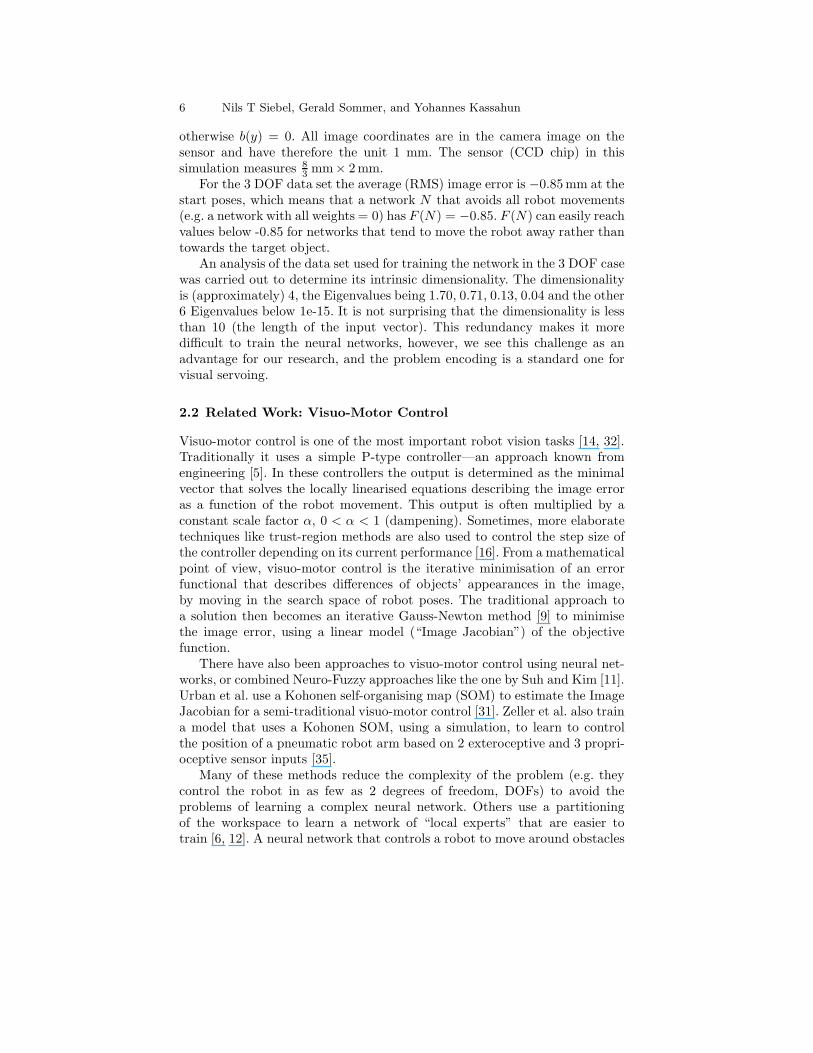
otherwise b(y) = 0. All image coordinates are in the camera image on thesensor and have therefore the unit 1 mm. The sensor (CCD chip) in thissimulation measures 8

3mm× 2 mm.

For the 3 DOF data set the average (RMS) image error is −0.85 mm at thestart poses, which means that a network N that avoids all robot movements(e.g. a network with all weights = 0) has F (N) = −0.85. F (N) can easily reachvalues below -0.85 for networks that tend to move the robot away rather thantowards the target object.

An analysis of the data set used for training the network in the 3 DOF casewas carried out to determine its intrinsic dimensionality. The dimensionalityis (approximately) 4, the Eigenvalues being 1.70, 0.71, 0.13, 0.04 and the other6 Eigenvalues below 1e-15. It is not surprising that the dimensionality is lessthan 10 (the length of the input vector). This redundancy makes it moredifficult to train the neural networks, however, we see this challenge as anadvantage for our research, and the problem encoding is a standard one forvisual servoing.

2.2 Related Work: Visuo-Motor Control

Visuo-motor control is one of the most important robot vision tasks [14, 32].Traditionally it uses a simple P-type controller—an approach known fromengineering [5]. In these controllers the output is determined as the minimalvector that solves the locally linearised equations describing the image erroras a function of the robot movement. This output is often multiplied by aconstant scale factor α, 0 < α < 1 (dampening). Sometimes, more elaboratetechniques like trust-region methods are also used to control the step size ofthe controller depending on its current performance [16]. From a mathematicalpoint of view, visuo-motor control is the iterative minimisation of an errorfunctional that describes differences of objects’ appearances in the image,by moving in the search space of robot poses. The traditional approach toa solution then becomes an iterative Gauss-Newton method [9] to minimisethe image error, using a linear model (“Image Jacobian”) of the objectivefunction.

There have also been approaches to visuo-motor control using neural net-works, or combined Neuro-Fuzzy approaches like the one by Suh and Kim [11].Urban et al. use a Kohonen self-organising map (SOM) to estimate the ImageJacobian for a semi-traditional visuo-motor control [31]. Zeller et al. also traina model that uses a Kohonen SOM, using a simulation, to learn to controlthe position of a pneumatic robot arm based on 2 exteroceptive and 3 propri-oceptive sensor inputs [35].

Many of these methods reduce the complexity of the problem (e.g. theycontrol the robot in as few as 2 degrees of freedom, DOFs) to avoid theproblems of learning a complex neural network. Others use a partitioningof the workspace to learn a network of “local experts” that are easier totrain [6, 12]. A neural network that controls a robot to move around obstacles

Evolutionary Learning of Neural Structures for Visuo-Motor Control 7

is presented in [23]. The network is optimised by a genetic algorithm, however,its structure (topology) is pre-defined and does not evolve.

There are a few methods that develop both the structure and the topologyof a neural network by evolutionary means. These methods will be discussedin section 3.5 below. However, we have not seen these methods applied tovisuo-motor control problems similar to ours.

To our mind it is a shortcoming of most (if not, all) existing visuo-motorcontrol methods that the solution to the control task is modelled by thedesigner of the software. Whether it be using again an Image Jacobian, orwhether it be selecting the size and structure of the neural network “byhand”—that is, by intuition and/or trial and error—these methods learn onlypart of the solution by themselves. Training the neural network then becomes“only” a parameter estimation, even though the curse of dimensionality stillmakes this very difficult.

We wish to avoid this pre-designing of the solution. Instead, our methodlearns both the structure (topology) and the parameters of the neural networkwithout being given any information about the nature of the problem. Toachieve this, we have used our own, recently developed method, EANT, Evo-lutionary Acquisition of Neural Topologies [19] and improved its convergencewith an optimisation technique called CMA-ES [10] to develop a neural net-work from scratch by evolutionary means to solve the visuo-motor controlproblem.

3 Developing Neural Networks with EANT

EANT, Evolutionary Acquisition of Neural Topologies [18, 19], is an evolution-ary reinforcement learning system that is suitable for learning and adaptingto the environment through interaction. It combines the principles of neuralnetworks, reinforcement learning and evolutionary methods.

3.1 EANT’s Encoding of Neural Networks: The Linear Genome

EANT uses a unique genetic encoding that uses a linear genome of genesthat can take different forms. A gene can be a neuron, an input to the neuralnetwork or a connection between two neurons. We call “irregular” connectionsbetween neural genes “jumper connections”. Jumper genes are introduced bystructural mutation along the evolution path. They can encode either forwardor recurrent connections.

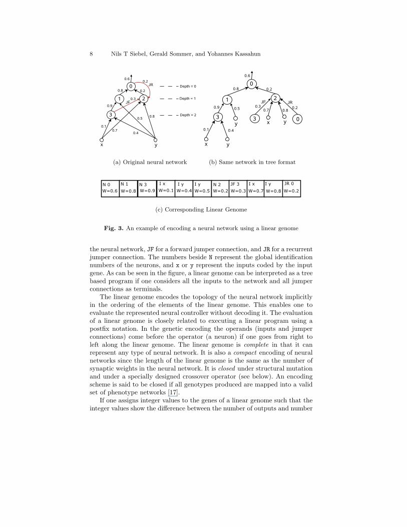
Figures 3(a) through 3(c) show an example encoding of a neural networkusing a linear genome. The figures show (a) the neural network to be encoded.It has one forward and one recurrent jumper connection; (b) the neural net-work interpreted as a tree structure; and (c) the linear genome encoding theneural network. In the linear genome, N stands for a neuron, I for an input to

8 Nils T Siebel, Gerald Sommer, and Yohannes Kassahun

(a) Original neural network (b) Same network in tree format

(c) Corresponding Linear Genome

Fig. 3. An example of encoding a neural network using a linear genome

the neural network, JF for a forward jumper connection, and JR for a recurrentjumper connection. The numbers beside N represent the global identificationnumbers of the neurons, and x or y represent the inputs coded by the inputgene. As can be seen in the figure, a linear genome can be interpreted as a treebased program if one considers all the inputs to the network and all jumperconnections as terminals.

The linear genome encodes the topology of the neural network implicitlyin the ordering of the elements of the linear genome. This enables one toevaluate the represented neural controller without decoding it. The evaluationof a linear genome is closely related to executing a linear program using apostfix notation. In the genetic encoding the operands (inputs and jumperconnections) come before the operator (a neuron) if one goes from right toleft along the linear genome. The linear genome is complete in that it canrepresent any type of neural network. It is also a compact encoding of neuralnetworks since the length of the linear genome is the same as the number ofsynaptic weights in the neural network. It is closed under structural mutationand under a specially designed crossover operator (see below). An encodingscheme is said to be closed if all genotypes produced are mapped into a validset of phenotype networks [17].

If one assigns integer values to the genes of a linear genome such that theinteger values show the difference between the number of outputs and number

Evolutionary Learning of Neural Structures for Visuo-Motor Control 9

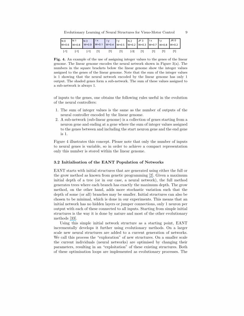
Fig. 4. An example of the use of assigning integer values to the genes of the lineargenome. The linear genome encodes the neural network shown in Figure 3(a). Thenumbers in the square brackets below the linear genome show the integer valuesassigned to the genes of the linear genome. Note that the sum of the integer valuesis 1 showing that the neural network encoded by the linear genome has only 1output. The shaded genes form a sub-network. The sum of these values assigned toa sub-network is always 1.

of inputs to the genes, one obtains the following rules useful in the evolutionof the neural controllers:

1. The sum of integer values is the same as the number of outputs of theneural controller encoded by the linear genome.

2. A sub-network (sub-linear genome) is a collection of genes starting from aneuron gene and ending at a gene where the sum of integer values assignedto the genes between and including the start neuron gene and the end geneis 1.

Figure 4 illustrates this concept. Please note that only the number of inputsto neural genes is variable, so in order to achieve a compact representationonly this number is stored within the linear genome.

3.2 Initialisation of the EANT Population of Networks

EANT starts with initial structures that are generated using either the full orthe grow method as known from genetic programming [2]. Given a maximuminitial depth of a tree (or in our case, a neural network), the full methodgenerates trees where each branch has exactly the maximum depth. The growmethod, on the other hand, adds more stochastic variation such that thedepth of some (or all) branches may be smaller. Initial structures can also bechosen to be minimal, which is done in our experiments. This means that aninitial network has no hidden layers or jumper connections, only 1 neuron peroutput with each of these connected to all inputs. Starting from simple initialstructures is the way it is done by nature and most of the other evolutionarymethods [33].

Using this simple initial network structure as a starting point, EANTincrementally develops it further using evolutionary methods. On a largerscale new neural structures are added to a current generation of networks.We call this process the “exploration” of new structures. On a smaller scalethe current individuals (neural networks) are optimised by changing theirparameters, resulting in an “exploitation” of these existing structures. Bothof these optimisation loops are implemented as evolutionary processes. The

10 Nils T Siebel, Gerald Sommer, and Yohannes Kassahun

N 1 N 2 I x I y N 3 I x I y

W=0.3 W=0.7 W=0.5 W=0.8 W=0.6 W=0.4 W=0.3

I x

W=0.9

N 1 N 2 I x I y N 3 I x I y

W=0.3 W=0.7 W=0.5 W=0.8 W=0.6 W=0.4 W=0.3

JR1

W=0.1

1

2 3

x y

0.7 0.6

0.9

0.5 0.3

0.4

0.8

1

2 3

x y

0.7 0.6

0.1

0.5 0.3

0.4

0.8

0.3 0.3

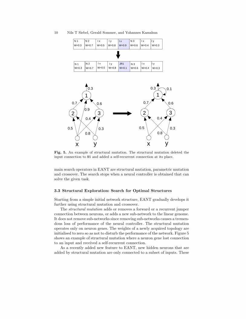
Fig. 5. An example of structural mutation. The structural mutation deleted theinput connection to N1 and added a self-recurrent connection at its place.

main search operators in EANT are structural mutation, parametric mutationand crossover. The search stops when a neural controller is obtained that cansolve the given task.

3.3 Structural Exploration: Search for Optimal Structures

Starting from a simple initial network structure, EANT gradually develops itfurther using structural mutation and crossover.

The structural mutation adds or removes a forward or a recurrent jumperconnection between neurons, or adds a new sub-network to the linear genome.It does not remove sub-networks since removing sub-networks causes a tremen-dous loss of performance of the neural controller. The structural mutationoperates only on neuron genes. The weights of a newly acquired topology areinitialised to zero so as not to disturb the performance of the network. Figure 5shows an example of structural mutation where a neuron gene lost connectionto an input and received a self-recurrent connection.

As a recently added new feature to EANT, new hidden neurons that areadded by structural mutation are only connected to a subset of inputs. These

Evolutionary Learning of Neural Structures for Visuo-Motor Control 11

inputs are randomly chosen. This makes the search for new structures “morestochastic”.

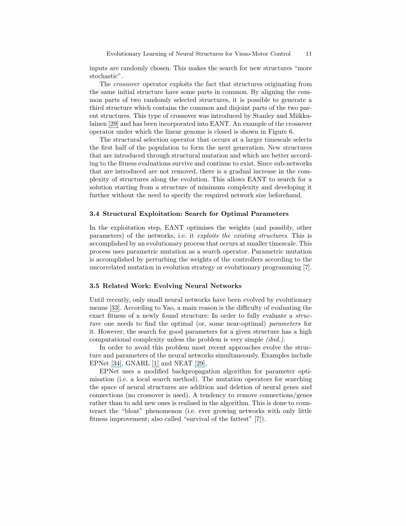
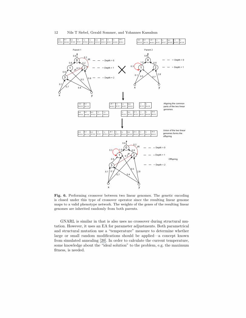
The crossover operator exploits the fact that structures originating fromthe same initial structure have some parts in common. By aligning the com-mon parts of two randomly selected structures, it is possible to generate athird structure which contains the common and disjoint parts of the two par-ent structures. This type of crossover was introduced by Stanley and Miikku-lainen [29] and has been incorporated into EANT. An example of the crossoveroperator under which the linear genome is closed is shown in Figure 6.

The structural selection operator that occurs at a larger timescale selectsthe first half of the population to form the next generation. New structuresthat are introduced through structural mutation and which are better accord-ing to the fitness evaluations survive and continue to exist. Since sub-networksthat are introduced are not removed, there is a gradual increase in the com-plexity of structures along the evolution. This allows EANT to search for asolution starting from a structure of minimum complexity and developing itfurther without the need to specify the required network size beforehand.

3.4 Structural Exploitation: Search for Optimal Parameters

In the exploitation step, EANT optimises the weights (and possibly, otherparameters) of the networks, i.e. it exploits the existing structures. This isaccomplished by an evolutionary process that occurs at smaller timescale. Thisprocess uses parametric mutation as a search operator. Parametric mutationis accomplished by perturbing the weights of the controllers according to theuncorrelated mutation in evolution strategy or evolutionary programming [7].

3.5 Related Work: Evolving Neural Networks

Until recently, only small neural networks have been evolved by evolutionarymeans [33]. According to Yao, a main reason is the difficulty of evaluating theexact fitness of a newly found structure: In order to fully evaluate a struc-ture one needs to find the optimal (or, some near-optimal) parameters forit. However, the search for good parameters for a given structure has a highcomputational complexity unless the problem is very simple (ibid.).

In order to avoid this problem most recent approaches evolve the struc-ture and parameters of the neural networks simultaneously. Examples includeEPNet [34], GNARL [1] and NEAT [29].

EPNet uses a modified backpropagation algorithm for parameter opti-misation (i.e. a local search method). The mutation operators for searchingthe space of neural structures are addition and deletion of neural genes andconnections (no crossover is used). A tendency to remove connections/genesrather than to add new ones is realised in the algorithm. This is done to coun-teract the “bloat” phenomenon (i.e. ever growing networks with only littlefitness improvement; also called “survival of the fattest” [7]).

12 Nils T Siebel, Gerald Sommer, and Yohannes Kassahun

Fig. 6. Performing crossover between two linear genomes. The genetic encodingis closed under this type of crossover operator since the resulting linear genomemaps to a valid phenotype network. The weights of the genes of the resulting lineargenomes are inherited randomly from both parents.

GNARL is similar in that is also uses no crossover during structural mu-tation. However, it uses an EA for parameter adjustments. Both parametricaland structural mutation use a “temperature” measure to determine whetherlarge or small random modifications should be applied—a concept knownfrom simulated annealing [20]. In order to calculate the current temperature,some knowledge about the “ideal solution” to the problem, e.g. the maximumfitness, is needed.

Evolutionary Learning of Neural Structures for Visuo-Motor Control 13

The author groups of both EPNet and GNARL are of the opinion thatusing crossover is not useful during the evolutionary development of neuralnetworks [34, 1]. The research work underlying NEAT, on the other hand,seems to suggest otherwise. The authors have designed and used the crossoveroperator described in section 3.3 above. It allows to produce valid offspringfrom two given neural networks by first aligning similar or equal subnetworksand then exchanging differing parts. Like GNARL, NEAT uses EAs for bothparametrical and structural mutation. However, the probabilities and stan-dard deviations used for random mutation are constant over time. NEAT alsoincorporates the concept of speciation, i.e. separated sub-populations that aimat cultivating and preserving diversity in the population [7, chap. 9].

4 Combining EANT with CMA-ES

4.1 Motivation

During and after its development in the recent years EANT was tested onsimple control problems like pole balancing where is has shown a very goodperformance and convergence rate—that is, it learns problems well with onlyfew evaluations of the fitness function. However, problems like pole balancingare relatively simple. For instance, the neural network found by EANT tosolve the double pole balancing problem without velocity information only has1 hidden neuron. The new task, visuo-motor control, is much more complexand therefore required some improvements to EANT on different levels.

In order to study the behaviour of EANT on large problems we have im-plemented visuo-motor control simulators both for 6 DOF and 3 DOF controlproblems with 16/6 and 10/3 network in-/outputs, respectively. As a fitnessfunction F for the individual networks N we used again the negative RMSof the remaining image errors, as defined in (1) above. This means that fit-ness takes on negative values with 0 being the optimal solution. Our studieswere carried out on a small Linux PC cluster with 4 machines that each have2 CPUs running at 3 GHz. This parallelisation was necessary because of thesignificant amount of CPU time required by our simulation. One evaluationof the fitness function in the 6 DOF case (58,677 robot movements and imageacquisitions) takes around 1 second. In the 3 DOF case (“only” 1023 robotmovements) the evaluation is of course considerably faster, however, paralleli-sation is still very helpful.

For our experiments we have set the following EANT parameters:

• population size: 20 individuals for exploration, 7 n for exploitation, n beingthe size of the network

• structural mutation: enabled with a probability of 0.5• parametric mutation: enabled; mutating all non-output weights• crossover: disabled

14 Nils T Siebel, Gerald Sommer, and Yohannes Kassahun

• initial structure: minimal; 1 gene per output, each connected to all inputs

The results from our initial studies have shown that EANT does developstructures of increasing complexity and performance. However, we were notsatisfied with the speed at which the performance (fitness) improved overtime.

4.2 Improving the convergence with CMA-ES

In order to find out whether the structural exploration or the structural ex-ploitation component needed improvement we took intermediate results (in-dividuals with 175–200+ weights) and tried to optimise these structures usinga different optimisation technique. Since our problem is highly non-linear andmulti-modal (i.e. it has multiple local optima) we needed to use a global op-timisation technique, not a local one like backpropagation, which is usuallyequivalent to a stochastic gradient descent method and therefore prone to getstuck in local minima. For our re-optimisation tests we used a global optimi-sation method called “CMA-ES” (Covariance Matrix Adaptation EvolutionStrategy) [10] that is based on an evolutionary method like the one used inEANT’s exploitation. CMA-ES includes features that improve its convergenceespecially with multi-modal functions in high-dimensional spaces.

One important difference between CMA-ES and the traditional evolution-ary optimisation method in EANT is in the calculation of the search area forsampling the optimisation space by individuals. In EANT, each parameterin a neural network carries with it a learning rate which corresponds to astandard deviation for sampling new values for this parameter. This learningrate is adapted over time, allowing for a more efficient search in the space:parameters (e.g. input weights) that have not been changed for a long timebecause they have been in the network for a while are assumed to be near-optimal. Therefore their learning rate can be decreases over time, effectivelyreducing the search area in this dimension of the parameter space. New pa-rameters (e.g. weights of newly added connections), on the other hand, stillrequire a large learning rate so that their values are sampled in a larger inter-val. This technique is closely related to the “Cascaded Learning” paradigmpresented by Fahlman and Lebiere [8]. It allows the algorithm to concentrateon the new parameters during optimisation and generally yields better op-timisation results in high-dimensional parameter spaces, even if a relativelysmall population is used.

In EANT, the adaptation of these search strategy parameters is done ran-domly using evolution strategies [7]. This means that new strategy parametersmay be generated by mutation and will then influence the search for optimalnetwork parameters. However, one problem with this approach is that it maytake a long time for new strategy parameters to have an effect on the fitnessvalue of the individual. Since adaptation is random the strategy parametermay have been changed again by then, or other changes may have influenced

Evolutionary Learning of Neural Structures for Visuo-Motor Control 15

0 50000 100000 150000 200000 250000 300000 350000 400000 450000function evaluations

-1.7

-1.6

-1.5

-1.4

-1.3

fitne

ss v

alue

init: EANTinit: unif. random [-1 1]init: zerosweights and sigmoidsall weights and sigmoids

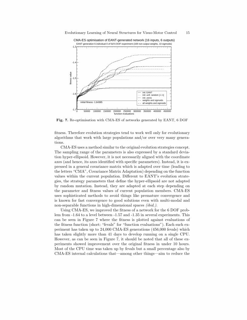
CMA-ES optimisation of EANT-generated network (16 inputs, 6 outputs)EANT generation 6 individual 0 of full 6 DOF experiment (169 non-output weights, 10 sigmoids)

initial fitness -1.64385

Fig. 7. Re-optimisation with CMA-ES of networks generated by EANT, 6 DOF

fitness. Therefore evolution strategies tend to work well only for evolutionaryalgorithms that work with large populations and/or over very many genera-tions.

CMA-ES uses a method similar to the original evolution strategies concept.The sampling range of the parameters is also expressed by a standard devia-tion hyper-ellipsoid. However, it is not necessarily aligned with the coordinateaxes (and hence, its axes identified with specific parameters). Instead, it is ex-pressed in a general covariance matrix which is adapted over time (leading tothe letters “CMA”, Covariance Matrix Adaptation) depending on the functionvalues within the current population. Different to EANT’s evolution strate-gies, the strategy parameters that define the hyper-ellipsoid are not adaptedby random mutation. Instead, they are adapted at each step depending onthe parameter and fitness values of current population members. CMA-ESuses sophisticated methods to avoid things like premature convergence andis known for fast convergence to good solutions even with multi-modal andnon-separable functions in high-dimensional spaces (ibid.).

Using CMA-ES, we improved the fitness of a network for the 6 DOF prob-lem from -1.64 to a level between -1.57 and -1.35 in several experiments. Thiscan be seen in Figure 7 where the fitness is plotted against evaluations ofthe fitness function (short: “fevals” for “function evaluations”). Each such ex-periment has taken up to 24,000 CMA-ES generations (456,000 fevals) whichhas taken slightly more than 41 days to develop running on a single CPU.However, as can be seen in Figure 7, it should be noted that all of these ex-periments showed improvement over the original fitness in under 10 hours.Most of the CPU time was taken up by fevals but a small percentage also byCMA-ES internal calculations that—among other things—aim to reduce the

16 Nils T Siebel, Gerald Sommer, and Yohannes Kassahun

total number of fevals needed for the optimisation. While these results showthat the optimisation still needs a large amount of CPU time (at least inthe 6 DOF case) the improvement in fitness was very significant. Experimentswith different initialisations have shown that the convergence of CMA-ES doesnot depend much on the initial values of the parameters. The variance in theresulting fitness values for optimisations with the same initial values is also anindicator for the multi-modality of our problem, which stems, in part, fromour definition of the fitness function as a sum of many functions.

These 6 DOF experiments are very expensive to run due to their enormousCPU usage. However, with only few experiments the results have only littlestatistical significance. Therefore we made further experiments with networksof similar size for the 3 DOF visuo-motor control scenario. In over 700 CMA-ES re-optimisation experiments we always achieved very similar results to theones shown in Figure 7 and conclude that the parameter optimisation withCMA-ES really does usually give a significant improvement in fitness value.

Our experiments have shown that by optimising only the parameters ofthe networks that were generated by EANT their fitness can be considerablyincreased. This indicates that for networks of this size the exploitation partof EANT that optimises these parameters can and should be improved. En-couraged by our positive results with CMA-ES we have therefore replaced thestructural exploitation loop of EANT by a new strategy that uses CMA-ESas its optimisation technique.

5 Experimental Evaluation

5.1 Experimental Setup

After the studies with 6 DOF visuo-motor control described in Section 4 wedecided that the 3 DOF case with 1023 start poses will be difficult enough totest the new CMA-ES-based EANT and compare it to the original version.With the same setup as before, 10/3 in-/outputs and starting from minimalstructures (3 output neurons, each connected to all 10 inputs) we startedEANT again on 4 PCs, each with 2 CPUs running at 3 GHz. One masterprocess was responsible for the exploration of new structures and distributedthe CMA-ES optimisation of the individuals (exploitation of current struc-tures) to slave processes. We used the same fitness function F (N) as beforefor evaluating the individual networks N , in this case

F (N) = −

√

√

√

√

√

1

1023

1023∑

i=1

1

4

4∑

j=1

∥

∥

∥(y⋆)2j−1,2j

− (yi)2j−1,2j

∥

∥

∥

2

2

+ b(yi)

, (3)

Evolutionary Learning of Neural Structures for Visuo-Motor Control 17

which means that fitness takes again on negative values with 0 being theoptimal solution.

Up to 15 runs of each method have been made to ensure a statisticallymeaningful analysis of results. Different runs of the methods with the sameparameters do not differ much; shown and discussed below are therefore simplythe mean results from our experiments.

5.2 Parameter Sets

Following our paradigm to put as little problem-specific knowledge into thesystem as possible, we used the standard parameters in EANT and CMA-ESto run our experiments. Additionally we introduced CMA-ES stop conditionsthat were determined in a few test runs. They were selected so as to make surethat the CMA-ES optimisation converges to a solution, i.e. the algorithm runsuntil the fitness does not improve any longer. These very lax CMA-ES stopcriteria (details below) allow for a long run with many function evaluations(fevals) and hence can take a lot of time to terminate. In order to find outhow much the solution depends on these stop criteria additional experimentswere made with a second set of CMA-ES parameters, effectively allowing only1

10of the fevals and hence speeding up the process enormously. Altogether

this makes 3 types of experiments:

1. the original EANT with its standard parameters;2. the CMA-ES-based EANT with a large allowance of fevals; and3. the CMA-ES-based EANT with a small allowance of fevals

The optimisations had the following parameters:

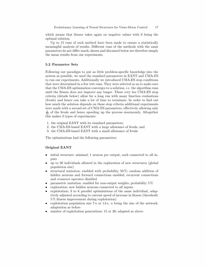
Original EANT

• initial structure: minimal; 1 neuron per output, each connected to all in-puts

• up to 20 individuals allowed in the exploration of new structures (globalpopulation size)

• structural mutation: enabled with probability 50%; random addition ofhidden neurons and forward connections enabled; recurrent connectionsand crossover operator disabled

• parametric mutation: enabled for non-output weights, probability 5%• exploration: new hidden neurons connected to all inputs• exploitation: 3 to 6 parallel optimisations of the same individual, adap-

tively adjusted according to current speed of increase in fitness (threshold:5% fitness improvement during exploitation)

• exploitation population size 7 n or 14n, n being the size of the network;adaptation as before

• number of exploitation generations: 15 or 30; adapted as above

18 Nils T Siebel, Gerald Sommer, and Yohannes Kassahun

0 10 20 30 40 50 60 70 80 90 100 110identification number of the individual

-0.48

-0.46

-0.44

-0.42

-0.40

-0.38

-0.36

-0.34

-0.32

-0.30

-0.28

-0.26

-0.24

-0.22

fitne

ss v

alue

training fitnesstesting fitness

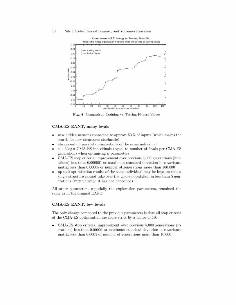
Comparison of Training vs Testing ResultsPlotted is the fitness of population members, which were sorted by training fitness

Fig. 8. Comparison Training vs. Testing Fitness Values

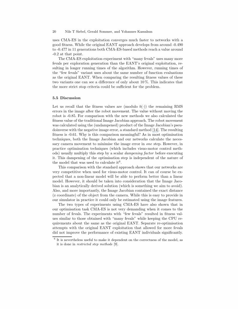
CMA-ES EANT, many fevals

• new hidden neurons connected to approx. 50% of inputs (which makes thesearch for new structures stochastic)

• always only 3 parallel optimisations of the same individual• 4 + 3 logn CMA-ES individuals (equal to number of fevals per CMA-ES

generation) when optimising n parameters• CMA-ES stop criteria: improvement over previous 5,000 generations (iter-

ations) less than 0.000001 or maximum standard deviation in covariancematrix less than 0.00005 or number of generations more than 100,000

• up to 2 optimisation results of the same individual may be kept, so that asingle structure cannot take over the whole population in less than 5 gen-erations (very unlikely; it has not happened)

All other parameters, especially the exploration parameters, remained thesame as in the original EANT.

CMA-ES EANT, few fevals

The only change compared to the previous parameters is that all stop criteriaof the CMA-ES optimisation are more strict by a factor of 10:

• CMA-ES stop criteria: improvement over previous 5,000 generations (it-erations) less than 0.00001 or maximum standard deviation in covariancematrix less than 0.0005 or number of generations more than 10,000

Evolutionary Learning of Neural Structures for Visuo-Motor Control 19

0 1 2 3 4 5 6 7 8 9 10EANT generation number

-0.7

-0.6

-0.5

-0.4

-0.3

-0.2

fitne

ss o

f bes

t ind

ivid

ual

original EANT, few fevalsCMA-ES EANT, many fevalsCMA-ES EANT, few fevalsImage Jacobian’s "fitness"

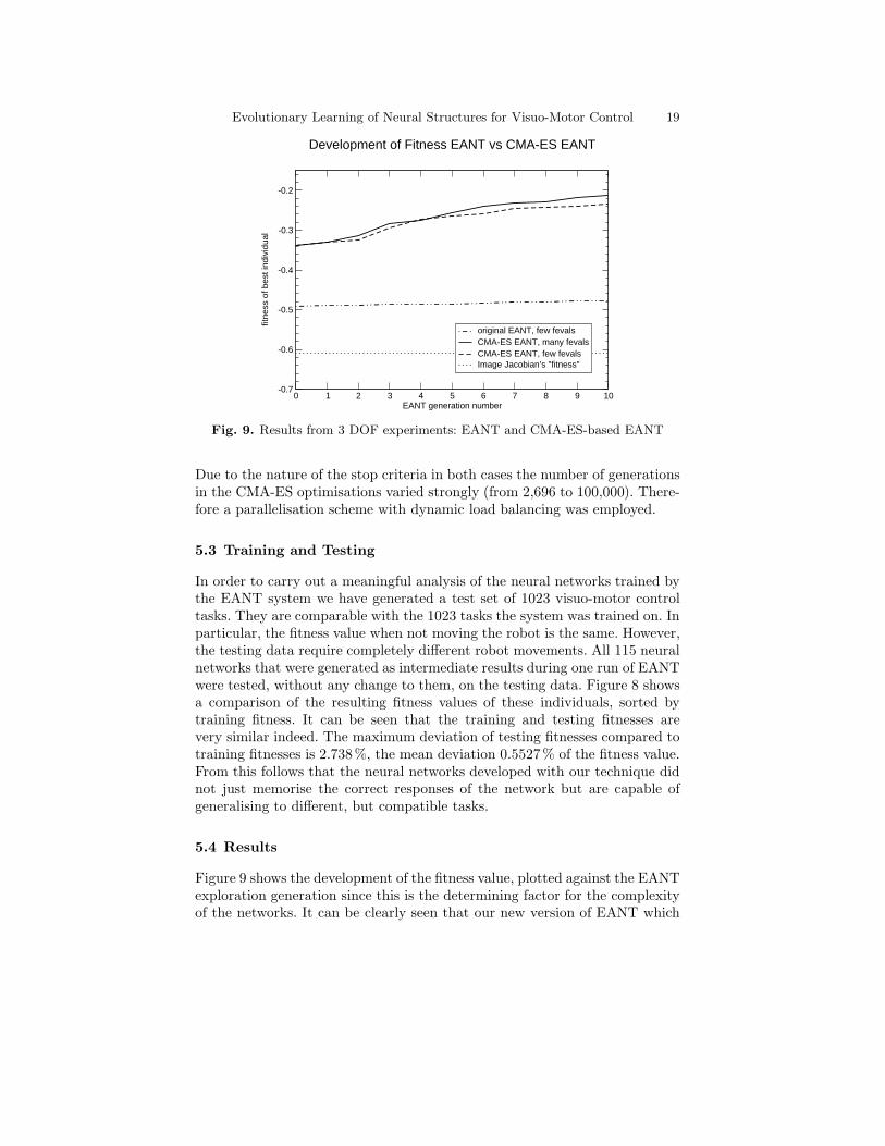
Development of Fitness EANT vs CMA-ES EANT

Fig. 9. Results from 3 DOF experiments: EANT and CMA-ES-based EANT

Due to the nature of the stop criteria in both cases the number of generationsin the CMA-ES optimisations varied strongly (from 2,696 to 100,000). There-fore a parallelisation scheme with dynamic load balancing was employed.

5.3 Training and Testing

In order to carry out a meaningful analysis of the neural networks trained bythe EANT system we have generated a test set of 1023 visuo-motor controltasks. They are comparable with the 1023 tasks the system was trained on. Inparticular, the fitness value when not moving the robot is the same. However,the testing data require completely different robot movements. All 115 neuralnetworks that were generated as intermediate results during one run of EANTwere tested, without any change to them, on the testing data. Figure 8 showsa comparison of the resulting fitness values of these individuals, sorted bytraining fitness. It can be seen that the training and testing fitnesses arevery similar indeed. The maximum deviation of testing fitnesses compared totraining fitnesses is 2.738%, the mean deviation 0.5527% of the fitness value.From this follows that the neural networks developed with our technique didnot just memorise the correct responses of the network but are capable ofgeneralising to different, but compatible tasks.

5.4 Results

Figure 9 shows the development of the fitness value, plotted against the EANTexploration generation since this is the determining factor for the complexityof the networks. It can be clearly seen that our new version of EANT which

20 Nils T Siebel, Gerald Sommer, and Yohannes Kassahun

uses CMA-ES in the exploitation converges much faster to networks with agood fitness. While the original EANT approach develops from around -0.490to -0.477 in 11 generations both CMA-ES-based methods reach a value around-0.2 at that point.

The CMA-ES exploitation experiment with “many fevals” uses many morefevals per exploration generation than the EANT’s original exploitation, re-sulting in longer running times of the algorithm. However, running times ofthe “few fevals” variant uses about the same number of function evaluationsas the original EANT. When comparing the resulting fitness values of thesetwo variants one can see a difference of only about 10%. This indicates thatthe more strict stop criteria could be sufficient for the problem.

5.5 Discussion

Let us recall that the fitness values are (modulo b(·)) the remaining RMSerrors in the image after the robot movement. The value without moving therobot is -0.85. For comparison with the new methods we also calculated thefitness value of the traditional Image Jacobian approach. The robot movementwas calculated using the (undampened) product of the Image Jacobian’s pseu-doinverse with the negative image error, a standard method [14]. The resultingfitness is -0.61. Why is this comparison meaningful? As in most optimisationtechniques, both the Image Jacobian and our networks calculate the neces-sary camera movement to minimise the image error in one step. However, inpractice optimisation techniques (which includes visuo-motor control meth-ods) usually multiply this step by a scalar dampening factor before executingit. This dampening of the optimisation step is independent of the nature ofthe model that was used to calculate it6.

This comparison with the standard approach shows that our networks arevery competitive when used for visuo-motor control. It can of course be ex-pected that a non-linear model will be able to perform better than a linearmodel. However, it should be taken into consideration that the Image Jaco-bian is an analytically derived solution (which is something we aim to avoid).Also, and more importantly, the Image Jacobian contained the exact distance(z coordinate) of the object from the camera. While this is easy to provide inour simulator in practice it could only be estimated using the image features.

The two types of experiments using CMA-ES have also shown that inour optimisation task CMA-ES is not very demanding when it comes to thenumber of fevals. The experiments with “few fevals” resulted in fitness val-ues similar to those obtained with “many fevals” while keeping the CPU re-quirements about the same as the original EANT. Separate re-optimisationattempts with the original EANT exploitation that allowed for more fevalsdid not improve the performance of existing EANT individuals significantly.

6 It is nevertheless useful to make it dependent on the correctness of the model, asit is done in restricted step methods [9].

Evolutionary Learning of Neural Structures for Visuo-Motor Control 21

It can therefore be assumed that the main performance increase stems fromthe use of CMA-ES, not from a the CPU time/feval allowance.

To conclude, it can be clearly seen that the use of CMA-ES in EANT’sexploitation results in better performance of neural networks of comparablesize while not increasing the computational requirements. The performanceof neural networks developed with our new method is also very much betterthan that of traditional methods for visuo-motor control.

6 Summary

Our aim was to develop neural networks automatically that can be used asa controller in a visuo-motor control scenario. At the same time, our secondgoal was to develop a method that would generate such networks with a min-imum of predetermined modelling. To achieve this, we used and improvedour own evolutionary method called EANT, Evolutionary Acquisition of Neu-ral Topologies. EANT uses evolutionary search methods on two levels: In anouter optimisation loop called structural exploration new networks are devel-oped by gradually adding new structures to an initially minimal network. Inan inner optimisation loop called structural exploitation the parameters ofcurrent networks are optimised. EANT was used with a complete simulationof a visuo-motor control scenario to learn neural networks by reinforcementlearning.

Initial experiments with a 6 DOF visuo-motor control scenario have shownthat EANT is generally well suitable for the task. However, the convergenceof the original EANT method needed to be improved. Tests with resultingnetworks have indicated that it is most useful to work on the exploitation ofnetwork structures. Re-optimisation of existing networks with an optimisationmethod called CMA-ES, Covariance Matrix Adaptation Evolution Strategyhave shown a significant improvement in the controller’s performance.

Based on these results the exploitation loop of EANT was replaced with anew strategy that uses CMA-ES as its optimisation algorithm. Experimentswith this new method have shown much improved results over the originalEANT method for developing a visuo-motor controller in the 3 DOF scenario.It could also be seen that varying the CPU time available to the CMA-ES-based parameter optimisation in the exploitation part by a factor of 10 didnot significantly influence the performance of the resulting networks. Theirperformance is also very much better than that of the traditional approachfor visuo-motor control.

Our experimental results show that the new EANT method with CMA-ES is capable of learning neural networks as solutions to complex and difficultproblems. The CMA-ES based EANT can be used as a “black-box” tool todevelop networks without being given much information about the nature ofthe problem. It also does not require a lot of parameter tuning to give usefulresults. The resulting networks show a very good performance.

22 Nils T Siebel, Gerald Sommer, and Yohannes Kassahun

Acknowledgements

The authors wish to thank Nikolaus Hansen, the developer of CMA-ES, forkindly providing source code which helped us to quickly start integrating hismethod into EANT.

References

1. Peter J Angeline, Gregory M Saunders, and Jordan B Pollack. An evolutionaryalgorithm that constructs recurrent neural networks. IEEE Transactions onNeural Networks, 5:54–65, 1994.

2. Wolfgang Banzhaf, Peter Nordin, Robert E Keller, and Frank D Francone. Ge-netic Programming: An Introduction on the Automatic Evolution of ComputerPrograms and Its Applications. Morgan Kaufmann, San Francisco, USA, 1998.

3. Richard Ernest Bellman. Adaptive Control Processes. Princeton UniversityPress, Princeton, USA, 1961.

4. Andrea Beltratti, Sergio Margarita, and Pietro Terna. Neural Networks forEconomic and Financial Modelling. International Thomson Computer Press,London, UK, 1996.

5. Chris C Bissell. Control Engineering. Number 15 in Tutorial Guides in Elec-tronic Engineering. CRC Press, Boca Raton, USA, 2nd edition, 1996.

6. Wolfram Blase, Josef Pauli, and Jorg Bruske. Vision-based manipulator navi-gation using mixtures of RBF neural networks. In International Conference onNeural Network and Brain, pages 531–534, Bejing, China, April 1998.

7. Agoston E Eiben and James E Smith. Introduction to Evolutionary Computing.Springer Verlag, Berlin, Germany, 2003.

8. Scott E Fahlman and Christian Lebiere. The cascade-correlation learning archi-tecture. Technical Report CMU-CS-90-100, Carnegie Mellon University, Pitts-burgh, USA, August 1991.

9. Roger Fletcher. Practical Methods of Optimization. John Wiley & Sons, NewYork, Chichester, 2nd edition, 1987.

10. Nikolaus Hansen and Andreas Ostermeier. Completely derandomized self-adaptation in evolution strategies. Evolutionary Computation, 9(2):159–195,2001.

11. Koichi Hashimoto, editor. Visual Servoing: Real-Time Control of Robot Manip-ulators Based on Visual Sensory Feedback, volume 7 of Series in Robotics andAutomated Systems. World Scientific Publishing Co., Singapore, 1994.

12. Gilles Hermann, Patrice Wira, and Jean-Philippe Urban. Neural networks orga-nizations to learn complex robotic functions. In Proceedings of the 11th EuropeanSymposium on Artificial Neural Networks (ESANN 2003), pages 33–38, Bruges,Belgium, April 2005.

13. Kurt Hornik, Maxwell B Stinchcombe, and Halbert White. Multilayer feedfor-ward networks are universal approximators. Neural Networks, 2:359–366, 1989.

14. Seth Hutchinson, Greg Hager, and Peter Corke. A tutorial on visual servocontrol. Tutorial notes, Yale University, New Haven, USA, May 1996.

15. William R Hutchison and Kenneth R Stephens. The airline marketing tactician(AMT): A commercial application of adaptive networking. In Proceedings ofthe 1st IEEE International Conference on Neural Networks, San Diego, USA,volume 2, pages 753–756, 1987.

Evolutionary Learning of Neural Structures for Visuo-Motor Control 23

16. Martin Jagersand. Visual servoing using trust region methods and estimationof the full coupled visual-motor Jacobian. In Proceedings of the IASTED Appli-cations of Control and Robotics, Orlando, USA, pages 105–108, January 1996.

17. Jae-Yoon Jung and James A Reggia. A descriptive encoding language for evolv-ing modular neural networks. In Proceedings of the Genetic and EvolutionaryComputation Conference (GECCO), pages 519–530. Springer Verlag, 2004.

18. Yohannes Kassahun and Gerald Sommer. Automatic neural robot controllerdesign using evolutionary acquisition of neural topologies. In 19. FachgesprachAutonome Mobile Systeme (AMS 2005), pages 259–266, Stuttgart, Germany,December 2005.

19. Yohannes Kassahun and Gerald Sommer. Efficient reinforcement learningthrough evolutionary acquisition of neural topologies. In Proceedings of the13th European Symposium on Artificial Neural Networks (ESANN 2005), pages259–266, Bruges, Belgium, April 2005.

20. Scott Kirkpatrick, Charles Daniel Gelatt, and Mario P Vecchi. Optimization bysimulated annealing. Science, 220(4598):671–680, May 1983.

21. James W Melody. On universal approximation using neural networks. Reportfrom project ECE 480, Decision and Control Laboratory, University of Illinois,Urbana, USA, June 1999.

22. Tom M Mitchell. Machine Learning. McGraw-Hill, London, UK, 1997.23. David E Moriarty and Risto Miikkulainen. Evolving obstacle avoidance behav-

ior in a robot arm. In Proceedings of the Fourth International Conference onSimulation of Adaptive Behavior, Cape Cod, USA, 1996.

24. Arnold Neumaier. Complete search in continuous global optimization and con-straint satisfaction. Acta Numerica, 13:271–369, June 2004.

25. Apostolos-Paul Refenes, editor. Neural Networks in the Capital Markets. JohnWiley & Sons, New York, Chichester, USA, 1995.

26. Claude Robert, Charles-Daniel Arreto, Jean Azerad, and Jean-Francois Gaudy.Bibliometric overview of the utilization of artificial neural networks in medicineand biology. Scientometrics, 59(1):117–130, 2004.

27. Raul Rojas. Neural Networks - A Systematic Introduction. Springer Verlag,Berlin, Germany, 1996.

28. James C Spall. Introduction to Stochastic Search and Optimization: Estimation,Simulation, and Control. John Wiley & Sons, Hoboken, USA, 2003.

29. Kenneth O Stanley and Risto Miikkulainen. Evolving neural networks throughaugmenting topologies. Evolutionary Computation, 10(2):99–127, 2002.

30. Robert R Trippi and Efraim Turban, editors. Neural Networks in Finance andInvesting. Probus Publishing Co., Chicago, USA, 1993.

31. Jean-Philippe Urban, Jean-Luc Buessler, and Julien Gresser. Neural networksfor visual servoing in robotics. Technical Report EEA-TROP-TR-97-05, Uni-versite de Haute-Alsace, Mulhouse-Colmar, France, November 1997.

32. Lee E Weiss, Arthur C Sanderson, and Charles P Neuman. Dynamic sensor-based control of robots with visual feedback. IEEE Journal of Robotics andAutomation, 3(5):404–417, October 1987.

33. Xin Yao. Evolving artificial neural networks. Proceedings of the IEEE,87(9):1423–1447, September 1999.

34. Xin Yao and Yong Liu. A new evolutionary system for evolving artificial neuralnetworks. IEEE Transactions on Neural Networks, 8(3):694–713, May 1997.

24 Nils T Siebel, Gerald Sommer, and Yohannes Kassahun

35. Michael Zeller, Kenneth R Wallace, and Klaus Schulten. Biological visuo-motorcontrol of a pneumatic robot arm. In Cihan Hayreddin Dagli, Metin Akay,C L Philip Chen, Benito R Fernandez, and Joydeep Ghosh, editors, IntelligentEngineering Systems Through Artificial Neural Networks. Proceedings of the Ar-tificial Neural Networks in Engineering Conference, New York, volume 5, pages645–650. American Society of Mechanical Engineers, 1995.