event date model: a robust bayesian tool for chronology
TRANSCRIPT
HAL Id: hal-01643509https://hal.archives-ouvertes.fr/hal-01643509
Preprint submitted on 21 Nov 2017
HAL is a multi-disciplinary open accessarchive for the deposit and dissemination of sci-entific research documents, whether they are pub-lished or not. The documents may come fromteaching and research institutions in France orabroad, or from public or private research centers.
L’archive ouverte pluridisciplinaire HAL, estdestinée au dépôt et à la diffusion de documentsscientifiques de niveau recherche, publiés ou non,émanant des établissements d’enseignement et derecherche français ou étrangers, des laboratoirespublics ou privés.
Event Date Model : A Robust Bayesian Tool forChronology Building
Philippe Lanos, Anne Philippe
To cite this version:Philippe Lanos, Anne Philippe. Event Date Model : A Robust Bayesian Tool for Chronology Building.2017. �hal-01643509�
EVENT DATE MODEL: A ROBUST BAYESIAN TOOL FOR
CHRONOLOGY BUILDING
LANOS PHILIPPE AND PHILIPPE ANNE
Abstract. We propose a robust event date model aiming to estimate the date
of a target event by the combination of individual dates obtained from archae-ological artifacts assumed to be contemporaneous. These dates are affected by
errors of different types: laboratory and calibration curve errors, irreducible
errors related to contaminations, taphonomic disturbances, etc, hence the pos-sible presence of outliers. This modeling, based on a hierarchical Bayesian sta-
tistical approach, provides a very simple way to automatically penalize outly-
ing data without having to remove them from the dataset. Prior informationon the individual irreducible errors is introduced using a uniform shrinkage
density with minimal assumptions about Bayesian parameters. We show thatthe event date model is more robust than models implemented in BCal or Ox-
Cal, although it generally yields less precise credibility intervals. The model
is extended in the case of stratigraphic sequences which involve several eventswith temporal order constraints (relative dating), or with duration, hiatus con-
straints. Calculations are based on MCMC numerical techniques and can be
performed using the ChronoModel software which is freeware, open source andcross-platform. Features of the software are presented in Vibet et al. (2016).
We finally compare our prior on event dates implemented in ChronoModel
with the prior in BCal and OxCal which involves supplementary parametersdefined as boundaries to phases or sequences.
Target event date model ; robust combination of dates ; prior information on
dates ; hierarchical Bayesian statistics ; individual errors ; outlier penalization ;MCMC computation ; Chronomodel software
1. Introduction
Bayesian chronological modeling appears as an important issue in archeologyand palaeo-environmental sciences. This methodology has been developed sincethe 1990s (Bayliss, 2009, 2015) and is now the method of choice especially for theinterpretation of radiocarbon dates. Most applications are undertaken using theflexible software packages, BCal (Buck et al., 1999), Datelab (Nicholls and Jones,2002) and OxCal (Bronk Ramsey, 1995, 1998, 2001, 2008, 2009a,b; Bronk Ramseyet al., 2001, 2010; Bronk Ramsey and Lee, 2013).
All of these models provide an estimation of a chronology of dated events (DE),the estimated dates correspond to the dates of events that are actually dated byany chronometric technique. However calibrated radiocarbon dates and date es-timates from other chronometric dating methods such as thermoluminescence, ar-chaeomagnetism, dendrochronology, etc. can be combined with prior archeological
Date: November 21, 2017Corresponding author: Professor, Laboratoire de mathematiquesJean Leray, Universite Nantes, UFR Sciences et techniques 2 rue de la Houssiniere 44322 NantesFrance. E-mail [email protected] .
1
2 LANOS PHILIPPE AND PHILIPPE ANNE
information of various kinds to produce a combined chronology that should be morereliable than its individual components.
We propose a new chronological Bayesian model based on the concept of targetevent. This is related to the concepts of the dated event and the target event pro-posed by Dean (1978). The target event (TE) is the event to which the date is to beapplied by the chronometrician. Usually, the target events are not directly relatedto the dated events. According to Dean (1978), the dated event is contemporane-ous with the target event when there is convergence (the two dates are coeval: DE= TE) and when the date is relevant to the target event. “Relevance” refers tothe degree to which the date is applicable to the TE : it must be demonstrated orargued on the basis of archaeological or other evidence. Because it is generally noteasy or possible to assure the relevance of the dated event to the target event dateof interest, it is recommended to get many dates of dated event , and if possiblefrom different dating techniques.
These dates can be outliers without having a means to determine if they aredating anomalies. In other words, we do not have any convincing archaeologicalarguments for rejecting them before modeling. This motivates the development ofa robust statistical model for combining theses dates in such a way that it is verylittle sensitive to outliers (see Lanos and Philippe, 2017). .
The target event model is a statistical model introduced in (Lanos and Philippe,2017) for estimating the date of an event called “target event” . This model allowsto combine in a robust way the dates of artifacts, which are assumed to be contem-porary to this target event. To validate the robustness of this model to outliers,we provide a comparison of our model with the t-type outlier model implementedin Oxcal application. Numerical experiments also illustrate the sensibility to theoutliers.
The target event model is then integrated to a most global model for construct-ing chronologies of target events. Prior information is brought upon the dates ofthe target events. We show how the prior archeological information based on rela-tive dating between the target events (in a stratigraphic sequence for instance) orbased on duration , hiatus or Terminus post quem (TPQ) or terminus ante quem(TAQ), assessment can be included in the model. The simulations and applicationillustrates the improvement brought in term of robustness. The proposed model isimplemented in ChronoModel software, whose features are described in Vibet et al.(2016). This model can be compared with the standard chronological models whenthe target event is associated to only one dated event. However the interest of ourapproach is to get a robust estimation of the date of target event even if the datedevents embeded dated events are outliers. We compare in the simulation part thisapproach with an outlier model based using discrete mixture distributions.
Many issues in archaeology raise the problem of phasing, that is how to charac-terize the beginning, the end and the duration of a given period. This question canbe viewed as a post processing of the chronological model as for instance in Philippeand Vibet (2017a); Guerin et al. (2017). It is also possible to include additionalparameters to characterise the phases. This requires the construction of a priordistribution on the dates of dated events, which belong to the phase. This point isdiscussed in this paper, we analyse the choice of model implemented in Oxcal appli-cation. We get an explicit form for the prior distribution of the dates, and we showthat this probability distribution behaves in the same way as the dates included in
EVENT DATE MODEL: A ROBUST BAYESIAN TOOL FOR CHRONOLOGY BUILDING 3
a target event in the sense that we observe a concentration of the dates belongingto the phase. Our result also shows the difficulty to construct appropriate prior ona sequence of dates.
The paper is organised as follows : In Section 2 we recall the construction ofthe target event model and we provide a theoretical comparison with the t-outliermodel. In Section 3 we propose a new Bayesian model to estimate dates of targetevent. In Section 4, we analyse the Bayesian modelling of phases implemented inOxcal application, and we compare this model with the target event model. InSections 5 - 6 we apply our models to simulated and real datasets.
2. A robust combination of dates : the target event date model
We propose a statistical Bayesian approach for combining dates, which is basedon a robust statistical model. This combination of dates is aiming to date a called“target” event defined on the basis of archaeological/historical arguments.
2.1. Description of the Bayesian model. We propose to use a hierarchicalBayesian model to estimate the date θ of a target event Et. It combines datesti (i = 1, ..., n) of dated events Ed in such a way that it is robust to outliers.This model is based on very few assumptions and does not need to tune hyper-parameters. It is described as follows.
The event dates ti are estimated from n independent measurements (observa-tions, also called determinations in Buck’s terminology) Mi yielded by the differentchronometric techniques. Each measurement Mi, obtained from a specific datingtechnique, can be related to an individual date ti through a calibration curve giand its error σgi (see Section 2 in Lanos and Philippe, 2017). Here this curve issupposedly known with some known uncertainty.
At this step, the random effect model can be written as follows:
Mi = µi + siεi, ∀ i = 1, ..., n
µi = gi(ti) + σgi(ti)ρi(1)
where (ε1, ...εn, ρ1, ..., ρn) are independent and identically Gaussian distributed ran-dom variables with zero mean and variance 1, and where :
• siεi represents the experimental error provided by the laboratory.• σgi(ti)ρi represents the error provided by the calibration curve.
We assume that the experimental error provided by the laboratory are inde-pendent. Dependence structure could be added between the (siεi)i=1,...,n in orderto take into account the systematic error associated to the dating techniques ofeach laboratory (see Combs and Philippe (2017) in the particular case of the opti-cally stimulated luminescence dating). However the construction of such a modelrequires additional information depending on each dating method and each labo-ratory, which is not available in most of the application of chronological models.
Remark 1. If we assume that all the measurements can be calibrated with a com-mon calibration curve (i.e. gi = g for all i = 1, ..., n), for example when the sameobject is analyzed by different laboratories, the measurements can be combined ac-cording to the R-combine model (Bronk Ramsey, 2009b) before being incorporatedin the event date model. This model can be viewed as a degenerated version of thetarget event model by taking σi = 0 for all i. On the contrary, if several calibration
4 LANOS PHILIPPE AND PHILIPPE ANNE
curves are involved, the R-combine model is no longer valid and chronometric datesare directly incorporated in the event date model.
The target event date θ is estimated from the dated events ti. The main assump-tion we make is the contemporaneity (relevance and convergence, following Dean(1978)), of the dates ti with the event date θ. However, because of error sources ofunknown origin, it can exist an “over-dispersion” or dating anomalies of the dateswith respect to θ. These errors can come from the way of ensuring that the samplesstudied can realistically provide results for the events that we wish to character-ize, the care in sampling in the field, the care in sample handling, preparation andmeasure in the laboratory, or other non-controllable random factors that can ap-pear during the process (Christen, 1994). This over-dispersion is also similar to theirreducible error described in (Niu et al., 2013) in the framework of radiocarboncalibration curve building.
Consequently, we model the over-dispersion by an individual error σi accordingto the following random effect model:
(2) ti = θ + σiλi
where (λ1, ..., λn) are independent and identically Gaussian distributed randomvariables with zero mean and variance 1. The individual error σi measures thedegree of disagreement which can exist between a date (Ed) and its target eventdate (Et). It will be a posteriori small when the dates (Ed) are consistent with thetarget date θ and high when the date ti is far from the target date θ. Consequently,the posterior distribution of the individual error σi will give some information aboutthe “outlying” state of a date with respect to the target date.
Finally, the joint distribution of the probabilistic model can be written accordingto a Bayesian hierarchical structure:(3)
p(M1, ...,Mn, µ1, ..., µn, t1, ..., tn, σ21 , ..., σ
2n, θ) = p(θ)
n∏i=1
p(Mi|µi)p(µi|ti)p(ti|σ2i , θ)p(σ
2i ),
where the conditional distributions that appear in the decomposition are givenby:
Mi|µi ∼ N (µi, s2i ),
µi|ti ∼ N (gi(ti), σ2gi(ti)),
ti|σ2i , θ ∼ N (θ, σ2
i ),
σ2i ∼ Shrink(s2
0).(4)
The parameter of interest θ is assumed to be uniformly distributed on an intervalT = [Ta, Tb]
(5) θ ∼ Uniform(T ).
This interval, called “study period”, is fixed by the user based on historical orarcheological evidences. This appears as an important a priori temporal informa-tion. Note that we do not assume that the same information is imparted to thedates ti. Consequently their support is the set of real numbers R.
EVENT DATE MODEL: A ROBUST BAYESIAN TOOL FOR CHRONOLOGY BUILDING 5
The uniform shrinkage distribution for the variance σ2i , denoted Shrink(s2
0),admits as density
(6) p(σ2i ) =
s20
(s20 + σ2
i )21[0,∞](σ
2i ),
where 1A(x) is the indicator function (= 1 if x ∈ A,= 0 if x /∈ A) and where theparameter s2
0 must be fixed.The motivation for this choice of prior is described in detail in (Lanos and
Philippe, 2017). Parameter s20 quantifies the magnitude of error on the measure-
ments. It is estimated according to the following process:
(1) An individual calibration step is done for each measurement Mi, i = 1, ..., n.It consists of the simple model
Mi|ti ∼ N (gi(ti), s2i + σ2
gi(ti)),
ti ∼ Uniform(T ).
using the same notation as (4) and (5). For each i,(a) Sample from the posterior distribution of ti given Mi
(7) p(ti|Mi) ∝1
Siexp
(−1
2S2i
(Mi − gi(ti))2
)1T (ti),
where S2i = s2
i + σ2gi(ti)
(b) Approximate the posterior variance var(ti|Mi) by its Monte Carlo ap-proximation denoted w2
i .(2) Take as shrinkage parameter s2
0:
1
s20
=1
n
n∑i=1
1
w2i
.
Remark 2. The calibration curve gi in radiocarbon or in archaeomagnetic datingis always defined on a bounded support [Tm, TM ]. Therefore an extension of gi onR is required to well defined the conditional distribution of ti in (4).
We suggest to extend the calibration curve by an arbitrary constant value with avery large variance with respect to the known reference curve: for instance
gi(t) = (gi(Tm) + gi(TM ))/2
and
σ2gi = 106
(sup
t∈[Tm;TM ]
(gi(t))− inft∈[Tm;TM ]
(gi(t))
)2
In the case of TL/OSL or Gauss measurements, there is no need for an extensionbecause gi(t) is defined whatever t in R.
This statistical approach does not model the outliers, i.e. we do not estimatethe posterior probability that a date is an outlier. Outlier modeling (See section2.2 for such an approach) can provide more accurate results, but it often requirestwo (maybe more) estimations of the model: the outliers are identified after a firstestimation and thus discarded from the dataset. Then the final model is estimatedagain from the new dataset (however, the question remains to know when to stop,because new outliers can appear during the subsequent runs). The event modelwhich is based on the choice of robustness, avoids this two-step procedure.
6 LANOS PHILIPPE AND PHILIPPE ANNE
2.2. Comparison with alternative outlier event models. Several outlier mod-els have been implemented since the 90’s, in the framework of radiocarbon dating.So we can distinguish between mainly three outlier modelings:
(1) Outlier model with respect to the measurement parameter (Christen, 1994;Buck et al., 2003).
(2) Outlier model with respect to the laboratory variance parameter (Christenand Perez, 2009).
(3) Outlier model with respect to the time parameter. This corresponds to thet-type outlier model (Bronk Ramsey, 2009b)
The t-type outlier model can be compared to the event model, by consideringthat the date parameter t directly coincides with our target event date parameterθ. It means that the hierarchical level between t and θ does no longer exist in thet-type outlier model. Hence the observed measurement will be noted Mj insteadof Mi, the true unknown measurement noted µj instead of µi and a date noted tjinstead of ti in order to avoid any confusion with index i used for chronometricdates (dated events) in the target event date model.
The model with random effect becomes :
Mj = µj + sjεj ,
µj = gj(tj + δjφj10u) + σgj (tj + δjφj10u)ρj(8)
where
• (ε1, ...εr, ρ1, ..., ρr) are independent and identically Gaussian distributedrandom variables with zero mean and variance 1.• sjεj represents the experimental error provided by the laboratory andσgj (tj + δjφj10u)ρj the calibration error.• the prior on φj is the Bernoulli distribution with parameter pj . A priori,φj takes the value 1 if the measurement requires a shift and 0 otherwise. Inpractice pj must be chosen and the recommended values are 0.1 in Christen(1994); Buck et al. (2003) or 0.05 in Bronk Ramsey (2009b).• δj corresponds to the shift on the measurement Mj if it is detected as an
outlier.• u is a scale parameter to offset δj . Parameter u can be fixed (for instance
0) or prior distributed as Uniform([0,4])
When parameter u is fixed, the joint distribution of the probabilistic model forr dates tj (j = 1, ..., r) can be written in the form:
(9) p(M,µ, t, δ, φ) =
r∏j=1
p(Mj |µj)p(µj |tj , δj , φj)p(tj)p(δj)p(φj),
where the conditional distributions that appear in the decomposition are given by:
Mj |µj ∼ N (µj , s2j )
µj |tj ∼ N (gj(tj + δjφj), σ2gj(tj + δjφj))
tj ∼ Uniform([Ta, Tb])
δj ∼ N (0, σ2δ ) or ∼ T (ν) : Student’s t- distribution with ν degrees of freedom
φj ∼ Bernoulli(pj)
EVENT DATE MODEL: A ROBUST BAYESIAN TOOL FOR CHRONOLOGY BUILDING 7
This modeling can be compared to the event date model if we consider severaldates nested in the Oxcal function “Combine” with t-type outlier model. The datestj (j = 1, ..., r) then becomes a common date t. Consequently, (9) is transformedinto:
(10) p(M,µ, t, δ, φ) ∝ p(t)r∏j=1
p(Mj |µj)p(µj |t, δj , φj)p(δj)p(φj),
If we consider linear calibration curves with constant errors, that is, by setting:
• gj(t) = t• σgj (t) = σg,
and knowing that
• δj ∼ N (0, σ2δ )
• φj ∼ Bernoulli(p),
it is possible to analytically integrate (10) with respect to δj , φj , and µj . Theposterior probability density of t is then given by:
(11) p(t|M) ∝ p(t)r∏j=1
p(Mj |t),
where the conditional distribution of Mj given t is a finite mixture distributiondefined by(12)
p(Mj |t) = p1
√2π√s2j + σ2
g + σ2δ
e
−(Mj−t)2
2(s2j+σ2g+σ
2δ) + (1− p) 1√
s2j + σ2
g
√2πe
−(Mj−t)2
−2(s2j+σ2g) .
Note that the outlier model operates well as a model averaging thanks to thestructure of mixture distribution in (12).
On the other hand, posterior density of event date θ = t deduced from (3) canbe compared to density of time t in (11) after integration with respect to µi = µjand σ2
i = σ2j . The posterior probability density of θ is given by:
(13) p(θ|M) ∝ p(θ)r∏j=1
p(Mj |θ),
where
(14) p(Mj |θ) =
∫ ∞0
1√2π(s2
j + σ2g + σ2
j )e
1
−2(s2j+σ2g+σ
2j)(Mj−θ)2 s2
0j
(s20j + σ2
j )2dσ2
j
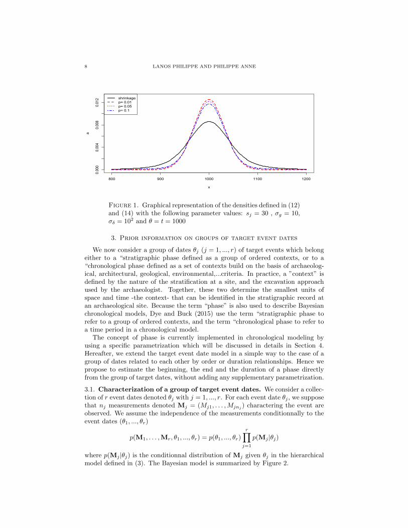
A graphical representation of the densities defined in (12) and (14) are shown inFigure 1 with the following parameter values: sj = 30 , σg = 10, σδ = 102 and θ =t = 1000. The density (12) is plotted for three different values p = 0.01, 0.05, 0.10. We can observe that shrinkage modeling in (14) leads to a more diffuse densitymaking it possible to better take into account the possible presence of outliers.
8 LANOS PHILIPPE AND PHILIPPE ANNE
800 900 1000 1100 1200
0.000
0.004
0.008
0.012
x
a
shrinkagep= 0.01p= 0.05p= 0.1
Figure 1. Graphical representation of the densities defined in (12)and (14) with the following parameter values: sj = 30 , σg = 10,σδ = 102 and θ = t = 1000
3. Prior information on groups of target event dates
We now consider a group of dates θj (j = 1, ..., r) of target events which belongeither to a “stratigraphic phase defined as a group of ordered contexts, or to a“chronological phase defined as a set of contexts build on the basis of archaeolog-ical, architectural, geological, environmental,...criteria. In practice, a ”context” isdefined by the nature of the stratification at a site, and the excavation approachused by the archaeologist. Together, these two determine the smallest units ofspace and time -the context- that can be identified in the stratigraphic record atan archaeological site. Because the term “phase” is also used to describe Bayesianchronological models, Dye and Buck (2015) use the term “stratigraphic phase torefer to a group of ordered contexts, and the term “chronological phase to refer toa time period in a chronological model.
The concept of phase is currently implemented in chronological modeling byusing a specific parametrization which will be discussed in details in Section 4.Hereafter, we extend the target event date model in a simple way to the case of agroup of dates related to each other by order or duration relationships. Hence wepropose to estimate the beginning, the end and the duration of a phase directlyfrom the group of target dates, without adding any supplementary parametrization.
3.1. Characterization of a group of target event dates. We consider a collec-tion of r event dates denoted θj with j = 1, ..., r. For each event date θj , we supposethat nj measurements denoted Mj = (Mj1, . . . ,Mjnj ) charactering the event areobserved. We assume the independence of the measurements conditionnally to theevent dates (θ1, ..., θr)
p(M1, . . . ,Mr, θ1, ..., θr) = p(θ1, ..., θr)
r∏j=1
p(Mj |θj)
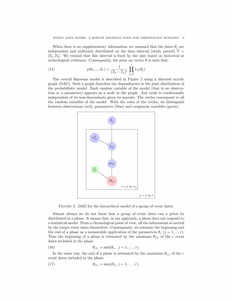
where p(Mj |θj) is the conditionnal distribution of Mj given θj in the hierarchicalmodel defined in (3). The Bayesian model is summarized by Figure 2.
EVENT DATE MODEL: A ROBUST BAYESIAN TOOL FOR CHRONOLOGY BUILDING 9
When there is no supplementary information, we assumed that the dates θj areindependent and uniformly distributed on the time interval (study period) T =[Ta, Tb]. We remind that this interval is fixed by the user based on historical orarcheological evidences. Consequently, the prior on vector θ is such that:
(15) p(θ1, ..., θr) =1
(Tb − Ta)r
r∏j=1
1T (θj)
The overall Bayesian model is described in Figure 2 using a directed acyclicgraph (DAG). Such a graph describes the dependencies in the joint distribution ofthe probabilistic model. Each random variable of the model (that is an observa-tion or a parameter) appears as a node in the graph. Any node is conditionallyindependent of its non-descendants given its parents. The circles correspond to allthe random variables of the model. With the color of the circles, we distinguishbetween observations (red), parameters (blue) and exogenous variables (green).
j = 1 to r
i = 1 to nj
θj
tji
µji
Mji
σ2ji
s2ji
Figure 2. DAG for the hierarchical model of a group of event dates.
Almost always we do not know how a group of event dates can a priori bedistributed in a phase. It means that, in our approach, a phase does not respond toa statistical model. From a chronological point of view, all the information is carriedby the target event dates themselves. Consequently, we estimate the beginning andthe end of a phase as a measurable application of the parameters θj (j = 1, ..., r).Thus the beginning of a phase is estimated by the minimum θ(1) of the r eventdates included in the phase
(16) θ(1) = min(θj , j = 1, . . . , r).
In the same way, the end of a phase is estimated by the maximum θ(r) of the revent dates included in the phase:
(17) θ(r) = max(θj , j = 1, . . . , r).
10 LANOS PHILIPPE AND PHILIPPE ANNE
By the plug-in principle, we estimate the duration of the phase by
(18) τ = θ(r) − θ(1)
Considering two phases Pk = {θk,1, ..., θk,rk}, k = 1, 2, the hiatus between P1
and P2 is the time gap between the end of P1 and the beginning P2. The hiatus isestimated by :
(19) γ = max(θ2,(1) − θ1,(r1) , 0)
where θ2,(1) = min(θ2,1, ..., θ2,r2) and where θ1,(r1) = max(θ1,1, ..., θ1,r1). Note thatthe estimate γ takes the value 0 if θ1,(r1) ≤ θ2,(1), that corresponds to the absenceof hiatus. The conditional distributions of the parameters θ(1), θ(r), γ and τ giventhe observations can be easily derived from the joint posterior distributions of theevent dates.
Remark 3. Let us remind that these parameters are estimated knowing the data,that is to say from the target event dates which are available in the phase of interest.In particular, a good estimation of the beginning (resp. the end) of a phase requiresthat the archaeologist has sampled artifacts belonging to target events which are verynear to this beginning (resp. this end).
These estimates are valid whatever the prior on the event dates are. Precision onthe estimation of these parameters can be gained if it is possible to add supplemen-tary information on the target event dates within the study period T . For instancesome temporal orders induce some restrictions on the support of the distribution.
Different prior on dates θj can be defined according to the following circum-stances:
• Relative dating based on stratigraphy as defined in Harris (1989) and De-sachy (2005, 2008), can imply antero-posteriority relationships between tar-get dates θj . This can also imply antero-posteriority relationships betweengroups of dates θj , these groups defining different phases.
• We can have some prior information about the maximal duration of a groupof target events.
• We can also have some prior information about the minimal temporal hiatusbetween two groups of target events.
It has been demonstrated that these types of supplementary prior informationcan significantly improve chronometric dates (see initial works of Naylor and Smith(1988); Buck et al. (1991, 1992, 1994, 1996) and Christen (1994)). In the nextthree subsections, we discuss each of these prior information in the framework ofthe target event date model. Our modeling approach is very soft thanks to thefact that all the relationships operate directly onto the target event dates θj . As aconsequence, in a global modeling project, different phasing systems (multiphasing)can be defined on the basis of different criteria and so a phasing system can intersectan other phasing system: for example a ceramic phasing can intersect a lithicphasing in the sense that some target events can belong to two or several phases.Such a constraints network, when available, can significantly contribute to improvethe precision of the estimates.
3.2. Prior information on temporal order. Target events or phases (groups)of target events can have to check order relationships. This order can be defined indifferent ways: by the stratigraphic relationship (physical relationship observed in
EVENT DATE MODEL: A ROBUST BAYESIAN TOOL FOR CHRONOLOGY BUILDING 11
the field) or by stylistic, technical, architectural,... criteria which may be a prioriknown. Thus, the constraint of succession is equivalent to a hiatus of unknownamplitude put between event dates or groups (phases) of event dates.
If we consider a stratigraphic sequence composed of target events, the prior onvector θ becomes:
(20) p(θ1, ..., θr) ∝1
(Tb − Ta)r1C(θ1, ..., θr)
with C = S ∩ T r and
• T r = [Ta, Tb]r the support which defines the study period,
• S = the group of r-uplets event dates θj which respect total or partial orderrelationships.
We can also consider two groups of target events, Pk = {θk,1, ..., θk,rk}, k = 1, 2,containing rk event dates such that all the dates of P1 are before all the dates ofP2. The following equations should be verified by all the events included in bothphases.
∀j ∈ {1, ..., r1}, ∀l ∈ {1, ..., r2}, θ1,j < θ2,l
ormax(θ1,j , j = 1, . . . , r1) < min(θ2,l, l = 1, . . . , r2)
or
(21) min(θ2,l, l = 1, . . . , r2)−max(θ1,j , j = 1, . . . , r1) > 0
The r-uplets event dates θj will then have to check total or partial stratigraphicconstraints and also to satisfy the inequality (21) between event dates of the twophases. We can see that a succession constraint between phases operates in thesame mathematical way as for a set of stratigraphic constraints put between all theindividual target events.
Remark 4. Estimating the date of a target event needs to incorporate several dates(Ed), otherwise the event date modeling will not yield a better posterior information.However, it is possible to nest only one date per target event provided that the groupof events is constrained by temporal order.
It is not rare to encounter dating results which contradict the stratigraphic order:one speaks of “stratigraphic inversion”. This situation often occurs when someartifact movements are provoked for example by bioturbations or establishmentof backfill soils. The target event date model makes it possible to manage suchsituations thanks to the individual variances σ2
i which automatically penalize thedates that are inconsistent with the stratigraphic order. This is illustrated in Section5.2.
3.3. Prior information about the duration. Prior information can be includedon the duration of a phase, that is on a group of target events. We can impose amaximal duration τ0. This means that all the event dates θj (j = 1, ..., r) in thephase have to verify the constraint of duration according to the following equation:
(22) max(θj , j = 1, . . . , r)−min(θj , j = 1, . . . , r) ≤ τ0The r-uplets event dates θj will have to check total or partial stratigraphic con-
straints and also to satisfy the inequality 22 between event dates in the phase. Thismeans that any r-uplet θj sampled during the MCMC process has a duration of atthe most τ0.
12 LANOS PHILIPPE AND PHILIPPE ANNE
3.4. Prior information about the amplitude of a hiatus. Prior informationabout a hiatus γ between two phases Pk = {θk,1, ..., θk,rk}, k = 1, 2, may be avail-able. Hence we can impose that the amplitude of the hiatus is higher than a knownvalue γ0 > 0. All the event dates of phase P1 and phase P2 have to verify thefollowing constraint :
(23) min(θ2,l, l = 1, ..., r2)−max(θ1j , j = 1, ..., r1) ≥ γ0
The event dates will have to check total or partial stratigraphic constraints andalso to satisfy the inequality (23). This means that any r-uplet θ1,j from phaseP1 and sampled during the MCMC process is separated by a time span of at leastγ0 from the r-uplet θ2,l of the next phase. Note that it is obviously not possibleto impose a hiatus between two phases when a same event belongs to these twophases.
3.5. Prior information about known event dates: the bounds. Bounds,such as historical dates, Terminus post quem (TPQ) or terminus ante quem (TAQ),may also be introduced in order to constrain one or several event dates θj . If weconsider a set of r events assumed to happen after a special event with true calendardate B such that
B < (θ1, ..., θr)
This condition must be included in the set of constraints that define the support ofthe prior distribution of the event dates.
The bound can be also defined with an uncertainty, i.e. B ∈ [Ba, Bb] ⊂ [Ta, Tb],and so it is included in the set of the parameters. The prior density of the eventdates can then be written as:
p(θ1, ..., θr, B) = p(θ1, ..., θr|B)p(B)
where
p(θ1, ..., θr|B) =1
(Tb −B)r
r∏j=1
1[B,Tb](θj)
and
p(B) =1
Bb −Ba1[Ba,Bb](B)
It is important to note that the introduction of bounds B in a global modelcomposed of groups (phases) of event dates must remain consistent with otherconstraints of temporal order, of duration or of hiatus described in previous sections.
4. Discussion on date prior probabilities
In this section we discuss the question of the specification of the prior on theevent dates θj . When there is no supplementary information, it may seem naturalto assume that the dates θj are independent and uniformly distributed on the timeinterval (study period) T = [Ta, Tb]. However, from an archaeological point of view,it may seem more natural to assert that the span ∆ = max(θj) − min(θj) has auniform prior distribution We can see that this assumption is not checked whenstarting from the prior density (15). After an appropriate change of variable and
EVENT DATE MODEL: A ROBUST BAYESIAN TOOL FOR CHRONOLOGY BUILDING 13
letting R = Tb − Ta, we can determine the density of the span according to thenumber of dates r and regardless their order:
(24) p(∆) =r(r − 1)
Rr(R−∆)∆r−2
A span of 2∆ is favoured over a span of ∆ by a factor of about ∆r−2 when ∆� R(spreading tendency when r becomes large). This behavior occurs regardless of theorder between dates.
Naylor and Smith (1988); Buck et al. (1992); Christen (1994); Buck et al. (1996);Nicholls and Jones (2002) propose a specific phase modeling which aims to avoidthis spreading bias. We study the properties of this modeling implemented in BCaland OxCal software. The Naylor-Smith-Buck-Christen (NSBC) prior is defined fora group of event dates which are placed between two additional hyperparametersα and β in the Bayesian hierarchical structure. These hyperparameters α and βrepresent boundaries where α is the beginning and β the end of the group of eventscalled Phase. The dates θj are assumed to be independent conditionally to thesetwo boundaries. Then, the prior density on vector θ becomes:
(25) p(θ1, . . . , θr|α, β) =1
(β − α)r1[α,β]r (θ1, . . . , θr)
In the absence of supplementary information, a non informative prior density isassigned to α and β :
(26) p(α, β) =2
(Tb − Ta)2.1P (α, β)
with P = {(α, β) | Ta ≤ α ≤ β ≤ Tb}. The pairs (α, β) are uniformly distributedon the triangle P .
From these hypotheses, it is possible to calculate the prior joint probabilitydensity of the event dates (θ1 . . . θr). This is carried out by integration against αand β between the two limits Ta and Tb. For 2 (ordered or non ordered) event datesθ1, θ2, we obtain:
p(θ1, θ2) =
∫p(θ1, θ2|α, β).p(α, β) dαdβ
=
∫1
(β − α)2.1[α,β](θ1).1[α,β](θ2)
2
(Tb − Ta)2.1[Ta≤α≤β≤Tb](α, β).dαdβ
=2
(Tb − Ta)2
∫ min(θ1,θ2)
Ta
∫ Tb
max(θ1,θ2)
1
(β − α)2dβ dα
=2
(Tb − Ta)2
∫ min(θ1,θ2)
Ta
[1
(max(θ1, θ2)− α)− 1
(Tb − α)] dα
Finally, we have:
(27) p(θ1, θ2) =4
(Tb − Ta)2(− ln(max(θ1, θ2)−min(θ1, θ2)) + ln(Tb −min(θ1, θ2))
+ ln(max(θ1, θ2)− Ta)− ln(Tb − Ta))1[Ta,Tb]2(θ1, θ2)
14 LANOS PHILIPPE AND PHILIPPE ANNE
The joint probability density for r (ordered or non ordered) event dates (θj , j = 1, . . . , r)with r ≥ 3, is obtained by following the same integration process:
(28) p(θ1, ..., θr) =2 r!
(r − 1)(r − 2)(Tb − Ta)2
(1
[θ(r) − θ(1)]r−2
− 1
[Tb − θ(1)]r−2− 1
[θ(r) − Ta]r−2+
1
[Tb − Ta]r−2
)1[Ta,Tb]2(θ(1), θ(r))
where θ(r) = max(θj , j = 1, . . . , r) and θ(1) = min(θj , j = 1, . . . , r).Equations (27) and (28) clearly show that the priors (25) and (26) provoke
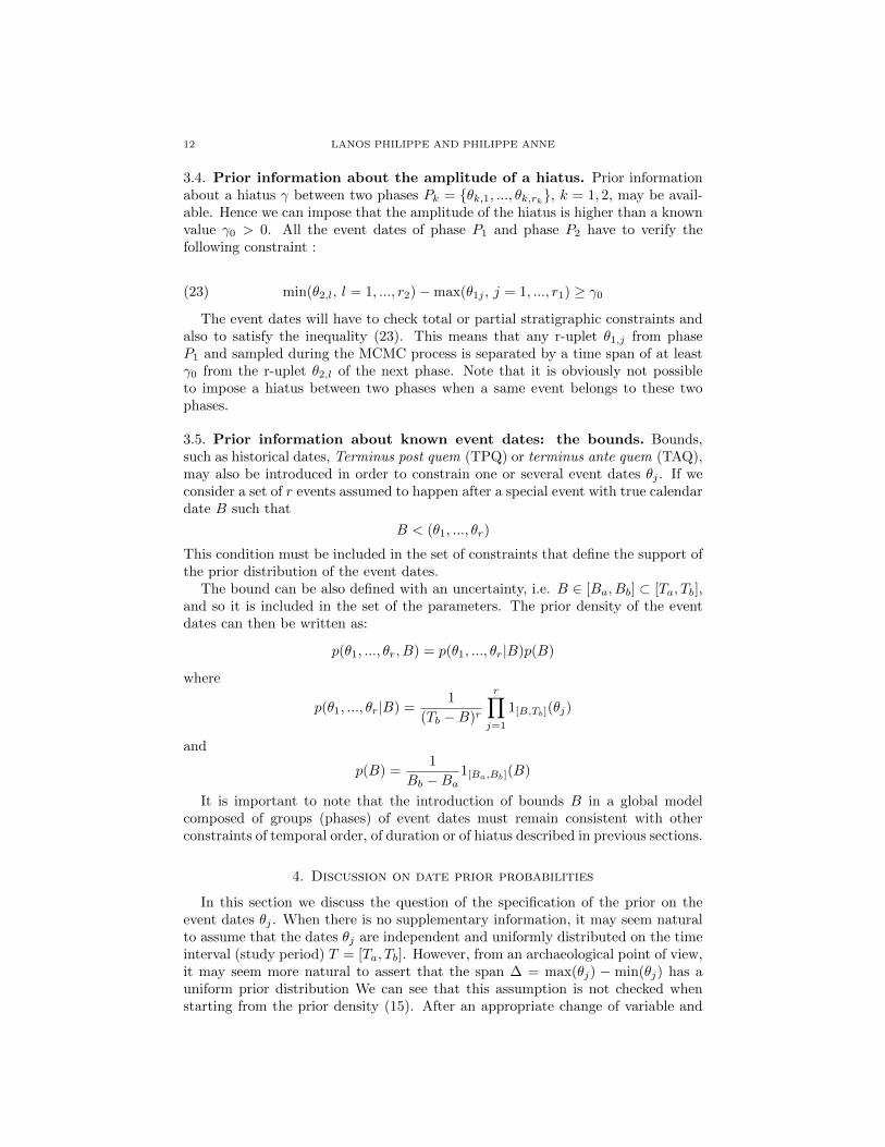
a strong concentration effect of the dates θj as illustrated in Figure 3 which iscalculated for two event dates with formula (27). The region of high probability of(θ1, θ2) is concentrated around the first diagonal (θ1 = θ2). In conclusion, the NSBCprior clearly favors the fact that dates (θ1, ..., θr) become near each other. Thisproperty of the phase can be compared with the assumption of contemporaneityimposed on the dates in the event model.
Figure 3. “NSBC” phase model: prior joint density on two (nonordered) event dates θ1 and θ2 between two boundaries α and β andafter integration against α and β: a concentration effect appearsaround values θ1 = θ2.
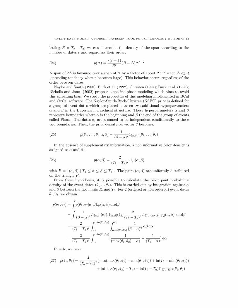
Starting from the prior densities (27) and (28), and after an appropriate change ofvariable, we can also determine the density of the span ∆ = max(θj , j = 1, ..., r)−min(θj , j = 1, ..., r), according to the number of dates r. Letting R = Tb − Ta, weobtain :
r = 2 : p(∆) =4
R2
[(R+ ∆)(ln(R)− ln(∆)) + 2(∆−R))
](29)
r = 3 : p(∆) =6
R2
[(R−∆)(1 +
∆
R) + 2∆(ln(∆)− ln(R))
](30)
r ≥ 4 : p(∆) =2r
(r − 2)R2
[(R−∆)(1 +
∆r−2
Rr−2)− 2
r − 2)(∆− ∆r−2
Rr−3)
](31)
EVENT DATE MODEL: A ROBUST BAYESIAN TOOL FOR CHRONOLOGY BUILDING 15
These distributions are shown in Figure 4. When r is small (r = 2, 3, 4), thedensities are very high for ∆ near zero, hence a high concentration effect. Whenr tends towards infinity, the distribution of ∆ tends to p(∆) = 2
R2 (R − ∆). Thislatter triangular distribution is still maximal when ∆ = 0, and it becomes moreand more flat as R increases. Nicholls and Jones (2002) proposed to make the prior
distribution on the dates θj uniform by multiplying the prior in (26) by R2
2(R−∆)
where min(θj , j = 1, ..., r) is replaced by α and max(θj , j = 1, ..., r) by β .This option is implemented in OxCal when setting UniformSpanPrior=true’ in amodeling project (Bronk Ramsey, 2009a).
Figure 4. Distributions of the span ∆ pour different values of thenumber r of event dates in a NSBC phase model with: Ta ≤ α ≤θ1, . . . , θr ≤ β ≤ Tb. When r is small (r = 2, 3, 4), the densities arevery high for ∆ near zero, reflecting a high concentration effect.
Instead of looking at the span ∆, we can look at the variance of the event datesθj , which is more representative of their scattering. This variance is proportionalto the sequence of the Euclidian distance of the event dates to the straight lineθ1 = θ2 = ... = θr in the space of dimension r and therefore it gives a good wayto characterize the scattering of the dates. We observe that this distance remainsnear zero whatever the number r of event dates. Figure 5 shows an evaluation ofthe dispersion of the dates through the density of the statistic
(32)1
r
r∑i=1
(θi −
1
r
r∑j=1
θj
)2
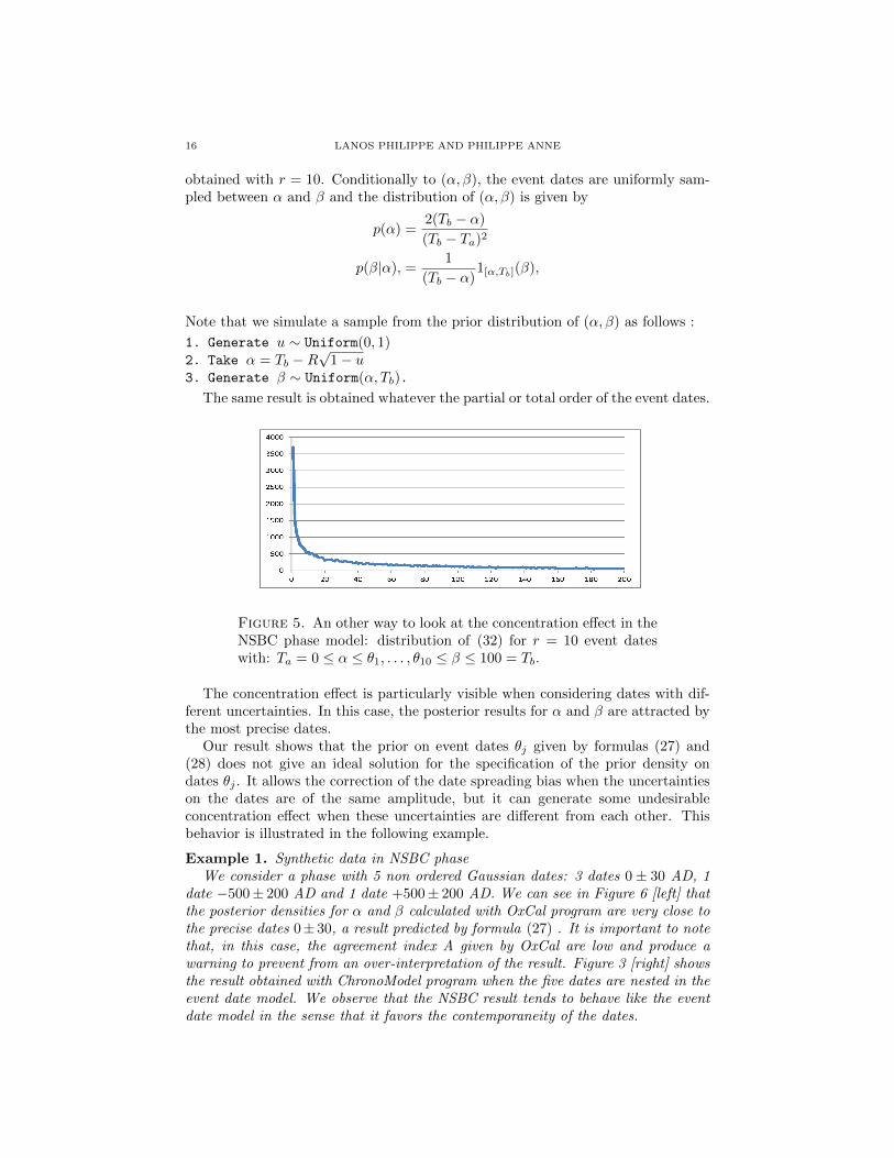
16 LANOS PHILIPPE AND PHILIPPE ANNE
obtained with r = 10. Conditionally to (α, β), the event dates are uniformly sam-pled between α and β and the distribution of (α, β) is given by
p(α) =2(Tb − α)
(Tb − Ta)2
p(β|α), =1
(Tb − α)1[α,Tb](β),
Note that we simulate a sample from the prior distribution of (α, β) as follows :
1. Generate u ∼ Uniform(0, 1)2. Take α = Tb −R
√1− u
3. Generate β ∼ Uniform(α, Tb).
The same result is obtained whatever the partial or total order of the event dates.
Figure 5. An other way to look at the concentration effect in theNSBC phase model: distribution of (32) for r = 10 event dateswith: Ta = 0 ≤ α ≤ θ1, . . . , θ10 ≤ β ≤ 100 = Tb.
The concentration effect is particularly visible when considering dates with dif-ferent uncertainties. In this case, the posterior results for α and β are attracted bythe most precise dates.
Our result shows that the prior on event dates θj given by formulas (27) and(28) does not give an ideal solution for the specification of the prior density ondates θj . It allows the correction of the date spreading bias when the uncertaintieson the dates are of the same amplitude, but it can generate some undesirableconcentration effect when these uncertainties are different from each other. Thisbehavior is illustrated in the following example.
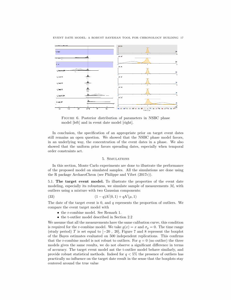
Example 1. Synthetic data in NSBC phaseWe consider a phase with 5 non ordered Gaussian dates: 3 dates 0 ± 30 AD, 1
date −500± 200 AD and 1 date +500± 200 AD. We can see in Figure 6 [left] thatthe posterior densities for α and β calculated with OxCal program are very close tothe precise dates 0± 30, a result predicted by formula (27) . It is important to notethat, in this case, the agreement index A given by OxCal are low and produce awarning to prevent from an over-interpretation of the result. Figure 3 [right] showsthe result obtained with ChronoModel program when the five dates are nested in theevent date model. We observe that the NSBC result tends to behave like the eventdate model in the sense that it favors the contemporaneity of the dates.
EVENT DATE MODEL: A ROBUST BAYESIAN TOOL FOR CHRONOLOGY BUILDING 17
Figure 6. Posterior distribution of parameters in NSBC phasemodel [left] and in event date model [right].
In conclusion, the specification of an appropriate prior on target event datesstill remains an open question. We showed that the NSBC phase model favors,in an underlying way, the concentration of the event dates in a phase. We alsoshowed that the uniform prior favors spreading dates, especially when temporalorder constraints act.
5. Simulations
In this section, Monte Carlo experiments are done to illustrate the performanceof the proposed model on simulated samples. All the simulations are done usingthe R package ArchaeoChron (see Philippe and Vibet (2017c)).
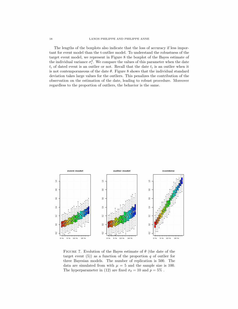
5.1. The target event model. To illustrate the properties of the event datemodeling, especially its robustness, we simulate sample of measurements Mi withoutliers using a mixture with two Gaussian components:
(33) (1− q)N (0, 1) + qN (µ, 1)
The date of the target event is 0, and q represents the proportion of outliers. Wecompare the event target model with
• the r-combine model. See Remark 1.• the t-outlier model described in Section 2.2
We assume that all the measurements have the same calibation curve, this conditionis required for the r-combine model. We take g(x) = x and σg = 0. The time range(study period) T is set equal to [−20 , 20], Figure 7 and 8 represent the boxplotof the Bayes estimates evaluated on 500 independent replications. This confirmsthat the r-combine model is not robust to outliers. For q = 0 (no outlier) the threemodels gives the same results, we do not observe a significant difference in termsof accuracy. The target event model ant the t-outlier model behave similarly, andprovide robust statistical methods. Indeed for q < 5% the presence of outliers haspractically no influence on the target date result in the sense that the boxplots staycentered around the true value
18 LANOS PHILIPPE AND PHILIPPE ANNE
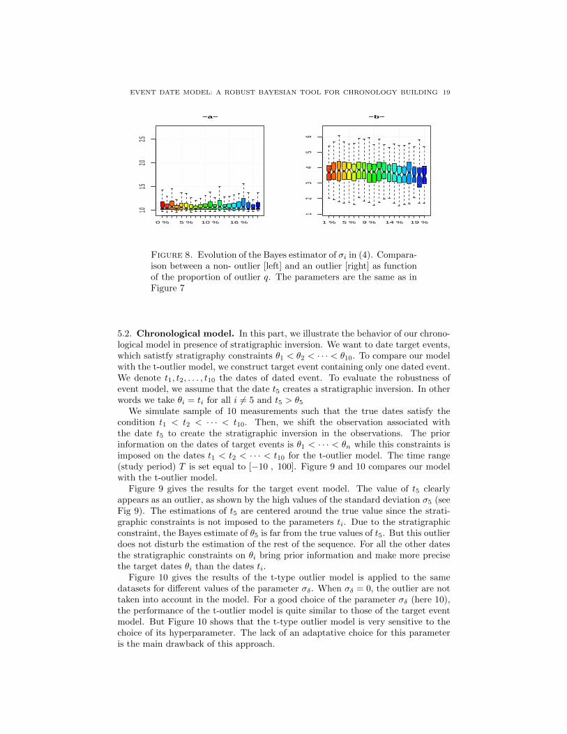
The lengths of the boxplots also indicate that the loss of accuracy if less impor-tant for event model than the t-outlier model. To understand the robustness of thetarget event model, we represent in Figure 8 the boxplot of the Bayes estimate ofthe individual variance σ2
i . We compare the values of this parameter when the dateti of dated event is an outlier or not. Recall that the date ti is an outlier when itis not contemporaneous of the date θ. Figure 8 shows that the individual standarddeviation takes large values for the outliers. This penalizes the contribution of theobservation on the estimation of the date, leading to robust procedure. Moreoverregardless to the proportion of outliers, the behavior is the same.
0 % 5 % 10 % 16 %
−0.2
0.00.2
0.40.6
0.81.0
event model
0 % 5 % 10 % 16 %
−0.2
0.00.2
0.40.6
0.81.0
outlier model
0 % 5 % 10 % 16 %
−0.2
0.00.2
0.40.6
0.81.0
rcombine
Figure 7. Evolution of the Bayes estimate of θ (the date of thetarget event (5)) as a function of the proportion q of outlier forthree Bayesian models. The number of replication is 500. Thedata are simulated from with µ = 5 and the sample size is 100.The hyperparameter in (12) are fixed σδ = 10 and p = 5% .
EVENT DATE MODEL: A ROBUST BAYESIAN TOOL FOR CHRONOLOGY BUILDING 19
0 % 5 % 10 % 16 %
1.01.5
2.02.5
−a−
1 % 5 % 9 % 14 % 19 %
12
34
56
−b−
Figure 8. Evolution of the Bayes estimator of σi in (4). Compara-ison between a non- outlier [left] and an outlier [right] as functionof the proportion of outlier q. The parameters are the same as inFigure 7
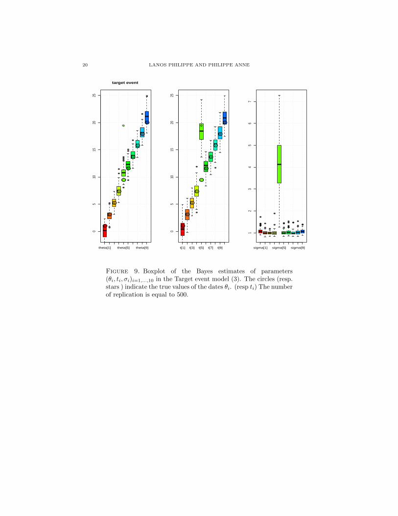
5.2. Chronological model. In this part, we illustrate the behavior of our chrono-logical model in presence of stratigraphic inversion. We want to date target events,which satistfy stratigraphy constraints θ1 < θ2 < · · · < θ10. To compare our modelwith the t-outlier model, we construct target event containing only one dated event.We denote t1, t2, . . . , t10 the dates of dated event. To evaluate the robustness ofevent model, we assume that the date t5 creates a stratigraphic inversion. In otherwords we take θi = ti for all i 6= 5 and t5 > θ5
We simulate sample of 10 measurements such that the true dates satisfy thecondition t1 < t2 < · · · < t10. Then, we shift the observation associated withthe date t5 to create the stratigraphic inversion in the observations. The priorinformation on the dates of target events is θ1 < · · · < θn while this constraints isimposed on the dates t1 < t2 < · · · < t10 for the t-outlier model. The time range(study period) T is set equal to [−10 , 100]. Figure 9 and 10 compares our modelwith the t-outlier model.
Figure 9 gives the results for the target event model. The value of t5 clearlyappears as an outlier, as shown by the high values of the standard deviation σ5 (seeFig 9). The estimations of t5 are centered around the true value since the strati-graphic constraints is not imposed to the parameters ti. Due to the stratigraphicconstraint, the Bayes estimate of θ5 is far from the true values of t5. But this outlierdoes not disturb the estimation of the rest of the sequence. For all the other datesthe stratigraphic constraints on θi bring prior information and make more precisethe target dates θi than the dates ti.
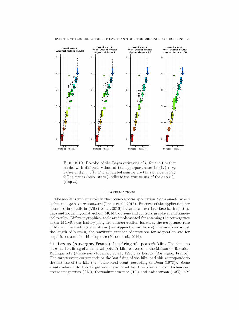
Figure 10 gives the results of the t-type outlier model is applied to the samedatasets for different values of the parameter σδ. When σδ = 0, the outlier are nottaken into account in the model. For a good choice of the parameter σδ (here 10),the performance of the t-outlier model is quite similar to those of the target eventmodel. But Figure 10 shows that the t-type outlier model is very sensitive to thechoice of its hyperparameter. The lack of an adaptative choice for this parameteris the main drawback of this approach.
20 LANOS PHILIPPE AND PHILIPPE ANNE
●
●
●
●
●
●
●
●
●
●
●
●
●
●
theta[1] theta[5] theta[9]
05
1015
2025
target event
●
●
●
●
●
●
●
●
●
●
●
●
●
●
●
●
●
●
●
●
●
●●
t[1] t[3] t[5] t[7] t[9]
05
1015
2025
●
●
●
●
●
●
●
●
●
●
●
●
●
●
●
●
●
●
●
●
●
●
●
●
● ●
●●
●
●●
●
● ●
●●●
●●●
●
●●●
sigma[1] sigma[5] sigma[9]1
23
45
67
Figure 9. Boxplot of the Bayes estimates of parameters(θi, ti, σi)i=1,...,10 in the Target event model (3). The circles (resp.stars ) indicate the true values of the dates θi. (resp ti) The numberof replication is equal to 500.
EVENT DATE MODEL: A ROBUST BAYESIAN TOOL FOR CHRONOLOGY BUILDING 21
●
●
●●●
●●●
●
theta[1] theta[7]
05
1015
2025
●
●
●
●
●
●
●
●
●
●
●
●
●
●
●
●
●
●
●
●
dated event whitout outlier model
●
●
●
●●
●
●●
●
theta[1] theta[7]
05
1015
2025
●
●
●
●
●
●
●
●
●
●
●
●
●
●
●
●
●
●
●
●
dated event with outlier model
sigma_delta = 1
●
●
●
●
●●
●
●
●●●
●●●●
theta[1] theta[7]
05
1015
2025
●
●
●
●
●
●
●
●
●
●
●
●
●
●
●
●
●
●
●
●
dated event with outlier model sigma_delta = 10
●
●
●
●
theta[1] theta[7]
05
1015
2025
●
●
●
●
●
●
●
●
●
●
●
●
●
●
●
●
●
●
●
●
dated event with outlier model sigma_delta = 100
Figure 10. Boxplot of the Bayes estimates of ti for the t-outliermodel with different values of the hyperparameter in (12) : σδvaries and p = 5%. The simulated sample are the same as in Fig.9 The circles (resp. stars ) indicate the true values of the dates θi.(resp ti)
6. Applications
The model is implemented in the cross-platform application Chronomodel whichis free and open source software (Lanos et al., 2016). Features of the application aredescribed in details in (Vibet et al., 2016) : graphical user interface for importingdata and modeling construction, MCMC options and controls, graphical and numer-ical results. Different graphical tools are implemented for assessing the convergenceof the MCMC: the history plot, the autocorrelation function, the acceptance rateof Metropolis-Hastings algorithms (see Appendix, for details) The user can adjustthe length of burn-in, the maximum number of iterations for adaptation and foracquisition, and the thinning rate (Vibet et al., 2016).
6.1. Lezoux (Auvergne, France): last firing of a potter’s kiln. The aim is todate the last firing of a medieval potter’s kiln recovered at the Maison-de-Retraite-Publique site (Mennessier-Jouannet et al., 1995), in Lezoux (Auvergne, France).The target event corresponds to the last firing of the kiln, and this corresponds tothe last use of the kiln (i.e. behavioral event, according to Dean (1978)). Someevents relevant to this target event are dated by three chronometric techniques:archaeomagnetism (AM), thermoluminescence (TL) and radiocarbon (14C). AM
22 LANOS PHILIPPE AND PHILIPPE ANNE
and TL dates are determined from baked clay and 14C date from charcoals of treesassumed to be felled at the same time as the last firing.
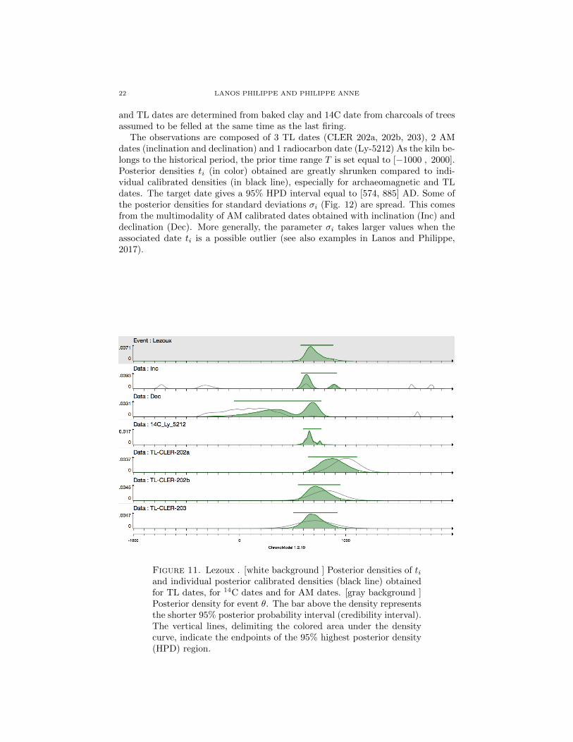
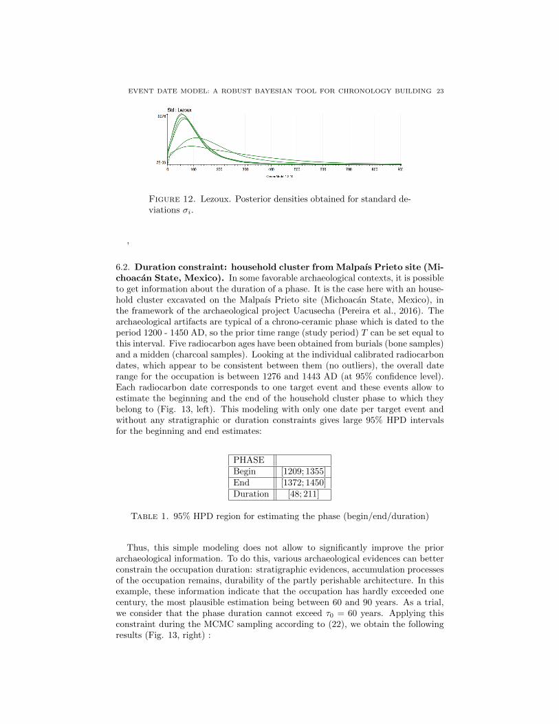
The observations are composed of 3 TL dates (CLER 202a, 202b, 203), 2 AMdates (inclination and declination) and 1 radiocarbon date (Ly-5212) As the kiln be-longs to the historical period, the prior time range T is set equal to [−1000 , 2000].Posterior densities ti (in color) obtained are greatly shrunken compared to indi-vidual calibrated densities (in black line), especially for archaeomagnetic and TLdates. The target date gives a 95% HPD interval equal to [574, 885] AD. Some ofthe posterior densities for standard deviations σi (Fig. 12) are spread. This comesfrom the multimodality of AM calibrated dates obtained with inclination (Inc) anddeclination (Dec). More generally, the parameter σi takes larger values when theassociated date ti is a possible outlier (see also examples in Lanos and Philippe,2017).
Figure 11. Lezoux . [white background ] Posterior densities of tiand individual posterior calibrated densities (black line) obtainedfor TL dates, for 14C dates and for AM dates. [gray background ]Posterior density for event θ. The bar above the density representsthe shorter 95% posterior probability interval (credibility interval).The vertical lines, delimiting the colored area under the densitycurve, indicate the endpoints of the 95% highest posterior density(HPD) region.
EVENT DATE MODEL: A ROBUST BAYESIAN TOOL FOR CHRONOLOGY BUILDING 23
Figure 12. Lezoux. Posterior densities obtained for standard de-viations σi.
,
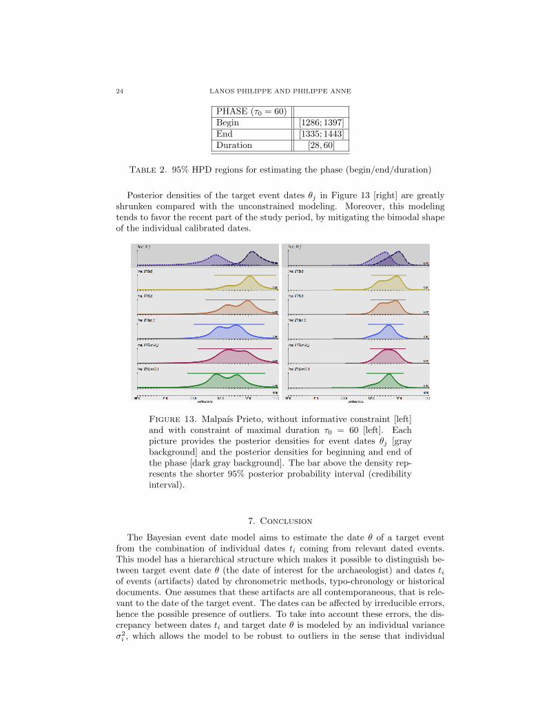
6.2. Duration constraint: household cluster from Malpaıs Prieto site (Mi-choacan State, Mexico). In some favorable archaeological contexts, it is possibleto get information about the duration of a phase. It is the case here with an house-hold cluster excavated on the Malpaıs Prieto site (Michoacan State, Mexico), inthe framework of the archaeological project Uacusecha (Pereira et al., 2016). Thearchaeological artifacts are typical of a chrono-ceramic phase which is dated to theperiod 1200 - 1450 AD, so the prior time range (study period) T can be set equal tothis interval. Five radiocarbon ages have been obtained from burials (bone samples)and a midden (charcoal samples). Looking at the individual calibrated radiocarbondates, which appear to be consistent between them (no outliers), the overall daterange for the occupation is between 1276 and 1443 AD (at 95% confidence level).Each radiocarbon date corresponds to one target event and these events allow toestimate the beginning and the end of the household cluster phase to which theybelong to (Fig. 13, left). This modeling with only one date per target event andwithout any stratigraphic or duration constraints gives large 95% HPD intervalsfor the beginning and end estimates:
PHASEBegin [1209; 1355]End [1372; 1450]Duration [48; 211]
Table 1. 95% HPD region for estimating the phase (begin/end/duration)
Thus, this simple modeling does not allow to significantly improve the priorarchaeological information. To do this, various archaeological evidences can betterconstrain the occupation duration: stratigraphic evidences, accumulation processesof the occupation remains, durability of the partly perishable architecture. In thisexample, these information indicate that the occupation has hardly exceeded onecentury, the most plausible estimation being between 60 and 90 years. As a trial,we consider that the phase duration cannot exceed τ0 = 60 years. Applying thisconstraint during the MCMC sampling according to (22), we obtain the followingresults (Fig. 13, right) :
24 LANOS PHILIPPE AND PHILIPPE ANNE
PHASE (τ0 = 60)Begin [1286; 1397]End [1335; 1443]Duration [28, 60]
Table 2. 95% HPD regions for estimating the phase (begin/end/duration)
Posterior densities of the target event dates θj in Figure 13 [right] are greatlyshrunken compared with the unconstrained modeling. Moreover, this modelingtends to favor the recent part of the study period, by mitigating the bimodal shapeof the individual calibrated dates.
Figure 13. Malpaıs Prieto, without informative constraint [left]and with constraint of maximal duration τ0 = 60 [left]. Eachpicture provides the posterior densities for event dates θj [graybackground] and the posterior densities for beginning and end ofthe phase [dark gray background]. The bar above the density rep-resents the shorter 95% posterior probability interval (credibilityinterval).
7. Conclusion
The Bayesian event date model aims to estimate the date θ of a target eventfrom the combination of individual dates ti coming from relevant dated events.This model has a hierarchical structure which makes it possible to distinguish be-tween target event date θ (the date of interest for the archaeologist) and dates tiof events (artifacts) dated by chronometric methods, typo-chronology or historicaldocuments. One assumes that these artifacts are all contemporaneous, that is rele-vant to the date of the target event. The dates can be affected by irreducible errors,hence the possible presence of outliers. To take into account these errors, the dis-crepancy between dates ti and target date θ is modeled by an individual varianceσ2i , which allows the model to be robust to outliers in the sense that individual
EVENT DATE MODEL: A ROBUST BAYESIAN TOOL FOR CHRONOLOGY BUILDING 25
variances act as outlier penalization. The posterior distribution of the varianceσ2i indicates if an observation is an outlier or not. Thanks to this modeling, it
is not necessary to discard outliers because the corresponding high values σ2i will
automatically penalize their contributions to the event date estimation. Moreover,this model does not require additional exogenous or hyperparameters. The onlyparameter involved in prior shrinkage, s2
0 , comes uniquely from the data analysisvia the individual calibration process. So, the approach is adapted to very differentdatasets. The good robustness properties of the event date model are paid withless precision in the dates. However, this loss of precision is compensated by betterreliability of the chronology. The event model constitutes the basic element in ourchronological modeling approach. Dating data are nested within target event dates(with or without stratigraphic constraints between them) which in turn may benested into phases (with or without succession constraints between them). Succes-sion constraint, maximal duration and/or minimal hiatus can be put on the eventdates in the phases.
8. Acknowledgments
The authors expressed their gratitude to Gregory Pereira (CNRS, UMR ArchAm,University of Paris 1 Pantheon-Sorbonne) for the exchange of information aboutthe example of “Malpaıs Prieto site in Mexico”.We thank Marie Anne Vibet for her very helpful discussions during the preparationof this paper.
References
Bayliss, A. (2009). Rolling out revolution: Using radiocarbon dating in archaeology.Radiocarbon, 51:123–147.
Bayliss, A. (2015). Quality in bayesian chronological models in archaeology. WorldArchaeology, 47(4):677–700.
Bronk Ramsey, C. (1995). Radiocarbon calibration and analysis of stratigraphy :the OxCal program. Radiocarbon, 37(2):425–430.
Bronk Ramsey, C. (1998). Probability and dating. Radiocarbon, 40:461–474.Bronk Ramsey, C. (2001). Development of the radiocarbon calibration program
OxCal. Radiocarbon, 43:355–363.Bronk Ramsey, C. (2008). Deposition models for chronological records. Quaternary
Science Reviews, 27:42–60.Bronk Ramsey, C. (2009a). Bayesian analysis of radiocarbon dates. Radiocarbon,
51(1):337–360.Bronk Ramsey, C. (2009b). Dealing with outliers and offsets in radiocarbon dating.
Radiocarbon, 51(3):1023–1045.Bronk Ramsey, C., Dee, M., Nakagawa, T., and Staff, R. (2010). Developments in
the calibration and modelling of radiocarbon dates. Radiocarbon, 52:953–961.Bronk Ramsey, C. and Lee, S. (2013). Recent and planned developments of the
program OxCal. Radiocarbon, 55:720–730.Bronk Ramsey, C., van der Plicht, J., and Weninger, B. (2001). Wiggle matching
radiocarbon dates. Radiocarbon, 43:381–389.Buck, C., Christen, J., and James, G. (1999). BCal : an on-line Bayesian radiocar-
bon calibration tool. Internet Archaeology, 7.
26 LANOS PHILIPPE AND PHILIPPE ANNE
Buck, C., Kenworthy, J., Litton, C., and Smith, A. (1991). Combining archaeologi-cal and radiocarbon information : a Bayesian approach to calibration. Antiquity,65:808–821.
Buck, C., Litton, C., and Shennan, S. (1994). A case study in combining radiocar-bon and archaeological information : the early bronze age of st-veit-klinglberg,land salzburg, austria. Germania, 72(2):427–447.
Buck, C., Litton, C., and Smith, A. (1992). Calibration of radiocarbon resultspertaining to related archaeological events. Journal of archaeological Science,19:497–512.
Buck, C. E., Higham, T. F. G., and Lowe, D. J. (2003). Bayesian tools fortephrochronology. The Holocene, 13(5):639–647.
Buck, C. E., Litton, C. D., and Cavanagh, W. G. (1996). The Bayesian Approachto Interpreting Archaeological Data. Chichester, J.Wiley and Son, England.
Christen, J. and Perez, S. (2009). A new robust statistical model for radiocarbondata. Radiocarbon, 51(3):1047–1059.
Christen, J. A. (1994). Summarizing a set of radiocarbon determinations: a robustapproach. Applied Statistics, 43(3):489–503.
Combs, B. and Philippe, A. (2017). Bayesian analysis of individual and system-atic multiplicative errors for estimating ages with stratigraphic constraints inoptically stimulated luminescence dating. Quaternary Geochronology, 39(Sup-plement C):24 – 34.
Dean, J. S. (1978). Independent dating in archaeological analysis. Advances inArchaeological Method and Theory, 1:223–255.
Desachy, B. (2005). Du temps ordonne au temps quantifie : application d’outilsmathematiques au modele d’analyse stratigraphique d’edward harris. Bulletin dela Societe Prehistorique Franaise, 102(4):729–740.
Desachy, B. (2008). De la formalisation du traitement des donnees stratigraphiquesen archeologie de terrain. These de doctorat de l’universite de Paris 1, Paris,France.
Dye, T. and Buck, C. (2015). Archaeological sequence diagrams and bayesianchronological models. Journal of Archaeological Science, 1:1–19.
Guerin, G., Antoine, P., Schmidt, E., Goval, E., D., H., Jamet, J., Reyss, J.-L.,Shao, Q., Philippe, A., Vibet, M.-A., and Bahain, J.-J. (2017). Chronologyof the upper pleistocene loess sequence of havrincourt (france) and associatedpalaeolithic occupations: A bayesian approach from pedostratigraphy, osl, radio-carbon, tl and esr/u-series data. Quaternary Geochronology, 42:15 – 30.
Harris, E. (1989). Principles of archaeological stratigraphy. Interdisciplinary Statis-ticss, XIV, 2nd edition. second ed. Academic Press, London.
Lanos, P. and Philippe, A. (2017). Hierarchical Bayesian modeling for combin-ing dates in archaeological context. Journal de la Socit Franaise de Statistique,158:72–88.
Lanos, P., Philippe, A., Lanos, H., and Dufresne, P. (2016). Chronomodel : Chrono-logical Modelling of Archaeological Data using Bayesian Statistics. (Version 1.5)http://www.chronomodel.fr.
Mennessier-Jouannet, C., Bucur, I., Evin, J., Lanos, P., and Miallier, D.(1995). Convergence de la typologie de ceramiques et de trois methodeschronometriques pour la datation d’un four de potier a lezoux (puy-de-dome).Revue d’Archeometrie, 19:37–47.
EVENT DATE MODEL: A ROBUST BAYESIAN TOOL FOR CHRONOLOGY BUILDING 27
Naylor, J. C. and Smith, A. F. M. (1988). An archaeological inference problem.Journal of the American Statistical Association, 83(403):588–595.
Nicholls, G. and Jones, M. (2002). New radiocarbon calibration software. Radio-carbon, 44:663–674.
Niu, M., Heaton, T., Blackwell, P., and Buck, C. (2013). The Bayesian approach toradiocarbon calibration curve estimation: the intcal13, marine 13, and shcal13methodologies. Radiocarbon, 55(4):1905–1922.
Pereira, G., Forest, M., Jadot, E., and Darras, V. (2016). Ephemeral cities? thelongevity of the postclassic tarascan urban sites of zacapu malpas and its conse-quences on the migration process. In Arnauld, M., Beekmann, C., and Pereira,G., editors, Ancient Mesoamerican Cities: Populations on the move, page inpress. University Press of Colorado, Denver, USA.
Philippe, A. and Vibet, M.-A. (2017a). Analysis of Archaeological Phases usingthe CRAN Package ArchaeoPhases. preprint hal-01347895.
Philippe, A. and Vibet, M.-A. (2017b). ArchaeoPhases: Post-Processing of theMarkov Chain Simulated by ’ChronoModel’, ’Oxcal’ or ’BCal’. R package version1.3.
Philippe, A. and Vibet, M.-A. (2017c). Bayesian Modeling of ArchaeologicalChronologies. R package version 0.1.
Plummer, M., Best, N., Cowles, K., and Vines, K. (2006). Coda: Convergencediagnosis and output analysis for mcmc. R News, 6(1):7–11.
R Core Team (2017). R: A Language and Environment for Statistical Computing.R Foundation for Statistical Computing, Vienna, Austria.
Vibet, M.-A., Philippe, A., Lanos, P., and Dufresne, P. (2016). Chronomodel v1.5user’s manual. www.chronomodel.fr.
MCMC computation
.1. Algorithms. The posterior distributions of the parameter of interest θ and ofother related parameters ti and σi can not be obtained explicitly. It is necessaryto implement a computational method to approximate the posterior distributions,their quantiles, the Bayes estimates and the highest posterior density (HPD) re-gions. We adopt a MCMC (Markov Chain Monte Carlo) algorithm known as theMetropolis-within-Gibbs strategy because the full conditionals cannot be simulatedby standard random generators. For each parameter, the full conditional distribu-tion is proportional to (3). Details on the algorithms used are given in (Lanos andPhilippe, 2017).
Here we give a more detailed insight on the way to estimate the date ti whichis defined on the set R due to the random effect model chosen in (2). The fullconditional distribution of ti (∀i = 1, ..., n) is given by
(34) p(ti| q) ∝ 1
Si(ti)exp
{−1
2S2i (ti)
(Mi − gi(ti))2
}exp
{−1
2σ2i
(ti − θ)2)
}where S2
i (ti) = s2i + σ2
gi(ti). Symbol q represents the observations and all otherparameters according to equation (3).
To estimate the posterior density of ti, we can choose between three MCMCalgorithms. In each case, the support of the proposal density includes the supportR of the target posterior density.
28 LANOS PHILIPPE AND PHILIPPE ANNE
• MH-1: A Metropolis-Hastings algorithm where the proposal is the priordistribution of the parameter. This method is recommended when no cal-ibration is needed, namely for TL/OSL, Gaussian measurements or typo-chronological references.• MH-2: A Metropolis-Hastings algorithm where the proposal is an adaptive
Gaussian random walk. This method is adapted when the density to beapproximated is unimodal. The variance of this proposal density is adaptedduring the process.• MH-3: Metropolis-Hastings algorithm where the proposal mimics the indi-
vidual calibration density. This method is adapted for multimodal densities,such as calibrated measurements.
We are frequently confronted with multimodal target distributions as, for in-stance, in archaeomagnetic dating (see example 6.1). In this case, algorithms MH1and MH-2 are not well adapted to ensure a good mixing of the Markov chain.Consequently, an alternative is to choose the MH-3 algorithm with a proposal dis-tribution that mimics the individual calibration density defined in (7). In order toensure the convergence of MCMC algorithm, the support of the proposal must beR. Thus we can consider a mixture having a gaussian component. This componentensures that the whole support is visited. So we take as proposal :
(35) λC + (1− λ)N (0,1
4(Tb − Ta)2)
where λ is a number fixed close to 1, and the distribution C approximates theindividual calibration density. We can choose for instance the empirical measurecalculated on the simulated sample from (7) or a mixture of uniform distribution:
M∑i=1
1
MUniform([ti, ti+1])
where (ti)i=1,...,M are the ordered values of the simulated sample.An alternative is to choose the distribution with density
1
C
p∑i=1
pi(τi)I[τi,τi+1], where C =
p∑i=1
f(τi)(τi+1 − τi)
where (τi)i is a deterministic grid of T and pi is the density of individual calibrationdensity (7).
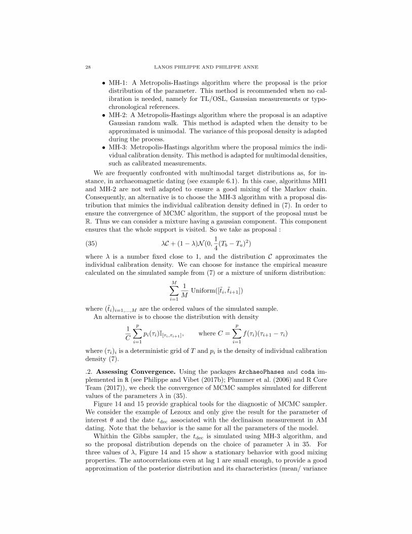
.2. Assessing Convergence. Using the packages ArchaeoPhases and coda im-plemented in R (see Philippe and Vibet (2017b); Plummer et al. (2006) and R CoreTeam (2017)), we check the convergence of MCMC samples simulated for differentvalues of the parameters λ in (35).
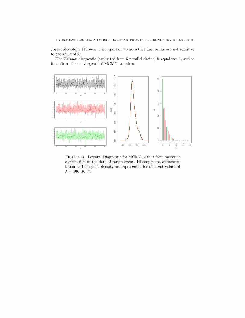
Figure 14 and 15 provide graphical tools for the diagnostic of MCMC sampler.We consider the example of Lezoux and only give the result for the parameter ofinterest θ and the date tdec associated with the declinaison measurement in AMdating. Note that the behavior is the same for all the parameters of the model.
Whithin the Gibbs sampler, the tdec is simulated using MH-3 algorithm, andso the proposal distribution depends on the choice of parameter λ in 35. Forthree values of λ, Figure 14 and 15 show a stationary behavior with good mixingproperties. The autocorrelations even at lag 1 are small enough, to provide a goodapproximation of the posterior distribution and its characteristics (mean/ variance
EVENT DATE MODEL: A ROBUST BAYESIAN TOOL FOR CHRONOLOGY BUILDING 29
/ quantiles etc) . Morever it is important to note that the results are not sensitiveto the value of λ.
The Gelman diagnostic (evaluated from 5 parallel chains) is equal two 1, and soit confirms the convergence of MCMC samplers.
0 1000 2000 3000 4000 5000
40
05
00
60
07
00
80
09
00
10
00
Index
0 1000 2000 3000 4000 5000
40
05
00
60
07
00
80
09
00
10
00
Index
0 1000 2000 3000 4000 5000
40
05
00
60
07
00
80
09
00
10
00
Index
400 600 800 1000
0.00
00.
001
0.00
20.
003
0.00
40.
005
0.00
60.
007
Dens
ity
0 5 10 15 20
0.0
0.2
0.4
0.6
0.8
1.0
lag
acf
Figure 14. Lezoux. Diagnostic for MCMC output from posteriordistribution of the date of target event. History plots, autocorre-lation and marginal density are represented for different values ofλ = .99, .9, .7.
30 LANOS PHILIPPE AND PHILIPPE ANNE
0 1000 2000 3000 4000 5000
50
01
50
0
Index
0 1000 2000 3000 4000 5000
50
01
50
0
Index
0 1000 2000 3000 4000 5000
50
01
50
0
Index
−500 0 500 1000 1500
0.00
00.
001
0.00
20.
003
Dens
ity
0 5 10 15 20
0.0
0.2
0.4
0.6
0.8
1.0
lag
acf
Figure 15. Lezoux. Diagnostic for MCMC output from posteriordistribution of AM-dec date. History plots, autocorrelation andmarginal density are represented for different values of λ =.99, .9, .7