equivalent viscous damping for steel concentrically braced frame structures

1 23

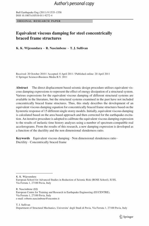
Bulletin of Earthquake EngineeringOfficial Publication of the EuropeanAssociation for EarthquakeEngineering ISSN 1570-761XVolume 9Number 5 Bull Earthquake Eng (2011)9:1535-1558DOI 10.1007/s10518-011-9272-4

Equivalent viscous damping for steelconcentrically braced frame structures

K. K. Wijesundara, R. Nascimbene &T. J. Sullivan

1 23

Your article is protected by copyright and

all rights are held exclusively by Springer

Science+Business Media B.V.. This e-offprint

is for personal use only and shall not be self-

archived in electronic repositories. If you

wish to self-archive your work, please use the

accepted author’s version for posting to your

own website or your institution’s repository.

You may further deposit the accepted author’s

version on a funder’s repository at a funder’s

request, provided it is not made publicly

available until 12 months after publication.

Bull Earthquake Eng (2011) 9:1535–1558DOI 10.1007/s10518-011-9272-4

ORIGINAL RESEARCH PAPER

Equivalent viscous damping for steel concentricallybraced frame structures

K. K. Wijesundara · R. Nascimbene · T. J. Sullivan

Received: 20 October 2010 / Accepted: 8 April 2011 / Published online: 20 April 2011© Springer Science+Business Media B.V. 2011

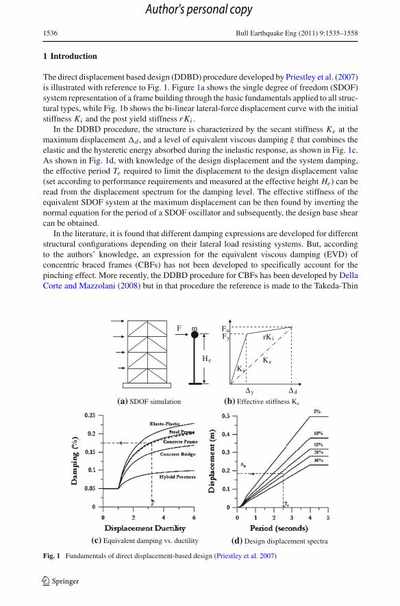
Abstract The direct displacement based seismic design procedure utilises equivalent vis-cous damping expressions to represent the effect of energy dissipation of a structural system.Various expressions for the equivalent viscous damping of different structural systems areavailable in the literature, but the structural systems examined in the past have not includedconcentrically braced frame structures. Thus, this study describes the development of anequivalent viscous damping equation for concentrically braced frame structures based on thehysteretic response of 15 different single storey models. Initially, equivalent viscous dampingis calculated based on the area based approach and then corrected for the earthquake excita-tion. An iterative procedure is adopted to calibrate the equivalent viscous damping expressionto the results of inelastic time history analyses using a number of spectrum-compatible realaccelerograms. From the results of this research, a new damping expression is developed asa function of the ductility and the non dimensional slenderness ratio.

Keywords Equivalent viscous damping · Non dimensional slenderness ratio ·Ductility · Concentrically braced frame

K. K. WijesundaraEuropean School for Advanced Studies in Reduction of Seismic Risk (ROSE School), IUSS,Via Ferrata 1, 27100 Pavia, Italy

R. Nascimbene (B)European Centre for Training and Research in Earthquake Engineering (EUCENTRE),Via Ferrata 1, 27100 Pavia, Italye-mail: [email protected]

T. J. SullivanDepartment of Structural Mechanics, Universita’ degli Studi di Pavia, Via Ferrata 1, 27100 Pavia, Italy

123

Author's personal copy

1536 Bull Earthquake Eng (2011) 9:1535–1558

1 Introduction

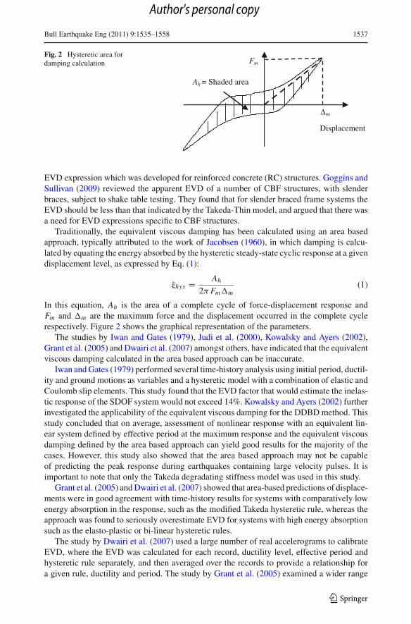
The direct displacement based design (DDBD) procedure developed by Priestley et al. (2007)is illustrated with reference to Fig. 1. Figure 1a shows the single degree of freedom (SDOF)system representation of a frame building through the basic fundamentals applied to all struc-tural types, while Fig. 1b shows the bi-linear lateral-force displacement curve with the initialstiffness Ki and the post yield stiffness r Ki .

In the DDBD procedure, the structure is characterized by the secant stiffness Ke at themaximum displacement �d , and a level of equivalent viscous damping ξ that combines theelastic and the hysteretic energy absorbed during the inelastic response, as shown in Fig. 1c.As shown in Fig. 1d, with knowledge of the design displacement and the system damping,the effective period Te required to limit the displacement to the design displacement value(set according to performance requirements and measured at the effective height He) can beread from the displacement spectrum for the damping level. The effective stiffness of theequivalent SDOF system at the maximum displacement can be then found by inverting thenormal equation for the period of a SDOF oscillator and subsequently, the design base shearcan be obtained.

In the literature, it is found that different damping expressions are developed for differentstructural configurations depending on their lateral load resisting systems. But, accordingto the authors’ knowledge, an expression for the equivalent viscous damping (EVD) ofconcentric braced frames (CBFs) has not been developed to specifically account for thepinching effect. More recently, the DDBD procedure for CBFs has been developed by DellaCorte and Mazzolani (2008) but in that procedure the reference is made to the Takeda-Thin

(a) SDOF simulation (b) Effective stiffness Ke

(c) Equivalent damping vs. ductility (d) Design displacement spectra

He

mF

KeKi

rK i

Δy Δd

Fy

Fu

Fig. 1 Fundamentals of direct displacement-based design (Priestley et al. 2007)

123


Bull Earthquake Eng (2011) 9:1535–1558 1537

Fig. 2 Hysteretic area fordamping calculation

Displacement

Δm

Fm

Ah = Shaded area

EVD expression which was developed for reinforced concrete (RC) structures. Goggins andSullivan (2009) reviewed the apparent EVD of a number of CBF structures, with slenderbraces, subject to shake table testing. They found that for slender braced frame systems theEVD should be less than that indicated by the Takeda-Thin model, and argued that there wasa need for EVD expressions specific to CBF structures.

Traditionally, the equivalent viscous damping has been calculated using an area basedapproach, typically attributed to the work of Jacobsen (1960), in which damping is calcu-lated by equating the energy absorbed by the hysteretic steady-state cyclic response at a givendisplacement level, as expressed by Eq. (1):

ξhys = Ah

2π Fm�m(1)

In this equation, Ah is the area of a complete cycle of force-displacement response andFm and �m are the maximum force and the displacement occurred in the complete cyclerespectively. Figure 2 shows the graphical representation of the parameters.

The studies by Iwan and Gates (1979), Judi et al. (2000), Kowalsky and Ayers (2002),Grant et al. (2005) and Dwairi et al. (2007) amongst others, have indicated that the equivalentviscous damping calculated in the area based approach can be inaccurate.

Iwan and Gates (1979) performed several time-history analysis using initial period, ductil-ity and ground motions as variables and a hysteretic model with a combination of elastic andCoulomb slip elements. This study found that the EVD factor that would estimate the inelas-tic response of the SDOF system would not exceed 14%. Kowalsky and Ayers (2002) furtherinvestigated the applicability of the equivalent viscous damping for the DDBD method. Thisstudy concluded that on average, assessment of nonlinear response with an equivalent lin-ear system defined by effective period at the maximum response and the equivalent viscousdamping defined by the area based approach can yield good results for the majority of thecases. However, this study also showed that the area based approach may not be capableof predicting the peak response during earthquakes containing large velocity pulses. It isimportant to note that only the Takeda degradating stiffness model was used in this study.

Grant et al. (2005) and Dwairi et al. (2007) showed that area-based predictions of displace-ments were in good agreement with time-history results for systems with comparatively lowenergy absorption in the response, such as the modified Takeda hysteretic rule, whereas theapproach was found to seriously overestimate EVD for systems with high energy absorptionsuch as the elasto-plastic or bi-linear hysteretic rules.

The study by Dwairi et al. (2007) used a large number of real accelerograms to calibrateEVD, where the EVD was calculated for each record, ductility level, effective period andhysteretic rule separately, and then averaged over the records to provide a relationship fora given rule, ductility and period. The study by Grant et al. (2005) examined a wider range

123



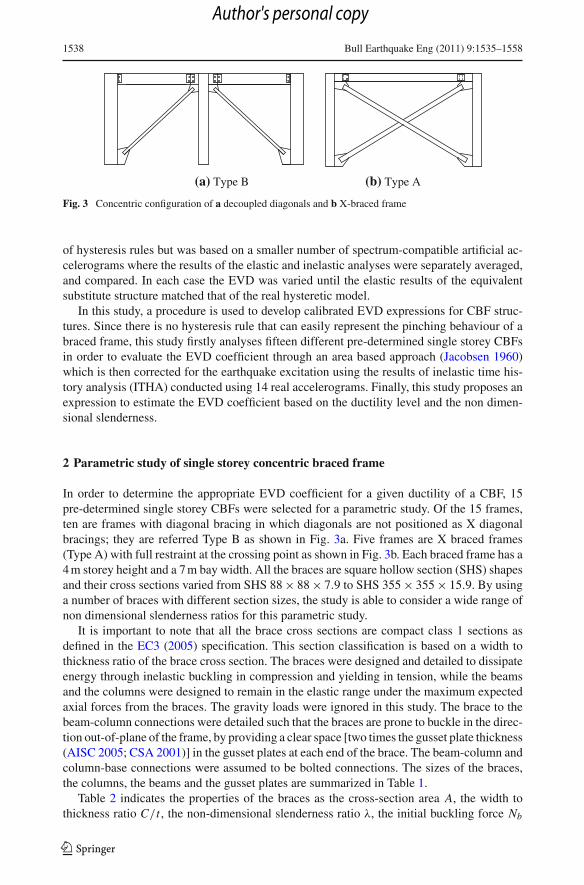
(a) Type B (b) Type A

Fig. 3 Concentric configuration of a decoupled diagonals and b X-braced frame

of hysteresis rules but was based on a smaller number of spectrum-compatible artificial ac-celerograms where the results of the elastic and inelastic analyses were separately averaged,and compared. In each case the EVD was varied until the elastic results of the equivalentsubstitute structure matched that of the real hysteretic model.

In this study, a procedure is used to develop calibrated EVD expressions for CBF struc-tures. Since there is no hysteresis rule that can easily represent the pinching behaviour of abraced frame, this study firstly analyses fifteen different pre-determined single storey CBFsin order to evaluate the EVD coefficient through an area based approach (Jacobsen 1960)which is then corrected for the earthquake excitation using the results of inelastic time his-tory analysis (ITHA) conducted using 14 real accelerograms. Finally, this study proposes anexpression to estimate the EVD coefficient based on the ductility level and the non dimen-sional slenderness.

2 Parametric study of single storey concentric braced frame

In order to determine the appropriate EVD coefficient for a given ductility of a CBF, 15pre-determined single storey CBFs were selected for a parametric study. Of the 15 frames,ten are frames with diagonal bracing in which diagonals are not positioned as X diagonalbracings; they are referred Type B as shown in Fig. 3a. Five frames are X braced frames(Type A) with full restraint at the crossing point as shown in Fig. 3b. Each braced frame has a4 m storey height and a 7 m bay width. All the braces are square hollow section (SHS) shapesand their cross sections varied from SHS 88 × 88 × 7.9 to SHS 355 × 355 × 15.9. By usinga number of braces with different section sizes, the study is able to consider a wide range ofnon dimensional slenderness ratios for this parametric study.

It is important to note that all the brace cross sections are compact class 1 sections asdefined in the EC3 (2005) specification. This section classification is based on a width tothickness ratio of the brace cross section. The braces were designed and detailed to dissipateenergy through inelastic buckling in compression and yielding in tension, while the beamsand the columns were designed to remain in the elastic range under the maximum expectedaxial forces from the braces. The gravity loads were ignored in this study. The brace to thebeam-column connections were detailed such that the braces are prone to buckle in the direc-tion out-of-plane of the frame, by providing a clear space [two times the gusset plate thickness(AISC 2005; CSA 2001)] in the gusset plates at each end of the brace. The beam-column andcolumn-base connections were assumed to be bolted connections. The sizes of the braces,the columns, the beams and the gusset plates are summarized in Table 1.

Table 2 indicates the properties of the braces as the cross-section area A, the width tothickness ratio C/t , the non-dimensional slenderness ratio λ, the initial buckling force Nb

123



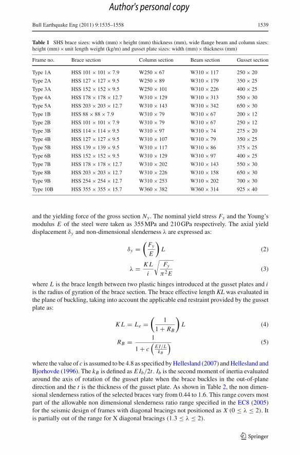
Table 1 SHS brace sizes: width (mm)×height (mm) thickness (mm), wide flange beam and column sizes:height (mm)×unit length weight (kg/m) and gusset plate sizes: width (mm)× thickness (mm)

Frame no. Brace section Column section Beam section Gusset section

Type 1A HSS 101 × 101 × 7.9 W250 × 67 W310 × 117 250 × 20

Type 2A HSS 127 × 127 × 9.5 W250 × 89 W310 × 179 350 × 25

Type 3A HSS 152 × 152 × 9.5 W250 × 101 W310 × 226 400 × 25

Type 4A HSS 178 × 178 × 12.7 W310 × 129 W310 × 313 550 × 30

Type 5A HSS 203 × 203 × 12.7 W310 × 143 W310 × 342 650 × 30

Type 1B HSS 88 × 88 × 7.9 W310 × 79 W310 × 67 200 × 12

Type 2B HSS 101 × 101 × 7.9 W310 × 79 W310 × 67 250 × 12

Type 3B HSS 114 × 114 × 9.5 W310 × 97 W310 × 74 275 × 20

Type 4B HSS 127 × 127 × 9.5 W310 × 107 W310 × 79 350 × 25

Type 5B HSS 139 × 139 × 9.5 W310 × 117 W310 × 86 375 × 25

Type 6B HSS 152 × 152 × 9.5 W310 × 129 W310 × 97 400 × 25

Type 7B HSS 178 × 178 × 12.7 W310 × 202 W310 × 143 550 × 30

Type 8B HSS 203 × 203 × 12.7 W310 × 226 W310 × 158 650 × 30

Type 9B HSS 254 × 254 × 12.7 W310 × 253 W310 × 202 700 × 30

Type 10B HSS 355 × 355 × 15.7 W360 × 382 W360 × 314 925 × 40

and the yielding force of the gross section Ny . The nominal yield stress Fy and the Young’smodulus E of the steel were taken as 355 MPa and 210 GPa respectively. The axial yielddisplacement δy and non-dimensional slenderness λ are expressed as:

δy =(

Fy

E

)L (2)

λ = K L

i

√Fy

π2 E(3)

where L is the brace length between two plastic hinges introduced at the gusset plates and iis the radius of gyration of the brace section. The brace effective length KL was evaluated inthe plane of buckling, taking into account the applicable end restraint provided by the gussetplate as:

K L = Le =(

1

1 + RB

)L (4)

RB = 1

1 + c(

E I/LkB

) (5)

where the value of c is assumed to be 4.8 as specified by Hellesland (2007) and Hellesland andBjorhovde (1996). The kB is defined as E Ib/2t . Ib is the second moment of inertia evaluatedaround the axis of rotation of the gusset plate when the brace buckles in the out-of-planedirection and the t is the thickness of the gusset plate. As shown in Table 2, the non dimen-sional slenderness ratios of the selected braces vary from 0.44 to 1.6. This range covers mostpart of the allowable non dimensional slenderness ratio range specified in the EC8 (2005)for the seismic design of frames with diagonal bracings not positioned as X (0 ≤ λ ≤ 2). Itis partially out of the range for X diagonal bracings (1.3 ≤ λ ≤ 2).

123



Table 2 The properties of the braces

Frame no. A (mm2) C/t λ Nb (kN) Ny (kN)

Type 1A 2,980 11 0.83 815 1,061

Type 2A 4,470 12 0.66 1,340 1,590

Type 3A 5,430 14 0.54 1,720 1,928

Type 4A 8,390 12 0.47 2,744 2,981

Type 5A 9,670 14 0.41 3,244 3,432

Type 1B 2,090 13 1.60 205 744

Type 2B 2,980 11 1.44 343 1,061

Type 3B 3,980 10 1.16 557 1,414

Type 4B 4,470 12 0.98 711 1,590

Type 5B 4,960 13 0.92 916 1,762

Type 6B 5,430 14 0.87 1,085 1,928

Type 7B 8,390 12 0.76 1,911 2,981

Type 8B 9,670 14 0.68 2,442 3,432

Type 9B 12,255 18 0.59 3,526 4,352

Type 10B 21,600 21 0.44 6,907 7,679

All the frames were modelled in the OpenSees (2006) computer programme in order toobtain the base shear-top lateral displacement hysteretic response. Note that the top lateraldisplacement was based on the axial elongation of the tension brace with account for short-ening of the compression brace, in order to eliminate the lateral deformation induced by therigid rotation of the floor due to the axial elongation and the shortening of the columns intension and compression respectively. Furthermore, the base shear forces were obtained fromthe resultant horizontal components of the brace axial forces developed in the tension andthe compression braces. The hysteretic response of each single storey model was obtained byapplying a symmetric displacement history at the top of the each frame. From the hystereticresponse, the EVD coefficients at six different ductility levels are determined via the areabased approach described earlier with reference to Eq. (1) and following the steps presentedin Sect. 3.

2.1 Modelling of the single storey braced frames

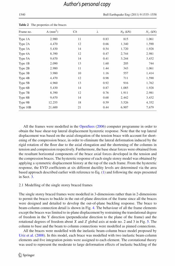
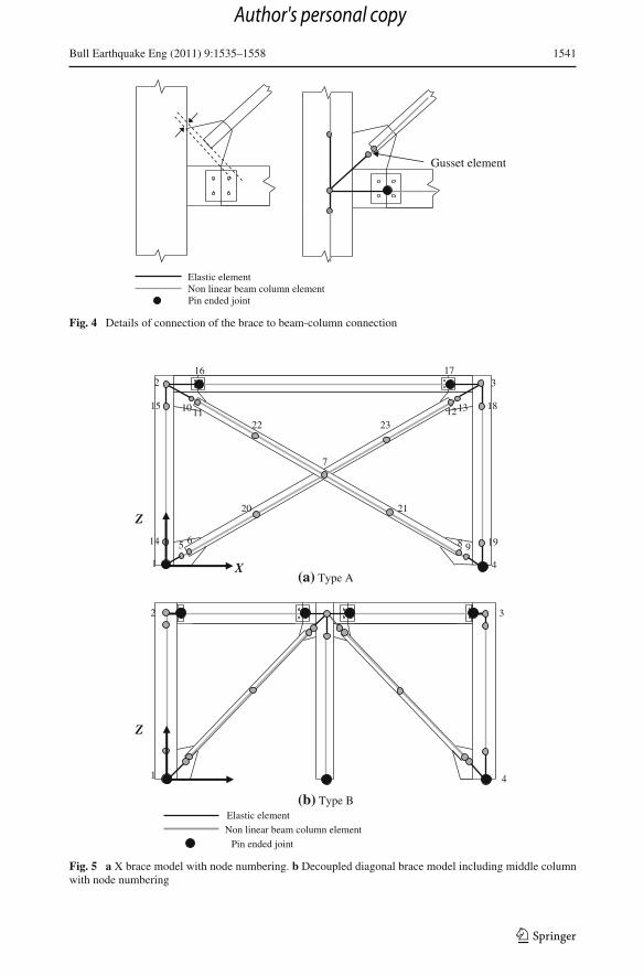
The single storey braced frames were modelled in 3-dimensions rather than in 2-dimensionsto permit the braces to buckle in the out-of-plane direction of the frame since all the braceswere designed and detailed to develop the out-of-plane buckling response. The brace tobeam-column connection detail is shown in Fig. 4. The behaviour of all the frame elementsexcept the braces was limited to in-plane displacement by restraining the translational degreeof freedom in the Y direction (perpendicular direction to the plane of the frame) and therotational degrees of freedom about X and Z global axis at node no. 2 and 3 in Fig. 5. Thecolumn to base and the beam to column connections were modelled as pinned connections.

All the braces were modelled with the inelastic beam-column brace model proposed byUriz et al. (2008). In this model, each brace was modelled with two inelastic beam-columnelements and five integration points were assigned to each element. The corotational theorywas used to represent the moderate to large deformation effects of inelastic buckling of the

123



Elastic element Non linear beam column element

Pin ended joint

Gusset element

Fig. 4 Details of connection of the brace to beam-column connection

(a) Type A

(b) Type B Elastic element

Non linear beam column element Pin ended joint

Z

1

2 3

4 X

5 6

20 21

7

23 22

8 9

11 3101 12

14 19

15 18

17 16

4 1

2 3

Z

Fig. 5 a X brace model with node numbering. b Decoupled diagonal brace model including middle columnwith node numbering

123



(a) Frame Type 1A

-1000

-500

0

500

1000

-0.08 -0.04 0 0.04 0.08-1500

-1000

-500

0

500

1000

1500

Top Lateral Displacement (m)

Lat

eral

For

ce (

kN)

Lat

eral

For

ce (

kN)

(b) Frame Type 1B

-0.08 -0.04 0 0.04 0.08

Top Lateral Displacement (m)

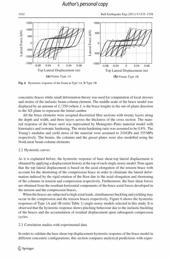
Fig. 6 Hysteretic response of the frame a Type 1A, b Type 1B

concentric braces while small deformation theory was used for computation of local stressesand strains of the inelastic beam-column element. The middle node of the brace model wasdisplaced by an amount of L/350 (where L is the brace length) in the out-of-plane directionto the XZ plane to represent the initial camber.

All the brace elements were assigned discretized fibre sections with twenty layers alongthe depth and width, and three layers across the thickness of the cross section. The mate-rial response of the brace steel was represented by Menegotto–Pinto material model withkinematics and isotropic hardening. The strain hardening ratio was assumed to be 0.8%. TheYoung’s modulus and yield stress of the material were assumed to 210 GPa and 355 MParespectively. The beams, the columns and the gusset plates were also modelled using theNonLinear beam-column elements.

2.2 Hysteretic curves

As it is explained before, the hysteretic response of base shear-top lateral displacement isobtained by applying a displacement history at the top of each single storey model. Note againthat the top lateral displacement is based on the axial elongation of the tension brace withaccount for the shortening of the compression brace in order to eliminate the lateral defor-mation induced by the rigid rotation of the floor due to the axial elongation and shorteningof the columns in tension and compression respectively. Furthermore, the base shear forcesare obtained from the resultant horizontal components of the brace axial forces developed inthe tension and the compression braces.

When the braces are subjected to high axial loads, simultaneous buckling and yielding mayoccur in the compression and the tension braces respectively. Figure 6 shows the hystereticresponses of Type 1A and 1B (refer Table 1) single storey models selected in this study. It isobserved that the hysteretic response shows pinching behaviour due to the inelastic bucklingof the braces and the accumulation of residual displacement upon subsequent compressioncycles.

2.3 Correlation studies with experimental data

In order to validate the base shear-top displacement hysteretic response of the brace model indifferent concentric configurations, this section compares analytical predictions with exper-

123



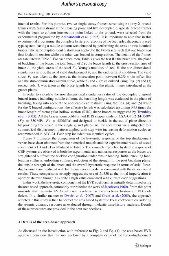
imental results. For this purpose, twelve single storey frames; seven single storey X bracedframes with full restraint at the crossing point and five decoupled diagonals braced frameswith the beam to column intersection point linked to the ground, were selected from theexperimental programme by Archambault et al. (1995). It is important to note that in thisexperimental programme, the complete hysteretic response of the decoupled diagonals bracedtype system having a middle column was obtained by performing the tests on two identicalbraces. The same displacement history was applied to the two braces such that one brace wasfirst loaded in tension while the other was loaded in compression. The details of the framesare tabulated in Table 3. For each specimen, Table 3 gives the test ID, the brace size, the planeof buckling of the brace, the total length of LT , the brace length L , the cross-section area ofbrace A, the yield stress of the steel Fy , Young’s modulus of steel E , the non-dimensionalslenderness ratio λ, the axial yield displacement δy and the end restraint condition. The yieldstress Fy was taken as the stress at the intersection point between 0.2% strain offset lineand the stub-column stress-strain curve, while δy and λ are calculated using Eqs. (2) and (3)respectively. L was taken as the brace length between the plastic hinges introduced at thegusset plates.

In order to calculate the non dimensional slenderness ratio of the decoupled diagonalbraced frames including middle column, the buckling length was evaluated in the plane ofbuckling, taking into account the applicable end restraint using the Eqs. (4) and (5) whilefor the X braced configurations, the effective length was calculated assuming 0.45 times thebrace length of rectangular hollow section (RHS) shape braces as suggested by Tremblayet al. (2003). All the braces were cold-formed RHS shapes made of CSA-G40.21M-350W(Fy = 350 MPa; Fu = 450 MPa) and designed to buckle in the out-of-plane directionby providing free space in the single gusset plates. All the specimens were subjected to asymmetrical displacement pattern applied with step wise increasing deformation cycles asrecommended in ATC-24. Each step included two identical cycles.

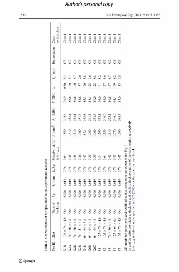
Figure 7 illustrates the comparison of the hysteretic response of the top displacementversus base shear obtained from the numerical models and the experimental results of testedspecimens X1B and S1 as tabulated in Table 3. The symmetric pinched hysteretic response ofCBF systems are observed in both the experimental and numerical responses as the braces arestraightened out from the buckled configuration under tensile loading. Initial buckling load,loading stiffness, unloading stiffness, reduction of the strength in the post buckling phase,the tensile strength of the brace and the overall hysteretic response in terms of axial force-displacement are predicted well by the numerical model as compared with the experimentalresults. These comparisons strongly suggest the use of L/350 as the initial imperfection isappropriate even though it is quite a high value compared with current code suggestions.

In this work, the hysteretic component of the EVD coefficient is initially determined usingthe area based approach, commonly attributed to the work of Jacobsen (1960). From this pointonwards, this hysteretic EVD coefficient is referred as the area based hysteretic EVD coef-ficient. In a similar manner to Dwairi et al. (2007) and Grant et al. (2005), the approachadopted in this study is then to correct the area based hysteretic EVD coefficient consideringthe seismic dynamic response as evaluated through inelastic time-history analyses. Detailsof these procedures are provided in the next two sections.

3 Details of the area-based approach

As discussed in the introduction with reference to Fig. 2 and Eq. (1), the area-based EVDapproach considers that the area enclosed by a complete cycle of the force-displacement

123



Tabl

e3

Cha

ract

eris

tics

ofth

esp

ecim

ens

inth

eex

peri

men

talr

esea

rch

Test

IDSi

zePl

ane

ofbu

cklin

gL

TL

(mm

)L/

LT

Max

(b/

t,d/

t)/

(c/

t)L

imit

A(m

m2)

Fy

(MPa

)E

(GPa

)λ

δy

(mm

)E

ndre

stra

int

Cro

ssse

ctio

ncl

ass

X1B

102

×76

×4.

8O

ut6,

096

4,61

40.

760.

641,

550

345.

619

1.9

0.80

8.3

GE

Cla

ss1

X2A

76×

76×

4.8

Out

6,09

64,

619

0.76

0.45

1,31

035

3.1

186.

81.

008.

7G

EC

lass

1

X2B

76×

76×

4.8

Out

6,09

64,

619

0.76

0.45

1,31

035

3.1

186.

81.

008.

7G

EC

lass

1

X3B

76×

51×

4.8

Out

6,09

64,

619

0.76

0.26

1,06

038

1.3

183.

81.

579.

6G

EC

lass

1

X4B

64×

64×

3.8

Out

6,09

64,

619

0.76

0.47

872

353.

818

5.3

1.20

8.8

GE

Cla

ss1

X6B

64×

64×

4.8

Out

6,09

64,

619

0.76

0.36

1,06

039

1.8

188.

11.

289.

6G

EC

lass

1

X6C

64×

64×

4.8

Out

6,09

64,

619

0.76

0.35

1,06

035

8.3

189.

01.

288.

8G

EC

lass

1

S112

7×

76×

4.8

Out

6,09

64,

614

0.76

0.84

1,79

035

3.1

198.

01.

018.

2G

EC

lass

1

S210

2×

76×

4.8

Out

6,09

64,

614

0.76

0.64

1,55

034

6.0

185.

01.

278.

6G

EC

lass

1

S376

×76

×4.

8O

ut6,

096

4,61

90.

760.

451,

310

353.

118

6.8

1.57

8.7

GE

Cla

ss1

S412

7×

64×

6.4

Out

6,09

64,

614

0.76

0.83

1,67

034

6.0

194.

41.

098.

2G

EC

lass

1

S510

2×

76×

4.8

Out

6,09

64,

614

0.76

0.47

1,99

038

8.3

183.

01.

339.

8G

EC

lass

1

GE

stan

dsfo

rgu

sset

ends

and

deta

ilsof

such

aco

nnec

tion

are

show

nin

the

Fig.

3b/

tand

d/tr

atio

sar

ew

idth

toth

ickn

ess

and

dept

hto

thic

knes

sra

tios

ofth

ecr

oss

sect

ion

resp

ectiv

ely

(c/

t)lim

itis

defin

edas

the

spec

ified

inE

C3

(200

5)fo

rth

ecr

oss

sect

ion

clas

s1

123



(a) (b)

-0.04 -0.02 0 0.02 0.04-800

-600

-400

-200

0

200

400

600

Top Displacement/(m)

Bas

e S

hear

/(kN

)

-0.04 -0.02 0 0.02 0.04-800

-600

-400

-200

0

200

400

600

800

Top Displacement/(m)

Bas

e S

hear

/(kN

)

OpenSeesExperiment

OpenSeesExperiment

Fig. 7 Comparison of experimental hysteretic responses and numerical results for tested a X1B specimenand b S1 specimen

Top lateral displacement (m) Ductility

Are

a ba

sed

ξ hys

Bas

e sh

ear

(kN

)

-0.08 -0.04 0 0.04 0.08-1000

-500

0

500

1000

0.00

0.05

0.10

0.15

0.0 1.0 2.0 3.0 4.0 5.0 6.0 7.0 8.0

(a)(b)

Fig. 8 a Hysteretic curve, b variation of area based hysteretic EVD coefficient against the ductility of frameType 1B

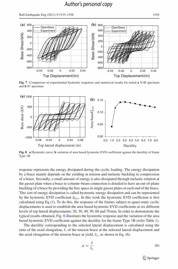
response represents the energy dissipated during the cyclic loading. The energy dissipationby a brace mainly depends on the yielding in tension and inelastic buckling in compressionof a brace. Secondly, a small amount of energy is also dissipated through inelastic rotation atthe gusset plate when a brace to column–beam connection is detailed to have an out-of-planebuckling of a brace by providing the free space in single gusset plates at each end of the brace.This sort of energy dissipation is called hysteretic energy dissipation and can be representedby the hysteretic EVD coefficient ξhys . In this work the hysteretic EVD coefficient is firstcalculated using Eq (1). To do this, the response of the frames subject to quasi-static cyclicdisplacements is used to establish the area based hysteretic EVD coefficients at six differentlevels of top lateral displacements; 20, 30, 40, 50, 60 and 70 mm. In order to demonstrate thetypical results obtained, Fig. 8 illustrates the hysteretic response and the variation of the areabased hysteretic EVD coefficient against the ductility for the frame Type 1B (refer Table 1).

The ductility corresponding to the selected lateral displacement is calculated using theratio of the axial elongation, δ, of the tension brace at the selected lateral displacement andthe axial elongation of the tension brace at yield, δy , as shown in Eq. (6).

μ = δ

δy(6)

123



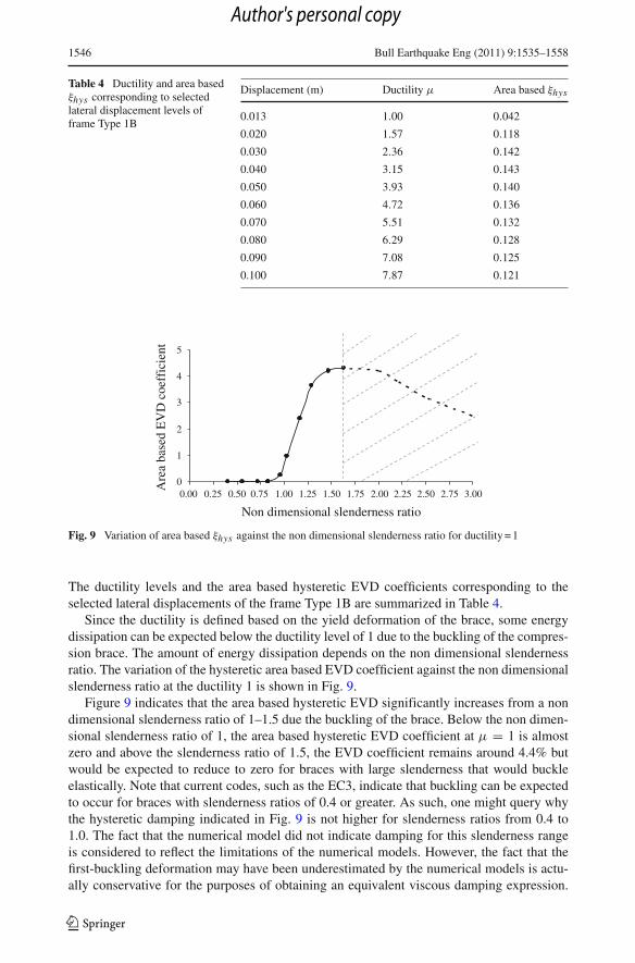
Table 4 Ductility and area basedξhys corresponding to selectedlateral displacement levels offrame Type 1B

Displacement (m) Ductility μ Area based ξhys

0.013 1.00 0.042

0.020 1.57 0.118

0.030 2.36 0.142

0.040 3.15 0.143

0.050 3.93 0.140

0.060 4.72 0.136

0.070 5.51 0.132

0.080 6.29 0.128

0.090 7.08 0.125

0.100 7.87 0.121

Are

a ba

sed

EV

D c

oeff

icie

nt

0

1

2

3

4

5

0.00 0.25 0.50 0.75 1.00 1.25 1.50 1.75 2.00 2.25 2.50 2.75 3.00

Non dimensional slenderness ratio

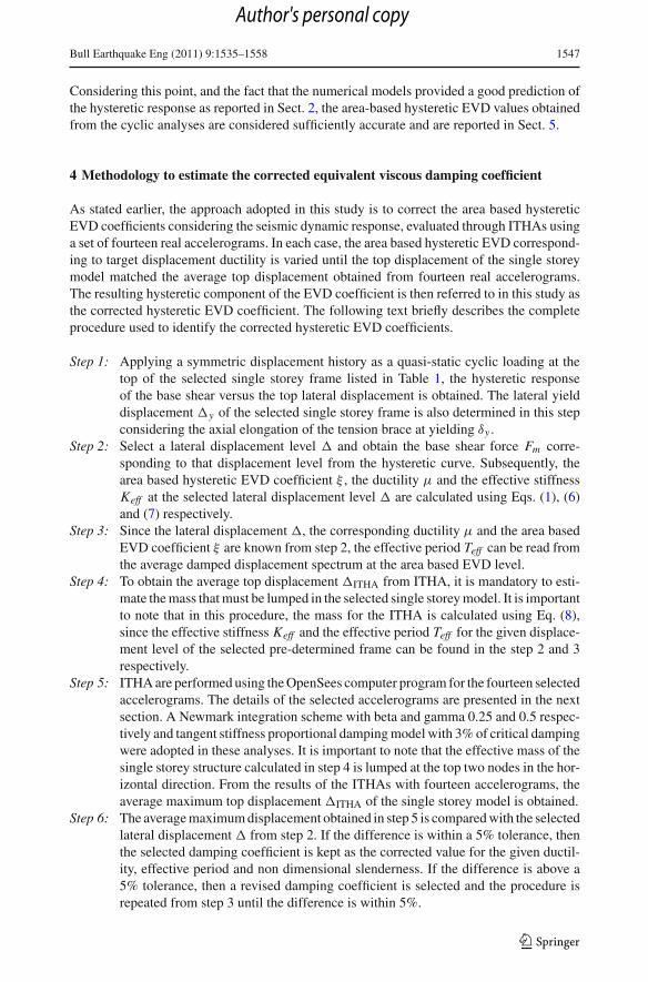
Fig. 9 Variation of area based ξhys against the non dimensional slenderness ratio for ductility = 1

The ductility levels and the area based hysteretic EVD coefficients corresponding to theselected lateral displacements of the frame Type 1B are summarized in Table 4.

Since the ductility is defined based on the yield deformation of the brace, some energydissipation can be expected below the ductility level of 1 due to the buckling of the compres-sion brace. The amount of energy dissipation depends on the non dimensional slendernessratio. The variation of the hysteretic area based EVD coefficient against the non dimensionalslenderness ratio at the ductility 1 is shown in Fig. 9.

Figure 9 indicates that the area based hysteretic EVD significantly increases from a nondimensional slenderness ratio of 1–1.5 due the buckling of the brace. Below the non dimen-sional slenderness ratio of 1, the area based hysteretic EVD coefficient at μ = 1 is almostzero and above the slenderness ratio of 1.5, the EVD coefficient remains around 4.4% butwould be expected to reduce to zero for braces with large slenderness that would buckleelastically. Note that current codes, such as the EC3, indicate that buckling can be expectedto occur for braces with slenderness ratios of 0.4 or greater. As such, one might query whythe hysteretic damping indicated in Fig. 9 is not higher for slenderness ratios from 0.4 to1.0. The fact that the numerical model did not indicate damping for this slenderness rangeis considered to reflect the limitations of the numerical models. However, the fact that thefirst-buckling deformation may have been underestimated by the numerical models is actu-ally conservative for the purposes of obtaining an equivalent viscous damping expression.

123



Considering this point, and the fact that the numerical models provided a good prediction ofthe hysteretic response as reported in Sect. 2, the area-based hysteretic EVD values obtainedfrom the cyclic analyses are considered sufficiently accurate and are reported in Sect. 5.

4 Methodology to estimate the corrected equivalent viscous damping coefficient

As stated earlier, the approach adopted in this study is to correct the area based hystereticEVD coefficients considering the seismic dynamic response, evaluated through ITHAs usinga set of fourteen real accelerograms. In each case, the area based hysteretic EVD correspond-ing to target displacement ductility is varied until the top displacement of the single storeymodel matched the average top displacement obtained from fourteen real accelerograms.The resulting hysteretic component of the EVD coefficient is then referred to in this study asthe corrected hysteretic EVD coefficient. The following text briefly describes the completeprocedure used to identify the corrected hysteretic EVD coefficients.

Step 1: Applying a symmetric displacement history as a quasi-static cyclic loading at thetop of the selected single storey frame listed in Table 1, the hysteretic responseof the base shear versus the top lateral displacement is obtained. The lateral yielddisplacement �y of the selected single storey frame is also determined in this stepconsidering the axial elongation of the tension brace at yielding δy .

Step 2: Select a lateral displacement level � and obtain the base shear force Fm corre-sponding to that displacement level from the hysteretic curve. Subsequently, thearea based hysteretic EVD coefficient ξ , the ductility μ and the effective stiffnessKeff at the selected lateral displacement level � are calculated using Eqs. (1), (6)and (7) respectively.

Step 3: Since the lateral displacement �, the corresponding ductility μ and the area basedEVD coefficient ξ are known from step 2, the effective period Teff can be read fromthe average damped displacement spectrum at the area based EVD level.

Step 4: To obtain the average top displacement �ITHA from ITHA, it is mandatory to esti-mate the mass that must be lumped in the selected single storey model. It is importantto note that in this procedure, the mass for the ITHA is calculated using Eq. (8),since the effective stiffness Keff and the effective period Teff for the given displace-ment level of the selected pre-determined frame can be found in the step 2 and 3respectively.

Step 5: ITHA are performed using the OpenSees computer program for the fourteen selectedaccelerograms. The details of the selected accelerograms are presented in the nextsection. A Newmark integration scheme with beta and gamma 0.25 and 0.5 respec-tively and tangent stiffness proportional damping model with 3% of critical dampingwere adopted in these analyses. It is important to note that the effective mass of thesingle storey structure calculated in step 4 is lumped at the top two nodes in the hor-izontal direction. From the results of the ITHAs with fourteen accelerograms, theaverage maximum top displacement �ITHA of the single storey model is obtained.

Step 6: The average maximum displacement obtained in step 5 is compared with the selectedlateral displacement � from step 2. If the difference is within a 5% tolerance, thenthe selected damping coefficient is kept as the corrected value for the given ductil-ity, effective period and non dimensional slenderness. If the difference is above a5% tolerance, then a revised damping coefficient is selected and the procedure isrepeated from step 3 until the difference is within 5%.

123



Step 7: Repeat the procedure from step 3, in order to obtain the corrected EVD coefficientat other levels of ductility for the same frame. The procedure from step 1 is repeatedfor all the predetermined frames and results are discussed in the Sect. 5.

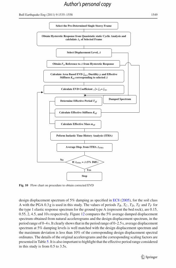
All the steps are summarized in Fig. 10. In order to explain some aspects of this process inmore detail, note firstly that the base shear force Fm at the selected lateral displacement isalso obtained from the hysteretic response in step 2. Since the base shear is known in this step,the secant stiffness Keff corresponding to the selected lateral displacement can be calculatedusing Eq. (7).

Keff = Fm

�(7)

In step 3, the effective period Teff can be read from the average damped displacement spec-trum at the EVD level since the ductility μ and the EVD coefficient ξ corresponding to theselected lateral displacement level � are known in step 2. For the initial step of the iterationin estimating the corrected EVD coefficient at the selected lateral displacement level, thearea based EVD coefficient together with elastic damping of 3% is considered as the EVDcoefficient.

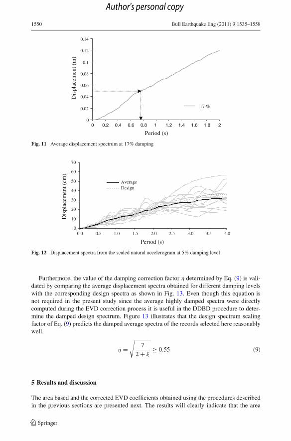
The following paragraphs illustrate the procedure to obtain the corrected EVD coefficientat a selected lateral displacement of � = 50mm. From Table 4, the corresponding ductilityμ and the EVD coefficient are taken as 3.93 and (3 + 14)% respectively, for the initial itera-tion. Subsequently, an effective period Teff of 0.76s is determined using the average dampeddisplacement spectrum at 17% damping level and the displacement of 50 mm as shown inFig. 11.

In step 4, the relation between the effective mass meff , the effective stiffness Keff and theeffective period Teff of a single degree of freedom system is utilised, inverting the normalequation for the period of a SDOF oscillator, as shown in Eq. (8).

meff = Keff T 2eff

4π2 (8)

Consequently, the required mass for the ITHA of the frame Type 1B to correct the area basedEVD coefficient for a corresponding ductility demand of 3.93 (or top lateral displacement of50 mm), is calculated combining the Eqs. (7) and (8) as:

meff =(

Fm

�

) (T 2

eff

4π2

)= 1500

0.050×

(0.762

4π2

)= 140 t

4.1 Selection of natural accelerograms for the correction process

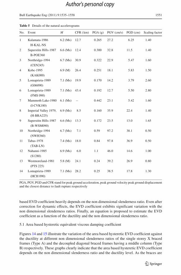
If the individual displacement spectrum is used to determine the effective period of the sys-tem for a given level of displacement in the step 3 of the procedure, then one could note thatseveral period values can be determined for the given level of displacement especially at thelower damping levels. Hence, it can be questioned which period value should represent theeffective period of the system for a given displacement level. In order to avoid this problem,the present study uses an almost linear average displacement spectrum obtained from a set ofreal accelerograms to determine the effective period for a given displacement level in step 3.The 5% average displacement If the individual displacement spectrum is used to determinethe effectivespectrum are obtained from fourteen accelerograms and compared with a designspectrum. The purpose to compare the 5% average spectrum with a design spectrum is toestimate the deviation of the average spectral ordinates from the linear spectral ordinates. The

123



Select the Pre-Determined Single Storey Frame

Obtain Hysteretic Response from Quasistatic static Cyclic Analysis and calclulate Δy of Selected Frame

Select Displacement Level, Δ

Calculate Area Based EVD ξhys, Ductility μ and Effective Stiffness Keff corresponding to selected Δ

Calculate EVD Coefficient , ξ= ξ el+ ξ hys

Determine Effective Period TeffDamped Spectrum

Calculate Effective Stiffness Keff

Calculate Effective Mass meff

Peform Inelastic Time History Analysis (ITHA)

Average Disp. from ITHA Δ ITHA

If Δ ITHA = Δ (5% Diff.)

Stop

Yes

Obtain Fm Reference to Δ from Hysteretic Response

No

Fig. 10 Flow chart on procedure to obtain corrected EVD

design displacement spectrum of 5% damping as specified in EC8 (2005), for the soil classA with the PGA 0.3 g is used in this study. The values of periods TB , TC , TD , TE and TF forthe type 1 elastic response spectrum for the ground type A (represent the bed rock), are 0.15,0.55, 2, 4.5, and 10 s respectively. Figure 12 compares the 5% average damped displacementspectrum obtained from natural accelerograms and the design displacement spectrum, in theperiod range of 0–4 s. It clearly shows that in the period range of 0–2.5 s, average displacementspectrum at 5% damping levels is well matched with the design displacement spectrum andthe maximum deviation is less than 10% of the corresponding design displacement spectralordinates. The details of the original accelerograms and the corresponding scaling factors arepresented in Table 5. It is also important to highlight that the effective period range consideredin this study is from 0.5 to 3.5s.

123



0

0.02

0.04

0.06

0.08

0.1

0.12

0.14

Period (s)

Dis

plac

emen

t (m

)

17 %

0 0.2 0.4 0.6 0.8 1 1.2 1.4 1.6 1.8 2

Fig. 11 Average displacement spectrum at 17% damping

0

10

20

30

40

50

60

70

Period (s)

Dis

plac

emen

t (cm

)

AverageDesign

0.0 0.5 1.0 1.5 2.0 2.5 3.0 3.5 4.0

Fig. 12 Displacement spectra from the scaled natural accelerogram at 5% damping level

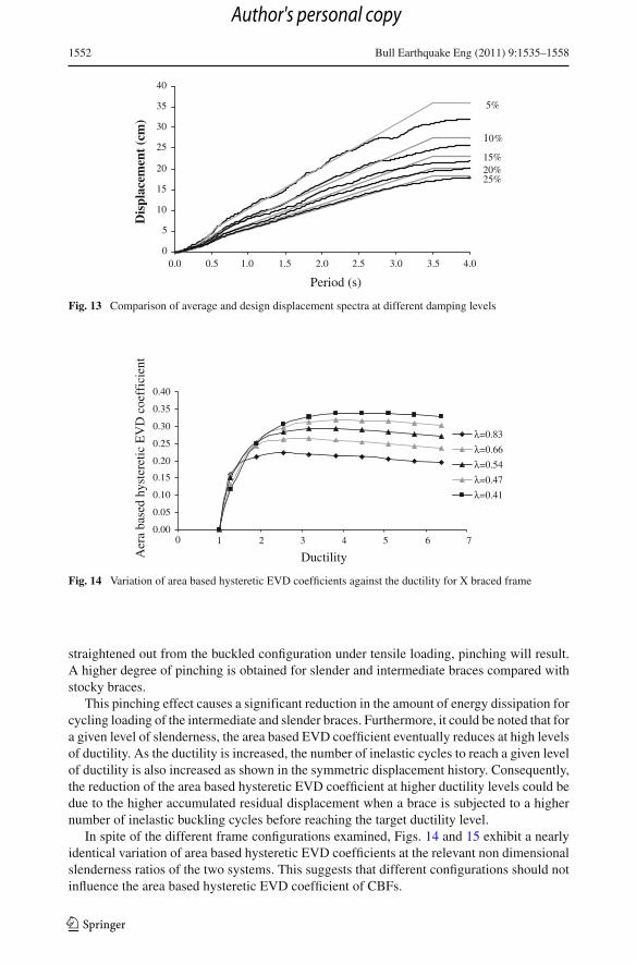
Furthermore, the value of the damping correction factor η determined by Eq. (9) is vali-dated by comparing the average displacement spectra obtained for different damping levelswith the corresponding design spectra as shown in Fig. 13. Even though this equation isnot required in the present study since the average highly damped spectra were directlycomputed during the EVD correction process it is useful in the DDBD procedure to deter-mine the damped design spectrum. Figure 13 illustrates that the design spectrum scalingfactor of Eq. (9) predicts the damped average spectra of the records selected here reasonablywell.

η =√

7

2 + ξ≥ 0.55 (9)

5 Results and discussion

The area based and the corrected EVD coefficients obtained using the procedures describedin the previous sections are presented next. The results will clearly indicate that the area

123



Table 5 Details of the natural accelerograms

No. Event M CFR ( km) PGA (g) PGV (cm/s) PGD (cm) Scaling factor

1 Kalamata-1986 6.2 (Ms) 12.7 0.265 27.2 6.25 1.40

H-KAL-NS

2 Superstitn Hills-1987 6.6 (Ms) 12.4 0.300 32.8 11.5 1.40

B-POE360

3 Northridge-1994 6.7 (Ms) 30.9 0.322 22.9 5.47 1.60

(CEN245)

4 Kobe-1995 6.9 (M) 26.4 0.251 18.1 5.83 1.50

(KAK000)

5 Lomaprieta-1989 7.1 (Ms) 19.9 0.170 14.2 3.79 2.60

(G06090)

6 Lomaprieta-1989 7.1 (Ms) 43.4 0.192 12.7 5.50 2.80

(FMS 090)

7 Mammoth Lake-1980 6.1 (Ms) − 0.442 23.1 5.42 1.60

(I-CVK180)

8 Imperial Valley 1979, 6.9 (Ms) 8.5 0.160 35.9 22.4 1.40

(H-BRA225)

9 Superstitn Hills-1987 6.6 (Ms) 13.3 0.172 23.5 13.0 1.65

(B-WSM090)

10 Northridge-1994 6.7 (Ms) 7.1 0.59 97.2 38.1 0.50

(NWH360)

11 Tabas-1978 7.4 (Ms) 18.0 0.84 97.8 36.9 0.50

(TAB-LN)

12 Nahanni-1985 6.9 (Ms) 6.0 1.1 46.0 14.6 1.00

(S1280)

13 Westmoreland-1981 5.8 (M) 24.1 0.24 39.2 26.9 0.80

(PTS 225)

14 Lomaprieta-1989 7.1 (Ms) 28.2 0.25 38.5 17.8 1.30

(HCH 090)

PGA, PGV, PGD and CFR stand for peak ground acceleration, peak ground velocity peak ground displacementand the closest distance to fault rupture respectively

based EVD coefficient heavily depends on the non dimensional slenderness ratio. Even aftercorrection for dynamic effects, the EVD coefficient exhibits significant variation with thenon dimensional slenderness ratios. Finally, an equation is proposed to estimate the EVDcoefficient as a function of the ductility and the non dimensional slenderness ratio.

5.1 Area based hysteretic equivalent viscous damping coefficient

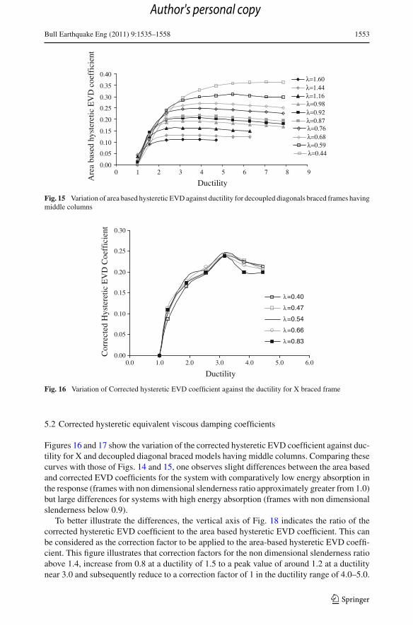
Figures 14 and 15 illustrate the variation of the area based hysteretic EVD coefficient againstthe ductility at different non dimensional slenderness ratios of the single storey X bracedframes (Type A) and the decoupled diagonal braced frames having a middle column (TypeB) respectively. These graphs clearly indicate that the area based hysteretic EVD coefficientdepends on the non dimensional slenderness ratio and the ductility level. As the braces are

123



0

5

10

15

20

25

30

35

40

Dis

plac

emen

t (c

m)

5%

10%

15%20%25%

Period (s)

0.0 0.5 1.0 1.5 2.0 2.5 3.0 3.5 4.0

Fig. 13 Comparison of average and design displacement spectra at different damping levels

0.00

0.05

0.10

0.15

0.20

0.25

0.30

0.35

0.40

DuctilityAer

a ba

sed

hyst

eret

ic E

VD

coe

ffic

ient

λ=0.83

λ=0.66

λ=0.54

λ=0.47

λ=0.41

0 1 2 3 4 5 6 7

Fig. 14 Variation of area based hysteretic EVD coefficients against the ductility for X braced frame

straightened out from the buckled configuration under tensile loading, pinching will result.A higher degree of pinching is obtained for slender and intermediate braces compared withstocky braces.

This pinching effect causes a significant reduction in the amount of energy dissipation forcycling loading of the intermediate and slender braces. Furthermore, it could be noted that fora given level of slenderness, the area based EVD coefficient eventually reduces at high levelsof ductility. As the ductility is increased, the number of inelastic cycles to reach a given levelof ductility is also increased as shown in the symmetric displacement history. Consequently,the reduction of the area based hysteretic EVD coefficient at higher ductility levels could bedue to the higher accumulated residual displacement when a brace is subjected to a highernumber of inelastic buckling cycles before reaching the target ductility level.

In spite of the different frame configurations examined, Figs. 14 and 15 exhibit a nearlyidentical variation of area based hysteretic EVD coefficients at the relevant non dimensionalslenderness ratios of the two systems. This suggests that different configurations should notinfluence the area based hysteretic EVD coefficient of CBFs.

123



0.00

0.05

0.10

0.15

0.20

0.25

0.30

0.35

0.40

DuctilityAre

a ba

sed

hyst

eret

ic E

VD

coe

ffic

ient

λ=1.60λ=1.44λ=1.16λ=0.98λ=0.92λ=0.87λ=0.76λ=0.68λ=0.59λ=0.44

0 1 2 3 4 5 6 7 8 9

Fig. 15 Variation of area based hysteretic EVD against ductility for decoupled diagonals braced frames havingmiddle columns

0.00

0.05

0.10

0.15

0.20

0.25

0.30

0.0 1.0 2.0 3.0 4.0 5.0 6.0

Ductility

Cor

rect

ed H

yste

retic

EV

D C

oeff

icie

nt

λ=0.40

λ=0.47

λ=0.54

λ=0.66

λ=0.83

Fig. 16 Variation of Corrected hysteretic EVD coefficient against the ductility for X braced frame

5.2 Corrected hysteretic equivalent viscous damping coefficients

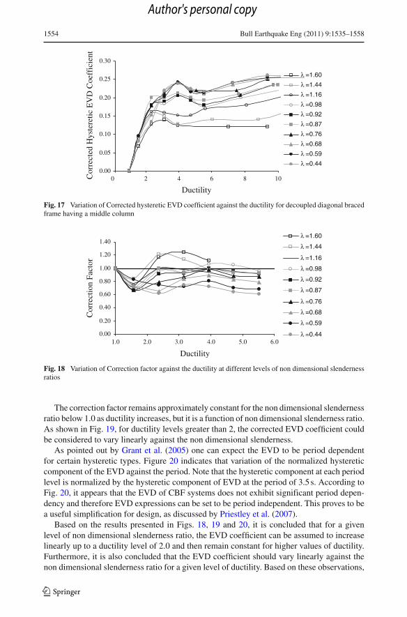
Figures 16 and 17 show the variation of the corrected hysteretic EVD coefficient against duc-tility for X and decoupled diagonal braced models having middle columns. Comparing thesecurves with those of Figs. 14 and 15, one observes slight differences between the area basedand corrected EVD coefficients for the system with comparatively low energy absorption inthe response (frames with non dimensional slenderness ratio approximately greater from 1.0)but large differences for systems with high energy absorption (frames with non dimensionalslenderness below 0.9).

To better illustrate the differences, the vertical axis of Fig. 18 indicates the ratio of thecorrected hysteretic EVD coefficient to the area based hysteretic EVD coefficient. This canbe considered as the correction factor to be applied to the area-based hysteretic EVD coeffi-cient. This figure illustrates that correction factors for the non dimensional slenderness ratioabove 1.4, increase from 0.8 at a ductility of 1.5 to a peak value of around 1.2 at a ductilitynear 3.0 and subsequently reduce to a correction factor of 1 in the ductility range of 4.0–5.0.

123



0.00

0.05

0.10

0.15

0.20

0.25

0.30

Ductility

Cor

rect

ed H

yste

retic

EV

D C

oeff

icie

nt

λ =1.60

λ =1.44

λ =1.16

λ =0.98

λ =0.92

λ =0.87

λ =0.76

λ =0.68

λ =0.59

λ =0.44

0 2 4 6 8 10

Fig. 17 Variation of Corrected hysteretic EVD coefficient against the ductility for decoupled diagonal bracedframe having a middle column

0.00

0.20

0.40

0.60

0.80

1.00

1.20

1.40

Ductility

Cor

rect

ion

Fact

or

λ =1.60

λ =1.44

λ =1.16

λ =0.98

λ =0.92

λ =0.87

λ =0.76

λ =0.68

λ =0.59

λ =0.441.0 2.0 3.0 4.0 5.0 6.0

Fig. 18 Variation of Correction factor against the ductility at different levels of non dimensional slendernessratios

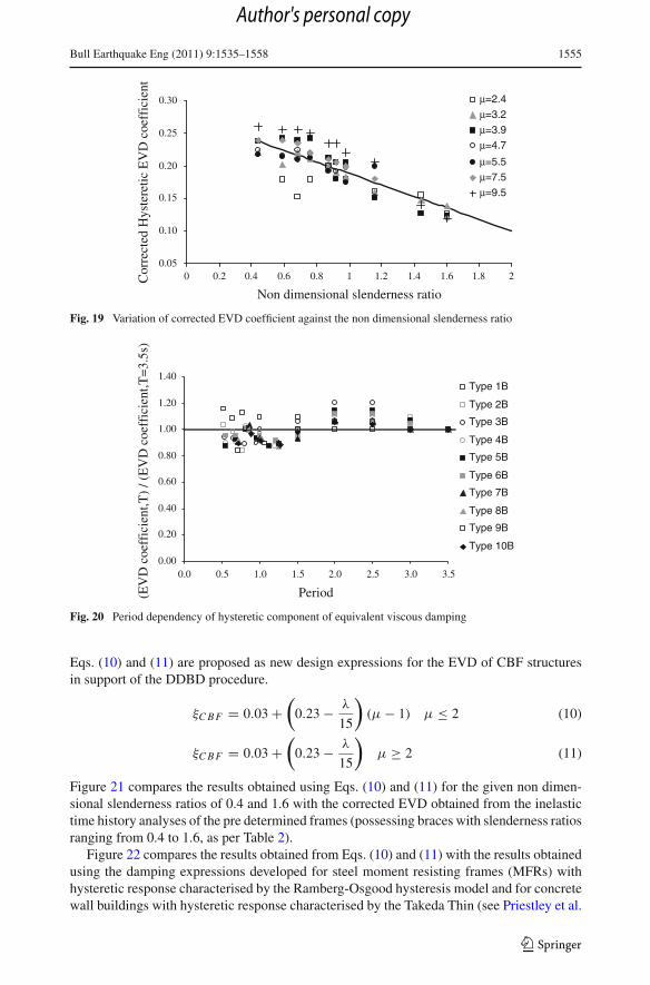
The correction factor remains approximately constant for the non dimensional slendernessratio below 1.0 as ductility increases, but it is a function of non dimensional slenderness ratio.As shown in Fig. 19, for ductility levels greater than 2, the corrected EVD coefficient couldbe considered to vary linearly against the non dimensional slenderness.

As pointed out by Grant et al. (2005) one can expect the EVD to be period dependentfor certain hysteretic types. Figure 20 indicates that variation of the normalized hystereticcomponent of the EVD against the period. Note that the hysteretic component at each periodlevel is normalized by the hysteretic component of EVD at the period of 3.5 s. According toFig. 20, it appears that the EVD of CBF systems does not exhibit significant period depen-dency and therefore EVD expressions can be set to be period independent. This proves to bea useful simplification for design, as discussed by Priestley et al. (2007).

Based on the results presented in Figs. 18, 19 and 20, it is concluded that for a givenlevel of non dimensional slenderness ratio, the EVD coefficient can be assumed to increaselinearly up to a ductility level of 2.0 and then remain constant for higher values of ductility.Furthermore, it is also concluded that the EVD coefficient should vary linearly against thenon dimensional slenderness ratio for a given level of ductility. Based on these observations,

123



0.05

0.10

0.15

0.20

0.25

0.30

0 0.2 0.4 0.6 0.8 1 1.2 1.4 1.6 1.8 2

Non dimensional slenderness ratio

Cor

rect

ed H

yste

retic

EV

D c

oeff

icie

nt

μ=2.4

μ=3.2

μ=3.9

μ=4.7

μ=5.5

μ=7.5

μ=9.5

Fig. 19 Variation of corrected EVD coefficient against the non dimensional slenderness ratio

0.00

0.20

0.40

0.60

0.80

1.00

1.20

1.40

Period(EV

D c

oeff

icie

nt,T

) / (

EV

D c

oeff

icie

nt,T

=3.

5s)

Type 1B

Type 2B

Type 3B

Type 4B

Type 5B

Type 6B

Type 7B

Type 8B

Type 9B

Type 10B

0.0 0.5 1.0 1.5 2.0 2.5 3.0 3.5

Fig. 20 Period dependency of hysteretic component of equivalent viscous damping

Eqs. (10) and (11) are proposed as new design expressions for the EVD of CBF structuresin support of the DDBD procedure.

ξC B F = 0.03 +(

0.23 − λ

15

)(μ − 1) μ ≤ 2 (10)

ξC B F = 0.03 +(

0.23 − λ

15

)μ ≥ 2 (11)

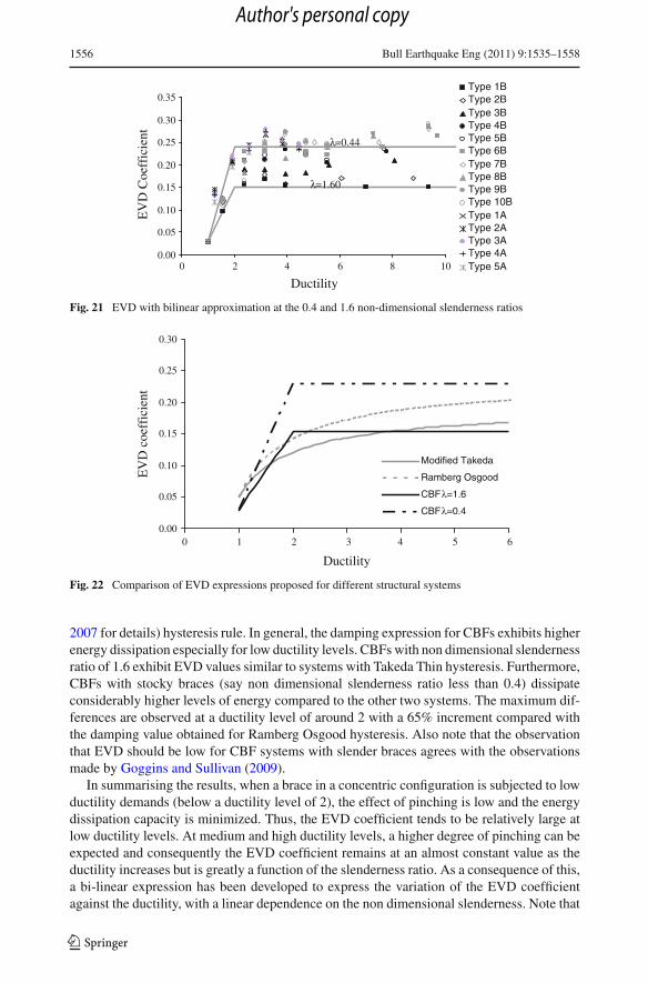
Figure 21 compares the results obtained using Eqs. (10) and (11) for the given non dimen-sional slenderness ratios of 0.4 and 1.6 with the corrected EVD obtained from the inelastictime history analyses of the pre determined frames (possessing braces with slenderness ratiosranging from 0.4 to 1.6, as per Table 2).

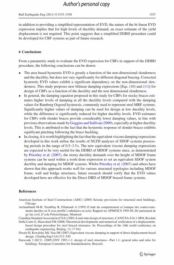
Figure 22 compares the results obtained from Eqs. (10) and (11) with the results obtainedusing the damping expressions developed for steel moment resisting frames (MFRs) withhysteretic response characterised by the Ramberg-Osgood hysteresis model and for concretewall buildings with hysteretic response characterised by the Takeda Thin (see Priestley et al.

123



0.00

0.05

0.10

0.15

0.20

0.25

0.30

0.35

Ductility

EV

D C

oeff

icie

nt

Type 1BType 2BType 3BType 4BType 5BType 6BType 7BType 8BType 9BType 10BType 1AType 2AType 3AType 4AType 5A0 2 4 6 8 10

λ=1.60

λ=0.44

Fig. 21 EVD with bilinear approximation at the 0.4 and 1.6 non-dimensional slenderness ratios

0.00

0.05

0.10

0.15

0.20

0.25

0.30

0 1 2 3 4 5 6

Ductility

EV

D c

oeff

icie

nt

Modified Takeda

Ramberg Osgood

CBF λ=1.6

CBF λ=0.4

Fig. 22 Comparison of EVD expressions proposed for different structural systems

2007 for details) hysteresis rule. In general, the damping expression for CBFs exhibits higherenergy dissipation especially for low ductility levels. CBFs with non dimensional slendernessratio of 1.6 exhibit EVD values similar to systems with Takeda Thin hysteresis. Furthermore,CBFs with stocky braces (say non dimensional slenderness ratio less than 0.4) dissipateconsiderably higher levels of energy compared to the other two systems. The maximum dif-ferences are observed at a ductility level of around 2 with a 65% increment compared withthe damping value obtained for Ramberg Osgood hysteresis. Also note that the observationthat EVD should be low for CBF systems with slender braces agrees with the observationsmade by Goggins and Sullivan (2009).

In summarising the results, when a brace in a concentric configuration is subjected to lowductility demands (below a ductility level of 2), the effect of pinching is low and the energydissipation capacity is minimized. Thus, the EVD coefficient tends to be relatively large atlow ductility levels. At medium and high ductility levels, a higher degree of pinching can beexpected and consequently the EVD coefficient remains at an almost constant value as theductility increases but is greatly a function of the slenderness ratio. As a consequence of this,a bi-linear expression has been developed to express the variation of the EVD coefficientagainst the ductility, with a linear dependence on the non dimensional slenderness. Note that

123



in addition to providing a simplified representation of EVD, the nature of the bi-linear EVDexpression implies that for high levels of ductility demand, an exact estimate of the yielddisplacement is not required. This point suggests that a simplified DDBD procedure couldbe developed for CBF systems as part of future research.

6 Conclusions

From a parametric study to evaluate the EVD expression for CBFs in support of the DDBDprocedure, the following conclusions can be drawn:

• The area based hysteretic EVD is greatly a function of the non-dimensional slendernessand the ductility, but does not vary significantly for different diagonal bracing. Correctedhysteretic EVD values exhibit a significant dependency on the non-dimensional slen-derness. This study proposes new bilinear damping expressions [Eqs. (10) and (11)] fordesign of CBFs as a function of the ductility and the non dimensional slenderness.

• In general, the damping equation proposed in this study for CBFs for stocky braces esti-mates higher levels of damping at all the ductility levels compared with the dampingvalues for Ramberg Osgood hysteresis, commonly used to represent steel MRF systems.Significantly higher values of damping can be used for design at low ductility levels,while the difference is significantly reduced for higher ductility levels. EVD estimatesfor CBFs with slender braces provide considerably lower damping values, in line withprevious observations made by Goggins and Sullivan (2009), especially at higher ductilitylevels. This is attributed to the fact that the hysteretic response of slender braces exhibitssignificant pinching following the brace buckling.

• In closing, it is worth highlighting the fact that the equivalent viscous damping expressionsdeveloped in this work utilise the results of NLTH analyses of SDOF systems possess-ing periods in the range of 0.5–3.5 s. The new equivalent viscous damping expressionsare expected to be very useful for the DDBD of MDOF systems since, as demonstratedby Priestley et al. (2007), the storey ductility demands over the height of MDOF framesystems can be used within a work-done expression to set an equivalent SDOF systemductility and damping for MDOF systems. Whilst Priestley et al. (2007) and others haveshown that this approach works well for various structural typologies including MDOFframe, wall and bridge structures, future research should verify that the EVD valuesdeveloped here are effective for the Direct DBD of MDOF braced frame systems.

References

American Institute of Steel Constructions (AISC) (2005) Seismic provisions for structural steel buildings,Chicago

Archambault M-H, Tremblay R, Filiatrault A (1995) E’tude du comportement se’ismique des contrevente-ments ductiles en X avec profile’s tubulaires en acier. Rapport no. EPM/GCS 1995-09, De’partement dege’nie civil, E’cole Polytechnique, Montreal

Canadian Standard Association (CSA) (2001) Limit state design of structures, CAN/CSA-S16.1-M94, RexdaleDella Corte G, Mazzolani FM (2008) Theoretical developments and numerical verification of a displacement-

based design procedure for steel braced structures. In: Proceedings of the 14th world conference onearthquake engineering, Beijing, 12–17 Oct

Dwairi H, Kowalsky MJ, Nau JM (2007) Equivalent viscous damping in support of direct displacement-baseddesign. J Earthq Eng11(4):512–530

Eurocode 3 (EC3) (2005) ENV 1993-1-1: design of steel structures—Part 1.1: general rules and rules forbuildings. European Committee for Standardisation, Brussels

123



Eurocode 8 (EC8) (2005) EN 1998-1: design provisions for earthquake resistance of structures, part 1: generalrules, seismic actions and rules for buildings. European Committee for Standardisation, Brussels

Goggins JG, Sullivan TJ (2009) Displacement-based seismic design of SDOF concentrically braced frames.In: Mazzolani, Ricles, Sause (eds) STESSA 2009. Taylor & Francis Group, pp 685–692

Grant DN, Blandon CA, Priestley MJN (2005) Modelling inelastic response in direct displacement-baseddesign. Report 2005/03, IUSS Press, Pavia

Hellesland J (2007) Mechanics and effective length of columns with positive and negative end restraints. EngStruct 29:3464–3474

Hellesland J, Bjorhovde R (1996) Improved frame stability analysis with effective lengths. J Struct Eng ASCE122(11):1275–1283

Iwan WD, Gates NC (1979) The effective period and damping of a hysteretic structures. Earthq Eng StructDyn 7:199–211

Jacobsen LS (1960) Damping in composite structures. In: Proceedings of 2nd world conference on earthquakeengineering, vol 2. Tokyo and Kyoto, Japan, pp 1029–1044

Judi HJ, Davidson BJ, Fenwick RC (2000) Direct displacement based design-A damping perspective. In:Proceedings of the 12th world conference on earthquake engineering, Auckland, Paper No. 0330

Kowalsky MJ, Ayers JP (2002) Investigation of equivalent viscous damping for direct displacement baseddesign PEER 2002/02. In: The 3rd Japan–US workshop on performance based earthquake engineeringmethodology for reinforced concrete building structures, 16–18 Aug 2001. Pacific Earthquake Engineer-ing Research Centre, University of California, Berkeley

OpenSees (2006) Open system for earthquake engineering simulation. Pacific Earthquake EngineeringResearch Center, University of California, Berkeley

Priestley MJN, Calvi GM, Kowalsky MJ (2007) Displacement-based design of structures. IUSS Press, PaviaTremblay R, Archambault MH, Filiatrault A (2003) Seismic response of concentrically braced steel frames

made with rectangular hollow bracing members. J Struct Eng 129:1626–1636Uriz P, Filippou FC, Mahin SA (2008) Model for cyclic inelastic buckling for steel member. J Struct Eng

ASCE 134(4):619–628

123


equivalent viscous damping for steel concentrically braced frame structures

Documents