Invent. math. 101,237-260 (1990) If~ventiones mathematicae �9 Springer-Verlag 1990

Damping oscillatory integrals*

Michael Cowling 1, Shaun Disney 1, Giancarlo Mauceri z, and Detlef Miiller 3

1 School of Mathematics, University of New South Wales, P.O. Box 1, Kensington N.S.W. 2033, Australia 2 Dipartimento di Matematica, Universitb~ di Genova, Via L.B. Alberti 4, 1-16132 Genova, Italia 3 Fakultat for Mathematik, Universit~it Bielefeld, Postfach 8640, D-4800 Bielefeld 1, Bundesrepublik Deutschland

Let S be a smooth compact convex hypersurface of finite type in R n+l, with surface measure #, and let u be a nonnegative-real-valued function on S. We shall study the behaviour of the Fourier transform of the measure u#. In particular, we are interested in obtaining inequalities for the decay of (u#) (4) as 4 goes to inifinty. This problem has been considered by various authors, including Hlawka [5], Herz [4], Littman [10], Randol [12], and Svensson [15]. For an overview of such results and their significance in harmonic analysis, we refer our readers to Stein [14].

By taking a partition of unity, and using suitable coordinate systems, the study of the Fourier transform integral may be reduced to that of an oscillatory integral I of the form

1(2)= ~ v(x)exp(i2(a(x))dx V2~R, R.

where the phase function q~ :R"--,[0, + o r ) is convex, smooth, and has a single critical point in the support of the compactly-supported smooth function v : R " ~ [0, + ~ ) ; this critical point may be taken to be a minimum at 0 with value 0, of finite type. We must examine the behaviour of this oscillatory integral as 2 gets large. As the direction in which 4 goes to infinity varies, the functions v and ~b vary, so our objective could be rephrased as trying to understand how the decay of the oscillatory integral is affected by variation of v and ~b. From the well-known principle of stationary phase, in most directions (u/~)^(4) decays as 141 -"/2, and our principal aim is to find conditions on u which will guarantee decay at this rate uniformly in all directions. Equivalently, we must find conditions on v so that the oscillatory integral decays as 121 -"/2 as 2 tends to infinity.

The oscillatory integral I is controlled by the volume integral V -

V(h)= ~ v(x)dx V h e R . O(xJ_-<h

Indeed, it is easy to see that

* Research supported by the Australian Research Council and the Italian Ministero della Pubblica Istruzione

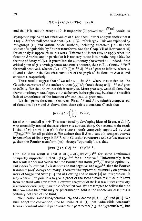
238 M. Cowling et al.

I (2 )=~ exp(i2h)dV(h) V2~R.

dr(h) and that V is smooth except at 0. Jeanquartier [7] proved that ~ admits an

asymptotic expansion for small values of h, and then Fourier analysis shows that if V(h) ~ Ch ~ for small positive h, then 1(2) ~ C'121-" for large 2. This was exploited by Malgrange [11] and various Soviet authors, including Var~enko [16], in their studies of singularities by Fourier transforms. See also Chap. VII of H6rmander [6] for an analytic approach to this work. This method is not easy to apply when the function ~b varies, and in particular it is not easy to use it to obtain inequalities for the rate of decay of 1(2). It generalises the stationary phase method - indeed, if the critical point of ~b is nondegenerate and v (0) is nonzero, then V(h) ~ Cv (0)K-1/2 h n/2

for small positive h, whence 1(2) ~ C'v(O) x -u2121-"/2 as 2 goes to infinity, where x, C, and C' denote the Gaussian curvature of the graph of the function q~ at 0, and constants, respectively.

These results suggest that if we take u to be xl/2, where ~ now denotes the Gaussian curvature of the surface S, then (up)^(~) should decay as 141-"/2 as ~ goes to infinity. We shall show that this is nearly so. More precisely, we shall show that the volume integrals analogous to Vdo behave in the right way, but that the possible lack of smoothness of the function ~l/Z can lead to problems.

We shall prove three main theorems. First, if V and �9 are suitable compact sets of functions like v and q~ above, then there exists a constant C such that

,I(2),<=CV( ~ ) V2~R,

for all v in Vand all ~b in ~. This is achieved by developing ideas of Bruna et al. [1], who essentially treated the case where v is nonvanishing. Our second main result is that if v ( . )=w( . )de t~b" ( . ) for some smooth compactly-supported w, then V(h) < Ch "/2 for all positive h. We deduce that if S is a smooth compact convex hypersurface of finite type in R" + 1, with Gaussian curvature ~ and surface measure p, then the Fourier transform (K#) A decays "optimally", i.e. that

I (~,u)^(~)l__<Cl~;I-"/2 V ~ R "+~ .

Our last main result is that if v(.)=w(.)detdp"(.) 1/2 for some continuous compactly supported w, then V(h)< Ch "/2 for all positive h. Unfortunately, from this result it does not follow that the Fourier transform (Ku2#) A decays optimally. But it does follow that ifu is smooth and nonnegative, and u < ~c 1/2, then the Fourier transform (u/~) ̂ decays optimally. These results improve substantially on previous work of Sogge and Stein [13] and of Cowling and Mauceri [3] on this problem. It may seem a little pointless to give a proof of the second main result, as it follows from the third with little effort. However, the proof of the last result uses convexity in a more essential way than those of the first two. We are tempted to believe that the first two main theorems may be generalised to hold in the nonconvex case; this is certainly not true of the third.

We mention some idiosyncrasies: NQ and I denote {0, 1 ..... Q } and [0, 1 ]. We shall adopt the convention, due to Bruna et al. [1], that "admissible constant" means a constant which depends on certain parameters (e. g. the hypersurfaces), but

Damping oscillatory integrals 239

not others (e. g. the Fourier transform variable r but these parameters vary from section to section. The constants themselves may vary from line to line. As some of the authors are interested in the numerical evaluation of oscillatory integrals, and so in the possibility of using these results to estimate error terms, we have com- puted some of the constants, especially in Sect. I (Lemmas 1.1-1.4) and Sect. 4 (Lemma 4.2). It should be stressed that the main theorems do not require these computations, and the reader can replace the constants by a generic " C " if desired.

In Sect. 1, we analyse convex functions of one variable, and prove estimates for these; Sect. 2 is about one-dimensional oscillatory integrals. Sect. 3 describes the coordinate systems we use to parametrise the hypersurface S, Sect. 4 proves an n-dimensional estimate, and in Sect. 5 we put these ingredients together to prove our main theorems. The final section gives a pair of examples which indicate the sharpness of our work.

Acknowledgements. We wish to thank Peter Donovan, George Szekeres, and Adrian Nelson for useful information about convex bodies.

1. Estimates

This section is devoted to proving the basic estimates about convex functions of one variable that we shall need. We consider the family ~(m,M,q,Q) (where m, MeR+,m<M,q, QeN, and 2 < q < Q ) of all functions f : I ~ R of class C Q which satisfy the conditions

f(O) =f'(O) = 0

f"(t)>O VteI

l f(j)(O) >m, (1.1) m a x 2<j<q J'.

max ~.f(J)(t)<M VteI O<j<=Q

and establish various other properties of these functions. Our strategy is like that of Randol [12] and Bruna et al. [1]: we approximate f by a polynomial p of degree q + l , and derive properties of f from those of p. We start by investigating polynomials (Lemmas 1.1, 1.2 and 1.3), then show how to approximate f in ~ ( m , M, q, Q) by a polynomial (Lemma 1.4), and finally derive the inequalities for f (Lemma 1.5 on).

In this section, any constant which depends only on m, M, q and Q is called "admissible". Any other parameters on which the constants may depend will be noted explicitly. We shall also write ~ rather than ~-(m, M, q, Q), except in the enunciation of our results. Our first result is a familiar but useful estimate for polynomials on [0, 1 ].

d Lemma 1.1. Suppose that p(t)= ~ aJJ, for all t in [ - 1 , 1].

j=O

Then

240 M. Cowling et al.

I fp ~ even, then

d

la~l~3 a max [p(t)l. j = O t e [ - 1 , 1 ]

d

iajl_<6 a/2 max ]p(t)l. j = O t e l

Proof These estimates can easily be proved by expanding p as a sum of ~eby~ev polynomials. [3

d

Lemma 1.2. Suppose that p(t) = ~ ajt j, for all t in L j = O

d

(a) ~ la~l<6 n max Ip(t)l. j = O t e l

(b) l f p is nonnegative and increasing, then d

laj]tJ<<_6ap(t) VtEI. j = O

(c) I f p is nonnegative and n ~ N, then d

E last ti+"<=(d+n)6n+" iP(S)S"-'ds VteI . j = O O

Proof To prove (a), we apply Lemma 1.1 to the even polynomial s~-*p(s2). Next, if p is nonnegative and increasing, then p ( 1 ) = IIpll ;thus

d

~.. lasl<6ap(l). j = 0

Applying this inequality to the polynomials p , wherept(s ) =p(st), for all s, t and L proves (b).

t

To prove (c), apply (b) to the polynomialp* wherep*(t)=jp(s)s"-lds, for all t in L Then o

~ oil j+" 1 ~ [a,[t '+" 1 a p * ( t ) = >~- -~ - - > ~ ]aj[t i+~,

j=o j+n ./=o j + n =(d+n)6 d+" ~/=o

and we are done. I-'1

Lemma 1.2 will allow us to pass from increasing nonnegative convex polynomials to polynomials with positive coefficients. The results we shall need about these are the content o f the next lemma.

q + l

Lemma 1.3. Suppose that p ( t ) = ~ ajt J, where aj~[0, M] for all j in Nq, max aj>m, andaq+x=M. Then j=2

2 ~ - j ~ q

(a) mt~<p(t)<qMt 2 and 2rntq-a<p'(t)<q(q+l)Mt u (b) [p'(t)] 2 < M q ( q + 1)2p(t) Vt~I

Damping oscillatory integrals 241

tkp(k)(t)< (q+ 1)] (C) = ( q ~ l ~ ) ! p ( t ) VteI, VkENq+ 1

Proof. It is trivial to prove (a). To prove (b), observe that, for all t i n / ,

[P'(t)]z:u:EJafiS L,x ja t'-=J < ( q + l ) 2 ajt j ajt j-2 <Mq(q+l)2p(t).

L j =2 I j=2

The proof of (c) is an easier version of that of (b). To prove (d), observe that if s > 1 and 0 < ps < 1, then, using (a), we have that

q+l q+l q

s 2 ~ arid< ~ aj#JsJ<=s q ~ ajpJ+i(ps) ~+1 j=2 j=2 j=2

~ sq j~__ 2 a j l-tJ + M ( bts ) q <= sq [p ( I-o + M P ( l't ) 1 �9

The proof of (e) is similar, and left to the reader. []

�9 For f i n ~ , we define/Ty and py, sometimes written simply as/7 and p, to be the following polynomials:

f~s)(O) /Ts(t) = ~, j ~ tS+Mtq+l

j=2

q If(S)(0)l tJ+Mtq+l py(t)= j=2 J!

Vt~I.

VteI (1.2)

The next lemma, based on Lemmas 3.1-3.3 of Bruna et al. [1 ], shows that/Ty and pf are good approximants t o f The reader familiar with [1 ] should be warned that our/7 andp correspond to their Q and Q respectively; as we usep more thanp we felt this notation worth the risk of some confusion. For the convenience of the reader not acquainted with [1 ], we have included the proof.

Lemma 1.4. For any f in ~ ( m , M, q, Q),

while

Furthermore

IfU)(t)l<pU)(t) Vt~I, VjeN~,

j ! IfU)(t)l__< p~+l)(t) VteI, Vj~NQ\N~.

(q+ l ) !

r m 7 .+ ' 4 I- m ?+' L ~ J P(t)>qL6TwmJ /7(') Vt~X,

242 M. Cowling et al.

f ' ( t ) > 2 ~ [ m lq > 2 ~ I m I q = q + l ~sq2(q-+l)M P' ( t )=q+l ~ S q 2 ( ~ l ) M fi'(t) Vt~I .

Proof. From Taylor's expansion, with the integral form of the remainder, for any t in I and k in Nq,

f(k)(t)=,~= k.= (j--k)!f(D(O) t'-k4- l~(q-k)! oi(t--s)q-kf<q+i)(s)ds" (1.3) If k = 0, 1, or 2, f~k)(t)> O, SO for all t in I,

If(ki(t)l=f(k)(t)<j~= (j--k)!f(J)(O)tS_k+l(q_k)! oi ( t - s ) q - k M ( q + l ) !ds

=ffk)(t) <=p~k)(t) ,

and consequently/7 and fi' are nonnegative and increasing. If 2 < k < q, then

Iftk)(t)l<j.= (j-k)!lftJ)(0)l tJ-k +--(q--k)! o ( t - -s)q-kM(q+ l)!ds=p(k)(t)

for all t in L while if q < k < Q, then trivially

k! If~kl(t)l < p~q+l)(t) V t e I .

= ( q + l ) !

We now obtain the converse inequalities when k = 0 or 1. For the case k = 0, from (1.3) we see that, for all t in L

f (t) > tJ + Mt ~+ l - 2 Mt q+ l = f i ( t ) - 2Mt q+ l . J!

Since/7 is nonnegative and increasing, by Lemma 1.2(a),

f ( t ) > 6 - q - i p ( t ) - 2 M t q+i >__6-q-lmtq-2Mt q+~

If t o = 6 - ~ - 2 m/M and 0 < t __< t o , then f ( t ) > ~ 6 - q - 1 mt q, so

6_~_ 1 p(t) <x~(t) < + ~ ( t ) - f ( t ) < l 2Mt q+l 3 f ( t ) = f ( t ) = l f ( t ) = + ] 6 - q - i m t ~<2 '

while if t o < t < 1, then, since p and f are increasing,

f i ( t )<p( t )< p ( l ) < 3 M q 6q+l r6q+2M] q.

f ( t ) = f ( t ) = f( to) = 2m [ _ m _ ]

of p'(t) The estimation ~ is analogous, and we omit the details. []

It is now straightforward to make the necessary estimates.

Lemma 1.5. For all f in ~ (m, M, q, Q ), there are admissible constants C o, C 1 , C 2 , C a , and C~Jl(j e NQ) such that (a) Cotq<___f(t)<=Mqt 2 V t ~ I (b) [ f ' ( t ) ]2~Ct f ( t ) V t ~ I

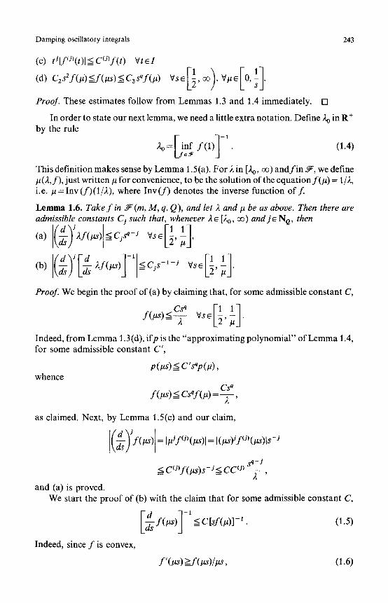
Damping oscillatory integrals 243 (c) tJlftJ)(t)[ <Ctj)f( t) V t~I

Proof. These estimates follow from Lemmas 1.3 and 1.4 immediately. []

In order to state our next lemma, we need a little extra notation. Define 20 in R § by the rule

20 = D n f f (i)1-1 . (1.4)

This definition makes sense by Lemma 1.5(a). For 2 in [20, oo) and f i n ~', we define It(2,f), just written # for convenience, to be the solution of the equation f(it) = 1/2, i.e. It= Inv (f)(1/2), where Inv(f ) denotes the inverse function o f f .

Lemma 1.6. Take f in ~ (m, M, q, Q), and let 2 and It be as above. Then there are admissible constants C j such that, whenever 2 ~ [2 o, oo ) and j ~ N o, then

d ~ (a) (~-ss)2f(its)<=Cjs ~-j Vs~I~, 1] ,

d ~ d - t 1 (b) (dss) I~-S ~'f(itS) 1 ~Cjs-I-J VS~[2'~I"

Proof. We begin the proof of (a) by claiming that, for some admissible constant C,

Indeed, from Lemma 1.3 (d), ifp is the "approximating polynomial" of Lemma 1.4, for some admissible constant C',

p(~s) <= C' s~p(it), whence

f (gs) <= Cs~ f (#) = --Cy ,

as claimed. Next, by Lemma 1.5(c) and our claim,

(~SS) j J (J) ./ (J) J f(its) = IIt 'f " (its)l = I(its)'f " (its)is- "

sq- J < C~J~f(ps)s- j < CC~J~ _ _

2 ' and (a) is proved.

We start the proof of (b) with the claim that for some admissible constant C,

d -x [ -d~s f (~ ) ]<C[s f ( i t ) ] -~ . (1.5)

Indeed, since f is convex,

f ' (ps) >__f (ps)/#s, (1.6)

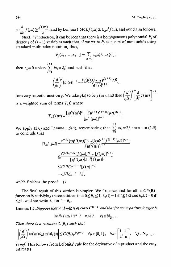
244 M. Cowling et al.

d f (ps ) S ~ s ' andbyLemmal '5 (d) ' f ( I z~)>C2s2f (u) 'and~176176

Next, by induction, it can be seen that there is a homogeneous polynomial Pj of degree j of ( j + 1) variables such that, if we write Pj as a sum o f monomia l s using s tandard mult i index notat ion, thus,

P j ( x , . . . . ,x~+0= Y~ c .x~l . . . xT+~l , I~[ =J

j+l then c~ = 0 unless ~ ia i = 2j, and such that

i=1

/ sY [g ' ( s ) l - I _ PJ (g (s) .... , g() + 1) (s)) - [ g , ( s ) l J + ~ ,

for every smoo th funct ion g. We take g (s) to be f (ps ) , and then f(/as)

is a weighted sum of terms T~ , where

[uf,(~)],,...iuj+,f(j+,(~)]~,+l T~f(~)= [uf,(~)]j+I

j + l

We apply (1.6) and L e m m a 1.5(d), r emember ing that ~ ' i~ti=2 j , then use (1.5) to conclude that i=

s-2J[spY'(us)]~'... [(su)J+lf(g+l)(US)]~,+l iT J ( ps)[ = [uf ' (us ) ]J + 1

< c t J ~ s - 2 j [ f ( ~ ) ] , l . . . [ f ( ~ ) ] , , +1

[uf'(las) l s - J [ f (us) ] j

~ CtJJ C s - l - J [ f (u) ] -1

=CtJ]Cs-I-J2,

which finishes the proof . []

The final result o f this section is simpler. We fix, once and for all, a C~176 function 00 satisfying the condit ions that 0 < 0 o < 1, Oo(t) = 1 if t < 1/2 and Oo(t ) = 0 if t > l , and we write 01 for 1 - 0 o.

L e m m a 1.7. Suppose that w : I ~ R is of class C Q- 1, and that for some positive integer b

Iw(J)(s)t<_j[s b-j V s e I , VjeNQ_ x.

Then there is a constant C(Oo) such that

w(p~)Oo(~)Ol(s) <C(0o)#% b-s VUe[0 ,1 ] , Vse , , V j e N e _ l .

Proof. This follows f rom Leibnitz ' rule for the derivative of a product and the easy estimates

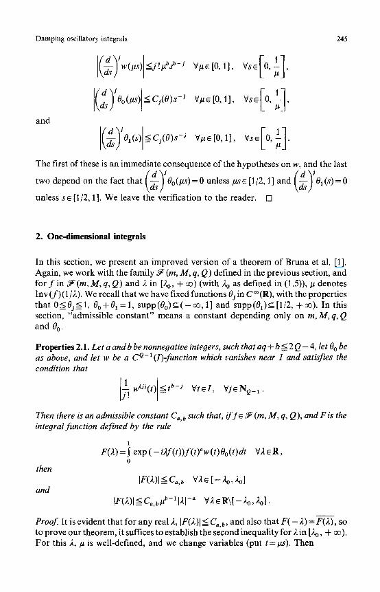
Damping oscillatory integrals

and

245

The first of these is an immediate consequence of the hypotheses on w, and the last

two depend on the fact that ~ 0o(~) - -0 unless #ss[1/2, 11 and ~ 01(s)=O

unless se [1/2, 1]. We leave the verification to the reader. []

2. One-dimensional integrals

In this section, we present an improved version of a theorem of Bruna et al. [1]. Again, we work with the family ~ ( m , M, q, Q) defined in the previous section, and for f in ~ ( m , M, q, Q) and 2 in [20, + oo) (with 2o as defined in (1.5)), # denotes tnv (f)(1/2). We recall that we have fixed functions Oj in C ~ (R), with the properties that 0 < Oj < 1, 00 + 01 = 1, supp (0o) _~ ( - 0% 1 ] and supp (01) c [1/2, + oo). In this section, "admissible constant" means a constant depending only on m, M, q, Q and 0 o.

Properties 2.1. Let a and b be nonnegative inteoers, such that aq + b < 2 Q - 4, let 0 o be as above, and let w be a CQ-l(I)-funetion which vanishes near 1 and satisfies the condition that

~. w~i)(t) <=t b- j Vt~I , V jeNQ-1 .

Then there is an admissible constant Ca, b such that, if f ~ ~ (m, M, q, Q ), and F is the integral function defined by the rule

1

F(2)=S exp ( - i2f( t ) ) f ( t )aw(t )0o( t )d t V2eR, o

then

and IF(~)I<C.,b V2~ [--2O,2O]

Proof It is evident that for any real 2, IF(2)[ ~ C~,b, and also that F ( - 2) = F(2), so to prove our theorem, it suffices to establish the second inequality for 2 in [2O, + oo). For this 2, # is well-defined, and we change variables (put t = ps). Then

[F(2)t_-< b+l -a C,.b/~ I,~1 V2eR\[--2O, ~].

246 M. Cowling et al.

1/u F(2)=2-a /~ ~ exp(-i2f(Ps))[2f(Ps)]"w(l~)Oo(P.s)ds

0

l /u

= 2-al't I exp(--iJf (12s))[2f (lls)]aw(lls)Oo(llS)Oo(s) dS o

1/# + 2 - " # j" exp(-i2f(lls))[2f(p~)]"w(l~s)Oo(#s)Ol(s)ds.

0

In the first integral, Oo(s ) = 0 unless s < 1, and then 2f (p~)<2f( /z )= 1, so

2 - " # 1/Uo ~ exp ( - i2f(/~s)) [2f(#s)]aw(#s)Oo(P~s)Oo(s)ds

i //b+l <=j.-"# w(~s)ds<=2 -a o b + l "

In the second integral, 01 (s)= 0 unless s > 1/2, so we must show that

l~u exp ( - i2f(#s)) [2f(/~)1" w (/z~) 0 o (/ts) 01 (s) as < c,, b #b, 1/2

for all 2 in (2 o, + oe). We recall f rom Lemma 1.6 that for all j there exist admissible constants Cj

such that

d j " V s e [ ~ , (ds) 2f(lts) <=Cjsq-J t_l l l '

and further from Lemma 1.7, for some admissible constants Cb, j,

(d)Jw(13"S)Oo(/'Is)OI(s) ~Cb,jP bSb-j VSe[~, ~I"

Integration by parts shows that

1//z

I exp ( - i2f(12s)) [2f(/as)]a w (/~s) 0 o (p3) 01 (s) ds 1/2

l/t*

= I exp ( - i2f(~)) D~ ([2f(/~s)]" w (~s) Oo ( ~ ) 01 (s)) ds 1]2

where d - 1

d (I-~s(i,~f(las)) 1 g(s)) VseI~ 1 1 D f(o)(s) =-ds ' "

In our integral, the function g : s ~ [2f(/~)] ~ w (/~) 00(~) 01 (s) grows (in absolute value) no faster than s~--~s "q+b, and its successive derivatives D~g grow no faster

1 than s~-*s aq+b-2k. Indeed, multiplication by (i2f(~)) decreases the growth

Damping oscillatory integrals 247

rate by a factor of at least s- 1, and differentiating a linear combination of products

of derivatives of s~--, dss 2O(/~s) , sw*[2~b(~)]", and s~-*w(~)Oo(l~)Ol(s ) also

decreases the growth rate by at least this factor, provided that k is no bigger than Q - 1. Our conditions on a, b, q and Q ensure that after at most Q - 1 integrations by parts, the integrand vanishes at least as fast as s- z (if aq + b is even) or s - 3 (if aq + b is odd), multiplied by/~b, so the integral is bounded. []

3. Surfaces

Let S be a compact convex hypersurface in Euclidean space R" + 1, of class C Q, all of whose tangent lines have order of contact at most q, where q < Q. For every p in S, we choose a coordinate system in R "+1 "based at p " by choosing an orthonormal frame {Zo, h ..... %} atp, such that z t ..... z. span Tp(S) and % points to the side of Tp(S) on which S lies. The orthogonal projection of S onto Tp(S) is the compact closure of an open set Up in Tp(S). By rescaling if necessary, we may assume that for everyp in S, the closed ball of radius 2 in Tp(S) is contained in Up, and that there is a nonnegative-real-valued CQ-function q~p on B(2), the ball of radius 2 in R", whose graph is a subset of S, i.e., in the coordinate system based at p,

{(q~p(t 1 . . . . . t,),q ..... t.): j=l ~ t~.<=4}cS.

We may also assume that there exists a constant M such that

(dtJ~)p(~Wtz)lt=o <:Mj! VjE NQ,

for all p in S and for all vectors ~ in S"- 1 and all ~ in B(2). Another compactness argument, using the fact that the order of contact of the

tangent lines to S is at most q, shows that there exists m in R + such that for allp, z and r as above,

1 ( ~ ) J tz)l,=o max qSp(~+ > m . 2<=j<q ~. Indeed, otherwise there would be a point p and vectors z and ~ with

( d ) J s p ( ~ + tz)lt=o =0 Vj~ Nq\{0, 1},

and then the point (q~p(r 4) on 6e would have a tangent line of order of contact more than q.

We denote by 5," (m, M, q, Q) the space of all functions q~ : B (2)~ [0, + ~ ) which satisfy the following conditions

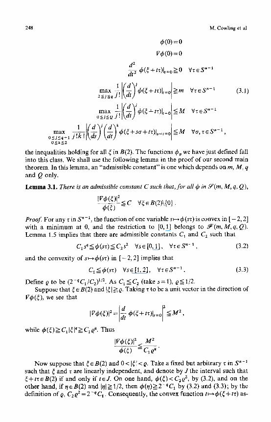
248 M. Cowling et al.

r =0

vr =0

d 2 dt 2 ~b(4 + tz)l,=o > 0

maxq~.(d)JqS(4+tz),,=o >_m

1 d j

Vz~S .-~

Vz~S "-~ (3.1)

V z e S n-i

m a x o<_j<_q+l ds -~ dP(~+sG+tz)l~=t=~ Vcr '*~S"- l ' 0<k_<2

the inequalities holding for all 4 in B(2). The functions Op we have just defined fall into this class. We shall use the following lemma in the proof of our second main theorem. In this lemma, an "admissible constant" is one which depends on m, M, q and Q only.

Lemma 3.1. There is an admissible constant C such that,for all c~ in ~(m, M, q, Q),

tV~b(~)[ 2 < C V4 ~ B(2)\{0}. r -

Proof. For any z in S "-1, the function of one variable s~-~b(sz) is convex in [ - 2 , 2] with a minimum at 0, and the restriction to [0,1] belongs to ~(m ,M,q ,Q) . Lemma 1.5 implies that there are admissible constants C a and C2 such that

Clsq<dp(sz)<C2 s2 Ys~[0,1], Vz~S "-x, (3.2)

and the convexity of s~-*(o(sz) in [ - 2 , 2] implies that

Cl<~(sz ) Vs~[1,2], V~eS "-1. (3.3)

Define Q to be (2-qCx/C2) x/2. As C 1 < C 2 (take s = 1), ~__< 1/2. Suppose that 4 e B(2) and 14[ > 0- Taking z to be a unit vector in the direction of

V~(4), we see that

i V r - d q ~ ( 4 + t z ) l t = o 2 < M z '

while r q. Thus

IVr < M2

r = c , e q"

Now suppose that ~ 6 B(2) and 0 < 141 < e. Take a fixed but arbitrary z in S n-1 such that 4 and z are linearly independent, and denote by J the interval such that ~+ t z6B ( 2 ) if and only if t~J. On one hand, r C~Q z, by (3.2), and on the other hand, if q a B(2) and I~l > 1/2, then r (O > 2- q Cl by (3.2) and (3.3); by the definition of Q, (?2 Qz = 2- ~ C 1 . Consequently, the convex function t ~ ~b (4 + tz) as-

Damping oscillatory integrals 249

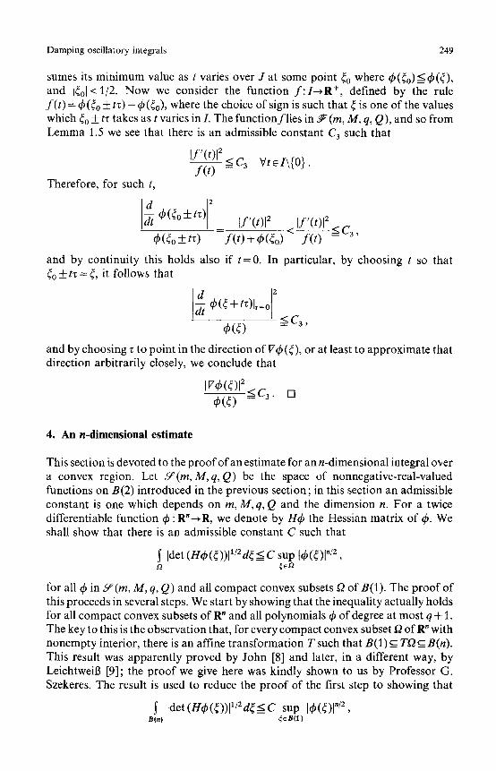
sumes its minimum value as t varies over J at some point 4o where q~(~o) < ~b(4), and 14o1< 1/2. Now we consider the function f : I - -*R +, defined by the rule f ( t ) = 49(40 +_ t z ) - ~b (40), where the choice of sign is such that 4 is one of the values which 40 + tz takes as t varies in L The function f l ies in ~ M, q, Q), and so from Lemma 1.5 we see that there is an admissible constant C 3 such that

If'(t)12<C3 Vt~I\{O} f ( t ) =

Therefore, for such t,

d~b(40 [f'(t)[2 < l f ' ( t ) [2<C3,

2 + t~)

d? (40 +- tz) f ( t ) + ck (40) f ( t )

and by continuity this holds also if t=0 . In particular, by choosing t so that 4o + tz = 4, it follows that 4o + tz = 4, it follows that

d r 2

~c3, r

and by choosing ~ to point in the direction of 17q~ (4), or at least to approximate that direction arbitrarily closely, we conclude that

1vr ~ r ~-~C3" []

4. An n-dimensional estimate

This section is devoted to the proof of an estimate for an n-dimensional integral over a convex region. Let 5P(m, M, q, Q) be the space of nonnegative-real-valued functions on B(2) introduced in the previous section; in this section an admissible constant is one which depends on m, M, q, Q and the dimension n. For a twice differentiable function ~b : R"~R, we denote by H~b the Hessian matrix of q~. We shall show that there is an admissible constant C such that

[det (H~b (4))11/2 d4 < C sup Iq~(4)[ "/2 ,

for all ~b in 5~ (rn, M, q, Q) and all compact convex subsets O of B(1). The proof of this proceeds in several steps. We start by showing that the inequality actually holds for all compact convex subsets of R" and all polynomials ~b of degree at most q + 1. The key to this is the observation that, for every compact convex subset t2 of R" with nonempty interior, there is an affine transformation T such that B(1)c_ TO ~_ B(n). This result was apparently proved by John [8] and later, in a different way, by LeichtweiB [9] ; the proof we give here was kindly shown to us by Professor G. Szekeres. The result is used to reduce the proof of the first step to showing that

Idet(Hqb(4))lll2d4<C sup I~b(4)l "I2, B(n) ~B(1)

250 M. Cowling et al.

for all polynomials of degree q + 1 in R". The second step of the proof involves an approximation argument to pass from polynomials to more general functions.

Lemma 4.1. For every compact convex subset O of R" with nonempty interior, there exists an affine transformation T such that

B ( 1 ) ~ O ~ B ( n ) .

Proof. As the set of all ellipsoids contained in O is compact, we may find an ellipsoid E contained in O of maximal volume. Choose the affine transformation T so that TE =B( l ) . Since affine transformations preserve the ratios of volumes, B(1) is an ellipsoid contained in TO of maximal volume. We claim that TO is contained in B(n). I f this were not so, then we could choose our coordinate system such that, for some R in (n, + ~ ) , (R, 0 ... . . 0) e TO. As TO is convex, TO would contain the convex hull O ' of this point and B(1). It is easy to check that if0 < r < (R - 1)/2, then O' contains the ellipsoid E~, given by the formula

(~1-0 2 ~ C a2 k-~- + ... + ~ - =<1,

where a = r + 1 and b = ( 1 - 2 r / ( R - 1)) 1/2. It is also easy to check that the volume of E, exceeds that of B(1) when r = ( R - n ) / ( n + l ) . This would contradict the maximality of the volume of B(1); thus TO is indeed contained in B(n), as required. []

It is worth noting that no smaller ball than B(n) will do in Lemma 4.1 - to see this, consider the regular simplex in R".

Lemma 4.2. There & a constant C.,q such that

[det Hn(~)l*/2d~ <= C,,q sup [~Z(~)[ n/2 ,

jor all polynomials n on R" of degree at most q + 1 and all compact convex subsets O of R".

Proof. Let O be a compact convex subset of R". If Q has empty interior, then its Lebesgue measure is 0, and there is nothing to prove, so we may and shall assume that O has nonempty interior. Take an affine transformation T as in Lemma 4.1. Now

[det H0r o T - 1) (~)[1/2 = [det T[- x [(det H n ) ( T - t ~)[1/2 and

~ o T - l ( ~ ) l d e t T l - l d ~ = ~ ~(~)d~ T~2 g2

for all polynomials n and ~, on R", so

[det Hlr(~)ll/2d~= ~ [de tH0zo T-1)(~)ll/2 d~ ; 1"2 Tg]

moreover, sup I~(~)l "/2 = sup [(~ 0 T - x)(~)l"/2. ~e~ ~eT~

Damping oscillatory integrals 251

Since B(1)_~ Tf2~_B(n), it will suffice to show that

[detHrt(~)ll/Zdr sup [rt(~)l "/2, B(n) ~B(1)

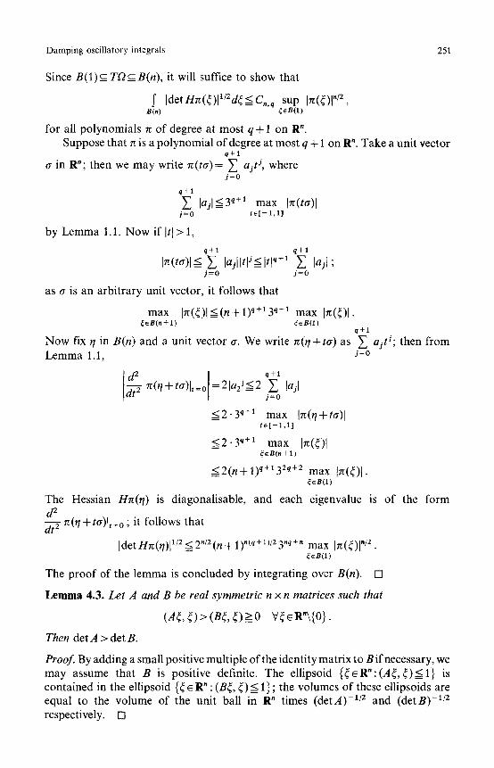
for all polynomials 7t of degree at most q + 1 on R". Suppose that ~ is a polynomial of degree at most q + 1 on R". Take a unit vector

a in R"; then we may write rc(ttr)= ~ ajt j, where j=0

q+l

lajl<3 q+l max I~(ur)[ j=0 t~[-1,1]

by Lemma 1.1. Now if [ t l>l ,

q+l q+l 17t(ttr)[~ ~ laj[[tlJ~[tl q+l ~ [a~[;

j=0 j=O

as a is an arbitrary unit vector, it follows that

max Ir~(~)l<(n+l)q+13q+t max Irc(OI. ~B(n+l ) ~eB(1)

q+l

Now fix q in B(n) and a unit vector a. We write ~r(q+ta) as ~ ajtg; then from Lemma 1.1, j =o

d~ ttr){, = o q + 1

n(r/+ =21a21~2 Z lail j=O

< 2 " 3 q+l max Irc(q+ta)l re[-1,1]

< 2 " 3 q+l max I~(OI ~eB(n+ l)

<2(n+l)q+132q+2 max I~(OI- ~eB(1)

The Hessian Hit(t/) is diagonalisable, and each eigenvalue is of the form d 2 dt 2 lr(r/+ta)]t=o ; it follows that

Idet H~z(q)[ 1/2 ~ 2 n/2 (n + 1 )"~q + 1)/2 3,q +, max I~t(OI "/z ~B(I)

The proof of the lemma is concluded by integrating over B(n). []

Lemma 4.3. Let A and B be real symmetric n x n matrices such that

(A~, ~) >(B~, ~ )>0 V~R" \{0} .

Then detA > detB.

Proof. By adding a small positive multiple of the identity matrix to B if necessary, we may assume that B is positive definite. The ellipsoid { ~ R " : ( A ~ , ~ ) < I } is contained in the ellipsoid {r E R" : (B~, ~)< 1 }; the volumes of these ellipsoids are equal to the volume of the unit ball in R" times (detA) - m and (de tB) -1/z respectively. []

252 M. Cowling et al.

Proposition 4.4. There is an admissible constant C such that

S [detn49(r < C sup 149(~)1,/2, I2 ~r

for all 49 in 5P(m, M,q, Q) and all compact convex subsets f2 of B(1), provided that q < Q - 2 .

Proof. We may and shall suppose that q is odd, and at least 3. For ifq is even, we may replace it by q+ 1. All we need for the rest of the proof is that q < Q - 1.

Take 49 in 5P(m, M, q, Q) and let rt be the polynomial, defined in standard multi- index notation, by the rule

49(')(0) R". 7t(r ~ ~! r q+~ Vr I~l<q

Fix a unit vector a in R', and write f~(t) andfi~(t) for 49 (ta) and ~ (ta) respectively. By definition, f~ lies in i f (m, M, q, Q) and

f2~)(O) f i ~ ( t ) = ~ j ! tJ+Mt q+l Vt~I.

j=O

By Lemma 1.4, there is an admissible constant C such that

O<___f,(t)<fi~(t)~Cf,(t) Vt~I,

and consequently ~(r162 Vr

It will suffice to show that

det H49(~) <det Hn(~) VCeB(1), (4.1)

since then by Lemma 4.2,

(det H49 (4))1/2 d~ < ~ (det Hn (4))1/2 d~

< C.,q sup u(~) "/u

<=C.,qC "/2 sup 49(~)./2,

as required. The inequality (4.1) is a consequence of Lemma 4.3 and the inequality

( H49( ~ )~, z) < (H~t( ~)z, ~),

d 2 d z (4.2) i.e. ( ~ ) 49(~+tv)l ,=o<(~)rc(~+tv)l ,=o

for all unit vectors ~ in R", and all r in B(1). To prove inequality (4.2), we write r = ua, for some unit vector a in R" and some

u in I. By Taylor's theorem, with the integral form of the remainder, as in (1.3),

Damping oscillatory integrals

~(~)- ~(r =~o(u)-f.(u)

= Muq+l -~ . i (u-s)qfjq+l)(s)ds 0

uq+l 1

---MIr q+l - - - .~ (1 -r)qfjq+t)(ur)dr q! o

F ( ~ "1 ] =Mlr o} 0-r)"Lt, Ys: qh(r*+s*) ,=odr" On the one hand,

d 2 [ ( ~ ) Ml'+tzlq+~3t=o=M(q+l' [ (q -1 ) ] e lq -3 ( , .z)2+ [,I. - t ]

>M(q-I - 1)1~1~-1 ;

on the other hand,

[(d)2 1 1~ ! (l_r)qLl~Yss)V/~ "kq+'dp((r+s)(~+tz))l,o=

:- i r,"'~:+'('~) ~ ] 1 (1 -r) ~ dp((r+s)(r dr q! o LtYs) ~7 ,-,=o

=q~o" Lt~s) ~ (r+s)Zq~((r+s)r

: i [ :~ 1 (1 _r)q r2 q! o ~ ~ss J r + sua + tz)

+ 2(q + l)r(~)q (~)2cp(r~ + surr+ tz)

~9 q-' (~1 q~(r~+sua+tz)] dr + ( q + l ) q ~ss \ / _.ll:=,:o

:- i [ ~":+'(d 1 (1 - r )~ rZu q+l q! o \~s) q~fr~ +sa+tz)

+ 2 ( q + 1)ru" \as) \3t t# dpfr~ + sa + tz)

:oy ,(~)2+.~+.~+,q. : +(q+ l)qu'- ' \ds]

<1__ [ (1 -r)q[2(q+l)!rEuq+~+4(q+l)!ruq+2(q+l)!uq-~]Udr -q!~

2M(a+l)uq_l[ 2q! + 2q! . q! -]

253

254 M. Cowling et al,

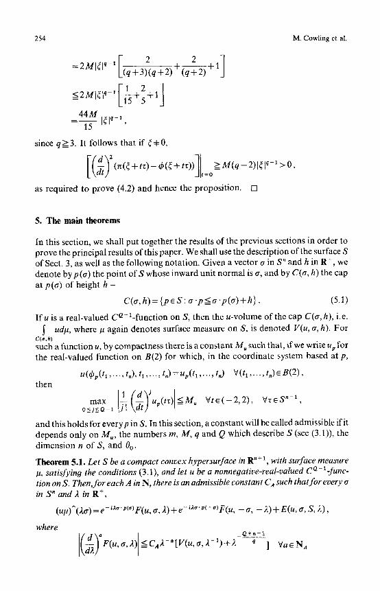
=2Ml~lq-~[-(q+ 23)(q+2) q - ( q ~ + 11

44M - I ~ 1 ~ - 1 ,

15

since q > 3. It follows that if r * 0,

Or(~+tz) = > M ( q - 2 ) l ~ l q-1 > [(d) ~ -~(~+n))l, ~ 0,

as required to prove (4.2) and hence the proposition. []

5. The main theorems

In this section, we shall put together the results of the previous sections in order to prove the principal results of this paper. We shall use the description of the surface S of Sect. 3, as well as the following notation. Given a vector cr in S" and h in R +, we denote by p (cr) the point of S whose inward unit normal is g, and by C(a, h) the cap at p(tr) of height h -

C(a, h) = {p ~ S : a -p _-< a .p (or) + h}. (5.1)

If u is a real-valued C Q- 1-function on S, then the u-volume of the cap C(a, h), i.e. ud#, where/~ again denotes surface measure on S, is denoted V(u, cr, h). For

C(s,h) such a function u, by compactness there is a constant M u such that, if we write up for the real-valued function on B(2) for which, in the coordinate system based at p,

u(q~p(t 1 .... , t.), t 1 ..... t .)=up(t 1 .... , t.) V(tl .... , tn)~B(2), then

max up(tz)<=M u V t e ( - 2 , 2 ) , VzeS n- t , o<_j__<Q-1

and this holds for everyp in S. In this section, a constant will be called admissible if it depends only on M u, the numbers m, M, q and Q which describe S (see (3.1)), the dimension n of S, and 0 o.

Theorem 5.1. Let S be a compact convex hypersurface in R "+1, with surface measure g, satisfying the conditions (3.1), and let u be a nonne9ative-real-valued C~ - tion on S. Then,for each A in N, there is an admissible constant CA such that for every t~ in S" and 2 in R +,

(u#)A(2a) =e-i~'P~*~ F(u, a, 2 ) + e-i~*" Pc-*) F(u, - a , - 2 ) + E ( u , a, S, 2),

where

F(u,a, CAX-"[V(u,g, 2-~) +2 q ] VaeNA

Damping oscillatory integrals 255

and

d E ( u , a , S , CA 2-(f2-1) VaeNa,

provided that A q + n < Q - 2.

Theorem 5.2. Let S be a compact convex hypersurface in R "+1, satisfy& 9 the conditions (3.1), with surface measure #, and Gaussian curvature K. Let u be a nonnegative-real-valued C Q- 1-function on S, with the property that 0 <_ u <_ K. For each `4 in N, there is an admissible constant C a such that for any a in S" and any 2 in R + ,

(u/0^(2a) = e - i~,. ,(,~ F(u, a, 2) + e-ia~. , ( - ~)F(u, - a, - 2) + E(u, a, S, 2),

where

~ ) a F ( u , a, )O ~Ca2 -~-"/2 Va6N A

and

( ' ~ ) a E ( u , cr, S, 2 )[<=CA}~-a-n /2VaENA,

provided that A q + n < Q - 2 and n q < 2 ( Q + n - 1 ) .

Theorem 5.3. Let S be a compact convex hypersurface in R ~+l, satisfying the conditions (3.1), with surface measure #, and Gaussian curvature x. Let u be a nonnegative-real-valued C o- l_function on S, with the property that 0 <- u <- ~1/2. For each .4 in N, there is an admissible constant C A such that f o r any a in S" and any 2 i n R +,

(u#) ~ (2a) = e - ~*'P(~) F(u, a, )0 + e - iz,. p(- ~) ff(u, - a, - 2) + E(u, a, S, 2),

where

/,4\[~fF(u, ty, A)<:CA~ -a-n/2 V a i N A \ - - - - /

and

S, Ca)~ -a-n/2 Va s N a ! ~ j a E ( u , or, 2 ) < ,

provided that A q + n < Q - 2 , n q < 2 ( Q + n - 1 ) and q<=Q-2 .

Proof o f Theorem 5.1. We split the integral I defining (ukt)^(2cr) into three parts - I=I1 +12 +I3 - where the first and second involve integrations over neighbour- hoods ofp (a) and p ( - a) respectively, while the third part involves integration over a compact subset K of S not containing p(a) or p ( - a ) . As a is not normal to any point of K, the third integral and its derivatives in 2 of arbitrary order vanish faster than [21 - (e- l ) as I21-oo~, by a standard argument (for which see, for example, Littman [10]). This gives rise to the E-term of the theorem. We write 11 in polar coordinates in Tm~(S ) -

11 =e-la~" P('~ F(u, a, 2), where

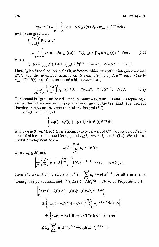
256 M. Cowling et al.

1

F(u,a, 2)= ~ f exp(-iAC~p(,)(tz))Oo(t)v,,~(t)t"-ldtdz, S ~-1 0

and, more generally,

2a(~)aF(u,a,~)

1

= ~ ~ exp(--i)~q~p(~)(tz))[-i2cpp(~)(tz)]"Oo(t)v~,~(t) t"-ldtdz, S n - 1 0

where

(5.2)

vo,~(t)=Up(o)(tz)[l +lVqbp(o)(tz)12] 1/2 VaeS", Vz~S "-1, Vt~I.

Here, 0 o is a fixed function in C~~ as before, which cuts off the integrand outside B(1), and the u-volume element on S near p(a) is v~,~(t)t"-ldtdz. Clearly v,,~Ce-l(I), and for some admissible constant My,

max v~,~(t) <M v Vff f fS n, Vz f fS n-l , gteI. (5.3) o<j<Q ~

The second integral can be written in the same way, with - 2 and - a replacing 2 and ~r; this is the complex conjugate of an integral of the first kind. The theorem therefore hinges on the estimation of the integral (5.2).

Consider the integral

1

S exp(--iAf(t))[--if(t)]av(t)Oo(t) t~-ldt, 0

wherefis in ~- (m, M, q, Q), v is a nonnegative-real-valued C ~ - 1.function on/ , (5.3) is satisfied ifv is substituted for v .... and 2>__20, where 2 0 is as in (1.4). We take the Taylor development of v -

Q - 2

v(t )= ~,, ajtJ+R(t), where lakl < My and j=o

~ . ( d ) J R ( t ) < ( Q ; 1 ) M j Q-x-j Vt~I, Vj~NQ_x.

Q - 2

Then v +, given by the rule that v+(t)= ~ ajtJ+MJ ~ for all t in L is a j=O

nonnegative polynomial, and v § (t) < v (t) + 2 M v t o - 1. Now, by Proposition 2.1,

i exp ( i 2 f ( t ) ) [- if(t)]av(t)Oo(t ) t n 1 dt

ol 0-2 ajt"+ J- l Oo( t)dt < S exp ( - i2f(t)) [- if(t)] ~ j=O

+ i exp(-i2f(t))[-if(t)]"R(t)t"-lO~

Q - 2

<<-CA ~ lajl2-a#j+n+CAMv2-a# Q+n-', j = 0

Damping oscillatory integrals 257

where p = Inv ( f ) (1/2). Applying Lemma 1.2(c),

Q-2 y~ [ajl/#+"+g~/~ Q+"-t <C ~ v+(t)t"-l dt

j=O 0

=C v(t)t"-Xdt-t Q + n - 1 J

<=C v(t) t"- tdt+2 q ,

since f (#) > C# q by Lemma 1.5. We estimate (5.2) by using the above inequalities:

~ 2 - a c A c I Inv(r v~,,(t) t"-ldtdz S n-I 0

Q+n-1 " } - 2 - a c A c I 2 q dT.

sn 1

< C a 2 - " V u,a, +2 []

Proof of Theorem 5.2. In light of Theorem 5.1, it is sufficient to show that if

VOc, o', h) = j" tcd, u, {paS:p.~r< p(a).a+ h}

then V(x, a, h) < Ch "/z ,

for some C independent of a in S" and h in R +. (The condition A q + n < Q - 2 implies that 2A + n < 2 Q - 2 , which in turn implies that the contribution of the

( d ) a ~ i s O ( 2 - " - " / 2 ) ; s i m i l a r l y t h e c o n d i t i o n E-term from Theorem 5.1 to ~ (x#) (2a) Q+n-1

nq < 2 (Q + n - 1) implies that the 2 q term in the estimate for F(x, a, 2) may be neglected).

The idea of this (with slightly different technical details) is sketched in Cowling and Disney [2]. The Gauss map from S to the sphere S" maps the cap C(a, h), defined in (5.1), onto a region of the sphere whose volume is exactly V(K, a, h). As in the previous section, for small values of h, we realise the part of S near p (a) as the graph of the function q~v(,), henceforth written simply as ~b,, defined on the tangent plane, and then, for small values of h, the cap C(a, h) is just

2 5 8 M . C o w l i n g e t al .

-i v o(4) and the point (~b~(4), 4) on S corresponds to (I +IVq~(4)12) ~' (I +IV~(~)Iz)~//

under the Gauss map. As (~b~(~), 4) varies over C(a, h), the corresponding point on S" lies inside the spherical cap {(-]i/I- Ixl z, x):xE R", [xl __<R(h)} where

{ 'Vr : <p~(~)__<h} R(h )=max (1 +IV~(~)I2) *

By Lemma 3.1, IVck~(~)?<C%(~) where C' is admissible, so for small h, R(h) < (C 'h )L This implies that the measure of the spherical cap is at most Ch "/2, as required. []

Proof o f Theorem 5.3. In light of Theorem 5.1, and the comments in parenthesis at the beginning of the proof of Theorem 5.2, it suffices to show that, if q < Q - 2 and

V(u, a, h) = S u @ , {pe s: p . o < p(a) .o + h}

then for some C independent of a in S" and h in R +,

V(u, a, h) < Ch n/2 .

We shall actually show that V(K '/2, ~, h) < Ch "/2 ,

which certainly suffices. By definition, if h is small enough (h < 2 0, with 2 0 as in (1.5)),

V(K 1/2, a, h) = ~ ~c~/2(4) (i + IVe~(~)12)l/2d4, {~B(1) :~a (~) < h}

= S (det HqS~(~))'/2 (1 +IV@~(4)I 2)-"/~d~

< S (det Hdp~(~))l/Zd4 ; {~EB(I ): ~br =< h}

here ~b~ and ~:~ denote ~b,<,) and s:p(~) respectively. Now {4 s B(1): ~b,(~)< h} is convex, so Proposition 4.4 implies that, for some

admissible constant C,

V ( K 1/2, a , h ) < Cmax {qS.(~) : ~6B(1), q5o(~) <h} "/2 = C h "/2 . []

6. Examples

In this section we give examples which indicate how our results are best possible and exhibit some of the difficulties associated with the nonconvex case.

Example 1. Let S in R "+1 be the algebraic hypersurface defined by the equation

4 2 . . . + x 2 = 1 . Xo + Xl +

The Gaussian curvature of this hypersurface is approximately 3x~0 , and

+ 1

00/2p)^(2,0 . . . . . 0 )= S ei~qt[h(t) dt , - i

Damping oscillatory integrals 259

where h is smoo th except at + 1, where it vanishes like (1 - I t l ) "/~, and h(0)4: 0. The singulari ty of x ~/2 a round the " e q u a t o r " x o = 0 forces this F o u r i e r t r ans fo rm to decay as IAt-2; this decay is slower than IAl-~/2 i fn is at least 5. I f n > 7, no measure (x~#), with ct less than one, has op t imal Four i e r t ransform decay.

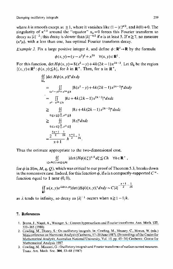
Example 2. Fix a large posi t ive integer k, and define q~ : R 2 ~ R by the fo rmula

~9(x,y):(y--x2)2d-x2k V ( x , y ) ~ R 2 .

F o r this function, detHc~(x,y)=8(x 2 - y ) + 4 k ( 2 k - 1)X 2k-2. Let O h be the region {(x,y)~RE:c~(x,y)<h}, for h in R +. Then, for 0t in R +,

~S Idet H~b(x,y)l=dxdy Oh

= ~ 18(x 2 - y ) + 4 k ( 2 k - 1)x2k-2l~dxdy (x2 -- y)2 + x 2 k <=h

= ~ 18z+4k(2k- l)x2k-El~dxdz z2 -t- x 2 k <= h

~ h k ~ h 0 = z =[/~2h-,x 2 =~-

> ~ 18zl~dxdz 0__<z=<l~,x~__<~

5~t+l 1 2 2 2k a + l q 1

- - - h 2 2k

~ + 1

18 z + 4k (2k - 1)x2k- 2l~ dxdz

Thus the es t imate app rop r i a t e to the two-d imens iona l case,

SS [det(n(9)(~){ 1/2d~<fh V h ~ R + , {~B(1):,~(~)_-< h}

for ~b in S(m, M, q, Q), which was crit ical to our p r o o f o f Theorem 5.3, breaks down in the nonconvex case. Indeed, for this funct ion ~b, i fu is a compac t ly - suppor t ed C 0% funct ion equal to 1 near (0, 0),

~t+l 1

~ u(x,y)ei~O~x,Y)ldet(H(o)(x,y)l,dxdy~Cl21 2 2k

II2

as 2 tends to infinity, so decay as 12[ -1 occurs when ~t> 1 - 1/k.

7. References

1. Bruna, J., Nagel, A., Wainger, S. : Convex hypersurfaces and Fourier transforms. Ann. Math. 127, 333-365 (1988)

2. Cowling, M., Disney, S. : On oscillatory integrals. In �9 Cowling, M., Meaney, C., Moran, W. (eds.) Miniconference on Harmonic Analysis (Canberra, 17-20 June 1987). (Proceedings of the Centre for Mathematical Analysis, Australian National University, Vol. 15, pp. 45-54) Canberra: Centre for Mathematical Analysis 1987

3. Cowling, M., Mauceri, G. : Oscillatory integrals and Fourier transforms of surface carried measures. Trans. Am. Math. Soc. 304, 53-68 (1987)

260 M. Cowling et al.

4. Herz, C.S.: Fourier transforms related to convex sets. Ann. Math. 75, 81-92 (1962) 5. Hlawka, E.: Uber Integrale auf konvexen K6rper. I. Monatsh. Math. 54, 1-36 (1950) 6. H6rmander, L. : The Analysis of Linear Partial Differential Operators, Volume I. Berlin Heidelberg

New York: Springer 1983 7. Jeanquartier, P. : D6veloppement asymptotique de la distribution de Dirac. C.R. Acad. Sci. Paris

271, 1159-1161 (1970) 8. John, F.: Extremum problems with inequalities as subsidiary conditions. In: Friedrichs, K.O.,

Neugebauer, O.E., Stoker, J.J. (eds.) Studies and Essays Presented to Richard Courant on his Sixtieth Birthday, January 8, 1948 (pp. 187-204) New York: Interscience 1948

9. Leichtweil3, K.: (Jber die affine Exzentrizit~it konvexer K6rper. Arch. Math. 10, 187-199 (1959) 10. Littman, W.: Fourier transforms of surface carried measures and differentiability of surface

averages. Bull. Am. Math. Soc. 69, 766-770 (1963) 11. Malgrange, B. : Int6grales asymptotiques et monodromie. Ann. Sci. Ec. Norm. Super. 7, 405-430

(1974) 12. Randol, B.: On the asymptotic behaviour of the Fourier transform of the indicator function of a

convex set. Trans. Am. Math. Soc. 139, 279-285 (1969) 13. Sogge, C.D., Stein, E.M.: Averages of functions over hypersurfaces in R". Invent. Math. 82,

543-556 (1985) 14. Stein, E.M.: Oscillatory integrals in Fourier analysis. In: Stein, E.M. (eds.) Beijing Lectures in

Harmonic Analysis. (Ann. Math. Stud. 112, pp. 307-355) Princeton, N.J. : Princeton University 1986

15. Svensson, I. : Estimates for the Fourier transform of the characteristic function of a convex set. Ark. Mat. 9, 11-22 (1971)

16. Var~enko, A.N. : Newton polyhedra and estimation of oscillating integrals. Funct. Anal. Appl. 10, 175-196 (1976)

Oblatum 13-IV-1989 & 5-VII-1989