multiple integrals unit iv

Engineering Mathematics - I Semester – 1 By Dr N V Nagendram

UNIT – IV Multiple Integrals and Its Applications

4.1 Introduction

4.2 Curve tracing

4.3 Procedure for tracing Cartesian curves

4.4 Procedure for tracing curves in parametric form x = f(t) and y = (t)

4.5 Procedure for tracing Polar curves

4.6 Areas of Cartesian curves

4.7 Areas of Polar curves

4.8 Lengths of curves

4.9 Volumes of Revolution by Double Integrals

4.10 Volumes of Revolution by Triple Integrals

4.11 Volumes of solids


UNIT – IV Introduction Class 1

In discussing the graph of xn for negative integral values of n, it was

explained how the curve approaches the axes of co-ordinates asymptotically.

We shall now consider the method of finding the asymptotes to a curve.

In many practical applications of integration, a knowledge about the shapes

of given equations is desirable. On drawing a sketch of the given equation,

we can easily study the behaviour of the curve as regards its symmetry,

asymptotes, the number of branches passing through a point etc.

4.1.1 Definition: Asymptote. A straight line which cuts a curve in two

points at an infinite distance from the origin, but which is not itself wholly

at infinity, is called an asymptote to a curve.

4.1.2 Method of finding asymptotes: Let f(x, y) = 0 ................ (1) be

a rational algebraic curve of degree n and let y = mx + c .................(2) be

the equation of any straight line.

Eliminating y between (1) and (2) we obtain f ( x, mx + c) = 0 .................. (3)

Whose roots are the abscissa of the points of intersection of the curve (1)

and the straight line (2).

Now let the equation (3) be expanded and expressed in descending powers of

x as A0 xn + A1 xn-1 + A2 xn-2 + ............ + An = 0 ................................ (4)

Where A0, A1, ........... etc., are functions of m and c.

Since the constants m and c of the straight line are at our choice. Let us

choose m and c to satisfy the equations A0 = 0, and A1 = 0 obtained by

equating to zero the co-efficients of the two highest powers of x in the

equation (4).

For these values, it is clear that two roots of the equation (4) becomes

infinite, i.e., two points of intersection of the line (2) and the curve (1) are at

an infinite distance from the origin, so that y = mx + c is an asymptote.

Hence, solving the equations A0 = 0 and A1 = 0 for m and c and substituting

their values in the equation y = mx + c we obtain the asymptotes.

It will be found that a curve of the nth degree does not possess more than n

asymptotes.

The method given above does not give the asymptotes parallel to the y – axis,

since they are of the form x = k and are not included in the form y = mx + c

for any finite m. the following method may therefore be adopted for finding

the asymptotes parallel to the axes.

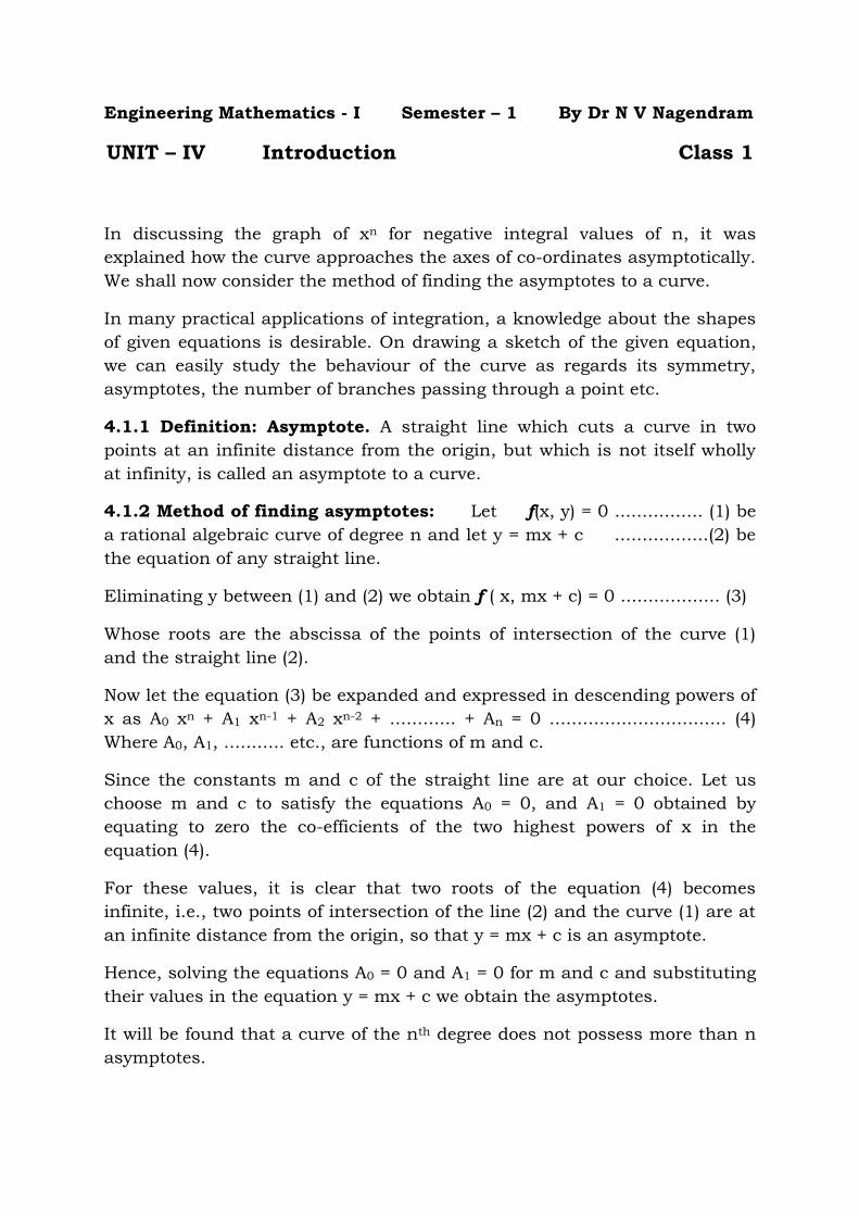
4.1.3 Definition: Double Point: A point through which two branches of a

curve pass is called a double point. At such point P, the curve has two

tangents, one for each branch.

P

P

Figure

4.1.4 Definition: Node. If the tangents are real and distinct, the double

point is called a node.

4.1.5 Definition: Cusp. If the tangents are real and coincident, the double

point is called a cusp.

4.1.6 Definition: Conjugate/isolated. If the tangents are imaginary, the

double point is called conjugate point or isolated point. Such a point can not

be shown in figurative expression.

4.2 Curve Tracing - Asymptotes parallel to the axes.

4.2.1 To find the asymptotes parallel to the x – axis.

Arrange the equation in descending powers of x and equate to zero the co-

efficients of the highest powers of x. Then two roots of the given equation is

as an equation in x become infinite. Hence for the value of y so obtained say

a, the equation y = a is an asymptote parallel to the x – axis.

4.2.2 To find the asymptotes parallel to the y – axis.

Arrange the equation in descending powers of y and equate to zero the co-

efficients of the two highest powers of y and solve the resulting equation for

x, then for the value of of x so obtained, the equation straight line x = is

an asymptote parallel to the y – axis.


UNIT – IV Class 2

4.3 procedure for tracing Cartesian curves.

4.3.1 Symmetry. (i) A curve is symmetrical about the x – axis, if only even

powers of y occur in its equation.

Example: y2 = 4ax is symmetrical about x – axis.

(ii) A curve is symmetrical about the y – axis, if only even powers of x occur

in its equation.

Example: x2 = 4ay is symmetrical about y – axis.

(iii) A curve is symmetrical about the line y = x, if on interchanging x and y

its equation remains unchanged.

Example: x3 + y3 = 3axy is symmetrical about the line y = x.

4.3.2 Origin. (i) see if the curve passes through the origin. A curve passes

through the origin if there is no constant term in its equation.

(ii) if it does, find the equation of the tangents thereat, by equating to zero

the lowest degree terms.

(iii) if the origin is a double point, find whether the origin is a node, cusp or

conjugate point.

4.3.3 Asymptotes. (i) see if the curve has any asymptote parallel to the axes

(ii) then find the inclined asymptotes.

4.3.4 Points. (i) Find the points where the curve crosses the axes and the

asymptotes.

(ii) find the points where the tangent is parallel or perpendicular to the x -

axis that is the points where ordx

dy0 .

(iii) Find the origin or regions in which no portion of the curve exists.

4.3.5 Some important curves.

Certain curves are of great importance in several branches of applied

mathematics. It is therefore desirable that the student should be familiar

with them. Besides the graphs of some elementary functions already

illustrated in the text, the student must be familiar with the conic sections.

The equations and the forms of a few curves are given below:

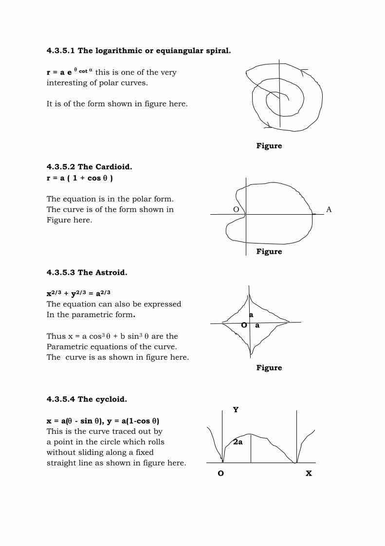
4.3.5.1 The logarithmic or equiangular spiral.

r = a e cot this is one of the very

interesting of polar curves.

It is of the form shown in figure here.

Figure

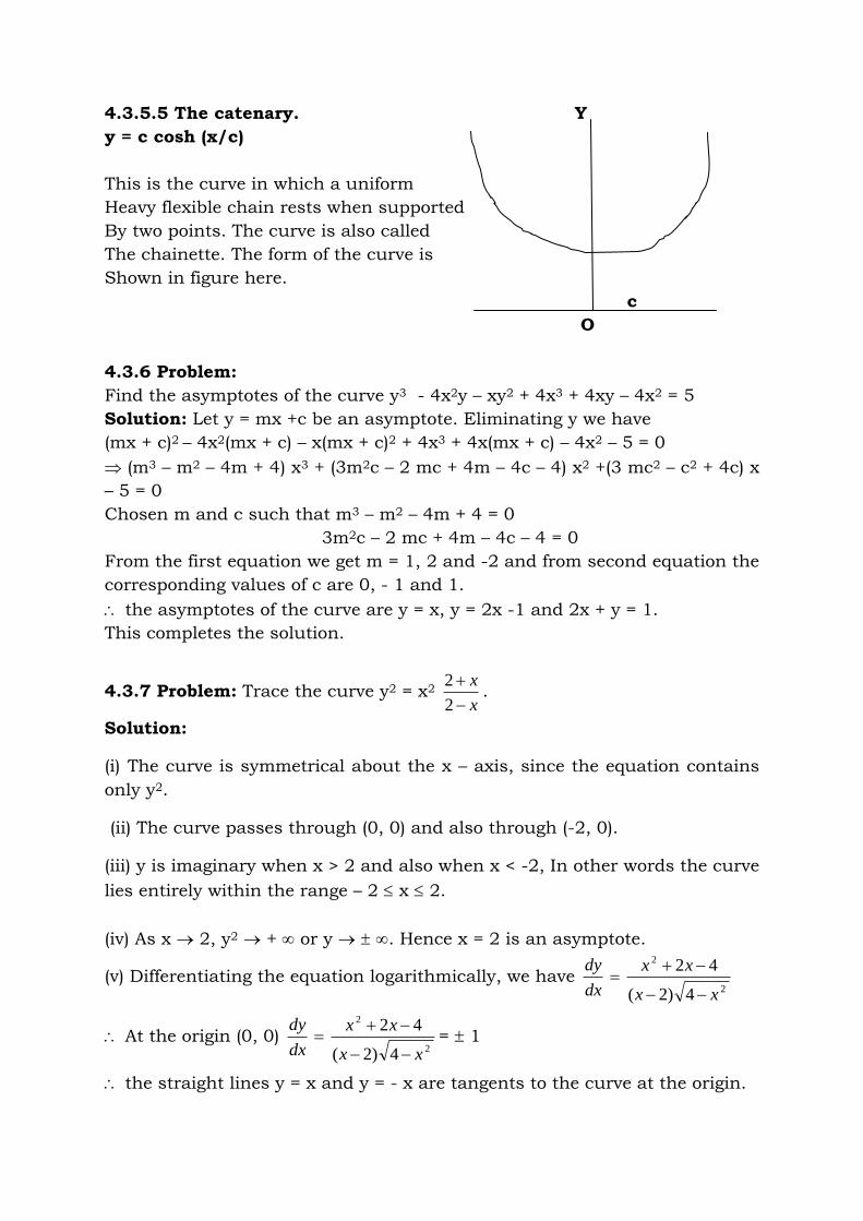
4.3.5.2 The Cardioid.

r = a ( 1 + cos )

The equation is in the polar form.

The curve is of the form shown in O A

Figure here.

Figure

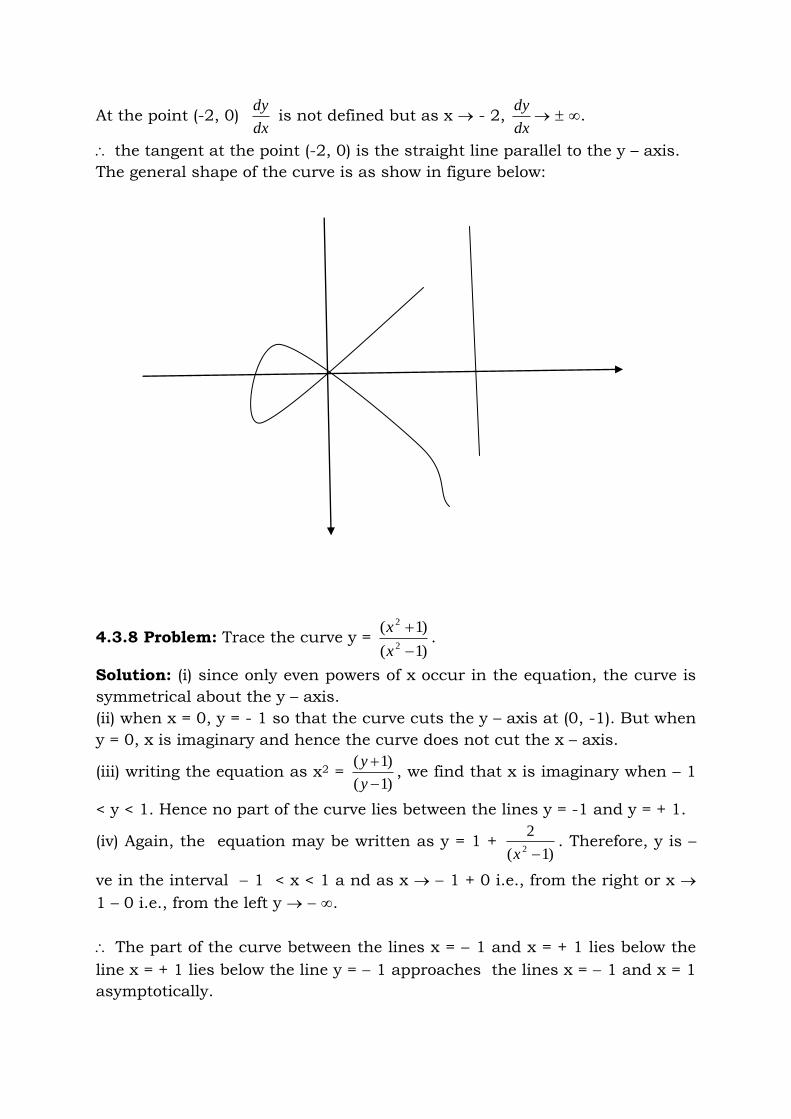
4.3.5.3 The Astroid.

x2/3 + y2/3 = a2/3

The equation can also be expressed

In the parametric form. a

O a

Thus x = a cos3 + b sin3 are the

Parametric equations of the curve.

The curve is as shown in figure here.

Figure

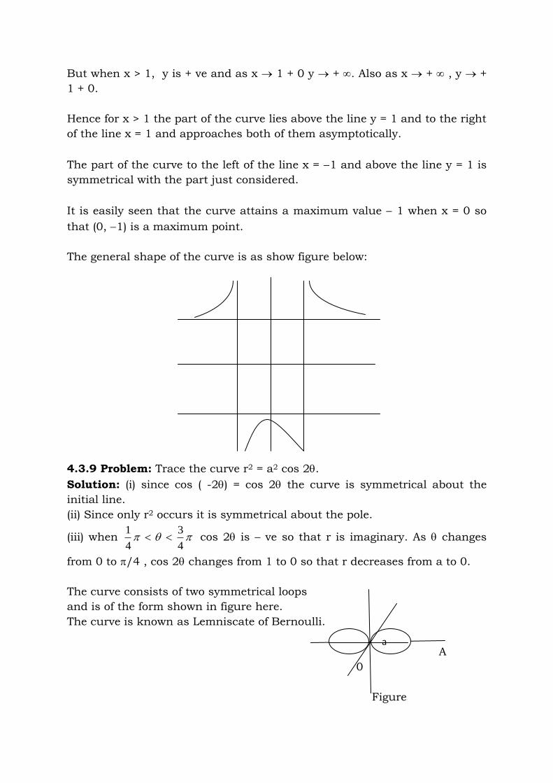
4.3.5.4 The cycloid.

Y

x = a( - sin ), y = a(1-cos )

This is the curve traced out by

a point in the circle which rolls 2a

without sliding along a fixed

straight line as shown in figure here.

O X

4.3.5.5 The catenary. Y

y = c cosh (x/c)

This is the curve in which a uniform

Heavy flexible chain rests when supported

By two points. The curve is also called

The chainette. The form of the curve is

Shown in figure here.

c

O

4.3.6 Problem:

Find the asymptotes of the curve y3 - 4x2y – xy2 + 4x3 + 4xy – 4x2 = 5

Solution: Let y = mx +c be an asymptote. Eliminating y we have

(mx + c)2 – 4x2(mx + c) – x(mx + c)2 + 4x3 + 4x(mx + c) – 4x2 – 5 = 0

(m3 – m2 – 4m + 4) x3 + (3m2c – 2 mc + 4m – 4c – 4) x2 +(3 mc2 – c2 + 4c) x

– 5 = 0

Chosen m and c such that m3 – m2 – 4m + 4 = 0

3m2c – 2 mc + 4m – 4c – 4 = 0

From the first equation we get m = 1, 2 and -2 and from second equation the

corresponding values of c are 0, - 1 and 1.

the asymptotes of the curve are y = x, y = 2x -1 and 2x + y = 1.

This completes the solution.

4.3.7 Problem: Trace the curve y2 = x2 x

x

2

2.

Solution:

(i) The curve is symmetrical about the x – axis, since the equation contains

only y2.

(ii) The curve passes through (0, 0) and also through (-2, 0).

(iii) y is imaginary when x > 2 and also when x < -2, In other words the curve

lies entirely within the range – 2 x 2.

(iv) As x 2, y2 + or y . Hence x = 2 is an asymptote.

(v) Differentiating the equation logarithmically, we have 2

2

4)2(

42

xx

xx

dx

dy

At the origin (0, 0) 2

2

4)2(

42

xx

xx

dx

dy

= 1

the straight lines y = x and y = - x are tangents to the curve at the origin.

At the point (-2, 0) dx

dy is not defined but as x - 2,

dx

dy .

the tangent at the point (-2, 0) is the straight line parallel to the y – axis.

The general shape of the curve is as show in figure below:

4.3.8 Problem: Trace the curve y = )1(

)1(2

2

x

x.

Solution: (i) since only even powers of x occur in the equation, the curve is

symmetrical about the y – axis.

(ii) when x = 0, y = - 1 so that the curve cuts the y – axis at (0, -1). But when

y = 0, x is imaginary and hence the curve does not cut the x – axis.

(iii) writing the equation as x2 = )1(

)1(

y

y, we find that x is imaginary when – 1

< y < 1. Hence no part of the curve lies between the lines y = -1 and y = + 1.

(iv) Again, the equation may be written as y = 1 + )1(

22 x

. Therefore, y is –

ve in the interval 1 < x < 1 a nd as x 1 + 0 i.e., from the right or x

1 – 0 i.e., from the left y .

The part of the curve between the lines x = 1 and x = + 1 lies below the

line x = + 1 lies below the line y = 1 approaches the lines x = 1 and x = 1

asymptotically.

But when x > 1, y is + ve and as x 1 + 0 y + . Also as x + , y +

1 + 0.

Hence for x > 1 the part of the curve lies above the line y = 1 and to the right

of the line x = 1 and approaches both of them asymptotically.

The part of the curve to the left of the line x = 1 and above the line y = 1 is

symmetrical with the part just considered.

It is easily seen that the curve attains a maximum value 1 when x = 0 so

that (0, 1) is a maximum point.

The general shape of the curve is as show figure below:

4.3.9 Problem: Trace the curve r2 = a2 cos 2.

Solution: (i) since cos ( -2) = cos 2 the curve is symmetrical about the

initial line.

(ii) Since only r2 occurs it is symmetrical about the pole.

(iii) when 4

3

4

1 cos 2 is – ve so that r is imaginary. As changes

from 0 to /4 , cos 2 changes from 1 to 0 so that r decreases from a to 0.

The curve consists of two symmetrical loops

and is of the form shown in figure here.

The curve is known as Lemniscate of Bernoulli.

A

0

Figure

a

Exercises By Dr N V Nagendram

4.3.10 Problem:

Find the asymptotes of the 2x2 + 3 x2y – 3xy2 – 2 y3 + 3x2 – 3y2 + y – 3.

4.3.11 Problem:

Find the asymptotes of the x3 + 2x2y – xy2 – 2y3 + xy – y2 = 1.

4.3.12 Problem: Find the asymptotes of the curve which are parallel to

either axes x3 + 3xy2 + y2 + 2x + y = 0.

4.3.13 Problem: Find the asymptotes of the curve which are parallel to

either axes x2y3 + x3y2 = x3 + y3.

4.3.14 Problem: Trace the curve ay2 = x2(x – a).

4.3.15 Problem: Trace the curve a4 y2 = x5(2a – x).

4.3.16 Problem: Trace the curve y2 = (x – 2)2 (x – 5).

4.3.17 Problem: Trace the curve (x2 – 1)y2 = x.

4.3.18 Problem: show that the curve (a2 + x2) y = a2x has three points of

inflexion. Trace the curve.

4.3.19 Problem: Trace the curve r = a cos 3.

4.3.20 Problem: Trace the curve y = )( 22

3

xa

a

4.3.21 Problem: Give a rough sketch of the curve y = e5-2x.


UNIT – IV Class 3

4.4 Procedure for tracing curves in parametric form x = f(t) and y = (t).

4.4.1 Symmetry. (i) A curve is symmetrical about the x – axis, if on

replacing t by – t , f(t) remains unchanged and (t) changes to – (t).

(ii) A curve is symmetrical about the y – axis, if on replacing t by – t , f(t)

changes to – f (t) and (t) remains unchanged.

(iii) A curve is symmetrical in the opposite quadrants, if on if on replacing t

by – t , both f(t) and (t) remains unchanged.

4.4.2 Limits. Find the greatest and least values of x and y so as to

determine the strips, parallel to the axes, within or outside which the curves

lies.

4.4.3 Points. (i) Determine the points where the curve crosses the axes. The

points of intersection of the curve with the x – axis are given by the roots of

(t) = 0, while those with the y – axis are given by the roots f (t) = 0.

(ii) Giving t a series of values, plot the corresponding values of x and y,

noting whether x and y increase or decrease for the intermediate values of t.

For this purpose, we consider the signs of dt

dyand

dt

dxfor different values of t.

(iii) Determine the points where the tangent is parallel or perpendicular to

the x – axis that is where ordx

dy0 .

(iv) when x and y are periodic functions of t with a common period, we need

study the curve only for one period, because the other values of t will repeat

the same curve over and over again.

4.4.4 Remark. Sometimes it is convenient to eliminate t between the given

equations and use the resulting Cartesian equation to the curve.

4.4.5 Problem: Trace the curve x = a cos3 t, y = a Sin3 t.

4.4.6 Problem: Trace the curve x = a ( + Sin ), y = a(1 + Cos ).


UNIT – IV Class 4

4.5 Procedure for tracing Polar curves.

4.5.1 Symmetry. See if the curve is symmetrical about any line.

(i) A curve is symmetrical about initial line OX, if only Cos or Sec occur

in its equation. That is it remains unchanged when is changed to – .

Example: r = a (1 + Cos ) is symmetrical about the initial line.

(ii) A curve is symmetrical about the line through the pole to the initial line

OY, if only sin or cosec occur in its equation that is it remains

unchanged when is changed to .

Example: r = a Sin 3 is symmetrical about OY.

(iii) A curve is symmetrical about the pole, if only even powers of r occur in

the equation that is it remains unchanged when r is changed to – r.

Example: r2 = a2 Cos 2 is symmetrical about the pole.

4.5.2 Limits. See if r and are confirmed between certain limits.

(i) Determine the numerically greatest value of r, so as to notice whether the

curve lies within a circle or not.

Example: r = a Sin 3 lies wholly within the circle r = a.

(ii) Determine the region in which no portion of the curve lies by finding

those values of for which r is imaginary.

Example: r2 = a2 Cos 2 does not lie between the lines = /4 and = 3/4.

4.5.3 Asymptotes. If the curve possesses an infinite branch, find the

asymptotes.

4.5.4 Points. (i) Giving successive values to find the corresponding values

of r.

(ii) Determine the points where the tangent coincides with the radius vector

or its perpendicular to it that is the points where tan = r dr

d = 0 or

4.5.5 Problem: Trace the curve r = a Sin 3.

4.5.6 Problem: Trace the curve r2 = a2 Cos 2.


UNIT – IV Class 5

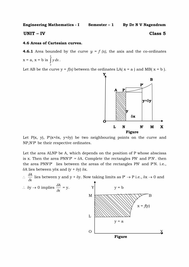
4.6 Areas of Cartesian curves.

4.6.1 Area bounded by the curve y = f (x), the axis and the co-ordinates

x = a, x = b is b

a

dxy .

Let AB be the curve y = f(x) between the ordinates LA( x = a ) and MB( x = b ).

Y

B

P

A P

y+y

y

x

O

L N N M X

Figure

Let P(x, y), P(x+x, y+y) be two neighbouring points on the curve and

NP,NP be their respective ordinates.

Let the area ALNP be A, which depends on the position of P whose abscissa

is x. Then the area PNNP = A. Complete the rectangles PN and PN. then

the area PNNP lies between the areas of the rectangles PN and PN. i.e.,

A lies between yx and (y + y) x.

x

A

lies between y and y + y. Now taking limits as P P i.e., x 0 and

y 0 implies x

A

= y. Y y = b

M B

x = f(y)

L

y = a

O X

Figure

Integrating both sides between the limits x = a , x = b, we have

b

aA =

b

a

dxy

or [ value of A for x = b ] = [value of A for x = a] = b

a

dxy .

Thus area ALMB = b

a

dxy .

4.6.2 Definition: Quadrature. The area bounded by a curve, the x-axis and

two ordinates is called the area under the curve. The process of finding the

area of plane curves is often called quadrature.

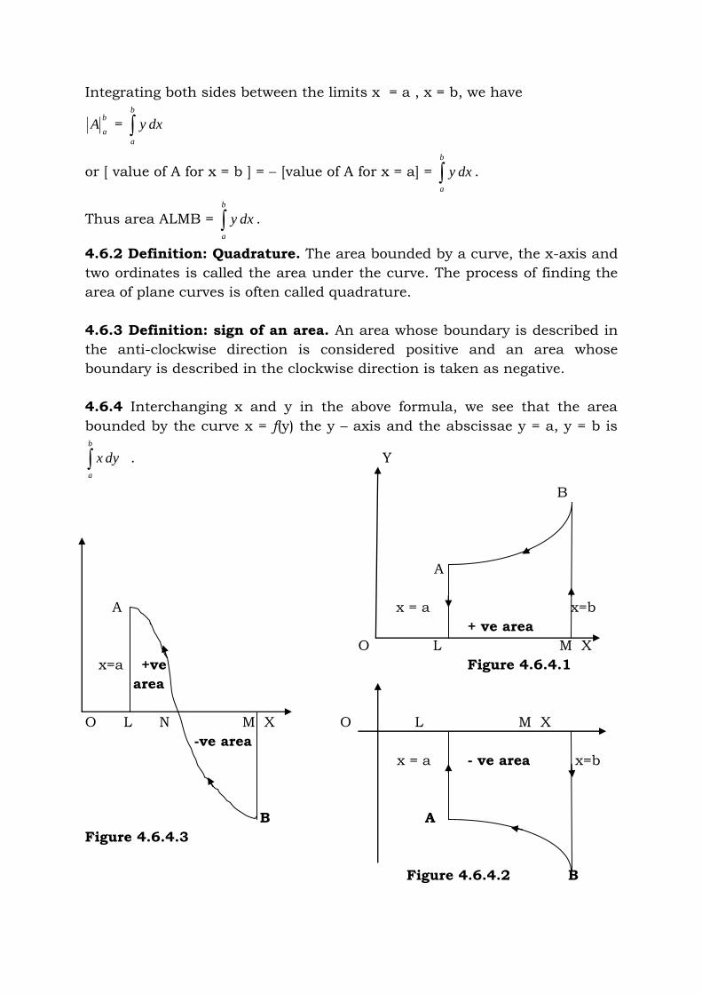
4.6.3 Definition: sign of an area. An area whose boundary is described in

the anti-clockwise direction is considered positive and an area whose

boundary is described in the clockwise direction is taken as negative.

4.6.4 Interchanging x and y in the above formula, we see that the area

bounded by the curve x = f(y) the y – axis and the abscissae y = a, y = b is

b

a

dyx . Y

B

A

A x = a x=b

+ ve area

O L M X

x=a +ve Figure 4.6.4.1

area

O L N M X O L M X

-ve area

x = a - ve area x=b

B A

Figure 4.6.4.3

Figure 4.6.4.2 B

In Figure 4.6.4.1 the area ALMB = b

a

dxy which is described in the

anticlockwise direction and lies above the x-axis, will give a positive result.


a

dxy which is described in the

anticlockwise direction and lies below the x-axis, will give a negative result.


a

dxy will not consist of the sum of the

area ALN = c

a

dxy and the area NMB = b

c

dxy but their difference.

4.6.3 Example: Find the area of the loop of the curve ay2 = x2 (a – x)

4.6.4 Example: Find the area included the curve between y2 (2a – x = x3 and

its asymptote.

4.6.5 Example: Find the area enclosed by the curve a2x2 = y3(2a – y).

4.6.6 Example: Find the area enclosed between one arch of the cycloid

x = a( - sin ), y = a(1 – Cos ) and its base.

4.6.7 Example: Find the area of the segment cut off from the parabola

x2 = 8y by the line x – 2y + 8 = 0.

4.6.8 Example: Find the area common to the parabola y2 ax and the circle

x2 + y2 = 4ax.


UNIT – IV Class 6

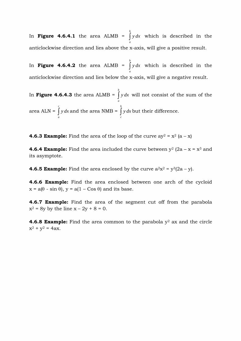
4.7 Areas of Polar curves.

Area bounded by the curve r = f() and the radii vectors = , = is

dr 2

2

1.

Let AB be the curve r = f() between the radii vectors OA ( = ) and

OB ( = ). Let P(r, ), P (r+r, +) be any two neighbouring points on the

curve.

B

P

= Q Q

r P

A

O X

Let the area OAP = A which is a function of . Then the area OPP = A. Mark

circular arcs PQ and PQ with centre O and radii OP and OP.

Evidently area OPP lies between the sectors OPQ and OPQ i.e., A lies

between 2

2

1r and 2)(

2

1rr .

A lies between 2

2

1r and 2)(

2

1rr .

Now taking limits as 0 r 0,

A = 2

2

1r .

Integrating both sides from = to = , we get

A =

2

1

dr 2

or [ value of A for = ] – [ value of A for = ] =

dr 2

1 2

Hence the required area OAB =

dr 2

1 2 .

4.7.1 Example: Find the area of the cardioids r = a ( 1 - Cos ).

4.7.2 Example: Find the area of a loop of the curve r = a Sin 3.

4.7.3 Example: Prove that the area of a loop of the curve x3 + y3 = 3axy is

3a2/2.

4.7.4 Example: Find the area common to the circles r = a2, r = 2a Cos .


UNIT – IV Class 7

4.8 Lengths of curves

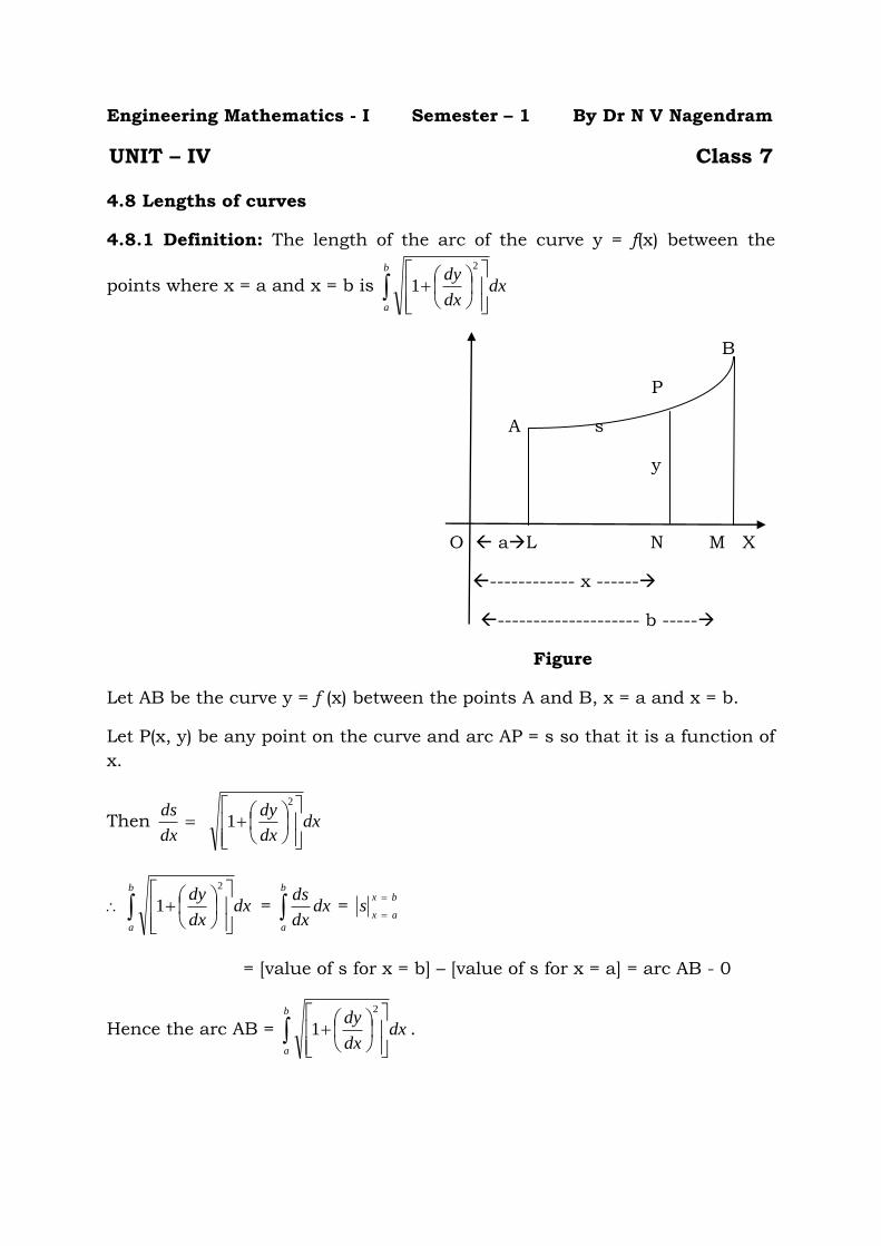
4.8.1 Definition: The length of the arc of the curve y = f(x) between the

points where x = a and x = b is

b

a

dxdx

dy2

1

B

P

A s

y

O aL N M X

------------ x ------

-------------------- b -----

Figure

Let AB be the curve y = f (x) between the points A and B, x = a and x = b.

Let P(x, y) be any point on the curve and arc AP = s so that it is a function of

x.

Then dx

dsdx

dx

dy

2

1

b

a

dxdx

dy2

1 = b

a

dxdx

ds=

bx

axs

= [value of s for x = b] – [value of s for x = a] = arc AB - 0

Hence the arc AB =

b

a

dxdx

dy2

1 .

4.8.2 Definition: The length of the arc of the curve x = f(y) between the

points where y = a and y = b is

b

a

dydy

dx2

1 .

4.8.3 Definition: The length of the arc of the curve x = f (t), y = (t) between

the points where t = a and t = b is

b

a

dtdt

dy

dt

dx22

.

4.8.4 Definition: The length of the arc of the curve r = f () between the

points where = and = is

dd

rdr

2

2 .

4.8.5 Definition: The length of the arc of the curve = f (r) between the

points where r = a and r = b is

rd

rd

dr

2

1 .

4.8.6 Example: Find the length of the arc of the parabola x2 = 4ay

measured from the vertex to one extremity of the latus - rectum.

4.8.7 Example: Find the perimeter of the of the loop of the curve

3ay2 = x( x – a )2.

4.8.8 Example: Prove that the length of one arc of the cycloid

x = a ( 1 – Sin t), y = a ( 1 – Cos t).

4.8.9 Example: Find the the entire length of the cardioids r = a(1+ Cos ).


UNIT – IV Class 8

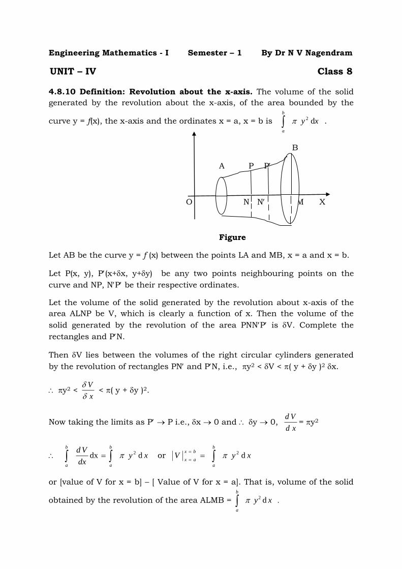
4.8.10 Definition: Revolution about the x-axis. The volume of the solid

generated by the revolution about the x-axis, of the area bounded by the

curve y = f(x), the x-axis and the ordinates x = a, x = b is b

a

xy d 2 .

B

A P P

O N N M X

Figure

Let AB be the curve y = f (x) between the points LA and MB, x = a and x = b.

Let P(x, y), P(x+x, y+y) be any two points neighbouring points on the

curve and NP, NP be their respective ordinates.

Let the volume of the solid generated by the revolution about x-axis of the

area ALNP be V, which is clearly a function of x. Then the volume of the

solid generated by the revolution of the area PNNP is V. Complete the

rectangles and PN.

Then V lies between the volumes of the right circular cylinders generated

by the revolution of rectangles PN and PN, i.e., y2 < V < ( y + y )2 x.

y2 < x

V

< ( y + y )2.

Now taking the limits as P P i.e., x 0 and y 0, xd

Vd= y2

b

a

b

a

xydx

Vd d dx 2 or

b

a

bx

axxyV d 2

or [value of V for x = b] – [ Value of V for x = a]. That is, volume of the solid

obtained by the revolution of the area ALMB = b

a

xy d 2 .

4.8.11 Definition: Revolution about the y-axis. Interchanging x and y in

the above formula we see that the volume of the solid generated by the

revolution, about y-axis, of the area, bounded by the curve x = f(y) the y-axis

and the abscissae y = a, y = b is b

a

yx d 2 .

4.8.12 Definition: Revolution about any axis. The volume of solid

generated by the revolution about any axis LM of the area bounded by the

curve AB, the axis LM and the perpendiculars AL, BM on the axis is

OM

OL

ONPN )(d)( 2 where O is fixed point in LM and PN is perpendicular from

any point P of the curve AB on LM.

With O as the origin, take OLM as the x-axis and OY perpendicular to it as

the y-axis.

Let the co-ordinates of P be (x, y) so that x = ON, y = NP. If OL = a, OM = b

then the required volume = b

a

y x d 2 = OM

OL

ONPN )(d)( 2 .

4.8.13 Example: Find the volume of a sphere of radius a.

4.8.14 Example: Find the volume formed by the revolution of loop of the

curve y2 (a + x) = x2 (3a – x ) about the x-axis.

4.8.15 Example: Prove that the volume of the reel formed by the revolution

of the cycloid x = a( + Sin ), y = a (1 – Cos ) about the tangent at the

vertex is 2a3.

4.8.16 Example: Find the volume of the reel – shaped solid formed by the

revolution about the y – axis, of the part of the parabola y2 = 4ax cut off by

the latus – rectum.

4.8.17 Example: Find the volume of the solid obtained by revolving the

cissoids y2 (2a – x) = x3 above its asymptote.


UNIT – IV Class 9

4.9 Volumes of Revolution by Double Integrals

4.9.1 Double integrals:

The definite integral b

a

dxxf )( is defined as the limit of the sum f(x1) x1 + f(x2)

x2 + f(x1) x1 +............ + f(xn) xn , where n and each of the lengths x1,

x2,......., xn tends to zero. A double integral is its counterpart in two

dimensions.

Consider a function f(x, y) of the independent variables x, y defined at each

point in the finite region R of the xy – plane. Divide R into n elementary

areas A1, A2, A3,......, An. Let (xr, yr) be any point within the r th

elementary area Ar consider the sum

f(x1, y1), A1 + f(x2, y2), A2 + ................... + f(xn, yn), An i.e.,

n

r

rrr Ayxf1

),( .

The limit of this sum, if it exists, as the number of sub-divisions increases

indefinitely and area of each sub-division decreases to zero, is defined as the

double integral of f(x, y) over the region R and is written as R

dAyxf ),( .

Thus R

dAyxf ),( = Lim

n

r

rrr

An

AyxfLim10

),(

........................................ (1)

The utility of double integral would be limited if it were required to take limit

of sums to evaluate them. However, there is another method of evaluating

double integrals by successive single integrations.

For purposes of evaluation, (1) is expressed as the repeated integral

2

1

2

1

),(

x

x

y

y

dydxyxf .

(i) when y1, y2 are functions of x and x1, x2 are constants , f(x,y) is first

integrated w.r.t. y and keeping x as fixed limits y1, y2 and then resulting

expression is integrated w.r.t. x within the limits x1, x2 i.e.,

I

I1 = 2

1

x

x

2

1

),(

y

y

dyyxfdx

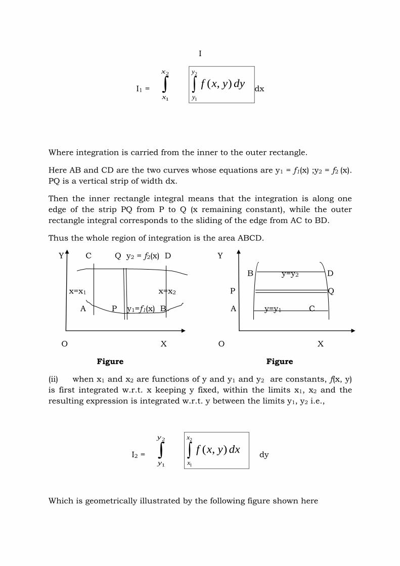
Where integration is carried from the inner to the outer rectangle.

Here AB and CD are the two curves whose equations are y1 = f1(x) ;y2 = f2 (x).

PQ is a vertical strip of width dx.

Then the inner rectangle integral means that the integration is along one

edge of the strip PQ from P to Q (x remaining constant), while the outer

rectangle integral corresponds to the sliding of the edge from AC to BD.

Thus the whole region of integration is the area ABCD.

Y C Q y2 = f2(x) D Y

B y=y2 D

x=x1 x=x2 P Q

A P y1=f1(x) B A y=y1 C

O X O X

Figure Figure

(ii) when x1 and x2 are functions of y and y1 and y2 are constants, f(x, y)

is first integrated w.r.t. x keeping y fixed, within the limits x1, x2 and the

resulting expression is integrated w.r.t. y between the limits y1, y2 i.e.,

I2 = 2

1

y

y

2

1

),(

x

x

dxyxf dy

Which is geometrically illustrated by the following figure shown here

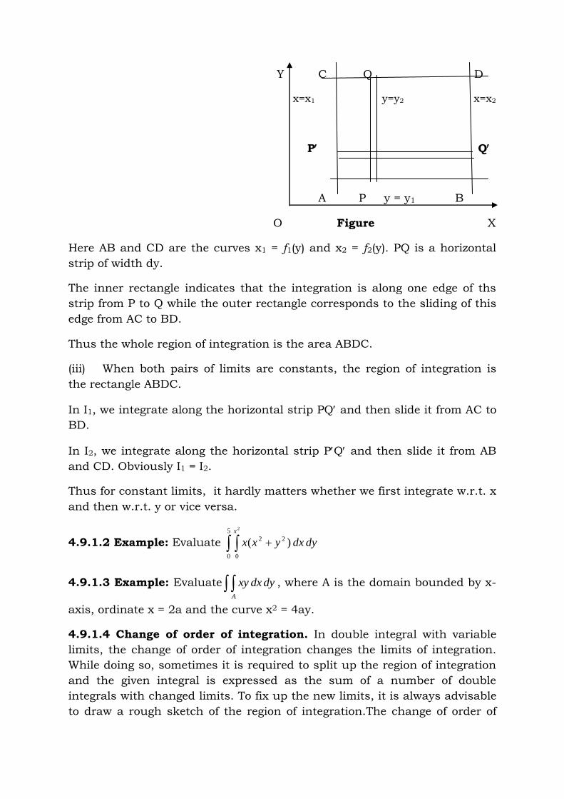
Y C Q D

x=x1 y=y2 x=x2

P Q

A P y = y1 B

O Figure X

Here AB and CD are the curves x1 = f1(y) and x2 = f2(y). PQ is a horizontal

strip of width dy.

The inner rectangle indicates that the integration is along one edge of ths

strip from P to Q while the outer rectangle corresponds to the sliding of this

edge from AC to BD.

Thus the whole region of integration is the area ABDC.

(iii) When both pairs of limits are constants, the region of integration is

the rectangle ABDC.

In I1, we integrate along the horizontal strip PQ and then slide it from AC to

BD.

In I2, we integrate along the horizontal strip PQ and then slide it from AB

and CD. Obviously I1 = I2.

Thus for constant limits, it hardly matters whether we first integrate w.r.t. x

and then w.r.t. y or vice versa.

4.9.1.2 Example: Evaluate

5

0 0

22

2

)(

x

dydxyxx

4.9.1.3 Example: Evaluate A

dydxxy , where A is the domain bounded by x-

axis, ordinate x = 2a and the curve x2 = 4ay.

4.9.1.4 Change of order of integration. In double integral with variable

limits, the change of order of integration changes the limits of integration.

While doing so, sometimes it is required to split up the region of integration

and the given integral is expressed as the sum of a number of double

integrals with changed limits. To fix up the new limits, it is always advisable

to draw a rough sketch of the region of integration.The change of order of

integration quite often facilities the evaluation of a double integral. The

following examples will make these ideas clear.

4.9.1.5 Example: Change the order of integration in the integral

I =

a

a

ya

dydxyxf

22

0

),( .

4.9.1.6 Example: Change the order of integration in the integral

I = 1

0

2

2

x

x

dydxxy .

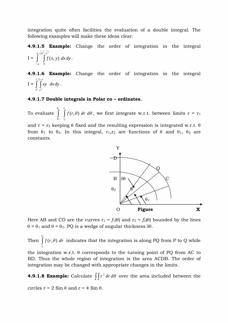
4.9.1.7 Double integrals in Polar co – ordinates.

To evaluate 2

1

2

1

),(

r

r

ddrrf , we first integrate w.r.t. between limits r = r1

and r = r2 keeping fixed and the resulting expression is integrated w.r.t.

from 1 to 2. In this integral, r1,r2 are functions of and 1, 2 are

constants.

Y

D

Q

B C

2

1

O Figure X

Here AB and CD are the curves r1 = f1() and r2 = f2() bounded by the lines

= 1 and = 2. PQ is a wedge of angular thickness .

Then 2

1

),(

r

r

drrf indicates that the integration is along PQ from P to Q while

the integration w.r.t. corresponds to the turning point of PQ from AC to

BD. Thus the whole region of integration is the area ACDB. The order of

integration may be changed with appropriate changes in the limits.

4.9.1.8 Example: Calculate ddrr 3 over the area included between the

circles r = 2 Sin and r = 4 Sin .

EXERCISES:

4.9.1.9 Problem: dydxxy 2

1

3

1

2 ;4.9.1.10 Problem: dydxyx

x

x

2

1

22 )(

4.9.1.11 Problem: dydxe

x

xy

4

0 0

2

)(

4.9.1.12 Problem: dydxyx

x

1

0

1

0

22

2

)(1

1

4.9.1.13 Problem: dydxxy over the +ve quadrant of the circle x2 + y2 = a2

4.9.1.14 Problem: dydxyx

2

)( over the area bounded by the ellipse

x2 /a2+ y2 /b2= 1.

4.9.1.15 Problem: dydxyxxy )( over the area between y = x2 and y = x.

Evaluate the following integrals by changing the order of integration:

4.9.1.16 Problem: dydxy

x

1

0

1

0

2

2

; 4.9.1.17 Problem: dydxyx

y

3

0

4

1

)(

4.9.1.18 Problem: dxdy

a x

ax

4

0

1

4/

2

2

; 4.9.1.19 Problem: dydxyxLog

a ya

y

2/

0

22

22

)(

4.9.1.20 Problem: dxdyy

e

x

y

0

; 4.9.1.21 Problem: dxdyex

x

yx

0 0

/2

4.9.1.22 Problem: Sketch the region of integration of

ddrrrf

ea

ar

4/

0

2/

)/(log2

),( and change the order of integration.

4.9.1.23 Problem: Evaluate ddrSinr over the cardioids r = a(1 – Cos

) above the initial line.

4.9.1.24 Problem: Show that 3/2 32 addrSinrR

, where R is the semi-

circle r = 2a Cos above the initial line.

4.9.1.25 Problem: Evaluate dydxra

ddrr

)( 22

over one loop of the

lemniscates r2 = a2 Cos 2.

4.9.2 Area enclosed by plane curves.

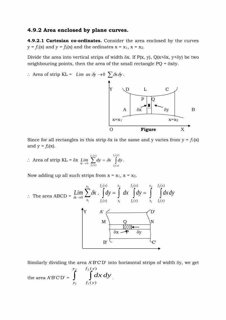
4.9.2.1 Cartesian co-ordinates. Consider the area enclosed by the curves

y = f1(x) and y = f2(x) and the ordinates x = x1, x = x2.

Divide the area into vertical strips of width x. If P(x, y), Q(x+x, y+y) be two

neighbouring points, then the area of the small rectangle PQ = xy.

Area of strip KL = yxyasLim 0 .

Y D L C

P Q

A x y B

x=x1 x=x2

O Figure X

Since for all rectangles in this strip x is the same and y varies from y = f1(x)

and y = f2(x).

Area of strip KL = x

)(

)(

)(

)(0

2

1

2

1

xf

xf

xf

xfy

dyxdyLim

.

Now adding up all such strips from x = x1, x = x2.

The area ABCD =

)(

)(

)(

)(

)(

)(0

2

1

2

1

2

1

2

1

2

1

2

1

.

xf

xf

x

x

xf

xf

x

x

xf

xf

x

xx

dydxdydxdyxLim

Y A D

M Q N

x P y

B C

Similarly dividing the area ABCD into horizontal strips of width y, we get

the area ABCD = )(

)(

2

1

2

1

yf

yf

y

y

dydx.

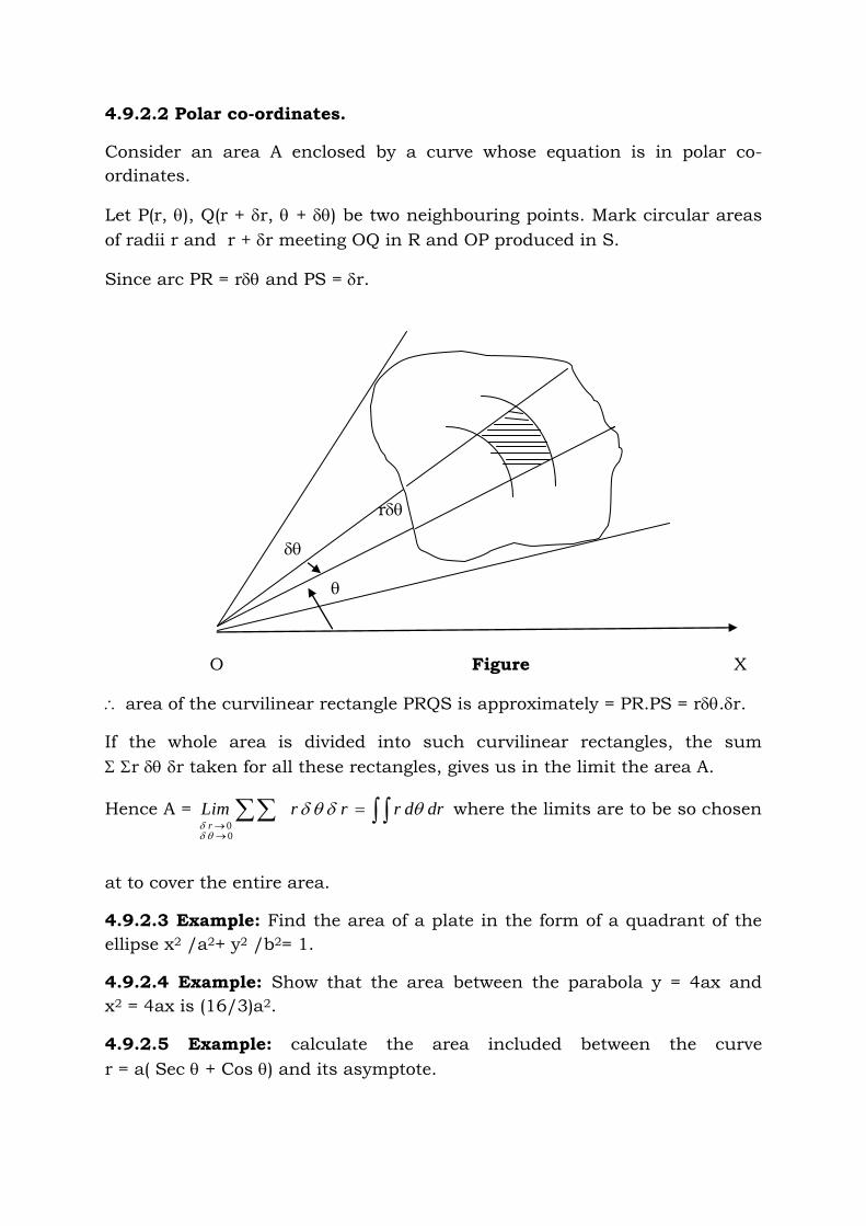
4.9.2.2 Polar co-ordinates.

Consider an area A enclosed by a curve whose equation is in polar co-

ordinates.

Let P(r, ), Q(r + r, + ) be two neighbouring points. Mark circular areas

of radii r and r + r meeting OQ in R and OP produced in S.

Since arc PR = r and PS = r.

Q

r

O Figure X

area of the curvilinear rectangle PRQS is approximately = PR.PS = r.r.

If the whole area is divided into such curvilinear rectangles, the sum

r r taken for all these rectangles, gives us in the limit the area A.

Hence A =

drdrrrLimr

00

where the limits are to be so chosen

at to cover the entire area.

4.9.2.3 Example: Find the area of a plate in the form of a quadrant of the

ellipse x2 /a2+ y2 /b2= 1.

4.9.2.4 Example: Show that the area between the parabola y = 4ax and

x2 = 4ax is (16/3)a2.

4.9.2.5 Example: calculate the area included between the curve

r = a( Sec + Cos ) and its asymptote.


UNIT – IV Class 10

4.10 Volumes of Revolution by Triple Integrals

4.10.1 Triple integrals. Consider a function f(x, y, z) defined at every point

of the 3 – dimensional finite region V. Divide V into n elementary volumes

V1, V2, .........., Vn.

Let (xr, yr, zr) be any point within the r th sub-division Vr. Consider the sum

n

r

rrrr Vzyxf1

),,( .

The limit of this sum, if it exists, as n and Vr 0 is called the triple

integral of function f(x, y, z) over the region V and is denoted by

dVzyxf ),,( .

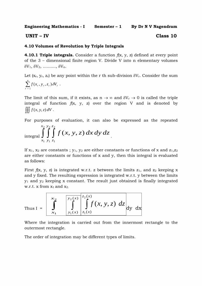
For purposes of evaluation, it can also be expressed as the repeated

integral 2

1

2

1

2

1

),,(

x

x

y

y

z

z

dzdydxzyxf.

If x1, x2 are constants ; y1, y2 are either constants or functions of x and z1,z2

are either constants or functions of x and y, then this integral is evaluated

as follows:

First f(x, y, z) is integrated w.r.t. z between the limits z1, and z2 keeping x

and y fixed. The resulting expression is integrated w.r.t. y between the limits

y1 and y2 keeping x constant. The result just obtained is finally integrated

w.r.t. x from x1 and x2.

Thus I = 2

1

x

x

)(

)(

2

1

xy

xy

)(

)(

2

1

),,(

xz

xz

dzzyxfdy dx

Where the integration is carried out from the innermost rectangle to the

outermost rectangle.

The order of integration may be different types of limits.

4.10.2 Example. Evaluate 1

0

1

0

1

0

2 22x yx

dzdydxxyz .

Solution. We have I = dxdydzzyx

yxx

222 1

0

1

0

1

0

= dxdyz

yx

yxx

22 1

0

21

0

1

02

= dxdyyxyx

x

)1(2

1 22

1

0

1

0

2

= 2

1dx

yyxx

x21

0

422

1

042

)1(

= 8

1 dxxxxxx .)1(2.)1( 4222

1

0

= 8

1 dxxxx

1

0

53 )2(

= 8

11

0

642

64

2

2

xxx =

8

1

48

1

6

1

2

1

2

1

Hence the solution.

4.10.3 Example. Evaluate

1

1 0

)(

z zx

zx

dzdydxzyx .

Solution. On integration w.r.t. y keeping x and z constant, we have

I = dzzz

xzxz

dzdxxzzzxdzdxyzy

xy

zzz zx

zx

1

1 0

22

2

0

1

10

21

122

242

12)(

2

= 04

423

2

1

1

41

1

33

3

z

dzz

zz

. Hence the solution.

Evaluate the following problems:

4.10.4 Problem: dzdydxyzx 1

0

2

0

2

1

2 [Ans. 1]

4.10.5 Problem: dzdydxzyx

c

c

b

b

a

a

)( 222 [Ans. )223(9

8 223 acabbca ]

4.10.6 Problem: dzdxdy

z xz

4

0

2

0

4

1

2

[Ans. 8]

4.10.7 Problem: dzdydxe

a x yx

zyx

0 0 0

[Ans. 8

3

4

3

8

1 24 aaa eee ]

4.10.8 Problem: dydxdzzLog

e yLog ex

1 1 1

[Ans. )138(2

1 2 ee ]

4.10.9 Problem:

ddrdzr

a a

ra

2

0

sin

0 0

22

[Ans.64

5 3a]

Try Ur Self ...


UNIT – IV Class 11

4.11 Volumes of Solids.

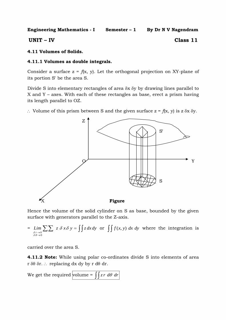
4.11.1 Volumes as double integrals.

Consider a surface z = f(x, y). Let the orthogonal projection on XY-plane of

its portion S be the area S.

Divide S into elementary rectangles of area x y by drawing lines parallel to

X and Y – axes. With each of these rectangles as base, erect a prism having

its length parallel to OZ.

Volume of this prism between S and the given surface z = f(x, y) is z x y.

Z

S S

O Y

S

X Figure

Hence the volume of the solid cylinder on S as base, bounded by the given

surface with generators parallel to the Z-axis.

=

dydxzyxzLimr

00

or dydxyxf ),( where the integration is

carried over the area S.

4.11.2 Note: While using polar co-ordinates divide S into elements of area

r r. replacing dx dy by r d dr.

We get the required volume = drdrz

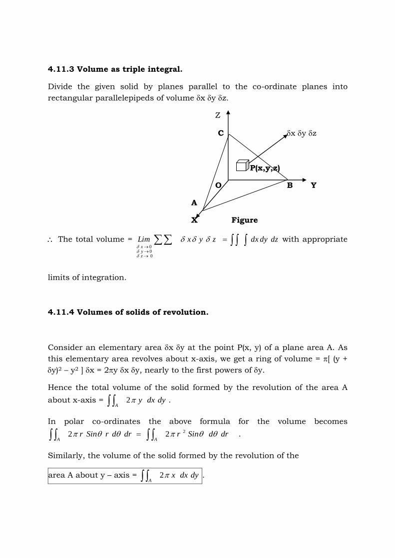
4.11.3 Volume as triple integral.

Divide the given solid by planes parallel to the co-ordinate planes into

rectangular parallelepipeds of volume x y z.

Z

C x y z

P(x,y,z)

O B Y

A

X Figure

The total volume = dzdydxzyxLim

zyx

000

with appropriate

limits of integration.

4.11.4 Volumes of solids of revolution.

Consider an elementary area x y at the point P(x, y) of a plane area A. As

this elementary area revolves about x-axis, we get a ring of volume = [ (y +

y)2 – y2 ] x = 2y x y, nearly to the first powers of y.

Hence the total volume of the solid formed by the revolution of the area A

about x-axis = A dydxy2 .

In polar co-ordinates the above formula for the volume becomes

AA

drdSinrdrdrSinr 222 .

Similarly, the volume of the solid formed by the revolution of the

area A about y – axis = A dydxx2 .

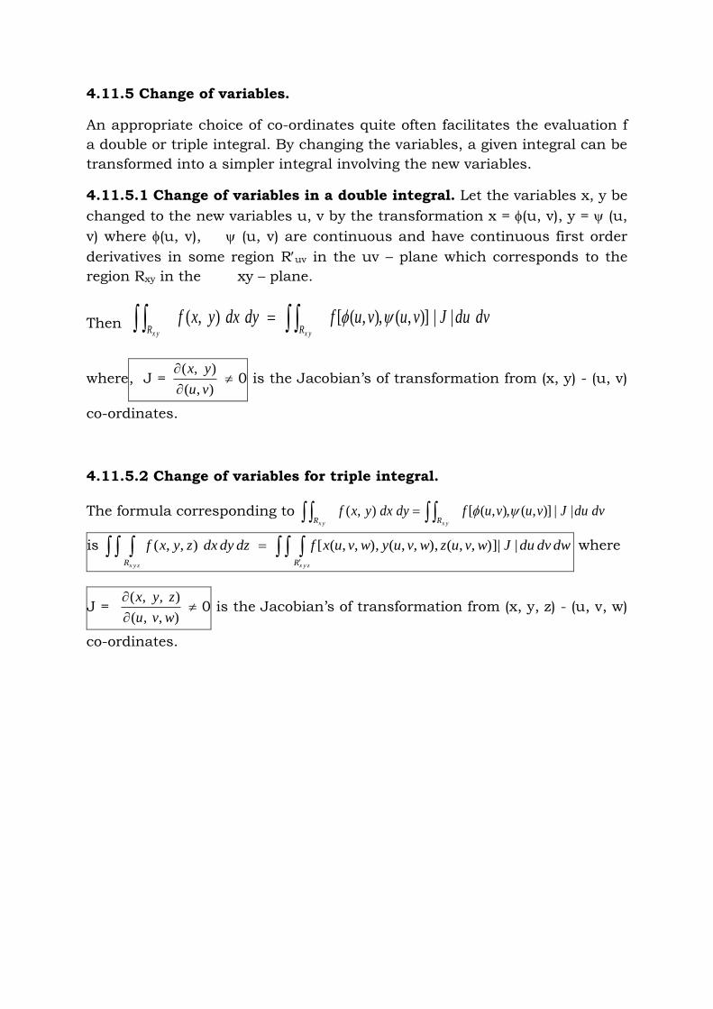
4.11.5 Change of variables.

An appropriate choice of co-ordinates quite often facilitates the evaluation f

a double or triple integral. By changing the variables, a given integral can be

transformed into a simpler integral involving the new variables.

4.11.5.1 Change of variables in a double integral. Let the variables x, y be

changed to the new variables u, v by the transformation x = (u, v), y = (u,

v) where (u, v), (u, v) are continuous and have continuous first order

derivatives in some region Ruv in the uv – plane which corresponds to the

region Rxy in the xy – plane.

Then yxyx RR

dvduJvuvufdydxyxf ||)],(),,([),(

where, J = ),(

),(

vu

yx

0 is the Jacobian’s of transformation from (x, y) - (u, v)

co-ordinates.

4.11.5.2 Change of variables for triple integral.

The formula corresponding to yxyx RR

dvduJvuvufdydxyxf ||)],(),,([),(

is

zyx zyxR R

dwdvduJwvuzwvuywvuxfdzdydxzyxf ||)],,(),,,(),,,([),,( where

J = ),,(

),,(

wvu

zyx

0 is the Jacobian’s of transformation from (x, y, z) - (u, v, w)

co-ordinates.

multiple integrals unit iv

Documents