ELECTROHYDRODYNAMICS OF THREE-DIMENSIONALVESICLES: A NUMERICAL APPROACH ‡

EBRAHIM M. KOLAHDOUZ∗ AND DAVID SALAC∗†

Abstract.A three-dimensional numerical model of vesicle electrohydrodynamics in the presence of DC

electric fields is presented. The vesicle membrane is modeled as a thin capacitive interface throughthe use of a semi-implicit, gradient-augmented level set Jet scheme. The enclosed volume andsurface area are conserved both locally and globally by a new Navier-Stokes projection method. Theelectric field calculations explicitly take into account the capacitive interface by an implicit ImmersedInterface Method formulation, which calculates the electric potential field and the trans-membranepotential simultaneously. The results match well with previously published experimental, analyticand two-dimensional computational works.

Key words. Vesicle, Stokes flow, Level set, Continuous surface force, Numerical method

1. Introduction. Giant liposome vesicles are enclosed bag-like membranes com-posed of lipid bilayers. These vesicles share many similarities in composition and sizewith other biological cells such as red blood cells. Experimental observations havedemonstrated that lipid vesicles exhibit a striking resemblance to more complicatedbiological cells in terms of their equilibrium shapes and dynamic behavior in variousfluid conditions [1, 2]. These make liposome vesicles a robust model system to studythe behavior of more complicated non-nucleated biological cells.

It is also quite easy to artificially create these soft particles in a laboratory setting;in an aqueous solution lipid molecules will self-assemble into two-dimensional sheets,which then fold and curve in three-dimensional space and form a fluid-filled vesicle[3]. The ease of liposome vesicle formation, in addition to their bio-compatibility, hasled to vesicles being proposed as building blocks for various biotechnologies such asdirected drug and gene delivery [4, 5] or biological microreaction [6, 7].

Vesicles interacting with external flows have been of major recent interest. Threewell-known types of vesicle dynamics in shear flow are tank-treading, tumbling and atransient state called trembling or vacillating breathing. These behaviors have beenextensively studied in theory [8, 9, 10, 11, 12] and experiments [13, 14, 15]. Sev-eral numerical simulations of vesicle dynamics have also appeared in the literature.Among the numerical studies in two dimensions are models using the boundary inte-gral method [16, 17], the phase field [18, 19, 20], a coupled level set and projectionmethod [21, 22], a coupled level set and finite-element method [23, 24] and the latticeBoltzmann method [25]. A few three-dimensional studies have been also reportedusing the phase-field approach [26], boundary integral method [27, 28, 29] and front-tracking [30]. Studies have shown the dynamics of the vesicle depends on three majorparameters: the viscosity ratio between the enclosed and surrounding fluids, the shearrate and the reduced-volume, which is defined as the ratio of the volume of the vesicleto the volume of a sphere with the same surface area as the vesicle.

The use of electric fields, in combination with fluid flow, has been proposed as apowerful method to direct the behavior of vesicles towards a wide range of biotechno-logical applications. Weak electric fields have found applications in cell manipulationtechniques such as electrofusion [31], tissue ablation [32], wound healing [33], and in

∗University at Buffalo, Department of Mechanical and Aerospace Engineering, Buffalo, NY, 14260†Corresponding Author davidsal@buffalo.edu‡This work supported by NSF Grant #1253739

1

arX

iv:1

409.

6381

v1 [

cond

-mat

.sof

t] 2

3 Se

p 20

14

the treatment of tumors [34]. Strong electric fields induce electro-poration in vesiclesthrough the formation of transient pores in the membrane and could play a role innovel biotechnological advances such as the delivery of drugs and DNA into livingcells [35, 36].

Recent experiments have reported on the topological behavior of vesicles subjectedto either a DC or AC electric field with different intensity, frequency and durationof exposure to the field [37, 38, 39, 40]. Experiments show that depending on theconductivity and permittivity differences between the enclosed and surrounding flu-ids the vesicle undergoes various shape transformations, such as prolate (major-axisaligned with the electric field) to oblate (major axes are perpendicular to the field).One very interesting phenomena in this context is the dynamics of an initial prolatevesicle in a strong DC field with a small enclosed fluid conductivity as compared tothe conductivity of the surrounding fluid. It is theoretically expected that as timeprogresses the vesicle transitions to an oblate shape first, then evolves back into theprolate shape. During such transition nearly cylindrical shapes with high-curvatureedges were observed for a vesicle subjected to strong pulses [38]. This behavior wasattributed to the presence of salt in the solution and not due to the membrane char-acteristics. However in [41] the poration of the vesicle membrane was proposed as thepossible explanation for both vesicle collapse and cylindrical deformations.

In addition to recent experimental works, theoretical models have also investi-gated the electrohydrodynamics of nearly-spherical vesicles. Leading-order perturba-tion analysis has been employed to obtain reduced models in the form of ordinarydifferential equations [42, 43, 44, 45]. In another work a spheroidal shell model hasbeen used to investigate the morphological change of the vesicle in AC electric field[46].

Despite numerous theoretical investigations, numerical studies of the vesicle elec-trohydrodynamics are rare. In a recent work, a boundary integral method was em-ployed to study different equilibrium states of a two-dimensional vesicle in the presenceof a uniform DC electric field [47]. A Prolate-Oblate-Prolate (POP) transition wascaptured for a vesicle with an inner-fluid conductivity smaller than the surroundingregion.

Currently, there is still a gap between the morphological changes observed inexperiments, what theoretical models predict, and methods to control this behav-ior. This gap needs to be addressed before vesicles can form a building block forelectrohydrodynamic based microfluidic systems and technologies. Part of the diffi-culty arises from modeling the complex physics of the vesicle electrohydrodynamicsand challenging phenomena such as membrane poration or fusion. Compared to hy-drodynamics investigations, the electrohydrodynamics of the vesicle has substantiallyfaster dynamics with much larger deformations which makes the numerical modelingnontrivial. Hence a lack of thorough numerical investigation with different materialproperties and electric field parameters still remains.

In a previous work by the authors the Immersed Interface Method (IIM) wasutilized to solve for both the electric potential and trans-membrane potential arounda vesicle in three dimensions [48]. The jump conditions for potential and its first andsecond derivatives on the interface were determined and utilized to obtain accurateelectric potential solutions for a three-dimensional vesicle with an arbitrary shape.In this paper the electric field model presented in this recent work is combined witha projection-based hydrodynamics solver and a semi-implicit jet scheme for captur-ing the interface. This model is used to study the electrohydrodynamics of three

2

dimensional vesicles in general flow. The dynamics of the vesicle is determined by theinterplay between the hydrodynamics, bending, tension and electric field stresses onthe membrane. This is one of the first attempts at investigating the electrohydrody-namics of vesicles in three-dimensions. As one may expect, for this kind of physicsa three dimensional model will result in a much richer and wider range of topolog-ical changes. The differences compared to a two dimensional model will be subtleand important at the same time. In addition to this, a full Navier-Stokes systemof equations is considered here unlike all the previous models which investigate theproblem in the Stokes region. For vesicles in strong DC field, the approximate velocitymay sometimes exceed 0.01 m/s [41], resulting in non-trivial Reynolds numbers, andtherefore, the Stokes assumption for the fluid flow might not always hold. Moreover,the method presented here allows for studying deflected vesicles with smaller reducedvolumes than what theoretical models normally address and is able to predict thetype of deformations observed in experiments.

The remainder of this paper is organized as follows. In Section 2 the physicalsystem and formulation behind the electrohydrodynamics of the vesicle are described.In Section 3 the numerical algorithm is presented. This will be followed by samplenumerical results in Section 4. Final remarks and possible future work then follow.

2. Theory and formulation. Let a three-dimensional vesicle of encapsulatedvolume V have a surface area of A. Deviation from a perfect sphere is measuredby a reduced volume parameter, v, defined as the ratio of the vesicle volume to thevolume of a sphere with the same surface area: v = 3V/(4πa3) where a =

√A/4π

is the characteristic length scale. The typical size of the vesicle is a ≈ 10 − 20 µmwhile the thickness of the bilayer membrane is d ≈ 5 nm [49]. Due to the three-ordersof magnitude difference between the vesicle size and the membrane thickness themembrane will be treated as an infinitesimally thin interface separating the inner andouter fluids. The vesicle membrane is assumed to be impermeable to fluid moleculesand the number of lipids on the membrane does not change over time, while the surfacedensity of lipids at room temperature is constant [49]. These two conditions resultin an inextensible membrane with constant enclosed volume and global surface area,along with local surface incompressibility. Another important feature of the membraneis its electrical insulating property and impermeability against ionic transfer [40, 42,47]. Therefore, in the presence of an external electric field the membrane acts as acapacitor. This capacitive property is an important factor in studying the dynamicsof vesicles in the presence of electric field.

2.1. Electric Field Equations. A schematic of a vesicle exposed to an externalelectric field is illustrated in Fig. 2.1. Different properties inside (−) and outside (+)of the membrane are shown in the figure. The embedded fluid (Ω−) is separatedfrom the surrounding fluid (Ω+) by the vesicle membrane represented as Γ. Thismembrane is assumed to be made of a charge-free lipid bilayer with uniform andconstant capacitance Cm and conductivity Gm. The vesicle is suspended in a fluidof conductivity s+ and permittivity ε+. The enclosed region is assumed to havea different conductivity s− and permittivity ε−. It is assumed that properties areconstant in each fluid, with a finite jump occurring across the membrane.

The leaky-dielectric model is assumed to hold in the whole domain [50]. Thisresults in no local free charge in the bulk fluids, and thus the electric field (E) isirrotational and given as the negative gradient of the electric potential (Φ)

Ek = −∇Φk, (2.1)

3

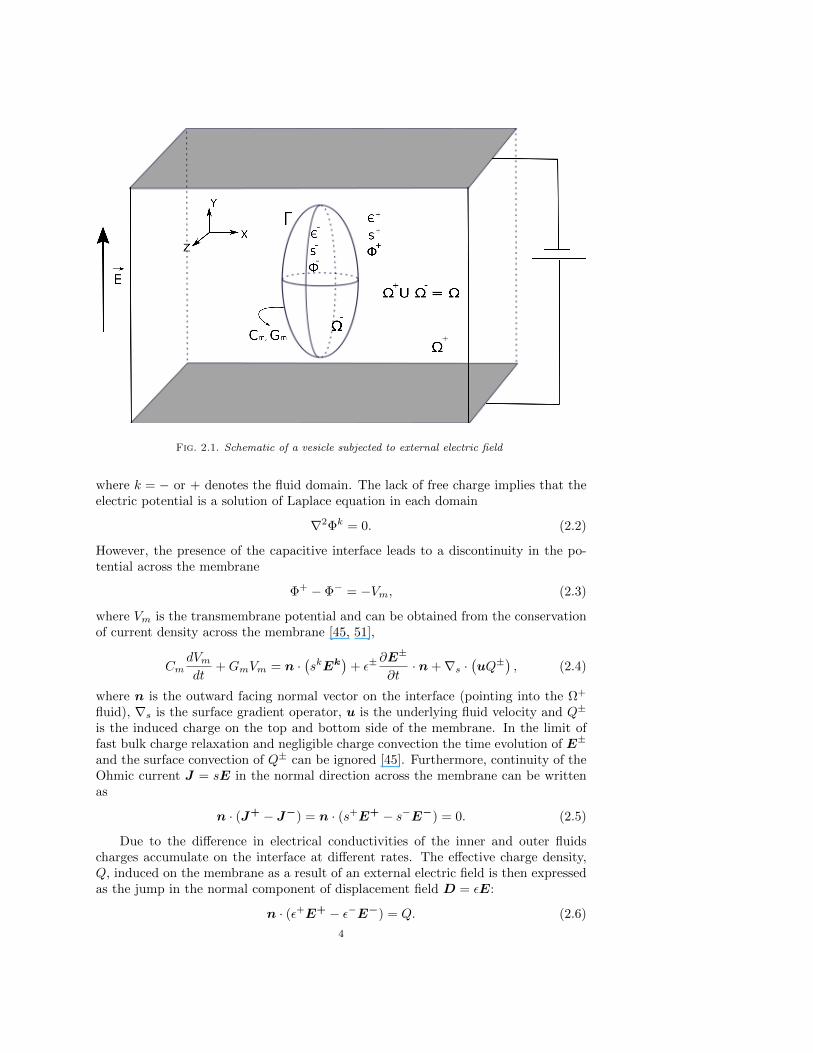
Fig. 2.1. Schematic of a vesicle subjected to external electric field

where k = − or + denotes the fluid domain. The lack of free charge implies that theelectric potential is a solution of Laplace equation in each domain

∇2Φk = 0. (2.2)

However, the presence of the capacitive interface leads to a discontinuity in the po-tential across the membrane

Φ+ − Φ− = −Vm, (2.3)

where Vm is the transmembrane potential and can be obtained from the conservationof current density across the membrane [45, 51],

CmdVmdt

+GmVm = n ·(skEk

)+ ε±

∂E±

∂t· n+∇s ·

(uQ±

), (2.4)

where n is the outward facing normal vector on the interface (pointing into the Ω+

fluid), ∇s is the surface gradient operator, u is the underlying fluid velocity and Q±

is the induced charge on the top and bottom side of the membrane. In the limit offast bulk charge relaxation and negligible charge convection the time evolution of E±

and the surface convection of Q± can be ignored [45]. Furthermore, continuity of theOhmic current J = sE in the normal direction across the membrane can be writtenas

n · (J+ − J−) = n · (s+E+ − s−E−) = 0. (2.5)

Due to the difference in electrical conductivities of the inner and outer fluidscharges accumulate on the interface at different rates. The effective charge density,Q, induced on the membrane as a result of an external electric field is then expressedas the jump in the normal component of displacement field D = εE:

n · (ε+E+ − ε−E−) = Q. (2.6)

4

The electric force τ el acting on the membrane is obtained from the MaxwellTensor T el:

τ el = n · [T el], T el = ε(EE − 1

2(E ·E) I) on Γ, (2.7)

where [ ] in the above relation and through the rest of this paper shows the jumpacross the interface. For an arbitrary quantity f at location xΓ on the interface ajump is mathematically defined as

[f ] = f+ − f− = limδ→0+

f(xΓ + δn)− limδ→0+

f(xΓ − δn). (2.8)

Note that when discussing jumps in quantities at the interface a superscript + or −does not denote a bulk value, but the value as one approaches the interface.

2.2. Fluid Flow Equations. Assume that both bulk fluids are Newtonian andincompressible with a matched density ρ. Consequently they both satisfy the Navier-Stokes equations

ρDu±

Dt= ∇ · T±hd with ∇ · u± = 0 in Ω±, (2.9)

where u is the velocity vector, D/Dt is the material (total) derivative, and T hd is thebulk hydrodynamic stress tensor defined as

T±hd = −p±I + µ±(∇u± +∇Tu±) in Ω±. (2.10)

The fluid flow in each region is coupled via the conditions on the inextensiblemembrane. The velocity is assumed to be continuous on the surface, [u] = 0. However,due to the forces exerted by the membrane the hydrodynamic stress undergoes a jumpacross the interface of the two fluids. This condition is obtained by balancing thehydrodynamic and electric stresses with the bending and in-extension tractions of themembrane,

τhd + τ el = τm + τ γ on Γ, (2.11)

where τhd = n · [T hd] is the normal component of the hydrodynamic stress while τmand τ γ are the bending and tension traction forces, respectively. These two forcestogether constitute the total membrane force per unit area and are calculated bytaking the variational derivative of the total energy of the membrane [8]. For a threedimensional vesicle and neglecting spontaneous curvature the ultimate forms of thebending and tension stresses are found to be [52]

τm = −κc(H3

2− 2HK +∇2

sH)n, τ γ = γHn−∇sγ. (2.12)

In this relation, H = ∇ · n is twice the mean curvature (the total curvature), K =∇ · [n∇ ·n+n× (∇×n)] is the Gaussian curvature, κc is the bending rigidity, κg isthe Gaussian bending rigidity, γ is the tension and ∇s = P∇ where P = (I −n⊗n)is the surface projection operator.

The last condition to consider is the local area incompressibility constraint onthe membrane. This condition is enforced by ensuring that the velocity is surface-divergence free on the membrane:

∇s · u = 0 on Γ. (2.13)

5

Note that the divergence conditions, ∇·u = 0 and ∇s ·u = 0, should be sufficientto conserve both volume and area. However, in practice it is difficult to ensure thatglobal surface area and enclosed volume are sufficiently conserved [20]. Therefore,when developing the numerical method in Sec. 3 global conservation will be explicitlyenforced as well.

2.3. Description of the Interface. The motion of the interface is trackedusing a gradient-augmented level set method. First developed by Osher and Sethian[53] the level set method is based upon an implicit representation of an interfaceas the zero level set of a higher dimensional function. This was later extended toexplicitly include information about the gradients of the level set [54]. The use ofgradient information allows for the accurate determination of the interface locationand curvature information away from grid node locations [54].

Using the same notation for the interface as Fig. 2.1 the level set function φ isdefined as

Γ(t) = x : φ(x, t) = 0 , (2.14)

while the level set gradient field is defined as

ψ = ∇φ. (2.15)

The level set value is chosen to be negative in the Ω− and positive in the Ω+ domain.This representation has the advantages of treating any topological changes naturallywithout complex remehsing, and the ability to calculate geometric quantities from thelevel set function and its derivatives. For example, the unit normal to the surface, n,can be easily computed as

n =ψ

‖ψ‖. (2.16)

The motion of the interface under the flow field u is modeled by a standardadvection equation

∂φ

∂t+ u · ∇φ = 0. (2.17)

The evolution of the gradient field is obtained by taking the gradient of the level setadvection equation,

∂ψ

∂t+ u · ∇ψ +∇u ·ψ = 0. (2.18)

Using the level set function one is able to define the viscosity at any location inthe computational domain, x, with a single relation,

µ(x) = µ− + (µ+ − µ−)H(φ(x)), (2.19)

where H is the Heaviside function. Different forms of the Heaviside approximationshave been proposed [55, 56, 57]. Here an accurate method based on an integralcalculation [58] is used. The Heaviside is defined as

H(φ(x)) =∇=(φ(x)) · ∇φ(x)

‖(∇φ(x))‖2(2.20)

6

where

=(z) =

∫ z

0

H(ζ)dζ and H(ζ) =

0 if ζ < 0

1 if ζ > 0

Similarly the Dirac delta function is expressed as

δ(φ(x)) =∇H(φ(x)) · ∇φ(x)

‖(∇φ(x))‖2(2.21)

These definitions will be used to localize the contributions of interface forces in Navier-Stokes equations.

2.4. Continuum Surface Force Model. The definitions of the Dirac andHeaviside functions in Sec. 2.3 allow for the use of a single equation to describethe dynamics of the fluid over the entire domain [59]. This is accomplished by writingthe singular contributions of the bending, tension, and electric field forces as localizedbody force terms, similar to what has been done for two dimensional vesicles [21, 22].This results in the following single-fluid formulation,

ρDu

Dt=−∇p+∇ ·

(µ(∇u+∇Tu

))+ δ (φ) ‖∇φ‖ (∇sγ − γH∇φ)

+ κcδ(φ)

(H3

2− 2KH +∇2

sH

)∇φ

+ δ(φ)‖∇φ‖[ε

(EE − 1

2(E ·E) I

)]· n,

(2.22)

with

∇ · u = 0 in Ω, (2.23)

∇s · u = 0 on Γ. (2.24)

Note that in this formulation all surface quantities, such as tension or the jump in theMaxwell stress tensor, are calculated on the interface and extended such that theyare constant in the direction normal to the interface.

2.5. Dimensionless Parameters. When an electric field is applied to the sys-tem charges from the bulk fluids migrate towards the interface. The time scale asso-ciated with this migration process is given by the bulk charge relaxation time [50, 60],

t±c =ε±

s±. (2.25)

For an ion-impermeable membrane the characteristic time scale associated withthe charging process is given by [36, 61]

tm = aCm

(1

s−+

1

2s+

), (2.26)

where a is the characteristic length scale. The applied electric stresses act to deformthe vesicle membrane on the electrohydrodynamic time scale given by

tehd =µ+(1 + η)

ε+E20

, (2.27)

7

where the applied electric field has a strength of E0 and η = µ−/µ+ is the viscosityratio. The bending forces act to restore the membrane to an equilibrium configurationon the bending time scale,

tκ =µ+a3(1 + η)

κc. (2.28)

Finally, the response time of a vesicle to any externally applied shear flow is simplythe inverse of the shear rate, γ0,

tγ =1

γ0. (2.29)

It is beneficial to estimate the order of magnitude for the times at which differentphysical processes occur. Typical values of the physical properties have been reportedas a ≈ 20 µm, κc ≈ 10−19 J, s+ ≈ 10−3 S/m, s− = s+/10, ε+ ≈ 10−9 F/m, Cm ≈10−2 F/m2, ρ ≈ 103 kg/m3, γ0 ≈ 1 s−1 and µ− = µ+ ≈ 10−3 Pa s [38, 40, 62, 63].Using these values the bulk charge relaxation time is tc ≈ 10−6 s, the bending timescale is tκc

≈ 160 s, the membrane charging time scale is tm ≈ 2×10−3 s, the time scalefor shear is tγ = 1 s and for an electric field of E0 = 105 V/m the electrohydrodynamicstime scale will be tehd ≈ 10−4 s.

It is worth noting that the bulk charge accumulation on the interface happens ina much faster time than any other events. Therefore, it can be concluded that theelectric field adjusts to a new configuration of the vesicle and fluid almost instanta-neously and the quasi-static assumption for the electric field in Eq (2.1) is valid. Itis also important to note that with this parameter set the electrohydrodynamics timescale, tehd, is faster than the membrane charging time scale, tm. If this is not the casethen the vesicle membrane will not be able to respond quickly enough to the appliedforces, and only small deformations will be observed [40, 43].

2.6. Nondimensional Model. Given a characteristic length a and time t0 thecharacteristic velocity is given by u0 = a/t0. Material quantities such as viscosityand permittivity are normalized by their counterparts in the (outer) bulk fluid (i.e.µ = µ/µ+ and ε = ε/ε+). The dimensionless fluid equations are written as

Du

Dt=− ∇p+

1

Re∇ · (µ(∇u+ ∇T u))

+ δ(φ)‖∇φ‖(∇sγ − γH∇φ

)+

1

Ca Reδ(φ)

(H3

2− 2KH + ∇2

sH

)∇φ

+Mn

Reδ(φ)‖∇φ‖

[ε

(EE − 1

2

(E · E

)I

)]· n

(2.30)

where dimensionless quantities are denoted by a hat. The velocity at the boundary ofthe domain is given as u∞ = χy where χ = γt0 is the normalized applied shear rate.The uniform DC electric field at the boundary is imposed as Φ∞ = Ey where E isthe normalized strength of the applied electric field. The dimensionless parametersare defined as follows. The Reynolds number is taken to be Re = ρu0a/µ

+, while thestrength of the bending is given by a capillary-like parameter, Ca = tκ/t0 and thestrength of the electric field is given by the Mason number, Mn = t0/tehd.

8

The time-evolution equation of the transmembrane potential is nondimensional-ized in a similar manner:

CmdVm

dt+ GmVm = λn · E− = n · E+, (2.31)

where the dimensionless membrane capacitance is given as Cm = (Cma) / (t0s+), the

dimensionless membrane conductivity is Gm = (Gma) /s+ and the conductivity ratiois expressed as λ = s−/s+.

For simulations in the absence of shear flow the most appropriate time scale is themembrane-charging time, tm [40]. Hence for all the electrohydrodynamic computa-tions with no imposed shear flow (χ = 0) in Sec. 4.2 the simulation time scale is set tot0 = tm and the dimensionless parameters Re, Ca and Mn are calculated accordingly.On the other hand, using the membrane charging time scale for the hydrodynamicsimulations (Mn = 0) will lead to abnormally huge number of iterations. Thereforefor the hydrodynamic computations in Sec. 4.1 the simulation time scale is set to thetime scale associated with shear flow (t0 = tγ). This time scale has been also used forthe investigation of the vesicle dynamics under combined shear flow and weak electricfield in Sec. 4.3. This seems to be a rational choice as the time scale of the appliedweak electric field is in the same range as the one for the shear flow.

Using the typical experimental values of the physical parameters discussed earlierin Sec. 2.5 the non-dimensional numbers for simulations in the absence of shear aret0 = tm = 2.1× 10−3 s, Cm = 0.095, Gm = 0, Re = 0.19, Ca = 3.8× 104, Mn = 18,E0 = 1, and χ = 0. Clearly, at this time scale the Reynolds number is not smallenough to justify the Stokes approximation while the bending contribution is almostnegligible. Despite the small contribution from the bending in this situation it is keptin the formulation as it may become important during other time-scales, such as whenshear is applied.

For simplicity the hat notation in the equations henceforth dropped. All theabove mentioned parameters along with the viscosity ratio, η, and reduced volume,v, will be used to investigate the dynamics of a three-dimensional vesicle in differentflow conditions and strength of electric field.

3. Numerical Methodology. In this section the specific numerical implemen-tation of the non-dimensional evolution equations described in Sec. 2.6 will be given.

3.1. Electric field solution: Immersed Interface Method. Using a secondorder time discretization scheme for the time-evolution equation of the transmembranepotential in (2.31) and treating the term Vm implicitly one obtains

Cm3V n+1

m − 4V nm + V n−1m

2∆t+ GmV

n+1m = λn ·E− = n ·E+. (3.1)

The right hand side of Eq. (3.1) shows that the solution of the electric field at thecurrent time step, tn+1, is needed in order to compute V n+1

m . To solve the electricfield equation with mismatched conductivity, a three-dimensional Immersed InterfaceMethod (IIM) with time-varying solution jumps is employed. To achieve second-orderaccuracy in space, the jump conditions for the electric potential are derived up to thesecond normal derivative. First define r = −n ·Eα with α representing the domainwith lower conductivity (i.e. if s− < s+ then α = −). Using this definition andemploying the relations given in Eqs. (2.3), (2.5) and (3.1) the complete set of jump

9

conditions can be derived as (for details of the derivation see [48])

[Φ] =0.5V n−1

m − 2V nm + ∆tsαr

1.5Cm + ∆tGm(3.2)[

∂Φ

∂n

]= − [s]

s−αr, (3.3)[

∂2Φ

∂n2

]= ∇2

s

(2V nm − 0.5V n−1

m −∆tsαr

1.5Cm + ∆tGm

)+H

[s]

s−αr, (3.4)

where s−α represents the higher of the two fluid conductivities.

The field equation Eq. (2.2), along with the above set of jump conditions areused to solve for r and Φ simultaneously. The new trans-membrane potential is thenupdated using Eq. (3.1), noting that r provides the solution to the electric field inone of the domains. The technique to solve the resulting linear system plus furtherdetails of the implementation and sample results can be found in Ref. [48].

To calculate the electric field contribution to the Navier-Stokes equation, Eq.(2.30), the normal component of the Maxwell stress tensor is needed. This tensor iscomputed at the interface for each domain, using the corrections in jump conditionsto obtain second-order accuracy. The difference between the normal component isthen calculated, giving the electric field force on the interface.

3.2. Level Set Advection. Many of the equations given in previous sectionsrequire high order geometric quantities, such as the curvature. To ensure that surfacequantities are smooth a semi-implicit level set advection scheme is utilized. Themethod used here is an improvement of the semi-implicit, gradient augmented levelset [64], and is briefly described here.

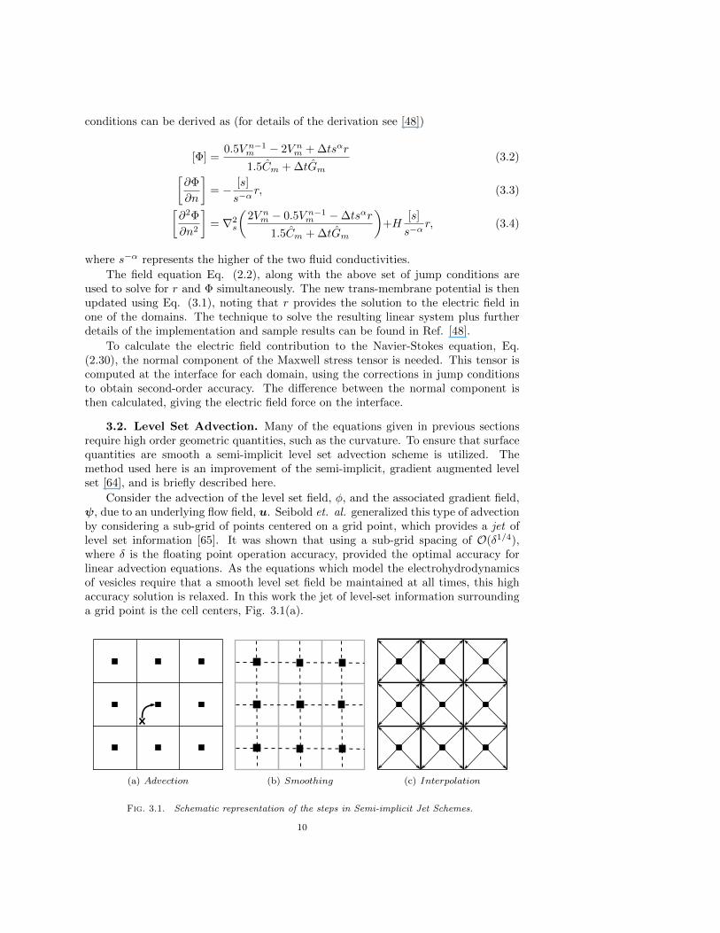
Consider the advection of the level set field, φ, and the associated gradient field,ψ, due to an underlying flow field, u. Seibold et. al. generalized this type of advectionby considering a sub-grid of points centered on a grid point, which provides a jet oflevel set information [65]. It was shown that using a sub-grid spacing of O(δ1/4),where δ is the floating point operation accuracy, provided the optimal accuracy forlinear advection equations. As the equations which model the electrohydrodynamicsof vesicles require that a smooth level set field be maintained at all times, this highaccuracy solution is relaxed. In this work the jet of level-set information surroundinga grid point is the cell centers, Fig. 3.1(a).

(a) Advection (b) Smoothing (c) Interpolation

Fig. 3.1. Schematic representation of the steps in Semi-implicit Jet Schemes.

10

The advection of the level set jet proceeds with the following three steps: 1) ad-vection of cell-centers, 2) smoothing at cell-centers, and 3) projection onto grid points.Unlike the original semi-implicit, gradient-augmented level set method [64] this hasthe advantage of only requiring a single smoothing operation, as described below.

The advection of cell-centers proceeds by using a Lagrangian advection scheme:

xd = xc −∆tunc , (3.5)

φc = I3 (φn,xd) , (3.6)

where xc is the cell-center location, φc is the tentative level set value at the cellcenter, and I3 (φn,xd) is a cubic interpolant of the previous time-steps level set valuesevaluated at the departure location, xd.

The values at cell-centers are then smoothed using a semi-implicit technique firstintroduced for standard level set advection [66]:

φc − φc

∆t= β∇2φc − β∇2φc, (3.7)

where β is a user-parameter, typically chosen to be 0.5 [64, 66]. Note that the gridin this smoothing step is the cell-center (offset) grid. The boundary condition is thecontinuity of derivatives using the tentative level set values. For example, on the rightedge the boundary condition is(

∂φc

∂x

)Nx,j,k

=φcNx−1/2,j,k − φ

cNx−3/2,j,k

hx, (3.8)

where Nx and hx are the the number of grid points and the grid-spacing in the x-direction, respectively.

Finally, the cell-center values are projected back onto the grid points by usingsecond-order stencils. For example, the updated level set values at grid point (i, j, k)are given by

φi,j,k =1

8

(φci+1/2,j+1/2,k+1/2 + φci−1/2,j+1/2,k+1/2 + φci+1/2,j−1/2,k+1/2 (3.9)

+ φci−1/2,j−1/2,k+1/2 + φci+1/2,j+1/2,k−1/2 + φci−1/2,j+1/2,k−1/2

+φci+1/2,j−1/2,k−1/2 + φci−1/2,j−1/2,k−1/2

),

while the gradient in the x-direction is given by

ψxi,j,k =1

8hx

(φci+1/2,j+1/2,k+1/2 − φ

ci−1/2,j+1/2,k+1/2 + φci+1/2,j−1/2,k+1/2 (3.10)

− φci−1/2,j−1/2,k+1/2 + φci+1/2,j+1/2,k−1/2 − φci−1/2,j+1/2,k−1/2

+φci+1/2,j−1/2,k−1/2 − φci−1/2,j−1/2,k−1/2

).

The other gradient values can be similarly evaluated. The advantage of this methodover that of Ref. [64] is that only a single smoothing operation is required, versusone for the level set and three for the gradient fields. Work is currently underwayinvestigating the full properties of this semi-implicit jet scheme.

11

3.3. Level Set Reinitialization and Closest Point Calculation. After theadvection of the level set a reinitialization procedure is used. This is done for tworeasons. First, it has been shown that reinitialization aids in the conservation ofmass in level set-based simulations [67]. Second, the point on the interface with theshortest distance to a given grid point, called the closest-point, is required for theevaluation of the surface equations given below. The method employed here uses avariant of Newton’s method and a tricubic interpolation to find the closest point onthe interface from an arbitrary grid location in the neighborhood, see Ref. [68] formore details. Once the closest points are determined the level set function is replacedby the corresponding signed distance value while the gradient field is set to the unitoutward normal vector, which is the normalized vector pointing from the closest pointto the grid point, corrected so that it points outward. This procedure does not needto be done everywhere in the domain, but only near the interface. In the results belowall nodes within five grid points of the interface have their closest point calculatedand explicitly reinitialized. The remaining nodes are reinitialized using a first-orderPDE based reinitialization scheme [69, 70].

3.4. Hydrodynamics Solution: Projection Method. There are four totalconservation conditions that must be satisfied during the course of the simulation:1) local surface area, 2) total surface area, 3) local fluid volume, 4) total fluid volume.Vesicle dynamics are extremely sensitive to any changes in these quantities [21, 22,26, 27] and thus high accuracy is required. Unfortunately, error in the solution ofthe fluid equations, in addition to the non-conservation properties of the level setmethod, can induce large errors over the course of the simulation. To account forthis, the fluid equations will be modified to explicitly correct any error accumulation.The idea presented here is based on the work of Laadhari et. al. [24]. The differenceis that in the previous work the corrections were not reflected in the fluid field, butinstead modified the velocity used to advect the level set. Here, the corrections areincluded in the fluid field calculation and therefore a modified advection field is notrequired. Preliminary results for standard multiphase flow problems were presentedin Ref. [71] and are extended here for vesicles.

A projection method is implemented to solve for the velocity, pressure and tension.First, a semi-implicit update is performed to obtain a tentative velocity field,

u∗ − un

∆t+ un · ∇u∗ = −∇pn +

1

Re∇ ·(∇u∗ + (∇un)

T)

+ fnH + fnγ + fnel, (3.11)

where fH , fγ and fel are the bending, tension, and electric field forces localizedaround the interface, Eq. (2.22). The superscript n refers to the solution at theprevious time step.

Next, the tentative velocity field is projected onto the divergence and surface-divergence free velocity space,

un+1 − u∗

∆t= −∇q + δ(φ)‖∇φ‖ (∇sξ − ξH∇φ) , (3.12)

where q and ξ are the corrections needed for the pressure and tension, respectively.Finally, the pressure and tension are updated by including the corrections,

pn+1 = pn + q, (3.13)

γn+1 = γn + ξ. (3.14)

12

The four conservation conditions can be written as [24]

∇ · un+1 = 0 (local volume conservation), (3.15)∫Γ

n · un+1 dA =dV

dt(global volume conservation), (3.16)

∇s · un+1 = 0 (local area conservation), (3.17)∫Γ

Hn · un+1 dA =dA

dt(global area conservation). (3.18)

The use of only the pressure and tension is not sufficient to satisfy all four conserva-tion conditions. There, the pressure and tension fields are split into a constant andspatially-varying component:

p = p+ (1−H(φ))p0, (3.19)

γ = γ + γ0, (3.20)

where p and γ are spatially varying while p0 and γ0 are constant. Note that p, γ,p0, and γ0 all vary in time. Conceptually, this splitting allows for the enforcement oflocal conservation through p and γ while global conservation is enforced through p0

and γ0.The corresponding corrections are now q = q + (1 − H(φ))q0, and ξ = ξ + ξ0,

while the projection step, Eq. (3.12), is now written as

un+1 = u∗ + ∆t(−∇q + δ(φ)q0∇φ+ δ(φ)‖∇φ‖

(∇sξ − ξH∇φ− ξ0H∇φ

)). (3.21)

Noting that the time derivatives of the volume and area are to correct any accu-mulated errors in the solution, and using Eq. (3.21), the four conservation equationscan be written in terms of the four unknowns (q, ξ, q0, and ξ0), the current areaand volume, and the initial area and volume. Specifically, applying the local areaconservation equation requires that

−∇·u∗ = ∆t∇·(−∇q + δ(φ)q0∇φ+ δ(φ)‖∇φ‖

(∇sξ − ξH∇φ+ ξ0H∇φ

)), (3.22)

while the total volume conservation requires that

V 0 − V n

∆t−∫

Γ

n · u∗ dA =

∆t

∫Γ

(−n · ∇q + δ(φ)q0‖∇φ‖ − δ(φ)‖∇φ‖2

(ξH + ξ0H

))dA, (3.23)

where V n is the current volume and the time-derivative of the volume is chosen sothat at the end of the time-step the volume equals the initial volume, V 0.

Conservation of local and global area results in the following two equations:

−∇s · u∗ = ∆t∇s ·(−∇q + δ(φ)q0∇φ+ δ(φ)‖∇φ‖

(∇sξ − ξH∇φ− ξ0H∇φ

)),

(3.24)and

A0 −An

∆t−∫

Γ

Hn · u∗ dA =

∆t

∫Γ

H(−n · ∇q + δ(φ)q0‖∇φ‖ − δ(φ)‖∇φ‖2

(ξH + ξ0H

))dA, (3.25)

13

where A0 is the initial surface area and An is the current surface area.Let q represent the vector holding the values of q in the entire, discretized domain

and ξ is the vector holding the values of ξ in the entire, discretized domain. It isnow possible to represent the conservation relationships, Eqs. (3.22)-(3.25), as linearoperators acting on q, q0, ξ, and ξ0. Local volume conservation, Eq. (3.22), can berepresented as

Lq + lq0 +Lξξ + lξξ0 = −Du∗, (3.26)

where D is the discrete divergence operator and

Lq ≈−∆t∇ · ∇q, lq0 ≈ q0∆t∇ · (δ(φ)∇φ) ,

(3.27)

Lξξ ≈∆t∇ ·(δ(φ)‖∇φ‖

(∇sξ − ξH∇φ

)), lξξ0 ≈ ξ0∆t∇ · (δ(φ)‖∇φ‖H∇φ) ,

(3.28)

are the discretizations of the continuous operations. Note that L and Lξ are a linearoperator matrices while l and lξ are linear operator vectors.

The integrals over the vesicle interface can be approximated as summations overthe discretized domain:

∫Γf dA ≈

∑δi,j,kfi,j,k∆V , where δi,j,k is the Dirac delta

function defined in Eq. (2.21) at a grid point, fi,j,k is the function value at thatgrid point, and ∆V = hxhyhz is the volume of a cell. In linear operator form thiscalculated by taking the dot product between the integration vector and the vectorcontaining the function values. Define the following linear operations:

sT q ≈−∆t

∫Γ

(n · ∇q) dA, aq0 ≈q0∆t

∫Γ

δ(φ)‖∇φ‖dA, (3.29)

sTξ ξ ≈−∆t

∫Γ

(δ(φ)‖∇φ‖2ξH

)dA, aξξ0 ≈ξ0∆t

∫Γ

(δ(φ)‖∇φ‖2H

)dA. (3.30)

In this case s and sξ are linear operator vectors while a and aξ are scalar values. Thisresults in the following linear equation:

sT q + aq0 + sTξ ξ + aξξ0 = EV , (3.31)

where EV ≈ (V 0 − V n)/∆t−∫

Γ(n · u∗) dA is the discrete form of the global volume

correction needed.The surface-conservation equations are written in a similar manner:

Lsq + lsq0 +Lsξξ + lsξξ0 = −Dsu∗, (3.32)

where Ds is the discrete surface-divergence operator and

Lsq ≈−∆t∇s · ∇q, lsq0 ≈ q0∆t∇s · (δ(φ)∇φ) ,

(3.33)

Lsξξ ≈∆t∇s ·(δ(φ)‖∇φ‖

(∇sξ − ξH∇φ

)), lsξξ0 ≈ ξ0∆t∇s · (δ(φ)‖∇φ‖H∇φ)

(3.34)

for the local surface-area conservation, Eq. (3.24) and

sTH q + bq0 + sTHξξ + bξξ0 = EA, (3.35)

14

where EA ≈ (A0 − An)/∆t −∫

Γ(Hn · u∗) dA is the discrete form of the global area

correction needed and

sTH q ≈−∆t

∫Γ

(Hn · ∇q) dA, bq0 ≈q0∆t

∫Γ

Hδ(φ)‖∇φ‖dA, (3.36)

sTHξξ ≈−∆t

∫Γ

(δ(φ)‖∇φ‖2ξH2

)dA, bξξ0 ≈ξ0∆t

∫Γ

(δ(φ)‖∇φ‖2H2

)dA. (3.37)

Using the notation above the set of four linear equations can be written in matrix-vector form:

L l Lξ lξsT a sTξ aξLs ls Lsξ lsξsTH b sTHξ bξ

qq0

ξξ0

=

−Du∗EV−Dsu

∗

EA

, (3.38)

Note that the specific spatial discretization have not yet been specified, as the generalconcepts are discretization-independent.

While it is possible to form a globally-assembled matrix for Eq. (3.38), it wouldbe computationally expensive. Not only would the size of the system be large, butit would also have to be re-formed every time step as many of the components, suchas Lsξ, l

sξ and sTH depend on the location of the interface, which changes over time.

Instead, write the complete system in the following simplified notation,[A BC D

] [qξ

]=

[eVeA

], (3.39)

where

A =

[L lsT a

], B =

[Lξ lξsTξ aξ

],

C =

[Ls ls

sTH b

], and D =

[Lsξ lsξsTHξ bξ

], (3.40)

with the combined vectors q = [q, q0]T , ξ = [ξ, ξ0]T , eV = [−Du∗, EV ]T and eA =[−Dsu

∗, EA]T . Using a Schur Complement approach the solution is[qξ

]=

[Iq 0

−D−1C Iξ

] [S−1 0

0 D−1

] [Iq −BD−1

0 Iξ

] [eVeA

], (3.41)

where S is the Schur Complement of the original partitioned matrix and is give by

S = A− BD−1C. (3.42)

The application of the Schur Complement is accomplished by a matrix-free iterativesolver, such as GMRES.

Let the focus now turn to the calculation of D−1. This inverse is given implicitlythrough the solution of the following, generalized linear system:[

Lsξ lsξsTH bξ

] [x0

x1

]=

[y0

y1

]. (3.43)

15

Turning to the Schur Decomposition the solution can be written as[x0

x1

]=

[I 0

b−1ξ s

TH 1

] [S−1 0

0 b−1ξ

] [I −b−1

ξ lsξ

0 1

] [y0

y1

], (3.44)

where the Schur Complement is a rank-1 update on the matrix Lsξ:

S = Lsξ −1

bξlsξs

TH . (3.45)

Using the Sherman–Morrison formula the inverse of this Schur Complement is givenby

S−1 =(Lsξ)−1

+

(Lsξ)−1

lsξsTH

(Lsξ)−1

bξ − sTH(Lsξ)−1

lsξ. (3.46)

So long as bξ 6= sTH(Lsξ)−1

lsξ this inverse is defined. While this inequality will not beproven here, a check during the course of the simulations presented below is performedevery time step and this condition has never been violated.

3.5. Evaluation and Advection of Surface Quantities. A word must besaid about the solution of surface equations. In the projection method the pressureis defined everywhere in the domain and thus standard techniques can be used. Thetension, on the other hand, is only defined on the interface and must be handled us-ing special methods. Unlike the immersed boundary method or other front-trackingtechniques Lagrangian points are not tracked over the course of the simulation. In-stead, all surface equations and quantities, such as the tension and trans-membranepotential, are evaluated using the Closest Point Method [72, 73]. The general idea isto replace surface equations by localized equations in the embedding space by extend-ing quantities from the interface in a systematic way. This is done by replacing thevalue at a grid point in a finite difference approximation by it’s interpolated value atthe closest point on the interface. Additional information can be found in References[72, 73]. All surface quantities, such as the tension and trans-membrane potential, areadvected along side the level set. After the level set is advected surface quantities areadvected by using the total-derivative form of the advection equation for a materialquantity f :

xd =x−∆tun, (3.47)

f =I3 (fn,xd) , (3.48)

where I3 (fn,xd) is the evaluation of the cubic interpolant using the previous time-steps value evaluated at the departure location xd. The values are then replaced bythe values at the closest point to a grid point,

f(x) = I3

(f ,xcp

), (3.49)

where xcp is the closest point on the interface to grid point x.

3.6. Overall algorithm. The overall algorithm to solve the electrohydrody-namics of the vesicle is performed using a time-staggered approach:

16

Step I: Solve for the updated electric field and trans-membrane potential using Sec.3.1.

Step II: Solve the hydrodynamics equations and obtain the updated velocity field,pressure and the tension using Sec. 3.4.

Step III: Using the updated velocity field from Step II advance the level set (inter-face) using Sec. 3.2.

Step IV: Reinitialize the level set values around the interface and recalculate theclosest point data, Sec. 3.3.

Step V: Advect surface quantities such as tension and trans-membrane potentialusing Sec. 3.5.

Step VI: One time step has been completed. Return to Step I and repeat until finaltime is reached.

4. Results. In this section the dynamics of the vesicle is studied in pure shearflow, in the presence of an electric field, and in combination of the two effects. Thevesicle surface area is fixed to 4π in all the situations while the enclosed volume isvaried. For all results presented here a collocated, Cartesian mesh with uniform gridspacing in each direction is used. Periodicity is assumed in the x- and z-directionswhile wall boundary conditions are given in the y-direction. Unless otherwise statedthe domain is a box covering the domain [−4.5, 4.5]3. Any externally applied shearflow is given by imposing a velocity of ubc = (χy, 0, 0) on the wall boundaries, where χis the normalized shear rate. Electric fields are applied by fixing the electric potentialin the y-direction at Ebc = E0y, where E0 is the normalized electric field strength.It is assumed that the trans-membrane conductance is zero and thus Gm = 0. Fi-nally, compact finite difference approximations for all spatial derivatives have beenimplemented (e.g. the pressure-Poisson term is approximated by ∇ · ∇q ≈ ∇2q atthe discrete level). For all results surface area and volume are all conserved to within0.01% error.

4.1. Hydrodynamics of Vesicle (Mn = 0). To demonstrate the robustnessand effectiveness of the hydrodynamic portion of the numerical method and for thepurpose of the verification, sample results are presented for a vesicle under linear shearflow in the absence of electric fields (Mn = 0). Note that the characteristic time scaleassociated with for this case is t0 = tγ = 1s. Using the typical experimental valuesgiven in Sec. 2.5 the dimensionless parameters are found to be Re = 0.001 andCa = 10. Unless otherwise stated, these parameters along with a dimensionless shearrate of χ = 1 at the boundary are used for the hydrodynamic simulations as well asthe results for combined effect of shear flow and the electric field.

Here two major modes of motions for the vesicle in shear flow are reported: tank-treading and tumbling. The tank-treading motion happens if the viscosity ratio, η,is less than a critical value ηc, which depends on the reduced volume of the vesicle[18]. In the tank-treading regime the vesicle reaches an equilibrium angle and staysat that position. When the viscosity ratio is above the critical viscosity the behaviorof the vesicle changes, and it starts to tumble end-over-end. Studies have shown thatthe dynamics depend primarily on the viscosity ratio, η and the reduced volume, v,with no remarkable dependence on the shear rate strength, χ [17].

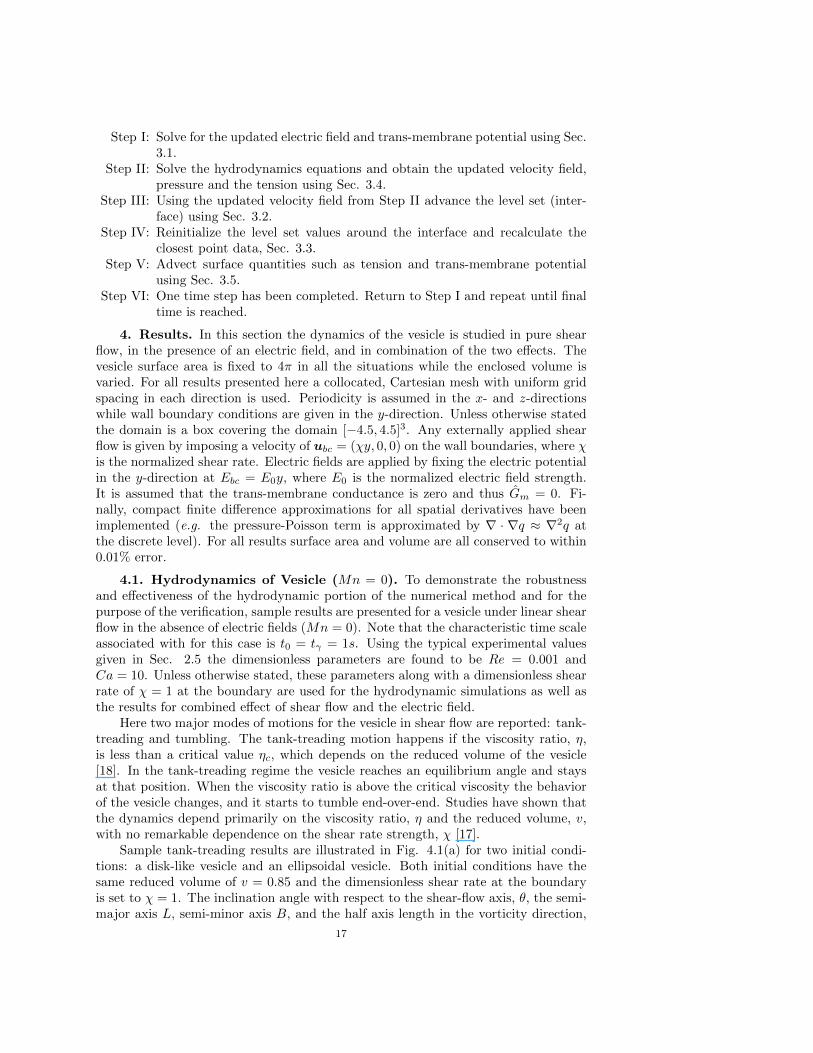
Sample tank-treading results are illustrated in Fig. 4.1(a) for two initial condi-tions: a disk-like vesicle and an ellipsoidal vesicle. Both initial conditions have thesame reduced volume of v = 0.85 and the dimensionless shear rate at the boundaryis set to χ = 1. The inclination angle with respect to the shear-flow axis, θ, the semi-major axis L, semi-minor axis B, and the half axis length in the vorticity direction,

17

L,B

,Z

0.0 5 10 15 20 250.2

0.4

0.6

0.8

1

1.2

1.4

1.6

1.8

B

Z

L

t/tγ

0.1

0.2

0.3

0.4

0.5

Eq

uili

bri

um

ang

le (θ/π

)

θ/π

Ellipsoidal vesicle

Disk-like vesicle

(a)

X

Y

(b)

Fig. 4.1. Sample result of tank treading vesicle with different initial shapes. The final equilib-rium shape and angle are the same for both initially prolate and oblate vesicles.

Z, are reported. These values are computed through the use of the inertia matrix ofthe vesicle [74]. The eigenvalues of the interia matrix correspond to the axis lengths,while the angle between the eigenvector associated with the largest eigenvalue andthe y−axis is the inclination angle.

It is clear from Fig. 4.1(a) that both initial conditions result in the same equi-librium shape and inclination angle. Figure 4.1(b) shows the vortices being formedin the interior of the vesicle at the equilibrium state. The streamlines demonstratethat the fluid velocity is tangent to the membrane which indicates the tank-treadingbehavior.

The equilibrium inclination angle as a function of reduced volume and viscosityratio is shown in Fig 4.2(a). A dimensionless shear rate of χ = 1 is applied at theboundary and results are compared to experimental data from Ref. [75]. The anglesfrom the numerical model are in good agreement with experimental measurements.Small discrepancies in the case of η = 4.9 could be related to the role of thermalfluctuations in the dynamics of vesicles with larger viscosity ratios [75]. This effect isabsent in the proposed model and further investigation is needed to fully understandthis phenomena.

The transition between tank-treading and tumbling happens at the critical vis-cosity ratio ηc. As v increases a larger ηc is required to transition from tank-treadingto tumbling. This behavior is shown in Fig 4.2(b). The present method compareswell to experimental data from [14], particularly for larger reduced volumes.

4.2. Vesicle dynamics in strong DC electric field. The response of a vesi-cle to an external electric field will depend on a number of factors, including themembrane properties, the viscosity ratio, the electrical properties of the fluids, andthe applied electric field. The shape of the vesicles is described by the deformationparameter:

D =ayax, (4.1)

where ay is the dimension of the vesicle in the direction parallel to the applied electricfield (the y-direction) while ax is the dimension of the vesicle in the direction per-

18

Reduced volume (v)0.7 0.8 0.9 10

0.05

0.1

0.15

0.2

0.25Exp. η=1.0

Exp. η=2.6

Exp. η=4.9

Present. η=1.0

Present. η=2.6

Present. η=4.9

Eq

uili

bri

um

an

gle

(θ/π

)

(a)

0.8 0.85 0.9 0.95 14

5

6

7

8

9

10

Cri

tica

l vis

cosi

ty r

ati

o (

ηc)

Reduced volume (v)

Experiment

Present

(b)

Fig. 4.2. Comparison of vesicle hydrodynamics to experiments. (a) The effects of reduced vol-ume and viscosity ratio on the inclination angle of a tank-treading vesicle. The results are comparedagainst the experimental data from Ref. [75]. (b) The critical viscosity ratio for vesicles with variousreduced areas. The results are compared to the experimental data in Ref. [14].

pendicular to the electric field, the x-direction. Note that these parameters are beingcalculated directly using the interface location and differ from the semi-axis valuesdefined in Sec. 4.1.

If the conductivity of the inner fluid is lower than the outer fluid, λ < 1, andthe electric field is strong enough such that tehd < tm, an initially prolate vesicle willundergo a prolate-oblate-prolate (POP) transition [40, 43]. An oblate shape is givenby D < 1 while a prolate shape has D > 1.

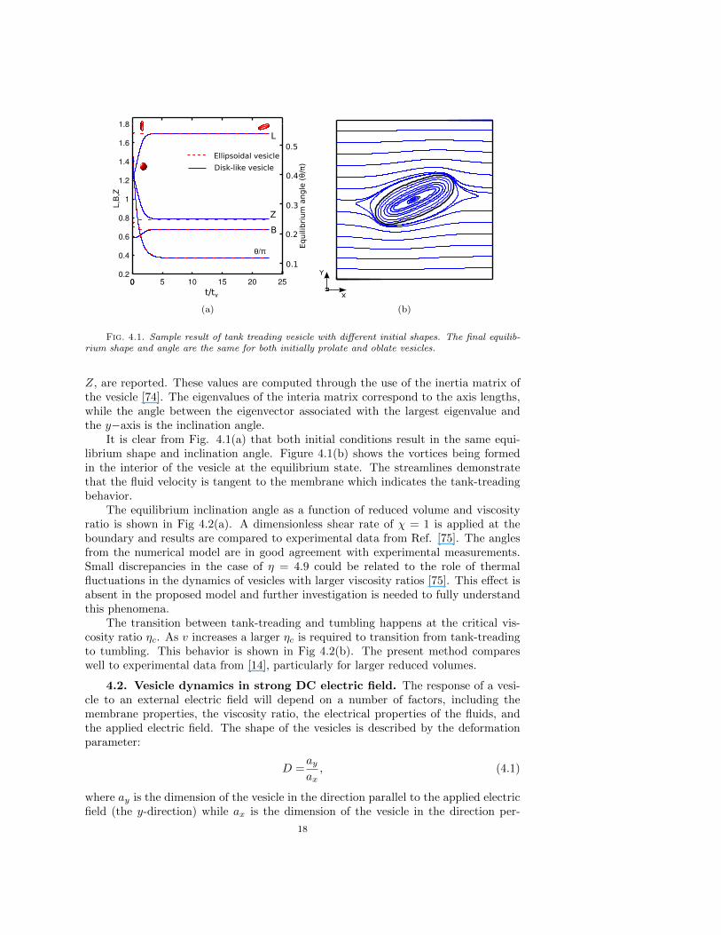
As verification of the method simulation results are compared to the analytic workof Schwalbe et. al. [43]. The reduced volume of the vesicle is v = 0.98. The initialshape is given by a second-order Spherical Harmonics parametric surface, see Ref. [43]for details. In Figs. 4.3-4.5 the influence of the time step, grid size, and domain sizeis explored and results are compared to Ref. [43]. Note that the membrane chargingtime is chosen as the characteristic time in these simulations. Recall that using thetypical experimental values of the physical parameters discussed earlier in Sec.2.5 thisresults in t0 = tm = 2.1 × 10−3 s, Cm = 0.095, Gm = 0, Re = 0.19, Ca = 3.8 × 104,Mn = 18, E0 = 1, and χ = 0. Also a matched dielectric ratio is used in all theelectrohydrodynamic simulations in this paper.

Several points need to be made about the results. First, the use of a time step ofsize ∆t = 5 × 10−4, grid size of N = 1203 with a domain of [−4.5, 4.5]3 results in aconverged solution and is therefore used in the following simulations. Second, thereis a discrepancy between the simulation results and the analytic results of Schwalbeet. al. While the general results are similar, for example the approximate time atwhich the prolate-oblate transition occurs and the time in the oblate shape, thereare important differences. The transition from the initial prolate to oblate shape isdelayed and is sharper for the current simulation versus the analytic result. Also,the deformation parameter increases slightly during the oblate shape (at a time of0.4tm) before decreasing again. Finally, the final equilibrium shape is slightly differentbetween the two methods, as demonstrated by the difference in the final deformation

19

t/tm

Def

orm

atio

npa

ram

eter

(D)

0.001 0.010

Schwalbe et al.

Δt=5e-04Δt=1e-03

Δt=2.5e-04

5.000.100 1.00

1.3

1.2

1.1

1.0

0.9

0.8

0.7

Fig. 4.3. Comparison of the method against analytic solution of Schwalbe et. al. [43]. Con-vergence test is done for three different time steps to check the temporal independence. The domainsize is [−4.5, 4.5] with a grid spacing of h = 0.075. The analysis demonstrates that ∆t = 5 × 10−4

is the maximum acceptable time-step.

Def

orm

atio

n pa

ram

eter

(D)

t/tm

Schwalbe et al.

N=120 (h=0.0750)N=100 (h=0.090)

N=160 (h=0.0653)

0.001 0.010 5.000.100 1.00

1.3

1.2

1.1

1.0

0.9

0.8

0.7

0.6

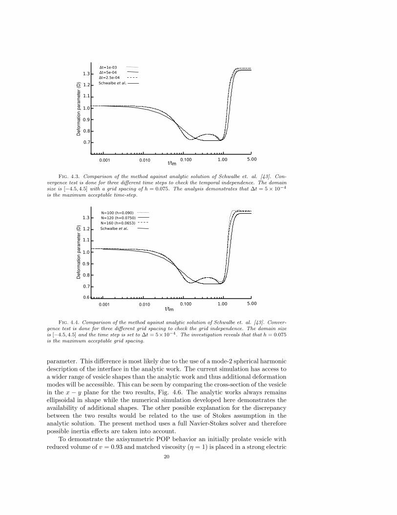
Fig. 4.4. Comparison of the method against analytic solution of Schwalbe et. al. [43]. Conver-gence test is done for three different grid spacing to check the grid independence. The domain sizeis [−4.5, 4.5] and the time step is set to ∆t = 5×10−4. The investigation reveals that that h = 0.075is the maximum acceptable grid spacing.

parameter. This difference is most likely due to the use of a mode-2 spherical harmonicdescription of the interface in the analytic work. The current simulation has access toa wider range of vesicle shapes than the analytic work and thus additional deformationmodes will be accessible. This can be seen by comparing the cross-section of the vesiclein the x − y plane for the two results, Fig. 4.6. The analytic works always remainsellipsoidal in shape while the numerical simulation developed here demonstrates theavailability of additional shapes. The other possible explanation for the discrepancybetween the two results would be related to the use of Stokes assumption in theanalytic solution. The present method uses a full Navier-Stokes solver and thereforepossible inertia effects are taken into account.

To demonstrate the axisymmetric POP behavior an initially prolate vesicle withreduced volume of v = 0.93 and matched viscosity (η = 1) is placed in a strong electric

20

t/tm

Def

orm

atio

n pa

ram

eter

(D) Schwalbe et al.

[-4.5,4.5]3[-3,3]3

[-6,6]31.3

1.2

1.1

1.0

0.9

0.8

0.7

0.6

0.001 0.010 5.000.100 1.00

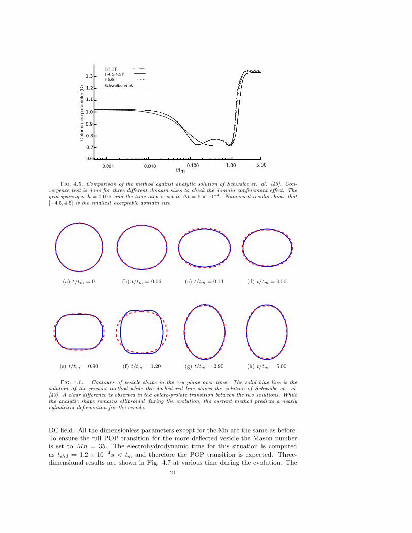
Fig. 4.5. Comparison of the method against analytic solution of Schwalbe et. al. [43]. Con-vergence test is done for three different domain sizes to check the domain confinement effect. Thegrid spacing is h = 0.075 and the time step is set to ∆t = 5 × 10−4. Numerical results shows that[−4.5, 4.5] is the smallest acceptable domain size.

(a) t/tm = 0 (b) t/tm = 0.06 (c) t/tm = 0.14 (d) t/tm = 0.50

(e) t/tm = 0.90 (f) t/tm = 1.20 (g) t/tm = 2.90 (h) t/tm = 5.00

Fig. 4.6. Contours of vesicle shape in the x-y plane over time. The solid blue line is thesolution of the present method while the dashed red line shows the solution of Schwalbe et. al.[43]. A clear difference is observed in the oblate-prolate transition between the two solutions. Whilethe analytic shape remains ellipsoidal during the evolution, the current method predicts a nearlycylindrical deformation for the vesicle.

DC field. All the dimensionless parameters except for the Mn are the same as before.To ensure the full POP transition for the more deflected vesicle the Mason numberis set to Mn = 35. The electrohydrodynamic time for this situation is computedas tehd = 1.2 × 10−4s < tm and therefore the POP transition is expected. Three-dimensional results are shown in Fig. 4.7 at various time during the evolution. The

21

(a) t/tm = 0 (b) t/tm = 0.25 (c) t/tm = 0.35 (d) t/tm = 0.65

(e) t/tm = 1.00 (f) t/tm = 1.40 (g) t/tm = 2.50 (h) t/tm = 5.00

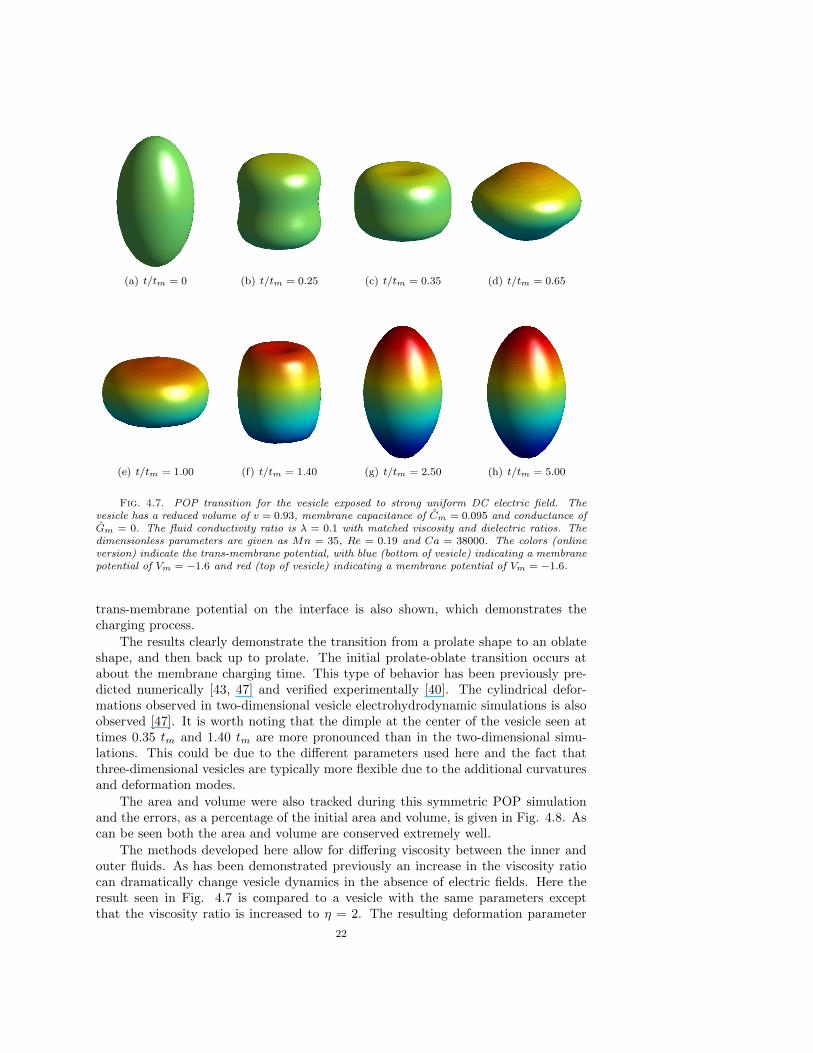
Fig. 4.7. POP transition for the vesicle exposed to strong uniform DC electric field. Thevesicle has a reduced volume of v = 0.93, membrane capacitance of Cm = 0.095 and conductance ofGm = 0. The fluid conductivity ratio is λ = 0.1 with matched viscosity and dielectric ratios. Thedimensionless parameters are given as Mn = 35, Re = 0.19 and Ca = 38000. The colors (onlineversion) indicate the trans-membrane potential, with blue (bottom of vesicle) indicating a membranepotential of Vm = −1.6 and red (top of vesicle) indicating a membrane potential of Vm = −1.6.

trans-membrane potential on the interface is also shown, which demonstrates thecharging process.

The results clearly demonstrate the transition from a prolate shape to an oblateshape, and then back up to prolate. The initial prolate-oblate transition occurs atabout the membrane charging time. This type of behavior has been previously pre-dicted numerically [43, 47] and verified experimentally [40]. The cylindrical defor-mations observed in two-dimensional vesicle electrohydrodynamic simulations is alsoobserved [47]. It is worth noting that the dimple at the center of the vesicle seen attimes 0.35 tm and 1.40 tm are more pronounced than in the two-dimensional simu-lations. This could be due to the different parameters used here and the fact thatthree-dimensional vesicles are typically more flexible due to the additional curvaturesand deformation modes.

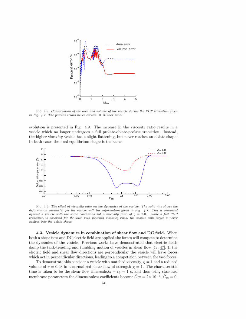
The area and volume were also tracked during this symmetric POP simulationand the errors, as a percentage of the initial area and volume, is given in Fig. 4.8. Ascan be seen both the area and volume are conserved extremely well.

The methods developed here allow for differing viscosity between the inner andouter fluids. As has been demonstrated previously an increase in the viscosity ratiocan dramatically change vesicle dynamics in the absence of electric fields. Here theresult seen in Fig. 4.7 is compared to a vesicle with the same parameters exceptthat the viscosity ratio is increased to η = 2. The resulting deformation parameter

22

0 1 2 3 4 510

-6

10-5

10-4

10-3

10-2

Volume error

Area error

t/tm

Percenterror%

Fig. 4.8. Conservation of the area and volume of the vesicle during the POP transition givenin Fig. 4.7. The percent errors never exceed 0.01% over time.

evolution is presented in Fig. 4.9. The increase in the viscosity ratio results in avesicle which no longer undergoes a full prolate-oblate-prolate transition. Instead,the higher viscosity vesicle has a slight flattening, but never reaches an oblate shape.In both cases the final equilibrium shape is the same.

0.4

0.6

0.8

1

1.2

1.4

1.6

1.8

2

0.10t/tm

1.00

Def

orm

atio

n pa

ram

eter

(D)

2.00 5.000.01 0.5

Λ=1.0Λ=2.0

0.05

Fig. 4.9. The effect of viscosity ratio on the dynamics of the vesicle. The solid line shows thedeformation parameter for the vesicle with the information given in Fig. 4.7. This is comparedagainst a vesicle with the same conditions but a viscosity ratio of η = 2.0. While a full POPtransition is observed for the case with matched viscosity ratio, the vesicle with larger η neverevolves into the oblate shape.

4.3. Vesicle dynamics in combination of shear flow and DC field. Whenboth a shear flow and DC electric field are applied the forces will compete to determinethe dynamics of the vesicle. Previous works have demonstrated that electric fieldsdamp the tank-treading and tumbling motion of vesicles in shear flow [43, 47]. If theelectric field and shear flow directions are perpendicular the vesicle will have forceswhich act in perpendicular directions, leading to a competition between the two forces.

To demonstrate this consider a vesicle with matched viscosity, η = 1 and a reducedvolume of v = 0.93 in a normalized shear flow of strength χ = 1. The characteristictime is taken to be the shear flow timescale,t0 = tγ = 1 s, and thus using standard

membrane parameters the dimensionless coefficients become Cm = 2×10−4, Gm = 0,

23

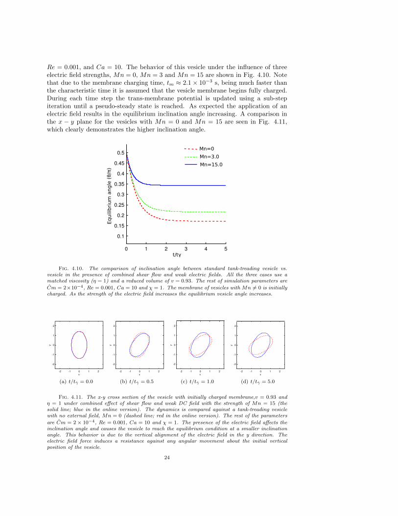
Re = 0.001, and Ca = 10. The behavior of this vesicle under the influence of threeelectric field strengths, Mn = 0, Mn = 3 and Mn = 15 are shown in Fig. 4.10. Notethat due to the membrane charging time, tm ≈ 2.1× 10−3 s, being much faster thanthe characteristic time it is assumed that the vesicle membrane begins fully charged.During each time step the trans-membrane potential is updated using a sub-stepiteration until a pseudo-steady state is reached. As expected the application of anelectric field results in the equilibrium inclination angle increasing. A comparison inthe x − y plane for the vesicles with Mn = 0 and Mn = 15 are seen in Fig. 4.11,which clearly demonstrates the higher inclination angle.

Equilibrium

angle

(θ/π)

0 1 2 3 4 5

0.1

0.15

0.2

0.25

0.3

0.35

0.4

0.45

0.5

t/tγ

Mn=0

Mn=3.0

Mn=15.0

Fig. 4.10. The comparison of inclination angle between standard tank-treading vesicle vs.vesicle in the presence of combined shear flow and weak electric fields. All the three cases use amatched viscosity (η = 1) and a reduced volume of v = 0.93. The rest of simulation parameters are

Cm = 2×10−4, Re = 0.001, Ca = 10 and χ = 1. The membrane of vesicles with Mn 6= 0 is initiallycharged. As the strength of the electric field increases the equilibrium vesicle angle increases.

x

y

-2 -1 0 1 2

-2

-1

0

1

2

(a) t/tγ = 0.0

x

y

-2 -1 0 1 2

-2

-1

0

1

2

(b) t/tγ = 0.5

x

y

-2 -1 0 1 2

-2

-1

0

1

2

(c) t/tγ = 1.0

x

y

-2 -1 0 1 2

-2

-1

0

1

2

(d) t/tγ = 5.0

Fig. 4.11. The x-y cross section of the vesicle with initially charged membrane,v = 0.93 andη = 1 under combined effect of shear flow and weak DC field with the strength of Mn = 15 (thesolid line; blue in the online version). The dynamics is compared against a tank-treading vesiclewith no external field, Mn = 0 (dashed line; red in the online version). The rest of the parameters

are Cm = 2 × 10−4, Re = 0.001, Ca = 10 and χ = 1. The presence of the electric field affects theinclination angle and causes the vesicle to reach the equilibrium condition at a smaller inclinationangle. This behavior is due to the vertical alignment of the electric field in the y direction. Theelectric field force induces a resistance against any angular movement about the initial verticalposition of the vesicle.

24

Next consider the application of an electric field to a vesicle in the tumblingregime, η = 10 > ηc. The other parameters are the same as the tank-treading case:v = 0.93, χ = 1, Cm = 2× 10−4, Gm = 0, Re = 0.001, and Ca = 10. As in the tank-treading case the trans-membrane potential is iterated until a pseudo-steady state isreached every time step.

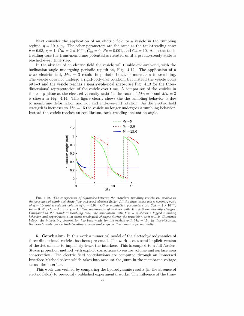
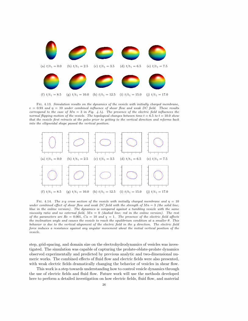
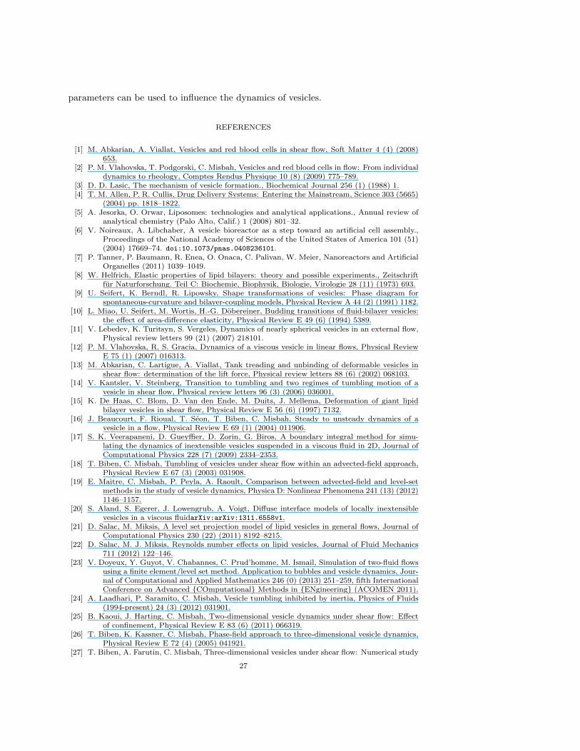
In the absence of an electric field the vesicle will tumble end-over-end, with theinclination angle undergoing periodic repetition, Fig. 4.12. The application of aweak electric field, Mn = 3 results in periodic behavior more akin to trembling.The vesicle does not undergo a rigid-body-like rotation, but instead the vesicle polesretract and the vesicle reaches a nearly-spherical shape, see Fig. 4.13 for the three-dimensional representation of the vesicle over time. A comparison of the vesicles inthe x − y plane at the elevated viscosity ratio for the cases of Mn = 0 and Mn = 3is shown in Fig. 4.14. This figure clearly shows the the tumbling behavior is dueto membrane deformation and not and end-over-end rotation. As the electric fieldstrength is increases to Mn = 15 the vesicle no longer undergoes a tumbling behavior.Instead the vesicle reaches an equilibrium, tank-treading inclination angle.

0 5 10 15

0

0.2

0.4

0.6

0.8

1

1.2

Equilibrium

angle

(θ/π)

t/tγ

Mn=0

Mn=3.0

Mn=15.0

Fig. 4.12. The comparison of dynamics between the standard tumbling vesicle vs. vesicle inthe presence of combined shear flow and weak electric fields. All the three cases use a viscosity ratioof η = 10 and a reduced volume of v = 0.93. Other simulation parameters are Cm = 2 × 10−4,Re = 0.001, Ca = 10 and χ = 1. The membranes of vesicles with Mn 6= 0 are initially charged.Compared to the standard tumbling case, the simulation with Mn = 3 shows a lagged tumblingbehavior and experiences a lot more topological changes during the transition as it will be illustratedbelow. An interesting observation has been made for the vesicle with Mn = 15. In this situation,the vesicle undergoes a tank-treading motion and stays at that position permanently.

5. Conclusion. In this work a numerical model of the electrohydrodynamics ofthree-dimensional vesicles has been presented. The work uses a semi-implicit versionof the Jet scheme to implicility track the interface. This is coupled to a full Navier-Stokes projection method with explicit corrections to ensure volume and surface areaconservation. The electric field contributions are computed through an ImmersedInterface Method solver which takes into account the jump in the membrane voltageacross the interface.

This work was verified by comparing the hydrodynamic results (in the absence ofelectric fields) to previously published experimental works. The influence of the time-

25

(a) t/tγ = 0.0 (b) t/tγ = 2.5 (c) t/tγ = 3.5 (d) t/tγ = 6.5 (e) t/tγ = 7.5

(f) t/tγ = 8.5 (g) t/tγ = 10.0 (h) t/tγ = 12.5 (i) t/tγ = 15.0 (j) t/tγ = 17.0

Fig. 4.13. Simulation results on the dynamics of the vesicle with initially charged membrane,v = 0.93 and η = 10 under combined influence of shear flow and weak DC field. These resultscorrespond to the case of Mn = 3 in Fig. 4.14. The presence of the electric field influences thenormal flipping motion of the vesicle. The topological changes between time t = 6.5 to t = 10.0 showthat the vesicle first retracts at the poles prior to getting to the vertical direction and reforms backinto the ellipsoidal shape passed the vertical position.

x

y

-2 -1 0 1 2

-2

-1

0

1

2

(a) t/tγ = 0.0

x

y

-2 -1 0 1 2

-2

-1

0

1

2

(b) t/tγ = 2.5

x

y

-2 -1 0 1 2

-2

-1

0

1

2

(c) t/tγ = 3.5

x

y

-2 -1 0 1 2

-2

-1

0

1

2

(d) t/tγ = 6.5

x

y

-2 -1 0 1 2

-2

-1

0

1

2

(e) t/tγ = 7.5

x

y

-2 -1 0 1 2

-2

-1

0

1

2

(f) t/tγ = 8.5

x

y

-2 -1 0 1 2

-2

-1

0

1

2

(g) t/tγ = 10.0

x

y

-2 -1 0 1 2

-2

-1

0

1

2

(h) t/tγ = 12.5

x

y

-2 -1 0 1 2

-2

-1

0

1

2

(i) t/tγ = 15.0

x

y

-2 -1 0 1 2

-2

-1

0

1

2

(j) t/tγ = 17.0

Fig. 4.14. The x-y cross section of the vesicle with initially charged membrane and η = 10under combined effect of shear flow and weak DC field with the strength of Mn = 3 (the solid line;blue in the online version). The dynamics is compared against a tumbling vesicle with the sameviscosity ratio and no external field, Mn = 0 (dashed line; red in the online version). The restof the parameters are Re = 0.001, Ca = 10 and χ = 1. The presence of the electric field affectsthe inclination angle and causes the vesicle to reach the equilibrium condition at a smaller θ. Thisbehavior is due to the vertical alignment of the electric field in the y direction. The electric fieldforce induces a resistance against any angular movement about the initial vertical position of thevesicle.

step, grid-spacing, and domain size on the electrohydrodynamics of vesicles was inves-tigated. The simulation was capable of capturing the prolate-oblate-prolate dynamicsobserved experimentally and predicted by previous analytic and two-dimensional nu-meric works. The combined effects of fluid flow and electric fields were also presented,with weak electric fields dramatically changing the behavior of vesicles in shear flow.

This work is a step towards understanding how to control vesicle dynamics throughthe use of electric fields and fluid flow. Future work will use the methods developedhere to perform a detailed investigation on how electric fields, fluid flow, and material

26

parameters can be used to influence the dynamics of vesicles.

REFERENCES

[1] M. Abkarian, A. Viallat, Vesicles and red blood cells in shear flow, Soft Matter 4 (4) (2008)653.

[2] P. M. Vlahovska, T. Podgorski, C. Misbah, Vesicles and red blood cells in flow: From individualdynamics to rheology, Comptes Rendus Physique 10 (8) (2009) 775–789.

[3] D. D. Lasic, The mechanism of vesicle formation., Biochemical Journal 256 (1) (1988) 1.[4] T. M. Allen, P. R. Cullis, Drug Delivery Systems: Entering the Mainstream, Science 303 (5665)

(2004) pp. 1818–1822.[5] A. Jesorka, O. Orwar, Liposomes: technologies and analytical applications., Annual review of

analytical chemistry (Palo Alto, Calif.) 1 (2008) 801–32.[6] V. Noireaux, A. Libchaber, A vesicle bioreactor as a step toward an artificial cell assembly.,

Proceedings of the National Academy of Sciences of the United States of America 101 (51)(2004) 17669–74. doi:10.1073/pnas.0408236101.

[7] P. Tanner, P. Baumann, R. Enea, O. Onaca, C. Palivan, W. Meier, Nanoreactors and ArtificialOrganelles (2011) 1039–1049.

[8] W. Helfrich, Elastic properties of lipid bilayers: theory and possible experiments., Zeitschriftfur Naturforschung. Teil C: Biochemie, Biophysik, Biologie, Virologie 28 (11) (1973) 693.

[9] U. Seifert, K. Berndl, R. Lipowsky, Shape transformations of vesicles: Phase diagram forspontaneous-curvature and bilayer-coupling models, Physical Review A 44 (2) (1991) 1182.

[10] L. Miao, U. Seifert, M. Wortis, H.-G. Dobereiner, Budding transitions of fluid-bilayer vesicles:the effect of area-difference elasticity, Physical Review E 49 (6) (1994) 5389.

[11] V. Lebedev, K. Turitsyn, S. Vergeles, Dynamics of nearly spherical vesicles in an external flow,Physical review letters 99 (21) (2007) 218101.

[12] P. M. Vlahovska, R. S. Gracia, Dynamics of a viscous vesicle in linear flows, Physical ReviewE 75 (1) (2007) 016313.

[13] M. Abkarian, C. Lartigue, A. Viallat, Tank treading and unbinding of deformable vesicles inshear flow: determination of the lift force, Physical review letters 88 (6) (2002) 068103.

[14] V. Kantsler, V. Steinberg, Transition to tumbling and two regimes of tumbling motion of avesicle in shear flow, Physical review letters 96 (3) (2006) 036001.

[15] K. De Haas, C. Blom, D. Van den Ende, M. Duits, J. Mellema, Deformation of giant lipidbilayer vesicles in shear flow, Physical Review E 56 (6) (1997) 7132.

[16] J. Beaucourt, F. Rioual, T. Seon, T. Biben, C. Misbah, Steady to unsteady dynamics of avesicle in a flow, Physical Review E 69 (1) (2004) 011906.

[17] S. K. Veerapaneni, D. Gueyffier, D. Zorin, G. Biros, A boundary integral method for simu-lating the dynamics of inextensible vesicles suspended in a viscous fluid in 2D, Journal ofComputational Physics 228 (7) (2009) 2334–2353.

[18] T. Biben, C. Misbah, Tumbling of vesicles under shear flow within an advected-field approach,Physical Review E 67 (3) (2003) 031908.

[19] E. Maitre, C. Misbah, P. Peyla, A. Raoult, Comparison between advected-field and level-setmethods in the study of vesicle dynamics, Physica D: Nonlinear Phenomena 241 (13) (2012)1146–1157.

[20] S. Aland, S. Egerer, J. Lowengrub, A. Voigt, Diffuse interface models of locally inextensiblevesicles in a viscous fluidarXiv:arXiv:1311.6558v1.

[21] D. Salac, M. Miksis, A level set projection model of lipid vesicles in general flows, Journal ofComputational Physics 230 (22) (2011) 8192–8215.

[22] D. Salac, M. J. Miksis, Reynolds number effects on lipid vesicles, Journal of Fluid Mechanics711 (2012) 122–146.

[23] V. Doyeux, Y. Guyot, V. Chabannes, C. Prud’homme, M. Ismail, Simulation of two-fluid flowsusing a finite element/level set method. Application to bubbles and vesicle dynamics, Jour-nal of Computational and Applied Mathematics 246 (0) (2013) 251–259, fifth InternationalConference on Advanced COmputational Methods in ENgineering (ACOMEN 2011).

[24] A. Laadhari, P. Saramito, C. Misbah, Vesicle tumbling inhibited by inertia, Physics of Fluids(1994-present) 24 (3) (2012) 031901.

[25] B. Kaoui, J. Harting, C. Misbah, Two-dimensional vesicle dynamics under shear flow: Effectof confinement, Physical Review E 83 (6) (2011) 066319.

[26] T. Biben, K. Kassner, C. Misbah, Phase-field approach to three-dimensional vesicle dynamics,Physical Review E 72 (4) (2005) 041921.

[27] T. Biben, A. Farutin, C. Misbah, Three-dimensional vesicles under shear flow: Numerical study

27

of dynamics and phase diagram, Physical Review E 83 (3) (2011) 031921.[28] H. ZHAO, E. S. G. SHAQFEH, The dynamics of a vesicle in simple shear flow, Journal of Fluid

Mechanics 674 (2011) 578–604.[29] S. K. Veerapaneni, A. Rahimian, G. Biros, D. Zorin, A fast algorithm for simulating vesicle

flows in three dimensions, Journal of Computational Physics 230 (14) (2011) 5610–5634.[30] A. Yazdani, P. Bagchi, Three-dimensional numerical simulation of vesicle dynamics using a

front-tracking method, Physical Review E 85 (5) (2012) 056308.[31] Z. Wang, N. Hu, L.-H. Yeh, X. Zheng, J. Yang, S. W. Joo, S. Qian, Electroformation and

electrofusion of giant vesicles in a microfluidic device, Colloids and Surfaces B: Biointerfaces110 (2013) 81–87.

[32] G. R. Campus, Irreversible electroporation: a new ablation modality–clinical implications,Technology in cancer research & treatment 6 (1).

[33] C. R. Keese, J. Wegener, S. R. Walker, I. Giaever, Electrical wound-healing assay for cells invitro, Proceedings of the National Academy of Sciences of the United States of America101 (6) (2004) 1554–1559.

[34] J. Skog, T. Wurdinger, S. van Rijn, D. H. Meijer, L. Gainche, W. T. Curry, B. S. Carter, A. M.Krichevsky, X. O. Breakefield, Glioblastoma microvesicles transport RNA and proteins thatpromote tumour growth and provide diagnostic biomarkers, Nature cell biology 10 (12)(2008) 1470–1476.

[35] E. Neumann, M. Schaefer-Ridder, Y. Wang, P. Hofschneider, Gene transfer into mouse lyomacells by electroporation in high electric fields., The EMBO journal 1 (7) (1982) 841.

[36] T. Y. Tsong, Electroporation of cell membranes, Biophysical journal 60 (2) (1991) 297–306.[37] K. a. Riske, R. Dimova, Electro-deformation and poration of giant vesicles viewed with high

temporal resolution., Biophysical journal 88 (2) (2005) 1143–55.[38] K. a. Riske, R. Dimova, Electric pulses induce cylindrical deformations on giant vesicles in salt

solutions., Biophysical journal 91 (5) (2006) 1778–86.[39] R. Dimova, K. A. Riske, S. Aranda, N. Bezlyepkina, R. L. Knorr, R. Lipowsky, Giant vesicles

in electric fields, Soft matter 3 (7) (2007) 817–827.[40] P. F. Salipante, P. M. Vlahovska, Vesicle deformation in DC electric pulses, Soft matter.[41] P. Salipnate, Electrohydrodynamics of simple and complex interfaces, Ph.d dissertation, Brown

University (2013).[42] P. M. Vlahovska, R. S. Gracia, S. Aranda-Espinoza, R. Dimova, Electrohydrodynamic model of

vesicle deformation in alternating electric fields, Biophysical journal 96 (12) (2009) 4789–4803.

[43] J. T. Schwalbe, P. M. Vlahovska, M. J. Miksis, Vesicle electrohydrodynamics, Physical ReviewE 83 (4) (2011) 046309.

[44] J. T. Schwalbe, P. M. Vlahovska, M. J. Miksis, Lipid membrane instability driven by capacitivecharging, Physics of Fluids (1994-present) 23 (4) (2011) 041701.

[45] J. Seiwert, M. J. Miksis, P. M. Vlahovska, Stability of biomimetic membranes in DC electricfields, Journal of Fluid Mechanics 706 (2012) 58–70.

[46] Y. L. Q. Y. Yugang Tang, Liquid crystal model of vesicle deformation in alternating electricfields, Theoretical and Applied Mechanics Letters 3 (5) (2013) 11.

[47] L. C. McConnell, M. J. Miksis, P. M. Vlahovska, Vesicle electrohydrodynamics in DC electricfields, IMA Journal of Applied Mathematics 78 (4) (2013) 797–817.

[48] E. M. Kolahdouz, D. Salac, A numerical model for the trans-membrane voltage of vesicles,Applied Mathematics Letters 39 (2015) 7–12.

[49] U. Seifert, Configurations of fluid membranes and vesicles, Advances in Physics 46 (1) (1997)13–137.

[50] D. A. Saville, Electrohydrodynamics: The Taylor-Melcher leaky dielectric model, Annual Re-view of Fluid Mechanics 29 (1962) (1997) 27–64.

[51] K. a. DeBruin, W. Krassowska, Modeling electroporation in a single cell. I. Effects Of fieldstrength and rest potential., Biophysical journal 77 (3) (1999) 1213–24.

[52] U. Seifert, Fluid membranes in hydrodynamic flow fields: Formalism and an application to fluc-tuating quasispherical vesicles in shear flow, The European Physical Journal B-CondensedMatter and Complex Systems 8 (3) (1999) 405–415.

[53] S. Osher, J. Sethian, Fronts Propagating with Curvature-Dependent Speed - Algorithms Basedon Hamilton-Jacobi Formulations, Journal of Computational Physics 79 (1) (1988) 12–49.

[54] J.-C. Nave, R. R. Rosales, B. Seibold, A Gradient-Augmented Level Set Method With anOptimally Local, Coherent Advection Scheme, Journal of Computational Physics 229 (10)(2010) 3802–3827.

[55] C. S. Peskin, The immersed boundary method, Acta numerica 11 (2002) 479–517.[56] P. Smereka, The numerical approximation of a delta function with application to level set

28

methods, Journal of Computational Physics 211 (1) (2006) 77–90.[57] B. Engquist, A.-K. Tornberg, R. Tsai, Discretization of Dirac delta functions in level set meth-

ods, Journal of Computational Physics 207 (1) (2005) 28–51.[58] J. D. Towers, A convergence rate theorem for finite difference approximations to delta functions,

Journal of Computational Physics 227 (13) (2008) 6591–6597.[59] Y. Chang, T. Hou, B. Merriman, S. Osher, A Level Set Formulation of Eulerian Interface

Capturing Methods for Incompressible Fluid Flows, Journal of Computational Physics124 (2) (1996) 449–464.

[60] J. Melcher, G. Taylor, Electrohydrodynamics: a review of the role of interfacial shear stresses,Annual Review of Fluid Mechanics 1 (1) (1969) 111–146.

[61] K. Kinosita Jr, I. Ashikawa, N. Saita, H. Yoshimura, H. Itoh, K. Nagayama, A. Ikegami,Electroporation of cell membrane visualized under a pulsed-laser fluorescence microscope,Biophysical journal 53 (6) (1988) 1015–1019.

[62] D. Needham, R. Hochmuth, Electro-mechanical permeabilization of lipid vesicles. Role of mem-brane tension and compressibility, Biophysical journal 55 (5) (1989) 1001–1009.

[63] M. M. Sadik, J. Li, J. W. Shan, D. I. Shreiber, H. Lin, Vesicle deformation and poration understrong dc electric fields, Physical Review E 83 (6) (2011) 066316.

[64] E. M. Kolahdouz, D. Salac, A semi-implicit gradient augmented level set method, SIAM Journalon Scientific Computing 35 (1) (2013) 231–254.

[65] B. Seibold, R. R. Rosales, J.-C. Nave, Jet schemes for advection problems, Discrete and Con-tinuous Dynamical Systems - Series B 17 (4) (2012) 1229–1259.

[66] P. Smereka, Semi-implicit level set methods for curvature and surface diffusion motion, Journalof Scientific Computing 19 (2003) 439–456.

[67] M. Sussman, E. Fatemi, An Efficient, Interface-Preserving Level Set Redistancing Algorithmand Its Application to Interfacial Incompressible Fluid Flow, SIAM Journal on ScientificComputing 20 (4) (1999) 1165–1191.

[68] D. L. Chopp, Some improvements of the fast marching method, SIAM Journal on ScientificComputing 23 (1) (2001) 230–244.

[69] D. Peng, B. Merriman, S. Osher, H. Zhao, M. Kang, A PDE-Based Fast Local Level SetMethod, Journal of Computational Physics 155 (2) (1999) 410–438.

[70] G. Russo, P. Smereka, A Remark on Computing Distance Functions, Journal of ComputationalPhysics 163 (1) (2000) 51–67.

[71] D. Salac, E. M. Kolahdouz, A fully mass-preserving projection method for incompressiblemultiphase flows, in Preparation.

[72] C. Macdonald, S. Ruuth, The Implicit Closest Point Method for the Numerical Solution ofPartial Differential Equations on Surfaces, SIAM Journal on Scientific Computing 31 (6)(2010) 4330–4350.

[73] C. Macdonald, S. Ruuth, Level Set Equations on Surfaces via the Closest Point Method, Journalof Scientific Computing 35 (2-3) 219–240.

[74] A. Laadhari, P. Saramito, C. Misbah, Computing the dynamics of biomembranes by combin-ing conservative level set and adaptive finite element methods, Journal of ComputationalPhysics 263 (2014) 328–352.

[75] N. J. Zabusky, E. Segre, J. Deschamps, V. Kantsler, V. Steinberg, Dynamics of vesicles in shearand rotational flows: Modal dynamics and phase diagram, Physics of Fluids (1994-present)23 (4) (2011) 041905.

29