numerical simulation of the three-dimensional structure and

A&A 414, 1121–1137 (2004)DOI: 10.1051/0004-6361:20031682c© ESO 2004

Astronomy&

Astrophysics

Numerical simulation of the three-dimensional structureand dynamics of the non-magnetic solar chromosphere

S. Wedemeyer1,2, B. Freytag3, M. Steffen4, H.-G. Ludwig5, and H. Holweger1

1 Institut fur Theoretische Physik und Astrophysik, Universitat Kiel, 24098 Kiel, Germany2 Kiepenheuer-Institut fur Sonnenphysik, Schoneckstrasse 6, 79104 Freiburg, Germany3 Department for Astronomy and Space Physics, Uppsala University, Box 515, 75120 Uppsala, Sweden4 Astrophysikalisches Institut Potsdam, An der Sternwarte 16, 14482 Potsdam, Germany5 Lund Observatory, Box 43, 22100 Lund, Sweden

Received 3 February 2003 / Accepted 30 October 2003

Abstract. Three-dimensional numerical simulations with CO5BOLD, a new radiation hydrodynamics code, result in a dynamic,thermally bifurcated model of the non-magnetic chromosphere of the quiet Sun. The 3D model includes the middle and lowchromosphere, the photosphere, and the top of the convection zone, where acoustic waves are excited by convective motions.While the waves propagate upwards, they steepen into shocks, dissipate, and deposit their mechanical energy as heat in thechromosphere. Our numerical simulations show for the first time a complex 3D structure of the chromospheric layers, formedby the interaction of shock waves. Horizontal temperature cross-sections of the model chromosphere exhibit a network of hotfilaments and enclosed cool regions. The horizontal pattern evolves on short time-scales of the order of typically 20−25 s, andhas spatial scales comparable to those of the underlying granulation. The resulting thermal bifurcation, i.e., the co-existenceof cold and hot regions, provides temperatures high enough to produce the observed chromospheric UV emission and – at thesame time – temperatures cold enough to allow the formation of molecules (e.g., carbon monoxide). Our 3D model corroboratesthe finding by Carlsson & Stein (1994) that the chromospheric temperature rise of semi-empirical models does not necessarilyimply an increase in the average gas temperature but can be explained by the presence of substantial spatial and temporaltemperature inhomogeneities.

Key words. Sun: chromosphere – hydrodynamics – radiative transfer

1. Introduction

Three-dimensional, time-dependent radiation hydrodynamicssimulations of solar and stellar surface convection have nowreached a level of sophistication which goes far beyond that ofidealised numerical experiments, and allows a direct confronta-tion of such models with real stars (e.g., Stein & Nordlund1998; Asplund et al. 2000; Freytag et al. 2002; Ludwig et al.2002). Extending this kind of simulation to include the lowchromosphere, it is possible to study – in a single model andbased on first principles – the generation of waves by the con-vective flow as well as the wave propagation and dissipation inthe higher layers. Extended simulations of this type may thenbe utilised to explore the hitherto poorly understood 3D thermalstructure and dynamics of the non-magnetic chromospheric in-ternetwork regions, and to obtain an independent theoretical es-timate of the amount of chromospheric heating due to acousticwaves.

A strong motivation for three-dimensional time-dependentmodelling arises from the need to reconcile apparently contra-dictory solar observations: carbon monoxide absorption lines

Send offprint requests to: S. Wedemeyer,e-mail: [email protected]

imply gas temperatures as low as ≈3700 K in the chromosphereof the quiet Sun (see Noyes & Hall 1972; Ayres & Testerman1981; Solanki et al. 1994; Uitenbroek et al. 1994; Uitenbroek2000a; Ayres 2002, and references therein), whereas chromo-spheric UV emission features require much higher tempera-tures at the same heights (e.g., Ayres & Linsky 1976; Carlssonet al. 1997).

Semi-empirical models which have been constructed basedon UV and microwave observations (e.g., Vernazza et al.1981, hereafter VAL; Maltby et al. 1986; Fontenla et al. 1993,hereafter FAL) commonly feature a temperature minimum ofTmin ≈ 4200−4400 K at a height of z ≈ 500 km above opticaldepth unity and an outwardly increasing temperature above.On the other hand, models based on CO observations (e.g.,Wiedemann et al. 1994) show a monotonic decrease of tem-perature with height.

These conflicting observations and the inferred represen-tative models have led to a controversy about the nature ofthe chromosphere of the non-magnetic quiet Sun which is go-ing on for many years now (see, e.g., Kalkofen 2001): is thechromosphere of the average quiet Sun a time-dependent phe-nomenon with a mostly cool background and large temperaturefluctuations due to upward propagating shock waves? Or is it

Article published by EDP Sciences and available at http://www.aanda.org or http://dx.doi.org/10.1051/0004-6361:20031682

http://www.edpsciences.org/

http://www.aanda.org

http://dx.doi.org/10.1051/0004-6361:20031682

1122 S. Wedemeyer et al.: Numerical simulation of the non-magnetic solar chromosphere

persistent and always hot with only small temperature fluctua-tions? In short: is the non-magnetic solar chromosphere hot orcool?

A large number of observations show that the chromo-sphere of the quiet Sun is indeed a very dynamic phe-nomenon (e.g., Carlsson et al. 1997; Muglach & Schmidt2001; Krijger et al. 2001; Wunnenberg et al. 2002). Obviously,static one-dimensional models can only describe selected time-averaged properties. More realistic modelling should thereforebe time-dependent.

Starting in the late 1960s, the pioneering work on1D time-dependent numerical models of chromospheric heat-ing by acoustic and magneto-hydrodynamic waves is due toUlmschneider and collaborators. In a long series of papers(e.g., Ulmschneider 1971; Ulmschneider & Kalkofen 1977;Ulmschneider et al. 1978; Muchmore & Ulmschneider 1985;Ulmschneider et al. 1987; Ulmschneider 1989; Cuntz et al.1994), they studied in detail the chromospheric energy bal-ance between dissipation of prescribed short-period (mostlymonochromatic) acoustic waves and radiative emission. Intheir models, the acoustic energy flux is supplied by a pistonacting as a lower boundary condition. Assuming that the gen-eration of acoustic waves by the “turbulent” flows in the upperconvection zone can be described by the Lighthill-Stein the-ory (Lighthill 1952; Stein 1967, 1968; Musielak et al. 1994;Ulmschneider et al. 1996, 1999), they compute dynamic chro-mospheric models not only for the Sun but also for a sam-ple of main-sequence stars and giants. Based on these models,they conclude that the observed “basal flux” from the chromo-spheres of late-type stars (Schrijver 1987; Rutten et al. 1991)is fully attributable to the dissipation of acoustic wave energy(Buchholz et al. 1998), and that the observed variation of chro-mospheric emission can be explained by the additional heatingof magnetohydrodynamic shock waves (Ulmschneider et al.2001).

The detailed radiation hydrodynamics simulations byCarlsson & Stein (1994, 1995, 1997, hereafter CS) areanother prominent example of sophisticated 1D time-dependent modelling. These authors successfully explained theCa H2v bright points as a result of propagating shock waves.In their model, the waves are excited by a piston which isdriven by a velocity variation derived from observed oscilla-tions at the photospheric level. Instead of a temperature mini-mum and a monotonic temperature increase above, as charac-teristic of the VAL and FAL models, CS find a chromospherewith a mostly cool background and large temperature fluctua-tions due to upward propagating shocks. Even more remarkableis the fact that they are able to reproduce the rise of the radiationtemperature without an increase of the mean gas temperature.Basic reasons are the nonlinear temperature dependence of thePlanck function in the UV and the extreme temperature peaksassociated with the shock waves. This led CS to the conclusionthat the chromosphere of the quiet Sun is not persistent but aspatially and temporally intermittent phenomenon which – ifaveraged over space and time – is mostly cool and not hot.

Although the one-dimensional models of the non-magneticsolar chromosphere mentioned above are highly elaborate,including a fully time-dependent H ionisation and detailed

NLTE radiative transfer, they suffer from the need for an exter-nal prescription of the wave excitation, and of course they can-not account for horizontal inhomogeneities and the associatedeffect of dynamic cooling on the atmospheric energy balance.

In this regard, the three-dimensional self-consistent mod-elling by Skartlien et al. (2000) can be considered as a ma-jor improvement. The idea of Skartlien and co-workers wasto extend the standard radiation hydrodynamics simulations ofthe solar granulation (Stein & Nordlund 1998) into the chro-mosphere, where local thermodynamic equilibrium (LTE) isknown to be a poor approximation. In order to adapt it to chro-mospheric conditions, Skartlien (2000) upgraded the radiativetransfer part of the Nordlund-Stein code by implementing an it-erative method to treat coherent isotropic scattering in 3D. Thesimulations enabled Skartlien et al. to analyse the generation,propagation, and dissipation of acoustic waves in three dimen-sions. The main emphasis of their study was on the excitationof transient wave emission resulting from the collapse of smallgranules, and the dynamic response of the chromosphericlayers to such acoustic events.

In the present paper, we present similar time-dependent3D models which extend from the upper convection zone to themiddle chromosphere. The radiation hydrodynamics simula-tions are performed with CO5BOLD, a new radiation hydrody-namics code developed by B. Freytag and M. Steffen (Freytaget al. 2002). In this exploratory simulation, we treat the radia-tive transport in LTE with grey opacities (see Sect. 2.2 and dis-cussion in Sect. 5). This simplification allows us to work at asignificantly higher spatial resolution (140 × 140 × 200 cells)than Skartlien et al. (32 × 32 × 100 grid). We find that the3D structure of the non-magnetic chromospheric layers is char-acterised by a complex pattern of interacting shocks, forminga network of hot filaments and enclosed cool “bubbles”. Thischromospheric pattern and its implications are chosen as ma-jor subject of this paper since the topology and the dynamicsof the pattern are likely not to be too sensitive to the LTE sim-plification. We conclude that the low chromosphere exhibits aprominent thermal bifurcation: hot and cool regions exist sideby side. Surprisingly, this small-scale (non-magnetic) networkwas not mentioned by Skartlien et al.; presumably, it was notnoticed due to the poor (horizontal) spatial resolution of theirnumerical model.

In Sect. 2 we will give a short overview of the numericaldetails of CO5BOLD. The 3D model is described in Sect. 3,followed by the results in Sect. 4. Finally, a discussion and con-clusions are presented in Sects. 5 and 6, respectively.

2. The radiation hydrodynamics code CO5BOLD

CO5BOLD solves the time-dependent hydrodynamic equationscoupled with the radiative transfer equation for a fully com-pressible, chemically homogeneous plasma in a constant grav-itational field in two or three spatial dimensions. Operator split-ting separates Eulerian hydrodynamics, 3D tensor viscosity,and radiation transport. Magnetic fields are not included so far,restricting this version of CO5BOLD to internetwork regions.

The most important properties of the code are described be-low (see also Freytag et al. 2002; Wedemeyer 2003). A more

S. Wedemeyer et al.: Numerical simulation of the non-magnetic solar chromosphere 1123

detailed paper on the code itself is in preparation (Freytag,in prep.).

2.1. Hydrodynamics

The relations for the conservation of mass, momentum, and en-ergy are solved on a fixed Cartesian grid allowing spatiallynon-equidistant meshes. Directional operator splitting trans-forms the 2D/3D problem into 1D sub steps which then canbe treated with a fast approximate Riemann solver (Roe 1986).The scheme is modified to account for a realistic equation ofstate and an external gravity field.

Additionally, a small amount of tensor viscosity is addedin a separate sub step. Although the hydrodynamics scheme isstable enough to handle 1D and most multi-dimensional prob-lems, there are special multi-dimensional cases which requirean additional tensor viscosity to ensure stability. Such casesoccur, e.g., near strong shocks which are aligned with the grid(Quirk 1994). Our numerical scheme has proven to be very ro-bust in handling shocks, which is important when modellingchromospheric conditions.

2.2. Radiation transport

The equation of radiative transfer is solved applying long char-acteristics (“rays”). A large number of rays traverse the compu-tational box under different azimuthal and inclination angles.Independently along each ray, the radiative transfer equa-tion is solved with a modified Feautrier scheme. The radia-tion transport is treated in strict LTE so far. In this work, agrey (frequency-independent) radiation transport with realisticopacities is used (see Sect. 2.3). The applied scheme is well-suited for the lower layers (convection zone and photosphere),but clearly requires further improvements for chromosphericconditions where substantial deviations from LTE prevail andthe UV radiative transfer is dominated by scattering. See alsothe discussion in Sect. 5.

2.3. Equation of state and opacities

The equation of state takes into account partial ionisation of Hand He, as well as formation and dissociation of H2, assumingthermodynamic equilibrium. It is solved by interpolation in atable which is computed in advance for a prescribed chemicalcomposition of hydrogen, helium, and a representative metal.The table consists of two-dimensional arrays as functions ofdensity and internal energy.

For the model presented in this work we used a Rosselandmean opacity look-up table which has been compiled and pro-cessed based on data of OPAL for temperatures above 12 000 K(Iglesias et al. 1992) and PHOENIX for temperatures be-low 12 000 K (Hauschildt et al. 1997, and references therein).The table provides the opacity as a function of temperature andgas pressure.

Although a large number of atomic lines and molecularfeatures are formally taken into account in the constructionof the opacity table, it is clear that the stronger lines are not

properly represented when computing the grey opacity accord-ing to the Rosseland averaging procedure. Consequently, thestronger spectral features are essentially ignored in the presentapproach (see also Sect. 5).

2.4. Boundary conditions

Located deep in the convectively unstable layers, the lowerboundary is open, i.e., material is allowed to flow in and outof the computational box. The inflow of material is constrainedto ensure a vanishing total mass flux across the lower bound-ary so that the total mass in the computational volume is pre-served – aside from smaller gains or losses across the upperboundary. The entropy of inflowing material is a prescribed pa-rameter, and indirectly controls the effective temperature of amodel. The vertical derivative of the velocity components iszero. The pressure in the bottom layer is kept close to plane-parallel by artificially reducing horizontal pressure fluctuationstowards zero with a prescribed time constant.

At the upper transmitting boundary the vertical derivativeof the velocity components and of the internal energy are zero;the density is assumed to decrease exponentially above the topboundary. Material can flow into the computational box if thevelocity at the boundary is directed downwards. The temper-ature of the inflowing material is then altered towards a tem-perature Ttop on a characteristic time scale of typically a fewseconds. This simple boundary condition turns out to be sta-ble and allows (shock) waves to leave the computational boxwithout noticeable reflections. Moreover, we have chosen thelocation of the upper boundary such that it is far away from theregions which are of particular interest in this work.

The lateral boundary conditions are periodic.

3. The 3D model

The 3D model consists of horizontally 140 grid points (x, y)with a constant resolution of 40 km, leading to a horizontal sizeof 5600 km which corresponds to an angle of ≈7.′′7 in ground-based observations. The total vertical height is 3110 km, reach-ing from the upper convection zone at z = −1400 km to themiddle chromosphere at a height of z = 1710 km. The ori-gin of the geometric height scale (z = 0 km) corresponds to thetemporally and horizontally averaged Rosseland optical depthunity. In the following we refer to the photosphere always asthe layer between 0 km and 500 km in model coordinates, andto the chromosphere as the layer above. The 200 vertical gridpoints are non-equidistant, with a resolution of 46 km at thebottom which decreases with height down to a constant dis-tance of 12 km for all layers above z = −270 km. The compu-tational time step is typically 0.1 to 0.2 s.

As an initial model, we extended an already evolved modelwhich reached up to the top of the photosphere. The tem-perature and density stratification for the new grid cells werecalculated under the assumption of hydrostatic equilibrium.Interestingly, the further evolution of the model does not de-pend strongly on the initial condition because the chromo-sphere turns out to be highly dynamical on short time-scales.


1000 2000 3000 4000 5000x [km]

-1000

-500

0

500

1000

1500

z [k

m]

3.4 3.6 3.8 4.0 4.2log. temperature

a

1000 2000 3000 4000 5000x [km]

-1000

-500

0

500

1000

1500

z [k

m]

3.4 3.6 3.8 4.0 4.2log. temperature

b

Fig. 1. Logarithmic temperature in vertical 2D slices taken from the 3D model at different horizontal positions (a) y = 1540 km, b) y =2820 km): top of the convection zone, photosphere, and low/middle chromosphere with propagating shock waves. The solid line marks theheight for optical depth unity. The dotted lines are contours for log T = 3.7, 3.95, 4.00, 4.05, ..., 4.20 (top to bottom). The temperature rangesfrom ≈16 400 K to ≈5200 K in the convection zone (i.e., below z = 0 km) and decreases to ≈3000 K in the photosphere and even downto ≈1800 K in the chromosphere.

After only a few minutes of simulation time the initial chro-mosphere already formed the typical structures which we willdiscuss below.

However, the first 170 min of the simulation sequence arenot used for data analysis to ensure that the model has suffi-ciently relaxed. The results presented in this work are based onanother 151 min of simulation time.

4. Results4.1. Structure of the model atmosphere

Figures 1–3 show the temperature in vertical and horizontalslices of the 3D model which is described in Sect. 3. The datafor Figs. 1–2 are taken from the same time step. Figure 2 illus-trates the depth-dependence of the structure of the model atmo-sphere by means of 2D temperature slices at various geometri-cal heights. The same figure also shows synthetic images of theemergent continuum intensity at λ = 5500 Å and λ = 1600 Åwhich were computed subsequent to the simulation for the se-lected time step. For these calculations LTE radiative transferwas assumed. We used pure continuum opacities (dominatedby Si b−f absorption at 1600 Å) taken from the Kiel spectrumsynthesis package LINFOR.

Obviously, there are striking differences between the hor-izontal patterns in the photosphere and the layers above. Thetemperature at the bottom of the photosphere (Fig. 2a) revealsthe granulation which comes out more clearly in the intensityimage for λ = 5500 Å (Fig. 2g). The granulation is very similarto observations in various aspects like shape, size distribution,and lifetime of the granules, indicating that in the lower part ofthe model the physics are realistically represented (Wedemeyer2003). Only 250 km above, a reversed granulation pattern ap-pears (Fig. 2b): the inner parts of the granules are dark due tothe rapid cooling of the ascending gas, and bright rims (notethe double structure) appear at the edges of the granules, rep-resenting hot shocked gas being directed into the intergranularlanes.

Higher up, the model chromosphere is characterised bya network of hot matter and small-scale hot spots on a coolbackground as can be seen in the horizontal cross-sections inFigs. 2d−f. The pattern is a result of interaction of propagat-ing hydrodynamic shock waves which are an ubiquitous phe-nomenon in the model chromosphere. The shock fronts are usu-ally inclined, so a horizontal cut through the temperature fieldshows a filamentary structure. There is also a clear signature ofoscillations with periods in the 3-min range (see Fig. 4). Shockwaves are present at all time steps, mostly several at the sametime (Figs. 1−3). The waves propagate in the vertical as well asin the horizontal direction and interfere with each other, com-pressing and heating the gas in the filaments (see Sect. 4.2).

As a consequence of the correlation between convectivemotions and the excitation of acoustic waves, the spatialscale of the pattern is comparable to that of the underlyinggranulation.

The network-like pattern appears more subtle in theUV continuum intensity at a wavelength of λ = 1600 Å(Fig. 2h). Rather, a small area of enhanced emission stands outof an otherwise dark background. This is caused by the highlynon-linear temperature response of the Planck function in theUV. Hence, the hot gas, which is connected to the propagatingshock waves, contributes by far more to the emergent UV con-tinuum intensity than the cool regions. Note that for more re-alistic results, scattering and line blocking must be taken intoaccount.

Due to the ongoing propagation of the waves the patternchanges continuously (see Fig. 3) on time-scales which aremuch shorter than derived for the granulation. We calculatedautocorrelation times for sequences of horizontal temperatureslices and determined height-dependent pattern evolution timescales as the time lags for which the autocorrelation decreasedto a value of 1/e. At chromospheric heights the characteristictime scales are as short as 20−25 s whereas the same analy-sis produces time scales of >∼120 s at the bottom of the pho-tosphere (z = 0). Using the emergent grey intensity, which


1000

2000

3000

4000

5000

y [k

m]

5000

6000

7000

8000

9000

10000

z =

0

km

Tem

per

atu

re [

K]

a

1000

2000

3000

4000

5000

y [k

m]

3500

4000

4500

5000

5500

z =

250

km

Tem

per

atu

re [

K]

b

1000

2000

3000

4000

5000

y [k

m]

3000

4000

5000

6000

z =

500

km

Tem

per

atu

re [

K]

c

1000

2000

3000

4000

5000

y [k

m]

2000

3000

4000

5000

6000

7000

z =

750

km

Tem

per

atu

re [

K]

d

1000

2000

3000

4000

5000

y [k

m]

2000

3000

4000

5000

6000

7000

z =

100

0 km

Tem

per

atu

re [

K]

e

1000

2000

3000

4000

5000

y [k

m]

2000

3000

4000

5000

6000

7000

z =

125

0 km

Tem

per

atu

re [

K]

f

1000 2000 3000 4000 5000x [km]

1000

2000

3000

4000

5000

y [k

m]

0.40

0.50

0.60

0.70

0.80

0.90

1.00

λ =

5500

A

Inte

nsi

ty

( δI

rms

= 20

.1 %

)

g

1000 2000 3000 4000 5000x [km]

1000

2000

3000

4000

5000

y [k

m]

0.10

0.20

0.30

0.40

0.50λ

= 16

00 A

Inte

nsi

ty

( δI

rms

= 22

4.7

% )

h

Fig. 2. Temperature in horizontal 2D slices at different heights in the photosphere at z = 0 km, 250 km, and 500 km (a)–c)), and in thechromosphere at z = 750 km, 1000 km, and 1250 km (d)–f)). Panels g) and h) show the emergent continuum intensity at λ = 5500 Åand λ = 1600 Å, respectively.

renders the low photosphere, instead of the gas temperatureleads to ∼200 s. The difference between temperature and in-tensity result can be understood if one considers that struc-tures also move up and down, for instance, due to oscillations.

Consequently, the pattern at a fixed geometrical height changesmore quickly than visible in the corresponding intensity.Furthermore, spatial smearing of the pattern, i.e., reducingthe image resolution to values caused by observational seeing


t = 0 s

1000 2000 3000 4000 5000x [km]

1000

2000

3000

4000

5000

y [k

m]

2000 3000 4000 5000 6000 7000Temperature [K]

at = 30 s

1000 2000 3000 4000 5000x [km]

1000

2000

3000

4000

5000

2000 3000 4000 5000 6000 7000Temperature [K]

bt = 60 s

1000 2000 3000 4000 5000x [km]

1000

2000

3000

4000

5000

2000 3000 4000 5000 6000 7000Temperature [K]

c

Fig. 3. Temperature in horizontal 2D slices at z = 1000 km for a short time sequence (∆t = 30 s).

0 500 1000 1500z [km]

0.0

0.2

0.4

0.6

0.8

1.0

rela

tive

pow

er

5 min band

3 min band

high freq. band

low freq. band

low freq. : < 2.4 mHz5 min : 2.4 - 4.0 mHz3 min : 4.0 - 7.2 mHzhigh freq. : > 7.2 mHz

Fig. 4. Variation of relative velocity power with height. At each heightthe power spectrum of the horizontal average of the vertical velocitywas integrated over the frequency intervals which are specified on theleft.

conditions, produces longer time scales. This should be keptin mind when comparing the theoretical results with empiricaldata.

4.2. Waves, oscillations, and shocks

Acoustic waves are excited by various processes concentratedin the uppermost layers of the solar convection zone. Excitationprocesses have been investigated by means of hydrodynamicalmodelling by Skartlien et al. (2000), Nordlund & Stein (2001),and Stein & Nordlund (2001). Skartlien et al. study the col-lapse of small granules which leads to transient wave emission.Nordlund & Stein focus on the interaction of convection withresonant oscillatory modes to derive an estimate of the power

input into the solar 5 min oscillations. Like the afore mentionedauthors, we observe in our model the excitation of both propa-gating and standing acoustic waves. The standing waves are themodel analogs to the solar 5 min oscillations. Together withthe propagating waves they generate a complex interferencepattern in the photospheric and chromospheric layers, whereshocks are frequently formed.

Figure 4 illustrates the distribution of power among radialoscillations as a function of height. Fourier spectra were cal-culated for a 151 min long time sequences of the horizontallyaveraged vertical velocity component at each height indepen-dently, and integrated over frequency bands roughly centredaround periods of 5 min and 3 min. Figure 4 shows that thedominant contribution to the velocity power shifts from the5-min band to the 3-min band at around z ∼ 1200 km. Wefind no significant power in the low frequency band (periodslarger than ∼420 s), while the high frequency band (periodsbelow ∼140 s) contributes some power in the higher layers.

The absolute energy of the oscillatory motions (not shown)decreases in all bands with increasing height. The largest en-ergies are found in the deepest layers, indicating that the ex-citation of the oscillations takes place in the convection zonefor all frequencies. The 5-min band lies below the acoustic cut-off frequency (∼5.5 mHz) rendering these waves evanescentwhile in the 3-min band some frequencies allow propagatingwaves. This implies a stronger damping in the 5-min band, andexplains why the “3-min” oscillations dominate in the chromo-sphere: the decline of energy with height is more pronounced inthe 5-min band than in the 3-min band. A localised non-linearprocess converting oscillatory energy in the 5-min band intoenergy in the 3-min band is not readily apparent.

Examples of propagating waves and shock formation areshown in Fig. 5. The example of the left-most column (Fig. 5a)is displayed more quantitatively in Fig. 6 for further discussionbelow. It shows the case of a rather localised shock which wastriggered by pressure disturbances emerging from the down-flow region visible in the deeper layers. The formation of aspherically shaped shock is a frequent pattern. The spherical


-400

-200

0

200

400

600

800

1000

z [k

m]

50 s

a

-400

-200

0

200

400

600

800

1000

50 s

b

-200

0

200

400

600

800

1000

150 s

c

-400

-200

0

200

400

600

800

1000

z [k

m]

40 s-400

-200

0

200

400

600

800

1000

40 s -200

0

200

400

600

800

1000

120 s

-400

-200

0

200

400

600

800

1000

z [k

m]

30 s-400

-200

0

200

400

600

800

1000

30 s -200

0

200

400

600

800

1000

90 s

-400

-200

0

200

400

600

800

1000

z [k

m]

20 s-400

-200

0

200

400

600

800

1000

20 s -200

0

200

400

600

800

1000

60 s

-400

-200

0

200

400

600

800

1000

z [k

m]

10 s-400

-200

0

200

400

600

800

1000

10 s -200

0

200

400

600

800

1000

30 s

-500 0 500x [km]

-400

-200

0

200

400

600

800

1000

z [k

m]

0 s

tim

e

-500 0 500x [km]

-400

-200

0

200

400

600

800

1000

0 s-500 0 500

x [km]

-200

0

200

400

600

800

1000

2000

3000

4000

5000

6000

7000

0 s

Tem

per

atu

re [

K]

Fig. 5. Formation and propagation of shock fronts: each column shows a time sequence of vertical slices (temperature) taken from differentpositions and times of the 3D model. a) (left column) arch-like/spherical wave, b) (middle column) plane wave, c) (right column) wavesexcited by merging downdrafts. Note the different time steps which are quoted in the lower left corners. The temperature is colour-coded forthe range T = 2000 K to T = 7500 K. Additional contour lines are present for T = 5000 K (dotted), and T = 7500 K, 9000 K, and 10 000 K(all solid).

shock front appears as an upward travelling arch-like featurein our 2D cuts. The middle column in Fig. 5 shows an exam-ple of a front which is horizontally more extended. In moviessuch events appear often as if the front detaches over a broaderarea from the photospheric granulation pattern. It can extendover more than one granule and tends to preserve the shapeof the granular pattern for some time. In the simulation, pref-erentially resonant modes of long horizontal wavelength areexcited. They provide the horizontally coherent oscillationswhich are necessary to produce these extended horizontal wavefronts. The right-most column (Fig. 5c) shows the formation of

shocks above merging downdrafts, i.e., downflows in theintergranular lanes. This kind of event corresponds to the col-lapse of small granules and has already been investigated indetail by Skartlien et al. (2000). From the vertical slices inFig. 5c it can be seen how two downdrafts are advected hor-izontally and eventually merge, producing a stronger and moreextended downdraft. During the process upward propagatingwaves are excited which may transform into shocks in higherlayers. Moreover, a strong downdraft is often accompanied byshocks of a different nature. They come about by fast horizon-tal flows towards the downdraft. Shocks form where the flow is


-1.0

-0.5

0.0

0.5

1.0

0.00.00.00.00.00.00.0

t = 50 sv 3, T

, log

P (

norm

.)

-1.0

-0.5

0.0

0.5

1.0

0.00.00.00.00.00.00.0

t = 40 sv 3, T

, log

P (

norm

.)

-1.0

-0.5

0.0

0.5

1.0

0.00.00.00.00.00.00.0

t = 30 sv 3, T

, log

P (

norm

.)

-1.0

-0.5

0.0

0.5

1.0

0.00.00.00.00.00.00.0

t = 20 sv 3, T

, log

P (

norm

.)

-1.0

-0.5

0.0

0.5

1.0

0.00.00.00.00.00.00.0

t = 10 sv 3, T

, log

P (

norm

.)

-1.0

-0.5

0.0

0.5

1.0

0.00.00.00.00.00.00.0

t = 0 sv 3, T

, log

P (

norm

.)

400 600 800 1000 1200z [km]

time

Fig. 6. Vertical profiles of the flow field shown in Fig. 5a at differenttimes along the horizontal position x = 0 km. We plot the temperature(solid), the vertical velocity component (triple-dot-dashed), and thelogarithmic pressure (dashed) on a linear scale. The data range 0 to 1corresponds to 0 K to 7000 K in temperature, −1.59 to 4.50 (cgs units)in the logarithmic pressure, and 0 km s−1 to 15 km s−1 in the verticalvelocity component. The vertical grid is shown at the top of the figure.

turned into the downdraft. In Fig. 5c they are visible as roughlyvertical features attached to the edges of a downdraft. Theseshocks interact with the shocks associated with the wave field(see frames at 60 s to 120 s). Note that Fig. 5 shows particu-larly clean examples of the types of shock events encounteredin the simulation. Usually, the pattern of shocks is very entan-gled, and often all features discussed before are present at thesame time.

The wave depicted in Fig. 6 (see also Fig. 5a) is an extremeexample as a positive vertical velocity of vz ≈ 11 km s−1 isreached in the chromosphere. Most velocities are smaller. Wefind approximate upper limits for 95% of all upward directedvertical velocities, depending on height: ≈4.9 km s−1 at z =800 km and ≈7.0 km s−1 at z = 1000 km. In contrast to one-dimensional simulations, the waves in our 3D model do notonly propagate in the vertical direction but also horizontally.At a height of z = 1000 km we find that 95% of all grid cellsexhibit horizontal velocities of less than ≈12 km s−1 and 50%have values of ≈5 km s−1 and below.

An important point is illustrated in Fig. 6: shocks are prefer-entially formed in low-density material which is flowing downfrom above at high velocities. The material has been pushedupwards by a precursory wave and now falls back again. Theshock front is travelling upstream into the down-flowing ma-terial. In extreme cases the downflowing material is close tofree-fall conditions, and flow velocities exceed the local soundspeed. The 1D simulations by Carlsson & Stein (1997) exhibita similar shock structure (see their Fig. 14). Judging from thesame figure, Carlsson & Stein find typically at most one welldeveloped shock in the photospheric and chromospheric layersat any given instant in time. Looking at one particular verticalcolumn in our 3D model we make a similar observation,finding typically one, sometimes two fronts. While in theirpiston-driven model Carlsson & Stein derive the wave excita-tion semi-empirically from observed time sequences of photo-spheric oscillations, the shock frequency in our case is a nat-ural outcome of the simulation. The spatial shock frequencytranslates into a temporal recurrence of shocks on a time scaleof ∼2−3 min (see also Fig. 10).

4.3. Thermal bifurcation

Although the chromospheric pattern evolves on very short timescales (see Sect. 4.1), the general picture remains the same intime, i.e., the chromosphere appears as a network of hot mat-ter with intermittent cool regions. This thermal bifurcation canbe quantified via a height-dependent temperature histogram.For each horizontal slice in the model (constant height z foreach slice) a histogram of the temperature values is calculatedfor temperature bins of ∆T = 100 K. The result is shown inFig. 7. In the photosphere, the temperature is distributed closeto a mean value with only moderate deviations, whereas in thechromosphere, the distribution splits up into low and high tem-peratures. Again, this indicates the co-existence of a cool back-ground and hot shocked material.

To facilitate a rough comparison with multi-componentmodels (e.g., Ayres et al. 1986; Avrett 1995; Ayres & Rabin1996; Ayres 2002), we give approximate values for a hot anda cool component of our model chromosphere (intermediatevalues are neglected): above z = 800 km the hot temperatureridge in Fig. 7 peaks at Thot = 5500−5900 K, whereas the cooltemperature peak decreases with height from Tcool = 2600 Kat z = 800 km to ≈2000 K for the upper layers of the modelchromosphere. Thus, the hot component is comparable to thetemperatures in the semi-empirical models C by VAL and C’


200

600

1000

1400 Heightz [km]

2000

4000

6000temperature (binned) [K]

0.00

0.04

0.08

0.12

rela

tive

abun

danc

e

a

0.00

0.05

0.10

0.15

rel.

abun

danc

e

b z = 200 km

<T> = 4707 K

2 3 4 5 6 7

c z = 500 km

<T> = 3981 K

0.00

0.05

0.10

0.15

2 3 4 5 6 7

2 3 4 5 6 7 temperature (binned) [ 103 K ]

0.00

0.05

0.10

0.15

rel.

abun

danc

e

d z = 800 km

<T> = 3231 K

2 3 4 5 6 7 temperature (binned) [ 103 K ]

e z = 1200 km

<T> = 3319 K

0.00

0.05

0.10

0.15

Fig. 7. Temperature histograms for the 3D model (151 min of simulation time). For each height step (and all time steps) the temperature valuesof all grid cells within the corresponding horizontal plane are sorted into temperature bins of ∆T = 100 K. The vertical axis denotes the relativeabundance of grid cells within a temperature bin with respect to all cells at that height. a) Height-dependent histogram surface. b–c) Histogramsat fixed heights in the photosphere and d–e) in the chromosphere. The dotted lines represent the corresponding mean temperature.

by Maltby et al. (1986) in the height range 800−1000 kmand 900−1100 km for the model A by FAL, respectively. Thecool component is much colder than COOLC by Ayres et al.(1986) and COOL0 by Ayres & Rabin (1996). It is much morelike COOL1 (Ayres 2002) around z = 800 km which, however,is only valid if there is a dominating warm component.

4.4. Temperature stratification

In this section we discuss the consequences of the thermal bi-furcation for the average temperature stratification. The hori-zontally and temporally averaged gas temperature for the se-quence of 151 min simulation time from our model (thin solidline in Fig. 8a) decreases with height until it reaches valuesbetween 3800 K and 3700 K above z = 730 km, i.e., in thechromosphere. It does not show a notable temperature min-imum nor a significant temperature increase in the chromo-sphere like it is the case in the semi-empirical models by VALand FAL (see Fig. 8a). This is qualitatively similar to themean gas temperature profile in the 1D simulation by Carlsson& Stein (1995) which also does not show a temperature in-crease (see Fig. 8a). However, we obtain chromospheric gastemperatures which are much lower than in the simulationsby CS. In fact, our mean chromospheric gas temperature liesabout 1000 K below the (grey) radiative equilibrium tempera-ture of 4680 K. The mean temperature stratification is roughlycomparable to model COOLC by Ayres et al. (1986), which

was constructed as the cool constituent in a multi-componentmodel (see Fig. 8a, where we converted the original columnmass density scale into a geometrical height scale on the basisof model C by VAL).

The semi-empirical models are based on spatially and tem-porally averaged intensities and thus refer to a static and homo-geneous chromosphere. We note that the mean gas temperaturefrom our model matches almost perfectly the semi-empiricalmodels up to a height of z ≈ 500 km. Above that height,the thermal bifurcation becomes increasingly significant, i.e.,the temperature fluctuations become large (see Figs. 7 and 9).Clearly, the assumption of spatial and temporal homogeneity isnot valid in the chromosphere, and any one-dimensional staticdescription must fail.

CS pointed out that the chromospheric temperature rise inthe semi-empirical models is only an artifact caused by the“temporal averaging of the highly nonlinear UV Planck func-tion”. Furthermore, CS confirmed this by calculating a temper-ature distribution for their dynamical model in a similar wayas VAL. They adjusted a steady-state temperature stratifica-tion to reproduce the time-averaged continuum and line inten-sities as a function of wavelength which are a result of theirdynamic simulation. The semi-empirical model derived in thisway by CS is a much better fit to the models VAL and FAL(see Fig. 8a).

Since no wavelength-dependent intensities are available forour simulation (except for a few images similar to those shown


Fig. 8. Temperature stratifications of different models on a geometric height scale a) and on an optical depth scale b): horizontally and tem-porally averaged grey emissivity temperature and mean gas temperature for the 3D model, model C by Vernazza et al. (1981), model A byFontenla et al. (1993), mean gas temperature and semi-empirical stratification of the dynamical model by Carlsson & Stein (1995), and COOLCby Ayres et al. (1986).

in Figs. 2g,h), we calculated a qualitatively similar quantity,namely an “average grey emissivity temperature”, by averag-ing the grey emissivity κ ρT 4, where κ is the opacity and ρ thedensity. The corresponding emissivity temperature Tem is thenevaluated as:

Tem(z) =

⟨( 〈 κ ρT 4 〉x,y〈 κ ρ 〉x,y

)1/4 ⟩t

· (1)

the brackets 〈 .〉x,y, 〈 .〉t indicate horizontal and temporal aver-aging, respectively. The resulting average temperature profile,calculated on a geometrical scale (thick solid line in Fig. 8a) isindeed similar to model C by VAL and model A by FAL. Itexhibits a temperature minimum at approximately the sameheight; the temperature values reached in the middle chromo-sphere are comparable. This qualitative match is better thanexpected from such a crude approximation. Thus, like CS weare able to produce an emissivity temperature stratificationqualitatively similar to the semi-empirical models, without asignificant increase in the mean gas temperature.

The averages presented so far are calculated on a geomet-rical height scale. In contrast, the average grey emissivity tem-perature and the simple arithmetic average shown in Fig. 8b arecalculated on the Rosseland optical depth scale which alreadyincorporates the distribution of opacity and density. Hence, theemissivity temperature is given by T 4

τ averaged over surfacesof constant optical depth.

We note that the mean chromospheric gas temperature ob-tained from averaging on the optical depth scale are system-atically higher (but still below the radiative equilibrium value)than those on the geometrical height scale; the minimum val-ues differ by more than 500 K. That is caused by the fact that

fluctuations appear much smaller on surfaces of equal opticaldepth (see e.g., Uitenbroek 2000b). In a wave front the opti-cal depth increases significantly. Thus, averaging on an opticaldepth scale is done on surfaces which are not plane but shapedby the spatial inhomogeneities while averaging on a geomet-rical height scale is done on strictly plane surfaces which cutthrough the inhomogeneities. Consequently, the temperaturedistribution on a surface for a particular optical depth differsfrom the one for a corresponding geometrical height, leadingto different horizontal averages and thus different temperaturestratifications.

4.5. RMS-temperature fluctuations

Here, we quantify the rms-temperature fluctuations which areanother measure characterising the thermal structure. They aredefined by

dTrms

T0=

√〈( T − T0 ) 2〉x,y,tT0

(2)

where T0 = 〈T 〉x,y,t is the temporally and horizontally aver-aged temperature stratification. The quantity dTrms/T0 has beencalculated on a geometrical and on an optical depth scale forthe same model sequence as in Sect. 4.4 (Fig. 9). It is stronglyheight-dependent as can also be seen directly from the horizon-tal slices in Fig. 2 for different heights and from the temporaltemperature variation in Fig. 10. Obviously, the lower layers ofthe solar atmosphere in our model are relatively homogenouswith only small temperature fluctuations, in contrast to the in-homogeneous chromosphere.


-1000 -500 0 500 1000 1500z [km]

0

500

1000

1500

2000

dTrm

s,z [K

]

0.0

0.1

0.2

0.3

0.4

dTrm

s,z /

T0,

z

a

4 2 0 -2 -4 -6log τ

0

500

1000

1500

2000

dTrm

s,τ [K

]

0.0

0.1

0.2

0.3

0.4

dTrm

s,τ /

T0,

τ

b

Fig. 9. Horizontally and temporally averaged temperature fluctua-tion: absolute deviations dTrms (solid, left axis) and relative de-viations dTrms/T0 (dashed, right axis) on the geometrical heightscale a) and on the optical depth scale b).

Like for the temperature stratification (Sect. 4.4) there is adifference between the geometrical height scale and the opti-cal depth scale. Again the temperature deviations are generallymuch smaller on a surface of a particular optical depth thanfor a corresponding geometrical height (see, e.g., Uitenbroek2000b). In both cases the average lies below dTrms/T0 ≈ 0.42.For particular vertical positions and time steps, maximum val-ues of ≈1.0 can be reached.

A comparable quantity δT/T has been used by Kalkofen(2001) to distinguish between the two opposing casesof a hot chromosphere with small temperature fluctua-tions (δT/T ≈ 0.1) and a cool one with large fluctuations(δT/T ≈ 10). Our model lies in between these cases. As men-tioned earlier, the inclusion of time-dependent ionisation likelyleads to higher temperature peaks and accordingly to largertemperature deviations.

4.6. Cool regions

As a consequence of the propagating shock waves, the temper-ature at a fixed position in the model chromosphere varies byseveral 1000 K with time, featuring sharp temperature peakson top of a cool background (Fig. 10c). Observations of the in-frared CO fundamental vibration-rotation lines imply temper-atures as low as 3700 K (e.g., Uitenbroek 2000a) which alsorepresent a lower limit for the average temperature stratifica-tion of the 3D model (see Sect. 4.4). We adopt this tempera-ture as a threshold value and determine how long the temper-ature at a fixed position in the model stays below this value.

200030004000500060007000

T [K

]

a: z = 350 km

200030004000500060007000

T [K

]

b: z = 500 km

200030004000500060007000

T [K

]

c: z = 800 km

0 500 1000 1500 2000time [s]

106 139 26 232 48 121 45 27 95 98 86 46 22

Tthres = 3700 K

Fig. 10. Variation of temperature with time for single grid cells at dif-ferent heights. In panel c) the cool episodes (time intervals with T <3700 K) are marked with horizontal bars, together with the durationin seconds.

In the following we will refer to these time intervals withT < Tthres = 3700 K as cool episodes. In Fig. 10c such episodesare illustrated. The duration of a cool episode is influenced bythe local background temperature and the temperature fluctu-ations due to the propagating waves. Therefore, it depends onheight. However, the average duration stays more or less con-stant throughout a wide height range in the chromosphere. Forthe 3D model, we determined the average duration of the coolepisodes in the chromosphere to be 70−100 s (Fig. 11a). Insome cases the cool episodes are much longer, up to severalhundred seconds.

With regard to a more global view of the chromosphere notonly the duration of single cool episodes but also the sum ofall durations is interesting. The temperature at a fixed positionin the chromosphere of the 3D model stays roughly half of thetime below Tthres = 3700 K (Fig. 11b). In the lower photospherecool episodes are rare and thus negligible with regard to thetotal time.

The spatial scales of the cool regions might also be interest-ing for the interpretation of observations. The average radius ofa cool region is hard to determine because the regions are of-ten not closed structures like a cloud but are connected to othercool regions in a complicated way. As can be seen from Fig. 2the spatial scales are on average comparable to the granulation,except for some rare cases with larger cool areas. The fractionof the integrated cool area at a particular height shows only rel-atively small temporal fluctuations (Fig. 12a). Thus, the modelchromosphere is never completely cold and never completelyhot. There are always cool regions next to a hot component. Theheight-dependent time-average of the cool area fraction (seeFig. 12b) is equal to the average ratio of cool time to total time


0 500 1000 1500z [km]

0

50

100

150

t coo

l [se

c]

a Tthres = 3700 K

0 500 1000 1500z [km]

0.0

0.2

0.4

0.6

0.8

t coo

l / t t

otal

b Tthres = 3700 K

Fig. 11. Height-dependent duration of cool episodes for a thresholdtemperature of Tthres = 3700 K in the 3D model. a) Absolute valuesfor the average (solid) and the average plus/minus standard deviation(dotted); b) Ratio of integrated cool time to total time.

(Fig. 11b) because both represent the horizontally and tempo-rally averaged number of grid cells with temperatures belowthe threshold value. On average 50 to 60% of the whole timeand of the whole area in a horizontal slice of the model chro-mosphere has a temperature below 3700 K. Consequently, thiscool component is not just a minor constituent in our 3D model.

4.7. Carbon monoxide

It is not obvious how the variable hydrodynamic conditionsaffect the formation, dissociation, and spatial distribution ofCO molecules in the outer solar layers. Here we present theresults of a simple time-dependent calculation of the CO con-centration, demonstrating that the predicted height distributionof CO can be very different in a static and in a dynamic solaratmosphere, because the reaction rates are highly non-linearfunctions of temperature.

For simplicity, we assume that CO is formed by direct ra-diative association, C + O → CO + hν, and is destroyed bycollisional dissociation, CO + H → C + O + H. In this case,the temporal evolution of the CO concentration [CO] is gov-erned by the differential equation

ddt

([CO]

)= k1 − k2 [CO], (3)

where [CO] = nCO/(nC + nCO); a value of 1 meansthat all carbon is bound in CO molecules. According toAyres & Rabin (1996), the constants k1 and k2 depend on the

0 1000 2000 3000 4000time

0.0

0.2

0.4

0.6

0.8

Aco

ol/A

tota

l

z = 200 km

z = 400 km

z = 500 km

z = 1000 km

a Tthres = 3700 K

0 500 1000 1500z [km]

0.0

0.2

0.4

0.6

0.8

< A

cool/A

tota

l >t

b Tthres = 3700 K

Fig. 12. Ratio of cool area to total area for a threshold temperatureof Tthres = 3700 K in the 3D model. a) Variation with time (solid)and time-averages (dotted) at different heights; b) Height-dependenttime-average (solid), ± standard deviation (dotted), and maximum andminimum values (dashed).

number density of neutral hydrogen, nH, and on the tempera-ture T as

k1 = 2.5 × 10−5 n15 T 0.6 (4)

and

k2 = k1

(1 + 40 T 22.2

)(5)

with the notations n15 = nH/(1015 cm−3) and T = T/(5000 K).In a static environment, the equilibrium CO concentration,

[CO]eq =k1

k2=

(1 + 40 T 22.2

)−1, (6)

is approached with a characteristic time scale

tchemCO = k−1

2 =4 104

n15

T−0.6

1 + 40 T 22.2[s]. (7)

The characteristic time scale tchemCO according to Eq. (7) and the

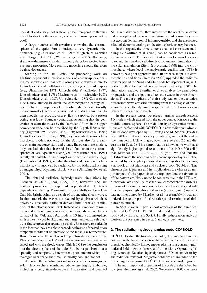
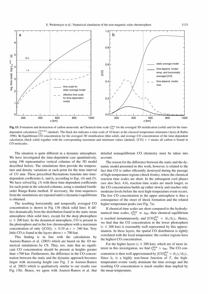
equilibrium CO concentration [CO]eq according to Eq. (6) areplotted as a function of height for the mean temperature anddensity structure of our 3D simulation in Fig. 13 (thin solidlines). tchem

CO varies by orders of magnitude, from ≈0.1 s at

z = 0 km (τ ≈ 1) to >∼106 s at z = 1000 km. This varia-tion is partly due to the temperature dependence of tchem

CO , butmainly due to the density factor. In the lower chromosphere(z >∼ 600 km), [CO] >∼ 0.9, implying that almost all carbon inthe chromosphere is bound in CO.


200 400 600 800 1000z [km]

0

1

2

3

4

5

6

7

log.

tim

e sc

ale

log

t CO

chem

[s

]

10 h

1 h

time scale forstatic average model

effective time scalefor time-dependentmodel

a

200 400 600 800 1000z [km]

0.0

0.2

0.4

0.6

0.8

1.0

[CO

]

static average model

time-depend. model:

temp. and horizontally

averaged [CO]

time-depend. model:

max.

b

Fig. 13. Formation and destruction of carbon monoxide. a) Chemical time scale tchemCO for the averaged 3D stratification (solid) and for the time-

dependent calculation tchem,dynCO (dashed). The black dot indicates a time scale of 10 hours at the classical temperature minimum (Ayres & Rabin

1996). b) Equilibrium CO concentration for the averaged 3D stratification (thin solid), and average CO concentration of the time-dependentcalculation (thick solid) together with the corresponding maximum and minimum values (dashed). [CO] = 1 means all carbon is bound inCO molecules.

The situation is quite different in a dynamic atmosphere.We have investigated the time-dependent case quantitatively,using 196 representative vertical columns of the 3D modeldescribed before. The simulations then provide the tempera-ture and density variations at each point for the time intervalof 151 min. These prescribed fluctuations translate into time-dependent coefficients k1 and k2 according to Eqs. (4) and (5).We have solved Eq. (3) with these time-dependent coefficientsfor each point in the selected columns, using a standard fourth-order Runge-Kutta method. If necessary, the time-sequencesfrom the simulations are repeated until a (dynamic) equilibriumis obtained.

The resulting horizontally and temporally averaged COconcentration is shown in Fig. 13b (thick solid line). It dif-fers dramatically from the distribution found in the static meanatmosphere (thin solid line), except for the deep photosphere(z <∼ 200 km). In the dynamical atmosphere, CO is present inthe photosphere and in the low chromosphere with a maximumconcentration of only 〈[CO]〉t ≈ 0.10 at z ≈ 340 km. Verylittle CO is found in the layers above z ≈ 700 km.

This finding is in line with the calculations byAsensio Ramos et al. (2003) which are based on the 1D nu-merical simulations by CS. They, too, state that no signifi-cant CO concentration should be present at heights greaterthan ≈700 km. Furthermore, the difference in the CO concen-tration between the static and the dynamic approach becomeslarger with increasing height (see Fig. 2 in Asensio Ramoset al. 2003) which is qualitatively similar to our results (seeFig. 13b). Hence, we agree with Asensio Ramos et al. that

detailed nonequilibrium CO chemistry must be taken intoaccount.

The reason for the difference between the static and the dy-namic model presented in this work, however, is related to thefact that CO is rather efficiently destroyed during the passageof high-temperature regions (shock fronts), where the chemicalreaction time scales are short. In the subsequent cool phases(see also Sect. 4.6), reaction time scales are much longer, sothe CO concentration builds up rather slowly and reaches onlymoderate levels before the next high-temperature event occurs.The low CO concentration in the upper atmosphere is thus aconsequence of the onset of shock formation and the relatedhigher temperature peaks (see Fig. 7a).

If chemical time scales are short compared to the hydrody-namical time scales, tchem

CO � tHD, then chemical equilibrium

is reached instantaneously, and [CO]dyneq ≈ 〈k1/k2〉t. Hence,

we find that the CO concentration in the lower photosphere(z <∼ 200 km) is reasonably well represented by this approx-imation. In these layers, the spatial CO distribution is tightlycorrelated with the local temperature: the coolest regions havethe highest CO concentration.

For the higher layers (z >∼ 200 km), which are of more in-terest in this investigation, we find tchem

CO > tHD. The CO con-

centration is then well approximated by [CO]dyneq ≈ 〈k1〉t/〈k2〉t.

Since k2 is a highly non-linear function of T , the high-temperature events vastly dominate the time average and theresulting CO concentration is much smaller than implied bythe mean temperature.


We can also conclude that the dynamical equilib-rium CO concentration is attained on a characteristic time scaletchem,dynCO = 〈k2〉−1

t , which is also shown in Fig. 13a (dashed).The correlation between [CO] and T is expected to be poorin the higher layers: the highest concentrations build up inplaces with the longest history of relatively undisturbed con-ditions ([CO] ≈ 0.4), and almost no CO is found just behindstrong shock fronts.

The results described above can only be a first estimate ofthe height profile of [CO] under time dependent conditions, be-cause the underlying calculations still have severe limitations.More secure conclusions about the CO distribution in the up-per solar atmosphere have to wait for more detailed future sim-ulations taking into account (i) the transport of CO moleculeswith the flow, (ii) a more complete chemical reaction networkincluding multi-step reactions affecting the CO balance (seeAyres & Rabin 1996; Asensio Ramos et al. 2003), and (iii) theback reaction of the CO concentration on the radiative coolingrate.

5. Discussion

Quantitatively, the results presented in the preceding sec-tions must be considered as preliminary, since the physicsof CO5BOLD are not yet properly adapted to chromosphericconditions. In particular, the assumption of LTE is a poorapproximation in the chromosphere (Carlsson & Stein 2002;Rammacher & Ulmschneider 2003). A realistic treatmentshould account for deviations from LTE and also requires thetime-dependent computation of the ionisation of hydrogen andother important species. Nevertheless, we believe that some ofthe basic features seen in our model are insensitive to the de-tailed treatment of thermodynamics and radiative transfer.

The 3D topology of the small-scale chromospheric networkwe discovered in our simulation, and its spatial and temporalscales are expected to be a robust feature. This is confirmedby test calculations with different values of the tensor viscos-ity, a different grey opacity table, and even with a frequency-dependent (multi-group) radiative transfer scheme using fiveopacity bins: the dynamical properties of these models (like theheight-dependent amplitude of the velocity fluctuations) turnout to be quite insusceptible to changes of the analysed numer-ical parameters. We attribute this to the fact that the dynamicsof the model chromosphere are governed by the lower layerswhere the excitation of acoustic waves takes place and that thenumerical modelling of these layers, i.e., the photosphere andthe top of the convection zone, is quite realistic. In this context,it is reassuring to find prominent chromospheric oscillations inthe 3-min range whose properties are largely independent ofthe numerical details of the simulation. The qualitative simi-larity to observations indicates that the dynamics are indeedmodelled reasonably well.

The horizontal structure of our model chromosphere, i.e.,its topology, is reminiscent of observed patterns like the chro-mospheric “background pattern” found by (Krijger et al. 2001)and the structure of Ca H observations (Sutterlin 2003). Thelatter, for instance, exhibits spatial scales which are comparableto the granulation and thus to the scales which are found in our

numerical simulation. However, the observed patterns originatepredominantly from lower layers and should therefore not beconfused with the patterning of the model chromosphere. Thedifferences might be revealed by determining the time scaleson which the different patterns evolve. This issue needs to beinvestigated more properly in the future.

In contrast to the spatial scales and the topology of the at-mospheric patterns, the amplitude of the temperature fluctu-ations in the model chromosphere is more susceptible to thetreatment of radiative transfer. Indeed, the temperature fluctua-tions are significantly smaller in the aforementioned test calcu-lation using a frequency-dependent radiative transfer scheme.However, we recall that, up to the mid-chromospheric layers(z = 1000 km), the peak shock temperatures in our grey sim-ulation are very similar to those found by Carlsson & Stein(1994, 1997) and by Skartlien (1998). More precisely, in thelower and mid chromospheric regions CS find peak tempera-tures which lie only somewhat (∼1000 K) above our values.

The shock peak temperatures are of importance sincemany spectral features are biased towards high temperatures.Theoretically, the peak temperatures depend on the shockstrength and are given by the Rankine-Hugoniot jump con-ditions. In the absence of radiation, a conservative numericalscheme guarantees that the jump conditions are fulfilled, i.e.,the post-shock temperature is independent of the spatial reso-lution. If radiation is important, however, the peak post-shocktemperature is reduced relative to the theoretical value by anamount that depends on the spatial resolution of the numericalgrid. This is because the shock heating is stretched out over afinite time interval, given by the time a volume element needsto cross the shock front which is smeared out over a num-ber of grid points. In this case, radiative cooling can reducethe attainable peak temperature if the radiative cooling time iscomparable or smaller than the time scale of shock heating.Furthermore, the overall energy dissipation in the shock is al-tered due to a change of the effective adiabatic exponent of thegas.

In our model based on grey radiative transfer all chromo-spheric layers are optically thin. Here, radiative cooling timesare independent of the flow geometry and mainly dependent ontemperature. The cooling time at a temperature of 7000 K –about the highest temperature we observe in the simulation –amounts to ∼200 s, and is increasing rapidly for lower tem-peratures. The dissipation time scale in the shocks is in theorder of a few seconds. This means that the thermal struc-ture of our shocks is hardly affected by radiation and primarilygiven by the shock strength. Only in the most extreme caseswe expect some limiting influence of radiative cooling on thepost-shock temperature. Similarly, the thermal structure of thepost-shock regions is mainly controlled by cooling via adia-batic expansion.

As mentioned above, the differences in the peak temper-atures of our model and the simulation by CS become largerin the higher layers. First, CS employ an adaptive grid intheir simulation with a grid spacing of typically 200 m nearshocks which is thus much finer than our fixed (vertical) spac-ing of 12 km. Furthermore, it appears plausible that our radia-tive transfer – based on Rosseland opacities including lines as


true absorption – produces shorter radiative cooling times com-pared to CS. The higher resolution and longer radiative coolingtimes in the model of CS lead us to expect that their shock peaktemperatures are also largely unaffected by radiation.

Two effects can explain the somewhat higher shock temper-atures of CS. First, the shock strength in the CS model mightsimply be higher than in our case. This could be related tothe semi-empirical piston velocity CS feed in at the bottom oftheir model, or their 1D geometry forcing shocks to remainplane-parallel. As we have seen above, extended horizontalshocks are more the exception than the rule in our 3D simula-tion; most shock fronts weaken as they propagate radially awayfrom their source. Another effect is related to our assumptionthat thermodynamic equilibrium conditions prevail in the chro-mosphere. In a recent paper, Carlsson & Stein (2002) demon-strated that this is a poor approximation. Ionisation equilibriacannot follow the rapid thermodynamic changes introduced bythe flow. One consequence is that the energy which is dissi-pated in shocks cannot go into ionisation but has to go intoa temperature increase of the post-shock gas. Moreover, ac-counting for finite recombination time scales instead of assum-ing ionisation equilibrium could reduce the ability of the post-shock gas to cool, thus leading to even higher temperatures.Since CS account for the thermodynamic non-equilibriumeffects, their shock temperatures should be higher.

We cannot decide on the basis of the available informa-tion which is the reason for the differences in the peak tem-peratures of the shocks. However, we conclude that the dif-ferences up to the mid-chromospheric layers (z = 1000 km)are modest: our peak temperatures are ≈7000 K comparedto ≈8000 K in the CS model. We further note that the chromo-spheric peak temperatures found by Skartlien (1998) (see hisFig. 9) are <∼7000 K in their case of frequency-dependent ra-diative transfer accounting for line scattering, which is surpris-ingly close to our result obtained with our grey LTE radiativetransfer.

This supports our conclusion that our grey radiative trans-fer employed in this work is more realistic than the frequency-dependent method available for CO5BOLD. The latter methodstrongly overestimates the (LTE) cooling in the strong spec-tral lines (treated as true absorption) and thus wrongly reducesthe maximum attainable temperatures. However, note that alsothe grey radiative transfer is not appropriate for chromosphericconditions. Rather, a detailed frequency-dependent non-LTEradiative transfer is necessary. Furthermore, for a quantitativecomparison with the observations it would be necessary to per-form three-dimensional spectrum synthesis, which is plannedfor the future.

In contrast to the peak temperatures, the mean chromo-spheric temperature (and also the minimum temperatures) inour simulation are significantly lower than those found by CS(see Fig. 8), and also somewhat cooler than in the Skartlien(1998) model. Obviously, the mean temperature structure ismore strongly influenced by the treatment of radiative trans-fer than it is the case for the peak temperatures. It shouldtherefore be considered as uncertain. Somewhat surprisingly,however, we note that our grey and our frequency-dependent

simulations produce almost identical mean chromospheric tem-perature structures.

Nevertheless, the differences in the average temperaturestratification between the one-dimensional simulation by CSand the presented 3D model can be understood if one watchesthe velocity field of a region which just has been traversed bya strong shock wave. The flows are mostly directed outwardsaway from the centre of such a region. We interpret this as fastand thus adiabatic expansion of the traversed region. This “dy-namic cooling” is obviously more efficient in 3D than 1D sim-ply due to the additional spatial dimensions. This effect thusproduces lower average and minimum temperatures in our sim-ulations compared to those of CS.

Furthermore, we point out that the thermal bifurcation inour 3D model (see Sect. 4.3) is not due to the action of carbonmonoxide as a cooling agent. Rather, it is caused by the acous-tic wave field and the resulting dynamic cooling of adiabati-cally expanding regions as discussed above. Carbon monox-ide is only taken into account in the grey opacity tables so far,and so its real influence is underestimated. A similar simula-tion with a different grey opacity table without molecular con-tributions (based on ATLAS6, Kurucz 1970) leads to very sim-ilar results. We thus conclude that CO plays no active role inour present simulations. On the other hand, the calculations de-scribed in Sect. 4.7 demonstrate that there is a non-negligibleamount of CO present in the lower chromosphere. Hence, afull treatment of CO as a cooling agent might even amplify thethermal bifurcation of the chromosphere (see, e.g., Ayres 1981;Anderson & Athay 1989; Steffen & Muchmore 1988).

Although the mean chromospheric temperature of our sim-ulation lies considerably below the radiative equilibrium tem-perature, we find a net radiative cooling of the chromosphericlayers: 〈∇ · Frad〉t is positive here. This apparent contradictioncan be explained by the presence of sufficiently strong temper-ature fluctuations and the highly non-linear temperature depen-dence of the radiative heating/cooling rates. We do not claim,however, that this situation is actually realized in the solar chro-mosphere.

Our simulations indicate that the wave generation is mainlycontrolled by the large-scale dynamical evolution of the granu-lation pattern (see Sect. 4.2). This is at variance with the classi-cal picture of the Lighthill-Stein theory (Lighthill 1952; Stein1967, 1968) where small-scale turbulent eddies make the maincontribution to the acoustic energy flux. Applying the Lighthill-Stein theory to the Sun, Musielak et al. (1994) find that theacoustic flux spectrum shows a maximum near ν >∼ 15 mHz,and hence is dominated by “short period waves”.

The presented simulation can marginally resolve turbu-lent eddies in the convection zone with wavenumbers upto kmax ≈ 2π/(5∆x). According to the classical theory, ed-dies with wavenumber k mostly contribute to the acoustic wavespectrum at frequency ω = kuk, where uk is the turbulent ve-locity of eddies with wavenumber k. Since uk <∼ 1 km s−1,the simulation cannot describe the turbulence spectrum be-yond ωmax <∼ 30 mHz, νmax <∼ 5 mHz. We conclude thatour present model cannot resolve the small-scale turbulencewhich is responsible for the sound generation in the Lighthill-Stein theory. The acoustic flux resulting from our simulation


decreases monotonically with frequency, and so has little incommon with the spectrum predicted by the Lighthill-Steinspectrum. Hence, it appears doubtful whether the classical the-ory, based on the assumption of isothermal, homogeneous, andisotropic turbulence, captures the essential physics of the vi-olent, highly anisotropic layers at the top of real stellar con-vection zones. We argue that our numerical simulation cor-rectly represents the basic mode of wave generation, even atthe present spatial resolution.

6. Conclusions

Based on a detailed 3D simulation of the solar granulation andthe overlying atmosphere, we have studied the generation ofwaves by the time-dependent convective flow, and the wavepropagation and dissipation in the higher layers. The most im-portant improvements compared to previous numerical simu-lations are (i) self-consistent dynamics without a need for adriving piston like done by CS and (ii) a high spatial resolu-tion which is obviously necessary for modelling the small-scalestructure of the solar chromosphere. On the other hand, theLTE treatment of the thermodynamics and the radiative trans-fer is certainly unrealistic in the chromospheric layers. We havepresented evidence that some of the basic features seen in ourmodel are nevertheless representative of the (non-magnetic) in-ternetwork regions of the solar chromosphere.

The main result of the present investigation is the discov-ery of a complex network of hot filaments pervading the oth-erwise cool chromospheric layers. Caused by interaction ofstanding and propagating hydrodynamic waves of large am-plitude, the model chromosphere is a highly dynamical, spa-tially and temporally intermittent phenomenon. Its tempera-ture structure is characterised by a thermal bifurcation: hot andcool regions co-exist side by side. Temperatures in the hot fil-aments are high enough to produce chromospheric emissionlines, and the cool “bubbles” are cold enough to form molecu-lar features. Thus, the chromosphere is hot and cold at the sametime. This picture of the 3D structure of the solar chromospherehas the potential to explain the apparently contradictory obser-vational diagnostics which cannot be understood in the frame-work of one-dimensional theoretical or semi-empirical models.

The presence of strong spatial and temporal temperaturefluctuations has a remarkable consequence: the temperatureminimum and the outward directed temperature rise inferredfrom semi-empirical models might be artifacts in the sensethat they do not necessarily imply an increase of the aver-age gas temperature with height. Our model suggests that theradiative emission can be sustained by the hot propagatingshock waves even though the main fraction of the chromo-spheric layers is cool and the mean gas temperature profileshows an almost monotonic decrease – a conclusion alreadyreached by Carlsson & Stein (1994, 1995, 1997) on the basisof one-dimensional hydrodynamical simulations.

We conclude that improved 3D radiation hydrodynamicsimulations of the kind presented in this work are likelyto lead the way towards a consistent physical model of thethermal structure and dynamics of the non-magnetic solar

chromosphere which eventually can explain the various obser-vational diagnostics.

Acknowledgements. We are grateful to M. Carlsson, R. F. Stein,M. Wunnenberg, and P. Sutterlin for providing data for comparisonand to R. J. Rutten for advice and critical comments. The numericalsimulations were carried out on the CRAY SV1 of the Rechenzentrumder Universitat Kiel. SW was supported by the Deutsche Forschungs-gemeinschaft (DFG), project Ho596/39. HGL acknowledges financialsupport of the Walter Gyllenberg Foundation (Lund), and the SwedishVetenskapsrådet. BF is supported by a grant from the SwedishSchonbergs Donation.

References

Anderson, L. S., & Athay, R. G. 1989, ApJ, 346, 1010Asensio Ramos, A., Trujillo Bueno, J., Carlsson, M., & Cernicharo, J.

2003, ApJ, 588, L61Asplund, M., Ludwig, H.-G., Nordlund, Å., & Stein, R. F. 2000, A&A,

359, 669Avrett, E. H. 1995, in Infrared Tools for Solar Astrophysics: What’s

Next? Proc. 15th NSO Sac Peak Workshop, ed. J. Kuhn, & M. Penn(Singapore: World Scientific), 303

Ayres, T. R. 1981, ApJ, 244, 1064Ayres, T. R. 2002, ApJ, 575, 1104Ayres, T. R., & Linsky, J. L. 1976, ApJ, 205, 874Ayres, T. R., & Rabin, D. 1996, ApJ, 460, 1042Ayres, T. R., & Testerman, L. 1981, ApJ, 245, 1124Ayres, T. R., Testerman, L., & Brault, J. W. 1986, ApJ, 304, 542Buchholz, B., Ulmschneider, P., & Cuntz, M. 1998, ApJ, 494, 700Carlsson, M., Judge, P. G., & Wilhelm, K. 1997, ApJ, 486, L63Carlsson, M., & Stein, R. F. 1994, in Proc. Mini-Workshop on

Chromospheric Dynamics, ed. M. Carlsson (Oslo: Inst. Theor.Astrophys.), 47

Carlsson, M., & Stein, R. F. 1995, ApJ, 440, L29Carlsson, M., & Stein, R. F. 1997, ApJ, 481, 500Carlsson, M., & Stein, R. F. 2002, ApJ, 572, 626Cuntz, M., Rammacher, W., & Ulmschneider, P. 1994, ApJ, 432, 690Fontenla, J. M., Avrett, E. H., & Loeser, R. 1993, ApJ, 406, 319Freytag, B., Steffen, M., & Dorch, B. 2002, Astron. Nachr., 323, 213Hauschildt, P. H., Baron, E., & Allard, F. 1997, ApJ, 483, 390Iglesias, C. A., Rogers, F. J., & Wilson, B. G. 1992, ApJ, 397, 717Kalkofen, W. 2001, ApJ, 557, 376Krijger, J. M., Rutten, R. J., Lites, B. W., et al. 2001, A&A, 379, 1052Kurucz, R. L. 1970, SAO Special Report, 308Lighthill, M. J. 1952, Proc. R. Soc. Lond., A 211, 564Ludwig, H.-G., Allard, F., & Hauschildt, P. H. 2002, A&A, 395, 99Maltby, P., Avrett, E. H., Carlsson, M., et al. 1986, ApJ, 306, 284Muchmore, D., & Ulmschneider, P. 1985, A&A, 142, 393Muglach, K., & Schmidt, W. 2001, A&A, 379, 592Musielak, Z. E., Rosner, R., Stein, R. F., & Ulmschneider, P. 1994,

ApJ, 423, 474Nordlund, Å., & Stein, R. F. 2001, ApJ, 546, 576Noyes, R. W., & Hall, D. N. B. 1972, BAAS, 4, 389Quirk, J. 1994, Int. J. for Numerical Methods in Fluids, 18, 555Rammacher, W., & Ulmschneider, P. 2003, ApJ, 589, 988Roe, P. L. 1986, Ann. Rev. Fluid Mech., 18, 337Rutten, R. G. M., Schrijver, C. J., Lemmens, A. F. P., & Zwaan, C.

1991, A&A, 252, 203Sutterlin, P. 2003, priv. comm.Schrijver, C. J. 1987, A&A, 172, 111Skartlien, R. 1998, Ph.D. Thesis, University of Oslo, NorwaySkartlien, R. 2000, ApJ, 536, 465


Skartlien, R., Stein, R. F., & Nordlund, Å. 2000, ApJ, 541, 468Solanki, S. K., Livingston, W., & Ayres, T. 1994, Science, 263, 64Steffen, M., & Muchmore, D. 1988, A&A, 193, 281Stein, R. F. 1967, Sol. Phys., 2, 385Stein, R. F. 1968, ApJ, 154, 297Stein, R. F., & Nordlund, A. 1998, ApJ, 499, 914Stein, R. F., & Nordlund, Å. 2001, ApJ, 546, 585Uitenbroek, H. 2000a, ApJ, 531, 571Uitenbroek, H. 2000b, ApJ, 536, 481Uitenbroek, H., Noyes, R. W., & Rabin, D. 1994, ApJ, 432, L67Ulmschneider, P. 1971, A&A, 12, 297Ulmschneider, P. 1989, A&A, 222, 171Ulmschneider, P., Fawzy, D., Musielak, Z. E., & Stepien, K. 2001,

ApJ, 559, L167

Ulmschneider, P., & Kalkofen, W. 1977, A&A, 57, 199Ulmschneider, P., Muchmore, D., & Kalkofen, W. 1987, A&A, 177,

292Ulmschneider, P., Schmitz, F., Kalkofen, W., & Bohn, H. U. 1978,

A&A, 70, 487Ulmschneider, P., Theurer, J., & Musielak, Z. E. 1996, A&A, 315, 212Ulmschneider, P., Theurer, J., Musielak, Z. E., & Kurucz, R. 1999,

A&A, 347, 243Vernazza, J. E., Avrett, E. H., & Loeser, R. 1981, ApJS, 45, 635Wedemeyer, S. 2003, Ph.D. Thesis, University of Kiel,http://e-diss.uni-kiel.de/diss 764/

Wiedemann, G., Ayres, T. R., Jennings, D. E., & Saar, S. H. 1994,ApJ, 423, 806

Wunnenberg, M., Kneer, F., & Hirzberger, J. 2002, A&A, 395, L51

numerical simulation of the three-dimensional structure and

Documents