numerical simulation of radiative heat transfer

American Institute of Aeronautics and Astronautics

1

Numerical Simulation of Radiative Heat Transfer

Babila Ramamoorthy1, Roy P. Koomullil2, Gary Cheng3 Department of Mechanical Engineering

University of Alabama at Birmingham, Birmingham, AL 35294-4461

Radiative heat transfer is an important physical phenomenon especially in the high speed and high temperature flow regime making its application important in space exploration vehicles. This paper presents the development and validation of computational tools for modeling the radiative heat transfer with an aim that the developed numerical module can be either employed by itself or coupled with a computational fluid dynamics solver to analyze aerothermodynamics environment of space exploration vehicles. A generalized grid based finite volume method is used for solving the radiative heat transfer equation. Solution of the radiative heat transfer equations in angular domain is carried out in a parallel environment. This numerical approach is validated with different benchmark test cases for gray gas radiation in irregular geometries. To enable the simulation of non-gray gas radiation, the full spectrum correlated-k model is implemented. A grid sensitivity study is conducted to analyze the dependency of mesh resolution on solution accuracy. The results of the validation studies, grid sensitivity studies, and parallel performance of the implementation are presented in this paper.

Nomenclature f = fractional Planck function g = equivalent Planck function gref = reference equivalent Planck function I = intensity of radiation Ib = black body intensity Ibη = blackbody intensity at wave number, η Ig = intensity at equivalent Planck function, g Il,f = intensity associated with the direction, ‘l ’at the face of the control volume Il,P = intensity at the control volume in the direction, ‘l ’ Il,e , Il,w Il,n , Il,s

= intensities associated with the direction, ‘l’ corresponding to east, west, north and south faces of a spatial mesh, respectively

Jf = geometric factor k = absorption coefficient M = number of control angles Nθ = number of control angle divisions in polar direction Nφ = number of control angle divisions in azimuthal direction

p = species partial pressure q = non-dimensionalized radiative heat flux q ′′ = heat flux at the wall r = position vector s = coordinate along the ray s = direction vector S = source term Sm = modified source term

1 Graduate Student, Dept. of Mechanical Eng., E-mail: [email protected], AIAA Student Member. 2 Associate Professor, Dept. of Mechanical Eng., E-mail: [email protected], AIAA Senior Member. 3 Associate Professor, Dept. of Mechanical Eng., E-mail: [email protected], AIAA Senior Member.

47th AIAA Aerospace Sciences Meeting Including The New Horizons Forum and Aerospace Exposition5 - 8 January 2009, Orlando, Florida

AIAA 2009-671

Copyright © 2009 by the American Institute of Aeronautics and Astronautics, Inc. All rights reserved.


2

T = temperature, K Tm = medium temperature, K Tref = reference temperature, K x = species mole fraction u = scaling function ΔV0 = volume of the control volume βm = modified extinction coefficient θ = polar angle subtended by the centroid of the solid control angle κ = raw absorption coefficient σ = Stefan-Boltzmann constant σs = scattering coefficient η = wave number φ = scattering phase function Ω′ = control angle direction

ll′φ = average scattering phase function from a control angle l′ to control angle l ϕ = azimuthal angle subtended by the centroid of the solid control angle ωl = solid angle corresponds to direction ‘l’

I. Introduction ADIATION is an important mode of heat transfer which has wide range of applications from combustion to aerodynamic heating of atmospheric re-entry vehicles. The radiative heat transfer is a function of fourth power

of the temperature, and thus is an important aspect to be accounted for in the high temperature flow environment. Numerical simulation of radiative heat transfer is a promising approach and can be a more practical alternative compared to the experimental and analytical methods of predicting radiative heat transfer. Extensive literature research has been done in the numerical simulation of radiative heat transfer, and several methodologies have been explored in this area1-5. This paper presents a generalized-grid based Finite Volume Method (FVM) for predicting gray gas radiative heat transfer and a global model (Full Spectrum Correlated-k model6,7,) adapted to the FVM framework to enable the prediction of non-gray gas radiation. The aim of this development is to build a framework for predicting non-equilibrium radiation by coupling the radiative solver with Computational Fluid Dynamics (CFD) solver. This development would enable the study of non-equilibrium radiation taking into account of the changes in the flow properties and species concentration which will be particularly helpful in handling most of the practical radiation problems.

II. Numerical Approach This section discusses A) the numerical approach employed in the developed radiative solver (RAD-FVM), B) the

FVM approach for solving the Radiative Transport Equation (RTE), and C) the FSCK method to account for the spectral integration of the RTE. Section B explains the radiation solver module which is based on the FVM for generalized grids. Section C explains the spectral integration module. Presently, a global model (FSCK) is implemented to perform this task. Though the radiation solver module and the spectral integration module work in an integrated fashion, they are represented as two different modules in this paper for the sake of clarity.

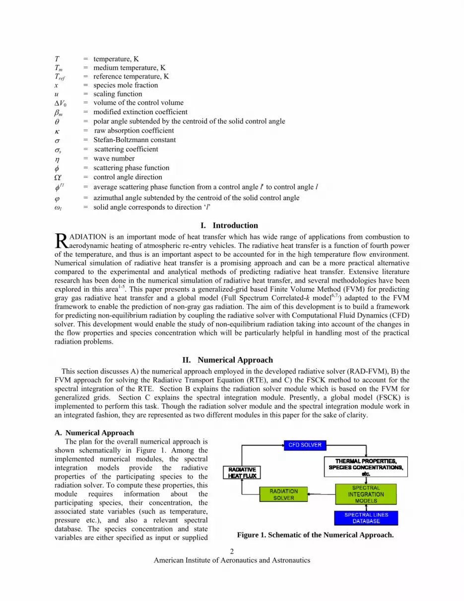
A. Numerical Approach The plan for the overall numerical approach is

shown schematically in Figure 1. Among the implemented numerical modules, the spectral integration models provide the radiative properties of the participating species to the radiation solver. To compute these properties, this module requires information about the participating species, their concentration, the associated state variables (such as temperature, pressure etc.), and also a relevant spectral database. The species concentration and state variables are either specified as input or supplied

R

Figure 1. Schematic of the Numerical Approach.


3

by the CFD solver. On obtaining the radiative properties from the spectral models, the radiation solver module computes the radiative heat transfer and feeds this information to the CFD solver. The CFD solver then updates the state variables and the species concentration information. This schematic explains the overall approach in terms of the input/output to the radiative heat transfer computation. There can be other modules required to be added to this loop based on the specific application. For example, the re-entry application requires a surface ablation module to be added to this approach.

B. Finite Volume Method for Non Equilibrium Radiative Heat Transfer Using Generalized Grids The popular approaches to compute radiative heat transfer like the zonal method, Monte Carlo simulations, and

Spherical Harmonics Method (SHM) are either computationally expensive or very complex for large applications. The FVM and Discrete Ordinates Method (DOM) provide a good compromise between computational cost and accuracy9-11. Also, the radiation problems are often solved by coupling with the flow field solvers using CFD for many applications. In such cases, FVM and DOM methods have the advantage of sharing the same spatial mesh with CFD solvers. But the DOM suffers from the disadvantage of the ‘ray’ effect due to its restriction in angular grid discretization. FVM does not pose any restriction on the angular grid discretization and allows for the ray effect to be addressed appropriately. FVM shares the conservation principle (of radiant energy) as in CFD flow solvers and the method of applying boundary conditions is also the same as that in CFD. A discussion on the generalized grid based finite volume method radiative solver (RAD-FVM) and validation of the solver using test cases with irregular geometries are presented in this paper. A more extensive discussion and validation of this method has been reported previously1,12. A small description of the RAD-FVM solver is presented here from Ref. 12.

The RTE that governs the radiation in a direction s can be written as1,

( ) ( ) ( )[ ] ( ) ( )srSsrIrrkds

srIds ˆ,ˆˆ,ˆˆˆˆ,ˆ

++−= σ (1)

where I is the intensity of radiation, s is the coordinate along the ray, k is the absorption coefficient, σs is the scattering coefficient, r is the position vector, and s is the direction vector. ( )srS ˆ,ˆ is the source term given by ( ) ( ) ( ) ( ) ( ) ( )∫ Ω+=

πφ

πσ

4'ˆ,'ˆ'ˆ,ˆ

4ˆˆˆˆ,ˆ dsssrIrrIrksrS s

b (2)

where Ib is the black body radiation intensity, φ is the scattering phase function, and Ω′ is the variable for control angle direction. This equation needs to be solved for each gray gas in the gas mixture. Also, this equation needs to be integrated over the spatial as well as the angular domain. In the finite volume discretization practice, spatial discretization is done by dividing the spatial domain into discrete control volumes or cells. The angular discretization is done using control angles as defined by Ref. 4. Both the control volumes and control angles can be discretized in any manner per the user requirements, which is the main advantage of this method. A radiation direction vector s , defined in terms of two angles in a three dimensional space, is shown in Figure 2.

Figure 2. A radiation direction vector defined in terms of polar and azimuthal angle.


4

The radiation direction varies within a control angle, whereas the magnitude of intensity is assumed constant in the control angle6. The angles (θ and ϕ) shown in Figure 2 are the polar and azimuthal angles subtended by the centroid of the solid control angle.

The RTE is integrated over a control volume and a control angle associated with each discrete direction. For each discrete direction l, Eq. (1) is integrated over the control volume and the solid angle corresponding to the l direction, ωl, to yield14

0,, ])([ VSIkIJ llPls

fflf Δ++−=∑ ωσ (3)

where flI ,: intensity associated with the direction ‘l’ at the face ‘f ’of the control volume,

PlI , : intensity at the cell centre of the control volume along the direction, ‘l’

PVΔ : volume of the control volume :fJ geometric factor

A more detailed discussion on the numerical approach employed by RAD-FVM can be found in Refs. 14, 15. The intensity at the cell faces can be constructed using step or exponential schemes. To relate the boundary intensity at the face of a control volume

flI , to nodal intensity

PlI ,, the step scheme equates the upstream nodal intensity, l

uI

to the boundary intensity ( lufl II =, ), i.e.

SlslWlwlPlnlPlel IIIIIIII ,,,,,,,, ;;; ==== (4)

where the notation of subscripts are schematically shown in Fig. 3. The exponential scheme is a higher-order spatial scheme that takes into account the exponential decay of the radiative intensity along the optical path in the cell, where the intensity at the cell face in the direction of l (Il,,f) can be calculated in terms of the intensity at the upstream face ( l

uI ), which can be expressed as

( )luPm

luPm d

m

mdlufl eSeII )()(

, 1 ββ

β−− −⎟⎟

⎠

⎞⎜⎜⎝

⎛+= (5)

where the modified extinction coefficient (βm) and the modified source term (Sm) can be expanded as ∑

≠′=′

′′′′′ ΔΩΦ+=ΔΩΦ−+=M

lll

llllsbm

lllssm IIkSk

,14;

4)(

πσ

πσσβ (6)

(a) Step scheme (b) Exponential scheme

Figure 3. Illustration of spatial schemes for interpolating radiative intensity. The discretization procedure explained above leads to a set of equations relating the intensity values at a cell

center to its neighboring cells. In the present solver, the matrix system resulting from the linearization of the governing equations can be solved using the Gauss-Seidel method, under-relaxation method or dynamic under-relaxation method. The radiation solver, RAD-FVM, has been validated with some bench mark test cases1, 12, which shows that the solutions of RAD-FVM agree better with the analytical results than the corresponding DOM solutions1.


5

C. Full Spectrum Correlated-k model The FSCK method6,7 is a global model based on reordering of the k-distribution of the full spectrum. This model

essentially extends the correlated-k model to the full spectrum. The re-ordering is based on the idea that inside a small enough spectral interval, where the Planck function can be assumed a constant, the frequency (or wave number η) of the spectral line is not an important factor. The model uses the scaling approximation (i.e. spectral and spatial dependence of absorption coefficient are independent of each other), which can be written as6, ( ) ( )xpTukxpT ,,)(,,, ηηκ ηη = (7) where

κη is the raw absorption coefficient kη is the spectrally dependent absorption coefficient u is the scaling function T is the temperature p is the species partial pressure x is the species mole fraction

when this scaling approximation is introduced in the RTE and the non-gray gas is represented by a mixture of gray gases, the resulting RTE is as follows6,

( ) ( ) ( ) .10,,4

][)()(4

''' ≤≤+−−= ∫ gdsssIIIaIsugksdId

gs

gsgbg

π

φφπσσ (8)

where

( )( )

( )( )

( )( ) ( )refref

refrefb

b

refg gTkgk

kTfkTf

kTfI

dkkIa

kTf

dkkII ,)(;

,,

,;

,00 ==

−=

−= ∫∫

∞∞ηδηδ ηηηη (9)

are determined at some reference g (equivalent Planck function) and T. This modified RTE is solved for a few gray gases with corresponding k(g). The total radiative intensity is

obtained by a numerical quadrature over Ig. The FSCK model is claimed to be very efficient within the assumptions of a global model (gray walls, gray scattering) and scaling approximation. Also it has been shown that the WSGG model is only an approximation of the FSCK model by Modest6. More details on this model have been thoroughly discussed in various papers by Modest and his group6,7.

III. Validation Test Cases Several test cases were used to validate the developed radiation solver and the implemented FSCK model. The

results obtained from the validation study are detailed in the following section.

A. Validation of Finite Volume Method based RTE Solver (RAD-FVM) An extensive validation of the RAD-FVM solver along with grid sensitivity study has been presented in Refs. 1

and 12. In this paper, further validation of RAD-FVM in handling irregular geometries is discussed.

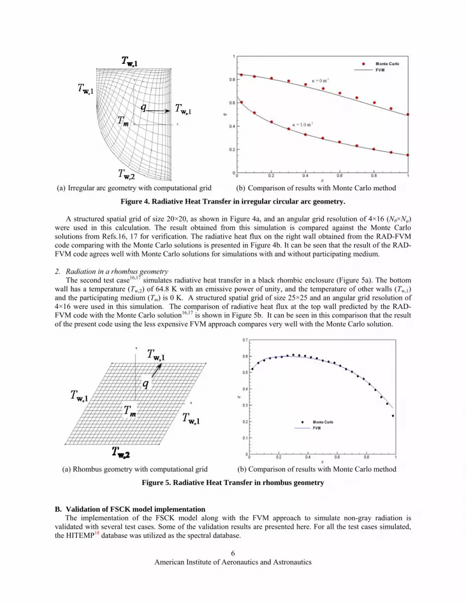
1. Radiation in a circular arc geometry The geometry for the first test case16,17 consists of a rectangle on top of a circular arc as shown in Figure 4a. The

curved wall is maintained at a higher temperature with a non-dimensional emissive power of unity. All the other walls are cold and black. This test case was simulated for two conditions,

i) in the absence of a participating medium ii) in the presence of a participating medium with an absorption coefficient, k = 1 m-1.


6

(a) Irregular arc geometry with computational grid

(b) Comparison of results with Monte Carlo method

Figure 4. Radiative Heat Transfer in irregular circular arc geometry.

A structured spatial grid of size 20×20, as shown in Figure 4a, and an angular grid resolution of 4×16 (Nθ×Nφ) were used in this calculation. The result obtained from this simulation is compared against the Monte Carlo solutions from Refs.16, 17 for verification. The radiative heat flux on the right wall obtained from the RAD-FVM code comparing with the Monte Carlo solutions is presented in Figure 4b. It can be seen that the result of the RAD-FVM code agrees well with Monte Carlo solutions for simulations with and without participating medium.

2. Radiation in a rhombus geometry

The second test case16,17 simulates radiative heat transfer in a black rhombic enclosure (Figure 5a). The bottom wall has a temperature (Tw,2) of 64.8 K with an emissive power of unity, and the temperature of other walls (Tw,1) and the participating medium (Tm) is 0 K. A structured spatial grid of size 25×25 and an angular grid resolution of 4×16 were used in this simulation. The comparison of radiative heat flux at the top wall predicted by the RAD-FVM code with the Monte Carlo solution16,17 is shown in Figure 5b. It can be seen in this comparison that the result of the present code using the less expensive FVM approach compares very well with the Monte Carlo solution.

(a) Rhombus geometry with computational grid (b) Comparison of results with Monte Carlo method

Figure 5. Radiative Heat Transfer in rhombus geometry

B. Validation of FSCK model implementation The implementation of the FSCK model along with the FVM approach to simulate non-gray radiation is

validated with several test cases. Some of the validation results are presented here. For all the test cases simulated, the HITEMP18 database was utilized as the spectral database.


7

1. Isothermal Homogeneous Test Case

The first test case7 considered for this study is under isothermal and homogeneous conditions. It is claimed that the only approximation made in the FSCK model is the use of scaling assumption under non-isothermal and inhomogeneous conditions6,7. So, for a homogeneous and isothermal test case, the FSCK model should produce accurate results. To verify this claim, the FSCK model implementation was tested with this isothermal and homogeneous test case. In this test case, a layer of 10% CO2 and 90% N2 gas is trapped between two black, parallel plates at a temperature (Tm) of 1500 K. Two plates are maintained at 0 K and are separated with a distance of L. This test case was simulated with two spatial grid resolutions of 40 and 80 cells between the plates and two angular grid resolutions of 4×16 and 4×32 (Nθ×Nφ) to study grid sensitivity. The numerical results are verified by comparing with the line-by-line calculations7. The divergence of radiative heat flux as a function of the distance between the plates for L = 1 m is demonstrated in the Figure 6a. The variation of local heat flux between the plates is plotted in Figure 6b. To examine the effect of optical thickness, the numerical study was also repeated for L = 1 cm. The result of this case is plotted in Figures 6c and 6d. It can be clearly observed that 1) for isothermal and homogeneous conditions the results predicted by the FSCK model with the FVM framework agree well with the line-by-line solutions, 2) the numerical results are almost independent of the spatial and angular grid resolutions, and 3) for the optically thin case there are some discrepancies between the present model and the line-by-line solution near the plates. This discrepancy may be attributed to the non-isothermal effect near the plate, where larger temperature gradient with respect to the width between the plates (L = 1 cm) leads to larger discrepancy.

(a) Divergence of heat flux (L = 1 m) (b) Local heat flux (L = 1 m)

(c) Divergence of heat flux (L = 1 cm) (d) Local heat flux (L = 1 cm)

Figure 6. Non-gray gas radiation in isothermal and homogeneous conditions


8

2. Non-isothermal and homogeneous test case The capability of the FSCK model to simulate non-isothermal conditions is validated here. In this test case7, two adjacent layers of a gas mixture (10% CO2 and 90% N2) maintained at different temperatures between two parallel plates is illustrated in Figure 7a. The hot gas layer is at a temperature (Thot) of 1500 K with a width of Lhot from one plate, and the cold gas layer is at a temperature (Tcold) of 500 K with a width of Lcold from the other plate. The plates are considered black and maintained at a temperature (Tw) of 300 K. This test case is simulated under three different hot and cold layer thicknesses as listed below.

Case #1: Lhot = 50 cm and Lcold = 25 cm Case #2: Lhot = 50 cm and Lcold = 50 cm Case #3: Lhot = 50 cm and Lcold = 150 cm This is a difficult condition to simulate due to the abrupt and high temperature gradient of 1000 K in terms of

scaling the absorption coefficient. This case is thus employed to test the scaling approximation used in the FSCK model. A grid convergence study was also performed for all three conditions. A spatial grid resolution of 40 cells distributed uniformly between two plates and a 4×16 angular grid resolution were used as the baseline mesh. The baseline mesh was refined to have either a uniform spatial grid resolution of 80 cells, or a 4×32 angular grid resolution.

The result of Case #1 is shown in Figure 7b. It can be seen that the divergence of heat flux in the hot temperature layer is slightly over-predicted comparing to the Line-by-Line (LBL) solution7. But the prediction of divergence of heat flux at the cold layer matches well with the LBL result. In addition, the jump of heat flux gradients at the interface between the hot and cold layers was not well captured. This may be due to the fact that a discontinuity in temperature at this region leads to large heat flux gradients. It should be noted that in this simulation 10 quadrature points have been used in the FSCK model with the Gauss-Legendre quadrature scheme. Figure 7c shows the result of Case #2. It can be seen that the predicted results match well with the LBL solution, except at the hot and cold gas interface. For this case, the Gauss-Jacobi quadrature scheme with 15 quadrature points was used in the FSCK model. For Case #3, the result is shown in Figure 7d. Similar to other cases, the Gauss-Legendre scheme with 10 quadrature points was initially used in the FSCK model. As can be seen in Figure 7d, the predicted divergence of heat flux is higher in the hot gas layer region comparing to the LBL results. As discussed earlier, in the FSCK model the non-gray gas is represented by a set of gray gases with the absorption coefficient values being selected from the quadrature points in the k vs. g distribution. Hence, the number of quadrature points and the quadrature scheme used can be an important factor contributing to the accuracy of the numerical results. Based on this, the number of quadrature points was increased to 30 points to examine its effect. It can be seen from Figure 7d that the increase of quadrature points led to improved accuracy, especially in the hot gas region. However, very large heat flux gradients were predicted at the interface of hot and cold gases when the number of quadrature points was increased. In addition, as the number of spatial grid points increases, the magnitude of the predicted heat flux gradients increases.

(a) Schematic of non-isothermal and homogeneous case (b) Divergence of radiative heat flux (Lcold = 25 cm)


9

(c) Divergence of radiative heat flux (Lcold = 50 cm) (d) Divergence of radiative heat flux (Lcold = 150 cm)

Figure 7. Non-gray gas radiation in non-isothermal and homogeneous conditions 3. Non-isothermal Parabolic Temperature Profile

In this test case, 10% CO2 gas is contained between two parallel plates with a parabolic temperature profile19. The temperature distribution (T) can be expressed as

( )2

12⎟⎠⎞

⎜⎝⎛ −−−=

LxTTTT wcc

(10)

where Tc is the temperature at the mid-point between two plates, Tw (= 500 K) is the plate (wall) temperature, x is the distance from the bottom plate, and L (= 1 m) is the distance between the two plates. Two different temperature distributions with Tc = 1000 K and Tc = 1500 K were studied. This test case represents realistic scenarios such as combustion applications where the temperature varies gradually over a small interval. For this test case, a spatial mesh resolution of 60 points was used to discretize the gas layer between the plates, and 15 quadrature points were used in the FSCK model.

The results of the case Tc = 1000 K are plotted in Fig. 8a. It can be seen that the predicted divergence of heat flux matches well with the LBL calculations19. In this simulation, the Planck Mean Temperature (= 850 K) is used as the reference temperature for the calculation of the scaling function. The results of the case Tc = 1500 K are plotted in Fig. 8b. It can be seen that for the case of larger temperature gradients there is a notable discrepancy between the result of the present numerical model and the LBL calculations. In this simulation, the Planck Mean Temperature (= 1205 K) was used as the reference temperature. The reasons for this discrepancy may be due to

i. an inadequate number of quadrature points (15) used to represent the k-distribution, ii. an inadequate spatial mesh resolution (60 points to represent the temperature distribution).

This test case requires further study to examine those two effects mentioned above and the effect of reference temperature used.


10

(a) Divergence of radiative heat flux (Tc = 1000 K) (b) Divergence of radiative heat flux (Tc = 1500 K)

Figure 8. Non-gray gas radiation in parabolic temperature distribution

IV. Parallel Performance To improve the computational speed of the radiative solver and to simulate practical problems of interest in a

reasonable time frame, domain decomposition and parallel algorithm implementation is needed. The present solution methodology for the calculations of radiative heat transfer leads to three types of domain decomposition for a parallel algorithm, namely, spatial, angular and frequency domain decomposition. The details of different types of domain decompositions and their comparative advantages as well as performance have been discussed in literature20,21. The conventional spatial domain decomposition methodology adopted in most CFD solvers can be used in the FVM based radiative solver also. Advantages of this approach include

i) Real-time problems with large number of spatial grids can be handled efficiently, ii) A common domain decomposition algorithm for both CFD and radiative solver can be adopted. However, the present solution methodology of simulating the radiative heat transfer process naturally lends itself

to the angular domain based decomposition in an efficient manner. But the use of angular domain decomposition alone can not resolve the restriction of the spatial grid size based on the available computer resources. Also, this type of decomposition is applicable only to the radiative solver, which makes the integration of radiation solvers with CFD solvers difficult. A comparison of the spatial and angular domain based decomposition is summarized in Table 1. In the current radiative solver, angular domain based decomposition was implemented to test its computational performance.

Table 1. Comparitive merits and demerits of domain decomposition methodologies

Domain Decomposition Methodology

Implementation Speed up Ability to handle large problems

Integration with CFD solvers

Spatial Domain Decomposition Complicated

Reasonable speed-up depending on the

efficiency of the algorithm Good

Easy / Common decomposition

algorithm can be adopted

Angular Domain Decomposition

Relatively simple

Close to linear speed-up is achievable

Restricted based on the available

computational resources

Difficult / Different from the CFD

domain decomposition

In the current implementation of the angular domain decomposition algorithm, the total number of angular

meshes, Nθ × Nφ is equally divided among the number of computer processors. Each processor computes the total


11

heat flux from all the directions corresponding to the angles assigned to it, and sends the result to the master processor using an MPI non-blocking SEND or MPI REDUCE routine. A schematic of this algorithm is presented in Figure 9.

Figure 9. Angular Domain based parallel decomposition algorithm

The performance of this parallel algorithm is verified for a cubical black enclosure with a gray participating

medium. Details of this test case can be found in Ref. 22. To study the parallel performance, a spatial grid of 15×15×15 and an angular grid of 8×12 is used. If the time required for this test case in a serial run is ts and the time taken by parallel computing using the number of processors of np is tnp, then speed up is defined as ts/tnp. It was verified for all the simulations that the results from a serial run is repeated in all the parallel computations. A plot of speed up vs. number of processors for this test case is shown in Figure 10. It can be seen from this figure that for the given test case good speed up characteristics (up to 80% speed-up with 12 processors) can be obtained by the parallel algorithm based on angular domain decomposition.

Figure 10. Speed up vs no. of processors (parallel performance)


12

V. Conclusion and Future Work Validations of a FVM based radiation solver (RAD-FVM) for handling irregular geometries are presented. It is

found that the solver has good numerical accuracy in handling problems of irregular geometries. The FSCK model was implemented to perform spectral integration and approximate the radiative property of the non-gray gas. Integration of the RAD-FVM code with the FSCK model to simulate non-gray gas radiation was validated with some test cases. The result shows that the developed radiation framework can accurately simulate non-gray gas radiation under homogeneous and isothermal conditions. However, the numerical accuracy of simulating non-gray gas radiation under non-isothermal conditions is not satisfactory, and needs further improvement. From this study, it can be concluded that increase in the spatial and angular grid resolution slightly improves the accuracy of the numerical results. However, for non-isothermal conditions, increasing the number of quadrature points contributed to a significant improvement of numerical accuracy, over spatial and angular grid resolutions. Use of other quadrature schemes best suited for representing the k-distribution with more quadrature points might improve the accuracy of the results further. For example, the Gaussian quadrature of moments is considered to be best suited to represent the k-distribution for some cases7. The implementation of an angular domain based parallel algorithm into the RAD-FVM code was performed and evaluated. The result shows that this parallel algorithm can achieve good computational speed up.

As discussed before, the goal of this development is to attain the capability to simulate radiative heat transfer in high speed flows, especially re-entry vehicle applications. To achieve this goal, the capabilities of the radiative solver have to be further expanded and improved. Future research efforts would include: 1) introducing the capability to simulate scattering in the RAD-FVM solver, 2) further validation of the code accuracy in simulating non-gray gas radiation under inhomogeneous and non-isothermal conditions, 3) studying the effect of different choices of the reference condition for the non-gray gas under non-isothermal conditions, 4) conducting grid sensitivity study of grid clustering and the number of quadrature points used in the FSCK model, and 5) exploring and acquiring the high-temperature databases of radiative properties. Calculations of the spectral absorption coefficient have to be improved to suit the high temperature applications, (such as implementation of voight profile computations etc.). More sophisticated spectral integration model can be implemented (eg. multi-group FSCK) to handle high-temperature applications where the hot lines in the spectrum become important. To efficiently simulate problems with large number of spatial grids and to facilitate integration with CFD solvers, a spatial domain based parallel algorithm has to be implemented.

Acknowledgments This work is partially funded under NASA CUIP program (NCC3-994). The authors would like to acknowledge

NASA sponsorship and NASA researchers’ technical guidance in this development. Dr. Peter Walsh at UAB provided guidance in understanding the spectral properties of radiative heat transfer. The authors wish to express their sincere thanks to Dr. Modest and his group at the Penn State University for their help in understanding the FSCK model. Also, the authors wish to acknowledge the help from Ertan Karaismail, West Virginia University, for all the help and support to understand the spectral properties of radiative heat transfer.

References

1 Rahmani, R. K., Koomullil, R. P., Cheng, G., and Ayasoufi, A., “Finite Volume Method for Non-Equilibrium Radiative Heat Transfer Using Generalized Grid”, AIAA Paper-2006-3782, 9th AIAA/ASME Joint Thermophysics and Heat Transfer Conference, San Francisco, CA. 5-8, June 2006. 2 Wong, B. T., and Mengϋc* M.P., “Monte Carlo Methods in Radiative Transfer and Electron Beam Processing”, Journal of Quantitative Spectroscopy and Radiative Transfer, 84, pp.437-450, 2004. 3 Modest, M.F., Radiative Heat Transfer, McGraw Hill, Inc., 1993. 4 Chai, J.C., Lee H.S., and Patankar S.V., “Finite Volume Method for Radiation Heat Transfer”, Journal of Thermophysics and Heat Transfer, Vol. 8, No 3, pp 419-425, July-Sept. 1994. 5 Fiveland, W.A., “Discrete-Ordinates Solutions of the Radiation Transport Equation for Rectangular Enclosures”, Journal of Heat Transfer, Vol. 106, pp.699-706, 1984. 6 Modest, M.F., and Zhang, H.,The Full-Spectrum correlated-k distribution for Thermal Radiation from molecular gas-particulate mixtures”, Journal of Heat Transfer, Vol. 124, Feb 2002. 7 Mazumdar, S., and Modest, M.F., “Application of the full spectrum correlated-k distribution approach to modeling non-gray radiation in combustion gases”, Combustion and Flame, Vol. 129, no. 4, pp. 416-438, 2002


13

8 Raithby, G.D., “Discussion of the Finite Volume Method for Radiation, and its Application Using 3D Unstructured Meshes”, Numerical Heat Transfer, Part B, Vol. 35, pp.389-405, 1999. 9 Joseph, D., El Hafi, M., Fournier, R., and Cuenot, B., “Comparison of three spatial differencing schemes in discrete ordinates method using three-dimensional unstructured meshes”, International Journal of Thermal Sciences, Vol. 44, pp. 851-864, 2005. 10 Chai, J. C., Lee, H. S., and Patankar, S. V., ‘‘Ray Effect and False Scattering in the Discrete Ordinates Method,’’ Numerical Heat Transfer, Part B, 24(2), pp. 373–389, 1993. 11 Raithby, G.D., and Chui, E.H., “A Finite-Volume Method for Predicting a Radiant Heat Transfer in Enclosures with Participating Media”, Journal of Heat Transfer, Vol. 112, pp. 415-423, 1990. 12 Ramamoorthy, B., Koomullil, R.P., Cheng, G., and Rahmani,R.K., “Computational Tools for Re-Entry Aerothermodynamics : Part 1 – Non Equilibrium Radiation”, AIAA Paper-2008-1271, 46th AIAA Aerospace Sciences Meeting and Exhibit, Reno, NV 13 Chui, E.H., and Raithby, G.D., “Computation of Radiant Heat transfer on a Non-Orthogonal Mesh using the Finite Volume Method”, Numerical Heat Transfer, Vol. 23, Part B, pp.269-288, 1993. 14 Murthy, J.Y., and Mathur, S.R., “Finite Volume Method for the Radiative Heat Transfer Using Unstructured Meshes”, Journal of Thermophysics and Heat Transfer, Vol. 12, pp.313-321, 1998. 15 Rahmani R. K., Ramamoorthy B., “FVM 3D User’s Guide” Department of Mechanical Eng., University of Alabama at Birmingham, October 2006. 16 Chai, J.C., Lee, H.S., and Pathankar, S.V., “Finite Volume Radiative Heat Transfer Procedure for Irregular Geometries”, Journal of Thermophysics and Heat Transfer, Vol. 9(3), pp.410-415, 1995. 17 Parthasarathy, G., Lee, H.S., Chai, J.C., and Patankar, S.V., “Monte Carlo solutions for radiative heat transfer in irregular two-dimensional geometries”, Journal of Heat Transfer, Vol. 117, pp.792-794, August 1995. 18 Rothman, L.S., et al., “The HITRAN 2004 Molecular Spectroscopic Database,” Journal of Quantitative Spectroscopy and Radiative Transfer, Vol. 96, pp.139-204, 2005. 19 Zhang, H., “Radiative Properties and Radiative Heat Transfer Calculations for High Temperature Combustion Gases”, Ph D. Thesis, Pennsylvania State University, 2002. 20 Liu, J., Shang, M., and Chen, Y.S., “Parallel simulation of radiative heat transfer using an unstructured finite volume method”, Numerical Heat Transfer, Part B, Vol. 36, pp. 115-137, 1999. 21 Novo, P.J., “Parallelization of the Discrete Transfer Method”, Numerical Heat Transfer, Part B, Vol. 35, pp.137-161, 1999 22 Kim, Seung H., and Huh, Kang Y.,“Assessment of the FInite-Volume Method and the Discrete Ordinates Method for radiative heat transfer in a three-dimensional rectangular enclosure”, Numerical Heat Transfer, Part B, Vol. 35, pp. 85-112, 1999.

numerical simulation of radiative heat transfer

Documents