Applied Mathematics and Computation 217 (2011) 5404–5415

Contents lists available at ScienceDirect

Applied Mathematics and Computation

journal homepage: www.elsevier .com/ locate /amc

Numerical solution of two-dimensional reaction–diffusionBrusselator system

R.C. Mittal ⇑, Ram JiwariDepartment of Mathematics, Indian Institute of Technology Roorkee, Roorkee-247667, Uttarakhand, India

a r t i c l e i n f o

Keywords:Reaction–diffusion Brusselator systemDifferential quadrature methodSystem of ordinary differential equationsRunge–Kutta Method

0096-3003/$ - see front matter � 2010 Published bdoi:10.1016/j.amc.2010.12.010

⇑ Corresponding author.E-mail address: rcmmmfa@iitr.ernet.in (R.C. Mit

a b s t r a c t

In this paper, polynomial based differential quadrature method (DQM) is applied for thenumerical solution of a class of two-dimensional initial-boundary value problemsgoverned by a non-linear system of partial differential equations. The system is knownas the reaction–diffusion Brusselator system. The system arises in the modeling of certainchemical reaction–diffusion processes. In Brusselator system the reaction terms arise fromthe mathematical modeling of chemical systems such as in enzymatic reactions, and inplasma and laser physics in multiple coupling between modes. The numerical resultsreported for three specific problems. Convergence and stability of the method is also exam-ined numerically.

� 2010 Published by Elsevier Inc.

1. Introduction

The problem of dealing with chemical reactions of systems involving two variable intermediates, together witha number of initial and final products whose concentrations are assumed to be controlled throughout the reaction processis an important one under quite realistic conditions and is discussed by Nicolis and Prigogine in [1]. It is necessary to con-sider at least a cubic nonlinearity in the rate equations [2]. This model has been referred to as the trimolecular model or Brus-selator [3]. The two-dimensional reaction–diffusion Brusselator system is the non-linear system of partial differentialequations

@u@t¼ Bþ u2v � ðAþ 1Þuþ a

@2u@x2 þ

@2u@y2

!; 0 < x; y < L; ð1Þ

@v@t¼ Au� u2v þ a

@2v@x2 þ

@2v@y2

!; 0 < x; y < L; ð2Þ

for u(x,y, t) and v(x,y, t) in a two-dimensional region R bounded by a simple closed curve C subject to the initial-boundaryconditions

uðx; y;0Þ;vðx; y;0Þð Þ ¼ f ðx; yÞ; gðx; yÞð Þ ð3Þ

and Neumann boundary conditions on the boundary @C of the square C defined by the lines x = 0, y = 0, x = L, y = L,

y Elsevier Inc.

tal).

R.C. Mittal, R. Jiwari / Applied Mathematics and Computation 217 (2011) 5404–5415 5405

@uð0;y;tÞ@x ¼ @uðL;y;tÞ

@x ¼ 0; t P 0;@uðx;0;tÞ

@y ¼ @uðx;L;tÞ@y ¼ 0; t P 0;

@vð0;y;tÞ@x ¼ @vðL;y;tÞ

@x ¼ 0; t P 0;@vðx;0;tÞ

@y ¼ @vðx;L;tÞ@y ¼ 0; t P 0;

ð4Þ

where A, B and a are suitably given constants, f(x,y) and g(x,y) are suitably prescribed functions.The non-linear system (1) and (2) represents a useful model for study of co-operative processes in chemical kinetics. Such

Brusselator system arises in the formation of ozone by atomic oxygen via a triple collision. It also arises in the modeling ofcertain chemicals reaction–diffusion processes such as in enzymatic reactions, and in plasma and laser physics in multiplecoupling between modes. Therefore these equations are of interest from the numerical point of view.

These types of problems have been solved by Dehghan and his coworkers in [4–9]. They proposed different numericalschemes for one dimensional heat and advection–diffusion equations, two dimensional transport equations, three dimen-sional advection–diffusion equations and coupled Burgers’ equation. Many researchers have proposed methods for thenumerical solutions and stability analyses of the Brusselator system (1) and (2). Twizell et al. [10] have given a second orderfinite-difference scheme for the Brusselator reaction–diffusion system. Adomain [11] and Wazwaz [12] have solved thesystem (1) by the decomposition method by taking initial conditions. Ang [13] has given the dual-reciprocity boundary ele-ment method for the numerical solution of the Brusselator system.

In this paper, we have applied a differential quadrature method (DQM) based polynomial to solve two-dimensional reac-tion–diffusion Brusselator system numerically. The equations are reduced into a system of non-linear ordinary differentialequations by DQM. The obtained system of ordinary differential equations is then solved by a four-stage RK4 scheme givenby Pike and Roe [14]. In order to demonstrate the accuracy of the present method, we have chosen three test problems givenin the literature. The investigated results are reported in Figs. 1–3 and convergence of the method has been shown throughthe Tables 1–3 numerically. Obtained solutions are found to be very good and useful. To the best of authors’ knowledge, thisis the first attempt when the system is solved up to big time level t = 50.

2. Differential quadrature method

The differential quadrature method is a numerical technique for solving differential equations. It was firstly, introducedby Bellman et al. [15]. By this method, we approximate the derivatives of a function at any location by a linear summation ofall the functional values at a finite number of grid points, then the equation can be transformed into a set of ordinary dif-ferential equations, if the equation is unsteady, otherwise a set of algebraic equations. The solutions can be obtained byapplying standard numerical methods.

First the domain D is discretized by taking N points along x direction and M points along y direction.According to the two dimensional DQM, the n-th and m-th partial derivatives of a dependent function u(x,y, t) can be

approximated the formula given in [16]

uðnÞx ðxi; yj; tÞ ffiXN

k¼1

aðnÞik uðxk; yj; tÞ; ð5Þ

uðmÞy ðxi; yj; tÞ ffiPMk¼1

bðmÞjk uðxi; yk; tÞ;

for i ¼ 1;2; . . . ;N; j ¼ 1;2; . . . ;M; n ¼ 1;2; . . . ;N � 1; m ¼ 1;2; . . . ;M � 1;ð6Þ

where uðnÞx ðxi; yj; tÞ and uðmÞy ðxi; yj; tÞ indicate the n-th and m-th order partial derivatives of u(x,y, t) with respect to x and y atgrid points (xi,yj) and aðnÞij and bðmÞij are the weighting coefficients related to uðnÞx ðxi; yj; tÞ and uðmÞy ðxi; yj; tÞ at (xi,yj). Bellman et al.[6] proposed two approaches to compute the weighting coefficients. To improve Bellman’s approaches in computing theweighting coefficients, many attempts have been made by researchers. One of the most useful approaches is the one intro-duced by Quan and Chang [17,18]. After that, Shu’s [16] general approach which was inspired from Bellman’s approach wasmade available in the literature. Shu’s recurrence formulation for higher order derivatives is given by

aðnÞij ¼ n axijaðn�1Þii �

aðn�1Þij

xi � xj

" #for i – j; ð7Þ

aðnÞii ¼ �XN

j¼1;j–i

aðnÞij for i ¼ j; ð8Þ

n ¼ 2;3; . . . ;N � 1; i; j ¼ 1;2; . . . ;N;

bðmÞij ¼ m byijbðn�1Þii �

bðm�1Þij

yi � yj

" #for i – j; ð9Þ

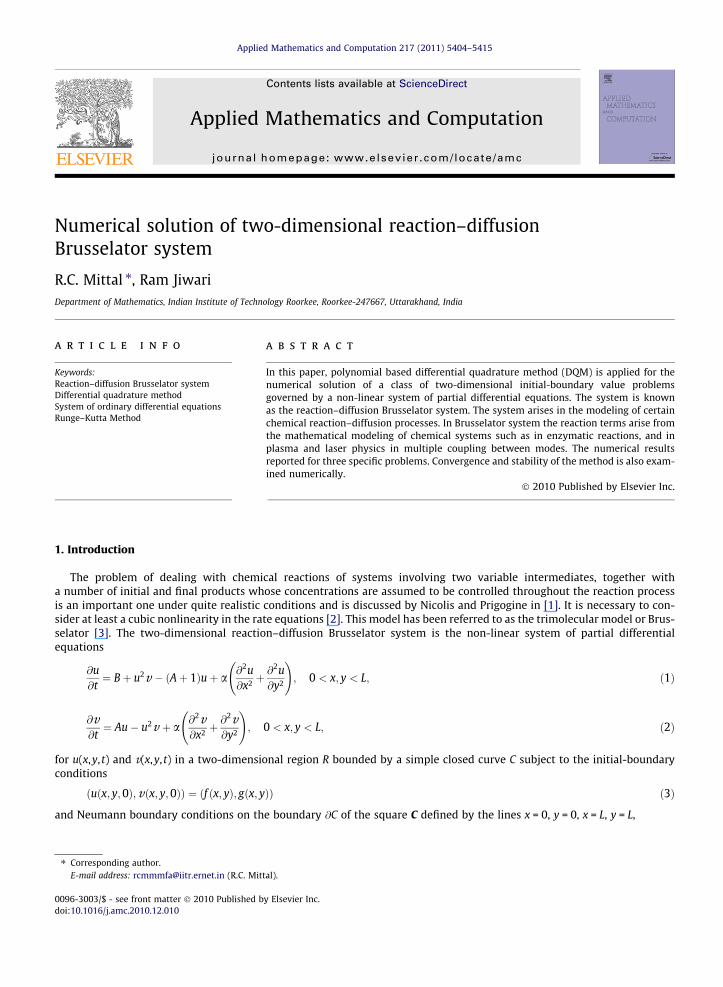
Fig. 1. Concentration profiles of u of Problem 1 at different time t = 0,1.0, . . . ,50.0.

5406 R.C. Mittal, R. Jiwari / Applied Mathematics and Computation 217 (2011) 5404–5415

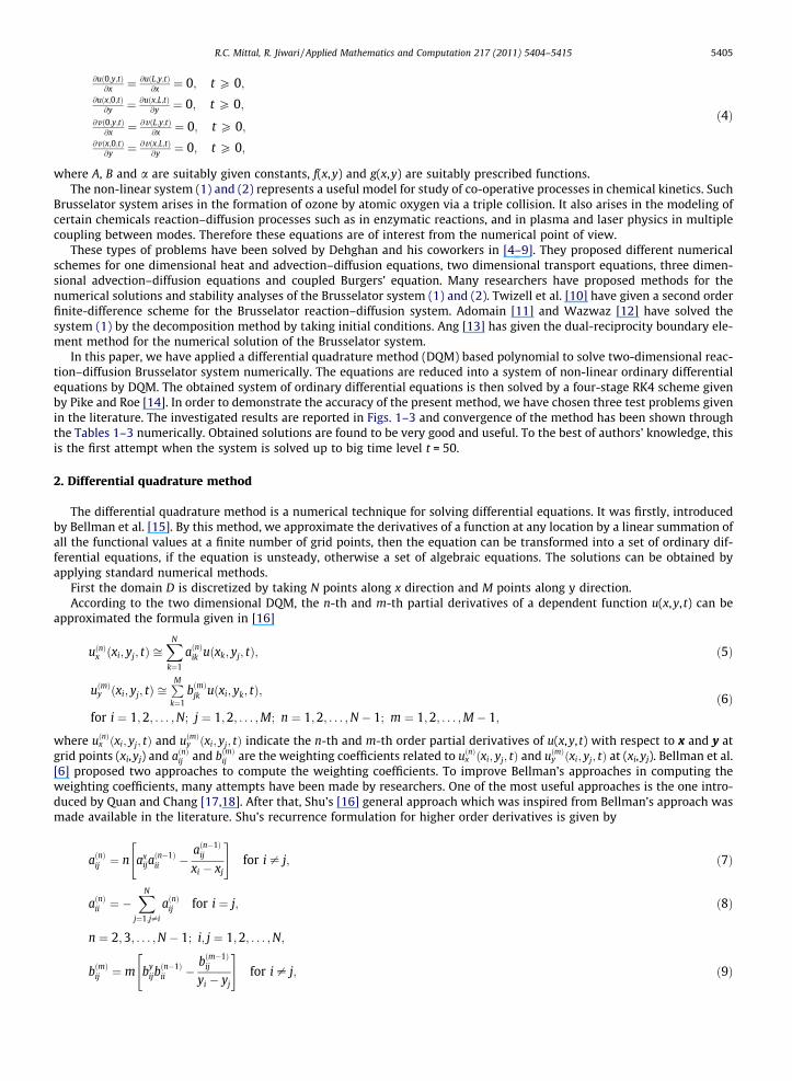
Fig. 2. Concentration profiles of v of Example 7.1 at different time t.

R.C. Mittal, R. Jiwari / Applied Mathematics and Computation 217 (2011) 5404–5415 5407

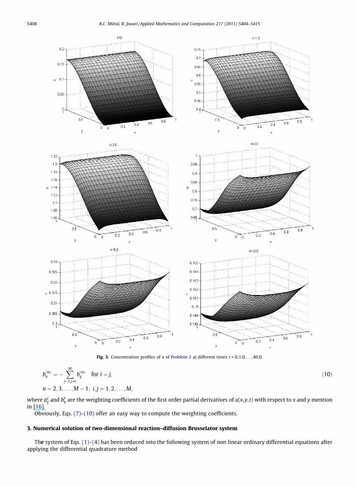
Fig. 3. Concentration profiles of u of Problem 2 at different times t = 0,1.0, . . . ,40.0.

5408 R.C. Mittal, R. Jiwari / Applied Mathematics and Computation 217 (2011) 5404–5415

bðmÞii ¼ �XM

j¼1;j–i

bðmÞij for i ¼ j; ð10Þ

n ¼ 2;3; . . . ;M � 1; i; j ¼ 1;2; . . . ;M;

where axij and by

ij are the weighting coefficients of the first order partial derivatives of u(x,y, t) with respect to x and y mentionin [16].

Obviously, Eqs. (7)–(10) offer an easy way to compute the weighting coefficients.

3. Numerical solution of two-dimensional reaction–diffusion Brusselator system

The system of Eqs. (1)–(4) has been reduced into the following system of non linear ordinary differential equations afterapplying the differential quadrature method

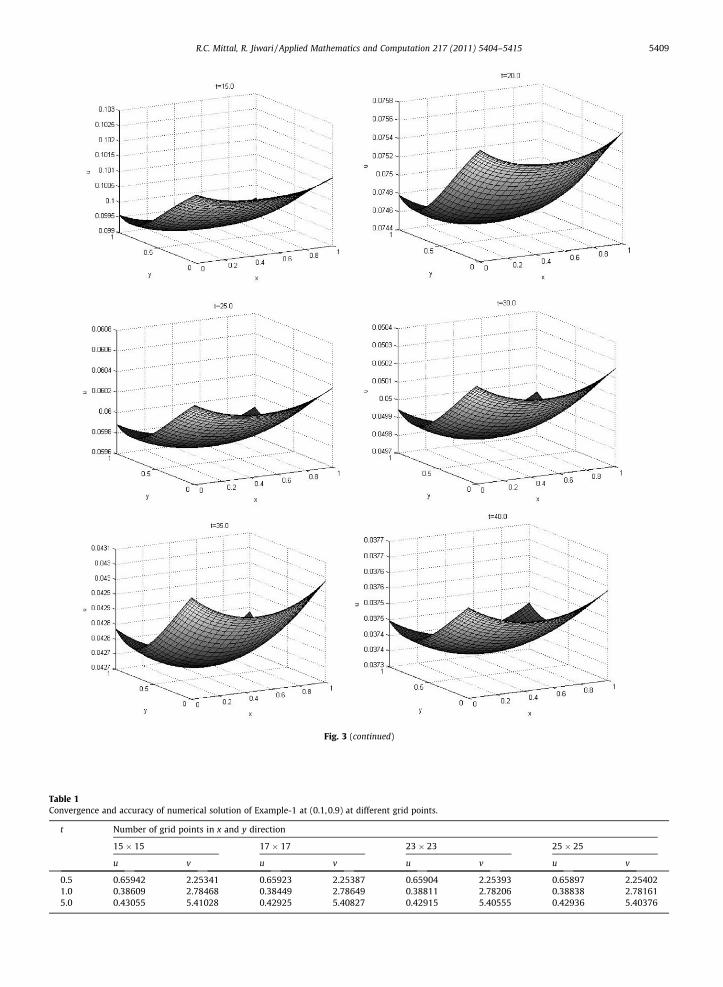
Fig. 3 (continued)

Table 1Convergence and accuracy of numerical solution of Example-1 at (0.1, 0.9) at different grid points.

t Number of grid points in x and y direction

15 � 15 17 � 17 23 � 23 25 � 25

u v u v u v u v

0.5 0.65942 2.25341 0.65923 2.25387 0.65904 2.25393 0.65897 2.254021.0 0.38609 2.78468 0.38449 2.78649 0.38811 2.78206 0.38838 2.781615.0 0.43055 5.41028 0.42925 5.40827 0.42915 5.40555 0.42936 5.40376

R.C. Mittal, R. Jiwari / Applied Mathematics and Computation 217 (2011) 5404–5415 5409

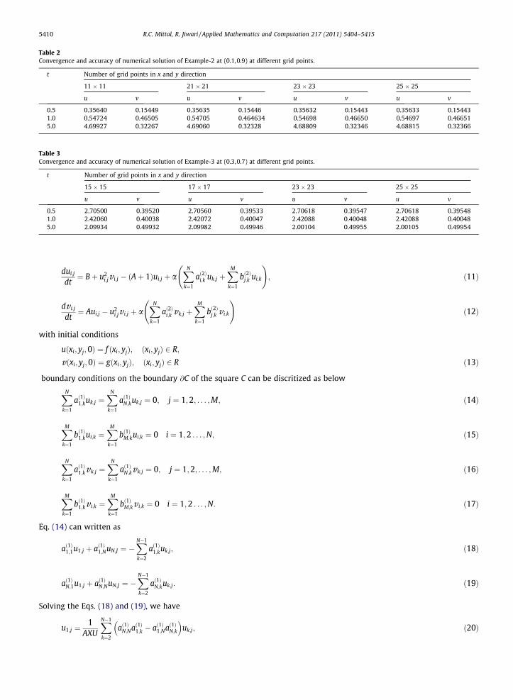
Table 2Convergence and accuracy of numerical solution of Example-2 at (0.1,0.9) at different grid points.

t Number of grid points in x and y direction

11 � 11 21 � 21 23 � 23 25 � 25

u v u v u v u v

0.5 0.35640 0.15449 0.35635 0.15446 0.35632 0.15443 0.35633 0.154431.0 0.54724 0.46505 0.54705 0.464634 0.54698 0.46650 0.54697 0.466515.0 4.69927 0.32267 4.69060 0.32328 4.68809 0.32346 4.68815 0.32366

Table 3Convergence and accuracy of numerical solution of Example-3 at (0.3,0.7) at different grid points.

t Number of grid points in x and y direction

15 � 15 17 � 17 23 � 23 25 � 25

u v u v u v u v

0.5 2.70500 0.39520 2.70560 0.39533 2.70618 0.39547 2.70618 0.395481.0 2.42060 0.40038 2.42072 0.40047 2.42088 0.40048 2.42088 0.400485.0 2.09934 0.49932 2.09982 0.49946 2.00104 0.49955 2.00105 0.49954

5410 R.C. Mittal, R. Jiwari / Applied Mathematics and Computation 217 (2011) 5404–5415

dui;j

dt¼ Bþ u2

i;jv i;j � ðAþ 1Þui;j þ aXN

k¼1

að2Þi;k uk;j þXM

k¼1

bð2Þj;k ui;k

!; ð11Þ

dv i;j

dt¼ Aui;j � u2

i;jv i;j þ aXN

k¼1

að2Þi;k vk;j þXM

k¼1

bð2Þj;k v i;k

!ð12Þ

with initial conditions

uðxi; yj;0Þ ¼ f ðxi; yjÞ; ðxi; yjÞ 2 R;

vðxi; yj;0Þ ¼ gðxi; yjÞ; ðxi; yjÞ 2 R ð13Þ

boundary conditions on the boundary @C of the square C can be discritized as below

XN

k¼1

að1Þ1;kuk;j ¼XN

k¼1

að1ÞN;kuk;j ¼ 0; j ¼ 1;2; . . . ;M; ð14Þ

XM

k¼1

bð1Þ1;kui;k ¼XM

k¼1

bð1ÞM;kui;k ¼ 0 i ¼ 1;2 . . . ;N; ð15Þ

XN

k¼1

að1Þ1;kvk;j ¼XN

k¼1

að1ÞN;kvk;j ¼ 0; j ¼ 1;2; . . . ;M; ð16Þ

XM

k¼1

bð1Þ1;kv i;k ¼XM

k¼1

bð1ÞM;kv i;k ¼ 0 i ¼ 1;2 . . . ;N: ð17Þ

Eq. (14) can written as

að1Þ1;1u1;j þ að1Þ1;NuN;J ¼ �XN�1

k¼2

að1Þ1;kuk;j; ð18Þ

að1ÞN;1u1;j þ að1ÞN;NuN;J ¼ �XN�1

k¼2

að1ÞN;kuk;j: ð19Þ

Solving the Eqs. (18) and (19), we have

u1;j ¼1

AXU

XN�1

k¼2

að1ÞN;Nað1Þ1;k � að1Þ1;Nað1ÞN;k

� �uk;j; ð20Þ

R.C. Mittal, R. Jiwari / Applied Mathematics and Computation 217 (2011) 5404–5415 5411

uN;j ¼1

AXU

XN�1

k¼2

að1Þ1;1að1ÞN;k � að1ÞN;1að1Þ1;k

� �uk;j; ð21Þ

for j = 1,2, . . . ,M, where AXU ¼ að1Þ1;Nað1ÞN;1 � að1Þ1;1að1ÞN;N .Similarly, from Eq. (16), we have

v1;j ¼1

AXV

XN�1

k¼2

að1ÞN;Nað1Þ1;k � að1Þ1;Nað1ÞN;k

� �vk;j; ð22Þ

vN;j ¼1

AXV

XN�1

k¼2

að1Þ1;1að1ÞN;k � að1ÞN;1að1Þ1;k

� �vk;j; ð23Þ

for j = 1,2, . . . ,M, where AXV ¼ að1Þ1;Nað1ÞN;1 � að1Þ1;1að1ÞN;N .In the similar way solve the Eqs. (15) and (17), we have

ui;1 ¼1

AYU

XM�1

k¼2

bð1ÞM;Mbð1Þ1;k � bð1Þ1;Mbð1ÞM;k

� �ui;k; ð24Þ

ui;M ¼1

AYU

XM�1

k¼2

bð1Þ1;1bð1ÞM;k � bð1ÞM;1bð1Þ1;k

� �ui;k; ð25Þ

v i;1 ¼1

AYV

XM�1

k¼2

bð1ÞM;Mbð1Þ1;k � bð1Þ1;Mbð1ÞM;k

� �v i;k; ð26Þ

v i;M ¼1

AYV

XM�1

k¼2

bð1Þ1;1bð1ÞM;k � bð1ÞM;1bð1Þ1;k

� �v i;k; ð27Þ

for i = 1,2, . . . ,N, where AYU ¼ bð1Þ1;Mbð1ÞM;1 � bð1Þ1;1bð1ÞM;M .where u(xi,yj, t) and v(xi,yj, t) is referred as ui,j and vi,j and að1Þi;j ; að2Þi;j ; bð1Þi;j and bð2Þi;j are the weighting coefficients of first and

second order partial derivatives of u, v with respect to x and y.The system of ordinary differential Eqs. (11)–(13), (18)–(25) are solved by Pike and Roe’s fourth-stage RK4 scheme [14]

for the event that function f contains no explicit dependent on t.

4. Selection of grid points

The stability of the DQM depends on the eigen-values of differential quadrature discretization matrices. These eigen-val-ues in turn very much depend on the distribution of grid points. It has been shown by Shu[16] in his book that the uniformgrid points distribution does not give stable solution which we have also notice in our numerical experiments. According toShu the stable solution can be obtained when Chebyshev–Gauss–Lobatto grid points are chosen. The Chebyshev–Gauss–Lob-atto grid points are given by

xi ¼ 12 1� cos ði�1Þpð Þ

N�1

� �Lx;

yj ¼ 12 1� cos ðj�1Þpð Þ

M�1

� �Ly i ¼ 1;2; . . . ;N; j ¼ 1;2; . . . ;M;

ð28Þ

where Lx and Ly are the rectangular domain length along x-axis and y-axis respectively.The convergence of the present approach is demonstrated by the Tables 1–3. These Tables show that as soon as grid

points increase, we get stable solutions. The Figures also show the stable solutions.

5. Numerical experiments and discussions

In this Section, we apply DQM on three test problems which are taken form literature by different researchers to show itsapplicability. In the whole numerical experiment done in all the three Examples, we have used the time step Dt = 0.001.

Problem 1 [19]. Consider the Brusselator system (1) and (2) subject to Neumann boundary conditions (4) and with theinitial conditions

uðx; y;0Þ ¼ 0:5þ y vðx; y;0Þ ¼ 1þ 5x: ð29Þ

The constants A, B and a are taken 1, 3.4 and 0.002 respectively similar to [19]. Table 1 shows that the numerical solutionsare converging as the grid points are increased. The concentration profiles of u and v computed at time from t = 1 to t = 50 are

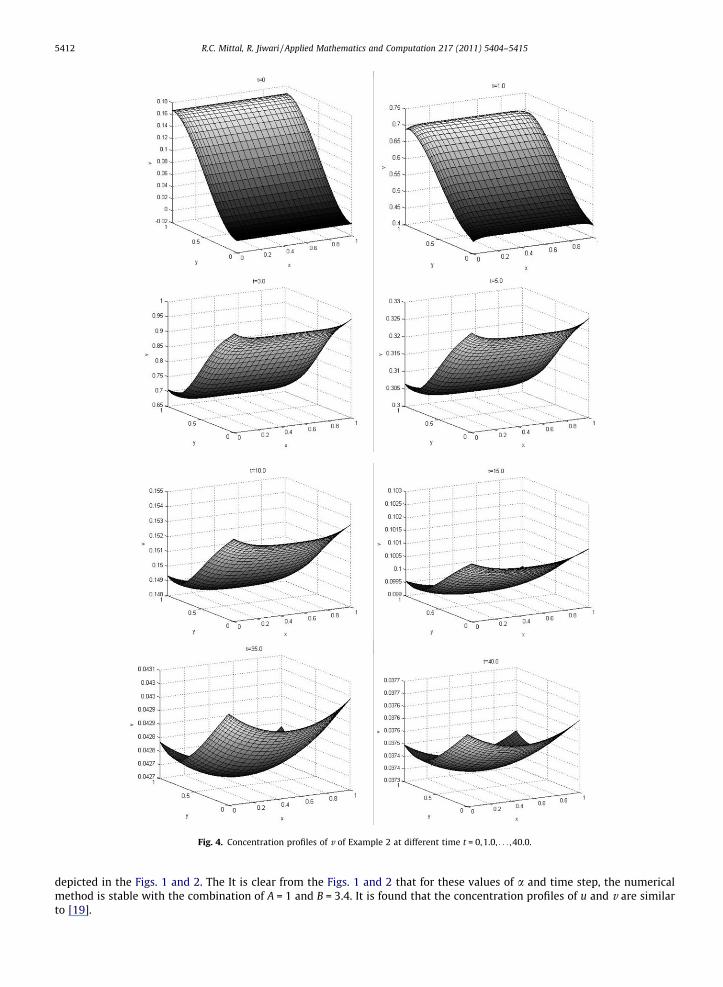
Fig. 4. Concentration profiles of v of Example 2 at different time t = 0,1.0, . . . ,40.0.

5412 R.C. Mittal, R. Jiwari / Applied Mathematics and Computation 217 (2011) 5404–5415

depicted in the Figs. 1 and 2. The It is clear from the Figs. 1 and 2 that for these values of a and time step, the numericalmethod is stable with the combination of A = 1 and B = 3.4. It is found that the concentration profiles of u and v are similarto [19].

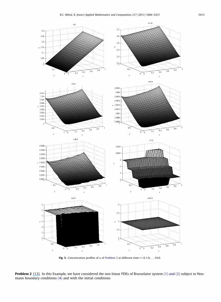
Fig. 5. Concentration profiles of u of Problem 3 at different time t = 0, 1.0, . . . ,10.0.

R.C. Mittal, R. Jiwari / Applied Mathematics and Computation 217 (2011) 5404–5415 5413

Problem 2 [13]. In this Example, we have considered the non linear PDEs of Brusselator system (1) and (2) subject to Neu-mann boundary conditions (4) and with the initial conditions

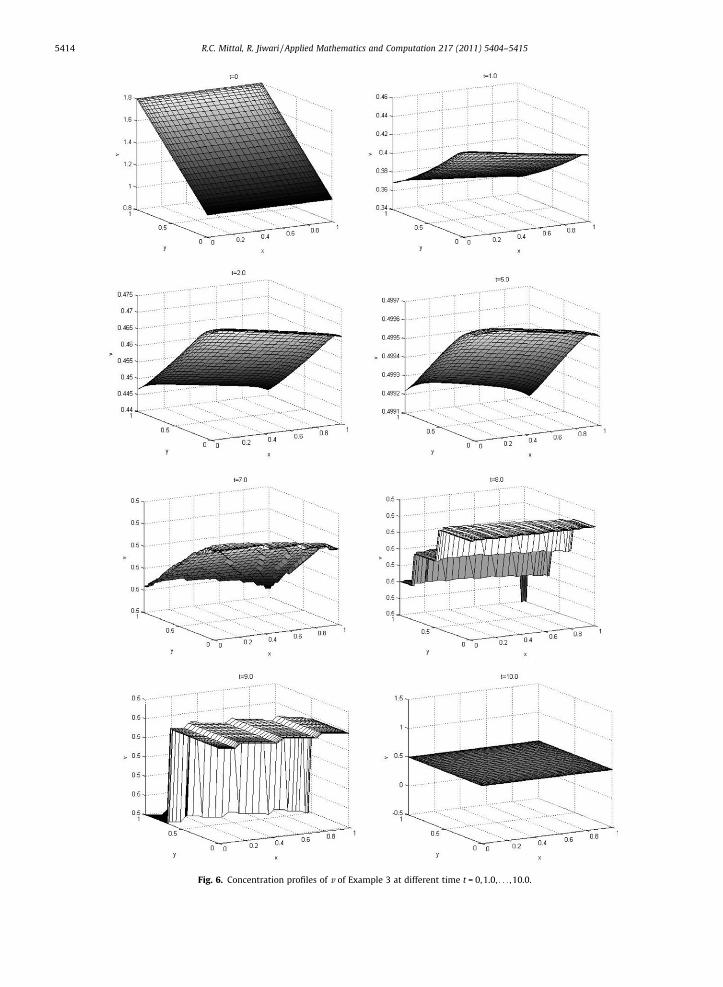
Fig. 6. Concentration profiles of v of Example 3 at different time t = 0,1.0, . . . ,10.0.

5414 R.C. Mittal, R. Jiwari / Applied Mathematics and Computation 217 (2011) 5404–5415

R.C. Mittal, R. Jiwari / Applied Mathematics and Computation 217 (2011) 5404–5415 5415

uðx; y;0Þ ¼ 0:5x2 � 13

x3 vðx; y;0Þ ¼ 0:5y2 � 13

y3: ð30Þ

The constants A, B and a are taken 0.5, 1 and 0.002 respectively similar to [13]. The Figs. 3 and 4 show the concentrationprofiles of u and v at time from t = 1 to t = 40. It is clear from Figs. 3 and 4 that for these values of a and time step, the numer-ical method is stable with the combination of A = 0.5 and B = 1. Table 2 shows the convergence and accuracy of the numericalsolutions.

Problem 3 [10]. Consider the Brusselator system (1) and (2) with Neumann boundary conditions (4) and with the initialconditions

uðx; y;0Þ ¼ 2:0þ 0:25y uðx; y; 0Þ ¼ 1:0þ 0:8x: ð31Þ

The constants A, B and a are taken 1, 2 and 0.002 respectively considered in [10]. Table 3 shows the convergence of numericalsolutions at different grid points. The concentration profiles of u and v computed at time from t = 1 to t = 10, are depicted inFigs. 5 and 6. It is clear from Figs. 5 and 6 that for these values of a and time step; the numerical method is stable with thecombination of A = 1 and B = 2.

6. Conclusion

In this paper, a polynomial based differential quadrature method (DQM) is employed for numerical solutions of two-dimensional non linear reaction–diffusion Brusselator system. The method is simple and straight forward which gives a sys-tem of ordinary differential equations. The resulting system of ordinary differential equations is solved by a four-stage RK4method. The method is applied on three test problems given in the literature. Convergence and stability of the method is alsoexamined numerically. It is shown in the Tables that the accuracy of the method depends on the number of grid points cho-sen for DQM. The strength of the method lies in its easiness to apply.

Acknowledgements

The author Ram Jiwari thankfully acknowledges the financial assistance provided by UGC India.

References

[1] G. Nicolis, I. Prigogine, Self-Organization in Nonequilibrium Systems, Wiley-Interscience, 1977.[2] I. Prigogine, R. Lefever, Symmetry breaking instabilities in dissipative systems, J. Chem. Phys. 48 (1968) 1695.[3] J. Tyson, Some further studies of nonlinear oscillations in chemical systems, J. Chem. Phys. 58 (1973) 3919.[4] A. Mohebbi, M. Dehghan, High-order compact solution of the one-dimensional heat and advection-diffusion equations, Appl. Math. Model. 34 (2010)

3071–3084.[5] M. Dehghan, Weighted finite difference techniques for the one-dimensional advection-diffusion equation, Appl. Math. Comput. 147 (2004) 307–319.[6] M. Dehghan, On the numerical solution of the one-dimensional convection–diffusion equation, Math. Prob. Eng. (2005) 61–74.[7] M. Dehghan, Time-splitting procedures for the solution of the two-dimensional transport equation, Kybernetes 36 (2007) 791–805.[8] M. Dehghan, Numerical solution of the three-dimensional advection-equation, Appl. Math. Comput. 150 (2004) 5–19.[9] M. Dehghan, A. Hamidi, M. Shakourifar, The solution of coupled Burgers’ equation using Adomain-Pade technique, Appl. Math. Comput. 189 (2007)

1034–1047.[10] E.H. Twizell, A.B. Gumel, Q. Cao, A second-order scheme for the ‘Brusselator’ reaction–diffusion system, J. Math. Chem. 26 (1999) 297–316.[11] G. Adomian, The diffusion-Brusselator equation, Comput. Math. Appl. 29 (1995) 1–3.[12] A.M. Wazwaz, The decomposition method applied to systems of partial differential equations and to the reaction–diffusion Brusselator model, Appl.

Math. Comput. 110 (2000) 251–264.[13] W.T. Ang, The two-dimensional reaction-diffusion Brusselator system: a dual-reciprocity boundary element solution, Eng. Anal. Bound Elem. 27 (2003)

897–903.[14] J. Pike, P.L. Roe, Accelerated convergence of Jameson’s finite volume Euler scheme using Van Der Houwen integrators, Comput. Fluids 13 (1985) 223–

236.[15] R. Bellman, B.G. Kashef, J. Casti, Differential quadrature: a technique for the rapid solution of nonlinear partial differential equations, J. Comput. Phys 10

(1972) 40–52.[16] Chang. Shu, Differential Quadrature and its Application in Engineering, Springer-Verlag London Ltd., Great Britain, 2000.[17] J.R. Quan, C.T. Chang, New insights in solving distributed system equations by the quadrature methods-I, Comput. Chem. Eng. 13 (1989) 779–788.[18] J.R. Quan, C.T. Chang, New insights in solving distributed system equations by the quadrature methods-II, Comput. Chem. Eng. 13 (1989) 1017–1024.[19] J.G. Verwer, W.H. Hundsdorfer, B.P. Sommeijer, Convergence properties of the Runge–Kutta–Chebyshev method, Numer. Math. 57 (1990) 157–178.