elbara ii, an l-band radiometer system for soil moisture research
TRANSCRIPT

Sensors 2010, 10, 584-612; doi:10.3390/s100100584
sensors ISSN 1424-8220
www.mdpi.com/journal/sensors Article
ELBARA II, an L-Band Radiometer System for Soil Moisture Research
Mike Schwank 1,2,*, Andreas Wiesmann 1, Charles Werner 1, Christian Mätzler 3, Daniel Weber 3, Axel Murk 3, Ingo Völksch 2 and Urs Wegmüller 1
1 Gamma Remote Sensing AG, Worbstrasse 225, 3073 Gümligen, Switzerland; E-Mails: [email protected] (A.W.); [email protected] (C.W.); [email protected] (U.W.)
2 Swiss Federal Research Institute WSL, Zürcherstrasse 111, 8903 Birmensdorf, Switzerland; E-Mail: [email protected] (I.V.)
3 Institute of Applied Physics, University Bern, Sidlerstr. 31, 3012 Bern, Switzerland; E-Mails: [email protected] (C.M.); [email protected] (D.W.); [email protected] (A.M.)
* Author to whom correspondence should be addressed; E-Mail: [email protected].
Received: 18 November 2009; in revised form: 9 December 2009 / Accepted: 15 December 2009 / Published: 13 January 2009
Abstract: L-band (1–2 GHz) microwave radiometry is a remote sensing technique that can be used to monitor soil moisture, and is deployed in the Soil Moisture and Ocean Salinity (SMOS) Mission of the European Space Agency (ESA). Performing ground-based radiometer campaigns before launch, during the commissioning phase and during the operative SMOS mission is important for validating the satellite data and for the further improvement of the radiative transfer models used in the soil-moisture retrieval algorithms. To address these needs, three identical L-band radiometer systems were ordered by ESA. They rely on the proven architecture of the ETH L-Band radiometer for soil moisture research (ELBARA) with major improvements in the microwave electronics, the internal calibration sources, the data acquisition, the user interface, and the mechanics. The purpose of this paper is to describe the design of the instruments and the main characteristics that are relevant for the user.
Keywords: microwave; radiometer; remote sensing; Soil Moisture and Ocean Salinity Mission (SMOS)
OPEN ACCESS
Sensors 2010, 10
585
Abbreviations
Symbol Meaning ACS Active Cold Source ADC Analog-to-Digital Converter AMP AMPlifier BP Band Pass filer CA Calibration Assembly ELBARA ETH L-Band Radiometer for soil-moisture research. ESA European Space Agency FC Feed Cable HS Hot Source IC Instrument Controller ISO ISOlator LP Low Pass filer MA Microwave Assembly ND Noise Diode PDA Power Detector Assembly PDU Power Distribution Unit PID Proportional–Integral–Derivative controller RFI Radio Frequency Interferences RM RadioMeter RS Resistive Source SMOS Soil Moisture and Ocean Salinity mission SW input SWitch TEC Thermo-Electric Cooler TPC Temperature and Power Controller USB / LSB Upper / Lower Side Band
1. Introduction
Heat fluxes through the terrestrial surface layer are major drivers of climate. For land areas with sparse or no vegetation, the quantities involved in this energy exchange are fundamentally linked with the moisture in the soil surface. Techniques for monitoring the surface moisture on the spatial scales relevant for climate and meteorological research are therefore of particular interest [1-5].
Almost 25 years ago, it was suggested that soil moisture could be retrieved from remotely sensed thermal radiance received with an L-band radiometer [6,7]. Today L-band radiometry is one of the most promising approaches for remote soil-moisture retrieval since: (i) the atmosphere and clouds are almost transparent, thus allowing for all-weather measurements; (ii) the impact of vegetation canopies and surface roughness is less distinct compared with passive measurements at higher frequencies and active remote sensing techniques (radar); (iii) solar radiation affects radiometer measurements at the L-band only insignificantly, which allows for measurements at any time of the day; (iv) the

Sensors 2010, 10
586
1,400−1,427 MHz frequency band is protected, which means that distortions of thermal radiance due to man-made radio frequency interferences (RFI) are minimized. However, in the past years several field experiments performed in Europe have shown that RFI is present even in the protected part of the L-band.
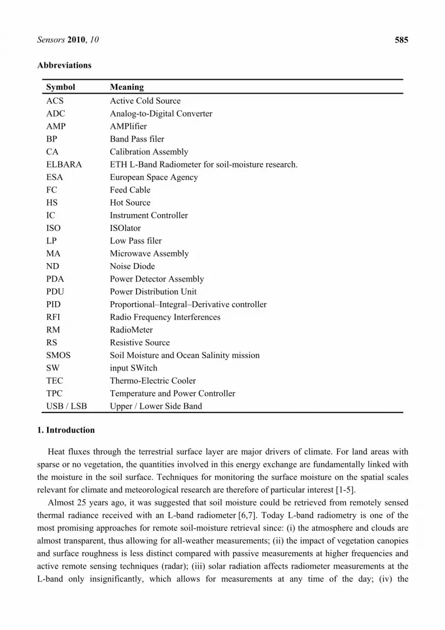
Figure 1. The ELBARA II systems mounted above the test site at the Swiss Federal Research Institute WSL, with the radiometer electronics and the power unit installed in the unit on the right.
During the calibration and validation activities associated with ESA’s SMOS mission [8] it turned out that further ground-based passive L-band experiments would be indispensable for the commissioning and the operative phase of the mission. To address this need, the three identical radiometers ELBARA II depicted in Figure 1 were built by Gamma Remote Sensing (Gümligen, Switzerland) as ordered by the ESTEC, in the framework of the contract ESTEC 21013/07/NL/FF" L-band Radiometer Systems to be deployed for SMOS Cal/Val Purposes".
In the following paragraphs, we describe some basics of microwave radiometry, the requirements of the SMOS mission, and the corresponding research activities. The design and the main characteristics of the ELBARA II instruments are described in Sections 2 and 3. The Appendix contains a list of the abbreviations used and the specifications of the electronic components used in the radiometer design.
1.1. Measurement Principle
Microwave radiometry is a passive remote-sensing technique that measures thermal radiation. The radiance TB
p emitted from a terrestrial surface at horizontal (p = H) or vertical (p = V) polarization depends on the surface temperature TS, and on the surface reflectivity Rp. The latter can be used as a proxy for the remote retrieval of soil moisture or sea salinity.
In the microwave range, the Planck function of thermal radiation is linear with the absolute temperature. In this so-called Rayleigh-Jeans approximation, the upwelling brightness temperature of
Sensors 2010, 10
587
the emitted radiation above a surface is TS⋅(1 - Rp). Since downwelling radiation Tsky also contributes to the observed radiation by the fraction reflected at the surface, the total radiation TB
p received by a radiometer oriented towards the surface can be expressed by:
B S sky(1 )p p pT R T R T= − + (1)
The value of Tsky is determined by the cosmic background temperature of ≈2.7 K and enhanced by an atmospheric contribution. At 1.4 GHz, this enhancement is almost constant, leading to 4 K < Tsky < 5 K. Since the terrestrial surface temperature is much larger than Tsky, the brightness temperature TB
p has a strong sensitivity to Rp. The sensitivity of TB
p with volumetric soil water content WC [m3 m-3] is established through Rp, being dependent on the relative dielectric constant. The latter is a strong function of WC due to the marked contrast between the permittivity of free water (≈80) and dry soil (≈3 to 5). This allows the soil surface-water content to be determined from its reflectivity by applying dielectric mixing (e.g., [9–11]) and radiative transfer models. Typically, TB
p of a very dry bare soil can be 150 K higher than for the same soil in the saturated moisture state.
Two different soil-depth ranges are of relevance: First, TS represents an effective soil temperature averaged over the emission depth of the microwave radiation in the soil [12]. For a dry soil this can be 1 m or even more at 1.4 GHz, whereas for a wet soil the emission depth may be as little as a few centimeters [13]. Second, Rp represents an effective surface reflectivity as a result of the dielectric transition from air to bulk soil with a more or less constant permittivity. In the simplest case of a homogeneous soil with a flat surface, the Fresnel equations [14] can be used to represent Rp at polarization p = H, V and for a certain observation angle. At 1.4 GHz, a requirement for applying the Fresnel equations is a transition depth of <1 cm. However, more sophisticated models are required to compute Rp if TB
p originates from a landscape, e.g., with vegetation. Recent results obtained from several theoretical studies and field experiments dedicated to the
retrieval of sea salinity as part of the SMOS mission are presented in [15]. For retrieving ocean salinity from TB
p measured at L-band, the principle is similar as applied for retrieving soil moisture. Again TBp
can be expressed by Equation (1). However, the dielectric constant of ocean water is in a quite different range. It is the imaginary part of the permittivity that increases with increasing salt content due to the increased conductivity. Sea salinity is measured in Practical Salinity Units (psu) defined as: Sea water with the salinity 35 psu has a conductivity ratio of unity at 15 °C (and 1 atmosphere pressure) with a potassium chloride (KCl) solution containing 32.4356 g of KCl per kg of solution. The salinity of the ocean is between 31 and 38 psu, but can be substantially less where mixing with fresh water occurs. The most saline open sea is the Red Sea (36–41 psu), but even higher values are found in isolated bodies of water, such as in the Dead Sea (300–400 psu). However, the sensitivity of TB
p measured with respect to the salinity of the open ocean is approximately 1 K⋅psu-1 at vertical polarization and the observation angel of 50° relative to nadir.
1.2. SMOS Requirements
ESA’s SMOS mission, proposed in the framework of the Earth Explorer Opportunity Missions [16] aims at deducing soil surface moisture and ocean salinity with near global coverage every three

Sensors 2010, 10
588
days [17]. The mission’s requirements regarding soil moisture are: the accuracy should be better than 4% volumetric moisture with a spatial resolution of 35–50 km of a single measurement. The desired accuracy of ocean salinity retrieved from a single measurement is 0.5–1.5 psu. For a 30–day average over an area of 100 km × 100 km, the accuracy is specified to 0.1 psu, implying that brightness temperatures measured with the SMOS L-band radiometer have to be within ±0.1 K.
1.3. SMOS Calibration and Validation Activities
SMOS is the outcome of a long process initiated in late 1970s. During recent years, many research activities have been performed to support this mission (see [18] for an extensive overview of recent research activities related to SMOS). Many of these activities focused on questions concerning calibration and validation issues for soil moisture and sea salinity retrieval. Others were dedicated to the detection of biomass, or to technical aspects of the sensor. Regarding soil moisture retrieval, many experimental and theoretical studies have been performed to explore the radiative properties of the basic land-cover types considered in the so-called ‘L-band Microwave Emission of the Biosphere’ (L-MEB) model [19] which is the Level-2 algorithm to produce soil-moisture data. This research has mostly been performed with ground-based L-band radiometers either mounted on towers or cranes. Thus, a considerable number of L-band radiometers with sometimes different characteristics have been built [20] and operated by the scientific community.
Although our knowledge about the interaction between microwaves and land-surface features has increased dramatically in the course of these activities, further ground-based experiments during the SMOS commissioning and operative phases are essential. For this reason and to overcome the problem of different instrument performances affecting the L-band signatures, the construction of three identical L-band radiometers was recommended to ESA. These instruments have been built by a consortium consisting of an industrial partner (Metaplan, Adliswil, Switzerland) and two university partners (Institute of Applied Physics, Bern, Switzerland and Swiss Federal Research Institute WSL, Birmensdorf, Switzerland), headed by the company Gamma Remote Sensing AG (Gümligen, Switzerland), with a total budget of approximately 360 kEuro. The architecture of the three ELBARA II L-band radiometers is based on the ETH L-Band radiometer for soil-moisture research (ELBARA), [21] designed and built by the Institute of Applied Physics, University of Berne. This instrument has been successfully deployed in a series of field experiments [22–27]. However, major improvements of the microwave electronics, the mechanics, and the user interface have been made to the successor, ELBARA II. In particular the development of an Active Cold Source as an instrument internal calibration noise source has improved the absolute accuracy significantly.
2. Instrument Design
A microwave radiometer is a receiver for electromagnetic radiation with sub–millimeter to centimeter wavelengths, corresponding to the frequency range of 1–1,000 GHz. The L–band, ranging from 1–2 GHz, has many commercial and military applications. It also contains the hydrogen line at 1,420.41 MHz, originating from the hyperfine transition of neutral hydrogen. For the imaging of neutral atomic hydrogen in interstellar space, passive measurements at this frequency are of great astronomical interest. As a consequence, the 27 MHz frequency band ranging from 1,400 to

Sensors 2010, 10
589
1,427 MHz has become a protected radio astronomy allocation world–wide, in which it is forbidden to transmit any kind of electromagnetic radiance. Likewise, an RFI–free environment is mandatory to measure microwave brightness temperatures emitted from terrestrial surfaces. The frequency transfer function of an L–band radiometer to be used for retrieving geophysical properties must therefore be narrow and within this protected band. This implies, however, that the power level P received by such a radiometer with bandwidth B = 27 MHz is very low. For a noise source at the physical temperature T, and with emissivity equal to unity (e.g., a perfectly matched resistor), the noise power received is:
P kTB= (2)
with k = 1.380658⋅10−23 J K-1 being the Boltzmann constant. The same expression holds true when a scene at the physical temperature T and with the emissivity 1 is observed with a radiometer. For T = 300 K, this gives P ≈ 0.11⋅10-12 W (≈-99.5 dBm) received with the radiometer antenna. To detect such an extremely low power, the radiometer (RM) must have the lowest possible residual noise TRM 0 and any instrument internal RFI disturbances must be rigorously mitigated. To allocate an absolute value to the noise power received with the antenna, the noise power must be compared with the power of at least two instrument internal calibration sources with known noise temperatures. Provided that the linearity of the receiver is sufficient and the gain is stable between several calibration cycles, this allows a certain brightness temperature to be assigned to the radiance entering the antenna. These requirements are important for the design of the ELBARA II electronics described below.
2.1. Block Diagram
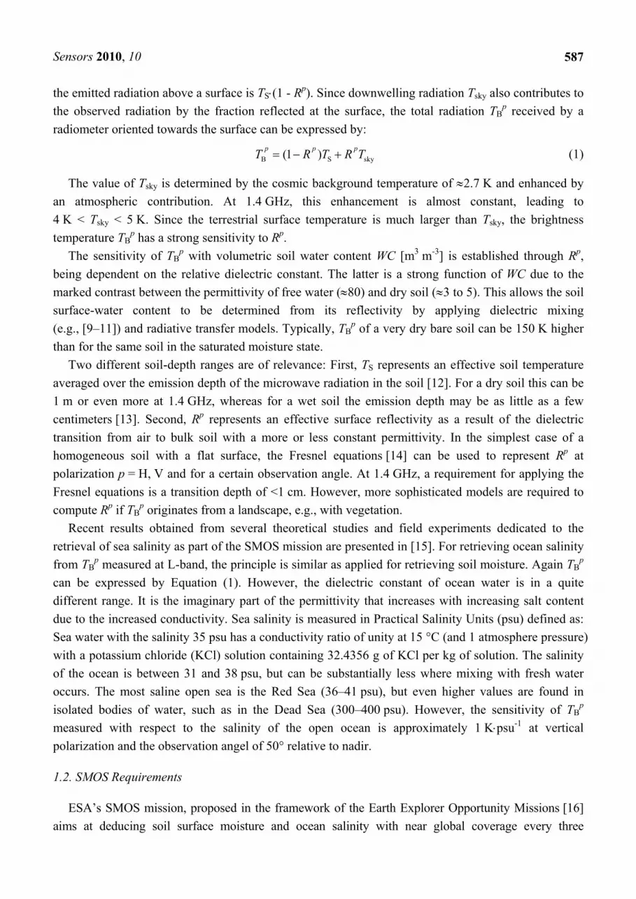
The block diagram of the ELBARA II radiometer is shown in Figure 2, and the relevant specifications of the individual components are listed in the Appendix. The block diagram is subdivided into the sub-systems: Microwave Assembly, Power Detector Assembly, Calibration Assembly, and the Temperature–Power Control unit. The functionality of these sub–systems are outlined in Sections 2.1.1 to 2.1.4.
2.1.1. Microwave Assembly
The Microwave Assembly (MA) consists of the components of the front-end and the back-end (Figure 2). The mechanical input switch (SW) allows the selection of the noise source fed to the MA input, which could be either one of the radiometer inputs TRM,in
H or TRM,inV to measure antenna
brightness at horizontal or vertical polarization, or one of the tree-internal reference noise sources. The output of the switch is fed through an isolator (ISO1) tuned to the center of the radiometer band at 1,413.5 MHz to ensures a good match of the selected noise input to the receiver path.
The microwave signal at the isolator output is directly fed into a 4-Section band-pass filter (BP1) before amplification. In this ELBARA II is unlike to other L-band radiometers currently used for the observation of terrestrial surfaces, e.g., the polarimetric radiometer EMIRAD [28] or the LEWIS radiometer [29]. The additional loss of <0.77 dB of the BP1 contributes less than 50 K to the total residual noise TRM,0 of the radiometer (see Section 2.2). This disadvantage is compensated for by the way RFI from outside the protected band is suppressed in the front-end before amplification, which avoids possible saturation of the first low-noise amplifier AMP1.

S
LwaIc
pALf
Sensors 201
Figurespecifi
To keep Lfront of the which is of accordance wn the bac
correspondinThe front
pass filter (BAssuming thLfront ≈ 0.15 factor tfront =
0, 10
e 2. Block fications of t
the residuafront-end mthe same owith (2), thk-end, the ng losses dot-end compBP1), and the loss of onDb + 0.20 d
= 0.72. Whe
diagram ofthe compon
al noise TRM
must be minrder as the is is typical
power leo not impacponents are three semi-rne cable as dB + 0.77 dere there is
f the ELBAnents are giv
M 0 of the ranimized. Thi
thermal nolly 10-13 Wevels are act TRM, 0 sign
the input nrigid coaxia0.1 dB and
dB + 3⋅0.1 d perfect ma
ARA II radiven in the A
adiometer ais is due to
oise caused ≈ -100 dBmapproximatenificantly. noise-poweral cables (Hd using the sdB = 1.42 dBatching (no
ometer. ThAppendix.
as low as pthe very loby the loss
m for the freely 77 dB
r switch (SHuber SuhnespecificatioB, corresporeflection)
e abbreviat
possible, theow power lees of the fr
equency andhigher, w
W), the isoer, ≈12 cm)ns given in onding to t, this corre
tions used a
e total transevel along thront-end comd bandwidth
which impli
olator (ISO1) with SMAthe Append
the power esponds to t
59
and the
smission loshe front-endmponents. Ih consideredies that th
1), the bandA connectordix results itransmissio
the front-en
90
ss d, In d. he
d-rs. in on nd

Sensors 2010, 10
591
absorptivity 1 - tfront. Where the electronic components are in thermal equilibrium at the typical temperature T0 = 313 K (40 °C), the absorptivity equals the emissivity and the noise power caused by the front-end loss is T0⋅(1 - tfront) ≈ 87 K. Besides the losses in the front-end, the performance of the first low-noise amplifier (AMP1) determines TRM 0. In accordance with its specified noise figure NF = 0.5 dB, the noise temperature TAMP1 of AMP1 is TAMP1 = T0⋅(10NF/10 - 1) ≈ 38 K. These considerations yield the residual noise of the ELBARA II radiometer estimated from the component specifications as TRM 0 = T0⋅(1 - tfront) + TAMP1 ≈ 125 K for T0 = s313 K.
The output of AMP1 is attenuated by 3 dB and amplified a further 40 dB by AMP2. The output of AMP2 is filtered using a 6-Section band-pass filter. The band-pass filters (BP1/2) are both centered at 1,413.5 MHz and have a bandwidth of 22 MHz at -3 dB to be within the protected band allocation from 1,400 MHz to 1,427 MHz. The 3 dB attenuator between the amplifiers avoids amplifier instabilities.
The output of the second amplifier (AMP2) is split into two channels using a symmetric power splitter. The two outputs of the splitter are then filtered by 4-Section band-pass filters (BP3a/b) with the center frequencies 1,407.5 MHz and 1,419.5 MHz, respectively each with a -3 dB bandwidth of 11 MHz. In this way, two slightly overlapping receiver channels within the protected band are created, which allow narrow-band RFI to be detected within the protected band. The corresponding lower side band (LSB) and the upper side band (USB) of the MA back-end are AC-coupled to the detectors through DC-blocks in order to remove any low-frequency internal RFI or DC-bias signals from ground loops or pick-up from the radiometer electronics.
Summing up the specified losses (see Appendix) of the back-end components (attenuator (3 dB) + BP2 (1.22 dB) + splitter (0.4 dB) + one-to-one splitting into the LSB and the USB (3 dB) + BP3a/b (1.3 dB) + DC-block (0.15 dB) + five connecting cables (5⋅0.1 dB)) yields the loss Lback ≈ 9.57 dB of each of the two frequency channels. The MA gain GMA ≈ 69.01 dB is estimated as the difference between the gain of the two low-noise amplifiers (2⋅40 dB) and the total loss LMA = Lfront + Lback = 10.99 dB of the MA.
Table 1 shows the typical noise temperatures applying at the MA inputs (column 1), the expected power levels Pfront at the output of the front-end (column 2), and the associated power levels PPDA (in units of dBm and μW) expected at the output of the back-end of the MA (columns 3 and 4). The selected MA inputs are: Tsky, in expected for a sky measurement; TACS, TRS, and THS of the active cold source (ACS), the resistive source (RS), and the hot source (HS); and Tscene,min, Tscene,max cover the range of land-surface brightness temperatures. The power levels Pfront are derived as the sum of the noise power associated with the radiometer residual noise TRM 0 ≈ 125 K, plus the power due to the noise temperature applying at the MA input. Thereby, equation (2) is used with the bandwidth B = 22 MHz of the BP1. In units of dBm, the PPDA are:
PDA front MAP P G= + (3)

Sensors 2010, 10
592
Table 1. Power levels Pfront at the output of the MA front-end and PPDA fed to the PDA for typical input noise temperatures at the MA. PDA output voltages UPDA, considering the measured PDA sensitivity (7), are shown in the last column.
MA input noise [K] Pfront [dBm] PPDA [dBm] PPDA [μW] UPDA [V] Tsky, in = 10 -103.8 -34.8 0.328 0.324 TACS = 48 -102.8 -33.8 0.420 0.416 Tscene, min = 100 -101.6 -32.6 0.545 0.540 Tscene, max = 300 -98.9 -29.9 1.029 1.019 TRS = 313 -98.8 -29.7 1.060 1.050 THS = 630 -96.4 -27.4 1.827 1.810
2.1.2. Power Detector Assembly
The power detector assembly (PDA) depicted in the block diagram (Figure 2) determines the performance of the radiometer. The PDA is symmetrical in respect to the two frequency channels implemented. The LSB and the USB outputs of the MA are fed to Planar-Doped Barrier diode detectors that are terminated resistively with 10 kΩ for best linearity and minimum insensitivity to temperature variation. For the estimated input power range PPDA (Table 1), the detectors operate well within their square-law regime. Therefore, the detector output voltage is directly proportional to PPDA with a voltage sensitivity of >0.5 mV μW-1.
The detector output voltages are amplified using instrumentation amplifiers with voltage gains of approximately 850, and finally low-pass filtered with a cut-off frequency of 400 Hz at -3dB. Buffer amplifiers (AMP4a/b) are used to drive the 16-bit analog to digital converter (ADC), operating at the nominal sample rate of 1,600 Hz. However, sampling at 800 Hz is also feasible to reduce data volume and incurs only a small loss of radiometric sensitivity. After this point, processing is carried out by the on-board Instrument Controller (IC), which is part of the temperature and power control (TPC) unit described in Section 2.1.4.
2.1.3. Calibration Assembly
Internal calibration noise sources are used to determine the absolute values of noise temperatures, TRM,in
H and TRM,inV, applying at the radiometer input ports for horizontal and vertical polarization,
respectively. As depicted in Figure 2, the input noise switch allows switching between TRM,inH and
TRM,inV at the input ports and the internal calibration sources mounted on the Calibration Assembly
(CA) depicted in Figure 3. The design is such that the losses between the radiometer input ports and the corresponding inputs of the switch are identical (≈0.05 dB). The same applies to the losses between the outputs of the three calibration sources and the inputs of the switch.
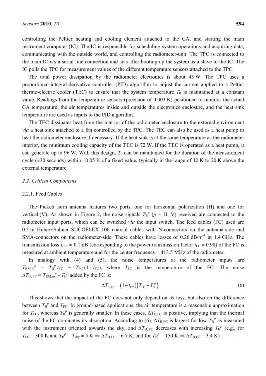
The CA consists of a heavy copper block (1.7 kg) on which the calibration sources and the two amplifiers (AMP1/2) used in the MA are mounted. A Thermo Electric Cooler (TEC) and a temperature sensor (T-sensor) are used for the thermal stabilization of the CA. This is crucial to maintain constant gains and noise added due to losses in the MA front-end. For the typical set point T0 = 313 K (40 °C), the temperature is measured to be within ±0.1 K. Furthermore, the CA is designed as a separate module to allow for independent operation for cross calibration among other L-band radiometers.

Sensors 2010, 10
593
Figure 3. Layout of the calibration assembly (CA).
The resistive source (RS) consists of a standard 50 Ω SMA resistor tightly pressed into a borehole
in the copper block to keep it constantly at the temperature T0. Accordingly, this results in the noise temperature TRS = T0 of the RS equal to the CA temperature.
The hot source (HS) is made up of a commercial noise diode (ND) with the output attenuated by 6 dB. Given the noise temperature TND ≈ 1575 K of the factory-calibrated ND and the physical temperature T0 = 313 K of the -6 dB attenuator (with power transmission factor t-6dB ≈ 0.251), the noise temperature THS of the HS is estimated as the transmitted part of TND plus the thermal noise of the attenuator. In case of perfect match between the components (no reflections) THS is:
( )HS ND -6dB 0 -6dB1 630 KT T t T t= ⋅ + ⋅ − ≈ (4)
The active cold source (ACS) is implemented with a low-noise amplifier (AMP5) with an isolator (ISO2) attached to the input and terminated with 50 Ω. The idea of this design is to use the low noise level of the amplifier (TAMP5 ≈ 34 K at T0 = 313 K) as a cold source. The isolator provides a good 50 Ω match between the ACS and the MA. In accordance with (4), the noise temperature TACS of the ACS is:
( )ACS AMP5 ISO2 0 ISO21 48 KT T t T t= ⋅ + ⋅ − ≈ (5)
The estimated TACS for T0 = 313 K is based on the component specifications and assumes perfect match between the components. However, TACS was determined more accurately by using TRS and sky measurements (see Section 3.1.4) as reference sources.
2.1.4. Temperature-Power Control
The ELBARA II instrument is controlled via two embedded computers. The temperature and power controller (TPC) is responsible for generating and monitoring the power used by the radiometer,
Sensors 2010, 10
594
controlling the Peltier heating and cooling element attached to the CA, and starting the main instrument computer (IC). The IC is responsible for scheduling system operations and acquiring data, communicating with the outside world, and controlling the radiometer-unit. The TPC is connected to the main IC via a serial line connection and acts after booting up the system as a slave to the IC. The IC polls the TPC for measurement values of the different temperature sensors attached to the TPC.
The total power dissipation by the radiometer electronics is about 45 W. The TPC uses a proportional-integral-derivative controller (PID) algorithm to adjust the current applied to a Peltier thermo-electric cooler (TEC) to ensure that the system temperature T0 is maintained at a constant value. Readings from the temperature sensors (precision of 0.003 K) positioned to monitor the actual CA temperature, the air temperatures inside and outside the electronics enclosure, and the heat sink temperature are used as inputs to the PID algorithm.
The TEC dissipates heat from the interior of the radiometer enclosure to the external environment via a heat sink attached to a fan controlled by the TPC. The TEC can also be used as a heat pump to heat the radiometer enclosure if necessary. If the heat sink is at the same temperature as the radiometer interior, the minimum cooling capacity of the TEC is 72 W. If the TEC is operated as a heat pump, it can generate up to 96 W. With this design, T0 can be maintained for the duration of the measurement cycle (≈30 seconds) within ±0.05 K of a fixed value, typically in the range of 10 K to 20 K above the external temperature.
2.2. Critical Components
2.2.1. Feed Cables
The Pickett horn antenna features two ports, one for horizontal polarization (H) and one for vertical (V). As shown in Figure 2, the noise signals TB
p (p = H, V) received are connected to the radiometer input ports, which can be switched via the input switch. The feed cables (FC) used are 0.3 m Huber+Suhner SUCOFLEX 106 coaxial cables with N-connectors on the antenna-side and SMA-connectors on the radiometer-side. These cables have losses of 0.26 dB⋅m-1 at 1.4 GHz. The transmission loss LFC ≈ 0.1 dB (corresponding to the power transmission factor tFC ≈ 0.98) of the FC is measured at ambient temperature and for the center frequency 1,413.5 MHz of the radiometer.
In analogy with (4) and (5), the noise temperatures at the radiometer inputs are TRM in
p = TBp⋅tFC + TFC⋅(1 - tFC), where TFC is the temperature of the FC. The noise
ΔTB, FC = TRM,inp - TB
p added by the FC is:
( ) ( )B, FC FC FC B1 pT t T TΔ = − − (6)
This shows that the impact of the FC does not only depend on its loss, but also on the difference between TB
p and TFC. In ground-based applications, the air temperature is a reasonable approximation for TFC, whereas TB
p is generally smaller. In these cases, ΔTB,FC is positive, implying that the thermal noise of the FC dominates its absorption. According to (6), ΔTB,FC is largest for low TB
p as measured with the instrument oriented towards the sky, and ΔTB, FC decreases with increasing TB
p (e.g., for TFC = 300 K and TB
p = Tsky ≈ 5 K ⇒ ΔTB,FC = 6.7 K, and for TBp = 150 K ⇒ ΔTB,FC = 3.4 K).
Sensors 2010, 10
595
In Section 3, this simple model will be used for correcting the contribution ΔTB,FC of the FC on the measurements TRM,in
p. However, the model is not perfect because TFC, for example, is not constant along the FC. Therefore, ΔTB,FC cannot be perfectly modeled, which makes it especially important to reduce the losses of the FC as far as possible.
2.2.2. Input switch
Central to the radiometer operation is the electro-mechanical “Single Pole 6 Throw” input switch (SW). This precision RF switch (Agilent 87106B) is controlled via a TTL level signal to toggle between the different noise sources fed to the receiver path (Figure 2). As the switch is part of the MA front-end, it has to meet high demands in terms of its insertion loss LSW, repeatability, isolation and life-time. It is important for LSW to be low and repeatable to minimize and control the noise added to the different inputs. High isolation is essential to prevent unwanted signals from interfering. For L-band frequencies, the maximum insertion loss is rated at LSW = 0.15 dB for 107 operations. The specified repeatability of the switch of 0.03 dB would imply that the residual noise TRM 0 can vary considerably (≈ 1.8 K). However, the repeatability measured was <0.005 dB (see Section 3.1.1) and therefore affects TRM 0 less than 0.3 K at T0 = 313 K. Hence, the switch performance is sufficient to function within the radiometer’s lifetime (at least 5 years), assuming that a full measurement cycle is performed every minute.
2.2.3. Filters and Isolators
The insertion loss LBP1 of the 4-Section band-pass filter BP1 in the front-end of the MA contributes significantly to the residual noise TRM 0 of the radiometer, while the losses of the filters after the front-end are no longer critical. The selectivity and LBP1 of BP1 are coupled such that higher selectivity implies higher losses. The BP1 was selected to minimize LBP1, while maintaining acceptable selectivity outside of the protected band. To minimize the noise TBP1 of the BP1, a high quality silver-plated cavity filter was selected with rated LBP1 = 0.77 dB (corresponding to the power transmission factor of tBP1 = 0.84). For T0 = 313 K, this yields TBP1 = T0⋅(1 - tBP1) ≈ 50 K, which is 40% of the estimated TRM 0 = 125 K. For the same reason, ISO1/2 were tuned to have very low insertion losses LISO < 0.20 dB within the protected band (1,400 MHz–1,427 MHz), resulting in the relatively low noise TISO ≈ 14 K for T0 = 313 K.
2.2.4. Amplifiers
Low-noise amplifiers AMP1/2/5 are selected to minimize the noises TAMP1/2/5 of the amplifiers in the low-signal parts of the radiometer (MA and ACS). Their noise figure is rated to NF < 0.5 dB over the protected band, corresponding to TAMP1/2/5 ≈ 34 K at T0 = 313 K. The instrumentation amplifiers AMP3a/b are selected to have a low input noise level, which contributes approximately 0.4 mV to the total uncertainty σURM of a single measurement URM performed with the shortest possible recording time τrec = 2.5 ms (see Section 3.2). Furthermore, the capability to easily set the gain with a single resistor was also considered in the selection.

S
2
dcaceh
frovdfleo(
awthhjo
Sensors 201
2.3. Antenna
The Pickdesign has scylindrical wadditional pcharacteristiexpected -3 horizontal an
The antenfrom two heof the antenvertically (Vdirections (bfilter) are mength, clam
of the λ/4-stsee Section
Figurethe wa
The largealuminum shwelded togehe aperture
horn, as weloints are a
0, 10
a
kett-horn antsome modifwaveguide phasing sectic of the oridB beam wnd vertical pnna feed, ceavy-wallednna feed coV) polarizedbetter than
mounted in bmped to the tructures are
n 3.2.1.).
e 4. Sketch ave characte
e antenna hheets (PE10
ether and rig opening ofll as its rotaalso used t
tenna desigfications comof the antention has beeiginal and t
width of 12 polarization
consisting od aluminumomprises thd radiance. T40 dB; see
between. Eainterior-cone fine-tuned
of the moderistics of th
horn (the fr00, semi-hagid aluminuf the horn a
ational symmto attach th
gn shown inmpared withnna feed (then introducthe modifie(±6 around
n with symmof the cylin
m tubes, resuhe two receTo achieve Section 3.
ach of the renductor of td to minimiz
dified Pickethe antenna a
ront part) sard). The thum rings (hare attachedmetry, whiche horn to
n Figure 4 wh the originhe rear part
ced betweened design isd the antennmetrical anddrical wave
ulting in an iving λ/4-sa good isol2.1.), 6 rod
eceiving λ/4the N-conneze the retur
tt-horn anteare in units
crewed to t
hree cones 6hatched) arod. This meach is of the oo the struct
was selectednal Pickett-ht) is smallen this waves the highlyna main dird identical beguide and accuracy b
structures tolation betweds parallel t4-structuresectors mounrn losses to
enna designof millimet
the feed is 670 mm, 93ound the coasure increaorder of ±1ture holdin
d for the ELhorn [30]: Fr, and seco
eguide and y directive frection). Thbeams with
the taper, ibetter than ±o receive theen the two to the horiz is made ofnted in the achieve val
. The dimenters.
produced f32 mm, andorrespondingases the memm. The tw
ng the ante
LBARA II First, the diand, a taper the step trafar-field pathe antenna asmall side lis fabricate±10 μm. Thhe horizont orthogonalzontal polarf a brass rodwaveguide.lues smaller
nsions relev
from three d 670 mm ing welding jchanical stawo rings menna (see F
59
system. Thameter of thacting as a
ansition. Onttern with aalso providelobes. ed by turninhe waveguidtally (H) anl polarizatiorization (pod 5.25 mm i. The lengthr than -20 d
vant for
rolled 3 mmn lengths arunctions anability of thounted at thFigure 1 an
96
his he an ne an es
ng de nd on ol. in hs
dB
m re nd he he nd

Sensors 2010, 10
597
Section 2.4). The ring at the antenna aperture can be used to mount auxiliary sensors, such as an infra-red radiometer or an optical camera, to observe the scene from the same observation angle as ELBARA II.
2.4. Scaffold and Elevation Tracker
The scaffold consists of a structure attached to the antenna horn (the antenna holder) and the suspension to mount the system either on a tower platform or on the cantilever of a crane (Figure 1). The construction is made of a space framework of rectangular hollow steel (EN 10219 S355J2H) sections welded together and hot-dip galvanized for corrosion protection. The cross beams with the most loads have cross-sections of 60 × 60 mm2 and thickness 3 mm, whereas the stabilizing cross beams have smaller dimensions (30 × 30 mm2).
The antenna holder is pivoted on the suspension which allows the antenna to be automatically angled to different elevations using a mechanical drive (elevation tracker). Elevation angles in the range 30° ≤ α ≤ 330° are supported (α = 180° is the zenith direction), enabling the observation of two diametrical footprints without rotating the instrument around its vertical axis. This is achieved by placing the suspension sufficiently high and by using a horseshoe-shaped base.
The elevation tracker comprises a two-stage worm gear (Atlanta, type BWS 58, reduction 1:39), attached to the antenna rotation axes and a planetary gear (Neugart, reduction 1:40) connected in series and propelled by an AC servo motor (JVL, type MAC141-A3AACA with MAC00-B4 extension module). This configuration results in the maximal mechanical torque of ≈1000 Nm, and features repeatable elevation positioning. The manufacturer of the gears rates the operational temperature range to be -20°C to +80°C.
The selected motor is equipped with an encoder that keeps the antenna at a constant orientation even under windy conditions. Furthermore, an inductive switch between the rotating part and the fixed scaffold is mounted to allow absolute positioning the antenna. The motor is powered and controlled through the embedded servo-drive, comprising an RS-232 interface that allows various state parameters also to be monitored, such as speed and torque. The motor conforms to IP67 and has a nominal operational temperature range of 0 °C to +40 °C, and a storage temperature range of -20°C to +85 °C. The electrical power consumption is 140 W at 48 V AC for 4,000 min-1. The entire system, including the scaffold, the elevation tracker, the antenna, and the radiometer electronics, weights approximately 500 kg.
2.5. Control of the Instrument
As discussed in Section 2 and illustrated in Figure 2, the instrument has two controllers, the Instrument Controller (IC) acting as master, and the Temperature Power Controller (TPC) acting as slave. The controllers communicate through two serial connections in master (IC)–slave (TPC) mode. The TPC is described in Section 2.1.4. In this section we will focus on the IC. The IC is based on a MSI GSE board with a low power Atom N270 processor running a stripped version of Ubuntu 9.04. Access to the IC is through an Ethernet (TCP/IP) connection. The selection of TCP/IP allows remote access to the instrument and has the advantage that various items that are available as shelf hardware can be built on, e.g., wireless links to the instrument. Two services for user interactions are running on
Sensors 2010, 10
598
the IC, a secure web server (lighttpd) and secure shell (openssh). The web server hosts an AJAX-enabled (PHP and Javascript) graphical user interface to operate the instrument, and can be accessed by any current web browser. The web interface enforces user authentication and communication is SSL encrypted. The following actions can be performed via the web interface: (i) accessing status information of the radiometer and of the elevation tracker; (ii) steering the elevation tracker; (iii) initiating ad-hoc measurements; (vi) managing files and maintaining the operating system (the full system is available through secure shell access); and (v) programming data acquisitions.
The selection of Free Open Source Software (FOSS) for the operating system, graphical user interface and instrument control (Python) has the advantage that additional functionality can easily be added to the instrument if necessary. For example a camera or additional sensors, such as an infrared radiometer, may be added. In addition to the instrument access through Ethernet, a hand-control interface can be used to start/stop the instrument, to show status information and to set some system parameters.
3. Instrument Characteristics and Tests
Section 3.1 presents the results from measurements performed on radiometer sub-systems. Section 3.2 focuses on the measured characteristics of the assembled ELBARA II system operated under field conditions.
3.1. Characteristics of Radiometer Sub-Systems
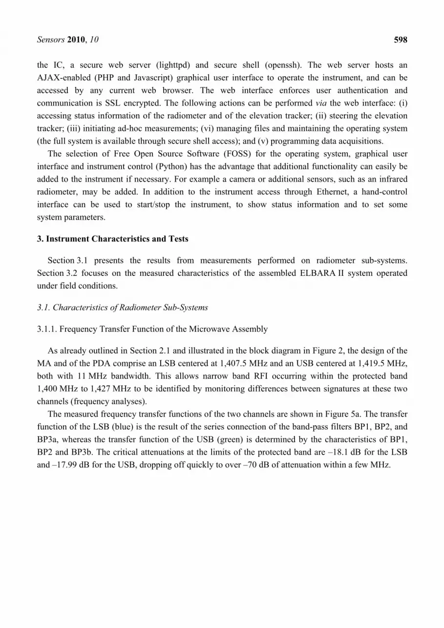
3.1.1. Frequency Transfer Function of the Microwave Assembly
As already outlined in Section 2.1 and illustrated in the block diagram in Figure 2, the design of the MA and of the PDA comprise an LSB centered at 1,407.5 MHz and an USB centered at 1,419.5 MHz, both with 11 MHz bandwidth. This allows narrow band RFI occurring within the protected band 1,400 MHz to 1,427 MHz to be identified by monitoring differences between signatures at these two channels (frequency analyses).
The measured frequency transfer functions of the two channels are shown in Figure 5a. The transfer function of the LSB (blue) is the result of the series connection of the band-pass filters BP1, BP2, and BP3a, whereas the transfer function of the USB (green) is determined by the characteristics of BP1, BP2 and BP3b. The critical attenuations at the limits of the protected band are –18.1 dB for the LSB and –17.99 dB for the USB, dropping off quickly to over –70 dB of attenuation within a few MHz.

Sensors 2010, 10
599
Figure 5. (a) Frequency transfer functions of the two frequency channels (LSB = blue, USB = green) of the microwave assembly. The borders of the protected part of the L-band at 1,400 MHz and 1,427 MHz are indicated in red. (b) Frequency response of the MA front-end. The loss measured at the radiometer center frequency of 1,413.5 MHz is Lfront = 1.09 dB.
3.1.2. Front-End Loss
The total loss Lfront of the front-end determines the residual noise TRM 0 of the radiometer. Based on the specifications (Appendx) of the front-end components (SW, ISO1, BP1, and three semi-rigid coaxial cables with SMA connectors) the total loss at the center frequency 1,314.5 MHz was estimated as Lfront ≈ 1.42 dB, yielding TRM 0 ≈ 125 K for the system temperature T0 = 313 K (see Section 2.1.1). Figure 5b shows the measured frequency transfer function of the front-end. For the different switch inputs the measurements were within 0.015 dB, and the repeatability of consecutive measurements was better than the sensitivity of the measurements (≈0.005 dB).
The frequency response of the front-end is dominated by the characteristics of the BP1 with the specified –3 dB bandwidth of 22 MHz at the radiometer center frequency 1,314.5 MHz. At this frequency, the overall front-end loss measured is Lfront ≈ 1.09 dB, which is well below the value expected from the specifications of the front-end components. Accordingly, the residual noise estimated from the measured Lfront is TRM 0 ≈ 108 K, which is smaller than TRM 0 ≈ 125 K estimated using the component specifications.
3.1.3. Linearity of the Power Detector Assembly
The PDA response is measured with the Micronetics noise module SNM 7114-C2A. Its output is band-pass filtered to cover the frequency range of 1,400 MHz–1,700 MHz, and then amplified by 30 dB yielding, a constant power level of P0 ≈ -25 dBm. Subsequently, P0 is passed through Agilent 9496B attenuators with the total attenuation variable in the range of 0 dB ≤ Atot ≤ 20 Db with a step size of 1 dB.

S
wleth
-0Mmoo(±fr
±oth
Sensors 201
For the awith an Agievels –25 dhe PDA. Th
Figure -38 dBm ≤
0.167 V ≤ UMA input nmeasured reoffset PPDA 0
offset PPDA 0
±0.05 dB) ofree, implyin
The asym±0.00247 μWof the PDA he instrume
Figurepower(7) witfor exp
0, 10
attenuators silent power
dBm ≥ PPDA
he resulting 6 shows PPDA ≤ –25
UPDA ≤ 3.33noise temperelation betw0 ≈ –0.00350 is not sigof the variang that the s
mptotic staW V-1. This
within a pent.
e 6. Measur in the rangth the gradipected MA
set to Atot =r meter. ThA ≥ –45 dBm
output voltthe resp
5 dBm (0.134 V (blackratures expe
ween the pow52 μW withnificant but
able attenuatsimple linea
[PDAP μ
andard erroand the co
ower range
ured voltagge –38 dBmient dPPDA/dinput noise
0 dB, the pis reference
m (correspotages UPDA o
ponse of 7 μW ≤ PP
k dots). Theected. Fittinwer PPDA [μ
h the standat explainedtor used in ar model de
] PDA
PDA
W dPdU
μ =
or of the rrelation co
e that includ
e response m ≤ PPDA ≤–dUPDA = 1.0e temperatur
power PPDA
e value andonding to 3.of the PDAthe PDA
PDA ≤ 3.33 μe red circlesng the modμW] and thrd error of
d by the errothe test setupicted in Fi
APDA
A
1.U⋅ =
power senoefficient Rdes the pow
UPDA(PPDA
–25 dBm (bl00939 μW Vres (Table 1
A ≈ –25 dBmd the select16 μW to 0
A are measurA with reμW), resultis are the PP
el PPDA = Phe voltages
±0.00564 μors in PPDA
up. Conseqigure 6 (soli
PDA.00939 U⋅
nsitivity dP= 0.99991
wer levels es
A) of the Plack dots). V-1. Red cir1).
m injected ted Atot is u
0.03 μW) inred with a mespect to ing in the rPDA from TaPPDA 0 + dPUPDA [V] y
μW. Hence,A caused byquently, the id line) is ad
[ ]A V
PPDA/dUPDA confirms thstimated for
DA with rThe solid licles are the
to the PDAused to injento the detemultimeter.
input porange of outable 1 estim
PPDA/dUPDA ⋅yields the sm, an appareny the knownPDA is virdequate:
= 1.0093he highly linr the operat
espect to inine is the lin
e estimates o
60
A is measurect the powector diode o
ower levetput voltage
mated for th⋅ UPDA to th
mall negativntly negativn uncertaintrtually offse
(7
39 μW V-1
near responstive mode o
njected near fit of PPDA
00
ed er of
els es he he ve ve ty
et-
7)
is se of

Sensors 2010, 10
601
3.1.4. Characteristics of the Active Cold Source
In Section 2.1.3, the ACS noise temperature is estimated to TACS ≈ 48 K, based on the specifications (Appendix) of the components involved (Figure 2, ISO2 and AMP5) at the physical temperature T0 = 313 K. The low TACS makes it challenging to calibrate the ACS absolutely in a lab experiment. On the one hand, the impact of losses is strong and difficult to control and, on the other, it is difficult to find a highly accurate noise standard with an even lower noise temperature.
Nevertheless, such lab measurements are performed using the resistive source (RS) at TRS = 300 K and the calibrated noise diode at TND = 1575 K as standards to be compared with TACS, which is to be determined. After amplifying these noise temperatures with the two amplifiers of the MA, their frequency responses are measured with a Agilent E4408B spectrum analyzer. The associated power levels for the frequency range (1,413 ± 500) MHz are determined to be PACS = 0.778 μW, PRS = 2.748 μW, and PHS = 11.888 μW. Finally, the known reference noise temperatures TRS = 300 K and TND = 1,575 K are used to determine TACS ≈ 39 K by considering a linear relation between power and injected noise.
This calibration of the ACS is error-prone due to the applied extrapolation, which multiplies the measurement uncertainties of the reference sources. Hence, a calibration procedure using the RS and the cold sky as a reference source is applied to determine TACS more accurately. The noise temperature of the RS is TRS = T0, which is significantly higher than TACS. In contrast, the noise standard Tsky, in = Tsky + ΔTB, FC ≈ 10 K (see Section 2) at the input of the radiometer looking towards the sky is smaller than TACS, which allows the ACS to be calibrated using linear interpolation instead of extrapolation:
( )RS sky, in
ACS ACS sky, in sky, inRS sky, in
T TT U U T
U U−
= − +−
(8)
The output voltage URS is measured for the resistive source (RS) switched to the radiometer input port, and Usky, in is measured with the instrument oriented towards the sky. As described in Section 2, Tsky, in = Tsky + ΔTB, FC is the received sky brightness Tsky, complemented with ΔTB, FC due to the loss of the FC. According to (6), the latter is particularly significant for low antenna brightness such as Tsky. If the radiometer is not pointing exactly towards the galaxy, the sun, or the moon, Tsky received varies marginally over the sky hemisphere. In this case Tsky can be computed as the sum of the down-welling atmospheric radiance plus the cosmic background emission (assumed to be 2.7 K), attenuated by the atmosphere [31]. Evaluating the model [31] for the radiometer set-up at WSL (zenith angle θ = 30 , elevation 554 m a.s.l.) and air temperatures between 0 °C and 30 °C yielded 4.44 K ≤ Tsky ≤ 4.48 K.
These theoretical values are used in the calibration procedure to determine TACS for 7 different set point temperatures T0 of the assembled ELBARA II system (Figure 1). The data to determine TACS consist of records of single radiometer voltages Usky in, URS, and UACS measured every 10 minutes between 10 p.m. and 2 a.m. on seven successive days in April 2009. This time period is selected in order to avoid disturbances caused by the galaxy passing through the field of view and to ensure the atmospheric conditions are comparable every day. The measurements are performed for T0 in the range

S
oth
naFtisσ
inteinTu
c
Sensors 201
of 21 °C–39he next mea
The voltanominal -3 dalmost the mFor the duraime of 10
settings yielσUsky, in, σU
The crossndicate theemperature ndicated in
TACS. It is asuses Tamb to
The solid
The posicaused by th
Figuretempertemper
0, 10
9 °C in stepsasurements,ages are redB cut-off
maximum tiation of datseconds ped data recor
URS, σUACS. ses in the to associatedfeedback lthe bottom
ssumed thacorrect for
d line in Fig
itive temperhe loss of th
e 7. Mean ratures T0 =ratures Tamb
s of 3 °C. T, T0 is switcecorded witfrequency ome resolutia recording
er voltage drds with me
op panel of d standard dloop is able
m panel of Ft most of ththe noise coure 7 is the
rature resphe isolator (I
noise temp= 21 °C, 24 b measured
To give the ched to the nth the ADCof the low-pon of nomin
g set to 10 sdata record.ean values ⟨
Figure 7 ardeviations σ
e to keep T0
Figure 7. Thhese variatioontribution linear inter
onse dTACS
ISO2), whic
peratures TA
°C, 27 °C, 3during the c
temperaturenext higher C samplingpass filters nally 2.5 mseconds, thi. As will b⟨Usky, in⟩, ⟨U
re the meanσTACS ≤ 0.
0 very stablehe variationons are dueΔTB, FC of t
rpolation to
S/dT0 ≈ 0.2ch increases
ACS of the A30 °C, 33 °Ccalibration m
e feedback value sever
g rate of fA
LPa/b in frms of the rad
is corresponbe discussed
URS⟩, ⟨UACS⟩
n TACS deriv.23 K and σe for the ra
n σTACS is lee to errors ihe FC to Ts
the mean T
24 K°C-1 is s with T0 (F
ACS measuC, 36 °C, 39measureme
loop sufficiral hours beADC = 800 Hront of the
diometer outnds to the nd in Sectionand very sm
ved for a spσT0 ≤ 0.1 K
anges of amess than 1%ntroduced b
sky. TACS:
mostly assigure 2).
ured for ins9 °C (top pants (bottom
ient time to fore measurHz, which ADC. Thistput voltage
nominal totan 3.2 (Tabmall standar
ecific T0. TK. This sh
mbient temp% of the meby the mod
sociated wi
strument seanel), and a
m panel).
60
settle beforring. is twice th
s implies the is recordedal integratiole 2b), thesrd deviation
The error barows that theratures Tam
easured meael (6), whic
(9)
ith the nois
et-point ambient
02
re
he at d. on se ns
rs he mb an ch
se

Sensors 2010, 10
603
The calibration procedure based on sky and RS measurements is also applied to the HS. The measured noise temperatures of the HS for 21 °C ≤ T0 ≤ 39 °C are in the range of 630 K < THS < 660 K, which is in good agreement with the estimated value given in Table 1. The temperature response dTHS/dT0 ≈ 1.60 K °C-1 measured is highly linear for the temperature range considered and mostly due to the increasing noise of the 6 dB attenuator attached to the output of the ND (Figure 2).
3.2. ELBARA II Characteristics
The radiometer output voltages, URS and UACS, recorded for the two frequency channels with the RS and the ACS switched to the MA are used to determine the most important system parameters. The same settings as these given in Section 3.1.4 applied to calibrate the ACS are used (sampling with fADC = 800 Hz during 10 seconds). The data set used consists of measurements performed every 10 minutes for 4 hours, resulting in a total of 2⋅24 data records for the RS and the ACS.
The characteristics measured for T0 = 313 K (40 °C) are summarized in Tables 2 and 3. The parameters measured are: The radiometer gain GRM, the residual noise temperature TRM 0, the time bandwidth product Bτ of a single measurement associated with the smallest possible integration time (nominally 2.5 ms), the voltage noise σUPDA of the PDA, the overall accuracies σURM of radiometer output voltages, and the corresponding accuracies σTB of brightness temperatures measured.
Table 2. System parameters of the ELBARA II radiometer measured at T0 = 313 K (40 °C).
System Parameter LSB channel
USB channel
both channels
GRM [mV K-1] 1.93 ± 0.01 1.79 ± 0.01 1.86 TRM, 0 [K] 147.0 ± 0.3 158.8 ± 0.3 153
Bτ [Hz s] 15,908 ± 291 15,828 ± 271 15,868
σUPDA [mV] 0.849 ± 0.150 0.449 ± 0.093 0.649
Table 3. Estimated uncertainties σURM and σTB of measured radiometer voltages URM and brightness TB for several radiometer inputs Tin, RM and durations τrec of the recorded data (T0 = 313 K).
τrec [s] σURM [mV] for several TRM, in σTB [K] for several TRM, in
10 K (sky) 41 K (ACS) 313 K (RS) 10 K (sky) 41 K (ACS) 313 K (RS)
2.5⋅10-3 2.493 2.937 6.911 1.34 1.58 3.72
1 0.125 0.147 0.346 0.07 0.08 0.19
3 0.072 0.085 0.199 0.04 0.05 0.11
10 0.039 0.046 0.109 0.02 0.02 0.06
The equations used to derive GRM, TRM 0, Bτ, σUPDA, and σURM, σTB from the measurements URS
and UACS are discussed below. The following conventions are used: (i) Voltages averaged over one

Sensors 2010, 10
604
data record of 10 seconds duration are ⟨URS⟩, ⟨UACS⟩ and their standard deviations are σUACS, σURS; (ii) the noise temperature of the RS is TRS = T0 (measured once for each data record); (iii) the expression (9) evaluated for measured T0 is used for TACS; (vi) the values given in Table 2 are mean values derived from the 2⋅24 data records URS, UACS.
Gain
The radiometer gain GRM = dURM/dTRM, in measures the response dURM of the radiometer output voltage URM with respect to a change dTRM, in in the input brightness temperature TRM, in. If the system response is considered linear, GRM is:
RS ACSRM
RS ACS
U UG
T T−
=−
(10)
The radiometer gains derived for the LSB and the USB channel differ by approximately 7%. This can be explained as due to small differences in the losses and gains of the components after the power splitter (Figure 2). However, the standard deviations of the GRM are very small for both channels. This is important to note, as it implies that GRM is highly stable during a measurement cycle, which lasts less than a minute, where the internal calibration and antenna are measured.
Residual noise
The linear extrapolation of the relation TRM, in(URM) to the value URM = 0 V yields the radiometer residual noise temperature:
RSRM, 0 RS
RM
UT T
G= −
(11)
As outlined in Section 2.1.1, TRM, 0 is mainly due to the noise of the first amplifier (AMP1) in the MA and to the loss along the front-end. As these microwave components are common for the two channels (Figure 2), the TRM, 0 for the LSB and the USB channels tend to be similar. However, TRM,0 ≈ 153 K given in Table 2 is larger than the value TRM,0 ≈ 125 K estimated from the component specifications, and also larger than TRM,0 ≈ 108 K estimated from the measured front-end loss. This is most likely due to small mismatches between the front-end components (SW, ISO1, BP1) causing reflections not considered in the estimation of TRM,0. Furthermore, a higher noise figure for the amplifier as a result of the higher internal physical temperature could explain the difference.
Time bandwidth product
The uncertainty σURM of the radiometer output voltage URM, depends on the product Bτ of the radiometer effective bandwidth Β and the effective integration time τ used to measure TRM, in. The low frequency noise σUPDA of the PDA may also contribute to σURM. Assuming these two voltage noise contributions are quasi-Gaussian and uncorrelated, the variance σURM
2 can then be expressed as:
( )22RM RM, in RM, 02 2
RM PDA
G T TU U
Bσ σ
τ
+= +
(12)

Sensors 2010, 10
605
Provided that measurements σURM = σUACS and σURM = σURS for the two different TRM,in = TACS and TRM,in = TRS are available, Bτ and σUPDA can be derived by solving the corresponding two equations of the form (12):
( ) ( )2 22
RM RS RM, 0 ACS RM, 0
2 2RS ACS
G T T T TB
U Uτ
σ σ
⎡ ⎤+ − +⎢ ⎥⎣ ⎦=−
and ( )22
RM RS RM, 02 2PDA RS
G T TU U
Bσ σ
τ
+= −
(13)
As can be seen in Table 2, the relative difference between Bτ found for the LSB and the USB are very small (≈0.5%), whereas the σUPDA of the two PDA channels differ significantly. Measurements on the PDA alone revealed σUPDA < 1 mV, mostly generated by the instrumentation amplifiers (≤0.6 mV), but also by noise leakage coupled e.g., through the power supply (≤0.3 mV). These measurements are in accordance with σUPDA given in Table 2. They also explain the significant difference between the USB and the LSB frequency channels.
Considering the nominal values for the bandwidth (11 MHz) and the integration time (2.5 ms), the nominal time bandwidth product would be Bτ = 27,500 Hz s, which is significantly larger than Bτ actually measured (Table 2). However, this is to be expected as neither the frequency transfer function of a channel (Figure 5a) nor the post detection frequency cut-off of fLP = 400 Hz (LPa/b) are ideal, which means that the real filter characteristics are not step functions at their band edges, but rather -3 dB values. This implies that the effective channel bandwidth, as well as the effective integration time, are both smaller than the nominal values. However, it is not critical to know the effective bandwidth and integration time precisely since the measured Bτ determine the measurement uncertainty.
Table 3 shows uncertainties σURM for three noise temperatures Tin, RM = 10 K, 41 K, 313 K at the MA input, corresponding to the approximate values for a sky measurement, the ACS and the RS noise. The σURM for τrec = 2.5 ms are uncertainties of single measurements URM with the shortest possible integration time (<2.5 ms), limited by the applied post-process low-pass filtering (fLP = 400 Hz). The corresponding values are computed with (12) using the parameters GRM, TRM 0, Bτ, σUPDA measured (right column in Table 2). The values shown in Table 3 agree well with the standard deviations of all the voltages, URM and UACS, measured (σURM = 6.912 mV and σUACS = 2.924 mV). Furthermore, the distribution of these voltages closely follows a Gaussian distribution.
The σURM for τrec = 1 s, 3 s, 10 s given in Table 3 are computed from σURM for τrec = 2.5 ms by considering that the standard deviation decays with N-1/2, where N = fLP⋅τrec is approximately the number of independent measurements available in a data record. This is the consequence of sampling the low-pass filtered signal with the -3 dB cut-off frequency fLP = 400 Hz with fADC = 2⋅ fLP = 800 Hz.
Accuracy of brightness temperatures
The uncertainty σTB of a brightness temperature TB measured is proportional to the uncertainty σURM scaled with the radiometer gain GRM:
RM
BRM
UTG
σσ =
(14)

Sensors 2010, 10
606
The uncertainties σTB given in the right three columns of Table 3 are expected for the indicated Tin, RM and τrec. The uncertainties σTB for τrec ≥ 3 s become smaller than 0.1 K for all input brightness temperatures that can be expected in applications of the radiometer. Therefore, a record duration ofτrec = 3 s, is recommended for operating ELBARA II.
3.2.1. Antenna
The return loss and the isolation between the horizontal and the vertical port of the antenna are important parameters. Both are measured with an Agilent E4408 spectrum analyzer attached to the antenna pointed towards the sky. Furthermore, knowing the directivity of the horn antenna is essential to know, as it determines the extent of the observed footprint. Measurements of these antenna characteristics are presented hereafter.
Return loss
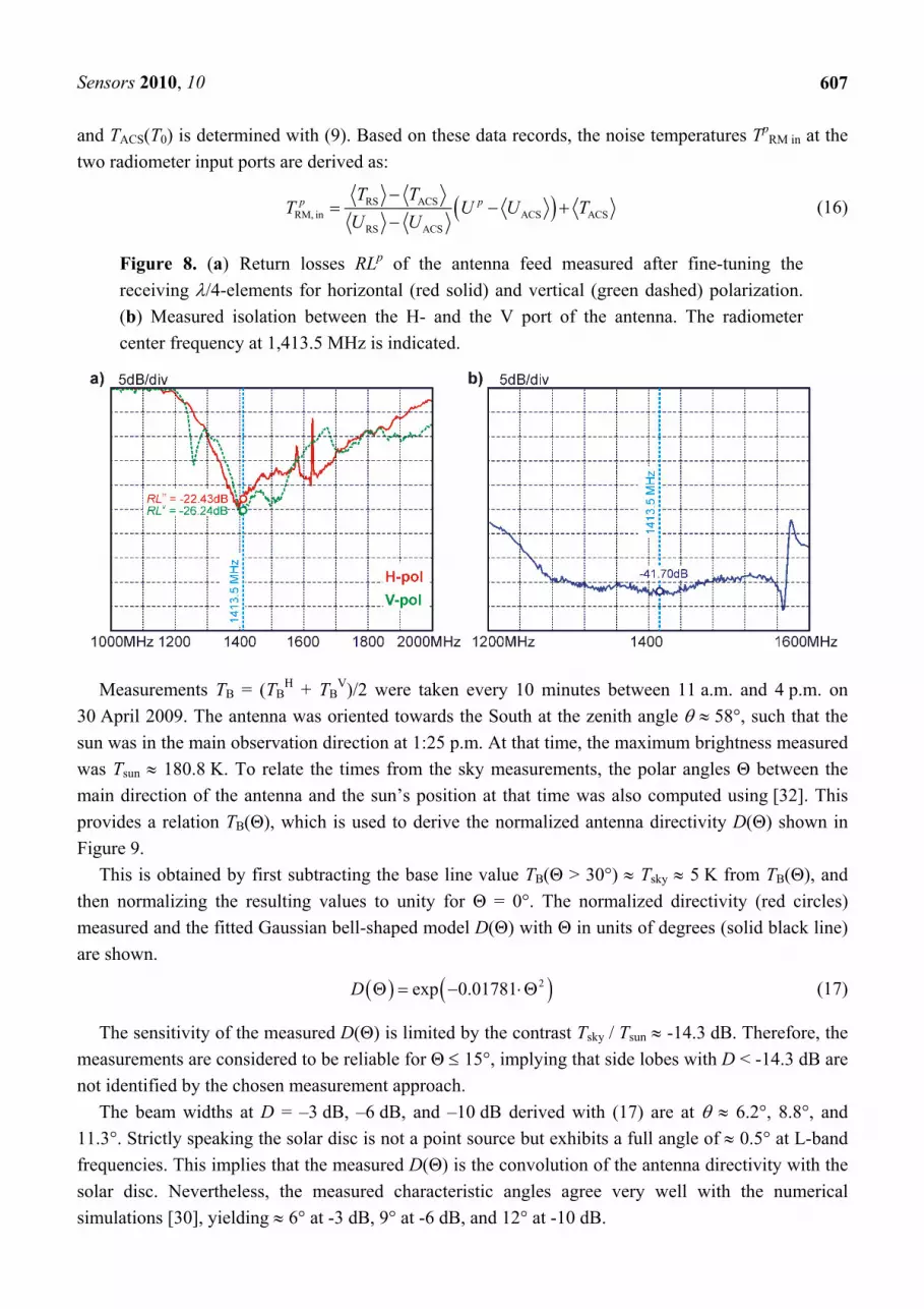
Figure 8a shows return losses RLp measured for the two ports (p = H, V) of the antenna. Measurements are performed for the frequency range of 1,000 MHz to 2,000 MHz using a spectrum analyzer and a directional coupler with directivity of about 20 dB–30 dB. The RLp [dB] shown are achieved after fine-tuning the length of the λ/4-structures receiving the radiances at H- and V-polarization, respectively (see Section 2.3). The measurements show that the specified value of RLp ≤ -20 dB are well met for the radiometer center frequency of 1,413.5 MHz.
H-V isolation
The isolation between the H- and V ports of the antenna (Figure 8b) was measured for 1,200 MHz to 1,600 MHz with the spectrum analyzer featuring an internal tracking source. The isolation is relatively constant over the radiometer bandwidth (1,400 MHz–1,427 MHz) and has a value of -41.7 dB at the radiometer center frequency. The measurements were the same, for either choosing the H- or the V port as the source. For a brightness temperature TB
p = 300 K this implies that the distortion caused by polarization crosstalk is less than 0.025 K, and therefore negligible.
Directivity
The directivity of the rotation-symmetric Pickett-horn antenna described in Section 2.3 is derived from polarization averaged brightness temperatures TB = (TB
H + TBV)/2, measured with the radiometer
looking towards the sky. Brightness temperatures TBp = TRM in
p - ΔTB, FC entering the antenna aperture are deduced from Tp
RM in (p = H, V) at the two radiometer input ports, corrected for the noise contribution ΔTB, FC of the FC computed with (6) (tFC = 0.98 corresponding to LFC ≈ 0.1 dB):
( )RM, in FC FC
BFC
1pp T t T
Tt
− −=
(15)
Data records, URS, UACS, UH, UV, with duration τrec = 5 s acquired with fADC = 800 Hz and the set point T0 = 305 K are measured every 10 minutes. The actual temperatures, T0 and TFC (FC temperature ≈ air temperature), are measured for each record. Furthermore, TRS = T0 = 32 °C (305 K) is assumed,
Sensors 2010, 10
607
and TACS(T0) is determined with (9). Based on these data records, the noise temperatures TpRM in at the
two radiometer input ports are derived as:
( )RS ACS
RM, in ACS ACSRS ACS
p pT TT U U T
U U−
= − +−
(16)
Figure 8. (a) Return losses RLp of the antenna feed measured after fine-tuning the receiving λ/4-elements for horizontal (red solid) and vertical (green dashed) polarization. (b) Measured isolation between the H- and the V port of the antenna. The radiometer center frequency at 1,413.5 MHz is indicated.
Measurements TB = (TB
H + TBV)/2 were taken every 10 minutes between 11 a.m. and 4 p.m. on
30 April 2009. The antenna was oriented towards the South at the zenith angle θ ≈ 58°, such that the sun was in the main observation direction at 1:25 p.m. At that time, the maximum brightness measured was Tsun ≈ 180.8 K. To relate the times from the sky measurements, the polar angles Θ between the main direction of the antenna and the sun’s position at that time was also computed using [32]. This provides a relation TB(Θ), which is used to derive the normalized antenna directivity D(Θ) shown in Figure 9.
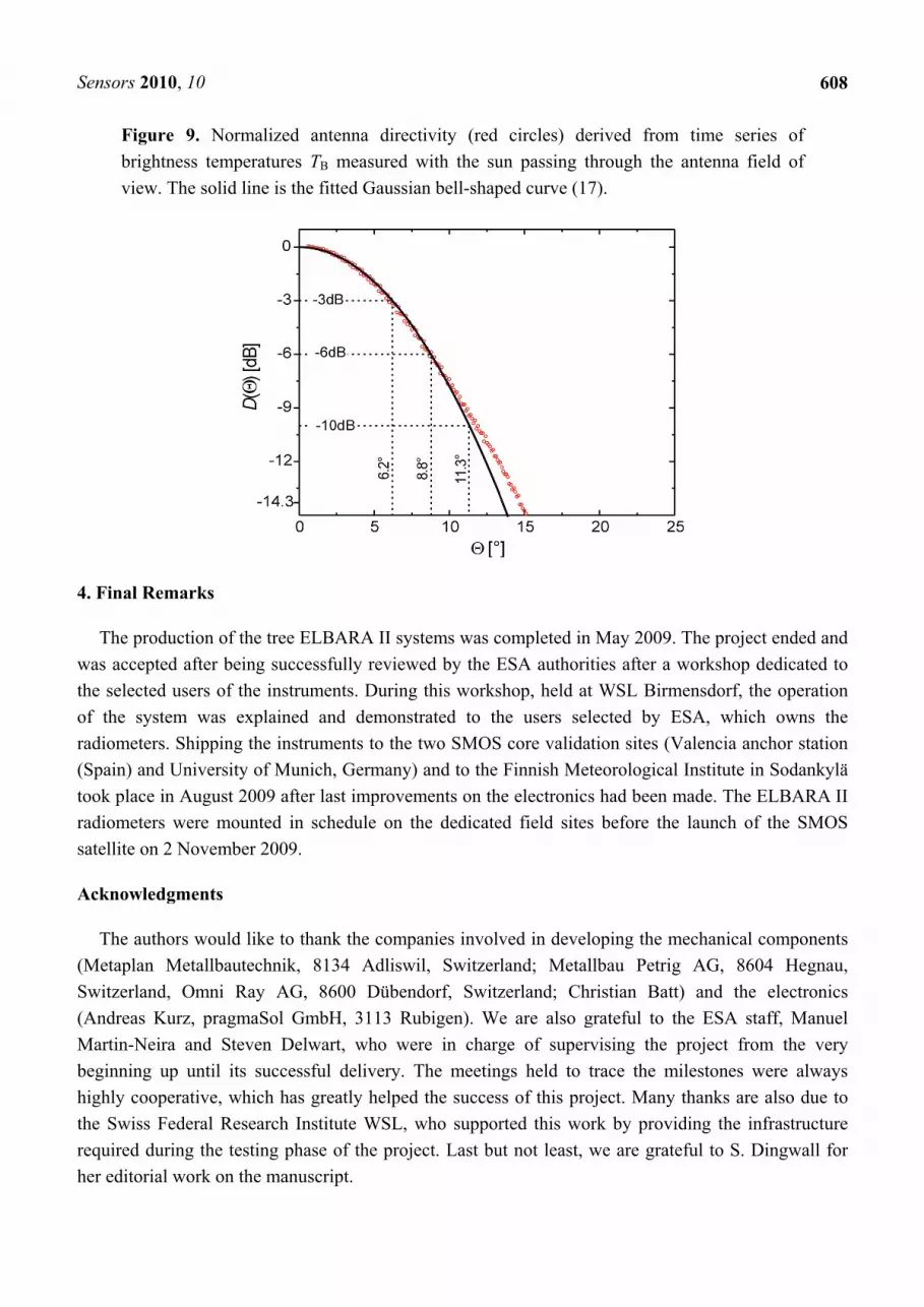
This is obtained by first subtracting the base line value TB(Θ > 30°) ≈ Tsky ≈ 5 K from TB(Θ), and then normalizing the resulting values to unity for Θ = 0°. The normalized directivity (red circles) measured and the fitted Gaussian bell-shaped model D(Θ) with Θ in units of degrees (solid black line) are shown.
( ) ( )2exp 0.01781D Θ = − ⋅Θ (17)
The sensitivity of the measured D(Θ) is limited by the contrast Tsky / Tsun ≈ -14.3 dB. Therefore, the measurements are considered to be reliable for Θ ≤ 15°, implying that side lobes with D < -14.3 dB are not identified by the chosen measurement approach.
The beam widths at D = –3 dB, –6 dB, and –10 dB derived with (17) are at θ ≈ 6.2°, 8.8°, and 11.3°. Strictly speaking the solar disc is not a point source but exhibits a full angle of ≈ 0.5° at L-band frequencies. This implies that the measured D(Θ) is the convolution of the antenna directivity with the solar disc. Nevertheless, the measured characteristic angles agree very well with the numerical simulations [30], yielding ≈ 6° at -3 dB, 9° at -6 dB, and 12° at -10 dB.
S
4
wthor(tors
A
(S(Mbhthrh
Sensors 201
Figurebrightnview.
4. Final Rem
The prodwas acceptehe selected
of the systeadiometers.Spain) and ook place inadiometers
satellite on 2
Acknowledg
The authoMetaplan M
SwitzerlandAndreas Ku
Martin-Neirbeginning uhighly coophe Swiss Fequired dur
her editorial
0, 10
e 9. Normness tempeThe solid li
marks
duction of thed after bein
users of them was ex. Shipping tUniversity n August 20were moun
2 November
gments
ors would lMetallbaute, Omni Ra
Kurz, pragmra and Stevup until its erative, whederal Resering the testl work on th
malized anteratures TB ine is the fit
he tree ELBng successfuhe instrumenxplained anthe instrumof Munich,
009 after lanted in schr 2009.
like to thankechnik, 813ay AG, 86
maSol GmbHven Delwar
successful hich has greearch Instituting phase o
he manuscri
enna directmeasured w
tted Gaussia
ARA II sysfully reviewnts. During
nd demonstents to the , Germany)st improvem
hedule on th
k the compa34 Adliswi600 DübendH, 3113 Rurt, who we
delivery. Teatly helpedute WSL, wof the projept.
tivity (red with the suan bell-shap
stems was cwed by the E
this workstrated to thtwo SMOS and to the
ments on thhe dedicate
anies involvil, Switzerldorf, Switzubigen). Were in chargThe meetind the succeswho supporect. Last bu
circles) dun passing ped curve (1
completed inESA authorshop, held ahe users se core validaFinnish Mee electronic
ed field site
ved in develand; Metazerland; Che are also gge of super
ngs held to s of this prrted this wout not least,
derived fromthrough the
17).
n May 2009rities after aat WSL Birmelected by ation sites (eteorologicacs had been es before th
eloping the mallbau Petrihristian Bagrateful to rvising the trace the m
roject. Manyork by provwe are gra
m time sere antenna f
9. The projea workshop mensdorf, tESA, whic
(Valencia anal Institute imade. The
he launch o
mechanicalig AG, 86
att) and thethe ESA sproject fro
milestones y thanks areviding the iateful to S. D
60
ries of field of
ect ended andedicated t
the operatioch owns thnchor statioin SodankyELBARA
of the SMO
l componen604 Hegnaue electronicstaff, Manuom the verwere alwaye also due tinfrastructurDingwall fo
08
nd to on he on lä II
OS
nts u, cs el ry ys to re or

Sensors 2010, 10
609
References
1. Jackson, T.J.; LeVine, D.M.; Hsu, A.Y.; Oldak, A.; Starks, P.J.; Swift, C.T.; Isham, J.D.; Haken, M. Soil moisture mapping at regional scales using microwave radiometry: the Southern Great Plains Hydrology Experiment. IEEE Trans. Geosci. Remot. Sensing 1999, 37, 2136−2151.
2. Njoku, E.G.; Jackson, T.J.; Lakshmi, V.; Nghiem, S.V. Soil moisture retrieval from AMSR-E. IEEE Trans. Geosci. Remot. Sensing 2003, 41, 215−229.
3. Schmugge, T. Applications of passive microwave observations of surface soil moisture. J. Hydrol. 1998, 212–213, 188−197.
4. Wigneron, J.P.; Kerr, Y.; Waldteufel, P.; Saleh, K.; Escorihuela, M.J.; Richaume, P.; Ferrazzoli, P.; Rosnay, P.D.; Gurney, R.; Calvet, J.C.; Grant, J.P.; Guglielmetti, M.; Hornbuckle, B.; Mätzler, C.; Pellarin, T.; Schwank, M. L-band Microwave Emission of the Biosphere (L-MEB) Model: Description and calibration against experimental data sets over crop fields. Remot. Sensing Env. 2007, 107, 639–655.
5. Grant, J.P.; Saleh, K.; Van de Griend, A.A.; Wigneron, J.P.; Guglielmetti, M.; Kerr, Y.; Schwank, M.; Skou, N. Calibration of the L-MEB model over a coniferous and a deciduous forest. IEEE Trans. Geosci. Remot. Sensing 2008, 46, 808–818.
6. Schmugge, T. Remote sensing of soil moisture. In encyclopedia of hydrological forecasting; Anderson, M.G., Burt, T., Eds.; John Wiley & Sons: Chichester, London, UK, 1985; pp. 101–124.
7. Shutko, A.M. Microwave radiometry of lands under natural and artificial moistening. IEEE Trans. Geosci. Remot. Sensing 1982, GE-20, 18–26.
8. Kerr, Y.; Waldteufel, P.; Wigneron, J.P.; Martinuzzi, J.M.; Font, J.; Berger, M. Soil moisture retrieval from space: The soil moisture and ocean salinity (SMOS) mission. IEEE Trans. Geosci. Remot. Sensing 2001, 39, 1729–1735.
9. Dobson, M.C.; Ulaby, F.T.; Hallikainen, M.T.; El-Rayes, M.A. Microwave dielectric behavior of wet soil-part II: Dielectric Mixing Models. IEEE Trans. Geosci. Remot. Sens. 1985, GE-23, 35–46.
10. Topp, G.C.; Davis, J.L.; Annan, A.P. Electromagnetic determination of soil water content: Measurements in coaxial transmission lines. Water Resour. Res. 1980, 16, 574–582.
11. Wang, J.R.; Schmugge, T. An empirical model for the complex dielectric permittivity of soils as a function of water content. IEEE Trans. Geosci. Remot. Sensing 1980, GE-18, 288–295.
12. Chanzy, A.; Kerr, Y.; Wigneron, J.P.; Calvet, J.C. Soil moisture estimation under sparse vegetation using microwave radiometry at C-band. IGARSS '97, Singapore, 1997; pp. 1090–1092.
13. Ulaby, F.; Moore, R.; Fung, A. Microwave Remote Sensing: Active and Passive, from Theory to Applications; Artech House: Norwood, MA, USA, 1986; Volume III.
14. Sharkov, E.A. Passive Microwave Remote Sensing of the Earth: Physical Foundations; Springer-Praxis Books in Geophysical Sciences: Berlin, Heidelberg, New York, NY, USA, 2003.
15. Font, J.; Lagerloef, G.S.E.; LeVine, D.M.; Camps, A.; Zanife, O.Z. The determination of surface salinity with the European SMOS space mission. IEEE Trans. Geosci. Remot. Sensing 2004, 42, 2196–2205.
16. European Space Agency. SMOS Earth Explorers. Available online: http://www.esa.int/esaLP/ LPsmos.html/ (accessed on 25 August 2009).

Sensors 2010, 10
610
17. European Space Agency. SMOS Technical Information and Publications. Available online: http://esamultimedia.esa.int/docs/SMOS_publications.pdf/ (accessed on 25 August 2009)
18. Special issue on the soil moisture and ocean salinity (smos) mission. IEEE Trans. Geosci. Remot. Sensing 2008; 44, 3471-3471.
19. Wigneron, J.P.; Kerr, Y.; Waldteufel, P.; Saleh, K.; Escorihuela, M.J.; Richaume, P.; Ferrazzoli, P.; de Rosnay, P.; Gurney, R.; Calvet, J.C.; Grant, J.P.; Guglielmetti, M.; Hornbuckle, B.; Mätzler, C.; Pellarin, T.; Schwank, M. L-band Microwave Emission of the Biosphere (L-MEB) Model: description and calibration against experimental data sets over crop fields. Remot. Sensing Envir. 2007, 107, 639–655.
20. IEEE GRSS. Newsletter June. Available online: http://www.grss-ieee.org/files/ngrs_NL_ 0609_Final.pdf/ (accessed on 25 August 2009).
21. Matzler, C.; Weber, D.; Wuthrich, M.; Schneeberger, K.; Stamm, C.; Wydler, H.; Fluhler, H. ELBARA, the ETH L-band radiometer for soil-moisture research. IEEE Int. Proc. 2003, 5, 3058–3060.
22. Guglielmetti, M.; Schwank, M.; Mätzler, C.; Oberdörster, C.; Vanderborght, J.; Flühler, H. FOSMEX: Forest soil moisture experiments with microwave radiometry. IEEE Trans. Geosci. Remote Sensing 2008, 46, 727–735.
23. Guglielmetti, M.; Schwank, M.; Mätzler, C.; Oberdörster, C.; Vanderborght, J.; Flühler, H. Measured microwave radiative transfer properties of a deciduous forest canopy. Remote Sens. Environ. 2007, 109, 523–532.
24. Schneeberger, K.; Schwank, M.; Stamm, C.; Rosnay, P.d.; Mätzler, C.; Flühler, H. Topsoil structure influencing soil water retrieval by microwave radiometry. Vadose Zone J. 2004, 3, 1169–1179.
25. Schwank, M.; Guglielmetti, M.; Mätzler, C.; Flühler, H. Testing a new model for the L-band radiation of moist leaf litter. IEEE Trans. Geosci. Remote Sensing 2008, 46, 1982–1994.
26. Schwank, M.; Mätzler, C.; Guglielmetti, M.; Flühler, H. L-Band radiometer measurements of soil water under growing clover grass. IEEE Trans. Geosci. Remote Sensing 2005, 43, 2225–2237.
27. Schwank, M.; Stähli, M.; Wydler, H.; Leuenberger, J.; Mätzler, C.; Flühler, H. Microwave L-Band Emission of Freezing Soil. IEEE Trans. Geosci. Remot. Sensing 2004, 42, 1252–1261.
28. Søbjærg, S.S. Polarimetric radiometers and their applications. Ph.D. Dissertation, Technical University of Denmark: Lyngby, Denmark. Available online: http://orbit.dtu.dk/getResource? recordId=60680&objectId=1&versionId=1/ (accessed on 25 August 2009).
29. Lemaître, F.; Poussière, J.C.; Kerr, Y.H.; Déjus, M.; Durbe, R.; Rosnay, P.d.; Calvet, J.C. Design and Test of the Ground-Based L-Band Radiometer for Estimating Water in Soils (LEWIS). IEEE Trans. Geosci. Remot. Sensing 2004, 42, 1666–1676.
30. Pickett, H.M.; Hardy, J.C.; Farhoomand, J. Characterization of a Dual-Mode Horn for Submillimeter Wavelengths. IEEE transactions Microwave Tech. 1984, 32, 936-937.
31. Pellarin, T.; Wigneron, J.P.; Calvet, J.C.; Berger, M.; Douville, H.; Ferrazzoli, P.; Kerr, Y.H.; Lopez-Baesa, E.; Pulliainen, J.; Simmonds, L.P.; Waldteufel, P. Two-year global simulation of L-band brightness temperatures over land. IEEE Trans. Geosci. Remot. Sensing 2003, 41, 2135–2139.

Sensors 2010, 10
611
32. High-resolution spectral modeling, Solar Calculator. GATS, Inc: Newport News, VA, USA. Available online: http://www.spectralcalc.com/ (accessed on 25 August 2009).
© 2010 by the authors; licensee Molecular Diversity Preservation International, Basel, Switzerland. This article is an open-access article distributed under the terms and conditions of the Creative Commons Attribution license (http://creativecommons.org/licenses/by/3.0/).

Sensors 2010, 10
612
Appendix
Specifications of the Electronic Components Used
Component Specifications Functionality
SW
Insertion loss < 0.1 dB Repeatability < 0.03 dB
Mechanical switch >107 operations
4-bit TTL control
Switching between H-, V-polarization and the calibration sources.
ISO1, ISO2
Tuned frequency = 1,413.5 MHz Loss = 0.20 dB Improve matching of amplifier inputs.
BP1
Center frequency = 1,413.5 MHz Insertion loss < 0.77 dB
-3 dB bandwidth = 22 MHz Min. attenuation at 1,391 MHz = 12 dB
Suppression of out-of-band RFI before amplification.
Determines the radiometer frequency response.
BP2
Center frequency = 1,413.5 MHz Insertion loss < 1.22 dB
-3 dB bandwidth = 22 MHz Min. attenuation at 1,391 MHz = 24 dB
Further suppression of out-of-band RFI.
Determines the radiometer frequency response.
BP3a, (BP3b)
Center frequency = 1,407.5 MHz (1,419.5 MHz)
Insertion loss < 1.3 dB -3 dB bandwidth = 11 MHz
Min. attenuation at 1,391 MHz = 21 dB
Split the noise power into 2 spectral bands for RFI detection in the
frequency domain.
LPa/b Cut-off frequency = 400 Hz G = 2 (active filter)
4th order LPF
Amplification and filtering of the detector output.
AMP1, AMP2, AMP5,
G = 40 dB NF = 0.5 dB (TAMP =34 K at T0 = 313 K)
Amplify noise power (AMP1/2) and act as cold noise source (AMP5).
AMP3a/b DC-instrumentation amplifier
Gain = 850 Noise = 8 nV⋅Hz-1/2
Offset < 25 μV
Amplification of detector output voltage.
AMP4a/b Buffer amplifier Gain = 1
Offset = < 10 mV Drive for ADC input.
splitter Insertion loss < 0.4 dB at 1,000 – 2,000 MHz
Amplitude imbalance < 0.01 dB.
Splitting RF into two channels for RFI detection in the frequency
domain.
DC-block Insertion loss < 0.15 dB remove low-frequency internal RFI or DC-bias signals.
detector
Zero-bias detector diode Low-level sensitivity = 0.4 mV/μW
Noise < 50 μV Frequency range: 0.01–12 GHz
Square-law detection of the RF-power.
ADC Number of channels = 4
Resolution = 16 bit Input voltage range = ±2.5V
Digitize the amplified, filtered, and detected noise.
source Noise temperature ≈ 1,575 K Additional hot calibration source.