MNRAS 000, 1–22 (2017) Preprint May 16, 2018 Compiled using MNRAS LATEX style file v3.0

Design and characterization of the Large-apertureExperiment to Detect the Dark Age (LEDA) radiometersystems

D.C. Price1,2,3?, L.J. Greenhill1†, A. Fialkov1, G. Bernardi4,5, H. Garsden1,B.R. Barsdell6, J. Kocz1,7, M.M. Anderson7, S.A. Bourke7, J. Craig8, M.R. Dexter2,J. Dowell8, M.W. Eastwood7, T. Eftekhari1,8, S.W. Ellingson9 G. Hallinan7,J.M. Hartman7, R. Kimberk1, T. Joseph W. Lazio10, S. Leiker1, D. MacMahon2,R. Monroe7, F. Schinzel8,11, G.B. Taylor8, E. Tong1, D. Werthimer2, D.P. Woody71Harvard-Smithsonian Center for Astrophysics, 60 Garden Street, Cambridge MA 02138 USA;2University of California Berkeley, 501 Campbell Hall, Berkeley CA 94720 USA;3Centre for Astrophysics & Supercomputing, Swinburne University of Technology, PO Box 218, Hawthorn, VIC 3122, Australia;4SKA SA, 3rd Floor, The Park, Park Road, Pinelands, 7405, South Africa;5Department of Physics and Electronics, Rhodes University, PO Box 94, Grahamstown, 6140, South Africa;6NVIDIA Corporation, 2701 San Tomas Expressway, Santa Clara, CA 95050, USA;7California Institute of Technology, 1200 E California Blvd, Pasadena, CA 91125 USA;8Department of Physics and Astronomy, University of New Mexico, Albuquerque, NM 87131, USA;9Bradley Dept. of Electrical & Computer Engineering, Virginia Tech, Blacksburg, VA 24061 USA;10Jet Propulsion Laboratory, California Institute of Technology, 4800 Oak Grove Dr., Pasadena CA 91106 USA11National Radio Astronomy Observatory, P.O. Box O, Socorro, NM 87801, USA

May 16, 2018

ABSTRACT

The Large-Aperture Experiment to Detect the Dark Age (LEDA) was designedto detect the predicted O(100)mK sky-averaged absorption of the Cosmic MicrowaveBackground by Hydrogen in the neutral pre- and intergalactic medium just after thecosmological Dark Age. The spectral signature would be associated with emergenceof a diffuse Lyα background from starlight during ‘Cosmic Dawn’. Recently, Bowmanet al. (2018) have reported detection of this predicted absorption feature, with an un-expectedly large amplitude of 530mK, centered at 78MHz. Verification of this resultby an independent experiment, such as LEDA, is pressing. In this paper, we detaildesign and characterization of the LEDA radiometer systems, and a first-generationpipeline that instantiates a signal path model. Sited at the Owens Valley Radio Ob-servatory Long Wavelength Array, LEDA systems include the station correlator, fivewell-separated redundant dual polarization radiometers and backend electronics. Theradiometers deliver a 30–85MHz band (16 < z < 34) and operate as part of thelarger interferometric array, for purposes ultimately of in situ calibration. Here, wereport on the LEDA system design, calibration approach, and progress in characteri-zation as of January 2016. The LEDA systems are currently being modified to improveperformance near 78MHz in order to verify the purported absorption feature.

Key words: telescopes, instrumentation: detectors, cosmology: observation, darkage, reionization, first stars

? E-mail: dancpr@berkeley.edu† E-mail: greenhill@cfa.harvard.edu

1 INTRODUCTION

Cosmic Dawn is a cosmological epoch extending betweenthe build up of the very first population of stars ∼ 100 Myr

c© 2017 The Authors

arX

iv:1

709.

0931

3v3

[as

tro-

ph.I

M]

15

May

201

8

2 Price et al.

after the Big Bang (z ∼ 30 Bromm & Yoshida 2011; Greif2015; Hirano & Bromm 2017), followed by correspondinggenerations of black holes (e.g., Becerra et al. 2015; Smithet al. 2017; Smidt et al. 2017), to the onset of widespreadreionization of the intergalactic medium (IGM) ∼ 500 Myrafter the Big Bang (z ∼ 10, Robertson et al. 2015). Thisis one of the most interesting and least understood epochsin the history of the Universe (for a recent review see, e.g.,Barkana 2016; Haiman 2016). Cosmic Dawn is marked bythe rise of the earliest populations of sources (stars and blackholes), rapid evolution of radiation fields, and the onset ofmetal enrichment (Safranek-Shrader et al. 2016; Wise et al.2014).

Recently, Bowman et al. (2018) reported detection ofthe sky-averaged spectral signature of the 21-cm ground-state transition of neutral Hydrogen (HI), placing CosmicDawn at redshifts 20>z>15. This signal, predicted by Shaveret al. (1999), is sensitive to both cosmological and astrophys-ical processes in the early Universe; as such, it is an excel-lent probe of the physics between the CMB decoupling andthe end of the epoch of reionization. Indeed, if verified, theBowman et al. (2018) result would constitute the earliest de-tection of the thermal footprint of the first stars (Greenhill2018).

Specifically, Bowman et al. (2018) report detection of an∼530mK absorption feature, centered at ∼78.1MHz, withwidth ∼18.7MHz, using a relatively simple—yet exquisitelycalibrated—dipole antenna and radiometer system knownas the Experiment to Detect the Global EoR Step (EDGES,Rogers & Bowman 2012; Monsalve et al. 2017). The am-plitude of this absorption feature is, remarkably, 2–3 timeshigher than that expected with the most optimistic mod-els (Pritchard & Loeb 2010; Fialkov et al. 2014; Fialkov& Loeb 2016; Cohen et al. 2017). Also at odds with ex-isting models, the feature is flat-bottomed, as opposed toGaussian-like. The Bowman et al. (2018) result suggests gastemperatures during Cosmic Dawn were far cooler than pre-viously predicted, and could even point toward interactionbetween baryons and dark-matter particles (Barkana 2018).An alternative explanation is that there was more radiationthan expected, such as a significant contribution from anextragalactic background Dowell & Taylor (2018).

Nevertheless, some concerns remain that the purportedCosmic Dawn signal could in fact be an artifact, due toan unmodelled periodic instrumental feature, for example(Hills et al. 2018). If verified, the Bowman et al. (2018) re-sult places virtually the first observational constraints onCosmic Dawn models. In comparison, the relatively more ex-plored Epoch of Reionization (EoR; z ∼ 6–10), is somewhatconstrained by (i) the integrated optical depth of Thomsonscattering of Cosmic Microwave Background (CMB) radia-tion (Planck Collaboration et al. 2016), (ii) the high-redshiftgalaxy UV luminosity function probed out to redshift ofz ∼ 10 (Bouwens et al. 2015; Atek et al. 2015), (iii) detec-tion of dusty galaxies at redshifts out to z ∼ 10 (Bouwenset al. 2016; Laporte et al. 2017), and (iv) supermassive blackholes at z ∼ 7 (Mortlock et al. 2011; Wu et al. 2015).

Cosmic Dawn is unique in terms of the astrophysicalprocesses and sources that played roles. In contrast to theEoR, which was likely populated by a ‘mature’ populationof galaxies residing in ∼ 108.5–1010 M halos (Mesingeret al. 2016) and producing copious ionizing radiation, Cos-

mic Dawn was populated by pockets of intense star forma-tion hosted in dark matter halos of ∼ 106–108 M, whichwere less efficient in ionizing their surroundings. Sources ofX-rays, Lyα and Lyman-Werner (LW, 11.2–13.6 eV) radi-ation, on the other hand, played major roles during thisepoch (e.g., Barkana 2016, and references therein), and di-rect study of this epoch is anticipated to deliver new knowl-edge about early stellar populations and to constrain forma-tion scenarios for supermassive black holes (complementaryto study of the EoR).

The preponderance of HI in the diffuse pre- and inter-galactic medium (P/IGM) during Cosmic Dawn, and thesensitivity of the transition to radiative backgrounds pro-duced by early stars and black holes makes the 21-cm linea unique tracer of the early Universe. To date, the mainfocus of radio instruments undertaking ‘21-cm cosmology’(Pritchard & Loeb 2010), has been detection of the of EoRpower spectrum (i.e. large-scale spatial fluctuations). TheGiant Meter-wave Radio Telescope (GMRT, Paciga et al.2013), the Precision Array for Probing the Epoch of Reion-ization (PAPER, Ali et al. 2015; Pober et al. 2015), theLow Frequency Array (LOFAR, Patil et al. 2017) and theMurchison Widefield Array (MWA, Beardsley et al. 2016;Ewall-Wice et al. 2016) have all placed upper limits on theamplitude of the EoR power spectrum. The upcoming Hy-drogen Epoch of Reionization Array (HERA, DeBoer et al.2017), and the Square Kilometre Array telescope (Koop-mans et al. 2015), also seek to constrain the EoR powerspectrum.

Several experiments have been deployed in an attemptto measure the global 21-cm EoR signal. The first con-straint on the global 21-cm EoR signal was provided byEDGES (Bowman et al. 2008; Rogers & Bowman 2012),which excluded reionization more rapid than ∆z > 0.06 with95% confidence. The Broadband Instrument for Global Hy-drOgen ReioNisation Signal (BIGHORNS, Sokolowski et al.2015), and the Shaped Antenna measurement of the back-ground RAdio Spectrum (SARAS, Patra et al. 2013; Singhet al. 2017) also target the global EoR signal, where resultsfrom the latter exclude at 68 to 95% confidence some param-eter combinations that correspond to late heating by X-raysin tandem with rapid reionization.

EDGES is one of several experiments designed to de-tect the global 21-cm Cosmic Dawn signal. The SARAS 2experiment (Singh et al. 2018), SCI-HI (Sonda Cosmológicade las Islas para la Detección de Hidrógeno Neutro, Voyteket al. 2014) and the related Probing Radio Intensity at highz from Marion (PRIZM) experiment, follow similar method-ology and instrumentation approaches. The Dark Ages Ra-dio Explorer (DARE) concept proposes a satellite-based ra-diometer in lunar orbit, where earth occultation and absenceof ionospheric effects are favorable (Datta et al. 2014; Burnset al. 2017).

Here, we detail the Large-Aperture Experiment to De-tect the Dark Age instrument (LEDA, see also Greenhill &Bernardi 2012; Bernardi et al. 2016), which observes at fre-quencies between the HF (3–30MHz) and FM (88–108MHz)radio broadcast bands (30<ν<88 MHz, 16 < z < 34). LEDAis unique in its embedding of radiometers in a densely inter-ferometric array to enable calibration of radiometric data (inpart) with observations of celestial sources (Sec. 8.1) and tocreate a ready path for exploration of power spectra estima-

MNRAS 000, 1–22 (2017)

Radiometer design and calibration for LEDA 3

tion for Cosmic Dawn. In this paper, we present the designand characterization of the radiometry system for LEDA.

The paper is organized as follows. In Section 2 we pro-vide a broad overview of the physics of Cosmic Dawn, detailsof the expected 21-cm signal, and outline of experimental re-quirements needed to observe the Cosmic Dawn signal. Wealso point out astrophysical scenarios that can be detectedor ruled out by LEDA. In Section 3 we set the stage dis-cussing the site and the architecture of the telescope. LEDAradiometers are discussed in Section 4. Calibration is dis-cussed in Section 5. In Section 6 we characterize the in-strument, including gain linearity, reflection and transmis-sion coefficients, receiver temperature, noise diode thermalstability, and temporal stability. Results, including absolutecalibration, RFI occupancy, spectral index measurements,and comparison to extant sky models appear in Section 7.Discussion folows in Section 8.

2 SCIENCE DRIVER

The 21-cm line is a tracer of HI at all stages of cosmic evolu-tion. Before the end of EoR, the signal is mainly produced bythe intergalactic neutral medium; at lower redshifts, galac-tic HI dominates. The signal is sensitive to both cosmologi-cal and astrophysical processes, and as such, is arguably thebest probe of the Universe at the intermediate redshift rangebetween the CMB decoupling and the end of reionization.

The observed differential brightness temperature rela-tive to the CMB is

T21 ≈ 27xHI

√1 + z

10

(TS − TCMB

TS

)[mK], (1)

where we have ignored terms of O(δ), with δ being spatialdensity fluctuations. In Eq. (1) xHI is the HI fraction, TCMB

is the CMB temperature, and TS is the spin temperaturedefined as

T−1S =

T−1CMB + xαT

−1c + xcT

−1K

1 + xα + xc(2)

where TK and Tc are kinetic and collisional temperatures,and xα and xc are Lyα and collisional coupling factors, re-spectively. Evolution of TS with redshift is complex anddepends on the intensity of the Lyα radiative backgroundthrough the Wouthuysen-Field (WF) effect (Wouthuysen1952; Field 1958) which sets xα, and on the thermal his-tory of the Universe via TK , Tc (with Tc ≈ TK) and xc. Thetemperature T21 may be positive or negative depending onthe sign of (TS − TCMB). For instance, when the transitionis coupled to the gas temperature and the P/IGM is colderthan the CMB, TS < TCMB and the signal is seen in ab-sorption (T21 < 0). When the gas is hotter than the CMB,TS > TCMB and the signal is seen in emission (T21 > 0).

For any particular scenario of structure and star forma-tion, the evolution of T21 can be used as a ‘cosmic clock’that tracks the evolution of the Universe. In what follows,we focus on the zero-mode of the signal from Eq. 1, a.k.a.,the global signal1. The predominant feature of the signal

1 Higher order modes are linked to spatial fluctuations and areoutside of the scope of this paper (for more details see Barkana2016, and references therein).

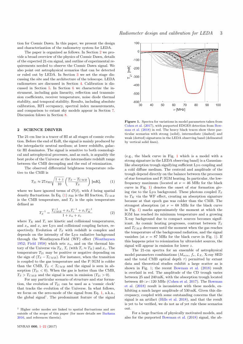
Figure 1. Spectra for variations in model parameters taken fromCohen et al. (2017), with purported EDGES detection from Bow-man et al. (2018) in red. The heavy black traces show three par-ticular scenarios with strong (solid), intermediate (dashed) andweak (dotted) signatures in the LEDA observing band (delineatedby vertical solid lines).

(e.g., the black curve in Fig. 1 which is a model with astrong signature in the LEDA observing band) is a Gaussian-like absorption trough signifying sufficient Lyα coupling anda cold diffuse medium. The centroid and amplitude of thetrough depend directly on the balance between the processesof star formation and P/IGM heating. In particular, the low-frequency maximum (located at ν = 46 MHz for the blackcurve in Fig. 1) denotes the onset of star formation giv-ing rise to the Lyα background. These photons coupled TSto TK via the WF effect, creating an absorption signaturebecause at that epoch gas was colder than the CMB. Thestrongest absorption (at ν = 68 MHz for the black curvein Fig. 1) marks approximately the moment at which theIGM has reached its minimum temperature and a growingX-ray background due to compact sources becomes signif-icant. As cosmic heating progresses, contrast between TSand TCMB decreases until the moment when the gas reachesthe temperature of the background radiation, and the signalvanishes (at ν = 87 MHz for the black curve in Fig. 1). Ifthis happens prior to reionization by ultraviolet sources, thesignal will appear in emission for lower z.

The 21-cm spectra for an ensemble of astrophysicalmodel parameters combinations (Mmin, f∗, LX , X-ray SEDand the total CMB optical depth τ) permitted by extantdata and theoretical studies exhibit a large scatter as isshown in Fig. 1; the recent Bowman et al. (2018) resultis overlaid in red. The amplitude of the CD trough variesbetween 25 and 240mK, with the absorption trough locatedbetween 40<ν<120 MHz (Cohen et al. 2017). The Bowmanet al. (2018) result is inconsistent with these models, ex-hibiting a much larger amplitude of 530mK. Given this dis-crepancy, coupled with some outstanding concerns that thesignal is an artifact (Hills et al. 2018), and that the resultis yet to be verified, we do not as of yet rule these scenariosout.

For a large fraction of physically motivated models, andalso for the purported Bowman et al. (2018) signal, the ab-

MNRAS 000, 1–22 (2017)

4 Price et al.

sorption minimum falls within the LEDA observing band,and, thus, could be detected by the instrument. This is dis-cussed further in the next section.

2.1 Observational Prospects

Radiometric detection requires separation of foreground sig-nals and the (background) 21-cm signal. The diffuse andcontinuum foreground sources are know to be spectrallysmooth; that is, they exhibit power-law spectra over the 30–88MHz band. As such, they are separable from the back-ground signal, which is expected to manifest as an ab-sorption trough. Pritchard & Loeb (2010) showed a ba-sic demonstration of concept, by convolving a Global SkyModel (GSM, de Oliveira-Costa et al. 2008) with an ana-lytical model for a simple dipole antenna to form simulatedmeasurements; this approach is followed by several CosmicDawn experiments (Singh et al. 2018; Voytek et al. 2014;Bowman et al. 2018), including LEDA.

The spectral smoothness of foregrounds allows retrievalof 21-cm features by modeling the brightness temperature ofthe foreground, Tfg, with a low-order log-polynomial. Harkeret al. (2012) expounded on this by including instrumentaleffects; Bernardi et al. (2015) showed that the angular struc-ture and frequency dependence of a more realistic broadbanddipole (modeled on the design of the Long Wavelength Ar-ray) increases the required polynomial order but not neces-sarily so much so as to confound detection. For this approachto work, any spectral structure introduced by the measure-ment apparatus must be accounted for and calibrated out.For this reason, zero-mode radiometer experiments have pre-ferred simple, low-gain dipole antennas over high-gain singledishes that exhibit more complex gain patterns (Bernardiet al. 2015; Mozdzen et al. 2016). We discuss the approachof LEDA to calibration in Section 5.

Significance of the detection by LEDA is determined bytiny deviations in the shape of the actual sky temperaturefrom the smooth foreground curve in the LEDA band. Toestimate which part of the astrophysical parameter space isactually targeted by LEDA, we use the signal to noise ratio(SNR) defined as

SN2 =∑i

(Tsky − Tfg)2

σ2i

(3)

where the sum is over frequency channels in the LEDA band,the mock data is defined as Tsky = Tfg+Tcosm and the fore-ground signal is modeled as a seventh order polynomial inlog ν (Bernardi et al. 2016). We fit out the foreground com-ponent by calculating Tfg as a best fit to the mock dataof the shape provided by Bernardi et al. (2016). The resid-ual signal is then compared to the rms noise given by theradiometer equation

σ ≈ 2.6× Tsys√∆νt

(4)

where ∆ν is the bandwidth over which the signal is mea-sured, and t is the integration time, and we assumed that thesystem temperature, Tsys, is dominated by the temperatureof the sky. The factor 2.6 is an approximation that takes intoaccount thermal uncertainties after calibration. (Here we as-sumed hot and cold reference diode temperatures of 6500Kand 1000K, as is explained in detail in Sec. 5, Eq. 18). Thus

for a sky temperature of 2000K and using ∆ν=1MHz, a 5σdetection of the Bowman et al. (2018) feature could be madein under 45minutes of observation with LEDA.

Alternatively, one may calculate SNR for each of the∼ 200 models shown in Fig. 1, assuming ∆ν = 1MHz andintegration time of 1000 hours. Out of ∼ 200 different as-trophysical scenarios (Fig. 1) the models with the highestSNR are those with strongest variation within the LEDAband. These models typically share high star formation ef-ficiency (often in low-mass halos) and high X-ray efficiency,which suggests that LEDA should have considerable lever-age in constraining (i) star formation during cosmic dawn,and in particular the roles of small halos, and (ii) the tim-ing of X-ray heating and properties of high-redshift X-raysources (e.g., XRB, mini-quasars). The model with the high-est signal to noise of SNR = 9.2 (heavy solid curve in Fig.1) shows both a strong absorption and an early emissionsignal within the LEDA band. These features are hard tomimic with smooth foregrounds. The underlying astrophysi-cal model assumes high star formation efficiency of f∗ = 50%in heavy halos above circular velocity of 35.5 km s−1 and avery luminous XRB population shining at the luminosity ofLX = 15× 1041 erg s−1 per unit star formation rate in Myr−1 (i.e., 50 times brighter than the low-redshift counter-parts).

In another detectable scenario (heavy dashed curve)only the absorption trough is located within the LEDA bandwhich makes the detection a bit more challenging. The un-derlying astrophysical model has moderate star formationefficiency, f∗ = 5%, stars form via cooling of atomic hydro-gen, X-ray heating is due to XRB with LX = 2.4 × 1041

erg s−1 per unit star formation rate in M yr−1, and thetotal CMB optical depth of τ = 0.066. The moderate starformation and heating result in a moderate SNR = 4 in theLEDA band. Finally, in Fig. 1 we also show an astrophysi-cal scenario that cannot be separated from the foregrounds,and, thus, is undetectable by LEDA (SNR = 0.1, dotted linein the figure). This case has low star formation efficiency,f∗ = 0.5%, star formation via molecular hydrogen coolingsubjected to strong LW feedback, and weak X-ray heatingwith LX = 0.03× 1041 erg s−1.

3 INSTRUMENT OVERVIEW

Motivated by limitations of single-antenna experiments,LEDA is a multi-antenna experiment, co-installed on theLong Wavelength Array stations at Owens Valley RadioObservatory (OVRO-LWA, 37.24N, 118.28W), and theNational Radio Astronomy Observatory in Socorro, NewMexico (LWA1, 34.07N, 107.63W). Initial work, based atLWA1, is presented in (Schinzel et al., LWA Memo #208);here we focus on work carried out at OVRO-LWA. Furtherdetails about the LWA systems may be found in Taylor et al.(2012); Ellingson et al. (2013).

At both the LWA1 and OVRO-LWA stations, an ad-ditional 5 outrigger stands (Fig. 2) were installed and out-fitted with the LEDA frontend receiver card (see Sec. 4).The LEDA outrigger stands, detailed further in Sec. 3.3,are placed at a distance from the core to minimize mutualcoupling effects. Bernardi et al. (2015) argue that detectionwill require precise knowledge of the antenna radiation pat-

MNRAS 000, 1–22 (2017)

Radiometer design and calibration for LEDA 5

300 200 100 0 100 200

Local X [WGS84, m]

200

100

0

100

200

300

Loca

l Y [

WG

S84, m

]

252253

254

255

256

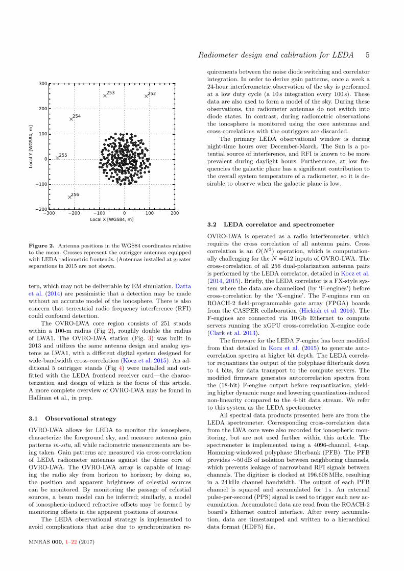
Figure 2. Antenna positions in the WGS84 coordinates relativeto the mean. Crosses represent the outrigger antennas equippedwith LEDA radiometric frontends. (Antennas installed at greaterseparations in 2015 are not shown.

tern, which may not be deliverable by EM simulation. Dattaet al. (2014) are pessimistic that a detection may be madewithout an accurate model of the ionosphere. There is alsoconcern that terrestrial radio frequency interference (RFI)could confound detection.

The OVRO-LWA core region consists of 251 standswithin a 100-m radius (Fig 2), roughly double the radiusof LWA1. The OVRO-LWA station (Fig. 3) was built in2013 and utilizes the same antenna design and analog sys-tems as LWA1, with a different digital system designed forwide-bandwidth cross-correlation (Kocz et al. 2015). An ad-ditional 5 outrigger stands (Fig 4) were installed and out-fitted with the LEDA frontend receiver card—the charac-terization and design of which is the focus of this article.A more complete overview of OVRO-LWA may be found inHallinan et al., in prep.

3.1 Observational strategy

OVRO-LWA allows for LEDA to monitor the ionosphere,characterize the foreground sky, and measure antenna gainpatterns in-situ, all while radiometric measurements are be-ing taken. Gain patterns are measured via cross-correlationof LEDA radiometer antennas against the dense core ofOVRO-LWA. The OVRO-LWA array is capable of imag-ing the radio sky from horizon to horizon; by doing so,the position and apparent brightness of celestial sourcescan be monitored. By monitoring the passage of celestialsources, a beam model can be inferred; similarly, a modelof ionospheric-induced refractive offsets may be formed bymonitoring offsets in the apparent positions of sources.

The LEDA observational strategy is implemented toavoid complications that arise due to synchronization re-

quirements between the noise diode switching and correlatorintegration. In order to derive gain patterns, once a week a24-hour interferometric observation of the sky is performedat a low duty cycle (a 10 s integration every 100 s). Thesedata are also used to form a model of the sky. During theseobservations, the radiometer antennas do not switch intodiode states. In contrast, during radiometric observationsthe ionosphere is monitored using the core antennas andcross-correlations with the outriggers are discarded.

The primary LEDA observational window is duringnight-time hours over December-March. The Sun is a po-tential source of interference, and RFI is known to be moreprevalent during daylight hours. Furthermore, at low fre-quencies the galactic plane has a significant contribution tothe overall system temperature of a radiometer, so it is de-sirable to observe when the galactic plane is low.

3.2 LEDA correlator and spectrometer

OVRO-LWA is operated as a radio interferometer, whichrequires the cross correlation of all antenna pairs. Crosscorrelation is an O(N2) operation, which is computation-ally challenging for the N =512 inputs of OVRO-LWA. Thecross-correlation of all 256 dual-polarization antenna pairsis performed by the LEDA correlator, detailed in Kocz et al.(2014, 2015). Briefly, the LEDA correlator is a FX-style sys-tem where the data are channelized (by ‘F-engines’) beforecross-correlation by the ‘X-engine’. The F-engines run onROACH-2 field-programmable gate array (FPGA) boardsfrom the CASPER collaboration (Hickish et al. 2016). TheF-engines are connected via 10Gb Ethernet to computeservers running the xGPU cross-correlation X-engine code(Clark et al. 2013).

The firmware for the LEDA F-engine has been modifiedfrom that detailed in Kocz et al. (2015) to generate auto-correlation spectra at higher bit depth. The LEDA correla-tor requantizes the output of the polyphase filterbank downto 4 bits, for data transport to the compute servers. Themodified firmware generates autocorrelation spectra fromthe (18-bit) F-engine output before requantization, yield-ing higher dynamic range and lowering quantization-inducednon-linearity compared to the 4-bit data stream. We referto this system as the LEDA spectrometer.

All spectral data products presented here are from theLEDA spectrometer. Corresponding cross-correlation datafrom the LWA core were also recorded for ionospheric mon-itoring, but are not used further within this article. Thespectrometer is implemented using a 4096-channel, 4-tap,Hamming-windowed polyphase filterbank (PFB). The PFBprovides ∼50 dB of isolation between neighboring channels,which prevents leakage of narrowband RFI signals betweenchannels. The digitizer is clocked at 196.608MHz, resultingin a 24 kHz channel bandwidth. The output of each PFBchannel is squared and accumulated for 1 s. An externalpulse-per-second (PPS) signal is used to trigger each new ac-cumulation. Accumulated data are read from the ROACH-2board’s Ethernet control interface. After every accumula-tion, data are timestamped and written to a hierarchicaldata format (HDF5) file.

MNRAS 000, 1–22 (2017)

6 Price et al.

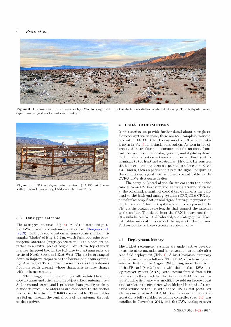
Figure 3. The core area of the Owens Valley LWA, looking north from the electronics shelter located at the edge. The dual-polarizationdipoles are aligned north-south and east-west.

Figure 4. LEDA outrigger antenna stand (ID 256) at OwensValley Radio Observatory, California, January 2015.

3.3 Outrigger antennas

The outrigger antennas (Fig. 4) are of the same design asthe LWA cross-dipole antennas, detailed in Ellingson et al.(2013). Each dual-polarization antenna consists of four tri-angular ’blades’ of length 1.4m, which form two pairs of or-thogonal antennas (single-polarization). The blades are at-tached to a central pole of height 1.5m, at the top of whichis a weatherproof box for the FE. The two antenna pairs areoriented North-South and East-West. The blades are angleddown to improve response at the horizon and beam symme-try. A wire-grid 3×3-m ground screen isolates the antennasfrom the earth ground, whose characteristics may changewith moisture content.

The outrigger antennas are physically isolated from thecore antennas and other metallic objects. Each antenna has a3×3m ground screen, and is protected from grazing cattle bya wooden fence. The antennas are connected to the sheltervia buried lengths of LMR400 coaxial cable. These cablesare fed up through the central pole of the antenna, throughto the receiver.

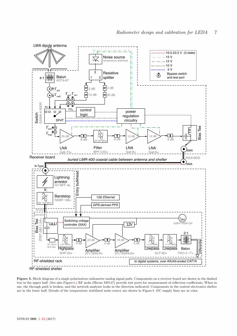
4 LEDA RADIOMETERS

In this section we provide further detail about a single ra-diometer system; in total, there are 5×2 complete radiome-ters within LEDA. A block diagram of a LEDA radiometeris given in Fig. 5 for a single polarization. As seen in the di-agram, there are four main components: the antenna, front-end receiver, back-end analog systems, and digital systems.Each dual-polarization antenna is connected directly at itsterminals to the front-end electronics (FE). The FE convertsthe balanced antenna terminal pair to unbalanced 50Ω viaa 4:1 balun, then amplifies and filters the signal, outputtingthe conditioned signal over a buried coaxial cable to theOVRO-LWA electronics shelter.

The entry bulkhead of the shelter connects the buriedcoaxial to an FM bandstop and lightning arrestor installedat the bulkhead; a length of coaxial cable connects the bulk-head to the back-end analog systems (CRX).The CRX ap-plies further amplification and signal filtering, in preparationfor digitization. The CRX systems also provide power to theFE, via the coaxial cable lengths that connect the antennato the shelter. The signal from the CRX is converted from50Ω unbalanced to 100Ω balanced, and Category-7A Ether-net cables are used to transport the signals to the digitizer.Further details of these systems are given below.

4.1 Deployment history

The LEDA radiometer systems are under active develop-ment; iterative upgrades and improvements are made aftereach field deployment (Tab. 1). A brief historical summaryof deployments is as follows. The LEDA correlator systemachieved first light in August 2013, using an early revisionof the FE card (ver 2.0) along with the standard LWA ana-log receiver system (ARX), with spectra formed from 4-bitdata sent to the correlator. In December 2013, the correla-tor F-engine firmware was modified to add an independentautocorrelator spectrometer with higher bit-depth. An up-dated version of the FE with added MS147 test ports (ver2.5) was installed in April 2014. Due to concerns of potentialcrosstalk, a fully shielded switching controller (Sec. 4.3) wasinstalled in November 2014, and the LWA analog receiver

MNRAS 000, 1–22 (2017)

Radiometer design and calibration for LEDA 7

controllogic

power regulation circuitry

Gali-74+LNA Filter

BPF-C45+ Gali-6+LNA

Gali-6+LNA

SP4T

GS

WA

-4-3

0D

RS

witc

h

2 dB

Resistivesplitter

SMA

25 dB 12 dB 12 dB

25-90 MHz

Bia

sTe

e

ADT4-6TBalun

LWA dipole antenna

88-108 MHz

Receiver board

RF-shielded shelter

RF-shielded rack

buried LMR-400 coaxial cable between antenna and shelter

NSBP-108+Bandstop

Lightning arrestor

Amplifier Amplifier

>27 MHz

Highpass

ZF

BT

-28

2-1

.5A

+

SHP-25+ ZFL-500LN+ ZFL-500HLN+

6 dB 6 dB 6 dB <115 MHz <115 MHz

Lowpass Lowpass SLP-90+

24 dB 19 dB

Switching voltage

controller (SAX)

GPS-derived PPS

RG316DS

1Gb Ethernet

En

try b

ulk

he

ad

12 dB

2 dB

20 dB

1 2

8 dB 6 dB 3 dB

16.5-23.5 V (3 state)

15 V

12 V

to digital systems, over ARJ45-ended CAT7A

Balun

TTL

GT-NFF-AL

SMA

RG316DS

N-Type

Diff

ere

ntia

l

TMO-2-1T+

Γant

Γsw0

NC

Γsw1Γ

ns1

Γsw3

Γlna0

Bypass switchand test port

Noise sourcetemperature stabilized

A28H1100M-230

+ -28V

RFC240

DC BlockBLK-89+

Bia

sTe

e

10 V

5 V

12V

2:1

4:1

Figure 5. Block diagram of a single polarization radiometer analog signal path. Components on a receiver board are shown in the dashedbox in the upper half. (See also Figure 6.) RF jacks (Hirose MS147) provide test ports for measurement of reflection coefficients. When inuse, the through path is broken, and the network analyzer looks in the direction indicated. Components in the central electronics shelterare in the lower half. Details of the temperature stabilized noise source are shown in Figure 8. DC supply lines are in color.

MNRAS 000, 1–22 (2017)

8 Price et al.

Table 1. Summary of radiometer system upgrades 2013–2016.

mmyy Deployment milestones

08/13 First light(1)

12/13 Embedded standalone 8-bit spectrometers(2)

04/14 FE ver. 2.5: bandpass filtering11/14 Shielded programmable switching controller12/14 Shielded, low cross-talk backend systems, high-

isolation standard for multi-channel cables(3)

01/16 FE ver. 2.9: improved impedance matches, betternoise source stability, high RF directivity

(1) FE ver. 2.0, unshielded 1Hz switching controller, LWAanalog backend, and LEDA correlator.(2) Phased out use of station correlator for precision radiometricdata.(3) Adoption of Bel-Stewart ARJ45 differential cable-endstandard for RF over twisted pair between analog receivers andcorrelator digital samplers.

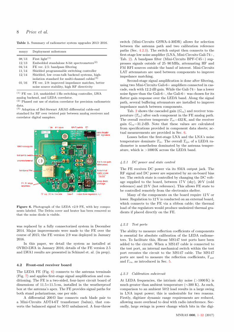
Figure 6. Photograph of the LEDA v2.9 FE, with key compo-nents labeled. The Delrin cover and heater has been removed sothat the noise diode is visible.

was replaced by a fully connectorized system in December2014. Major improvements were made to the FE over thecourse of 2015; the FE version 2.9 was deployed in January2016.

In this paper, we detail the system as installed atOVRO-LWA in January 2016; details of the FE version 2.5and LWA1 results are presented in Schinzel et. al. (in prep).

4.2 Front-end receiver board

The LEDA FE (Fig. 6) connects to the antenna terminals(Fig. 7) and applies first-stage signal amplification and con-ditioning. The FE is a two-sided, four-layer circuit board ofdimensions of 11.5×11.5 cm, installed in the weatherproofbox at the antenna’s apex. The FE provides signal paths forboth stand polarizations, one per side.

A differential 200Ω line connects each blade pair toa Mini-Circuits ADT4-6T transformer (balun), that con-verts the balanced signal to 50Ω unbalanced. A four-throw

switch (Mini-Circuits GSWA-4-30DR) allows for selectionbetween the antenna path and two calibration referencepaths (Sec. 4.2.3). The switch output then connects to thefirst-stage low noise amplifier (LNA, Mini-Circuits Gali-74+,Tab. 2). A bandpass filter (Mini-Circuits BPF-C45+) sup-presses signals outside of 25–90MHz, attenuating HF andFM RFI sources outside the band of interest. Mini-CircuitsLAT attenuators are used between components to improveimpedance matching.

Second-stage signal amplification is done after filtering,using two Mini-Circuits Gali-6+ amplifiers connected in cas-cade, each with 12.2 dB gain. While the Gali-74+ has a lowernoise figure than the Gali-6+, the Gali-6+ was chosen for itsflatter gain response over the LEDA band. Along the signalpath, several buffering attenuators are installed to improveimpedance match between components.

Tab. 2 shows the cascaded gain (Grx) and receiver tem-perature (Trx) after each component in the FE analog path.The overall receiver temperate Trx=432K, and the receivergain Grx=31.2 dB. Note that these values are calculatedfrom specifications provided in component data sheets; ac-tual measurements are provided in Sec. 6.

Losses before the first-stage LNA and the LNA’s noisetemperature dominate Trx. The overall Tsys of a LEDA ra-diometer is nonetheless dominated by the antenna temper-ature, which is >1000K across the LEDA band.

4.2.1 DC power and state control

The FE receives DC power via its SMA output jack. TheRF signal and DC power are separated by an on-board biastee. The switch state is controlled by changing the DC volt-age supplied to the board, between 17V (sky), 20V (coldreference) and 23V (hot reference). This allows FE state tobe controlled remotely from the electronics shelter.

Many of the components on the board require 12V orlower. Regulation to 12V is conducted on an external board,which connects to the FE via a ribbon cable; the thermalload of the regulators would produce undesired thermal gra-dients if placed directly on the FE.

4.2.2 Test ports

The ability to measure reflection coefficients of componentsis essential for absolute calibration of the LEDA radiome-ters. To facilitate this, Hirose MS147 test ports have beenadded to the circuit. When a MS147 cable is connected tothe test port, an internal mechanical switch within the testport reroutes the circuit to the MS147 cable. The MS147ports are used to measure the reflection coefficients, Γant

and Γrx, as introduced in Sec. 5.

4.2.3 Calibration subcircuit

At LEDA frequencies, the intrinsic sky noise (>1000K) ismuch greater than ambient temperature (∼300 K). As such,comparison to an ambient 50Ω load results in a large swingin LNA input power; this is undesirable for two reasons.Firstly, digitizer dynamic range requirements are reduced,allowing more overhead to deal with radio interference. Sec-ondly, large swings in power change which bits in the digi-

MNRAS 000, 1–22 (2017)

Radiometer design and calibration for LEDA 9

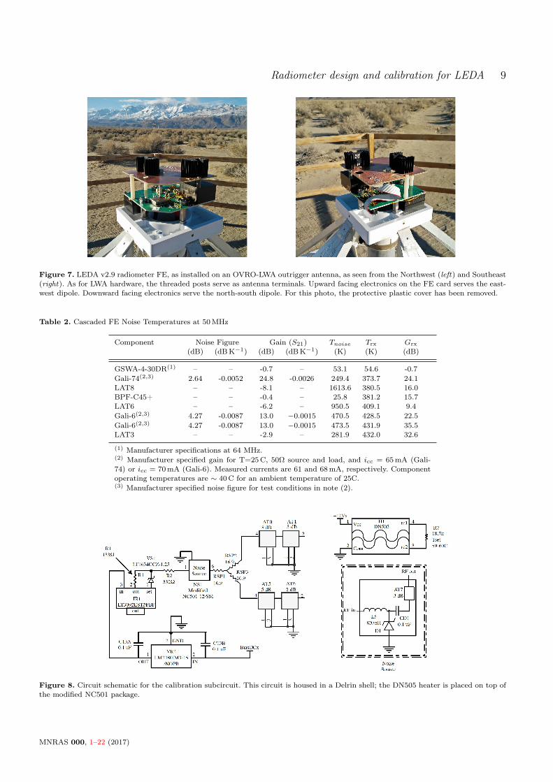
Figure 7. LEDA v2.9 radiometer FE, as installed on an OVRO-LWA outrigger antenna, as seen from the Northwest (left) and Southeast(right). As for LWA hardware, the threaded posts serve as antenna terminals. Upward facing electronics on the FE card serves the east-west dipole. Downward facing electronics serve the north-south dipole. For this photo, the protective plastic cover has been removed.

Table 2. Cascaded FE Noise Temperatures at 50MHz

Component Noise Figure Gain (S21) Tnoise Trx Grx

(dB) (dBK−1) (dB) (dBK−1) (K) (K) (dB)

GSWA-4-30DR(1) – – -0.7 – 53.1 54.6 -0.7Gali-74(2,3) 2.64 -0.0052 24.8 -0.0026 249.4 373.7 24.1LAT8 – – -8.1 – 1613.6 380.5 16.0BPF-C45+ – – -0.4 – 25.8 381.2 15.7LAT6 – – -6.2 – 950.5 409.1 9.4Gali-6(2,3) 4.27 -0.0087 13.0 −0.0015 470.5 428.5 22.5Gali-6(2,3) 4.27 -0.0087 13.0 −0.0015 473.5 431.9 35.5LAT3 – – -2.9 – 281.9 432.0 32.6

(1) Manufacturer specifications at 64 MHz.(2) Manufacturer specified gain for T=25C, 50Ω source and load, and icc = 65mA (Gali-74) or icc = 70mA (Gali-6). Measured currents are 61 and 68mA, respectively. Componentoperating temperatures are ∼ 40C for an ambient temperature of 25C.(3) Manufacturer specified noise figure for test conditions in note (2).

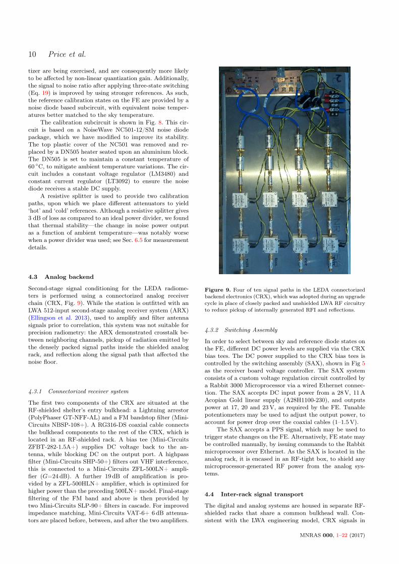
Figure 8. Circuit schematic for the calibration subcircuit. This circuit is housed in a Delrin shell; the DN505 heater is placed on top ofthe modified NC501 package.

MNRAS 000, 1–22 (2017)

10 Price et al.

tizer are being exercised, and are consequently more likelyto be affected by non-linear quantization gain. Additionally,the signal to noise ratio after applying three-state switching(Eq. 19) is improved by using stronger references. As such,the reference calibration states on the FE are provided by anoise diode based subcircuit, with equivalent noise temper-atures better matched to the sky temperature.

The calibration subcircuit is shown in Fig. 8. This cir-cuit is based on a NoiseWave NC501-12/SM noise diodepackage, which we have modified to improve its stability.The top plastic cover of the NC501 was removed and re-placed by a DN505 heater seated upon an aluminium block.The DN505 is set to maintain a constant temperature of60 C, to mitigate ambient temperature variations. The cir-cuit includes a constant voltage regulator (LM3480) andconstant current regulator (LT3092) to ensure the noisediode receives a stable DC supply.

A resistive splitter is used to provide two calibrationpaths, upon which we place different attenuators to yield‘hot’ and ‘cold’ references. Although a resistive splitter gives3 dB of loss as compared to an ideal power divider, we foundthat thermal stability—the change in noise power outputas a function of ambient temperature—was notably worsewhen a power divider was used; see Sec. 6.5 for measurementdetails.

4.3 Analog backend

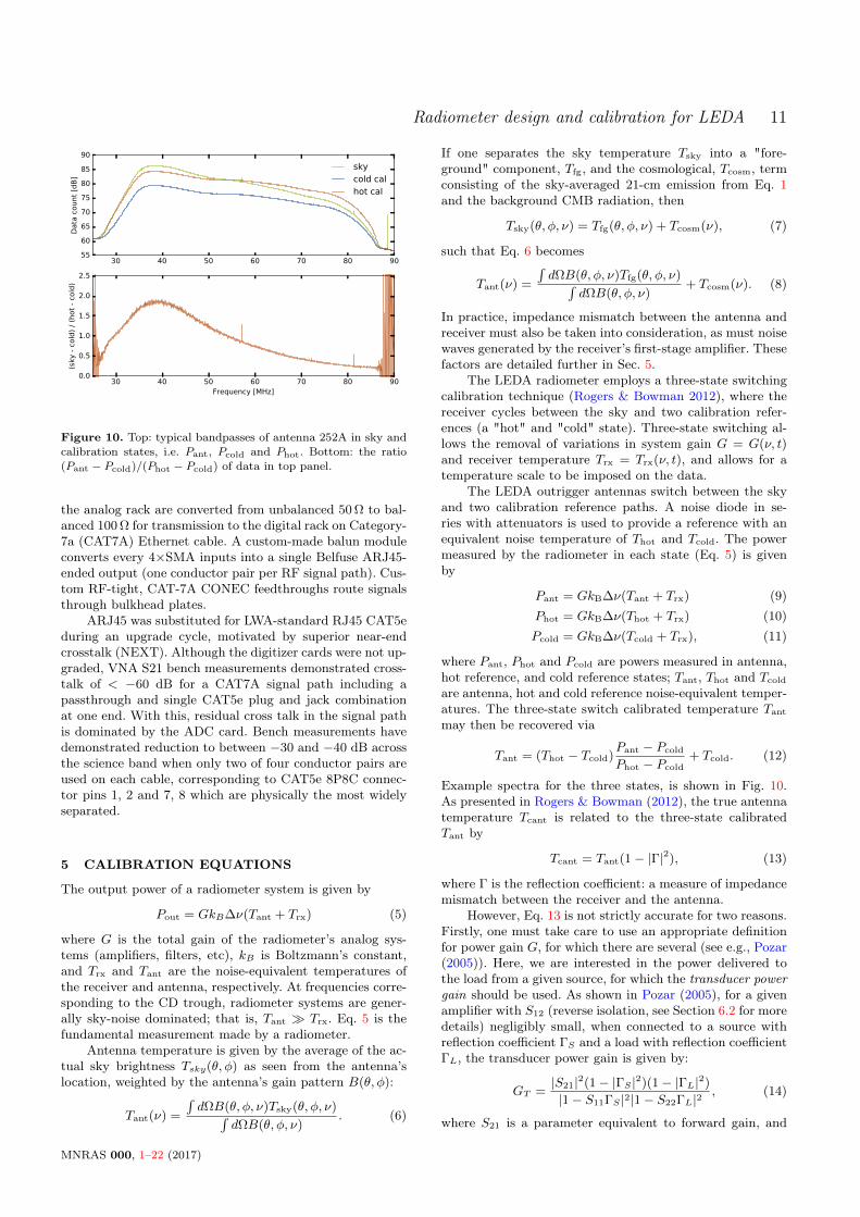
Second-stage signal conditioning for the LEDA radiome-ters is performed using a connectorized analog receiverchain (CRX, Fig. 9). While the station is outfitted with anLWA 512-input second-stage analog receiver system (ARX)(Ellingson et al. 2013), used to amplify and filter antennasignals prior to correlation, this system was not suitable forprecision radiometry: the ARX demonstrated crosstalk be-tween neighboring channels, pickup of radiation emitted bythe densely packed signal paths inside the shielded analograck, and reflection along the signal path that affected thenoise floor.

4.3.1 Connectorized receiver system

The first two components of the CRX are situated at theRF-shielded shelter’s entry bulkhead: a Lightning arrestor(PolyPhaser GT-NFF-AL) and a FM bandstop filter (Mini-Circuits NBSP-108+). A RG316-DS coaxial cable connectsthe bulkhead components to the rest of the CRX, which islocated in an RF-shielded rack. A bias tee (Mini-CircuitsZFBT-282-1.5A+) supplies DC voltage back to the an-tenna, while blocking DC on the output port. A highpassfilter (Mini-Circuits SHP-50+) filters out VHF interference,this is connected to a Mini-Circuits ZFL-500LN+ ampli-fier (G=24dB). A further 19 dB of amplification is pro-vided by a ZFL-500HLN+ amplifier, which is optimized forhigher power than the preceding 500LN+ model. Final-stagefiltering of the FM band and above is then provided bytwo Mini-Circuits SLP-90+ filters in cascade. For improvedimpedance matching, Mini-Circuits VAT-6+ 6dB attenua-tors are placed before, between, and after the two amplifiers.

Figure 9. Four of ten signal paths in the LEDA connectorizedbackend electronics (CRX), which was adopted during an upgradecycle in place of closely packed and unshielded LWA RF circuitryto reduce pickup of internally generated RFI and reflections.

4.3.2 Switching Assembly

In order to select between sky and reference diode states onthe FE, different DC power levels are supplied via the CRXbias tees. The DC power supplied to the CRX bias tees iscontrolled by the switching assembly (SAX), shown in Fig 5as the receiver board voltage controller. The SAX systemconsists of a custom voltage regulation circuit controlled bya Rabbit 3000 Microprocessor via a wired Ethernet connec-tion. The SAX accepts DC input power from a 28V, 11AAcopian Gold linear supply (A28H1100-230), and outputspower at 17, 20 and 23V, as required by the FE. Tunablepotentiometers may be used to adjust the output power, toaccount for power drop over the coaxial cables (1–1.5V).

The SAX accepts a PPS signal, which may be used totrigger state changes on the FE. Alternatively, FE state maybe controlled manually, by issuing commands to the Rabbitmicroprocessor over Ethernet. As the SAX is located in theanalog rack, it is encased in an RF-tight box, to shield anymicroprocessor-generated RF power from the analog sys-tems.

4.4 Inter-rack signal transport

The digital and analog systems are housed in separate RF-shielded racks that share a common bulkhead wall. Con-sistent with the LWA engineering model, CRX signals in

MNRAS 000, 1–22 (2017)

Radiometer design and calibration for LEDA 11

30 40 50 60 70 80 9055

60

65

70

75

80

85

90

Data

count

[dB

]

skycold calhot cal

30 40 50 60 70 80 90Frequency [MHz]

0.0

0.5

1.0

1.5

2.0

2.5

(sky

- c

old

) /

(hot

- co

ld)

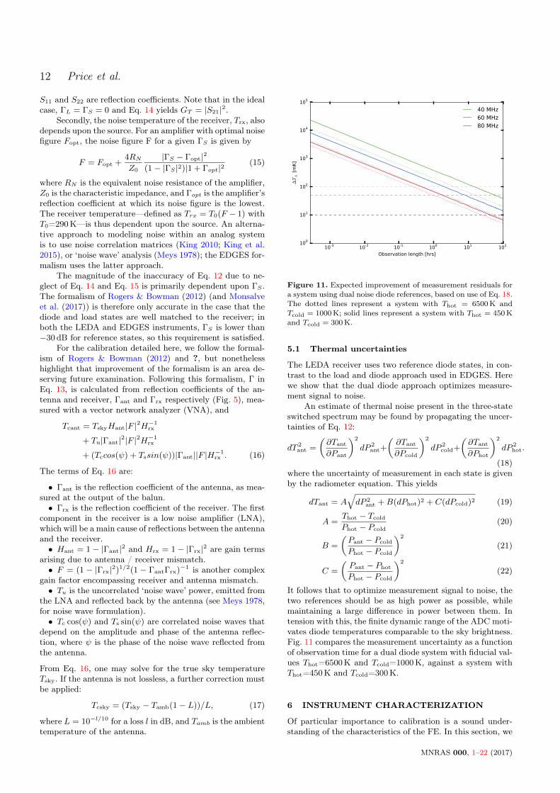
Figure 10. Top: typical bandpasses of antenna 252A in sky andcalibration states, i.e. Pant, Pcold and Phot. Bottom: the ratio(Pant − Pcold)/(Phot − Pcold) of data in top panel.

the analog rack are converted from unbalanced 50Ω to bal-anced 100Ω for transmission to the digital rack on Category-7a (CAT7A) Ethernet cable. A custom-made balun moduleconverts every 4×SMA inputs into a single Belfuse ARJ45-ended output (one conductor pair per RF signal path). Cus-tom RF-tight, CAT-7A CONEC feedthroughs route signalsthrough bulkhead plates.

ARJ45 was substituted for LWA-standard RJ45 CAT5eduring an upgrade cycle, motivated by superior near-endcrosstalk (NEXT). Although the digitizer cards were not up-graded, VNA S21 bench measurements demonstrated cross-talk of < −60 dB for a CAT7A signal path including apassthrough and single CAT5e plug and jack combinationat one end. With this, residual cross talk in the signal pathis dominated by the ADC card. Bench measurements havedemonstrated reduction to between −30 and −40 dB acrossthe science band when only two of four conductor pairs areused on each cable, corresponding to CAT5e 8P8C connec-tor pins 1, 2 and 7, 8 which are physically the most widelyseparated.

5 CALIBRATION EQUATIONS

The output power of a radiometer system is given by

Pout = GkB∆ν(Tant + Trx) (5)

where G is the total gain of the radiometer’s analog sys-tems (amplifiers, filters, etc), kB is Boltzmann’s constant,and Trx and Tant are the noise-equivalent temperatures ofthe receiver and antenna, respectively. At frequencies corre-sponding to the CD trough, radiometer systems are gener-ally sky-noise dominated; that is, Tant Trx. Eq. 5 is thefundamental measurement made by a radiometer.

Antenna temperature is given by the average of the ac-tual sky brightness Tsky(θ, φ) as seen from the antenna’slocation, weighted by the antenna’s gain pattern B(θ, φ):

Tant(ν) =

∫dΩB(θ, φ, ν)Tsky(θ, φ, ν)∫

dΩB(θ, φ, ν). (6)

If one separates the sky temperature Tsky into a "fore-ground" component, Tfg, and the cosmological, Tcosm, termconsisting of the sky-averaged 21-cm emission from Eq. 1and the background CMB radiation, then

Tsky(θ, φ, ν) = Tfg(θ, φ, ν) + Tcosm(ν), (7)

such that Eq. 6 becomes

Tant(ν) =

∫dΩB(θ, φ, ν)Tfg(θ, φ, ν)∫

dΩB(θ, φ, ν)+ Tcosm(ν). (8)

In practice, impedance mismatch between the antenna andreceiver must also be taken into consideration, as must noisewaves generated by the receiver’s first-stage amplifier. Thesefactors are detailed further in Sec. 5.

The LEDA radiometer employs a three-state switchingcalibration technique (Rogers & Bowman 2012), where thereceiver cycles between the sky and two calibration refer-ences (a "hot" and "cold" state). Three-state switching al-lows the removal of variations in system gain G = G(ν, t)and receiver temperature Trx = Trx(ν, t), and allows for atemperature scale to be imposed on the data.

The LEDA outrigger antennas switch between the skyand two calibration reference paths. A noise diode in se-ries with attenuators is used to provide a reference with anequivalent noise temperature of Thot and Tcold. The powermeasured by the radiometer in each state (Eq. 5) is givenby

Pant = GkB∆ν(Tant + Trx) (9)Phot = GkB∆ν(Thot + Trx) (10)Pcold = GkB∆ν(Tcold + Trx), (11)

where Pant, Phot and Pcold are powers measured in antenna,hot reference, and cold reference states; Tant, Thot and Tcold

are antenna, hot and cold reference noise-equivalent temper-atures. The three-state switch calibrated temperature Tant

may then be recovered via

Tant = (Thot − Tcold)Pant − Pcold

Phot − Pcold+ Tcold. (12)

Example spectra for the three states, is shown in Fig. 10.As presented in Rogers & Bowman (2012), the true antennatemperature Tcant is related to the three-state calibratedTant by

Tcant = Tant(1− |Γ|2), (13)

where Γ is the reflection coefficient: a measure of impedancemismatch between the receiver and the antenna.

However, Eq. 13 is not strictly accurate for two reasons.Firstly, one must take care to use an appropriate definitionfor power gain G, for which there are several (see e.g., Pozar(2005)). Here, we are interested in the power delivered tothe load from a given source, for which the transducer powergain should be used. As shown in Pozar (2005), for a givenamplifier with S12 (reverse isolation, see Section 6.2 for moredetails) negligibly small, when connected to a source withreflection coefficient ΓS and a load with reflection coefficientΓL, the transducer power gain is given by:

GT =|S21|2(1− |ΓS |2)(1− |ΓL|2)

|1− S11ΓS |2|1− S22ΓL|2, (14)

where S21 is a parameter equivalent to forward gain, and

MNRAS 000, 1–22 (2017)

12 Price et al.

S11 and S22 are reflection coefficients. Note that in the idealcase, ΓL = ΓS = 0 and Eq. 14 yields GT = |S21|2.

Secondly, the noise temperature of the receiver, Trx, alsodepends upon the source. For an amplifier with optimal noisefigure Fopt, the noise figure F for a given ΓS is given by

F = Fopt +4RNZ0

|ΓS − Γopt|2

(1− |ΓS |2)|1 + Γopt|2(15)

where RN is the equivalent noise resistance of the amplifier,Z0 is the characteristic impedance, and Γopt is the amplifier’sreflection coefficient at which its noise figure is the lowest.The receiver temperature—defined as Trx = T0(F − 1) withT0=290K—is thus dependent upon the source. An alterna-tive approach to modeling noise within an analog systemis to use noise correlation matrices (King 2010; King et al.2015), or ‘noise wave’ analysis (Meys 1978); the EDGES for-malism uses the latter approach.

The magnitude of the inaccuracy of Eq. 12 due to ne-glect of Eq. 14 and Eq. 15 is primarily dependent upon ΓS .The formalism of Rogers & Bowman (2012) (and Monsalveet al. (2017)) is therefore only accurate in the case that thediode and load states are well matched to the receiver; inboth the LEDA and EDGES instruments, ΓS is lower than−30dB for reference states, so this requirement is satisfied.

For the calibration detailed here, we follow the formal-ism of Rogers & Bowman (2012) and ?, but nonethelesshighlight that improvement of the formalism is an area de-serving future examination. Following this formalism, Γ inEq. 13, is calculated from reflection coefficients of the an-tenna and receiver, Γant and Γrx respectively (Fig. 5), mea-sured with a vector network analyzer (VNA), and

Tcant = TskyHant|F |2H−1rx

+ Tu|Γant|2|F |2H−1rx

+ (Tccos(ψ) + Tssin(ψ))|Γant||F |H−1rx . (16)

The terms of Eq. 16 are:

• Γant is the reflection coefficient of the antenna, as mea-sured at the output of the balun.• Γrx is the reflection coefficient of the receiver. The first

component in the receiver is a low noise amplifier (LNA),which will be a main cause of reflections between the antennaand the receiver.• Hant = 1− |Γant|2 and Hrx = 1− |Γrx|2 are gain terms

arising due to antenna / receiver mismatch.• F = (1 − |Γrx|2)1/2(1 − ΓantΓrx)−1 is another complex

gain factor encompassing receiver and antenna mismatch.• Tu is the uncorrelated ‘noise wave’ power, emitted from

the LNA and reflected back by the antenna (see Meys 1978,for noise wave formulation).• Tc cos(ψ) and Ts sin(ψ) are correlated noise waves that

depend on the amplitude and phase of the antenna reflec-tion, where ψ is the phase of the noise wave reflected fromthe antenna.

From Eq. 16, one may solve for the true sky temperatureTsky. If the antenna is not lossless, a further correction mustbe applied:

Tcsky = (Tsky − Tamb(1− L))/L, (17)

where L = 10−l/10 for a loss l in dB, and Tamb is the ambienttemperature of the antenna.

10-3 10-2 10-1 100 101 102

Observation length [hrs]

100

101

102

103

104

105

∆TA

[m

K]

40 MHz60 MHz80 MHz

Figure 11. Expected improvement of measurement residuals fora system using dual noise diode references, based on use of Eq. 18.The dotted lines represent a system with Thot = 6500K andTcold = 1000K; solid lines represent a system with Thot = 450Kand Tcold = 300K.

5.1 Thermal uncertainties

The LEDA receiver uses two reference diode states, in con-trast to the load and diode approach used in EDGES. Herewe show that the dual diode approach optimizes measure-ment signal to noise.

An estimate of thermal noise present in the three-stateswitched spectrum may be found by propagating the uncer-tainties of Eq. 12:

dT 2ant =

(∂Tant

∂Pant

)2

dP 2ant+

(∂Tant

∂Pcold

)2

dP 2cold+

(∂Tant

∂Phot

)2

dP 2hot.

(18)where the uncertainty of measurement in each state is givenby the radiometer equation. This yields

dTant = A√dP 2

ant +B(dPhot)2 + C(dPcold)2 (19)

A =Thot − Tcold

Phot − Pcold(20)

B =

(Pant − Pcold

Phot − Pcold

)2

(21)

C =

(Pant − Phot

Phot − Pcold

)2

(22)

It follows that to optimize measurement signal to noise, thetwo references should be as high power as possible, whilemaintaining a large difference in power between them. Intension with this, the finite dynamic range of the ADC moti-vates diode temperatures comparable to the sky brightness.Fig. 11 compares the measurement uncertainty as a functionof observation time for a dual diode system with fiducial val-ues Thot=6500K and Tcold=1000K, against a system withThot=450K and Tcold=300K.

6 INSTRUMENT CHARACTERIZATION

Of particular importance to calibration is a sound under-standing of the characteristics of the FE. In this section, we

MNRAS 000, 1–22 (2017)

Radiometer design and calibration for LEDA 13

30 28 26 24 22 20 18 16Input power [dBm]

3.0

2.5

2.0

1.5

1.0

0.5

0.0

0.5

Gain

Com

pre

ssio

n [

dB

]

50 MHz

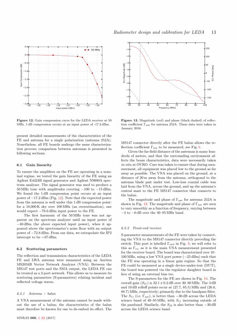
Figure 12. Gain compression curve for the LEDA receiver at 50MHz. 1 dB compression occurs at an input power of -17.2 dBm.

present detailed measurements of the characteristics of theFE and antenna for a single polarization (antenna 252A).Nonetheless, all FE boards undergo the same characteriza-tion process; comparison between antennas is presented infollowing sections.

6.1 Gain linearity

To ensure the amplifiers on the FE are operating in a nom-inal regime, we tested the gain linearity of the FE using anAgilent E4424B signal generator and Agilent N9000A spec-trum analyzer. The signal generator was used to produce a50MHz tone with amplitudes covering −100 to −15dBm.We found the 1 dB compression point occurs at an inputpower of −17.2dBm (Fig. 12). Note that the expected powerfrom the antenna is well under this 1 dB compression point:for a 10,000K sky over 100MHz (an overestimation), onewould expect −78.6dBm input power to the FE.

The first harmonic of the 50MHz tone was not ap-parent on the spectrum analyzer until an input power of−40dBm (far above expected input power), when it ap-peared above the spectrometer’s noise floor with an outputpower of −72.8dBm. From our data, we extrapolate the IP2intercept to be ∼37 dBm.

6.2 Scattering parameters

The reflection and transmission characteristics of the LEDAFE and LWA antenna were measured using an AnritsuMS2034B Vector Network Analyzer (VNA). Between theMS147 test ports and the SMA output, the LEDA FE canbe treated as a 2-port network. This allows us to measure itsscattering parameters (S-parameters) relating incident andreflected voltage waves.

6.2.1 Antenna + balun

A VNA measurement of the antenna cannot be made with-out the use of a balun; the characteristics of the balunmust therefore be known for one to de-embed its effect. The

20 30 40 50 60 70 80 90 100Frequency [MHz]

9

8

7

6

5

4

3

2

1

0

S1

1 M

agnit

ude [

dB

]

150

100

50

0

50

100

150

S1

1 P

hase

[deg]

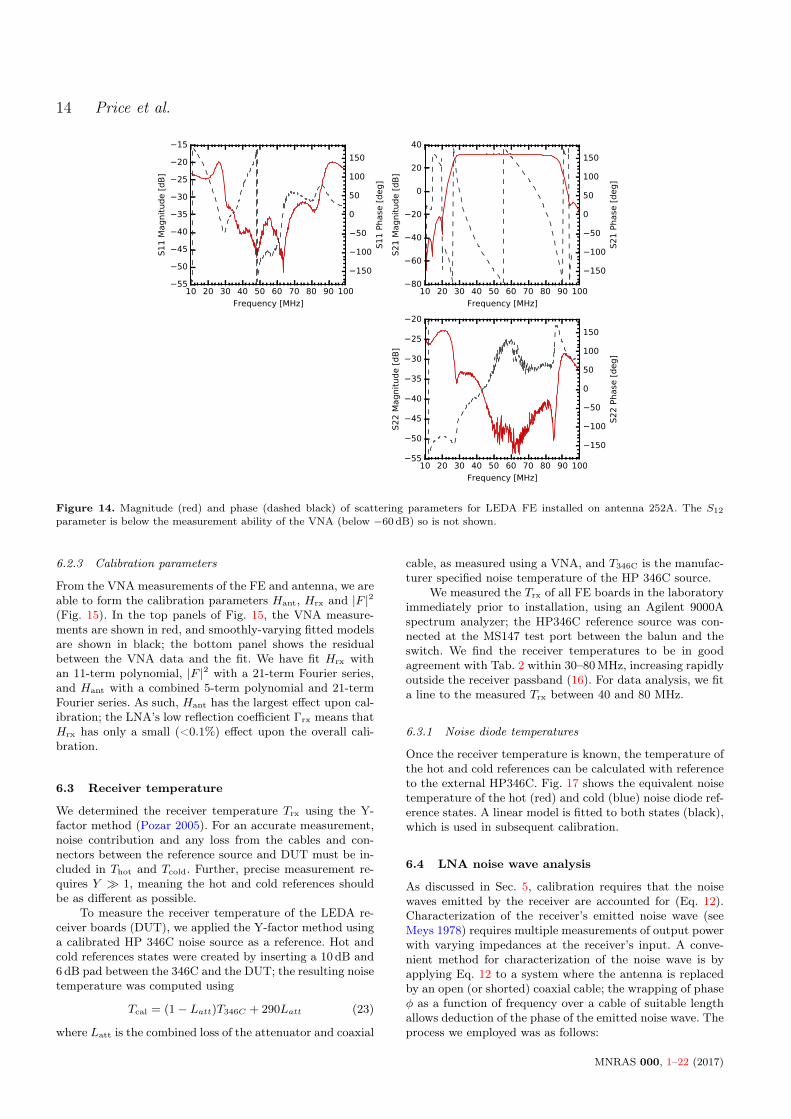
Figure 13. Magnitude (red) and phase (black dashed) of reflec-tion coefficient Γant for antenna 252A. These data were taken inJanuary 2016.

MS147 connector directly after the FE balun allows the re-flection coefficient Γant to be measured, see Fig. 5.

Given the far-field distance of the antennas is many hun-dreds of meters, and that the surrounding environment af-fects the beam characteristics, data were necessarily takenin-situ at OVRO. Care was taken to ensure that during mea-surement, all equipment was placed low to the ground as faraway as possible. The VNA was placed on the ground, at adistance of 20m away from the antenna, orthogonal to theantenna blade pair under test. Low-loss coaxial cable waslaid from the VNA, across the ground, and up the antenna’scentral mast to the FE MS147 connector that connects tothe balun.

The magnitude and phase of Γant for antenna 252A isshown in Fig. 13. The magnitude and phase of Γant are seento vary smoothly as a function of frequency, varying between−4 to −6 dB over the 40–85MHz band.

6.2.2 Front-end receiver

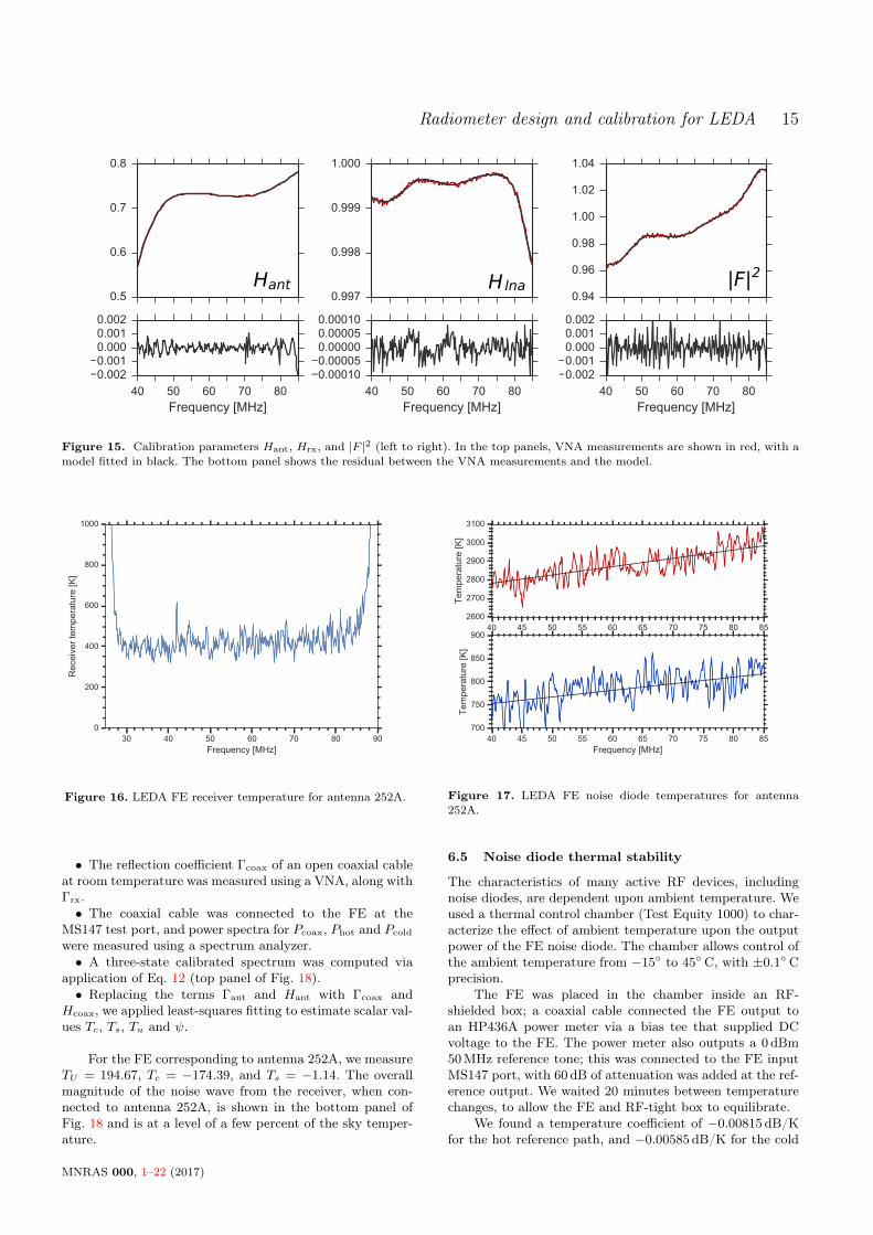
S-parameter measurements of the FE were taken by connect-ing the VNA to the MS147 connector directly preceding theswitch. This port is labelled Γsw0 in Fig. 5; we will refer tothis as Γrx, as it is the main VNA measurement presentedfor the receiver board. The board was characterized over 10–100MHz, using a low VNA port power (−25 dBm) such thatthe FE was operating in a linear gain regime. So that theFE could be measured as a single device-under-test (DUT),the board was powered via the regulator daughter board inlieu of using an external bias tee.

The S-parameters for the FE are shown in Fig. 14. Theoverall gain (S21) is 32.1±0.2 dB over 30–80MHz. The 3 dBand 10 dB rolloff points occur at (27.7, 85.5)MHz and (26.0,88.7)MHz, respectively; primarily due to the bandpass filter.The S11 (i.e. Γant), is better than −30dB across the LEDAscience band of 40–85MHz, with S11 increasing outside ofthe passband. Similarly, the S22 is also better than −30dBacross the LEDA science band.

MNRAS 000, 1–22 (2017)

14 Price et al.

10 20 30 40 50 60 70 80 90 100

Frequency [MHz]

55

50

45

40

35

30

25

20

15

S1

1 M

agnit

ude [

dB

]

150

100

50

0

50

100

150

S1

1 P

hase

[deg]

10 20 30 40 50 60 70 80 90 100

Frequency [MHz]

80

60

40

20

0

20

40

S2

1 M

agnit

ude [

dB

]

150

100

50

0

50

100

150

S2

1 P

hase

[deg]

10 20 30 40 50 60 70 80 90 100

Frequency [MHz]

55

50

45

40

35

30

25

20

S2

2 M

agnit

ude [

dB

]

150

100

50

0

50

100

150

S2

2 P

hase

[deg]

Figure 14. Magnitude (red) and phase (dashed black) of scattering parameters for LEDA FE installed on antenna 252A. The S12

parameter is below the measurement ability of the VNA (below −60dB) so is not shown.

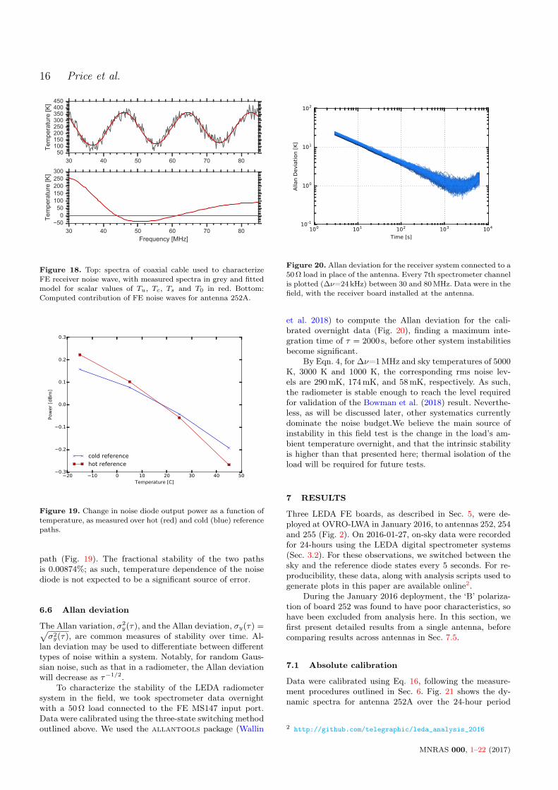
6.2.3 Calibration parameters

From the VNA measurements of the FE and antenna, we areable to form the calibration parameters Hant, Hrx and |F |2(Fig. 15). In the top panels of Fig. 15, the VNA measure-ments are shown in red, and smoothly-varying fitted modelsare shown in black; the bottom panel shows the residualbetween the VNA data and the fit. We have fit Hrx withan 11-term polynomial, |F |2 with a 21-term Fourier series,and Hant with a combined 5-term polynomial and 21-termFourier series. As such, Hant has the largest effect upon cal-ibration; the LNA’s low reflection coefficient Γrx means thatHrx has only a small (<0.1%) effect upon the overall cali-bration.

6.3 Receiver temperature

We determined the receiver temperature Trx using the Y-factor method (Pozar 2005). For an accurate measurement,noise contribution and any loss from the cables and con-nectors between the reference source and DUT must be in-cluded in Thot and Tcold. Further, precise measurement re-quires Y 1, meaning the hot and cold references shouldbe as different as possible.

To measure the receiver temperature of the LEDA re-ceiver boards (DUT), we applied the Y-factor method usinga calibrated HP 346C noise source as a reference. Hot andcold references states were created by inserting a 10 dB and6 dB pad between the 346C and the DUT; the resulting noisetemperature was computed using

Tcal = (1− Latt)T346C + 290Latt (23)

where Latt is the combined loss of the attenuator and coaxial

cable, as measured using a VNA, and T346C is the manufac-turer specified noise temperature of the HP 346C source.

We measured the Trx of all FE boards in the laboratoryimmediately prior to installation, using an Agilent 9000Aspectrum analyzer; the HP346C reference source was con-nected at the MS147 test port between the balun and theswitch. We find the receiver temperatures to be in goodagreement with Tab. 2 within 30–80MHz, increasing rapidlyoutside the receiver passband (16). For data analysis, we fita line to the measured Trx between 40 and 80 MHz.

6.3.1 Noise diode temperatures

Once the receiver temperature is known, the temperature ofthe hot and cold references can be calculated with referenceto the external HP346C. Fig. 17 shows the equivalent noisetemperature of the hot (red) and cold (blue) noise diode ref-erence states. A linear model is fitted to both states (black),which is used in subsequent calibration.

6.4 LNA noise wave analysis

As discussed in Sec. 5, calibration requires that the noisewaves emitted by the receiver are accounted for (Eq. 12).Characterization of the receiver’s emitted noise wave (seeMeys 1978) requires multiple measurements of output powerwith varying impedances at the receiver’s input. A conve-nient method for characterization of the noise wave is byapplying Eq. 12 to a system where the antenna is replacedby an open (or shorted) coaxial cable; the wrapping of phaseφ as a function of frequency over a cable of suitable lengthallows deduction of the phase of the emitted noise wave. Theprocess we employed was as follows:

MNRAS 000, 1–22 (2017)

Radiometer design and calibration for LEDA 15

0.5

0.6

0.7

0.8

40 50 60 70 80Frequency [MHz]

0.0020.0010.0000.0010.002

0.997

0.998

0.999

1.000

40 50 60 70 80Frequency [MHz]

0.000100.000050.000000.000050.00010

0.94

0.96

0.98

1.00

1.02

1.04

40 50 60 70 80Frequency [MHz]

0.0020.0010.0000.0010.002

H |F|Hant lna2

Figure 15. Calibration parameters Hant, Hrx, and |F |2 (left to right). In the top panels, VNA measurements are shown in red, with amodel fitted in black. The bottom panel shows the residual between the VNA measurements and the model.

30 40 50 60 70 80 90Frequency [MHz]

0

200

400

600

800

1000

Rec

eive

r tem

pera

ture

[K]

Figure 16. LEDA FE receiver temperature for antenna 252A.

• The reflection coefficient Γcoax of an open coaxial cableat room temperature was measured using a VNA, along withΓrx.• The coaxial cable was connected to the FE at the

MS147 test port, and power spectra for Pcoax, Phot and Pcold

were measured using a spectrum analyzer.• A three-state calibrated spectrum was computed via

application of Eq. 12 (top panel of Fig. 18).• Replacing the terms Γant and Hant with Γcoax and

Hcoax, we applied least-squares fitting to estimate scalar val-ues Tc, Ts, Tu and ψ.

For the FE corresponding to antenna 252A, we measureTU = 194.67, Tc = −174.39, and Ts = −1.14. The overallmagnitude of the noise wave from the receiver, when con-nected to antenna 252A, is shown in the bottom panel ofFig. 18 and is at a level of a few percent of the sky temper-ature.

40 45 50 55 60 65 70 75 80 85Frequency [MHz]

2600

2700

2800

2900

3000

3100

Tem

pera

ture

[K]

40 45 50 55 60 65 70 75 80 85Frequency [MHz]

700

750

800

850

900

Tem

pera

ture

[K]

Figure 17. LEDA FE noise diode temperatures for antenna252A.

6.5 Noise diode thermal stability

The characteristics of many active RF devices, includingnoise diodes, are dependent upon ambient temperature. Weused a thermal control chamber (Test Equity 1000) to char-acterize the effect of ambient temperature upon the outputpower of the FE noise diode. The chamber allows control ofthe ambient temperature from −15 to 45 C, with ±0.1 Cprecision.

The FE was placed in the chamber inside an RF-shielded box; a coaxial cable connected the FE output toan HP436A power meter via a bias tee that supplied DCvoltage to the FE. The power meter also outputs a 0 dBm50MHz reference tone; this was connected to the FE inputMS147 port, with 60 dB of attenuation was added at the ref-erence output. We waited 20 minutes between temperaturechanges, to allow the FE and RF-tight box to equilibrate.

We found a temperature coefficient of −0.00815dB/Kfor the hot reference path, and −0.00585dB/K for the cold

MNRAS 000, 1–22 (2017)

16 Price et al.

30 40 50 60 70 8050

100150200250300350400450

Tem

pera

ture

[K]

30 40 50 60 70 80Frequency [MHz]

500

50100150200250300

Tem

pera

ture

[K]

Figure 18. Top: spectra of coaxial cable used to characterizeFE receiver noise wave, with measured spectra in grey and fittedmodel for scalar values of Tu, Tc, Ts and T0 in red. Bottom:Computed contribution of FE noise waves for antenna 252A.

20 10 0 10 20 30 40 50Temperature [C]

0.3

0.2

0.1

0.0

0.1

0.2

0.3

Pow

er

[dB

m]

cold referencehot reference

Figure 19. Change in noise diode output power as a function oftemperature, as measured over hot (red) and cold (blue) referencepaths.

path (Fig. 19). The fractional stability of the two pathsis 0.00874%; as such, temperature dependence of the noisediode is not expected to be a significant source of error.

6.6 Allan deviation

The Allan variation, σ2y(τ), and the Allan deviation, σy(τ) =√

σ2y(τ), are common measures of stability over time. Al-

lan deviation may be used to differentiate between differenttypes of noise within a system. Notably, for random Gaus-sian noise, such as that in a radiometer, the Allan deviationwill decrease as τ−1/2.

To characterize the stability of the LEDA radiometersystem in the field, we took spectrometer data overnightwith a 50Ω load connected to the FE MS147 input port.Data were calibrated using the three-state switching methodoutlined above. We used the allantools package (Wallin

100 101 102 103 104

Time [s]

10-1

100

101

102

Alla

n D

evia

tion [

K]

Figure 20. Allan deviation for the receiver system connected to a50Ω load in place of the antenna. Every 7th spectrometer channelis plotted (∆ν=24 kHz) between 30 and 80MHz. Data were in thefield, with the receiver board installed at the antenna.

et al. 2018) to compute the Allan deviation for the cali-brated overnight data (Fig. 20), finding a maximum inte-gration time of τ = 2000 s, before other system instabilitiesbecome significant.

By Eqn. 4, for ∆ν=1MHz and sky temperatures of 5000K, 3000 K and 1000 K, the corresponding rms noise lev-els are 290mK, 174mK, and 58mK, respectively. As such,the radiometer is stable enough to reach the level requiredfor validation of the Bowman et al. (2018) result. Neverthe-less, as will be discussed later, other systematics currentlydominate the noise budget.We believe the main source ofinstability in this field test is the change in the load’s am-bient temperature overnight, and that the intrinsic stabilityis higher than that presented here; thermal isolation of theload will be required for future tests.

7 RESULTS

Three LEDA FE boards, as described in Sec. 5, were de-ployed at OVRO-LWA in January 2016, to antennas 252, 254and 255 (Fig. 2). On 2016-01-27, on-sky data were recordedfor 24-hours using the LEDA digital spectrometer systems(Sec. 3.2). For these observations, we switched between thesky and the reference diode states every 5 seconds. For re-producibility, these data, along with analysis scripts used togenerate plots in this paper are available online2.

During the January 2016 deployment, the ‘B’ polariza-tion of board 252 was found to have poor characteristics, sohave been excluded from analysis here. In this section, wefirst present detailed results from a single antenna, beforecomparing results across antennas in Sec. 7.5.

7.1 Absolute calibration

Data were calibrated using Eq. 16, following the measure-ment procedures outlined in Sec. 6. Fig. 21 shows the dy-namic spectra for antenna 252A over the 24-hour period

2 http://github.com/telegraphic/leda_analysis_2016

MNRAS 000, 1–22 (2017)

Radiometer design and calibration for LEDA 17

30 40 50 60 70 80Frequency [MHz]

0

5

10

15

20

LST

[hr]

252A

2500

5000

7500

10000

12500

15000

17500

20000

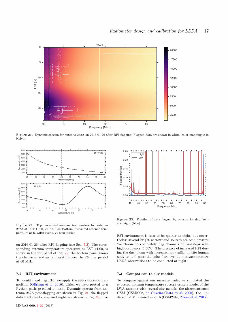
Figure 21. Dynamic spectra for antenna 252A on 2016-01-26 after RFI flagging. Flagged data are shown in white; color mapping is inKelvin.

40 45 50 55 60 65 70 75 80 85Frequency [MHz]

1000

2000

3000

4000

5000

6000

7000

Tem

pera

ture

[K]

LST 11:00

0 4 8 12 16 20Sidereal time [hr]

2000

2500

3000

3500

4000

4500

5000

Tem

pera

ture

[K]

60 MHz

Figure 22. Top: measured antenna temperature for antenna252A at LST 11:00, 2016-01-26. Bottom: measured antenna tem-perature at 60MHz over a 24-hour period.

on 2016-01-26, after RFI flagging (see Sec. 7.2). The corre-sponding antenna temperature spectrum at LST 11:00, isshown in the top panel of Fig. 22; the bottom panel showsthe change in system temperature over the 24-hour periodat 60 MHz.

7.2 RFI environment

To identify and flag RFI, we apply the sumthreshold al-gorithm (Offringa et al. 2010), which we have ported to aPython package called dpflgr. Dynamic spectra from an-tenna 252A post-flagging are shown in Fig. 21; the flaggeddata fractions for day and night are shown in Fig. 23. The

40 45 50 55 60 65 70 75 80 85Frequency [MHz]

0.00

0.05

0.10

0.15

0.20

0.25

Flag

ged

fract

ion

nightday

Figure 23. Fraction of data flagged by dpflgr for day (red)and night (blue).

RFI environment is seen to be quieter at night, but never-theless several bright narrowband sources are omnipresent.We choose to completely flag channels or timesteps withhigh occupancy (>40%). The presence of increased RFI dur-ing the day, along with increased air traffic, on-site humanactivity, and potential solar flare events, motivate primaryLEDA observations to be conducted at night.

7.3 Comparison to sky models

To compare against our measurements, we simulated theexpected antenna temperature spectra using a model of theLWA antenna with several sky models: the aforementionedGSM (GSM2008, de Oliveira-Costa et al. 2008), the ‘up-dated’ GSM released in 2016 (GSM2016, Zheng et al. 2017),

MNRAS 000, 1–22 (2017)

18 Price et al.

0 50 100 150 200 250 300 350Azimuth [deg]

01020304050607080

Alt

itude [

deg]

Beam Response: EW pol. @ 50.00 MHz

0.00 0.15 0.30 0.45 0.60 0.75 0.90

Figure 24. Empirical model of the LWA dipole antenna patternat 50MHz for the East-West polarization.(Dowell et al. 2017).

40 45 50 55 60 65 70 75 80100020003000400050006000700080009000

10000

Tem

pera

ture

[K]

LFSMGSM2008GSM2016

40 45 50 55 60 65 70 75 80Frequency [MHz]

200100

0100200

Res

idua

ls [K

]

Figure 25. Simulated sky brightness for models of diffuse emis-sion at LST 12:00 (top). A model of the LWA1 antenna is con-volved with the sky models for an observer at OVRO-LWA. Bot-tom: Residuals after subtraction of a 5th order log-polynomial fit.

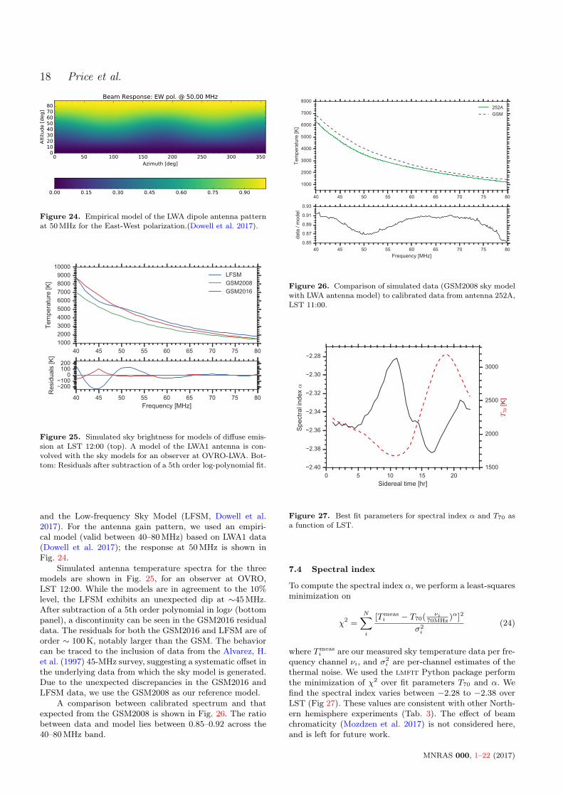
and the Low-frequency Sky Model (LFSM, Dowell et al.2017). For the antenna gain pattern, we used an empiri-cal model (valid between 40–80MHz) based on LWA1 data(Dowell et al. 2017); the response at 50MHz is shown inFig. 24.

Simulated antenna temperature spectra for the threemodels are shown in Fig. 25, for an observer at OVRO,LST 12:00. While the models are in agreement to the 10%level, the LFSM exhibits an unexpected dip at ∼45MHz.After subtraction of a 5th order polynomial in logν (bottompanel), a discontinuity can be seen in the GSM2016 residualdata. The residuals for both the GSM2016 and LFSM are oforder ∼ 100K, notably larger than the GSM. The behaviorcan be traced to the inclusion of data from the Alvarez, H.et al. (1997) 45-MHz survey, suggesting a systematic offset inthe underlying data from which the sky model is generated.Due to the unexpected discrepancies in the GSM2016 andLFSM data, we use the GSM2008 as our reference model.

A comparison between calibrated spectrum and thatexpected from the GSM2008 is shown in Fig. 26. The ratiobetween data and model lies between 0.85–0.92 across the40–80MHz band.

40 45 50 55 60 65 70 75 80

1000

2000

3000

4000

5000

6000

7000

8000

Tem

pera

ture

[K]

252AGSM

40 45 50 55 60 65 70 75 80Frequency [MHz]

0.85

0.87

0.89

0.91

0.93

data

/ m

odel

Figure 26. Comparison of simulated data (GSM2008 sky modelwith LWA antenna model) to calibrated data from antenna 252A,LST 11:00.

0 5 10 15 20Sidereal time [hr]

2.40

2.38

2.36

2.34

2.32

2.30

2.28

Spe

ctra

l ind

ex α

1500

2000

2500

3000

T70

[K]

Figure 27. Best fit parameters for spectral index α and T70 asa function of LST.

7.4 Spectral index

To compute the spectral index α, we perform a least-squaresminimization on

χ2 =

N∑i

[Tmeasi − T70( νi

70MHz)α]2

σ2i

(24)

where Tmeasi are our measured sky temperature data per fre-

quency channel νi, and σ2i are per-channel estimates of the

thermal noise. We used the lmfit Python package performthe minimization of χ2 over fit parameters T70 and α. Wefind the spectral index varies between −2.28 to −2.38 overLST (Fig 27). These values are consistent with other North-ern hemisphere experiments (Tab. 3). The effect of beamchromaticity (Mozdzen et al. 2017) is not considered here,and is left for future work.

MNRAS 000, 1–22 (2017)

Radiometer design and calibration for LEDA 19

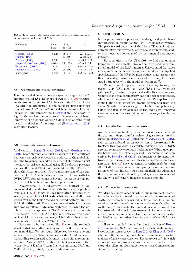
Table 3. Experimental measurements of the spectral index ofradio emission α below 200 MHz.

Reference Decl. Freq. α(deg) (MHz)

Costain (1960) +52.16 38–178 −2.37±0.04Purton (1966) 13–100 −2.38±0.05Andrew (1966) +52.16 10–38 −2.43 ± 0.03Rogers & Bowman (2008) −26.5 100–200 −2.5 ± 0.1Patra et al. (2017) +13.6 110–175 −2.30 to −2.45Mozdzen et al. (2017) −26.7 90–190 −2.5 to −2.6This work +37.24 40–80 −2.28 to −2.38

7.5 Comparisons across antennas

The fractional difference between spectra integrated for 20minutes around LST 12:00 are shown in Fig. 29; measure-ments are consistent to ±5% between 40–83MHz. Above∼83MHz, the attenuation due to bandpass filters gives riseto non-linear ADC gain effects, which act to artificially at-tenuate the sky temperature (Backer 2007). As shown inFig. 16, the receiver temperature also increases out-of-band.Improving the response above 83MHz is an ongoing efforttoward verification of the purported (Bowman et al. 2018)absorption feature.

7.6 Residuals across antennas

As detailed in Bernardi et al. (2015) and Mozdzen et al.(2016), beam chromaticity must be accounted for to mitigatefrequency-dependent structure introduced to the global sig-nal. The frequency-dependent response of the antenna musttherefore be either simulated using EM software packagessuch as HFSS and FEKO, or measured directly; LEDA em-ploys the latter approach. In-situ measurement of the gainpattern of LEDA antennas via cross-correlation with theOVRO-LWA core antennas is beyond the scope of this pa-per and will be detailed in a future publication.

Nevertheless, it is illustrative to subtract a log-polynomial sky model from the calibrated data to produceresiduals. Fig. 30 shows the residuals after subtraction oflog-polynomial fits for LEDA data between 50–80MHz, av-eraged over a one-hour observation period centered an LSTof 11:00, 2016-01-26. The calibration and reduction proce-dure was as follows. Data were calibrated following the ab-solute calibration approach of Sec. 5, after which RFI eventswere flagged (Sec. 7.2). After flagging, data were averagedin time (1 hr total) and frequency (1.008 MHz bins) to formmean observed spectra, Tmeas(ν) for each.

From top to bottom panel, Fig. 30 shows the residualsof calibrated data after subtraction of 1, 3, 5 and 7-termpolynomial fits. We attribute differences between antennastands primarily to beam chromaticity due to differences insurrounding terrain and differences in as-built antenna ge-ometries. Antenna 252A exhibits the best performance (be-tween −5 to 5 K after 7-term fit), with antennas 255A and255B exhibiting notably higher residual values.

8 DISCUSSION

In this paper, we have presented the design and preliminarycharacterization results for the LEDA radiometer systems.The path toward detection of the 21-cm CD trough will re-quire iterative improvements of the analog systems and anal-ysis methods, as knowledge of the instrumental systematicsimprove.

By comparison to the GSM2008, we find our antennatemperature is within 10−15% of that predicted for an em-pirical model of the LWA antenna. Unaccounted for lossesin the antenna, or inaccuracy of the maunfacturer-suppliedspecifications of the HP346C noise source could account forthis; if a multiplicative scale factor of 1.12 is applied, mea-sured data agree with the model to within ±3%.

We measure the spectral index of the sky to vary be-tween −2.28 (LST 11:00) to −2.38 (LST 17:00, when thegalaxy is high). While in agreement with other observations,we note that beam chromaticity has not been accounted for,which would improve the measurement. Pickup from theground due to an imperfect ground screen, and from theSierra Nevada mountain range on the horizon, potentiallyflatten the true spectral index of the radio sky. Improvedmeasurement of the spectral index is the subject of futurework.

8.1 In-situ beam measurements

An important outstanding step is empirical measurement ofthe antenna gain pattern for each outrigger antenna. As dis-cussed in Bernardi et al. (2015) and Mozdzen et al. (2016),gain-pattern-induced chromaticity limits foreground sub-traction: this motivated a complete redesign of the EDGESantenna to improve chromatic performance. While an empir-ical beammodel for (closely-packed) LWA antennas has beenderived by Dowell et al. (2017), calibration requirements mo-tivate a per-antenna model. Measurements between threeantennas (Sec. 7.5) show agreement to within ±5% between40−83MHz; variation in antenna gain pattern may accountfor much of this. Indeed, these data highlight the advantagethat the redundancy offered by multiple measurements ofthe sky with different radiometer systems provides.

8.2 Future improvements

We identify several areas in which our instrument charac-terization can be improved. Firstly, periodic measurement ofscattering parameters measured in the field would allow lon-gitudinal monitoring of the receiver and antenna’s reflectioncoefficients. Additionally, the emitted noise waves could alsobe measured in the field. Measurement of the noise waves us-ing a commercial impedance tuner in lieu of an open cablewould offer an alternative characterization of the LNA noisewaves.

Here, we applied the calibration formalism of Rogers& Bowman (2012). Other approaches, such as the matrix-based calibration approach of King (2010); King et al. (2015)offer an alternative approach based on more modern for-malisms of noise characteristics. The approach of ?, in whichextra calibration parameters are included to better fit thedata, also offers an alternative avenue toward improved in-strument modeling.

MNRAS 000, 1–22 (2017)

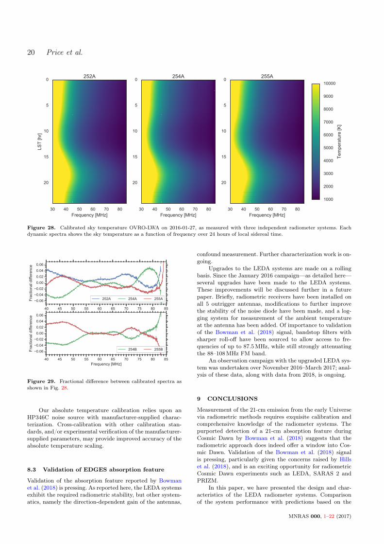
20 Price et al.

30 40 50 60 70 80Frequency [MHz]

0

5

10

15

20

LST

[hr]

252A

30 40 50 60 70 80Frequency [MHz]

0

5

10

15

20

254A

30 40 50 60 70 80Frequency [MHz]

0

5

10

15

20

255A

1000

2000

3000

4000

5000

6000

7000

8000

9000

10000

Tem

pera

ture

[K]

Figure 28. Calibrated sky temperature OVRO-LWA on 2016-01-27, as measured with three independent radiometer systems. Eachdynamic spectra shows the sky temperature as a function of frequency over 24 hours of local sidereal time.

40 45 50 55 60 65 70 75 80 85Frequency [MHz]

0.060.040.020.000.020.040.06

Frac

tiona

l diff

eren

ce

252A 254A 255A

40 45 50 55 60 65 70 75 80 85Frequency [MHz]

0.060.040.020.000.020.040.06

Frac

tiona

l diff

eren

ce

254B 255B

Figure 29. Fractional difference between calibrated spectra asshown in Fig. 28.

Our absolute temperature calibration relies upon anHP346C noise source with manufacturer-supplied charac-terization. Cross-calibration with other calibration stan-dards, and/or experimental verification of the manufacturer-supplied parameters, may provide improved accuracy of theabsolute temperature scaling.

8.3 Validation of EDGES absorption feature

Validation of the absorption feature reported by Bowmanet al. (2018) is pressing. As reported here, the LEDA systemsexhibit the required radiometric stability, but other system-atics, namely the direction-dependent gain of the antennas,

confound measurement. Further characterization work is on-going.

Upgrades to the LEDA systems are made on a rollingbasis. Since the January 2016 campaign—as detailed here—several upgrades have been made to the LEDA systems.These improvements will be discussed further in a futurepaper. Briefly, radiometric receivers have been installed onall 5 outrigger antennas, modifications to further improvethe stability of the noise diode have been made, and a log-ging system for measurement of the ambient temperatureat the antenna has been added. Of importance to validationof the Bowman et al. (2018) signal, bandstop filters withsharper roll-off have been sourced to allow access to fre-quencies of up to 87.5MHz, while still strongly attenuatingthe 88–108MHz FM band.

An observation campaign with the upgraded LEDA sys-tem was undertaken over November 2016–March 2017; anal-ysis of these data, along with data from 2018, is ongoing.

9 CONCLUSIONS

Measurement of the 21-cm emission from the early Universevia radiometric methods requires exquisite calibration andcomprehensive knowledge of the radiometer systems. Thepurported detection of a 21-cm absorption feature duringCosmic Dawn by Bowman et al. (2018) suggests that theradiometric approach does indeed offer a window into Cos-mic Dawn. Validation of the Bowman et al. (2018) signalis pressing, particularly given the concerns raised by Hillset al. (2018), and is an exciting opportunity for radiometricCosmic Dawn experiments such as LEDA, SARAS 2 andPRIZM.

In this paper, we have presented the design and char-acteristics of the LEDA radiometer systems. Comparisonof the system performance with predictions based on the

MNRAS 000, 1–22 (2017)

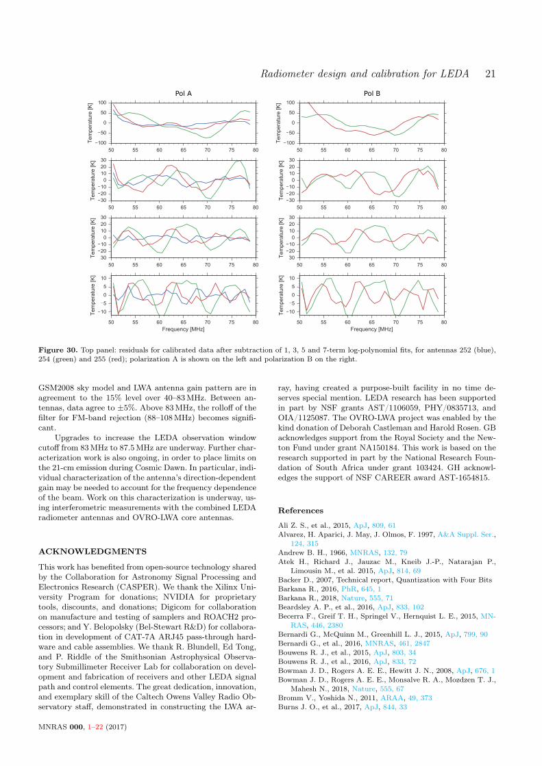
Radiometer design and calibration for LEDA 21

50 55 60 65 70 75 80

100

50

0

50

100

Tem

pera

ture

[K]

50 55 60 65 70 75 80

302010

0102030

Tem

pera

ture

[K]

50 55 60 65 70 75 80

302010

0102030

Tem

pera

ture

[K]

50 55 60 65 70 75 80Frequency [MHz]

10

5

0

5

10

Tem

pera

ture

[K]

50 55 60 65 70 75 80

100

50

0

50

100

Tem

pera

ture

[K]

50 55 60 65 70 75 80

302010

0102030

Tem

pera

ture

[K]

50 55 60 65 70 75 80

302010

0102030

Tem

pera

ture

[K]

50 55 60 65 70 75 80Frequency [MHz]

10

5

0

5

10T

empe

ratu

re [K

]

Pol A Pol B

Figure 30. Top panel: residuals for calibrated data after subtraction of 1, 3, 5 and 7-term log-polynomial fits, for antennas 252 (blue),254 (green) and 255 (red); polarization A is shown on the left and polarization B on the right.

GSM2008 sky model and LWA antenna gain pattern are inagreement to the 15% level over 40–83MHz. Between an-tennas, data agree to ±5%. Above 83MHz, the rolloff of thefilter for FM-band rejection (88–108MHz) becomes signifi-cant.

Upgrades to increase the LEDA observation windowcutoff from 83MHz to 87.5MHz are underway. Further char-acterization work is also ongoing, in order to place limits onthe 21-cm emission during Cosmic Dawn. In particular, indi-vidual characterization of the antenna’s direction-dependentgain may be needed to account for the frequency dependenceof the beam. Work on this characterization is underway, us-ing interferometric measurements with the combined LEDAradiometer antennas and OVRO-LWA core antennas.

ACKNOWLEDGMENTS

This work has benefited from open-source technology sharedby the Collaboration for Astronomy Signal Processing andElectronics Research (CASPER). We thank the Xilinx Uni-versity Program for donations; NVIDIA for proprietarytools, discounts, and donations; Digicom for collaborationon manufacture and testing of samplers and ROACH2 pro-cessors; and Y. Belopolsky (Bel-Stewart R&D) for collabora-tion in development of CAT-7A ARJ45 pass-through hard-ware and cable assemblies. We thank R. Blundell, Ed Tong,and P. Riddle of the Smithsonian Astrophysical Observa-tory Submillimeter Receiver Lab for collaboration on devel-opment and fabrication of receivers and other LEDA signalpath and control elements. The great dedication, innovation,and exemplary skill of the Caltech Owens Valley Radio Ob-servatory staff, demonstrated in constructing the LWA ar-

ray, having created a purpose-built facility in no time de-serves special mention. LEDA research has been supportedin part by NSF grants AST/1106059, PHY/0835713, andOIA/1125087. The OVRO-LWA project was enabled by thekind donation of Deborah Castleman and Harold Rosen. GBacknowledges support from the Royal Society and the New-ton Fund under grant NA150184. This work is based on theresearch supported in part by the National Research Foun-dation of South Africa under grant 103424. GH acknowl-edges the support of NSF CAREER award AST-1654815.

References

Ali Z. S., et al., 2015, ApJ, 809, 61Alvarez, H. Aparici, J. May, J. Olmos, F. 1997, A&A Suppl. Ser.,

124, 315Andrew B. H., 1966, MNRAS, 132, 79Atek H., Richard J., Jauzac M., Kneib J.-P., Natarajan P.,

Limousin M., et al. 2015, ApJ, 814, 69Backer D., 2007, Technical report, Quantization with Four BitsBarkana R., 2016, PhR, 645, 1Barkana R., 2018, Nature, 555, 71Beardsley A. P., et al., 2016, ApJ, 833, 102Becerra F., Greif T. H., Springel V., Hernquist L. E., 2015, MN-

RAS, 446, 2380Bernardi G., McQuinn M., Greenhill L. J., 2015, ApJ, 799, 90Bernardi G., et al., 2016, MNRAS, 461, 2847Bouwens R. J., et al., 2015, ApJ, 803, 34Bouwens R. J., et al., 2016, ApJ, 833, 72Bowman J. D., Rogers A. E. E., Hewitt J. N., 2008, ApJ, 676, 1Bowman J. D., Rogers A. E. E., Monsalve R. A., Mozdzen T. J.,

Mahesh N., 2018, Nature, 555, 67Bromm V., Yoshida N., 2011, ARAA, 49, 373Burns J. O., et al., 2017, ApJ, 844, 33

MNRAS 000, 1–22 (2017)

22 Price et al.

Clark M. A., Plante P. L., Greenhill L. J., 2013, Int. Journal ofHigh Performance Computing Applications, 27, 178

Cohen A., Fialkov A., Barkana R., Lotem M., 2017, MNRAS,472, 1915

Costain C. H., 1960, MNRAS, 120, 248Datta A., Bradley R., Nhan B. D., Burns J. O., 2014, Radio

Science Meeting (USNC-URSI NRSM), 2014 United StatesNational Committee of URSI National, p. 1

DeBoer D. R., et al., 2017, PASP, 129, 045001Dowell J., Taylor G., 2018, preprint, (arXiv:1804.08581)Dowell J., Taylor G. B., Schinzel F. K., Kassim N. E., 2017, MN-

RAS, 469, 4537Ellingson S., et al., 2013, Antennas and Propagation, IEEE Trans-

actions on, 61, 2540Ewall-Wice A., et al., 2016, MNRAS, 460, 4320Fialkov A., Loeb A., 2016, ApJ, 821, 59Fialkov A., Barkana R., Visbal E., 2014, Nature, 506, 197Field G. B., 1958, in Proceedings of the IRE. pp 240–250,

doi:10.1109/JRPROC.1958.286741Greenhill L., 2018, Nature, 555, 38Greenhill L. J., Bernardi G., 2012, preprint, (arXiv:1201.1700)Greif T. H., 2015, Computational Astrophysics and Cosmology,

2, 3Haiman Z., 2016, Understanding the Epoch of Cosmic Reioniza-

tion: Challenges and Progress, 423, 1Harker G. J. A., Pritchard J. R., Burns J. O., Bowman J. D.,

2012, MNRAS, 419, 1070Hickish J., et al., 2016, J. Astron. Instrum., 5, 1641001Hills R., Kulkarni G., Meerburg P. D., Puchwein E., 2018,

preprint, (arXiv:1805.01421)Hirano S., Bromm V., 2017, MNRAS, 470, 898King O. G., 2010, Twenty-First International Symposium on

Space Terahertz Technology, pp 379–388King O. G., et al., 2015, MNRAS, 446, 2Kocz J., et al., 2014, J. Astron. Instrum., 03, 1450002Kocz J., et al., 2015, J. Astron. Instrum., 4, 1550003Koopmans L., et al., 2015, Advancing Astrophysics with the

Square Kilometre Array (AASKA14), p. 1Laporte N., et al., 2017, ApJL, 837, L21Mesinger A., Greig B., Sobacchi E., 2016, MNRAS, 459, 2342Meys R. P., 1978, IEEE Transactions on Microwave Theory and

Techniques, 26, 34Monsalve R. A., Rogers A. E. E., Bowman J. D., Mozdzen T. J.,

2017, ApJ, 835, 49Mortlock D. J., et al., 2011, Nature, 474, 616Mozdzen T. J., Bowman J. D., Monsalve R. A., Rogers A. E. E.,

2016, MNRAS, 455, 3890Mozdzen T. J., Bowman J. D., Monsalve R. A., Rogers A. E. E.,

2017, MNRAS, 464, 4995Offringa A. R., de Bruyn A. G., Biehl M., Zaroubi S., Bernardi

G., Pandey V. N., 2010, MNRAS, 405, 155Paciga G., et al., 2013, MNRAS, 433, 639Patil A. H., et al., 2017, ApJ, 838, 65Patra N., Subrahmanyan R., Raghunathan A., Udaya Shankar

N., 2013, Exp. Astron., 36, 319Patra N., Bray J. D., Roberts P., Ekers R. D., 2017, Experimental

Astronomy, 43, 119Planck Collaboration et al., 2016, A&A, 596Pober J. C., et al., 2015, ApJ, 809, 62Pozar D. M., 2005, Microwave Engineering, 3rd edn. John Wiley

and Sons Inc.Pritchard J. R., Loeb A., 2010, PRD, 82, 023006Purton C. R., 1966, MNRAS, 133, 463Robertson B. E., Ellis R. S., Furlanetto S. R., Dunlop J. S., 2015,

ApJ, 802Rogers A. E. E., Bowman J. D., 2008, AJ, 136, 641Rogers A. E. E., Bowman J. D., 2012, Radio Science, 47

Safranek-Shrader C., Montgomery M. H., Milosavljević M.,Bromm V., 2016, MNRAS, 455, 3288

Shaver P. A., Windhorst R. A., Madau P., de Bruyn A. G., 1999,A&A, 345, 380

Singh S., et al., 2017, ApJ, 845, L12Singh S., Subrahmanyan R., Shankar N. U., Rao M. S., Girish

B. S., Raghunathan A., Somashekar R., Srivani K. S., 2018,Experimental Astronomy, 45, 269

Smidt J., Whalen D. J., Johnson J. L., Li H., 2017, preprint,(arXiv:1703.00449)

Smith A., Bromm V., Loeb A., 2017, Astronomy and Geophysics,58, 3.22

Sokolowski M., et al., 2015, PASA, 32, e004Taylor G. B., et al., 2012, J. of Astron. Instrum., 1, 1250004Voytek T. C., Natarajan A., Jáuregui García J. M., Peterson J. B.,

López-Cruz O., 2014, ApJ, 782, L9Wallin A. E. E., Price D. C., Carson C. G., Meynadier F., 2018,

allantools: Allan deviation calculation, Astrophysics SourceCode Library (ascl:1804.021)

Wise J. H., Demchenko V. G., Halicek M. T., Norman M. L.,Turk M. J., Abel T., Smith B. D., 2014, MNRAS, 442, 2560

Wouthuysen S. A., 1952, AJ, 57, 31Wu X.-B., et al., 2015, Nature, 518, 512Zheng H., et al., 2017, MNRAS, 464, 3486de Oliveira-Costa A., Tegmark M., Gaensler B. M., Jonas J., Lan-

decker T. L., Reich P., 2008, MNRAS, 388, 247

This paper has been typeset from a TEX/LATEX file prepared bythe author.

MNRAS 000, 1–22 (2017)