Edge image quality assessment: a new formulation for degraded edge imaging

M. L. Calvoa,*, A. Manzanaresa, M. Chevalierb, V. Lakshminarayananc

aDepartamento de O´ ptica, Facultad de Ciencias Fı´sicas, Universidad Complutense, 28040 Madrid, SpainbFısica Medica, Departamento de Radiologı´a, Facultad de Medicina, Universidad Complutense, 28040 Madrid, Spain

cUniversity of Missouri–St Louis, School of Optometry and Department of Physics and Astronomy, 8001 Natural Bridge Road, St Louis, MO 63121-4499, USA

Received 6 May 1997; received in revised form 18 December 1997; accepted 9 January 1998

Abstract

We discuss a formalism to characterize degraded edge images formed in a diffraction limited system (with circular pupil of unit radius)under conditions of incoherent illumination. We introduce a novel definition of degraded edges and consider this approach to model a basicoptical mechanism involved in the perception of visual depth and edge detection. We introduce a degradation parameter to quantize thedegree of edge blur. We present a generalization of such a procedure by assuming the Heaviside function to be a systematic generator ofdegraded edges. We reproduce experimentally the predictions made by the formalism proposed herein.q 1998 Elsevier Science B.V. Allrights reserved.

Keywords:Image processing; Signal processing; Vision; Edge detection

1. Introduction

During the past 40 years, the mathematical framework foredge representation has been extensively analyzed in differ-ent branches of optics and related areas such as digitalimage, signal processing, pattern recognition, robotic visionand artificial intelligence [1,2]. The models were mainlyapplied to the theory of edge detection, to characterize aspecific system by the edge spread function (ESF) or edgetrace [3], and for feature extraction and image enhancementby applying an edge detection procedure. Specifically,numerous algorithms have been proposed in digital imageprocessing for image quality improvement in a wide varietyof applications (image enhancement, edge and line location,boundary definition, etc.). The majority of the existing algo-rithms for detection and localization of details and their edgesrely substantially on the ideas of optimal linear filters [4].

In the theory of edge detection edges are defined as dis-continuities in the image intensity due to changes in thescene structure. These discontinuities originate from differ-ent scene features. In digital image processing importantcontributions have been made in the past decades to solvethis problem, especially by implementing edge localizationtechniques. For example, Bergholm [5] has designed a pro-cedure by applying a gradual focusing algorithm based on agaussian blurring operator.

A complex mechanism is required to explain the edgesignal processing by the visual system. The high demandfor edge imaging quality assessment has produced recentlyseveral interesting contributions such as the ones fromKayargadde and Martens [6–8] in which they relate thehuman visual system for edge perception mechanism anda computational model by defining a psychometric space tocharacterize the computational images and a perceptualspace that characterizes the edge detection human perfor-mance. A blur index estimation algorithm was developed byintroducing an intrinsic blur parameter of the visual system.On the other hand, the experiments by Shapley and Tolhurst[9] and Kulikowski and King-Smith [10] (among others)suggest that there are edge detector mechanisms in thehuman visual system with a rather uniform efficiency overa wide range of spatial frequencies. Marr and Hildreth [11]proposed a theory of early information processing in com-plex visual systems, based on the detection of zero-crossingpoints associated with any edge (binary output response)and its second derivatives. They referred the zero-crossingas the values in the convolution of the image intensity with amask formed by the application of a laplacian operator on atwo-dimensional gaussian distribution. The zero valueswould correspond to the location of abrupt intensity changeson the image and could be considered as indicators of edges.

In the context of optical image processing, the incoherent(white illumination: absence of interference phenomena),and coherent (light amplitude correlation: interferences

0262-8856/98/$ - see front matterq 1998 Elsevier Science B.V. All rights reserved.PII: S0262-8856(98)00072-9

* Corresponding author.

Image and Vision Computing 16 (1998) 1003–1017

background), hard edge imaging is a classical subject withvery well known results [12], that accounts for diffractionand propagation phenomena as a consequence of theRayleigh’s limit application (light diffraction by the aper-ture pupil of the system). One defines theESF, line spreadfunction (LSF) and modulation transfer function (MTF) aswell as theLSF/MTF reciprocal relationship introduced byMarchand [13] for linear and invariant perfect systems hav-ing rotational symmetry of revolution. Characterizing a sys-tem by the ESF definition [14–16] is an alternativeprocedure to the use of the point spread function (PSF).To enhance the differences one argues that in anESFchar-acterization Young’s theory applies while in thePSF, Huy-gen’s theory is the basis.

Our intention in the present work is to introduce a generalprocedure to represent systematically various types ofdegraded edge-objects dealing with the real conditions foran optical instrument to perform an output response, whichcan be detected by the human visual system or by an experi-mental set up. We describe a method to characterize theedge degradation in an edge image processing system(EIPS): a diffracted limited system having a circular pupilof unit radius, without aberrations and under normal condi-tions of illumination (incoherent: absence of interferencebackground noise). Assuming that a degrading process ofthe edge-object takes place in the system, the present form-alism proposes a judgment (edge image quality assessment)of the image quality in terms of its contrast reduction oredge quality degradation. Our main goal in this analysis isto establish a mathematical formalism to represent realedges through which one could account for the influenceof significant parameters. We consider in the present analysisnot only hard perfect edges at the input of the system, but alsonon-symmetrical degraded ones, which have a specific degreeof blur or defocusing and a non-symmetrical shape. We con-sider ‘degraded edges’ since in real systems, the object is notnecessarily symmetric or perfectly sharp: real images haveedges (or boundaries) with an amount of degradation or blurthat depends, for example, on its position of depth in the scene,or may be on a degradation mechanism intrinsic to the edge-object (for example, a degradation due to atmospheric agentsaction or any other external agent degrading the edge quality).

The novelty proposed in this paper comes from the math-ematical representation for edge degradation. Earlier con-tributions on this subject [14,15] suppose a degradingoptical system that images a hard edge, that is, a systemcharacterized by a degrading impulse response (LSF orPSF). Otherwise, we consider a perfect system (character-ized by a perfectLSF or PSF), solely limited by diffraction(being the first effect on degrading the image as consideredfrom Rayleigh’s limit) and assume that the input edge functionis affected by a degree of blur. Then, the performance of thediffracted limited system at the output is analyzed. It is obviousthat real-life vision systems introduce blur (as observed inearlier experiments [11]), but in order to study the edge blur,we start up by considering theLSFof a perfect system.

In Section 2 we present a background on the analyticalformulation for perfect edge imaging and degraded edgerepresentation under incoherent illumination. Section 3 con-tains specific formulation for the intensity transmissionfunction associated with the object and its correspondingimage intensity distribution. We introduce the edge degra-dation as a modified Heaviside function or step functionaffected by an exponential factor or gradient that accountsfor the degradation [17]. We present new ideas in Section 4:the LSF andMTF associated with a degraded edge. Thesetwo functions are derived by using the previous definition ofdegraded edge. By differentiating the image intensity dis-tribution of the degraded edge one obtains an associatedLSF. The MTF is directly derived by taking the modulusof the Fourier transform of the associatedLSF. Since thesetwo functions have valid connection to blur, they are bothaffected by a degradation parameter. In particular, theLSFprovides a natural procedure for establishing resolution cri-teria for degraded edges, while the associatedMTF defines aspatial frequency carrier operating under a degradationmechanism (a spatial frequency domain analysis) giving acontrast factor in terms of blur. In Section 5, we introduce acontrast reduction function in terms of theMTF associatedwith a degraded edge and theMTF of the perfect system.We develop this idea by explaining the basic concept andfurther applications, as the calculus of the system depth offocus. Section 6 gives some experimental data obtained forreal edges captured by a CCD camera and showing thepossible connections with the proposed models. We endwith Section 7 for discussion and conclusions.

2. Background: perfect and degraded edge definitions

In the classical paper by Weinstein [14] it is proposed theuse of the incoherent hard edge image distribution to intro-duce an image quality criterion for incoherent illuminationin high aberrated systems (up tol/4). This overcomes thePSF definition that shows a complex behavior (fringesstructure) and it can be only applied to low aberratedsystems (underl/4). This author did not consider blur influ-ence or degradation on the edge and introduced a similarparameter to the associatedLSF, namely, the flux densitygradient, which it is a measure of the image quality in thecase of simple defocusing.

Barakat and Houston [15] expressed theESF in terms ofan accumulativeLSFfor a system in the presence of off-axisaberrations. In their treatment, they define theESF as thehard edge image. Swanter and Hayslett [16] formulated theedge responses for such obscured aperture optical systemsas the integral of the line response, considering a perfectedge as object.

In their pioneering work Shanmugam et al. [1] defined theedge as a great and sudden change in an image attribute,usually the brightness. They consider not only the hardedges but the degraded or blurred ones, defined as sigmoids.

1004 M. L. Calvo et al./Image and Vision Computing 16 (1998) 1003–1017

The sigmoid function has good properties of symmetry, butit does not represent real edges, since they are non-symme-trical due to effects arising from the capturing procedure.

In their theory of edge detection, Marr and Hildreth [11]proposed a theory related to the early processing of visualinformation in complex vision systems. They consideredany sharp intensity change in the image as the presence ofan edge. They detected the changes by searching for thezero-crossing of the second derivative of the image intensitydistribution. No specific expression for the image intensitydistribution was supposed, but the task of isolated edgesdetection is made by comparing the obtained magnitudeswith that for the hard edges.

In an interesting paper, Pentland [18] proposed a new cuefor depth information based on the use of perfect edge dis-continuities. Pentland calculated the image of the edge byconvolving the hard edge object with thePSFof the system,but in the case of defocused edges, Pentland’s proceduredoes not include a blurred magnitude on the edge itself,but in thePSFof the system.

Related to Pentland’s contributions, Marshall et al. [19]proposed other cues to relative visual depth based on the per-ception of edges. The edges were defined as steps, but con-volved with a gaussian blur kernel, representing the degradingLSFof the system. The edge image can be defocused or not,depending on this kernel and not on the edge itself.

We find a different definition of a real edge in a paper ofBasu [2], where it is defined as a combination of steps, peaksand roofs. It also considers white noise added to the signal,since Basu gives a model for edge enhancement and not foredge detection.

3. Degraded edge-object and edge-image intensitydistributions

We consider an image forming system, working underincoherent illumination, and having a circular pupil of

unit radius (see Fig. 1). Let (x0, y0) be the rectangularcoordinates at the object plane. In this plane we define thedegraded edge as:

DE0(x0) ¼ H(x0) 1¹ exp¹ x0

t

� �h i(1)

wheret is the degradation parameter (with dimensions of alength) andH(x0) is the Heaviside or step function. The termin brackets represents the degrading factor. These edges arenon-symmetrical: they do not present a curve zone in thetransition from zero intensity to the increasing values whenthe spatial variable (x) increases (see Fig. 2). Since there is a

Fig. 1. An image forming system. It is limited by the diffraction of the telecentric effective circular pupil, having unit radius. Incoherent conditions ofillumination are assumed.

Fig. 2. Intensity distribution associated with the edge object as defined inEq. (1). To account the effect of the degradation parameter several values oft are considered. The gray level is 0 for white and 1 for black.

1005M. L. Calvo et al./Image and Vision Computing 16 (1998) 1003–1017

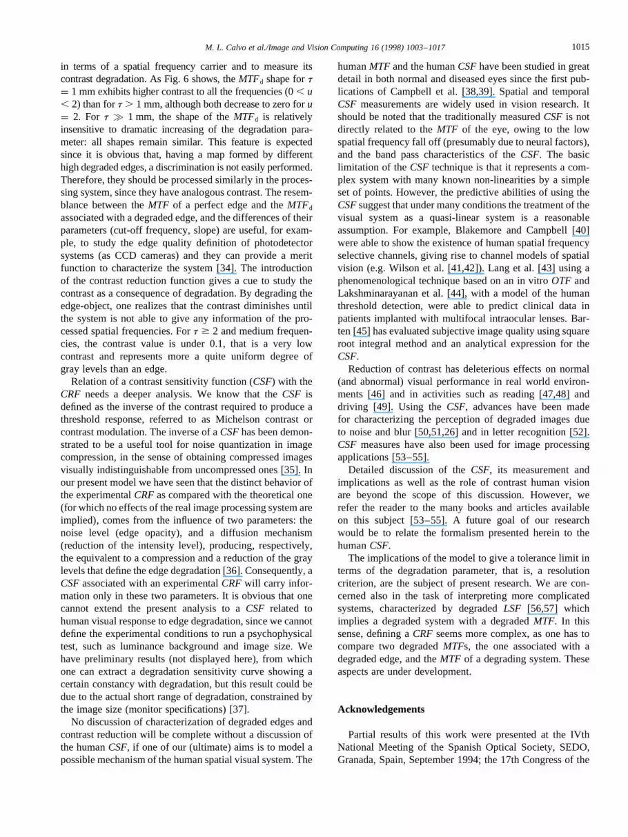
sudden change in the intensity, they do not fit with a sigmoigas many authors suppose,* but clearly saturation is not actu-ally a symmetric effect, only the function appears to bemathematically more manageable. Fig. 2 shows the shape ofthe degraded edge-object for some values oft. The parametert is related to the smoothness of the edge-object, thust ¼ 0reproduces the perfect edge, whiletq 1 accounts for a highlydegraded one. The degradation parameter represents approxi-mately the half-distance required for the step to increase from0 to 90% its maximum intensity (see Fig. 3). It can be seen asthe blur width [1] of the degraded edge. Eq. (1) is defined as acontinuous function (with continuous derivatives) that willguarantee a suitable numerical behavior.

In the Fourier plane, with coordinates (u, v), the objectFourier transformF(u, v) of Eq. (1) is filtered by the opticaltransfer function (OTF) of the system. For simplicity thepupil of the system is located close to the Fourier transformplane (a negligible distance to it). This simplificationimplies that we consider a telecentric effective stop [20]and introduces the diffraction limited conditions of the sys-tem. The filtered Fourier transform signal is:

FDE(u:v) ¼ F(u,v)·OTF(u, v) (2)

where,

F(u,v) ¼ td(n)d(u)2t

¹1

1þ (2ptu)2

�

¹ i(2ptu)

1þ (2ptu)2 ¹1

2ptu)

� �#ð3Þ

OTF(u,v) ¼ circr2

� �p p circ

r2

� �circ p p circ (4)

and ** denotes autocorrelation,d is the Dirac–delta func-tion, and circ(r/2) ¼ 1 (for r ¼ Î(u2 þ v2) , 1), 0 (forr . 1).

The image intensity distribution at the image plane,DE(x,y), is the inverse Fourier transform ofFDE(u, v) given in Eq.(2). As F(u, v) depends on a single coordinate, its inverseFourier transform also depends on a single one:

DE(x) ¼ DE0(x) pJ1(2pr)

r

� �2

(5)

with DE0(x) as expressed in Eq. (1),r¼ Î(x2 þ y2) is theradial coordinate, and * denotes correlation. Then,

DE(x) ¼

∫þ `

¹ `

DE0(x¹a)∫þ `

¹ `

J1(2p������������������(a2 þ b2)

p)������������������

(a2 þ b2)p" #2

db

8<:9=;da

(6)The expression between parentheses is the well-knownLSFof a perfect system having a circular pupil of unit radius,denoted byLSF(a). It follows:

DE(x) ¼

∫þ `

¹ `

DE0(x¹a)LSF(a)da (7)

and, according to Eq. (1),

DE(x) ¼

∫þ `

¹ `

LSF(a)da ¹ exp¹ xt

� � ∫x¹ `

a

t

� �LSF(a)da

(8)

Eq. (8) is the key equation to represent the image intensitydistribution of a degraded edge. To obtain an analyticalexpression for Eq. (8) one needs to substitute theLSF fora more straightforward expression which can be easy tocompute. A certain number of exact formulas and approx-imations are given in the literature [21,22] but we use herethe expression recently proposed by us [23]:

LSF(a) ¼

∫þ `

¹ `

J1(2p������������������(a2 þ b2)

p)������������������

(a2 þb2)p" #2

3 db ¼8p2

∑n¼ 1

n2

4n2 ¹ 1J2n(4pa)

a2 ð9Þ

whereJ2n(x) is the Bessel function of order 2n. By substitut-ing Eq. (9) into Eq. (7), the degraded edge image intensitydistribution is:

DE(x) ¼16p3

∑n¼ 1

n2

4n2 ¹ 1

∫x¹ `

3 1¹ exp¹ xþ a

t

� �h i J2n(4pa)a2 da ð10Þ

The final result (Eq. (10)) has been normalized in this nota-tion to:

DE(`) ¼

∫þ `

¹ `

LSF(a)da ¼p

2(11)

Fig. 3. Graphical explanation of the meaning of a degradation parameter(t).

* For example, Shanmugan et al. in [1] introduced the sigmoid function asa symmetric function to represent an edge affected by a gray level as adegradation from the capturing procedure of the detector.

1006 M. L. Calvo et al./Image and Vision Computing 16 (1998) 1003–1017

Eq. (10) represents theESFfor blurred edges. The possibleoscillations arising from the numerical behavior of the Bes-sel functions [24,25] are suppressed due to the optimizedBessel functions expansion used in the computation [23]. Asan example, Fig. 9(a) shows the comparison between thetheoretical and experimental image intensity distribution fora focused edge processed in a real optical system. Onlyoscillations due to experimental procedure will appear.Obvious differences appear comparing the theoretical objectand image distributions. The transition from zero intensityto higher intensity is smoother in the imaged one: a gradualchange in the slope appears in this zone for edges with lowdegradation parameters (0, t , 1). Obviously, this featuredisappears for higher defocused edges (t q 1). Thus, thegeometrical shadow region of the edge is not equallydefined. As the argument reaches zero, low degradededges will cut the intensity axis at a particular point, havinga well-defined geometrical shadow (for example, for datanot displayed here for brevity, the area under the left elbowon the image intensity distribution, the intensity varies from65% to 95%).

4. LSF and MTF associated with degraded edges

One can apply the well-known operation for theLSFto beobtained by differentiating theESF, or inversely, theESFiscalculated by integrating the line response orLSF in theorthogonal direction to its axis [14–16]. Thus, we definethe one dimensional gradient of the edge image intensitydistribution as anLSF associated with this specific edge.The gradient of the incoherent edge intensity distribution

decreases uniformly and continuously across the spatialcoordinate and it is a measure of the image quality [14] inthe case of simple defocusing. Since edge degradation canbe a consequence of defocusing, this associatedLSF givesinformation on the edge image quality:

LSFd(x) ¼ddx

(DE(x)) (12)

By using the Leibniz rule [24] to differentiate under theintegral sign in Eq. (12):

LSFd(x) ¼16p3t

∑n¼ 1

n2

4n2 ¹ 1

∫x¹ `

exp¹ xþ a

t

� � J2n(4pa)a2 da

(13)

Eq. (13) is represented in Fig. 4 for various degradationparameters (0# t # 5). Fort . 0 the shape of thisLSFd

is not a symmetrical one. This feature appears directly con-nected to the definition of the real degraded edges, that areinherently non-symmetrical. Moreover, the higher thedegradation parameter, the more spreading theLSFd. Asthe degree of blur increases, the energy distribution tendsto equalize over the spatial coordinate and the central max-imum decreases. This corresponds to an edge image highlydegraded and embedded into the geometrical shadow, ascommented in the later section. Opposite, if the degradationparameter is smaller than unity (t , 1), theLSFd shows ahigh central peak: the distribution of the energy is concen-trate at the origin (location of the edge).

We shall introduce a new definition: the modulationtransfer function associated with a degraded edge (MTFd).This magnitude provides information on the response of thesystem to degraded edges for a spatial frequency range,giving data on the contrast. The cut-off frequency remainsconstant for all defocused edge objects [26], as it is deter-mined by the system aperture, but the shape of theMTFd

will vary according to the degradation parameters. As iswell-known [27,28], theMTF of a rotationally invariantsystem, whosePSFdepends on a single variable, is givenas the modulus of the Fourier transform of theLSFd. There-fore,

MTFd(u) ¼ lFT(LSFd(x))l (14)

whereu is the spatial frequency of the system. By using awell-known property of the Fourier transform related to thederivative:

MTFd(u) ¼

�����FTddx

DE(x)� � �����¼ l2piuFT(DE(x))l (15)

Notice that this theorem has restrictions: it must be appliedto monotonically decreasing functionsDE(x). Our casesatisfies this condition, since we are considering a diffrac-tion-limited system (limited by the aperture pupil) where theedge function is zero outside the pupil region. Applicationof derivatives enhances the high frequencies, attenuates thelow ones and suppresses the zero frequency, as the operation

Fig. 4.LSFassociated with the image of the degraded edge objects, accord-ing to Eq. (15). The ‘3 ’ represents the spatial coordinate. Ordinate axisrepresents the line radiant flux density (in arbitrary units).

1007M. L. Calvo et al./Image and Vision Computing 16 (1998) 1003–1017

corresponds to a filtering process with a complex filter withconstant phase shiftp/2 and linear attenuation.

By considering that the edge image intensity distributionis given by the convolution between the edge object and theLSF of the system, the Fourier transform appearing in theright-hand-side of Eq. (15) is:

FT[DE(x)] ¼ FT[DE0(x) p LSF(x)]

¼ FT[DE0(x)]FT[LSF(x)]

¼ FT[DE0(x)]MTF(u) ð16Þ

¼16p3

∑n¼ 1

n2

4n2 ¹ 1

∫þ `

¹ `

FT 1¹ exp¹ xþ a

t

� �� �H(x¹a)

h i3 FT

J2n(4pa)a2

� �da ð17Þ

Eqs. (15) and (16) denote that theMTFd(u) is proportional(factor 2piu) to the product of the Fourier transform of thedegraded edge-object and theMTF associated with theperfect optical system forming the image.

By calculating the two FT [25] of Eq. (17) and substitut-ing the result, we find:

MTFd(u)¼

����� 32ip

u∑`

n¼ 18n2

4n2 ¹ 1·2F1 ¹ n¹

12, n¹

12,

12;

u2

4

� �·

(18)

d(u)2

¹t

1þ (2put)2 ¹ ti2pitu

1þ (2ptu)2 ¹1

(2ptu)

� �� � �����where2F1[a, b, c; z] is the Hypergeometric function of firstkind and second order [28,29]. This result is valid for 0, u

, 2, that represents the cut in frequencies due to the pupilsize limit. Fig. 5 shows the shape of theMTFd for somevalues of the degradation parameter. For 0, t , 1, theassociatedMTFd reduces monotonically its contrast, whilefor t q 1 very highly degraded edges exhibit a similar fastdecreasing shape.

This feature may play an important role in edge recogni-tion. Obviously, matched filtering adapted to a specific edgeobject with a certain degradation (a specifict) will berequired, but to recognize a large class of highly degradededges having different degree of blur (whenever thet valuewas high), a unique correlation will operate.

5. Contrast reduction function

According to Eqs. (15) and (16), theMTFd depends on theMTF of the perfect system. By using the properties of themodulus, we have:

MTFd(u) ¼ l2piuF(u)MTF(u)l # l2piuF(u)l·lMTF(u)l(19)

whereF(u) is given in Eq. (3). TheMTF(u) can be calcu-lated by taking the modulus of the Fourier transform of theperfect system’sLSF(see Eq. (9)). Here, one can define theratio MTFd(u)/lMTF(u)l where the contrast reduction berelated to the edge-object quality. Thus:

Cd(u) ¼MTFd(u)lMTF(u)l

# l2piuF(u)l (20)

The degradation mechanism appears to be bounded by thenature of the Fourier transform of the edge-object. By sub-stituting Eq. (3) in Eq. (20) and operating, one obtains:

Cd(u) #

������������������������1

1þ (2ptu)2

s(21)

As a proof of consistence, one evaluates the value of thecontrast for the zero-frequency component. This value hasto be equal to the unity. It is immediate to realize that:Cd(0)# 1. On the other hand, fort ¼ 0 we obtain the perfect edgecontrast, that is, the contrast without reduction sinceCd(u,t¼ 0) ¼ 1.

Fig. 6 displays the contrast reduction function for 0# t #5. As an example, foru ¼ 1 mm¹1 one has that from 0# t

# 0.5 the reduction is about 70%, but from 0# t # 1 is85%. Fort ¼ 5 the contrast is very low since the contrastreduction is about 97%. Fig. 6 shows that the contrast reduc-tion depends on edge-object degradation: the higher thedegradation parameter, the larger the contrast reduction inrelation to the hard perfect edge. For very low spatial fre-quencies (0# u # 0.05), the contrast reduction for 0# t #5 is small, since all shapes are over the 50% of contrast. Forlow spatial frequencies (0.05# u # 0.2), the contrast for 0# t # 1 decreases but not dramatically. However, fort . 1the contrast is under 0.5. For an intermediate range of spatialfrequencies (0.2# u # 1) the contrast diminishes strongly

Fig. 5.MTF associated with the image of degraded edge objects, accordingto Eq. (20).

1008 M. L. Calvo et al./Image and Vision Computing 16 (1998) 1003–1017

for all t. The shapes fort . 1 become similar and tend toequalize as the spatial frequencies increase. For very highvalues of the spatial frequency (u $ 1) and degradationparameters of 0# t # 1, the contrast reduction tends tothe zero value, although for highert it tends faster. As thespatial frequency increases, the contrast also diminishes.Related for example to visual acuity, a reduction on thecontrast for higher spatial frequencies has been reportedfor defocused small letter contrast sensitivity (SLCS) [30].The results show that a shift takes place with respect to the

contrast sensitivity for focused SLCS. The change in theslope of the contrast sensitivity function, depending on theobject contrast, implies a reduction in visual acuity.

On the other hand, Artal and Navarro have obtained themonochromaticMTF of the human eye for different pupildiameters [31], where a similar behavior for degradation tothe one we are discussing is presented. TheMTFs are fittedby using an analytical expression in terms of a two expo-nential functions addition: the function with higher weightand slope fits the low-spatial frequency range, and the otherfits the high spatial frequency range. In this case, no cut-offfrequency can be defined since the exponentials never reachzero and, therefore, these parametricMTFs yieldPSFs thatare narrower than the actual ones.

6. Experimental degraded edges

In order to prove the correctness of our representation forreal degraded edges, we have set-up an experimental systemdisplayed in Fig. 7. The system carries out all the require-ments expressed in Section 2 related to degraded edges.Edge degradation is taken by defocusing the optical system.

We used the monochromatic illumination from a helium–neon/20 mW laser. Since we needed temporal incoherentlight (to suppress all correlations from temporal and spatialinterferences), a spatial filtering operation (SPF) is made upand a rotating diffuser (RD) is placed. A condenser lens(CL) is located after the diffuser (where the incoherentsource is now defined, having a certain extension or smallarea) to collect the light and to give a uniform illuminationat the object plane (DE0(x0, y0)) where a knife edge (half-plane) acts as a perfect straight edge. The object plane islocated at a distancedo from a convergent lens (L), withfocal distancef ¼ 10 cm, that forms the image intensitydistribution at the image plane, at a distancedi. Both

Fig. 6. Contrast reduction function, according to Eq. (21). Two behaviorscan be determined: (a) 0# t # 1, the contrast function decreases mono-tonically (there is a contrast reduction for high frequencies); (b) 1, t # 10,the shape is rather similar for allt (there is a dramatic reduction for highfrequencies).

Fig. 7. Experimental optical system (see text for details).

1009M. L. Calvo et al./Image and Vision Computing 16 (1998) 1003–1017

distances (do anddi) are approximately related by the con-jugation relation for convergent thin lenses. In the imageplane, a CCD camera connected to a PC computer is placed.We have used a Data Translation 2861 frame grabber tocapture the images from the CCD camera to the computer.In order to avoid excessive saturation of the camera, a polar-izer (P) is placed after the laser. By rotating the polarizer,one can select the amount of illumination in the system. Toobtain the defocused or degraded edges, the image plane I isshifted to some different positions I9 far from the distancedi

(the position of perfect focusing or perfect straight edge).This positive and increasing distance is denoted by the defo-cusing distance (denoted in mm).

Fig. 8(a)–(e) displays various photographs of degradededges, for defocusing distances: 0 (focused edge), 2, 5, 10and 20 cm; and Fig. 8(f)–(j) shows their respective line pro-files. The shape for the edge-image intensity distribution asso-ciated with various experimental blurred edges fits apparentlywith the theoretical predictions, as can be seen in Fig. 8(f)–(j).For small defocusing distances (0, 2 and 5 cm), the slope ofthe edge is higher. Defocusing causes an increasing shift withrespect to the location of the hard edge. The slope for highdefocused edges becomes lesser than for the hard perfectedge, since the degree of gray levels increases.

Apart from the localization of the edge, which is given bythe argument of the Heaviside function, two maincharacteristics arise from the comparison between the the-oretical and the experimental edges (Fig. 9(a)): intensitydegradation and noise background. It is necessary to con-sider this features to fit exactly our model with the experi-mental results.

6.1. Intensity degradation

The decreasing of the maximum intensity is due to theway we use to degrade the original hard edge. Since weremove the image plane far from its focusing position,less light will be captured by the CCD detector eachtime and, therefore, less intensity will arrive. This char-acteristic can be observed in Fig. 8(f)–(j) where the edgeintensity decreases in proportion to the increasing ofdefocus. In Fig. 8(g) it is displayed the quantity ‘edgeheight’ (EH), that represents mathematically the intensitydiminish.

6.2. Noise background

In Fig. 8(h) one can see two types of noise. Electronicnoise appears in every experimental set up. It is present inthe small oscillations of the shape and it is caused by therecording device (CCD camera). It only supposes a 1% inintensity oscillations. Noise background appears in the zoneof the edge that should have zero values of intensity (blackzone of the edge). This happens because the hard edge-object used to generate the object was not totally opaqueand then light could pass through the black part of the edge

giving a background, which was not considered in themodel. We call this background noise ‘edge opacity’ (EO)and it is approximately equal for all the imaged edges, sincethe object edge is physically the same for all.

We introduce this two parameters, as well as the edgelocation, by simply operating in the previous definition ofthe degraded edge (Eq. (1)):

DE0(x0) ¼ EOþ EH·H(x0 ¹ a) 1¹ exp¹ x0 þ a

t

� �� �(22)

with a¼ localization of the edge and the restrictions 0# EO# 1 and 0# EH # 1.

Convolving this expression with theLSF of the perfectsystem (Eq. (9)), one obtains the theoretical fitting to theempirical edges. Fig. 9(a) displays the comparison betweenthe theoretical, experimental and fitted shape for the focusededge. Fig. 9(b) shows the fitting and the experimental shapesfor the five captured edges. The model fits better with thelow degraded edges than with the high degraded ones, sincethe low degraded edges have a well-defined geometricalshadow and therefore they are easily reconstructed by thesystem. For high degraded edges, the image intensity dis-tribution does not present the same behavior since the gra-dual change of the slope is not well-defined. This gives riseto an ambiguous geometrical shadow region (intensity vary-ing from 10% to 20%) and avoids a correct definition of it.In this case, the degraded edge is embedded into the geome-trical shadow and it is impossible to reconstruct or recognizeit, due to the small variation in the slope, and therefore, adramatic reduction of contrast takes place (see Fig. 9(b)).

Starting from this curve fitting the empirical edges, onecan derive the already defined associated functions (LSF,MTF, CRF) and obtain information about image quality,frequencies processed and contrast reduction by applyingthe previous formalism. Fig. 10 displays theMTF asso-ciated with the experimental edges given by the line pro-files of Fig. 8(f)–(j). We have represented also theMTF ofthe theoretical focused edge. The experimental focusededge appears degraded in comparison with the theoreticalone, but not excessively since the merit function (areabetween the theoretical prediction and the experimentalresult) is negligible. As it is expected, when defocusingincreases, the modulation transfer decreases. Fig. 11shows the associatedCRF. This function has been calcu-lated by dividing theMTF associated with an experimentaledge of a certain degradation and theMTF associated withthe theoretical focused edge. This fact is somehow a nor-malization that gives the contrast reduction of the experi-mental imaging related to the theoretical predictions.Although theCRF is mathematically given in terms ofthe edge object spectrum, it is not possible experimentallyto apply this relation, since we do not know a priori thevalues of the parametersEO, EH andt. Therefore,CRF isgiven experimentally as a rate of bothMTFs.

1010 M. L. Calvo et al./Image and Vision Computing 16 (1998) 1003–1017

Another interesting magnitude can be computed: thedepth of focus (DOF) of the system. There are severalways to define the DOF:• The dioptric distance between the two points that deter-

mine the depth of field of the system [26].• The dioptric range for which theMTF exceeds the 50%

of its maximum for a given spatial frequency [26].• The range of defocus for which theCRF exceeds the

80% of its maximum for a given frequency [32].

In any case it is possible to give a value for the DOFstarting from other known functions. In this work, we usetheCRF to compute the DOF in terms of defocusing for anaverage spatial frequency. The election of this frequencydepends on the considered experimental system. We show apractical case of the DOF fixing a spatial frequency value andrepresenting theCRFin terms of the defocusing (t). The rangeof defocusing for which theCRFsurpass 80% of its maximumvalue is a measure of the depth of focus, which is given in

Fig. 8. Images captured of the experimental degraded edges, for various defocusing distances: (a) focused edge (0 cm); (b) defocusing¼ 2 cm, (c) defocusing¼ 5 cm; (d) defocusing¼ 10 cm and (e) defocusing¼ 20 cm. The corresponding line profiles of these images are given in (f)–(j). All the line profiles werecentered at the 256 pixel line of the digitized image (5123 512) and normalized with respect the maximum gray level of the hard edge (255¼ absolute white).The ‘ 3 ’ represents the spatial coordinate. Since the optical image of the degraded edge has been digitized, the spatial coordinate was translated from pixels tomillimeters, using the conversion: 1 pixel¼ 0.013 mm. The gray level is 1 for white and 0 for black.

1011M. L. Calvo et al./Image and Vision Computing 16 (1998) 1003–1017

dioptric units sincet has units mm¹1. Then, we can obtain anobjective measure of the system depth of focus solely havingthe image of some defocused edges processed by the system,as well as other information of interest. Fig. 12 shows theresults for theCRF in terms of defocusing. In this case, foru ¼ 1, the depth of focus is 1.24 mm¹1 (diopters).

7. Discussion and conclusions

We have presented in this paper a characterization ofdegraded edge imaged by a perfect system by introducinga convenient ‘degradation parameter’ (t). This parameter is

related to a defocusing in the image plane in any experi-mental diffraction limited system with circular pupil underconditions of incoherent illumination. To typify a degradededge it is necessary and useful for many applications toquantize the degree of blur. For example, a scene (e.g. areal life picture) is basically composed of many objects alldefined within certain boundaries with their correspondingedges (or gradual changes in the luminance). Depending onthe depth situation of the object in the visual scene, theedges of the boundaries become more or less degraded.According to Pentland’s psychophysical experiments [18],the further the object, the more degraded are its boundaryedges. Observers can interpret an increase in defocusing as

Fig. 8.Continued

1012 M. L. Calvo et al./Image and Vision Computing 16 (1998) 1003–1017

an increase in distance, maybe because they focus having asa reference the nearest object in the visual field. In thissense, it is interesting to characterize the degraded edgesof the scene, not as a function related to the imaging system(as a degradedLSF), but as a function that describes theedges themselves, defining intrinsic characteristics, andthe degraded edge as a depth cue. These avoid connecting

the degrading mechanism to the concrete features of thesystem that provides the scene.

To study a method to characterize the degraded edge, wefirst analyze the associated image intensity distribution.Its expression is given in Eq. (12) in terms of aconvolution between the degraded edge object and theLSF associated with a perfect system. In the interval

Fig. 8.Continued

Fig. 9. (a) A joint representation of the experimental (dashed line) and theoretical (solid line) intensity image distribution for the focused edge.(b) Experi-mental degraded edge images as in Fig. 8(f)–(j) fitted with the modified formula (see Eq. (22)) for the corresponding (values (defocusing equivalence). Forfocused and low defocused edges (0–5 cm) the model fits better, apart from experimental electronic noise. The edge opacity remains unchanged for all theconsidered cases. The edge heights are related with the slope. For high defocused edges the standard deviations are important.

1013M. L. Calvo et al./Image and Vision Computing 16 (1998) 1003–1017

under analysis (see Fig. 4), the degraded edges have a par-ticular stabilization for increasing arguments: they tend tounity, but as the degradation parameter increases, the ten-dency is less noticeable. Two main magnitudes characterizethe edge-image intensity distribution: edge oscillations and

geometrical shadow. For an incoherently illuminated system,the oscillations are not remarkable and only small fluctuationsappear mainly due to the numerical behavior of the Besselfunctions. The transition between zero intensity (black) andthe maximum intensity (white) is smooth, depending on thedegradation parameter. The value of the intensity at the originof the edge-image is higher than the edge-object. There is azone for negative values of the argument where the edge-image intensity is not zero whereas in the edge-object inten-sity it is null. Then, a transition region appears in the edge-image distribution while in the edge-object distribution thereis an abrupt change. The area defined under this zone is thegeometrical shadow region of the edge-image. The geometri-cal shadow region appears to be small for high degradededges. However, these edges show such a large variety ofgray levels that they do not have a high contrast and, therefore,they seem to be embedded on the geometrical shadow. As aconsequence, they cannot be reconstructed since these highdegraded edges are images with low quality and low defini-tion. This is an important feature in the design of an imagequality assessment procedure in terms of the contrast degra-dation.

The other magnitude referred to the quality of the edge isthe associatedLSF (LSFd). The spreading shape and thecentral peak value are two features that characterize theedge quality. The more spreading theLSFd, the less con-centrated the energy, and the smaller the edge quality. TheLSFcould also be useful to establish resolution criteria [33]in the case of defocusing.

The shape of the associatedMTF (MTFd) provides amechanism to analyze the edge processing of the system

Fig. 12.CRF in terms of defocusing (t). The range of defocusing for whichthe CRF surpass the 80% of its maximum value determines the depth offocus of the system, in dioptric units (cm¹1). The distribution correspondsto a fixed normalized spatial frequencyu ¼ 1.

Fig. 10. EmpiricalMTF obtained from the experimental fitted edge imagesgiven in Eq. (9). The perfect and the focused have a similarMTF. As t

increases (increasing defocusing) theMTF behaves as a narrower low-passfilter.

Fig. 11. The correspondingCRF obtained by normalizing theMTF asso-ciated with an experimental edge (with a certain degradation) with respectthe theoretical perfect systemMTF (t ¼ 0).

1014 M. L. Calvo et al./Image and Vision Computing 16 (1998) 1003–1017

in terms of a spatial frequency carrier and to measure itscontrast degradation. As Fig. 6 shows, theMTFd shape fort¼ 1 mm exhibits higher contrast to all the frequencies (0, u, 2) than fort . 1 mm, although both decrease to zero foru¼ 2. For t q 1 mm, the shape of theMTFd is relativelyinsensitive to dramatic increasing of the degradation para-meter: all shapes remain similar. This feature is expectedsince it is obvious that, having a map formed by differenthigh degraded edges, a discrimination is not easily performed.Therefore, they should be processed similarly in the proces-sing system, since they have analogous contrast. The resem-blance between theMTF of a perfect edge and theMTFd

associated with a degraded edge, and the differences of theirparameters (cut-off frequency, slope) are useful, for exam-ple, to study the edge quality definition of photodetectorsystems (as CCD cameras) and they can provide a meritfunction to characterize the system [34]. The introductionof the contrast reduction function gives a cue to study thecontrast as a consequence of degradation. By degrading theedge-object, one realizes that the contrast diminishes untilthe system is not able to give any information of the pro-cessed spatial frequencies. Fort $ 2 and medium frequen-cies, the contrast value is under 0.1, that is a very lowcontrast and represents more a quite uniform degree ofgray levels than an edge.

Relation of a contrast sensitivity function (CSF) with theCRF needs a deeper analysis. We know that theCSF isdefined as the inverse of the contrast required to produce athreshold response, referred to as Michelson contrast orcontrast modulation. The inverse of aCSFhas been demon-strated to be a useful tool for noise quantization in imagecompression, in the sense of obtaining compressed imagesvisually indistinguishable from uncompressed ones [35]. Inour present model we have seen that the distinct behavior ofthe experimentalCRFas compared with the theoretical one(for which no effects of the real image processing system areimplied), comes from the influence of two parameters: thenoise level (edge opacity), and a diffusion mechanism(reduction of the intensity level), producing, respectively,the equivalent to a compression and a reduction of the graylevels that define the edge degradation [36]. Consequently, aCSFassociated with an experimentalCRFwill carry infor-mation only in these two parameters. It is obvious that onecannot extend the present analysis to aCSF related tohuman visual response to edge degradation, since we cannotdefine the experimental conditions to run a psychophysicaltest, such as luminance background and image size. Wehave preliminary results (not displayed here), from whichone can extract a degradation sensitivity curve showing acertain constancy with degradation, but this result could bedue to the actual short range of degradation, constrained bythe image size (monitor specifications) [37].

No discussion of characterization of degraded edges andcontrast reduction will be complete without a discussion ofthe humanCSF, if one of our (ultimate) aims is to model apossible mechanism of the human spatial visual system. The

humanMTF and the humanCSFhave been studied in greatdetail in both normal and diseased eyes since the first pub-lications of Campbell et al. [38,39]. Spatial and temporalCSF measurements are widely used in vision research. Itshould be noted that the traditionally measuredCSF is notdirectly related to theMTF of the eye, owing to the lowspatial frequency fall off (presumably due to neural factors),and the band pass characteristics of theCSF. The basiclimitation of theCSFtechnique is that it represents a com-plex system with many known non-linearities by a simpleset of points. However, the predictive abilities of using theCSFsuggest that under many conditions the treatment of thevisual system as a quasi-linear system is a reasonableassumption. For example, Blakemore and Campbell [40]were able to show the existence of human spatial frequencyselective channels, giving rise to channel models of spatialvision (e.g. Wilson et al. [41,42]). Lang et al. [43] using aphenomenological technique based on an in vitroOTF andLakshminarayanan et al. [44], with a model of the humanthreshold detection, were able to predict clinical data inpatients implanted with multifocal intraocular lenses. Bar-ten [45] has evaluated subjective image quality using squareroot integral method and an analytical expression for theCSF.

Reduction of contrast has deleterious effects on normal(and abnormal) visual performance in real world environ-ments [46] and in activities such as reading [47,48] anddriving [49]. Using theCSF, advances have been madefor characterizing the perception of degraded images dueto noise and blur [50,51,26] and in letter recognition [52].CSF measures have also been used for image processingapplications [53–55].

Detailed discussion of theCSF, its measurement andimplications as well as the role of contrast human visionare beyond the scope of this discussion. However, werefer the reader to the many books and articles availableon this subject [53–55]. A future goal of our researchwould be to relate the formalism presented herein to thehumanCSF.

The implications of the model to give a tolerance limit interms of the degradation parameter, that is, a resolutioncriterion, are the subject of present research. We are con-cerned also in the task of interpreting more complicatedsystems, characterized by degradedLSF [56,57] whichimplies a degraded system with a degradedMTF. In thissense, defining aCRF seems more complex, as one has tocompare two degradedMTFs, the one associated with adegraded edge, and theMTF of a degrading system. Theseaspects are under development.

Acknowledgements

Partial results of this work were presented at the IVthNational Meeting of the Spanish Optical Society, SEDO,Granada, Spain, September 1994; the 17th Congress of the

1015M. L. Calvo et al./Image and Vision Computing 16 (1998) 1003–1017

International Commission for Optics (ICO), Taejon, Korea,August 1996; and the Annual Meeting of the OpticalSociety of America, Long Beach, USA, October 1997.The financial support of the Spanish Ministry of Health,the Institute of Health ‘Carlos III’ and the Health ResearchFoundation, under project 95/1518, and project PR160/93-4829/93 from the Rectorate of the Complutense Universityare acknowledged. We are indebted to Ivan Sanz Rodriguezfor his collaboration. Also, Carmen Bravo gave us compu-tational assistance at the Computing Center of theComplutense University of Madrid. We thank ProfessorJ.M. Enoch for helpful suggestions.

References

[1] K.S. Shanmugam, F.M. Dickey, J.A. Green, An optimal frequencydomain filter for edge detection, IEEE Trans. Patt. Anal. Mach. Intell.1 (1) (1979) 37–49.

[2] M. Basu, Gaussian derivative model for edge enhancement, PatternRecog. 27 (11) (1994) 1451–1461.

[3] C.S. Williams, O.A. Becklund, Introduction to the optical transferfunction, Wiley Series in Pure and Applied Optics, Wiley, NewYork, 1989, pp. 57–59.

[4] L. Yaroslavsky, The theory of optimal methods for localization ofobjects in pictures, in: M.L. Calvo and M. Chevalier (Eds.),Fundamentals, Applications and Analysis of Digital ImageProcessing, Book Notes, Spanish Optical Society (SEDO), CSIC,Madrid, 1994, pp. 70–272.

[5] F. Bergholm, Edge focusing, IEEE Trans. Pattern Anal. Mach. Intell.9 (6) (1987) 726–740.

[6] V. Kayargadde, J.B. Martens, Perceptual characterization of imagesdegraded by blur and noise: model, J. Opt. Soc. Am. A 13 (6) (1996)1178–1188.

[7] V. Kayargadde, J.B. Martens, Perceptual characterization of imagesdegraded by blur and noise: experiments, J. Opt. Soc. Am. A 13 (6)(1996) 1166–1177.

[8] V. Kayargadde, J.B. Martens, Estimation of perceived image blurusing edge features, Int. J. Imaging Systems Technol. 7 (1996)102–109.

[9] R.M. Shapley, D.J. Tolhurst, Edge detectors in human vision, J.Physiol. (Lond.) 229 (1973) 165–183.

[10] J.J. Kulikowski, P.E. King-Smith, Spatial arrangement of line, edgeand grating detectors revealed by subthreshold summation, VisionRes. 13 (1973) 1455–1478.

[11] D. Marr, E. Hildreth, Theory of edge detection, Proc. R. Soc. Lond.B207 (1980) 187–217.

[12] J. Gaskill, Linear Systems, Fourier Transforms and Optics, Wiley,New York, 1978, chap. 11.

[13] E.W. Marchand, Derivation of the point spread function from the linespread function, J. Opt. Soc. Am. 54 (1964) 915–919.

[14] W. Weinstein, Light distribution in the image of an incoherentilluminated edge, J. Opt. Soc. Am. 44 (8) (1954) 610–615.

[15] R. Barakat, A. Houston, Line spread and edge spread functions in thepresence of off-axis aberrations, J. Opt. Soc. Am. 55 (1965) 1132–1135.

[16] W. H. Swanter, Ch. R. Hayslett, Point spread functions, edge responseand modulation transfer functions of obscured aperture opticalsystems, Research Projects Office, Technical Memorandum, USA,1975.

[17] M.L. Calvo, A. Manzanares, M. Chevalier, V. Lakshminarayanan, Aformalism for analyzing degraded edges using modified Heavisidefunctions, in: V. Lakshminarayanan (Eds.), Basic and Clinical

Applications of Vision Science, Kluwer Academic, Dordrecht,1997, pp. 77–81.

[18] A.P. Pentland, A new sense for depth of field, IEEE Trans. PatternAnal. Mach. Intell. 9 (4) (1987) 523–531.

[19] J.A. Marshall, Ch.A. Burbeck, D. Ariely, J.P. Rolland, K.E. Martin,Occlusion edge blur: a cue to relative visual depth, J. Opt. Soc. Am. 13(4) (1996) 681–688.

[20] B.N. Begunov, N.P. Zakaznov, S.I. Kiryushin, V.I. Kuzichev, OpticalInstrumentation Theory and Design, Mir, Moscow, 1988, chap. 6,Section 6-2.

[21] H. Struve, Wied. Ann. 47 (1882) 1008.[22] W.H. Steel, Calcul de la re´partition de la lumie`re dans l’image d’une

ligne, Revu. Opt. 31 (7) (1952) 334–340.[23] A. Manzanares, M.L. Calvo, M. Chevalier, V. Lakshminarayanan,

W.H. Line spread Function proposed by, Steel: a revision (TechnicalNote), Appl. Opt. 36 (19) (1997) 4362–4366.

[24] M. R. Spiegel, L. Abellanas, Fo´rmulas y tablas de matema´ticaaplicada, McGraw-Hill, New York, 1988.

[25] Gradshteyn, I.M.R., in: A. Jeffrey (Ed.), Table of Integrals, Series andProducts, Academic Press, New York, 1994.

[26] G.E. Legge, K.T. Mullen, G.C. Woo, F.W. Campbell, Tolerance tovisual defocus, J. Opt. Soc. Am. A 4 (1987) 851–863.

[27] E.W. Marchand, From line to point spread function: the general case,J. Opt. Soc. Am 55 (4) (1964) 352–355.

[28] R. Barakat, A. Houston, Line spread function and cumulative linespread function for systems with rotational symmetry, J. Opt. Soc.Am. 54 (1964) 768–773.

[29] M. Abramowitz, I. Stegun, Handbook of Mathematical Functions,Dover, New York, 1968, p. 556.

[30] J. Rabin, Luminance effects on visual acuity and small letter contrastsensitivity, Optom. Vision Sci. 71 (11) (1994) 685–688.

[31] P. Artal, R. Navarro, Monochromatic modulation transfer function ofthe human eye for different pupil diameters: an analytical expression,J. Opt. Soc. Am. A 11 (1) (1994) 246–249.

[32] S. Marcos, E. Moreno, R. Navarro, Depth of field of the human eye, in:Proceedings of the Vth Optical National Meeting, Valencia, Spain,1997, pp. 335–336 (in Spanish).

[33] M.L. Calvo, M. Chevalier, V. Lakshminarayanan, P.K. Mondal,Resolution criteria and modulation transfer function (MTF)/linespread function (LSF) relationship in diffraction limited systems, J.Opt. 25 (1) (1996) 1–21.

[34] A. Simon, E. Shaw, M.L. Calvo, Merit functions of CCD camerasbased on edge image processing, in: J.S. Chang, J.H. Lee, S.Y. Leeanad C.H. Nam (Eds.), 17th Congress of the InternationalCommission for Optics: Optics for Science and New Technology,Proceedings of SPIE, vol. 2778, 1996, 65–66.

[35] S. Daly, Application of a noise-adaptive contrast sensitivity functionto image data compression, Opt. Engng 29 (8) (1990) 977–987.

[36] I.Sanz, M.L. Calvo and M. Chevalier, Digitally implemented softedges with predetermined luminance: an analysis of its influence onimage degradation, in: E. Wenger et al. (Eds.), Digital Image Proces-sing and Computer Graphics (DIP-97) Proceedings of SPIE, vol.3346, 1998, 72–83.

[37] M.L. Calvo, I. Sanz, M. Chevalier, V. Lakshminarayanan, Apsychophysical test based on degraded edge imaging: contrast sensitivityand threshold luminance, in: A. Sanfeliu, J.J. Villanueva, J. Vitria´ (Eds.),Proceedings of the VIIth National Symposium on Pattern Recognition andImage Analysis UAB, Barcelona, vol. 2, 1997, pp. 118–119.

[38] F.W. Campbell, R.W. Gubisch, Optical quality of the human eye, J.Physiol. Lond. 186 (1966) 558–578.

[39] F.W. Campbell, J.G. Robson, Applications of Fourier analysis to thevisibility of gratings, J. Physiol. Lond. 197 (1968) 551–566.

[40] C. Blakemore, F.W. Campbell, On the existance of neurons in thehuman visual system selectively sensitive to the orientation and sizeof retinal images, J. Physiol. Lond. 203 (1969) 237–260.

[41] H.R. Wilson, J.R. Bergen, A four-mechanism model for thresholdspatial vision, Vision Res. 19 (1979) 19–32.

1016 M. L. Calvo et al./Image and Vision Computing 16 (1998) 1003–1017

[42] H.R. Wilson, D.J. Gelb, Modified line element theory for spatialfrequency and width discrimination, J. Opt. Soc. Am. A 1 (1984)124–131.

[43] A. Lang, V. Lakshminarayanan, V. Portney, A phenomenologicalmodel for interpreting the clinical significance of the in-vitro OTF,J. Opt. Soc. Am. A 10 (1995) 1600–1610.

[44] V. Lakshminarayanan, A. Lang, V. Portney, The ‘expected visualoutcome’ model: methodology and clinical validation, Optom. VisionSci. 72 (1995) 511–521.

[45] P.G.J. Barten, Evaluation of subjective image quality with the square-root integral method, J. Opt. Soc. Am. A 7 (1990) 2024–2031.

[46] C. Owsley, M. Sloane, Contrast sensitivity, acuity and the perceptionof real world targets, Br. J. Ophthal. 71 (1987) 791–796.

[47] G.E. Legge, Three perspectives on low vision reading, Optom. VisionSci. 68 (1991) 763–769.

[48] G.E. Legge, G.S. Rubin, A. Luebker, Psychophysics of reading—V. Therole of contrast in normal vision, Vision Res. 27 (1987) 1165–1177.

[49] W. Adrian, Visibility of targets: model for calculation, Lighting Res.Technol. 21 (1989) 181–188.

[50] V. Lakshminarayanan, A. Lang, The relationship between defocusedMTF and spatial frequencies needed for letter recognition, in: VisionScience and its Applications. Technical Digest, vol. 1, Optical Societyof America, Washington DC, 1995, pp. 159–162.

[51] K.N. Ngan, H.C. Koh, W.C. Wong, Hybrid image coding schemeincorporating human visual system characteristics, Opt. Engng 30(7) (1991) 940–947.

[52] L.A. Saghri, P.S. Cheatham, A. Habibi, Image quality measurebased on a human visual system model, Opt. Engng 28 (7) (1989)813–819.

[53] R.L. DeValois, K.K. DeValois, Spatial Vision, Oxford UniversityPress, New York, 1988.

[54] R.Shapley, D.Man-Kit Lam, Contrast Sensitivity, MIT Press,Cambridge, MA, 1993.

[55] M.P.Nadler, D.Miller, D.J.Nadler, Glare and Contrast Sensitivity forClinicians, Springer, Heidelberg, 1990.

[56] M.L. Calvo, M. Chevalier, V. Lakshminarayanan, A. Manzanares,Analysis of the Heaviside function as a systematic generator oflines and edges: failure on LSF/MTF reciprocity and sampling, in:Proceedings of the IVth National meeting of the Spanish OpticalSociety (SEDO), Granada, Spain, 1994, pp. 29–30 (in Spanish).

[57] M.L. Calvo, A. Manzanares, M. Chevalier, V. Lakshminarayanan,Edge image processing: an analysis of modified Heaviside functionsas degraded edge generators, in: J.S. Chang, J.H. Lee, S.Y. Lee, C.H.Nam (Eds.), Proceedings of the 17th Congress of the InternationalCommision for Optics: Optics for Science and New Technology,Proceedings of SPIE, vol. 2778, 1996, pp. 63–64.

1017M. L. Calvo et al./Image and Vision Computing 16 (1998) 1003–1017