dnv-os-c501: composite components - wordpress.com
TRANSCRIPT
OFFSHORE STANDARD
DET NORSKE VERITAS AS
The electronic pdf version of this document found through http://www.dnv.com is the officially binding version
DNV-OS-C501
Composite ComponentsNOVEMBER 2013

© Det Norske Veritas AS November 2013
Any comments may be sent by e-mail to [email protected]
This service document has been prepared based on available knowledge, technology and/or information at the time of issuance of this document, and is believed to reflect the best ofcontemporary technology. The use of this document by others than DNV is at the user's sole risk. DNV does not accept any liability or responsibility for loss or damages resulting fromany use of this document.
FOREWORD
DNV is a global provider of knowledge for managing risk. Today, safe and responsible business conduct is both a licenseto operate and a competitive advantage. Our core competence is to identify, assess, and advise on risk management. Fromour leading position in certification, classification, verification, and training, we develop and apply standards and bestpractices. This helps our customers safely and responsibly improve their business performance. DNV is an independentorganisation with dedicated risk professionals in more than 100 countries, with the purpose of safeguarding life, propertyand the environment.
DNV service documents consist of among others the following types of documents:
— Service Specifications. Procedural requirements.
— Standards. Technical requirements.
— Recommended Practices. Guidance.
The Standards and Recommended Practices are offered within the following areas:
A) Qualification, Quality and Safety Methodology
B) Materials Technology
C) Structures
D) Systems
E) Special Facilities
F) Pipelines and Risers
G) Asset Operation
H) Marine Operations
J) Cleaner Energy
O) Subsea Systems
U) Unconventional Oil & Gas
DET NORSKE VERITAS AS
Offshore Standard DNV-OS-C501, November 2013
CHANGES – CURRENT – Page 3
CHANGES – CURRENT
General
This document supersedes DNV-OS-C501, October 2010.
Text affected by the main changes in this edition is highlighted in red colour. However, if the changes involvea whole chapter, section or sub-section, normally only the title will be in red colour.
Main changes November 2013
• General
— A new approach to the specification of characteristic strength has been introduced The new approach willresult in a more consistent reliability level less dependent on application and availability of information inthe form of test results.
— The new approach will result in less conservative designs in some frequent applications. This may savecost, weight etc.
The structure of this document has been converted to decimal numbering. Older references to this documentmay normally be interpreted by analogy to this example:
— “DNV-OSS-101” Ch.2 Sec.3 D506 is now “DNV-OSS-101 Ch.2 Sec.3 [4.5.6].”
• Sec.1 General
— [2.1.4]: Text has been updated to reflect the new approach. A guidance note has been added.
• Sec.2 Design philosophy and design principles
— [3.3.2] Definition of safety classes have been clarified.
• Sec.4 Materials - laminates
— [2.4] Characteristic strength
The section has been restructured as follows:
— Deleted: Characteristic values shall be established with 95% confidence.— Table 4-3, Table 4-4 and Table 4-5 replace the previous Table B2 for derivation of factor km.
— [3.2.9], [3.3.8], [3.5.8], [5.1.10] and [5.8] have been amended.— Table 4-8 has been amended.
• Sec.5 Materials - sandwich structures
— Table 5-1 Has been amended. — [1.2.3] and [1.2.4]: Text have been added.
• Sec.6 Failure mechanisms and design criteria
— [3.1.5] and [3.1.7]: Text have been clarified.— [18]: Text has been added.
• Sec.7 Joints and interfaces
— Table 7-1 has been amended.
• Sec.10 Component testing
— [2.2.2], [2.3.2] and [3.3.5] have been amended.
• Sec. 12 Operation, maintenance, reassessment, repair
— [2.2.3] has been amended.
• Sec.14 Calculation example: Two pressure vessels
— [5.2.1]: Formulas has been amended.
• App.F Example for representative data: Glass reinforced polyester laminate
— Table F-8: Note has been added.
• App.G Example for representative data: Unidirectional carbon tape AS4 12K
— Table G-3 has been amended.

DET NORSKE VERITAS AS
Offshore Standard DNV-OS-C501, November 2013
CHANGES – CURRENT – Page 4
• App.H Example for representative data: Unidirectional carbon tapes made of TPW tape with “5631” fibres
— Table H-3 has been amended.
• Appendix J Method of estimation of characteristic strength
— This is new appendix.
In addition to the above stated main changes, editorial corrections may have been made.
Editorial Corrections
DET NORSKE VERITAS AS
Offshore Standard DNV-OS-C501, November 2013
Contents – Page 5
CONTENTS
CHANGES – CURRENT ................................................................................................................... 3
Sec. 1 General............................................................................................................................... 15
1 Objectives................................................................................................................................................. 15
1.1 Objectives ...................................................................................................................................... 15
2 Application - scope ................................................................................................................................ 15
2.1 General ........................................................................................................................................... 15
3 How to use the standard ......................................................................................................................... 15
3.1 Users of the standard...................................................................................................................... 153.2 Flow chart of the standard.............................................................................................................. 163.3 How to use the standard................................................................................................................. 16
4 Normative references .............................................................................................................................. 17
4.1 Offshore service specifications ...................................................................................................... 174.2 Offshore Standards......................................................................................................................... 174.3 Recommended practices ................................................................................................................ 174.4 Rules .............................................................................................................................................. 174.5 Standards for certification and classification notes ....................................................................... 174.6 Other references ............................................................................................................................. 17
Sec. 2 Design philosophy and design principles ........................................................................ 18
1 General ..................................................................................................................................................... 18
1.1 Objective ........................................................................................................................................ 18
2 Safety philosophy..................................................................................................................................... 18
2.1 General ........................................................................................................................................... 182.2 Risk assessment ............................................................................................................................. 182.3 Quality assurance ........................................................................................................................... 18
3 Design format........................................................................................................................................... 18
3.1 General principles .......................................................................................................................... 183.2 Limit states..................................................................................................................................... 193.3 Safety classes and service classes .................................................................................................. 193.4 Failure types................................................................................................................................... 203.5 Selection of partial safety factors .................................................................................................. 203.6 Design by LRFD method ............................................................................................................... 203.7 Structural Reliability Analysis....................................................................................................... 23
4 Design approach ...................................................................................................................................... 23
4.1 Approaches .................................................................................................................................... 234.2 Analytical approach ....................................................................................................................... 234.3 Component testing ......................................................................................................................... 244.4 Analyses combined with updating ................................................................................................. 24
5 Requirements to documentation ............................................................................................................ 24
5.1 Design Drawings and Tolerances .................................................................................................. 245.2 Guidelines for the design report..................................................................................................... 24
Sec. 3 Design input....................................................................................................................... 25
1 Introduction ............................................................................................................................................. 25
1.1 ........................................................................................................................................................ 25
2 Product specifications ............................................................................................................................. 25
2.1 General function or main purpose of the product .......................................................................... 25
3 Division of the product or structure into components, parts and details........................................... 25
3.1 ........................................................................................................................................................ 25
4 Phases ....................................................................................................................................................... 26
4.1 Phases............................................................................................................................................. 26
5 Safety and service classes........................................................................................................................ 26
5.1 Safety classes ................................................................................................................................. 265.2 Service classes ............................................................................................................................... 26
6 Functional requirements......................................................................................................................... 26
6.1 ........................................................................................................................................................ 26
7 Failure modes........................................................................................................................................... 27
7.1 General ........................................................................................................................................... 277.2 Failure modes................................................................................................................................. 27
DET NORSKE VERITAS AS
Offshore Standard DNV-OS-C501, November 2013
Contents – Page 6
7.3 Identification of the type of limit states ......................................................................................... 27
8 Exposure from the surroundings ........................................................................................................... 28
8.1 General ........................................................................................................................................... 288.2 Loads and environment.................................................................................................................. 288.3 Obtaining loads from the exposure from the surroundings ........................................................... 28
9 Loads ........................................................................................................................................................ 29
9.1 General ........................................................................................................................................... 299.2 Probabilistic representation of load effects.................................................................................... 309.3 Simplified representation of load effects ....................................................................................... 309.4 Characteristic load effect ............................................................................................................... 309.5 The sustained load effect ............................................................................................................... 319.6 The fatigue load effects.................................................................................................................. 33
10 Environment ............................................................................................................................................ 34
10.1 General ........................................................................................................................................... 3410.2 Effects of the environment on the material properties .................................................................. 35
11 Combination of load effects and environment ..................................................................................... 36
11.1 General ........................................................................................................................................... 3611.2 Load effect and environmental conditions for ultimate limit state ............................................... 3611.3 Load effect and environmental conditions for time-dependent material properties ...................... 3811.4 Load effect and environmental conditions for fatigue analysis ..................................................... 3811.5 Direct combination of loads........................................................................................................... 38
Sec. 4 Materials - laminates ........................................................................................................ 39
1 General ..................................................................................................................................................... 39
1.1 Introduction.................................................................................................................................... 391.2 Laminate specification ................................................................................................................... 391.3 Lay-up specification....................................................................................................................... 391.4 Orthotropic plies ............................................................................................................................ 401.5 Mechanical properties.................................................................................................................... 411.6 Characteristic values of mechanical properties.............................................................................. 411.7 Properties of laminates with damage ............................................................................................. 42
2 Static properties....................................................................................................................................... 42
2.1 General ........................................................................................................................................... 422.2 Static properties ............................................................................................................................. 422.3 Relationship between strength and strain to failure....................................................................... 442.4 Characteristic strength ................................................................................................................... 442.5 km ................................................................................................................................................... 442.6 km for structures or components subjected loads with known maximum load effect.................... 452.7 km for well-known material combinations..................................................................................... 452.8 Experimental measurement of matrix and fibre dominated strain to failure ................................. 462.9 Experimental measurement of ply shear properties....................................................................... 47
3 Properties under long term static and cyclic and high rate loads ...................................................... 48
3.1 Introduction.................................................................................................................................... 483.2 Creep .............................................................................................................................................. 483.3 Stress rupture ................................................................................................................................. 493.4 Static strength reduction due to permanent static loads................................................................. 503.5 Stress relaxation ............................................................................................................................. 503.6 Change of modulus of elasticity under cyclic fatigue.................................................................... 513.7 Cycles to failure under cyclic fatigue loads................................................................................... 513.8 Cycles to failure under fatigue loads for matrix dominated strengths ........................................... 533.9 Static strength reduction due to cyclic loads.................................................................................. 543.10 Effect of high loading rates - shock loads - impact ....................................................................... 543.11 Characteristic values ...................................................................................................................... 54
4 Other properties ...................................................................................................................................... 56
4.1 Thermal expansion coefficient....................................................................................................... 564.2 Swelling coefficient for water or other liquids .............................................................................. 564.3 Diffusion coefficient ...................................................................................................................... 564.4 Thermal conductivity ..................................................................................................................... 564.5 Friction coefficient......................................................................................................................... 564.6 Wear resistance .............................................................................................................................. 56
5 Influence of the environment on properties.......................................................................................... 58
5.1 Introduction.................................................................................................................................... 585.2 Effect of temperature ..................................................................................................................... 595.3 Effect of water................................................................................................................................ 605.4 Effect of chemicals ........................................................................................................................ 615.5 Effect of UV radiation ................................................................................................................... 615.6 Electrolytic Corrosion.................................................................................................................... 61
DET NORSKE VERITAS AS
Offshore Standard DNV-OS-C501, November 2013
Contents – Page 7
5.7 Combination of environmental effects........................................................................................... 615.8 Blisters/osmosis ............................................................................................................................. 61
6 Influence of process parameters ............................................................................................................ 61
6.1 Introduction.................................................................................................................................... 616.2 Change of production method........................................................................................................ 626.3 Change of processing temperature and pressure............................................................................ 626.4 Change of post cure procedure ...................................................................................................... 626.5 Change of void content .................................................................................................................. 626.6 Correction for change in fibre volume fraction ............................................................................. 626.7 Control of fibre orientation: ........................................................................................................... 636.8 Control of fibre tension:................................................................................................................. 63
7 Properties under fire............................................................................................................................... 64
7.1 Introduction.................................................................................................................................... 647.2 Fire reaction ................................................................................................................................... 647.3 Fire resistance ................................................................................................................................ 647.4 Insulation........................................................................................................................................ 647.5 Properties after the fire................................................................................................................... 64
8 Qualification of material properties ...................................................................................................... 65
8.1 Introduction.................................................................................................................................... 658.2 General test requirements .............................................................................................................. 658.3 Selection of material qualification method .................................................................................... 658.4 Direct measurement ....................................................................................................................... 658.5 Representative data ........................................................................................................................ 668.6 Qualification against representative data ....................................................................................... 668.7 Confirmation testing for static data................................................................................................ 698.8 Confirmation testing for long term data - high safety class........................................................... 708.9 Confirmation testing for long term data - normal safety class....................................................... 708.10 Use of manufacturers data or data from the literature as representative data ................................ 718.11 Confirming material data by component testing............................................................................ 718.12 Comparing results from different processes and lay-ups............................................................... 72
9 Properties with damaged or nonlinearly deformed matrix................................................................. 72
9.1 Introduction.................................................................................................................................... 729.2 Default values ................................................................................................................................ 729.3 Experimental approach .................................................................................................................. 73
Sec. 5 Materials – sandwich structures...................................................................................... 75
1 General ..................................................................................................................................................... 75
1.1 Introduction.................................................................................................................................... 751.2 Sandwich specification .................................................................................................................. 751.3 Lay-up specification....................................................................................................................... 761.4 Isotropic/orthotropic core layers .................................................................................................... 761.5 Mechanical and physical properties............................................................................................... 761.6 Characteristic values of mechanical properties.............................................................................. 77
2 Static properties....................................................................................................................................... 77
2.1 General ........................................................................................................................................... 772.2 Static properties ............................................................................................................................. 772.3 Relationship between strength and strain to failure....................................................................... 802.4 Characteristic values ...................................................................................................................... 802.5 Shear properties ............................................................................................................................. 812.6 Core skin interface properties ........................................................................................................ 83
3 Properties under long term static and cyclic loads .............................................................................. 83
3.1 General ........................................................................................................................................... 833.2 Creep .............................................................................................................................................. 843.3 Stress rupture under permanent static loads................................................................................... 843.4 Static strength reduction due to permanent static loads................................................................. 843.5 Stress relaxation ............................................................................................................................. 853.6 Change of modulus of elasticity under cyclic fatigue.................................................................... 853.7 Cycles to failure under fatigue loads ............................................................................................. 863.8 Static strength reduction due to cyclic loading .............................................................................. 863.9 Effect of high loading rates - shock loads - impact ....................................................................... 873.10 Characteristic values ...................................................................................................................... 87
4 Other properties ...................................................................................................................................... 88
4.1 Thermal expansion coefficient....................................................................................................... 884.2 Swelling coefficient for water or other liquids .............................................................................. 884.3 Diffusion coefficient ...................................................................................................................... 884.4 Thermal conductivity ..................................................................................................................... 884.5 Friction coefficient......................................................................................................................... 884.6 Wear resistance .............................................................................................................................. 88

DET NORSKE VERITAS AS
Offshore Standard DNV-OS-C501, November 2013
Contents – Page 8
5 Influence of the environment on properties.......................................................................................... 88
5.1 Introduction.................................................................................................................................... 885.2 Effect of temperature ..................................................................................................................... 895.3 Effect of water................................................................................................................................ 905.4 Effect of chemicals ........................................................................................................................ 905.5 Effect of UV radiation ................................................................................................................... 905.6 Electrolytic corrosion..................................................................................................................... 905.7 Combination of environmental effects........................................................................................... 90
6 Influence of process parameters and core density ............................................................................... 91
6.1 Core production ............................................................................................................................. 916.2 Sandwich production ..................................................................................................................... 916.3 Influence of core density................................................................................................................ 91
7 Properties under fire............................................................................................................................... 91
7.1 Introduction.................................................................................................................................... 917.2 Fire reaction ................................................................................................................................... 917.3 Fire resistance ................................................................................................................................ 927.4 Insulation........................................................................................................................................ 927.5 Properties after the fire................................................................................................................... 92
8 Qualification of material properties ...................................................................................................... 92
8.1 Introduction.................................................................................................................................... 928.2 General test requirements .............................................................................................................. 928.3 Selection of material qualification method .................................................................................... 938.4 Direct measurement ....................................................................................................................... 938.5 Representative data ........................................................................................................................ 938.6 Qualification against representative data ....................................................................................... 948.7 Confirmation testing for static data................................................................................................ 958.8 Confirmation testing for long term data......................................................................................... 958.9 Use of manufacturers data or data from the literature as representative data ................................ 958.10 Confirming material data by component testing............................................................................ 96
Sec. 6 Failure mechanisms and design criteria ......................................................................... 97
1 Mechanisms of failure............................................................................................................................. 97
1.1 General ........................................................................................................................................... 971.2 FRP laminates - failure mechanisms and failure type ................................................................. 1001.3 Sandwich structures - failure mechanisms and failure type......................................................... 1001.4 Displacements and long term failure mechanisms and failure type ............................................ 1021.5 Link between failure modes and failure mechanisms.................................................................. 102
2 Design criteria - general approach ...................................................................................................... 103
2.1 General ......................................................................................................................................... 1032.2 Design criteria for single loads ................................................................................................... 1042.3 Design criteria for combined loads .............................................................................................. 1042.4 Time dependency and influence of the environment................................................................... 105
3 Fibre failure ........................................................................................................................................... 105
3.1 General ......................................................................................................................................... 1053.2 Fibre failure at the ply level ......................................................................................................... 1063.3 Fibre failure check using a modified Tsai-Wu criterion.............................................................. 1063.4 Special considerations for fibre failure under in-plane compressive loads ................................. 1083.5 Fibre failure checked by component testing ................................................................................ 1093.6 Fracture mechanics approach....................................................................................................... 109
4 Matrix cracking ..................................................................................................................................... 111
4.1 General ......................................................................................................................................... 1114.2 Matrix failure based on simple stress criterion ............................................................................ 1114.3 Matrix failure based on Puck's criterion ...................................................................................... 1134.4 Obtaining orientation of the failure surface ................................................................................. 1154.5 Matrix cracking caused only by shear ......................................................................................... 1154.6 Matrix failure checked by component testing.............................................................................. 115
5 Delamination.......................................................................................................................................... 115
5.1 General ......................................................................................................................................... 1155.2 Onset of delamination .................................................................................................................. 1155.3 Delamination growth ................................................................................................................... 116
6 Yielding .................................................................................................................................................. 116
6.1 General ......................................................................................................................................... 116
7 Ultimate failure of orthotropic homogenous materials ..................................................................... 117
7.1 General ......................................................................................................................................... 117
8 Buckling.................................................................................................................................................. 118
8.1 Concepts and definitions.............................................................................................................. 118
DET NORSKE VERITAS AS
Offshore Standard DNV-OS-C501, November 2013
Contents – Page 9
8.2 General requirements ................................................................................................................... 1198.3 Requirements when buckling resistance is determined by testing............................................... 1198.4 Requirements when buckling is assessed by analysis.................................................................. 120
9 Displacements ........................................................................................................................................ 121
9.1 General ......................................................................................................................................... 121
10 Long term static loads........................................................................................................................... 122
10.1 General ......................................................................................................................................... 12210.2 Creep ............................................................................................................................................ 12210.3 Stress relaxation ........................................................................................................................... 12210.4 Stress rupture - stress corrosion ................................................................................................... 122
11 Long term cyclic loads .......................................................................................................................... 124
11.1 General ......................................................................................................................................... 12411.2 Change of elastic properties......................................................................................................... 12411.3 Initiation of fatigue damage ......................................................................................................... 12511.4 Growth of fatigue damage ........................................................................................................... 126
12 Impact..................................................................................................................................................... 126
12.1 General ......................................................................................................................................... 12612.2 Impact testing............................................................................................................................... 12612.3 Evaluation after impact testing .................................................................................................... 127
13 Wear ....................................................................................................................................................... 127
13.1 General ......................................................................................................................................... 12713.2 Calculation of the wear depth ...................................................................................................... 12713.3 Component testing ....................................................................................................................... 127
14 High / low temperature / fire................................................................................................................ 128
14.1 General ......................................................................................................................................... 128
15 Resistance to explosive decompression................................................................................................ 128
15.1 Materials ...................................................................................................................................... 12815.2 Interfaces...................................................................................................................................... 128
16 Special aspects related to sandwich structures................................................................................... 128
16.1 General ......................................................................................................................................... 12816.2 Failure of sandwich faces............................................................................................................. 12816.3 Failure of the sandwich core ........................................................................................................ 12816.4 Failure of the sandwich skin-core interface ................................................................................. 12916.5 Buckling of sandwich structures.................................................................................................. 129
17 Chemical decomposition / galvanic corrosion .................................................................................... 129
17.1 General ......................................................................................................................................... 129
18 Static electricity ..................................................................................................................................... 130
18.1 General ......................................................................................................................................... 130
19 Requirements for other design criteria ............................................................................................... 130
19.1 General ......................................................................................................................................... 130
Sec. 7 Joints and interfaces ....................................................................................................... 131
1 General ................................................................................................................................................... 131
1.1 Introduction.................................................................................................................................. 1311.2 Joints ............................................................................................................................................ 1311.3 Interfaces...................................................................................................................................... 1311.4 Thermal properties ....................................................................................................................... 1311.5 Examples...................................................................................................................................... 131
2 Joints....................................................................................................................................................... 131
2.1 Analysis and testing ..................................................................................................................... 1312.2 Qualification of analysis method for other load conditions or joints........................................... 1322.3 Multiple failure modes................................................................................................................. 1322.4 Evaluation of in-service experience............................................................................................. 132
3 Specific joints ......................................................................................................................................... 133
3.1 Laminated joints........................................................................................................................... 1333.2 Adhesive Joints ............................................................................................................................ 1333.3 Mechanical joints ......................................................................................................................... 1333.4 Joints in sandwich structures ....................................................................................................... 133
4 Interfaces................................................................................................................................................ 134
4.1 General ......................................................................................................................................... 134
Sec. 8 Safety-, model- and system factors................................................................................ 135
1 Overview of the various factors used in the standard........................................................................ 135
DET NORSKE VERITAS AS
Offshore Standard DNV-OS-C501, November 2013
Contents – Page 10
1.1 General ......................................................................................................................................... 135
2 Partial load effect and resistance factors ............................................................................................ 135
2.1 General ......................................................................................................................................... 1352.2 How to select the partial safety factors ........................................................................................ 1352.3 Simplified set of partial safety factors (general).......................................................................... 1362.4 Simplified set of partial safety factors (for known maximum load effect).................................. 1362.5 Full set of partial safety factors.................................................................................................... 1362.6 Partial safety factors for functional and environmental loads as typically defined for risers...... 1372.7 Partial safety factors for functional and environmental loads as typically defined for TLPs...... 137
3 Model factors ......................................................................................................................................... 138
3.1 General ......................................................................................................................................... 1383.2 Load model factors ...................................................................................................................... 1383.3 Resistance model factors.............................................................................................................. 138
4 System effect factor ............................................................................................................................... 139
4.1 General ......................................................................................................................................... 139
5 Factors for static and dynamic fatigue analysis ................................................................................. 139
5.1 ...................................................................................................................................................... 139
Sec. 9 Structural analysis .......................................................................................................... 140
1 General ................................................................................................................................................... 140
1.1 Objective ...................................................................................................................................... 1401.2 Input data ..................................................................................................................................... 1401.3 Analysis types .............................................................................................................................. 1401.4 Transfer function.......................................................................................................................... 1411.5 Global and local analysis ............................................................................................................. 1411.6 Material levels.............................................................................................................................. 1411.7 Non-linear analysis ...................................................................................................................... 141
2 Linear and non-linear analysis of monolithic structures................................................................... 142
2.1 General ......................................................................................................................................... 1422.2 In-plane 2-D progressive failure analysis .................................................................................... 1432.3 3-D progressive failure analysis................................................................................................... 1442.4 Linear failure analysis with non-degraded properties.................................................................. 1442.5 Linear failure analysis with degraded properties ......................................................................... 1452.6 Two-step non-linear failure analysis method............................................................................... 1462.7 Through thickness 2-D analysis................................................................................................... 146
3 Connection between analysis methods and failure criteria............................................................... 147
3.1 General ......................................................................................................................................... 1473.2 Modification of failure criteria..................................................................................................... 1473.3 Creep, stress relaxation and stress rupture-stress relaxation........................................................ 1483.4 Fatigue.......................................................................................................................................... 148
4 Analytical methods................................................................................................................................ 148
4.1 General ......................................................................................................................................... 1484.2 Assumptions and limitations........................................................................................................ 1484.3 Link to numerical methods .......................................................................................................... 148
5 Finite element analysis .......................................................................................................................... 149
5.1 General ......................................................................................................................................... 1495.2 Modelling of structures – general ................................................................................................ 1495.3 Software requirements ................................................................................................................. 1505.4 Execution of analysis ................................................................................................................... 1515.5 Evaluation of results .................................................................................................................... 1515.6 Validation and verification .......................................................................................................... 151
6 Dynamic response analysis ................................................................................................................... 151
6.1 General ......................................................................................................................................... 1516.2 Dynamics and finite element analysis.......................................................................................... 152
7 Impact response..................................................................................................................................... 152
7.1 Testing.......................................................................................................................................... 152
8 Thermal stresses .................................................................................................................................... 152
8.1 General ......................................................................................................................................... 152
9 Swelling effects....................................................................................................................................... 153
9.1 General ......................................................................................................................................... 153
10 Analysis of sandwich structures........................................................................................................... 153
10.1 General ......................................................................................................................................... 15310.2 Elastic constants........................................................................................................................... 15310.3 2-D non-linear failure analysis..................................................................................................... 154
DET NORSKE VERITAS AS
Offshore Standard DNV-OS-C501, November 2013
Contents – Page 11
10.4 3-D progressive failure analysis................................................................................................... 15510.5 Long term damage considerations ............................................................................................... 155
11 Buckling.................................................................................................................................................. 155
11.1 General ......................................................................................................................................... 15511.2 Buckling analysis of isolated components................................................................................... 15511.3 Buckling analysis of more complex elements or entire structures .............................................. 15611.4 Buckling analysis of stiffened plates and shells .......................................................................... 15611.5 Buckling analysis for sandwich structures................................................................................... 157
12 Partial load-model factor...................................................................................................................... 157
12.1 General ......................................................................................................................................... 15712.2 Connection between partial load-model factor and analytical analysis....................................... 15712.3 Connection between partial load-model factor and finite element analysis ................................ 15712.4 Connection between partial load-model factor and dynamic response analysis.......................... 15812.5 Connection between partial load-model factor and transfer function.......................................... 158
Sec. 10 Component testing .......................................................................................................... 159
1 General ................................................................................................................................................... 159
1.1 Introduction.................................................................................................................................. 1591.2 Failure mode analysis .................................................................................................................. 1591.3 Representative samples................................................................................................................ 159
2 Qualification based on tests on full scale components ....................................................................... 160
2.1 General ......................................................................................................................................... 1602.2 Short term properties.................................................................................................................... 1602.3 Long term properties.................................................................................................................... 160
3 Verification of analysis by testing and updating ................................................................................ 161
3.1 Verification of design assumptions.............................................................................................. 1613.2 Short term tests ............................................................................................................................ 1623.3 Long term testing ......................................................................................................................... 1623.4 Procedure for updating the predicted resistance of a component ................................................ 1633.5 Specimen geometry - scaled specimen ........................................................................................ 164
4 Testing components with multiple failure mechanisms..................................................................... 165
4.1 General ......................................................................................................................................... 1654.2 Static tests .................................................................................................................................... 1654.3 Long term tests............................................................................................................................. 1654.4 Example of multiple failure mechanisms .................................................................................... 166
5 Updating material parameters in the analysis based on component testing ................................... 167
5.1 ...................................................................................................................................................... 167
Sec. 11 Fabrication ...................................................................................................................... 168
1 Introduction ........................................................................................................................................... 168
1.1 Objective ...................................................................................................................................... 1681.2 Quality system ............................................................................................................................. 168
2 Link of process parameters to production machine parameters...................................................... 168
2.1 Introduction.................................................................................................................................. 1682.2 Process parameters....................................................................................................................... 1682.3 Production machine parameters................................................................................................... 168
3 Processing steps ..................................................................................................................................... 169
3.1 General ......................................................................................................................................... 1693.2 Raw materials............................................................................................................................... 1693.3 Storage of materials ..................................................................................................................... 1693.4 Mould construction ...................................................................................................................... 1693.5 Resin ............................................................................................................................................ 1703.6 Producing laminates and sandwich panels................................................................................... 1703.7 Producing joints ........................................................................................................................... 1703.8 Injection of resin and cure............................................................................................................ 1713.9 Evaluation of the final product .................................................................................................... 171
4 Quality assurance and quality control ................................................................................................ 171
4.1 ...................................................................................................................................................... 171
5 Component testing................................................................................................................................. 171
5.1 General ......................................................................................................................................... 1715.2 Factory acceptance test and system integrity test ........................................................................ 1715.3 Pressure testing of vessels and pipes ........................................................................................... 1725.4 Other testing................................................................................................................................. 1725.5 Dimensions .................................................................................................................................. 172
6 Installation ............................................................................................................................................. 173
DET NORSKE VERITAS AS
Offshore Standard DNV-OS-C501, November 2013
Contents – Page 12
6.1 ...................................................................................................................................................... 173
7 Safety, health and environment ........................................................................................................... 173
7.1 ...................................................................................................................................................... 173
Sec. 12 Operation, maintenance, reassessment, repair ............................................................ 174
1 General ................................................................................................................................................... 174
1.1 Objective ...................................................................................................................................... 174
2 Inspection ............................................................................................................................................... 174
2.1 General ......................................................................................................................................... 1742.2 Inspection methods ...................................................................................................................... 174
3 Reassessment.......................................................................................................................................... 174
3.1 General ......................................................................................................................................... 174
4 Repair ..................................................................................................................................................... 175
4.1 Repair procedure.......................................................................................................................... 1754.2 Requirements for a repair............................................................................................................. 1754.3 Qualification of a repair ............................................................................................................... 175
5 Maintenance........................................................................................................................................... 175
5.1 General ......................................................................................................................................... 175
6 Retirement.............................................................................................................................................. 175
6.1 General ......................................................................................................................................... 175
Sec. 13 Definitions, abbreviations & figures ............................................................................. 176
1 Definitions .............................................................................................................................................. 176
1.1 General ......................................................................................................................................... 1761.2 Terms ........................................................................................................................................... 176
2 Symbols and abbreviations................................................................................................................... 179
3 Figures .................................................................................................................................................... 181
3.1 Ply and laminate co-ordinate systems.......................................................................................... 1813.2 Sandwich co-ordinate system and symbols ................................................................................. 181
Sec. 14 Calculation example: two pressure vessels................................................................... 183
1 Objective ................................................................................................................................................ 183
1.1 General ......................................................................................................................................... 183
2 Design input ........................................................................................................................................... 183
2.1 Overview...................................................................................................................................... 1832.2 General function (ref. Sec.3 [2.1]) ............................................................................................... 1832.3 Product specifications (ref. Sec.3 [2]).......................................................................................... 1832.4 Division of the product into components (ref. Sec.3 [3]) ............................................................ 1842.5 Phases and safety class definitions (ref. Sec.3 [4] and [5]) ......................................................... 1842.6 Functional requirements (ref. Sec.3 [6]) ...................................................................................... 1852.7 Failure modes (ref. Sec.3 [7]) ...................................................................................................... 1862.8 Loads (ref. Sec.3 [9]) ................................................................................................................... 1862.9 Environment (ref. Sec.3 [10]) ...................................................................................................... 187
3 Failure mechanisms............................................................................................................................... 187
3.1 Identification of failure mechanisms (ref. Sec.6 [1]) ................................................................... 1873.2 Classification of failure mechanisms by failure types (ref. Sec.6 [1])......................................... 1893.3 Failure mechanisms and target reliabilities (ref. Sec.2 [3.5]) ...................................................... 189
4 Material properties ............................................................................................................................... 190
4.1 General (ref. Sec.4) ...................................................................................................................... 1904.2 Ply modulus in fibre direction E1 ................................................................................................ 1914.3 Matrix dominated elastic properties............................................................................................. 1914.4 Fibre dominated ply strength and strain to failure ....................................................................... 1924.5 Matrix dominated ply strength and strain to failure..................................................................... 1934.6 Time to failure for fibre dominated properties ............................................................................ 1934.7 Time to failure for matrix dominated properties.......................................................................... 1934.8 Test requirements......................................................................................................................... 193
5 Analysis of gas vessel with liner ........................................................................................................... 194
5.1 General ......................................................................................................................................... 1945.2 Analysis procedure (ref. Sec.9).................................................................................................... 1945.3 Fibre failure - short-term (ref. Sec.6 [3]) ..................................................................................... 1955.4 Fibre dominated ply failure due to static long-term loads (ref. Sec.6 [10])................................. 1965.5 Fibre dominated ply failure due to cyclic fatigue loads (ref. Sec.6 [11]) .................................... 1975.6 Matrix cracking (ref. Sec.6 [4]) ................................................................................................... 1985.7 Unacceptably large displacement (ref. Sec.6 [9]) ........................................................................ 198
DET NORSKE VERITAS AS
Offshore Standard DNV-OS-C501, November 2013
Contents – Page 13
5.8 Impact resistance (ref. Sec.6 [12]) ............................................................................................... 1985.9 Explosive decompression (ref. Sec.6 [15]) .................................................................................. 1995.10 Chemical decomposition (ref. Sec.6 [17]) ................................................................................... 1995.11 Summary evaluation .................................................................................................................... 199
6 Non-linear analysis of vessel for water without liner......................................................................... 199
6.1 General ......................................................................................................................................... 1996.2 Analysis procedure (ref. Sec.9 [2]) .............................................................................................. 1996.3 Matrix cracking (short term) at 1.48 MPa pressure (ref. Sec.6 [4])............................................. 2016.4 Matrix cracking under long-term static loads (ref. Sec.4 [3.4])................................................... 2016.5 Matrix cracking under long-term cyclic fatigue loads (ref. Sec.4 [3.9]) ..................................... 2026.6 Fibre failure - short term (ref. Sec.6 [3]) ..................................................................................... 2026.7 Fibre dominated ply failure due to static long term loads (ref. Sec.6 [10]) ................................. 2026.8 Fibre dominated ply failure due to cyclic fatigue loads (ref. Sec.6 [11]) .................................... 2036.9 Unacceptably large displacement (ref. Sec.6 [9]) ........................................................................ 2036.10 Impact resistance (ref. Sec.6 [12]) ............................................................................................... 2036.11 Explosive decompression (ref. Sec.6 [15]) .................................................................................. 2036.12 Chemical decomposition (ref. Sec.6 [17]) ................................................................................... 2036.13 Component testing (ref. Sec.10) .................................................................................................. 2036.14 Summary evaluation .................................................................................................................... 204
7 Linear analysis of vessel for water without liner................................................................................ 204
7.1 General ......................................................................................................................................... 2047.2 Analysis procedure (ref. Sec.9 [2]) .............................................................................................. 2047.3 Matrix cracking (short term) (ref. Sec.6 [4]) ............................................................................... 2057.4 Matrix cracking under long-term static loads (ref. Sec.4 [3.4])................................................... 2057.5 Matrix cracking under long-term cyclic fatigue loads (ref. Sec.4 [3.9]) ..................................... 2057.6 Fibre failure – short-term (ref. Sec.6 [3]) .................................................................................... 2057.7 Fibre dominated ply failure due to static long-term loads (ref. Sec.6 [10])................................. 2077.8 Fibre dominated ply failure due to cyclic fatigue loads (ref. Sec.6 [11]) .................................... 2077.9 Unacceptably large displacement ................................................................................................ 2077.10 Impact resistance.......................................................................................................................... 2077.11 Explosive decompression............................................................................................................. 2077.12 Chemical decomposition.............................................................................................................. 2077.13 Summary evaluation .................................................................................................................... 207
App. A Check-lists for design input .......................................................................................... 208A.1 Phases ..................................................................................................................................................... 208A.2 Functional requirements and failure modes ........................................................................................... 208A.3 Loads ...................................................................................................................................................... 210A.4 Environments ......................................................................................................................................... 211A.5 Distribution types of basic variables ...................................................................................................... 211
App. B Lay-up and laminate specification ................................................................................ 213B.1 Unique definition of a laminate.............................................................................................................. 213
App. C Test methods for laminates ............................................................................................ 215C.1 General ................................................................................................................................................... 215C.2 Static tests for laminates......................................................................................................................... 215C.3 Tests to obtain properties under long term static and cyclic loads......................................................... 217C.4 Tests to obtain the fibre fraction ............................................................................................................ 217C.5 Tests on tubular specimens .................................................................................................................... 218C.6 Evaluation of stress versus strain curves................................................................................................ 218
App. D Test methods for sandwich materials............................................................................ 220D.1 General ................................................................................................................................................... 220D.2 Core materials - static tests..................................................................................................................... 220D.3 Adhesive materials - static tests ............................................................................................................. 222D.4 Core skin interface properties ................................................................................................................ 222D.5 Tests for other properties........................................................................................................................ 223
App. E Tables of safety factors ................................................................................................... 225E.1 Partial safety factors ............................................................................................................................... 225
App. F Example for representative data - Glass reinforced polyester laminate.............................................................................. 230F.1 General ................................................................................................................................................... 230F.2 Definition of material ............................................................................................................................. 230F.3 Quasi static properties in air (QSA) ....................................................................................................... 231F.4 Long term properties in air..................................................................................................................... 234F.5 Long term properties in water ................................................................................................................ 239
App. G Example for representative data – Unidirectional carbon tape AS4 12k ............................................................................. 240
DET NORSKE VERITAS AS
Offshore Standard DNV-OS-C501, November 2013
Contents – Page 14
G.1 General ................................................................................................................................................... 240G.2 Definition of material ............................................................................................................................. 240G.3 Quasi static properties in air (QSA) ....................................................................................................... 241G.4 Long term properties ............................................................................................................................. 242
App. H Example for representative data –Unidirectional carbon tapes made of TPW tape with “5631” fibres......................................................................................... 243H.1 General ................................................................................................................................................... 243H.2 Definition of material ............................................................................................................................. 243H.3 Quasi static properties in air (QSA) ....................................................................................................... 244H.4 Long term properties ............................................................................................................................. 245
App. I Example for representative data unidirectional carbon tape TPW 0434 Prepreg ........................................................... 246I.1 General ................................................................................................................................................... 246I.2 Definition of material ............................................................................................................................. 246I.3 Quasi static properties in air (QSA) ....................................................................................................... 247I.4 Long term properties .............................................................................................................................. 248
App. J Method of estimation of characteristic strength .......................................................... 249
CHANGES – HISTORIC ............................................................................................................... 250
DET NORSKE VERITAS AS
Offshore Standard DNV-OS-C501, November 2013
Sec.1 General – Page 15
SECTION 1 GENERAL
1 Objectives
1.1 Objectives
1.1.1 The main objectives of this standard is to:
— serve as a basic philosophy and standard— provide an internationally acceptable standard for safe design with respect to strength and performance by
defining minimum requirements for design, materials, fabrication and installation of load-carrying FibreReinforced Plastic (FRP) laminates and sandwich structures and components
— serve as a technical reference document in contractual matters between client and contractor and or supplier— provide cost-effective solutions based on complete limit state design with reliability based calibration of
safety factors— reflect the state-of-the-art and consensus on accepted industry practice— to provide guidance and requirements for efficient global analyses and introduce a consistent link between
design checks (failure modes), load conditions and load effect assessment in the course of the globalanalyses.
2 Application - scope
2.1 General
2.1.1 This standard provides requirements and recommendations for structural design and structural analysisprocedures for composite components. Emphasis with respect to loads and environmental conditions is put onapplications in the offshore and processing industry. The materials description and calculation methods can beapplied to any applications. Aspects related to documentation, verification, inspection, materials, fabrication,testing and quality control are also addressed.
2.1.2 The standard is applicable to all products and parts made of composite material and may be applied tomodifications, operation and upgrading made to existing ones. It is intended to serve as a common referencefor designers, manufacturers and end-users, thereby reducing the need for company specifications.
2.1.3 This standard assumes that material properties such as strength and stiffness are normally distributed. Ifthe properties of a material deviate significantly from the assumption of a normal distribution, a different setof safety factors than specified herein has to be used.
2.1.4 All properties shall be estimated with 95% confidence except where noted.
Guidance note:
Different confidence levels are specified some places in this standard in order to ensure a uniform level of reliability.
---e-n-d---of---G-u-i-d-a-n-c-e---n-o-t-e---
3 How to use the standard
3.1 Users of the standard
3.1.1 The client is understood to be the party ultimately responsible for the system as installed and its intendeduse in accordance with the prevailing laws, statutory rules and regulations.
3.1.2 The authorities are the national or international regulatory bodies.
3.1.3 The contractor is understood to be the party contracted by the client to perform all or part of thenecessary work needed to bring the system to an installed and operable condition.
3.1.4 The designer is understood to be the party contracted by the contractor to fulfil all or part of the activitiesassociated with the design.
3.1.5 The manufacturer is understood to be the party contracted by the contractor to manufacture all or part ofthe system. Two types of manufacturers can be distinguished: the material manufacturers, which supply thecomposite material or its constituents (i.e. resin, fibres) and the product manufacturers, which fabricate all orpart of the system.
3.1.6 The third party verifier is an independent neutral party that verifies the design of a structure orcomponent.
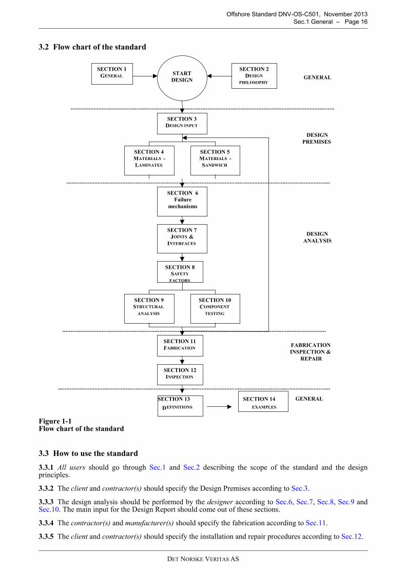
DET NORSKE VERITAS AS
Offshore Standard DNV-OS-C501, November 2013
Sec.1 General – Page 16
3.2 Flow chart of the standard
Figure 1-1 Flow chart of the standard
3.3 How to use the standard
3.3.1 All users should go through Sec.1 and Sec.2 describing the scope of the standard and the designprinciples.
3.3.2 The client and contractor(s) should specify the Design Premises according to Sec.3.
3.3.3 The design analysis should be performed by the designer according to Sec.6, Sec.7, Sec.8, Sec.9 andSec.10. The main input for the Design Report should come out of these sections.
3.3.4 The contractor(s) and manufacturer(s) should specify the fabrication according to Sec.11.
3.3.5 The client and contractor(s) should specify the installation and repair procedures according to Sec.12.
FABRICATION
INSPECTION &
REPAIR
SECTION 1
GENERAL
SECTION 2
DESIGN
PHILOSOPHY
SECTION 3
DESIGN INPUT
START
DESIGNGENERAL
DESIGN
PREMISES
DESIGN
ANALYSIS
GENERAL
SECTION 6
Failure
mechanisms
SECTION 7
JOINTS &
INTERFACES
SECTION 8
SAFETY
FACTORS
SECTION 9
STRUCTURAL
ANALYSIS
SECTION 10
COMPONENT
TESTING
SECTION 11
FABRICATION
SECTION 12
INSPECTION
SECTION 14
EXAMPLES
SECTION 13
DEFINITIONS
SECTION 4
MATERIALS -
LAMINATES
SECTION 5
MATERIALS -
SANDWICH
DET NORSKE VERITAS AS
Offshore Standard DNV-OS-C501, November 2013
Sec.1 General – Page 17
3.3.6 The third party verifier should verify that the design documentation is according to the requirements ofSec.2 [5].
4 Normative references
The latest revision of the following documents applies:
4.1 Offshore service specifications
DNV-OSS-301 Certification and Verification of Pipelines
4.2 Offshore Standards
DNV-OS-F101 Submarine Pipeline SystemsDNV-OS-F201 Dynamic RisersDNV-OS-C105 Structural Design of TLPs by the LRFD MethodDNV-OS-C106 Structural Design of Deep Draught Floating Units DNV-OS-C501 Composite Components
4.3 Recommended practices
DNV-RP-B401 Cathodic Protection Design DNV-RP-C203 Fatigue Strength DNV-RP-C205 Environmental Conditions and Environmental Loads DNV-RP-F101 Corroded PipelinesDNV-RP-F104 Mechanical Pipeline CouplingsDNV-RP-F105 Free Spanning Pipelines DNV-RP-F106 Factory applied Pipeline Coatings for Corrosion Control (under development)DNV-RP-F108 Fracture Control for Reeling of Pipelines (under development)DNV-RP-F201 Titanium RisersDNV-RP-F202 Composite RisersDNV-RP-O501 Erosive Wear in Piping Systems
4.4 Rules
DNV Rules for Certification of Flexible Risers and PipesDNV Rules for Planning and Execution of Marine operationsDNV Rules for Classification of Fixed Offshore Installations
4.5 Standards for certification and classification notes
DNV CN 1.2 Conformity Certification Services, Type ApprovalDNV CN 7 Ultrasonic Inspection of Weld ConnectionsDNV CN 30.2 Fatigue Strength Analysis for Mobile Offshore UnitsDNV CN 30.4 FoundationsDNV CN 30.6 Structural Reliability Analysis of Marine Structures
4.6 Other references
API RP1111 Design, Construction, Operation, and Maintenance of Offshore Hydrocarbon Pipelines(Limit State Design)
API RP2RD Design of Risers for Floating Production Systems (FPSs) and Tension-Leg Platforms(TLPs)
ISO/FDIS 2394 General Principles on Reliability for StructuresIS0/CD 13628-7 Petroleum and natural gas industries - Design and operation of subsea production systems
- Part 7: Completion/workover riser systems
Method of analysis (App.J):
— Ronold, K. and Lotsberg, I.: On the Estimation of Characteristic S-N curves with Confidence. MarineStructures, vol. 27, 2012, pp. 29-44.
Guidance note:
The latest revision of the DNV documents may be found in the publication list at the DNV website www.dnv.com.
---e-n-d---of---G-u-i-d-a-n-c-e---n-o-t-e---

DET NORSKE VERITAS AS
Offshore Standard DNV-OS-C501, November 2013
Sec.2 Design philosophy and design principles – Page 18
SECTION 2 DESIGN PHILOSOPHY AND DESIGN PRINCIPLES
1 General
1.1 Objective
1.1.1 The purpose of this section is to identify and address key issues which need to be considered for thedesign, fabrication, and operation of FRP components and structures. Furthermore, the purpose is to presentthe safety philosophy and corresponding design format applied throughout this Standard.
2 Safety philosophy
2.1 General
2.1.1 An overall safety objective is to be established, planned and implemented covering all phases fromconceptual development until abandonment of the structure.
2.1.2 This Standard gives the possibility to design structures or structural components with different structuralsafety requirements, depending on the Safety Class to which the structure or part of the structure belongs.Safety classes are based on the consequence of failures related to the Ultimate Limit State (ULS).
2.1.3 Structural reliability of the structure is ensured by the use of partial safety factors that are specified inthis Standard. Partial safety factors are calibrated to meet given target structural reliability levels. Note thatgross errors are not accounted for. Gross errors have to be prevented by a quality system. The quality systemshall set requirements to the organisation of the work, and require minimum standards of competence forpersonnel performing the work. Quality assurance shall be applicable in all phases of the project, like design,design verification, operation, etc.
2.2 Risk assessment
2.2.1 To the extent it is practically feasible, all work associated with the design, construction and operationshall ensure that no single failure is to lead to life-threatening situations for any persons, or to unacceptabledamage to material or to environment.
2.2.2 A systematic review or analysis shall be carried out at all phases to identify and evaluate theconsequences of single failures and series of failure in the structure such that necessary remedial measures maybe taken. The extent of such a review is to reflect the criticality of the structure, the criticality of plannedoperations, and previous experience with similar structures or operations.
Guidance note:
A methodology for such a systematic review is the Quantitative Risk Analysis (QRA) which may provide anestimation of the overall risk to human health and safety, environment and assets and comprises (i) hazardidentification, (ii) assessment of probability of failure events, (iii) accident development and (iv) consequence andrisk assessment. It should be noted that legislation in some countries requires risk analysis to be performed, at least atan overall level to identify critical scenarios, which may jeopardise the safety and reliability of the structure. Othermethodologies for identification of potential hazards are Failure Mode Effect Analysis (FMEA) and HazardousOperations studies (HAZOP).
---e-n-d---of---G-u-i-d-a-n-c-e---n-o-t-e---
2.3 Quality assurance
2.3.1 The safety format of this Standard requires that gross errors (human errors) shall be controlled byrequirements to the organisation of the work, competence of persons performing the work, verification of thedesign and Quality Assurance during all relevant phases.
3 Design format
3.1 General principles
3.1.1 The basic approach of the Limit State Design method consists in recognising the different failure modesrelated to each functional requirement and associating to each mode of failure a specific limit state beyondwhich the structure no longer satisfies the functional requirement. Different limit states are defined, each limitstate being related to the kind of failure mode and its anticipated consequences.
3.1.2 The design analysis consists in associating each failure mode to all the possible failure mechanisms (i.e.the mechanisms at the material level). A design equation or a failure criterion is defined for each failuremechanism, and failure becomes interpreted as synonymous to the design equation no longer being satisfied.
DET NORSKE VERITAS AS
Offshore Standard DNV-OS-C501, November 2013
Sec.2 Design philosophy and design principles – Page 19
3.1.3 The design equations are formulated in the so-called Load and Resistance Factor Design (LRFD) format,where partial safety factors (load factors and resistance factors) are applied to the load effects (characteristicload values) and to the resistance variables (characteristic resistance values) that enter the design equations.
3.1.4 The partial safety factors, which are recommended in this Standard, have been established such thatacceptable and consistent reliability levels are achieved over a wide range of structure configurations andapplications.
3.1.5 This section discusses the limit states that have been considered relevant for the design of structuresmade of FRP materials, presents the underlying safety considerations for the recommended safety factors andfinally introduces the adopted LRFD format.
3.1.6 As an alternative to the LRFD format a recognised Structural Reliability Analysis (SRA) may be applied.The conditions for application of an SRA are discussed at the end of this section.
3.2 Limit states
3.2.1 The following two limit state categories shall be considered in the design of the structure:
— Ultimate Limit State (ULS) — Serviceability Limit State (SLS).
3.2.2 The Ultimate Limit State shall be related to modes of failure for which safety is an issue. The ULSgenerally corresponds to the maximum load carrying capacity and is related to structural failure modes. SafetyClasses are defined in accordance with the consequences of these failure modes on safety, environment andeconomy. The ULS is not reversible.
3.2.3 The Serviceability Limit State should be related to failure modes for which human risks or environmentalrisks are not an issue. The SLS is usually related to failure modes leading to service interruptions or restrictions.Service Classes are defined in accordance with the frequency of service interruptions due these modes offailure. The SLS is usually reversible, i.e. after repair or after modification of the operating conditions (e.g.interruption of operation, reduction of pressure or speed) the structure will again be able to meet its functionalrequirements in all specified design conditions.
Guidance note:
Ultimate Limit States correspond to, for example:
- loss of static equilibrium of the structure, or part of the structure, considered as a rigid body
- rupture of critical sections of the structure caused by exceeding the ultimate strength or the ultimate deformationof the material
- transformation of the structure into a mechanism (collapse).
- loss of stability (buckling, etc…)
Serviceability Limit States corresponds to, for example:
- deformations which affect the efficient use or appearance of structural or non-structural elements
- excessive vibrations producing discomfort or affecting non-structural elements or equipment
- local damage (including cracking) which reduces the durability of the structure or affects the efficiency orappearance of structural or non-structural elements.
---e-n-d---of---G-u-i-d-a-n-c-e---n-o-t-e---
3.3 Safety classes and service classes
3.3.1 Safety classes are based on the consequences of failure when the mode of failure is related to the UltimateLimit State. The operator shall specify the safety class according to which the structure shall be designed.Suggestions are given below.
3.3.2 Safety classes are defined as follows:
— Low Safety Class, where failure of the structure implies low risk of human injury and minor environmental,economic and political consequences.
— Normal Safety Class, where failure of the structure implies risk of human injury, significant environmentalpollution or significant economic or political consequences.
— High Safety Class, where failure of the structure implies high risk of human injury, significantenvironmental pollution or very high economic or political consequences.
3.3.3 Service classes are based on the frequency of service interruptions or restrictions caused by modes offailure related to the Serviceability Limit State. These modes of failure imply no risk of human injury and minorenvironmental consequences. The operator shall specify the service class according to which the structure shallbe designed. Suggestions are given below.
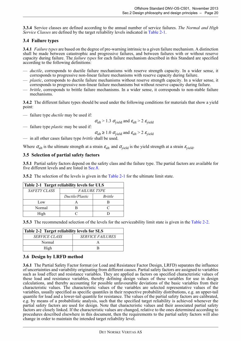
DET NORSKE VERITAS AS
Offshore Standard DNV-OS-C501, November 2013
Sec.2 Design philosophy and design principles – Page 20
3.3.4 Service classes are defined according to the annual number of service failures. The Normal and HighService Classes are defined by the target reliability levels indicated in Table 2-1.
3.4 Failure types
3.4.1 Failure types are based on the degree of pre-warning intrinsic to a given failure mechanism. A distinctionshall be made between catastrophic and progressive failures, and between failures with or without reservecapacity during failure. The failure types for each failure mechanism described in this Standard are specifiedaccording to the following definitions:
— ductile, corresponds to ductile failure mechanisms with reserve strength capacity. In a wider sense, itcorresponds to progressive non-linear failure mechanisms with reserve capacity during failure.
— plastic, corresponds to ductile failure mechanisms without reserve strength capacity. In a wider sense, itcorresponds to progressive non-linear failure mechanisms but without reserve capacity during failure.
— brittle, corresponds to brittle failure mechanisms. In a wider sense, it corresponds to non-stable failuremechanisms.
3.4.2 The different failure types should be used under the following conditions for materials that show a yieldpoint:
— failure type ductile may be used if:
σult > 1.3 σyield and εult > 2 εyield
— failure type plastic may be used if:
σult ≥ 1.0 σyield and εult > 2 εyield
— in all other cases failure type brittle shall be used.
Where σult is the ultimate strength at a strain εult and σyield is the yield strength at a strain εyield.
3.5 Selection of partial safety factors
3.5.1 Partial safety factors depend on the safety class and the failure type. The partial factors are available forfive different levels and are listed in Sec.8.
3.5.2 The selection of the levels is given in the Table 2-1 for the ultimate limit state.
3.5.3 The recommended selection of the levels for the serviceability limit state is given in the Table 2-2.
3.6 Design by LRFD method
3.6.1 The Partial Safety Factor format (or Load and Resistance Factor Design, LRFD) separates the influenceof uncertainties and variability originating from different causes. Partial safety factors are assigned to variablessuch as load effect and resistance variables. They are applied as factors on specified characteristic values ofthese load and resistance variables, thereby defining design values of these variables for use in designcalculations, and thereby accounting for possible unfavourable deviations of the basic variables from theircharacteristic values. The characteristic values of the variables are selected representative values of thevariables, usually specified as specific quantiles in their respective probability distributions, e.g. an upper-tailquantile for load and a lower-tail quantile for resistance. The values of the partial safety factors are calibrated,e.g. by means of a probabilistic analysis, such that the specified target reliability is achieved whenever thepartial safety factors are used for design. Note that characteristic values and their associated partial safetyfactors are closely linked. If the characteristic values are changed, relative to the ones determined according toprocedures described elsewhere in this document, then the requirements to the partial safety factors will alsochange in order to maintain the intended target reliability level.
Table 2-1 Target reliability levels for ULS
SAFETY CLASS FAILURE TYPE
Ductile/Plastic Brittle
Low A B
Normal B C
High C D
Table 2-2 Target reliability levels for SLS
SERVICE CLASS SERVICE FAILURES
Normal A
High B
DET NORSKE VERITAS AS
Offshore Standard DNV-OS-C501, November 2013
Sec.2 Design philosophy and design principles – Page 21
Guidance note:
The following uncertainties are usually considered:
- Uncertainties in the loads, caused by natural variability, which is usually a temporal variability
- Uncertainties in the material properties, caused by natural variability, which is usually a spatial variability
- Uncertainties in the geometrical parameters, caused by
- deviations of the geometrical parameters from their characteristic (normal) value- tolerance limits- cumulative effects of a simultaneous occurrence of several geometrical variation
- Uncertainties in the applied engineering models
- uncertainties in the models for representation of the real structure or structural elements- uncertainties in the models for prediction of loads, owing to simplifications and idealisations made- uncertainties in the models for prediction of resistance, owing to simplifications and idealisations made- effect of the sensitivity of the structural system (under- or over-proportional behaviour)
---e-n-d---of---G-u-i-d-a-n-c-e---n-o-t-e---
3.6.2 Partial safety factors are applied in design inequalities for deterministic design as shown by examples in[3.6.6]. The partial safety factors are usually or preferably calibrated to a specified target reliability by meansof a probabilistic analysis. Sometimes the design inequalities include model factors or bias correction factorsas well. Such model or bias correction factors appear in the inequalities in the same manner as the partial safetyfactors, but they are not necessarily to be interpreted as partial safety factors as they are used to correct forsystematic errors rather than accounting for any variability or uncertainty. Model factors and bias correctionfactors are usually calibrated experimentally.
3.6.3 The following two types of partial safety factors are used in this standard:
— Partial load effect factors, designated in this standard by γF .— Partial resistance factors, designated in this standard by γM .
3.6.4 In some cases it is useful to work with only one overall safety factor. The uncertainties in loads andresistance are then accounted for by one common safety factor denoted gFM. The following simple relationshipbetween this common safety factor on the one hand and the partial load and resistance factors on the other areassumed here corresponding to the general design inequality quoted in [3.6.6]:
γFM= γF x γM
3.6.5 The following two types of model factors are used in this Standard:
— Load model factors, designated in this Standard by γSd .— Resistance model factors, designated in this Standard by γRd .
Guidance note:
- Partial load effect factors γF are applicable to the characteristic values of the local response of the structure. Theyaccount for uncertainties associated with the variability of the local responses of the structure (local stresses orstrains). The uncertainties in the local response are linked to the uncertainties on the loads applied to the structurethrough the transfer function.
- Partial resistance factors γM account for uncertainties associated with the variability of the strength.
- Load model factors γSd account for inaccuracies, idealisations, and biases in the engineering model used forrepresentation of the real response of the structure, e.g. simplifications in the transfer function (see Sec.9). Forexample, wind characterised by a defined wind speed will induce wind loads on the structure, and those loads willinduce local stresses and strains in the structure. The load model factor account for the inaccuracies all the wayfrom wind speed to local response in the material.
- Resistance model factors γRd account for differences between true and predicted resistance values, e.g. differencesbetween test and in-situ materials properties (size effects), differences associated with the capability of themanufacturing processes (e.g. deviations of the geometrical parameters from the characteristic value, tolerancelimits on the geometrical parameters), and differences owing to temporal degradation processes.
- Uncertainties or biases in a failure criterion are accounted for by the resistance model factor.
- Geometrical uncertainties and tolerances should be included in the load model factor.
---e-n-d---of---G-u-i-d-a-n-c-e---n-o-t-e---
3.6.6 A factored design load effect is obtained by multiplying a characteristic load effect by a load effectfactor. A factored design resistance is obtained by dividing the characteristic resistance by a resistance factor. The structural reliability is considered to be satisfactory if the following design inequalities are satisfied:
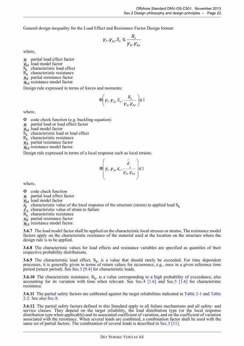
DET NORSKE VERITAS AS
Offshore Standard DNV-OS-C501, November 2013
Sec.2 Design philosophy and design principles – Page 22
General design inequality for the Load Effect and Resistance Factor Design format:
where,
γF partial load effect factorγSd load model factorSk characteristic load effectRk characteristic resistanceγM partial resistance factorγRd resistance model factor.
Design rule expressed in terms of forces and moments:
where,
Φ code check function (e.g. buckling equation)γF partial load or load effect factorγSd load model factorSk characteristic load or load effectRk characteristic resistanceγM partial resistance factorγRd resistance model factor.
Design rule expressed in terms of a local response such as local strains:
where,
Φ code check functionγF partial load effect factorγSd load model factor εk characteristic value of the local response of the structure (strain) to applied load Sk
k characteristic value of strain to failureRk characteristic resistanceγM partial resistance factorγRd resistance model factor.
3.6.7 The load model factor shall be applied on the characteristic local stresses or strains. The resistance modelfactors apply on the characteristic resistance of the material used at the location on the structure where thedesign rule is to be applied.
3.6.8 The characteristic values for load effects and resistance variables are specified as quantiles of theirrespective probability distributions.
3.6.9 The characteristic load effect, Sk, is a value that should rarely be exceeded. For time dependentprocesses, it is generally given in terms of return values for occurrence, e.g., once in a given reference timeperiod (return period). See Sec.3 [9.4] for characteristic loads.
3.6.10 The characteristic resistance, Rk, is a value corresponding to a high probability of exceedance, alsoaccounting for its variation with time when relevant. See Sec.4 [1.6] and Sec.5 [1.6] for characteristicresistance.
3.6.11 The partial safety factors are calibrated against the target reliabilities indicated in Table 2-1 and Table2-2. See also Sec.8.
3.6.12 The partial safety factors defined in this Standard apply to all failure mechanisms and all safety- andservice classes. They depend on the target reliability, the load distribution type (or the local responsedistribution type when applicable) and its associated coefficient of variation, and on the coefficient of variationassociated with the resistance. When several loads are combined, a combination factor shall be used with thesame set of partial factors. The combination of several loads is described in Sec.3 [11].
RdM
kkSdF
RS
γγγγ
... ≤
1.
,.. ≤
Φ
RdM
kkSdF
RS
γγγγ
1.
,.. ≤
Φ
∧
RdM
kkSdF γγ
εεγγ
ε
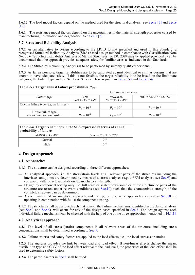
DET NORSKE VERITAS AS
Offshore Standard DNV-OS-C501, November 2013
Sec.2 Design philosophy and design principles – Page 23
3.6.13 The load model factors depend on the method used for the structural analysis. See Sec.8 [3] and Sec.9[12].
3.6.14 The resistance model factors depend on the uncertainties in the material strength properties caused bymanufacturing, installation and degradation. See Sec.8 [2].
3.7 Structural Reliability Analysis
3.7.1 As an alternative to design according to the LRFD format specified and used in this Standard, arecognised Structural Reliability Analysis (SRA) based design method in compliance with Classification NoteNo. 30.6 “Structural Reliability Analysis of Marine Structures” or ISO 2394 may be applied provided it can bedocumented that the approach provides adequate safety for familiar cases as indicated in this Standard.
3.7.2 The Structural Reliability Analysis is to be performed by suitably qualified personnel.
3.7.3 As far as possible, target reliabilities are to be calibrated against identical or similar designs that areknown to have adequate safety. If this is not feasible, the target reliability is to be based on the limit statecategory, the failure type and the Safety or Service Class as given in Table 2-3 and Table 2-4.
4 Design approach
4.1 Approaches
4.1.1 The structure can be designed according to three different approaches:
— An analytical approach, i.e. the stress/strain levels at all relevant parts of the structures including theinterfaces and joints are determined by means of a stress analyses (e.g. a FEM-analyses, see Sec.9) andcompared with the relevant data on the mechanical strength.
— Design by component testing only, i.e. full scale or scaled down samples of the structure or parts of thestructure are tested under relevant conditions (see Sec.10) such that the characteristic strength of thecomplete structure can be determined.
— A combination of an analytical approach and testing, i.e. the same approach specified in Sec.10 forupdating in combination with full scale component testing.
4.1.2 The structure shall be designed such that none of the failure mechanisms, identified in the design analysis(see Sec.3 and Sec.6), will occur for any of the design cases specified in Sec.3. The design against eachindividual failure mechanism can be checked with the help of one of the three approaches mentioned in [4.1.1].
4.2 Analytical approach
4.2.1 The level of all stress (strain) components in all relevant areas of the structure, including stressconcentrations, shall be determined according to Sec.9.
4.2.2 Failure criteria and safety factors are applied to the load effects, i.e., the local stresses or strains.
4.2.3 The analysis provides the link between load and load effect. If non-linear effects change the mean,distribution type and COV of the load effect relative to the load itself, the properties of the load effect shall beused to determine safety factors.
4.2.4 The partial factors in Sec.8 shall be used.
Table 2-3 Target annual failure probabilities PFT
Failure consequence
Failure type LOW SAFETY CLASS
NORMAL SAFETY CLASS
HIGH SAFETY CLASS
Ductile failure type (e.g. as for steel)PF = 10-3 PF = 10-4 PF = 10-5
Brittle failure type(basis case for composite) PF = 10-4 PF = 10-5 PF = 10-6
Table 2-4 Target reliabilities in the SLS expressed in terms of annual probability of failure
SERVICE CLASS SERVICE FAILURES
Normal 10-3
High 10-4

DET NORSKE VERITAS AS
Offshore Standard DNV-OS-C501, November 2013
Sec.2 Design philosophy and design principles – Page 24
4.3 Component testing
4.3.1 The purpose of this approach is to define the characteristic strength of the finished and complete structureunder relevant load conditions. If deemed relevant, the resistance may be found by testing scaled models orparts of the finished structure.
4.3.2 Details about component testing are given in Sec.10 and Sec.7.
4.3.3 A sufficiently large number of tests shall be carried out in order to be able to define the characteristicstrength of the structure with a confidence level at least as large as required for the data used with the analyticalapproach.
4.3.4 The failure mode(s), failure mechanism(s) and location(s) of failure shall be verified during and or afterthe tests.
4.4 Analyses combined with updating
4.4.1 Analyses of the structure may be complicated and a conservative bias may have to be introduced in theanalyses. The reasons for such biases may be:
— Scaling effects.— Uncertainties in the relevance of the design rules, e.g. in areas with large stress gradients.— The analytical models for analysing the stress level in the structure.— The effect of the environment on the mechanical properties.— Etc.
4.4.2 In such cases the analyses that have been carried out may be combined with the procedure for updatinggiven in Sec.10 [3]. The purpose of this approach is to update the predicted resistance of the structure with theresults from a limited number of tests in a manner consistent with the reliability approach of the standard.
4.4.3 It is a basic assumption that that all biases are handled in a conservative way, i.e. that the bias lead to aconservative prediction of the resistance of the structure.
5 Requirements to documentation
5.1 Design Drawings and Tolerances
5.1.1 Design drawings shall be provided according to general standards.
5.1.2 Tolerances shall be indicated.
5.2 Guidelines for the design report
5.2.1 The design Report should contain the following as a minimum:
— Description of the entire structure and of its components.— Design input as described in Sec.3, including design life, environmental conditions.— Relevant design assumptions and conditions including applicable limitations.— Description of analysis from design phase, evaluation of problem areas, highly utilised and critical areas of
the structure and highlighting points that require special attention during subsequent phases.— Reference to accepted calculations and other documents verifying compliance with governing technical
requirements for all phases.— Fabrication procedures giving a concentrated description of the manufacturing/ fabrication history,
reference to specifications, drawings etc., discussion of problem areas, deviations from specifications anddrawings, of importance for the operational phase identification of areas deemed to require special attentionduring normal operation and maintenance.
— Reference to documentation needed for repair and modification.
5.2.2 All failure modes and failure mechanisms shall be clearly identified and listed in a systematic way,preferably in a table. It shall be shown that each combination of identified failure modes and mechanisms wasaddressed in the design.
DET NORSKE VERITAS AS
Offshore Standard DNV-OS-C501, November 2013
Sec.3 Design input – Page 25
SECTION 3 DESIGN INPUT
1 Introduction
1.1
1.1.1 This section identifies the input needed for the analysis of the structure. The material properties areaddressed separately in Sec.4 for laminates and Sec.5 for sandwich structures.
1.1.2 The Design Input of this section (Sec.3) and Sec.4 and Sec.5 for Material Properties, form the basis ofthe Design Premises.
2 Product specifications
2.1 General function or main purpose of the product
2.1.1 The general function or the main purpose of the product and its main interactions with other componentsand the environment shall be specified in the product specifications.
2.1.2 The design life in service should be specified in the product specifications.
Guidance note:
E.g. the product is a gas pressure bottle for diving activities. The filling pressure will be 200 bars, the volume 100 land the lifetime in service 20 years.
---e-n-d---of---G-u-i-d-a-n-c-e---n-o-t-e---
3 Division of the product or structure into components, parts and details
3.1
3.1.1 The following levels of division of the product or structure are used in this standard:
— structure / product— sub-structure / sub-product— components— parts— details.
3.1.2 The term product or structure designates in this standard the entity being designed.
3.1.3 The product or structure can be divided into sub-products or sub-structures, each of which may belongto different safety and service classes.
3.1.4 The structure or product can be divided into components corresponding to the same Safety Class but maybe subject to different functional requirements.
3.1.5 Each component can be divided into parts and each part into details.
Guidance note:
For example:
Structure = pipeline
Sub-structure = the pipeline portion close to human activity should be classed under high safety class, whereas therest of the pipeline can be classed under low or normal safety class. The pipeline can be divided into to sub-structurescorresponding to different safety classes
Components = the pipeline could be constituted of an inner liner and an outer shell. The liner’s function is to keep thepipeline tight, whereas the shell’s function is to hold the pressure loads. The two components have different functionalrequirements
Parts and details = the pipeline can be divided into pipe body, couplers and fittings. Different design approaches anddesign solutions may be used for the different parts and details
---e-n-d---of---G-u-i-d-a-n-c-e---n-o-t-e---
3.1.6 A structure or substructure is an independent part for which a safety class can be defined. Components,parts and details are part of a structure or substructure. Failure of any of these components, parts or details shallbe seen in combination with each other. See also Sec.8 [4].
3.1.7 The interfaces between parts, components or structures shall be considered carefully. Interfaces shall beanalysed as a part itself if they belong to a continuous structure. If the interfaces are physical interfaces, therequirements of Sec.7 [4] shall be considered.
DET NORSKE VERITAS AS
Offshore Standard DNV-OS-C501, November 2013
Sec.3 Design input – Page 26
4 Phases
4.1 Phases
4.1.1 The design life of the product shall be divided into phases, i.e. well defined periods within the life spanof the product.
4.1.2 All phases that could have an influence on the design of the product shall be considered.
Guidance note:
E.g. For some products, the transportation phase is critical and is actually driving the design.
---e-n-d---of---G-u-i-d-a-n-c-e---n-o-t-e---
4.1.3 As a minimum the construction phase and the operation phase shall be considered. However, it may beconvenient to split the design life into more detailed phases. A list of phases is presented in App.A.
4.1.4 A decommissioning phase may be specified in some cases.
4.1.5 The duration of each phase shall be specified. Especially, the lifetime in service shall be specified.
5 Safety and service classes
5.1 Safety classes
5.1.1 The product can be divided into sub-products, each of which may belong to different safety classes.
5.1.2 For each sub-product the safety classes, as described in Sec.2 [3.3], shall be specified and documented.
5.1.3 Possible deviations in target probabilities of failure from the ones specified for the safety classes in Sec.2Table 2-1 and Sec.2 Table 2-2 shall be documented and justified.
Guidance note:
This may be needed if clients or authorities want other target reliability levels than specified here.
---e-n-d---of---G-u-i-d-a-n-c-e---n-o-t-e---
5.1.4 The safety class of a product or sub-product may change from one phase to the other during the life ofthe structure.
5.2 Service classes
5.2.1 The product can be divided into sub-products, each of which may belong to different service classes.
Guidance note:
Service classes may be used to discriminate between parts of a product with different maintenance requirements. Forexample, some parts of a pipeline system, which are less accessible, could be designed for a lower maintenancefrequency.
---e-n-d---of---G-u-i-d-a-n-c-e---n-o-t-e---
5.2.2 For each sub-product the service classes as described in Sec.2 [3.3] shall be specified when applicable.
6 Functional requirements
6.1
6.1.1 A functional requirement is defined as a requirement that the product and or a component has to fulfil.The functional requirements shall be checked for every component of the product.
6.1.2 The structure or product can be divided into components corresponding to the same safety class but maybe subject to different functional requirements.
6.1.3 The functional requirements shall be defined for each phase during the design life.
6.1.4 A list of functional requirements that should be considered as a minimum is given in App.A.
Guidance note:
Functional requirements may be related to structural or non-structural performances. This standard is orientatedtowards structural performances. However, it should be noted that non-structural functional requirements might lead
DET NORSKE VERITAS AS
Offshore Standard DNV-OS-C501, November 2013
Sec.3 Design input – Page 27
to safety issues (e.g. static electricity properties). Moreover, some structural failures may affect non-structuralperformances, e.g. matrix cracking might influence acoustic performances.
---e-n-d---of---G-u-i-d-a-n-c-e---n-o-t-e---
7 Failure modes
7.1 General
7.1.1 A complete list of all failure modes shall be established for every component of the product.
7.1.2 Subsequent failure scenarios shall be taken into consideration. For example, rupture of a protectivecoating may in itself not be a severe event. However, subsequent corrosion of the material behind the coatingmay cause serious damage.
7.2 Failure modes
7.2.1 A failure is defined as a state of inability to perform a normal function, or an event causing an undesirableor adverse condition, e.g. violation of functional requirement, loss of component or system function, ordeterioration of functional capability to such an extent that the safety of the unit, personnel or environment issignificantly reduced.
7.2.2 A failure mode is a symptom or condition that leads to failure, in general the fashion in which thestructure fails.
Guidance note:
A failure mode is the manner in which one or several functional requirements fail. The importance of all failure modesshall be agreed between the designer and the contractor, i.e. the associated type of limit state shall be identified foreach failure mode (see Sec.3 [7.3] below and Sec.2 [3.2] for the definition of the type of limit states).
---e-n-d---of---G-u-i-d-a-n-c-e---n-o-t-e---
7.2.3 Failure shall be considered for all locations of the product taking into account all levels of detail, asdefined in [3].
7.2.4 The potential failure modes shall be listed for each location of the product. A list of failure modes thatshould be considered as a minimum is given in App.A.
7.2.5 Some products may fail by other failure modes than those listed above. Such failure modes shall beidentified and documented.
7.2.6 For each location a link between possible failure modes and functional requirements shall be established.A table describing links that should be considered as a minimum is given in App.A.
7.2.7 If a number of failure modes can cause a violation of a functional requirement all possible failure modesshall be indicated.
7.2.8 If any of the indicated failure modes occurs for a single functional requirement the structure shall beconsidered as failed. Each failure mode shall be evaluated with respect to the type of limit state it is associatedwith (see [7.3]).
7.2.9 In some cases several failure modes may interact to violate a certain functional requirement. Thatinteraction shall be specified if relevant.
7.2.10 If a failure mode is not associated with any functional requirement it should be evaluated carefully thatthis failure mode is not critical in any sense.
7.3 Identification of the type of limit states
7.3.1 For each phase and each part of the product the consequence of a failure (violation of one of thefunctional requirements) shall be evaluated and it shall be decided whether the mode of failure is related to theultimate limit state or to the serviceability limit state.
Guidance note:
Note: the client and/or authorities should make this decision. This defines the level of severity of each failure.
---e-n-d---of---G-u-i-d-a-n-c-e---n-o-t-e---
7.3.2 All possible failures of the product at each location in each phase shall be considered.
7.3.3 If a failure mode has increasing consequence of failure severity in subsequent phases, it shall be designedfor the most severe consequence of failure in all phases, unless the product can be inspected in between phasesand it can be insured that the failure mode has not occurred in the previous phase.
DET NORSKE VERITAS AS
Offshore Standard DNV-OS-C501, November 2013
Sec.3 Design input – Page 28
8 Exposure from the surroundings
8.1 General
8.1.1 Surroundings shall be understood in this standard in a general sense. It designates the natural, functionaland human phenomena to which the product is exposed to during its lifetime.
8.1.2 It shall be determined to which surroundings the product or parts of the product are exposed to in eachphase.
Guidance note:
Surroundings can be divided into:
- Natural surroundings, which covers natural phenomena such as wind, wave and currents
- Functional surroundings, which cover phenomena due to the functional surrounding of the structure such aschemicals, fire, temperature or weight of content
- Human surroundings, which cover events due to human activity such as dropped objects or weld spatter.
---e-n-d---of---G-u-i-d-a-n-c-e---n-o-t-e---
8.1.3 This document does not specify the surroundings, since they are dependent on the applications.However, a list is provided in App.A to ensure that at least the most frequently encountered surroundings areconsidered in the design.
8.2 Loads and environment
8.2.1 A distinction is made in this standard between:
— loads— environment.
8.2.2 The term loads designates in this standard the direct and indirect loads on the product, e.g. wave load ona structure, or thermal expansion loads. Both direct and indirect loads impose load effects, like stresses orstrains on the product. Loads can be different in nature: functional loads, environmental loads or accidentalloads. The loads on the product shall be specified according to Sec.3 [9].
8.2.3 Calculations of the load effects on the product to the various environmental phenomena, i.e.environmental loads, are made by a transfer function. Specific transfer functions are not described in thisstandard (e.g. calculation of the load effect on a structure due to wind, with a specified wind speed). The loadeffects should be determined according to relevant standards or guidelines. As guidance for calculation ofcharacteristic environmental loads on a structure the principles given in DNV-RP-C205 “Environmentalconditions and environmental loads” may be used.
8.2.4 The term environment designates in this standard the surroundings that impose no direct load on theproduct, e.g. ambient temperature or moisture. The environment shall be specified according to therequirements of Sec.3 [10].
8.2.5 The environment is generally considered for its effect on the degradation of material strength (see Sec.4[5] and Sec.5 [5]).
8.2.6 The environment may also impose indirect loads on the structure, e.g. thermal stresses or swelling dueto moisture uptake. This effect should be considered as a load, according to Sec.3 [9] and Sec.9 [8] and Sec.9[9] (structural analysis).
8.2.7 Material properties may be influenced in the long-term not only by the environment but also by the loads,or by the combination of environment with loads, e.g. creep and stress rupture. The combination of loads andenvironment to be considered when assessing the degradation of material properties is detailed in Sec.3 [11].
8.3 Obtaining loads from the exposure from the surroundings
8.3.1 The surrounding environment can often not be described as a direct load acting on a structure. In such acase a transfer function shall be established that transforms the surrounding environment into a load. Anyuncertainties in the transfer function shall be included in the load model factor described in Sec.8 and Sec.9.
8.3.2 It is recommended to use a conservative transfer function. In that case it is not necessary to consider themodel uncertainties of the transfer function in the load model factor.
DET NORSKE VERITAS AS
Offshore Standard DNV-OS-C501, November 2013
Sec.3 Design input – Page 29
Guidance note:
The wind load is a typical example where the speed of the wind is transformed to a load on a structure. The loaddepends not only on the speed but also on the exposed surface and the aerodynamic profile of the structure. Thetransfer function is the mathematical model that transforms wind speed to a load on the structure.
---e-n-d---of---G-u-i-d-a-n-c-e---n-o-t-e---
9 Loads
9.1 General
9.1.1 This standard does not specify specific load conditions and characteristic load effects, since these aredependent on the applications.
Guidance note:
A non-exhaustive list of the most common loads to be considered in design is given as guidance in App.A of thissection. This list is organised according to a classical classification into functional, environmental and accidentalloads. This classical classification is only used in this standard as a checklist. The load factors are dependent on theprobabilistic representation of the loads.
---e-n-d---of---G-u-i-d-a-n-c-e---n-o-t-e---
9.1.2 A load is defined as an assembly of one or more concentrated or distributed forces acting on the structure(direct loads), or the cause of imposed or constrained deformations in the structure (indirect loads).
Guidance note:
The environment may impose indirect loads on the structure, e.g. thermal stresses or swelling due to moisture uptake.This should be considered as a load effect, and calculated according to the relevant parts of Sec.9. However, theenvironment is generally considered for its effect on the degradation of material strength.
---e-n-d---of---G-u-i-d-a-n-c-e---n-o-t-e---
9.1.3 All the load cases shall be described separately for each phase during the design life of the structure.
9.1.4 All loads have to be represented as appropriate with due consideration of:
— type of load and load effect: global, regional or local load, or response— direction of load— variation with time.
9.1.5 A representative time history of all loads should be documented for the entire life of the structure. Thisincludes a probabilistic representation as specified in Sec.3 [9.2].
9.1.6 Different load values are defined in this standard:
— the characteristic value (Sec.3 [9.4]) is defined based on the probabilistic representation of the load— the sustained value (Sec.3 [9.5]) is defined based on the time representation of the load— the fatigue value (Sec.3 [9.6]) is defined based on the time representation of the load.
Guidance note:
The definition of the different load values is summarised in the Table 3-1. The detailed definition presented in therelevant chapters shall be used.
---e-n-d---of---G-u-i-d-a-n-c-e---n-o-t-e---
9.1.7 The notion of accidental value is not used in this standard. It shall be decided whether the product shouldbe designed for a given accidental event (e.g. fire, impact) or whether it should not be designed for it and insteadprotected against it by other means (e.g. impact protection structure around the product).
9.1.8 Different types of loads and environments shall be combined. Depending on which load and environmentvalues are combined, different load and environmental conditions are defined. These different load and
Table 3-1 Definition of load values
Designation Definition To be used for
Characteristic value Extreme value with return period of 100 years Check of Ultimate Limit States
Sustained value Average value over a long period Long-term degradation of material properties
Fatigue value Mean and amplitude of variations Check of Fatigue Limit States
Accidental value Same as characteristic value
DET NORSKE VERITAS AS
Offshore Standard DNV-OS-C501, November 2013
Sec.3 Design input – Page 30
environmental conditions define the different design cases to be considered. These design cases are describedin Sec.3 [11].
9.2 Probabilistic representation of load effects
9.2.1 The response of the structure to applied loads shall be calculated on a global or a local level dependingon the failure mechanism being checked and its associated design rule. See Sec.9 [1.4].
9.2.2 A probabilistic representation should be established for the effect of each load on the structure in everyrelevant location. The load effect is obtained by from the basic load by structural analysis. The basic load isobtained directly or by a transfer function (e.g. converting wind speed to a basic load on the surface).
9.2.3 The probability distribution function representative for each load process should be determined. Theprobability distribution function representative for the response of the structure associated with each loadprocess, the load effect, should also be determined in every relevant location. In particular, the type ofdistribution should be determined for each distribution function.
9.2.4 The arbitrary value distribution over the lifetime of the structure and annual extreme value distributionshall be determined for all loads and the corresponding response of the structure.
9.2.5 A recognised procedure for determination of the distribution type shall be used. The procedure requiredin the DNV Classification Note No.30.6 “Structural reliability analysis of marine structures” may be used.
9.2.6 If two types of distributions give equally good fits to data, the distribution with most probability contentin the upper tail should be chosen, unless one of the distributions fits possible data observations in the tail betterthan the other.
9.2.7 If no satisfactory distribution fit can be obtained or if insufficient data are available, then the simplifiedprobabilistic representation of load effects presented in Sec.3 [9.3] shall be used.
Guidance note:
The partial safety factors specified for the simplified probabilistic representation of load effects are conservative. Aprecise determination of the extreme-value distribution for load would normally lead to lower requirements to thevalues of the partial safety factors.
---e-n-d---of---G-u-i-d-a-n-c-e---n-o-t-e---
9.2.8 For some load variables, sufficient knowledge and or experience is available to provide a basis forrecommendation of distribution types. A list of variables with their recommended distribution types is given inApp.A.
9.2.9 The coefficient of variation of each load variable and the corresponding load effect shall be specified. Ifinsufficient data are available the simplified probabilistic representation of load effects presented in I300should be used.
9.3 Simplified representation of load effects
9.3.1 A simplified set of partial safety factors is given for use whenever a satisfactory probabilisticrepresentation of the load effects, as required in Sec.3 [9.2], is not available.
9.3.2 The characteristic load effect shall be defined as specified in Sec.3 [9.4].
9.3.3 The simplified set of partial safety factors given in Sec.8 [2.3] was determined assuming that thecoefficient of variation of load effects were not larger than 20%. These partial safety factors shall not be usedfor load effects with a COV larger than 20%.
9.3.4 The simplified set of partial safety factors given in Sec.8 [2.4] was determined assuming that thecoefficient of variation of load effects is 0%, i.e. the load effects are exactly known and they do not have anystatistical variation. This is usually based on a very conservative description of the load effect.
9.3.5 The simplified set of partial safety factors shall be used when the characteristic strength is defined as the2.5% quantile, as generally required in this standard.
9.3.6 Loads may also be defined as combinations of functional loads and environmental loads according tooffshore standards like DNV-OS-F201 “Dynamic risers” or DNV-OS-F101 “Submarine pipeline systems”.Partial safety factors for this choice are given in Sec.8 [2.6].
9.4 Characteristic load effect
9.4.1 The characteristic load effect value, Sk, is a value that will only rarely be exceeded. For time-dependentprocesses, it is generally given in terms of a return value for occurrence, i.e. a load effect which on average isexceeded once in a specified reference time period (denoted return period or recurrence period).
DET NORSKE VERITAS AS
Offshore Standard DNV-OS-C501, November 2013
Sec.3 Design input – Page 31
9.4.2 A unique definition of the characteristic load effect is prescribed and used throughout this standard. Itshall be used both in case of single and multiple load processes.
9.4.3 In principle, the characteristic load effect shall be determined as the characteristic value of the localresponse of the structure to the applied load. It shall be based on a probabilistic representation of the variabilityin the local response, as defined in Sec.3 [9.2].
Guidance note:
The partial safety factors specified in this standard and calibrated against specified probabilities of failure apply onthe characteristic values of the load effect, i.e., the local response of the structure. Simplifications in the transferfunction (from loads to local response) lead to uncertainties. These uncertainties are accounted for by the load modelfactors. When the transfer function from applied loads to local response is linear, the probabilistic representation ofthe variability in the local response is identical to the probabilistic representation of the variability of the loads. In thatcase, partial safety factors can be applied directly on the characteristic values of the applied loads.
---e-n-d---of---G-u-i-d-a-n-c-e---n-o-t-e---
9.4.4 The characteristic load effect can be determined as the characteristic value of the externally appliedglobal load in the following cases:
— when the design rule is expressed in terms of the global response of the structure— when the transfer function from global to local response and the analysis is linear.
9.4.5 The characteristic load effect is defined as the 99% quantile in the distribution of the annual extremevalue of the local response of the structure, or of the applied global load when relevant.
9.4.6 The 99% quantile in the distribution of the annual maximum load effect is used as the characteristic loadvalue throughout this document. The 99% quantile may be interpreted as the 100-year load, i.e., the load valuewhich has a return period of 100 years. This is the load effect value, which on average will be exceeded onceevery 100 years.
9.4.7 Extreme values driving the design can be maximum as well as minimum values. Should minimum valuesof load effects be driving the design, the characteristic load effect shall be defined as the 1% quantile in thedistribution of the annual minimum load. For example, the pressure on the wall of a submerged pressure vesselis function of the differential between internal pressure and external hydrostatic pressure and increases whenthe external pressure decreases (i.e. when the depth decreases).
9.5 The sustained load effect
9.5.1 The sustained load effect value should be used for the determination of time-dependent materialproperties as described in Sec.4 [3] (for laminates) and Sec.5 [3] (for sandwich structures).
Guidance note:
In general, it would be very conservative to determine the time dependent degradation of material properties underlong-term loads by using the characteristic load effect value (i.e. extreme load effect value). The sustained value isdefined in this standard as a kind of average load effect value over the lifetime of the product.
---e-n-d---of---G-u-i-d-a-n-c-e---n-o-t-e---
9.5.2 Sustained load values are defined over an observation period, which can correspond to the entire designlife of the product or to a part of that design life. This observation period shall be divided into several timeintervals. Time intervals should not be chosen shorter than 1 hour. The maximum length of a time intervaldepends on the load variations. Variations in magnitude of the load within a time interval shall not be largerthan half the absolute load amplitude during the total observation period.
9.5.3 Load effects are divided, according to their variation with time, into:
— permanent load effects; effects which are likely to act or be sustained throughout the design life and forwhich variations in magnitude with time are negligible relative to their mean values; or load effects whichare monotonically in- or decreasing until they attain some limiting values
— variable load effects; effects which are unlikely to act throughout the specified design life or whosevariations in magnitude with time are random rather than monotonic and not negligible relative to theirmean values.
9.5.4 The sustained value of permanent load effects shall correspond to their characteristic value, as definedin Sec.3 [9.4].
9.5.5 The sustained value of variable load effects is defined as the mean value of the effects over the timeinterval. The sustained value Ss during the time interval to is determined such that the corresponding totalduration above Ss is a portion µ = 0,5 of the exposure period ts. See Figure 3-1:
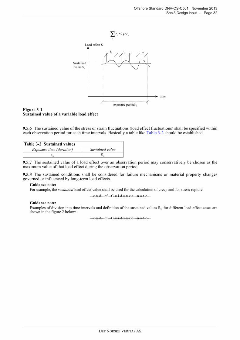
DET NORSKE VERITAS AS
Offshore Standard DNV-OS-C501, November 2013
Sec.3 Design input – Page 32
Figure 3-1 Sustained value of a variable load effect
9.5.6 The sustained value of the stress or strain fluctuations (load effect fluctuations) shall be specified withineach observation period for each time intervals. Basically a table like Table 3-2 should be established.
9.5.7 The sustained value of a load effect over an observation period may conservatively be chosen as themaximum value of that load effect during the observation period.
9.5.8 The sustained conditions shall be considered for failure mechanisms or material property changesgoverned or influenced by long-term load effects.
Guidance note:
For example, the sustained load effect value shall be used for the calculation of creep and for stress rupture.
---e-n-d---of---G-u-i-d-a-n-c-e---n-o-t-e---
Guidance note:
Examples of division into time intervals and definition of the sustained values Ssi for different load effect cases areshown in the figure 2 below:
---e-n-d---of---G-u-i-d-a-n-c-e---n-o-t-e---
Table 3-2 Sustained values
Exposure time (duration) Sustained value
ts Ss
∑ ≤i
si tt .µ
time
Load effect S
Sustainedvalue Ss
exposure period ts
t1 t2 t3
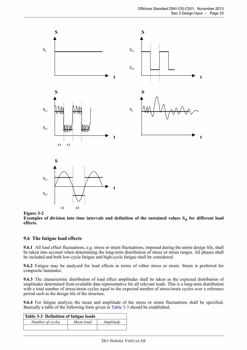
DET NORSKE VERITAS AS
Offshore Standard DNV-OS-C501, November 2013
Sec.3 Design input – Page 33
Figure 3-2 Examples of division into time intervals and definition of the sustained values Ssi for different loadeffects.
9.6 The fatigue load effects
9.6.1 All load effect fluctuations, e.g. stress or strain fluctuations, imposed during the entire design life, shallbe taken into account when determining the long-term distribution of stress or strain ranges. All phases shallbe included and both low-cycle fatigue and high-cycle fatigue shall be considered.
9.6.2 Fatigue may be analysed for load effects in terms of either stress or strain. Strain is preferred forcomposite laminates.
9.6.3 The characteristic distribution of load effect amplitudes shall be taken as the expected distribution ofamplitudes determined from available data representative for all relevant loads. This is a long-term distributionwith a total number of stress/strain cycles equal to the expected number of stress/strain cycles over a referenceperiod such as the design life of the structure.
9.6.4 For fatigue analysis the mean and amplitude of the stress or strain fluctuations shall be specified.Basically a table of the following form given in Table 3-3 should be established.
Table 3-3 Definition of fatigue loads
Number of cycles Mean load Amplitude
S
t
Ss
S
t
Ss1
Ss2
S
t
Ss
S
t
Ss1
Ss2
t 1 t 2
S
t
Ss1
Ss2
t 1 t 2
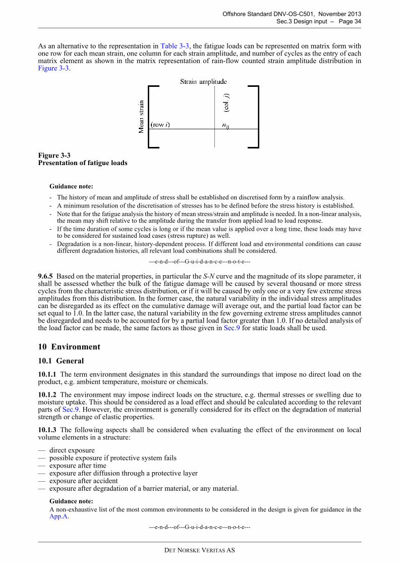
DET NORSKE VERITAS AS
Offshore Standard DNV-OS-C501, November 2013
Sec.3 Design input – Page 34
As an alternative to the representation in Table 3-3, the fatigue loads can be represented on matrix form withone row for each mean strain, one column for each strain amplitude, and number of cycles as the entry of eachmatrix element as shown in the matrix representation of rain-flow counted strain amplitude distribution inFigure 3-3.
Figure 3-3 Presentation of fatigue loads
Guidance note:
- The history of mean and amplitude of stress shall be established on discretised form by a rainflow analysis.
- A minimum resolution of the discretisation of stresses has to be defined before the stress history is established.
- Note that for the fatigue analysis the history of mean stress/strain and amplitude is needed. In a non-linear analysis,the mean may shift relative to the amplitude during the transfer from applied load to load response.
- If the time duration of some cycles is long or if the mean value is applied over a long time, these loads may haveto be considered for sustained load cases (stress rupture) as well.
- Degradation is a non-linear, history-dependent process. If different load and environmental conditions can causedifferent degradation histories, all relevant load combinations shall be considered.
---e-n-d---of---G-u-i-d-a-n-c-e---n-o-t-e---
9.6.5 Based on the material properties, in particular the S-N curve and the magnitude of its slope parameter, itshall be assessed whether the bulk of the fatigue damage will be caused by several thousand or more stresscycles from the characteristic stress distribution, or if it will be caused by only one or a very few extreme stressamplitudes from this distribution. In the former case, the natural variability in the individual stress amplitudescan be disregarded as its effect on the cumulative damage will average out, and the partial load factor can beset equal to 1.0. In the latter case, the natural variability in the few governing extreme stress amplitudes cannotbe disregarded and needs to be accounted for by a partial load factor greater than 1.0. If no detailed analysis ofthe load factor can be made, the same factors as those given in Sec.9 for static loads shall be used.
10 Environment
10.1 General
10.1.1 The term environment designates in this standard the surroundings that impose no direct load on theproduct, e.g. ambient temperature, moisture or chemicals.
10.1.2 The environment may impose indirect loads on the structure, e.g. thermal stresses or swelling due tomoisture uptake. This should be considered as a load effect and should be calculated according to the relevantparts of Sec.9. However, the environment is generally considered for its effect on the degradation of materialstrength or change of elastic properties.
10.1.3 The following aspects shall be considered when evaluating the effect of the environment on localvolume elements in a structure:
— direct exposure— possible exposure if protective system fails— exposure after time— exposure after diffusion through a protective layer— exposure after accident— exposure after degradation of a barrier material, or any material.
Guidance note:
A non-exhaustive list of the most common environments to be considered in the design is given for guidance in theApp.A.
---e-n-d---of---G-u-i-d-a-n-c-e---n-o-t-e---
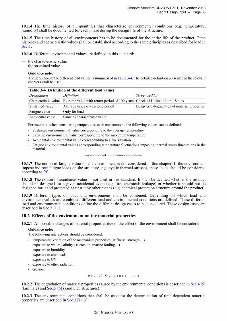
DET NORSKE VERITAS AS
Offshore Standard DNV-OS-C501, November 2013
Sec.3 Design input – Page 35
10.1.4 The time history of all quantities that characterise environmental conditions (e.g. temperature,humidity) shall be documented for each phase during the design life of the structure.
10.1.5 The time history of all environments has to be documented for the entire life of the product. Timehistories and characteristic values shall be established according to the same principles as described for load inSec.1.
10.1.6 Different environmental values are defined in this standard:
— the characteristic value — the sustained value.
Guidance note:
The definition of the different load values is summarised in Table 3-4. The detailed definition presented in the relevantchapters shall be used.
For example: when considering temperature as an environment, the following values can be defined:
- Sustained environmental value corresponding to the average temperature
- Extreme environmental value corresponding to the maximum temperature
- Accidental environmental value corresponding to a fire situation
- Fatigue environmental values corresponding temperature fluctuations imposing thermal stress fluctuations in thematerial
---e-n-d---of---G-u-i-d-a-n-c-e---n-o-t-e---
10.1.7 The notion of fatigue value for the environment is not considered in this chapter. If the environmentimpose indirect fatigue loads on the structure, e.g. cyclic thermal stresses, these loads should be consideredaccording to [9].
10.1.8 The notion of accidental value is not used in this standard. It shall be decided whether the productshould be designed for a given accidental event (e.g. fire, chemicals leakage) or whether it should not dedesigned for it and protected against it by other means (e.g. chemical protection structure around the product).
10.1.9 Different types of loads and environment shall be combined. Depending on which load andenvironment values are combined, different load and environmental conditions are defined. These differentload and environmental conditions define the different design cases to be considered. These design cases aredescribed in Sec.3 [11].
10.2 Effects of the environment on the material properties
10.2.1 All possible changes of material properties due to the effect of the environment shall be considered.
Guidance note:
The following interactions should be considered:
- temperature: variation of the mechanical properties (stiffness, strength…)
- exposure to water (salinity / corrosion, marine fouling…)
- exposure to humidity
- exposure to chemicals
- exposure to UV
- exposure to other radiation
- erosion.
---e-n-d---of---G-u-i-d-a-n-c-e---n-o-t-e---
10.2.2 The degradation of material properties caused by the environmental conditions is described in Sec.4 [5](laminate) and Sec.5 [5] (sandwich structures).
10.2.3 The environmental conditions that shall be used for the determination of time-dependent materialproperties are described in Sec.3 [11.3].
Table 3-4 Definition of the different load values
Designation Definition To be used for
Characteristic value Extreme value with return period of 100 years Check of Ultimate Limit States
Sustained value Average value over a long period Long-term degradation of material properties
Fatigue value Only for loads
Accidental value Same as characteristic value

DET NORSKE VERITAS AS
Offshore Standard DNV-OS-C501, November 2013
Sec.3 Design input – Page 36
11 Combination of load effects and environment
11.1 General
11.1.1 The combination and severity of load effects and or environmental conditions should be determinedtaking into account the probability of their simultaneous occurrence.
Guidance note:
For example, a severe wave climate producing a large wave load is usually accompanied by a severe wind climateproducing a large wind load.
---e-n-d---of---G-u-i-d-a-n-c-e---n-o-t-e---
11.1.2 If the load effect is related to the actual load in a linear way loads may be combined directly instead ofcombining load effects. Reference is also made to DNV-OS-F201 Appendix C on how to combine loads fornon-linear systems.
11.1.3 Load effects and or environmental conditions, which are mutually exclusive, should not enter togetherinto a combination, e.g. ice load effects and wave load effects in a riser environment.
11.1.4 All directions of load effects are to be taken as equally probable, unless data clearly show that theprobability of occurrence is different in different directions, or unless load effects in a particular direction isparticularly critical.
11.1.5 Permanent load effects and permanent environmental conditions shall be taken into consideration in allcombinations of load effects and environmental conditions. When combined with other load effects orenvironmental conditions, their characteristic values shall be included in the combination.
11.1.6 The following load effect and environmental conditions are defined in this standard:
— load effects and environmental conditions for ultimate limit state— load effects and environmental conditions for time-dependent material properties— load effects and environmental conditions for fatigue analysis.
11.1.7 The Table 3-5 summarises the load and environmental conditions that should be considered for thedetermination of the time-dependent material properties and those that should be used for the design checks atvarious times during the life of the product.
11.2 Load effect and environmental conditions for ultimate limit state
11.2.1 At any time during the design life of the structure it should be documented that the structure can fulfilits functional requirements for:
— all characteristic load effect values combined with all sustained environmental values— all sustained load effect values combined with all characteristic environmental values.
11.2.2 When environment and load effect are fully-correlated, their characteristic values shall be combined.
11.2.3 The combination of characteristic load effects and environment should be determined such that thecombined characteristic effect has a return-period of 100 years.
Guidance note:
A method to determine the 100-years combined effect of several load effects and environments is described in thischapter. It is based on the so-called Turkstra’s rule.
---e-n-d---of---G-u-i-d-a-n-c-e---n-o-t-e---
11.2.4 When several stochastic load effect and/or environmental conditions occur simultaneously, the extremecombined effects of the associated stochastic processes are required for design against the ultimate limit state.Each process is characterised by a characteristic value. The characteristic values are to be factored and
Table 3-5 Combinations of load and environmental conditions to be considered for the determination of material degradation and for design checks
Loads
Characteristic value Sustained value Fatigue value
Environment Characteristic value ULS checkFully correlated onlySee [11.2.2]
ULS checkNot fully correlatedSee [11.2.6]
Sustained value ULS checkNot fully correlatedSee [11.2.6]
Material degradationSee [11.3]
Fatigue analysisSee [11.4]
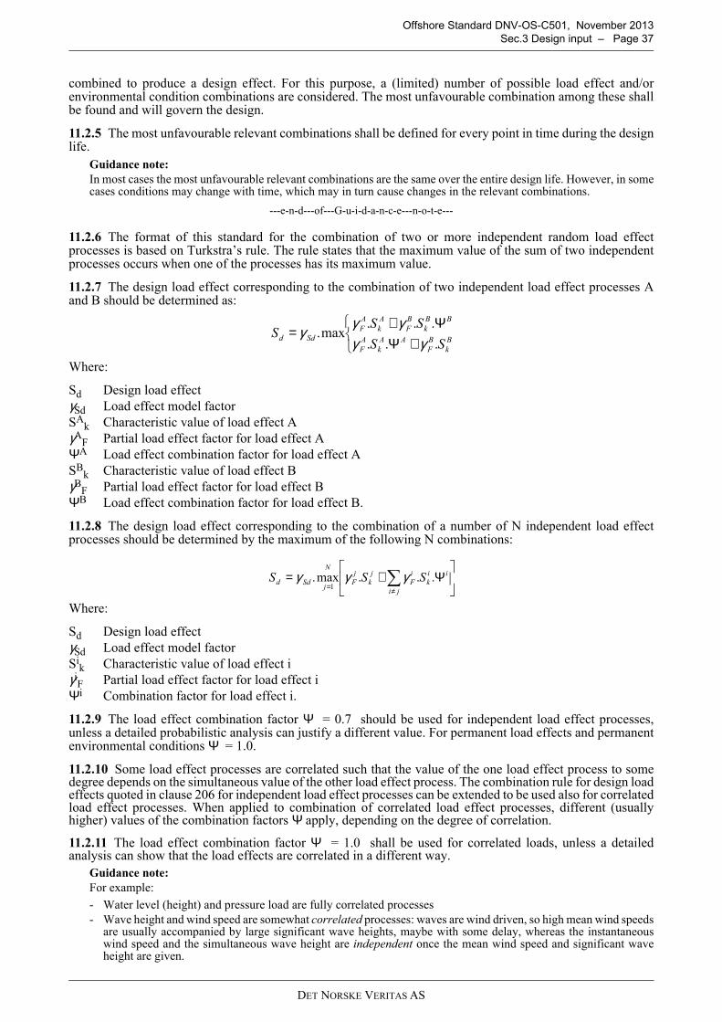
DET NORSKE VERITAS AS
Offshore Standard DNV-OS-C501, November 2013
Sec.3 Design input – Page 37
combined to produce a design effect. For this purpose, a (limited) number of possible load effect and/orenvironmental condition combinations are considered. The most unfavourable combination among these shallbe found and will govern the design.
11.2.5 The most unfavourable relevant combinations shall be defined for every point in time during the designlife.
Guidance note:
In most cases the most unfavourable relevant combinations are the same over the entire design life. However, in somecases conditions may change with time, which may in turn cause changes in the relevant combinations.
---e-n-d---of---G-u-i-d-a-n-c-e---n-o-t-e---
11.2.6 The format of this standard for the combination of two or more independent random load effectprocesses is based on Turkstra’s rule. The rule states that the maximum value of the sum of two independentprocesses occurs when one of the processes has its maximum value.
11.2.7 The design load effect corresponding to the combination of two independent load effect processes Aand B should be determined as:
Where:
Sd Design load effect γSd Load effect model factorSA
k Characteristic value of load effect AγA
F Partial load effect factor for load effect AΨA Load effect combination factor for load effect ASB
k Characteristic value of load effect BγB
F Partial load effect factor for load effect BΨB Load effect combination factor for load effect B.
11.2.8 The design load effect corresponding to the combination of a number of N independent load effectprocesses should be determined by the maximum of the following N combinations:
Where:
Sd Design load effect γSd Load effect model factorSi
k Characteristic value of load effect iγi
F Partial load effect factor for load effect iΨi Combination factor for load effect i.
11.2.9 The load effect combination factor Ψ = 0.7 should be used for independent load effect processes,unless a detailed probabilistic analysis can justify a different value. For permanent load effects and permanentenvironmental conditions Ψ = 1.0.
11.2.10 Some load effect processes are correlated such that the value of the one load effect process to somedegree depends on the simultaneous value of the other load effect process. The combination rule for design loadeffects quoted in clause 206 for independent load effect processes can be extended to be used also for correlatedload effect processes. When applied to combination of correlated load effect processes, different (usuallyhigher) values of the combination factors Ψ apply, depending on the degree of correlation.
11.2.11 The load effect combination factor Ψ = 1.0 shall be used for correlated loads, unless a detailedanalysis can show that the load effects are correlated in a different way.
Guidance note:
For example:
- Water level (height) and pressure load are fully correlated processes
- Wave height and wind speed are somewhat correlated processes: waves are wind driven, so high mean wind speedsare usually accompanied by large significant wave heights, maybe with some delay, whereas the instantaneouswind speed and the simultaneous wave height are independent once the mean wind speed and significant waveheight are given.
+ΨΨ+
=B
k
B
F
AA
k
A
F
BB
k
B
F
A
k
A
F
SddSS
SSS
...
...max.
γγγγγ
Ψ+= ∑
≠=ji
ii
k
i
F
j
k
j
F
N
jSdd SSS ...max.
1γγγ

DET NORSKE VERITAS AS
Offshore Standard DNV-OS-C501, November 2013
Sec.3 Design input – Page 38
- Self-weight and wind load on a bridge are non-correlated processes.- Snow load and wind load on a roof may be fully negatively correlated processes, i.e. the maximum value of the
one process and the minimum value of the other process may occur simultaneously.
---e-n-d---of---G-u-i-d-a-n-c-e---n-o-t-e---
11.3 Load effect and environmental conditions for time-dependent material properties
11.3.1 The sustained load effect values or the fatigue load effect values (when relevant) and the sustainedenvironmental values should be used for the determination of time-dependent material properties as specifiedin Sec.3 [9.5].
11.4 Load effect and environmental conditions for fatigue analysis
11.4.1 The fatigue load effects should be combined with the sustained environmental values for the fatigueanalysis as specified in Sec.3 [9.6].
11.5 Direct combination of loads
11.5.1 The combination of load effects and environments as described above should be used to obtain the loadeffects, i.e., local stresses and strains.
11.5.2 If transfer functions and structural analysis are linear, loads or moments can be combined by theprocedures given above instead of the load effects.

DET NORSKE VERITAS AS
Offshore Standard DNV-OS-C501, November 2013
Sec.4 Materials - laminates – Page 39
SECTION 4 MATERIALS - LAMINATES
1 General
1.1 Introduction
1.1.1 This section describes the mechanical material properties needed for design. It describes how to obtainall strength properties used in the failure criteria and all elastic properties needed for stress calculations.
1.1.2 The basic material properties used in these rules are orthotropic ply properties.
1.1.3 All properties shall be obtained directly by measurements or shall be traced back to measurements. Thequalification of material properties is described in this section. Under certain conditions, typical values fromdatabases can be used. Strength and stiffness values should be documented as characteristic values.
1.1.4 It is only necessary to obtain properties that are used in the design calculations and failure criteria.
1.2 Laminate specification
1.2.1 A composite laminate is made of many constituent materials arranged and produced in a specific way.Laminates used in a component shall be clearly specified and all materials shall be traceable.
1.2.2 A minimum set of process parameters and constituent material characterisations is given in Table 4-1.All these items shall be specified.
1.3 Lay-up specification
1.3.1 A laminate is made of a sequence of layers. All materials and they stacking sequence shall be clearlyidentified.
1.3.2 The orientation of non-homogenous or anisotropic materials shall be clearly specified on the materialslevel and the structural level.
1.3.3 Laminates shall be specified in a way that they can be described by a sequence of stacked orthotropicplies.
1.3.4 The procedures of App.B should be followed to describe a lay-up.
Table 4-1 Basic information to identify a laminate
Constituent materials:
Generic Fibre type
Type of weave
Generic resin type (e.g. epoxy, polyester)
Specific resin type (trade name)
Process parameters:
Processing method
Processing temperature
Processing pressure
Process atmosphere (e.g. vacuum)
Post curing (temperature and time)
Control of fibre orientation
Fibre volume fraction
Void content
Conditioning parameters:
Temperature
Water content of the laminate (wet, dry)
Chemical environment
Loading rate
Measured values
Guaranteed minimum value
Standard deviation
Number of specimens
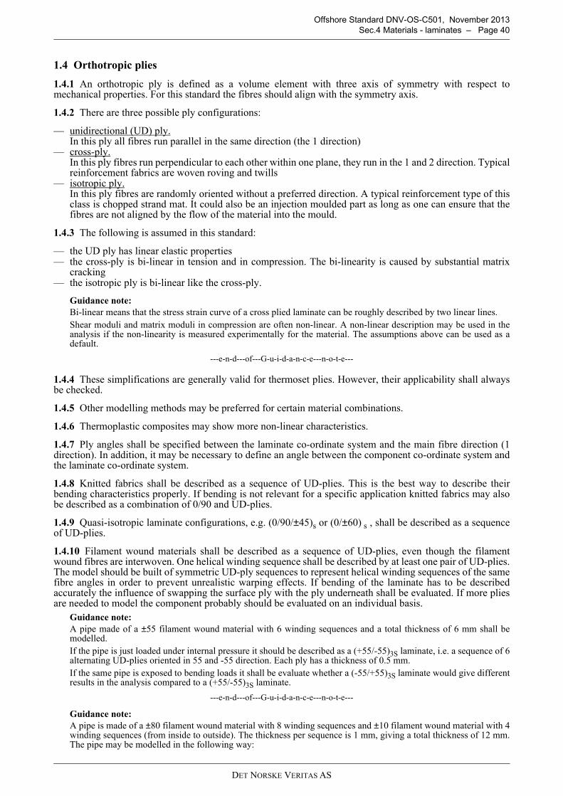
DET NORSKE VERITAS AS
Offshore Standard DNV-OS-C501, November 2013
Sec.4 Materials - laminates – Page 40
1.4 Orthotropic plies
1.4.1 An orthotropic ply is defined as a volume element with three axis of symmetry with respect tomechanical properties. For this standard the fibres should align with the symmetry axis.
1.4.2 There are three possible ply configurations:
— unidirectional (UD) ply. In this ply all fibres run parallel in the same direction (the 1 direction)
— cross-ply. In this ply fibres run perpendicular to each other within one plane, they run in the 1 and 2 direction. Typicalreinforcement fabrics are woven roving and twills
— isotropic ply. In this ply fibres are randomly oriented without a preferred direction. A typical reinforcement type of thisclass is chopped strand mat. It could also be an injection moulded part as long as one can ensure that thefibres are not aligned by the flow of the material into the mould.
1.4.3 The following is assumed in this standard:
— the UD ply has linear elastic properties— the cross-ply is bi-linear in tension and in compression. The bi-linearity is caused by substantial matrix
cracking— the isotropic ply is bi-linear like the cross-ply.
Guidance note:
Bi-linear means that the stress strain curve of a cross plied laminate can be roughly described by two linear lines.
Shear moduli and matrix moduli in compression are often non-linear. A non-linear description may be used in theanalysis if the non-linearity is measured experimentally for the material. The assumptions above can be used as adefault.
---e-n-d---of---G-u-i-d-a-n-c-e---n-o-t-e---
1.4.4 These simplifications are generally valid for thermoset plies. However, their applicability shall alwaysbe checked.
1.4.5 Other modelling methods may be preferred for certain material combinations.
1.4.6 Thermoplastic composites may show more non-linear characteristics.
1.4.7 Ply angles shall be specified between the laminate co-ordinate system and the main fibre direction (1direction). In addition, it may be necessary to define an angle between the component co-ordinate system andthe laminate co-ordinate system.
1.4.8 Knitted fabrics shall be described as a sequence of UD-plies. This is the best way to describe theirbending characteristics properly. If bending is not relevant for a specific application knitted fabrics may alsobe described as a combination of 0/90 and UD-plies.
1.4.9 Quasi-isotropic laminate configurations, e.g. (0/90/±45)s or (0/±60) s , shall be described as a sequenceof UD-plies.
1.4.10 Filament wound materials shall be described as a sequence of UD-plies, even though the filamentwound fibres are interwoven. One helical winding sequence shall be described by at least one pair of UD-plies.The model should be built of symmetric UD-ply sequences to represent helical winding sequences of the samefibre angles in order to prevent unrealistic warping effects. If bending of the laminate has to be describedaccurately the influence of swapping the surface ply with the ply underneath shall be evaluated. If more pliesare needed to model the component probably should be evaluated on an individual basis.
Guidance note:
A pipe made of a ±55 filament wound material with 6 winding sequences and a total thickness of 6 mm shall bemodelled.
If the pipe is just loaded under internal pressure it should be described as a (+55/-55)3S laminate, i.e. a sequence of 6alternating UD-plies oriented in 55 and -55 direction. Each ply has a thickness of 0.5 mm.
If the same pipe is exposed to bending loads it shall be evaluate whether a (-55/+55)3S laminate would give differentresults in the analysis compared to a (+55/-55)3S laminate.
---e-n-d---of---G-u-i-d-a-n-c-e---n-o-t-e---
Guidance note:
A pipe is made of a ±80 filament wound material with 8 winding sequences and ±10 filament wound material with 4winding sequences (from inside to outside). The thickness per sequence is 1 mm, giving a total thickness of 12 mm.The pipe may be modelled in the following way:
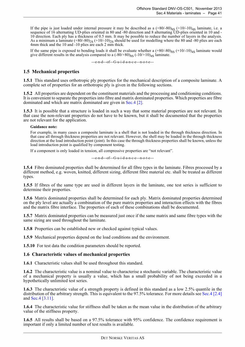
DET NORSKE VERITAS AS
Offshore Standard DNV-OS-C501, November 2013
Sec.4 Materials - laminates – Page 41
If the pipe is just loaded under internal pressure it may be described as a (+80/-80)8S (+10/-10)4S laminate, i.e. asequence of 16 alternating UD-plies oriented in 80 and -80 direction and 8 alternating UD-plies oriented in 10 and -10 direction. Each ply has a thickness of 0.5 mm. It may be possible to reduce the number of layers in the analysis.As a minimum a laminate (+80/-80)2S (+10/-10)2S should be used for modelling where the 80 and -80 plies are each4mm thick and the 10 and -10 plies are each 2 mm thick.
If the same pipe is exposed to bending loads it shall be evaluate whether a (+80/-80)8S (+10/-10)4S laminate wouldgive different results in the analysis compared to a (-80/+80)8S (-10/+10)4S laminate.
---e-n-d---of---G-u-i-d-a-n-c-e---n-o-t-e---
1.5 Mechanical properties
1.5.1 This standard uses orthotropic ply properties for the mechanical description of a composite laminate. Acomplete set of properties for an orthotropic ply is given in the following sections.
1.5.2 All properties are dependent on the constituent materials and the processing and conditioning conditions.It is convenient to separate the properties into fibre and matrix dominated properties. Which properties are fibredominated and which are matrix dominated are given in Sec.4 [2].
1.5.3 It is possible that a structure is loaded in such a way that some material properties are not relevant. Inthat case the non-relevant properties do not have to be known, but it shall be documented that the propertiesare not relevant for the application.
Guidance note:
For example, in many cases a composite laminate is a shell that is not loaded in the through thickness direction. Inthat case all through thickness properties are not relevant. However, the shell may be loaded in the through thicknessdirection at the load introduction point (joint). In this case the through thickness properties shall be known, unless theload introduction point is qualified by component testing.
If a component is only loaded in tension, all compressive properties are “not relevant”.
---e-n-d---of---G-u-i-d-a-n-c-e---n-o-t-e---
1.5.4 Fibre dominated properties shall be determined for all fibre types in the laminate. Fibres processed by adifferent method, e.g. woven, knitted, different sizing, different fibre material etc. shall be treated as differenttypes.
1.5.5 If fibres of the same type are used in different layers in the laminate, one test series is sufficient todetermine their properties.
1.5.6 Matrix dominated properties shall be determined for each ply. Matrix dominated properties determinedon the ply level are actually a combination of the pure matrix properties and interaction effects with the fibresand the matrix fibre interface. The properties of each of these combinations shall be documented.
1.5.7 Matrix dominated properties can be measured just once if the same matrix and same fibre types with thesame sizing are used throughout the laminate.
1.5.8 Properties can be established new or checked against typical values.
1.5.9 Mechanical properties depend on the load conditions and the environment.
1.5.10 For test data the condition parameters should be reported.
1.6 Characteristic values of mechanical properties
1.6.1 Characteristic values shall be used throughout this standard.
1.6.2 The characteristic value is a nominal value to characterise a stochastic variable. The characteristic valueof a mechanical property is usually a value, which has a small probability of not being exceeded in ahypothetically unlimited test series.
1.6.3 The characteristic value of a strength property is defined in this standard as a low 2.5% quantile in thedistribution of the arbitrary strength. This is equivalent to the 97.5% tolerance. For more details see Sec.4 [2.4]and Sec.4 [3.11].
1.6.4 The characteristic value for stiffness shall be taken as the mean value in the distribution of the arbitraryvalue of the stiffness property.
1.6.5 All results shall be based on a 97.5% tolerance with 95% confidence. The confidence requirement isimportant if only a limited number of test results is available.
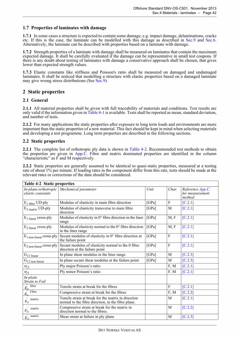
DET NORSKE VERITAS AS
Offshore Standard DNV-OS-C501, November 2013
Sec.4 Materials - laminates – Page 42
1.7 Properties of laminates with damage
1.7.1 In some cases a structure is expected to contain some damage, e.g. impact damage, delaminations, cracksetc. If this is the case, the laminate can be modelled with this damage as described in Sec.9 and Sec.6.Alternatively, the laminate can be described with properties based on a laminate with damage.
1.7.2 Strength properties of a laminate with damage shall be measured on laminates that contain the maximumexpected damage. It shall be carefully evaluated if the damage can be representative in small test coupons. Ifthere is any doubt about testing of laminates with damage a conservative approach shall be chosen, that giveslower than expected strength values.
1.7.3 Elastic constants like stiffness and Poisson's ratio shall be measured on damaged and undamagedlaminates. It shall be noticed that modelling a structure with elastic properties based on a damaged laminatemay give wrong stress distributions (See Sec.9).
2 Static properties
2.1 General
2.1.1 All material properties shall be given with full traceability of materials and conditions. Test results areonly valid if the information given in Table 4-1 is available. Tests shall be reported as mean, standard deviation,and number of tests.
2.1.2 For many applications the static properties after exposure to long term loads and environments are moreimportant than the static properties of a new material. This fact should be kept in mind when selecting materialsand developing a test programme. Long term properties are described in the following sections.
2.2 Static properties
2.2.1 The complete list of orthotropic ply data is shown in Table 4-2. Recommended test methods to obtainthe properties are given in App.C. Fibre and matrix dominated properties are identified in the column“characteristic” as F and M respectively.
2.2.2 Static properties are generally assumed to be identical to quasi-static properties, measured at a testingrate of about 1% per minute. If loading rates in the component differ from this rate, tests should be made at therelevant rates or corrections of the data should be considered.
Table 4-2 Static properties
In-plane orthotropic elastic constants
Mechanical parameter Unit Char. Reference App.Cfor measurement method
E1 fibre UD-ply Modulus of elasticity in main fibre direction [GPa] F [C.2.1]
E2 matrix UD-ply Modulus of elasticity transverse to main fibre direction
[GPa] M [C.2.1]
E1 linear cross-ply Modulus of elasticity in 0° fibre direction in the liner range
[GPa] M, F [C.2.1]
E2 linear cross-ply Modulus of elasticity normal to the 0° fibre direction in the liner range
[GPa] M, F [C.2.1]
E1 non-linear cross-ply Secant modulus of elasticity in 0° fibre direction at the failure point
[GPa] F [C.2.1]
E2 non-linear cross-ply Secant modulus of elasticity normal to the 0 fibre direction at the failure point
[GPa] F [C.2.1]
G12 linear In plane shear modulus in the liner range [GPa] M [C.2.3]
G12 non-linear In plane secant shear modulus at the failure point [GPa] M [C.2.3]
ν12 Ply major Poisson’s ratio F, M [C.2.1]
ν21 Ply minor Poisson’s ratio F, M [C.2.1]
In-plain Strain to Fail
fibre Tensile strain at break for the fibres F [C.2.1]Fibre Compressive strain at break for the fibres F, M [C.2.2]
matrix Tensile strain at break for the matrix in direction normal to the fibre direction, in the fibre plane.
M [C.2.1]
matrix Compressive strain at break for the matrix in direction normal to the fibres.
M [C.2.2]
matrix Shear strain at failure in ply plane M [C.2.3]
t1ε∧
c1ε∧
t2ε∧
c2ε∧
12ε∧
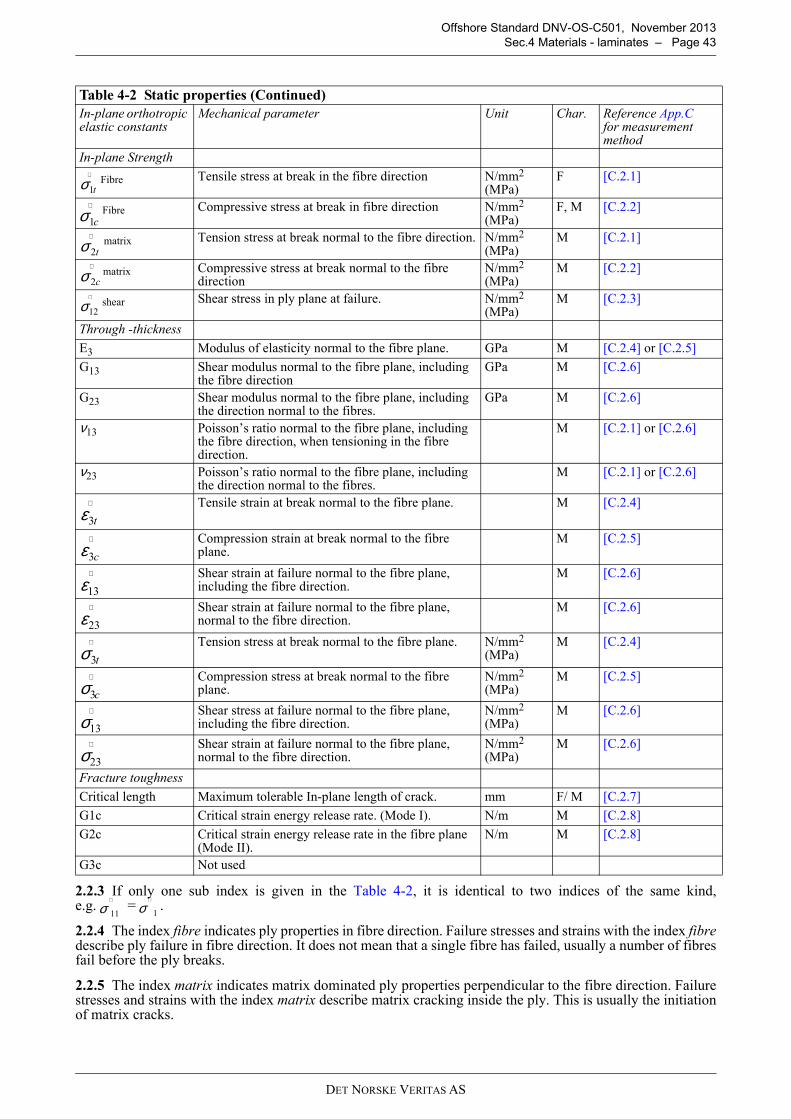
DET NORSKE VERITAS AS
Offshore Standard DNV-OS-C501, November 2013
Sec.4 Materials - laminates – Page 43
2.2.3 If only one sub index is given in the Table 4-2, it is identical to two indices of the same kind,e.g. = .
2.2.4 The index fibre indicates ply properties in fibre direction. Failure stresses and strains with the index fibredescribe ply failure in fibre direction. It does not mean that a single fibre has failed, usually a number of fibresfail before the ply breaks.
2.2.5 The index matrix indicates matrix dominated ply properties perpendicular to the fibre direction. Failurestresses and strains with the index matrix describe matrix cracking inside the ply. This is usually the initiationof matrix cracks.
In-plane Strength
Fibre Tensile stress at break in the fibre direction N/mm2 (MPa)
F [C.2.1]
Fibre Compressive stress at break in fibre direction N/mm2 (MPa)
F, M [C.2.2]
matrix Tension stress at break normal to the fibre direction. N/mm2 (MPa)
M [C.2.1]
matrix Compressive stress at break normal to the fibre direction
N/mm2 (MPa)
M [C.2.2]
shear Shear stress in ply plane at failure. N/mm2 (MPa)
M [C.2.3]
Through -thickness
E3 Modulus of elasticity normal to the fibre plane. GPa M [C.2.4] or [C.2.5]
G13 Shear modulus normal to the fibre plane, including the fibre direction
GPa M [C.2.6]
G23 Shear modulus normal to the fibre plane, including the direction normal to the fibres.
GPa M [C.2.6]
ν13 Poisson’s ratio normal to the fibre plane, including the fibre direction, when tensioning in the fibre direction.
M [C.2.1] or [C.2.6]
ν23 Poisson’s ratio normal to the fibre plane, including the direction normal to the fibres.
M [C.2.1] or [C.2.6]
Tensile strain at break normal to the fibre plane. M [C.2.4]
Compression strain at break normal to the fibre plane.
M [C.2.5]
Shear strain at failure normal to the fibre plane, including the fibre direction.
M [C.2.6]
Shear strain at failure normal to the fibre plane, normal to the fibre direction.
M [C.2.6]
Tension stress at break normal to the fibre plane. N/mm2 (MPa)
M [C.2.4]
Compression stress at break normal to the fibre plane.
N/mm2 (MPa)
M [C.2.5]
Shear stress at failure normal to the fibre plane, including the fibre direction.
N/mm2 (MPa)
M [C.2.6]
Shear strain at failure normal to the fibre plane, normal to the fibre direction.
N/mm2 (MPa)
M [C.2.6]
Fracture toughness
Critical length Maximum tolerable In-plane length of crack. mm F/ M [C.2.7]
G1c Critical strain energy release rate. (Mode I). N/m M [C.2.8]
G2c Critical strain energy release rate in the fibre plane (Mode II).
N/m M [C.2.8]
G3c Not used
Table 4-2 Static properties (Continued)
In-plane orthotropic elastic constants
Mechanical parameter Unit Char. Reference App.Cfor measurement method
t1σ∧
c1σ∧
t2σ∧
c2σ∧
12σ∧
t3ε∧
c3ε∧
13ε∧
23ε∧
t3σ∧
c3σ∧
13σ∧
23σ∧
11σ∧
1σ∧
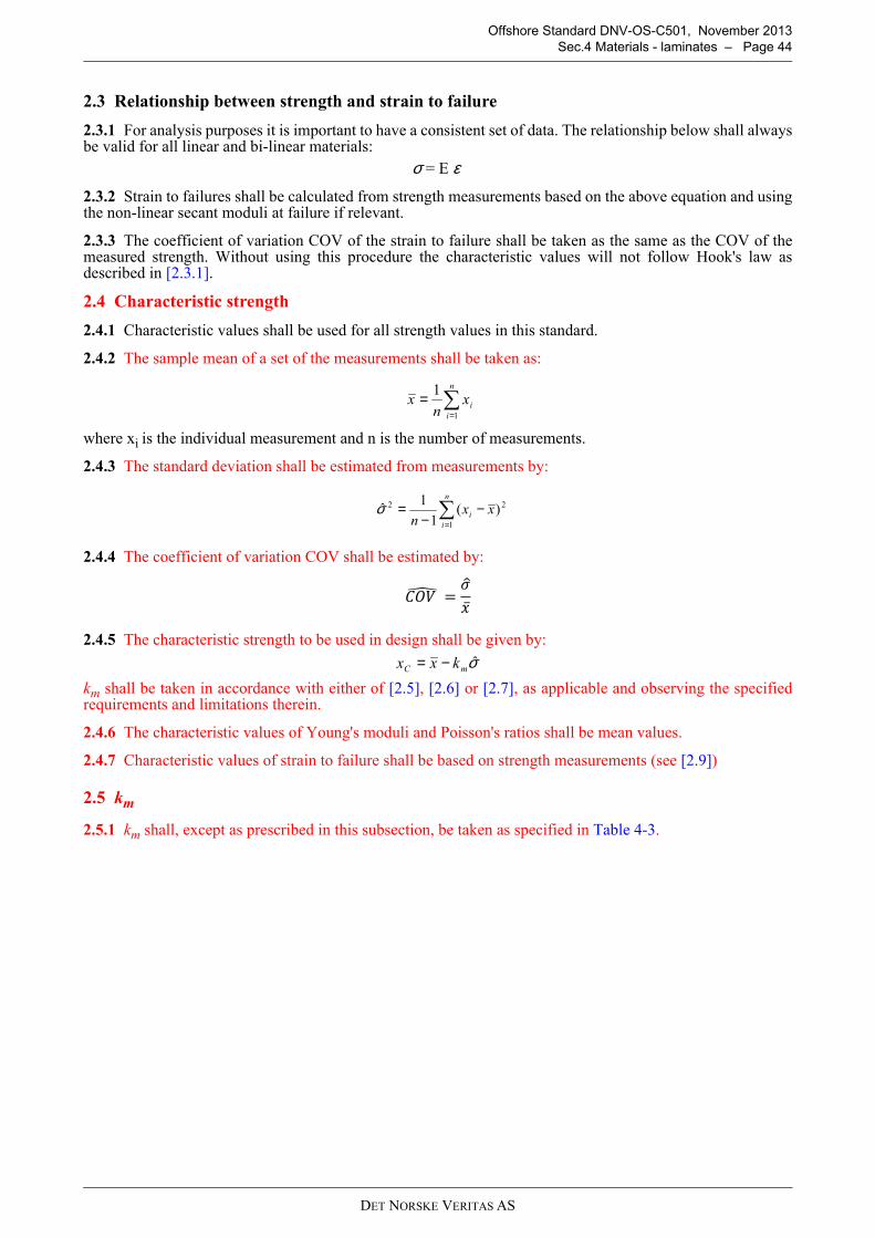
DET NORSKE VERITAS AS
Offshore Standard DNV-OS-C501, November 2013
Sec.4 Materials - laminates – Page 44
2.3 Relationship between strength and strain to failure
2.3.1 For analysis purposes it is important to have a consistent set of data. The relationship below shall alwaysbe valid for all linear and bi-linear materials:
σ = E ε
2.3.2 Strain to failures shall be calculated from strength measurements based on the above equation and usingthe non-linear secant moduli at failure if relevant.
2.3.3 The coefficient of variation COV of the strain to failure shall be taken as the same as the COV of themeasured strength. Without using this procedure the characteristic values will not follow Hook's law asdescribed in [2.3.1].
2.4 Characteristic strength
2.4.1 Characteristic values shall be used for all strength values in this standard.
2.4.2 The sample mean of a set of the measurements shall be taken as:
where xi is the individual measurement and n is the number of measurements.
2.4.3 The standard deviation shall be estimated from measurements by:
2.4.4 The coefficient of variation COV shall be estimated by:
2.4.5 The characteristic strength to be used in design shall be given by:
km shall be taken in accordance with either of [2.5], [2.6] or [2.7], as applicable and observing the specifiedrequirements and limitations therein.
2.4.6 The characteristic values of Young's moduli and Poisson's ratios shall be mean values.
2.4.7 Characteristic values of strain to failure shall be based on strength measurements (see [2.9])
2.5 km
2.5.1 km shall, except as prescribed in this subsection, be taken as specified in Table 4-3.
∑=
=n
i
ixn
x1
1
∑=
−−
=n
i
i xxn 1
22 )(1
1σ
��� � =��
σmC kxx −=
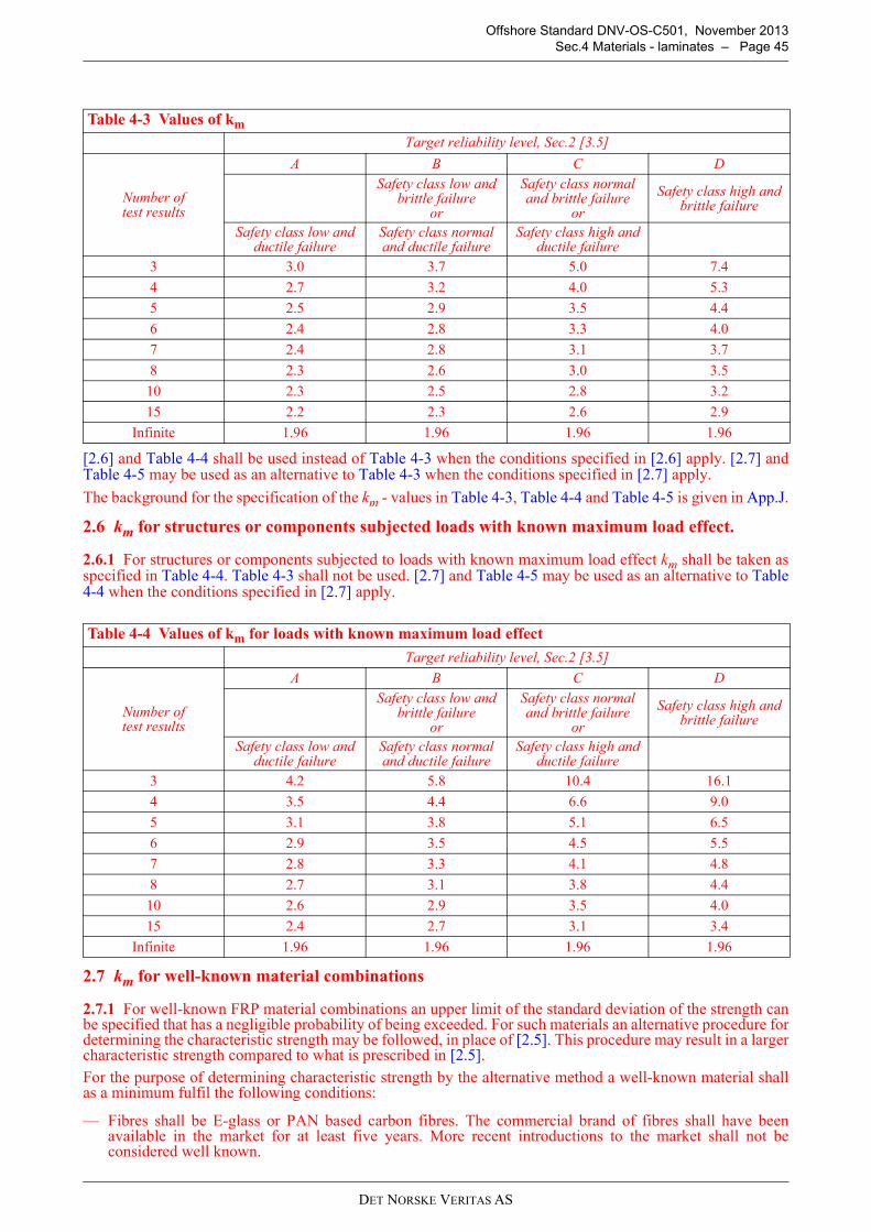
DET NORSKE VERITAS AS
Offshore Standard DNV-OS-C501, November 2013
Sec.4 Materials - laminates – Page 45
[2.6] and Table 4-4 shall be used instead of Table 4-3 when the conditions specified in [2.6] apply. [2.7] andTable 4-5 may be used as an alternative to Table 4-3 when the conditions specified in [2.7] apply.
The background for the specification of the km - values in Table 4-3, Table 4-4 and Table 4-5 is given in App.J.
2.6 km for structures or components subjected loads with known maximum load effect.
2.6.1 For structures or components subjected to loads with known maximum load effect km shall be taken asspecified in Table 4-4. Table 4-3 shall not be used. [2.7] and Table 4-5 may be used as an alternative to Table4-4 when the conditions specified in [2.7] apply.
2.7 km for well-known material combinations
2.7.1 For well-known FRP material combinations an upper limit of the standard deviation of the strength canbe specified that has a negligible probability of being exceeded. For such materials an alternative procedure fordetermining the characteristic strength may be followed, in place of [2.5]. This procedure may result in a largercharacteristic strength compared to what is prescribed in [2.5].
For the purpose of determining characteristic strength by the alternative method a well-known material shallas a minimum fulfil the following conditions:
— Fibres shall be E-glass or PAN based carbon fibres. The commercial brand of fibres shall have beenavailable in the market for at least five years. More recent introductions to the market shall not beconsidered well known.
Table 4-3 Values of km
Target reliability level, Sec.2 [3.5]
Number of test results
A B C D
Safety class low and brittle failure
or
Safety class normal and brittle failure
or
Safety class high and brittle failure
Safety class low and ductile failure
Safety class normal and ductile failure
Safety class high and ductile failure
3 3.0 3.7 5.0 7.4
4 2.7 3.2 4.0 5.3
5 2.5 2.9 3.5 4.4
6 2.4 2.8 3.3 4.0
7 2.4 2.8 3.1 3.7
8 2.3 2.6 3.0 3.5
10 2.3 2.5 2.8 3.2
15 2.2 2.3 2.6 2.9
Infinite 1.96 1.96 1.96 1.96
Table 4-4 Values of km for loads with known maximum load effect
Target reliability level, Sec.2 [3.5]
Number of test results
A B C D
Safety class low and brittle failure
or
Safety class normal and brittle failure
or
Safety class high and brittle failure
Safety class low and ductile failure
Safety class normal and ductile failure
Safety class high and ductile failure
3 4.2 5.8 10.4 16.1
4 3.5 4.4 6.6 9.0
5 3.1 3.8 5.1 6.5
6 2.9 3.5 4.5 5.5
7 2.8 3.3 4.1 4.8
8 2.7 3.1 3.8 4.4
10 2.6 2.9 3.5 4.0
15 2.4 2.7 3.1 3.4
Infinite 1.96 1.96 1.96 1.96
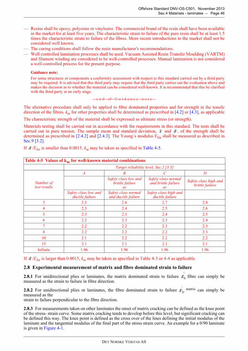
DET NORSKE VERITAS AS
Offshore Standard DNV-OS-C501, November 2013
Sec.4 Materials - laminates – Page 46
— Resins shall be epoxy, polyester or vinylester. The commercial brand of the resin shall have been availablein the market for at least five years. The characteristic strain to failure of the pure resin shall be at least 1.5times the characteristic strain to failure of the fibres. More recent introductions to the market shall not beconsidered well known.
— The curing conditions shall follow the resin manufacturer's recommendations.— Well controlled lamination processes shall be used. Vacuum Assisted Resin Transfer Moulding (VARTM)
and filament winding are considered to be well-controlled processes. Manual lamination is not considereda well-controlled process for the present purpose.
Guidance note:
For some structures or components a conformity assessment with respect to this standard carried out by a third partymay be required. It is advised that this third party may require that the third party carries out the evaluation above andmakes the decision as to whether the material can be considered well-known. It is recommended that this be clarifiedwith the third party at an early stage.
---e-n-d---of---G-u-i-d-a-n-c-e---n-o-t-e---
The alternative procedure shall only be applied to fibre dominated properties and for strength in the tensiledirection of the fibres. km for other properties shall be determined as prescribed in [4.2] or [4.3], as applicable
The characteristic strength of the material shall be expressed as ultimate stress (or strength).
Materials testing shall be carried out in accordance with the requirements in this standard. The tests shall becarried out in pure tension. The sample mean and standard deviation, and , of the strength shall bedetermined as prescribed in [2.4.2] and [2.4.3]. The Young´s modulus Elin shall be measured as described inSec.9 [3.2].
If /Elin is smaller than 0.0015, km may be taken as specified in Table 4-5.
If /Elin is larger than 0.0015, km may be taken as specified in Table 4-3 or 4-4 as applicable.
2.8 Experimental measurement of matrix and fibre dominated strain to failure
2.8.1 For unidirectional plies or laminates, the matrix dominated strain to failure fibre can simply bemeasured as the strain to failure in fibre direction.
2.8.2 For unidirectional plies or laminates, the fibre dominated strain to failure matrix can simply bemeasured as the strain to failure perpendicular to the fibre direction.
2.8.3 For measurements taken on other laminates the onset of matrix cracking can be defined as the knee pointof the stress- strain curve. Some matrix cracking tends to develop before this level, but significant cracking canbe defined this way. The knee point is defined as the cross over of the lines defining the initial modulus of thelaminate and the tangential modulus of the final part of the stress strain curve. An example for a 0/90 laminateis given in Figure 4-1.
Table 4-5 Values of km for well-known material combinations
Target reliability level, Sec.2 [3.5]
Number of test results
A B C D
Safety class low and brittle failure
or
Safety class normal and brittle failure
or
Safety class high and brittle failure
Safety class low and ductile failure
Safety class normal and ductile failure
Safety class high and ductile failure
3 2.5 2.6 2.7 2.8
4 2.3 2.4 2.5 2.6
5 2.3 2.3 2.4 2.5
6 2.2 2.3 2.3 2.4
7 2.2 2.2 2.3 2.3
8 2.2 2.2 2.2 2.3
10 2.1 2.2 2.2 2.2
15 2.1 2.1 2.1 2.1
Infinite 1.96 1.96 1.96 1.96
��
��
��
t1ε∧
t2ε∧
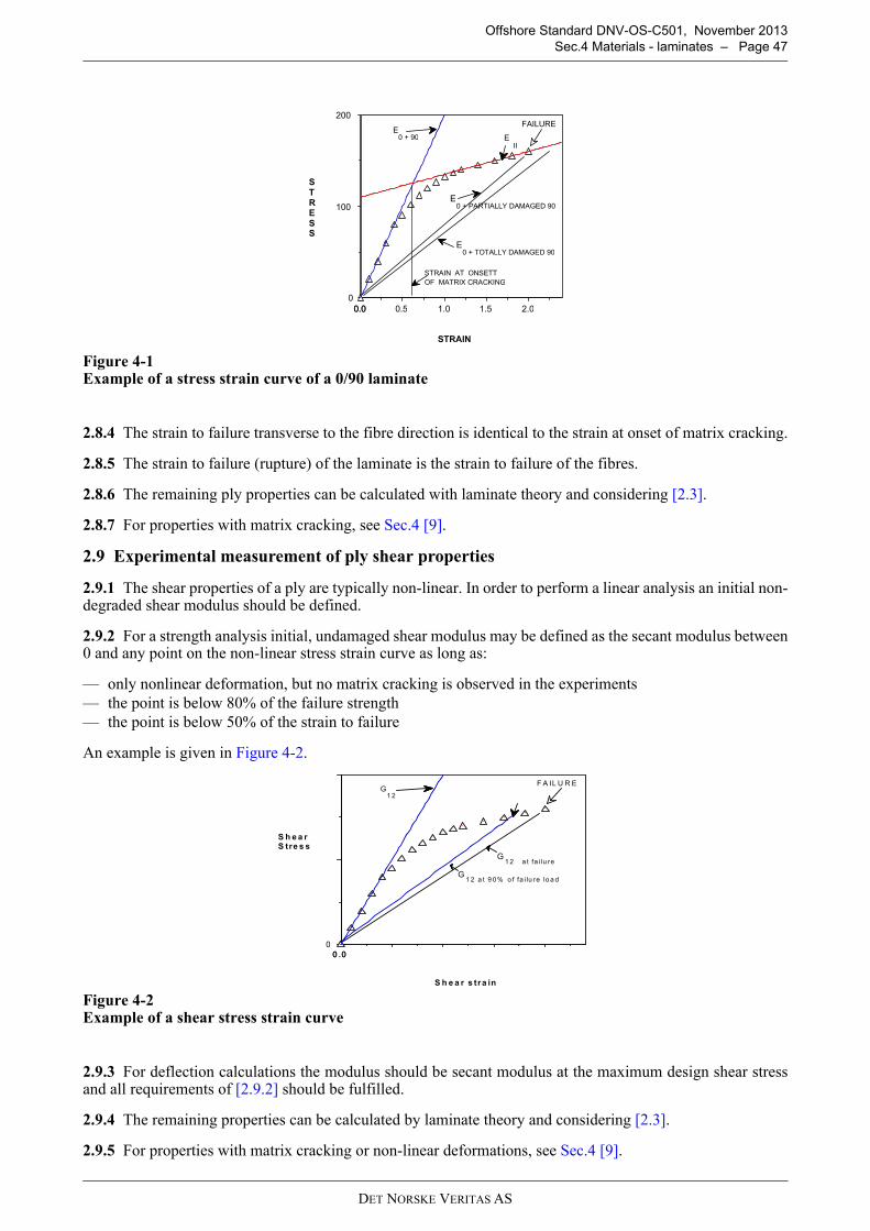
DET NORSKE VERITAS AS
Offshore Standard DNV-OS-C501, November 2013
Sec.4 Materials - laminates – Page 47
Figure 4-1 Example of a stress strain curve of a 0/90 laminate
2.8.4 The strain to failure transverse to the fibre direction is identical to the strain at onset of matrix cracking.
2.8.5 The strain to failure (rupture) of the laminate is the strain to failure of the fibres.
2.8.6 The remaining ply properties can be calculated with laminate theory and considering [2.3].
2.8.7 For properties with matrix cracking, see Sec.4 [9].
2.9 Experimental measurement of ply shear properties
2.9.1 The shear properties of a ply are typically non-linear. In order to perform a linear analysis an initial non-degraded shear modulus should be defined.
2.9.2 For a strength analysis initial, undamaged shear modulus may be defined as the secant modulus between0 and any point on the non-linear stress strain curve as long as:
— only nonlinear deformation, but no matrix cracking is observed in the experiments— the point is below 80% of the failure strength— the point is below 50% of the strain to failure
An example is given in Figure 4-2.
Figure 4-2 Example of a shear stress strain curve
2.9.3 For deflection calculations the modulus should be secant modulus at the maximum design shear stressand all requirements of [2.9.2] should be fulfilled.
2.9.4 The remaining properties can be calculated by laminate theory and considering [2.3].
2.9.5 For properties with matrix cracking or non-linear deformations, see Sec.4 [9].
2.01.51.00.50.00.0
0
100
200
.
STRAIN
STRESS
STRAIN AT ONSETT
OF MATRIX CRACKING
EII
E0 + 90
E0 + PARTIALLY DAMAGED 90
FAILURE
E0 + TOTALLY DAMAGED 90
0 .00 .0
0
S h e a r s tra in
S h e a rS tre s s
G1 2
G1 2 a t fa ilu re
F A IL U R E
G1 2 a t 9 0 % o f fa ilu re lo a d
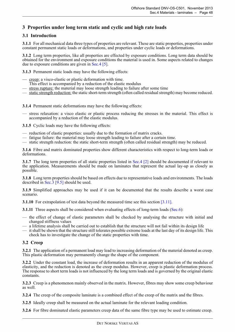
DET NORSKE VERITAS AS
Offshore Standard DNV-OS-C501, November 2013
Sec.4 Materials - laminates – Page 48
3 Properties under long term static and cyclic and high rate loads
3.1 Introduction
3.1.1 For all mechanical data three types of properties are relevant. These are static properties, properties underconstant permanent static loads or deformations, and properties under cyclic loads or deformations.
3.1.2 Long term properties, like all properties are effected by exposure conditions. Long term data should beobtained for the environment and exposure conditions the material is used in. Some aspects related to changesdue to exposure conditions are given in Sec.4 [5].
3.1.3 Permanent static loads may have the following effects:
— creep: a visco-elastic or plastic deformation with time. This effect is accompanied by a reduction of the elastic modulus
— stress rupture: the material may loose strength leading to failure after some time— static strength reduction: the static short-term strength (often called residual strength) may become reduced.
3.1.4 Permanent static deformations may have the following effects:
— stress relaxation: a visco elastic or plastic process reducing the stresses in the material. This effect isaccompanied by a reduction of the elastic modulus.
3.1.5 Cyclic loads may have the following effects:
— reduction of elastic properties: usually due to the formation of matrix cracks.— fatigue failure: the material may loose strength leading to failure after a certain time.— static strength reduction: the static short-term strength (often called residual strength) may be reduced.
3.1.6 Fibre and matrix dominated properties show different characteristics with respect to long-term loads ordeformations.
3.1.7 The long term properties of all static properties listed in Sec.4 [2] should be documented if relevant tothe application. Measurements should be made on laminates that represent the actual lay-up as closely aspossible.
3.1.8 Long term properties should be based on effects due to representative loads and environments. The loadsdescribed in Sec.3 [9.5] should be used.
3.1.9 Simplified approaches may be used if it can be documented that the results describe a worst casescenario.
3.1.10 For extrapolation of test data beyond the measured time see this section [3.11].
3.1.11 Three aspects shall be considered when evaluating effects of long-term loads (Sec.6):
— the effect of change of elastic parameters shall be checked by analysing the structure with initial andchanged stiffness values
— a lifetime analysis shall be carried out to establish that the structure will not fail within its design life— it shall be shown that the structure still tolerates possible extreme loads at the last day of its design life. This
check has to investigate the change of the static properties with time.
3.2 Creep
3.2.1 The application of a permanent load may lead to increasing deformation of the material denoted as creep.This plastic deformation may permanently change the shape of the component.
3.2.2 Under the constant load, the increase of deformation results in an apparent reduction of the modulus ofelasticity, and the reduction is denoted as the creep modulus. However, creep is plastic deformation process.The response to short term loads is not influenced by the long term loads and is governed by the original elasticconstants.
3.2.3 Creep is a phenomenon mainly observed in the matrix. However, fibres may show some creep behaviouras well.
3.2.4 The creep of the composite laminate is a combined effect of the creep of the matrix and the fibres.
3.2.5 Ideally creep shall be measured on the actual laminate for the relevant loading condition.
3.2.6 For fibre dominated elastic parameters creep data of the same fibre type may be used to estimate creep.
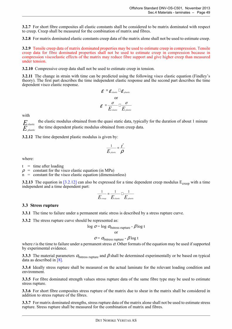
DET NORSKE VERITAS AS
Offshore Standard DNV-OS-C501, November 2013
Sec.4 Materials - laminates – Page 49
3.2.7 For short fibre composites all elastic constants shall be considered to be matrix dominated with respectto creep. Creep shall be measured for the combination of matrix and fibres.
3.2.8 For matrix dominated elastic constants creep data of the matrix alone shall not be used to estimate creep.
3.2.9 Tensile creep data of matrix dominated properties may be used to estimate creep in compression. Tensilecreep data for fibre dominated properties shall not be used to estimate creep in compression because incompression viscoelastic effects of the matrix may reduce fibre support and give higher creep than measuredunder tension.
3.2.10 Compressive creep data shall not be used to estimate creep in tension.
3.2.11 The change in strain with time can be predicted using the following visco elastic equation (Findley’stheory). The first part describes the time independent elastic response and the second part describes the timedependent visco elastic response.
or
with
the elastic modulus obtained from the quasi static data, typically for the duration of about 1 minute
the time dependent plastic modulus obtained from creep data.
3.2.12 The time dependent plastic modulus is given by:
where:
t = time after loadingρ = constant for the visco elastic equation (in MPa)n = constant for the visco elastic equation (dimensionless)
3.2.13 The equation in [3.2.12] can also be expressed for a time dependent creep modulus Ecreep with a timeindependent and a time dependent part:
3.3 Stress rupture
3.3.1 The time to failure under a permanent static stress is described by a stress rupture curve.
3.3.2 The stress rupture curve should be represented as:
log σ = log σ0stress rupture - β log t
or
σ = σ0stress rupture - β log t
where t is the time to failure under a permanent stress σ. Other formats of the equation may be used if supportedby experimental evidence.
3.3.3 The material parameters σ0stress rupture and β shall be determined experimentally or be based on typicaldata as described in [8].
3.3.4 Ideally stress rupture shall be measured on the actual laminate for the relevant loading condition andenvironment.
3.3.5 For fibre dominated strength values stress rupture data of the same fibre type may be used to estimatestress rupture.
3.3.6 For short fibre composites stress rupture of the matrix due to shear in the matrix shall be considered inaddition to stress rupture of the fibres.
3.3.7 For matrix dominated strengths, stress rupture data of the matrix alone shall not be used to estimate stressrupture. Stress rupture shall be measured for the combination of matrix and fibres.
εεε plasticelastic+=
EE plasticelastic
σσε +=
Eelastic
E plastic
ρt
E
n
plastic
=1
EEE plasticelasticcreep
111 +=
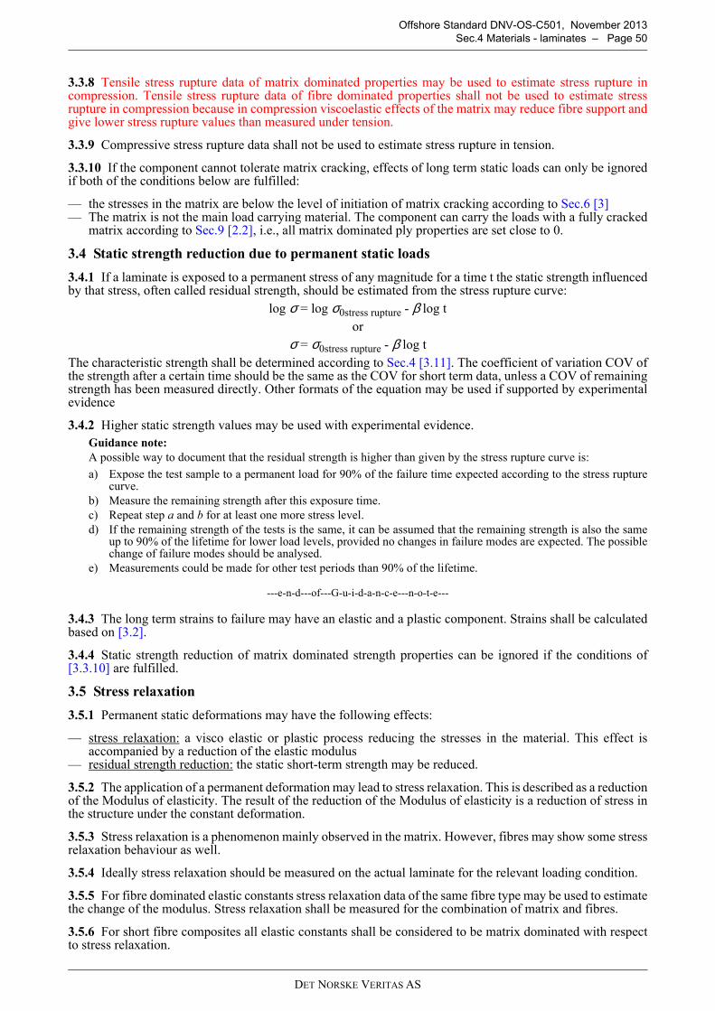
DET NORSKE VERITAS AS
Offshore Standard DNV-OS-C501, November 2013
Sec.4 Materials - laminates – Page 50
3.3.8 Tensile stress rupture data of matrix dominated properties may be used to estimate stress rupture incompression. Tensile stress rupture data of fibre dominated properties shall not be used to estimate stressrupture in compression because in compression viscoelastic effects of the matrix may reduce fibre support andgive lower stress rupture values than measured under tension.
3.3.9 Compressive stress rupture data shall not be used to estimate stress rupture in tension.
3.3.10 If the component cannot tolerate matrix cracking, effects of long term static loads can only be ignoredif both of the conditions below are fulfilled:
— the stresses in the matrix are below the level of initiation of matrix cracking according to Sec.6 [3]— The matrix is not the main load carrying material. The component can carry the loads with a fully cracked
matrix according to Sec.9 [2.2], i.e., all matrix dominated ply properties are set close to 0.
3.4 Static strength reduction due to permanent static loads
3.4.1 If a laminate is exposed to a permanent stress of any magnitude for a time t the static strength influencedby that stress, often called residual strength, should be estimated from the stress rupture curve:
log σ = log σ0stress rupture - β log t
or
σ = σ0stress rupture - β log t
The characteristic strength shall be determined according to Sec.4 [3.11]. The coefficient of variation COV ofthe strength after a certain time should be the same as the COV for short term data, unless a COV of remainingstrength has been measured directly. Other formats of the equation may be used if supported by experimentalevidence
3.4.2 Higher static strength values may be used with experimental evidence.
Guidance note:
A possible way to document that the residual strength is higher than given by the stress rupture curve is:
a) Expose the test sample to a permanent load for 90% of the failure time expected according to the stress rupturecurve.
b) Measure the remaining strength after this exposure time.c) Repeat step a and b for at least one more stress level.d) If the remaining strength of the tests is the same, it can be assumed that the remaining strength is also the same
up to 90% of the lifetime for lower load levels, provided no changes in failure modes are expected. The possiblechange of failure modes should be analysed.
e) Measurements could be made for other test periods than 90% of the lifetime.
---e-n-d---of---G-u-i-d-a-n-c-e---n-o-t-e---
3.4.3 The long term strains to failure may have an elastic and a plastic component. Strains shall be calculatedbased on [3.2].
3.4.4 Static strength reduction of matrix dominated strength properties can be ignored if the conditions of[3.3.10] are fulfilled.
3.5 Stress relaxation
3.5.1 Permanent static deformations may have the following effects:
— stress relaxation: a visco elastic or plastic process reducing the stresses in the material. This effect isaccompanied by a reduction of the elastic modulus
— residual strength reduction: the static short-term strength may be reduced.
3.5.2 The application of a permanent deformation may lead to stress relaxation. This is described as a reductionof the Modulus of elasticity. The result of the reduction of the Modulus of elasticity is a reduction of stress inthe structure under the constant deformation.
3.5.3 Stress relaxation is a phenomenon mainly observed in the matrix. However, fibres may show some stressrelaxation behaviour as well.
3.5.4 Ideally stress relaxation should be measured on the actual laminate for the relevant loading condition.
3.5.5 For fibre dominated elastic constants stress relaxation data of the same fibre type may be used to estimatethe change of the modulus. Stress relaxation shall be measured for the combination of matrix and fibres.
3.5.6 For short fibre composites all elastic constants shall be considered to be matrix dominated with respectto stress relaxation.
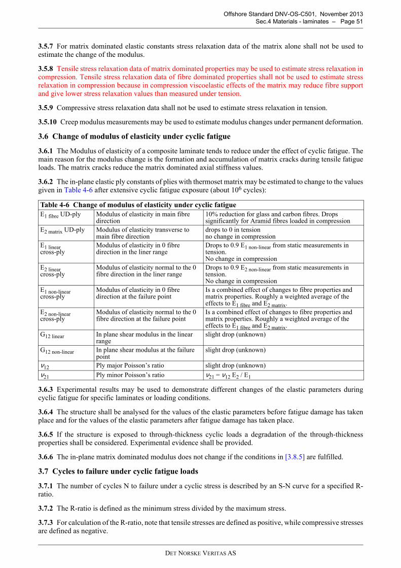
DET NORSKE VERITAS AS
Offshore Standard DNV-OS-C501, November 2013
Sec.4 Materials - laminates – Page 51
3.5.7 For matrix dominated elastic constants stress relaxation data of the matrix alone shall not be used toestimate the change of the modulus.
3.5.8 Tensile stress relaxation data of matrix dominated properties may be used to estimate stress relaxation incompression. Tensile stress relaxation data of fibre dominated properties shall not be used to estimate stressrelaxation in compression because in compression viscoelastic effects of the matrix may reduce fibre supportand give lower stress relaxation values than measured under tension.
3.5.9 Compressive stress relaxation data shall not be used to estimate stress relaxation in tension.
3.5.10 Creep modulus measurements may be used to estimate modulus changes under permanent deformation.
3.6 Change of modulus of elasticity under cyclic fatigue
3.6.1 The Modulus of elasticity of a composite laminate tends to reduce under the effect of cyclic fatigue. Themain reason for the modulus change is the formation and accumulation of matrix cracks during tensile fatigueloads. The matrix cracks reduce the matrix dominated axial stiffness values.
3.6.2 The in-plane elastic ply constants of plies with thermoset matrix may be estimated to change to the valuesgiven in Table 4-6 after extensive cyclic fatigue exposure (about 106 cycles):
3.6.3 Experimental results may be used to demonstrate different changes of the elastic parameters duringcyclic fatigue for specific laminates or loading conditions.
3.6.4 The structure shall be analysed for the values of the elastic parameters before fatigue damage has takenplace and for the values of the elastic parameters after fatigue damage has taken place.
3.6.5 If the structure is exposed to through-thickness cyclic loads a degradation of the through-thicknessproperties shall be considered. Experimental evidence shall be provided.
3.6.6 The in-plane matrix dominated modulus does not change if the conditions in [3.8.5] are fulfilled.
3.7 Cycles to failure under cyclic fatigue loads
3.7.1 The number of cycles N to failure under a cyclic stress is described by an S-N curve for a specified R-ratio.
3.7.2 The R-ratio is defined as the minimum stress divided by the maximum stress.
3.7.3 For calculation of the R-ratio, note that tensile stresses are defined as positive, while compressive stressesare defined as negative.
Table 4-6 Change of modulus of elasticity under cyclic fatigue
E1 fibre UD-ply Modulus of elasticity in main fibre direction
10% reduction for glass and carbon fibres. Drops significantly for Aramid fibres loaded in compression
E2 matrix UD-ply Modulus of elasticity transverse to main fibre direction
drops to 0 in tensionno change in compression
E1 linearcross-ply
Modulus of elasticity in 0 fibre direction in the liner range
Drops to 0.9 E1 non-linear from static measurements in tension.No change in compression
E2 linearcross-ply
Modulus of elasticity normal to the 0 fibre direction in the liner range
Drops to 0.9 E2 non-linear from static measurements in tension.No change in compression
E1 non-linearcross-ply
Modulus of elasticity in 0 fibre direction at the failure point
Is a combined effect of changes to fibre properties and matrix properties. Roughly a weighted average of the effects to E1 fibre and E2 matrix.
E2 non-linearcross-ply
Modulus of elasticity normal to the 0 fibre direction at the failure point
Is a combined effect of changes to fibre properties and matrix properties. Roughly a weighted average of the effects to E1 fibre and E2 matrix.
G12 linear In plane shear modulus in the linear range
slight drop (unknown)
G12 non-linear In plane shear modulus at the failure point
slight drop (unknown)
ν12 Ply major Poisson’s ratio slight drop (unknown)
ν21 Ply minor Poisson’s ratio ν21 = ν12 E2 / E1
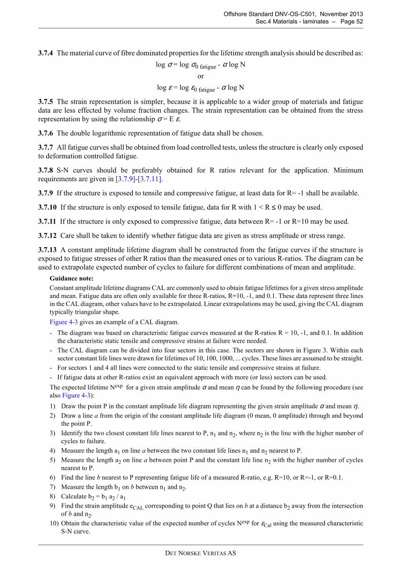
DET NORSKE VERITAS AS
Offshore Standard DNV-OS-C501, November 2013
Sec.4 Materials - laminates – Page 52
3.7.4 The material curve of fibre dominated properties for the lifetime strength analysis should be described as:
log σ = log σ0 fatigue - α log N
or
log ε = log ε0 fatigue - α log N
3.7.5 The strain representation is simpler, because it is applicable to a wider group of materials and fatiguedata are less effected by volume fraction changes. The strain representation can be obtained from the stressrepresentation by using the relationship σ = E ε.
3.7.6 The double logarithmic representation of fatigue data shall be chosen.
3.7.7 All fatigue curves shall be obtained from load controlled tests, unless the structure is clearly only exposedto deformation controlled fatigue.
3.7.8 S-N curves should be preferably obtained for R ratios relevant for the application. Minimumrequirements are given in [3.7.9]-[3.7.11].
3.7.9 If the structure is exposed to tensile and compressive fatigue, at least data for R= -1 shall be available.
3.7.10 If the structure is only exposed to tensile fatigue, data for R with 1 < R ≤ 0 may be used.
3.7.11 If the structure is only exposed to compressive fatigue, data between R= -1 or R=10 may be used.
3.7.12 Care shall be taken to identify whether fatigue data are given as stress amplitude or stress range.
3.7.13 A constant amplitude lifetime diagram shall be constructed from the fatigue curves if the structure isexposed to fatigue stresses of other R ratios than the measured ones or to various R-ratios. The diagram can beused to extrapolate expected number of cycles to failure for different combinations of mean and amplitude.
Guidance note:
Constant amplitude lifetime diagrams CAL are commonly used to obtain fatigue lifetimes for a given stress amplitudeand mean. Fatigue data are often only available for three R-ratios, R=10, -1, and 0.1. These data represent three linesin the CAL diagram, other values have to be extrapolated. Linear extrapolations may be used, giving the CAL diagramtypically triangular shape.
Figure 4-3 gives an example of a CAL diagram.
- The diagram was based on characteristic fatigue curves measured at the R-ratios R = 10, -1, and 0.1. In additionthe characteristic static tensile and compressive strains at failure were needed.
- The CAL diagram can be divided into four sectors in this case. The sectors are shown in Figure 3. Within eachsector constant life lines were drawn for lifetimes of 10, 100, 1000, ... cycles. These lines are assumed to be straight.
- For sectors 1 and 4 all lines were connected to the static tensile and compressive strains at failure.
- If fatigue data at other R-ratios exist an equivalent approach with more (or less) sectors can be used.
The expected lifetime Nexp for a given strain amplitude α and mean η can be found by the following procedure (seealso Figure 4-3):
1) Draw the point P in the constant amplitude life diagram representing the given strain amplitude α and mean η.
2) Draw a line a from the origin of the constant amplitude life diagram (0 mean, 0 amplitude) through and beyondthe point P.
3) Identify the two closest constant life lines nearest to P, n1 and n2, where n2 is the line with the higher number ofcycles to failure.
4) Measure the length a1 on line a between the two constant life lines n1 and n2 nearest to P.
5) Measure the length a2 on line a between point P and the constant life line n2 with the higher number of cyclesnearest to P.
6) Find the line b nearest to P representing fatigue life of a measured R-ratio, e.g. R=10, or R=-1, or R=0.1.
7) Measure the length b1 on b between n1 and n2.
8) Calculate b2 = b1 a2 / a1
9) Find the strain amplitude eCAL corresponding to point Q that lies on b at a distance b2 away from the intersectionof b and n2.
10) Obtain the characteristic value of the expected number of cycles Nexp for εCal using the measured characteristicS-N curve.
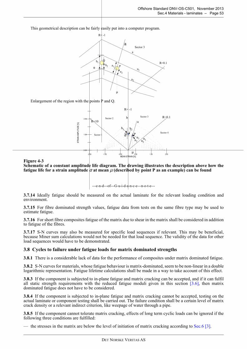
DET NORSKE VERITAS AS
Offshore Standard DNV-OS-C501, November 2013
Sec.4 Materials - laminates – Page 53
This geometrical description can be fairly easily put into a computer program.
Enlargement of the region with the points P and Q.
Figure 4-3 Schematic of a constant amplitude life diagram. The drawing illustrates the description above how thefatigue life for a strain amplitude α at mean µ (described by point P as an example) can be found
---e-n-d---of---G-u-i-d-a-n-c-e---n-o-t-e---
3.7.14 Ideally fatigue should be measured on the actual laminate for the relevant loading condition andenvironment.
3.7.15 For fibre dominated strength values, fatigue data from tests on the same fibre type may be used toestimate fatigue.
3.7.16 For short fibre composites fatigue of the matrix due to shear in the matrix shall be considered in additionto fatigue of the fibres.
3.7.17 S-N curves may also be measured for specific load sequences if relevant. This may be beneficial,because Miner sum calculations would not be needed for that load sequence. The validity of the data for otherload sequences would have to be demonstrated.
3.8 Cycles to failure under fatigue loads for matrix dominated strengths
3.8.1 There is a considerable lack of data for the performance of composites under matrix dominated fatigue.
3.8.2 S-N curves for materials, whose fatigue behaviour is matrix-dominated, seem to be non-linear in a doublelogarithmic representation. Fatigue lifetime calculations shall be made in a way to take account of this effect.
3.8.3 If the component is subjected to in-plane fatigue and matrix cracking can be accepted, and if it can fulfilall static strength requirements with the reduced fatigue moduli given in this section [3.6], then matrixdominated fatigue does not have to be considered.
3.8.4 If the component is subjected to in-plane fatigue and matrix cracking cannot be accepted, testing on theactual laminate or component testing shall be carried out. The failure condition shall be a certain level of matrixcrack density or a relevant indirect criterion, like weepage of water through a pipe.
3.8.5 If the component cannot tolerate matrix cracking, effects of long term cyclic loads can be ignored if thefollowing three conditions are fulfilled:
— the stresses in the matrix are below the level of initiation of matrix cracking according to Sec.6 [3].
a
R= -1
R=0.1
Sector 3
a
n2
n1
a1
a2
P
Qb1
b2
µ
α
-2.50 -1.50 -0.50 0.50 1.50 2.50
MEAN STRAIN [%]
0.00
1.00
2.00
ST
RA
IN A
MP
LIT
UD
E [
%]
Sector 2
Sector 1
Sector 3
Sector 4P
µ
α
a
n2
n1a1
R= -1
R=0.1
R=10b
a2
b1 b2
Q
DET NORSKE VERITAS AS
Offshore Standard DNV-OS-C501, November 2013
Sec.4 Materials - laminates – Page 54
— the matrix is not the main load carrying material. The component can carry the loads with a fully crackedmatrix according to Sec.9 [2.2], i.e., all matrix dominated ply properties are set close to 0.
— the total number of cycles does not exceed 1500.
3.8.6 If the structure is exposed to through thickness cyclic loads the fatigue performance shall bedemonstrated by testing on the actual laminate or component.
Guidance note:
Matrix cracks develop very easily during fatigue. A design should be avoided where the structural integrity or anycritical performance requirement relies on matrix cracking not occurring under fatigue conditions.
---e-n-d---of---G-u-i-d-a-n-c-e---n-o-t-e---
3.9 Static strength reduction due to cyclic loads
3.9.1 Fibre dominated static strength is not changed under cyclic fatigue for most continuous glass and carbonfibres. The same is true for Aramid fibres loaded in tension only. The long term static strength according to[3.4] may be used as the strength at the end of cyclic loading. The mean fatigue load should be used as thepermanent static load under fatigue.
3.9.2 In all other cases: If a laminate is exposed to a cyclic stress of any magnitude for a number of cycles N,the static strength (or strain to failure) influenced by that stress shall be estimated from the pertinent S-N curve:
log σ = log σ0fatige - α log N
or
log ε = log ε0 fatigue - α log N
where N is the number of cycles expected during the lifetime of the structure.
The characteristic strength shall be determined according to Sec.4 [3.11]. The coefficient of variation COV ofthe strength after a certain time should be the same as the COV for short term data, unless a COV of remainingstrength has been measured directly.
3.9.3 If the S-N curve is not linear in a log-log presentation, the static strength cannot be calculated by theabove equation, but shall be taken directly from the S-N curve.
3.9.4 Higher static strength values may be used with experimental evidence.
Guidance note:
A possible way to document that the residual strength is higher than given by the S-N curve is:
a) Expose the test sample to a fatigue load for 90% of the cycles to failure expected according to the S-N curve.
b) Measure the remaining strength after this exposure time.
c) Repeat step a and b for at least one more stress level.
d) If the remaining strength of the tests is the same, it can be assumed that the remaining strength is also the sameup to 90% of the lifetime for lower load levels, provided no changes in failure modes are expected. The possiblechange of failure modes should be analysed
e) Measurements could be made for other test periods than 90% of the lifetime.
---e-n-d---of---G-u-i-d-a-n-c-e---n-o-t-e---
3.9.5 The reduction of strength of matrix dominated properties may be ignored if the conditions of [3.8.5] aremet.
3.9.6 If the cycle dependent strength is known, static strains to failure shall be obtained from the reduced staticstrength and the cycle dependent stiffness value. If the cycle dependent strain to failure is known, staticstrengths shall be obtained from the reduced static strains to failure and the cycle dependent stiffness value.
3.10 Effect of high loading rates - shock loads - impact
3.10.1 The effect of high loading rates is a slight increase of stiffness, slight increase of strength and possiblya reduction of strain to failure, especially for ductile materials.
3.10.2 It is conservative to assume the same strength values as for static properties. Higher strength valuesshall be documented.
3.11 Characteristic values
3.11.1 Characteristic values shall be used for all stress rupture and S-N curves in this standard.
3.11.2 Characteristic values shall be established with a 97.5% tolerance (probability of not being exceeded)and 95% confidence.
DET NORSKE VERITAS AS
Offshore Standard DNV-OS-C501, November 2013
Sec.4 Materials - laminates – Page 55
3.11.3 This section is applicable for estimating the characteristic (and subsequently the design) time to failureunder a specified load for a laminate exposed to static or cyclic load, provided the plot of log stress vs. log timeis linear.
3.11.4 If the linear relationship cannot be documented, an equivalent approach shall be used, taking the non-linearity into account.
3.11.5 Values shall be based on data that are fairly evenly distributed over the plot of log time to failure vs. logload, or log number of cycles vs. log load. Load is usually expressed as stress or strain. At least 15 data pointsshould be used.
3.11.6 To obtain the characteristic curve the mean S-N curve of the form:
log σ = log σ0 fatigue - α log N
or the mean stress rupture curve of the form:
log σ = log σ0 stress rupture - β log t
shall be converted to the form:
log(X)mean = log(X0) – k⋅logσwhere X represents the time (or number of cycles) to failure under a sustained stress σ (or stress range σ). X isa function of σ and exhibits a natural variability from point to point within the material.
Guidance note:
Usually, estimates of k and logσ0stressrupture (or logσ0fatigue) can be obtained from linear regression analysis of log Xon log σ.
---e-n-d---of---G-u-i-d-a-n-c-e---n-o-t-e---
3.11.7 When the standard deviation σε of the variations in log(X) about the mean is constant, i.e. when σε doesnot depend on the sustained load or stress range σ, then the characteristic value of log(X)c can be taken as:
log(X)c = log(X0) – k⋅logσ - x⋅σεin which σε is estimated from available tests, and x is taken from Table 4-7 depending on the number n ofavailable data pairs (logs, log X) from tests.
3.11.8 The coefficient values marked as Case 1 are valid and can be used for sustained loads or cyclic stresseswithin the range of σ-values covered by available tests, i.e. whenever the available tests cover a wide enoughrange of σ-values. These coefficient values will be non-conservative if applied for sustained loads or stressesσ outside the range of log σ-values covered by available tests. When values for x are needed for σ-valuesoutside this range, coefficient values marked as Case 2 can be used for extrapolation within a concentric rangeof logσ twice the length of the range covered by tests.
3.11.9 The mean curve can be transformed back into the standard formulation of an S-N curve, or stress ruptureor fatigue curve using the same equations as given above.
— Stress rupture curve: and with X0 as time.
— Fatigue curve: and with X0 as number of cycles.
3.11.10 The characteristic mean curve can be transformed back into the standard formulation of an S-N curveor stress rupture curve using the same equations as given above.
or
or
Table 4-7 Values of coefficient x
x
n (# of tests) Case 1 Case 2
10152050
100Infinite
3.93.43.12.62.42.0
4.74.03.73.02.62.0
βσ rupturestress
X 0
0
loglog =
ασ fatigue
X0
0
loglog =
β1=k
α1=k
βσ X
rupturestress0
0
loglog =
k
1=β
ασ X
fatigue0
0
loglog =
k
1=α
DET NORSKE VERITAS AS
Offshore Standard DNV-OS-C501, November 2013
Sec.4 Materials - laminates – Page 56
— Stress rupture curve: and with X0 as time.
— Fatigue curve: and with X0 as number of cycles.
3.11.11 When a fixed time span T is considered, the characteristic value of the logarithm of the residualstrength σ after the time T has elapsed can be taken as:
(logσ)c = logσstress rupture - β logT - x σεwhere logσ0stress rupture and β can be obtained from a linear regression analysis of log σ on log t, and where σεis the standard deviation of the variations in log σ about the mean. The factor x is to be taken from Table 4-7depending on the number n of available data pairs (log t , log σ) from tests.
Guidance note:
Usually, estimates of β and logσ0stressrupture (or logσ0fatigue) can be obtained from linear regression analysis of logσon log t, and the standard deviation σε of the residuals in log σ results as a by-product of the regression analysis. Notethat this standard deviation is different from the standard deviation σε of [3.11.7].
---e-n-d---of---G-u-i-d-a-n-c-e---n-o-t-e---
4 Other properties
4.1 Thermal expansion coefficient
4.1.1 Thermal expansion coefficient of the plies in the relevant temperature range should be measured in thefibre direction and transverse to the fibre direction.
4.1.2 Stresses due to thermal deformation should be considered. The stresses should be added to stresses fromother loads like a combination of load cases as described in Sec.3 [11].
4.2 Swelling coefficient for water or other liquids
4.2.1 Swelling coefficient of the plies in the relevant temperature range should be measured in the fibredirection and transverse to the fibre direction.
4.2.2 Stresses due to swelling should be considered.
4.3 Diffusion coefficient
4.3.1 Relevant data shall be obtained as needed for the actual service and exposure of the component. Ifrelevant, the following material data may be required:
— diffusion rate through the laminate for the relevant fluid (Hydrocarbon gas, oil, gasoline, glycol, methanol,water etc.).
4.4 Thermal conductivity
4.4.1 Thermal conductivity is anisotropic in composite laminates. The anisotropic effects shall be consideredwhen measurements are done.
4.5 Friction coefficient
4.5.1 Friction coefficient against support, clamps etc. (Both first movements and after a large number of cyclesshall be considered if relevant.
4.5.2 Friction coefficient range shall be measured in the relevant temperature range.
4.6 Wear resistance
4.6.1 Wear is the loss of material from a solid surface as a result of pressure sliding exerted by one body onanother. Wear properties are not material properties but are very dependent on the system in which the surfacesfunction:
— the two surfaces in contact (basic part and counterpart)— the applied loads— the external environment— the interlayer environment.
4.6.2 The wear resistance is a property of the entire wear system and shall be measured for the entire system.
4.6.3 Friction is the force that tends to prevent the relative motion of two surfaces in contact. The termlubrication stands for the interposing of a surface between the two interacting surfaces for the purpose ofreducing friction.
βχ
σ σ ε−= X
rupturestress0
0
loglog
k
1=β
αχ
σ σ ε−= X
fatigue0
0
loglog
k
1=α
DET NORSKE VERITAS AS
Offshore Standard DNV-OS-C501, November 2013
Sec.4 Materials - laminates – Page 57
Guidance note:
In general, the frictional force is associated with the expenditure of energy in the contact region, and it is the processof energy dissipation that may lead to destruction of the surface layers and to the eventual wearing of the material.While both friction and wear are the result of surface interaction, there is often no absolute correlation between thetwo. Especially the rate of wear may change by several orders of magnitude by varying certain factor of the wearsystems and the material properties, yet the friction force remains nearly constant. However, frictional forces are aprerequisite for wear of materials.
---e-n-d---of---G-u-i-d-a-n-c-e---n-o-t-e---
4.6.4 In most polymer sliding systems, wear takes place by one of the following processes or a combinationof them: adhesive wear, abrasive wear, fatigue wear and corrosive wear. In practical situations, the four typesof wear interact in a complex and unpredictable way. In addition, the wear process may modify the contactsurfaces and thus change the relative importance of the separate mechanisms:
— Adhesive wear arises as a result of a process by which isolated spots on two sliding surfaces adhere togethermomentarily, weld or stick together, removing a wear particle. It often involves the transfer of materialfrom one surface to the other. It is the only wear mechanism that is always present and, unlike the others,cannot be eliminated. Friction is not involved in adhesive wear.
— Abrasive wear occurs especially when the surface of a material is loaded by hard and sharp mineralparticles. In addition, abrasion can be effective when relatively soft materials slide against rough metalliccounterparts. In that case, the abrasive wear is usually highest for the softest material. Abrasive wear is themost destructive wear mechanism and produce the highest material loss in the shortest time. Abrasive wearmay be the result of a two body abrasion (e.g. a surface against sandpaper) or a three body abrasion (e.g.sand particles between two moving surfaces).
— Fatigue wear arises from cyclic loading of surface layers with repetitive compressive and tangentialstresses. Material is removed after fatigue crack growth in and below the surface by producing spalledparticles. Fatigue wear is extremely small compared with adhesion or abrasion.
4.6.5 The following wear properties are defined to characterise the properties of a wear system:
— The length related wear rate designates the ratio between the wear depth dy (thickness of removedmaterial) and the sliding distance dx. It is dimensionless.
— The specific wear rate designates the ratio between the wear rate and the contact pressure p betweenthe two surfaces. It has the dimension of a (stress)-1.
— The wear factor k* is numerically the same as the specific wear rate . It has the dimension of a (stress)-1.
— The time related wear rate designates the ratio between the wear depth dy (thickness of removedmaterial) and the sliding time dt. It has the dimension of a speed.
4.6.6 The wear properties are related together according to the following equations:
where: v = dx / dt - is the sliding speed.
4.6.7 The (pv) factor is used as a performance criterion for bearings. The (pv) factors are widely quoted in theliterature and may take one of the two forms:
— the “limiting” (pv) above which wear increases rapidly either as a consequence of thermal effects or stressesapproaching the elastic limit
— the (pv) factor for continuous operation at some arbitrarily specified wear rate.
Guidance note:
In neither case is the (pv) factor a unique criterion of performance because the assumptions made in the derivation ofthe equations are usually valid over only a very restricted range of p and v (see Figure 4-4 below). At low speed, themaximum pressure that can be used is limited by the strength of the material, and, as this pressure is approached, thespecific wear rate no longer remains independent of load but begins to increase as a result of possible changes in thewear mechanisms. At high speeds, the generation of frictional heat raises the temperature of the surface layers andtends to increase the specific wear rate.
•w
(m/m) dx
dyw =•
•
Sw•w
(m3/Nm) p
wwS
••
=
•
Sw•
tw
(m/s) dt
dywt =•
pv
w
p
wwk t
S
•••
===*
DET NORSKE VERITAS AS
Offshore Standard DNV-OS-C501, November 2013
Sec.4 Materials - laminates – Page 58
Figure 4-4 Wear rate (plotted against log pv)
---e-n-d---of---G-u-i-d-a-n-c-e---n-o-t-e---
4.6.8 Wear properties usually degrade at elevated temperatures. The effects of ambient temperature and offrictional heating should be considered.
4.6.9 The presence of water between the two surfaces in contact usually has a lubricating effect, i.e. the wearproperties of the wear system are better than those of the same system without presence of water.
4.6.10 Frictional coefficients and wear rates of materials are strongly influenced by the roughness of thecounter-face against which they are sliding. In the steady state wear condition abrasive wear can become thedominant mechanism if the surface of the wearing material has been modified during previous passages.Typically, the wear mechanism changes from adhesion in the range of very smooth surfaces to abrasion forrough surfaces, leading to an increase of the wear rate.
4.6.11 The presence of fibres usually improves the wear resistance of a polymer matrix. The fibres are exposedat the sliding surface and support part of the applied loads. Moreover, the fibres smooth the surface of thecounter-face to reduce the localised stresses at the asperity contacts.
Guidance note:
Carbon fibres are usually superior to glass fibres in reducing the wear rate and the frictional coefficient. Especially athigh sliding speeds and high loads, they clearly improve the wear properties of the base polymer. For practicalapplication of composites where friction becomes an important problem ,the use of a hybrid material (glass and carbonfibres) can be recommended.
---e-n-d---of---G-u-i-d-a-n-c-e---n-o-t-e---
4.6.12 The orientation of the fibres in a polymer material with a given fibre content has also an influence onits wear properties:
— for unidirectional laminates, the lowest wear rates are often obtained when the fibres are orientatedperpendicular (normal) to the sliding surface
— when the fibres are orientated parallel to the sliding surface, the differences between anti-parallel andparallel orientation are less clear.
4.6.13 The presence of fillers usually helps to reduce wear. However, the wear reducing action of fillers isdependent on factors such as shape and size, as well as the composition of the filler material.
4.6.14 Internal lubricant such as PTFE or silicone can be used to improve the wear resistance of a material.The two materials combine at the wear surface and form a high lubricate film, which acts in addition as aprotecting layer for the fibres.
5 Influence of the environment on properties
5.1 Introduction
5.1.1 The environment can effect composites. Properties change usually gradually with time and longexposure times (a year and longer) are needed before properties change significantly.
5.1.2 Fibres and matrix are effected in different ways due to their different chemical nature.
5.1.3 The fibre matrix interface can have an important influence on the environmental resistance. The interfaceproperties are influenced by the type of fibre, the sizing, the matrix, and the processing conditions.
5.1.4 Void content and the presence of matrix cracks can also influence the environmental resistance.
Log p
Log v
Wear rate proportionalto (pv)
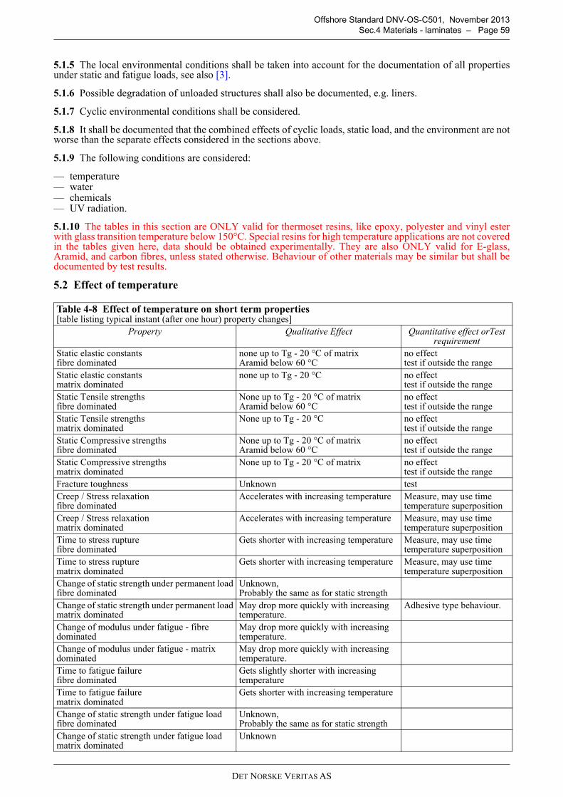
DET NORSKE VERITAS AS
Offshore Standard DNV-OS-C501, November 2013
Sec.4 Materials - laminates – Page 59
5.1.5 The local environmental conditions shall be taken into account for the documentation of all propertiesunder static and fatigue loads, see also [3].
5.1.6 Possible degradation of unloaded structures shall also be documented, e.g. liners.
5.1.7 Cyclic environmental conditions shall be considered.
5.1.8 It shall be documented that the combined effects of cyclic loads, static load, and the environment are notworse than the separate effects considered in the sections above.
5.1.9 The following conditions are considered:
— temperature— water— chemicals— UV radiation.
5.1.10 The tables in this section are ONLY valid for thermoset resins, like epoxy, polyester and vinyl esterwith glass transition temperature below 150°C. Special resins for high temperature applications are not coveredin the tables given here, data should be obtained experimentally. They are also ONLY valid for E-glass,Aramid, and carbon fibres, unless stated otherwise. Behaviour of other materials may be similar but shall bedocumented by test results.
5.2 Effect of temperature
Table 4-8 Effect of temperature on short term properties [table listing typical instant (after one hour) property changes]
Property Qualitative Effect Quantitative effect orTest requirement
Static elastic constantsfibre dominated
none up to Tg - 20 °C of matrixAramid below 60 °C
no effecttest if outside the range
Static elastic constantsmatrix dominated
none up to Tg - 20 °C no effecttest if outside the range
Static Tensile strengthsfibre dominated
None up to Tg - 20 °C of matrixAramid below 60 °C
no effecttest if outside the range
Static Tensile strengthsmatrix dominated
None up to Tg - 20 °C no effecttest if outside the range
Static Compressive strengthsfibre dominated
None up to Tg - 20 °C of matrixAramid below 60 °C
no effecttest if outside the range
Static Compressive strengthsmatrix dominated
None up to Tg - 20 °C of matrix no effecttest if outside the range
Fracture toughness Unknown test
Creep / Stress relaxationfibre dominated
Accelerates with increasing temperature Measure, may use time temperature superposition
Creep / Stress relaxationmatrix dominated
Accelerates with increasing temperature Measure, may use time temperature superposition
Time to stress rupturefibre dominated
Gets shorter with increasing temperature Measure, may use time temperature superposition
Time to stress rupturematrix dominated
Gets shorter with increasing temperature Measure, may use time temperature superposition
Change of static strength under permanent loadfibre dominated
Unknown,Probably the same as for static strength
Change of static strength under permanent loadmatrix dominated
May drop more quickly with increasing temperature.
Adhesive type behaviour.
Change of modulus under fatigue - fibre dominated
May drop more quickly with increasing temperature.
Change of modulus under fatigue - matrix dominated
May drop more quickly with increasing temperature.
Time to fatigue failurefibre dominated
Gets slightly shorter with increasing temperature
Time to fatigue failurematrix dominated
Gets shorter with increasing temperature
Change of static strength under fatigue loadfibre dominated
Unknown,Probably the same as for static strength
Change of static strength under fatigue loadmatrix dominated
Unknown
DET NORSKE VERITAS AS
Offshore Standard DNV-OS-C501, November 2013
Sec.4 Materials - laminates – Page 60
5.3 Effect of water
Table 4-9 Effect of water on properties [listing typical property changes after long exposures of 106 cycles or 10 years]
Property Qualitative Effect Quantitative effect orTest requirement
Static elastic constantsfibre dominated
Slight reduction
Static elastic constantsmatrix dominated
Slight reduction
Static Tensile strengthsfibre dominated
Glass: small reductionHydrolysis may reduce strength at high temperatures.Carbon: slight reductionAramid: slight reduction?
Glass: reduce strength by 10%Carbon: measureAramid: measure
Static Tensile strengthsmatrix dominated
some reduction measure wet properties
Static Compressive strengthsfibre dominated
Glass: small reductionHydrolysis may reduce strength at high temperatures.Carbon: slight reductionAramid: slight reduction?The combination of water and high temperature may give a severe strength reduction, because the supporting matrix can get weakened.
Glass: reduce strength by 10%Carbon: measureAramid: measure
Static Compressive strengthsmatrix dominated
some reductionThe combination of water and high temperature may give a severe strength reduction,
measure wet propertiescan use the same reduction as for tensile strength
Fracture toughness Unknown, may increase due to plastification effect.
test
Creep / Stress relaxationfibre dominated
Accelerates in the presence of water measure
Creep / Stress relaxationmatrix dominated
Accelerates in the presence of water measure
Time to stress rupturefibre dominated
Gets shorter with the presence of water.The combination of water, high temperature and compressive load may give a severe reduction in time to failure, because the supporting matrix can get weakened.
measure
Time to stress rupturematrix dominated
Gets shorter with the presence of water.The combination of water and high temperature may give a severe reduction of time to failure.
measure
Change of static strength under permanent load fibre dominated
Unknown,Probably the same as for static strength
measure
Change of static strength under permanent load matrix dominated
Unknown,Probably the same as for static strength
Change of modulus under fatigue - fibre dominated
Unknown, probably small effect
Change of modulus under fatigue - matrix dominated
Unknown
Time to fatigue failurefibre dominated
Typically a slight reduction.If compressive loads are involved combined with water and high temperature fatigue lifetime may be severely reduced.
reduce stress level by 10%
Time to fatigue failurematrix dominated
Typically a slight reduction.If compressive loads are involved combined with water and high temperature fatigue lifetime may be severely reduced.
Change of static strength under fatigue load fibre dominated
Probably the same as for static strength
Change of static strength under fatigue load matrix dominated
Unknown
DET NORSKE VERITAS AS
Offshore Standard DNV-OS-C501, November 2013
Sec.4 Materials - laminates – Page 61
5.3.1 The effect of seawater is generally less severe than the effect of fresh water.
5.3.2 The effect of distilled water is more severe than the effect of fresh water.
5.3.3 The combination of water and high temperature may be worse than the individual effects of temperatureand water.
5.3.4 Aramid fibres shall not be exposed to the combination of water and temperature cycles above and below 0°C.
5.4 Effect of chemicals
5.4.1 The compatibility of a laminate to the exposure to chemicals shall be demonstrated.
5.4.2 In a qualitative way most chemicals tend to have similar effects as water on a composite. The degradationrates shall be obtained for the actual materials in question. In addition, chemicals may break down the matrix,attack the matrix / fibre interface or destroy the fibres.
5.5 Effect of UV radiation
5.5.1 UV radiation can break down the polymers and reduce their strength. The resistance of surface layers toUV radiation shall be documented and quantified if necessary.
5.5.2 Glass and carbon fibres are very resistant to UV radiation.
5.5.3 Aramid fibres are not resistant to UV radiation and shall be protected.
5.5.4 Polyesters tend to have a good UV resistance.
5.5.5 Epoxies tend to have a bad UV resistance.
5.5.6 Vinylester tend to have a variable UV resistance.
5.6 Electrolytic Corrosion
5.6.1 Carbon fibre laminates shall be isolated from direct contact with all metal parts to prevent electrolyticcorrosion.
5.6.2 It is recommended to check the quality of the isolation by resistance measurements.
Guidance note:
Electrical connection between carbon fibres and steel in submerged conditions (with or without anodes) will causecathodic protection of the carbon fibres where they are exposed to sea water (in cracks, cut surfaces etc.). Whenpolarised the local pH at the fibre surface will be increased to ≈ 13 and salts from the sea water will precipitate on thefibres. The associated volume increase will force the crack to open more (“The wedging effect”). As a result, themechanical properties of the laminate may be reduced, due to the gradually increasing loss of adhesion between thecarbon fibres and the matrix.
---e-n-d---of---G-u-i-d-a-n-c-e---n-o-t-e---
5.7 Combination of environmental effects
5.7.1 The combination of environmental effects on materials, like combined humidity and heat, may be worsethan the individual effects.
5.7.2 Test data should be obtained of the combined effect of environments on the material properties ifrelevant. The worst relevant combination of environments should be used for testing.
5.8 Blisters/osmosis
5.8.1 Some matrix systems develop blisters after some time of water exposure. Matrix systems should bechosen that have been proven to be blister resistant. A proper mixture of hardener and curing agent is alsoimportant to prevent blistering. Blistering can also be related to weak bonding between gelcoat and laminate.Blistering is also sometimes referred to as “Osmosis”.
6 Influence of process parameters
6.1 Introduction
6.1.1 Composite laminates can be produced in many ways. Changes to the process parameters may influencesome or all-material parameters.
6.1.2 Process parameters are seen here in a wider sense. Change of void content or fibre fraction are part ofthis section, even though these changes are a results of other changes of more fundamental productionparameters.

DET NORSKE VERITAS AS
Offshore Standard DNV-OS-C501, November 2013
Sec.4 Materials - laminates – Page 62
6.2 Change of production method
6.2.1 A change in production method, e.g., going from hand lay-up to filament winding, is usuallyaccompanied by many other changes. Different resins are used, different fibres or sizings may be used, and thefibre fraction and void content may change significantly.
6.2.2 A re-qualification of the materials data shall be done if the production process is not similar to theoriginal process - see [8.3]. A production process is similar as long as changes introduced by the new processcan be quantified as described in the following parts of [6] and the process group is not changed.
6.2.3 Examples of process groups are:
— hand-lay-up— spray-lay-up — pre-preg lay-up— autoclave curing (in combination with one of the other processes— resin injection processes — resin transfer moulding— centrifugal moulding— filament winding— tape winding.
6.3 Change of processing temperature and pressure
6.3.1 For simple processes of thermoset materials with only one cure temperature:
— curing temperature of the reference data was higher than in reality. data shall be re-qualified
— curing temperature of the reference data was lower than in reality: data are valid, as long as the temperature did not exceed the resin manufacturer's maximum curingtemperature.
6.3.2 For simple processes of thermoset materials with only one cure pressure:
— curing pressure of the reference data was higher than in reality: data shall be re-qualified
— curing pressure of the reference data was lower than in reality: data are valid, as long as the pressure did not exceed the resin manufacturer's maximum curing pressure.
6.3.3 For thermoplastic composites where the plies are welded or fused together, a processing window ofpressure and temperature should be established in which test data are applicable.
6.3.4 For complex curing cycles with varying temperature and pressure, any change to the process shall requirerequalification of the data.
6.4 Change of post cure procedure
6.4.1 Post-curing has no influence on fibre dominated tensile properties.
6.4.2 Post curing may improve fibre dominated compressive properties and all matrix dominated properties.
6.4.3 For some matrix systems post curing accelerates some slow crosslinking reactions that would also takeplace at room temperature. This is the case for many types of polyester. For these systems data obtained frompost cured specimens are also valid for materials that were not post cured.
6.4.4 For some matrix systems post curing creates a better crosslinked network that will never be achieved ifthe laminate remains at room temperature. This is the case for many vinyl esters and epoxies. For these systemsdata obtained from post cured specimens are not valid for materials that were not post cured.
6.5 Change of void content
6.5.1 If the void content of the reference data was higher than in reality, data are valid.
6.5.2 If the void content of the reference data was more than 10% (relative) lower than in reality, data shall bere-qualified.
6.6 Correction for change in fibre volume fraction
6.6.1 For UD-plies:
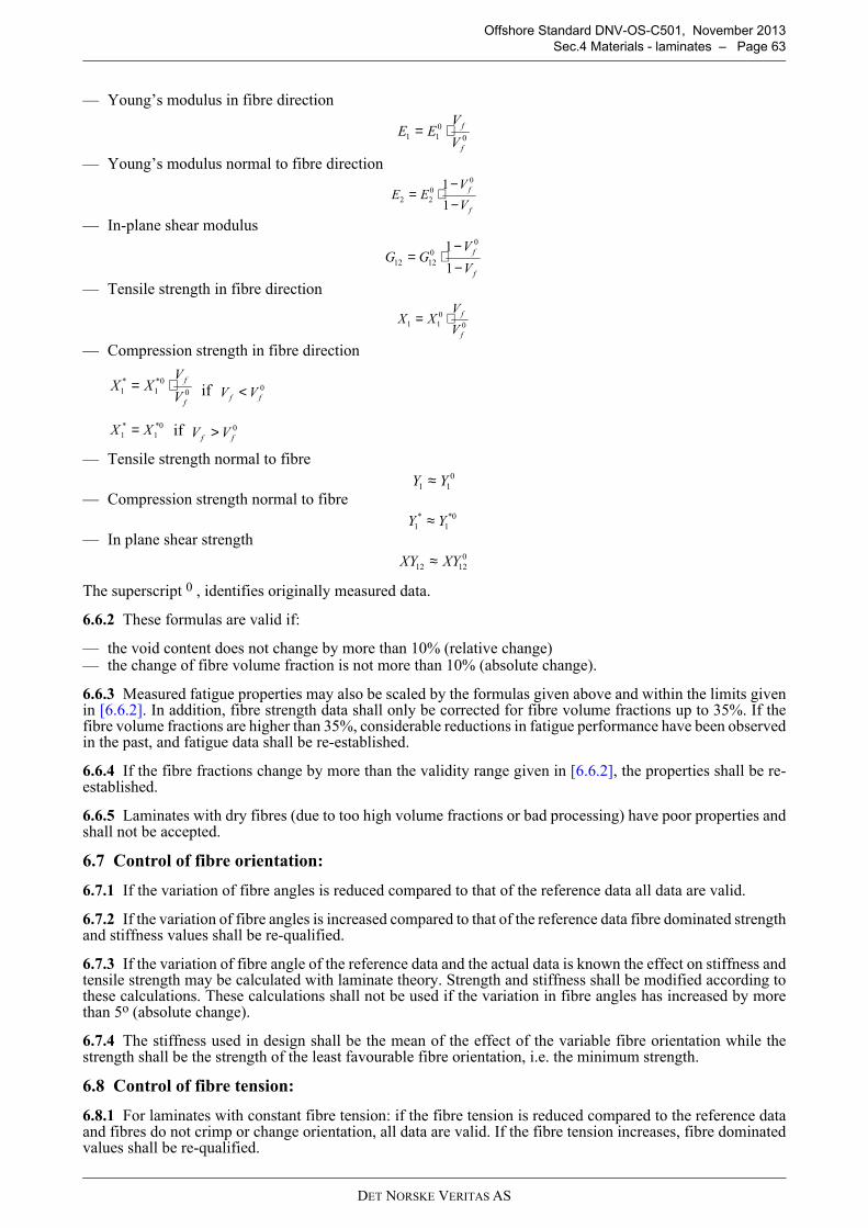
DET NORSKE VERITAS AS
Offshore Standard DNV-OS-C501, November 2013
Sec.4 Materials - laminates – Page 63
— Young’s modulus in fibre direction
— Young’s modulus normal to fibre direction
— In-plane shear modulus
— Tensile strength in fibre direction
— Compression strength in fibre direction
if
if
— Tensile strength normal to fibre
— Compression strength normal to fibre
— In plane shear strength
The superscript 0 , identifies originally measured data.
6.6.2 These formulas are valid if:
— the void content does not change by more than 10% (relative change)— the change of fibre volume fraction is not more than 10% (absolute change).
6.6.3 Measured fatigue properties may also be scaled by the formulas given above and within the limits givenin [6.6.2]. In addition, fibre strength data shall only be corrected for fibre volume fractions up to 35%. If thefibre volume fractions are higher than 35%, considerable reductions in fatigue performance have been observedin the past, and fatigue data shall be re-established.
6.6.4 If the fibre fractions change by more than the validity range given in [6.6.2], the properties shall be re-established.
6.6.5 Laminates with dry fibres (due to too high volume fractions or bad processing) have poor properties andshall not be accepted.
6.7 Control of fibre orientation:
6.7.1 If the variation of fibre angles is reduced compared to that of the reference data all data are valid.
6.7.2 If the variation of fibre angles is increased compared to that of the reference data fibre dominated strengthand stiffness values shall be re-qualified.
6.7.3 If the variation of fibre angle of the reference data and the actual data is known the effect on stiffness andtensile strength may be calculated with laminate theory. Strength and stiffness shall be modified according tothese calculations. These calculations shall not be used if the variation in fibre angles has increased by morethan 5o (absolute change).
6.7.4 The stiffness used in design shall be the mean of the effect of the variable fibre orientation while thestrength shall be the strength of the least favourable fibre orientation, i.e. the minimum strength.
6.8 Control of fibre tension:
6.8.1 For laminates with constant fibre tension: if the fibre tension is reduced compared to the reference dataand fibres do not crimp or change orientation, all data are valid. If the fibre tension increases, fibre dominatedvalues shall be re-qualified.
0
011
f
f
V
VEE ⋅=
f
f
V
VEE
−−
⋅=1
1 0
022
f
f
V
VGG
−−
⋅=1
1 0
01212
0
011
f
f
V
VXX ⋅=
0
0*1
*1
f
f
V
VXX ⋅= 0
ff VV <
0*1
*1 XX = 0
ff VV >
011 YY ≈
0*1
*1 YY ≈
01212 XYXY ≈
DET NORSKE VERITAS AS
Offshore Standard DNV-OS-C501, November 2013
Sec.4 Materials - laminates – Page 64
6.8.2 Laminates made by filament winding, tape winding and similar processes may show a variation in fibretension, especially through the thickness. Laminate and ply properties should be established for a representativecombination of fibre tensions.
6.8.3 If fibre tensions vary, but the change in tension is known, the change in fibre tension may be added tothe loads acting on the ply in a stress analysis. If such an analysis can be carried out with sufficient accuracy are-qualification of the material properties is not required.
7 Properties under fire
7.1 Introduction
7.1.1 The performance of composites in a fire is a complex process, because the various constituent materialsrespond differently to a fire.
7.1.2 The requirements under fire conditions can usually be found in the fire codes for a particular application.
7.1.3 Fire codes may implicitly assume that the structure is built of steel or metal. The relevance of a fire codeto composite materials shall be checked carefully.
7.1.4 Since most composites are flammable and temperature sensitive most applications use protectivemeasures to reduce the impact of fire. In this case the fire performance of the complete system, i.e. a compositestructure with fire protection shall be evaluated.
7.1.5 An advantage of composite laminates is their low thermal conductivity and the usually long timesrequired to reach burn through conditions.
7.1.6 Some aspects of fire performance can be modelled, but some experimental testing shall always be doneto demonstrate fire performance.
7.2 Fire reaction
7.2.1 Fire reaction describes the response of a composite to fire in terms of flammability, flame spread, smokedevelopment and emission of toxic gases. All these aspects shall be documented if relevant.
7.2.2 Special additives or fillers are often added to composites to improve fire reaction.
7.2.3 The influence of such additives or fillers on the basic mechanical properties shall be evaluated.
7.3 Fire resistance
7.3.1 Fire resistance describes the remaining strength of a composite structure under a fire.
7.3.2 As a first estimate of fire resistance the temperature dependent properties, as described in [5.2], can beused.
7.3.3 The temperature within a composite laminate can be calculated by means of appropriate models.
7.3.4 If chemical reactions can occur within the laminate their influence on the temperature distribution shallbe considered.
7.3.5 Through thickness properties and matrix dominated properties shall be carefully evaluated, especially inthe region of joints. Matrix dominated properties tend to degrade rapidly in a fire.
Guidance note:
A panel with stiffeners may loose most of its stiffness if the stiffeners delaminate from the panel due to the fire.
---e-n-d---of---G-u-i-d-a-n-c-e---n-o-t-e---
7.4 Insulation
7.4.1 The properties of the insulation with respect to fire reaction and fire resistance shall be evaluated.
7.4.2 Special consideration shall be given to the joints of the insulation and the method the insulation isattached to the component. Attachment points and joints may create hot spots in the component.
7.4.3 All large scale testing shall be done with jointed insulation and the same attachments as used in the realapplication.
7.5 Properties after the fire
7.5.1 A fire is usually seen as an accidental load case and properties after the fire shall be evaluated for eachindividual case.
DET NORSKE VERITAS AS
Offshore Standard DNV-OS-C501, November 2013
Sec.4 Materials - laminates – Page 65
7.5.2 If the temperature has locally exceeded the Tg of the component it is very likely that permanent damagehas been made to the component in that area.
7.5.3 If the temperature remained locally under Tg damage may be introduced due to overloads from otherparts of the structure.
8 Qualification of material properties
8.1 Introduction
8.1.1 All material properties needed to describe the performance of a component shall be documented.
8.1.2 As a general principal, material properties should be obtained form test results of laminates that representthe laminates of the component as closely as possible.
Guidance note:
If laminates are used on pipes, it is recommended to obtain material data from tubular specimens.
---e-n-d---of---G-u-i-d-a-n-c-e---n-o-t-e---
8.1.3 Material properties may be documented by the following methods:
— direct measurements— qualification against representative data— qualification against manufacturers data— qualification against data from the open literature— qualification by component testing.
8.1.4 Each individual material property may be qualified by any of the different methods.
8.1.5 Which data can be used for qualification depends mainly on two aspects:
— data obtained from laminates that are similar to the laminates used in the component— data obtained from reputable sources.
8.2 General test requirements
8.2.1 All relevant information about the material tested, the test method, and the test conditions shallaccompany test results. The information requested in [1.2] shall be provided.
8.2.2 Static test results shall be reported as mean, standard deviation, coefficient of variation, and number oftest specimens. The characteristic values of static tests shall be calculated as described in [2.4].
8.2.3 Long-term test results shall be reported as mean regression curve, standard deviation with respect to timeor cycles, number of test specimen, range of test time or number of cycles. Test points shall be spread outrelatively evenly over the logarithmic test period. The characteristic values of long-term tests shall becalculated as described in [3.11].
8.3 Selection of material qualification method
8.3.1 The test results shall apply to the laminates used in the component to be designed and built. Test resultsare only applicable if the test laminate and the component laminate are similar enough that the test results arevalid or conservative for the actual component.
8.3.2 If the material is the same as an already tested material no further testing is required. The same materialmeans:
— same fibres, same weave or fabric from the same producer— same matrix system (same resin, curing agent and fillers)— similar production process, as defined in [6.2.2].
8.3.3 If the material is similar to an already tested material qualification against a representative material maybe carried out. Requirements for similarity are given in [8.6], requirements for representative data are given in[8.5].
8.3.4 Direct measurements as described in [8.4] shall be carried out if [8.3.2] or [8.3.3] cannot be applied.
8.4 Direct measurement
8.4.1 The various properties of a composite may be measured directly for a particular material. Data will bevalid for that particular material that was tested. The material shall be characterised as required in [1.2].
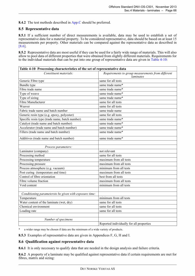
DET NORSKE VERITAS AS
Offshore Standard DNV-OS-C501, November 2013
Sec.4 Materials - laminates – Page 66
8.4.2 The test methods described in App.C should be preferred.
8.5 Representative data
8.5.1 If a sufficient number of direct measurements is available, data may be used to establish a set ofrepresentative data for a material property. To be considered representative, data should be based on at least 15measurements per property. Other materials can be compared against the representative data as described in[8.6].
8.5.2 Representative data are most useful if they can be used for a fairly wide range of materials. This will alsoallow to pool data of different properties that were obtained from slightly different materials. Requirements forto the individual materials that can be put into one group of representative data are given in Table 4-10:
* a wider range may be chosen if data are the minimum of a wide variety of products.
8.5.3 Examples of representative data are given in Appendices F, G, H and I.
8.6 Qualification against representative data
8.6.1 It is only necessary to qualify data that are needed in the design analysis and failure criteria.
8.6.2 A property of a laminate may be qualified against representative data if certain requirements are met forfibres, matrix and sizing:
Table 4-10 Processing characteristics of the set of representative data
Constituent materials: Requirements to group measurements from different laminates
Generic Fibre type same for all tests
Bundle type same trade name*
Fibre trade name same trade name*
Type of weave same trade name*
Type of sizing same trade name*
Fibre Manufacturer same for all tests
Weaver same for all tests
Fabric trade name and batch number same trade name
Generic resin type (e.g. epoxy, polyester) same for all tests
Specific resin type (trade name, batch number) same trade name*
Catalyst (trade name and batch number) same trade name*
Accelerator (trade name and batch number) same trade name*
Fillers (trade name and batch number) same trade name*
Additives (trade name and batch number) same trade name*
Process parameters:
Laminator (company) not relevant
Processing method same for all tests
Processing temperature maximum from all tests
Processing pressure maximum from all tests
Process atmosphere (e.g. vacuum) minimum from all tests
Post curing (temperature and time) maximum from all tests
Control of fibre orientation best from all tests
Fibre volume fraction maximum from all tests
Void content minimum from all tests
Conditioning parametersto be given with exposure time:
Temperature minimum from all tests
Water content of the laminate (wet, dry) same for all tests
Chemical environment same for all tests
Loading rate same for all tests
Number of specimens
Reported individually for all properties
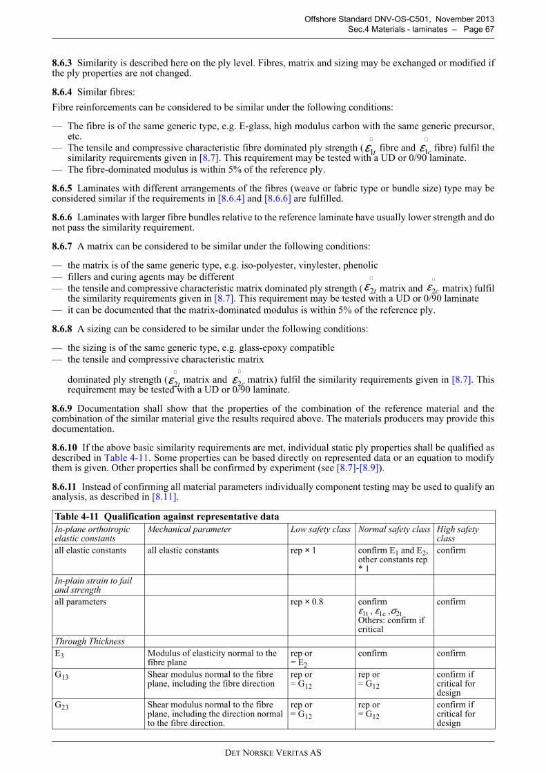
DET NORSKE VERITAS AS
Offshore Standard DNV-OS-C501, November 2013
Sec.4 Materials - laminates – Page 67
8.6.3 Similarity is described here on the ply level. Fibres, matrix and sizing may be exchanged or modified ifthe ply properties are not changed.
8.6.4 Similar fibres:
Fibre reinforcements can be considered to be similar under the following conditions:
— The fibre is of the same generic type, e.g. E-glass, high modulus carbon with the same generic precursor,etc.
— The tensile and compressive characteristic fibre dominated ply strength ( fibre and fibre) fulfil thesimilarity requirements given in [8.7]. This requirement may be tested with a UD or 0/90 laminate.
— The fibre-dominated modulus is within 5% of the reference ply.
8.6.5 Laminates with different arrangements of the fibres (weave or fabric type or bundle size) type may beconsidered similar if the requirements in [8.6.4] and [8.6.6] are fulfilled.
8.6.6 Laminates with larger fibre bundles relative to the reference laminate have usually lower strength and donot pass the similarity requirement.
8.6.7 A matrix can be considered to be similar under the following conditions:
— the matrix is of the same generic type, e.g. iso-polyester, vinylester, phenolic— fillers and curing agents may be different— the tensile and compressive characteristic matrix dominated ply strength ( matrix and matrix) fulfil
the similarity requirements given in [8.7]. This requirement may be tested with a UD or 0/90 laminate— it can be documented that the matrix-dominated modulus is within 5% of the reference ply.
8.6.8 A sizing can be considered to be similar under the following conditions:
— the sizing is of the same generic type, e.g. glass-epoxy compatible— the tensile and compressive characteristic matrix
dominated ply strength ( matrix and matrix) fulfil the similarity requirements given in [8.7]. Thisrequirement may be tested with a UD or 0/90 laminate.
8.6.9 Documentation shall show that the properties of the combination of the reference material and thecombination of the similar material give the results required above. The materials producers may provide thisdocumentation.
8.6.10 If the above basic similarity requirements are met, individual static ply properties shall be qualified asdescribed in Table 4-11. Some properties can be based directly on represented data or an equation to modifythem is given. Other properties shall be confirmed by experiment (see [8.7]-[8.9]).
8.6.11 Instead of confirming all material parameters individually component testing may be used to qualify ananalysis, as described in [8.11].
Table 4-11 Qualification against representative data
In-plane orthotropic elastic constants
Mechanical parameter Low safety class Normal safety class High safety class
all elastic constants all elastic constants rep × 1 confirm E1 and E2, other constants rep * 1
confirm
In-plain strain to fail and strength
all parameters rep × 0.8 confirm ε1t , ε1c ,σ2t Others: confirm if critical
confirm
Through Thickness
E3 Modulus of elasticity normal to the fibre plane
rep or= E2
confirm confirm
G13 Shear modulus normal to the fibre plane, including the fibre direction
rep or= G12
rep or= G12
confirm if critical for design
G23 Shear modulus normal to the fibre plane, including the direction normal to the fibre direction.
rep or= G12
rep or= G12
confirm if critical for design
t1ε∧
c1ε∧
t2ε∧
c2ε∧
t2ε∧
c2ε∧
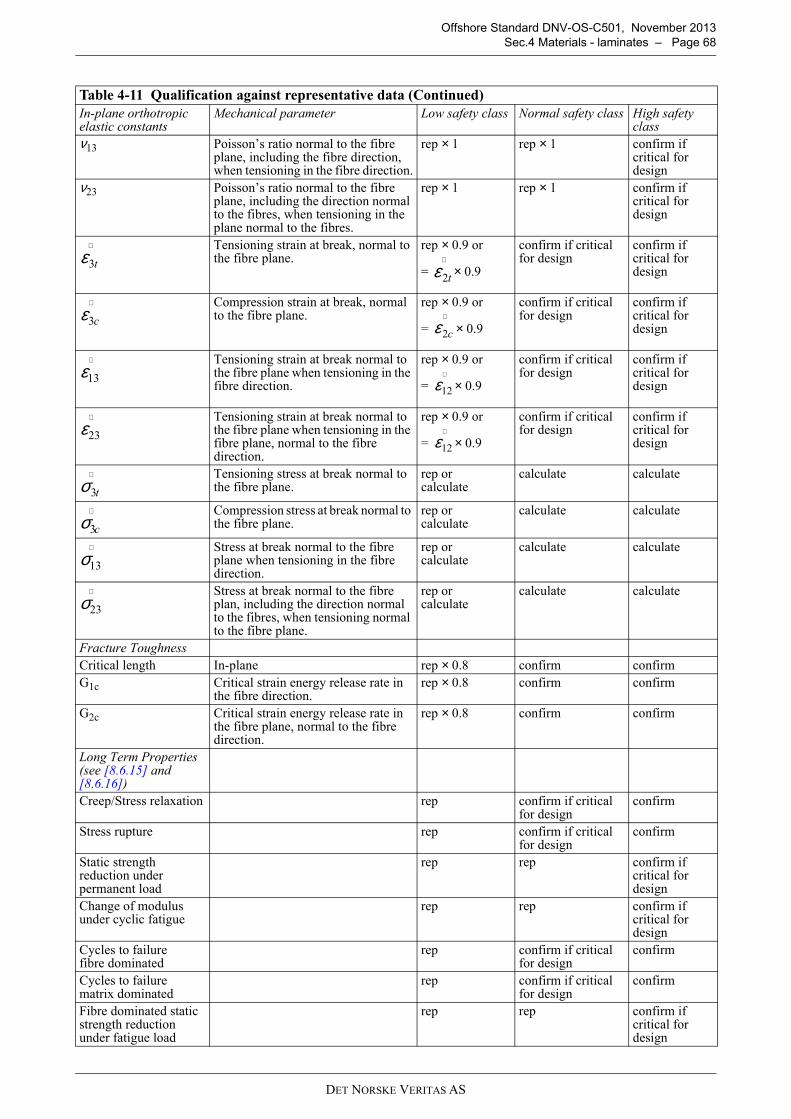
DET NORSKE VERITAS AS
Offshore Standard DNV-OS-C501, November 2013
Sec.4 Materials - laminates – Page 68
ν13 Poisson’s ratio normal to the fibre plane, including the fibre direction, when tensioning in the fibre direction.
rep × 1 rep × 1 confirm if critical for design
ν23 Poisson’s ratio normal to the fibre plane, including the direction normal to the fibres, when tensioning in the plane normal to the fibres.
rep × 1 rep × 1 confirm if critical for design
Tensioning strain at break, normal to the fibre plane.
rep × 0.9 or
= × 0.9
confirm if critical for design
confirm if critical for design
Compression strain at break, normal to the fibre plane.
rep × 0.9 or
= × 0.9
confirm if critical for design
confirm if critical for design
Tensioning strain at break normal to the fibre plane when tensioning in the fibre direction.
rep × 0.9 or
= × 0.9
confirm if critical for design
confirm if critical for design
Tensioning strain at break normal to the fibre plane when tensioning in the fibre plane, normal to the fibre direction.
rep × 0.9 or
= × 0.9
confirm if critical for design
confirm if critical for design
Tensioning stress at break normal to the fibre plane.
rep orcalculate
calculate calculate
Compression stress at break normal to the fibre plane.
rep orcalculate
calculate calculate
Stress at break normal to the fibre plane when tensioning in the fibre direction.
rep orcalculate
calculate calculate
Stress at break normal to the fibre plan, including the direction normal to the fibres, when tensioning normal to the fibre plane.
rep orcalculate
calculate calculate
Fracture Toughness
Critical length In-plane rep × 0.8 confirm confirm
G1c Critical strain energy release rate in the fibre direction.
rep × 0.8 confirm confirm
G2c Critical strain energy release rate in the fibre plane, normal to the fibre direction.
rep × 0.8 confirm confirm
Long Term Properties (see [8.6.15] and [8.6.16])
Creep/Stress relaxation rep confirm if critical for design
confirm
Stress rupture rep confirm if critical for design
confirm
Static strength reduction under permanent load
rep rep confirm if critical for design
Change of modulus under cyclic fatigue
rep rep confirm if critical for design
Cycles to failure fibre dominated
rep confirm if critical for design
confirm
Cycles to failurematrix dominated
rep confirm if critical for design
confirm
Fibre dominated static strength reduction under fatigue load
rep rep confirm if critical for design
Table 4-11 Qualification against representative data (Continued)
In-plane orthotropic elastic constants
Mechanical parameter Low safety class Normal safety class High safety class
t3ε∧
t2ε∧
c3ε∧
c2ε∧
13ε∧
12ε∧
23ε∧
12ε∧
t3σ∧
c3σ∧
13σ∧
23σ∧
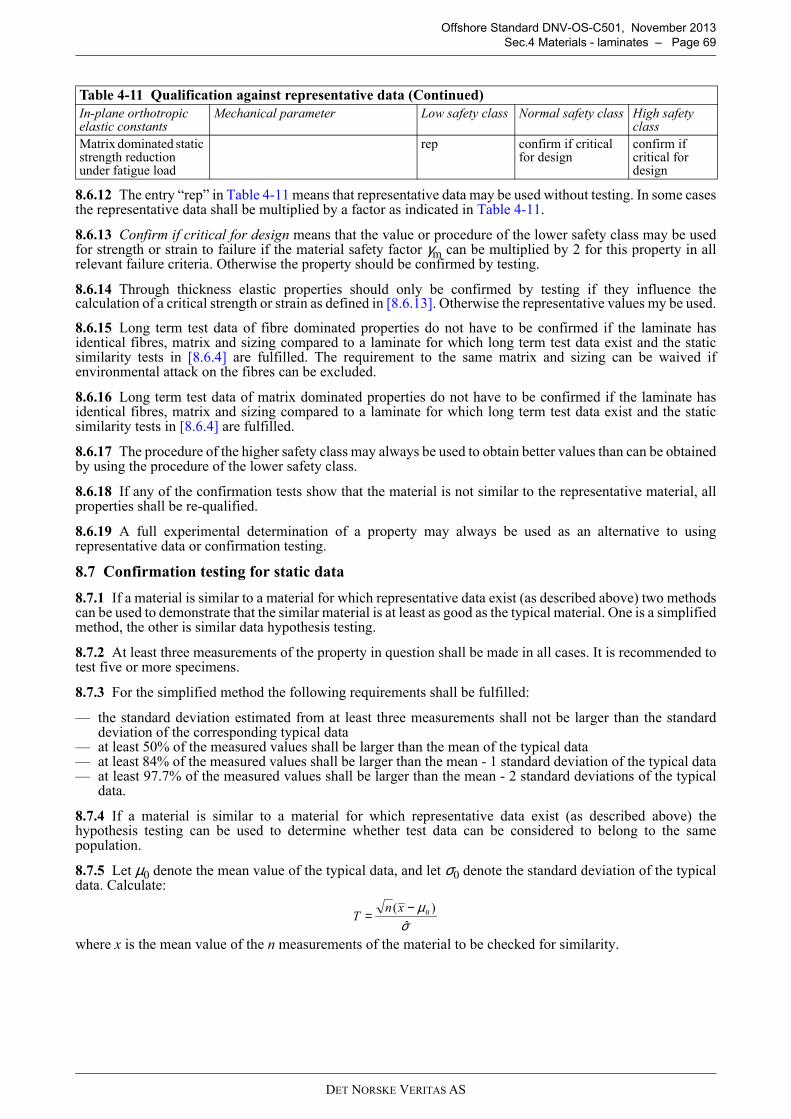
DET NORSKE VERITAS AS
Offshore Standard DNV-OS-C501, November 2013
Sec.4 Materials - laminates – Page 69
8.6.12 The entry “rep” in Table 4-11 means that representative data may be used without testing. In some casesthe representative data shall be multiplied by a factor as indicated in Table 4-11.
8.6.13 Confirm if critical for design means that the value or procedure of the lower safety class may be usedfor strength or strain to failure if the material safety factor γm can be multiplied by 2 for this property in allrelevant failure criteria. Otherwise the property should be confirmed by testing.
8.6.14 Through thickness elastic properties should only be confirmed by testing if they influence thecalculation of a critical strength or strain as defined in [8.6.13]. Otherwise the representative values my be used.
8.6.15 Long term test data of fibre dominated properties do not have to be confirmed if the laminate hasidentical fibres, matrix and sizing compared to a laminate for which long term test data exist and the staticsimilarity tests in [8.6.4] are fulfilled. The requirement to the same matrix and sizing can be waived ifenvironmental attack on the fibres can be excluded.
8.6.16 Long term test data of matrix dominated properties do not have to be confirmed if the laminate hasidentical fibres, matrix and sizing compared to a laminate for which long term test data exist and the staticsimilarity tests in [8.6.4] are fulfilled.
8.6.17 The procedure of the higher safety class may always be used to obtain better values than can be obtainedby using the procedure of the lower safety class.
8.6.18 If any of the confirmation tests show that the material is not similar to the representative material, allproperties shall be re-qualified.
8.6.19 A full experimental determination of a property may always be used as an alternative to usingrepresentative data or confirmation testing.
8.7 Confirmation testing for static data
8.7.1 If a material is similar to a material for which representative data exist (as described above) two methodscan be used to demonstrate that the similar material is at least as good as the typical material. One is a simplifiedmethod, the other is similar data hypothesis testing.
8.7.2 At least three measurements of the property in question shall be made in all cases. It is recommended totest five or more specimens.
8.7.3 For the simplified method the following requirements shall be fulfilled:
— the standard deviation estimated from at least three measurements shall not be larger than the standarddeviation of the corresponding typical data
— at least 50% of the measured values shall be larger than the mean of the typical data— at least 84% of the measured values shall be larger than the mean - 1 standard deviation of the typical data— at least 97.7% of the measured values shall be larger than the mean - 2 standard deviations of the typical
data.
8.7.4 If a material is similar to a material for which representative data exist (as described above) thehypothesis testing can be used to determine whether test data can be considered to belong to the samepopulation.
8.7.5 Let µ0 denote the mean value of the typical data, and let σ0 denote the standard deviation of the typicaldata. Calculate:
where x is the mean value of the n measurements of the material to be checked for similarity.
Matrix dominated static strength reduction under fatigue load
rep confirm if critical for design
confirm if critical for design
Table 4-11 Qualification against representative data (Continued)
In-plane orthotropic elastic constants
Mechanical parameter Low safety class Normal safety class High safety class
σµ
ˆ
)( 0−=
xnT
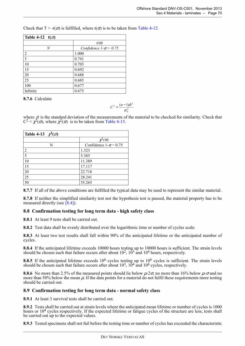
DET NORSKE VERITAS AS
Offshore Standard DNV-OS-C501, November 2013
Sec.4 Materials - laminates – Page 70
Check that T > -t(α) is fulfilled, where t(α) is to be taken from Table 4-12.
8.7.6 Calculate
where is the standard deviation of the measurements of the material to be checked for similarity. Check thatC2 < χ2(α), where χ2(α) is to be taken from Table 4-13.
8.7.7 If all of the above conditions are fulfilled the typical data may be used to represent the similar material.
8.7.8 If neither the simplified similarity test nor the hypothesis test is passed, the material property has to bemeasured directly (see [8.4]).
8.8 Confirmation testing for long term data - high safety class
8.8.1 At least 9 tests shall be carried out.
8.8.2 Test data shall be evenly distributed over the logarithmic time or number of cycles scale.
8.8.3 At least two test results shall fall within 90% of the anticipated lifetime or the anticipated number ofcycles.
8.8.4 If the anticipated lifetime exceeds 10000 hours testing up to 10000 hours is sufficient. The strain levelsshould be chosen such that failure occurs after about 102, 103 and 104 hours, respectively.
8.8.5 If the anticipated lifetime exceeds 106 cycles testing up to 106 cycles is sufficient. The strain levelsshould be chosen such that failure occurs after about 103, 104 and 106 cycles, respectively.
8.8.6 No more than 2.5% of the measured points should lie below µ-2σ, no more than 16% below µ-σ and nomore than 50% below the mean µ. If the data points for a material do not fulfil these requirements more testingshould be carried out.
8.9 Confirmation testing for long term data - normal safety class
8.9.1 At least 3 survival tests shall be carried out.
8.9.2 Tests shall be carried out at strain levels where the anticipated mean lifetime or number of cycles is 1000hours or 104 cycles respectively. If the expected lifetime or fatigue cycles of the structure are less, tests shallbe carried out up to the expected values.
8.9.3 Tested specimens shall not fail before the testing time or number of cycles has exceeded the characteristic
Table 4-12 t(α)
t(α)
N Confidence 1-α = 0.75
2 1.000
5 0.741
10 0.703
15 0.692
20 0.688
25 0.685
100 0.677
Infinity 0.675
Table 4-13 χ2(α)
χ2(α)
N Confidence 1-α = 0.75
2 1.323
5 5.385
10 11.389
15 17.117
20 22.718
25 28.241
50 55.265
20
22 ˆ)1(
σσ−= n
C
σ
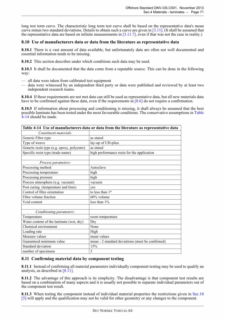
DET NORSKE VERITAS AS
Offshore Standard DNV-OS-C501, November 2013
Sec.4 Materials - laminates – Page 71
long test term curve. The characteristic long term test curve shall be based on the representative data's meancurve minus two standard deviations. Details to obtain such a curve are given in [3.11]. (It shall be assumed thatthe representative data are based on infinite measurements in [3.11.7], even if that was not the case in reality.)
8.10 Use of manufacturers data or data from the literature as representative data
8.10.1 There is a vast amount of data available, but unfortunately data are often not well documented andessential information tends to be missing.
8.10.2 This section describes under which conditions such data may be used.
8.10.3 It shall be documented that the data come from a reputable source. This can be done in the followingway:
— all data were taken from calibrated test equipment— data were witnessed by an independent third party or data were published and reviewed by at least two
independent research teams.
8.10.4 If these requirements are not met data can still be used as representative data, but all new materials datahave to be confirmed against these data, even if the requirements in [8.6] do not require a confirmation.
8.10.5 If information about processing and conditioning is missing, it shall always be assumed that the bestpossible laminate has been tested under the most favourable conditions. The conservative assumptions in Table4-14 should be made.
8.11 Confirming material data by component testing
8.11.1 Instead of confirming all material parameters individually component testing may be used to qualify ananalysis, as described in [8.11].
8.11.2 The advantage of this approach is its simplicity. The disadvantage is that component test results arebased on a combination of many aspects and it is usually not possible to separate individual parameters out ofthe component test result.
8.11.3 When testing the component instead of individual material properties the restrictions given in Sec.10[5] will apply and the qualification may not be valid for other geometry or any changes to the component.
Table 4-14 Use of manufacturers data or data from the literature as representative data
Constituent materials:
Generic Fibre type as stated
Type of weave lay-up of UD-plies
Generic resin type (e.g. epoxy, polyester) as stated
Specific resin type (trade name) high performance resin for the application
Process parameters:
Processing method Autoclave
Processing temperature high
Processing pressure high
Process atmosphere (e.g. vacuum) vacuum
Post curing (temperature and time) yes
Control of fibre orientation to less than 1o
Fibre volume fraction 60% volume
Void content less than 1%
Conditioning parameters:
Temperature room temperature
Water content of the laminate (wet, dry) Dry
Chemical environment None
Loading rate High
Measure values mean values
Guaranteed minimum value mean - 2 standard deviations (must be confirmed)
Standard deviation 15%
number of specimens 3
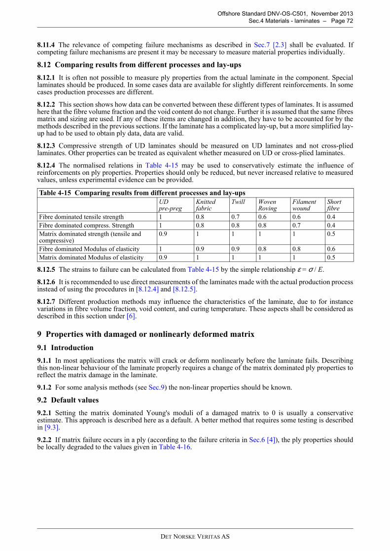
DET NORSKE VERITAS AS
Offshore Standard DNV-OS-C501, November 2013
Sec.4 Materials - laminates – Page 72
8.11.4 The relevance of competing failure mechanisms as described in Sec.7 [2.3] shall be evaluated. Ifcompeting failure mechanisms are present it may be necessary to measure material properties individually.
8.12 Comparing results from different processes and lay-ups
8.12.1 It is often not possible to measure ply properties from the actual laminate in the component. Speciallaminates should be produced. In some cases data are available for slightly different reinforcements. In somecases production processes are different.
8.12.2 This section shows how data can be converted between these different types of laminates. It is assumedhere that the fibre volume fraction and the void content do not change. Further it is assumed that the same fibresmatrix and sizing are used. If any of these items are changed in addition, they have to be accounted for by themethods described in the previous sections. If the laminate has a complicated lay-up, but a more simplified lay-up had to be used to obtain ply data, data are valid.
8.12.3 Compressive strength of UD laminates should be measured on UD laminates and not cross-pliedlaminates. Other properties can be treated as equivalent whether measured on UD or cross-plied laminates.
8.12.4 The normalised relations in Table 4-15 may be used to conservatively estimate the influence ofreinforcements on ply properties. Properties should only be reduced, but never increased relative to measuredvalues, unless experimental evidence can be provided.
8.12.5 The strains to failure can be calculated from Table 4-15 by the simple relationship ε = σ / E.
8.12.6 It is recommended to use direct measurements of the laminates made with the actual production processinstead of using the procedures in [8.12.4] and [8.12.5].
8.12.7 Different production methods may influence the characteristics of the laminate, due to for instancevariations in fibre volume fraction, void content, and curing temperature. These aspects shall be considered asdescribed in this section under [6].
9 Properties with damaged or nonlinearly deformed matrix
9.1 Introduction
9.1.1 In most applications the matrix will crack or deform nonlinearly before the laminate fails. Describingthis non-linear behaviour of the laminate properly requires a change of the matrix dominated ply properties toreflect the matrix damage in the laminate.
9.1.2 For some analysis methods (see Sec.9) the non-linear properties should be known.
9.2 Default values
9.2.1 Setting the matrix dominated Young's moduli of a damaged matrix to 0 is usually a conservativeestimate. This approach is described here as a default. A better method that requires some testing is describedin [9.3].
9.2.2 If matrix failure occurs in a ply (according to the failure criteria in Sec.6 [4]), the ply properties shouldbe locally degraded to the values given in Table 4-16.
Table 4-15 Comparing results from different processes and lay-ups
UD pre-preg
Knitted fabric
Twill Woven Roving
Filament wound
Short fibre
Fibre dominated tensile strength 1 0.8 0.7 0.6 0.6 0.4
Fibre dominated compress. Strength 1 0.8 0.8 0.8 0.7 0.4
Matrix dominated strength (tensile and compressive)
0.9 1 1 1 1 0.5
Fibre dominated Modulus of elasticity 1 0.9 0.9 0.8 0.8 0.6
Matrix dominated Modulus of elasticity 0.9 1 1 1 1 0.5
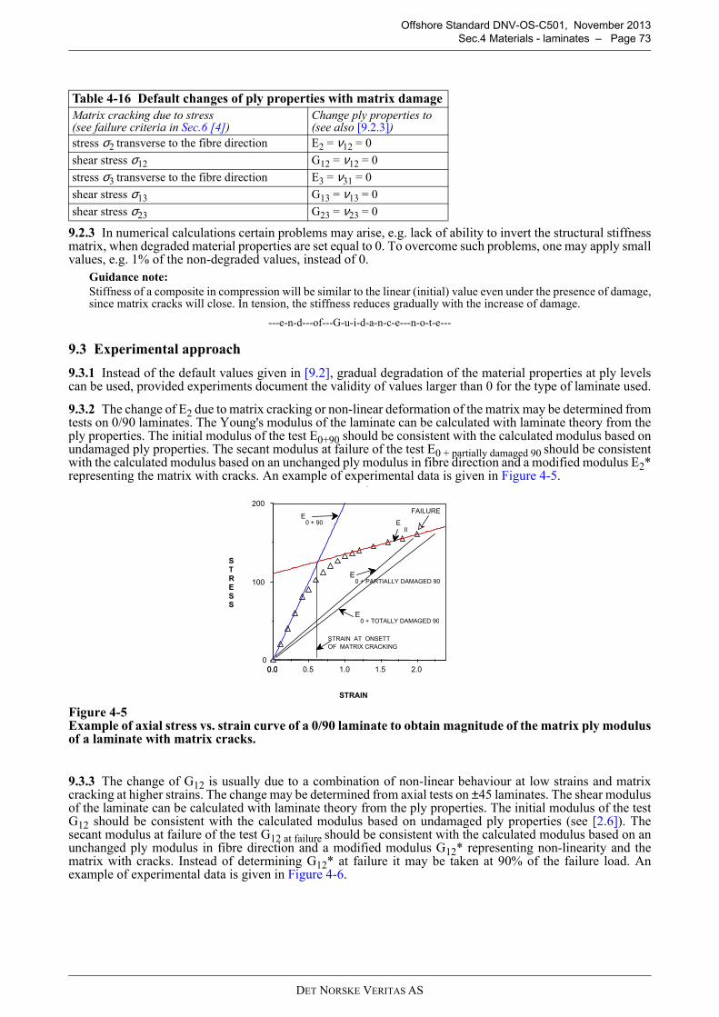
DET NORSKE VERITAS AS
Offshore Standard DNV-OS-C501, November 2013
Sec.4 Materials - laminates – Page 73
9.2.3 In numerical calculations certain problems may arise, e.g. lack of ability to invert the structural stiffnessmatrix, when degraded material properties are set equal to 0. To overcome such problems, one may apply smallvalues, e.g. 1% of the non-degraded values, instead of 0.
Guidance note:
Stiffness of a composite in compression will be similar to the linear (initial) value even under the presence of damage,since matrix cracks will close. In tension, the stiffness reduces gradually with the increase of damage.
---e-n-d---of---G-u-i-d-a-n-c-e---n-o-t-e---
9.3 Experimental approach
9.3.1 Instead of the default values given in [9.2], gradual degradation of the material properties at ply levelscan be used, provided experiments document the validity of values larger than 0 for the type of laminate used.
9.3.2 The change of E2 due to matrix cracking or non-linear deformation of the matrix may be determined fromtests on 0/90 laminates. The Young's modulus of the laminate can be calculated with laminate theory from theply properties. The initial modulus of the test E0+90 should be consistent with the calculated modulus based onundamaged ply properties. The secant modulus at failure of the test E0 + partially damaged 90 should be consistentwith the calculated modulus based on an unchanged ply modulus in fibre direction and a modified modulus E2*representing the matrix with cracks. An example of experimental data is given in Figure 4-5.
Figure 4-5 Example of axial stress vs. strain curve of a 0/90 laminate to obtain magnitude of the matrix ply modulusof a laminate with matrix cracks.
9.3.3 The change of G12 is usually due to a combination of non-linear behaviour at low strains and matrixcracking at higher strains. The change may be determined from axial tests on ±45 laminates. The shear modulusof the laminate can be calculated with laminate theory from the ply properties. The initial modulus of the testG12 should be consistent with the calculated modulus based on undamaged ply properties (see [2.6]). Thesecant modulus at failure of the test G12 at failure should be consistent with the calculated modulus based on anunchanged ply modulus in fibre direction and a modified modulus G12* representing non-linearity and thematrix with cracks. Instead of determining G12* at failure it may be taken at 90% of the failure load. Anexample of experimental data is given in Figure 4-6.
Table 4-16 Default changes of ply properties with matrix damage
Matrix cracking due to stress(see failure criteria in Sec.6 [4])
Change ply properties to (see also [9.2.3])
stress σ2 transverse to the fibre direction E2 = ν12 = 0
shear stress σ12 G12 = ν12 = 0
stress σ3 transverse to the fibre direction E3 = ν31 = 0
shear stress σ13 G13 = ν13 = 0
shear stress σ23 G23 = ν23 = 0
2.01.51.00.50.00.0
0
100
200
.
STRAIN
STRESS
STRAIN AT ONSETT
OF MATRIX CRACKING
EII
E0 + 90
E0 + PARTIALLY DAMAGED 90
FAILURE
E0 + TOTALLY DAMAGED 90
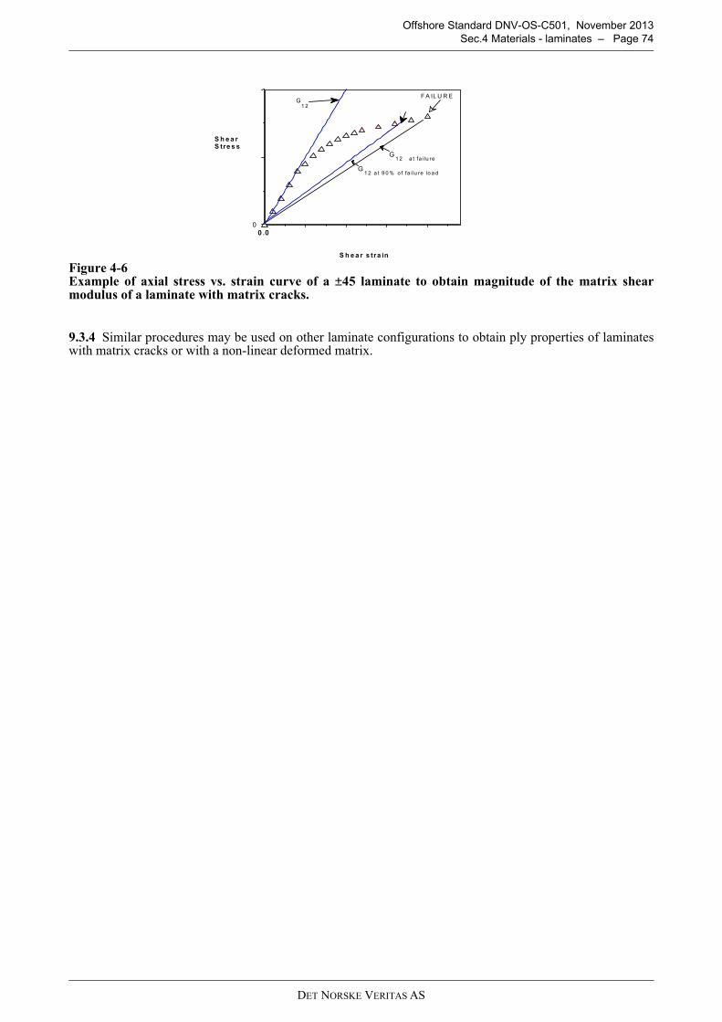
DET NORSKE VERITAS AS
Offshore Standard DNV-OS-C501, November 2013
Sec.4 Materials - laminates – Page 74
Figure 4-6 Example of axial stress vs. strain curve of a ±45 laminate to obtain magnitude of the matrix shearmodulus of a laminate with matrix cracks.
9.3.4 Similar procedures may be used on other laminate configurations to obtain ply properties of laminateswith matrix cracks or with a non-linear deformed matrix.
0 .00 .0
0
S h e a r s tra in
S h e a rS tre s s
G1 2
G1 2 a t fa ilu re
F A IL U R E
G1 2 a t 9 0 % o f fa ilu re lo a d
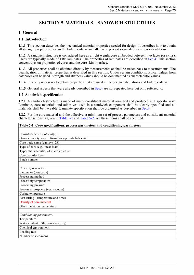
DET NORSKE VERITAS AS
Offshore Standard DNV-OS-C501, November 2013
Sec.5 Materials – sandwich structures – Page 75
SECTION 5 MATERIALS – SANDWICH STRUCTURES
1 General
1.1 Introduction
1.1.1 This section describes the mechanical material properties needed for design. It describes how to obtainall strength properties used in the failure criteria and all elastic properties needed for stress calculations.
1.1.2 A sandwich structure is considered here as a light weight core embedded between two faces (or skins).Faces are typically made of FRP laminates. The properties of laminates are described in Sec.4. This sectionconcentrates on properties of cores and the core skin interface.
1.1.3 All properties shall be obtained directly by measurements or shall be traced back to measurements. Thequalification of material properties is described in this section. Under certain conditions, typical values fromdatabases can be used. Strength and stiffness values should be documented as characteristic values.
1.1.4 It is only necessary to obtain properties that are used in the design calculations and failure criteria.
1.1.5 General aspects that were already described in Sec.4 are not repeated here but only referred to.
1.2 Sandwich specification
1.2.1 A sandwich structure is made of many constituent material arranged and produced in a specific way.Laminate, core materials and adhesives used in a sandwich component shall be clearly specified and allmaterials shall be traceable. Laminate specification shall be organised as described in Sec.4.
1.2.2 For the core material and the adhesive, a minimum set of process parameters and constituent materialcharacterisations is given in Table 5-1 and Table 5-2. All these items shall be specified.
Table 5-1 Core specifications, process parameters and conditioning parameters
Constituent core material(s):
Generic core type (e.g. foam, honeycomb, balsa etc.)
Core trade name (e.g. xyz123)
Type of core (e.g. linear foam)
Type/ characteristics of microstructure
Core manufacturer
Batch number
Process parameters:
Laminator (company)
Processing method
Processing temperature
Processing pressure
Process atmosphere (e.g. vacuum)
Curing temperature
Post curing (temperature and time)
Density of core material
Glass transition temperature
Conditioning parameters:
Temperature
Water content of the core (wet, dry)
Chemical environment
Loading rate
Number of specimens
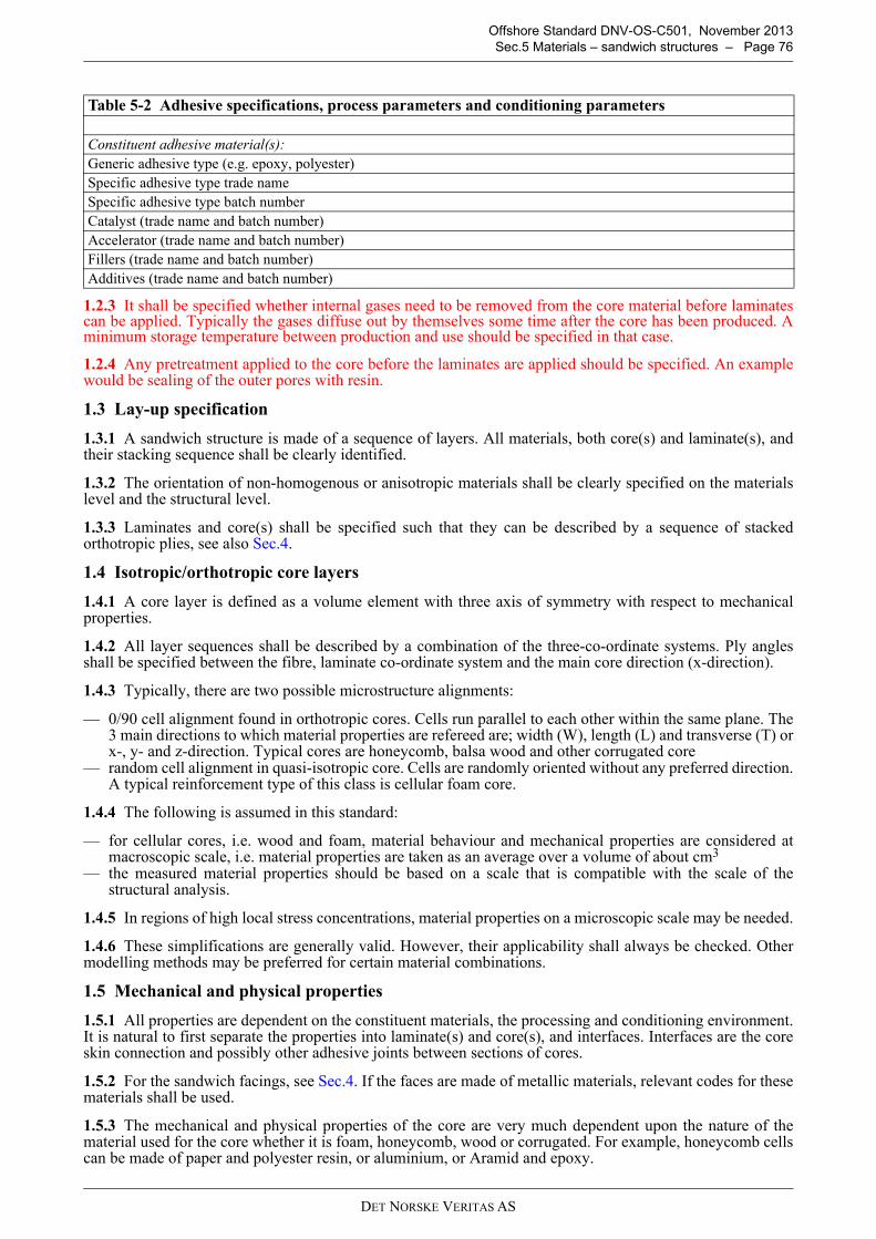
DET NORSKE VERITAS AS
Offshore Standard DNV-OS-C501, November 2013
Sec.5 Materials – sandwich structures – Page 76
1.2.3 It shall be specified whether internal gases need to be removed from the core material before laminatescan be applied. Typically the gases diffuse out by themselves some time after the core has been produced. Aminimum storage temperature between production and use should be specified in that case.
1.2.4 Any pretreatment applied to the core before the laminates are applied should be specified. An examplewould be sealing of the outer pores with resin.
1.3 Lay-up specification
1.3.1 A sandwich structure is made of a sequence of layers. All materials, both core(s) and laminate(s), andtheir stacking sequence shall be clearly identified.
1.3.2 The orientation of non-homogenous or anisotropic materials shall be clearly specified on the materialslevel and the structural level.
1.3.3 Laminates and core(s) shall be specified such that they can be described by a sequence of stackedorthotropic plies, see also Sec.4.
1.4 Isotropic/orthotropic core layers
1.4.1 A core layer is defined as a volume element with three axis of symmetry with respect to mechanicalproperties.
1.4.2 All layer sequences shall be described by a combination of the three-co-ordinate systems. Ply anglesshall be specified between the fibre, laminate co-ordinate system and the main core direction (x-direction).
1.4.3 Typically, there are two possible microstructure alignments:
— 0/90 cell alignment found in orthotropic cores. Cells run parallel to each other within the same plane. The3 main directions to which material properties are refereed are; width (W), length (L) and transverse (T) orx-, y- and z-direction. Typical cores are honeycomb, balsa wood and other corrugated core
— random cell alignment in quasi-isotropic core. Cells are randomly oriented without any preferred direction.A typical reinforcement type of this class is cellular foam core.
1.4.4 The following is assumed in this standard:
— for cellular cores, i.e. wood and foam, material behaviour and mechanical properties are considered atmacroscopic scale, i.e. material properties are taken as an average over a volume of about cm3
— the measured material properties should be based on a scale that is compatible with the scale of thestructural analysis.
1.4.5 In regions of high local stress concentrations, material properties on a microscopic scale may be needed.
1.4.6 These simplifications are generally valid. However, their applicability shall always be checked. Othermodelling methods may be preferred for certain material combinations.
1.5 Mechanical and physical properties
1.5.1 All properties are dependent on the constituent materials, the processing and conditioning environment.It is natural to first separate the properties into laminate(s) and core(s), and interfaces. Interfaces are the coreskin connection and possibly other adhesive joints between sections of cores.
1.5.2 For the sandwich facings, see Sec.4. If the faces are made of metallic materials, relevant codes for thesematerials shall be used.
1.5.3 The mechanical and physical properties of the core are very much dependent upon the nature of thematerial used for the core whether it is foam, honeycomb, wood or corrugated. For example, honeycomb cellscan be made of paper and polyester resin, or aluminium, or Aramid and epoxy.
Table 5-2 Adhesive specifications, process parameters and conditioning parameters
Constituent adhesive material(s):
Generic adhesive type (e.g. epoxy, polyester)
Specific adhesive type trade name
Specific adhesive type batch number
Catalyst (trade name and batch number)
Accelerator (trade name and batch number)
Fillers (trade name and batch number)
Additives (trade name and batch number)
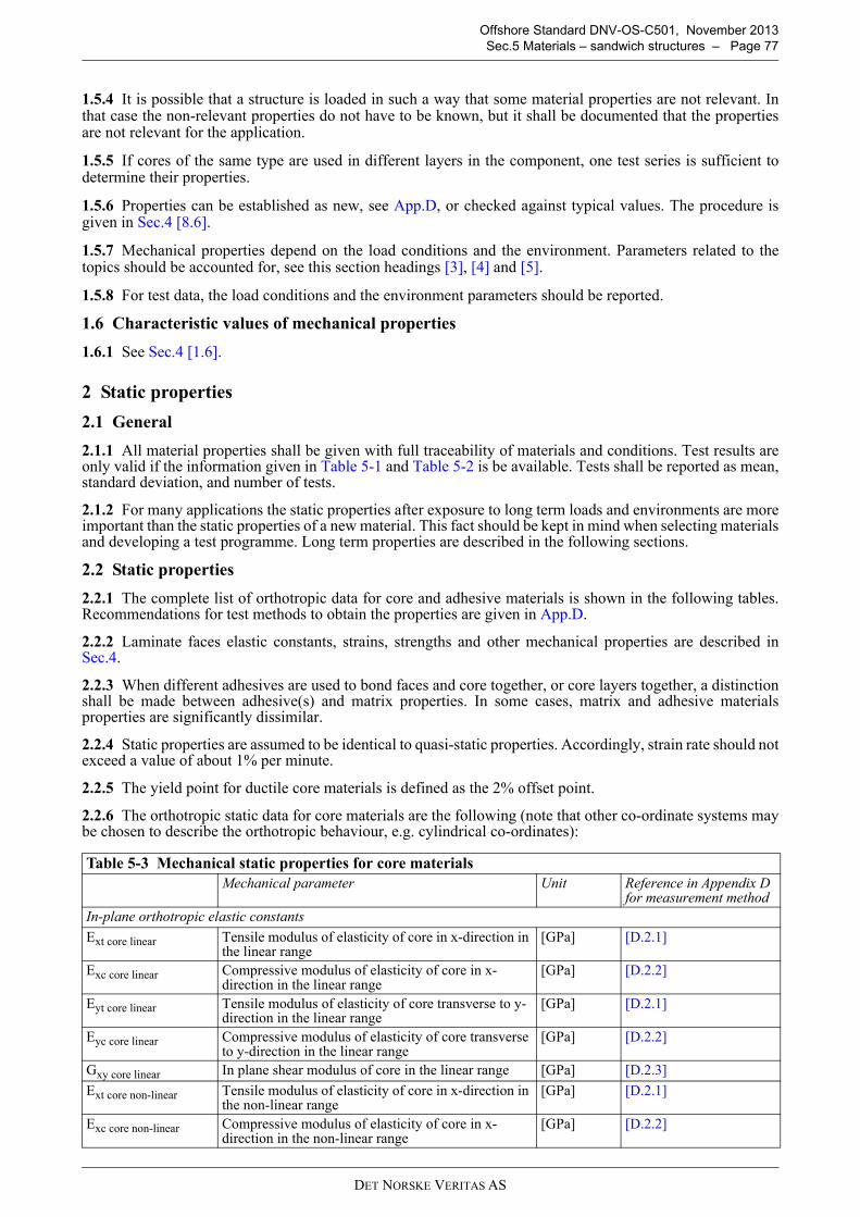
DET NORSKE VERITAS AS
Offshore Standard DNV-OS-C501, November 2013
Sec.5 Materials – sandwich structures – Page 77
1.5.4 It is possible that a structure is loaded in such a way that some material properties are not relevant. Inthat case the non-relevant properties do not have to be known, but it shall be documented that the propertiesare not relevant for the application.
1.5.5 If cores of the same type are used in different layers in the component, one test series is sufficient todetermine their properties.
1.5.6 Properties can be established as new, see App.D, or checked against typical values. The procedure isgiven in Sec.4 [8.6].
1.5.7 Mechanical properties depend on the load conditions and the environment. Parameters related to thetopics should be accounted for, see this section headings [3], [4] and [5].
1.5.8 For test data, the load conditions and the environment parameters should be reported.
1.6 Characteristic values of mechanical properties
1.6.1 See Sec.4 [1.6].
2 Static properties
2.1 General
2.1.1 All material properties shall be given with full traceability of materials and conditions. Test results areonly valid if the information given in Table 5-1 and Table 5-2 is be available. Tests shall be reported as mean,standard deviation, and number of tests.
2.1.2 For many applications the static properties after exposure to long term loads and environments are moreimportant than the static properties of a new material. This fact should be kept in mind when selecting materialsand developing a test programme. Long term properties are described in the following sections.
2.2 Static properties
2.2.1 The complete list of orthotropic data for core and adhesive materials is shown in the following tables.Recommendations for test methods to obtain the properties are given in App.D.
2.2.2 Laminate faces elastic constants, strains, strengths and other mechanical properties are described inSec.4.
2.2.3 When different adhesives are used to bond faces and core together, or core layers together, a distinctionshall be made between adhesive(s) and matrix properties. In some cases, matrix and adhesive materialsproperties are significantly dissimilar.
2.2.4 Static properties are assumed to be identical to quasi-static properties. Accordingly, strain rate should notexceed a value of about 1% per minute.
2.2.5 The yield point for ductile core materials is defined as the 2% offset point.
2.2.6 The orthotropic static data for core materials are the following (note that other co-ordinate systems maybe chosen to describe the orthotropic behaviour, e.g. cylindrical co-ordinates):
Table 5-3 Mechanical static properties for core materials
Mechanical parameter Unit Reference in Appendix D for measurement method
In-plane orthotropic elastic constants
Ext core linear Tensile modulus of elasticity of core in x-direction in the linear range
[GPa] [D.2.1]
Exc core linear Compressive modulus of elasticity of core in x-direction in the linear range
[GPa] [D.2.2]
Eyt core linear Tensile modulus of elasticity of core transverse to y-direction in the linear range
[GPa] [D.2.1]
Eyc core linear Compressive modulus of elasticity of core transverse to y-direction in the linear range
[GPa] [D.2.2]
Gxy core linear In plane shear modulus of core in the linear range [GPa] [D.2.3]
Ext core non-linear Tensile modulus of elasticity of core in x-direction in the non-linear range
[GPa] [D.2.1]
Exc core non-linear Compressive modulus of elasticity of core in x-direction in the non-linear range
[GPa] [D.2.2]
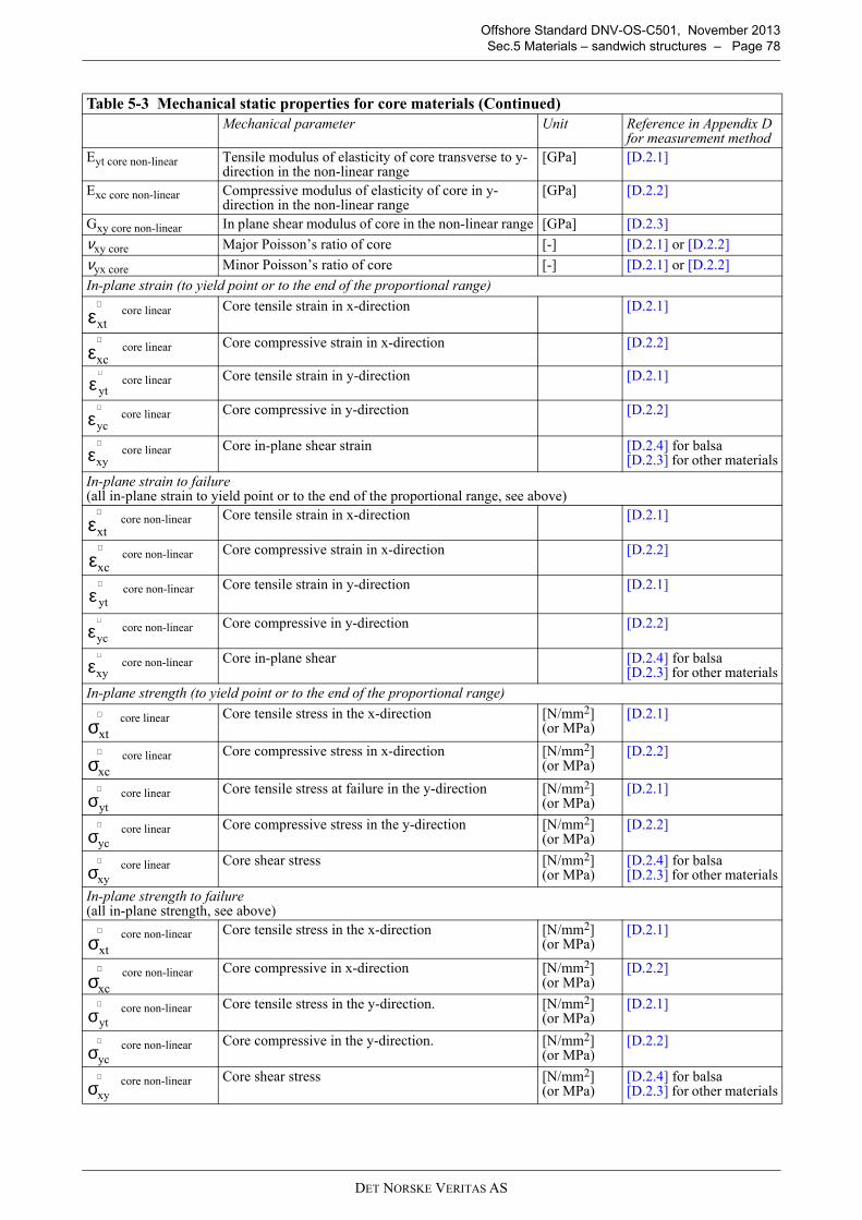
DET NORSKE VERITAS AS
Offshore Standard DNV-OS-C501, November 2013
Sec.5 Materials – sandwich structures – Page 78
Eyt core non-linear Tensile modulus of elasticity of core transverse to y-direction in the non-linear range
[GPa] [D.2.1]
Exc core non-linear Compressive modulus of elasticity of core in y-direction in the non-linear range
[GPa] [D.2.2]
Gxy core non-linear In plane shear modulus of core in the non-linear range [GPa] [D.2.3]
νxy core Major Poisson’s ratio of core [-] [D.2.1] or [D.2.2]
νyx core Minor Poisson’s ratio of core [-] [D.2.1] or [D.2.2]
In-plane strain (to yield point or to the end of the proportional range)
core linear Core tensile strain in x-direction [D.2.1]
core linear Core compressive strain in x-direction [D.2.2]
core linear Core tensile strain in y-direction [D.2.1]
core linear Core compressive in y-direction [D.2.2]
core linear Core in-plane shear strain [D.2.4] for balsa[D.2.3] for other materials
In-plane strain to failure(all in-plane strain to yield point or to the end of the proportional range, see above)
core non-linear Core tensile strain in x-direction [D.2.1]
core non-linear Core compressive strain in x-direction [D.2.2]
core non-linear Core tensile strain in y-direction [D.2.1]
core non-linear Core compressive in y-direction [D.2.2]
core non-linear Core in-plane shear [D.2.4] for balsa[D.2.3] for other materials
In-plane strength (to yield point or to the end of the proportional range)
core linear Core tensile stress in the x-direction [N/mm2](or MPa)
[D.2.1]
core linear Core compressive stress in x-direction [N/mm2](or MPa)
[D.2.2]
core linear Core tensile stress at failure in the y-direction [N/mm2](or MPa)
[D.2.1]
core linear Core compressive stress in the y-direction [N/mm2](or MPa)
[D.2.2]
core linear Core shear stress [N/mm2](or MPa)
[D.2.4] for balsa[D.2.3] for other materials
In-plane strength to failure(all in-plane strength, see above)
core non-linear Core tensile stress in the x-direction [N/mm2](or MPa)
[D.2.1]
core non-linear Core compressive in x-direction [N/mm2](or MPa)
[D.2.2]
core non-linear Core tensile stress in the y-direction. [N/mm2](or MPa)
[D.2.1]
core non-linear Core compressive in the y-direction. [N/mm2](or MPa)
[D.2.2]
core non-linear Core shear stress [N/mm2](or MPa)
[D.2.4] for balsa[D.2.3] for other materials
Table 5-3 Mechanical static properties for core materials (Continued)
Mechanical parameter Unit Reference in Appendix D for measurement method
xtε∧
xcε∧
ytε∧
ycε∧
xyε∧
xtε∧
xcε∧
ytε∧
ycε∧
xyε∧
xtσ∧
xcσ∧
ytσ∧
ycσ∧
xyσ∧
xtσ∧
xcσ∧
ytσ∧
ycσ∧
xyσ∧
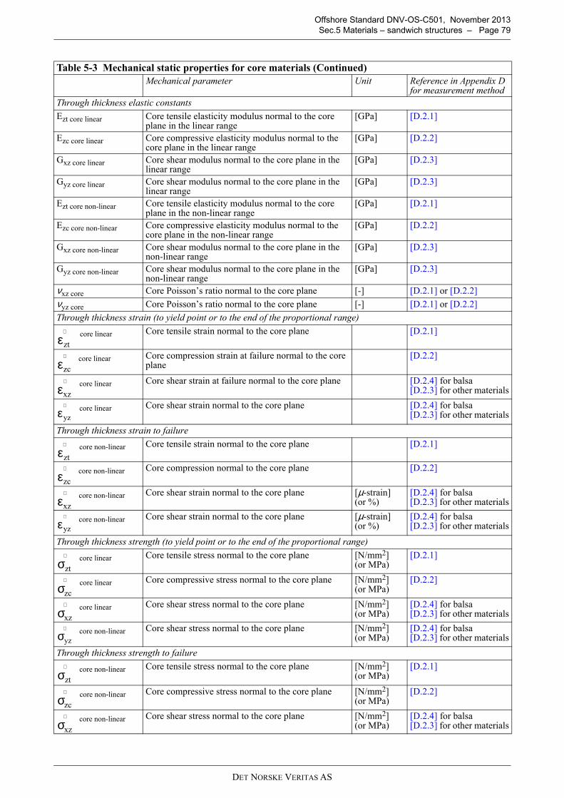
DET NORSKE VERITAS AS
Offshore Standard DNV-OS-C501, November 2013
Sec.5 Materials – sandwich structures – Page 79
Through thickness elastic constants
Ezt core linear Core tensile elasticity modulus normal to the core plane in the linear range
[GPa] [D.2.1]
Ezc core linear Core compressive elasticity modulus normal to the core plane in the linear range
[GPa] [D.2.2]
Gxz core linear Core shear modulus normal to the core plane in the linear range
[GPa] [D.2.3]
Gyz core linear Core shear modulus normal to the core plane in the linear range
[GPa] [D.2.3]
Ezt core non-linear Core tensile elasticity modulus normal to the core plane in the non-linear range
[GPa] [D.2.1]
Ezc core non-linear Core compressive elasticity modulus normal to the core plane in the non-linear range
[GPa] [D.2.2]
Gxz core non-linear Core shear modulus normal to the core plane in the non-linear range
[GPa] [D.2.3]
Gyz core non-linear Core shear modulus normal to the core plane in the non-linear range
[GPa] [D.2.3]
νxz core Core Poisson’s ratio normal to the core plane [-] [D.2.1] or [D.2.2]
νyz core Core Poisson’s ratio normal to the core plane [-] [D.2.1] or [D.2.2]
Through thickness strain (to yield point or to the end of the proportional range)
core linear Core tensile strain normal to the core plane [D.2.1]
core linear Core compression strain at failure normal to the core plane
[D.2.2]
core linear Core shear strain at failure normal to the core plane [D.2.4] for balsa[D.2.3] for other materials
core linear Core shear strain normal to the core plane [D.2.4] for balsa[D.2.3] for other materials
Through thickness strain to failure
core non-linear Core tensile strain normal to the core plane [D.2.1]
core non-linear Core compression normal to the core plane [D.2.2]
core non-linear Core shear strain normal to the core plane [µ-strain](or %)
[D.2.4] for balsa[D.2.3] for other materials
core non-linear Core shear strain normal to the core plane [µ-strain](or %)
[D.2.4] for balsa[D.2.3] for other materials
Through thickness strength (to yield point or to the end of the proportional range)
core linear Core tensile stress normal to the core plane [N/mm2](or MPa)
[D.2.1]
core linear Core compressive stress normal to the core plane [N/mm2](or MPa)
[D.2.2]
core linear Core shear stress normal to the core plane [N/mm2](or MPa)
[D.2.4] for balsa[D.2.3] for other materials
core non-linear Core shear stress normal to the core plane [N/mm2](or MPa)
[D.2.4] for balsa[D.2.3] for other materials
Through thickness strength to failure
core non-linear Core tensile stress normal to the core plane [N/mm2](or MPa)
[D.2.1]
core non-linear Core compressive stress normal to the core plane [N/mm2](or MPa)
[D.2.2]
core non-linear Core shear stress normal to the core plane [N/mm2](or MPa)
[D.2.4] for balsa[D.2.3] for other materials
Table 5-3 Mechanical static properties for core materials (Continued)
Mechanical parameter Unit Reference in Appendix D for measurement method
ztε∧
zcε∧
xzε∧
yzε∧
ztε∧
zcε∧
xzε∧
yzε∧
ztσ∧
zcσ∧
xzσ∧
yzσ∧
ztσ∧
zcσ∧
xzσ∧
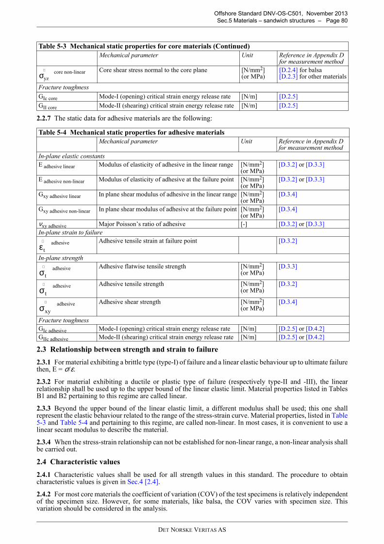
DET NORSKE VERITAS AS
Offshore Standard DNV-OS-C501, November 2013
Sec.5 Materials – sandwich structures – Page 80
2.2.7 The static data for adhesive materials are the following:
2.3 Relationship between strength and strain to failure
2.3.1 For material exhibiting a brittle type (type-I) of failure and a linear elastic behaviour up to ultimate failurethen, E = σ/ε.
2.3.2 For material exhibiting a ductile or plastic type of failure (respectively type-II and -III), the linearrelationship shall be used up to the upper bound of the linear elastic limit. Material properties listed in TablesB1 and B2 pertaining to this regime are called linear.
2.3.3 Beyond the upper bound of the linear elastic limit, a different modulus shall be used; this one shallrepresent the elastic behaviour related to the range of the stress-strain curve. Material properties, listed in Table5-3 and Table 5-4 and pertaining to this regime, are called non-linear. In most cases, it is convenient to use alinear secant modulus to describe the material.
2.3.4 When the stress-strain relationship can not be established for non-linear range, a non-linear analysis shallbe carried out.
2.4 Characteristic values
2.4.1 Characteristic values shall be used for all strength values in this standard. The procedure to obtaincharacteristic values is given in Sec.4 [2.4].
2.4.2 For most core materials the coefficient of variation (COV) of the test specimens is relatively independentof the specimen size. However, for some materials, like balsa, the COV varies with specimen size. Thisvariation should be considered in the analysis.
core non-linear Core shear stress normal to the core plane [N/mm2](or MPa)
[D.2.4] for balsa[D.2.3] for other materials
Fracture toughness
GIc core Mode-I (opening) critical strain energy release rate [N/m] [D.2.5]
GII core Mode-II (shearing) critical strain energy release rate [N/m] [D.2.5]
Table 5-4 Mechanical static properties for adhesive materials
Mechanical parameter Unit Reference in Appendix D for measurement method
In-plane elastic constants
E adhesive linear Modulus of elasticity of adhesive in the linear range [N/mm2](or MPa)
[D.3.2] or [D.3.3]
E adhesive non-linear Modulus of elasticity of adhesive at the failure point [N/mm2](or MPa)
[D.3.2] or [D.3.3]
Gxy adhesive linear In plane shear modulus of adhesive in the linear range [N/mm2](or MPa)
[D.3.4]
Gxy adhesive non-linear In plane shear modulus of adhesive at the failure point [N/mm2](or MPa)
[D.3.4]
νxy adhesive Major Poisson’s ratio of adhesive [-] [D.3.2] or [D.3.3]
In-plane strain to failure
adhesive Adhesive tensile strain at failure point [D.3.2]
In-plane strength
adhesive Adhesive flatwise tensile strength [N/mm2](or MPa)
[D.3.3]
adhesive Adhesive tensile strength [N/mm2](or MPa)
[D.3.2]
adhesive Adhesive shear strength [N/mm2](or MPa)
[D.3.4]
Fracture toughness
GIc adhesive Mode-I (opening) critical strain energy release rate [N/m] [D.2.5] or [D.4.2]
GIIc adhesive Mode-II (shearing) critical strain energy release rate [N/m] [D.2.5] or [D.4.2]
Table 5-3 Mechanical static properties for core materials (Continued)
Mechanical parameter Unit Reference in Appendix D for measurement method
yzσ∧
tε∧
tσ∧
tσ∧
xyσ∧
DET NORSKE VERITAS AS
Offshore Standard DNV-OS-C501, November 2013
Sec.5 Materials – sandwich structures – Page 81
2.4.3 Balsa sandwich structures show a reduction of COV with specimen size. If global properties are neededthe COV of large specimens may be used. If local properties are needed, e.g., for a joint analysis, COV valuesof the critical dimensions in the analysis shall be used.
2.5 Shear properties
2.5.1 Shear properties of core materials are difficult to measure. Suitable test methods should be used for thedetermination of shear design properties, see Sec.5 [2.2] and App.D. When using data from the literature, itshould be checked that the proper test methods are used.
Guidance note:
Using the block shear tests data to obtain the shear strength of balsa beams and panels will in many relevant casesoverestimates the shear strength by a factor of 2 to 4. Block shear test, such as the one used in ASTM C 273-00 orISO 1922, should not be used to obtain design shear strength of balsa cored sandwich beams and panels. The flexuraltest method used in ASTM C 393-00 can be used instead, see App.D.
---e-n-d---of---G-u-i-d-a-n-c-e---n-o-t-e---
2.5.2 Ideally the test method shall measure core yield or ultimate strength that is independent of the specimengeometry and that can be used for all structural geometry. If such a method cannot be found, e.g. for materialslike balsa, corrections may have to be applied to the test results. Typical effects that require corrections arechange in core thickness, change in skin thickness, in-plane size, effects of bending and shear loadsuperposition.
2.5.3 For polymeric cellular material the effects due to size and bending/shear load superposition on shearproperties are negligible.
2.5.4 For honeycomb materials thickness correction factor should be applied to strengths and moduli, whenusing other thickness than those available from test data or from the literature. Mechanical properties areusually available from manufacturers according to material, density, cell size, and thickness.
2.5.5 For balsa wood material there are two important size effects: core thickness size effect and an in-planesize effect. Further, the influence of bending and shear load superposition is significant and reduces the shearstrength.
2.5.6 For balsa wood material the value of the ultimate shear strength obtained from test results should onlybe used directly for the design of balsa-cored sandwich structures having identical geometrical, physical andloading characteristics as the test specimens. Otherwise the shear strength should be corrected.
2.5.7 If the core thickness of the component is less than the thickness of the test specimens a core thicknesscorrection is not necessary. This is a conservative simplification.
2.5.8 The corrected shear strength should be calculated as follows:
For sandwich beams as
and for sandwich panels as , where,
— τref is the mean value of the shear strengths measured from the reference specimen— ftc is a correction factor for the effect of core thickness— fi is a correction factor for the in-plane size of the sandwich beam— fip is a correction factor for the in-plane size of the sandwich panel— fb is a correction factor accounting for the effect of bending.
2.5.9 The correction factors can be obtained experimentally by testing specimens of at least three differentdimensions. The corrections factors are based on Weibull theory. A method to obtain the correction factorsexperimentally is described in McGeorge, D and Hayman B.: “Shear Strength of balsa-cored-sandwichpanels”, in proceedings of the 4th international conference on sandwich construction, Olsson, K-A (Ed), EMASPublishing, UK, 1998. The factors are given in Table 5-5.
bitc.refcorrected fffτ=τbiptc.refcorrecetd fffτ=τ
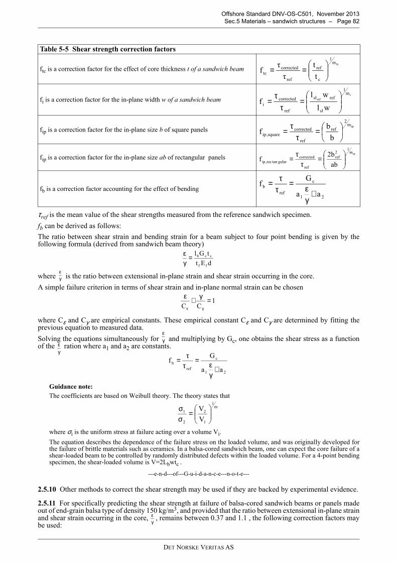
DET NORSKE VERITAS AS
Offshore Standard DNV-OS-C501, November 2013
Sec.5 Materials – sandwich structures – Page 82
τref is the mean value of the shear strengths measured from the reference sandwich specimen.
fb can be derived as follows:
The ratio between shear strain and bending strain for a beam subject to four point bending is given by thefollowing formula (derived from sandwich beam theory)
where is the ratio between extensional in-plane strain and shear strain occurring in the core.
A simple failure criterion in terms of shear strain and in-plane normal strain can be chosen
where Cε and Cγ are empirical constants. These empirical constant Cε and Cγ are determined by fitting theprevious equation to measured data.
Solving the equations simultaneously for and multiplying by Gc, one obtains the shear stress as a functionof the ration where a1 and a2 are constants.
Guidance note:
The coefficients are based on Weibull theory. The theory states that
where σi is the uniform stress at failure acting over a volume Vi.
The equation describes the dependence of the failure stress on the loaded volume, and was originally developed forthe failure of brittle materials such as ceramics. In a balsa-cored sandwich beam, one can expect the core failure of ashear-loaded beam to be controlled by randomly distributed defects within the loaded volume. For a 4-point bendingspecimen, the shear-loaded volume is V=2Lbwtc .
---e-n-d---of---G-u-i-d-a-n-c-e---n-o-t-e---
2.5.10 Other methods to correct the shear strength may be used if they are backed by experimental evidence.
2.5.11 For specifically predicting the shear strength at failure of balsa-cored sandwich beams or panels madeout of end-grain balsa type of density 150 kg/m3, and provided that the ratio between extensional in-plane strainand shear strain occurring in the core, , remains between 0.37 and 1.1 , the following correction factors maybe used:
Table 5-5 Shear strength correction factors
ftc is a correction factor for the effect of core thickness t of a sandwich beam
fi is a correction factor for the in-plane width w of a sandwich beam
fip is a correction factor for the in-plane size b of square panels
fip is a correction factor for the in-plane size ab of rectangular panels
fb is a correction factor accounting for the effect of bending
tcm1
c
ref
ref
correctedtc
t
t
τ
τf
==
i
ref
m1
sl
refsl
ref
correctedi
wl
wlf
=
ττ
=
ipm2
ref
ref
correctedsquare,ip
b
bf
=τ
τ=
ipm1
2ref
ref
correctedgulartanrec,ip
ab
b2f
=
ττ
=
21
c
ref
b
aa
Gf
+γε
=ττ=
dEt
tGl
ff
ccb=γε
γε
1CC
=γ+ε
γε
γε
γε
21
c
ref
b
aa
Gf
+γε
=ττ=
m1
1
2
2
1
V
V
=
σσ
γε
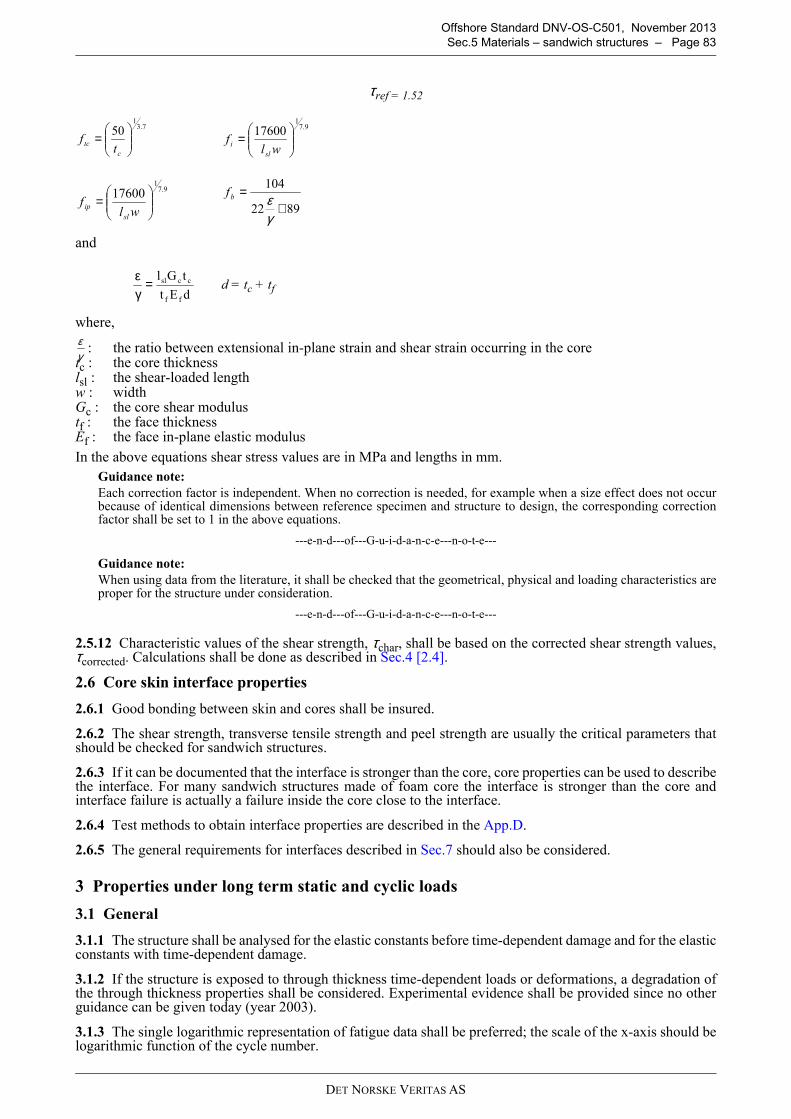
DET NORSKE VERITAS AS
Offshore Standard DNV-OS-C501, November 2013
Sec.5 Materials – sandwich structures – Page 83
τref = 1.52
and
where,
: the ratio between extensional in-plane strain and shear strain occurring in the coretc : the core thicknesslsl : the shear-loaded lengthw : widthGc : the core shear modulustf : the face thicknessEf : the face in-plane elastic modulus
In the above equations shear stress values are in MPa and lengths in mm.
Guidance note:
Each correction factor is independent. When no correction is needed, for example when a size effect does not occurbecause of identical dimensions between reference specimen and structure to design, the corresponding correctionfactor shall be set to 1 in the above equations.
---e-n-d---of---G-u-i-d-a-n-c-e---n-o-t-e---
Guidance note:
When using data from the literature, it shall be checked that the geometrical, physical and loading characteristics areproper for the structure under consideration.
---e-n-d---of---G-u-i-d-a-n-c-e---n-o-t-e---
2.5.12 Characteristic values of the shear strength, τchar, shall be based on the corrected shear strength values,τcorrected. Calculations shall be done as described in Sec.4 [2.4].
2.6 Core skin interface properties
2.6.1 Good bonding between skin and cores shall be insured.
2.6.2 The shear strength, transverse tensile strength and peel strength are usually the critical parameters thatshould be checked for sandwich structures.
2.6.3 If it can be documented that the interface is stronger than the core, core properties can be used to describethe interface. For many sandwich structures made of foam core the interface is stronger than the core andinterface failure is actually a failure inside the core close to the interface.
2.6.4 Test methods to obtain interface properties are described in the App.D.
2.6.5 The general requirements for interfaces described in Sec.7 should also be considered.
3 Properties under long term static and cyclic loads
3.1 General
3.1.1 The structure shall be analysed for the elastic constants before time-dependent damage and for the elasticconstants with time-dependent damage.
3.1.2 If the structure is exposed to through thickness time-dependent loads or deformations, a degradation ofthe through thickness properties shall be considered. Experimental evidence shall be provided since no otherguidance can be given today (year 2003).
3.1.3 The single logarithmic representation of fatigue data shall be preferred; the scale of the x-axis should belogarithmic function of the cycle number.
d = tc + tf
7.31
50
=
c
tct
f9.7
1
17600
=
wlf
sl
i
9.71
17600
=
wlf
sl
ip 8922
104
+=
γεbf
dEt
tGl
ff
ccsl=γε
γε
DET NORSKE VERITAS AS
Offshore Standard DNV-OS-C501, November 2013
Sec.5 Materials – sandwich structures – Page 84
3.1.4 For low and normal safety class, the effects of creep and stress relaxation may be ignored if the maximumstress does not exceed 10% of the characteristic strength and the loading time does not exceed 104 hours.
3.1.5 For low and normal safety class: the effects of cyclic fatigue may be ignored if the maximum stress doesnot exceed 10% of the characteristic strength and the number of cycles does not exceed 108.
3.1.6 See also Sec.4.
3.2 Creep
3.2.1 The application of a permanent load may lead to creep of the structure and of some of the constituentmaterial. This is described as a reduction of the modulus of elasticity.
3.2.2 Under the constant load, the increase of deformation results in an apparent reduction of the modulus ofelasticity, called creep modulus.
3.2.3 The creep of the composite sandwich structure is a combined effect of the creep of the matrix, adhesive,core and the fibres. However, creep is a phenomenon observed mainly in the matrix and mainly in the core.
3.2.4 Depending on the sandwich structure geometry and loading conditions, creep may occur principally inone constituent material. Creep deformation can then be neglected in the constituent materials bearing littlestress.
3.2.5 Ideally, creep shall be measured on the actual sandwich structure for the relevant loading condition.
3.2.6 Creep is dependant on material, material density, stress level, temperature and loading time.
Guidance note:
For balsa - creep of end-grain balsa is independent on density at both room and elevated temperature.
For polymeric foam - creep of polymeric foam is dependant on density at room temperature and elevated temperature;long-term creep behaviour prediction can be estimated from short-term data using the time-temperature superpositionprinciple or curve fitting functions. For PVC foams, ductile foams exhibits larger creep than brittle foams.
For honeycomb - creep of Nomex honeycomb is dependant of density at room temperature and elevated temperature.
---e-n-d---of---G-u-i-d-a-n-c-e---n-o-t-e---
Guidance note:
Time-temperature superposition principle (TTSP) can be used for the long-term prediction of creep of somepolymeric foam. The principle applied to some type of foams but not all; the fundament application is indeeddependant on the chemical nature of the polymer. So far, it has been showed that the TTSP is applicable to linear PVCfoam but not to cross linked PVC foam. For the latter curve fitting functions may be used to determine long-termproperties.
Shift parameters for the determination of tensile or compressive modulus (for the determination of long-term creepbehaviour using short-term data) may be different.
---e-n-d---of---G-u-i-d-a-n-c-e---n-o-t-e---
3.2.7 Creep of adhesive can be described in the same fashion as the creep of matrices in matrix-dominatedlaminate properties, see Sec.4.
3.3 Stress rupture under permanent static loads
3.3.1 The time to failure under a permanent static stress is described by a stress rupture curve.
3.3.2 The stress rupture curve may be described as:
log = log σ0stress rupture - β log t
or
= σ0stress rupture - β log t
3.3.3 where t is the time to failure under a permanent stress σ.
3.3.4 The material parameters σ0stress rupture and β shall be determined experimentally or be based on typicaldata as described in this section [8] and App.D.
3.3.5 Ideally, stress rupture shall be measured on the actual core for the relevant loading condition andenvironment.
3.4 Static strength reduction due to permanent static loads
3.4.1 If a sandwich structure is exposed to a permanent stress of any magnitude for a time t, the static strengthinfluenced by that stress, often called residual strength, shall be estimated from the stress rupture curve:
σ
σ
DET NORSKE VERITAS AS
Offshore Standard DNV-OS-C501, November 2013
Sec.5 Materials – sandwich structures – Page 85
log = log σ0stress rupture - β log t
or
= σ0stress rupture - β log t
3.4.2 Residual strains shall be obtained from the residual stress and the time dependent stiffness value.
3.4.3 If static strength reduction curve are not available, stress rupture curve may be used.
Guidance note:
Static strength values estimated from an stress rupture curves are typically conservative.
For low cycle fatigue, when a component is subjected to high load over a short fatigue lifetime, reduced static strengthmay be comparatively lower than estimated value from stress rupture curves.
---e-n-d---of---G-u-i-d-a-n-c-e---n-o-t-e---
3.4.4 If the stress rupture curve is used and is not linear in a log presentation, the static strength cannot becalculated by the above equation, but shall be taken directly from the stress rupture curve.
3.4.5 Higher static mechanical properties values may be used on the ground of experimental evidence. Theprocedure in [3.4] may be used.
3.5 Stress relaxation
3.5.1 Under the constant deformations, stress relaxation and/or residual strength reduction may occur.
3.5.2 Stress relaxation is a visco-elastic or plastic process reducing the stresses in the material. This effect isaccompanied by a reduction of the elastic modulus.
3.5.3 Residual strength reduction is defined as the static short-term strength of the material after creepconditioning.
3.5.4 Stress relaxation is a phenomenon mainly observed in the matrix and core materials. However, fibresmay also show some stress relaxation behaviour.
3.5.5 Ideally, stress relaxation should be measured on the actual core for the relevant loading condition.
3.5.6 In some cases, tensile stress relaxation data may be used to estimate stress relaxation in compression andvice-versa, as long as it can be shown to be an equivalent or conservative approach.
3.5.7 For FRP faces, the same paragraphs apply as in Sec.4.
3.6 Change of modulus of elasticity under cyclic fatigue
3.6.1 The reduction of stiffness or stability properties of sandwich structures due to cyclic fatigue should beconsidered. This reduction may be caused by:
— a reduction in modulus of elasticity in the facings materials and/or in the core(s) materials due to varioustypes of damage, e.g. micro cracks
— a local debonding between faces and core at the interface.
3.6.2 The proportion of the contributions in the modulus reduction of the facings and core varies according tothe geometrical, mechanical and loading specifications of the sandwich structure.
3.6.3 The change of modulus of elasticity of FRP facings and adhesives is described in Sec.4.
3.6.4 There can be a decrease of the value of the core elasticity modulus.
3.6.5 The reduction in core elasticity modulus differs according to materials and is dependant on loadingconditions, i.e. stress nature, stress level, load ratio, strain rate, exposure time.
Guidance note:
Creep can be induced under cyclic fatigue, especially for R ratio different from –1.
---e-n-d---of---G-u-i-d-a-n-c-e---n-o-t-e---
3.6.6 Experimental results may be used to demonstrate different changes of the elastic constants during cyclicfor specific cores or adhesives or loading conditions.
σ
σ
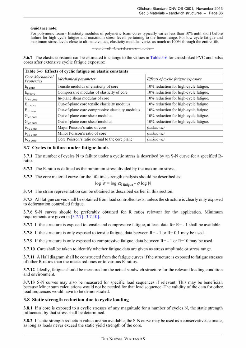
DET NORSKE VERITAS AS
Offshore Standard DNV-OS-C501, November 2013
Sec.5 Materials – sandwich structures – Page 86
Guidance note:
For polymeric foam - Elasticity modulus of polymeric foam cores typically varies less than 10% until short beforefailure for high cycle fatigue and maximum stress levels pertaining to the linear range. For low cycle fatigue andmaximum stress levels close to ultimate values, elasticity modulus varies as much as 100% through the entire life.
---e-n-d---of---G-u-i-d-a-n-c-e---n-o-t-e---
3.6.7 The elastic constants can be estimated to change to the values in Table 5-6 for crosslinked PVC and balsacores after extensive cyclic fatigue exposure:
3.7 Cycles to failure under fatigue loads
3.7.1 The number of cycles N to failure under a cyclic stress is described by an S-N curve for a specified R-ratio.
3.7.2 The R-ratio is defined as the minimum stress divided by the maximum stress.
3.7.3 The core material curve for the lifetime strength analysis should be described as:
log = log σ0 fatigue - α log N
3.7.4 The strain representation can be obtained as described earlier in this section.
3.7.5 All fatigue curves shall be obtained from load controlled tests, unless the structure is clearly only exposedto deformation controlled fatigue.
3.7.6 S-N curves should be preferably obtained for R ratios relevant for the application. Minimumrequirements are given in [3.7.7]-[3.7.10].
3.7.7 If the structure is exposed to tensile and compressive fatigue, at least data for R= - 1 shall be available.
3.7.8 If the structure is only exposed to tensile fatigue, data between R= - 1 or R= 0.1 may be used.
3.7.9 If the structure is only exposed to compressive fatigue, data between R= - 1 or R=10 may be used.
3.7.10 Care shall be taken to identify whether fatigue data are given as stress amplitude or stress range.
3.7.11 A Hall diagram shall be constructed from the fatigue curves if the structure is exposed to fatigue stressesof other R ratios than the measured ones or to various R-ratios.
3.7.12 Ideally, fatigue should be measured on the actual sandwich structure for the relevant loading conditionand environment.
3.7.13 S-N curves may also be measured for specific load sequences if relevant. This may be beneficial,because Miner sum calculations would not be needed for that load sequence. The validity of the data for otherload sequences would have to be demonstrated.
3.8 Static strength reduction due to cyclic loading
3.8.1 If a core is exposed to a cyclic stresses of any magnitude for a number of cycles N, the static strengthinfluenced by that stress shall be determined.
3.8.2 If static strength reduction values are not available, the S-N curve may be used as a conservative estimate,as long as loads never exceed the static yield strength of the core.
Table 5-6 Effects of cyclic fatigue on elastic constants
Core Mechanical Properties
Mechanical parameter Effects of cyclic fatigue exposure
Et core Tensile modulus of elasticity of core 10% reduction for high-cycle fatigue.
Ec core Compressive modulus of elasticity of core 10% reduction for high-cycle fatigue.
Gxy core In-plane shear modulus of core 10% reduction for high-cycle fatigue.
Ezt core Out-of-plane core tensile elasticity modulus 10% reduction for high-cycle fatigue
Ezc core Out-of-plane core compressive elasticity modulus 10% reduction for high-cycle fatigue.
Gxz core Out-of-plane core shear modulus 10% reduction for high-cycle fatigue.
Gyz core Out-of-plane core shear modulus 10% reduction for high-cycle fatigue.
νxy core Major Poisson’s ratio of core (unknown)
νyx core Minor Poisson’s ratio of core (unknown)
νxz core Core Poisson’s ratio normal to the core plane (unknown)
σ
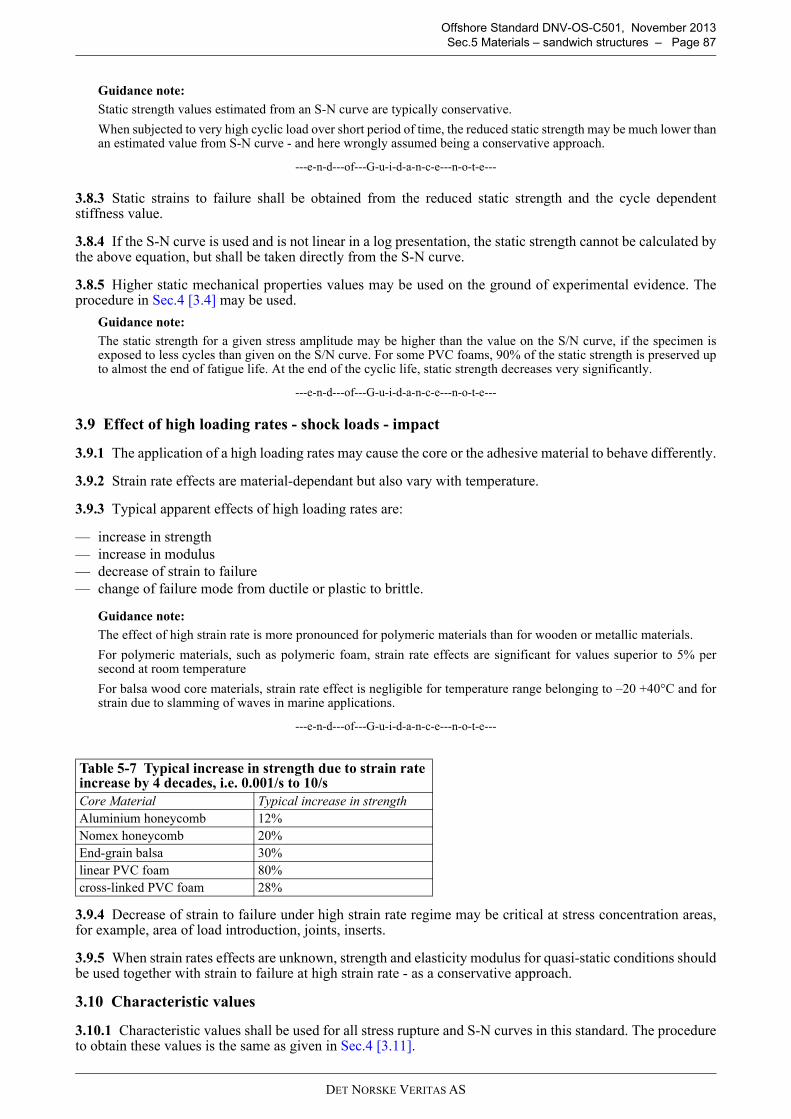
DET NORSKE VERITAS AS
Offshore Standard DNV-OS-C501, November 2013
Sec.5 Materials – sandwich structures – Page 87
Guidance note:
Static strength values estimated from an S-N curve are typically conservative.
When subjected to very high cyclic load over short period of time, the reduced static strength may be much lower thanan estimated value from S-N curve - and here wrongly assumed being a conservative approach.
---e-n-d---of---G-u-i-d-a-n-c-e---n-o-t-e---
3.8.3 Static strains to failure shall be obtained from the reduced static strength and the cycle dependentstiffness value.
3.8.4 If the S-N curve is used and is not linear in a log presentation, the static strength cannot be calculated bythe above equation, but shall be taken directly from the S-N curve.
3.8.5 Higher static mechanical properties values may be used on the ground of experimental evidence. Theprocedure in Sec.4 [3.4] may be used.
Guidance note:
The static strength for a given stress amplitude may be higher than the value on the S/N curve, if the specimen isexposed to less cycles than given on the S/N curve. For some PVC foams, 90% of the static strength is preserved upto almost the end of fatigue life. At the end of the cyclic life, static strength decreases very significantly.
---e-n-d---of---G-u-i-d-a-n-c-e---n-o-t-e---
3.9 Effect of high loading rates - shock loads - impact
3.9.1 The application of a high loading rates may cause the core or the adhesive material to behave differently.
3.9.2 Strain rate effects are material-dependant but also vary with temperature.
3.9.3 Typical apparent effects of high loading rates are:
— increase in strength— increase in modulus— decrease of strain to failure— change of failure mode from ductile or plastic to brittle.
Guidance note:
The effect of high strain rate is more pronounced for polymeric materials than for wooden or metallic materials.
For polymeric materials, such as polymeric foam, strain rate effects are significant for values superior to 5% persecond at room temperature
For balsa wood core materials, strain rate effect is negligible for temperature range belonging to –20 +40°C and forstrain due to slamming of waves in marine applications.
---e-n-d---of---G-u-i-d-a-n-c-e---n-o-t-e---
3.9.4 Decrease of strain to failure under high strain rate regime may be critical at stress concentration areas,for example, area of load introduction, joints, inserts.
3.9.5 When strain rates effects are unknown, strength and elasticity modulus for quasi-static conditions shouldbe used together with strain to failure at high strain rate - as a conservative approach.
3.10 Characteristic values
3.10.1 Characteristic values shall be used for all stress rupture and S-N curves in this standard. The procedureto obtain these values is the same as given in Sec.4 [3.11].
Table 5-7 Typical increase in strength due to strain rate increase by 4 decades, i.e. 0.001/s to 10/s
Core Material Typical increase in strength
Aluminium honeycomb 12%
Nomex honeycomb 20%
End-grain balsa 30%
linear PVC foam 80%
cross-linked PVC foam 28%
DET NORSKE VERITAS AS
Offshore Standard DNV-OS-C501, November 2013
Sec.5 Materials – sandwich structures – Page 88
4 Other properties
4.1 Thermal expansion coefficient
4.1.1 Thermal expansion coefficient of the cores in the relevant temperature range shall be measured in themain material directions.
4.1.2 Stresses due to thermal deformation shall be considered.
4.2 Swelling coefficient for water or other liquids
4.2.1 Swelling coefficient of the plies in the relevant temperature range shall be measured in the main materialdirections.
4.2.2 Stresses due to swelling shall be considered.
4.3 Diffusion coefficient
4.3.1 Relevant data shall be obtained as needed for the actual service and exposure of the component. Ifrelevant, the following material data may be required:
— diffusion rate through the thickness of the core— diffusion rate along the in-plane axis of the core— diffusion rate along the interfaces between core and skin.
4.3.2 A special property related to diffusion is vapour transmission. This value is sometime of importance forsandwich structures.
4.4 Thermal conductivity
4.4.1 Thermal conductivity may be anisotropic for cores. If relevant thermal conductivity shall be obtained.
4.5 Friction coefficient
4.5.1 Core materials are generally not exposed to friction. If they are the same procedure as given in Sec.4 shallbe applied.
4.6 Wear resistance
4.6.1 Core materials are generally not exposed to wear. If they are the same procedure as given in Sec.4 shallbe applied.
5 Influence of the environment on properties
5.1 Introduction
5.1.1 The environment can affects composites. Both adhesives and cores can be affected in different ways dueto their different chemical nature and micro-structure.
5.1.2 Void content and the presence of matrix cracks in the face laminates can indirectly influence theenvironmental resistance of the core and adhesive materials. Rapid and excessive water penetration can forexample damage quickly the interface bond between faces and core.
5.1.3 The nature of the core cells, whether closed or opened, influences very significantly the environmentalresistance of the core materials.
5.1.4 The quality of interface bonding between faces and cores, or between cores themselves can alsoinfluence the environmental resistance of the adhesive joints, and thereby the entire sandwich structure.
5.1.5 The local environmental conditions shall be taken into account for the documentation of all propertiesunder static and fatigue loads, as described above.
5.1.6 Degradation of joining structures shall also be documented, e.g. end enclosures, connections, corners, T-joints and other fasteners.
5.1.7 Cyclic environmental conditions shall be considered.
5.1.8 It shall be documented that the combined effects of cyclic loads, static load, and the environment are notworse than the separate effects.
5.1.9 The following conditions are considered:
— temperature
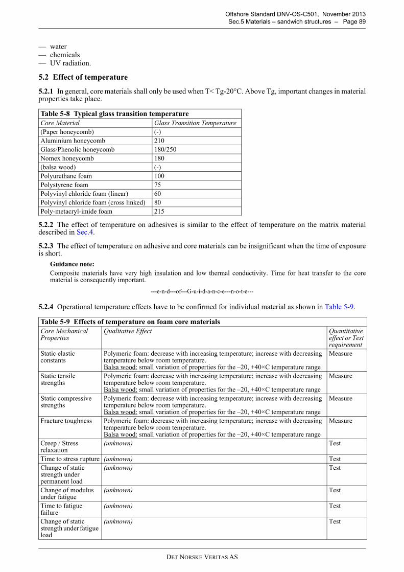
DET NORSKE VERITAS AS
Offshore Standard DNV-OS-C501, November 2013
Sec.5 Materials – sandwich structures – Page 89
— water— chemicals— UV radiation.
5.2 Effect of temperature
5.2.1 In general, core materials shall only be used when T< Tg-20°C. Above Tg, important changes in materialproperties take place.
5.2.2 The effect of temperature on adhesives is similar to the effect of temperature on the matrix materialdescribed in Sec.4.
5.2.3 The effect of temperature on adhesive and core materials can be insignificant when the time of exposureis short.
Guidance note:
Composite materials have very high insulation and low thermal conductivity. Time for heat transfer to the corematerial is consequently important.
---e-n-d---of---G-u-i-d-a-n-c-e---n-o-t-e---
5.2.4 Operational temperature effects have to be confirmed for individual material as shown in Table 5-9.
Table 5-8 Typical glass transition temperature
Core Material Glass Transition Temperature
(Paper honeycomb) (-)
Aluminium honeycomb 210
Glass/Phenolic honeycomb 180/250
Nomex honeycomb 180
(balsa wood) (-)
Polyurethane foam 100
Polystyrene foam 75
Polyvinyl chloride foam (linear) 60
Polyvinyl chloride foam (cross linked) 80
Poly-metacryl-imide foam 215
Table 5-9 Effects of temperature on foam core materials
Core Mechanical Properties
Qualitative Effect Quantitative effect or Test requirement
Static elastic constants
Polymeric foam: decrease with increasing temperature; increase with decreasing temperature below room temperature.Balsa wood: small variation of properties for the –20, +40×C temperature range
Measure
Static tensile strengths
Polymeric foam: decrease with increasing temperature; increase with decreasing temperature below room temperature.Balsa wood: small variation of properties for the –20, +40×C temperature range
Measure
Static compressive strengths
Polymeric foam: decrease with increasing temperature; increase with decreasing temperature below room temperature.Balsa wood: small variation of properties for the –20, +40×C temperature range
Measure
Fracture toughness Polymeric foam: decrease with increasing temperature; increase with decreasing temperature below room temperature.Balsa wood: small variation of properties for the –20, +40×C temperature range
Measure
Creep / Stress relaxation
(unknown) Test
Time to stress rupture (unknown) Test
Change of static strength under permanent load
(unknown) Test
Change of modulus under fatigue
(unknown) Test
Time to fatigue failure
(unknown) Test
Change of static strength under fatigue load
(unknown) Test
DET NORSKE VERITAS AS
Offshore Standard DNV-OS-C501, November 2013
Sec.5 Materials – sandwich structures – Page 90
5.2.5 In the case of recently-manufactured foam core materials used in sandwich structures, the effect of out-gassing under elevated temperature may induce subsequent delamination at the core-facing interface.
5.3 Effect of water
5.3.1 The effect of water on adhesive and core materials can be insignificant when the time of exposure isshort.
5.3.2 If the laminate of the sandwich protect the entire core and the adhesive from the exposure, the resistanceto water may be less critical. However, water diffuses through laminates and may degrade core properties.
5.3.3 Some core materials are specially treated or sealed to reduce any effects of water. The advantageouseffect of the treatment shall be documented. If the treated core material is used in a component a qualityprocedure shall ensure that no untreated core material is used.
5.3.4 The effect of water on cellular core materials is typically severe for open-cell micro-structure and muchless severe for closed-cell materials.
5.3.5 Moisture content has an important influence on the mechanical properties of wooden core materials.
5.3.6 Balsa and other wood core materials are very susceptible to water penetration and consequent swelling,debonding and rot, unless properly sealed and laminated.
Guidance note:
Flat-grain balsa (in which the grain lies parallel to the panel surface) has greater susceptibility to water permeationand is generally less satisfactory as a core material than 'End-grain balsa'.
---e-n-d---of---G-u-i-d-a-n-c-e---n-o-t-e---
5.3.7 Crosslinked PVC cores and specially sealed and treated end grain balsa cores have demonstrated nodegradation in a marine environment when embedded in typical laminates. Some documentation with respectto the resistance to a sea water environment shall be provided.
5.3.8 Resistance to water of core materials at high pressures in deep water is unknown and shall bedemonstrated if relevant.
5.3.9 The effect of seawater is generally less severe than the effect of fresh water.
5.3.10 The effect of distilled water is more severe than the effect of fresh water.
5.3.11 The combination of water and high temperature may be worse than the individual effects of temperatureand water.
5.3.12 In case of a core material permanently exposed to water, long term properties should be documented.
5.4 Effect of chemicals
5.4.1 The compatibility of cores and adhesives to the exposure to chemicals shall be demonstrated.
5.4.2 In a qualitative way chemicals tend to have the same effects as water on cores and adhesives. Thedegradation rates shall be obtained for the actual materials in question.
5.4.3 If the laminate of the sandwich protect the core and the adhesive from the exposure, the resistance tochemicals may be less critical. However, most chemicals can diffuse through laminates and may attack thecore.
5.5 Effect of UV radiation
5.5.1 Core materials are typically embedded in a laminate and are not exposed to direct UV radiation.
5.5.2 If core materials are exposed to UV radiation their resistance shall be documented and quantified ifnecessary.
5.6 Electrolytic corrosion
5.6.1 Possible electrolytic corrosion should be considered when metallic components and carbon fibres areused in a sandwich structure.
5.7 Combination of environmental effects
5.7.1 The combination of environmental effects on materials, like combined humidity and heat, may be worsethan the individual effects.
DET NORSKE VERITAS AS
Offshore Standard DNV-OS-C501, November 2013
Sec.5 Materials – sandwich structures – Page 91
5.7.2 Test data should be obtained of the combined effect of environments on the material properties ifrelevant. The worst relevant combination of environments should be used for testing.
6 Influence of process parameters and core density
6.1 Core production
6.1.1 Core materials are generally manufactured in a well-controlled process. This standard does not addressmanufacturing methods of core materials. It is assumed that the measured and reported core properties can bereproduced and guaranteed by the core manufacturer.
6.1.2 In some cases the core properties may be influenced by the joining methods used to join the skins or coresections. This aspect is described in [6.2].
6.2 Sandwich production
6.2.1 The skins are usually laminated onto the core or glued onto the core. Sections of the core may also bejoined with adhesives or some fillers.
6.2.2 The joints may influence the properties of the core either by modifying the core material itself or bybecoming part of the core system. Core properties shall be measured and evaluated with the presence of suchjoints.
6.2.3 Changes in process parameters effect joints in a similar way as described for the matrix in a laminate in[6].
6.3 Influence of core density
6.3.1 For core materials that are available in different densities, all mechanical properties shall be assumed todepend on the density unless evidence exists that suggests otherwise.
6.3.2 All relationships between properties and density shall be confirmed by experimental evidence for theparticular core type. Data may be interpolated, but should not be extrapolated to densities outside the measuredrange.
6.3.3 If a relationship can be established between core density and certain core properties qualification ofmaterial properties may be simplified as described in section [8.6].
7 Properties under fire
7.1 Introduction
7.1.1 The performance of composites in a fire is a complex process, because the various constituent materialsrespond differently to a fire.
7.1.2 The requirements under fire conditions can usually be found in the fire codes for a particular application.
7.1.3 Fire codes may implicitly assume that the structure is built of steel or metal. The relevance of a fire codeto composite materials shall be checked carefully.
7.1.4 Since most composites are flammable and temperature sensitive most applications use protectivemeasures to reduce the impact of fire. In this case the fire performance of the complete system, compositestructure with fire protection shall be evaluated.
7.1.5 Some aspects of fire performance can be modelled, but some experimental testing shall always be doneto demonstrate fire performance.
Guidance note:
Sandwich panels with no internal cavities, such as wood and foam core materials, will not allow any stack effect orneither help the transportation of combustion products. Conversely, sandwich structures with internal cavities willenhance these phenomenon.
---e-n-d---of---G-u-i-d-a-n-c-e---n-o-t-e---
7.2 Fire reaction
7.2.1 Fire reaction describes the response of a composite to fire in terms of flammability, flame spread, smokedevelopment and emission of toxic gases. All these aspects shall be documented if relevant.
7.2.2 Special additives or fillers are often added to composites to improve fire reaction.

DET NORSKE VERITAS AS
Offshore Standard DNV-OS-C501, November 2013
Sec.5 Materials – sandwich structures – Page 92
7.2.3 The influence of such additives or fillers on the basic mechanical properties shall be evaluated.
7.3 Fire resistance
7.3.1 Fire resistance describes the remaining strength of a composite structure under a fire.
7.3.2 As a first estimate of fire resistance, the temperature-dependent properties as described in [5.2] can be used.
7.3.3 The temperature within a sandwich component can be calculated by means of appropriate models.
7.3.4 If chemical reactions can occur within the sandwich component, their influence on the temperaturedistribution shall be considered.
7.3.5 Through thickness properties and core properties shall be carefully evaluated, especially in the region ofjoints.
Guidance note:
A panel with stiffeners may loose most of its stiffness if the stiffeners delaminate from the panel due to the fire.
---e-n-d---of---G-u-i-d-a-n-c-e---n-o-t-e---
7.4 Insulation
7.4.1 The properties of the insulation with respect to fire reaction and fire resistance shall be evaluated.
7.4.2 Special consideration shall be given to the joints of the insulation and the method the insulation isattached to the component. Attachment points and joints may create hot spots in the component.
7.4.3 All large scale testing shall be done with jointed insulation and the same attachments as used in the realapplication.
7.5 Properties after the fire
7.5.1 A fire is usually seen as an accidental load case and properties after the fire shall be evaluated for eachindividual case.
7.5.2 If the temperature has locally exceeded the Tg of the component it is very likely that permanent damagehas been made to the component in that area.
7.5.3 If the temperature remained locally under Tg damage may be introduced due to overloads from otherparts of the structure.
8 Qualification of material properties
8.1 Introduction
8.1.1 All material properties needed to describe the performance of a component shall be documented.
8.1.2 As a general principal, material properties should be obtained form test results of laminates that representthe laminates of the component as closely as possible.
8.1.3 Material properties may be documented by the following methods:
— direct measurements— qualification against representative data— qualification against manufacturers data— qualification against data from the open literature— qualification by component testing.
8.1.4 Each individual material property may be qualified by any of the different methods.
8.1.5 Which data can be used for qualification depends mainly on two aspects:
— were the data obtained form laminates that are similar to the laminates used in the component— were the data obtained from reputable sources.
8.2 General test requirements
8.2.1 All relevant information about the material tested, the test method, and the test conditions shallaccompany test results. The information requested in [1.2] shall be provided.
8.2.2 Static test results shall be reported as mean, standard deviation, coefficient of variation, and number oftest specimens. The characteristic values of static tests shall be calculated as described in Sec.4 [2.4].
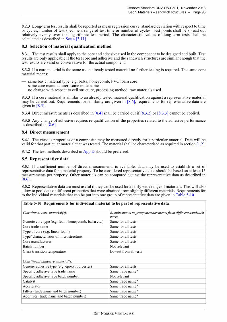
DET NORSKE VERITAS AS
Offshore Standard DNV-OS-C501, November 2013
Sec.5 Materials – sandwich structures – Page 93
8.2.3 Long-term test results shall be reported as mean regression curve, standard deviation with respect to timeor cycles, number of test specimen, range of test time or number of cycles. Test points shall be spread outrelatively evenly over the logarithmic test period. The characteristic values of long-term tests shall becalculated as described in Sec.4 [3.11].
8.3 Selection of material qualification method
8.3.1 The test results shall apply to the core and adhesive used in the component to be designed and built. Testresults are only applicable if the test core and adhesive and the sandwich structures are similar enough that thetest results are valid or conservative for the actual component.
8.3.2 If a core material is the same as an already tested material no further testing is required. The same corematerial means:
— same basic material type, e.g. balsa, honeycomb, PVC foam core— same core manufacturer, same trade name— no change with respect to cell structure, processing method, raw materials used.
8.3.3 If a core material is similar to an already tested material qualification against a representative materialmay be carried out. Requirements for similarity are given in [8.6], requirements for representative data aregiven in [8.5].
8.3.4 Direct measurements as described in [8.4] shall be carried out if [8.3.2] or [8.3.3] cannot be applied.
8.3.5 Any change of adhesive requires re-qualification of the properties related to the adhesive performanceas described in [8.6].
8.4 Direct measurement
8.4.1 The various properties of a composite may be measured directly for a particular material. Data will bevalid for that particular material that was tested. The material shall be characterised as required in section [1.2].
8.4.2 The test methods described in App.D should be preferred.
8.5 Representative data
8.5.1 If a sufficient number of direct measurements is available, data may be used to establish a set ofrepresentative data for a material property. To be considered representative, data should be based on at least 15measurements per property. Other materials can be compared against the representative data as described in[8.6].
8.5.2 Representative data are most useful if they can be used for a fairly wide range of materials. This will alsoallow to pool data of different properties that were obtained from slightly different materials. Requirements forto the individual materials that can be put into one group of representative data are given in Table 5-10.
Table 5-10 Requirements for individual material to be part of representative data
Constituent core material(s): Requirements to group measurements from different sandwich cores
Generic core type (e.g. foam, honeycomb, balsa etc.) Same for all tests
Core trade name Same for all tests
Type of core (e.g. linear foam) Same for all tests
Type/ characteristics of microstructure Same for all tests
Core manufacturer Same for all tests
Batch number Not relevant
Glass transition temperature Lowest from all tests
Constituent adhesive material(s):
Generic adhesive type (e.g. epoxy, polyester) Same for all tests
Specific adhesive type trade name Same trade name*
Specific adhesive type batch number Not relevant
Catalyst Same trade name*
Accelerator Same trade name*
Fillers (trade name and batch number) Same trade name*
Additives (trade name and batch number) Same trade name*
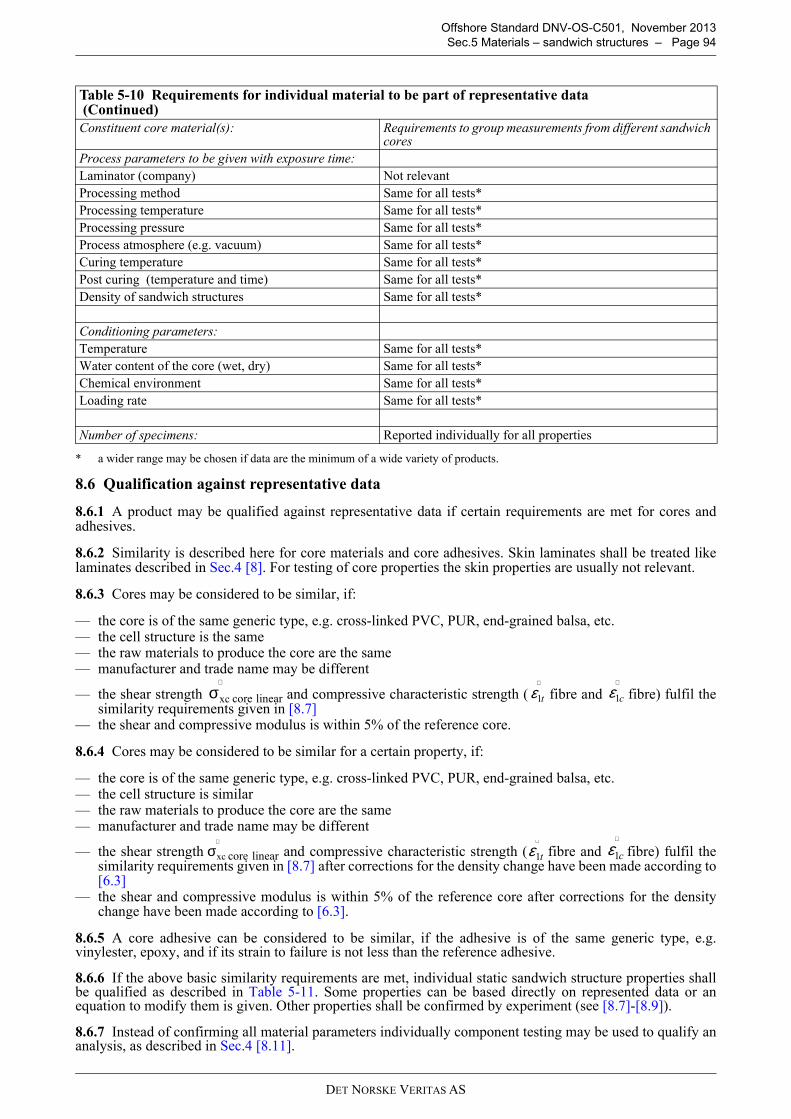
DET NORSKE VERITAS AS
Offshore Standard DNV-OS-C501, November 2013
Sec.5 Materials – sandwich structures – Page 94
* a wider range may be chosen if data are the minimum of a wide variety of products.
8.6 Qualification against representative data
8.6.1 A product may be qualified against representative data if certain requirements are met for cores andadhesives.
8.6.2 Similarity is described here for core materials and core adhesives. Skin laminates shall be treated likelaminates described in Sec.4 [8]. For testing of core properties the skin properties are usually not relevant.
8.6.3 Cores may be considered to be similar, if:
— the core is of the same generic type, e.g. cross-linked PVC, PUR, end-grained balsa, etc.— the cell structure is the same— the raw materials to produce the core are the same— manufacturer and trade name may be different
— the shear strength core linear and compressive characteristic strength ( fibre and fibre) fulfil thesimilarity requirements given in [8.7]
— the shear and compressive modulus is within 5% of the reference core.
8.6.4 Cores may be considered to be similar for a certain property, if:
— the core is of the same generic type, e.g. cross-linked PVC, PUR, end-grained balsa, etc.— the cell structure is similar— the raw materials to produce the core are the same— manufacturer and trade name may be different
— the shear strength core linear and compressive characteristic strength ( fibre and fibre) fulfil thesimilarity requirements given in [8.7] after corrections for the density change have been made according to[6.3]
— the shear and compressive modulus is within 5% of the reference core after corrections for the densitychange have been made according to [6.3].
8.6.5 A core adhesive can be considered to be similar, if the adhesive is of the same generic type, e.g.vinylester, epoxy, and if its strain to failure is not less than the reference adhesive.
8.6.6 If the above basic similarity requirements are met, individual static sandwich structure properties shallbe qualified as described in Table 5-11. Some properties can be based directly on represented data or anequation to modify them is given. Other properties shall be confirmed by experiment (see [8.7]-[8.9]).
8.6.7 Instead of confirming all material parameters individually component testing may be used to qualify ananalysis, as described in Sec.4 [8.11].
Process parameters to be given with exposure time:
Laminator (company) Not relevant
Processing method Same for all tests*
Processing temperature Same for all tests*
Processing pressure Same for all tests*
Process atmosphere (e.g. vacuum) Same for all tests*
Curing temperature Same for all tests*
Post curing (temperature and time) Same for all tests*
Density of sandwich structures Same for all tests*
Conditioning parameters:
Temperature Same for all tests*
Water content of the core (wet, dry) Same for all tests*
Chemical environment Same for all tests*
Loading rate Same for all tests*
Number of specimens: Reported individually for all properties
Table 5-10 Requirements for individual material to be part of representative data (Continued)
Constituent core material(s): Requirements to group measurements from different sandwich cores
xcσ∧
t1ε∧
c1ε∧
xcσ∧
t1ε∧
c1ε∧
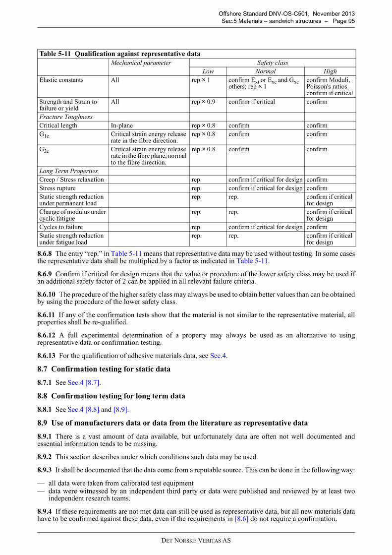
DET NORSKE VERITAS AS
Offshore Standard DNV-OS-C501, November 2013
Sec.5 Materials – sandwich structures – Page 95
8.6.8 The entry “rep.” in Table 5-11 means that representative data may be used without testing. In some casesthe representative data shall be multiplied by a factor as indicated in Table 5-11.
8.6.9 Confirm if critical for design means that the value or procedure of the lower safety class may be used ifan additional safety factor of 2 can be applied in all relevant failure criteria.
8.6.10 The procedure of the higher safety class may always be used to obtain better values than can be obtainedby using the procedure of the lower safety class.
8.6.11 If any of the confirmation tests show that the material is not similar to the representative material, allproperties shall be re-qualified.
8.6.12 A full experimental determination of a property may always be used as an alternative to usingrepresentative data or confirmation testing.
8.6.13 For the qualification of adhesive materials data, see Sec.4.
8.7 Confirmation testing for static data
8.7.1 See Sec.4 [8.7].
8.8 Confirmation testing for long term data
8.8.1 See Sec.4 [8.8] and [8.9].
8.9 Use of manufacturers data or data from the literature as representative data
8.9.1 There is a vast amount of data available, but unfortunately data are often not well documented andessential information tends to be missing.
8.9.2 This section describes under which conditions such data may be used.
8.9.3 It shall be documented that the data come from a reputable source. This can be done in the following way:
— all data were taken from calibrated test equipment— data were witnessed by an independent third party or data were published and reviewed by at least two
independent research teams.
8.9.4 If these requirements are not met data can still be used as representative data, but all new materials datahave to be confirmed against these data, even if the requirements in [8.6] do not require a confirmation.
Table 5-11 Qualification against representative data
Mechanical parameter Safety class
Low Normal High
Elastic constants All rep × 1 confirm Ext or Exc and Gxcothers: rep × 1
confirm Moduli,Poisson's ratios confirm if critical
Strength and Strain to failure or yield
All rep × 0.9 confirm if critical confirm
Fracture Toughness
Critical length In-plane rep × 0.8 confirm confirm
G1c Critical strain energy release rate in the fibre direction.
rep × 0.8 confirm confirm
G2c Critical strain energy release rate in the fibre plane, normal to the fibre direction.
rep × 0.8 confirm confirm
Long Term Properties
Creep / Stress relaxation rep. confirm if critical for design confirm
Stress rupture rep. confirm if critical for design confirm
Static strength reduction under permanent load
rep. rep. confirm if critical for design
Change of modulus under cyclic fatigue
rep. rep. confirm if critical for design
Cycles to failure rep. confirm if critical for design confirm
Static strength reduction under fatigue load
rep. rep. confirm if critical for design

DET NORSKE VERITAS AS
Offshore Standard DNV-OS-C501, November 2013
Sec.5 Materials – sandwich structures – Page 96
8.10 Confirming material data by component testing
See Sec.4 [8.11].
DET NORSKE VERITAS AS
Offshore Standard DNV-OS-C501, November 2013
Sec.6 Failure mechanisms and design criteria – Page 97
SECTION 6 FAILURE MECHANISMS AND DESIGN CRITERIA
1 Mechanisms of failure
1.1 General
1.1.1 A mechanism of failure is the underlying phenomenon at the material level that determines the mode offailure. Depending on its level of severity a mechanism of failure can lead to various failure modes. Forexample, matrix cracking can lead to seepage of a fluid through the laminate or lead to fracture depending onthe severity of the cracks. Failure mechanism can be regarded as the cause of failure and failure mode as theeffect. The failure terminology used in this standard is shown in Figure 6-1.
Guidance note:
Local and global failure shall be distinguished. On a material level, failure tends to be local, i.e. over an area of a fewcm2, or even less. This local failure may have global consequences immediately, or after some growth with time. Insome cases, the local failure does not grow and does not have any global consequences and does not effect any of thedesign requirements of the structure. In such a case local failure may be acceptable.
---e-n-d---of---G-u-i-d-a-n-c-e---n-o-t-e---
1.1.2 Only failure mechanisms that are related to critical failure modes, as identified in Sec.3 should beconsidered.
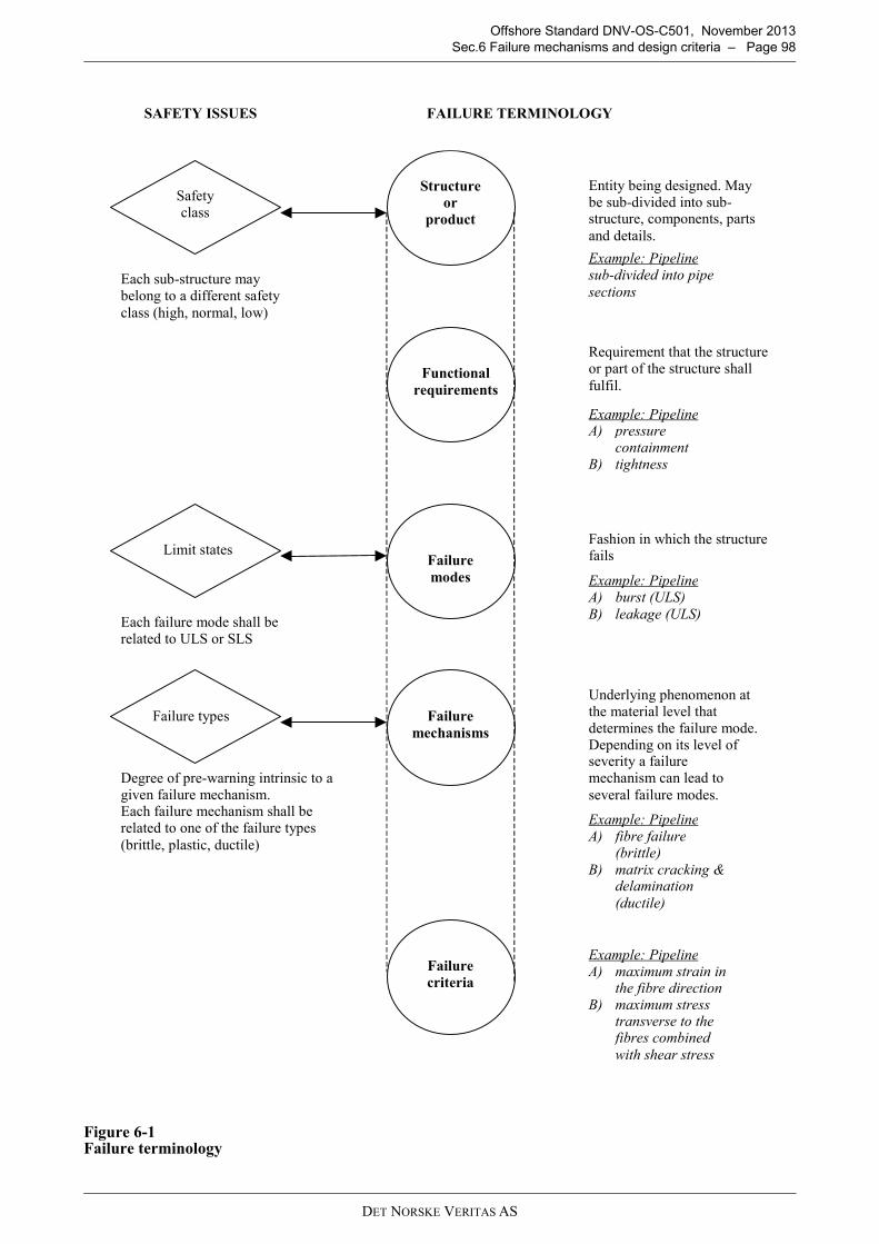
DET NORSKE VERITAS AS
Offshore Standard DNV-OS-C501, November 2013
Sec.6 Failure mechanisms and design criteria – Page 98
Figure 6-1 Failure terminology
Failure
criteria
Failure types Failure
mechanisms
Limit statesFailure
modes
Functional
requirements
Safetyclass
Each sub-structure maybelong to a different safetyclass (high, normal, low)
Structure
or
product
Entity being designed. Maybe sub-divided into sub-structure, components, partsand details.
Example: Pipelinesub-divided into pipe
sections
Requirement that the structureor part of the structure shallfulfil.
Example: PipelineA) pressure
containmentB) tightness
Fashion in which the structurefails
Each failure mode shall berelated to ULS or SLS
Example: PipelineA) burst (ULS)
B) leakage (ULS)
Underlying phenomenon atthe material level thatdetermines the failure mode.Depending on its level ofseverity a failuremechanism can lead toseveral failure modes.
Degree of pre-warning intrinsic to agiven failure mechanism.Each failure mechanism shall berelated to one of the failure types(brittle, plastic, ductile)
Example: PipelineA) fibre failure
(brittle)
B) matrix cracking &delamination
(ductile)
Example: PipelineA) maximum strain in
the fibre directionB) maximum stress
transverse to thefibres combined
with shear stress
FAILURE TERMINOLOGYSAFETY ISSUES
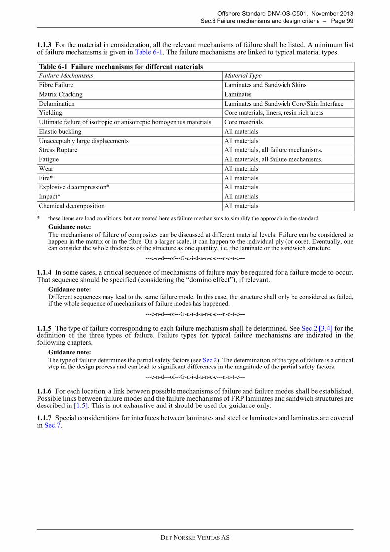
DET NORSKE VERITAS AS
Offshore Standard DNV-OS-C501, November 2013
Sec.6 Failure mechanisms and design criteria – Page 99
1.1.3 For the material in consideration, all the relevant mechanisms of failure shall be listed. A minimum listof failure mechanisms is given in Table 6-1. The failure mechanisms are linked to typical material types.
* these items are load conditions, but are treated here as failure mechanisms to simplify the approach in the standard.
Guidance note:
The mechanisms of failure of composites can be discussed at different material levels. Failure can be considered tohappen in the matrix or in the fibre. On a larger scale, it can happen to the individual ply (or core). Eventually, onecan consider the whole thickness of the structure as one quantity, i.e. the laminate or the sandwich structure.
---e-n-d---of---G-u-i-d-a-n-c-e---n-o-t-e---
1.1.4 In some cases, a critical sequence of mechanisms of failure may be required for a failure mode to occur.That sequence should be specified (considering the “domino effect”), if relevant.
Guidance note:
Different sequences may lead to the same failure mode. In this case, the structure shall only be considered as failed,if the whole sequence of mechanisms of failure modes has happened.
---e-n-d---of---G-u-i-d-a-n-c-e---n-o-t-e---
1.1.5 The type of failure corresponding to each failure mechanism shall be determined. See Sec.2 [3.4] for thedefinition of the three types of failure. Failure types for typical failure mechanisms are indicated in thefollowing chapters.
Guidance note:
The type of failure determines the partial safety factors (see Sec.2). The determination of the type of failure is a criticalstep in the design process and can lead to significant differences in the magnitude of the partial safety factors.
---e-n-d---of---G-u-i-d-a-n-c-e---n-o-t-e---
1.1.6 For each location, a link between possible mechanisms of failure and failure modes shall be established.Possible links between failure modes and the failure mechanisms of FRP laminates and sandwich structures aredescribed in [1.5]. This is not exhaustive and it should be used for guidance only.
1.1.7 Special considerations for interfaces between laminates and steel or laminates and laminates are coveredin Sec.7.
Table 6-1 Failure mechanisms for different materials
Failure Mechanisms Material Type
Fibre Failure Laminates and Sandwich Skins
Matrix Cracking Laminates
Delamination Laminates and Sandwich Core/Skin Interface
Yielding Core materials, liners, resin rich areas
Ultimate failure of isotropic or anisotropic homogenous materials Core materials
Elastic buckling All materials
Unacceptably large displacements All materials
Stress Rupture All materials, all failure mechanisms.
Fatigue All materials, all failure mechanisms.
Wear All materials
Fire* All materials
Explosive decompression* All materials
Impact* All materials
Chemical decomposition All materials
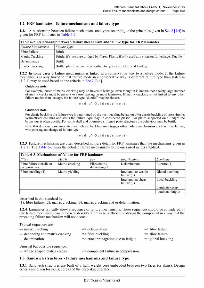
DET NORSKE VERITAS AS
Offshore Standard DNV-OS-C501, November 2013
Sec.6 Failure mechanisms and design criteria – Page 100
1.2 FRP laminates - failure mechanisms and failure type
1.2.1 A relationship between failure mechanisms and types according to the principles given in Sec.2 [3.4] isgiven for FRP laminates in Table 6-2.
1.2.2 In some cases a failure mechanisms is linked in a conservative way to a failure mode. If the failuremechanisms is only linked to that failure mode in a conservative way, a different failure type than stated in[1.2.1] may be used based on the criteria in Sec.2 [3.4].
Guidance note:
For example: onset of matrix cracking may be linked to leakage, even though it is known that a fairly large numberof matrix cracks must be present to cause leakage in most laminates. If matrix cracking is not linked to any otherfailure modes than leakage, the failure type “ductile” may be chosen.
---e-n-d---of---G-u-i-d-a-n-c-e---n-o-t-e---
Guidance note:
For elastic buckling the failure type is determined by the post-buckling behaviour. For elastic buckling of most simple,symmetrical columns and struts the failure type may be considered plastic. For plates supported on all edges thebehaviour is often ductile. For some shell and optimised stiffened plate structures the behaviour may be brittle.
Note that deformations associated with elastic buckling may trigger other failure mechanisms such as fibre failure,with consequent change of failure type.
---e-n-d---of---G-u-i-d-a-n-c-e---n-o-t-e---
1.2.3 Failure mechanisms are often described in more detail for FRP laminates than the mechanisms given in[1.2.1]. The Table 6-3 links the detailed failure mechanisms to the ones used in this standard.
described in this standard by (1): fibre failure, (2): matrix cracking, (3): matrix cracking and or delamination.
1.2.4 Laminates typically show a sequence of failure mechanisms. These sequences should be considered. Ifone failure mechanism cannot be well described it may be sufficient to design the component in a way that thepreceding failure mechanism will not occur.
1.3 Sandwich structures - failure mechanisms and failure type
1.3.1 Sandwich structures are built of a light weight core embedded between two faces (or skins). Designcriteria are given for skins, cores and the core-skin interface.
Table 6-2 Relationship between failure mechanism and failure type for FRP laminates
Failure Mechanisms Failure Type
Fibre Failure Brittle
Matrix Cracking Brittle, if cracks are bridged by fibres: Plastic if only used as a criterion for leakage: Ductile
Delamination Brittle
Elastic buckling Brittle, plastic or ductile according to type of structure and loading.
Table 6-3 Mechanisms of failure for FRP laminates
Fibre Matrix Ply Inter-laminar Laminate
Fibre failure (tensile or compressive)
Matrix cracking Fibre/matrix debonding (2)
Delamination Rupture (1)
Fibre buckling (1) Matrix yielding Interlaminar tensile failure (3)
Global buckling
Interlaminar shear failure (3)
Local buckling
Laminate creep
Laminate fatigue
Typical sequences are:
— matrix cracking => delamination => fibre failure
— debonding and matrix cracking => fibre buckling => fibre failure
— delamination => crack propagation due to fatigue => global buckling.
Unusual but possible sequence:
— wedge shaped matrix cracks => component failure in compression.
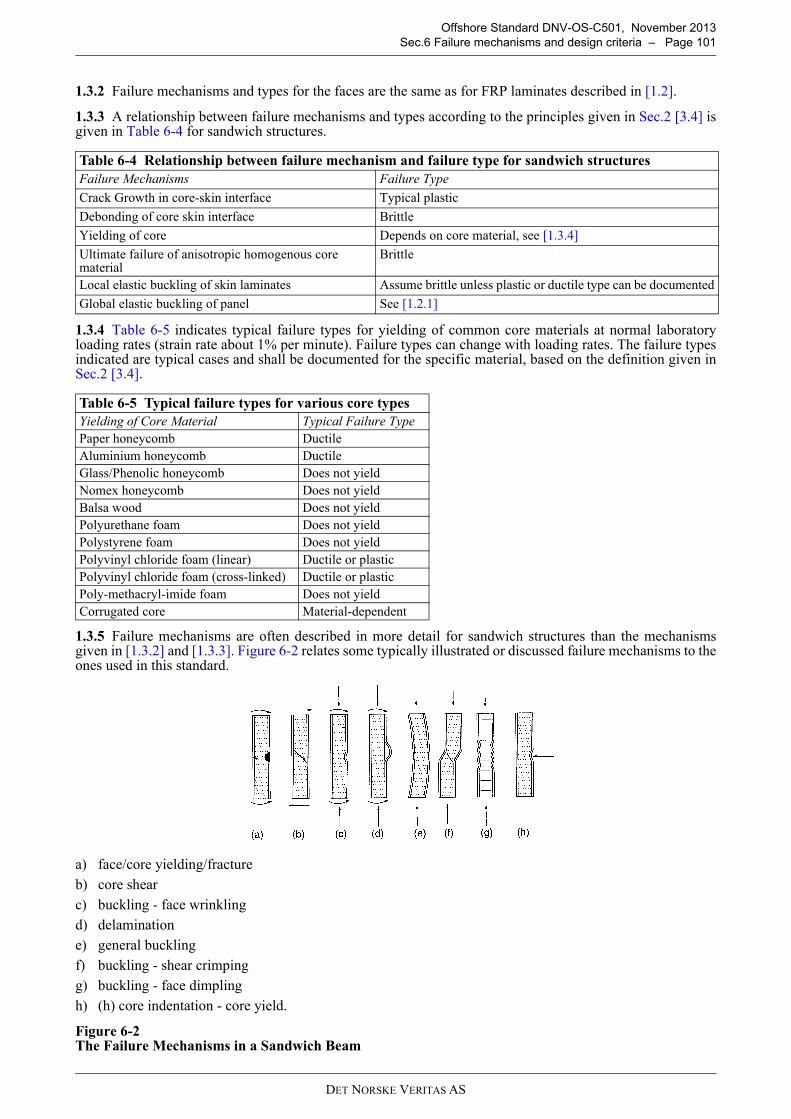
DET NORSKE VERITAS AS
Offshore Standard DNV-OS-C501, November 2013
Sec.6 Failure mechanisms and design criteria – Page 101
1.3.2 Failure mechanisms and types for the faces are the same as for FRP laminates described in [1.2].
1.3.3 A relationship between failure mechanisms and types according to the principles given in Sec.2 [3.4] isgiven in Table 6-4 for sandwich structures.
1.3.4 Table 6-5 indicates typical failure types for yielding of common core materials at normal laboratoryloading rates (strain rate about 1% per minute). Failure types can change with loading rates. The failure typesindicated are typical cases and shall be documented for the specific material, based on the definition given inSec.2 [3.4].
1.3.5 Failure mechanisms are often described in more detail for sandwich structures than the mechanismsgiven in [1.3.2] and [1.3.3]. Figure 6-2 relates some typically illustrated or discussed failure mechanisms to theones used in this standard.
a) face/core yielding/fracture
b) core shear
c) buckling - face wrinkling
d) delamination
e) general buckling
f) buckling - shear crimping
g) buckling - face dimpling
h) (h) core indentation - core yield.
Figure 6-2 The Failure Mechanisms in a Sandwich Beam
Table 6-4 Relationship between failure mechanism and failure type for sandwich structures
Failure Mechanisms Failure Type
Crack Growth in core-skin interface Typical plastic
Debonding of core skin interface Brittle
Yielding of core Depends on core material, see [1.3.4]
Ultimate failure of anisotropic homogenous core material
Brittle
Local elastic buckling of skin laminates Assume brittle unless plastic or ductile type can be documented
Global elastic buckling of panel See [1.2.1]
Table 6-5 Typical failure types for various core types
Yielding of Core Material Typical Failure Type
Paper honeycomb Ductile
Aluminium honeycomb Ductile
Glass/Phenolic honeycomb Does not yield
Nomex honeycomb Does not yield
Balsa wood Does not yield
Polyurethane foam Does not yield
Polystyrene foam Does not yield
Polyvinyl chloride foam (linear) Ductile or plastic
Polyvinyl chloride foam (cross-linked) Ductile or plastic
Poly-methacryl-imide foam Does not yield
Corrugated core Material-dependent
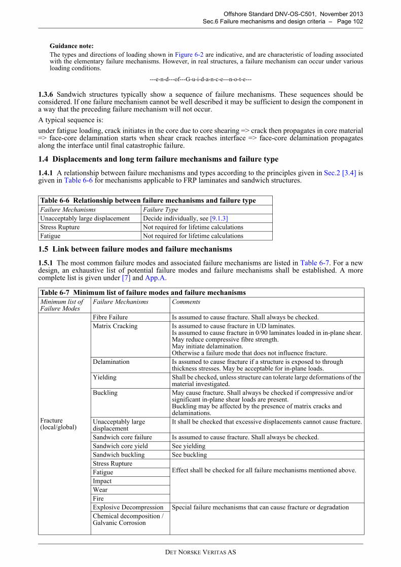
DET NORSKE VERITAS AS
Offshore Standard DNV-OS-C501, November 2013
Sec.6 Failure mechanisms and design criteria – Page 102
Guidance note:
The types and directions of loading shown in Figure 6-2 are indicative, and are characteristic of loading associatedwith the elementary failure mechanisms. However, in real structures, a failure mechanism can occur under variousloading conditions.
---e-n-d---of---G-u-i-d-a-n-c-e---n-o-t-e---
1.3.6 Sandwich structures typically show a sequence of failure mechanisms. These sequences should beconsidered. If one failure mechanism cannot be well described it may be sufficient to design the component ina way that the preceding failure mechanism will not occur.
A typical sequence is:
under fatigue loading, crack initiates in the core due to core shearing => crack then propagates in core material=> face-core delamination starts when shear crack reaches interface => face-core delamination propagatesalong the interface until final catastrophic failure.
1.4 Displacements and long term failure mechanisms and failure type
1.4.1 A relationship between failure mechanisms and types according to the principles given in Sec.2 [3.4] isgiven in Table 6-6 for mechanisms applicable to FRP laminates and sandwich structures.
1.5 Link between failure modes and failure mechanisms
1.5.1 The most common failure modes and associated failure mechanisms are listed in Table 6-7. For a newdesign, an exhaustive list of potential failure modes and failure mechanisms shall be established. A morecomplete list is given under [7] and App.A.
Table 6-6 Relationship between failure mechanisms and failure type
Failure Mechanisms Failure Type
Unacceptably large displacement Decide individually, see [9.1.3]
Stress Rupture Not required for lifetime calculations
Fatigue Not required for lifetime calculations
Table 6-7 Minimum list of failure modes and failure mechanisms
Minimum list of Failure Modes
Failure Mechanisms Comments
Fracture (local/global)
Fibre Failure Is assumed to cause fracture. Shall always be checked.
Matrix Cracking Is assumed to cause fracture in UD laminates.Is assumed to cause fracture in 0/90 laminates loaded in in-plane shear.May reduce compressive fibre strength.May initiate delamination.Otherwise a failure mode that does not influence fracture.
Delamination Is assumed to cause fracture if a structure is exposed to through thickness stresses. May be acceptable for in-plane loads.
Yielding Shall be checked, unless structure can tolerate large deformations of the material investigated.
Buckling May cause fracture. Shall always be checked if compressive and/or significant in-plane shear loads are present.Buckling may be affected by the presence of matrix cracks and delaminations.
Unacceptably large displacement
It shall be checked that excessive displacements cannot cause fracture.
Sandwich core failure Is assumed to cause fracture. Shall always be checked.
Sandwich core yield See yielding
Sandwich buckling See buckling
Stress RuptureEffect shall be checked for all failure mechanisms mentioned above.Fatigue
Impact
Wear
Fire
Explosive Decompression Special failure mechanisms that can cause fracture or degradation
Chemical decomposition /Galvanic Corrosion
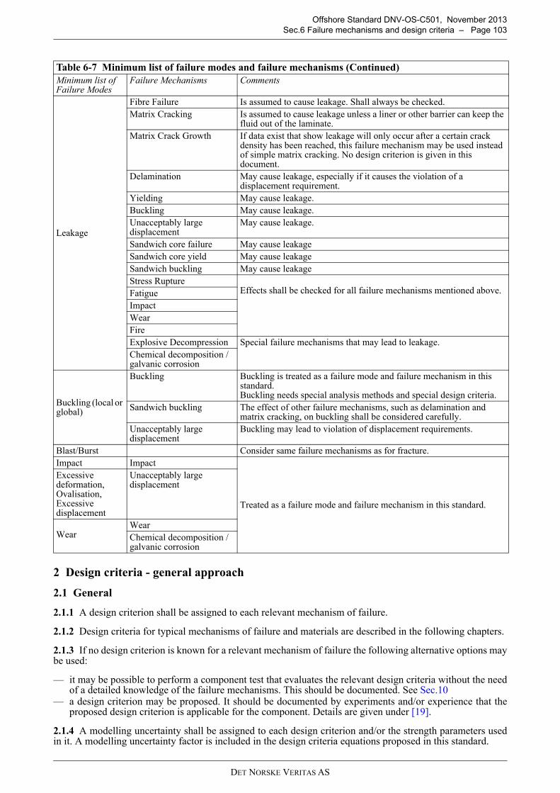
DET NORSKE VERITAS AS
Offshore Standard DNV-OS-C501, November 2013
Sec.6 Failure mechanisms and design criteria – Page 103
2 Design criteria - general approach
2.1 General
2.1.1 A design criterion shall be assigned to each relevant mechanism of failure.
2.1.2 Design criteria for typical mechanisms of failure and materials are described in the following chapters.
2.1.3 If no design criterion is known for a relevant mechanism of failure the following alternative options maybe used:
— it may be possible to perform a component test that evaluates the relevant design criteria without the needof a detailed knowledge of the failure mechanisms. This should be documented. See Sec.10
— a design criterion may be proposed. It should be documented by experiments and/or experience that theproposed design criterion is applicable for the component. Details are given under [19].
2.1.4 A modelling uncertainty shall be assigned to each design criterion and/or the strength parameters usedin it. A modelling uncertainty factor is included in the design criteria equations proposed in this standard.
Leakage
Fibre Failure Is assumed to cause leakage. Shall always be checked.
Matrix Cracking Is assumed to cause leakage unless a liner or other barrier can keep the fluid out of the laminate.
Matrix Crack Growth If data exist that show leakage will only occur after a certain crack density has been reached, this failure mechanism may be used instead of simple matrix cracking. No design criterion is given in this document.
Delamination May cause leakage, especially if it causes the violation of a displacement requirement.
Yielding May cause leakage.
Buckling May cause leakage.
Unacceptably large displacement
May cause leakage.
Sandwich core failure May cause leakage
Sandwich core yield May cause leakage
Sandwich buckling May cause leakage
Stress RuptureEffects shall be checked for all failure mechanisms mentioned above.Fatigue
Impact
Wear
Fire
Explosive Decompression Special failure mechanisms that may lead to leakage.
Chemical decomposition / galvanic corrosion
Buckling (local or global)
Buckling Buckling is treated as a failure mode and failure mechanism in this standard.Buckling needs special analysis methods and special design criteria.
Sandwich buckling The effect of other failure mechanisms, such as delamination and matrix cracking, on buckling shall be considered carefully.
Unacceptably large displacement
Buckling may lead to violation of displacement requirements.
Blast/Burst Consider same failure mechanisms as for fracture.
Impact Impact
Treated as a failure mode and failure mechanism in this standard.
Excessive deformation,Ovalisation,Excessive displacement
Unacceptably large displacement
WearWear
Chemical decomposition / galvanic corrosion
Table 6-7 Minimum list of failure modes and failure mechanisms (Continued)
Minimum list of Failure Modes
Failure Mechanisms Comments
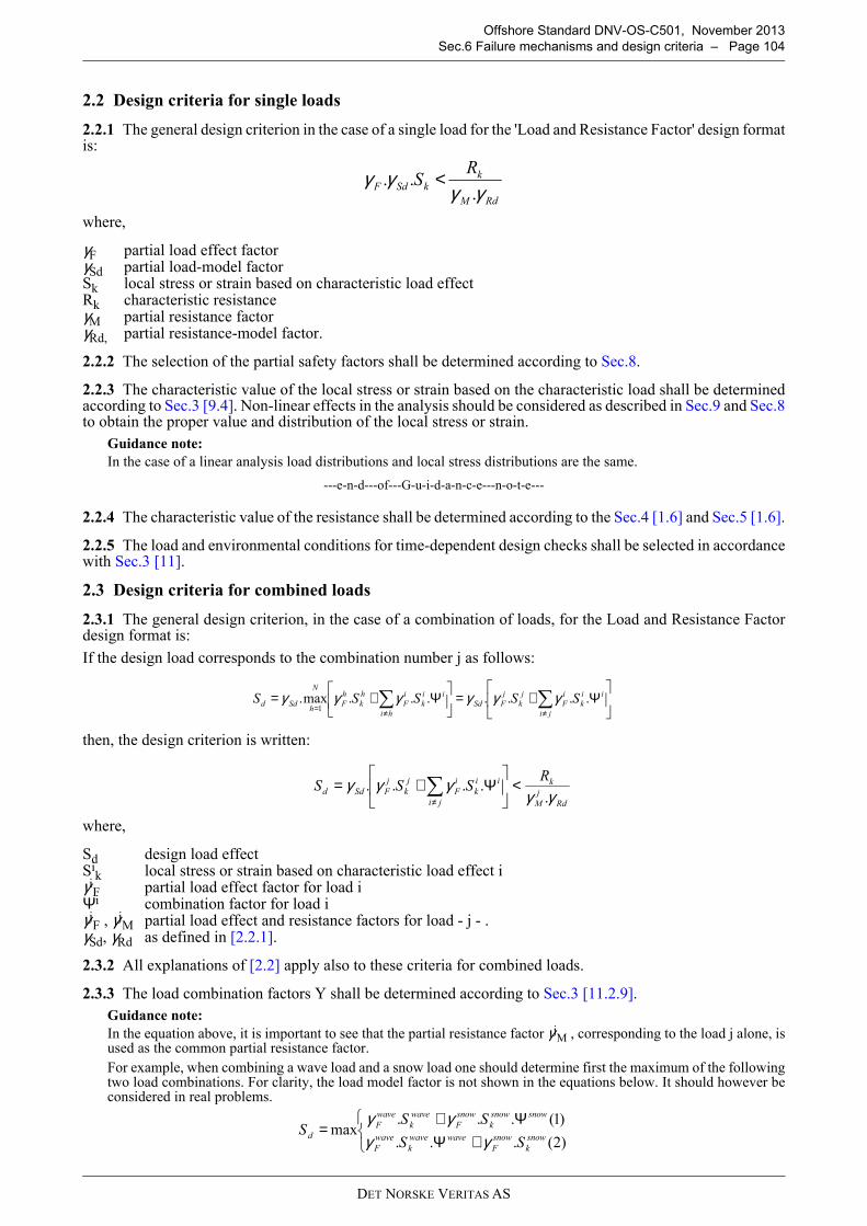
DET NORSKE VERITAS AS
Offshore Standard DNV-OS-C501, November 2013
Sec.6 Failure mechanisms and design criteria – Page 104
2.2 Design criteria for single loads
2.2.1 The general design criterion in the case of a single load for the 'Load and Resistance Factor' design formatis:
where,
γF partial load effect factorγSd partial load-model factorSk local stress or strain based on characteristic load effectRk characteristic resistanceγM partial resistance factor γRd, partial resistance-model factor.
2.2.2 The selection of the partial safety factors shall be determined according to Sec.8.
2.2.3 The characteristic value of the local stress or strain based on the characteristic load shall be determinedaccording to Sec.3 [9.4]. Non-linear effects in the analysis should be considered as described in Sec.9 and Sec.8to obtain the proper value and distribution of the local stress or strain.
Guidance note:
In the case of a linear analysis load distributions and local stress distributions are the same.
---e-n-d---of---G-u-i-d-a-n-c-e---n-o-t-e---
2.2.4 The characteristic value of the resistance shall be determined according to the Sec.4 [1.6] and Sec.5 [1.6].
2.2.5 The load and environmental conditions for time-dependent design checks shall be selected in accordancewith Sec.3 [11].
2.3 Design criteria for combined loads
2.3.1 The general design criterion, in the case of a combination of loads, for the Load and Resistance Factordesign format is:
If the design load corresponds to the combination number j as follows:
then, the design criterion is written:
where,
Sd design load effectSi
k local stress or strain based on characteristic load effect iγi
F partial load effect factor for load iΨi combination factor for load iγj
F , γjM partial load effect and resistance factors for load - j - .
γSd, γRd as defined in [2.2.1].
2.3.2 All explanations of [2.2] apply also to these criteria for combined loads.
2.3.3 The load combination factors Y shall be determined according to Sec.3 [11.2.9].
Guidance note:
In the equation above, it is important to see that the partial resistance factor γjM , corresponding to the load j alone, is
used as the common partial resistance factor.
For example, when combining a wave load and a snow load one should determine first the maximum of the followingtwo load combinations. For clarity, the load model factor is not shown in the equations below. It should however beconsidered in real problems.
RdM
kkSdF
RS
γγγγ
... <
Ψ+=
Ψ+= ∑∑≠≠=
ji
ii
k
i
F
j
k
j
FSd
hi
ii
k
i
F
h
k
h
F
N
hSdd SSSSS .......max.
1γγγγγγ
Rd
j
M
k
ji
ii
k
i
F
j
k
j
FSdd
RSSS
γγγγγ
..... <
Ψ+= ∑
≠
+ΨΨ+
=)2(...
)1(...max
snow
k
snow
F
wavewave
k
wave
F
snowsnow
k
snow
F
wave
k
wave
F
dSS
SSS
γγγγ
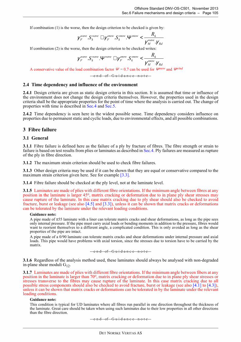
DET NORSKE VERITAS AS
Offshore Standard DNV-OS-C501, November 2013
Sec.6 Failure mechanisms and design criteria – Page 105
If combination (1) is the worse, then the design criterion to be checked is given by:
If combination (2) is the worse, then the design criterion to be checked writes:
A conservative value of the load combination factor Ψ = 0.7 can be used for Ψsnow and Ψwind
---e-n-d---of---G-u-i-d-a-n-c-e---n-o-t-e---
2.4 Time dependency and influence of the environment
2.4.1 Design criteria are given as static design criteria in this section. It is assumed that time or influence ofthe environment does not change the design criteria themselves. However, the properties used in the designcriteria shall be the appropriate properties for the point of time where the analysis is carried out. The change ofproperties with time is described in Sec.4 and Sec.5.
2.4.2 Time dependency is seen here in the widest possible sense. Time dependency considers influence onproperties due to permanent static and cyclic loads, due to environmental effects, and all possible combinations.
3 Fibre failure
3.1 General
3.1.1 Fibre failure is defined here as the failure of a ply by fracture of fibres. The fibre strength or strain tofailure is based on test results from plies or laminates as described in Sec.4. Ply failures are measured as ruptureof the ply in fibre direction.
3.1.2 The maximum strain criterion should be used to check fibre failures.
3.1.3 Other design criteria may be used if it can be shown that they are equal or conservative compared to themaximum strain criterion given here. See for example [3.3].
3.1.4 Fibre failure should be checked at the ply level, not at the laminate level.
3.1.5 Laminates are made of plies with different fibre orientations. If the minimum angle between fibres at anyposition in the laminate is larger 45o, matrix cracking or deformation due to in plane ply shear stresses maycause rupture of the laminate. In this case matrix cracking due to ply shear should also be checked to avoidfracture, burst or leakage (see also [4.5] and [3.3]), unless it can be shown that matrix cracks or deformationscan be tolerated by the laminate under the relevant loading conditions.
Guidance note:
A pipe made of ±55 laminate with a liner can tolerate matrix cracks and shear deformations, as long as the pipe seesonly internal pressure. If the pipe must carry axial loads or bending moments in addition to the pressure, fibres wouldwant to reorient themselves to a different angle, a complicated condition. This is only avoided as long as the shearproperties of the pipe are intact.
A pipe made of a 0/90 laminate can tolerate matrix cracks and shear deformations under internal pressure and axialloads. This pipe would have problems with axial torsion, since the stresses due to torsion have to be carried by thematrix.
---e-n-d---of---G-u-i-d-a-n-c-e---n-o-t-e---
3.1.6 Regardless of the analysis method used, these laminates should always be analysed with non-degradedin-plane shear moduli G12.
3.1.7 Laminates are made of plies with different fibre orientations. If the minimum angle between fibers at anyposition in the laminate is larger than 70o, matrix cracking or deformation due to in plane ply shear stresses orstresses transverse to the fibres may cause rupture of the laminate. In this case matrix cracking due to allpossible stress components should also be checked to avoid fracture, burst or leakage (see also [4.1] to [4.3]),unless it can be shown that matrix cracks or deformations can be tolerated in by the laminate under the relevantloading conditions.
Guidance note:
This condition is typical for UD laminates where all fibres run parallel in one direction throughout the thickness ofthe laminate. Great care should be taken when using such laminates due to their low properties in all other directionsthan the fibre direction.
---e-n-d---of---G-u-i-d-a-n-c-e---n-o-t-e---
Rd
wave
M
ksnowsnow
k
snow
F
wave
k
wave
F
RSS
γγγγ
.... <Ψ+
Rd
snow
M
ksnow
k
snow
F
wavewave
k
wave
F
RSS
γγγγ
.... <+Ψ
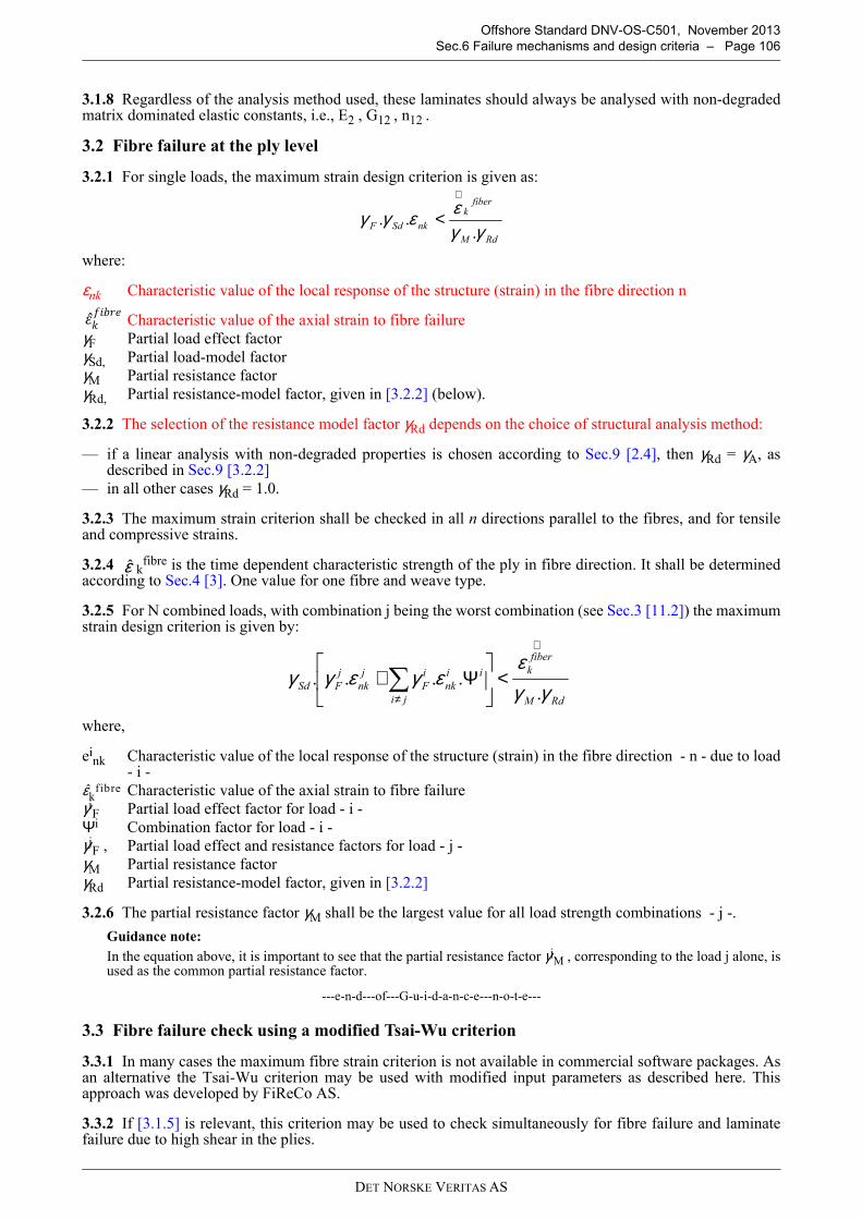
DET NORSKE VERITAS AS
Offshore Standard DNV-OS-C501, November 2013
Sec.6 Failure mechanisms and design criteria – Page 106
3.1.8 Regardless of the analysis method used, these laminates should always be analysed with non-degradedmatrix dominated elastic constants, i.e., E2 , G12 , n12 .
3.2 Fibre failure at the ply level
3.2.1 For single loads, the maximum strain design criterion is given as:
where:
εnk Characteristic value of the local response of the structure (strain) in the fibre direction n
Characteristic value of the axial strain to fibre failureγF Partial load effect factorγSd, Partial load-model factorγM Partial resistance factorγRd, Partial resistance-model factor, given in [3.2.2] (below).
3.2.2 The selection of the resistance model factor γRd depends on the choice of structural analysis method:
— if a linear analysis with non-degraded properties is chosen according to Sec.9 [2.4], then γRd = γA, asdescribed in Sec.9 [3.2.2]
— in all other cases γRd = 1.0.
3.2.3 The maximum strain criterion shall be checked in all n directions parallel to the fibres, and for tensileand compressive strains.
3.2.4 kfibre is the time dependent characteristic strength of the ply in fibre direction. It shall be determined
according to Sec.4 [3]. One value for one fibre and weave type.
3.2.5 For N combined loads, with combination j being the worst combination (see Sec.3 [11.2]) the maximumstrain design criterion is given by:
where,
eink Characteristic value of the local response of the structure (strain) in the fibre direction - n - due to load
- i - Characteristic value of the axial strain to fibre failure
γiF Partial load effect factor for load - i -
Ψi Combination factor for load - i - γj
F , Partial load effect and resistance factors for load - j - γM Partial resistance factor γRd Partial resistance-model factor, given in [3.2.2]
3.2.6 The partial resistance factor γM shall be the largest value for all load strength combinations - j -.
Guidance note:
In the equation above, it is important to see that the partial resistance factor γjM , corresponding to the load j alone, is
used as the common partial resistance factor.
---e-n-d---of---G-u-i-d-a-n-c-e---n-o-t-e---
3.3 Fibre failure check using a modified Tsai-Wu criterion
3.3.1 In many cases the maximum fibre strain criterion is not available in commercial software packages. Asan alternative the Tsai-Wu criterion may be used with modified input parameters as described here. Thisapproach was developed by FiReCo AS.
3.3.2 If [3.1.5] is relevant, this criterion may be used to check simultaneously for fibre failure and laminatefailure due to high shear in the plies.
RdM
fiberk
nkSdF γγεεγγ
...
∧
<
� �����
ε
RdM
fiber
k
ji
ii
nk
i
F
j
nk
j
FSd γγε
εγεγγ.
....
∧
≠
<
Ψ+∑
εkfibre
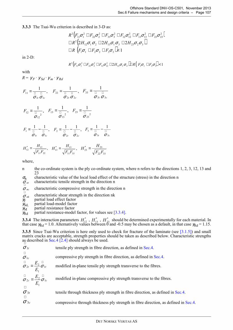
DET NORSKE VERITAS AS
Offshore Standard DNV-OS-C501, November 2013
Sec.6 Failure mechanisms and design criteria – Page 107
3.3.3 The Tsai-Wu criterion is described in 3-D as:
in 2-D:
with
R = γ F · γ Sd · γ m · γ Rd
where,
n the co-ordinate system is the ply co-ordinate system, where n refers to the directions 1, 2, 3, 12, 13 and23
σn characteristic value of the local load effect of the structure (stress) in the direction n characteristic tensile strength in the direction n
characteristic compressive strength in the direction n
characteristic shear strength in the direction nkγF partial load effect factorγSd, partial load-model factorγM partial resistance factorγRd partial resistance-model factor, for values see [3.3.4].
3.3.4 The interaction parameters , , should be determined experimentally for each material. Inthat case γRd = 1.0. Alternatively values between 0 and -0.5 may be chosen as a default, in that case γRd = 1.15.
3.3.5 Since Tsai-Wu criterion is here only used to check for fracture of the laminate (see [3.1.5]) and smallmatrix cracks are acceptable, strength properties should be taken as described below. Characteristic strengthsas described in Sec.4 [2.4] should always be used.
tensile ply strength in fibre direction, as defined in Sec.4.
compressive ply strength in fibre direction, as defined in Sec.4.
modified in-plane tensile ply strength transverse to the fibres.
modified in-plane compressive ply strength transverse to the fibres.
tensile through thickness ply strength in fibre direction, as defined in Sec.4.
compressive through thickness ply strength in fibre direction, as defined in Sec.4.
( )( )( ) 1
222
332211
3223311321122
22323
21313
21212
2333
2222
2111
2
<+++
+++
+++++
σσσσσσσσσ
σσσσσσ
FFFR
HHHR
FFFFFFR
( ) ( ) 12 2211211221212
2222
2111
2 <+++++ σσσσσσσ FFRHFFFR
,1
11
11
ct
F ∧∧=σσ
,1
22
22
ct
F ∧∧=σσ ct
F
33
33
1∧∧=σσ
,1
212
12 ∧=σ
F ,1
213
13 ∧=σ
F2
23
23
1∧=σ
F
,11
11
1
ct
F ∧∧ −=σσ
,11
22
2
ct
F ∧∧ −=σσ ct
F
33
3
11∧∧ −=σσ
,2211
12*12
FF
HH = ,
3311
13*13
FF
HH =
3322
23*23
FF
HH =
nt
∧σ
nc
∧σ
nk
∧σ
*12H *
13H *23H
t1
∧σ
c1
∧σ
tt
E
E1
1
22
∧∧= σσ
cc
E
E1
1
22
∧∧= σσ
t3
∧σ
c3
∧σ
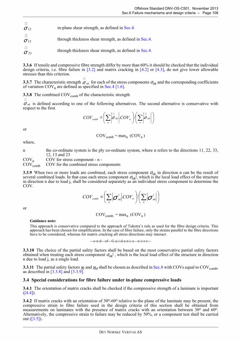
DET NORSKE VERITAS AS
Offshore Standard DNV-OS-C501, November 2013
Sec.6 Failure mechanisms and design criteria – Page 108
in-plane shear strength, as defined in Sec.4.
through thickness shear strength, as defined in Sec.4.
through thickness shear strength, as defined in Sec.4.
3.3.6 If tensile and compressive fibre strength differ by more than 60% it should be checked that the individualdesign criteria, i.e. fibre failure in [3.2] and matrix cracking in [4.2] or [4.3], do not give lower allowablestresses than this criterion.
3.3.7 The characteristic strength for each of the stress components σnk and the corresponding coefficientsof variation COVn are defined as specified in Sec.4 [1.6].
3.3.8 The combined COVcomb of the characteristic strength
is defined according to one of the following alternatives. The second alternative is conservative withrespect to the first.
or
COVcomb = maxn (COVn )
where,
n the co-ordinate system is the ply co-ordinate system, where n refers to the directions 11, 22, 33,12, 13 and 23
COVn COV for stress component - n -COVcomb COV for the combined stress components
3.3.9 When two or more loads are combined, each stress component σnk in direction n can be the result ofseveral combined loads. In that case each stress component σnk
j, which is the local load effect of the structurein direction n due to load j, shall be considered separately as an individual stress component to determine theCOV.
or
COVcomb. = maxn (COVn )
Guidance note:
This approach is conservative compared to the approach of Tukstra’s rule as used for the fibre design criteria. Thisapproach has been chosen for simplification. In the case of fibre failure, only the strains parallel to the fibre directionshave to be considered, whereas for matrix cracking all stress directions may interact.
---e-n-d---of---G-u-i-d-a-n-c-e---n-o-t-e---
3.3.10 The choice of the partial safety factors shall be based on the most conservative partial safety factorsobtained when treating each stress component σnk
j , which is the local load effect of the structure in directionn due to load j, as a single load.
3.3.11 The partial safety factors γF and γM shall be chosen as described in Sec.8 with COVs equal to COVcomb,as described in [3.3.8] and [3.3.9].
3.4 Special considerations for fibre failure under in-plane compressive loads
3.4.1 The orientation of matrix cracks shall be checked if the compressive strength of a laminate is important([4.4]).
3.4.2 If matrix cracks with an orientation of 30o-60o relative to the plane of the laminate may be present, thecompressive strain to fibre failure used in the design criteria of this section shall be obtained frommeasurements on laminates with the presence of matrix cracks with an orientation between 30o and 60o.Alternatively, the compressive strain to failure may be reduced by 50%, or a component test shall be carriedout ([3.5]).
12
∧σ
13
∧σ
23
∧σ
nk
∧σ
nk
∧σ
= ∑∑∧∧
n
nk
n
nnkcomb COVCOV σσ /.
= ∑∑n
j
nkn
n
j
nkcomb COVCOV σσ /.
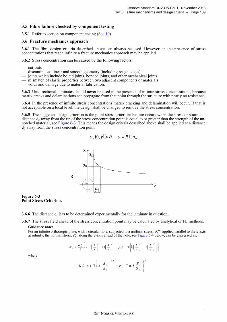
DET NORSKE VERITAS AS
Offshore Standard DNV-OS-C501, November 2013
Sec.6 Failure mechanisms and design criteria – Page 109
3.5 Fibre failure checked by component testing
3.5.1 Refer to section on component testing (Sec.10)
3.6 Fracture mechanics approach
3.6.1 The fibre design criteria described above can always be used. However, in the presence of stressconcentrations that reach infinity a fracture mechanics approach may be applied.
3.6.2 Stress concentration can be caused by the following factors:
— cut-outs— discontinuous linear and smooth geometry (including rough edges)— joints which include bolted joints, bonded joints, and other mechanical joints— mismatch of elastic properties between two adjacent components or materials— voids and damage due to material fabrication.
3.6.3 Unidirectional laminates should never be used in the presence of infinite stress concentrations, becausematrix cracks and delaminations can propagate from that point through the structure with nearly no resistance.
3.6.4 In the presence of infinite stress concentrations matrix cracking and delamination will occur. If that isnot acceptable on a local level, the design shall be changed to remove the stress concentration.
3.6.5 The suggested design criterion is the point stress criterion: Failure occurs when the stress or strain at adistance d0 away from the tip of the stress concentration point is equal to or greater than the strength of the un-notched material, see Figure 6-3. This means the design criteria described above shall be applied at a distanced0 away from the stress concentration point.
Figure 6-3 Point Stress Criterion.
3.6.6 The distance d0 has to be determined experimentally for the laminate in question.
3.6.7 The stress field ahead of the stress concentration point may be calculated by analytical or FE methods.
Guidance note:
For an infinite orthotropic plate, with a circular hole, subjected to a uniform stress, σx∞, applied parallel to the x-axis
at infinity, the normal stress, σx, along the y-axis ahead of the hole, see Figure 6-4 below, can be expressed as:
where
( ) σσ ˆ,0 <yx 0dRy +=
x
y
R
σ0
σx
d0
( )
−
−−
+
+= ∞
∞ 8642
753322 y
R
y
RK
y
R
y
RT
x
x
σσ
5.05.0
5.021
+−
+=∞
xy
xxy
y
xT
G
E
E
EK ν
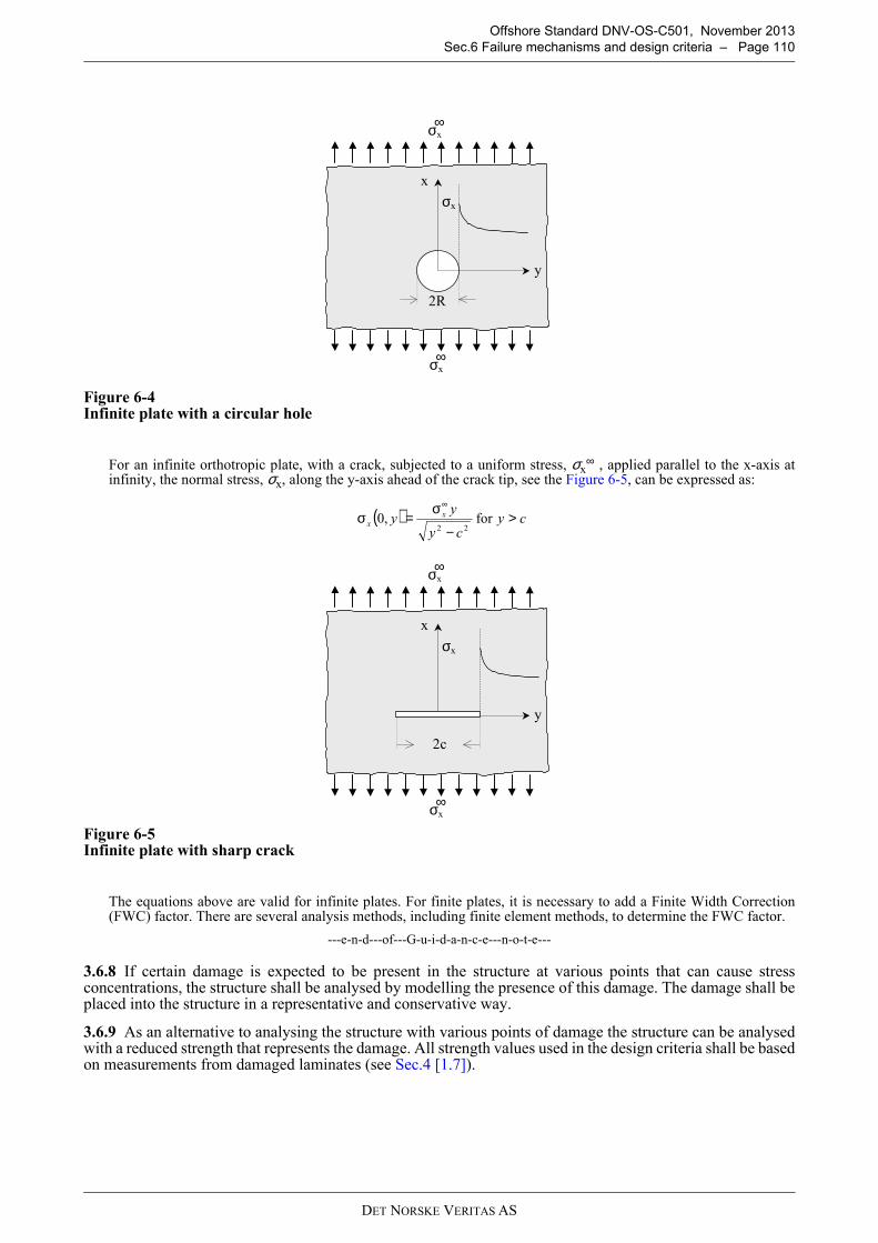
DET NORSKE VERITAS AS
Offshore Standard DNV-OS-C501, November 2013
Sec.6 Failure mechanisms and design criteria – Page 110
Figure 6-4 Infinite plate with a circular hole
For an infinite orthotropic plate, with a crack, subjected to a uniform stress, σx∞ , applied parallel to the x-axis at
infinity, the normal stress, σx, along the y-axis ahead of the crack tip, see the Figure 6-5, can be expressed as:
Figure 6-5 Infinite plate with sharp crack
The equations above are valid for infinite plates. For finite plates, it is necessary to add a Finite Width Correction(FWC) factor. There are several analysis methods, including finite element methods, to determine the FWC factor.
---e-n-d---of---G-u-i-d-a-n-c-e---n-o-t-e---
3.6.8 If certain damage is expected to be present in the structure at various points that can cause stressconcentrations, the structure shall be analysed by modelling the presence of this damage. The damage shall beplaced into the structure in a representative and conservative way.
3.6.9 As an alternative to analysing the structure with various points of damage the structure can be analysedwith a reduced strength that represents the damage. All strength values used in the design criteria shall be basedon measurements from damaged laminates (see Sec.4 [1.7]).
y
x
2R
σx
σx∞
σx∞
( ) cycy
yy x
x >−
σ=σ
∞
for,022
y
x
2c
σx
σx∞
σx∞
DET NORSKE VERITAS AS
Offshore Standard DNV-OS-C501, November 2013
Sec.6 Failure mechanisms and design criteria – Page 111
4 Matrix cracking
4.1 General
4.1.1 Matrix design criteria apply to a matrix in a ply where the deformation of the matrix is restrained by thefibres of the ply or the surrounding laminate.
Guidance note:
Matrix cracking is a simple concept at first sight but quite involved in details.
Some laminates have already matrix cracks after manufacturing. These cracks can be introduced by thermal stressesor by shrinkage of the matrix during cure.
Laminates without matrix cracks have an initial ply stress when the first cracks start to form.
Once cracks are formed they start to propagate at higher ply stresses and additional cracks are formed.
Crack formation will eventually lead to a change in stiffness. This point is usually referred to as the matrix crack pointor first ply failure etc., because this is what can easily be measured.
Eventually laminates show crack saturation and no further cracks form when loaded more. The change of modulushas been related to matrix crack density in some publications.
See [1.1.2] and [1.1.3] for relevance of matrix cracking for a particular application.
---e-n-d---of---G-u-i-d-a-n-c-e---n-o-t-e---
4.1.2 Matrix cracking is defined here as the onset of matrix cracking. The increase of the number of matrixcracks at higher stresses or strains is not covered by the matrix cracking criteria presented in this section.
4.1.3 Characteristic strength shall be defined according to Sec.4 [1.6].
4.1.4 Matrix cracking shall be checked on the ply level.
4.1.5 Two alternative design criteria may be used. The simple stress criterion ([4.2]) or the Puck criterion([4.3]).
4.1.6 If the component may fail due to wedge shaped matrix cracks in compression, the Puck criterion mustbe used to obtain the direction of the failure surface([4.3] and [4.4]).
4.2 Matrix failure based on simple stress criterion
4.2.1 The following design criterion should be used when the stress in one direction is dominating comparedto the stresses in the other directions. The stress in one direction is said to be dominating when the criterion in[4.2.2] is not satisfied.
where,
n direction of the dominating stressσnk characteristic value of the local load effect of the structure (stress) in the direction n
characteristic value of the stress components to matrix cracking in direction nγF partial load effect factorγSd partial load-model factorγM partial resistance factorγRd partial resistance-model factor, γRd = 1.0
The co-ordinate system is the ply co-ordinate system.
Guidance note:
The stress to matrix cracking is in general direction-dependent. This is due to the presence of fibres that concentratethe stresses, such that the matrix stress to failure in the direction parallel to the fibres is in generally larger than in theperpendicular direction.
---e-n-d---of---G-u-i-d-a-n-c-e---n-o-t-e---
4.2.2 The combination between the stress components in several directions shall be taken into considerationwhen the criterion below is satisfied. In that case, there is no dominating stress and the combination cannot bedisregarded.
maxi
RdM
matrixnk
nkSdF γγσσγγ
...
∧
<
matrixnk
∧σ
10/ ≤∑≠ ∧∧
in matrixnk
nk
matrixik
ik
σ
σσ
σ
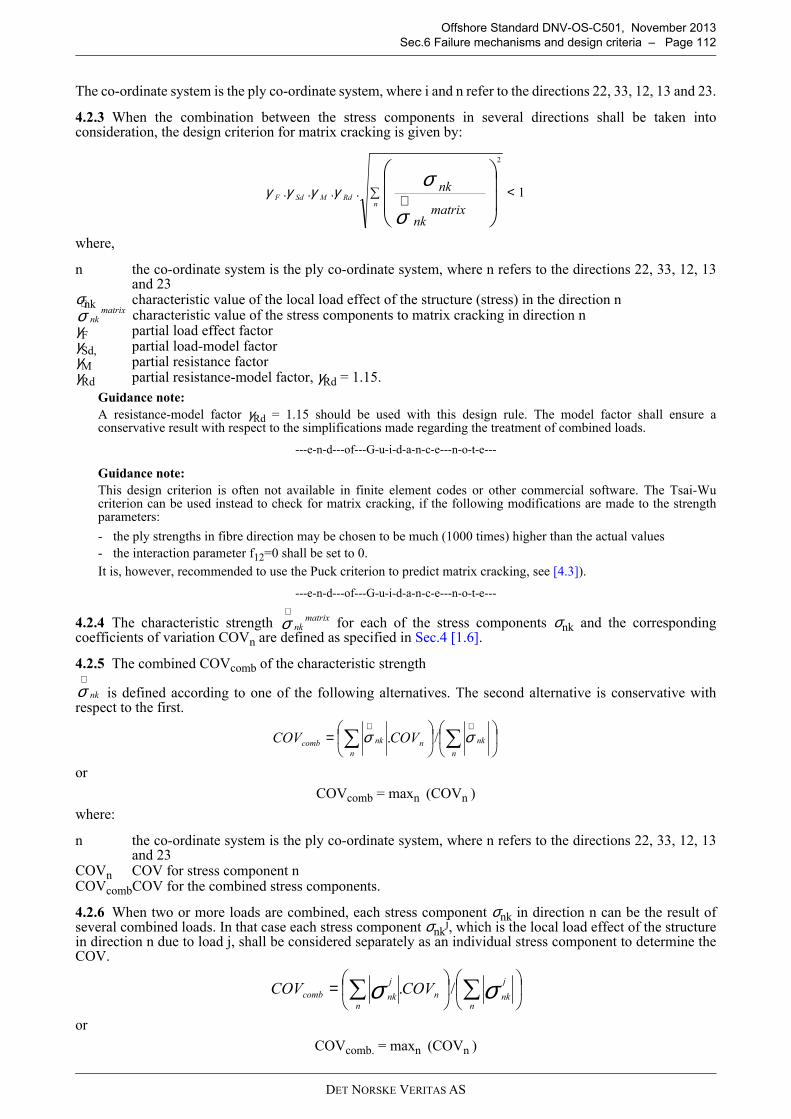
DET NORSKE VERITAS AS
Offshore Standard DNV-OS-C501, November 2013
Sec.6 Failure mechanisms and design criteria – Page 112
The co-ordinate system is the ply co-ordinate system, where i and n refer to the directions 22, 33, 12, 13 and 23.
4.2.3 When the combination between the stress components in several directions shall be taken intoconsideration, the design criterion for matrix cracking is given by:
where,
n the co-ordinate system is the ply co-ordinate system, where n refers to the directions 22, 33, 12, 13and 23
σnk characteristic value of the local load effect of the structure (stress) in the direction n characteristic value of the stress components to matrix cracking in direction n
γF partial load effect factorγSd, partial load-model factorγM partial resistance factorγRd partial resistance-model factor, γRd = 1.15.
Guidance note:
A resistance-model factor γRd = 1.15 should be used with this design rule. The model factor shall ensure aconservative result with respect to the simplifications made regarding the treatment of combined loads.
---e-n-d---of---G-u-i-d-a-n-c-e---n-o-t-e---
Guidance note:
This design criterion is often not available in finite element codes or other commercial software. The Tsai-Wucriterion can be used instead to check for matrix cracking, if the following modifications are made to the strengthparameters:
- the ply strengths in fibre direction may be chosen to be much (1000 times) higher than the actual values
- the interaction parameter f12=0 shall be set to 0.
It is, however, recommended to use the Puck criterion to predict matrix cracking, see [4.3]).
---e-n-d---of---G-u-i-d-a-n-c-e---n-o-t-e---
4.2.4 The characteristic strength for each of the stress components σnk and the correspondingcoefficients of variation COVn are defined as specified in Sec.4 [1.6].
4.2.5 The combined COVcomb of the characteristic strength
is defined according to one of the following alternatives. The second alternative is conservative withrespect to the first.
or
COVcomb = maxn (COVn )
where:
n the co-ordinate system is the ply co-ordinate system, where n refers to the directions 22, 33, 12, 13and 23
COVn COV for stress component nCOVcombCOV for the combined stress components.
4.2.6 When two or more loads are combined, each stress component σnk in direction n can be the result ofseveral combined loads. In that case each stress component σnk
j, which is the local load effect of the structurein direction n due to load j, shall be considered separately as an individual stress component to determine theCOV.
or
COVcomb. = maxn (COVn )
1....
2
<∑ ∧
nRdMSdF
matrixnk
nk
σ
σγγγγ
matrixnk
∧σ
matrixnk
∧σ
nk
∧σ
= ∑∑∧∧
n
nk
n
nnkcomb COVCOV σσ /.
= ∑∑n
j
nkn
n
j
nkcomb COVCOV σσ /.
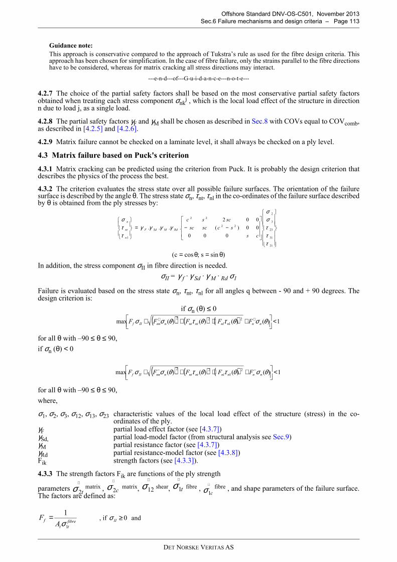
DET NORSKE VERITAS AS
Offshore Standard DNV-OS-C501, November 2013
Sec.6 Failure mechanisms and design criteria – Page 113
Guidance note:
This approach is conservative compared to the approach of Tukstra’s rule as used for the fibre design criteria. Thisapproach has been chosen for simplification. In the case of fibre failure, only the strains parallel to the fibre directionshave to be considered, whereas for matrix cracking all stress directions may interact.
---e-n-d---of---G-u-i-d-a-n-c-e---n-o-t-e---
4.2.7 The choice of the partial safety factors shall be based on the most conservative partial safety factorsobtained when treating each stress component σnk
j , which is the local load effect of the structure in directionn due to load j, as a single load.
4.2.8 The partial safety factors γF and γM shall be chosen as described in Sec.8 with COVs equal to COVcomb,as described in [4.2.5] and [4.2.6].
4.2.9 Matrix failure cannot be checked on a laminate level, it shall always be checked on a ply level.
4.3 Matrix failure based on Puck's criterion
4.3.1 Matrix cracking can be predicted using the criterion from Puck. It is probably the design criterion thatdescribes the physics of the process the best.
4.3.2 The criterion evaluates the stress state over all possible failure surfaces. The orientation of the failuresurface is described by the angle θ. The stress state σn, τnt, τnl in the co-ordinates of the failure surface describedby θ is obtained from the ply stresses by:
In addition, the stress component σII in fibre direction is needed.
σII = γ f · γ Sd · γ M · Rd σ1
Failure is evaluated based on the stress state σn, τnt, τnl for all angles q between - 90 and + 90 degrees. Thedesign criterion is:
if σn (θ) ≤ 0
for all θ with –90 ≤ θ ≤ 90,
if σn (θ) < 0
for all θ with –90 ≤ θ ≤ 90,
where,
σ1, σ2, σ3, σ12, σ13, σ23 characteristic values of the local load effect of the structure (stress) in the co-ordinates of the ply.
γF partial load effect factor (see [4.3.7])γSd, partial load-model factor (from structural analysis see Sec.9)γM partial resistance factor (see [4.3.7])γRd partial resistance-model factor (see [4.3.8])Fik strength factors (see [4.3.3]).
4.3.3 The strength factors Fik are functions of the ply strength
parameters matrix , matrix, shear, fibre , fibre , and shape parameters of the failure surface.The factors are defined as:
, if and
−−=
21
31
23
3
2
22
22
1 000
00)(
002
....
τττσσ
γγγγττσ
cs
scscsc
scsc
RdMSdF
n
nt
n
)sins;cosc( θ=θ=
( ) ( ) ( ) 1)()()()(max2
1
22 <
++++ ++ θσθτθτθσσ nnnnlntntnnnIIf FFFFF
( ) ( ) ( ) 1)()()()(max2
1
22 <
++++ −− θσθτθτθσσ nnnnlntntnnnIIf FFFFF
t2σ∧
c2σ∧
12σ∧
t1σ∧
c1σ∧
fibre
tt
fA
F1
1
σ= 0≥IIσ
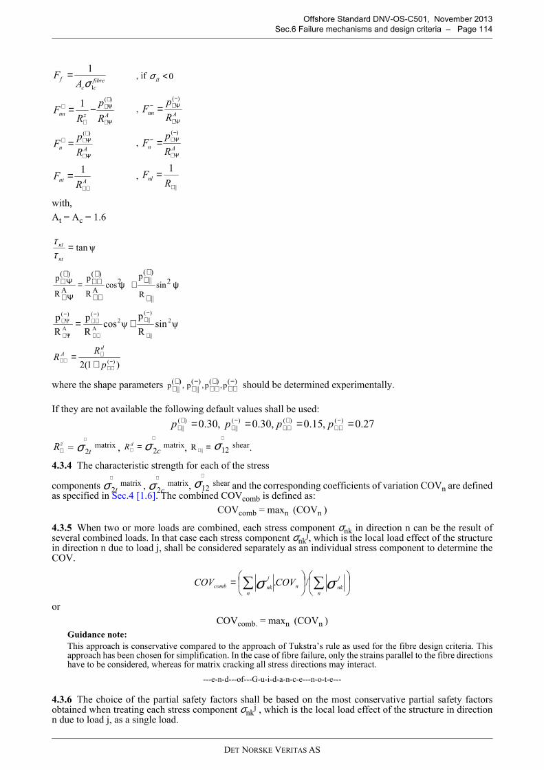
DET NORSKE VERITAS AS
Offshore Standard DNV-OS-C501, November 2013
Sec.6 Failure mechanisms and design criteria – Page 114
with,
At = Ac = 1.6
where the shape parameters should be determined experimentally.
If they are not available the following default values shall be used:
= matrix , matrix, shear.
4.3.4 The characteristic strength for each of the stress
components matrix , matrix, shear and the corresponding coefficients of variation COVn are definedas specified in Sec.4 [1.6]. The combined COVcomb is defined as:
COVcomb = maxn (COVn )
4.3.5 When two or more loads are combined, each stress component σnk in direction n can be the result ofseveral combined loads. In that case each stress component σnk
j, which is the local load effect of the structurein direction n due to load j, shall be considered separately as an individual stress component to determine theCOV.
or
COVcomb. = maxn (COVn )
Guidance note:
This approach is conservative compared to the approach of Tukstra’s rule as used for the fibre design criteria. Thisapproach has been chosen for simplification. In the case of fibre failure, only the strains parallel to the fibre directionshave to be considered, whereas for matrix cracking all stress directions may interact.
---e-n-d---of---G-u-i-d-a-n-c-e---n-o-t-e---
4.3.6 The choice of the partial safety factors shall be based on the most conservative partial safety factorsobtained when treating each stress component σnk
j , which is the local load effect of the structure in directionn due to load j, as a single load.
, if
,
,
,
fibre
cc
fA
F1
1
σ= 0<IIσ
AznnR
p
RF
Ψ⊥
+Ψ⊥
⊥
+ −=)(
1Ann
R
pF
Ψ⊥
−Ψ⊥− =)(
AnR
pF
Ψ⊥
+Ψ⊥+ =)(
AnR
pF
Ψ⊥
−Ψ⊥− =)(
AntR
F⊥⊥
= 1
||
1
⊥
=R
Fnl
ψtan=nt
nl
ττ
ψ+ψ=⊥
+⊥
⊥⊥
+⊥⊥
Ψ⊥
+Ψ⊥ 2
||
)(||2
A
)(
A
)(
sinR
pcos
R
p
R
p
ψsinR
pψcos
R
p
R
p 2
||
)(||2
A
)(
AΨ
)(Ψ
⊥
−⊥
⊥⊥
−⊥⊥
⊥
−⊥ +=
)1(2 )(−⊥⊥
⊥⊥⊥ +
=p
RR
d
A
)()()(||
)(||
p,p,p,p−
⊥⊥+
⊥⊥−
⊥+
⊥
27.0,15.0,30.0,30.0 )()()(||
)(|| ==== −
⊥⊥+
⊥⊥−
⊥+
⊥ pppp
zR⊥ t2σ∧
=⊥dR
c2σ∧
=⊥||R 12σ∧
t2σ∧
c2σ∧
12σ∧
= ∑∑n
j
nkn
n
j
nkcomb COVCOV σσ /.
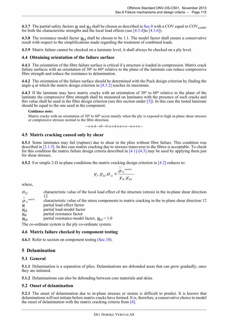
DET NORSKE VERITAS AS
Offshore Standard DNV-OS-C501, November 2013
Sec.6 Failure mechanisms and design criteria – Page 115
4.3.7 The partial safety factors γF and γM shall be chosen as described in Sec.8 with a COV equal to COVcomb,for both the characteristic strengths and the local load effects (see [4.3.4]to [4.3.6]).
4.3.8 The resistance model factor γRd shall be chosen to be 1.1. The model factor shall ensure a conservativeresult with respect to the simplifications made regarding the treatment of combined loads.
4.3.9 Matrix failure cannot be checked on a laminate level, it shall always be checked on a ply level.
4.4 Obtaining orientation of the failure surface
4.4.1 The orientation of the fibre failure surface is critical if a structure is loaded in compression. Matrix crackfailure surfaces with an orientation of 30o to 60o relative to the plane of the laminate can reduce compressivefibre strength and reduce the resistance to delamination.
4.4.2 The orientation of the failure surface should be determined with the Puck design criterion by finding theangle q at which the matrix design criterion in [4.3.2] reaches its maximum.
4.4.3 If the laminate may have matrix cracks with an orientation of 30o to 60o relative to the plane of thelaminate the compressive fibre strength shall be measured on laminates with the presence of such cracks andthis value shall be used in the fibre design criterion (see this section under [3]). In this case the tested laminateshould be equal to the one used in the component.
Guidance note:
Matrix cracks with an orientation of 30o to 60o occur mainly when the ply is exposed to high in-plane shear stressesor compressive stresses normal to the fibre direction.
---e-n-d---of---G-u-i-d-a-n-c-e---n-o-t-e---
4.5 Matrix cracking caused only by shear
4.5.1 Some laminates may fail (rupture) due to shear in the plies without fibre failure. This condition wasdescribed in [3.1.5]. In this case matrix cracking due to stresses transverse to the fibres is acceptable. To checkfor this condition the matrix failure design criteria described in [4.1]-[4.3] may be used by applying them justfor shear stresses.
4.5.2 For simple 2-D in-plane conditions the matrix cracking design criterion in [4.2] reduces to:
where,
σ12 characteristic value of the local load effect of the structure (stress) in the in-plane shear direction12characteristic value of the stress components to matrix cracking in the in-plane shear direction 12
γF partial load effect factorγSd partial load-model factorγM partial resistance factorγRd partial resistance-model factor, γRd = 1.0
The co-ordinate system is the ply co-ordinate system.
4.6 Matrix failure checked by component testing
4.6.1 Refer to section on component testing (Sec.10).
5 Delamination
5.1 General
5.1.1 Delamination is a separation of plies. Delaminations are debonded areas that can grow gradually, oncethey are initiated.
5.1.2 Delaminations can also be debonding between core materials and skins.
5.2 Onset of delamination
5.2.1 The onset of delamination due to in-plane stresses or strains is difficult to predict. It is known thatdelaminations will not initiate before matrix cracks have formed. It is, therefore, a conservative choice to modelthe onset of delamination with the matrix cracking criteria from [4].
RdM
matrix
SdF γγσσγγ
...
12
12
∧
<
matrix12
∧σ
DET NORSKE VERITAS AS
Offshore Standard DNV-OS-C501, November 2013
Sec.6 Failure mechanisms and design criteria – Page 116
5.3 Delamination growth
5.3.1 Growth of interlaminar cracks can be analysed with a fracture mechanics approach. The crack willpropagate when the strain energy release rate G will reach the critical strain energy release rate Gcritical. Thedesign criterion is then given by:
G shall be calculated using local interlaminar stresses. For γRd see [5.3.2].
5.3.2 Gcritical depends often on the crack length:
— if the dependence on crack length can be considered γRd = 1— if the dependence on crack length is not known γRd = 2
5.3.3 Gcritical has to be chosen for the appropriate crack opening mode. For mixed mode conditions Gcriticalcan be calculated as a weighted average of GI critical and GII critical.
6 Yielding
6.1 General
6.1.1 Yielding design criteria apply to most polymer core materials of sandwich structures.
6.1.2 Yielding design criteria may apply to a matrix material with plastic characteristics if the matrix is locatedin a region where it is not restrained between fibres, e.g. in the case of resin rich layers.
6.1.3 Yielding applies also to typical liner materials, like thermoplastics or resin rich layers.
6.1.4 The von Mises' yield criterion shall be used to describe materials that yield. The stresses used in thiscriterion are the principal stresses.
where,
σn characteristic principal stresses, n=1,2,3σy characteristic value of the yield stress of the materialγF partial load effect factorγSd, load-model factorγM partial resistance factorγRd resistance-model factor, γRd = 1.0.
6.1.5 The characteristic yield strength σy and the corresponding coefficients of variation COV are defined asspecified in Sec.4 [1.6] and Sec.5 [1.6].
6.1.6 When two or several loads are combined, each stress component σn in direction n can be the result ofseveral combined loads. In that case each stress component σn
j, local response of the structure in direction ndue to load j, shall be considered separately as an individual stress component.
6.1.7 The choice of the partial safety factors shall be based on the most conservative partial safety factorsobtained when treating each stress component σn
j , local response of the structure in direction n due to load j,as a single load. The material's COV shall always be the COV of the yield strength.
6.1.8 Foam cores under significant hydrostatic pressure or tension shall be checked in addition for ultimatefailure of orthotropic homogenous materials [7]. Significant hydrostatic pressure or tension exists if:
where σ1, σ2, σ3 are the principal stresses with σ1 > σ2 > σ3.
RdM
SdF Gγγ
γγ.
G.. critical<
( ) ( ) ( ) yRdMSdF σσσσσσσγγγγ <−+−+− 2
13
2
32
2
21....
( ) 13213 1.03
11.0 σσσσσ ≤++≤
DET NORSKE VERITAS AS
Offshore Standard DNV-OS-C501, November 2013
Sec.6 Failure mechanisms and design criteria – Page 117
7 Ultimate failure of orthotropic homogenous materials
7.1 General
7.1.1 The criterion can only be used for orthotropic homogenous materials, i.e. materials with three axes ofsymmetry. Isotropic materials are included, since they are a sub-group of orthotropic materials. This criterionis typically applied to core materials. Strength values shall be determined relative to the axes of materialsymmetry ([1.4]). The criterion is not valid for fibre reinforced laminates, because laminates are nothomogeneous.
7.1.2 The criterion can be applied to brittle core materials or to polymeric materials after yield.
7.1.3 The following design criterion should be used when the stress in one direction is dominating comparedto the stresses in the other directions. The stress in one direction is said to be dominating when the criterion in[7.1.4] is not satisfied. The criterion shall be applied for tensile and compressive stresses.
where,
n direction of the dominating stressσnk characteristic value of the local load effect of the structure (stress) in direction n
characteristic value of the strength (stress to failure for component n)γF partial load effect factorγSd partial load-model factorγM partial resistance factorγRd partial resistance-model factor, γRd = 1.0.
Local response and strength must be given in the same co-ordinate system.
Guidance note:
A typical example for core materials in a sandwich would be to check that the through thickness shear stress does notexceed the shear strength. In many cases the shear stress is the dominating stress component, however, this shall bechecked with the criterion in [7.1.4].
---e-n-d---of---G-u-i-d-a-n-c-e---n-o-t-e---
7.1.4 The interaction between the stress components in several directions shall be taken into considerationwhen the following criterion is satisfied. In that case, there is no dominating stress and the interaction can notbe disregarded.
where i and n refer to the directions: 11, 22, 33, 12, 13, 23.
For isotropic materials the directions shall be either the principal normal stresses or the principal shear stresses.For orthotropic materials the directions shall be the material axes.
The same co-ordinate systems shall be used in [7.1.3] and [7.1.4].
7.1.5 When the interaction between the stress components in several directions shall be taken intoconsideration, the design criterion below shall be applied. The criterion shall be applied for tensile andcompressive stresses.
where,
n refers to the directions 11, 22, 33, 12, 13, 23σnk characteristic value of the local load effect of the structure (stress) in the direction n
characteristic value of the strength (stress to failure for component n)γF partial load effect factorγSd, partial load-model factorγM partial resistance factorγRd partial resistance-model factor, γRd = 1.25.
maxi
RdM
nk
nkSdF γγσσγγ
...
∧
<
nk
∧σ
10/ ≤∑≠ ∧∧
innk
nk
ik
ik
σ
σσ
σ
1....
2
<∑ ∧
nRdMSdF
nk
nk
σ
σγγγγ
nk
∧σ
DET NORSKE VERITAS AS
Offshore Standard DNV-OS-C501, November 2013
Sec.6 Failure mechanisms and design criteria – Page 118
For orthotropic materials the directions shall be the material axes. For isotropic materials the directions shallbe along either the principal normal stresses or the principal shear stresses.
This is a conservative design criterion. It has been chosen due to a lack of data and experience with ultimatefailure under multiple stress conditions. Other design criteria may be used if experimental evidence for theirvalidity can be given (see under [19]).
Guidance note:
A resistance-model factor γRd = 1.25 should be used with this design rule. The modelling factor shall ensure aconservative result with respect to the simplifications made regarding the treatment of combined loads.
---e-n-d---of---G-u-i-d-a-n-c-e---n-o-t-e---
7.1.6 The characteristic strength for each of the stress components σnk and the corresponding coefficientsof variation COVn are defined as specified in Sec.4 [1.6] andSec.5 [1.6].
7.1.7 The combined COVcomb is defined according to one of the following alternatives. The second alternativeis conservative with respect to the first.
or
COVcomb = maxn (COVn )
where,
n refers to the directions 11, 22, 33, 12, 13, 23COVn COV for stress component nCOVcomb COV for the combined stress components.
7.1.8 When two or several loads are combined, each characteristic stress component σnk in direction n can bethe result of several combined loads. In that case each stress component σnk
j, local load effect of the structure indirection n due to load j, shall be considered separately as an individual stress component to determine the COV.
or
COVcomb. = maxn (COVn )
The design criterion has then the form:
7.1.9 The choice of the partial safety factors shall be based on the most conservative partial safety factorsobtained when treating each stress component σnk
j, local response of the structure in direction n due to load j,as a single load.
7.1.10 The partial safety factors γF and γM shall be chosen as described in Sec.8 with a resistance COV equalto COVcomb.
8 Buckling
8.1 Concepts and definitions
8.1.1 Elastic buckling phenomena are commonly considered in two main categories:
— Bifurcation buckling: Increasing the applied loading induces at first deformations that are entirely (orpredominantly) axial or in-plane deformations. At a critical value of applied load (elastic critical load) anew mode of deformation involving bending is initiated. This may develop in an unstable, uncontrolledfashion without further increase of load (unstable post-buckling behaviour, brittle type of failure), or growto large values with little or no increase of load (neutral post-buckling behaviour, plastic type of failure) ordevelop gradually in a stable manner as the load is increased further (stable post-buckling behaviour,ductile type of failure).
— Limit point buckling: As the applied load is increased the structure becomes less stiff until the relationshipbetween load and deflection reaches a smooth maximum (elastic critical load) at which the deformationsincrease in an uncontrolled way (brittle type of failure).
nk
∧σ
= ∑∑n
nk
n
nnkcomb COVCOV σσ /.
= ∑∑n
j
nkn
n
j
nkcomb COVCOV σσ /.
1....
2
<∑ ∧
∑
nRdMSdF
nk
j
jnk
σ
σγγγγ
DET NORSKE VERITAS AS
Offshore Standard DNV-OS-C501, November 2013
Sec.6 Failure mechanisms and design criteria – Page 119
8.1.2 Determination of the elastic critical load of a structure or member that experiences bifurcation bucklingcorresponds to the solution of an 'eigenvalue' problem in which the elastic buckling load is an 'eigenvalue' andthe corresponding mode of buckling deformation is described by the corresponding 'eigenvector'.
8.1.3 Elastic buckling may occur at different levels:
— global level for the structure; this involves deformation of the structure as a whole.— global level for a structural member; this is confined mainly to one structural member or element but
involves the whole of that member or element.— local level for a structural member; only a part of a structural member or element is involved (e.g. local
buckling of the flange of an I-beam or of a plate zone between stiffeners in a stiffened plate).
8.1.4 Resistance of a structural member to elastic buckling is normally expressed as a critical value of load(applied force, or stress resultant induced in a member) or as a critical value of a nominal average stress (e.g.axial or shear force divided by area of cross-section). However, such resistance may also be expressed as acritical value of mean strain induced at a cross-section in a member.
8.1.5 Initial geometrical imperfections (out-of-straightness, out-of-roundness, or eccentricity of appliedloading) that lead to a situation where compressive forces in a structural part are not coincident with the neutralaxis of that part may influence significantly the buckling behaviour. An idealised structure without suchimperfections is referred to as “geometrically perfect”.
8.1.6 Bifurcation buckling is essentially a feature of geometrically perfect structures. Geometricalimperfections generally destroy the bifurcation and lead to a situation where bending deformations begin togrow as the load is increased from zero. An elastic critical load may still be associated with the structure, andmay provide a good indication of the load level at which the deformations become large. However, somestructures with unstable post-buckling behaviour are highly sensitive to geometric imperfections. In thepresence of imperfections, such structures may experience limit point buckling at loads that are significantlylower than the elastic critical load of the geometrically perfect structure.
8.1.7 Elastic buckling deformation of a geometrically perfect or imperfect structure may trigger other failuremechanisms such as fibre failure (compressive or tensile) or matrix cracking.
8.1.8 The presence of failure mechanisms such as matrix cracking or delamination may influence significantlythe buckling behaviour of structures and structural members.
8.2 General requirements
8.2.1 Resistance of structures or structural members in the presence of buckling may be determined by meansof testing or analysis.
8.2.2 The effects of initial geometrical imperfections shall always be evaluated for structures or structuralmembers being checked for buckling.
8.2.3 Assumptions regarding geometrical imperfections shall wherever possible be based on
— knowledge of production methods and corresponding production tolerances— knowledge of how imperfections of given shape and magnitude influence the structural behaviour, and — experience from previous measurements and tests.
If an adequate knowledge base does not exist, a programme of measurement and/or testing shall be agreed todemonstrate that the design assumptions are justified.
8.3 Requirements when buckling resistance is determined by testing
8.3.1 If the resistance of a structure or structural member is determined by testing, the requirements in 302 to306 shall be satisfied. Testing shall be done as described in Sec.10 'Component Testing'.
8.3.2 Sufficient tests shall be performed to provide statistical data so that both the mean resistance and theCOV may be determined.
8.3.3 The structures or members tested shall incorporate the least favourable geometrical imperfections thatare possible within the specified production tolerances. Alternatively, the structures or structural memberstested may incorporate a representative range of geometrical imperfections that may arise in the intendedproduction process; however, in such a case it must be demonstrated that the imperfections considered arerepresentative in terms of their distributions of shape and amplitude.
8.3.4 The design criterion shall normally be applied at the level of overall load for a structure, or either force(stress resultant) or nominal stress or strain (averaged over the member cross-section) for a structural member.
DET NORSKE VERITAS AS
Offshore Standard DNV-OS-C501, November 2013
Sec.6 Failure mechanisms and design criteria – Page 120
8.3.5 The design criterion for buckling when the resistance is determined by testing is as follows:
where,
F characteristic value of the load, or induced stress resultant, or nominal stress or straincharacteristic value of the test load when the component buckles
γF partial load or load effect factorγSd partial load or load effect model factorγMbuckle partial resistance factorγRdbuckle partial resistance-model factor.
8.3.6 The partial factors shall be determined according to Sec.10 [2] 'Component Testing'.
8.4 Requirements when buckling is assessed by analysis
8.4.1 If the resistance of a structure or structural member is determined by analysis, the requirements under[8.4.2] to [8.4.15] shall be satisfied.
8.4.2 Buckling analysis may be carried out by analytical or numerical methods as described in Sec.9 [11]. Suchanalyses may be applied to either geometrically perfect or imperfect structures. Analytical methods are mainlyconfined to geometrically perfect structures, except for some simple structural members with imperfections ofsimple shape.
8.4.3 When performing a buckling analysis the boundary conditions shall be evaluated carefully.
8.4.4 If in any buckling analysis the applied load is higher than the load that would introduce partial damagein the structure, e.g. matrix cracking or delaminations, the buckling calculations shall take this partial damageinto account.
8.4.5 For structures or structural elements that are expected to exhibit bifurcation buckling, an analysis todetermine the elastic critical load (or critical stress or strain) shall normally be carried out as described in Sec.9[11.2.2] or Sec.9 [11.3.2], before more complex non-linear analysis is performed.
The purpose of this is to establish:
— whether it may be acceptable to perform only geometrically linear analysis as described in Sec.9 [11.2.5](see also [8.4.11] below)
— whether the structure is clearly under-dimensioned against buckling (if the applied load clearly exceeds, oris close to, the elastic critical load)
— in the case of finite element analysis, the required fineness of mesh for a more complex buckling analysis.
8.4.6 Analytical formulae for elastic buckling shall be checked carefully if they contain empirical safetyfactors or not and if they are based on structures with or without imperfections. Without this knowledgeanalytical formulas should not be used.
8.4.7 Except in the case of analysis for elastic critical loads (or elastic critical stresses or strains), the analysismodel shall incorporate the least favourable geometrical imperfections that are possible within the specifiedproduction tolerances. Alternatively, a series of analyses may be performed incorporating a representativerange of geometrical imperfections that may arise in the intended production process, these may then becombined with statistical information about the imperfections that arise in practical production, in terms of theirdistributions of shape and amplitude.
8.4.8 If imperfections are not directly included in the buckling analysis as described in [8.4.7], their effectsshall be evaluated by other means such as supplementary analysis or testing. However, if it is demonstrated thatthe eccentricities or local bending moments induced by the least favourable geometrical imperfections are lessthan 10% of the corresponding quantities resulting from other features inherent in the structure or its loading,such as out-of-plane loads, the geometrical imperfections may be neglected.
8.4.9 In assessing buckling-induced failure, the design criteria shall normally be applied at the level of localstress or strain state, considered at all points in the structure. The criteria related to fibre failure, matrixcracking, delamination, yield and ultimate failure given under [3], [4], [5], [6] and [7] shall be applied asappropriate. For sandwich structures the special criteria given under [16] shall be applied in addition.Additionally the displacement criterion given under [9] shall be applied both globally and locally to ensure thatthere are no excessive buckling displacements.
8.4.10 To obtain the resistance quantities required for the checks in [8.4.9], geometrically non-linear analysis
RdbuckleMbuckle
buckling
SdF
FF
γγγγ
...
∧
<
bucklingF∧
DET NORSKE VERITAS AS
Offshore Standard DNV-OS-C501, November 2013
Sec.6 Failure mechanisms and design criteria – Page 121
shall be performed as described in Sec.9 [11]. Reduction of mechanical properties due to local failure such asmatrix cracking or delamination shall be taken into account.
8.4.11 If the condition described in Sec.9 [11.2.5] is satisfied, the analysis may be performed withoutgeometric non-linearity provided the load effect modelling factor is increased as specified. In such a case thegeometrical imperfections must still be included.
8.4.12 Sec.9 [11.2.4] provides an approximate way of estimating the combined influence of imperfections andin-plane or axial loading, based on the use of linear analysis.
8.4.13 The calculated resistance is to be considered as a mean strength from a probabilistic point of view.
8.4.14 Variability to the mean strength is introduced by:
— uncertainties in the stiffness parameters that are used in the buckling calculations— uncertainties in geometric parameters— uncertainties in size of imperfections and how imperfections are considered.
8.4.15 To reflect the uncertainty introduced by geometrical imperfections, the partial load effect model factorfor checks on failure mechanisms referred to in [8.4.8] shall be based on a COV of 15% unless lower valuescan be justified.
9 Displacements
9.1 General
9.1.1 Maximum displacements shall be defined as extreme values with a small probability of being exceededand without uncertainties or tolerances associated with them. The following design criterion shall be fulfilled:
where,
dn characteristic value of the local response of the structure (here displacement) dspec specified requirement on maximum displacement γF partial load effect factorγSd, load model factor
Displacements may also be defined as maximum strains, curvatures etc.
9.1.2 Displacements shall be calculated as described in Sec.9 or shall be measured directly. A reduction ofstiffness of the structure due to material non-linearity or due to time dependent effects on the elastic constantsshall be considered. Plastic deformations due to permanent static or fatigue loads shall also be considered.
9.1.3 The failure type (Sec.2 [3.4]) associated with a displacement requirement shall be decided on anindividual basis.
Guidance note:
If the displacement requirement requires that:
- the structure should never touch the neighbouring structure locally, the failure type would be brittle
- the structure can touch the neighbouring structure locally at low loads, the failure type would be plastic
- the structure can touch the neighbouring structure locally at loads that may cause some permanent damage thefailure type would be ductile.
If the structures may touch each other slightly, the corresponding loads and possible damage effects shall be analysed.
---e-n-d---of---G-u-i-d-a-n-c-e---n-o-t-e---
9.1.4 If the criterion is used in combination with a linear non-degraded analysis according to Sec.9 [2.4], allstrains and stresses in fibre direction above the level to initiate matrix cracking shall be multiplied by theanalysis factor γa from Sec.9 [3.2].
dd specnSdF <..γγ
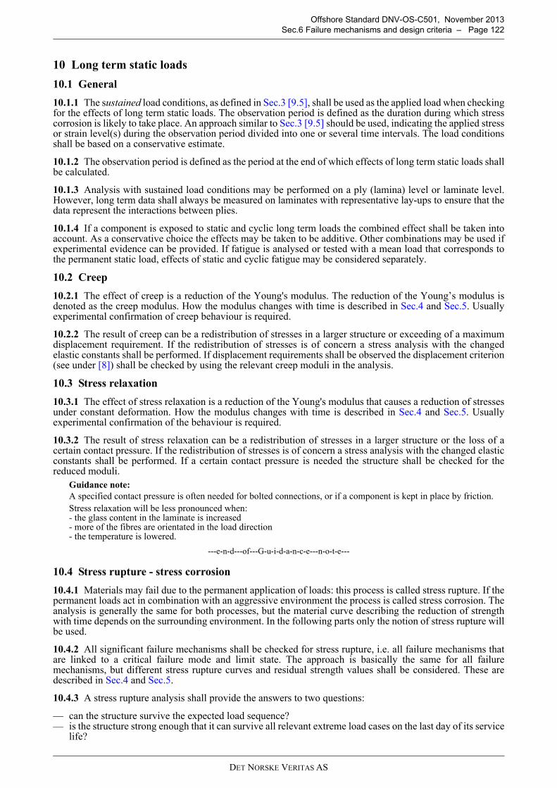
DET NORSKE VERITAS AS
Offshore Standard DNV-OS-C501, November 2013
Sec.6 Failure mechanisms and design criteria – Page 122
10 Long term static loads
10.1 General
10.1.1 The sustained load conditions, as defined in Sec.3 [9.5], shall be used as the applied load when checkingfor the effects of long term static loads. The observation period is defined as the duration during which stresscorrosion is likely to take place. An approach similar to Sec.3 [9.5] should be used, indicating the applied stressor strain level(s) during the observation period divided into one or several time intervals. The load conditionsshall be based on a conservative estimate.
10.1.2 The observation period is defined as the period at the end of which effects of long term static loads shallbe calculated.
10.1.3 Analysis with sustained load conditions may be performed on a ply (lamina) level or laminate level.However, long term data shall always be measured on laminates with representative lay-ups to ensure that thedata represent the interactions between plies.
10.1.4 If a component is exposed to static and cyclic long term loads the combined effect shall be taken intoaccount. As a conservative choice the effects may be taken to be additive. Other combinations may be used ifexperimental evidence can be provided. If fatigue is analysed or tested with a mean load that corresponds tothe permanent static load, effects of static and cyclic fatigue may be considered separately.
10.2 Creep
10.2.1 The effect of creep is a reduction of the Young's modulus. The reduction of the Young’s modulus isdenoted as the creep modulus. How the modulus changes with time is described in Sec.4 and Sec.5. Usuallyexperimental confirmation of creep behaviour is required.
10.2.2 The result of creep can be a redistribution of stresses in a larger structure or exceeding of a maximumdisplacement requirement. If the redistribution of stresses is of concern a stress analysis with the changedelastic constants shall be performed. If displacement requirements shall be observed the displacement criterion(see under [8]) shall be checked by using the relevant creep moduli in the analysis.
10.3 Stress relaxation
10.3.1 The effect of stress relaxation is a reduction of the Young's modulus that causes a reduction of stressesunder constant deformation. How the modulus changes with time is described in Sec.4 and Sec.5. Usuallyexperimental confirmation of the behaviour is required.
10.3.2 The result of stress relaxation can be a redistribution of stresses in a larger structure or the loss of acertain contact pressure. If the redistribution of stresses is of concern a stress analysis with the changed elasticconstants shall be performed. If a certain contact pressure is needed the structure shall be checked for thereduced moduli.
Guidance note:
A specified contact pressure is often needed for bolted connections, or if a component is kept in place by friction.
Stress relaxation will be less pronounced when:- the glass content in the laminate is increased- more of the fibres are orientated in the load direction- the temperature is lowered.
---e-n-d---of---G-u-i-d-a-n-c-e---n-o-t-e---
10.4 Stress rupture - stress corrosion
10.4.1 Materials may fail due to the permanent application of loads: this process is called stress rupture. If thepermanent loads act in combination with an aggressive environment the process is called stress corrosion. Theanalysis is generally the same for both processes, but the material curve describing the reduction of strengthwith time depends on the surrounding environment. In the following parts only the notion of stress rupture willbe used.
10.4.2 All significant failure mechanisms shall be checked for stress rupture, i.e. all failure mechanisms thatare linked to a critical failure mode and limit state. The approach is basically the same for all failuremechanisms, but different stress rupture curves and residual strength values shall be considered. These aredescribed in Sec.4 and Sec.5.
10.4.3 A stress rupture analysis shall provide the answers to two questions:
— can the structure survive the expected load sequence?— is the structure strong enough that it can survive all relevant extreme load cases on the last day of its service
life?
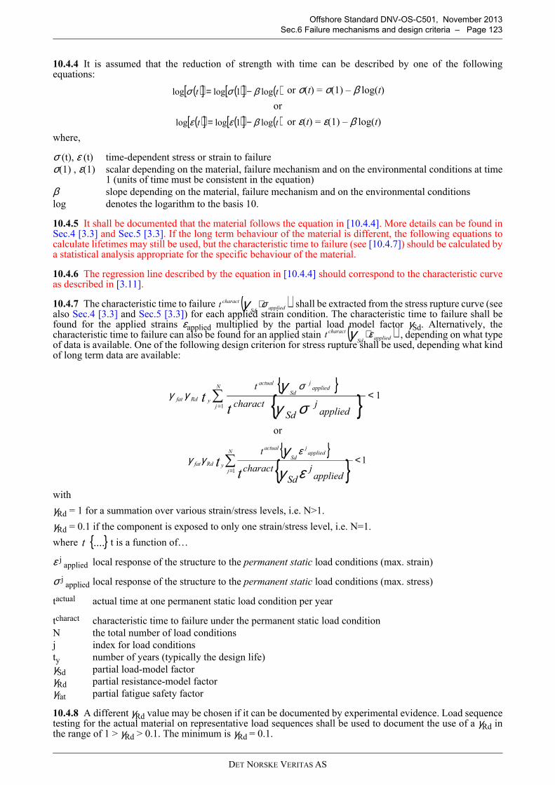
DET NORSKE VERITAS AS
Offshore Standard DNV-OS-C501, November 2013
Sec.6 Failure mechanisms and design criteria – Page 123
10.4.4 It is assumed that the reduction of strength with time can be described by one of the followingequations:
or σ(t) = σ(1) – β log(t)
or
or ε(t) = ε(1) – β log(t)
where,
σ (t), ε (t) time-dependent stress or strain to failureσ(1) , ε(1) scalar depending on the material, failure mechanism and on the environmental conditions at time
1 (units of time must be consistent in the equation)β slope depending on the material, failure mechanism and on the environmental conditionslog denotes the logarithm to the basis 10.
10.4.5 It shall be documented that the material follows the equation in [10.4.4]. More details can be found inSec.4 [3.3] and Sec.5 [3.3]. If the long term behaviour of the material is different, the following equations tocalculate lifetimes may still be used, but the characteristic time to failure (see [10.4.7]) should be calculated bya statistical analysis appropriate for the specific behaviour of the material.
10.4.6 The regression line described by the equation in [10.4.4] should correspond to the characteristic curveas described in [3.11].
10.4.7 The characteristic time to failure shall be extracted from the stress rupture curve (seealso Sec.4 [3.3] and Sec.5 [3.3]) for each applied strain condition. The characteristic time to failure shall befound for the applied strains εapplied multiplied by the partial load model factor γSd. Alternatively, thecharacteristic time to failure can also be found for an applied stain , depending on what typeof data is available. One of the following design criterion for stress rupture shall be used, depending what kindof long term data are available:
or
with
γRd = 1 for a summation over various strain/stress levels, i.e. N>1.
γRd = 0.1 if the component is exposed to only one strain/stress level, i.e. N=1.
where t is a function of…
ε j applied local response of the structure to the permanent static load conditions (max. strain)
σ j applied local response of the structure to the permanent static load conditions (max. stress)
tactual actual time at one permanent static load condition per year
tcharact characteristic time to failure under the permanent static load conditionN the total number of load conditionsj index for load conditionsty number of years (typically the design life)γSd partial load-model factorγRd partial resistance-model factorγfat partial fatigue safety factor
10.4.8 A different γRd value may be chosen if it can be documented by experimental evidence. Load sequencetesting for the actual material on representative load sequences shall be used to document the use of a γRd inthe range of 1 > γRd > 0.1. The minimum is γRd = 0.1.
( )[ ] ( )[ ] ( )tt log1loglog βσσ −=
( )[ ] ( )[ ] ( )tt log1loglog βεε −=
( )appliedSd
charactt σγ ⋅
( )appliedSd
charactt εγ ⋅
{ }{ } 1
1
<∑=
N
j
appliedj
Sd
actual
yRdfat
appliedj
Sdcharact
t
tt
σγγ σ
γγ
{ }{ } 1
1
<∑=
N
j
appliedj
Sd
actual
yRdfat
appliedj
Sdcharact
t
tt
εγγ ε
γγ
{ }....t
DET NORSKE VERITAS AS
Offshore Standard DNV-OS-C501, November 2013
Sec.6 Failure mechanisms and design criteria – Page 124
Guidance note:
The factors γfat γRd are designed in such a way that they account for the uncertainty in Miner sum for composites andprovide the desired level of safety. When choosing the default value γRd =1 an uncertainty of 10 is assumed for theMiner sum.
---e-n-d---of---G-u-i-d-a-n-c-e---n-o-t-e---
10.4.9 If the design criterion in [10.4.8] is fulfilled even if γRd can be multiplied by 20 it may be sufficient touse typical fatigue data for the laminate without confirming the data by testing. A minimum requirement forusing this clause is that all similarity checks in Sec.4 [8] are fulfilled. A cases by case evaluation should bemade in addition, in particular evaluating whether environmental effect could change the fatigue properties ofthe laminate relative to the reference data.
10.4.10 The selection of the partial safety factors is based on the following assumptions: The long term staticload is defined as a conservative mean value, i.e. no uncertainty needs to be considered for that variable. Thepartial load effect factor γF is set equal to 1.0.
10.4.11 Under permanent loads, composite materials show a reduction of strength with time for various failuremechanisms under permanent loads. All relevant failure mechanisms shall be checked for the reduced strengthvalues under extreme load conditions. More details about strength reduction can be found in Sec.4 and Sec.5.Possible reduction of Young's moduli should also be considered, depending on the analysis methods used (seeSec.9).
10.4.12 If the criterion is used in combination with a linear non-degraded analysis according to Sec.9 [2.4], allstrains and stresses in fibre direction above the level to initiate matrix cracking shall be multiplied by theanalysis factor γa from [3.2].
10.4.13 The partial fatigue safety factor γfat is defined in Sec.8 [5] for different safety classes. The same safetyclass as determined for the static failure mechanism shall be used.
11 Long term cyclic loads
11.1 General
11.1.1 The fatigue load conditions, as defined in Sec.3 [9.6], shall be used as the applied load when checkingfatigue. An approach similar to the one given in Sec.3 [9.6.5] should be used, indicating the mean andamplitude of applied stress or strain as a function of the number of cycles. The load conditions shall be basedon a conservative estimate.
11.1.2 Fatigue analysis may be performed on a ply (lamina) level or on a laminate level. However, fatigue datashall always be measured on laminates with representative lay-ups to ensure that the data represent theinteractions between plies.
11.1.3 If a component is exposed to static and cyclic long term loads the combined effect shall be taken intoaccount. As a conservative choice the effects may be taken to be additive. Other combinations may be used ifexperimental evidence can be provided. If fatigue is analysed or tested with a mean load that corresponds tothe permanent static load, effects of static and cyclic fatigue may be considered separately.
11.1.4 Matrix cracks may develop under cyclic loads even if the maximum stress is below the level to initiatematrix cracking in a static test.
11.2 Change of elastic properties
11.2.1 Fatigue loads may change the elastic properties of a material. The change is of permanent nature in mostcases. How the modulus changes with the number of cycles is described in Sec.4 and Sec.5. Usuallyexperimental confirmation of the change of elastic properties is required.
11.2.2 The result of a change of the elastic properties can be a redistribution of stresses in a larger structure orexceeding a maximum displacement requirement. If the redistribution of stresses is of concern a stress analysiswith the changed elastic constants shall be performed. If displacement requirements shall be observed thedisplacement criterion (see Sec.6 [9]) shall be fulfilled for the relevant elastic properties in the analysis.
Guidance note:
The change of elastic constants is usually a result of an accumulation of matrix cracks under cyclic fatigue.
---e-n-d---of---G-u-i-d-a-n-c-e---n-o-t-e---
11.2.3 In some cases a certain contact pressure may be needed for a component. It shall be documented thatthe change of elastic constants due to cyclic fatigue will not reduce the contact pressure to an unacceptablelevel.
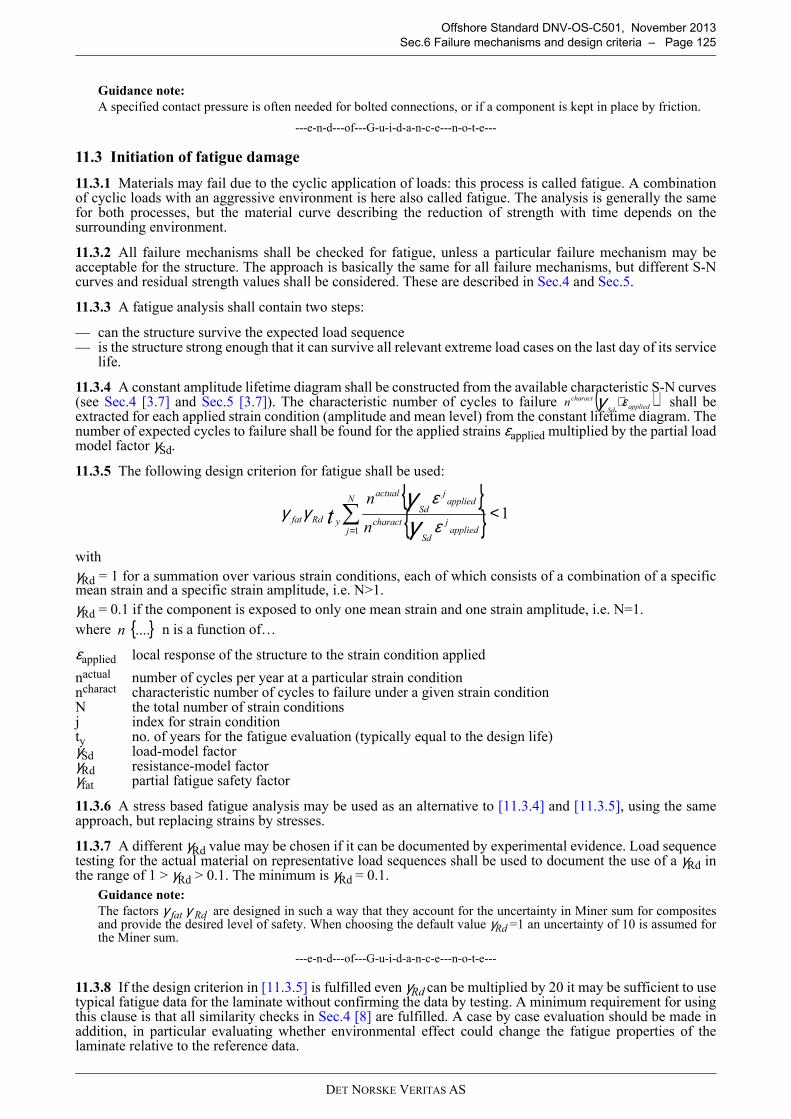
DET NORSKE VERITAS AS
Offshore Standard DNV-OS-C501, November 2013
Sec.6 Failure mechanisms and design criteria – Page 125
Guidance note:
A specified contact pressure is often needed for bolted connections, or if a component is kept in place by friction.
---e-n-d---of---G-u-i-d-a-n-c-e---n-o-t-e---
11.3 Initiation of fatigue damage
11.3.1 Materials may fail due to the cyclic application of loads: this process is called fatigue. A combinationof cyclic loads with an aggressive environment is here also called fatigue. The analysis is generally the samefor both processes, but the material curve describing the reduction of strength with time depends on thesurrounding environment.
11.3.2 All failure mechanisms shall be checked for fatigue, unless a particular failure mechanism may beacceptable for the structure. The approach is basically the same for all failure mechanisms, but different S-Ncurves and residual strength values shall be considered. These are described in Sec.4 and Sec.5.
11.3.3 A fatigue analysis shall contain two steps:
— can the structure survive the expected load sequence— is the structure strong enough that it can survive all relevant extreme load cases on the last day of its service
life.
11.3.4 A constant amplitude lifetime diagram shall be constructed from the available characteristic S-N curves(see Sec.4 [3.7] and Sec.5 [3.7]). The characteristic number of cycles to failure shall beextracted for each applied strain condition (amplitude and mean level) from the constant lifetime diagram. Thenumber of expected cycles to failure shall be found for the applied strains εapplied multiplied by the partial loadmodel factor γSd.
11.3.5 The following design criterion for fatigue shall be used:
with
γRd = 1 for a summation over various strain conditions, each of which consists of a combination of a specificmean strain and a specific strain amplitude, i.e. N>1.
γRd = 0.1 if the component is exposed to only one mean strain and one strain amplitude, i.e. N=1.
where n is a function of…
εapplied local response of the structure to the strain condition applied
nactual number of cycles per year at a particular strain conditionncharact characteristic number of cycles to failure under a given strain conditionN the total number of strain conditionsj index for strain conditionty no. of years for the fatigue evaluation (typically equal to the design life)γSd load-model factorγRd resistance-model factorγfat partial fatigue safety factor
11.3.6 A stress based fatigue analysis may be used as an alternative to [11.3.4] and [11.3.5], using the sameapproach, but replacing strains by stresses.
11.3.7 A different γRd value may be chosen if it can be documented by experimental evidence. Load sequencetesting for the actual material on representative load sequences shall be used to document the use of a γRd inthe range of 1 > γRd > 0.1. The minimum is γRd = 0.1.
Guidance note:
The factors γ fat γ Rd are designed in such a way that they account for the uncertainty in Miner sum for compositesand provide the desired level of safety. When choosing the default value γRd =1 an uncertainty of 10 is assumed forthe Miner sum.
---e-n-d---of---G-u-i-d-a-n-c-e---n-o-t-e---
11.3.8 If the design criterion in [11.3.5] is fulfilled even γRd can be multiplied by 20 it may be sufficient to usetypical fatigue data for the laminate without confirming the data by testing. A minimum requirement for usingthis clause is that all similarity checks in Sec.4 [8] are fulfilled. A case by case evaluation should be made inaddition, in particular evaluating whether environmental effect could change the fatigue properties of thelaminate relative to the reference data.
( )appliedSd
charactn εγ ⋅
{ }{ } 1
1
<∑=
N
j appliedj
Sd
charact
appliedj
Sd
actual
yRdfatn
n
t ε
εγγ γ
γ
{ }....n
DET NORSKE VERITAS AS
Offshore Standard DNV-OS-C501, November 2013
Sec.6 Failure mechanisms and design criteria – Page 126
11.3.9 If the structure is exposed to a known load sequence and the S-N curve has been obtained for that loadsequence the Miner sum calculation is not required. If the load sequence changes Miner sum calculations areneeded.
11.3.10 The selection of the partial safety factors is based on the following assumptions: The fatigue load(mean and amplitude) is defined as a conservative mean value, i.e. no uncertainty needs to be considered forthat variable. The partial load effect factor γF is set equal to 1.0.
11.3.11 Composite materials may show a reduction of strength with numbers of cycles for various failuremechanisms. All relevant failure mechanisms shall be checked for the reduced strength values under extremeload conditions. More details about strength reduction can be found in Sec.4 and Sec.5. Possible reduction ofYoung's moduli should also be considered, depending on the analysis methods used (see Sec.9).
11.3.12 If the criterion is used in combination with a linear non-degraded analysis according to Sec.9 [2.4], allstrains and stresses in fibre direction above the level to initiate matrix cracking shall be multiplied by theanalysis factor γa from Sec.9 [3.2].
11.3.13 The partial fatigue safety factor γfat is defined in Sec.8 [5] for different safety classes. The same safetyclass as determined for the static failure mechanism shall be used.
11.4 Growth of fatigue damage
11.4.1 Growth of fatigue damage is defined here as the accumulation of damage due to fatigue loads, e.g. theincrease of the number of cracks in the matrix or the growth of a delamination.
11.4.2 The initiation of damage due to long term static and cyclic loads is described under [11] and [12].
11.4.3 The growth of damage is a complicated process that shall be documented based on experimentalevidence. The simplified approach of assuming that the component is always completely saturated withdamage may be used.
11.4.4 If a component may accumulate damage due to fatigue, the component shall be analysed with andwithout that damage.
12 Impact
12.1 General
12.1.1 Impact of an object may have two effects on a structure. The impact may be so strong that failure modesare introduced that will immediately lead to a violation of functional requirements. More often impact maycause some minor failures that may lead to further damage and violation of functional requirements in thefuture.
12.1.2 When considering the effects of impact, it should be documented that no unintended failuremechanisms will happen due to impact.
12.1.3 The resistance of a structure to impact should be tested experimentally. This can be done in two ways.
— The material or a small section is exposed to a relevant impact scenario. The strength of the material withthe impact damage is determined as described in Sec.4 or Sec.5. This strength can be used for further designof the component.
— The full component is exposed to a relevant impact scenario. The component is tested afterwards to showthat it can still tolerate the critical loads.
12.1.4 Impact design criteria may be used if experimental evidence shows that they are applicable for theapplication.
12.2 Impact testing
12.2.1 The geometry of the impactor and the boundary conditions should represent a worst case for theapplication. A change of impactor geometry, boundary conditions, material properties or testing rate oftenchanges the structural response completely.
12.2.2 The points of impact should be chosen carefully to represent all worst case scenario. In some cases asingle point may be sufficient for testing.
12.2.3 It should further be evaluated whether the component should be able to withstand more than one impactscenario. In that case the component should be exposed to the expected number of impact events.
DET NORSKE VERITAS AS
Offshore Standard DNV-OS-C501, November 2013
Sec.6 Failure mechanisms and design criteria – Page 127
12.3 Evaluation after impact testing
12.3.1 The impact tests should demonstrate that no unacceptable damage is introduced into the component.Once the component has been exposed to impact it should be carefully inspected to ensure that no unexpectedfailure mechanisms occurred that may reduce the component's performance, in particular long termperformance. If the component will be taken out of service after an impact, long term considerations do nothave to be made.
12.3.2 It shall be shown further that the component can carry all relevant loads after impact until it can be takenout of service for repair or replacement. This can be done by analysis taking the observed impact damage intoaccount, by testing, or a combination of analysis and testing. Testing should be done according to Sec.10.
12.3.3 If the component may be exposed to impact but can or should not be repaired afterwards, it should beshown that the component can withstand all long-term loads with the damage induced by the impact. The sameapproach as in [12.3.2] should be used.
Guidance note:
A typical example is impact of dropped objects on a pipe.
The pipe is tested by dropping representative objects, like tools from the maximum possible height onto the pipe.
Damage analysis shows matrix cracking and delamination but no fibre failures. Since the pipe has a liner one couldassume that the capability to hold pressure is not reduced in the short term.
One pressure test is used to confirm this prediction according to Sec.10 [3].
---e-n-d---of---G-u-i-d-a-n-c-e---n-o-t-e---
13 Wear
13.1 General
13.1.1 Wear is a complicated process that is influenced by the entire system. All material data used for wearcalculations shall be relevant for the system investigated.
13.2 Calculation of the wear depth
13.2.1 The wear depth may be calculated based on the sliding distance, using the length related wear rate for the corresponding wear system. The wear rate varies with the surfaces in contact, the magnitude of thecontact pressure and the environment. The wear depth dy (thickness of removed material) is given by:
The total sliding distance dx shall be calculated assuming one contact point for the entire duration of the wearphase.
13.2.2 Another option is to calculate the wear depth based on the sliding time, using the time related wearrate for the corresponding wear system. The wear rate varies with the surfaces in contact, the magnitude ofthe contact pressure and the environment. The wear depth dy (thickness of removed material) is given by:
The total sliding time dt shall be calculated assuming the same contact point for the entire duration of the wearphase.
13.2.3 The consequences of removing material with respect to all other failure mechanisms shall be evaluated.
13.3 Component testing
13.3.1 Refer to section on component testing: Sec.10.
Guidance note:
The performance of a wear system should ideally be assessed by a practical trial in the intended application. However,this trial is often impractical and it is necessary to resort to laboratory testing. Accelerated laboratory tests with simplergeometrical configurations are often used although there is still a considerable amount of controversy about thevalidity of the results due to the geometry of the test samples.
---e-n-d---of---G-u-i-d-a-n-c-e---n-o-t-e---
•w
(m/m) dx
dyw =•
•
tw
(m/s) dt
dywt =•
DET NORSKE VERITAS AS
Offshore Standard DNV-OS-C501, November 2013
Sec.6 Failure mechanisms and design criteria – Page 128
14 High / low temperature / fire
14.1 General
14.1.1 The effects of fire and high/low temperature shall be considered by using the appropriate materialproperties as described in Sec.4 and Sec.5 within the design criteria described in this section.
14.1.2 High temperatures and fire may introduce changes in the material, even if no other design criteria areviolated. The following shall be considered as a minimum:
— melting— burning— removal of material— phase transitions
14.1.3 Specific requirements to fire performance are not given in this standard. These requirements shall beobtained from other codes or regulations covering the application.
14.1.4 Composite structures usually need special fire protection to fulfil fire performance requirements.Special care shall be taken to ensure that the insulation works properly, including joints and attachments. Thejoints should remain tight in a fire and insulation should not detach.
15 Resistance to explosive decompression
15.1 Materials
15.1.1 Materials that are exposed to fluids under high pressure tend to absorb some fluid. If the pressure isremoved rapidly (rapid decompression) the fluid inside the material wants to expand and wants to diffuse outof the material. If the material's structure does not allow the fluid to move out rapidly, or if the molecularstrength of the material is not strong enough to contain the expanding fluid, severe microscopic damage mayhappen to the material.
15.1.2 The resistance of a material to the effects of rapid decompression shall be tested experimentally, ifrelevant. Tests shall be carried out at two pressure levels: The maximum expected pressure and the low typicalservice pressure.
Guidance note:
The reason to test at two pressures is based on the two effects interacting during a rapid decompression scenario:Diffusion and Molecular strength.
---e-n-d---of---G-u-i-d-a-n-c-e---n-o-t-e---
15.2 Interfaces
15.2.1 Similar to the effect observed in materials, fluids can accumulate between interfaces of materials withdifferent diffusion constants. A rapid reduction of pressure may destroy the interface, because the fluid wantsto expand. In the case of liners or thin materials, the liner may deform substantially, buckle, or even crack.
15.2.2 The designer should think about venting arrangements in the structure to avoid the build-up of fluids ininterfaces.
15.2.3 The resistance of an interface to the effects of rapid decompression shall be tested at the maximumexpected pressure, unless it can be shown that venting arrangements prevent the build-up of fluids.
16 Special aspects related to sandwich structures
16.1 General
16.1.1 Sandwich structures are built of a light weight core embedded between two faces (or skins). Designcriteria are discussed for skins, cores and the core skin interface.
16.2 Failure of sandwich faces
16.2.1 The same general design criteria as discussed above apply.
16.2.2 Both faces shall be checked for failure, since they may be exposed to different stress states.
16.3 Failure of the sandwich core
16.3.1 Many core materials show plastic behaviour. If yielding cannot be accepted in the sandwich structurethe yield criterion under [6] shall be applied.
DET NORSKE VERITAS AS
Offshore Standard DNV-OS-C501, November 2013
Sec.6 Failure mechanisms and design criteria – Page 129
16.3.2 Ultimate failure of brittle and plastic core materials shall be checked with the design criterion fororthotropic homogenous materials under [7].
16.3.3 In many cases the dominant stress in a core is shear, causing shear yield or failure or tensile failure in45o to the through thickness direction. This case is also covered by the criteria given under [6] and [7].
16.3.4 Core indentation due to local compressive stress shall be checked. The core will indent if thecompressive strength of the core is exceeded (see [16.3.1] and [16.3.2]).
16.4 Failure of the sandwich skin-core interface
16.4.1 Interface failure between the skin and core of a sandwich can be treated the same way as a delamination([5]).
16.4.2 Care shall be taken to use proper material properties when applying the design criterion. Interfaceproperties may differ from the core or laminate properties.
16.4.3 Sandwich structures with PVC core show typically no failure directly in the interface, but they failinside the PVC core close to the interface. PVC core properties may be used in the design criteria.
16.4.4 Sandwich structures with Balsa core fail typically in the interface.
16.5 Buckling of sandwich structures
16.5.1 The same buckling criteria as for general structures apply, see under [8].
16.5.2 Sandwich structures show some special buckling modes. The following modes shall be considered:
16.5.3 Face wrinkling will occur when the compressive direct stress in the face will reach the local instability(or wrinkling) stress, i.e.
16.5.4 Global buckling will occur when the axial load will reach the critical buckling load, i.e.
16.5.5 Shear crimping will occur when the direct stress will reach the crimping stress, i.e.
16.5.6 Face dimpling or intercellular buckling occurs only in sandwich structures with honeycomb andcorrugated cores. Face dimpling will occur when the compressive stress in the cell wall reaches the bucklingstress of a honeycomb cell or a corrugated core, i.e.
17 Chemical decomposition / galvanic corrosion
17.1 General
17.1.1 A material may degrade due to chemical decomposition. This effect is covered in principle in thisstandard by the time dependence of strength and stiffness values.
17.1.2 The extrapolation of long term data under environmental exposure describes usually the gradual effectof environment or load on the properties. Chemical decomposition may act suddenly and rapidly and may notbe detected by mechanical long term tests.
17.1.3 If a material is exposed to chemicals, possible chemical decomposition should be considered.
17.1.4 Possible galvanic corrosion should be considered when carbon fibre composites are in contact withmetal. Usually the metal degrades first, but in some cases also damage to the matrix and the fibres can happen.Carbon composites should be electrically isolated from metal components.
wrinklingface σσ ˆ≥
.crPP ≥
crimpingface σσ ˆ≥
dinplingcore σσ ˆ≥
DET NORSKE VERITAS AS
Offshore Standard DNV-OS-C501, November 2013
Sec.6 Failure mechanisms and design criteria – Page 130
18 Static electricity
18.1 General
18.1.1 Static electricity can develop on composite surfaces, especially if the surrounding air is dry.
If the potential electrical sparks created by static electricity can cause a fire, explosion or other hazard thebuildup of static electricity shall be prevented.
It should be shown that the air is either humid enough that static electricity cannot build up or some conductivesurface layer with grounding should be applied.
The conductive layer should be applied over all free surface and everything needs to be grounded, ensuring thatno ungrounded or unconductive layers are left.
19 Requirements for other design criteria
19.1 General
19.1.1 If a structure or component shows a failure mechanism not described above it may be necessary todescribe a design criterion for this failure mechanism.
19.1.2 All design criteria shall be verified against experimental evidence. The model factor assigned to thedesign criterion shall compensate for the discrepancies between prediction and experiment. The model factoris a deterministic factor.
19.1.3 It shall be confirmed that the design criterion is of general nature and does not just apply to one materialor one load case, unless the criterion is only used for that particular condition.
19.1.4 The partial safety factors in the criterion shall calibrated by probabilistic methods to ensure a consistentlevel of safety with respect to the rest of the standard.
DET NORSKE VERITAS AS
Offshore Standard DNV-OS-C501, November 2013
Sec.7 Joints and interfaces – Page 131
SECTION 7 JOINTS AND INTERFACES
1 General
1.1 Introduction
1.1.1 Joints and interfaces are special sections or components of a structure. They can in principle be analysedan tested the same way as a structure or component. However, some special considerations are described in thefollowing sections.
1.1.2 Requirements for joints and interfaces are based on achieving the same level of reliability as the structureof which it is part.
1.1.3 If metal components are part of a joint or interface, the metal components shall be designed according torelevant standards for such components. This standard does not cover metal components.
1.2 Joints
1.2.1 Joints are defined here as load bearing connections between structures, components or parts.
1.2.2 Three basic types of joints are considered in this standard:
— laminated joints, i.e. joints fabricated from the same constituent materials as the laminates that are joined,such as e.g. over-laminations, lap joints, scarf joints etc.
— adhesive joints, i.e. joints between laminates, cores or between laminates and other materials e.g. metals— mechanical joints, i.e. joints including fasteners, e.g. bolted connections.
1.3 Interfaces
1.3.1 Interfaces are defined here as the area or region where different structures, components or parts meeteach other. All joints have interfaces.
1.3.2 If the interface shall transfer loads it also has the function of a joint. All requirements for joints apply tosuch an interface.
1.3.3 A typical interface is the area where the surface of a load bearing structure and a liner meet.
1.4 Thermal properties
1.4.1 The effects of thermal stresses and strains and displacements shall be considered for all joints andinterfaces.
1.5 Examples
1.5.1 Examples of good practise shall be evaluated with great care. The examples are usually given for certainload and environmental conditions, without stating those explicitly. The qualification and analysisrequirements of this standard shall also be applied joints based on good practise. See also [2.4] on howexperience can be utilised.
2 Joints
2.1 Analysis and testing
2.1.1 The same design rules as applied for the rest of the structure shall be applied to joints, as relevant.
2.1.2 Joints are usually difficult to evaluate, because they have complicated stress fields and the materialproperties at the interfaces are difficult to determine.
2.1.3 Joints may be designed according to three different approaches:
— An analytical approach, i.e. the stress/strain levels at all relevant parts of the joint including the interfaceare determined by means of a stress analyses (e.g. a FEM-analyses) and compared with the relevant dataon the mechanical strength.
— Design by qualification testing only, i.e. full scale or scaled down samples of the joint are tested underrelevant conditions such that the characteristic strength of the complete joint can be determined.
— A combination of an analytical approach and testing, i.e. the same approach specified in Sec.10 [3] forupdating in combination with full scale component testing.
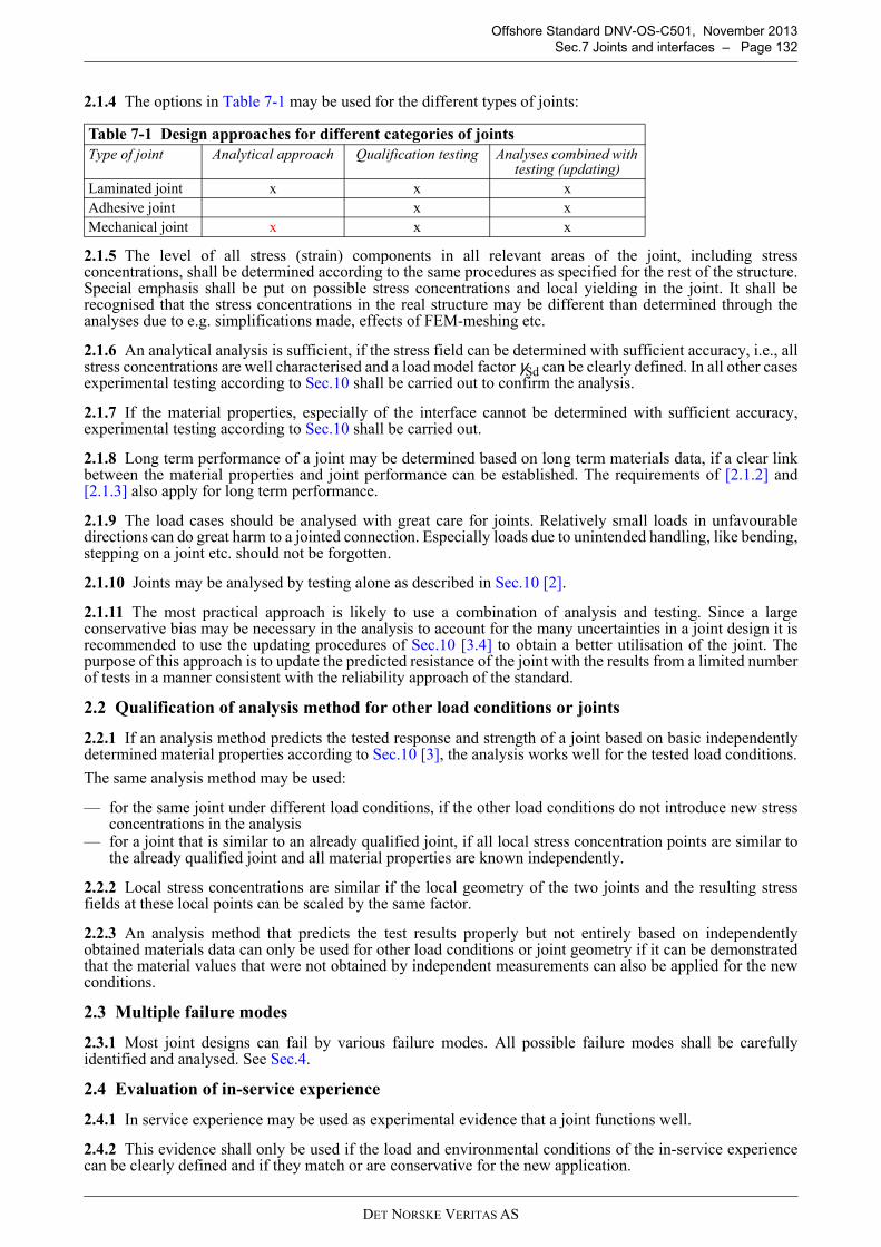
DET NORSKE VERITAS AS
Offshore Standard DNV-OS-C501, November 2013
Sec.7 Joints and interfaces – Page 132
2.1.4 The options in Table 7-1 may be used for the different types of joints:
2.1.5 The level of all stress (strain) components in all relevant areas of the joint, including stressconcentrations, shall be determined according to the same procedures as specified for the rest of the structure.Special emphasis shall be put on possible stress concentrations and local yielding in the joint. It shall berecognised that the stress concentrations in the real structure may be different than determined through theanalyses due to e.g. simplifications made, effects of FEM-meshing etc.
2.1.6 An analytical analysis is sufficient, if the stress field can be determined with sufficient accuracy, i.e., allstress concentrations are well characterised and a load model factor γSd can be clearly defined. In all other casesexperimental testing according to Sec.10 shall be carried out to confirm the analysis.
2.1.7 If the material properties, especially of the interface cannot be determined with sufficient accuracy,experimental testing according to Sec.10 shall be carried out.
2.1.8 Long term performance of a joint may be determined based on long term materials data, if a clear linkbetween the material properties and joint performance can be established. The requirements of [2.1.2] and[2.1.3] also apply for long term performance.
2.1.9 The load cases should be analysed with great care for joints. Relatively small loads in unfavourabledirections can do great harm to a jointed connection. Especially loads due to unintended handling, like bending,stepping on a joint etc. should not be forgotten.
2.1.10 Joints may be analysed by testing alone as described in Sec.10 [2].
2.1.11 The most practical approach is likely to use a combination of analysis and testing. Since a largeconservative bias may be necessary in the analysis to account for the many uncertainties in a joint design it isrecommended to use the updating procedures of Sec.10 [3.4] to obtain a better utilisation of the joint. Thepurpose of this approach is to update the predicted resistance of the joint with the results from a limited numberof tests in a manner consistent with the reliability approach of the standard.
2.2 Qualification of analysis method for other load conditions or joints
2.2.1 If an analysis method predicts the tested response and strength of a joint based on basic independentlydetermined material properties according to Sec.10 [3], the analysis works well for the tested load conditions.
The same analysis method may be used:
— for the same joint under different load conditions, if the other load conditions do not introduce new stressconcentrations in the analysis
— for a joint that is similar to an already qualified joint, if all local stress concentration points are similar tothe already qualified joint and all material properties are known independently.
2.2.2 Local stress concentrations are similar if the local geometry of the two joints and the resulting stressfields at these local points can be scaled by the same factor.
2.2.3 An analysis method that predicts the test results properly but not entirely based on independentlyobtained materials data can only be used for other load conditions or joint geometry if it can be demonstratedthat the material values that were not obtained by independent measurements can also be applied for the newconditions.
2.3 Multiple failure modes
2.3.1 Most joint designs can fail by various failure modes. All possible failure modes shall be carefullyidentified and analysed. See Sec.4.
2.4 Evaluation of in-service experience
2.4.1 In service experience may be used as experimental evidence that a joint functions well.
2.4.2 This evidence shall only be used if the load and environmental conditions of the in-service experiencecan be clearly defined and if they match or are conservative for the new application.
Table 7-1 Design approaches for different categories of joints
Type of joint Analytical approach Qualification testing Analyses combined with testing (updating)
Laminated joint x x x
Adhesive joint x x
Mechanical joint x x x
DET NORSKE VERITAS AS
Offshore Standard DNV-OS-C501, November 2013
Sec.7 Joints and interfaces – Page 133
2.4.3 Material properties of the joints to be compared should be similar. The analysis method should be ableto address all differences between the joints according to [2.1] and [2.2].
3 Specific joints
3.1 Laminated joints
3.1.1 Laminated joints rely on the strength of the interface for load transfer. The interface has resin dominatedstrength properties. Defects in the interface tend to be more critical than defects in the interface of plies oflaminate, because the joint interface is the only and critical load path.
3.1.2 The strength of the joint may be different from the through thickness matrix properties of the laminate,because the joint may be a resin rich layer and the joint may be applied to an already cured surface instead ofa wet on wet connection. (see manufacturing). The strength of the joint should be documented.
3.1.3 Laminated joints are very sensitive to peel conditions. Peel stresses should be avoided.
3.1.4 For the interface between the joining laminates the matrix design rules given in Sec.5 apply. Theresistance of the interface shall be determined with the same level of confidence as specified in Sec.4 [1.6]. Itshall be recognised that the resistance of the interface between the laminates may not be the same as thecorresponding resistance parameter of the joining laminates. Resin rich layers may even have to be analysedby different failure criteria, e.g., the yield criterion in Sec.6 [6].
3.1.5 The laminates themselves, including possible over-laminations, shall be analysed like regular laminates.
3.2 Adhesive Joints
3.2.1 All issues related to laminated joints also apply to adhesive joints.
3.2.2 Geometrical details should be clearly specified, especially at points of stress concentrations like theedges of the joints.
3.2.3 The relationship between all elastic constants of both substrates and the adhesive should be carefullyconsidered. Mismatches may introduce stresses or strains that can cause failure of the joint.
3.2.4 Thermal stresses should be considered.
3.2.5 Long term performance of adhesive should be established with great care. The long term performance isnot only influenced by properties of the substrate, the adhesive and the interface, but also by the surfacepreparation and application method.
3.2.6 Relevant long term data shall be established exactly for the combination of materials, geometry, surfacepreparation and fabrication procedures used in the joint.
3.2.7 An adhesive joint may also introduce local through thickness stresses in the composite laminate that canlead to failure inside the laminate in the joint region.
3.3 Mechanical joints
3.3.1 Mechanical joints are often very sensitive to geometrical tolerances.
3.3.2 Creep of the materials shall be considered.
3.3.3 The pretension of bolted connections shall be chosen by considering possible creep of the material underthe bolt.
3.3.4 It is preferred to design the joint in a way that its performance is independent of the matrix. This waymatrix cracking or degradation of matrix properties are not important for the performance of the joint.
3.4 Joints in sandwich structures
3.4.1 All aspects related to laminated, adhesive and mechanical joint apply also to sandwich structures.
3.4.2 Sandwich structures have internal joints between core and skin and between cores. These joints areusually evaluated independently, but their properties are treated as an internal part of the sandwich system.Often the core properties are modified to incorporate the joint properties.
3.4.3 When two sandwich structures are joined complicated stress fields may result inside the sandwichstructure. Stresses inside the core can be very different near a joint compared to the typical shear stresses in apanel.
DET NORSKE VERITAS AS
Offshore Standard DNV-OS-C501, November 2013
Sec.7 Joints and interfaces – Page 134
3.4.4 A large sandwich plate can be well described by core shear properties obtained from large test specimens.In the neighbourhood of joints local variations in properties of the core may become critical.
4 Interfaces
4.1 General
4.1.1 If loads shall be transferred across an interface all aspects related to joints shall be considered.
4.1.2 If interfaces only touch each other friction and wear should be considered according to Sec.6 [13].
4.1.3 Fluids may accumulate between interfaces. They may accumulate in voids or debonded areas and/orbreak the bond of the interface. The effect of such fluids should be analysed. Possible rapid decompression ofgases should be considered Sec.6 [12].
4.1.4 Liners that do not carry any structural loads shall have a high enough strain to failure or yield that theycan follow all possible movements of the interface. Yielding of liners should be avoided, since yielding cancause local thinning or introduce permanent stresses after yield. If yielding cannot be avoided it shall beanalysed carefully. The effect of local yielding on the surrounding structure shall also be considered.
4.1.5 If one substrate may crack (e.g. have matrix cracks), but the other shall not crack, it shall be shown thatcracks cannot propagate from one substrate across the interface into the other substrate. Possible debonding ofthe interface due to the high stresses at the crack tip should also be considered.
4.1.6 It is recommended to demonstrate by experiments that cracks cannot propagate across the interface fromone substrate to the other. It should be shown that by stretching or bending both substrates and their interfacethat no cracks forms in the one substrate even if the other substrate has the maximum expected crack density.
Guidance note:
This is a typical situation for pressure vessels with liners. The load bearing laminate may have some matrix cracks,but the liner shall not crack to keep the vessel tight. Local debonding of the liner may be acceptable if the liner willnot collapse due to its own weight, negative internal pressure or other effects.
---e-n-d---of---G-u-i-d-a-n-c-e---n-o-t-e---
Guidance note:
A weak bond between the substrates is beneficial to prevent crack growth across the interface. However, it means thatdebonding may happen easily.
---e-n-d---of---G-u-i-d-a-n-c-e---n-o-t-e---
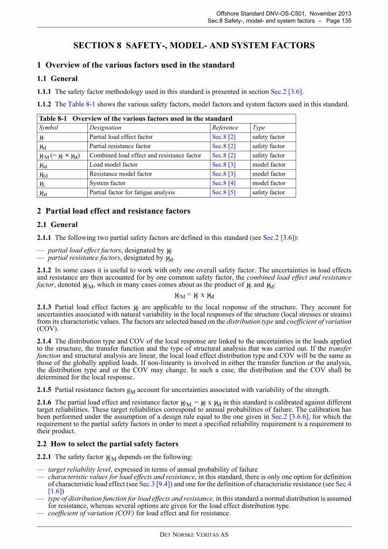
DET NORSKE VERITAS AS
Offshore Standard DNV-OS-C501, November 2013
Sec.8 Safety-, model- and system factors – Page 135
SECTION 8 SAFETY-, MODEL- AND SYSTEM FACTORS
1 Overview of the various factors used in the standard
1.1 General
1.1.1 The safety factor methodology used in this standard is presented in section Sec.2 [3.6].
1.1.2 The Table 8-1 shows the various safety factors, model factors and system factors used in this standard.
2 Partial load effect and resistance factors
2.1 General
2.1.1 The following two partial safety factors are defined in this standard (see Sec.2 [3.6]):
— partial load effect factors, designated by γF— partial resistance factors, designated by γM.
2.1.2 In some cases it is useful to work with only one overall safety factor. The uncertainties in load effectsand resistance are then accounted for by one common safety factor, the combined load effect and resistancefactor, denoted γFM, which in many cases comes about as the product of γF and γM:
γFM = γF x γM
2.1.3 Partial load effect factors γF are applicable to the local response of the structure. They account foruncertainties associated with natural variability in the local responses of the structure (local stresses or strains)from its characteristic values. The factors are selected based on the distribution type and coefficient of variation(COV).
2.1.4 The distribution type and COV of the local response are linked to the uncertainties in the loads appliedto the structure, the transfer function and the type of structural analysis that was carried out. If the transferfunction and structural analysis are linear, the local load effect distribution type and COV will be the same asthose of the globally applied loads. If non-linearity is involved in either the transfer function or the analysis,the distribution type and or the COV may change. In such a case, the distribution and the COV shall bedetermined for the local response.
2.1.5 Partial resistance factors gM account for uncertainties associated with variability of the strength.
2.1.6 The partial load effect and resistance factor γFM. = γF x γM in this standard is calibrated against differenttarget reliabilities. These target reliabilities correspond to annual probabilities of failure. The calibration hasbeen performed under the assumption of a design rule equal to the one given in Sec.2 [3.6.6], for which therequirement to the partial safety factors in order to meet a specified reliability requirement is a requirement totheir product.
2.2 How to select the partial safety factors
2.2.1 The safety factor γFM depends on the following:
— target reliability level, expressed in terms of annual probability of failure— characteristic values for load effects and resistance, in this standard, there is only one option for definition
of characteristic load effect (see Sec.3 [9.4]) and one for the definition of characteristic resistance (see Sec.4[1.6])
— type of distribution function for load effects and resistance, in this standard a normal distribution is assumedfor resistance, whereas several options are given for the load effect distribution type.
— coefficient of variation (COV) for load effect and for resistance.
Table 8-1 Overview of the various factors used in the standard
Symbol Designation Reference Type
γF Partial load effect factor Sec.8 [2] safety factor
γM Partial resistance factor Sec.8 [2] safety factor
γFM (= γF × γM) Combined load effect and resistance factor Sec.8 [2] safety factor
γSd Load model factor Sec.8 [3] model factor
γRd Resistance model factor Sec.8 [3] model factor
γS System factor Sec.8 [4] model factor
γfat Partial factor for fatigue analysis Sec.8 [5] safety factor
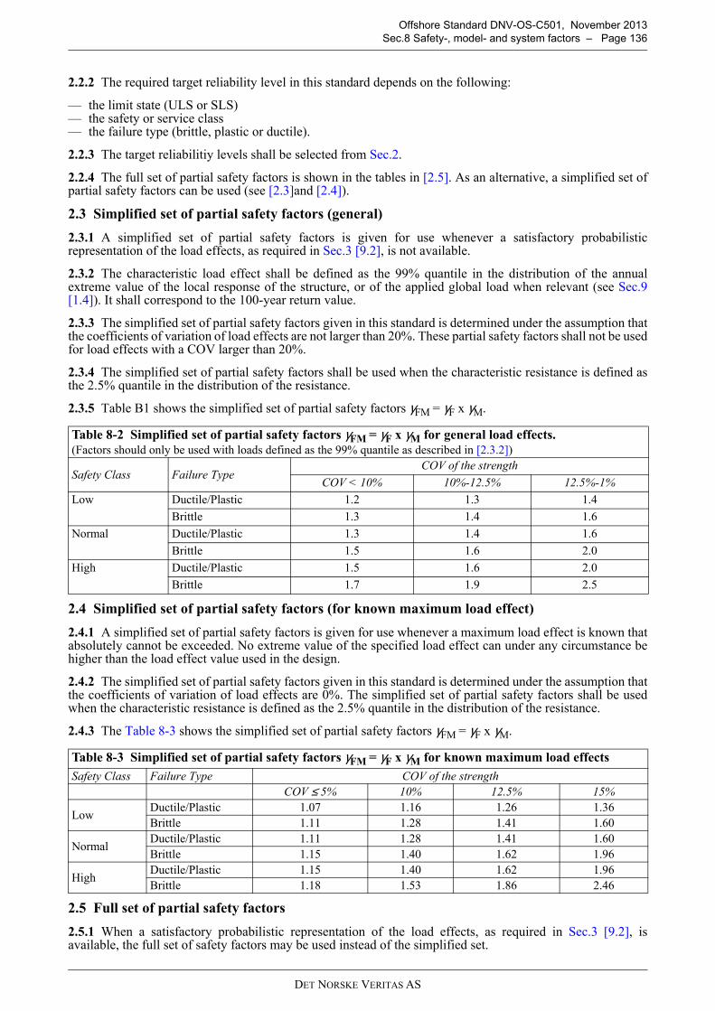
DET NORSKE VERITAS AS
Offshore Standard DNV-OS-C501, November 2013
Sec.8 Safety-, model- and system factors – Page 136
2.2.2 The required target reliability level in this standard depends on the following:
— the limit state (ULS or SLS)— the safety or service class— the failure type (brittle, plastic or ductile).
2.2.3 The target reliabilitiy levels shall be selected from Sec.2.
2.2.4 The full set of partial safety factors is shown in the tables in [2.5]. As an alternative, a simplified set ofpartial safety factors can be used (see [2.3]and [2.4]).
2.3 Simplified set of partial safety factors (general)
2.3.1 A simplified set of partial safety factors is given for use whenever a satisfactory probabilisticrepresentation of the load effects, as required in Sec.3 [9.2], is not available.
2.3.2 The characteristic load effect shall be defined as the 99% quantile in the distribution of the annualextreme value of the local response of the structure, or of the applied global load when relevant (see Sec.9[1.4]). It shall correspond to the 100-year return value.
2.3.3 The simplified set of partial safety factors given in this standard is determined under the assumption thatthe coefficients of variation of load effects are not larger than 20%. These partial safety factors shall not be usedfor load effects with a COV larger than 20%.
2.3.4 The simplified set of partial safety factors shall be used when the characteristic resistance is defined asthe 2.5% quantile in the distribution of the resistance.
2.3.5 Table B1 shows the simplified set of partial safety factors γFM = γF x γM.
2.4 Simplified set of partial safety factors (for known maximum load effect)
2.4.1 A simplified set of partial safety factors is given for use whenever a maximum load effect is known thatabsolutely cannot be exceeded. No extreme value of the specified load effect can under any circumstance behigher than the load effect value used in the design.
2.4.2 The simplified set of partial safety factors given in this standard is determined under the assumption thatthe coefficients of variation of load effects are 0%. The simplified set of partial safety factors shall be usedwhen the characteristic resistance is defined as the 2.5% quantile in the distribution of the resistance.
2.4.3 The Table 8-3 shows the simplified set of partial safety factors γFM = γF x γM.
2.5 Full set of partial safety factors
2.5.1 When a satisfactory probabilistic representation of the load effects, as required in Sec.3 [9.2], isavailable, the full set of safety factors may be used instead of the simplified set.
Table 8-2 Simplified set of partial safety factors γFM = γF x γM for general load effects.
(Factors should only be used with loads defined as the 99% quantile as described in [2.3.2])
Safety Class Failure TypeCOV of the strength
COV < 10% 10%-12.5% 12.5%-1%
Low Ductile/Plastic 1.2 1.3 1.4
Brittle 1.3 1.4 1.6
Normal Ductile/Plastic 1.3 1.4 1.6
Brittle 1.5 1.6 2.0
High Ductile/Plastic 1.5 1.6 2.0
Brittle 1.7 1.9 2.5
Table 8-3 Simplified set of partial safety factors γFM = γF x γM for known maximum load effects
Safety Class Failure Type COV of the strength
COV ≤ 5% 10% 12.5% 15%
LowDuctile/Plastic 1.07 1.16 1.26 1.36
Brittle 1.11 1.28 1.41 1.60
NormalDuctile/Plastic 1.11 1.28 1.41 1.60
Brittle 1.15 1.40 1.62 1.96
HighDuctile/Plastic 1.15 1.40 1.62 1.96
Brittle 1.18 1.53 1.86 2.46
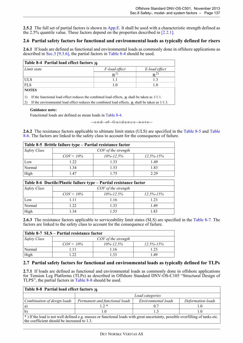
DET NORSKE VERITAS AS
Offshore Standard DNV-OS-C501, November 2013
Sec.8 Safety-, model- and system factors – Page 137
2.5.2 The full set of partial factors is shown in App.E. It shall be used with a characteristic strength defined asthe 2.5% quantile value. These factors depend on the properties described in [2.2.1].
2.6 Partial safety factors for functional and environmental loads as typically defined for risers
2.6.1 If loads are defined as functional and environmental loads as commonly done in offshore applications asdescribed in Sec.3 [9.3.6], the partial factors in Table 8-4 should be used.
Guidance note:
Functional loads are defined as mean loads in Table 8-4.
---e-n-d---of---G-u-i-d-a-n-c-e---n-o-t-e---
2.6.2 The resistance factors applicable to ultimate limit states (ULS) are specified in the Table 8-5 and Table8-6. The factors are linked to the safety class to account for the consequence of failure.
2.6.3 The resistance factors applicable to serviceability limit states (SLS) are specified in the Table 8-7. Thefactors are linked to the safety class to account for the consequence of failure.
2.7 Partial safety factors for functional and environmental loads as typically defined for TLPs
2.7.1 If loads are defined as functional and environmental loads as commonly done in offshore applicationsfor Tension Leg Platforms (TLPs) as described in Offshore Standard DNV-OS-C105 “Structural Design ofTLPS”, the partial factors in Table 8-8 should be used.
Table 8-4 Partial load effect factors γF
Limit state F-load effect E-load effect
γF1) γE
2)
ULS 1.1 1.3
FLS 1.0 1.0
NOTES
1) If the functional load effect reduces the combined load effects, γF shall be taken as 1/1.1.
2) If the environmental load effect reduces the combined load effects, γE shall be taken as 1/1.3.
Table 8-5 Brittle failure type – Partial resistance factor
Safety Class COV of the strength
COV < 10% 10%-12.5% 12.5%-15%
Low 1.22 1.33 1.49
Normal 1.34 1.53 1.83
High 1.47 1.75 2.29
Table 8-6 Ductile/Plastic failure type – Partial resistance factor
Safety Class COV of the strength
COV < 10% 10%-12.5% 12.5%-15%
Low 1.11 1.16 1.23
Normal 1.22 1.33 1.49
High 1.34 1.53 1.83
Table 8-7 SLS – Partial resistance factor
Safety Class COV of the strength
COV < 10% 10%-12.5% 12.5%-15%
Normal 1.11 1.16 1.23
High 1.22 1.33 1.49
Table 8-8 Partial load effect factors γF
Load categories
Combination of design loads Permanent and functional loads Environmental loads Deformation loads
a) 1.2 * 0.7 1.0
b) 1.0 1.3 1.0
* ) If the load is not well defined e.g. masses or functional loads with great uncertainty, possible overfilling of tanks etc. the coefficient should be increased to 1.3.
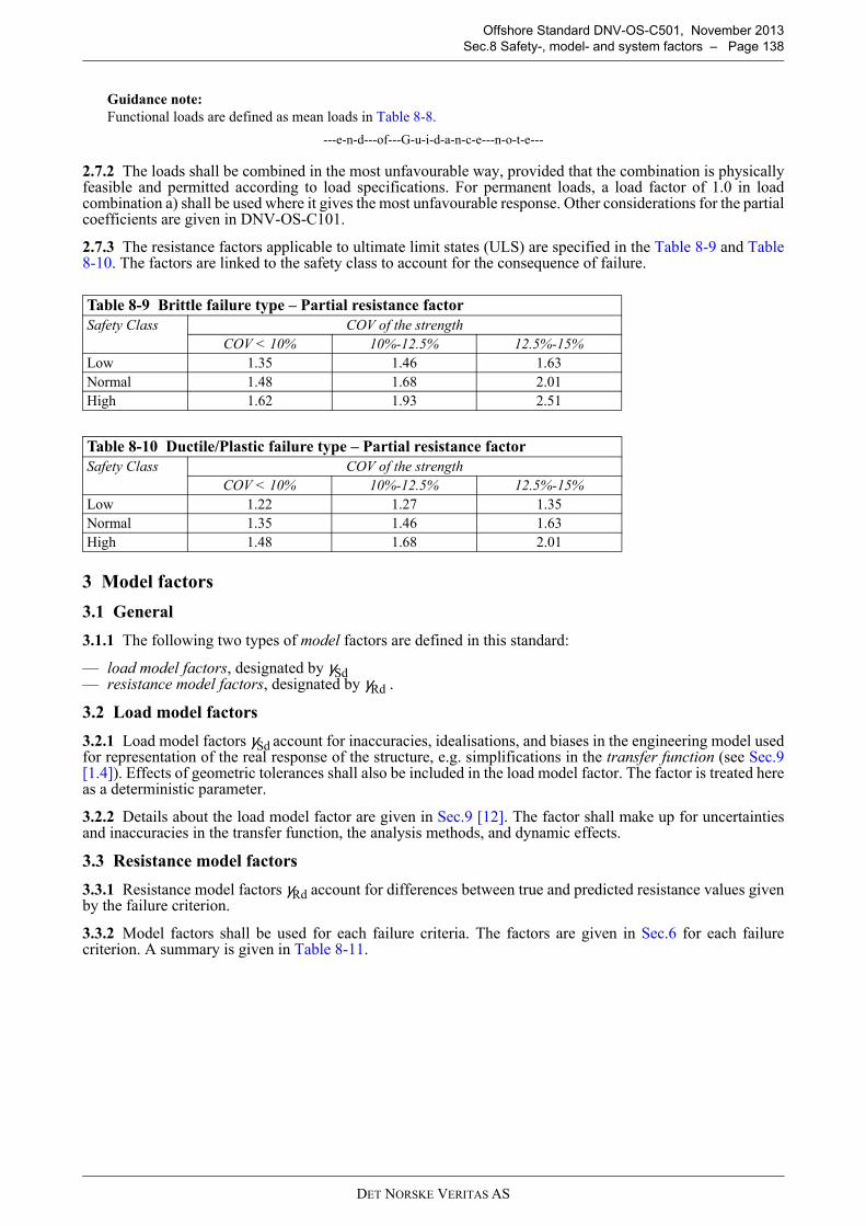
DET NORSKE VERITAS AS
Offshore Standard DNV-OS-C501, November 2013
Sec.8 Safety-, model- and system factors – Page 138
Guidance note:
Functional loads are defined as mean loads in Table 8-8.
---e-n-d---of---G-u-i-d-a-n-c-e---n-o-t-e---
2.7.2 The loads shall be combined in the most unfavourable way, provided that the combination is physicallyfeasible and permitted according to load specifications. For permanent loads, a load factor of 1.0 in loadcombination a) shall be used where it gives the most unfavourable response. Other considerations for the partialcoefficients are given in DNV-OS-C101.
2.7.3 The resistance factors applicable to ultimate limit states (ULS) are specified in the Table 8-9 and Table8-10. The factors are linked to the safety class to account for the consequence of failure.
3 Model factors
3.1 General
3.1.1 The following two types of model factors are defined in this standard:
— load model factors, designated by γSd— resistance model factors, designated by γRd .
3.2 Load model factors
3.2.1 Load model factors γSd account for inaccuracies, idealisations, and biases in the engineering model usedfor representation of the real response of the structure, e.g. simplifications in the transfer function (see Sec.9[1.4]). Effects of geometric tolerances shall also be included in the load model factor. The factor is treated hereas a deterministic parameter.
3.2.2 Details about the load model factor are given in Sec.9 [12]. The factor shall make up for uncertaintiesand inaccuracies in the transfer function, the analysis methods, and dynamic effects.
3.3 Resistance model factors
3.3.1 Resistance model factors γRd account for differences between true and predicted resistance values givenby the failure criterion.
3.3.2 Model factors shall be used for each failure criteria. The factors are given in Sec.6 for each failurecriterion. A summary is given in Table 8-11.
Table 8-9 Brittle failure type – Partial resistance factor
Safety Class COV of the strength
COV < 10% 10%-12.5% 12.5%-15%
Low 1.35 1.46 1.63
Normal 1.48 1.68 2.01
High 1.62 1.93 2.51
Table 8-10 Ductile/Plastic failure type – Partial resistance factor
Safety Class COV of the strength
COV < 10% 10%-12.5% 12.5%-15%
Low 1.22 1.27 1.35
Normal 1.35 1.46 1.63
High 1.48 1.68 2.01
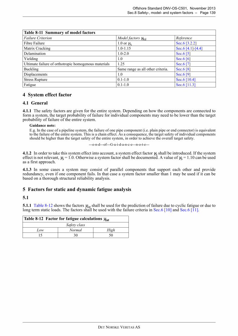
DET NORSKE VERITAS AS
Offshore Standard DNV-OS-C501, November 2013
Sec.8 Safety-, model- and system factors – Page 139
4 System effect factor
4.1 General
4.1.1 The safety factors are given for the entire system. Depending on how the components are connected toform a system, the target probability of failure for individual components may need to be lower than the targetprobability of failure of the entire system.
Guidance note:
E.g. In the case of a pipeline system, the failure of one pipe component (i.e. plain pipe or end connector) is equivalentto the failure of the entire system. This is a chain effect. As a consequence, the target safety of individual componentsshould be higher than the target safety of the entire system, in order to achieve the overall target safety.
---e-n-d---of---G-u-i-d-a-n-c-e---n-o-t-e---
4.1.2 In order to take this system effect into account, a system effect factor γS shall be introduced. If the systemeffect is not relevant, γS = 1.0. Otherwise a system factor shall be documented. A value of γS = 1.10 can be usedas a first approach.
4.1.3 In some cases a system may consist of parallel components that support each other and provideredundancy, even if one component fails. In that case a system factor smaller than 1 may be used if it can bebased on a thorough structural reliability analysis.
5 Factors for static and dynamic fatigue analysis
5.1
5.1.1 Table 8-12 shows the factors γfat shall be used for the prediction of failure due to cyclic fatigue or due tolong term static loads. The factors shall be used with the failure criteria in Sec.6 [10] and Sec.6 [11].
Table 8-11 Summary of model factors
Failure Criterion Model factors γRd Reference
Fibre Failure 1.0 or γA Sec.6 [3.2.2]
Matrix Cracking 1.0-1.15 Sec.6 [4.1]-[4.4]
Delamination 1.0-2.0 Sec.6 [5]
Yielding 1.0 Sec.6 [6]
Ultimate failure of orthotropic homogenous materials 1.25 Sec.6 [7]
Buckling Same range as all other criteria. Sec.6 [8]
Displacements 1.0 Sec.6 [9]
Stress Rupture 0.1-1.0 Sec.6 [10.4]
Fatigue 0.1-1.0 Sec.6 [11.3]
Table 8-12 Factor for fatigue calculations γfat
Safety class
Low Normal High
15 30 50
DET NORSKE VERITAS AS
Offshore Standard DNV-OS-C501, November 2013
Sec.9 Structural analysis – Page 140
SECTION 9 STRUCTURAL ANALYSIS
1 General
1.1 Objective
1.1.1 The aim of the structural analysis is to obtain the stresses, strains and displacements (denoted load effectsin the following) in the structure as a result of loads and environmental conditions. The load effects aresubsequently evaluated against failure criteria, see Sec.6. The following procedures are typically involved insuch an analysis:
— procedure to calculate load effects in the structure based on the loads— procedure to check for global or local failure.
1.1.2 The objective of the present section is to provide methods to calculate the response, including evaluationof failure, of structures for specified loads, surrounding environments and boundary conditions.
1.2 Input data
1.2.1 The input data for the structural analysis should be established as described in the relevant parts of Sec.3.
1.2.2 Environmental conditions should be converted into loads based on well established physical principles.Guidance may be found in Sec.3 and in relevant standards or guidelines.
1.2.3 The boundary conditions should be selected carefully in order to represent the nature of the problem inthe best possible way. It should be demonstrated that the chosen boundary conditions lead to a realistic orconservative analysis of the structure.
1.2.4 Thermal stresses that result from production process or in service loading should be considered in allanalysis.
1.2.5 Stresses due to swelling from absorbed fluids should be included if relevant.
1.2.6 The elastic properties of the materials constituting the structure should be taken as described in Sec.4 forlaminates and Sec.5 for sandwich structures. In particular, time-dependent stiffness properties based on theexpected degradation due to environmental and loading conditions should be considered. Local variations ofthese conditions should also be considered.
1.2.7 Each ply should be described by 4 elastic constants (E1, E2, G12, ν12) for in-plane 2-D analysis and by 9elastic constants (E1, E2, G12, ν12, E3, G13, G23, ν13, ν23) in 3-D analysis. A nomenclature for the various elasticconstants is defined in section 14.
1.2.8 As an alternative to elastic constants, the stiffness matrix for orthotropic plies may be used.
1.2.9 It should be shown that the estimated stiffness gives conservative results with respect to load effects. Thechoice of stiffness values may be different in the cases of strength and stiffness limited design. More details aregiven in the sections below.
1.3 Analysis types
1.3.1 Analytical and/or numerical calculations may be used in the structural analysis. The finite element (FE)method is presently the most commonly used numerical method for structural analysis, but other methods, suchas finite difference or finite series methods may also be applied.
Guidance note:
While the FE method is applicable for a wide range of problems, analytical solutions and the finite series approachoften put too many restrictions on laminate lay-up, geometry etc., and are thus insufficient in the design of most realworld composite structures.
---e-n-d---of---G-u-i-d-a-n-c-e---n-o-t-e---
1.3.2 Laminate analysis is an additional type of analysis that is applied to layered composites in order to derivethe properties of a laminate from the properties of its constituent plies.
1.3.3 The structural analysis should be performed for all phases over the entire lifetime of the structure. Initialand degraded material properties should be considered if relevant.
1.3.4 A decision to use 2-D or 3-D analysis methods should generally be made depending on the level ofsignificance of the through thickness stresses. If these stresses can be neglected, in-plane 2-D analysis may beapplied. Additionally, the analysis of certain laminate and sandwich structures may be simplified by a throughthickness (cross section) 2-D approach, in which plane strain condition is assumed to prevail.
DET NORSKE VERITAS AS
Offshore Standard DNV-OS-C501, November 2013
Sec.9 Structural analysis – Page 141
Guidance note:
In-plane 2-D analysis is generally preferred when analysing relatively large and complex structures, in which throughthickness stresses can be neglected. However, structural details with significant through thickness stresses, such asjoints, require a more accurate analysis. In these cases 3-D or through thickness 2-D (for components possessing planestrain conditions) approaches should be applied.
---e-n-d---of---G-u-i-d-a-n-c-e---n-o-t-e---
1.4 Transfer function
1.4.1 The loads and environments described as input to the analysis in Sec.3, i.e. wind, wave and currents, arenot always directly suitable in a stress analysis. A transfer function shall be defined that converts the specifiedloads to loads that can be used in the analysis.
1.4.2 Any non-linear effect in the transfer function may change the characteristics of the load distribution.These changes shall be taken into account when selecting the load-model factor under [12].
1.5 Global and local analysis
1.5.1 The global response of the structure is defined as the response (displacement and stability) of thestructure as a whole.
1.5.2 The local response of the structure is defined as the stresses and strains (and deformations) in every localpart of the structure.
1.5.3 The response of the structure shall be calculated on a global or local level depending on the failuremechanism being checked and its associated failure criterion.
Guidance note:
The failure of the structure shall generally be checked on the basis of the local response of the structure by the use offailure criteria for each failure mechanism as described in Sec.6.
Buckling is generally checked on larger parts of the structure and based on average stresses over large areas. Undersuch conditions a coarser analysis may be sufficient. However, if the FE method is used to calculate buckling stresses,a very local analysis of the structure may be needed.
---e-n-d---of---G-u-i-d-a-n-c-e---n-o-t-e---
1.6 Material levels
1.6.1 The local response of the structure can in principle be analysed at the following different material levels:
— the “constituent level” corresponding to the fibre, matrix and core, separately— the “ply level” corresponding to the individual layers in a laminate or the faces of a sandwich structure— the “laminate level” corresponding to the whole laminate or sandwich structure.
1.6.2 Each failure mechanism can in principle be checked at any material level. However, due to the lack oftheoretical knowledge or for practical reasons, it is not always possible to check a given failure mechanism atall material levels.
1.6.3 The local response of the structure shall be analysed at a material level consistent with the failure criteriaused in the failure analysis as described in Sec.6.
1.6.4 This standard does not cover stress analysis on the level of the individual fibre or the matrix between thefibres, i.e. on the constituent level (except for sandwich core materials).
1.6.5 All failure criteria in this standard (except for buckling) require the stresses or strains to be accuratelyrepresented on the level of each ply.
1.7 Non-linear analysis
1.7.1 Non-linear analysis should be performed when geometrical and/or material non-linearity are present andwhen linear and non-linear analysis results are expected to differ.
1.7.2 Geometrical non-linearity are associated with, e.g., large displacements and/or large strains, boundaryconditions varying according to deformations, non-symmetric geometry of structure and buckling.
1.7.3 Non-linear material behaviour is associated with the stress–strain relation. Following damage in thematerial, i.e. matrix cracking or yield, stress–strain relationships usually become non-linear.
1.7.4 Structures with non-linear materials should be checked either against early failure mechanisms, e.g.matrix cracking or yield, or against ultimate failure, or both.
1.7.5 A decision to use a progressive, non-linear failure analysis or a simplified (linear) failure analysis shouldbe based on the failure modes of the structure/component and the failure mechanisms investigated, see [2] and [3].
DET NORSKE VERITAS AS
Offshore Standard DNV-OS-C501, November 2013
Sec.9 Structural analysis – Page 142
2 Linear and non-linear analysis of monolithic structures
2.1 General
2.1.1 Most composite structures possess linear material properties when intact. However, composites candevelop various failure mechanisms, e.g. matrix cracking, at very low strains leading to reduced stiffnessparameters.
2.1.2 This non-linear behaviour of the material shall be taken into account when failure analysis of compositecomponents is performed.
2.1.3 In the present section several analysis methods will be presented. These methods may be combined withanalytically [4] or numerically [5] based response calculations. Under [3] the applicability of the analysismethods will be linked to various failure criteria.
2.1.4 All response calculations shall be based on time-dependent material properties related to, for example,natural or environmental degradation during service life.
2.1.5 Regardless of the analysis method being used geometrical non-linear effects shall be taken into accountwhen significant, see [1.7].
2.1.6 For the choice of 2-D or 3-D analysis methods, see [1.3.4].
2.1.7 The development of failures is most accurately described by progressive non-linear analysis methods(presented in [2.2] and [2.3] for in-plane 2-D and 3-D problems, respectively), in which degradation of materialproperties in case of, e.g., matrix cracking is included. However, such methods may be extremely time-consuming in problems of practical interest.
2.1.8 In many cases the simplified analysis methods presented in [2.4], [2.5] and [2.6] may be applied.
2.1.9 When using one of the analysis methods based on locally degraded material properties, conservativeresults are ensured provided the element mesh is sufficiently fine. However, when one of the simple linearfailure methods (non-degraded ([2.4]) or globally degraded ([2.5])) is applied, the distribution of stresses/strains may be incorrect, in particular, near sharp corners or other kinds of geometrical or materialdiscontinuities. The analyst shall beware of the possibility of introducing serious errors.
2.1.10 The simplified methods presented in [2.4], [2.5] and [2.6] are derived under the assumption that matrixfailure occurs prior to fibre failure, which is satisfied for most fibre reinforced plastic composites.
Guidance note:
For certain metal matrix composites, fibre failure may occur prior to matrix failure. In such cases the simplified failuremethods must be modified.
---e-n-d---of---G-u-i-d-a-n-c-e---n-o-t-e---
2.1.11 In the sections containing simplified analysis methods the problems to be solved will be divided intothree categories:
— statically determinate problems, which mean problems where it is possible to determine all the forces/moments (and laminate stresses) involved by using only the equilibrium requirements without regard to thedeformations
— problems where displacements (and laminate strains) are independent of material properties (and can thusbe regarded as known)
— general (or statically indeterminate) problems, which are problems where the forces/moments involvedcannot be determined from equilibrium requirements without regard to the deformations.
2.1.12 Some of the main features of the analysis methods to be presented in the following are listed in Table9-1.
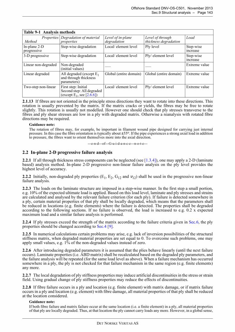
DET NORSKE VERITAS AS
Offshore Standard DNV-OS-C501, November 2013
Sec.9 Structural analysis – Page 143
2.1.13 If fibres are not oriented in the principle stress directions they want to rotate into these directions. Thisrotation is usually prevented by the matrix. If the matrix cracks or yields, the fibres may be free to rotateslightly. This rotation is usually not modelled. However one should check that ply stresses transverse to thefibres and ply shear stresses are low in a ply with degraded matrix. Otherwise a reanalysis with rotated fibredirections may be required.
Guidance note:
The rotation of fibres may, for example, be important in filament wound pipe designed for carrying just internalpressure. In this case the fibre orientation is typically about ±55o. If the pipe experiences a strong axial load in additionto pressure, the fibres want to orient themselves more into the axial direction.
---e-n-d---of---G-u-i-d-a-n-c-e---n-o-t-e---
2.2 In-plane 2-D progressive failure analysis
2.2.1 If all through thickness stress components can be neglected (see [1.3.4]), one may apply a 2-D (laminatebased) analysis method. In-plane 2-D progressive non-linear failure analysis on the ply level provides thehighest level of accuracy.
2.2.2 Initially, non-degraded ply properties (E1, E2, G12 and ν12) shall be used in the progressive non-linearfailure analysis.
2.2.3 The loads on the laminate structure are imposed in a step-wise manner. In the first step a small portion,e.g. 10% of the expected ultimate load is applied. Based on this load level, laminate and ply stresses and strainsare calculated and analysed by the relevant failure criterion (for each ply). If failure is detected somewhere ina ply, certain material properties of that ply shall be locally degraded, which means that the parameters shallbe reduced in locations (e.g. finite elements) where the failure is detected. The properties shall be degradedaccording to the following sections. If no failure is observed, the load is increased to e.g. 0.2 x expectedmaximum load and a similar failure analysis is performed.
2.2.4 If ply stresses exceed the strength of the matrix according to the failure criteria given in Sec.6, the plyproperties should be changed according to Sec.4 [9].
2.2.5 In numerical calculations certain problems may arise, e.g. lack of inversion possibilities of the structuralstiffness matrix, when degraded material properties are set equal to 0. To overcome such problems, one mayapply small values, e.g. 1% of the non-degraded values instead of zero.
2.2.6 After introducing degraded parameters it is assumed that the plies behave linearly (until the next failureoccurs). Laminate properties (i.e. ABD matrix) shall be recalculated based on the degraded ply parameters, andthe failure analysis will be repeated (for the same load level as above). When a failure mechanism has occurredsomewhere in a ply, the ply is not checked for that failure mechanism in the same region (e.g. finite elements)any more.
2.2.7 The local degradation of ply stiffness properties may induce artificial discontinuities in the stress or strainfield. Using gradual change of ply stiffness properties may reduce the effects of discontinuities.
2.2.8 If fibre failure occurs in a ply and location (e.g. finite element) with matrix damage, or if matrix failureoccurs in a ply and location (e.g. element) with fibre damage, all material properties of that ply shall be reducedat the location considered.
Guidance note:
If both fibre failure and matrix failure occur at the same location (i.e. a finite element) in a ply, all material propertiesof that ply are locally degraded. Thus, at that location the ply cannot carry loads any more. However, in a global sense,
Table 9-1 Analysis methods
Properties Method
Degradation of material properties
Level of in-plane degradation
Level of through thickness degradation
Load
In-plane 2-D progressive
Step-wise degradation Local/ element level Ply level Step-wise increase
3-D progressive Step-wise degradation Local/ element level Ply/ element level Step-wise increase
Linear non-degraded Non-degraded(initial values)
___ ___ Extreme value
Linear degraded All degraded (except E1 and through thickness parameters)
Global (entire domain) Global (entire domain) Extreme value
Two-step non-linear First step: InitialSecond step: All degraded (except E1, see [2.6.6])
Local/ element level Ply/ element level Extreme value
DET NORSKE VERITAS AS
Offshore Standard DNV-OS-C501, November 2013
Sec.9 Structural analysis – Page 144
the ply may still carry loads because stresses can be redistributed around the location of failure. The redistribution ofstresses can be of type in-plane (within the same ply) or through thickness (into the neighbouring plies). Ifconsiderable through thickness redistribution occurs, a 3-D progressive failure analysis should be applied, see [2.3].
---e-n-d---of---G-u-i-d-a-n-c-e---n-o-t-e---
2.2.9 The failure analysis is repeated (for the same load level) until no new failure mechanism is detected.Then, the load level is increased, and a similar failure analysis is performed.
2.2.10 Whenever a violation of the ultimate limit state (ULS) condition is detected the analysis is terminated.
2.3 3-D progressive failure analysis
2.3.1 If at least one of the through thickness stress components cannot be neglected (see [1.3.4]), 3-D effectsshall be taken into account. Then the development of failure is most accurately predicted by 3-D progressivefailure analysis on the ply level.
2.3.2 Initially, non-degraded 3-D ply properties (E1, E2, G12, ν12, E3, G13, G23, ν13 and ν23) shall be used inthe progressive non-linear failure analysis.
2.3.3 A crucial effect of the through thickness stresses is the possibility of delamination.
2.3.4 In addition to the failure criteria accounted for in the 2-D failure analysis in [2.2], the delamination failurecriterion at the ply level should now be considered (see Sec.6 [5]).
2.3.5 Otherwise, the 3-D progressive failure algorithm follows the same steps as the 2-D method presentedunder [2.2].
2.3.6 3-D ply properties shall be degraded by the same principles as described for 2-D properties in [2.2] andSec.4 [9].
2.4 Linear failure analysis with non-degraded properties
2.4.1 In this simplest approximate failure method non-degraded or initial material properties are applied.
2.4.2 The method may be used for both 2-D and 3-D problems, see [1.3.4].
2.4.3 In the results presented for this method, it is assumed that matrix failure occurs prior to fibre breakage,see [2.1.10]. On the other hand, if fibre failure is not the last failure type to occur in the laminate, the overviewof the connection between analysis methods and failure criteria under [3] is not applicable.
2.4.4 In certain cases, this simplified method, without local degradation of material properties, may offerconsiderably incorrect stress/strain distributions, see [2.1.9]. If the error cannot be analysed and included intothe model factor (see [12.3]) a more refined method shall be used.
2.4.5 Stresses and strains should be calculated on the laminate and ply levels.
2.4.6 Before matrix cracking (and other kinds of failure mechanisms) the method predicts correct responsevalues provided that the underlying analytical or numerical (FE) analysis method is applied within itsassumptions and limitations (see [4] and [5]).
2.4.7 After matrix cracking statically determinate problems result in:
— laminate stiffness – too high— laminate stresses – correct— laminate strains – too small— ply stiffness – E1 is correct, the other ply properties are generally too large— ply stresses – σ1 is too small, the other stress components are generally too large— ply strains – too small.
2.4.8 After matrix cracking problems with known displacements result in:
— laminate stiffness – too high— laminate stresses – too large— laminate strains – correct— ply stiffness – E1 is correct, the other ply properties are generally too large— ply stresses – σ1 is correct, the other stress components are generally too large— ply strains – correct.
2.4.9 After matrix cracking statically indeterminate problems result in:
— laminate stiffness – too high
DET NORSKE VERITAS AS
Offshore Standard DNV-OS-C501, November 2013
Sec.9 Structural analysis – Page 145
— laminate stresses – between correct and too large— laminate strains – generally too small— ply stiffness – E1 is correct, the other ply properties are generally too large— ply stresses – σ1 is too small, the other stress components are generally too large— ply strains – generally too small.
2.4.10 The applicability of this method in conjunction with various failure mechanisms and the need formodifying certain failure criteria are discussed under [3]. The fibre failure criterion shall only be used with thefactor γa defined in [3.2]. It shall also be ensured that the ply strain and stress in fibre direction are multipliedby γa in all other failure criteria or analysis where strain or stress values exceed the level of matrix cracking.
2.5 Linear failure analysis with degraded properties
2.5.1 In this approximate failure method globally degraded material properties are applied. This implieseffectively that matrix cracking has occurred in the laminate, and that the laminate is not checked for matrixcracking, see [3.1.3].
2.5.2 The method may be applied for both 2-D and 3-D problems, see [1.3.4] and [2.5.5].
2.5.3 In the results presented for this method it is assumed that fibre breakage is the last failure mechanism tooccur, see [2.4.3].
2.5.4 This method should be mainly used for statically determined problems. Otherwise this simplifiedmethod, with global degradation of material properties, may offer considerably incorrect stress/straindistributions, see [2.1.9]. If the error cannot be analysed and included into the model factor (see [12.3]) a morerefined method shall be used.
2.5.5 The material properties are degraded in the entire domain by changing certain ply elasticity parameters.For in-plane 2-D analysis the stiffness in the fibre direction, E1, of each ply is kept unaltered, while the rest ofthe 2-D ply properties should be changed according to Sec.4 [9], assuming the matrix has cracked due to highply stresses τ12 and σ2. This is equivalent to using the degraded stiffness (Enonlin see Figure 9-1) in the laminatestress-strain relation for loads in the fibre directions. If 3-D analysis is required, the in-plane parameters aredealt with as in the 2-D analysis. Through thickness parameters should only be changed according to Sec.4 [9],if through thickness stresses cause matrix cracking.
2.5.6 For difficulties arising in numerical calculations when using degraded values equal to 0, and thepossibilities to apply larger values for the degraded parameters, refer to [2.2.5] and Sec.4 [9].
2.5.7 Stresses and strains should be calculated at the laminate and ply levels.
2.5.8 For in-plane 2-D analysis statically determined problems result in:
— laminate stiffness – too low— laminate stresses – correct— laminate strains – too large— ply stiffness – E1 is correct, the other ply properties are generally too small— ply stresses – σ1 is too large, the other stress components are generally too small(zero)— ply strains – too large.
2.5.9 For in-plane 2-D analysis problems with known displacements result in:
— laminate stiffness – too low— laminate stresses – too small— laminate strains – correct— ply stiffness – E1 is correct, the other ply properties are generally too small— ply stresses – σ1 is correct, the other stress components are generally too small (zero)— ply strains – correct.
2.5.10 For in-plane 2-D analysis statically indeterminate problems result in:
— laminate stiffness – too low— laminate stresses – between too small and correct— laminate strains – generally too large— ply stiffness – E1 is correct, the other ply properties are generally too small— ply stresses – σ1 is too large, the other stress components are generally too small(zero)— ply strains – generally too large.
2.5.11 The applicability of this method in conjunction with various failure mechanisms is discussed under [3].
DET NORSKE VERITAS AS
Offshore Standard DNV-OS-C501, November 2013
Sec.9 Structural analysis – Page 146
2.6 Two-step non-linear failure analysis method
2.6.1 The method may be applied for both 2-D and 3-D problems, see [1.3.4].
2.6.2 In the results presented for this method it is assumed that matrix failure occurs prior to fibre breakage,see [2.4.3].
2.6.3 In the first step response calculations are performed with non-degraded material properties.
2.6.4 In regions (e.g. finite elements) where the strains (or stresses) exceed the level for matrix cracking (orother failure mechanisms), the in-plane material properties are degraded according to the method presented in[2.5.5].
2.6.5 The final step consists of response calculations with the locally degraded material properties.
2.6.6 If the final calculations break down, e.g. due to ill-conditioned structural matrices, one should repeat thefinal step with non-degraded through thickness parameters.
2.6.7 For problems related to the local degradation of material properties, see [2.2.7].
2.6.8 For difficulties arising in numerical calculations when using locally degraded values equal to 0, and thepossibilities to apply larger values for the degraded parameters, refer to [2.2.4] and [2.2.5].
2.6.9 Before matrix cracking (and other kinds of failure mechanisms) the method predicts correct responsevalues provided that the underlying analytical or numerical (FE) analysis method is applied within itsassumptions and limitations (see under [4] and [5]).
2.6.10 After local occurrences of matrix cracking statically determined problems result in:
— laminate stiffness – generally correct, locally too low— laminate stresses – correct— laminate strains – generally correct, locally too large— ply stiffness – generally correct, locally E1 is correct and the other ply properties are mostly too small— ply stresses – generally correct, locally σ1 is too large and the other stress components are mostly too small
(zero)— ply strains – generally correct, locally too large.
2.6.11 After local occurrences of matrix cracking problems with known displacements result in:
— laminate stiffness – generally correct, locally too low— laminate stresses – generally correct, locally too small— laminate strains – correct— ply stiffness – generally correct, locally E1 is correct and the other ply properties are mostly too small— ply stresses – generally correct, locally σ1 is correct and the other stress components are mostly too small
(zero)— ply strains – correct.
2.6.12 After local occurrences of matrix cracking statically indeterminate problems result in:
— laminate stiffness – generally correct, locally too low— laminate stresses – generally correct, locally between too small and correct— laminate strains – generally correct, locally too large— ply stiffness – generally correct, locally E1 is correct and the other ply properties are mostly too small— ply stresses – generally correct, locally σ1 is too large and the other stress components are mostly too small
(zero)— ply strains - generally correct, locally too large.
2.6.13 The applicability of this method in conjunction with various failure mechanisms is discussed under [3].
2.7 Through thickness 2-D analysis
2.7.1 [2.2] deals with an in-plane 2-D analysis method that is applicable if through thickness stresses can beneglected, see [1.3.4]. The in-plane 2-D approach is frequently used in conjunction with global analysis ofrelatively large composite structures.
2.7.2 On the other hand, certain structural details, in which plane strain conditions prevail, may be analysedby a through thickness (cross section) 2-D approach.
DET NORSKE VERITAS AS
Offshore Standard DNV-OS-C501, November 2013
Sec.9 Structural analysis – Page 147
Guidance note:
Examples on problems that may be analysed by the through thickness 2-D approach include several adhesive bondedjoints with a width to thickness ratio that is much larger than unity and certain effects related to bolted joints, includingpre-tension, in which symmetric conditions along axes prevail.
---e-n-d---of---G-u-i-d-a-n-c-e---n-o-t-e---
2.7.3 All the analysis methods that are applicable for in-plane 2-D problems (presented in [2.2], [2.4], [2.5]and [2.6]) may be adopted to through thickness 2-D analysis.
2.7.4 The simplifications introduced in the through thickness analysis shall be carefully investigated to ensurethat no crucial effect is lost.
3 Connection between analysis methods and failure criteria
3.1 General
3.1.1 In this section the connection between the analysis methods from [2] and the failure criteria from Sec.6is presented, see Table 9-2.
3.1.2 Progressive failure analysis is applicable for all kinds of failure criteria.
3.1.3 However, as can be seen from Table 9-2, the simplified analysis methods are also applicable inconjunction with several failure criteria.
3.2 Modification of failure criteria
3.2.1 In order to obtain conservative predictions of fibre failure from the linear non-degraded method (see[2.4.7] and [2.4.9]) a partial analysis factor, γA, shall be introduced for the fibre failure criterion related to eachfibre direction of the laminate.
3.2.2 For each fibre direction of the laminate the partial analysis factor shall be given by
γA = Elin/Enonlin,
where Elin and Enonlin are laminate moduli (stiffness) related to loading in the fibre direction of consideration.Elin is the laminate stiffness based on initial (non-degraded) ply properties, while Enonlin is the reduced laminatestiffness obtained from degraded ply properties (see [2.5.5]). A further explanation is provided by Figure 1 andthe guidance note below.
Guidance note:
The introduction of partial analysis factors, γA, above may be thought of as a reduction of the effective strain to failurefrom to corr (mean values). Figure 9-1 shows a typical laminate stress-strain curve for a laminate containing 0, 45and 90 layers when loaded in the 0 direction.
A partial analysis factor shall be calculated for each fibre direction of the laminate, which in this example correspondsto obtaining laminate stress-strain relations for loading in the 0, 45 and 90 degrees directions for the laminate in Figure9-1.
---e-n-d---of---G-u-i-d-a-n-c-e---n-o-t-e---
Table 9-2 Analysis methods and their failure criteria
Analysis Method Failure criteria
Progressive Linear non-degraded Linear degraded Two-step non-linear
Fibre failure Yes Yes (see [3.2.1]) Yes Yes
Matrix cracking and delamination
Yes First occurrence No (it is assumed that matrix cracking has already occurred)
First occurrence
Yielding Yes Onset of yielding No (see above) Onset of yielding
Maximum deformation Yes No Yes Yes
ε ε
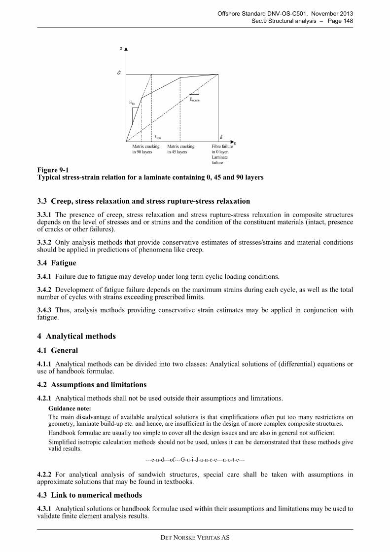
DET NORSKE VERITAS AS
Offshore Standard DNV-OS-C501, November 2013
Sec.9 Structural analysis – Page 148
Figure 9-1 Typical stress-strain relation for a laminate containing 0, 45 and 90 layers
3.3 Creep, stress relaxation and stress rupture-stress relaxation
3.3.1 The presence of creep, stress relaxation and stress rupture-stress relaxation in composite structuresdepends on the level of stresses and or strains and the condition of the constituent materials (intact, presenceof cracks or other failures).
3.3.2 Only analysis methods that provide conservative estimates of stresses/strains and material conditionsshould be applied in predictions of phenomena like creep.
3.4 Fatigue
3.4.1 Failure due to fatigue may develop under long term cyclic loading conditions.
3.4.2 Development of fatigue failure depends on the maximum strains during each cycle, as well as the totalnumber of cycles with strains exceeding prescribed limits.
3.4.3 Thus, analysis methods providing conservative strain estimates may be applied in conjunction withfatigue.
4 Analytical methods
4.1 General
4.1.1 Analytical methods can be divided into two classes: Analytical solutions of (differential) equations oruse of handbook formulae.
4.2 Assumptions and limitations
4.2.1 Analytical methods shall not be used outside their assumptions and limitations.
Guidance note:
The main disadvantage of available analytical solutions is that simplifications often put too many restrictions ongeometry, laminate build-up etc. and hence, are insufficient in the design of more complex composite structures.
Handbook formulae are usually too simple to cover all the design issues and are also in general not sufficient.
Simplified isotropic calculation methods should not be used, unless it can be demonstrated that these methods givevalid results.
---e-n-d---of---G-u-i-d-a-n-c-e---n-o-t-e---
4.2.2 For analytical analysis of sandwich structures, special care shall be taken with assumptions inapproximate solutions that may be found in textbooks.
4.3 Link to numerical methods
4.3.1 Analytical solutions or handbook formulae used within their assumptions and limitations may be used tovalidate finite element analysis results.
Matrix cracking
in 45 layers
Elin
ε
Enonlin
εεcorr
Fibre failurein 0 layer.Laminatefailure
Matrix cracking
in 90 layers
σ
σ
DET NORSKE VERITAS AS
Offshore Standard DNV-OS-C501, November 2013
Sec.9 Structural analysis – Page 149
5 Finite element analysis
5.1 General
5.1.1 Only recognised FE programs should be used. Other programs shall be verified by comparison withanalytical solutions of relevant problems, recognised FE codes and/or experimental testing.
5.2 Modelling of structures – general
5.2.1 Element types shall be chosen on the basis of the physics of the problem.
5.2.2 The choice of the mesh should be based on a systematic iterative process, which includes meshrefinements in areas with large stress/strain gradients.
5.2.3 Problems of moderate or large complexity shall be analysed in a stepwise way, starting with a simplifiedmodel.
5.2.4 Model behaviour shall be checked against behaviour of the structure. The following modelling aspectsshall be treated carefully:
— loads— boundary conditions— important and unimportant actions— static, quasi-static or dynamic problem— damping— possibility of buckling— isotropic or anisotropic material— temperature or strain rate dependent material properties— plastic flow— non-linearity (due to geometrical and material properties)— membrane effects.
5.2.5 Stresses and strains may be evaluated in nodal points or Gauss points. Gauss point evaluation is generallymost accurate, in particular for layered composites, in which the distribution of stresses is discontinuous, andshould therefore be applied when possible.
Guidance note:
The analyst shall beware that Gauss point results are calculated in local (element or ply based) co-ordinates and mustbe transformed (which is automatically performed in most FE codes) in order to represent global results. Thus, Gausspoint evaluation is more time-consuming than nodal point calculations.
---e-n-d---of---G-u-i-d-a-n-c-e---n-o-t-e---
5.2.6 Support conditions shall be treated with care. Apparently minor changes in support can substantiallyaffect results. In FE models, supports are typically idealised as completely rigid, or as ideally hinged, whereasactual supports often lie somewhere in between. In-plane restraints shall also be carefully treated.
5.2.7 Joints shall be modelled carefully. Joints may have less stiffness than inherited in a simple model, whichmay lead to incorrect predictions of global model stiffness. Individual modelling of joints is usually notappropriate unless the joint itself is the object of the study. See also requirements for the analysis of joints inSec.7.
5.2.8 Element shapes shall be kept compact and regular to perform optimally. Different element types havedifferent sensitivities to shape distortion. Element compatibility shall be kept satisfactory to avoid locally poorresults, such as artificial discontinuities. Mesh should be graded rather than piecewise uniform, therebyavoiding great discrepancy in size between adjacent elements.
5.2.9 Models shall be checked (ideally independently) before results are computed.
5.2.10 The following points shall be satisfied in order to avoid ill-conditioning, locking and instability:
— a stiff element shall not be supported by a flexible element, but rigid-body constraints shall be imposed onthe stiff element
— for plane strain and solid problems, the analyst shall not let the Poisson’s ratio approach 0.5, unless a specialformulation is used
— 3-D elements, Mindlin plate or shell elements shall not be allowed to be extremely thin— the analyst shall not use reduced integration rule without being aware of possible mechanism (e.g.
hourglass nodes).
DET NORSKE VERITAS AS
Offshore Standard DNV-OS-C501, November 2013
Sec.9 Structural analysis – Page 150
Guidance note:
Some of these difficulties can be detected by error tests in the coding, such as a test for the condition number of thestructure stiffness matrix or a test for diagonal decay during equation solving. Such tests are usually made posteriorrather than prior.
---e-n-d---of---G-u-i-d-a-n-c-e---n-o-t-e---
5.2.11 Need for mesh refinement is usually indicated by visual inspection of stress discontinuities in the stressbands. Analogous numerical indices are also coded.
5.2.12 For local analysis, a local mesh refinement shall be used. In such an analysis, the original mesh is stifferthan the refined mesh. When the portion of the mesh that contains the refined mesh is analysed separately, acorrection shall be made so the boundary displacements to be imposed on the local mesh are consistent withthe mesh refinement.
5.2.13 For non-linear problems, the following special considerations shall be taken into account:
— the analyst shall make several trial runs in order to discover and remove any mistake— solution strategy shall be guided by what is learned from the previous attempts— the analyst shall start with a simple model, possibly the linear form of the problem, and then add the non-
linearity one by one.
5.2.14 Computed results shall be checked for self-consistency and compared with, for example, approximateanalytical results, experimental data, text-book and handbook cases, preceding numerical analysis of similarproblems and results predicted for the same problem by another program. If disagreements appear, then thereason for the discrepancy shall be sought, and the amount of disagreement adequately clarified.
5.2.15 The analyst shall beware the following aspects:
— for vibrations, buckling or non-linear analysis, symmetric geometry and loads shall be used with care sincein such problems symmetric response is not guaranteed. Unless symmetry is known to prevail, it shall notbe imposed by choice of boundary conditions
— for crack analysis, a quarter point element can be too large or too small, thereby possibly making resultsfrom mesh refinement worse
— the wrong choice of elements may display a dependence on Poison’s ratio in problems that shall beindependent of Poisson’s ratio
— if plane elements are warped, so that the nodes of the elements are not co-planar, results may be erratic andvery sensitive to changes in mesh
— imperfections of load, geometry, supports and mesh may be far more important in a buckling problem thanin problems involving only linear response.
5.2.16 In the context of finite element analysis (FEA) of laminate structures (one of) the following elementtypes should be applied:
— layered shell elements with orthotropic material properties for each layer (for in-plane 2-D analysis, see[1.3.4])
— solid elements with orthotropic material properties (for 3-D and through thickness 2-D analysis, see[1.3.4]).
Guidance note:
There are two options for the solid elements: The modelling may be performed with (at least) two solid elementsthrough the thickness of each ply. Alternatively, one may apply layered solid elements where the thickness of a singleelement includes two or more plies.
---e-n-d---of---G-u-i-d-a-n-c-e---n-o-t-e---
5.3 Software requirements
5.3.1 Selection of finite element software package shall be based on the followings:
— software availability— availability of qualified personnel having experience with the software and type of analysis to be carried out— necessary model size— analysis options required— validated software for intended analysis.
5.3.2 Useful options for the analysis of composite structures include:
— layered solid elements with orthotropic and anisotropic material behaviour— layered shell elements— solid elements with suitable core shear deformation models (for analysis of sandwich structures)
DET NORSKE VERITAS AS
Offshore Standard DNV-OS-C501, November 2013
Sec.9 Structural analysis – Page 151
— solid elements with correct material models or appropriate interface elements allowing for debond (foranalysis of bonded and laminated joints)
— interface elements allowing for large aspect ratio (for analysis of thin layer bonds)— the possibility to select different co-ordinate systems in a clear and unambiguous way.
5.3.3 Depending on the area of application, additional analysis options should be available e.g.:
— appropriate solver with stable and reliable analysis procedures— options characterising large displacements and large strains (for geometrically non-linear analysis)— material models describing the behaviour of, e.g., laminates beyond first failure as well as ductile sandwich
cores (for materially non-linear analysis)— robust incremental procedures (for non-linear analysis in general)— tools for frequency domain analysis and/or options such as time integration procedures (for dynamic
analyses)— appropriate post-processing functionality— database options— sub-structuring or sub-modelling.
5.4 Execution of analysis
5.4.1 FEA tasks shall be carried out by qualified engineers under the supervision of an experienced seniorengineer.
5.4.2 Analysis shall be performed according to a plan, which has been defined prior to the analysis.
5.4.3 Extreme care shall be taken when working with different relevant co-ordinate systems, i.e. global, plybased, laminate based, element based and stiffener based systems.
5.4.4 The approach shall be documented.
5.5 Evaluation of results
5.5.1 Analysis results shall be presented in a clear and concise way using appropriate post-processing options.The use of graphics is highly recommended, i.e. contour plots, (amplified) displacement plots, time histories,stress and strain distributions etc.
5.5.2 The results shall be documented in a way to help the designer in assessing the adequacy of the structure,identifying weaknesses and ways of correcting them and, where desired, optimising the structure.
5.6 Validation and verification
5.6.1 FE programs shall be validated against analytical solutions, test results, or shall be benchmarked againsta number of finite element programs.
5.6.2 Analysis designer shall check whether the envisaged combination of options has been validated bysuppliers. If this is not the case, he shall perform the necessary validation analysis himself.
5.6.3 FEA results shall be verified by comparing against relevant analytical results, experimental data and/orresults from previous similar analysis.
5.6.4 Analysis and model assumptions shall be verified.
5.6.5 Results shall be checked against the objectives of the analysis.
5.6.6 Verification whether the many different relevant co-ordinate systems have been applied correctly shallbe considered.
6 Dynamic response analysis
6.1 General
6.1.1 Dynamic analysis should generally be performed when loads are time-dependent and/or when othereffects such as inertia (and added mass) and damping forces are significant.
6.1.2 In a dynamic analysis one may be interested in the transient response of a structure due to prescribed,time-dependent loads or the 'eigenvalues' (natural or resonance frequencies) of the structure.
6.1.3 In order to obtain an accurate transient analysis a detailed structural model and small time steps shouldbe used, in particular for rapid varying loads.
6.1.4 For slowly varying loads a quasi-static analysis may be applied. In such an analysis inertia and dampingforces are neglected, and the corresponding static problem is solved for a series of time steps.
DET NORSKE VERITAS AS
Offshore Standard DNV-OS-C501, November 2013
Sec.9 Structural analysis – Page 152
6.1.5 In vibration analysis one may use a coarse structural model if only the first few 'eigenvalues' are ofinterest, see [6.2.2]. Nevertheless, a reasonable representation of structural mass and stiffness is crucial.
6.1.6 If a large number of 'eigenfrequencies' are required, one shall apply a detailed description of the structure.
6.1.7 Due account should be taken of fluid-structure interaction effects where these are significant. These mayinclude resonance between structural response and wave excitation frequencies, or more complex, high-frequency vibration phenomena (ringing and springing) caused by non-linear wave loads. In some cases offluid-structure interaction it may be necessary to perform a dynamic analysis of the coupled fluid-structuresystem.
6.1.8 In case of accidental loads, such as explosions, dynamic effects should be considered carefully.
6.1.9 The dependence of the material properties on strain rate should be taken into account, see Sec.4 [3.10].
Guidance note:
Although static material properties may yield conservative predictions of displacements, a strength assessment basedon static properties is not necessarily conservative since both the material strength and the material stiffness may beenhanced at high strain rates. The higher stiffness may increase the induced stress so that the benefit of the increasein the material strength may be lost. Furthermore, ductile materials often become brittle at high rates. Thus, the extramargin provided by ductile behaviour may be destroyed.
There is a lack of sophisticated material models taking the rate dependent behaviour into consideration.
---e-n-d---of---G-u-i-d-a-n-c-e---n-o-t-e---
6.2 Dynamics and finite element analysis
6.2.1 For analysis including dynamic loads with frequencies of interest up to ωcr., the mesh shall be able toaccurately represent modes associated with frequencies up to 3ωcr., and a mode superposition analysis shallinclude frequencies up to about 3ωcr..
6.2.2 For 'eigenvalue' analysis, there should be 4 or more times as many degrees of freedom as 'eigenvalues'to be calculated.
6.2.3 For direct integration methods, the following points should be ensured:
— the time step Dt should be approximately 0.3/ωcr. or less, and should provide numerical stability if theintegration method is conditionally stable
— there should be a match between the type of algorithm and the mass matrix— abrupt changes in element size should be avoided, thereby avoiding spurious wave reflection and numerical
noise.
7 Impact response
7.1 Testing
7.1.1 Impact test requirements shall be defined since there are no well-established calculation methods today.
7.1.2 Component testing (see Sec.10) should be carried out in order to evaluate the impact characteristics ofthe structure/component.
8 Thermal stresses
8.1 General
8.1.1 Changes in temperature from the environment resulting in dimensional changes of the body shall betaken in account. The general thermal strains, ei, can be expressed as:
where αi is the thermal expansion coefficients. Temperature is denoted by T.
8.1.2 Residual strains shall be calculated against the reference temperature for which αi was determined. It isusually the curing temperature.
8.1.3 Accordingly, the stress-strain relations shall be modified to account for the stress free environmentallyinduced expansion strains as follows:
Te ii ∆= α
{ } [ ]{ } { }eS += σε
DET NORSKE VERITAS AS
Offshore Standard DNV-OS-C501, November 2013
Sec.9 Structural analysis – Page 153
9 Swelling effects
9.1 General
9.1.1 Changes in gas or fluid absorption from the environment resulting in dimensional changes of the bodyshall be taken in account. The general swelling strains, ei, can be expressed as
where βi is the swelling expansion coefficients and C is swelling agent concentration inside the laminate.
9.1.2 Accordingly, the stress-strain relations shall be modified to account for the stress free environmentallyinduced expansion strains as follows:
10 Analysis of sandwich structures
10.1 General
10.1.1 A typical load carrying sandwich structure has the following characteristics; it is build up of threeelements: two faces, usually stiff and strong; a core, weaker and lighter; a joint, continuous along each of thetwo interfaces. Additionally, see the definition in Sec.14.
10.1.2 All the sandwich structures that do not fall into the above definition are denoted special sandwichstructures. A distinction is made between typical and special sandwich panels. Simple formulas are providedfor design of typical sandwich panels whereas special ones shall be designed on the basis of more rigorousanalyses and possibly testing.
10.1.3 A decision to use 2-D or 3-D analysis shall be made depending on the level of significance of thethrough thickness stresses/through width strains (see [1.3.4]). If all through thickness stress components maybe neglected, in-plane 2-D analysis may be applied, and if plane strain conditions prevail, a through thickness2-D approach may be adopted. Otherwise, 3-D analysis should be performed.
10.1.4 In the context of FEA of sandwich structures (one of) the following element types or combinationsshould be applied:
— a single layer of layered shell elements through the thickness of the entire sandwich material (for in-plane2-D analysis, see [1.3.4])
— (layered) shell elements for the faces and solid elements for the core (for 3-D and through thickness 2-Danalysis, see [1.3.4]). In this case a compensation may be desirable for the change in stiffness, oralternatively, in order to avoid overlapping areas, shell elements can be positioned adequately without theneed for modifying the material properties by using the eccentricity property of the element. Depending onthe commercial package used this option is not always available
— solid elements for both faces and core (for detailed 3-D and through thickness 2-D analysis, see [1.3.4]).
10.1.5 For the analysis of sandwich structures, special considerations shall be taken into account, such as:
— elements including core shear deformation shall be selected— for honeycomb cores one shall account for material orthotropy, since honeycomb has different shear
moduli in different directions— local load introductions, corners and joints, shall be checked— curved panels with small radii of curvature shall be analysed in 2-D (through thickness direction) or 3-D to
account for the transverse normal stresses not included in shell elements.
10.1.6 The load combinations and associated load factors and the surrounding environmental conditionsestablished in Sec.3 shall be applied to the loads to calculate stresses and strains in the structure.
10.1.7 Each point in the structure shall be checked for all times against the specified functional requirementand corresponding failure modes.
10.1.8 Failure criteria for each mechanisms of failure are described in Sec.6.
10.2 Elastic constants
10.2.1 Each laminate shall be described with the suitable set of elastic constants as mentioned in section 4dealing with monolithic structures.
10.2.2 Core materials are generally orthotropic and are described by more than two elastic constants (seeSec.5). However, most FE codes can only describe isotropic core materials. If the elements applied in the FEA
Ce ii β=
{ } [ ]{ } { }eS += σε
DET NORSKE VERITAS AS
Offshore Standard DNV-OS-C501, November 2013
Sec.9 Structural analysis – Page 154
do not allow values for all three parameters to be specified, one should generally use the measured values forG and ν, and let the E value be calculated (from the formula above) by the program. In that case the shearresponse of the core will be described accurately. However, in particular applications, in which core sheareffects are negligible and axial stresses/strains are crucial, correct E values shall be applied.
Guidance note:
For many core materials experimentally measured values of E, G and ν are not in agreement with the isotropicformula:
---e-n-d---of---G-u-i-d-a-n-c-e---n-o-t-e---
10.2.3 Anisotropic core shall be described with 4 elastic constants in a 2-D analysis, i.e. Ex, Ez, Gxz, νxz.
10.2.4 Anisotropic core shall be described with 9 elastic constants in a 3-D analysis, i.e. Ex, Ey, Ez, Gxy, Gyz,Gxz, νxy, νyz, νxz.
10.3 2-D non-linear failure analysis
10.3.1 If the through thickness stresses or the through width strains are insignificant, see [10.1.3], a 2-Dprogressive analysis may be carried out.
10.3.2 At the beginning of the analysis, the analyst shall use non-degraded material properties.
10.3.3 All displacement calculations shall be based on time-dependent material properties related to, e.g.,naturally or environmentally degradation during service life.
10.3.4 For an undamaged sandwich structure, the following stresses and load shall typically be calculated:, , and .
Guidance note:
Example: Transverse loading case for an open beam.
Stresses shall be calculated as follows:
Identically for a box beam:
10.3.5 For given loading conditions, stresses and strains shall be calculated and failure criteria shall bechecked.
10.3.6 Any failure of the face material shall be modelled the same way as for monolithic laminates accordingto Sec.4 and Sec.9 [2].
10.3.7 If core failure of type ductile or plastic occurs due to core yielding (in tension or compression), Ecore*shall be set equal to the secant modulus at the corresponding σ level; Gcore* shall be proportionally reduced bythe same amount. If is reached, Ecore and Gcore shall be reduced to 0 (default value) or to positive valuesas described in [10.3.11].
in N-direction, and
in direction perpendicular to N.
)1(2 ν+= E
G
faceσcoreσ coreτ
crP
faceface ED
Mz=σ
corecore ED
Mz=σ
+=
422
2
corecoreface
facecore
tEdtE
D
Tτ
faceface ED
Mz=σ
NI
bd
24=τ
( )N
I
ddbcore
28
2 +=τ
coreσ
DET NORSKE VERITAS AS
Offshore Standard DNV-OS-C501, November 2013
Sec.9 Structural analysis – Page 155
10.3.8 If core failure of type brittle occurs due to core fracture (in tension or compression), Ecore shall bereduced to 0 (default value) or to a positive value as described in [10.3.11].
10.3.9 If core failure of type ductile or plastic occurs due to core shearing , Gcore* shall be set equal to thesecant modulus at the corresponding τ level; Ecore* shall be proportionally reduced by the same amount. If is reached, Gcore and Ecore shall be reduced to 0 (default value) or to positive values as described in [10.3.11].
10.3.10 If core failure of type brittle occurs due to core shearing, Gcore shall be reduced to 0 (default value) orto a positive value as described in [10.3.11].
10.3.11 Instead of using the default value 0 for the parameters in [10.3.7]-[10.3.10], gradual degradation of thematerial properties can be used, provided experiments document the validity of values larger than 0 for thematerial used.
10.3.12 In numerical calculations certain problems arise, e.g. lack of inversion possibility of the structurestiffness matrix, when setting degraded material properties equal to 0. Thus, one should apply small values, i.e.1% of the non-degraded values, instead of 0.
10.3.13 If the non-linear behaviour of the core cannot be modelled properly, the core shall not be used beyondits yield point and the yield criterion in Sec.6 shall be applied as the ultimate limit state for sandwich failure.
10.4 3-D progressive failure analysis
10.4.1 If the through thickness stresses and through width strains are significant, see [10.1.3], a 3-Dprogressive analysis shall be carried out.
10.4.2 A similar progressive failure analysis as presented for monolithic structures in [2.3], shall be carriedout. However, failure mechanisms related to the core, see Sec.6 and [10.3], shall be included.
10.5 Long term damage considerations
10.5.1 The same progressive failure analysis as the one presented in [2.2] and [2.3] shall be carried out usingdegraded (long-term) material properties as described in Sec.5 [3].
10.5.2 Degraded material properties shall be used in the calculations of stresses and strains and in thedetermination of the strength used in the failure criteria.
11 Buckling
11.1 General
11.1.1 The need for special buckling analysis shall be assessed carefully in every case. In particular thefollowing aspects shall be considered in making this assessment:
— presence of axial compressive stresses in beam or column-type members or structural elements— presence of in-plane compressive or shear stresses in flat, plate-like elements— presence of in-plane compressive or shear stresses in shell-like elements.
11.1.2 Two alternative approaches may be used in analysing buckling problems:
— analysis of isolated components of standard type, such as beams, plates and shells of simple shape— analysis of an entire structure (or of an entire, complex structural component).
11.2 Buckling analysis of isolated components
11.2.1 When a member or component that is a part of a larger structure is analysed separately a global analysisof the structure shall be first applied to establish:
— the effective loading applied to the member/component by the adjoining structural parts— the boundary conditions for the structural member, in terms of translational and rotational stiffness
components in all relevant directions.
11.2.2 For simple members or components standard formulae or tables may be used to estimate elastic criticalloads (Pe), critical stresses (σe) or critical strains (εe), and the corresponding elastic buckling mode shapes.Alternatively these quantities may be calculated using analytical or numerical methods. It shall always bechecked that the buckling mode shape is consistent with the boundary conditions.
11.2.3 An assessment shall be made of the shape and size of initial, geometrical imperfections that mayinfluence the buckling behaviour of the member. Normally the most critical imperfection shape for a givenbuckling mode has a similar form to the buckling mode itself. However, any geometrical feature (including
coreτ
DET NORSKE VERITAS AS
Offshore Standard DNV-OS-C501, November 2013
Sec.9 Structural analysis – Page 156
eccentricity of loading) that results in compressive forces that are not coincident with the neutral axis of themember may require consideration. The assumed form and amplitude of the imperfection shall be decided onthe basis of the production process used with due consideration of the relevant production tolerances. Refer toSec.6 [8].
11.2.4 In some cases a geometrically non-linear analysis may be avoided as follows. The elastic critical load(without imperfections) Pe is calculated. In addition an ultimate failure load Pf is estimated at which the entirecross-section would fail by compressive fibre failure, in the absence of bending stresses at the section inquestion. If Pe > Pf the further assessment may be based on geometrically linear analysis provided geometricalimperfections are included and the partial load effect modelling factor is increased by multiplying it by thefactor:
11.2.5 In cases where it is possible to establish the bending responses (stresses, strains or displacements)associated with an in-plane loading separately from the in-plane (axial) responses, a first estimate of theinfluence of geometrical non-linearity combined with the imperfection may be obtained by multiplying therelevant bending response parameter obtained from a geometrically linear analysis by a factor:
and combining the modified bending responses with the (unmodified) in-plane responses.
11.2.6 The above procedures ([11.2.5] and [11.2.4]) may be non-conservative for some cases where the post-buckling behaviour is unstable. Examples include cylindrical shells and cylindrical panels under axial loading.Such cases shall be subject to special analysis and or tests.
11.3 Buckling analysis of more complex elements or entire structures
11.3.1 Buckling analysis of more complex elements or entire structures shall be carried out with the aid ofverified finite element software or equivalent.
11.3.2 Initially an 'eigenvalue' buckling analysis shall be performed assuming initial (non-degraded) elasticproperties for the laminates and, for sandwich structures, for the core. This shall be repeated with alternative,finer meshes, until the lowest 'eigenvalues' and corresponding 'eigenmodes' are not significantly affected byfurther refinement. The main purposes of this analysis are to clarify the relevant buckling mode shapes and toestablish the required mesh density for subsequent analysis.
11.3.3 Careful attention shall be paid to correct modelling of boundary conditions.
11.3.4 If the applied load exceeds, or is close to, the calculated elastic critical load, the design should bemodified to improve the buckling strength before proceeding further.
11.3.5 A step-by-step non-linear analysis shall be carried out. Geometrical non-linearity shall be included inthe model. The failure criteria shall be checked at each step. If failure such as matrix cracking or delaminationis predicted, any analysis for higher loads shall be performed with properties reduced as described in Sec.4 [9].
11.3.6 Alternatively to the requirement in [11.3.5] a geometrically non-linear analysis may be performed usingentirely degraded properties throughout the structure. This will normally provide conservative estimates ofstresses and deformations. Provided reinforcing fibres are present in sufficient directions, so that the largestrange of un-reinforced directions does not exceed 60º, such an estimate will not normally be excessivelyconservative.
11.3.7 The influence of geometric imperfections should be assessed, on the basis of the production method andproduction tolerances. Refer to Sec.6 [8].
11.4 Buckling analysis of stiffened plates and shells
11.4.1 When stiffened plate or shell structures are analysed for buckling, special attention shall be paid to thefollowing failure modes:
— local buckling of laminate (plate) between stiffeners— possible local buckling of individual plate-like elements in the stiffeners themselves— overall buckling of the stiffened plate or shell, in which case separation (debonding) of the stiffener from
the plate or shell laminate must be explicitly considered.
11.4.2 The finite element model shall be able to reproduce all the relevant failure modes as listed in [11.4.1].Stiffener debonding shall be evaluated by the insertion of appropriate elements at the interface to monitor thetensile and shear forces that are transmitted across the bond, together with an appropriate criterion based ontests or relevant published data.
ef P4P1
1
−
eee 1
1or
1
1
PP1
1
εεσσ −−−,
DET NORSKE VERITAS AS
Offshore Standard DNV-OS-C501, November 2013
Sec.9 Structural analysis – Page 157
11.5 Buckling analysis for sandwich structures
11.5.1 Sandwich structures may be exposed to highly localised buckling modes such as wrinkling anddimpling, in addition to more global modes. For simple stress states these local modes may often be checkedusing standard formulae.
11.5.2 The wave-lengths for wrinkling are normally very short (often of the order of the sandwich thickness).If a direct FE analysis of wrinkling is carried out it is essential that a sufficiently fine mesh be used in the skinlaminates, such that the mode shape is well represented. If each skin laminate is modelled using shell elements,the element size should not normally be greater than λ/12, where λ is the buckling wavelength. The core shallbe modelled with solid elements of similar size. The required element size shall be established using iterativecalculations.
11.5.3 In performing FE analysis of wrinkling it is not normally necessary to model a large area of thestructure, provided the in-plane stress state in the skin is well represented. A portion of the panel extending overa few wavelengths is normally sufficient. The result is not normally sensitive to the size of the panel selectedfor modelling.
11.5.4 In the absence of detailed information about geometrical imperfections and their consequences, thesemay be allowed for by reducing the critical wrinkling stress by 40%. The face wrinkling stress in some textbook formulas may already includes such allowance.
11.5.5 Wrinkling of skin laminates may be accompanied by yielding of the core if the core is made of a ductilematerial. This may in turn lead to a reduction in the tangent stiffness of the core and a lowering of the criticalstress for wrinkling. This is mainly a problem at points of load application and at joints, where the coreexperiences local loading, and may be avoided by adequate thickening of the skin laminate, insertion of higherstrength core material locally or by other local design features. The adequacy shall be proved by testing oranalysis unless previous experience shows the solution is adequate.
12 Partial load-model factor
12.1 General
12.1.1 A deterministic factor shall be assigned to each structural analysis method. It is designated in thisstandard as the partial load-model factor γSd (see Sec.3, Sec.2 [3.6] and Sec.8 [2.2]).
12.1.2 The load-model factor accounts for uncertainties of the structural analysis method being used toaccurately describe and quantify the response of the structure.
12.1.3 Model factors for the main structural analysis methods are given in the following sub-sections.
12.1.4 In some cases a structure is only evaluated by testing, and such an approach evaluates only the particularconditions tested. A procedure for this approach is given in Sec.10.
12.2 Connection between partial load-model factor and analytical analysis
12.2.1 When analytical methods are used within their assumptions and limitations a model factor of 1.0 shouldbe used.
12.2.2 If analytical methods are used outside their assumptions and limitations, it shall be documented that themagnitude of the model factor ensures that all predicted stresses and strains are higher than in reality. If thechoice of model factor cannot be documented, the analytical method shall not be used.
12.3 Connection between partial load-model factor and finite element analysis
12.3.1 The accuracy of FE methods is generally very good when the structure is properly modelled. The useof these methods with unsatisfactory models is much more uncertain.
12.3.2 When FE methods are used within their assumptions and limitations (and according to [5]) a modelfactor of 1.0 may be used.
12.3.3 If FE methods are used outside their assumptions and limitations, it shall be documented that themagnitude of the model factor ensures that all predicted stresses and strains are higher than in reality. If themodel factor cannot be documented, the analysis method shall not be used.
12.3.4 If the boundary conditions do not exactly represent the real conditions the effect on the load modelfactor shall be evaluated. As a minimum a factor of 1.1 shall be used.
12.3.5 If the load-model factor cannot be determined for calculations in a critical region, e.g. a critical joint orregion of stress concentrations, experimental qualification should be done (see Sec.10).
DET NORSKE VERITAS AS
Offshore Standard DNV-OS-C501, November 2013
Sec.9 Structural analysis – Page 158
12.4 Connection between partial load-model factor and dynamic response analysis
12.4.1 The accuracy of the dynamic analysis shall be estimated. The load-model factor used, which isdescribed in [12.2] and [12.3], shall include all uncertainties due to dynamic effects.
12.5 Connection between partial load-model factor and transfer function
12.5.1 The accuracy of the transfer function (see [1.4]) shall be estimated. The load-model factor used, whichis described in [12.2] and [12.3], shall include all uncertainties due to the transfer function.
DET NORSKE VERITAS AS
Offshore Standard DNV-OS-C501, November 2013
Sec.10 Component testing – Page 159
SECTION 10 COMPONENT TESTING
1 General
1.1 Introduction
1.1.1 Component testing is carried out for either:
— qualification based entirely on tests on full scale or large scale components, or— updating or verification of analysis by testing.
1.1.2 This standard gives procedures to evaluate test results and shows procedures to determine testprogrammes.
1.1.3 A structure or part of a structure can in some cases be qualified by testing only, i.e. no structural analysisas presented in Sec.9 is performed. This approach is presented in [2].
1.1.4 Testing can in some cases be carried out to document the design or increase confidence in designcalculations. It is an alternative or complement to analysis based on basic material properties. See [3].
1.1.5 If the component is checked by qualification testing only, design calculations are not relevant. The testresults are the only relevant information to evaluate whether the component is fit for purpose. This also meansthat the qualification is only valid for the conditions tested.
1.1.6 If testing is carried out to complement the analysis, it is done to reduce or to eliminate the influence ofsystematic errors introduced in the design methodology or to verify that the assumptions regarding failuremechanisms, failure modes etc. on which the design is based are correct.
1.1.7 In most practical cases component testing is used in combination with a structural analysis to evaluatethe component for a wider range than the actual test conditions.
1.2 Failure mode analysis
1.2.1 An analysis of all possible failure modes in the structure shall be done as described in Sec.3.
1.2.2 It shall be shown by testing or analysis that none of the possible failure modes will be critical for theperformance and safety of the structure.
Guidance note:
A special concern with composite materials is that minor loads may cause failures even though the structure can wellwithstand the main loads for which it was designed or built. Such minor loads can be through thickness loads inlaminates or sandwich structures or loads oriented perpendicular to the main fibre direction in the laminate.
---e-n-d---of---G-u-i-d-a-n-c-e---n-o-t-e---
1.2.3 An evaluation of failure modes is especially critical if long-term performance shall be documented anddata must be extrapolated to longer lifetimes than test times. In that case failure may be caused by failure modesthat were not critical in a short-term test (see [4]).
1.2.4 Temperature changes may introduce different failure mechanism. If the structure is exposed to differenttemperatures and resulting thermal stresses, possible changes of failure modes should be evaluated.Analytically these changes are modelled by temperature dependent material properties and by possible changesin the failure criteria that are applied, e.g. ductile brittle transition. Testing should be done for all conditionsthat cannot be modelled in a satisfactory way.
1.3 Representative samples
1.3.1 Test specimens shall represent the actual structure.
1.3.2 Production methods and materials shall be exactly the same, and production tolerances should be knownand controlled. The tolerances for producing the test samples should be representative of production conditionsof the product.
1.3.3 If the qualification is based on testing only [2], no changes shall be made to materials or productionwithout new tests.
1.3.4 If testing is combined with analysis changes in materials or geometry may be permitted, if theconsequences of the changes can be treated with confidence by the analytical methods.
DET NORSKE VERITAS AS
Offshore Standard DNV-OS-C501, November 2013
Sec.10 Component testing – Page 160
2 Qualification based on tests on full scale components
2.1 General
2.1.1 The purpose of tests is to investigate the load effects. Usually displacements and the characteristicstrength are determined.
2.1.2 The load cases in the tests shall be combined in a realistic manner. Test results are only valid for the loadcases tested.
2.1.3 The environment defined in Sec.3 [10] shall be represented in a realistic manner. The environmentaleffect can be accounted for either by:
— carrying out tests on components that have been subjected to a representative ageing (accelerated or notaccelerated)
— carrying out tests on components combined with ageing (accelerated or not accelerated). An example is thestandard techniques used for qualification of pipes.
Test results are only valid for the environments tested.
2.1.4 The failure mode(s), failure mechanism(s) and location(s) of failure shall be recorded and verifiedduring/after the tests. The partial/safety factor(s) applied shall correspond to the actual failure mechanisms.
2.2 Short term properties
2.2.1 Short term failure shall be analysed based on the general failure criteria for single or multiple loads asdescribed in Sec.6 [2.2] - [2.3]:
— the partial resistance model factor gRd can be set equal to 1.0, if the tests represent design and materialproperties in a satisfactory manner
— the partial load model factor gSd can be set equal to 1.0, if the tests represent actual applied loads in asatisfactory manner. If loads are representing effects of other phenomena, uncertainties in the conversionfrom the other phenomena to the loads shall be included in γSd, i.e. uncertainties in the transfer function asdescribe in Sec.9 [1.4] shall be included
— the characteristic strength of the tested component shall be determined based on the test results as describedin Sec.4 [2.4] for static data
— the safety factors shall be chosen based on distribution and COV of the load and COV of the component testresults (material’s COV) as in Sec.8. The distribution and COV of the load shall be based on the loads thestructure will experience in the application, not on the loads of the test.
2.2.2 At least three specimens shall be tested. The relationship between number of tests and characteristicstrength is given in Sec.4 [2.4].
2.3 Long term properties
2.3.1 Long term failure shall be analysed based on the principles for obtaining time dependent propertiesdescribed in Sec.6 [10] and [11]:
— the partial resistance model factor γRd can be set equal to 1.0, if the tests represent design and materialproperties in a satisfactory manner
— the partial load model factor γSd can be set equal to 1.0, if the tests represent actual applied loads in asatisfactory manner. If loads are representing effects of other phenomena, uncertainties in the conversionfrom the other phenomena to the loads shall be included in γSd, i.e. uncertainties in the transfer function asdescribe in Sec.9 [1.4] shall be included
— The characteristic strength shall be determined based on the test results as described in Sec.4 [3.11] for timedependent data
— the safety factors shall be chosen based on distribution and COV of the load and COV of the component testresults (material’s COV) as in Sec.8. The distribution and COV of the load shall be based on the loads thestructure will experience in the application, not on the loads of the test.
2.3.2 At least ten specimens shall be tested. The relationship between number of tests and characteristicstrength is given in Sec.4 [3.11] for data that must be extrapolated to longer lifetimes and for data that can beused within the test period.
2.3.3 If data must be extrapolated to longer lifetimes than the measured time it shall be shown that no otherfailure modes may develop between the test time and the expected lifetime of the structure or component. It isusually not possible to show this by component testing only. Some analysis and calculations are necessary, see[4.3.5].
2.3.4 The static strength of the structure after long term exposure shall be the same as the extrapolation of thelong term test data of the fatigue or stress rupture tests.
DET NORSKE VERITAS AS
Offshore Standard DNV-OS-C501, November 2013
Sec.10 Component testing – Page 161
2.3.5 Higher static strength values after long term exposure may be used if experimental evidence can beprovided. A procedure to obtain strength data after long term exposure is suggested in Sec.4 [3.4] and [3.9].
3 Verification of analysis by testing and updating
3.1 Verification of design assumptions
3.1.1 Tests under this category are carried out to verify that the assumptions on which the design is based arecorrect and that no important aspects of the design have been overlooked. Verification tests should be carriedout to compensate for:
— incorrect description of, or an unsatisfactory large uncertainty in the failure mechanisms— incorrect description of load combinations or corresponding large uncertainties— incomplete understanding of the effect of the environment— lack of experience of similar structures or components— uncertainty in the accuracy of modelling large stress gradients— assumptions that can be questioned or are difficult to document— unknown effect of large scale manufacturing procedures.
3.1.2 Tests under this category are carried out to verify that the analysis tools predict the response to the mostcritical load cases and environments in a correct or conservative manner. This type of testing shall be done ifthe particular analysis method has never been used for a similar structure and load situation before.
3.1.3 As it is not possible to test all load conditions that the structure will experience, the most critical loadconditions should be selected. The selection shall be based not only on the most critical loads the structure ismost likely to see. It shall also show that critical failure modes that can be caused by secondary loads areadequately modelled ([1.2]).
3.1.4 It may be necessary to test more than one aspect of an analysis. This may mean that two or more separatetest programmes should be carried out, unless both aspects can be evaluated in one test. The remaining parts ofthis section explain the requirement for one test programme.
Guidance note:
The end fitting of a pipe has been analysed. There is uncertainty about fatigue performance and long term staticstrength. In this case both aspects should be tested separately.
There is uncertainty about long term fatigue performance of new specimens and of specimens with impact damage.In this case the specimen can most likely be exposed to impact before the fatigue testing and only one test programmeis needed. This test programme would cover both aspects in a conservative way.
---e-n-d---of---G-u-i-d-a-n-c-e---n-o-t-e---
3.1.5 In general the environment defined in Sec.3 [10] should be represented in a realistic manner. Theenvironmental effect can be accounted for either by:
— carrying out tests on components that have been subjected to a representative ageing (accelerated or notaccelerated)
— carrying out tests on components combined with ageing (accelerated or not accelerated). An example is thestandard techniques used for qualification of pipes.
Since these tests are used to increase the confidence in calculation techniques other environments may bechosen if it can be demonstrated that the effects of the real environment can be predicted in a conservative wayby a combination of analytical tools and the test results obtained from a special test environment.
3.1.6 The following steps shall be followed when defining and carrying out test under this category:
1) The load condition(s) and environments are defined as specified in Sec.3.
2) The failure mode, failure mechanism and location of failure etc. on which the design is based are specified.
3) The number of test specimens required per load condition is specified. The number of test specimens mayhave to be determined based on an engineering judgement.
4) Carry out testing.
5) Verify failure mode, failure mechanism and location of failure. If these are as predicted in 2. theassumptions for the design are considered corroborated. If one or more of these are not as predicted in 2.the reason for the discrepancy shall be investigated and the validity of design assumptions re-evaluated.
3.1.7 Instead of testing the full component it may be more relevant to test parts or details. Which test is thebest should to be evaluated considering relevant failure modes and all possible interaction effects.
3.1.8 The failure mode(s), failure mechanism(s) and location(s) of failure shall be recorded and verifiedduring/after the tests.
DET NORSKE VERITAS AS
Offshore Standard DNV-OS-C501, November 2013
Sec.10 Component testing – Page 162
3.1.9 If analysis and test results agree with each other based on the criteria given in [3.2] and [3.3] the analysismethod is suitable for the application. (See also Sec.7 [2.2]).
3.2 Short term tests
3.2.1 The requirements here apply to one test aspect as determined in [3.1].
3.2.2 The sequence of the failure modes in the test shall be the same as predicted in the design. If the sequenceis different or if other failure modes are observed, the design shall be carefully re-evaluated.
3.2.3 The measured strength of each critical failure mode shall never be less than the predicted characteristicstrength. Critical failure modes are failure modes that are linked to a limit state. The characteristic strength ofthe component shall be updated according to [3.3].
3.2.4 In addition to the requirements above ([3.2.1] and [3.2.2]), one of the following requirements shall bemet:
— the test results fulfil the requirements for “confirmation testing for static data” given in Sec.4 [8.7].Application of this criterion requires that at least three tests are carried out
— the characteristic strength of the structure is updated by the test results as described in [3.4]. One test issufficient to use this method, but more tests are recommended.
3.3 Long term testing
3.3.1 Whether cyclic load testing or long term static load testing or both is required depends on the evaluationof the test programme done in [3.1]. The approach for both testing types is similar and will be treated here inone part.
3.3.2 Fatigue testing for high safety class: at least two survival tests shall be carried out. The specimen shouldnot fail during the survival test and it should not show unexpected damage. The requirements to the testing are:
— tests should be carried out up to five times the maximum number of design cycles with realistic amplitudesand mean loads that the component will experience. If constant amplitude testing is carried out tests shouldbe carried out up to 50 times the maximum number of design cycles to compensate for uncertainty insequence effects.
— if the anticipated lifetime exceeds 105 cycles testing up to 105 cycles may be sufficient. The load levelsshould be chosen such that testing of the two specimens is completed after at least 104 and 105 cyclesrespectively. The logarithms of the two test results shall fall within µ-σ of the logarithm of the anticipatednumber of cycles to failure, where µ is the mean of the logarithm of the predicted number of cycles tofailure and σ is one standard deviation of the logarithm of the predicted number of cycles to failure, bothinterpreted from a log(stress)-log(lifetime) diagram for the anticipated number of cycles to failure. If moretests are made the requirements are given in DNV-OS-C501 Sec.4 [8.8.6].
3.3.3 Fatigue testing for normal safety class: at least one survival test shall be carried out. The specimen shouldnot fail during the survival test and it should not show unexpected damage. The requirements to the testing are:
— tests should be carried out up to three times the maximum number of design cycles with realistic amplitudesand mean loads that the component will experience. If constant amplitude testing is carried out tests shouldbe carried out up to 30 times the maximum number of design cycles to compensate for uncertainty insequence effects.
— if the anticipated lifetime exceeds 105 cycles testing up to 105 cycles may be sufficient. The load levelsshould be chosen such that testing of the two specimens is completed after at least 104 and 105 cyclesrespectively. The logarithms of the two test results shall fall within µ-2σ of the logarithm of the anticipatednumber of cycles to failure, where µ is the mean of the logarithm of the predicted number of cycles tofailure and σ is one standard deviation of the logarithm of the predicted number of cycles to failure, bothinterpreted from a log(stress)-log(lifetime) diagram for the anticipated number of cycles to failure. If moretests are made the requirements are given in DNV-OS-C501 Sec.4 [8.8.6].
3.3.4 Stress rupture testing for high safety class: at least two survival tests shall be carried out. The specimenshould not fail during the survival test and it should not show unexpected damage. The requirements to the testresults are:
— tests should be carried out up to five times the maximum design life with realistic mean loads that thecomponent will experience. If constant load testing is carried out tests should be carried out up to 50 timesthe design life to compensate for uncertainty in sequence effects.
— if the anticipated lifetime exceeds 1000 hours testing up to 1000 hours may be sufficient. The load levelsshould be chosen such that testing is completed after 103 hours. The logarithms of the two test results shallfall within µ-σ of the logarithm of the anticipated lifetime, where µ is the mean of the logarithm of thepredicted lifetime and σ is one standard deviation of the logarithm of the predicted lifetime, both interpreted
DET NORSKE VERITAS AS
Offshore Standard DNV-OS-C501, November 2013
Sec.10 Component testing – Page 163
from a log(stress)-log(lifetime) diagram for the anticipated lifetime. If more tests are made the requirementsare given in DNV-OS-C501 Sec.4 [8.8.6].
3.3.5 Stress rupture testing for normal safety class: at least one survival test shall be carried out. The specimenshould not fail during the survival test and it should not show unexpected damage. The requirements to the testresults are:
— tests should be carried out up to three times the maximum design life with realistic mean loads that thecomponent will experience. If constant load testing is carried out tests should be carried out up to 30 timesthe design life to compensate for uncertainty in sequence effects.
— if the anticipated lifetime exceeds 1000 hours testing up to 1000 hours may be sufficient. The load levelsshould be chosen such that testing is completed after 103 hours. The logarithms of the two test results shallfall within µ-2σ of the logarithm of the anticipated lifetime, where µ is the mean of the logarithm of thepredicted lifetime and σ is one standard deviation of the logarithm of the predicted lifetime, both interpretedfrom a log(stress)-log(lifetime) diagram for the anticipated lifetime. If more tests are made the requirementsare given in DNV-OS-C501 Sec.4 [8.8.6].
3.3.6 For low safety class long term testing is not required.
3.3.7 The sequence of the failure modes in the test shall be the same as predicted in the design. If the sequenceis different or if other failure modes are observed, the design shall be carefully re-evaluated.
3.3.8 The average of the measured number of cycles or time until occurrence of each critical failure shall neverbe less than the predicted characteristic lifetime or numbers of cycles. Critical failure modes are failure modesthat are linked to a limit state.
3.3.9 Tests should be carried out with a typical load sequence or with constant load amplitude. If a clearlydefined load sequence exists, load sequence testing should be preferred.
3.3.10 Whether reduced test times compared to the component's life are acceptable should be evaluated basedon the anticipated failure modes and whether extrapolation of the data to longer lifetimes is possible. This willmainly depend on the confidence and previous knowledge one has about the failure modes that are tested.
3.3.11 In some cases high amplitude fatigue testing may introduce unrealistic failure modes in the structure.In other cases, the required number of test cycles may lead to unreasonable long test times. In these cases anindividual evaluation of the test conditions should be made that fulfils the requirements of [3.3.2] or [3.3.3] asclosely as possible.
3.3.12 The static strength of the structure after long term exposure shall be taken as the extrapolation of thelong term test data of the fatigue or stress rupture tests.
3.3.13 Higher static strength values after long term exposure may be used if experimental or theoreticalevidence can be provided. The same arguments as given in Sec.4 [3] may be used for matrix and fibredominated properties. A procedure to obtain strength data after long term exposure is suggested in Sec.4 [3.4]and [3.9].
3.3.14 Additional tests may be required if resistance to a failure mode cannot be shown by analysis withsufficient confidence and if this failure mode is not tested by the tests described above.
3.4 Procedure for updating the predicted resistance of a component
3.4.1 The resistance of the component is R and is assumed to be normally distributed:
R∈N(µR,σR2)
where,
µR = mean value of the resistance of the component (generally unknown).σR = standard deviation of the resistance of the component, representing the natural variability in the material
properties and the manufacturing/production process, and here assumed known.
3.4.2 The characteristic value of the resistance is specified as a specific quantile in the distribution of theresistance, here defined as:
xC =µR -2σR
However, because µR is unknown, the true characteristic value xC is also unknown.
3.4.3 Estimates of µR and xC prior to testing are sought. One way of obtaining such prior estimates is to carryout an analysis of the component by means of available analysis models.
The estimate µRA of µR is obtained from a single analysis using mean values for the material properties. Theuncertainty in the estimate µRA should also be assessed, expressed in terms of a standard deviation σm’, and
DET NORSKE VERITAS AS
Offshore Standard DNV-OS-C501, November 2013
Sec.10 Component testing – Page 164
reflecting uncertainties in the underlying material property estimates as well as uncertainties in the appliedanalysis models.
3.4.4 If the results of an analysis by means of the available analysis models are unbiased, the mean of theestimate of µR is to be taken as:
µµ’=µRA
3.4.5 If the results of an analysis by means of the available analysis models are encumbered with a bias, themean of the estimate of µR is to be taken as:
µµ’=µRA+∆in which ∆ represents the effect of the conservatism implied in the analysis leading to µRA. ∆ is sometimesreferred to as the bias and needs to be estimated.
3.4.6 An estimate of the characteristic value of the resistance, prior to any component testing, can now beobtained with 95% confidence as:
xC’=µµ’-1.64σµ’-2σR
3.4.7 After component testing is performed, the characteristic value of the component should be updated basedon the test results (and Bayesian updating theory).
3.4.8 When a total of n tests are performed, leading to n resistance values x1,…xn, the sample mean is defined as
3.4.9 Based on the test results, the following updated values of the mean and the standard deviation of theestimate of the mean resistance mR can be obtained:
µµ” = [n ⋅ µtest ⋅σµ’2 + µµ’ ⋅ σR2]/( n ⋅ σµ’2 + σR
2)
and
σµ” = [(σµ’2 ⋅ σR2)/( n ⋅ σµ’2 + σR
2)]1/2
3.4.10 Based on this, the following updated estimate of the characteristic resistance can be obtained with aconfidence of 95%:
xC”=µµ”-1.64σm”-2σR
3.4.11 When the standard deviation σµ’of the mean resistance estimate prior to testing is not available, andwhen a significant, conservative bias ∆ in the resistance estimate is implied by the available analysis models,then σµ’ may be approximated by ∆/2, unless a better approximation can be estimated. This approximation isnot valid when the bias ∆ is small or zero.
Guidance note:
The present note gives some more details related to the derivations above (see [3.4.1]-[3.4.11]). Assume that anestimate of µR is sought. The estimate can be based on a prediction by means of available engineering models. Suchmodels are usually encumbered with uncertainty owing to simplifications and idealisations, so the estimate becomesuncertain. The combined effect of simplifications and idealisations are on the conservative side, such that they implysystematic errors in the predictions, i.e., the estimator µR’* applied in the estimation of µR comes out with a bias andis thus not a central estimator. The bias is denoted ∆ and is defined as:
∆=µR -E[µR’*]
where E[µR’*] = the mean value of the estimator µR’* for µR.
The bias ∆ has to be estimated based on all available information and a best possible engineering judgement. Thisestimation of ∆ is a very crucial stage. Once the bias ∆ has been estimated, an unbiased central estimate of the meanresistance can be established with mean value:
µµ’=E[µR’]= E[µR’*]+∆The standard deviation of the unbiased central estimate of the mean resistance is taken as:
σµ’=D[µR’*] where D[µR’*] = standard deviation of the estimator µR’* for µR.
---e-n-d---of---G-u-i-d-a-n-c-e---n-o-t-e---
3.5 Specimen geometry - scaled specimen
3.5.1 The specimen geometry for testing may be chosen to be different from the actual under certainconditions.
3.5.2 Scaled specimens may be used if analytical calculations can demonstrate that:
— all critical stress states and local stress concentrations in the critical part of the scaled specimen and the
∑=
=n
i
itest xn 1
1µ
DET NORSKE VERITAS AS
Offshore Standard DNV-OS-C501, November 2013
Sec.10 Component testing – Page 165
actual component are similar, i.e., all stresses are scaled by the same factor between actual component andtest specimen
— the behaviour and failure of the test specimen and the actual component can be calculated based onindependently obtained material parameters. This means no parameters in the analysis should be based onadjustments to make large scale data fit
— the sequence of predicted failure modes is the same for the scaled specimen and the actual component overthe entire lifetime of the component
— an analysis method that predicts the test results properly but not entirely based on independently obtainedmaterials data may be used for other joint geometry if it can be demonstrated that the material values thatwere not obtained by independent measurements can also be applied for the new conditions.
3.5.3 Tests on previous components may be used as testing evidence if the scaling requirement in [3.5.2] isfulfilled.
4 Testing components with multiple failure mechanisms
4.1 General
4.1.1 A component or structure may fail by more than one failure mechanism. In that case it is important thatall the critical failure mechanisms will not occur during the lifetime of the structure. Critical failuremechanisms are the ones that are linked to functional requirements in Sec.3 and their occurrence will be aviolation of a limit state.
Guidance note:
A typical case for a component with multiple failure mechanisms is an adhesive joint. If the joint is loaded failure mayoccur in one of the substrates, in the adhesive, or in one of the two interfaces.
---e-n-d---of---G-u-i-d-a-n-c-e---n-o-t-e---
4.2 Static tests
4.2.1 Static tests are usually dominated by one failure mode. In that case the testing described in [2] and [3] issufficient.
4.2.2 If the tests show more than one failure mode each failure mode shall be evaluated individually accordingto the methods given in [2] and [3].
4.2.3 If a component shows two failure modes (X and Y) test results with failure X may be interpreted for thestatistical analysis in [2] and [3] in a way that failure mode Y occurred also at the same load as failure mode X.The same approach can be applied for more than two failure modes. More advanced statistical treatments maybe used to evaluate two or more failure modes.
4.2.4 If testing is carried out to verify an analysis of the structure the analysis should predict possible two (ormore) failure modes for the given test load.
4.2.5 Generally, the occurrence of two different failure modes should be avoided.
4.3 Long term tests
4.3.1 Even if static tests show only one failure mode a change of failure modes may happen over time. Such achange can be caused by different time dependencies of the changes in material properties or by changes infailure mechanisms, e.g. a ductile-brittle transition.
4.3.2 If test periods to obtain long term data are as long as the design life or design number of cycles, data canbe evaluated the same way as described in [4.2].
4.3.3 If design life or number of cycles exceed testing conditions it is not possible to qualify a component withmore than one failure mode just by component testing. Some additional information about the long termcharacteristics of the individual failure modes is needed. This information must be combined with test resultsby analytical reasoning.
4.3.4 The designer shall document that none of the critical failure mode will occur within the lifetime of thestructure.
4.3.5 One possible way to document that none of the critical failure mode will occur within the lifetime of thestructure is:
— if the design life is longer than the testing time the reduction of strength with time shall be establishedindividually for each failure mode by testing or analysis
— if the expected number of cycles is more than the tested number the reduction of strength with number ofcycles shall be established individually for each failure mode by testing or analysis
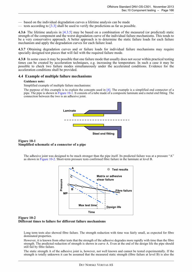
DET NORSKE VERITAS AS
Offshore Standard DNV-OS-C501, November 2013
Sec.10 Component testing – Page 166
— based on the individual degradation curves a lifetime analysis can be made— tests according to [3.3] shall be used to verify the predictions as far as possible.
4.3.6 The lifetime analysis in [4.3.5] may be based on a combination of the measured (or predicted) staticstrength of the component and the worst degradation curve of the individual failure mechanisms. This tends tobe a very conservative approach. A better approach is to determine the static failure loads for each failuremechanism and apply the degradation curves for each failure load.
4.3.7 Obtaining degradation curves and or failure loads for individual failure mechanisms may requirespecially designed test pieces that will fail with the required failure mode.
4.3.8 In some cases it may be possible that one failure mode that usually does not occur within practical testingtimes can be created by acceleration techniques, e.g. increasing the temperature. In such a case it may bepossible to check two failure modes simultaneously under the accelerated conditions. Evidence for theacceleration conditions shall be provided.
4.4 Example of multiple failure mechanisms
Guidance note:
Simplified example of multiple failure mechanisms:
The purpose of this example is to explain the concepts used in [4]. The example is a simplified end connector of apipe. The pipe is shown in Figure 10-1. It consists of a tube made of a composite laminate and a metal end fitting. Theconnection between the two is an adhesive joint.
Figure 10-1 Simplified schematic of a connector of a pipe
The adhesive joint was designed to be much stronger than the pipe itself. Its predicted failure was at a pressure “A”as shown in Figure 10-2. Short-term pressure tests confirmed fibre failure in the laminate at level B.
Figure 10-2 Different times to failure for different failure mechanisms
Long term tests also showed fibre failure. The strength reduction with time was fairly small, as expected for fibredominated properties.
However, it is known from other tests that the strength of the adhesive degrades more rapidly with time than the fibrestrength. The predicted reduction of strength is shown in curve A. Even at the end of the design life the pipe shouldstill fail by fibre failure.
The static strength A of the adhesive joint is, however, not well known and cannot be tested experimentally. If thestrength is totally unknown it can be assumed that the measured static strength (fibre failure at level B) is also the
Steel end fitting
Laminate
Pre
ss
ure
Time
Fibre failure
Design lifeMax test time
A
B
C Matrix or adhesive
shear failure
MP
Test results
DET NORSKE VERITAS AS
Offshore Standard DNV-OS-C501, November 2013
Sec.10 Component testing – Page 167
strength of the adhesive joint. Applying the degradation curve to this strength gives curve B. This is the approach in306, giving very conservative long-term pressures.
Alternatively, if testing up to a certain time has always shown that the tube failed by fibre failure, then it is possibleto apply the degradation curve of the adhesive joint to the longest test time. This is done in curve C, based on theapproach in [4.3.5]. The resulting maximum pressure MP, is relatively good value.
The simplifications of this example are mainly that more than two failure mechanisms are involved in such a joint.The laminate may show matrix cracking and delamination due to through thickness stresses. The adhesive joint mayfail in the adhesive or one of the interfaces. Each of these may have different degradation curves.
---e-n-d---of---G-u-i-d-a-n-c-e---n-o-t-e---
5 Updating material parameters in the analysis based on component testing
5.1
5.1.1 If test results do not agree with the analysis a change of few material parameters in the analysis maycreate agreement between test results and analysis. Such changes should be avoided and shall be made withgreat caution.
5.1.2 Material parameters may be changed if the results can be confirmed by independent tests on the materiallevel.
5.1.3 If such tests cannot be made the analysis is closely linked to the particular test geometry. Such an analysisshall not be used for other geometry or loading conditions unless it can be shown that the adjusted materialparameters have a physical meaning.
Guidance note:
Changes of material parameters due to damage, like matrix cracking, as described in Sec.4 can be made. These valuesare based on independent material tests and are needed for a non-linear analysis.
---e-n-d---of---G-u-i-d-a-n-c-e---n-o-t-e---
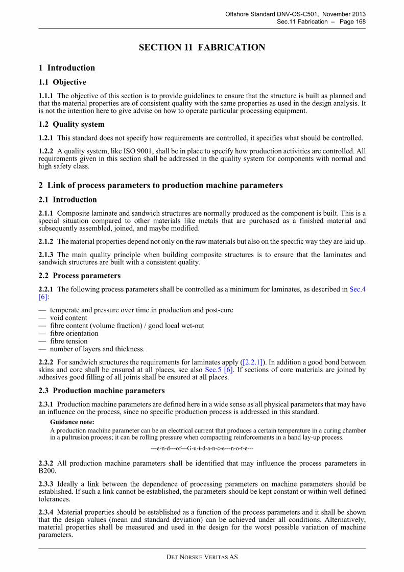
DET NORSKE VERITAS AS
Offshore Standard DNV-OS-C501, November 2013
Sec.11 Fabrication – Page 168
SECTION 11 FABRICATION
1 Introduction
1.1 Objective
1.1.1 The objective of this section is to provide guidelines to ensure that the structure is built as planned andthat the material properties are of consistent quality with the same properties as used in the design analysis. Itis not the intention here to give advise on how to operate particular processing equipment.
1.2 Quality system
1.2.1 This standard does not specify how requirements are controlled, it specifies what should be controlled.
1.2.2 A quality system, like ISO 9001, shall be in place to specify how production activities are controlled. Allrequirements given in this section shall be addressed in the quality system for components with normal andhigh safety class.
2 Link of process parameters to production machine parameters
2.1 Introduction
2.1.1 Composite laminate and sandwich structures are normally produced as the component is built. This is aspecial situation compared to other materials like metals that are purchased as a finished material andsubsequently assembled, joined, and maybe modified.
2.1.2 The material properties depend not only on the raw materials but also on the specific way they are laid up.
2.1.3 The main quality principle when building composite structures is to ensure that the laminates andsandwich structures are built with a consistent quality.
2.2 Process parameters
2.2.1 The following process parameters shall be controlled as a minimum for laminates, as described in Sec.4[6]:
— temperate and pressure over time in production and post-cure— void content— fibre content (volume fraction) / good local wet-out— fibre orientation— fibre tension— number of layers and thickness.
2.2.2 For sandwich structures the requirements for laminates apply ([2.2.1]). In addition a good bond betweenskins and core shall be ensured at all places, see also Sec.5 [6]. If sections of core materials are joined byadhesives good filling of all joints shall be ensured at all places.
2.3 Production machine parameters
2.3.1 Production machine parameters are defined here in a wide sense as all physical parameters that may havean influence on the process, since no specific production process is addressed in this standard.
Guidance note:
A production machine parameter can be an electrical current that produces a certain temperature in a curing chamberin a pultrusion process; it can be rolling pressure when compacting reinforcements in a hand lay-up process.
---e-n-d---of---G-u-i-d-a-n-c-e---n-o-t-e---
2.3.2 All production machine parameters shall be identified that may influence the process parameters inB200.
2.3.3 Ideally a link between the dependence of processing parameters on machine parameters should beestablished. If such a link cannot be established, the parameters should be kept constant or within well definedtolerances.
2.3.4 Material properties should be established as a function of the process parameters and it shall be shownthat the design values (mean and standard deviation) can be achieved under all conditions. Alternatively,material properties shall be measured and used in the design for the worst possible variation of machineparameters.

DET NORSKE VERITAS AS
Offshore Standard DNV-OS-C501, November 2013
Sec.11 Fabrication – Page 169
3 Processing steps
3.1 General
3.1.1 Bending of composites shall be avoided. A minimum bending radius shall be defined if the processrequires bending of materials.
3.1.2 Materials and components shall not be exposed to point-loads. All possible point loads shall be evaluatedand it shall be ensured that they will not damage the material.
3.1.3 The working conditions are important when producing composite parts. Ambient temperature rangesshall be defined and production areas should be well ventilated. Dust, fumes, chemicals etc. may influencecuring conditions or may attack the material later during service. The working conditions shall be defined.
3.1.4 Humidity shall be controlled at places where chemical reactions occur. If humidity cannot be controlledits effect shall be evaluated.
3.2 Raw materials
3.2.1 All raw materials shall be traceable for applications with normal and high safety class.
3.3 Storage of materials
3.3.1 The manufactures recommended storage conditions should be followed. All materials shall be stored inclean and dry environments.
3.3.2 Fibres should be stored in a clean environment, preferably wrapped up.
3.3.3 Resins and other chemicals should be stored in tight containers or tanks.
3.3.4 All resins and chemicals shall not be used after their shelf life has expired.
3.3.5 Some foam cores have internal gases from the production process that diffuse out with time. Such coresshall be stored long enough to allow the gases to diffuse out. Core skin delaminations may be the result if thegases remain in the core.
3.3.6 When taking materials out of storage it is important that they reach the same temperature as in theproduction facility while inside their sealed storage bag or container. This step prevents the formation ofhumidity on the materials.
3.4 Mould construction
3.4.1 The word moulds is interpreted in this section in a wide sense, covering many processes. Laying tables,mandrels and vacuum bags are considered as moulds or parts of moulds.
3.4.2 Moulds should match all tolerances required by the design.
3.4.3 Sharp corners and discontinuities at joining points should be avoided.
3.4.4 The surface finish shall be as specified. It shall be demonstrated that the mould surface finish can producecomponents with the required surface finish of the component.
3.4.5 Compatibility of mould release agents with the material and further operations should be considered.Especially adhesive joining or re-lamination may be effected by residues of mould release agents on the surfaceof the component. This applies for mould release agents that were applied to the mould and for mould releaseagents that were added to the resin.
3.4.6 The structural stability of moulds or mandrels should be ensured.
3.4.7 Possible deformations of the moulds should be considered in the design. The structure should be able towithstand all resulting loads and strains.
3.4.8 If moulds are heated a controlled distribution of temperature shall be ensured.
3.4.9 If a vacuum is applied inside the mould (or some bag), it shall be ensured that no leaks exist. The vacuumshall be measured far away from the point where the vacuum is pulled. Large moulds may require more thanone measurement point.
3.4.10 When removing the part from the mould large stresses and deformations may be induced, especially ifthe component got stuck somewhere. These effects should be avoided or at least carefully controlled. Possiblestresses or strains due to these operations should be considered in the design. If such a situation occursaccidentally the loads shall be estimated and the component shall be reanalysed.
DET NORSKE VERITAS AS
Offshore Standard DNV-OS-C501, November 2013
Sec.11 Fabrication – Page 170
3.5 Resin
3.5.1 Two or more component resins shall be carefully mixed according to manufacturers instructions, this isessential for a good cure.
3.5.2 The curing system shall be chosen in a way to prevent exothermic overheating.
3.5.3 Changing accelerators or other ingredients that control the speed of the cure are only permitted if theyhave no effect on the mechanical properties. The resin supplier shall confirm this. In addition, tensile testsaccording to Sec.4 [8.6.7] shall confirm no change in strength and stiffness for components of normal and highsafety class.
3.5.4 Barcol's hardness tests or other means should be used to check the quality of the cure.
3.5.5 The viscosity of the resin and or the gel time should be measured for all processes where the flowproperties of the resin are important.
3.5.6 It is recommended to take a sample from each batch of resin used in components of normal or high safetyclass. The sample of resin without fibres should be cured separately. A tensile or bending test should be usedto confirm that properties are within acceptable tolerances.
3.6 Producing laminates and sandwich panels
3.6.1 Procedures to confirm the lay-up of fabrics shall be established. A log shall be kept for components ofnormal or high safety class. The accuracy of the lay-ups shall be verified independently during production forhigh safety class components. Whether the verification shall be done by the manufacturer himself, by thecustomer, or by a third party should be decided by the project.
3.6.2 The accuracy of fibre orientations shall be specified for high safety class components.
3.6.3 Fibres shall be well aligned showing no local distortions or kinks.
3.6.4 Minimum and maximum overlap lengths of adjacent fabrics shall be specified. The effect of overlapsmay be similar to damage in the laminate and shall be evaluated as described in Sec.4 [1.7].
3.6.5 The tolerances for gaps between cores shall be defined.
3.6.6 The surfaces of cores shall have smooth transitions across the gaps. This is especially critical if cores aretapered.
3.6.7 Procedures shall be established to ensure a good bond between skins and cores for all geometrical shapesin the component. The quality of the interfacial bond shall be documented for all relevant geometry, e.g.,convex and concave surfaces.
3.6.8 Any gaps between cores shall be filled with the specified resin or adhesives, unless it was specified thatcores shall not be filled and core properties were measured on cores with unfilled gaps, see Sec.5 [6.2].
3.6.9 Absorption of resin by the core shall be considered with respect to weight of the total structure and theamount of resin needed to obtain the desired fibre volume fraction in the laminates.
3.6.10 The curing temperature and pressure shall not effect the properties of the core.
3.6.11 The temperature of all materials and the mould should be the same during the lay-up, unless the processspecifically requires other conditions.
3.7 Producing joints
3.7.1 The same requirements as for laminates and sandwich plates in [3.5] apply.
3.7.2 Overlap lengths shall be clearly specified and tolerances shall be given.
3.7.3 Surface preparations of adhesive or laminated joints shall be clearly specified and shall be the same asfor the specimens that were tested to qualify the joint.
3.7.4 The application of adhesives shall follow well described procedures. The procedures shall be exactly thesame as for the specimens that were tested to qualify the joint.
3.7.5 Surface preparation of adhesive or laminated joints and the application of adhesives shall be verifiedindependently during production for normal and high safety class components. Whether the verification shallbe done by the manufacturer himself, by the customer, or by a third party should be decided by the project.
3.7.6 The alignment of components and tolerances shall be specified.
DET NORSKE VERITAS AS
Offshore Standard DNV-OS-C501, November 2013
Sec.11 Fabrication – Page 171
3.7.7 Hole diameters positions and tolerances shall be specified for bolted connections.
3.7.8 Washer sizes or other supports shall be specified.
3.7.9 Torque of the bolts shall be specified.
3.7.10 Bolted joints shall be verified independently during production for high safety class components.Whether the verification shall be done by the manufacturer himself, by the customer, or by a third party shouldbe decided by the project.
3.8 Injection of resin and cure
3.8.1 The viscosity of the resin should be specified and controlled for all processes where the flow is important(see also [3.5.5]. As a minimum the gel time should be checked.
3.8.2 The flow patterns of injection processes shall be documented. Every part of the component shall be filledwith resin. No paths shall be blocked by resin that is already cured.
3.8.3 The curing schedule shall be specified and documented. A log shall be kept for component of normal orhigh safety class. The accuracy of the process shall be verified.
3.9 Evaluation of the final product
3.9.1 A procedure should be given to describe the evaluation of the finished product.
4 Quality assurance and quality control
4.1
4.1.1 A programme shall be established to ensure constant quality of the laminates that are produced.
4.1.2 The programme may rely mainly on testing of the product or it may utilise the control of production andmachine parameters.
4.1.3 Tests shall be carried out to check whether a consistent quality of the product or products is maintained.
4.1.4 Which tests should be carried out depends on the processing method and the particular structure. Theprinciples given here shall be followed, but details may be changed.
4.1.5 All tests that are performed for quality control shall also be performed on the materials that were used toobtain the design properties. The results of the tests shall be used a reference values for all following QC tests.
4.1.6 Allowable ranges of test results shall be established for all tests.
4.1.7 The easiest way to establish ranges of test results is to produce the materials for obtaining design datawith the worst acceptable process parameters. Such values can then be taken as minimum values.
4.1.8 Statistical process control methods may be used.
5 Component testing
5.1 General
5.1.1 Testing on components is done to detect possible manufacturing defects. The testing is not intended toqualify design aspects. These tests are described in Sec.10.
5.1.2 Testing on the system addresses the same aspects as for components. In addition the interaction betweenthe components is tested to detect possible mistakes in the way the components were put together.
5.1.3 The testing to check for fabrication errors shall be considered in the design analysis. No unintendeddamage (failure mechanisms, e.g. matrix cracking) shall be introduced into the structure by the tests.
5.2 Factory acceptance test and system integrity test
5.2.1 The factory acceptance test (FAT) is performed before the component leaves the factory. The test shouldidentify manufacturing errors before the component leaves the factory.
5.2.2 The FAT should be performed on all structures with safety class normal and high according to therequirements for pressure testing or other testing.
5.2.3 It is common practise to perform a FAT test, especially for pressurised components. The test is
DET NORSKE VERITAS AS
Offshore Standard DNV-OS-C501, November 2013
Sec.11 Fabrication – Page 172
recommended but not required by this standard. If a FAT test is not planned to be performed all parties of theproject shall be informed about this decision and the system integrity test shall identify the same aspects as aFAT test.
Guidance note:
The factory acceptance test has the advantage that gross manufacturing errors are detected before the componentleaves the factory. In some cases it is inconvenient or to perform a FAT test. The system integrity test will detect thesame manufacturing mistakes as a FAT test, and the defect will be detected before operation starts. However,replacement or repair may be more complicated if a defect is detected as late as in a system integrity test.
---e-n-d---of---G-u-i-d-a-n-c-e---n-o-t-e---
5.2.4 The system integrity test is performed after final installation of all components and before the systemgoes into service.
5.2.5 The system integrity test shall be performed on all structures according to the requirements for pressuretesting or other testing.
5.3 Pressure testing of vessels and pipes
5.3.1 All pressure vessels and pipes of safety class normal or high shall be pressure tested before going intoservice.
5.3.2 A test pressure of 1.3 x maximum service pressure shall be used unless such a pressure would introducedamage to the component that may reduce its lifetime. The maximum service pressure shall be the minimumtest pressure.
5.3.3 A detailed test programme shall be defined. The following shall be stated as a minimum:
— rates of pressure increase— holding times— time over which the pressure in the system shall not drop without actively applying pressure, i.e. a leakage
test.
5.3.4 The test schedule shall be developed for each application. The testing should allow detecting as manypossible defects in the structure as possible. As a general guidance the following schedules are recommended:
— the minimum time over which the maximum test pressure in the system (from [5.3.2]) shall not dropwithout actively applying pressure should be at least 10 minutes for systems that do not creep
— for systems that show creep the maximum test pressure should be kept for 1 hour applying active pressure.The pressure should be monitored for another hour without actively applying pressure. The pressure dropshall be predicted before the test and the test result should be within 10% of the prediction.
5.3.5 Pressure vessels of low safety class shall be tested up to their service pressure. Pressures shall be appliedfor at least 10 minutes.
5.3.6 Most authorities give general test requirements for pressure vessels. The requirements of the authoritiesthat govern the location of the application shall be followed.
5.4 Other testing
5.4.1 It is recommended to test structures of safety class normal or high up to their main maximum serviceloads before going into service.
5.4.2 A test programme should be established based on the requirements of the application and the possibilitiesto test the structure before it goes into service.
5.4.3 An equivalent approach as the one described for pressure testing should be used.
5.5 Dimensions
5.5.1 The dimensions of the component shall be checked to be within the specified tolerances.
DET NORSKE VERITAS AS
Offshore Standard DNV-OS-C501, November 2013
Sec.11 Fabrication – Page 173
6 Installation
6.1
6.1.1 The installation of composite structures shall be carefully planned. It shall be part of the design analysis.
6.1.2 Handling composite structures like metal structures may introduce severe damage. Any aspects ofhandling that deviates from typically practice with metal structures should be identified. Procedures should bein place to describe special handling requirements for composites.
6.1.3 Handling of composite structures requires special care. Handling instructions should follow eachcomponent.
6.1.4 Point loads and should be avoided.
6.1.5 Scraping, wear and tear should be avoided.
6.1.6 Bending the structure into place should be avoided.
6.1.7 Lifting shall only be done at specially indicated spots that were designed to take such loads.
6.1.8 All installation activities shall be verified independently for high safety class components. Whether theverification shall be done by the manufacturer himself, by the customer, or by a third party should be decidedby the project.
7 Safety, health and environment
7.1
7.1.1 The fabrication of laminates may involve certain health risks. This standard does not address these issues.
7.1.2 All regulations with respect to safety, health and environment should be followed.
7.1.3 It is also recommended to perform a careful evaluation of all risks involved in producing compositestructures.

DET NORSKE VERITAS AS
Offshore Standard DNV-OS-C501, November 2013
Sec.12 Operation, maintenance, reassessment, repair – Page 174
SECTION 12 OPERATION, MAINTENANCE, REASSESSMENT, REPAIR
1 General
1.1 Objective
1.1.1 The objective of this section is to provide requirements for operation and in-service inspections. Thissection also provides general guidance on structural integrity assessment of composite components todemonstrate fitness for purpose in case deviations from design appear during operation.
2 Inspection
2.1 General
2.1.1 An inspection philosophy for the component should be established. The philosophy shall at least contain:
— the items to be inspected, arranged according to their order of importance— the parameters to look for and or measure, e.g.
cracks, delaminations, impact damages, overheating (or damages from local burning), visible overloading(bending, unintended use), discoloration
— methods of inspection to be applied for each item— inspection frequency— acceptance criteria— reporting routines.
2.1.2 In case of findings at the inspections, a plan should be worked out listing suggested actions to be taken,depending on the type of findings. The plan may be included in the inspection philosophy.
2.1.3 Inspection procedures shall be defined for:
— manufacturing control— detection of damage due to accidental loads or overloads in all phases— detection of damage due to unexpected high degradation of long term properties in all phases.
2.1.4 Inspection shall be linked to possible failure modes and mechanisms identified in the design.
2.2 Inspection methods
2.2.1 Available inspection methods can often not detect all critical failure mechanisms. However, the methodsmay detect preceding failure mechanisms. A link between detectable failure mechanisms and critical failuremechanisms shall be established.
2.2.2 The reliability and functionality of all inspection methods should be documented.
2.2.3 In many cases a complete inspection programme cannot be developed due to the limited capabilities ofavailable NDE equipment. In that case the following alternatives in [2.2.4] to [2.2.8] may be used.
2.2.4 Inspection of components during or right after manufacturing may be replaced by well documentedproduction control.
2.2.5 Inspection to detect damage due to accidental loads or overloads may be compensated for by monitoringthe loads and comparing them to the design loads.
2.2.6 Effect of higher degradation than expected can be compensated for by using the failure type brittle in thelong term analysis. If this method is used the component must be replaced or re-evaluated after all overloadsor other events exceeding the design requirements. This approach shall be agreed upon with the customer.
2.2.7 If the failure mechanisms are not fully understood, or competing failure mechanism are present and oneis uncertain about their sequence, inspection is required.
2.2.8 Inspection frequencies and acceptance criteria should be determined for each project.
3 Reassessment
3.1 General
3.1.1 Reassessment of composite components shall be based on the same criteria as designing and building anew component.
3.1.2 Old calculations and test data may be used as far as applicable.
DET NORSKE VERITAS AS
Offshore Standard DNV-OS-C501, November 2013
Sec.12 Operation, maintenance, reassessment, repair – Page 175
4 Repair
4.1 Repair procedure
4.1.1 A repair procedure shall be given for each component.
4.1.2 A repair shall restore the same level of safety and functionality as the original structure, unless changesare accepted by all parties in the project.
4.1.3 An acceptable repair solution is to replace the entire component if it is damaged. This approach requiresthat the component can be taken out of the system.
4.1.4 It may also be acceptable to keep a component in service with a certain amount of damage withoutrepairing it. The size and kind of acceptable damage shall be defined and it must be possible to inspect thedamage. The possible damage shall be considered in the design of the structure.
4.1.5 If local damage may happen to the structure detailed procedures to repair such anticipated damage shallbe given.
4.1.6 If the damage is due to an unknown loading condition or accident, an analysis of the damage situationshall be carried out. The analysis shall identify whether the damage was due to a design mistake or anunexpected load condition. If the unexpected load may reoccur a design change may be required.
4.2 Requirements for a repair
4.2.1 A repair should restore the stiffness and strength of the original part. If the stiffness and or strengthcannot be restored, the performance of the component and the total system under the new conditions shall beevaluated.
4.2.2 It shall be documented that local reduction in strength may not be critical for the total performance of thestructure.
4.3 Qualification of a repair
4.3.1 A repair is basically a joint introduced into the structure. The repair shall be qualified in the same wayas a joint (see Sec.7).
4.3.2 The repair procedure used to qualify the joint shall also be applicable for each particular repair situation.
4.3.3 Suitable conditions for repair work shall be arranged and maintained during the repair. This ismandatory, irrespective of whether the repair is carried out on site or elsewhere. If suitable conditions cannotbe arranged and maintained on site, the component should be moved to a more suitable site.
5 Maintenance
5.1 General
5.1.1 A maintenance procedure shall be given for each component. All aspects related to maintenance shouldbe covered.
Guidance note:
Most composites are fairly maintenance free. Cleaning agents and solvents that can be used and others that should notbe used should be described in the manual.
If the component is painted methods to remove the paint and to apply new paint should be described
---e-n-d---of---G-u-i-d-a-n-c-e---n-o-t-e---
6 Retirement
6.1 General
6.1.1 A method for retirement of all components shall be documented.
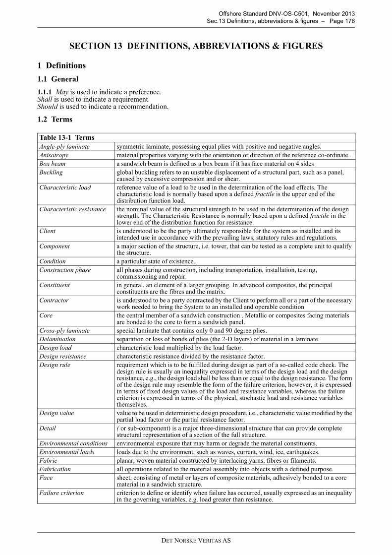
DET NORSKE VERITAS AS
Offshore Standard DNV-OS-C501, November 2013
Sec.13 Definitions, abbreviations & figures – Page 176
SECTION 13 DEFINITIONS, ABBREVIATIONS & FIGURES
1 Definitions
1.1 General
1.1.1 May is used to indicate a preference.Shall is used to indicate a requirementShould is used to indicate a recommendation.
1.2 Terms
Table 13-1 Terms
Angle-ply laminate symmetric laminate, possessing equal plies with positive and negative angles.
Anisotropy material properties varying with the orientation or direction of the reference co-ordinate.
Box beam a sandwich beam is defined as a box beam if it has face material on 4 sides
Buckling global buckling refers to an unstable displacement of a structural part, such as a panel, caused by excessive compression and or shear.
Characteristic load reference value of a load to be used in the determination of the load effects. The characteristic load is normally based upon a defined fractile is the upper end of the distribution function load.
Characteristic resistance the nominal value of the structural strength to be used in the determination of the design strength. The Characteristic Resistance is normally based upon a defined fractile in the lower end of the distribution function for resistance.
Client is understood to be the party ultimately responsible for the system as installed and its intended use in accordance with the prevailing laws, statutory rules and regulations.
Component a major section of the structure, i.e. tower, that can be tested as a complete unit to qualify the structure.
Condition a particular state of existence.
Construction phase all phases during construction, including transportation, installation, testing, commissioning and repair.
Constituent in general, an element of a larger grouping. In advanced composites, the principal constituents are the fibres and the matrix.
Contractor is understood to be a party contracted by the Client to perform all or a part of the necessary work needed to bring the System to an installed and operable condition
Core the central member of a sandwich construction . Metallic or composites facing materials are bonded to the core to form a sandwich panel.
Cross-ply laminate special laminate that contains only 0 and 90 degree plies.
Delamination separation or loss of bonds of plies (the 2-D layers) of material in a laminate.
Design load characteristic load multiplied by the load factor.
Design resistance characteristic resistance divided by the resistance factor.
Design rule requirement which is to be fulfilled during design as part of a so-called code check. The design rule is usually an inequality expressed in terms of the design load and the design resistance, e.g., the design load shall be less than or equal to the design resistance. The form of the design rule may resemble the form of the failure criterion, however, it is expressed in terms of fixed design values of the load and resistance variables, whereas the failure criterion is expressed in terms of the physical, stochastic load and resistance variables themselves.
Design value value to be used in deterministic design procedure, i.e., characteristic value modified by the partial load factor or the partial resistance factor.
Detail ( or sub-component) is a major three-dimensional structure that can provide complete structural representation of a section of the full structure.
Environmental conditions environmental exposure that may harm or degrade the material constituents.
Environmental loads loads due to the environment, such as waves, current, wind, ice, earthquakes.
Fabric planar, woven material constructed by interlacing yarns, fibres or filaments.
Fabrication all operations related to the material assembly into objects with a defined purpose.
Face sheet, consisting of metal or layers of composite materials, adhesively bonded to a core material in a sandwich structure.
Failure criterion criterion to define or identify when failure has occurred, usually expressed as an inequality in the governing variables, e.g. load greater than resistance.
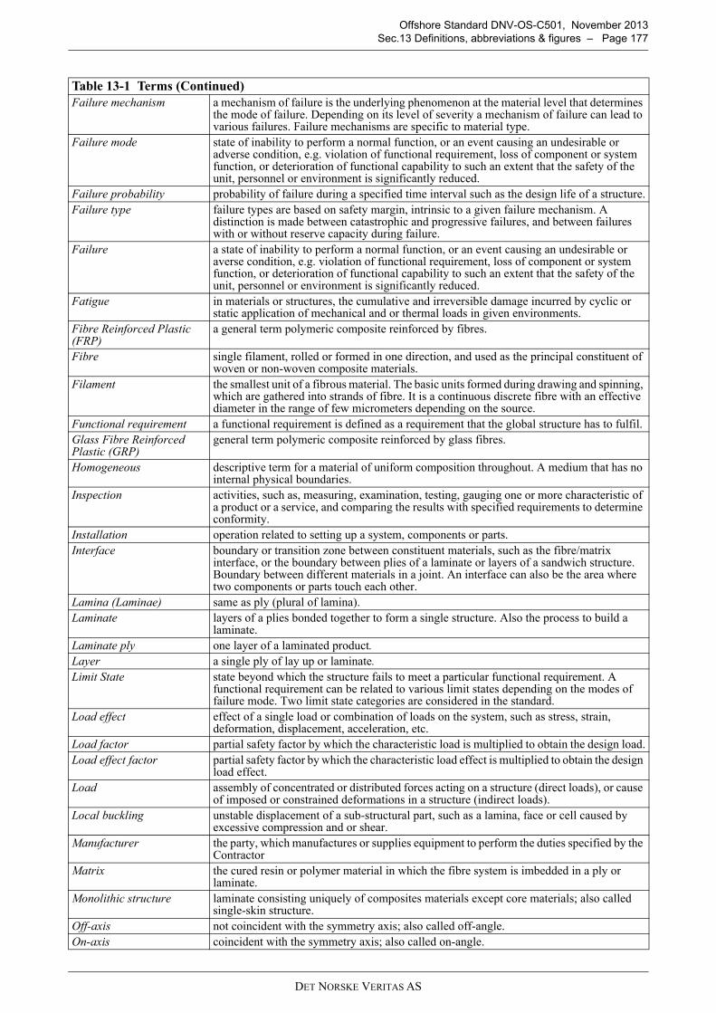
DET NORSKE VERITAS AS
Offshore Standard DNV-OS-C501, November 2013
Sec.13 Definitions, abbreviations & figures – Page 177
Failure mechanism a mechanism of failure is the underlying phenomenon at the material level that determines the mode of failure. Depending on its level of severity a mechanism of failure can lead to various failures. Failure mechanisms are specific to material type.
Failure mode state of inability to perform a normal function, or an event causing an undesirable or adverse condition, e.g. violation of functional requirement, loss of component or system function, or deterioration of functional capability to such an extent that the safety of the unit, personnel or environment is significantly reduced.
Failure probability probability of failure during a specified time interval such as the design life of a structure.
Failure type failure types are based on safety margin, intrinsic to a given failure mechanism. A distinction is made between catastrophic and progressive failures, and between failures with or without reserve capacity during failure.
Failure a state of inability to perform a normal function, or an event causing an undesirable or averse condition, e.g. violation of functional requirement, loss of component or system function, or deterioration of functional capability to such an extent that the safety of the unit, personnel or environment is significantly reduced.
Fatigue in materials or structures, the cumulative and irreversible damage incurred by cyclic or static application of mechanical and or thermal loads in given environments.
Fibre Reinforced Plastic (FRP)
a general term polymeric composite reinforced by fibres.
Fibre single filament, rolled or formed in one direction, and used as the principal constituent of woven or non-woven composite materials.
Filament the smallest unit of a fibrous material. The basic units formed during drawing and spinning, which are gathered into strands of fibre. It is a continuous discrete fibre with an effective diameter in the range of few micrometers depending on the source.
Functional requirement a functional requirement is defined as a requirement that the global structure has to fulfil.
Glass Fibre Reinforced Plastic (GRP)
general term polymeric composite reinforced by glass fibres.
Homogeneous descriptive term for a material of uniform composition throughout. A medium that has no internal physical boundaries.
Inspection activities, such as, measuring, examination, testing, gauging one or more characteristic of a product or a service, and comparing the results with specified requirements to determine conformity.
Installation operation related to setting up a system, components or parts.
Interface boundary or transition zone between constituent materials, such as the fibre/matrix interface, or the boundary between plies of a laminate or layers of a sandwich structure. Boundary between different materials in a joint. An interface can also be the area where two components or parts touch each other.
Lamina (Laminae) same as ply (plural of lamina).
Laminate layers of a plies bonded together to form a single structure. Also the process to build a laminate.
Laminate ply one layer of a laminated product.
Layer a single ply of lay up or laminate.
Limit State state beyond which the structure fails to meet a particular functional requirement. A functional requirement can be related to various limit states depending on the modes of failure mode. Two limit state categories are considered in the standard.
Load effect effect of a single load or combination of loads on the system, such as stress, strain, deformation, displacement, acceleration, etc.
Load factor partial safety factor by which the characteristic load is multiplied to obtain the design load.
Load effect factor partial safety factor by which the characteristic load effect is multiplied to obtain the design load effect.
Load assembly of concentrated or distributed forces acting on a structure (direct loads), or cause of imposed or constrained deformations in a structure (indirect loads).
Local buckling unstable displacement of a sub-structural part, such as a lamina, face or cell caused byexcessive compression and or shear.
Manufacturer the party, which manufactures or supplies equipment to perform the duties specified by the Contractor
Matrix the cured resin or polymer material in which the fibre system is imbedded in a ply or laminate.
Monolithic structure laminate consisting uniquely of composites materials except core materials; also calledsingle-skin structure.
Off-axis not coincident with the symmetry axis; also called off-angle.
On-axis coincident with the symmetry axis; also called on-angle.
Table 13-1 Terms (Continued)
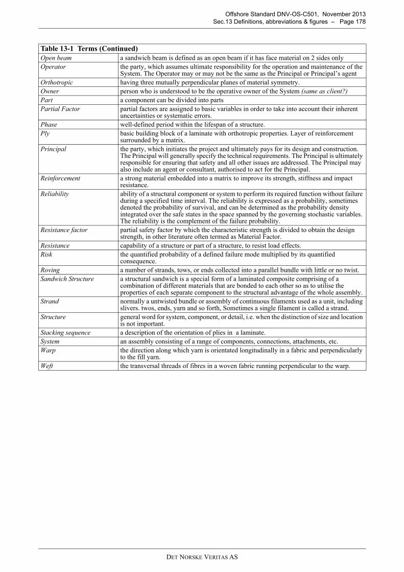
DET NORSKE VERITAS AS
Offshore Standard DNV-OS-C501, November 2013
Sec.13 Definitions, abbreviations & figures – Page 178
Open beam a sandwich beam is defined as an open beam if it has face material on 2 sides only
Operator the party, which assumes ultimate responsibility for the operation and maintenance of the System. The Operator may or may not be the same as the Principal or Principal’s agent
Orthotropic having three mutually perpendicular planes of material symmetry.
Owner person who is understood to be the operative owner of the System (same as client?)
Part a component can be divided into parts
Partial Factor partial factors are assigned to basic variables in order to take into account their inherent uncertainties or systematic errors.
Phase well-defined period within the lifespan of a structure.
Ply basic building block of a laminate with orthotropic properties. Layer of reinforcement surrounded by a matrix.
Principal the party, which initiates the project and ultimately pays for its design and construction. The Principal will generally specify the technical requirements. The Principal is ultimately responsible for ensuring that safety and all other issues are addressed. The Principal may also include an agent or consultant, authorised to act for the Principal.
Reinforcement a strong material embedded into a matrix to improve its strength, stiffness and impact resistance.
Reliability ability of a structural component or system to perform its required function without failure during a specified time interval. The reliability is expressed as a probability, sometimes denoted the probability of survival, and can be determined as the probability density integrated over the safe states in the space spanned by the governing stochastic variables. The reliability is the complement of the failure probability.
Resistance factor partial safety factor by which the characteristic strength is divided to obtain the design strength, in other literature often termed as Material Factor.
Resistance capability of a structure or part of a structure, to resist load effects.
Risk the quantified probability of a defined failure mode multiplied by its quantified consequence.
Roving a number of strands, tows, or ends collected into a parallel bundle with little or no twist.
Sandwich Structure a structural sandwich is a special form of a laminated composite comprising of a combination of different materials that are bonded to each other so as to utilise the properties of each separate component to the structural advantage of the whole assembly.
Strand normally a untwisted bundle or assembly of continuous filaments used as a unit, including slivers. twos, ends, yarn and so forth, Sometimes a single filament is called a strand.
Structure general word for system, component, or detail, i.e. when the distinction of size and location is not important.
Stacking sequence a description of the orientation of plies in a laminate.
System an assembly consisting of a range of components, connections, attachments, etc.
Warp the direction along which yarn is orientated longitudinally in a fabric and perpendicularly to the fill yarn.
Weft the transversal threads of fibres in a woven fabric running perpendicular to the warp.
Table 13-1 Terms (Continued)
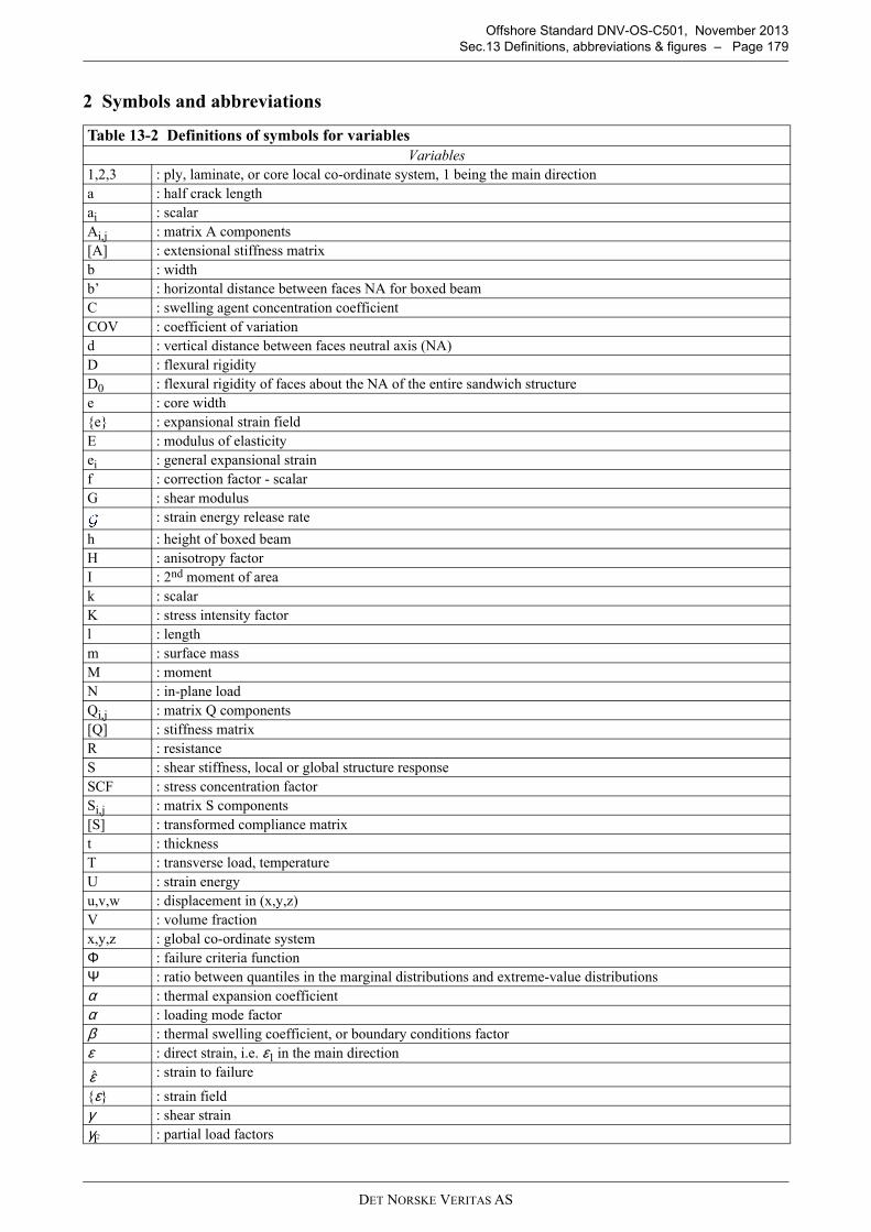
DET NORSKE VERITAS AS
Offshore Standard DNV-OS-C501, November 2013
Sec.13 Definitions, abbreviations & figures – Page 179
2 Symbols and abbreviations
Table 13-2 Definitions of symbols for variables
Variables
1,2,3 : ply, laminate, or core local co-ordinate system, 1 being the main direction
a : half crack length
ai : scalar
Ai,j : matrix A components
[A] : extensional stiffness matrix
b : width
b’ : horizontal distance between faces NA for boxed beam
C : swelling agent concentration coefficient
COV : coefficient of variation
d : vertical distance between faces neutral axis (NA)
D : flexural rigidity
D0 : flexural rigidity of faces about the NA of the entire sandwich structure
e : core width
{e} : expansional strain field
E : modulus of elasticity
ei : general expansional strain
f : correction factor - scalar
G : shear modulus
: strain energy release rate
h : height of boxed beam
H : anisotropy factor
I : 2nd moment of area
k : scalar
K : stress intensity factor
l : length
m : surface mass
M : moment
N : in-plane load
Qi,j : matrix Q components
[Q] : stiffness matrix
R : resistance
S : shear stiffness, local or global structure response
SCF : stress concentration factor
Si,j : matrix S components
[S] : transformed compliance matrix
t : thickness
T : transverse load, temperature
U : strain energy
u,v,w : displacement in (x,y,z)
V : volume fraction
x,y,z : global co-ordinate system
Φ : failure criteria function
Ψ : ratio between quantiles in the marginal distributions and extreme-value distributions
α : thermal expansion coefficient
α : loading mode factor
β : thermal swelling coefficient, or boundary conditions factor
ε : direct strain, i.e. ε1 in the main direction
: strain to failure
{ε} : strain field
γ : shear strain
γF : partial load factors
ε
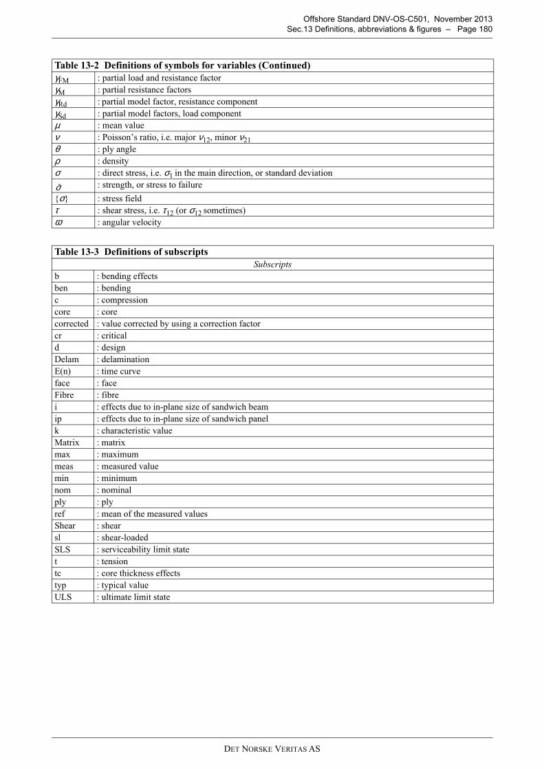
DET NORSKE VERITAS AS
Offshore Standard DNV-OS-C501, November 2013
Sec.13 Definitions, abbreviations & figures – Page 180
γFM : partial load and resistance factor
γM : partial resistance factors
γRd : partial model factor, resistance component
γSd : partial model factors, load component
µ : mean value
ν : Poisson’s ratio, i.e. major ν12, minor ν21
θ : ply angle
ρ : density
σ : direct stress, i.e. σ1 in the main direction, or standard deviation
: strength, or stress to failure
{σ} : stress field
τ : shear stress, i.e. τ12 (or σ12 sometimes)
ω : angular velocity
Table 13-3 Definitions of subscripts
Subscripts
b : bending effects
ben : bending
c : compression
core : core
corrected : value corrected by using a correction factor
cr : critical
d : design
Delam : delamination
E(n) : time curve
face : face
Fibre : fibre
i : effects due to in-plane size of sandwich beam
ip : effects due to in-plane size of sandwich panel
k : characteristic value
Matrix : matrix
max : maximum
meas : measured value
min : minimum
nom : nominal
ply : ply
ref : mean of the measured values
Shear : shear
sl : shear-loaded
SLS : serviceability limit state
t : tension
tc : core thickness effects
typ : typical value
ULS : ultimate limit state
Table 13-2 Definitions of symbols for variables (Continued)
σ
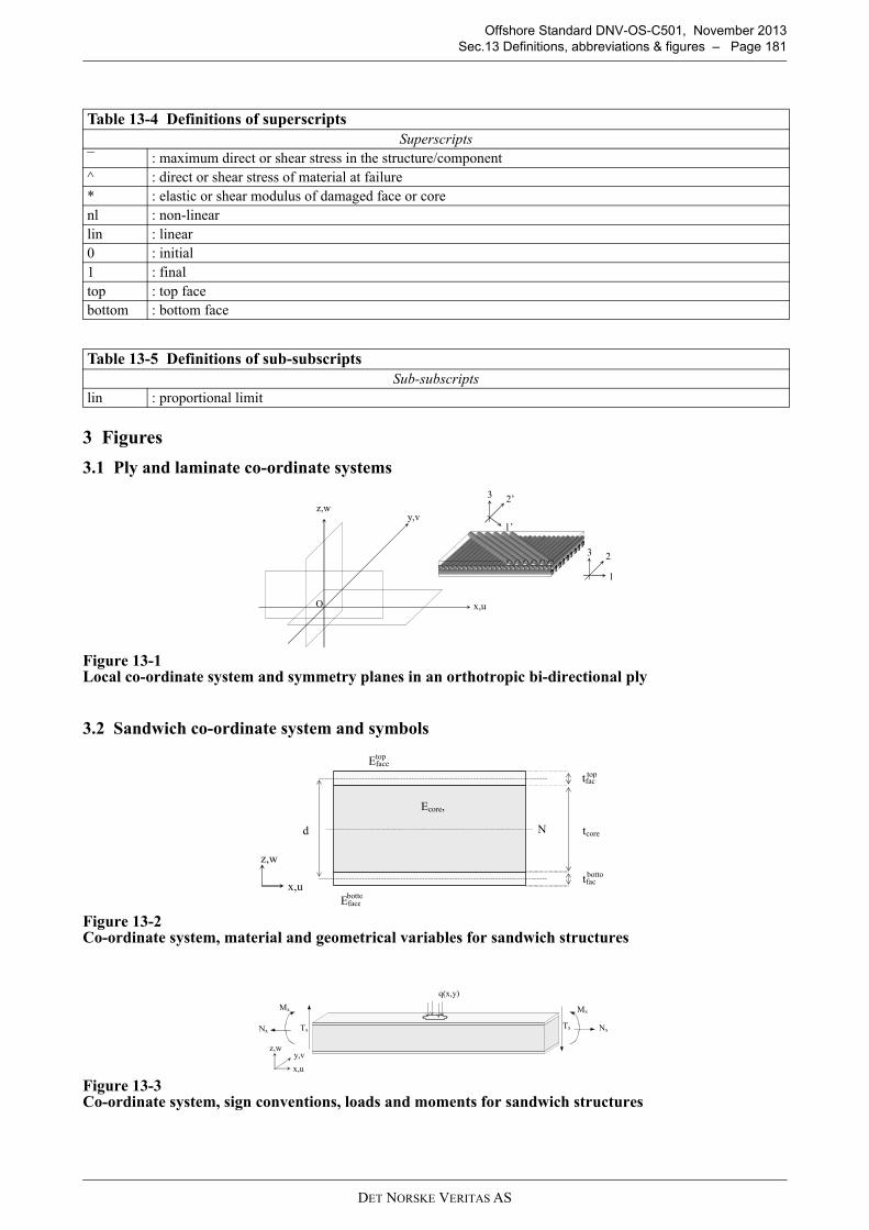
DET NORSKE VERITAS AS
Offshore Standard DNV-OS-C501, November 2013
Sec.13 Definitions, abbreviations & figures – Page 181
3 Figures
3.1 Ply and laminate co-ordinate systems
Figure 13-1 Local co-ordinate system and symmetry planes in an orthotropic bi-directional ply
3.2 Sandwich co-ordinate system and symbols
Figure 13-2 Co-ordinate system, material and geometrical variables for sandwich structures
Figure 13-3 Co-ordinate system, sign conventions, loads and moments for sandwich structures
Table 13-4 Definitions of superscripts
Superscripts
¯ : maximum direct or shear stress in the structure/component
^ : direct or shear stress of material at failure
* : elastic or shear modulus of damaged face or core
nl : non-linear
lin : linear
0 : initial
1 : final
top : top face
bottom : bottom face
Table 13-5 Definitions of sub-subscripts
Sub-subscripts
lin : proportional limit
y,v z,w
x,u O
2 3
1’
2’ 3’
1
x,u
z,w
tfac
Ecore, G
tcore
tfac
d
Eface
Eface
NA
top
botto
top
botto
q(x,y)
Tx
Mx
x,u
z,w
Nx Tx
Mx
Nx
y,v
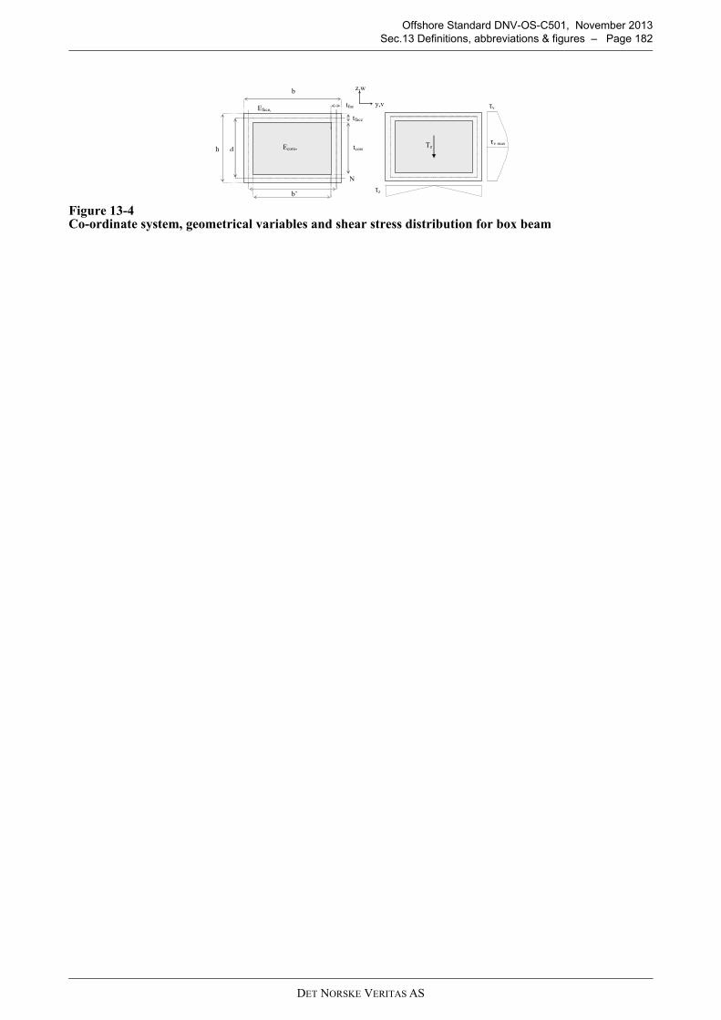
DET NORSKE VERITAS AS
Offshore Standard DNV-OS-C501, November 2013
Sec.13 Definitions, abbreviations & figures – Page 182
Figure 13-4 Co-ordinate system, geometrical variables and shear stress distribution for box beam
y,v
z,w
tface
Ecore, G
tfac
tcore
Eface,
G
NA
b’
Tz
τy
τz
τy max
b
d h
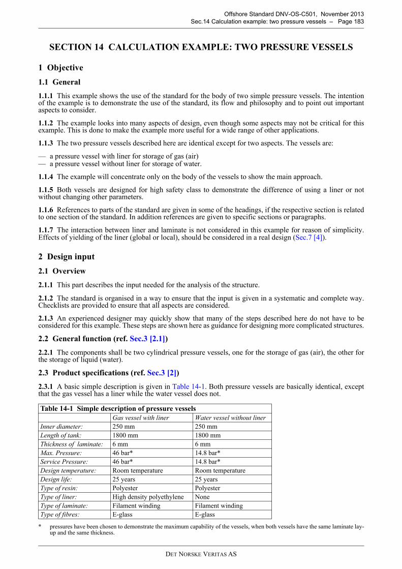
DET NORSKE VERITAS AS
Offshore Standard DNV-OS-C501, November 2013
Sec.14 Calculation example: two pressure vessels – Page 183
SECTION 14 CALCULATION EXAMPLE: TWO PRESSURE VESSELS
1 Objective
1.1 General
1.1.1 This example shows the use of the standard for the body of two simple pressure vessels. The intentionof the example is to demonstrate the use of the standard, its flow and philosophy and to point out importantaspects to consider.
1.1.2 The example looks into many aspects of design, even though some aspects may not be critical for thisexample. This is done to make the example more useful for a wide range of other applications.
1.1.3 The two pressure vessels described here are identical except for two aspects. The vessels are:
— a pressure vessel with liner for storage of gas (air)— a pressure vessel without liner for storage of water.
1.1.4 The example will concentrate only on the body of the vessels to show the main approach.
1.1.5 Both vessels are designed for high safety class to demonstrate the difference of using a liner or notwithout changing other parameters.
1.1.6 References to parts of the standard are given in some of the headings, if the respective section is relatedto one section of the standard. In addition references are given to specific sections or paragraphs.
1.1.7 The interaction between liner and laminate is not considered in this example for reason of simplicity.Effects of yielding of the liner (global or local), should be considered in a real design (Sec.7 [4]).
2 Design input
2.1 Overview
2.1.1 This part describes the input needed for the analysis of the structure.
2.1.2 The standard is organised in a way to ensure that the input is given in a systematic and complete way.Checklists are provided to ensure that all aspects are considered.
2.1.3 An experienced designer may quickly show that many of the steps described here do not have to beconsidered for this example. These steps are shown here as guidance for designing more complicated structures.
2.2 General function (ref. Sec.3 [2.1])
2.2.1 The components shall be two cylindrical pressure vessels, one for the storage of gas (air), the other forthe storage of liquid (water).
2.3 Product specifications (ref. Sec.3 [2])
2.3.1 A basic simple description is given in Table 14-1. Both pressure vessels are basically identical, exceptthat the gas vessel has a liner while the water vessel does not.
* pressures have been chosen to demonstrate the maximum capability of the vessels, when both vessels have the same laminate lay-up and the same thickness.
Table 14-1 Simple description of pressure vessels
Gas vessel with liner Water vessel without liner
Inner diameter: 250 mm 250 mm
Length of tank: 1800 mm 1800 mm
Thickness of laminate: 6 mm 6 mm
Max. Pressure: 46 bar* 14.8 bar*
Service Pressure: 46 bar* 14.8 bar*
Design temperature: Room temperature Room temperature
Design life: 25 years 25 years
Type of resin: Polyester Polyester
Type of liner: High density polyethylene None
Type of laminate: Filament winding Filament winding
Type of fibres: E-glass E-glass
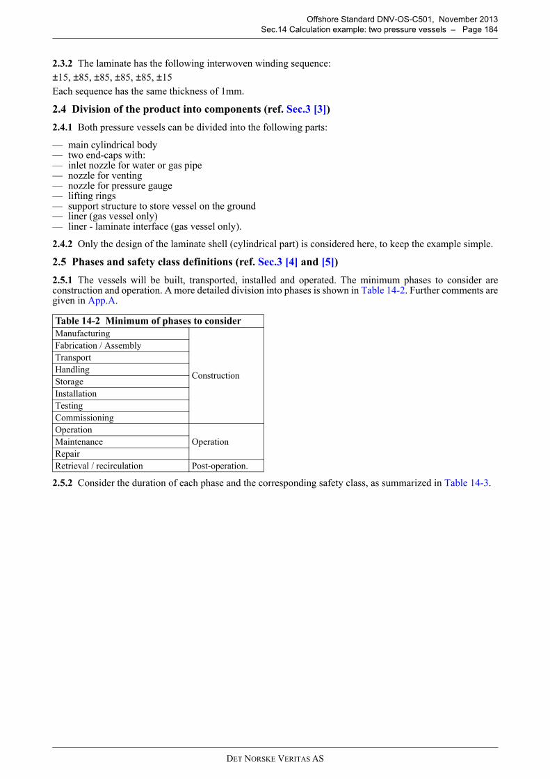
DET NORSKE VERITAS AS
Offshore Standard DNV-OS-C501, November 2013
Sec.14 Calculation example: two pressure vessels – Page 184
2.3.2 The laminate has the following interwoven winding sequence:
±15, ±85, ±85, ±85, ±85, ±15
Each sequence has the same thickness of 1mm.
2.4 Division of the product into components (ref. Sec.3 [3])
2.4.1 Both pressure vessels can be divided into the following parts:
— main cylindrical body— two end-caps with:— inlet nozzle for water or gas pipe— nozzle for venting— nozzle for pressure gauge— lifting rings— support structure to store vessel on the ground— liner (gas vessel only)— liner - laminate interface (gas vessel only).
2.4.2 Only the design of the laminate shell (cylindrical part) is considered here, to keep the example simple.
2.5 Phases and safety class definitions (ref. Sec.3 [4] and [5])
2.5.1 The vessels will be built, transported, installed and operated. The minimum phases to consider areconstruction and operation. A more detailed division into phases is shown in Table 14-2. Further comments aregiven in App.A.
2.5.2 Consider the duration of each phase and the corresponding safety class, as summarized in Table 14-3.
Table 14-2 Minimum of phases to consider
Manufacturing
Construction
Fabrication / Assembly
Transport
Handling
Storage
Installation
Testing
Commissioning
Operation
OperationMaintenance
Repair
Retrieval / recirculation Post-operation.
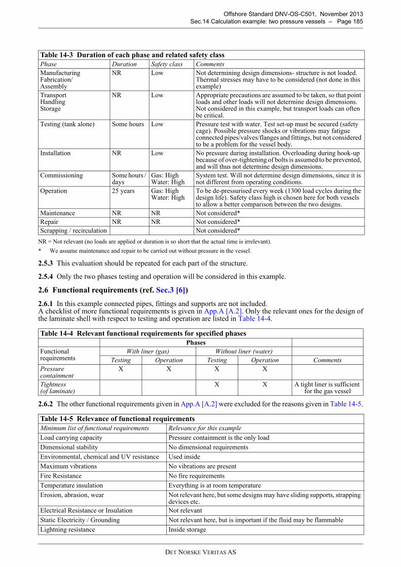
DET NORSKE VERITAS AS
Offshore Standard DNV-OS-C501, November 2013
Sec.14 Calculation example: two pressure vessels – Page 185
NR = Not relevant (no loads are applied or duration is so short that the actual time is irrelevant).
* We assume maintenance and repair to be carried out without pressure in the vessel.
2.5.3 This evaluation should be repeated for each part of the structure.
2.5.4 Only the two phases testing and operation will be considered in this example.
2.6 Functional requirements (ref. Sec.3 [6])
2.6.1 In this example connected pipes, fittings and supports are not included. A checklist of more functional requirements is given in App.A [A.2]. Only the relevant ones for the design ofthe laminate shell with respect to testing and operation are listed in Table 14-4.
2.6.2 The other functional requirements given in App.A [A.2] were excluded for the reasons given in Table 14-5.
Table 14-3 Duration of each phase and related safety class
Phase Duration Safety class Comments
ManufacturingFabrication/Assembly
NR Low Not determining design dimensions- structure is not loaded. Thermal stresses may have to be considered (not done in this example)
TransportHandlingStorage
NR Low Appropriate precautions are assumed to be taken, so that point loads and other loads will not determine design dimensions. Not considered in this example, but transport loads can often be critical.
Testing (tank alone) Some hours Low Pressure test with water. Test set-up must be secured (safety cage). Possible pressure shocks or vibrations may fatigue connected pipes/valves/flanges and fittings, but not considered to be a problem for the vessel body.
Installation NR Low No pressure during installation. Overloading during hook-up because of over-tightening of bolts is assumed to be prevented, and will thus not determine design dimensions.
Commissioning Some hours / days
Gas: HighWater: High
System test. Will not determine design dimensions, since it is not different from operating conditions.
Operation 25 years Gas: HighWater: High
To be de-pressurised every week (1300 load cycles during the design life). Safety class high is chosen here for both vessels to allow a better comparison between the two designs.
Maintenance NR NR Not considered*
Repair NR NR Not considered*
Scrapping / recirculation Not considered*
Table 14-4 Relevant functional requirements for specified phases
Phases
Functionalrequirements
With liner (gas) Without liner (water)
Testing Operation Testing Operation Comments
Pressure containment
X X X X
Tightness (of laminate)
X X A tight liner is sufficient for the gas vessel
Table 14-5 Relevance of functional requirements
Minimum list of functional requirements Relevance for this example
Load carrying capacity Pressure containment is the only load
Dimensional stability No dimensional requirements
Environmental, chemical and UV resistance Used inside
Maximum vibrations No vibrations are present
Fire Resistance No fire requirements
Temperature insulation Everything is at room temperature
Erosion, abrasion, wear Not relevant here, but some designs may have sliding supports, strapping devices etc.
Electrical Resistance or Insulation Not relevant
Static Electricity / Grounding Not relevant here, but is important if the fluid may be flammable
Lightning resistance Inside storage
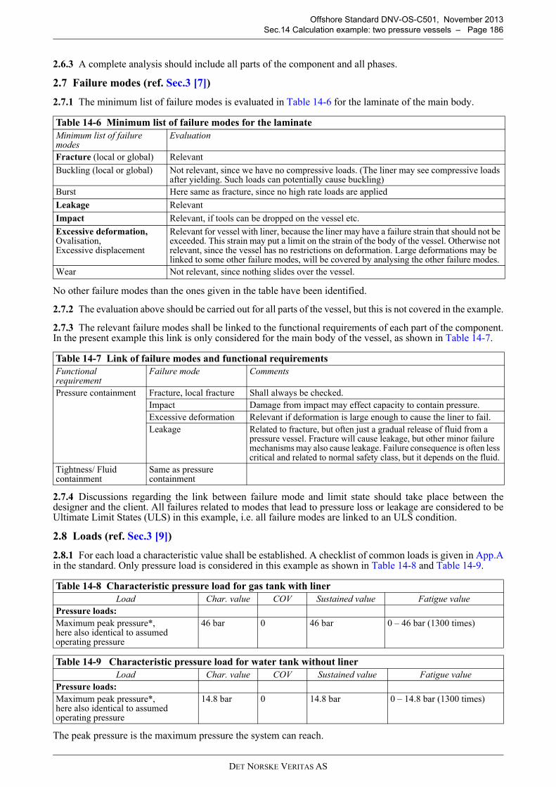
DET NORSKE VERITAS AS
Offshore Standard DNV-OS-C501, November 2013
Sec.14 Calculation example: two pressure vessels – Page 186
2.6.3 A complete analysis should include all parts of the component and all phases.
2.7 Failure modes (ref. Sec.3 [7])
2.7.1 The minimum list of failure modes is evaluated in Table 14-6 for the laminate of the main body.
No other failure modes than the ones given in the table have been identified.
2.7.2 The evaluation above should be carried out for all parts of the vessel, but this is not covered in the example.
2.7.3 The relevant failure modes shall be linked to the functional requirements of each part of the component.In the present example this link is only considered for the main body of the vessel, as shown in Table 14-7.
2.7.4 Discussions regarding the link between failure mode and limit state should take place between thedesigner and the client. All failures related to modes that lead to pressure loss or leakage are considered to beUltimate Limit States (ULS) in this example, i.e. all failure modes are linked to an ULS condition.
2.8 Loads (ref. Sec.3 [9])
2.8.1 For each load a characteristic value shall be established. A checklist of common loads is given in App.Ain the standard. Only pressure load is considered in this example as shown in Table 14-8 and Table 14-9.
The peak pressure is the maximum pressure the system can reach.
Table 14-6 Minimum list of failure modes for the laminate
Minimum list of failure modes
Evaluation
Fracture (local or global) Relevant
Buckling (local or global) Not relevant, since we have no compressive loads. (The liner may see compressive loads after yielding. Such loads can potentially cause buckling)
Burst Here same as fracture, since no high rate loads are applied
Leakage Relevant
Impact Relevant, if tools can be dropped on the vessel etc.
Excessive deformation,Ovalisation,Excessive displacement
Relevant for vessel with liner, because the liner may have a failure strain that should not be exceeded. This strain may put a limit on the strain of the body of the vessel. Otherwise not relevant, since the vessel has no restrictions on deformation. Large deformations may be linked to some other failure modes, will be covered by analysing the other failure modes.
Wear Not relevant, since nothing slides over the vessel.
Table 14-7 Link of failure modes and functional requirements
Functional requirement
Failure mode Comments
Pressure containment Fracture, local fracture Shall always be checked.
Impact Damage from impact may effect capacity to contain pressure.
Excessive deformation Relevant if deformation is large enough to cause the liner to fail.
Leakage Related to fracture, but often just a gradual release of fluid from a pressure vessel. Fracture will cause leakage, but other minor failure mechanisms may also cause leakage. Failure consequence is often less critical and related to normal safety class, but it depends on the fluid.
Tightness/ Fluid containment
Same as pressure containment
Table 14-8 Characteristic pressure load for gas tank with liner
Load Char. value COV Sustained value Fatigue value
Pressure loads:
Maximum peak pressure*,here also identical to assumed operating pressure
46 bar 0 46 bar 0 – 46 bar (1300 times)
Table 14-9 Characteristic pressure load for water tank without liner
Load Char. value COV Sustained value Fatigue value
Pressure loads:
Maximum peak pressure*,here also identical to assumed operating pressure
14.8 bar 0 14.8 bar 0 – 14.8 bar (1300 times)
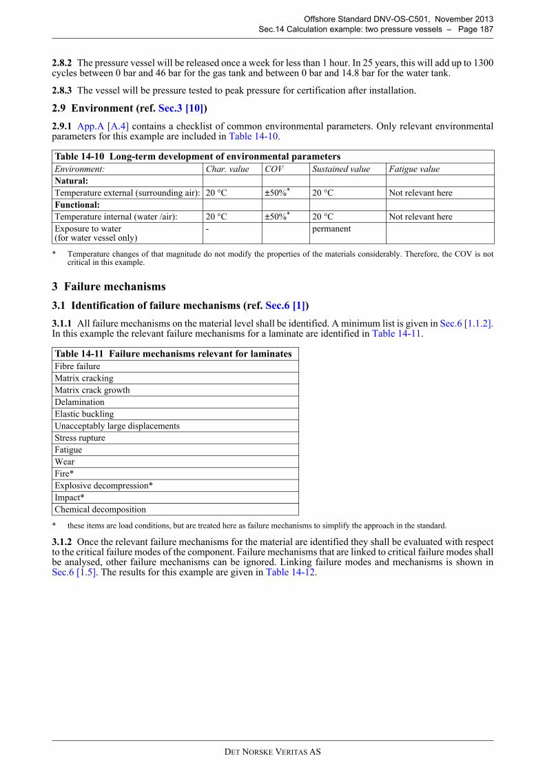
DET NORSKE VERITAS AS
Offshore Standard DNV-OS-C501, November 2013
Sec.14 Calculation example: two pressure vessels – Page 187
2.8.2 The pressure vessel will be released once a week for less than 1 hour. In 25 years, this will add up to 1300cycles between 0 bar and 46 bar for the gas tank and between 0 bar and 14.8 bar for the water tank.
2.8.3 The vessel will be pressure tested to peak pressure for certification after installation.
2.9 Environment (ref. Sec.3 [10])
2.9.1 App.A [A.4] contains a checklist of common environmental parameters. Only relevant environmentalparameters for this example are included in Table 14-10.
* Temperature changes of that magnitude do not modify the properties of the materials considerably. Therefore, the COV is notcritical in this example.
3 Failure mechanisms
3.1 Identification of failure mechanisms (ref. Sec.6 [1])
3.1.1 All failure mechanisms on the material level shall be identified. A minimum list is given in Sec.6 [1.1.2].In this example the relevant failure mechanisms for a laminate are identified in Table 14-11.
* these items are load conditions, but are treated here as failure mechanisms to simplify the approach in the standard.
3.1.2 Once the relevant failure mechanisms for the material are identified they shall be evaluated with respectto the critical failure modes of the component. Failure mechanisms that are linked to critical failure modes shallbe analysed, other failure mechanisms can be ignored. Linking failure modes and mechanisms is shown inSec.6 [1.5]. The results for this example are given in Table 14-12.
Table 14-10 Long-term development of environmental parameters
Environment: Char. value COV Sustained value Fatigue value
Natural:
Temperature external (surrounding air): 20 °C ±50%* 20 °C Not relevant here
Functional:
Temperature internal (water /air): 20 °C ±50%* 20 °C Not relevant here
Exposure to water (for water vessel only)
- permanent
Table 14-11 Failure mechanisms relevant for laminates
Fibre failure
Matrix cracking
Matrix crack growth
Delamination
Elastic buckling
Unacceptably large displacements
Stress rupture
Fatigue
Wear
Fire*
Explosive decompression*
Impact*
Chemical decomposition
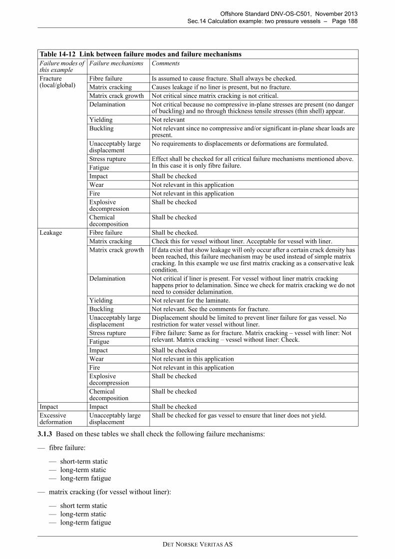
DET NORSKE VERITAS AS
Offshore Standard DNV-OS-C501, November 2013
Sec.14 Calculation example: two pressure vessels – Page 188
3.1.3 Based on these tables we shall check the following failure mechanisms:
— fibre failure:
— short-term static— long-term static— long-term fatigue
— matrix cracking (for vessel without liner):
— short term static— long-term static— long-term fatigue
Table 14-12 Link between failure modes and failure mechanisms
Failure modes of this example
Failure mechanisms Comments
Fracture (local/global)
Fibre failure Is assumed to cause fracture. Shall always be checked.
Matrix cracking Causes leakage if no liner is present, but no fracture.
Matrix crack growth Not critical since matrix cracking is not critical.
Delamination Not critical because no compressive in-plane stresses are present (no danger of buckling) and no through thickness tensile stresses (thin shell) appear.
Yielding Not relevant
Buckling Not relevant since no compressive and/or significant in-plane shear loads are present.
Unacceptably large displacement
No requirements to displacements or deformations are formulated.
Stress rupture Effect shall be checked for all critical failure mechanisms mentioned above. In this case it is only fibre failure.Fatigue
Impact Shall be checked
Wear Not relevant in this application
Fire Not relevant in this application
Explosive decompression
Shall be checked
Chemical decomposition
Shall be checked
Leakage Fibre failure Shall be checked.
Matrix cracking Check this for vessel without liner. Acceptable for vessel with liner.
Matrix crack growth If data exist that show leakage will only occur after a certain crack density has been reached, this failure mechanism may be used instead of simple matrix cracking. In this example we use first matrix cracking as a conservative leak condition.
Delamination Not critical if liner is present. For vessel without liner matrix cracking happens prior to delamination. Since we check for matrix cracking we do not need to consider delamination.
Yielding Not relevant for the laminate.
Buckling Not relevant. See the comments for fracture.
Unacceptably large displacement
Displacement should be limited to prevent liner failure for gas vessel. No restriction for water vessel without liner.
Stress rupture Fibre failure: Same as for fracture. Matrix cracking – vessel with liner: Not relevant. Matrix cracking – vessel without liner: Check.Fatigue
Impact Shall be checked
Wear Not relevant in this application
Fire Not relevant in this application
Explosive decompression
Shall be checked
Chemical decomposition
Shall be checked
Impact Impact Shall be checked
Excessive deformation
Unacceptably large displacement
Shall be checked for gas vessel to ensure that liner does not yield.
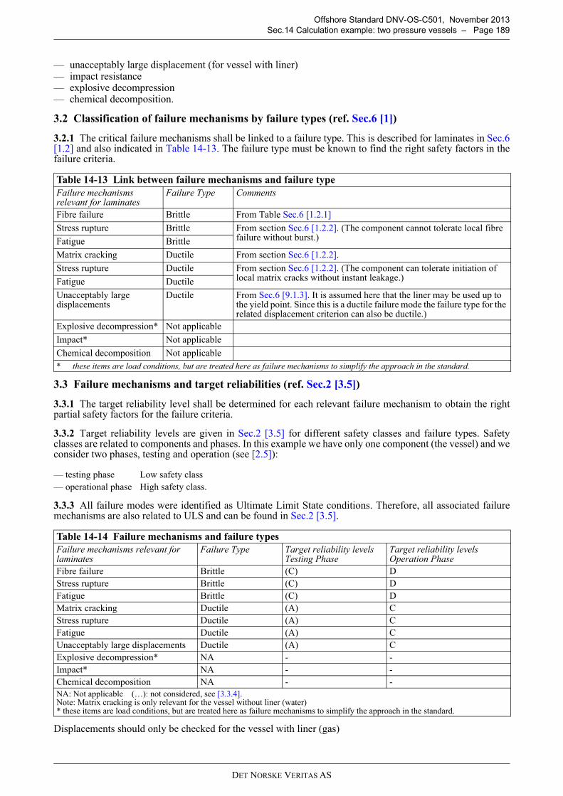
DET NORSKE VERITAS AS
Offshore Standard DNV-OS-C501, November 2013
Sec.14 Calculation example: two pressure vessels – Page 189
— unacceptably large displacement (for vessel with liner)— impact resistance— explosive decompression— chemical decomposition.
3.2 Classification of failure mechanisms by failure types (ref. Sec.6 [1])
3.2.1 The critical failure mechanisms shall be linked to a failure type. This is described for laminates in Sec.6[1.2] and also indicated in Table 14-13. The failure type must be known to find the right safety factors in thefailure criteria.
3.3 Failure mechanisms and target reliabilities (ref. Sec.2 [3.5])
3.3.1 The target reliability level shall be determined for each relevant failure mechanism to obtain the rightpartial safety factors for the failure criteria.
3.3.2 Target reliability levels are given in Sec.2 [3.5] for different safety classes and failure types. Safetyclasses are related to components and phases. In this example we have only one component (the vessel) and weconsider two phases, testing and operation (see [2.5]):
3.3.3 All failure modes were identified as Ultimate Limit State conditions. Therefore, all associated failuremechanisms are also related to ULS and can be found in Sec.2 [3.5].
Displacements should only be checked for the vessel with liner (gas)
Table 14-13 Link between failure mechanisms and failure type
Failure mechanisms relevant for laminates
Failure Type Comments
Fibre failure Brittle From Table Sec.6 [1.2.1]
Stress rupture Brittle From section Sec.6 [1.2.2]. (The component cannot tolerate local fibre failure without burst.)Fatigue Brittle
Matrix cracking Ductile From section Sec.6 [1.2.2].
Stress rupture Ductile From section Sec.6 [1.2.2]. (The component can tolerate initiation of local matrix cracks without instant leakage.)Fatigue Ductile
Unacceptably large displacements
Ductile From Sec.6 [9.1.3]. It is assumed here that the liner may be used up to the yield point. Since this is a ductile failure mode the failure type for the related displacement criterion can also be ductile.)
Explosive decompression* Not applicable
Impact* Not applicable
Chemical decomposition Not applicable
* these items are load conditions, but are treated here as failure mechanisms to simplify the approach in the standard.
— testing phase Low safety class
— operational phase High safety class.
Table 14-14 Failure mechanisms and failure types
Failure mechanisms relevant for laminates
Failure Type Target reliability levelsTesting Phase
Target reliability levels Operation Phase
Fibre failure Brittle (C) D
Stress rupture Brittle (C) D
Fatigue Brittle (C) D
Matrix cracking Ductile (A) C
Stress rupture Ductile (A) C
Fatigue Ductile (A) C
Unacceptably large displacements Ductile (A) C
Explosive decompression* NA - -
Impact* NA - -
Chemical decomposition NA - -
NA: Not applicable (…): not considered, see [3.3.4].Note: Matrix cracking is only relevant for the vessel without liner (water)* these items are load conditions, but are treated here as failure mechanisms to simplify the approach in the standard.
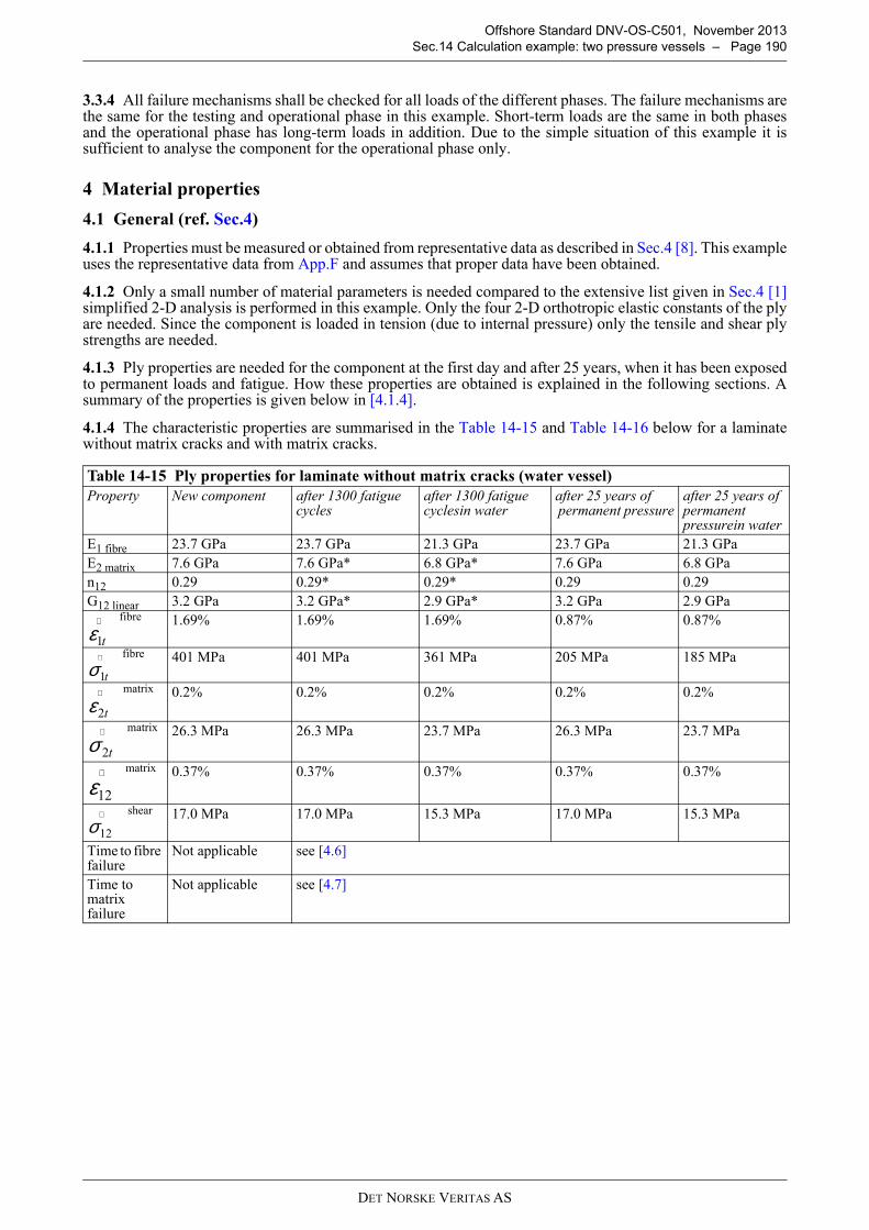
DET NORSKE VERITAS AS
Offshore Standard DNV-OS-C501, November 2013
Sec.14 Calculation example: two pressure vessels – Page 190
3.3.4 All failure mechanisms shall be checked for all loads of the different phases. The failure mechanisms arethe same for the testing and operational phase in this example. Short-term loads are the same in both phasesand the operational phase has long-term loads in addition. Due to the simple situation of this example it issufficient to analyse the component for the operational phase only.
4 Material properties
4.1 General (ref. Sec.4)
4.1.1 Properties must be measured or obtained from representative data as described in Sec.4 [8]. This exampleuses the representative data from App.F and assumes that proper data have been obtained.
4.1.2 Only a small number of material parameters is needed compared to the extensive list given in Sec.4 [1]simplified 2-D analysis is performed in this example. Only the four 2-D orthotropic elastic constants of the plyare needed. Since the component is loaded in tension (due to internal pressure) only the tensile and shear plystrengths are needed.
4.1.3 Ply properties are needed for the component at the first day and after 25 years, when it has been exposedto permanent loads and fatigue. How these properties are obtained is explained in the following sections. Asummary of the properties is given below in [4.1.4].
4.1.4 The characteristic properties are summarised in the Table 14-15 and Table 14-16 below for a laminatewithout matrix cracks and with matrix cracks.
Table 14-15 Ply properties for laminate without matrix cracks (water vessel)
Property New component after 1300 fatigue cycles
after 1300 fatigue cyclesin water
after 25 years of permanent pressure
after 25 years of permanent pressurein water
E1 fibre 23.7 GPa 23.7 GPa 21.3 GPa 23.7 GPa 21.3 GPa
E2 matrix 7.6 GPa 7.6 GPa* 6.8 GPa* 7.6 GPa 6.8 GPa
n12 0.29 0.29* 0.29* 0.29 0.29
G12 linear 3.2 GPa 3.2 GPa* 2.9 GPa* 3.2 GPa 2.9 GPafibre 1.69% 1.69% 1.69% 0.87% 0.87%
fibre 401 MPa 401 MPa 361 MPa 205 MPa 185 MPa
matrix 0.2% 0.2% 0.2% 0.2% 0.2%
matrix 26.3 MPa 26.3 MPa 23.7 MPa 26.3 MPa 23.7 MPa
matrix 0.37% 0.37% 0.37% 0.37% 0.37%
shear 17.0 MPa 17.0 MPa 15.3 MPa 17.0 MPa 15.3 MPa
Time to fibre failure
Not applicable see [4.6]
Time to matrix failure
Not applicable see [4.7]
t1ε∧
t1σ∧
t2ε∧
t2σ∧
12ε∧
12σ∧
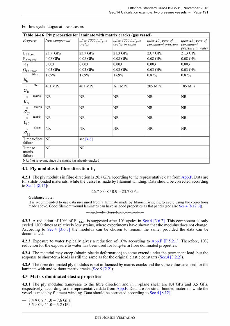
DET NORSKE VERITAS AS
Offshore Standard DNV-OS-C501, November 2013
Sec.14 Calculation example: two pressure vessels – Page 191
For low cycle fatigue at low stresses
4.2 Ply modulus in fibre direction E1
4.2.1 The ply modulus in fibre direction is 26.7 GPa according to the representative data from App.F. Data arefor stitch-bonded materials, while the vessel is made by filament winding. Data should be corrected accordingto Sec.4 [8.12]:
26.7 × 0.8 / 0.9 = 23.7 GPa.
Guidance note:
It is recommended to use data measured from a laminate made by filament winding to avoid using the correctionsmade above. Good filament wound laminates can have as good properties as flat panels (see also Sec.4 [8.12.6]).
---e-n-d---of---G-u-i-d-a-n-c-e---n-o-t-e---
4.2.2 A reduction of 10% of E1 fibre is suggested after 106 cycles in Sec.4 [3.6.2]. This component is onlycycled 1300 times at relatively low strains, where experiments have shown that the modulus does not change.According to Sec.4 [3.6.3] the modulus can be chosen to remain the same, provided the data can bedocumented.
4.2.3 Exposure to water typically gives a reduction of 10% according to App.F [F.5.2.1]. Therefore, 10%reduction for the exposure to water has been used for long-term fibre dominated properties.
4.2.4 The material may creep (obtain plastic deformation) to some extend under the permanent load, but theresponse to short-term loads is still the same as for the original elastic constants (Sec.4 [3.2.2]).
4.2.5 The fibre dominated ply modulus is not influenced by matrix cracks and the same values are used for thelaminate with and without matrix cracks (Sec.9 [2.2]).
4.3 Matrix dominated elastic properties
4.3.1 The ply modulus transverse to the fibre direction and in in-plane shear are 8.4 GPa and 3.5 GPa,respectively, according to the representative data from App.F. Data are for stitch-bonded materials while thevessel is made by filament winding. Data should be corrected according to Sec.4 [8.12]:
— 8.4 × 0.9 / 1.0 = 7.6 GPa— 3.5 × 0.9 / 1.0 = 3.2 GPa.
Table 14-16 Ply properties for laminate with matrix cracks (gas vessel)
Property New component after 3000 fatigue cycles
after 3000 fatigue cycles in water
after 25 years of permanent pressure
after 25 years of permanent pressure in water
E1 fibre 23.7 GPa 23.7 GPa 21.3 GPa 23.7 GPa 21.3 GPa
E2 matrix 0.08 GPa 0.08 GPa 0.08 GPa 0.08 GPa 0.08 GPa
ν12 0.003 0.003 0.003 0.003 0.003
G12 linear 0.03 GPa 0.03 GPa 0.03 GPa 0.03 GPa 0.03 GPafibre 1.69% 1.69% 1.69% 0.87% 0.87%
fibre 401 MPa 401 MPa 361 MPa 205 MPa 185 MPa
matrix NR NR NR NR NR
matrix NR NR NR NR NR
matrix NR NR NR NR NR
shear NR NR NR NR NR
Time to fibre failure
NR see [4.6]
Time to matrix failure
NR NR
NR: Not relevant, since the matrix has already cracked
t1ε∧
t1σ∧
t2ε∧
t2σ∧
12ε∧
12σ∧
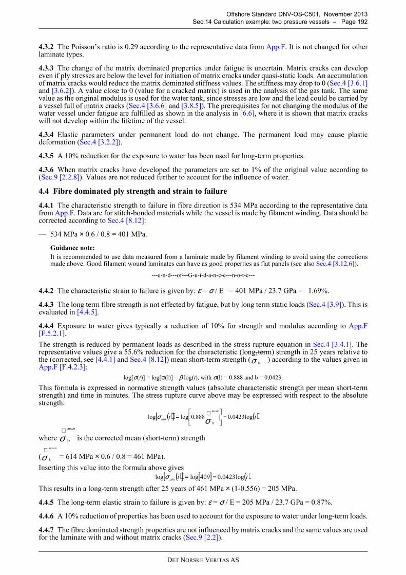
DET NORSKE VERITAS AS
Offshore Standard DNV-OS-C501, November 2013
Sec.14 Calculation example: two pressure vessels – Page 192
4.3.2 The Poisson’s ratio is 0.29 according to the representative data from App.F. It is not changed for otherlaminate types.
4.3.3 The change of the matrix dominated properties under fatigue is uncertain. Matrix cracks can developeven if ply stresses are below the level for initiation of matrix cracks under quasi-static loads. An accumulationof matrix cracks would reduce the matrix dominated stiffness values. The stiffness may drop to 0 (Sec.4 [3.6.1]and [3.6.2]). A value close to 0 (value for a cracked matrix) is used in the analysis of the gas tank. The samevalue as the original modulus is used for the water tank, since stresses are low and the load could be carried bya vessel full of matrix cracks (Sec.4 [3.6.6] and [3.8.5]). The prerequisites for not changing the modulus of thewater vessel under fatigue are fulfilled as shown in the analysis in [6.6], where it is shown that matrix crackswill not develop within the lifetime of the vessel.
4.3.4 Elastic parameters under permanent load do not change. The permanent load may cause plasticdeformation (Sec.4 [3.2.2]).
4.3.5 A 10% reduction for the exposure to water has been used for long-term properties.
4.3.6 When matrix cracks have developed the parameters are set to 1% of the original value according to(Sec.9 [2.2.8]). Values are not reduced further to account for the influence of water.
4.4 Fibre dominated ply strength and strain to failure
4.4.1 The characteristic strength to failure in fibre direction is 534 MPa according to the representative datafrom App.F. Data are for stitch-bonded materials while the vessel is made by filament winding. Data should becorrected according to Sec.4 [8.12]:
— 534 MPa × 0.6 / 0.8 = 401 MPa.
Guidance note:
It is recommended to use data measured from a laminate made by filament winding to avoid using the correctionsmade above. Good filament wound laminates can have as good properties as flat panels (see also Sec.4 [8.12.6]).
---e-n-d---of---G-u-i-d-a-n-c-e---n-o-t-e---
4.4.2 The characteristic strain to failure is given by: ε = σ / E = 401 MPa / 23.7 GPa = 1.69%.
4.4.3 The long term fibre strength is not effected by fatigue, but by long term static loads (Sec.4 [3.9]). This isevaluated in [4.4.5].
4.4.4 Exposure to water gives typically a reduction of 10% for strength and modulus according to App.F[F.5.2.1].
The strength is reduced by permanent loads as described in the stress rupture equation in Sec.4 [3.4.1]. Therepresentative values give a 55.6% reduction for the characteristic (long-term) strength in 25 years relative tothe (corrected, see [4.4.1] and Sec.4 [8.12]) mean short-term strength ( ) according to the values given inApp.F [F.4.2.3]:
log[σ(t)] = log[σ(l)] – β log(t), with σ(l) = 0.888 and b = 0,0423.
This formula is expressed in normative strength values (absolute characteristic strength per mean short-termstrength) and time in minutes. The stress rupture curve above may be expressed with respect to the absolutestrength:
where is the corrected mean (short-term) strength
( = 614 MPa × 0.6 / 0.8 = 461 MPa).
Inserting this value into the formula above gives
This results in a long-term strength after 25 years of 461 MPa × (1-0.556) = 205 MPa.
4.4.5 The long-term elastic strain to failure is given by: ε = σ / E = 205 MPa / 23.7 GPa = 0.87%.
4.4.6 A 10% reduction of properties has been used to account for the exposure to water under long-term loads.
4.4.7 The fibre dominated strength properties are not influenced by matrix cracks and the same values are usedfor the laminate with and without matrix cracks (Sec.9 [2.2]).
∧σ
mean
t1
( )[ ] ( )ttmean
tabs log0423.0888.0loglog
1
−
∧= σσ
∧σ
mean
t1
∧σ
mean
t1
( )[ ] [ ] ( )ttabs log0423.0409loglog −=σ
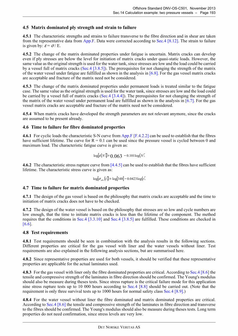
DET NORSKE VERITAS AS
Offshore Standard DNV-OS-C501, November 2013
Sec.14 Calculation example: two pressure vessels – Page 193
4.5 Matrix dominated ply strength and strain to failure
4.5.1 The characteristic strengths and strains to failure transverse to the fibre direction and in shear are takenfrom the representative data from App.F. Data were corrected according to Sec.4 [8.12]. The strain to failureis given by: ε = σ / E.
4.5.2 The change of the matrix dominated properties under fatigue is uncertain. Matrix cracks can developeven if ply stresses are below the level for initiation of matrix cracks under quasi-static loads. However, thesame value as the original strength is used for the water tank, since stresses are low and the load could be carriedby a vessel full of matrix cracks (Sec.4 [3.8.5]). The prerequisites for not changing the strength of the matrixof the water vessel under fatigue are fulfilled as shown in the analysis in [6.8]. For the gas vessel matrix cracksare acceptable and fracture of the matrix need not be considered.
4.5.3 The change of the matrix dominated properties under permanent loads is treated similar to the fatiguecase. The same value as the original strength is used for the water tank, since stresses are low and the load couldbe carried by a vessel full of matrix cracks (Sec.4 [3.4.4]). The prerequisites for not changing the strength ofthe matrix of the water vessel under permanent load are fulfilled as shown in the analysis in [6.7]. For the gasvessel matrix cracks are acceptable and fracture of the matrix need not be considered.
4.5.4 When matrix cracks have developed the strength parameters are not relevant anymore, since the cracksare assumed to be present already.
4.6 Time to failure for fibre dominated properties
4.6.1 For cyclic loads the characteristic S-N curve from App.F [F.4.2.2] can be used to establish that the fibreshave sufficient lifetime. The curve for R = 0.1 can be used since the pressure vessel is cycled between 0 andmaximum load. The characteristic fatigue curve is given as:
4.6.2 The characteristic stress rupture curve from [4.4.5] can be used to establish that the fibres have sufficientlifetime. The characteristic stress curve is given as:
4.7 Time to failure for matrix dominated properties
4.7.1 The design of the gas vessel is based on the philosophy that matrix cracks are acceptable and the time toinitiation of matrix cracks does not have to be checked.
4.7.2 The design of the water vessel is based on the philosophy that stresses are so low and cycle numbers arelow enough, that the time to initiate matrix cracks is less than the lifetime of the component. The methodrequires that the conditions in Sec.4 [3.3.10] and Sec.4 [3.8.5] are fulfilled. These conditions are checked in[6.6].
4.8 Test requirements
4.8.1 Test requirements should be seen in combination with the analysis results in the following sections.Different properties are critical for the gas vessel with liner and the water vessels without liner. Testrequirements are also explained in the following analysis sections, but are summarised here.
4.8.2 Since representative properties are used for both vessels, it should be verified that these representativeproperties are applicable for the actual laminates used.
4.8.3 For the gas vessel with liner only the fibre dominated properties are critical. According to Sec.4 [8.6] thetensile and compressive strength of the laminates in fibre direction should be confirmed. The Young's modulusshould also be measure during theses tests. Since stress rupture is the critical failure mode for this applicationnine stress rupture tests up to 10 000 hours according to Sec.4 [8.8] should be carried out. (Note that therequirement is only three survival tests up to 1000 hours for normal safety class Sec.4 [8.9].)
4.8.4 For the water vessel without liner the fibre dominated and matrix dominated properties are critical.According to Sec.4 [8.6] the tensile and compressive strength of the laminates in fibre direction and transverseto the fibres should be confirmed. The Young's modulus should also be measure during theses tests. Long termproperties do not need confirmation, since stress levels are very low.
( )[ ] ( )NN log101.0log 063.0 −=ε
( )[ ] [ ] ( )ttabs log0423.0348loglog −=σ
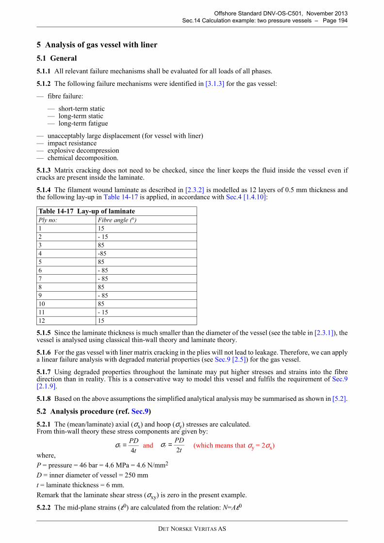
DET NORSKE VERITAS AS
Offshore Standard DNV-OS-C501, November 2013
Sec.14 Calculation example: two pressure vessels – Page 194
5 Analysis of gas vessel with liner
5.1 General
5.1.1 All relevant failure mechanisms shall be evaluated for all loads of all phases.
5.1.2 The following failure mechanisms were identified in [3.1.3] for the gas vessel:
— fibre failure:
— short-term static— long-term static— long-term fatigue
— unacceptably large displacement (for vessel with liner)— impact resistance— explosive decompression— chemical decomposition.
5.1.3 Matrix cracking does not need to be checked, since the liner keeps the fluid inside the vessel even ifcracks are present inside the laminate.
5.1.4 The filament wound laminate as described in [2.3.2] is modelled as 12 layers of 0.5 mm thickness andthe following lay-up in Table 14-17 is applied, in accordance with Sec.4 [1.4.10]:
5.1.5 Since the laminate thickness is much smaller than the diameter of the vessel (see the table in [2.3.1]), thevessel is analysed using classical thin-wall theory and laminate theory.
5.1.6 For the gas vessel with liner matrix cracking in the plies will not lead to leakage. Therefore, we can applya linear failure analysis with degraded material properties (see Sec.9 [2.5]) for the gas vessel.
5.1.7 Using degraded properties throughout the laminate may put higher stresses and strains into the fibredirection than in reality. This is a conservative way to model this vessel and fulfils the requirement of Sec.9[2.1.9].
5.1.8 Based on the above assumptions the simplified analytical analysis may be summarised as shown in [5.2].
5.2 Analysis procedure (ref. Sec.9)
5.2.1 The (mean/laminate) axial (σx) and hoop (σy) stresses are calculated. From thin-wall theory these stress components are given by:
and (which means that σy = 2σx)
where,
P = pressure = 46 bar = 4.6 MPa = 4.6 N/mm2
D = inner diameter of vessel = 250 mm
t = laminate thickness = 6 mm.
Remark that the laminate shear stress (σxy) is zero in the present example.
5.2.2 The mid-plane strains (ε0) are calculated from the relation: N=Aε0
Table 14-17 Lay-up of laminate
Ply no: Fibre angle (°)
1 15
2 - 15
3 85
4 -85
5 85
6 - 85
7 - 85
8 85
9 - 85
10 85
11 - 15
12 15
t
PDx
4=σ
t
PDy
2=σ
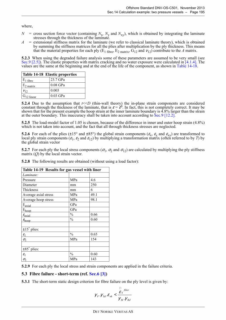
DET NORSKE VERITAS AS
Offshore Standard DNV-OS-C501, November 2013
Sec.14 Calculation example: two pressure vessels – Page 195
where,
N = cross section force vector (containing Nx, Ny and Nxy), which is obtained by integrating the laminatestresses through the thickness of the laminate.
A = extensional stiffness matrix for the laminate (we refer to classical laminate theory), which is obtainedby summing the stiffness matrices for all the plies after multiplication by the ply thickness. This meansthat the material properties for each ply (E1 fibre, E2 matrix, G12 and ν12) contribute to the A matrix.
5.2.3 When using the degraded failure analysis some of these parameters are assumed to be very small (seeSec.9 [2.5]). The elastic properties with matrix cracking and no water exposure were calculated in [4.1.4]. Thevalues are the same at the beginning and at the end of the life of the component, as shown in Table 14-18.
5.2.4 Due to the assumption that t<<D (thin-wall theory) the in-plane strain components are consideredconstant through the thickness of the laminate, that is ε = ε0. In fact, this is not completely correct. It may beshown that for the present example the hoop strain at the inner laminate boundary is 4.8% larger than the strainat the outer boundary. This inaccuracy shall be taken into account according to Sec.9 [12.2].
5.2.5 The load-model factor of 1.05 is chosen, because of the difference in inner and outer hoop strain (4.8%)which is not taken into account, and the fact that all through thickness stresses are neglected.
5.2.6 For each of the plies (±15° and ±85°) the global strain components (εx, εy and εxy) are transformed tolocal ply strain components (ε1, ε2 and ε12) by multiplying a transformation matrix (often referred to by T) bythe global strain vector
5.2.7 For each ply the local stress components (σ1, σ2 and σ12) are calculated by multiplying the ply stiffnessmatrix (Q) by the local strain vector.
5.2.8 The following results are obtained (without using a load factor):
5.2.9 For each ply the local stress and strain components are applied in the failure criteria.
5.3 Fibre failure - short-term (ref. Sec.6 [3])
5.3.1 The short-term static design criterion for fibre failure on the ply level is given by:
Table 14-18 Elastic properties
E1 fibre 23.7 GPa
E2 matrix 0.08 GPa
ν12 0.003
G12 linear 0.03 GPa
Table 14-19 Results for gas vessel with liner
Laminate:
Pressure MPa 4.6
Diameter mm 250
Thickness mm 6
Average axial stress MPa 49.1
Average hoop stress MPa 98.1
Eaxial GPa
Ehoop GPa
εaxial % 0.66
εhoop % 0.60
±15° plies:
ε1 % 0.65
σ1 MPa 154
±85° plies:
ε1 % 0.60
σ1 MPa 143
RdM
fiberk
nkSdF γγεεγγ
...
∧
<
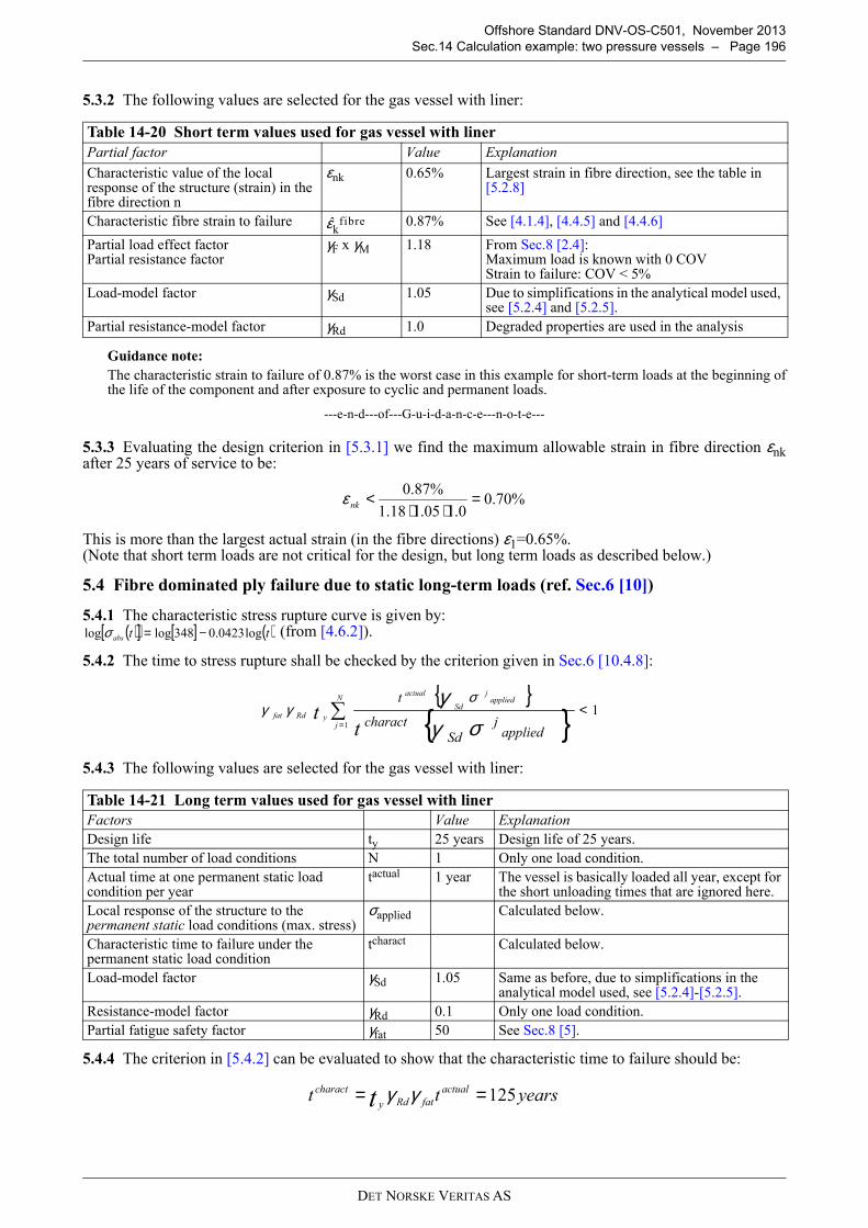
DET NORSKE VERITAS AS
Offshore Standard DNV-OS-C501, November 2013
Sec.14 Calculation example: two pressure vessels – Page 196
5.3.2 The following values are selected for the gas vessel with liner:
Guidance note:
The characteristic strain to failure of 0.87% is the worst case in this example for short-term loads at the beginning ofthe life of the component and after exposure to cyclic and permanent loads.
---e-n-d---of---G-u-i-d-a-n-c-e---n-o-t-e---
5.3.3 Evaluating the design criterion in [5.3.1] we find the maximum allowable strain in fibre direction εnkafter 25 years of service to be:
This is more than the largest actual strain (in the fibre directions) ε1=0.65%. (Note that short term loads are not critical for the design, but long term loads as described below.)
5.4 Fibre dominated ply failure due to static long-term loads (ref. Sec.6 [10])
5.4.1 The characteristic stress rupture curve is given by: (from [4.6.2]).
5.4.2 The time to stress rupture shall be checked by the criterion given in Sec.6 [10.4.8]:
5.4.3 The following values are selected for the gas vessel with liner:
5.4.4 The criterion in [5.4.2] can be evaluated to show that the characteristic time to failure should be:
Table 14-20 Short term values used for gas vessel with liner
Partial factor Value Explanation
Characteristic value of the local response of the structure (strain) in the fibre direction n
εnk 0.65% Largest strain in fibre direction, see the table in [5.2.8]
Characteristic fibre strain to failure 0.87% See [4.1.4], [4.4.5] and [4.4.6]
Partial load effect factorPartial resistance factor
γF x γM 1.18 From Sec.8 [2.4]:Maximum load is known with 0 COVStrain to failure: COV < 5%
Load-model factor γSd 1.05 Due to simplifications in the analytical model used, see [5.2.4] and [5.2.5].
Partial resistance-model factor γRd 1.0 Degraded properties are used in the analysis
Table 14-21 Long term values used for gas vessel with liner
Factors Value Explanation
Design life ty 25 years Design life of 25 years.
The total number of load conditions N 1 Only one load condition.
Actual time at one permanent static load condition per year
tactual 1 year The vessel is basically loaded all year, except for the short unloading times that are ignored here.
Local response of the structure to the permanent static load conditions (max. stress)
σapplied Calculated below.
Characteristic time to failure under the permanent static load condition
tcharact Calculated below.
Load-model factor γSd 1.05 Same as before, due to simplifications in the analytical model used, see [5.2.4]-[5.2.5].
Resistance-model factor γRd 0.1 Only one load condition.
Partial fatigue safety factor γfat 50 See Sec.8 [5].
εkfibre
%70.00.105.118.1
%87.0 =⋅⋅
<nkε
( )[ ] [ ] ( )ttabs log0423.0348loglog −=σ
{ }{ } 1
1
<∑=
N
j
appliedj
Sd
actual
yRdfat
appliedj
Sdcharact
t
tt
σγγ σ
γγ
yearstt actual
fatRdy
charact
t 125== γγ
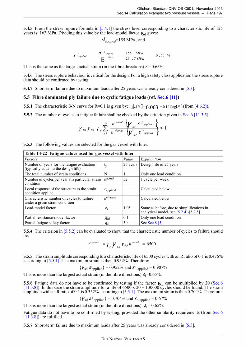
DET NORSKE VERITAS AS
Offshore Standard DNV-OS-C501, November 2013
Sec.14 Calculation example: two pressure vessels – Page 197
5.4.5 From the stress rupture formula in [5.4.1] the stress level corresponding to a characteristic life of 125years is: 163 MPa. Dividing this value by the load-model factor γSd gives:
σjapplied=155 MPa , and
This is the same as the largest actual strain (in the fibre directions) ε1=0.65%.
5.4.6 The stress rupture behaviour is critical for the design. For a high safety class application the stress rupturedata should be confirmed by testing.
5.4.7 Short-term failure due to maximum loads after 25 years was already considered in [5.3].
5.5 Fibre dominated ply failure due to cyclic fatigue loads (ref. Sec.6 [11])
5.5.1 The characteristic S-N curve for R=0.1 is given by: (from [4.6.2]).
5.5.2 The number of cycles to fatigue failure shall be checked by the criterion given in Sec.6 [11.3.5]:
5.5.3 The following values are selected for the gas vessel with liner:
5.5.4 The criterion in [5.5.2] can be evaluated to show that the characteristic number of cycles to failure shouldbe:
5.5.5 The strain amplitude corresponding to a characteristic life of 6500 cycles with an R ratio of 0.1 is 0.476%according to [5.5.1]. The maximum strain is then 0.952%. Therefore:
{γ sd εjapplied} = 0.952% and ε j applied = 0.907%
This is more than the largest actual strain (in the fibre directions) ε1=0.65%.
5.5.6 Fatigue data do not have to be confirmed by testing if the factor γRd can be multiplied by 20 (Sec.6[11.3.8]). In this case the strain amplitude for a life of 6500 x 20 = 130000 cycles should be found. The strainamplitude with an R ratio of 0.1 is 0.352% according to [5.5.1]. The maximum strain is then 0.704%. Therefore:
{γ sd ε j applied} = 0.704% and ε j applied = 0.67%
This is more than the largest actual strain (in the fibre directions): ε1= 0.65%.
Fatigue data do not have to be confirmed by testing, provided the other similarity requirements (from Sec.6[11.3.8]) are fulfilled.
5.5.7 Short-term failure due to maximum loads after 25 years was already considered in [5.3].
Table 14-22 Fatigue values used for gas vessel with liner
Factors Value Explanation
Number of years for the fatigue evaluation (typically equal to the design life)
ty 25 years Design life of 25 years
The total number of strain conditions N 1 Only one load condition
Number of cycles per year at a particular strain condition
nactual 52 1 cycle per week
Local response of the structure to the strain condition applied
εapplied Calculated below
Characteristic number of cycles to failure under a given strain condition
ncharact Calculated below
Load-model factor γSd 1.05 Same as before, due to simplifications in analytical model, see [5.2.4]-[5.2.5]
Partial resistance-model factor γRd 0.1 Only one load condition
Partial fatigue safety factor γfat 50 See Sec.8 [5]
%65.07.23
155fibre
1E===
GPa
MPaappliedj
appliedj σε
( )[ ] ( )NN log101.0log 063.0 −=ε
{ }{ } 1
1
<∑=
N
j appliedj
Sd
charact
appliedj
Sd
actual
yRdfatn
n
t ε
εγγ γ
γ
6500== actual
Rdfaty
charact nn t γγ
DET NORSKE VERITAS AS
Offshore Standard DNV-OS-C501, November 2013
Sec.14 Calculation example: two pressure vessels – Page 198
5.6 Matrix cracking (ref. Sec.6 [4])
5.6.1 Matrix cracking does not have to be considered for the gas vessel with liner.
5.7 Unacceptably large displacement (ref. Sec.6 [9])
5.7.1 It is assumed for the purpose of this example that the long-term yield strain of the liner is 5%, and thisvalue should not be exceeded to ensure that the liner will not yield.
5.7.2 The liner in this example is thin and does not contribute to the load bearing capabilities of the vessel. Theliner will follow the deformations of the laminate body of the vessel.
5.7.3 For simplicity we assume that the liner has the same strain as the laminate. In reality the liner will haveslightly larger strain since it is located on the inside of the cylindrical vessel, see [5.2.4]-[5.2.5]. This is takeninto account by introducing a load-model factor, γSd = 1.05.
5.7.4 The criterion for unacceptably large displacements from Sec.6 [9.1.1] shall be used.
5.7.5 The following values are selected for the gas vessel with liner:
5.7.6 The maximum principle strain in the laminate should be less than 5/(1.15 × 1.1) = 4.14%.
5.7.7 The highest elastic strain in fibre direction is only 0.65%. However, in this case we have to look at theelastic strain and the plastic strain due to creep. A method to calculate elastic and plastic strain is given in Sec.4[3.2.11].
or
5.7.8 Creep in the ±15o plies: The elastic strain is 0.65%. The plastic strain can be calculated according to therepresentative data of App.F for creep:
with time in hours and strain in %.
The total strain for the maximum stress of 154 MPa (see [5.2.8]) and 219000 hours is: 0.65%+1.18%=1.83%.
5.7.9 Creep in the ±85o plies can be calculated the same way. Since the ply stresses are slightly lower, the creepstrain is also slightly less.
5.7.10 The principle strains of the laminate should be calculated from the ply strains and applied to the designcriterion. Since the ply strains are so much below the acceptable levels this calculation is not done here.
5.8 Impact resistance (ref. Sec.6 [12])
5.8.1 Impact may be caused by dropped tools etc. The possible impact scenarios, if any, should be defined.
5.8.2 There is no good theoretical criterion to evaluate the resistance to impact. According to Sec.6 [12], theresistance of a structure to impact shall be tested experimentally.
5.8.3 The critical failure mechanisms in this example is fibre failure. It would have to be shown that the definedimpact scenarios do not cause any fibre failure. This could be shown on full scale specimens or onrepresentative laminates.
Table 14-23 Displacement values used for gas vessel with liner
Factors Value Explanation
Specified requirement on maximum displacement
dspec 5% See [5.3.2]
Characteristic value of the local response of the structure (here strain)
dn Calculated below
Partial load effect factor γF 1.15 From Sec.8 [2.4]:Maximum load is known with 0 COVStrain to failure COV 5%Target reliability level C
Load-model factor γSd 1.05 Same as before, due to simplifications in analytical model, see [5.2.4]-[5.2.5]
dd specnSdF <..γγ
εεε plasticelastic+=
EE plasticelastic
σσε +=
2.0
1520tplastic
σε =
DET NORSKE VERITAS AS
Offshore Standard DNV-OS-C501, November 2013
Sec.14 Calculation example: two pressure vessels – Page 199
5.8.4 Alternatively, the vessel could be protected against impact by covers or other protection devices.
5.9 Explosive decompression (ref. Sec.6 [15])
5.9.1 If the air diffuses through the liner more rapidly than it can diffuse out of the laminate, a layer ofpressurised air may build up in the interface between liner and laminate. In such a case the interface should bevented or experiments should be made to show that the liner will not collapse when the internal pressure isreduced (Sec.6 [15.2]).
5.9.2 The rate of air flow through the liner is most likely much less than through the laminate and explosivedecompression should be no problem, as long as the vessel is not exposed to external pressures as well, likeunder water usage.
5.10 Chemical decomposition (ref. Sec.6 [17])
5.10.1 It is proven by many applications that composite laminates do not chemically decompose in air within25 years.
5.11 Summary evaluation
5.11.1 Summary is as follows:
— Impact resistance should be evaluated experimentally if the vessel may be exposed to impact loads.Experiments should show that possible impact loads will not cause fibre damage.
— The gas vessel passed all other requirements for service at 46 bar.— The reduction of fibre dominated ply strength due to permanent loads is the design limiting factor for this
vessel.— Obtaining material data from tubular specimens instead of flat plates (as used in this example) would allow
better utilisation of the cylinder.
6 Non-linear analysis of vessel for water without liner
6.1 General
6.1.1 For the water vessel (without liner) it is assumed that leakage will occur if matrix cracking is present inone of the plies. We apply the 2-D in-plane progressive failure analysis (Sec.9 [2.2]) to evaluate fibre failure.An alternative method is given under [7].
6.1.2 All relevant failure mechanisms shall be evaluated for all loads of all phases.
6.1.3 The following failure mechanisms were identified in [3.1.3] for the water vessel:
— fibre failure:
— short-term static— long-term static— long-term fatigue
— matrix cracking (for vessel without liner):
— short-term static— long-term static— long-term fatigue
— impact resistance— explosive decompression— chemical decomposition
6.1.4 The filament wound laminate is the same as for the gas vessel in [5.1.4].
6.2 Analysis procedure (ref. Sec.9 [2])
6.2.1 The thin shell method for calculations of laminate stresses is the same as for the gas vessel. The elasticproperties used in the analysis are different.
6.2.2 The elastic properties without and with matrix cracking were calculated in [4.1.4]. The values aredifferent at the beginning and the end of the life of the component.
DET NORSKE VERITAS AS
Offshore Standard DNV-OS-C501, November 2013
Sec.14 Calculation example: two pressure vessels – Page 200
6.2.3 Using properties of the laminate in water addresses possible diffusion of water into the laminate.
6.2.4 A load-model factor of 1.05 is chosen, for the same reasons as described in [5.2.4]-[5.2.5].
6.2.5 The following results are obtained from the stress and laminate theory analysis (without using a loadfactor):
na: not applicable, since the matrix is cracked.
6.2.6 The component is checked for the pressure of: 1.48 MPa.
6.2.7 For each ply the local stress and strain components are applied in the failure criteria.
Table 14-24 Elastic ply properties
Property New component After 25 years in water
No matrix cracks No matrix cracks With matrix cracks in ±15 plies
With matrix cracks in ±15 plies and ±85 plies
±15 plies
E1 fibre 23.7 GPa 21.3 GPa 21.3 GPa 21.3 GPa
E2 matrix 7.6 GPa 6.8 GPa 0.08 GPa 0.08 GPa
ν12 0.29 0.29 0.003 0.003
G12 linear 3.2 GPa 2.9 GPa 0.03 GPa 0.03 GPa
±85 plies
E1 fibre 23.7 GPa 21.3 GPa 21.3 GPa 21.3 GPa
E2 matrix 7.6 GPa 6.8 GPa 6.8 GPa 0.08 GPa
ν12 0.29 0.29 0.29 0.003
G12 linear 3.2 GPa 2.9 GPa 2.9 GPa 0.03 GPa
Table 14-25 Results for vessel for water without liner
Laminate After 25 years in water, with
no matrix cracks matrix cracks
Pressure MPa 1.48 1.48
Diameter mm 250 250
Thickness mm 6 6
Average axial stress MPa 15.8 15.8
Average hoop stress MPa 31.6 31.6
Eaxial GPa 11.02 6.22
Ehoop GPa 16.34 14.0
±15o plies:
ε1 % 0.108 0.233
ε2 % 0.168 0.217
ε12 % 0.035 0.009
σ1 MPa 27.0 49.5
σ2 MPa 13.9 NA
σ12 MPa 1.01 NA
±85o plies:
ε1 % 0.17 0.216
ε2 % 0.10 0.234
ε12 % 0.01 0.003
σ1 MPa 39.9 45.9
σ2 MPa 10.7 NA
σ12 MPa 0.35 NA
DET NORSKE VERITAS AS
Offshore Standard DNV-OS-C501, November 2013
Sec.14 Calculation example: two pressure vessels – Page 201
6.3 Matrix cracking (short term) at 1.48 MPa pressure (ref. Sec.6 [4])
6.3.1 The criterion of Sec.6 [4.2.2] is not fulfilled and stress combinations should be taken into account.
maxi
6.3.2 Since there is interaction the design criterion from Sec.6 [4.2.3] shall be used:
6.3.3 The following values are selected for the water vessel without liner:
6.3.4 Checking the design criterion in [6.3.2] we find that stresses in the ±15 plies are just acceptable, whileno matrix cracking is predicted for the ±85 plies:
for ±15 plies:
for ±85 plies:
6.3.5 First matrix cracking anywhere in the structure is usually used as the criterion for onset of leakage.Matrix cracking determines the design pressure for this component. A maximum pressure of 14.8 bar isacceptable.
6.4 Matrix cracking under long-term static loads (ref. Sec.4 [3.4])
6.4.1 Matrix cracking under long-term static loads can be ignored if the stresses are below the level to initiatematrix cracking, and if the vessel can carry the loads with a fully cracked matrix according to Sec.4 [3.3.10]and [3.4.4]. The first point was shown in [6.3]. The second point is shown in [6.6], where all loads can becarried by a laminate with a fully degraded matrix.
Table 14-26 Short term values used for vessel for water without liner
Partial factor Value Explanation
Characteristic value of the local load effect of the structure (stress) in the direction n
σnk 13.9 MPa1.01 MPa10.7 MPa0.35 MPa
Ply stresses in +15 and +85 ply.See [6.2.5]
Characteristic value of the stress components to matrix cracking in the direction 2
26.3 MPa23.7 MPa
For the new vesselFor the vessel after 25 yearsSee [4.1.4] and [4.4.5], [4.4.6]
Characteristic value of the stress components to matrix cracking in the direction 12
17.0 MPa15.3 MPa
For the new vesselFor the vessel after 25 yearsSee [4.1.4] and [4.4.5], [4.4.6]
Partial load effect factorPartial resistance factor
γF × γM 1.4 From Sec.8 [2.4]:Maximum load is known with 0 COVStrain to failure COV ≤ 10%Target reliability level C
Load-model factor γSd 1.05 Due to simplifications in analytical model, see [5.2.5].
Partial resistance-model factor γRd 1.15 Given in Sec.6 [4.2.1]
10/ ≤∑≠ ∧∧
in matrixnk
nk
matrixik
ik
σ
σσ
σ
1....
2
<∑ ∧
nRdMSdF
matrixnk
nk
σ
σγγγγ
matrix2
∧σ
matrix12
∧σ
00.13.15
01.1
7.23
9.1315.14.105.1
22
=
+
⋅⋅MPa
MPa
MPa
MPa
76.03.15
35.0
7.23
7.1015.14.105.1
22
=
+
⋅⋅MPa
MPa
MPa
MPa
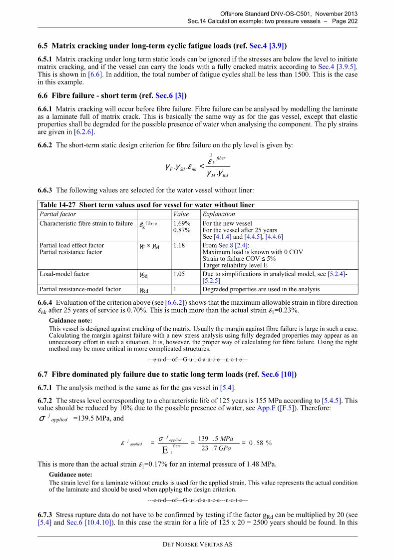
DET NORSKE VERITAS AS
Offshore Standard DNV-OS-C501, November 2013
Sec.14 Calculation example: two pressure vessels – Page 202
6.5 Matrix cracking under long-term cyclic fatigue loads (ref. Sec.4 [3.9])
6.5.1 Matrix cracking under long term static loads can be ignored if the stresses are below the level to initiatematrix cracking, and if the vessel can carry the loads with a fully cracked matrix according to Sec.4 [3.9.5].This is shown in [6.6]. In addition, the total number of fatigue cycles shall be less than 1500. This is the casein this example.
6.6 Fibre failure - short term (ref. Sec.6 [3])
6.6.1 Matrix cracking will occur before fibre failure. Fibre failure can be analysed by modelling the laminateas a laminate full of matrix crack. This is basically the same way as for the gas vessel, except that elasticproperties shall be degraded for the possible presence of water when analysing the component. The ply strainsare given in [6.2.6].
6.6.2 The short-term static design criterion for fibre failure on the ply level is given by:
6.6.3 The following values are selected for the water vessel without liner:
6.6.4 Evaluation of the criterion above (see [6.6.2]) shows that the maximum allowable strain in fibre directionεnk after 25 years of service is 0.70%. This is much more than the actual strain ε1=0.23%.
Guidance note:
This vessel is designed against cracking of the matrix. Usually the margin against fibre failure is large in such a case.Calculating the margin against failure with a new stress analysis using fully degraded properties may appear as anunnecessary effort in such a situation. It is, however, the proper way of calculating for fibre failure. Using the rightmethod may be more critical in more complicated structures.
---e-n-d---of---G-u-i-d-a-n-c-e---n-o-t-e---
6.7 Fibre dominated ply failure due to static long term loads (ref. Sec.6 [10])
6.7.1 The analysis method is the same as for the gas vessel in [5.4].
6.7.2 The stress level corresponding to a characteristic life of 125 years is 155 MPa according to [5.4.5]. Thisvalue should be reduced by 10% due to the possible presence of water, see App.F ([F.5]). Therefore:
=139.5 MPa, and
This is more than the actual strain ε1=0.17% for an internal pressure of 1.48 MPa.
Guidance note:
The strain level for a laminate without cracks is used for the applied strain. This value represents the actual conditionof the laminate and should be used when applying the design criterion.
---e-n-d---of---G-u-i-d-a-n-c-e---n-o-t-e---
6.7.3 Stress rupture data do not have to be confirmed by testing if the factor gRd can be multiplied by 20 (see[5.4] and Sec.6 [10.4.10]). In this case the strain for a life of 125 x 20 = 2500 years should be found. In this
Table 14-27 Short term values used for vessel for water without liner
Partial factor Value Explanation
Characteristic fibre strain to failure 1.69%0.87%
For the new vesselFor the vessel after 25 yearsSee [4.1.4] and [4.4.5], [4.4.6]
Partial load effect factorPartial resistance factor
γF × γM 1.18 From Sec.8 [2.4]:Maximum load is known with 0 COVStrain to failure COV ≤ 5%Target reliability level E
Load-model factor γSd 1.05 Due to simplifications in analytical model, see [5.2.4]-[5.2.5]
Partial resistance-model factor γRd 1 Degraded properties are used in the analysis
RdM
fiberk
nkSdF γγεεγγ
...
∧
<
εkfibre
appliedjσ
%58.07.23
5.139fibre
1E===
GPa
MPaappliedj
appliedj σε
DET NORSKE VERITAS AS
Offshore Standard DNV-OS-C501, November 2013
Sec.14 Calculation example: two pressure vessels – Page 203
case the acceptable characteristic stress level is 143 MPa, after applying the load model factor and the 10%reduction for sea water we get 123 MPa. Therefore:
This is more than the actual strain ε1=0.17% for an internal pressure of 1.48 MPa. Stress rupture data do nothave to be confirmed by testing, provided the other similarity requirements from (Sec.6 [11.3.8])are fulfilled.
6.7.4 Short-term failure due to maximum loads after 25 years was already considered in [6.6].
6.8 Fibre dominated ply failure due to cyclic fatigue loads (ref. Sec.6 [11])
6.8.1 The analysis method is the same as for the gas vessel in [5.5].
6.8.2 The maximum strain corresponding to a characteristic life of 6500 cycles is: .
This is more than the maximum actual strain: ε1= 0.17%.
6.8.3 The strain in the laminate: ε1=0.17% is also less than 0.67%. Therefore, the fatigue properties do not haveto be confirmed by testing, provided the similarity requirements from Sec.6 [11.3.8] are fulfilled (see also[5.5.6]).
6.8.4 Short-term failure due to maximum loads after 25 years was already considered in [6.6].
6.9 Unacceptably large displacement (ref. Sec.6 [9])
6.9.1 No requirements to be checked.
6.10 Impact resistance (ref. Sec.6 [12])
6.10.1 Impact may be caused by dropped tools etc. The possible impact scenarios, if any, should be defined.
6.10.2 There is no good theoretical criterion to evaluate the resistance to impact. According to Sec.6 [12], theresistance of a structure to impact shall be tested experimentally.
6.10.3 The critical failure mode in this example is leakage and burst, linked to the mechanisms fibre failureand matrix cracking. It would have to be shown that the defined impact scenarios do not cause any fibre failureor matrix cracking. This could be shown on full scale specimens or on representative laminates.
6.10.4 Some matrix cracks after impact may be acceptable as long as they do not cause leakage. This could beshown on tests on pressurised pipes.
6.10.5 Alternatively, the vessel could be protected against impact by covers or other protection devices.
6.11 Explosive decompression (ref. Sec.6 [15])
6.11.1 Water can diffuse through the laminate at low rates. It is unlikely that water can accumulate in thelaminate and cause effects related to explosive decompression.
6.11.2 There is no interface in this design where water could accumulate.
6.12 Chemical decomposition (ref. Sec.6 [17])
6.12.1 It is proven by many applications that composite laminates do not chemically decompose in waterwithin 25 years.
6.13 Component testing (ref. Sec.10)
6.13.1 The results show that the design limiting factor is matrix cracking. Matrix cracking is assumed here asthe beginning of leakage. It is known however, that many more matrix cracks are needed before leakage starts.
6.13.2 Testing a component with this laminate can show when leakage really starts and would allow to utilisethe design much better than it is done here. Short term and long term performance with respect to leakage canbe tested according to Sec.10 [2.2]-[2.3]. Having obtained those data they can be used instead of the checksmade here for matrix cracking. This would allow a much better utilisation of the vessel.
6.13.3 Another alternative to utilise the component better is to use a liner, as shown in the example of the gasvessel.
%518.07.23
123fibre
1E===
GPa
MPaappliedj
appliedj σε
%907.0=appliedjε
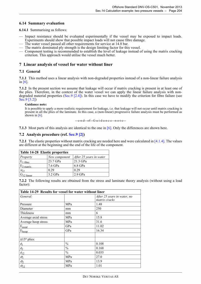
DET NORSKE VERITAS AS
Offshore Standard DNV-OS-C501, November 2013
Sec.14 Calculation example: two pressure vessels – Page 204
6.14 Summary evaluation
6.14.1 Summarising as follows:
— Impact resistance should be evaluated experimentally if the vessel may be exposed to impact loads.Experiments should show that possible impact loads will not cause fibre damage.
— The water vessel passed all other requirements for service at 14.8 bar.— The matrix dominated ply strength is the design limiting factor for this vessel.— Component testing is recommended to establish the level of leakage instead of using the matrix cracking
criterion. This approach would utilise the vessel much better.
7 Linear analysis of vessel for water without liner
7.1 General
7.1.1 This method uses a linear analysis with non-degraded properties instead of a non-linear failure analysisin [6].
7.1.2 In the present section we assume that leakage will occur if matrix cracking is present in at least one ofthe plies. Therefore, in the context of the water vessel we can apply the linear failure analysis with non-degraded material properties (Sec.9 [2.4]). In this case we have to modify the criterion for fibre failure (seeSec.9 [3.2])
Guidance note:
It is possible to apply a more realistic requirement for leakage, i.e. that leakage will not occur until matrix cracking ispresent in all the plies of the laminate. In this case, a (non-linear) progressive failure analysis must be performed asshown in [6].
---e-n-d---of---G-u-i-d-a-n-c-e---n-o-t-e---
7.1.3 Most parts of this analysis are identical to the one in [6]. Only the differences are shown here.
7.2 Analysis procedure (ref. Sec.9 [2])
7.2.1 The elastic properties without matrix cracking are needed here and were calculated in [4.1.4]. The valuesare different at the beginning and the end of the life of the component.
7.2.2 The following results are obtained from the stress and laminate theory analysis (without using a loadfactor):
Table 14-28 Elastic properties
Property New component After 25 years in water
E1 fibre 23.7 GPa 21.3 GPa
E2 matrix 7.6 GPa 6.8 GPa
ν12 0.29 0.29
G12 linear 3.2 GPa 2.9 GPa
Table 14-29 Results for vessel for water without liner
General: After 25 years in water, no matrix cracks
Pressure MPa 1.48
Diameter mm 250
Thickness mm 6
Average axial stress MPa 15.8
Average hoop stress MPa 31.6
Eaxial GPa 11.02
Ehoop GPa 16.34
±15o plies:
ε1 % 0.108
ε2 % 0.168
ε12 % 0.035
σ1 MPa 27.0
σ2 MPa 13.9
σ12 MPa 1.01
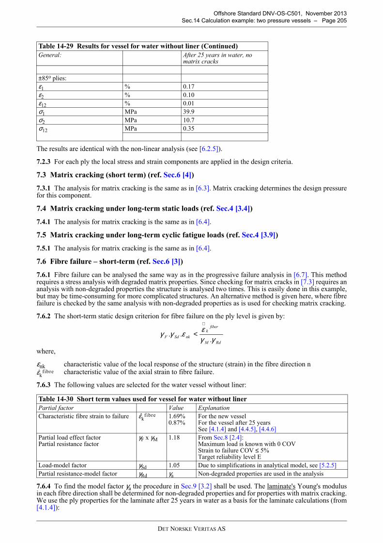
DET NORSKE VERITAS AS
Offshore Standard DNV-OS-C501, November 2013
Sec.14 Calculation example: two pressure vessels – Page 205
The results are identical with the non-linear analysis (see [6.2.5]).
7.2.3 For each ply the local stress and strain components are applied in the design criteria.
7.3 Matrix cracking (short term) (ref. Sec.6 [4])
7.3.1 The analysis for matrix cracking is the same as in [6.3]. Matrix cracking determines the design pressurefor this component.
7.4 Matrix cracking under long-term static loads (ref. Sec.4 [3.4])
7.4.1 The analysis for matrix cracking is the same as in [6.4].
7.5 Matrix cracking under long-term cyclic fatigue loads (ref. Sec.4 [3.9])
7.5.1 The analysis for matrix cracking is the same as in [6.4].
7.6 Fibre failure – short-term (ref. Sec.6 [3])
7.6.1 Fibre failure can be analysed the same way as in the progressive failure analysis in [6.7]. This methodrequires a stress analysis with degraded matrix properties. Since checking for matrix cracks in [7.3] requires ananalysis with non-degraded properties the structure is analysed two times. This is easily done in this example,but may be time-consuming for more complicated structures. An alternative method is given here, where fibrefailure is checked by the same analysis with non-degraded properties as is used for checking matrix cracking.
7.6.2 The short-term static design criterion for fibre failure on the ply level is given by:
where,
εnk characteristic value of the local response of the structure (strain) in the fibre direction ncharacteristic value of the axial strain to fibre failure.
7.6.3 The following values are selected for the water vessel without liner:
7.6.4 To find the model factor γa the procedure in Sec.9 [3.2] shall be used. The laminate's Young's modulusin each fibre direction shall be determined for non-degraded properties and for properties with matrix cracking.We use the ply properties for the laminate after 25 years in water as a basis for the laminate calculations (from[4.1.4]):
±85o plies:
ε1 % 0.17
ε2 % 0.10
ε12 % 0.01
σ1 MPa 39.9
σ2 MPa 10.7
σ12 MPa 0.35
Table 14-30 Short term values used for vessel for water without liner
Partial factor Value Explanation
Characteristic fibre strain to failure 1.69%0.87%
For the new vesselFor the vessel after 25 yearsSee [4.1.4] and [4.4.5], [4.4.6]
Partial load effect factorPartial resistance factor
γF x γM 1.18 From Sec.8 [2.4]:Maximum load is known with 0 COVStrain to failure COV ≤ 5%Target reliability level E
Load-model factor γSd 1.05 Due to simplifications in analytical model, see [5.2.5]
Partial resistance-model factor γRd γa Non-degraded properties are used in the analysis
Table 14-29 Results for vessel for water without liner (Continued)
General: After 25 years in water, no matrix cracks
RdM
fiberk
nkSdF γγεεγγ
...
∧
<
εkfibre
εkfibre
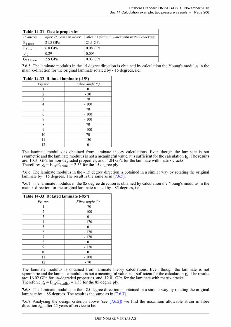
DET NORSKE VERITAS AS
Offshore Standard DNV-OS-C501, November 2013
Sec.14 Calculation example: two pressure vessels – Page 206
7.6.5 The laminate modulus in the 15 degree direction is obtained by calculation the Young's modulus in themain x-direction for the original laminate rotated by - 15 degrees, i.e.:
The laminate modulus is obtained from laminate theory calculations. Even though the laminate is notsymmetric and the laminate modulus is not a meaningful value, it is sufficient for the calculation γa . The resultsare: 10.31 GPa for non-degraded properties, and: 4.04 GPa for the laminate with matrix cracks. Therefore: γA = Elin/Enonlin, = 2.55 for the 15 degree ply.
7.6.6 The laminate modulus in the - 15 degree direction is obtained in a similar way by rotating the originallaminate by +15 degrees. The result is the same as in [7.6.5].
7.6.7 The laminate modulus in the 85 degree direction is obtained by calculation the Young's modulus in themain x-direction for the original laminate rotated by - 85 degrees, i.e.:
The laminate modulus is obtained from laminate theory calculations. Even though the laminate is notsymmetric and the laminate modulus is not a meaningful value, it is sufficient for the calculation γa . The resultsare: 16.02 GPa for un-degraded properties, and: 12.01 GPa for the laminate with matrix cracks. Therefore: γA = Elin/Enonlin, = 1.33 for the 85 degree ply.
7.6.8 The laminate modulus in the - 85 degree direction is obtained in a similar way by rotating the originallaminate by + 85 degrees. The result is the same as in [7.6.7].
7.6.9 Analysing the design criterion above (see [7.6.2]) we find the maximum allowable strain in fibredirection εnk after 25 years of service to be:
Table 14-31 Elastic properties
Property after 25 years in water after 25 years in water with matrix cracking
E1 fibre 21.3 GPa 21.3 GPa
E2 matrix 6.8 GPa 0.08 GPa
ν12 0.29 0.003
G12 linear 2.9 GPa 0.03 GPa
Table 14-32 Rotated laminate (-15°)
Ply no: Fibre angle (°)
1 0
2 - 30
3 70
4 - 100
5 70
6 - 100
7 - 100
8 70
9 - 100
10 70
11 - 30
12 0
Table 14-33 Rotated laminate (-85°)
Ply no: Fibre angle (°)
1 - 70
2 - 100
3 0
4 - 170
5 0
6 - 170
7 - 170
8 0
9 - 170
10 0
11 - 100
12 - 70
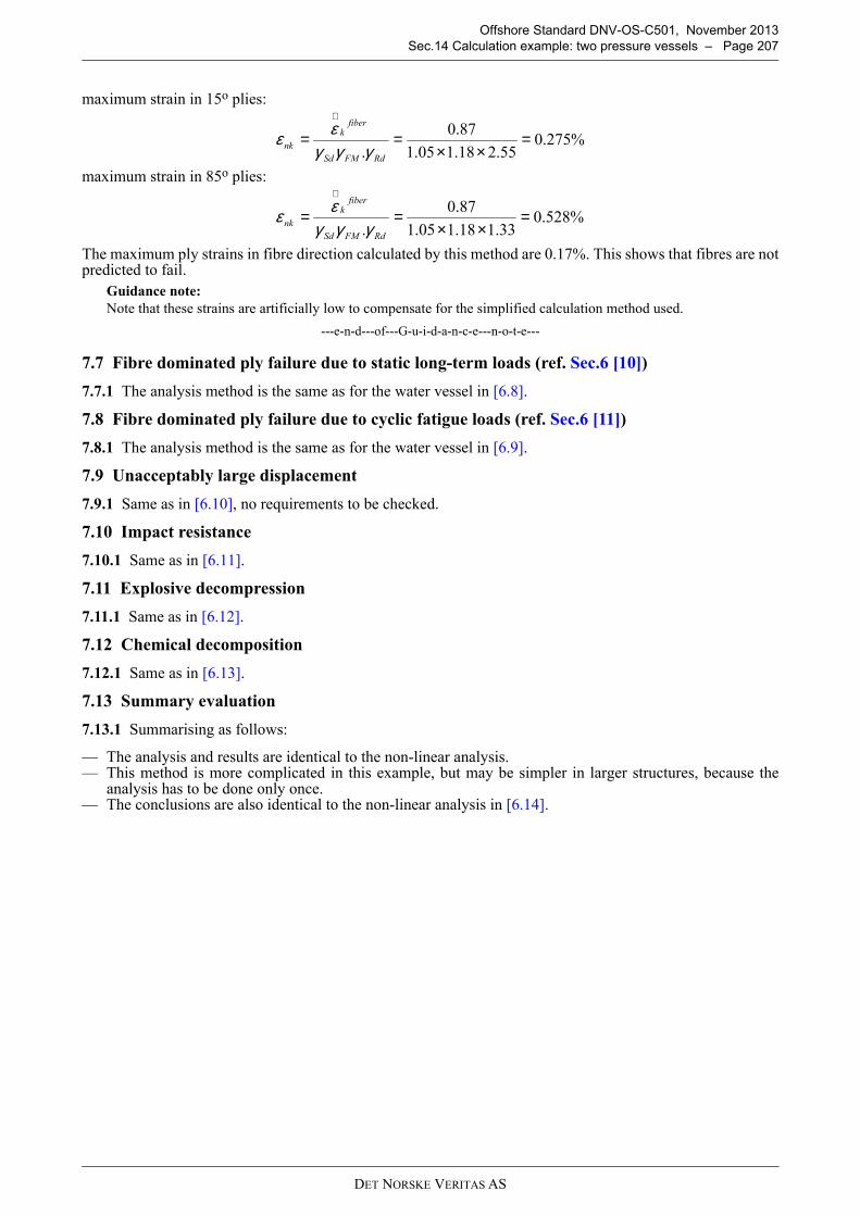
DET NORSKE VERITAS AS
Offshore Standard DNV-OS-C501, November 2013
Sec.14 Calculation example: two pressure vessels – Page 207
maximum strain in 15o plies:
maximum strain in 85o plies:
The maximum ply strains in fibre direction calculated by this method are 0.17%. This shows that fibres are notpredicted to fail.
Guidance note:
Note that these strains are artificially low to compensate for the simplified calculation method used.
---e-n-d---of---G-u-i-d-a-n-c-e---n-o-t-e---
7.7 Fibre dominated ply failure due to static long-term loads (ref. Sec.6 [10])
7.7.1 The analysis method is the same as for the water vessel in [6.8].
7.8 Fibre dominated ply failure due to cyclic fatigue loads (ref. Sec.6 [11])
7.8.1 The analysis method is the same as for the water vessel in [6.9].
7.9 Unacceptably large displacement
7.9.1 Same as in [6.10], no requirements to be checked.
7.10 Impact resistance
7.10.1 Same as in [6.11].
7.11 Explosive decompression
7.11.1 Same as in [6.12].
7.12 Chemical decomposition
7.12.1 Same as in [6.13].
7.13 Summary evaluation
7.13.1 Summarising as follows:
— The analysis and results are identical to the non-linear analysis.— This method is more complicated in this example, but may be simpler in larger structures, because the
analysis has to be done only once.— The conclusions are also identical to the non-linear analysis in [6.14].
%275.055.218.105.1
87.0
.=
××==
∧
RdFMSd
fiberk
nk γγγεε
%528.033.118.105.1
87.0
.=
××==
∧
RdFMSd
fiberk
nk γγγεε

DET NORSKE VERITAS AS
Offshore Standard DNV-OS-C501, November 2013
App.A Check-lists for design input – Page 208
APPENDIX A CHECK-LISTS FOR DESIGN INPUT
A.1 Phases
A.2 Functional requirements and failure modes
A.2.1 Functional requirements that shall be checked as a minimum
A.2.2 Failure modes that shall be checked as a minimum
Table A-1 Minimum list of phases
Manufacturing
Construction
Fabrication / Assembly
Transport
Handling
Storage
Installation
Testing
Commissioning
OperationOperationMaintenance
Repair
Retrieval / recirculation Post-operation
Table A-2 Minimum list of Functional Requirements
Minimum list of Functional Requirements
Load carrying capacity
Pressure containment
Tightness/Fluid containment
Dimensional stability
Environmental, chemical and UV resistance
Maximum vibrations
Fire Resistance
Temperature insulation
Erosion, abrasion, wear
Electrical Resistance or Insulation
Static Electricity / Grounding
Lightning resistance
Table A-3 Minimum list of Failure Modes
Minimum list of Failure Modes
Fracture (local or global)
Burst
Leakage
Impact
Excessive deformation
Ovalisation
Excessive displacement
Wear
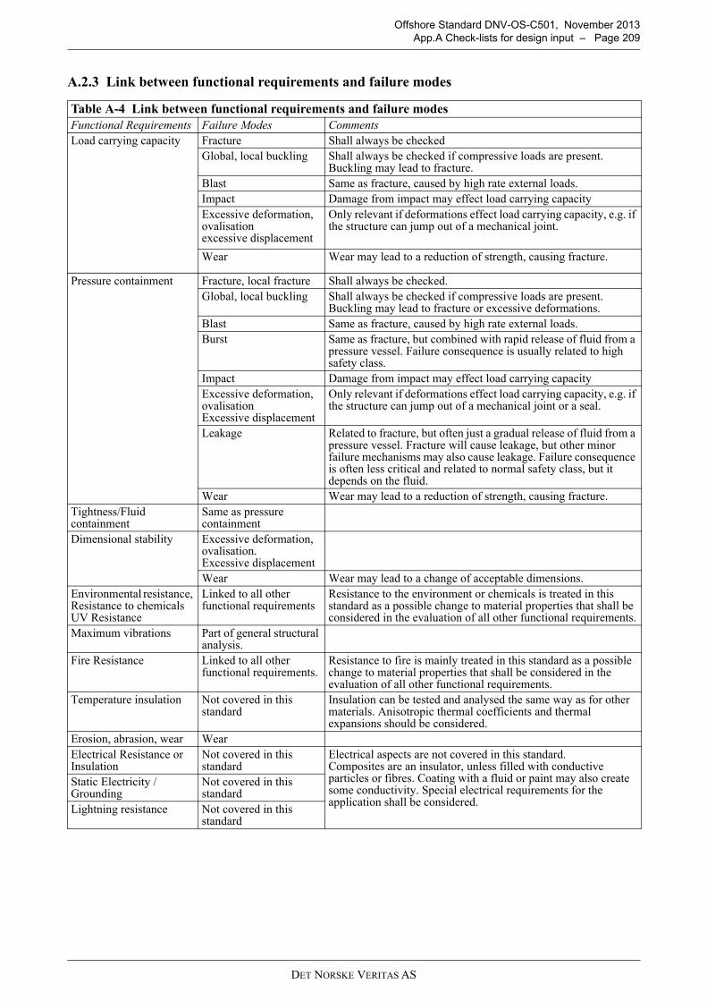
DET NORSKE VERITAS AS
Offshore Standard DNV-OS-C501, November 2013
App.A Check-lists for design input – Page 209
A.2.3 Link between functional requirements and failure modes
Table A-4 Link between functional requirements and failure modes
Functional Requirements Failure Modes Comments
Load carrying capacity Fracture Shall always be checked
Global, local buckling Shall always be checked if compressive loads are present. Buckling may lead to fracture.
Blast Same as fracture, caused by high rate external loads.
Impact Damage from impact may effect load carrying capacity
Excessive deformation, ovalisationexcessive displacement
Only relevant if deformations effect load carrying capacity, e.g. if the structure can jump out of a mechanical joint.
Wear Wear may lead to a reduction of strength, causing fracture.
Pressure containment Fracture, local fracture Shall always be checked.
Global, local buckling Shall always be checked if compressive loads are present. Buckling may lead to fracture or excessive deformations.
Blast Same as fracture, caused by high rate external loads.
Burst Same as fracture, but combined with rapid release of fluid from a pressure vessel. Failure consequence is usually related to high safety class.
Impact Damage from impact may effect load carrying capacity
Excessive deformation, ovalisationExcessive displacement
Only relevant if deformations effect load carrying capacity, e.g. if the structure can jump out of a mechanical joint or a seal.
Leakage Related to fracture, but often just a gradual release of fluid from a pressure vessel. Fracture will cause leakage, but other minor failure mechanisms may also cause leakage. Failure consequence is often less critical and related to normal safety class, but it depends on the fluid.
Wear Wear may lead to a reduction of strength, causing fracture.
Tightness/Fluid containment
Same as pressure containment
Dimensional stability Excessive deformation, ovalisation.Excessive displacement
Wear Wear may lead to a change of acceptable dimensions.
Environmental resistance, Resistance to chemicalsUV Resistance
Linked to all other functional requirements
Resistance to the environment or chemicals is treated in this standard as a possible change to material properties that shall be considered in the evaluation of all other functional requirements.
Maximum vibrations Part of general structural analysis.
Fire Resistance Linked to all other functional requirements.
Resistance to fire is mainly treated in this standard as a possible change to material properties that shall be considered in the evaluation of all other functional requirements.
Temperature insulation Not covered in this standard
Insulation can be tested and analysed the same way as for other materials. Anisotropic thermal coefficients and thermal expansions should be considered.
Erosion, abrasion, wear Wear
Electrical Resistance or Insulation
Not covered in this standard
Electrical aspects are not covered in this standard. Composites are an insulator, unless filled with conductive particles or fibres. Coating with a fluid or paint may also create some conductivity. Special electrical requirements for the application shall be considered.
Static Electricity / Grounding
Not covered in this standard
Lightning resistance Not covered in this standard

DET NORSKE VERITAS AS
Offshore Standard DNV-OS-C501, November 2013
App.A Check-lists for design input – Page 210
A.3 Loads
A.3.1 Functional loads
— Weight — Reactions from components — Interactions with other components (wear, friction, interference)— Applied tension— Pre-stressing (permanent curvature, mooring/anchoring…)— Permanent deformation of supporting structure— External hydrostatic pressure— Vacuum — Service induced vacuum— Internal pressure — Thermal stresses due to temperature of content— Slugging flow— Internal fluid flow— Loads induced by frequent pigging operations— Loads related to operations and normal use of the installation (cranes, helicopters, drilling, engorgement…) — Fouling— Traffic loads— Live loads— Installation loads.
A.3.2 Environmental loads
— Wind— Waves— Currents— Ice — Possible loads due to ice bulb growth— Snow— Earthquake— Movement of earth— Cover (soil, rock, and mattresses…) — Reaction from seafloor— Permanent deformation due to subsidence of ground— Soil conditions— Thermal expansion and contraction due to external temperatures— Moisture (swelling loads)— Tides— Vibrations— Trawl — Flooding / ground water buoyancy.
A.3.3 Accidental loads
— Collisions (vessel impact or other drifting items)— Dropped objects— Explosion— Fire (load redistribution during / after fire)— Operational malfunction (e.g. leakage or other effects from nearby pipes…)— Trawl (hooking is normally to be classified as accidental loads)— Dragging anchor— Unintended change in ballast condition— Mud slides — Failure of an anchor line or dynamic positioning system— Weld spatter— Handling by forklift.

DET NORSKE VERITAS AS
Offshore Standard DNV-OS-C501, November 2013
App.A Check-lists for design input – Page 211
A.4 Environments
The term environment designates in this standard the surroundings that impose no direct load on the structure.
The environment may impose indirect loads on the structure, e.g. thermal stresses or swelling due to moistureuptake. This should be considered as a load effect, and calculated according to the relevant parts of Sec.8.However, the environment is generally considered for its effect on the degradation of material strength.
A.5 Distribution types of basic variables
From DNV Classification Notes – No. 30.6 - Table 2.1
Table A-5 Examples of Environments
NATURAL
Temperature internal and external
Temperature variations
Temperature gradients
UV radiation
Moisture
Sea water
Lightning
Acid rain
Atmospheric electrical field
Animals (e.g. shark bites on tethers, elephants walking on pipes)
FUNCTIONAL
Transported or contained fluids and chemicals
Temperature internal and external
Pressure internal and external
Oil spill
Cleaning materials
Paint solvents
Accidental chemicals
Fire
Process gas leaks
Service induced shocks
Accidental high pressure steam
Table A-6 Standard variables and corresponding distribution types
Variable name Distribution type
Wind Short-term instantaneous gust speed Normal
Long-term n-minute average speed Weibull
Extreme speed yearly Gumbel
Waves Short-term instantaneous surface elevation (deep-water) Normal
Short-term heights Rayleigh
Wave period Longuet-Higgins
Long-term significant wave height Weibull
Long-term mean zero upcrossing or peak period Lognormal
Joint significant height/mean zero upcrossing or peak period 3-parameter Weibull (height) / Log-normal period conditioned on height
Extreme height yearly Gumbel
Current Long-term speed Weibull
Extreme yearly Gumbel
Forces Hydro-dynamic coefficients Lognormal
Fatigue Scale parameter on S-N curve Lognormal
Fatigue threshold Lognormal

DET NORSKE VERITAS AS
Offshore Standard DNV-OS-C501, November 2013
App.A Check-lists for design input – Page 212
Fracture mechanics Scale parameter on da/ dN curve Lognormal
Initial crack size Exponential
P.O.D. - curve Lognormal
Properties Yield strength (steel) Lognormal
Young’s modulus Normal
Initial deformation of panel Normal
Ship data Still water bending moment Normal
Joint still water moment / draught Joint normal
Ship speed Lognormal
Model uncertainty of linear calculations Normal
Table A-6 Standard variables and corresponding distribution types (Continued)
Variable name Distribution type
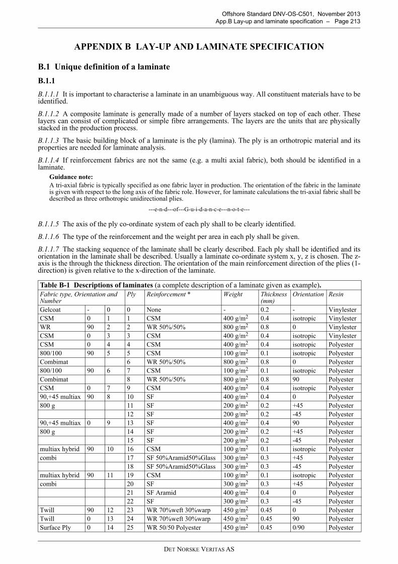
DET NORSKE VERITAS AS
Offshore Standard DNV-OS-C501, November 2013
App.B Lay-up and laminate specification – Page 213
APPENDIX B LAY-UP AND LAMINATE SPECIFICATION
B.1 Unique definition of a laminate
B.1.1
B.1.1.1 It is important to characterise a laminate in an unambiguous way. All constituent materials have to beidentified.
B.1.1.2 A composite laminate is generally made of a number of layers stacked on top of each other. Theselayers can consist of complicated or simple fibre arrangements. The layers are the units that are physicallystacked in the production process.
B.1.1.3 The basic building block of a laminate is the ply (lamina). The ply is an orthotropic material and itsproperties are needed for laminate analysis.
B.1.1.4 If reinforcement fabrics are not the same (e.g. a multi axial fabric), both should be identified in alaminate.
Guidance note:
A tri-axial fabric is typically specified as one fabric layer in production. The orientation of the fabric in the laminateis given with respect to the long axis of the fabric role. However, for laminate calculations the tri-axial fabric shall bedescribed as three orthotropic unidirectional plies.
---e-n-d---of---G-u-i-d-a-n-c-e---n-o-t-e---
B.1.1.5 The axis of the ply co-ordinate system of each ply shall to be clearly identified.
B.1.1.6 The type of the reinforcement and the weight per area in each ply shall be given.
B.1.1.7 The stacking sequence of the laminate shall be clearly described. Each ply shall be identified and itsorientation in the laminate shall be described. Usually a laminate co-ordinate system x, y, z is chosen. The z-axis is the through the thickness direction. The orientation of the main reinforcement direction of the plies (1-direction) is given relative to the x-direction of the laminate.
Table B-1 Descriptions of laminates (a complete description of a laminate given as example). Fabric type, Orientation and Number
Ply Reinforcement * Weight Thickness(mm)
Orientation Resin
Gelcoat - 0 0 None - 0.2 - Vinylester
CSM 0 1 1 CSM 400 g/m2 0.4 isotropic Vinylester
WR 90 2 2 WR 50%/50% 800 g/m2 0.8 0 Vinylester
CSM 0 3 3 CSM 400 g/m2 0.4 isotropic Vinylester
CSM 0 4 4 CSM 400 g/m2 0.4 isotropic Polyester
800/100 90 5 5 CSM 100 g/m2 0.1 isotropic Polyester
Combimat 6 WR 50%/50% 800 g/m2 0.8 0 Polyester
800/100 90 6 7 CSM 100 g/m2 0.1 isotropic Polyester
Combimat 8 WR 50%/50% 800 g/m2 0.8 90 Polyester
CSM 0 7 9 CSM 400 g/m2 0.4 isotropic Polyester
90,+45 multiax 90 8 10 SF 400 g/m2 0.4 0 Polyester
800 g 11 SF 200 g/m2 0.2 +45 Polyester
12 SF 200 g/m2 0.2 -45 Polyester
90,+45 multiax 0 9 13 SF 400 g/m2 0.4 90 Polyester
800 g 14 SF 200 g/m2 0.2 +45 Polyester
15 SF 200 g/m2 0.2 -45 Polyester
multiax hybrid 90 10 16 CSM 100 g/m2 0.1 isotropic Polyester
combi 17 SF 50%Aramid50%Glass 300 g/m2 0.3 +45 Polyester
18 SF 50%Aramid50%Glass 300 g/m2 0.3 -45 Polyester
multiax hybrid 90 11 19 CSM 100 g/m2 0.1 isotropic Polyester
combi 20 SF 300 g/m2 0.3 +45 Polyester
21 SF Aramid 400 g/m2 0.4 0 Polyester
22 SF 300 g/m2 0.3 -45 Polyester
Twill 90 12 23 WR 70%weft 30%warp 450 g/m2 0.45 0 Polyester
Twill 0 13 24 WR 70%weft 30%warp 450 g/m2 0.45 90 Polyester
Surface Ply 0 14 25 WR 50/50 Polyester 450 g/m2 0.45 0/90 Polyester

DET NORSKE VERITAS AS
Offshore Standard DNV-OS-C501, November 2013
App.B Lay-up and laminate specification – Page 214
* if no material is mentioned it is glass, % are given in weight fraction of reinforcement.WR: Woven Roving, CSM: Chopped Strand Mat, SF: Straight Fibres
B.1.1.8 The thickness of each ply has to be estimated. This can be done by the following formula (for non-hybrid reinforcements):
where Vf is the fibre volume fraction and rf is the density of the fibre. M is the mass per area of the fibres.
ff V
Mt
ρ=
DET NORSKE VERITAS AS
Offshore Standard DNV-OS-C501, November 2013
App.C Test methods for laminates – Page 215
APPENDIX C TEST METHODS FOR LAMINATES
C.1 General
C.1.1 Introduction
C.1.1.1 This appendix describes recommended and preferred test methods for laminates. Other test methodsthan the ones described here may be used if they measure the same physical properties under the sameconditions.
C.1.1.2 If no standard tests exist and no test methods are suggested, tests shall be chosen that measure thedesired properties with no or small side effects from specimen size and geometry. It shall be ensured that thetest results are correct or conservative with respect to the way they are used in the design.
C.1.1.3 The complete list of mechanical static properties of orthotropic plies needed for structural analysis inthis standard is shown under [C.2] of this appendix - for static properties.
C.1.1.4 The properties of the standard are based on ply properties. These can be measured most directly fromlaminates made of unidirectional plies all oriented in the same direction.
C.1.1.5 Ply properties may also be obtained from measurements on laminates, if it is possible to back calculatethe orthotropic ply properties from the test results of the laminates. Some examples are given under [C.4] ofthis appendix.
C.1.1.6 The evaluation of stress vs. strain curves is described under F of this appendix for brittle, plastic andductile materials.
C.1.1.7 Guidelines for the testing of sandwich are presented in App.D.
C.1.1.8 It is generally recommended to obtain data from laminates that represent the actual product andprocessing methods as closely as possible.
C.1.1.9 Health and safety shall be considered when performing tests. This standard does not address theseaspects and reference to applicable health and safety regulations shall be made.
C.1.2 General testing information
C.1.2.1 For anisotropic material, mechanical properties should be determined relative to the relevant directionof anisotropy.
C.1.2.2 Tests should be carried at a loading rates corresponding to about 1% per minute, unless specifieddifferently in the standard.
C.1.2.3 For the preparation of test samples, curing conditions, surface treatment and application procedureshall be according to the specifications as described in Sec.4 [1].
C.1.2.4 Measuring the thickness can be difficult for some materials, like laminates made of a coarse wovenstructure. Micrometers shall be used for thickness measurements and callipers shall not be used. Modulusmeasurements shall be based on an average thickness. Strength measurements shall be based on the maximumthickness or the thickness at the failure point.
C.1.2.5 Strains shall be measured directly on the specimen with either extensometer or strain gauge.Extensometers tend to give better results. Strain gauges shall be long enough to be not influenced by the weavecharacteristics of the reinforcement.
C.2 Static tests for laminates
C.2.1 In-plane tensile tests
C.2.1.1 Tensile tests can be performed on straight specimens with or without tabs or on specimens withreduced cross-sections in the middle (dogbone or dumbbell tests).
C.2.1.2 The recommended test procedure for straight specimens is ISO 527 or ASTM D3039. Somepreliminary testing may be needed to find the best tab arrangements and gripping fixtures.
C.2.1.3 The recommended test procedure for dogbone shape specimens is ISO 527 or ASTM D638M. Thecurvature of the shoulder specified by the standards is often too sharp to obtain good results. It is recommendedto use specimens with smaller curvatures or straight specimens (see [C.2.1.2]).
DET NORSKE VERITAS AS
Offshore Standard DNV-OS-C501, November 2013
App.C Test methods for laminates – Page 216
Guidance note:
The Young’s modulus can be measured well with all test arrangements. Measuring strength and strain to failure canbe more complicated, because stress concentrations at the grips or shoulder may cause premature failure. However,choosing a non-optimised test method gives conservative results for static tests.
---e-n-d---of---G-u-i-d-a-n-c-e---n-o-t-e---
C.2.2 In-plane compression tests
C.2.2.1 Compressive tests can be performed on straight specimens with or without tabs or on specimens withreduced cross-sections in the middle (dogbone or dumbbell tests). An anti-buckling devise should be used inmost cases.
C.2.2.2 The recommended test procedure is ASTM D3410 using the Celanese test fixture.
C.2.2.3 It should be ensured that test specimens do not buckle in the test fixture.
Guidance note:
One way to ensure that a specimen does not buckle is to place at least one strain gauge or extensometer at each sideto ensure that the specimen does not buckle. Strain readings should not deviate by more than 10%.
---e-n-d---of---G-u-i-d-a-n-c-e---n-o-t-e---
C.2.3 In-plane shear tests
C.2.3.1 In-plane shear tests tend to show non-linear stress vs. strain curves and the interpretation of the resultsis often difficult.
C.2.3.2 Recommended test procedures are the 2-rail shear test ASTM D4255 or a tensile or compressive teston a laminate with (±45)s reinforcement.
C.2.3.3 Test results from axial tests on (±45)s laminates must be converted into ply properties using laminatetheory. The following formulas shall be used to convert measurements of laminate stress in load direction σx,laminate strain in load direction εx and laminate strain perpendicular to the load direction εy into ply shear stressτ12 and strain γ12:
τ12 = σx /2 and γ12 = -( εx - εy)
C.2.3.4 The non-linear stress vs. strain curve looks usually like a ductile curve, see [C.6.3]. The results shallbe analysed accordingly.
C.2.4 Through thickness tensile tests
C.2.4.1 Test can be performed on straight, cylindrical or dogbone specimens.
C.2.4.2 To increase the length of the specimens, sections of laminates may be glued together. However, careshall be taken that in such case the adhesive properties do not influence the results. If the adhesive fails, the testvalues may be used as a conservative estimate of the laminate properties.
C.2.4.3 A widely used test is ASTM C297.
C.2.5 Through thickness compressive tests
C.2.5.1 Tests are usually performed on straight or cylindrical specimens. ASTM D1621 could be used for thesetests.
C.2.5.2 An anti-buckling devise is usually not required, provided the specimen is not too slender.
C.2.5.3 Specimens should not be too short. Short specimens may show wrong stress distributions if the cross-sectional surfaces are not totally parallel. In addition, the surfaces touching the test fixture cannot widen due tofriction like the rest of the specimen. Due to this effect a too high modulus can be measured if the specimen istoo short.
C.2.5.4 To increase the length of the specimens, sections of laminates may be glued together.
C.2.6 Interlaminar shear tests (through thickness)
C.2.6.1 The recommended test method is the interlaminar shear test (ILSS) according to ISO 4585 or ASTMD2344.
C.2.6.2 The ILSS test is not a pure shear test and the results are, therefore, not ideal for use in design. Othertests may be used if better results can be obtained with them.
DET NORSKE VERITAS AS
Offshore Standard DNV-OS-C501, November 2013
App.C Test methods for laminates – Page 217
C.2.7 In-plane fracture toughness tests
C.2.7.1 In-plane fracture toughness of laminates can be described by the point stress criterion, see Sec.6 [3.6].
C.2.7.2 The point stress criterion needs a critical distance that is a material parameter. The critical distance canbe measured on specimens with different crack length or hole sizes. At least three different crack or hole sizesshould be measured.
C.2.7.3 The critical distance for cracked specimens may differ from the critical distance for specimens withholes. The two tests should not be mixed.
C.2.7.4 It is recommended to prepare specimens with cracks or holes that resemble closely the real application.
C.2.7.5 The specimen width should be wider than the defect size, to avoid measuring edge effects.
C.2.7.6 No standard tests are known for measuring fracture toughness.
C.2.8 Interlaminar fracture toughness tests
C.2.8.1 The Double Cantilever Beam (DCB) test is recommended to obtain the Mode I fracture toughness GIC.
C.2.8.2 The End Notch Flexure (ENF) test is recommended to obtain the Mode I fracture toughness GIIC.
C.2.8.3 No standards are developed for these tests.
C.2.8.4 Both specimens use a starter crack to initiate crack growth.
C.2.8.5 The starter crack should be introduced by placing a thin film between the two plies that shalldelaminate. The film should not adhere to the matrix.
C.2.8.6 It is best to grow a natural starter crack from the film by applying a few low amplitude fatigue cycles.Static testing can then be performed based on the crack length of the artificial crack and the naturally growncrack.
C.2.8.7 If tests are performed based on the artificial crack only, the film should be very thin, less than 13 µm.
C.3 Tests to obtain properties under long term static and cyclic loads
C.3.1
C.3.1.1 The same tests as for measuring static properties can be used.
C.3.1.2 Loads and test environments shall be carefully controlled over the entire test period.
C.3.1.3 The strain rate should be kept constant for cyclic fatigue tests of visco elastic materials. This meansthe test frequency can be increased for lower strain (test) amplitudes.
C.3.1.4 The temperature of the specimens should be monitored to avoid heating of the specimen due to testingat too high frequencies.
C.4 Tests to obtain the fibre fraction
C.4.1
C.4.1.1 The fibre volume fraction should be obtained using one of the following standards:
— ASTM D3171 and ASTM D3553 Fibre volume fraction, digestion method.
Guidance note:
This method is used to find the fibre volume fraction by digestion of the matrix. The choice of chemical to digest thematrix depends on the matrix and fibres. Suggestions for chemicals are given in the standards. The composite weightis determined before and after the digestion of the matrix. The fibre volume fraction can be calculated from thosemeasurements. Calculations are based on the density of the fibres. However, this density can vary, especially forcarbon fibres. In this case only approximate values can be obtained.
---e-n-d---of---G-u-i-d-a-n-c-e---n-o-t-e---
— ASTM D3171 Fibre volume fraction, burnoff method— ISO 1172
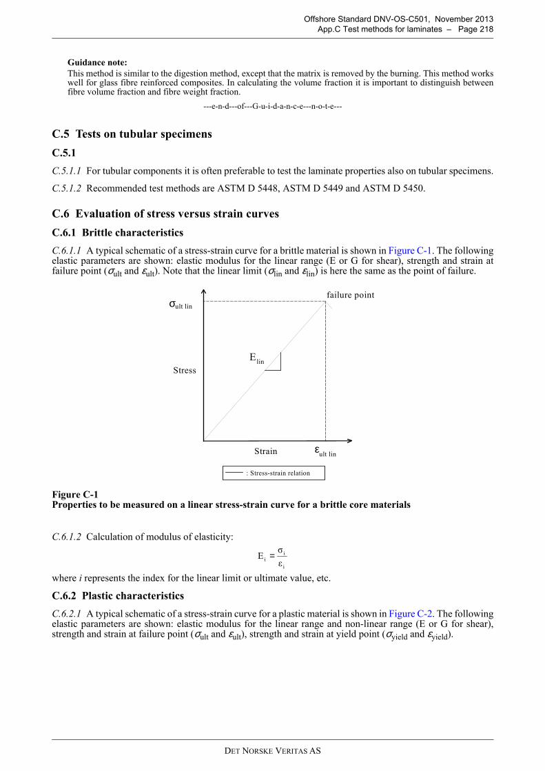
DET NORSKE VERITAS AS
Offshore Standard DNV-OS-C501, November 2013
App.C Test methods for laminates – Page 218
Guidance note:
This method is similar to the digestion method, except that the matrix is removed by the burning. This method workswell for glass fibre reinforced composites. In calculating the volume fraction it is important to distinguish betweenfibre volume fraction and fibre weight fraction.
---e-n-d---of---G-u-i-d-a-n-c-e---n-o-t-e---
C.5 Tests on tubular specimens
C.5.1
C.5.1.1 For tubular components it is often preferable to test the laminate properties also on tubular specimens.
C.5.1.2 Recommended test methods are ASTM D 5448, ASTM D 5449 and ASTM D 5450.
C.6 Evaluation of stress versus strain curves
C.6.1 Brittle characteristics
C.6.1.1 A typical schematic of a stress-strain curve for a brittle material is shown in Figure C-1. The followingelastic parameters are shown: elastic modulus for the linear range (E or G for shear), strength and strain atfailure point (σult and εult). Note that the linear limit (σlin and εlin) is here the same as the point of failure.
Figure C-1 Properties to be measured on a linear stress-strain curve for a brittle core materials
C.6.1.2 Calculation of modulus of elasticity:
where i represents the index for the linear limit or ultimate value, etc.
C.6.2 Plastic characteristics
C.6.2.1 A typical schematic of a stress-strain curve for a plastic material is shown in Figure C-2. The followingelastic parameters are shown: elastic modulus for the linear range and non-linear range (E or G for shear),strength and strain at failure point (σult and εult), strength and strain at yield point (σyield and εyield).
Stress
Strain ε
: Stress-strain relation
Elin
σfailure point
ult lin
ult lin
i
ii
ε
σE =
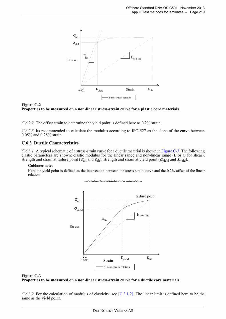
DET NORSKE VERITAS AS
Offshore Standard DNV-OS-C501, November 2013
App.C Test methods for laminates – Page 219
Figure C-2 Properties to be measured on a non-linear stress-strain curve for a plastic core materials
C.6.2.2 The offset strain to determine the yield point is defined here as 0.2% strain.
C.6.2.3 Its recommended to calculate the modulus according to ISO 527 as the slope of the curve between0.05% and 0.25% strain.
C.6.3 Ductile Characteristics
C.6.3.1 A typical schematic of a stress-strain curve for a ductile material is shown in Figure C-3. The followingelastic parameters are shown: elastic modulus for the linear range and non-linear range (E or G for shear),strength and strain at failure point (σult and εult), strength and strain at yield point (σyield and εyield).
Guidance note:
Here the yield point is defined as the intersection between the stress-strain curve and the 0.2% offset of the linearrelation.
---e-n-d---of---G-u-i-d-a-n-c-e---n-o-t-e---
Figure C-3 Properties to be measured on a non-linear stress-strain curve for a ductile core materials.
C.6.3.2 For the calculation of modulus of elasticity, see [C.3.1.2]. The linear limit is defined here to be thesame as the yield point.
Stress
Strain ε
Stress-strain relation
Enon-linE
lin
σult
ult
σyield
0.002 ε
εyield
Stress
Strainε
: Sress-strain relation
Enon-linE
lin
σ
ult
σyield
0.002 ε
εyield
ult
failure point
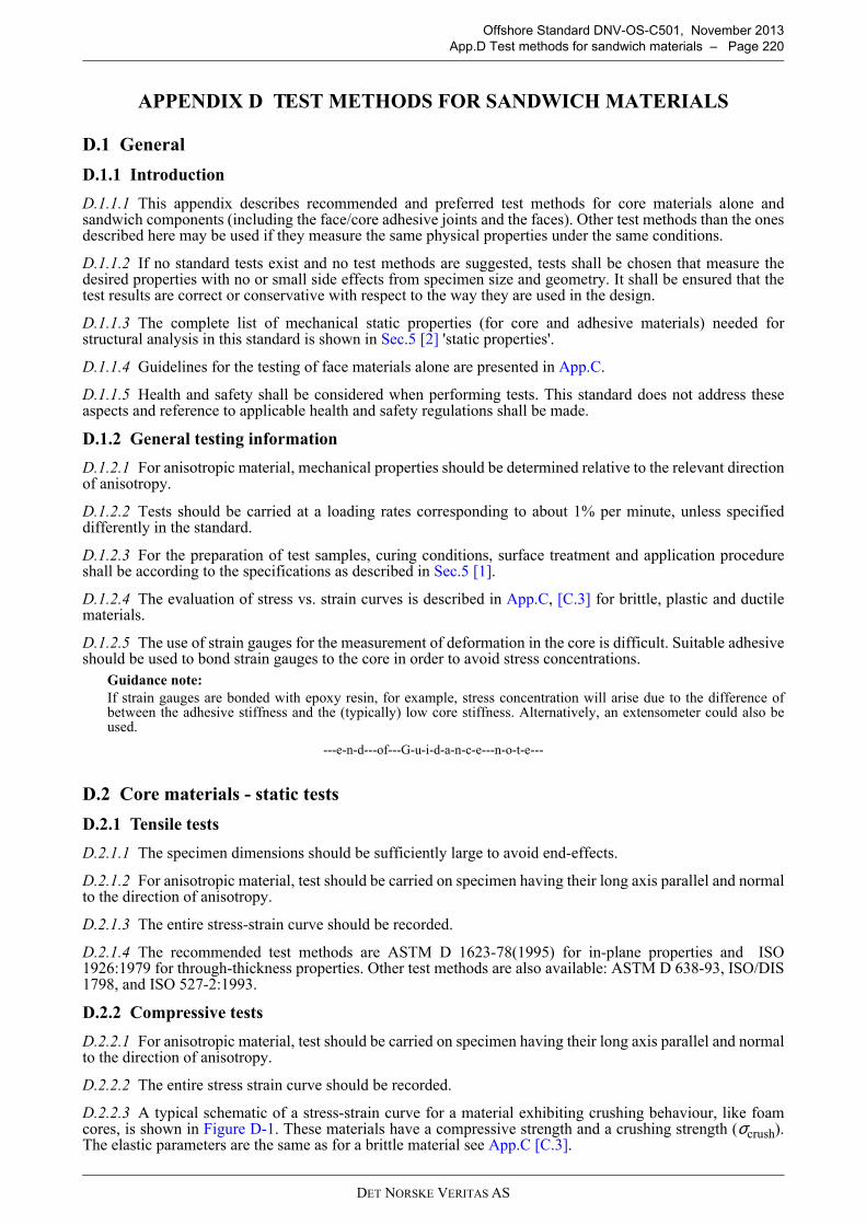
DET NORSKE VERITAS AS
Offshore Standard DNV-OS-C501, November 2013
App.D Test methods for sandwich materials – Page 220
APPENDIX D TEST METHODS FOR SANDWICH MATERIALS
D.1 General
D.1.1 Introduction
D.1.1.1 This appendix describes recommended and preferred test methods for core materials alone andsandwich components (including the face/core adhesive joints and the faces). Other test methods than the onesdescribed here may be used if they measure the same physical properties under the same conditions.
D.1.1.2 If no standard tests exist and no test methods are suggested, tests shall be chosen that measure thedesired properties with no or small side effects from specimen size and geometry. It shall be ensured that thetest results are correct or conservative with respect to the way they are used in the design.
D.1.1.3 The complete list of mechanical static properties (for core and adhesive materials) needed forstructural analysis in this standard is shown in Sec.5 [2] 'static properties'.
D.1.1.4 Guidelines for the testing of face materials alone are presented in App.C.
D.1.1.5 Health and safety shall be considered when performing tests. This standard does not address theseaspects and reference to applicable health and safety regulations shall be made.
D.1.2 General testing information
D.1.2.1 For anisotropic material, mechanical properties should be determined relative to the relevant directionof anisotropy.
D.1.2.2 Tests should be carried at a loading rates corresponding to about 1% per minute, unless specifieddifferently in the standard.
D.1.2.3 For the preparation of test samples, curing conditions, surface treatment and application procedureshall be according to the specifications as described in Sec.5 [1].
D.1.2.4 The evaluation of stress vs. strain curves is described in App.C, [C.3] for brittle, plastic and ductilematerials.
D.1.2.5 The use of strain gauges for the measurement of deformation in the core is difficult. Suitable adhesiveshould be used to bond strain gauges to the core in order to avoid stress concentrations.
Guidance note:
If strain gauges are bonded with epoxy resin, for example, stress concentration will arise due to the difference ofbetween the adhesive stiffness and the (typically) low core stiffness. Alternatively, an extensometer could also beused.
---e-n-d---of---G-u-i-d-a-n-c-e---n-o-t-e---
D.2 Core materials - static tests
D.2.1 Tensile tests
D.2.1.1 The specimen dimensions should be sufficiently large to avoid end-effects.
D.2.1.2 For anisotropic material, test should be carried on specimen having their long axis parallel and normalto the direction of anisotropy.
D.2.1.3 The entire stress-strain curve should be recorded.
D.2.1.4 The recommended test methods are ASTM D 1623-78(1995) for in-plane properties and ISO1926:1979 for through-thickness properties. Other test methods are also available: ASTM D 638-93, ISO/DIS1798, and ISO 527-2:1993.
D.2.2 Compressive tests
D.2.2.1 For anisotropic material, test should be carried on specimen having their long axis parallel and normalto the direction of anisotropy.
D.2.2.2 The entire stress strain curve should be recorded.
D.2.2.3 A typical schematic of a stress-strain curve for a material exhibiting crushing behaviour, like foamcores, is shown in Figure D-1. These materials have a compressive strength and a crushing strength (σcrush).The elastic parameters are the same as for a brittle material see App.C [C.3].
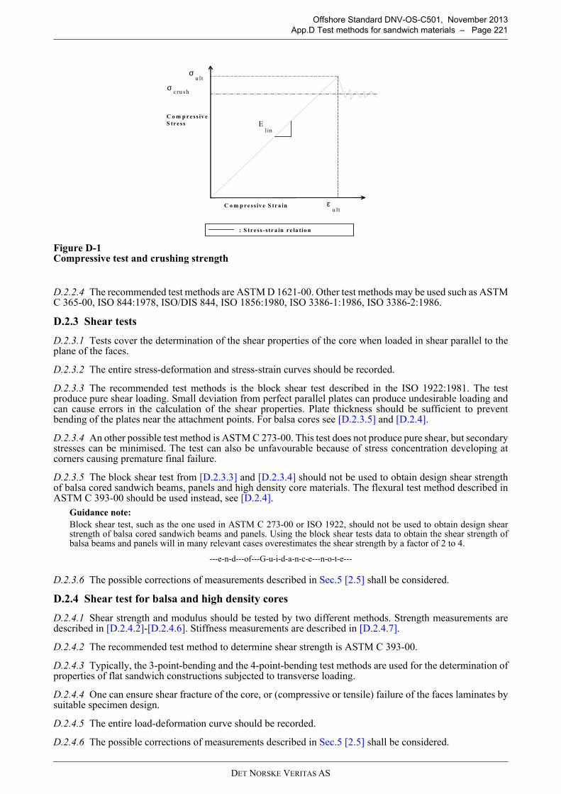
DET NORSKE VERITAS AS
Offshore Standard DNV-OS-C501, November 2013
App.D Test methods for sandwich materials – Page 221
Figure D-1 Compressive test and crushing strength
D.2.2.4 The recommended test methods are ASTM D 1621-00. Other test methods may be used such as ASTMC 365-00, ISO 844:1978, ISO/DIS 844, ISO 1856:1980, ISO 3386-1:1986, ISO 3386-2:1986.
D.2.3 Shear tests
D.2.3.1 Tests cover the determination of the shear properties of the core when loaded in shear parallel to theplane of the faces.
D.2.3.2 The entire stress-deformation and stress-strain curves should be recorded.
D.2.3.3 The recommended test methods is the block shear test described in the ISO 1922:1981. The testproduce pure shear loading. Small deviation from perfect parallel plates can produce undesirable loading andcan cause errors in the calculation of the shear properties. Plate thickness should be sufficient to preventbending of the plates near the attachment points. For balsa cores see [D.2.3.5] and [D.2.4].
D.2.3.4 An other possible test method is ASTM C 273-00. This test does not produce pure shear, but secondarystresses can be minimised. The test can also be unfavourable because of stress concentration developing atcorners causing premature final failure.
D.2.3.5 The block shear test from [D.2.3.3] and [D.2.3.4] should not be used to obtain design shear strengthof balsa cored sandwich beams, panels and high density core materials. The flexural test method described inASTM C 393-00 should be used instead, see [D.2.4].
Guidance note:
Block shear test, such as the one used in ASTM C 273-00 or ISO 1922, should not be used to obtain design shearstrength of balsa cored sandwich beams and panels. Using the block shear tests data to obtain the shear strength ofbalsa beams and panels will in many relevant cases overestimates the shear strength by a factor of 2 to 4.
---e-n-d---of---G-u-i-d-a-n-c-e---n-o-t-e---
D.2.3.6 The possible corrections of measurements described in Sec.5 [2.5] shall be considered.
D.2.4 Shear test for balsa and high density cores
D.2.4.1 Shear strength and modulus should be tested by two different methods. Strength measurements aredescribed in [D.2.4.2]-[D.2.4.6]. Stiffness measurements are described in [D.2.4.7].
D.2.4.2 The recommended test method to determine shear strength is ASTM C 393-00.
D.2.4.3 Typically, the 3-point-bending and the 4-point-bending test methods are used for the determination ofproperties of flat sandwich constructions subjected to transverse loading.
D.2.4.4 One can ensure shear fracture of the core, or (compressive or tensile) failure of the faces laminates bysuitable specimen design.
D.2.4.5 The entire load-deformation curve should be recorded.
D.2.4.6 The possible corrections of measurements described in Sec.5 [2.5] shall be considered.
C o m p r ess iv e
S tress
C o m p re ss iv e S tra in ε
: S tre ss -s tr a in re la tio n
El in
σu lt
u lt
σc ru sh
DET NORSKE VERITAS AS
Offshore Standard DNV-OS-C501, November 2013
App.D Test methods for sandwich materials – Page 222
D.2.4.7 The recommended test method to determine shear modulus is ASTM C 273-00.
D.2.5 Fracture toughness – Strain energy release rate
D.2.5.1 This section covers the determination of fracture toughness Kc, or strain energy release rate Gc of corematerials.
D.2.5.2 For anisotropic material, tests should be carried in the direction parallel and normal to the direction ofanisotropy.
D.2.5.3 For mode-I fracture toughness measurement, two test specimen can be used: the single-edge-notchbending specimen (SENB) or the compact-tension specimen (CT).
D.2.5.4 For mode-II fracture toughness measurement, the end-notch flexure specimen (ENF) or the compact-tension-shear (CTS) specimen can be used.
Guidance note:
Fracture toughness represents the resistance of a material to fracture. Mode-I refers to tensile stress conditions at thecrack tip, whereas mode-II refers to shear stress conditions. Mode-I and mode-II load cases are the principal load casesencountered when designing sandwich constructions.
---e-n-d---of---G-u-i-d-a-n-c-e---n-o-t-e---
D.2.5.5 No specific standard test exist for core materials.
D.2.6 Tests to obtain properties under long term static and cyclic loads
D.2.6.1 The same tests as for measuring static properties can be used.
D.2.6.2 Loads and test environments shall be carefully controlled over the entire test period.
D.2.6.3 The strain rate should be kept constant for cyclic fatigue tests of visco elastic materials. This meansthe test frequency can be increased for lower strain (test) amplitudes.
D.3 Adhesive materials - static tests
D.3.1 General
D.3.1.1 For testing of shear and flatwise tension, the test samples shall be made of two pieces of high densitycore material (preferably PVC foam) with the sandwich adhesive located in the midplane parallel to the steelsupports. The adhesive should be thicker than 1mm thick and the core material shall be specified.
D.3.2 Tensile tests
D.3.2.1 The recommended test method is ISO-527-1997 to determine the strength and fracture elongation intension of the adhesive.
D.3.3 Flatwise tensile tests
D.3.3.1 The recommended test method is ASTM C 297-61 to determine the strength in tension, flatwise, ofthe adhesive.
D.3.4 Shear tests
D.3.4.1 The recommended test method is ISO-1922-1981 to determine the strength of the adhesive.
D.3.5 Tests to obtain properties under long term static and cyclic loads
D.3.5.1 The same tests as for measuring static properties can be used.
D.3.5.2 Loads and test environments shall be carefully controlled over the entire test period.
D.3.5.3 The strain rate should be kept constant for cyclic fatigue tests of visco elastic materials. This meansthe test frequency can be increased for lower strain (test) amplitudes.
D.4 Core skin interface properties
D.4.1 Tensile tests
D.4.1.1 The recommended test method is ASTM C 297-61 to determine the strength in tension, flatwise, ofthe core, or of the bond between the core and the faces, of an assembled sandwich beam or panel.
DET NORSKE VERITAS AS
Offshore Standard DNV-OS-C501, November 2013
App.D Test methods for sandwich materials – Page 223
D.4.2 Fracture toughness of the interface
D.4.2.1 The test method covers the determination of the fracture toughness parameters occurring in aninterfacial crack.
Guidance note:
At the cracked interface face/core of a transversely loaded sandwich structure, the crack tip is subjected to both mode-I and mode-II stress fields.
---e-n-d---of---G-u-i-d-a-n-c-e---n-o-t-e---
D.4.2.2 For mode-I fracture toughness measurement, two test specimen can be used: the double-cantilever testspecimen (DCB), or its modified version fitted with hinges.
D.4.2.3 The interlaminar fracture toughness for isotropic materials is given by:
D.4.2.4 For mode-I fracture toughness measurement, the 'Cracked-Sandwich-Beam' (CSB) test specimen canbe used.
D.4.2.5 Delamination strength of honeycomb type core material can be determined by carrying out the testASTM C 363-57.
D.4.3 Other tests
D.4.3.1 Sandwich peel tests are used to determine the peel resistance of adhesive bonds between facings andcores. Several tests methods exist; the climbing drum tests methods, ASTM D 1781; DCB-type peel test; peeltests using air pressure; the recommended test methods is ASTM D 1781-93.
D.5 Tests for other properties
D.5.1 Coefficient of thermal expansion
D.5.1.1 The test covers the determination of the coefficient of linear thermal expansion of core materials.
D.5.1.2 The recommended test methods are ASTM D 696-91 (within the range of +30 and -30ºC), ISO4897:1985.
D.5.2 Water absorption tests
D.5.2.1 The test covers the determination of the relative rate of water absorption when immersed in a highlyhumid environment.
D.5.2.2 The recommended test method is ASTM D 2842-6. Other test methods are available such as ASTMC 272-91, IDO 2896:1987.
D.5.3 Diffusion and vapour transmission
D.5.3.1 The test aims to determine the permeability of water vapour through permeable or semi-permeablematerials.
D.5.3.2 The water vapour permeability (WVP) is calculated as:
where - ∆W - is the weight change, - t - is time and - A - the test area.
D.5.3.3 The recommended test method is SS 02 15 82. Other tests are available: ASTM E 96-94, ISO1663:1981, ISO/DIS 1663.
D.5.4 Tests for thermal conductivity measurements
D.5.4.1 The recommended test method is ASTM C 177-85. Other test methods can be used such as ASTM C168-90, ASTM C 236-89, ASTM C 1045-90. The test covers the determination of the steady-state heat fluxthrough flat specimens.
,2
Ic2Ic
1
EGK
ν−= ( )
a
Pd
w2
PG c
Ic ∂∂=
tA
WWVT
∆=

DET NORSKE VERITAS AS
Offshore Standard DNV-OS-C501, November 2013
App.D Test methods for sandwich materials – Page 224
D.5.5 Overall volume shrinkage for gap filling fillers
D.5.5.1 The recommended test method is ISO-3251-1990 to determine the overall volume shrinkage at roomtemperature.
D.5.6 Density tests
D.5.6.1 The recommended test method is ASTM D 1622-88. Other tests are available such as ASTM C 271-94, ISO 845:1988.
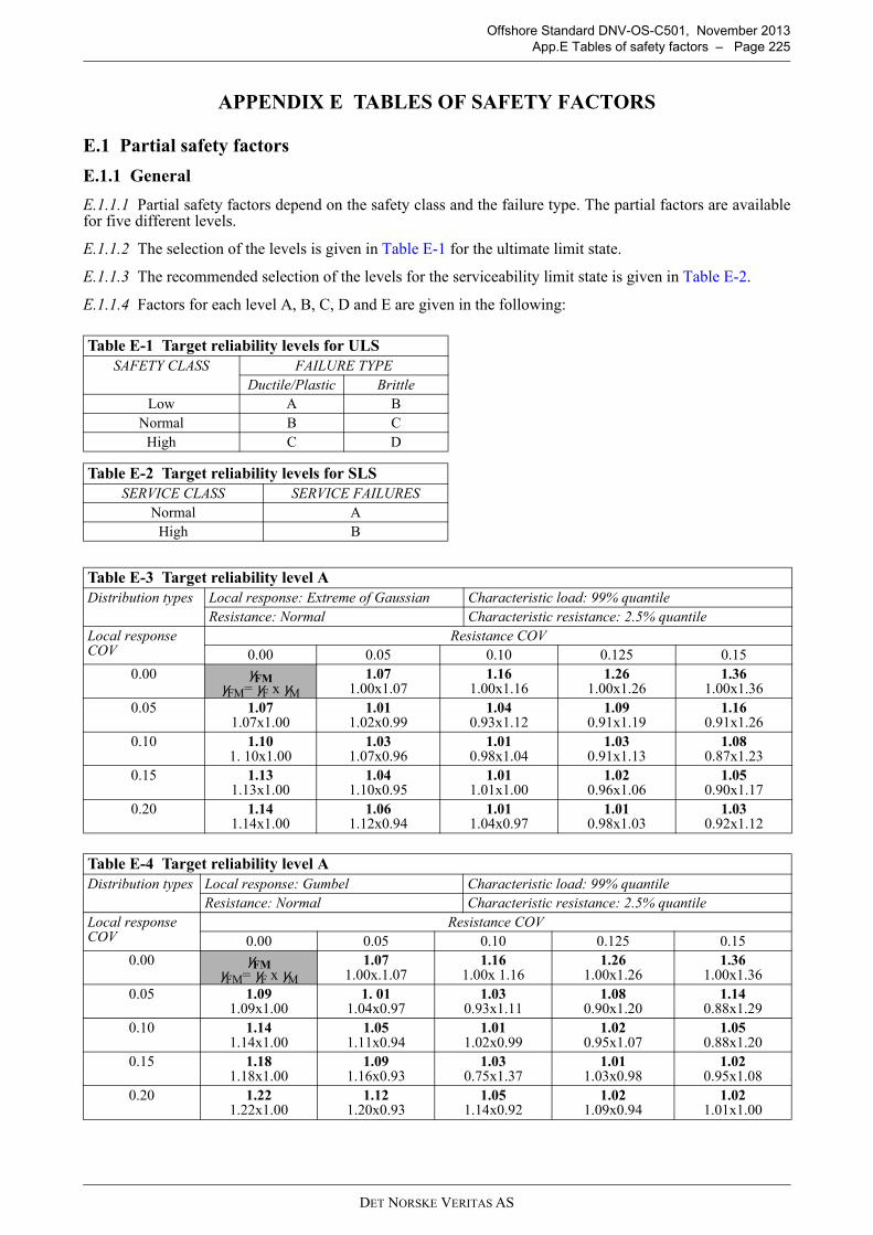
DET NORSKE VERITAS AS
Offshore Standard DNV-OS-C501, November 2013
App.E Tables of safety factors – Page 225
APPENDIX E TABLES OF SAFETY FACTORS
E.1 Partial safety factors
E.1.1 General
E.1.1.1 Partial safety factors depend on the safety class and the failure type. The partial factors are availablefor five different levels.
E.1.1.2 The selection of the levels is given in Table E-1 for the ultimate limit state.
E.1.1.3 The recommended selection of the levels for the serviceability limit state is given in Table E-2.
E.1.1.4 Factors for each level A, B, C, D and E are given in the following:
Table E-1 Target reliability levels for ULS
SAFETY CLASS FAILURE TYPE
Ductile/Plastic Brittle
Low A B
Normal B C
High C D
Table E-2 Target reliability levels for SLS
SERVICE CLASS SERVICE FAILURES
Normal A
High B
Table E-3 Target reliability level A
Distribution types Local response: Extreme of Gaussian Characteristic load: 99% quantile
Resistance: Normal Characteristic resistance: 2.5% quantile
Local response COV
Resistance COV
0.00 0.05 0.10 0.125 0.15
0.00 γFMγFM= γF x γM
1.071.00x1.07
1.161.00x1.16
1.261.00x1.26
1.361.00x1.36
0.05 1.071.07x1.00
1.011.02x0.99
1.040.93x1.12
1.090.91x1.19
1.160.91x1.26
0.10 1.101. 10x1.00
1.031.07x0.96
1.010.98x1.04
1.030.91x1.13
1.080.87x1.23
0.15 1.131.13x1.00
1.041.10x0.95
1.011.01x1.00
1.020.96x1.06
1.050.90x1.17
0.20 1.141.14x1.00
1.061.12x0.94
1.011.04x0.97
1.010.98x1.03
1.030.92x1.12
Table E-4 Target reliability level A
Distribution types Local response: Gumbel Characteristic load: 99% quantile
Resistance: Normal Characteristic resistance: 2.5% quantile
Local response COV
Resistance COV
0.00 0.05 0.10 0.125 0.15
0.00 γFMγFM= γF x γM
1.071.00x.1.07
1.161.00x 1.16
1.261.00x1.26
1.361.00x1.36
0.05 1.091.09x1.00
1. 011.04x0.97
1.030.93x1.11
1.080.90x1.20
1.140.88x1.29
0.10 1.141.14x1.00
1.051.11x0.94
1.011.02x0.99
1.020.95x1.07
1.050.88x1.20
0.15 1.181.18x1.00
1.091.16x0.93
1.030.75x1.37
1.011.03x0.98
1.020.95x1.08
0.20 1.221.22x1.00
1.121.20x0.93
1.051.14x0.92
1.021.09x0.94
1.021.01x1.00
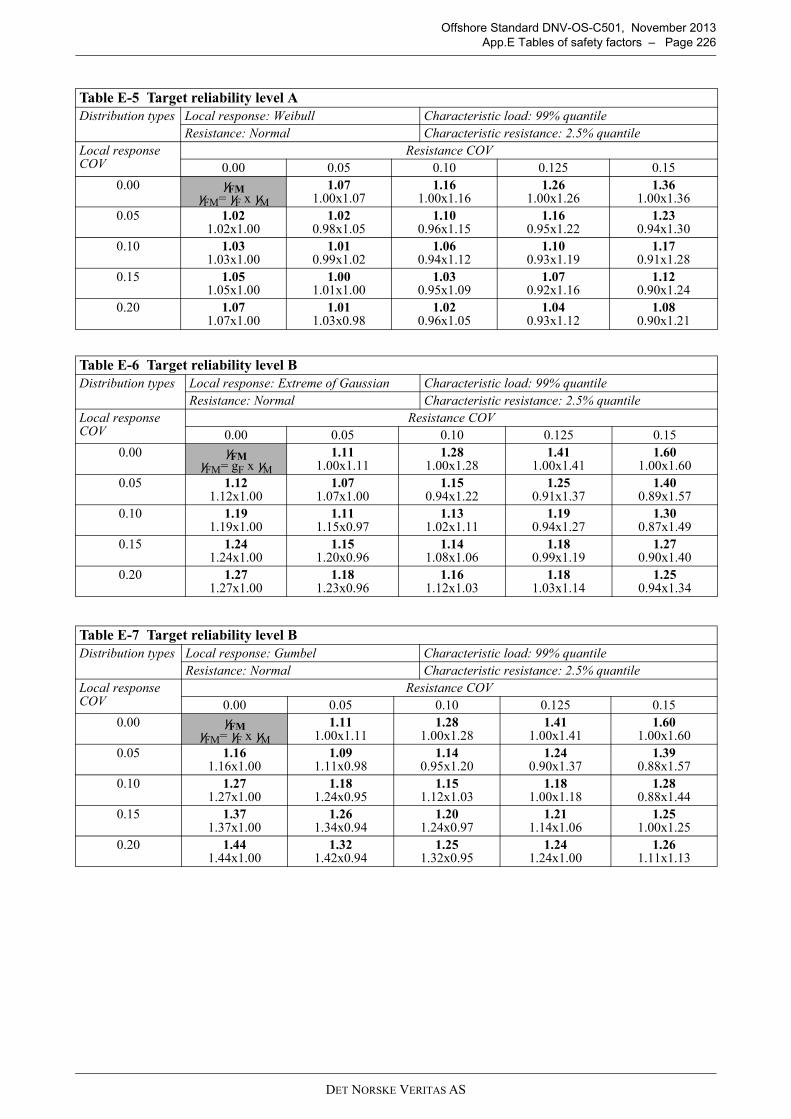
DET NORSKE VERITAS AS
Offshore Standard DNV-OS-C501, November 2013
App.E Tables of safety factors – Page 226
Table E-5 Target reliability level A
Distribution types Local response: Weibull Characteristic load: 99% quantile
Resistance: Normal Characteristic resistance: 2.5% quantile
Local response COV
Resistance COV
0.00 0.05 0.10 0.125 0.15
0.00 γFMγFM= γF x γM
1.071.00x1.07
1.161.00x1.16
1.261.00x1.26
1.361.00x1.36
0.05 1.021.02x1.00
1.020.98x1.05
1.100.96x1.15
1.160.95x1.22
1.230.94x1.30
0.10 1.031.03x1.00
1.010.99x1.02
1.060.94x1.12
1.100.93x1.19
1.170.91x1.28
0.15 1.051.05x1.00
1.001.01x1.00
1.030.95x1.09
1.070.92x1.16
1.120.90x1.24
0.20 1.071.07x1.00
1.011.03x0.98
1.020.96x1.05
1.040.93x1.12
1.080.90x1.21
Table E-6 Target reliability level B
Distribution types Local response: Extreme of Gaussian Characteristic load: 99% quantile
Resistance: Normal Characteristic resistance: 2.5% quantile
Local response COV
Resistance COV
0.00 0.05 0.10 0.125 0.15
0.00 γFMγFM= gF x γM
1.111.00x1.11
1.281.00x1.28
1.411.00x1.41
1.601.00x1.60
0.05 1.121.12x1.00
1.071.07x1.00
1.150.94x1.22
1.250.91x1.37
1.400.89x1.57
0.10 1.191.19x1.00
1.111.15x0.97
1.131.02x1.11
1.190.94x1.27
1.300.87x1.49
0.15 1.241.24x1.00
1.151.20x0.96
1.141.08x1.06
1.180.99x1.19
1.270.90x1.40
0.20 1.271.27x1.00
1.181.23x0.96
1.161.12x1.03
1.181.03x1.14
1.250.94x1.34
Table E-7 Target reliability level B
Distribution types Local response: Gumbel Characteristic load: 99% quantile
Resistance: Normal Characteristic resistance: 2.5% quantile
Local response COV
Resistance COV
0.00 0.05 0.10 0.125 0.15
0.00 γFMγFM= γF x γM
1.111.00x1.11
1.281.00x1.28
1.411.00x1.41
1.601.00x1.60
0.05 1.161.16x1.00
1.091.11x0.98
1.140.95x1.20
1.240.90x1.37
1.390.88x1.57
0.10 1.271.27x1.00
1.181.24x0.95
1.151.12x1.03
1.181.00x1.18
1.280.88x1.44
0.15 1.371.37x1.00
1.261.34x0.94
1.201.24x0.97
1.211.14x1.06
1.251.00x1.25
0.20 1.441.44x1.00
1.321.42x0.94
1.251.32x0.95
1.241.24x1.00
1.261.11x1.13
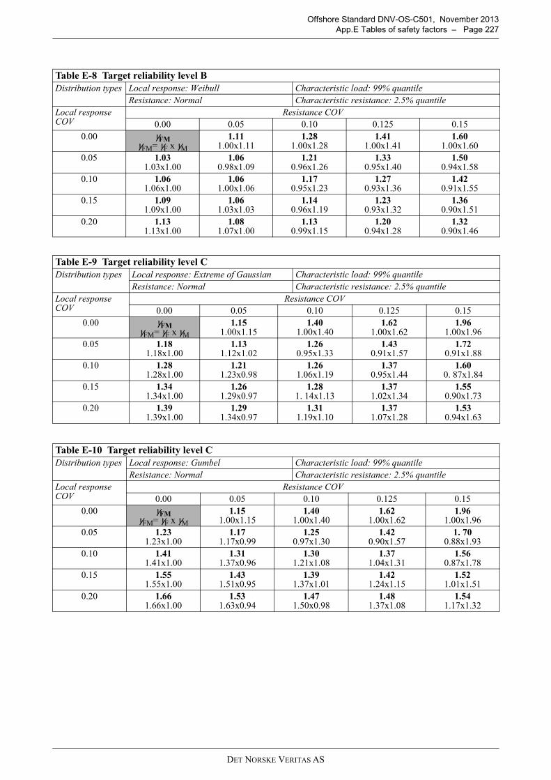
DET NORSKE VERITAS AS
Offshore Standard DNV-OS-C501, November 2013
App.E Tables of safety factors – Page 227
Table E-8 Target reliability level B
Distribution types Local response: Weibull Characteristic load: 99% quantile
Resistance: Normal Characteristic resistance: 2.5% quantile
Local response COV
Resistance COV
0.00 0.05 0.10 0.125 0.15
0.00 γFMγFM= γF x γM
1.111.00x1.11
1.281.00x1.28
1.411.00x1.41
1.601.00x1.60
0.05 1.031.03x1.00
1.060.98x1.09
1.210.96x1.26
1.330.95x1.40
1.500.94x1.58
0.10 1.061.06x1.00
1.061.00x1.06
1.170.95x1.23
1.270.93x1.36
1.420.91x1.55
0.15 1.091.09x1.00
1.061.03x1.03
1.140.96x1.19
1.230.93x1.32
1.360.90x1.51
0.20 1.131.13x1.00
1.081.07x1.00
1.130.99x1.15
1.200.94x1.28
1.320.90x1.46
Table E-9 Target reliability level C
Distribution types Local response: Extreme of Gaussian Characteristic load: 99% quantile
Resistance: Normal Characteristic resistance: 2.5% quantile
Local response COV
Resistance COV
0.00 0.05 0.10 0.125 0.15
0.00 γFMγFM= γF x γM
1.151.00x1.15
1.401.00x1.40
1.621.00x1.62
1.961.00x1.96
0.05 1.181.18x1.00
1.131.12x1.02
1.260.95x1.33
1.430.91x1.57
1.720.91x1.88
0.10 1.281.28x1.00
1.211.23x0.98
1.261.06x1.19
1.370.95x1.44
1.600. 87x1.84
0.15 1.341.34x1.00
1.261.29x0.97
1.281. 14x1.13
1.371.02x1.34
1.550.90x1.73
0.20 1.391.39x1.00
1.291.34x0.97
1.311.19x1.10
1.371.07x1.28
1.530.94x1.63
Table E-10 Target reliability level C
Distribution types Local response: Gumbel Characteristic load: 99% quantile
Resistance: Normal Characteristic resistance: 2.5% quantile
Local response COV
Resistance COV
0.00 0.05 0.10 0.125 0.15
0.00 γFMγFM= γF x γM
1.151.00x1.15
1.401.00x1.40
1.621.00x1.62
1.961.00x1.96
0.05 1.231.23x1.00
1.171.17x0.99
1.250.97x1.30
1.420.90x1.57
1. 700.88x1.93
0.10 1.411.41x1.00
1.311.37x0.96
1.301.21x1.08
1.371.04x1.31
1.560.87x1.78
0.15 1.551.55x1.00
1.431.51x0.95
1.391.37x1.01
1.421.24x1.15
1.521.01x1.51
0.20 1.661.66x1.00
1.531.63x0.94
1.471.50x0.98
1.481.37x1.08
1.541.17x1.32
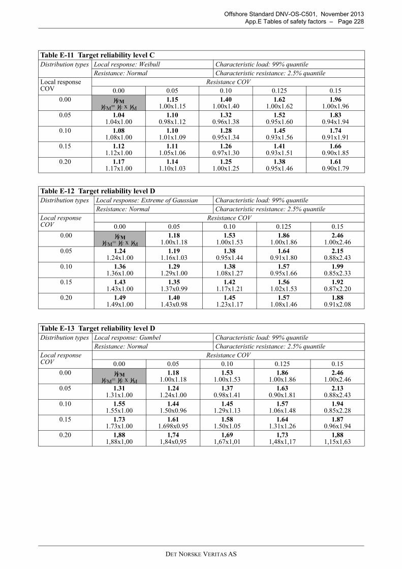
DET NORSKE VERITAS AS
Offshore Standard DNV-OS-C501, November 2013
App.E Tables of safety factors – Page 228
Table E-11 Target reliability level C
Distribution types Local response: Weibull Characteristic load: 99% quantile
Resistance: Normal Characteristic resistance: 2.5% quantile
Local response COV
Resistance COV
0.00 0.05 0.10 0.125 0.15
0.00 γFMγFM= γF x γM
1.151.00x1.15
1.401.00x1.40
1.621.00x1.62
1.961.00x1.96
0.05 1.041.04x1.00
1.100.98x1.12
1.320.96x1.38
1.520.95x1.60
1.830.94x1.94
0.10 1.081.08x1.00
1.101.01x1.09
1.280.95x1.34
1.450.93x1.56
1.740.91x1.91
0.15 1.121.12x1.00
1.111.05x1.06
1.260.97x1.30
1.410.93x1.51
1.660.90x1.85
0.20 1.171.17x1.00
1.141.10x1.03
1.251.00x1.25
1.380.95x1.46
1.610.90x1.79
Table E-12 Target reliability level D
Distribution types Local response: Extreme of Gaussian Characteristic load: 99% quantile
Resistance: Normal Characteristic resistance: 2.5% quantile
Local response COV
Resistance COV
0.00 0.05 0.10 0.125 0.15
0.00 γFMγFM= γF x γM
1.181.00x1.18
1.531.00x1.53
1.861.00x1.86
2.461.00x2.46
0.05 1.241.24x1.00
1.191.16x1.03
1.380.95x1.44
1.640.91x1.80
2.150.88x2.43
0.10 1.361.36x1.00
1.291.29x1.00
1.381.08x1.27
1.570.95x1.66
1.990.85x2.33
0.15 1.431.43x1.00
1.351.37x0.99
1.421.17x1.21
1.561.02x1.53
1.920.87x2.20
0.20 1.491.49x1.00
1.401.43x0.98
1.451.23x1.17
1.571.08x1.46
1.880.91x2.08
Table E-13 Target reliability level D
Distribution types Local response: Gumbel Characteristic load: 99% quantile
Resistance: Normal Characteristic resistance: 2.5% quantile
Local response COV
Resistance COV
0.00 0.05 0.10 0.125 0.15
0.00 γFMγFM= γF x γM
1.181.00x1.18
1.531.00x1.53
1.861.00x1.86
2.461.00x2.46
0.05 1.311.31x1.00
1.241.24x1.00
1.370.98x1.41
1.630.90x1.81
2.130.88x2.43
0.10 1.551.55x1.00
1.441.50x0.96
1.451.29x1.13
1.571.06x1.48
1.940.85x2.28
0.15 1.731.73x1.00
1.611.698x0.95
1.581.50x1.05
1.641.31x1.26
1.870.96x1.94
0.20 1,881,88x1,00
1,741,84x0,95
1,691,67x1,01
1,731,48x1,17
1,881,15x1,63
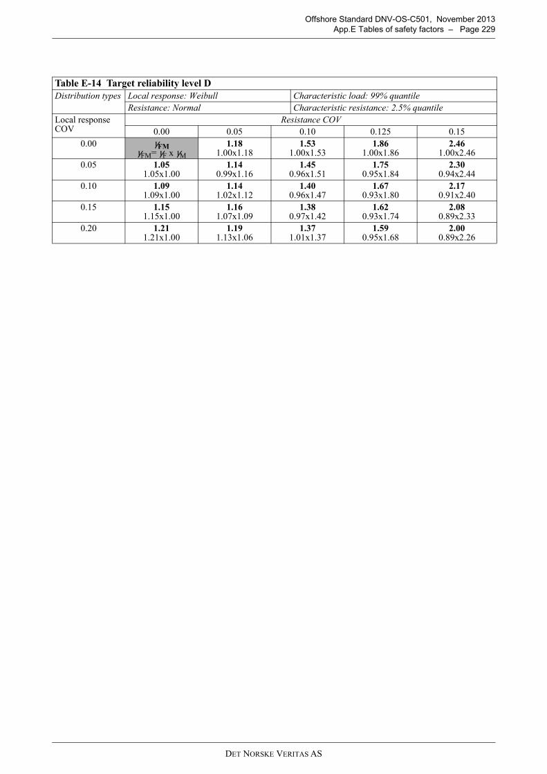
DET NORSKE VERITAS AS
Offshore Standard DNV-OS-C501, November 2013
App.E Tables of safety factors – Page 229
Table E-14 Target reliability level D
Distribution types Local response: Weibull Characteristic load: 99% quantile
Resistance: Normal Characteristic resistance: 2.5% quantile
Local response COV
Resistance COV
0.00 0.05 0.10 0.125 0.15
0.00 γFMγFM= γF x γM
1.181.00x1.18
1.531.00x1.53
1.861.00x1.86
2.461.00x2.46
0.05 1.051.05x1.00
1.140.99x1.16
1.450.96x1.51
1.750.95x1.84
2.300.94x2.44
0.10 1.091.09x1.00
1.141.02x1.12
1.400.96x1.47
1.670.93x1.80
2.170.91x2.40
0.15 1.151.15x1.00
1.161.07x1.09
1.380.97x1.42
1.620.93x1.74
2.080.89x2.33
0.20 1.211.21x1.00
1.191.13x1.06
1.371.01x1.37
1.590.95x1.68
2.000.89x2.26
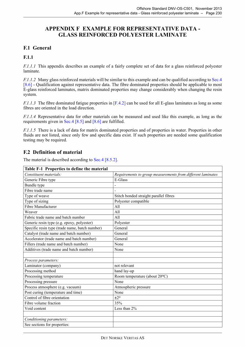
DET NORSKE VERITAS AS
Offshore Standard DNV-OS-C501, November 2013
App.F Example for representative data - Glass reinforced polyester laminate – Page 230
APPENDIX F EXAMPLE FOR REPRESENTATIVE DATA - GLASS REINFORCED POLYESTER LAMINATE
F.1 General
F.1.1
F.1.1.1 This appendix describes an example of a fairly complete set of data for a glass reinforced polyesterlaminate.
F.1.1.2 Many glass reinforced materials will be similar to this example and can be qualified according to Sec.4[8.6] - Qualification against representative data. The fibre dominated properties should be applicable to mostE-glass reinforced laminates, matrix dominated properties may change considerably when changing the resinsystem.
F.1.1.3 The fibre dominated fatigue properties in [F.4.2] can be used for all E-glass laminates as long as somefibres are oriented in the load direction.
F.1.1.4 Representative data for other materials can be measured and used like this example, as long as therequirements given in Sec.4 [8.5] and [8.6] are fulfilled.
F.1.1.5 There is a lack of data for matrix dominated properties and of properties in water. Properties in otherfluids are not listed, since only few and specific data exist. If such properties are needed some qualificationtesting may be required.
F.2 Definition of material
The material is described according to Sec.4 [8.5.2].
Table F-1 Properties to define the material
Constituent materials: Requirements to group measurements from different laminates
Generic Fibre type E-Glass
Bundle type -
Fibre trade name -
Type of weave Stitch bonded straight parallel fibres
Type of sizing Polyester compatible
Fibre Manufacturer All
Weaver All
Fabric trade name and batch number All
Generic resin type (e.g. epoxy, polyester) Polyester
Specific resin type (trade name, batch number) General
Catalyst (trade name and batch number) General
Accelerator (trade name and batch number) General
Fillers (trade name and batch number) None
Additives (trade name and batch number) None
Process parameters:
Laminator (company) not relevant
Processing method hand lay-up
Processing temperature Room temperature (about 20oC)
Processing pressure None
Process atmosphere (e.g. vacuum) Atmospheric pressure
Post curing (temperature and time) None
Control of fibre orientation ±2o
Fibre volume fraction 35%
Void content Less than 2%
Conditioning parameters:
See sections for properties:
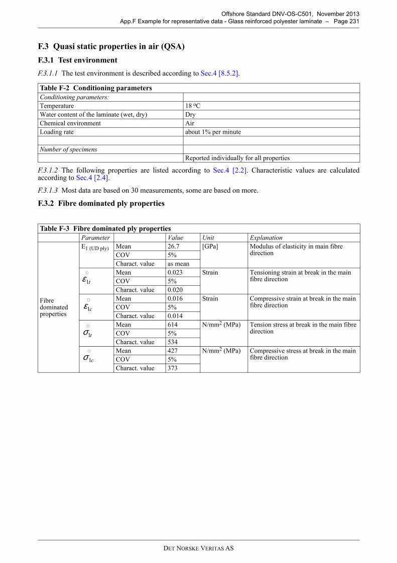
DET NORSKE VERITAS AS
Offshore Standard DNV-OS-C501, November 2013
App.F Example for representative data - Glass reinforced polyester laminate – Page 231
F.3 Quasi static properties in air (QSA)
F.3.1 Test environment
F.3.1.1 The test environment is described according to Sec.4 [8.5.2].
F.3.1.2 The following properties are listed according to Sec.4 [2.2]. Characteristic values are calculatedaccording to Sec.4 [2.4].
F.3.1.3 Most data are based on 30 measurements, some are based on more.
F.3.2 Fibre dominated ply properties
Table F-2 Conditioning parameters
Conditioning parameters:
Temperature 18 oC
Water content of the laminate (wet, dry) Dry
Chemical environment Air
Loading rate about 1% per minute
Number of specimens
Reported individually for all properties
Table F-3 Fibre dominated ply properties
Parameter Value Unit Explanation
Fibre dominated properties
E1 (UD ply) Mean 26.7 [GPa] Modulus of elasticity in main fibre direction COV 5%
Charact. value as mean
Mean 0.023 Strain Tensioning strain at break in the main fibre directionCOV 5%
Charact. value 0.020
Mean 0.016 Strain Compressive strain at break in the main fibre directionCOV 5%
Charact. value 0.014
Mean 614 N/mm2 (MPa) Tension stress at break in the main fibre direction COV 5%
Charact. value 534
Mean 427 N/mm2 (MPa) Compressive stress at break in the main fibre directionCOV 5%
Charact. value 373
t1ε∧
c1ε∧
t1σ∧
c1σ∧
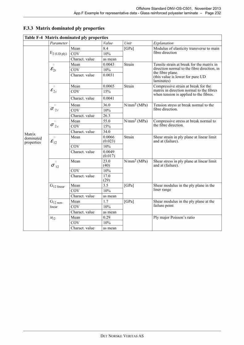
DET NORSKE VERITAS AS
Offshore Standard DNV-OS-C501, November 2013
App.F Example for representative data - Glass reinforced polyester laminate – Page 232
F.3.3 Matrix dominated ply properties
Table F-4 Matrix dominated ply properties
Parameter Value Unit Explanation
Matrix dominated properties
E2 (UD ply)
Mean 8.4 [GPa] Modulus of elasticity transverse to main fibre direction COV 10%
Charact. value as mean
Mean 0.0043 Strain Tensile strain at break for the matrix in direction normal to the fibre direction, in the fibre plane.(this value is lower for pure UD laminates)
COV 10%
Charact. value 0.0031
Mean 0.0065 Strain Compressive strain at break for the matrix in direction normal to the fibres when tension is applied to the fibres.
COV 15%
Charact. value 0.0041
Mean 36.0 N/mm2 (MPa) Tension stress at break normal to the fibre direction.COV 10%
Charact. value 26.3
Mean 55.0 N/mm2 (MPa) Compressive stress at break normal to the fibre direction.COV 15%
Charact. value 34.0
Mean 0.0066(0.023)
Strain Shear strain in ply plane at linear limit and at (failure).
COV 10%
Charact. value 0.0049(0.017)
Mean 23.0 (40)
N/mm2 (MPa) Shear stress in ply plane at linear limit and at (failure).
COV 10%
Charact. value 17.0(29)
G12 linear Mean 3.5 [GPa] Shear modulus in the ply plane in the liner rangeCOV 10%
Charact. value as mean
G12 non-
linear
Mean 1.7 [GPa] Shear modulus in the ply plane at the failure pointCOV 10%
Charact. value as mean
ν12 Mean 0.29 Ply major Poisson’s ratio
COV 10%
Charact. value as mean
t2ε∧
c2ε∧
t2σ∧
c2σ∧
12ε∧
12σ∧
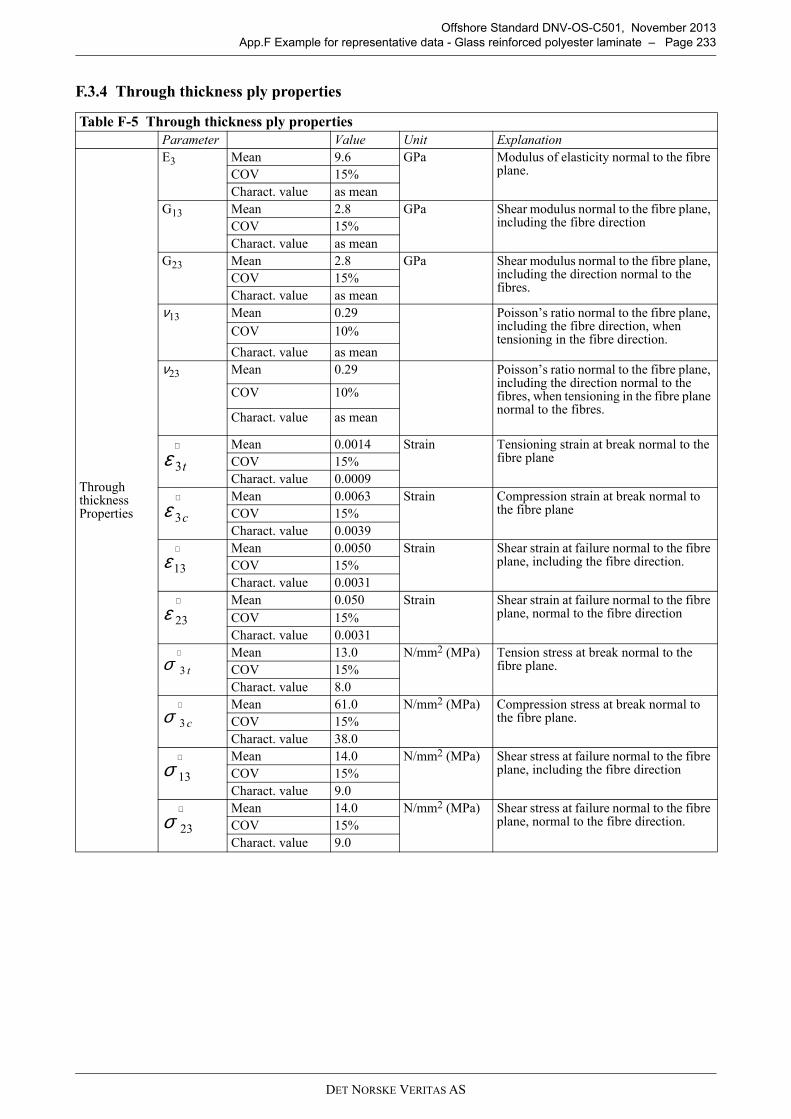
DET NORSKE VERITAS AS
Offshore Standard DNV-OS-C501, November 2013
App.F Example for representative data - Glass reinforced polyester laminate – Page 233
F.3.4 Through thickness ply properties
Table F-5 Through thickness ply properties
Parameter Value Unit Explanation
Through thicknessProperties
E3 Mean 9.6 GPa Modulus of elasticity normal to the fibre plane.COV 15%
Charact. value as mean
G13 Mean 2.8 GPa Shear modulus normal to the fibre plane, including the fibre directionCOV 15%
Charact. value as mean
G23 Mean 2.8 GPa Shear modulus normal to the fibre plane, including the direction normal to the fibres.
COV 15%
Charact. value as mean
ν13 Mean 0.29 Poisson’s ratio normal to the fibre plane, including the fibre direction, when tensioning in the fibre direction.
COV 10%
Charact. value as mean
ν23 Mean 0.29 Poisson’s ratio normal to the fibre plane, including the direction normal to the fibres, when tensioning in the fibre plane normal to the fibres.
COV 10%
Charact. value as mean
Mean 0.0014 Strain Tensioning strain at break normal to the fibre planeCOV 15%
Charact. value 0.0009
Mean 0.0063 Strain Compression strain at break normal to the fibre planeCOV 15%
Charact. value 0.0039
Mean 0.0050 Strain Shear strain at failure normal to the fibre plane, including the fibre direction.COV 15%
Charact. value 0.0031
Mean 0.050 Strain Shear strain at failure normal to the fibre plane, normal to the fibre directionCOV 15%
Charact. value 0.0031
Mean 13.0 N/mm2 (MPa) Tension stress at break normal to the fibre plane.COV 15%
Charact. value 8.0
Mean 61.0 N/mm2 (MPa) Compression stress at break normal to the fibre plane.COV 15%
Charact. value 38.0
Mean 14.0 N/mm2 (MPa) Shear stress at failure normal to the fibre plane, including the fibre directionCOV 15%
Charact. value 9.0
Mean 14.0 N/mm2 (MPa) Shear stress at failure normal to the fibre plane, normal to the fibre direction.COV 15%
Charact. value 9.0
t3ε∧
c3ε∧
13ε∧
23ε∧
t3σ∧
c3σ∧
13σ∧
23σ∧
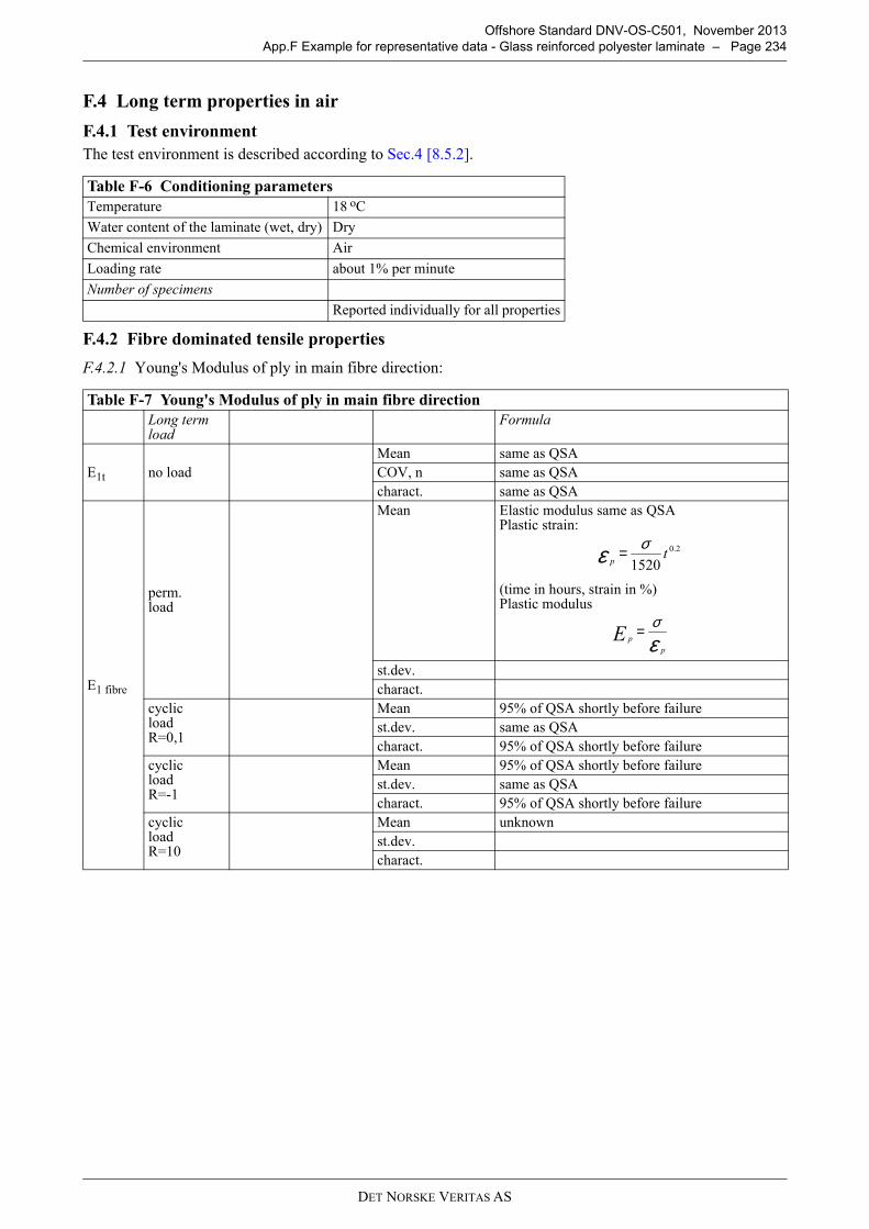
DET NORSKE VERITAS AS
Offshore Standard DNV-OS-C501, November 2013
App.F Example for representative data - Glass reinforced polyester laminate – Page 234
F.4 Long term properties in air
F.4.1 Test environment
The test environment is described according to Sec.4 [8.5.2].
F.4.2 Fibre dominated tensile properties
F.4.2.1 Young's Modulus of ply in main fibre direction:
Table F-6 Conditioning parameters
Temperature 18 oC
Water content of the laminate (wet, dry) Dry
Chemical environment Air
Loading rate about 1% per minute
Number of specimens
Reported individually for all properties
Table F-7 Young's Modulus of ply in main fibre direction
Long term load
Formula
E1t no load
Mean same as QSA
COV, n same as QSA
charact. same as QSA
E1 fibre
perm.load
Mean Elastic modulus same as QSAPlastic strain:
(time in hours, strain in %)Plastic modulus
st.dev.
charact.
cyclicloadR=0,1
Mean 95% of QSA shortly before failure
st.dev. same as QSA
charact. 95% of QSA shortly before failure
cyclicloadR=-1
Mean 95% of QSA shortly before failure
st.dev. same as QSA
charact. 95% of QSA shortly before failure
cyclicloadR=10
Mean unknown
st.dev.
charact.
2.0
1520t
p
σε =
εσ
p
pE =
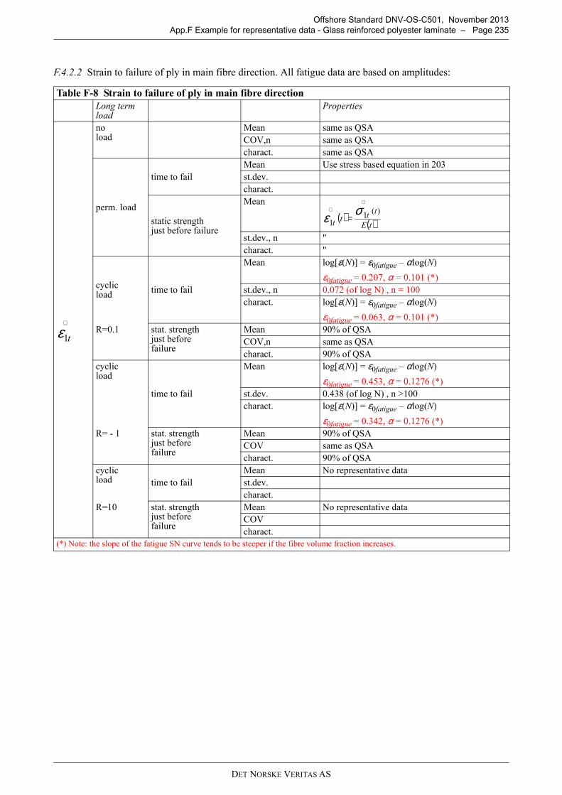
DET NORSKE VERITAS AS
Offshore Standard DNV-OS-C501, November 2013
App.F Example for representative data - Glass reinforced polyester laminate – Page 235
F.4.2.2 Strain to failure of ply in main fibre direction. All fatigue data are based on amplitudes:
Table F-8 Strain to failure of ply in main fibre direction
Long term load
Properties
noload
Mean same as QSA
COV,n same as QSA
charact. same as QSA
perm. load
time to fail
Mean Use stress based equation in 203
st.dev.
charact.
static strengthjust before failure
Mean
st.dev., n "
charact. "
cyclic load
time to fail
Mean log[ε(N)] = ε0fatigue – αlog(N)
ε0fatigue = 0.207, α = 0.101 (*)
st.dev., n 0.072 (of log N) , n = 100
charact. log[ε(N)] = ε0fatigue – αlog(N)
ε0fatigue = 0.063, α = 0.101 (*)
R=0.1 stat. strengthjust before failure
Mean 90% of QSA
COV,n same as QSA
charact. 90% of QSA
cyclicload
time to fail
Mean log[ε(N)] = ε0fatigue – αlog(N)
ε0fatigue = 0.453, α = 0.1276 (*)
st.dev. 0.438 (of log N) , n >100
charact. log[ε(N)] = ε0fatigue – αlog(N)
ε0fatigue = 0.342, α = 0.1276 (*)
R= - 1 stat. strengthjust beforefailure
Mean 90% of QSA
COV same as QSA
charact. 90% of QSA
cyclicload time to fail
Mean No representative data
st.dev.
charact.
R=10 stat. strengthjust beforefailure
Mean No representative data
COV
charact.
(*) Note: the slope of the fatigue SN curve tends to be steeper if the fibre volume fraction increases.
t1ε∧
( ) ( )tE
ttt
t
)(1
1
σε∧
∧
=
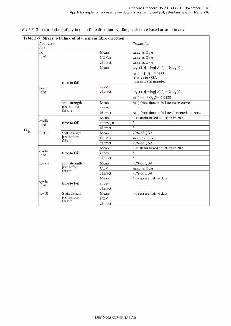
DET NORSKE VERITAS AS
Offshore Standard DNV-OS-C501, November 2013
App.F Example for representative data - Glass reinforced polyester laminate – Page 236
F.4.2.3 Stress to failure of ply in main fibre direction. All fatigue data are based on amplitudes:
Table F-9 Stress to failure of ply in main fibre direction
Long term load
Properties
noload
Mean same as QSA
COV,n same as QSA
charact. same as QSA
perm.load
time to fail
Mean log[σ(t)] = log[σ(1)] – β log(t)
σ(1) = 1, β = 0.0423relative to QSAtime scale in minutes
st.dev.
charact. log[σ(t)] = log[σ(1)] – β log(t)
σ(1) = 0.888, β = 0.0423
stat. strengthjust beforefailure
Mean σ(1) from time to failure mean curve
st.dev.
charact. σ(1) from time to failure characteristic curve
cyclicload
time to fail
Mean Use strain based equation in 202
st.dev., n "
charact. "
R=0.1 Stat.strengthjust beforefailure
Mean 90% of QSA
COV,n same as QSA
charact. 90% of QSA
cyclicload
time to fail
Mean Use strain based equation in 202
st.dev. "
charact. "
R= - 1 stat. strengthjust beforefailure
Mean 90% of QSA
COV same as QSA
charact. 90% of QSA
cyclicload
time to fail
Mean No representative data
st.dev.
charact.
R=10 Stat.strengthjust beforefailure
Mean No representative data
COV
charact.
t1σ∧
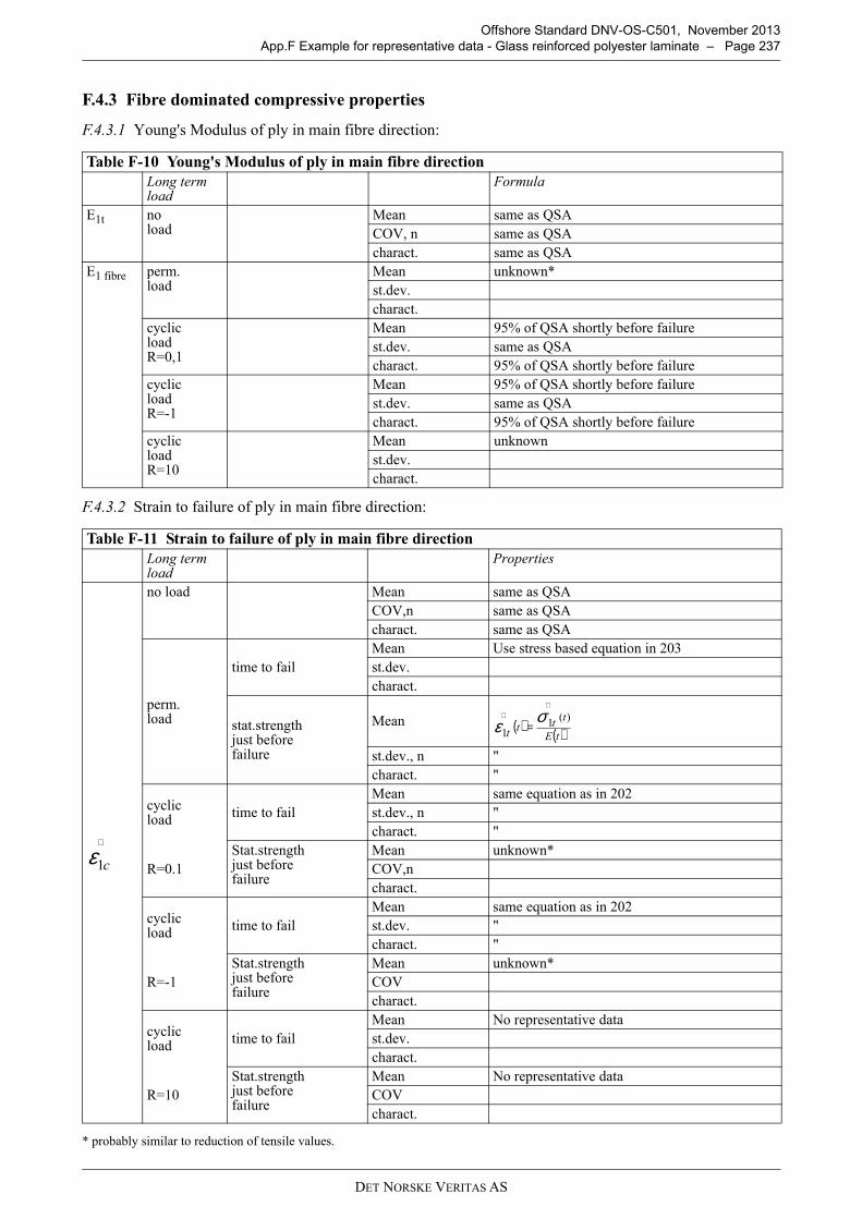
DET NORSKE VERITAS AS
Offshore Standard DNV-OS-C501, November 2013
App.F Example for representative data - Glass reinforced polyester laminate – Page 237
F.4.3 Fibre dominated compressive properties
F.4.3.1 Young's Modulus of ply in main fibre direction:
F.4.3.2 Strain to failure of ply in main fibre direction:
* probably similar to reduction of tensile values.
Table F-10 Young's Modulus of ply in main fibre direction
Long term load
Formula
E1t noload
Mean same as QSA
COV, n same as QSA
charact. same as QSA
E1 fibre perm.load
Mean unknown*
st.dev.
charact.
cyclicloadR=0,1
Mean 95% of QSA shortly before failure
st.dev. same as QSA
charact. 95% of QSA shortly before failure
cyclicloadR=-1
Mean 95% of QSA shortly before failure
st.dev. same as QSA
charact. 95% of QSA shortly before failure
cyclicloadR=10
Mean unknown
st.dev.
charact.
Table F-11 Strain to failure of ply in main fibre direction
Long term load
Properties
no load Mean same as QSA
COV,n same as QSA
charact. same as QSA
perm.load
time to fail
Mean Use stress based equation in 203
st.dev.
charact.
stat.strengthjust beforefailure
Mean
st.dev., n "
charact. "
cyclicload
time to fail
Mean same equation as in 202
st.dev., n "
charact. "
R=0.1
Stat.strengthjust beforefailure
Mean unknown*
COV,n
charact.
cyclicload
time to fail
Mean same equation as in 202
st.dev. "
charact. "
R=-1
Stat.strengthjust beforefailure
Mean unknown*
COV
charact.
cyclicload
time to fail
Mean No representative data
st.dev.
charact.
R=10
Stat.strengthjust beforefailure
Mean No representative data
COV
charact.
c1ε∧
( ) ( )tE
ttt
t
)(1
1
σε∧
∧
=
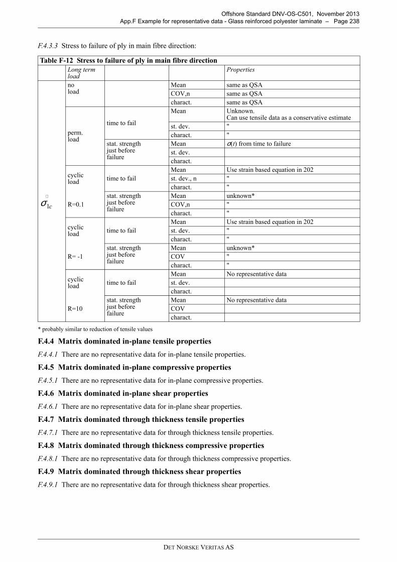
DET NORSKE VERITAS AS
Offshore Standard DNV-OS-C501, November 2013
App.F Example for representative data - Glass reinforced polyester laminate – Page 238
F.4.3.3 Stress to failure of ply in main fibre direction:
* probably similar to reduction of tensile values
F.4.4 Matrix dominated in-plane tensile properties
F.4.4.1 There are no representative data for in-plane tensile properties.
F.4.5 Matrix dominated in-plane compressive properties
F.4.5.1 There are no representative data for in-plane compressive properties.
F.4.6 Matrix dominated in-plane shear properties
F.4.6.1 There are no representative data for in-plane shear properties.
F.4.7 Matrix dominated through thickness tensile properties
F.4.7.1 There are no representative data for through thickness tensile properties.
F.4.8 Matrix dominated through thickness compressive properties
F.4.8.1 There are no representative data for through thickness compressive properties.
F.4.9 Matrix dominated through thickness shear properties
F.4.9.1 There are no representative data for through thickness shear properties.
Table F-12 Stress to failure of ply in main fibre direction
Long term load
Properties
noload
Mean same as QSA
COV,n same as QSA
charact. same as QSA
perm.load
time to fail
Mean Unknown.Can use tensile data as a conservative estimate
st. dev. "
charact. "
stat. strengthjust beforefailure
Mean σ(t) from time to failure
st. dev.
charact.
cyclicload
time to fail
Mean Use strain based equation in 202
st. dev., n "
charact. "
R=0.1
stat. strengthjust beforefailure
Mean unknown*
COV,n "
charact. "
cyclicload
time to fail
Mean Use strain based equation in 202
st. dev. "
charact. "
R= -1
stat. strengthjust beforefailure
Mean unknown*
COV "
charact. "
cyclicload
time to fail
Mean No representative data
st. dev.
charact.
R=10
stat. strengthjust beforefailure
Mean No representative data
COV
charact.
c1σ∧
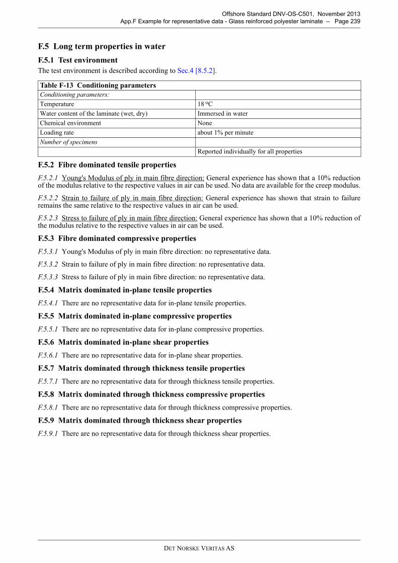
DET NORSKE VERITAS AS
Offshore Standard DNV-OS-C501, November 2013
App.F Example for representative data - Glass reinforced polyester laminate – Page 239
F.5 Long term properties in water
F.5.1 Test environment
The test environment is described according to Sec.4 [8.5.2].
F.5.2 Fibre dominated tensile properties
F.5.2.1 Young's Modulus of ply in main fibre direction: General experience has shown that a 10% reductionof the modulus relative to the respective values in air can be used. No data are available for the creep modulus.
F.5.2.2 Strain to failure of ply in main fibre direction: General experience has shown that strain to failureremains the same relative to the respective values in air can be used.
F.5.2.3 Stress to failure of ply in main fibre direction: General experience has shown that a 10% reduction ofthe modulus relative to the respective values in air can be used.
F.5.3 Fibre dominated compressive properties
F.5.3.1 Young's Modulus of ply in main fibre direction: no representative data.
F.5.3.2 Strain to failure of ply in main fibre direction: no representative data.
F.5.3.3 Stress to failure of ply in main fibre direction: no representative data.
F.5.4 Matrix dominated in-plane tensile properties
F.5.4.1 There are no representative data for in-plane tensile properties.
F.5.5 Matrix dominated in-plane compressive properties
F.5.5.1 There are no representative data for in-plane compressive properties.
F.5.6 Matrix dominated in-plane shear properties
F.5.6.1 There are no representative data for in-plane shear properties.
F.5.7 Matrix dominated through thickness tensile properties
F.5.7.1 There are no representative data for through thickness tensile properties.
F.5.8 Matrix dominated through thickness compressive properties
F.5.8.1 There are no representative data for through thickness compressive properties.
F.5.9 Matrix dominated through thickness shear properties
F.5.9.1 There are no representative data for through thickness shear properties.
Table F-13 Conditioning parameters
Conditioning parameters:
Temperature 18 oC
Water content of the laminate (wet, dry) Immersed in water
Chemical environment None
Loading rate about 1% per minute
Number of specimens
Reported individually for all properties
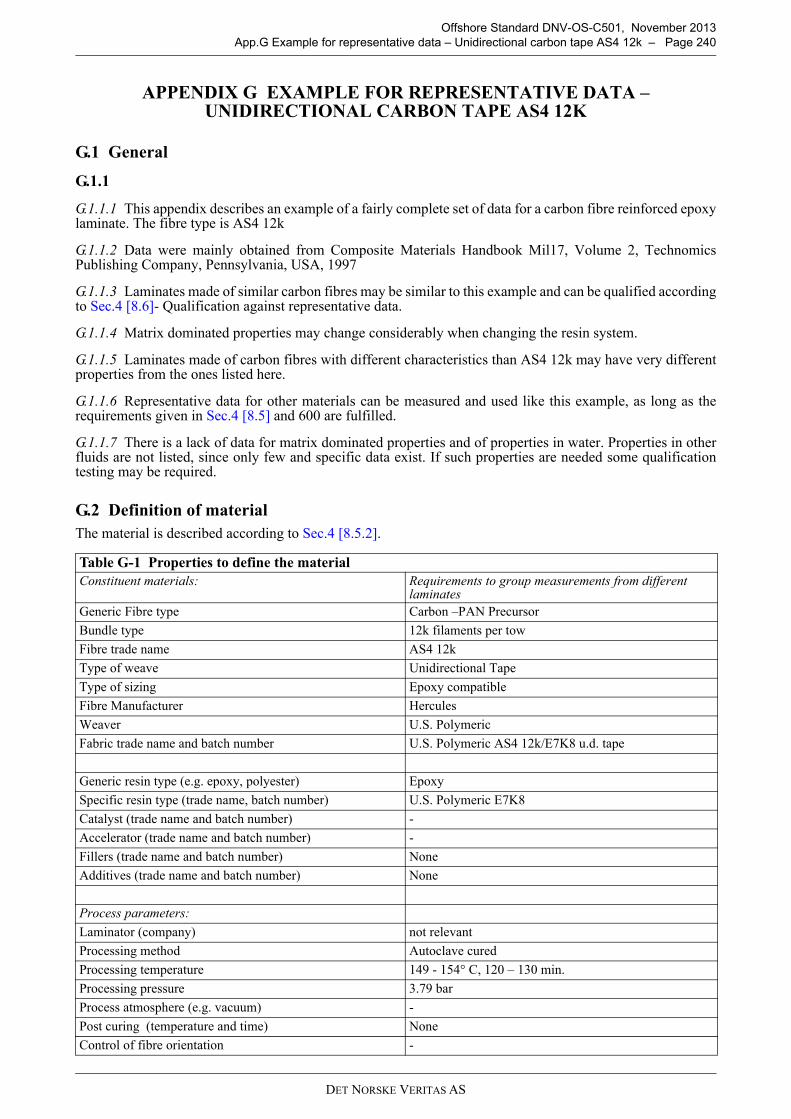
DET NORSKE VERITAS AS
Offshore Standard DNV-OS-C501, November 2013
App.G Example for representative data – Unidirectional carbon tape AS4 12k – Page 240
APPENDIX G EXAMPLE FOR REPRESENTATIVE DATA – UNIDIRECTIONAL CARBON TAPE AS4 12K
G.1 General
G.1.1
G.1.1.1 This appendix describes an example of a fairly complete set of data for a carbon fibre reinforced epoxylaminate. The fibre type is AS4 12k
G.1.1.2 Data were mainly obtained from Composite Materials Handbook Mil17, Volume 2, TechnomicsPublishing Company, Pennsylvania, USA, 1997
G.1.1.3 Laminates made of similar carbon fibres may be similar to this example and can be qualified accordingto Sec.4 [8.6]- Qualification against representative data.
G.1.1.4 Matrix dominated properties may change considerably when changing the resin system.
G.1.1.5 Laminates made of carbon fibres with different characteristics than AS4 12k may have very differentproperties from the ones listed here.
G.1.1.6 Representative data for other materials can be measured and used like this example, as long as therequirements given in Sec.4 [8.5] and 600 are fulfilled.
G.1.1.7 There is a lack of data for matrix dominated properties and of properties in water. Properties in otherfluids are not listed, since only few and specific data exist. If such properties are needed some qualificationtesting may be required.
G.2 Definition of material
The material is described according to Sec.4 [8.5.2].
Table G-1 Properties to define the material
Constituent materials: Requirements to group measurements from different laminates
Generic Fibre type Carbon –PAN Precursor
Bundle type 12k filaments per tow
Fibre trade name AS4 12k
Type of weave Unidirectional Tape
Type of sizing Epoxy compatible
Fibre Manufacturer Hercules
Weaver U.S. Polymeric
Fabric trade name and batch number U.S. Polymeric AS4 12k/E7K8 u.d. tape
Generic resin type (e.g. epoxy, polyester) Epoxy
Specific resin type (trade name, batch number) U.S. Polymeric E7K8
Catalyst (trade name and batch number) -
Accelerator (trade name and batch number) -
Fillers (trade name and batch number) None
Additives (trade name and batch number) None
Process parameters:
Laminator (company) not relevant
Processing method Autoclave cured
Processing temperature 149 - 154° C, 120 – 130 min.
Processing pressure 3.79 bar
Process atmosphere (e.g. vacuum) -
Post curing (temperature and time) None
Control of fibre orientation -
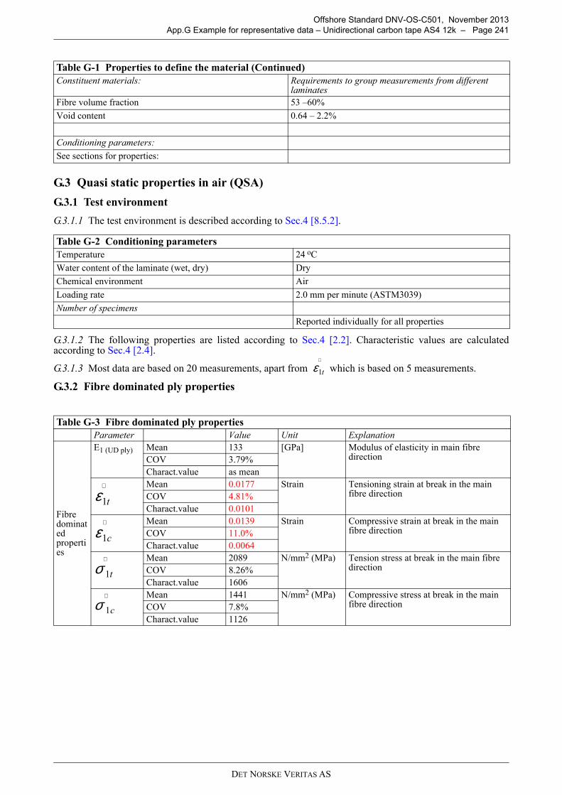
DET NORSKE VERITAS AS
Offshore Standard DNV-OS-C501, November 2013
App.G Example for representative data – Unidirectional carbon tape AS4 12k – Page 241
G.3 Quasi static properties in air (QSA)
G.3.1 Test environment
G.3.1.1 The test environment is described according to Sec.4 [8.5.2].
G.3.1.2 The following properties are listed according to Sec.4 [2.2]. Characteristic values are calculatedaccording to Sec.4 [2.4].
G.3.1.3 Most data are based on 20 measurements, apart from which is based on 5 measurements.
G.3.2 Fibre dominated ply properties
Fibre volume fraction 53 –60%
Void content 0.64 – 2.2%
Conditioning parameters:
See sections for properties:
Table G-2 Conditioning parameters
Temperature 24 oC
Water content of the laminate (wet, dry) Dry
Chemical environment Air
Loading rate 2.0 mm per minute (ASTM3039)
Number of specimens
Reported individually for all properties
Table G-3 Fibre dominated ply properties
Parameter Value Unit Explanation
Fibre dominated properties
E1 (UD ply) Mean 133 [GPa] Modulus of elasticity in main fibre direction COV 3.79%
Charact.value as mean
Mean 0.0177 Strain Tensioning strain at break in the main fibre directionCOV 4.81%
Charact.value 0.0101
Mean 0.0139 Strain Compressive strain at break in the main fibre directionCOV 11.0%
Charact.value 0.0064
Mean 2089 N/mm2 (MPa) Tension stress at break in the main fibre direction COV 8.26%
Charact.value 1606
Mean 1441 N/mm2 (MPa) Compressive stress at break in the main fibre directionCOV 7.8%
Charact.value 1126
Table G-1 Properties to define the material (Continued)
Constituent materials: Requirements to group measurements from different laminates
t1ε∧
t1ε∧
c1ε∧
t1σ∧
c1σ∧
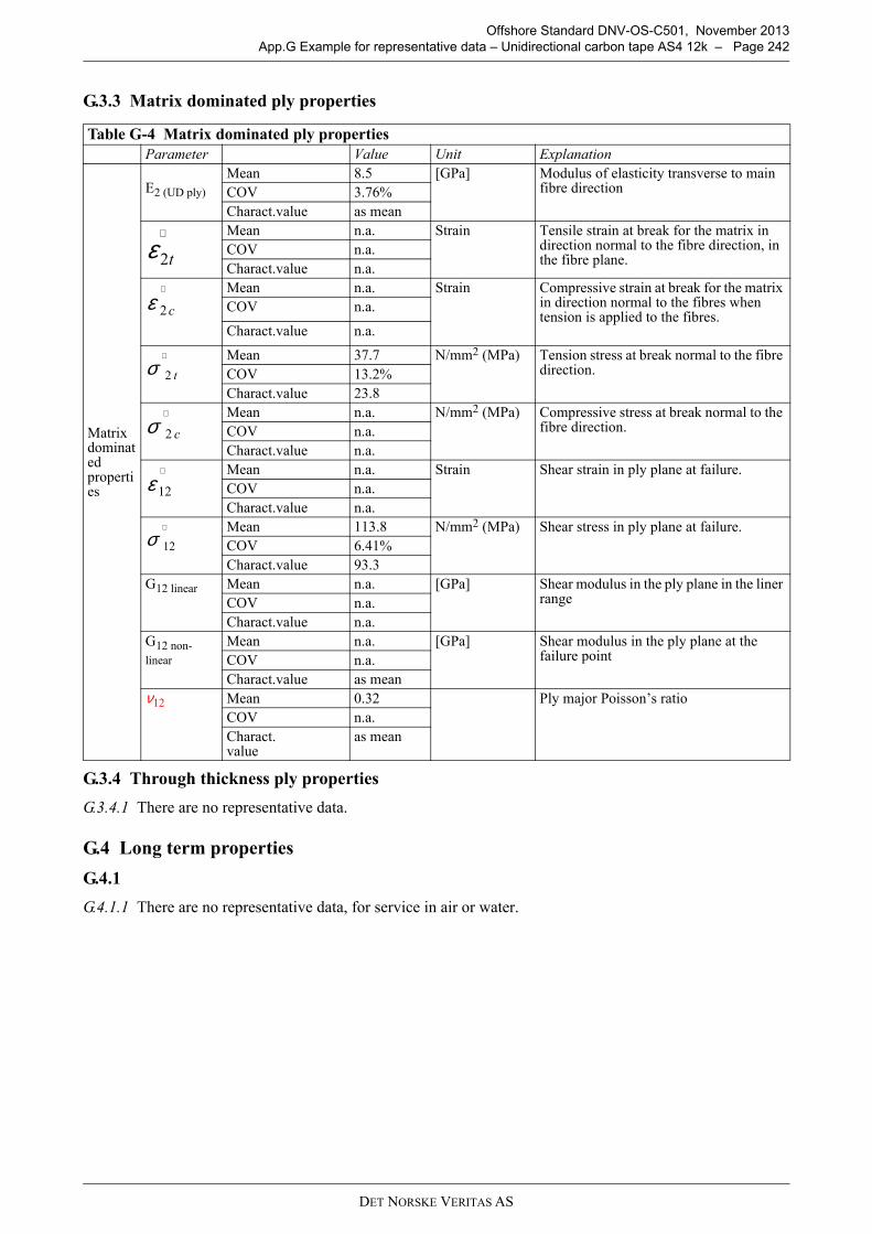
DET NORSKE VERITAS AS
Offshore Standard DNV-OS-C501, November 2013
App.G Example for representative data – Unidirectional carbon tape AS4 12k – Page 242
G.3.3 Matrix dominated ply properties
G.3.4 Through thickness ply properties
G.3.4.1 There are no representative data.
G.4 Long term properties
G.4.1
G.4.1.1 There are no representative data, for service in air or water.
Table G-4 Matrix dominated ply properties
Parameter Value Unit Explanation
Matrix dominated properties
E2 (UD ply)
Mean 8.5 [GPa] Modulus of elasticity transverse to main fibre direction COV 3.76%
Charact.value as mean
Mean n.a. Strain Tensile strain at break for the matrix in direction normal to the fibre direction, in the fibre plane.
COV n.a.
Charact.value n.a.
Mean n.a. Strain Compressive strain at break for the matrix in direction normal to the fibres when tension is applied to the fibres.
COV n.a.
Charact.value n.a.
Mean 37.7 N/mm2 (MPa) Tension stress at break normal to the fibre direction.COV 13.2%
Charact.value 23.8
Mean n.a. N/mm2 (MPa) Compressive stress at break normal to the fibre direction.COV n.a.
Charact.value n.a.
Mean n.a. Strain Shear strain in ply plane at failure.
COV n.a.
Charact.value n.a.
Mean 113.8 N/mm2 (MPa) Shear stress in ply plane at failure.
COV 6.41%
Charact.value 93.3
G12 linear Mean n.a. [GPa] Shear modulus in the ply plane in the liner rangeCOV n.a.
Charact.value n.a.
G12 non-
linear
Mean n.a. [GPa] Shear modulus in the ply plane at the failure pointCOV n.a.
Charact.value as mean
ν12 Mean 0.32 Ply major Poisson’s ratio
COV n.a.
Charact.value
as mean
t2ε∧
c2ε∧
t2σ∧
c2σ∧
12ε∧
12σ∧
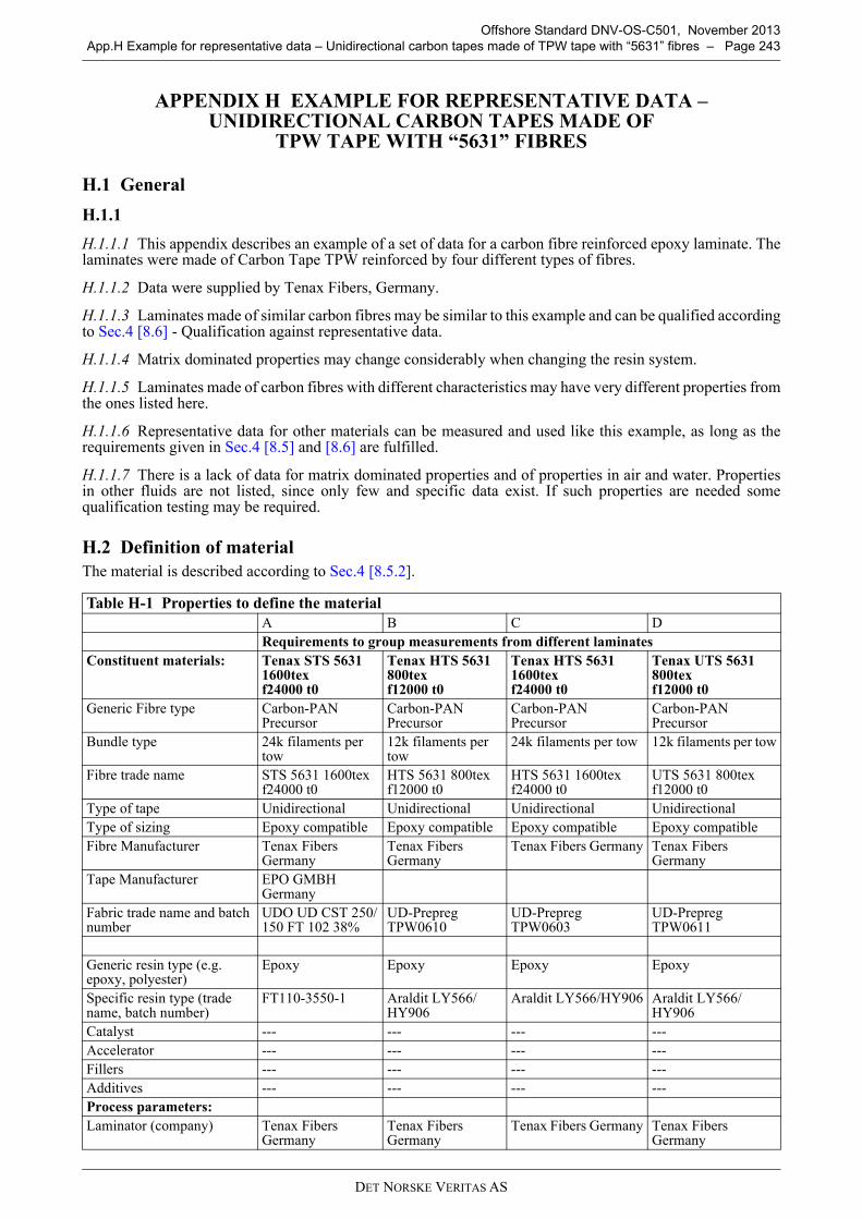
DET NORSKE VERITAS AS
Offshore Standard DNV-OS-C501, November 2013
App.H Example for representative data – Unidirectional carbon tapes made of TPW tape with “5631” fibres – Page 243
APPENDIX H EXAMPLE FOR REPRESENTATIVE DATA –UNIDIRECTIONAL CARBON TAPES MADE OF
TPW TAPE WITH “5631” FIBRES
H.1 General
H.1.1
H.1.1.1 This appendix describes an example of a set of data for a carbon fibre reinforced epoxy laminate. Thelaminates were made of Carbon Tape TPW reinforced by four different types of fibres.
H.1.1.2 Data were supplied by Tenax Fibers, Germany.
H.1.1.3 Laminates made of similar carbon fibres may be similar to this example and can be qualified accordingto Sec.4 [8.6] - Qualification against representative data.
H.1.1.4 Matrix dominated properties may change considerably when changing the resin system.
H.1.1.5 Laminates made of carbon fibres with different characteristics may have very different properties fromthe ones listed here.
H.1.1.6 Representative data for other materials can be measured and used like this example, as long as therequirements given in Sec.4 [8.5] and [8.6] are fulfilled.
H.1.1.7 There is a lack of data for matrix dominated properties and of properties in air and water. Propertiesin other fluids are not listed, since only few and specific data exist. If such properties are needed somequalification testing may be required.
H.2 Definition of material
The material is described according to Sec.4 [8.5.2].
Table H-1 Properties to define the material
A B C D
Requirements to group measurements from different laminates
Constituent materials: Tenax STS 56311600texf24000 t0
Tenax HTS 5631800texf12000 t0
Tenax HTS 56311600texf24000 t0
Tenax UTS 5631800texf12000 t0
Generic Fibre type Carbon-PAN Precursor
Carbon-PAN Precursor
Carbon-PAN Precursor
Carbon-PAN Precursor
Bundle type 24k filaments per tow
12k filaments per tow
24k filaments per tow 12k filaments per tow
Fibre trade name STS 5631 1600tex f24000 t0
HTS 5631 800texf12000 t0
HTS 5631 1600tex f24000 t0
UTS 5631 800texf12000 t0
Type of tape Unidirectional Unidirectional Unidirectional Unidirectional
Type of sizing Epoxy compatible Epoxy compatible Epoxy compatible Epoxy compatible
Fibre Manufacturer Tenax Fibers Germany
Tenax Fibers Germany
Tenax Fibers Germany Tenax Fibers Germany
Tape Manufacturer EPO GMBH Germany
Fabric trade name and batch number
UDO UD CST 250/150 FT 102 38%
UD-Prepreg TPW0610
UD-Prepreg TPW0603
UD-Prepreg TPW0611
Generic resin type (e.g. epoxy, polyester)
Epoxy Epoxy Epoxy Epoxy
Specific resin type (trade name, batch number)
FT110-3550-1 Araldit LY566/HY906
Araldit LY566/HY906 Araldit LY566/HY906
Catalyst --- --- --- ---
Accelerator --- --- --- ---
Fillers --- --- --- ---
Additives --- --- --- ---
Process parameters:
Laminator (company) Tenax Fibers Germany
Tenax Fibers Germany
Tenax Fibers Germany Tenax Fibers Germany
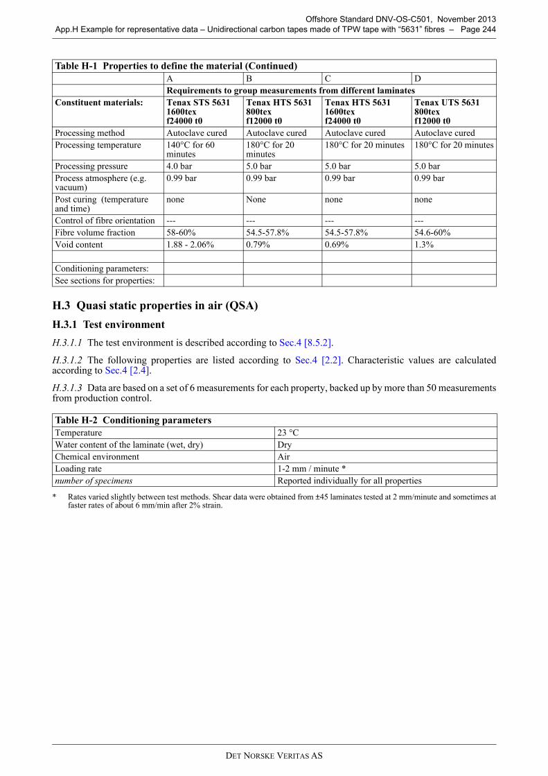
DET NORSKE VERITAS AS
Offshore Standard DNV-OS-C501, November 2013
App.H Example for representative data – Unidirectional carbon tapes made of TPW tape with “5631” fibres – Page 244
H.3 Quasi static properties in air (QSA)
H.3.1 Test environment
H.3.1.1 The test environment is described according to Sec.4 [8.5.2].
H.3.1.2 The following properties are listed according to Sec.4 [2.2]. Characteristic values are calculatedaccording to Sec.4 [2.4].
H.3.1.3 Data are based on a set of 6 measurements for each property, backed up by more than 50 measurementsfrom production control.
* Rates varied slightly between test methods. Shear data were obtained from ±45 laminates tested at 2 mm/minute and sometimes atfaster rates of about 6 mm/min after 2% strain.
Processing method Autoclave cured Autoclave cured Autoclave cured Autoclave cured
Processing temperature 140°C for 60 minutes
180°C for 20 minutes
180°C for 20 minutes 180°C for 20 minutes
Processing pressure 4.0 bar 5.0 bar 5.0 bar 5.0 bar
Process atmosphere (e.g. vacuum)
0.99 bar 0.99 bar 0.99 bar 0.99 bar
Post curing (temperature and time)
none None none none
Control of fibre orientation --- --- --- ---
Fibre volume fraction 58-60% 54.5-57.8% 54.5-57.8% 54.6-60%
Void content 1.88 - 2.06% 0.79% 0.69% 1.3%
Conditioning parameters:
See sections for properties:
Table H-2 Conditioning parameters
Temperature 23 °C
Water content of the laminate (wet, dry) Dry
Chemical environment Air
Loading rate 1-2 mm / minute *
number of specimens Reported individually for all properties
Table H-1 Properties to define the material (Continued)
A B C D
Requirements to group measurements from different laminates
Constituent materials: Tenax STS 56311600texf24000 t0
Tenax HTS 5631800texf12000 t0
Tenax HTS 56311600texf24000 t0
Tenax UTS 5631800texf12000 t0
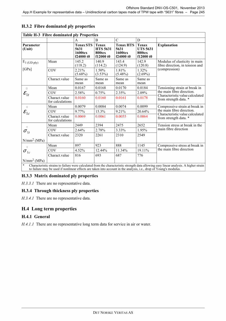
DET NORSKE VERITAS AS
Offshore Standard DNV-OS-C501, November 2013
App.H Example for representative data – Unidirectional carbon tapes made of TPW tape with “5631” fibres – Page 245
H.3.2 Fibre dominated ply properties
H.3.3 Matrix dominated ply properties
H.3.3.1 There are no representative data.
H.3.4 Through thickness ply properties
H.3.4.1 There are no representative data.
H.4 Long term properties
H.4.1 General
H.4.1.1 There are no representative long term data for service in air or water.
Table H-3 Fibre dominated ply Properties
A B C D
Parameter(Unit)
Tenax STS 56311600texf24000 t0
Tenax HTS 5631800texf12000 t0
Tenax HTS 56311600texf24000 t0
Tenax UTS 5631800texf12000 t0
Explanation
E1 (UD ply)
[GPa]
Mean 145.2(118.2)
140.9(114.2)
143.4(124.9)
142.9(120.8)
Modulus of elasticity in main fibre direction, in tension and (compression)COV 2.21%
(5.68%)1.50%(3.53%)
1.81%(5.48%)
1.32%(2.69%)
Charact.value Same as mean
Same as mean
Same as mean
Same as mean
Mean 0.0167 0.0168 0.0170 0.0184 Tensioning strain at break in the main fibre direction.Characteristic value calculated from strength data. *
COV 2.58% 0.75% 2.35% 2.09%
Charact.valuefor calculations
0.0160 0.0160 0.0161 0.0178
Mean 0.0079 0.0084 0.0074 0.0099 Compressive strain at break in the main fibre direction.Characteristic value calculated from strength data. *
COV 9.77% 15.3% 9.21% 20.64%
Charact.valuefor calculations
0.0069 0.0061 0.0055 0.0064
N/mm2 (MPa)
Mean 2449 2394 2475 2652 Tension stress at break in the main fibre direction COV 2.64% 2.78% 3.33% 1.95%
Charact.value 2320 2261 2310 2549
N/mm2 (MPa)
Mean 897 923 888 1145 Compressive stress at break in the main fibre directionCOV 4.52% 12.44% 11.34% 19.11%
Charact.value 816 693 687 776
* Characteristic strains to failure were calculated from the characteristic strength data allowing easy linear analysis. A higher strainto failure may be used if nonlinear effects are taken into account in the analysis, i.e., drop of Young's modulus.
t1ε∧
c1ε∧
t1σ∧
c1σ∧
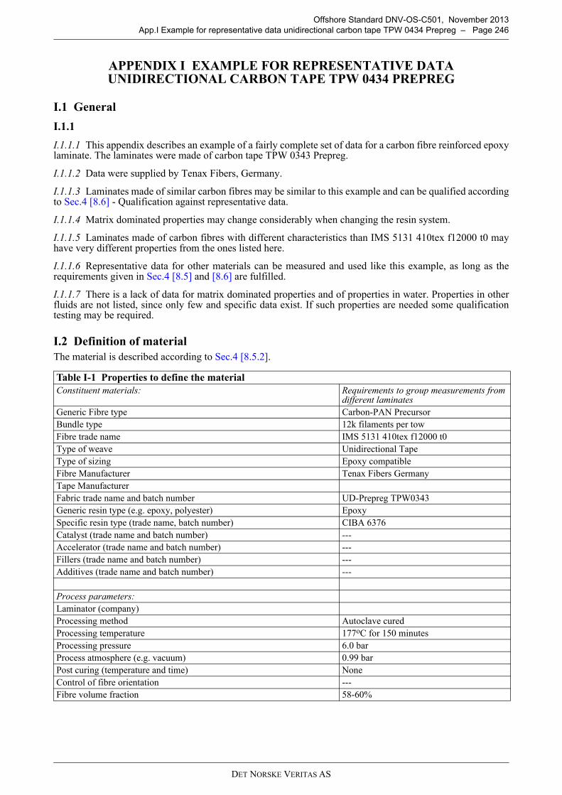
DET NORSKE VERITAS AS
Offshore Standard DNV-OS-C501, November 2013
App.I Example for representative data unidirectional carbon tape TPW 0434 Prepreg – Page 246
APPENDIX I EXAMPLE FOR REPRESENTATIVE DATA UNIDIRECTIONAL CARBON TAPE TPW 0434 PREPREG
I.1 General
I.1.1
I.1.1.1 This appendix describes an example of a fairly complete set of data for a carbon fibre reinforced epoxylaminate. The laminates were made of carbon tape TPW 0343 Prepreg.
I.1.1.2 Data were supplied by Tenax Fibers, Germany.
I.1.1.3 Laminates made of similar carbon fibres may be similar to this example and can be qualified accordingto Sec.4 [8.6] - Qualification against representative data.
I.1.1.4 Matrix dominated properties may change considerably when changing the resin system.
I.1.1.5 Laminates made of carbon fibres with different characteristics than IMS 5131 410tex f12000 t0 mayhave very different properties from the ones listed here.
I.1.1.6 Representative data for other materials can be measured and used like this example, as long as therequirements given in Sec.4 [8.5] and [8.6] are fulfilled.
I.1.1.7 There is a lack of data for matrix dominated properties and of properties in water. Properties in otherfluids are not listed, since only few and specific data exist. If such properties are needed some qualificationtesting may be required.
I.2 Definition of material
The material is described according to Sec.4 [8.5.2].
Table I-1 Properties to define the material
Constituent materials: Requirements to group measurements from different laminates
Generic Fibre type Carbon-PAN Precursor
Bundle type 12k filaments per tow
Fibre trade name IMS 5131 410tex f12000 t0
Type of weave Unidirectional Tape
Type of sizing Epoxy compatible
Fibre Manufacturer Tenax Fibers Germany
Tape Manufacturer
Fabric trade name and batch number UD-Prepreg TPW0343
Generic resin type (e.g. epoxy, polyester) Epoxy
Specific resin type (trade name, batch number) CIBA 6376
Catalyst (trade name and batch number) ---
Accelerator (trade name and batch number) ---
Fillers (trade name and batch number) ---
Additives (trade name and batch number) ---
Process parameters:
Laminator (company)
Processing method Autoclave cured
Processing temperature 177oC for 150 minutes
Processing pressure 6.0 bar
Process atmosphere (e.g. vacuum) 0.99 bar
Post curing (temperature and time) None
Control of fibre orientation ---
Fibre volume fraction 58-60%
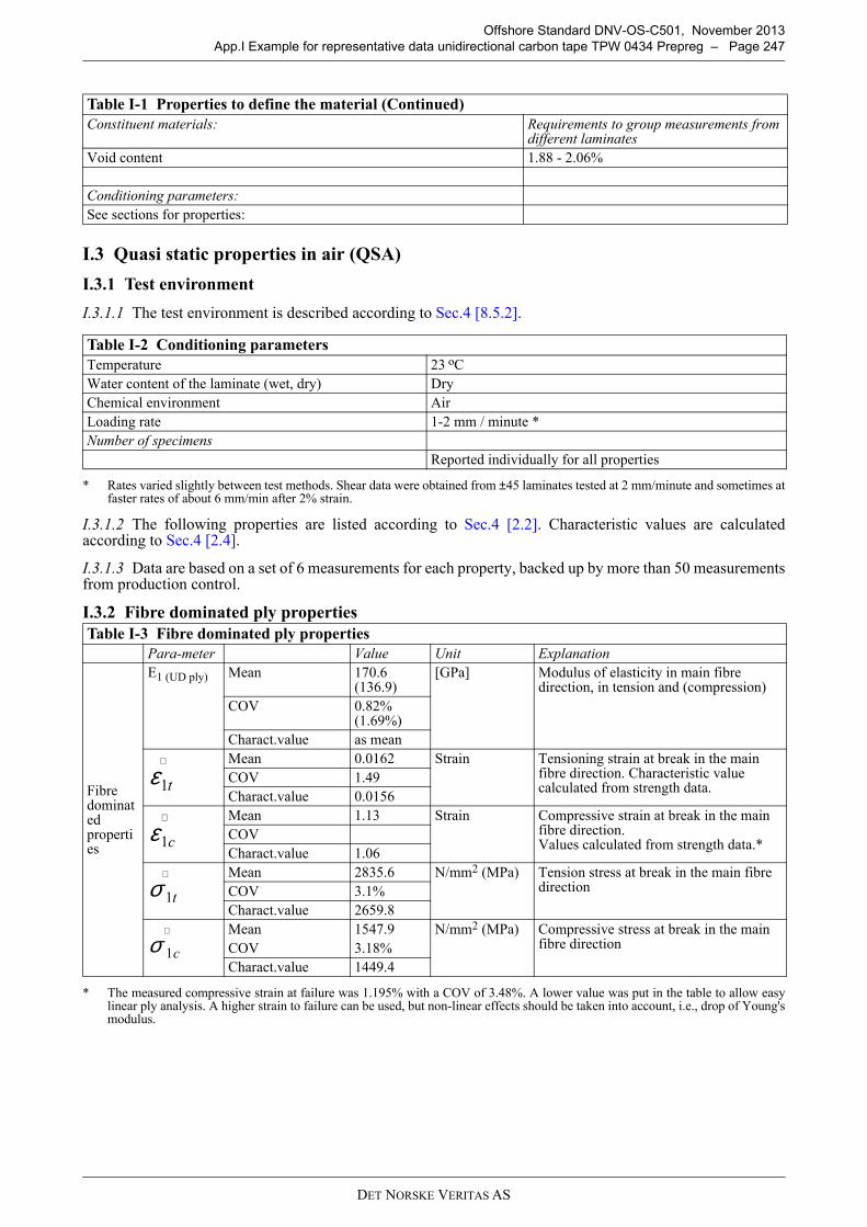
DET NORSKE VERITAS AS
Offshore Standard DNV-OS-C501, November 2013
App.I Example for representative data unidirectional carbon tape TPW 0434 Prepreg – Page 247
I.3 Quasi static properties in air (QSA)
I.3.1 Test environment
I.3.1.1 The test environment is described according to Sec.4 [8.5.2].
* Rates varied slightly between test methods. Shear data were obtained from ±45 laminates tested at 2 mm/minute and sometimes atfaster rates of about 6 mm/min after 2% strain.
I.3.1.2 The following properties are listed according to Sec.4 [2.2]. Characteristic values are calculatedaccording to Sec.4 [2.4].
I.3.1.3 Data are based on a set of 6 measurements for each property, backed up by more than 50 measurementsfrom production control.
I.3.2 Fibre dominated ply properties
* The measured compressive strain at failure was 1.195% with a COV of 3.48%. A lower value was put in the table to allow easylinear ply analysis. A higher strain to failure can be used, but non-linear effects should be taken into account, i.e., drop of Young'smodulus.
Void content 1.88 - 2.06%
Conditioning parameters:
See sections for properties:
Table I-2 Conditioning parameters
Temperature 23 oC
Water content of the laminate (wet, dry) Dry
Chemical environment Air
Loading rate 1-2 mm / minute *
Number of specimens
Reported individually for all properties
Table I-3 Fibre dominated ply properties
Para-meter Value Unit Explanation
Fibre dominated properties
E1 (UD ply) Mean 170.6(136.9)
[GPa] Modulus of elasticity in main fibre direction, in tension and (compression)
COV 0.82%(1.69%)
Charact.value as mean
Mean 0.0162 Strain Tensioning strain at break in the main fibre direction. Characteristic value calculated from strength data.
COV 1.49
Charact.value 0.0156
Mean 1.13 Strain Compressive strain at break in the main fibre direction.Values calculated from strength data.*
COV
Charact.value 1.06
Mean 2835.6 N/mm2 (MPa) Tension stress at break in the main fibre direction COV 3.1%
Charact.value 2659.8
Mean 1547.9 N/mm2 (MPa) Compressive stress at break in the main fibre directionCOV 3.18%
Charact.value 1449.4
Table I-1 Properties to define the material (Continued)
Constituent materials: Requirements to group measurements from different laminates
t1ε∧
c1ε∧
t1σ∧
c1σ∧
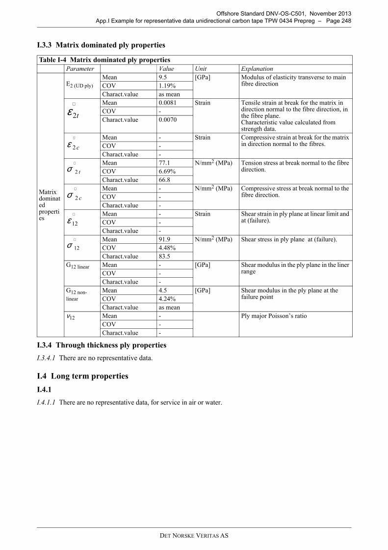
DET NORSKE VERITAS AS
Offshore Standard DNV-OS-C501, November 2013
App.I Example for representative data unidirectional carbon tape TPW 0434 Prepreg – Page 248
I.3.3 Matrix dominated ply properties
I.3.4 Through thickness ply properties
I.3.4.1 There are no representative data.
I.4 Long term properties
I.4.1
I.4.1.1 There are no representative data, for service in air or water.
Table I-4 Matrix dominated ply properties
Parameter Value Unit Explanation
Matrix dominated properties
E2 (UD ply)
Mean 9.5 [GPa] Modulus of elasticity transverse to main fibre direction COV 1.19%
Charact.value as mean
Mean 0.0081 Strain Tensile strain at break for the matrix in direction normal to the fibre direction, in the fibre plane.Characteristic value calculated from strength data.
COV -
Charact.value 0.0070
Mean - Strain Compressive strain at break for the matrix in direction normal to the fibres.COV -
Charact.value -
Mean 77.1 N/mm2 (MPa) Tension stress at break normal to the fibre direction.COV 6.69%
Charact.value 66.8
Mean - N/mm2 (MPa) Compressive stress at break normal to the fibre direction.COV -
Charact.value -
Mean - Strain Shear strain in ply plane at linear limit and at (failure).COV -
Charact.value -
Mean 91.9 N/mm2 (MPa) Shear stress in ply plane at (failure).
COV 4.48%
Charact.value 83.5
G12 linear Mean - [GPa] Shear modulus in the ply plane in the liner rangeCOV -
Charact.value -
G12 non-
linear
Mean 4.5 [GPa] Shear modulus in the ply plane at the failure pointCOV 4.24%
Charact.value as mean
ν12 Mean - Ply major Poisson’s ratio
COV -
Charact.value -
t2ε∧
c2ε∧
t2σ∧
c2σ∧
12ε∧
12σ∧
DET NORSKE VERITAS AS
Offshore Standard DNV-OS-C501, November 2013
App.J Method of estimation of characteristic strength – Page 249
APPENDIX J METHOD OF ESTIMATION OF CHARACTERISTIC STRENGTH
The characteristic strength is defined as the 2.5% quantile in the strength distribution. The method forestimating the characteristic strength is based on requiring the level of safety given in this standard to be metregardless of the number of available strength test data. Tabulated values of km in Table 4-3, Table 4-4 andTable 4-5 in Sec.4 have been derived such that the confidence levels at which the characteristic strength inSec.4 [2.4.5] is estimated, ensure that the same target reliability level is achieved. This level is achievedregardless of the available number of results from material testing or testing of components. It is noted that thenecessary confidence level to achieve this varies with the number of available test results.
The km values have been obtained based on the results from probability analyses in which the reliability levelis calculated for the case that a limited number of data for the strength is available and for the case that there isperfect knowledge of the strength (i.e. when an infinite number of test results would be available). km has beenobtained by adjusting the value of the characteristic strength for the case with a limited number of tests resultssuch that the reliability level comes out the same as for the case with perfect knowledge.
The method of analysis is described in:
— Ronold, K. and Lotsberg, I.: On the Estimation of Characteristic S-N curves with Confidence. MarineStructures, vol. 27, 2012, pp. 29-44.
DET NORSKE VERITAS AS
Offshore Standard DNV-OS-C501, November 2013
CHANGES – HISTORIC – Page 250
CHANGES – HISTORIC
Note that historic changes older than the editions shown below have not been included. Older historic changes(if any) may be retrieved through http://www.dnv.com.
October 2010 edition
MOTIVES
No design code for Fibre Reinforced Plastic, often called composite structures, exists today except for somespecial applications like FRP pipes, pressure vessels and ships.
The realization of even simple designs of FRP structures tends to become a major undertaking due to the lackof applicable design standards. It is DNV's impression that the lack of a good FRP guideline is one of the majorobstacles to utilize FRP structurally in a reliable and economical way.
For this reason DNV started a JIP to develop a general standard for the design of load carrying structures andcomponents fabricated from fibre-reinforced plastics and sandwich structures.
Upon termination of the JIP, the members participating i.e. Advanced Research Partnership, ABB OffshoreTechnology, Ahlstrøm Glassfibre, AMOCO, Akzo Nobel Faser AG, Baltek, Devold AMT, FiReCo, MMS, NorskHydro, Reichold, Saga Petroleum, Tenax Fibers, Umoe Shat Harding agreed that DNV shall transform theresulting project report into a DNV Offshore Standard.
The new DNV Offshore Standard is indexed: DNV-OS-C501 Composite Components, and has a contentslayout as shown overleaf.
CHANGES
• General
As of October 2010 all DNV service documents are primarily published electronically.
In order to ensure a practical transition from the “print” scheme to the “electronic” scheme, all documentshaving incorporated amendments and corrections more recent than the date of the latest printed issue, have beengiven the date October 2010.
An overview of DNV service documents, their update status and historical “amendments and corrections” maybe found through http://www.dnv.com/resources/rules_standards/.
• Main changes
Since the previous edition (January 2003), this document has been amended, most recently in April 2009. Allchanges have been incorporated and a new date (October 2010) has been given as explained under “General”.