stofat - dnv
TRANSCRIPT
SESAM USER MANUAL
STOFATFatigue Damage Calculation of Welded Plates and Shells
Valid from program version 4.1-00
SAFER, SMARTER, GREENER

Sesam User Manual
Date:
Prepared by DNV GL - Digital Solutions
E-mail support: [email protected]
E-mail sales: [email protected]
©DNV GL AS. All rights reserved
This publication or parts thereof may not be reproduced or transmitted in any form or by any means, including copying
or recording, without the prior written consent of DNV GL AS.
Table of contents
1 Introduction . . . . . . . . . . . . . . . . . . . . . . . . . . . . . . . . . . . . . . . . . . . . . . . 11.1 General . . . . . . . . . . . . . . . . . . . . . . . . . . . . . . . . . . . . . . . . . . . . . . . . . . . 11.2 Stofat in the Sesam System . . . . . . . . . . . . . . . . . . . . . . . . . . . . . . . . . . . . . . . 1
2 Features of Stofat . . . . . . . . . . . . . . . . . . . . . . . . . . . . . . . . . . . . . . . . . . . . 32.1 Analysis Capabilities . . . . . . . . . . . . . . . . . . . . . . . . . . . . . . . . . . . . . . . . . . . . 32.2 Environment Loading . . . . . . . . . . . . . . . . . . . . . . . . . . . . . . . . . . . . . . . . . . . 32.2.1 Wave Loading . . . . . . . . . . . . . . . . . . . . . . . . . . . . . . . . . . . . . . . . . . . . . . . 32.2.2 Wave Energy Spreading Function . . . . . . . . . . . . . . . . . . . . . . . . . . . . . . . . . . . . 32.2.3 Wave Statistics . . . . . . . . . . . . . . . . . . . . . . . . . . . . . . . . . . . . . . . . . . . . . . . 42.2.4 Wave Direction Probability . . . . . . . . . . . . . . . . . . . . . . . . . . . . . . . . . . . . . . . . 42.3 Stochastic Fatigue Calculations . . . . . . . . . . . . . . . . . . . . . . . . . . . . . . . . . . . . . . 42.4 Time Domain Fatigue Calculations . . . . . . . . . . . . . . . . . . . . . . . . . . . . . . . . . . . . 52.5 SN-curves . . . . . . . . . . . . . . . . . . . . . . . . . . . . . . . . . . . . . . . . . . . . . . . . . 62.6 Structural Model and Fatigue Points . . . . . . . . . . . . . . . . . . . . . . . . . . . . . . . . . . . 72.7 Long Term Response . . . . . . . . . . . . . . . . . . . . . . . . . . . . . . . . . . . . . . . . . . . . 82.8 Analysis Results . . . . . . . . . . . . . . . . . . . . . . . . . . . . . . . . . . . . . . . . . . . . . . 8
3 User’s Guide to Stofat . . . . . . . . . . . . . . . . . . . . . . . . . . . . . . . . . . . . . . . . . 103.1 Modelling . . . . . . . . . . . . . . . . . . . . . . . . . . . . . . . . . . . . . . . . . . . . . . . . . . 103.2 Hydrodynamic Load . . . . . . . . . . . . . . . . . . . . . . . . . . . . . . . . . . . . . . . . . . . . 103.3 Structural Analysis . . . . . . . . . . . . . . . . . . . . . . . . . . . . . . . . . . . . . . . . . . . . . 103.4 Fatigue Calculation . . . . . . . . . . . . . . . . . . . . . . . . . . . . . . . . . . . . . . . . . . . . 103.4.1 Results File . . . . . . . . . . . . . . . . . . . . . . . . . . . . . . . . . . . . . . . . . . . . . . . . . 103.4.2 Wave Statictics . . . . . . . . . . . . . . . . . . . . . . . . . . . . . . . . . . . . . . . . . . . . . . . 103.4.3 Wave Direction Probability . . . . . . . . . . . . . . . . . . . . . . . . . . . . . . . . . . . . . . . . 113.4.4 Wave Spreading . . . . . . . . . . . . . . . . . . . . . . . . . . . . . . . . . . . . . . . . . . . . . . 113.4.5 Wave Spectrum . . . . . . . . . . . . . . . . . . . . . . . . . . . . . . . . . . . . . . . . . . . . . . 113.4.6 SN-Curve . . . . . . . . . . . . . . . . . . . . . . . . . . . . . . . . . . . . . . . . . . . . . . . . . . 113.4.7 Stress Concentration Factor . . . . . . . . . . . . . . . . . . . . . . . . . . . . . . . . . . . . . . . 123.4.8 Inclusion of Static Stresses . . . . . . . . . . . . . . . . . . . . . . . . . . . . . . . . . . . . . . . . 123.4.9 Use of Weld Normal Lines . . . . . . . . . . . . . . . . . . . . . . . . . . . . . . . . . . . . . . . . . 133.4.10 Creating Fatigue Check Points . . . . . . . . . . . . . . . . . . . . . . . . . . . . . . . . . . . . . . 133.4.11 Computing Fatigue Usage Factors . . . . . . . . . . . . . . . . . . . . . . . . . . . . . . . . . . . . 133.5 Submodel Analysis . . . . . . . . . . . . . . . . . . . . . . . . . . . . . . . . . . . . . . . . . . . . 133.6 Long Term Response Calculation . . . . . . . . . . . . . . . . . . . . . . . . . . . . . . . . . . . . . 143.7 Saving of Analysis Results and Limitation of Model Size to be Executed . . . . . . . . . . . . . . . 14
4 Execution of Stofat . . . . . . . . . . . . . . . . . . . . . . . . . . . . . . . . . . . . . . . . . . . 174.1 Files . . . . . . . . . . . . . . . . . . . . . . . . . . . . . . . . . . . . . . . . . . . . . . . . . . . . . 174.2 Starting Stofat . . . . . . . . . . . . . . . . . . . . . . . . . . . . . . . . . . . . . . . . . . . . . . . 184.2.1 Starting Stofat from Manager with Result Menu . . . . . . . . . . . . . . . . . . . . . . . . . . . . 184.2.2 Starting Stofat from Manager with Utility/Run Menu . . . . . . . . . . . . . . . . . . . . . . . . . . 204.2.3 Starting Stofat from Manager Command Line or Journal File. . . . . . . . . . . . . . . . . . . . . . 214.2.4 Starting Stofat on PC with Windows . . . . . . . . . . . . . . . . . . . . . . . . . . . . . . . . . . . 214.2.5 Starting Stofat from DOS Command Window or with a Batch Script . . . . . . . . . . . . . . . . . 234.3 The Graphic Mode User Interface . . . . . . . . . . . . . . . . . . . . . . . . . . . . . . . . . . . . 24
5 Command Description . . . . . . . . . . . . . . . . . . . . . . . . . . . . . . . . . . . . . . . . . 275.1 Line-Mode Commands . . . . . . . . . . . . . . . . . . . . . . . . . . . . . . . . . . . . . . . . . . . 285.2 ASSIGN . . . . . . . . . . . . . . . . . . . . . . . . . . . . . . . . . . . . . . . . . . . . . . . . . . . 315.3 ASSIGN K-FACTORS . . . . . . . . . . . . . . . . . . . . . . . . . . . . . . . . . . . . . . . . . . . . 325.4 ASSIGN SN-CURVE . . . . . . . . . . . . . . . . . . . . . . . . . . . . . . . . . . . . . . . . . . . . . 335.5 ASSIGN SN-CURVE-SORTED . . . . . . . . . . . . . . . . . . . . . . . . . . . . . . . . . . . . . . . . 345.6 ASSIGN STRESS-TYPE-K-FACTOR . . . . . . . . . . . . . . . . . . . . . . . . . . . . . . . . . . . . . 365.7 ASSIGN THICKNESS-CORRECTION . . . . . . . . . . . . . . . . . . . . . . . . . . . . . . . . . . . . 385.8 ASSIGN WAVE-DIRECTION-PROBABILITY . . . . . . . . . . . . . . . . . . . . . . . . . . . . . . . . . 405.9 ASSIGN WAVE-SPECTRUM-SHAPE . . . . . . . . . . . . . . . . . . . . . . . . . . . . . . . . . . . . 41
|Sesam User Manual|Stofat|[V4.1-00] www.dnvgl.com/software Page i
5.10 ASSIGN WAVE-SPREADING-FUNCTION . . . . . . . . . . . . . . . . . . . . . . . . . . . . . . . . . . 435.11 ASSIGN WAVE-STATISTICS . . . . . . . . . . . . . . . . . . . . . . . . . . . . . . . . . . . . . . . . . 445.12 ASSIGN WELD-NORMAL-LINE . . . . . . . . . . . . . . . . . . . . . . . . . . . . . . . . . . . . . . . 455.13 ASSIGN WELD-NORMAL-LINE-METHOD . . . . . . . . . . . . . . . . . . . . . . . . . . . . . . . . . 465.14 CHANGE . . . . . . . . . . . . . . . . . . . . . . . . . . . . . . . . . . . . . . . . . . . . . . . . . . 475.15 CHANGE SN-CURVE . . . . . . . . . . . . . . . . . . . . . . . . . . . . . . . . . . . . . . . . . . . . 485.16 CHANGE WAVE-SPREADING-FUNCTION . . . . . . . . . . . . . . . . . . . . . . . . . . . . . . . . . 505.17 CHANGE WAVE-STATISTICS . . . . . . . . . . . . . . . . . . . . . . . . . . . . . . . . . . . . . . . . 515.18 CREATE . . . . . . . . . . . . . . . . . . . . . . . . . . . . . . . . . . . . . . . . . . . . . . . . . . . 535.19 CREATE FATIGUE-CHECK-POINTS . . . . . . . . . . . . . . . . . . . . . . . . . . . . . . . . . . . . . 545.20 CREATE FATIGUE-CHECK-POINTS ELEMENT-CHECK . . . . . . . . . . . . . . . . . . . . . . . . . . . 555.21 CREATE FATIGUE-CHECK-POINTS HOTSPOT-CHECK . . . . . . . . . . . . . . . . . . . . . . . . . . . 575.22 CREATE SN-CURVE . . . . . . . . . . . . . . . . . . . . . . . . . . . . . . . . . . . . . . . . . . . . . 615.23 CREATE WAVE-SPREADING-FUNCTION . . . . . . . . . . . . . . . . . . . . . . . . . . . . . . . . . . 635.24 CREATE WAVE-STATISTICS . . . . . . . . . . . . . . . . . . . . . . . . . . . . . . . . . . . . . . . . 645.25 CREATE WELD-NORMAL-LINE . . . . . . . . . . . . . . . . . . . . . . . . . . . . . . . . . . . . . . . 665.26 DEFINE . . . . . . . . . . . . . . . . . . . . . . . . . . . . . . . . . . . . . . . . . . . . . . . . . . . 685.27 DEFINE FATIGUE-RAINFLOW-COUNTING . . . . . . . . . . . . . . . . . . . . . . . . . . . . . . . . . 695.28 DEFINE FATIGUE-RESULTS-DUMP . . . . . . . . . . . . . . . . . . . . . . . . . . . . . . . . . . . . . 705.29 DEFINE FATIGUE-RESULTS-VTF-FILE . . . . . . . . . . . . . . . . . . . . . . . . . . . . . . . . . . . 735.30 DEFINE LONG-TERM-PROBABILITY . . . . . . . . . . . . . . . . . . . . . . . . . . . . . . . . . . . . 765.31 DEFINE LONG-TERM-RETURN-PERIOD . . . . . . . . . . . . . . . . . . . . . . . . . . . . . . . . . . 775.32 DEFINE LONG-TERM-STRESS . . . . . . . . . . . . . . . . . . . . . . . . . . . . . . . . . . . . . . . 785.33 DEFINE LONG-TERM-STRESS-AMPLITUDE . . . . . . . . . . . . . . . . . . . . . . . . . . . . . . . . 805.34 DEFINE SHELL-FATIGUE-CONSTANTS . . . . . . . . . . . . . . . . . . . . . . . . . . . . . . . . . . . 815.35 DEFINE STATIC-LOAD-CASE . . . . . . . . . . . . . . . . . . . . . . . . . . . . . . . . . . . . . . . . 835.36 DEFINE TIME-HISTORY-FATIGUE-TIME . . . . . . . . . . . . . . . . . . . . . . . . . . . . . . . . . . . 845.37 DEFINE WEIBULL-PARAMETERS . . . . . . . . . . . . . . . . . . . . . . . . . . . . . . . . . . . . . . 865.38 DEFINE WIDE-BAND-CORRECTION-FACTOR . . . . . . . . . . . . . . . . . . . . . . . . . . . . . . . 875.39 DELETE . . . . . . . . . . . . . . . . . . . . . . . . . . . . . . . . . . . . . . . . . . . . . . . . . . . 885.40 DELETE HOTSPOT . . . . . . . . . . . . . . . . . . . . . . . . . . . . . . . . . . . . . . . . . . . . . 895.41 DELETE RUN . . . . . . . . . . . . . . . . . . . . . . . . . . . . . . . . . . . . . . . . . . . . . . . . 905.42 DELETE SN-CURVE . . . . . . . . . . . . . . . . . . . . . . . . . . . . . . . . . . . . . . . . . . . . . 915.43 DELETE WAVE-SPREADING-FUNCTION . . . . . . . . . . . . . . . . . . . . . . . . . . . . . . . . . . 925.44 DELETE WAVE-STATISTICS . . . . . . . . . . . . . . . . . . . . . . . . . . . . . . . . . . . . . . . . 935.45 DELETE WELD-NORMAL-LINE . . . . . . . . . . . . . . . . . . . . . . . . . . . . . . . . . . . . . . . 945.46 DISPLAY . . . . . . . . . . . . . . . . . . . . . . . . . . . . . . . . . . . . . . . . . . . . . . . . . . . 955.47 DISPLAY FATIGUE-CHECK-RESULTS . . . . . . . . . . . . . . . . . . . . . . . . . . . . . . . . . . . . 965.48 DISPLAY LABEL . . . . . . . . . . . . . . . . . . . . . . . . . . . . . . . . . . . . . . . . . . . . . . . 985.49 DISPLAY PRESENTATION . . . . . . . . . . . . . . . . . . . . . . . . . . . . . . . . . . . . . . . . . . 995.50 DISPLAY SN-CURVE . . . . . . . . . . . . . . . . . . . . . . . . . . . . . . . . . . . . . . . . . . . 1005.51 DISPLAY SN-CURVE-SORTED . . . . . . . . . . . . . . . . . . . . . . . . . . . . . . . . . . . . . . 1015.52 DISPLAY STRESS-TRANSFER-FUNCTION . . . . . . . . . . . . . . . . . . . . . . . . . . . . . . . . 1025.53 DISPLAY WAVE-SPREADING-FUNCTION . . . . . . . . . . . . . . . . . . . . . . . . . . . . . . . . . 1045.54 FILE . . . . . . . . . . . . . . . . . . . . . . . . . . . . . . . . . . . . . . . . . . . . . . . . . . . . 1055.55 FILE OPEN . . . . . . . . . . . . . . . . . . . . . . . . . . . . . . . . . . . . . . . . . . . . . . . . 1065.56 FILE TRANSFER . . . . . . . . . . . . . . . . . . . . . . . . . . . . . . . . . . . . . . . . . . . . . . 1075.57 PLOT . . . . . . . . . . . . . . . . . . . . . . . . . . . . . . . . . . . . . . . . . . . . . . . . . . . 1085.58 PRINT . . . . . . . . . . . . . . . . . . . . . . . . . . . . . . . . . . . . . . . . . . . . . . . . . . . 1095.59 PRINT FATIGUE-CHECK-RESULTS . . . . . . . . . . . . . . . . . . . . . . . . . . . . . . . . . . . . 1105.60 PRINT FATIGUE-RESULTS-DUMP . . . . . . . . . . . . . . . . . . . . . . . . . . . . . . . . . . . . . 1115.61 PRINT FATIGUE-RESULTS-VTF-FILE . . . . . . . . . . . . . . . . . . . . . . . . . . . . . . . . . . . 1125.62 PRINT LONG-TERM-RESPONSE . . . . . . . . . . . . . . . . . . . . . . . . . . . . . . . . . . . . . 1155.63 PRINT RUN-OVERVIEW . . . . . . . . . . . . . . . . . . . . . . . . . . . . . . . . . . . . . . . . . . 1175.64 PRINT SIN-FILE-LOAD-CASES . . . . . . . . . . . . . . . . . . . . . . . . . . . . . . . . . . . . . . 1185.65 PRINT SN-CURVE . . . . . . . . . . . . . . . . . . . . . . . . . . . . . . . . . . . . . . . . . . . . . 1195.66 PRINT SN-CURVE-SORTED . . . . . . . . . . . . . . . . . . . . . . . . . . . . . . . . . . . . . . . . 1205.67 PRINT WAVE-SPREADING-FUNCTION . . . . . . . . . . . . . . . . . . . . . . . . . . . . . . . . . . 1215.68 PRINT WAVE-STATISTICS . . . . . . . . . . . . . . . . . . . . . . . . . . . . . . . . . . . . . . . . . 122
|Sesam User Manual|Stofat|[V4.1-00] www.dnvgl.com/software Page ii
5.69 RUN . . . . . . . . . . . . . . . . . . . . . . . . . . . . . . . . . . . . . . . . . . . . . . . . . . . . 1235.70 SELECT . . . . . . . . . . . . . . . . . . . . . . . . . . . . . . . . . . . . . . . . . . . . . . . . . . 1245.71 SET . . . . . . . . . . . . . . . . . . . . . . . . . . . . . . . . . . . . . . . . . . . . . . . . . . . . 1265.72 SET COMPANY-NAME . . . . . . . . . . . . . . . . . . . . . . . . . . . . . . . . . . . . . . . . . . . 1275.73 SET DISPLAY . . . . . . . . . . . . . . . . . . . . . . . . . . . . . . . . . . . . . . . . . . . . . . . 1285.74 SET DRAWING . . . . . . . . . . . . . . . . . . . . . . . . . . . . . . . . . . . . . . . . . . . . . . 1305.75 SET GRAPH . . . . . . . . . . . . . . . . . . . . . . . . . . . . . . . . . . . . . . . . . . . . . . . . 1315.76 SET GRAPH LINE-OPTIONS . . . . . . . . . . . . . . . . . . . . . . . . . . . . . . . . . . . . . . . 1325.77 SET GRAPH XAXIS-ATTRIBUTES . . . . . . . . . . . . . . . . . . . . . . . . . . . . . . . . . . . . . 1335.78 SET GRAPH YAXIS-ATTRIBUTES . . . . . . . . . . . . . . . . . . . . . . . . . . . . . . . . . . . . . 1345.79 SET GRAPH ZAXIS-ATTRIBUTES . . . . . . . . . . . . . . . . . . . . . . . . . . . . . . . . . . . . . 1355.80 SET PLOT . . . . . . . . . . . . . . . . . . . . . . . . . . . . . . . . . . . . . . . . . . . . . . . . . 1365.81 SET PRINT . . . . . . . . . . . . . . . . . . . . . . . . . . . . . . . . . . . . . . . . . . . . . . . . 1375.82 SET TITLE . . . . . . . . . . . . . . . . . . . . . . . . . . . . . . . . . . . . . . . . . . . . . . . . . 1395.83 VIEW . . . . . . . . . . . . . . . . . . . . . . . . . . . . . . . . . . . . . . . . . . . . . . . . . . . 1405.84 VIEW FRAME . . . . . . . . . . . . . . . . . . . . . . . . . . . . . . . . . . . . . . . . . . . . . . . 1425.85 VIEW PAN . . . . . . . . . . . . . . . . . . . . . . . . . . . . . . . . . . . . . . . . . . . . . . . . . 1435.86 VIEW POSITION . . . . . . . . . . . . . . . . . . . . . . . . . . . . . . . . . . . . . . . . . . . . . . 1445.87 VIEW ROTATE . . . . . . . . . . . . . . . . . . . . . . . . . . . . . . . . . . . . . . . . . . . . . . . 1455.88 VIEW ZOOM . . . . . . . . . . . . . . . . . . . . . . . . . . . . . . . . . . . . . . . . . . . . . . . 147
Appendix A Tutorial Examples . . . . . . . . . . . . . . . . . . . . . . . . . . . . . . . . . . . . 148A.1 Double Bottom Stiffener Connection of a Ship Hull . . . . . . . . . . . . . . . . . . . . . . . . . . 148A.2 Floater Deck Structure . . . . . . . . . . . . . . . . . . . . . . . . . . . . . . . . . . . . . . . . . 153A.3 Stiffener Connection of a Ship Hull . . . . . . . . . . . . . . . . . . . . . . . . . . . . . . . . . . . 155A.4 Tabulated Prints of Fatigue Check Results . . . . . . . . . . . . . . . . . . . . . . . . . . . . . . . 161A.4.1 Hotspot Fatigue Check Results . . . . . . . . . . . . . . . . . . . . . . . . . . . . . . . . . . . . . 161A.4.2 Element Fatigue Check Results . . . . . . . . . . . . . . . . . . . . . . . . . . . . . . . . . . . . . 166A.5 Dump Print of fatigue Results . . . . . . . . . . . . . . . . . . . . . . . . . . . . . . . . . . . . . . 171
Appendix B Load and Response Modelling . . . . . . . . . . . . . . . . . . . . . . . . . . . . . 177B.1 Sea State Description . . . . . . . . . . . . . . . . . . . . . . . . . . . . . . . . . . . . . . . . . . 177B.1.1 Main Wave Directions . . . . . . . . . . . . . . . . . . . . . . . . . . . . . . . . . . . . . . . . . . 177B.1.2 Main Scatter Diagram . . . . . . . . . . . . . . . . . . . . . . . . . . . . . . . . . . . . . . . . . . 178B.1.3 Wave Energy Spreading Function . . . . . . . . . . . . . . . . . . . . . . . . . . . . . . . . . . . 179B.1.4 Wave Spectrum . . . . . . . . . . . . . . . . . . . . . . . . . . . . . . . . . . . . . . . . . . . . . 181B.1.5 Torsethaugen Wave Spectrum . . . . . . . . . . . . . . . . . . . . . . . . . . . . . . . . . . . . . 184B.2 Global Structural Analysis . . . . . . . . . . . . . . . . . . . . . . . . . . . . . . . . . . . . . . . . 188B.2.1 Structural Response . . . . . . . . . . . . . . . . . . . . . . . . . . . . . . . . . . . . . . . . . . . 188B.2.2 Wave Load Calculation . . . . . . . . . . . . . . . . . . . . . . . . . . . . . . . . . . . . . . . . . 189B.2.3 Structural Analysis . . . . . . . . . . . . . . . . . . . . . . . . . . . . . . . . . . . . . . . . . . . . 189B.2.4 Stochastic Linearization . . . . . . . . . . . . . . . . . . . . . . . . . . . . . . . . . . . . . . . . . 189B.3 Local Stress Calculation . . . . . . . . . . . . . . . . . . . . . . . . . . . . . . . . . . . . . . . . . 192B.3.1 Hotspot Stresses for Other Welded Connections . . . . . . . . . . . . . . . . . . . . . . . . . . . 193B.3.2 Hotspot Stresses for Details in Ship Structures . . . . . . . . . . . . . . . . . . . . . . . . . . . . 193B.4 Stress Ranges and Cycles . . . . . . . . . . . . . . . . . . . . . . . . . . . . . . . . . . . . . . . . 195B.5 Effect of Forward Speed . . . . . . . . . . . . . . . . . . . . . . . . . . . . . . . . . . . . . . . . . 196B.6 Effect of Static Stresses . . . . . . . . . . . . . . . . . . . . . . . . . . . . . . . . . . . . . . . . . 197B.7 Weld Normal Line . . . . . . . . . . . . . . . . . . . . . . . . . . . . . . . . . . . . . . . . . . . . 197B.8 Calibration of Weibull Long Term Stress Range Distribution . . . . . . . . . . . . . . . . . . . . . 198B.8.1 Deterministic Calibration . . . . . . . . . . . . . . . . . . . . . . . . . . . . . . . . . . . . . . . . 199B.8.2 Calculation of Weibull parameters in Stofat . . . . . . . . . . . . . . . . . . . . . . . . . . . . . . 200B.9 Long Term Response . . . . . . . . . . . . . . . . . . . . . . . . . . . . . . . . . . . . . . . . . . . 200B.9.1 Calculation Procedure . . . . . . . . . . . . . . . . . . . . . . . . . . . . . . . . . . . . . . . . . . 200B.9.2 Print of Long Term Response . . . . . . . . . . . . . . . . . . . . . . . . . . . . . . . . . . . . . . 206B.9.3 Long Term Response Results . . . . . . . . . . . . . . . . . . . . . . . . . . . . . . . . . . . . . . 207
Appendix C Fatigue Strength Based on Wöhler Curves . . . . . . . . . . . . . . . . . . . . . 213C.1 Calculation Steps . . . . . . . . . . . . . . . . . . . . . . . . . . . . . . . . . . . . . . . . . . . . 213C.1.1 Establish Finite Element Model of the Structure . . . . . . . . . . . . . . . . . . . . . . . . . . . 213
|Sesam User Manual|Stofat|[V4.1-00] www.dnvgl.com/software Page iii
C.1.2 Perform Hydrodynamic Wave Load Calculation . . . . . . . . . . . . . . . . . . . . . . . . . . . . 213C.1.3 Perform Finite Element Structural Calculation . . . . . . . . . . . . . . . . . . . . . . . . . . . . . 213C.1.4 Spectral Fatigue Damage Calculation . . . . . . . . . . . . . . . . . . . . . . . . . . . . . . . . . 213C.2 Codified SN Curves . . . . . . . . . . . . . . . . . . . . . . . . . . . . . . . . . . . . . . . . . . . 213C.2.1 SN Curve Equations . . . . . . . . . . . . . . . . . . . . . . . . . . . . . . . . . . . . . . . . . . . 213C.2.2 SN Curve Parameters . . . . . . . . . . . . . . . . . . . . . . . . . . . . . . . . . . . . . . . . . . 215C.3 Fatigue Damage Model and Failure Criterion . . . . . . . . . . . . . . . . . . . . . . . . . . . . . 219
Appendix D Stofat Elements and Fatigue Check Points . . . . . . . . . . . . . . . . . . . . . 222D.1 Fatigue Check Points . . . . . . . . . . . . . . . . . . . . . . . . . . . . . . . . . . . . . . . . . . 222D.2 Elements Implemented in Stofat . . . . . . . . . . . . . . . . . . . . . . . . . . . . . . . . . . . 222D.2.1 Shell Elements . . . . . . . . . . . . . . . . . . . . . . . . . . . . . . . . . . . . . . . . . . . . . . 222D.2.2 Solid Elements . . . . . . . . . . . . . . . . . . . . . . . . . . . . . . . . . . . . . . . . . . . . . . 227D.2.3 Element centre point locations . . . . . . . . . . . . . . . . . . . . . . . . . . . . . . . . . . . . . 233D.2.4 Display of element fatigue results in Xtract . . . . . . . . . . . . . . . . . . . . . . . . . . . . . . 235D.3 Hotspots . . . . . . . . . . . . . . . . . . . . . . . . . . . . . . . . . . . . . . . . . . . . . . . . . 236D.3.1 Hotspots and Interpolation Points . . . . . . . . . . . . . . . . . . . . . . . . . . . . . . . . . . . 236D.3.2 Interpolation of Stresses of the Hotspot . . . . . . . . . . . . . . . . . . . . . . . . . . . . . . . . 237D.3.3 Creation of Hotspots and Interpolation Points . . . . . . . . . . . . . . . . . . . . . . . . . . . . . 237D.3.4 Moving Points to the Element Surface . . . . . . . . . . . . . . . . . . . . . . . . . . . . . . . . . 238D.3.5 Points Placed Outside the Elements . . . . . . . . . . . . . . . . . . . . . . . . . . . . . . . . . . 239D.4 Reference Frame for Coordinates and Stresses . . . . . . . . . . . . . . . . . . . . . . . . . . . . 243D.4.1 Coordinates . . . . . . . . . . . . . . . . . . . . . . . . . . . . . . . . . . . . . . . . . . . . . . . 243D.4.2 Stresses . . . . . . . . . . . . . . . . . . . . . . . . . . . . . . . . . . . . . . . . . . . . . . . . . 243D.4.3 Interpolation of Stresses within the Elements . . . . . . . . . . . . . . . . . . . . . . . . . . . . . 243D.5 Stress Applied in the Fatigue Damage Calculation . . . . . . . . . . . . . . . . . . . . . . . . . . 244D.6 Stresses Applied in the Long Term Response Calculation . . . . . . . . . . . . . . . . . . . . . . 245
Appendix E SN Curves . . . . . . . . . . . . . . . . . . . . . . . . . . . . . . . . . . . . . . . . . 246E.1 SN curve equations . . . . . . . . . . . . . . . . . . . . . . . . . . . . . . . . . . . . . . . . . . . 246E.2 SN curve table data . . . . . . . . . . . . . . . . . . . . . . . . . . . . . . . . . . . . . . . . . . . 247E.3 Nomenclature . . . . . . . . . . . . . . . . . . . . . . . . . . . . . . . . . . . . . . . . . . . . . . 247E.4 ABS SN curves . . . . . . . . . . . . . . . . . . . . . . . . . . . . . . . . . . . . . . . . . . . . . . 248E.5 API SN curves . . . . . . . . . . . . . . . . . . . . . . . . . . . . . . . . . . . . . . . . . . . . . . 251E.6 DNV SN curves . . . . . . . . . . . . . . . . . . . . . . . . . . . . . . . . . . . . . . . . . . . . . . 255E.6.1 DNV Older . . . . . . . . . . . . . . . . . . . . . . . . . . . . . . . . . . . . . . . . . . . . . . . . 255E.6.2 DNV-RP-C203 2010 . . . . . . . . . . . . . . . . . . . . . . . . . . . . . . . . . . . . . . . . . . . 256E.6.3 DNV-CN-30.7 2010 . . . . . . . . . . . . . . . . . . . . . . . . . . . . . . . . . . . . . . . . . . . . 260E.7 DOE SN curves . . . . . . . . . . . . . . . . . . . . . . . . . . . . . . . . . . . . . . . . . . . . . . 261E.8 HSE SN curves . . . . . . . . . . . . . . . . . . . . . . . . . . . . . . . . . . . . . . . . . . . . . . 262E.9 ISO SN curves . . . . . . . . . . . . . . . . . . . . . . . . . . . . . . . . . . . . . . . . . . . . . . 265E.10 NORSOK SN curves . . . . . . . . . . . . . . . . . . . . . . . . . . . . . . . . . . . . . . . . . . . 272E.11 NS SN curves . . . . . . . . . . . . . . . . . . . . . . . . . . . . . . . . . . . . . . . . . . . . . . . 274
Appendix F PULLDOWN MENUS AND DIALOG WINDOWS OF STOFAT . . . . . . . . . . . . . 276F.1 FILE Menu . . . . . . . . . . . . . . . . . . . . . . . . . . . . . . . . . . . . . . . . . . . . . . . . 277F.2 ASSIGN Menu . . . . . . . . . . . . . . . . . . . . . . . . . . . . . . . . . . . . . . . . . . . . . . 278F.3 CHANGE Menu . . . . . . . . . . . . . . . . . . . . . . . . . . . . . . . . . . . . . . . . . . . . . . 283F.4 CREATE Menu . . . . . . . . . . . . . . . . . . . . . . . . . . . . . . . . . . . . . . . . . . . . . . 285F.5 DEFINE Menu . . . . . . . . . . . . . . . . . . . . . . . . . . . . . . . . . . . . . . . . . . . . . . . 290F.6 DELETE Menu . . . . . . . . . . . . . . . . . . . . . . . . . . . . . . . . . . . . . . . . . . . . . . 299F.7 DISPLAY Menu . . . . . . . . . . . . . . . . . . . . . . . . . . . . . . . . . . . . . . . . . . . . . . 301F.8 PRINT Menu . . . . . . . . . . . . . . . . . . . . . . . . . . . . . . . . . . . . . . . . . . . . . . . 305F.9 RUN Menu . . . . . . . . . . . . . . . . . . . . . . . . . . . . . . . . . . . . . . . . . . . . . . . . 310F.10 SELECT Menu . . . . . . . . . . . . . . . . . . . . . . . . . . . . . . . . . . . . . . . . . . . . . . 311F.11 SET Menu . . . . . . . . . . . . . . . . . . . . . . . . . . . . . . . . . . . . . . . . . . . . . . . . . 312F.12 HELP Menu . . . . . . . . . . . . . . . . . . . . . . . . . . . . . . . . . . . . . . . . . . . . . . . . 315F.13 VIEW Menu . . . . . . . . . . . . . . . . . . . . . . . . . . . . . . . . . . . . . . . . . . . . . . . . 316
|Sesam User Manual|Stofat|[V4.1-00] www.dnvgl.com/software Page iv
1 Introduction
1.1 General
Stofat is an interactive postprocessor performing stochastic fatigue calculations, and time domain analy-sis based on rainflow counting of welded shell and plate structures. The fatigue calculations are based onresponses given as stress transfer functions. The stresses are generated by hydrodynamic pressure loadsacting on the model. These loads are applied for a number of wave directions and for a range of wavefrequencies covering the necessary sea states, or on time domain. The loads are applied to a finite elementmodel of the structure whereupon the finite element calculation produces results as stresses in the ele-ments. Stofat uses these results to calculate fatigue damages at given points in the structural model.
A brief overview of the program features is given in Chapter 2 of the present manual. Chapter 3 outlinesshortly the use of Stofat and the execution is described in Chapter 4. The interactive commands are pre-sented in Chapter 5.
Tutorial examples are given Appendix A. A description of load and response modelling is given in AppendixB. The fatigue strength calculation method used in Stofat is described in Appendix C. Finite elements imple-mented in Stofat and definition of fatigue check points are thoroughly described in Appendix D. Pull downmenus and dialogue boxes of the graphic input mode are shown in Appendix F.
1.2 Stofat in the Sesam System
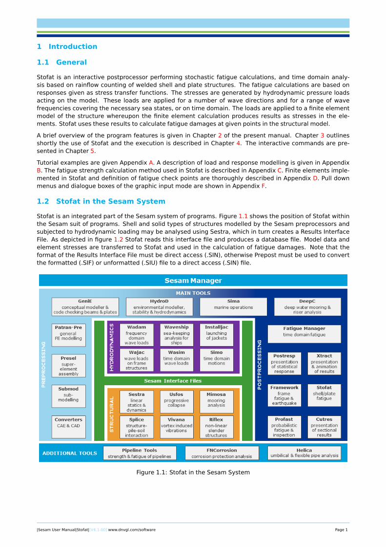
Stofat is an integrated part of the Sesam system of programs. Figure 1.1 shows the position of Stofat withinthe Sesam suit of programs. Shell and solid types of structures modelled by the Sesam preprocessors andsubjected to hydrodynamic loading may be analysed using Sestra, which in turn creates a Results InterfaceFile. As depicted in figure 1.2 Stofat reads this interface file and produces a database file. Model data andelement stresses are transferred to Stofat and used in the calculation of fatigue damages. Note that theformat of the Results Interface File must be direct access (.SIN), otherwise Prepost must be used to convertthe formatted (.SIF) or unformatted (.SIU) file to a direct access (.SIN) file.
Figure 1.1: Stofat in the Sesam System
|Sesam User Manual|Stofat|[V4.1-00] www.dnvgl.com/software Page 1
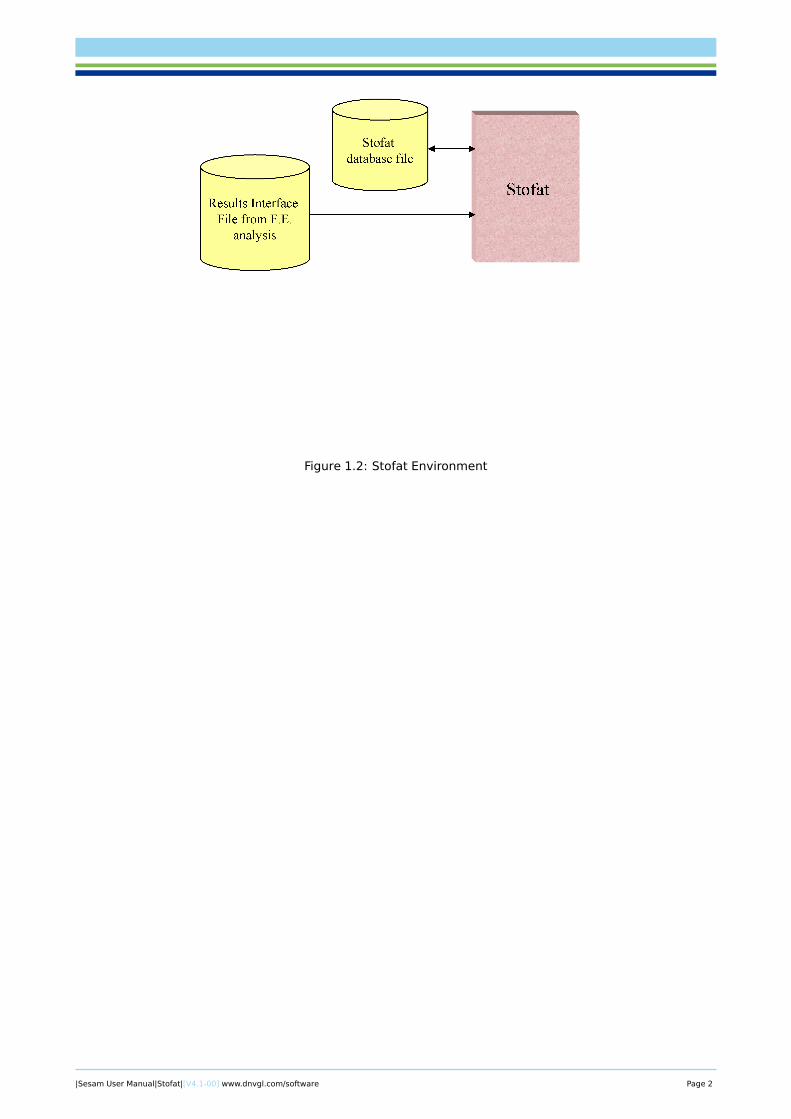
Figure 1.2: Stofat Environment
|Sesam User Manual|Stofat|[V4.1-00] www.dnvgl.com/software Page 2
2 Features of Stofat
2.1 Analysis Capabilities
Stofat performs stochastic fatigue analysis on structures modelled by 3D shell and solid elements and as-sesses whether the structure is likely to suffer failure due to the action of repeated loading. The assessmentis made by an SN-curve based fatigue approach accumulating partial damages weighted over sea statesand wave directions or by analysis of a time domain analysis based on rainflow counting methodology. Theprogram delivers usage factors representing the amount of fatigue damage that the structure has sufferedduring the specific period. The loads must be computed from a hydrodynamic analysis using a stochastic ortime-domain approach. A stochastic approach implies that the computed loads are ‘complex’, comprisingreal and imaginary components. Stofat may also account for the effect of static stresses from still waterload cases in the fatigue assessment.
From version V4.1 analysis can be performed on any units system. Previous versions would only be correct ifthe analysis was carried out inN/m2. Results file could be in any other system but the user should transformstresses into N/m2 using the features defined in command DEFINE SHELL FATIGUE CONSTANTS.
Current version identifies the results file units and transforms SN-curves in accordance.
2.2 Environment Loading
2.2.1 Wave Loading
The wave spectra are different types of wave load spectra. There are four different standard wave spectraavailable. The wave spectra are:
• Pierson-Moskowitz with input of the significant wave height HS and the zero up-crossing period TZ .
• Jonswap with input of either the significant wave height HS , the zero up-crossing period TZ and theparameters γ, σA and σB.
• General Gamma, with input of the significant wave height HS , the zero up-crossing period TZ andthe parameters l and n. When l = 5 and n = 4, the general gamma spectrum will correspond to aPierson-Moskowitz spectrum.
• Torsethaugen, with input of the significant wave height HS and the period of the dominating spectralTP , is a double peak spectral model for ocean waves described for locally fully developed sea states.For this model it is assumed that ocean waves at a location can be divide into two main parts; windsea generated by the local wind and swell sea where waves are entering in to the location from otherareas.
In addition the double peaks, six parameters Ochi-Hubble spectrum and the ISSC (International Ship andOffshore Structure Congress) spectrum are available. The Ochi-Hubble spectrum can be used to modeldouble peaks present in a wave energy density, e.g. low frequency swell along with high frequency windgenerated waves, and may represent almost all stages of development of a sea in a storm. The ISSCspectrum is a single peak spectrum with input of the significant wave height HS and the mean periodT1.
2.2.2 Wave Energy Spreading Function
The wave energy spreading functions are used when statistical calculations are required for short crestedsea, i.e. if the user wants to take into account other directions than the current main wave direction.
The wave energy spreading function may be a cosn(θ) where n is an integer value, i.e. cos2(θ), cos3(θ)etc. The function value is not directly the cosn(θ) value, but the integral of the function from −∆θ/2 to+∆θ/2.
A user specified spreading function is typed in with the relative directions and the corresponding weights.
When a wave spreading function based on a cosine function is printed, displayed or plotted, the programwill ask for which relative spacing to use in the presentation.
|Sesam User Manual|Stofat|[V4.1-00] www.dnvgl.com/software Page 3
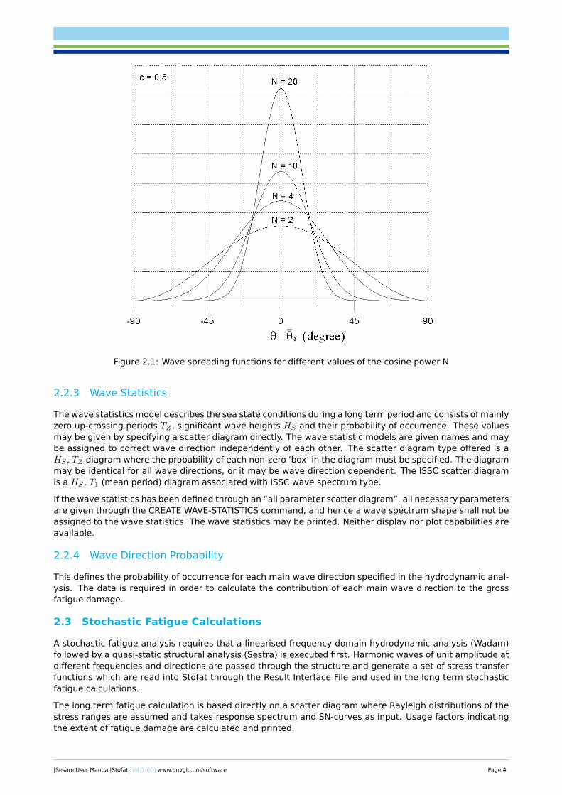
Figure 2.1: Wave spreading functions for different values of the cosine power N
2.2.3 Wave Statistics
The wave statistics model describes the sea state conditions during a long term period and consists of mainlyzero up-crossing periods TZ , significant wave heights HS and their probability of occurrence. These valuesmay be given by specifying a scatter diagram directly. The wave statistic models are given names and maybe assigned to correct wave direction independently of each other. The scatter diagram type offered is aHS , TZ diagram where the probability of each non-zero ‘box’ in the diagram must be specified. The diagrammay be identical for all wave directions, or it may be wave direction dependent. The ISSC scatter diagramis a HS , T1 (mean period) diagram associated with ISSC wave spectrum type.
If the wave statistics has been defined through an “all parameter scatter diagram”, all necessary parametersare given through the CREATE WAVE-STATISTICS command, and hence a wave spectrum shape shall not beassigned to the wave statistics. The wave statistics may be printed. Neither display nor plot capabilities areavailable.
2.2.4 Wave Direction Probability
This defines the probability of occurrence for each main wave direction specified in the hydrodynamic anal-ysis. The data is required in order to calculate the contribution of each main wave direction to the grossfatigue damage.
2.3 Stochastic Fatigue Calculations
A stochastic fatigue analysis requires that a linearised frequency domain hydrodynamic analysis (Wadam)followed by a quasi-static structural analysis (Sestra) is executed first. Harmonic waves of unit amplitude atdifferent frequencies and directions are passed through the structure and generate a set of stress transferfunctions which are read into Stofat through the Result Interface File and used in the long term stochasticfatigue calculations.
The long term fatigue calculation is based directly on a scatter diagram where Rayleigh distributions of thestress ranges are assumed and takes response spectrum and SN-curves as input. Usage factors indicatingthe extent of fatigue damage are calculated and printed.
|Sesam User Manual|Stofat|[V4.1-00] www.dnvgl.com/software Page 4

The long term fatigue calculation may also be based on generation of stress time series by Fast FourierTransform (FFT) from stress auto spectrum, i.e. rainflow cycle counting in the time domain. This option isturned on by the command DEFINE FATIGUE-RAINFLOW-COUNTING.
Static stresses from still water load cases may be accounted for in the fatigue evaluation by the commandDEFINE STATIC-LOAD.
2.4 Time Domain Fatigue Calculations
Almost intuitively, fatigue can be understood as the weakening of a given structural component by appli-cation of a repeatedly applied cyclic loads. It has a progressive and localized effect, usually computed andcommonly designated as "damage".
Stofat’s current version only supports time domain fatigue damage calculations for selected elements andand hotspots.
A stress time history will present an evolution of the stresses along time, where cyclic behavior might notbe present. Without a measure of the number of cycles no fatigue damage can be computed. To circumventthis problem, engineers come up with an algorithm "rainflow counting". This algorithm reduces a spectrumof varying stress into a set of simple stress reversals. The rainflow counting algorithm implemented ispresented in [10].
Stresses are retrieved from a results file for the required stress result points. A time domain fatigue anal-ysis requires a direct time integration with arbitrary time variating load (Wasim), using HydroD as pre-processor.
A dynamic analysis in (Sestra) is run prior to a Stofat analysis. Currently Stofat only supports elementselection analyses with the possibility of selecting groups of fatigue points within selected elements. Foreach fatigue point a stress time history is retrieved and correspondent principal stress computed for eachtime instant.
Time domain fatigue analysis in Stofat comprises three main steps: peaks and valleys identification, stressrange calculations and damage computations. Peaks and valleys are computed by analyzing the slopes bythree consecutive points. This method skips any peak or valley that could be located on the first or last timeinstant of the time series. Stress range calculations are based on [10], presented as in accordance withalgorithm 2. Damage calculations, are as usual, dependent on the definition of the SN curve, namely thenumber of slopes defining the SN curve.
It is also possible to establish which direction to take into consideration by using the weld normal line (WNL)feature. The stress ranges are then obtained by using a rainflow counting algorithm on the principal stresstime series.
Current Stofat version only allows to perform calculations for thin shell elements FQUS(24) and FTRS(25)when a Weld Normal Line is defined. If the elements are thick shell SCQS(28) and SCTS(26), the sameprocedure will be applied if the stress representation is two-dimensional. If the Weld Normal Line is notdefined, fatigue calculations will be skipped, and a message is provided. Not including the directional effectprovided by the Weld Normal Line might leads to a conservative analysis. Results will be conservativebecause the calculation will account for principal stresses from all directions, and moreover will includespurious principal stresses perpendicular to the element plane (principal stresses close to zero), neglectingnegative principal stress values if both principal stresses are negative. Including the Weld Normal conceptwill remove the near-zero principal stresses perpendicular to the finite element plane. For more information,and how to apply the Weld Normal Line concept, please check section B.7.
If intended to keep the planar stress state, then it is advised to use the weld normal line concept (WNL) andthe results will be the same as if the planar stress plane was considered.
The same technique can be used to compute the planar (two-dimensional principal stresses) by setting thestress sector angle to 90 °.
Previous Stofat version (V4.0-03) produces a fatigue damage file F1.SIF (or .SIN/SIU). Those files were cre-ated based on beam-type damage results transfer but a plate-type damage results transfer shall be imple-mented. Previous version of fatigue damage file could not be used. Current version will not produce fatiguedamage files until further developments are carried out.
|Sesam User Manual|Stofat|[V4.1-00] www.dnvgl.com/software Page 5
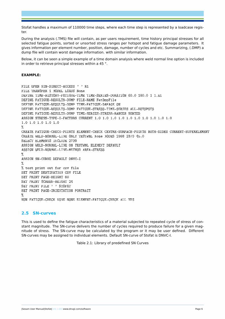
Stofat handles a maximum of 110000 time steps, where each time step is represented by a loadcase regis-ter.
During the analysis (.TMS) file will contain, as per users requirement, time history principal stresses for allselected fatigue points, sorted or unsorted stress ranges per hotspot and fatigue damage parameters. Itgives information per element number, position, damage, number of cycles and etc. Summarizing, (.DMP) adump file will contain worst damage information. with similar information.
Below, it can be seen a simple example of a time domain analysis where weld normal line option is includedin order to retrieve principal stresses within a 45 °.
EXAMPLE:
FILE OPEN SIN-DIRECT-ACCESS ' ' R1
FILE TRANSFER 1 MODEL LOADS None
DEFINE TIME-HISTORY-FATIGUE-TIME TIME-SERIES-DURATION 60.0 180.0 1 1.E1
DEFINE FATIGUE-RESULTS-DUMP FILE-NAME FatDmpFile
DEFINE FATIGUE-RESULTS-DUMP TIME-FATIGUE-DAMAGE ON
DEFINE FATIGUE-RESULTS-DUMP FATIGUE-STRESS-TIME-SERIES ALL-HOTSPOTS
DEFINE FATIGUE-RESULTS-DUMP TIME-SERIES-STRESS-RANGES SORTED
ASSIGN STRESS-TYPE-K-FACTORS CURRENT 1.0 1.0 1.0 1.0 1.0 1.0 1.0 1.0 1.0 1.0
1.0 1.0 1.0 1.0 1.0
%
CREATE FATIGUE-CHECK-POINTS ELEMENT-CHECK CENTRE-SURFACE-POINTS BOTH-SIDES CURRENT-SUPERELEMENT
CREATE WELD-NORMAL-LINE ONLY TESTWNL None NODES 2368 2370 45.0
SELECT ELEMENTS INCLUDE 2739
ASSIGN WELD-NORMAL-LINE ON TESTWNL ELEMENT DEFAULT
ASSIGN WELD-NORMAL-LINE-METHOD AREA-STRESS
%
ASSIGN SN-CURVE DEFAULT DNVC-I
%
% test print out for csv file
SET PRINT DESTINATION CSV-FILE
SET PRINT PAGE-HEIGHT 60
SET PRINT SCREEN-HEIGHT 24
SET PRINT FILE ' ' STOFAT
SET PRINT PAGE-ORIENTATION PORTRAIT
%
RUN FATIGUE-CHECK NONE NONE ELEMENT-FATIGUE-CHECK ALL YES
2.5 SN-curves
This is used to define the fatigue characteristics of a material subjected to repeated cycle of stress of con-stant magnitude. The SN-curve delivers the number of cycles required to produce failure for a given mag-nitude of stress. The SN-curve may be calculated by the program or it may be user defined. DifferentSN-curves may be assigned to individual elements. Default SN-curve of Stofat is DNVC-I.
Table 2.1: Library of predefined SN Curves
|Sesam User Manual|Stofat|[V4.1-00] www.dnvgl.com/software Page 6
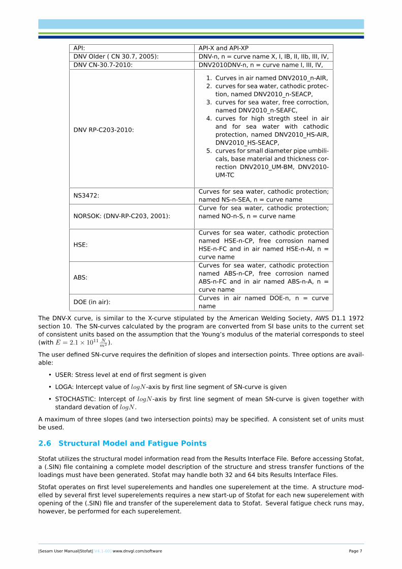
API: API-X and API-XPDNV Older ( CN 30.7, 2005): DNV-n, n = curve name X, I, IB, II, IIb, III, IV,DNV CN-30.7-2010: DNV2010DNV-n, n = curve name I, III, IV,
DNV RP-C203-2010:
1. Curves in air named DNV2010_n-AIR,2. curves for sea water, cathodic protec-
tion, named DNV2010_n-SEACP,3. curves for sea water, free corroction,
named DNV2010_n-SEAFC,4. curves for high stregth steel in air
and for sea water with cathodicprotection, named DNV2010_HS-AIR,DNV2010_HS-SEACP,
5. curves for small diameter pipe umbili-cals, base material and thickness cor-rection DNV2010_UM-BM, DNV2010-UM-TC
NS3472:Curves for sea water, cathodic protection;named NS-n-SEA, n = curve name
NORSOK: (DNV-RP-C203, 2001):Curve for sea water, cathodic protection;named NO-n-S, n = curve name
HSE:
Curves for sea water, cathodic protectionnamed HSE-n-CP, free corrosion namedHSE-n-FC and in air named HSE-n-AI, n =curve name
ABS:
Curves for sea water, cathodic protectionnamed ABS-n-CP, free corrosion namedABS-n-FC and in air named ABS-n-A, n =curve name
DOE (in air):Curves in air named DOE-n, n = curvename
The DNV-X curve, is similar to the X-curve stipulated by the American Welding Society, AWS D1.1 1972section 10. The SN-curves calculated by the program are converted from SI base units to the current setof consistent units based on the assumption that the Young’s modulus of the material corresponds to steel(with E = 2.1× 10¹¹ N
m2 ).
The user defined SN-curve requires the definition of slopes and intersection points. Three options are avail-able:
• USER: Stress level at end of first segment is given
• LOGA: Intercept value of logN -axis by first line segment of SN-curve is given
• STOCHASTIC: Intercept of logN -axis by first line segment of mean SN-curve is given together withstandard devation of logN .
A maximum of three slopes (and two intersection points) may be specified. A consistent set of units mustbe used.
2.6 Structural Model and Fatigue Points
Stofat utilizes the structural model information read from the Results Interface File. Before accessing Stofat,a (.SIN) file containing a complete model description of the structure and stress transfer functions of theloadings must have been generated. Stofat may handle both 32 and 64 bits Results Interface Files.
Stofat operates on first level superelements and handles one superelement at the time. A structure mod-elled by several first level superelements requires a new start-up of Stofat for each new superelement withopening of the (.SIN) file and transfer of the superelement data to Stofat. Several fatigue check runs may,however, be performed for each superelement.
|Sesam User Manual|Stofat|[V4.1-00] www.dnvgl.com/software Page 7
Stofat performs fatigue checks for 3D shell and solid elements. Elements implemented in Stofat are de-scribed in Appendix D. When other elements are represented in the model, Stofat passes them withoutperforming any fatigue damage calculation.
Fatigue assessment may be executed by performing an element fatigue check (ELEMENT-FATIGUE-CHECKoption) or a hotspot fatigue check (HOTSPOT-FATIGUE-CHECK option), see command RUN FATIGUE-CHECK.The element fatigue check runs through all elements selected for the fatigue assessment and delivers oneusage factor per element. The hotspot fatigue check performs fatigue assessment of specific points inthe structure defined by the user and delivers one usage factor per hotspot. The hotspots may be placedanywhere inside the superelement model treated by Stofat, but must be located at or inside the borders ofelements implemented in Stofat. Hotspots are generated directly in Stofat.
In an element fatigue assessment the fatigue points may be located 1) at element stress points, 2) atelement surfaces, 3) at element corners or 4) at middle planes of the shell elements. The number of fatiguecheck points is the same as the number of stress points for the elements. For the middle plane location, thenumber of fatigue points is half the number of stress points. Fatigue damage is calculated for all the fatiguepoints and the usage factor of the point suffering most damage within an element is taken as the usagefactor of the element. For further details, see Appendix D.
Calculation of the fatigue damage is based on the maximum principal stress component (real and imaginaryparts) of the fatigue check point. Stresses are interpolated component by component to the fatigue checkpoint whereupon the principal stresses are calculated and applied in the fatigue damage assessment. Thestresses may be multiplied with stress concentration factors (K-factors) when applied in the fatigue calcula-tion. For shell elements, stress type dependent K-factors may be specified for the membrane-, bending- andshear stresses and assigned to elements.
A Weld Normal (WN) line may be defined with the purpose of selecting the maximum principal stress withina given stress sector for use in the fatigue calculation and disregard principal stresses outside this sector.This facility may be useful when assessing fatigue damage at weld toes of welded structures where stresseswithin a sector of 45 degrees to the weld normal contribute mostly to the fatigue damage. Further detailsare given in Appendix B.7.
2.7 Long Term Response
Long term response is calculated on basis of the short term response for a given response spectrum and ascatter diagram for the sea state conditions during the long term period. The short term response spectrumis formed by the energy spectrum for a stationary sea state and the transfer function for the structure.
The print from the long term calculation includes response levels for given probability levels or return peri-ods, defined by the user. Up to 5 levels may given. Weibull parameters of the Weibull distribution functionare calculated fitting the response parameters to response levels. All of these are printed for each wavedirection calculated and, if requested, with all wave directions included.
Results are given in form of table print of the response parameters and print to a vtf file for graphic presen-tation of results in Xtract. The following parameters may be printed: Maximum and minimum stress, returnperiods or probability levels, exceedances, Weibull scale and shape parameters, stress amplitude and staticstress.
The response parameters may be calculated on basis of various stress components including the principalstresses, normal and shear stress components, and the von Mises equivalent stress component.
2.8 Analysis Results
Stofat produces usage factors expressing the extent of fatigue damage to the structure as a consequence ofthe applied loading. Analysis results are presented to the user in form of tabulated prints and graphic displayof the usage factors. Along with the usage factors key parameters related to the fatigue check points areprinted. Examples of tabulated prints of results are given in A.4.
Extended print of detailed results (dump print) is possible by executing the command DEFINE FATIGUE-RESULTS-DUMP prior to the RUN command or PRINT FATIGUE-RESULTS-DUMP after the runs have been ex-ecuted if results are saved. Such print includes print of hotspot transfer functions, moments of responsespectrum, damages per sea state, damages per sea directions, damages per hotspots/elements, excee-
|Sesam User Manual|Stofat|[V4.1-00] www.dnvgl.com/software Page 8

dence probabilities and stress range levels. The number of pages may easily be very large and this printoption should therefore be used with care.
The fatigue analysis results may be written to file (.VTF) and displayed as contour plots by Xtract, seecommand DEFINE FATIGUE-RESULTS-VTF-FILE and PRINT FATIGUE-RESULTS-VTF-FILE. Stresses as function ofthe angular frequencies may also be written to file (.VTF) by the command DISPLAY STRESS-TRANSFER-FUNCTION and displayed as 2D curve plots by Xtract.
|Sesam User Manual|Stofat|[V4.1-00] www.dnvgl.com/software Page 9
3 User’s Guide to Stofat
Typical steps in use of the Stofat program to perform fatigue calculations in welded shell and plate structuresare given in the following sections.
3.1 Modelling
Create a finite element model using either of the programs Prefem, GeniE or ship modeller. The struc-ture should be modelled in sufficient detail so that the distribution of forces within the model is correctlyrepresented and the structural parts to be checked are adequately described. The model should also besufficiently large to apply loads without disturbing the stress distribution in critical areas. For a structurefloating in water it may be necessary to model the wet surface of the structure.
Modelling and computations in several steps of refinement may be needed to attain satisfactory modelrepresentation of critical areas, see 3.5.
3.2 Hydrodynamic Load
The Sesam program Wadam may be used to calculate hydrodynamic pressure loads acting on the model.Loads should be calculated for a number of wave directions and for a range of wave frequencies coveringthe wave statistics to be used.
See the Wadam User Manual for further information.
3.3 Structural Analysis
The Sesam program Sestra performs the finite element calculation and equation solution and producesresults represented as stresses in the elements caused by the loads on the model.
A linear static calculation may be sufficient in cases when the structure does not have resonance frequencieswithin the range of wave frequencies.
If the structure may have modes of vibration that may be excited by the wave frequencies, dynamic analysismust be considered.
See the Sestra User Manual for more information.
3.4 Fatigue Calculation
3.4.1 Results File
The Stofat program reads the results from Sestra and performs the fatigue damage calculation.
The results file is identified by:
• FILE OPEN SIN-DIRECT-ACCESS prefix name item FILE TRANSFER superel name loaset
3.4.2 Wave Statictics
Long term wave statistics data are represented in the program as a “Scatter diagram”.
A few scatter diagrams according to DNV classification note 30.7 “Fatigue Assessment of Ship Structures”(1998) are predefined in the program. Other scatter diagrams according to other specifications, or measure-ments may be specified by selecting CREATE WAVE-STATISTICS SCATTER-DIAGRAM. If the wave statistics hasbeen defined through an “all parameter scatter diagram”, all necessary parameters are given through theCREATE WAVE-STATISTICS command, and hence a wave spectrum shape shall not be assigned to the wavestatistics.
For a sailing ship the same scatter diagram is normally used for all wave directions. For a fixed structureon a specific location, different scatter diagrams may be used for different wave directions based on localmeasurements. The scatter diagram to use is selected by ASSIGN WAVE-STATISTICS.
|Sesam User Manual|Stofat|[V4.1-00] www.dnvgl.com/software Page 10
3.4.3 Wave Direction Probability
The main wave directions for calculation of fatigue damage are determined by the directions of the waveloads specified as input to the load calculation program (e.g. Wadam).
The probability of waves from different wave directions must be specified by selecting ASSIGN WAVE-DIRECTION-PROBABILITY and filling in the probability of waves from the different directions. The sum ofprobabilities for all directions must be 1.0.
For a slow moving sailing ship, the wave direction probability is typically equal for all directions. For a fixedstructure, the probability may be different for different directions based on local measurements.
For a slow moving sailing ship, the wave direction probability is typically equal for all directions.
For a fixed structure, the probability may be different for different directions based on local measure-ments.
3.4.4 Wave Spreading
Real sea waves are not all moving in the same direction even within a short period of time. In Stofat awave energy spreading function is assumed to be independent of the wave frequency. The wave energyis assumed to be spread over a set of directions +90 to -90 degrees on both sides of each main wavedirection.
A typical wave spreading function is defined by selecting CREATE WAVE-SPREADING-FUNCTION COSINE-POWER.
The wave spreading function is discretised into the wave directions available and scaled such that the sumof the probabilities are 1.0.
The wave spreading function may also be specified directly as a histogram.
The wave spreading function to be used is selected by ASSIGN WAVE-SPREADING-FUNCTION.
If no wave spreading function is assigned, long crested waves are assumed.
3.4.5 Wave Spectrum
A short-term sea-state is characterized by a wave spectrum. This spectrum accounts for the variation of thewave energy over the frequencies in the sea-state.
The most commonly used spectrum is the Pierson-Moskowitz spectrum. The Pierson-Moskowitz spectrumapplies to deep water conditions and fully developed seas.
The ISSC spectrum, recommended by the 15th ITTC (International Towing Tank Conference) is available andapplies to open sea conditions and fully developed sea.
The Jonswap spectrum is also available and applies to limited fetch areas and homogenous wind fields.
The wave spectrum type to be used is selected by ASSIGN WAVE-SPECTRUM-SHAPE.
If the wave statistics has been defined through an “all parameter scatter diagram”, all necessary parametersare given through the CREATE WAVE-STATISTICS command, and hence a wave spectrum shape shall not beassigned to the wave statistics.
3.4.6 SN-Curve
SN curves represent material strength properties obtained from fatigue tests. The SN-curve defines thepredicted number of cycles to failure N for a stress range S.
Some SN curves are predefined in the program according to DNV Classification note 30.7 and NorwegianStandard NS 3472. These S-N curves are based on mean measurement results minus 2 times the stan-dard deviations for the experimental data. The SN-curves are thus associated with 97.6% probability ofsurvival.
Other SN-curves may be defined by command CREATE SN-CURVE.
Each SN-curve defined by NS 3472 is established for a class of structural details according to:
|Sesam User Manual|Stofat|[V4.1-00] www.dnvgl.com/software Page 11
• The geometrical arrangement of the detail
• The direction of the fluctuating stress relative to the detail
• The method of fabrication and inspection of the detail
The SN curve is then used directly for fatigue check of the detail without use of stress concentration fac-tors.
SN-curves specified by DNV classification note 30.7 correspond to test results from smooth specimens hav-ing a stress concentration factor K = 1.0. These should be adjusted with the SCF for the actual geome-try.
SN-curves may be assigned to individual elements by the command ASSIGN SN-CURVE.
The default SN-curve to be used in fatigue calculation is specified by DEFINE SHELL-FATIGUE-CONSTANTSDEFAULT-SN-CURVE. Note that, if the default SN-curve is changed, the new default curve is applied to allelements in the model and supersedes all previously SN-curve assignments.
Library SN-curves of Stofat are converted from SI base units to the current set of consistent units based onthe assumption that the Young's modulus of the material corresponds to steel (with E = 2.1×10¹¹ N
m2 ).
3.4.7 Stress Concentration Factor
Fatigue computation according to DNV Classification note 30.7 requires use of Stress concentration factors(K-factors). Stress concentration factors are dependent upon the level of detail in the model.
The geometrical stress concentration factor, denoted Kg, is specified when the structural analysis has calcu-lated nominal stresses in the structural parts, but for a mesh too coarse to represent local stress gradients.The geometrical stress concentration factor may be estimated from the rules by experience, or from a de-tailed finite element computation.
When the finite element analysis is sufficiently accurate to simulate the stress gradient caused by the struc-tural detail, the common practice is to omit the geometrical stress concentration factor, that is set it to1.0. To achieve this the finite elements near the detail should have sizes approximately equal to the platethickness.
A stress concentration factor due to the weld itself, denoted Kw, is usually taken from the rules.
For 2D shell elements, stress type dependent K-factors may be specified for the membrane-, bending- andshear stresses and assigned to shell elements. It is not possible to assign stress dependent K-factors to 3Dsolid elements.
Default values of the stress concentration factors are specified by the command DEFINE SHELL-FATIGUE-CONSTANTS. Values assigned to individual elements are specified by the commands ASSIGN K-FACTORS(same K-factor for all stress components) and ASSIGN STRESS-TYPE-K-FACTORS (K-factor specified for membrane-, bending- and shear stresses components).
3.4.8 Inclusion of Static Stresses
Static stresses due to still water loads may considered in the fatigue calculation. The effect of static stressesis accounted for by performing a possible reduction in the cyclic stress range according to procedure de-scribed in DNV Classification Notes No. 30.7, see [30]. A stress range reduction factor is calculated and ap-plied to principal stresses before entering the SN-curve. Further details are described in Appendix B.6.
Stresses of the static load case to be applied in the fatigue analysis must be added to the SIN result interfacefile containing the stress transfer functions of the wave loading before being read by Stofat. If the staticload case is a combination of basic static load cases, Stofat will combine the stresses of the basic loadcases provided they are present on the interface file together with data type records defining the load casecombination.
Static load case is accounted for by the command DEFINE STATIC-LOAD-CASE.
|Sesam User Manual|Stofat|[V4.1-00] www.dnvgl.com/software Page 12
3.4.9 Use of Weld Normal Lines
DNV Classification Notes No. 30.7, see [30], prescribes that the maximum principal stress range within asector of 45 degrees of the weld normal at the weld toe, should be used for fatigue assessment of weldedstructures. Fatigue damage at the weld toe is mostly caused by stresses within this sector.
The Weld Normal (WN) line facility of Stofat may be used to introduce such a stress sector in the fatiguecalculation. A WN line is specified by the user together with an angle, α, defining the extension of the stresssector. The angle α is counted from the WN line to the border of the stress sector and may have valuesbetween α = 0°and α = +90 °.
Principal stresses and principal directions are calculated on basis of component stresses at the fatigue checkpoint. The principal stress axes are tested to be inside or outside the stress sector. The maximum stresscomponent of the principal axes inside the sector is applied in the fatigue assessment.
A WN line must be assigned to an element or a hotspot to be applied in the fatigue calculation. A WN lineis created by the command CREATE WELD-NORMAL-LINE and assigned to elements and hotspots by thecommand ASSIGN WELD-NORMAL-LINE. WN line concept can be applied to time domain analysis in order toselect a preferencial direction when considering principal stresses calculations.
3.4.10 Creating Fatigue Check Points
Two types of fatigue checks may be performed by Stofat element fatigue check and hotspot fatigue check.
The element fatigue check calculates fatigue usage factors for the current selection of elements. Locationof the fatigue check points within the elements is set by the command CREATE FATIGUE-CHECK-POINTSELEMENT-CHECK. Four options are available; 1) element stress points, 2) element middle plane, 3) elementsurfaces and 4) element corners. In addition an option for using membrane stresses in the fatigue calculationfor shell elements is available. Membrane stresses are in-plane stresses at the middle plane of the shellelements. For 3D solid elements the middle plane and membrane stress options are converted to theelement stress point option.
The hotspot fatigue check calculates fatigue usage factors at individual points (fatigue points) defined bythe user. A detailed description is given in Appendix D. Hotspots are created by the command CREATEFATIGUE-CHECK-POINTS HOTSPOT-CHECK.
3.4.11 Computing Fatigue Usage Factors
The RUN FATIGUE-CHECK command performs fatigue calculation for current selection of elements whenthe ELEMENT-FATGUE-CHECK option is selected, and for current selection of hotspots when the HOTSPOT-FATIGUE-CHECK option is selected. ELEMENT-FATIGUE-CHECK is the default option.
Note that an element fatigue check and a hotspot fatigue check cannot be executed in the same run.
Each time the RUN command is repeated a different name must be specified.
A table of results may be stored on a print file, or displayed in a window by the command PRINT FATIGUE-CHECK-RESULTS.
A wireframe display of the model may be performed with usage factors annotated on the display by thecommand DISPLAY FATIGUE-CHECK-RESULTS.
Contour plots of the fatigue results may be displayed by the visualization program Xtract. Xtract reads a(.vtf) file containing the Stofat results. Stofat writes results to the vtf file during the run when the YES optionof the command DEFINE FATIGUE-RESULTS-VTF-FILE is applied before the RUN command is executed.
3.5 Submodel Analysis
If fatigue sensitive areas in the structure have been identified, but uncertainties remain about stress con-centration factors or stress gradients, analysis of a submodel may be useful. Submodelling is performed bythe program Submod. Typical steps are:
• Make a new finite element model of the area in question
• Apply a refined mesh to represent local stress gradients of the area with sufficient accuracy
|Sesam User Manual|Stofat|[V4.1-00] www.dnvgl.com/software Page 13
• Specify prescribed (“driven”) boundary conditions around the perimeter where the submodel is to beconnected to the original model
• Run Submod to transfer displacement results from the original model into prescribed displacementalong the boundary of the submodel
A finite element analysis of the submodel in Sestra and further studies in Stofat may then be performed.
For further details, see the Submod User Manual.
3.6 Long Term Response Calculation
In order to perform calculation of long term responses, stress components must be defined by the com-mand DEFINE LONG-TERM-STRESS prior run execution since spectral moments of the stress components arerequired to be calculated during the run.
Response parameters may be printed for probability levels and return periods defined by the commandsDEFINE LONG-TERM-PROBABILITY and DEFINE LONG-TERM-RETURN-PERIOD.
Table print of the response parameters is obtained by the command PRINT LONG-TERM-RESPONSE and printto the vtf file is obtained by the command PRINT FATIGUE-RESULTS-VTF-FILE LONG-TERM-RESPONSE. Thecommand DEFINE FATIGUE-RESULTS-VTF-FILE LONG-TERM-RESPONSE prints one response parameter to thevtf file during run execution.
Print is performed for selected response parameters, wave directions and stress components. Print to thevtf file is performed for a single probability level and return period, entered in the print command.
3.7 Saving of Analysis Results and Limitation of Model Size to be Executed
Analysis results of Stofat may be saved in order to postprocess the fatigue results. When Stofat has beenstarted several Stofat analyses may be carried out and results of the analyses may be postprocessed afterthe runs are completed provided that results are saved.
Saving of results is decided by the user in the RUN command, see Chapter 5.
If results are not saved, postprocessing will not be available with respect to dump print and print of resultsto the vtf file. However, such print will be generated during the analysis process if the commands DEFINE-FATIGUE-RESULTS-VTF-FILE and DEFINE FATIGUE-RESULTS-DUMP are set prior to the run.
Stofat saves principal stresses and part damage results for all sea states at all stress points of the elementsincluded in the run. For large models this may sum up to quit a big number of data to be saved. The database applied by Stofat has limitation in the number of data that may be stored. Saved data are stored in 10different directories of the data base. The size of each directory has a upper limit of 256× 220 = 268435456spaces.
The size limit of the data base directories puts restrictions on the size of the problem that may be handledby Stofat. For very big models it may happen that the model itself is too big to be saved in the database directory and reading of the SIN file will fail in Stofat. However, if the model has been successfullytransferred to Stofat the size limit is practically not present when fatigue results are not saved during therun but printed directly to the vtf file if required. The size limit is a function of the number of wave directions,wave frequencies, sea states and elements included in a Stofat run. Analysis results are stored in 8 database directories (numbered from 3 to 10) and provides a maximum possible utilization of the data basecapacity for a Stofat run.
The required number of results to be saved for an element is a product of the number of element stresspoints and the number of wave directions, wave frequencies and sea states as given below.
The number of data saved for an element in directory 3 and 4:
nsave3 = npnt× (1 + 2× nwdir × nfreq) + 21
nsave4 = npnt× (3 + 2× nwdir × nfreq) + 21
The number of data saved for an element in each of the directories 5 to 10:
nsave5−10 = npnt× nsea+ 15
where:
|Sesam User Manual|Stofat|[V4.1-00] www.dnvgl.com/software Page 14

npnt = number of stress points of the element
nsea = number of sea states (= nwdir*nscpnt, in case of same scatter diagram for all wave directions)
nwdir = number of wave directions
nscpnt = number of points of scatter diagram
nfreq = number of wave frequencies
nsave3 = Number data saved for each element in directory 3
nsave4 = Number data saved for each element in directory 4
nsave5− 10 = Number data saved for each element in each of the directories 5 to 10
The number of stress points of the elements varies from 1 to 10 points depending on the element typesapplied, see Table D.1 in D .
The data base uses a paging system when storing data. The size of a data base page is 4096 and the numberof pages of a directory is 65536. If the number of result data in a data block to be saved exceed the size ofone page, as many pages as necessary are used for storage of the data block. Each new saved data blockstarts at the beginning of a new page when the data block exceeds on page in size.
Knowing the storing system of the data base, the number of elements that may be included in a Stofat runwithout exceeding the saving capacity may be estimated. Stofat puts analysis results into the data base inblocks element by element. When such a block occupies one data base page in size, a maximum of 65535elements may be included in a Stofat run supposing that no other runs have been executed in advance (onepage is used for administration data). When the block occupies two data base pages in size, 32767 elementsmay be included in the run, and so on.
In Table 3.1 the maximum number of elements that may be included in a Stofat run are listed as functionthe number of sea states, wave directions and wave frequencies. The maximum number of the elementsdepends also on the number of element stress points for the element types applied. In Table 3.1 all elementsare assumed to have 8 stress points.
An example of how to find the maximum element capacity of a problem may be illustrated by assumingnpnt = 8, nwdir = 12, nfreq = 20, nscpnt = 100. It is assumed that the same scatter diagram is applied toall wave directions which gives nsea = nwdir × nscpnt = 1200. From Table 3.1 it is found that the capacitiesof the data base directories are 218454 elements (column 1: nsea = 1200) and 65535 elements (column 2:nwdir × nfreq = 240), respectively, which, gives an upper limit of elements of 21845 without exceeding thestorage capacity of the data base.
At the commence of a run (when the run command is executed), Stofat estimates required data base spacefor saving results of the problem to be analysed. If the required space exceeds the storage capacity of thedata base, the run is stopped and capacity limits are printed. Also, during the run execution, the programcurrently checks remaining free space of the data base and stops the execution when the free space left istoo small to save results of the element to be analysed.
The problem size must be reduced if the saving capacity of the data base is being exceeded. This may bedone by either reducing the number of sea states, wave direction or elements. The most convenient way tohandle this problem is to establish suitable element sets of the model with respect to the fatigue analysisand run set by set in several fatigue check runs. Element sets can not be generated by Stofat, and must beestablished by the preprocessors.
When fatigue checks are split into more than one Stofat run for very large models, Stofat must be closeddown and started again in order to empty the data base directories between each run. When Stofat isclosed down after a run the model and analysis results of the run are saved in the STOFAT.MOD file. This fileis deleted and an empty STOFAT.MOD file is opened when the NEW option is chosen in the opening sequenceof Stofat. The OLD option opens the existing STOFAT.MOD file without emptying it.
When several Stofat runs are executed in a sequence of closing and restarting processes of Stofat, and anempty data base is accessed each time, the STOFAT.MOD file should be renamed prior to each restart ifpostprocessing of results of the various runs are necessary to perform later on (e.g STOFAT1.MOD, STO-FAT2.MOD, etc.) Saved MOD files may be accessed by choosing the "Old" option of the database status inthe opening sequence of Stofat. However, the MOD file that is accessed must be named STOFAT.MOD.
|Sesam User Manual|Stofat|[V4.1-00] www.dnvgl.com/software Page 15
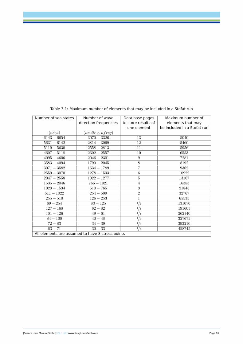
Table 3.1: Maximum number of elements that may be included in a Stofat run
Number of sea states Number of wave Data base pages Maximum number ofdirection frequencies to store results of elements that may
one element be included in a Stofat run(nsea) (nwdir × nfreq)
6143− 6654 3070− 3326 13 50405631− 6142 2814− 3069 12 54605119− 5630 2558− 2813 11 59564607− 5118 2302− 2557 10 65534095− 4606 2046− 2301 9 72813583− 4094 1790− 2045 8 81923071− 3582 1534− 1789 7 93622559− 3070 1278− 1533 6 109222047− 2558 1022− 1277 5 131071535− 2046 766− 1021 4 163831023− 1534 510− 765 3 21845511− 1022 254− 509 2 32767255− 510 126− 253 1 6553569− 254 83− 125 1/2 131070127− 168 62− 82 1/3 191605101− 126 49− 61 1/4 26214084− 100 40− 48 1/5 32767572− 83 34− 39 1/6 39321063− 71 30− 33 1/7 458745
All elements are assumed to have 8 stress points
|Sesam User Manual|Stofat|[V4.1-00] www.dnvgl.com/software Page 16
4 Execution of Stofat
4.1 Files
Stofat uses the following files:
Database The database file is a direct access file that is used to keep the model andanalysis results. It has the extension .mod.
Journal The journal file is a log of the commands that are accepted during a Stofatsession. If an existing (Old) database is opened, the journal will be appended tothe corresponding old journal file. The journal file has the extension .jnl.
Command Input This file is used to read commands and data into StofatThe default extension ofacommand input file is .jnl, but this default is not used if another extension isspecified.
Print The print file is used to keep output from the PRINT command when the printdestination is set to File or Csv File in the SET PRINT command. The exten-sion is .lis for the SET PRINT FILE option and .csv for the SET PRINT CSV-FILEoption.The purpose of the Csv File option is to print a more proper format forspreadsheets. The .csv file has separation signs (semicolons) between fields oftable results.The semicolons serve as column delimiters when the file is openedinspreadsheet.The print file name and settings are specified by the command SET PRINT. It ispossible to use more than one print file during the same Stofat session, but onlyone can be open at a time.
Print Dump The print dump files are generated when print details of the fatigue analysis re-sults are turned on by the command DEFINE FATIGUE DUMP. A print fileDmp.liswith default name StofatDmp.lis is generated when print of stress transfer func-tions, moments of response spectrum, or fatigue damages are turned on. Theymay be changed by the user. Likewise a print file Pex.lis with default nameStofatPex.lis is generated when print of probability exceedence levels, or stressrange distributions are turned on. Note that the print options have to be turnedon before the RUN command is executed to generate the print dump files.
Message log The start-up heading and messages printed on the screen during the executionare written to the file stofat.mlg.
Plot The plot file is used to keep output from the DISPLAY command when the displaydestination is set to file. The plot file name and settings is specified using thecommand:SET PLOT. The extension of the plot file depends on the plot formatused. Several formats are available. It is possible to use more than one plot fileduring the same Stofat session, but only one can be open at a time.
Results Interface File The Sesam Results Interface File is used for transferring data from the struc-tural analysis program. The file consists of all modelling data of the structureand stress transfer functions generated from the hydrodynamic pressure loadsacting on the model.It is required that the Results Interface File is given on DIRECT ACCESS format(i.e. R#.SIN)
|Sesam User Manual|Stofat|[V4.1-00] www.dnvgl.com/software Page 17
vtf vtf files (extension .vtf) are written in ViewTech File (vtf) - ASCII format and areused as input files for presentation of Stofat results by Xtract. Stofat results arewritten to a vtf file by executing the command DEFINE FATIGUE-RESULTS-VTF-FILE. Stress transfer functions are written to a vtf file by executing the commandDISPLAY STRESS-TRANSFER-FUNCTION. The commands must be executed be-fore the RUN command is executed. The vtf files have the extension .vtf andthe default name is Stofat. vtf and StofatStf.vtf, respectively. It is possible towrite Stofat results to more than one vtf file during a Stofat session by changingthe file name from one run to the next. Only one result type is written to the fileduring a run execution.
Long Term Response Print of long term response parameters is accessed by the PRINT LONG-TERM-RESPONSE command. Table print of results may be generated for both elementand hotspot fatigue check runs provided that long term stress components aredefined prior to the runs. The print can not be executed unless long term proba-bilities or long term return periods are defined. A print file .lis with default nameStofatLtr.lis is generated. They may be changed by the user.
Stofat has been designed to protect the user against loss of valuable data. Thus, for some of the errors thatmay occur Stofat will close the database file before exiting the program. It is however not always possibleto catch a program crash and close the database file properly when it happens.
If the database file has been corrupted, the information may be reconstructed by use of the journal file. Itis therefore recommended to take good care of the journal files. It can also be a good idea to take backupcopies of the journal and database file at regular intervals.
4.2 Starting Stofat
Stofat application may be run in line mode (text input mode) and/or in graphic mode (with a graphic userinterface).
The graphic mode applies user interface menus. The menus are presented graphically with pulldown menus,fixed menus, push buttons, dialogue boxes, etc., which initiate program actions, or open dialogue windowsfor user communication.
In line mode the text input lines are interpreted directly by the program. The line mode facilities are alsoavailable in the graphic mode through a window which accept line mode input.
Stofat logs all commands given by the user independent of the mode actually used. This implies that it ispossible to run Stofat with a command input file originally created from a graphic mode run. The functionalityis identical in the two modes.
4.2.1 Starting Stofat from Manager with Result Menu
In Manager the ‘Result’ menu will be available when a Results Interface File exits for the current project.In the ‘Result’ menu Stofat is available under the selection ‘Shell fatigue STOFAT...’, see Figure 4.1. Ifthe ‘Result’ menu is not available (“grey out”), click ‘Option/Superelement’ to specify the actual superele-ment.
The ‘Shell Fatigue Postprocessing’ dialogue for Stofat see Figure 4.2, has the following parameters:
Database status:
New When Stofat has not been run before, or when it is wanted to start Stofat withand empty database.
Old To restart Stofat with an existing model.
Reconstruct To reconstruct accumulated journal file into a new database and restart Stofat.
Input mode:
|Sesam User Manual|Stofat|[V4.1-00] www.dnvgl.com/software Page 18
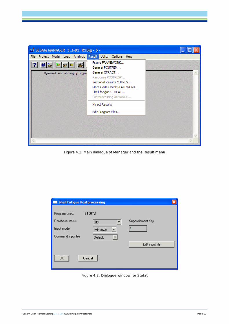
Figure 4.1: Main dialague of Manager and the Result menu
Figure 4.2: Dialogue window for Stofat
|Sesam User Manual|Stofat|[V4.1-00] www.dnvgl.com/software Page 19
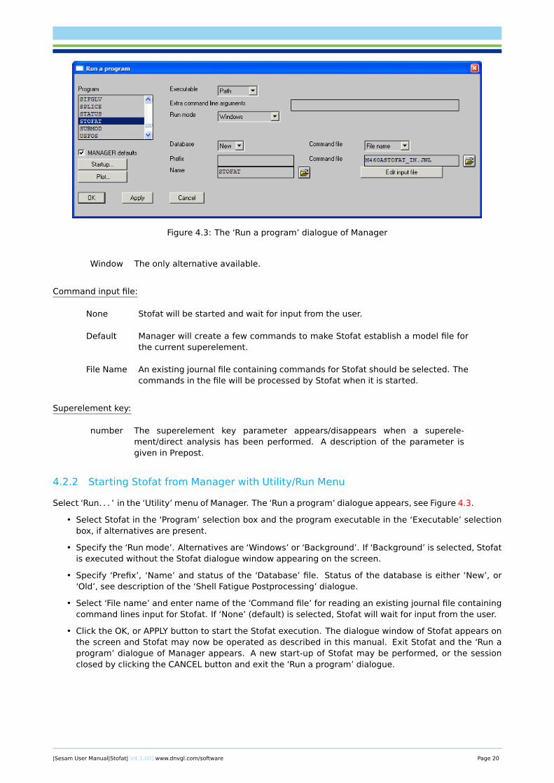
Figure 4.3: The ‘Run a program’ dialogue of Manager
Window The only alternative available.
Command input file:
None Stofat will be started and wait for input from the user.
Default Manager will create a few commands to make Stofat establish a model file forthe current superelement.
File Name An existing journal file containing commands for Stofat should be selected. Thecommands in the file will be processed by Stofat when it is started.
Superelement key:
number The superelement key parameter appears/disappears when a superele-ment/direct analysis has been performed. A description of the parameter isgiven in Prepost.
4.2.2 Starting Stofat from Manager with Utility/Run Menu
Select ‘Run. . . ’ in the ‘Utility’ menu of Manager. The ‘Run a program’ dialogue appears, see Figure 4.3.
• Select Stofat in the ‘Program’ selection box and the program executable in the ‘Executable’ selectionbox, if alternatives are present.
• Specify the ‘Run mode’. Alternatives are ‘Windows’ or ‘Background’. If ‘Background’ is selected, Stofatis executed without the Stofat dialogue window appearing on the screen.
• Specify ‘Prefix’, ‘Name’ and status of the ‘Database’ file. Status of the database is either ‘New’, or‘Old’, see description of the ‘Shell Fatigue Postprocessing’ dialogue.
• Select ‘File name’ and enter name of the ‘Command file’ for reading an existing journal file containingcommand lines input for Stofat. If ‘None’ (default) is selected, Stofat will wait for input from the user.
• Click the OK, or APPLY button to start the Stofat execution. The dialogue window of Stofat appears onthe screen and Stofat may now be operated as described in this manual. Exit Stofat and the ‘Run aprogram’ dialogue of Manager appears. A new start-up of Stofat may be performed, or the sessionclosed by clicking the CANCEL button and exit the ‘Run a program’ dialogue.
|Sesam User Manual|Stofat|[V4.1-00] www.dnvgl.com/software Page 20
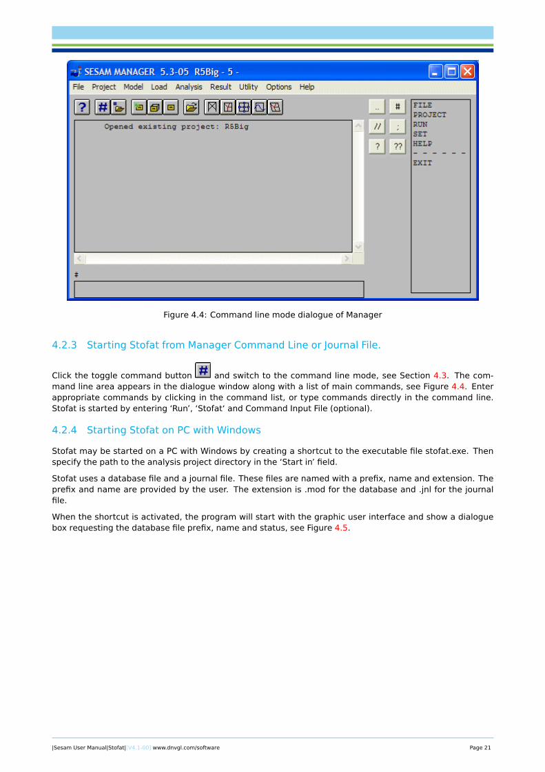
Figure 4.4: Command line mode dialogue of Manager
4.2.3 Starting Stofat from Manager Command Line or Journal File.
Click the toggle command button and switch to the command line mode, see Section 4.3. The com-mand line area appears in the dialogue window along with a list of main commands, see Figure 4.4. Enterappropriate commands by clicking in the command list, or type commands directly in the command line.Stofat is started by entering ‘Run’, ‘Stofat‘ and Command Input File (optional).
4.2.4 Starting Stofat on PC with Windows
Stofat may be started on a PC with Windows by creating a shortcut to the executable file stofat.exe. Thenspecify the path to the analysis project directory in the ‘Start in’ field.
Stofat uses a database file and a journal file. These files are named with a prefix, name and extension. Theprefix and name are provided by the user. The extension is .mod for the database and .jnl for the journalfile.
When the shortcut is activated, the program will start with the graphic user interface and show a dialoguebox requesting the database file prefix, name and status, see Figure 4.5.
|Sesam User Manual|Stofat|[V4.1-00] www.dnvgl.com/software Page 21
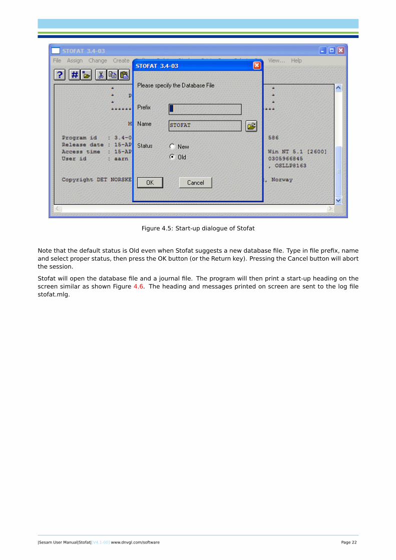
Figure 4.5: Start-up dialogue of Stofat
Note that the default status is Old even when Stofat suggests a new database file. Type in file prefix, nameand select proper status, then press the OK button (or the Return key). Pressing the Cancel button will abortthe session.
Stofat will open the database file and a journal file. The program will then print a start-up heading on thescreen similar as shown Figure 4.6. The heading and messages printed on screen are sent to the log filestofat.mlg.
|Sesam User Manual|Stofat|[V4.1-00] www.dnvgl.com/software Page 22
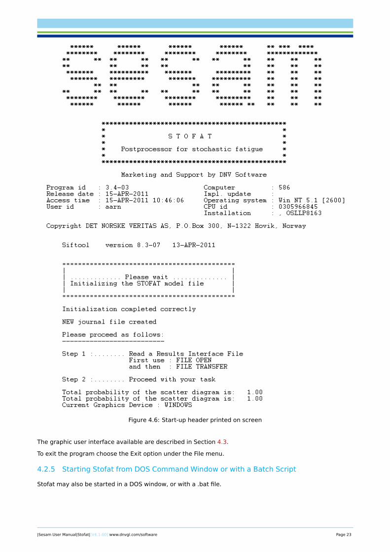
Figure 4.6: Start-up header printed on screen
The graphic user interface available are described in Section 4.3.
To exit the program choose the Exit option under the File menu.
4.2.5 Starting Stofat from DOS Command Window or with a Batch Script
Stofat may also be started in a DOS window, or with a .bat file.
|Sesam User Manual|Stofat|[V4.1-00] www.dnvgl.com/software Page 23
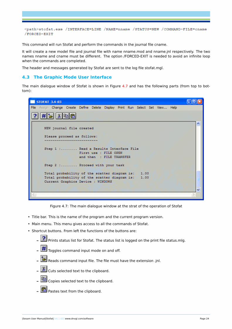
This command will run Stofat and perform the commands in the journal file cname.
It will create a new model file and journal file with name nname.mod and nname.jnl respectively. The twonames nname and cname must be different. The option /FORCED-EXIT is needed to avoid an infinite loopwhen the commands are completed.
The header and messages generated by Stofat are sent to the log file stofat.mgl.
4.3 The Graphic Mode User Interface
The main dialogue window of Stofat is shown in Figure 4.7 and has the following parts (from top to bot-tom):
Figure 4.7: The main dialogue window at the strat of the operation of Stofat
• Title bar. This is the name of the program and the current program version.
• Main menu. This menu gives access to all the commands of Stofat.
• Shortcut buttons. From left the functions of the buttons are:
– Prints status list for Stofat. The status list is logged on the print file status.mlg.
– Toggles command input mode on and off.
– Reads command input file. The file must have the extension .jnl.
– Cuts selected text to the clipboard.
– Copies selected text to the clipboard.
– Pastes text from the clipboard.
|Sesam User Manual|Stofat|[V4.1-00] www.dnvgl.com/software Page 24
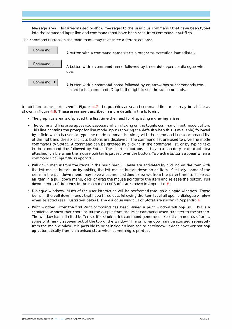
Message area. This area is used to show messages to the user plus commands that have been typedinto the command input line and commands that have been read from command input files.
The command buttons in the main manu may take three different actions:
A button with a command name starts a programs execution immediately.
A botton with a command name followed by three dots opens a dialogue win-dow.
A button with a command name followed by an arrow has subcommands con-nected to the command. Drag to the right to see the subcommands.
In addition to the parts seen in Figure 4.7, the graphics area and command line areas may be visible asshown in Figure 4.8. These areas are described in more details in the following:
• The graphics area is displayed the first time the need for displaying a drawing arises.
• The command line area appears/disappears when clicking on the toggle command input mode button.This line contains the prompt for line mode input (showing the default when this is available) followedby a field which is used to type line mode commands. Along with the command line a command listat the right and the six shortcut buttons are displayed. The command list are used to give line modecommands to Stofat. A command can be entered by clicking in the command list, or by typing textin the command line followed by Enter. The shortcut buttons all have explanatory texts (tool tips)attached, visible when the mouse pointer is paused over the button. Two extra buttons appear when acommand line input file is opened.
• Pull down menus from the items in the main menu. These are activated by clicking on the item withthe left mouse button, or by holding the left mouse button down on an item. Similarly, some of theitems in the pull down menu may have a submenu sliding sideways from the parent menu. To selectan item in a pull down menu, click or drag the mouse pointer to the item and release the button. Pulldown menus of the items in the main menu of Stofat are shown in Appendix F.
• Dialogue windows. Much of the user interaction will be performed through dialogue windows. Thoseitems in the pull down menus that have three dots following the item label all open a dialogue windowwhen selected (see illustration below). The dialogue windows of Stofat are shown in Appendix F.
• Print window. After the first Print command has been issued a print window will pop up. This is ascrollable window that contains all the output from the Print command when directed to the screen.The window has a limited buffer so, if a single print command generates excessive amounts of print,some of it may disappear out of the top of the window. The print window may be iconised separatelyfrom the main window. It is possible to print inside an iconised print window. It does however not popup automatically from an iconised state when something is printed.
|Sesam User Manual|Stofat|[V4.1-00] www.dnvgl.com/software Page 25
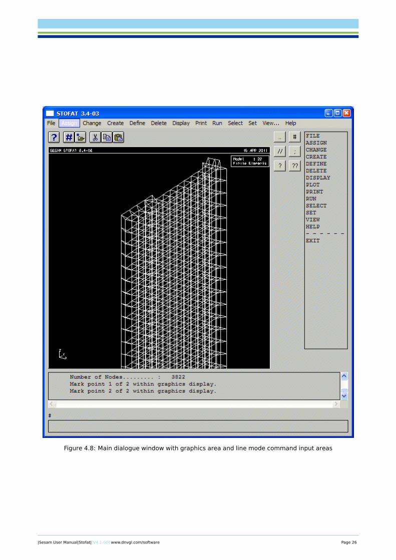
Figure 4.8: Main dialogue window with graphics area and line mode command input areas
|Sesam User Manual|Stofat|[V4.1-00] www.dnvgl.com/software Page 26
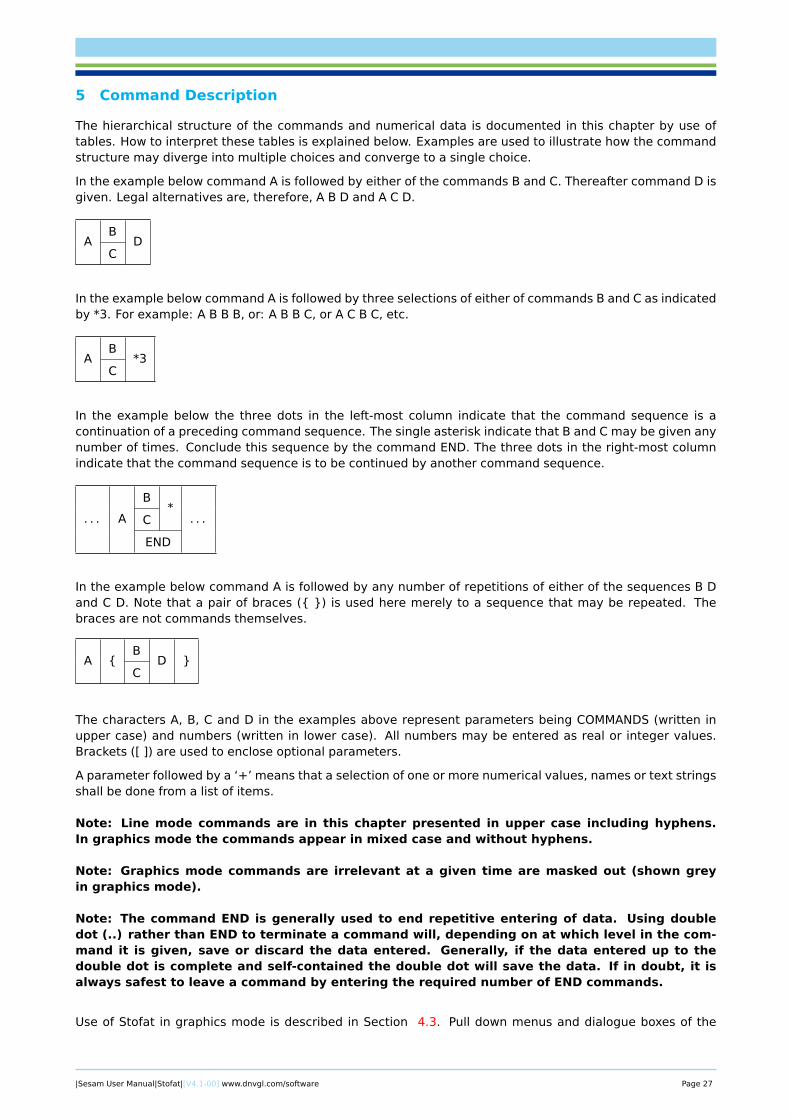
5 Command Description
The hierarchical structure of the commands and numerical data is documented in this chapter by use oftables. How to interpret these tables is explained below. Examples are used to illustrate how the commandstructure may diverge into multiple choices and converge to a single choice.
In the example below command A is followed by either of the commands B and C. Thereafter command D isgiven. Legal alternatives are, therefore, A B D and A C D.
AB
DC
In the example below command A is followed by three selections of either of commands B and C as indicatedby *3. For example: A B B B, or: A B B C, or A C B C, etc.
AB
*3C
In the example below the three dots in the left-most column indicate that the command sequence is acontinuation of a preceding command sequence. The single asterisk indicate that B and C may be given anynumber of times. Conclude this sequence by the command END. The three dots in the right-most columnindicate that the command sequence is to be continued by another command sequence.
. . . A
B*
. . .C
END
In the example below command A is followed by any number of repetitions of either of the sequences B Dand C D. Note that a pair of braces ({ }) is used here merely to a sequence that may be repeated. Thebraces are not commands themselves.
A {B
D }C
The characters A, B, C and D in the examples above represent parameters being COMMANDS (written inupper case) and numbers (written in lower case). All numbers may be entered as real or integer values.Brackets ([ ]) are used to enclose optional parameters.
A parameter followed by a ‘+’ means that a selection of one or more numerical values, names or text stringsshall be done from a list of items.
Note: Line mode commands are in this chapter presented in upper case including hyphens.In graphics mode the commands appear in mixed case and without hyphens.
Note: Graphics mode commands are irrelevant at a given time are masked out (shown greyin graphics mode).
Note: The command END is generally used to end repetitive entering of data. Using doubledot (..) rather than END to terminate a command will, depending on at which level in the com-mand it is given, save or discard the data entered. Generally, if the data entered up to thedouble dot is complete and self-contained the double dot will save the data. If in doubt, it isalways safest to leave a command by entering the required number of END commands.
Use of Stofat in graphics mode is described in Section 4.3. Pull down menus and dialogue boxes of the
|Sesam User Manual|Stofat|[V4.1-00] www.dnvgl.com/software Page 27
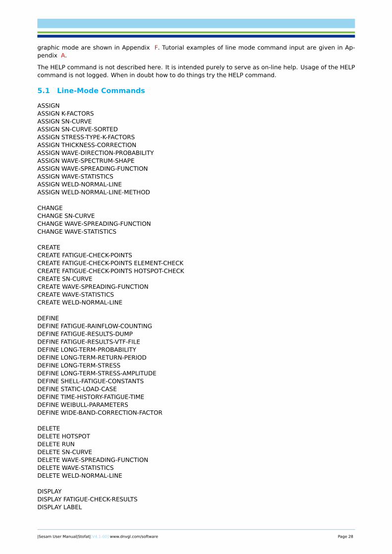
graphic mode are shown in Appendix F. Tutorial examples of line mode command input are given in Ap-pendix A.
The HELP command is not described here. It is intended purely to serve as on-line help. Usage of the HELPcommand is not logged. When in doubt how to do things try the HELP command.
5.1 Line-Mode Commands
ASSIGNASSIGN K-FACTORSASSIGN SN-CURVEASSIGN SN-CURVE-SORTEDASSIGN STRESS-TYPE-K-FACTORSASSIGN THICKNESS-CORRECTIONASSIGN WAVE-DIRECTION-PROBABILITYASSIGN WAVE-SPECTRUM-SHAPEASSIGN WAVE-SPREADING-FUNCTIONASSIGN WAVE-STATISTICSASSIGN WELD-NORMAL-LINEASSIGN WELD-NORMAL-LINE-METHOD
CHANGECHANGE SN-CURVECHANGE WAVE-SPREADING-FUNCTIONCHANGE WAVE-STATISTICS
CREATECREATE FATIGUE-CHECK-POINTSCREATE FATIGUE-CHECK-POINTS ELEMENT-CHECKCREATE FATIGUE-CHECK-POINTS HOTSPOT-CHECKCREATE SN-CURVECREATE WAVE-SPREADING-FUNCTIONCREATE WAVE-STATISTICSCREATE WELD-NORMAL-LINE
DEFINEDEFINE FATIGUE-RAINFLOW-COUNTINGDEFINE FATIGUE-RESULTS-DUMPDEFINE FATIGUE-RESULTS-VTF-FILEDEFINE LONG-TERM-PROBABILITYDEFINE LONG-TERM-RETURN-PERIODDEFINE LONG-TERM-STRESSDEFINE LONG-TERM-STRESS-AMPLITUDEDEFINE SHELL-FATIGUE-CONSTANTSDEFINE STATIC-LOAD-CASEDEFINE TIME-HISTORY-FATIGUE-TIMEDEFINE WEIBULL-PARAMETERSDEFINE WIDE-BAND-CORRECTION-FACTOR
DELETEDELETE HOTSPOTDELETE RUNDELETE SN-CURVEDELETE WAVE-SPREADING-FUNCTIONDELETE WAVE-STATISTICSDELETE WELD-NORMAL-LINE
DISPLAYDISPLAY FATIGUE-CHECK-RESULTSDISPLAY LABEL
|Sesam User Manual|Stofat|[V4.1-00] www.dnvgl.com/software Page 28
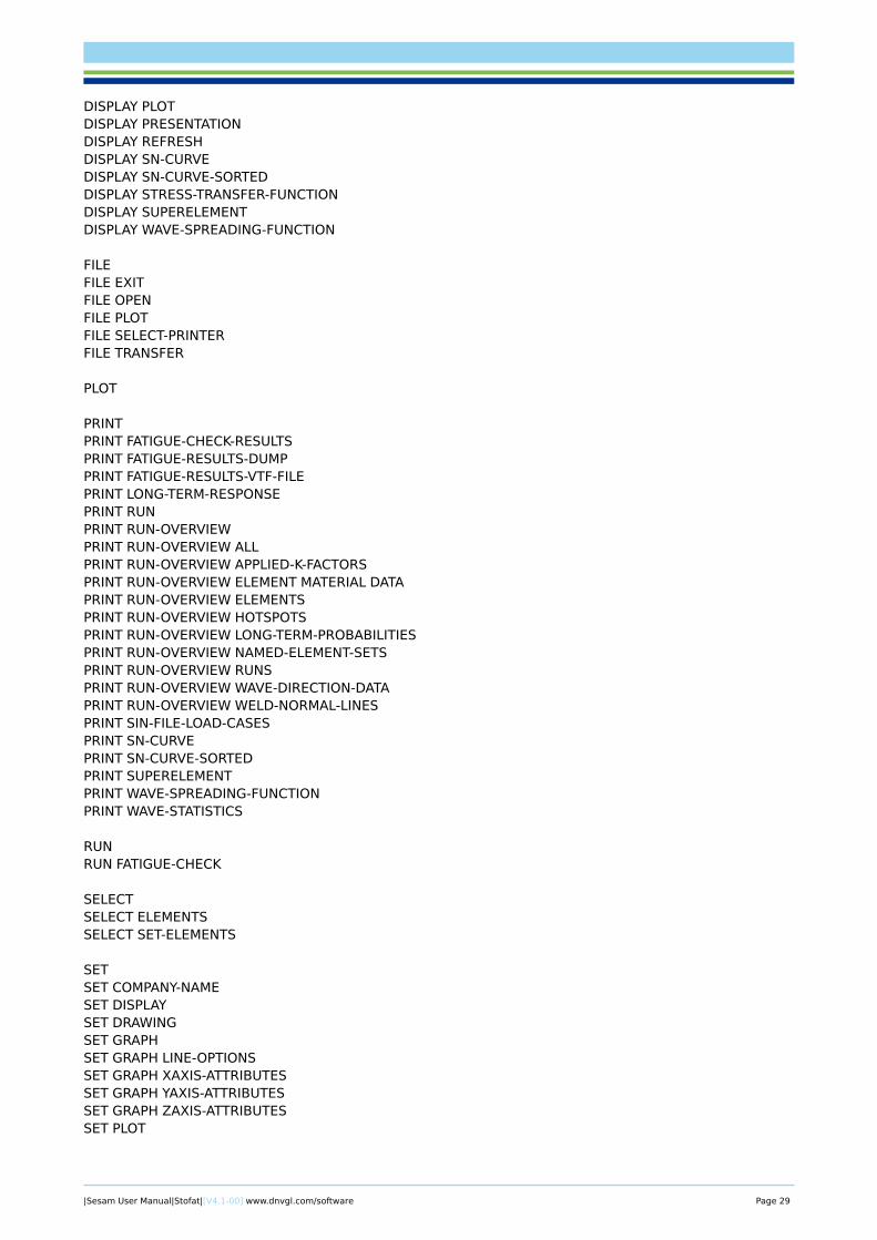
DISPLAY PLOTDISPLAY PRESENTATIONDISPLAY REFRESHDISPLAY SN-CURVEDISPLAY SN-CURVE-SORTEDDISPLAY STRESS-TRANSFER-FUNCTIONDISPLAY SUPERELEMENTDISPLAY WAVE-SPREADING-FUNCTION
FILEFILE EXITFILE OPENFILE PLOTFILE SELECT-PRINTERFILE TRANSFER
PLOT
PRINTPRINT FATIGUE-CHECK-RESULTSPRINT FATIGUE-RESULTS-DUMPPRINT FATIGUE-RESULTS-VTF-FILEPRINT LONG-TERM-RESPONSEPRINT RUNPRINT RUN-OVERVIEWPRINT RUN-OVERVIEW ALLPRINT RUN-OVERVIEW APPLIED-K-FACTORSPRINT RUN-OVERVIEW ELEMENT MATERIAL DATAPRINT RUN-OVERVIEW ELEMENTSPRINT RUN-OVERVIEW HOTSPOTSPRINT RUN-OVERVIEW LONG-TERM-PROBABILITIESPRINT RUN-OVERVIEW NAMED-ELEMENT-SETSPRINT RUN-OVERVIEW RUNSPRINT RUN-OVERVIEW WAVE-DIRECTION-DATAPRINT RUN-OVERVIEW WELD-NORMAL-LINESPRINT SIN-FILE-LOAD-CASESPRINT SN-CURVEPRINT SN-CURVE-SORTEDPRINT SUPERELEMENTPRINT WAVE-SPREADING-FUNCTIONPRINT WAVE-STATISTICS
RUNRUN FATIGUE-CHECK
SELECTSELECT ELEMENTSSELECT SET-ELEMENTS
SETSET COMPANY-NAMESET DISPLAYSET DRAWINGSET GRAPHSET GRAPH LINE-OPTIONSSET GRAPH XAXIS-ATTRIBUTESSET GRAPH YAXIS-ATTRIBUTESSET GRAPH ZAXIS-ATTRIBUTESSET PLOT
|Sesam User Manual|Stofat|[V4.1-00] www.dnvgl.com/software Page 29

SET PRINTSET TITLE
VIEWVIEW FRAMEVIEW PANVIEW POSITIONVIEW ROTATEVIEW ZOOM
|Sesam User Manual|Stofat|[V4.1-00] www.dnvgl.com/software Page 30
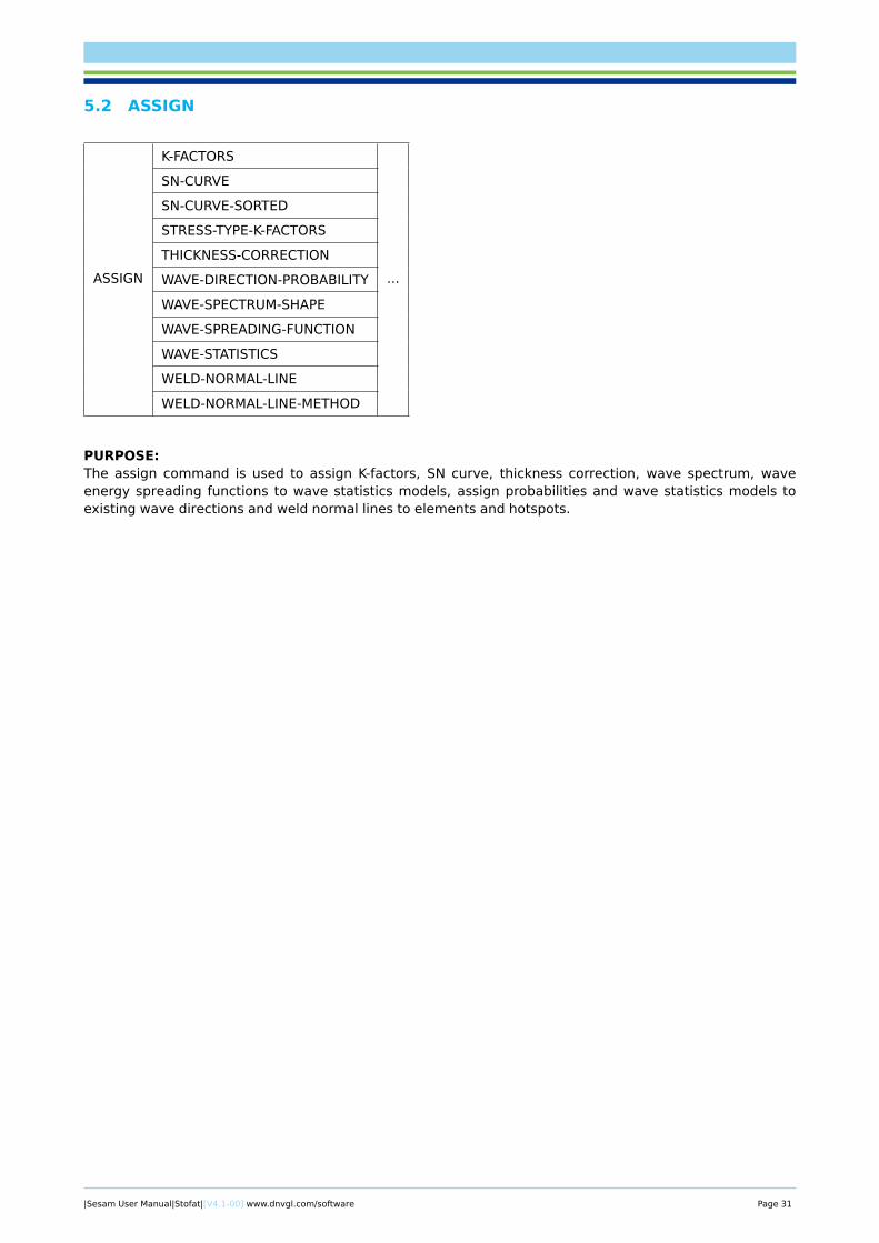
5.2 ASSIGN
ASSIGN
K-FACTORS
...
SN-CURVE
SN-CURVE-SORTED
STRESS-TYPE-K-FACTORS
THICKNESS-CORRECTION
WAVE-DIRECTION-PROBABILITY
WAVE-SPECTRUM-SHAPE
WAVE-SPREADING-FUNCTION
WAVE-STATISTICS
WELD-NORMAL-LINE
WELD-NORMAL-LINE-METHOD
PURPOSE:The assign command is used to assign K-factors, SN curve, thickness correction, wave spectrum, waveenergy spreading functions to wave statistics models, assign probabilities and wave statistics models toexisting wave directions and weld normal lines to elements and hotspots.
|Sesam User Manual|Stofat|[V4.1-00] www.dnvgl.com/software Page 31

5.3 ASSIGN K-FACTORS
... K-FACTORS elmnam
GEOMETRIC-STRESS-CONCENTRATION gstrco
WELD-STRESS-CONCENTRATION wstrco
ECCENTRICITY-STRESS-CONCENTRATION estrco
ANGULAR-MISMATCH-FACTOR anmfac
LATERAL-PANEL-LOAD-FACTOR lplfac
PURPOSE:To assign K-factors to elements.
PARAMETERS:
elmnam Element or element set to which the K-factors shall be assigned.
GEOMETRIC-STRESS-CONCENTRATION gstrco
Geometric stress concentration factor
WELD-STRESS-CONCENTRATIONwstrco
Welded stress concentration factor
ECCENTRICITY-STRESS-CONCENTRATION estrco
Eccentricity stress concentration factor
ANGULAR-MISMATCH-FACTOR anmfac Angular mismatch factor
LATERAL-PANEL-LOAD-FACTOR lplfac Lateral panel load factor
NOTES:The resulting K-factor to be used for fatigue calculation is derived by multiplying the five factors above, seeAppendix B.3.2. The default K-factors will be applied (see DEFINE SHELL-FATIGUE-CONSTANTS) if the result-ing K-factor is zero or less than zero.
Note that according to DNV Classification Note 30.7, see [30], the lateral panel load factor (lplfac) is for un-symmetric stiffeners on laterally loaded panels, applicable when the nominal stress is derived from simplebeam analysis. [30] prescribes different factors for the web and flange or the stiffener. In Stofat, which isbased on stresses derived from finite element models, this factor should be applied with care, in accordancewith rule specifcations and recommendations, and only to unsymmetric stiffeners when these are includedin the Stofat model.
Elements that are not assigned K-factors take the default K-factors, see command DEFINE-SHELL-CONSTANTS.
EXAMPLES:
ASSIGN K-FACTORS Current 1.0 1.5 1.0 1.0 1.0
|Sesam User Manual|Stofat|[V4.1-00] www.dnvgl.com/software Page 32
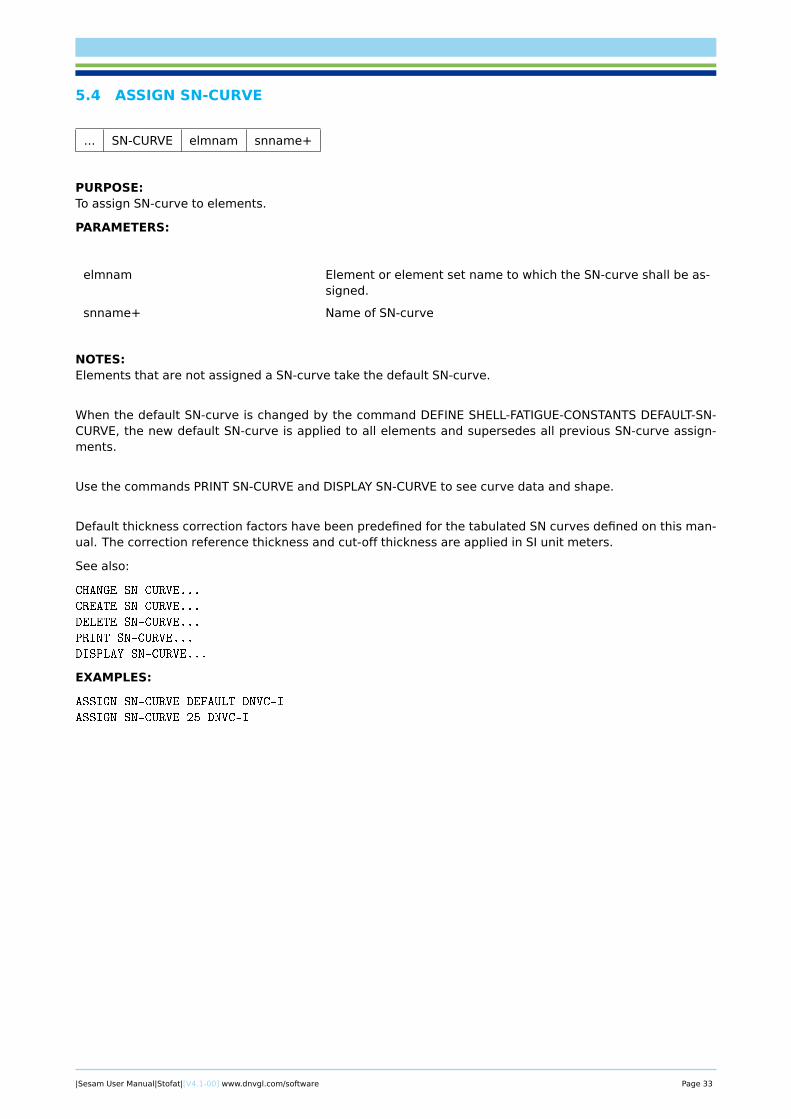
5.4 ASSIGN SN-CURVE
... SN-CURVE elmnam snname+
PURPOSE:To assign SN-curve to elements.
PARAMETERS:
elmnam Element or element set name to which the SN-curve shall be as-signed.
snname+ Name of SN-curve
NOTES:Elements that are not assigned a SN-curve take the default SN-curve.
When the default SN-curve is changed by the command DEFINE SHELL-FATIGUE-CONSTANTS DEFAULT-SN-CURVE, the new default SN-curve is applied to all elements and supersedes all previous SN-curve assign-ments.
Use the commands PRINT SN-CURVE and DISPLAY SN-CURVE to see curve data and shape.
Default thickness correction factors have been predefined for the tabulated SN curves defined on this man-ual. The correction reference thickness and cut-off thickness are applied in SI unit meters.
See also:
CHANGE SN-CURVE...
CREATE SN-CURVE...
DELETE SN-CURVE...
PRINT SN-CURVE...
DISPLAY SN-CURVE...
EXAMPLES:
ASSIGN SN-CURVE DEFAULT DNVC-I
ASSIGN SN-CURVE 25 DNVC-I
|Sesam User Manual|Stofat|[V4.1-00] www.dnvgl.com/software Page 33
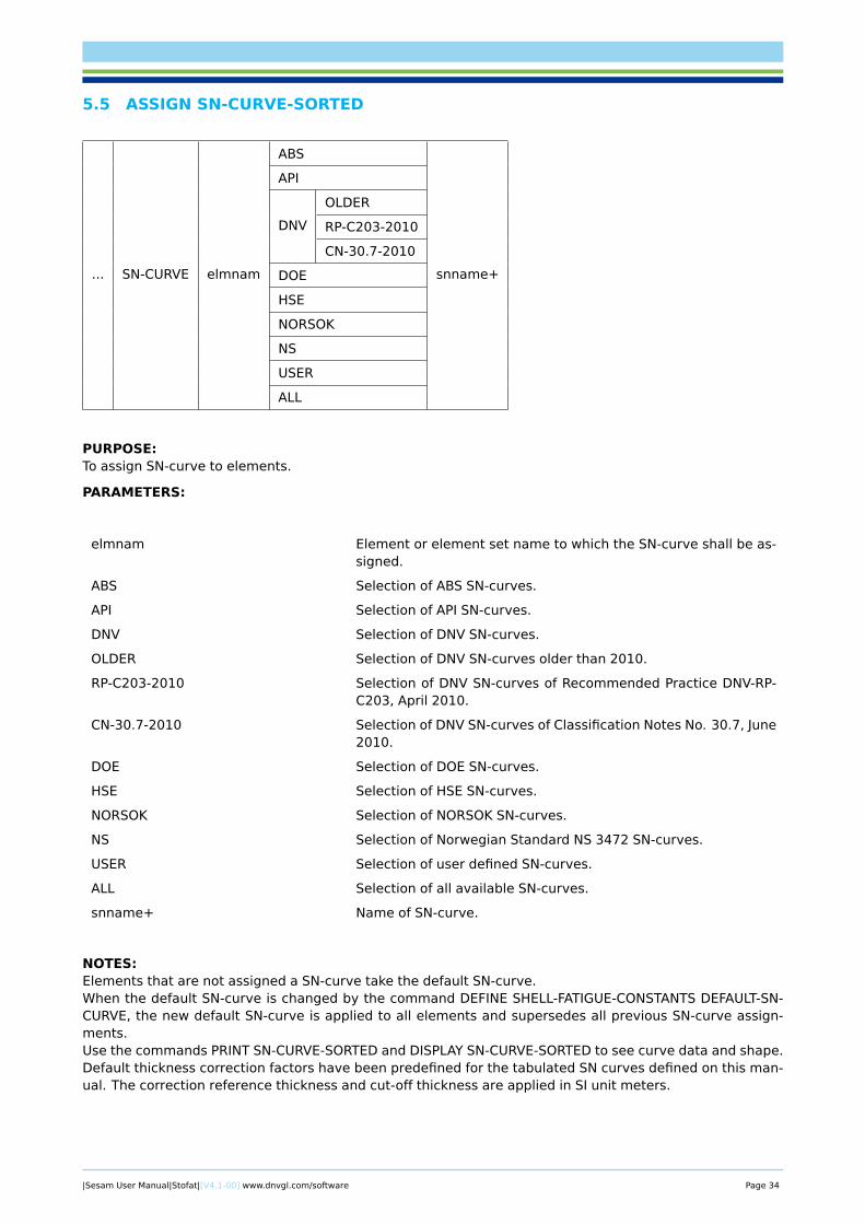
5.5 ASSIGN SN-CURVE-SORTED
... SN-CURVE elmnam
ABS
snname+
API
DNV
OLDER
RP-C203-2010
CN-30.7-2010
DOE
HSE
NORSOK
NS
USER
ALL
PURPOSE:To assign SN-curve to elements.
PARAMETERS:
elmnam Element or element set name to which the SN-curve shall be as-signed.
ABS Selection of ABS SN-curves.
API Selection of API SN-curves.
DNV Selection of DNV SN-curves.
OLDER Selection of DNV SN-curves older than 2010.
RP-C203-2010 Selection of DNV SN-curves of Recommended Practice DNV-RP-C203, April 2010.
CN-30.7-2010 Selection of DNV SN-curves of Classification Notes No. 30.7, June2010.
DOE Selection of DOE SN-curves.
HSE Selection of HSE SN-curves.
NORSOK Selection of NORSOK SN-curves.
NS Selection of Norwegian Standard NS 3472 SN-curves.
USER Selection of user defined SN-curves.
ALL Selection of all available SN-curves.
snname+ Name of SN-curve.
NOTES:Elements that are not assigned a SN-curve take the default SN-curve.When the default SN-curve is changed by the command DEFINE SHELL-FATIGUE-CONSTANTS DEFAULT-SN-CURVE, the new default SN-curve is applied to all elements and supersedes all previous SN-curve assign-ments.Use the commands PRINT SN-CURVE-SORTED and DISPLAY SN-CURVE-SORTED to see curve data and shape.Default thickness correction factors have been predefined for the tabulated SN curves defined on this man-ual. The correction reference thickness and cut-off thickness are applied in SI unit meters.
|Sesam User Manual|Stofat|[V4.1-00] www.dnvgl.com/software Page 34

See also:
CHANGE SN-CURVE...
CREATE SN-CURVE...
DELETE SN-CURVE...
PRINT SN-CURVE...
DISPLAY SN-CURVE...
EXAMPLES:
ASSIGN SN-CURVE-SORTED DEFAULT DNV RP-C203-2010 DNV2010_B1-SEAFC
ASSIGN SN-CURVE-SORTED 25 NS NS-F2-SE
|Sesam User Manual|Stofat|[V4.1-00] www.dnvgl.com/software Page 35
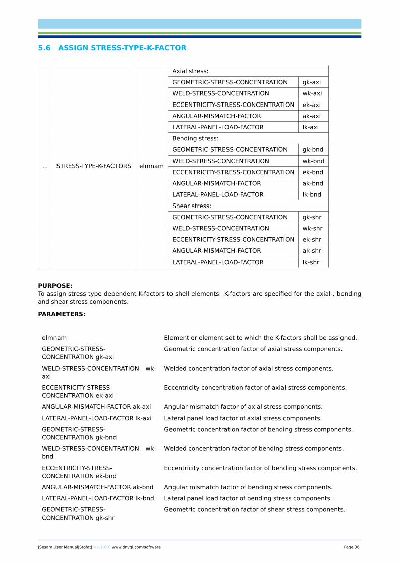
5.6 ASSIGN STRESS-TYPE-K-FACTOR
... STRESS-TYPE-K-FACTORS elmnam
Axial stress:
GEOMETRIC-STRESS-CONCENTRATION gk-axi
WELD-STRESS-CONCENTRATION wk-axi
ECCENTRICITY-STRESS-CONCENTRATION ek-axi
ANGULAR-MISMATCH-FACTOR ak-axi
LATERAL-PANEL-LOAD-FACTOR lk-axi
Bending stress:
GEOMETRIC-STRESS-CONCENTRATION gk-bnd
WELD-STRESS-CONCENTRATION wk-bnd
ECCENTRICITY-STRESS-CONCENTRATION ek-bnd
ANGULAR-MISMATCH-FACTOR ak-bnd
LATERAL-PANEL-LOAD-FACTOR lk-bnd
Shear stress:
GEOMETRIC-STRESS-CONCENTRATION gk-shr
WELD-STRESS-CONCENTRATION wk-shr
ECCENTRICITY-STRESS-CONCENTRATION ek-shr
ANGULAR-MISMATCH-FACTOR ak-shr
LATERAL-PANEL-LOAD-FACTOR lk-shr
PURPOSE:To assign stress type dependent K-factors to shell elements. K-factors are specified for the axial-, bendingand shear stress components.
PARAMETERS:
elmnam Element or element set to which the K-factors shall be assigned.
GEOMETRIC-STRESS-CONCENTRATION gk-axi
Geometric concentration factor of axial stress components.
WELD-STRESS-CONCENTRATION wk-axi
Welded concentration factor of axial stress components.
ECCENTRICITY-STRESS-CONCENTRATION ek-axi
Eccentricity concentration factor of axial stress components.
ANGULAR-MISMATCH-FACTOR ak-axi Angular mismatch factor of axial stress components.
LATERAL-PANEL-LOAD-FACTOR lk-axi Lateral panel load factor of axial stress components.
GEOMETRIC-STRESS-CONCENTRATION gk-bnd
Geometric concentration factor of bending stress components.
WELD-STRESS-CONCENTRATION wk-bnd
Welded concentration factor of bending stress components.
ECCENTRICITY-STRESS-CONCENTRATION ek-bnd
Eccentricity concentration factor of bending stress components.
ANGULAR-MISMATCH-FACTOR ak-bnd Angular mismatch factor of bending stress components.
LATERAL-PANEL-LOAD-FACTOR lk-bnd Lateral panel load factor of bending stress components.
GEOMETRIC-STRESS-CONCENTRATION gk-shr
Geometric concentration factor of shear stress components.
|Sesam User Manual|Stofat|[V4.1-00] www.dnvgl.com/software Page 36
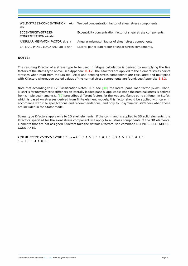
WELD-STRESS-CONCENTRATION wk-shr
Welded concentration factor of shear stress components.
ECCENTRICITY-STRESS-CONCENTRATION ek-shr
Eccentricity concentration factor of shear stress components.
ANGULAR-MISMATCH-FACTOR ak-shr Angular mismatch factor of shear stress components.
LATERAL-PANEL-LOAD-FACTOR lk-shr Lateral panel load factor of shear stress components.
NOTES:
The resulting K-factor of a stress type to be used in fatigue calculation is derived by multiplying the fivefactors of the stress type above, see Appendix B.3.2. The K-factors are applied to the element stress pointsstresses when read from the SIN file. Axial and bending stress components are calculated and multipliedwith K-factors whereupon scaled values of the normal stress components are found, see Appendix B.3.2.
Note that according to DNV Classification Notes 30.7, see [30], the lateral panel load factor (lk-axi, lkbnd,lk-shr) is for unsymmetric stiffeners on laterally loaded panels, applicable when the nominal stress is derivedfrom simple beam analysis. [30] prescribes different factors for the web and flange ot he stiffener. In Stofat,which is based on stresses derived from finite element models, this factor should be applied with care, inaccordance with rule specifcations and recommendations, and only to unsymmetric stiffeners when theseare included in the Stofat model.
Stress type K-factors apply only to 2D shell elements. If the command is applied to 3D solid elements, theK-factors specified for the axial stress component will apply to all stress components of the 3D elements.Elements that are not assigned K-factors take the default K-factors, see command DEFINE SHELL-FATIGUE-CONSTANTS.
ASSIGN STRESS-TYPE-K-FACTORS Current 1.5 1.0 1.5 1.0 1.0 1.2 1.0 1.2 1.0 1.0
1.4 1.0 1.4 1.0 1.0
|Sesam User Manual|Stofat|[V4.1-00] www.dnvgl.com/software Page 37
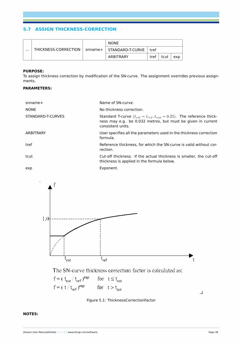
5.7 ASSIGN THICKNESS-CORRECTION
... THICKNESS-CORRECTION snname+
NONE
STANDARD-T-CURVE tref
ARBITRARY tref tcut exp
PURPOSE:To assign thickness correction by modification of the SN-curve. The assignment overrides previous assign-ments.
PARAMETERS:
snname+ Name of SN-curve.
NONE No thickness correction.
STANDARD-T-CURVES Standard T-curve (tcut = tref , texp = 0.25). The reference thick-ness may e.g. be 0.032 metres, but must be given in currentconsistent units.
ARBITRARY User specifies all the parameters used in the thickness correctionformula.
tref Reference thickness, for which the SN-curve is valid without cor-rection.
tcut Cut-off thickness. If the actual thickness is smaller, the cut-offthickness is applied in the formula below.
exp Exponent.
Figure 5.1: ThicknessCorrectionFactor
NOTES:
|Sesam User Manual|Stofat|[V4.1-00] www.dnvgl.com/software Page 38

The unit of the thickness correction and cut-off criteria are related to the units of the SN-curve and the lengthunit applied in the analysis. For user defined SN-curves, both SN-curve data and thickness corrections mustbe consistent with the units applied in the analysis. Thickness corrections must accordingly be assigned insame length unit as applied in the analysis.
Build-in library SN-curves of Stofat may have predefined default thickness corrections (reference thicknessand cut-off thickness) defined in SI unit meters. These values are multiplied with a unit length factor enteredby the command DEFINE SHELL-FATIGUE-CONSTANTS. The purpose is to convert the thickness correctionsto the length unit of the current analysis.
If the length unit of the analysis is mm and default thickness corrections (in meters) of library SN-curves areapplied, a unit length factor of 1000 must be used. However, if thickness corrections are assigned by theuser in same length unit as applied in the analysis, a unit length factor of 1.0 should be used.
Note that the unit length factor is only applied to thickness corrections of build-in library SN-curves and thatthe same unit length factor is applied to all library SN-curves applied in the analysis. Thickness correctionsof all library SN-curves applied must accordingly be in same length unit, i.e if predefined thickness correc-tions are used for one library SN-curve, thickness corrections assigned to another library SN-curve by theuser must also be in meters.
See also:
CHANGE SN-CURVE...
CREATE SN-CURVE...
DELETE SN-CURVE...
PRINT SN-CURVE...
DISPLAY SN-CURVE...
EXAMPLES:
ASSIGN THICKNESS-CORRECTION USE-X NONE
ASSIGN THICKNESS-CORRECTION USE-Y STANDARD-T-CURVE 0.032
|Sesam User Manual|Stofat|[V4.1-00] www.dnvgl.com/software Page 39
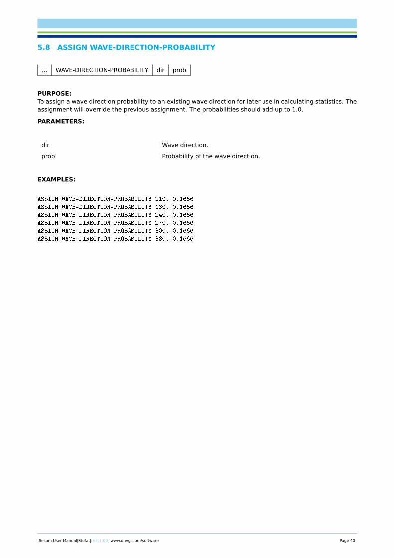
5.8 ASSIGN WAVE-DIRECTION-PROBABILITY
... WAVE-DIRECTION-PROBABILITY dir prob
PURPOSE:To assign a wave direction probability to an existing wave direction for later use in calculating statistics. Theassignment will override the previous assignment. The probabilities should add up to 1.0.
PARAMETERS:
dir Wave direction.
prob Probability of the wave direction.
EXAMPLES:
ASSIGN WAVE-DIRECTION-PROBABILITY 210. 0.1666
ASSIGN WAVE-DIRECTION-PROBABILITY 180. 0.1666
ASSIGN WAVE-DIRECTION-PROBABILITY 240. 0.1666
ASSIGN WAVE-DIRECTION-PROBABILITY 270. 0.1666
ASSIGN WAVE-DIRECTION-PROBABILITY 300. 0.1666
ASSIGN WAVE-DIRECTION-PROBABILITY 330. 0.1666
|Sesam User Manual|Stofat|[V4.1-00] www.dnvgl.com/software Page 40

5.9 ASSIGN WAVE-SPECTRUM-SHAPE
... WAVE-SPECTRUM-SHAPE name+
PIERSON-MOSKOWITZ
...ALL
JONSWAP gam sma smb
GENERAL-GAMMA lsp nsp PART hsl hsu tzl tzu
ISSC ...ALL
PART hsl hsu tll t1u
TORSETHAUGENFULL
...ALL
SIMPLIFIED PART hsl hsu tpl tpu
PURPOSE:To assign a wave spectrum shape to a wave scatter diagram. The assignment may be to the total scatterdiagram, or to a selected part of the diagram. The assignments will override the previous assignments.
It is only possible to assign a wave spectrum shape to the total sea state area if the wave statistics is de-scribed through a Nordenstrøm’s model.
PARAMETERS:
name+ Name of the wave statistics model.
PIERSON-MOSKOWITZ Wave spectrum of type Pierson-Moskowitz.
JONSWAP Wave spectrum of type Jonswap.
GENERAL-GAMMA Wave spectrum of type general gamma.
ISSC Wave spectrum of type ISSC (International Ship and OffshoreStructure Congress).
TORSETHAUGEN Wave spectrum of type Torsethaugen.
gam Enhancement factor, γ, of Jonswap spectrum.
sma Left width, σa, of Jonswap spectrum.
smb Right width,σa, of Jonswap spectrum.
lsp l-parameter in the General Gamma spectrum.
nsp n-parameter in the General Gamma spectrum.
FULL Full option for the Torsethagen spectrum.
SIMPLIFIED Simplified option for the Torsethagen spectrum.
ALL Wave spectrum shape will be assign to the total area of the wavestatistics mode.
PART Wave spectrum shape will be assign to an area of the scatterdiagram limited by the square made of HS−lower, HS−upper andTZ−lower, TZ−upper.
hsl Lower limit of the significant wave height, HS .
hsu Upper limit of the significant wave height, HS .
tzl Lower limit of the zero up crossing wave period, TZ .
tzu Upper limit of the zero up crossing wave period, TZ .
t1l Lower limit of mean wave period, T1.
t1u Upper limit of mean wave period, T1.
tpl Lower limit of peak wave period, Tp.
tpu Upper limit of peak wave period, Tp.
|Sesam User Manual|Stofat|[V4.1-00] www.dnvgl.com/software Page 41

NOTES:If the command is not given a Pierson-Moskowitz spectrum will be assumed.Stofat applies a quadratic interpolation rule in the calculation of the spectral moments for the Pierson-Moskowitz wave spectrum. This integration rule may, however, give negative spectral moments for abruptand large changes in the wave spectrum (.e.g. big and sharp peaks at single frequencies). Negative spectralmoments are not valid and are recalculated by using linear interpolation of the wave spectrum to ensurenon-zero positive spectral moments. When negative spectral moments occur, a message is printed for firstoccurrence with output of the wave spectrum.
EXAMPLES:
ASSIGN WAVE-SPECTRUM-SHAPE BMT GENERAL-GAMMA 5.0 4.0 ALL
ASSIGN WAVE-SPECTRUM-SHAPE DNV-NA JONSWAP 3.3 0.07 0.09 ALL
ASSIGN WAVE-SPECTRUM-SHAPE DNV-WW PIERSON-MOSKOWITZ ALL
ASSIGN WAVE-SPECTRUM-SHAPE ISSC1 ISSC ALL
|Sesam User Manual|Stofat|[V4.1-00] www.dnvgl.com/software Page 42
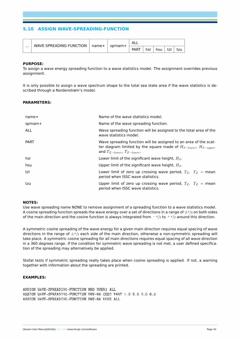
5.10 ASSIGN WAVE-SPREADING-FUNCTION
... WAVE-SPREADING-FUNCTION name+ sprnam+ALL
PART hsl hsu tzl tzu
PURPOSE:To assign a wave energy spreading function to a wave statistics model. The assignment overrides previousassignment.
It is only possible to assign a wave spectrum shape to the total sea state area if the wave statistics is de-scribed through a Nordenstrøm’s model.
PARAMETERS:
name+ Name of the wave statistics model.
sprnam+ Name of the wave spreading function.
ALL Wave spreading function will be assigned to the total area of thewave statistics model.
PART Wave spreading function will be assigned to an area of the scat-ter diagram limited by the square made of HS−lower, HS−upperand TZ−lower, TZ−lower.
hsl Lower limit of the significant wave height, HS .
hsu Upper limit of the significant wave height, HS .
tzl Lower limit of zero up crossing wave period, TZ . TZ = meanperiod when ISSC wave statistics.
tzu Upper limit of zero up crossing wave period, TZ . TZ = meanperiod when ISSC wave statistics.
NOTES:Use wave spreading name NONE to remove assignment of a spreading function to a wave statistics model.A cosine spreading function spreads the wave energy over a set of directions in a range of±π/2 on both sidesof the main direction and the cosine function is always integrated from − π/2 to + π/2 around this direction.
A symmetric cosine spreading of the wave energy for a given main direction requires equal spacing of wavedirections in the range of ±π/2 each side of the main direction, otherwise a non-symmetric spreading willtake place. A symmetric cosine spreading for all main directions requires equal spacing of all wave directionin a 360 degrees range. If the condition for symmetric wave spreading is not met, a user defined specifica-tion of the spreading may alternatively be applied.
Stofat tests if symmetric spreading really takes place when cosine spreading is applied. If not, a warningtogether with information about the spreading are printed.
EXAMPLES:
ASSIGN WAVE-SPREADING-FUNCTION NRD USER1 ALL
ASSIGN WAVE-SPREADING-FUNCTION DNV-NA COS2 PART 1.0 5.0 2.0 6.0
ASSIGN WAVE-SPREADING-FUNCTION DNV-NA NONE ALL
|Sesam User Manual|Stofat|[V4.1-00] www.dnvgl.com/software Page 43
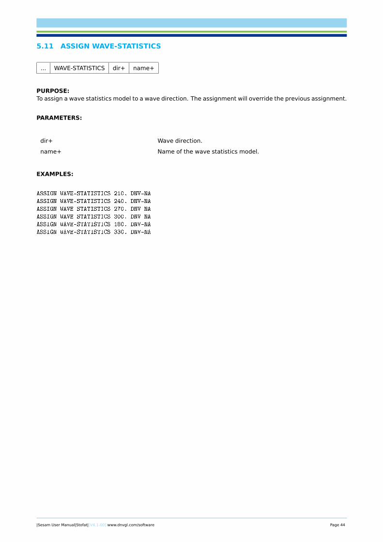
5.11 ASSIGN WAVE-STATISTICS
... WAVE-STATISTICS dir+ name+
PURPOSE:To assign a wave statistics model to a wave direction. The assignment will override the previous assignment.
PARAMETERS:
dir+ Wave direction.
name+ Name of the wave statistics model.
EXAMPLES:
ASSIGN WAVE-STATISTICS 210. DNV-NA
ASSIGN WAVE-STATISTICS 240. DNV-NA
ASSIGN WAVE-STATISTICS 270. DNV-NA
ASSIGN WAVE-STATISTICS 300. DNV-NA
ASSIGN WAVE-STATISTICS 180. DNV-NA
ASSIGN WAVE-STATISTICS 330. DNV-NA
|Sesam User Manual|Stofat|[V4.1-00] www.dnvgl.com/software Page 44

5.12 ASSIGN WELD-NORMAL-LINE
... WELD-NORMAL-LINE
OFF
ON wnlnam+ELEMENT elmnam
HOTSPOT ( ONLY hotnam+ )
PURPOSE:To assign weld normal line to element and hotspot.
PARAMETERS:
OFF/ON Switch off/on using assigned weld normal lines in the fatigue cal-culation (default is OFF).
ELEMENT Assign weld normal line to element.
HOTSPOT Assign weld normal line to hotspot.
elmnam Element or element set name to which the weld normal line shallbe assigned.
hotnam+ Hotspots to which the weld normal line shall be assigned.
wnlnam+ Name of weld normal line.
ONLY Mandatory attribute.
( ) Mandatory parentheses.
NOTES:An element or a hotspot can be connected to only one WN line which are applied to all fatigue check pointsof the element and the interpolation points of the hotspot. If several assignments are made to the sameelement or hotspot the last assignment will apply.
Assignments are deleted by the command DELETE WELD-NORMAL-LINE DELETE-ASSIGNMENT. Weld normallines are created by the command CREATE WELD-NORMAL-LINE.
Use the command PRINT RUN-OVERVIEW WELD-NORMAL-LINES or press the Show button in the dialoguebox to see current status on defined weld normal lines and assignments to elements and hotspots.
EXAMPLES:
ASSIGN WELD-NORMAL-LINE OFF
ASSIGN WELD-NORMAL-LINE ON WNL2 ELEMENT 86
SELECT ELEMENTS INCLUDE CURRENT
ASSIGN WELD-NORMAL-LINE ON WNL3 ELEMENT DEFAULT
ASSIGN WELD-NORMAL-LINE ON WNL1 HOTSPOT ( ONLY HOT1 HOT2 HOT3 HOT4 HOT5 HOT6 )
|Sesam User Manual|Stofat|[V4.1-00] www.dnvgl.com/software Page 45
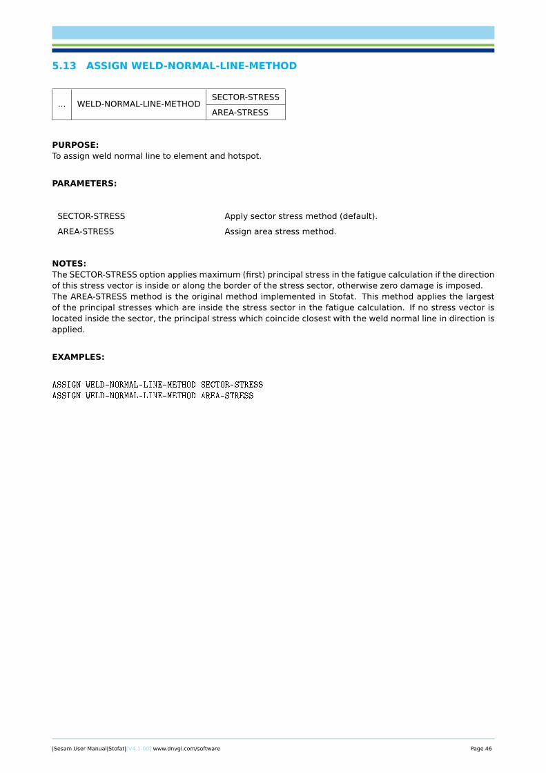
5.13 ASSIGN WELD-NORMAL-LINE-METHOD
... WELD-NORMAL-LINE-METHODSECTOR-STRESS
AREA-STRESS
PURPOSE:To assign weld normal line to element and hotspot.
PARAMETERS:
SECTOR-STRESS Apply sector stress method (default).
AREA-STRESS Assign area stress method.
NOTES:The SECTOR-STRESS option applies maximum (first) principal stress in the fatigue calculation if the directionof this stress vector is inside or along the border of the stress sector, otherwise zero damage is imposed.The AREA-STRESS method is the original method implemented in Stofat. This method applies the largestof the principal stresses which are inside the stress sector in the fatigue calculation. If no stress vector islocated inside the sector, the principal stress which coincide closest with the weld normal line in direction isapplied.
EXAMPLES:
ASSIGN WELD-NORMAL-LINE-METHOD SECTOR-STRESS
ASSIGN WELD-NORMAL-LINE-METHOD AREA-STRESS
|Sesam User Manual|Stofat|[V4.1-00] www.dnvgl.com/software Page 46

5.14 CHANGE
CHANGE
SN-CURVE
...WAVE-SPREADING-FUNCTION
WAVE-STATISTICS
PURPOSE:This is used to change previously created SN-curves, wave spreading functions and wave statistic tools.
The options and subcommands are mainly the same as for the corresponding CREATE command. The pro-gram will ask for the name of the object and the default values of the different subcommands will be asgiven before.
|Sesam User Manual|Stofat|[V4.1-00] www.dnvgl.com/software Page 47
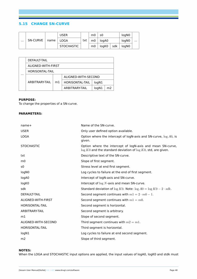
5.15 CHANGE SN-CURVE
... SN-CURVE name
USER
txt
m0 s0 logN0
...LOGA m0 logA0 logN0
STOCHASTIC m0 logK0 sdk logN0
...
DEFAULT-TAIL
ALIGNED-WITH-FIRST
HORISONTAL-TAIL
ARBITRARY-TAIL m1
ALIGNED-WITH-SECOND
HORISONTAL-TAIL logN1
ARBITRARY-TAIL logN1 m2
PURPOSE:To change the properties of a SN-curve.
PARAMETERS:
name+ Name of the SN-curve.
USER Only user defined option available.
LOGA Option where the intercept of logN-axis and SN-curve, logA0, isgiven.
STOCHASTIC Option where the intercept of logN-axis and mean SN-curve,logK0 and the standard deviation of logK0, std, are given.
txt Descriptive text of the SN-curve.
m0 Slope of first segment.
s0 Stress level at end first segment.
logN0 Log cycles to failure at the end of first segment.
logA0 Intercept of logN-axis and SN-curve.
logK0 Intercept of logN -axis and mean SN-curve.
sdk Standard deviation of logK0. Note: logA0 = logK0− 2 · sdk.
DEFAULT-TAIL Second segment continues with m1 = 2 ·m0− 1.
ALIGNED-WITH-FIRST Second segment continues with m1 = m0.
HORISONTAL-TAIL Second segment is horizontal.
ARBITRARY-TAIL Second segment is arbitrary.
m1 Slope of second segment.
ALIGNED-WITH-SECOND Third segment continues with m2 = m1.
HORISONTAL-TAIL Third segment is horizontal.
logN1 Log cycles to failure at end second segment.
m2 Slope of third segment.
NOTES:When the LOGA and STOCHASTIC input options are applied, the input values of logA0, logK0 and stdk must
|Sesam User Manual|Stofat|[V4.1-00] www.dnvgl.com/software Page 48
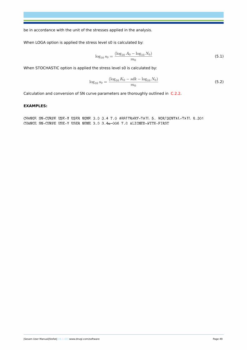
be in accordance with the unit of the stresses applied in the analysis.
When LOGA option is applied the stress level s0 is calculated by:
log10 s0 =(log10A0 − log10N0)
m0(5.1)
When STOCHASTIC option is applied the stress level s0 is calculated by:
log10 s0 =(log10K0 − sdk − log10N0)
m0(5.2)
Calculation and conversion of SN curve parameters are thoroughly outlined in C.2.2.
EXAMPLES:
CHANGE SN-CURVE USE-X USER NONE 3.0 3.4 7.0 ARBITRARY-TAIL 5. HORISONTAL-TAIL 8.301
CHANGE SN-CURVE USE-Y USER NONE 3.0 3.4e+006 7.0 ALIGNED-WITH-FIRST
|Sesam User Manual|Stofat|[V4.1-00] www.dnvgl.com/software Page 49
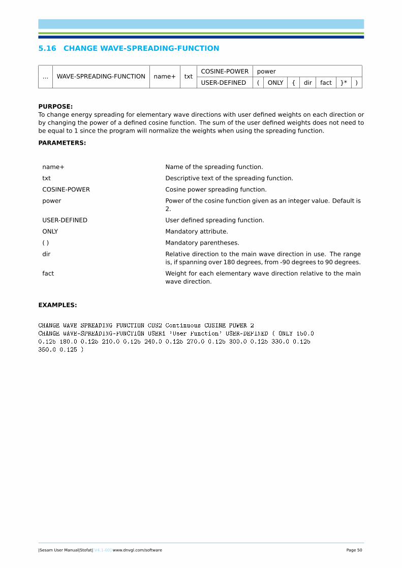
5.16 CHANGE WAVE-SPREADING-FUNCTION
... WAVE-SPREADING-FUNCTION name+ txtCOSINE-POWER power
USER-DEFINED ( ONLY { dir fact }* )
PURPOSE:To change energy spreading for elementary wave directions with user defined weights on each direction orby changing the power of a defined cosine function. The sum of the user defined weights does not need tobe equal to 1 since the program will normalize the weights when using the spreading function.
PARAMETERS:
name+ Name of the spreading function.
txt Descriptive text of the spreading function.
COSINE-POWER Cosine power spreading function.
power Power of the cosine function given as an integer value. Default is2.
USER-DEFINED User defined spreading function.
ONLY Mandatory attribute.
( ) Mandatory parentheses.
dir Relative direction to the main wave direction in use. The rangeis, if spanning over 180 degrees, from -90 degrees to 90 degrees.
fact Weight for each elementary wave direction relative to the mainwave direction.
EXAMPLES:
CHANGE WAVE-SPREADING-FUNCTION COS2 Continuous COSINE-POWER 2
CHANGE WAVE-SPREADING-FUNCTION USER1 'User Function' USER-DEFINED ( ONLY 150.0
0.125 180.0 0.125 210.0 0.125 240.0 0.125 270.0 0.125 300.0 0.125 330.0 0.125
350.0 0.125 )
|Sesam User Manual|Stofat|[V4.1-00] www.dnvgl.com/software Page 50
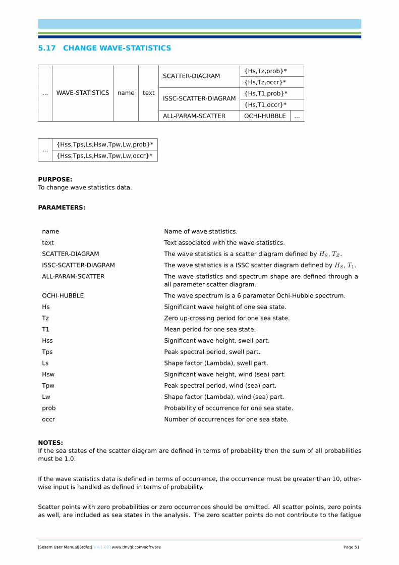
5.17 CHANGE WAVE-STATISTICS
... WAVE-STATISTICS name text
SCATTER-DIAGRAM{Hs,Tz,prob}*
{Hs,Tz,occr}*
ISSC-SCATTER-DIAGRAM{Hs,T1,prob}*
{Hs,T1,occr}*
ALL-PARAM-SCATTER OCHI-HUBBLE ...
...{Hss,Tps,Ls,Hsw,Tpw,Lw,prob}*
{Hss,Tps,Ls,Hsw,Tpw,Lw,occr}*
PURPOSE:To change wave statistics data.
PARAMETERS:
name Name of wave statistics.
text Text associated with the wave statistics.
SCATTER-DIAGRAM The wave statistics is a scatter diagram defined by HS , TZ .
ISSC-SCATTER-DIAGRAM The wave statistics is a ISSC scatter diagram defined by HS , T1.
ALL-PARAM-SCATTER The wave statistics and spectrum shape are defined through aall parameter scatter diagram.
OCHI-HUBBLE The wave spectrum is a 6 parameter Ochi-Hubble spectrum.
Hs Significant wave height of one sea state.
Tz Zero up-crossing period for one sea state.
T1 Mean period for one sea state.
Hss Significant wave height, swell part.
Tps Peak spectral period, swell part.
Ls Shape factor (Lambda), swell part.
Hsw Significant wave height, wind (sea) part.
Tpw Peak spectral period, wind (sea) part.
Lw Shape factor (Lambda), wind (sea) part.
prob Probability of occurrence for one sea state.
occr Number of occurrences for one sea state.
NOTES:If the sea states of the scatter diagram are defined in terms of probability then the sum of all probabilitiesmust be 1.0.
If the wave statistics data is defined in terms of occurrence, the occurrence must be greater than 10, other-wise input is handled as defined in terms of probability.
Scatter points with zero probabilities or zero occurrences should be omitted. All scatter points, zero pointsas well, are included as sea states in the analysis. The zero scatter points do not contribute to the fatigue
|Sesam User Manual|Stofat|[V4.1-00] www.dnvgl.com/software Page 51
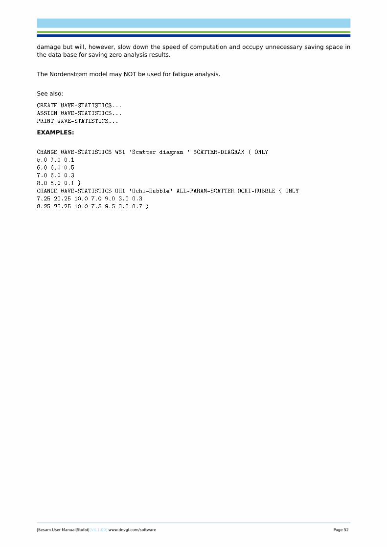
damage but will, however, slow down the speed of computation and occupy unnecessary saving space inthe data base for saving zero analysis results.
The Nordenstrøm model may NOT be used for fatigue analysis.
See also:
CREATE WAVE-STATISTICS...
ASSIGN WAVE-STATISTICS...
PRINT WAVE-STATISTICS...
EXAMPLES:
CHANGE WAVE-STATISTICS WS1 'Scatter diagram ' SCATTER-DIAGRAM ( ONLY
5.0 7.0 0.1
6.0 6.0 0.5
7.0 6.0 0.3
8.0 5.0 0.1 )
CHANGE WAVE-STATISTICS OH1 'Ochi-Hubble' ALL-PARAM-SCATTER OCHI-HUBBLE ( ONLY
7.25 20.25 10.0 7.0 9.0 3.0 0.3
8.25 25.25 10.0 7.5 9.5 3.0 0.7 )
|Sesam User Manual|Stofat|[V4.1-00] www.dnvgl.com/software Page 52

5.18 CREATE
CREATE
FATIGUE-CHECK-POINTS
...
SN-CURVE
WAVE-SPREADING-FUNCTION
WAVE-STATISTICS
WELD-NORMAL-LINE
PURPOSE:The create command is the main command for creation of fatigue check points and different tools such asSN-curves, wave spectra, wave energy spreading functions, wave statistics models and weld normal lines.
|Sesam User Manual|Stofat|[V4.1-00] www.dnvgl.com/software Page 53

5.19 CREATE FATIGUE-CHECK-POINTS
... FATIGUE-CHECK-POINTSHOTSPOT-CHECK
...ELEMENT-CHECK
PURPOSE:To create hotspot fatigue check points and to set location of element fatigue check points.
|Sesam User Manual|Stofat|[V4.1-00] www.dnvgl.com/software Page 54
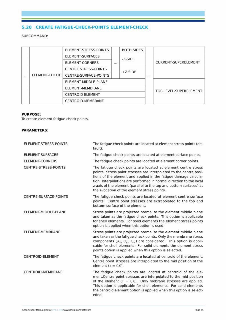
5.20 CREATE FATIGUE-CHECK-POINTS ELEMENT-CHECK
SUBCOMMAND:
... ELEMENT-CHECK
ELEMENT-STRESS-POINTS
...
BOTH-SIDES
...
CURRENT-SUPERELEMENT
ELEMENT-SURFACES-Z-SIDE
ELEMENT-CORNERS
CENTRE STRESS-POINTS+Z-SIDE
CENTRE-SURFACE-POINTS
ELEMENT-MIDDLE-PLANE
TOP-LEVEL-SUPERELEMENTELEMENT-MEMBRANE
CENTROID ELEMENT
CENTROID-MEMBRANE
PURPOSE:To create element fatigue check points.
PARAMETERS:
ELEMENT-STRESS-POINTS The fatigue check points are located at element stress points (de-fault).
ELEMENT-SURFACES The fatigue check points are located at element surface points.
ELEMENT-CORNERS The fatigue check points are located at element corner points.
CENTRE-STRESS-POINTS The fatigue check points are located at element centre stresspoints. Stress point stresses are interpolated to the centre posi-tions of the element and applied in the fatigue damage calcula-tion. Interpolations are performed in normal direction to the localz-axis of the element (parallel to the top and bottom surfaces) atthe z-location of the element stress points.
CENTRE-SURFACE-POINTS The fatigue check points are located at element centre surfacepoints. Centre point stresses are extrapolated to the top andbottom surface of the element.
ELEMENT-MIDDLE-PLANE Stress points are projected normal to the element middle planeand taken as the fatigue check points. This option is applicablefor shell elements. For solid elements the element stress pointsoption is applied when this option is used.
ELEMENT-MEMBRANE Stress points are projected normal to the element middle planeand taken as the fatigue check points. Only the membrane stresscomponents (σx, σy, τxy) are considered. This option is appli-cable for shell elements. For solid elements the element stresspoints option is applied when this option is selected.
CENTROID-ELEMENT The fatigue check points are located at centroid of the element.Centre point stresses are interpolated to the mid position of theelement (z = 0.0).
CENTROID-MEMBRANE The fatigue check points are located at centroid of the ele-ment.Centre point stresses are interpolated to the mid positionof the element (z = 0.0). Only mebrane stresses are applied.This option is applicable for shell elements. For solid elementsthe centroid element option is applied when this option is select-eded.
|Sesam User Manual|Stofat|[V4.1-00] www.dnvgl.com/software Page 55
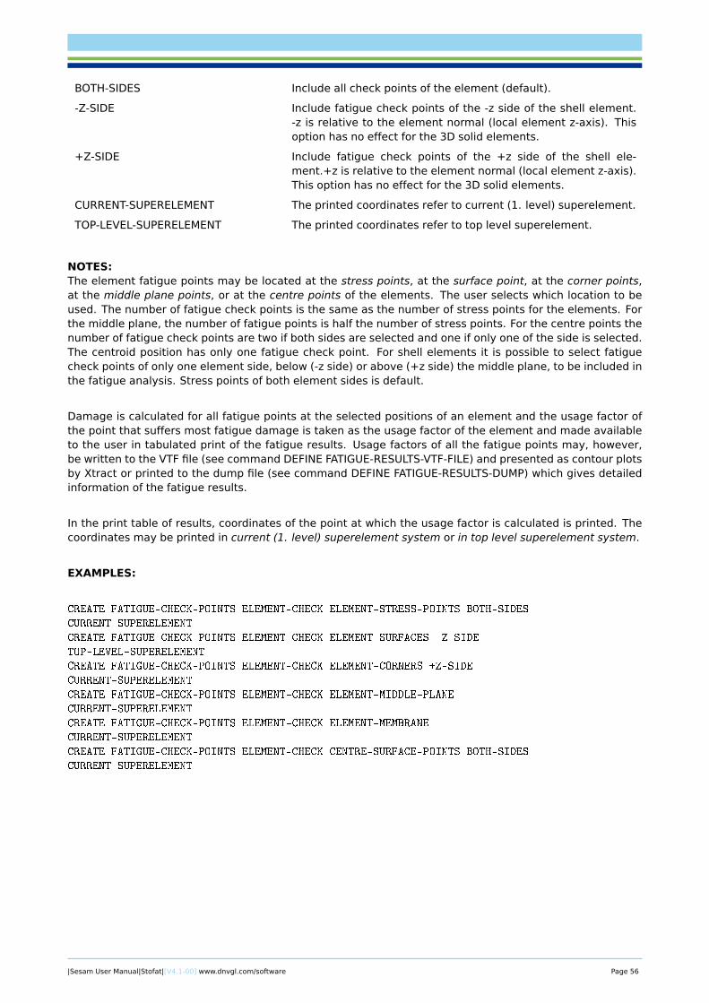
BOTH-SIDES Include all check points of the element (default).
-Z-SIDE Include fatigue check points of the -z side of the shell element.-z is relative to the element normal (local element z-axis). Thisoption has no effect for the 3D solid elements.
+Z-SIDE Include fatigue check points of the +z side of the shell ele-ment.+z is relative to the element normal (local element z-axis).This option has no effect for the 3D solid elements.
CURRENT-SUPERELEMENT The printed coordinates refer to current (1. level) superelement.
TOP-LEVEL-SUPERELEMENT The printed coordinates refer to top level superelement.
NOTES:The element fatigue points may be located at the stress points, at the surface point, at the corner points,at the middle plane points, or at the centre points of the elements. The user selects which location to beused. The number of fatigue check points is the same as the number of stress points for the elements. Forthe middle plane, the number of fatigue points is half the number of stress points. For the centre points thenumber of fatigue check points are two if both sides are selected and one if only one of the side is selected.The centroid position has only one fatigue check point. For shell elements it is possible to select fatiguecheck points of only one element side, below (-z side) or above (+z side) the middle plane, to be included inthe fatigue analysis. Stress points of both element sides is default.
Damage is calculated for all fatigue points at the selected positions of an element and the usage factor ofthe point that suffers most fatigue damage is taken as the usage factor of the element and made availableto the user in tabulated print of the fatigue results. Usage factors of all the fatigue points may, however,be written to the VTF file (see command DEFINE FATIGUE-RESULTS-VTF-FILE) and presented as contour plotsby Xtract or printed to the dump file (see command DEFINE FATIGUE-RESULTS-DUMP) which gives detailedinformation of the fatigue results.
In the print table of results, coordinates of the point at which the usage factor is calculated is printed. Thecoordinates may be printed in current (1. level) superelement system or in top level superelement system.
EXAMPLES:
CREATE FATIGUE-CHECK-POINTS ELEMENT-CHECK ELEMENT-STRESS-POINTS BOTH-SIDES
CURRENT-SUPERELEMENT
CREATE FATIGUE-CHECK-POINTS ELEMENT-CHECK ELEMENT-SURFACES -Z-SIDE
TOP-LEVEL-SUPERELEMENT
CREATE FATIGUE-CHECK-POINTS ELEMENT-CHECK ELEMENT-CORNERS +Z-SIDE
CURRENT-SUPERELEMENT
CREATE FATIGUE-CHECK-POINTS ELEMENT-CHECK ELEMENT-MIDDLE-PLANE
CURRENT-SUPERELEMENT
CREATE FATIGUE-CHECK-POINTS ELEMENT-CHECK ELEMENT-MEMBRANE
CURRENT-SUPERELEMENT
CREATE FATIGUE-CHECK-POINTS ELEMENT-CHECK CENTRE-SURFACE-POINTS BOTH-SIDES
CURRENT-SUPERELEMENT
|Sesam User Manual|Stofat|[V4.1-00] www.dnvgl.com/software Page 56
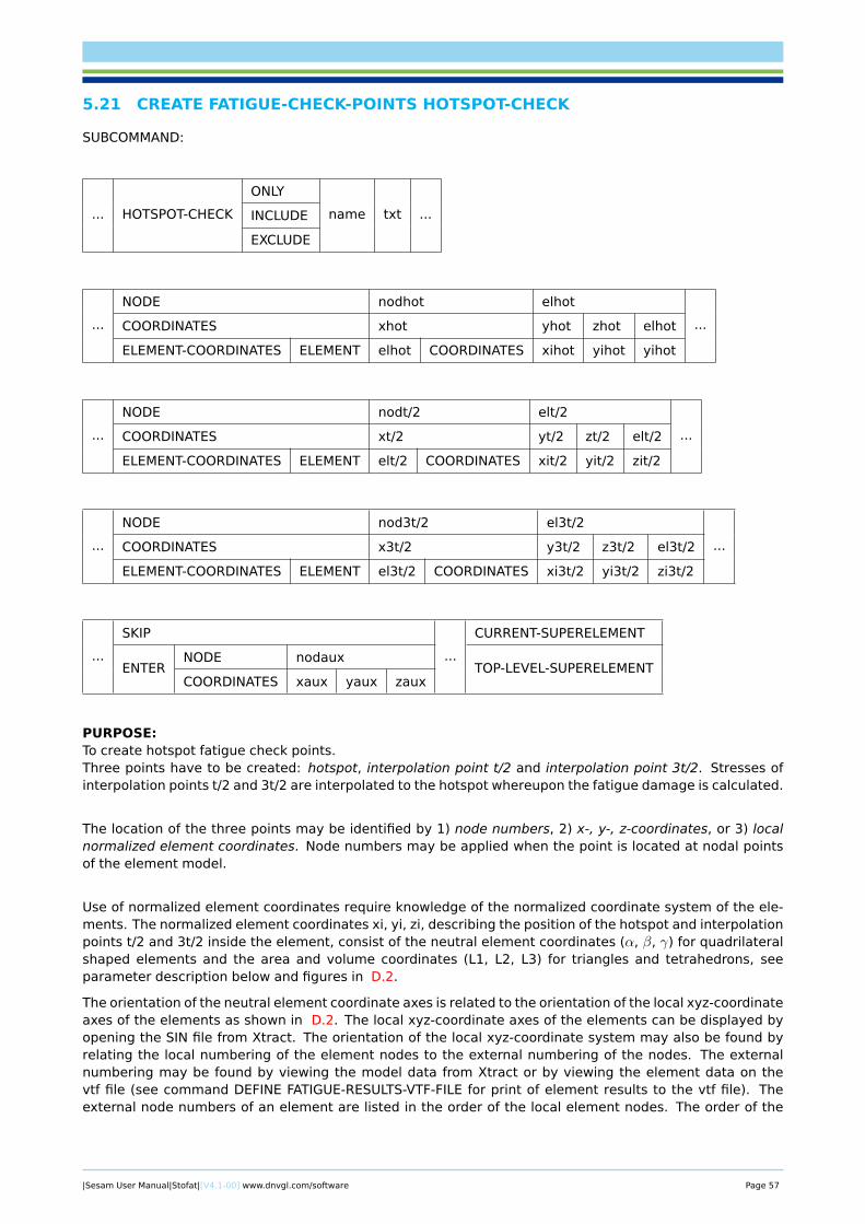
5.21 CREATE FATIGUE-CHECK-POINTS HOTSPOT-CHECK
SUBCOMMAND:
... HOTSPOT-CHECK
ONLY
name txt ...INCLUDE
EXCLUDE
...
NODE nodhot elhot
...COORDINATES xhot yhot zhot elhot
ELEMENT-COORDINATES ELEMENT elhot COORDINATES xihot yihot yihot
...
NODE nodt/2 elt/2
...COORDINATES xt/2 yt/2 zt/2 elt/2
ELEMENT-COORDINATES ELEMENT elt/2 COORDINATES xit/2 yit/2 zit/2
...
NODE nod3t/2 el3t/2
...COORDINATES x3t/2 y3t/2 z3t/2 el3t/2
ELEMENT-COORDINATES ELEMENT el3t/2 COORDINATES xi3t/2 yi3t/2 zi3t/2
...
SKIP
...
CURRENT-SUPERELEMENT
ENTERNODE nodaux
TOP-LEVEL-SUPERELEMENTCOORDINATES xaux yaux zaux
PURPOSE:To create hotspot fatigue check points.Three points have to be created: hotspot, interpolation point t/2 and interpolation point 3t/2. Stresses ofinterpolation points t/2 and 3t/2 are interpolated to the hotspot whereupon the fatigue damage is calculated.
The location of the three points may be identified by 1) node numbers, 2) x-, y-, z-coordinates, or 3) localnormalized element coordinates. Node numbers may be applied when the point is located at nodal pointsof the element model.
Use of normalized element coordinates require knowledge of the normalized coordinate system of the ele-ments. The normalized element coordinates xi, yi, zi, describing the position of the hotspot and interpolationpoints t/2 and 3t/2 inside the element, consist of the neutral element coordinates (α, β, γ) for quadrilateralshaped elements and the area and volume coordinates (L1, L2, L3) for triangles and tetrahedrons, seeparameter description below and figures in D.2.
The orientation of the neutral element coordinate axes is related to the orientation of the local xyz-coordinateaxes of the elements as shown in D.2. The local xyz-coordinate axes of the elements can be displayed byopening the SIN file from Xtract. The orientation of the local xyz-coordinate system may also be found byrelating the local numbering of the element nodes to the external numbering of the nodes. The externalnumbering may be found by viewing the model data from Xtract or by viewing the element data on thevtf file (see command DEFINE FATIGUE-RESULTS-VTF-FILE for print of element results to the vtf file). Theexternal node numbers of an element are listed in the order of the local element nodes. The order of the
|Sesam User Manual|Stofat|[V4.1-00] www.dnvgl.com/software Page 57

local element node numbering applied in Xtract differs from the order applied in Sesam and Stofat for someelements, see D.2.
Element number must be entered along with the point identification. The element number is used to iden-tify correct element stresses when the point is connected to more than one element (at an element node oralong an element border). When 0 (zero) is entered as element number, the program search through themodel and prints the elements that are connected to the point (not applicable for the element coordinatesoption). The user must then re-enter the input and specify an element number.
A point located inside an element may be moved to the surface of the element by the program. In thisregard an auxiliary point has to be entered. The auxiliary point may be located anywhere inside or outsidethe element model. The point is moved to the element surface that is closest to the auxiliary point. Theprogram prints the coordinates of the new point. If the position of the new point is accepted by the user, thehotspot must be re-entered, where the coordinates of the old point is replaced with the coordinates of thenew point and the auxiliary point is skipped.
The hotspot and the interpolation points must be located inside or at the border of the elements. When theuser creates a point that is located outside an element, the program does not accept the point and prints amessage along with the location of the point projected to the element border. Input must then be re-enteredwith a position that is not outside the element.
Note that input of a hotspot has to be accepted by the program before fatigue damage of the point is calcu-lated in the run execution.
Coordinates may be entered in current (1. level) superelement system or in top level superelement system.Default is current superelement.
Element stresses of the Results Interface File (R#.SIN) may be transformed to a global system, which maybe the coordinate system of the current superelement or the top level superelement.
Further details are given in D.3.
PARAMETERS:
ONLY Include the hotspot and its interpolation points (if new) and makethe hotspot active (if inactive). All other created hotspots aremade inactive and not available for use. Inactive hotspots aremade active by the INCLUDE parameter. A hotspot may bedeleted by the DELETE HOTSPOT command.
INCLUDE Include the hotspot and its interpolation points (if new) or makethe hotspot active (if inactive). Original data are kept when ahotspot is made active.
EXCLUDE Exclude the hotspot and its interpolation points. The excludedhotspot is made inactive and not available for use. Inactivehotspots are made active by the INCLUDE parameter. A hotspotmay be deleted by the DELETE HOTSPOT command.
name Name of the hotspot.
txt Descriptive text.
NODE Enter node number for identification of the point.
COORDINATES Enter coordinates for identification of the point.
ELEMENT-COORDINATES Enter normalised element coordinates for identification of thepoint.
ELEMENT Enter element number for identification of the point by nor-malised element coordinates.
|Sesam User Manual|Stofat|[V4.1-00] www.dnvgl.com/software Page 58
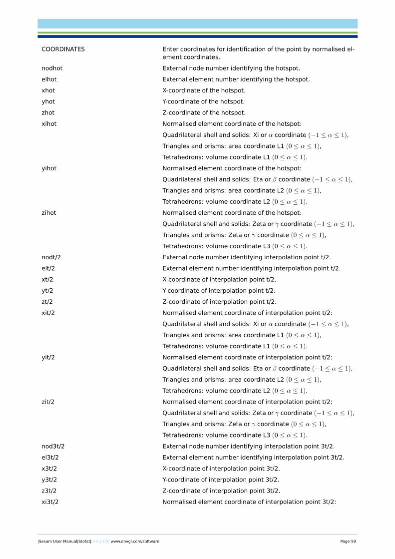
COORDINATES Enter coordinates for identification of the point by normalised el-ement coordinates.
nodhot External node number identifying the hotspot.
elhot External element number identifying the hotspot.
xhot X-coordinate of the hotspot.
yhot Y-coordinate of the hotspot.
zhot Z-coordinate of the hotspot.
xihot Normalised element coordinate of the hotspot:
Quadrilateral shell and solids: Xi or α coordinate (−1 ≤ α ≤ 1),
Triangles and prisms: area coordinate L1 (0 ≤ α ≤ 1),
Tetrahedrons: volume coordinate L1 (0 ≤ α ≤ 1).
yihot Normalised element coordinate of the hotspot:
Quadrilateral shell and solids: Eta or β coordinate (−1 ≤ α ≤ 1),
Triangles and prisms: area coordinate L2 (0 ≤ α ≤ 1),
Tetrahedrons: volume coordinate L2 (0 ≤ α ≤ 1).
zihot Normalised element coordinate of the hotspot:
Quadrilateral shell and solids: Zeta or γ coordinate (−1 ≤ α ≤ 1),
Triangles and prisms: Zeta or γ coordinate (0 ≤ α ≤ 1),
Tetrahedrons: volume coordinate L3 (0 ≤ α ≤ 1).
nodt/2 External node number identifying interpolation point t/2.
elt/2 External element number identifying interpolation point t/2.
xt/2 X-coordinate of interpolation point t/2.
yt/2 Y-coordinate of interpolation point t/2.
zt/2 Z-coordinate of interpolation point t/2.
xit/2 Normalised element coordinate of interpolation point t/2:
Quadrilateral shell and solids: Xi or α coordinate (−1 ≤ α ≤ 1),
Triangles and prisms: area coordinate L1 (0 ≤ α ≤ 1),
Tetrahedrons: volume coordinate L1 (0 ≤ α ≤ 1).
yit/2 Normalised element coordinate of interpolation point t/2:
Quadrilateral shell and solids: Eta or β coordinate (−1 ≤ α ≤ 1),
Triangles and prisms: area coordinate L2 (0 ≤ α ≤ 1),
Tetrahedrons: volume coordinate L2 (0 ≤ α ≤ 1).
zit/2 Normalised element coordinate of interpolation point t/2:
Quadrilateral shell and solids: Zeta or γ coordinate (−1 ≤ α ≤ 1),
Triangles and prisms: Zeta or γ coordinate (0 ≤ α ≤ 1),
Tetrahedrons: volume coordinate L3 (0 ≤ α ≤ 1).
nod3t/2 External node number identifying interpolation point 3t/2.
el3t/2 External element number identifying interpolation point 3t/2.
x3t/2 X-coordinate of interpolation point 3t/2.
y3t/2 Y-coordinate of interpolation point 3t/2.
z3t/2 Z-coordinate of interpolation point 3t/2.
xi3t/2 Normalised element coordinate of interpolation point 3t/2:
|Sesam User Manual|Stofat|[V4.1-00] www.dnvgl.com/software Page 59
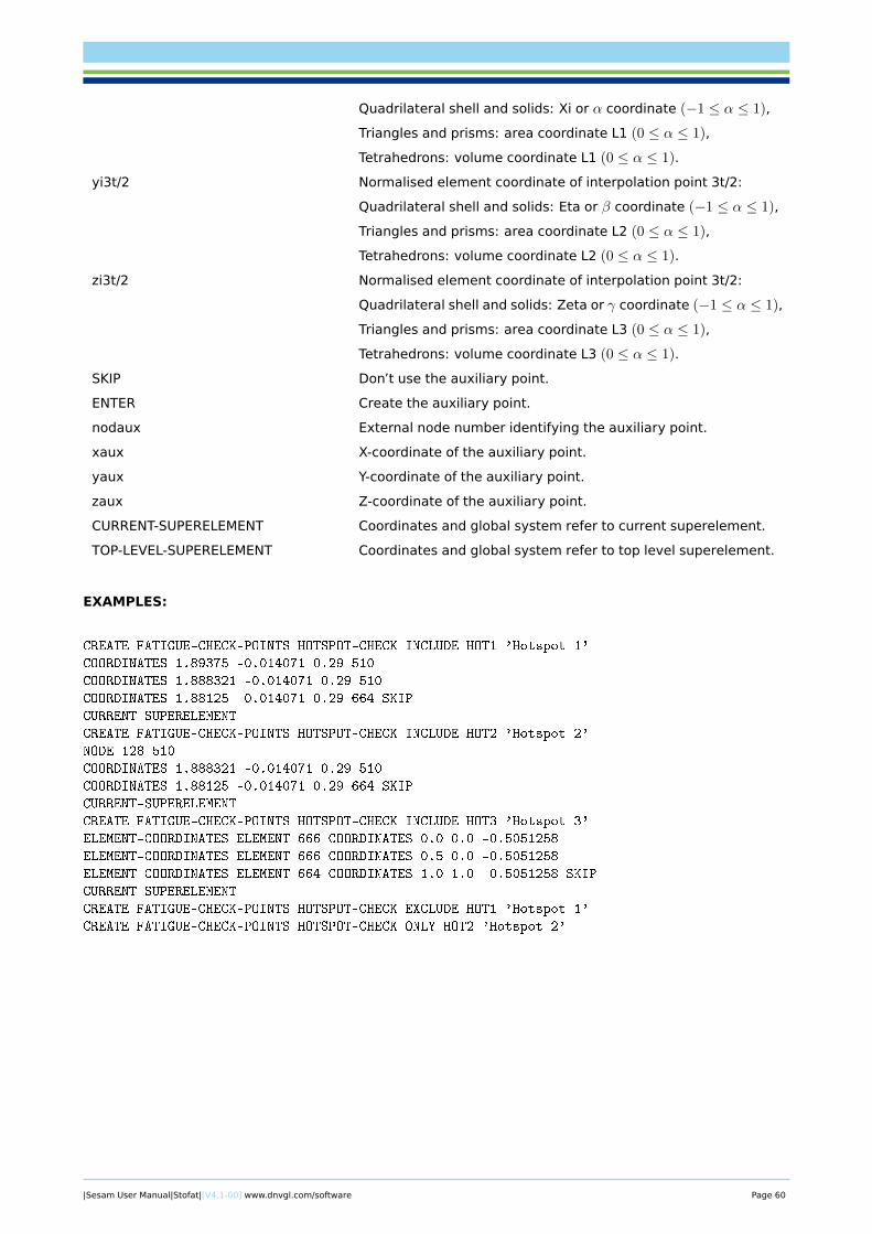
Quadrilateral shell and solids: Xi or α coordinate (−1 ≤ α ≤ 1),
Triangles and prisms: area coordinate L1 (0 ≤ α ≤ 1),
Tetrahedrons: volume coordinate L1 (0 ≤ α ≤ 1).
yi3t/2 Normalised element coordinate of interpolation point 3t/2:
Quadrilateral shell and solids: Eta or β coordinate (−1 ≤ α ≤ 1),
Triangles and prisms: area coordinate L2 (0 ≤ α ≤ 1),
Tetrahedrons: volume coordinate L2 (0 ≤ α ≤ 1).
zi3t/2 Normalised element coordinate of interpolation point 3t/2:
Quadrilateral shell and solids: Zeta or γ coordinate (−1 ≤ α ≤ 1),
Triangles and prisms: area coordinate L3 (0 ≤ α ≤ 1),
Tetrahedrons: volume coordinate L3 (0 ≤ α ≤ 1).
SKIP Don’t use the auxiliary point.
ENTER Create the auxiliary point.
nodaux External node number identifying the auxiliary point.
xaux X-coordinate of the auxiliary point.
yaux Y-coordinate of the auxiliary point.
zaux Z-coordinate of the auxiliary point.
CURRENT-SUPERELEMENT Coordinates and global system refer to current superelement.
TOP-LEVEL-SUPERELEMENT Coordinates and global system refer to top level superelement.
EXAMPLES:
CREATE FATIGUE-CHECK-POINTS HOTSPOT-CHECK INCLUDE HOT1 'Hotspot 1'
COORDINATES 1.89375 -0.014071 0.29 510
COORDINATES 1.888321 -0.014071 0.29 510
COORDINATES 1.88125 -0.014071 0.29 664 SKIP
CURRENT-SUPERELEMENT
CREATE FATIGUE-CHECK-POINTS HOTSPOT-CHECK INCLUDE HOT2 'Hotspot 2'
NODE 128 510
COORDINATES 1.888321 -0.014071 0.29 510
COORDINATES 1.88125 -0.014071 0.29 664 SKIP
CURRENT-SUPERELEMENT
CREATE FATIGUE-CHECK-POINTS HOTSPOT-CHECK INCLUDE HOT3 'Hotspot 3'
ELEMENT-COORDINATES ELEMENT 666 COORDINATES 0.0 0.0 -0.5051258
ELEMENT-COORDINATES ELEMENT 666 COORDINATES 0.5 0.0 -0.5051258
ELEMENT-COORDINATES ELEMENT 664 COORDINATES 1.0 1.0 -0.5051258 SKIP
CURRENT-SUPERELEMENT
CREATE FATIGUE-CHECK-POINTS HOTSPOT-CHECK EXCLUDE HOT1 'Hotspot 1'
CREATE FATIGUE-CHECK-POINTS HOTSPOT-CHECK ONLY HOT2 'Hotspot 2'
|Sesam User Manual|Stofat|[V4.1-00] www.dnvgl.com/software Page 60
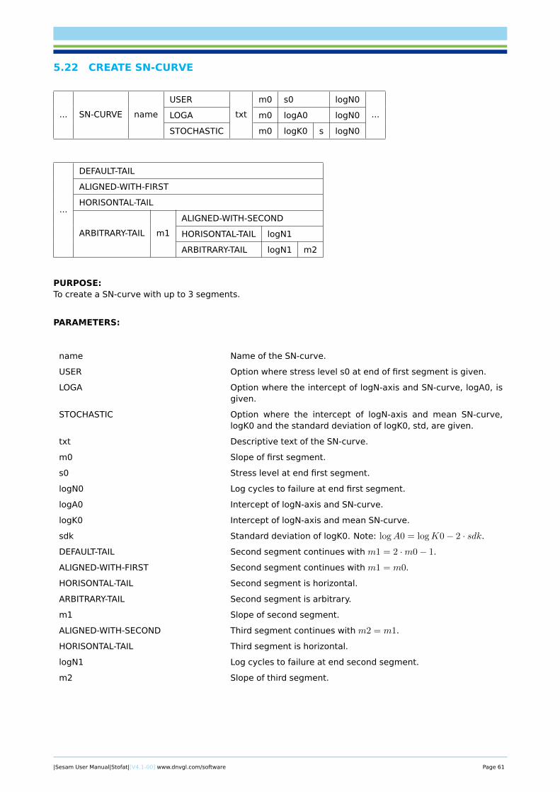
5.22 CREATE SN-CURVE
... SN-CURVE name
USER
txt
m0 s0 logN0
...LOGA m0 logA0 logN0
STOCHASTIC m0 logK0 s logN0
...
DEFAULT-TAIL
ALIGNED-WITH-FIRST
HORISONTAL-TAIL
ARBITRARY-TAIL m1
ALIGNED-WITH-SECOND
HORISONTAL-TAIL logN1
ARBITRARY-TAIL logN1 m2
PURPOSE:To create a SN-curve with up to 3 segments.
PARAMETERS:
name Name of the SN-curve.
USER Option where stress level s0 at end of first segment is given.
LOGA Option where the intercept of logN-axis and SN-curve, logA0, isgiven.
STOCHASTIC Option where the intercept of logN-axis and mean SN-curve,logK0 and the standard deviation of logK0, std, are given.
txt Descriptive text of the SN-curve.
m0 Slope of first segment.
s0 Stress level at end first segment.
logN0 Log cycles to failure at end first segment.
logA0 Intercept of logN-axis and SN-curve.
logK0 Intercept of logN-axis and mean SN-curve.
sdk Standard deviation of logK0. Note: logA0 = logK0− 2 · sdk.
DEFAULT-TAIL Second segment continues with m1 = 2 ·m0− 1.
ALIGNED-WITH-FIRST Second segment continues with m1 = m0.
HORISONTAL-TAIL Second segment is horizontal.
ARBITRARY-TAIL Second segment is arbitrary.
m1 Slope of second segment.
ALIGNED-WITH-SECOND Third segment continues with m2 = m1.
HORISONTAL-TAIL Third segment is horizontal.
logN1 Log cycles to failure at end second segment.
m2 Slope of third segment.
|Sesam User Manual|Stofat|[V4.1-00] www.dnvgl.com/software Page 61
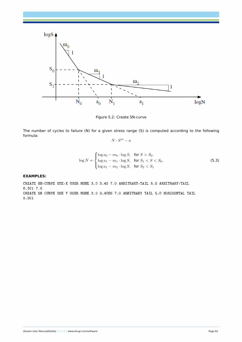
Figure 5.2: Create SN-curve
The number of cycles to failure (N) for a given stress range (S) is computed according to the followingformula:
N · Sm − a
logN =
log a0 −m0 · logS, for S > S0.
log a1 −m1 · logS, for S1 < S < S0.
log a1 −m2 · logS, for S2 < S1
(5.3)
EXAMPLES:
CREATE SN-CURVE USE-X USER NONE 3.0 3.40 7.0 ARBITRARY-TAIL 5.0 ARBITRARY-TAIL
8.301 7.0
CREATE SN-CURVE USE-Y USER NONE 3.0 3.40E6 7.0 ARBITRARY-TAIL 5.0 HORISONTAL-TAIL
8.301
|Sesam User Manual|Stofat|[V4.1-00] www.dnvgl.com/software Page 62
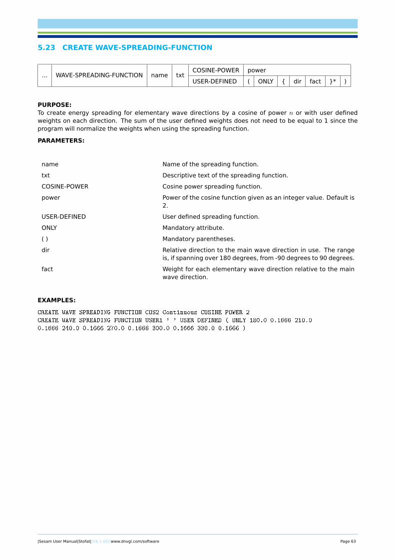
5.23 CREATE WAVE-SPREADING-FUNCTION
... WAVE-SPREADING-FUNCTION name txtCOSINE-POWER power
USER-DEFINED ( ONLY { dir fact }* )
PURPOSE:To create energy spreading for elementary wave directions by a cosine of power n or with user definedweights on each direction. The sum of the user defined weights does not need to be equal to 1 since theprogram will normalize the weights when using the spreading function.
PARAMETERS:
name Name of the spreading function.
txt Descriptive text of the spreading function.
COSINE-POWER Cosine power spreading function.
power Power of the cosine function given as an integer value. Default is2.
USER-DEFINED User defined spreading function.
ONLY Mandatory attribute.
( ) Mandatory parentheses.
dir Relative direction to the main wave direction in use. The rangeis, if spanning over 180 degrees, from -90 degrees to 90 degrees.
fact Weight for each elementary wave direction relative to the mainwave direction.
EXAMPLES:
CREATE WAVE-SPREADING-FUNCTION COS2 Continuous COSINE-POWER 2
CREATE WAVE-SPREADING-FUNCTION USER1 ' ' USER-DEFINED ( ONLY 180.0 0.1666 210.0
0.1666 240.0 0.1666 270.0 0.1666 300.0 0.1666 330.0 0.1666 )
|Sesam User Manual|Stofat|[V4.1-00] www.dnvgl.com/software Page 63
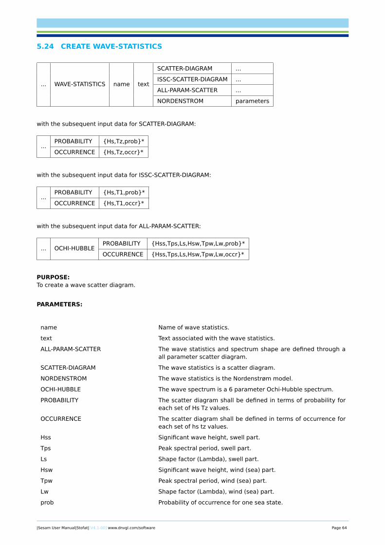
5.24 CREATE WAVE-STATISTICS
... WAVE-STATISTICS name text
SCATTER-DIAGRAM ...
ISSC-SCATTER-DIAGRAM ...
ALL-PARAM-SCATTER ...
NORDENSTROM parameters
with the subsequent input data for SCATTER-DIAGRAM:
...PROBABILITY {Hs,Tz,prob}*
OCCURRENCE {Hs,Tz,occr}*
with the subsequent input data for ISSC-SCATTER-DIAGRAM:
...PROBABILITY {Hs,T1,prob}*
OCCURRENCE {Hs,T1,occr}*
with the subsequent input data for ALL-PARAM-SCATTER:
... OCHI-HUBBLEPROBABILITY {Hss,Tps,Ls,Hsw,Tpw,Lw,prob}*
OCCURRENCE {Hss,Tps,Ls,Hsw,Tpw,Lw,occr}*
PURPOSE:To create a wave scatter diagram.
PARAMETERS:
name Name of wave statistics.
text Text associated with the wave statistics.
ALL-PARAM-SCATTER The wave statistics and spectrum shape are defined through aall parameter scatter diagram.
SCATTER-DIAGRAM The wave statistics is a scatter diagram.
NORDENSTROM The wave statistics is the Nordenstrøm model.
OCHI-HUBBLE The wave spectrum is a 6 parameter Ochi-Hubble spectrum.
PROBABILITY The scatter diagram shall be defined in terms of probability foreach set of Hs Tz values.
OCCURRENCE The scatter diagram shall be defined in terms of occurrence foreach set of hs tz values.
Hss Significant wave height, swell part.
Tps Peak spectral period, swell part.
Ls Shape factor (Lambda), swell part.
Hsw Significant wave height, wind (sea) part.
Tpw Peak spectral period, wind (sea) part.
Lw Shape factor (Lambda), wind (sea) part.
prob Probability of occurrence for one sea state.
|Sesam User Manual|Stofat|[V4.1-00] www.dnvgl.com/software Page 64

occr Number of occurrences for one sea state.
Hs Significant wave height of one sea state.
Tz Zero up-crossing period for one sea state.
T1 Mean period for one sea state.
NOTES:If the sea states of the scatter diagram are defined in terms of probability then the sum of all probabilitiesmust be 1.0.
When all parameters are given through the CREATE WAVE-STATISTICS command, a wave spectrum shapeshall not be assigned to the wave statistics.
Scatter points with zero probabilities or zero occurrences should be omitted. All scatter points, zero pointsas well, are included as sea states in the analysis. The zero scatter points do not contribute to the fatiguedamage but will, however, slow down the speed of computation and occupy unnecessary saving space inthe data base for saving zero analysis results.
The Nordenstrøm model may NOT be used for fatigue analysis.
See also:
ASSIGN WAVE-STATISTICS...
PRINT WAVE-STATISTICS...
EXAMPLES:
CREATE WAVE-STATISTICS WS1 'Scatter diagram for SESAM field'
SCATTER PROBABILITY
( 5.0 7.0 0.1
7.0 6.0 0.3
6.0 6.0 0.5
8.0 5.0 0.1 )
|Sesam User Manual|Stofat|[V4.1-00] www.dnvgl.com/software Page 65
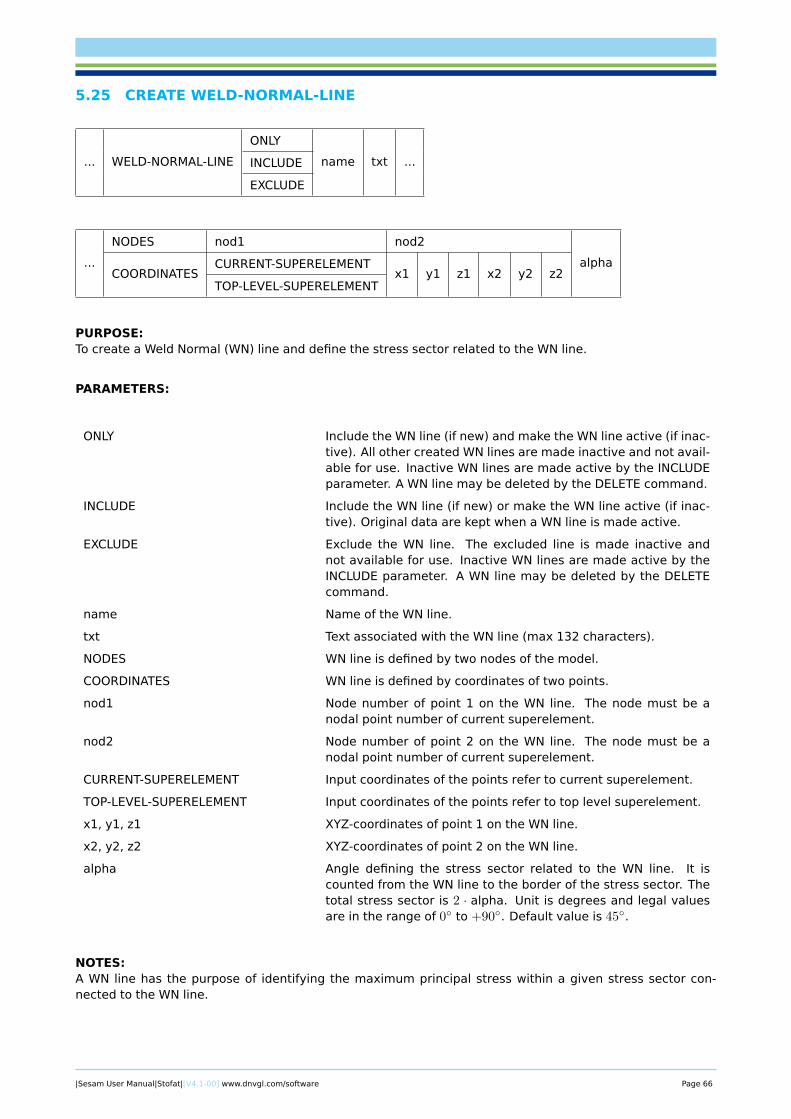
5.25 CREATE WELD-NORMAL-LINE
... WELD-NORMAL-LINE
ONLY
name txt ...INCLUDE
EXCLUDE
...
NODES nod1 nod2
alphaCOORDINATES
CURRENT-SUPERELEMENTx1 y1 z1 x2 y2 z2
TOP-LEVEL-SUPERELEMENT
PURPOSE:To create a Weld Normal (WN) line and define the stress sector related to the WN line.
PARAMETERS:
ONLY Include the WN line (if new) and make the WN line active (if inac-tive). All other created WN lines are made inactive and not avail-able for use. Inactive WN lines are made active by the INCLUDEparameter. A WN line may be deleted by the DELETE command.
INCLUDE Include the WN line (if new) or make the WN line active (if inac-tive). Original data are kept when a WN line is made active.
EXCLUDE Exclude the WN line. The excluded line is made inactive andnot available for use. Inactive WN lines are made active by theINCLUDE parameter. A WN line may be deleted by the DELETEcommand.
name Name of the WN line.
txt Text associated with the WN line (max 132 characters).
NODES WN line is defined by two nodes of the model.
COORDINATES WN line is defined by coordinates of two points.
nod1 Node number of point 1 on the WN line. The node must be anodal point number of current superelement.
nod2 Node number of point 2 on the WN line. The node must be anodal point number of current superelement.
CURRENT-SUPERELEMENT Input coordinates of the points refer to current superelement.
TOP-LEVEL-SUPERELEMENT Input coordinates of the points refer to top level superelement.
x1, y1, z1 XYZ-coordinates of point 1 on the WN line.
x2, y2, z2 XYZ-coordinates of point 2 on the WN line.
alpha Angle defining the stress sector related to the WN line. It iscounted from the WN line to the border of the stress sector. Thetotal stress sector is 2 · alpha. Unit is degrees and legal valuesare in the range of 0◦ to +90◦. Default value is 45◦.
NOTES:A WN line has the purpose of identifying the maximum principal stress within a given stress sector con-nected to the WN line.
|Sesam User Manual|Stofat|[V4.1-00] www.dnvgl.com/software Page 66

The two points defining the WN line can not be located at same position. The order the two points are en-tered as input is not of importance.
Principal stresses and principal directions are calculated on basis of the component stresses at the fatiguecheck points. The axes of the principal stresses are tested to be inside or outside the stress sector. Themaximum stress component of the principal axes inside the sector is applied in the fatigue analysis.
A sector of alpha = 90◦ includes the whole area around the fatigue check point. All three principal stressaxes will be inside the sector and the first principal stress component is always used. This gives the samefatigue damage as when not using the WN line.
A sector of alpha < 90◦ includes necessarily not all three principal stress axes. The principal stress com-ponents of the axes outside the sector are disregarded when the maximum principal stress component issearched for.
A sector of alpha = 0◦ may not include one or none of the principal stress axes. In this case the stress com-ponent of the principal axis closest in direction to the WN line is used. The three principal axes are projectedorthogonal on the WN line and the axis with the largest length component along the WN line is selected.
A WN line must be assigned to an element or a hotspot to be applied in the fatigue analysis. The WN lineapplies to all fatigue check points of the element and to the interpolation points of the hotspot as well as thehotspot itself. WN lines are assigned to individual elements and hotspots by the command ASSIGN WELD-NORMAL-LINE.
When an active WN line is made inactive and not available for use, assignments of the line are also madeinactive. When an inactive line is made active and available for use, all assignments of the line are madeactive.
Use the command PRINT RUN-OVERVIEW WELD-NORMAL-LINES or press the Show button in the dialoguebox to see current status on defined weld normal lines and assignments to elements and hotspots.
Weld normal lines and weld normal line assignments may be deleted by the commands DELETE WELD-NORMAL-LINE DELETE-LINE and DELETE WELD-NORMAL-LINE DELETE-ASSIGNMENT.
EXAMPLES:
CREATE WELD-NORMAL-LINE INCLUDE WNL1 'Line defined by nodes' NODES 179 134 45.0
CREATE WELD-NORMAL-LINE INCLUDE WNL2 'Line defined by coordinates'
COORDINATES CURRENT-SUPERELEMENT -9.5 -14.36 12.495 27.36 20.91 20.505 60.0
|Sesam User Manual|Stofat|[V4.1-00] www.dnvgl.com/software Page 67
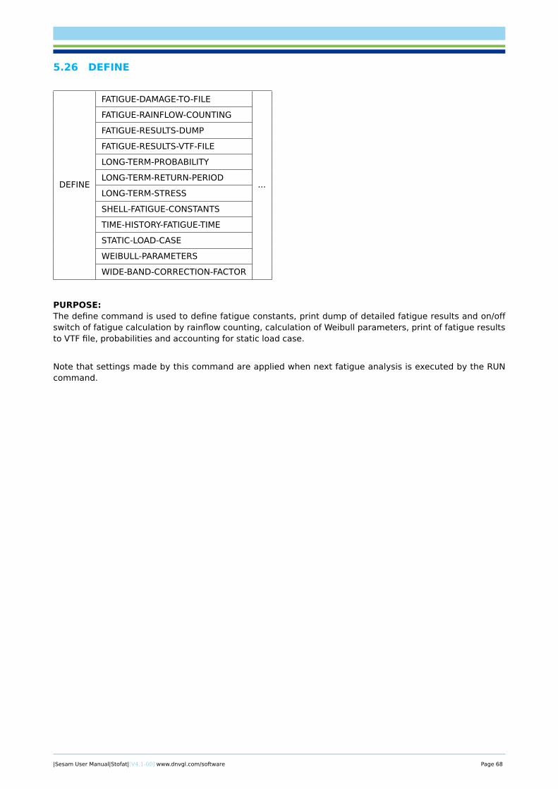
5.26 DEFINE
DEFINE
FATIGUE-DAMAGE-TO-FILE
...
FATIGUE-RAINFLOW-COUNTING
FATIGUE-RESULTS-DUMP
FATIGUE-RESULTS-VTF-FILE
LONG-TERM-PROBABILITY
LONG-TERM-RETURN-PERIOD
LONG-TERM-STRESS
SHELL-FATIGUE-CONSTANTS
TIME-HISTORY-FATIGUE-TIME
STATIC-LOAD-CASE
WEIBULL-PARAMETERS
WIDE-BAND-CORRECTION-FACTOR
PURPOSE:The define command is used to define fatigue constants, print dump of detailed fatigue results and on/offswitch of fatigue calculation by rainflow counting, calculation of Weibull parameters, print of fatigue resultsto VTF file, probabilities and accounting for static load case.
Note that settings made by this command are applied when next fatigue analysis is executed by the RUNcommand.
|Sesam User Manual|Stofat|[V4.1-00] www.dnvgl.com/software Page 68
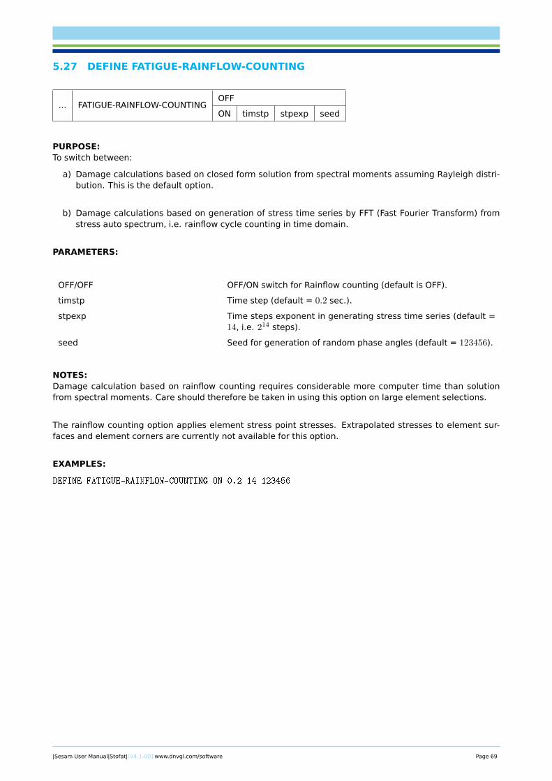
5.27 DEFINE FATIGUE-RAINFLOW-COUNTING
... FATIGUE-RAINFLOW-COUNTINGOFF
ON timstp stpexp seed
PURPOSE:To switch between:
a) Damage calculations based on closed form solution from spectral moments assuming Rayleigh distri-bution. This is the default option.
b) Damage calculations based on generation of stress time series by FFT (Fast Fourier Transform) fromstress auto spectrum, i.e. rainflow cycle counting in time domain.
PARAMETERS:
OFF/OFF OFF/ON switch for Rainflow counting (default is OFF).
timstp Time step (default = 0.2 sec.).
stpexp Time steps exponent in generating stress time series (default =14, i.e. 214 steps).
seed Seed for generation of random phase angles (default = 123456).
NOTES:Damage calculation based on rainflow counting requires considerable more computer time than solutionfrom spectral moments. Care should therefore be taken in using this option on large element selections.
The rainflow counting option applies element stress point stresses. Extrapolated stresses to element sur-faces and element corners are currently not available for this option.
EXAMPLES:
DEFINE FATIGUE-RAINFLOW-COUNTING ON 0.2 14 123456
|Sesam User Manual|Stofat|[V4.1-00] www.dnvgl.com/software Page 69
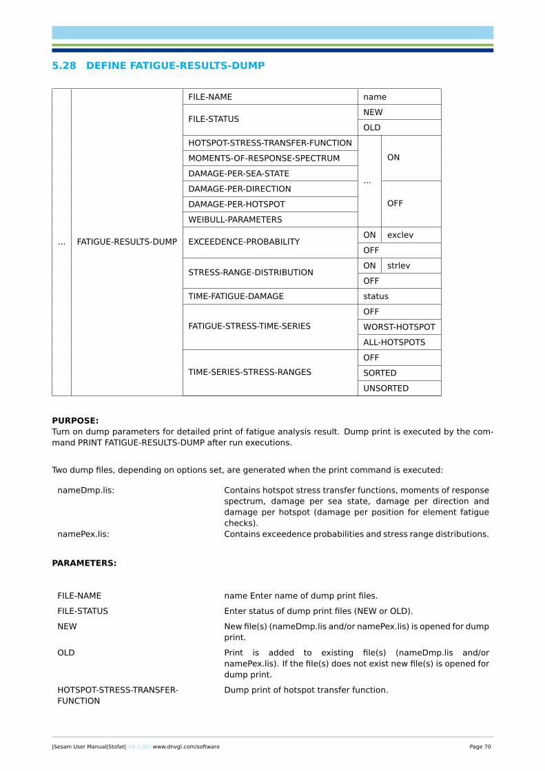
5.28 DEFINE FATIGUE-RESULTS-DUMP
... FATIGUE-RESULTS-DUMP
FILE-NAME name
FILE-STATUSNEW
OLD
HOTSPOT-STRESS-TRANSFER-FUNCTION
...
ONMOMENTS-OF-RESPONSE-SPECTRUM
DAMAGE-PER-SEA-STATE
DAMAGE-PER-DIRECTION
OFFDAMAGE-PER-HOTSPOT
WEIBULL-PARAMETERS
EXCEEDENCE-PROBABILITYON exclev
OFF
STRESS-RANGE-DISTRIBUTIONON strlev
OFF
TIME-FATIGUE-DAMAGE status
FATIGUE-STRESS-TIME-SERIES
OFF
WORST-HOTSPOT
ALL-HOTSPOTS
TIME-SERIES-STRESS-RANGES
OFF
SORTED
UNSORTED
PURPOSE:Turn on dump parameters for detailed print of fatigue analysis result. Dump print is executed by the com-mand PRINT FATIGUE-RESULTS-DUMP after run executions.
Two dump files, depending on options set, are generated when the print command is executed:
nameDmp.lis: Contains hotspot stress transfer functions, moments of responsespectrum, damage per sea state, damage per direction anddamage per hotspot (damage per position for element fatiguechecks).
namePex.lis: Contains exceedence probabilities and stress range distributions.
PARAMETERS:
FILE-NAME name Enter name of dump print files.
FILE-STATUS Enter status of dump print files (NEW or OLD).
NEW New file(s) (nameDmp.lis and/or namePex.lis) is opened for dumpprint.
OLD Print is added to existing file(s) (nameDmp.lis and/ornamePex.lis). If the file(s) does not exist new file(s) is opened fordump print.
HOTSPOT-STRESS-TRANSFER-FUNCTION
Dump print of hotspot transfer function.
|Sesam User Manual|Stofat|[V4.1-00] www.dnvgl.com/software Page 70
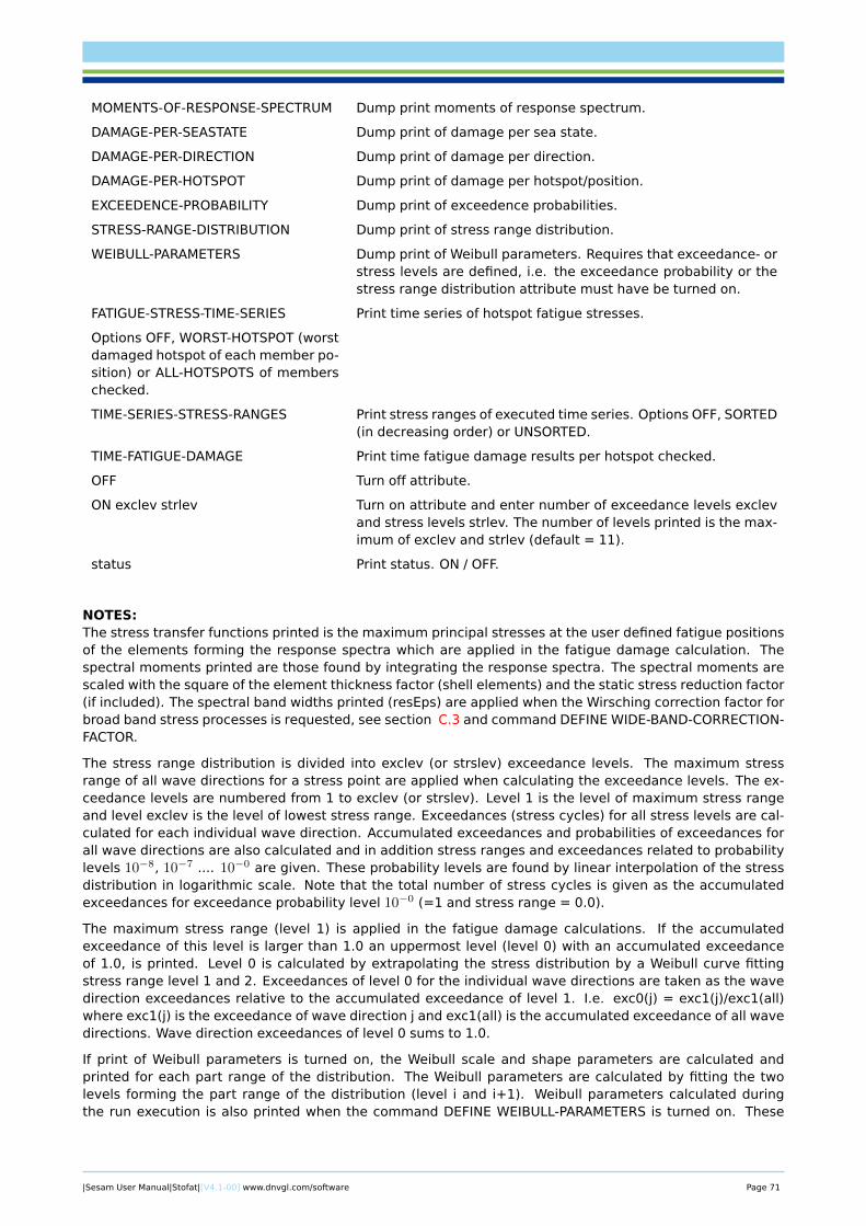
MOMENTS-OF-RESPONSE-SPECTRUM Dump print moments of response spectrum.
DAMAGE-PER-SEASTATE Dump print of damage per sea state.
DAMAGE-PER-DIRECTION Dump print of damage per direction.
DAMAGE-PER-HOTSPOT Dump print of damage per hotspot/position.
EXCEEDENCE-PROBABILITY Dump print of exceedence probabilities.
STRESS-RANGE-DISTRIBUTION Dump print of stress range distribution.
WEIBULL-PARAMETERS Dump print of Weibull parameters. Requires that exceedance- orstress levels are defined, i.e. the exceedance probability or thestress range distribution attribute must have be turned on.
FATIGUE-STRESS-TIME-SERIES Print time series of hotspot fatigue stresses.
Options OFF, WORST-HOTSPOT (worstdamaged hotspot of each member po-sition) or ALL-HOTSPOTS of memberschecked.
TIME-SERIES-STRESS-RANGES Print stress ranges of executed time series. Options OFF, SORTED(in decreasing order) or UNSORTED.
TIME-FATIGUE-DAMAGE Print time fatigue damage results per hotspot checked.
OFF Turn off attribute.
ON exclev strlev Turn on attribute and enter number of exceedance levels exclevand stress levels strlev. The number of levels printed is the max-imum of exclev and strlev (default = 11).
status Print status. ON / OFF.
NOTES:The stress transfer functions printed is the maximum principal stresses at the user defined fatigue positionsof the elements forming the response spectra which are applied in the fatigue damage calculation. Thespectral moments printed are those found by integrating the response spectra. The spectral moments arescaled with the square of the element thickness factor (shell elements) and the static stress reduction factor(if included). The spectral band widths printed (resEps) are applied when the Wirsching correction factor forbroad band stress processes is requested, see section C.3 and command DEFINE WIDE-BAND-CORRECTION-FACTOR.
The stress range distribution is divided into exclev (or strslev) exceedance levels. The maximum stressrange of all wave directions for a stress point are applied when calculating the exceedance levels. The ex-ceedance levels are numbered from 1 to exclev (or strslev). Level 1 is the level of maximum stress rangeand level exclev is the level of lowest stress range. Exceedances (stress cycles) for all stress levels are cal-culated for each individual wave direction. Accumulated exceedances and probabilities of exceedances forall wave directions are also calculated and in addition stress ranges and exceedances related to probabilitylevels 10−8, 10−7 .... 10−0 are given. These probability levels are found by linear interpolation of the stressdistribution in logarithmic scale. Note that the total number of stress cycles is given as the accumulatedexceedances for exceedance probability level 10−0 (=1 and stress range = 0.0).
The maximum stress range (level 1) is applied in the fatigue damage calculations. If the accumulatedexceedance of this level is larger than 1.0 an uppermost level (level 0) with an accumulated exceedanceof 1.0, is printed. Level 0 is calculated by extrapolating the stress distribution by a Weibull curve fittingstress range level 1 and 2. Exceedances of level 0 for the individual wave directions are taken as the wavedirection exceedances relative to the accumulated exceedance of level 1. I.e. exc0(j) = exc1(j)/exc1(all)where exc1(j) is the exceedance of wave direction j and exc1(all) is the accumulated exceedance of all wavedirections. Wave direction exceedances of level 0 sums to 1.0.
If print of Weibull parameters is turned on, the Weibull scale and shape parameters are calculated andprinted for each part range of the distribution. The Weibull parameters are calculated by fitting the twolevels forming the part range of the distribution (level i and i+1). Weibull parameters calculated duringthe run execution is also printed when the command DEFINE WEIBULL-PARAMETERS is turned on. These
|Sesam User Manual|Stofat|[V4.1-00] www.dnvgl.com/software Page 71

parameters are average values of the stress range distribution calculated by fitting the Weibull function bya least square technique using 10 levels for the stress range distribution.
EXAMPLES:
DEFINE FATIGUE-RESULTS-DUMP FILE-NAME STOFAT
DEFINE FATIGUE-RESULTS-DUMP FILE-STATUS NEW
DEFINE FATIGUE-RESULTS-DUMP HOTSPOT-STRESS-TRANSFER-FUNCTION OFF
DEFINE FATIGUE-RESULTS-DUMP MOMENTS-OF-RESPONSE-SPECTRUM OFF
DEFINE FATIGUE-RESULTS-DUMP DAMAGE-PER-SEASTATE OFF
DEFINE FATIGUE-RESULTS-DUMP DAMAGE-PER-DIRECTION OFF
DEFINE FATIGUE-RESULTS-DUMP DAMAGE-PER-HOTSPOT ON
DEFINE FATIGUE-RESULTS-DUMP EXCEEDENCE-PROBABILITY ON 11
DEFINE FATIGUE-RESULTS-DUMP STRESS-RANGE-DISTRIBUTION ON 11
DEFINE FATIGUE-RESULTS-DUMP WEIBULL-PARAMETERS ON
|Sesam User Manual|Stofat|[V4.1-00] www.dnvgl.com/software Page 72
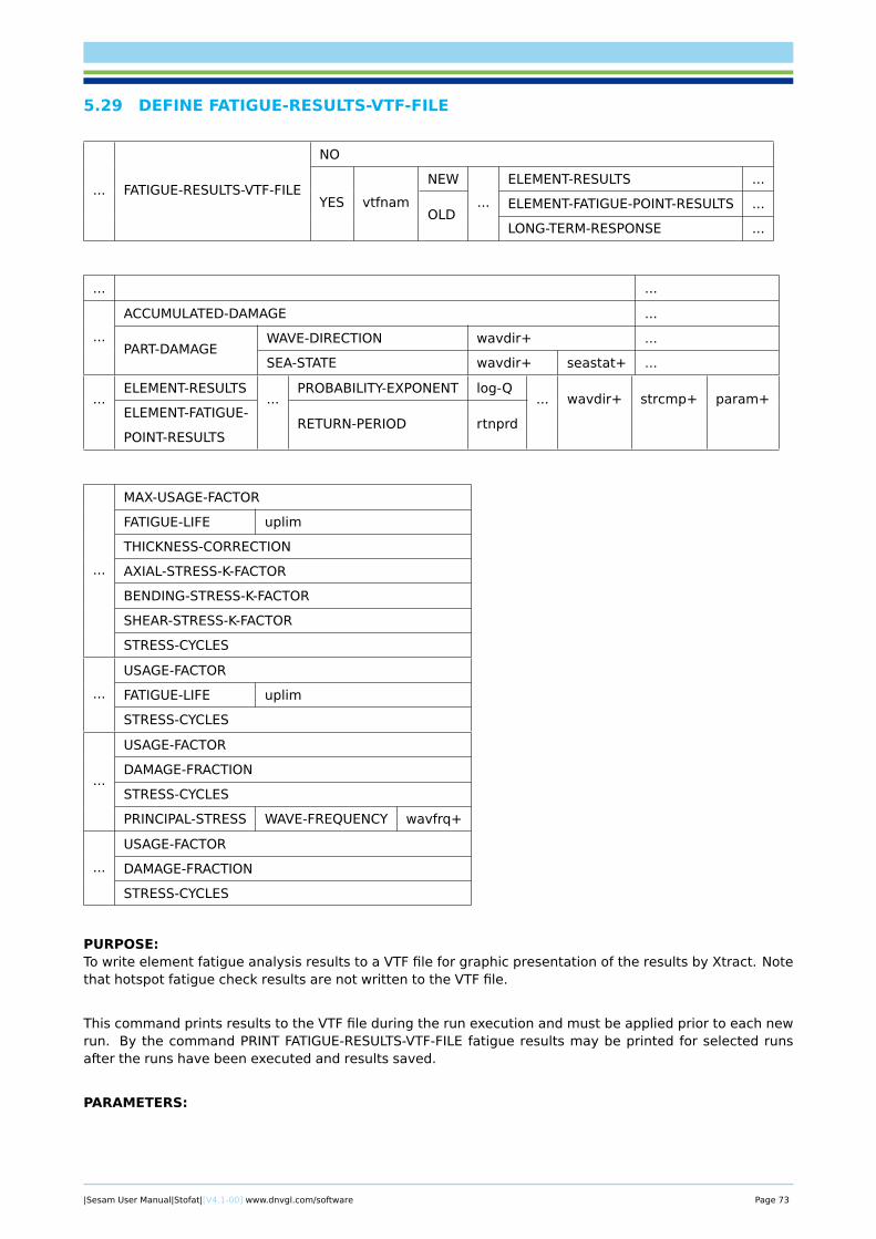
5.29 DEFINE FATIGUE-RESULTS-VTF-FILE
... FATIGUE-RESULTS-VTF-FILE
NO
YES vtfnam
NEW
...
ELEMENT-RESULTS ...
OLDELEMENT-FATIGUE-POINT-RESULTS ...
LONG-TERM-RESPONSE ...
... ...
...
ACCUMULATED-DAMAGE ...
PART-DAMAGEWAVE-DIRECTION wavdir+ ...
SEA-STATE wavdir+ seastat+ ...
...ELEMENT-RESULTS
...PROBABILITY-EXPONENT log-Q
... wavdir+ strcmp+ param+ELEMENT-FATIGUE-
POINT-RESULTSRETURN-PERIOD rtnprd
...
MAX-USAGE-FACTOR
FATIGUE-LIFE uplim
THICKNESS-CORRECTION
AXIAL-STRESS-K-FACTOR
BENDING-STRESS-K-FACTOR
SHEAR-STRESS-K-FACTOR
STRESS-CYCLES
...
USAGE-FACTOR
FATIGUE-LIFE uplim
STRESS-CYCLES
...
USAGE-FACTOR
DAMAGE-FRACTION
STRESS-CYCLES
PRINCIPAL-STRESS WAVE-FREQUENCY wavfrq+
...
USAGE-FACTOR
DAMAGE-FRACTION
STRESS-CYCLES
PURPOSE:To write element fatigue analysis results to a VTF file for graphic presentation of the results by Xtract. Notethat hotspot fatigue check results are not written to the VTF file.
This command prints results to the VTF file during the run execution and must be applied prior to each newrun. By the command PRINT FATIGUE-RESULTS-VTF-FILE fatigue results may be printed for selected runsafter the runs have been executed and results saved.
PARAMETERS:
|Sesam User Manual|Stofat|[V4.1-00] www.dnvgl.com/software Page 73

NO Fatigue results are not written to the VTF file (default).
YES Fatigue results are written to the VTF file.
vtfnam Name of the VTF file. The default name is Stofat. The extensionof the file is.vtf and the full name is vtfnam.vtf.
NEW A new file with name vtfnam.vtf is opened for print.
OLD Results are appended to existing VTF file with name vtf-nam.vtf.If the file does not exist, a new file is opened for print.
ELEMENT-RESULTS Write one result per element of current element selection. Thefatigue check point with maximum usage factor is printed.
ELEMENT-FATIGUE-POINT-RESULTS Write results of all element fatigue check points of current ele-ment selection.
LONG-TERM-RESPONSE Write response results. Availability of this option requires that astress component is defined, see command DEFINE LONGTERM-STRESS.
PROBABILITY-EXPONENT Write results for given probability exponent. Availability of thisoption requires that probability levels are defined, see commandDEFINE LONG-TERM PROBABILITY.
RETURN-PERIOD Write results for given return period. Availability of this optionrequires that return periods are defined, see command DEFINELONG-TERM-RETURN-PERIOD.
ACCUMULATED-DAMAGE Write accumulated damage results of the element fatigue checkpoints.
PART-DAMAGE Write part damage results of the element fatigue check points.
WAVE-DIRECTION Write part damage results for wave direction.
SEA-STATE Write part damage results for sea state.
MAX-USAGE-FACTOR Write maximum usage factor of the element.
USAGE-FACTOR Write usage factor.
FATIGUE-LIFE Write fatigue life.
THICKNESS-CORRECTION Write thickness correction applied to the element.
AXIAL-STRESS-K-FACTOR Write K-factor applied to axial stress components.
BENDING-STRESS-K-FACTOR Write K-factor applied to bending stress components.
SHEAR-STRESS-K-FACTOR Write K-factor applied to shear stress components.
STRESS-CYCLES Write the number of stress cycles.
DAMAGE-FRACTION Write fraction of damage of part damage result.
PRINCIPAL-STRESS Write maximum principal stress.
WAVE-FREQUENCY Write maximum principal stress for wave frequency.
wavdir+ Wave direction.
seastat+ Sea state.
wavfrq+ Wave frequency.
log-Q+ Probability exponent, as an absolute real number, defining theprobability level Q, i.e. Q = 10−(log (−Q)).
rtnprd+ Return period in years.
strcmp+ Stress component to be applied in response calculation. Validcomponents: ‘Sp1’, ‘Seq’, ‘Sxx’, ‘Syy’, ‘Szz’, ‘Sxy’, ‘Sxz’, ‘Syz’,‘Sp2’, ‘Sp3’.
|Sesam User Manual|Stofat|[V4.1-00] www.dnvgl.com/software Page 74
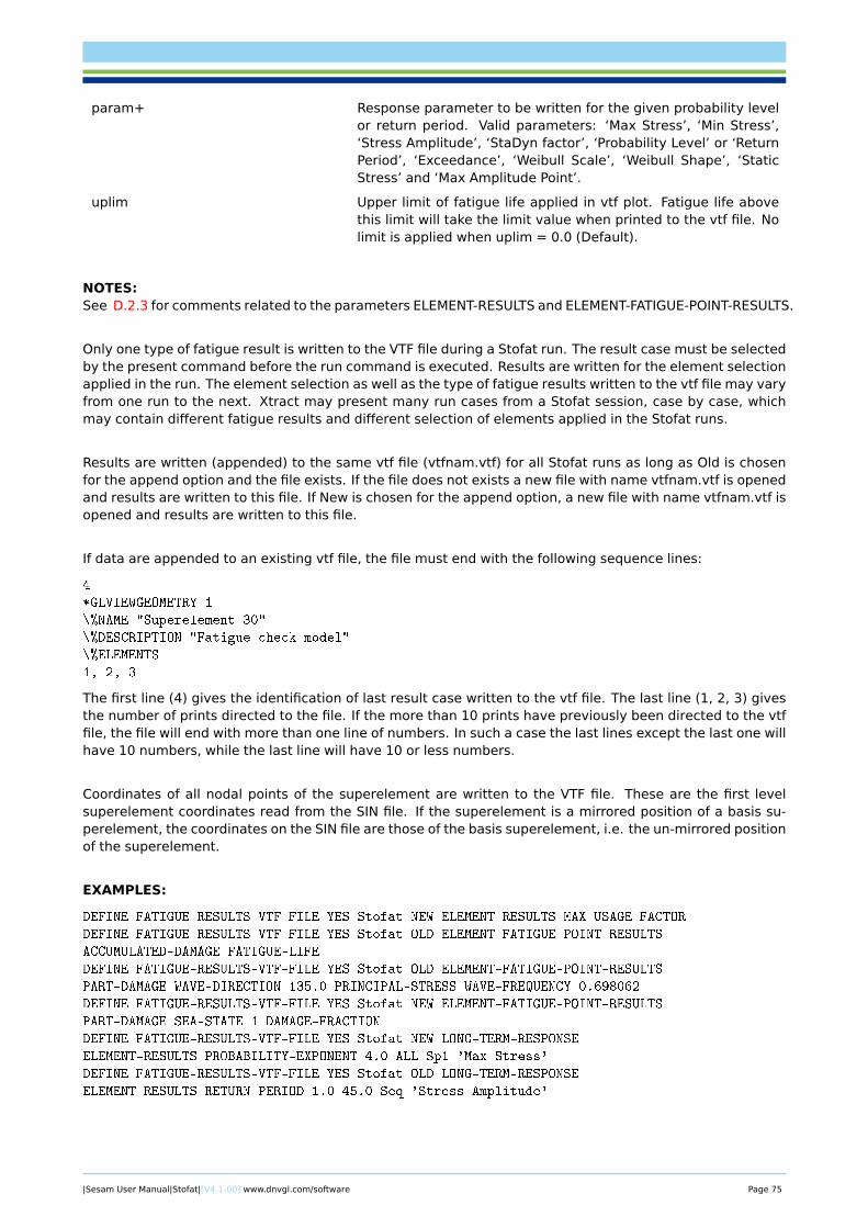
param+ Response parameter to be written for the given probability levelor return period. Valid parameters: ‘Max Stress’, ‘Min Stress’,‘Stress Amplitude’, ‘StaDyn factor’, ‘Probability Level’ or ‘ReturnPeriod’, ‘Exceedance’, ‘Weibull Scale’, ‘Weibull Shape’, ‘StaticStress’ and ‘Max Amplitude Point’.
uplim Upper limit of fatigue life applied in vtf plot. Fatigue life abovethis limit will take the limit value when printed to the vtf file. Nolimit is applied when uplim = 0.0 (Default).
NOTES:See D.2.3 for comments related to the parameters ELEMENT-RESULTS and ELEMENT-FATIGUE-POINT-RESULTS.
Only one type of fatigue result is written to the VTF file during a Stofat run. The result case must be selectedby the present command before the run command is executed. Results are written for the element selectionapplied in the run. The element selection as well as the type of fatigue results written to the vtf file may varyfrom one run to the next. Xtract may present many run cases from a Stofat session, case by case, whichmay contain different fatigue results and different selection of elements applied in the Stofat runs.
Results are written (appended) to the same vtf file (vtfnam.vtf) for all Stofat runs as long as Old is chosenfor the append option and the file exists. If the file does not exists a new file with name vtfnam.vtf is openedand results are written to this file. If New is chosen for the append option, a new file with name vtfnam.vtf isopened and results are written to this file.
If data are appended to an existing vtf file, the file must end with the following sequence lines:
4
*GLVIEWGEOMETRY 1
\%NAME "Superelement 30"
\%DESCRIPTION "Fatigue check model"
\%ELEMENTS
1, 2, 3
The first line (4) gives the identification of last result case written to the vtf file. The last line (1, 2, 3) givesthe number of prints directed to the file. If the more than 10 prints have previously been directed to the vtffile, the file will end with more than one line of numbers. In such a case the last lines except the last one willhave 10 numbers, while the last line will have 10 or less numbers.
Coordinates of all nodal points of the superelement are written to the VTF file. These are the first levelsuperelement coordinates read from the SIN file. If the superelement is a mirrored position of a basis su-perelement, the coordinates on the SIN file are those of the basis superelement, i.e. the un-mirrored positionof the superelement.
EXAMPLES:
DEFINE FATIGUE-RESULTS-VTF-FILE YES Stofat NEW ELEMENT-RESULTS MAX-USAGE-FACTOR
DEFINE FATIGUE-RESULTS-VTF-FILE YES Stofat OLD ELEMENT-FATIGUE-POINT-RESULTS
ACCUMULATED-DAMAGE FATIGUE-LIFE
DEFINE FATIGUE-RESULTS-VTF-FILE YES Stofat OLD ELEMENT-FATIGUE-POINT-RESULTS
PART-DAMAGE WAVE-DIRECTION 135.0 PRINCIPAL-STRESS WAVE-FREQUENCY 0.698062
DEFINE FATIGUE-RESULTS-VTF-FILE YES Stofat NEW ELEMENT-FATIGUE-POINT-RESULTS
PART-DAMAGE SEA-STATE 1 DAMAGE-FRACTION
DEFINE FATIGUE-RESULTS-VTF-FILE YES Stofat NEW LONG-TERM-RESPONSE
ELEMENT-RESULTS PROBABILITY-EXPONENT 4.0 ALL Sp1 'Max Stress'
DEFINE FATIGUE-RESULTS-VTF-FILE YES Stofat OLD LONG-TERM-RESPONSE
ELEMENT-RESULTS RETURN-PERIOD 1.0 45.0 Seq 'Stress Amplitude'
|Sesam User Manual|Stofat|[V4.1-00] www.dnvgl.com/software Page 75
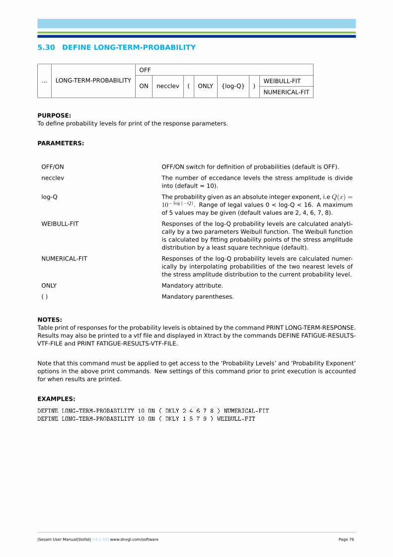
5.30 DEFINE LONG-TERM-PROBABILITY
... LONG-TERM-PROBABILITY
OFF
ON necclev ( ONLY {log-Q} )WEIBULL-FIT
NUMERICAL-FIT
PURPOSE:To define probability levels for print of the response parameters.
PARAMETERS:
OFF/ON OFF/ON switch for definition of probabilities (default is OFF).
necclev The number of eccedance levels the stress amplitude is divideinto (default = 10).
log-Q The probability given as an absolute integer exponent, i.eQ(x) =10− log (−Q). Range of legal values 0 < log-Q < 16. A maximumof 5 values may be given (default values are 2, 4, 6, 7, 8).
WEIBULL-FIT Responses of the log-Q probability levels are calculated analyti-cally by a two parameters Weibull function. The Weibull functionis calculated by fitting probability points of the stress amplitudedistribution by a least square technique (default).
NUMERICAL-FIT Responses of the log-Q probability levels are calculated numer-ically by interpolating probabilities of the two nearest levels ofthe stress amplitude distribution to the current probability level.
ONLY Mandatory attribute.
( ) Mandatory parentheses.
NOTES:Table print of responses for the probability levels is obtained by the command PRINT LONG-TERM-RESPONSE.Results may also be printed to a vtf file and displayed in Xtract by the commands DEFINE FATIGUE-RESULTS-VTF-FILE and PRINT FATIGUE-RESULTS-VTF-FILE.
Note that this command must be applied to get access to the ‘Probability Levels’ and ‘Probability Exponent’options in the above print commands. New settings of this command prior to print execution is accountedfor when results are printed.
EXAMPLES:
DEFINE LONG-TERM-PROBABILITY 10 ON ( ONLY 2 4 6 7 8 ) NUMERICAL-FIT
DEFINE LONG-TERM-PROBABILITY 10 ON ( ONLY 1 5 7 9 ) WEIBULL-FIT
|Sesam User Manual|Stofat|[V4.1-00] www.dnvgl.com/software Page 76
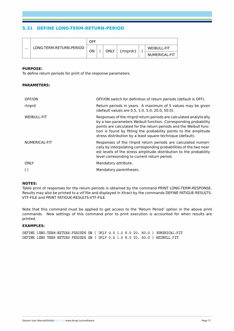
5.31 DEFINE LONG-TERM-RETURN-PERIOD
... LONG-TERM-RETURN-PERIOD
OFF
ON ( ONLY {rtnprdr} )WEIBULL-FIT
NUMERICAL-FIT
PURPOSE:To define return periods for print of the response parameters.
PARAMETERS:
OFF/ON OFF/ON switch for definition of return periods (default is OFF).
rtnprd Return periods in years. A maximum of 5 values may be given(default values are 0.5, 1.0, 5.0, 20.0, 50.0).
WEIBULL-FIT Responses of the rtnprd return periods are calculated analyticallyby a two parameters Weibull function. Corresponding probabilitypoints are calculated for the return periods and the Weibull func-tion is found by fitting the probability points to the amplitudestress distribution by a least square technique (default).
NUMERICAL-FIT Responses of the rtnprd return periods are calculated numeri-cally by interpolating corresponding probabilities of the two near-est levels of the stress amplitude distribution to the probabilitylevel corresonding to current return period.
ONLY Mandatory attribute.
( ) Mandatory parentheses.
NOTES:Table print of responses for the return periods is obtained by the command PRINT LONG-TERM-RESPONSE.Results may also be printed to a vtf file and displayed in Xtract by the commands DEFINE FATIGUE-RESULTS-VTF-FILE and PRINT FATIGUE-RESULTS-VTF-FILE.
Note that this command must be applied to get access to the ‘Return Period’ option in the above printcommands. New settings of this command prior to print execution is accounted for when results areprinted.
EXAMPLES:
DEFINE LONG-TERM-RETURN-PERIODS ON ( ONLY 0.5 1.0 5.0 20. 50.0 ) NUMERICAL-FIT
DEFINE LONG-TERM-RETURN-PERIODS ON ( ONLY 0.5 1.0 5.0 20. 50.0 ) WEIBULL-FIT
|Sesam User Manual|Stofat|[V4.1-00] www.dnvgl.com/software Page 77
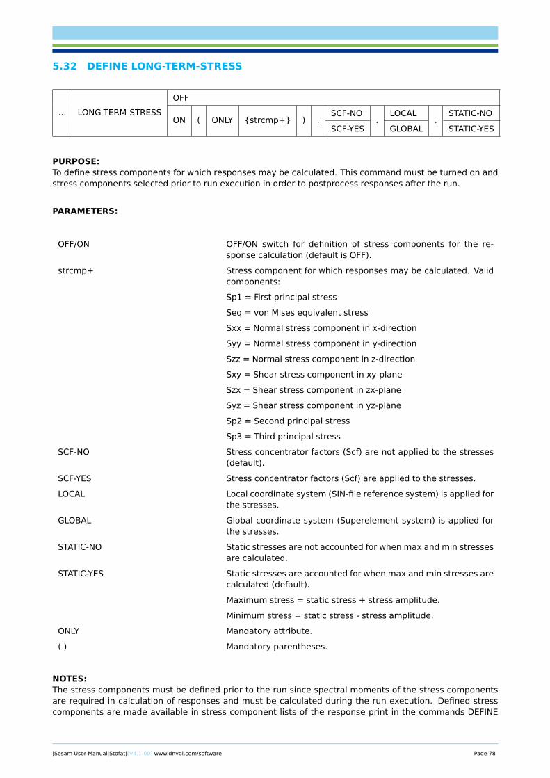
5.32 DEFINE LONG-TERM-STRESS
... LONG-TERM-STRESS
OFF
ON ( ONLY {strcmp+} ) .SCF-NO
.LOCAL
.STATIC-NO
SCF-YES GLOBAL STATIC-YES
PURPOSE:To define stress components for which responses may be calculated. This command must be turned on andstress components selected prior to run execution in order to postprocess responses after the run.
PARAMETERS:
OFF/ON OFF/ON switch for definition of stress components for the re-sponse calculation (default is OFF).
strcmp+ Stress component for which responses may be calculated. Validcomponents:
Sp1 = First principal stress
Seq = von Mises equivalent stress
Sxx = Normal stress component in x-direction
Syy = Normal stress component in y-direction
Szz = Normal stress component in z-direction
Sxy = Shear stress component in xy-plane
Szx = Shear stress component in zx-plane
Syz = Shear stress component in yz-plane
Sp2 = Second principal stress
Sp3 = Third principal stress
SCF-NO Stress concentrator factors (Scf) are not applied to the stresses(default).
SCF-YES Stress concentrator factors (Scf) are applied to the stresses.
LOCAL Local coordinate system (SIN-file reference system) is applied forthe stresses.
GLOBAL Global coordinate system (Superelement system) is applied forthe stresses.
STATIC-NO Static stresses are not accounted for when max and min stressesare calculated.
STATIC-YES Static stresses are accounted for when max and min stresses arecalculated (default).
Maximum stress = static stress + stress amplitude.
Minimum stress = static stress - stress amplitude.
ONLY Mandatory attribute.
( ) Mandatory parentheses.
NOTES:The stress components must be defined prior to the run since spectral moments of the stress componentsare required in calculation of responses and must be calculated during the run execution. Defined stresscomponents are made available in stress component lists of the response print in the commands DEFINE
|Sesam User Manual|Stofat|[V4.1-00] www.dnvgl.com/software Page 78

FATIGUE-RESULTS-VTF-FILE, PRINT FATIGUE-RESULTS-VTF-FILE and PRINT LONG-TERM-PROBABILIIES.
The CPU-time consumption may increase by a factor of 2-4 when stresses are selected for the run, depend-ing on the number of stress components included. Care should therefore be given to include only relevantcomponents in order to keep the CPU-time as low as possible.
Note that in order to account for static stress in the response calculation the command DEFINE STATIC-LOAD-CASE must have been turned on and load case number given prior to run execution.
The options SCF-NO/SCF-YEA and LOCAL/GLOBAL must be set prior to run execution. The option STATIC-NO/STATIC-YES may be set prior to each print execution.
Note that inclusion of static stresses applies to the calculation of maximum and minimum stresses only. Thespectral moments are not scaled with a static stress reduction factor in the long term response analysis asperformed in the fatigue damage calculation. The stress amplitude calculated by the spectral moments isaccordingly not affected by the static stresses.
Depending on the user input, static stresses are then added to maximum and minimum stresses in accor-dance with:
Maximum stress = static stress + stress amplitudeMinimum stress = static stress - stress amplitude
The above expression helds except in case of von Mises stress is selected, therefore minimum and maximumstresses coincide.
EXAMPLES:
DEFINE LONG-TERM-STRESS ON ( ONLY Sp1 Seq Sxx Syy Szz Sxy Syz Szx Sp2 Sp3 )
SCF-NO LOCAL STATIC-NO
DEFINE LONG-TERM-STRESS ON ( ONLY Seq Sxx Syy ) SCF-YES GLOBAL STATIC-YES
|Sesam User Manual|Stofat|[V4.1-00] www.dnvgl.com/software Page 79
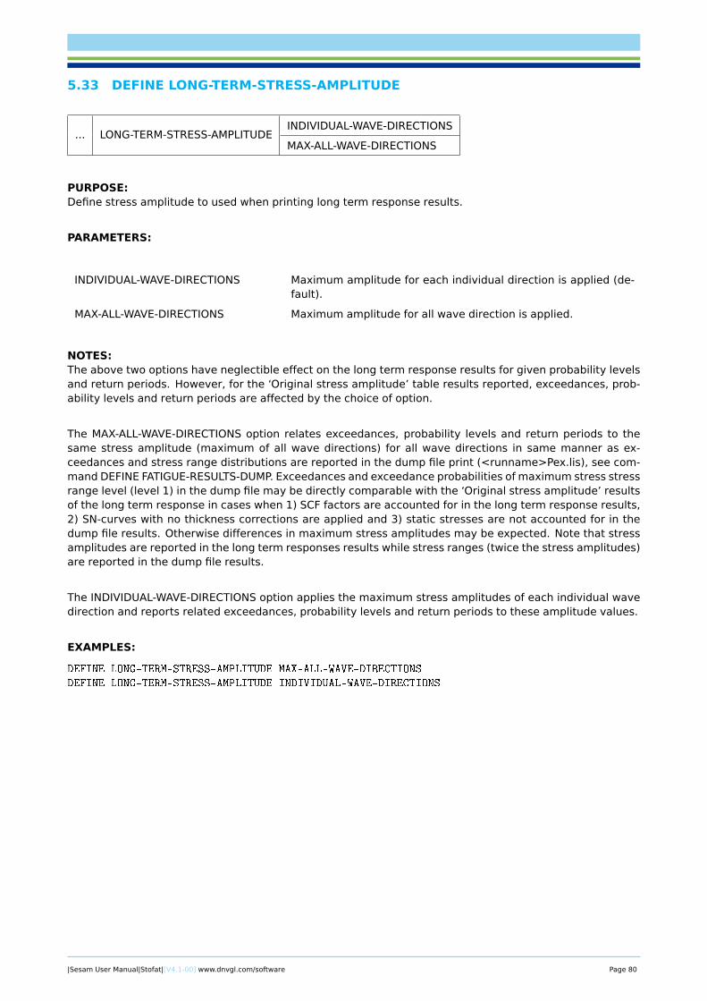
5.33 DEFINE LONG-TERM-STRESS-AMPLITUDE
... LONG-TERM-STRESS-AMPLITUDEINDIVIDUAL-WAVE-DIRECTIONS
MAX-ALL-WAVE-DIRECTIONS
PURPOSE:Define stress amplitude to used when printing long term response results.
PARAMETERS:
INDIVIDUAL-WAVE-DIRECTIONS Maximum amplitude for each individual direction is applied (de-fault).
MAX-ALL-WAVE-DIRECTIONS Maximum amplitude for all wave direction is applied.
NOTES:The above two options have neglectible effect on the long term response results for given probability levelsand return periods. However, for the ‘Original stress amplitude’ table results reported, exceedances, prob-ability levels and return periods are affected by the choice of option.
The MAX-ALL-WAVE-DIRECTIONS option relates exceedances, probability levels and return periods to thesame stress amplitude (maximum of all wave directions) for all wave directions in same manner as ex-ceedances and stress range distributions are reported in the dump file print (<runname>Pex.lis), see com-mand DEFINE FATIGUE-RESULTS-DUMP. Exceedances and exceedance probabilities of maximum stress stressrange level (level 1) in the dump file may be directly comparable with the ‘Original stress amplitude’ resultsof the long term response in cases when 1) SCF factors are accounted for in the long term response results,2) SN-curves with no thickness corrections are applied and 3) static stresses are not accounted for in thedump file results. Otherwise differences in maximum stress amplitudes may be expected. Note that stressamplitudes are reported in the long term responses results while stress ranges (twice the stress amplitudes)are reported in the dump file results.
The INDIVIDUAL-WAVE-DIRECTIONS option applies the maximum stress amplitudes of each individual wavedirection and reports related exceedances, probability levels and return periods to these amplitude values.
EXAMPLES:
DEFINE LONG-TERM-STRESS-AMPLITUDE MAX-ALL-WAVE-DIRECTIONS
DEFINE LONG-TERM-STRESS-AMPLITUDE INDIVIDUAL-WAVE-DIRECTIONS
|Sesam User Manual|Stofat|[V4.1-00] www.dnvgl.com/software Page 80
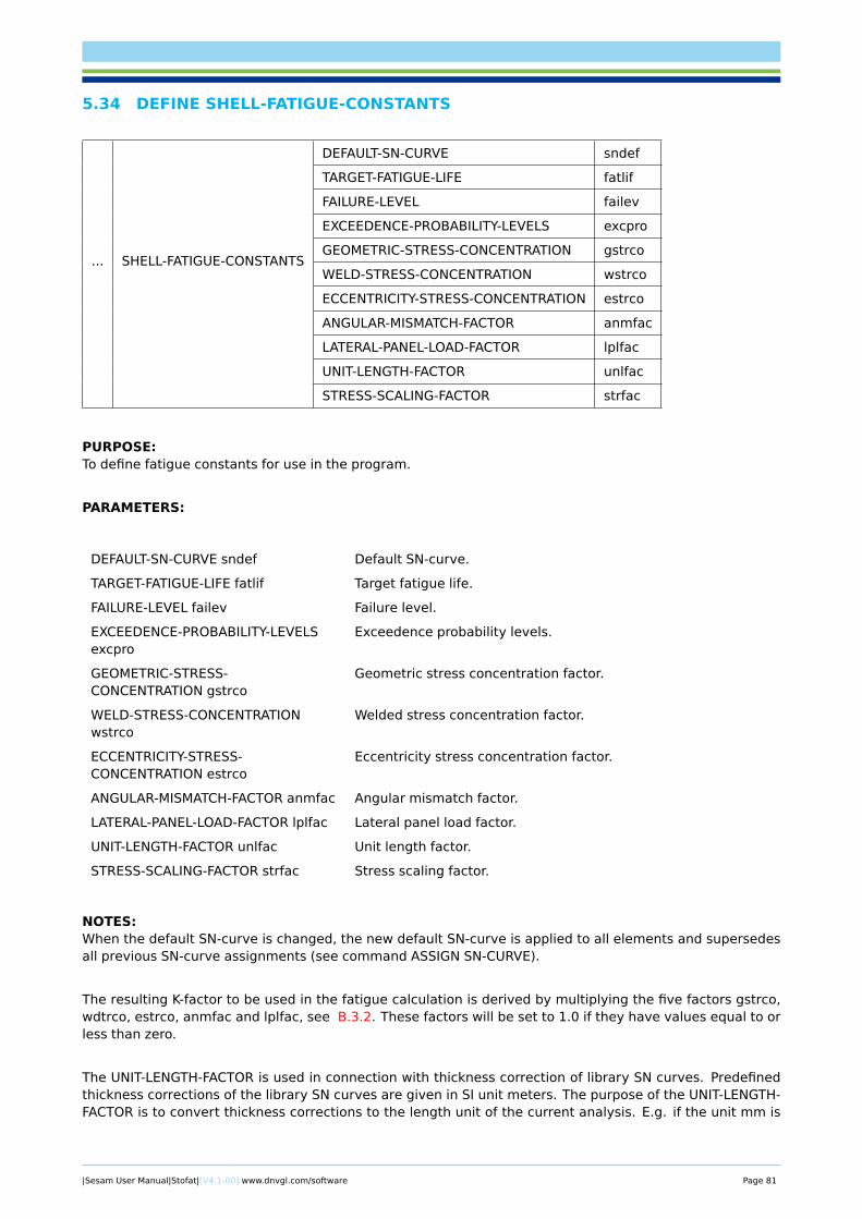
5.34 DEFINE SHELL-FATIGUE-CONSTANTS
... SHELL-FATIGUE-CONSTANTS
DEFAULT-SN-CURVE sndef
TARGET-FATIGUE-LIFE fatlif
FAILURE-LEVEL failev
EXCEEDENCE-PROBABILITY-LEVELS excpro
GEOMETRIC-STRESS-CONCENTRATION gstrco
WELD-STRESS-CONCENTRATION wstrco
ECCENTRICITY-STRESS-CONCENTRATION estrco
ANGULAR-MISMATCH-FACTOR anmfac
LATERAL-PANEL-LOAD-FACTOR lplfac
UNIT-LENGTH-FACTOR unlfac
STRESS-SCALING-FACTOR strfac
PURPOSE:To define fatigue constants for use in the program.
PARAMETERS:
DEFAULT-SN-CURVE sndef Default SN-curve.
TARGET-FATIGUE-LIFE fatlif Target fatigue life.
FAILURE-LEVEL failev Failure level.
EXCEEDENCE-PROBABILITY-LEVELSexcpro
Exceedence probability levels.
GEOMETRIC-STRESS-CONCENTRATION gstrco
Geometric stress concentration factor.
WELD-STRESS-CONCENTRATIONwstrco
Welded stress concentration factor.
ECCENTRICITY-STRESS-CONCENTRATION estrco
Eccentricity stress concentration factor.
ANGULAR-MISMATCH-FACTOR anmfac Angular mismatch factor.
LATERAL-PANEL-LOAD-FACTOR lplfac Lateral panel load factor.
UNIT-LENGTH-FACTOR unlfac Unit length factor.
STRESS-SCALING-FACTOR strfac Stress scaling factor.
NOTES:When the default SN-curve is changed, the new default SN-curve is applied to all elements and supersedesall previous SN-curve assignments (see command ASSIGN SN-CURVE).
The resulting K-factor to be used in the fatigue calculation is derived by multiplying the five factors gstrco,wdtrco, estrco, anmfac and lplfac, see B.3.2. These factors will be set to 1.0 if they have values equal to orless than zero.
The UNIT-LENGTH-FACTOR is used in connection with thickness correction of library SN curves. Predefinedthickness corrections of the library SN curves are given in SI unit meters. The purpose of the UNIT-LENGTH-FACTOR is to convert thickness corrections to the length unit of the current analysis. E.g. if the unit mm is
|Sesam User Manual|Stofat|[V4.1-00] www.dnvgl.com/software Page 81
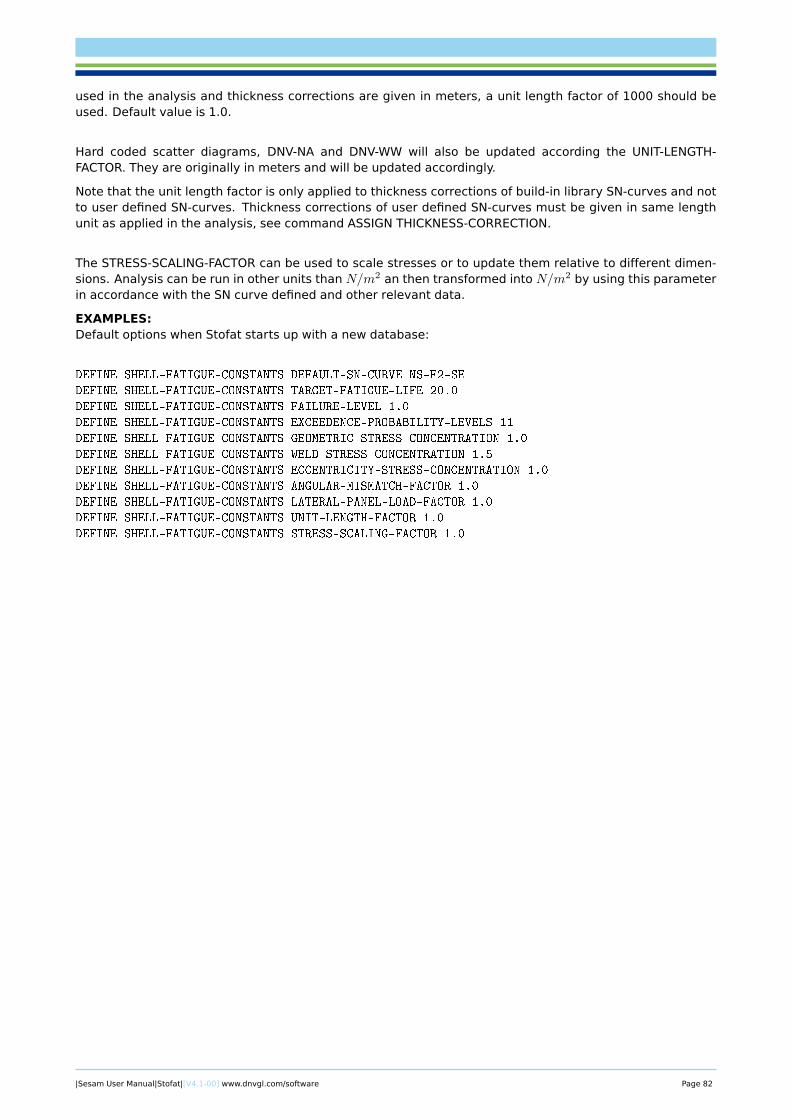
used in the analysis and thickness corrections are given in meters, a unit length factor of 1000 should beused. Default value is 1.0.
Hard coded scatter diagrams, DNV-NA and DNV-WW will also be updated according the UNIT-LENGTH-FACTOR. They are originally in meters and will be updated accordingly.
Note that the unit length factor is only applied to thickness corrections of build-in library SN-curves and notto user defined SN-curves. Thickness corrections of user defined SN-curves must be given in same lengthunit as applied in the analysis, see command ASSIGN THICKNESS-CORRECTION.
The STRESS-SCALING-FACTOR can be used to scale stresses or to update them relative to different dimen-sions. Analysis can be run in other units than N/m2 an then transformed into N/m2 by using this parameterin accordance with the SN curve defined and other relevant data.
EXAMPLES:Default options when Stofat starts up with a new database:
DEFINE SHELL-FATIGUE-CONSTANTS DEFAULT-SN-CURVE NS-F2-SE
DEFINE SHELL-FATIGUE-CONSTANTS TARGET-FATIGUE-LIFE 20.0
DEFINE SHELL-FATIGUE-CONSTANTS FAILURE-LEVEL 1.0
DEFINE SHELL-FATIGUE-CONSTANTS EXCEEDENCE-PROBABILITY-LEVELS 11
DEFINE SHELL-FATIGUE-CONSTANTS GEOMETRIC-STRESS-CONCENTRATION 1.0
DEFINE SHELL-FATIGUE-CONSTANTS WELD-STRESS-CONCENTRATION 1.5
DEFINE SHELL-FATIGUE-CONSTANTS ECCENTRICITY-STRESS-CONCENTRATION 1.0
DEFINE SHELL-FATIGUE-CONSTANTS ANGULAR-MISMATCH-FACTOR 1.0
DEFINE SHELL-FATIGUE-CONSTANTS LATERAL-PANEL-LOAD-FACTOR 1.0
DEFINE SHELL-FATIGUE-CONSTANTS UNIT-LENGTH-FACTOR 1.0
DEFINE SHELL-FATIGUE-CONSTANTS STRESS-SCALING-FACTOR 1.0
|Sesam User Manual|Stofat|[V4.1-00] www.dnvgl.com/software Page 82
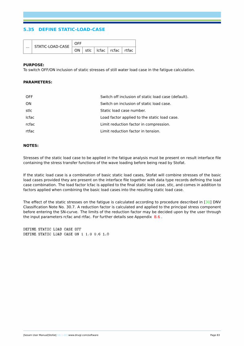
5.35 DEFINE STATIC-LOAD-CASE
... STATIC-LOAD-CASEOFF
ON stlc lcfac rcfac rtfac
PURPOSE:To switch OFF/ON inclusion of static stresses of still water load case in the fatigue calculation.
PARAMETERS:
OFF Switch off inclusion of static load case (default).
ON Switch on inclusion of static load case.
stlc Static load case number.
lcfac Load factor applied to the static load case.
rcfac Limit reduction factor in compression.
rtfac Limit reduction factor in tension.
NOTES:
Stresses of the static load case to be applied in the fatigue analysis must be present on result interface filecontaining the stress transfer functions of the wave loading before being read by Stofat.
If the static load case is a combination of basic static load cases, Stofat will combine stresses of the basicload cases provided they are present on the interface file together with data type records defining the loadcase combination. The load factor lcfac is applied to the final static load case, stlc, and comes in addition tofactors applied when combining the basic load cases into the resulting static load case.
The effect of the static stresses on the fatigue is calculated according to procedure described in [30] DNVClassification Note No. 30.7. A reduction factor is calculated and applied to the principal stress componentbefore entering the SN-curve. The limits of the reduction factor may be decided upon by the user throughthe input parameters rcfac and rtfac. For further details see Appendix B.6 .
DEFINE STATIC-LOAD-CASE OFF
DEFINE STATIC-LOAD-CASE ON 1 1.0 0.6 1.0
|Sesam User Manual|Stofat|[V4.1-00] www.dnvgl.com/software Page 83
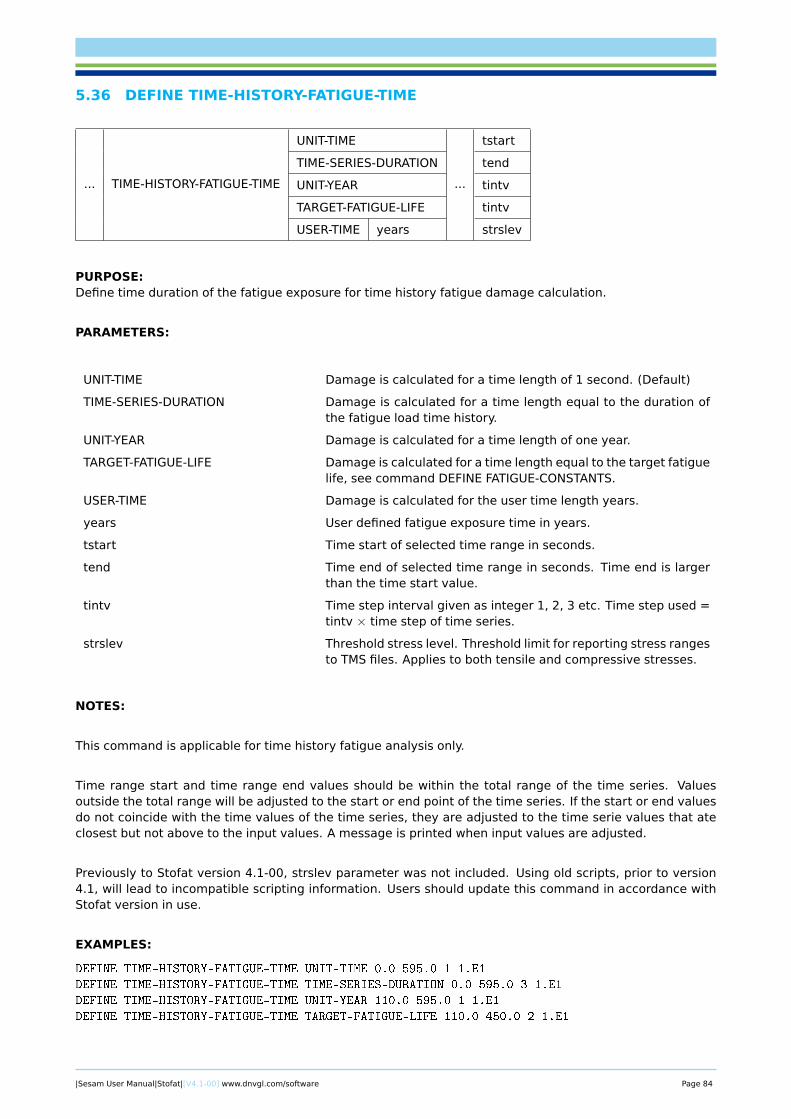
5.36 DEFINE TIME-HISTORY-FATIGUE-TIME
... TIME-HISTORY-FATIGUE-TIME
UNIT-TIME
...
tstart
TIME-SERIES-DURATION tend
UNIT-YEAR tintv
TARGET-FATIGUE-LIFE tintv
USER-TIME years strslev
PURPOSE:Define time duration of the fatigue exposure for time history fatigue damage calculation.
PARAMETERS:
UNIT-TIME Damage is calculated for a time length of 1 second. (Default)
TIME-SERIES-DURATION Damage is calculated for a time length equal to the duration ofthe fatigue load time history.
UNIT-YEAR Damage is calculated for a time length of one year.
TARGET-FATIGUE-LIFE Damage is calculated for a time length equal to the target fatiguelife, see command DEFINE FATIGUE-CONSTANTS.
USER-TIME Damage is calculated for the user time length years.
years User defined fatigue exposure time in years.
tstart Time start of selected time range in seconds.
tend Time end of selected time range in seconds. Time end is largerthan the time start value.
tintv Time step interval given as integer 1, 2, 3 etc. Time step used =tintv × time step of time series.
strslev Threshold stress level. Threshold limit for reporting stress rangesto TMS files. Applies to both tensile and compressive stresses.
NOTES:
This command is applicable for time history fatigue analysis only.
Time range start and time range end values should be within the total range of the time series. Valuesoutside the total range will be adjusted to the start or end point of the time series. If the start or end valuesdo not coincide with the time values of the time series, they are adjusted to the time serie values that ateclosest but not above to the input values. A message is printed when input values are adjusted.
Previously to Stofat version 4.1-00, strslev parameter was not included. Using old scripts, prior to version4.1, will lead to incompatible scripting information. Users should update this command in accordance withStofat version in use.
EXAMPLES:
DEFINE TIME-HISTORY-FATIGUE-TIME UNIT-TIME 0.0 595.0 1 1.E1
DEFINE TIME-HISTORY-FATIGUE-TIME TIME-SERIES-DURATION 0.0 595.0 3 1.E1
DEFINE TIME-HISTORY-FATIGUE-TIME UNIT-YEAR 110.0 595.0 1 1.E1
DEFINE TIME-HISTORY-FATIGUE-TIME TARGET-FATIGUE-LIFE 110.0 450.0 2 1.E1
|Sesam User Manual|Stofat|[V4.1-00] www.dnvgl.com/software Page 84

DEFINE TIME-HISTORY-FATIGUE-TIME USER-TIME 0.5 0.0 300.0 1 1.E1
|Sesam User Manual|Stofat|[V4.1-00] www.dnvgl.com/software Page 85

5.37 DEFINE WEIBULL-PARAMETERS
... WEIBULL-PARAMETERSOFF
ON
PURPOSE:To switch OFF/ON calculation of the scale and shape parameters of the Weibull function during run execu-tions. The parameters are printed in the fatigue results table of the run only when calculation is switched on.
PARAMETERS:
OFF Switch off calculation of the Weibull parameters (default).
ON Switch on calculation of the Weibull parameters.
NOTES:The Weibull parameters are calculated by fitting the Weibull function to stress range distributions consistingof ten range levels by a least square technique.
EXAMPLES:
DEFINE WEIBULL-PARAMETERS ON
|Sesam User Manual|Stofat|[V4.1-00] www.dnvgl.com/software Page 86

5.38 DEFINE WIDE-BAND-CORRECTION-FACTOR
... WIDE-BAND-CORRECTION-FACTOROFF
ON
PURPOSE:To switch OFF/ON Wirsching correction factor for wide banded stress processes. The correction factor isgiven in C.3.
PARAMETERS:
OFF Switch off Wirsching correction factor (default).
ON Switch on Wirsching correction factor.
EXAMPLES:
DEFINE WIDE-BAND-CORRECTION-FACTOR ON
|Sesam User Manual|Stofat|[V4.1-00] www.dnvgl.com/software Page 87

5.39 DELETE
DELETE
HOTSPOT
...
RUN
SN-CURVE
WAVE-SPREADING-FUNCTION
WAVE-STATISTICS
WELD-NORMAL-LINE
PURPOSE:To delete items previously created.The program will ask for the name of the item and delete all data stored under this name.
|Sesam User Manual|Stofat|[V4.1-00] www.dnvgl.com/software Page 88

5.40 DELETE HOTSPOT
... HOTSPOT ( ONLY name+ )
PURPOSE:To delete a hotspot created by the user.
PARAMETERS:
name+ Name of the hotspot.
ONLY Mandatory attribute.
( ) Mandatory parentheses.
EXAMPLES:
DELETE HOTSPOT ( ONLY BOT1249 TOP1249 MID1249 )
|Sesam User Manual|Stofat|[V4.1-00] www.dnvgl.com/software Page 89

5.41 DELETE RUN
... RUN ( ONLY name+ )
PURPOSE:To delete an executed run case and fatigue results related to the run.
PARAMETERS:
name+ Name of the run.
ONLY Mandatory attribute.
( ) Mandatory parentheses.
EXAMPLES:
DELETE RUN ( ONLY RUN1 )
|Sesam User Manual|Stofat|[V4.1-00] www.dnvgl.com/software Page 90

5.42 DELETE SN-CURVE
... SN-CURVE ( ONLY name+ )
PURPOSE:To delete a user specified SN-curve.
PARAMETERS:
name+ Name of the user specified SN-curve.
ONLY Mandatory attribute.
( ) Mandatory parentheses.
EXAMPLES:
DELETE SN-CURVE ( ONLY USE-X USE-Y )
|Sesam User Manual|Stofat|[V4.1-00] www.dnvgl.com/software Page 91
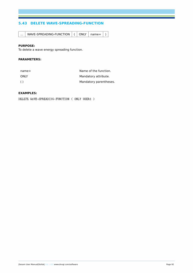
5.43 DELETE WAVE-SPREADING-FUNCTION
... WAVE-SPREADING-FUNCTION ( ONLY name+ )
PURPOSE:To delete a wave energy spreading function.
PARAMETERS:
name+ Name of the function.
ONLY Mandatory attribute.
( ) Mandatory parentheses.
EXAMPLES:
DELETE WAVE-SPREADING-FUNCTION ( ONLY USER1 )
|Sesam User Manual|Stofat|[V4.1-00] www.dnvgl.com/software Page 92

5.44 DELETE WAVE-STATISTICS
... WAVE-STATISTICS ( ONLY name+ )
PURPOSE:To delete a wave statistics model.
PARAMETERS:
name+ Name of the model.
ONLY Mandatory attribute.
( ) Mandatory parentheses.
EXAMPLES:
DELETE WAVE-STATISTICS ( ONLY NRD SCATTER )
|Sesam User Manual|Stofat|[V4.1-00] www.dnvgl.com/software Page 93

5.45 DELETE WELD-NORMAL-LINE
... WELD-NORMAL-LINE
DELETE-LINE ( ONLY wnlnam+ )
DELETE-ASSIGNMENT
ALL
ELEMENT elmnam
HOTSPOT ( ONLY hotnam+ )
PURPOSE:To delete weld normal lines and assignments of weld normal lines.
PARAMETERS:
DELETE-LINE Delete weld normal lines.
DELETE-ASSIGNMENT Delete assignments of weld normal lines.
ALL Delete all assignments of weld normal lines.
ELEMENT Delete assignment of weld normal lines to elements.
HOTSPOT Delete assignment of weld normal lines to hotspots.
wnlnam+ Names of weld normal lines which shall be deleted.
elmnam Name of element or element set to which assignment of weldnormal lines shall be deleted.
hotnam+ Names of hotspots to which assignment of weld normal lines shallbe deleted.
ONLY Mandatory attribute.
( ) Mandatory parentheses.
NOTES:Use the command PRINT RUN-OVERVIEW WELD-NORMAL-LINES or press the Show button in the dialoguebox to see current status on defined weld normal lines and assignments to elements and hotspots.
EXAMPLES:
DELETE WELD-NORMAL-LINE DELETE-LINE ( ONLY WNL4 )
DELETE WELD-NORMAL-LINE DELETE-ASSIGNMENT ELEMENT 86
SELECT ELEMENTS INCLUDE CURRENT
DELETE WELD-NORMAL-LINE DELETE-ASSIGNMENT ELEMENT DEFAULT
DELETE WELD-NORMAL-LINE DELETE-ASSIGNMENT HOTSPOT ( ONLY HOT2 HOT3 )
DELETE WELD-NORMAL-LINE DELETE-ASSIGNMENT ALL
|Sesam User Manual|Stofat|[V4.1-00] www.dnvgl.com/software Page 94
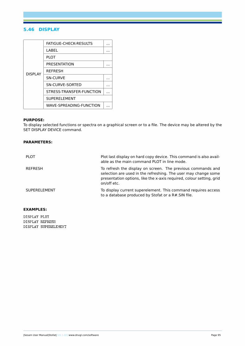
5.46 DISPLAY
DISPLAY
FATIGUE-CHECK-RESULTS ...
LABEL ...
PLOT
PRESENTATION ...
REFRESH
SN-CURVE ...
SN-CURVE-SORTED ...
STRESS-TRANSFER-FUNCTION ...
SUPERELEMENT
WAVE-SPREADING-FUNCTION ...
PURPOSE:To display selected functions or spectra on a graphical screen or to a file. The device may be altered by theSET DISPLAY DEVICE command.
PARAMETERS:
PLOT Plot last display on hard copy device. This command is also avail-able as the main command PLOT in line mode.
REFRESH To refresh the display on screen. The previous commands andselection are used in the refreshing. The user may change somepresentation options, like the x-axis required, colour setting, gridon/off etc.
SUPERELEMENT To display current superelement. This command requires accessto a database produced by Stofat or a R#.SIN file.
EXAMPLES:
DISPLAY PLOT
DISPLAY REFRESH
DISPLAY SUPERELEMENT
|Sesam User Manual|Stofat|[V4.1-00] www.dnvgl.com/software Page 95
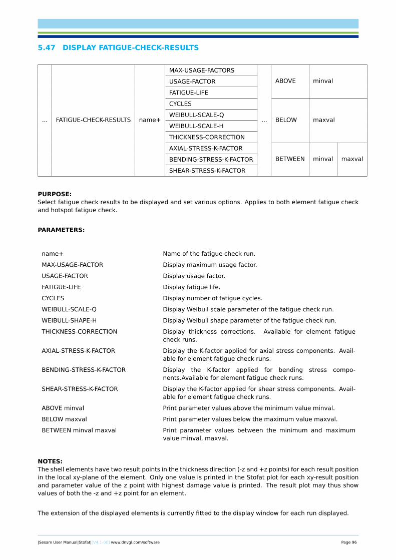
5.47 DISPLAY FATIGUE-CHECK-RESULTS
... FATIGUE-CHECK-RESULTS name+
MAX-USAGE-FACTORS
...
ABOVE minvalUSAGE-FACTOR
FATIGUE-LIFE
CYCLES
BELOW maxvalWEIBULL-SCALE-Q
WEIBULL-SCALE-H
THICKNESS-CORRECTION
AXIAL-STRESS-K-FACTOR
BETWEEN minval maxvalBENDING-STRESS-K-FACTOR
SHEAR-STRESS-K-FACTOR
PURPOSE:Select fatigue check results to be displayed and set various options. Applies to both element fatigue checkand hotspot fatigue check.
PARAMETERS:
name+ Name of the fatigue check run.
MAX-USAGE-FACTOR Display maximum usage factor.
USAGE-FACTOR Display usage factor.
FATIGUE-LIFE Display fatigue life.
CYCLES Display number of fatigue cycles.
WEIBULL-SCALE-Q Display Weibull scale parameter of the fatigue check run.
WEIBULL-SHAPE-H Display Weibull shape parameter of the fatigue check run.
THICKNESS-CORRECTION Display thickness corrections. Available for element fatiguecheck runs.
AXIAL-STRESS-K-FACTOR Display the K-factor applied for axial stress components. Avail-able for element fatigue check runs.
BENDING-STRESS-K-FACTOR Display the K-factor applied for bending stress compo-nents.Available for element fatigue check runs.
SHEAR-STRESS-K-FACTOR Display the K-factor applied for shear stress components. Avail-able for element fatigue check runs.
ABOVE minval Print parameter values above the minimum value minval.
BELOW maxval Print parameter values below the maximum value maxval.
BETWEEN minval maxval Print parameter values between the minimum and maximumvalue minval, maxval.
NOTES:The shell elements have two result points in the thickness direction (-z and +z points) for each result positionin the local xy-plane of the element. Only one value is printed in the Stofat plot for each xy-result positionand parameter value of the z point with highest damage value is printed. The result plot may thus showvalues of both the -z and +z point for an element.
The extension of the displayed elements is currently fitted to the display window for each run displayed.
|Sesam User Manual|Stofat|[V4.1-00] www.dnvgl.com/software Page 96
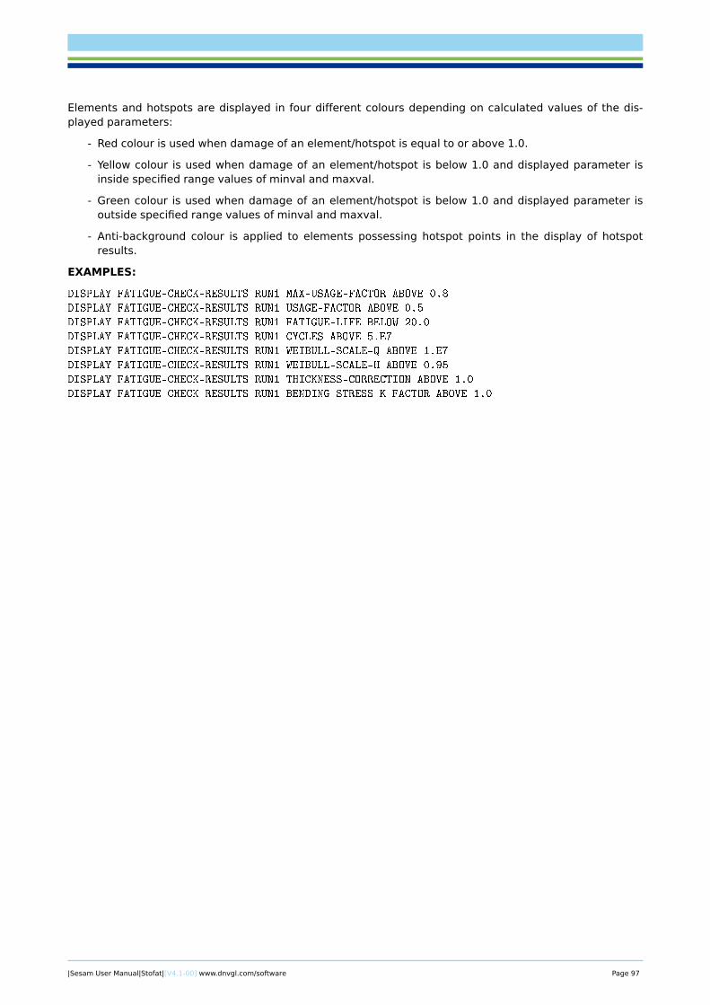
Elements and hotspots are displayed in four different colours depending on calculated values of the dis-played parameters:
- Red colour is used when damage of an element/hotspot is equal to or above 1.0.
- Yellow colour is used when damage of an element/hotspot is below 1.0 and displayed parameter isinside specified range values of minval and maxval.
- Green colour is used when damage of an element/hotspot is below 1.0 and displayed parameter isoutside specified range values of minval and maxval.
- Anti-background colour is applied to elements possessing hotspot points in the display of hotspotresults.
EXAMPLES:
DISPLAY FATIGUE-CHECK-RESULTS RUN1 MAX-USAGE-FACTOR ABOVE 0.8
DISPLAY FATIGUE-CHECK-RESULTS RUN1 USAGE-FACTOR ABOVE 0.5
DISPLAY FATIGUE-CHECK-RESULTS RUN1 FATIGUE-LIFE BELOW 20.0
DISPLAY FATIGUE-CHECK-RESULTS RUN1 CYCLES ABOVE 5.E7
DISPLAY FATIGUE-CHECK-RESULTS RUN1 WEIBULL-SCALE-Q ABOVE 1.E7
DISPLAY FATIGUE-CHECK-RESULTS RUN1 WEIBULL-SCALE-H ABOVE 0.95
DISPLAY FATIGUE-CHECK-RESULTS RUN1 THICKNESS-CORRECTION ABOVE 1.0
DISPLAY FATIGUE-CHECK-RESULTS RUN1 BENDING-STRESS-K-FACTOR ABOVE 1.0
|Sesam User Manual|Stofat|[V4.1-00] www.dnvgl.com/software Page 97
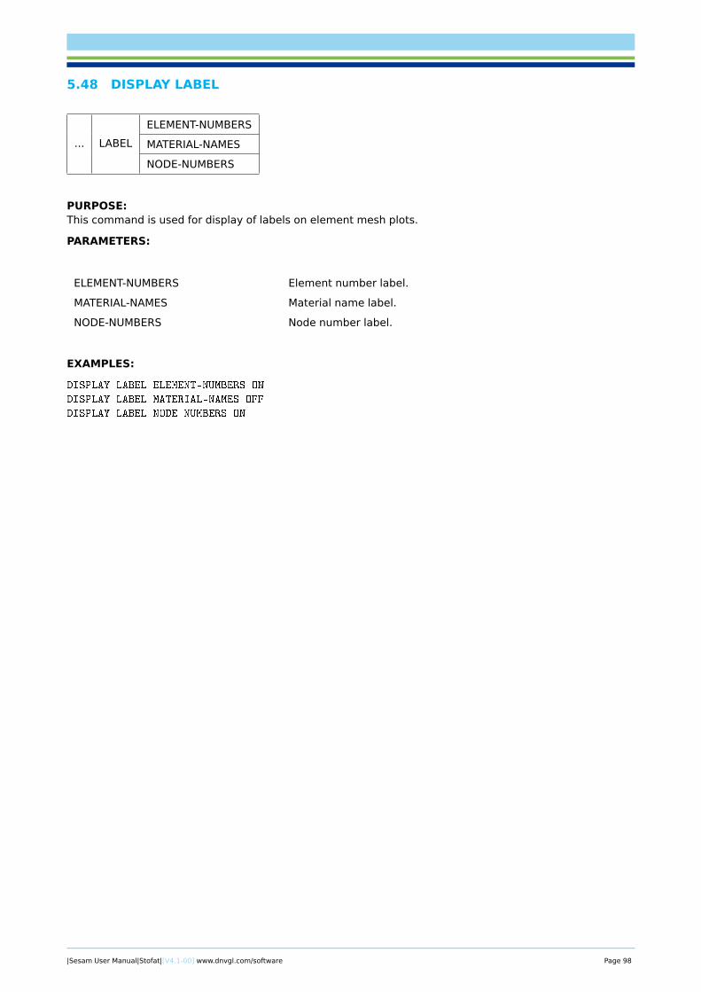
5.48 DISPLAY LABEL
... LABEL
ELEMENT-NUMBERS
MATERIAL-NAMES
NODE-NUMBERS
PURPOSE:This command is used for display of labels on element mesh plots.
PARAMETERS:
ELEMENT-NUMBERS Element number label.
MATERIAL-NAMES Material name label.
NODE-NUMBERS Node number label.
EXAMPLES:
DISPLAY LABEL ELEMENT-NUMBERS ON
DISPLAY LABEL MATERIAL-NAMES OFF
DISPLAY LABEL NODE-NUMBERS ON
|Sesam User Manual|Stofat|[V4.1-00] www.dnvgl.com/software Page 98
5.49 DISPLAY PRESENTATION
... PRESENTATIONWIREFRAME
HIDDEN-SURFACE resol
PURPOSE:To set presentation mode for display of superelement plot.
PARAMETERS:
WIREFRAME Line display.
HIDDEN-SURFACE resol Hidden surface display. The numeric factor resol defines resolu-tion for the hidden display (default value is 1.0, a value of 0.1 willgive a coarse resolution).
EXAMPLES:
DISPLAY PRESENTATION WIREFRAME
DISPLAY PRESENTATION HIDDEN-SURFACE 0.5
|Sesam User Manual|Stofat|[V4.1-00] www.dnvgl.com/software Page 99

5.50 DISPLAY SN-CURVE
... SN-CURVE ( ONLY snname+ )
PURPOSE:To display one or several SN-curves.
PARAMETERS:
snname+ Name of the SN-curve.
ONLY Mandatory attribute.
( ) Mandatory parentheses.
NOTES:This SN-curves will always be shown in a log-log scale.
EXAMPLES:
DISPLAY SN-CURVE ( ONLY USE-X USE-Y )
|Sesam User Manual|Stofat|[V4.1-00] www.dnvgl.com/software Page 100
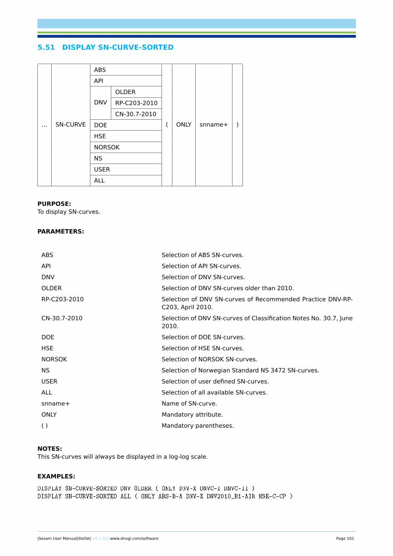
5.51 DISPLAY SN-CURVE-SORTED
... SN-CURVE
ABS
( ONLY snname+ )
API
DNV
OLDER
RP-C203-2010
CN-30.7-2010
DOE
HSE
NORSOK
NS
USER
ALL
PURPOSE:To display SN-curves.
PARAMETERS:
ABS Selection of ABS SN-curves.
API Selection of API SN-curves.
DNV Selection of DNV SN-curves.
OLDER Selection of DNV SN-curves older than 2010.
RP-C203-2010 Selection of DNV SN-curves of Recommended Practice DNV-RP-C203, April 2010.
CN-30.7-2010 Selection of DNV SN-curves of Classification Notes No. 30.7, June2010.
DOE Selection of DOE SN-curves.
HSE Selection of HSE SN-curves.
NORSOK Selection of NORSOK SN-curves.
NS Selection of Norwegian Standard NS 3472 SN-curves.
USER Selection of user defined SN-curves.
ALL Selection of all available SN-curves.
snname+ Name of SN-curve.
ONLY Mandatory attribute.
( ) Mandatory parentheses.
NOTES:This SN-curves will always be displayed in a log-log scale.
EXAMPLES:
DISPLAY SN-CURVE-SORTED DNV OLDER ( ONLY DNV-X DNVC-I DNVC-II )
DISPLAY SN-CURVE-SORTED ALL ( ONLY ABS-B-A DNV-X DNV2010_B1-AIR HSE-C-CP )
|Sesam User Manual|Stofat|[V4.1-00] www.dnvgl.com/software Page 101
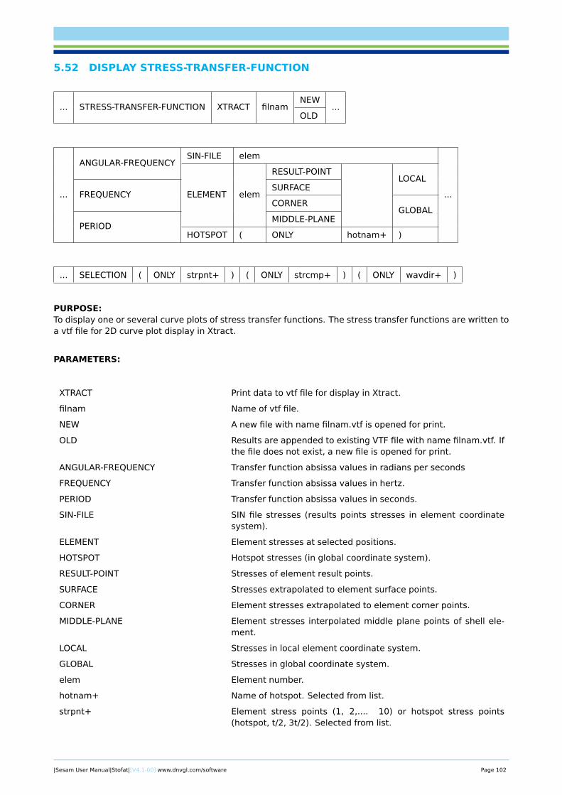
5.52 DISPLAY STRESS-TRANSFER-FUNCTION
... STRESS-TRANSFER-FUNCTION XTRACT filnamNEW
...OLD
...
ANGULAR-FREQUENCYSIN-FILE elem
...ELEMENT elem
RESULT-POINTLOCAL
FREQUENCYSURFACE
CORNERGLOBAL
PERIODMIDDLE-PLANE
HOTSPOT ( ONLY hotnam+ )
... SELECTION ( ONLY strpnt+ ) ( ONLY strcmp+ ) ( ONLY wavdir+ )
PURPOSE:To display one or several curve plots of stress transfer functions. The stress transfer functions are written toa vtf file for 2D curve plot display in Xtract.
PARAMETERS:
XTRACT Print data to vtf file for display in Xtract.
filnam Name of vtf file.
NEW A new file with name filnam.vtf is opened for print.
OLD Results are appended to existing VTF file with name filnam.vtf. Ifthe file does not exist, a new file is opened for print.
ANGULAR-FREQUENCY Transfer function absissa values in radians per seconds
FREQUENCY Transfer function absissa values in hertz.
PERIOD Transfer function absissa values in seconds.
SIN-FILE SIN file stresses (results points stresses in element coordinatesystem).
ELEMENT Element stresses at selected positions.
HOTSPOT Hotspot stresses (in global coordinate system).
RESULT-POINT Stresses of element result points.
SURFACE Stresses extrapolated to element surface points.
CORNER Element stresses extrapolated to element corner points.
MIDDLE-PLANE Element stresses interpolated middle plane points of shell ele-ment.
LOCAL Stresses in local element coordinate system.
GLOBAL Stresses in global coordinate system.
elem Element number.
hotnam+ Name of hotspot. Selected from list.
strpnt+ Element stress points (1, 2,.... 10) or hotspot stress points(hotspot, t/2, 3t/2). Selected from list.
|Sesam User Manual|Stofat|[V4.1-00] www.dnvgl.com/software Page 102
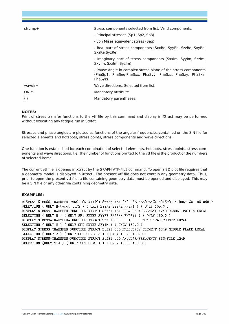
strcmp+ Stress components selected from list. Valid components:
- Principal stresses (Sp1, Sp2, Sp3)
- von Mises equivalent stress (Seq)
- Real part of stress components (SxxRe, SyyRe, SzzRe, SxyRe,SxzRe,SyzRe)
- Imaginary part of stress components (SxxIm, SyyIm, SzzIm,SxyIm, SxzIm, SyzIm)
- Phase angle in complex stress plane of the stress components(PhaSp1, PhaSeq,PhaSxx, PhaSyy, PhaSzz, PhaSxy, PhaSxz,PhaSyz)
wavdir+ Wave directions. Selected from list.
ONLY Mandatory attribute.
( ) Mandatory parentheses.
NOTES:Print of stress transfer functions to the vtf file by this command and display in Xtract may be performedwithout executing any fatigue run in Stofat.
Stresses and phase angles are plotted as functions of the angular frequencies contained on the SIN file forselected elements and hotspots, stress points, stress components and wave directions.
One function is established for each combination of selected elements, hotspots, stress points, stress com-ponents and wave directions. I.e. the number of functions printed to the vtf file is the product of the numbersof selected items.
The current vtf file is opened in Xtract by the GRAPH VTF-FILE command. To open a 2D plot file requires thata geometry model is displayed in Xtract. The present vtf file does not contain any geometry data. Thus,prior to open the present vtf file, a file containing geometry data must be opened and displayed. This maybe a SIN file or any other file containing geometry data.
EXAMPLES:
DISPLAY STRESS-TRANSFER-FUNCTION XTRACT StfHp NEW ANGULAR-FREQUENCY HOTSPOT ( ONLY CUI BOT969 )
SELECTION ( ONLY Hotspot 1t/2 ) ( ONLY SYYRE SZZRE PHSP1 ) ( ONLY 165.0 )
DISPLAY STRESS-TRANSFER-FUNCTION XTRACT StfEl NEW FREQUENCY ELEMENT 1249 RESULT-POINTS LOCAL
SELECTION ( ONLY 5 ) ( ONLY SP1 SXXRE SYYRE PHASXX PHASYY ) ( ONLY 180.0 )
DISPLAY STRESS-TRANSFER-FUNCTION XTRACT StfEl OLD PERIOD ELEMENT 1249 CORNER LOCAL
SELECTION ( ONLY 8 ) ( ONLY SP2 SXYRE SXYIM ) ( ONLY 180.0 )
DISPLAY STRESS-TRANSFER-FUNCTION XTRACT StfEl OLD FREQUENCY ELEMENT 1249 MIDDLE-PLANE LOCAL
SELECTION ( ONLY 3 ) ( ONLY SP1 SP2 SP3 ) ( ONLY 165.0 180.0 )
DISPLAY STRESS-TRANSFER-FUNCTION XTRACT StfEl OLD ANGULAR-FREQUENCY SIN-FILE 1249
SELECTION (ONLY 3 4 ) ( ONLY SP1 PHASP1 ) ( ONLY 165.0 180.0 )
|Sesam User Manual|Stofat|[V4.1-00] www.dnvgl.com/software Page 103

5.53 DISPLAY WAVE-SPREADING-FUNCTION
... WAVE-SPREADING-FUNCTION name+ [space]
PURPOSE:To display energy spreading for elementary wave directions created by the user.
PARAMETERS:
name+ User given name of the function.
space User input space between each wave direction angle for whichthe energy spreading function will be displayed. This space isindependent of what the program will use in calculating the re-sponse spectra. Only asked for if the name of the function corre-sponds to a cosine power function.
EXAMPLES:
DISPLAY WAVE-SPREADING-FUNCTION COS2 30.0
|Sesam User Manual|Stofat|[V4.1-00] www.dnvgl.com/software Page 104
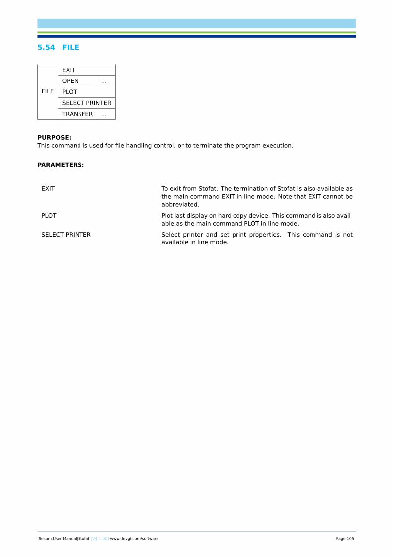
5.54 FILE
FILE
EXIT
OPEN ...
PLOT
SELECT PRINTER
TRANSFER ...
PURPOSE:This command is used for file handling control, or to terminate the program execution.
PARAMETERS:
EXIT To exit from Stofat. The termination of Stofat is also available asthe main command EXIT in line mode. Note that EXIT cannot beabbreviated.
PLOT Plot last display on hard copy device. This command is also avail-able as the main command PLOT in line mode.
SELECT PRINTER Select printer and set print properties. This command is notavailable in line mode.
|Sesam User Manual|Stofat|[V4.1-00] www.dnvgl.com/software Page 105
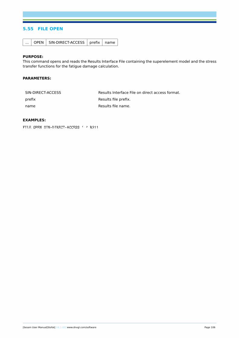
5.55 FILE OPEN
... OPEN SIN-DIRECT-ACCESS prefix name
PURPOSE:This command opens and reads the Results Interface File containing the superelement model and the stresstransfer functions for the fatigue damage calculation.
PARAMETERS:
SIN-DIRECT-ACCESS Results Interface File on direct access format.
prefix Results file prefix.
name Results file name.
EXAMPLES:
FILE OPEN SIN-DIRECT-ACCESS ` ' R211
|Sesam User Manual|Stofat|[V4.1-00] www.dnvgl.com/software Page 106
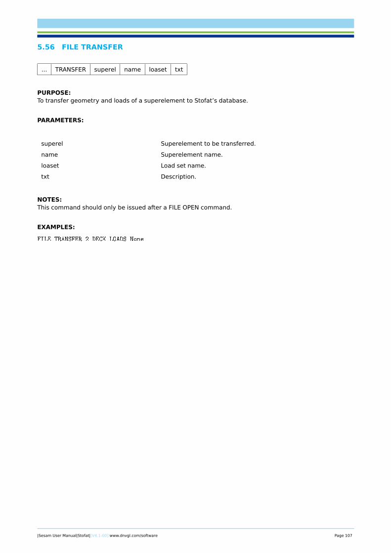
5.56 FILE TRANSFER
... TRANSFER superel name loaset txt
PURPOSE:To transfer geometry and loads of a superelement to Stofat’s database.
PARAMETERS:
superel Superelement to be transferred.
name Superelement name.
loaset Load set name.
txt Description.
NOTES:This command should only be issued after a FILE OPEN command.
EXAMPLES:
FILE TRANSFER 2 DECK LOADS None
|Sesam User Manual|Stofat|[V4.1-00] www.dnvgl.com/software Page 107

5.57 PLOT
PLOT
PURPOSE:Plot last display on hard copy device. The previous commands and selection are used in the plotting. Theuser may change some presentation options, like the x-axis required, colour setting, grid on/off etc. Thiscommand is not available from the menu bar in graphics mode. Use FILE PLOT or DISPLAY PLOT instead.
|Sesam User Manual|Stofat|[V4.1-00] www.dnvgl.com/software Page 108
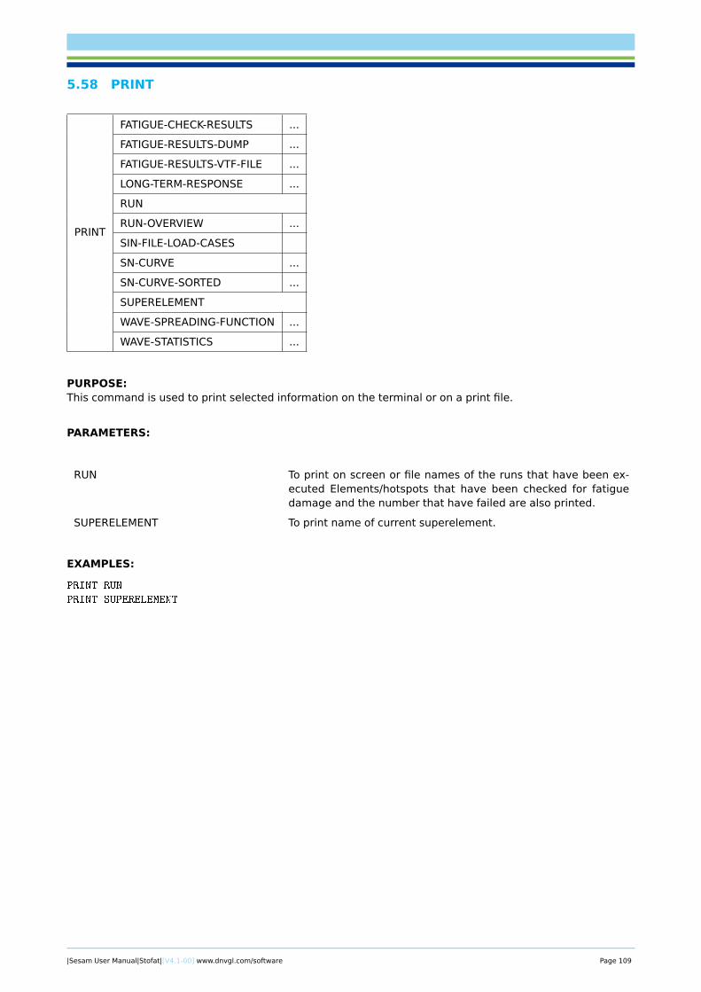
5.58 PRINT
FATIGUE-CHECK-RESULTS ...
FATIGUE-RESULTS-DUMP ...
FATIGUE-RESULTS-VTF-FILE ...
LONG-TERM-RESPONSE ...
RUN
RUN-OVERVIEW ...
SIN-FILE-LOAD-CASES
SN-CURVE ...
SN-CURVE-SORTED ...
SUPERELEMENT
WAVE-SPREADING-FUNCTION ...
WAVE-STATISTICS ...
PURPOSE:This command is used to print selected information on the terminal or on a print file.
PARAMETERS:
RUN To print on screen or file names of the runs that have been ex-ecuted Elements/hotspots that have been checked for fatiguedamage and the number that have failed are also printed.
SUPERELEMENT To print name of current superelement.
EXAMPLES:
PRINT RUN
PRINT SUPERELEMENT
|Sesam User Manual|Stofat|[V4.1-00] www.dnvgl.com/software Page 109
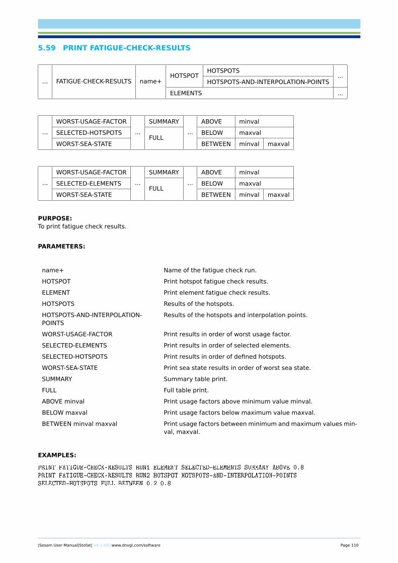
5.59 PRINT FATIGUE-CHECK-RESULTS
... FATIGUE-CHECK-RESULTS name+HOTSPOT
HOTSPOTS...
HOTSPOTS-AND-INTERPOLATION-POINTS
ELEMENTS ...
...
WORST-USAGE-FACTOR
...
SUMMARY
...
ABOVE minval
SELECTED-HOTSPOTSFULL
BELOW maxval
WORST-SEA-STATE BETWEEN minval maxval
...
WORST-USAGE-FACTOR
...
SUMMARY
...
ABOVE minval
SELECTED-ELEMENTSFULL
BELOW maxval
WORST-SEA-STATE BETWEEN minval maxval
PURPOSE:To print fatigue check results.
PARAMETERS:
name+ Name of the fatigue check run.
HOTSPOT Print hotspot fatigue check results.
ELEMENT Print element fatigue check results.
HOTSPOTS Results of the hotspots.
HOTSPOTS-AND-INTERPOLATION-POINTS
Results of the hotspots and interpolation points.
WORST-USAGE-FACTOR Print results in order of worst usage factor.
SELECTED-ELEMENTS Print results in order of selected elements.
SELECTED-HOTSPOTS Print results in order of defined hotspots.
WORST-SEA-STATE Print sea state results in order of worst sea state.
SUMMARY Summary table print.
FULL Full table print.
ABOVE minval Print usage factors above minimum value minval.
BELOW maxval Print usage factors below maximum value maxval.
BETWEEN minval maxval Print usage factors between minimum and maximum values min-val, maxval.
EXAMPLES:
PRINT FATIGUE-CHECK-RESULTS RUN1 ELEMENT SELECTED-ELEMENTS SUMMARY ABOVE 0.8
PRINT FATIGUE-CHECK-RESULTS RUN2 HOTSPOT HOTSPOTS-AND-INTERPOLATION-POINTS
SELECTED-HOTSPOTS FULL BETWEEN 0.2 0.8
|Sesam User Manual|Stofat|[V4.1-00] www.dnvgl.com/software Page 110
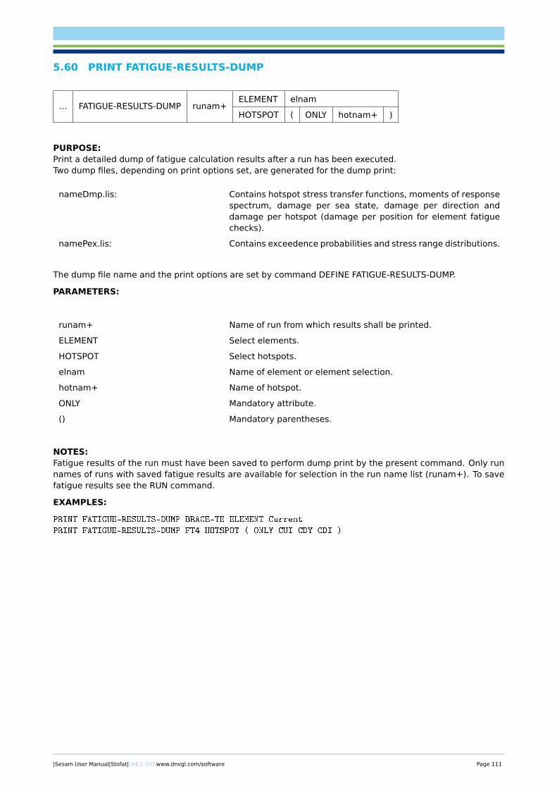
5.60 PRINT FATIGUE-RESULTS-DUMP
... FATIGUE-RESULTS-DUMP runam+ELEMENT elnam
HOTSPOT ( ONLY hotnam+ )
PURPOSE:Print a detailed dump of fatigue calculation results after a run has been executed.Two dump files, depending on print options set, are generated for the dump print:
nameDmp.lis: Contains hotspot stress transfer functions, moments of responsespectrum, damage per sea state, damage per direction anddamage per hotspot (damage per position for element fatiguechecks).
namePex.lis: Contains exceedence probabilities and stress range distributions.
The dump file name and the print options are set by command DEFINE FATIGUE-RESULTS-DUMP.
PARAMETERS:
runam+ Name of run from which results shall be printed.
ELEMENT Select elements.
HOTSPOT Select hotspots.
elnam Name of element or element selection.
hotnam+ Name of hotspot.
ONLY Mandatory attribute.
() Mandatory parentheses.
NOTES:Fatigue results of the run must have been saved to perform dump print by the present command. Only runnames of runs with saved fatigue results are available for selection in the run name list (runam+). To savefatigue results see the RUN command.
EXAMPLES:
PRINT FATIGUE-RESULTS-DUMP BRACE-TE ELEMENT Current
PRINT FATIGUE-RESULTS-DUMP FT4 HOTSPOT ( ONLY CUI CDY CDI )
|Sesam User Manual|Stofat|[V4.1-00] www.dnvgl.com/software Page 111
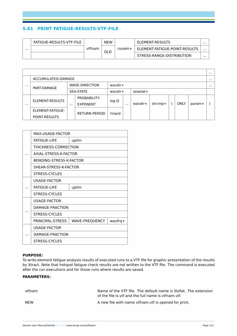
5.61 PRINT FATIGUE-RESULTS-VTF-FILE
...
FATIGUE-RESULTS-VTF-FILE
vtfnam
NEW
runam+
ELEMENT-RESULTS ...
OLDELEMENT-FATIGUE-POINT-RESULTS ...
STRESS-RANGE-DISTRIBUTION ...
...
...
ACCUMULATED-DAMAGE ...
PART-DAMAGEWAVE-DIRECTION wavdir+ ...
SEA-STATE wavdir+ seastat+
...ELEMENT-RESULTS
...
PROBABILITY-
EXPONENTlog-Q
... wavdir+ strcmp+ ( ONLY param+ )
ELEMENT-FATIGUE-
POINT-RESULTSRETURN-PERIOD rtnprd
...
MAX-USAGE-FACTOR
FATIGUE-LIFE uplim
THICKNESS-CORRECTION
AXIAL-STRESS-K-FACTOR
BENDING-STRESS-K-FACTOR
SHEAR-STRESS-K-FACTOR
STRESS-CYCLES
...
USAGE-FACTOR
FATIGUE-LIFE uplim
STRESS-CYCLES
...
USAGE-FACTOR
DAMAGE-FRACTION
STRESS-CYCLES
PRINCIPAL-STRESS WAVE-FREQUENCY wavfrq+
...
USAGE-FACTOR
DAMAGE-FRACTION
STRESS-CYCLES
PURPOSE:To write element fatigue analysis results of executed runs to a VTF file for graphic presentation of the resultsby Xtract. Note that hotspot fatigue check results are not written to the VTF file. The command is executedafter the run executions and for those runs where results are saved.
PARAMETERS:
vtfnam Name of the VTF file. The default name is Stofat. The extensionof the file is.vtf and the full name is vtfnam.vtf.
NEW A new file with name vtfnam.vtf is opened for print.
|Sesam User Manual|Stofat|[V4.1-00] www.dnvgl.com/software Page 112

OLD Results are appended to existing VTF file with name vtfnam.vtf.If the file does not exist, a new file is opened for print.
runam+ Name of executed run from which fatigue results are printed.
ELEMENT-RESULTS Write one result per element of current element selection. Thefatigue check point with maximum usage factor is printed.
ELEMENT-FATIGUE-POINT-RESULTS Write results of all element fatigue check points of current ele-ment selection.
LONG-TERM-RESPONSE Write response results. Availability of this option requires that astress component has been defined prior to the run, see com-mand DEFINE LONG-TERM-STRESS.
PROBABILITY-EXPONENT Write results for given probability exponent. Availability of thisoption requires that probability levels are defined, see commandDEFINE LONG-TERM PROBABILITY.
RETURN-PERIOD Write results for given return period. Availability of this optionrequires that return periods are defined, see command DEFINELONG-TERM-RETURN-PERIOD.
ACCUMULATED-DAMAGE Write accumulated damage results of the element fatigue checkpoints.
PART-DAMAGE Write part damage results of the element fatigue check points.
WAVE-DIRECTION Write part damage results for wave direction.
SEA-STATE Write part damage results for sea state.
MAX-USAGE-FACTOR Write maximum usage factor of the element.
USAGE-FACTOR Write usage factor.
FATIGUE-LIFE Write fatigue life.
THICKNESS-CORRECTION Write thickness correction applied to the element.
AXIAL-STRESS-K-FACTOR Write K-factor applied to axial stress components.
BENDING-STRESS-K-FACTOR Write K-factor applied to bending stress components.
SHEAR-STRESS-K-FACTOR Write K-factor applied to shear stress components.
STRESS-CYCLES Write the number of stress cycles.
DAMAGE-FRACTION Write fraction of damage of part damage result.
PRINCIPAL-STRESS Write maximum principal stress.
WAVE-FREQUENCY Write maximum principal stress for wave frequency.
wavdir+ Wave direction.
seastat+ Sea state.
wavfrq+ Wave frequency.
log-Q+ Probability exponent, as an absolute real number, defining theprobability level Q, i.e. Q = 10−(log (−Q)).
rtnprd+ Return period in years.
strcmp+ Stress component to be applied in response calculation. Validcomponents: ‘Sp1’, ‘Seq’, ‘Sxx’, ‘Syy’, ‘Szz’, ‘Sxy’, ‘Sxz’, ‘Syz’,‘Sp2’, ‘Sp3’.
uplim Upper limit of fatigue life applied in vtf plot. Fatigue lives abovethis limit will take the limit value when printed to the vtf file. Nolimit is applied when uplim = 0.0 (Default).
ONLY Mandatory attribute.
() Mandatory parentheses.
|Sesam User Manual|Stofat|[V4.1-00] www.dnvgl.com/software Page 113
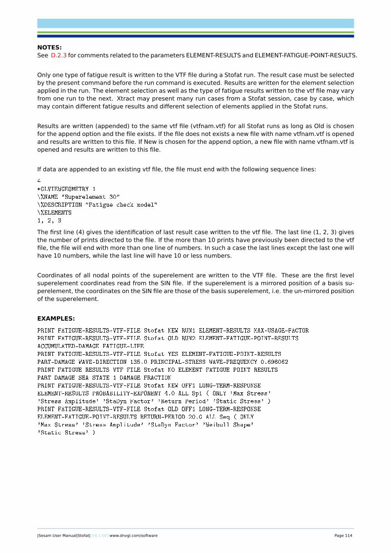
NOTES:See D.2.3 for comments related to the parameters ELEMENT-RESULTS and ELEMENT-FATIGUE-POINT-RESULTS.
Only one type of fatigue result is written to the VTF file during a Stofat run. The result case must be selectedby the present command before the run command is executed. Results are written for the element selectionapplied in the run. The element selection as well as the type of fatigue results written to the vtf file may varyfrom one run to the next. Xtract may present many run cases from a Stofat session, case by case, whichmay contain different fatigue results and different selection of elements applied in the Stofat runs.
Results are written (appended) to the same vtf file (vtfnam.vtf) for all Stofat runs as long as Old is chosenfor the append option and the file exists. If the file does not exists a new file with name vtfnam.vtf is openedand results are written to this file. If New is chosen for the append option, a new file with name vtfnam.vtf isopened and results are written to this file.
If data are appended to an existing vtf file, the file must end with the following sequence lines:
4
*GLVIEWGEOMETRY 1
\%NAME "Superelement 30"
\%DESCRIPTION "Fatigue check model"
\%ELEMENTS
1, 2, 3
The first line (4) gives the identification of last result case written to the vtf file. The last line (1, 2, 3) givesthe number of prints directed to the file. If the more than 10 prints have previously been directed to the vtffile, the file will end with more than one line of numbers. In such a case the last lines except the last one willhave 10 numbers, while the last line will have 10 or less numbers.
Coordinates of all nodal points of the superelement are written to the VTF file. These are the first levelsuperelement coordinates read from the SIN file. If the superelement is a mirrored position of a basis su-perelement, the coordinates on the SIN file are those of the basis superelement, i.e. the un-mirrored positionof the superelement.
EXAMPLES:
PRINT FATIGUE-RESULTS-VTF-FILE Stofat NEW RUN1 ELEMENT-RESULTS MAX-USAGE-FACTOR
PRINT FATIGUE-RESULTS-VTF-FILE Stofat OLD RUN2 ELEMENT-FATIGUE-POINT-RESULTS
ACCUMULATED-DAMAGE FATIGUE-LIFE
PRINT FATIGUE-RESULTS-VTF-FILE Stofat YES ELEMENT-FATIGUE-POINT-RESULTS
PART-DAMAGE WAVE-DIRECTION 135.0 PRINCIPAL-STRESS WAVE-FREQUENCY 0.698062
PRINT FATIGUE-RESULTS-VTF-FILE Stofat NO ELEMENT-FATIGUE-POINT-RESULTS
PART-DAMAGE SEA-STATE 1 DAMAGE-FRACTION
PRINT FATIGUE-RESULTS-VTF-FILE Stofat NEW OFF1 LONG-TERM-RESPONSE
ELEMENT-RESULTS PROBABILITY-EXPONENT 4.0 ALL Sp1 ( ONLY 'Max Stress'
'Stress Amplitude' 'StaDyn Factor' 'Return Period' 'Static Stress' )
PRINT FATIGUE-RESULTS-VTF-FILE Stofat OLD OFF1 LONG-TERM-RESPONSE
ELEMENT-FATIGUE-POINT-RESULTS RETURN-PERIOD 20.0 ALL Seq ( ONLY
'Max Stress' 'Stress Amplitude' 'StaDyn Factor' 'Weibull Shape'
'Static Stress' )
|Sesam User Manual|Stofat|[V4.1-00] www.dnvgl.com/software Page 114
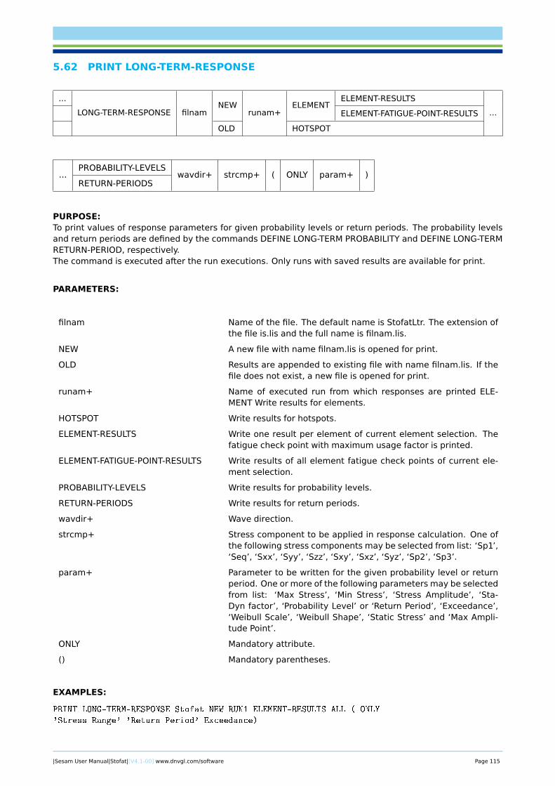
5.62 PRINT LONG-TERM-RESPONSE
...
LONG-TERM-RESPONSE filnamNEW
runam+ELEMENT
ELEMENT-RESULTS
...ELEMENT-FATIGUE-POINT-RESULTS
OLD HOTSPOT
...PROBABILITY-LEVELS
wavdir+ strcmp+ ( ONLY param+ )RETURN-PERIODS
PURPOSE:To print values of response parameters for given probability levels or return periods. The probability levelsand return periods are defined by the commands DEFINE LONG-TERM PROBABILITY and DEFINE LONG-TERMRETURN-PERIOD, respectively.The command is executed after the run executions. Only runs with saved results are available for print.
PARAMETERS:
filnam Name of the file. The default name is StofatLtr. The extension ofthe file is.lis and the full name is filnam.lis.
NEW A new file with name filnam.lis is opened for print.
OLD Results are appended to existing file with name filnam.lis. If thefile does not exist, a new file is opened for print.
runam+ Name of executed run from which responses are printed ELE-MENT Write results for elements.
HOTSPOT Write results for hotspots.
ELEMENT-RESULTS Write one result per element of current element selection. Thefatigue check point with maximum usage factor is printed.
ELEMENT-FATIGUE-POINT-RESULTS Write results of all element fatigue check points of current ele-ment selection.
PROBABILITY-LEVELS Write results for probability levels.
RETURN-PERIODS Write results for return periods.
wavdir+ Wave direction.
strcmp+ Stress component to be applied in response calculation. One ofthe following stress components may be selected from list: ‘Sp1’,‘Seq’, ‘Sxx’, ‘Syy’, ‘Szz’, ‘Sxy’, ‘Sxz’, ‘Syz’, ‘Sp2’, ‘Sp3’.
param+ Parameter to be written for the given probability level or returnperiod. One or more of the following parameters may be selectedfrom list: ‘Max Stress’, ‘Min Stress’, ‘Stress Amplitude’, ‘Sta-Dyn factor’, ‘Probability Level’ or ‘Return Period’, ‘Exceedance’,‘Weibull Scale’, ‘Weibull Shape’, ‘Static Stress’ and ‘Max Ampli-tude Point’.
ONLY Mandatory attribute.
() Mandatory parentheses.
EXAMPLES:
PRINT LONG-TERM-RESPONSE Stofat NEW RUN1 ELEMENT-RESULTS ALL ( ONLY
'Stress Range' 'Return Period' Exceedance)
|Sesam User Manual|Stofat|[V4.1-00] www.dnvgl.com/software Page 115

PRINT LONG-TERM-RESPONSE Stofat NEW RUN1 ELEMENT-FATIGUE-POINT-RESULTS 0.0 ( ONLY
'Weibull Scale q' )
|Sesam User Manual|Stofat|[V4.1-00] www.dnvgl.com/software Page 116

5.63 PRINT RUN-OVERVIEW
... RUN-OVERVIEW
ALL
APPLIED-K-FACTORS
ELEMENT MATERIAL DATA
ELEMENTS
HOTSPOTS
LONG-TERM-PROBABILITIES
NAMED-ELEMENT-SETS
RUNS
WAVE-DIRECTION-DATA
WELD-NORMAL-LINES
PURPOSE:To print on screen or file overview of fatigue check runs, created hotspots, current element selection, prob-abilities of executed runs, named element sets, applied K-factors and current weld normal lines and assign-ments made to elements and hotspots.
PARAMETERS:
ALL Prints overview of executed runs, created hotspots, current ele-ment selection and named element sets.
APPLIED-K-FACTORS Prints K-factors of executed runs and current assigned K-factorsof current element selection.
ELEMENT MATERIAL DATA Prints overview of material data for current element selection.
ELEMENTS Prints overview of current element selection.
HOTSPOTS Prints overview of created hotspots and the positions of thehotspots and related interpolation points.
LONG-TERM-PROBABILITIES Prints overview of user defined probabilities of executed runs.
NAMED-ELEMENT-SETS Prints overview of current element sets (set names and elementsof the sets).
RUNS Prints overview of executed runs.
WAVE-DIRECTION-DATA Prints overview of wave direction data of executed runs.
WELD-NORMAL-LINES Prints overview of current weld normal lines and assignmentsmade to elements and hotspots.
EXAMPLES:
PRINT RUN-OVERVIEW ALL
PRINT RUN-OVERVIEW APPLIED-K-FACTORS
PRINT RUN-OVERVIEW ELEMENTS
PRINT RUN-OVERVIEW LONG-TERM-PROBABILITIES
PRINT RUN-OVERVIEW HOTSPOTS
PRINT RUN-OVERVIEW NAMED-ELEMENT-SETS
PRINT RUN-OVERVIEW RUNS
PRINT RUN-OVERVIEW WAVE-DIRECTION-DATA
PRINT RUN-OVERVIEW WELD-NORMAL-LINES
|Sesam User Manual|Stofat|[V4.1-00] www.dnvgl.com/software Page 117
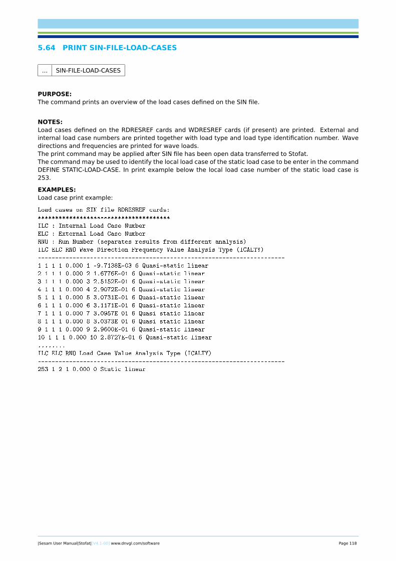
5.64 PRINT SIN-FILE-LOAD-CASES
... SIN-FILE-LOAD-CASES
PURPOSE:The command prints an overview of the load cases defined on the SIN file.
NOTES:Load cases defined on the RDRESREF cards and WDRESREF cards (if present) are printed. External andinternal load case numbers are printed together with load type and load type identification number. Wavedirections and frequencies are printed for wave loads.The print command may be applied after SIN file has been open data transferred to Stofat.The command may be used to identify the local load case of the static load case to be enter in the commandDEFINE STATIC-LOAD-CASE. In print example below the local load case number of the static load case is253.
EXAMPLES:Load case print example:
Load cases on SIN file RDRESREF cards:
**************************************
ILC : Internal Load Case Number
ELC : External Load Case Number
RNO : Run Number (separates results from different analysis)
ILC ELC RNO Wave Direction Frequency Value Analysis Type (ICALTY)
-----------------------------------------------------------------------
1 1 1 1 0.000 1 -9.7138E-03 6 Quasi-static linear
2 1 1 1 0.000 2 1.6776E-01 6 Quasi-static linear
3 1 1 1 0.000 3 2.5152E-01 6 Quasi-static linear
4 1 1 1 0.000 4 2.9072E-01 6 Quasi-static linear
5 1 1 1 0.000 5 3.0731E-01 6 Quasi-static linear
6 1 1 1 0.000 6 3.1171E-01 6 Quasi-static linear
7 1 1 1 0.000 7 3.0957E-01 6 Quasi-static linear
8 1 1 1 0.000 8 3.0373E-01 6 Quasi-static linear
9 1 1 1 0.000 9 2.9600E-01 6 Quasi-static linear
10 1 1 1 0.000 10 2.8727E-01 6 Quasi-static linear
........
ILC ELC RNO Load Case Value Analysis Type (ICALTY)
-----------------------------------------------------------------------
253 1 2 1 0.000 0 Static linear
|Sesam User Manual|Stofat|[V4.1-00] www.dnvgl.com/software Page 118

5.65 PRINT SN-CURVE
... SN-CURVE ( ONLY snname+ )
PURPOSE:To print data related to an SN-curve.
PARAMETERS:
snname+ Name of the SN-curve.
ONLY Mandatory attribute.
( ) Mandatory parentheses.
EXAMPLES:
PRINT SN-CURVE (ONLY USE-X USE-Y )
|Sesam User Manual|Stofat|[V4.1-00] www.dnvgl.com/software Page 119
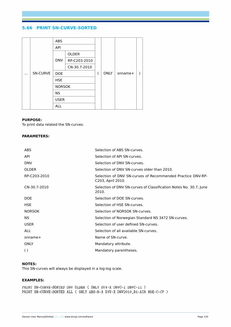
5.66 PRINT SN-CURVE-SORTED
... SN-CURVE
ABS
( ONLY snname+ )
API
DNV
OLDER
RP-C203-2010
CN-30.7-2010
DOE
HSE
NORSOK
NS
USER
ALL
PURPOSE:To print data related the SN-curves.
PARAMETERS:
ABS Selection of ABS SN-curves.
API Selection of API SN-curves.
DNV Selection of DNV SN-curves.
OLDER Selection of DNV SN-curves older than 2010.
RP-C203-2010 Selection of DNV SN-curves of Recommended Practice DNV-RP-C203, April 2010.
CN-30.7-2010 Selection of DNV SN-curves of Classification Notes No. 30.7, June2010.
DOE Selection of DOE SN-curves.
HSE Selection of HSE SN-curves.
NORSOK Selection of NORSOK SN-curves.
NS Selection of Norwegian Standard NS 3472 SN-curves.
USER Selection of user defined SN-curves.
ALL Selection of all available SN-curves.
snname+ Name of SN-curve.
ONLY Mandatory attribute.
( ) Mandatory parentheses.
NOTES:This SN-curves will always be displayed in a log-log scale.
EXAMPLES:
PRINT SN-CURVE-SORTED DNV OLDER ( ONLY DNV-X DNVC-I DNVC-II )
PRINT SN-CURVE-SORTED ALL ( ONLY ABS-B-A DNV-X DNV2010_B1-AIR HSE-C-CP )
|Sesam User Manual|Stofat|[V4.1-00] www.dnvgl.com/software Page 120

5.67 PRINT WAVE-SPREADING-FUNCTION
... WAVE-SPREADING-FUNCTION name+ [space]
PURPOSE:To print energy spreading for elementary wave directions created by the user.
PARAMETERS:
name+ User name of the function.
space User input space between each wave direction angle for whichthe energy spreading function will be printed. This space is inde-pendent of what the program will use in calculating the responsespectra. Only asked for if one of the names selected correspondsto a cosine power function.
EXAMPLES:
PRINT WAVE-SPREADING-FUNCTION COS2 30.0
|Sesam User Manual|Stofat|[V4.1-00] www.dnvgl.com/software Page 121

5.68 PRINT WAVE-STATISTICS
... WAVE-STATISTICS ( ONLY name+ )
PURPOSE:To print wave statistics defined.
PARAMETERS:
ONLY Mandatory attribute.
( ) Mandatory parentheses.
name+ Name of the wave statistics.
EXAMPLES:
DISPLAY WAVE-STATISTICS BMT
|Sesam User Manual|Stofat|[V4.1-00] www.dnvgl.com/software Page 122
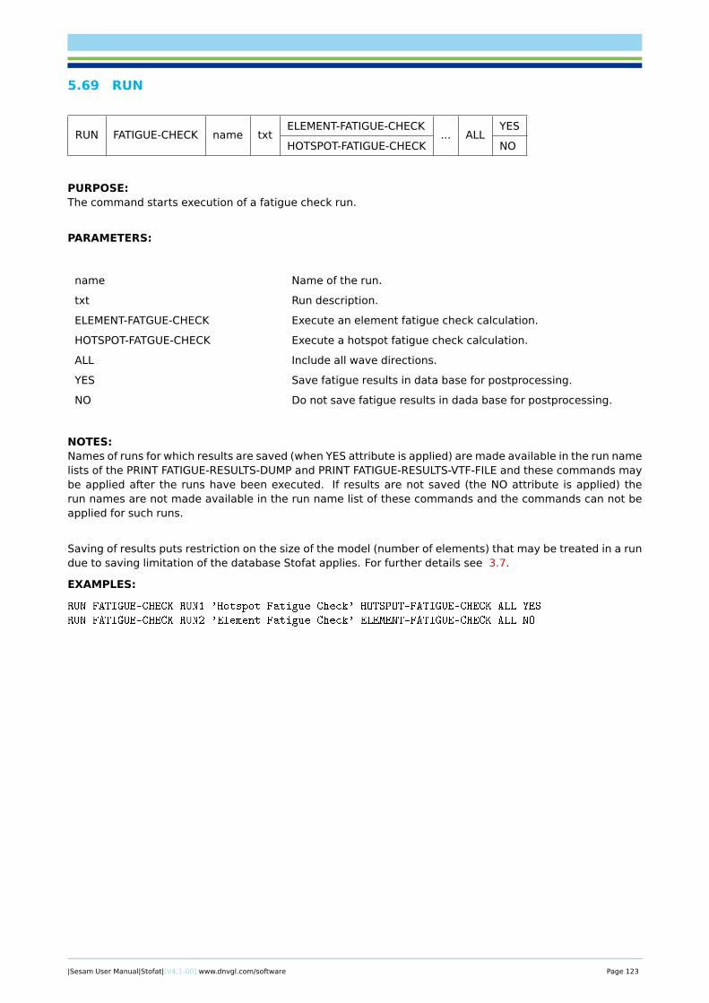
5.69 RUN
RUN FATIGUE-CHECK name txtELEMENT-FATIGUE-CHECK
... ALLYES
HOTSPOT-FATIGUE-CHECK NO
PURPOSE:The command starts execution of a fatigue check run.
PARAMETERS:
name Name of the run.
txt Run description.
ELEMENT-FATGUE-CHECK Execute an element fatigue check calculation.
HOTSPOT-FATGUE-CHECK Execute a hotspot fatigue check calculation.
ALL Include all wave directions.
YES Save fatigue results in data base for postprocessing.
NO Do not save fatigue results in dada base for postprocessing.
NOTES:Names of runs for which results are saved (when YES attribute is applied) are made available in the run namelists of the PRINT FATIGUE-RESULTS-DUMP and PRINT FATIGUE-RESULTS-VTF-FILE and these commands maybe applied after the runs have been executed. If results are not saved (the NO attribute is applied) therun names are not made available in the run name list of these commands and the commands can not beapplied for such runs.
Saving of results puts restriction on the size of the model (number of elements) that may be treated in a rundue to saving limitation of the database Stofat applies. For further details see 3.7.
EXAMPLES:
RUN FATIGUE-CHECK RUN1 'Hotspot Fatigue Check' HOTSPOT-FATIGUE-CHECK ALL YES
RUN FATIGUE-CHECK RUN2 'Element Fatigue Check' ELEMENT-FATIGUE-CHECK ALL NO
|Sesam User Manual|Stofat|[V4.1-00] www.dnvgl.com/software Page 123
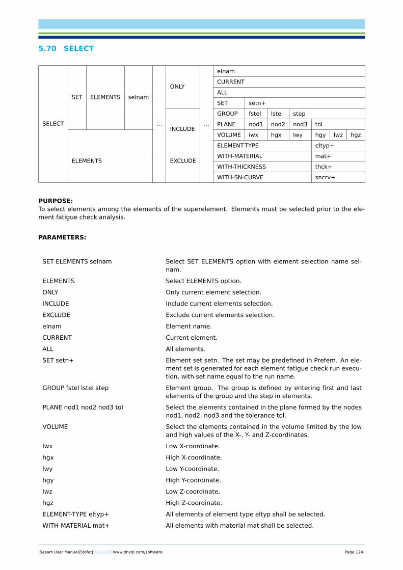
5.70 SELECT
SELECT
SET ELEMENTS selnam
...
ONLY
...
elnam
CURRENT
ALL
SET setn+
INCLUDE
GROUP fstel lstel step
PLANE nod1 nod2 nod3 tol
ELEMENTS
VOLUME lwx hgx lwy hgy lwz hgz
EXCLUDE
ELEMENT-TYPE eltyp+
WITH-MATERIAL mat+
WITH-THICKNESS thck+
WITH-SN-CURVE sncrv+
PURPOSE:To select elements among the elements of the superelement. Elements must be selected prior to the ele-ment fatigue check analysis.
PARAMETERS:
SET ELEMENTS selnam Select SET ELEMENTS option with element selection name sel-nam.
ELEMENTS Select ELEMENTS option.
ONLY Only current element selection.
INCLUDE Include current elements selection.
EXCLUDE Exclude current elements selection.
elnam Element name.
CURRENT Current element.
ALL All elements.
SET setn+ Element set setn. The set may be predefined in Prefem. An ele-ment set is generated for each element fatigue check run execu-tion, with set name equal to the run name.
GROUP fstel lstel step Element group. The group is defined by entering first and lastelements of the group and the step in elements.
PLANE nod1 nod2 nod3 tol Select the elements contained in the plane formed by the nodesnod1, nod2, nod3 and the tolerance tol.
VOLUME Select the elements contained in the volume limited by the lowand high values of the X-, Y- and Z-coordinates.
lwx Low X-coordinate.
hgx High X-coordinate.
lwy Low Y-coordinate.
hgy High Y-coordinate.
lwz Low Z-coordinate.
hgz High Z-coordinate.
ELEMENT-TYPE eltyp+ All elements of element type eltyp shall be selected.
WITH-MATERIAL mat+ All elements with material mat shall be selected.
|Sesam User Manual|Stofat|[V4.1-00] www.dnvgl.com/software Page 124
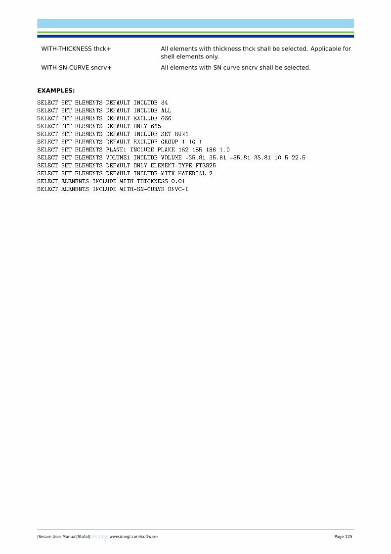
WITH-THICKNESS thck+ All elements with thickness thck shall be selected. Applicable forshell elements only.
WITH-SN-CURVE sncrv+ All elements with SN curve sncrv shall be selected.
EXAMPLES:
SELECT SET ELEMENTS DEFAULT INCLUDE 34
SELECT SET ELEMENTS DEFAULT INCLUDE ALL
SELECT SET ELEMENTS DEFAULT EXCLUDE 666
SELECT SET ELEMENTS DEFAULT ONLY 665
SELECT SET ELEMENTS DEFAULT INCLUDE SET RUN1
SELECT SET ELEMENTS DEFAULT EXCLUDE GROUP 1 10 1
SELECT SET ELEMENTS PLANE1 INCLUDE PLANE 162 185 186 1.0
SELECT SET ELEMENTS VOLUME1 INCLUDE VOLUME -35.81 35.81 -35.81 35.81 10.5 22.5
SELECT SET ELEMENTS DEFAULT ONLY ELEMENT-TYPE FTRS25
SELECT SET ELEMENTS DEFAULT INCLUDE WITH-MATERIAL 2
SELECT ELEMENTS INCLUDE WITH-THICKNESS 0.01
SELECT ELEMENTS INCLUDE WITH-SN-CURVE DNVC-I
|Sesam User Manual|Stofat|[V4.1-00] www.dnvgl.com/software Page 125
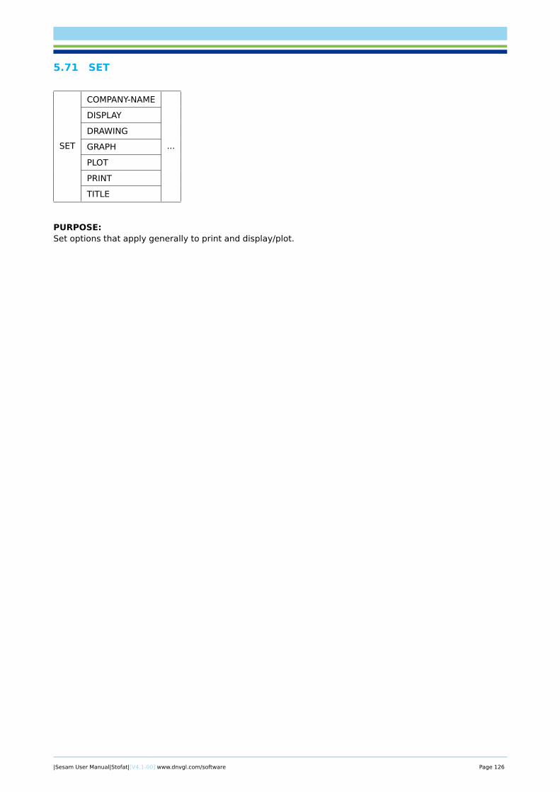
5.71 SET
SET
COMPANY-NAME
...
DISPLAY
DRAWING
GRAPH
PLOT
TITLE
PURPOSE:Set options that apply generally to print and display/plot.
|Sesam User Manual|Stofat|[V4.1-00] www.dnvgl.com/software Page 126
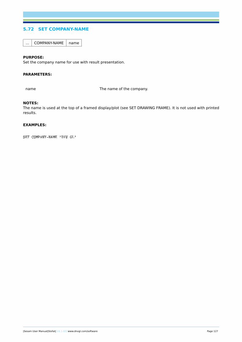
5.72 SET COMPANY-NAME
... COMPANY-NAME name
PURPOSE:Set the company name for use with result presentation.
PARAMETERS:
name The name of the company.
NOTES:The name is used at the top of a framed display/plot (see SET DRAWING FRAME). It is not used with printedresults.
EXAMPLES:
SET COMPANY-NAME 'DNV GL'
|Sesam User Manual|Stofat|[V4.1-00] www.dnvgl.com/software Page 127
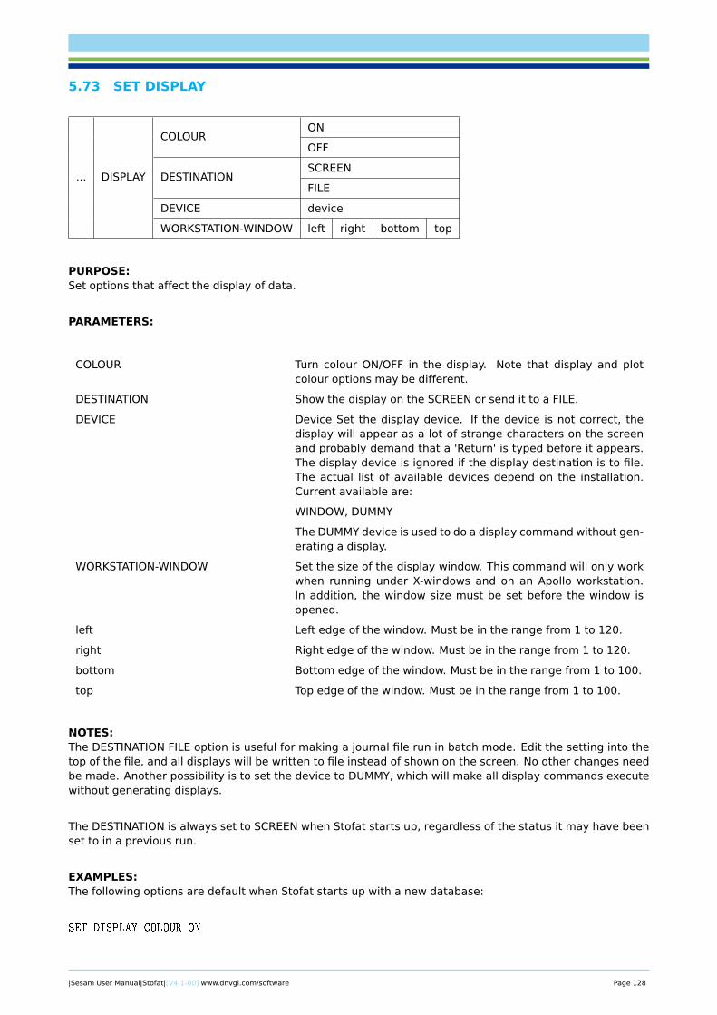
5.73 SET DISPLAY
... DISPLAY
COLOURON
OFF
DESTINATIONSCREEN
FILE
DEVICE device
WORKSTATION-WINDOW left right bottom top
PURPOSE:Set options that affect the display of data.
PARAMETERS:
COLOUR Turn colour ON/OFF in the display. Note that display and plotcolour options may be different.
DESTINATION Show the display on the SCREEN or send it to a FILE.
DEVICE Device Set the display device. If the device is not correct, thedisplay will appear as a lot of strange characters on the screenand probably demand that a 'Return' is typed before it appears.The display device is ignored if the display destination is to file.The actual list of available devices depend on the installation.Current available are:
WINDOW, DUMMY
The DUMMY device is used to do a display command without gen-erating a display.
WORKSTATION-WINDOW Set the size of the display window. This command will only workwhen running under X-windows and on an Apollo workstation.In addition, the window size must be set before the window isopened.
left Left edge of the window. Must be in the range from 1 to 120.
right Right edge of the window. Must be in the range from 1 to 120.
bottom Bottom edge of the window. Must be in the range from 1 to 100.
top Top edge of the window. Must be in the range from 1 to 100.
NOTES:The DESTINATION FILE option is useful for making a journal file run in batch mode. Edit the setting into thetop of the file, and all displays will be written to file instead of shown on the screen. No other changes needbe made. Another possibility is to set the device to DUMMY, which will make all display commands executewithout generating displays.
The DESTINATION is always set to SCREEN when Stofat starts up, regardless of the status it may have beenset to in a previous run.
EXAMPLES:The following options are default when Stofat starts up with a new database:
SET DISPLAY COLOUR ON
|Sesam User Manual|Stofat|[V4.1-00] www.dnvgl.com/software Page 128

SET DISPLAY DESTINATION SCREEN
SET DISPLAY DEVICE DUMMY (if running line mode)
SET DISPLAY DEVICE WINDOWS (if running graphics mode)
SET DISPLAY WORKSTATION-WINDOW 49 120 1 70
|Sesam User Manual|Stofat|[V4.1-00] www.dnvgl.com/software Page 129
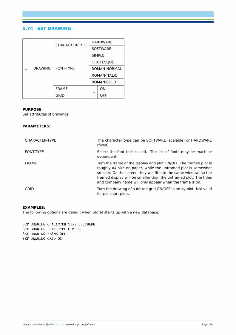
5.74 SET DRAWING
... DRAWING
CHARACTER-TYPEHARDWARE
SOFTWARE
FONT-TYPE
SIMPLE
GROTESQUE
ROMAN-NORMAL
ROMAN-ITALIC
ROMAN-BOLD
FRAME...
ON
GRID OFF
PURPOSE:Set attributes of drawings.
PARAMETERS:
CHARACTER-TYPE The character type can be SOFTWARE (scalable) or HARDWARE(fixed).
FONT-TYPE Select the font to be used. The list of fonts may be machinedependent.
FRAME Turn the frame of the display and plot ON/OFF. The framed plot isroughly A4 size on paper, while the unframed plot is somewhatsmaller. On the screen they will fit into the same window, so theframed display will be smaller than the unframed plot. The titlesand company name will only appear when the frame is on.
GRID Turn the drawing of a dotted grid ON/OFF in an xy-plot. Not validfor pie chart plots.
EXAMPLES:The following options are default when Stofat starts up with a new database:
SET DRAWING CHARACTER-TYPE SOFTWARE
SET DRAWING FONT-TYPE SIMPLE
SET DRAWING FRAME OFF
SET DRAWING GRID ON
|Sesam User Manual|Stofat|[V4.1-00] www.dnvgl.com/software Page 130
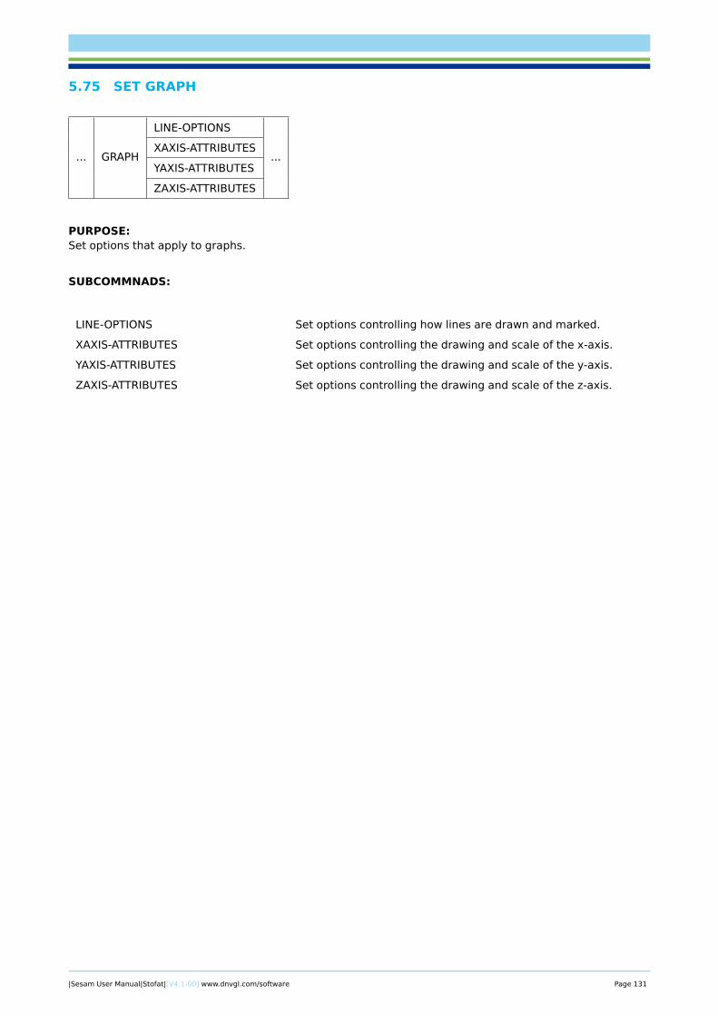
5.75 SET GRAPH
... GRAPH
LINE-OPTIONS
...XAXIS-ATTRIBUTES
YAXIS-ATTRIBUTES
ZAXIS-ATTRIBUTES
PURPOSE:Set options that apply to graphs.
SUBCOMMNADS:
LINE-OPTIONS Set options controlling how lines are drawn and marked.
XAXIS-ATTRIBUTES Set options controlling the drawing and scale of the x-axis.
YAXIS-ATTRIBUTES Set options controlling the drawing and scale of the y-axis.
ZAXIS-ATTRIBUTES Set options controlling the drawing and scale of the z-axis.
|Sesam User Manual|Stofat|[V4.1-00] www.dnvgl.com/software Page 131
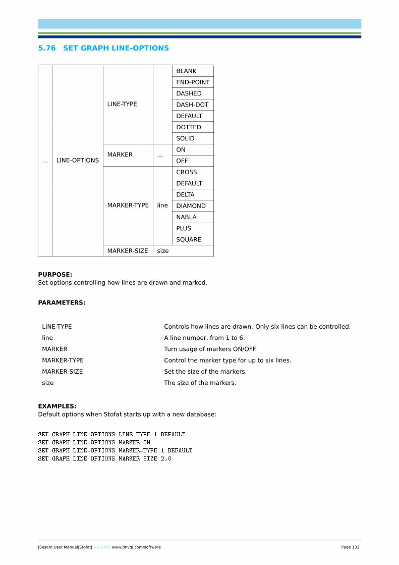
5.76 SET GRAPH LINE-OPTIONS
... LINE-OPTIONS
LINE-TYPE
BLANK
END-POINT
DASHED
DASH-DOT
DEFAULT
DOTTED
SOLID
MARKER ...ON
OFF
MARKER-TYPE line
CROSS
DEFAULT
DELTA
DIAMOND
NABLA
PLUS
SQUARE
MARKER-SIZE size
PURPOSE:Set options controlling how lines are drawn and marked.
PARAMETERS:
LINE-TYPE Controls how lines are drawn. Only six lines can be controlled.
line A line number, from 1 to 6.
MARKER Turn usage of markers ON/OFF.
MARKER-TYPE Control the marker type for up to six lines.
MARKER-SIZE Set the size of the markers.
size The size of the markers.
EXAMPLES:Default options when Stofat starts up with a new database:
SET GRAPH LINE-OPTIONS LINE-TYPE 1 DEFAULT
SET GRAPH LINE-OPTIONS MARKER ON
SET GRAPH LINE-OPTIONS MARKER-TYPE 1 DEFAULT
SET GRAPH LINE-OPTIONS MARKER-SIZE 2.0
|Sesam User Manual|Stofat|[V4.1-00] www.dnvgl.com/software Page 132

5.77 SET GRAPH XAXIS-ATTRIBUTES
... XAXIS-ATTRIBUTES
DECIMAL-FORMAT
EXPONENTIAL
FIXED
GENERAL
INTEGER
LIMITSFREE
FIXED xmin xmax
SPACINGLINEAR
LOGARITHMIC
TITLEDEFAULT
SPECIFIED xtitle
PURPOSE:Set options controlling the attributes of the x axis in a graph.
PARAMETERS:
DECIMAL-FORMAT Controls the presentation of numbers labelling the x axis. Thenumbers can be presented in EXPONENTIAL format, in FIXED for-mat, as INTEGERs or in GENERAL (free) format.
LIMITS Controls the limits of the x axis. These can either be FREE (i.e.determined by the data that are being presented) or FIXED to theminimum value xmin and the maximum value xmax.
SPACING Controls the spacing of numbers along the axis. The axis canhave a LINEAR spacing or be LOGARITHMIC with base 10.
TITLE The title at the x axis can be specified by Stofat (DEFAULT) oroverridden with a SPECIFIED text: xtitle.
EXAMPLES:The following options are default when Stofat starts up with a new database:
SET GRAPH XAXIS-ATTRIBUTES DECIMAL-FORMAT GENERAL
SET GRAPH XAXIS-ATTRIBUTES LIMITS FREE
SET GRAPH XAXIS-ATTRIBUTES SPACING LINEAR
SET GRAPH XAXIS-ATTRIBUTES TITLE DEFAULT
|Sesam User Manual|Stofat|[V4.1-00] www.dnvgl.com/software Page 133

5.78 SET GRAPH YAXIS-ATTRIBUTES
... YAXIS-ATTRIBUTES
DECIMAL-FORMAT
EXPONENTIAL
FIXED
GENERAL
INTEGER
LIMITSFREE
FIXED ymin ymax
SPACINGLINEAR
LOGARITHMIC
TITLEDEFAULT
SPECIFIED ytitle
PURPOSE:Set options controlling the attributes of the y axis in a graph.
PARAMETERS:
DECIMAL-FORMAT Controls the presentation of numbers labelling the y axis. Thenumbers can be presented in EXPONENTIAL format, in FIXED for-mat, as INTEGERs or in GENERAL (free) format.
LIMITS Controls the limits of the y axis. These can either be FREE (i.e.determined by the data that are being presented) or FIXED to theminimum value ymin and the maximum value ymax.
SPACING Controls the spacing of numbers along the axis. The axis canhave a LINEAR spacing or be LOGARITHMIC with base 10.
TITLE The title at the y axis can be specified by Stofat (DEFAULT) oroverridden with a SPECIFIED text: ytitle.
EXAMPLES:The following options are default when Stofat starts up with a new database:
SET GRAPH YAXIS-ATTRIBUTES DECIMAL-FORMAT GENERAL
SET GRAPH YAXIS-ATTRIBUTES LIMITS FREE
SET GRAPH YAXIS-ATTRIBUTES SPACING LINEAR
SET GRAPH YAXIS-ATTRIBUTES TITLE DEFAULT
|Sesam User Manual|Stofat|[V4.1-00] www.dnvgl.com/software Page 134
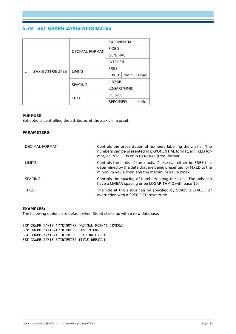
5.79 SET GRAPH ZAXIS-ATTRIBUTES
... ZAXIS-ATTRIBUTES
DECIMAL-FORMAT
EXPONENTIAL
FIXED
GENERAL
INTEGER
LIMITSFREE
FIXED zmin zmax
SPACINGLINEAR
LOGARITHMIC
TITLEDEFAULT
SPECIFIED ztitle
PURPOSE:Set options controlling the attributes of the z axis in a graph.
PARAMETERS:
DECIMAL-FORMAT Controls the presentation of numbers labelling the z axis. Thenumbers can be presented in EXPONENTIAL format, in FIXED for-mat, as INTEGERs or in GENERAL (free) format.
LIMITS Controls the limits of the z axis. These can either be FREE (i.e.determined by the data that are being presented) or FIXED to theminimum value zmin and the maximum value zmax.
SPACING Controls the spacing of numbers along the axis. The axis canhave a LINEAR spacing or be LOGARITHMIC with base 10.
TITLE The title at the z axis can be specified by Stofat (DEFAULT) oroverridden with a SPECIFIED text: ztitle.
EXAMPLES:The following options are default when Stofat starts up with a new database:
SET GRAPH ZAXIS-ATTRIBUTES DECIMAL-FORMAT GENERAL
SET GRAPH ZAXIS-ATTRIBUTES LIMITS FREE
SET GRAPH ZAXIS-ATTRIBUTES SPACING LINEAR
SET GRAPH ZAXIS-ATTRIBUTES TITLE DEFAULT
|Sesam User Manual|Stofat|[V4.1-00] www.dnvgl.com/software Page 135
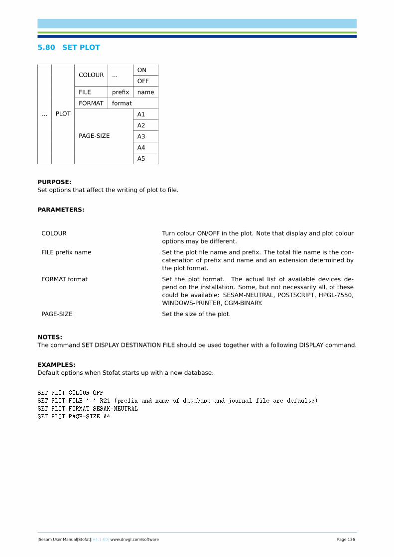
5.80 SET PLOT
... PLOT
COLOUR ...ON
OFF
FILE prefix name
FORMAT format
PAGE-SIZE
A1
A2
A3
A4
A5
PURPOSE:Set options that affect the writing of plot to file.
PARAMETERS:
COLOUR Turn colour ON/OFF in the plot. Note that display and plot colouroptions may be different.
FILE prefix name Set the plot file name and prefix. The total file name is the con-catenation of prefix and name and an extension determined bythe plot format.
FORMAT format Set the plot format. The actual list of available devices de-pend on the installation. Some, but not necessarily all, of thesecould be available: SESAM-NEUTRAL, POSTSCRIPT, HPGL-7550,WINDOWS-PRINTER, CGM-BINARY.
PAGE-SIZE Set the size of the plot.
NOTES:The command SET DISPLAY DESTINATION FILE should be used together with a following DISPLAY command.
EXAMPLES:Default options when Stofat starts up with a new database:
SET PLOT COLOUR OFF
SET PLOT FILE ` ` R21 (prefix and name of database and journal file are defaults)
SET PLOT FORMAT SESAM-NEUTRAL
SET PLOT PAGE-SIZE A4
|Sesam User Manual|Stofat|[V4.1-00] www.dnvgl.com/software Page 136
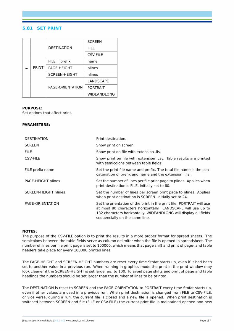
5.81 SET PRINT
DESTINATION
SCREEN
FILE
CSV-FILE
FILE prefix name
PAGE-HEIGHT plines
SCREEN-HEIGHT nlines
PAGE-ORIENTATION
LANDSCAPE
PORTRAIT
WIDEANDLONG
PURPOSE:Set options that affect print.
PARAMETERS:
DESTINATION Print destination.
SCREEN Show print on screen.
FILE Show print on file with extension .lis.
CSV-FILE Show print on file with extension .csv. Table results are printedwith semicolons between table fields.
FILE prefix name Set the print file name and prefix. The total file name is the con-catenation of prefix and name and the extension ‘.lis’.
PAGE-HEIGHT plines Set the number of lines per file print page to plines. Applies whenprint destination is FILE. Initially set to 60.
SCREEN-HEIGHT nlines Set the number of lines per screen print page to nlines. Applieswhen print destination is SCREEN. Initially set to 24.
PAGE-ORIENTATION Set the orientation of the print in the print file. PORTRAIT will useat most 80 characters horizontally. LANDSCAPE will use up to132 characters horizontally. WIDEANDLONG will display all fieldssequencially on the same line.
NOTES:The purpose of the CSV-FILE option is to print the results in a more proper format for spread sheets. Thesemicolons between the table fields serve as column delimiter when the file is opened in spreadsheet. Thenumber of lines per file print page is set to 100000, which means that page shift and print of page- and tableheaders take place for every 100000 printed lines.
The PAGE-HEIGHT and SCREEN-HEIGHT numbers are reset every time Stofat starts up, even if it had beenset to another value in a previous run. When running in graphics mode the print in the print window maylook cleaner if the SCREEN-HEIGHT is set large, eg. to 100. To avoid page shifts and print of page and tableheadings the numbers should be set larger than the number of lines to be printed.
The DESTINATION is reset to SCREEN and the PAGE-ORIENTATION to PORTRAIT every time Stofat starts up,even if other values are used in a previous run. When print destination is changed from FILE to CSV-FILE,or vice versa, during a run, the current file is closed and a new file is opened. When print destination isswitched between SCREEN and file (FILE or CSV-FILE) the current print file is maintained opened and new
|Sesam User Manual|Stofat|[V4.1-00] www.dnvgl.com/software Page 137
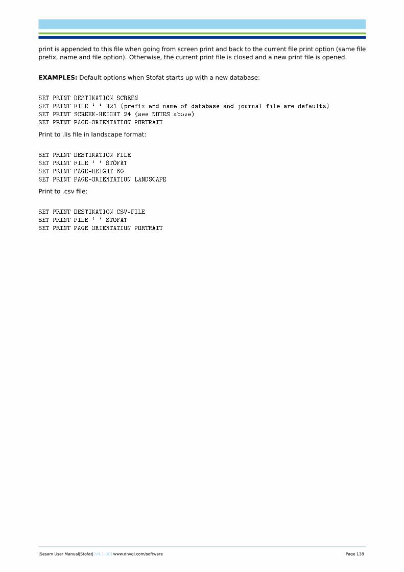
print is appended to this file when going from screen print and back to the current file print option (same fileprefix, name and file option). Otherwise, the current print file is closed and a new print file is opened.
EXAMPLES: Default options when Stofat starts up with a new database:
SET PRINT DESTINATION SCREEN
SET PRINT FILE ` ` R21 (prefix and name of database and journal file are defaults)
SET PRINT SCREEN-HEIGHT 24 (see NOTES above)
SET PRINT PAGE-ORIENTATION PORTRAIT
Print to .lis file in landscape format:
SET PRINT DESTINATION FILE
SET PRINT FILE ` ` STOFAT
SET PRINT PAGE-HEIGHT 60
SET PRINT PAGE-ORIENTATION LANDSCAPE
Print to .csv file:
SET PRINT DESTINATION CSV-FILE
SET PRINT FILE ` ` STOFAT
SET PRINT PAGE-ORIENTATION PORTRAIT
|Sesam User Manual|Stofat|[V4.1-00] www.dnvgl.com/software Page 138
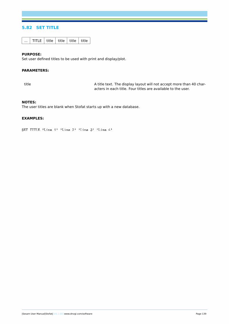
5.82 SET TITLE
... TITLE title title title title
PURPOSE:Set user defined titles to be used with print and display/plot.
PARAMETERS:
title A title text. The display layout will not accept more than 40 char-acters in each title. Four titles are available to the user.
NOTES:The user titles are blank when Stofat starts up with a new database.
EXAMPLES:
SET TITLE 'Line 1' 'Line 2' 'Line 3' 'Line 4'
|Sesam User Manual|Stofat|[V4.1-00] www.dnvgl.com/software Page 139

5.83 VIEW
VIEW
FRAME
...
PAN
POSITION
ROTATE
ZOOM
PURPOSE:To control the appearance of the 3D view, by specification of angles, zoom and pan.
PARAMETERS:
FRAME Performs an automatic zoom to fit the current view within theframe of the display.
PAN Pan (shift) the current view in the plane of the screen.
POSITION Define the view angles by specifying a point in space which, to-gether with the centre of the model’s coordinate system, definesthe direction of the user’s observation.
ROTATE Rotate view by specifying rotation angles.
ZOOM Zoom in or out.
NOTES:
1 All subcommands and data are fully explained subsequently as each command is described in detail.
2 This command is not logged.
3 The VIEW command works differently in the graphics user interface. The manipulations are performedby typing in the relevant numbers, then clicking on the buttons in the dialogue box, see Figure 5.3below.
|Sesam User Manual|Stofat|[V4.1-00] www.dnvgl.com/software Page 140
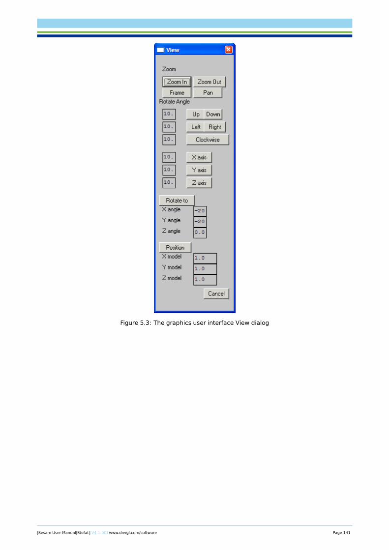
Figure 5.3: The graphics user interface View dialog
|Sesam User Manual|Stofat|[V4.1-00] www.dnvgl.com/software Page 141

5.84 VIEW FRAME
... FRAME
PURPOSE:Perform an automatic zoom to fit the current view within the frame of the display.
PARAMETERS:
None
NOTES:
1 This command is not logged.
|Sesam User Manual|Stofat|[V4.1-00] www.dnvgl.com/software Page 142

5.85 VIEW PAN
... PAN pick_from pick_to
PURPOSE:Pan (shift) the current view in the plane screen. The view is shifted by defining a vector in the plane of thescreen. The vector is defined by picking the ‘from’ and the ‘to’ position, see below.
PARAMETERS:
pick_from Pick (using mouse or cross-hair) a point on the screen to definethe ‘from’ position.
pick_to Pick (using mouse or cross-hair) a point on the screen to definethe ‘to’ position.
NOTES:
1 This command is not logged.
|Sesam User Manual|Stofat|[V4.1-00] www.dnvgl.com/software Page 143

5.86 VIEW POSITION
... POSITION x-model y-model z-model
PURPOSE:Define the view angles by specifying a point in space. The imaginary line from this point towards the originof the model’s coordinate system defines the direction of the user’s observation.
PARAMETERS:
x-model x-coordinate in the model’s coordinate system.
y-model y-coordinate in the model’s coordinate system.
z-model z-coordinate in the model’s coordinate system.
NOTES:
1 This command is not logged.
2 This command is independent of any previously entered rotations and can therefore be used to ‘reset’the viewing direction.
|Sesam User Manual|Stofat|[V4.1-00] www.dnvgl.com/software Page 144
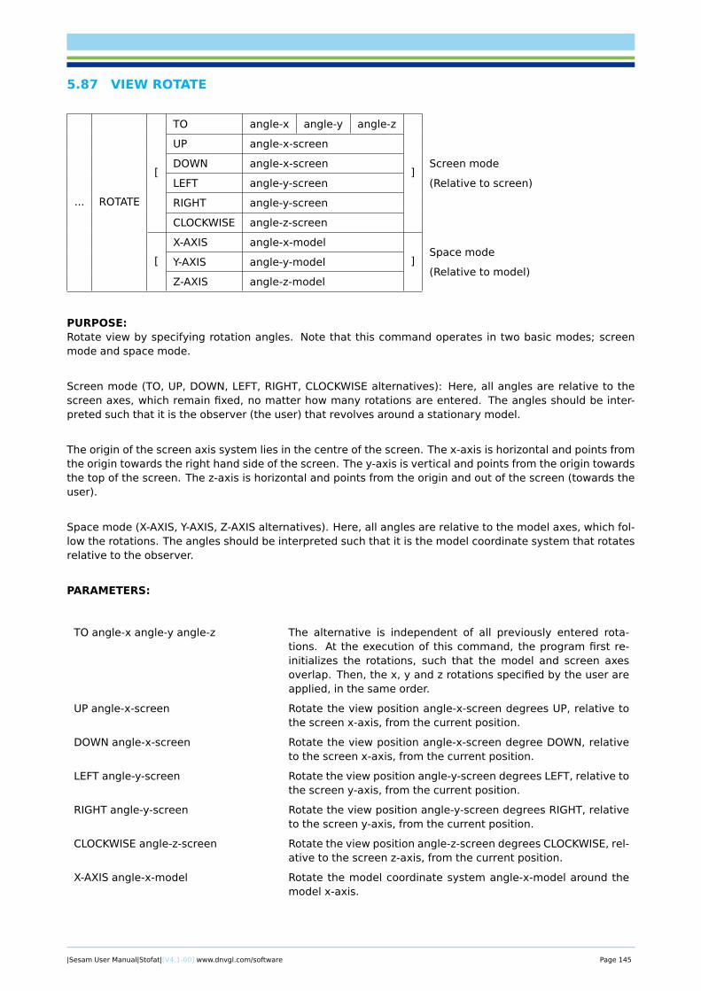
5.87 VIEW ROTATE
... ROTATE
[
TO angle-x angle-y angle-z
]Screen mode
(Relative to screen)
UP angle-x-screen
DOWN angle-x-screen
LEFT angle-y-screen
RIGHT angle-y-screen
CLOCKWISE angle-z-screen
[
X-AXIS angle-x-model
]Space mode
(Relative to model)Y-AXIS angle-y-model
Z-AXIS angle-z-model
PURPOSE:Rotate view by specifying rotation angles. Note that this command operates in two basic modes; screenmode and space mode.
Screen mode (TO, UP, DOWN, LEFT, RIGHT, CLOCKWISE alternatives): Here, all angles are relative to thescreen axes, which remain fixed, no matter how many rotations are entered. The angles should be inter-preted such that it is the observer (the user) that revolves around a stationary model.
The origin of the screen axis system lies in the centre of the screen. The x-axis is horizontal and points fromthe origin towards the right hand side of the screen. The y-axis is vertical and points from the origin towardsthe top of the screen. The z-axis is horizontal and points from the origin and out of the screen (towards theuser).
Space mode (X-AXIS, Y-AXIS, Z-AXIS alternatives). Here, all angles are relative to the model axes, which fol-low the rotations. The angles should be interpreted such that it is the model coordinate system that rotatesrelative to the observer.
PARAMETERS:
TO angle-x angle-y angle-z The alternative is independent of all previously entered rota-tions. At the execution of this command, the program first re-initializes the rotations, such that the model and screen axesoverlap. Then, the x, y and z rotations specified by the user areapplied, in the same order.
UP angle-x-screen Rotate the view position angle-x-screen degrees UP, relative tothe screen x-axis, from the current position.
DOWN angle-x-screen Rotate the view position angle-x-screen degree DOWN, relativeto the screen x-axis, from the current position.
LEFT angle-y-screen Rotate the view position angle-y-screen degrees LEFT, relative tothe screen y-axis, from the current position.
RIGHT angle-y-screen Rotate the view position angle-y-screen degrees RIGHT, relativeto the screen y-axis, from the current position.
CLOCKWISE angle-z-screen Rotate the view position angle-z-screen degrees CLOCKWISE, rel-ative to the screen z-axis, from the current position.
X-AXIS angle-x-model Rotate the model coordinate system angle-x-model around themodel x-axis.
|Sesam User Manual|Stofat|[V4.1-00] www.dnvgl.com/software Page 145

Y-AXIS angle-y-model Rotate the model coordinate system angle-y-model around themodel y-axis.
Z-AXIS angle-y-model Rotate the model coordinate system angle-z-model around themodel z-axis.
NOTES:
1 This command is not logged.
|Sesam User Manual|Stofat|[V4.1-00] www.dnvgl.com/software Page 146
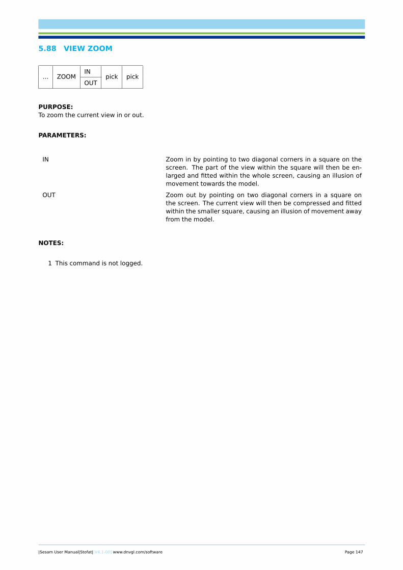
5.88 VIEW ZOOM
... ZOOMIN
pick pickOUT
PURPOSE:To zoom the current view in or out.
PARAMETERS:
IN Zoom in by pointing to two diagonal corners in a square on thescreen. The part of the view within the square will then be en-larged and fitted within the whole screen, causing an illusion ofmovement towards the model.
OUT Zoom out by pointing on two diagonal corners in a square onthe screen. The current view will then be compressed and fittedwithin the smaller square, causing an illusion of movement awayfrom the model.
NOTES:
1 This command is not logged.
|Sesam User Manual|Stofat|[V4.1-00] www.dnvgl.com/software Page 147
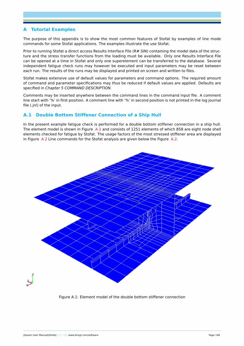
A Tutorial Examples
The purpose of this appendix is to show the most common features of Stofat by examples of line modecommands for some Stofat applications. The examples illustrate the use Stofat.
Prior to running Stofat a direct access Results Interface File (R#.SIN) containing the model data of the struc-ture and the stress transfer functions from the loading must be available. Only one Results Interface Filecan be opened at a time in Stofat and only one superelement can be transferred to the database. Severalindependent fatigue check runs may however be executed and input parameters may be reset betweeneach run. The results of the runs may be displayed and printed on screen and written to files.
Stofat makes extensive use of default values for parameters and command options. The required amountof command and parameter specifications may thus be reduced if default values are applied. Defaults arespecified in Chapter 5 COMMAND DESCRIPTION.
Comments may be inserted anywhere between the command lines in the command input file. A commentline start with ‘%’ in first position. A comment line with ‘%’ in second position is not printed in the log journalfile (.jnl) of the input.
A.1 Double Bottom Stiffener Connection of a Ship Hull
In the present example fatigue check is performed for a double bottom stiffener connection in a ship hull.The element model is shown in Figure A.1 and consists of 1251 elements of which 858 are eight node shellelements checked for fatigue by Stofat. The usage factors of the most stressed stiffener area are displayedin Figure A.2 Line commands for the Stofat analysis are given below the Figure A.2.
Figure A.1: Element model of the double bottom stiffener connection
|Sesam User Manual|Stofat|[V4.1-00] www.dnvgl.com/software Page 148
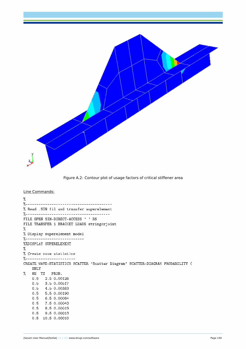
Figure A.2: Contour plot of usage factors of critical stiffener area
Line Commands:
%
%----------------------------------------
% Read .SIN fil and transfer superelement
%---------------------------------------
FILE OPEN SIN-DIRECT-ACCESS ' ' R5
FILE TRANSFER 1 BRACKET LOADS stringerjoint
%
% Display superelement model
%---------------------------
%%DISPLAY SUPERELEMENT
%
% Create wave statistics
%-----------------------
CREATE WAVE-STATISTICS SCATTER 'Scatter Diagram' SCATTER-DIAGRAM PROBABILITY (
ONLY
% HS TZ PROB.
0.5 2.5 0.00126
0.5 3.5 0.00517
0.5 4.5 0.00383
0.5 5.5 0.00190
0.5 6.5 0.00084
0.5 7.5 0.00043
0.5 8.5 0.00019
0.5 9.5 0.00013
0.5 10.5 0.00010
|Sesam User Manual|Stofat|[V4.1-00] www.dnvgl.com/software Page 149
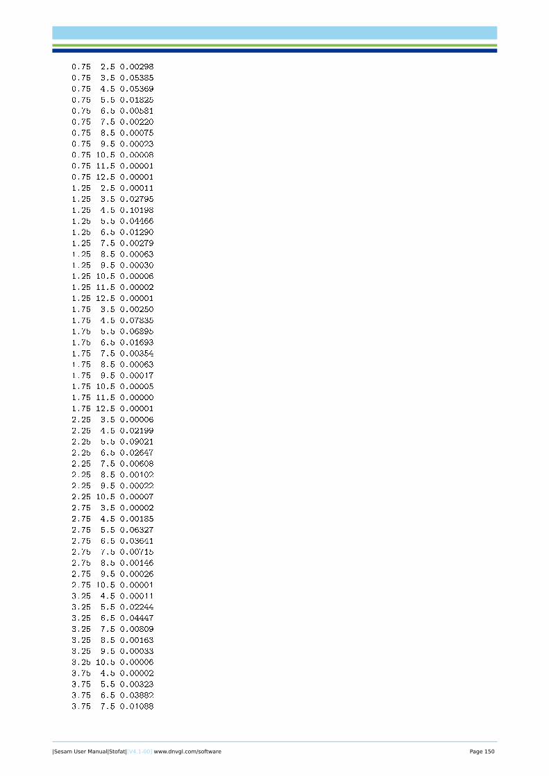
0.75 2.5 0.00298
0.75 3.5 0.05385
0.75 4.5 0.05369
0.75 5.5 0.01825
0.75 6.5 0.00581
0.75 7.5 0.00220
0.75 8.5 0.00075
0.75 9.5 0.00023
0.75 10.5 0.00008
0.75 11.5 0.00001
0.75 12.5 0.00001
1.25 2.5 0.00011
1.25 3.5 0.02795
1.25 4.5 0.10198
1.25 5.5 0.04466
1.25 6.5 0.01290
1.25 7.5 0.00279
1.25 8.5 0.00063
1.25 9.5 0.00030
1.25 10.5 0.00006
1.25 11.5 0.00002
1.25 12.5 0.00001
1.75 3.5 0.00250
1.75 4.5 0.07835
1.75 5.5 0.06895
1.75 6.5 0.01693
1.75 7.5 0.00354
1.75 8.5 0.00063
1.75 9.5 0.00017
1.75 10.5 0.00005
1.75 11.5 0.00000
1.75 12.5 0.00001
2.25 3.5 0.00006
2.25 4.5 0.02199
2.25 5.5 0.09021
2.25 6.5 0.02647
2.25 7.5 0.00608
2.25 8.5 0.00102
2.25 9.5 0.00022
2.25 10.5 0.00007
2.75 3.5 0.00002
2.75 4.5 0.00185
2.75 5.5 0.06327
2.75 6.5 0.03641
2.75 7.5 0.00715
2.75 8.5 0.00146
2.75 9.5 0.00026
2.75 10.5 0.00001
3.25 4.5 0.00011
3.25 5.5 0.02244
3.25 6.5 0.04447
3.25 7.5 0.00809
3.25 8.5 0.00163
3.25 9.5 0.00033
3.25 10.5 0.00006
3.75 4.5 0.00002
3.75 5.5 0.00323
3.75 6.5 0.03882
3.75 7.5 0.01088
|Sesam User Manual|Stofat|[V4.1-00] www.dnvgl.com/software Page 150
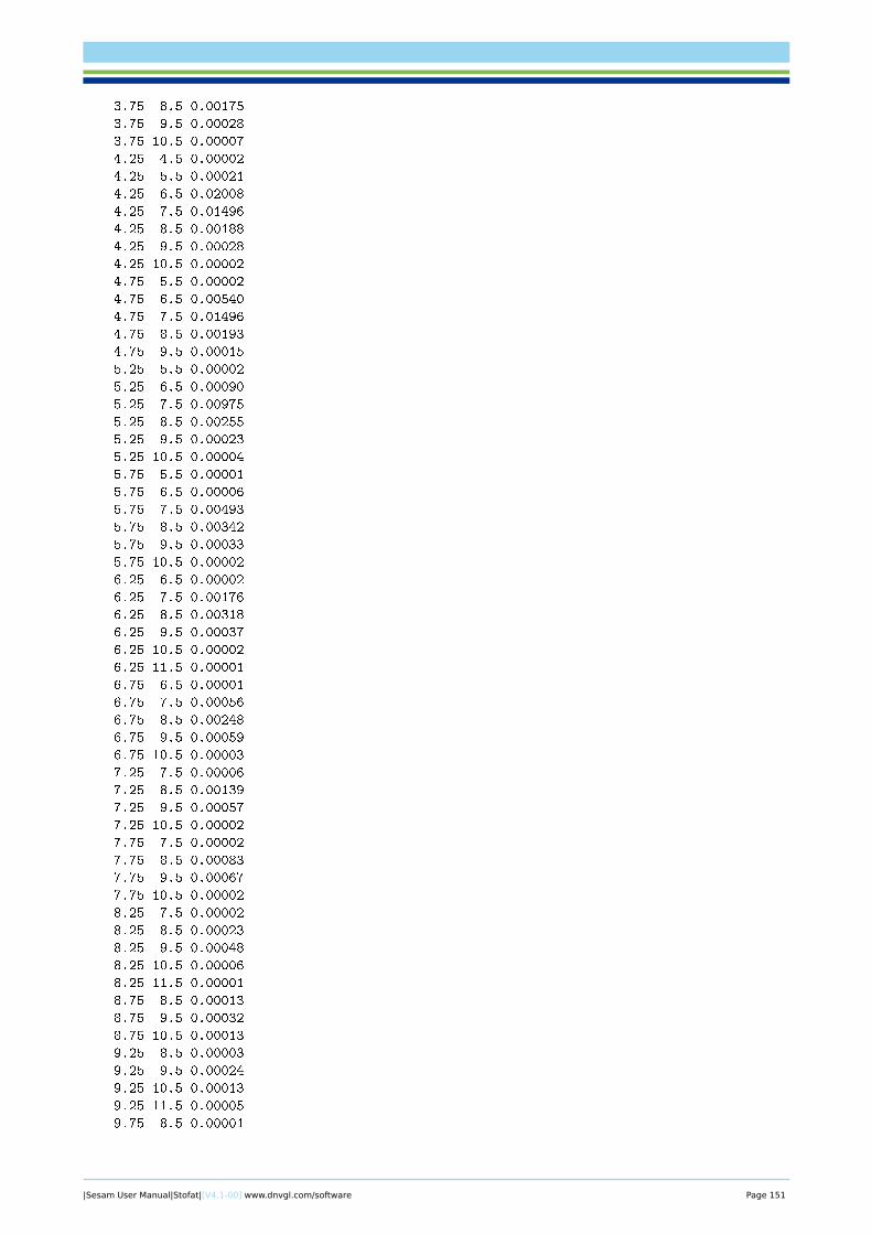
3.75 8.5 0.00175
3.75 9.5 0.00028
3.75 10.5 0.00007
4.25 4.5 0.00002
4.25 5.5 0.00021
4.25 6.5 0.02008
4.25 7.5 0.01496
4.25 8.5 0.00188
4.25 9.5 0.00028
4.25 10.5 0.00002
4.75 5.5 0.00002
4.75 6.5 0.00540
4.75 7.5 0.01496
4.75 8.5 0.00193
4.75 9.5 0.00015
5.25 5.5 0.00002
5.25 6.5 0.00090
5.25 7.5 0.00975
5.25 8.5 0.00255
5.25 9.5 0.00023
5.25 10.5 0.00004
5.75 5.5 0.00001
5.75 6.5 0.00006
5.75 7.5 0.00493
5.75 8.5 0.00342
5.75 9.5 0.00033
5.75 10.5 0.00002
6.25 6.5 0.00002
6.25 7.5 0.00176
6.25 8.5 0.00318
6.25 9.5 0.00037
6.25 10.5 0.00002
6.25 11.5 0.00001
6.75 6.5 0.00001
6.75 7.5 0.00056
6.75 8.5 0.00248
6.75 9.5 0.00059
6.75 10.5 0.00003
7.25 7.5 0.00006
7.25 8.5 0.00139
7.25 9.5 0.00057
7.25 10.5 0.00002
7.75 7.5 0.00002
7.75 8.5 0.00083
7.75 9.5 0.00067
7.75 10.5 0.00002
8.25 7.5 0.00002
8.25 8.5 0.00023
8.25 9.5 0.00048
8.25 10.5 0.00006
8.25 11.5 0.00001
8.75 8.5 0.00013
8.75 9.5 0.00032
8.75 10.5 0.00013
9.25 8.5 0.00003
9.25 9.5 0.00024
9.25 10.5 0.00013
9.25 11.5 0.00005
9.75 8.5 0.00001
|Sesam User Manual|Stofat|[V4.1-00] www.dnvgl.com/software Page 151
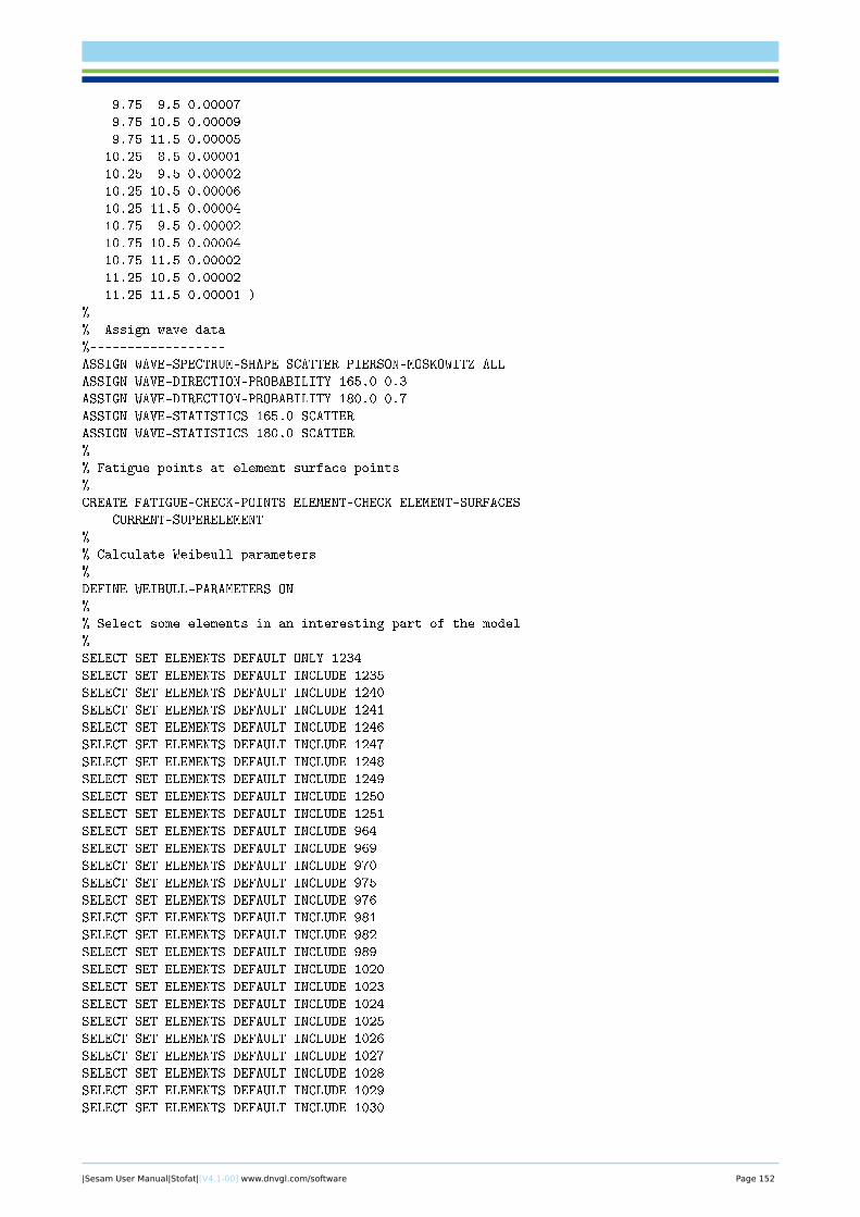
9.75 9.5 0.00007
9.75 10.5 0.00009
9.75 11.5 0.00005
10.25 8.5 0.00001
10.25 9.5 0.00002
10.25 10.5 0.00006
10.25 11.5 0.00004
10.75 9.5 0.00002
10.75 10.5 0.00004
10.75 11.5 0.00002
11.25 10.5 0.00002
11.25 11.5 0.00001 )
%
% Assign wave data
%------------------
ASSIGN WAVE-SPECTRUM-SHAPE SCATTER PIERSON-MOSKOWITZ ALL
ASSIGN WAVE-DIRECTION-PROBABILITY 165.0 0.3
ASSIGN WAVE-DIRECTION-PROBABILITY 180.0 0.7
ASSIGN WAVE-STATISTICS 165.0 SCATTER
ASSIGN WAVE-STATISTICS 180.0 SCATTER
%
% Fatigue points at element surface points
%
CREATE FATIGUE-CHECK-POINTS ELEMENT-CHECK ELEMENT-SURFACES
CURRENT-SUPERELEMENT
%
% Calculate Weibeull parameters
%
DEFINE WEIBULL-PARAMETERS ON
%
% Select some elements in an interesting part of the model
%---------------------------------------------------------
SELECT SET ELEMENTS DEFAULT ONLY 1234
SELECT SET ELEMENTS DEFAULT INCLUDE 1235
SELECT SET ELEMENTS DEFAULT INCLUDE 1240
SELECT SET ELEMENTS DEFAULT INCLUDE 1241
SELECT SET ELEMENTS DEFAULT INCLUDE 1246
SELECT SET ELEMENTS DEFAULT INCLUDE 1247
SELECT SET ELEMENTS DEFAULT INCLUDE 1248
SELECT SET ELEMENTS DEFAULT INCLUDE 1249
SELECT SET ELEMENTS DEFAULT INCLUDE 1250
SELECT SET ELEMENTS DEFAULT INCLUDE 1251
SELECT SET ELEMENTS DEFAULT INCLUDE 964
SELECT SET ELEMENTS DEFAULT INCLUDE 969
SELECT SET ELEMENTS DEFAULT INCLUDE 970
SELECT SET ELEMENTS DEFAULT INCLUDE 975
SELECT SET ELEMENTS DEFAULT INCLUDE 976
SELECT SET ELEMENTS DEFAULT INCLUDE 981
SELECT SET ELEMENTS DEFAULT INCLUDE 982
SELECT SET ELEMENTS DEFAULT INCLUDE 989
SELECT SET ELEMENTS DEFAULT INCLUDE 1020
SELECT SET ELEMENTS DEFAULT INCLUDE 1023
SELECT SET ELEMENTS DEFAULT INCLUDE 1024
SELECT SET ELEMENTS DEFAULT INCLUDE 1025
SELECT SET ELEMENTS DEFAULT INCLUDE 1026
SELECT SET ELEMENTS DEFAULT INCLUDE 1027
SELECT SET ELEMENTS DEFAULT INCLUDE 1028
SELECT SET ELEMENTS DEFAULT INCLUDE 1029
SELECT SET ELEMENTS DEFAULT INCLUDE 1030
|Sesam User Manual|Stofat|[V4.1-00] www.dnvgl.com/software Page 152
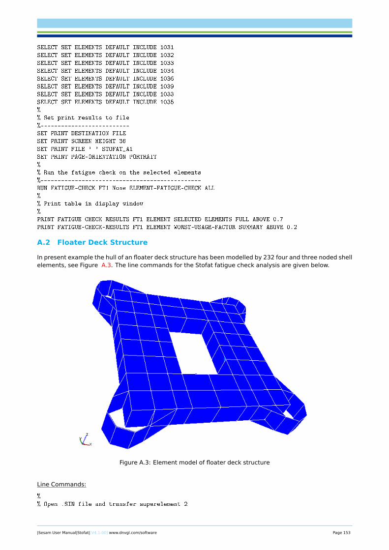
SELECT SET ELEMENTS DEFAULT INCLUDE 1031
SELECT SET ELEMENTS DEFAULT INCLUDE 1032
SELECT SET ELEMENTS DEFAULT INCLUDE 1033
SELECT SET ELEMENTS DEFAULT INCLUDE 1034
SELECT SET ELEMENTS DEFAULT INCLUDE 1036
SELECT SET ELEMENTS DEFAULT INCLUDE 1039
SELECT SET ELEMENTS DEFAULT INCLUDE 1033
SELECT SET ELEMENTS DEFAULT INCLUDE 1035
%
% Set print results to file
%--------------------------
SET PRINT DESTINATION FILE
SET PRINT SCREEN-HEIGHT 36
SET PRINT FILE ' ' STOFAT_A1
SET PRINT PAGE-ORIENTATION PORTRAIT
%
% Run the fatigue check on the selected elements
%-----------------------------------------------
RUN FATIGUE-CHECK FT1 None ELEMENT-FATIGUE-CHECK ALL
%
% Print table in display window
%------------------------------
PRINT FATIGUE-CHECK-RESULTS FT1 ELEMENT SELECTED-ELEMENTS FULL ABOVE 0.7
PRINT FATIGUE-CHECK-RESULTS FT1 ELEMENT WORST-USAGE-FACTOR SUMMARY ABOVE 0.2
A.2 Floater Deck Structure
In present example the hull of an floater deck structure has been modelled by 232 four and three noded shellelements, see Figure A.3. The line commands for the Stofat fatigue check analysis are given below.
Figure A.3: Element model of floater deck structure
Line Commands:
%
% Open .SIN file and transfer superelement 2
|Sesam User Manual|Stofat|[V4.1-00] www.dnvgl.com/software Page 153
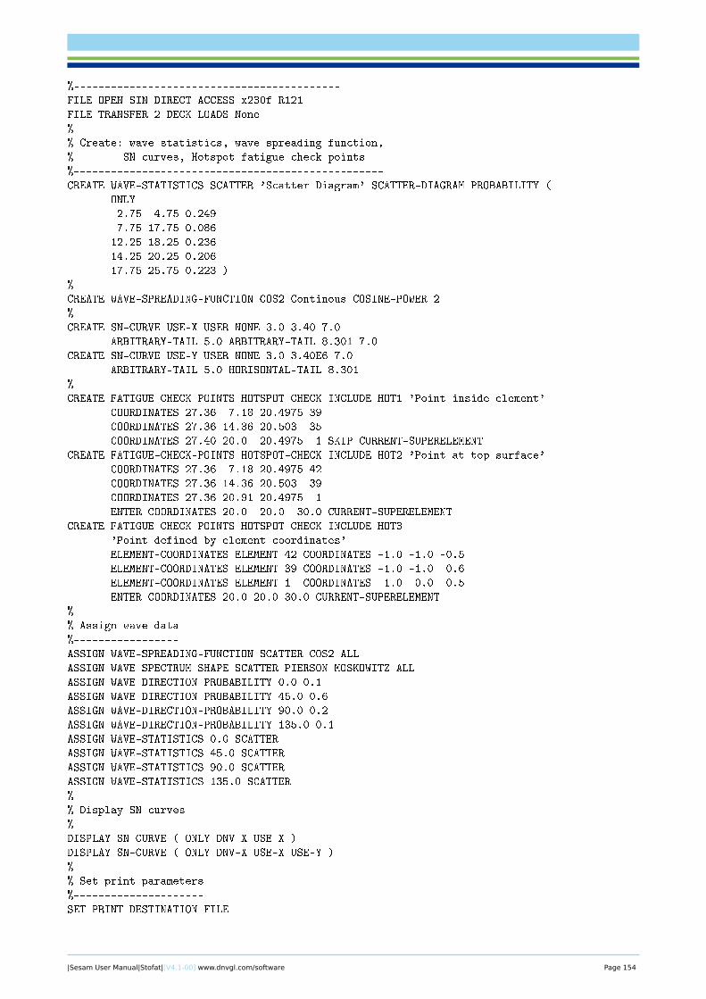
%-------------------------------------------
FILE OPEN SIN-DIRECT-ACCESS x230f R121
FILE TRANSFER 2 DECK LOADS None
%
% Create: wave statistics, wave spreading function,
% SN curves, Hotspot fatigue check points
%--------------------------------------------------
CREATE WAVE-STATISTICS SCATTER 'Scatter Diagram' SCATTER-DIAGRAM PROBABILITY (
ONLY
2.75 4.75 0.249
7.75 17.75 0.086
12.25 18.25 0.236
14.25 20.25 0.206
17.75 25.75 0.223 )
%
CREATE WAVE-SPREADING-FUNCTION COS2 Continous COSINE-POWER 2
%
CREATE SN-CURVE USE-X USER NONE 3.0 3.40 7.0
ARBITRARY-TAIL 5.0 ARBITRARY-TAIL 8.301 7.0
CREATE SN-CURVE USE-Y USER NONE 3.0 3.40E6 7.0
ARBITRARY-TAIL 5.0 HORISONTAL-TAIL 8.301
%
CREATE FATIGUE-CHECK-POINTS HOTSPOT-CHECK INCLUDE HOT1 'Point inside element'
COORDINATES 27.36 7.18 20.4975 39
COORDINATES 27.36 14.36 20.503 35
COORDINATES 27.40 20.0 20.4975 1 SKIP CURRENT-SUPERELEMENT
CREATE FATIGUE-CHECK-POINTS HOTSPOT-CHECK INCLUDE HOT2 'Point at top surface'
COORDINATES 27.36 7.18 20.4975 42
COORDINATES 27.36 14.36 20.503 39
COORDINATES 27.36 20.91 20.4975 1
ENTER COORDINATES 20.0 20.0 30.0 CURRENT-SUPERELEMENT
CREATE FATIGUE-CHECK-POINTS HOTSPOT-CHECK INCLUDE HOT3
'Point defined by element coordinates'
ELEMENT-COORDINATES ELEMENT 42 COORDINATES -1.0 -1.0 -0.5
ELEMENT-COORDINATES ELEMENT 39 COORDINATES -1.0 -1.0 0.6
ELEMENT-COORDINATES ELEMENT 1 COORDINATES 1.0 0.0 0.5
ENTER COORDINATES 20.0 20.0 30.0 CURRENT-SUPERELEMENT
%
% Assign wave data
%-----------------
ASSIGN WAVE-SPREADING-FUNCTION SCATTER COS2 ALL
ASSIGN WAVE-SPECTRUM-SHAPE SCATTER PIERSON-MOSKOWITZ ALL
ASSIGN WAVE-DIRECTION-PROBABILITY 0.0 0.1
ASSIGN WAVE-DIRECTION-PROBABILITY 45.0 0.6
ASSIGN WAVE-DIRECTION-PROBABILITY 90.0 0.2
ASSIGN WAVE-DIRECTION-PROBABILITY 135.0 0.1
ASSIGN WAVE-STATISTICS 0.0 SCATTER
ASSIGN WAVE-STATISTICS 45.0 SCATTER
ASSIGN WAVE-STATISTICS 90.0 SCATTER
ASSIGN WAVE-STATISTICS 135.0 SCATTER
%
% Display SN curves
%------------------
DISPLAY SN-CURVE ( ONLY DNV-X USE-X )
DISPLAY SN-CURVE ( ONLY DNV-X USE-X USE-Y )
%
% Set print parameters
%---------------------
SET PRINT DESTINATION FILE
|Sesam User Manual|Stofat|[V4.1-00] www.dnvgl.com/software Page 154
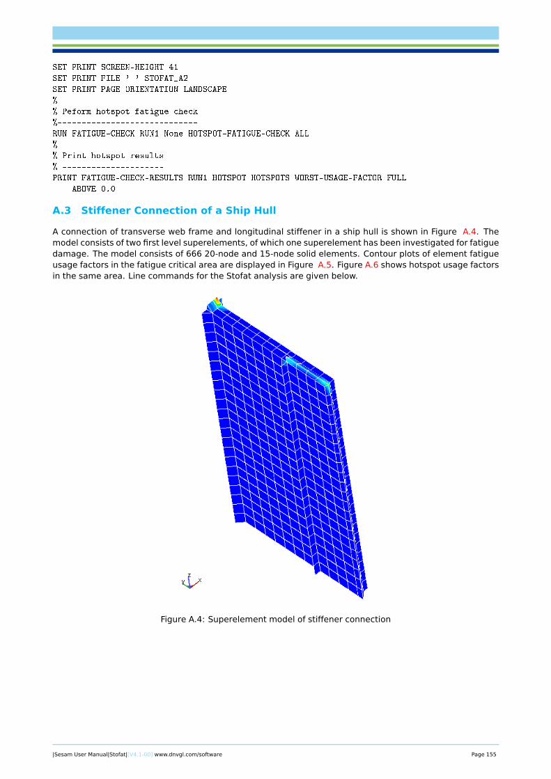
SET PRINT SCREEN-HEIGHT 41
SET PRINT FILE ' ' STOFAT_A2
SET PRINT PAGE-ORIENTATION LANDSCAPE
%
% Peform hotspot fatigue check
%-----------------------------
RUN FATIGUE-CHECK RUN1 None HOTSPOT-FATIGUE-CHECK ALL
%
% Print hotspot results
% ---------------------
PRINT FATIGUE-CHECK-RESULTS RUN1 HOTSPOT HOTSPOTS WORST-USAGE-FACTOR FULL
ABOVE 0.0
A.3 Stiffener Connection of a Ship Hull
A connection of transverse web frame and longitudinal stiffener in a ship hull is shown in Figure A.4. Themodel consists of two first level superelements, of which one superelement has been investigated for fatiguedamage. The model consists of 666 20-node and 15-node solid elements. Contour plots of element fatigueusage factors in the fatigue critical area are displayed in Figure A.5. Figure A.6 shows hotspot usage factorsin the same area. Line commands for the Stofat analysis are given below.
Figure A.4: Superelement model of stiffener connection
|Sesam User Manual|Stofat|[V4.1-00] www.dnvgl.com/software Page 155
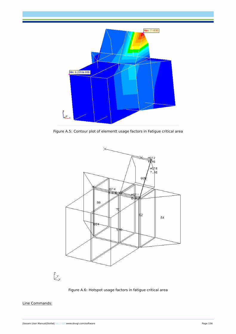
Figure A.5: Contour plot of elementt usage factors in Fatigue critical area
Figure A.6: Hotspot usage factors in fatigue critical area
Line Commands:
|Sesam User Manual|Stofat|[V4.1-00] www.dnvgl.com/software Page 156
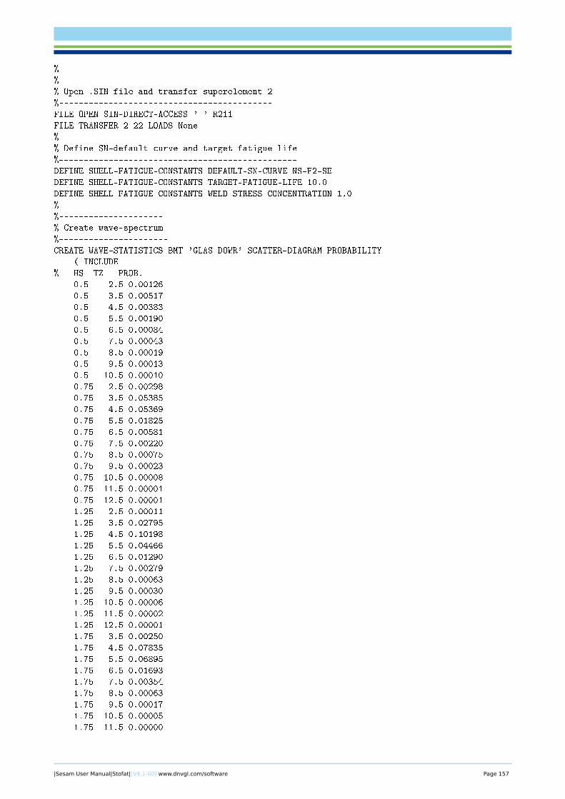
%
%-------------------------------------------
% Open .SIN file and transfer superelement 2
%-------------------------------------------
FILE OPEN SIN-DIRECT-ACCESS ' ' R211
FILE TRANSFER 2 22 LOADS None
%
% Define SN-default curve and target fatigue life
%------------------------------------------------
DEFINE SHELL-FATIGUE-CONSTANTS DEFAULT-SN-CURVE NS-F2-SE
DEFINE SHELL-FATIGUE-CONSTANTS TARGET-FATIGUE-LIFE 10.0
DEFINE SHELL-FATIGUE-CONSTANTS WELD-STRESS-CONCENTRATION 1.0
%
%---------------------
% Create wave-spectrum
%----------------------
CREATE WAVE-STATISTICS BMT 'GLAS DOWR' SCATTER-DIAGRAM PROBABILITY
( INCLUDE
% HS TZ PROB.
0.5 2.5 0.00126
0.5 3.5 0.00517
0.5 4.5 0.00383
0.5 5.5 0.00190
0.5 6.5 0.00084
0.5 7.5 0.00043
0.5 8.5 0.00019
0.5 9.5 0.00013
0.5 10.5 0.00010
0.75 2.5 0.00298
0.75 3.5 0.05385
0.75 4.5 0.05369
0.75 5.5 0.01825
0.75 6.5 0.00581
0.75 7.5 0.00220
0.75 8.5 0.00075
0.75 9.5 0.00023
0.75 10.5 0.00008
0.75 11.5 0.00001
0.75 12.5 0.00001
1.25 2.5 0.00011
1.25 3.5 0.02795
1.25 4.5 0.10198
1.25 5.5 0.04466
1.25 6.5 0.01290
1.25 7.5 0.00279
1.25 8.5 0.00063
1.25 9.5 0.00030
1.25 10.5 0.00006
1.25 11.5 0.00002
1.25 12.5 0.00001
1.75 3.5 0.00250
1.75 4.5 0.07835
1.75 5.5 0.06895
1.75 6.5 0.01693
1.75 7.5 0.00354
1.75 8.5 0.00063
1.75 9.5 0.00017
1.75 10.5 0.00005
1.75 11.5 0.00000
|Sesam User Manual|Stofat|[V4.1-00] www.dnvgl.com/software Page 157
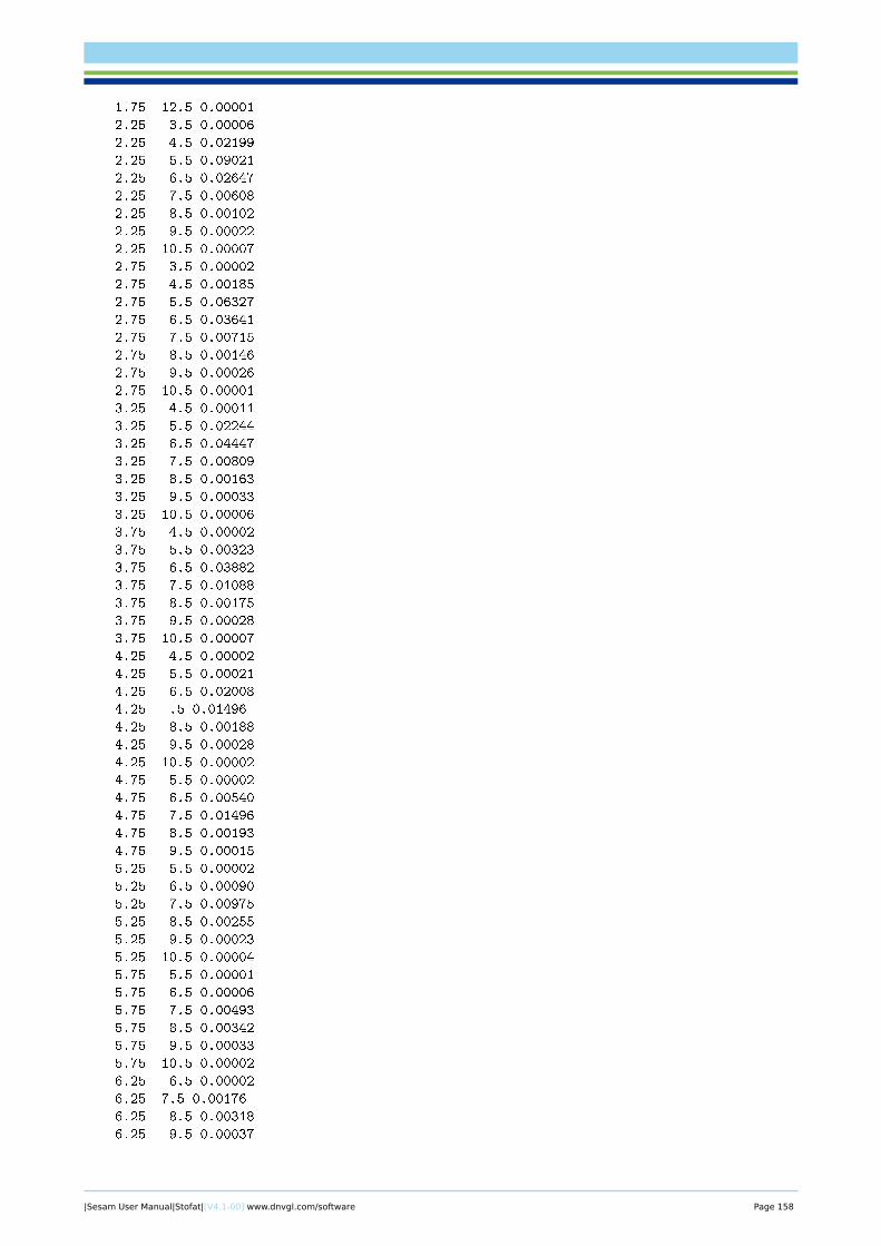
1.75 12.5 0.00001
2.25 3.5 0.00006
2.25 4.5 0.02199
2.25 5.5 0.09021
2.25 6.5 0.02647
2.25 7.5 0.00608
2.25 8.5 0.00102
2.25 9.5 0.00022
2.25 10.5 0.00007
2.75 3.5 0.00002
2.75 4.5 0.00185
2.75 5.5 0.06327
2.75 6.5 0.03641
2.75 7.5 0.00715
2.75 8.5 0.00146
2.75 9.5 0.00026
2.75 10.5 0.00001
3.25 4.5 0.00011
3.25 5.5 0.02244
3.25 6.5 0.04447
3.25 7.5 0.00809
3.25 8.5 0.00163
3.25 9.5 0.00033
3.25 10.5 0.00006
3.75 4.5 0.00002
3.75 5.5 0.00323
3.75 6.5 0.03882
3.75 7.5 0.01088
3.75 8.5 0.00175
3.75 9.5 0.00028
3.75 10.5 0.00007
4.25 4.5 0.00002
4.25 5.5 0.00021
4.25 6.5 0.02008
4.25 .5 0.01496
4.25 8.5 0.00188
4.25 9.5 0.00028
4.25 10.5 0.00002
4.75 5.5 0.00002
4.75 6.5 0.00540
4.75 7.5 0.01496
4.75 8.5 0.00193
4.75 9.5 0.00015
5.25 5.5 0.00002
5.25 6.5 0.00090
5.25 7.5 0.00975
5.25 8.5 0.00255
5.25 9.5 0.00023
5.25 10.5 0.00004
5.75 5.5 0.00001
5.75 6.5 0.00006
5.75 7.5 0.00493
5.75 8.5 0.00342
5.75 9.5 0.00033
5.75 10.5 0.00002
6.25 6.5 0.00002
6.25 7.5 0.00176
6.25 8.5 0.00318
6.25 9.5 0.00037
|Sesam User Manual|Stofat|[V4.1-00] www.dnvgl.com/software Page 158
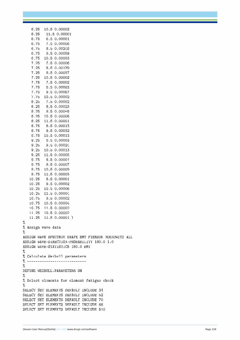
6.25 10.5 0.00002
6.25 11.5 0.00001
6.75 6.5 0.00001
6.75 7.5 0.00056
6.75 8.5 0.00248
6.75 9.5 0.00059
6.75 10.5 0.00003
7.25 7.5 0.00006
7.25 8.5 0.00139
7.25 9.5 0.00057
7.25 10.5 0.00002
7.75 7.5 0.00002
7.75 8.5 0.00083
7.75 9.5 0.00067
7.75 10.5 0.00002
8.25 7.5 0.00002
8.25 8.5 0.00023
8.25 9.5 0.00048
8.25 10.5 0.00006
8.25 11.5 0.00001
8.75 8.5 0.00013
8.75 9.5 0.00032
8.75 10.5 0.00013
9.25 8.5 0.00003
9.25 9.5 0.00024
9.25 10.5 0.00013
9.25 11.5 0.00005
9.75 8.5 0.00001
9.75 9.5 0.00007
9.75 10.5 0.00009
9.75 11.5 0.00005
10.25 8.5 0.00001
10.25 9.5 0.00002
10.25 10.5 0.00006
10.25 11.5 0.00004
10.75 9.5 0.00002
10.75 10.5 0.00004
10.75 11.5 0.00002
11.25 10.5 0.00002
11.25 11.5 0.00001 )
%
% Assign wave data
%-----------------
ASSIGN WAVE-SPECTRUM-SHAPE BMT PIERSON-MOSKOWITZ ALL
ASSIGN WAVE-DIRECTION-PROBABILITY 180.0 1.0
ASSIGN WAVE-STATISTICS 180.0 BMT
%
% Calculate Weibull parameters
% ----------------------------
%
DEFINE WEIBULL-PARAMETERS ON
%
% Select elements for element fatigue check
%------------------------------------------
SELECT SET ELEMENTS DEFAULT INCLUDE 34
SELECT SET ELEMENTS DEFAULT INCLUDE 52
SELECT SET ELEMENTS DEFAULT INCLUDE 70
SELECT SET ELEMENTS DEFAULT INCLUDE 88
SELECT SET ELEMENTS DEFAULT INCLUDE 510
|Sesam User Manual|Stofat|[V4.1-00] www.dnvgl.com/software Page 159
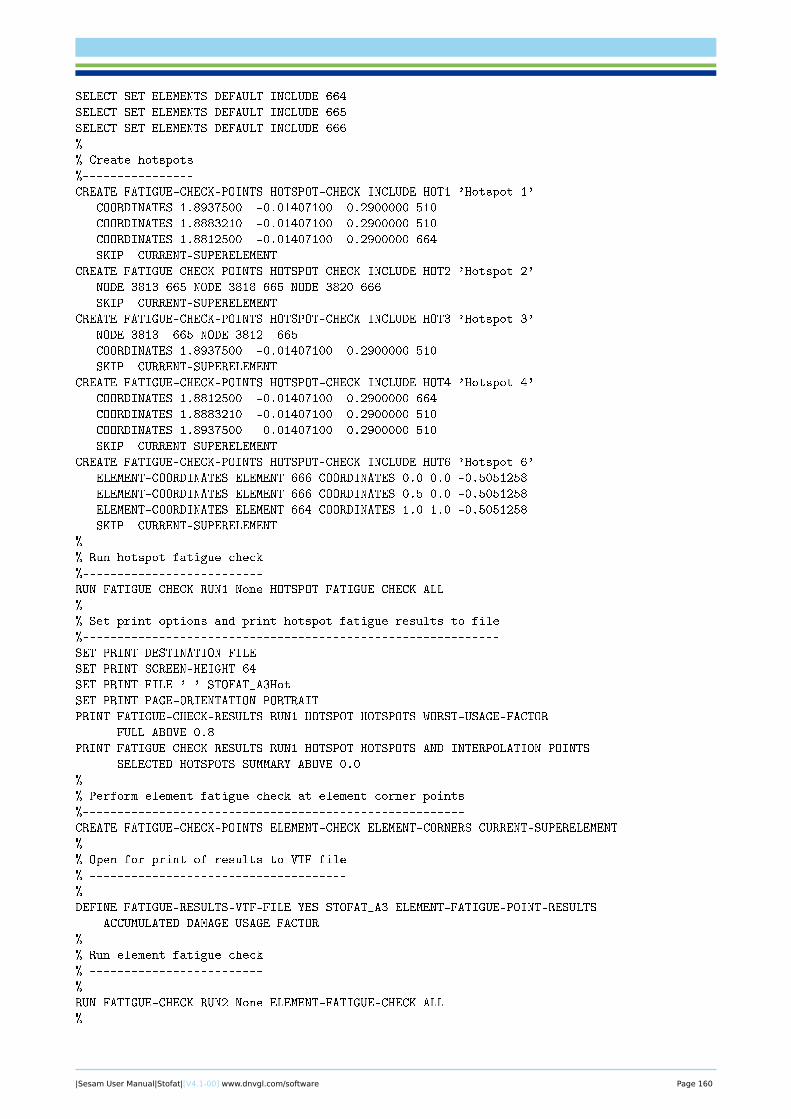
SELECT SET ELEMENTS DEFAULT INCLUDE 664
SELECT SET ELEMENTS DEFAULT INCLUDE 665
SELECT SET ELEMENTS DEFAULT INCLUDE 666
%
% Create hotspots
%----------------
CREATE FATIGUE-CHECK-POINTS HOTSPOT-CHECK INCLUDE HOT1 'Hotspot 1'
COORDINATES 1.8937500 -0.01407100 0.2900000 510
COORDINATES 1.8883210 -0.01407100 0.2900000 510
COORDINATES 1.8812500 -0.01407100 0.2900000 664
SKIP CURRENT-SUPERELEMENT
CREATE FATIGUE-CHECK-POINTS HOTSPOT-CHECK INCLUDE HOT2 'Hotspot 2'
NODE 3813 665 NODE 3818 665 NODE 3820 666
SKIP CURRENT-SUPERELEMENT
CREATE FATIGUE-CHECK-POINTS HOTSPOT-CHECK INCLUDE HOT3 'Hotspot 3'
NODE 3813 665 NODE 3812 665
COORDINATES 1.8937500 -0.01407100 0.2900000 510
SKIP CURRENT-SUPERELEMENT
CREATE FATIGUE-CHECK-POINTS HOTSPOT-CHECK INCLUDE HOT4 'Hotspot 4'
COORDINATES 1.8812500 -0.01407100 0.2900000 664
COORDINATES 1.8883210 -0.01407100 0.2900000 510
COORDINATES 1.8937500 -0.01407100 0.2900000 510
SKIP CURRENT-SUPERELEMENT
CREATE FATIGUE-CHECK-POINTS HOTSPOT-CHECK INCLUDE HOT6 'Hotspot 6'
ELEMENT-COORDINATES ELEMENT 666 COORDINATES 0.0 0.0 -0.5051258
ELEMENT-COORDINATES ELEMENT 666 COORDINATES 0.5 0.0 -0.5051258
ELEMENT-COORDINATES ELEMENT 664 COORDINATES 1.0 1.0 -0.5051258
SKIP CURRENT-SUPERELEMENT
%
% Run hotspot fatigue check
%--------------------------
RUN FATIGUE-CHECK RUN1 None HOTSPOT-FATIGUE-CHECK ALL
%
% Set print options and print hotspot fatigue results to file
%------------------------------------------------------------
SET PRINT DESTINATION FILE
SET PRINT SCREEN-HEIGHT 64
SET PRINT FILE ' ' STOFAT_A3Hot
SET PRINT PAGE-ORIENTATION PORTRAIT
PRINT FATIGUE-CHECK-RESULTS RUN1 HOTSPOT HOTSPOTS WORST-USAGE-FACTOR
FULL ABOVE 0.8
PRINT FATIGUE-CHECK-RESULTS RUN1 HOTSPOT HOTSPOTS-AND-INTERPOLATION-POINTS
SELECTED-HOTSPOTS SUMMARY ABOVE 0.0
%
% Perform element fatigue check at element corner points
%-------------------------------------------------------
CREATE FATIGUE-CHECK-POINTS ELEMENT-CHECK ELEMENT-CORNERS CURRENT-SUPERELEMENT
%
% Open for print of results to VTF file
% -------------------------------------
%
DEFINE FATIGUE-RESULTS-VTF-FILE YES STOFAT_A3 ELEMENT-FATIGUE-POINT-RESULTS
ACCUMULATED-DAMAGE USAGE-FACTOR
%
% Run element fatigue check
% -------------------------
%
RUN FATIGUE-CHECK RUN2 None ELEMENT-FATIGUE-CHECK ALL
%
|Sesam User Manual|Stofat|[V4.1-00] www.dnvgl.com/software Page 160
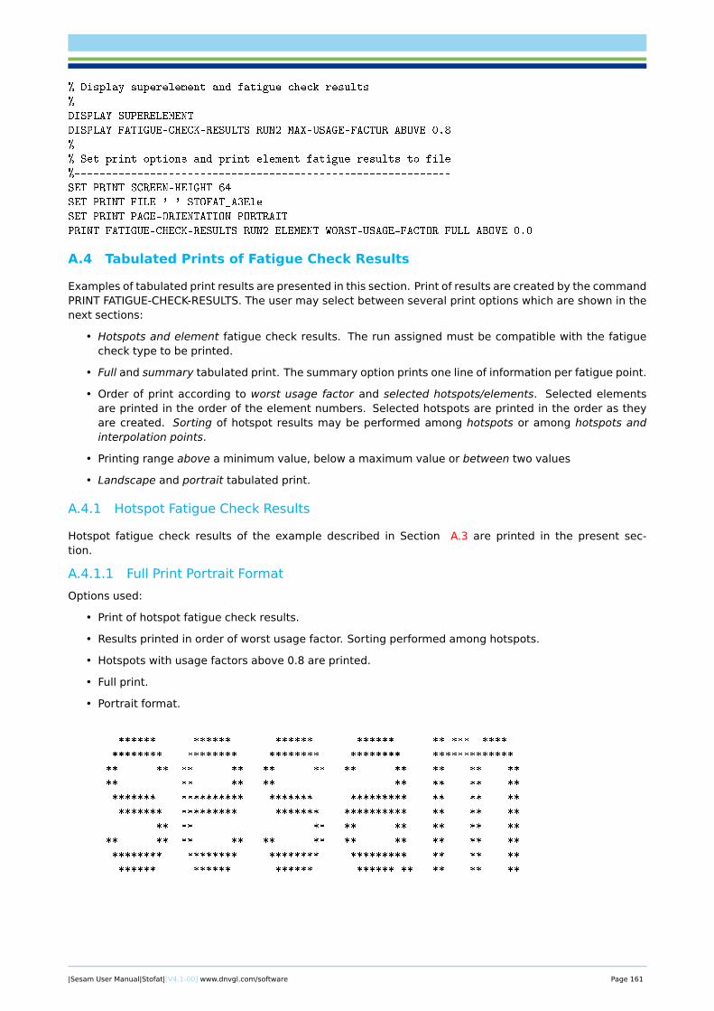
% Display superelement and fatigue check results
%-----------------------------------------------
DISPLAY SUPERELEMENT
DISPLAY FATIGUE-CHECK-RESULTS RUN2 MAX-USAGE-FACTOR ABOVE 0.8
%
% Set print options and print element fatigue results to file
%------------------------------------------------------------
SET PRINT SCREEN-HEIGHT 64
SET PRINT FILE ' ' STOFAT_A3Ele
SET PRINT PAGE-ORIENTATION PORTRAIT
PRINT FATIGUE-CHECK-RESULTS RUN2 ELEMENT WORST-USAGE-FACTOR FULL ABOVE 0.0
A.4 Tabulated Prints of Fatigue Check Results
Examples of tabulated print results are presented in this section. Print of results are created by the commandPRINT FATIGUE-CHECK-RESULTS. The user may select between several print options which are shown in thenext sections:
• Hotspots and element fatigue check results. The run assigned must be compatible with the fatiguecheck type to be printed.
• Full and summary tabulated print. The summary option prints one line of information per fatigue point.
• Order of print according to worst usage factor and selected hotspots/elements. Selected elementsare printed in the order of the element numbers. Selected hotspots are printed in the order as theyare created. Sorting of hotspot results may be performed among hotspots or among hotspots andinterpolation points.
• Printing range above a minimum value, below a maximum value or between two values
• Landscape and portrait tabulated print.
A.4.1 Hotspot Fatigue Check Results
Hotspot fatigue check results of the example described in Section A.3 are printed in the present sec-tion.
A.4.1.1 Full Print Portrait Format
Options used:
• Print of hotspot fatigue check results.
• Results printed in order of worst usage factor. Sorting performed among hotspots.
• Hotspots with usage factors above 0.8 are printed.
• Full print.
• Portrait format.
****** ****** ****** ****** ** *** ****
******** ******** ******** ******** *************
** ** ** ** ** ** ** ** ** ** **
** ** ** ** ** ** ** **
******* ********** ******* ********* ** ** **
******* ********* ******* ********** ** ** **
** ** ** ** ** ** ** **
** ** ** ** ** ** ** ** ** ** **
******** ******** ******** ********* ** ** **
****** ****** ****** ****** ** ** ** **
|Sesam User Manual|Stofat|[V4.1-00] www.dnvgl.com/software Page 161
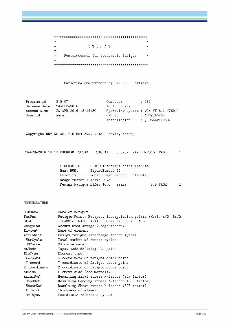
***********************************************
* *
* S T O F A T *
* *
* Postprocessor for stochastic fatigue *
* *
***********************************************
Marketing and Support by DNV GL - Software
Program id : 3.5-07 Computer : 586
Release date : 24-FEB-2016 Impl. update :
Access time : 20-APR-2016 13:13:50 Operating system : Win NT 6.1 [7601]
User id : aarn CPU id : 1337246785
Installation : , OSLLP110507
Copyright DNV GL AS, P.O.Box 300, N-1322 Hovik, Norway
20-APR-2016 13:13 PROGRAM: SESAM STOFAT 3.5-07 24-FEB-2016 PAGE: 1
STOCHASTIC HOTSPOT fatigue check results
Run: RUN1 Superelement 22
Priority.....: Worst Usage Factor. Hotspots
Usage factor : Above 0.80
Design Fatigue Life: 10.0 Years SUB PAGE: 1
NOMENCLATURE:
HotName Name of hotspot
FatPnt Fatigue Point: Hotspot, interpolation points (HotS, t/2, 3t/2
Stat = PASS or FAIL: *FAIL = UsageFactor > 1.0
UsageFac Accumulated damage (Usage factor)
Element Name of element
AccFatLif Design fatigue life/usage factor (year)
StrCycle Total number of stress cycles
SNCurve SN curve name.
atNode Input node defining the point
EleType Element type
X-coord. X coordinate of fatigue check point
Y-coord. Y coordinate of fatigue check point
Z-coordinate Z coordinate of fatigue check point
atSide Element side (see manual).
AxialScf Resulting Axial stress K-factor (SCF factor)
BendScf Resulting Bending stress K-factor (SCF factor)
ShearScf Resulting Shear stress K-factor (SCF factor)
ElThick Thickness of element
RefSyst Coordinate reference system
|Sesam User Manual|Stofat|[V4.1-00] www.dnvgl.com/software Page 162
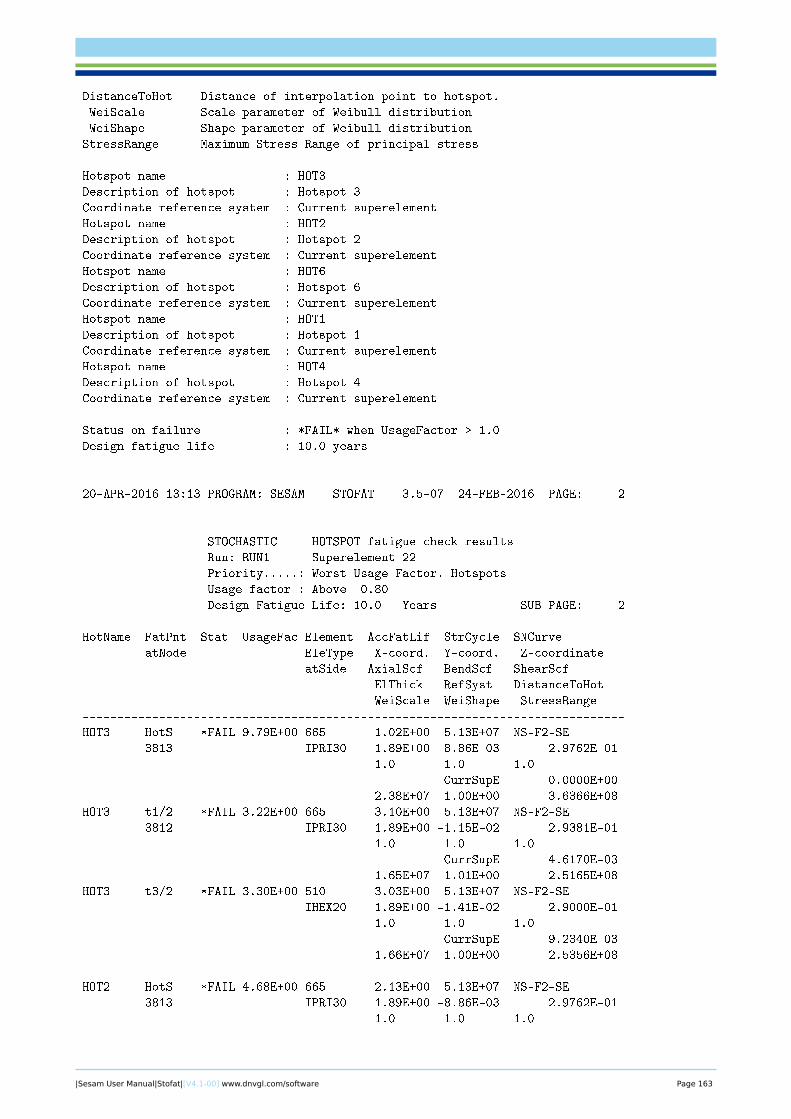
DistanceToHot Distance of interpolation point to hotspot.
WeiScale Scale parameter of Weibull distribution
WeiShape Shape parameter of Weibull distribution
StressRange Maximum Stress Range of principal stress
Hotspot name : HOT3
Description of hotspot : Hotspot 3
Coordinate reference system : Current superelement
Hotspot name : HOT2
Description of hotspot : Hotspot 2
Coordinate reference system : Current superelement
Hotspot name : HOT6
Description of hotspot : Hotspot 6
Coordinate reference system : Current superelement
Hotspot name : HOT1
Description of hotspot : Hotspot 1
Coordinate reference system : Current superelement
Hotspot name : HOT4
Description of hotspot : Hotspot 4
Coordinate reference system : Current superelement
Status on failure : *FAIL* when UsageFactor > 1.0
Design fatigue life : 10.0 years
20-APR-2016 13:13 PROGRAM: SESAM STOFAT 3.5-07 24-FEB-2016 PAGE: 2
STOCHASTIC HOTSPOT fatigue check results
Run: RUN1 Superelement 22
Priority.....: Worst Usage Factor. Hotspots
Usage factor : Above 0.80
Design Fatigue Life: 10.0 Years SUB PAGE: 2
HotName FatPnt Stat UsageFac Element AccFatLif StrCycle SNCurve
atNode EleType X-coord. Y-coord. Z-coordinate
atSide AxialScf BendScf ShearScf
ElThick RefSyst DistanceToHot
WeiScale WeiShape StressRange
------------------------------------------------------------------------------
HOT3 HotS *FAIL 9.79E+00 665 1.02E+00 5.13E+07 NS-F2-SE
3813 IPRI30 1.89E+00 -8.86E-03 2.9762E-01
1.0 1.0 1.0
CurrSupE 0.0000E+00
2.38E+07 1.00E+00 3.6366E+08
HOT3 t1/2 *FAIL 3.22E+00 665 3.10E+00 5.13E+07 NS-F2-SE
3812 IPRI30 1.89E+00 -1.15E-02 2.9381E-01
1.0 1.0 1.0
CurrSupE 4.6170E-03
1.65E+07 1.01E+00 2.5165E+08
HOT3 t3/2 *FAIL 3.30E+00 510 3.03E+00 5.13E+07 NS-F2-SE
IHEX20 1.89E+00 -1.41E-02 2.9000E-01
1.0 1.0 1.0
CurrSupE 9.2340E-03
1.66E+07 1.00E+00 2.5356E+08
HOT2 HotS *FAIL 4.68E+00 665 2.13E+00 5.13E+07 NS-F2-SE
3813 IPRI30 1.89E+00 -8.86E-03 2.9762E-01
1.0 1.0 1.0
|Sesam User Manual|Stofat|[V4.1-00] www.dnvgl.com/software Page 163
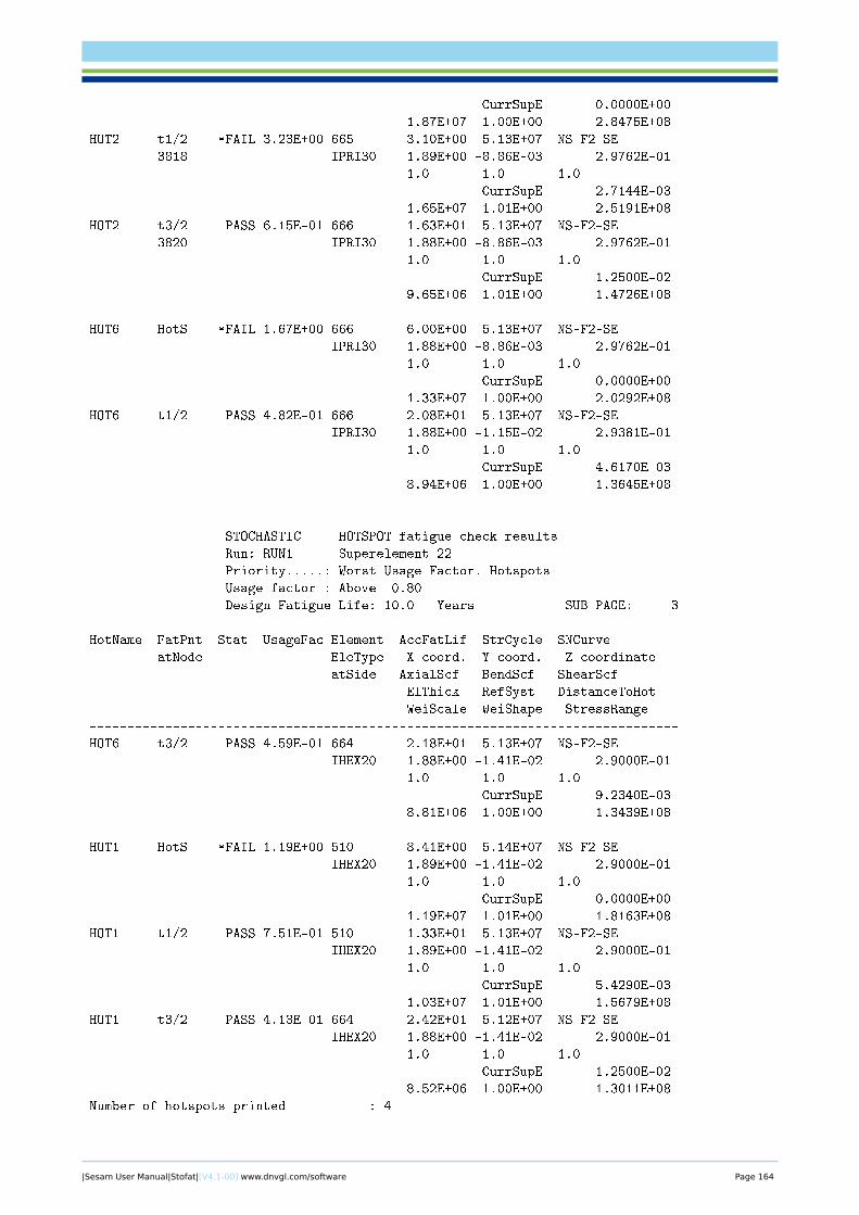
CurrSupE 0.0000E+00
1.87E+07 1.00E+00 2.8475E+08
HOT2 t1/2 *FAIL 3.23E+00 665 3.10E+00 5.13E+07 NS-F2-SE
3818 IPRI30 1.89E+00 -8.86E-03 2.9762E-01
1.0 1.0 1.0
CurrSupE 2.7144E-03
1.65E+07 1.01E+00 2.5191E+08
HOT2 t3/2 PASS 6.15E-01 666 1.63E+01 5.13E+07 NS-F2-SE
3820 IPRI30 1.88E+00 -8.86E-03 2.9762E-01
1.0 1.0 1.0
CurrSupE 1.2500E-02
9.65E+06 1.01E+00 1.4726E+08
HOT6 HotS *FAIL 1.67E+00 666 6.00E+00 5.13E+07 NS-F2-SE
IPRI30 1.88E+00 -8.86E-03 2.9762E-01
1.0 1.0 1.0
CurrSupE 0.0000E+00
1.33E+07 1.00E+00 2.0292E+08
HOT6 t1/2 PASS 4.82E-01 666 2.08E+01 5.13E+07 NS-F2-SE
IPRI30 1.88E+00 -1.15E-02 2.9381E-01
1.0 1.0 1.0
CurrSupE 4.6170E-03
8.94E+06 1.00E+00 1.3645E+08
STOCHASTIC HOTSPOT fatigue check results
Run: RUN1 Superelement 22
Priority.....: Worst Usage Factor. Hotspots
Usage factor : Above 0.80
Design Fatigue Life: 10.0 Years SUB PAGE: 3
HotName FatPnt Stat UsageFac Element AccFatLif StrCycle SNCurve
atNode EleType X-coord. Y-coord. Z-coordinate
atSide AxialScf BendScf ShearScf
ElThick RefSyst DistanceToHot
WeiScale WeiShape StressRange
------------------------------------------------------------------------------
HOT6 t3/2 PASS 4.59E-01 664 2.18E+01 5.13E+07 NS-F2-SE
IHEX20 1.88E+00 -1.41E-02 2.9000E-01
1.0 1.0 1.0
CurrSupE 9.2340E-03
8.81E+06 1.00E+00 1.3439E+08
HOT1 HotS *FAIL 1.19E+00 510 8.41E+00 5.14E+07 NS-F2-SE
IHEX20 1.89E+00 -1.41E-02 2.9000E-01
1.0 1.0 1.0
CurrSupE 0.0000E+00
1.19E+07 1.01E+00 1.8163E+08
HOT1 t1/2 PASS 7.51E-01 510 1.33E+01 5.13E+07 NS-F2-SE
IHEX20 1.89E+00 -1.41E-02 2.9000E-01
1.0 1.0 1.0
CurrSupE 5.4290E-03
1.03E+07 1.01E+00 1.5679E+08
HOT1 t3/2 PASS 4.13E-01 664 2.42E+01 5.12E+07 NS-F2-SE
IHEX20 1.88E+00 -1.41E-02 2.9000E-01
1.0 1.0 1.0
CurrSupE 1.2500E-02
8.52E+06 1.00E+00 1.3011E+08
Number of hotspots printed : 4
|Sesam User Manual|Stofat|[V4.1-00] www.dnvgl.com/software Page 164
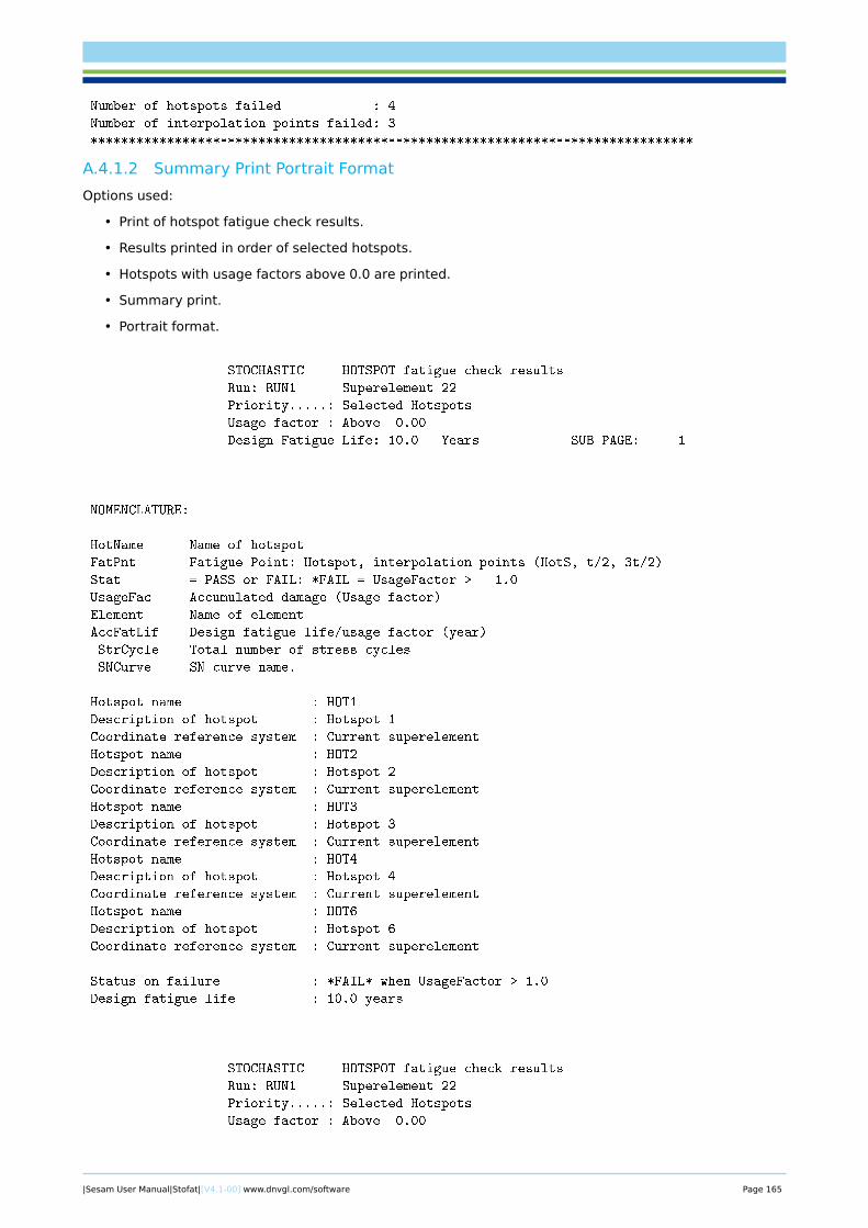
Number of hotspots failed : 4
Number of interpolation points failed: 3
*******************************************************************************
A.4.1.2 Summary Print Portrait Format
Options used:
• Print of hotspot fatigue check results.
• Results printed in order of selected hotspots.
• Hotspots with usage factors above 0.0 are printed.
• Summary print.
• Portrait format.
STOCHASTIC HOTSPOT fatigue check results
Run: RUN1 Superelement 22
Priority.....: Selected Hotspots
Usage factor : Above 0.00
Design Fatigue Life: 10.0 Years SUB PAGE: 1
NOMENCLATURE:
HotName Name of hotspot
FatPnt Fatigue Point: Hotspot, interpolation points (HotS, t/2, 3t/2)
Stat = PASS or FAIL: *FAIL = UsageFactor > 1.0
UsageFac Accumulated damage (Usage factor)
Element Name of element
AccFatLif Design fatigue life/usage factor (year)
StrCycle Total number of stress cycles
SNCurve SN curve name.
Hotspot name : HOT1
Description of hotspot : Hotspot 1
Coordinate reference system : Current superelement
Hotspot name : HOT2
Description of hotspot : Hotspot 2
Coordinate reference system : Current superelement
Hotspot name : HOT3
Description of hotspot : Hotspot 3
Coordinate reference system : Current superelement
Hotspot name : HOT4
Description of hotspot : Hotspot 4
Coordinate reference system : Current superelement
Hotspot name : HOT6
Description of hotspot : Hotspot 6
Coordinate reference system : Current superelement
Status on failure : *FAIL* when UsageFactor > 1.0
Design fatigue life : 10.0 years
STOCHASTIC HOTSPOT fatigue check results
Run: RUN1 Superelement 22
Priority.....: Selected Hotspots
Usage factor : Above 0.00
|Sesam User Manual|Stofat|[V4.1-00] www.dnvgl.com/software Page 165
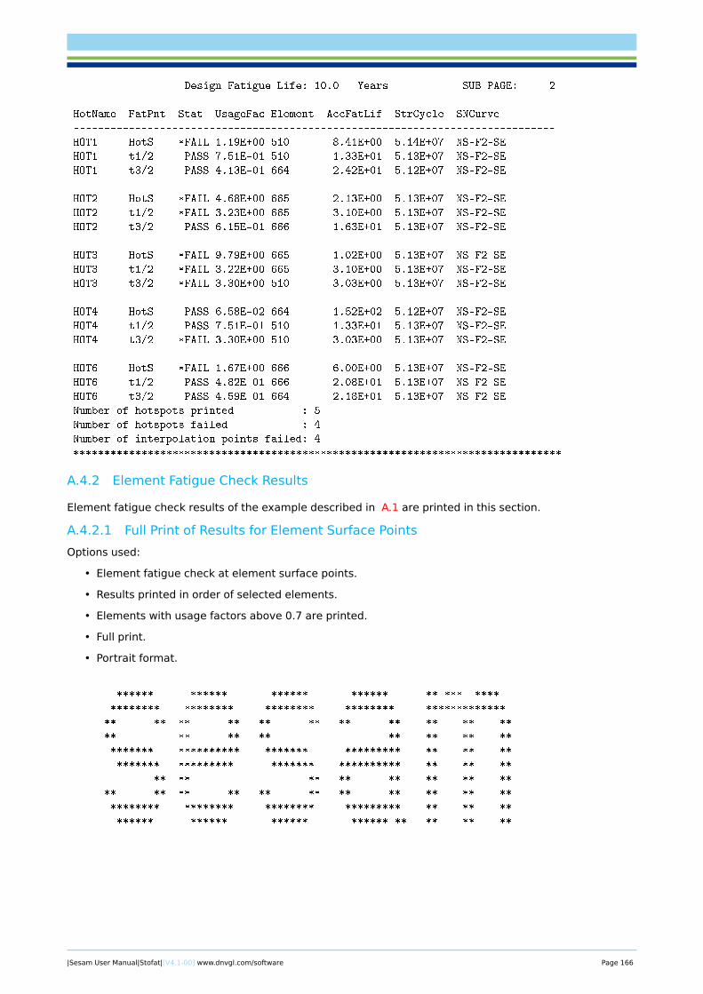
Design Fatigue Life: 10.0 Years SUB PAGE: 2
HotName FatPnt Stat UsageFac Element AccFatLif StrCycle SNCurve
------------------------------------------------------------------------------
HOT1 HotS *FAIL 1.19E+00 510 8.41E+00 5.14E+07 NS-F2-SE
HOT1 t1/2 PASS 7.51E-01 510 1.33E+01 5.13E+07 NS-F2-SE
HOT1 t3/2 PASS 4.13E-01 664 2.42E+01 5.12E+07 NS-F2-SE
HOT2 HotS *FAIL 4.68E+00 665 2.13E+00 5.13E+07 NS-F2-SE
HOT2 t1/2 *FAIL 3.23E+00 665 3.10E+00 5.13E+07 NS-F2-SE
HOT2 t3/2 PASS 6.15E-01 666 1.63E+01 5.13E+07 NS-F2-SE
HOT3 HotS *FAIL 9.79E+00 665 1.02E+00 5.13E+07 NS-F2-SE
HOT3 t1/2 *FAIL 3.22E+00 665 3.10E+00 5.13E+07 NS-F2-SE
HOT3 t3/2 *FAIL 3.30E+00 510 3.03E+00 5.13E+07 NS-F2-SE
HOT4 HotS PASS 6.58E-02 664 1.52E+02 5.12E+07 NS-F2-SE
HOT4 t1/2 PASS 7.51E-01 510 1.33E+01 5.13E+07 NS-F2-SE
HOT4 t3/2 *FAIL 3.30E+00 510 3.03E+00 5.13E+07 NS-F2-SE
HOT6 HotS *FAIL 1.67E+00 666 6.00E+00 5.13E+07 NS-F2-SE
HOT6 t1/2 PASS 4.82E-01 666 2.08E+01 5.13E+07 NS-F2-SE
HOT6 t3/2 PASS 4.59E-01 664 2.18E+01 5.13E+07 NS-F2-SE
Number of hotspots printed : 5
Number of hotspots failed : 4
Number of interpolation points failed: 4
*******************************************************************************
A.4.2 Element Fatigue Check Results
Element fatigue check results of the example described in A.1 are printed in this section.
A.4.2.1 Full Print of Results for Element Surface Points
Options used:
• Element fatigue check at element surface points.
• Results printed in order of selected elements.
• Elements with usage factors above 0.7 are printed.
• Full print.
• Portrait format.
****** ****** ****** ****** ** *** ****
******** ******** ******** ******** *************
** ** ** ** ** ** ** ** ** ** **
** ** ** ** ** ** ** **
******* ********** ******* ********* ** ** **
******* ********* ******* ********** ** ** **
** ** ** ** ** ** ** **
** ** ** ** ** ** ** ** ** ** **
******** ******** ******** ********* ** ** **
****** ****** ****** ****** ** ** ** **
|Sesam User Manual|Stofat|[V4.1-00] www.dnvgl.com/software Page 166
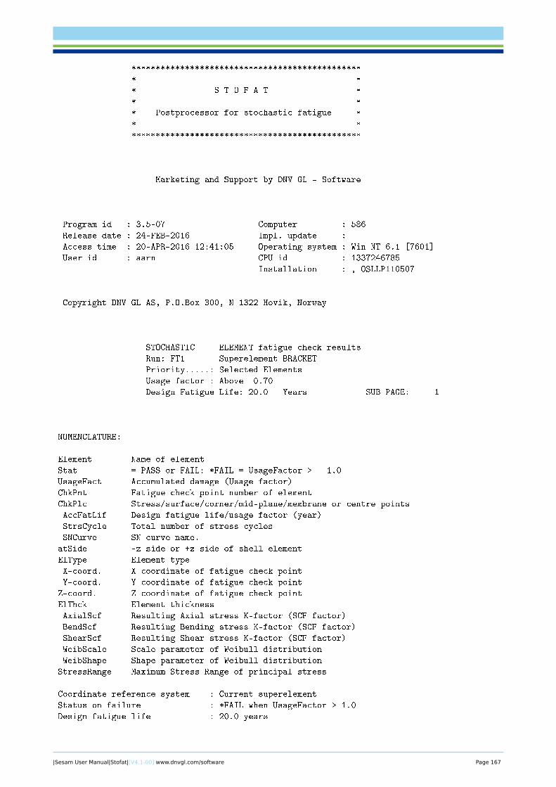
***********************************************
* *
* S T O F A T *
* *
* Postprocessor for stochastic fatigue *
* *
***********************************************
Marketing and Support by DNV GL - Software
Program id : 3.5-07 Computer : 586
Release date : 24-FEB-2016 Impl. update :
Access time : 20-APR-2016 12:41:05 Operating system : Win NT 6.1 [7601]
User id : aarn CPU id : 1337246785
Installation : , OSLLP110507
Copyright DNV GL AS, P.O.Box 300, N-1322 Hovik, Norway
STOCHASTIC ELEMENT fatigue check results
Run: FT1 Superelement BRACKET
Priority.....: Selected Elements
Usage factor : Above 0.70
Design Fatigue Life: 20.0 Years SUB PAGE: 1
NOMENCLATURE:
Element Name of element
Stat = PASS or FAIL: *FAIL = UsageFactor > 1.0
UsageFact Accumulated damage (Usage factor)
ChkPnt Fatigue check point number of element
ChkPlc Stress/surface/corner/mid-plane/membrane or centre points
AccFatLif Design fatigue life/usage factor (year)
StrsCycle Total number of stress cycles
SNCurve SN curve name.
atSide -z side or +z side of shell element
ElType Element type
X-coord. X coordinate of fatigue check point
Y-coord. Y coordinate of fatigue check point
Z-coord. Z coordinate of fatigue check point
ElThck Element thickness
AxialScf Resulting Axial stress K-factor (SCF factor)
BendScf Resulting Bending stress K-factor (SCF factor)
ShearScf Resulting Shear stress K-factor (SCF factor)
WeibScale Scale parameter of Weibull distribution
WeibShape Shape parameter of Weibull distribution
StressRange Maximum Stress Range of principal stress
Coordinate reference system : Current superelement
Status on failure : *FAIL when UsageFactor > 1.0
Design fatigue life : 20.0 years
|Sesam User Manual|Stofat|[V4.1-00] www.dnvgl.com/software Page 167
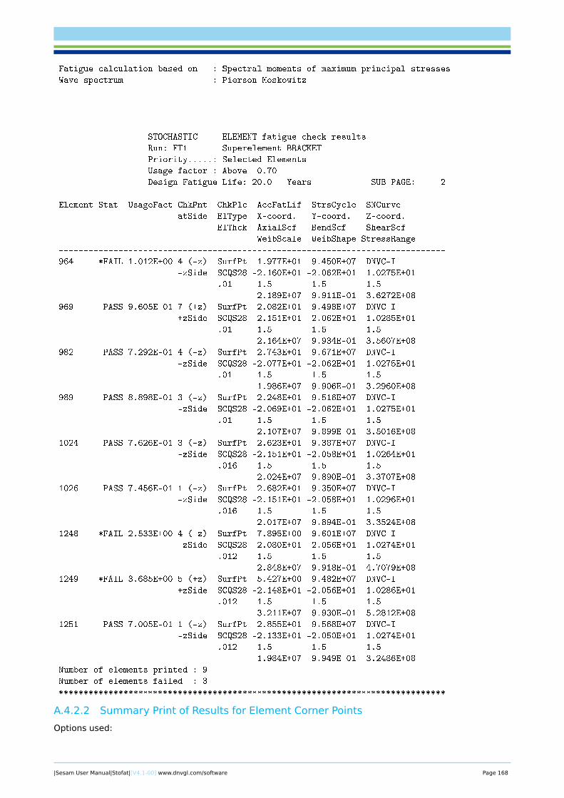
Fatigue calculation based on : Spectral moments of maximum principal stresses
Wave spectrum : Pierson Moskowitz
STOCHASTIC ELEMENT fatigue check results
Run: FT1 Superelement BRACKET
Priority.....: Selected Elements
Usage factor : Above 0.70
Design Fatigue Life: 20.0 Years SUB PAGE: 2
Element Stat UsageFact ChkPnt ChkPlc AccFatLif StrsCycle SNCurve
atSide ElType X-coord. Y-coord. Z-coord.
ElThck AxialScf BendScf ShearScf
WeibScale WeibShape StressRange
------------------------------------------------------------------------------
964 *FAIL 1.012E+00 4 (-z) SurfPt 1.977E+01 9.450E+07 DNVC-I
-zSide SCQS28 -2.160E+01 -2.062E+01 1.0275E+01
.01 1.5 1.5 1.5
2.189E+07 9.911E-01 3.6272E+08
969 PASS 9.605E-01 7 (+z) SurfPt 2.082E+01 9.498E+07 DNVC-I
+zSide SCQS28 -2.151E+01 -2.062E+01 1.0285E+01
.01 1.5 1.5 1.5
2.164E+07 9.934E-01 3.5607E+08
982 PASS 7.292E-01 4 (-z) SurfPt 2.743E+01 9.671E+07 DNVC-I
-zSide SCQS28 -2.077E+01 -2.062E+01 1.0275E+01
.01 1.5 1.5 1.5
1.986E+07 9.906E-01 3.2960E+08
989 PASS 8.898E-01 3 (-z) SurfPt 2.248E+01 9.516E+07 DNVC-I
-zSide SCQS28 -2.069E+01 -2.062E+01 1.0275E+01
.01 1.5 1.5 1.5
2.107E+07 9.899E-01 3.5016E+08
1024 PASS 7.626E-01 3 (-z) SurfPt 2.623E+01 9.387E+07 DNVC-I
-zSide SCQS28 -2.151E+01 -2.058E+01 1.0264E+01
.016 1.5 1.5 1.5
2.024E+07 9.890E-01 3.3707E+08
1026 PASS 7.456E-01 1 (-z) SurfPt 2.682E+01 9.350E+07 DNVC-I
-zSide SCQS28 -2.151E+01 -2.058E+01 1.0296E+01
.016 1.5 1.5 1.5
2.017E+07 9.894E-01 3.3524E+08
1248 *FAIL 2.533E+00 4 (-z) SurfPt 7.895E+00 9.601E+07 DNVC-I
-zSide SCQS28 -2.080E+01 -2.056E+01 1.0274E+01
.012 1.5 1.5 1.5
2.848E+07 9.918E-01 4.7079E+08
1249 *FAIL 3.685E+00 5 (+z) SurfPt 5.427E+00 9.482E+07 DNVC-I
+zSide SCQS28 -2.148E+01 -2.056E+01 1.0286E+01
.012 1.5 1.5 1.5
3.211E+07 9.930E-01 5.2812E+08
1251 PASS 7.005E-01 1 (-z) SurfPt 2.855E+01 9.568E+07 DNVC-I
-zSide SCQS28 -2.133E+01 -2.050E+01 1.0274E+01
.012 1.5 1.5 1.5
1.984E+07 9.949E-01 3.2486E+08
Number of elements printed : 9
Number of elements failed : 3
******************************************************************************
A.4.2.2 Summary Print of Results for Element Corner Points
Options used:
|Sesam User Manual|Stofat|[V4.1-00] www.dnvgl.com/software Page 168
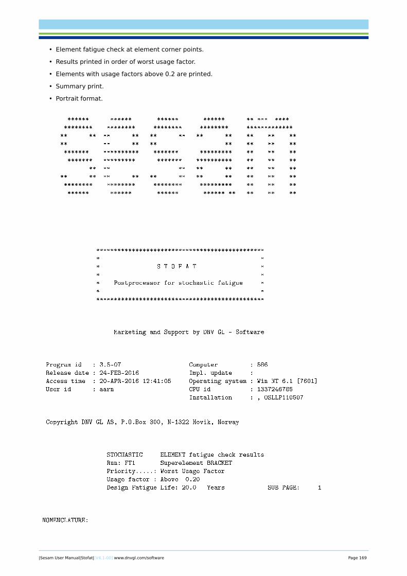
• Element fatigue check at element corner points.
• Results printed in order of worst usage factor.
• Elements with usage factors above 0.2 are printed.
• Summary print.
• Portrait format.
****** ****** ****** ****** ** *** ****
******** ******** ******** ******** *************
** ** ** ** ** ** ** ** ** ** **
** ** ** ** ** ** ** **
******* ********** ******* ********* ** ** **
******* ********* ******* ********** ** ** **
** ** ** ** ** ** ** **
** ** ** ** ** ** ** ** ** ** **
******** ******** ******** ********* ** ** **
****** ****** ****** ****** ** ** ** **
***********************************************
* *
* S T O F A T *
* *
* Postprocessor for stochastic fatigue *
* *
***********************************************
Marketing and Support by DNV GL - Software
Program id : 3.5-07 Computer : 586
Release date : 24-FEB-2016 Impl. update :
Access time : 20-APR-2016 12:41:05 Operating system : Win NT 6.1 [7601]
User id : aarn CPU id : 1337246785
Installation : , OSLLP110507
Copyright DNV GL AS, P.O.Box 300, N-1322 Hovik, Norway
STOCHASTIC ELEMENT fatigue check results
Run: FT1 Superelement BRACKET
Priority.....: Worst Usage Factor
Usage factor : Above 0.20
Design Fatigue Life: 20.0 Years SUB PAGE: 1
NOMENCLATURE:
|Sesam User Manual|Stofat|[V4.1-00] www.dnvgl.com/software Page 169
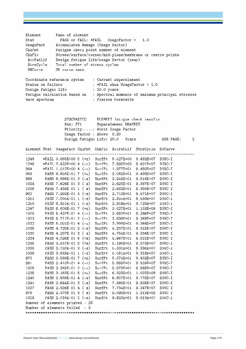
Element Name of element
Stat = PASS or FAIL: *FAIL = UsageFactor > 1.0
UsageFact Accumulated damage (Usage factor)
ChkPnt Fatigue check point number of element
ChkPlc Stress/surface/corner/mid-plane/membrane or centre points
AccFatLif Design fatigue life/usage factor (year)
StrsCycle Total number of stress cycles
SNCurve SN curve name.
Coordinate reference system : Current superelement
Status on failure : *FAIL when UsageFactor > 1.0
Design fatigue life : 20.0 years
Fatigue calculation based on : Spectral moments of maximum principal stresses
Wave spectrum : Pierson Moskowitz
STOCHASTIC ELEMENT fatigue check results
Run: FT1 Superelement BRACKET
Priority.....: Worst Usage Factor
Usage factor : Above 0.20
Design Fatigue Life: 20.0 Years SUB PAGE: 2
Element Stat UsageFact ChkPnt ChkPlc AccFatLif StrsCycle SNCurve
------------------------------------------------------------------------------
1249 *FAIL 3.685E+00 5 (+z) SurfPt 5.427E+00 9.482E+07 DNVC-I
1248 *FAIL 2.533E+00 4 (-z) SurfPt 7.895E+00 9.601E+07 DNVC-I
964 *FAIL 1.012E+00 4 (-z) SurfPt 1.977E+01 9.450E+07 DNVC-I
969 PASS 9.605E-01 7 (+z) SurfPt 2.082E+01 9.498E+07 DNVC-I
989 PASS 8.898E-01 3 (-z) SurfPt 2.248E+01 9.516E+07 DNVC-I
1024 PASS 7.626E-01 3 (-z) SurfPt 2.623E+01 9.387E+07 DNVC-I
1026 PASS 7.456E-01 1 (-z) SurfPt 2.682E+01 9.350E+07 DNVC-I
982 PASS 7.292E-01 4 (-z) SurfPt 2.743E+01 9.671E+07 DNVC-I
1251 PASS 7.005E-01 1 (-z) SurfPt 2.855E+01 9.568E+07 DNVC-I
1250 PASS 6.851E-01 1 (-z) SurfPt 2.919E+01 9.723E+07 DNVC-I
1247 PASS 6.608E-01 7 (+z) SurfPt 3.027E+01 1.133E+08 DNVC-I
1020 PASS 5.432E-01 4 (-z) SurfPt 3.682E+01 9.386E+07 DNVC-I
1023 PASS 5.211E-01 2 (-z) SurfPt 3.838E+01 9.349E+07 DNVC-I
1033 PASS 5.001E-01 4 (-z) SurfPt 3.999E+01 9.344E+07 DNVC-I
1035 PASS 4.720E-01 2 (-z) SurfPt 4.237E+01 9.315E+07 DNVC-I
1030 PASS 4.207E-01 3 (-z) SurfPt 4.754E+01 9.334E+07 DNVC-I
1234 PASS 4.026E-01 6 (+z) SurfPt 4.967E+01 9.821E+07 DNVC-I
1246 PASS 3.847E-01 8 (+z) SurfPt 5.198E+01 9.878E+07 DNVC-I
1036 PASS 3.750E-01 3 (-z) SurfPt 5.334E+01 9.336E+07 DNVC-I
1039 PASS 3.649E-01 1 (-z) SurfPt 5.481E+01 9.318E+07 DNVC-I
970 PASS 3.588E-01 7 (+z) SurfPt 5.574E+01 9.492E+07 DNVC-I
981 PASS 3.410E-01 4 (-z) SurfPt 5.866E+01 9.939E+07 DNVC-I
1025 PASS 3.345E-01 2 (-z) SurfPt 5.979E+01 9.565E+07 DNVC-I
1235 PASS 3.163E-01 5 (+z) SurfPt 6.323E+01 1.022E+08 DNVC-I
1240 PASS 2.938E-01 4 (-z) SurfPt 6.807E+01 9.775E+07 DNVC-I
1241 PASS 2.644E-01 3 (-z) SurfPt 7.565E+01 9.925E+07 DNVC-I
1027 PASS 2.586E-01 4 (-z) SurfPt 7.734E+01 9.247E+07 DNVC-I
976 PASS 2.470E-01 4 (-z) SurfPt 8.098E+01 1.019E+08 DNVC-I
1029 PASS 2.016E-01 2 (-z) SurfPt 9.923E+01 9.614E+07 DNVC-I
Number of elements printed : 29
Number of elements failed : 3
******************************************************************************
|Sesam User Manual|Stofat|[V4.1-00] www.dnvgl.com/software Page 170

A.5 Dump Print of fatigue Results
Example of dump print of fatigue results are given in the present section. Dump print is generated bythe command PRINT FATIGUE-RESULTS-DUMP. Prior to this command, dump print options must be set bythe command DEFINE FATIGUE-RESULTS-DUMP. Two dump print files are generated; <name>Dmp.lis and<name>Pex.lis. The <name> is given by the command DEFINE FATIGUE-RESULTS-DUMP FILENAME, defaultname is Stofat. Dump print may be generated both for element and hotspots fatigue check results. Notethat the dump print files may be excessive big for dump print of all elements of large models. Dump printshould therefor be executed with care and limited to a restricted number of elements.
Results are printed to the nameDmp.lis file when one of the following commands are ticked ON.
DEFINE FATIGUE-RESULTS-DUMP HOTSPOT-STRESS-TRANSFER-FUNCTION ONDEFINE FATIGUE-RESULTS-DUMP MOMENTS-OF-RESPONSE-SPECTRUM ONDEFINE FATIGUE-RESULTS-DUMP DAMAGE-PER-SEASTATE ONDEFINE FATIGUE-RESULTS-DUMP DAMAGE-PER-DIRECTION ONDEFINE FATIGUE-RESULTS-DUMP DAMAGE-PER-HOTSPOT ON
Results are printed to the namePex.lis file when one of the following commands are ticked ON.
DEFINE FATIGUE-RESULTS-DUMP EXCEEDENCE-PROBABILITY ON 11DEFINE FATIGUE-RESULTS-DUMP STRESS-RANGE-DISTRIBUTION ON 11DEFINE FATIGUE-RESULTS-DUMP WEIBULL-PARAMETERS ON
The following data are printed in the nameDmp.lis file:
• Stress transfer functions
• Spectral moments, mean zero-up crossing periods and spectral band width per sea state
• Damages and stress cycles per sea state
• Damages and stress cycles per wave direction
• Damage and stress cycles per element position or hotspot
The stress transfer functions printed is the maximum principal stresses at the user defined fatigue positionsof the elements forming the response spectra which are applied in the fatigue damage calculation. Thespectral moments printed are those found by integrating the response spectra. The spectral moments arescaled with the square of the element thickness factor (shell elements) and the static stress reduction factor(if included). The spectral band widths printed (resEps) are applied when the Wirsching correction factorfor broad band stress processes is requested, see section Appendix C.3 and command DEFINE WIDE-BAND-CORRECTION-FACTOR.
Only results of position 1 for one element are shown in present example and static stresses are not in-cluded.
nameDmp.lis file:
***************************************************************
** **
** S T O F A T **
** **
** F A T I G U E C H E C K R E S U L T S **
** O F **
** E L E M E N T S **
** **
** RUN : DMP1 **
** DATE/TIME: 2016-04-20 13:49:56 **
** **
***************************************************************
PRINT OF:
|Sesam User Manual|Stofat|[V4.1-00] www.dnvgl.com/software Page 171
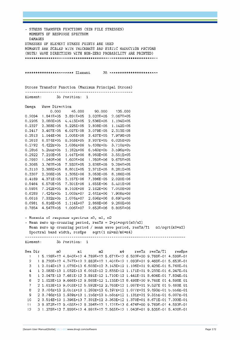
- STRESS TRANSFER FUNCTIONS (SIN FILE STRESSES)
- MOMENTS OF RESPONSE SPECTRUM
- DAMAGES
STRESSES OF ELEMENT STRESS POINTS ARE USED
MOMENTS ARE SCALED WITH THICKNESS AND STATIC REDUCTION FACTORS
(NOTE! WAVE DIRECTIONS WITH NON-ZERO PROBABILITY ARE PRINTED)
***************************************************************
*********************** Element 35 ***********************
Stress Transfer Function (Maximum Principal Stress)
---------------------------------------------------
Element: 35 Position: 1
Omega Wave Direction
0.000 45.000 90.000 135.000
0.2094 1.841E+05 3.891E+05 3.032E+05 2.067E+05
0.2205 2.050E+05 4.413E+05 2.536E+05 1.194E+05
0.2327 2.358E+05 5.225E+05 2.808E+05 1.142E+05
0.2417 3.407E+05 6.027E+05 3.079E+05 2.313E+05
0.2513 1.044E+06 1.005E+06 3.437E+05 7.979E+05
0.2618 6.874E+05 8.346E+05 3.937E+05 6.025E+05
0.2792 4.422E+05 1.036E+06 5.408E+05 3.710E+05
0.2856 5.255E+05 1.182E+06 6.540E+05 3.596E+05
0.2922 7.210E+05 1.447E+06 8.983E+05 3.551E+05
0.2992 1.040E+06 1.602E+06 1.250E+06 9.675E+05
0.3065 3.762E+05 7.932E+05 3.828E+05 9.284E+05
0.3110 2.385E+05 8.801E+05 2.371E+05 8.281E+05
0.3307 2.205E+05 1.305E+06 3.053E+05 8.186E+05
0.4189 4.371E+05 3.157E+06 7.386E+05 2.020E+06
0.5464 6.570E+05 7.301E+06 1.655E+06 5.401E+06
0.5984 7.242E+05 9.140E+06 2.162E+06 7.040E+06
0.6283 7.424E+05 1.003E+07 2.441E+06 7.906E+06
0.6616 7.332E+05 1.076E+07 2.696E+06 8.697E+06
0.6981 6.816E+05 1.114E+07 2.868E+06 9.260E+06
0.7854 4.547E+05 1.006E+07 2.653E+06 8.805E+06
- Moments of response spectrum m0, m1, m2
- Mean zero up-crossing period, resTz = 2*pi*sqrt(m0/m2)
- Mean zero up-crossing period / mean wave period, resTz/T1 = m1/sqrt(m0*m2)
- Spectral band width, resEps = sqrt(1-m2*m2/m0*m4)
----------------------------------------------------------------------------
Element: 35 Position: 1
Sea Dir m0 m1 m2 m4 resTz resTz/T1 resEps
1 1 5.128E+12 4.840E+12 4.789E+12 5.671E+12 6.502E+00 9.768E-01 4.599E-01
2 1 8.720E+12 4.747E+12 2.883E+12 1.401E+12 1.093E+01 9.468E-01 5.653E-01
3 1 2.014E+13 1.079E+13 6.503E+12 3.143E+12 1.106E+01 9.429E-01 5.760E-01
4 1 2.083E+13 1.032E+13 6.001E+12 2.835E+12 1.171E+01 9.233E-01 6.247E-01
5 1 2.047E+13 7.681E+12 3.891E+12 1.710E+12 1.441E+01 8.606E-01 7.534E-01
6 2 1.023E+13 9.666E+12 9.568E+12 1.135E+13 6.498E+00 9.768E-01 4.598E-01
7 2 1.613E+13 9.048E+12 5.592E+12 2.763E+12 1.067E+01 9.527E-01 5.463E-01
8 2 3.704E+13 2.051E+13 1.260E+13 6.197E+12 1.077E+01 9.493E-01 5.556E-01
9 2 3.746E+13 1.939E+13 1.156E+13 5.585E+12 1.131E+01 9.315E-01 6.007E-01
10 2 3.514E+13 1.398E+13 7.391E+12 3.363E+12 1.370E+01 8.671E-01 7.333E-01
11 3 9.973E+12 9.455E+12 9.394E+12 1.121E+13 6.474E+00 9.769E-01 4.593E-01
12 3 1.375E+13 7.899E+12 4.991E+12 2.565E+12 1.043E+01 9.535E-01 5.420E-01
|Sesam User Manual|Stofat|[V4.1-00] www.dnvgl.com/software Page 172
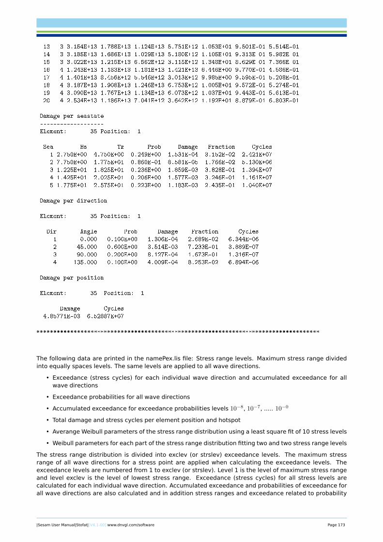
13 3 3.154E+13 1.788E+13 1.124E+13 5.751E+12 1.053E+01 9.501E-01 5.514E-01
14 3 3.185E+13 1.686E+13 1.029E+13 5.180E+12 1.105E+01 9.313E-01 5.982E-01
15 3 3.022E+13 1.215E+13 6.562E+12 3.115E+12 1.348E+01 8.629E-01 7.366E-01
16 4 1.243E+13 1.183E+13 1.181E+13 1.421E+13 6.446E+00 9.770E-01 4.586E-01
17 4 1.401E+13 8.456E+12 5.546E+12 3.013E+12 9.985E+00 9.595E-01 5.208E-01
18 4 3.187E+13 1.908E+13 1.246E+13 6.753E+12 1.005E+01 9.572E-01 5.274E-01
19 4 3.090E+13 1.767E+13 1.134E+13 6.073E+12 1.037E+01 9.443E-01 5.613E-01
20 4 2.534E+13 1.186E+13 7.041E+12 3.642E+12 1.192E+01 8.879E-01 6.803E-01
Damage per seastate
-------------------
Element: 35 Position: 1
Sea Hs Tz Prob Damage Fraction Cycles
1 2.750E+00 4.750E+00 0.249E+00 1.531E-04 3.152E-02 2.421E+07
2 7.750E+00 1.775E+01 0.860E-01 8.581E-05 1.766E-02 5.130E+06
3 1.225E+01 1.825E+01 0.236E+00 1.859E-03 3.828E-01 1.394E+07
4 1.425E+01 2.025E+01 0.206E+00 1.577E-03 3.246E-01 1.161E+07
5 1.775E+01 2.575E+01 0.223E+00 1.183E-03 2.435E-01 1.040E+07
Damage per direction
--------------------
Element: 35 Position: 1
Dir Angle Prob Damage Fraction Cycles
1 0.000 0.100E+00 1.306E-04 2.689E-02 6.344E+06
2 45.000 0.600E+00 3.514E-03 7.233E-01 3.889E+07
3 90.000 0.200E+00 8.127E-04 1.673E-01 1.316E+07
4 135.000 0.100E+00 4.009E-04 8.253E-02 6.894E+06
Damage per position
-------------------
Element: 35 Position: 1
Damage Cycles
4.85771E-03 6.52887E+07
************************************************************************************
The following data are printed in the namePex.lis file: Stress range levels. Maximum stress range dividedinto equally spaces levels. The same levels are applied to all wave directions.
• Exceedance (stress cycles) for each individual wave direction and accumulated exceedance for allwave directions
• Exceedance probabilities for all wave directions
• Accumulated exceedance for exceedance probabilities levels 10−8, 10−7, ..... 10−0
• Total damage and stress cycles per element position and hotspot
• Averange Weibull parameters of the stress range distribution using a least square fit of 10 stress levels
• Weibull parameters for each part of the stress range distribution fitting two and two stress range levels
The stress range distribution is divided into exclev (or strslev) exceedance levels. The maximum stressrange of all wave directions for a stress point are applied when calculating the exceedance levels. Theexceedance levels are numbered from 1 to exclev (or strslev). Level 1 is the level of maximum stress rangeand level exclev is the level of lowest stress range. Exceedance (stress cycles) for all stress levels arecalculated for each individual wave direction. Accumulated exceedance and probabilities of exceedance forall wave directions are also calculated and in addition stress ranges and exceedance related to probability
|Sesam User Manual|Stofat|[V4.1-00] www.dnvgl.com/software Page 173
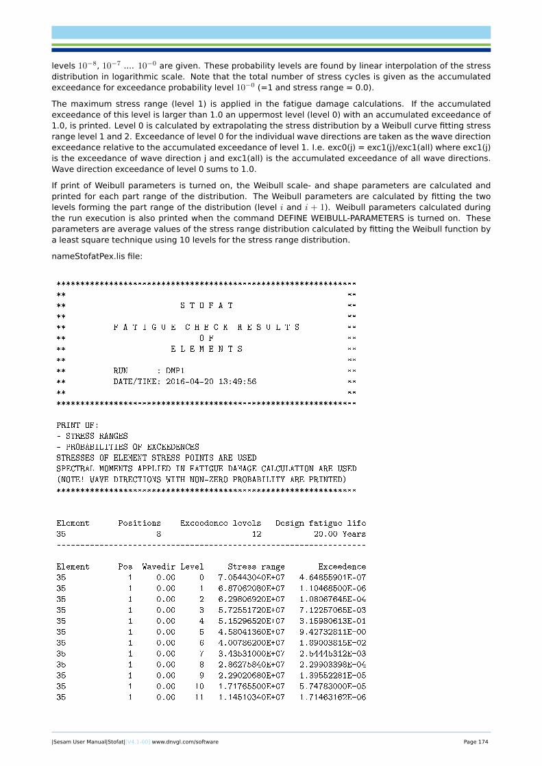
levels 10−8, 10−7 .... 10−0 are given. These probability levels are found by linear interpolation of the stressdistribution in logarithmic scale. Note that the total number of stress cycles is given as the accumulatedexceedance for exceedance probability level 10−0 (=1 and stress range = 0.0).
The maximum stress range (level 1) is applied in the fatigue damage calculations. If the accumulatedexceedance of this level is larger than 1.0 an uppermost level (level 0) with an accumulated exceedance of1.0, is printed. Level 0 is calculated by extrapolating the stress distribution by a Weibull curve fitting stressrange level 1 and 2. Exceedance of level 0 for the individual wave directions are taken as the wave directionexceedance relative to the accumulated exceedance of level 1. I.e. exc0(j) = exc1(j)/exc1(all) where exc1(j)is the exceedance of wave direction j and exc1(all) is the accumulated exceedance of all wave directions.Wave direction exceedance of level 0 sums to 1.0.
If print of Weibull parameters is turned on, the Weibull scale- and shape parameters are calculated andprinted for each part range of the distribution. The Weibull parameters are calculated by fitting the twolevels forming the part range of the distribution (level i and i + 1). Weibull parameters calculated duringthe run execution is also printed when the command DEFINE WEIBULL-PARAMETERS is turned on. Theseparameters are average values of the stress range distribution calculated by fitting the Weibull function bya least square technique using 10 levels for the stress range distribution.
nameStofatPex.lis file:
***************************************************************
** **
** S T O F A T **
** **
** F A T I G U E C H E C K R E S U L T S **
** O F **
** E L E M E N T S **
** **
** RUN : DMP1 **
** DATE/TIME: 2016-04-20 13:49:56 **
** **
***************************************************************
PRINT OF:
- STRESS RANGES
- PROBABILITIES OF EXCEEDENCES
STRESSES OF ELEMENT STRESS POINTS ARE USED
SPECTRAL MOMENTS APPLIED IN FATIGUE DAMAGE CALCULATION ARE USED
(NOTE! WAVE DIRECTIONS WITH NON-ZERO PROBABILITY ARE PRINTED)
***************************************************************
Element Positions Exceedence levels Design fatigue life
35 8 12 20.00 Years
-----------------------------------------------------------------
Element Pos Wavedir Level Stress range Exceedence
35 1 0.00 0 7.05443040E+07 4.64855901E-07
35 1 0.00 1 6.87062080E+07 1.10468500E-06
35 1 0.00 2 6.29806920E+07 1.08067645E-04
35 1 0.00 3 5.72551720E+07 7.12257065E-03
35 1 0.00 4 5.15296520E+07 3.15980613E-01
35 1 0.00 5 4.58041360E+07 9.42732811E+00
35 1 0.00 6 4.00786200E+07 1.89003815E+02
35 1 0.00 7 3.43531000E+07 2.54445312E+03
35 1 0.00 8 2.86275840E+07 2.29903398E+04
35 1 0.00 9 2.29020680E+07 1.39552281E+05
35 1 0.00 10 1.71765500E+07 5.74783000E+05
35 1 0.00 11 1.14510340E+07 1.71463162E+06
|Sesam User Manual|Stofat|[V4.1-00] www.dnvgl.com/software Page 174
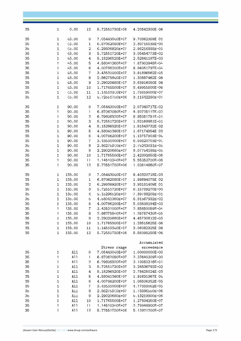
35 1 0.00 12 5.72551750E+06 4.20542300E+06
35 1 45.00 0 7.05443040E+07 9.70862389E-01
35 1 45.00 1 6.87062080E+07 2.30716038E+00
35 1 45.00 2 6.29806920E+07 2.96216888E+01
35 1 45.00 3 5.72551720E+07 3.05454773E+02
35 1 45.00 4 5.15296520E+07 2.52841187E+03
35 1 45.00 5 4.58041360E+07 1.67903945E+04
35 1 45.00 6 4.00786200E+07 8.94051797E+04
35 1 45.00 7 3.43531000E+07 3.81696562E+05
35 1 45.00 8 2.86275840E+07 1.30887462E+06
35 1 45.00 9 2.29020680E+07 3.63916050E+06
35 1 45.00 10 1.71765500E+07 8.49955800E+06
35 1 45.00 11 1.14510340E+07 1.76659000E+07
35 1 45.00 12 5.72551750E+06 3.11642280E+07
35 1 90.00 0 7.05443040E+07 2.07340717E-02
35 1 90.00 1 6.87062080E+07 4.92725112E-02
35 1 90.00 2 6.29806920E+07 9.85051751E-01
35 1 90.00 3 5.72551720E+07 1.52169981E+01
35 1 90.00 4 5.15296520E+07 1.81543732E+02
35 1 90.00 5 4.58041360E+07 1.67174854E+03
35 1 90.00 6 4.00786200E+07 1.18757803E+04
35 1 90.00 7 3.43531000E+07 6.50620703E+04
35 1 90.00 8 2.86275840E+07 2.75243031E+05
35 1 90.00 9 2.29020680E+07 9.07754188E+05
35 1 90.00 10 1.71765500E+07 2.42392850E+06
35 1 90.00 11 1.14510340E+07 5.55353700E+06
35 1 90.00 12 5.72551750E+06 1.03614860E+07
35 1 135.00 0 7.05443040E+07 8.40320718E-03
35 1 135.00 1 6.87062080E+07 1.99694075E-02
35 1 135.00 2 6.29806920E+07 3.98181409E-01
35 1 135.00 3 5.72551720E+07 6.15789270E+00
35 1 135.00 4 5.15296520E+07 7.39788208E+01
35 1 135.00 5 4.58041360E+07 6.91567932E+02
35 1 135.00 6 4.00786200E+07 5.03638184E+03
35 1 135.00 7 3.43531000E+07 2.85850059E+04
35 1 135.00 8 2.86275840E+07 1.26757430E+05
35 1 135.00 9 2.29020680E+07 4.45730812E+05
35 1 135.00 10 1.71765500E+07 1.28515625E+06
35 1 135.00 11 1.14510340E+07 3.06082325E+06
35 1 135.00 12 5.72551750E+06 5.56098250E+06
Accumulated
Stress range exceedence
35 1 All 0 7.05443040E+07 1.00000000E+00
35 1 All 1 6.87062080E+07 2.37640309E+00
35 1 All 2 6.29806920E+07 3.10050316E+01
35 1 All 3 5.72551720E+07 3.26836792E+02
35 1 All 4 5.15296520E+07 2.78425024E+03
35 1 All 5 4.58041360E+07 1.91631367E+04
35 1 All 6 4.00786200E+07 1.06506352E+05
35 1 All 7 3.43531000E+07 4.77888062E+05
35 1 All 8 2.86275840E+07 1.73386550E+06
35 1 All 9 2.29020680E+07 5.13219900E+06
35 1 All 10 1.71765500E+07 1.27834250E+07
35 1 All 11 1.14510340E+07 2.79948900E+07
35 1 All 12 5.72551750E+06 5.12921200E+07
|Sesam User Manual|Stofat|[V4.1-00] www.dnvgl.com/software Page 175
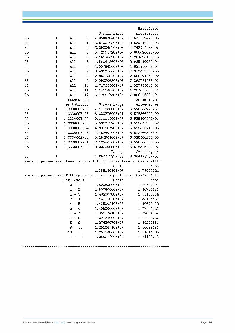
Exceedence
Stress range probability
35 1 All 0 7.05443040E+07 1.53165942E-08
35 1 All 1 6.87062080E+07 3.63984043E-08
35 1 All 2 6.29806920E+07 4.74891493E-07
35 1 All 3 5.72551720E+07 5.00602664E-06
35 1 All 4 5.15296520E+07 4.26452316E-05
35 1 All 5 4.58041360E+07 2.93513993E-04
35 1 All 6 4.00786200E+07 1.63131463E-03
35 1 All 7 3.43531000E+07 7.31961755E-03
35 1 All 8 2.86275840E+07 2.65569147E-02
35 1 All 9 2.29020680E+07 7.86078125E-02
35 1 All 10 1.71765500E+07 1.95798546E-01
35 1 All 11 1.14510340E+07 4.28786367E-01
35 1 All 12 5.72551750E+06 7.85620630E-01
Exceedence Accumulated
probability Stress range exceedences
35 1 1.000000E-08 7.17800080E+07 6.52886629E-01
35 1 1.000000E-07 6.63937600E+07 6.52886629E+00
35 1 1.000000E-06 6.11111560E+07 6.52886658E+01
35 1 1.000000E-05 5.53395320E+07 6.52886597E+02
35 1 1.000000E-04 4.89166720E+07 6.52886621E+03
35 1 1.000000E-03 4.16350200E+07 6.52886680E+04
35 1 1.000000E-02 3.28696140E+07 6.52886625E+05
35 1 1.000000E-01 2.12286560E+07 6.52886650E+06
35 1 1.000000E+00 0.00000000E+00 6.52886640E+07
Damage Cycles/year
35 1 4.85771289E-03 3.26443325E+06
Weibull parameters. Least square fit. 10 range levels. WavDir=All:
Scale Shape
1.35513030E+07 1.73909724
Weibull parameters. Fitting two and two range levels. WavDir=All:
Fit levels Scale Shape
0 - 1 1.50085960E+07 1.86742401
1 - 2 1.50060490E+07 1.86721671
2 - 3 1.48230780E+07 1.85138214
3 - 4 1.46112040E+07 1.83186531
4 - 5 1.43590210E+07 1.80690432
5 - 6 1.40500640E+07 1.77364624
6 - 7 1.36693410E+07 1.72834957
7 - 8 1.32134990E+07 1.66699767
8 - 9 1.27439970E+07 1.59247661
9 - 10 1.25164710E+07 1.54499471
10 - 11 1.26920860E+07 1.61611986
11 - 12 1.25521400E+07 1.81129718
***********************************************************************
|Sesam User Manual|Stofat|[V4.1-00] www.dnvgl.com/software Page 176
B Load and Response Modelling
The major time varying loads on marine structures are generally those caused by waves. An adequate de-scription of ocean waves is therefore necessary for a fatigue analysis. When the long term stress rangeresponse distribution is assigned to be a sum of Rayleigh distributions (or for a Weibull fit of the sum ofRayleigh distributions), Stofat apply spectral fatigue analysis where only the load response caused by fluc-tuating wave loading is considered. For the real sea state, the wave model assumptions applied in Stofatare not exactly fulfilled. However, from an engineering point of view they are very attractive due to thesimplification they imply in the structural analysis.
This chapter focus on the load and response modelling applied in Stofat when the long-term stress rangedistribution is assigned to be a sum of Rayleigh distributions. First the sea environment model is considered.Then the load model and the global structural analysis are described leading to transfer functions for se-lected forces. Finally the local stress analysis is discussed. The sources of uncertainty and their treatmentis presented throughout the chapter.
B.1 Sea State Description
The load model in Stofat is based on a description of the wave conditions into a set of stationary short termsea states. Each sea state is characterized by
• Main wave direction θ0, measured relative to a given reference direction.
• Wave spectrum model e.g. Jonswap
• Characteristic sea state parameters
– significant wave height HS , defined as the average of the upper third of the wave heights.
– Mean zero up-crossing period TZ , defined as the time between sucessive up-crossing of the stillwater level, averaged over the number of waves
• wave spreading function
For each sea state the long term probabilities of the different main wave directions are given along witha wave scatter diagram for each direction. A wave scatter diagram gives either the occurrence or theprobability for each set of HS and TZ values. A unique wave spreading function is either assigned to all ora subset of the wave-statistics given by each assigned scatter diagram. If no wave spreading function isassigned, long crested sea is assumed.
B.1.1 Main Wave Directions
Sets of wave observations may be sorted with respect to the corresponding main wave directions if direc-tional buoy or hindcast data are available (or wind directions). Statistics on the observations may be madeindividually for each sector, or one may assume that the statistical properties for the occurrence of wavesare the same in all sectors. The word ‘main wave direction’ denotes the middle direction for each of thesectors. The analysis may only be performed for waves in these discrete directions. In Stofat each mainwave direction i is defined by the angle θi, measured relative to a given reference direction, usually de-fined as the structures global x-axis. An example of sector numbering and main wave directions is shown inFigure B.1
|Sesam User Manual|Stofat|[V4.1-00] www.dnvgl.com/software Page 177
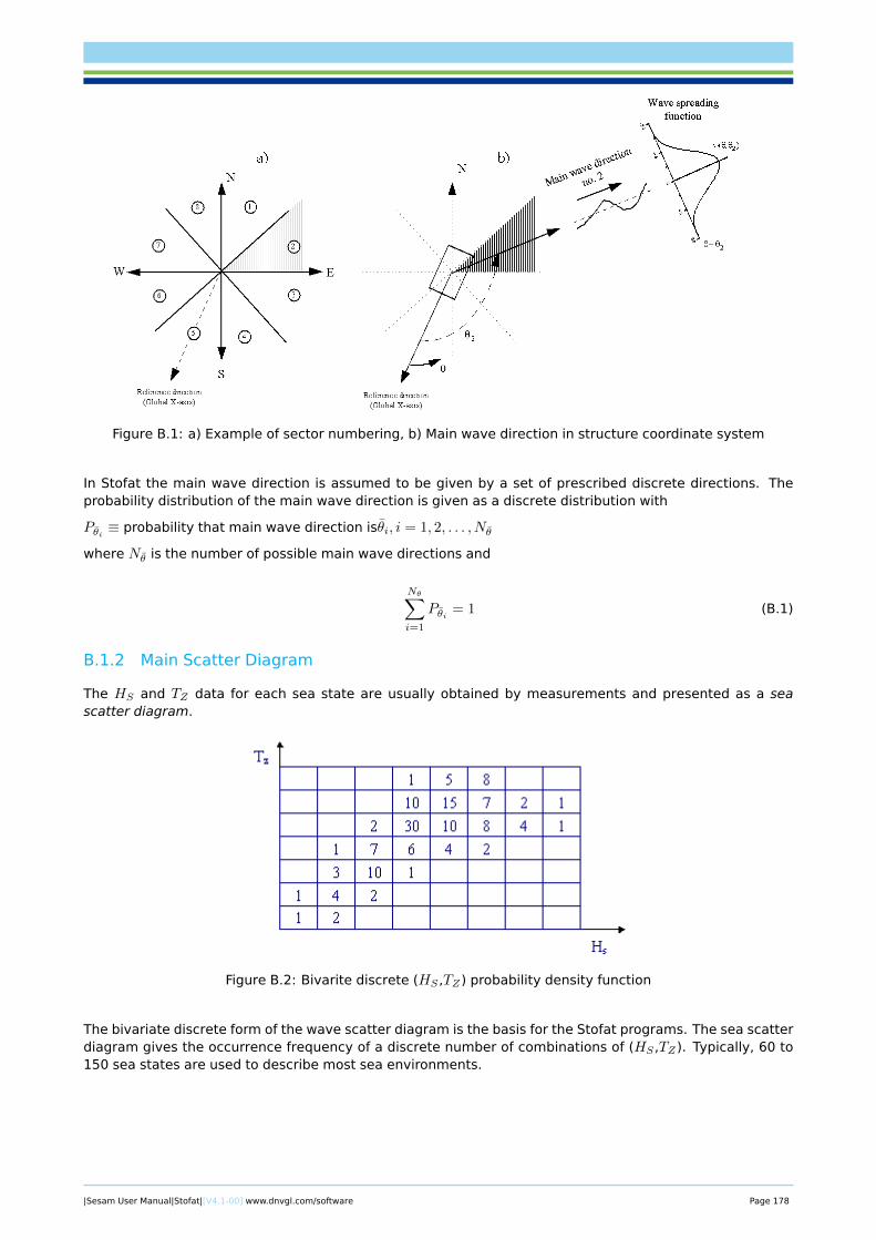
Figure B.1: a) Example of sector numbering, b) Main wave direction in structure coordinate system
In Stofat the main wave direction is assumed to be given by a set of prescribed discrete directions. Theprobability distribution of the main wave direction is given as a discrete distribution with
Pθi ≡ probability that main wave direction isθi, i = 1, 2, . . . , Nθ
where Nθ is the number of possible main wave directions and
Nθ∑i=1
Pθi = 1 (B.1)
B.1.2 Main Scatter Diagram
The HS and TZ data for each sea state are usually obtained by measurements and presented as a seascatter diagram.
Figure B.2: Bivarite discrete (HS ,TZ) probability density function
The bivariate discrete form of the wave scatter diagram is the basis for the Stofat programs. The sea scatterdiagram gives the occurrence frequency of a discrete number of combinations of (HS ,TZ). Typically, 60 to150 sea states are used to describe most sea environments.
|Sesam User Manual|Stofat|[V4.1-00] www.dnvgl.com/software Page 178
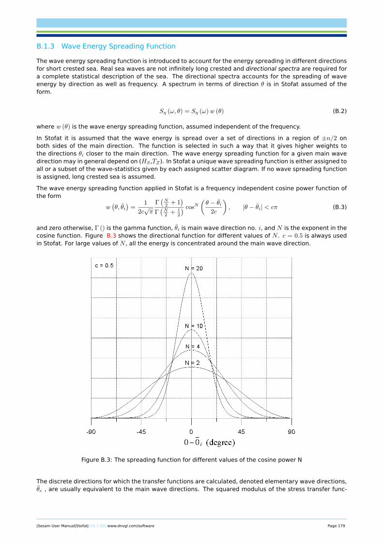
B.1.3 Wave Energy Spreading Function
The wave energy spreading function is introduced to account for the energy spreading in different directionsfor short crested sea. Real sea waves are not infinitely long crested and directional spectra are required fora complete statistical description of the sea. The directional spectra accounts for the spreading of waveenergy by direction as well as frequency. A spectrum in terms of direction θ is in Stofat assumed of theform.
Sη (ω, θ) = Sη (ω)w (θ) (B.2)
where w (θ) is the wave energy spreading function, assumed independent of the frequency.
In Stofat it is assumed that the wave energy is spread over a set of directions in a region of ±n/2 onboth sides of the main direction. The function is selected in such a way that it gives higher weights tothe directions θi closer to the main direction. The wave energy spreading function for a given main wavedirection may in general depend on (HS ,TZ). In Stofat a unique wave spreading function is either assigned toall or a subset of the wave-statistics given by each assigned scatter diagram. If no wave spreading functionis assigned, long crested sea is assumed.
The wave energy spreading function applied in Stofat is a frequency independent cosine power function ofthe form
w(θ, θi
)=
1
2c√π
Γ(N2 + 1
)Γ(N2 + 1
2
) cosN(θ − θi
2c
), |θ − θi| < cπ (B.3)
and zero otherwise, Γ () is the gamma function, θi is main wave direction no. i, and N is the exponent in thecosine function. Figure B.3 shows the directional function for different values of N . c = 0.5 is always usedin Stofat. For large values of N , all the energy is concentrated around the main wave direction.
Figure B.3: The spreading function for different values of the cosine power N
The discrete directions for which the transfer functions are calculated, denoted elementary wave directions,θe , are usually equivalent to the main wave directions. The squared modulus of the stress transfer func-
|Sesam User Manual|Stofat|[V4.1-00] www.dnvgl.com/software Page 179
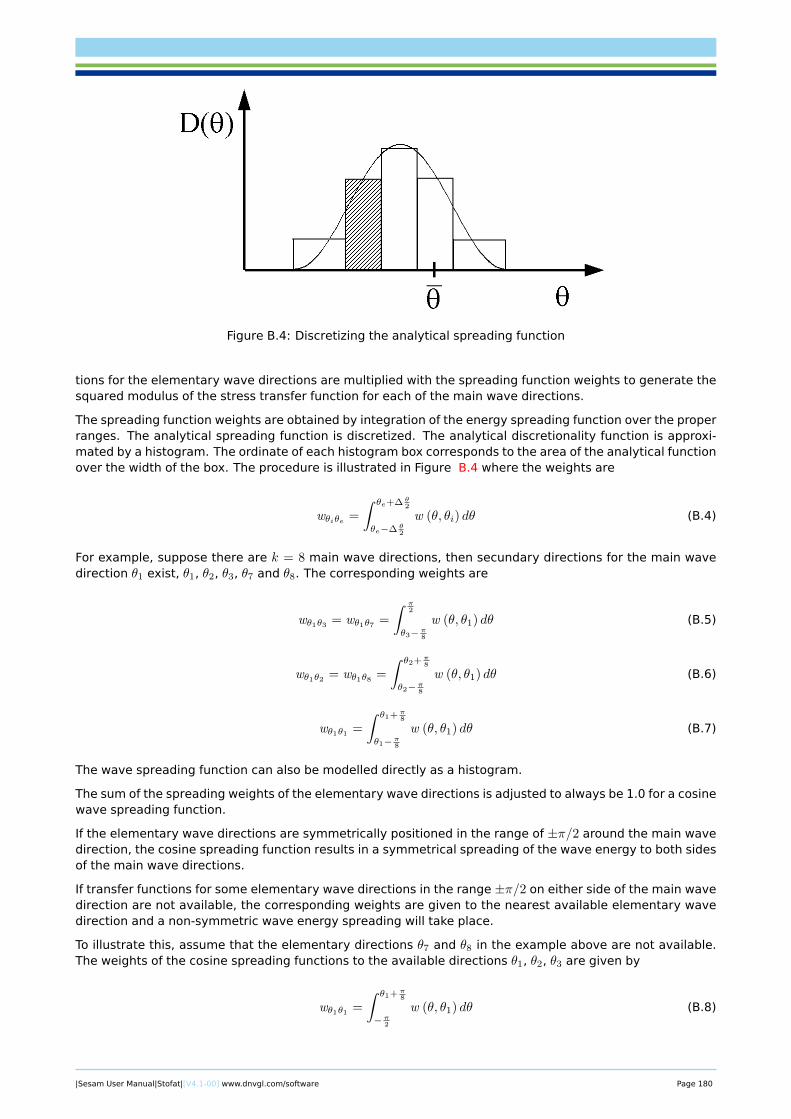
Figure B.4: Discretizing the analytical spreading function
tions for the elementary wave directions are multiplied with the spreading function weights to generate thesquared modulus of the stress transfer function for each of the main wave directions.
The spreading function weights are obtained by integration of the energy spreading function over the properranges. The analytical spreading function is discretized. The analytical discretionality function is approxi-mated by a histogram. The ordinate of each histogram box corresponds to the area of the analytical functionover the width of the box. The procedure is illustrated in Figure B.4 where the weights are
wθiθe =
∫ θe+∆ θ2
θe−∆ θ2
w (θ, θi) dθ (B.4)
For example, suppose there are k = 8 main wave directions, then secundary directions for the main wavedirection θ1 exist, θ1, θ2, θ3, θ7 and θ8. The corresponding weights are
wθ1θ3 = wθ1θ7 =
∫ π2
θ3−π8w (θ, θ1) dθ (B.5)
wθ1θ2 = wθ1θ8 =
∫ θ2+π8
θ2−π8w (θ, θ1) dθ (B.6)
wθ1θ1 =
∫ θ1+π8
θ1−π8w (θ, θ1) dθ (B.7)
The wave spreading function can also be modelled directly as a histogram.
The sum of the spreading weights of the elementary wave directions is adjusted to always be 1.0 for a cosinewave spreading function.
If the elementary wave directions are symmetrically positioned in the range of ±π/2 around the main wavedirection, the cosine spreading function results in a symmetrical spreading of the wave energy to both sidesof the main wave directions.
If transfer functions for some elementary wave directions in the range ±π/2 on either side of the main wavedirection are not available, the corresponding weights are given to the nearest available elementary wavedirection and a non-symmetric wave energy spreading will take place.
To illustrate this, assume that the elementary directions θ7 and θ8 in the example above are not available.The weights of the cosine spreading functions to the available directions θ1, θ2, θ3 are given by
wθ1θ1 =
∫ θ1+π8
−π2w (θ, θ1) dθ (B.8)
|Sesam User Manual|Stofat|[V4.1-00] www.dnvgl.com/software Page 180
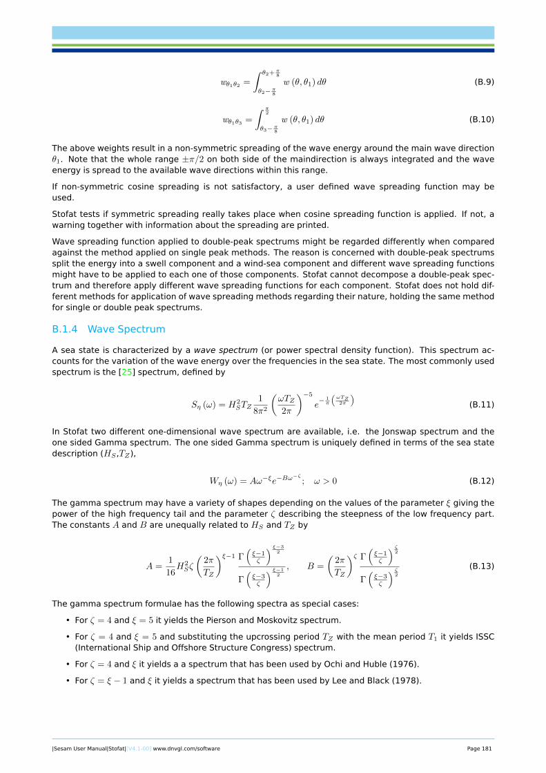
wθ1θ2 =
∫ θ2+π8
θ2−π8w (θ, θ1) dθ (B.9)
wθ1θ3 =
∫ π2
θ3−π8w (θ, θ1) dθ (B.10)
The above weights result in a non-symmetric spreading of the wave energy around the main wave directionθ1. Note that the whole range ±π/2 on both side of the maindirection is always integrated and the waveenergy is spread to the available wave directions within this range.
If non-symmetric cosine spreading is not satisfactory, a user defined wave spreading function may beused.
Stofat tests if symmetric spreading really takes place when cosine spreading function is applied. If not, awarning together with information about the spreading are printed.
Wave spreading function applied to double-peak spectrums might be regarded differently when comparedagainst the method applied on single peak methods. The reason is concerned with double-peak spectrumssplit the energy into a swell component and a wind-sea component and different wave spreading functionsmight have to be applied to each one of those components. Stofat cannot decompose a double-peak spec-trum and therefore apply different wave spreading functions for each component. Stofat does not hold dif-ferent methods for application of wave spreading methods regarding their nature, holding the same methodfor single or double peak spectrums.
B.1.4 Wave Spectrum
A sea state is characterized by a wave spectrum (or power spectral density function). This spectrum ac-counts for the variation of the wave energy over the frequencies in the sea state. The most commonly usedspectrum is the [25] spectrum, defined by
Sη (ω) = H2STZ
1
8π2
(ωTZ2π
)−5
e− 1π
(ωTZ2π
)(B.11)
In Stofat two different one-dimensional wave spectrum are available, i.e. the Jonswap spectrum and theone sided Gamma spectrum. The one sided Gamma spectrum is uniquely defined in terms of the sea statedescription (HS ,TZ),
Wη (ω) = Aω−ξe−Bω−ζ
; ω > 0 (B.12)
The gamma spectrum may have a variety of shapes depending on the values of the parameter ξ giving thepower of the high frequency tail and the parameter ζ describing the steepness of the low frequency part.The constants A and B are unequally related to HS and TZ by
A =1
16H2Sζ
(2π
TZ
)ξ−1 Γ(ξ−1ζ
) ξ−32
Γ(ξ−3ζ
) ξ−12
, B =
(2π
TZ
)ζ Γ(ξ−1ζ
) ζ2
Γ(ξ−3ζ
) ζ2
(B.13)
The gamma spectrum formulae has the following spectra as special cases:
• For ζ = 4 and ξ = 5 it yields the Pierson and Moskovitz spectrum.
• For ζ = 4 and ξ = 5 and substituting the upcrossing period TZ with the mean period T1 it yields ISSC(International Ship and Offshore Structure Congress) spectrum.
• For ζ = 4 and ξ it yields a a spectrum that has been used by Ochi and Huble (1976).
• For ζ = ξ − 1 and ξ it yields a spectrum that has been used by Lee and Black (1978).
|Sesam User Manual|Stofat|[V4.1-00] www.dnvgl.com/software Page 181
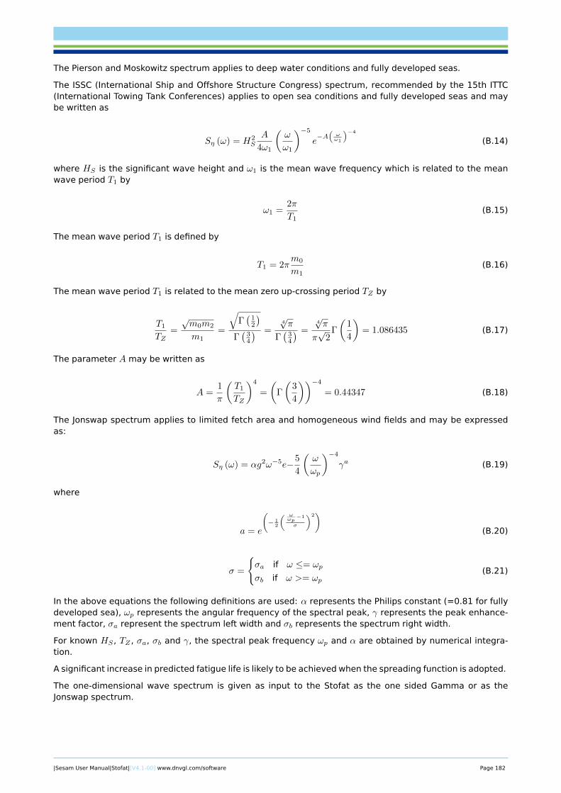
The Pierson and Moskowitz spectrum applies to deep water conditions and fully developed seas.
The ISSC (International Ship and Offshore Structure Congress) spectrum, recommended by the 15th ITTC(International Towing Tank Conferences) applies to open sea conditions and fully developed seas and maybe written as
Sη (ω) = H2S
A
4ω1
(ω
ω1
)−5
e−A(ωω1
)−4
(B.14)
where HS is the significant wave height and ω1 is the mean wave frequency which is related to the meanwave period T1 by
ω1 =2π
T1(B.15)
The mean wave period T1 is defined by
T1 = 2πm0
m1(B.16)
The mean wave period T1 is related to the mean zero up-crossing period TZ by
T1
TZ=
√m0m2
m1=
√Γ(
12
)Γ(
34
) =4√π
Γ(
34
) =4√π
π√
2Γ
(1
4
)= 1.086435 (B.17)
The parameter A may be written as
A =1
π
(T1
TZ
)4
=
(Γ
(3
4
))−4
= 0.44347 (B.18)
The Jonswap spectrum applies to limited fetch area and homogeneous wind fields and may be expressedas:
Sη (ω) = αg2ω−5e−5
4
(ω
ωp
)−4
γa (B.19)
where
a = e
(− 1
2
( ωωp
−1
σ
)2)
(B.20)
σ =
{σa if ω ≤= ωp
σb if ω >= ωp(B.21)
In the above equations the following definitions are used: α represents the Philips constant (=0.81 for fullydeveloped sea), ωp represents the angular frequency of the spectral peak, γ represents the peak enhance-ment factor, σa represent the spectrum left width and σb represents the spectrum right width.
For known HS , TZ , σa, σb and γ, the spectral peak frequency ωp and α are obtained by numerical integra-tion.
A significant increase in predicted fatigue life is likely to be achieved when the spreading function is adopted.
The one-dimensional wave spectrum is given as input to the Stofat as the one sided Gamma or as theJonswap spectrum.
|Sesam User Manual|Stofat|[V4.1-00] www.dnvgl.com/software Page 182
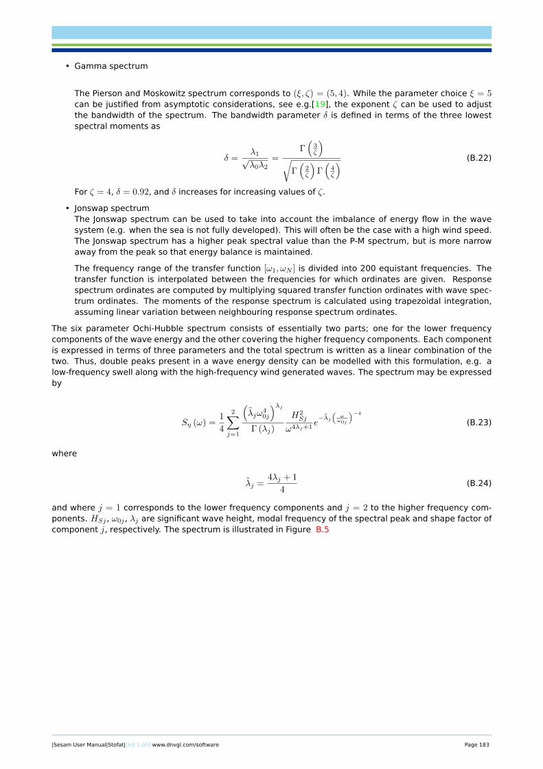
• Gamma spectrum
The Pierson and Moskowitz spectrum corresponds to (ξ, ζ) = (5, 4). While the parameter choice ξ = 5can be justified from asymptotic considerations, see e.g.[19], the exponent ζ can be used to adjustthe bandwidth of the spectrum. The bandwidth parameter δ is defined in terms of the three lowestspectral moments as
δ =λ1√λ0λ2
=Γ(
3ζ
)√
Γ(
2ζ
)Γ(
4ζ
) (B.22)
For ζ = 4, δ = 0.92, and δ increases for increasing values of ζ.
• Jonswap spectrumThe Jonswap spectrum can be used to take into account the imbalance of energy flow in the wavesystem (e.g. when the sea is not fully developed). This will often be the case with a high wind speed.The Jonswap spectrum has a higher peak spectral value than the P-M spectrum, but is more narrowaway from the peak so that energy balance is maintained.
The frequency range of the transfer function [ω1, ωN ] is divided into 200 equistant frequencies. Thetransfer function is interpolated between the frequencies for which ordinates are given. Responsespectrum ordinates are computed by multiplying squared transfer function ordinates with wave spec-trum ordinates. The moments of the response spectrum is calculated using trapezoidal integration,assuming linear variation between neighbouring response spectrum ordinates.
The six parameter Ochi-Hubble spectrum consists of essentially two parts; one for the lower frequencycomponents of the wave energy and the other covering the higher frequency components. Each componentis expressed in terms of three parameters and the total spectrum is written as a linear combination of thetwo. Thus, double peaks present in a wave energy density can be modelled with this formulation, e.g. alow-frequency swell along with the high-frequency wind generated waves. The spectrum may be expressedby
Sη (ω) =1
4
2∑j=1
(λjω
40j
)λjΓ (λj)
H2Sj
ω4λj+1e−λj
(ωω0j
)−4
(B.23)
where
λj =4λj + 1
4(B.24)
and where j = 1 corresponds to the lower frequency components and j = 2 to the higher frequency com-ponents. HSj , ω0j , λj are significant wave height, modal frequency of the spectral peak and shape factor ofcomponent j, respectively. The spectrum is illustrated in Figure B.5
|Sesam User Manual|Stofat|[V4.1-00] www.dnvgl.com/software Page 183
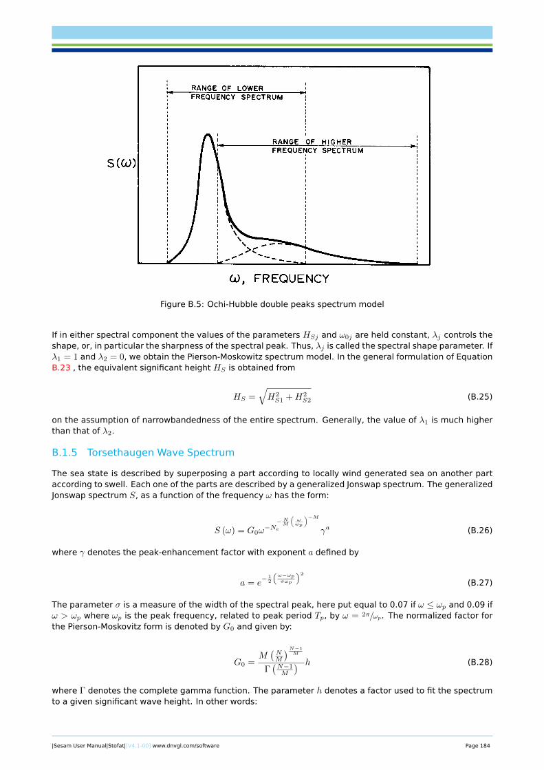
Figure B.5: Ochi-Hubble double peaks spectrum model
If in either spectral component the values of the parameters HSj and ω0j are held constant, λj controls theshape, or, in particular the sharpness of the spectral peak. Thus, λj is called the spectral shape parameter. Ifλ1 = 1 and λ2 = 0, we obtain the Pierson-Moskowitz spectrum model. In the general formulation of EquationB.23 , the equivalent significant height HS is obtained from
HS =√H2S1 +H2
S2 (B.25)
on the assumption of narrowbandedness of the entire spectrum. Generally, the value of λ1 is much higherthan that of λ2.
B.1.5 Torsethaugen Wave Spectrum
The sea state is described by superposing a part according to locally wind generated sea on another partaccording to swell. Each one of the parts are described by a generalized Jonswap spectrum. The generalizedJonswap spectrum S, as a function of the frequency ω has the form:
S (ω) = G0ω−N
− NM
(ωωp
)−Me γa (B.26)
where γ denotes the peak-enhancement factor with exponent a defined by
a = e− 1
2
(ω−ωpσωp
)2
(B.27)
The parameter σ is a measure of the width of the spectral peak, here put equal to 0.07 if ω ≤ ωp and 0.09 ifω > ωp where ωp is the peak frequency, related to peak period Tp, by ω = 2π/ωp. The normalized factor forthe Pierson-Moskovitz form is denoted by G0 and given by:
G0 =M(NM
)N−1M
Γ(N−1M
) h (B.28)
where Γ denotes the complete gamma function. The parameter h denotes a factor used to fit the spectrumto a given significant wave height. In other words:
|Sesam User Manual|Stofat|[V4.1-00] www.dnvgl.com/software Page 184
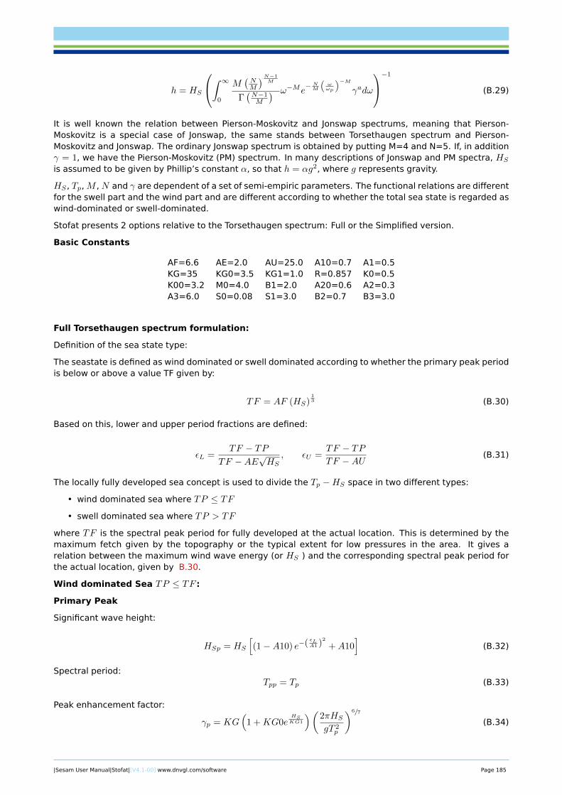
h = HS
∫ ∞0
M(NM
)N−1M
Γ(N−1M
) ω−Me− NM
(ωωp
)−M
γadω
−1
(B.29)
It is well known the relation between Pierson-Moskovitz and Jonswap spectrums, meaning that Pierson-Moskovitz is a special case of Jonswap, the same stands between Torsethaugen spectrum and Pierson-Moskovitz and Jonswap. The ordinary Jonswap spectrum is obtained by putting M=4 and N=5. If, in additionγ = 1, we have the Pierson-Moskovitz (PM) spectrum. In many descriptions of Jonswap and PM spectra, HS
is assumed to be given by Phillip’s constant α, so that h = αg2, where g represents gravity.
HS , Tp,M ,N and γ are dependent of a set of semi-empiric parameters. The functional relations are differentfor the swell part and the wind part and are different according to whether the total sea state is regarded aswind-dominated or swell-dominated.
Stofat presents 2 options relative to the Torsethaugen spectrum: Full or the Simplified version.
Basic Constants
AF=6.6 AE=2.0 AU=25.0 A10=0.7 A1=0.5KG=35 KG0=3.5 KG1=1.0 R=0.857 K0=0.5K00=3.2 M0=4.0 B1=2.0 A20=0.6 A2=0.3A3=6.0 S0=0.08 S1=3.0 B2=0.7 B3=3.0
Full Torsethaugen spectrum formulation:
Definition of the sea state type:
The seastate is defined as wind dominated or swell dominated according to whether the primary peak periodis below or above a value TF given by:
TF = AF (HS)13 (B.30)
Based on this, lower and upper period fractions are defined:
εL =TF − TP
TF −AE√HS
, εU =TF − TPTF −AU
(B.31)
The locally fully developed sea concept is used to divide the Tp −HS space in two different types:
• wind dominated sea where TP ≤ TF
• swell dominated sea where TP > TF
where TF is the spectral peak period for fully developed at the actual location. This is determined by themaximum fetch given by the topography or the typical extent for low pressures in the area. It gives arelation between the maximum wind wave energy (or HS ) and the corresponding spectral peak period forthe actual location, given by B.30.
Wind dominated Sea TP ≤ TF :
Primary Peak
Significant wave height:
HSp = HS
[(1−A10) e−( εLA1 )
2
+A10]
(B.32)
Spectral period:Tpp = Tp (B.33)
Peak enhancement factor:
γp = KG(
1 +KG0eHSKG1
)(2πHS
gT 2p
)6/7
(B.34)
|Sesam User Manual|Stofat|[V4.1-00] www.dnvgl.com/software Page 185
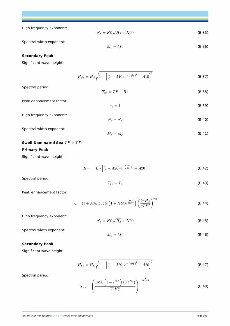
High frequency exponent:Np = K0
√HS +K00 (B.35)
Spectral width exponent:Mp = M0 (B.36)
Secondary Peak
Significant wave height:
HSs = HS
√1−
[(1−A10) e−( εLA1 )
2
+A10]2
(B.37)
Spectral period:Tps = TF +B1 (B.38)
Peak enhancement factor:γs = 1 (B.39)
High frequency exponent:Ns = Np (B.40)
Spectral width exponent:Ms = Mp (B.41)
Swell Dominated Sea TP > TF :
Primary Peak
Significant wave height:
HSp = HS
[(1−A20) e−( εU12 )
2
+A20]
(B.42)
Spectral period:Tpp = Tp (B.43)
Peak enhancement factor:
γp = (1 +A3εU )KG(
1 +KG0eHSKG1
)(2πHS
gTF 2
)6/7
(B.44)
High frequency exponent:Np = K0
√HS +K00 (B.45)
Spectral width exponent:Mp = M0 (B.46)
Secondary Peak
Significant wave height:
HSs = HS
√1−
[(1−A20) e−( εUA2 )
2
+A20]2
(B.47)
Spectral period:
Tps =
16S0(
1− eHSS1
) (0.4Ns
)G0H2
ss
−1
Ns−1
(B.48)
|Sesam User Manual|Stofat|[V4.1-00] www.dnvgl.com/software Page 186
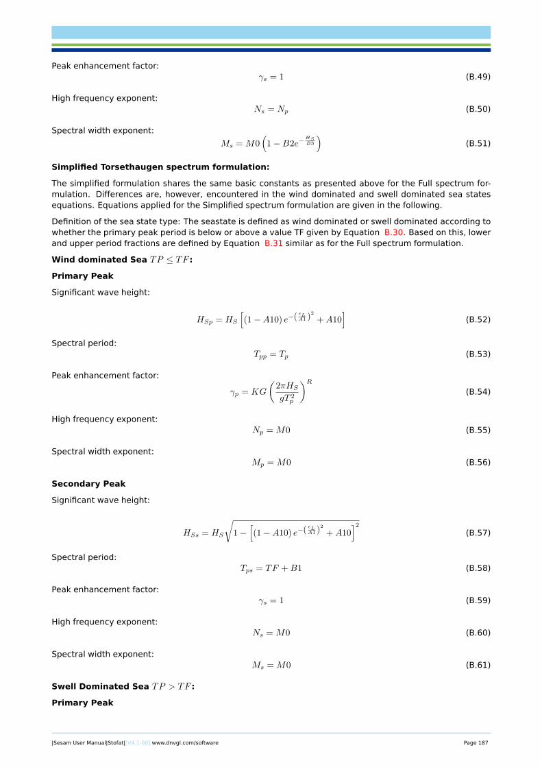
Peak enhancement factor:γs = 1 (B.49)
High frequency exponent:Ns = Np (B.50)
Spectral width exponent:
Ms = M0(
1−B2e−HSB3
)(B.51)
Simplified Torsethaugen spectrum formulation:
The simplified formulation shares the same basic constants as presented above for the Full spectrum for-mulation. Differences are, however, encountered in the wind dominated and swell dominated sea statesequations. Equations applied for the Simplified spectrum formulation are given in the following.
Definition of the sea state type: The seastate is defined as wind dominated or swell dominated according towhether the primary peak period is below or above a value TF given by Equation B.30. Based on this, lowerand upper period fractions are defined by Equation B.31 similar as for the Full spectrum formulation.
Wind dominated Sea TP ≤ TF :
Primary Peak
Significant wave height:
HSp = HS
[(1−A10) e−( εLA1 )
2
+A10]
(B.52)
Spectral period:Tpp = Tp (B.53)
Peak enhancement factor:
γp = KG
(2πHS
gT 2p
)R(B.54)
High frequency exponent:Np = M0 (B.55)
Spectral width exponent:Mp = M0 (B.56)
Secondary Peak
Significant wave height:
HSs = HS
√1−
[(1−A10) e−( εLA1 )
2
+A10]2
(B.57)
Spectral period:Tps = TF +B1 (B.58)
Peak enhancement factor:γs = 1 (B.59)
High frequency exponent:Ns = M0 (B.60)
Spectral width exponent:Ms = M0 (B.61)
Swell Dominated Sea TP > TF :
Primary Peak
|Sesam User Manual|Stofat|[V4.1-00] www.dnvgl.com/software Page 187
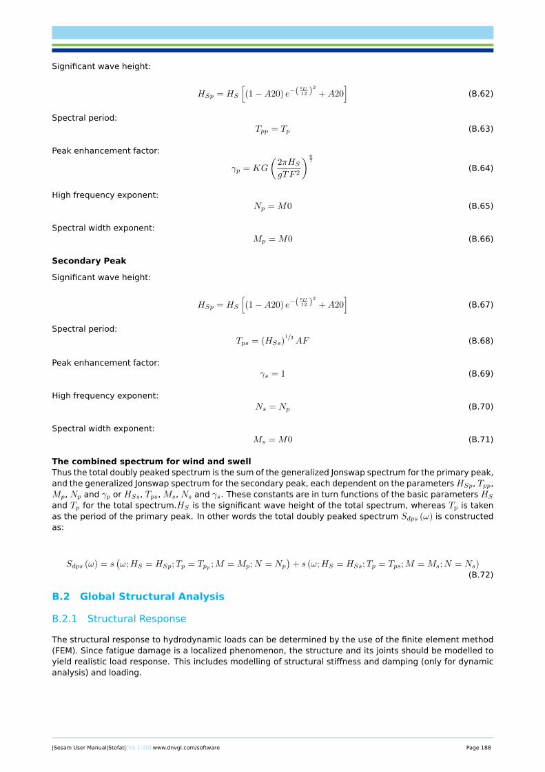
Significant wave height:
HSp = HS
[(1−A20) e−( εU12 )
2
+A20]
(B.62)
Spectral period:Tpp = Tp (B.63)
Peak enhancement factor:
γp = KG
(2πHS
gTF 2
) 67
(B.64)
High frequency exponent:Np = M0 (B.65)
Spectral width exponent:Mp = M0 (B.66)
Secondary Peak
Significant wave height:
HSp = HS
[(1−A20) e−( εU12 )
2
+A20]
(B.67)
Spectral period:Tps = (HSs)
1/3AF (B.68)
Peak enhancement factor:γs = 1 (B.69)
High frequency exponent:Ns = Np (B.70)
Spectral width exponent:Ms = M0 (B.71)
The combined spectrum for wind and swellThus the total doubly peaked spectrum is the sum of the generalized Jonswap spectrum for the primary peak,and the generalized Jonswap spectrum for the secondary peak, each dependent on the parametersHSp, Tpp,Mp, Np and γp or HSs, Tps, Ms, Ns and γs. These constants are in turn functions of the basic parameters HS
and Tp for the total spectrum.HS is the significant wave height of the total spectrum, whereas Tp is takenas the period of the primary peak. In other words the total doubly peaked spectrum Sdps (ω) is constructedas:
Sdps (ω) = s(ω;HS = HSp;Tp = Tpp ;M = Mp;N = Np
)+ s (ω;HS = HSs;Tp = Tps;M = Ms;N = Ns)
(B.72)
B.2 Global Structural Analysis
B.2.1 Structural Response
The structural response to hydrodynamic loads can be determined by the use of the finite element method(FEM). Since fatigue damage is a localized phenomenon, the structure and its joints should be modelled toyield realistic load response. This includes modelling of structural stiffness and damping (only for dynamicanalysis) and loading.
|Sesam User Manual|Stofat|[V4.1-00] www.dnvgl.com/software Page 188
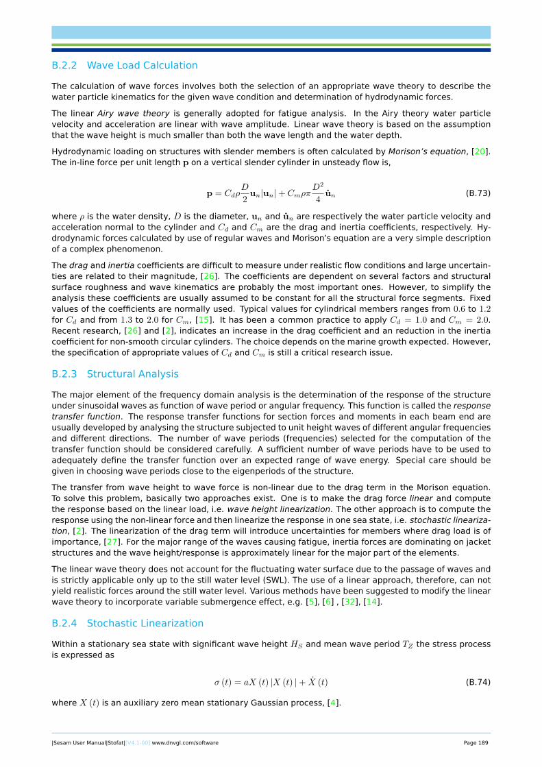
B.2.2 Wave Load Calculation
The calculation of wave forces involves both the selection of an appropriate wave theory to describe thewater particle kinematics for the given wave condition and determination of hydrodynamic forces.
The linear Airy wave theory is generally adopted for fatigue analysis. In the Airy theory water particlevelocity and acceleration are linear with wave amplitude. Linear wave theory is based on the assumptionthat the wave height is much smaller than both the wave length and the water depth.
Hydrodynamic loading on structures with slender members is often calculated by Morison’s equation, [20].The in-line force per unit length p on a vertical slender cylinder in unsteady flow is,
p = CdρD
2un|un|+ Cmρπ
D2
4un (B.73)
where ρ is the water density, D is the diameter, un and un are respectively the water particle velocity andacceleration normal to the cylinder and Cd and Cm are the drag and inertia coefficients, respectively. Hy-drodynamic forces calculated by use of regular waves and Morison’s equation are a very simple descriptionof a complex phenomenon.
The drag and inertia coefficients are difficult to measure under realistic flow conditions and large uncertain-ties are related to their magnitude, [26]. The coefficients are dependent on several factors and structuralsurface roughness and wave kinematics are probably the most important ones. However, to simplify theanalysis these coefficients are usually assumed to be constant for all the structural force segments. Fixedvalues of the coefficients are normally used. Typical values for cylindrical members ranges from 0.6 to 1.2for Cd and from 1.3 to 2.0 for Cm, [15]. It has been a common practice to apply Cd = 1.0 and Cm = 2.0.Recent research, [26] and [2], indicates an increase in the drag coefficient and an reduction in the inertiacoefficient for non-smooth circular cylinders. The choice depends on the marine growth expected. However,the specification of appropriate values of Cd and Cm is still a critical research issue.
B.2.3 Structural Analysis
The major element of the frequency domain analysis is the determination of the response of the structureunder sinusoidal waves as function of wave period or angular frequency. This function is called the responsetransfer function. The response transfer functions for section forces and moments in each beam end areusually developed by analysing the structure subjected to unit height waves of different angular frequenciesand different directions. The number of wave periods (frequencies) selected for the computation of thetransfer function should be considered carefully. A sufficient number of wave periods have to be used toadequately define the transfer function over an expected range of wave energy. Special care should begiven in choosing wave periods close to the eigenperiods of the structure.
The transfer from wave height to wave force is non-linear due to the drag term in the Morison equation.To solve this problem, basically two approaches exist. One is to make the drag force linear and computethe response based on the linear load, i.e. wave height linearization. The other approach is to compute theresponse using the non-linear force and then linearize the response in one sea state, i.e. stochastic lineariza-tion, [2]. The linearization of the drag term will introduce uncertainties for members where drag load is ofimportance, [27]. For the major range of the waves causing fatigue, inertia forces are dominating on jacketstructures and the wave height/response is approximately linear for the major part of the elements.
The linear wave theory does not account for the fluctuating water surface due to the passage of waves andis strictly applicable only up to the still water level (SWL). The use of a linear approach, therefore, can notyield realistic forces around the still water level. Various methods have been suggested to modify the linearwave theory to incorporate variable submergence effect, e.g. [5], [6] , [32], [14].
B.2.4 Stochastic Linearization
Within a stationary sea state with significant wave height HS and mean wave period TZ the stress processis expressed as
σ (t) = aX (t) |X (t) |+ X (t) (B.74)
where X (t) is an auxiliary zero mean stationary Gaussian process, [4].
|Sesam User Manual|Stofat|[V4.1-00] www.dnvgl.com/software Page 189
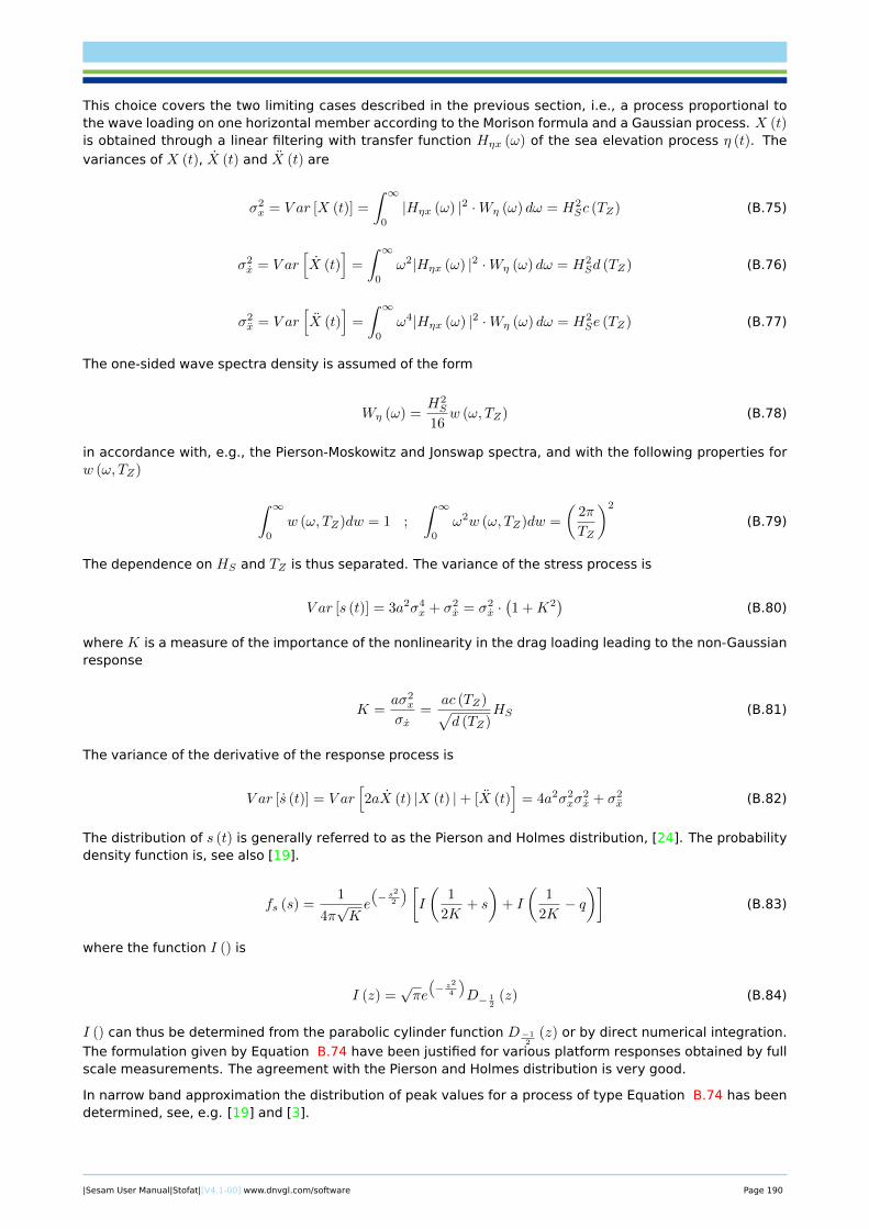
This choice covers the two limiting cases described in the previous section, i.e., a process proportional tothe wave loading on one horizontal member according to the Morison formula and a Gaussian process. X (t)is obtained through a linear filtering with transfer function Hηx (ω) of the sea elevation process η (t). Thevariances of X (t), X (t) and X (t) are
σ2x = V ar [X (t)] =
∫ ∞0
|Hηx (ω) |2 ·Wη (ω) dω = H2Sc (TZ) (B.75)
σ2x = V ar
[X (t)
]=
∫ ∞0
ω2|Hηx (ω) |2 ·Wη (ω) dω = H2Sd (TZ) (B.76)
σ2x = V ar
[X (t)
]=
∫ ∞0
ω4|Hηx (ω) |2 ·Wη (ω) dω = H2Se (TZ) (B.77)
The one-sided wave spectra density is assumed of the form
Wη (ω) =H2S
16w (ω, TZ) (B.78)
in accordance with, e.g., the Pierson-Moskowitz and Jonswap spectra, and with the following properties forw (ω, TZ)
∫ ∞0
w (ω, TZ)dw = 1 ;
∫ ∞0
ω2w (ω, TZ)dw =
(2π
TZ
)2
(B.79)
The dependence on HS and TZ is thus separated. The variance of the stress process is
V ar [s (t)] = 3a2σ4x + σ2
x = σ2x ·(1 +K2
)(B.80)
where K is a measure of the importance of the nonlinearity in the drag loading leading to the non-Gaussianresponse
K =aσ2
x
σx=
ac (TZ)√d (TZ)
HS (B.81)
The variance of the derivative of the response process is
V ar [s (t)] = V ar[2aX (t) |X (t) |+ [X (t)
]= 4a2σ2
xσ2x + σ2
x (B.82)
The distribution of s (t) is generally referred to as the Pierson and Holmes distribution, [24]. The probabilitydensity function is, see also [19].
fs (s) =1
4π√Ke
(− s22
) [I
(1
2K+ s
)+ I
(1
2K− q)]
(B.83)
where the function I () is
I (z) =√πe
(− z24
)D− 1
2(z) (B.84)
I () can thus be determined from the parabolic cylinder function D−12
(z) or by direct numerical integration.
The formulation given by Equation B.74 have been justified for various platform responses obtained by fullscale measurements. The agreement with the Pierson and Holmes distribution is very good.
In narrow band approximation the distribution of peak values for a process of type Equation B.74 has beendetermined, see, e.g. [19] and [3].
|Sesam User Manual|Stofat|[V4.1-00] www.dnvgl.com/software Page 190
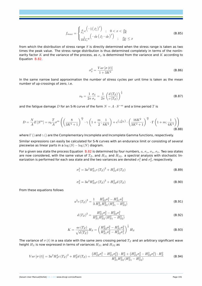
fmax =
xσxe
(− 1
2
(xσx
)2)
; 0 < x < σx2K
12Kσx
e
(− 1
2K
(xσx− 1
4K
)2)
; σx2K ≤ x
(B.85)
from which the distribution of stress range S is directly determined when the stress range is taken as twotimes the peak value. The stress range distribution is thus determined completely in terms of the nonlin-earity factor K and the variance of the process, as σx is determined from the variance and K according toEquation B.82.
σ2x =
V ar [σ (t)]
1 + 3K2(B.86)
In the same narrow band approximation the number of stress cycles per unit time is taken as the meannumber of up-crossings of zero, i.e.
ν0 =1
2π
σxσx
=1
2π
(d (TZ)
c (TZ)
) 12
(B.87)
and the fatigue damage D for an S-N curve of the form N = A · S−m and a time period T is
D =N
AE [Sm] = ν0
T
Aσm
((8
3K2 + 1
)m2
· γ(
1 +m
2;
1
8K2
)+ e(
18K2 ) ·
(16K2
3K2 + 1
)m2
· Γ(
1 +m;1
4K2
))(B.88)
where Γ () and γ () are the Complementary Incomplete and Incomplete Gamma functions, respectively.
Similar expressions can easily be calculated for S-N curves with an endurance limit or consisting of severalpiecewise as linear parts in a log (S)− log (N) diagram.
For a given sea state the process Equation B.82 is determined by four numbers, a, σx, σx, σx. Two sea statesare now considered, with the same value of TZ , and HS1 and HS2. a spectral analysis with stochastic lin-earization is performed for each sea state and the two variances are denoted σ2
1 and σ22 , respectively.
σ21 = 3a2H4
S1c (TZ)2
+H2S1d (TZ) (B.89)
σ22 = 3a2H4
S2c (TZ)2
+H2S2d (TZ) (B.90)
From these equations follows
a2c (TZ)2
=1
3
H2S2σ
21 −H2
S1σ22
H2S1H
2S2 (H2
S1 −H2S2)
(B.91)
d (TZ)2
=H4S1σ
22 −H2
S2σ21
H2S1H
2S2 (H2
S1 −H2S2)
(B.92)
K =ac (TZ)√d (TZ)
HS =
(H2S2σ
21 −H2
S1σ22
H4S1σ
22 −H2
S2σ21
) 12
HS (B.93)
The variance of σ (t) in a sea state with the same zero crossing period TZ and an arbitrary significant waveheight HS is now expressed in terms of variances HS1 and HS2 as
V ar [σ (t)] = 3a2H4Sc (TZ)
2+H2
Sd (TZ) =
(H2S2σ
21 −H2
S1σ22
)·H4
S +(H2S1σ
22 −H2
S2σ21
)·H2
S
H2S1H
2S2 (H2
S1 −H2S2)
(B.94)
|Sesam User Manual|Stofat|[V4.1-00] www.dnvgl.com/software Page 191
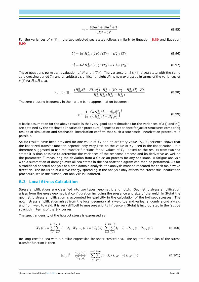
γ2 =105K4 + 18K2 + 3
(3K2 + 1)2 (B.95)
For the variances of σ (t) in the two selected sea states follows similarly to Equation B.89 and EquationB.90
σ21 = 4a2H4
S1c (TZ) d (TZ) +H2S1e (TZ) (B.96)
σ22 = 4a2H4
S2c (TZ) d (TZ) +H2S2e (TZ) (B.97)
These equations permit an evaluation of a2 and e (TZ). The variance on σ (t) in a sea state with the samezero crossing period TZ and an arbitrary significant height HS is now expressed in terms of the variances ofσ (t) for HS1HS2 as
V ar [σ (t)] =
(H2S2σ
21 −H2
S1σ22
)·H4
S +(H2S1σ
22 −H2
S2σ21
)·H2
S
H2S1H
2S2 (H2
S1 −H2S2)
(B.98)
The zero crossing frequency in the narrow band approximation becomes
ν0 =1
2π
(3
4
H2S2σ
21 −H2
S1σ22
H2S2σ
21 −H2
S1σ22
) 12
(B.99)
A basic assumption for the above results is that very good approximations for the variances of σ () and σ ()are obtained by the stochastic linearization procedure. Reported experience for jacket structures comparingresults of simulation and stochastic linearization confirm that such a stochastic linearization procedure ispossible.
So far results have been provided for one value of TZ and an arbitrary value HS . Experience shows thatthe linearized transfer function depends only very little on the value of TZ used in the linearization. It istherefore suggested to use the transfer functions for all values of TZ . Based on the results from two seastates it is thus possible to determine the variances of the response process and its derivative as well asthe parameter K measuring the deviation from a Gaussian process for any sea-state. A fatigue analysiswith a summation of damage over all sea states in the sea scatter diagram can then be performed. As fora traditional spectral analysis or a time domain analysis, the analysis must be repeated for each main wavedirection. The inclusion of a wave energy spreading in the analysis only affects the stochastic linearizationprocedure, while the subsequent analysis is unaltered.
B.3 Local Stress Calculation
Stress amplifications are classified into two types; geometric and notch. Geometric stress amplificationarises from the gross geometrical configuration including the presence and size of the weld. In Stofat thegeometric stress amplification is accounted for explicitly in the calculation of the hot spot stresses. Thenotch stress amplification arises from the local geometry at a weld toe and varies randomly along a weldand from weld to weld. It is very difficult to measure and its influence in Stofat is incorporated in the fatiguestrength in terms of the S-N curves.
The spectral density of the hotspot stress is expressed as
Wσ (ω) =
k−6∑i=1
k−6∑j=1
Ii · Jj ·WFiWj(ω) = Wη (ω) ·
k−6∑i=1
k−6∑j=1
Ii · Jj ·HηFi (ω)HηFi (ω) (B.100)
for long crested sea with a similar expression for short crested sea. The squared modulus of the stresstransfer function is then
|Hησ|2 =Wσ (ω)
Wη (ω)=
k−6∑i=1
k−6∑j=1
Ii · Jj ·HηFi (ω)HηFi (ω) (B.101)
|Sesam User Manual|Stofat|[V4.1-00] www.dnvgl.com/software Page 192
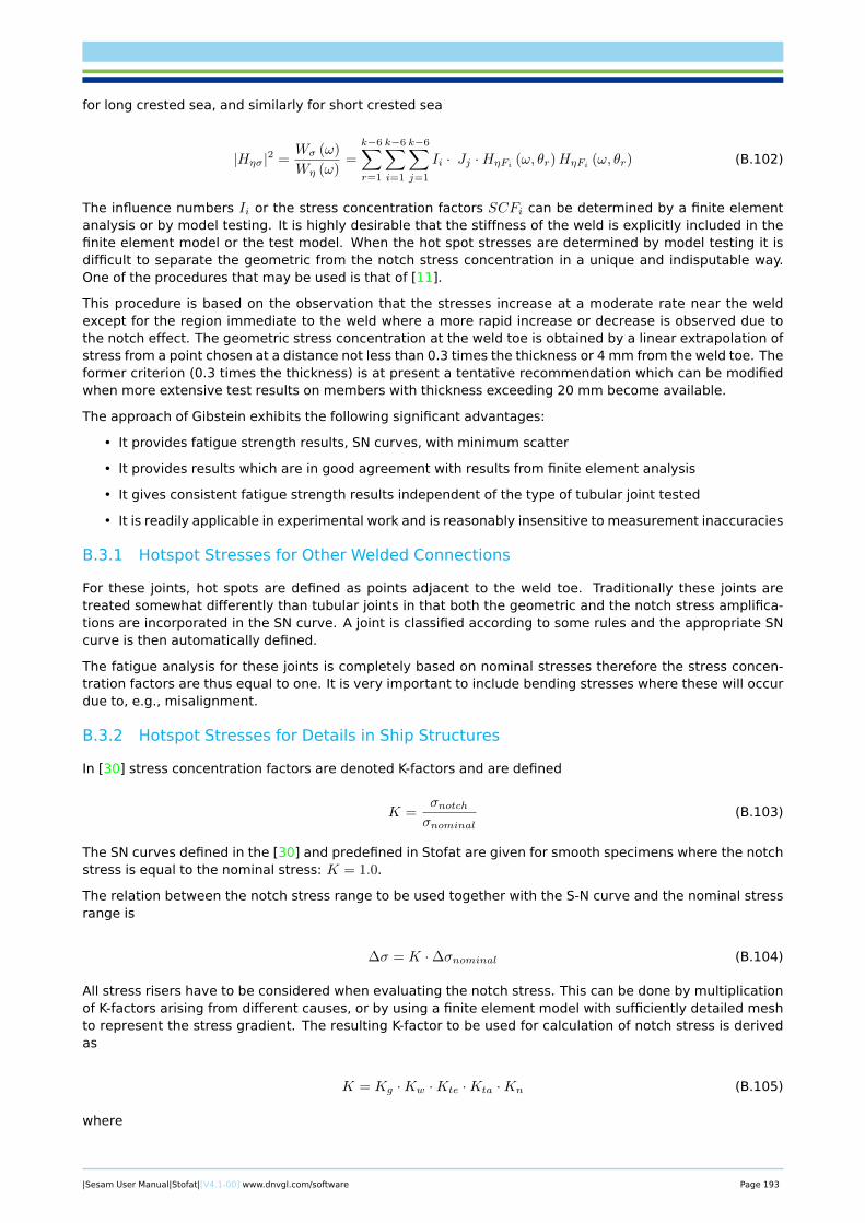
for long crested sea, and similarly for short crested sea
|Hησ|2 =Wσ (ω)
Wη (ω)=
k−6∑r=1
k−6∑i=1
k−6∑j=1
Ii · Jj ·HηFi (ω, θr)HηFi (ω, θr) (B.102)
The influence numbers Ii or the stress concentration factors SCFi can be determined by a finite elementanalysis or by model testing. It is highly desirable that the stiffness of the weld is explicitly included in thefinite element model or the test model. When the hot spot stresses are determined by model testing it isdifficult to separate the geometric from the notch stress concentration in a unique and indisputable way.One of the procedures that may be used is that of [11].
This procedure is based on the observation that the stresses increase at a moderate rate near the weldexcept for the region immediate to the weld where a more rapid increase or decrease is observed due tothe notch effect. The geometric stress concentration at the weld toe is obtained by a linear extrapolation ofstress from a point chosen at a distance not less than 0.3 times the thickness or 4 mm from the weld toe. Theformer criterion (0.3 times the thickness) is at present a tentative recommendation which can be modifiedwhen more extensive test results on members with thickness exceeding 20 mm become available.
The approach of Gibstein exhibits the following significant advantages:
• It provides fatigue strength results, SN curves, with minimum scatter
• It provides results which are in good agreement with results from finite element analysis
• It gives consistent fatigue strength results independent of the type of tubular joint tested
• It is readily applicable in experimental work and is reasonably insensitive to measurement inaccuracies
B.3.1 Hotspot Stresses for Other Welded Connections
For these joints, hot spots are defined as points adjacent to the weld toe. Traditionally these joints aretreated somewhat differently than tubular joints in that both the geometric and the notch stress amplifica-tions are incorporated in the SN curve. A joint is classified according to some rules and the appropriate SNcurve is then automatically defined.
The fatigue analysis for these joints is completely based on nominal stresses therefore the stress concen-tration factors are thus equal to one. It is very important to include bending stresses where these will occurdue to, e.g., misalignment.
B.3.2 Hotspot Stresses for Details in Ship Structures
In [30] stress concentration factors are denoted K-factors and are defined
K =σnotchσnominal
(B.103)
The SN curves defined in the [30] and predefined in Stofat are given for smooth specimens where the notchstress is equal to the nominal stress: K = 1.0.
The relation between the notch stress range to be used together with the S-N curve and the nominal stressrange is
∆σ = K ·∆σnominal (B.104)
All stress risers have to be considered when evaluating the notch stress. This can be done by multiplicationof K-factors arising from different causes, or by using a finite element model with sufficiently detailed meshto represent the stress gradient. The resulting K-factor to be used for calculation of notch stress is derivedas
K = Kg ·Kw ·Kte ·Kta ·Kn (B.105)
where
|Sesam User Manual|Stofat|[V4.1-00] www.dnvgl.com/software Page 193
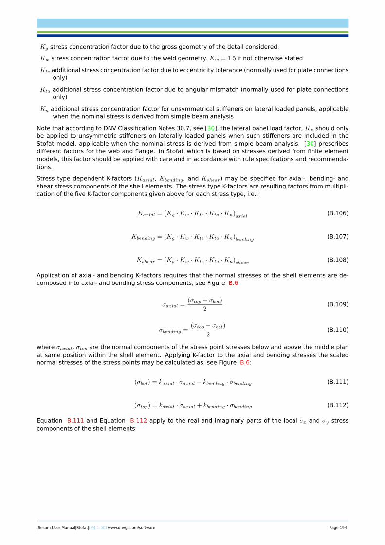
Kg stress concentration factor due to the gross geometry of the detail considered.
Kw stress concentration factor due to the weld geometry. Kw = 1.5 if not otherwise stated
Kte additional stress concentration factor due to eccentricity tolerance (normally used for plate connectionsonly)
Kta additional stress concentration factor due to angular mismatch (normally used for plate connectionsonly)
Kn additional stress concentration factor for unsymmetrical stiffeners on lateral loaded panels, applicablewhen the nominal stress is derived from simple beam analysis
Note that according to DNV Classification Notes 30.7, see [30], the lateral panel load factor, Kn should onlybe applied to unsymmetric stiffeners on laterally loaded panels when such stiffeners are included in theStofat model, applicable when the nominal stress is derived from simple beam analysis. [30] prescribesdifferent factors for the web and flange. In Stofat which is based on stresses derived from finite elementmodels, this factor should be applied with care and in accordance with rule specifcations and recommenda-tions.
Stress type dependent K-factors (Kaxial, Kbending, and Kshear) may be specified for axial-, bending- andshear stress components of the shell elements. The stress type K-factors are resulting factors from multipli-cation of the five K-factor components given above for each stress type, i.e.:
Kaxial = (Kg ·Kw ·Kte ·Kta ·Kn)axial (B.106)
Kbending = (Kg ·Kw ·Kte ·Kta ·Kn)bending (B.107)
Kshear = (Kg ·Kw ·Kte ·Kta ·Kn)shear (B.108)
Application of axial- and bending K-factors requires that the normal stresses of the shell elements are de-composed into axial- and bending stress components, see Figure B.6
σaxial =(σtop + σbot)
2(B.109)
σbending =(σtop − σbot)
2(B.110)
where σaxial, σtop are the normal components of the stress point stresses below and above the middle planat same position within the shell element. Applying K-factor to the axial and bending stresses the scalednormal stresses of the stress points may be calculated as, see Figure B.6:
(σbot) = kaxial · σaxial − kbending · σbending (B.111)
(σtop) = kaxial · σaxial + kbending · σbending (B.112)
Equation B.111 and Equation B.112 apply to the real and imaginary parts of the local σx and σy stresscomponents of the shell elements
|Sesam User Manual|Stofat|[V4.1-00] www.dnvgl.com/software Page 194
Figure B.6: Normal stress component of shell elements scaled by axial and bending stress K-factors
B.4 Stress Ranges and Cycles
The fatigue strength is expressed in terms of the number of stress cycles N of constant stress range S lead-ing to failure. Statistics for the number of stress cycles and the stress range distribution must consequentlybe produced from the statistical description of the hotspot stress process.
For a random stress process the definition of stress cycles is not unique and several different methodsare used, including the peak counting method, the range counting method and the rain flow counting. Adetailed description of the methods can be found in e.g., [19]. For a narrow band stress process there isonly one maximum between two consecutive up-crossings of the mean level making the identification ofstress cycles straightforward. The three mentioned counting methods also give identical results for such aprocess. For a wide band process or a process with a multi mode spectral density function there may beseveral local maxima between one up-crossing of the mean level and the following up-crossing, and thethree counting methods give different results. It is generally believed that the rainflow counting methodgives results which are in better agreement with experimental results than the peak counting method whichtends to overestimate damage and the range counting method which tends to underestimate damage. Therain flow counting method is, however, used for time series of the stress process. The rainflow countingmethod is made available in Stofat and may be switched on by the command DEFINE FATIGUE-RAINFLOW-COUNTING. Time history of the stresses are generated from the frequency domain representation of thestresses by Inverse Fast Fourier Transformation (IFFT). It should be noted that use of rainflow counting inStofat is considerable more time consuming than using the spectral density approach.
For offshore jacket structures the hot spot stress process tends to be narrow-banded. The wave loading isreasonably narrow banded and structures behaving in a quasi static manner therefore have a narrow bandedresponse although cancellation effects may give rise to a bimodal or even multi modal spectral density ofthe response.
In [19] it is shown that applying the peak counting method the number of stress cycles is equal to thenumber of up-crossings of the mean level. The mean number of stress cycles for a stationary stress processin a time period t is then
Nt = ν0t (B.113)
where ν0 is the mean up-crossing rate of the process.
|Sesam User Manual|Stofat|[V4.1-00] www.dnvgl.com/software Page 195
The stress range S is a random variable and its density function is obtained in connection with stress peakdensity function. It can be shown, see [18], that the stress peak density may be taken as
fmax (x) = − 1
ν0
dν+ (x)
dx; x > 0 (B.114)
where ν+ is the mean up-crossing rate for the stress process. For a zero mean Gaussian process withvariance σ2, fmax (x) becomes
fmax (x) =x
σ2e
(− x2
2σ2
); x > 0 (B.115)
i.e., a Rayleigh distribution. The probability density of minima is similar to Equation B.114
fmin (x) =1
ν0
dν− (x)
dx; x < 0 (B.116)
where ν− is the mean down crossing rate of level x. Due to symmetry fmax (x) = fmin (−x) for the stressprocesses obtained in Stofat. The stress range is therefore taken as two times the peak value and its densityfunction is for a Gaussian stress process
fs (s) =s
2σ2e
(− s2
8σ2
); s > 0 (B.117)
When a steady current is introduced fmax (x) 6= fmin (−x) and calculation of the stress range distributionbecomes more complicated. This is described in detail in [19].
For a Gaussian stress process it is observed that the number of stress cycles and the stress range densityfunction are given solely in terms of the mean up-crossing ν0 and the variance σ2. These two parametersare determined from the moments of the one sided stress spectral density function. The spectral momentsare denoted,
λi =
∫ ∞0
ωiWi (ω) dω (B.118)
The variance σ2 and the mean up-crossing rate ν0 of the stress process s (t)
σ2 = V ar [s (t)] = λ0 (B.119)
ν0 =1
2π
√λ2
λ0(B.120)
B.5 Effect of Forward Speed
When the structure is moving relative to the sea, both the values of the transfer function and the frequencyof encounter will be affected.
It is assumed that any effects on the loading of the structure is taken care of by the wave loading pro-grams.
A shift in frequency is taken into account by retrieving both wave frequency and frequency of encounterfrom the wave loading program. The wave frequency is used when computing the wave spectrum for eachsea state, and when computing the response spectrum from the transfer functions. When Jonswap wavespectrum is selected, calculation of moments of the response spectrum is performed by numeric integrationover a fixed number of intervals taking the frequency of encounter into account.
|Sesam User Manual|Stofat|[V4.1-00] www.dnvgl.com/software Page 196
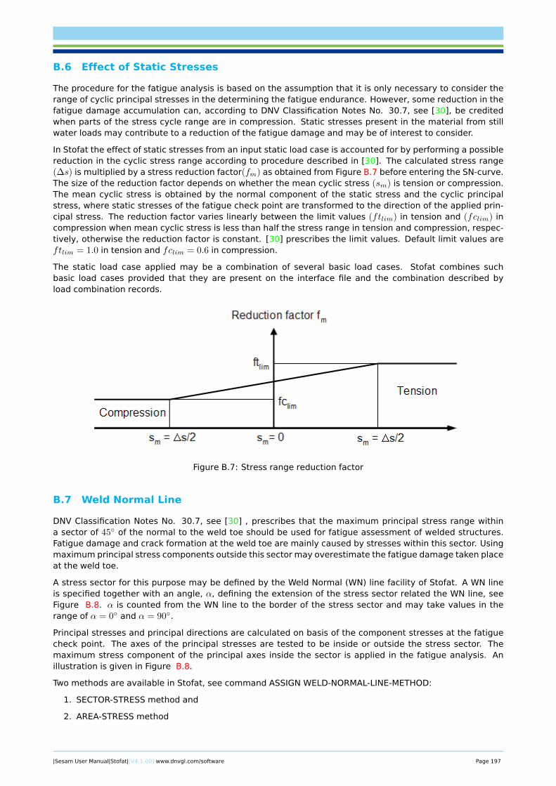
B.6 Effect of Static Stresses
The procedure for the fatigue analysis is based on the assumption that it is only necessary to consider therange of cyclic principal stresses in the determining the fatigue endurance. However, some reduction in thefatigue damage accumulation can, according to DNV Classification Notes No. 30.7, see [30], be creditedwhen parts of the stress cycle range are in compression. Static stresses present in the material from stillwater loads may contribute to a reduction of the fatigue damage and may be of interest to consider.
In Stofat the effect of static stresses from an input static load case is accounted for by performing a possiblereduction in the cyclic stress range according to procedure described in [30]. The calculated stress range(∆s) is multiplied by a stress reduction factor(fm) as obtained from Figure B.7 before entering the SN-curve.The size of the reduction factor depends on whether the mean cyclic stress (sm) is tension or compression.The mean cyclic stress is obtained by the normal component of the static stress and the cyclic principalstress, where static stresses of the fatigue check point are transformed to the direction of the applied prin-cipal stress. The reduction factor varies linearly between the limit values (ftlim) in tension and (fclim) incompression when mean cyclic stress is less than half the stress range in tension and compression, respec-tively, otherwise the reduction factor is constant. [30] prescribes the limit values. Default limit values areftlim = 1.0 in tension and fclim = 0.6 in compression.
The static load case applied may be a combination of several basic load cases. Stofat combines suchbasic load cases provided that they are present on the interface file and the combination described byload combination records.
Figure B.7: Stress range reduction factor
B.7 Weld Normal Line
DNV Classification Notes No. 30.7, see [30] , prescribes that the maximum principal stress range withina sector of 45◦ of the normal to the weld toe should be used for fatigue assessment of welded structures.Fatigue damage and crack formation at the weld toe are mainly caused by stresses within this sector. Usingmaximum principal stress components outside this sector may overestimate the fatigue damage taken placeat the weld toe.
A stress sector for this purpose may be defined by the Weld Normal (WN) line facility of Stofat. A WN lineis specified together with an angle, α, defining the extension of the stress sector related the WN line, seeFigure B.8. α is counted from the WN line to the border of the stress sector and may take values in therange of α = 0◦ and α = 90◦.
Principal stresses and principal directions are calculated on basis of the component stresses at the fatiguecheck point. The axes of the principal stresses are tested to be inside or outside the stress sector. Themaximum stress component of the principal axes inside the sector is applied in the fatigue analysis. Anillustration is given in Figure B.8.
Two methods are available in Stofat, see command ASSIGN WELD-NORMAL-LINE-METHOD:
1. SECTOR-STRESS method and
2. AREA-STRESS method
|Sesam User Manual|Stofat|[V4.1-00] www.dnvgl.com/software Page 197
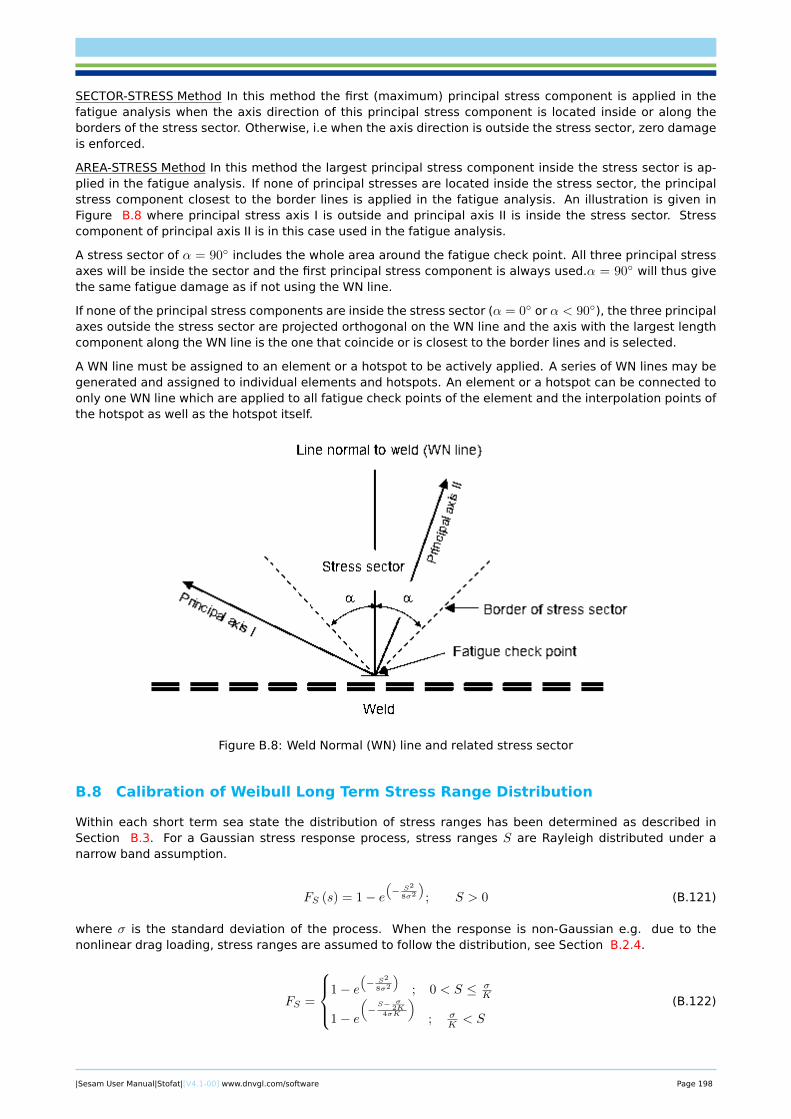
SECTOR-STRESS Method In this method the first (maximum) principal stress component is applied in thefatigue analysis when the axis direction of this principal stress component is located inside or along theborders of the stress sector. Otherwise, i.e when the axis direction is outside the stress sector, zero damageis enforced.
AREA-STRESS Method In this method the largest principal stress component inside the stress sector is ap-plied in the fatigue analysis. If none of principal stresses are located inside the stress sector, the principalstress component closest to the border lines is applied in the fatigue analysis. An illustration is given inFigure B.8 where principal stress axis I is outside and principal axis II is inside the stress sector. Stresscomponent of principal axis II is in this case used in the fatigue analysis.
A stress sector of α = 90◦ includes the whole area around the fatigue check point. All three principal stressaxes will be inside the sector and the first principal stress component is always used.α = 90◦ will thus givethe same fatigue damage as if not using the WN line.
If none of the principal stress components are inside the stress sector (α = 0◦ or α < 90◦), the three principalaxes outside the stress sector are projected orthogonal on the WN line and the axis with the largest lengthcomponent along the WN line is the one that coincide or is closest to the border lines and is selected.
A WN line must be assigned to an element or a hotspot to be actively applied. A series of WN lines may begenerated and assigned to individual elements and hotspots. An element or a hotspot can be connected toonly one WN line which are applied to all fatigue check points of the element and the interpolation points ofthe hotspot as well as the hotspot itself.
Figure B.8: Weld Normal (WN) line and related stress sector
B.8 Calibration of Weibull Long Term Stress Range Distribution
Within each short term sea state the distribution of stress ranges has been determined as described inSection B.3. For a Gaussian stress response process, stress ranges S are Rayleigh distributed under anarrow band assumption.
FS (s) = 1− e(− S2
8σ2
); S > 0 (B.121)
where σ is the standard deviation of the process. When the response is non-Gaussian e.g. due to thenonlinear drag loading, stress ranges are assumed to follow the distribution, see Section B.2.4.
FS =
1− e(− S2
8σ2
); 0 < S ≤ σ
K
1− e
(−S− σ
2K4σK
); σ
K < S
(B.122)
|Sesam User Manual|Stofat|[V4.1-00] www.dnvgl.com/software Page 198
The long term distribution of stress ranges is obtained as a weighted average of the short term distributions,with the weights proportional to the number of stress cycles in a specific short term sea state. Each seastate is described by the significant wave height HS , the mean zero crossing period TZ , and the mean wavedirection Θ. For a hot spot the short term stress range distribution function for the i-th sea state is denotedas FS (S,HS , TZ ,Θ)i, where FS () is given in by the equations above where the standard deviation σ dependson (HS , TZ ,Θ).
The fraction of sea states with the ith combination of (HS , TZ ,Θ) is denoted by qi, and the mean zerocrossing frequency for the stress process with this sea state parameter combination is denoted as ν0,j . Thelong term mean zero crossing frequency is
ν0,long term =∑HS
∑TZ
∑Θi
q0 · ν0,i (B.123)
since the sum of the weights qi is unity. The expected number of stress cycles in a time period t is obtainedby multiplying ν0,long term by t.
The long term distribution of stress ranges may now be determined as
FS,long term =1
ν0,long term·∑HS
∑TZ
∑Θi
q0 · ν0,i · FS (S,HS , TZ ,Θ)i (B.124)
This long term distribution function is of a somewhat complicated form and requires considerable compu-tation time. A fit to a simpler distribution is therefore of interest. During the 1960’s research related tosuch distribution fitting was performed by [21]. Among the distribution types considered, the best fit wasreported for a Weibull distribution and this choice has been confirmed in many later studies. The two pa-rameter Weibull distribution has the form
FS (S) = 1− e(−( SA )
B)
; S > 0 (B.125)
and the task is to determine values for the scale parameter A and the shape parameter B which result in aclose agreement between the original and fitted distribution. In this analysis the closeness of fit is judgedby the difference in fatigue life from use of the two distributions.
Experience shows that the value of B is typically between 0.8 and 1.2, with the lower values for drag loadingdominated structures and the higher values for inertia loading dominated. The fatigue damage D in a timeperiod t for a Weibull stress range distribution and an S-N curve without a threshold or change in slope isgiven as
D =ν0,long term · t
K· E [Sm] =
ν0,long term · tK
·A · Γ(
1 +m
B
)(B.126)
B.8.1 Deterministic Calibration
The two Weibull parameters can be determined by fitting at two or more fractile levels.
When two levels are used, the fractiles corresponding to these two levels determine three stress rangeintervals. An intuitively good choice is the levels giving the same fatigue damage contribution from stressranges in these three intervals.
With the SN curve slope parameter m = 3 and B = 1 it turns out that the fitting should be performed at the95th and 99th percentile levels. Let S95 and S99 denote these fractiles as obtained from the original longterm distribution. The Weibull parameters A and B for the fitted distribution are then determined by solvingthe equations
A = e(k lnS0.99−ln a0.95
k−1 ) B =ln (− ln 0.05)
lnS0.99 − ln a(B.127)
where
|Sesam User Manual|Stofat|[V4.1-00] www.dnvgl.com/software Page 199
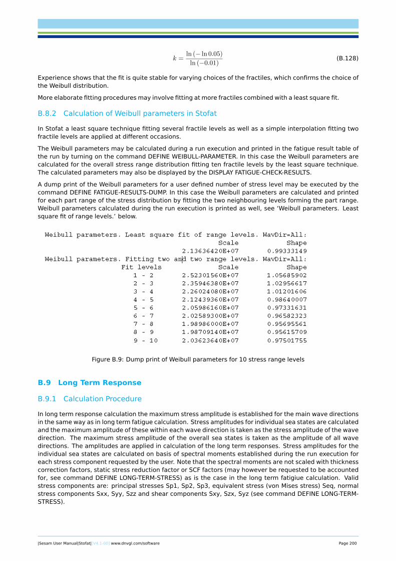
k =ln (− ln 0.05)
ln (−0.01)(B.128)
Experience shows that the fit is quite stable for varying choices of the fractiles, which confirms the choice ofthe Weibull distribution.
More elaborate fitting procedures may involve fitting at more fractiles combined with a least square fit.
B.8.2 Calculation of Weibull parameters in Stofat
In Stofat a least square technique fitting several fractile levels as well as a simple interpolation fitting twofractile levels are applied at different occasions.
The Weibull parameters may be calculated during a run execution and printed in the fatigue result table ofthe run by turning on the command DEFINE WEIBULL-PARAMETER. In this case the Weibull parameters arecalculated for the overall stress range distribution fitting ten fractile levels by the least square technique.The calculated parameters may also be displayed by the DISPLAY FATIGUE-CHECK-RESULTS.
A dump print of the Weibull parameters for a user defined number of stress level may be executed by thecommand DEFINE FATIGUE-RESULTS-DUMP. In this case the Weibull parameters are calculated and printedfor each part range of the stress distribution by fitting the two neighbouring levels forming the part range.Weibull parameters calculated during the run execution is printed as well, see ‘Weibull parameters. Leastsquare fit of range levels.’ below.
Figure B.9: Dump print of Weibull parameters for 10 stress range levels
B.9 Long Term Response
B.9.1 Calculation Procedure
In long term response calculation the maximum stress amplitude is established for the main wave directionsin the same way as in long term fatigue calculation. Stress amplitudes for individual sea states are calculatedand the maximum amplitude of these within each wave direction is taken as the stress amplitude of the wavedirection. The maximum stress amplitude of the overall sea states is taken as the amplitude of all wavedirections. The amplitudes are applied in calculation of the long term responses. Stress amplitudes for theindividual sea states are calculated on basis of spectral moments established during the run execution foreach stress component requested by the user. Note that the spectral moments are not scaled with thicknesscorrection factors, static stress reduction factor or SCF factors (may however be requested to be accountedfor, see command DEFINE LONG-TERM-STRESS) as is the case in the long term fatigiue calculation. Validstress components are: principal stresses Sp1, Sp2, Sp3, equivalent stress (von Mises stress) Seq, normalstress components Sxx, Syy, Szz and shear components Sxy, Szx, Syz (see command DEFINE LONG-TERM-STRESS).
|Sesam User Manual|Stofat|[V4.1-00] www.dnvgl.com/software Page 200
The stress amplitude of a sea state for a given stress point is;
∆σ =√λ√
2 ln (ns) (B.129)
where
ns =T
2π
√λ2
λ0ps =
T · YdTZs
(B.130)
dTZs =2π
ps
√λ0
λ2(B.131)
∆σs Stress amplitude of the sea statens Stress cycles of the sea statedTZs Mean zero up-crossing period of the sea stateT Duration of a year in seconds, T = 3.1536× 10⁷
Y Design fatigue life in yearsps Probability of the sea state and current wave directionλ0 Zero spectral moment of the sea stateλ2 Second spectral moment of the sea state
Stress amplitude of wave direction j, ∆σj , is taken as maximum stress amplitude of the sea states of wavedirection j, and stress amplitude of the stress point, ∆σ0 (all wave directions), is maximum stress amplitudeof all wave directions (or sea states), i.e.;
Stress amplitude of wave direction j∆σj = max (∆σs)j (B.132)
Stress amplitude of all wave directions∆σ0 = max (∆σj) (B.133)
The stress amplitudes ∆σj and ∆σ0 are divided into a number of equally spaced stress levels, nl, decidedby the user (default is 10 levels). Exceedances and probability of exceedances are calculated for each of thestress levels.
Amplitude of stress level i is given by; Amplitude of stress level i, wave direction j
∆σji = ∆σji
nl(B.134)
Amplitiude of stress level i, all wave directions
∆σ0i = ∆σ0i
nl(B.135)
Contributions from the sea states are accumulated for each wave direction; Stress cycles, wave directionj
nj =
j∑seastates
ns (B.136)
Mean zero up-crossing period, wave direction j
dTZj =
j∑seastates
dTZs (B.137)
Exceedance of stress level i, wave direction j
eji =
j∑seastates
esi (B.138)
|Sesam User Manual|Stofat|[V4.1-00] www.dnvgl.com/software Page 201
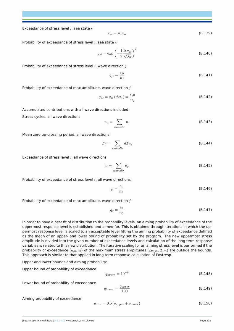
Exceedance of stress level i, sea state sesi = nsqsi (B.139)
Probability of exceedance of stress level i, sea state s
qsi = exp
(−1
2
∆σji√λ0
)2
(B.140)
Probability of exceedance of stress level i, wave direction j
qji =ejinj
(B.141)
Probability of exceedance of max amplitude, wave direction j
qj0 = qji (∆σj) =ej0nj
(B.142)
Accumulated contributions with all wave directions included;
Stress cycles, all wave directions
n0 =∑
wavedir
nj (B.143)
Mean zero up-crossing period, all wave directions
TZ =∑
wavedir
dTZj (B.144)
Exceedance of stress level i, all wave directions
ei =∑
wavedir
eji (B.145)
Probability of exceedance of stress level i, all wave directions
qi =ein0
(B.146)
Probability of exceedance of max amplitude, wave direction j
q0 =e0
n0(B.147)
In order to have a best fit of distribution to the probability levels, an aiming probability of exceedance of theuppermost response level is established and aimed for. This is obtained through iterations in which the up-permost response level is scaled to an acceptable level fitting the aiming probability of exceedance definedas the mean of an upper- and lower bound of probability set by the program. The new uppermost stressamplitude is divided into the given number of exceedance levels and calculation of the long term responsevariables is related to this new distribution. The iterative scaling for an aiming stress level is performed if theprobability of exceedance (qj0, q0) of the maximum stress amplitudes (∆σj0,∆σ0) are outside the bounds.This approach is similar to that applied in long term response calculation of Postresp.
Upper-and lower bounds and aiming probability:
Upper bound of probability of exceedancequpper = 10−8 (B.148)
Lower bound of probability of exceedance
qlower =qupper100
(B.149)
Aiming probability of exceedanceqaim = 0.5 (qupper + qlower) (B.150)
|Sesam User Manual|Stofat|[V4.1-00] www.dnvgl.com/software Page 202
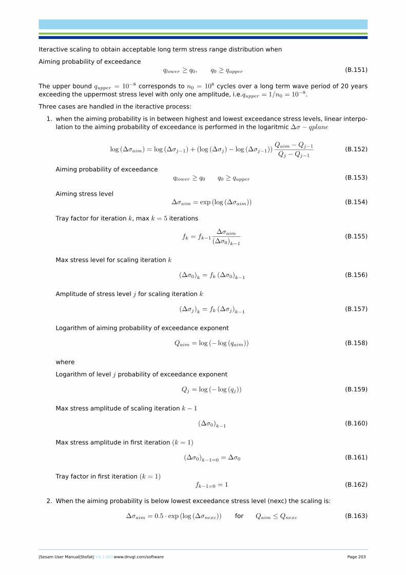
Iteractive scaling to obtain acceptable long term stress range distribution when
Aiming probability of exceedanceqlower ≥ q0, q0 ≥ qupper (B.151)
The upper bound qupper = 10−8 corresponds to n0 = 108 cycles over a long term wave period of 20 yearsexceeding the uppermost stress level with only one amplitude, i.e.qupper = 1/n0 = 10−8.
Three cases are handled in the iteractive process:
1. when the aiming probability is in between highest and lowest exceedance stress levels, linear interpo-lation to the aiming probability of exceedance is performed in the logaritmic ∆σ − qplane
log (∆σaim) = log (∆σj−1) + (log (∆σj)− log (∆σj−1))Qaim −Qj−1
Qj −Qj−1(B.152)
Aiming probability of exceedanceqlower ≥ q0 q0 ≥ qupper (B.153)
Aiming stress level∆σaim = exp (log (∆σaim)) (B.154)
Tray factor for iteration k, max k = 5 iterations
fk = fk−1∆σaim
(∆σ0)k−1
(B.155)
Max stress level for scaling iteration k
(∆σ0)k = fk (∆σ0)k−1 (B.156)
Amplitude of stress level j for scaling iteration k
(∆σj)k = fk (∆σj)k−1 (B.157)
Logarithm of aiming probability of exceedance exponent
Qaim = log (− log (qaim)) (B.158)
where
Logarithm of level j probability of exceedance exponent
Qj = log (− log (qj)) (B.159)
Max stress amplitude of scaling iteration k − 1
(∆σ0)k−1 (B.160)
Max stress amplitude in first iteration (k = 1)
(∆σ0)k−1=0 = ∆σ0 (B.161)
Tray factor in first iteration (k = 1)fk−1=0 = 1 (B.162)
2. When the aiming probability is below lowest exceedance stress level (nexc) the scaling is:
∆σaim = 0.5 · exp (log (∆σnexc)) for Qaim ≤ Qnexc (B.163)
|Sesam User Manual|Stofat|[V4.1-00] www.dnvgl.com/software Page 203
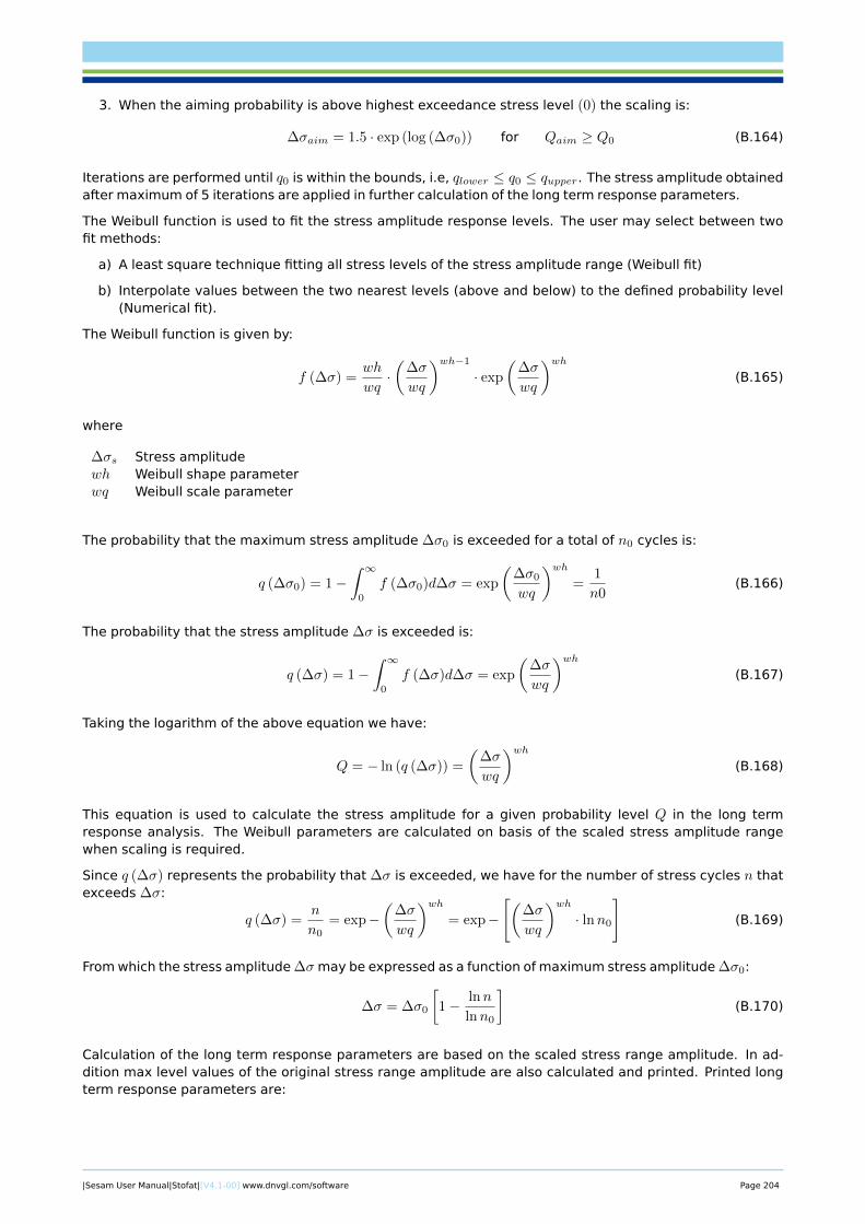
3. When the aiming probability is above highest exceedance stress level (0) the scaling is:
∆σaim = 1.5 · exp (log (∆σ0)) for Qaim ≥ Q0 (B.164)
Iterations are performed until q0 is within the bounds, i.e, qlower ≤ q0 ≤ qupper. The stress amplitude obtainedafter maximum of 5 iterations are applied in further calculation of the long term response parameters.
The Weibull function is used to fit the stress amplitude response levels. The user may select between twofit methods:
a) A least square technique fitting all stress levels of the stress amplitude range (Weibull fit)
b) Interpolate values between the two nearest levels (above and below) to the defined probability level(Numerical fit).
The Weibull function is given by:
f (∆σ) =wh
wq·(
∆σ
wq
)wh−1
· exp
(∆σ
wq
)wh(B.165)
where
∆σs Stress amplitudewh Weibull shape parameterwq Weibull scale parameter
The probability that the maximum stress amplitude ∆σ0 is exceeded for a total of n0 cycles is:
q (∆σ0) = 1−∫ ∞
0
f (∆σ0)d∆σ = exp
(∆σ0
wq
)wh=
1
n0(B.166)
The probability that the stress amplitude ∆σ is exceeded is:
q (∆σ) = 1−∫ ∞
0
f (∆σ)d∆σ = exp
(∆σ
wq
)wh(B.167)
Taking the logarithm of the above equation we have:
Q = − ln (q (∆σ)) =
(∆σ
wq
)wh(B.168)
This equation is used to calculate the stress amplitude for a given probability level Q in the long termresponse analysis. The Weibull parameters are calculated on basis of the scaled stress amplitude rangewhen scaling is required.
Since q (∆σ) represents the probability that ∆σ is exceeded, we have for the number of stress cycles n thatexceeds ∆σ:
q (∆σ) =n
n0= exp−
(∆σ
wq
)wh= exp−
[(∆σ
wq
)wh· lnn0
](B.169)
From which the stress amplitude ∆σ may be expressed as a function of maximum stress amplitude ∆σ0:
∆σ = ∆σ0
[1− lnn
lnn0
](B.170)
Calculation of the long term response parameters are based on the scaled stress range amplitude. In ad-dition max level values of the original stress range amplitude are also calculated and printed. Printed longterm response parameters are:
|Sesam User Manual|Stofat|[V4.1-00] www.dnvgl.com/software Page 204
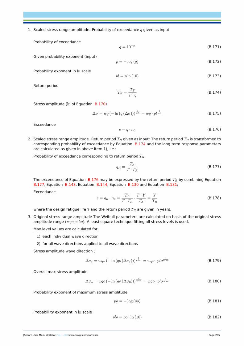
1. Scaled stress range amplitude. Probability of exceedance q given as input:
Probability of exceedanceq = 10−p (B.171)
Given probability exponent (input)p = − log (q) (B.172)
Probability exponent in ln scalepl = p ln (10) (B.173)
Return period
TR =TZT · q
(B.174)
Stress amplitude (ln of Equation B.170)
∆σ = wq (− ln (q (∆σ)))1wh = wq · pl 1
wh (B.175)
Exceedancee = q · n0 (B.176)
2. Scaled stress range amplitude. Return period TR given as input: The return period TR is transformed tocorresponding probability of exceedance by Equation B.174 and the long term response parametersare calculated as given in above item 1), i.e.:
Probability of exceedance corresponding to return period TR
qR =TZ
T · TR(B.177)
The exceedance of Equation B.176 may be expressed by the return period TR by combining EquationB.177, Equation B.143, Equation B.144, Equation B.130 and Equation B.131;
Exceedance
e = qR · n0 =TZ
T · TR· T · YTZ
=Y
TR(B.178)
where the design fatigue life Y and the return period TR are given in years.
3. Original stress range amplitude The Weibull parameters are calculated on basis of the original stressamplitude range (wqo,who). A least square technique fitting all stress levels is used.
Max level values are calculated for
1) each individual wave direction
2) for all wave directions applied to all wave directions
Stress amplitude wave direction j
∆σj = wqo (− ln (qo (∆σj)))1
who = wqo · plo 1who (B.179)
Overall max stress amplitude
∆σo = wqo (− ln (qo (∆σ0)))1
who = wqo · plo 1who (B.180)
Probability exponent of maximum stress amplitude
po = − log (qo) (B.181)
Probablility exponent in ln scaleplo = po · ln (10) (B.182)
|Sesam User Manual|Stofat|[V4.1-00] www.dnvgl.com/software Page 205
Probability of exceedance of maximum stress level
qo =eon0
(B.183)
Return period of maximum stress level
TRo =TZT · qo
(B.184)
where eo is the exceedance of each wave direction related to the maximum stress amplitude appliedfor the wave direction (Equation B.179 or Equation B.180), see Equation B.138 and Equation B.145.
It should be noted that stress amplitudes reported in the long term response table print are calculatedby the spectral moments, see Equation B.129 and not by the Weibull function of Equation B.179 andEquation B.180. This is done in order to compare amplitude values directly with maximum stress rangevalues reported in the dump file. However, stress amplitudes calculated by the Weibull function are close tothe amplitude values calculated by the spectral moments.
B.9.2 Print of Long Term Response
Results are given in form of table print of the response parameters and storage on a vtf file for graphicpresentation of results in Xtract, see commands PRINT LONG-TERM-RESPONSE and PRINT FATIGUE-RESULTS-VTF-FILE STRESS-RANGE-DISTRIBUTION. Print is performed for selected response parameters, wave direc-tions and stress components. Print to the vtf file is performed for a single probability level or return period,entered in the print command.
Table print of long term parameters is given for:
• Each stress component requested by the user, see command DEFINE LONG-TERM-STRESS
• Individual or all wave directions
• All element stress points or point with maximum stress amplitude
• Hotspots and interpolation points
• Input probability levels or return periods given by the user. One print for each.
• Exceedance, exceedance probability, return period and Weibull parameters related to original stressamplitudes applied for the wave directions
• Parameter values reported for max stress amplitude of all wave directions applied to all wave directionor using stress amplitudes of each individual wave direction. Option choice selected by the commandDEFINE LONG-TERM-STRESS-AMPLITUDE
Parameters printed for scaled stress amplitude range:
Stress Amplitude Amplitude stress ∆σ for given probability levels or return periods
Maximum stress Maximum stress amplitude including static stress offset for given
probability levels or return periods, i.e: ∆σmax = ∆σstatic + ∆σ
Note! ∆σstatic is the static stress component of current element
stress point corresponding to the long term stress component.
Minimum stress Minimum stress amplitude including static stress offset for given
probability levels or return periods, i.e: ∆σmax = ∆σstatic −∆σ
Peak factor Stress peak amplification factor,
d = |∆σmax|∆σ = |∆σstatic|+∆σ
∆σ = 1 + |∆σstatic|∆σ
Exceedance Exceedance e, see Equation B.176 and Equation B.178
Return period Return period TR, see Equation B.174 when probability levels are input
Probability level Probability level qR, see Equation B.177 when return periods are input
Weibull scale Weibull scale parameter wq
Weibull shape Weibull shape parameter wh
|Sesam User Manual|Stofat|[V4.1-00] www.dnvgl.com/software Page 206
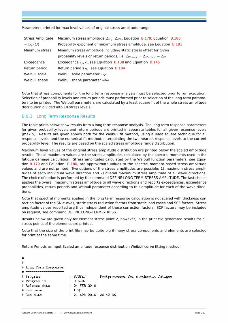
Parameters printed for max level values of original stress amplitude range:
Stress Amplitude Maximum stress amplitude ∆σj , ∆σ0, Equation B.179, Equation B.180
− log (Q) Probability exponent of maximum stress amplitude, see Equation B.181
Minimum stress Minimum stress amplitude including static stress offset for given
probability levels or return periods, i.e: ∆σmax = ∆σstatic −∆σ
Exceedance Exceedance ej , eo see Equation B.138 and Equation B.145
Return period Return period TRo , see Equation B.184
Weibull scale Weibull scale parameter wqo
Weibull shape Weibull shape parameter who
Note that stress components for the long term response analysis must be selected prior to run execution.Selection of probability levels and return periods must performed prior to selection of the long term parame-ters to be printed. The Weibull parameters are calculated by a least square fit of the whole stress amplitudedistribution divided into 10 stress levels.
B.9.3 Long Term Response Results
The table prints below show results from a long term response analysis. The long term response parametersfor given probability levels and return periods are printed in separate tables for all given response levels(max 5). Results are given shown both for the Weibull fit method, using a least square technique for allresponse levels, and the numerical fit method, interpolating the two nearest response levels to the currentprobability level. The results are based on the scaled stress amplitude range distribution.
Maximum level values of the original stress amplitude distribution are printed below the scaled amplituderesults. These maximum values are the stress amplitudes calculated by the spectral moments used in thefatigue damage calculation. Stress amplitudes calculated by the Weibull function parameters, see Equa-tion B.179 and Equation B.180, are approximate values to the spectral moment based stress amplitudevalues and are not printed. Two options of the stress amplitudes are possible; 1) maximum stress ampli-tudes of each individual wave direction and 2) overall maximum stress amplitude of all wave directions.The choice of option is performed by the command DEFINE LONG-TERM-STRESS-AMPLITUDE. The last choiceapplies the overall maximum stress amplitude to all wave directions and reports exceedances, exceedanceprobabilities, return periods and Weibull parameter according to this amplitude for each of the wave direc-tions.
Note that spectral moments applied in the long term response calculation is not scaled with thickness cor-rection factor of the SN-curves, static stress reduction factors from static load cases and SCF factors. Stressamplitude values reported are thus independent of these correction factors. SCF factors may be includedon request, see command DEFINE LONG-TERM-STRESS.
Results below are given only for element stress point 2, however, in the print file generated results for allstress points of the elements are printed.
Note that the size of the print file may be quite big if many stress components and elements are selectedfor print at the same time.
Return Periods as input Scaled amplitude response distribution Weibull curve fitting method:
#
#
# Long Term Responses
# ===================
# Program : STOFAT Postprocessor for stochastic fatigue
# Program id : 3.5-07
# Release date : 24-FEB-2016
# Run name : LTR1
# Run date : 21-APR-2016 06:42:06
|Sesam User Manual|Stofat|[V4.1-00] www.dnvgl.com/software Page 207
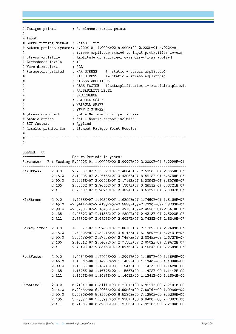
# Fatigue points : At element stress points
#
# Input:
# Curve fitting method : Weibull fit
# Return periods (years): 5.000E-01 1.000E+00 5.000E+00 2.000E+01 5.000E+01
# : Stress amplitude scaled to input probability levels
# Stress amplitude : Amplitude of indiviual wave directions applied
# Exceedance levels : 10
# Wave directions : ALL
# Parameters printed : MAX STRESS (= static + stress amplitude)
# : MIN STRESS (= static - stress amplitude)
# : STRESS AMPLITUDE
# : PEAK FACTOR (PeakAmplification=1+|static|/amplitude
# : PROBABILITY LEVEL
# : EXCEEDANCE
# : WEIBULL SCALE
# : WEIBULL SHAPE
# : STATIC STRESS
# Stress component : Sp1 - Maximum principal stress
# Static stress : Sp1 - Static stress included
# SCF factors : Applied
# Results printed for : Element Fatigue Point Results
#
#------------------------------------------------------------------------------
#
ELEMENT: 35
=========== Return Periods in years:
Parameter Pnt Heading 5.0000E-01 1.0000E+00 5.0000E+00 2.0000E+01 5.0000E+01
-------------------------------------------------------------------------------
MaxStress 2 0.0 2.2936E+07 2.3532E+07 2.4864E+07 2.5958E+07 2.6658E+07
2 45.0 3.1909E+07 3.2676E+07 3.4396E+07 3.5818E+07 3.6730E+07
2 90.0 2.9296E+07 3.0044E+07 3.1716E+07 3.3094E+07 3.3976E+07
2 135. 2.8880E+07 2.9656E+07 3.1387E+07 3.2811E+07 3.3721E+07
2 All 3.2068E+07 3.2824E+07 3.4524E+07 3.5932E+07 3.6837E+07
MinStress 2 0.0 -1.4438E+07-1.5035E+07-1.6366E+07-1.7460E+07-1.8160E+07
2 45.0 -2.3411E+07-2.4178E+07-2.5898E+07-2.7320E+07-2.8233E+07
2 90.0 -2.0798E+07-2.1546E+07-2.3219E+07-2.4596E+07-2.5478E+07
2 135. -2.0382E+07-2.1158E+07-2.2890E+07-2.4313E+07-2.5223E+07
2 All -2.3570E+07-2.4326E+07-2.6027E+07-2.7435E+07-2.8340E+07
StrAmplitude 2 0.0 1.8687E+07 1.9283E+07 2.0615E+07 2.1709E+07 2.2409E+07
2 45.0 2.7660E+07 2.8427E+07 3.0147E+07 3.1569E+07 3.2481E+07
2 90.0 2.5047E+07 2.5795E+07 2.7467E+07 2.8845E+07 2.9727E+07
2 135. 2.4631E+07 2.5407E+07 2.7138E+07 2.8562E+07 2.9472E+07
2 All 2.7819E+07 2.8575E+07 3.0275E+07 3.1684E+07 3.2589E+07
PeakFactor 2 0.0 1.2274E+00 1.2203E+00 1.2061E+00 1.1957E+00 1.1896E+00
2 45.0 1.1536E+00 1.1495E+00 1.1409E+00 1.1346E+00 1.1308E+00
2 90.0 1.1696E+00 1.1647E+00 1.1547E+00 1.1473E+00 1.1429E+00
2 135. 1.1725E+00 1.1672E+00 1.1566E+00 1.1488E+00 1.1442E+00
2 All 1.1527E+00 1.1487E+00 1.1403E+00 1.1341E+00 1.1304E+00
ProbLevel 2 0.0 5.2101E+00 5.5111E+00 6.2101E+00 6.8121E+00 7.2101E+00
2 45.0 5.9956E+00 6.2966E+00 6.9956E+00 7.5976E+00 7.9956E+00
2 90.0 5.5230E+00 5.8240E+00 6.5230E+00 7.1250E+00 7.5230E+00
2 135. 5.2387E+00 5.5397E+00 6.2387E+00 6.8408E+00 7.2387E+00
2 All 6.2198E+00 6.5208E+00 7.2198E+00 7.8218E+00 8.2198E+00
|Sesam User Manual|Stofat|[V4.1-00] www.dnvgl.com/software Page 208
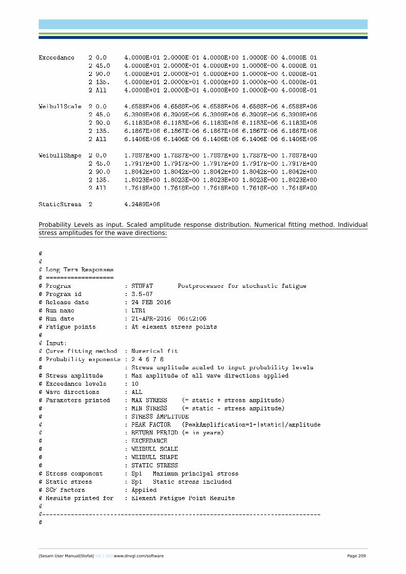
Exceedance 2 0.0 4.0000E+01 2.0000E+01 4.0000E+00 1.0000E+00 4.0000E-01
2 45.0 4.0000E+01 2.0000E+01 4.0000E+00 1.0000E+00 4.0000E-01
2 90.0 4.0000E+01 2.0000E+01 4.0000E+00 1.0000E+00 4.0000E-01
2 135. 4.0000E+01 2.0000E+01 4.0000E+00 1.0000E+00 4.0000E-01
2 All 4.0000E+01 2.0000E+01 4.0000E+00 1.0000E+00 4.0000E-01
WeibullScale 2 0.0 4.6588E+06 4.6588E+06 4.6588E+06 4.6588E+06 4.6588E+06
2 45.0 6.3909E+06 6.3909E+06 6.3909E+06 6.3909E+06 6.3909E+06
2 90.0 6.1183E+06 6.1183E+06 6.1183E+06 6.1183E+06 6.1183E+06
2 135. 6.1867E+06 6.1867E+06 6.1867E+06 6.1867E+06 6.1867E+06
2 All 6.1406E+06 6.1406E+06 6.1406E+06 6.1406E+06 6.1406E+06
WeibullShape 2 0.0 1.7887E+00 1.7887E+00 1.7887E+00 1.7887E+00 1.7887E+00
2 45.0 1.7917E+00 1.7917E+00 1.7917E+00 1.7917E+00 1.7917E+00
2 90.0 1.8042E+00 1.8042E+00 1.8042E+00 1.8042E+00 1.8042E+00
2 135. 1.8023E+00 1.8023E+00 1.8023E+00 1.8023E+00 1.8023E+00
2 All 1.7618E+00 1.7618E+00 1.7618E+00 1.7618E+00 1.7618E+00
StaticStress 2 4.2489E+06
Probability Levels as input. Scaled amplitude response distribution. Numerical fitting method. Individualstress amplitudes for the wave directions:
#
#
# Long Term Responses
# ===================
# Program : STOFAT Postprocessor for stochastic fatigue
# Program id : 3.5-07
# Release date : 24-FEB-2016
# Run name : LTR1
# Run date : 21-APR-2016 06:42:06
# Fatigue points : At element stress points
#
# Input:
# Curve fitting method : Numerical fit
# Probability exponents : 2 4 6 7 8
# : Stress amplitude scaled to input probability levels
# Stress amplitude : Max amplitude of all wave directions applied
# Exceedance levels : 10
# Wave directions : ALL
# Parameters printed : MAX STRESS (= static + stress amplitude)
# : MIN STRESS (= static - stress amplitude)
# : STRESS AMPLITUDE
# : PEAK FACTOR (PeakAmplification=1+|static|/amplitude
# : RETURN PERIOD (= in years)
# : EXCEEDANCE
# : WEIBULL SCALE
# : WEIBULL SHAPE
# : STATIC STRESS
# Stress component : Sp1 - Maximum principal stress
# Static stress : Sp1 - Static stress included
# SCF factors : Applied
# Results printed for : Element Fatigue Point Results
#
#------------------------------------------------------------------------------
#
|Sesam User Manual|Stofat|[V4.1-00] www.dnvgl.com/software Page 209
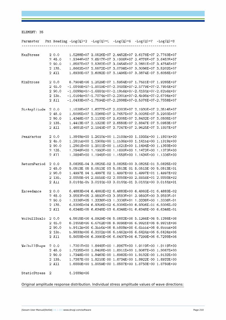
ELEMENT: 35
===========
Parameter Pnt Heading -Log(Q)=2 -Log(Q)=4 -Log(Q)=6 -Log(Q)=7 -Log(Q)=8
------------------------------------------------------------------------------
MaxStress 2 0.0 1.5288E+07 2.0526E+07 2.4452E+07 2.6178E+07 2.7763E+07
2 45.0 1.9344E+07 2.6517E+07 3.1906E+07 3.4276E+07 3.6452E+07
2 90.0 1.8597E+07 2.5382E+07 3.0454E+07 3.2681E+07 3.4754E+07
2 135. 1.8662E+07 2.5572E+07 3.0798E+07 3.3096E+07 3.5202E+07
2 All 1.8930E+07 2.6092E+07 3.1496E+07 3.3874E+07 3.6056E+07
MinStress 2 0.0 -6.7904E+06-1.2029E+07-1.5954E+07-1.7681E+07-1.9265E+07
2 45.0 -1.0846E+07-1.8019E+07-2.3408E+07-2.5779E+07-2.7954E+07
2 90.0 -1.0099E+07-1.6884E+07-2.1956E+07-2.4184E+07-2.6256E+07
2 135. -1.0164E+07-1.7074E+07-2.2301E+07-2.4598E+07-2.6704E+07
2 All -1.0433E+07-1.7594E+07-2.2998E+07-2.5376E+07-2.7558E+07
StrAmplitude 2 0.0 1.1039E+07 1.6277E+07 2.0203E+07 2.1930E+07 2.3514E+07
2 45.0 1.5095E+07 2.2268E+07 2.7657E+07 3.0028E+07 3.2203E+07
2 90.0 1.4348E+07 2.1133E+07 2.6205E+07 2.8432E+07 3.0505E+07
2 135. 1.4413E+07 2.1323E+07 2.6550E+07 2.8847E+07 3.0953E+07
2 All 1.4681E+07 2.1843E+07 2.7247E+07 2.9625E+07 3.1807E+07
PeakFactor 2 0.0 1.3849E+00 1.2610E+00 1.2103E+00 1.1938E+00 1.1807E+00
2 45.0 1.2815E+00 1.1908E+00 1.1536E+00 1.1415E+00 1.1319E+00
2 90.0 1.2961E+00 1.2011E+00 1.1621E+00 1.1494E+00 1.1393E+00
2 135. 1.2948E+00 1.1993E+00 1.1600E+00 1.1473E+00 1.1373E+00
2 All 1.2894E+00 1.1945E+00 1.1559E+00 1.1434E+00 1.1336E+00
ReturnPeriod 2 0.0 3.0825E-04 3.0825E-02 3.0825E+00 3.0825E+01 3.0825E+02
2 45.0 5.0513E-05 5.0513E-03 5.0513E-01 5.0513E+00 5.0513E+01
2 90.0 1.4997E-04 1.4997E-02 1.4997E+00 1.4997E+01 1.4997E+02
2 135. 2.8858E-04 2.8858E-02 2.8858E+00 2.8858E+01 2.8858E+02
2 All 3.0144E-05 3.0144E-03 3.0144E-01 3.0144E+00 3.0144E+01
Exceedance 2 0.0 6.4883E+04 6.4883E+02 6.4883E+00 6.4883E-01 6.4883E-02
2 45.0 3.9593E+05 3.9593E+03 3.9593E+01 3.9593E+00 3.9593E-01
2 90.0 1.3336E+05 1.3336E+03 1.3336E+01 1.3336E+00 1.3336E-01
2 135. 6.9306E+04 6.9306E+02 6.9306E+00 6.9306E-01 6.9306E-02
2 All 6.6348E+05 6.6348E+03 6.6348E+01 6.6348E+00 6.6348E-01
WeibullScale 2 0.0 4.5615E+06 4.8929E+06 5.0682E+06 5.1266E+06 5.1266E+06
2 45.0 6.2455E+06 6.6762E+06 6.9096E+06 6.9921E+06 6.9921E+06
2 90.0 5.9412E+06 6.3556E+06 6.5809E+06 6.6555E+06 6.6555E+06
2 135. 5.9833E+06 6.3102E+06 6.5462E+06 6.6424E+06 6.6424E+06
2 All 5.9659E+06 6.3990E+06 6.6437E+06 6.7299E+06 6.7299E+06
WeibullShape 2 0.0 1.7201E+00 1.8448E+00 1.8967E+00 1.9119E+00 1.9119E+00
2 45.0 1.7225E+00 1.8408E+00 1.8911E+00 1.9067E+00 1.9067E+00
2 90.0 1.7248E+00 1.8463E+00 1.8982E+00 1.9132E+00 1.9132E+00
2 135. 1.7287E+00 1.8210E+00 1.8734E+00 1.8922E+00 1.8922E+00
2 All 1.6880E+00 1.8059E+00 1.8587E+00 1.8750E+00 1.8750E+00
StaticStress 2 4.2489E+06
Original amplitude response distribution. Individual stress amplitude values of wave directions:
|Sesam User Manual|Stofat|[V4.1-00] www.dnvgl.com/software Page 210
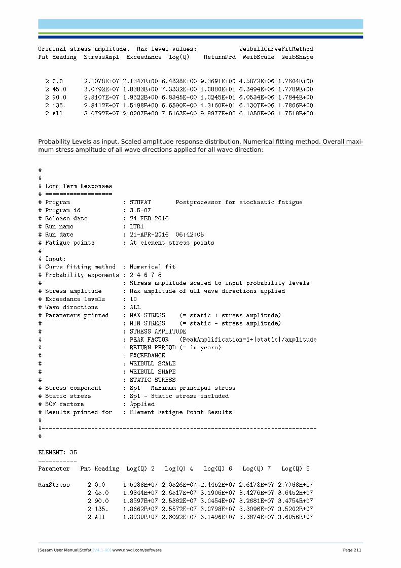
Original stress amplitude. Max level values: WeibullCurveFitMethod
Pnt Heading StressAmpl Exceedance -log(Q) ReturnPrd WeibScale WeibShape
------------------------------------------------------------------------------
2 0.0 2.1078E+07 2.1347E+00 6.4828E+00 9.3691E+00 4.5872E+06 1.7604E+00
2 45.0 3.0792E+07 1.8383E+00 7.3332E+00 1.0880E+01 6.3494E+06 1.7789E+00
2 90.0 2.8107E+07 1.9522E+00 6.8345E+00 1.0245E+01 6.0534E+06 1.7844E+00
2 135. 2.8112E+07 1.5198E+00 6.6590E+00 1.3160E+01 6.1307E+06 1.7866E+00
2 All 3.0792E+07 2.0207E+00 7.5163E+00 9.8977E+00 6.1058E+06 1.7519E+00
Probability Levels as input. Scaled amplitude response distribution. Numerical fitting method. Overall maxi-mum stress amplitude of all wave directions applied for all wave direction:
#
#
# Long Term Responses
# ===================
# Program : STOFAT Postprocessor for stochastic fatigue
# Program id : 3.5-07
# Release date : 24-FEB-2016
# Run name : LTR1
# Run date : 21-APR-2016 06:42:06
# Fatigue points : At element stress points
#
# Input:
# Curve fitting method : Numerical fit
# Probability exponents : 2 4 6 7 8
# : Stress amplitude scaled to input probability levels
# Stress amplitude : Max amplitude of all wave directions applied
# Exceedance levels : 10
# Wave directions : ALL
# Parameters printed : MAX STRESS (= static + stress amplitude)
# : MIN STRESS (= static - stress amplitude)
# : STRESS AMPLITUDE
# : PEAK FACTOR (PeakAmplification=1+|static|/amplitude
# : RETURN PERIOD (= in years)
# : EXCEEDANCE
# : WEIBULL SCALE
# : WEIBULL SHAPE
# : STATIC STRESS
# Stress component : Sp1 - Maximum principal stress
# Static stress : Sp1 - Static stress included
# SCF factors : Applied
# Results printed for : Element Fatigue Point Results
#
#------------------------------------------------------------------------------
#
ELEMENT: 35
===========
Parameter Pnt Heading -Log(Q)=2 -Log(Q)=4 -Log(Q)=6 -Log(Q)=7 -Log(Q)=8
------------------------------------------------------------------------------
MaxStress 2 0.0 1.5288E+07 2.0526E+07 2.4452E+07 2.6178E+07 2.7763E+07
2 45.0 1.9344E+07 2.6517E+07 3.1906E+07 3.4276E+07 3.6452E+07
2 90.0 1.8597E+07 2.5382E+07 3.0454E+07 3.2681E+07 3.4754E+07
2 135. 1.8662E+07 2.5572E+07 3.0798E+07 3.3096E+07 3.5202E+07
2 All 1.8930E+07 2.6092E+07 3.1496E+07 3.3874E+07 3.6056E+07
|Sesam User Manual|Stofat|[V4.1-00] www.dnvgl.com/software Page 211
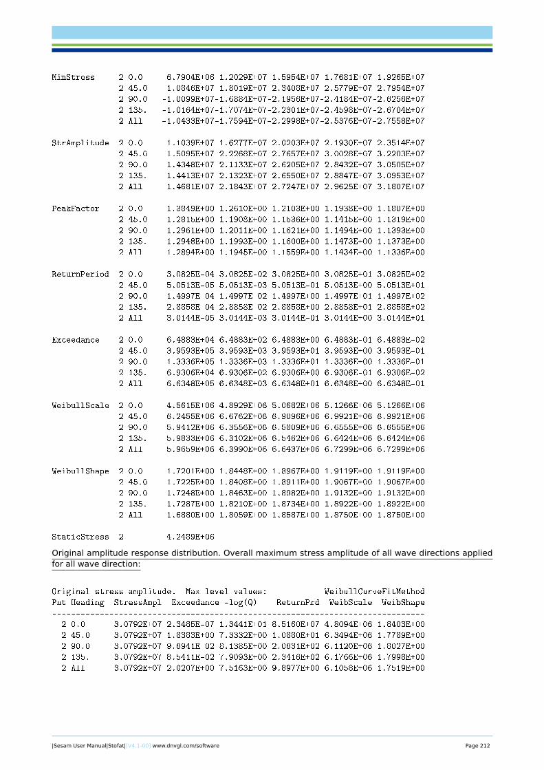
MinStress 2 0.0 -6.7904E+06-1.2029E+07-1.5954E+07-1.7681E+07-1.9265E+07
2 45.0 -1.0846E+07-1.8019E+07-2.3408E+07-2.5779E+07-2.7954E+07
2 90.0 -1.0099E+07-1.6884E+07-2.1956E+07-2.4184E+07-2.6256E+07
2 135. -1.0164E+07-1.7074E+07-2.2301E+07-2.4598E+07-2.6704E+07
2 All -1.0433E+07-1.7594E+07-2.2998E+07-2.5376E+07-2.7558E+07
StrAmplitude 2 0.0 1.1039E+07 1.6277E+07 2.0203E+07 2.1930E+07 2.3514E+07
2 45.0 1.5095E+07 2.2268E+07 2.7657E+07 3.0028E+07 3.2203E+07
2 90.0 1.4348E+07 2.1133E+07 2.6205E+07 2.8432E+07 3.0505E+07
2 135. 1.4413E+07 2.1323E+07 2.6550E+07 2.8847E+07 3.0953E+07
2 All 1.4681E+07 2.1843E+07 2.7247E+07 2.9625E+07 3.1807E+07
PeakFactor 2 0.0 1.3849E+00 1.2610E+00 1.2103E+00 1.1938E+00 1.1807E+00
2 45.0 1.2815E+00 1.1908E+00 1.1536E+00 1.1415E+00 1.1319E+00
2 90.0 1.2961E+00 1.2011E+00 1.1621E+00 1.1494E+00 1.1393E+00
2 135. 1.2948E+00 1.1993E+00 1.1600E+00 1.1473E+00 1.1373E+00
2 All 1.2894E+00 1.1945E+00 1.1559E+00 1.1434E+00 1.1336E+00
ReturnPeriod 2 0.0 3.0825E-04 3.0825E-02 3.0825E+00 3.0825E+01 3.0825E+02
2 45.0 5.0513E-05 5.0513E-03 5.0513E-01 5.0513E+00 5.0513E+01
2 90.0 1.4997E-04 1.4997E-02 1.4997E+00 1.4997E+01 1.4997E+02
2 135. 2.8858E-04 2.8858E-02 2.8858E+00 2.8858E+01 2.8858E+02
2 All 3.0144E-05 3.0144E-03 3.0144E-01 3.0144E+00 3.0144E+01
Exceedance 2 0.0 6.4883E+04 6.4883E+02 6.4883E+00 6.4883E-01 6.4883E-02
2 45.0 3.9593E+05 3.9593E+03 3.9593E+01 3.9593E+00 3.9593E-01
2 90.0 1.3336E+05 1.3336E+03 1.3336E+01 1.3336E+00 1.3336E-01
2 135. 6.9306E+04 6.9306E+02 6.9306E+00 6.9306E-01 6.9306E-02
2 All 6.6348E+05 6.6348E+03 6.6348E+01 6.6348E+00 6.6348E-01
WeibullScale 2 0.0 4.5615E+06 4.8929E+06 5.0682E+06 5.1266E+06 5.1266E+06
2 45.0 6.2455E+06 6.6762E+06 6.9096E+06 6.9921E+06 6.9921E+06
2 90.0 5.9412E+06 6.3556E+06 6.5809E+06 6.6555E+06 6.6555E+06
2 135. 5.9833E+06 6.3102E+06 6.5462E+06 6.6424E+06 6.6424E+06
2 All 5.9659E+06 6.3990E+06 6.6437E+06 6.7299E+06 6.7299E+06
WeibullShape 2 0.0 1.7201E+00 1.8448E+00 1.8967E+00 1.9119E+00 1.9119E+00
2 45.0 1.7225E+00 1.8408E+00 1.8911E+00 1.9067E+00 1.9067E+00
2 90.0 1.7248E+00 1.8463E+00 1.8982E+00 1.9132E+00 1.9132E+00
2 135. 1.7287E+00 1.8210E+00 1.8734E+00 1.8922E+00 1.8922E+00
2 All 1.6880E+00 1.8059E+00 1.8587E+00 1.8750E+00 1.8750E+00
StaticStress 2 4.2489E+06
Original amplitude response distribution. Overall maximum stress amplitude of all wave directions appliedfor all wave direction:
Original stress amplitude. Max level values: WeibullCurveFitMethod
Pnt Heading StressAmpl Exceedance -log(Q) ReturnPrd WeibScale WeibShape
------------------------------------------------------------------------------
2 0.0 3.0792E+07 2.3485E-07 1.3441E+01 8.5160E+07 4.8094E+06 1.8403E+00
2 45.0 3.0792E+07 1.8383E+00 7.3332E+00 1.0880E+01 6.3494E+06 1.7789E+00
2 90.0 3.0792E+07 9.6941E-02 8.1385E+00 2.0631E+02 6.1120E+06 1.8027E+00
2 135. 3.0792E+07 8.5411E-02 7.9093E+00 2.3416E+02 6.1766E+06 1.7998E+00
2 All 3.0792E+07 2.0207E+00 7.5163E+00 9.8977E+00 6.1058E+06 1.7519E+00
|Sesam User Manual|Stofat|[V4.1-00] www.dnvgl.com/software Page 212

C Fatigue Strength Based on Wöhler Curves
Stofat program will perform fatigue check calculations for shell and plate structures. It is based on spectralcalculation methods.
Using the program requires previous calculation of wave loads on a finite element model and calculation ofstresses caused by these loads.
Typical steps in a fatigue calculation using Stofat:
C.1 Calculation Steps
C.1.1 Establish Finite Element Model of the Structure
The modelling may be performed in different level of detail depending upon the details to be analysed andprevious knowledge of stress concentrations in the structure. Modelling and computations in several stepsof refinement may be needed.
C.1.2 Perform Hydrodynamic Wave Load Calculation
The Wadam program will calculate hydrodynamic pressure loads on the submerged surfaces of the finiteelement model. Input data to the wave load calculation are wave directions and wave frequencies.
C.1.3 Perform Finite Element Structural Calculation
Sestra program will compute stresses in the finite element model caused by the loads applied. Computa-tion is commonly performed as static linear analysis. Linear dynamic analysis may also be performed ifresonance may occur in the frequency ranges excited by the wave loads.
C.1.4 Spectral Fatigue Damage Calculation
Input data for the fatigue damage calculations in Stofat are wave statistics, SN curve, stress concentrationfactors and stresses from the previous calculations. Two scatter diagrams and some SN curves availablepredefined in the program. Other data may be specified by the user.
Long term wave statistics data is specified to the program as a scatter diagram and a wave direction prob-ability distribution. Short term wave statistics is specified by selecting a wave spectrum model and settingappropriate parameters. Wave spreading may be used to specify short term distribution of wave direc-tions.
The modelling may be performed in different level of detail depending SN data are experimental data givingthe number of cycles N of stress range S necessary to cause fatigue failure. These data are summarized inSN curves.
SN data are generally obtained from testing with constant amplitude sinusoidal loading. The mean loading,which is often expressed in terms of the ratio between the smallest stress and the largest stress in a stresscycle known as the R-ratio, is also fixed. For welded structures the influence of the mean stress or R-ratio isgenerally small since the welding procedure sets up residual stresses which are close to the yield limit. Inthis case only the stress range determines the number of stress cycles to failure.
The definition of the stress, used to obtain the stress range entering the SN curve, is not unique and dependson the specific application. For tubular joints, it is the geometrically amplified stress being measured orcomputed normal to the weld direction at a hot spot. For other welded connections it is a nominal stress.This lack of uniqueness has some influence on the presentation of code based design curves.
C.2 Codified SN Curves
C.2.1 SN Curve Equations
For practical fatigue design, welded joints are divided into several classes, each with a corresponding designSN curve.
|Sesam User Manual|Stofat|[V4.1-00] www.dnvgl.com/software Page 213
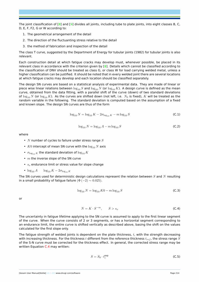
The joint classification of [8] and [9] divides all joints, including tube to plate joints, into eight classes B, C,D, E, F, F2, G or W according to:
1. The geometrical arrangement of the detail
2. The direction of the fluctuanting stress relative to the detail
3. the method of fabrication and inspection of the detail
The class T curve, suggested by the Department of Energy for tubular joints (1982) for tubular joints is alsorelevant.
Each construction detail at which fatigue cracks may develop must, whenever possible, be placed in itsrelevant class in accordance with the criterion given by [8]. Details which cannot be classified according tothe classification of DNV should be treated as class G, or class W for load carrying welded metal, unless ahigher classification can be justified. It should be noted that in every welded joint there are several locationsat which fatigue cracks may develop and each location should be classified separately.
The design SN curves are based on a statistical analysis of experimental data. They are made of linear orpiece wise linear relations between log10 S and log10N (or log10K). A design curve is defined as the meancurve, obtained from the data fitting, with a parallel shift of the curve (down) of two standard deviationsof log10N (or log10K). As the curves are shifted down (not left, i.e. N0 is fixed), K will be treated as therandom variable in the following. The standard deviation is computed based on the assumption of a fixedand known slope. The design SN curves are thus of the form
log10N = log10K − 2σlog10K −m log10 S (C.1)
log10N = log10A−m log10 S (C.2)
where
• N number of cycles to failure under stress range S
• K0 intercept of mean SN curve with the log10N axis
• σlog10K the standard deviation of log10K
• m the inverse slope of the SN curve
• so endurance limit or stress value for slope change
• log10A log10K − 2σlog10K
The SN curves used for deterministic design calculations represent the relation between S and N resultingin a small probability of fatigue failure (Φ (−2) ∼ 0.025).
log10N = log10K0−m log10 S (C.3)
or
N = K · S−m, S > so (C.4)
The uncertainty in fatigue lifetime applying to the SN curve is assumed to apply to the first linear segmentof the curve. When the curve consists of 2 or 3 segments, or has a horizontal segment corresponding toan endurance limit, the entire curve is shifted vertically as described above, basing the shift on the valuescalculated for the first slope only.
The fatigue strength of welded joints is dependent on the plate thickness, t, with the strength decreasingwith increasing thickness. For the thickness t different from the reference thickness tref , the stress range Sof the S-N curve must be corrected for the thickness effect. In general, the corrected stress range may bewritten Equation C.4 may written:
S = S0 · texpc (C.5)
|Sesam User Manual|Stofat|[V4.1-00] www.dnvgl.com/software Page 214
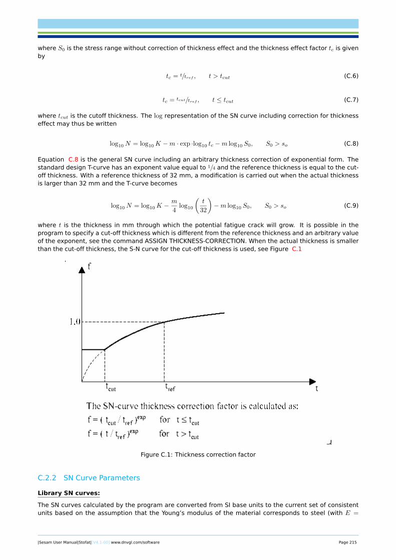
where S0 is the stress range without correction of thickness effect and the thickness effect factor tc is givenby
tc = t/tref , t > tcut (C.6)
tc = tcut/tref , t ≤ tcut (C.7)
where tcut is the cutoff thickness. The log representation of the SN curve including correction for thicknesseffect may thus be written
log10N = log10K −m · exp ·log10 tc −m log10 S0, S0 > so (C.8)
Equation C.8 is the general SN curve including an arbitrary thickness correction of exponential form. Thestandard design T-curve has an exponent value equal to 1/4 and the reference thickness is equal to the cut-off thickness. With a reference thickness of 32 mm, a modification is carried out when the actual thicknessis larger than 32 mm and the T-curve becomes
log10N = log10K −m
4log10
(t
32
)−m log10 S0, S0 > so (C.9)
where t is the thickness in mm through which the potential fatigue crack will grow. It is possible in theprogram to specify a cut-off thickness which is different from the reference thickness and an arbitrary valueof the exponent, see the command ASSIGN THICKNESS-CORRECTION. When the actual thickness is smallerthan the cut-off thickness, the S-N curve for the cut-off thickness is used, see Figure C.1
Figure C.1: Thickness correction factor
C.2.2 SN Curve Parameters
Library SN curves:
The SN curves calculated by the program are converted from SI base units to the current set of consistentunits based on the assumption that the Young’s modulus of the material corresponds to steel (with E =
|Sesam User Manual|Stofat|[V4.1-00] www.dnvgl.com/software Page 215
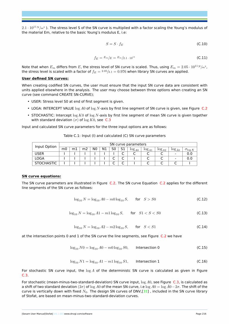
2.1 · 1011N/m2 ). The stress level S of the SN curve is multiplied with a factor scaling the Young’s modulus ofthe material Em, relative to the basic Young’s modulus E, i.e:
S = S · fE (C.10)
fE = Em/E = Em/2.1 · 1011 (C.11)
Note that when Em differs from E, the stress level of SN curve is scaled. Thus, using Em = 2.05 · 1011N/m2,the stress level is scaled with a factor of fE = 2.05/2.1 = 0.976 when library SN curves are applied.
User defined SN curves:
When creating codified SN curves, the user must ensure that the input SN curve data are consistent withunits applied elsewhere in the analysis. The user may choose between three options when creating an SNcurve (see command CREATE SN-CURVE);
• USER: Stress level S0 at end of first segment is given.
• LOGA: INTERCEPT VALUE logA0 of logN -axis by first line segment of SN curve is given, see Figure C.2
• STOCHASTIC: Intercept logK0 of logN -axis by first line segment of mean SN curve is given togetherwith standard deviation (σ) of logK0, see C.3
Input and calculated SN curve parameters for the three input options are as follows:
Table C.1: Input (I) and calculated (C) SN curve parameters
Input OptionSN curve parameters
m0 m1 m2 N0 N1 S0 S1 logA0 logA1 logA2 logA0 σlogK
USER I I I I I I C C C C - 0.0LOGA I I I I I C C I C C - 0.0STOCHASTIC I I I I I C C I C C C I
SN curve equations:
The SN curve parameters are illustrated in Figure C.2. The SN curve Equation C.2 applies for the differentline segments of the SN curve as follows:
log10N = log10A0−m0 log10 S, for S > S0 (C.12)
log10N = log10A1−m1 log10 S, for S1 < S < S0 (C.13)
log10N = log10A2−m2 log10 S, for S < S1 (C.14)
at the intersection points 0 and 1 of the SN curve the line segments, see Figure C.2 we have
log10N0 = log10A0−m0 log10 S0, Intersection 0 (C.15)
log10N1 = log10A1−m1 log10 S1, Intersection 1 (C.16)
For stochastic SN curve input, the logA of the deterministc SN curve is calculated as given in FigureC.3.
For stochastic (mean-minus-two-standard-deviation) SN curve input, logA0, see Figure C.3, is calculated asa shift of two standard deviation (2σ) of logA0 of the mean SN curve, i.e logA0 = log A0−2σ. The shift of thecurve is vertically down with fixed N0. The design SN curves of DNV,[31] , included in the SN curve libraryof Stofat, are based on mean-minus-two-standard-deviation curves.
|Sesam User Manual|Stofat|[V4.1-00] www.dnvgl.com/software Page 216
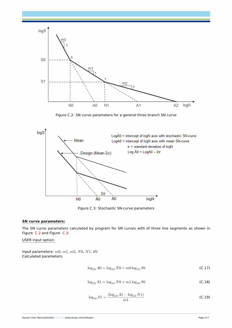
Figure C.2: SN curve parameters for a general three branch SN curve
Figure C.3: Stochastic SN-curve parameters
SN curve parameters:
The SN curve parameters calculated by program for SN curves with of three line segments as shown inFigure C.2 and Figure C.3:
USER input option:
Input parameters: m0, m1, m2, N0, N1, S0Calculated parameters:
log10A0 = log10N0 +m0 log10 S0 (C.17)
log10A1 = log10N0 +m1 log10 S0 (C.18)
log10 S1 =(log10A1− log10N1)
m1(C.19)
|Sesam User Manual|Stofat|[V4.1-00] www.dnvgl.com/software Page 217
log10A2 = log10N1 +m2 log10 S1 (C.20)
LOGA input option:
Input parameters: m0, m1, m2, N0, N1, logA0
Calculated parameters:
log10 S0 =(log10A0− log10N0)
m0(C.21)
log10A1 = log10N0 +m1 log10 S0 (C.22)
log10 S1 =(log10A1− log10N1)
m1(C.23)
log10A2 = log10N1 +m2 log10 S1 (C.24)
STOCHASTIC input option:
Input parameters: m0, m1, m2, N0, N1, logK0, σlogK
Calculated parameters:
log10 A0 = log10A0 − 2σlog10K (C.25)
log10 S0 =
(log10 A0− log10N0
)m0
(C.26)
log10 A1 = log10N0 +m1 log10 S0 (C.27)
log10 S1 =(log10A1− log10N1)
m1(C.28)
log10 A2 = log10N1 +m2 log10 S1 (C.29)
Units convertion of SN curve parameters:
Use of consistent units in the fatigue analysis is required for valid analysis results. Convertion of SN curvedata from one unit to another may be required. Units of parameters calculated by the program are inaccordance with units of the input parameters.
When S0 is given as input (USER input option), the values of the calculated parameters (e.g. logA0, logA1)are in accordance with unit and value of S0. When logA0 is given as input (LOGA input option) the valuemust be in accordance with the unit of the stresses applied in the analysis.
logA0, m1 and m2 are commonly used parameters in SN curve data specifications. The value of logA0reflects the stress unit of the SN curve. The unit of the SN curve data do not always coincide with the unitapplied in the analysis and a conversion of the SN curve data may be required.
A conversion rule may easily established by expressing Equation C.2 in two different stress values. Ageneral stress value may S may be written as an exponent of 10, e.g.:
|Sesam User Manual|Stofat|[V4.1-00] www.dnvgl.com/software Page 218
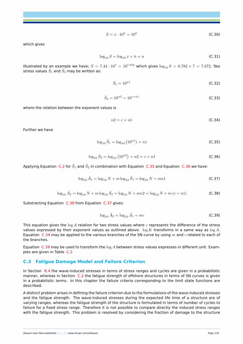
S = x · 10n = 10n (C.30)
which gives
log10 S = log10 x+ n = n (C.31)
Illustrated by an example we have; S = 7.44 · 107 = 107.872 which gives log10 S = 0.782 + 7 = 7.872, Twostress values S1 and S2 may be written as:
S1 = 10n1 (C.32)
S2 = 10n2 = 10c+n1 (C.33)
where the relation between the exponent values is
n2 = c+ n1 (C.34)
Further we have
log10 S1 = log10
(10n1
)= n1 (C.35)
log10 S2 = log10
(10n2
)= n2 = c+ n1 (C.36)
Applying Equation C.2 for S1 and S2 in combination with Equation C.35 and Equation C.36 we have:
log10 A1 = log10N +m log10 S1 = log10N +mn1 (C.37)
log10 A2 = log10N +m log10 S2 = log10N +mn2 = log10N +m (c+ n1) (C.38)
Substracting Equation C.38 from Equation C.37 gives:
log10 A2 = log10 A1 +mc (C.39)
This equation gives the logA relation for two stress values where c represents the difference of the stressvalues expressed by their exponent values as outlined above. logK transforms in a same way as logA.Equation C.34 may be applied to the various branches of the SN curve by using m and c related to each ofthe branches.
Equation C.39 may be used to transform the logA between stress values expresses in different unit. Exam-ples are given in Table C.2
C.3 Fatigue Damage Model and Failure Criterion
In Section B.4 the wave-induced stresses in terms of stress ranges and cycles are given in a probabilisticmanner, whereas in Section C.2 the fatigue strength of offshore structures in terms of SN curves is givenin a probabilistic terms. In this chapter the failure criteria corresponding to the limit state functions aredescribed.
A distinct problem arises in defining the failure criterion due to the formulations of the wave-induced stressesand the fatigue strength. The wave-induced stresses during the expected life time of a structure are ofvarying ranges, whereas the fatigue strength of the structure is formulated in terms of number of cycles tofailure for a fixed stress range. Therefore it is not possible to compare directly the induced stress rangeswith the fatigue strength. This problem is resolved by considering the fraction of damage to the structure
|Sesam User Manual|Stofat|[V4.1-00] www.dnvgl.com/software Page 219
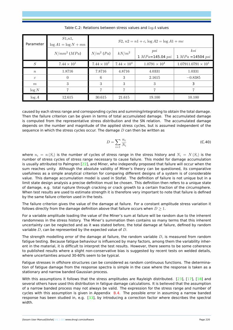
Table C.2: Relations between stress values and logA values
Parameter
S1,n1,
logA1 = logN +mnS2, n2 = n1 + c, logA2 = logA1 +mc
N/mm2 (MPa) N/m2 (Pa) kN/m2psi
1 MPa=145.04 psi
ksi
1 MPa =14504 psi
S 7.44× 101 7.44× 10⁷ 7.44× 10⁴ 1.0791× 10⁴ 1.07911.0791× 101
n 1.8716 7.8716 4.8716 4.0331 1.0331
c 0 6 3 2.1615 −0.8385
m 3 3 3 3 3
logN 7 7 7 7 7
logA 12.615 30.615 21.615 19.100 10.100
caused by each stress range and corresponding cycles and summing/integrating to obtain the total damage.Then the failure criterion can be given in terms of total accumulated damage. The accumulated damageis computed from the representative stress distribution and the SN relation. The accumulated damagedepends on the number and magnitude of the applied stress cycles, but is assumed independent of thesequence in which the stress cycles occur. The damage D can then be written as
D =∑i=1
niNi
(C.40)
where ni = n (Si) is the number of cycles of stress range in the stress history and Ni = N (Si) is thenumber of stress cycles of stress range necessary to cause failure. This model for damage accumulationis usually attributed to Palmgren [22], and Miner, who independly proposed that failure will occur when thesum reaches unity. Although the absolute validity of Miner’s theory can be questioned, its comparativeusefulness as a simple analytical criterion for comparing different designs of a system is of considerablevalue. This damage accumulation model is used in Stofat. The definition of failure is not unique but in alimit state design analysis a precise definition must be chosen. This definition then refers to a unique stateof damage, e.g. total rupture through cracking or crack growth to a certain fraction of the circumsphere.When test results are used to estimate strength it is therefore very important to note that failure is definedby the same failure criterion used in the tests.
The failure criterion gives the value of the damage at failure. For a constant amplitude stress variation itfollows directly from the damage definition above that failure occurs when D ≥ 1.
For a variable amplitude loading the value of the Miner’s sum at failure will be random due to the inherentrandomness in the stress history. The Miner’s summation then contains so many terms that this inherentuncertainty can be neglected and as it was stated before, the total damage at failure, defined by randomvariable D, can be represented by the expected value of D.
The strength modelling error of the damage at failure, the random variable D, is measured from randomfatigue testing. Because fatigue behaviour is influenced by many factors, among them the variability inher-ent in the material, it is difficult to interpret the test results. However, there seems to be some coherenceto published results where a slight non-conservative bias is suggested by recent tests on welded details,where uncertainties around 30-60% seem to be typical.
Fatigue stresses in offshore structures can be considered as random continuous functions. The determina-tion of fatigue damage from the response spectra is simple in the case where the response is taken as astationary and narrow banded Gaussian process.
With this assumptions it follows that the stress amplitudes are Rayleigh distributed. [23], [17], [18] andseveral others have used this distribution in fatigue damage calculations. It is believed that the assumptionof a narrow banded process may not always be valid. The expression for the stress range and number ofcycles with this assumption is given in Appendix B.4. The possible error in assuming a narrow bandedresponse has been studied in, e.g. [33], by introducing a correction factor where describes the spectralwidth.
|Sesam User Manual|Stofat|[V4.1-00] www.dnvgl.com/software Page 220
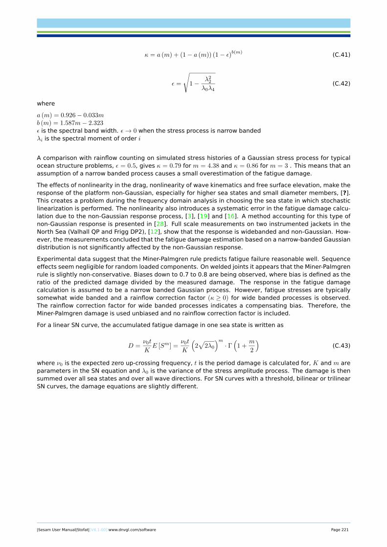
κ = a (m) + (1− a (m)) (1− ε)b(m) (C.41)
ε =
√1− λ2
2
λ0λ4(C.42)
where
a (m) = 0.926− 0.033mb (m) = 1.587m− 2.323ε is the spectral band width. ε→ 0 when the stress process is narrow bandedλi is the spectral moment of order i
A comparison with rainflow counting on simulated stress histories of a Gaussian stress process for typicalocean structure problems, ε = 0.5, gives κ = 0.79 for m = 4.38 and κ = 0.86 for m = 3 . This means that anassumption of a narrow banded process causes a small overestimation of the fatigue damage.
The effects of nonlinearity in the drag, nonlinearity of wave kinematics and free surface elevation, make theresponse of the platform non-Gaussian, especially for higher sea states and small diameter members, [?].This creates a problem during the frequency domain analysis in choosing the sea state in which stochasticlinearization is performed. The nonlinearity also introduces a systematic error in the fatigue damage calcu-lation due to the non-Gaussian response process, [3], [19] and [16]. A method accounting for this type ofnon-Gaussian response is presented in [28]. Full scale measurements on two instrumented jackets in theNorth Sea (Valhall QP and Frigg DP2), [12], show that the response is widebanded and non-Gaussian. How-ever, the measurements concluded that the fatigue damage estimation based on a narrow-banded Gaussiandistribution is not significantly affected by the non-Gaussian response.
Experimental data suggest that the Miner-Palmgren rule predicts fatigue failure reasonable well. Sequenceeffects seem negligible for random loaded components. On welded joints it appears that the Miner-Palmgrenrule is slightly non-conservative. Biases down to 0.7 to 0.8 are being observed, where bias is defined as theratio of the predicted damage divided by the measured damage. The response in the fatigue damagecalculation is assumed to be a narrow banded Gaussian process. However, fatigue stresses are typicallysomewhat wide banded and a rainflow correction factor (κ ≥ 0) for wide banded processes is observed.The rainflow correction factor for wide banded processes indicates a compensating bias. Therefore, theMiner-Palmgren damage is used unbiased and no rainflow correction factor is included.
For a linear SN curve, the accumulated fatigue damage in one sea state is written as
D =ν0t
KE [Sm] =
ν0t
K
(2√
2λ0
)m· Γ(
1 +m
2
)(C.43)
where ν0 is the expected zero up-crossing frequency, t is the period damage is calculated for, K and m areparameters in the SN equation and λ0 is the variance of the stress amplitude process. The damage is thensummed over all sea states and over all wave directions. For SN curves with a threshold, bilinear or trilinearSN curves, the damage equations are slightly different.
|Sesam User Manual|Stofat|[V4.1-00] www.dnvgl.com/software Page 221

D Stofat Elements and Fatigue Check Points
D.1 Fatigue Check Points
Two types of fatigue check calculations are performed by Stofat; 1) element fatigue check and 2) hotspotfatigue check. Element fatigue check is performed for individual elements selected by the used and hotspotfatigue check is performed for critical points in the structure specified by the user.
Element fatigue check points may be located at following positions within an element, 1) at the stress points(result points), 2) at the element surface points, 3) at the element corner points and 4) at the elementmiddle plane points, 5) at element centre points, see Section D.2. The middle plane fatigue check points areapplicable for shell elements and are located at the projections normal to the middle plane of the elementstress points. Use of only membrane stresses in the fatigue calculation for the middle plane points is alsopossible. The user selects the fatigue point locations by the command CREATE FATIGUE-CHECK-POINTSELEMENT-CHECK.
The number of fatigue check points of an element is the same as the number of stress points for the element.For the middle plane, the number of fatigue points is half the number of stress points, see D.1. Damageis calculated for all fatigue points of an element and the usage factor of the point that suffers most fatiguedamage is taken as the usage factor of the element and is made available to the user in tabulated prints ofthe fatigue results. Usage factors of all the fatigue points may, however, be printed to a dump print file orwritten to the VTF file and presented as contour plots by Xtract.
Hotspots may be placed anywhere inside or at the borders of the elements. Creation of a hotspot is describedin Section D.3.
Stofat interpolates stresses to element surface points, element corner points, element middle plane pointsand hotspots on basis of stresses of the stress points which are read from the Result Interface File (.SIN).Linear interpolation schemes are applied, see Section D.3.2.
Element fatigue check and hotspot fatigue check cannot be mixed and have to be executed in a separateruns. The user selects the fatigue check type to be executed in the RUN FATIGUE-CHECK command.
Note that fatigue calculations are not performed for element types that are not implemented in Stofat. Ifsuch elements are present in the model, Stofat neglects them and prints a message.
D.2 Elements Implemented in Stofat
Stofat performs fatigue check calculations of structural models based on shell and solid elements. The el-ements implemented in Stofat are listed in D.1 which gives an overview of the nodes, stress points, stresscomponents and fatigue point locations of the elements. Key information about the elements and specifica-tion of the fatigue point locations are described in the next sections. Node numbering applied in Xtract forStofat elements are also given since the numbering do not coincide for the higher order elements.
D.2.1 Shell Elements
Four types of shell elements are implemented in Stofat:
• Flat thin shell elements - quadrilateral FQUS(24) and triangular FTRS(25) elements
• Subparametric curved thick shell element - quadrilateral SCQS(28) and triangular SCTS(26) elements
D.2.1.1 Thin Shell Elements
The flat thin shell element FQUS and FTRS have 4 and 3 nodes, respectively. The nodes are located in thecorners of the middle plane of the elements. The stress points are located at the element corners and at thecentre point of the element surfaces, see Figure D.1 and Figure D.2. The elements have 10 and 8 stresspoints, respectively. Stress points and corner points coincide for the thin shell elements and the middleplane points coincide with the nodes of the elements.
The elements have two surfaces, numbered as 1 and 2, where surface 1 is the lower surface of the element(at γ = −1) and surface 2 is the upper surface (at γ = +1). The natural element coordinate axes α, β,γ and the i, j, k axes (which relates to the I, J, K planes) are shown in the figures. The stress points arenumbered according to the Results Interface File numbering sequence in the order of the i,j, k directions.Area coordinates of a triangular shell element is shown in Figure D.3.
|Sesam User Manual|Stofat|[V4.1-00] www.dnvgl.com/software Page 222
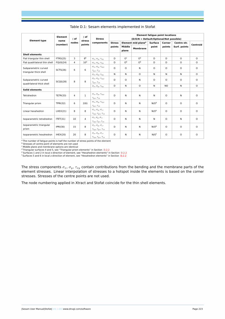
Table D.1: Sesam elements implemented in Stofat
Element type
Element
name
(number)
] of
nodes
] of
stress
points
Stress
components
Element fatigue point locations
(D/O/N = Default/Optional/Not possible)
Stress
points
Element mid-planea Surface
point
Corner
points
Centre str.
Surf. pointsCentroid
Middle
planeMembrane
Shell elements
Flat triangular thin shell FTRS(25) 3 8b σx, σy, τxy D Oc Ob D D O O
Flat quadrilateral thin shell FQUS(24) 4 10a σx, σy, τxy D Ob Ob D D O O
Subparametric curved
triangular thick shellSCTS(26) 6 6
σx, σy, τxy,
τyz, τzxD O N O O O O
σx, σy, τxy N N O N N N O
Subparametric curved
quadrilateral thick shellSCQS(28) 8 8
σx, σy, τxy,
τyz, τzxD O N O O O O
σx, σy, τxy D N O N NO N O
Solid elements
Tetrahedron TETR(33) 4 1σx, σy, τxy,
τyz, τzxD N N N O N O
Triangular prism TPRI(32) 6 2(6)σx, σy, τxy,
τyz, τzxD N N N/Od O O O
Linear hexahedron LHEX(21) 8 8σx, σy, σz,
τxy, τyz, τzxD N N N/Oe O O O
Isoparametric tetrahedron ITET(31) 10 4σx, σy, σz,
τxy, τyz, τzxD N N N O N O
Isoparametric triangular
prismIPRI(30) 15 8
σx, σy, σz,
τxy, τyz, τzxD N N N/Ob O O O
Isoparametric hexahedron IHEX(20) 20 8σx, σy, σz,
τxy, τyz, τzxD N N N/Of O O O
a The number of fatigue points is half the number of stress points of the elementb Stresses of centre point of elements are not usedc Middle plane and membrane options are identicald Triangular surfaces 4 and 5, see “Triangular prism elements” in Section D.2.2e Surfaces 1 and 2 in local z-direction of element, see “Hexahedron elements” in Section D.2.2f Surfaces 5 and 6 in local z-direction of element, see “Hexahedron elements” in Section D.2.2
The stress components σx, σy, τxy contain contributions from the bending and the membrane parts of theelement stresses. Linear interpolation of stresses to a hotspot inside the elements is based on the cornerstresses. Stresses of the centre points are not used.
The node numbering applied in Xtract and Stofat coincide for the thin shell elements.
|Sesam User Manual|Stofat|[V4.1-00] www.dnvgl.com/software Page 223
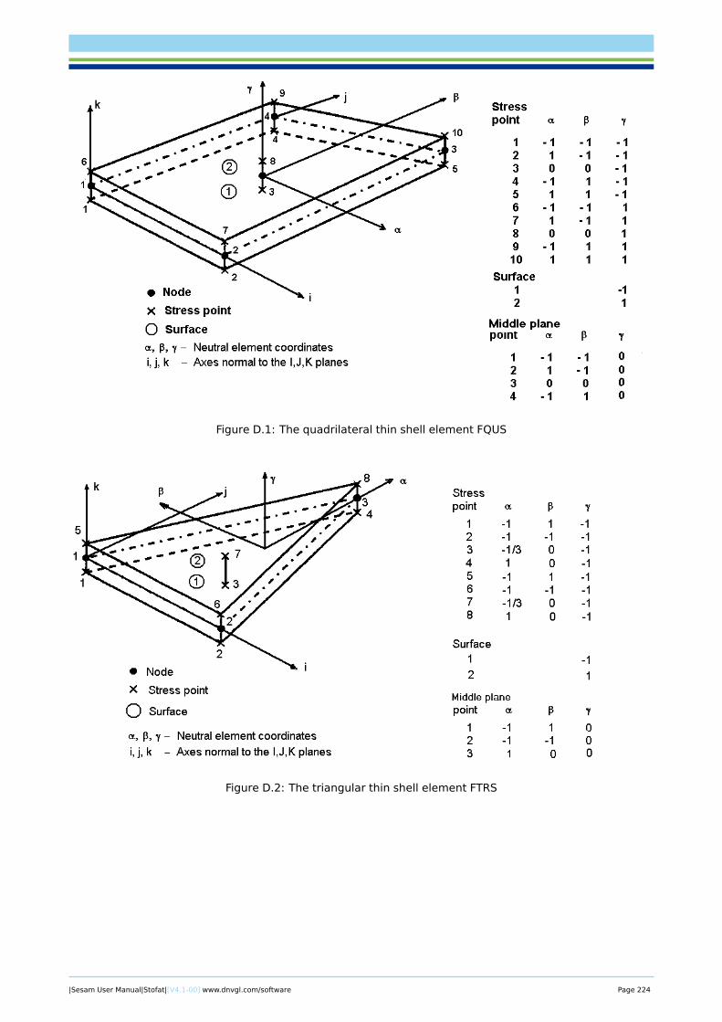
Figure D.1: The quadrilateral thin shell element FQUS
Figure D.2: The triangular thin shell element FTRS
|Sesam User Manual|Stofat|[V4.1-00] www.dnvgl.com/software Page 224
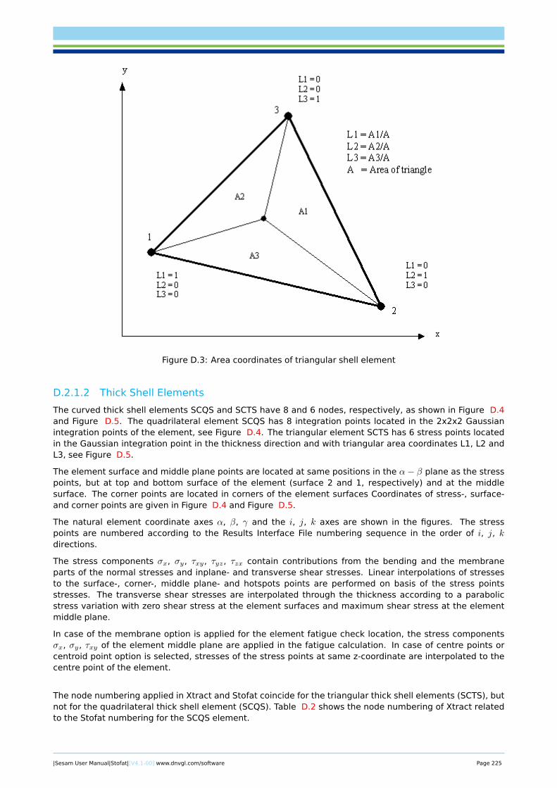
Figure D.3: Area coordinates of triangular shell element
D.2.1.2 Thick Shell Elements
The curved thick shell elements SCQS and SCTS have 8 and 6 nodes, respectively, as shown in Figure D.4and Figure D.5. The quadrilateral element SCQS has 8 integration points located in the 2x2x2 Gaussianintegration points of the element, see Figure D.4. The triangular element SCTS has 6 stress points locatedin the Gaussian integration point in the thickness direction and with triangular area coordinates L1, L2 andL3, see Figure D.5.
The element surface and middle plane points are located at same positions in the α− β plane as the stresspoints, but at top and bottom surface of the element (surface 2 and 1, respectively) and at the middlesurface. The corner points are located in corners of the element surfaces Coordinates of stress-, surface-and corner points are given in Figure D.4 and Figure D.5.
The natural element coordinate axes α, β, γ and the i, j, k axes are shown in the figures. The stresspoints are numbered according to the Results Interface File numbering sequence in the order of i, j, kdirections.
The stress components σx, σy, τxy, τyz, τzx contain contributions from the bending and the membraneparts of the normal stresses and inplane- and transverse shear stresses. Linear interpolations of stressesto the surface-, corner-, middle plane- and hotspots points are performed on basis of the stress pointsstresses. The transverse shear stresses are interpolated through the thickness according to a parabolicstress variation with zero shear stress at the element surfaces and maximum shear stress at the elementmiddle plane.
In case of the membrane option is applied for the element fatigue check location, the stress componentsσx, σy, τxy of the element middle plane are applied in the fatigue calculation. In case of centre points orcentroid point option is selected, stresses of the stress points at same z-coordinate are interpolated to thecentre point of the element.
The node numbering applied in Xtract and Stofat coincide for the triangular thick shell elements (SCTS), butnot for the quadrilateral thick shell element (SCQS). Table D.2 shows the node numbering of Xtract relatedto the Stofat numbering for the SCQS element.
|Sesam User Manual|Stofat|[V4.1-00] www.dnvgl.com/software Page 225
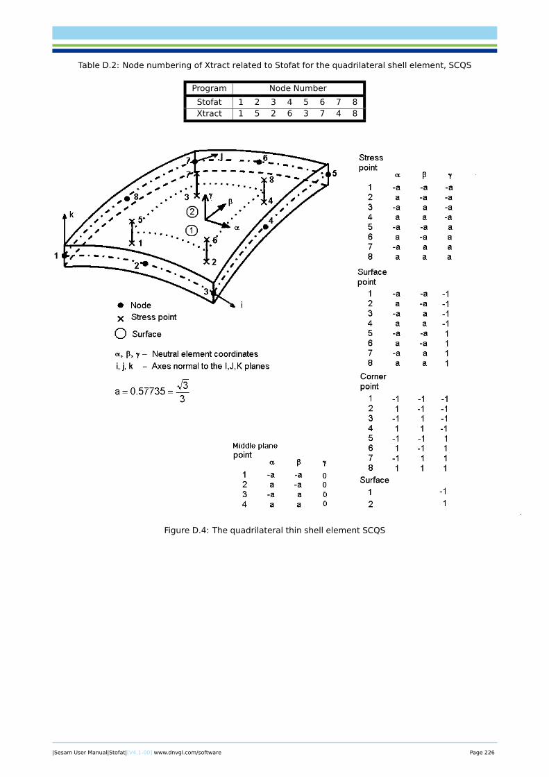
Table D.2: Node numbering of Xtract related to Stofat for the quadrilateral shell element, SCQS
Program Node Number
Stofat 1 2 3 4 5 6 7 8Xtract 1 5 2 6 3 7 4 8
Figure D.4: The quadrilateral thin shell element SCQS
|Sesam User Manual|Stofat|[V4.1-00] www.dnvgl.com/software Page 226
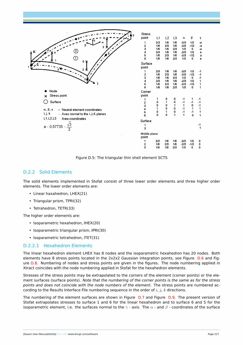
Figure D.5: The triangular thin shell element SCTS
D.2.2 Solid Elements
The solid elements implemented in Stofat consist of three lower order elements and three higher orderelements. The lower order elements are:
• Linear haxahedron, LHEX(21)
• Triangular prism, TPRI(32)
• Tetrahedron, TETR(33)
The higher order elements are:
• Isoparametric hexahedron, IHEX(20)
• Isoparametric triangular prism, IPRI(30)
• Isoparametric tetrahedron, ITET(31)
D.2.2.1 Hexahedron Elements
The linear hexahedron element LHEX has 8 nodes and the isoparametric hexahedron has 20 nodes. Bothelements have 8 stress points located in the 2x2x2 Gaussian integration points, see Figure D.6 and Fig-ure D.8. Numbering of nodes and stress points are given in the figures. The node numbering applied inXtract coincides with the node numbering applied in Stofat for the hexahedron elements.
Stresses of the stress points may be extrapolated to the corners of the element (corner points) or the ele-ment surfaces (surface points). Note that the numbering of the corner points is the same as for the stresspoints and does not coincide with the node numbers of the element. The stress points are numbered ac-cording to the Results Interface File numbering sequence in the order of i, j, k directions.
The numbering of the element surfaces are shown in Figure D.7 and Figure D.9. The present version ofStofat extrapolates stresses to surface 1 and 6 for the linear hexahedron and to surface 6 and 5 for theisoparametric element, i.e. the surfaces normal to the γ - axis. The α - and β - coordinates of the surface
|Sesam User Manual|Stofat|[V4.1-00] www.dnvgl.com/software Page 227
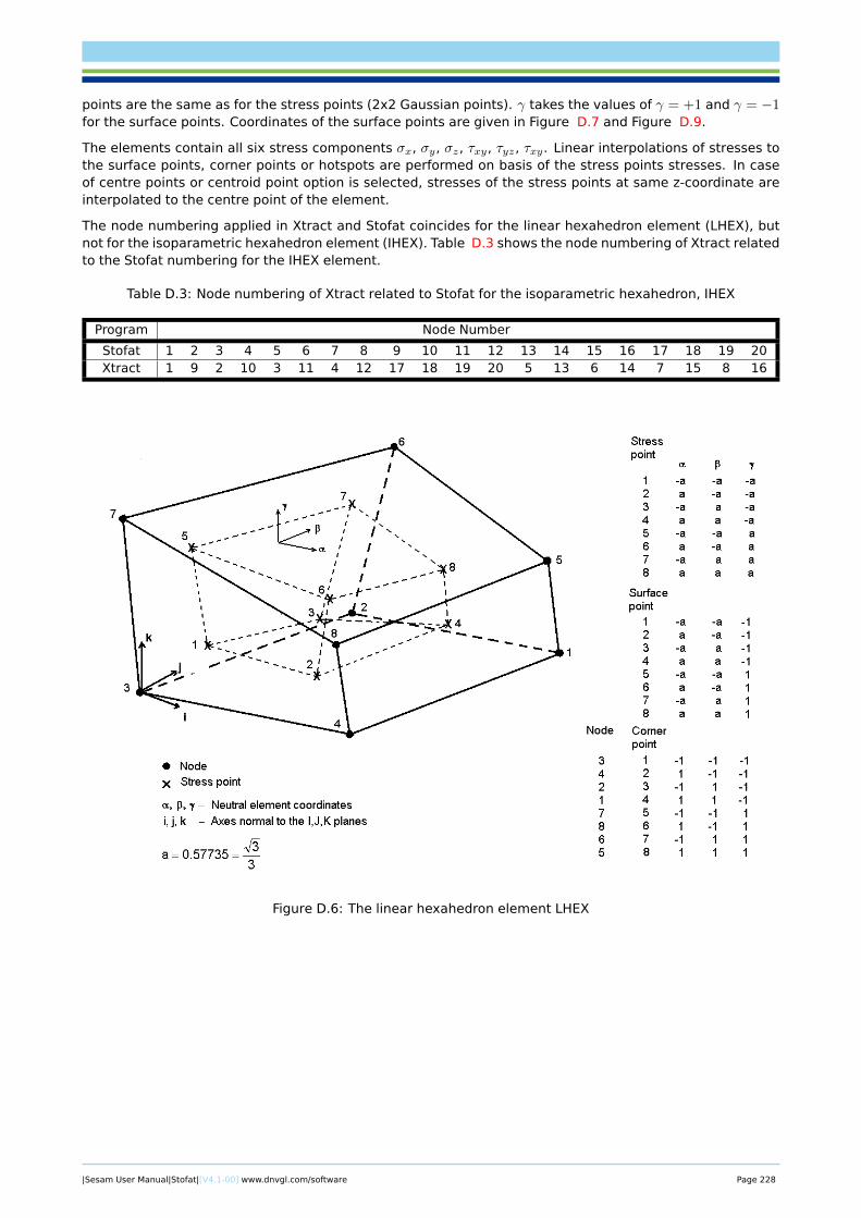
points are the same as for the stress points (2x2 Gaussian points). γ takes the values of γ = +1 and γ = −1for the surface points. Coordinates of the surface points are given in Figure D.7 and Figure D.9.
The elements contain all six stress components σx, σy, σz, τxy, τyz, τxy. Linear interpolations of stresses tothe surface points, corner points or hotspots are performed on basis of the stress points stresses. In caseof centre points or centroid point option is selected, stresses of the stress points at same z-coordinate areinterpolated to the centre point of the element.
The node numbering applied in Xtract and Stofat coincides for the linear hexahedron element (LHEX), butnot for the isoparametric hexahedron element (IHEX). Table D.3 shows the node numbering of Xtract relatedto the Stofat numbering for the IHEX element.
Table D.3: Node numbering of Xtract related to Stofat for the isoparametric hexahedron, IHEX
Program Node Number
Stofat 1 2 3 4 5 6 7 8 9 10 11 12 13 14 15 16 17 18 19 20Xtract 1 9 2 10 3 11 4 12 17 18 19 20 5 13 6 14 7 15 8 16
Figure D.6: The linear hexahedron element LHEX
|Sesam User Manual|Stofat|[V4.1-00] www.dnvgl.com/software Page 228
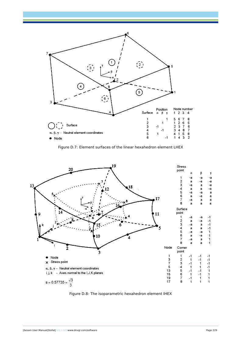
Figure D.7: Element surfaces of the linear hexahedron element LHEX
Figure D.8: The isoparametric hexahedron element IHEX
|Sesam User Manual|Stofat|[V4.1-00] www.dnvgl.com/software Page 229
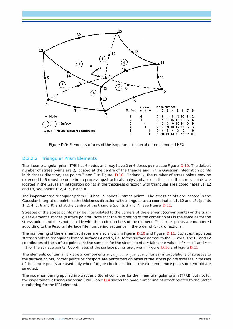
Figure D.9: Element surfaces of the isoparametric hexahedron element LHEX
D.2.2.2 Triangular Prism Elements
The linear triangular prism TPRI has 6 nodes and may have 2 or 6 stress points, see Figure D.10. The defaultnumber of stress points are 2, located at the centre of the triangle and in the Gaussian integration pointsin thickness direction, see points 3 and 7 in Figure D.10. Optionally, the number of stress points may beextended to 6 (must be done in preprocessing/structural analysis phase). In this case the stress points arelocated in the Gaussian integration points in the thickness direction with triangular area coordinates L1, L2and L3, see points 1, 2, 4, 5, 6 and 8.
The isoparametric triangular prism IPRI has 15 nodes 8 stress points. The stress points are located in theGaussian integration points in the thickness direction with triangular area coordinates L1, L2 and L3, (points1, 2, 4, 5, 6 and 8) and at the centre of the triangle (points 3 and 7), see Figure D.11.
Stresses of the stress points may be interpolated to the corners of the element (corner points) or the trian-gular element surfaces (surface points). Note that the numbering of the corner points is the same as for thestress points and does not coincide with the node numbers of the element. The stress points are numberedaccording to the Results Interface File numbering sequence in the order of i, j, k directions.
The numbering of the element surfaces are also shown in Figure D.10 and Figure D.11. Stofat extrapolatesstresses only to triangular element surfaces 4 and 5, i.e. to the surface normal to the γ - axis. The L1 and L2coordinates of the surface points are the same as for the stress points. γ takes the values of γ = +1 and γ =−1 for the surface points. Coordinates of the surface points are given in Figure D.10 and Figure D.11.
The elements contain all six stress components σx, σy, σz, σxy, σzx, σzx. Linear interpolations of stresses tothe surface points, corner points or hotspots are performed on basis of the stress points stresses. Stressesof the centre points are used only when fatigue check location at the element centre points or centroid areselected.
The node numbering applied in Xtract and Stofat coincides for the linear triangular prism (TPRI), but not forthe isoparametric triangular prism (IPRI) Table D.4 shows the node numbering of Xtract related to the Stofatnumbering for the IPRI element.
|Sesam User Manual|Stofat|[V4.1-00] www.dnvgl.com/software Page 230

Table D.4: Node numbering of Xtract related to Stofat for the isoparametric triangular prism, IPRI
Program Node Number
Stofat 1 2 3 4 5 6 7 8 9 10 11 12 13 14 15Xtract 1 7 2 8 3 9 13 14 15 4 10 5 11 6 12
Figure D.10: The triangular prism TPRI
|Sesam User Manual|Stofat|[V4.1-00] www.dnvgl.com/software Page 231
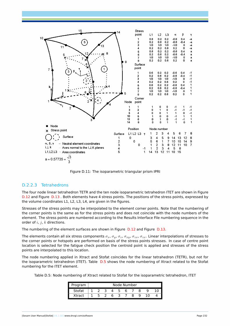
Figure D.11: The isoparametric triangular prism IPRI
D.2.2.3 Tetrahedrons
The four node linear tetrahedron TETR and the ten node isoparametric tetrahedron ITET are shown in FigureD.12 and Figure D.13 . Both elements have 4 stress points. The positions of the stress points, expressed bythe volume coordinates L1, L2, L3, L4, are given in the figures.
Stresses of the stress points may be interpolated to the element corner points. Note that the numbering ofthe corner points is the same as for the stress points and does not coincide with the node numbers of theelement. The stress points are numbered according to the Results Interface File numbering sequence in theorder of i, j, k directions.
The numbering of the element surfaces are shown in Figure D.12 and Figure D.13.
The elements contain all six stress components σx, σy, σz, σxy, σzx, σzx. Linear interpolations of stresses tothe corner points or hotspots are performed on basis of the stress points stresses. In case of centre pointlocation is selected for the fatigue check position the centroid point is applied and stresses of the stresspoints are interpolated to this location.
The node numbering applied in Xtract and Stofat coincides for the linear tetrahedron (TETR), but not forthe isoparametric tetrahedron (ITET). Table D.5 shows the node numbering of Xtract related to the Stofatnumbering for the ITET element.
Table D.5: Node numbering of Xtract related to Stofat for the isoparametric tetrahedron, ITET
Program Node Number
Stofat 1 2 3 4 5 6 7 8 9 10Xtract 1 5 2 6 3 7 8 9 10 4
|Sesam User Manual|Stofat|[V4.1-00] www.dnvgl.com/software Page 232
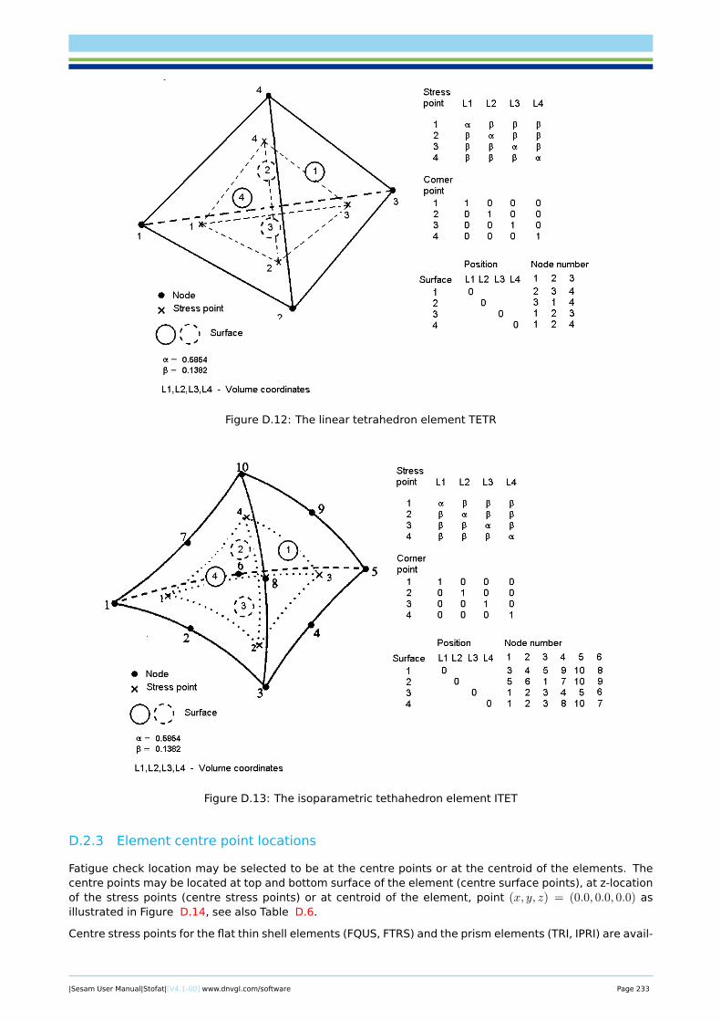
Figure D.12: The linear tetrahedron element TETR
Figure D.13: The isoparametric tethahedron element ITET
D.2.3 Element centre point locations
Fatigue check location may be selected to be at the centre points or at the centroid of the elements. Thecentre points may be located at top and bottom surface of the element (centre surface points), at z-locationof the stress points (centre stress points) or at centroid of the element, point (x, y, z) = (0.0, 0.0, 0.0) asillustrated in Figure D.14, see also Table D.6.
Centre stress points for the flat thin shell elements (FQUS, FTRS) and the prism elements (TRI, IPRI) are avail-
|Sesam User Manual|Stofat|[V4.1-00] www.dnvgl.com/software Page 233
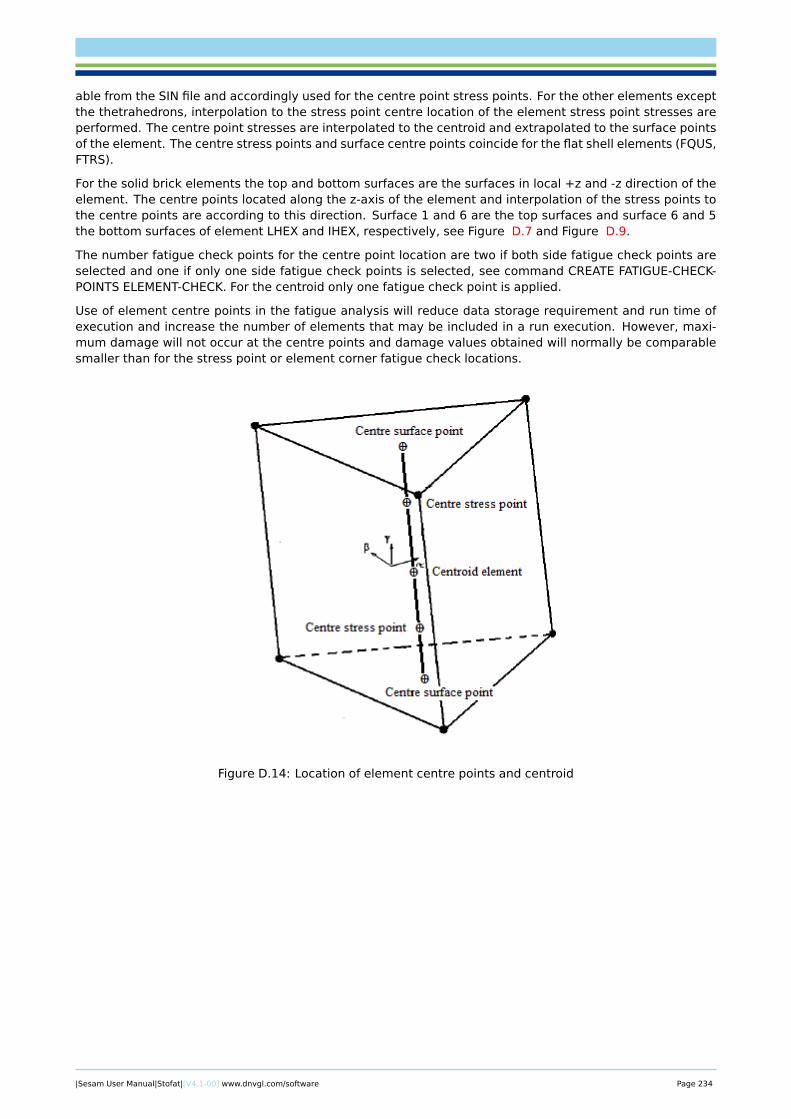
able from the SIN file and accordingly used for the centre point stress points. For the other elements exceptthe thetrahedrons, interpolation to the stress point centre location of the element stress point stresses areperformed. The centre point stresses are interpolated to the centroid and extrapolated to the surface pointsof the element. The centre stress points and surface centre points coincide for the flat shell elements (FQUS,FTRS).
For the solid brick elements the top and bottom surfaces are the surfaces in local +z and -z direction of theelement. The centre points located along the z-axis of the element and interpolation of the stress points tothe centre points are according to this direction. Surface 1 and 6 are the top surfaces and surface 6 and 5the bottom surfaces of element LHEX and IHEX, respectively, see Figure D.7 and Figure D.9.
The number fatigue check points for the centre point location are two if both side fatigue check points areselected and one if only one side fatigue check points is selected, see command CREATE FATIGUE-CHECK-POINTS ELEMENT-CHECK. For the centroid only one fatigue check point is applied.
Use of element centre points in the fatigue analysis will reduce data storage requirement and run time ofexecution and increase the number of elements that may be included in a run execution. However, maxi-mum damage will not occur at the centre points and damage values obtained will normally be comparablesmaller than for the stress point or element corner fatigue check locations.
Figure D.14: Location of element centre points and centroid
|Sesam User Manual|Stofat|[V4.1-00] www.dnvgl.com/software Page 234
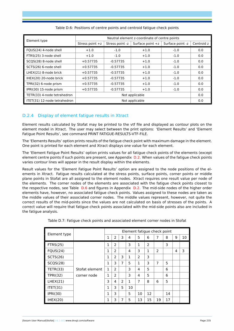
Table D.6: Positions of centre points and centroid fatigue check points
Element typeNeutral element z-coordinate of centre points
Stress point +z Stress point -z Surface point +z Surface point -z Centroid z
FQUS(24) 4-node shell +1.0 -1.0 +1.0 -1.0 0.0
FTRS(25) 3-node shell +1.0 -1.0 +1.0 -1.0 0.0
SCQS(28) 8-node shell +0.57735 -0.57735 +1.0 -1.0 0.0
SCTS(26) 6-node shell +0.57735 -0.57735 +1.0 -1.0 0.0
LHEX(21) 8-node brick +0.57735 -0.57735 +1.0 -1.0 0.0
IHEX(20) 20-node brick +0.57735 -0.57735 +1.0 -1.0 0.0
TPRI(32) 6-node prism +0.57735 -0.57735 +1.0 -1.0 0.0
IPRI(30) 15-node prism +0.57735 -0.57735 +1.0 -1.0 0.0
TETR(33) 4-node tetrahedron Not applicable 0.0
ITET(31) 12-node tetrahedron Not applicable 0.0
D.2.4 Display of element fatigue results in Xtract
Element results calculated by Stofat may be printed to the vtf file and displayed as contour plots on theelement model in Xtract. The user may select between the print options: ‘Element Results’ and ‘ElementFatigue Point Results’, see command PRINT FATIGUE-RESULTS-VTF-FILE.
The ‘Elements Results’ option prints results of the fatigue check point with maximum damage in the element.One point is printed for each element and Xtract displays one value for each element.
The ‘Element Fatigue Point Results’ option prints values for all fatigue check points of the elements (exceptelement centre points if such points are present, see Appendix D.2. When values of the fatigue check pointsvaries contour lines will appear in the result display within the elements.
Result values for the ‘Element Fatigue Point Results’ option are assigned to the node positions of the el-ements in Xtract. Fatigue results calculated at the stress points, surface points, corner points or middleplane points in Stofat are all assigned to the element nodes. Xtract requires one result value per node ofthe elements. The corner nodes of the elements are associated with the fatigue check points closest tothe respective nodes, see Table D.6 and figures in Appendix D.2. The mid-side nodes of the higher orderelements have, however, no associated fatigue check points. Values assigned to these nodes are taken asthe middle values of their associated corner nodes. The middle values represent, however, not quite thecorrect results of the mid-points since the values are not calculated on basis of stresses of the points. Acorrect value will require that fatigue check points associated with the mid-side points also are included inthe fatigue analysis.
Table D.7: Fatigue check points and associated element corner nodes in Stofat
Element typeElement fatigue check point
1 2 3 4 5 6 7 8 9 10
FTRS(25)
Stofat element
corner node
1 2 3 1 2 3
FQUS(24) 1 2 4 3 1 2 4 3
SCTS(26) 1 2 3 1 2 3
SCQS(28) 1 3 7 5 1 3 7 5
TETR(33) 1 2 3 4 5 6
TPRI(32) 1 2 3 4 5 6
LHEX(21) 3 4 2 1 7 8 6 5
ITET(31) 1 3 5 10
IPRI(30) 1 3 5 10 12 14
IHEX(20) 1 3 7 5 13 15 19 17
|Sesam User Manual|Stofat|[V4.1-00] www.dnvgl.com/software Page 235
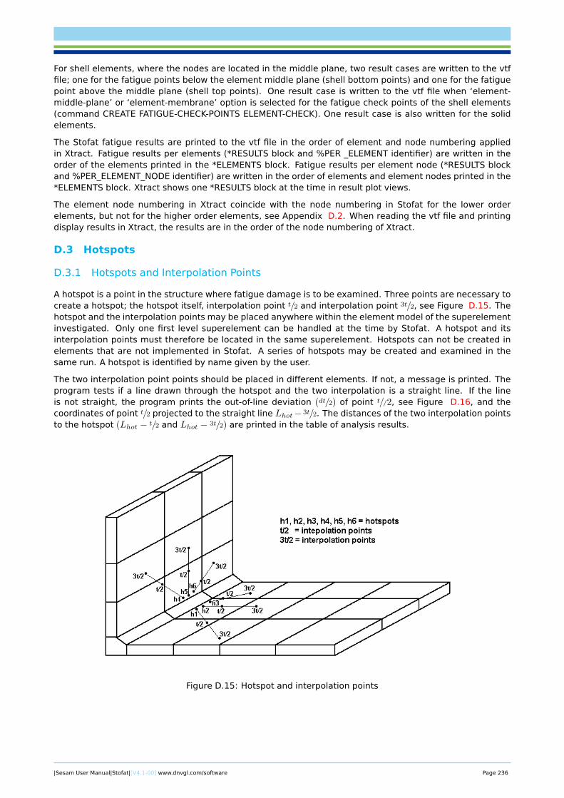
For shell elements, where the nodes are located in the middle plane, two result cases are written to the vtffile; one for the fatigue points below the element middle plane (shell bottom points) and one for the fatiguepoint above the middle plane (shell top points). One result case is written to the vtf file when ‘element-middle-plane’ or ‘element-membrane’ option is selected for the fatigue check points of the shell elements(command CREATE FATIGUE-CHECK-POINTS ELEMENT-CHECK). One result case is also written for the solidelements.
The Stofat fatigue results are printed to the vtf file in the order of element and node numbering appliedin Xtract. Fatigue results per elements (*RESULTS block and %PER _ELEMENT identifier) are written in theorder of the elements printed in the *ELEMENTS block. Fatigue results per element node (*RESULTS blockand %PER_ELEMENT_NODE identifier) are written in the order of elements and element nodes printed in the*ELEMENTS block. Xtract shows one *RESULTS block at the time in result plot views.
The element node numbering in Xtract coincide with the node numbering in Stofat for the lower orderelements, but not for the higher order elements, see Appendix D.2. When reading the vtf file and printingdisplay results in Xtract, the results are in the order of the node numbering of Xtract.
D.3 Hotspots
D.3.1 Hotspots and Interpolation Points
A hotspot is a point in the structure where fatigue damage is to be examined. Three points are necessary tocreate a hotspot; the hotspot itself, interpolation point t/2 and interpolation point 3t/2, see Figure D.15. Thehotspot and the interpolation points may be placed anywhere within the element model of the superelementinvestigated. Only one first level superelement can be handled at the time by Stofat. A hotspot and itsinterpolation points must therefore be located in the same superelement. Hotspots can not be created inelements that are not implemented in Stofat. A series of hotspots may be created and examined in thesame run. A hotspot is identified by name given by the user.
The two interpolation point points should be placed in different elements. If not, a message is printed. Theprogram tests if a line drawn through the hotspot and the two interpolation is a straight line. If the lineis not straight, the program prints the out-of-line deviation (dt/2) of point t//2, see Figure D.16, and thecoordinates of point t/2 projected to the straight line Lhot− 3t/2. The distances of the two interpolation pointsto the hotspot (Lhot − t/2 and Lhot − 3t/2) are printed in the table of analysis results.
Figure D.15: Hotspot and interpolation points
|Sesam User Manual|Stofat|[V4.1-00] www.dnvgl.com/software Page 236
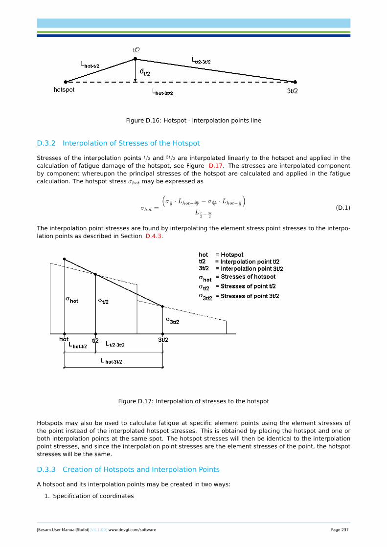
Figure D.16: Hotspot - interpolation points line
D.3.2 Interpolation of Stresses of the Hotspot
Stresses of the interpolation points t/2 and 3t/2 are interpolated linearly to the hotspot and applied in thecalculation of fatigue damage of the hotspot, see Figure D.17. The stresses are interpolated componentby component whereupon the principal stresses of the hotspot are calculated and applied in the fatiguecalculation. The hotspot stress σhot may be expressed as
σhot =
(σ t
2· Lhot− 3t
2− σ 3t
2· Lhot− t2
)L t
2−3t2
(D.1)
The interpolation point stresses are found by interpolating the element stress point stresses to the interpo-lation points as described in Section D.4.3.
Figure D.17: Interpolation of stresses to the hotspot
Hotspots may also be used to calculate fatigue at specific element points using the element stresses ofthe point instead of the interpolated hotspot stresses. This is obtained by placing the hotspot and one orboth interpolation points at the same spot. The hotspot stresses will then be identical to the interpolationpoint stresses, and since the interpolation point stresses are the element stresses of the point, the hotspotstresses will be the same.
D.3.3 Creation of Hotspots and Interpolation Points
A hotspot and its interpolation points may be created in two ways:
1. Specification of coordinates
|Sesam User Manual|Stofat|[V4.1-00] www.dnvgl.com/software Page 237
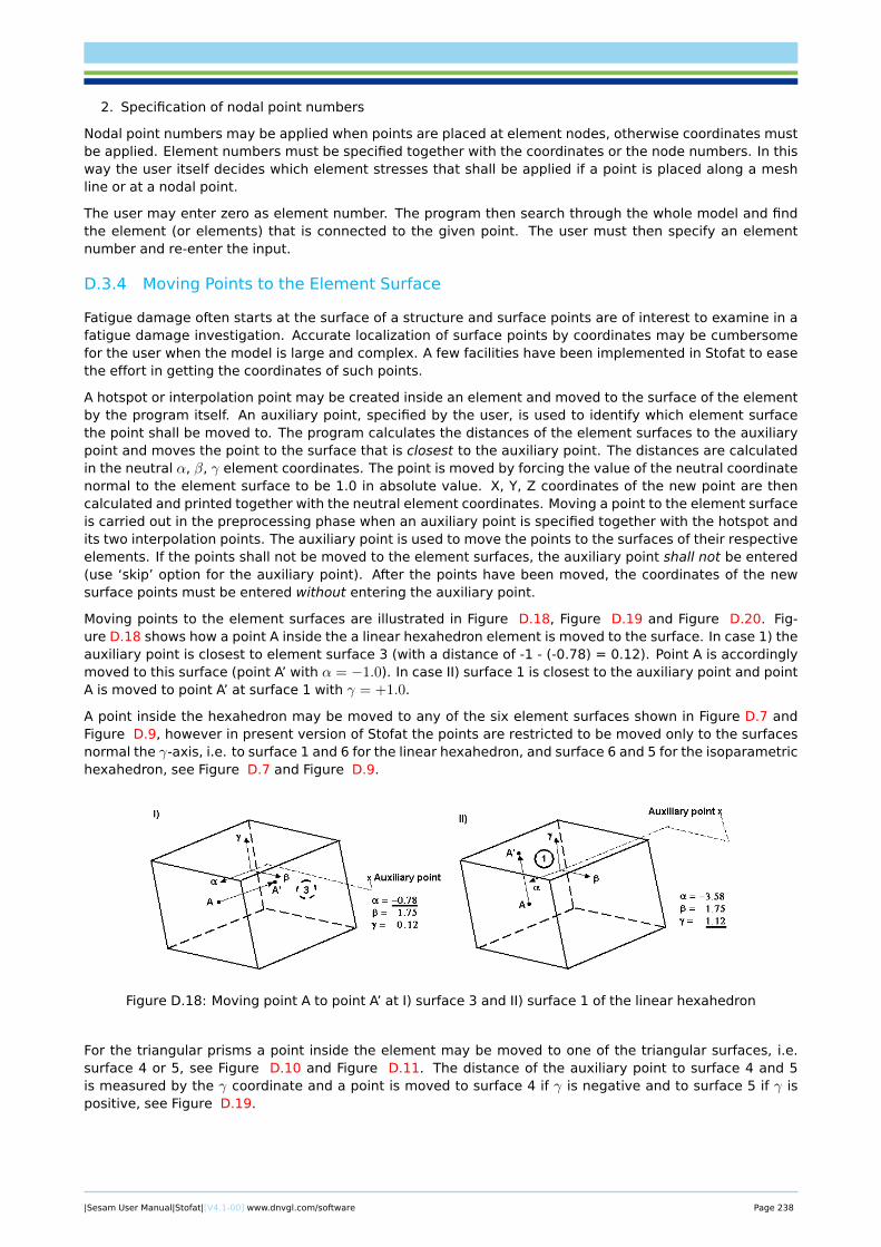
2. Specification of nodal point numbers
Nodal point numbers may be applied when points are placed at element nodes, otherwise coordinates mustbe applied. Element numbers must be specified together with the coordinates or the node numbers. In thisway the user itself decides which element stresses that shall be applied if a point is placed along a meshline or at a nodal point.
The user may enter zero as element number. The program then search through the whole model and findthe element (or elements) that is connected to the given point. The user must then specify an elementnumber and re-enter the input.
D.3.4 Moving Points to the Element Surface
Fatigue damage often starts at the surface of a structure and surface points are of interest to examine in afatigue damage investigation. Accurate localization of surface points by coordinates may be cumbersomefor the user when the model is large and complex. A few facilities have been implemented in Stofat to easethe effort in getting the coordinates of such points.
A hotspot or interpolation point may be created inside an element and moved to the surface of the elementby the program itself. An auxiliary point, specified by the user, is used to identify which element surfacethe point shall be moved to. The program calculates the distances of the element surfaces to the auxiliarypoint and moves the point to the surface that is closest to the auxiliary point. The distances are calculatedin the neutral α, β, γ element coordinates. The point is moved by forcing the value of the neutral coordinatenormal to the element surface to be 1.0 in absolute value. X, Y, Z coordinates of the new point are thencalculated and printed together with the neutral element coordinates. Moving a point to the element surfaceis carried out in the preprocessing phase when an auxiliary point is specified together with the hotspot andits two interpolation points. The auxiliary point is used to move the points to the surfaces of their respectiveelements. If the points shall not be moved to the element surfaces, the auxiliary point shall not be entered(use ‘skip’ option for the auxiliary point). After the points have been moved, the coordinates of the newsurface points must be entered without entering the auxiliary point.
Moving points to the element surfaces are illustrated in Figure D.18, Figure D.19 and Figure D.20. Fig-ure D.18 shows how a point A inside the a linear hexahedron element is moved to the surface. In case 1) theauxiliary point is closest to element surface 3 (with a distance of -1 - (-0.78) = 0.12). Point A is accordinglymoved to this surface (point A’ with α = −1.0). In case II) surface 1 is closest to the auxiliary point and pointA is moved to point A’ at surface 1 with γ = +1.0.
A point inside the hexahedron may be moved to any of the six element surfaces shown in Figure D.7 andFigure D.9, however in present version of Stofat the points are restricted to be moved only to the surfacesnormal the γ-axis, i.e. to surface 1 and 6 for the linear hexahedron, and surface 6 and 5 for the isoparametrichexahedron, see Figure D.7 and Figure D.9.
Figure D.18: Moving point A to point A’ at I) surface 3 and II) surface 1 of the linear hexahedron
For the triangular prisms a point inside the element may be moved to one of the triangular surfaces, i.e.surface 4 or 5, see Figure D.10 and Figure D.11. The distance of the auxiliary point to surface 4 and 5is measured by the γ coordinate and a point is moved to surface 4 if γ is negative and to surface 5 if γ ispositive, see Figure D.19.
|Sesam User Manual|Stofat|[V4.1-00] www.dnvgl.com/software Page 238
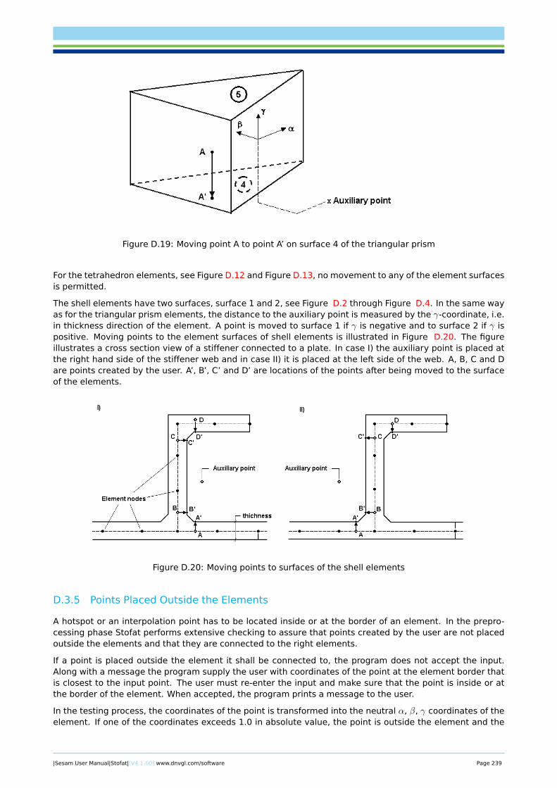
Figure D.19: Moving point A to point A’ on surface 4 of the triangular prism
For the tetrahedron elements, see Figure D.12 and Figure D.13, no movement to any of the element surfacesis permitted.
The shell elements have two surfaces, surface 1 and 2, see Figure D.2 through Figure D.4. In the same wayas for the triangular prism elements, the distance to the auxiliary point is measured by the γ-coordinate, i.e.in thickness direction of the element. A point is moved to surface 1 if γ is negative and to surface 2 if γ ispositive. Moving points to the element surfaces of shell elements is illustrated in Figure D.20. The figureillustrates a cross section view of a stiffener connected to a plate. In case I) the auxiliary point is placed atthe right hand side of the stiffener web and in case II) it is placed at the left side of the web. A, B, C and Dare points created by the user. A’, B’, C’ and D’ are locations of the points after being moved to the surfaceof the elements.
Figure D.20: Moving points to surfaces of the shell elements
D.3.5 Points Placed Outside the Elements
A hotspot or an interpolation point has to be located inside or at the border of an element. In the prepro-cessing phase Stofat performs extensive checking to assure that points created by the user are not placedoutside the elements and that they are connected to the right elements.
If a point is placed outside the element it shall be connected to, the program does not accept the input.Along with a message the program supply the user with coordinates of the point at the element border thatis closest to the input point. The user must re-enter the input and make sure that the point is inside or atthe border of the element. When accepted, the program prints a message to the user.
In the testing process, the coordinates of the point is transformed into the neutral α, β, γ coordinates of theelement. If one of the coordinates exceeds 1.0 in absolute value, the point is outside the element and the
|Sesam User Manual|Stofat|[V4.1-00] www.dnvgl.com/software Page 239
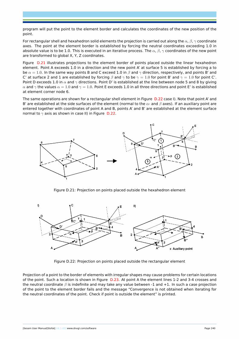
program will put the point to the element border and calculates the coordinates of the new position of thepoint.
For rectangular shell and hexahedron solid elements the projection is carried out along the α, β, γ coordinateaxes. The point at the element border is established by forcing the neutral coordinates exceeding 1.0 inabsolute value is to be 1.0. This is executed in an iterative process. The α, β, γ coordinates of the new pointare transformed to global X, Y, Z coordinates.
Figure D.21 illustrates projections to the element border of points placed outside the linear hexahedronelement. Point A exceeds 1.0 in a direction and the new point A’ at surface 5 is established by forcing a tobe α = 1.0. In the same way points B and C exceed 1.0 in β and γ direction, respectively, and points B’ andC’ at surface 2 and 1 are established by forcing β and γ to be γ = 1.0 for point B’ and γ = 1.0 for point C’.Point D exceeds 1.0 in α and γ directions. Point D’ is established at the line between node 5 and 8 by givingα and γ the values α = 1.0 and γ = 1.0. Point E exceeds 1.0 in all three directions and point E’ is establishedat element corner node 6.
The same operations are shown for a rectangular shell element in Figure D.22 case I). Note that point A’ andB’ are established at the side surfaces of the element (normal to the α- and β axes). If an auxiliary point areentered together with coordinates of point A and B, points A’ and B’ are established at the element surfacenormal to γ axis as shown in case II) in Figure D.22.
Figure D.21: Projection on points placed outside the hexahedron element
Figure D.22: Projection on points placed outside the rectangular element
Projection of a point to the border of elements with irregular shapes may cause problems for certain locationsof the point. Such a location is shown in Figure D.23. At point A the element lines 1-2 and 3-4 crosses andthe neutral coordinate β is indefinite and may take any value between -1 and +1. In such a case projectionof the point to the element border fails and the message “Convergence is not obtained when iterating forthe neutral coordinates of the point. Check if point is outside the element” is printed.
|Sesam User Manual|Stofat|[V4.1-00] www.dnvgl.com/software Page 240
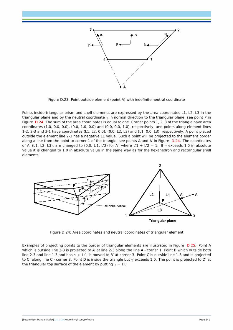
Figure D.23: Point outside element (point A) with indefinite neutral coordinate
Points inside triangular prism and shell elements are expressed by the area coordinates L1, L2, L3 in thetriangular plane and by the neutral coordinate γ in normal direction to the triangular plane, see point P inFigure D.24. The sum of the area coordinates is equal to one. Corner points 1, 2, 3 of the triangle have areacoordinates (1.0, 0.0, 0.0), (0.0, 1.0, 0.0) and (0.0, 0.0, 1.0), respectively, and points along element lines1-2, 2-3 and 3-1 have coordinates (L1, L2, 0.0), (0.0, L2, L3) and (L1, 0.0, L3), respectively. A point placedoutside the element line 2-3 has a negative L1 value. Such a point will be projected to the element borderalong a line from the point to corner 1 of the triangle, see points A and A’ in Figure D.24. The coordinatesof A, (L1, L2, L3), are changed to (0.0, L’1, L’2) for A’, where L’1 + L’2 = 1. If γ exceeds 1.0 in absolutevalue it is changed to 1.0 in absolute value in the same way as for the hexahedron and rectangular shellelements.
Figure D.24: Area coordinates and neutral coordinates of triangular element
Examples of projecting points to the border of triangular elements are illustrated in Figure D.25. Point Awhich is outside line 2-3 is projected to A’ at line 2-3 along the line A - corner 1. Point B which outside bothline 2-3 and line 1-3 and has γ > 1.0, is moved to B’ at corner 3. Point C is outside line 1-3 and is projectedto C’ along line C - corner 3. Point D is inside the triangle but γ exceeds 1.0. The point is projected to D’ atthe triangular top surface of the element by putting γ = 1.0.
|Sesam User Manual|Stofat|[V4.1-00] www.dnvgl.com/software Page 241
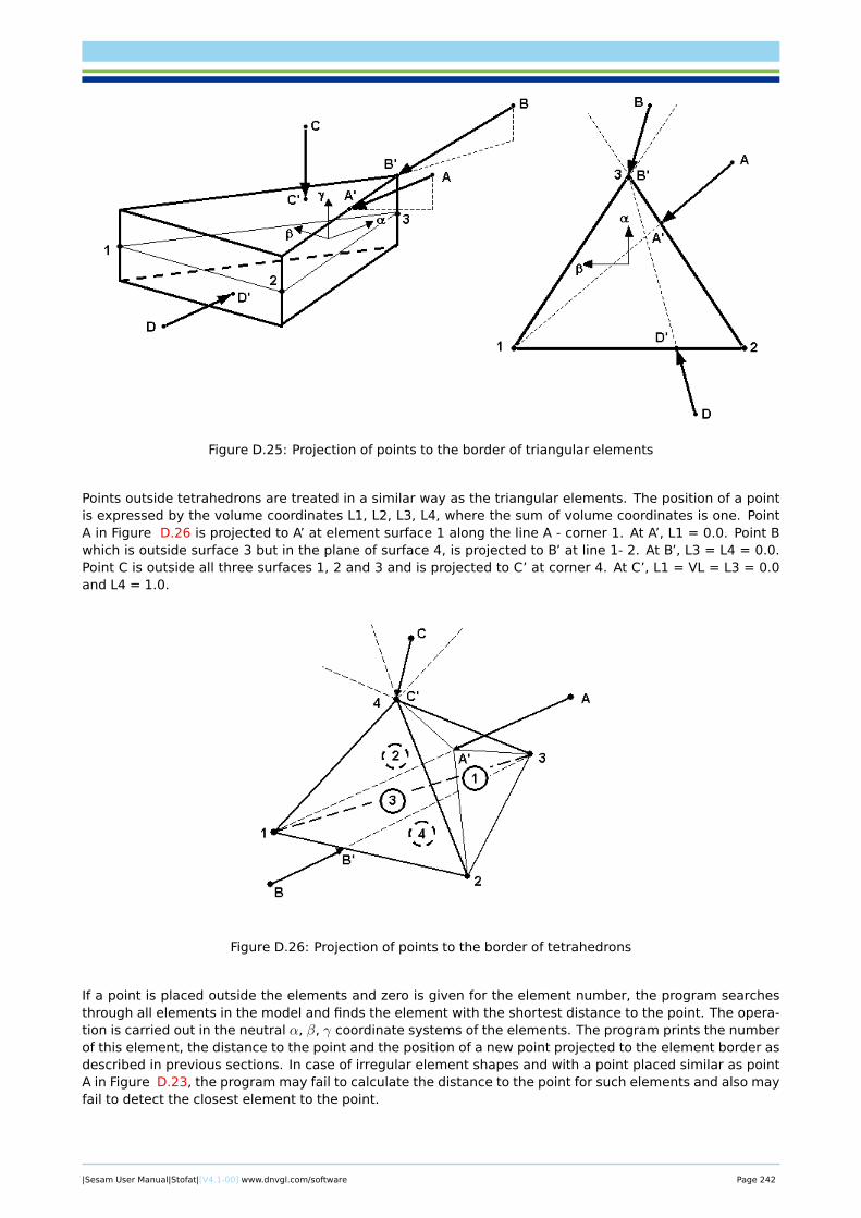
Figure D.25: Projection of points to the border of triangular elements
Points outside tetrahedrons are treated in a similar way as the triangular elements. The position of a pointis expressed by the volume coordinates L1, L2, L3, L4, where the sum of volume coordinates is one. PointA in Figure D.26 is projected to A’ at element surface 1 along the line A - corner 1. At A’, L1 = 0.0. Point Bwhich is outside surface 3 but in the plane of surface 4, is projected to B’ at line 1- 2. At B’, L3 = L4 = 0.0.Point C is outside all three surfaces 1, 2 and 3 and is projected to C’ at corner 4. At C’, L1 = VL = L3 = 0.0and L4 = 1.0.
Figure D.26: Projection of points to the border of tetrahedrons
If a point is placed outside the elements and zero is given for the element number, the program searchesthrough all elements in the model and finds the element with the shortest distance to the point. The opera-tion is carried out in the neutral α, β, γ coordinate systems of the elements. The program prints the numberof this element, the distance to the point and the position of a new point projected to the element border asdescribed in previous sections. In case of irregular element shapes and with a point placed similar as pointA in Figure D.23, the program may fail to calculate the distance to the point for such elements and also mayfail to detect the closest element to the point.
|Sesam User Manual|Stofat|[V4.1-00] www.dnvgl.com/software Page 242
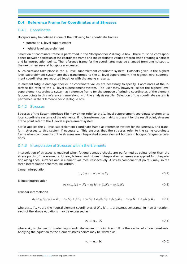
D.4 Reference Frame for Coordinates and Stresses
D.4.1 Coordinates
Hotspots may be defined in one of the following two coordinate frames:
• current or 1. level superelement
• highest level superelement
Selection of coordinate frame is performed in the ‘Hotspot-check’ dialogue box. There must be correspon-dence between selection of the coordinate frame and the coordinate values entered when creating a hotspotand its interpolation points. The reference frame for the coordinates may be changed from one hotspot tothe next when several hotspots are created.
All calculations take place in the 1. level superelement coordinate system. Hotspots given in the highestlevel superelement system are thus transformed to the 1. level superelement, the highest level superele-ment coordinates are reported together with the analysis results.
In element fatigue damage checks, no coordinate values are necessary to specify. Coordinates of the in-terface file refer to the 1. level superelement system. The user may, however, select the highest levelsuperelement coordinate system as reference frame for the purpose of printing coordinates of the elementfatigue points in this reference frame along with the analysis results. Selection of the coordinate system isperformed in the ‘Element-check’ dialogue box.
D.4.2 Stresses
Stresses of the Sesam Interface File may either refer to the 1. level superelement coordinate system or tolocal coordinate systems of the elements. If no transformation matrix is present for the result point, stressesof the point refer to the 1. level superelement system.
Stofat applies the 1. level superelement coordinate frame as reference system for the stresses, and trans-form stresses to this system if necessary. This ensures that the stresses refer to the same coordinateframe when components of the stresses are interpolated across element borders in hotspot fatigue calcula-tions.
D.4.3 Interpolation of Stresses within the Elements
Interpolation of stresses is required when fatigue damage checks are performed at points other than thestress points of the elements. Linear, bilinear and trilinear interpolation schemes are applied for interpola-tion along lines, surfaces and in element volumes, respectively. A stress component at point h may, in thethree interpolation schemes, be written:
Linear interpolationσh (αh) = K1 + αhK2 (D.2)
Bilinear interpolationσh (αh, βh) = K1 + αhK2 + βhK3 + αhβhK4 (D.3)
Trilinear interpolation
σh (αh, βh, γh) = K1 + αhK2 + βK3 + γhK4 + αhβhK5 + βhγhK6 + αhγhK7 + αhβhγhK8 (D.4)
where αh, βh, γh are the neutral element coordinates of K1, K2, . . . are stress constants. In matrix notation,each of the above equations may be expressed as:
σh = Ah ·K (D.5)
where Ah is the vector containing coordinate values of point h and K is the vector of stress constants.Applying the equation to the element stress points may be written as:
σs = As ·K (D.6)
|Sesam User Manual|Stofat|[V4.1-00] www.dnvgl.com/software Page 243
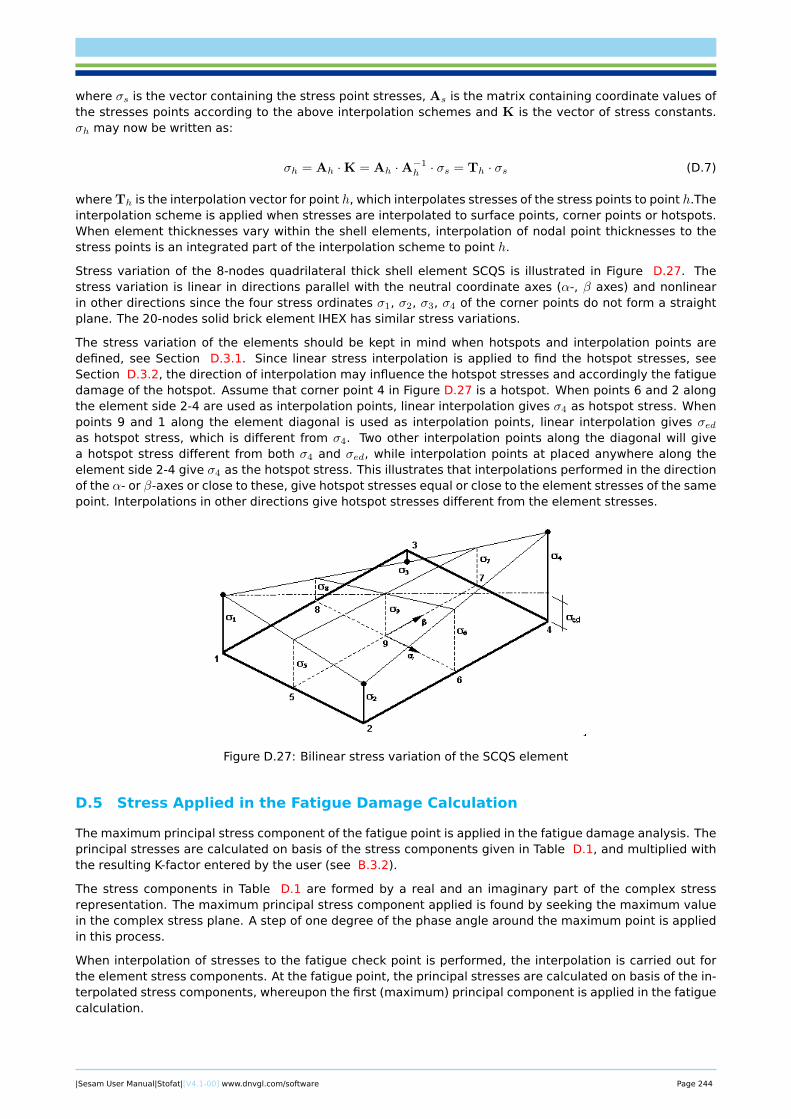
where σs is the vector containing the stress point stresses, As is the matrix containing coordinate values ofthe stresses points according to the above interpolation schemes and K is the vector of stress constants.σh may now be written as:
σh = Ah ·K = Ah ·A−1h · σs = Th · σs (D.7)
where Th is the interpolation vector for point h, which interpolates stresses of the stress points to point h.Theinterpolation scheme is applied when stresses are interpolated to surface points, corner points or hotspots.When element thicknesses vary within the shell elements, interpolation of nodal point thicknesses to thestress points is an integrated part of the interpolation scheme to point h.
Stress variation of the 8-nodes quadrilateral thick shell element SCQS is illustrated in Figure D.27. Thestress variation is linear in directions parallel with the neutral coordinate axes (α-, β axes) and nonlinearin other directions since the four stress ordinates σ1, σ2, σ3, σ4 of the corner points do not form a straightplane. The 20-nodes solid brick element IHEX has similar stress variations.
The stress variation of the elements should be kept in mind when hotspots and interpolation points aredefined, see Section D.3.1. Since linear stress interpolation is applied to find the hotspot stresses, seeSection D.3.2, the direction of interpolation may influence the hotspot stresses and accordingly the fatiguedamage of the hotspot. Assume that corner point 4 in Figure D.27 is a hotspot. When points 6 and 2 alongthe element side 2-4 are used as interpolation points, linear interpolation gives σ4 as hotspot stress. Whenpoints 9 and 1 along the element diagonal is used as interpolation points, linear interpolation gives σedas hotspot stress, which is different from σ4. Two other interpolation points along the diagonal will givea hotspot stress different from both σ4 and σed, while interpolation points at placed anywhere along theelement side 2-4 give σ4 as the hotspot stress. This illustrates that interpolations performed in the directionof the α- or β-axes or close to these, give hotspot stresses equal or close to the element stresses of the samepoint. Interpolations in other directions give hotspot stresses different from the element stresses.
Figure D.27: Bilinear stress variation of the SCQS element
D.5 Stress Applied in the Fatigue Damage Calculation
The maximum principal stress component of the fatigue point is applied in the fatigue damage analysis. Theprincipal stresses are calculated on basis of the stress components given in Table D.1, and multiplied withthe resulting K-factor entered by the user (see B.3.2).
The stress components in Table D.1 are formed by a real and an imaginary part of the complex stressrepresentation. The maximum principal stress component applied is found by seeking the maximum valuein the complex stress plane. A step of one degree of the phase angle around the maximum point is appliedin this process.
When interpolation of stresses to the fatigue check point is performed, the interpolation is carried out forthe element stress components. At the fatigue point, the principal stresses are calculated on basis of the in-terpolated stress components, whereupon the first (maximum) principal component is applied in the fatiguecalculation.
|Sesam User Manual|Stofat|[V4.1-00] www.dnvgl.com/software Page 244
The stresses applied in the fatigue damage calculation process may be printed to a vtf file as function ofthe angular frequencies for graphic presentation (2D curve plots) by the Xtract program. SIN file stresses,elements stresses and hotspot stresses may be printed for selected wave directions, stress components andpositions in the elements. Principal stresses, real and complex parts of the stress components and phaseangle in the complex stress plane are available for print.
D.6 Stresses Applied in the Long Term Response Calculation
Stress components applied in long term response calcuation are selected by the user prior to run execution.Principal stresses (Sp1, Sp2, Sp3), von Mises equivalent stress (Seq), normal stress components (Sxx, Syy,Szz) and shear stress components (Sxy, Sxz, Syz) may be selected.
The stress components of the transfer functions are formed by a real and an imaginary part of the complexstress representation. For each sea state and for each fatigue point stress components are retrieved from re-sults file. Stress components are computed for each phase angle iteration and maximum value is searched.A step of one degree phase angle around the maximum point is applied to get the stress value of each longterm stress component applied in the calculation. Equivalent stress is computed for each frequency and willbe used to compute spectral moments. Stress amplitude is computed from spectral moments. Static stressis calculated from static load case for any stress component or equivalent stress.
Depending on the user input, static stresses are then added to maximum and minimum stresses in accor-dance with:
Maximum stress = static stress + stress amplitudeMinimum stress = static stress - stress amplitude
The above expression helds except in case of von Mises stress is selected, therefore minimum and maximumstresses coincide.
The long term stresses may be transformed to global coordinates (superelement coordinate system) whenapplied in long term respons calculation. Stress concentration factors are applied only on request by user.Static reduction factor, applied in fatigue check, is not applied to the long term stresses. Static stresses areaccounted for in the maximum and minimum stresses calculated, where the static stress is added to thepositive and negative stress amplitude values, respectively.
|Sesam User Manual|Stofat|[V4.1-00] www.dnvgl.com/software Page 245
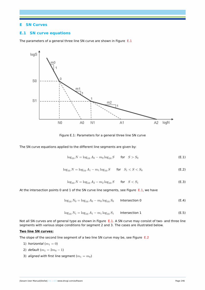
E SN Curves
E.1 SN curve equations
The parameters of a general three line SN curve are shown in Figure E.1
Figure E.1: Parameters for a general three line SN curve
The SN curve equations applied to the different line segments are given by:
log10N = log10A0 −m0 log10 S for S > S0 (E.1)
log10N = log10A1 −m1 log10 S for S1 < S < S0 (E.2)
log10N = log10A2 −m2 log10 S for S < S1 (E.3)
At the intersection points 0 and 1 of the SN curve line segments, see Figure E.1, we have
log10N0 = log10A0 −m0 log10 S0 Intersection 0 (E.4)
log10N1 = log10A1 −m1 log10 S1 Intersection 1 (E.5)
Not all SN curves are of general type as shown in Figure E.1. A SN curve may consist of two- and three linesegments with various slope conditions for segment 2 and 3. The cases are illustrated below.
Two line SN curves:
The slope of the second line segment of a two line SN curve may be, see Figure E.2
1) horizontal (m1 = 0)
2) default (m1 = 2m0 − 1)
3) aligned with first line segment (m1 = m0)
|Sesam User Manual|Stofat|[V4.1-00] www.dnvgl.com/software Page 246
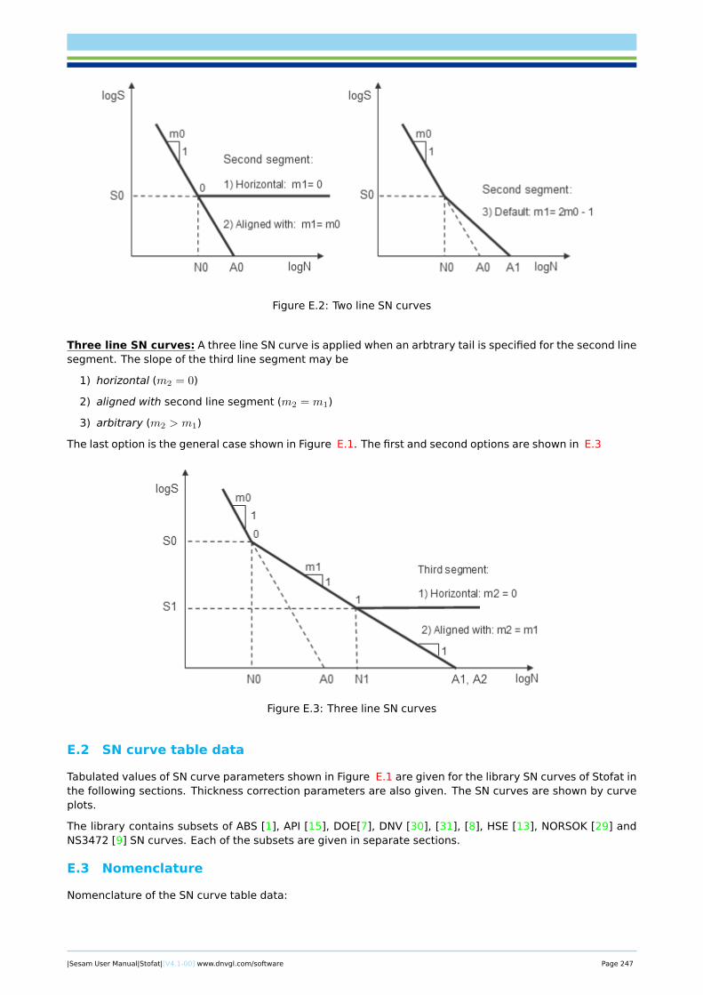
Figure E.2: Two line SN curves
Three line SN curves: A three line SN curve is applied when an arbtrary tail is specified for the second linesegment. The slope of the third line segment may be
1) horizontal (m2 = 0)
2) aligned with second line segment (m2 = m1)
3) arbitrary (m2 > m1)
The last option is the general case shown in Figure E.1. The first and second options are shown in E.3
Figure E.3: Three line SN curves
E.2 SN curve table data
Tabulated values of SN curve parameters shown in Figure E.1 are given for the library SN curves of Stofat inthe following sections. Thickness correction parameters are also given. The SN curves are shown by curveplots.
The library contains subsets of ABS [1], API [15], DOE[7], DNV [30], [31], [8], HSE [13], NORSOK [29] andNS3472 [9] SN curves. Each of the subsets are given in separate sections.
E.3 Nomenclature
Nomenclature of the SN curve table data:
|Sesam User Manual|Stofat|[V4.1-00] www.dnvgl.com/software Page 247
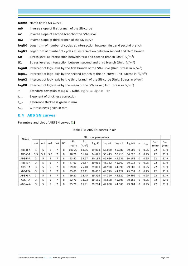
Name Name of the SN Curve
m0 Inverse slope of first branch of the SN-curve
m1 Inverse slope of second branchof the SN-curve
m2 Inverse slope of third branch of the SN-curve
logN0 Logarithm of number of cycles at intersection between first and second branch
logN1 Logarithm of number of cycles at instersection between second and third branch
S0 Stress level at intersection between first and second branch (Unit: N/m2)
S1 Stress level at intersection between second and third branch (Unit: N/m2)
logA0 Intercept of logN-axis by the first branch of the SN-curve (Unit: Stress in N/m2)
logA1 Intercept of logN-axis by the second branch of the SN-curve (Unit: Stress in N/m2)
logA2 Intercept of logN-axis by the third branch of the SN-curve (Unit: Stress in N/m2)
logK0 Intercept of logN-axis by the mean of the SN-curve (Unit: Stress in N/m2)
σ Standard deviation of logK0. Note. logA0 = logK0− 2σ
texp Exponent of thickness correction
tref Reference thickness given in mm
tcut Cut thickness given in mm
E.4 ABS SN curves
Paramters and plot of ABS SN curves [1]
Table E.1: ABS SN curves in air
NameSN curve parameters
m0 m1 m2 N0 N1S0(∗106
) S1(∗106
) logA0 logA1 logA2 logK0 σ texptref
(mm)
tcut
(mm)
ABS-B-A 4 6 6 7 8 100.20 68.35 39.003 55.080 55.080 39.003 0 0.25 22 21.9
ABS-C-A 3.5 5.5 5.5 7 8 78.20 51.46 34.626 50.413 50.413 34.626 0 0.25 22 21.9
ABS-D-A 3 5 5 7 8 53.40 33.67 30.183 45.636 45.636 30.183 0 0.25 22 21.9
ABS-E-A 3 5 5 7 8 47.00 29.67 30.016 45.362 45.362 30.016 0 0.25 22 21.9
ABS-F-A 3 5 5 7 8 39.80 25.10 29.800 44.998 44.998 29.800 0 0.25 22 21.9
ABS-F2A 3 5 5 7 8 35.00 22.11 29.632 44.729 44.729 29.632 0 0.25 22 21.9
ABS-G-A 3 5 5 7 8 29.20 18.45 29.396 44.320 44.320 29.396 0 0.25 22 21.9
ABS-T-A 3 5 5 7 8 52.70 33.23 30.165 45.608 45.608 30.165 0 0.25 32 22.0
ABS-W-A 3 5 5 7 8 25.20 15.91 29.204 44.008 44.008 29.204 0 0.25 22 21.9
|Sesam User Manual|Stofat|[V4.1-00] www.dnvgl.com/software Page 248
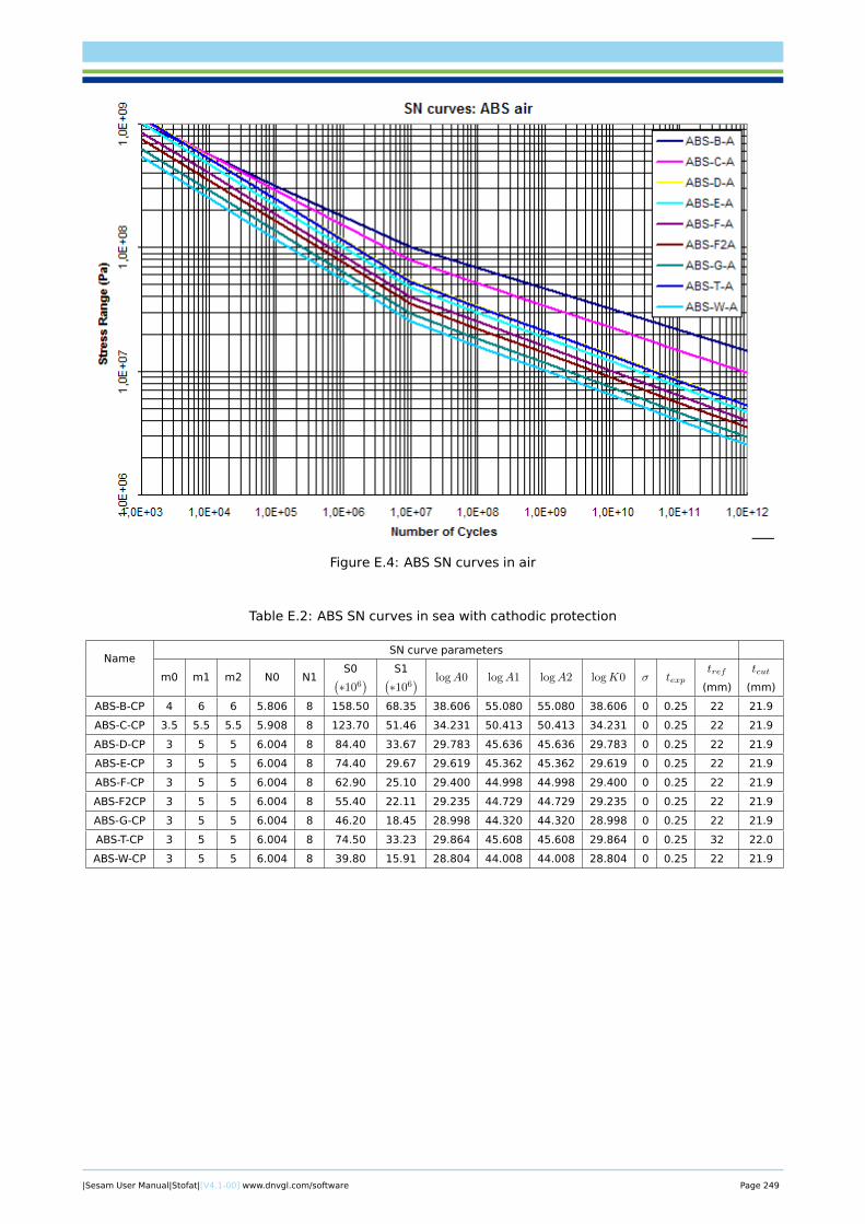
Figure E.4: ABS SN curves in air
Table E.2: ABS SN curves in sea with cathodic protection
NameSN curve parameters
m0 m1 m2 N0 N1S0(∗106
) S1(∗106
) logA0 logA1 logA2 logK0 σ texptref
(mm)
tcut
(mm)
ABS-B-CP 4 6 6 5.806 8 158.50 68.35 38.606 55.080 55.080 38.606 0 0.25 22 21.9
ABS-C-CP 3.5 5.5 5.5 5.908 8 123.70 51.46 34.231 50.413 50.413 34.231 0 0.25 22 21.9
ABS-D-CP 3 5 5 6.004 8 84.40 33.67 29.783 45.636 45.636 29.783 0 0.25 22 21.9
ABS-E-CP 3 5 5 6.004 8 74.40 29.67 29.619 45.362 45.362 29.619 0 0.25 22 21.9
ABS-F-CP 3 5 5 6.004 8 62.90 25.10 29.400 44.998 44.998 29.400 0 0.25 22 21.9
ABS-F2CP 3 5 5 6.004 8 55.40 22.11 29.235 44.729 44.729 29.235 0 0.25 22 21.9
ABS-G-CP 3 5 5 6.004 8 46.20 18.45 28.998 44.320 44.320 28.998 0 0.25 22 21.9
ABS-T-CP 3 5 5 6.004 8 74.50 33.23 29.864 45.608 45.608 29.864 0 0.25 32 22.0
ABS-W-CP 3 5 5 6.004 8 39.80 15.91 28.804 44.008 44.008 28.804 0 0.25 22 21.9
|Sesam User Manual|Stofat|[V4.1-00] www.dnvgl.com/software Page 249
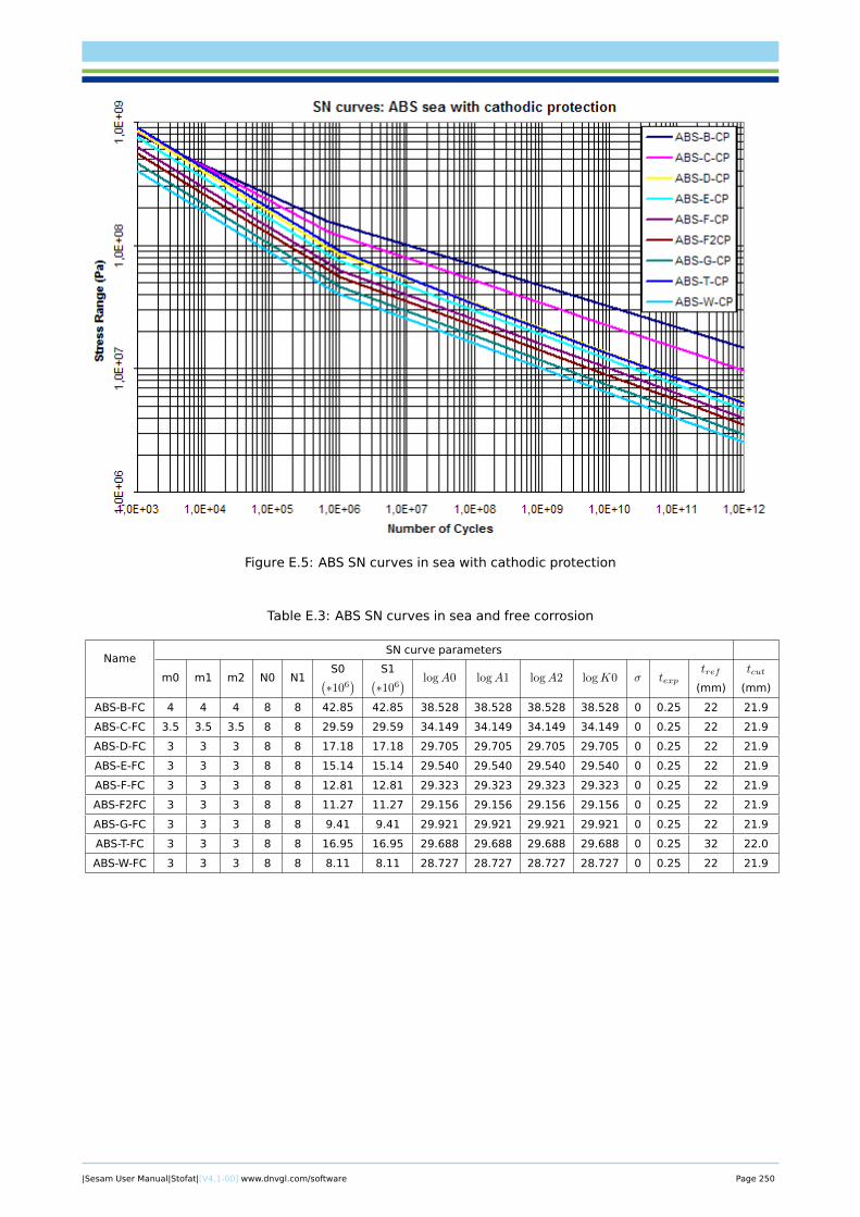
Figure E.5: ABS SN curves in sea with cathodic protection
Table E.3: ABS SN curves in sea and free corrosion
NameSN curve parameters
m0 m1 m2 N0 N1S0(∗106
) S1(∗106
) logA0 logA1 logA2 logK0 σ texptref
(mm)
tcut
(mm)
ABS-B-FC 4 4 4 8 8 42.85 42.85 38.528 38.528 38.528 38.528 0 0.25 22 21.9
ABS-C-FC 3.5 3.5 3.5 8 8 29.59 29.59 34.149 34.149 34.149 34.149 0 0.25 22 21.9
ABS-D-FC 3 3 3 8 8 17.18 17.18 29.705 29.705 29.705 29.705 0 0.25 22 21.9
ABS-E-FC 3 3 3 8 8 15.14 15.14 29.540 29.540 29.540 29.540 0 0.25 22 21.9
ABS-F-FC 3 3 3 8 8 12.81 12.81 29.323 29.323 29.323 29.323 0 0.25 22 21.9
ABS-F2FC 3 3 3 8 8 11.27 11.27 29.156 29.156 29.156 29.156 0 0.25 22 21.9
ABS-G-FC 3 3 3 8 8 9.41 9.41 29.921 29.921 29.921 29.921 0 0.25 22 21.9
ABS-T-FC 3 3 3 8 8 16.95 16.95 29.688 29.688 29.688 29.688 0 0.25 32 22.0
ABS-W-FC 3 3 3 8 8 8.11 8.11 28.727 28.727 28.727 28.727 0 0.25 22 21.9
|Sesam User Manual|Stofat|[V4.1-00] www.dnvgl.com/software Page 250
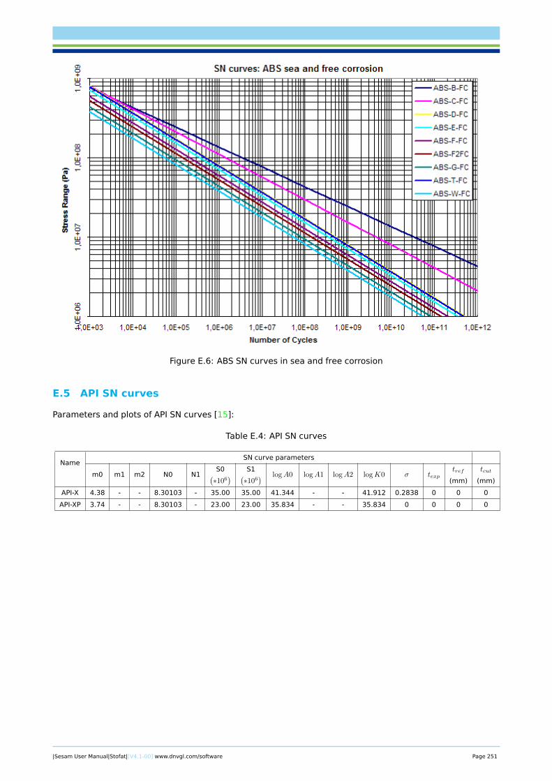
Figure E.6: ABS SN curves in sea and free corrosion
E.5 API SN curves
Parameters and plots of API SN curves [15]:
Table E.4: API SN curves
NameSN curve parameters
m0 m1 m2 N0 N1S0(∗106
) S1(∗106
) logA0 logA1 logA2 logK0 σ texptref
(mm)
tcut
(mm)
API-X 4.38 - - 8.30103 - 35.00 35.00 41.344 - - 41.912 0.2838 0 0 0
API-XP 3.74 - - 8.30103 - 23.00 23.00 35.834 - - 35.834 0 0 0 0
|Sesam User Manual|Stofat|[V4.1-00] www.dnvgl.com/software Page 251
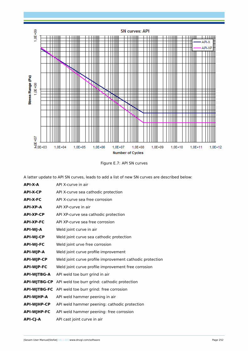
Figure E.7: API SN curves
A latter update to API SN curves, leads to add a list of new SN curves are described below:
API-X-A API X-curve in air
API-X-CP API X-curve sea cathodic protection
API-X-FC API X-curve sea free corrosion
API-XP-A API XP-curve in air
API-XP-CP API XP-curve sea cathodic protection
API-XP-FC API XP-curve sea free corrosion
API-WJ-A Weld joint curve in air
API-WJ-CP Weld joint curve sea cathodic protection
API-WJ-FC Weld joint urve free corrosion
API-WJP-A Weld joint curve profile improvement
API-WJP-CP Weld joint curve profile improvement cathodic protection
API-WJP-FC Weld joint curve profile improvement free corrosion
API-WJTBG-A API weld toe burr grind in air
API-WJTBG-CP API weld toe burr grind: cathodic protection
API-WJTBG-FC API weld toe burr grind: free corrosion
API-WJHP-A API weld hammer peening in air
API-WJHP-CP API weld hammer peening: cathodic protection
API-WJHP-FC API weld hammer peening: free corrosion
API-CJ-A API cast joint curve in air
|Sesam User Manual|Stofat|[V4.1-00] www.dnvgl.com/software Page 252
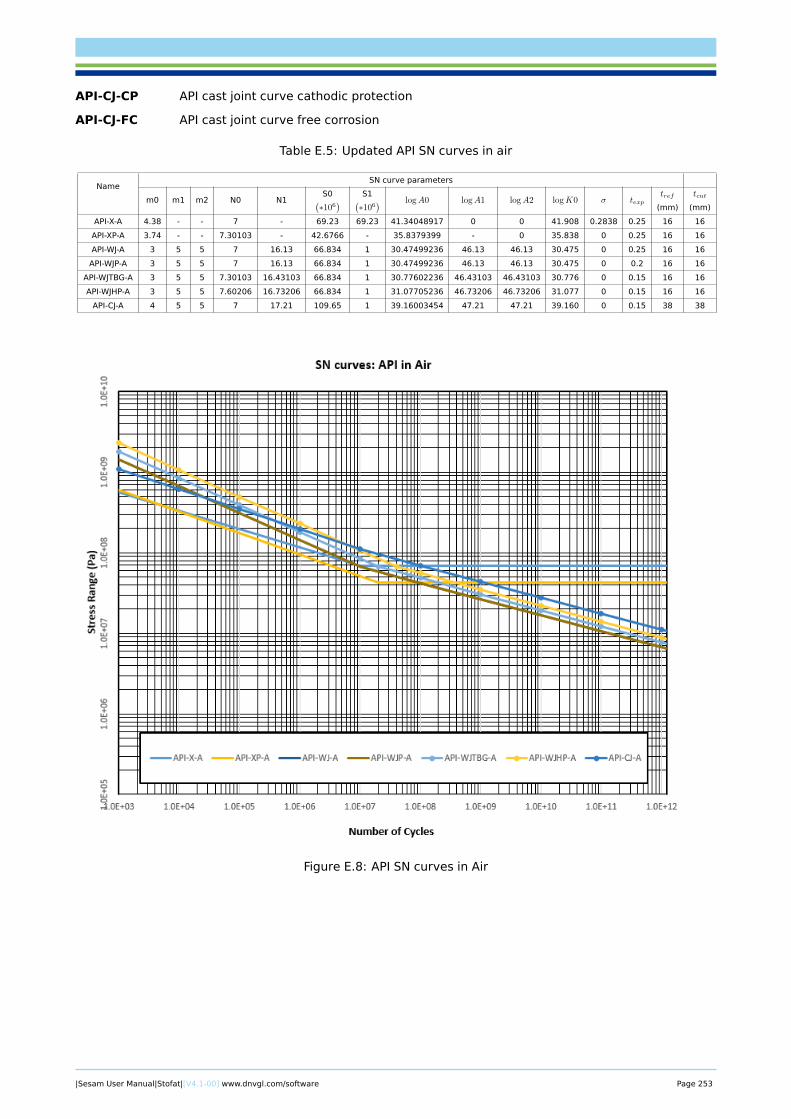
API-CJ-CP API cast joint curve cathodic protection
API-CJ-FC API cast joint curve free corrosion
Table E.5: Updated API SN curves in air
NameSN curve parameters
m0 m1 m2 N0 N1S0(∗106
) S1(∗106
) logA0 logA1 logA2 logK0 σ texptref
(mm)
tcut
(mm)
API-X-A 4.38 - - 7 - 69.23 69.23 41.34048917 0 0 41.908 0.2838 0.25 16 16
API-XP-A 3.74 - - 7.30103 - 42.6766 - 35.8379399 - 0 35.838 0 0.25 16 16
API-WJ-A 3 5 5 7 16.13 66.834 1 30.47499236 46.13 46.13 30.475 0 0.25 16 16
API-WJP-A 3 5 5 7 16.13 66.834 1 30.47499236 46.13 46.13 30.475 0 0.2 16 16
API-WJTBG-A 3 5 5 7.30103 16.43103 66.834 1 30.77602236 46.43103 46.43103 30.776 0 0.15 16 16
API-WJHP-A 3 5 5 7.60206 16.73206 66.834 1 31.07705236 46.73206 46.73206 31.077 0 0.15 16 16
API-CJ-A 4 5 5 7 17.21 109.65 1 39.16003454 47.21 47.21 39.160 0 0.15 38 38
Figure E.8: API SN curves in Air
|Sesam User Manual|Stofat|[V4.1-00] www.dnvgl.com/software Page 253
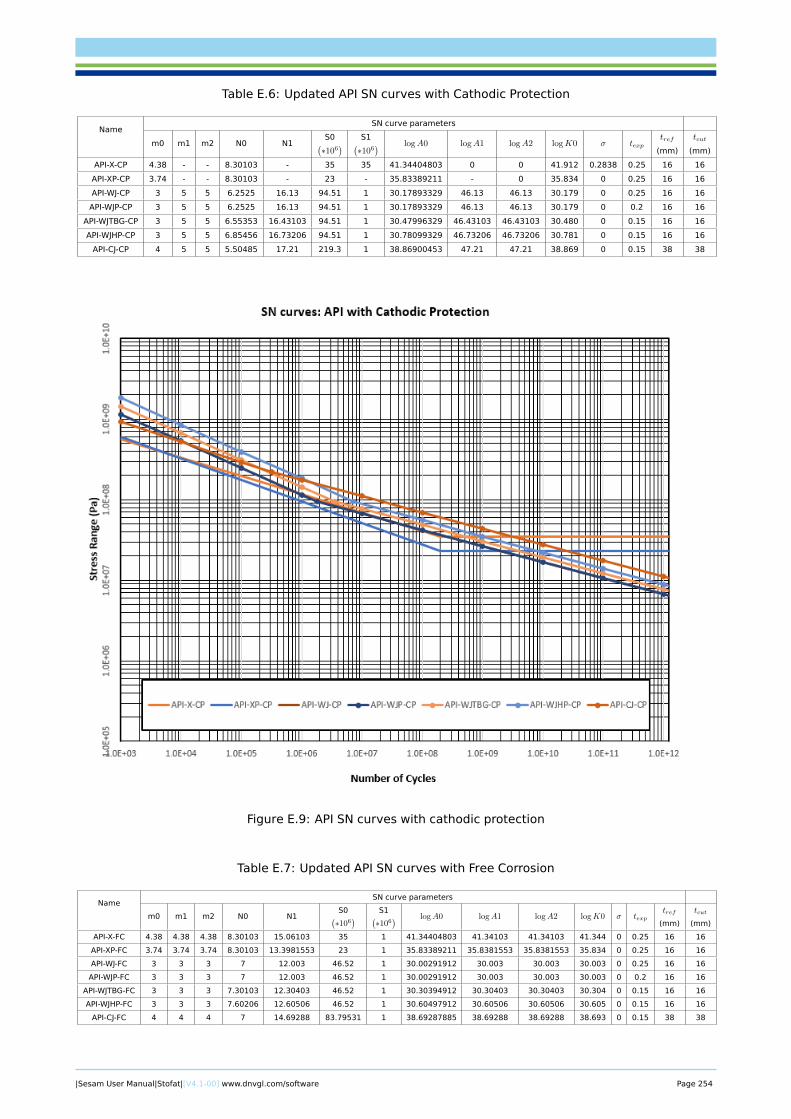
Table E.6: Updated API SN curves with Cathodic Protection
NameSN curve parameters
m0 m1 m2 N0 N1S0(∗106
) S1(∗106
) logA0 logA1 logA2 logK0 σ texptref
(mm)
tcut
(mm)
API-X-CP 4.38 - - 8.30103 - 35 35 41.34404803 0 0 41.912 0.2838 0.25 16 16
API-XP-CP 3.74 - - 8.30103 - 23 - 35.83389211 - 0 35.834 0 0.25 16 16
API-WJ-CP 3 5 5 6.2525 16.13 94.51 1 30.17893329 46.13 46.13 30.179 0 0.25 16 16
API-WJP-CP 3 5 5 6.2525 16.13 94.51 1 30.17893329 46.13 46.13 30.179 0 0.2 16 16
API-WJTBG-CP 3 5 5 6.55353 16.43103 94.51 1 30.47996329 46.43103 46.43103 30.480 0 0.15 16 16
API-WJHP-CP 3 5 5 6.85456 16.73206 94.51 1 30.78099329 46.73206 46.73206 30.781 0 0.15 16 16
API-CJ-CP 4 5 5 5.50485 17.21 219.3 1 38.86900453 47.21 47.21 38.869 0 0.15 38 38
Figure E.9: API SN curves with cathodic protection
Table E.7: Updated API SN curves with Free Corrosion
NameSN curve parameters
m0 m1 m2 N0 N1S0(∗106
) S1(∗106
) logA0 logA1 logA2 logK0 σ texptref
(mm)
tcut
(mm)
API-X-FC 4.38 4.38 4.38 8.30103 15.06103 35 1 41.34404803 41.34103 41.34103 41.344 0 0.25 16 16
API-XP-FC 3.74 3.74 3.74 8.30103 13.3981553 23 1 35.83389211 35.8381553 35.8381553 35.834 0 0.25 16 16
API-WJ-FC 3 3 3 7 12.003 46.52 1 30.00291912 30.003 30.003 30.003 0 0.25 16 16
API-WJP-FC 3 3 3 7 12.003 46.52 1 30.00291912 30.003 30.003 30.003 0 0.2 16 16
API-WJTBG-FC 3 3 3 7.30103 12.30403 46.52 1 30.30394912 30.30403 30.30403 30.304 0 0.15 16 16
API-WJHP-FC 3 3 3 7.60206 12.60506 46.52 1 30.60497912 30.60506 30.60506 30.605 0 0.15 16 16
API-CJ-FC 4 4 4 7 14.69288 83.79531 1 38.69287885 38.69288 38.69288 38.693 0 0.15 38 38
|Sesam User Manual|Stofat|[V4.1-00] www.dnvgl.com/software Page 254
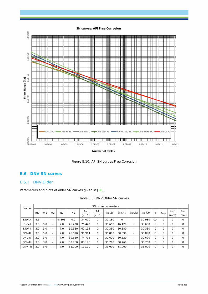
Figure E.10: API SN curves Free Corrosion
E.6 DNV SN curves
E.6.1 DNV Older
Parameters and plots of older SN curves given in [30]
Table E.8: DNV Older SN curves
NameSN curve parameters
m0 m1 m2 N0 N1S0(∗106
) S1(∗106
) logA0 logA1 logA2 logK0 σ texptref
(mm)
tcut
(mm)
DNV-X 4.1 - - 8.301 0.0 34.000 0 39.180 0 - 39.980 0.4 0 0 0
DNV-I 3.0 5.0 - 7.0 46.420 76.442 0 30.650 46.420 - 30.650 0 0 0 0
DNV-II 3.0 3.0 - 7.0 30.380 62.135 0 30.380 30.380 - 30.380 0 0 0 0
DNV-III 3.0 5.0 - 7.0 46.810 91.904 0 30.890 30.890 - 30.890 0 0 0 0
DNV-IV 3.0 3.0 - 7.0 30.620 74.702 0 30.620 30.620 - 30.620 0 0 0 0
DNV-Ib 3.0 3.0 - 7.0 30.760 83.176 0 30.760 30.760 - 30.760 0 0 0 0
DNV-IIb 3.0 3.0 - 7.0 31.000 100.00 0 31.000 31.000 - 31.000 0 0 0 0
|Sesam User Manual|Stofat|[V4.1-00] www.dnvgl.com/software Page 255
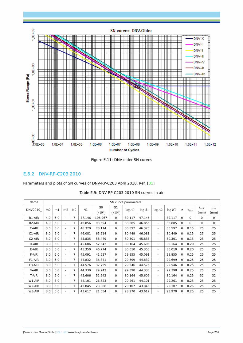
Figure E.11: DNV older SN curves
E.6.2 DNV-RP-C203 2010
Parameters and plots of SN curves of DNV-RP-C203 April 2010, Ref. [31]
Table E.9: DNV-RP-C203 2010 SN curves in air
Name SN curve parameters
DNV2010_ m0 m1 m2 N0 N1S0(∗106
) S1(∗106
) logA0 logA1 logA2 logK0 σ texptref
(mm)
tcut
(mm)
B1-AIR 4.0 5.0 - 7 47.146 106.967 0 39.117 47.146 - 39.117 0 0 0 0
B2-AIR 4.0 5.0 - 7 46.856 93.594 0 38.885 46.856 - 38.885 0 0 0 0
C-AIR 3.0 5.0 - 7 46.320 73.114 0 30.592 46.320 - 30.592 0 0.15 25 25
C1-AIR 3.0 5.0 - 7 46.081 65.514 0 30.449 46.081 - 30.449 0 0.15 25 25
C2-AIR 3.0 5.0 - 7 45.835 58.479 0 30.301 45.835 - 30.301 0 0.15 25 25
D-AIR 3.0 5.0 - 7 45.606 52.642 0 30.164 45.606 - 30.164 0 0.20 25 25
E-AIR 3.0 5.0 - 7 45.350 46.774 0 30.010 45.350 - 30.010 0 0.20 25 25
F-AIR 3.0 5.0 - 7 45.091 41.527 0 29.855 45.091 - 29.855 0 0.25 25 25
F1-AIR 3.0 5.0 - 7 44.832 36.841 0 29.699 44.832 - 29.699 0 0.25 25 25
F3-AIR 3.0 5.0 - 7 44.576 32.759 0 29.546 44.576 - 29.546 0 0.25 25 25
G-AIR 3.0 5.0 - 7 44.330 29.242 0 29.398 44.330 - 29.398 0 0.25 25 25
T-AIR 3.0 5.0 - 7 45.606 52.642 0 30.164 45.606 - 30.164 0 0.25 32 32
W1-AIR 3.0 5.0 - 7 44.101 26.323 0 29.261 44.101 - 29.261 0 0.25 25 25
W2-AIR 3.0 5.0 - 7 43.845 23.388 0 29.107 43.845 - 29.107 0 0.25 25 25
W3-AIR 3.0 5.0 - 7 43.617 21.054 0 28.970 43.617 - 28.970 0 0.25 25 25
|Sesam User Manual|Stofat|[V4.1-00] www.dnvgl.com/software Page 256
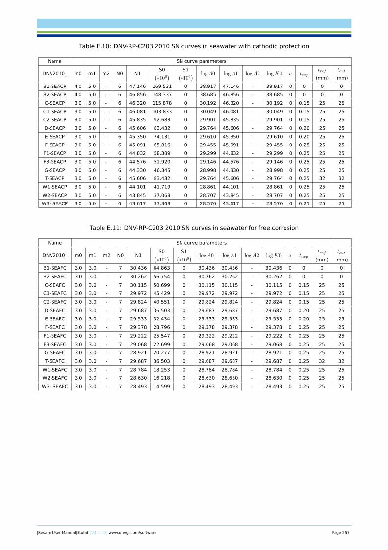
Table E.10: DNV-RP-C203 2010 SN curves in seawater with cathodic protection
Name SN curve parameters
DNV2010_ m0 m1 m2 N0 N1S0(∗106
) S1(∗106
) logA0 logA1 logA2 logK0 σ texptref
(mm)
tcut
(mm)
B1-SEACP 4.0 5.0 - 6 47.146 169.531 0 38.917 47.146 - 38.917 0 0 0 0
B2-SEACP 4.0 5.0 - 6 46.856 148.337 0 38.685 46.856 - 38.685 0 0 0 0
C-SEACP 3.0 5.0 - 6 46.320 115.878 0 30.192 46.320 - 30.192 0 0.15 25 25
C1-SEACP 3.0 5.0 - 6 46.081 103.833 0 30.049 46.081 - 30.049 0 0.15 25 25
C2-SEACP 3.0 5.0 - 6 45.835 92.683 0 29.901 45.835 - 29.901 0 0.15 25 25
D-SEACP 3.0 5.0 - 6 45.606 83.432 0 29.764 45.606 - 29.764 0 0.20 25 25
E-SEACP 3.0 5.0 - 6 45.350 74.131 0 29.610 45.350 - 29.610 0 0.20 25 25
F-SEACP 3.0 5.0 - 6 45.091 65.816 0 29.455 45.091 - 29.455 0 0.25 25 25
F1-SEACP 3.0 5.0 - 6 44.832 58.389 0 29.299 44.832 - 29.299 0 0.25 25 25
F3-SEACP 3.0 5.0 - 6 44.576 51.920 0 29.146 44.576 - 29.146 0 0.25 25 25
G-SEACP 3.0 5.0 - 6 44.330 46.345 0 28.998 44.330 - 28.998 0 0.25 25 25
T-SEACP 3.0 5.0 - 6 45.606 83.432 0 29.764 45.606 - 29.764 0 0.25 32 32
W1-SEACP 3.0 5.0 - 6 44.101 41.719 0 28.861 44.101 - 28.861 0 0.25 25 25
W2-SEACP 3.0 5.0 - 6 43.845 37.068 0 28.707 43.845 - 28.707 0 0.25 25 25
W3- SEACP 3.0 5.0 - 6 43.617 33.368 0 28.570 43.617 - 28.570 0 0.25 25 25
Table E.11: DNV-RP-C203 2010 SN curves in seawater for free corrosion
Name SN curve parameters
DNV2010_ m0 m1 m2 N0 N1S0(∗106
) S1(∗106
) logA0 logA1 logA2 logK0 σ texptref
(mm)
tcut
(mm)
B1-SEAFC 3.0 3.0 - 7 30.436 64.863 0 30.436 30.436 - 30.436 0 0 0 0
B2-SEAFC 3.0 3.0 - 7 30.262 56.754 0 30.262 30.262 - 30.262 0 0 0 0
C-SEAFC 3.0 3.0 - 7 30.115 50.699 0 30.115 30.115 - 30.115 0 0.15 25 25
C1-SEAFC 3.0 3.0 - 7 29.972 45.429 0 29.972 29.972 - 29.972 0 0.15 25 25
C2-SEAFC 3.0 3.0 - 7 29.824 40.551 0 29.824 29.824 - 29.824 0 0.15 25 25
D-SEAFC 3.0 3.0 - 7 29.687 36.503 0 29.687 29.687 - 29.687 0 0.20 25 25
E-SEAFC 3.0 3.0 - 7 29.533 32.434 0 29.533 29.533 - 29.533 0 0.20 25 25
F-SEAFC 3.0 3.0 - 7 29.378 28.796 0 29.378 29.378 - 29.378 0 0.25 25 25
F1-SEAFC 3.0 3.0 - 7 29.222 25.547 0 29.222 29.222 - 29.222 0 0.25 25 25
F3-SEAFC 3.0 3.0 - 7 29.068 22.699 0 29.068 29.068 - 29.068 0 0.25 25 25
G-SEAFC 3.0 3.0 - 7 28.921 20.277 0 28.921 28.921 - 28.921 0 0.25 25 25
T-SEAFC 3.0 3.0 - 7 29.687 36.503 0 29.687 29.687 - 29.687 0 0.25 32 32
W1-SEAFC 3.0 3.0 - 7 28.784 18.253 0 28.784 28.784 - 28.784 0 0.25 25 25
W2-SEAFC 3.0 3.0 - 7 28.630 16.218 0 28.630 28.630 - 28.630 0 0.25 25 25
W3- SEAFC 3.0 3.0 - 7 28.493 14.599 0 28.493 28.493 - 28.493 0 0.25 25 25
|Sesam User Manual|Stofat|[V4.1-00] www.dnvgl.com/software Page 257
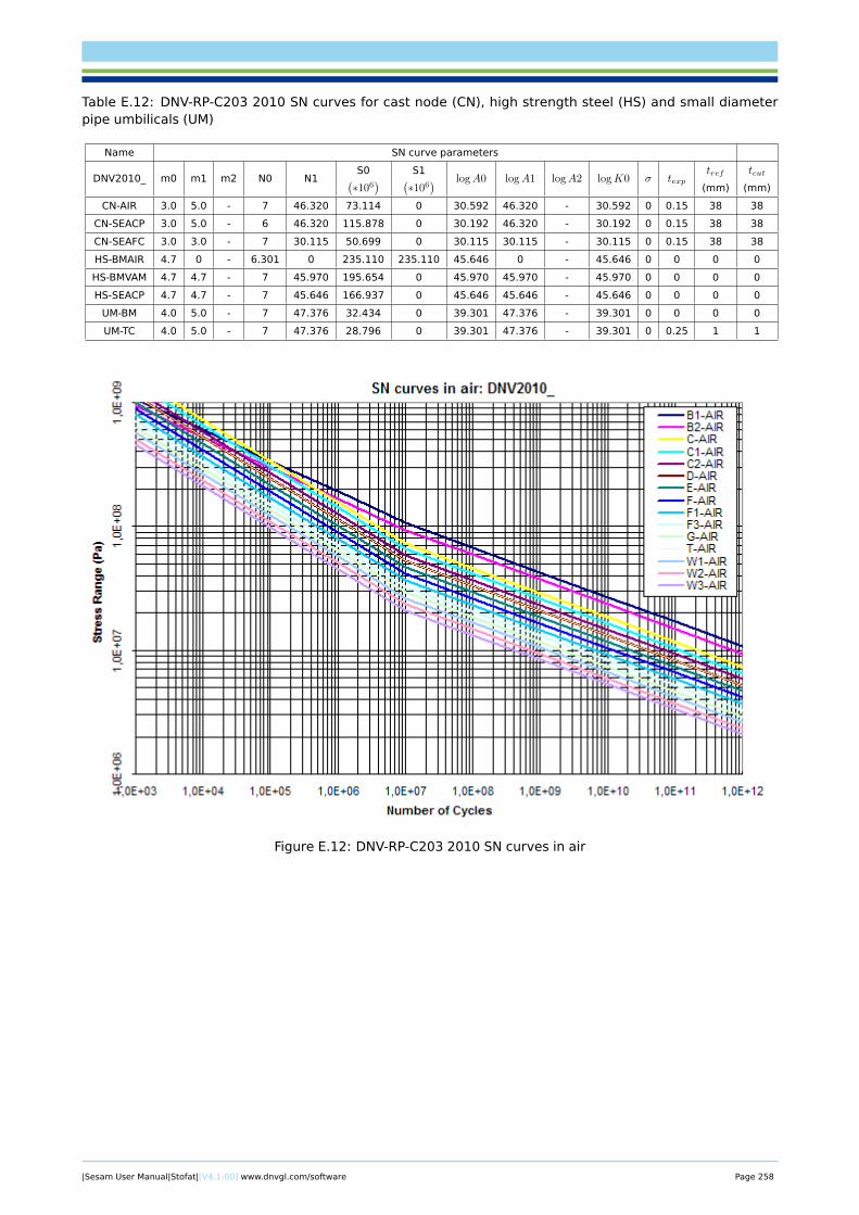
Table E.12: DNV-RP-C203 2010 SN curves for cast node (CN), high strength steel (HS) and small diameterpipe umbilicals (UM)
Name SN curve parameters
DNV2010_ m0 m1 m2 N0 N1S0(∗106
) S1(∗106
) logA0 logA1 logA2 logK0 σ texptref
(mm)
tcut
(mm)
CN-AIR 3.0 5.0 - 7 46.320 73.114 0 30.592 46.320 - 30.592 0 0.15 38 38
CN-SEACP 3.0 5.0 - 6 46.320 115.878 0 30.192 46.320 - 30.192 0 0.15 38 38
CN-SEAFC 3.0 3.0 - 7 30.115 50.699 0 30.115 30.115 - 30.115 0 0.15 38 38
HS-BMAIR 4.7 0 - 6.301 0 235.110 235.110 45.646 0 - 45.646 0 0 0 0
HS-BMVAM 4.7 4.7 - 7 45.970 195.654 0 45.970 45.970 - 45.970 0 0 0 0
HS-SEACP 4.7 4.7 - 7 45.646 166.937 0 45.646 45.646 - 45.646 0 0 0 0
UM-BM 4.0 5.0 - 7 47.376 32.434 0 39.301 47.376 - 39.301 0 0 0 0
UM-TC 4.0 5.0 - 7 47.376 28.796 0 39.301 47.376 - 39.301 0 0.25 1 1
Figure E.12: DNV-RP-C203 2010 SN curves in air
|Sesam User Manual|Stofat|[V4.1-00] www.dnvgl.com/software Page 258
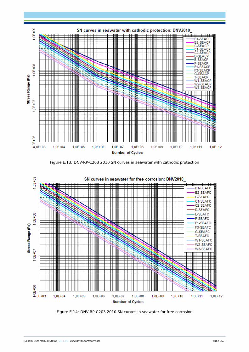
Figure E.13: DNV-RP-C203 2010 SN curves in seawater with cathodic protection
Figure E.14: DNV-RP-C203 2010 SN curves in seawater for free corrosion
|Sesam User Manual|Stofat|[V4.1-00] www.dnvgl.com/software Page 259
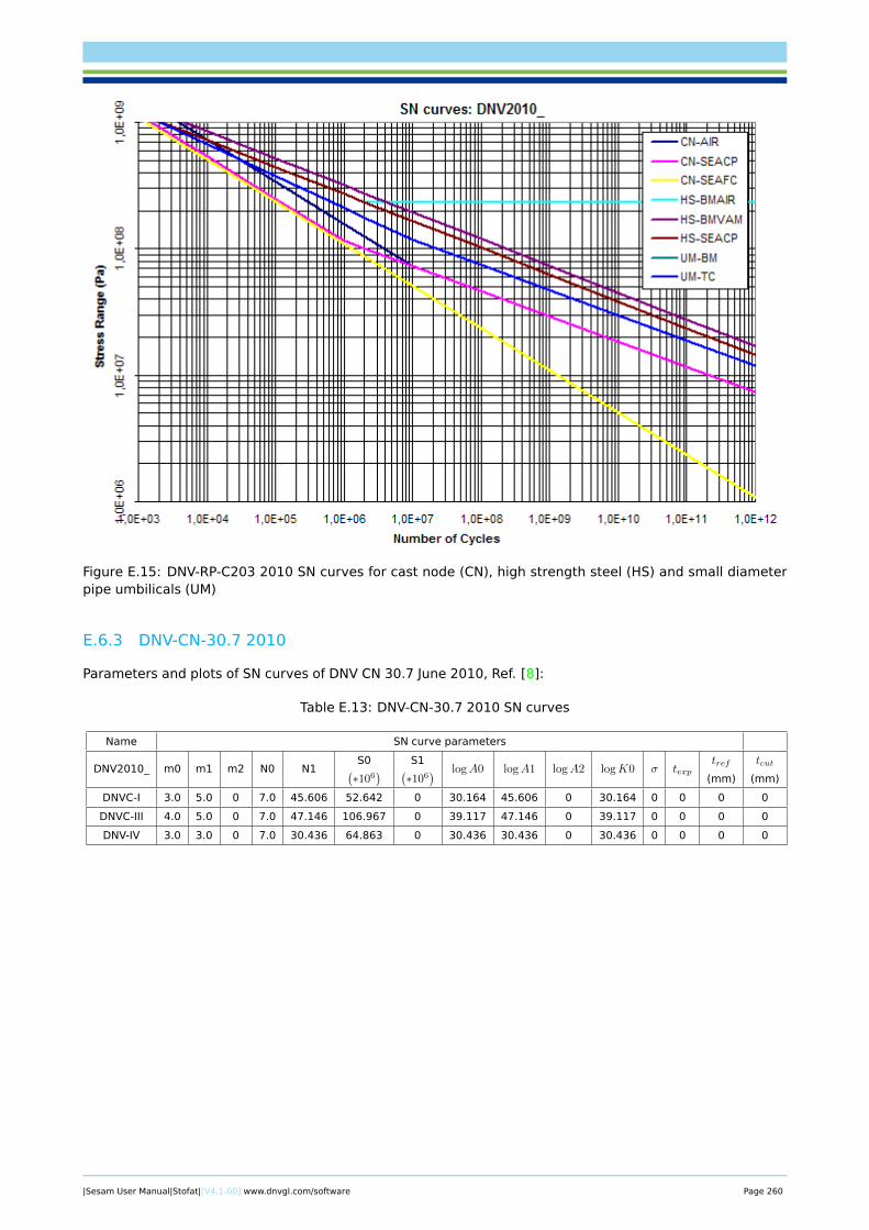
Figure E.15: DNV-RP-C203 2010 SN curves for cast node (CN), high strength steel (HS) and small diameterpipe umbilicals (UM)
E.6.3 DNV-CN-30.7 2010
Parameters and plots of SN curves of DNV CN 30.7 June 2010, Ref. [8]:
Table E.13: DNV-CN-30.7 2010 SN curves
Name SN curve parameters
DNV2010_ m0 m1 m2 N0 N1S0(∗106
) S1(∗106
) logA0 logA1 logA2 logK0 σ texptref
(mm)
tcut
(mm)
DNVC-I 3.0 5.0 0 7.0 45.606 52.642 0 30.164 45.606 0 30.164 0 0 0 0
DNVC-III 4.0 5.0 0 7.0 47.146 106.967 0 39.117 47.146 0 39.117 0 0 0 0
DNV-IV 3.0 3.0 0 7.0 30.436 64.863 0 30.436 30.436 0 30.436 0 0 0 0
|Sesam User Manual|Stofat|[V4.1-00] www.dnvgl.com/software Page 260
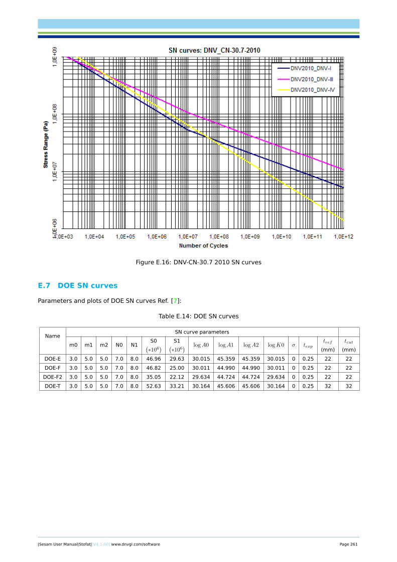
Figure E.16: DNV-CN-30.7 2010 SN curves
E.7 DOE SN curves
Parameters and plots of DOE SN curves Ref. [7]:
Table E.14: DOE SN curves
NameSN curve parameters
m0 m1 m2 N0 N1S0(∗106
) S1(∗106
) logA0 logA1 logA2 logK0 σ texptref
(mm)
tcut
(mm)
DOE-E 3.0 5.0 5.0 7.0 8.0 46.96 29.63 30.015 45.359 45.359 30.015 0 0.25 22 22
DOE-F 3.0 5.0 5.0 7.0 8.0 46.82 25.00 30.011 44.990 44.990 30.011 0 0.25 22 22
DOE-F2 3.0 5.0 5.0 7.0 8.0 35.05 22.12 29.634 44.724 44.724 29.634 0 0.25 22 22
DOE-T 3.0 5.0 5.0 7.0 8.0 52.63 33.21 30.164 45.606 45.606 30.164 0 0.25 32 32
|Sesam User Manual|Stofat|[V4.1-00] www.dnvgl.com/software Page 261
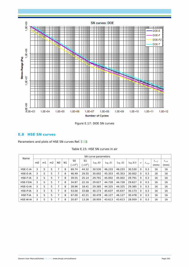
Figure E.17: DOE SN curves
E.8 HSE SN curves
Parameters and plots of HSE SN curves Ref. [13]:
Table E.15: HSE SN curves in air
NameSN curve parameters
m0 m1 m2 N0 N1S0(∗106
) S1(∗106
) logA0 logA1 logA2 logK0 σ texptref
(mm)
tcut
(mm)
HSE-C-IA 3 5 5 7 8 69.74 44.32 30.530 46.233 46.233 30.530 0 0.3 16 16
HSE-E-IA 3 5 5 7 8 46.49 29.55 30.002 45.353 45.353 30.002 0 0.3 16 16
HSE-F-IA 3 5 5 7 8 39.55 25.14 29.791 45.002 45.002 29.791 0 0.3 16 16
HSE-F2IA 3 5 5 7 8 34.87 22.16 29.627 44.728 44.728 29.627 0 0.3 16 16
HSE-G-IA 3 5 5 7 8 28.96 18.41 29.385 44.325 44.325 29.385 0 0.3 16 16
HSE-P-IA 3 5 5 7 8 53.00 33.68 30.173 45.637 45.637 30.173 0 0.3 16 16
HSE-T-IA 3 5 5 7 8 67.00 42.21 30.478 46.127 46.127 30.478 0 0.3 16 16
HSE-W-IA 3 5 5 7 8 20.87 13.26 28.959 43.613 43.613 28.959 0 0.3 16 16
|Sesam User Manual|Stofat|[V4.1-00] www.dnvgl.com/software Page 262
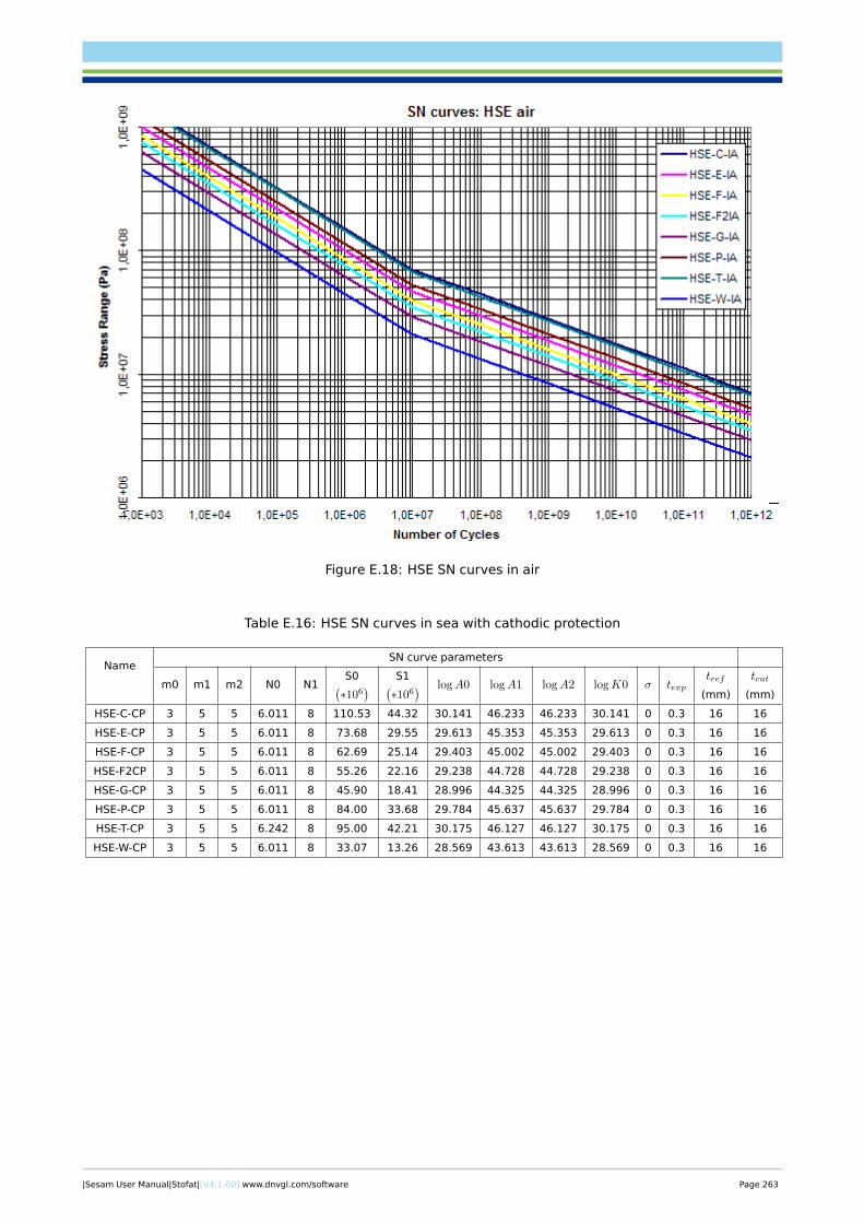
Figure E.18: HSE SN curves in air
Table E.16: HSE SN curves in sea with cathodic protection
NameSN curve parameters
m0 m1 m2 N0 N1S0(∗106
) S1(∗106
) logA0 logA1 logA2 logK0 σ texptref
(mm)
tcut
(mm)
HSE-C-CP 3 5 5 6.011 8 110.53 44.32 30.141 46.233 46.233 30.141 0 0.3 16 16
HSE-E-CP 3 5 5 6.011 8 73.68 29.55 29.613 45.353 45.353 29.613 0 0.3 16 16
HSE-F-CP 3 5 5 6.011 8 62.69 25.14 29.403 45.002 45.002 29.403 0 0.3 16 16
HSE-F2CP 3 5 5 6.011 8 55.26 22.16 29.238 44.728 44.728 29.238 0 0.3 16 16
HSE-G-CP 3 5 5 6.011 8 45.90 18.41 28.996 44.325 44.325 28.996 0 0.3 16 16
HSE-P-CP 3 5 5 6.011 8 84.00 33.68 29.784 45.637 45.637 29.784 0 0.3 16 16
HSE-T-CP 3 5 5 6.242 8 95.00 42.21 30.175 46.127 46.127 30.175 0 0.3 16 16
HSE-W-CP 3 5 5 6.011 8 33.07 13.26 28.569 43.613 43.613 28.569 0 0.3 16 16
|Sesam User Manual|Stofat|[V4.1-00] www.dnvgl.com/software Page 263
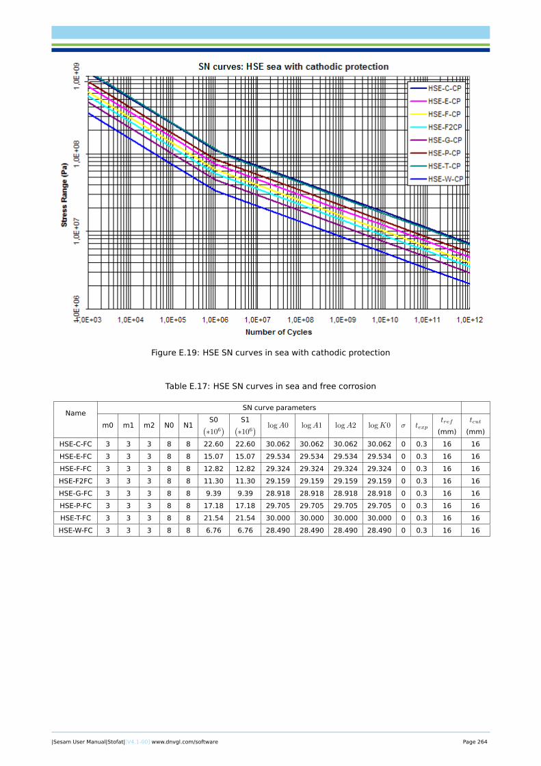
Figure E.19: HSE SN curves in sea with cathodic protection
Table E.17: HSE SN curves in sea and free corrosion
NameSN curve parameters
m0 m1 m2 N0 N1S0(∗106
) S1(∗106
) logA0 logA1 logA2 logK0 σ texptref
(mm)
tcut
(mm)
HSE-C-FC 3 3 3 8 8 22.60 22.60 30.062 30.062 30.062 30.062 0 0.3 16 16
HSE-E-FC 3 3 3 8 8 15.07 15.07 29.534 29.534 29.534 29.534 0 0.3 16 16
HSE-F-FC 3 3 3 8 8 12.82 12.82 29.324 29.324 29.324 29.324 0 0.3 16 16
HSE-F2FC 3 3 3 8 8 11.30 11.30 29.159 29.159 29.159 29.159 0 0.3 16 16
HSE-G-FC 3 3 3 8 8 9.39 9.39 28.918 28.918 28.918 28.918 0 0.3 16 16
HSE-P-FC 3 3 3 8 8 17.18 17.18 29.705 29.705 29.705 29.705 0 0.3 16 16
HSE-T-FC 3 3 3 8 8 21.54 21.54 30.000 30.000 30.000 30.000 0 0.3 16 16
HSE-W-FC 3 3 3 8 8 6.76 6.76 28.490 28.490 28.490 28.490 0 0.3 16 16
|Sesam User Manual|Stofat|[V4.1-00] www.dnvgl.com/software Page 264
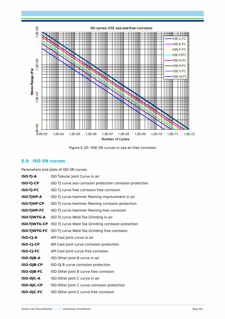
Figure E.20: HSE SN curves in sea an free corrosion
E.9 ISO SN curves
Parameters and plots of ISO SN curves.
ISO-TJ-A ISO Tubular Joint Curve in air
ISO-TJ-CP ISO TJ curve sea corrosion protection corrosion protection
ISO-TJ-FC ISO TJ curve free corrosion free corrosion
ISO-TJHP-A ISO TJ curve Hammer Peening improvement in air
ISO-TJHP-CP ISO TJ curve Hammer Peening corrosion protection
ISO-TJHP-FC ISO TJ curve Hammer Peening free corrosion
ISO-TJWTG-A ISO TJ curve Weld Toe Grinding in air
ISO-TJWTG-CP ISO TJ curve Weld Toe Grinding corrosion protection
ISO-TJWTG-FC ISO TJ curve Weld Toe Grinding free corrosion
ISO-CJ-A API Cast Joint curve in air
ISO-CJ-CP API Cast Joint curve corrosion protection
ISO-CJ-FC API Cast Joint curve free corrosion
ISO-OJB-A ISO Other Joint B curve in air
ISO-OJB-CP ISO OJ B curve corrosion protection
ISO-OJB-FC ISO Other Joint B curve free corrosion
ISO-OJC-A ISO Other Joint C curve in air
ISO-OJC-CP ISO Other Joint C curve corrosion protection
ISO-OJC-FC ISO Other Joint C curve free corrosion
|Sesam User Manual|Stofat|[V4.1-00] www.dnvgl.com/software Page 265
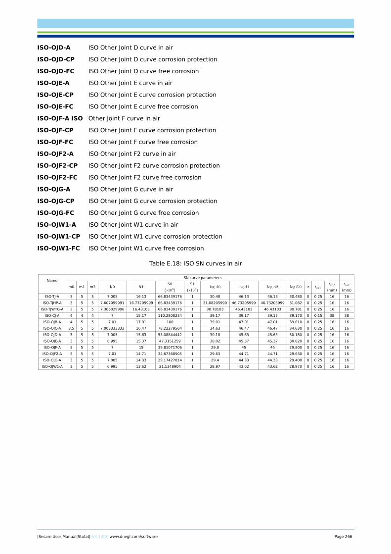
ISO-OJD-A ISO Other Joint D curve in air
ISO-OJD-CP ISO Other Joint D curve corrosion protection
ISO-OJD-FC ISO Other Joint D curve free corrosion
ISO-OJE-A ISO Other Joint E curve in air
ISO-OJE-CP ISO Other Joint E curve corrosion protection
ISO-OJE-FC ISO Other Joint E curve free corrosion
ISO-OJF-A ISO Other Joint F curve in air
ISO-OJF-CP ISO Other Joint F curve corrosion protection
ISO-OJF-FC ISO Other Joint F curve free corrosion
ISO-OJF2-A ISO Other Joint F2 curve in air
ISO-OJF2-CP ISO Other Joint F2 curve corrosion protection
ISO-OJF2-FC ISO Other Joint F2 curve free corrosion
ISO-OJG-A ISO Other Joint G curve in air
ISO-OJG-CP ISO Other Joint G curve corrosion protection
ISO-OJG-FC ISO Other Joint G curve free corrosion
ISO-OJW1-A ISO Other Joint W1 curve in air
ISO-OJW1-CP ISO Other Joint W1 curve corrosion protection
ISO-OJW1-FC ISO Other Joint W1 curve free corrosion
Table E.18: ISO SN curves in air
NameSN curve parameters
m0 m1 m2 N0 N1S0(∗106
) S1(∗106
) logA0 logA1 logA2 logK0 σ texptref
(mm)
tcut
(mm)
ISO-TJ-A 3 5 5 7.005 16.13 66.83439176 1 30.48 46.13 46.13 30.480 0 0.25 16 16
ISO-TJHP-A 3 5 5 7.607059991 16.73205999 66.83439176 1 31.08205999 46.73205999 46.73205999 31.082 0 0.25 16 16
ISO-TJWTG-A 3 5 5 7.306029996 16.43103 66.83439176 1 30.78103 46.43103 46.43103 30.781 0 0.25 16 16
ISO-CJ-A 4 4 4 7 15.17 110.2808234 1 39.17 39.17 39.17 39.170 0 0.15 38 38
ISO-OJB-A 4 5 5 7.01 17.01 100 1 39.01 47.01 47.01 39.010 0 0.25 16 16
ISO-OJC-A 3.5 5 5 7.003333333 16.47 78.22279564 1 34.63 46.47 46.47 34.630 0 0.25 16 16
ISO-OJD-A 3 5 5 7.005 15.63 53.08844442 1 30.18 45.63 45.63 30.180 0 0.25 16 16
ISO-OJE-A 3 5 5 6.995 15.37 47.3151259 1 30.02 45.37 45.37 30.020 0 0.25 16 16
ISO-OJF-A 3 5 5 7 15 39.81071706 1 29.8 45 45 29.800 0 0.25 16 16
ISO-OJF2-A 3 5 5 7.01 14.71 34.67368505 1 29.63 44.71 44.71 29.630 0 0.25 16 16
ISO-OJG-A 3 5 5 7.005 14.33 29.17427014 1 29.4 44.33 44.33 29.400 0 0.25 16 16
ISO-OJW1-A 3 5 5 6.995 13.62 21.1348904 1 28.97 43.62 43.62 28.970 0 0.25 16 16
|Sesam User Manual|Stofat|[V4.1-00] www.dnvgl.com/software Page 266
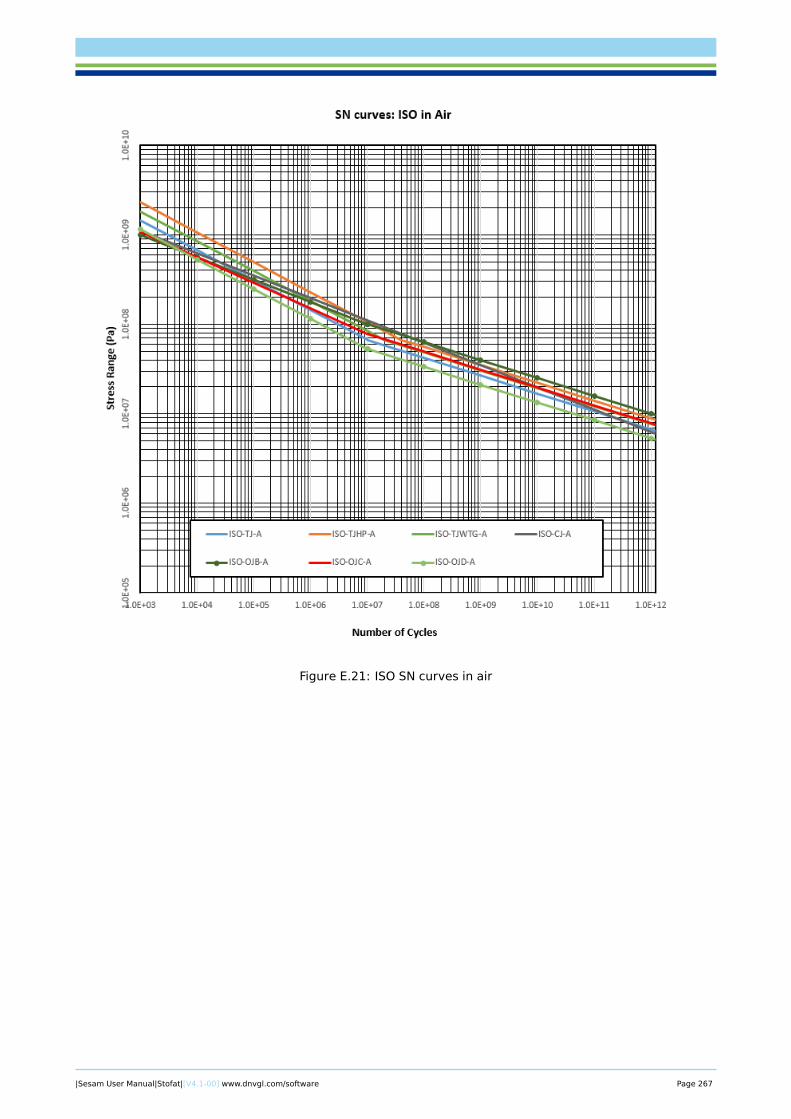
Figure E.21: ISO SN curves in air
|Sesam User Manual|Stofat|[V4.1-00] www.dnvgl.com/software Page 267
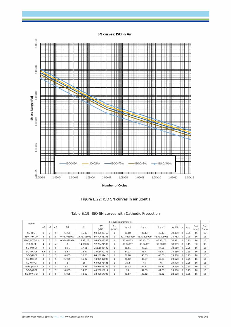
Figure E.22: ISO SN curves in air (cont.)
Table E.19: ISO SN curves with Cathodic Protection
NameSN curve parameters
m0 m1 m2 N0 N1S0(∗106
) S1(∗106
) logA0 logA1 logA2 logK0 σ texptref
(mm)
tcut
(mm)
ISO-TJ-CP 3 5 5 6.255 16.13 94.40608763 1 30.18 46.13 46.13 30.180 0 0.25 16 16
ISO-TJHP-CP 3 5 5 6.857059991 16.73205999 94.40608763 1 30.78205999 46.73205999 46.73205999 30.782 0 0.25 16 16
ISO-TJWTG-CP 3 5 5 6.556029996 16.43103 94.40608763 1 30.48103 46.43103 46.43103 30.481 0 0.25 16 16
ISO-CJ-CP 4 4 4 7 14.86897 92.73474906 1 38.86897 38.86897 38.86897 38.869 0 0.15 38 38
ISO-OJB-CP 4 5 5 5.01 17.01 251.1886432 1 38.61 47.01 47.01 38.610 0 0.25 16 16
ISO-OJC-CP 3.5 5 5 5.67 16.47 144.5439771 1 34.23 46.47 46.47 34.230 0 0.25 16 16
ISO-OJD-CP 3 5 5 6.005 15.63 84.13951416 1 29.78 45.63 45.63 29.780 0 0.25 16 16
ISO-OJE-CP 3 5 5 5.995 15.37 74.98942093 1 29.62 45.37 45.37 29.620 0 0.25 16 16
ISO-OJF-CP 3 5 5 6 15 63.09573445 1 29.4 45 45 29.400 0 0.25 16 16
ISO-OJF2-CP 3 5 5 6.01 14.71 54.95408739 1 29.23 44.71 44.71 29.230 0 0.25 16 16
ISO-OJG-CP 3 5 5 6.005 14.33 46.23810214 1 29 44.33 44.33 29.000 0 0.25 16 16
ISO-OJW1-CP 3 5 5 5.995 13.62 33.49654392 1 28.57 43.62 43.62 28.570 0 0.25 16 16
|Sesam User Manual|Stofat|[V4.1-00] www.dnvgl.com/software Page 268
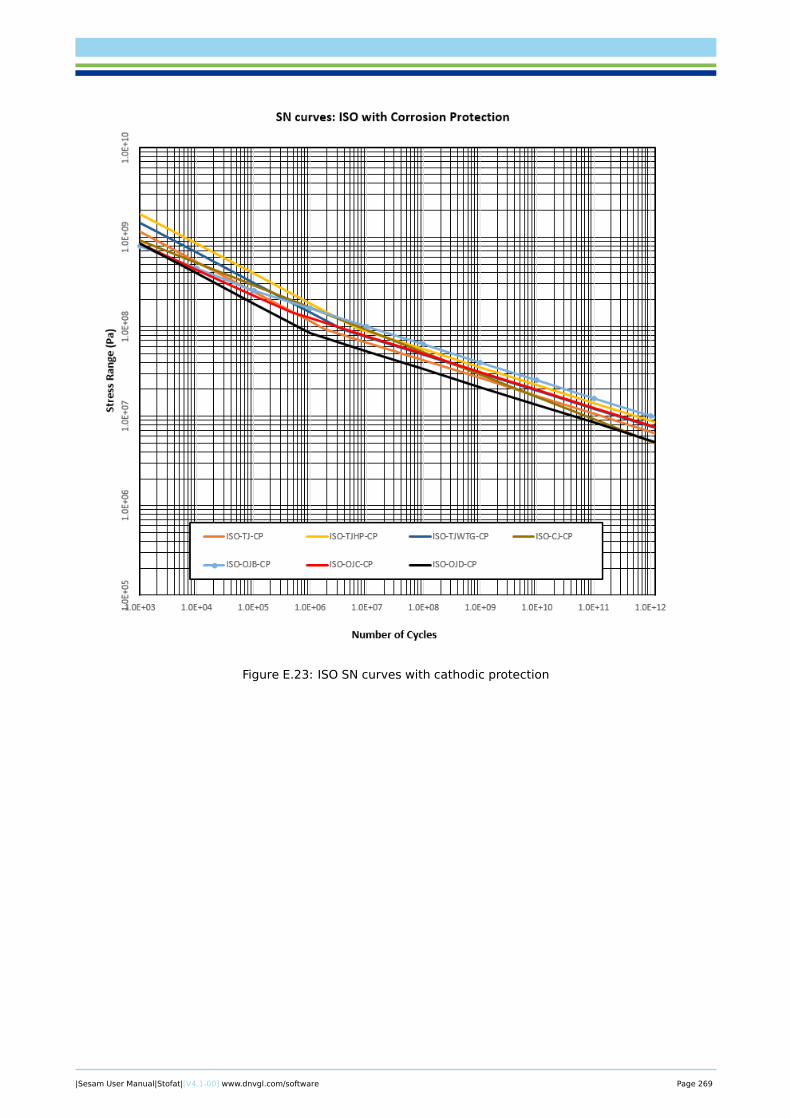
Figure E.23: ISO SN curves with cathodic protection
|Sesam User Manual|Stofat|[V4.1-00] www.dnvgl.com/software Page 269
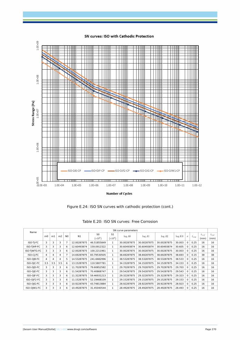
Figure E.24: ISO SN curves with cathodic protection (cont.)
Table E.20: ISO SN curves: Free Corrosion
NameSN curve parameters
m0 m1 m2 N0 N1S0(∗106
) S1(∗106
) logA0 logA1 logA2 logK0 σ texptref
(mm)
tcut
(mm)
ISO-TJ-FC 3 3 3 7 12.00287875 46.51855849 1 30.00287875 30.00287875 30.00287875 30.003 0 0.25 16 16
ISO-TJHP-FC 3 3 3 6 12.60493874 159.0912322 1 30.60493874 30.60493874 30.60493874 30.605 0 0.25 16 16
ISO-TJWTG-FC 3 3 3 6 12.00287875 100.2211961 1 30.00287875 30.00287875 30.00287875 30.003 0 0.25 16 16
ISO-CJ-FC 4 4 4 7 14.69287875 83.79530505 1 38.69287875 38.69287875 38.69287875 38.693 0 0.15 38 38
ISO-OJB-FC 4 4 4 5 14.53287875 241.6682996 1 38.53287875 38.53287875 38.53287875 38.533 0 0.25 16 16
ISO-OJC-FC 3.5 3.5 3.5 6 13.15287875 110.5807781 1 34.15287875 34.15287875 34.15287875 34.153 0 0.25 16 16
ISO-OJD-FC 3 3 3 6 11.70287875 79.60852582 1 29.70287875 29.70287875 29.70287875 29.703 0 0.25 16 16
ISO-OJE-FC 3 3 3 6 11.54287875 70.40868747 1 29.54287875 29.54287875 29.54287875 29.543 0 0.25 16 16
ISO-OJF-FC 3 3 3 6 11.32287875 59.46931213 1 29.32287875 29.32287875 29.32287875 29.323 0 0.25 16 16
ISO-OJF2-FC 3 3 3 6 11.15287875 52.19468109 1 29.15287875 29.15287875 29.15287875 29.153 0 0.25 16 16
ISO-OJG-FC 3 3 3 6 10.92287875 43.74813884 1 28.92287875 28.92287875 28.92287875 28.923 0 0.25 16 16
ISO-OJW1-FC 3 3 3 6 10.49287875 31.45040544 1 28.49287875 28.49287875 28.49287875 28.493 0 0.25 16 16
|Sesam User Manual|Stofat|[V4.1-00] www.dnvgl.com/software Page 270
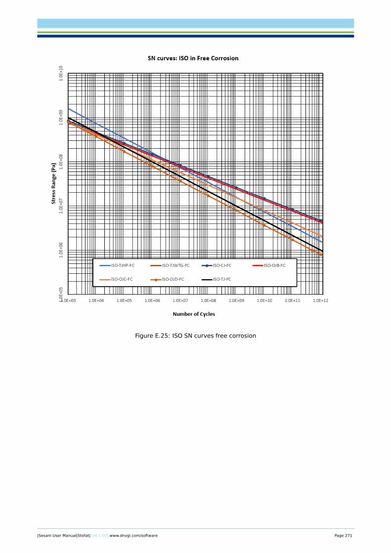
Figure E.25: ISO SN curves free corrosion
|Sesam User Manual|Stofat|[V4.1-00] www.dnvgl.com/software Page 271
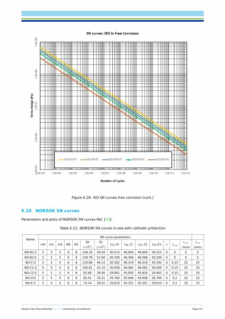
Figure E.26: ISO SN curves free corrosion (cont.)
E.10 NORSOK SN curves
Parameters and plots of NORSOK SN curves Ref. [29]:
Table E.21: NORSOK SN curves in sea with cathodic protection
NameSN curve parameters
m0 m1 m2 N0 N1S0(∗106
) S1(∗106
) logA0 logA1 logA2 logK0 σ texptref
(mm)
tcut
(mm)
NO-B1-S 3 5 5 6 8 148.30 59.04 30.513 46.856 46.856 30.513 0 0 0 0
NO-B2-S 3 5 5 6 8 129.76 51.66 30.339 46.566 46.566 30.339 0 0 0 0
NO-C-S 3 5 5 6 8 115.86 46.12 30.192 46.319 46.319 30.192 0 0.15 25 25
NO-C1-S 3 5 5 6 8 103.81 41.33 30.049 46.081 46.081 30.049 0 0.15 25 25
NO-C2-S 3 5 5 6 8 92.68 36.90 29.901 45.835 45.835 29.901 0 0.15 25 25
NO-D-S 3 5 5 6 8 83.41 33.21 29.764 45.606 45.606 29.764 0 0.2 25 25
NO-E-S 3 5 5 6 8 74.14 29.52 29.610 45.351 45.351 29.610 0 0.2 25 25
|Sesam User Manual|Stofat|[V4.1-00] www.dnvgl.com/software Page 272
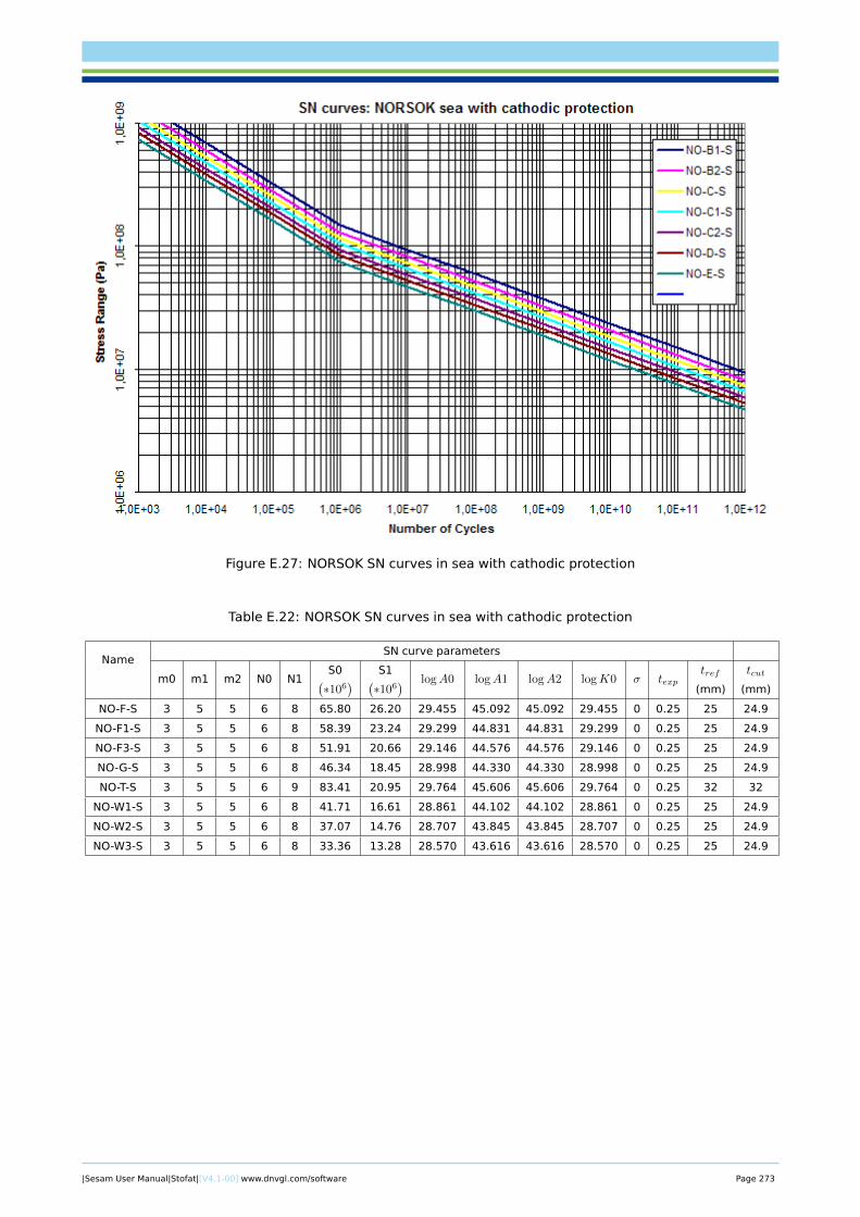
Figure E.27: NORSOK SN curves in sea with cathodic protection
Table E.22: NORSOK SN curves in sea with cathodic protection
NameSN curve parameters
m0 m1 m2 N0 N1S0(∗106
) S1(∗106
) logA0 logA1 logA2 logK0 σ texptref
(mm)
tcut
(mm)
NO-F-S 3 5 5 6 8 65.80 26.20 29.455 45.092 45.092 29.455 0 0.25 25 24.9
NO-F1-S 3 5 5 6 8 58.39 23.24 29.299 44.831 44.831 29.299 0 0.25 25 24.9
NO-F3-S 3 5 5 6 8 51.91 20.66 29.146 44.576 44.576 29.146 0 0.25 25 24.9
NO-G-S 3 5 5 6 8 46.34 18.45 28.998 44.330 44.330 28.998 0 0.25 25 24.9
NO-T-S 3 5 5 6 9 83.41 20.95 29.764 45.606 45.606 29.764 0 0.25 32 32
NO-W1-S 3 5 5 6 8 41.71 16.61 28.861 44.102 44.102 28.861 0 0.25 25 24.9
NO-W2-S 3 5 5 6 8 37.07 14.76 28.707 43.845 43.845 28.707 0 0.25 25 24.9
NO-W3-S 3 5 5 6 8 33.36 13.28 28.570 43.616 43.616 28.570 0 0.25 25 24.9
|Sesam User Manual|Stofat|[V4.1-00] www.dnvgl.com/software Page 273
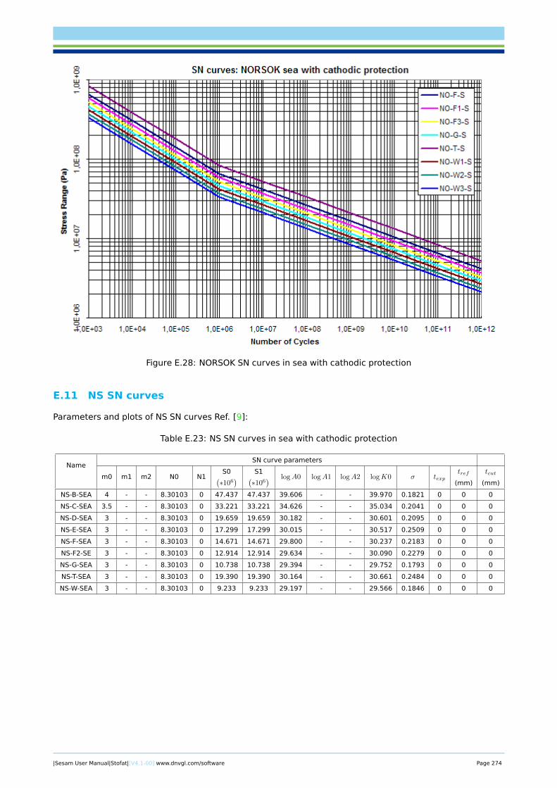
Figure E.28: NORSOK SN curves in sea with cathodic protection
E.11 NS SN curves
Parameters and plots of NS SN curves Ref. [9]:
Table E.23: NS SN curves in sea with cathodic protection
NameSN curve parameters
m0 m1 m2 N0 N1S0(∗106
) S1(∗106
) logA0 logA1 logA2 logK0 σ texptref
(mm)
tcut
(mm)
NS-B-SEA 4 - - 8.30103 0 47.437 47.437 39.606 - - 39.970 0.1821 0 0 0
NS-C-SEA 3.5 - - 8.30103 0 33.221 33.221 34.626 - - 35.034 0.2041 0 0 0
NS-D-SEA 3 - - 8.30103 0 19.659 19.659 30.182 - - 30.601 0.2095 0 0 0
NS-E-SEA 3 - - 8.30103 0 17.299 17.299 30.015 - - 30.517 0.2509 0 0 0
NS-F-SEA 3 - - 8.30103 0 14.671 14.671 29.800 - - 30.237 0.2183 0 0 0
NS-F2-SE 3 - - 8.30103 0 12.914 12.914 29.634 - - 30.090 0.2279 0 0 0
NS-G-SEA 3 - - 8.30103 0 10.738 10.738 29.394 - - 29.752 0.1793 0 0 0
NS-T-SEA 3 - - 8.30103 0 19.390 19.390 30.164 - - 30.661 0.2484 0 0 0
NS-W-SEA 3 - - 8.30103 0 9.233 9.233 29.197 - - 29.566 0.1846 0 0 0
|Sesam User Manual|Stofat|[V4.1-00] www.dnvgl.com/software Page 274
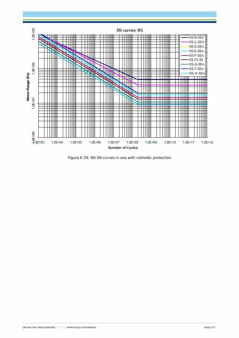
Figure E.29: NS SN curves in sea with cathodic protection
|Sesam User Manual|Stofat|[V4.1-00] www.dnvgl.com/software Page 275

F PULLDOWN MENUS AND DIALOG WINDOWS OF STOFAT
This appendix shows the pulldown menus of the Stofat commands and dialog windows connected to theitems in the pulldown menus.
When clicking an item in the pull down menus, three different actions may take place;
1. the command initiates a program execution immediately
2. the command opens a dialog window through which user interaction may take place
3. a subcommand list pops up to the right of the command
The action rules are illustrated below.
Action rules for items in the pulldown menu:
1. The command button initiates a program execution
2. The command button opens a dialog window
3. The command button shows a list of commands to the right of the button
|Sesam User Manual|Stofat|[V4.1-00] www.dnvgl.com/software Page 276
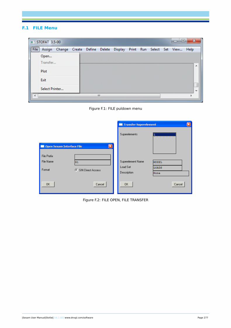
F.1 FILE Menu
Figure F.1: FILE puldown menu
Figure F.2: FILE OPEN, FILE TRANSFER
|Sesam User Manual|Stofat|[V4.1-00] www.dnvgl.com/software Page 277
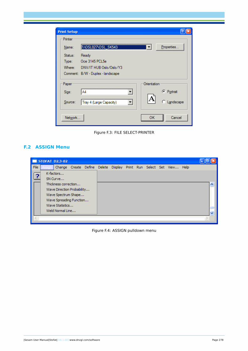
Figure F.3: FILE SELECT-PRINTER
F.2 ASSIGN Menu
Figure F.4: ASSIGN pulldown menu
|Sesam User Manual|Stofat|[V4.1-00] www.dnvgl.com/software Page 278
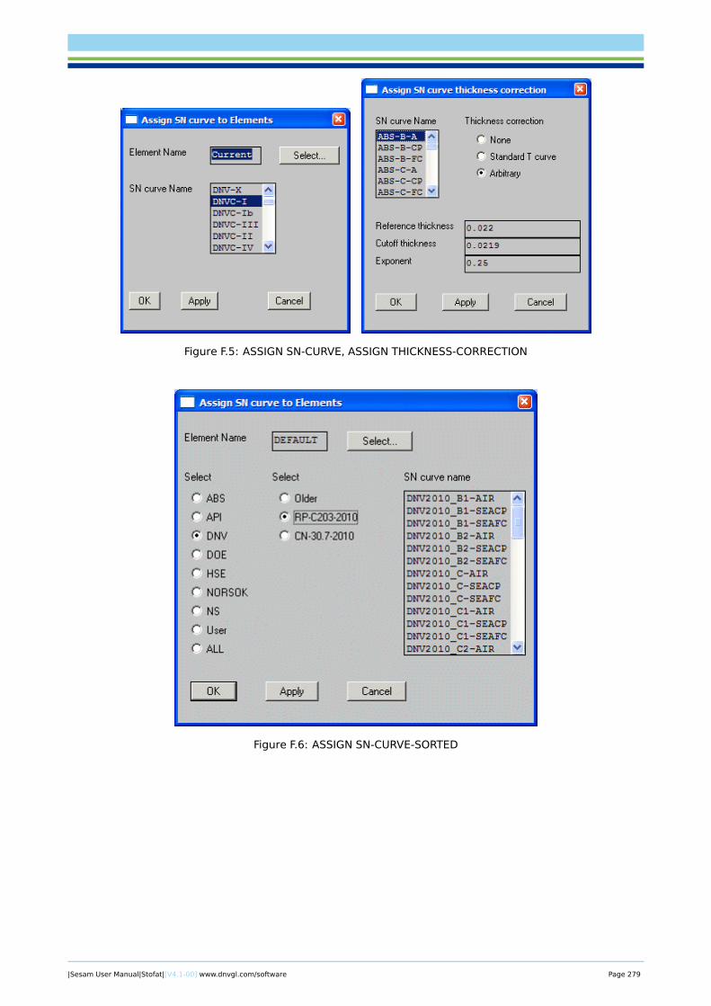
Figure F.5: ASSIGN SN-CURVE, ASSIGN THICKNESS-CORRECTION
Figure F.6: ASSIGN SN-CURVE-SORTED
|Sesam User Manual|Stofat|[V4.1-00] www.dnvgl.com/software Page 279
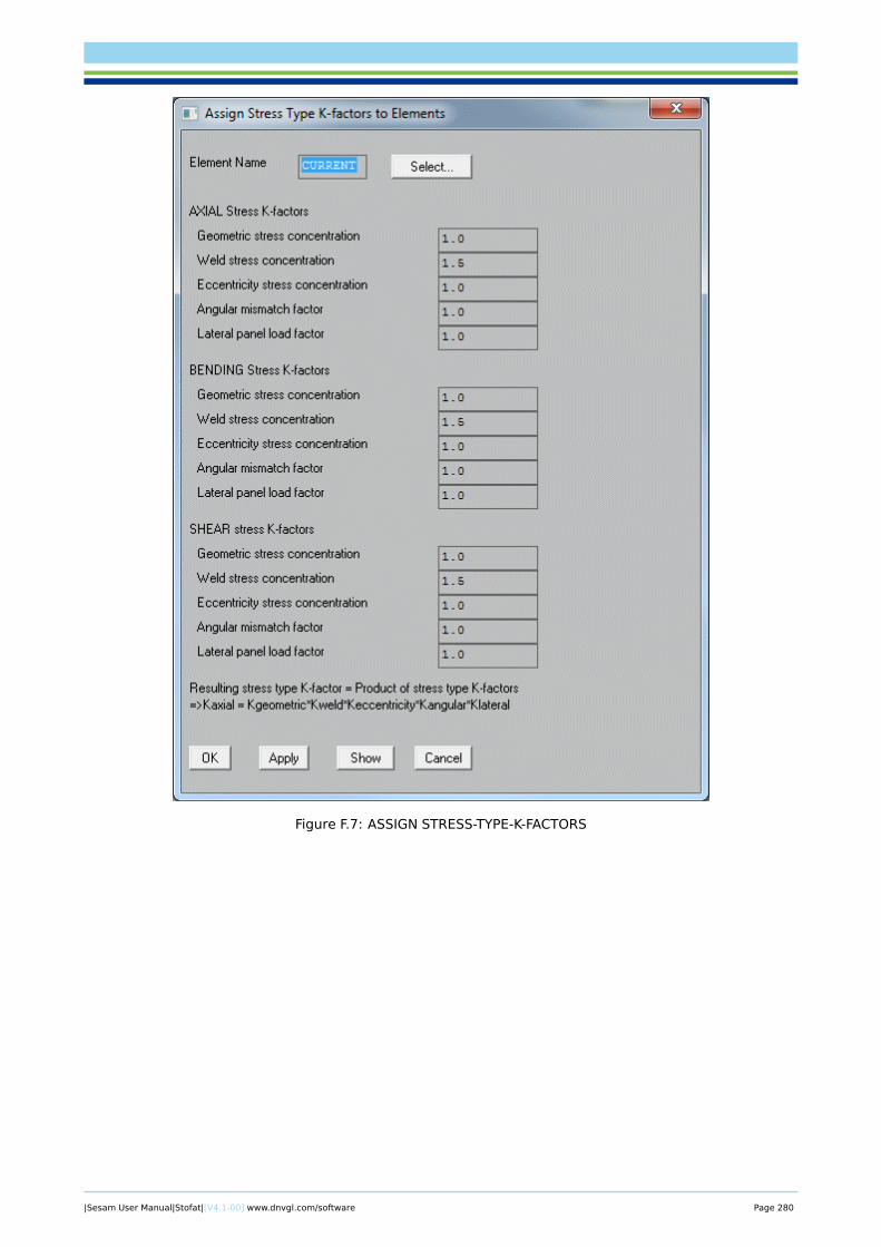
Figure F.7: ASSIGN STRESS-TYPE-K-FACTORS
|Sesam User Manual|Stofat|[V4.1-00] www.dnvgl.com/software Page 280
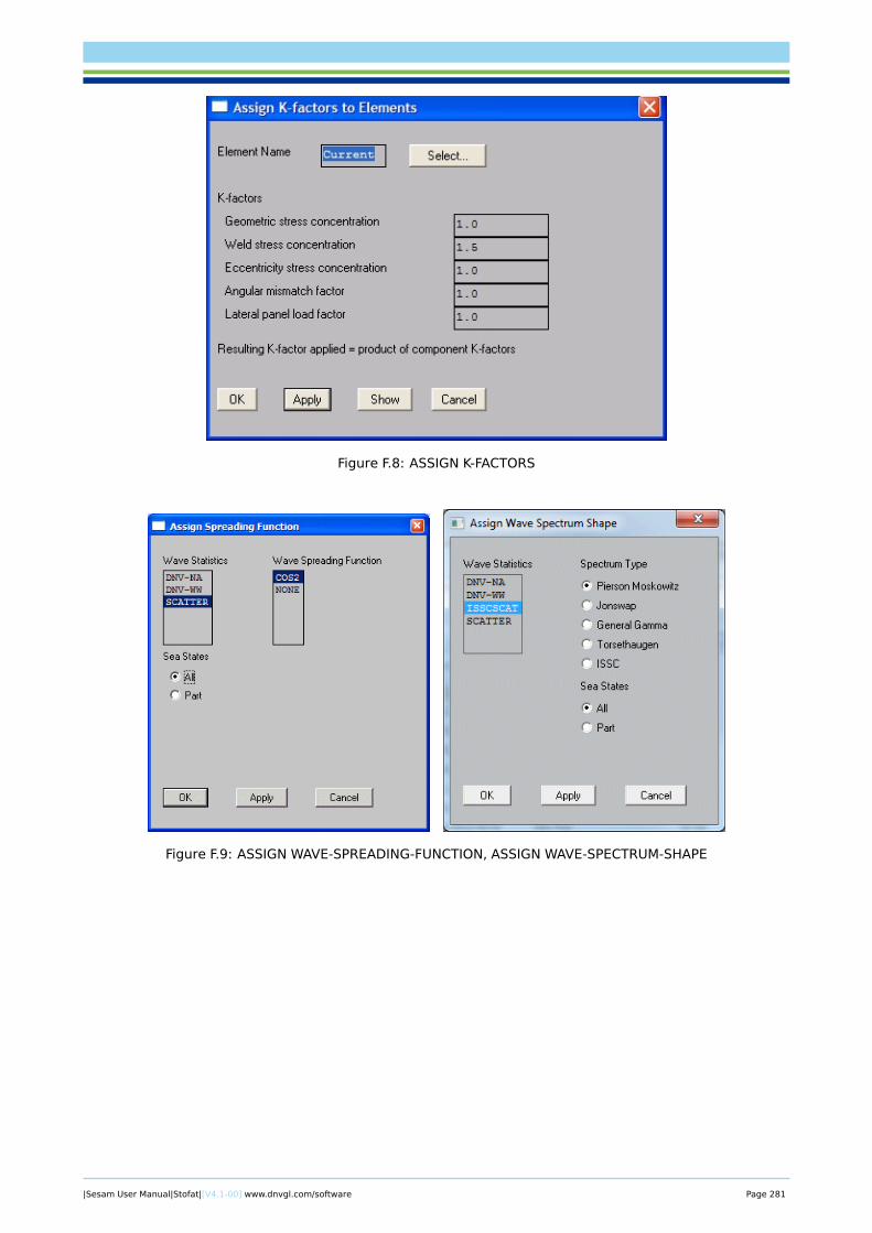
Figure F.8: ASSIGN K-FACTORS
Figure F.9: ASSIGN WAVE-SPREADING-FUNCTION, ASSIGN WAVE-SPECTRUM-SHAPE
|Sesam User Manual|Stofat|[V4.1-00] www.dnvgl.com/software Page 281
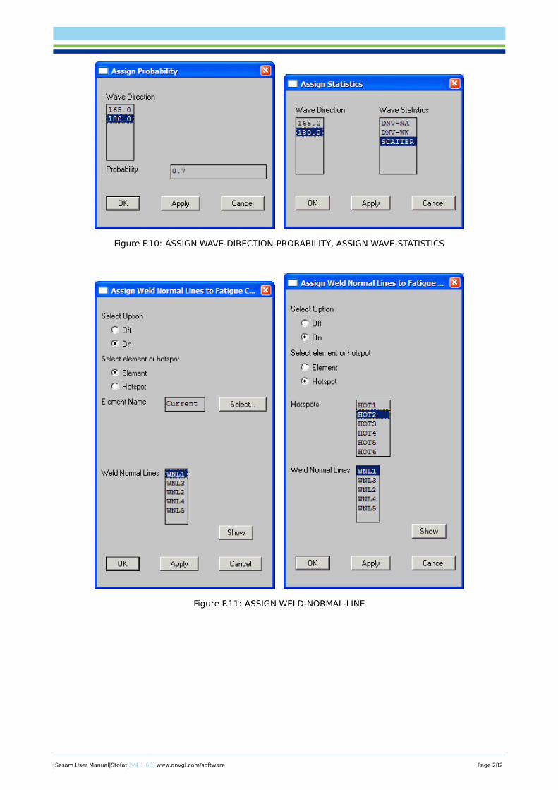
Figure F.10: ASSIGN WAVE-DIRECTION-PROBABILITY, ASSIGN WAVE-STATISTICS
Figure F.11: ASSIGN WELD-NORMAL-LINE
|Sesam User Manual|Stofat|[V4.1-00] www.dnvgl.com/software Page 282
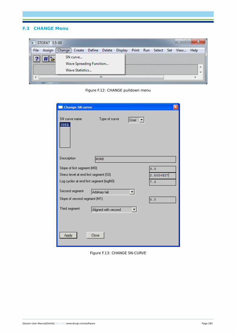
F.3 CHANGE Menu
Figure F.12: CHANGE pulldown menu
Figure F.13: CHANGE SN-CURVE
|Sesam User Manual|Stofat|[V4.1-00] www.dnvgl.com/software Page 283
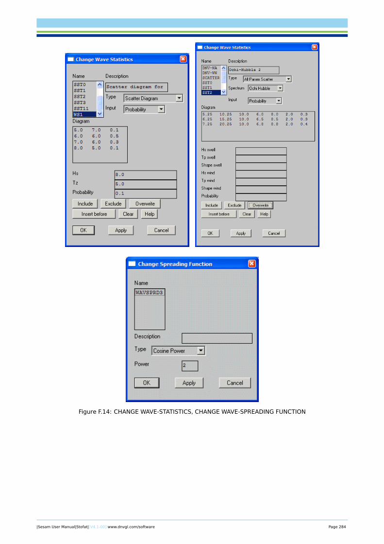
Figure F.14: CHANGE WAVE-STATISTICS, CHANGE WAVE-SPREADING FUNCTION
|Sesam User Manual|Stofat|[V4.1-00] www.dnvgl.com/software Page 284
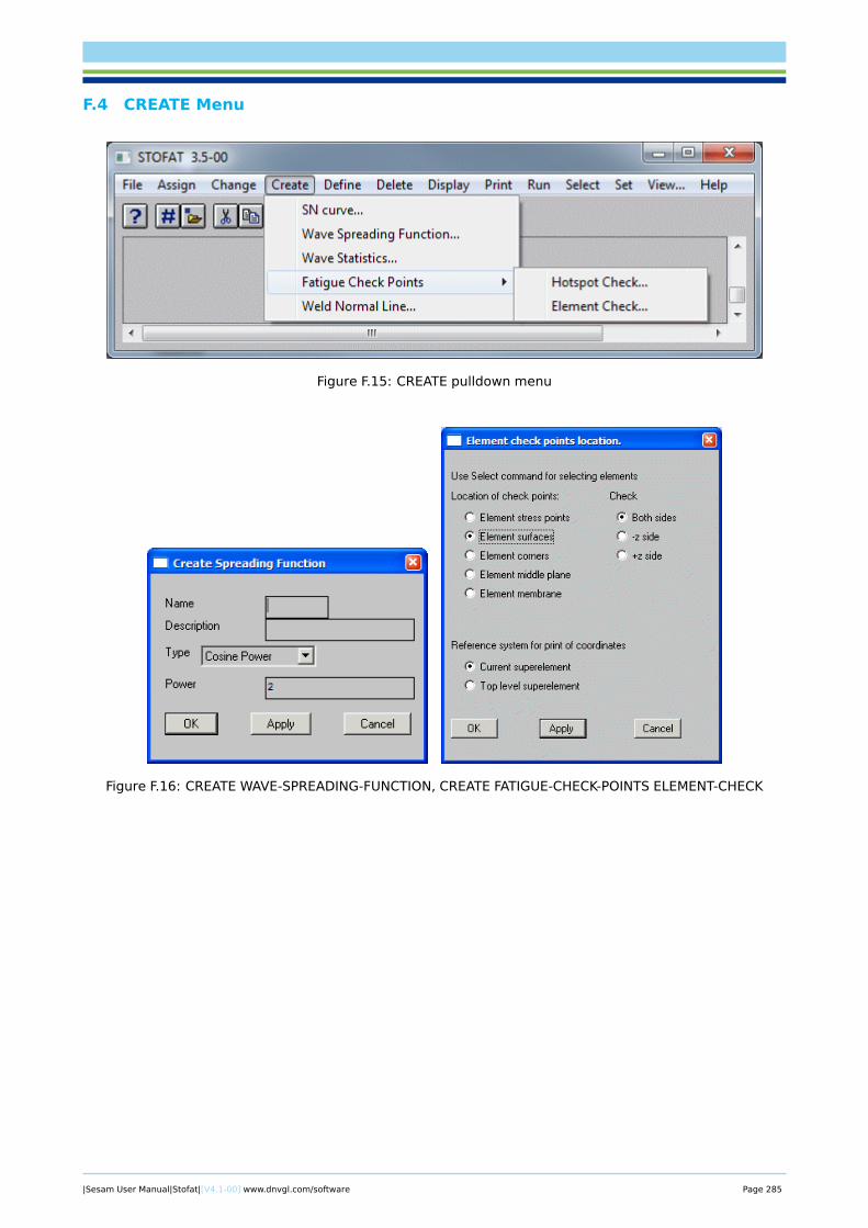
F.4 CREATE Menu
Figure F.15: CREATE pulldown menu
Figure F.16: CREATE WAVE-SPREADING-FUNCTION, CREATE FATIGUE-CHECK-POINTS ELEMENT-CHECK
|Sesam User Manual|Stofat|[V4.1-00] www.dnvgl.com/software Page 285
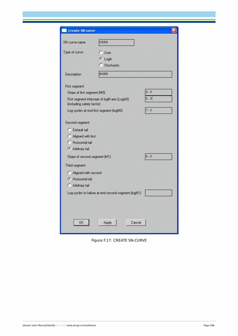
Figure F.17: CREATE SN-CURVE
|Sesam User Manual|Stofat|[V4.1-00] www.dnvgl.com/software Page 286
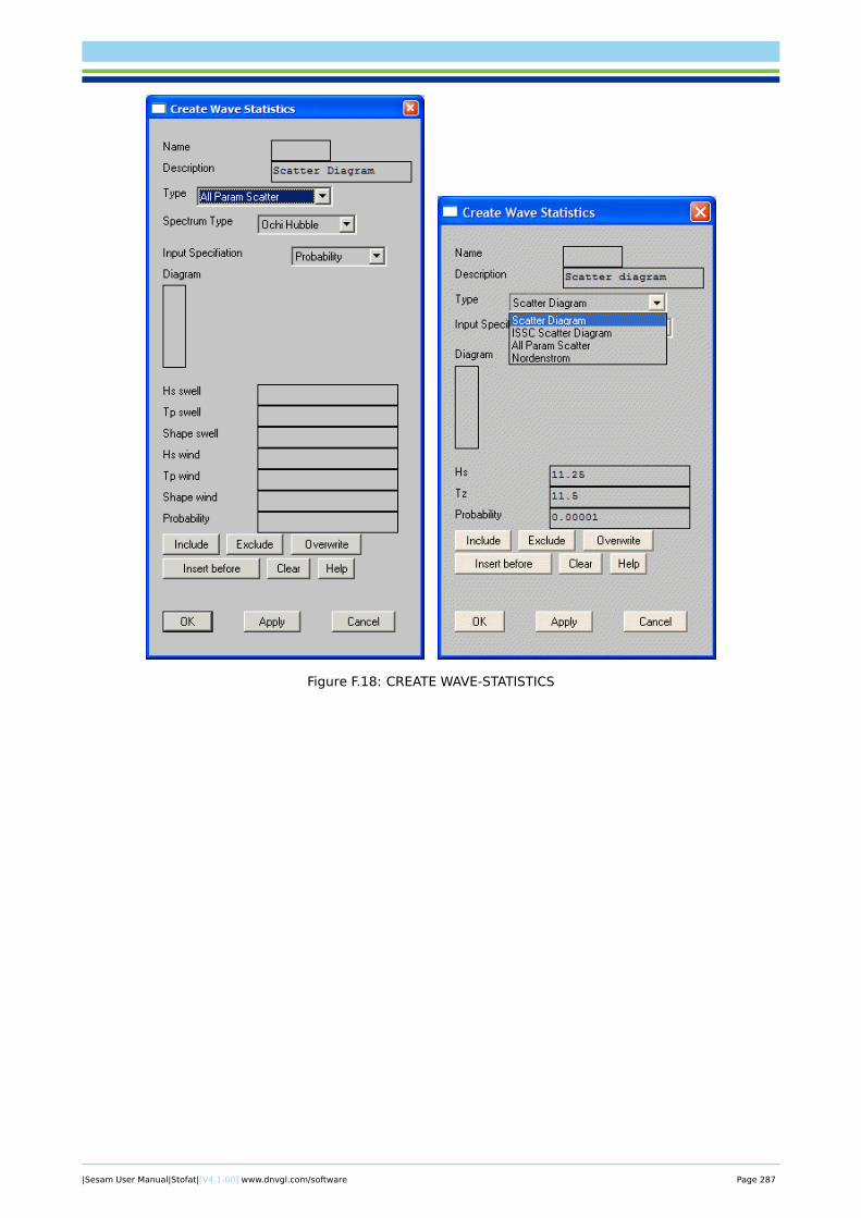
Figure F.18: CREATE WAVE-STATISTICS
|Sesam User Manual|Stofat|[V4.1-00] www.dnvgl.com/software Page 287
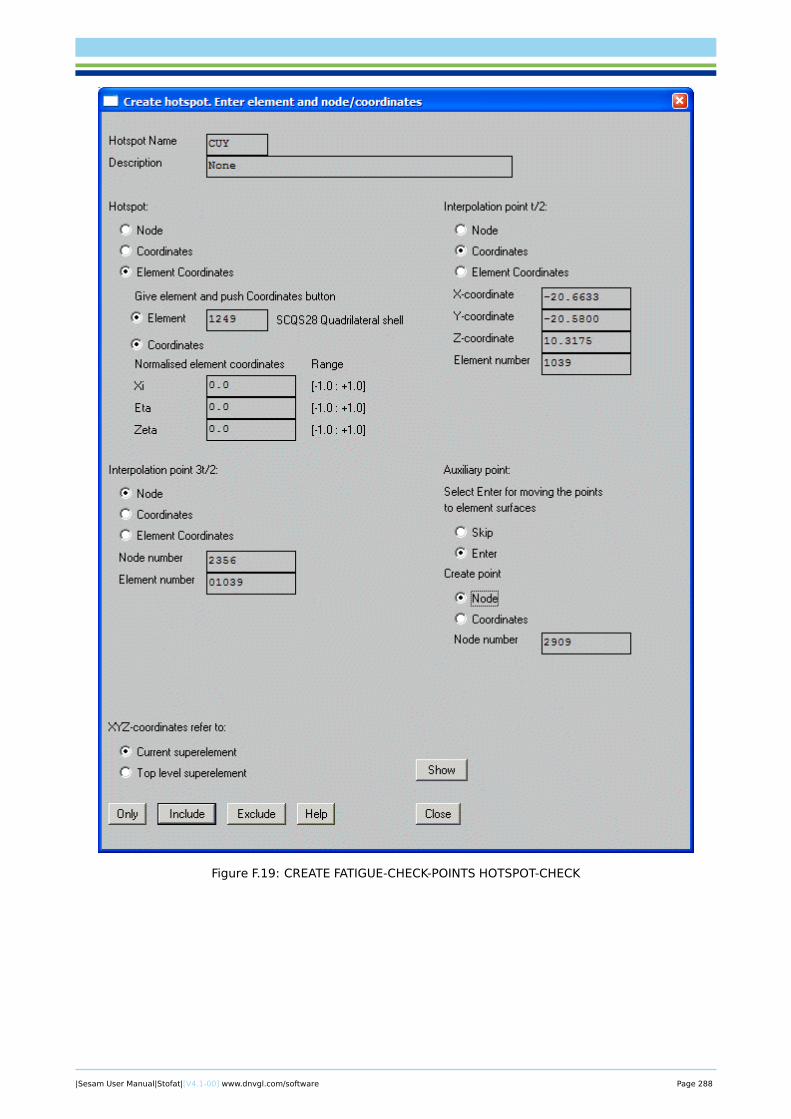
Figure F.19: CREATE FATIGUE-CHECK-POINTS HOTSPOT-CHECK
|Sesam User Manual|Stofat|[V4.1-00] www.dnvgl.com/software Page 288
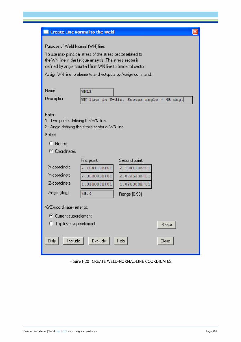
Figure F.20: CREATE WELD-NORMAL-LINE COORDINATES
|Sesam User Manual|Stofat|[V4.1-00] www.dnvgl.com/software Page 289
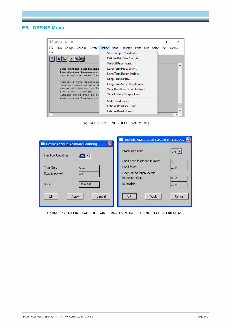
F.5 DEFINE Menu
Figure F.21: DEFINE PULLDOWN MENU
Figure F.22: DEFINE FATIGUE RAINFLOW-COUNTING, DEFINE STATIC-LOAD-CASE
|Sesam User Manual|Stofat|[V4.1-00] www.dnvgl.com/software Page 290
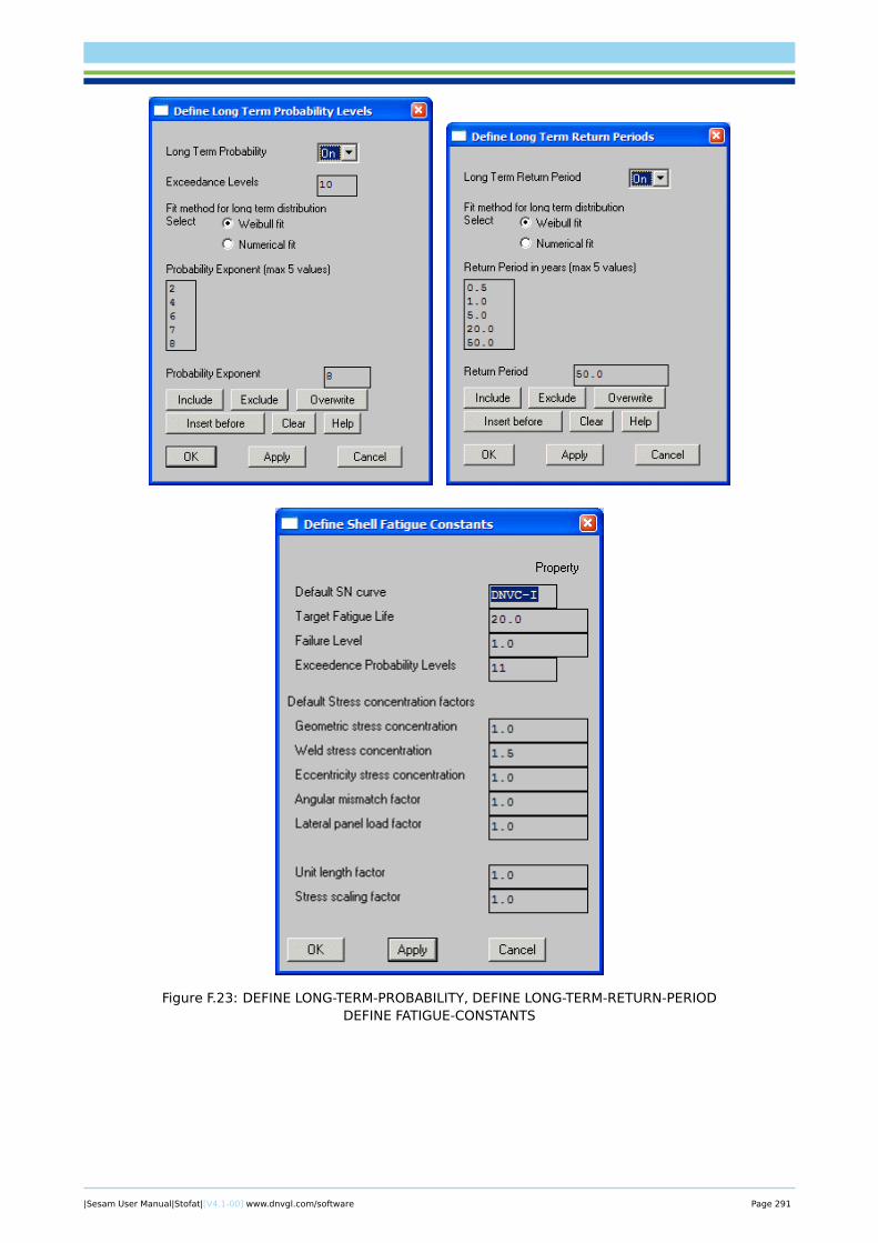
Figure F.23: DEFINE LONG-TERM-PROBABILITY, DEFINE LONG-TERM-RETURN-PERIODDEFINE FATIGUE-CONSTANTS
|Sesam User Manual|Stofat|[V4.1-00] www.dnvgl.com/software Page 291
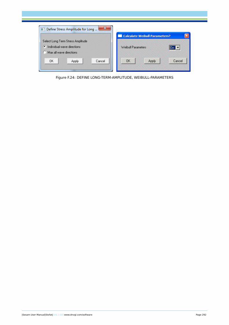
Figure F.24: DEFINE LONG-TERM-AMPLITUDE, WEIBULL-PARAMETERS
|Sesam User Manual|Stofat|[V4.1-00] www.dnvgl.com/software Page 292
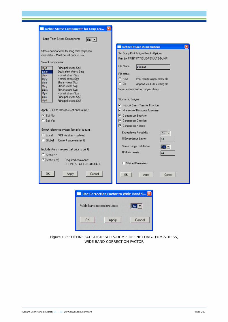
Figure F.25: DEFINE FATIGUE-RESULTS-DUMP, DEFINE LONG-TERM-STRESS,WIDE-BAND-CORRECTION-FACTOR
|Sesam User Manual|Stofat|[V4.1-00] www.dnvgl.com/software Page 293
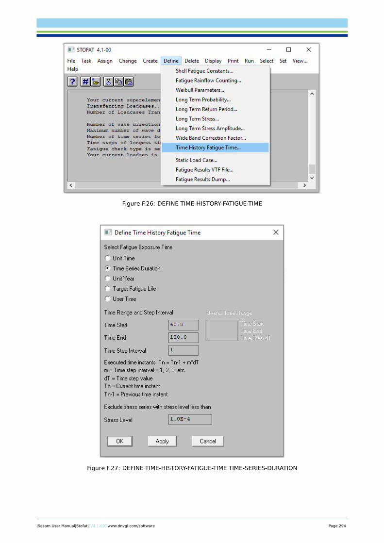
Figure F.26: DEFINE TIME-HISTORY-FATIGUE-TIME
Figure F.27: DEFINE TIME-HISTORY-FATIGUE-TIME TIME-SERIES-DURATION
|Sesam User Manual|Stofat|[V4.1-00] www.dnvgl.com/software Page 294
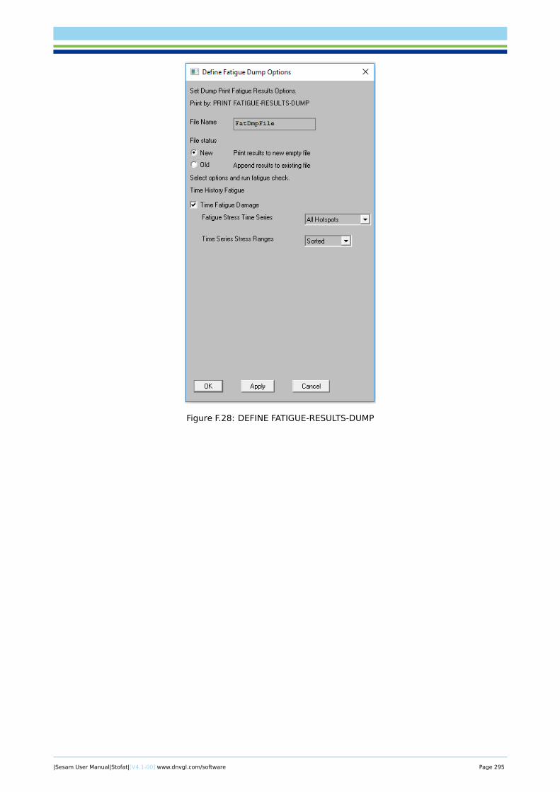
Figure F.28: DEFINE FATIGUE-RESULTS-DUMP
|Sesam User Manual|Stofat|[V4.1-00] www.dnvgl.com/software Page 295
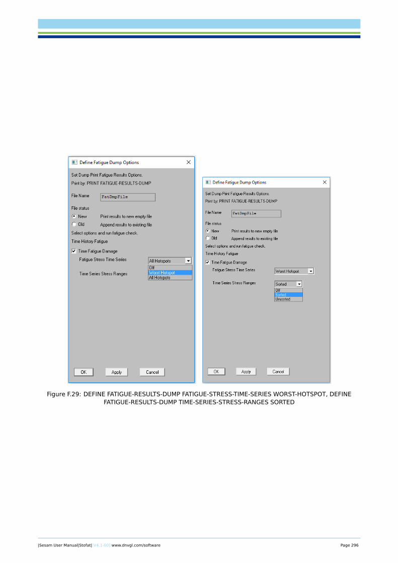
Figure F.29: DEFINE FATIGUE-RESULTS-DUMP FATIGUE-STRESS-TIME-SERIES WORST-HOTSPOT, DEFINEFATIGUE-RESULTS-DUMP TIME-SERIES-STRESS-RANGES SORTED
|Sesam User Manual|Stofat|[V4.1-00] www.dnvgl.com/software Page 296
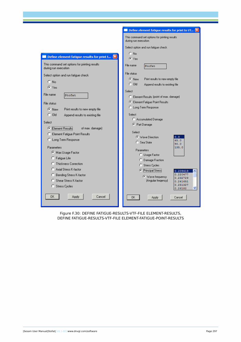
Figure F.30: DEFINE FATIGUE-RESULTS-VTF-FILE ELEMENT-RESULTS,DEFINE FATIGUE-RESULTS-VTF-FILE ELEMENT-FATIGUE-POINT-RESULTS
|Sesam User Manual|Stofat|[V4.1-00] www.dnvgl.com/software Page 297
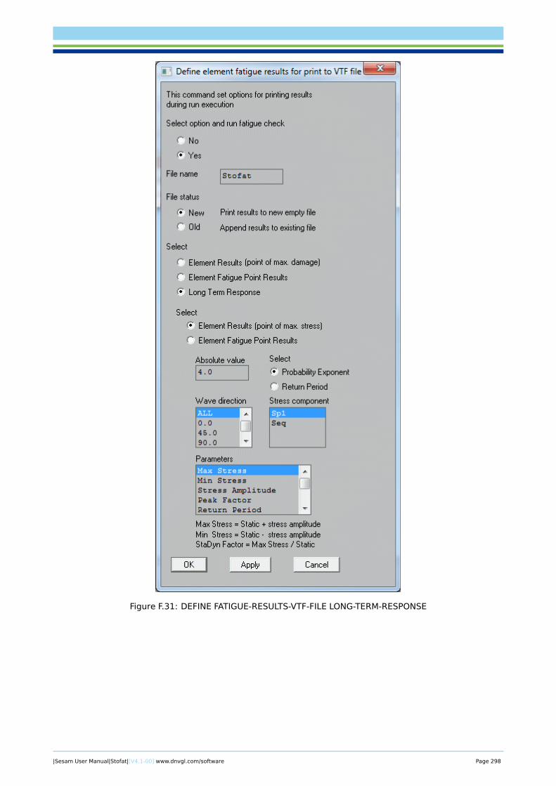
Figure F.31: DEFINE FATIGUE-RESULTS-VTF-FILE LONG-TERM-RESPONSE
|Sesam User Manual|Stofat|[V4.1-00] www.dnvgl.com/software Page 298
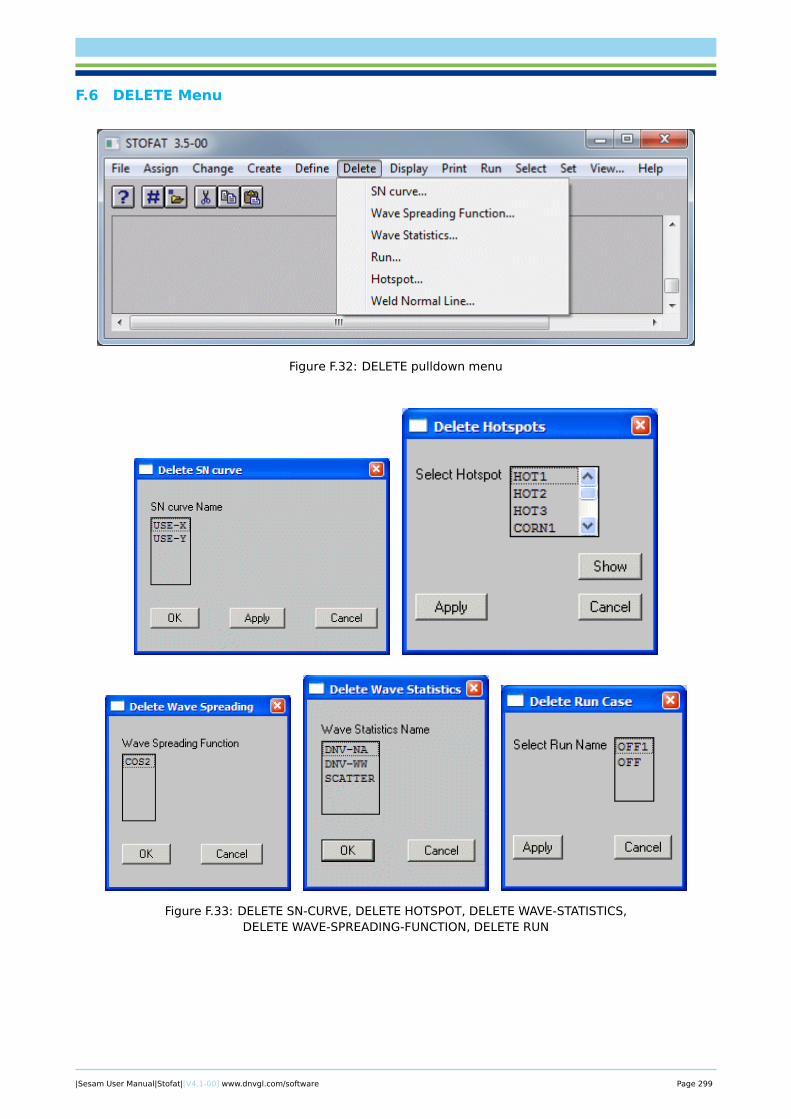
F.6 DELETE Menu
Figure F.32: DELETE pulldown menu
Figure F.33: DELETE SN-CURVE, DELETE HOTSPOT, DELETE WAVE-STATISTICS,DELETE WAVE-SPREADING-FUNCTION, DELETE RUN
|Sesam User Manual|Stofat|[V4.1-00] www.dnvgl.com/software Page 299
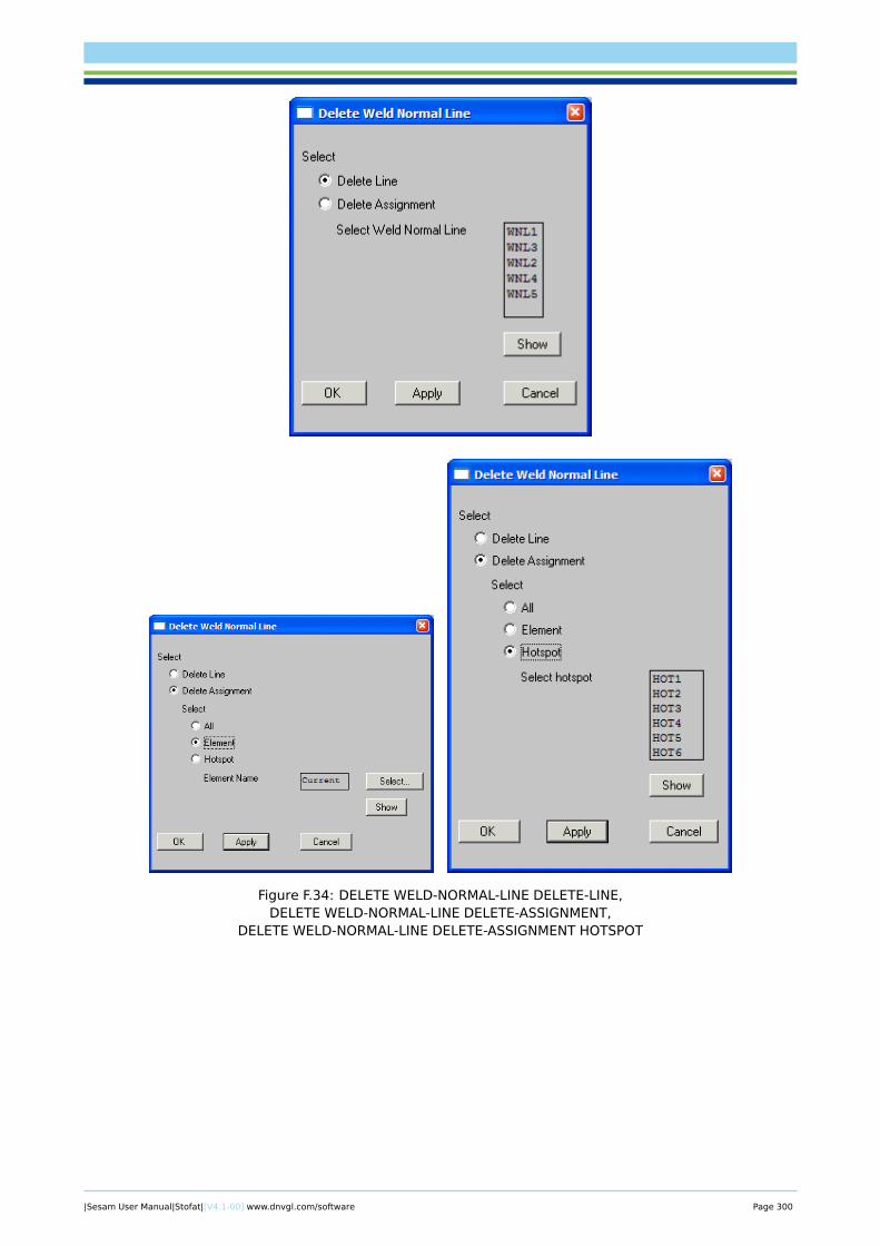
Figure F.34: DELETE WELD-NORMAL-LINE DELETE-LINE,DELETE WELD-NORMAL-LINE DELETE-ASSIGNMENT,
DELETE WELD-NORMAL-LINE DELETE-ASSIGNMENT HOTSPOT
|Sesam User Manual|Stofat|[V4.1-00] www.dnvgl.com/software Page 300
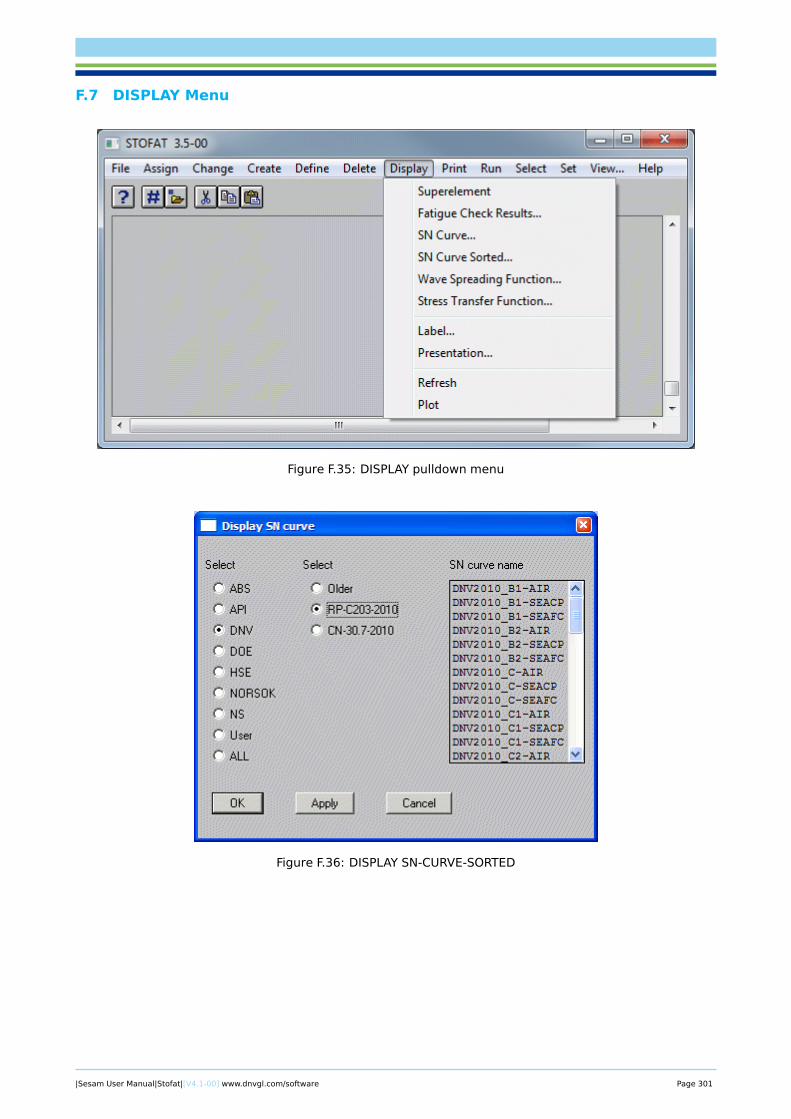
F.7 DISPLAY Menu
Figure F.35: DISPLAY pulldown menu
Figure F.36: DISPLAY SN-CURVE-SORTED
|Sesam User Manual|Stofat|[V4.1-00] www.dnvgl.com/software Page 301
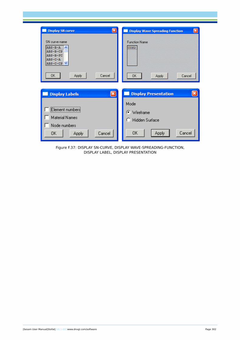
Figure F.37: DISPLAY SN-CURVE, DISPLAY WAVE-SPREADING-FUNCTION,DISPLAY LABEL, DISPLAY PRESENTATION
|Sesam User Manual|Stofat|[V4.1-00] www.dnvgl.com/software Page 302
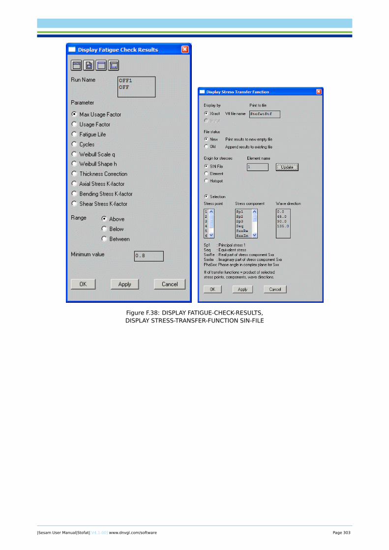
Figure F.38: DISPLAY FATIGUE-CHECK-RESULTS,DISPLAY STRESS-TRANSFER-FUNCTION SIN-FILE
|Sesam User Manual|Stofat|[V4.1-00] www.dnvgl.com/software Page 303
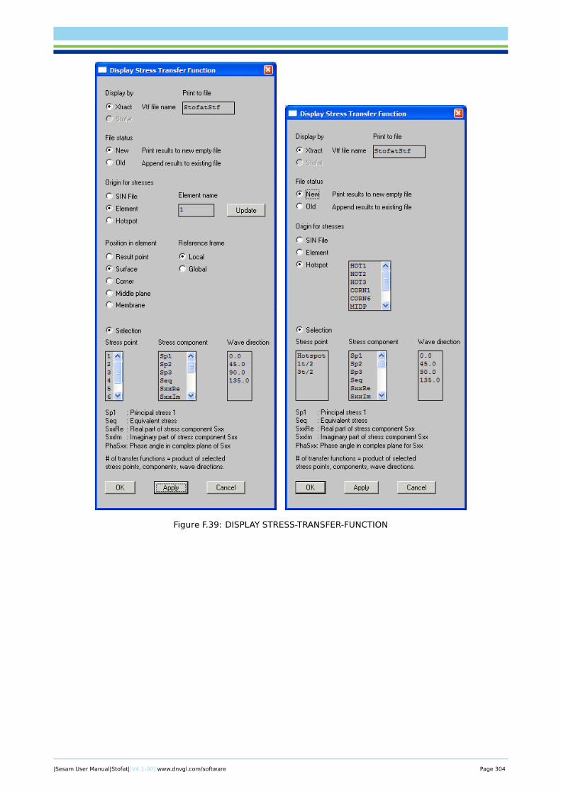
Figure F.39: DISPLAY STRESS-TRANSFER-FUNCTION
|Sesam User Manual|Stofat|[V4.1-00] www.dnvgl.com/software Page 304
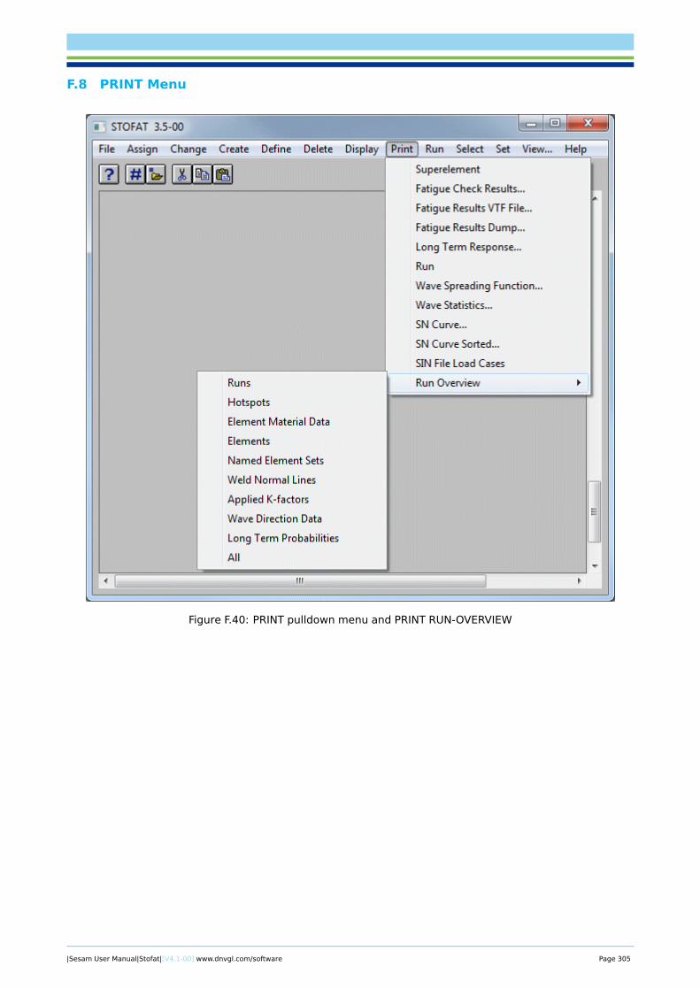
F.8 PRINT Menu
Figure F.40: PRINT pulldown menu and PRINT RUN-OVERVIEW
|Sesam User Manual|Stofat|[V4.1-00] www.dnvgl.com/software Page 305
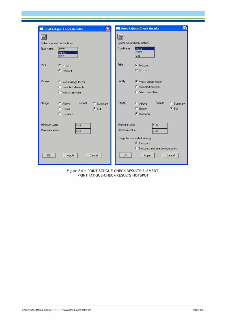
Figure F.41: PRINT FATIGUE-CHECK-RESULTS ELEMENT,PRINT FATIGUE-CHECK-RESULTS HOTSPOT
|Sesam User Manual|Stofat|[V4.1-00] www.dnvgl.com/software Page 306
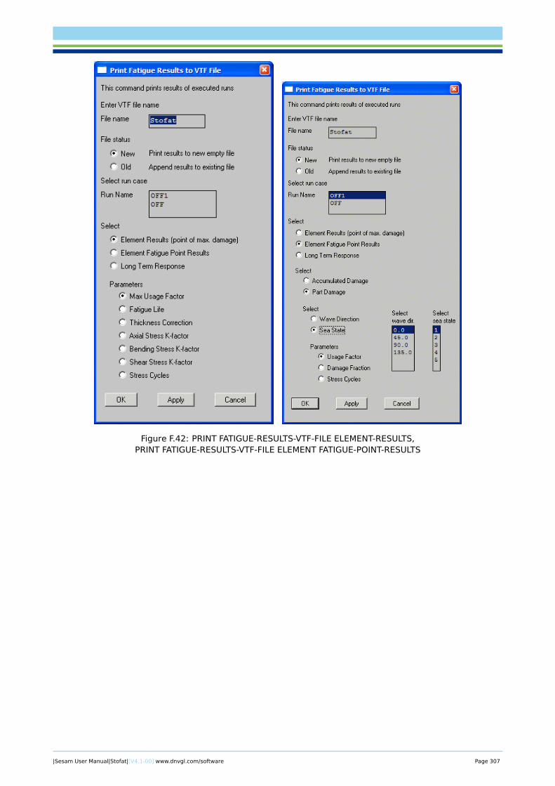
Figure F.42: PRINT FATIGUE-RESULTS-VTF-FILE ELEMENT-RESULTS,PRINT FATIGUE-RESULTS-VTF-FILE ELEMENT FATIGUE-POINT-RESULTS
|Sesam User Manual|Stofat|[V4.1-00] www.dnvgl.com/software Page 307
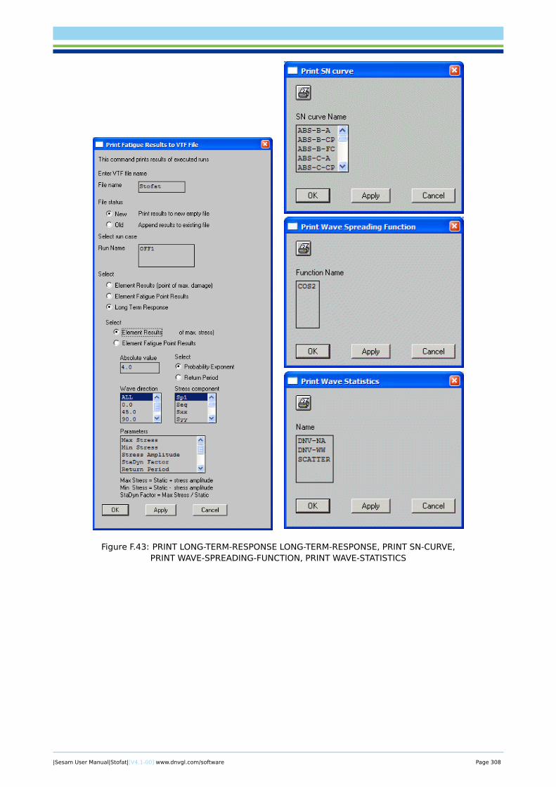
Figure F.43: PRINT LONG-TERM-RESPONSE LONG-TERM-RESPONSE, PRINT SN-CURVE,PRINT WAVE-SPREADING-FUNCTION, PRINT WAVE-STATISTICS
|Sesam User Manual|Stofat|[V4.1-00] www.dnvgl.com/software Page 308
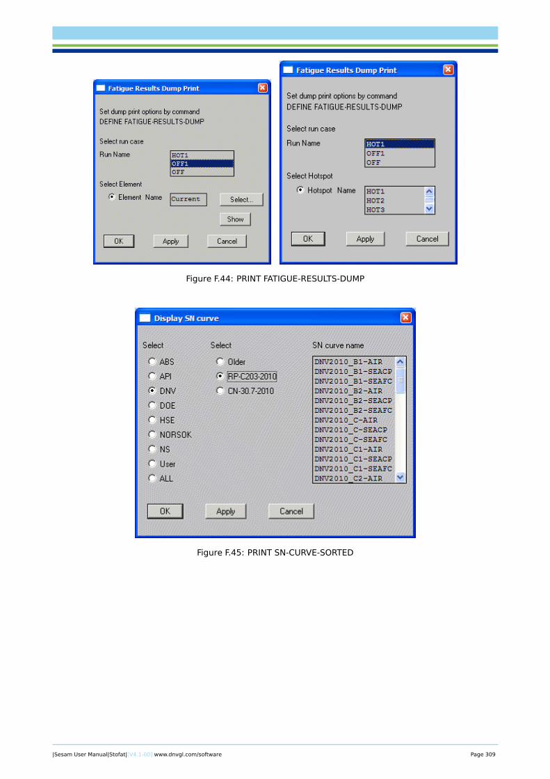
Figure F.44: PRINT FATIGUE-RESULTS-DUMP
Figure F.45: PRINT SN-CURVE-SORTED
|Sesam User Manual|Stofat|[V4.1-00] www.dnvgl.com/software Page 309
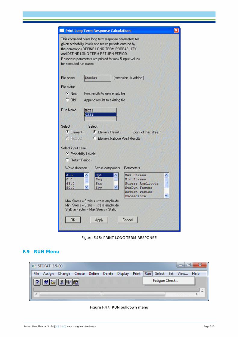
Figure F.46: PRINT LONG-TERM-RESPONSE
F.9 RUN Menu
Figure F.47: RUN pulldown menu
|Sesam User Manual|Stofat|[V4.1-00] www.dnvgl.com/software Page 310
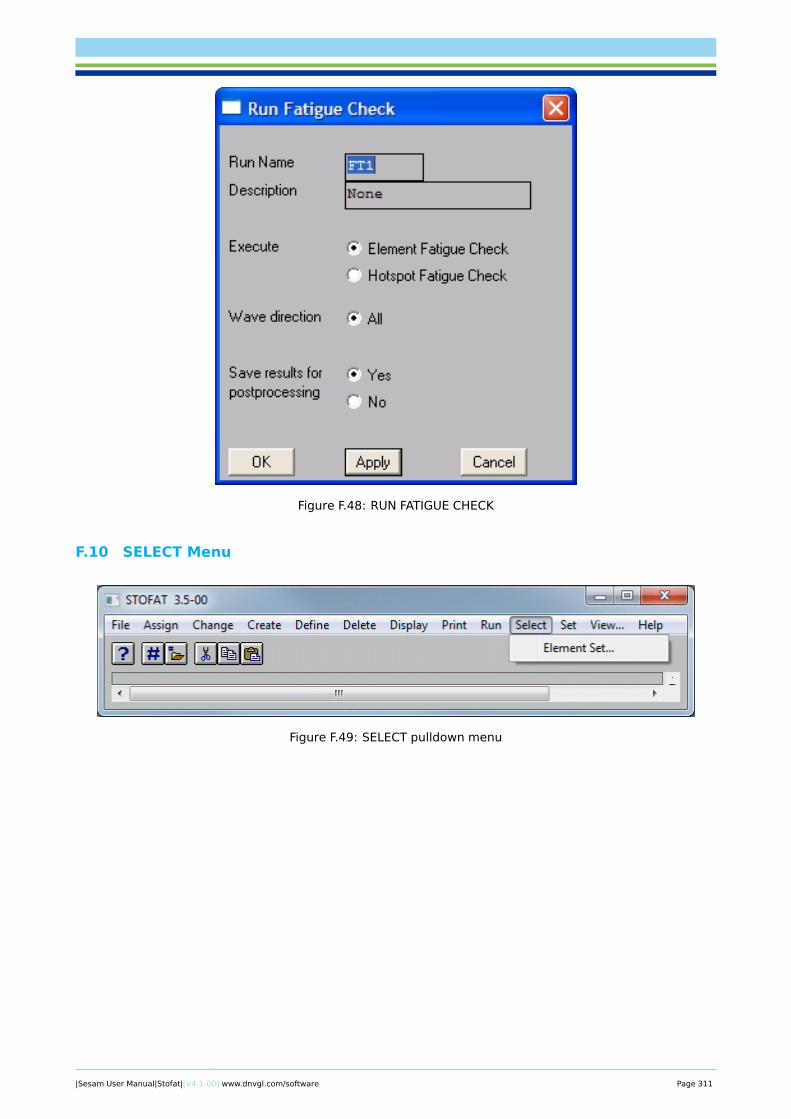
Figure F.48: RUN FATIGUE CHECK
F.10 SELECT Menu
Figure F.49: SELECT pulldown menu
|Sesam User Manual|Stofat|[V4.1-00] www.dnvgl.com/software Page 311
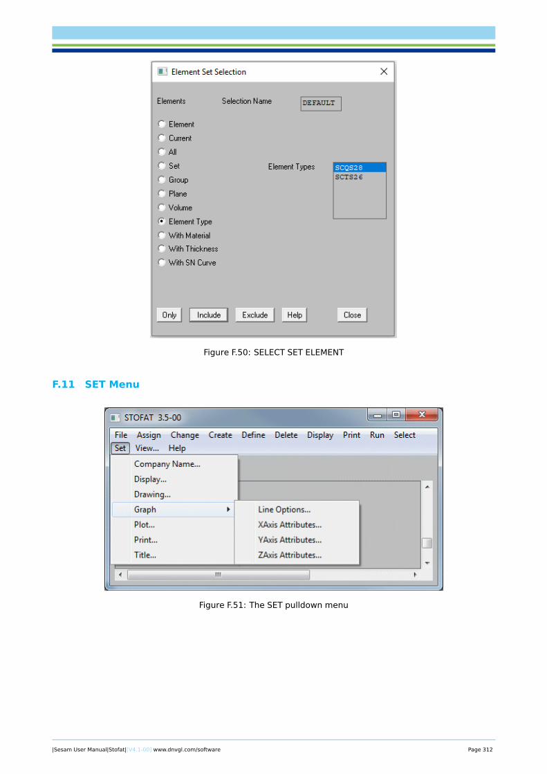
Figure F.50: SELECT SET ELEMENT
F.11 SET Menu
Figure F.51: The SET pulldown menu
|Sesam User Manual|Stofat|[V4.1-00] www.dnvgl.com/software Page 312
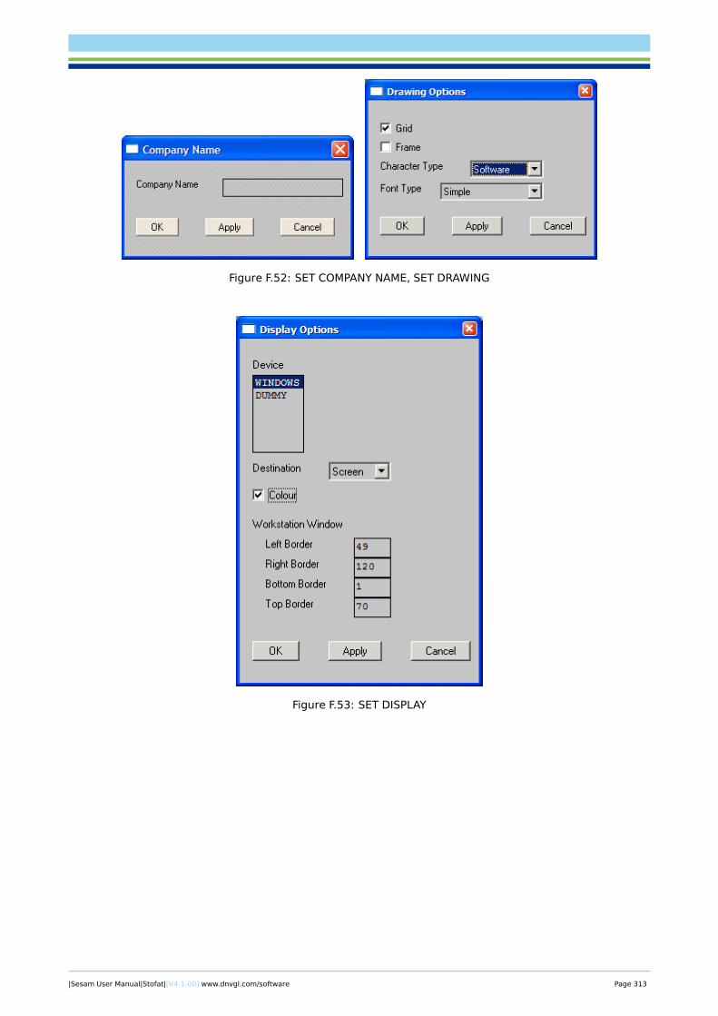
Figure F.52: SET COMPANY NAME, SET DRAWING
Figure F.53: SET DISPLAY
|Sesam User Manual|Stofat|[V4.1-00] www.dnvgl.com/software Page 313
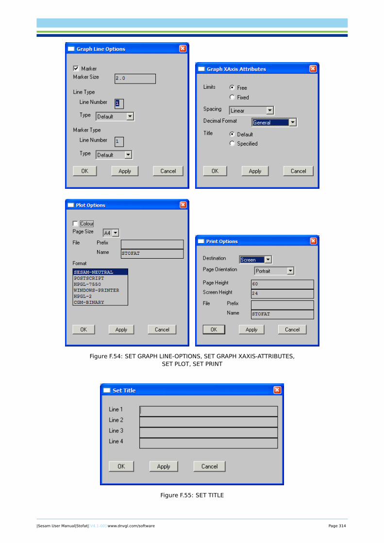
Figure F.54: SET GRAPH LINE-OPTIONS, SET GRAPH XAXIS-ATTRIBUTES,SET PLOT, SET PRINT
Figure F.55: SET TITLE
|Sesam User Manual|Stofat|[V4.1-00] www.dnvgl.com/software Page 314
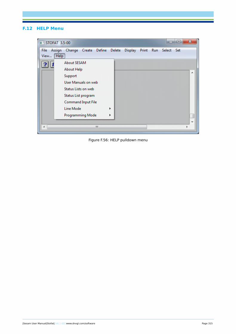
F.12 HELP Menu
Figure F.56: HELP pulldown menu
|Sesam User Manual|Stofat|[V4.1-00] www.dnvgl.com/software Page 315
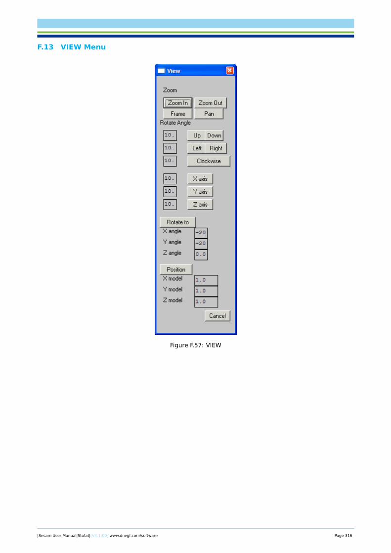
F.13 VIEW Menu
Figure F.57: VIEW
|Sesam User Manual|Stofat|[V4.1-00] www.dnvgl.com/software Page 316
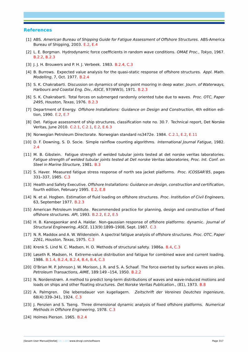
References
[1] ABS. American Bureau of Shipping Guide for Fatigue Assessment of Offshore Structures. ABS-AmericaBureau of Shipping, 2003. E.2, E.4
[2] L. E. Borgman. Hydrodynamic force coefficients in random wave conditions. OMAE Proc., Tokyo, 1967.B.2.2, B.2.3
[3] J. J. H. Brouwers and P. H. J. Verbeek. 1983. B.2.4, C.3
[4] B. Burrows. Expected value analysis for the quasi-static response of offshore structures. Appl. Math.Modelling, 7, Oct. 1977. B.2.4
[5] S. K. Chakrabarti. Discussion on dynamics of single point mooring in deep water. Journ. of Waterways,Harbours and Coastal Eng. Div., ASCE, 97(WW3), 1971. B.2.3
[6] S. K. Chakrabarti. Total forces on submerged randomly oriented tube due to waves. Proc. OTC, Paper2495, Houston, Texas, 1976. B.2.3
[7] Department of Energy. Offshore Installations: Guidance on Design and Construction, 4th edition edi-tion, 1990. E.2, E.7
[8] Det. Fatigue assessment of ship structures, classification note no. 30.7. Technical report, Det NorskeVeritas, June 2010. C.2.1, C.2.1, E.2, E.6.3
[9] Norwegian Petroleum Directorate. Norwegian standard ns3472e. 1984. C.2.1, E.2, E.11
[10] D. F. Downing, S. D. Socie. Simple rainflow counting algorithms. International Journal Fatigue, 1982.2.4
[11] M. B. Gibstein. Fatigue strength of welded tubular joints tested at det norske veritas laboratories.Fatigue strength of welded tubular joints tested at Det norske Veritas laboratories, Proc. Int. Conf. onSteel in Marine Structure, 1981. B.3
[12] S. Haver. Measured fatigue stress response of north sea jacket platforms. Proc. ICOSSAR’85, pages331–337, 1985. C.3
[13] Health and Safety Executive. Offshore Installations: Guidance on design, construction and certification,fourth edition, February 1995. E.2, E.8
[14] N. et al. Hogben. Estimation of fluid loading on offshore structures. Proc. Institution of Civil Engineers,63, September 1977. B.2.3
[15] American Petroleum Institute. Recommended practice for planning, design and construction of fixedoffshore structures. API, 1993. B.2.2, E.2, E.5
[16] H. B. Kanegaonkar and A. Haldar. Non-gaussian response of offshore platforms: dynamic. Journal ofStructural Engineering, ASCE, 113(9):1899–1908, Sept. 1987. C.3
[17] N. R. Maddox and A. W. Wildenstein. A spectral fatigue analysis of offshore structures. Proc. OTC, Paper2261, Houston, Texas, 1975. C.3
[18] Krenk S. Lind N. C. Madsen, H. O. Methods of structural safety. 1986a. B.4, C.3
[19] Løseth R. Madsen, H. Extreme-value distribution and fatigue for combined wave and current loading.1986. B.1.4, B.2.4, B.2.4, B.4, B.4, C.3
[20] O’Brian M. P. Johnson J. W. Morison, J. R. and S. A. Schaaf. The force exerted by surface waves on piles.Petroleum Transactions, AIME, 189:149 –154, 1950. B.2.2
[21] N. Nordenstrøm. A method to predict long-term distributions of waves and wave-induced motions andloads on ships and other floating structures. Det Norske Veritas Publication., (81), 1973. B.8
[22] A. Palmgren. Die lebensdauer von kugellagern. Zeitschrift der Vereines Deutches Ingenieure,68(4):339–341, 1924. C.3
[23] J. Penzien and S. Tseng. Three dimensional dynamic analysis of fixed offshore platforms. NumericalMethods in Offshore Engineering, 1978. C.3
[24] Holmes Pierson. 1965. B.2.4
|Sesam User Manual|Stofat|[V4.1-00] www.dnvgl.com/software Page 317
[25] W. J. Pierson and L. Moskowitz. A proposed spectral form for fully developed wind seas based onsimilarity theory of s. a. kitaigorodskii. Journ. of Geophysical Research, 69(24, December), 1964. B.1.4
[26] T. Sarpkaya and M. Isaacson. Mechanics of wave forces on offshore structures. 1981. B.2.2
[27] I. Scherf and T. Thuestad. Fatigue design of the oseberg jacket structure. Proc. OMAE, Houston, Texas.,1987. B.2.3
[28] R. Skjong and H. O. Madsen. Practical stochastic fatigue analysis of offshore platforms. Ocean Engi-neering, 14(4):313–324, 1987. C.3
[29] NORSOK Standard. Design of steel structures, n-004. Technical report, NORSOK, October 2004. E.2,E.10
[30] Det Norske Veritas. Fatigue assessment of ship structures, classification note no. 30.7. 2005. 3.4.8,3.4.9, 5.3, 5.6, 5.35, B.3.2, B.3.2, B.3.2, B.6, B.7, E.2, E.6.1
[31] Det Norske Veritas. Recommended practice dnv-rp-c203, fatigue design of offshore steel structures.Technical report, Det Norske Veritas, April 2012. C.2.2, E.2, E.6.2
[32] J. D. Wheeler. Methods for calculation forces produced by irregular waves. Journ. of Petroleum Technol-ogy, 1970. B.2.3
[33] P. Wirsching and M. Light. Fatigue under wide band random process. Journal of the Structural Division,106(ST7):1593–1607, July 1980. C.3
|Sesam User Manual|Stofat|[V4.1-00] www.dnvgl.com/software Page 318

ABOUT DNV GLDNV GL is a global quality assurance and risk management company. Driven by our purpose of safeguarding life,
property and the environment, we enable our customers to advance the safety and sustainability of their business.
Operating in more than 100 countries, our professionals are dedicated to helping customers in the maritime, oil & gas,
power and renewables and other industries to make the world safer, smarter and greener.
DIGITAL SOLUTIONSDNV GL is a world-leading provider of digital solutions for managing risk and improving safety and asset performance
for ships, pipelines, processing plants, offshore structures, electric grids, smart cities and more. Our open industry
platform Veracity, cyber security and software solutions support business-critical activities across many industries,
including maritime, energy and healthcare.
|Sesam User Manual|Stofat|[V4.1-00] www.dnvgl.com/software Page 319