development of a theoretical workflow for metabolic
TRANSCRIPT
Technische Universität MünchenFachgebiet für Systembiotechnologie
Development of a Theoretical Workflowfor Metabolic Engineering and its
Application to Terpenoid Production inEscherichia coli
Miguel Ángel Valderrama Gómez
Vollständiger Abdruck der von der Fakultät für Maschinenwesen der TechnischenUniversität München zur Erlangung des akademischen Grades eines
Doktor-Ingenieurs genehmigten Dissertation.
Vorsitzender: Prof. Dr.-Ing. Dirk Weuster-Botz
Prüfer der Dissertation: 1. Prof. Dr.-Ing. Andreas Kremling2. Prof. Dr. rer. nat. Christoph Kaleta
Die Dissertation wurde am 10.04.2018 bei der Technischen Universität München
eingereicht und durch die Fakultät für Maschinenwesen am 12.07.2018 angenommen.

Contents
Acknowledgments xi
Abstract xiii
1. Introduction 1
I. Theory 5
2. Metabolic Modeling & Strain Engineering 72.1. Constraint-based Methods . . . . . . . . . . . . . . . . . . . . . . . . . . . . 8
2.1.1. Dynamic Flux Balance Analysis . . . . . . . . . . . . . . . . . . . . . 102.1.2. Experimental Determination of Reaction Rates . . . . . . . . . . . . 12
2.2. Elementary modes-based Methods . . . . . . . . . . . . . . . . . . . . . . . 162.3. Kinetic-based Methods . . . . . . . . . . . . . . . . . . . . . . . . . . . . . . 18
2.3.1. Ensemble Modeling Approach of Metabolic Networks . . . . . . . . . 182.4. Strain Design Algorithms . . . . . . . . . . . . . . . . . . . . . . . . . . . . 242.5. Computational Tools . . . . . . . . . . . . . . . . . . . . . . . . . . . . . . . 28
3. Theoretical Workflow for Metabolic Engineering 313.1. Model-guided Strain Engineering . . . . . . . . . . . . . . . . . . . . . . . . 313.2. Model-guided Process Optimization . . . . . . . . . . . . . . . . . . . . . . . 32
II. Results: Strain Engineering 35
4. Metabolic Burden 394.1. Strains & Experimental Data . . . . . . . . . . . . . . . . . . . . . . . . . . 394.2. Substrate Quality . . . . . . . . . . . . . . . . . . . . . . . . . . . . . . . . . 41
4.2.1. Conversion Factors for Substrate Uptake Standardization . . . . . . 424.2.2. Data Standardization . . . . . . . . . . . . . . . . . . . . . . . . . . 47
4.3. Yield, Acetate and Formate Lines . . . . . . . . . . . . . . . . . . . . . . . . 484.4. Process-level Strategy to Reduce Detrimental Effects of Metabolic Burden . 524.5. Discussion . . . . . . . . . . . . . . . . . . . . . . . . . . . . . . . . . . . . . 54
5. Strain Design Algorithms for Target Identification 575.1. Strains & Experimental Data . . . . . . . . . . . . . . . . . . . . . . . . . . 575.2. Reduction of Metabolic Burden Through Genomic Integration . . . . . . . . 585.3. Constraint-based Assessment of Taxadiene Production Potential . . . . . . . 615.4. Application of Strain-design Algorithms for Target Identification . . . . . . 61
5.4.1. Constraint-based Methods: The OptKnock Algorithm . . . . . . . . 62
i
Contents
5.4.2. Kinetic-based Methods: The OptEM Algorithm . . . . . . . . . . . . 655.5. Discussion . . . . . . . . . . . . . . . . . . . . . . . . . . . . . . . . . . . . . 74
6. Simultaneous Utilization of D-Xylose & Glucose in E. coli 776.1. Strains & Experimental Data . . . . . . . . . . . . . . . . . . . . . . . . . . 776.2. Constraint-based Characterization of Simultaneous Sugar Utilization . . . . 79
6.2.1. Biomass Yield & Growth Rate . . . . . . . . . . . . . . . . . . . . . 806.2.2. Acetate Lines & Metabolic Burden . . . . . . . . . . . . . . . . . . . 82
6.3. Assessing Taxadiene Production Potential . . . . . . . . . . . . . . . . . . . 856.4. Model-based Identification of Optimal Production Strain Candidates . . . . 906.5. Discussion . . . . . . . . . . . . . . . . . . . . . . . . . . . . . . . . . . . . . 90
III. Results: Process Optimization 95
7. Model-based Medium Optimization 997.1. Performance Criteria for Substrate Selection . . . . . . . . . . . . . . . . . . 99
7.1.1. Single Substrates . . . . . . . . . . . . . . . . . . . . . . . . . . . . . 1007.2. Synergy as Design Principle for Pathway Selection . . . . . . . . . . . . . . 102
7.2.1. Three-Substrate Mixtures . . . . . . . . . . . . . . . . . . . . . . . . 1037.3. Discussion . . . . . . . . . . . . . . . . . . . . . . . . . . . . . . . . . . . . . 107
8. Model-based Semi-Batch Optimization 1098.1. Strain & Experimental Data . . . . . . . . . . . . . . . . . . . . . . . . . . . 1098.2. Mathematical Identification of Characteristic Process Phases and Rates Cal-
culation . . . . . . . . . . . . . . . . . . . . . . . . . . . . . . . . . . . . . . 1118.3. Dependence of Model Parameters on Production Temperature . . . . . . . . 1138.4. In silico Optimization of Production Temperature and Time Point of Induction1168.5. Discussion . . . . . . . . . . . . . . . . . . . . . . . . . . . . . . . . . . . . . 118
9. Product Yield Prediction 1219.1. Strain & Experimental Data . . . . . . . . . . . . . . . . . . . . . . . . . . . 1219.2. Constraint-based Product Yield Prediction . . . . . . . . . . . . . . . . . . . 1229.3. Kinetic-based Product Yield Prediction . . . . . . . . . . . . . . . . . . . . 1239.4. Application of KAY to Predict Optimal Biomass Yield During Production . 1249.5. Discussion . . . . . . . . . . . . . . . . . . . . . . . . . . . . . . . . . . . . . 126
10.Concluding Remarks and Outlook 12910.1. Lessons From Succinate Production in Engineered Strains . . . . . . . . . . 12910.2. Lessons From Taxadiene Production in Escherichia coli (E. coli) . . . . . . 130
Acronyms 143
A. Appendix for Strain Engineering 145A.1. Metabolic Burden . . . . . . . . . . . . . . . . . . . . . . . . . . . . . . . . . 145
A.1.1. Slope of Acetate Line . . . . . . . . . . . . . . . . . . . . . . . . . . 145A.1.2. Amino Acid Sequences . . . . . . . . . . . . . . . . . . . . . . . . . . 146A.1.3. Concentration Time Courses . . . . . . . . . . . . . . . . . . . . . . 147A.1.4. Flux Distribution Patters for Three Zones . . . . . . . . . . . . . . . 147
ii
Contents
A.2. Strain Design Algorithms for Target Identification . . . . . . . . . . . . . . 152A.2.1. Mevalonate, Non-Mevalonate & Taxadiene Formation Pathways . . . 152A.2.2. Concentration Time Courses for Taxadiene Producing Strains . . . . 152A.2.3. 13C Labeling Data . . . . . . . . . . . . . . . . . . . . . . . . . . . . 152A.2.4. Metabolic Model Used for the Software 13CFlux2 . . . . . . . . . . . 156A.2.5. Constraint-based Assessment of Taxadiene Production Potential . . 166
A.3. Simultaneous Utilization of D-Xylose and Glucose in E. coli . . . . . . . . . 166A.3.1. Concentration Time Courses for All Strains . . . . . . . . . . . . . . 166A.3.2. 13C Labeling Data . . . . . . . . . . . . . . . . . . . . . . . . . . . . 166A.3.3. Dependency of Oxygen Uptake Rate on Sugar Co-Utilization . . . . 169A.3.4. Experimental Protein Content . . . . . . . . . . . . . . . . . . . . . . 169
B. Appendix for Process Engineering 171B.1. Model-based Medium Optimization . . . . . . . . . . . . . . . . . . . . . . . 171
B.1.1. Extending Metabolic Models to Allow Taxadiene Synthesis . . . . . 171B.1.2. Ranking of 180 Substrates According to Yields . . . . . . . . . . . . 173B.1.3. Ranking of 180 Substrates According to Profit . . . . . . . . . . . . . 175
B.2. Model-based Fed-batch Optimization . . . . . . . . . . . . . . . . . . . . . . 178B.2.1. Concentration Time Courses for Process Development . . . . . . . . 178B.2.2. Temperature Dependencies of Phases Duration and Exchange Rates 178B.2.3. Modeling Concentration Time Courses for All Fermentations . . . . 178
iii

List of Tables
2.1. Genome-Scale Metabolic Reconstructions for E. coli . . . . . . . . . . . . . 92.2. Overview of Variables Used to Describe Reactor Dynamics . . . . . . . . . . 112.3. Substrate-level Enzyme Regulation Considered for the E. coli Core Model . 222.4. Theoretical Approaches Used in the in silico Strain Optimization for the
Succinate Overproduction . . . . . . . . . . . . . . . . . . . . . . . . . . . . 242.5. Commonly Used Computational Tools for the Analysis of Metabolic Networks 29
4.1. Experimentally Calculated Exchange Rates for Three Strains. Growth onGlucose. . . . . . . . . . . . . . . . . . . . . . . . . . . . . . . . . . . . . . . 40
4.2. Conversion Factors for Three Quality Criteria . . . . . . . . . . . . . . . . . 434.3. Substrate Uptake Rates Used to Assess Quality Criteria . . . . . . . . . . . 45
5.1. Taxadiene Producing Strains . . . . . . . . . . . . . . . . . . . . . . . . . . 585.2. Taxadiene Producing Strains: Exchange Rates . . . . . . . . . . . . . . . . . 595.3. Objective Functions for OptEM . . . . . . . . . . . . . . . . . . . . . . . . . 685.4. Enzyme Perturbations Identified by OptEM Leading to an Increased Tax-
adiene Yield in Strain ∆XylE_1p . . . . . . . . . . . . . . . . . . . . . . . . 705.5. Strain Design Strategy Identified by OptEM for the Maximization of Tax-
adiene Yield in Strain ∆XylE_1p Using a Solver Approach . . . . . . . . . 72
6.1. Strains Used in Sugar Co-utilization Studies . . . . . . . . . . . . . . . . . . 786.2. Experimental Characterization of Strains Used in Sugar Co-utilization Studies 786.3. Strain Performance Parameters . . . . . . . . . . . . . . . . . . . . . . . . . 79
7.1. Metabolic Models Used for Synergy Studies . . . . . . . . . . . . . . . . . . 102
8.1. Experimental Process Parameters for Six Semi-Batch Fermentations . . . . 1108.2. Growth, Production and Substrate Uptake Rates for Different Process Phases
and Production Temperatures . . . . . . . . . . . . . . . . . . . . . . . . . . 112
9.1. Biomass and Product Yields for Six Semi-Batch Fermentations . . . . . . . 1229.2. Average Biomass and Product Yields for Four Different Production Tem-
peratures . . . . . . . . . . . . . . . . . . . . . . . . . . . . . . . . . . . . . 122
A.1. Concentration Time Courses for Galactose as Carbon Source . . . . . . . . 147A.2. Concentration Time Courses for Glucose as Carbon Source . . . . . . . . . . 147A.3. Concentration Time Courses for Mannose as Carbon Source . . . . . . . . . 147A.4. Concentration Time Courses for Fructose as Carbon Source . . . . . . . . . 148A.5. Time Courses for Acetate as Carbon Source . . . . . . . . . . . . . . . . . . 148A.6. Exchange Rates for Three Strains and Five Sugars . . . . . . . . . . . . . . 148A.7. Concentration Time Courses for Taxadiene Producing Strains . . . . . . . . 154A.8. 13C-labeling Data for Five Taxadiene Producing Strains . . . . . . . . . . . 155
v
List of Tables
A.9. Confidence Intervals for Taxadiene Production Flux Calculated Considering13C Labeling Data and Exchange Rates . . . . . . . . . . . . . . . . . . . . 166
A.10.Concentration Time Courses For Six Strains . . . . . . . . . . . . . . . . . . 167A.11.Concentration Time Courses For Parent Strains: Re-measurement . . . . . . 167A.12.13C-labeling Data for Strains Used in Sugar Co-Utilization Studies . . . . . 168
B.1. Maximal Taxadiene Yields Calculated for 180 Carbon Sources . . . . . . . . 173B.2. Maximal Profit Calculated for 180 Carbon Sources . . . . . . . . . . . . . . 175B.3. Concentration Time Courses for Batch ID 1 . . . . . . . . . . . . . . . . . . 178B.4. Concentration Time Courses for Batch ID 2 . . . . . . . . . . . . . . . . . . 179B.5. Concentration Time Courses for Batch ID 3 . . . . . . . . . . . . . . . . . . 179B.6. Concentration Time Courses for Batch ID 4 . . . . . . . . . . . . . . . . . . 180B.7. Concentration Time Courses for Batch ID 5 . . . . . . . . . . . . . . . . . . 180B.8. Concentration Time Courses for Batch ID 6 . . . . . . . . . . . . . . . . . . 181B.9. Formulas Used to Describe the Effect of Production Temperature on Phase
Duration . . . . . . . . . . . . . . . . . . . . . . . . . . . . . . . . . . . . . . 181B.10.Formulas Used to Describe the Effect of Production Temperature on Ex-
change Rates . . . . . . . . . . . . . . . . . . . . . . . . . . . . . . . . . . . 182B.11.Determination Coefficients for All Batches . . . . . . . . . . . . . . . . . . . 183
vi
List of Figures
1.1. Motivation & Project’s Aim . . . . . . . . . . . . . . . . . . . . . . . . . . . 21.2. Modeling Workflow . . . . . . . . . . . . . . . . . . . . . . . . . . . . . . . . 3
2.1. Dynamic Flux Balance Analysis . . . . . . . . . . . . . . . . . . . . . . . . . 102.2. Experimental Determination of Cellular Growth Rates . . . . . . . . . . . . 132.3. Experimental Determination of Glucose Uptake Rate . . . . . . . . . . . . . 142.4. Statistical Workflow . . . . . . . . . . . . . . . . . . . . . . . . . . . . . . . 172.5. Ensemble Forecasting for Hurricane Path Prediction . . . . . . . . . . . . . 192.6. Parallelization Strategy in Linux Cluster . . . . . . . . . . . . . . . . . . . . 23
3.1. The Workflow . . . . . . . . . . . . . . . . . . . . . . . . . . . . . . . . . . . 33
4.1. Strains Used for the Characterization of the Metabolic Burden. . . . . . . . 404.2. Growth Rate vs. Substrate Uptake Rate for Three Strains and Five Substrates. 414.3. Real-Life Analogy for Concept of Substrate Quality . . . . . . . . . . . . . . 424.4. Energy Content As a Function of Oxygen Availability for Five Substrates . 434.5. Assessment of Three Different Quality Criteria for Data Standardization.
High Oxygen Availability . . . . . . . . . . . . . . . . . . . . . . . . . . . . . 454.6. Assessment of Three Different Quality Criteria for Data Standardization at
Low Oxygen Availability . . . . . . . . . . . . . . . . . . . . . . . . . . . . . 464.7. Standardized versus Raw Experimental Data . . . . . . . . . . . . . . . . . 474.8. Load-induced Oxygen Limitation . . . . . . . . . . . . . . . . . . . . . . . . 494.9. Relationship between Biomass Yield, Acetate and Formate Lines . . . . . . 504.10. Qualitative Comparison Between Experimental Data and in silico Calculations 514.11. Process-level Strategy to Reduce Metabolic Burden . . . . . . . . . . . . . . 534.12. Emergence of Yield and Acetate Lines By Constraining Flux Through Res-
piratory Chain . . . . . . . . . . . . . . . . . . . . . . . . . . . . . . . . . . 55
5.1. Taxadiene Producing Strains . . . . . . . . . . . . . . . . . . . . . . . . . . 595.2. Acetate Lines for Taxadiene Producing Strains . . . . . . . . . . . . . . . . 605.3. Constraint-based Assessment of Production Potential . . . . . . . . . . . . . 625.4. Application of OptKnock to the Production of Taxadiene in E. coli : Basic
Idea . . . . . . . . . . . . . . . . . . . . . . . . . . . . . . . . . . . . . . . . 635.5. Application of OptKnock to the Production of Taxadiene in E. coli : De-
pendence on Growth Rate and Oxygen Availability. . . . . . . . . . . . . . . 645.6. Application of OptKnock to the Production of Taxadiene in E. coli : Targets. 655.7. Overview of the Main Steps Comprising the OptEM Strain Design Algorithm 665.8. Effect of Single Enzyme Up- and Down-regulation Predicted by OptEM for
the Maximization of Taxadiene Yield in Strain ∆XylE_1p via a Brute ForceApproach. . . . . . . . . . . . . . . . . . . . . . . . . . . . . . . . . . . . . . 69
vii
List of Figures
5.9. Strain Design Strategy Identified by OptEM for the Maximization of Tax-adiene Yield in Strain ∆XylE_1p Using a Solver Approach. . . . . . . . . . 73
6.1. Strain Performance Parameters as a Function of Simultaneous Sugar Co-utilization Extent . . . . . . . . . . . . . . . . . . . . . . . . . . . . . . . . . 80
6.2. In silico Calculated Effect of Sugar Co-Utilization on Growth Rate andBiomass Yield: Case Study I . . . . . . . . . . . . . . . . . . . . . . . . . . 81
6.3. In silico Calculated Effect of Sugar Co-Utilization on Growth Rate andBiomass Yield: Case Study II . . . . . . . . . . . . . . . . . . . . . . . . . . 82
6.4. Expected Shift in Acetate Lines as a Result of Plasmid-based XylE-Expression 836.5. Effect of Glucose and Xylose Co-utilization on Growth Rate and Its Asso-
ciated Metabolic Burden . . . . . . . . . . . . . . . . . . . . . . . . . . . . . 846.6. Effect of Glucose and Xylose Co-utilization on Growth Rate and Its Asso-
ciated Metabolic Burden. Re-measurement of Selected Strains . . . . . . . . 846.7. Assessing Taxadiene Production Potential by a Constraint-based Approach 866.8. Assessing Taxadiene Production Potential by a Kinetic-based Approach . . 876.9. Dependence of Taxadiene Production Potential on % Carbon Xylose . . . . 886.10. Dependence of Taxadiene Production Potential on Growth Characteristics . 896.11. Model-based Identification of Optimal Production Strain Candidates . . . . 916.12. Substrate Quality: Glucose vs Xylose for Different Oxygen to Substrate Ratios 92
7.1. Substrate Ranking via Four Different Performance Criteria . . . . . . . . . . 1017.2. Synergy as Design Principle for Pathway Selection. Glucose As a Case Study.1047.3. Synergy as Design Principle for Pathway Selection. 180 Substrates . . . . . 1057.4. Maximal Product Yield for Three-Substrate Mixtures . . . . . . . . . . . . . 106
8.1. Process Set-up and Experimental Data . . . . . . . . . . . . . . . . . . . . . 1108.2. Modeling Experimental Data: Characteristic Process Times . . . . . . . . . 1108.3. Modeling Experimental Data: Mathematical Identification of Process Phases 1128.4. Modeling Experimental Data: Results . . . . . . . . . . . . . . . . . . . . . 1128.5. Dependence of Characteristic Process Times on Temperature and Time
Point of Induction . . . . . . . . . . . . . . . . . . . . . . . . . . . . . . . . 1148.6. Modeling Experimental Data: Temperature Dependence of Duration of Pro-
cess Phases . . . . . . . . . . . . . . . . . . . . . . . . . . . . . . . . . . . . 1148.7. Modeling Experimental Data: Temperature Dependence of Exchange Rates 1158.8. Volumetric Productivity for Batches 2 and 5 . . . . . . . . . . . . . . . . . . 1168.9. Model-based Optimization of Process Parameters . . . . . . . . . . . . . . . 117
9.1. Constraint-based Product Yield Prediction . . . . . . . . . . . . . . . . . . . 1239.2. Kinetically Accessible Yield (KAY) for Experimental Product Yield Prediction1259.3. Dependence of Maximal Product Yield on Biomass Yield . . . . . . . . . . . 1269.4. Increasing the Utility of the KAY Concept . . . . . . . . . . . . . . . . . . . 127
10.1. Application of the Workflow to the Production of Taxadiene in E. coli : Con-clusion . . . . . . . . . . . . . . . . . . . . . . . . . . . . . . . . . . . . . . . 133
A.1. Determination of the Acetate Line Slope for E. coli HMS . . . . . . . . . . 145A.2. Flux Variability Analysis for Phase I . . . . . . . . . . . . . . . . . . . . . . 149A.3. Flux Variability Analysis for Phase II . . . . . . . . . . . . . . . . . . . . . . 150
viii
List of Figures
A.4. Flux Variability Analysis for Phase III . . . . . . . . . . . . . . . . . . . . . 151A.5. Non-Mevalonate Pathway (MEP) . . . . . . . . . . . . . . . . . . . . . . . . 152A.6. Mevalonate Pathway (MVA) . . . . . . . . . . . . . . . . . . . . . . . . . . . 153A.7. Taxadiene Production Pathway . . . . . . . . . . . . . . . . . . . . . . . . . 153A.8. Estimation of Oxygen Uptake Rate as a Function of Sugar Co-Uptake . . . 169A.9. Protein Measurement. . . . . . . . . . . . . . . . . . . . . . . . . . . . . . . 170
B.1. Modeling Time Course Concentrations: Batch 2 . . . . . . . . . . . . . . . . 182B.2. Modeling Time Course Concentrations: Batch 3 . . . . . . . . . . . . . . . . 182B.3. Modeling Time Course Concentrations: Batch 4 . . . . . . . . . . . . . . . . 183B.4. Modeling Time Course Concentrations: Batch 5 . . . . . . . . . . . . . . . . 183B.5. Modeling Time Course Concentrations: Batch 6 . . . . . . . . . . . . . . . . 183
ix

千里之行,始於足下A journey of a thousand miles begins
with a single stepLaozi
Acknowledgments
I love sayings. That is why I invented this one: “man promoviert nicht an einem einzigenTag”, which would be translated into English as: “you don’t do a PhD in just one singleday”. Thinking about all the people who supported me in some way in these three and ahalf years, I realized I need to extend my saying: “you don’t do a PhD in just one singleday, and you cannot do it alone, so get some help!”. I do not pretend this saying to beuniversal, but it describes my situation and the way I see the process of getting a PhDpretty well.
First, I would like to start by thanking my Doktorvater, Prof. Dr.-Ing. Andreas Kremlingfor providing me the life-changing opportunity of doing a PhD at his group, at the TechnicalUniversity of Munich (TUM). Thank you for being so patient with me, especially in thefirst months of my PhD, when I spoke such a broken German. Thank you for letting mediscover so many parts of the world, and for allowing me to do the three months researchvisit at the University of California, Los Angeles, which vastly enriched me personally andprofessionally. During the time of my PhD, I even learned how to ski by attending ourlegendary winter seminar in the German Alps once in a year - which is pretty cool, giventhe fact that in Colombia we do not really have snow-. I feel so grateful for all that, thankyou Prof. Kremling!
Next, I would like to thank Michael Frank Panfil for his constant support and guidance.Many of my crazy projects would have not been even thinkable without your unconditionalhelp. From the very first idea of doing my master studies in Germany, to actually finishingmy PhD, you have positively shaped much of what I am today. You made Munich my newhome town. You were always there for me when I needed you. For that, I will be in debtwith you my whole life. Thank you so much Frank!
My special thanks to Boyu Yang -BB- for patiently reading all pages of this dissertationand for providing grammatical advice, for constantly correcting my English. Thank youfor sharing your love for Los Angeles with me, and for showing me what a wonderfulplace California is. Thanks Alberto for the many exciting and interesting discussions, forproviding me access to the LRZ computing cluster, which made the calculations for theensemble modeling approach so interesting. Thank you for introducing me to MichaelSavageau and for suggesting him that hiring me for a postdoctoral position would be agood idea. Thank you Kati for clarifying my questions related to biological background andfor your valuable feedback when it came to orally presenting research results. I also wantto thank my colleagues Sayuri Hortsch, Hannes Löwe, Sabine Wagner, Diana Kreitmayer,Viktoria Kindzersky and Christiana Sehr for making the daily routine at work so enjoyable.My special thanks to Sayuri Hortsch for the constant mathematical support you providedme, for being there to hear my worries and for sharing your point of view about so manythings. Thanks to my cooperation partners Lars Janoschek, Max Hirte, Sabine Wagner andKatarina Kemper for the exciting discussions and for sharing your experimental data with
xi
Acknolwedgments
me. Thanks to my master students Laura López, Thomas Mainka, Niklas Farke and DarianO’connor and my HiWi students Philipp Schneider and Makis Kolaitis for your great workand valuable input. Thanks to Professor James Liao for allowing me to perform a researchvisit at your laboratory. Thanks to his lab members Po-Wei Cheng and Mathew Theisenfor providing me with Matlab code pre-publication and for answering all of my questionsrelated to the ensemble modeling approach. Thanks to Susanne Kuchenbaur for guidingme through the bureaucracy at TUM.
Finalmente quisiera dedicarle este logro a mis padres Nora y Jinmer; a mis hermanosAdriana y Cesar; a mi tía Norma y a mi primos Luana y Julian. Nada de esto hubiera sidoposible sin su apoyo y compania constante e incondicional. Es dificil expresar en palabrasmi gratitud. Me siento infinitamente afortunado de tenerlos a mi lado y espero que lavida nos permita compartir muchos anhos mas de vida para seguir compartiendo nuestroslogros y felicidades.
This work was financed by the German Federal Ministry of Education and Research. Mosttravel expenses were financed by the Joachim Herz Foundation. Research visit at UCLAwas partly financed by the TUM Graduate School.
xii
Abstract
Metabolic Engineering is an emerging science aiming at the development of cellular factor-ies for the overproduction of valuable chemicals. Target molecules can be either naturallyproduced by endogenous metabolic pathways, or the host metabolism should be comple-mented by a non-inherent metabolic pathway to enable their heterologous production. Overthe past decades, mathematical modeling of cellular metabolism for strain and process op-timization has given rise to a more rational, model-based Metabolic Engineering science.However, theoretical workflows providing advice on limitations and proper application ofthe vast number of available mathematical tools are still scarce. Initially, we review theapplication of mathematical methods to increase the production of succinate in engineeredstrains. Succinate is an important building block whose biotechnological production hasgained much attention in the last decade. From this initial work, we conclude that directexperimental implementation of model predictions (in silico knowledge) is not a straight-forward process yet. One of the many reasons is the intrinsic complexity of living systems,which cannot be fully captured by the simplicity of widely used stoichiometric models ofmetabolism. Additionally, incongruences in the modeling process and the reporting ofexperimental results hamper a proper assessment of the prediction power of current mod-eling approaches. Motivated by these observations, we developed a theoretical workflowfor metabolic engineering, highlighting capabilities and limitations of each method. Theworkflow considers the application of not only constraint-based methods like Flux BalanceAnalysis (FBA), which have been traditionally used to understand optimality principlesshaping bacterial metabolism, but also of kinetic-based methods whose spread has beenhindered so far by limitations related to model parametrization and to high demand oncomputational power required to analyze genome-scale kinetic models. While developingthe workflow, we paid special attention to consider the so-called metabolic burden, a phe-nomenon presented in "loaded" cells and characterized by the reduction of both biomassyield and critical growth rate for acetate secretion. The suggested protocol was mainlyapplied to generate in silico knowledge, aimed to guide future experimental efforts towardsoptimization of taxadiene production in Escherichia coli (E. coli) at the strain and processlevel. Taxadiene is a precursor molecule for the anticancer drug taxol and its biotech-nological production has gained much attention due to the low yields of the traditionalextraction process from the bark of the pacific yew tree. During the development of a flex-ible taxadiene producing strain, simultaneous utilization of glucose and xylose by E. coliwas also analyzed. By applying various tools described in the protocol, metabolic loadand effects arising from simultaneous sugar uptake were assessed, especially focusing onthe production potential of each strain. This analysis should allow the selection of straincandidates for further optimization.
xiii

1. Introduction
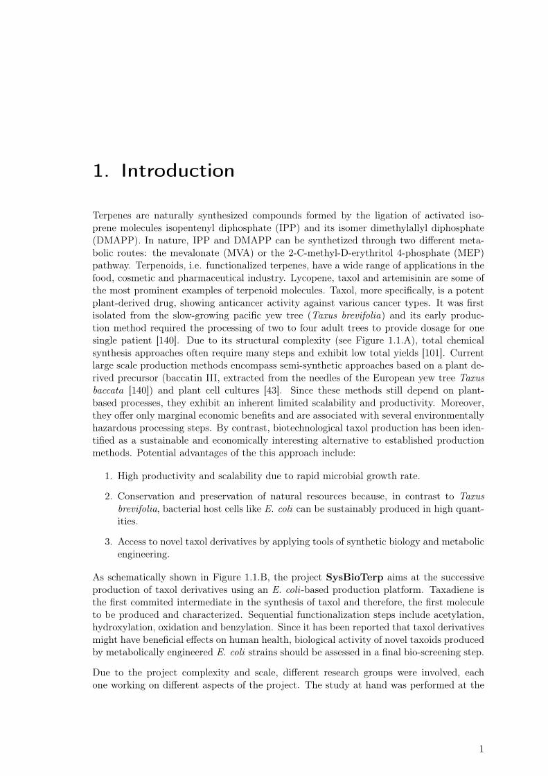
Terpenes are naturally synthesized compounds formed by the ligation of activated iso-prene molecules isopentenyl diphosphate (IPP) and its isomer dimethylallyl diphosphate(DMAPP). In nature, IPP and DMAPP can be synthetized through two different meta-bolic routes: the mevalonate (MVA) or the 2-C-methyl-D-erythritol 4-phosphate (MEP)pathway. Terpenoids, i.e. functionalized terpenes, have a wide range of applications in thefood, cosmetic and pharmaceutical industry. Lycopene, taxol and artemisinin are some ofthe most prominent examples of terpenoid molecules. Taxol, more specifically, is a potentplant-derived drug, showing anticancer activity against various cancer types. It was firstisolated from the slow-growing pacific yew tree (Taxus brevifolia) and its early produc-tion method required the processing of two to four adult trees to provide dosage for onesingle patient [140]. Due to its structural complexity (see Figure 1.1.A), total chemicalsynthesis approaches often require many steps and exhibit low total yields [101]. Currentlarge scale production methods encompass semi-synthetic approaches based on a plant de-rived precursor (baccatin III, extracted from the needles of the European yew tree Taxusbaccata [140]) and plant cell cultures [43]. Since these methods still depend on plant-based processes, they exhibit an inherent limited scalability and productivity. Moreover,they offer only marginal economic benefits and are associated with several environmentallyhazardous processing steps. By contrast, biotechnological taxol production has been iden-tified as a sustainable and economically interesting alternative to established productionmethods. Potential advantages of the this approach include:
1. High productivity and scalability due to rapid microbial growth rate.
2. Conservation and preservation of natural resources because, in contrast to Taxusbrevifolia, bacterial host cells like E. coli can be sustainably produced in high quant-ities.
3. Access to novel taxol derivatives by applying tools of synthetic biology and metabolicengineering.
As schematically shown in Figure 1.1.B, the project SysBioTerp aims at the successiveproduction of taxol derivatives using an E. coli -based production platform. Taxadiene isthe first commited intermediate in the synthesis of taxol and therefore, the first moleculeto be produced and characterized. Sequential functionalization steps include acetylation,hydroxylation, oxidation and benzylation. Since it has been reported that taxol derivativesmight have beneficial effects on human health, biological activity of novel taxoids producedby metabolically engineered E. coli strains should be assessed in a final bio-screening step.
Due to the project complexity and scale, different research groups were involved, eachone working on different aspects of the project. The study at hand was performed at the
1
1. Introduction
Taxus brevifolia
Taxoid ProductsEscherichia coli
Genes for TaxolBiosynthesis
E. coli Fermentation
SysBioTerp
Taxol
?
A
B
Figure 1.1.: Motivation & Project’s Aim Motivation and project’s aim is shown. A. Taxol is apotent plant-derived drug used to treat a number of types of cancer, including ovarian, breast,lung, cervical, and pancreatic cancer. Before current production methods were developed,producing enough taxol to provide dosage for one patient required the processing of twoto four adult, slow-growing Taxus brevifolia trees. B. The SysBioTerp project aims atthe development of a E. coli-based taxoid production platform, thus contributing to thedevelopment of sustainable and environmentally friendly production processes. Additionally,produced taxoids should undergo a bioactivity screening. More specifically, anticancer andantimicrobial activity of each novel taxoid should be determined.
specialty division for systems biotechnology (SBT). The task of our group was the data-driven development and implementation of modeling approaches on both the process andmicrobial metabolism level. From this task, three goals are derived:
1. Reduction of metabolic burden caused by heterologous enzyme overexpression. Meta-bolic burden is a phenomenon observed in microorganisms supporting plasmid-basedenzyme overexpression. It is characterized by a reduction of the overall cellular fit-ness, which leads to a reduction of cellular growth rate, a reduction of biomass yieldand early acetate secretion [11,15,58]. Since the native E. coli metabolism has to beexpanded and re-directed by expressing a number of native and heterologous enzymesto allow for taxoid production, it is expected that metabolic burden will be a majorfactor limiting the production capabilities of the selected host E. coli . In a first step,detrimental effect of enzyme overexpression on cellular fitness should be experiment-ally characterized. Then, model-driven strategies aiming at the minimization of themetabolic burden should be developed and if possible, experimentally validated.
2. Development of production strains through rational design. Over the past years, theemerging science of Metabolic Engineering [7, 139] has allowed the construction of
2
microbial cellular factories for the overproduction of many relevant target molecules.The development of genome-scale metabolic reconstructions, which are mathematicalrepresentations of the cellular metabolism, together with strain-design algorithms,which employ metabolic reconstructions to identify genetic perturbations leading tothe overproduction of the target molecule, has given rise to the development of amore rational, model-based Metabolic Engineering. Consequently, state of the artmathematical tools and modeling approaches should be applied to guide the processof strain development, which should ultimately lead to the construction of an optimaltaxoid production strain.
3. Optimization of bio-reactor parameters for maximal process performance. It is expec-ted that optimal reactor parameters (production temperature, time point of cultureinduction, aeration level, etc.) that maximize performance indicators, such as yieldor productivity, will be highly strain dependent and must therefore be independentlyidentified for each new production strain. Aiming at the reduction of this time-consuming and costly experimental work, modeling approaches should be applied toguide and accelerate experimental process optimization.
Taxoid ProductsMetabolic Burden
Genes for TaxolBiosynthesis
E. coli Fermentation
+
Metabolic Modeling Process Modeling
Strain Development Process Design
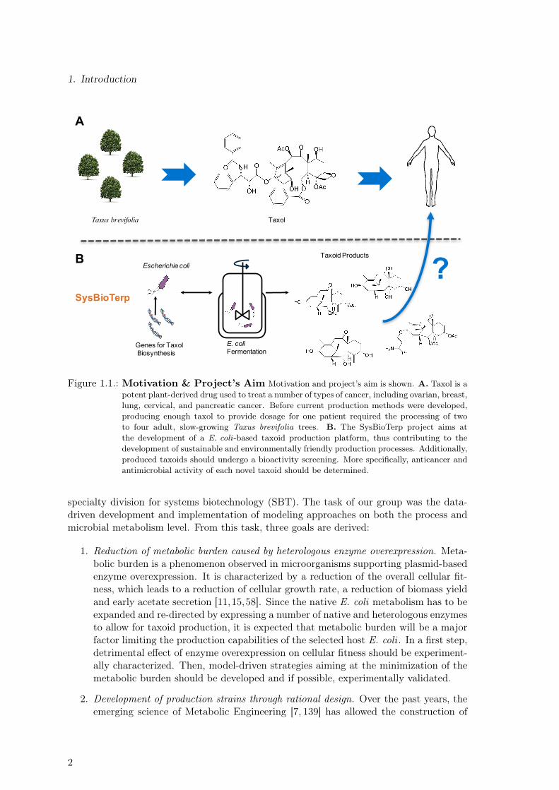
Figure 1.2.: Modeling Workflow. Interdependencies between our three main goals, minimizationof metabolic burden, strain development and process optimization, should be consistentlyaddressed during the modeling process in order to generate integral optimization strategiesleading to maximal overall process performance. Data provided by our cooperation partnersfor model construction mainly consisted of concentration time courses for biomass, substrate,acetate and product. Additionally, cellular metabolism of selected strains was elucidatedby means of 13C labeling experiments. Applied modeling approaches encompassed bothstoichiometric- and kinetic-based methods.
Figure 1.2 shows schematically each of these three goals and the interactions betweenthem. Clearly, all three task - minimization of metabolic burden, strain development andprocess optimization - are interdependent. For instance, optimal process parameters willnecessarily depend on the production strain genotype. Additionally, strategies aiming atreducing the metabolic burden caused by enzyme overexpression will certainly depend onthe extend and identity of the enzymes being overexpressed, which in turn is substantiallydefined by the target molecule. These dependencies should be consistently addressed dur-ing the modeling process in order to generate integral optimization strategies leading to
3
1. Introduction
maximal process performance.
The work at hand is not the first model-driven optimization approach ever developed. Thesame holds true for mathematical tools to be developed. Indeed, the number of existingstrain-design algorithms is vast [87]. However, with very few exceptions [170], existingmathematical approaches have been mainly focused on single aspects - strain design, pro-cess optimization or minimization of metabolic burden-. Additionally, theoretical work-flows providing advice on limitations and proper application of these mathematical toolsare still scarce. Consequently, newly developed as well as existing computational methodsshould be framed into a theoretical workflow addressing the issue of model-driven processoptimization in an integral fashion, considering all three previously mentioned aspects andtheir interdependecies.
This thesis is divided into three parts. We start describing the theoretical methods usedin this work and propose a workflow for Metabolic Engineering. The results obtained fromthe application of this workflow to the terpenoid production in E. coli are described in thesecond and third part.
4

Part I.
Theory
5

2. Metabolic Modeling & StrainEngineering
Modeling the cellular metabolism provides a deep understanding of the cellular response toenvironmental or genetic perturbations and enables the rational design of cellular factories.The aim of strain engineering is to redirect the metabolism of these cell factories in orderto maximize the bio-synthesis of natural or non-natural target products. This is achievedthrough genetic modifications of the host genotype or through adequate culture conditions,i.e. medium composition, culture temperature, etc. Modeling the cellular metabolism canbe a challenging task. Additionally, the proper approach greatly depends on the level ofdetail required for the specific application. Over the past decades, many mathematicalapproaches have been proposed. Each method is based on different assumptions and con-sequently, allows for different types of predictions. In general, the cellular metabolism canbe mathematically described by setting up a mass balance for all metabolites in the cell:
dc
dt= S r − µ c, (2.1)
where r is the vector of fluxes through the reactions, µ is the growth rate, c is a vectorof intracellular metabolite concentrations and S represents the stoichiometric matrix ofthe reaction network. The first term represents the rates of consumption or production ofa specific metabolite, while the second describes the dilution rate caused by cell growth.Since the dilution rate is normally much lower than the reaction rates, the Equation (2.1)can be simplified to:
dc
dt= S r. (2.2)
At steady state, there is no accumulation of metabolites in the cell and Equation (2.2) canbe further simplified to:
0 = S r. (2.3)
In the following sections, the three most commonly used modeling approaches for analyzingEquation (2.3) are presented, namely kinetic-, constraint- and elementary modes-basedmethods.
7
2. Metabolic Modeling & Strain Engineering
2.1. Constraint-based Methods
Since the stoichiometric matrix S of a real biological network is typically non-square, con-taining more unknown rates than equations, it does not have an inverse. Consequently,a flux vector r satisfying Equation (2.3) is not unique. Additional constraints on the fluxvector r can be applied to further reduce the number of allowable flux distributions [31].Limits on the range of individual flux values can be used for this purpose: thermodynamicconstraints expressed as reaction reversibility can thus be included by setting one of theboundaries of an irreversible reaction to zero [53]. In a similar way, maximum flux valuescan be estimated based on enzymatic capacity limitations [13], or for the case of exchangereactions (i.e. reactions that transfer mass between the culture medium and the cell), ex-perimentally determined maximal uptake or production rates can be used. Regulation ofgene expression can also be considered in cases where the regulatory effects have a great in-flucence on cellular behavior [32]. Usually, these constraints are not sufficient to reduce thesolution space to a single solution. Constraint-based models have been popularly used tocalculate a flux vector r that represents the cellular phenotype at steady-state using differ-ent approaches. Flux Balance Analysis (FBA) has been the most widely applied method.It consists of a linear programming formulation that, by imposing an objective function,enables the calculation of a flux distribution that maximizes or minimizes that objective.Typically, the objective function used coincides with an assumed cellular objective, suchas growth. Other commonly used cellular objectives include the sum of all intracellularfluxes or ATP generation [128]. Mathematically, the FBA formulation reads:
Maximize Z = c r
subject to:S r = 0
lb 6 r 6 ub,
(2.4)
where Z is the objective function resulting from a linear combination of selected reactionsof the flux vector r, as determined by the vector c. lb and ub are lower and upper fluxboundaries, respectively.
Due to redundancies in the architecture of the cellular metabolism, alternate optimal solu-tions can exist. Mahadevan et al. [88] introduced the concept of Flux Variability Analysis(FVA) to characterize this issue. The approach begins with determining the optimal valueof the objective function by solving the linear optimization problem outlined in Equation2.4. From this solution, the range of variability that can exist in each flux in the net-work due to alternate optimal solutions can be calculated through a series of optimizationproblems. In each problem, the value of the original objective (Zoptimal) is fixed and eachreaction in the network is maximized (Equation 2.5) and minimized (Equation 2.6) to de-termine the feasible range of flux values for each reaction. The mathematical formulationof the FVA reads:
8
2.1. Constraint-based Methods
Maximize risubject to:
c r = Zoptimal
S r = 0
lb 6r 6 ub,
(2.5)
Minimize risubject to:
c r = Zoptimal
S r = 0
lb 6r 6 ub,
(2.6)
If for a given reaction it holds that rmax = rmin (rmax and rmin are obtained from Equations2.5 and 2.6 respectively), then no variability is allowed for that reaction and a unique fluxvalue associated to that reaction is required to obtain Zoptimal.
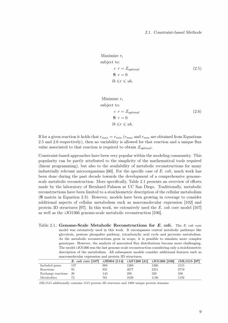
Constraint-based approaches have been very popular within the modeling community. Thispopularity can be partly attributed to the simplicity of the mathematical tools required(linear programming), but also to the availability of metabolic reconstructions for manyindustrially relevant microorganisms [66]. For the specific case of E. coli , much work hasbeen done during the past decade towards the development of a comprehensive genome-scale metabolic reconstruction. More specifically, Table 2.1 presents an overview of effortsmade by the laboratory of Bernhard Palsson at UC San Diego. Traditionally, metabolicreconstructions have been limited to a stoichiometric description of the cellular metabolism(S matrix in Equation 2.3). However, models have been growing in coverage to consideradditional aspects of cellular metabolism such as macromolecular expression [102] andprotein 3D structures [97]. In this work, we extensively used the E. coli core model [107]as well as the iJO1366 genome-scale metabolic reconstruction [106].
Table 2.1.: Genome-Scale Metabolic Reconstructions for E. coli . The E. coli coremodel was extensively used in this work. It encompasses central metabolic pathways likeglycolysis, pentose phospahte pathway, tricarboxylic acid cycle and pyruvate metabolism.As the metabolic reconstructions grow in scope, it is possible to simulate more complexgenotypes. However, the analysis of associated flux distributions become more challenging.The model iJO1366 was the last genome-scale reconstruction considering only a stoichiometricdescription of the metabolism. All subsequent models consider additional features such asmacromolecular expression and protein 3D structures.
E. coli core [107] iJR904 [114] iAF1260 [41] iJO1366 [106] iML1515 [97]Included genes 137 904 1260 1366 1515Reactions 95 931 2077 2251 2719Exchange reactions 20 143 298 329 338Metabolites 72 761 1039 1136 1192
iML1515 additionally contains 1515 protein 3D stuctures and 1888 unique protein domains
9
2. Metabolic Modeling & Strain Engineering
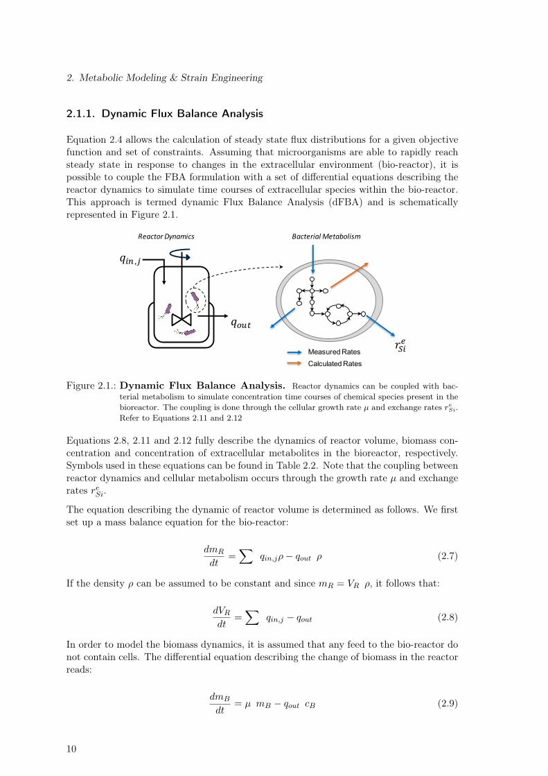
2.1.1. Dynamic Flux Balance Analysis
Equation 2.4 allows the calculation of steady state flux distributions for a given objectivefunction and set of constraints. Assuming that microorganisms are able to rapidly reachsteady state in response to changes in the extracellular environment (bio-reactor), it ispossible to couple the FBA formulation with a set of differential equations describing thereactor dynamics to simulate time courses of extracellular species within the bio-reactor.This approach is termed dynamic Flux Balance Analysis (dFBA) and is schematicallyrepresented in Figure 2.1.
𝑞"#,%
𝑞&'(
Bacterial Metabolism
Measured RatesCalculated Rates
Reactor Dynamics
𝑟*"+
Figure 2.1.: Dynamic Flux Balance Analysis. Reactor dynamics can be coupled with bac-terial metabolism to simulate concentration time courses of chemical species present in thebioreactor. The coupling is done through the cellular growth rate µ and exchange rates reSi.Refer to Equations 2.11 and 2.12
Equations 2.8, 2.11 and 2.12 fully describe the dynamics of reactor volume, biomass con-centration and concentration of extracellular metabolites in the bioreactor, respectively.Symbols used in these equations can be found in Table 2.2. Note that the coupling betweenreactor dynamics and cellular metabolism occurs through the growth rate µ and exchangerates reSi.
The equation describing the dynamic of reactor volume is determined as follows. We firstset up a mass balance equation for the bio-reactor:
dmR
dt=∑
qin,jρ− qout ρ (2.7)
If the density ρ can be assumed to be constant and since mR = VR ρ, it follows that:
dVRdt
=∑
qin,j − qout (2.8)
In order to model the biomass dynamics, it is assumed that any feed to the bio-reactor donot contain cells. The differential equation describing the change of biomass in the reactorreads:
dmB
dt= µ mB − qout cB (2.9)
10
2.1. Constraint-based Methods
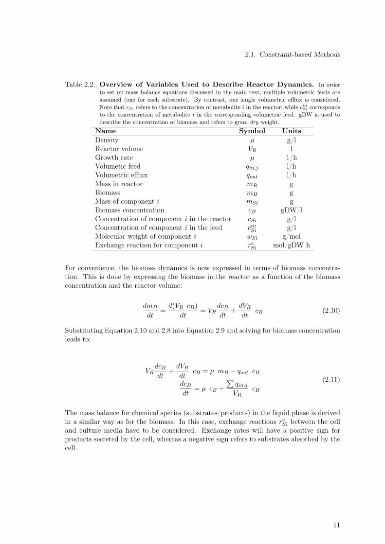
Table 2.2.: Overview of Variables Used to Describe Reactor Dynamics. In orderto set up mass balance equations discussed in the main text, multiple volumetric feeds areassumed (one for each substrate). By contrast, one single volumetric efflux is considered.Note that cSi refers to the concentration of metabolite i in the reactor, while cinSi correspondsto the concentration of metabolite i in the corresponding volumetric feed. gDW is used todescribe the concentration of biomass and refers to gram dry weight.
Name Symbol UnitsDensity ρ g/lReactor volume VR lGrowth rate µ 1/hVolumetic feed qin,j l/hVolumetric efflux qout l/hMass in reactor mR gBiomass mB gMass of component i mSi gBiomass concentration cB gDW/lConcentration of component i in the reactor cSi g/lConcentration of component i in the feed cinSi g/lMolecular weight of component i wSi g/molExchange reaction for component i reSi mol/gDW h
For convenience, the biomass dynamics is now expressed in terms of biomass concentra-tion. This is done by expressing the biomass in the reactor as a function of the biomassconcentration and the reactor volume:
dmB
dt=d(VR cB)
dt= VR
dcBdt
+dVRdt
cB (2.10)
Substituting Equation 2.10 and 2.8 into Equation 2.9 and solving for biomass concentrationleads to:
VRdcBdt
+dVRdt
cB = µ mB − qout cBdcBdt
= µ cB −∑qin,jVR
cB
(2.11)
The mass balance for chemical species (substrates/products) in the liquid phase is derivedin a similar way as for the biomass. In this case, exchange reactions reSi between the celland culture media have to be considered. Exchange rates will have a positive sign forproducts secreted by the cell, whereas a negative sign refers to substrates absorbed by thecell.
11
2. Metabolic Modeling & Strain Engineering
dmSi
dt= qin,j c
inSi − qout csi + reSi cB VR wSi
dcSidt
=qin,jVR
cinSi −∑qin,jVR
cSi + reSi cB wSi
(2.12)
The mass balance equations derived for biomass, reactor volume and components in theliquid phase can be used to describe the dynamics of a continuous (qin,j 6= 0; qout 6= 0), abatch (qin,j = qout = 0) , or a fed-batch process (qin,j 6= 0, qout = 0).
2.1.2. Experimental Determination of Reaction Rates
As stated before, experimentally determined reaction rates can be used to constrain thespace of allowable flux distributions satisfying the linear programming problem defined byEquation 2.4. By doing so, the biological significance of the obtained flux distributionscan be increased. Since ordinary measurements of concentration time courses in the fer-mentation broth allows the estimation of exchange rates (rates describing the exchangeof mass between the cell and the culture medium, that is substrate uptake, product andby-product secretion rates), these are normally used to constraint the solution of Equation2.4. Additionally, more complex data, such as the obtained in 13C labeling experimentscan also be used to estimate a number of intracellular rates. The methodology used inthis work to calculate both exchange and intracellular rates from experimental data willbe discussed in this section.
Determination of Exchange Rates
Concentration time courses for the substrate (or substrates) and the product are usuallyavailable for modeling studies, because this data are routinely obtained during experimentalstrain characterization to assess the production performance of a given strain. Time coursesfor by-products like acetate, ethanol, pyruvate, lactate, etc. might also be available, sincetheir signals are normally contained in the chromatogram used to quantify the main carbonsource if a standard High Performance Liquid Chromatography (HPLC) method is usedfor sugar quantification. Figures 2.2.A and 2.3.A show exemplary concentration timecourses for biomass and glucose, respectively. In the case of biomass, Optical Density (OD)measurements along with a conversion factor have been traditionally used to determinethe biomass concentration in the culture in units of gram dry weight (gDW) per liter.It has been shown that the gDW/OD conversion factor strongly depends on the geneticbackground of the strain [83]. In this study, strain-specific conversion factors were usedto obtain biomass concentration in units of gDW/l. For the specific case shown in Figure2.2.A, a conversion factor of 0.54 was used to calculate the biomass concentration in unitsof gDW/l.
The first step to calculate any exchange rate is the determination of the cellular growthrate µ. As shown in Equation 2.13, µ is a proportionality constant used to describe theincrease of the biomass concentration over time as a function of the biomass concentrationin a certain point in time:
12
2.1. Constraint-based Methods
dcBdt
= µ cB (2.13)
As defined in section 2.1.1, cB refers to the biomass concentration. Equation 2.13 isobtained by setting
∑qin,j to zero in Equation 2.11. This is true for a batch process or
when the total volumetric feed∑qin,j is low compared to the total volume of the reactor.
By assuming that µ is not a function of time, Equation 2.13 can be integrated to obtain:
ln(cB,f ) = µ(tf − to) + ln(cB,o). (2.14)
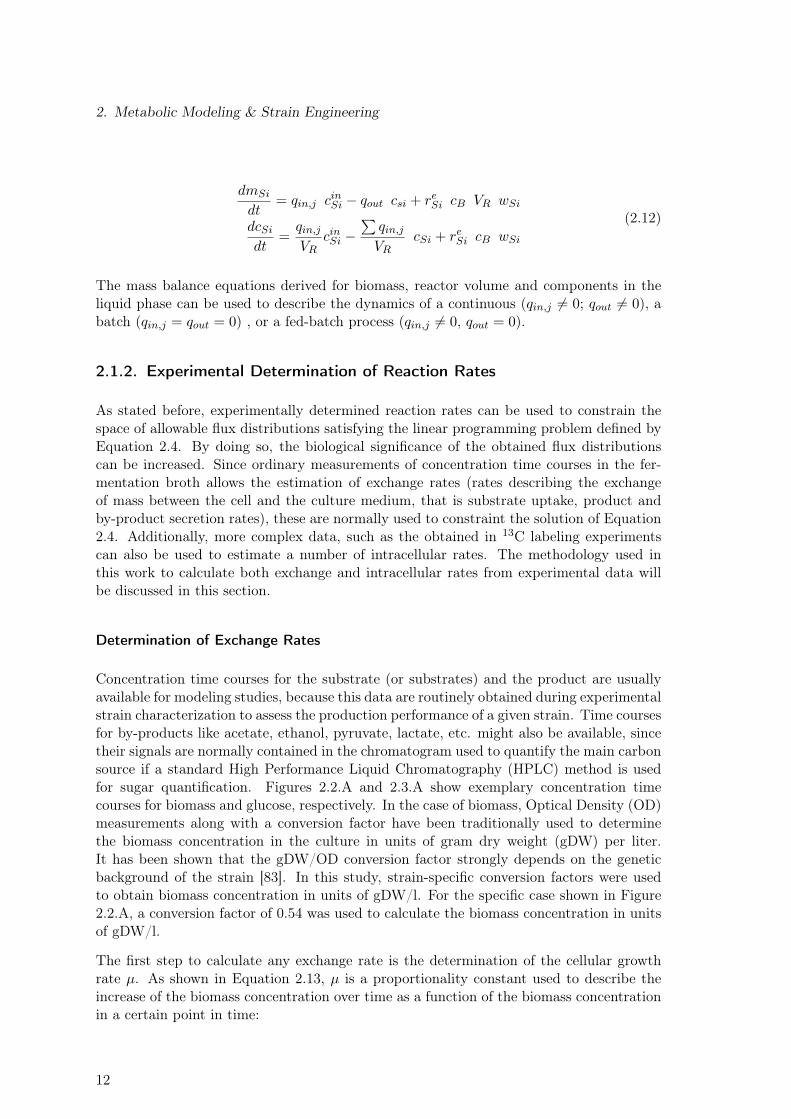
to and tf refer to the initial and final time points, while cB,o and cB,f represent the corres-ponding biomass concentration. Note that the assumption of constant µ is generally validduring the exponential growth phase. By plotting the natural logarithm of experimentallymeasured biomass concentration as a function of time, it is possible to calculate µ as theslope of the resulting straight line. Figure 2.2.B shows this procedure for the biomassconcentration time course shown in Figure 2.2.A. In this case, the analyzed culture had agrowth rate of 0.49 1/h.
0 2 4 6 8Time, [h]
0
0.5
1
1.5
2
2.5
OD
0 2 4 6 8Time, [h]
-3
-2.5
-2
-1.5
-1
-0.5
0
0.5
1
LN(O
D)
𝑦 = 0.49𝑥 − 2.71𝑅- = 0.9997
A B
Figure 2.2.: Experimental Determination of Cellular Growth Rates. A. OD timecourse B. Natural logarithm of OD measurements as a function of time. The slope of thestraight line corresponds to the cellular growth rate µ.
Once µ has been estimated from the experimental OD time course, exchange rates reSican be calculated. As indicated before, strain characterization normally occurs in batchprocesses (shaking flask). By setting qin,j and
∑qin,j to zero, Equation 2.12 can be
simplified to:
dcSidt
= reSicBwSi. (2.15)
Flux distributions are normally calculated in units of mmol/gDW h. By dividing Equation2.15 by wSi (molecular weight), it is possible to change the units of the balance equationfor the metabolite Si from g/l to mol/l (or mmol/l). Combining Equations 2.15 and 2.13and solving the resulting equation for reSi one obtains:
reSi = µdcSidcB
. (2.16)
13
2. Metabolic Modeling & Strain Engineering
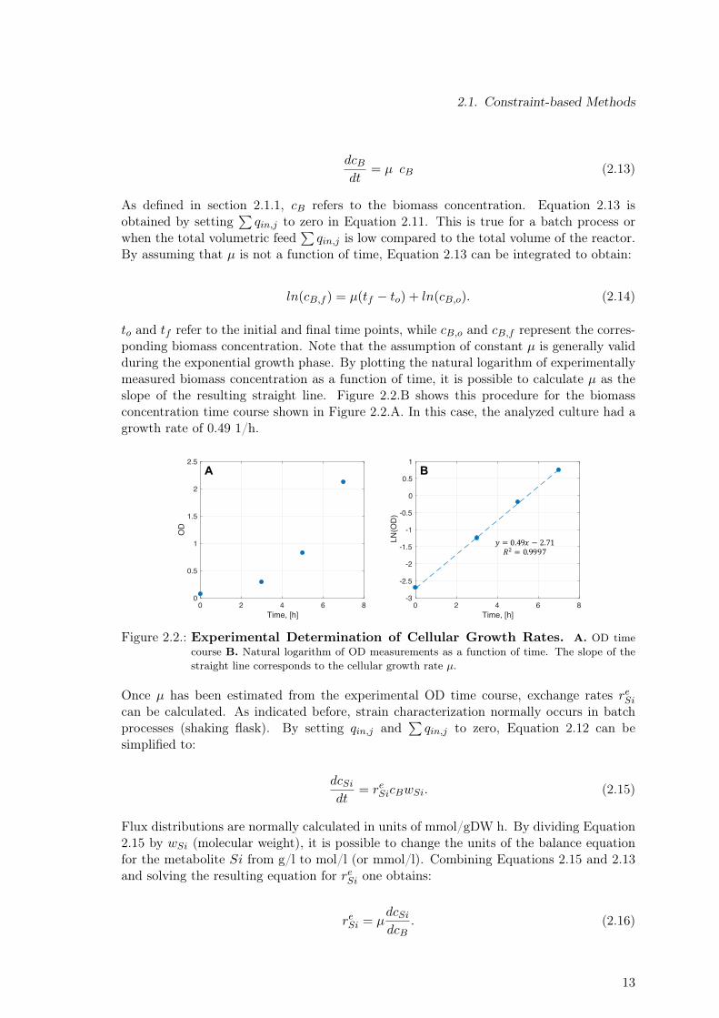
Equation 2.16 states that the exchange rate for metabolite reSi can be obtained by multiply-ing the cellular growth rate µ by the slope of the curve obtained when plotting cSi againstcB. Figure 2.3.B exemplarily shows this procedure. The glucose uptake rate reGlucose canbe then calculated as: (−11.75mmol/gDW )(0.491/h) = −5.75mmol/gDWh. Note thatthe slopes in Figures 2.2.B and 2.3.B were calculated using least-squares regression.
0 2 4 6 8Time, [h]
0
2
4
6
8
10
12
14
Glu
cose
, [m
mol
/l]
0 0.2 0.4 0.6 0.8 1 1.2Biomass Dry Weight, [g/l]
0
2
4
6
8
10
12
14
Glu
cose
, [m
mol
/l]
A B
𝑦 = −11.75𝑥 + 13.55𝑅, = 0.999
Figure 2.3.: Experimental Determination of Glucose Uptake Rate. A. Concentrationtime course for glucose. B. Glucose concentration is plotted against biomass concentration.Note that the biomass concentration was obtained by multiplying OD measurements by aconversion factor of 0.54 gDW/OD. The slope of this straight line corresponds to the termdcSidcB
of Equation 2.16.
Determination of Intracellular Rates: 13C-Metabolic Flux Analysis
Even though exchange rates can be easily calculated from respective concentration timecourses for a number of by-products, they do not provide enough constraints to preciselyestimate all fluxes in complex biological systems containing reversible reactions, parallelpathways and internal cycles [5, 127, 157]. 13C-Metabolic Flux Analysis (13C-MFA) offersa means for the indirect estimation of a number of intracellular fluxes [157]. Typically,cells are grown on 13C-labeled substrates until the isotope label is distributed throughoutthe network. The cell reaches isotopic steady state when the labeling patterns do notchange over time. At this point, cells are harvested and Mass Spectromety (MS) or Nuc-lear Magnetic Resonance (NMR) analysis are implemented to detect the 13C patterns ofeither protein-bound amino acids or free metabolic intermediates. The analysis of protein-bound amino acids is preferred because protein is stable and abundant. On the otherhand, free metabolic intermediates provides the richest source of information, but highturnover and very low concentrations of intermediates poses serious technical challenges tosample preparation, separation and analytical sensitivity [167]. Specific labeling patternsoccur in the metabolic intermediates (free intermediates or protein-bound amino acids) asa function of the particular distribution of fluxes in an organism [157]. Indirect estima-tion means in the context of 13C-MFA that intracellular fluxes must be extracted frommeasured labeling patters using a model-based approach. Comprehensive mathematicalmodels that describe the relationship between metabolite labeling patterns and fluxes areused to simulate isotopic abundances of all metabolites in a network for any set of steadystate fluxes. Various mathematical approaches have been developed to describe the re-lationship between flux distribution and labeling patterns. Usually, these models consistof the complete set of isotopomer (isotope isomer [157]) balances, which may be derived
14
2.1. Constraint-based Methods
using a matrix based method as described by Schmidt et al. [126]. Alternative modelingstrategies have been proposed based on the concept of cumomer balances [158], bundomerbalances [150] and Elementary Metabolite Units (EMU) [6]. Regardless of the approachused, the flux distribution responsible for the measured labeling pattern is identified byminimizing the difference between observed and simulated isotope spectra. In essence, fluxdetermination is a large-scale nonlinear parameter estimation problem:
Minimize Φ =(x(r)− xobs)TΣ−1x (x(r)− xobs)
subject to:S r = 0
(2.17)
where the objective function Φ is the covariance-weighted sum of squared residuals, x(r)is the vector of simulated measurements (which is a function of the flux vector r), xobs
is the vector of experimental data containing both labeling measurements and exchangerates measurements, and Σx is the covariance matrix, which contains variances of themeasurements on the diagonal. Note that the stoichiometric matrix S is a m× k matrix,where m refers to the number of metabolites and k to the number of reactions.
During the iterative optimization process of Equation 2.17, not all flux values in the vectorr can be freely chosen by the solver. In fact, there are only k − rank(S) independentvariables, also referred to as free fluxes [126,158]. Independent fluxes can be obtained fromthe general solution of Equation 2.3:
r = N u (2.18)
Where, N is the null space matrix of S and u is the vector of independent fluxes. Inorder to reduce computational time, one can introduce Equation 2.18 into Equation 2.17to obtain a new optimization problem in terms of the free fluxes vector u:
Minimize Φ =(x(u)− xobs)TΣ−1x (x(u)− xobs)
subject to:N u ≥ 0
(2.19)
Reversible reactions are usually simulated as two independent reactions. Consequently,the constraint N u ≥ 0 requires that all fluxes are non-negative.
Calculating Confidence Intervals for Reactions
Confidence intervals for intracellular fluxes obtained from Equation 2.19 are useful to estim-ate the precision of a certain reaction flux given a certain set of labeling data. Confidenceintervals have been calculated from estimated local standard deviations, but it has beenshown that these intervals may not accurately describe the true uncertainty due to inherentnonlinearities of isotopomer balances [5]. In this work, we calculate confidence intervals forfluxes using the approach developed by Antoniewicz et al. [5], in which for each reaction,the sensitivity of the minimized sum of squared residuals is determined as a function ofthe flux value. The approach starts by stating that the difference between the objectivefunction evaluated at the optimal solution u and the objective function when one flux is
15
2. Metabolic Modeling & Strain Engineering
fixed follows a χ2-distribution with one degree of freedom:
(Φ(u)|ri=ri0 − Φ(u)) ∼ χ2(1), (2.20)
where Φ(u)|ri=ri0 indicates the value of the objective function when the flux i is fixed at ri0and the other degrees of freedom are used to minimize the objective function. The 1 − αconfidence interval for flux i is given by the flux values for which following statement istrue:
Φ(u)|ri=ri0 ≤(Φ(u) + χ2
1−α(1)). (2.21)
Note that α reffers to the probability of error. The threshold values for χ21−α(1) corres-
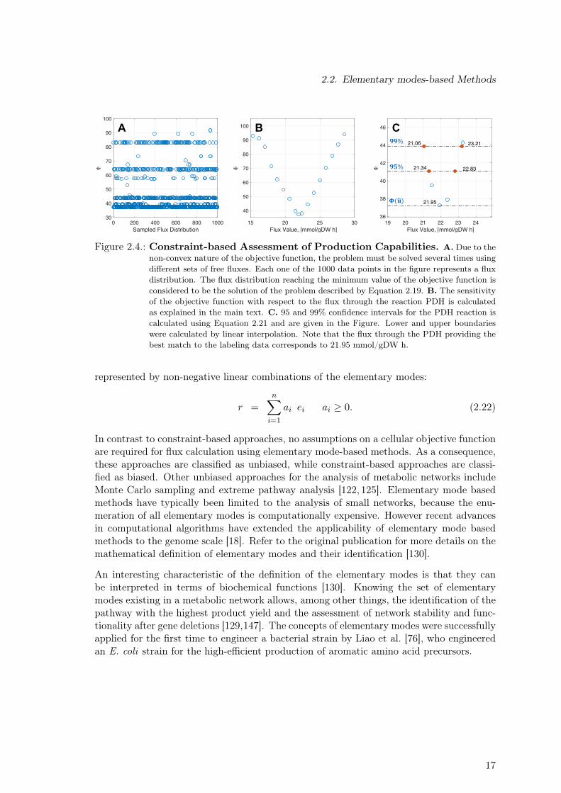
ponding to 80%, 90%, 95% and 99% confidence intervals of fluxes are 1.64, 2.71, 3.84 and6.63, respectively [5]. Thus, in order to obtain accurate confidence intervals we need todetermine the minimized sum of squared residuals as a function of the flux value. Smallsensitivities of the objective function with respect to changes in a certain flux indicatethat that flux cannot be estimated precisely. Conversely, large sensitivities indicate thatthe flux is well determined [5]. Figure 2.4 illustrate the three-step implementation of thisapproach for the estimation of the reaction flux of the reaction catalyzed by the enyzmepyruvate dehydrogenase (PDH) and its confidence interval.
1. Generate multiple initial flux distributions by sampling free fluxes. Then, solve theoptimization problem described by Equation 2.19. Note that not all flux distribu-tions will converge to the same value of the objective function. The optimal fluxdistribution is the one exhibiting the lowest objective function among all sampledinitial flux distributions [48]. See Figure 2.4.A
2. In order to estimate the confidence interval for a given reaction, increase and decreasethe flux through that reaction starting from the optimal solution obtained in theprevious point. For each perturbed flux distribution, solve the optimization problemdescribed by Equation 2.19. See Figure 2.4.B
3. Values for the upper and lower bound of the confidence interval can be identified byapplying Equation 2.21. See Figure 2.4.C
All confidence intervals reported in this work were calculated using an α of 5% (95%confindence intervals). The number of sampled initial flux distributions varied between500 and 1000.
2.2. Elementary modes-based Methods
As discussed before, the number of flux vectors r satisfying Equation (2.3) is infinite.Elementary mode analysis calculates all the solutions of Equation (2.3) by adding a non-decomposability or genetic independence constraint to the reaction directionality constraintintroduced by the FBA formulation. Genetic independence implies that enzymes catalyzingthe reactions in one solution, represented by flux vector r1 are not a subset of another fluxvector r2 [68, 130]. If this condition is satisfied, the flux vectors r1 and r2 belong to theset of elementary modes e. Through this definition all feasible flux distributions r can be
16
2.2. Elementary modes-based Methods
0 200 400 600 800 1000Sampled Flux Distribution
30
40
50
60
70
80
90
100
15 20 25 30Flux Value, [mmol/gDW h]
40
50
60
70
80
90
100
19 20 21 22 23 24Flux Value, [mmol/gDW h]
36
38
40
42
44
46
22.83
23.21
21.34
21.06
21.95
A B C𝟗𝟗%
𝟗𝟓%
𝚽(𝐮')
Figure 2.4.: Constraint-based Assessment of Production Capabilities. A. Due to thenon-convex nature of the objective function, the problem must be solved several times usingdifferent sets of free fluxes. Each one of the 1000 data points in the figure represents a fluxdistribution. The flux distribution reaching the minimum value of the objective function isconsidered to be the solution of the problem described by Equation 2.19. B. The sensitivityof the objective function with respect to the flux through the reaction PDH is calculatedas explained in the main text. C. 95 and 99% confidence intervals for the PDH reaction iscalculated using Equation 2.21 and are given in the Figure. Lower and upper boundarieswere calculated by linear interpolation. Note that the flux through the PDH providing thebest match to the labeling data corresponds to 21.95 mmol/gDW h.
represented by non-negative linear combinations of the elementary modes:
r =
n∑i=1
ai ei ai ≥ 0. (2.22)
In contrast to constraint-based approaches, no assumptions on a cellular objective functionare required for flux calculation using elementary mode-based methods. As a consequence,these approaches are classified as unbiased, while constraint-based approaches are classi-fied as biased. Other unbiased approaches for the analysis of metabolic networks includeMonte Carlo sampling and extreme pathway analysis [122, 125]. Elementary mode basedmethods have typically been limited to the analysis of small networks, because the enu-meration of all elementary modes is computationally expensive. However recent advancesin computational algorithms have extended the applicability of elementary mode basedmethods to the genome scale [18]. Refer to the original publication for more details on themathematical definition of elementary modes and their identification [130].
An interesting characteristic of the definition of the elementary modes is that they canbe interpreted in terms of biochemical functions [130]. Knowing the set of elementarymodes existing in a metabolic network allows, among other things, the identification of thepathway with the highest product yield and the assessment of network stability and func-tionality after gene deletions [129,147]. The concepts of elementary modes were successfullyapplied for the first time to engineer a bacterial strain by Liao et al. [76], who engineeredan E. coli strain for the high-efficient production of aromatic amino acid precursors.
17
2. Metabolic Modeling & Strain Engineering
2.3. Kinetic-based Methods
Kinetic models can describe the rates of intracellular reactions as a function of enzyme de-pendent kinetic parameters as well as metabolite and enzyme concentrations participatingin the reaction. The rate expressions are then used to describe concentration changes by aset of ordinary differential equations. In terms of Equation (2.2), this means that the ratevector r has the form: r = f(p, c), where p represents kinetic parameters and c metaboliteconcentrations.
Usually, kinetic approaches have been used to describe the dynamics of small to mediumsize systems, such as the central metabolism of E. coli [14,22,69]. Despite the high poten-tial of kinetic based methods for strain development, the construction of large-scale kineticmodels has been hindered by many difficulties mainly related to unambiguous parameterestimation. This is due to the need for big sets of kinetic parameters and the fact, thatthe values of individual kinetic parameters and even the form of the kinetic rate laws mayneed to be adjusted in response to genetic or environmental perturbations [63]. These dif-ficulties have been tackled by many authors [4,21,82,146] and call for alternative modelingstrategies which require less parameters or no parameters at all: ’Qualitative and quant-itative understanding and corresponding methodologies for designing desired properties ofmany complex systems have been successfully achieved in the fields of chemistry, physics,and the associted engineering disciplines without knowing all aspects of systems structureand certainly without knowing all parameter values involved. The same must be possiblefor biology.’ [8]. Two approaches popularly used in metabolic engineering that requiresno exhaustive knowledge of kinetic parameter values and rely only on the knowledge ofthe stoichiometry of the reactions in the network, i.e. the stoichiometric matrix S, werealready presented in sections 2.2 and 2.1. In this section, we summarize some of the mainaspects of the pioneering work done by the laboratory of James Liao at the University ofCalifornia (UC) Los Angeles to overcome the issues related to unknown parameter valuesin large-scale kinetic models. In Chapter 5, 6 and 9, we demonstrate the prediction powerof some of these tools and develop new applications based on the theoretical foundation ofthe Ensemble Modeling approach of metabolic networks [71,74,144,146].
2.3.1. Ensemble Modeling Approach of Metabolic Networks
In a first paper, Tran et al. [146] applied the idea of Ensemble Modeling (EM) to the centralmetabolism of E. coli . The approach builds an ensemble of dynamic models that reach thesame reference steady state in terms of flux distribution and metabolite concentrations.Within the ensemble, all models share the same kinetic structure but differ in the specificparameter values. Rate laws for each reaction can be assigned to match known mechanismsand regulations [146] or can be automatically generated based in rules involving the numberof substrates, products and reversibilities [71, 74, 144] by applying the concept of modularrate laws developed by Liebermeister et al. [78, 79].
The idea of building an ensemble of models instead of using one single model to describecomplex dynamic systems is not entirely new. In fact, ensemble forecasting is commonlyused in numerical weather prediction [12, 23, 96, 168], where an ensemble of typically 50models are used to account for mainly two sources of uncertainty, namely errors introduced
18
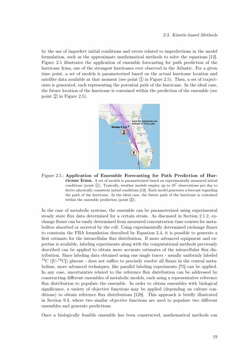
2.3. Kinetic-based Methods
by the use of imperfect initial conditions and errors related to imperfections in the modelformulation, such as the approximate mathematical methods to solve the equations [12].Figure 2.5 illustrates the application of ensemble forecasting for path prediction of thehurricane Irma, one of the strongest hurricanes ever observed in the Atlantic. For a giventime point, a set of models is parameterized based on the actual hurricane location andsatellite data available at that moment (see point 1 in Figure 2.5). Then, a set of traject-ories is generated, each representing the potential path of the hurricane. In the ideal case,the future location of the hurricane is contained within the prediction of the ensemble (seepoint 2 in Figure 2.5).
1
2
Figure 2.5.: Application of Ensemble Forecasting for Path Prediction of Hur-ricane Irma. A set of models is parameterized based on experimentally measured initialconditions (point 1 ). Typically, weather models employ up to 107 observations per day toderive physically consistent initial conditions [12]. Each model generates a forecast regardingthe path of the hurricane. In the ideal case, the future path of the hurricane is containedwithin the ensemble prediction (point 2 ).
In the case of metabolic systems, the ensemble can be parameterized using experimentalsteady state flux data determined for a certain strain. As discussed in Section 2.1.2, ex-change fluxes can be easily determined from measured concentration time courses for meta-bolites absorbed or secreted by the cell. Using experimentally determined exchange fluxesto constrain the FBA formulation described by Equation 2.4, it is possible to generate afirst estimate for the intracellular flux distribution. If more advanced equipment and ex-pertise is available, labeling experiments along with the computational methods previouslydescribed can be applied to obtain more accurate estimates of the intracellular flux dis-tribution. Since labeling data obtained using one single tracer - usually uniformly labeled13C ([U-13C]) glucose - does not suffice to precisely resolve all fluxes in the central meta-bolism, more advanced techniques, like parallel labeling experiments [75] can be applied.In any case, uncertainties related to the reference flux distribution can be addressed byconstructing different ensembles of metabolic models, each using a representative referenceflux distribution to populate the ensemble. In order to obtain ensembles with biologicalsignificance, a variety of objective functions may be applied (depending on culture con-ditions) to obtain reference flux distributions [128]. This approach is briefly illustratedin Section 9.3, where two similar objective functions are used to populate two differentensembles and generate predictions.
Once a biologically feasible ensemble has been constructed, mathematical methods can
19
2. Metabolic Modeling & Strain Engineering
be applied to assess the effect of genetic perturbations on the cellular metabolism. Atsteady state, the concentration of intracellular metabolites does not change over time andwe obtain:
dc
dt= S r(css, p) = F (css, p) = 0, (2.23)
where css refers to a vector of steady state metabolite concentrations. Equation 2.23 isanalogous to Equations 2.2 and 2.3. The only difference is the definition of the functionF (css, p). Since F (css, p) = 0, it follows that the total derivative with respect to p is alsozero:
dF
dp=
∂F
∂css
dcssdp
+∂F
∂p= 0. (2.24)
Solving Equation 2.24 for dcssdp yields:
dcssdp
= −(∂F
∂css
)−1 ∂F
∂p. (2.25)
Starting from a reference steady state, Equation 2.25 describes the effect of parameterperturbations (for instance enzyme concentration) on the vector of steady state metaboliteconcentrations css. Since the calculation of the inverse of the matrix ∂F
∂cssis necessary to
solve Equation 2.25, it is crucial to detect the point where this matrix becomes singular.Interestingly, this points is also a bifurcation point, beyond which the system no longerreaches a stable steady state [74].
So far, two methods have been developed that analyze different aspects of Equation 2.25.The first method is termed Ensemble Modeling for Robustness Analysis (EMRA) [74] andwas designed to estimate the robustness of non-native pathways towards perturbations. Byperturbing the activity of a certain enzyme in the pathway and calculating the percentageof models in the ensemble that remained stable, the robustness of the pathway/enzymecan be assessed. In the original publication [74], the robustness of two synthetic centralmetabolic pathways that achieve carbon conservation (non-oxidative glycolysis [17] andreverse glyoxylate cycle [90]) was compared. In a subsequent paper [144], experimental dataof three different cell-free enzymatic systems were used to demonstrate the existing linkbetween production performance (product end titer, productivity) and system robustness.As predicted by EMRA, unstable systems exhibited a lower production performance.
A second method, termed Kinetically Accessible Yield (KAY), uses the maximal flux valuethrough a given pathway before the metabolic system loses stability (or any metaboliteconcentration becomes negative) to estimate experimentally measured product yields. Inthe original publication, Lafontaine Rivera et al. [71] used the KAY formulation to success-fully predict the isobutanol yield of three different genotypes. Interestingly, the authorsdemonstrated that KAY can be calculated by either flux or kinetic parameter integration.In both cases, the calculated KAY value is the same [71]. Throughout this work, KAYvalues were calculated using flux integration. In this case, no specific knowledge of re-action kinetics of the production pathway is required. Instead, a single lumped reactionrepresenting the whole production pathway is used as input.
20
2.3. Kinetic-based Methods
Metabolic Reconstructions for the Ensemble Modeling Approach
One of the main advantages of the EM approach is that it allows for a kinetic-basedanalysis of available metabolic reconstructions (refer to Table 2.1). These reconstructionshave been manually curated and are frequently updated, thus becoming more accurate andcomplete over the years. Instead of automatically generating the metabolic network fromthe EcoCyc [60,61] database, as done by Lafontaine Rivera et al. [71], we adapted alreadyexisting metabolic reconstructions to make them suitable inputs for the EM approach asfollows:
1. Check exchange reactions. Exchange reactions are required to have positive flux val-ues within the EM framework for both uptake and export reactions. By contrast,traditionally used metabolic reconstructions (refer to Table 2.1) exhibit negative fluxvalues for uptake reactions and positive flux values for export reactions. There-fore, uptake reactions must be converted from the form “metabolite −→ ” into“ −→ metabolite”. This can be simply done by multiplying the column i of thestoichiometric matrix S by -1. i refers to the reaction(s) responsible for the uptakeof a given substrate(s).
2. Split reaction describing biomass production. Biomass formation is represented withinthe EM approach by a set of efflux reactions [71]. By contrast, cellular growthis mathematically described by one single reaction in traditionally used metabolicreconstructions. While a stoichiometric representation of a reaction involving over100 substrates is straightforward, a kinetic representation of such a reaction wouldnot be practical. For that reason, the metabolic reconstruction should be modifiedby splitting the biomass reaction into many reactions involving one single substrate.Alternative strategies, in which related substrates are grouped in a single reactionare also possible, for instance to represent DNA formation.
For all kinetic-based analyses, we used an extended version of the E. coli core metabolism[107]. Refer to Appendix B.1.1 for more details on model modification. Since the EMframework allows to incorporate known substrate-level regulation of enzyme activity, weused the regulatory interactions contained in Table 2.3 for the construction of rate laws forall ensembles. Additionally, we used the rate law described by Equation 2.26 to describethe flux through the phosphotransferase system (PTS) system, as suggested by LafontaineRivera et al. [71]. Note that the rate law described in the Equation 2.26 includes knownregulatory interactions, such as flux control through the PEP/Pyruvate ratio [22, 33, 109]and product inhibition by glucose-6-phosphate [22,29,59].
rPTS =Vm,PTS CPEP /CPY R CGLC
(km,1 + km,2 CPEP /CPY R + km,3 CGLC + CGLC CPEP /CPY R)(1 + CG6P /ki,G6P ). (2.26)
Parallelization Strategies in Large Multi-core Computers and Computer Clusters
EM-based analyses are computationally expensive. Luckily, the process of ensemble con-struction by parameter sampling and the analysis itself of each model within a given
21
2. Metabolic Modeling & Strain Engineering
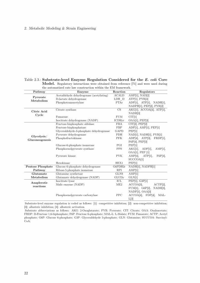
Table 2.3.: Substrate-level Enzyme Regulation Considered for the E. coli CoreModel. Regulatory interactions were obtained from reference [71] and were used duringthe automatized rate law construction within the EM framework.
Pathway Enzyme Reaction Regulators
PyruvateMetabolism
Acetaldehyde dehydrogenase (acetylating) ACALD AMP[1], NAD[2]D-lactate dehydrogenase LDH_D ATP[1], PYR[4]Phosphotransacetylase PTAr ADP[1], ATP[1], NADH[1],
NADPH[1], PEP[2], PYR[2]
Citric AcidCycle
Citrate synthase CS AKG[1], ACCOA[4], ATP[1],NADH[3]
Fumarase FUM CIT[1]Isocitrate dehydrogenase (NADP) ICDHyr OAA[1], PEP[3]
Glycolysis/Gluconeogenesis
Fructose-bisphosphate aldolase FBA CIT[2], PEP[2]Fructose-bisphosphatase FBP ADP[1], AMP[1], PEP[1]Glyceraldehyde-3-phosphate dehydrogenase GAPD PEP[1]Pyruvate dehydrogenase PDH NAD[1], NADH[1], PYR[1]Phosphofructokinase PFK ADP[4], ATP[3], FRDP[1],
F6P[4], PEP[3]Glucose-6-phosphate isomerase PGI PEP[1]Phosphoenolpyruvate synthase PPS AKG[1], ADP[1], AMP[1],
OAA[1], PEP [1]Pyruvate kinase PYK AMP[4], ATP[1], F6P[4],
SUCCOA[1]Hexokinase HEX1 PEP[1]
Pentose PhosphatePathway
Glucose 6-phosphate dehydrogenase G6PDH2r NADH[1], NADPH[1]Ribose-5-phosphate isomerase RPI AMP[1]
GlutamateMetabolism
Glutamine synthetase GLNS AMP[1]Glutamate dehydrogenase (NADP) GLUDy GLN[1]
Anapleroticreactions
Isocitrate lyase ICL PEP[1], G3P[1]Malic enzyme (NADP) ME2 ACCOA[3], ACTP[2],
FUM[1], G6P[2], NADH[3],NADP[1], OAA[3]
Phosphoenolpyruvate carboxylase PPC ACCOA[4], FDP[4], MAL-L[3]
Substrate-level enzyme regulation is coded as follows: [1]: competitive inhibition; [2]: non-competitive inhibition;[3]: allosteric inhibition; [4]: allosteric activation.Substrate abbreviations as follows: AKG: 2-Oxoglutarate; PYR: Pyruvate; CIT: Citrate; OAA: Oxaloacetate;FRDP: D-Fructose 1,6-biphosphate; F6P: Fructose 6-phosphate; MAL-L: L-Malate; FUM: Fumarate; ACTP: Acetylphosphate; G6P: Glucose 6-phosphate; G3P: Glyceraldehyde 3-phosphate; GLN: Glutamine; SUCCOA: Succinyl-CoA;
22
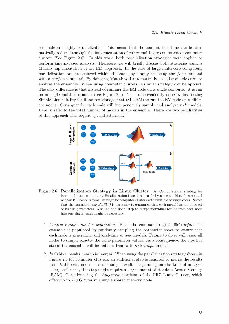
2.3. Kinetic-based Methods
ensemble are highly parallelizable. This means that the computation time can be dra-matically reduced through the implementation of either multi-core computers or computerclusters (See Figure 2.6). In this work, both parallelization strategies were applied toperform kinetic-based analysis. Therefore, we will briefly discuss both strategies using aMatlab implementation of the EM approach. In the case of large multi-core computers,parallelization can be achieved within the code, by simply replacing the for-commandwith a parfor-command. By doing so, Matlab will automatically use all available cores toanalyze the ensemble. When using computer clusters, a similar strategy can be applied.The only difference is that instead of running the EM code on a single computer, it is runon multiple multi-core nodes (see Figure 2.6). This is conveniently done by instructingSimple Linux Utility for Resource Management (SLURM) to run the EM code on k differ-ent nodes. Consequently, each node will independently sample and analyze n/k models.Here, n refer to the total number of models in the ensemble. There are two peculiaritiesof this approach that require special attention.
…
Node 1
Node 2
Node k
EM Analysis Prediction
PredictionEM Analysis
Larg
e M
ultic
ore
Com
pute
rsC
ompu
ter
Clu
ster
s
Merge Results
Model 1
Model 4
Model 2
Model 3
…
Model n
n/k Models
Model 1
Model 4
Model 2
Model 3
…Model n
A
B
Figure 2.6.: Parallelization Strategy in Linux Cluster. A. Computational strategy forlarge multi-core computers. Parallelization is achieved easily by using the Matlab commandparfor B. Computational strategy for computer clusters with multiple or single cores. Noticethat the command rng(’shuffle’) is necessary to guarantee that each model has a unique setof kinetic parameters. Also, an additional step to merge individual results from each nodeinto one single result might be necessary.
1. Control random number generation. Place the command rng(’shuffle’) before theensemble is populated by randomly sampling the parameter space to ensure thateach node is generating and analyzing unique models. Failure to do so will cause allnodes to sample exactly the same parameter values. As a consequence, the effectivesize of the ensemble will be reduced from n to n/k unique models.
2. Individual results need to be merged. When using the parallelization strategy shown inFigure 2.6 for computer clusters, an additional step is required to merge the resultsfrom k different nodes into one single result. Depending on the kind of analysisbeing performed, this step might require a large amount of Random Access Memory(RAM). Consider using the hugemem partition of the LRZ Linux Cluster, whichoffers up to 240 GBytes in a single shared memory node.
23
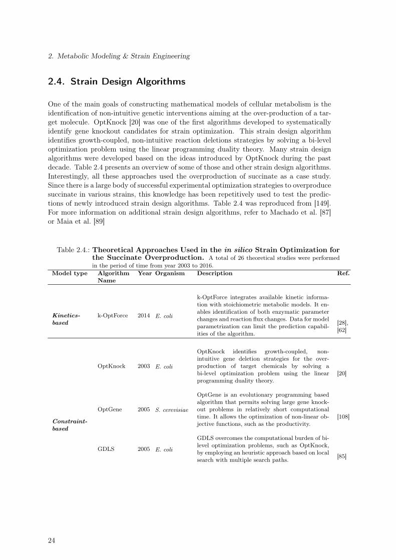
2. Metabolic Modeling & Strain Engineering
2.4. Strain Design Algorithms
One of the main goals of constructing mathematical models of cellular metabolism is theidentification of non-intuitive genetic interventions aiming at the over-production of a tar-get molecule. OptKnock [20] was one of the first algorithms developed to systematicallyidentify gene knockout candidates for strain optimization. This strain design algorithmidentifies growth-coupled, non-intuitive reaction deletions strategies by solving a bi-leveloptimization problem using the linear programming duality theory. Many strain designalgorithms were developed based on the ideas introduced by OptKnock during the pastdecade. Table 2.4 presents an overview of some of those and other strain design algorithms.Interestingly, all these approaches used the overproduction of succinate as a case study.Since there is a large body of successful experimental optimization strategies to overproducesuccinate in various strains, this knowledge has been repetitively used to test the predic-tions of newly introduced strain design algorithms. Table 2.4 was reproduced from [149].For more information on additional strain design algorithms, refer to Machado et al. [87]or Maia et al. [89]
Table 2.4.: Theoretical Approaches Used in the in silico Strain Optimization forthe Succinate Overproduction. A total of 26 theoretical studies were performedin the period of time from year 2003 to 2016.
Model type AlgorithmName
Year Organism Description Ref.
Kinetics-based
k-OptForce 2014 E. coli
k-OptForce integrates available kinetic informa-tion with stoichiometric metabolic models. It en-ables identification of both enzymatic parameterchanges and reaction flux changes. Data for modelparametrization can limit the prediction capabil-ities of the algorithm.
[28],[62]
Constraint-based
OptKnock 2003 E. coli
OptKnock identifies growth-coupled, non-intuitive gene deletion strategies for the over-production of target chemicals by solving abi-level optimization problem using the linearprogramming duality theory.
[20]
OptGene 2005 S. cerevisiae
OptGene is an evolutionary programming basedalgorithm that permits solving large gene knock-out problems in relatively short computationaltime. It allows the optimization of non-linear ob-jective functions, such as the productivity.
[108]
GDLS 2005 E. coli
GDLS overcomes the computational burden of bi-level optimization problems, such as OptKnock,by employing an heuristic approach based on localsearch with multiple search paths. [85]
24
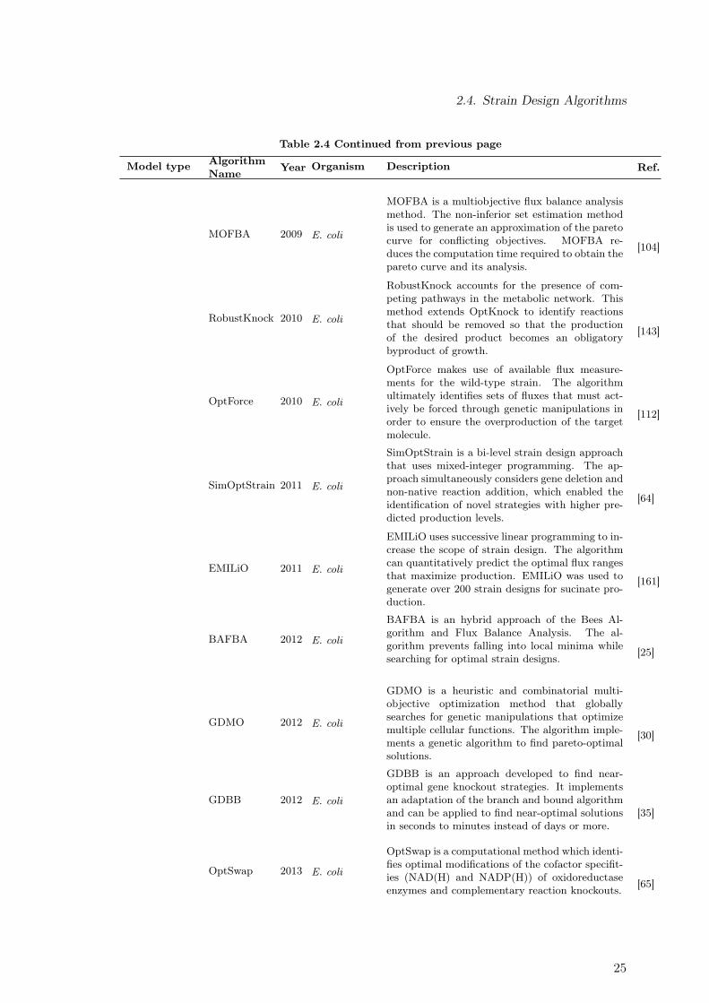
2.4. Strain Design Algorithms
Table 2.4 Continued from previous page
Model type AlgorithmName Year Organism Description Ref.
MOFBA 2009 E. coli
MOFBA is a multiobjective flux balance analysismethod. The non-inferior set estimation methodis used to generate an approximation of the paretocurve for conflicting objectives. MOFBA re-duces the computation time required to obtain thepareto curve and its analysis.
[104]
RobustKnock 2010 E. coli
RobustKnock accounts for the presence of com-peting pathways in the metabolic network. Thismethod extends OptKnock to identify reactionsthat should be removed so that the productionof the desired product becomes an obligatorybyproduct of growth.
[143]
OptForce 2010 E. coli
OptForce makes use of available flux measure-ments for the wild-type strain. The algorithmultimately identifies sets of fluxes that must act-ively be forced through genetic manipulations inorder to ensure the overproduction of the targetmolecule.
[112]
SimOptStrain 2011 E. coli
SimOptStrain is a bi-level strain design approachthat uses mixed-integer programming. The ap-proach simultaneously considers gene deletion andnon-native reaction addition, which enabled theidentification of novel strategies with higher pre-dicted production levels.
[64]
EMILiO 2011 E. coli
EMILiO uses successive linear programming to in-crease the scope of strain design. The algorithmcan quantitatively predict the optimal flux rangesthat maximize production. EMILiO was used togenerate over 200 strain designs for sucinate pro-duction.
[161]
BAFBA 2012 E. coli
BAFBA is an hybrid approach of the Bees Al-gorithm and Flux Balance Analysis. The al-gorithm prevents falling into local minima whilesearching for optimal strain designs. [25]
GDMO 2012 E. coli
GDMO is a heuristic and combinatorial multi-objective optimization method that globallysearches for genetic manipulations that optimizemultiple cellular functions. The algorithm imple-ments a genetic algorithm to find pareto-optimalsolutions.
[30]
GDBB 2012 E. coli
GDBB is an approach developed to find near-optimal gene knockout strategies. It implementsan adaptation of the branch and bound algorithmand can be applied to find near-optimal solutionsin seconds to minutes instead of days or more.
[35]
OptSwap 2013 E. coli
OptSwap is a computational method which identi-fies optimal modifications of the cofactor specifit-ies (NAD(H) and NADP(H)) of oxidoreductaseenzymes and complementary reaction knockouts. [65]
25
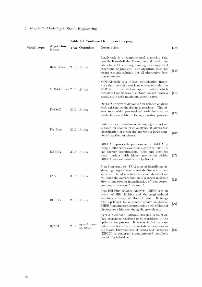
2. Metabolic Modeling & Strain Engineering
Table 2.4 Continued from previous page
Model type AlgorithmName Year Organism Description Ref.
ReacKnock 2013 E. coli
ReacKnock is a computational algorithm thatuses the Karush-Kuhn-Tucker method to reformu-late a bilevel linear programming to a single levelprogramming problem. The algorithm does notreturn a single solution but all alternative dele-tion strategies.
[159]
MOMAKnock 2013 E. coli
MOMAKnock is a bi-level optimization frame-work that identifies knockout strategies under theMOMA flux distribution approximation, whichconsiders that knockout mutants do not reach asteady state with maximum growth rates.
[115]
DySScO 2013 E. coli
DySScO integrates dynamic flux balance analysiswith existing strain design algorithms. This al-lows to consider process-level variables such asproductivity and titer in the optimization process. [170]
FastPros 2013 E. coli
FastPros is an iterative screening algorithm thatis based on shadow price analysis. It allows fastidentification of strain designs with a large num-ber of reaction knockouts.
[105]
DBFBA 2014 E. coli
DBFBA improves the performance of BAFBA byusing a differential evolution algorithm. DBFBAhas shorter computational time and identifiesstrain designs with higher production yields.DBFBA was validated with OptKnock.
[27]
FSA 2015 E. coli
Flux-Sum Analysis (FSA) aims at identifying en-gineering targets from a metabolite-centric per-spective. The idea is to identify metabolites thatwill force the overproduction of a target moleculeafter attenuation or intensification of their corres-ponding turnover or "flux-sum".
[72]
BHFBA 2015 E. coli
Bees Hill Flux Balance Analysis (BHFBA) is anhybrid of Hill climbing and the neighborhoodsearching strategy of BAFBA [25]. It integ-rates optKnock for automatic results validation.BHFBAmaximizes the production yield of desiredphenotypes while sustaining the growth rate.
[26]
HyMeP 2016 Synechosystissp. 6803
Hybrid Metabolic Pathway Design (HyMeP) al-lows exogenous reactions to be considered in theoptimization process. It selects individual can-didate reactions from the metabolic reactions inthe Kyoto Encyclopedia of Genes and Genomes(KEGG) to construct a computerized metabolicmodel of a hybrid cell.
[137]
26
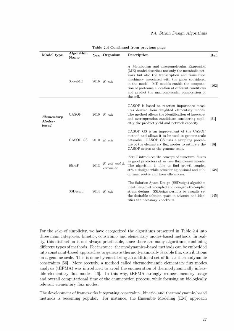
2.4. Strain Design Algorithms
Table 2.4 Continued from previous page
Model type AlgorithmName Year Organism Description Ref.
SolveME 2016 E. coli
A Metabolism and macromolecular Expression(ME) model describes not only the metabolic net-work but also the transcription and translationmachinery associated with the genes consideredin the model. ME models enable the computa-tion of proteome allocation at different conditionsand predict the macromolecular composition ofthe cell.
[162]
ElementaryModes-based
CASOP 2010 E. coli
CASOP is based on reaction importance meas-ures derived from weighted elementary modes.The method allows the identification of knockoutand overexpression candidates considering expli-citly the product yield and network capacity.
[51]
CASOP GS 2010 E. coli
CASOP GS is an improvement of the CASOPmethod and allows it to be used in genome-scalenetworks. CASOP GS uses a sampling proced-ure of the elementary flux modes to estimate theCASOP-scores at the genome-scale.
[18]
iStruF 2013 E. coli and S.cerevisiae
iStruF introduces the concept of structural fluxesas good predictors of in vivo flux measurements.The algorithm is able to find growth-coupledstrain designs while considering optimal and sub-optimal routes and their efficiencies.
[138]
SSDesign 2014 E. coli
The Solution Space Design (SSDesign) algorithmidentifies growth-coupled and non-growth-coupledstrain designs. SSDesign permits to visually setthe desirable solution space in advance and iden-tifies the necessary knockouts.
[145]
For the sake of simplicity, we have categorized the algorithms presented in Table 2.4 intothree main categories: kinetic-, constraint- and elementary modes-based methods. In real-ity, this distinction is not always practicable, since there are many algorithms combiningdifferent types of methods. For instance, thermodynamics-based methods can be embeddedinto constraint-based approaches to generate thermodynamically feasible flux distributionson a genome scale. This is done by considering an additional set of linear thermodynamicconstraints [56]. More recently, a method called thermodynamic elementary flux modesanalysis (tEFMA) was introduced to avoid the enumeration of thermodynamically infeas-ible elementary flux modes [46]. In this way, tEFMA strongly reduces memory usageand overall computational time of the enumeration process, while focusing on biologicallyrelevant elementary flux modes.
The development of frameworks integrating constraint-, kinetic- and thermodynamic-basedmethods is becoming popular. For instance, the Ensemble Modeling (EM) approach
27
2. Metabolic Modeling & Strain Engineering
[141,142,146], which introduced an elegant solution for difficulties related to unambiguousparameter estimation of large-scale kinetic models, has the potential to integrate constraint-based methods like FBA to identify biologically meaningful steady-state flux distributions,if no 13C-labeling data is available. Additionally, thermodynamic constraints can be ap-plied not only to complement FBA calculations [56], but also to perform thermodynamic-ally safe parameterization using independent parameter sets [77–79]. In this way, kineticparameters will satisfy Haldane relationships and Wegscheider conditions, necessary to en-sure thermodynamical consistency of the kinetic model [79]. In a more recent work, Sehret al. [135] proposed a modeling workflow that integrates FBA with Thermodynamic Feas-ibility Analysis [94]. The results of both approaches are then translated to parameters fora dynamic model. The dynamic model is then formulated and analyzed according to Bio-chemical Systems Theory [118–120] and Mathematically Controlled Comparison [3, 121].The authors used this approach to analyze three different case studies. We refer interestedreaders to the original publication for further details on mathematical implementation andresults [135].
2.5. Computational Tools
As shown in Table 2.1, the size of the stoichiometric matrix S [metabolites x reactions] ofcommonly used metabolic reconstructions can rapidly increase as the metabolic reconstruc-tion becomes more comprehensive. In order to effectively handle the size and complexityof genome-scale metabolic reconstructions, many computational approaches have been de-veloped. Some prominent examples are listed in Table 2.5. Out of those methods, theCOnstraint-Based Reconstruction and Analysis (COBRA) Toolbox has emerged as one ofthe preferred modeling tools. The COBRA toolbox consist of a compilation of various Mat-lab scripts designed to allow for a rapid implementation of basic and advanced analyses.The current functionality allows for network gap filling analysis, determination of intra-cellular flux distributions by analyzing 13C labeling data, implementation of strain designalgorithms, omics-guided analysis, visualization of calculated flux distributions, amongothers.
Throughout this work, the functionality provided by the COBRA Toolbox v2.0 [124] wasextensively implemented. For instance, FVA was used in Chapter 4 to identify changesin by-product secretion pattern as the substrate uptake rate was increased. In the samechapter, relative quality for various substrates was quantitatively assessed by calculatingthe maximal flux through the ATPM reaction of the E. coli core model [107]. In Chapter5, the OptKnock implementation provided by the COBRA toolbox was used to analyzethe effect of oxygen availability on genetic targets improving taxadiene production. Inorder to demonstrate the simplicity of application of the COBRA toolbox, we show howthe maximal theoretical taxadiene yield on glucose can be calculated using some basiccommands. The code shown encompasses the following steps:
1. Load a metabolic reconstruction. In this case, we use the E. coli core model. Seecode line 2.
2. Expand the scope of the metabolic reconstruction by adding a set of new reactions.In this case, 12 new reactions along with their corresponding substrates and productsare added to the model. See code lines 6 to 46.
28
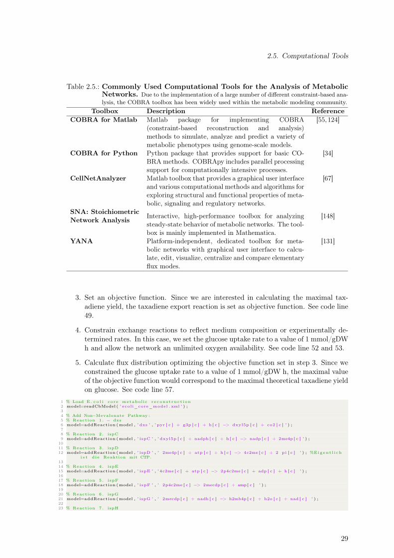
2.5. Computational Tools
Table 2.5.: Commonly Used Computational Tools for the Analysis of MetabolicNetworks. Due to the implementation of a large number of different constraint-based ana-lysis, the COBRA toolbox has been widely used within the metabolic modeling community.
Toolbox Description ReferenceCOBRA for Matlab Matlab package for implementing COBRA
(constraint-based reconstruction and analysis)methods to simulate, analyze and predict a variety ofmetabolic phenotypes using genome-scale models.
[55, 124]
COBRA for Python Python package that provides support for basic CO-BRA methods. COBRApy includes parallel processingsupport for computationally intensive processes.
[34]
CellNetAnalyzer Matlab toolbox that provides a graphical user interfaceand various computational methods and algorithms forexploring structural and functional properties of meta-bolic, signaling and regulatory networks.
[67]
SNA: StoichiometricNetwork Analysis Interactive, high-performance toolbox for analyzing
steady-state behavior of metabolic networks. The tool-box is mainly implemented in Mathematica.
[148]
YANA Platform-independent, dedicated toolbox for meta-bolic networks with graphical user interface to calcu-late, edit, visualize, centralize and compare elementaryflux modes.
[131]
3. Set an objective function. Since we are interested in calculating the maximal tax-adiene yield, the taxadiene export reaction is set as objective function. See code line49.
4. Constrain exchange reactions to reflect medium composition or experimentally de-termined rates. In this case, we set the glucose uptake rate to a value of 1 mmol/gDWh and allow the network an unlimited oxygen availability. See code line 52 and 53.
5. Calculate flux distribution optimizing the objective function set in step 3. Since weconstrained the glucose uptake rate to a value of 1 mmol/gDW h, the maximal valueof the objective function would correspond to the maximal theoretical taxadiene yieldon glucose. See code line 57.
1 % Load E. c o l i core metabol ic r e c on s t ru c t i on2 model=readCbModel ( ’ ecol i_core_model . xml ’ ) ;34 % Add Non−Mevalonate Pathway :5 % Reaction 1 . − dxs6 model=addReaction (model , ’ dxs ’ , ’ pyr [ c ] + g3p [ c ] + h [ c ] −> dxyl5p [ c ] + co2 [ c ] ’ ) ;78 % Reaction 2 . ispC9 model=addReaction (model , ’ ispC ’ , ’ dxyl5p [ c ] + nadph [ c ] + h [ c ] −> nadp [ c ] + 2me4p [ c ] ’ ) ;
1011 % Reaction 3 . ispD12 model=addReaction (model , ’ ispD ’ , ’ 2me4p [ c ] + atp [ c ] + h [ c ] −> 4c2me [ c ] + 2 pi [ c ] ’ ) ; %E i g en t l i c h
i s t d i e Reaktion mit CTP.1314 % Reaction 4 . ispE15 model=addReaction (model , ’ ispE ’ , ’ 4c2me [ c ] + atp [ c ] −> 2p4c2me [ c ] + adp [ c ] + h [ c ] ’ ) ;1617 % Reaction 5 . ispF18 model=addReaction (model , ’ ispF ’ , ’ 2p4c2me [ c ] −> 2mecdp [ c ] + amp [ c ] ’ ) ;1920 % Reaction 6 . ispG21 model=addReaction (model , ’ ispG ’ , ’ 2mecdp [ c ] + nadh [ c ] −> h2mb4p [ c ] + h2o [ c ] + nad [ c ] ’ ) ;2223 % Reaction 7 . ispH
29
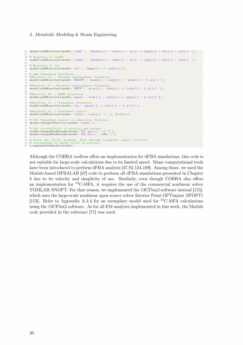
2. Metabolic Modeling & Strain Engineering
24 model=addReaction (model , ’ ispH ’ , ’ h2mb4p [ c ] + nadh [ c ] + h [ c ] −> dmpp [ c ] + h2o [ c ] + nad [ c ] ’ ) ;2526 % Reaction 8 . ispH227 model=addReaction (model , ’ ispH2 ’ , ’ h2mb4p [ c ] + nadh [ c ] + h [ c ] −> ipdp [ c ] + h2o [ c ] + nad [ c ] ’ ) ;2829 % Reaction 9 . i d i30 model=addReaction (model , ’ i d i ’ , ’ dmpp [ c ] <=> ipdp [ c ] ’ ) ;3132 % Add Taxadiene Synthes i s :33 %Reaction 10 . − Geranyl diphosphate formation .34 model=addReaction (model , ’DMATT’ , ’ dmpp [ c ] + ipdp [ c ] −> grdp [ c ] + 2 pi [ c ] ’ ) ;3536 %Reaction 9 . − Farnesy l diphosphate formation37 model=addReaction (model , ’GRTT’ , ’ grdp [ c ] + ipdp [ c ] −> frdp [ c ] + 2 pi [ c ] ’ ) ;3839 %Reaction 10 . − GGPP formation40 model=addReaction (model , ’ ggpps ’ , ’ f rdp [ c ] + ipdp [ c ] −> ggpp [ c ] + 2 pi [ c ] ’ ) ;4142 %Reaction 11 . − Taxadiene formation43 model=addReaction (model , ’ txs ’ , ’ ggpp [ c ] −> txdn [ c ] + 2 pi [ c ] ’ ) ;4445 %Reaction 12 . − Taxadiene export46 model=addReaction (model , ’ txdnx ’ , ’ txdn [ c ] −> ’ ) ; %txdn [ e ]4748 % Set Taxadiene export as ob j e c t i v e func t i on .49 model=changeObject ive (model , ’ txdnx ’ ) ;5051 % Set a v a i l a b i l i t y o f g luco s e and oxygen .52 model=changeRxnBounds (model , ’EX_glc ( e ) ’ ,−1 , ’ l ’ ) ;53 model=changeRxnBounds (model , ’EX_o2( e ) ’ ,−100 , ’ l ’ ) ;5455 % Solve the l i n e a r problem . Flux through taxadiene export r e a c t i on56 % corresponds to molar y i e l d on g luco s e .57 s=optimizeCbModel (model ) ;
Although the COBRA toolbox offers an implementation for dFBA simulations, this code isnot suitable for large-scale calculations due to its limited speed. Many computational toolshave been introduced to perform dFBA analysis [47,92,124,169]. Among those, we used theMatlab-based DFBALAB [47] code to perform all dFBA simulations presented in Chapter8 due to its velocity and simplicity of use. Similarly, even though COBRA also offersan implementation for 13C-MFA, it requires the use of the commercial nonlinear solverTOMLAB/SNOPT. For that reason, we implemented the 13CFlux2 software instead [155],which uses the large-scale nonlinear open source solver Interior Point OPTimizer (IPOPT)[153]. Refer to Appendix A.2.4 for an exemplary model used for 13C-MFA calculationsusing the 13CFlux2 software. As for all EM analyses implemented in this work, the Matlabcode provided in the reference [71] was used.
30
3. Theoretical Workflow for MetabolicEngineering
One of the main objectives of this work was the development a theoretical workflow forMetabolic Engineering. Here, we propose such a workflow, incorporating state of the artconstraint- and kinetic-based modeling approaches along with the concept of metabolicburden. Our workflow consist of two main steps. The first one covers model-guided devel-opment of production strains, while the second step targets model-driven process optim-ization, as shown in Figure 3.1. Even though the proposed workflow exhibits a sequentialnature, with strain engineering preceding process development, other scenarios are alsoconceivable. For instance, process parameters, e.g., medium composition, production tem-perature, aeration levels, etc., could be previously fixed so that strain optimization shouldbe performed to reach high strain performance under such conditions. The workflow wasdesigned to reflect current trends of rational strain engineering and systems biotechno-logy [73, 117], characterized by cyclic steps of modeling (dry-lab) and experimental work(wet-lab). In line with the main structure of the workflow, this thesis consist of two resultsparts, one for strain engineering - Part II - and one for process optimization - Part III -,each being comprised of three chapters. Note that the application of the methods describedin each chapter is not limited by its assignment to one of the two main topics, meaningthat some model predictions can be applied to guide both strain and process optimization.
3.1. Model-guided Strain Engineering
The workflow starts with the selection of a metabolic reconstruction for the organismof interest. In the case of E. coli , different models of diverse scope and complexity areavailable. Some of the most commonly used are listed in Table 2.1. Once a metabolicreconstruction has been chosen, adapted or constructed, an initial in silico strain charac-terization can is performed. By calculating theoretical maximum product yield on singlecarbon sources or substrate mixtures, optimal medium composition for the synthesis ofthe desired product can be identified. Analogously, constraint-based approaches can alsobe applied to aid pathway selection, when more than one metabolic routes are availablefor the desired bio-transformation. The results of this initial in silico characterization canbe applied to inform following steps: decide whether the selected host strain meets min-imum requirements on product yield to allow for an economically viable process; guide theselection of initial process parameters for process optimization and, define experimentalconditions in early steps of strain characterization. Refer to Chapter 7 for more detailson the specific application of these methods to the taxadiene overproduction in E. coli .The results of an initial experimental strain characterization are then used to construct astrain-specific metabolic model. This is done by updating model boundaries of exchangereactions corresponding to substrate uptake, by-products secretion and if available, product
31
3. Theoretical Workflow for Metabolic Engineering
formation. Stoichiometric coefficients of the reaction describing biomass synthesis can alsobe updated if protein, DNA, RNA or lipids content measurements are available. Calcu-lations regarding in silico medium optimization can be repeated and, if necessary, actualmedium composition should be adjusted. Additionally, constraint- and kinetic-based straindesign algorithms can be implemented to guide genetic interventions aiming at the over-production of the molecule of interest. Refer to Chapters 5 and 6 for more details on thespecific application of these methods to the taxadiene overproduction in E. coli . The nextstep is experimental strain construction and characterization. Here, genetic interventionssuggested by strain design algorithms are experimentally implemented and the resultingstrain is characterized to assess its production performance. If the mutant strain meetsperformance requirements, it is categorized as optimal production strain and the processof strain engineering can be concluded. In the case that strain production performanceis not satisfactory, predictive power of the algorithms and methods used for strain designneeds to be reviewed. This can be done by thoroughly comparing model predictions withactual strain behavior. The idea is to identify and correct potential model flaws causingdiscrepancies between in silico and in vivo behavior. Once model and methods have beenreviewed, new predictions are generated. The process of hypothesis generation and ex-perimental validation is repeated until generated mutant strains meet minimal productionperformance and an optimal production strain is generated.
3.2. Model-guided Process Optimization
In the first step of the model-driven process optimization workflow, the production perform-ance of a given production strain is experimentally assessed in a fermentation system forthe first time, using a non-optimal initial set of process parameters (e.g., medium compos-ition, production temperature, time point of system induction, growth rate/dilution rate,etc.). The choice of concrete process parameter values can be guided by theoretical toolsdescribed in this work. More specifically, the cellular growth rate during the productionphase can be selected to consider theoretical aspects related to minimization of metabolicburden (refer to Chapter 4) and/or optimal biomass yield resulting in a maximal productyield (refer to Chapter 9). Empirical models can also be applied for process optimization,as demonstrated in Chapter 8. In this case, a simple model, based on the dynamic fluxbalance framework, allowed the identification of optimal production temperature and timepoint of induction, which in silico increased the maximal taxadiene productivity by 25%.Additionally, theoretical studies regarding optimal carbon source can be used to guide theprocess of medium composition optimization, as described in Chapter 7. If observedstrain performance does not fulfill minimal production requirements, an iterative process,similar to the one applied for strain optimization, can be applied, in which metabolic mod-els are updated so that their predictions match experimental data. Strain performance isthen characterized using an improved set of process parameters and the optimization cycleis repeated until strain performance meets minimum production requirements.
32
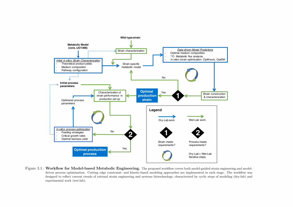
Metabolic Model(core, iJO1366)
Initial in silico Strain Characterization- Theoretical product yields- Medium composition- Pathway configuration
Strain-specificmetabolic model
Strain construction& characterization
Data-driven Model Predictions- Optimal medium composition- 13C- Metabolic flux analysis.- In silico strain optimization: OptKnock, OptEM
Wild-type strain
Strain characterization
1
In silico process optimization- Feeding strategies- Critical growth rates- Optimal biomass yield
Optimal production
strain
Characterization of strain performance in
production set upOptimized process parameters
Optimal productionprocess
Initial process parameters
Dry-Lab work
Strain meets requirements?
Process meets requirements?
Yes
No
Yes
No
Dry-Lab + Wet-Lab Iterative steps
Wet-Lab work
2 1 2
Legend
Figure 3.1.: Workflow for Model-based Metabolic Engineering. The proposed workflow covers both model-guided strain engineering and model-driven process optimization. Cutting edge constraint- and kinetic-based modeling approaches are implemented in each stage. The workflow wasdesigned to reflect current trends of rational strain engineering and systems biotechnology, characterized by cyclic steps of modeling (dry-lab) andexperimental work (wet-lab).

Part II.
Results: Strain Engineering
35

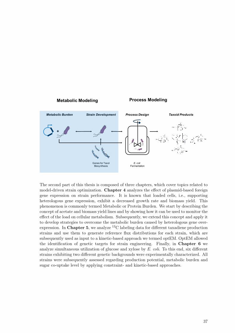
Taxoid ProductsMetabolic Burden
Genes for TaxolBiosynthesis
E. coli Fermentation
+
Metabolic Modeling Process Modeling
Strain Development Process Design
The second part of this thesis is composed of three chapters, which cover topics related tomodel-driven strain optimization. Chapter 4 analyzes the effect of plasmid-based foreigngene expression on strain performance. It is known that loaded cells, i.e., supportingheterologous gene expression, exhibit a decreased growth rate and biomass yield. Thisphenomenon is commonly termed Metabolic or Protein Burden. We start by describing theconcept of acetate and biomass yield lines and by showing how it can be used to monitor theeffect of the load on cellular metabolism. Subsequently, we extend this concept and apply itto develop strategies to overcome the metabolic burden caused by heterologous gene over-expression. In Chapter 5, we analyze 13C labeling data for different taxadiene productionstrains and use them to generate reference flux distributions for each strain, which aresubsequently used as input to a kinetic-based approach we termed optEM. OptEM allowedthe identification of genetic targets for strain engineering. Finally, in Chapter 6 weanalyze simultaneous utilization of glucose and xylose by E. coli. To this end, six differentstrains exhibiting two different genetic backgrounds were experimentally characterized. Allstrains were subsequently assessed regarding production potential, metabolic burden andsugar co-uptake level by applying constraint- and kinetic-based approaches.
37

4. Metabolic Burden
In order to analyze the detrimental effect that gene over-expression has on strain perform-ance, our cooperation partner Sabine Wagner at Fachgebiet Systembiotechnologie (SBT)designed, constructed and experimentally characterized three strains, each of which exhib-ited a different protein load, as shown in Figure 4.1. Strain cultivation was conducted inshaking flasks. Five different carbon sources were used to obtain a relatively wide rangeof growth rates, ranging from approximately 0.2 1/h for acetate, to almost 0.5 1/h forglucose. We used a constraint-based approach to qualitatively reproduce observed acetatesecretion patterns in the three strains. As previously described [11], acetate lines can beused as an indicator of cellular fitness. We found a connection between biomass yieldlines and acetate lines. The point where the slope of the biomass yield line is decreasedfor the first time defines a threshold beyond which cellular growth is always accompaniedby acetate secretion under aerobic conditions. By analyzing acetate secretion patterns ofstrains exhibiting different burden levels, we hypothesize that cells growing below a cer-tain threshold can fulfill the imposed burden, while simultaneously growing with wild-typeyields. Our in silico analysis also suggests that acetate lines do not have a unique slopeas initially suggested, but are rather composed of at least two straight lines with differentslopes.
4.1. Strains & Experimental Data
Main genetic features of the strains analyzed in this chapter are shown in Figure 4.1. Thestrains were designed by Sabine Wagner to exhibit an increasing protein burden. Thefluorescent protein mCherry was used as a monitor of the cellular capacity, by placing thetranscription of the mCherry gene under the control of a constitutive promotor. On theother hand, the protein eGFP was used to load the cell. Since both mCherry and eGFP arefluorescent proteins, their synthesis can be easily determined by measuring light emissionat different wavelengths.
Five different carbon sources - glucose, mannose, fructose, galactose and acetate - wereused to allow for the analysis of the metabolic burden (caused by plasmid-based heterolog-ous gene expression) at different growth rates. Experimental strain characterization wasconducted in shaking flask at 37°C and 200 revolutions per minute (rpm). Additional tolight emission at mCherry- and eGFP-specific wavelengths, time courses for OD, substrateand acetate concentration were experimentally determined (see Appendix A.1.3 for rawdata). Calculated rates for glucose as carbon source are exemplarily provided in Table 4.1.Refer to Appendix A.1.3, Table A.6 for a complete overview of the results.
In order to analyze the effect of gene over-expression on growth rate and biomass yield,we plot growth rates versus substrate uptake rates for all strains and substrates (Figure
39
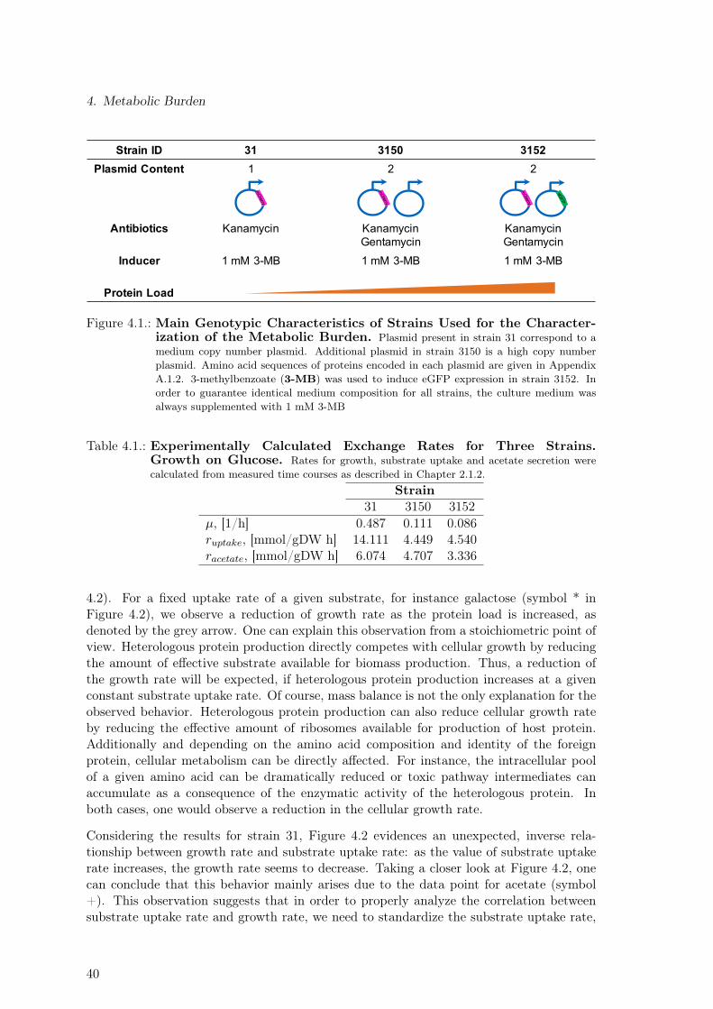
4. Metabolic Burden
Strain ID 31 3150 3152Plasmid Content 1 2 2
Antibiotics Kanamycin KanamycinGentamycin
KanamycinGentamycin
Inducer 1 mM 3-MB 1 mM 3-MB 1 mM 3-MB
Protein Load
Figure 4.1.: Main Genotypic Characteristics of Strains Used for the Character-ization of the Metabolic Burden. Plasmid present in strain 31 correspond to amedium copy number plasmid. Additional plasmid in strain 3150 is a high copy numberplasmid. Amino acid sequences of proteins encoded in each plasmid are given in AppendixA.1.2. 3-methylbenzoate (3-MB) was used to induce eGFP expression in strain 3152. Inorder to guarantee identical medium composition for all strains, the culture medium wasalways supplemented with 1 mM 3-MB
Table 4.1.: Experimentally Calculated Exchange Rates for Three Strains.Growth on Glucose. Rates for growth, substrate uptake and acetate secretion werecalculated from measured time courses as described in Chapter 2.1.2.
Strain31 3150 3152
µ, [1/h] 0.487 0.111 0.086ruptake, [mmol/gDW h] 14.111 4.449 4.540racetate, [mmol/gDW h] 6.074 4.707 3.336
4.2). For a fixed uptake rate of a given substrate, for instance galactose (symbol * inFigure 4.2), we observe a reduction of growth rate as the protein load is increased, asdenoted by the grey arrow. One can explain this observation from a stoichiometric point ofview. Heterologous protein production directly competes with cellular growth by reducingthe amount of effective substrate available for biomass production. Thus, a reduction ofthe growth rate will be expected, if heterologous protein production increases at a givenconstant substrate uptake rate. Of course, mass balance is not the only explanation for theobserved behavior. Heterologous protein production can also reduce cellular growth rateby reducing the effective amount of ribosomes available for production of host protein.Additionally and depending on the amino acid composition and identity of the foreignprotein, cellular metabolism can be directly affected. For instance, the intracellular poolof a given amino acid can be dramatically reduced or toxic pathway intermediates canaccumulate as a consequence of the enzymatic activity of the heterologous protein. Inboth cases, one would observe a reduction in the cellular growth rate.
Considering the results for strain 31, Figure 4.2 evidences an unexpected, inverse rela-tionship between growth rate and substrate uptake rate: as the value of substrate uptakerate increases, the growth rate seems to decrease. Taking a closer look at Figure 4.2, onecan conclude that this behavior mainly arises due to the data point for acetate (symbol+). This observation suggests that in order to properly analyze the correlation betweensubstrate uptake rate and growth rate, we need to standardize the substrate uptake rate,
40
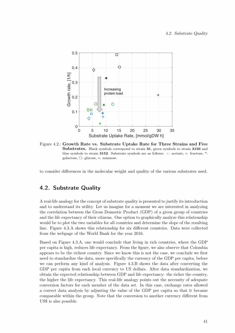
4.2. Substrate Quality
0 5 10 15 20 25 30 35Substrate Uptake Rate, [mmol/gDW h]
0
0.1
0.2
0.3
0.4
0.5
Gro
wth
rate
, [1/
h]
Increasing protein load
Figure 4.2.: Growth Rate vs. Substrate Uptake Rate for Three Strains and FiveSubstrates. Black symbols correspond to strain 31, green symbols to strain 3150 andblue symbols to strain 3152. Substrate symbols are as follows: +: acetate, ◦: fructose, *:galactose, �: glucose, �: mannose.
to consider differences in the molecular weight and quality of the various substrates used.
4.2. Substrate Quality
A real-life analogy for the concept of substrate quality is presented to justify its introductionand to understand its utility. Let us imagine for a moment we are interested in analyzingthe correlation between the Gross Domestic Product (GDP) of a given group of countriesand the life expectancy of their citizens. One option to graphically analyze this relationshipwould be to plot the two variables for all countries and determine the slope of the resultingline. Figure 4.3.A shows this relationship for six different countries. Data were collectedfrom the webpage of the World Bank for the year 2016.
Based on Figure 4.3.A, one would conclude that living in rich countries, where the GDPper capita is high, reduces life expectancy. From the figure, we also observe that Colombiaappears to be the richest country. Since we know this is not the case, we conclude we firstneed to standardize the data, more specifically the currency of the GDP per capita, beforewe can perform any kind of analysis. Figure 4.3.B shows the data after converting theGDP per capita from each local currency to US dollars. After data standardization, weobtain the expected relationship between GDP and life expectancy: the richer the country,the higher the life expectancy. This real-life analogy points out the necessity of adequateconversion factors for each member of the data set. In this case, exchange rates alloweda correct data analysis by adjusting the value of the GDP per capita so that it becamecomparable within the group. Note that the conversion to another currency different fromUS$ is also possible.
41
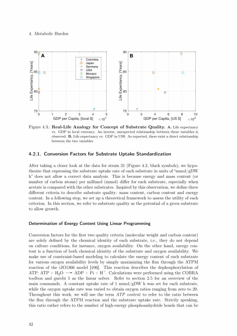
4. Metabolic Burden
0 1 2 3 4 5GDP per Capita, [local $] 107
75
80
85
90
Life
Exp
enta
ncy,
[Yea
rs]
0 2 4 6 8 10GDP per Capita, [US $] 104
75
80
85
90
Life
Exp
enta
ncy,
[Yea
rs]Colombia
JapanGermanyUSAMonacoSingapore
A B
Figure 4.3.: Real-Life Analogy for Concept of Substrate Quality. A. Life expectancyvs. GDP in local currency. An inverse, unexpected relationship between these variables isobserved. B. Life expectancy vs. GDP in US$. As expected, there exist a direct relationshipbetween the two variables
4.2.1. Conversion Factors for Substrate Uptake Standardization
After taking a closer look at the data for strain 31 (Figure 4.2, black symbols), we hypo-thesize that expressing the substrate uptake rate of each substrate in units of “mmol/gDWh” does not allow a correct data analysis. This is because energy and mass content (ornumber of carbon atoms) per millimol (mmol) differ for each substrate, especially whenacetate is compared with the other substrates. Inspired by this observation, we define threedifferent criteria to describe substrate quality: mass content, carbon content and energycontent. In a following step, we set up a theoretical framework to assess the utility of eachcriterion. In this section, we refer to substrate quality as the potential of a given substrateto allow growth.
Determination of Energy Content Using Linear Programming
Conversion factors for the first two quality criteria (molecular weight and carbon content)are solely defined by the chemical identity of each substrate, i.e., they do not dependon culture conditions, for instance, oxygen availability. On the other hand, energy con-tent is a function of both chemical identity of the substrate and oxygen availability. Wemake use of constraint-based modeling to calculate the energy content of each substratefor various oxygen availability levels by simply maximizing the flux through the ATPMreaction of the iJO1366 model [106]. This reaction describes the dephosphorylation ofATP: ATP + H2O ADP + Pi + H+. Calculations were performed using the COBRAtoolbox and gurobi 5 as the linear solver. Refer to section 2.5 for an overview of themain commands. A constant uptake rate of 1 mmol/gDW h was set for each substrate,while the oxygen uptake rate was varied to obtain oxygen ratios ranging from zero to 20.Throughout this work, we will use the term ATP content to refer to the ratio betweenthe flux through the ATPM reaction and the substrate uptake rate. Strictly speaking,this ratio rather refers to the number of high-energy phosphoanhydride bonds that can be
42
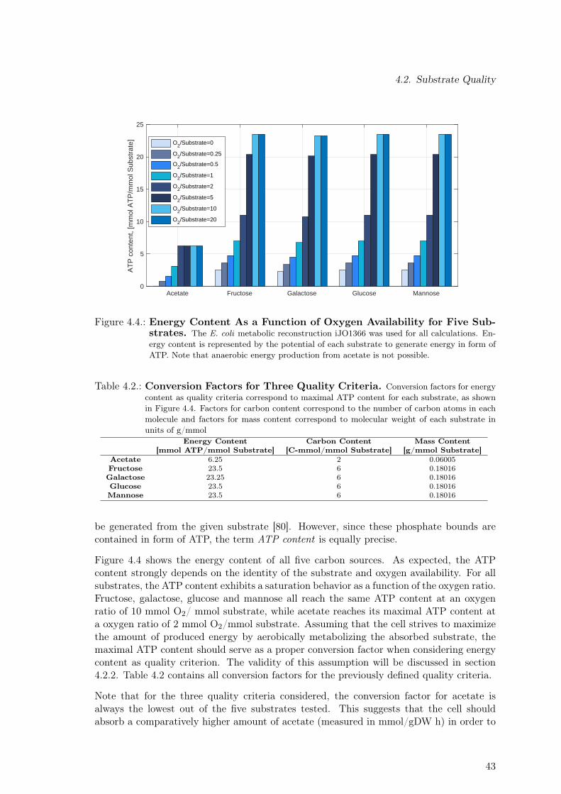
4.2. Substrate Quality
Acetate Fructose Galactose Glucose Mannose0
5
10
15
20
25A
TP
con
tent
, [m
mol
AT
P/m
mol
Sub
stra
te] O2/Substrate=0
O2/Substrate=0.25
O2/Substrate=0.5
O2/Substrate=1
O2/Substrate=2
O2/Substrate=5
O2/Substrate=10
O2/Substrate=20
Figure 4.4.: Energy Content As a Function of Oxygen Availability for Five Sub-strates. The E. coli metabolic reconstruction iJO1366 was used for all calculations. En-ergy content is represented by the potential of each substrate to generate energy in form ofATP. Note that anaerobic energy production from acetate is not possible.
Table 4.2.: Conversion Factors for Three Quality Criteria. Conversion factors for energycontent as quality criteria correspond to maximal ATP content for each substrate, as shownin Figure 4.4. Factors for carbon content correspond to the number of carbon atoms in eachmolecule and factors for mass content correspond to molecular weight of each substrate inunits of g/mmol
Energy Content[mmol ATP/mmol Substrate]
Carbon Content[C-mmol/mmol Substrate]
Mass Content[g/mmol Substrate]
Acetate 6.25 2 0.06005Fructose 23.5 6 0.18016Galactose 23.25 6 0.18016Glucose 23.5 6 0.18016Mannose 23.5 6 0.18016
be generated from the given substrate [80]. However, since these phosphate bounds arecontained in form of ATP, the term ATP content is equally precise.
Figure 4.4 shows the energy content of all five carbon sources. As expected, the ATPcontent strongly depends on the identity of the substrate and oxygen availability. For allsubstrates, the ATP content exhibits a saturation behavior as a function of the oxygen ratio.Fructose, galactose, glucose and mannose all reach the same ATP content at an oxygenratio of 10 mmol O2/ mmol substrate, while acetate reaches its maximal ATP content ata oxygen ratio of 2 mmol O2/mmol substrate. Assuming that the cell strives to maximizethe amount of produced energy by aerobically metabolizing the absorbed substrate, themaximal ATP content should serve as a proper conversion factor when considering energycontent as quality criterion. The validity of this assumption will be discussed in section4.2.2. Table 4.2 contains all conversion factors for the previously defined quality criteria.
Note that for the three quality criteria considered, the conversion factor for acetate isalways the lowest out of the five substrates tested. This suggests that the cell shouldabsorb a comparatively higher amount of acetate (measured in mmol/gDW h) in order to
43
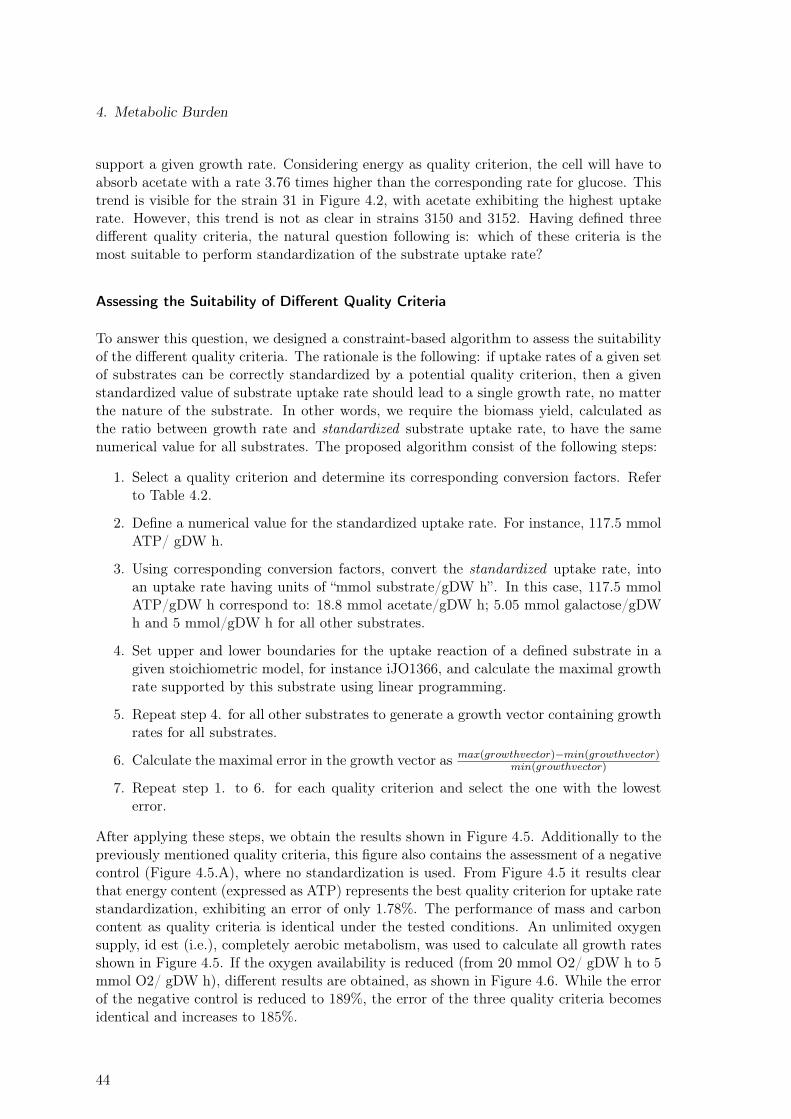
4. Metabolic Burden
support a given growth rate. Considering energy as quality criterion, the cell will have toabsorb acetate with a rate 3.76 times higher than the corresponding rate for glucose. Thistrend is visible for the strain 31 in Figure 4.2, with acetate exhibiting the highest uptakerate. However, this trend is not as clear in strains 3150 and 3152. Having defined threedifferent quality criteria, the natural question following is: which of these criteria is themost suitable to perform standardization of the substrate uptake rate?
Assessing the Suitability of Different Quality Criteria
To answer this question, we designed a constraint-based algorithm to assess the suitabilityof the different quality criteria. The rationale is the following: if uptake rates of a given setof substrates can be correctly standardized by a potential quality criterion, then a givenstandardized value of substrate uptake rate should lead to a single growth rate, no matterthe nature of the substrate. In other words, we require the biomass yield, calculated asthe ratio between growth rate and standardized substrate uptake rate, to have the samenumerical value for all substrates. The proposed algorithm consist of the following steps:
1. Select a quality criterion and determine its corresponding conversion factors. Referto Table 4.2.
2. Define a numerical value for the standardized uptake rate. For instance, 117.5 mmolATP/ gDW h.
3. Using corresponding conversion factors, convert the standardized uptake rate, intoan uptake rate having units of “mmol substrate/gDW h”. In this case, 117.5 mmolATP/gDW h correspond to: 18.8 mmol acetate/gDW h; 5.05 mmol galactose/gDWh and 5 mmol/gDW h for all other substrates.
4. Set upper and lower boundaries for the uptake reaction of a defined substrate in agiven stoichiometric model, for instance iJO1366, and calculate the maximal growthrate supported by this substrate using linear programming.
5. Repeat step 4. for all other substrates to generate a growth vector containing growthrates for all substrates.
6. Calculate the maximal error in the growth vector as max(growthvector)−min(growthvector)min(growthvector)
7. Repeat step 1. to 6. for each quality criterion and select the one with the lowesterror.
After applying these steps, we obtain the results shown in Figure 4.5. Additionally to thepreviously mentioned quality criteria, this figure also contains the assessment of a negativecontrol (Figure 4.5.A), where no standardization is used. From Figure 4.5 it results clearthat energy content (expressed as ATP) represents the best quality criterion for uptake ratestandardization, exhibiting an error of only 1.78%. The performance of mass and carboncontent as quality criteria is identical under the tested conditions. An unlimited oxygensupply, id est (i.e.), completely aerobic metabolism, was used to calculate all growth ratesshown in Figure 4.5. If the oxygen availability is reduced (from 20 mmol O2/ gDW h to 5mmol O2/ gDW h), different results are obtained, as shown in Figure 4.6. While the errorof the negative control is reduced to 189%, the error of the three quality criteria becomesidentical and increases to 185%.
44
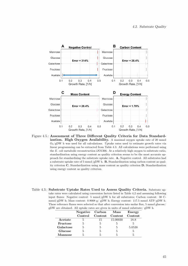
4.2. Substrate Quality
Error = 314% Error = 28.4%
Error = 28.4% Error = 1.78%
A B
DC
Figure 4.5.: Assessment of Three Different Quality Criteria for Data Standard-ization. High Oxygen Availability. A maximal oxygen uptake rate of 20 mmolO2/gDW h was used for all calculations. Uptake rates used to estimate growth rates vialinear programming can be extracted from Table 4.3. All calculations were performed usingthe E. coli metabolic reconstruction iJO1366. At a relatively high oxygen to substrate ratio,standardization using energy content as quality criterion seems to be the most accurate ap-proach for standardizing the substrate uptake rate. A. Negative control. All substrates hada substrate uptake rate of 5 mmol/gDW h. B. Standardization using carbon content as qual-ity criterion C. Standardization using mass content as quality criterion D. Standardizationusing energy content as quality criterion.
Table 4.3.: Substrate Uptake Rates Used to Assess Quality Criteria. Substrate up-take rates were calculated using conversion factors listed in Table 4.2 and assuming followinginput fluxes: Negative control: 5 mmol/gDW h for all substrates; Carbon content: 30 C-mmol/gDW h; Mass content: 0.9008 g/ gDW h; Energy content: 117.5 mmol ATP/gDW h.These reference fluxes were selected so that after conversion into molar flux, 5 mmol glucose/gDW are obtained. All uptake rates are given in units of mmol substrate/ gDW h.
NegativeControl
CarbonContent
MassContent
EnergyContent
Acetate 5 15 15.00030 18.8Fructose 5 5 5 5Galactose 5 5 5 5.0538Glucose 5 5 5 5Mannose 5 5 5 5
45
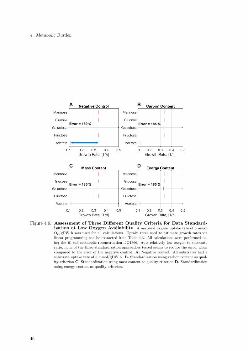
4. Metabolic Burden
Error = 189 % Error = 185 %
Error = 185 % Error = 185 %
A B
DC
Figure 4.6.: Assessment of Three Different Quality Criteria for Data Standard-ization at Low Oxygen Availability. A maximal oxygen uptake rate of 5 mmolO2/gDW h was used for all calculations. Uptake rates used to estimate growth rates vialinear programming can be extracted from Table 4.3. All calculations were performed us-ing the E. coli metabolic reconstruction iJO1366. At a relatively low oxygen to substrateratio, none of the three standardization approaches tested seems to reduce the error, whencompared to the error of the negative control. A. Negative control. All substrates had asubstrate uptake rate of 5 mmol/gDW h. B. Standardization using carbon content as qual-ity criterion C. Standardization using mass content as quality criterion D. Standardizationusing energy content as quality criterion.
46
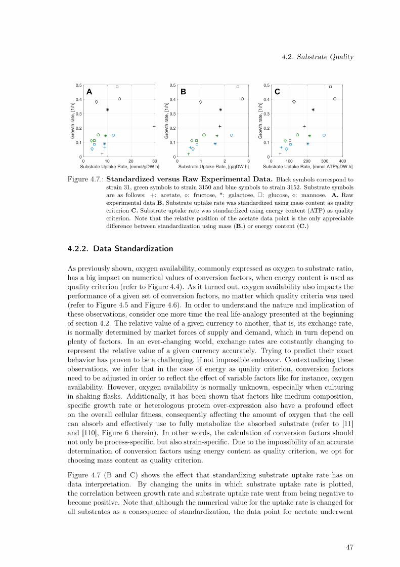
4.2. Substrate Quality
0 10 20 30Substrate Uptake Rate, [mmol/gDW h]
0
0.1
0.2
0.3
0.4
0.5
Gro
wth
rate
, [1/
h]
0 1 2 3Substrate Uptake Rate, [g/gDW h]
0
0.1
0.2
0.3
0.4
0.5
Gro
wth
rate
, [1/
h]0 100 200 300 400
Substrate Uptake Rate, [mmol ATP/gDW h]
0
0.1
0.2
0.3
0.4
0.5
Gro
wth
rate
, [1/
h]
A B C
Figure 4.7.: Standardized versus Raw Experimental Data. Black symbols correspond tostrain 31, green symbols to strain 3150 and blue symbols to strain 3152. Substrate symbolsare as follows: +: acetate, ◦: fructose, *: galactose, �: glucose, �: mannose. A. Rawexperimental data B. Substrate uptake rate was standardized using mass content as qualitycriterion C. Substrate uptake rate was standardized using energy content (ATP) as qualitycriterion. Note that the relative position of the acetate data point is the only appreciabledifference between standardization using mass (B.) or energy content (C.)
4.2.2. Data Standardization
As previously shown, oxygen availability, commonly expressed as oxygen to substrate ratio,has a big impact on numerical values of conversion factors, when energy content is used asquality criterion (refer to Figure 4.4). As it turned out, oxygen availability also impacts theperformance of a given set of conversion factors, no matter which quality criteria was used(refer to Figure 4.5 and Figure 4.6). In order to understand the nature and implication ofthese observations, consider one more time the real life-analogy presented at the beginningof section 4.2. The relative value of a given currency to another, that is, its exchange rate,is normally determined by market forces of supply and demand, which in turn depend onplenty of factors. In an ever-changing world, exchange rates are constantly changing torepresent the relative value of a given currency accurately. Trying to predict their exactbehavior has proven to be a challenging, if not impossible endeavor. Contextualizing theseobservations, we infer that in the case of energy as quality criterion, conversion factorsneed to be adjusted in order to reflect the effect of variable factors like for instance, oxygenavailability. However, oxygen availability is normally unknown, especially when culturingin shaking flasks. Additionally, it has been shown that factors like medium composition,specific growth rate or heterologous protein over-expression also have a profound effecton the overall cellular fitness, consequently affecting the amount of oxygen that the cellcan absorb and effectively use to fully metabolize the absorbed substrate (refer to [11]and [110], Figure 6 therein). In other words, the calculation of conversion factors shouldnot only be process-specific, but also strain-specific. Due to the impossibility of an accuratedetermination of conversion factors using energy content as quality criterion, we opt forchoosing mass content as quality criterion.
Figure 4.7 (B and C) shows the effect that standardizing substrate uptake rate has ondata interpretation. By changing the units in which substrate uptake rate is plotted,the correlation between growth rate and substrate uptake rate went from being negative tobecome positive. Note that although the numerical value for the uptake rate is changed forall substrates as a consequence of standardization, the data point for acetate underwent
47
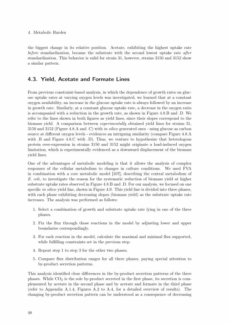
4. Metabolic Burden
the biggest change in its relative position. Acetate, exhibiting the highest uptake ratebefore standardization, became the substrate with the second lowest uptake rate afterstandardization. This behavior is valid for strain 31, however, strains 3150 and 3152 showa similar pattern.
4.3. Yield, Acetate and Formate Lines
From previous constraint-based analysis, in which the dependence of growth rates on gluc-ose uptake rates at varying oxygen levels was investigated, we learned that at a constantoxygen availability, an increase in the glucose uptake rate is always followed by an increasein growth rate. Similarly, at a constant glucose uptake rate, a decrease in the oxygen ratiois accompanied with a reduction in the growth rate, as shown in Figure 4.8.B and .D. Werefer to the lines shown in both figures as yield lines, since their slopes correspond to thebiomass yield. A comparison between experimentally obtained yield lines for strains 31,3150 and 3152 (Figure 4.8.A and .C) with in silico generated ones - using glucose as carbonsource at different oxygen levels - evidences an intriguing similarity (compare Figure 4.8.Awith .B and Figure 4.8.C with .D). Thus, we venture to hypothesize that heterologousprotein over-expression in strains 3150 and 3152 might originate a load-induced oxygenlimitation, which is experimentally evidenced as a downward displacement of the biomassyield lines.
One of the advantages of metabolic modeling is that it allows the analysis of complexresponses of the cellular metabolism to changes in culture conditions. We used FVAin combination with a core metabolic model [107], describing the central metabolism ofE. coli , to investigate the reason for the systematic reduction of biomass yield at highersubstrate uptake rates observed in Figure 4.8.B and .D. For our analysis, we focused on onespecific in silico yield line, shown in Figure 4.9. This yield line is divided into three phases,with each phase exhibiting decreasing slopes (biomass yield) as the substrate uptake rateincreases. The analysis was performed as follows:
1. Select a combination of growth and substrate uptake rate lying in one of the threephases.
2. Fix the flux through those reactions in the model by adjusting lower and upperboundaries correspondingly.
3. For each reaction in the model, calculate the maximal and minimal flux supported,while fulfilling constraints set in the previous step.
4. Repeat step 1 to step 3 for the other two phases.
5. Compare flux distribution ranges for all three phases, paying special attention toby-product secretion patterns.
This analysis identified clear differences in the by-product secretion patterns of the threephases. While CO2 is the sole by-product secreted in the first phase, its secretion is com-plemented by acetate in the second phase and by acetate and formate in the third phase(refer to Appendix A.1.4, Figures A.2 to A.4, for a detailed overview of results). Thechanging by-product secretion pattern can be understood as a consequence of decreasing
48
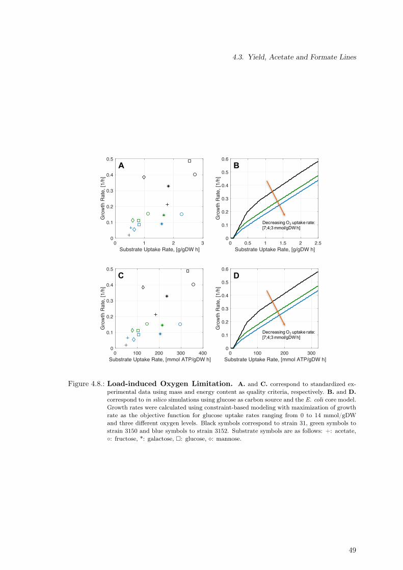
4.3. Yield, Acetate and Formate Lines
0 1 2 3Substrate Uptake Rate, [g/gDW h]
0
0.1
0.2
0.3
0.4
0.5
Gro
wth
Rat
e, [1
/h]
0 0.5 1 1.5 2 2.5Substrate Uptake Rate, [g/gDW h]
0
0.1
0.2
0.3
0.4
0.5
0.6
Gro
wth
Rat
e, [1
/h]
0 100 200 300 400Substrate Uptake Rate, [mmol ATP/gDW h]
0
0.1
0.2
0.3
0.4
0.5
Gro
wth
Rat
e, [1
/h]
0 100 200 300Substrate Uptake Rate, [mmol ATP/gDW h]
0
0.1
0.2
0.3
0.4
0.5
0.6
Gro
wth
Rat
e, [1
/h]
A B
C D
Decreasing O2 uptake rate: [7;4;3 mmol/gDW h]
Decreasing O2 uptake rate: [7;4;3 mmol/gDW h]
Figure 4.8.: Load-induced Oxygen Limitation. A. and C. correspond to standardized ex-perimental data using mass and energy content as quality criteria, respectively. B. and D.correspond to in silico simulations using glucose as carbon source and the E. coli core model.Growth rates were calculated using constraint-based modeling with maximization of growthrate as the objective function for glucose uptake rates ranging from 0 to 14 mmol/gDWand three different oxygen levels. Black symbols correspond to strain 31, green symbols tostrain 3150 and blue symbols to strain 3152. Substrate symbols are as follows: +: acetate,◦: fructose, *: galactose, �: glucose, �: mannose.
49
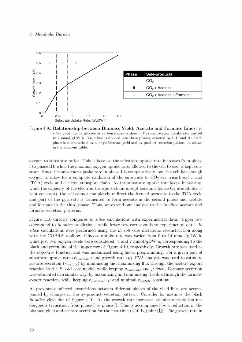
4. Metabolic Burden
0 0.5 1 1.5 2 2.5Substrate Uptake Rate, [g/gDW h]
0
0.1
0.2
0.3
0.4
0.5
0.6
Gro
wth
Rat
e, [1
/h]
Phase Side-productsI CO2
II CO2 + Acetate
III CO2 + Acetate + Formate
I II III
Figure 4.9.: Relationship between Biomass Yield, Acetate and Formate Lines. Insilico yield line for glucose as carbon source is shown. Maximal oxygen uptake rate was setto 7 mmol/gDW h. Yield line is divided into three phases, denoted by I, II and III. Eachphase is characterized by a single biomass yield and by-product secretion pattern, as shownin the adjacent table.
oxygen to substrate ratios. This is because the substrate uptake rate increases from phaseI to phase III, while the maximal oxygen uptake rate, allowed to the cell to use, is kept con-stant. Since the substrate uptake rate in phase I is comparatively low, the cell has enoughoxygen to allow for a complete oxidation of the substrate to CO2 via tricarboxylic acid(TCA) cycle and electron transport chain. As the substrate uptake rate keeps increasing,while the capacity of the electron transport chain is kept constant (since O2 availability iskept constant), the cell cannot completely redirect the formed pyruvate to the TCA cycleand part of the pyruvate is fermented to form acetate in the second phase and acetateand formate in the third phase. Thus, we extend our analysis to the in silico acetate andformate secretion patterns.
Figure 4.10 directly compares in silico calculations with experimental data. Upper rowcorrespond to in silico predictions, while lower row corresponds to experimental data. Insilico calculations were performed using the E. coli core metabolic reconstruction alongwith the COBRA toolbox. Glucose uptake rate was varied from 0 to 14 mmol/gDW h,while just two oxygen levels were considered: 4 and 7 mmol/gDW h, corresponding to theblack and green line of the upper row of Figure 4.10, respectively. Growth rate was used asthe objective function and was maximized using linear programming. For a given pair ofsubstrate uptake rate (rsubstrate) and growth rate (µ), FVA analysis was used to estimateacetate secretion (racetate) by minimizing and maximizing flux through the acetate exportreaction in the E. coli core model, while keeping rsubstrate and µ fixed. Formate secretionwas estimated in a similar way, by maximizing and minimizing the flux through the formateexport reaction, while keeping rsubstrate, µ and minimal racetate constant.
As previously inferred, transitions between different phases of the yield lines are accom-panied by changes in the by-product secretion pattern. Consider for instance the blackin silico yield line of Figure 4.10. As the growth rate increases, cellular metabolism un-dergoes a transition, from phase I to phase II. This is accompanied by a reduction in thebiomass yield and acetate secretion for the first time (4.10.B, point 1 ). The growth rate in
50
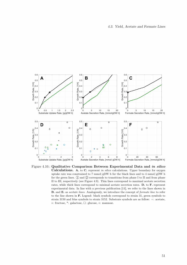
4.3. Yield, Acetate and Formate Lines
0 0.5 1 1.5 2 2.5Substrate Uptake Rate, [g/gDW h]
0
0.1
0.2
0.3
0.4
0.5
0.6
Gro
wth
Rat
e, [1
/h]
0 5 10 15 20Acetate Secretion Rate, [mmol/gDW h]
0
0.1
0.2
0.3
0.4
0.5
0.6G
row
th R
ate,
[1/h
]
0 5 10 15 20Formate Secretion Rate, [mmol/gDW h]
0
0.1
0.2
0.3
0.4
0.5
0.6
Gro
wth
Rat
e, [1
/h]
0 1 2 3Substrate Uptake Rate, [g/gDW h]
0
0.1
0.2
0.3
0.4
0.5
Gro
wth
Rat
e, [1
/h]
0 2 4 6 8Acetate Secretion Rate, [mmol/ gDW h]
0
0.1
0.2
0.3
0.4
0.5
Gro
wth
Rat
e, [1
/h]
0 20 40 60Formate Secretion Rate, [mmol/gDW h]
0
0.1
0.2
0.3
0.4
0.5G
row
th R
ate,
[1/h
]
A B C
D E F
1
2
1
2 2
Figure 4.10.: Qualitative Comparison Between Experimental Data and in silicoCalculations. A. to C. represent in silico calculations. Upper boundary for oxygenuptake rate was constrained to 7 mmol/gDW h for the black lines and to 4 mmol/gDW hfor the green lines. 1 and 2 corresponds to transitions from phase I to II and from phaseII to III, respectively (see Figure 4.9). Thin lines correspond to maximal acetate secretionrates, while thick lines correspond to minimal acetate secretion rates. D. to F. representexperimental data. In line with a previous publication [11], we refer to the lines shown inB. and E. as acetate lines. Analogously, we introduce the concept of formate line to referto the line shown in F. Legend: black symbols correspond to strain 31, green symbols tostrain 3150 and blue symbols to strain 3152. Substrate symbols are as follow: +: acetate,◦: fructose, *: galactose, �: glucose, �: mannose.
51
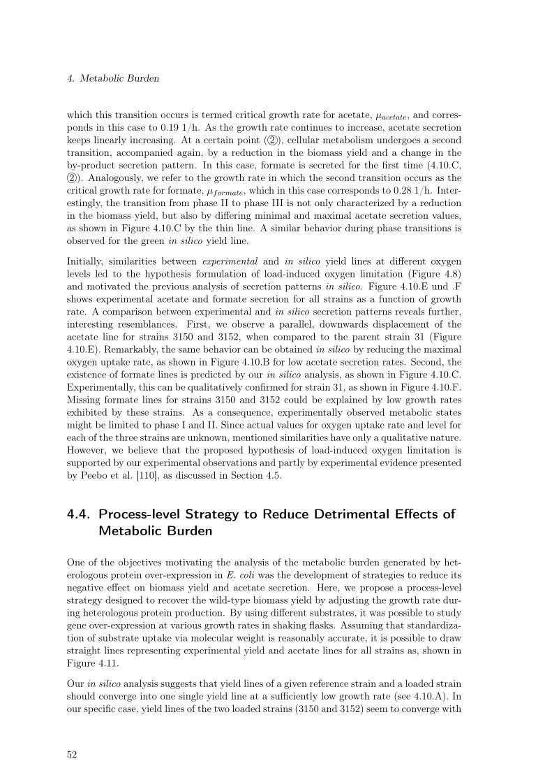
4. Metabolic Burden
which this transition occurs is termed critical growth rate for acetate, µacetate, and corres-ponds in this case to 0.19 1/h. As the growth rate continues to increase, acetate secretionkeeps linearly increasing. At a certain point ( 2 ), cellular metabolism undergoes a secondtransition, accompanied again, by a reduction in the biomass yield and a change in theby-product secretion pattern. In this case, formate is secreted for the first time (4.10.C,2 ). Analogously, we refer to the growth rate in which the second transition occurs as thecritical growth rate for formate, µformate, which in this case corresponds to 0.28 1/h. Inter-estingly, the transition from phase II to phase III is not only characterized by a reductionin the biomass yield, but also by differing minimal and maximal acetate secretion values,as shown in Figure 4.10.C by the thin line. A similar behavior during phase transitions isobserved for the green in silico yield line.
Initially, similarities between experimental and in silico yield lines at different oxygenlevels led to the hypothesis formulation of load-induced oxygen limitation (Figure 4.8)and motivated the previous analysis of secretion patterns in silico. Figure 4.10.E und .Fshows experimental acetate and formate secretion for all strains as a function of growthrate. A comparison between experimental and in silico secretion patterns reveals further,interesting resemblances. First, we observe a parallel, downwards displacement of theacetate line for strains 3150 and 3152, when compared to the parent strain 31 (Figure4.10.E). Remarkably, the same behavior can be obtained in silico by reducing the maximaloxygen uptake rate, as shown in Figure 4.10.B for low acetate secretion rates. Second, theexistence of formate lines is predicted by our in silico analysis, as shown in Figure 4.10.C.Experimentally, this can be qualitatively confirmed for strain 31, as shown in Figure 4.10.F.Missing formate lines for strains 3150 and 3152 could be explained by low growth ratesexhibited by these strains. As a consequence, experimentally observed metabolic statesmight be limited to phase I and II. Since actual values for oxygen uptake rate and level foreach of the three strains are unknown, mentioned similarities have only a qualitative nature.However, we believe that the proposed hypothesis of load-induced oxygen limitation issupported by our experimental observations and partly by experimental evidence presentedby Peebo et al. [110], as discussed in Section 4.5.
4.4. Process-level Strategy to Reduce Detrimental Effects ofMetabolic Burden
One of the objectives motivating the analysis of the metabolic burden generated by het-erologous protein over-expression in E. coli was the development of strategies to reduce itsnegative effect on biomass yield and acetate secretion. Here, we propose a process-levelstrategy designed to recover the wild-type biomass yield by adjusting the growth rate dur-ing heterologous protein production. By using different substrates, it was possible to studygene over-expression at various growth rates in shaking flasks. Assuming that standardiza-tion of substrate uptake via molecular weight is reasonably accurate, it is possible to drawstraight lines representing experimental yield and acetate lines for all strains as, shown inFigure 4.11.
Our in silico analysis suggests that yield lines of a given reference strain and a loaded strainshould converge into one single yield line at a sufficiently low growth rate (see 4.10.A). Inour specific case, yield lines of the two loaded strains (3150 and 3152) seem to converge with
52
4.4. Process-level Strategy to Reduce Detrimental Effects of Metabolic Burden
0 0.5 1 1.5 2 2.5 3Substrate Uptake Rate, [g/gDW h]
0
0.1
0.2
0.3
0.4
0.5
Gro
wth
Rat
e, [1
/h]
0 2 4 6 8Acetate Secretion Rate, [mmol/gDW h]
0
0.1
0.2
0.3
0.4
0.5
Gro
wth
Rat
e, [1
/h]
Wild-type biomass yield A B
∆= 𝑓(𝑙𝑜𝑎𝑑)
Figure 4.11.: Process-level Strategy to Reduce Metabolic Burden. A. Experimentalyield lines. B. Experimental acetate lines. Dashed lines were obtained using linear re-gression. Black symbols correspond to strain 31, green symbols to strain 3150 and bluesymbols to strain 3152. The metabolic burden (∆), defined as a reduction in µAcetate, isa function of the load exerted on the strain. We predict that by modulating the load instrain 3152, burden-free eGFP expression (blue region) can occur at higher growth rates,when compared to current load level. Substrate symbols are as follows: +: acetate, ◦:fructose, *: galactose, �: glucose, �: mannose. Critical growth rates for acetate secretionare: µ31
Acetate = 0.33, µ3150Acetate = 0.03, µ3152
Acetate = 0.022 1/h.
the reference strain (31) at the same point into one single yield line, as shown in Figure4.11.A. The growth rate at which yield lines converge can also be obtained from Figure4.11.B and corresponds to µAcetate of loaded strains. In theory, µAcetate for a given straindefines the transition from phase I to phase II, as discussed in section 4.3. Experimentallydetermined µAcetate for strains 3150 and 3152 (y-intercept of acetate lines shown in Figure4.11.B) are in accordance with their respective transition phases, obtained from Figure4.11.A. This observation provides further support for our load-induced oxygen limitationhypothesis. Additionally, in silico predictions generated by this analysis can be used toguide the design of a fed-batch process by providing a threshold for cellular growth ratethat should not be exceeded during the production phase, once the plasmid-based systemhas been induced. In this way, cells producing heterologous proteins will not secrete acetateand their biomass yield will be consequentially identical to that of the wild-type or thereference strain. The range of growth rates allowing protein over-expression with no burdenis highlighted in blue in Figure 4.11.A. For the concrete case of the eGFP over-productionin strain 3152, a critical growth rate for acetate of 0.022 1/h might cause this burden-freezone be too small to be technically and economically feasible. A potential solution to thisproblem would be to modulate the load imposed by the eGFP expression by using low-copyplasmids [58] and by tuning the strength of promoter and ribosome biding site. As a result,µ3152Acetate should increase, allowing a burden-free eGFP expression at much higher growth
rates than the current system.
53
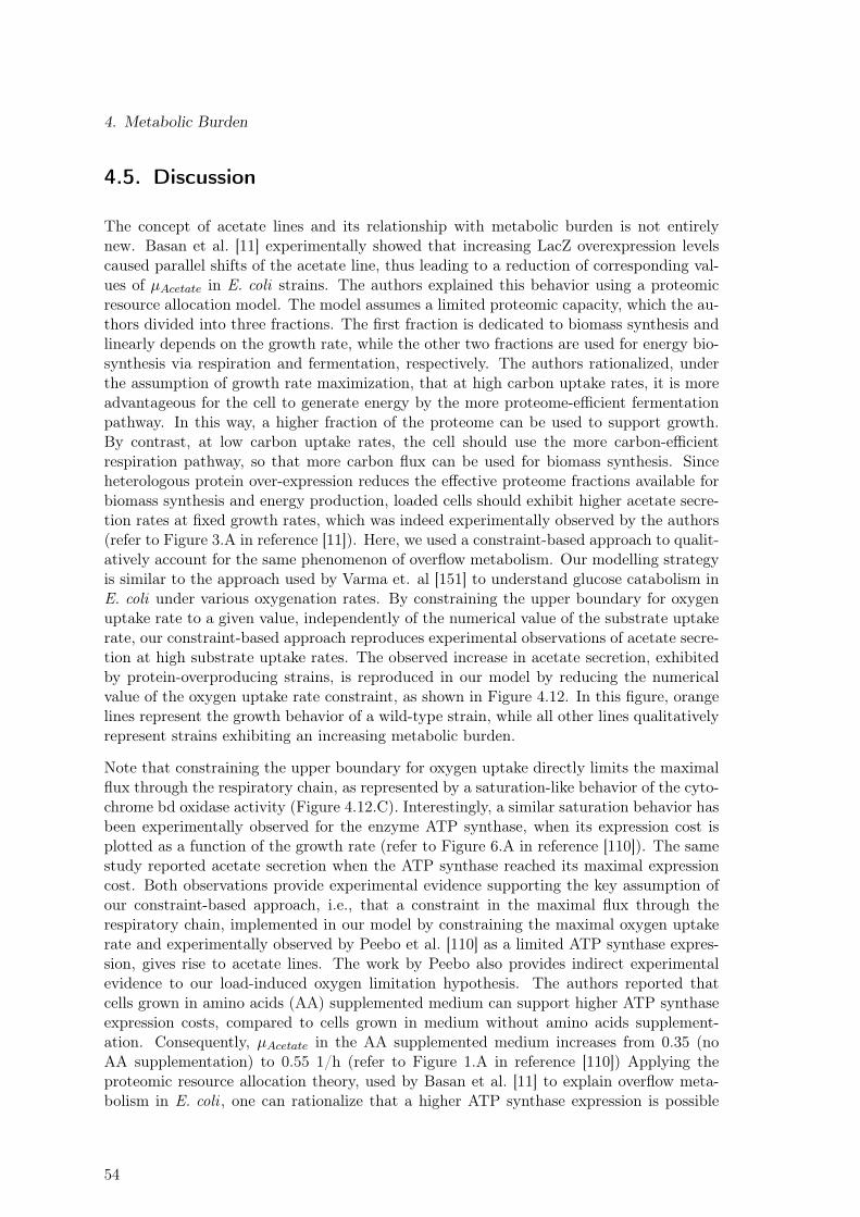
4. Metabolic Burden
4.5. Discussion
The concept of acetate lines and its relationship with metabolic burden is not entirelynew. Basan et al. [11] experimentally showed that increasing LacZ overexpression levelscaused parallel shifts of the acetate line, thus leading to a reduction of corresponding val-ues of µAcetate in E. coli strains. The authors explained this behavior using a proteomicresource allocation model. The model assumes a limited proteomic capacity, which the au-thors divided into three fractions. The first fraction is dedicated to biomass synthesis andlinearly depends on the growth rate, while the other two fractions are used for energy bio-synthesis via respiration and fermentation, respectively. The authors rationalized, underthe assumption of growth rate maximization, that at high carbon uptake rates, it is moreadvantageous for the cell to generate energy by the more proteome-efficient fermentationpathway. In this way, a higher fraction of the proteome can be used to support growth.By contrast, at low carbon uptake rates, the cell should use the more carbon-efficientrespiration pathway, so that more carbon flux can be used for biomass synthesis. Sinceheterologous protein over-expression reduces the effective proteome fractions available forbiomass synthesis and energy production, loaded cells should exhibit higher acetate secre-tion rates at fixed growth rates, which was indeed experimentally observed by the authors(refer to Figure 3.A in reference [11]). Here, we used a constraint-based approach to qualit-atively account for the same phenomenon of overflow metabolism. Our modelling strategyis similar to the approach used by Varma et. al [151] to understand glucose catabolism inE. coli under various oxygenation rates. By constraining the upper boundary for oxygenuptake rate to a given value, independently of the numerical value of the substrate uptakerate, our constraint-based approach reproduces experimental observations of acetate secre-tion at high substrate uptake rates. The observed increase in acetate secretion, exhibitedby protein-overproducing strains, is reproduced in our model by reducing the numericalvalue of the oxygen uptake rate constraint, as shown in Figure 4.12. In this figure, orangelines represent the growth behavior of a wild-type strain, while all other lines qualitativelyrepresent strains exhibiting an increasing metabolic burden.
Note that constraining the upper boundary for oxygen uptake directly limits the maximalflux through the respiratory chain, as represented by a saturation-like behavior of the cyto-chrome bd oxidase activity (Figure 4.12.C). Interestingly, a similar saturation behavior hasbeen experimentally observed for the enzyme ATP synthase, when its expression cost isplotted as a function of the growth rate (refer to Figure 6.A in reference [110]). The samestudy reported acetate secretion when the ATP synthase reached its maximal expressioncost. Both observations provide experimental evidence supporting the key assumption ofour constraint-based approach, i.e., that a constraint in the maximal flux through therespiratory chain, implemented in our model by constraining the maximal oxygen uptakerate and experimentally observed by Peebo et al. [110] as a limited ATP synthase expres-sion, gives rise to acetate lines. The work by Peebo also provides indirect experimentalevidence to our load-induced oxygen limitation hypothesis. The authors reported thatcells grown in amino acids (AA) supplemented medium can support higher ATP synthaseexpression costs, compared to cells grown in medium without amino acids supplement-ation. Consequently, µAcetate in the AA supplemented medium increases from 0.35 (noAA supplementation) to 0.55 1/h (refer to Figure 1.A in reference [110]) Applying theproteomic resource allocation theory, used by Basan et al. [11] to explain overflow meta-bolism in E. coli , one can rationalize that a higher ATP synthase expression is possible
54
4.5. Discussion
0 5 10 15Glucose Uptake Rate, [mmol/gDW h]
0
0.2
0.4
0.6
0.8
1
1.2
Gro
wth
Rat
e, [1
/h]
0 5 10 15 20Acetate Secretion Rate, [mmol/gDW h]
0
0.2
0.4
0.6
0.8
1
1.2
Gro
wth
Rat
e, [1
/h]
0 0.2 0.4 0.6 0.8 1 1.2Growth Rate, [1/h]
5
10
15
20
25
30
35
40
45
Flux
Thr
ough
CYT
BD,
[mm
ol/g
DW
h]
A B C
11
1
Figure 4.12.: Emergence of Yield and Acetate Lines By Constraining FluxThrough Respiratory Chain. The effect of constraining the upper boundaryfor oxygen uptake rate on biomass yield (A.); acetate lines -thin and thick lines corres-pond to maximal and minimal acetate secretion, respectively- (B.) and the flux throughrespiratory chain (C.) is shown. Simulations were performed using the E. coli core modeland a varying upper boundary for the oxygen uptake rate, as follows: green lines: 4mmol/gDW h; black lines: 7 mmol/gDW h; blue lines: 14 mmol/gDW h; orange lines:20 mmol/gDW h. CYTBD refers to the enzyme cytochrome bd oxidase, which producesa proton motive force in the E. coli core model by reducing oxygen to water as follows:2 h[c] + 1
2 o2[c] + q8h2[c] 2 h[e] + h2o[c] + q8[c]. q8h2 and q8 represent reduced andoxidized ubiquinone pools, respectively. Note that constraining the upper boundary of theoxygen uptake reaction directly limits the maximal flux through the enzyme CYTBD. In-terestingly, the growth rate at which the maximal CYTBD activity is reached correspondto the transition from phase I to phase II. This point is exemplarily marked for the bluelines 1 . Since the maximal respiration capacity is exhausted, the cell starts using ferment-ation pathways to generate energy. As a consequence, acetate is secreted and the biomassyield is reduced.
55
4. Metabolic Burden
because amino acid supplementation increases proteomic resources by reducing the frac-tion of the proteome that is dedicated to amino acid biosynthesis. Conversely, heterologousprotein overexpression would decrease proteomic resources available for biomass synthesisand energy generation, thus leading to a relative decrease in the maximal ATP synthaseexpression capacity and a consequent reduction in the flux through the respiratory chain.
Note that our simple constraint-based approach provides a flux-based explanation of theoverflow metabolism in E. coli and allows for the generation of multiple testable hypothesis:
1. Acetate lines are not always composed of a single straight line. Basan et al. [11]reported that plotting growth rates against acetate secretion rates leads to a straightline, which the authors termed acetate line. Here, we showed that this is only thecase, if acetate is the only fermentation product, i.e., cellular metabolism is confinedto phase II (refer to Figure 4.9 and 4.10). Experimental evidence reported by Peeboet al. [110] (refer to Figure 1.A therein) supports this hypothesis.
2. Protein over-expression originates a load-induced oxygen limitation, as discussed inSection 4.3.
3. There exist a relationship between biomass yield, acetate and formate lines, as dis-cussed in Section 4.3 and evidenced in Figure 4.10.A to .C.
4. Burden-free protein over-expression should possible for growth rates lower than µAcetate.Consequently, a process-level strategy, as discussed in Section 4.11, can be developedto minimize or eliminate the metabolic burden, expressed as a decrease in biomassyield along with an increase in acetate secretion rate.
Further experimental studies can be designed to test the above mentioned hypothesis.Since oxygen uptake rate plays a central role in both defining the cellular metabolic state(phase I, II or III) and estimating conversion factors used to standardize substrate uptakerates of different carbon sources when energy content is used a quality criterion, its ex-perimental determination should be prioritized. Similarly, experimental determination ofprotein content in loaded strains should be also considered in order to accurately describethe effect of protein over-expression on oxygen uptake capacity and proteome allocation.Finally, it is recommended that modeling efforts are only conducted on high-quality, re-producible data. Only under this circumstances the design-build-test-learn cycle can beoptimally executed.
56
5. Strain Design Algorithms for TargetIdentification
The EM approach developed by the James Liao group at the UC, Los Angeles was usedas framework to develop a strain design algorithm that we refer to as optEM. This al-gorithm uses EM to build an ensemble of kinetic models that fulfill a given reference fluxdistribution. optEM facilitates the maximization of complex user-tailored objective func-tions, for instance the weighted sum of volumetric productivity (mmol/l h), product yield(mmol/mmol) and production rate (mmol/gDW h). The kinetic nature of the optEM al-gorithm allows for consideration of typically inaccessible design parameters such as enzymeover-expression level, overall system stability and metabolite concentration pattern afterenzyme perturbation. Using the optEM approach, we identified many genetic targets thatwere already reported in the literature to have beneficial effects on taxadiene yield, thusconfirming the prediction power of our approach. We also identified targets not reportedin the literature yet [37].
5.1. Strains & Experimental Data
Five production strains were constructed and experimentally characterized by our cooper-ation partner Monica Fuchs at IBK. Table 5.1 describes main genetic features of each ofthe strains, which are schematically represented in Figure 5.1 for a better overview. Allstrains are provided with a genetic makeup necessary to synthesize taxadiene. In strains∆xylE_1p and ∆ptsG_1p, genes contained in plasmid pET28a_DS (ispF, ispD, idi anddxs) were genomically integrated in the xylE and ptsG position, respectively. In contrast,all enzymes required for the taxadiene biosynthesis are encoded in two plasmids in strains∆xylE_2p and ∆ptsG_2p. Refer to Table 5.1 for plasmid description. Gene integrationaimed at the reduction of the metabolic burden caused by heterologous enzyme expres-sion. Strain cultivation was performed in shaking flask (220 rpm) at 37°C using Riesenbergmedium with a mixture of 12C (4.5 g/l) and 13C (0.5 g/l) glucose as carbon source. Exper-imental strain characterization was performed in duplicate and consisted of measurementof concentration time courses for biomass, glucose and acetate. These data were processedas described in Chapter 2.1.2 in order to calculate growth, substrate uptake and acetatesecretion rates, respectively. Exchange rates and their standard deviations are reported inTable 5.2. Growth rates exhibit lower variability compared to acetate secretion rates (seeFigure 5.2). This is because growth rates were calculated based on OD time courses, whosemeasurements require a less extent of experimental handling compared to the determina-tion of glucose or acetate concentration time courses via HPLC measurements. Taxadienecould not be detected in the culture medium for any strain, due to low production ratesexhibited by all strains combined with low sample volumes. Additional to concentrationtime courses, 13C-labeling data were also available for all strains. These measurements
57
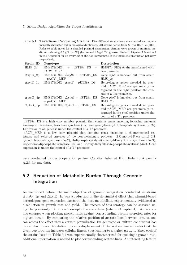
5. Strain Design Algorithms for Target Identification
Table 5.1.: Taxadiene Producing Strains. Five different strains were constructed and experi-mentally characterized in biological duplicates. All strains derive from E. coli HMS174(DE3).Refer to table notes for a detailed plasmid description. Strains were grown in minimal me-dium containing 0.5 g/l [U-13C] glucose and 4.5 g/l 12C glucose. Refer to Figures A.5 and A.7in the Appendix for an overview of the non-mevalonate & the taxadiene production pathway,respectively.
Strain ID Genotype DescriptionHMS_2p HMS174(DE3) + pET28a_DS +
pACY_MEPHMS174(DE3) strain transformed withtwo plasmids.
∆xylE_2p HMS174(DE3) ∆xylE + pET28a_DS+ pACY _MEP
Gene xylE is knocked out from strainHMS_2p
∆xylE_1p HMS174(DE3) ∆xylE + pET28a_DS Heterologous genes encoded in plas-mid pACY_MEP are genomically in-tegrated in the xylE position the con-trol of a Trc promoter.
∆ptsG_2p HMS174(DE3) ∆ptsG + pET28a_DS+ pACY _MEP
Gene ptsG is knocked out from strainHMS_2p.
∆ptsG_1p HMS174(DE3) ∆ptsG + pET28a_DS Heterologous genes encoded in plas-mid pACY_MEP are genomically in-tegrated in the ptsG position under thecontrol of a Trc promoter.
pET28a_DS is a high copy number plasmid that contains genes encoding following enzymes:kanamycin resistance, taxadiene synthase (txs) and geranylgeranyl diphosphate synthase (crtE ).Expression of all genes is under the control of a T7 promoter.pACY_MEP is a low copy plasmid that contains genes encoding a chlorampenicol res-istance and selected enzymes of the non-mevalonate pathway: 2-C-methyl-D-erythritol 2,4-cyclodiphosphate synthase (ispF ), 4-diphosphocytidyl-2C-methyl-D-erythritol synthase (ispD),isopentenyl-diphosphate isomerase (idi) and 1-deoxy-D-xylulose-5-phosphate synthase (dxs). Geneexpression is under the control of a T7 promoter.
were conducted by our cooperation partner Claudia Huber at Bio. Refer to AppendixA.2.3 for raw data.
5.2. Reduction of Metabolic Burden Through GenomicIntegration
As mentioned before, the main objective of genomic integration conducted in strains∆ptsG_1p and ∆xylE_1p was a reduction of the detrimental effect that plasmid-basedheterologous gene expression exerts on the host metabolism, experimentally evidenced asa reduction in growth rate and yield. The success of this strategy can be assessed us-ing the previously introduced concept of acetate lines (refer to Chapter 4). An acetateline emerges when plotting growth rates against corresponding acetate secretion rates fora given strain. By comparing the relative position of acetate lines between strains, onecan assess the effect that a certain perturbation (in genotype or culture conditions) hason cellular fitness. A relative upwards displacement of the acetate line indicates that thegiven perturbation increases cellular fitness, thus leading to a higher µAcetate. Since each ofthe strains listed in Table 5.1 was experimentally characterized for one single growth rate,additional information is needed to plot corresponding acetate lines. An interesting feature
58
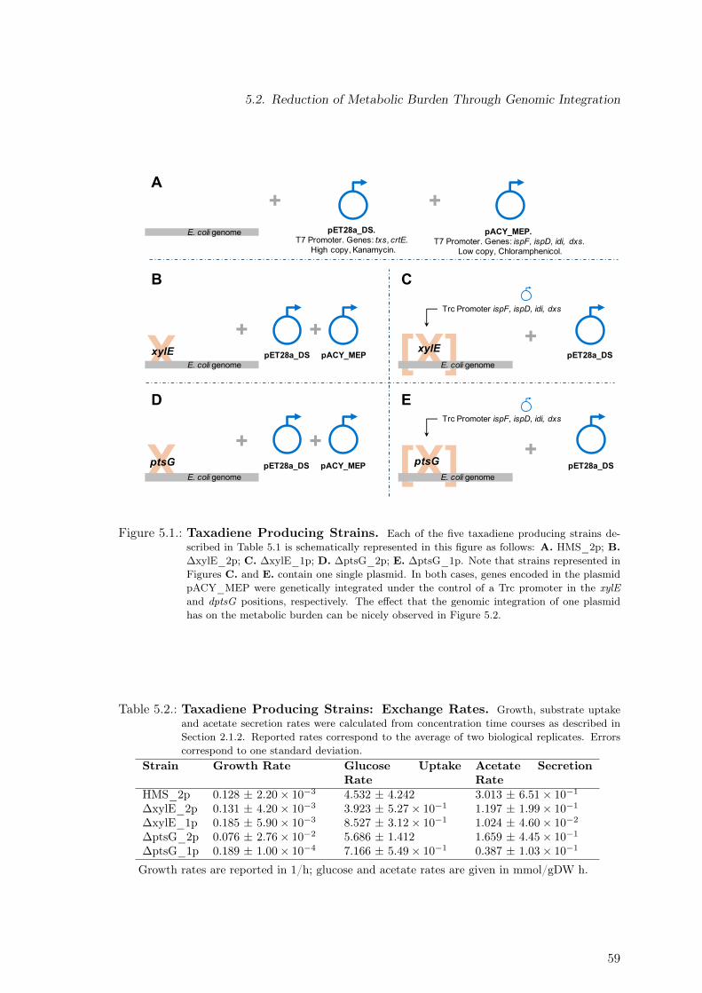
5.2. Reduction of Metabolic Burden Through Genomic Integration
XxylE
pET28a_DS.T7 Promoter. Genes: txs, crtE.
High copy, Kanamycin.
pACY_MEP.T7 Promoter. Genes: ispF, ispD, idi, dxs.
Low copy, Chloramphenicol.
[X]xylE
XptsG [X]ptsG
pET28a_DS pACY_MEP pET28a_DS
Trc Promoter ispF, ispD, idi, dxs
Trc Promoter ispF, ispD, idi, dxs
pET28a_DS
E. coli genome
A
B C
D E
E. coli genome
E. coli genome E. coli genome
E. coli genome
pET28a_DS pACY_MEP
+ +
+ +
+ +
+
+
Figure 5.1.: Taxadiene Producing Strains. Each of the five taxadiene producing strains de-scribed in Table 5.1 is schematically represented in this figure as follows: A. HMS_2p; B.∆xylE_2p; C. ∆xylE_1p; D. ∆ptsG_2p; E. ∆ptsG_1p. Note that strains represented inFigures C. and E. contain one single plasmid. In both cases, genes encoded in the plasmidpACY_MEP were genetically integrated under the control of a Trc promoter in the xylEand dptsG positions, respectively. The effect that the genomic integration of one plasmidhas on the metabolic burden can be nicely observed in Figure 5.2.
Table 5.2.: Taxadiene Producing Strains: Exchange Rates. Growth, substrate uptakeand acetate secretion rates were calculated from concentration time courses as described inSection 2.1.2. Reported rates correspond to the average of two biological replicates. Errorscorrespond to one standard deviation.
Strain Growth Rate Glucose UptakeRate
Acetate SecretionRate
HMS_2p 0.128 ± 2.20× 10⁻³ 4.532 ± 4.242 3.013 ± 6.51× 10⁻¹
∆xylE_2p 0.131 ± 4.20× 10⁻³ 3.923 ± 5.27× 10⁻¹ 1.197 ± 1.99× 10⁻¹
∆xylE_1p 0.185 ± 5.90× 10⁻³ 8.527 ± 3.12× 10⁻¹ 1.024 ± 4.60× 10⁻²
∆ptsG_2p 0.076 ± 2.76× 10⁻² 5.686 ± 1.412 1.659 ± 4.45× 10⁻¹
∆ptsG_1p 0.189 ± 1.00× 10⁻⁴ 7.166 ± 5.49× 10⁻¹ 0.387 ± 1.03× 10⁻¹
Growth rates are reported in 1/h; glucose and acetate rates are given in mmol/gDW h.
59
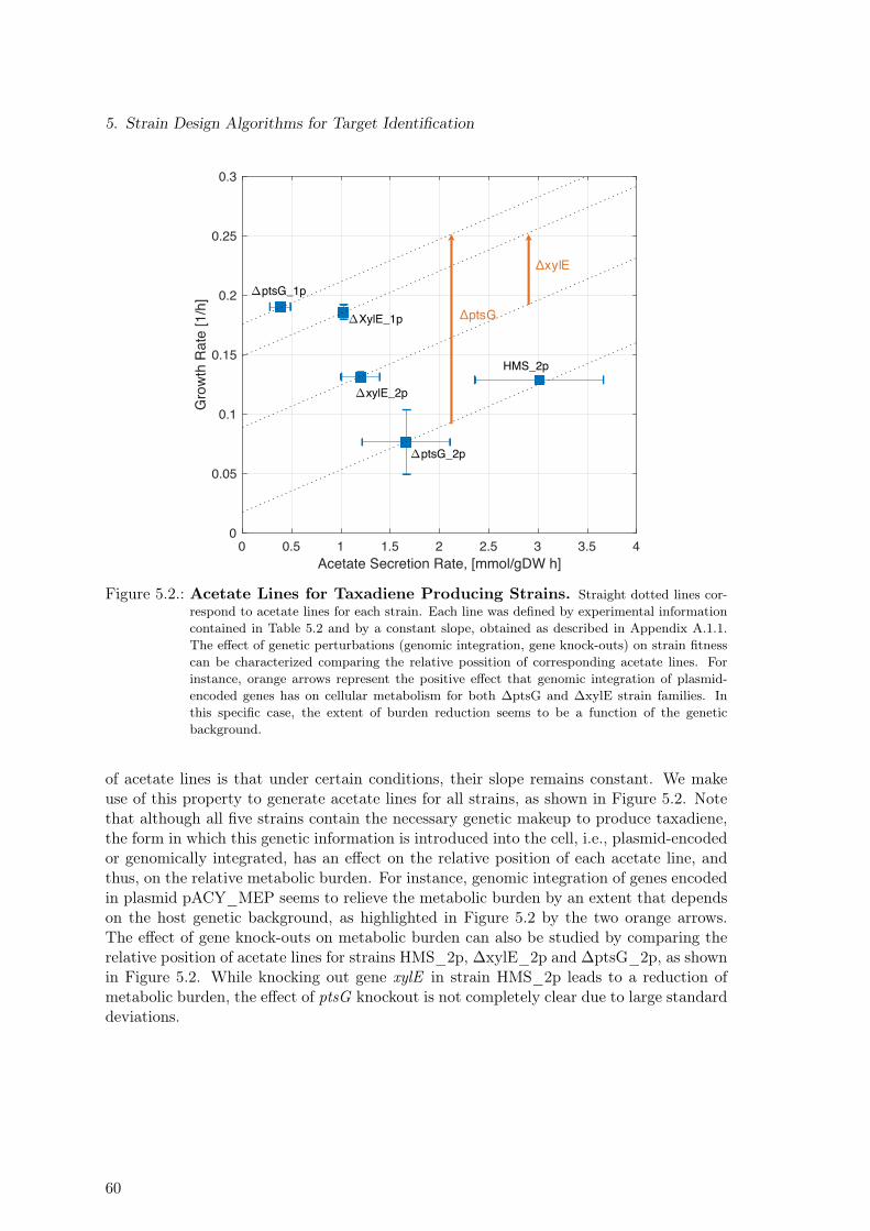
5. Strain Design Algorithms for Target Identification
0 0.5 1 1.5 2 2.5 3 3.5 4Acetate Secretion Rate, [mmol/gDW h]
0
0.05
0.1
0.15
0.2
0.25
0.3G
row
th R
ate
[1/h
]
HMS_2p
ptsG_2p
ptsG_1p
xylE_2p
XylE_1p
ΔxylE
ΔptsG
Figure 5.2.: Acetate Lines for Taxadiene Producing Strains. Straight dotted lines cor-respond to acetate lines for each strain. Each line was defined by experimental informationcontained in Table 5.2 and by a constant slope, obtained as described in Appendix A.1.1.The effect of genetic perturbations (genomic integration, gene knock-outs) on strain fitnesscan be characterized comparing the relative possition of corresponding acetate lines. Forinstance, orange arrows represent the positive effect that genomic integration of plasmid-encoded genes has on cellular metabolism for both ∆ptsG and ∆xylE strain families. Inthis specific case, the extent of burden reduction seems to be a function of the geneticbackground.
of acetate lines is that under certain conditions, their slope remains constant. We makeuse of this property to generate acetate lines for all strains, as shown in Figure 5.2. Notethat although all five strains contain the necessary genetic makeup to produce taxadiene,the form in which this genetic information is introduced into the cell, i.e., plasmid-encodedor genomically integrated, has an effect on the relative position of each acetate line, andthus, on the relative metabolic burden. For instance, genomic integration of genes encodedin plasmid pACY_MEP seems to relieve the metabolic burden by an extent that dependson the host genetic background, as highlighted in Figure 5.2 by the two orange arrows.The effect of gene knock-outs on metabolic burden can also be studied by comparing therelative position of acetate lines for strains HMS_2p, ∆xylE_2p and ∆ptsG_2p, as shownin Figure 5.2. While knocking out gene xylE in strain HMS_2p leads to a reduction ofmetabolic burden, the effect of ptsG knockout is not completely clear due to large standarddeviations.
60
5.3. Constraint-based Assessment of Taxadiene Production Potential
5.3. Constraint-based Assessment of Taxadiene ProductionPotential
The main objective of constructing strains listed in Table 5.1 was to generate a pool ofproduction strain candidates. Experimental data generated during strain characterization,including 13C-labeling data and concentration time courses for biomass, glucose and acet-ate should now be used to identify strains exhibiting a superior production performancefor further engineering rounds. Since taxadiene concentration could not be experiment-ally measured due to its presumably low concentration in the medium and to low samplevolume, our initial modeling efforts were focused on the estimation of production capabil-ities of each strain. We start our analysis by calculating flux ranges for each reaction in theE. coli central metabolism best matching experimentally measured amino acids labelingpatterns. For that, we used the software 13CFLUX2 [155] along with a modified versionof the E. coli metabolic model iRL2013 [75]. Refer to Section 2.1.2 for details on themetabolic model and mathematical implementation. The procedure can be summarizedas follows:
for each strain in Table 5.1:
1. Generate input file for the software 13CFLUX2 containing experimentally determinedexchange rates, as summarized in Table 5.2 and labeling data (refer to Table A.8 inthe Appendix). An exemplary input file can be found in Appendix A.2.4.
2. Calculate intracellular flux distribution that minimizes squared sum of residuals forlabeling data.
3. Apply statistical workflow described in Section 2.1.2 in order to calculate flux rangesfor free reactions.
4. Calculate flux ranges for each reaction in the metabolic network using flux variabilityanalysis (FVA) considering experimentally determined exchange rates and flux rangesfor free reactions calculated in the previous step.
5. Calculate maximal theoretical taxadiene yield as the ratio between taxadiene pro-duction rate and glucose uptake rate.
Calculated maximal theoretical taxadiene yields using the previously described steps areplotted in Figure 5.3 for all strains. At this point, it is important to state that productyields shown in Figure 5.3 are not experimental values, but rather a theoretical estimationrepresenting the potential of each strain to produce taxadiene with a certain product yield.One can clearly observe that a reduction in the metabolic burden in strains ∆xylE_1P and∆ptsG_1P, achieved by genomic integration of genes encoded in plasmid pACY_MEP,leads to a marked increase in the taxadiene production potential.
5.4. Application of Strain-design Algorithms for TargetIdentification
One valuable application of metabolic modeling is the possibility to in silico analyze theeffect of a large number of perturbations on cellular metabolism in a fast, efficient and
61
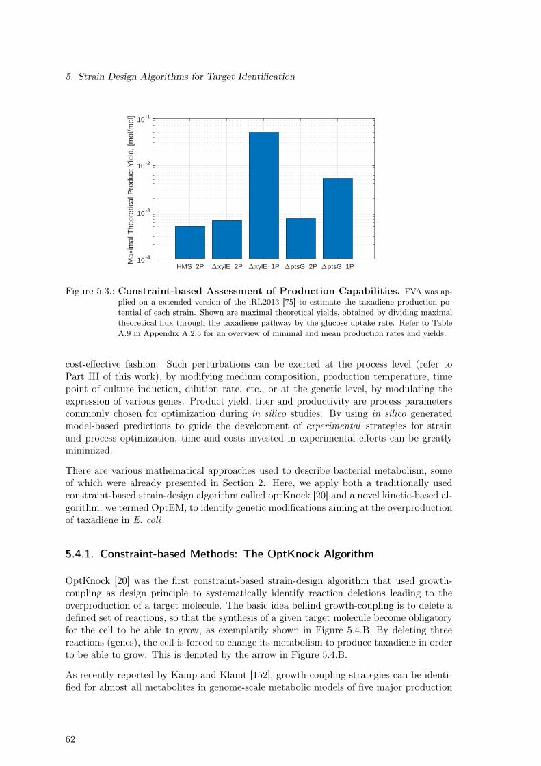
5. Strain Design Algorithms for Target Identification
HMS_2P xylE_2P xylE_1P ptsG_2P ptsG_1P10 -4
10 -3
10 -2
10 -1
Max
imal
The
oret
ical
Pro
duct
Yie
ld, [
mol
/mol
]
Figure 5.3.: Constraint-based Assessment of Production Capabilities. FVA was ap-plied on a extended version of the iRL2013 [75] to estimate the taxadiene production po-tential of each strain. Shown are maximal theoretical yields, obtained by dividing maximaltheoretical flux through the taxadiene pathway by the glucose uptake rate. Refer to TableA.9 in Appendix A.2.5 for an overview of minimal and mean production rates and yields.
cost-effective fashion. Such perturbations can be exerted at the process level (refer toPart III of this work), by modifying medium composition, production temperature, timepoint of culture induction, dilution rate, etc., or at the genetic level, by modulating theexpression of various genes. Product yield, titer and productivity are process parameterscommonly chosen for optimization during in silico studies. By using in silico generatedmodel-based predictions to guide the development of experimental strategies for strainand process optimization, time and costs invested in experimental efforts can be greatlyminimized.
There are various mathematical approaches used to describe bacterial metabolism, someof which were already presented in Section 2. Here, we apply both a traditionally usedconstraint-based strain-design algorithm called optKnock [20] and a novel kinetic-based al-gorithm, we termed OptEM, to identify genetic modifications aiming at the overproductionof taxadiene in E. coli .
5.4.1. Constraint-based Methods: The OptKnock Algorithm
OptKnock [20] was the first constraint-based strain-design algorithm that used growth-coupling as design principle to systematically identify reaction deletions leading to theoverproduction of a target molecule. The basic idea behind growth-coupling is to delete adefined set of reactions, so that the synthesis of a given target molecule become obligatoryfor the cell to be able to grow, as exemplarily shown in Figure 5.4.B. By deleting threereactions (genes), the cell is forced to change its metabolism to produce taxadiene in orderto be able to grow. This is denoted by the arrow in Figure 5.4.B.
As recently reported by Kamp and Klamt [152], growth-coupling strategies can be identi-fied for almost all metabolites in genome-scale metabolic models of five major production
62
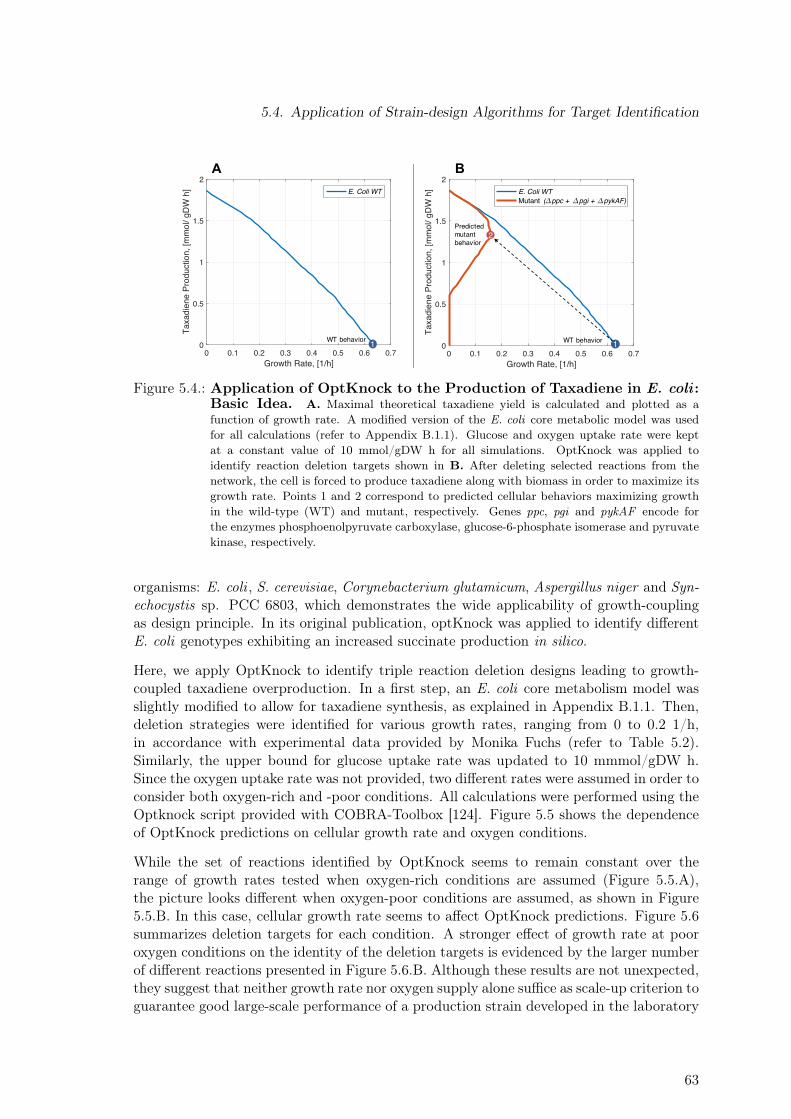
5.4. Application of Strain-design Algorithms for Target Identification
0 0.1 0.2 0.3 0.4 0.5 0.6 0.7Growth Rate, [1/h]
0
0.5
1
1.5
2
Taxa
dien
e Pr
oduc
tion,
[mm
ol/ g
DW
h] E. Coli WT
Mutant ( ppc + pgi + pykAF)
0 0.1 0.2 0.3 0.4 0.5 0.6 0.7Growth Rate, [1/h]
0
0.5
1
1.5
2Ta
xadi
ene
Prod
uctio
n, [m
mol
/ gD
W h
] E. Coli WT
WT behavior
Predicted mutant behavior
2
11 WT behavior
A B
Figure 5.4.: Application of OptKnock to the Production of Taxadiene in E. coli :Basic Idea. A. Maximal theoretical taxadiene yield is calculated and plotted as afunction of growth rate. A modified version of the E. coli core metabolic model was usedfor all calculations (refer to Appendix B.1.1). Glucose and oxygen uptake rate were keptat a constant value of 10 mmol/gDW h for all simulations. OptKnock was applied toidentify reaction deletion targets shown in B. After deleting selected reactions from thenetwork, the cell is forced to produce taxadiene along with biomass in order to maximize itsgrowth rate. Points 1 and 2 correspond to predicted cellular behaviors maximizing growthin the wild-type (WT) and mutant, respectively. Genes ppc, pgi and pykAF encode forthe enzymes phosphoenolpyruvate carboxylase, glucose-6-phosphate isomerase and pyruvatekinase, respectively.
organisms: E. coli , S. cerevisiae, Corynebacterium glutamicum, Aspergillus niger and Syn-echocystis sp. PCC 6803, which demonstrates the wide applicability of growth-couplingas design principle. In its original publication, optKnock was applied to identify differentE. coli genotypes exhibiting an increased succinate production in silico.
Here, we apply OptKnock to identify triple reaction deletion designs leading to growth-coupled taxadiene overproduction. In a first step, an E. coli core metabolism model wasslightly modified to allow for taxadiene synthesis, as explained in Appendix B.1.1. Then,deletion strategies were identified for various growth rates, ranging from 0 to 0.2 1/h,in accordance with experimental data provided by Monika Fuchs (refer to Table 5.2).Similarly, the upper bound for glucose uptake rate was updated to 10 mmmol/gDW h.Since the oxygen uptake rate was not provided, two different rates were assumed in order toconsider both oxygen-rich and -poor conditions. All calculations were performed using theOptknock script provided with COBRA-Toolbox [124]. Figure 5.5 shows the dependenceof OptKnock predictions on cellular growth rate and oxygen conditions.
While the set of reactions identified by OptKnock seems to remain constant over therange of growth rates tested when oxygen-rich conditions are assumed (Figure 5.5.A),the picture looks different when oxygen-poor conditions are assumed, as shown in Figure5.5.B. In this case, cellular growth rate seems to affect OptKnock predictions. Figure 5.6summarizes deletion targets for each condition. A stronger effect of growth rate at pooroxygen conditions on the identity of the deletion targets is evidenced by the larger numberof different reactions presented in Figure 5.6.B. Although these results are not unexpected,they suggest that neither growth rate nor oxygen supply alone suffice as scale-up criterion toguarantee good large-scale performance of a production strain developed in the laboratory
63
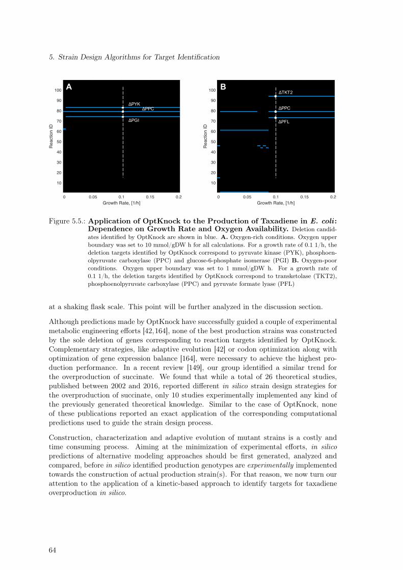
5. Strain Design Algorithms for Target Identification
Oxygen/Glucose = 1 mol/mol
0 0.05 0.1 0.15 0.2Growth Rate, [1/h]
10
20
30
40
50
60
70
80
90
100
Rea
ctio
n ID
Oxygen/Glucose = 0.1 mol/mol
0 0.05 0.1 0.15 0.2Growth Rate, [1/h]
10
20
30
40
50
60
70
80
90
100
Rea
ctio
n ID
ΔPYK
ΔPGI
ΔPPC
ΔTKT2
ΔPPC
ΔPFL
A B
Figure 5.5.: Application of OptKnock to the Production of Taxadiene in E. coli :Dependence on Growth Rate and Oxygen Availability. Deletion candid-ates identified by OptKnock are shown in blue. A. Oxygen-rich conditions. Oxygen upperboundary was set to 10 mmol/gDW h for all calculations. For a growth rate of 0.1 1/h, thedeletion targets identified by OptKnock correspond to pyruvate kinase (PYK), phosphoen-olpyruvate carboxylase (PPC) and glucose-6-phosphate isomerase (PGI) B. Oxygen-poorconditions. Oxygen upper boundary was set to 1 mmol/gDW h. For a growth rate of0.1 1/h, the deletion targets identified by OptKnock correspond to transketolase (TKT2),phosphoenolpyruvate carboxylase (PPC) and pyruvate formate lyase (PFL)
at a shaking flask scale. This point will be further analyzed in the discussion section.
Although predictions made by OptKnock have successfully guided a couple of experimentalmetabolic engineering efforts [42,164], none of the best production strains was constructedby the sole deletion of genes corresponding to reaction targets identified by OptKnock.Complementary strategies, like adaptive evolution [42] or codon optimization along withoptimization of gene expression balance [164], were necessary to achieve the highest pro-duction performance. In a recent review [149], our group identified a similar trend forthe overproduction of succinate. We found that while a total of 26 theoretical studies,published between 2002 and 2016, reported different in silico strain design strategies forthe overproduction of succinate, only 10 studies experimentally implemented any kind ofthe previously generated theoretical knowledge. Similar to the case of OptKnock, noneof these publications reported an exact application of the corresponding computationalpredictions used to guide the strain design process.
Construction, characterization and adaptive evolution of mutant strains is a costly andtime consuming process. Aiming at the minimization of experimental efforts, in silicopredictions of alternative modeling approaches should be first generated, analyzed andcompared, before in silico identified production genotypes are experimentally implementedtowards the construction of actual production strain(s). For that reason, we now turn ourattention to the application of a kinetic-based approach to identify targets for taxadieneoverproduction in silico.
64
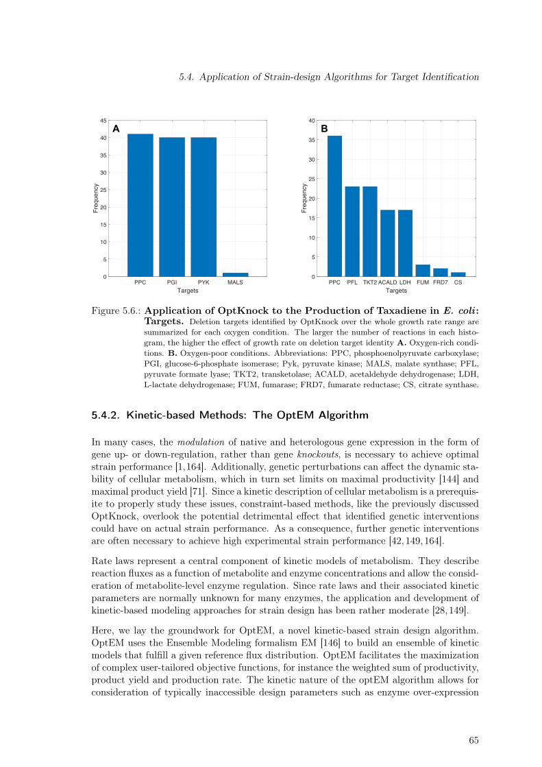
5.4. Application of Strain-design Algorithms for Target Identification
Oxygen/Glucose = 1 mol/mol
PPC PGI PYK MALSTargets
0
5
10
15
20
25
30
35
40
45
Frequency
Oxygen/Glucose = 0.1 mol/mol
PPC PFL TKT2 ACALD LDH FUM FRD7 CSTargets
0
5
10
15
20
25
30
35
40
Frequency
A B
Figure 5.6.: Application of OptKnock to the Production of Taxadiene in E. coli :Targets. Deletion targets identified by OptKnock over the whole growth rate range aresummarized for each oxygen condition. The larger the number of reactions in each histo-gram, the higher the effect of growth rate on deletion target identity A. Oxygen-rich condi-tions. B. Oxygen-poor conditions. Abbreviations: PPC, phosphoenolpyruvate carboxylase;PGI, glucose-6-phosphate isomerase; Pyk, pyruvate kinase; MALS, malate synthase; PFL,pyruvate formate lyase; TKT2, transketolase; ACALD, acetaldehyde dehydrogenase; LDH,L-lactate dehydrogenase; FUM, fumarase; FRD7, fumarate reductase; CS, citrate synthase.
5.4.2. Kinetic-based Methods: The OptEM Algorithm
In many cases, the modulation of native and heterologous gene expression in the form ofgene up- or down-regulation, rather than gene knockouts, is necessary to achieve optimalstrain performance [1,164]. Additionally, genetic perturbations can affect the dynamic sta-bility of cellular metabolism, which in turn set limits on maximal productivity [144] andmaximal product yield [71]. Since a kinetic description of cellular metabolism is a prerequis-ite to properly study these issues, constraint-based methods, like the previously discussedOptKnock, overlook the potential detrimental effect that identified genetic interventionscould have on actual strain performance. As a consequence, further genetic interventionsare often necessary to achieve high experimental strain performance [42,149,164].
Rate laws represent a central component of kinetic models of metabolism. They describereaction fluxes as a function of metabolite and enzyme concentrations and allow the consid-eration of metabolite-level enzyme regulation. Since rate laws and their associated kineticparameters are normally unknown for many enzymes, the application and development ofkinetic-based modeling approaches for strain design has been rather moderate [28,149].
Here, we lay the groundwork for OptEM, a novel kinetic-based strain design algorithm.OptEM uses the Ensemble Modeling formalism EM [146] to build an ensemble of kineticmodels that fulfill a given reference flux distribution. OptEM facilitates the maximizationof complex user-tailored objective functions, for instance the weighted sum of productivity,product yield and production rate. The kinetic nature of the optEM algorithm allows forconsideration of typically inaccessible design parameters such as enzyme over-expression
65
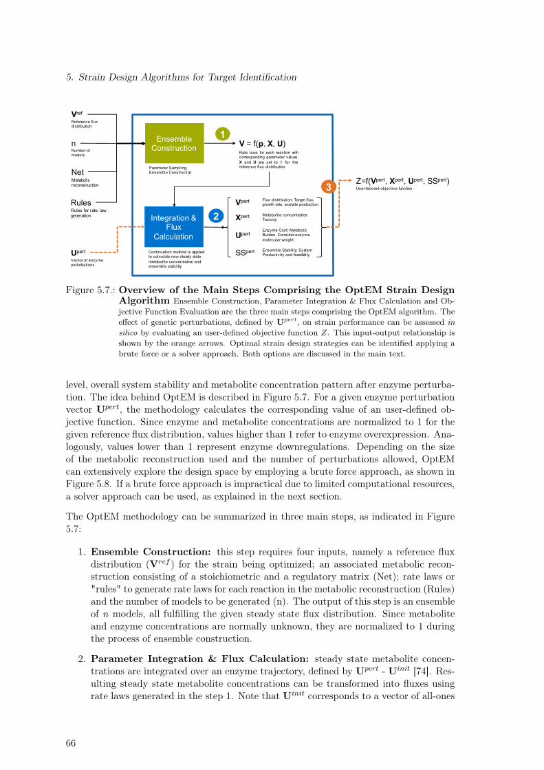
5. Strain Design Algorithms for Target Identification
Ensemble Construction
Parameter Sampling, Ensemble Construction
VrefReference flux distribution
V = f(p, X, U)Rate laws for each reaction withcorresponding parameter values.X and U are set to 1 for thereference flux distribution
Integration & Flux
Calculation
Continuation method is applied to calculate new steady state metabolite concentration and ensemble stability
Vpert Flux distribution: Target flux, growth rate, acetate production
Xpert Metabolite concentration: Toxicity
UpertEnzyme Cost: Metabolic Burden. Consider enzyme molecular weight
SSpert Ensemble Stability: System Productivity and feasibility Upert
Vector of enzyme perturbations
Z=f(Vpert, Xpert, Upert, SSpert)User-tailored objective function.
nNumber of models
NetMetabolic reconstruction
RulesRules for rate law generation
1
2
3
Figure 5.7.: Overview of the Main Steps Comprising the OptEM Strain DesignAlgorithm Ensemble Construction, Parameter Integration & Flux Calculation and Ob-jective Function Evaluation are the three main steps comprising the OptEM algorithm. Theeffect of genetic perturbations, defined by Upert, on strain performance can be assessed insilico by evaluating an user-defined objective function Z. This input-output relationship isshown by the orange arrows. Optimal strain design strategies can be identified applying abrute force or a solver approach. Both options are discussed in the main text.
level, overall system stability and metabolite concentration pattern after enzyme perturba-tion. The idea behind OptEM is described in Figure 5.7. For a given enzyme perturbationvector Upert, the methodology calculates the corresponding value of an user-defined ob-jective function. Since enzyme and metabolite concentrations are normalized to 1 for thegiven reference flux distribution, values higher than 1 refer to enzyme overexpression. Ana-logously, values lower than 1 represent enzyme downregulations. Depending on the sizeof the metabolic reconstruction used and the number of perturbations allowed, OptEMcan extensively explore the design space by employing a brute force approach, as shown inFigure 5.8. If a brute force approach is impractical due to limited computational resources,a solver approach can be used, as explained in the next section.
The OptEM methodology can be summarized in three main steps, as indicated in Figure5.7:
1. Ensemble Construction: this step requires four inputs, namely a reference fluxdistribution (Vref ) for the strain being optimized; an associated metabolic recon-struction consisting of a stoichiometric and a regulatory matrix (Net); rate laws or"rules" to generate rate laws for each reaction in the metabolic reconstruction (Rules)and the number of models to be generated (n). The output of this step is an ensembleof n models, all fulfilling the given steady state flux distribution. Since metaboliteand enzyme concentrations are normally unknown, they are normalized to 1 duringthe process of ensemble construction.
2. Parameter Integration & Flux Calculation: steady state metabolite concen-trations are integrated over an enzyme trajectory, defined by Upert - Uinit [74]. Res-ulting steady state metabolite concentrations can be transformed into fluxes usingrate laws generated in the step 1. Note that Uinit corresponds to a vector of all-ones
66
5.4. Application of Strain-design Algorithms for Target Identification
of adequate size. Output of this step are the vectors Vpert, Xpert and Upert de-scribing flux distribution, metabolite concentration and enzyme concentration, all ofthem after conducting enzyme perturbation dictated by Upert, respectively. VariableSSpert describes the percentage of models remaining stable after perturbation.
3. Objective Function Evaluation: output of step 2 can be used to evaluate anuser-defined objective function described by Z = f(Vpert, Xpert, Upert, SSpert ). Bydoing so, the specific effect of the genetic perturbation described by Upert on strainperformance can be numerically assessed and compared with alternative genetic per-turbations, thus leading to the identification of strain designs maximizing Z. Notethat the evaluation of the objective function should be performed for each model inthe ensemble. The effect of a given perturbation on the objective function Z can bethen characterized by calculating the median and 25th and 75th percentiles.
Objective Functions
The vast majority of Metabolic Engineering efforts to date have aimed at the optimizationof product yield. However, it has been recognized that not only high product yields butalso high volumetric productivity and product titer, strain robustness and the ability touse low-cost substrates are key factors defining process viability and should therefore beprimary objectives for bio-process development [74, 86]. In line with this, OptEM wasdeveloped to allow the optimization of user-tailored objective functions, considering themost relevant process parameters. Table 5.3 lists various examples. While each of theseobjective functions targets product yield maximization, they also maximize or minimizesecondary objectives like concentration of toxic pathway intermediates, strain robustnessand protein burden.
Brute Force Approach
In order to illustrate the probabilistic nature of OptEM predictions, the effect of singleenzyme up- and down-regulation on product yield for the strain ∆XylE_1p is exemplarilyshown in Figure 5.8. This particular strain was selected as case study out of all productionstrain candidates (see Table 5.1) because of its superior taxadiene production potential, asidentified by a constraint-based analysis -see Figure 5.3 and refer to section 5.3 for detailson the estimation of production potential using 13C-labeling data-. The reference fluxdistribution used to construct the ensemble of kinetic models was calculated assuming ataxadiene yield of 2.860× 10⁻⁵ mol taxadiene/mol glucose, which corresponds to a meantaxadiene production level, as shown in Table A.9 in Appendix A.2.5. This assumption isjustified by the fact that, as mentioned earlier, no experimental taxadiene concentrationwas available for this set of strains.
As specified in Figure 5.8 by the arrows, the outcome of single up- or down-regulationof a given enzyme with respect to the numerical value of the objective function can becategorized into three different groups. The first group exhibits an increase of the objectivefunction for all models in the ensemble, as shown by the green arrows. In this case, the25th percentile characterizing the effect of the given enzyme perturbation lies above thebasal level of the objective function. Conversely, the second group is characterized by
67
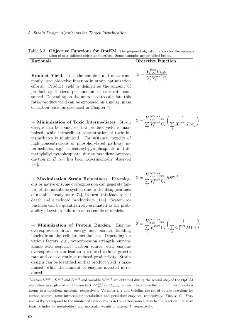
5. Strain Design Algorithms for Target Identification
Table 5.3.: Objective Functions for OptEM. The proposed algorithm allows for the optimiz-ation of user-tailored objective functions. Some examples are provided below.
Rationale Objective Function
Product Yield. It is the simplest and most com-monly used objective function in strain optimizationefforts. Product yield is defined as the amount ofproduct synthesized per amount of substrate con-sumed. Depending on the units used to calculate thisratio, product yield can be expressed on a molar, massor carbon basis, as discussed in Chapter 7.
Z =V perttxdn Ctxdn∑iV perti Ci
+ Minimization of Toxic Intermediates. Straindesigns can be found so that product yield is max-imized, while intracellular concentration of toxic in-termediates is minimized. For instance, toxicity ofhigh concentrations of phosphorylated pathway in-termediates, e.g., isopentenyl pyrophosphate and di-methylallyl pyrophosphate, during taxadiene overpro-duction in E. coli has been experimentally observed[93].
Z =V perttxdn Ctxd∑iV perti Ci
(1∑
jXpertj Toxj
)
+ Maximization Strain Robustness. Heterolog-ous or native enzyme overexpression can generate fail-ure of the metabolic system due to the disappearanceof a stable steady state [74]. In turn, this leads to celldeath and a reduced productivity [144]. System ro-bustness can be quantitatively estimated as the prob-ability of system failure in an ensemble of models.
Z =V perttxdn Ctxd∑iV perti Ci
SSpert
+ Minimization of Protein Burden. Enzymeoverexpression draws energy and biomass buildingblocks from the cellular metabolism. Depending onvarious factors, e.g., overexpression strength, enzymeamino acid sequence, carbon source, etc., enzymeoverexpression can lead to a reduced cellular growthrate and consequently, a reduced productivity. Straindesigns can be identified so that product yield is max-imized, while the amount of enzyme invested is re-duced.
Z =V perttxdn Ctxd∑iV perti Ci
(1∑
k
Upertk MWk
)
Vectors V pert, Xpert and Upert and variable SSpert are obtained during the second step of the OptEMalgorithm, as explained in the main text. V pert
txdn and Ctxdn represent taxadiene flux and number of carbonatoms in a taxadiene molecule, respectively. Variables i, j and k define the set of uptake reactions forcarbon sources, toxic intracellular metabolites and perturbed enzymes, respectively. Finally, Ci, ToxjandMWk correspond to the number of carbon atoms in the carbon source absorbed in reaction i, relativetoxicity index for metabolite j and molecular weight of enzyme k, respectively.
68
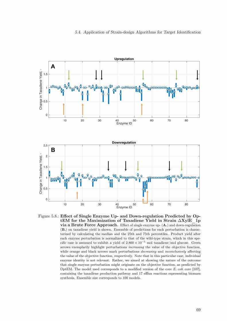
5.4. Application of Strain-design Algorithms for Target Identification
10 20 30 40 50 60 70 80
0
0.5
1
1.5
Cha
nge
in T
axad
iene
Yie
ld, -
Upregulation
Enzyme ID
10 20 30 40 50 60 70 800
0.5
1
1.5
2
2.5
Cha
nge
in T
axad
iene
Yie
ld, -
Downregulation
Enzyme ID
A
B
Figure 5.8.: Effect of Single Enzyme Up- and Down-regulation Predicted by Op-tEM for the Maximization of Taxadiene Yield in Strain ∆XylE_1pvia a Brute Force Approach. Effect of single enzyme up- (A.) and down-regulation(B.) on taxadiene yield is shown. Ensemble of predictions for each perturbation is charac-terized by calculating the median and the 25th and 75th percentiles. Product yield aftereach enzyme perturbation is normalized to that of the wild-type strain, which in this spe-cific case is assumed to exhibit a yield of 2.860× 10⁻⁵ mol taxadiene/mol glucose. Greenarrows exemplarily highlight perturbations increasing the value of the objective function,while orange and black arrows mark perturbations decreasing and inconclusively affectingthe value of the objective function, respectively. Note that in this particular case, individualenzyme identity is not relevant. Rather, we aimed at showing the nature of the outcomethat single enzyme perturbation might originate on the objective function, as predicted byOptEM. The model used corresponds to a modified version of the core E. coli core [107],containing the taxadiene production pathway and 17 efflux reactions representing biomasssynthesis. Ensemble size corresponds to 100 models.
69
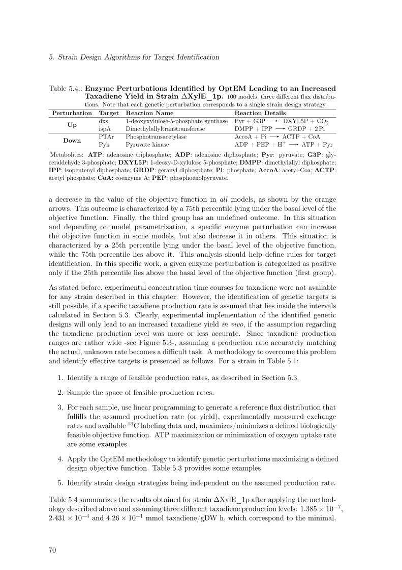
5. Strain Design Algorithms for Target Identification
Table 5.4.: Enzyme Perturbations Identified by OptEM Leading to an IncreasedTaxadiene Yield in Strain ∆XylE_1p. 100 models, three different flux distribu-tions. Note that each genetic perturbation corresponds to a single strain design strategy.
Perturbation Target Reaction Name Reaction Details
Up dxs 1-deoxyxylulose-5-phosphate synthase Pyr + G3P DXYL5P + CO2ispA Dimethylallyltranstransferase DMPP + IPP GRDP + 2Pi
Down PTAr Phosphotransacetylase AccoA + Pi ACTP + CoAPyk Pyruvate kinase ADP + PEP + H+ ATP + Pyr
Metabolites: ATP: adenosine triphosphate; ADP: adenosine diphosphate; Pyr: pyruvate; G3P: gly-ceraldehyde 3-phosphate; DXYL5P: 1-deoxy-D-xylulose 5-phosphate; DMPP: dimethylallyl diphosphate;IPP: isopentenyl diphosphate; GRDP: geranyl diphosphate; Pi: phosphate; AccoA: acetyl-Coa; ACTP:acetyl phosphate; CoA: coenzyme A; PEP: phosphoenolpyruvate.
a decrease in the value of the objective function in all models, as shown by the orangearrows. This outcome is characterized by a 75th percentile lying under the basal level of theobjective function. Finally, the third group has an undefined outcome. In this situationand depending on model parametrization, a specific enzyme perturbation can increasethe objective function in some models, but also decrease it in others. This situation ischaracterized by a 25th percentile lying under the basal level of the objective function,while the 75th percentile lies above it. This analysis should help define rules for targetidentification. In this specific work, a given enzyme perturbation is categorized as positiveonly if the 25th percentile lies above the basal level of the objective function (first group).
As stated before, experimental concentration time courses for taxadiene were not availablefor any strain described in this chapter. However, the identification of genetic targets isstill possible, if a specific taxadiene production rate is assumed that lies inside the intervalscalculated in Section 5.3. Clearly, experimental implementation of the identified geneticdesigns will only lead to an increased taxadiene yield in vivo, if the assumption regardingthe taxadiene production level was more or less accurate. Since taxadiene productionranges are rather wide -see Figure 5.3-, assuming a production rate accurately matchingthe actual, unknown rate becomes a difficult task. A methodology to overcome this problemand identify effective targets is presented as follows. For a strain in Table 5.1:
1. Identify a range of feasible production rates, as described in Section 5.3.
2. Sample the space of feasible production rates.
3. For each sample, use linear programming to generate a reference flux distribution thatfulfills the assumed production rate (or yield), experimentally measured exchangerates and available 13C labeling data and, maximizes/minimizes a defined biologicallyfeasible objective function. ATP maximization or minimization of oxygen uptake rateare some examples.
4. Apply the OptEMmethodology to identify genetic perturbations maximizing a defineddesign objective function. Table 5.3 provides some examples.
5. Identify strain design strategies being independent on the assumed production rate.
Table 5.4 summarizes the results obtained for strain ∆XylE_1p after applying the method-ology described above and assuming three different taxadiene production levels: 1.385× 10−7,2.431× 10−4 and 4.26× 10⁻¹ mmol taxadiene/gDW h, which correspond to the minimal,
70
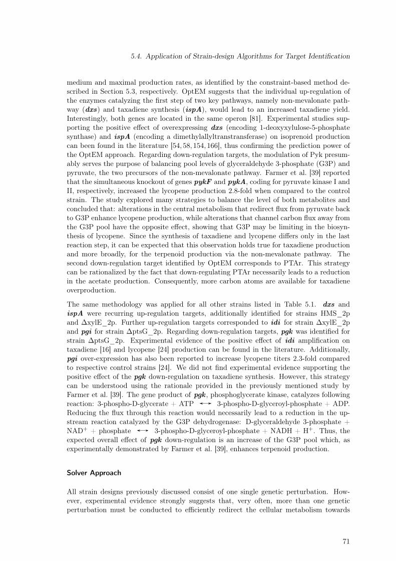
5.4. Application of Strain-design Algorithms for Target Identification
medium and maximal production rates, as identified by the constraint-based method de-scribed in Section 5.3, respectively. OptEM suggests that the individual up-regulation ofthe enzymes catalyzing the first step of two key pathways, namely non-mevalonate path-way (dxs) and taxadiene synthesis (ispA), would lead to an increased taxadiene yield.Interestingly, both genes are located in the same operon [81]. Experimental studies sup-porting the positive effect of overexpressing dxs (encoding 1-deoxyxylulose-5-phosphatesynthase) and ispA (encoding a dimethylallyltranstransferase) on isoprenoid productioncan been found in the literature [54, 58, 154, 166], thus confirming the prediction power ofthe OptEM approach. Regarding down-regulation targets, the modulation of Pyk presum-ably serves the purpose of balancing pool levels of glyceraldehyde 3-phosphate (G3P) andpyruvate, the two precursors of the non-mevalonate pathway. Farmer et al. [39] reportedthat the simultaneous knockout of genes pykF and pykA, coding for pyruvate kinase I andII, respectively, increased the lycopene production 2.8-fold when compared to the controlstrain. The study explored many strategies to balance the level of both metabolites andconcluded that: alterations in the central metabolism that redirect flux from pyruvate backto G3P enhance lycopene production, while alterations that channel carbon flux away fromthe G3P pool have the opposite effect, showing that G3P may be limiting in the biosyn-thesis of lycopene. Since the synthesis of taxadiene and lycopene differs only in the lastreaction step, it can be expected that this observation holds true for taxadiene productionand more broadly, for the terpenoid production via the non-mevalonate pathway. Thesecond down-regulation target identified by OptEM corresponds to PTAr. This strategycan be rationalized by the fact that down-regulating PTAr necessarily leads to a reductionin the acetate production. Consequently, more carbon atoms are available for taxadieneoverproduction.
The same methodology was applied for all other strains listed in Table 5.1. dxs andispA were recurring up-regulation targets, additionally identified for strains HMS_2pand ∆xylE_2p. Further up-regulation targets corresponded to idi for strain ∆xylE_2pand pgi for strain ∆ptsG_2p. Regarding down-regulation targets, pgk was identified forstrain ∆ptsG_2p. Experimental evidence of the positive effect of idi amplification ontaxadiene [16] and lycopene [24] production can be found in the literature. Additionally,pgi over-expression has also been reported to increase lycopene titers 2.3-fold comparedto respective control strains [24]. We did not find experimental evidence supporting thepositive effect of the pgk down-regulation on taxadiene synthesis. However, this strategycan be understood using the rationale provided in the previously mentioned study byFarmer et al. [39]. The gene product of pgk , phosphoglycerate kinase, catalyzes followingreaction: 3-phospho-D-glycerate + ATP 3-phospho-D-glyceroyl-phosphate + ADP.Reducing the flux through this reaction would necessarily lead to a reduction in the up-stream reaction catalyzed by the G3P dehydrogenase: D-glyceraldehyde 3-phosphate +NAD+ + phosphate 3-phospho-D-glyceroyl-phosphate + NADH + H+. Thus, theexpected overall effect of pgk down-regulation is an increase of the G3P pool which, asexperimentally demonstrated by Farmer et al. [39], enhances terpenoid production.
Solver Approach
All strain designs previously discussed consist of one single genetic perturbation. How-ever, experimental evidence strongly suggests that, very often, more than one geneticperturbation must be conducted to efficiently redirect the cellular metabolism towards
71
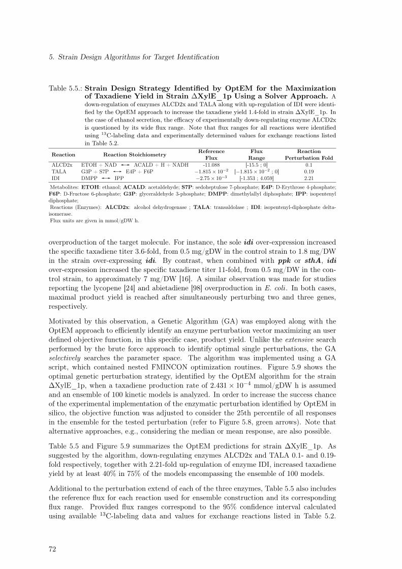
5. Strain Design Algorithms for Target Identification
Table 5.5.: Strain Design Strategy Identified by OptEM for the Maximizationof Taxadiene Yield in Strain ∆XylE_1p Using a Solver Approach. Adown-regulation of enzymes ALCD2x and TALA along with up-regulation of IDI were identi-fied by the OptEM approach to increase the taxadiene yield 1.4-fold in strain ∆XylE_1p. Inthe case of ethanol secretion, the efficacy of experimentally down-regulating enzyme ALCD2xis questioned by its wide flux range. Note that flux ranges for all reactions were identifiedusing 13C-labeling data and experimentally determined values for exchange reactions listedin Table 5.2.
Reaction Reaction Stoichiometry ReferenceFlux
FluxRange
ReactionPerturbation Fold
ALCD2x ETOH + NAD ACALD + H + NADH -11.088 [-15.5 ; 0] 0.1TALA G3P + S7P E4P + F6P −1.815× 10⁻² [−1.815× 10⁻² ; 0] 0.19IDI DMPP IPP −2.75× 10⁻³ [-1.353 ; 4.059] 2.21
Metabolites: ETOH: ethanol; ACALD: acetaldehyde; S7P: sedoheptulose 7-phosphate; E4P: D-Erythrose 4-phosphate;F6P: D-Fructose 6-phosphate; G3P: glyceraldehyde 3-phosphate; DMPP: dimethylallyl diphosphate; IPP: isopentenyldiphosphate;Reactions (Enzymes): ALCD2x: alcohol dehydrogenase ; TALA: transaldolase ; IDI: isopentenyl-diphosphate delta-isomerase.Flux units are given in mmol/gDW h.
overproduction of the target molecule. For instance, the sole idi over-expression increasedthe specific taxadiene titer 3.6-fold, from 0.5 mg/gDW in the control strain to 1.8 mg/DWin the strain over-expressing idi. By contrast, when combined with ppk or sthA, idiover-expression increased the specific taxadiene titer 11-fold, from 0.5 mg/DW in the con-trol strain, to approximately 7 mg/DW [16]. A similar observation was made for studiesreporting the lycopene [24] and abietadiene [98] overproduction in E. coli . In both cases,maximal product yield is reached after simultaneously perturbing two and three genes,respectively.
Motivated by this observation, a Genetic Algorithm (GA) was employed along with theOptEM approach to efficiently identify an enzyme perturbation vector maximizing an userdefined objective function, in this specific case, product yield. Unlike the extensive searchperformed by the brute force approach to identify optimal single perturbations, the GAselectively searches the parameter space. The algorithm was implemented using a GAscript, which contained nested FMINCON optimization routines. Figure 5.9 shows theoptimal genetic perturbation strategy, identified by the OptEM algorithm for the strain∆XylE_1p, when a taxadiene production rate of 2.431× 10⁻⁴ mmol/gDW h is assumedand an ensemble of 100 kinetic models is analyzed. In order to increase the success chanceof the experimental implementation of the enzymatic perturbation identified by OptEM insilico, the objective function was adjusted to consider the 25th percentile of all responsesin the ensemble for the tested perturbation (refer to Figure 5.8, green arrows). Note thatalternative approaches, e.g., considering the median or mean response, are also possible.
Table 5.5 and Figure 5.9 summarizes the OptEM predictions for strain ∆XylE_1p. Assuggested by the algorithm, down-regulating enzymes ALCD2x and TALA 0.1- and 0.19-fold respectively, together with 2.21-fold up-regulation of enzyme IDI, increased taxadieneyield by at least 40% in 75% of the models encompassing the ensemble of 100 models.
Additional to the perturbation extend of each of the three enzymes, Table 5.5 also includesthe reference flux for each reaction used for ensemble construction and its correspondingflux range. Provided flux ranges correspond to the 95% confidence interval calculatedusing available 13C-labeling data and values for exchange reactions listed in Table 5.2.
72
5.4. Application of Strain-design Algorithms for Target Identification
G6P
F6P
FBP
DHAP
3PG
PEP
Pyr
AcCoA
OAC Cit
ICit
AKG
SucCoASuc
Fum
Mal
X5P
S7P
R5P
KDPG
Glyox
CO2 +NADH
NADH + 0.5 O2 2 ATP
NADH NADPH
ACONTa_ACONTb
AKGDH
CS
GLCt2pp-HEX1
PGI
FBA
GND
RPE RPI
PFK FBP
GAPD, PGK
PGM
PYKPPS
PDH
PTAr, ACKr
MALS ICL
SUCDi
FUM
MDH
ME
PPCK PPC
TPI
EDD
EDA
G6PDH-PGL
GLCptspp
ICDHyr
TALA
NADH_CYTBD_HYD_ATPS4r
NADTRHD_THD2pp
SUCOAS
G3PPyr
DXP
HMBDP
IPPDMPP
GRDP
FRDP
GGPP
TXDN
Glucose
Ac
G3P
Pyr
For AcCoA
Acald
Ac
Etoh
EX_pyr
EX_for
EX_ac
EX_etoh
EX_ac
PFL
ACALD
ALDD2x
ALCD2x
IDI
DXS
DXR_IspDEFG
IspH
IspA
IspA
GGPPS
TXS
Taxadiene
E4P
G3P
F6P
6PG Ru5P
TKT1
TKT2
Figure 5.9.: Strain Design Strategy Identified by OptEM for the Maximization ofTaxadiene Yield in Strain ∆XylE_1p Using a Solver Approach. Modelused corresponds to the E. coli core metabolism (reactions contained in the blue rectangle),which was extended to allow for taxadiene synthesis (reactions contained in the orangerectangle). The model contains a total of 87 reactions and 69 metabolites. Reference fluxdistribution was generated considering available 13C-labeling data, experimentally determ-ined exchange rates and an assumed taxadiene production rate of 2.431× 10⁻⁴ mmol/gDWh. Matlab scripts used correspond to the FMINCON and GA optimization routines. Forthe GA, a population size of 10 was used, with a maximal number of 5 generations. Addi-tionally, three reactions were allowed to be simultaneously up- and down-regulated 10- and0.1-fold, respectively. Solver converged after 185 hours and identified strain design shown,which improved the reference taxadiene production 1.4-fold.
73
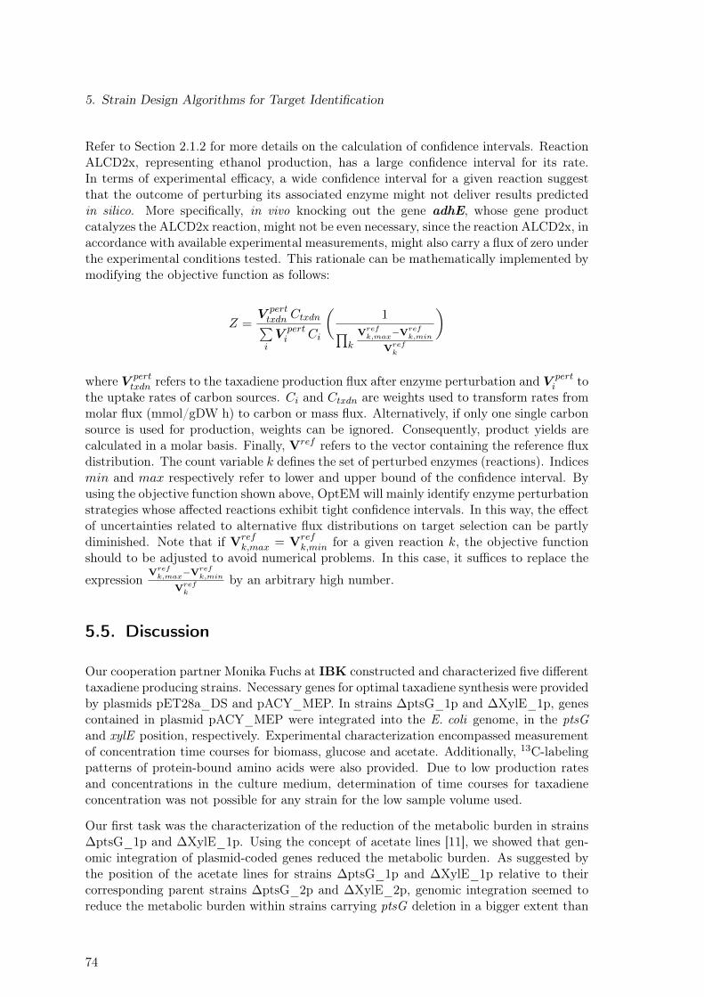
5. Strain Design Algorithms for Target Identification
Refer to Section 2.1.2 for more details on the calculation of confidence intervals. ReactionALCD2x, representing ethanol production, has a large confidence interval for its rate.In terms of experimental efficacy, a wide confidence interval for a given reaction suggestthat the outcome of perturbing its associated enzyme might not deliver results predictedin silico. More specifically, in vivo knocking out the gene adhE, whose gene productcatalyzes the ALCD2x reaction, might not be even necessary, since the reaction ALCD2x, inaccordance with available experimental measurements, might also carry a flux of zero underthe experimental conditions tested. This rationale can be mathematically implemented bymodifying the objective function as follows:
Z =V perttxdn Ctxdn∑iV perti Ci
(1∏
k
Vrefk,max−Vref
k,min
Vrefk
)
where V perttxdn refers to the taxadiene production flux after enzyme perturbation and V pert
i tothe uptake rates of carbon sources. Ci and Ctxdn are weights used to transform rates frommolar flux (mmol/gDW h) to carbon or mass flux. Alternatively, if only one single carbonsource is used for production, weights can be ignored. Consequently, product yields arecalculated in a molar basis. Finally, Vref refers to the vector containing the reference fluxdistribution. The count variable k defines the set of perturbed enzymes (reactions). Indicesmin and max respectively refer to lower and upper bound of the confidence interval. Byusing the objective function shown above, OptEM will mainly identify enzyme perturbationstrategies whose affected reactions exhibit tight confidence intervals. In this way, the effectof uncertainties related to alternative flux distributions on target selection can be partlydiminished. Note that if Vref
k,max = Vrefk,min for a given reaction k, the objective function
should to be adjusted to avoid numerical problems. In this case, it suffices to replace the
expressionVrefk,max−Vref
k,min
Vrefk
by an arbitrary high number.
5.5. Discussion
Our cooperation partner Monika Fuchs at IBK constructed and characterized five differenttaxadiene producing strains. Necessary genes for optimal taxadiene synthesis were providedby plasmids pET28a_DS and pACY_MEP. In strains ∆ptsG_1p and ∆XylE_1p, genescontained in plasmid pACY_MEP were integrated into the E. coli genome, in the ptsGand xylE position, respectively. Experimental characterization encompassed measurementof concentration time courses for biomass, glucose and acetate. Additionally, 13C-labelingpatterns of protein-bound amino acids were also provided. Due to low production ratesand concentrations in the culture medium, determination of time courses for taxadieneconcentration was not possible for any strain for the low sample volume used.
Our first task was the characterization of the reduction of the metabolic burden in strains∆ptsG_1p and ∆XylE_1p. Using the concept of acetate lines [11], we showed that gen-omic integration of plasmid-coded genes reduced the metabolic burden. As suggested bythe position of the acetate lines for strains ∆ptsG_1p and ∆XylE_1p relative to theircorresponding parent strains ∆ptsG_2p and ∆XylE_2p, genomic integration seemed toreduce the metabolic burden within strains carrying ptsG deletion in a bigger extent than
74
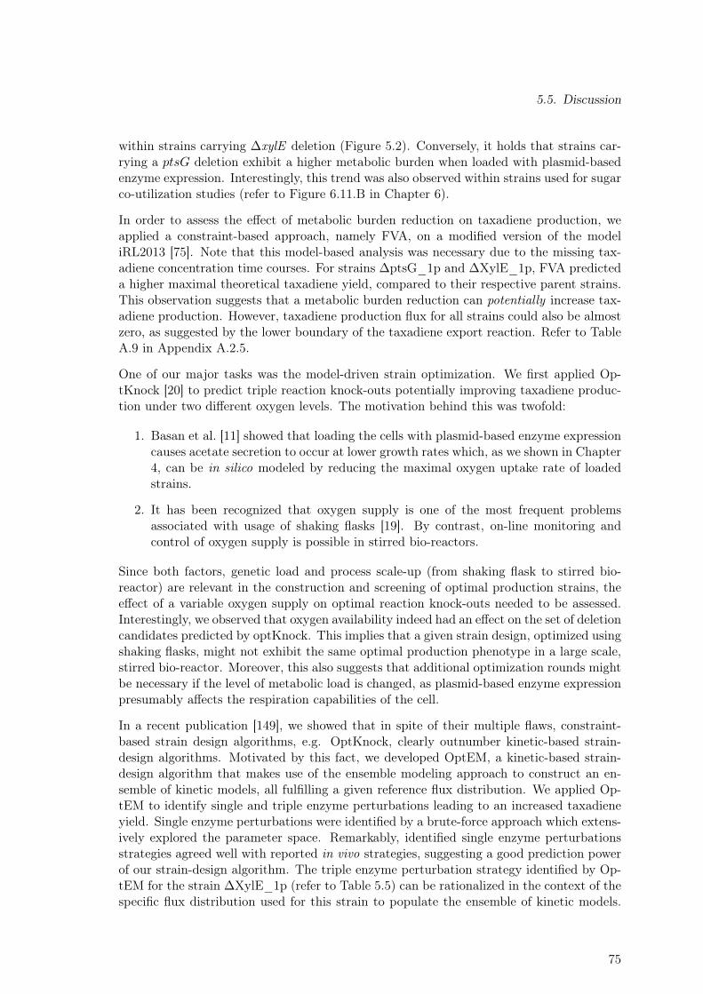
5.5. Discussion
within strains carrying ∆xylE deletion (Figure 5.2). Conversely, it holds that strains car-rying a ptsG deletion exhibit a higher metabolic burden when loaded with plasmid-basedenzyme expression. Interestingly, this trend was also observed within strains used for sugarco-utilization studies (refer to Figure 6.11.B in Chapter 6).
In order to assess the effect of metabolic burden reduction on taxadiene production, weapplied a constraint-based approach, namely FVA, on a modified version of the modeliRL2013 [75]. Note that this model-based analysis was necessary due to the missing tax-adiene concentration time courses. For strains ∆ptsG_1p and ∆XylE_1p, FVA predicteda higher maximal theoretical taxadiene yield, compared to their respective parent strains.This observation suggests that a metabolic burden reduction can potentially increase tax-adiene production. However, taxadiene production flux for all strains could also be almostzero, as suggested by the lower boundary of the taxadiene export reaction. Refer to TableA.9 in Appendix A.2.5.
One of our major tasks was the model-driven strain optimization. We first applied Op-tKnock [20] to predict triple reaction knock-outs potentially improving taxadiene produc-tion under two different oxygen levels. The motivation behind this was twofold:
1. Basan et al. [11] showed that loading the cells with plasmid-based enzyme expressioncauses acetate secretion to occur at lower growth rates which, as we shown in Chapter4, can be in silico modeled by reducing the maximal oxygen uptake rate of loadedstrains.
2. It has been recognized that oxygen supply is one of the most frequent problemsassociated with usage of shaking flasks [19]. By contrast, on-line monitoring andcontrol of oxygen supply is possible in stirred bio-reactors.
Since both factors, genetic load and process scale-up (from shaking flask to stirred bio-reactor) are relevant in the construction and screening of optimal production strains, theeffect of a variable oxygen supply on optimal reaction knock-outs needed to be assessed.Interestingly, we observed that oxygen availability indeed had an effect on the set of deletioncandidates predicted by optKnock. This implies that a given strain design, optimized usingshaking flasks, might not exhibit the same optimal production phenotype in a large scale,stirred bio-reactor. Moreover, this also suggests that additional optimization rounds mightbe necessary if the level of metabolic load is changed, as plasmid-based enzyme expressionpresumably affects the respiration capabilities of the cell.
In a recent publication [149], we showed that in spite of their multiple flaws, constraint-based strain design algorithms, e.g. OptKnock, clearly outnumber kinetic-based strain-design algorithms. Motivated by this fact, we developed OptEM, a kinetic-based strain-design algorithm that makes use of the ensemble modeling approach to construct an en-semble of kinetic models, all fulfilling a given reference flux distribution. We applied Op-tEM to identify single and triple enzyme perturbations leading to an increased taxadieneyield. Single enzyme perturbations were identified by a brute-force approach which extens-ively explored the parameter space. Remarkably, identified single enzyme perturbationsstrategies agreed well with reported in vivo strategies, suggesting a good prediction powerof our strain-design algorithm. The triple enzyme perturbation strategy identified by Op-tEM for the strain ∆XylE_1p (refer to Table 5.5) can be rationalized in the context of thespecific flux distribution used for this strain to populate the ensemble of kinetic models.
75
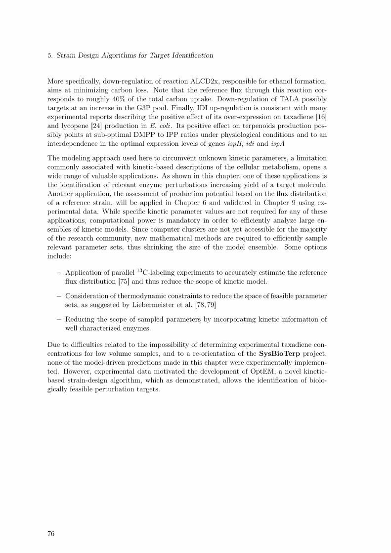
5. Strain Design Algorithms for Target Identification
More specifically, down-regulation of reaction ALCD2x, responsible for ethanol formation,aims at minimizing carbon loss. Note that the reference flux through this reaction cor-responds to roughly 40% of the total carbon uptake. Down-regulation of TALA possiblytargets at an increase in the G3P pool. Finally, IDI up-regulation is consistent with manyexperimental reports describing the positive effect of its over-expression on taxadiene [16]and lycopene [24] production in E. coli . Its positive effect on terpenoids production pos-sibly points at sub-optimal DMPP to IPP ratios under physiological conditions and to aninterdependence in the optimal expression levels of genes ispH, idi and ispA
The modeling approach used here to circumvent unknown kinetic parameters, a limitationcommonly associated with kinetic-based descriptions of the cellular metabolism, opens awide range of valuable applications. As shown in this chapter, one of these applications isthe identification of relevant enzyme perturbations increasing yield of a target molecule.Another application, the assessment of production potential based on the flux distributionof a reference strain, will be applied in Chapter 6 and validated in Chapter 9 using ex-perimental data. While specific kinetic parameter values are not required for any of theseapplications, computational power is mandatory in order to efficiently analyze large en-sembles of kinetic models. Since computer clusters are not yet accessible for the majorityof the research community, new mathematical methods are required to efficiently samplerelevant parameter sets, thus shrinking the size of the model ensemble. Some optionsinclude:
− Application of parallel 13C-labeling experiments to accurately estimate the referenceflux distribution [75] and thus reduce the scope of kinetic model.
− Consideration of thermodynamic constraints to reduce the space of feasible parametersets, as suggested by Liebermeister et al. [78, 79]
− Reducing the scope of sampled parameters by incorporating kinetic information ofwell characterized enzymes.
Due to difficulties related to the impossibility of determining experimental taxadiene con-centrations for low volume samples, and to a re-orientation of the SysBioTerp project,none of the model-driven predictions made in this chapter were experimentally implemen-ted. However, experimental data motivated the development of OptEM, a novel kinetic-based strain-design algorithm, which as demonstrated, allows the identification of biolo-gically feasible perturbation targets.
76
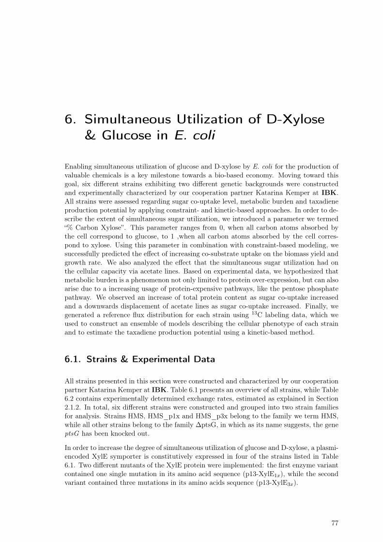
6. Simultaneous Utilization of D-Xylose& Glucose in E. coli
Enabling simultaneous utilization of glucose and D-xylose by E. coli for the production ofvaluable chemicals is a key milestone towards a bio-based economy. Moving toward thisgoal, six different strains exhibiting two different genetic backgrounds were constructedand experimentally characterized by our cooperation partner Katarina Kemper at IBK.All strains were assessed regarding sugar co-uptake level, metabolic burden and taxadieneproduction potential by applying constraint- and kinetic-based approaches. In order to de-scribe the extent of simultaneous sugar utilization, we introduced a parameter we termed“% Carbon Xylose”. This parameter ranges from 0, when all carbon atoms absorbed bythe cell correspond to glucose, to 1 ,when all carbon atoms absorbed by the cell corres-pond to xylose. Using this parameter in combination with constraint-based modeling, wesuccessfully predicted the effect of increasing co-substrate uptake on the biomass yield andgrowth rate. We also analyzed the effect that the simultaneous sugar utilization had onthe cellular capacity via acetate lines. Based on experimental data, we hypothesized thatmetabolic burden is a phenomenon not only limited to protein over-expression, but can alsoarise due to a increasing usage of protein-expensive pathways, like the pentose phosphatepathway. We observed an increase of total protein content as sugar co-uptake increasedand a downwards displacement of acetate lines as sugar co-uptake increased. Finally, wegenerated a reference flux distribution for each strain using 13C labeling data, which weused to construct an ensemble of models describing the cellular phenotype of each strainand to estimate the taxadiene production potential using a kinetic-based method.
6.1. Strains & Experimental Data
All strains presented in this section were constructed and characterized by our cooperationpartner Katarina Kemper at IBK. Table 6.1 presents an overview of all strains, while Table6.2 contains experimentally determined exchange rates, estimated as explained in Section2.1.2. In total, six different strains were constructed and grouped into two strain familiesfor analysis. Strains HMS, HMS_p1x and HMS_p3x belong to the family we term HMS,while all other strains belong to the family ∆ptsG, in which as its name suggests, the geneptsG has been knocked out.
In order to increase the degree of simultaneous utilization of glucose and D-xylose, a plasmi-encoded XylE symporter is constitutively expressed in four of the strains listed in Table6.1. Two different mutants of the XylE protein were implemented: the first enzyme variantcontained one single mutation in its amino acid sequence (p13-XylE1x), while the secondvariant contained three mutations in its amino acids sequence (p13-XylE3x).
77
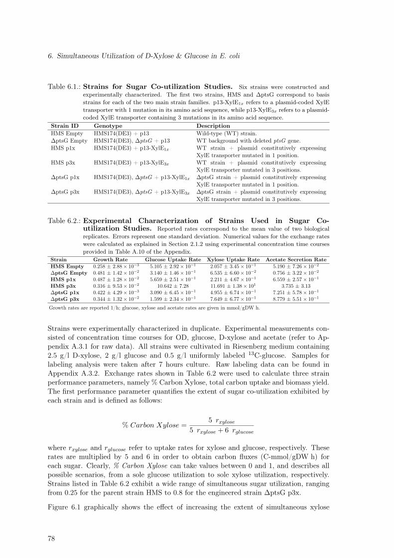
6. Simultaneous Utilization of D-Xylose & Glucose in E. coli
Table 6.1.: Strains for Sugar Co-utilization Studies. Six strains were constructed andexperimentally characterized. The first two strains, HMS and ∆ptsG correspond to basisstrains for each of the two main strain families. p13-XylE1x refers to a plasmid-coded XylEtransporter with 1 mutation in its amino acid sequence, while p13-XylE3x refers to a plasmid-coded XylE transporter containing 3 mutations in its amino acid sequence.
Strain ID Genotype DescriptionHMS Empty HMS174(DE3) + p13 Wild-type (WT) strain.∆ptsG Empty HMS174(DE3), ∆ptsG + p13 WT background with deleted ptsG gene.HMS p1x HMS174(DE3) + p13-XylE1x WT strain + plasmid constitutively expressing
XylE transporter mutated in 1 position.HMS p3x HMS174(DE3) + p13-XylE3x WT strain + plasmid constitutively expressing
XylE transporter mutated in 3 positions.∆ptsG p1x HMS174(DE3), ∆ptsG + p13-XylE1x ∆ptsG strain + plasmid constitutively expressing
XylE transporter mutated in 1 position.∆ptsG p3x HMS174(DE3), ∆ptsG + p13-XylE3x ∆ptsG strain + plasmid constitutively expressing
XylE transporter mutated in 3 positions.
Table 6.2.: Experimental Characterization of Strains Used in Sugar Co-utilization Studies. Reported rates correspond to the mean value of two biologicalreplicates. Errors represent one standard deviation. Numerical values for the exchange rateswere calculated as explained in Section 2.1.2 using experimental concentration time coursesprovided in Table A.10 of the Appendix.
Strain Growth Rate Glucose Uptake Rate Xylose Uptake Rate Acetate Secretion RateHMS Empty 0.258 ± 2.88× 10⁻³ 5.105 ± 2.92× 10⁻¹ 2.057 ± 3.45× 10⁻¹ 5.190 ± 7.26× 10⁻²
∆ptsG Empty 0.481 ± 1.42× 10⁻² 3.140 ± 1.46× 10⁻¹ 6.535 ± 6.60× 10⁻² 0.756 ± 3.22× 10⁻²
HMS p1x 0.487 ± 1.28× 10⁻² 5.659 ± 2.51× 10⁻¹ 2.211 ± 4.67× 10⁻¹ 6.559 ± 2.57× 10⁻¹
HMS p3x 0.316 ± 9.53× 10⁻² 10.642 ± 7.28 11.691 ± 1.38× 101 3.735 ± 3.13∆ptsG p1x 0.422 ± 4.29× 10⁻³ 3.090 ± 6.45× 10⁻¹ 4.955 ± 6.74× 10⁻¹ 7.251 ± 5.78× 10⁻¹
∆ptsG p3x 0.344 ± 1.32× 10⁻² 1.599 ± 2.34× 10⁻¹ 7.649 ± 6.77× 10⁻¹ 8.779 ± 5.51× 10⁻¹
Growth rates are reported 1/h; glucose, xylose and acetate rates are given in mmol/gDW h.
Strains were experimentally characterized in duplicate. Experimental measurements con-sisted of concentration time courses for OD, glucose, D-xylose and acetate (refer to Ap-pendix A.3.1 for raw data). All strains were cultivated in Riesenberg medium containing2.5 g/l D-xylose, 2 g/l glucose and 0.5 g/l uniformly labeled 13C-glucose. Samples forlabeling analysis were taken after 7 hours culture. Raw labeling data can be found inAppendix A.3.2. Exchange rates shown in Table 6.2 were used to calculate three strainperformance parameters, namely % Carbon Xylose, total carbon uptake and biomass yield.The first performance parameter quantifies the extent of sugar co-utilization exhibited byeach strain and is defined as follows:
% Carbon Xylose =5 rxylose
5 rxylose + 6 rglucose
where rxylose and rglucose refer to uptake rates for xylose and glucose, respectively. Theserates are multiplied by 5 and 6 in order to obtain carbon fluxes (C-mmol/gDW h) foreach sugar. Clearly, % Carbon Xylose can take values between 0 and 1, and describes allpossible scenarios, from a sole glucose utilization to sole xylose utilization, respectively.Strains listed in Table 6.2 exhibit a wide range of simultaneous sugar utilization, rangingfrom 0.25 for the parent strain HMS to 0.8 for the engineered strain ∆ptsG p3x.
Figure 6.1 graphically shows the effect of increasing the extent of simultaneous xylose
78
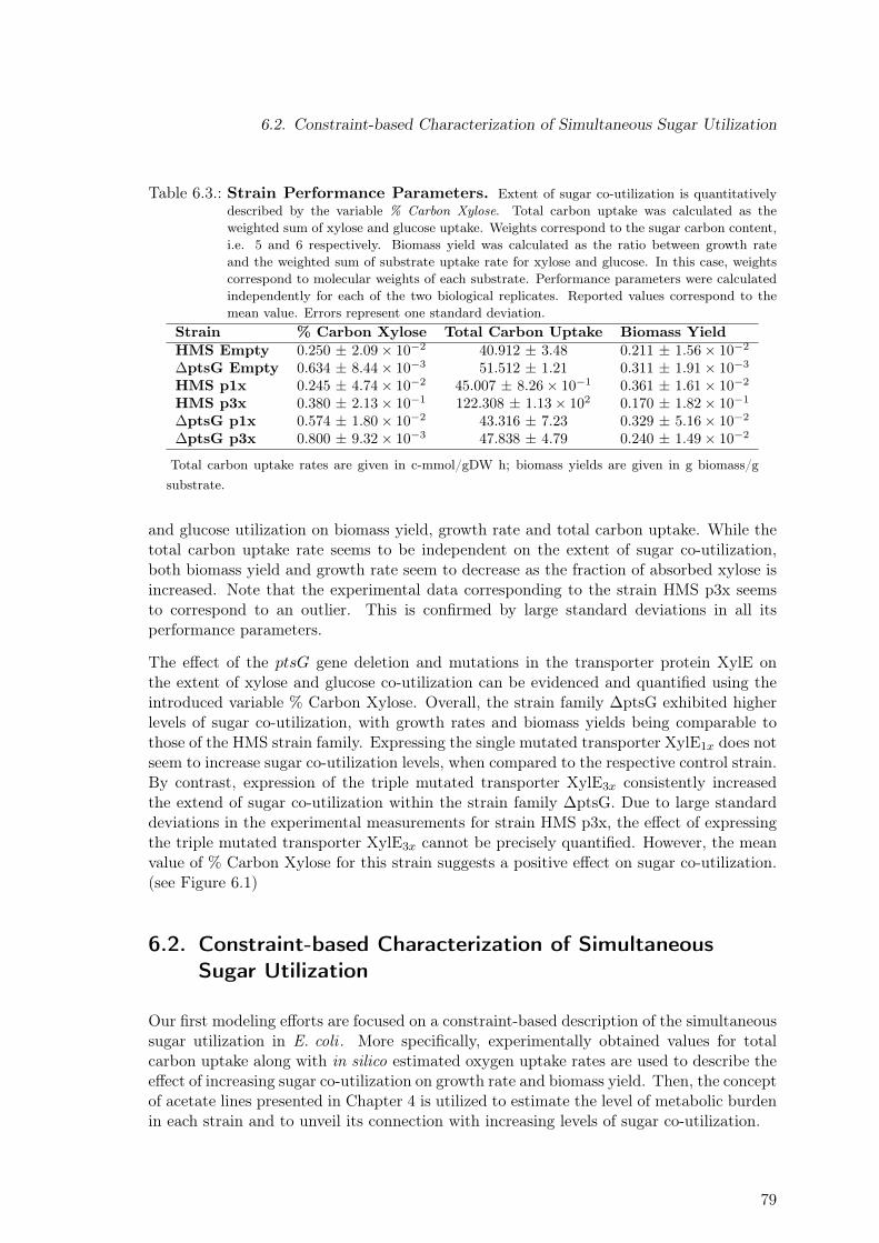
6.2. Constraint-based Characterization of Simultaneous Sugar Utilization
Table 6.3.: Strain Performance Parameters. Extent of sugar co-utilization is quantitativelydescribed by the variable % Carbon Xylose. Total carbon uptake was calculated as theweighted sum of xylose and glucose uptake. Weights correspond to the sugar carbon content,i.e. 5 and 6 respectively. Biomass yield was calculated as the ratio between growth rateand the weighted sum of substrate uptake rate for xylose and glucose. In this case, weightscorrespond to molecular weights of each substrate. Performance parameters were calculatedindependently for each of the two biological replicates. Reported values correspond to themean value. Errors represent one standard deviation.
Strain % Carbon Xylose Total Carbon Uptake Biomass YieldHMS Empty 0.250 ± 2.09× 10⁻² 40.912 ± 3.48 0.211 ± 1.56× 10⁻²
∆ptsG Empty 0.634 ± 8.44× 10⁻³ 51.512 ± 1.21 0.311 ± 1.91× 10⁻³
HMS p1x 0.245 ± 4.74× 10⁻² 45.007 ± 8.26× 10⁻¹ 0.361 ± 1.61× 10⁻²
HMS p3x 0.380 ± 2.13× 10⁻¹ 122.308 ± 1.13× 10² 0.170 ± 1.82× 10⁻¹
∆ptsG p1x 0.574 ± 1.80× 10⁻² 43.316 ± 7.23 0.329 ± 5.16× 10⁻²
∆ptsG p3x 0.800 ± 9.32× 10⁻³ 47.838 ± 4.79 0.240 ± 1.49× 10⁻²
Total carbon uptake rates are given in c-mmol/gDW h; biomass yields are given in g biomass/gsubstrate.
and glucose utilization on biomass yield, growth rate and total carbon uptake. While thetotal carbon uptake rate seems to be independent on the extent of sugar co-utilization,both biomass yield and growth rate seem to decrease as the fraction of absorbed xylose isincreased. Note that the experimental data corresponding to the strain HMS p3x seemsto correspond to an outlier. This is confirmed by large standard deviations in all itsperformance parameters.
The effect of the ptsG gene deletion and mutations in the transporter protein XylE onthe extent of xylose and glucose co-utilization can be evidenced and quantified using theintroduced variable % Carbon Xylose. Overall, the strain family ∆ptsG exhibited higherlevels of sugar co-utilization, with growth rates and biomass yields being comparable tothose of the HMS strain family. Expressing the single mutated transporter XylE1x does notseem to increase sugar co-utilization levels, when compared to the respective control strain.By contrast, expression of the triple mutated transporter XylE3x consistently increasedthe extend of sugar co-utilization within the strain family ∆ptsG. Due to large standarddeviations in the experimental measurements for strain HMS p3x, the effect of expressingthe triple mutated transporter XylE3x cannot be precisely quantified. However, the meanvalue of % Carbon Xylose for this strain suggests a positive effect on sugar co-utilization.(see Figure 6.1)
6.2. Constraint-based Characterization of SimultaneousSugar Utilization
Our first modeling efforts are focused on a constraint-based description of the simultaneoussugar utilization in E. coli . More specifically, experimentally obtained values for totalcarbon uptake along with in silico estimated oxygen uptake rates are used to describe theeffect of increasing sugar co-utilization on growth rate and biomass yield. Then, the conceptof acetate lines presented in Chapter 4 is utilized to estimate the level of metabolic burdenin each strain and to unveil its connection with increasing levels of sugar co-utilization.
79
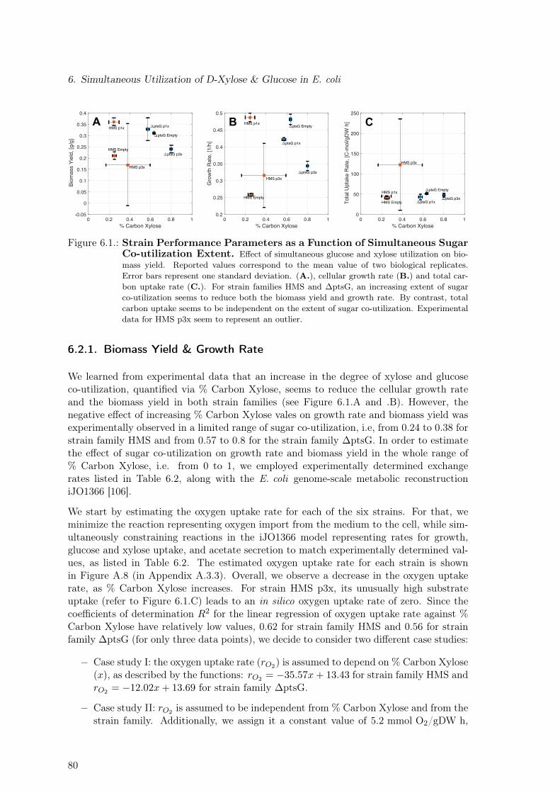
6. Simultaneous Utilization of D-Xylose & Glucose in E. coli
0 0.2 0.4 0.6 0.8 1% Carbon Xylose
-0.05
0
0.05
0.1
0.15
0.2
0.25
0.3
0.35
0.4
Bio
mas
s Yi
eld,
[g/g
]
HMS p3x
HMS p1x
HMS Empty
ptsG Empty
ptsG p3x
ptsG p1x
0 0.2 0.4 0.6 0.8 1% Carbon Xylose
0.2
0.25
0.3
0.35
0.4
0.45
0.5
Gro
wth
Rat
e, [1
/h]
HMS p1x
HMS p3x
ptsG p1x
ptsG p3x
HMS Empty
ptsG Empty
0 0.2 0.4 0.6 0.8 1% Carbon Xylose
0
50
100
150
200
250
Tota
l Upt
ake
Rat
e, [C
-mol
/gD
W h
]
HMS p1x
HMS p3x
ptsG p1xptsG p3x
HMS Empty
ptsG Empty
A B C
Figure 6.1.: Strain Performance Parameters as a Function of Simultaneous SugarCo-utilization Extent. Effect of simultaneous glucose and xylose utilization on bio-mass yield. Reported values correspond to the mean value of two biological replicates.Error bars represent one standard deviation. (A.), cellular growth rate (B.) and total car-bon uptake rate (C.). For strain families HMS and ∆ptsG, an increasing extent of sugarco-utilization seems to reduce both the biomass yield and growth rate. By contrast, totalcarbon uptake seems to be independent on the extent of sugar co-utilization. Experimentaldata for HMS p3x seem to represent an outlier.
6.2.1. Biomass Yield & Growth Rate
We learned from experimental data that an increase in the degree of xylose and glucoseco-utilization, quantified via % Carbon Xylose, seems to reduce the cellular growth rateand the biomass yield in both strain families (see Figure 6.1.A and .B). However, thenegative effect of increasing % Carbon Xylose vales on growth rate and biomass yield wasexperimentally observed in a limited range of sugar co-utilization, i.e, from 0.24 to 0.38 forstrain family HMS and from 0.57 to 0.8 for the strain family ∆ptsG. In order to estimatethe effect of sugar co-utilization on growth rate and biomass yield in the whole range of% Carbon Xylose, i.e. from 0 to 1, we employed experimentally determined exchangerates listed in Table 6.2, along with the E. coli genome-scale metabolic reconstructioniJO1366 [106].
We start by estimating the oxygen uptake rate for each of the six strains. For that, weminimize the reaction representing oxygen import from the medium to the cell, while sim-ultaneously constraining reactions in the iJO1366 model representing rates for growth,glucose and xylose uptake, and acetate secretion to match experimentally determined val-ues, as listed in Table 6.2. The estimated oxygen uptake rate for each strain is shownin Figure A.8 (in Appendix A.3.3). Overall, we observe a decrease in the oxygen uptakerate, as % Carbon Xylose increases. For strain HMS p3x, its unusually high substrateuptake (refer to Figure 6.1.C) leads to an in silico oxygen uptake rate of zero. Since thecoefficients of determination R2 for the linear regression of oxygen uptake rate against %Carbon Xylose have relatively low values, 0.62 for strain family HMS and 0.56 for strainfamily ∆ptsG (for only three data points), we decide to consider two different case studies:
− Case study I: the oxygen uptake rate (rO2) is assumed to depend on % Carbon Xylose(x), as described by the functions: rO2 = −35.57x+ 13.43 for strain family HMS andrO2 = −12.02x+ 13.69 for strain family ∆ptsG.
− Case study II: rO2 is assumed to be independent from % Carbon Xylose and from thestrain family. Additionally, we assign it a constant value of 5.2 mmol O2/gDW h,
80
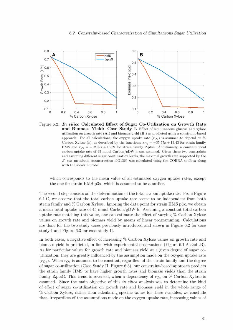
6.2. Constraint-based Characterization of Simultaneous Sugar Utilization
0 0.2 0.4 0.6 0.8 1% Carbon Xylose
0.1
0.2
0.3
0.4
0.5
0.6
0.7
0.8
Gro
wth
Rat
e, [1
/h]
HMSptsG
0 0.2 0.4 0.6 0.8 1% Carbon Xylose
0.1
0.2
0.3
0.4
0.5
0.6
Biom
ass
Yiel
d [g
/g]
A B
Figure 6.2.: In silico Calculated Effect of Sugar Co-Utilization on Growth Rateand Biomass Yield: Case Study I. Effect of simultaneous glucose and xyloseutilization on growth rate (A.) and biomass yield (B.) as predicted using a constraint-basedapproach. For all calculations, the oxygen uptake rate (rO2) is assumed to depend on %Carbon Xylose (x), as described by the functions: rO2 = −35.57x+ 13.43 for strain familyHMS and rO2 = −12.02x+ 13.69 for strain family ∆ptsG. Additionally, a constant totalcarbon uptake rate of 45 mmol Carbon/gDW h was assumed. Given these two constraintsand assuming different sugar co-utilization levels, the maximal growth rate supported by theE. coli metabolic reconstruction iJO1366 was calculated using the COBRA toolbox alongwith the solver Gurobi.
which corresponds to the mean value of all estimated oxygen uptake rates, exceptthe one for strain HMS p3x, which is assumed to be a outlier.
The second step consists on the determination of the total carbon uptake rate. From Figure6.1.C, we observe that the total carbon uptake rate seems to be independent from bothstrain family and % Carbon Xylose. Ignoring the data point for strain HMS p3x, we obtaina mean total uptake rate of 45 mmol Carbon/gDW h. Assuming a constant total carbonuptake rate matching this value, one can estimate the effect of varying % Carbon Xylosevalues on growth rate and biomass yield by means of linear programming. Calculationsare done for the two study cases previously introduced and shown in Figure 6.2 for casestudy I and Figure 6.3 for case study II.
In both cases, a negative effect of increasing % Carbon Xylose values on growth rate andbiomass yield is predicted, in line with experimental observations (Figure 6.1.A and .B).As for particular values for growth rate and biomass yield at a given degree of sugar co-utilization, they are greatly influenced by the assumption made on the oxygen uptake rate(rO2). When rO2 is assumed to be constant, regardless of the strain family and the degreeof sugar co-utilization (Case Study II, Figure 6.3), our constraint-based approach predictsthe strain family HMS to have higher growth rates and biomass yields than the strainfamily ∆ptsG. This trend is reversed, when a dependency of rO2 on % Carbon Xylose isassumed. Since the main objective of this in silico analysis was to determine the kindof effect of sugar co-utilization on growth rate and biomass yield in the whole range of% Carbon Xylose, rather than calculating specific values for these variables, we concludethat, irregardless of the assumptions made on the oxygen uptake rate, increasing values of
81
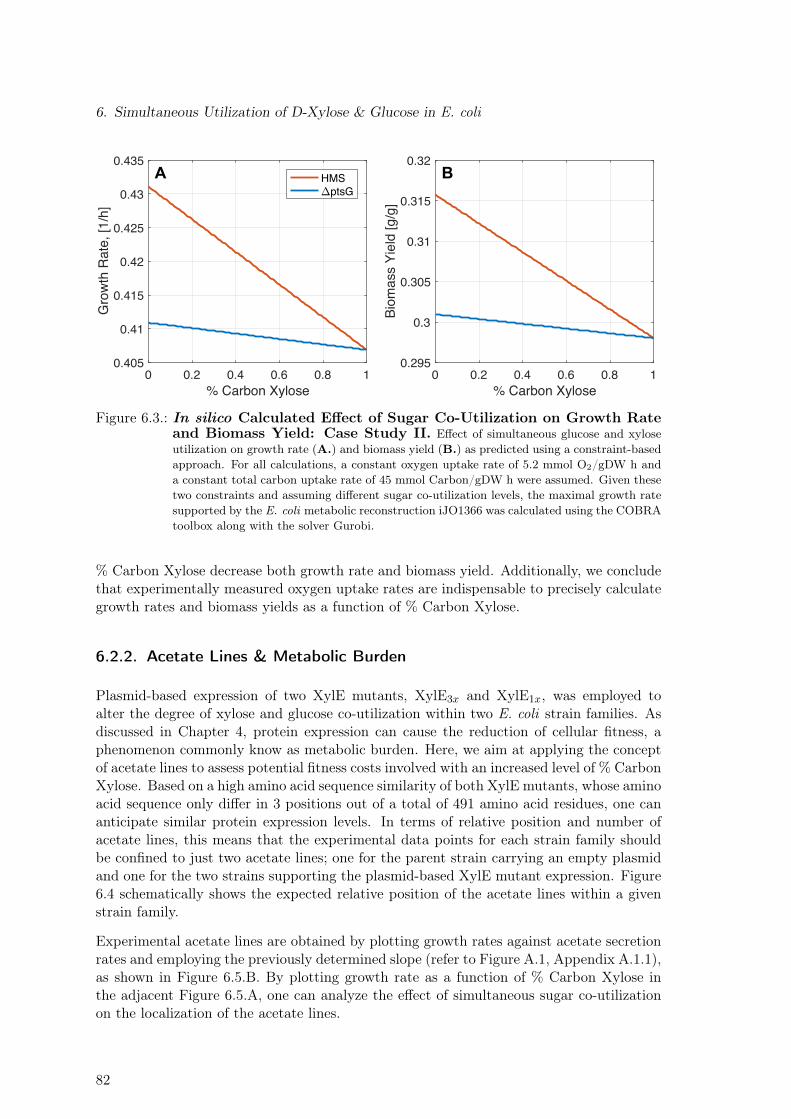
6. Simultaneous Utilization of D-Xylose & Glucose in E. coli
0 0.2 0.4 0.6 0.8 1% Carbon Xylose
0.405
0.41
0.415
0.42
0.425
0.43
0.435
Gro
wth
Rat
e, [1
/h]
HMSptsG
0 0.2 0.4 0.6 0.8 1% Carbon Xylose
0.295
0.3
0.305
0.31
0.315
0.32
Biom
ass
Yiel
d [g
/g]
A B
Figure 6.3.: In silico Calculated Effect of Sugar Co-Utilization on Growth Rateand Biomass Yield: Case Study II. Effect of simultaneous glucose and xyloseutilization on growth rate (A.) and biomass yield (B.) as predicted using a constraint-basedapproach. For all calculations, a constant oxygen uptake rate of 5.2 mmol O2/gDW h anda constant total carbon uptake rate of 45 mmol Carbon/gDW h were assumed. Given thesetwo constraints and assuming different sugar co-utilization levels, the maximal growth ratesupported by the E. coli metabolic reconstruction iJO1366 was calculated using the COBRAtoolbox along with the solver Gurobi.
% Carbon Xylose decrease both growth rate and biomass yield. Additionally, we concludethat experimentally measured oxygen uptake rates are indispensable to precisely calculategrowth rates and biomass yields as a function of % Carbon Xylose.
6.2.2. Acetate Lines & Metabolic Burden
Plasmid-based expression of two XylE mutants, XylE3x and XylE1x, was employed toalter the degree of xylose and glucose co-utilization within two E. coli strain families. Asdiscussed in Chapter 4, protein expression can cause the reduction of cellular fitness, aphenomenon commonly know as metabolic burden. Here, we aim at applying the conceptof acetate lines to assess potential fitness costs involved with an increased level of % CarbonXylose. Based on a high amino acid sequence similarity of both XylE mutants, whose aminoacid sequence only differ in 3 positions out of a total of 491 amino acid residues, one cananticipate similar protein expression levels. In terms of relative position and number ofacetate lines, this means that the experimental data points for each strain family shouldbe confined to just two acetate lines; one for the parent strain carrying an empty plasmidand one for the two strains supporting the plasmid-based XylE mutant expression. Figure6.4 schematically shows the expected relative position of the acetate lines within a givenstrain family.
Experimental acetate lines are obtained by plotting growth rates against acetate secretionrates and employing the previously determined slope (refer to Figure A.1, Appendix A.1.1),as shown in Figure 6.5.B. By plotting growth rate as a function of % Carbon Xylose inthe adjacent Figure 6.5.A, one can analyze the effect of simultaneous sugar co-utilizationon the localization of the acetate lines.
82
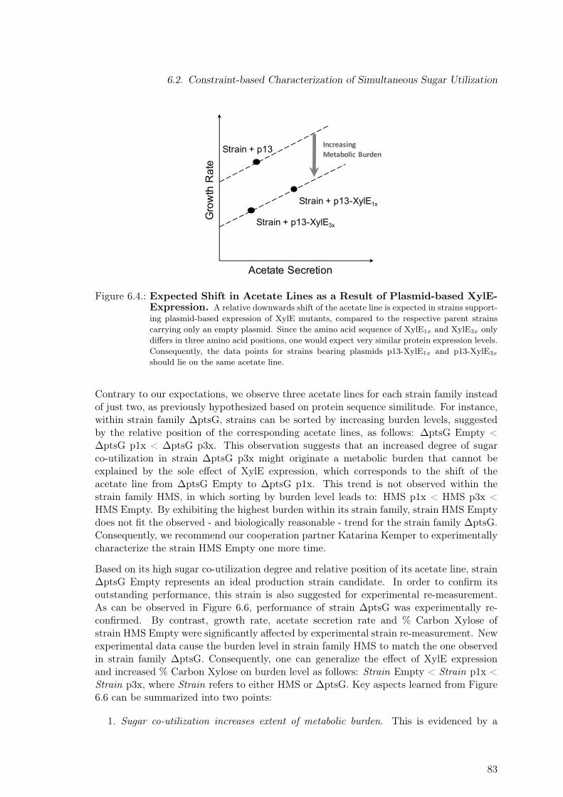
6.2. Constraint-based Characterization of Simultaneous Sugar Utilization
Acetate Secretion
Gro
wth
Rat
e
Strain + p13
Strain + p13-XylE1x
Increasing Metabolic Burden
Strain + p13-XylE3x
Figure 6.4.: Expected Shift in Acetate Lines as a Result of Plasmid-based XylE-Expression. A relative downwards shift of the acetate line is expected in strains support-ing plasmid-based expression of XylE mutants, compared to the respective parent strainscarrying only an empty plasmid. Since the amino acid sequence of XylE1x and XylE3x onlydiffers in three amino acid positions, one would expect very similar protein expression levels.Consequently, the data points for strains bearing plasmids p13-XylE1x and p13-XylE3x
should lie on the same acetate line.
Contrary to our expectations, we observe three acetate lines for each strain family insteadof just two, as previously hypothesized based on protein sequence similitude. For instance,within strain family ∆ptsG, strains can be sorted by increasing burden levels, suggestedby the relative position of the corresponding acetate lines, as follows: ∆ptsG Empty <∆ptsG p1x < ∆ptsG p3x. This observation suggests that an increased degree of sugarco-utilization in strain ∆ptsG p3x might originate a metabolic burden that cannot beexplained by the sole effect of XylE expression, which corresponds to the shift of theacetate line from ∆ptsG Empty to ∆ptsG p1x. This trend is not observed within thestrain family HMS, in which sorting by burden level leads to: HMS p1x < HMS p3x <HMS Empty. By exhibiting the highest burden within its strain family, strain HMS Emptydoes not fit the observed - and biologically reasonable - trend for the strain family ∆ptsG.Consequently, we recommend our cooperation partner Katarina Kemper to experimentallycharacterize the strain HMS Empty one more time.
Based on its high sugar co-utilization degree and relative position of its acetate line, strain∆ptsG Empty represents an ideal production strain candidate. In order to confirm itsoutstanding performance, this strain is also suggested for experimental re-measurement.As can be observed in Figure 6.6, performance of strain ∆ptsG was experimentally re-confirmed. By contrast, growth rate, acetate secretion rate and % Carbon Xylose ofstrain HMS Empty were significantly affected by experimental strain re-measurement. Newexperimental data cause the burden level in strain family HMS to match the one observedin strain family ∆ptsG. Consequently, one can generalize the effect of XylE expressionand increased % Carbon Xylose on burden level as follows: Strain Empty < Strain p1x <Strain p3x, where Strain refers to either HMS or ∆ptsG. Key aspects learned from Figure6.6 can be summarized into two points:
1. Sugar co-utilization increases extent of metabolic burden. This is evidenced by a
83
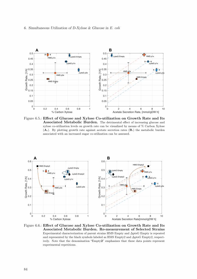
6. Simultaneous Utilization of D-Xylose & Glucose in E. coli
A B
0 0.2 0.4 0.6 0.8 1% Carbon Xylose
0
0.05
0.1
0.15
0.2
0.25
0.3
0.35
0.4
0.45
0.5
Gro
wth
Rat
e, [1
/h]
HMS p1x
HMS p3x
ptsG p1x
ptsG p3x
HMS Empty
ptsG Empty
0 2 4 6 8 10Acetate Secretion Rate, [mmol/gDW h]
0
0.05
0.1
0.15
0.2
0.25
0.3
0.35
0.4
0.45
0.5
Gro
wth
Rat
e, [1
/h]
HMS p1x
HMS p3x
ptsG p1x
ptsG p3x
HMS Empty
ptsG Empty
Figure 6.5.: Effect of Glucose and Xylose Co-utilization on Growth Rate and ItsAssociated Metabolic Burden. The detrimental effect of increasing glucose andxylose co-utilization levels on growth rate can be visualized by means of % Carbon Xylose(A.). By plotting growth rate against acetate secretion rates (B.) the metabolic burdenassociated with an increased sugar co-utilization can be assessed.
0 0.2 0.4 0.6 0.8 1% Carbon Xylose
0
0.1
0.2
0.3
0.4
0.5
0.6
Gro
wth
Rat
e, [1
/h]
HMS p1x
HMS p3x
ptsG p1x
ptsG p3x
HMS Empty
ptsG EmptyHMS Empty2
ptsG Empty2
0 2 4 6 8 10Acetate Secretion Rate[mmol/gDW h]
0
0.1
0.2
0.3
0.4
0.5
0.6
Gro
wth
Rat
e, [1
/h]
HMS p1x
HMS p3x
ptsG p1x
ptsG p3xHMS Empty
ptsG Empty
HMS Empty2
ptsG Empty2
A B
Figure 6.6.: Effect of Glucose and Xylose Co-utilization on Growth Rate and ItsAssociated Metabolic Burden. Re-measurement of Selected StrainsExperimental characterization of parent strains HMS Empty and ∆ptsG Empty is repeatedand represented by the black symbols labeled as HMS Empty2 and ∆ptsG Empty2, respect-ively. Note that the denomination “Empty2” emphasizes that these data points representexperimental repetitions.
84
6.3. Assessing Taxadiene Production Potential
downwards displacement of the acetate line for strain HMS p3x and ∆ptsG p3x,relative to the acetate line of the corresponding strain expressing the XylE transporterwith one single mutation. A tentative explanation for this observation is that xylosemetabolism should be associated with an increased expression of protein-expensivepathways.
2. Strain family ∆ptsG does not seem to allow for robust plasmid-based protein expres-sion. This is evidenced by the different extent in the response to protein expressionobserved for the two different strain families. Consider for example the expression ofXylE1x. While the acetate lines for HMS Empty2 and HMS p1x are almost identical,acetate lines for ∆ptsG Empty2 and ∆ptsG p1x are clearly differentiated, suggestingthat the extent of metabolic burden caused by XylE1x expression is much higherin the strain family ∆ptsG than in the family HMS. Similar trends are observedfor the expression of XylE3x. Additionally, Figure 5.2 provides further experimentalevidence to this observation.
6.3. Assessing Taxadiene Production Potential
Does an increased degree of sugar co-utilization have a beneficial effect on taxadiene pro-duction? Which strain has the highest taxadiene production potential? Here, we applyboth a constraint- and a kinetic-based approach to help answer these questions.
The calculation of maximal theoretical product yields by means of linear programmingrepresents the simplest approach to assess the production capabilities of a given metabolicnetwork under consideration of a given set of constraints. Here, we use the E. coli genome-scale metabolic reconstruction iJO1366 along with experimentally determined total carbonand estimated oxygen uptake rate to highlight the effect of increasing degrees of % CarbonXylose on maximal theoretical taxadiene yields. As shown in Figure 6.7, calculations aredone assuming two different growth scenarios. In the first case, a growth rate of zero isassumed (Figure 6.7.A), while in the second case, the same reaction is constrained to havean arbitrary value of 0.2 1/h for all % Carbon Xylose values (6.7.B). Regarding the oxygenuptake rate, it is assumed to be independent from % Carbon Xylose values and the geneticbackground (refer to case study II, Section 6.2.1). Additionally, a constant value of 7 mmolO2/gDW h was assumed in order to ensure the existence of a flux distribution fulfilling allconstraints over the whole range of % Carbon Xylose.
Since E. coli does not naturally produce taxadiene, the stoichiometric matrix of modeliJO1366 is correspondingly expanded to allow for taxadiene biosynthesis from IPP andDMAPP as pathway precursors (refer to Appendix B.1.1). By maximizing the flux throughthe taxadiene export reaction, under consideration of constraints on growth rate and ofglucose, xylose and oxygen uptake rates, one can assess the maximal production capabilityof the network. Usually, the production capability is expressed in terms of product yield.In this case, since two carbon sources are considered, product yield is expressed on a carbonbasis:
Taxadiene Carbon Y ield =20 rtxdn
5 rxylose + 6 rglucose,
85
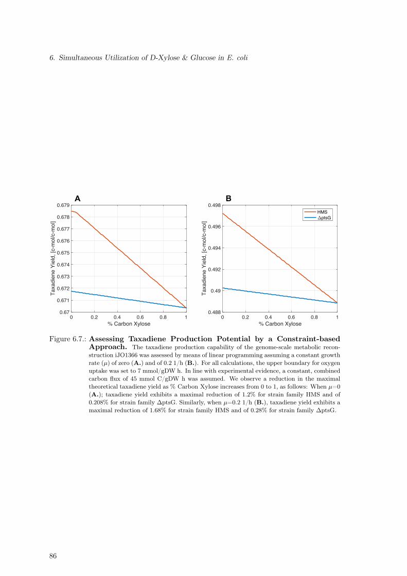
6. Simultaneous Utilization of D-Xylose & Glucose in E. coli
0 0.2 0.4 0.6 0.8 1% Carbon Xylose
0.488
0.49
0.492
0.494
0.496
0.498Ta
xadi
ene
Yiel
d, [c
-mol
/c-m
ol]
HMSptsG
0 0.2 0.4 0.6 0.8 1% Carbon Xylose
0.67
0.671
0.672
0.673
0.674
0.675
0.676
0.677
0.678
0.679
Taxa
dien
e Yi
eld,
[c-m
ol/c
-mol
]
A B
Figure 6.7.: Assessing Taxadiene Production Potential by a Constraint-basedApproach. The taxadiene production capability of the genome-scale metabolic recon-struction iJO1366 was assessed by means of linear programming assuming a constant growthrate (µ) of zero (A.) and of 0.2 1/h (B.). For all calculations, the upper boundary for oxygenuptake was set to 7 mmol/gDW h. In line with experimental evidence, a constant, combinedcarbon flux of 45 mmol C/gDW h was assumed. We observe a reduction in the maximaltheoretical taxadiene yield as % Carbon Xylose increases from 0 to 1, as follows: When µ=0(A.); taxadiene yield exhibits a maximal reduction of 1.2% for strain family HMS and of0.208% for strain family ∆ptsG. Similarly, when µ=0.2 1/h (B.), taxadiene yield exhibits amaximal reduction of 1.68% for strain family HMS and of 0.28% for strain family ∆ptsG.
86
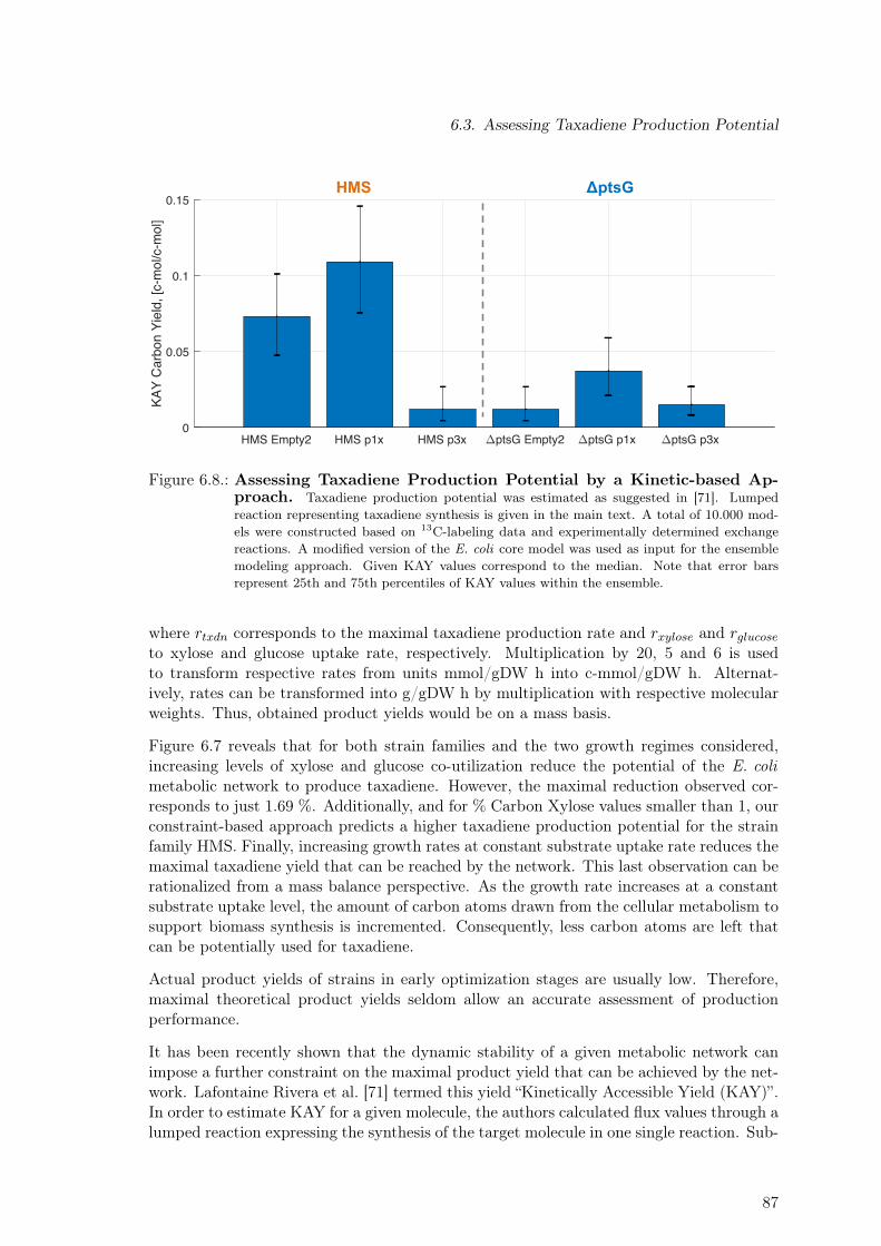
6.3. Assessing Taxadiene Production Potential
HMS Empty2 HMS p1x HMS p3x ptsG Empty2 ptsG p1x ptsG p3x0
0.05
0.1
0.15
KAY
Car
bon
Yiel
d, [c
-mol
/c-m
ol]
ΔptsGHMS
Figure 6.8.: Assessing Taxadiene Production Potential by a Kinetic-based Ap-proach. Taxadiene production potential was estimated as suggested in [71]. Lumpedreaction representing taxadiene synthesis is given in the main text. A total of 10.000 mod-els were constructed based on 13C-labeling data and experimentally determined exchangereactions. A modified version of the E. coli core model was used as input for the ensemblemodeling approach. Given KAY values correspond to the median. Note that error barsrepresent 25th and 75th percentiles of KAY values within the ensemble.
where rtxdn corresponds to the maximal taxadiene production rate and rxylose and rglucoseto xylose and glucose uptake rate, respectively. Multiplication by 20, 5 and 6 is usedto transform respective rates from units mmol/gDW h into c-mmol/gDW h. Alternat-ively, rates can be transformed into g/gDW h by multiplication with respective molecularweights. Thus, obtained product yields would be on a mass basis.
Figure 6.7 reveals that for both strain families and the two growth regimes considered,increasing levels of xylose and glucose co-utilization reduce the potential of the E. colimetabolic network to produce taxadiene. However, the maximal reduction observed cor-responds to just 1.69 %. Additionally, and for % Carbon Xylose values smaller than 1, ourconstraint-based approach predicts a higher taxadiene production potential for the strainfamily HMS. Finally, increasing growth rates at constant substrate uptake rate reduces themaximal taxadiene yield that can be reached by the network. This last observation can berationalized from a mass balance perspective. As the growth rate increases at a constantsubstrate uptake level, the amount of carbon atoms drawn from the cellular metabolism tosupport biomass synthesis is incremented. Consequently, less carbon atoms are left thatcan be potentially used for taxadiene.
Actual product yields of strains in early optimization stages are usually low. Therefore,maximal theoretical product yields seldom allow an accurate assessment of productionperformance.
It has been recently shown that the dynamic stability of a given metabolic network canimpose a further constraint on the maximal product yield that can be achieved by the net-work. Lafontaine Rivera et al. [71] termed this yield “Kinetically Accessible Yield (KAY)”.In order to estimate KAY for a given molecule, the authors calculated flux values through alumped reaction expressing the synthesis of the target molecule in one single reaction. Sub-
87
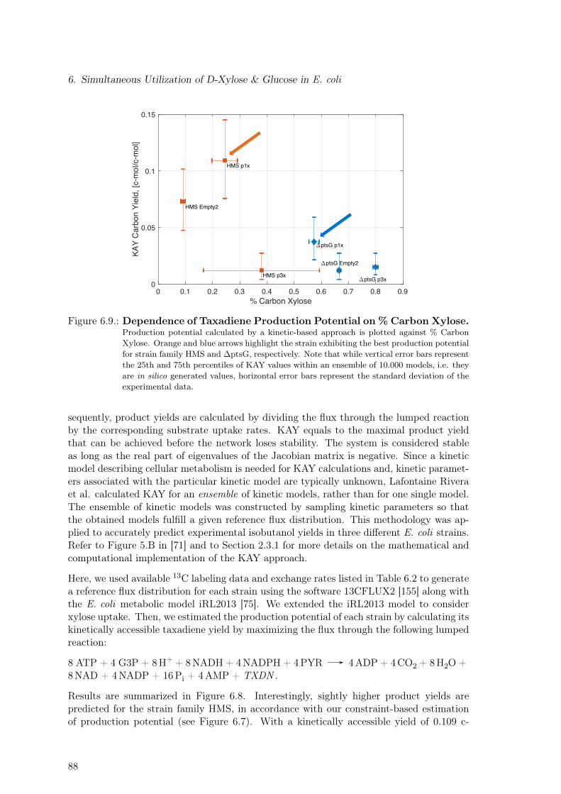
6. Simultaneous Utilization of D-Xylose & Glucose in E. coli
0 0.1 0.2 0.3 0.4 0.5 0.6 0.7 0.8 0.9% Carbon Xylose
0
0.05
0.1
0.15
KAY
Car
bon
Yiel
d, [c
-mol
/c-m
ol]
HMS Empty2
HMS p1x
HMS p3x
ptsG Empty2
ptsG p1x
ptsG p3x
Figure 6.9.: Dependence of Taxadiene Production Potential on % Carbon Xylose.Production potential calculated by a kinetic-based approach is plotted against % CarbonXylose. Orange and blue arrows highlight the strain exhibiting the best production potentialfor strain family HMS and ∆ptsG, respectively. Note that while vertical error bars representthe 25th and 75th percentiles of KAY values within an ensemble of 10.000 models, i.e. theyare in silico generated values, horizontal error bars represent the standard deviation of theexperimental data.
sequently, product yields are calculated by dividing the flux through the lumped reactionby the corresponding substrate uptake rates. KAY equals to the maximal product yieldthat can be achieved before the network loses stability. The system is considered stableas long as the real part of eigenvalues of the Jacobian matrix is negative. Since a kineticmodel describing cellular metabolism is needed for KAY calculations and, kinetic paramet-ers associated with the particular kinetic model are typically unknown, Lafontaine Riveraet al. calculated KAY for an ensemble of kinetic models, rather than for one single model.The ensemble of kinetic models was constructed by sampling kinetic parameters so thatthe obtained models fulfill a given reference flux distribution. This methodology was ap-plied to accurately predict experimental isobutanol yields in three different E. coli strains.Refer to Figure 5.B in [71] and to Section 2.3.1 for more details on the mathematical andcomputational implementation of the KAY approach.
Here, we used available 13C labeling data and exchange rates listed in Table 6.2 to generatea reference flux distribution for each strain using the software 13CFLUX2 [155] along withthe E. coli metabolic model iRL2013 [75]. We extended the iRL2013 model to considerxylose uptake. Then, we estimated the production potential of each strain by calculating itskinetically accessible taxadiene yield by maximizing the flux through the following lumpedreaction:
8 ATP + 4 G3P + 8H+ + 8NADH + 4NADPH + 4PYR 4ADP + 4CO2 + 8H2O +8NAD + 4NADP + 16Pi + 4AMP + TXDN .
Results are summarized in Figure 6.8. Interestingly, sightly higher product yields arepredicted for the strain family HMS, in accordance with our constraint-based estimationof production potential (see Figure 6.7). With a kinetically accessible yield of 0.109 c-
88
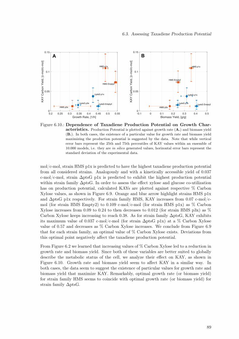
6.3. Assessing Taxadiene Production Potential
0.2 0.25 0.3 0.35 0.4 0.45 0.5 0.55Growth Rate, [1/h]
0
0.05
0.1
0.15
KAY
Car
bon
Yiel
d, [c
-mol
/c-m
ol]
HMS Empty2
HMS p1x
HMS p3xptsG Empty2
ptsG p1x
ptsG p3x
-0.1 0 0.1 0.2 0.3 0.4 0.5Biomass Yield, [g/g]
0
0.05
0.1
0.15
KAY
Car
bon
Yiel
d, [c
-mol
/c-m
ol]
HMS Empty2
HMS p1x
HMS p3xptsG Empty2
ptsG p1x
ptsG p3x
A B
Figure 6.10.: Dependence of Taxadiene Production Potential on Growth Char-acteristics. Production Potential is plotted against growth rate (A.) and biomass yield(B.). In both cases, the existence of a particular value for growth rate and biomass yieldmaximizing the production potential is suggested by the data. Note that while verticalerror bars represent the 25th and 75th percentiles of KAY values within an ensemble of10.000 models, i.e. they are in silico generated values, horizontal error bars represent thestandard deviation of the experimental data.
mol/c-mol, strain HMS p1x is predicted to have the highest taxadiene production potentialfrom all considered strains. Analogously and with a kinetically accessible yield of 0.037c-mol/c-mol, strain ∆ptsG p1x is predicted to exhibit the highest production potentialwithin strain family ∆ptsG. In order to assess the effect xylose and glucose co-utilizationhas on production potential, calculated KAYs are plotted against respective % CarbonXylose values, as shown in Figure 6.9. Orange and blue arrow highlight strains HMS p1xand ∆ptsG p1x respectively. For strain family HMS, KAY increases from 0.07 c-mol/c-mol (for strain HMS Empty2) to 0.109 c-mol/c-mol (for strain HMS p1x) as % CarbonXylose increases from 0.09 to 0.24 to then decreases to 0.012 (for strain HMS p3x) as %Carbon Xylose keeps increasing to reach 0.38. As for strain family ∆ptsG, KAY exhibitsits maximum value of 0.037 c-mol/c-mol (for strain ∆ptsG p1x) at a % Carbon Xylosevalue of 0.57 and decreases as % Carbon Xylose increases. We conclude from Figure 6.9that for each strain family, an optimal value of % Carbon Xylose exists. Deviations fromthis optimal point negatively affect the taxadiene production potential.
From Figure 6.2 we learned that increasing values of % Carbon Xylose led to a reduction ingrowth rate and biomass yield. Since both of these variables are better suited to globallydescribe the metabolic status of the cell, we analyze their effect on KAY, as shown inFigure 6.10. Growth rate and biomass yield seem to affect KAY in a similar way. Inboth cases, the data seem to suggest the existence of particular values for growth rate andbiomass yield that maximize KAY. Remarkably, optimal growth rate (or biomass yield)for strain family HMS seems to coincide with optimal growth rate (or biomass yield) forstrain family ∆ptsG.
89
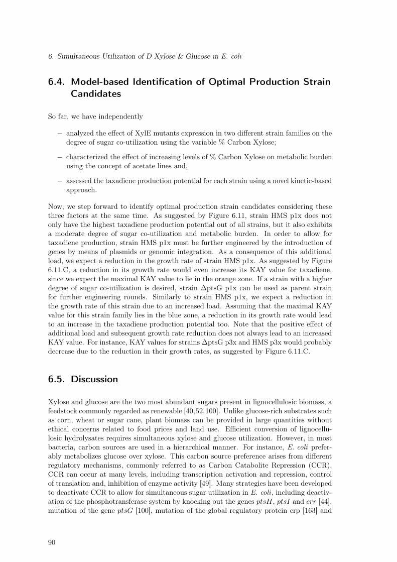
6. Simultaneous Utilization of D-Xylose & Glucose in E. coli
6.4. Model-based Identification of Optimal Production StrainCandidates
So far, we have independently
− analyzed the effect of XylE mutants expression in two different strain families on thedegree of sugar co-utilization using the variable % Carbon Xylose;
− characterized the effect of increasing levels of % Carbon Xylose on metabolic burdenusing the concept of acetate lines and,
− assessed the taxadiene production potential for each strain using a novel kinetic-basedapproach.
Now, we step forward to identify optimal production strain candidates considering thesethree factors at the same time. As suggested by Figure 6.11, strain HMS p1x does notonly have the highest taxadiene production potential out of all strains, but it also exhibitsa moderate degree of sugar co-utilization and metabolic burden. In order to allow fortaxadiene production, strain HMS p1x must be further engineered by the introduction ofgenes by means of plasmids or genomic integration. As a consequence of this additionalload, we expect a reduction in the growth rate of strain HMS p1x. As suggested by Figure6.11.C, a reduction in its growth rate would even increase its KAY value for taxadiene,since we expect the maximal KAY value to lie in the orange zone. If a strain with a higherdegree of sugar co-utilization is desired, strain ∆ptsG p1x can be used as parent strainfor further engineering rounds. Similarly to strain HMS p1x, we expect a reduction inthe growth rate of this strain due to an increased load. Assuming that the maximal KAYvalue for this strain family lies in the blue zone, a reduction in its growth rate would leadto an increase in the taxadiene production potential too. Note that the positive effect ofadditional load and subsequent growth rate reduction does not always lead to an increasedKAY value. For instance, KAY values for strains ∆ptsG p3x and HMS p3x would probablydecrease due to the reduction in their growth rates, as suggested by Figure 6.11.C.
6.5. Discussion
Xylose and glucose are the two most abundant sugars present in lignocellulosic biomass, afeedstock commonly regarded as renewable [40,52,100]. Unlike glucose-rich substrates suchas corn, wheat or sugar cane, plant biomass can be provided in large quantities withoutethical concerns related to food prices and land use. Efficient conversion of lignocellu-losic hydrolysates requires simultaneous xylose and glucose utilization. However, in mostbacteria, carbon sources are used in a hierarchical manner. For instance, E. coli prefer-ably metabolizes glucose over xylose. This carbon source preference arises from differentregulatory mechanisms, commonly referred to as Carbon Catabolite Repression (CCR).CCR can occur at many levels, including transcription activation and repression, controlof translation and, inhibition of enzyme activity [49]. Many strategies have been developedto deactivate CCR to allow for simultaneous sugar utilization in E. coli , including deactiv-ation of the phosphotransferase system by knocking out the genes ptsH, ptsI and crr [44],mutation of the gene ptsG [100], mutation of the global regulatory protein crp [163] and
90
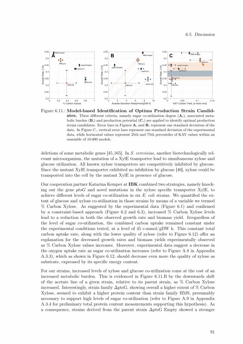
6.5. Discussion
0 0.2 0.4 0.6 0.8 1% Carbon Xylose
0.2
0.25
0.3
0.35
0.4
0.45
0.5
0.55
Gro
wth
Rat
e, [1
/h]
HMS p1x
HMS p3x
ptsG p1x
ptsG p3x
HMS Empty2
ptsG Empty2
0 2 4 6 8 10Acetate Secretion Rate[mmol/gDW h]
0.2
0.25
0.3
0.35
0.4
0.45
0.5
0.55
Gro
wth
Rat
e, [1
/h] HMS p1x
HMS p3x
ptsG p1x
ptsG p3x
HMS Empty2
ptsG Empty2
0 0.05 0.1 0.15KAY Carbon Yield, [c-mol/c-mol]
0.2
0.25
0.3
0.35
0.4
0.45
0.5
0.55
Gro
wth
Rat
e, [1
/h]
HMS Empty2
HMS p1x
HMS p3x
ptsG Empty2
ptsG p1x
ptsG 3x
A B C
Figure 6.11.: Model-based Identification of Optima Production Strain Candid-ates. Three different criteria, namely sugar co-utilization degree (A.), associated meta-bolic burden (B.) and production potential (C.) are applied to identify optimal productionstrain candidates. Error bars in Figures A. and B. represent one standard deviation of thedata. In Figure C., vertical error bars represent one standard deviation of the experimentaldata, while horizontal values represent 25th and 75th percentiles of KAY values within anensemble of 10.000 models.
deletions of some metabolic genes [45,165]. In S. cerevisiae, another biotechnologically rel-evant microorganism, the mutation of a XylE transporter lead to simultaneous xylose andglucose utilization. All known xylose transporters are competitively inhibited by glucose.Since the mutant XylE transporter exhibited no inbihition by glucose [40], xylose could betransported into the cell by the mutant XylE in presence of glucose.
Our cooperation partner Katarina Kemper at IBK combined two strategies, namely knock-ing out the gene ptsG and novel mutations in the xylose specific transporter XylE, toachieve different levels of sugar co-utilization in six E. coli strains. We quantified the ex-tent of glucose and xylose co-utilization in those strains by means of a variable we termed% Carbon Xylose. As suggested by the experimental data (Figure 6.1) and confirmedby a constraint-based approach (Figure 6.2 and 6.3), increased % Carbon Xylose levelslead to a reduction in both the observed growth rate and biomass yield. Irregardless ofthe level of sugar co-utilization, the combined carbon uptake remained constant underthe experimental conditions tested, at a level of 45 c-mmol/gDW h. This constant totalcarbon uptake rate, along with the lower quality of xylose (refer to Figure 6.12) offer anexplanation for the decreased growth rates and biomass yields experimentally observedas % Carbon Xylose values increases. Moreover, experimental data suggest a decrease inthe oxygen uptake rate as sugar co-utilization increases (refer to Figure A.8 in AppendixA.3.3), which as shown in Figure 6.12, should decrease even more the quality of xylose assubstrate, expressed by its specific energy content.
For our strains, increased levels of xylose and glucose co-utilization come at the cost of anincreased metabolic burden. This is evidenced in Figure 6.11.B by the downwards shiftof the acetate line of a given strain, relative to its parent strain, as % Carbon Xyloseincreased. Interestingly, strain family ∆ptsG, showing overall a higher extent of % CarbonXylose, seemed to exhibit a higher protein content than strain family HMS, presumablynecessary to support high levels of sugar co-utilization (refer to Figure A.9 in AppendixA.3.4 for preliminary total protein content measurements supporting this hypothesis). Asa consequence, strains derived from the parent strain ∆ptsG Empty showed a stronger
91
6. Simultaneous Utilization of D-Xylose & Glucose in E. coli
Glucose XyloseSubstrates
0
5
10
15
20
25
ATP
Cont
ent,
[mm
ol A
TP/m
mol
Sub
stra
te]
O2/Substrate=0O2/Substrate=0.25O2/Substrate=0.5O2/Substrate=1O2/Substrate=2O2/Substrate=5O2/Substrate=10O2/Substrate=20
0 5 10 15 20Oxygen to Substrate Ratio, [mmol O2/mmol Substrate]
1.05
1.1
1.15
1.2
1.25
1.3
1.35
1.4
Qua
lity G
luco
se/Q
uality
Xylo
se
A B
Figure 6.12.: Substrate Quality: Glucose vs Xylose for Different Oxygen to Sub-strate Ratios. Quality of glucose and xylose as substrates was assessed using energycontent as quality criteria for different oxygen to substrate ratios (A.). The energy contentratio between glucose and xylose (B.) shows that glucose exhibits a higher substrate qual-ity. However, this advantage over xylose greatly depends on the oxygen to substrate ratio.All calculations were performed using the genome-scale metabolic reconstruction iJO1366,as explained in Section 4.2.1.
downwards shift in its acetate lines, when compared to the shifts observed within thestrain family HMS (see Figure 6.11.B). Since the introduction of further genetic elementsinto the strains and their expression is necessary to yield a strain capable of producingtaxadiene, strain response to an additional load should be considered for the selection ofoptimal production strain candidates.
In order to accurately select optimal production strain candidates for further engineeringrounds and thus to contribute the reduction of in vivo experimentation, we applied both aconstraint- and a kinetic-based approach to quantitatively assess the taxadiene productionpotential of all strains. The constraint-based approach indicated a linear reduction in thetheoretical maximal taxadiene yield as % Carbon Xylose increased for both strain families.Additionally, strain family HMS exhibited a superior performance when % Carbon Xylose< 1. Considering these predictions, the strain HMS Empty should be further engineeredinto a production strain, as it exhibits the lowest % Carbon Xylose out of all strains.On the other hand, the kinetic-based approach suggested a more complex relationshipbetween the kinetically accessible taxadiene yield and % Carbon Xylose. This methodpredicted an overall higher taxadiene production potential for the strain family HMS, justas the constraint-based approach did. However, unlike the constraint-based approach, thekinetic based approach suggested the existence of a maximal taxadiene yield for each strainfamily, located at % Carbon Xylose values different from zero. Remarkably, the kinetic-based approach suggested that optimal taxadiene production was only indirectly definedby % Carbon Xylose. The true variable determining the kinetically accessible yield fortaxadiene was the growth rate or the biomass yield. Experimental evidence supportingthis observation was provided by our cooperation partner Lars Janoschek at STT; refer toFigure 9.3.A in Chapter 9. Based on three aspects, namely extent of sugar co-utilization, itsassociated metabolic burden and taxadiene production potential, we suggest strain HMSp1x for further engineering rounds towards the construction of an optimal production
92

6.5. Discussion
strain. Since a further load, exerted by additional genetic elements introduced to allowtaxadiene synthesis, is expected to reduce growth rate and biomass yield, we expect theexperimental taxadiene yield to surpass the predicted KAY value for this strain, as shown inFigure 6.11.C. To the best of our knowledge, this work represents the first reported effort toguide the selection of strain candidates potentially exhibiting high production performancewhile considering concepts of metabolic burden and kinetically accessible yields.
At the moment of the submission of this work, experimental implementation of this model-driven suggestion was still pending.
93

Part III.
Results: Process Optimization
95

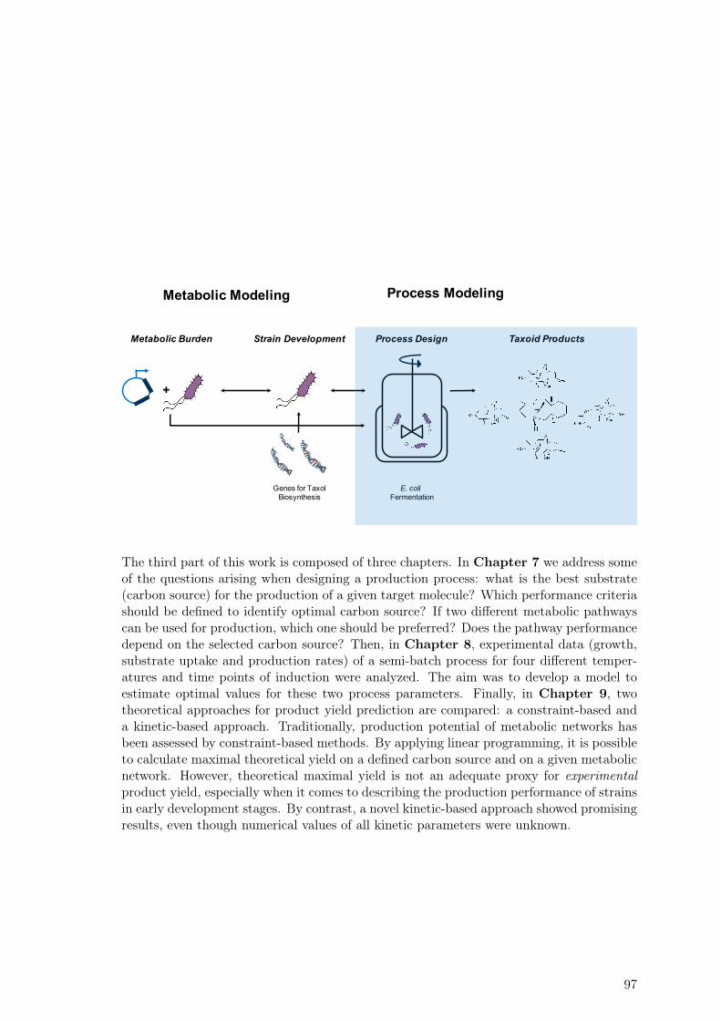
Taxoid ProductsMetabolic Burden
Genes for TaxolBiosynthesis
E. coli Fermentation
+
Metabolic Modeling Process Modeling
Strain Development Process Design
The third part of this work is composed of three chapters. In Chapter 7 we address someof the questions arising when designing a production process: what is the best substrate(carbon source) for the production of a given target molecule? Which performance criteriashould be defined to identify optimal carbon source? If two different metabolic pathwayscan be used for production, which one should be preferred? Does the pathway performancedepend on the selected carbon source? Then, in Chapter 8, experimental data (growth,substrate uptake and production rates) of a semi-batch process for four different temper-atures and time points of induction were analyzed. The aim was to develop a model toestimate optimal values for these two process parameters. Finally, in Chapter 9, twotheoretical approaches for product yield prediction are compared: a constraint-based anda kinetic-based approach. Traditionally, production potential of metabolic networks hasbeen assessed by constraint-based methods. By applying linear programming, it is possibleto calculate maximal theoretical yield on a defined carbon source and on a given metabolicnetwork. However, theoretical maximal yield is not an adequate proxy for experimentalproduct yield, especially when it comes to describing the production performance of strainsin early development stages. By contrast, a novel kinetic-based approach showed promisingresults, even though numerical values of all kinetic parameters were unknown.
97

7. Model-based Medium Optimization
Typically, the following questions are to be addressed in early design stages of a givenbiotechnological production process: what is the best substrate for the production of thetarget molecule? Which performance criteria should be applied to identify the optimalcarbon source? If two different metabolic pathways can be used for production, which oneshould be preferred? Does pathway performance depend on the selected carbon source?Here, we apply constraint-based modeling to answer these questions. First, we defined twodifferent performance criteria to assess the performance of various substrates, namely themaximal profit and the maximal theoretical yield. We calculate theoretical yields usingthree different bases: a carbon, a molar and a mass basis. Then, we used these criteriato rank 180 different growth-supporting carbon sources. The underlying calculation isthe potential of the substrate to be transformed into taxadiene by the E. coli metabolicnetwork. Three-substrate mixtures were also considered in the calculations. Additionally,aerobic and anaerobic optimal network performance was compared. Since taxadiene pro-duction via the non-mevalonate pathway requires energy in the form of ATP and CTP,our model-driven analysis suggests an aerobic production process. Surprisingly, no singlecarbon source tested allowed a complete conversion into taxadiene, i.e., all substrates ex-hibited a maximal theoretical yield lower than 1 c-mol taxadiene/c-mol substrate. Thelargest maximal theoretical yield was obtained for ethanol as single carbon source, witha value of 0.92 c-mol taxadiene/c-mol ethanol. By contrast, glucose exhibited a maximalcarbon yield of 0.65 c-mol taxadiene/c-mol glucose. An analysis of optimal flux distribu-tions identified CO2 as the main source for carbon loss. Finally, we found out that theendogenous non-mevalonate pathway allows for a higher theoretical yield than the hetero-logous mevalonate pathway for glucose as the carbon source. However, this is not true forall 180 carbon sources analyzed. When both pathways were active in an optimal ratio, weobserved a small degree of synergy (<6%) for some substrates, including glucose.
7.1. Performance Criteria for Substrate Selection
Before one can actually select the best substrate from a list of candidates, performancecriteria need to be defined. For biotechnological production processes, product yield hasbeen traditionally used to assess and to compare the production performance of differentsubstrates and strains. Product yield is defined as the ratio of product gained to substrateconsumed. Depending on the units used to calculate the ratio, one can express productyield on three different bases: on a molar basis (mol product/mol substrate), on a carbonbasis (c-mol product/c-mol substrate) or on a mass basis (g product/g substrate). Whenassessing the economic performance of a given set of substrates, profit can be used as aperformance criterion. We define profit as the ratio of US dollars gained to US dollarsinvested.
99
7. Model-based Medium Optimization
The choice of a particular performance criterion to identify the best carbon source dependson the aim of the optimization process. Thus, if the process designer is interested inmaximizing revenue, the performance criterion to be applied seems obvious. On the otherhand, if network efficiency is to be optimized, product yield on a carbon or mass basisshould be preferred over product yield on a molar basis. This is because maximal values ofmolar yield are not constrained to a defined interval, but rather depend on the substrateused. This leads to difficulties while assessing a given product yield on a molar basis. Forinstance, is a product yield of 0.1 mol taxadiene/mol glucose good enough? By contrast,values for product yield expressed on a carbon or mass basis will always range from 0 to1. Substrates exhibiting a product yield of 1 c-mol product/c-mol substrate allow for acomplete conversion of substrate into product. In other words, the network performanceis already optimal and can not be further improved.
7.1.1. Single Substrates
We start our constraint-based analysis by assessing 180 different growth-supporting sub-strates, based on the performance criteria previously described. The E. coli metabolicreconstruction iJO1366 [106] was used for all calculations. Growth-supporting refers to theability of the iJO1366 network to in silico grow on a given substrate. In order to calculatemaximal theoretical yields representing true upper boundaries, both the Non-growth Asso-ciated Maintenance (NGAM) term and the cellular growth rate were set to 0. Additionally,oxygen uptake rate was set to an artificially high value of 100 mmol/gDW h to ensure suf-ficient oxygen availability. Since the E. coli metabolism does not allow for an endogenoustaxadiene production, the iJO166 model was extended by adding necessary reactions al-lowing taxadiene production as shown in Appendix B.1.1. Following steps were appliedto calculate maximal profit and taxadiene yields using the endogenous non-mevalonatepathway for precursor production.
1. Choose one of the 180 substrates listed in Table B.1 (see Appendix B.1.2).
2. Set a rate of 1 mmol substrate/gDW h by adjusting the lower and upper bound ofthe respective uptake reaction.
3. Maximize flux through the taxadiene export reaction using linear programming.
4. The numerical value of the maximal flux calculated in previous step coincides withthe taxadiene yield on a molar basis, i.e. mol txd/mol substrate. This is becausesubstrate uptake rate was set to 1 mmol/gDW h. txd refers to taxadiene.
5. Calculate product yield on a carbon basis by multiplying yield obtained in step 4 bythe factor:
[ 20 c−mol txd1 mol txd
x c−mol substrate1 mol substrate
)]; x c−mol refers to the number of carbon atoms in the
substrate chosen in step 1.
6. Calculate product yield on a mass basis by multiplying yield obtained in step 4 by the
factor:[ 272.48 g txd
1 mol txdx g substrate
1 mol substrate
]; x g substrate refers to the molecular weight of the substrate
chosen in step 1.
100
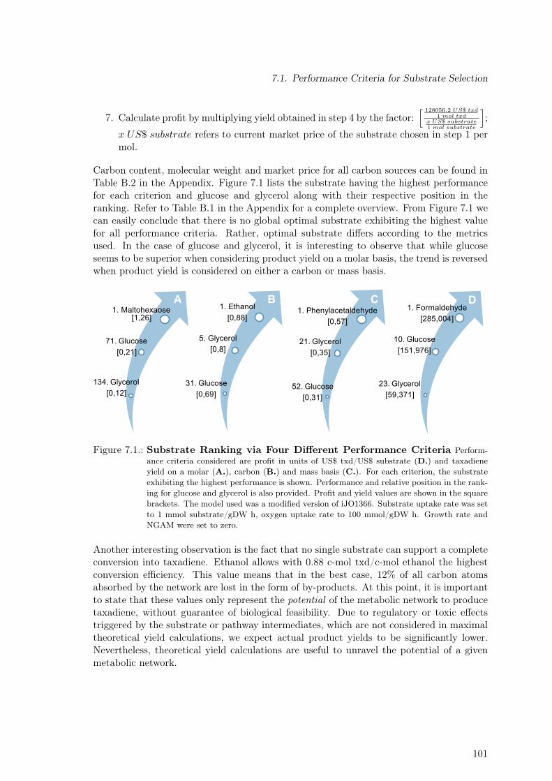
7.1. Performance Criteria for Substrate Selection
7. Calculate profit by multiplying yield obtained in step 4 by the factor:[ 128056.2 US$ txd
1 mol txdx US$ substrate1 mol substrate
];
x US$ substrate refers to current market price of the substrate chosen in step 1 permol.
Carbon content, molecular weight and market price for all carbon sources can be found inTable B.2 in the Appendix. Figure 7.1 lists the substrate having the highest performancefor each criterion and glucose and glycerol along with their respective position in theranking. Refer to Table B.1 in the Appendix for a complete overview. From Figure 7.1 wecan easily conclude that there is no global optimal substrate exhibiting the highest valuefor all performance criteria. Rather, optimal substrate differs according to the metricsused. In the case of glucose and glycerol, it is interesting to observe that while glucoseseems to be superior when considering product yield on a molar basis, the trend is reversedwhen product yield is considered on either a carbon or mass basis.
31. Glucose [0,69]
5. Glycerol [0,8]
1. Ethanol[0,88]
52. Glucose [0,31]
21. Glycerol [0,35]
1. Phenylacetaldehyde[0,57]
134. Glycerol [0,12]
71. Glucose [0,21]
1. Maltohexaose[1,26]
23. Glycerol[59,371]
10. Glucose [151,976]
1. Formaldehyde[285,004]
A B DC
Figure 7.1.: Substrate Ranking via Four Different Performance Criteria Perform-ance criteria considered are profit in units of US$ txd/US$ substrate (D.) and taxadieneyield on a molar (A.), carbon (B.) and mass basis (C.). For each criterion, the substrateexhibiting the highest performance is shown. Performance and relative position in the rank-ing for glucose and glycerol is also provided. Profit and yield values are shown in the squarebrackets. The model used was a modified version of iJO1366. Substrate uptake rate was setto 1 mmol substrate/gDW h, oxygen uptake rate to 100 mmol/gDW h. Growth rate andNGAM were set to zero.
Another interesting observation is the fact that no single substrate can support a completeconversion into taxadiene. Ethanol allows with 0.88 c-mol txd/c-mol ethanol the highestconversion efficiency. This value means that in the best case, 12% of all carbon atomsabsorbed by the network are lost in the form of by-products. At this point, it is importantto state that these values only represent the potential of the metabolic network to producetaxadiene, without guarantee of biological feasibility. Due to regulatory or toxic effectstriggered by the substrate or pathway intermediates, which are not considered in maximaltheoretical yield calculations, we expect actual product yields to be significantly lower.Nevertheless, theoretical yield calculations are useful to unravel the potential of a givenmetabolic network.
101
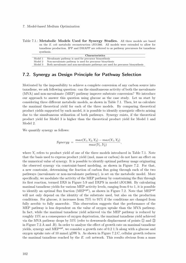
7. Model-based Medium Optimization
Table 7.1.: Metabolic Models Used for Synergy Studies. All three models are basedon the E. coli metabolic reconstruction iJO1366. All models were extended to allow fortaxadiene production. IPP and DMAPP are referred to as pathway precursors for taxadienesynthesis.
CharacteristicsModel 1 Mevalonate pathway is used for precursor biosynthesisModel 2 Non-mevalonate pathway is used for precursor biosythesisModel 3 Both mevalonate and non-mevalonate pathways are used for precursor biosynthesis
7.2. Synergy as Design Principle for Pathway Selection
Motivated by the impossibility to achieve a complete conversion of any carbon source intotaxadiene, we ask following question: can the simultaneous activity of both the mevalonate(MVA) and non-mevalonate (MEP) pathway improve substrate conversion? We introduceour approach to answer this question using glucose as the case study. Let us start byconsidering three different metabolic models, as shown in Table 7.1. Then, let us calculatethe maximal theoretical yield for each of the three models. By comparing theoreticalproduct yields supported by each model, it is possible to identify synergistic effects arisingdue to the simultaneous utilization of both pathways. Synergy exists, if the theoreticalproduct yield for Model 3 is higher than the theoretical product yield for Model 1 andModel 2.
We quantify synergy as follows:
Synergy =max(Y1, Y2, Y3)−max(Y1, Y2)
max(Y1, Y2),
where Yi refers to product yield of one of the three models introduced in Table 7.1. Notethat the basis used to express product yield (mol, mass or carbon) do not have an effect onthe numerical value of synergy. It is possible to identify optimal pathway usage originatingthe observed synergy via constraint-based modeling, as shown in Figure 7.2. For that,a new constraint, determining the fraction of carbon flux going through each of the twopathways (mevalonate or non-mevalonate pathway), is set on the metabolic model. Morespecifically, we modulate the activity of the MEP pathway by constraining the flux throughits first reaction, termed DXS in Figure 5.9 and DXPS in model iJO1366. By calculatingmaximal taxadiene yields for various MEP activity levels, ranging from 0 to 1, it is possibleto identify an optimal flux fraction (MEPopt), as shown in Figure 7.2. Note that MEPopt
will not only depend on the identity of the substrate used, but also on the productionconditions. For glucose, it increases from 75% to 91% if the conditions are changed fromfully aerobic to fully anaerobic. This observation suggests that the performance of theMEP pathway is less dependent on the value of oxygen uptake than the MVA pathway.In fact, while the maximal taxadiene yield achieved via the MEP pathway is reduced byroughly 15% as a consequence of oxygen deprivation, the maximal taxadiene yield achievedvia the MVA pathway drops by 55% (refer to downwards displacement of points 1 and 3in Figure 7.2.A and .B). In order to analyze the effect of growth rate on maximal taxadieneyields, synergy and MEPopt, we consider a growth rate of 0.2 1/h along with a glucose andoxygen uptake rate of 10 mmol/gDW h. As shown in Figure 7.2.C, cellular growth reducesthe maximal taxadiene reached by the E. coli network. This results obvious from a mass
102
7.2. Synergy as Design Principle for Pathway Selection
balance perspective. Since growth and taxadiene production compete for a limited supplyof carbon atoms, an increase in the growth rate will necessarily lead to a reduction inthe maximal taxadiene yield. Interestingly, MEPopt decreases from 75% to 70% if growthis considered (compare Figure 7.2.C and .A). This trend continues if growth is increasedto 0.4 1/h. In this case, MEPopt amounts to 56%, suggesting that taxadiene productionvia MVA pathway is less affected by growth than the MEP pathway (results not shown).However, at a growth rate of 0.4 1/h, the synergy between the MEP and MVA pathwayonly reaches 0.4 %.
Now, we extend synergy calculations to all carbon sources considering fully aerobic condi-tions and setting NGAM and growth rate to 0. Figure 7.3 summarizes the synergy observedfor 180 substrates (refer to Table B.1 in the Appendix for a complete overview of the res-ults). We observe that the simultaneous activity of the MEP and MVA pathway does notlead to an increased taxadiene yield for all substrates, i.e. synergy amounts to 0%. In total,57 carbon sources belongs to this group, almost the half of which (28 substrates) exhibithigher taxadiene yield using the MEP pathway. With only 14 substrates having a synergyhigher than 2.5% but lower than 5.7%, we conclude that simultaneous activity of boththe MEP and MVA pathway does not lead to a substantial product yield improvement.A closer look at obtained carbon yields (refer to column “MEP+MVA. Carbon Yield” inTable B.1 in the Apendix) reveals that ethanol, with a carbon yield of 0.92 c-mol txd/c-molethanol, still exhibits the highest carbon efficiency. Although the synergy between MEPand MVA pathways increased the carbon yield for ethanol from 0.88 to 0.92 c-mol/c-mol,network performance is not optimal yet, since still 8% of all carbon atoms are lost in theform of by-products.
7.2.1. Three-Substrate Mixtures
Determined to find a network configuration that allows a complete substrate conversioninto product, we asked the question, if substrate mixtures can potentially increase networkperformance. In order to keep the problem computationally tractable, we limited ourstudy to two- and three-substrate mixtures. In total, we tested 972,150 different mediumcompositions:
(180
1
)+
(180
2
)+
(180
3
)=
180!
1! 179!+
180!
2! 178!+
180!
3! 177!
= 972, 150
As in section 7.1.1, we used a constraint-based approach along with the E. coli metabolicreconstruction iJO1366 to obtain results shown in Figure 7.4. Since substrate mixtures areconsidered, product yields calculated on a molar basis do not allow a direct assessment ofthe network carbon efficiency. Consequently, product yields are reported on a carbon basis.Calculations for profit and product yields on a mass basis can be performed analogously.To guarantee that the maximal possible product yield is identified during calculations, bothpathways for precursor production (mevalonate and non-mevalonate) were introduced inthe model iJO1366. The applied procedure was the following:
103
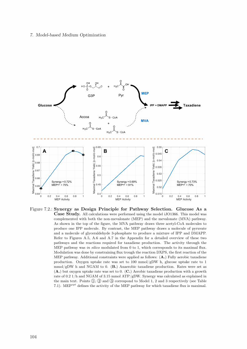
7. Model-based Medium Optimization
0 0.2 0.4 0.6 0.8 1MEP Activity
0.64
0.65
0.66
0.67
0.68
0.69
0.7
Max
imal
Tax
adie
ne Y
ield
, [c-
mol
/c-m
ol]
0 0.2 0.4 0.6 0.8 1MEP Activity
0.4
0.45
0.5
0.55
0.6
0.65
Max
imal
Tax
adie
ne Y
ield
, [c-
mol
/c-m
ol]
0 0.2 0.4 0.6 0.8 1MEP Activity
0.515
0.52
0.525
0.53
0.535
0.54
0.545
0.55
Max
imal
Tax
adie
ne Y
ield
, [c-
mol
/c-m
ol]
A B C
1
3
2
Glucose Taxadiene
+
IPP + DMAPP
MVA
MEP
Accoa
G3P Pyr
+
Synergy = 0.72%MEPopt = 75%
Synergy = 0.69%MEPopt = 91%
Synergy = 0.73%MEPopt = 70%
Figure 7.2.: Synergy as Design Principle for Pathway Selection. Glucose As aCase Study. All calculations were performed using the model iJO1366. This model wascomplemented with both the non-mevalonate (MEP) and the mevalonate (MVA) pathway.As shown in the top of the figure, the MVA pathway draws three acetyl-CoA molecules toproduce one IPP molecule. By contrast, the MEP pathway draws a molecule of pyruvateand a molecule of glyceraldehyde 3-phosphate to produce a mixture of IPP and DMAPP.Refer to Figures A.5, A.6 and A.7 in the Appendix for a detailed overview of these twopathways and the reactions required for taxadiene production. The activity through theMEP pathway was in silico modulated from 0 to 1, which corresponds to its maximal flux.Modulation was done by constraining flux trough the reaction DXPS, the first reaction of theMEP pathway. Additional constraints were applied as follows: (A.) Fully aerobic taxadieneproduction. Oxygen uptake rate was set to 100 mmol/gDW h, glucose uptake rate to 1mmol/gDW h and NGAM to 0. (B.) Anaerobic taxadiene production. Rates were set as(A.) but oxygen uptake rate was set to 0. (C.) Aerobic taxadiene production with a growthrate of 0.2 1/h and NGAM of 3.15 mmol ATP/gDW. Synergy was calculated as explained inthe main text. Points 1 , 2 and 3 correspond to Model 1, 2 and 3 respectively (see Table7.1). MEPopt defines the activity of the MEP pathway for which taxadiene flux is maximal.
104
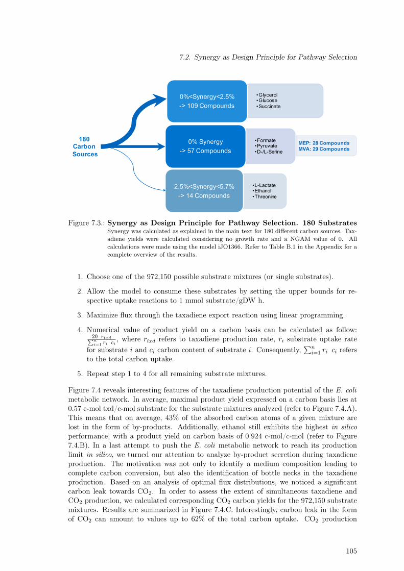
7.2. Synergy as Design Principle for Pathway Selection
•Formate•Pyruvate•D-/L-Serine
0% Synergy-> 57 Compounds
•Glycerol•Glucose•Succinate
0%<Synergy<2.5%-> 109 Compounds
•L-Lactate•Ethanol•Threonine
2.5%<Synergy<5.7%-> 14 Compounds
180 Carbon Sources
MEP: 28 CompoundsMVA: 29 Compounds
Figure 7.3.: Synergy as Design Principle for Pathway Selection. 180 SubstratesSynergy was calculated as explained in the main text for 180 different carbon sources. Tax-adiene yields were calculated considering no growth rate and a NGAM value of 0. Allcalculations were made using the model iJO1366. Refer to Table B.1 in the Appendix for acomplete overview of the results.
1. Choose one of the 972,150 possible substrate mixtures (or single substrates).
2. Allow the model to consume these substrates by setting the upper bounds for re-spective uptake reactions to 1 mmol substrate/gDW h.
3. Maximize flux through the taxadiene export reaction using linear programming.
4. Numerical value of product yield on a carbon basis can be calculated as follow:20 rtxd∑ni=1 ri ci
, where rtxd refers to taxadiene production rate, ri substrate uptake ratefor substrate i and ci carbon content of substrate i. Consequently,
∑ni=1 ri ci refers
to the total carbon uptake.
5. Repeat step 1 to 4 for all remaining substrate mixtures.
Figure 7.4 reveals interesting features of the taxadiene production potential of the E. colimetabolic network. In average, maximal product yield expressed on a carbon basis lies at0.57 c-mol txd/c-mol substrate for the substrate mixtures analyzed (refer to Figure 7.4.A).This means that on average, 43% of the absorbed carbon atoms of a given mixture arelost in the form of by-products. Additionally, ethanol still exhibits the highest in silicoperformance, with a product yield on carbon basis of 0.924 c-mol/c-mol (refer to Figure7.4.B). In a last attempt to push the E. coli metabolic network to reach its productionlimit in silico, we turned our attention to analyze by-product secretion during taxadieneproduction. The motivation was not only to identify a medium composition leading tocomplete carbon conversion, but also the identification of bottle necks in the taxadieneproduction. Based on an analysis of optimal flux distributions, we noticed a significantcarbon leak towards CO2. In order to assess the extent of simultaneous taxadiene andCO2 production, we calculated corresponding CO2 carbon yields for the 972,150 substratemixtures. Results are summarized in Figure 7.4.C. Interestingly, carbon leak in the formof CO2 can amount to values up to 62% of the total carbon uptake. CO2 production
105
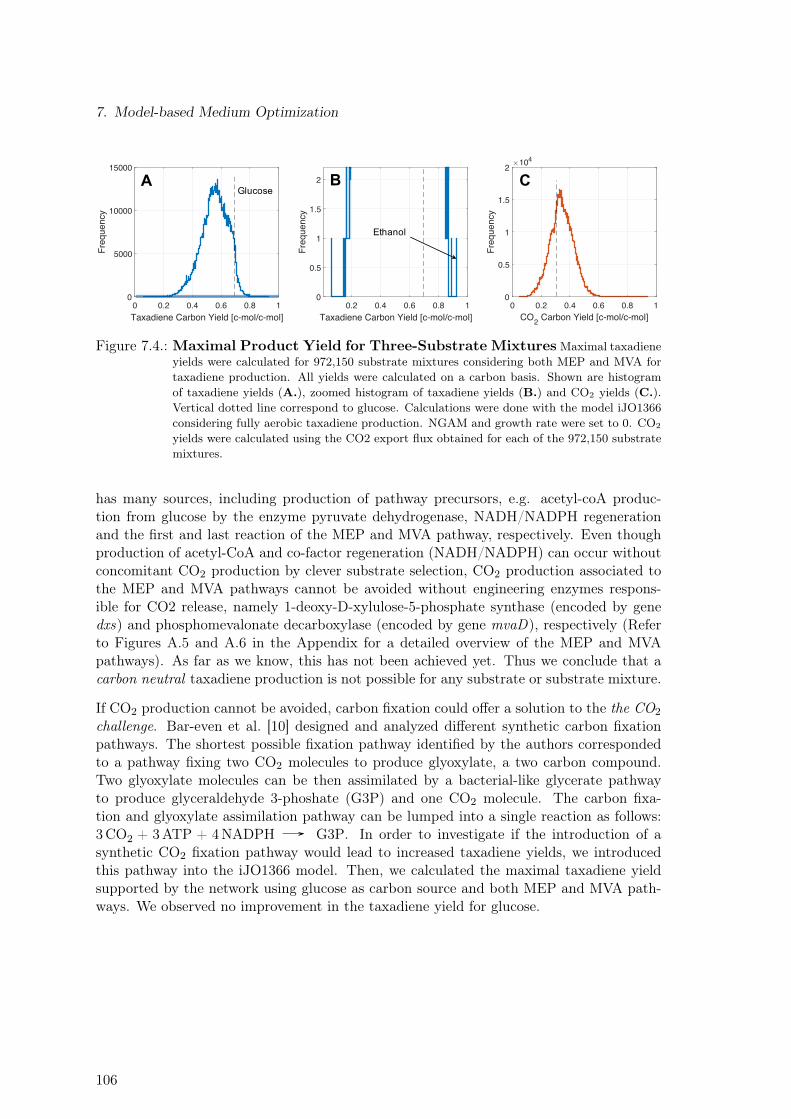
7. Model-based Medium Optimization
0 0.2 0.4 0.6 0.8 1Taxadiene Carbon Yield [c-mol/c-mol]
0
5000
10000
15000
Freq
uenc
y
0.2 0.4 0.6 0.8 1Taxadiene Carbon Yield [c-mol/c-mol]
0
0.5
1
1.5
2
Freq
uenc
y0 0.2 0.4 0.6 0.8 1
CO2 Carbon Yield [c-mol/c-mol]
0
0.5
1
1.5
2
Freq
uenc
y
104
Ethanol
GlucoseA B C
Figure 7.4.: Maximal Product Yield for Three-Substrate Mixtures Maximal taxadieneyields were calculated for 972,150 substrate mixtures considering both MEP and MVA fortaxadiene production. All yields were calculated on a carbon basis. Shown are histogramof taxadiene yields (A.), zoomed histogram of taxadiene yields (B.) and CO2 yields (C.).Vertical dotted line correspond to glucose. Calculations were done with the model iJO1366considering fully aerobic taxadiene production. NGAM and growth rate were set to 0. CO2
yields were calculated using the CO2 export flux obtained for each of the 972,150 substratemixtures.
has many sources, including production of pathway precursors, e.g. acetyl-coA produc-tion from glucose by the enzyme pyruvate dehydrogenase, NADH/NADPH regenerationand the first and last reaction of the MEP and MVA pathway, respectively. Even thoughproduction of acetyl-CoA and co-factor regeneration (NADH/NADPH) can occur withoutconcomitant CO2 production by clever substrate selection, CO2 production associated tothe MEP and MVA pathways cannot be avoided without engineering enzymes respons-ible for CO2 release, namely 1-deoxy-D-xylulose-5-phosphate synthase (encoded by genedxs) and phosphomevalonate decarboxylase (encoded by gene mvaD), respectively (Referto Figures A.5 and A.6 in the Appendix for a detailed overview of the MEP and MVApathways). As far as we know, this has not been achieved yet. Thus we conclude that acarbon neutral taxadiene production is not possible for any substrate or substrate mixture.
If CO2 production cannot be avoided, carbon fixation could offer a solution to the the CO2
challenge. Bar-even et al. [10] designed and analyzed different synthetic carbon fixationpathways. The shortest possible fixation pathway identified by the authors correspondedto a pathway fixing two CO2 molecules to produce glyoxylate, a two carbon compound.Two glyoxylate molecules can be then assimilated by a bacterial-like glycerate pathwayto produce glyceraldehyde 3-phoshate (G3P) and one CO2 molecule. The carbon fixa-tion and glyoxylate assimilation pathway can be lumped into a single reaction as follows:3CO2 + 3ATP + 4NADPH G3P. In order to investigate if the introduction of asynthetic CO2 fixation pathway would lead to increased taxadiene yields, we introducedthis pathway into the iJO1366 model. Then, we calculated the maximal taxadiene yieldsupported by the network using glucose as carbon source and both MEP and MVA path-ways. We observed no improvement in the taxadiene yield for glucose.
106
7.3. Discussion
7.3. Discussion
Even though the conclusion of the CO2 challenge is rather unsatisfactory, we generated anextensive in silico knowledge regarding optimal carbon sources for taxadiene production.As such, this knowledge can be used to optimize experimental medium composition byemploying substrates exhibiting high in silico performance values as carbon source. Forinstance, substrates potentially increasing the taxadiene production performance of a givenmain carbon source, for example glucose, can be rapidly identified and experimentallytested. Additionally, profit as performance criterion can be used in early stage techno-economic feasibility studies. By defining a minimum profit level that should be achievedby the process, it is possible to determine if a given host microorganism and a determinedsubstrate have the potential to yield an economically feasible production process.
Many studies have assessed and compared the production potential of various substratesusing the MEP, MVA or both pathways in silico [1,50,95,162]. However, the work reportedhere surpasses the scope of any of these studies, as we assessed and compared a total of972,150 unique substrate mixtures. We demonstrated that it is impossible to convert anysingle substrate or substrate mixture into taxadiene in a carbon neutral fashion. Ethanol,with a taxadiene yield of of 0.924 c-mol/c-mol, was identified by our large-scale in silicoanalysis as the substrate allowing the highest carbon efficiency. Interestingly, as identifiedby Gruchattka et al. [50], ethanol along with the MVA pathway has allowed the highestexperimental terpenoid yield (on a carbon basis) reported to date (refer to Table 2 in[50], for original publication refer to [156]). Even though the host microorganism was S.cerevisiae and the terpenoid produced corresponded to artemisinic acid, this study stronglypoints at the potential of ethanol as an efficient carbon source for taxadiene and in general,for terpenoids production.
As for the synergistic effects arising from the simultaneous utilization of the MEP and MVApathway, a recent publication [160] experimentally reported an improvement in isopreneyield, when both pathways were active in E. coli . Yield improvement amounted to 20-foldand threefold respectively, compared to the sole usage of the MEP or the MVA pathway. Inthe case of the fully aerobic taxadiene production in E. coli , our constraint-based approachpredicted an increment of 0.72% and 7.38%, compared to the sole performance of the MEPand MVA pathways, respectively (refer to Figure 7.2.A). Even though the extent of thesynergy experimentally observed by Yang et al. [160] can not be directly compared to our insilico simulations, his study suggests that synergy calculations based on sole stoichiometricconstraints do possess a predictive power. An additional study supporting the validity ofconstraint-based assessment of pathway synergy was provided by Shen et al. [136]. Theauthors showed that in silico predicted synergistic effects arising from the simultaneousactivity of two different pathways for the 1-propanol production, namely the threonine andthe citramalate pathway, could be also observed in vivo.
Unlike our constraint-based calculations and additional reports [1,50,95] predicting a higherin silico potential of the MEP pahtway over the MVA pathway for taxadiene production,Yang et al. [160] experimentally demonstrated the superiority of the MVA pathway overthe MEP pathway for isoprene production. Since both taxadiene and isoprene productiondepends on the DMAPP production flux, supported by either the MEP or MVA path-way, the report by Yang et al. [160] clearly evidences one of the intrinsic limitations ofconstraint-based modeling. Since pathway regulation at the transcription-, translation- or
107
7. Model-based Medium Optimization
enzyme activity-level are poorly considered or not considered at all in genome-scale meta-bolic reconstructions, biologically relevant aspects constraining flux through metabolicpathways can be overseen. Since the MVA pathway is a non-native pathway in E. coli , theflux through this pathway is not constrained by any regulatory elements. Consequently,terpenoid yields using the heterologous MVA pathway have been repeatedly reported tosurpass the performance of the native MEP pathway [93, 98, 160]. In spite of its flaws,constraint-based modeling represents a valuable modeling tool. This is because large scaleconstraint-based analyses are computationally tractable (due to the efficiency of availablelinear-programming solvers) and because high quality genome-scale metabolic reconstruc-tions for many relevant industrial microorganisms are easily accessible to the researchcommunity [66,123]. More importantly, the metabolism of all microorganisms is subjectedto mass balance constraints. Hence, theoretical yields calculated using constraint-basedapproaches are true constraints, representing the maximal potential of a given host meta-bolism.
108
8. Model-based Semi-Batch Optimization
The performance of a plasmid-based production strain was experimentally assessed in asemi-batch process at different temperatures and time points of induction. Available dataconsisted of concentration time courses for biomass, substrate and product. The mod-eling task was to identify optimal production temperature and time point of inductionin silico. To that end, we applied dFBA as modeling framework to describe the avail-able experimental data. We used Arrhenius-like functions to mathematically describe thetemperature dependence of calculated rates (growth, substrate uptake and production).Maximal productivity was used as the performance metric to be optimized by the model.By perturbing both production temperature and time point of induction and analyzing thesystem response, we identified a process setting that increased the maximal productivityby 56% in silico [84]. Unfortunately, Experimental implementation of this model-basedprediction by our cooperation partner was not possible due to lacking reproducibility ofexperimental results. This was potentially caused by strain/plasmid instability. However,we believe that the proposed approach represents a valid proof of concept for process op-timization using readily available experimental data in early stages of strain and processdevelopment.
8.1. Strain & Experimental Data
The strain used in this work was constructed by our cooperation partner Max Hirte at IBKand experimentally characterized by Lars Janoscheck at STT. Experimental strain char-acterization was performed in a 1.5 liter bio-reactor and was limited to the measurementof concentration time courses for glucose, biomass and taxadiene. Production was inducedby adding Isopropyl β-D-1-thiogalactopyranoside (IPTG) to the bio-reactor after a previ-ously defined biomass concentration was reached. We termed this moment the inductiontime point, tinduction. As shown in Table 8.1, this process parameter remained relativelyconstant for all processes, ranging from 6.25 to 8.25 hours. Since the main objective of thisfirst characterization round was to identify an optimal production temperature, four dif-ferent temperatures ranging from 16 to 37°C were tested. Note that while the productiontemperature (Tproduction) was varied, the temperature before induction was kept constantat a value of 37°C to ensure fast biomass formation. Figure 8.1 shows a schematic rep-resentation of the process set-up and experimental time courses obtained for a productiontemperature of 16 °C. Data for all other temperatures can be found in Tables B.3 to B.8,in Appendix B.2.1. The effect of IPTG addition on taxadiene production can be clearlyobserved in Figure 8.1.D. Shortly after induction, taxadiene is formed and its concentrationkeeps increasing as the process continues.
In order to use provided experimental data to identify optimal process parameters (pro-duction temperature and time point of induction), it is first necessary to develop a process
109
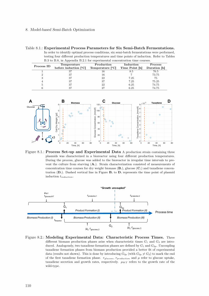
8. Model-based Semi-Batch Optimization
Table 8.1.: Experimental Process Parameters for Six Semi-Batch Fermentations.In order to identify optimal process conditions, six semi-batch fermentations were performed,testing four different production temperatures and time points of induction. Refer to TablesB.3 to B.8, in Appendix B.2.1 for experimental concentration time courses.
Process ID Temperaturebefore induction [°C]
ProductionTemperature [°C]
InductionTime Point [h]
ProcessDuration [h]
1 37 16 8.5 76.52 37 16 7 73.753 37 22 7.25 754 37 37 7.25 75.255 37 22 6.25 74.756 37 27 6.25 74.75
0 20 40 60 80Time, [h]
0
1
2
3
4
5
6
Cel
l Dry
Wei
ght,
[g/l]
Biomass
0 20 40 60 80Time, [h]
0
20
40
60
80
100
120
Glu
cose
Con
cent
ratio
n, [m
mol
/l]
Glucose
0 20 40 60 80Time, [h]
0
1
2
3
4
5
6
7
8
9
Taxa
dien
e C
once
ntra
tion,
[mm
ol/l]
10-3 Taxadiene
+
A
x3
B C DGlucose
Figure 8.1.: Process Set-up and Experimental Data A production strain containing threeplasmids was characterized in a bioreactor using four different production temperatures.During the process, glucose was added to the bioreactor in irregular time intervals to pre-vent the culture from starving (A.). Strain characterization consisted of measurements ofconcentration time courses for dry weight biomass (B.), glucose (C.) and taxadiene concen-tration (D.). Dashed vertical line in Figure B. to D. represents the time point of plasmidinduction tinduction.
tInduction
G1
rproduction,1
G2µ2, rglucose,2
µ3, rglucose,3
Process time
rproduction,2
G2p
µWTrglucose,WT
“Growth uncoupled”
Biomass Production (I)
Product Formation (I) Product Formation (II)
Biomass Production (II) Biomass Production (III)
Figure 8.2.: Modeling Experimental Data: Characteristic Process Times. Threedifferent biomass production phases arise when characteristic times G1 and G2 are intro-duced. Analogously, two taxadiene formation phases are defined by G1 and G2p. Uncouplingtaxadiene formation phases from biomass production provided a better fit of experimentaldata (results not shown). This is done by introducing G2p (with G2p 6= G2) to mark the endof the first taxadiene formation phase. rglucose, rproduction and µ refer to glucose uptake,taxadiene secretion and growth rates, respectively. µWT refers to the growth rate of thewild-type.
110
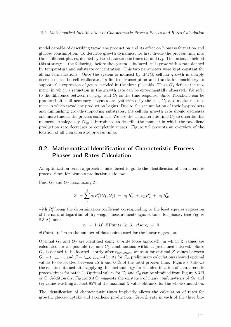
8.2. Mathematical Identification of Characteristic Process Phases and Rates Calculation
model capable of describing taxadiene production and its effect on biomass formation andglucose consumption. To describe growth dynamics, we first divide the process time intothree different phases, defined by two characteristic times G1 and G2. The rationale behindthis strategy is the following: before the system is induced, cells grow with a rate definedby temperature and substrate concentration. This two parameters were kept constant forall six fermentations. Once the system is induced by IPTG, cellular growth is sharplydecreased, as the cell reallocates its limited transcription and translation machinery tosupport the expression of genes encoded in the three plasmids. Thus, G1 defines the mo-ment, in which a reduction in the growth rate can be experimentally observed. We referto the difference between tinduction and G1 as the time response. Since Taxadiene can beproduced after all necessary enzymes are synthetized by the cell, G1 also marks the mo-ment in which taxadiene production begins. Due to the accumulation of toxic by-productsand diminishing growth-supporting substrates, the cellular growth rate should decreasesone more time as the process continues. We use the characteristic time G2 to describe thismoment. Analogously, G2p is introduced to describe the moment in which the taxadieneproduction rate decreases or completely ceases. Figure 8.2 presents an overview of thelocation of all characteristic process times.
8.2. Mathematical Identification of Characteristic ProcessPhases and Rates Calculation
An optimization-based approach is introduced to guide the identification of characteristicprocess times for biomass production as follows:
Find G1 and G2 maximizing Z:
Z =3∑i
ciR2i (G1, G2) = c1R
21 + c2R
22 + c3R
23,
with R2i being the determination coefficient corresponding to the least squares regression
of the natural logarithm of dry weight measurements against time, for phase i (see Figure8.3.A), and:
ci = 1 if #Points ≥ 3, else ci = 0.
#Points refers to the number of data points used for the linear regression.
Optimal G1 and G2 are identified using a brute force approach, in which Z values arecalculated for all possible G1 and G2 combinations within a predefined interval. SinceG1 is defined to be located shortly after tinduction, we scan for optimal Z values betweenG1 = tinduction and G = tinduction+4 h. As for G2, preliminary calculations showed optimalvalues to be located between 15 h and 60% of the total process time. Figure 8.3 showsthe results obtained after applying this methodology for the identification of characteristicprocess times for batch 1. Optimal values for G1 and G2 can be obtained from Figure 8.3.Bor C. Additionally, Figure 8.3.C, suggests the existence of many combinations of G1 andG2 values reaching at least 95% of the maximal Z value obtained for the whole simulation.
The identification of characteristic times implicitly allows the calculation of rates forgrowth, glucose uptake and taxadiene production. Growth rate in each of the three bio-
111
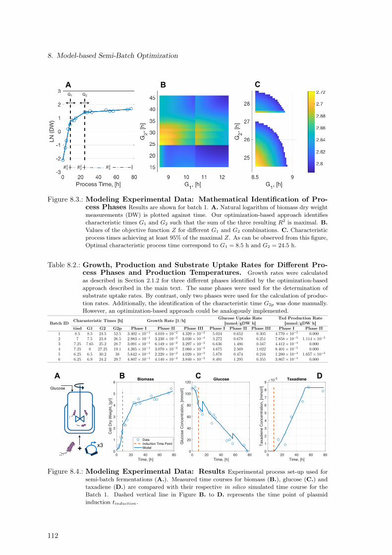
8. Model-based Semi-Batch Optimization
𝑅"# 𝑅$#𝑅##
G1 G2
A B C
Figure 8.3.: Modeling Experimental Data: Mathematical Identification of Pro-cess Phases Results are shown for batch 1. A. Natural logarithm of biomass dry weightmeasurements (DW) is plotted against time. Our optimization-based approach identifiescharacteristic times G1 and G2 such that the sum of the three resulting R2 is maximal. B.Values of the objective function Z for different G1 and G2 combinations. C. Characteristicprocess times achieving at least 95% of the maximal Z. As can be observed from this figure,Optimal characteristic process time correspond to G1 = 8.5 h and G2 = 24.5 h.
Table 8.2.: Growth, Production and Substrate Uptake Rates for Different Pro-cess Phases and Production Temperatures. Growth rates were calculatedas described in Section 2.1.2 for three different phases identified by the optimization-basedapproach described in the main text. The same phases were used for the determination ofsubstrate uptake rates. By contrast, only two phases were used for the calculation of produc-tion rates. Additionally, the identification of the characteristic time G2p was done manually.However, an optimization-based approach could be analogously implemented.
Batch ID Charasteristic Times [h] Growth Rate [1/h] Glucose Uptake Rate[mmol/gDW h]
Txd Production Rate[mmol/gDW h]
tind G1 G2 G2p Phase I Phase II Phase III Phase I Phase II Phase III Phase I Phase II1 8.5 8.5 24.5 52.5 3.402× 10⁻¹ 4.010× 10⁻² 4.320× 10⁻³ 5.024 0.652 0.305 4.770× 10⁻⁵ 0.0002 7 7.5 23.8 26.5 2.983× 10⁻¹ 3.230× 10⁻² 3.030× 10⁻⁴ 3.272 0.678 0.251 7.858× 10⁻⁵ 1.114× 10⁻⁵
3 7.25 7.65 25.2 28.7 3.091× 10⁻¹ 6.149× 10⁻² 3.297× 10⁻³ 6.636 1.486 0.347 4.412× 10⁻⁴ 0.0004 7.25 8 27.25 19.1 4.265× 10⁻¹ 3.070× 10⁻² 2.060× 10⁻³ 4.675 2.569 1.022 8.401× 10⁻⁵ 0.0005 6.25 6.5 30.2 38 5.642× 10⁻¹ 2.220× 10⁻² 4.020× 10⁻³ 5.878 0.474 0.216 1.280× 10⁻⁴ 1.657× 10⁻⁵
6 6.25 6.9 24.2 29.7 4.807× 10⁻¹ 4.140× 10⁻² 3.840× 10⁻³ 8.491 1.295 0.355 3.867× 10⁻⁴ 0.000
0 20 40 60 80Time, [h]
0
1
2
3
4
5
6
Cel
l Dry
Wei
ght,
[g/l]
Biomass
0 20 40 60 80Time, [h]
0
20
40
60
80
100
120
Glu
cose
Con
cent
ratio
n, [m
mol
/l]
Glucose
0 20 40 60 80Time, [h]
0
1
2
3
4
5
6
7
8
9
Taxa
dien
e C
once
ntra
tion,
[mm
ol/l]
10-3 Taxadiene
DataInduction Time PointModel+
A
x3
Glucose
B C D
Figure 8.4.: Modeling Experimental Data: Results Experimental process set-up used forsemi-batch fermentations (A.). Measured time courses for biomass (B.), glucose (C.) andtaxadiene (D.) are compared with their respective in silico simulated time course for theBatch 1. Dashed vertical line in Figure B. to D. represents the time point of plasmidinduction tinduction.
112
8.3. Dependence of Model Parameters on Production Temperature
mass production phases equals the slope of the corresponding line shown in Figure 8.3.A.Glucose uptake and taxadiene secretion rates are calculated by multiplying the growthrate of each of the phases by the slope of the straight line that results from plotting theglucose (or taxadiene) concentration as a function of biomass dry weight. Refer to Section2.1.2 for more details on the calculation of rates from concentration time courses. Table 8.2summarizes characteristic process times and respective rates for all six data sets. Note thattaxadiene production rate in the second product formation phase (see Figure 8.2) was set tozero for Batches 1, 3 4 and 6. While this is a valid assumption in Batches 1 and 6 (refer toFigures 8.4 and B.5, respectively) because the taxadiene concentration remains relativelyconstant during this phase, we clearly observe a reduction in the taxadiene concentrationfor Batches 3 and 4 (refer to Figures B.2 and B.3 in Appendix B.2.3). This means thatthe taxadiene production rate in the second product formation phase should be negativerather than zero. Since the number of experimental points for taxadiene concentration inthis phase is very limited, we assume a zero production rate to be more accurate than arate calculated using just two data points. Independently of the validity of this assump-tion, it does not have an effect on predicted optimal Tproduction or tinduction values, as wewill discuss later.
Exchange rates and characteristic process times are parameters that allow for a completedescription of respective experimental concentration time courses. To demonstrate this,we applied dFBA to generate in silico time courses for each semi-batch fermentationprocess using parameters listed in Table 8.2 along with information regarding glucosepulses and initial biomass and glucose concentrations for each batch (refer to Tables B.3to B.8, in Appendix B.2.1 for numerical values). As explained in Section 2.1.1, dFBAallows for the combination of reactor dynamics with cellular metabolism, thus allowingthe simulation of concentration time courses of extra-cellular metabolites in the reactor.Figure 8.4 exemplarily shows the performance of dFBA simulations for batch 1 (refer toFigures B.1 to B.5 in Appendix B.2.3 for a complete results overview). As observed, insilico generated concentration time courses closely match experimental data (see TableB.11 in Appendix B.2.3 for R2 values). All dFBA simulations reported in this work wereperformed using MATLAB functions provided by DFBALab [47].
8.3. Dependence of Model Parameters on ProductionTemperature
The main objective of the modeling effort presented in this chapter is the identificationof optimal values for two process parameters, namely production temperature and timepoint of induction. So far, we have developed a modeling approach that allows the sim-ulation of concentration time courses, closely matching experimental data. Since not allparameters listed in Table 8.2 are directly accessible, meaning that their numerical valuescannot be freely adjusted experimentally, we venture to explore the effect of both produc-tion temperature (Tproduction) and time point of induction (tinduction) on them. Note thatnumerical values of growth and glucose uptake rate during the first production phase, µWT
and rglucose,WT in Figure 8.2, are considered to be constant, since strain, initial mediumcomposition and temperature in the first biomass production phase were not changed andare not subject to optimization in this work.
113
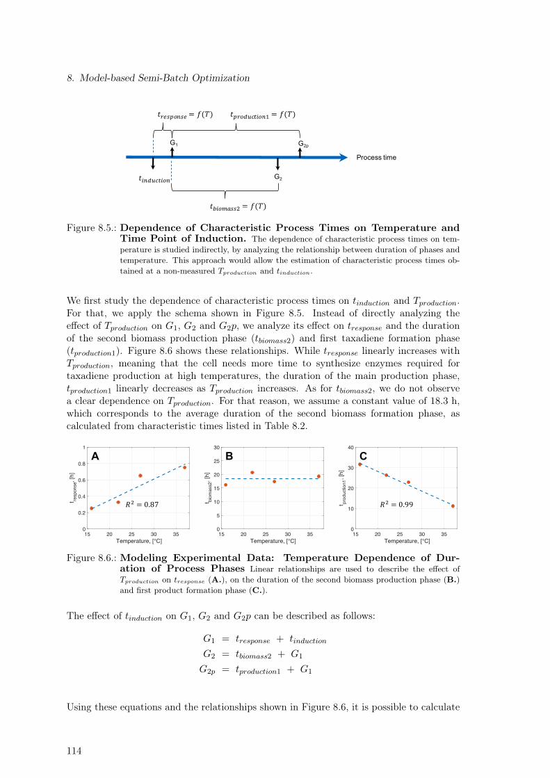
8. Model-based Semi-Batch Optimization
G1
𝑡"#$%&'$# = 𝑓(𝑇)
G2
Process time
G2p
𝑡-.&/0$$1 = 𝑓(𝑇)
𝑡.'2345.&'
𝑡%"&2345.&'6 = 𝑓(𝑇)
Figure 8.5.: Dependence of Characteristic Process Times on Temperature andTime Point of Induction. The dependence of characteristic process times on tem-perature is studied indirectly, by analyzing the relationship between duration of phases andtemperature. This approach would allow the estimation of characteristic process times ob-tained at a non-measured Tproduction and tinduction.
We first study the dependence of characteristic process times on tinduction and Tproduction.For that, we apply the schema shown in Figure 8.5. Instead of directly analyzing theeffect of Tproduction on G1, G2 and G2p, we analyze its effect on tresponse and the durationof the second biomass production phase (tbiomass2) and first taxadiene formation phase(tproduction1). Figure 8.6 shows these relationships. While tresponse linearly increases withTproduction, meaning that the cell needs more time to synthesize enzymes required fortaxadiene production at high temperatures, the duration of the main production phase,tproduction1 linearly decreases as Tproduction increases. As for tbiomass2, we do not observea clear dependence on Tproduction. For that reason, we assume a constant value of 18.3 h,which corresponds to the average duration of the second biomass formation phase, ascalculated from characteristic times listed in Table 8.2.
15 20 25 30 35Temperature, [°C]
0
0.2
0.4
0.6
0.8
1
t resp
onse
, [h]
15 20 25 30 35Temperature, [°C]
0
5
10
15
20
25
30
t biom
ass2
, [h]
15 20 25 30 35Temperature, [°C]
0
10
20
30
40
t prod
uctio
n1, [
h]
A B C
𝑅" = 0.87 𝑅" = 0.99
Figure 8.6.: Modeling Experimental Data: Temperature Dependence of Dur-ation of Process Phases Linear relationships are used to describe the effect ofTproduction on tresponse (A.), on the duration of the second biomass production phase (B.)and first product formation phase (C.).
The effect of tinduction on G1, G2 and G2p can be described as follows:
G1 = tresponse + tinduction
G2 = tbiomass2 + G1
G2p = tproduction1 + G1
Using these equations and the relationships shown in Figure 8.6, it is possible to calculate
114
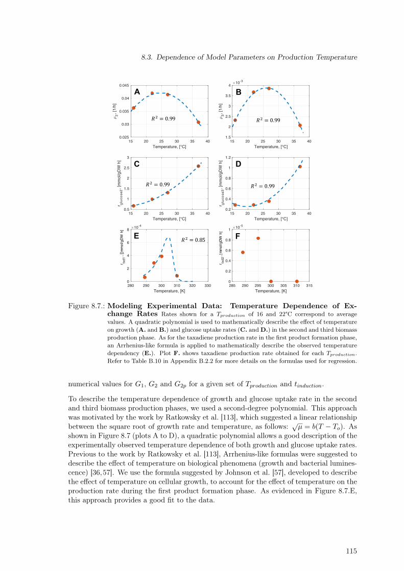
8.3. Dependence of Model Parameters on Production Temperature
15 20 25 30 35 40Temperature, [°C]
0.025
0.03
0.035
0.04
0.045
2, [1/
h]
15 20 25 30 35 40Temperature, [°C]
1.5
2
2.5
3
3.5
4
3, [1/
h]
10-3
15 20 25 30 35 40Temperature, [°C]
0.5
1
1.5
2
2.5
3
r gluc
ose2
, [m
mol
/gD
W h
]
15 20 25 30 35 40Temperature, [°C]
0.2
0.4
0.6
0.8
1
1.2
r gluc
ose3
, [m
mol
/gD
W h
]
280 290 300 310 320 330Temperature, [K]
0
2
4
6
8
r txd1
, [1/
h]
10-4
285 290 295 300 305 310 315Temperature, [K]
0
0.2
0.4
0.6
0.8
1
r txd2
, [1/
h]
10-5
A B
C D
E F
𝑅" = 0.99 𝑅" = 0.99
𝑅" = 0.99 𝑅" = 0.99
𝑅" = 0.85
[mmol/gDW
h]
[mmol/gDW
h]
Figure 8.7.: Modeling Experimental Data: Temperature Dependence of Ex-change Rates Rates shown for a Tproduction of 16 and 22°C correspond to averagevalues. A quadratic polynomial is used to mathematically describe the effect of temperatureon growth (A. and B.) and glucose uptake rates (C. and D.) in the second and third biomassproduction phase. As for the taxadiene production rate in the first product formation phase,an Arrhenius-like formula is applied to mathematically describe the observed temperaturedependency (E.). Plot F. shows taxadiene production rate obtained for each Tproduction.Refer to Table B.10 in Appendix B.2.2 for more details on the formulas used for regression.
numerical values for G1, G2 and G2p for a given set of Tproduction and tinduction.
To describe the temperature dependence of growth and glucose uptake rate in the secondand third biomass production phases, we used a second-degree polynomial. This approachwas motivated by the work by Ratkowsky et al. [113], which suggested a linear relationshipbetween the square root of growth rate and temperature, as follows: √µ = b(T − To). Asshown in Figure 8.7 (plots A to D), a quadratic polynomial allows a good description of theexperimentally observed temperature dependence of both growth and glucose uptake rates.Previous to the work by Ratkowsky et al. [113], Arrhenius-like formulas were suggested todescribe the effect of temperature on biological phenomena (growth and bacterial lumines-cence) [36,57]. We use the formula suggested by Johnson et al. [57], developed to describethe effect of temperature on cellular growth, to account for the effect of temperature on theproduction rate during the first product formation phase. As evidenced in Figure 8.7.E,this approach provides a good fit to the data.
115
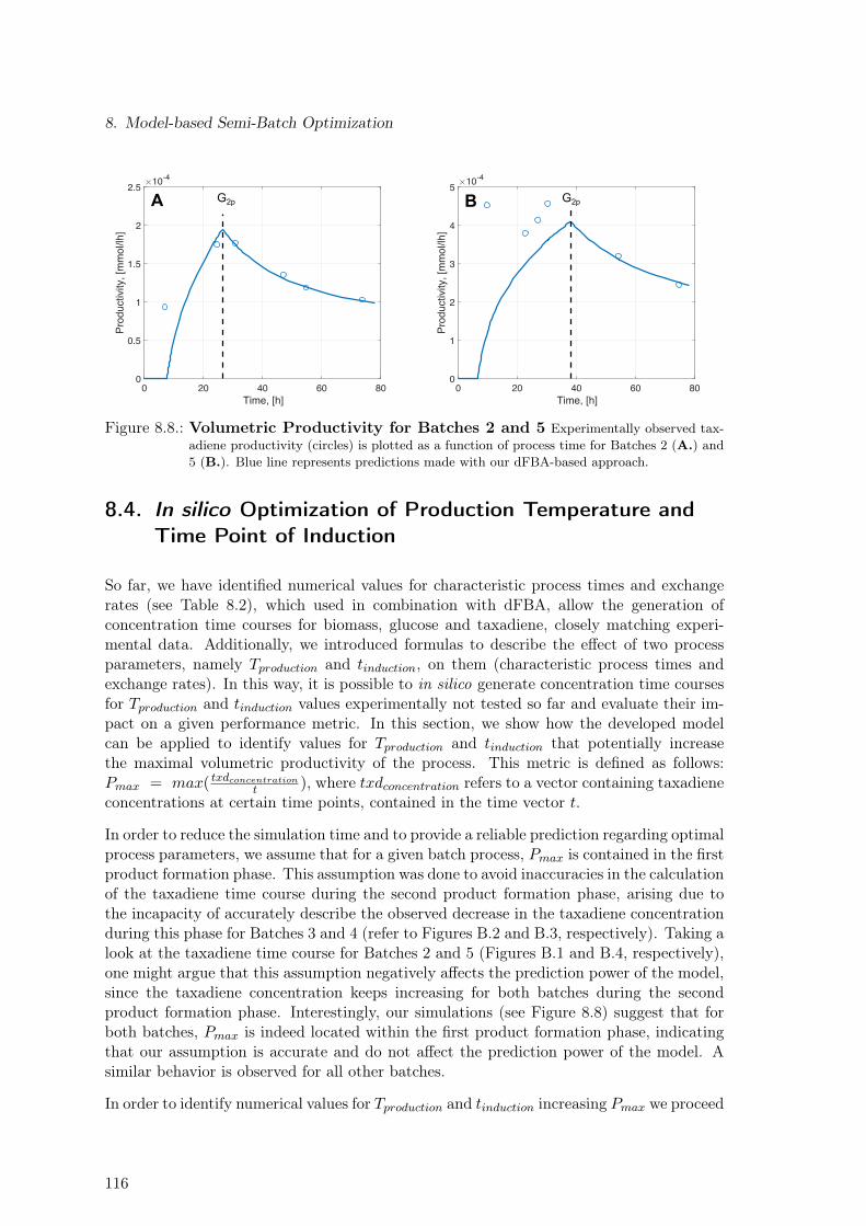
8. Model-based Semi-Batch Optimization
0 20 40 60 80Time, [h]
0
0.5
1
1.5
2
2.5
Prod
uctiv
ity, [
mm
ol/lh
]
10-4
0 20 40 60 80Time, [h]
0
1
2
3
4
5
Prod
uctiv
ity, [
mm
ol/lh
]
10-4
G2p G2pA B
Figure 8.8.: Volumetric Productivity for Batches 2 and 5 Experimentally observed tax-adiene productivity (circles) is plotted as a function of process time for Batches 2 (A.) and5 (B.). Blue line represents predictions made with our dFBA-based approach.
8.4. In silico Optimization of Production Temperature andTime Point of Induction
So far, we have identified numerical values for characteristic process times and exchangerates (see Table 8.2), which used in combination with dFBA, allow the generation ofconcentration time courses for biomass, glucose and taxadiene, closely matching experi-mental data. Additionally, we introduced formulas to describe the effect of two processparameters, namely Tproduction and tinduction, on them (characteristic process times andexchange rates). In this way, it is possible to in silico generate concentration time coursesfor Tproduction and tinduction values experimentally not tested so far and evaluate their im-pact on a given performance metric. In this section, we show how the developed modelcan be applied to identify values for Tproduction and tinduction that potentially increasethe maximal volumetric productivity of the process. This metric is defined as follows:Pmax = max( txdconcentrationt ), where txdconcentration refers to a vector containing taxadieneconcentrations at certain time points, contained in the time vector t.
In order to reduce the simulation time and to provide a reliable prediction regarding optimalprocess parameters, we assume that for a given batch process, Pmax is contained in the firstproduct formation phase. This assumption was done to avoid inaccuracies in the calculationof the taxadiene time course during the second product formation phase, arising due tothe incapacity of accurately describe the observed decrease in the taxadiene concentrationduring this phase for Batches 3 and 4 (refer to Figures B.2 and B.3, respectively). Taking alook at the taxadiene time course for Batches 2 and 5 (Figures B.1 and B.4, respectively),one might argue that this assumption negatively affects the prediction power of the model,since the taxadiene concentration keeps increasing for both batches during the secondproduct formation phase. Interestingly, our simulations (see Figure 8.8) suggest that forboth batches, Pmax is indeed located within the first product formation phase, indicatingthat our assumption is accurate and do not affect the prediction power of the model. Asimilar behavior is observed for all other batches.
In order to identify numerical values for Tproduction and tinduction increasing Pmax we proceed
116
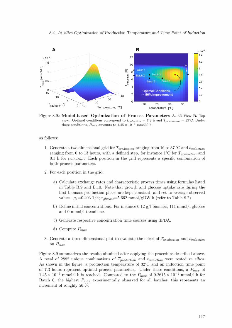
8.4. In silico Optimization of Production Temperature and Time Point of Induction
A B
Batch 1
Optimal Conditions.≈ 56% improvement
Batch 2 Batch 3
Batch 5 Batch 6
Batc
h 4
Figure 8.9.: Model-based Optimization of Process Parameters A. 3D-View B. Topview. Optimal conditions correspond to tinduction = 7.3 h and Tproduction = 32°C. Underthese conditions, Pmax amounts to 1.45× 10⁻³ mmol/l h.
as follows:
1. Generate a two dimensional grid for Tproduction ranging from 16 to 37 °C and tinductionranging from 0 to 13 hours, with a defined step, for instance 1°C for Tproduction and0.1 h for tinduction. Each position in the grid represents a specific combination ofboth process parameters.
2. For each position in the grid:
a) Calculate exchange rates and characteristic process times using formulas listedin Table B.9 and B.10. Note that growth and glucose uptake rate during thefirst biomass production phase are kept constant, and set to average observedvalues: µ1=0.403 1/h; rglucose=5.662 mmol/gDW h (refer to Table 8.2)
b) Define initial concentrations. For instance 0.12 g/l biomass, 111 mmol/l glucoseand 0 mmol/l taxadiene.
c) Generate respective concentration time courses using dFBA.
d) Compute Pmax
3. Generate a three dimensional plot to evaluate the effect of Tproduction and tinductionon Pmax
Figure 8.9 summarizes the results obtained after applying the procedure described above.A total of 2882 unique combinations of Tproduction and tinduction were tested in silico.As shown in the figure, a production temperature of 32°C and an induction time pointof 7.3 hours represent optimal process parameters. Under these conditions, a Pmax of1.45× 10−3 mmol/l h is reached. Compared to the Pmax of 9.2615× 10⁻⁴ mmol/l h forBatch 6, the highest Pmax experimentally observed for all batches, this represents anincrement of roughly 56 %.
117
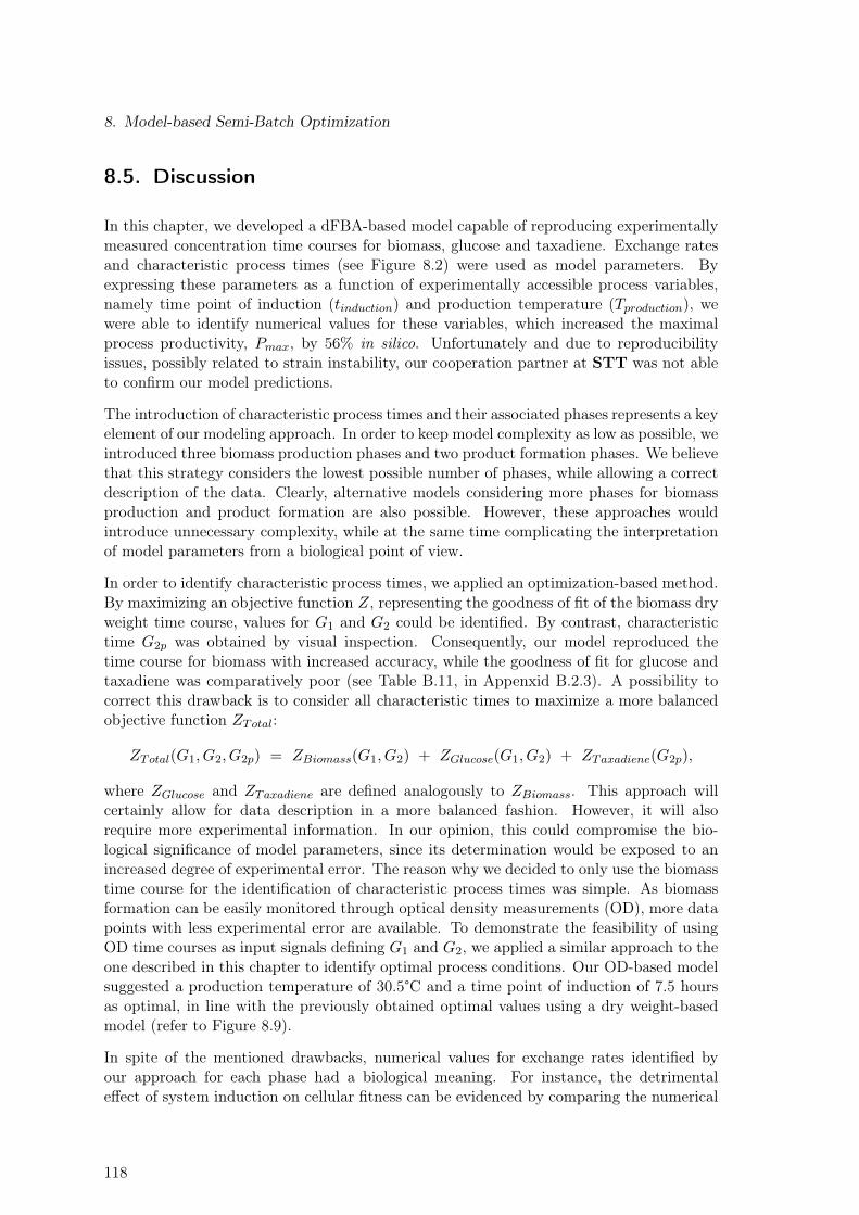
8. Model-based Semi-Batch Optimization
8.5. Discussion
In this chapter, we developed a dFBA-based model capable of reproducing experimentallymeasured concentration time courses for biomass, glucose and taxadiene. Exchange ratesand characteristic process times (see Figure 8.2) were used as model parameters. Byexpressing these parameters as a function of experimentally accessible process variables,namely time point of induction (tinduction) and production temperature (Tproduction), wewere able to identify numerical values for these variables, which increased the maximalprocess productivity, Pmax, by 56% in silico. Unfortunately and due to reproducibilityissues, possibly related to strain instability, our cooperation partner at STT was not ableto confirm our model predictions.
The introduction of characteristic process times and their associated phases represents a keyelement of our modeling approach. In order to keep model complexity as low as possible, weintroduced three biomass production phases and two product formation phases. We believethat this strategy considers the lowest possible number of phases, while allowing a correctdescription of the data. Clearly, alternative models considering more phases for biomassproduction and product formation are also possible. However, these approaches wouldintroduce unnecessary complexity, while at the same time complicating the interpretationof model parameters from a biological point of view.
In order to identify characteristic process times, we applied an optimization-based method.By maximizing an objective function Z, representing the goodness of fit of the biomass dryweight time course, values for G1 and G2 could be identified. By contrast, characteristictime G2p was obtained by visual inspection. Consequently, our model reproduced thetime course for biomass with increased accuracy, while the goodness of fit for glucose andtaxadiene was comparatively poor (see Table B.11, in Appenxid B.2.3). A possibility tocorrect this drawback is to consider all characteristic times to maximize a more balancedobjective function ZTotal:
ZTotal(G1, G2, G2p) = ZBiomass(G1, G2) + ZGlucose(G1, G2) + ZTaxadiene(G2p),
where ZGlucose and ZTaxadiene are defined analogously to ZBiomass. This approach willcertainly allow for data description in a more balanced fashion. However, it will alsorequire more experimental information. In our opinion, this could compromise the bio-logical significance of model parameters, since its determination would be exposed to anincreased degree of experimental error. The reason why we decided to only use the biomasstime course for the identification of characteristic process times was simple. As biomassformation can be easily monitored through optical density measurements (OD), more datapoints with less experimental error are available. To demonstrate the feasibility of usingOD time courses as input signals defining G1 and G2, we applied a similar approach to theone described in this chapter to identify optimal process conditions. Our OD-based modelsuggested a production temperature of 30.5°C and a time point of induction of 7.5 hoursas optimal, in line with the previously obtained optimal values using a dry weight-basedmodel (refer to Figure 8.9).
In spite of the mentioned drawbacks, numerical values for exchange rates identified byour approach for each phase had a biological meaning. For instance, the detrimentaleffect of system induction on cellular fitness can be evidenced by comparing the numerical
118
8.5. Discussion
values for growth and substrate uptake rate between Phase I and II (see Table 8.2). Asa consequence of taxadiene production, the cellular growth rate decreased by roughly oneorder of magnitude. This behavior is in line with the phenomenon of metabolic burden,discussed in Chapter 4. Additionally, the temperature dependence of growth, glucoseuptake and taxadiene production rates could be accurately described using establishedmodels [36,57,113].
Even though we limited our analysis to the identification of optimal values for two differentprocess parameters, the spectrum of potential applications of the developed model is wide,including among others:
1. Development of substrate feeding strategies. Using a model-based approach to sys-tematically design feeding strategies, starving phases in the bioreactor along withtheir associated negative impact on Pmax, can be minimized/eliminated. Refer toFigure B.3 in Appendix B.2.3 for an illustration of this issue.
2. Estimation of optimal batch duration. After the maximal productivity (Pmax) hasbeen reached, additional process duration generates the process productivity to de-crease (see Figure 8.8). Our model allows the identification of optimal values for thisprocess variable, so that no unnecessary production time is wasted.
3. Estimation of by-product secretion patterns. For each point of time during the pro-cess, dFBA calculates flux distributions fulfilling certain constraints. In our specificcase, these constraints correspond to growth, glucose uptake and taxadiene produc-tion rates for each phase. By maximizing and minimizing the flux through exchangereactions of interest, for instance acetate secretion, concentration time courses for thedesired by-product can be estimated. A similar strategy can be applied to analyzedifferences in the intracellular flux distributions for the various process phases, thusallowing the identification of potential bottle necks limiting the production flux.
119

9. Product Yield Prediction
A theoretical approach for accurate product yield prediction would reduce experimentalefforts during the development of optimal production strains. It would radically boostthe pace of the science of Metabolic Engineering. Traditionally, constraint-based methodshave been used to asses the production potential of metabolic networks. By applyinglinear programming, it is possible to calculate the maximal theoretical product yield for adefined carbon source and a given metabolic network (refer to Chapter 7). However, thismetric only serves as a maximal bound for product yield and does not always representan adequate proxy for experimental product yield. This is especially true when it comesto describing the production performance of strains in early development stages (refer toTable 2 in [50]).
Here, a kinetic-based approach was applied to predict experimental yields of six differentsemi-batch processes. The method is based on the EM approach and was introduced bythe group of James Liao [71]. It requires three inputs: a metabolic network, a reference fluxdistribution and a rate law for each reaction. Unknown kinetic parameters are sampled sothat the provided reference flux distribution is fulfilled. We observed that this method pre-dicted experimental yields more accurately than its ad hoc constraint-based counterpart.Since labeling data for the semi-batch experiments were lacking, reference flux distribu-tions were estimated using constraint-based methods along with two different objectivefunctions: minimization of oxygen uptake and minimization of citrate synthase activity.We observed a dependence of calculated yield values on the reference flux distribution.However, regardless of the objective function used, predictions made by the kinetic-basedmethod were by up to two orders of magnitude more accurate than the constraint-basedmethod. We also adjusted traditionally used E. coli metabolic reconstructions [106, 107],making them suitable inputs for the EM approach. Finally, we used the COBRA Tool-box [124] to create required Matlab structures for the EM approach [70, 71, 74, 144, 146].Thus, we created a missing bridge between widespread constraint-based and emergingkinetic modeling platforms [91].
9.1. Strain & Experimental Data
Experimental data used correspond to experimental taxadiene yields obtained for the sixsemi-batch fermentations introduced in Chapter 8. Taxadiene yields shown in Table 9.1were calculated as the ratio of taxadiene production rate to glucose uptake rate for eachof the two production phases. Biomass yields were calculated analogously, as the ratiobetween growth rate in each phase and corresponding glucose uptake rate. Refer to Section8.1 and Table 8.2 for a description of experimental set-up and rates determination.
Since taxadiene production ceased during the second phase (between G2p and process end)for the majority of the fermentations (batches 1, 3, 4, 6), we will focus our analysis on the
121
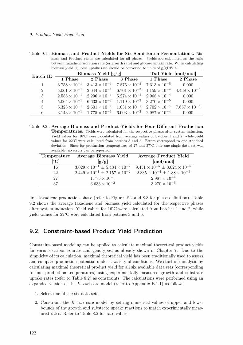
9. Product Yield Prediction
Table 9.1.: Biomass and Product Yields for Six Semi-Batch Fermentations. Bio-mass and Product yields are calculated for all phases. Yields are calculated as the ratiobetween taxadiene secretion rate (or growth rate) and glucose uptake rate. When calculatingbiomass yield, glucose uptake rate should be converted to units of g/gDW h.
Batch ID Biomass Yield [g/g] Txd Yield [mol/mol]1 Phase 2 Phase 3 Phase 1 Phase 2 Phase
1 3.758× 10⁻¹ 3.413× 10⁻¹ 7.875× 10⁻² 7.313× 10⁻⁵ 0.0002 5.061× 10⁻¹ 2.644× 10⁻¹ 6.701× 10⁻³ 1.159× 10⁻⁴ 4.438× 10⁻⁵
3 2.585× 10⁻¹ 2.296× 10⁻¹ 5.274× 10⁻² 2.968× 10⁻⁴ 0.0004 5.064× 10⁻¹ 6.633× 10⁻² 1.119× 10⁻² 3.270× 10⁻⁵ 0.0005 5.328× 10⁻¹ 2.601× 10⁻¹ 1.031× 10⁻¹ 2.702× 10⁻⁴ 7.657× 10⁻⁵
6 3.143× 10⁻¹ 1.775× 10⁻¹ 6.003× 10⁻² 2.987× 10⁻⁴ 0.000
Table 9.2.: Average Biomass and Product Yields for Four Different ProductionTemperatures. Yields were calculated for the respective phases after system induction.Yield values for 16°C were calculated from average values of batches 1 and 2, while yieldvalues for 22°C were calculated from batches 3 and 5. Errors correspond to one standarddeviation. Since for production temperatures of 27 and 37°C only one single data set wasavailable, no errors can be reported.
Temperature[°C]
Average Biomass Yield[g/g]
Average Product Yield[mol/mol]
16 3.029× 10⁻¹ ± 5.434× 10⁻² 9.451× 10⁻⁵ ± 3.024× 10⁻⁵
22 2.449× 10⁻¹ ± 2.157× 10⁻² 2.835× 10⁻⁴ ± 1.88× 10⁻⁵
27 1.775× 10⁻¹ 2.987× 10⁻⁴
37 6.633× 10⁻² 3.270× 10⁻⁵
first taxadiene production phase (refer to Figures 8.2 and 8.3 for phase definition). Table9.2 shows the average taxadiene and biomass yield calculated for the respective phasesafter system induction. Yield values for 16°C were calculated from batches 1 and 2, whileyield values for 22°C were calculated from batches 3 and 5.
9.2. Constraint-based Product Yield Prediction
Constraint-based modeling can be applied to calculate maximal theoretical product yieldsfor various carbon sources and genotypes, as already shown in Chapter 7. Due to thesimplicity of its calculation, maximal theoretical yield has been traditionally used to assessand compare production potential under a variety of conditions. We start our analysis bycalculating maximal theoretical product yield for all six available data sets (correspondingto four production temperatures) using experimentally measured growth and substrateuptake rates (refer to Table 8.2) as constraints. The calculations were performed using anexpanded version of the E. coli core model (refer to Appendix B.1.1) as follows:
1. Select one of the six data sets.
2. Constraint the E. coli core model by setting numerical values of upper and lowerbounds of the growth and substrate uptake reactions to match experimentally meas-ured rates. Refer to Table 8.2 for rate values.
122
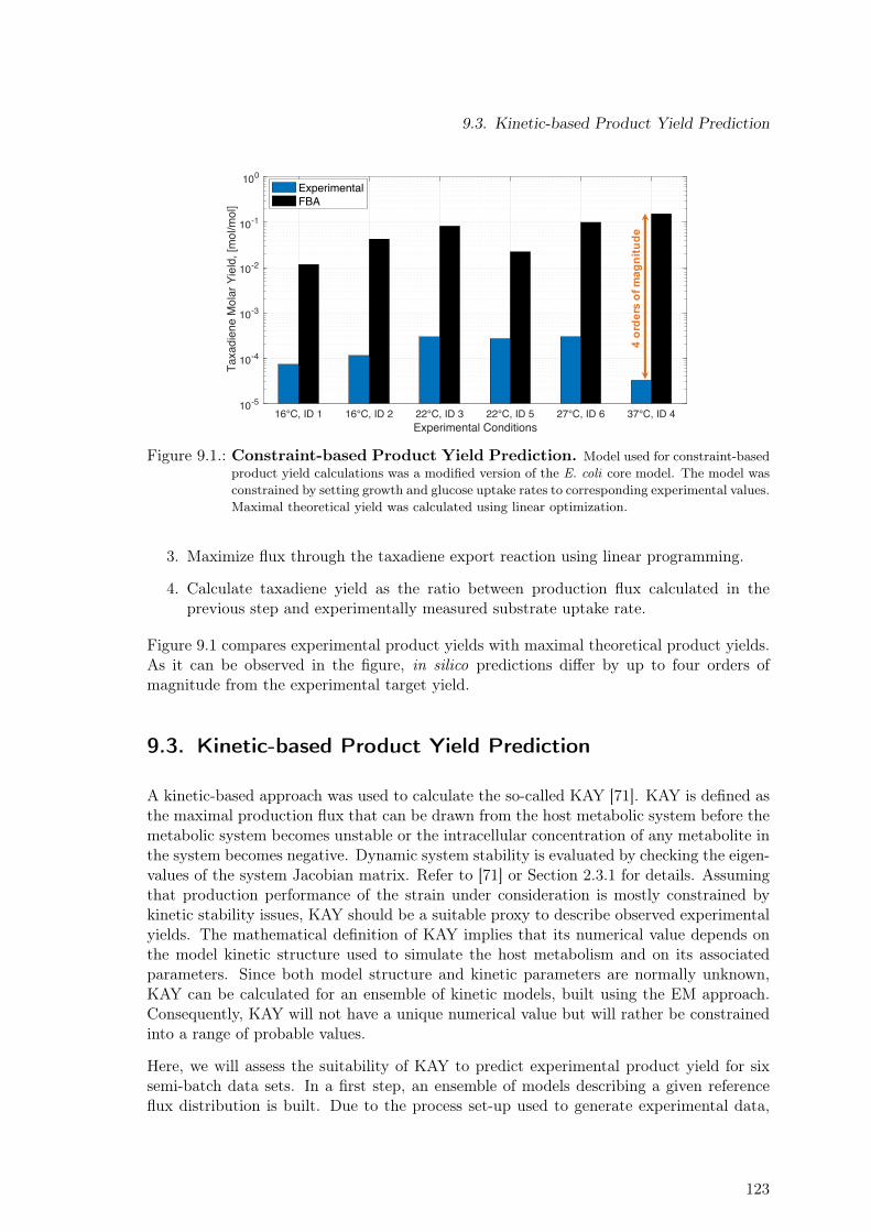
9.3. Kinetic-based Product Yield Prediction
16°C, ID 1 16°C, ID 2 22°C, ID 3 22°C, ID 5 27°C, ID 6 37°C, ID 4Experimental Conditions
10-5
10-4
10-3
10-2
10-1
100
Taxa
dien
e M
olar
Yie
ld, [
mol
/mol
]
ExperimentalFBA
4 or
ders
of m
agni
tude
Figure 9.1.: Constraint-based Product Yield Prediction. Model used for constraint-basedproduct yield calculations was a modified version of the E. coli core model. The model wasconstrained by setting growth and glucose uptake rates to corresponding experimental values.Maximal theoretical yield was calculated using linear optimization.
3. Maximize flux through the taxadiene export reaction using linear programming.
4. Calculate taxadiene yield as the ratio between production flux calculated in theprevious step and experimentally measured substrate uptake rate.
Figure 9.1 compares experimental product yields with maximal theoretical product yields.As it can be observed in the figure, in silico predictions differ by up to four orders ofmagnitude from the experimental target yield.
9.3. Kinetic-based Product Yield Prediction
A kinetic-based approach was used to calculate the so-called KAY [71]. KAY is defined asthe maximal production flux that can be drawn from the host metabolic system before themetabolic system becomes unstable or the intracellular concentration of any metabolite inthe system becomes negative. Dynamic system stability is evaluated by checking the eigen-values of the system Jacobian matrix. Refer to [71] or Section 2.3.1 for details. Assumingthat production performance of the strain under consideration is mostly constrained bykinetic stability issues, KAY should be a suitable proxy to describe observed experimentalyields. The mathematical definition of KAY implies that its numerical value depends onthe model kinetic structure used to simulate the host metabolism and on its associatedparameters. Since both model structure and kinetic parameters are normally unknown,KAY can be calculated for an ensemble of kinetic models, built using the EM approach.Consequently, KAY will not have a unique numerical value but will rather be constrainedinto a range of probable values.
Here, we will assess the suitability of KAY to predict experimental product yield for sixsemi-batch data sets. In a first step, an ensemble of models describing a given referenceflux distribution is built. Due to the process set-up used to generate experimental data,
123
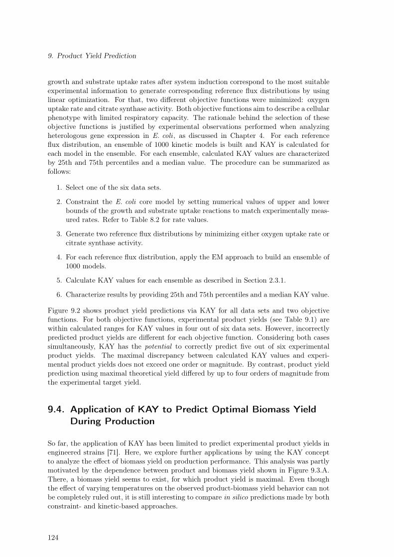
9. Product Yield Prediction
growth and substrate uptake rates after system induction correspond to the most suitableexperimental information to generate corresponding reference flux distributions by usinglinear optimization. For that, two different objective functions were minimized: oxygenuptake rate and citrate synthase activity. Both objective functions aim to describe a cellularphenotype with limited respiratory capacity. The rationale behind the selection of theseobjective functions is justified by experimental observations performed when analyzingheterologous gene expression in E. coli , as discussed in Chapter 4. For each referenceflux distribution, an ensemble of 1000 kinetic models is built and KAY is calculated foreach model in the ensemble. For each ensemble, calculated KAY values are characterizedby 25th and 75th percentiles and a median value. The procedure can be summarized asfollows:
1. Select one of the six data sets.
2. Constraint the E. coli core model by setting numerical values of upper and lowerbounds of the growth and substrate uptake reactions to match experimentally meas-ured rates. Refer to Table 8.2 for rate values.
3. Generate two reference flux distributions by minimizing either oxygen uptake rate orcitrate synthase activity.
4. For each reference flux distribution, apply the EM approach to build an ensemble of1000 models.
5. Calculate KAY values for each ensemble as described in Section 2.3.1.
6. Characterize results by providing 25th and 75th percentiles and a median KAY value.
Figure 9.2 shows product yield predictions via KAY for all data sets and two objectivefunctions. For both objective functions, experimental product yields (see Table 9.1) arewithin calculated ranges for KAY values in four out of six data sets. However, incorrectlypredicted product yields are different for each objective function. Considering both casessimultaneously, KAY has the potential to correctly predict five out of six experimentalproduct yields. The maximal discrepancy between calculated KAY values and experi-mental product yields does not exceed one order or magnitude. By contrast, product yieldprediction using maximal theoretical yield differed by up to four orders of magnitude fromthe experimental target yield.
9.4. Application of KAY to Predict Optimal Biomass YieldDuring Production
So far, the application of KAY has been limited to predict experimental product yields inengineered strains [71]. Here, we explore further applications by using the KAY conceptto analyze the effect of biomass yield on production performance. This analysis was partlymotivated by the dependence between product and biomass yield shown in Figure 9.3.A.There, a biomass yield seems to exist, for which product yield is maximal. Even thoughthe effect of varying temperatures on the observed product-biomass yield behavior can notbe completely ruled out, it is still interesting to compare in silico predictions made by bothconstraint- and kinetic-based approaches.
124
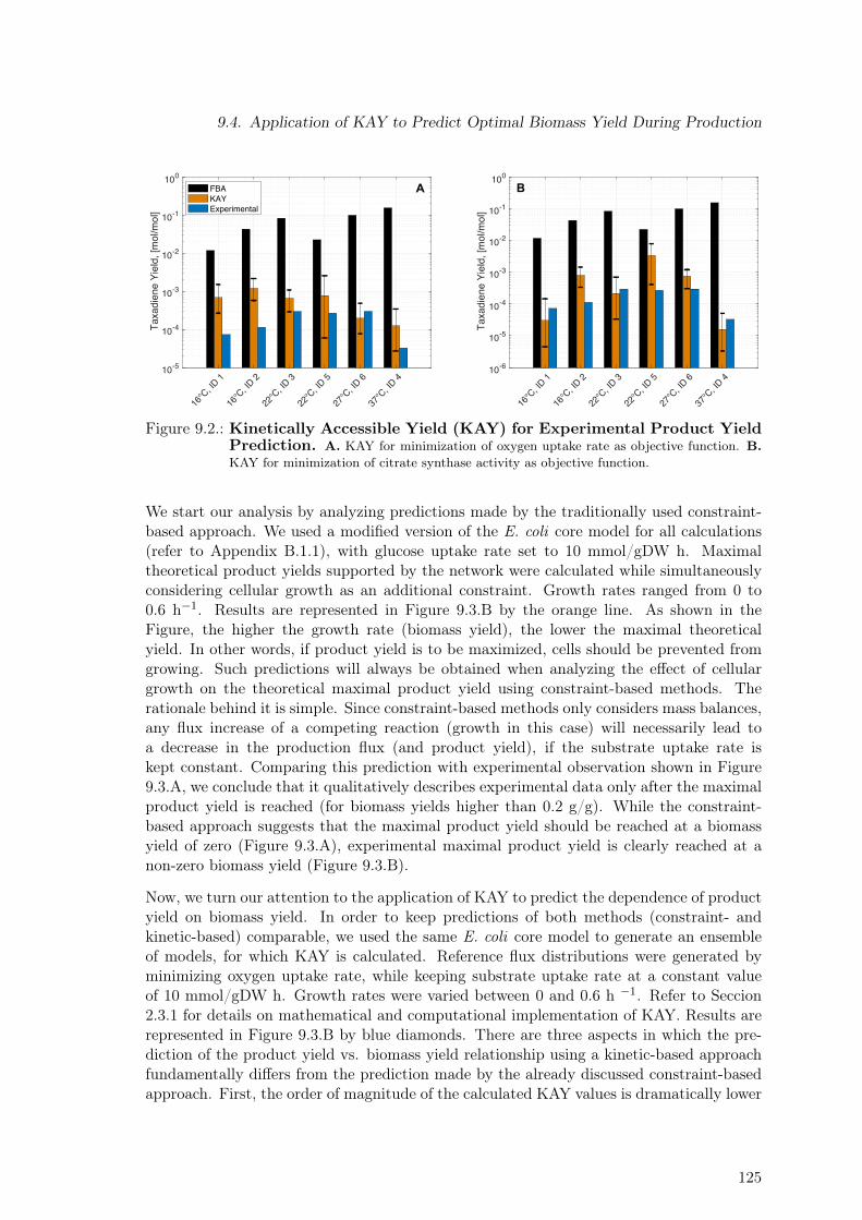
9.4. Application of KAY to Predict Optimal Biomass Yield During Production
16°C
, ID 1
16°C
, ID 2
22°C
, ID 3
22°C
, ID 5
27°C
, ID 6
37°C
, ID 4
10-5
10-4
10-3
10-2
10-1
100
Taxa
dien
e Yi
eld,
[mol
/mol
]
16°C
, ID 1
16°C
, ID 2
22°C
, ID 3
22°C
, ID 5
27°C
, ID 6
37°C
, ID 4
10-6
10-5
10-4
10-3
10-2
10-1
100
Taxa
dien
e Yi
eld,
[mol
/mol
]
FBAKAYExperimental
A B
Figure 9.2.: Kinetically Accessible Yield (KAY) for Experimental Product YieldPrediction. A. KAY for minimization of oxygen uptake rate as objective function. B.KAY for minimization of citrate synthase activity as objective function.
We start our analysis by analyzing predictions made by the traditionally used constraint-based approach. We used a modified version of the E. coli core model for all calculations(refer to Appendix B.1.1), with glucose uptake rate set to 10 mmol/gDW h. Maximaltheoretical product yields supported by the network were calculated while simultaneouslyconsidering cellular growth as an additional constraint. Growth rates ranged from 0 to0.6 h−1. Results are represented in Figure 9.3.B by the orange line. As shown in theFigure, the higher the growth rate (biomass yield), the lower the maximal theoreticalyield. In other words, if product yield is to be maximized, cells should be prevented fromgrowing. Such predictions will always be obtained when analyzing the effect of cellulargrowth on the theoretical maximal product yield using constraint-based methods. Therationale behind it is simple. Since constraint-based methods only considers mass balances,any flux increase of a competing reaction (growth in this case) will necessarily lead toa decrease in the production flux (and product yield), if the substrate uptake rate iskept constant. Comparing this prediction with experimental observation shown in Figure9.3.A, we conclude that it qualitatively describes experimental data only after the maximalproduct yield is reached (for biomass yields higher than 0.2 g/g). While the constraint-based approach suggests that the maximal product yield should be reached at a biomassyield of zero (Figure 9.3.A), experimental maximal product yield is clearly reached at anon-zero biomass yield (Figure 9.3.B).
Now, we turn our attention to the application of KAY to predict the dependence of productyield on biomass yield. In order to keep predictions of both methods (constraint- andkinetic-based) comparable, we used the same E. coli core model to generate an ensembleof models, for which KAY is calculated. Reference flux distributions were generated byminimizing oxygen uptake rate, while keeping substrate uptake rate at a constant valueof 10 mmol/gDW h. Growth rates were varied between 0 and 0.6 h −1. Refer to Seccion2.3.1 for details on mathematical and computational implementation of KAY. Results arerepresented in Figure 9.3.B by blue diamonds. There are three aspects in which the pre-diction of the product yield vs. biomass yield relationship using a kinetic-based approachfundamentally differs from the prediction made by the already discussed constraint-basedapproach. First, the order of magnitude of the calculated KAY values is dramatically lower
125
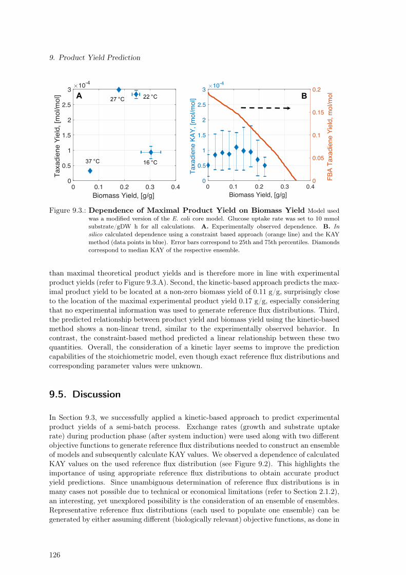
9. Product Yield Prediction
0 0.1 0.2 0.3 0.4Biomass Yield, [g/g]
0
0.5
1
1.5
2
2.5
3
Taxa
dien
e KA
Y, [m
ol/m
ol]
10-4
0
0.05
0.1
0.15
0.2
FBA
Taxa
dien
e Yi
eld,
mol
/mol
0 0.1 0.2 0.3 0.4Biomass Yield, [g/g]
0
0.5
1
1.5
2
2.5
3
Taxa
dien
e Yi
eld,
[mol
/mol
]
10-4
A B
16 °C
22 °C27 °C
37 °C
Figure 9.3.: Dependence of Maximal Product Yield on Biomass Yield Model usedwas a modified version of the E. coli core model. Glucose uptake rate was set to 10 mmolsubstrate/gDW h for all calculations. A. Experimentally observed dependence. B. Insilico calculated dependence using a constraint based approach (orange line) and the KAYmethod (data points in blue). Error bars correspond to 25th and 75th percentiles. Diamondscorrespond to median KAY of the respective ensemble.
than maximal theoretical product yields and is therefore more in line with experimentalproduct yields (refer to Figure 9.3.A). Second, the kinetic-based approach predicts the max-imal product yield to be located at a non-zero biomass yield of 0.11 g/g, surprisingly closeto the location of the maximal experimental product yield 0.17 g/g, especially consideringthat no experimental information was used to generate reference flux distributions. Third,the predicted relationship between product yield and biomass yield using the kinetic-basedmethod shows a non-linear trend, similar to the experimentally observed behavior. Incontrast, the constraint-based method predicted a linear relationship between these twoquantities. Overall, the consideration of a kinetic layer seems to improve the predictioncapabilities of the stoichiometric model, even though exact reference flux distributions andcorresponding parameter values were unknown.
9.5. Discussion
In Section 9.3, we successfully applied a kinetic-based approach to predict experimentalproduct yields of a semi-batch process. Exchange rates (growth and substrate uptakerate) during production phase (after system induction) were used along with two differentobjective functions to generate reference flux distributions needed to construct an ensembleof models and subsequently calculate KAY values. We observed a dependence of calculatedKAY values on the used reference flux distribution (see Figure 9.2). This highlights theimportance of using appropriate reference flux distributions to obtain accurate productyield predictions. Since unambiguous determination of reference flux distributions is inmany cases not possible due to technical or economical limitations (refer to Section 2.1.2),an interesting, yet unexplored possibility is the consideration of an ensemble of ensembles.Representative reference flux distributions (each used to populate one ensemble) can begenerated by either assuming different (biologically relevant) objective functions, as done in
126
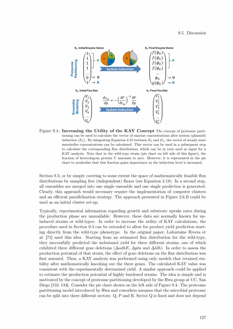
9.5. Discussion
1111. .01
E0, Initial Enzyme Vector
P
UR
𝑓(𝜙')𝑓(𝜙')𝑓(𝜙')𝑓(𝜙'). .𝜙'
𝑔(𝜙')
Ef, Final Enzyme Vector
𝑉+,
𝑉-,𝑉.,
𝑉/,. .𝑉0,
𝑉+𝑉-𝑉.𝑉/. .𝑉0
System Induction
System Induction
𝑑𝑐33𝑑𝑝
= −𝜕𝐹𝜕𝑐33
9+ 𝜕𝐹𝜕𝑝
Prot
eom
e Pa
rtitio
ning
Ense
mbl
e M
odel
ing
V0, Initial Flux Dist. Vf, Final Flux Dist.
P
UR
Figure 9.4.: Increasing the Utility of the KAY Concept The concept of proteome parti-tioning can be used to calculate the vector of enzyme concentrations after system (plasmid)induction (Ef ). By integrating Equation 2.25 between E0 and Ef , the vector of steady statemetabolite concentrations can be calculated. This vector can be used in a subsequent stepto calculate the corresponding flux distribution, which can be in turn used as input for aKAY analysis. Note that in the wild-type strain (pie chart on left side of this figure), thefraction of heterologous protein U amounts to zero. However, it is represented in the piechart to symbolize that this fraction gains importance as the induction level is increased.
Section 9.3, or by simply covering to some extent the space of mathematically feasible fluxdistributions by sampling free (independent) fluxes (see Equation 2.18). In a second step,all ensembles are merged into one single ensemble and one single prediction is generated.Clearly, this approach would necessary require the implementation of computer clustersand an efficient parallelization strategy. The approach presented in Figure 2.6.B could beused as an initial cluster set-up.
Typically, experimental information regarding growth and substrate uptake rates duringthe production phase are unavailable. However, these data are normally known for un-induced strains or wild-types. In order to increase the utility of KAY calculations, theprocedure used in Section 9.3 can be extended to allow for product yield prediction start-ing directly from the wild-type phenotype. In the original paper, Lafontaine Rivera etal. [71] used this idea. Starting from an estimated flux distribution for the wild-type,they successfully predicted the isobutanol yield for three different strains, one of whichexhibited three different gene deletions (∆adhE, ∆pta and ∆ldh). In order to assess theproduction potential of that strain, the effect of gene deletions on the flux distribution wasfirst assessed. Then, a KAY analysis was performed using only models that retained sta-bility after mathematically knocking out the three genes. The calculated KAY value wasconsistent with the experimentally determined yield. A similar approach could be appliedto estimate the production potential of highly burdened strains. The idea is simple and ismotivated by the concept of proteome partitioning developed by the Hwa group at UC, SanDiego [132–134]. Consider the pie chart shown on the left side of Figure 9.4. The proteomepartitioning model introduced by Hwa and coworkers assumes that the microbial proteomecan be split into three different sectors: Q, P and R. Sector Q is fixed and does not depend
127
9. Product Yield Prediction
on the cellular growth rate. R contains all ribosomal proteins and their affiliates, whileP represents all proteins responsible for nutrient influx and metabolism. Since the size ofthe proteome is limited, the expression of an heterologous protein U effectively decreasesthe fraction allocable to the P and R sectors, as represented in the pie chart on the leftside of Figure 9.4. If functions describing the fraction of sectors P (φP ) and R (φR) independence of the heterologous fraction U (φU ) are known, then it should be possible toestimate changes in the flux distribution as φU increases. For a given φU fraction, KAYvalues can be then calculated using the calculated flux distribution as a starting point (Vfin Figure 9.4) [91].
The results and outlook presented in this chapter evidences the huge potential of kinetic-based modeling, more specifically, of EM-based methods. In our opinion, Figures 9.3 and9.2 directly support the predictive power of EM-based methods like KAY itself and optEM(see Section 5.4.2). Additional experimental work, including measurements of proteincontent in both wild-type and induced strains, will be required to further extend andvalidate the applicability of KAY as proposed in Figure 9.4. An interesting prediction ofKAY is the interdependence between biomass and product yield, shown in this Chapter (seeFigure 9.3) but also in Chapter 6 (refer to Figure 6.10.B). The validity of this relationshipand the ability of KAY to successfully describe it could be exploited not only for theoptimal design of fermentation processes but also for the calculation of optimal inductionlevels, described by the fraction of heterologous protein φU .
128
10. Concluding Remarks and Outlook
The coverage of this thesis is mostly limited to the taxadiene production in E. coli . How-ever, a review on the application of computational methods to increase succinate pro-duction in engineered strains evidenced interesting trends of the current model-based,rational Metabolic Engineering. Even though the details of that review can be found else-where [149], we will highlight some of the key lessons learned from that review in order tounderstand the way how it motivated and guided parts of the in silico studies presentedhere. Then, we will provide some conclusions and future perspectives concerning the mainresults of this work.
10.1. Lessons From Succinate Production in EngineeredStrains
Biotechnological production of succinate has been one of the preferred case studies to testpredictions made by strain-design algorithms. Since the introduction of OptKnock in 2003and until 2016, a total of 26 different strain-design algorithms in silico targeting the succin-ate overproduction (refer to Table 1 in [149] or Table 2.4 of this work) have been published.None of these studies was accompanied by an in vivo validation of the algorithm’s predic-tions. Rather, the rich biological knowledge available, gained over decades of research insuccinate production in a variety of industrially relevant microorganisms, was used to testthe predictive power of the algorithms. An analysis of the nature of mathematical methodsused to develop these strain-design algorithms and the way how their predictions are usedto guide in vivo strain development leads to three key conclusions:
1. Constraint-based methods predominate. Roughly 80% of the 26 strain-design al-gorithms targeting succinate overproduction have a constraint-based nature. Thisobservation is not surprising and is, in our opinion, mainly justified in the relativesimplicity of its mathematical formulation, availability of the required information(a genome-scale metabolic reconstruction and an objective function), and its compu-tational tractability.
2. Kinetic-based methods are underrepresented. Contrasting the predominance of constraint-based methods, only one single method, out of 26 strain design algorithms reviewed,had a kinetic-based nature. In our opinion, this evidences the difficulties associatedwith kinetic descriptions of cellular metabolism. In addition to a stoichiometric layer,kinetic information in form of rate laws, describing the flux through each reaction asa function of enzyme-specific parameters and metabolite concentrations, are also re-quired. Since this information is typically unavailable, the construction of large-scalekinetic models have been hindered.
129
10. Concluding Remarks and Outlook
3. In silico predictions are not always precise. We found out that only 10 studies re-ported the model-guided construction of strains exhibiting an enhanced succinateproduction (refer to Table 2 in [149]). Within these studies, only two used one of the26 strain-design algorithms previously developed. All other studies reported the con-struction of production strains based on knowledge gained from FBA calculations.Additionally, none of the 10 studies reported an exact implementation of in silicopredictions. Often, complementary strategies like directed evolution were necessaryto achieve high succinate yields. Altogether, these observations point to a limitedpredictive power of constraint-based methods, especially when aspects like fine tuningof enzyme expression or dynamic stability of the system become important factorsdetermining the effectiveness of a given genetic intervention [1, 2].
10.2. Lessons From Taxadiene Production in E. coli
As previously mentioned, advantages of constraint-based methods over kinetic-based meth-ods include the simplicity of use, while simultaneously offering a moderate predictive power.Due to their computational tractability, constraint-based simulations can be performed ona large-scale, thus allowing the identification of non-trivial network properties. In thespecific case of taxadiene production in E. coli , we demonstrated that a carbon-neutraltaxadiene production is not possible for any substrate or substrate mixture. This obser-vation can be easily extended to the production any terpene. This is because carbon leakin form of CO2 is concomitant to the formation of both IPP and DMAPP, the universalterpene precursors, via either the mevalonate or the non-mevalonate pathway. Addition-ally, our large-scale constraint-based analysis pointed at a synergy between the mevalonateand the non-mevalonate pathway in silico (Chapter 7). Remarkably, this synergy wasexperimentally observed, although in a greater extent, for the production of isoprene inE. coli [160].
The predictive power of constraint-based modeling is increased, if biologically meaningfulconstraints are used. In Chapter 4, we applied a constraint-based approach to simulatethe experimentally observed effect of protein load on by-product secretion. By reducingthe upper boundary of oxygen uptake rate as protein/plasmid load increases, we couldqualitatively reproduce the downwards shift of the acetate line experimentally observed inloaded strains. Our assumption on decreasing respiratory capacity is in part justified byproteomic measurements reported by Peebo et al. [110].
One of the main disadvantages of constraint-based methods, which paradoxically has itsorigin in the simplicity of the mathematical formulation of constraint-based approaches,is the omission of enzyme kinetics. As a consequence, important aspects such as dynamicstability of the cellular metabolism, intracellular concentration of potentially toxic meta-bolites, metabolite-level enzyme regulation and fine tuning of enzyme expression cannot beadequately considered. By contrast, multiple studies have highlighted the importance of atleast one of these factors for the construction of terpenoids overproducing strains [1,2,38].Motivated by this and by the fact that kinetic-based models are underrepresented despiteof their application potential in rational Metabolic Engineering, we ventured to explore theutility of the ensemble modeling, an emerging approach for the construction and analysisof kinetic models. The predictive power of the ensemble modeling approach was evaluated
130
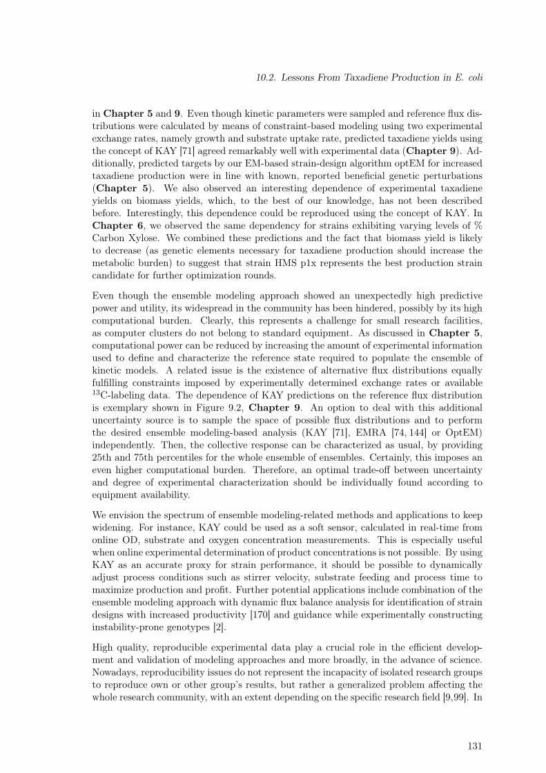
10.2. Lessons From Taxadiene Production in E. coli
in Chapter 5 and 9. Even though kinetic parameters were sampled and reference flux dis-tributions were calculated by means of constraint-based modeling using two experimentalexchange rates, namely growth and substrate uptake rate, predicted taxadiene yields usingthe concept of KAY [71] agreed remarkably well with experimental data (Chapter 9). Ad-ditionally, predicted targets by our EM-based strain-design algorithm optEM for increasedtaxadiene production were in line with known, reported beneficial genetic perturbations(Chapter 5). We also observed an interesting dependence of experimental taxadieneyields on biomass yields, which, to the best of our knowledge, has not been describedbefore. Interestingly, this dependence could be reproduced using the concept of KAY. InChapter 6, we observed the same dependency for strains exhibiting varying levels of %Carbon Xylose. We combined these predictions and the fact that biomass yield is likelyto decrease (as genetic elements necessary for taxadiene production should increase themetabolic burden) to suggest that strain HMS p1x represents the best production straincandidate for further optimization rounds.
Even though the ensemble modeling approach showed an unexpectedly high predictivepower and utility, its widespread in the community has been hindered, possibly by its highcomputational burden. Clearly, this represents a challenge for small research facilities,as computer clusters do not belong to standard equipment. As discussed in Chapter 5,computational power can be reduced by increasing the amount of experimental informationused to define and characterize the reference state required to populate the ensemble ofkinetic models. A related issue is the existence of alternative flux distributions equallyfulfilling constraints imposed by experimentally determined exchange rates or available13C-labeling data. The dependence of KAY predictions on the reference flux distributionis exemplary shown in Figure 9.2, Chapter 9. An option to deal with this additionaluncertainty source is to sample the space of possible flux distributions and to performthe desired ensemble modeling-based analysis (KAY [71], EMRA [74, 144] or OptEM)independently. Then, the collective response can be characterized as usual, by providing25th and 75th percentiles for the whole ensemble of ensembles. Certainly, this imposes aneven higher computational burden. Therefore, an optimal trade-off between uncertaintyand degree of experimental characterization should be individually found according toequipment availability.
We envision the spectrum of ensemble modeling-related methods and applications to keepwidening. For instance, KAY could be used as a soft sensor, calculated in real-time fromonline OD, substrate and oxygen concentration measurements. This is especially usefulwhen online experimental determination of product concentrations is not possible. By usingKAY as an accurate proxy for strain performance, it should be possible to dynamicallyadjust process conditions such as stirrer velocity, substrate feeding and process time tomaximize production and profit. Further potential applications include combination of theensemble modeling approach with dynamic flux balance analysis for identification of straindesigns with increased productivity [170] and guidance while experimentally constructinginstability-prone genotypes [2].
High quality, reproducible experimental data play a crucial role in the efficient develop-ment and validation of modeling approaches and more broadly, in the advance of science.Nowadays, reproducibility issues do not represent the incapacity of isolated research groupsto reproduce own or other group’s results, but rather a generalized problem affecting thewhole research community, with an extent depending on the specific research field [9,99]. In
131
10. Concluding Remarks and Outlook
this work, model-based improvement strategies for strains (Chapter 4 & 5) and a produc-tion process (Chapter 8) were identified. Unfortunately and due to reproducibility issues,none of these strategies could be validated. This limited the experimental implementationof the theoretical workflow developed (refer to Chapter 3) and hindered the desired op-timization of strains and their associated production processes through the implementationof model-based predictions in an iterative fashion. However, various theoretical methodsfor each of the steps of the workflow were developed and applied. Figure 10.1 provides anoverview of these methods and summarizes relevant input-output relationships used alongthis work.
Chapter 6 was concluded by suggesting strain HMS p1x as an optimal production straincandidate. After genetic elements allowing terpenoid production are introduced into thisstrain, modifications in its metabolism leading to an increased production performance canbe identified by applying the tools discussed in Chapter 5. Once the desired productionperformance has been reached, associated optimal process parameters can be identified asshown in Chapter 8. As for culture medium composition, a similar procedure to the oneused in Chapter 7 can be applied to identify promising carbon sources. These steps areillustrated in Figure 10.1 by the dashed lines and represent one possible implementationof the workflow using all tools described in this work.
Two opposite approaches have been suggested to increase reproducibility of results, namelystandardization [111] and heterogenization of experimental conditions [116]. In either case,future experimental efforts should aim to keep increasing confidence in experimental data.On the modeling side, strategies should be developed to properly handle uncertainties andexperimental error, thus allowing the generation of predictions that are robust to noise.
132
dFBA
Strain Characterization Batch Data
(Janoschek, STT)
Optimal Process Strategy
Experimental Rates
𝜇𝑟#$%&
𝑟'( , 𝑌+'(
KAY 𝑌+'( Prediction
Relationship𝑌+'( 𝑣𝑠𝑌'
Production Strains Data(Fuchs, IBK)
13CFlux2
FVA optEMStrain Ranking
Optimal StrainDesigns
Sugar Co-uptakeData
(Kemper, IBK)
FBA
KAY
13CFlux2
Taxadiene Production Potential
Biomass Yield &Growth Rates
Optimal ProductionStrain Candidate
Metabolic Burden(Wagner, SBT) FBA
Process-level strategy for burden reduction
Slope of Acetate Lines
iJO1366 FBA
Synergy Prediction
Medium Optimization
Chapter 4
Chapter 5
Chapter 6
Chapter 7
Chapter 8
Chapter 9
Figure 10.1.: Application of the Workflow to the Production of Taxadiene in E. coli : Conclusion. The proposed workflow,covering both model-guided strain engineering and model-driven process optimization, was applied to the production of taxadiene in E. coli . Eventhough model-based optimization strategies for strain and production process could not be experimentally validated due to reproducibility issuesof experimental data, we demonstrated the utility of a variety in silico approaches. Refer to each chapter for more details. Main input-outputrelationships are shown for each chapter. Applied methods are given in boxes. Dashed lines represent further steps towards the construction of anoptimal terpenoid producing strain and the optimization of its performance in a bio-reactor.

Bibliography
[1] P. K. Ajikumar, W.-H. Xiao, K. E. J. Tyo,Y. Wang, F. Simeon, E. Leonard, O. Mucha, T. H.Phon, B. Pfeifer, and G. Stephanopoulos. Iso-prenoid pathway optimization for Taxol precursoroverproduction in Escherichia coli. Science (NewYork, N.Y.), 330(6000):70–4, oct 2010.
[2] J. Alonso-Gutierrez, D. Koma, Q. Hu, Y. Yang,L. J. G. Chan, C. J. Petzold, P. D. Adams, C. E.Vickers, L. K. Nielsen, J. D. Keasling, and T. S.Lee. Towards industrial production of isopren-oids in Escherichia coli : lessons learned fromCRISPR-Cas9 based optimization of a chromo-somally integrated mevalonate pathway. Biotech-nology and Bioengineering, dec 2017.
[3] R. Alves and M. A. Savageau. Systemic propertiesof ensembles of metabolic networks: applicationof graphical and statistical methods to simple un-branched pathways. Bioinformatics (Oxford, Eng-land), 16(6):534–47, jun 2000.
[4] S. Andreozzi, L. Miskovic, and V. Hatzimanikatis.ISCHRUNK - In Silico Approach to Characteriz-ation and Reduction of Uncertainty in the Kin-etic Models of Genome-scale Metabolic Networks.Metabolic Engineering, 33:158–168, 2016.
[5] M. R. Antoniewicz, J. K. Kelleher, andG. Stephanopoulos. Determination of confidenceintervals of metabolic fluxes estimated from stableisotope measurements. Metabolic Engineering,8(4):324–337, 2006.
[6] M. R. Antoniewicz, J. K. Kelleher, andG. Stephanopoulos. Elementary metabolite units(EMU): A novel framework for modeling isotopicdistributions. Metabolic Engineering, 9(1):68–86,2007.
[7] J. Bailey. Toward a science of metabolic engineer-ing. Science, 252(5013):1668–1675, 1991.
[8] J. E. Bailey. Complex biology with no parameters.Nature Biotechnology, 19(6):503–4, jun 2001.
[9] M. Baker. 1,500 scientists lift the lid on reprodu-cibility. Nature, 533(7604):452–454, may 2016.
[10] A. Bar-Even, E. Noor, N. E. Lewis, and R. Milo.Design and analysis of synthetic carbon fixationpathways. Proceedings of the National Academyof Sciences of the United States of America,107(19):8889–94, 2010.
[11] M. Basan, S. Hui, H. Okano, Z. Zhang, Y. Shen,J. R. Williamson, and T. Hwa. Overflow metabol-ism in Escherichia coli results from efficient pro-teome allocation. Nature, 528(7580):99–104, 2015.
[12] P. Bauer, A. Thorpe, and G. Brunet. The quiet re-volution of numerical weather prediction. Nature,525(7567):47–55, 2015.
[13] Q. K. Beg, A. Vazquez, J. Ernst, M. A. de Me-nezes, Z. Bar-Joseph, A.-L. Barabási, and Z. N.Oltvai. Intracellular crowding defines the modeand sequence of substrate uptake by Escherichiacoli and constrains its metabolic activity. Pro-ceedings of the National Academy of Sciences ofthe United States of America, 104(31):12663–8, jul2007.
[14] K. Bettenbrock, S. Fischer, A. Kremling,K. Jahreis, T. Sauter, and E.-D. Gilles. A quantit-ative approach to catabolite repression in Escheri-chia coli. The Journal of Biological Chemistry,281(5):2578–84, feb 2006.
[15] S. Birnbaum and J. E. Bailey. Plasmid presencechanges the relative levels of many host cell pro-teins and ribosome components in recombinant Es-cherichia coli . Biotechnology and Bioengineering,37(8):736–745, apr 1991.
[16] B. A. Boghigian, J. Armando, D. Salas, and B. A.Pfeifer. Computational identification of gene over-expression targets for metabolic engineering of tax-adiene production. Applied Microbiology and Bio-technology, 93(5):2063–73, mar 2012.
[17] I. W. Bogorad, T.-S. Lin, and J. C. Liao. Syn-thetic non-oxidative glycolysis enables completecarbon conservation. Nature, 502(7473):693–697,oct 2013.
[18] K. Bohl, L. F. de Figueiredo, O. Hadicke, S. Klamt,C. Kost, S. Schuster, and C. Kaleta. CASOP GS:Computing intervention strategies targeted at pro-duction improvement in genome-scale metabolicnetworks. GCB 2010 - German Conference onBioinformatics 2010 (2010), pages 71–80, 2010.
[19] J. Büchs. Introduction to advantages and prob-lems of shaken cultures. In Biochemical Engineer-ing Journal, volume 7, pages 91–98, 2001.
[20] A. P. Burgard, P. Pharkya, and C. D. Maranas.Optknock: A bilevel programming framework foridentifying gene knockout strategies for microbialstrain optimization. Biotechnology and Bioengin-eering, 84(6):647–657, dec 2003.
[21] A. Chakrabarti, L. Miskovic, K. C. Soh, andV. Hatzimanikatis. Towards kinetic model-ing of genome-scale metabolic networks withoutsacrificing stoichiometric, thermodynamic andphysiological constraints. Biotechnology Journal,8(9):1043–1057, 2013.
135
Bibliography
[22] C. Chassagnole, N. Noisommit-Rizzi, J. W.Schmid, K. Mauch, and M. Reuss. Dynamicmodeling of the central carbon metabolism of Es-cherichia coli . Biotechnology and Bioengineering,79(1):53–73, jul 2002.
[23] K. K. Cheung. A review of ensemble forecast-ing techniques with a focus on tropical cycloneforecasting. Meteorological Applications, 8(3):315–332, 2001.
[24] H. S. Choi, S. Y. Lee, T. Y. Kim, and H. M.Woo. In Silico Identification of Gene Amplific-ation Targets for Improvement of Lycopene Pro-duction. Applied and Environmental Microbiology,76(10):3097–3105, mar 2010.
[25] Y. Choon, M. Mohamad, S. Deris, C. Chong,L. Chai, Z. Ibrahim, and S. Omatu. Identifyinggene knockout strategies using a hybrid of bees al-gorithm and flux balance analysis for in silico op-timization of microbial strains. In S. Omatu, J. F.De Paz Santana, S. R. González, J. M. Molina,A. M. Bernardos, and J. M. C. Rodríguez, edit-ors, Distributed Computing and Artificial Intelli-gence, volume 151 of Advances in Intelligent andSoft Computing, pages 371–378. Springer BerlinHeidelberg, 2012.
[26] Y. W. Choon, M. S. Mohamad, S. Deris, C. K.Chong, S. Omatu, and J. M. Corchado. Geneknockout identification using an extension of BeesHill Flux Balance Analysis. BioMed Research In-ternational, 2015:124537, 2015.
[27] Y. W. Choon, M. S. Mohamad, S. Deris, R. M. Il-lias, C. K. Chong, L. E. Chai, S. Omatu, and J. M.Corchado. Differential Bees Flux Balance Analysiswith OptKnock for in silico microbial strains op-timization. PloS One, 9(7):e102744, jan 2014.
[28] A. Chowdhury, A. R. Zomorrodi, and C. D.Maranas. k-OptForce: integrating kinetics withflux balance analysis for strain design. PLoS Com-putational Biology, 10(2):e1003487, feb 2014.
[29] B. CLARK and W. H. HOLMS. Control of theSequential Utilization of Glucose and Fructose byEscherichia coli . Journal of General Microbiology,95(2):191–201, 1976.
[30] J. Costanza, G. Carapezza, C. Angione, P. Lió,and G. Nicosia. Robust design of microbial strains.Bioinformatics (Oxford, England), 28(23):3097–104, dec 2012.
[31] M. W. Covert, I. Famili, and B. O. Palsson. Identi-fying constraints that govern cell behavior: a keyto converting conceptual to computational mod-els in biology? Biotechnology and Bioengineering,84(7):763–72, dec 2003.
[32] M. W. Covert, C. H. Schilling, and B. Palsson.Regulation of gene expression in flux balance mod-els of metabolism. Journal of Theoretical Biology,213(1):73–88, nov 2001.
[33] J. Deutscher. The mechanisms of carbon cataboliterepression in bacteria. Current Opinion in Micro-biology, 11(2):87–93, 2008.
[34] A. Ebrahim, J. A. Lerman, B. O. Palsson, andD. R. Hyduke. COBRApy: COnstraints-Based Re-construction and Analysis for Python. BMC sys-tems biology, 7(1):74, jan 2013.
[35] D. Egen and D. S. Lun. Truncated branchand bound achieves efficient constraint-based ge-netic design. Bioinformatics (Oxford, England),28(12):1619–23, jul 2012.
[36] H. Eyring and J. Magee. Application of the the-ory of absolute reaction rates to bacterial lumin-escence. J Cell Comp Physiol, 20(2):169–177, oct1942.
[37] N. Farke. Ensemble Modeling Approach for Meta-bolic Engineering: Optimising the diterpene pro-duction in Escherichia coli. Master Thesis. Tech-nical University of Munich., 2017.
[38] W. R. Farmer and J. C. Liao. Improving ly-copene production in Escherichia coli by engin-eering metabolic control. Nature Biotechnology,18(5):533–7, may 2000.
[39] W. R. Farmer and J. C. Liao. Precursor balan-cing for metabolic engineering of lycopene produc-tion in Escherichia coli . Biotechnology Progress,17(1):57–61, feb 2001.
[40] A. Farwick, S. Bruder, V. Schadeweg, M. Oreb,and E. Boles. Engineering of yeast hexose trans-porters to transport D-xylose without inhibi-tion by D-glucose. Proceedings of the NationalAcademy of Sciences, 111(14):5159–5164, 2014.
[41] A. M. Feist, C. S. Henry, J. L. Reed, M. Krummen-acker, A. R. Joyce, P. D. Karp, L. J. Broadbelt,V. Hatzimanikatis, and B. Ø. Palsson. A genome-scale metabolic reconstruction for Escherichia coliK-12 MG1655 that accounts for 1260 ORFs andthermodynamic information. Molecular SystemsBiology, 3:121, jan 2007.
[42] S. S. Fong, A. P. Burgard, C. D. Herring, E. M.Knight, F. R. Blattner, C. D. Maranas, and B. O.Palsson. In silico design and adaptive evolution ofEscherichia coli for production of lactic acid. Bi-otechnology and Bioengineering, 91(5):643–8, oct2005.
[43] D. Frense. Taxanes: Perspectives for biotechnolo-gical production. Applied Microbiology and Bio-technology, 73(6):1233–1240, jan 2007.
[44] J. García, G. Wagner, L. Sörnmo, S. Olmos,P. Lander, and P. Laguna. Characterization ofsugar mixtures utilization by an Escherichia colimutant devoid of the phosphotransferase system.Applied Microbiology and Biotechnology, 57(1-2):186–191, 2001.
[45] P. Gawand, P. Hyland, A. Ekins, V. J. Martin, andR. Mahadevan. Novel approach to engineer strainsfor simultaneous sugar utilization. Metabolic En-gineering, 20:63–72, 2013.
[46] M. P. Gerstl, C. Jungreuthmayer, andJ. Zanghellini. tEFMA: computing thermo-dynamically feasible elementary flux modes in
136
Bibliography
metabolic networks. Bioinformatics (Oxford,England), 31(13):2232–4, jul 2015.
[47] J. A. Gomez, K. Höffner, and P. I. Barton. DF-BAlab: A fast and reliable MATLAB code for dy-namic flux balance analysis. BMC Bioinformatics,15(1), 2014.
[48] S. Gopalakrishnan and C. D. Maranas. 13C meta-bolic flux analysis at a genome-scale. MetabolicEngineering, 32:12–22, 2015.
[49] B. Görke and J. Stülke. Carbon catabolite repres-sion in bacteria: Many ways to make the mostout of nutrients. Nature Reviews Microbiology,6(8):613–624, 2008.
[50] E. Gruchattka, O. Hädicke, S. Klamt, V. Schütz,and O. Kayser. In silico profiling of Escherichiacoli and Saccharomyces cerevisiae as terpenoidfactories. Microbial cell factories, 12(1):84, jan2013.
[51] O. Hädicke and S. Klamt. CASOP: A Compu-tational Approach for Strain Optimization aimingat high Productivity. Journal of Biotechnology,147:88–101, 2010.
[52] B. Hahn-Hägerdal, C. F. Wahlbom, M. Gárdonyi,W. H. van Zyl, R. R. Cordero Otero, and L. J.Jönsson. Metabolic engineering of Saccharomy-ces cerevisiae for xylose utilization. Advances inbiochemical engineering/biotechnology, 73:53–84,2001.
[53] J. J. Hamilton, V. Dwivedi, and J. L. Reed. Quant-itative assessment of thermodynamic constraintson the solution space of genome-scale metabolicmodels. Biophysical Journal, 105(2):512–22, jul2013.
[54] M. Harker and P. M. Bramley. Expression of proka-ryotic 1-deoxy-d-xylulose-5-phosphatases in Es-cherichia coli increases carotenoid and ubiquinonebiosynthesis. FEBS Letters, 448(1):115–119, 1999.
[55] L. Heirendt, S. Arreckx, T. Pfau, S. N.Mendoza, A. Richelle, A. Heinken, I. Thiele,J. Orth, A. Feist, D. Zielinski, A. Bordbar,N. Lewis, S. Rahmanian, J. Kang, B. Palsson,and R. M. Fleming. Creation and analysis ofbiochemical constraint-based models: the CO-BRA Toolbox v3.0. Quantitative Methods, pagearXiv:1710.04038, 2017.
[56] C. S. Henry, L. J. Broadbelt, and V. Hatzi-manikatis. Thermodynamics-based metabolic fluxanalysis. Biophysical Journal, 92(5):1792–1805,2007.
[57] F. H. Johnson and I. Lewin. The growth rate ofE. coli in relation to temperature, quinine andcoenzyme. Journal of Cellular and ComparativePhysiology, 28(1):47–75, aug 1946.
[58] K. L. Jones, S. W. Kim, and J. D. Keasling. Low-copy plasmids can perform as well as or betterthan high-copy plasmids for metabolic engineeringof bacteria. Metabolic engineering, 2(4):328–338,2000.
[59] H. R. Kaback. Regulation of sugar transportin isolated bacterial membrane preparations fromEscherichia coli. Proceedings of the NationalAcademy of Sciences of the United States of Amer-ica, 63:724–731, 1969.
[60] P. Karp. EcoCyc: an encyclopedia of Escheri-chia coli genes and metabolism. Nucleic AcidsResearch, 24:32–39, 1996.
[61] I. M. Keseler, A. Mackie, M. Peralta-Gil, A. Santos-Zavaleta, S. Gama-Castro,C. Bonavides-Martínez, C. Fulcher, A. M. Huerta,A. Kothari, M. Krummenacker, M. Latendresse,L. Muñiz-Rascado, Q. Ong, S. Paley, I. Schröder,A. G. Shearer, P. Subhraveti, M. Travers,D. Weerasinghe, V. Weiss, J. Collado-Vides, R. P.Gunsalus, I. Paulsen, and P. D. Karp. EcoCyc:Fusing model organism databases with systemsbiology. Nucleic Acids Research, 41(D1), 2013.
[62] A. Khodayari, A. Chowdhury, and C. D. Maranas.Succinate Overproduction: A Case Study of Com-putational Strain Design Using a Comprehens-ive Escherichia coli Kinetic Model. Frontiersin Bioengineering and Biotechnology, 2(January),2015.
[63] A. Khodayari, A. R. Zomorrodi, J. C. Liao, andC. D. Maranas. A kinetic model of Escherichia colicore metabolism satisfying multiple sets of mutantflux data. Metabolic Engineering, 25:50–62, sep2014.
[64] J. Kim, J. L. Reed, and C. T. Maravelias. Large-scale bi-level strain design approaches and mixed-integer programming solution techniques. PloSOne, 6(9):e24162, jan 2011.
[65] Z. A. King and A. M. Feist. OptimizingCofactor Specificity of Oxidoreductase Enzymesfor the Generation of Microbial Production StrainsOptSwap. Industrial Biotechnology, 9(4):236–246,aug 2013.
[66] Z. A. King, J. Lu, A. Dräger, P. Miller, S. Federow-icz, J. A. Lerman, A. Ebrahim, B. O. Palsson, andN. E. Lewis. BiGG Models: A platform for in-tegrating, standardizing and sharing genome-scalemodels. Nucleic Acids Research, 44(D1):D515–D522, 2016.
[67] S. Klamt, J. Saez-Rodriguez, and E. Gilles. Struc-tural and functional analysis of cellular networkswith CellNetAnalyzer. BMC Systems Biology,1(1):2, 2007.
[68] S. Klamt and J. Stelling. Two approaches for meta-bolic pathway analysis? Trends in Biotechnology,21(2):64–9, feb 2003.
[69] O. Kotte, J. B. Zaugg, and M. Heinemann. Bac-terial adaptation through distributed sensing ofmetabolic fluxes. Molecular Systems Biology, 6,2010.
[70] J. G. Lafontaine Rivera, Y. Lee, and J. C. Liao. Anentropy-like index of bifurcational robustness formetabolic systems. Integrative Biology: quantitat-ive biosciences from nano to macro, 7(8):895–903,aug 2015.
137
Bibliography
[71] J. G. Lafontaine Rivera, M. K. Theisen, P. W.Chen, and J. C. Liao. Kinetically accessible yield(KAY) for redirection of metabolism to produceexo-metabolites. Metabolic Engineering, 41:144–151, may 2017.
[72] M. Lakshmanan, T. Y. Kim, B. K. S. Chung, S. Y.Lee, and D.-Y. Lee. Flux-sum analysis identifiesmetabolite targets for strain improvement. BMCSystems Biology, 9(1):73, dec 2015.
[73] S. Y. Lee. Systems Biology and Biotechnology ofEscherichia coli. Springer, 2009.
[74] Y. Lee, J. G. Lafontaine Rivera, and J. C. Liao.Ensemble Modeling for Robustness Analysis in en-gineering non-native metabolic pathways. Meta-bolic Engineering, 25:63–71, sep 2014.
[75] R. W. Leighty and M. R. Antoniewicz.COMPLETE-MFA: Complementary parallellabeling experiments technique for metabolic fluxanalysis. Metabolic Engineering, 20:49–55, nov2013.
[76] J. C. Liao, S. Y. Hou, and Y. P. Chao. Path-way analysis, engineering, and physiological con-siderations for redirecting central metabolism. Bi-otechnology and Bioengineering, 52(1):129–40, oct1996.
[77] W. Liebermeister and E. Klipp. Biochemical net-works with uncertain parameters. Systems Bio-logy, 152(3):97–107, sep 2005.
[78] W. Liebermeister and E. Klipp. Bringing meta-bolic networks to life: convenience rate law andthermodynamic constraints. Theoretical Biology& Medical Modelling, 3:41, 2006.
[79] W. Liebermeister, J. Uhlendorf, and E. Klipp.Modular rate laws for enzymatic reactions: ther-modynamics, elasticities and implementation.Bioinformatics (Oxford, England), 26(12):1528–34, jun 2010.
[80] F. Lipmann. Metabolic Generation and Utiliza-tion of Phosphate Bond Energy. In Advances inEnzymology and Related Areas of Molecular Bio-logy, pages 99–162. John Wiley & Sons, Inc., nov2006.
[81] L. M. Lois, N. Campos, S. R. Putra, K. Danielsen,M. Rohmer, and A. Boronat. Cloning and charac-terization of a gene from Escherichia coli encodinga transketolase-like enzyme that catalyzes the syn-thesis of D-1-deoxyxylulose 5-phosphate, a com-mon precursor for isoprenoid, thiamin, and pyri-doxol biosynthesis. Proceedings of the NationalAcademy of Sciences of the United States of Amer-ica, 95(5):2105–2110, mar 1998.
[82] J. G. Lomnitz and M. A. Savageau. Design spacetoolbox V2: Automated software enabling a novelphenotype-centric modeling strategy for naturaland synthetic biological systems. Frontiers in Ge-netics, 7(JUL), 2016.
[83] C. P. Long, J. E. Gonzalez, N. R. Sandoval, andM. R. Antoniewicz. Characterization of physiolo-gical responses to 22 gene knockouts in Escherichiacoli central carbon metabolism. Metabolic Engin-eering, 37:102–113, 2016.
[84] L. Lopez Pineda. In-silico Process Optimization ofthe Taxoid Production by Escherichia coli. MasterThesis. Technical University of Munich., 2016.
[85] D. S. Lun, G. Rockwell, N. J. Guido, M. Baym,J. A. Kelner, B. Berger, J. E. Galagan, and G. M.Church. Large-scale identification of genetic designstrategies using local search. Molecular SystemsBiology, 5:296, jan 2009.
[86] L. R. Lynd, C. E. Wyman, and T. U. Gerngross.Biocommodity engineering. Biotechnology Pro-gress, 15(5):777–793, 1999.
[87] D. Machado and M. Herrgård. Co-evolution ofstrain design methods based on flux balance andelementary mode analysis. Metabolic EngineeringCommunications, 2:85–92, may 2015.
[88] R. Mahadevan and C. H. Schilling. The effectsof alternate optimal solutions in constraint-basedgenome-scale metabolic models. Metabolic Engin-eering, 5(4):264–76, oct 2003.
[89] P. Maia, M. Rocha, and I. Rocha. In SilicoConstraint-Based Strain Optimization Methods:the Quest for Optimal Cell Factories. Microbio-logy and Molecular Biology Reviews, 80(1):45–67,2016.
[90] S. E. Mainguet, L. S. Gronenberg, S. S. Wong, andJ. C. Liao. A reverse glyoxylate shunt to builda non-native route from C4 to C2 in Escherichiacoli . Metabolic Engineering, 19:116–127, 2013.
[91] T. Mainka. Model-driven Process Optimization ofthe Taxoid Production with Escherichia coli. Mas-ter Thesis. Technical University of Munich., 2017.
[92] L. Mao and W. S. Verwoerd. ORCA: A COBRAtoolbox extension for model-driven discovery andanalysis. Bioinformatics, 30(4):584–585, 2014.
[93] V. J. J. Martin, D. J. Piteral, S. T. Withers,J. D. Newman, and J. D. Keasling. Engineer-ing a mevalonate pathway in Escherichia coli forproduction of terpenoids. Nature Biotechnology,21(7):796–802, 2003.
[94] T. Maskow and U. von Stockar. How reliable arethermodynamic feasibility statements of biochem-ical pathways? Biotechnology and bioengineering,92(2):223–30, oct 2005.
[95] H. Meng, Y. Wang, Q. Hua, S. Zhang, andX. Wang. In silico analysis and experimental im-provement of taxadiene heterologous biosynthesisin Escherichia coli . Biotechnology and BioprocessEngineering, 16(2):205–215, apr 2011.
[96] F. Molteni, R. Buizza, T. N. Palmer, and T. Petro-liagis. The ECMWF ensemble prediction system:Methodology and validation. Quarterly Journal ofthe Royal Meteorological Society, 122(529):73–119,1996.
138
Bibliography
[97] J. M. Monk, C. J. Lloyd, E. Brunk, N. Mih,A. Sastry, Z. King, R. Takeuchi, W. Nomura,Z. Zhang, H. Mori, A. M. Feist, and B. O. Palsson.iML1515, a knowledgebase that computes Escheri-chia coli traits. Nature Biotechnology, 35(10):904–908, 2017.
[98] D. Morrone, L. Lowry, M. K. Determan, D. M.Hershey, M. Xu, and R. J. Peters. Increasing diter-pene yield with a modular metabolic engineeringsystem in E. coli : Comparison of MEV and MEPisoprenoid precursor pathway engineering. AppliedMicrobiology and Biotechnology, 85(6):1893–1906,2010.
[99] M. R. Munafò, B. A. Nosek, D. V. Bishop, K. S.Button, C. D. Chambers, N. Percie Du Sert, U. Si-monsohn, E. J. Wagenmakers, J. J. Ware, and J. P.Ioannidis. A manifesto for reproducible science.Nature Human Behaviour, 1(1):0021, jan 2017.
[100] N. N. Nichols, B. S. Dien, and R. J. Bothast. Useof catabolite repression mutants for fermentationof sugar mixtures to ethanol. Applied Microbiologyand Biotechnology, 56(1-2):120–125, 2001.
[101] K. C. Nicolaou, Z. Yang, J. J. Liu, H. Ueno,P. G. Nantermet, R. K. Guy, C. F. Claiborne,J. Renaud, E. A. Couladouros, K. Paulvannan, andE. J. Sorensen. Total synthesis of taxol. Nature,367(6464):630–634, feb 1994.
[102] E. J. O’Brien, J. A. Lerman, R. L. Chang, D. R.Hyduke, and B. Ø. Palsson. Genome-scale modelsof metabolism and gene expression extend and re-fine growth phenotype prediction. Molecular Sys-tems Biology, 9(1):693, jan 2013.
[103] H. Ogata, S. Goto, K. Sato, W. Fujibuchi,H. Bono, and M. Kanehisa. KEGG: Kyoto en-cyclopedia of genes and genomes, 1999.
[104] Y.-G. Oh, D.-Y. Lee, S. Y. Lee, and S. Park. Mul-tiobjective flux balancing using the NISE methodfor metabolic network analysis. Biotechnology Pro-gress, 25(4):999–1008, jan 2009.
[105] S. Ohno, H. Shimizu, and C. Furusawa. FastPros:screening of reaction knockout strategies for meta-bolic engineering. Bioinformatics (Oxford, Eng-land), 30(7):981–7, apr 2014.
[106] J. D. Orth, T. M. Conrad, J. Na, J. A. Lerman,H. Nam, A. M. Feist, and B. Ø. Palsson. A com-prehensive genome-scale reconstruction of Escheri-chia coli metabolism–2011. Molecular SystemsBiology, 7:535, jan 2011.
[107] J. D. Orth, B. Ø. Palsson, and R. M. T. Flem-ing. Reconstruction and Use of Microbial Meta-bolic Networks: the Core Escherichia coli Meta-bolic Model as an Educational Guide. EcoSal Plus,4(1), sep 2010.
[108] K. R. Patil, I. Rocha, J. Förster, and J. Nielsen.Evolutionary programming as a platform for insilico metabolic engineering. BMC Bioinformat-ics, 6(1):308, jan 2005.
[109] R. Patnaik, W. D. Roof, R. F. Young, and J. C.Liao. Stimulation of glucose catabolism in Escheri-chia coli by a potential futile cycle. Journal ofBacteriology, 174(23):7527–7532, 1992.
[110] K. Peebo, K. Valgepea, A. Maser, R. Nahku,K. Adamberg, and R. Vilu. Proteome reallocationin Escherichia coli with increasing specific growthrate. Mol. BioSyst., 11(4):1184–1193, 2015.
[111] P. Phillips, G. J. Lithgow, and M. Driscoll. Along journey to reproducible results. Nature,548(7668):387–388, aug 2017.
[112] S. Ranganathan, P. F. Suthers, and C. D.Maranas. OptForce: an optimization procedurefor identifying all genetic manipulations leadingto targeted overproductions. PLoS ComputationalBiology, 6(4):e1000744, apr 2010.
[113] D. A. Ratkowsky, J. Olley, T. A. McMeekin, andA. Ball. Relationship between temperature andgrowth rate of bacterial cultures. Journal of Bac-teriology, 149(1):1–5, jan 1982.
[114] J. L. Reed, T. D. Vo, C. H. Schilling, and B. O.Palsson. An expanded genome-scale model of Es-cherichia coli K-12 (iJR904 GSM/GPR). GenomeBiology, 4(9):R54, jan 2003.
[115] S. Ren, B. Zeng, and X. Qian. Adaptive bi-level programming for optimal gene knockouts fortargeted overproduction under phenotypic con-straints. BMC Bioinformatics, 14 Suppl 2(Suppl2):S17, jan 2013.
[116] S. H. Richter, J. P. Garner, C. Auer, J. Kunert,and H. Würbel. Systematic variation improves re-producibility of animal experiments. Nature Meth-ods, 7(3):167–168, mar 2010.
[117] Y. L. Sang, D. Y. Lee, and Y. K. Tae. Systemsbiotechnology for strain improvement. Trends inBiotechnology, 23(7):349–358, 2005.
[118] M. A. Savageau. Biochemical systems analysis: I.Some mathematical properties of the rate law forthe component enzymatic reactions. Journal ofTheoretical Biology, 25(3):365–369, 1969.
[119] M. A. Savageau. Biochemical systems analysis: II.The steady-state solutions for an n-pool system us-ing a power-law approximation. Journal of Theor-etical Biology, 25(3):370–379, 1969.
[120] M. A. Savageau. Biochemical systems analysis: III.Dynamic solutions using a power-law approxima-tion. Journal of Theoretical Biology, 26(2):215–226, 1970.
[121] M. A. Savageau. A theory of alternative designsfor biochemical control systems. Biomed. Biochim.Acta, 44(6):875–80, 1985.
[122] J. Schellenberger and B. Ø. Palsson. Use of ran-domized sampling for analysis of metabolic net-works. The Journal of Biological Chemistry,284(9):5457–61, feb 2009.
139
Bibliography
[123] J. Schellenberger, J. O. Park, T. M. Conrad, andB. Ø. Palsson. BiGG: a Biochemical Genetic andGenomic knowledgebase of large scale metabolicreconstructions. BMC Bioinformatics, 11(1):213,jan 2010.
[124] J. Schellenberger, R. Que, R. M. T. Fleming,I. Thiele, J. D. Orth, A. M. Feist, D. C. Zielinski,A. Bordbar, N. E. Lewis, S. Rahmanian, J. Kang,D. R. Hyduke, and B. Ø. Palsson. Quantitativeprediction of cellular metabolism with constraint-based models: the COBRA Toolbox v2.0. NatureProtocols, 6(9):1290–307, sep 2011.
[125] C. H. Schilling, D. Letscher, and B. O. Pals-son. Theory for the systemic definition of meta-bolic pathways and their use in interpreting meta-bolic function from a pathway-oriented perspect-ive. Journal of Theoretical Biology, 203(3):229–48,apr 2000.
[126] K. Schmidt, M. Carlsen, J. Nielsen, and J. Vil-ladsen. Modeling isotopomer distributions inbiochemical networks using isotopomer mappingmatrices. Biotechnology and Bioengineering,55(6):831–840, 1997.
[127] K. Schmidt, A. Marx, de Graaf AA, W. Wiechert,H. Sahm, J. Nielsen, and J. Villadsen. 13C tracerexperiments and metabolite balancing for meta-bolic flux analysis: comparing two approaches.Biotechnology and Bioengineering, 58(2-3):254–7,apr 1998.
[128] R. Schuetz, L. Kuepfer, and U. Sauer. Systematicevaluation of objective functions for predicting in-tracellular fluxes in Escherichia coli. MolecularSystems Biology, 3:119, jan 2007.
[129] S. Schuster, T. Dandekar, and D. A. Fell. Detec-tion of elementary flux modes in biochemical net-works: a promising tool for pathway analysis andmetabolic engineering. Trends in Biotechnology,17(2):53–60, feb 1999.
[130] S. Schuster and C. Hilgetag. On elementary fluxmodes in biochemical reaction systems at steadystate. Journal of Biological Systems, 02(02):165–182, jun 1994.
[131] R. Schwarz, P. Musch, A. von Kamp, B. Engels,H. Schirmer, S. Schuster, and T. Dandekar. YANA- a software tool for analyzing flux modes, gene-expression and enzyme activities. BMC Bioin-formatics, 6(1):135, jan 2005.
[132] M. Scott, C. W. Gunderson, E. M. Mateescu,Z. Zhang, and T. Hwa. Interdependence of cellgrowth and gene expression: Origins and con-sequences. Science, 330(6007):1099–1102, 2010.
[133] M. Scott and T. Hwa. Bacterial growth laws andtheir applications. Current Opinion in Biotechno-logy, 22(4):559–565, 2011.
[134] M. Scott, S. Klumpp, E. M. Mateescu, andT. Hwa. Emergence of robust growth laws fromoptimal regulation of ribosome synthesis. Molecu-lar Systems Biology, 10(8):747–747, 2014.
[135] C. Sehr, A. Kremling, and A. Marin-Sanguino.Design Principles as a Guide for Constraint Basedand Dynamic Modeling: Towards an IntegrativeWorkflow. Metabolites, 5(4):601–35, oct 2015.
[136] C. R. Shen and J. C. Liao. Synergy as designprinciple for metabolic engineering of 1-propanolproduction in Escherichia coli. Metabolic Engin-eering, 17:12–22, may 2013.
[137] T. Shirai, T. Osanai, and A. Kondo. Designingintracellular metabolism for production of targetcompounds by introducing a heterologous meta-bolic reaction based on a Synechosystis sp. 6803genome-scale model. Microbial Cell Factories,15(1):13, dec 2016.
[138] Z. I. T. A. Soons, E. C. Ferreira, K. R. Patil,and I. Rocha. Identification of metabolic engineer-ing targets through analysis of optimal and sub-optimal routes. PloS One, 8(4):e61648, jan 2013.
[139] G. Stephanopoulos. Metabolic Fluxes and Meta-bolic Engineering. Metabolic Engineering, 1(1):1–11, 1999.
[140] M. Suffness. Taxol : science and applications.CRC Press, 1995.
[141] Y. Tan, J. G. Lafontaine Rivera, C. A. Contador,J. A. Asenjo, and J. C. Liao. Reducing the al-lowable kinetic space by constructing ensemble ofdynamic models with the same steady-state flux.Metabolic Engineering, 13(1):60–75, 2011.
[142] Y. Tan and J. C. Liao. Metabolic ensemble mod-eling for strain engineers. Biotechnology Journal,7(3):343–53, mar 2012.
[143] N. Tepper and T. Shlomi. Predicting metabolic en-gineering knockout strategies for chemical produc-tion: accounting for competing pathways. Bioin-formatics (Oxford, England), 26(4):536–43, feb2010.
[144] M. K. Theisen, J. G. Lafontaine Rivera, and J. C.Liao. Stability of Ensemble Models Predicts Pro-ductivity of Enzymatic Systems. PLoS Computa-tional Biology, 12(3), 2016.
[145] Y. Toya, T. Shiraki, and H. Shimizu. SSDesign:Computational metabolic pathway design based onflux variability using elementary flux modes. Bio-technology and Bioengineering, 112(4):759–68, apr2015.
[146] L. M. Tran, M. L. Rizk, and J. C. Liao. En-semble modeling of metabolic networks. Biophys-ical Journal, 95(12):5606–17, dec 2008.
[147] C. T. Trinh, A. Wlaschin, and F. Srienc. Ele-mentary mode analysis: a useful metabolic path-way analysis tool for characterizing cellular meta-bolism. Applied Microbiology and Biotechnology,81(5):813–26, jan 2009.
[148] R. Urbanczik. SNA–a toolbox for the stoichiomet-ric analysis of metabolic networks. BMC Bioin-formatics, 7(1):129, jan 2006.
140
Bibliography
[149] M. A. Valderrama-Gomez, D. Kreitmayer, S. Wolf,A. Marin-Sanguino, and A. Kremling. Applica-tion of theoretical methods to increase succinateproduction in engineered strains. Bioprocess andBiosystems Engineering, 40(4):479–497, 2017.
[150] W. A. Van Winden, J. J. Heijnen, and P. J. T. Ver-heijen. Cumulative bondomers: A new concept influx analysis from 2D [13C,1H] COSY NMR data.Biotechnology and Bioengineering, 80(7):731–745,2002.
[151] A. Varma, B. W. Boesch, and B. O. Pals-son. Stoichiometric interpretation of Escherichiacoli glucose catabolism under various oxygenationrates. Applied and Environmental Microbiology,59(8):2465–73, aug 1993.
[152] A. von Kamp and S. Klamt. Growth-coupled over-production is feasible for almost all metabolites infive major production organisms. Nature Commu-nications, 8:15956, 2017.
[153] A. Wächter and L. T. Biegler. On the implementa-tion of an interior-point filter line-search algorithmfor large-scale nonlinear programming. Mathemat-ical Programming, 106(1):25–57, 2006.
[154] C. W. Wang, M. K. Oh, and J. C. Liao. Engineeredisoprenoid pathway enhances astaxanthin produc-tion in Escherichia coli . Biotechnology and Bioen-gineering, 62(2):235–241, 1999.
[155] M. Weitzel, K. Nöh, T. Dalman, S. Niedenführ,B. Stute, and W. Wiechert. 13CFLUX2 - High-performance software suite for 13C-metabolic fluxanalysis. Bioinformatics, 29(1):143–145, jan 2013.
[156] P. J. Westfall, D. J. Pitera, J. R. Lenihan,D. Eng, F. X. Woolard, R. Regentin, T. Horn-ing, H. Tsuruta, D. J. Melis, A. Owens, S. Fickes,D. Diola, K. R. Benjamin, J. D. Keasling, M. D.Leavell, D. J. McPhee, N. S. Renninger, J. D.Newman, and C. J. Paddon. Production ofamorphadiene in yeast, and its conversion to di-hydroartemisinic acid, precursor to the antimal-arial agent artemisinin. Proceedings of the Na-tional Academy of Sciences, 109(3):E111–E118,2012.
[157] W. Wiechert. 13C metabolic flux analysis. Meta-bolic Engineering, 3(3):195–206, jul 2001.
[158] W. Wiechert, M. Möllney, N. Isermann,M. Wurzel, and A. A. De Graaf. Bidirec-tional reaction steps in metabolic networks: III.Explicit solution and analysis of isotopomer la-beling systems. Biotechnology and Bioengineering,66(2):69–85, 1999.
[159] Z. Xu, P. Zheng, J. Sun, and Y. Ma. ReacKnock:identifying reaction deletion strategies for micro-bial strain optimization based on genome-scalemetabolic network. PloS One, 8(12):e72150, jan2013.
[160] C. Yang, X. Gao, Y. Jiang, B. Sun, F. Gao, andS. Yang. Synergy between methylerythritol phos-phate pathway and mevalonate pathway for iso-prene production in Escherichia coli . MetabolicEngineering, 37:79–91, 2016.
[161] L. Yang, W. R. Cluett, and R. Mahadevan.EMILiO: a fast algorithm for genome-scale straindesign. Metabolic Engineering, 13(3):272–81, may2011.
[162] L. Yang, D. Ma, A. Ebrahim, C. J. Lloyd, M. A.Saunders, and B. O. Palsson. solveME: fast andreliable solution of nonlinear ME models for meta-bolic engineering. BMC Bioinformatics, 2016.
[163] R. Yao, Y. Hirose, D. Sarkar, K. Nakahigashi,Q. Ye, and K. Shimizu. Catabolic regulation ana-lysis of Escherichia coli and its crp, mlc, mgsA,pgi and ptsG mutants. Microbial Cell Factories,10, 2011.
[164] H. Yim, R. Haselbeck, W. Niu, C. Pujol-Baxley,A. Burgard, J. Boldt, J. Khandurina, J. D.Trawick, R. E. Osterhout, R. Stephen, J. Estadilla,S. Teisan, H. B. Schreyer, S. Andrae, T. H. Yang,S. Y. Lee, M. J. Burk, and S. Van Dien. Metabolicengineering of Escherichia coli for direct produc-tion of 1,4-butanediol. Nature Chemical Biology,7(7):445–52, jul 2011.
[165] L. P. Yomano, S. W. York, K. T. Shanmugam,and L. O. Ingram. Deletion of methylglyoxal syn-thase gene (mgsA) increased sugar co-metabolismin ethanol-producing Escherichia coli . Biotechno-logy Letters, 31(9):1389–1398, 2009.
[166] L. Z. Yuan, P. E. Rouvière, R. A. Larossa, andW. Suh. Chromosomal promoter replacement ofthe isoprenoid pathway for enhancing carotenoidproduction in E. coli. Metabolic Engineering,8(1):79–90, jan 2006.
[167] N. Zamboni, S.-M. Fendt, M. Rühl, and U. Sauer.13C-based metabolic flux analysis. Nature Proto-cols, 4(6):878–892, may 2009.
[168] H. Zhang and Z. Pu. Beating the Uncertainties:Ensemble Forecasting and Ensemble-Based DataAssimilation in Modern Numerical Weather Pre-diction. Advances in Meteorology, 2010:1–10, 2010.
[169] K. Zhuang, M. Izallalen, P. Mouser, H. Richter,C. Risso, R. Mahadevan, and D. R. Lovley.Genome-scale dynamic modeling of the compet-ition between Rhodoferax and Geobacter in an-oxic subsurface environments. ISME Journal,5(2):305–316, 2011.
[170] K. Zhuang, L. Yang, W. R. Cluett, and R. Ma-hadevan. Dynamic strain scanning optimization:an efficient strain design strategy for balancedyield, titer, and productivity. DySScO strategy forstrain design. BMC Biotechnology, 13(1):8, jan2013.
141

Acronyms
13C-MFA 13C-Metabolic Flux Analysis.
[U-13C] uniformly labeled 13C.
E. coli Escherichia coli .
CCR Carbon Catabolite Repression.
dFBA dynamic Flux Balance Analysis.
DMAPP dimethylallyl diphosphate.
EM Ensemble Modeling.
EMRA Ensemble Modeling for Robustness Analysis.
EMU Elementary Metabolite Units.
FBA Flux Balance Analysis.
FVA Flux Variability Analysis.
G3P glyceraldehyde 3-phosphate.
GA Genetic Algorithm.
GDP Gross Domestic Product.
gDW gram dry weight.
HPLC High Performance Liquid Chromatography.
i.e. id est.
IPOPT Interior Point OPTimizer.
IPP isopentenyl diphosphate.
IPTG Isopropyl β-D-1-thiogalactopyranoside.
KAY Kinetically Accessible Yield.
143
Acronyms
MEP non-mevalonate.
mmol millimol.
MS Mass Spectromety.
MVA mevalonate.
NGAM Non-growth Associated Maintenance.
NMR Nuclear Magnetic Resonance.
OD Optical Density.
PTS phosphotransferase system.
RAM Random Access Memory.
rpm revolutions per minute.
SBT Fachgebiet Systembiotechnologie.
SLURM Simple Linux Utility for Resource Management.
TCA tricarboxylic acid.
UC University of California.
WT wild-type.
144
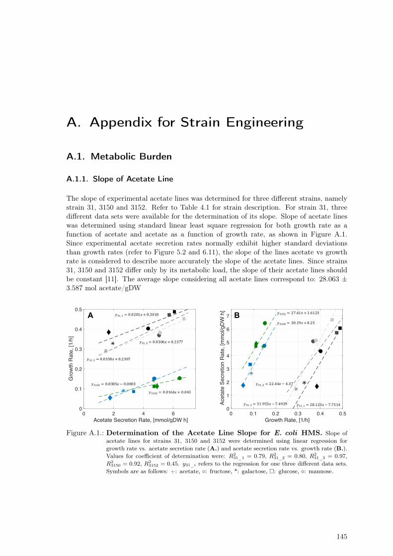
A. Appendix for Strain Engineering
A.1. Metabolic Burden
A.1.1. Slope of Acetate Line
The slope of experimental acetate lines was determined for three different strains, namelystrain 31, 3150 and 3152. Refer to Table 4.1 for strain description. For strain 31, threedifferent data sets were available for the determination of its slope. Slope of acetate lineswas determined using standard linear least square regression for both growth rate as afunction of acetate and acetate as a function of growth rate, as shown in Figure A.1.Since experimental acetate secretion rates normally exhibit higher standard deviationsthan growth rates (refer to Figure 5.2 and 6.11), the slope of the lines acetate vs growthrate is considered to describe more accurately the slope of the acetate lines. Since strains31, 3150 and 3152 differ only by its metabolic load, the slope of their acetate lines shouldbe constant [11]. The average slope considering all acetate lines correspond to: 28.063 ±3.587 mol acetate/gDW
0 2 4 6Acetate Secretion Rate, [mmol/gDW h]
0
0.1
0.2
0.3
0.4
0.5
Gro
wth
Rat
e, [1
/h]
0 0.1 0.2 0.3 0.4 0.5Growth Rate, [1/h]
0
1
2
3
4
5
6
7
Acet
ate
Secr
etio
n R
ate,
[mm
ol/g
DW
h]
𝑦"#_# = 0.0281𝑥+0.3018
𝑦"#_. = 0.0358𝑥+0.2307
𝑦"#_" = 0.0306𝑥+0.2377
𝑦"#23 = 0.0305𝑥− 0.0003
𝑦"#2. = 0.0166𝑥+ 0.043
𝑦"#_# = 28.123𝑥−7.7514
𝑦"#_. = 22.44𝑥− 4.37
𝑦"#_" = 31.953𝑥−7.4929
𝑦"#2. = 27.61𝑥+1.6123
𝑦"#23 = 30.19𝑥+0.25A B
Figure A.1.: Determination of the Acetate Line Slope for E. coli HMS. Slope ofacetate lines for strains 31, 3150 and 3152 were determined using linear regression forgrowth rate vs. acetate secretion rate (A.) and acetate secretion rate vs. growth rate (B.).Values for coefficient of determination were: R2
31_1 = 0.79, R231_2 = 0.80, R2
31_3 = 0.97,R2
3150 = 0.92, R23152 = 0.45. y31_i refers to the regression for one three different data sets.
Symbols are as follows: +: acetate, ◦: fructose, *: galactose, �: glucose, �: mannose.
145
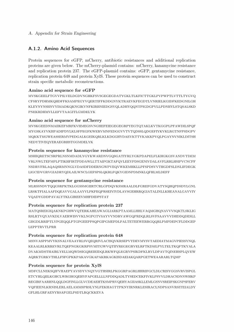
A. Appendix for Strain Engineering
A.1.2. Amino Acid Sequences
Protein sequences for eGFP, mCherry, antibiotic resistances and additional replicationproteins are given below. The mCherry-plasmid contains: mCherry, kanamycine resistanceand replication protein 237. The eGFP-plasmid contains: eGFP, gentamycine resistance,replication protein 648 and protein XylS. These protein sequences can be used to constructstrain specific metabolic reconstructions.
Amino acid sequence for eGFPMVSKGEELFTGVVPILVELDGDVNGHKFSVSGEGEGDATYGKLTLKFICTTGKLPVPWPTLVTTLTYGVQ
CFSRYPDHMKQHDFFKSAMPEGYVQERTIFFKDDGNYKTRAEVKFEGDTLVNRIELKGIDFKEDGNILGH
KLEYNYNSHNVYIMADKQKNGIKVNFKIRHNIEDGSVQLADHYQQNTPIGDGPVLLPDNHYLSTQSALSKD
PNEKRDHMVLLEFVTAAGITLGMDELYK
Amino acid sequence for mCherryMVSKGEEDNMAIIKEFMRFKVHMEGSVNGHEFEIEGEGEGRPYEGTQTAKLKVTKGGPLPFAWDILSPQF
MYGSKAYVKHPADIPDYLKLSFPEGFKWERVMNFEDGGVVTVTQDSSLQDGEFIYKVKLRGTNFPSDGPV
MQKKTMGWEASSERMYPEDGALKGEIKQRLKLKDGGHYDAEVKTTYKAKKPVQLPGAYNVNIKLDITSH
NEDYTIVEQYERAEGRHSTGGMDELYK
Protein sequence for kanamycine resistanceMSHIQRETSCSRPRLNSNMDADLYGYKWARDNVGQSGATIYRLYGKPDAPELFLKHGKGSVANDVTDEM
VRLNWLTEFMPLPTIKHFIRTPDDAWLLTTAIPGKTAFQVLEEYPDSGENIVDALAVFLRRLHSIPVCNCPF
NSDRVFRLAQAQSRMNNGLVDASDFDDERNGWPVEQVWKEMHKLLPFSPDSVVTHGDFSLDNLIFDEGK
LIGCIDVGRVGIADRYQDLAILWNCLGEFSPSLQKRLFQKYGIDNPDMNKLQFHLMLDEFF
Protein sequence for gentamycine resistanceMLRSSNDVTQQGSRPKTKLGGSSMGIIRTCRLGPDQVKSMRAALDLFGREFGDVATYSQHQPDSDYLGNL
LRSKTFIALAAFDQEAVVGALAAYVLPKFEQPRSEIYIYDLAVSGEHRRQGIATALINLLKHEANALGAYVIY
VQADYGDDPAVALYTKLGIREEVMHFDIDPSTAT
Protein sequence for replication protein 237MATQSREIGIQAKNKPGHWVQTERKAHEAWAGLIARKPTAAMLLHHLVAQMGHQNAVVVSQKTLSKLIG
RSLRTVQYAVKDLVAERWISVVKLNGPGTVSAYVVNDRVAWGQPRDQLRLSVFSAAVVVDHDDQDESLL
GHGDLRRIPTLYPGEQQLPTGPGEEPPSQPGIPGMEPDLPALTETEEWERRGQQRLPMPDEPCFLDDGEP
LEPPTRVTLPRR
Protein sequence for replication protein 648MSNVASPPMVYKSNALVEAAYRLSVQEQRIVLACISQVKRSEPVTDEVMYSVTAEDIATMAGVPIESSYNQL
KEAALRLKRREVRLTQEPNGKGKRPSVMITGWVQTIIYREGEGRVELRFTKDMLPYLTELTKQFTKYALA
DVAKMDSTHAIRLYELLMQWDSIGQREIEIDQLRKWFQLEGRYPSIKDFKLRVLDPAVTQINEHSPLQVEW
AQRKTGRKVTHLLFSFGPKKPAKAVGKAPAKRKAGKISDAEIAKQARPGETWEAARARLTQMP
Protein sequence for protein XylSMDFCLLNEKSQIFVHAEPYAVSDYVNQYVGTHSIRLPKGGRPAGRLHHRIFGCLDLCRISYGGSVRVISPGL
ETCYHLQIILKGHCLWRGHGQEHYFAPGELLLLNPDDQADLTYSEDCEKFIVKLPSVVLDRACSDNNWHKP
REGIRFAARHNLQQLDGFINLLGLVCDEAEHTKSMPRVQEHYAGIIASKLLEMLGSNVSREIFSKGNPSFERV
VQFIEENLKRNISLERLAELAMMSPRSLYNLFEKHAGTTPKNYIRNRKLESIRACLNDPSANVRSITEIALDY
GFLHLGRFAENYRSAFGELPSDTLRQCKKEVA
146
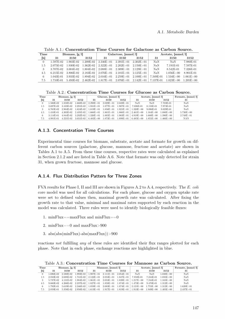
A.1. Metabolic Burden
Table A.1.: Concentration Time Courses for Galactose as Carbon Source.Time[h]
Biomass, [g/l] Galactose, [mmol/l] Acetate, [mmol/l]31 3150 3152 31 3150 3152 31 3150 3152
0 1.597E-02 1.903E-02 1.209E-02 2.346E+01 2.391E+01 2.302E+01 NaN NaN 7.980E-011.5 2.075E-02 1.930E-02 1.362E-02 2.322E+01 2.202E+01 2.150E+01 NaN 7.191E-01 7.597E-013 3.707E-02 3.004E-02 1.804E-02 2.088E+01 2.309E+01 2.129E+01 NaN 8.542E-01 7.326E-014.5 6.215E-02 3.806E-02 2.183E-02 2.076E+01 2.101E+01 2.125E+01 NaN 1.056E+00 8.901E-016 1.043E-01 3.933E-02 1.894E-02 2.016E+01 2.259E+01 2.100E+01 7.349E-01 1.534E+00 1.061E+007.5 1.710E-01 5.493E-02 2.462E-02 1.817E+01 2.076E+01 2.142E+01 7.137E-01 1.823E+00 1.205E+00
Table A.2.: Concentration Time Courses for Glucose as Carbon Source.Time[h]
Biomass, [g/l] Glucose, [mmol/l] Acetate, [mmol/l] Formate, [mmol/l]31 3150 3152 31 3150 3152 31 3150 3152 31
0 1.506E-02 1.858E-02 1.660E-02 2.298E+01 2.029E+01 2.049E+01 NaN NaN 7.703E-01 NaN1.5 2.697E-02 3.103E-02 2.291E-02 1.931E+01 1.877E+01 1.907E+01 7.026E-01 8.158E-01 7.973E-01 NaN3 6.765E-02 2.904E-02 1.624E-02 1.819E+01 1.856E+01 1.921E+01 1.320E+00 9.096E-01 9.029E-01 NaN4.5 1.410E-01 4.303E-02 2.435E-02 1.666E+01 1.861E+01 1.866E+01 2.461E+00 1.164E+00 1.080E+00 5.730E+006 3.114E-01 4.844E-02 3.292E-02 1.326E+01 1.885E+01 1.903E+01 4.919E+00 1.600E+00 1.390E+00 2.748E+017.5 4.991E-01 4.221E-02 3.031E-02 6.482E+00 1.873E+01 1.899E+01 6.485E+00 1.855E+00 1.466E+00 NAN
A.1.3. Concentration Time Courses
Experimental time courses for biomass, substrate, acetate and formate for growth on dif-ferent carbon sources (galactose, glucose, mannose, fructose and acetate) are shown inTables A.1 to A.5. From these time courses, respective rates were calculated as explainedin Section 2.1.2 and are listed in Table A.6. Note that formate was only detected for strain31, when grown fructose, mannose and glucose.
A.1.4. Flux Distribution Patters for Three Zones
FVA results for Phase I, II and III are shown in Figures A.2 to A.4, respectively. The E. colicore model was used for all calculations. For each phase, glucose and oxygen uptake ratewere set to defined values then, maximal growth rate was calculated. After fixing thegrowth rate to that value, minimal and maximal rates supported by each reaction in themodel was calculated. Three rules were used to identify biologically feasible fluxes:
1. minFlux==maxFlux and minFlux==0
2. minFlux==0 and maxFlux>900
3. abs(abs(minFlux)-abs(maxFlux))>900
reactions not fulfilling any of these rules are identified their flux ranges plotted for eachphase. Note that in each phase, exchange reactions are highlighted in blue.
Table A.3.: Concentration Time Courses for Mannose as Carbon Source.Time[h]
Biomass, [g/l] Mannose, [mmol/l] Acetate, [mmol/l] Formate, [mmol/l]31 3150 3152 31 3150 3152 31 3150 3152 31
0 1.696E-02 2.580E-02 1.993E-02 1.987E+01 2.111E+01 2.054E+01 NaN NaN 1.038E+00 NaN1.5 2.850E-02 2.688E-02 1.741E-02 2.122E+01 2.053E+01 1.847E+01 7.858E-01 7.244E-01 1.035E+00 NaN3 5.737E-02 4.131E-02 1.984E-02 1.861E+01 2.053E+01 1.839E+01 1.217E+00 7.244E-01 1.165E+00 NaN4.5 9.660E-02 4.266E-02 2.237E-02 1.827E+01 1.858E+01 1.874E+01 1.473E+00 9.470E-01 1.312E+00 NaN6 1.792E-01 5.619E-02 2.246E-02 1.859E+01 2.083E+01 1.874E+01 2.121E+00 1.755E+00 1.312E+00 1.620E+017.5 2.859E-01 5.358E-02 2.950E-02 1.613E+01 1.917E+01 1.819E+01 1.913E+00 1.949E+00 1.405E+00 2.437E+01
147
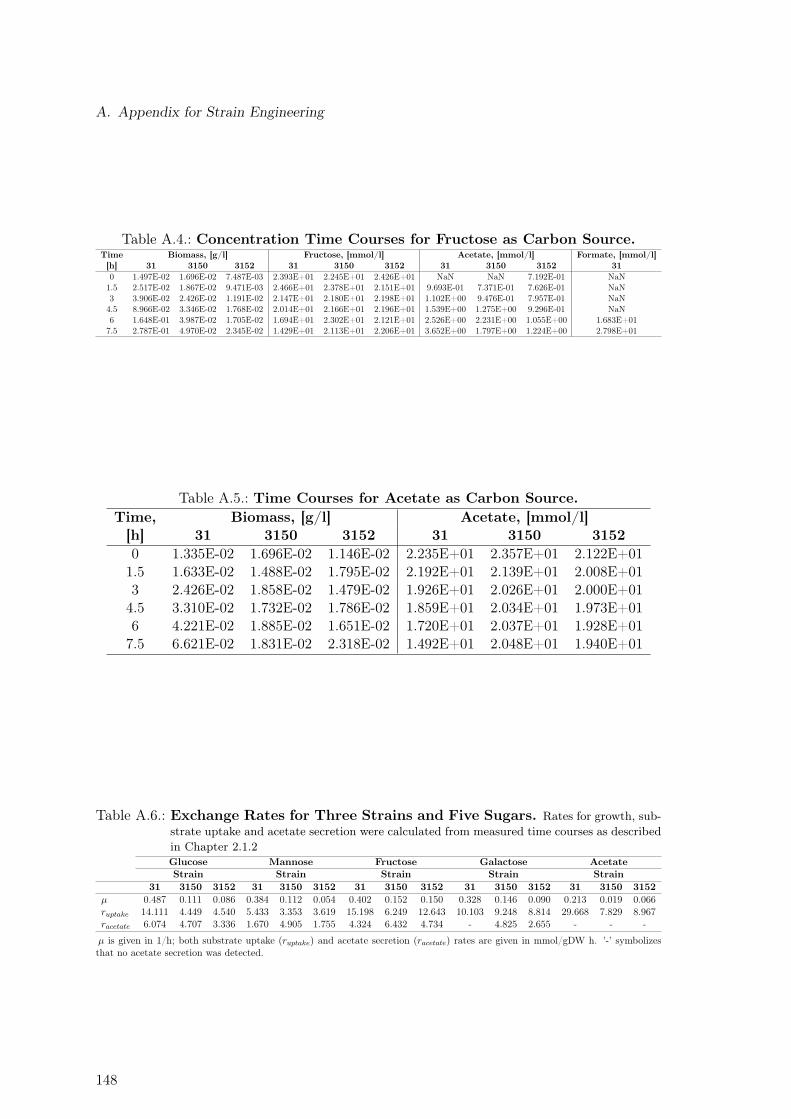
A. Appendix for Strain Engineering
Table A.4.: Concentration Time Courses for Fructose as Carbon Source.Time[h]
Biomass, [g/l] Fructose, [mmol/l] Acetate, [mmol/l] Formate, [mmol/l]31 3150 3152 31 3150 3152 31 3150 3152 31
0 1.497E-02 1.696E-02 7.487E-03 2.393E+01 2.245E+01 2.426E+01 NaN NaN 7.192E-01 NaN1.5 2.517E-02 1.867E-02 9.471E-03 2.466E+01 2.378E+01 2.151E+01 9.693E-01 7.371E-01 7.626E-01 NaN3 3.906E-02 2.426E-02 1.191E-02 2.147E+01 2.180E+01 2.198E+01 1.102E+00 9.476E-01 7.957E-01 NaN4.5 8.966E-02 3.346E-02 1.768E-02 2.014E+01 2.166E+01 2.196E+01 1.539E+00 1.275E+00 9.296E-01 NaN6 1.648E-01 3.987E-02 1.705E-02 1.694E+01 2.302E+01 2.121E+01 2.526E+00 2.231E+00 1.055E+00 1.683E+017.5 2.787E-01 4.970E-02 2.345E-02 1.429E+01 2.113E+01 2.206E+01 3.652E+00 1.797E+00 1.224E+00 2.798E+01
Table A.5.: Time Courses for Acetate as Carbon Source.Time,[h]
Biomass, [g/l] Acetate, [mmol/l]31 3150 3152 31 3150 3152
0 1.335E-02 1.696E-02 1.146E-02 2.235E+01 2.357E+01 2.122E+011.5 1.633E-02 1.488E-02 1.795E-02 2.192E+01 2.139E+01 2.008E+013 2.426E-02 1.858E-02 1.479E-02 1.926E+01 2.026E+01 2.000E+014.5 3.310E-02 1.732E-02 1.786E-02 1.859E+01 2.034E+01 1.973E+016 4.221E-02 1.885E-02 1.651E-02 1.720E+01 2.037E+01 1.928E+017.5 6.621E-02 1.831E-02 2.318E-02 1.492E+01 2.048E+01 1.940E+01
Table A.6.: Exchange Rates for Three Strains and Five Sugars. Rates for growth, sub-strate uptake and acetate secretion were calculated from measured time courses as describedin Chapter 2.1.2Glucose Mannose Fructose Galactose AcetateStrain Strain Strain Strain Strain
31 3150 3152 31 3150 3152 31 3150 3152 31 3150 3152 31 3150 3152µ 0.487 0.111 0.086 0.384 0.112 0.054 0.402 0.152 0.150 0.328 0.146 0.090 0.213 0.019 0.066ruptake 14.111 4.449 4.540 5.433 3.353 3.619 15.198 6.249 12.643 10.103 9.248 8.814 29.668 7.829 8.967racetate 6.074 4.707 3.336 1.670 4.905 1.755 4.324 6.432 4.734 - 4.825 2.655 - - -
µ is given in 1/h; both substrate uptake (ruptake) and acetate secretion (racetate) rates are given in mmol/gDW h. ’-’ symbolizesthat no acetate secretion was detected.
148
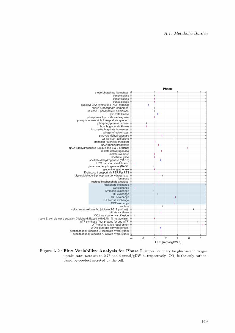
A.1. Metabolic Burden
-4 -2 0 2 4 6 8Flux, [mmol/gDW h]
aconitase (half-reaction A, Citrate hydro-lyase)aconitase (half-reaction B, Isocitrate hydro-lyase)
2-Oxogluterate dehydrogenaseATP maintenance requirement
ATP synthase (four protons for one ATP)core E. coli biomass equation (Neidhardt Based with GAM, N metabolism)
CO2 transporter via diffusioncitrate synthase
cytochrome oxidase bd (ubiquinol-8: 2 protons)enolase
CO2 exchangeD-Glucose exchange
H2O exchangeH+ exchange
Ammonia exchangeO2 exchange
Phosphate exchangefructose-bisphosphate aldolase
fumaraseglyceraldehyde-3-phosphate dehydrogenase
D-glucose transport via PEP:Pyr PTSglutamine synthetase
glutamate dehydrogenase (NADP)H2O transport via diffusion
isocitrate dehydrogenase (NADP)Isocitrate lyase
malate synthasemalate dehydrogenase
NADH dehydrogenase (ubiquinone-8 & 3 protons)NAD transhydrogenase
ammonia reversible transporto2 transport (diffusion)
pyruvate dehydrogenasephosphofructokinase
glucose-6-phosphate isomerasephosphoglycerate kinase
phosphoglycerate mutasephosphate reversible transport via symport
phosphoenolpyruvate carboxylasepyruvate kinase
ribulose 5-phosphate 3-epimeraseribose-5-phosphate isomerase
succinyl-CoA synthetase (ADP-forming)transaldolasetransketolasetransketolase
triose-phosphate isomerasePhase I
Figure A.2.: Flux Variability Analysis for Phase I. Upper boundary for glucose and oxygenuptake rates were set to 0.75 and 4 mmol/gDW h, respectively. CO2 is the only carbon-based by-product secreted by the cell.
149
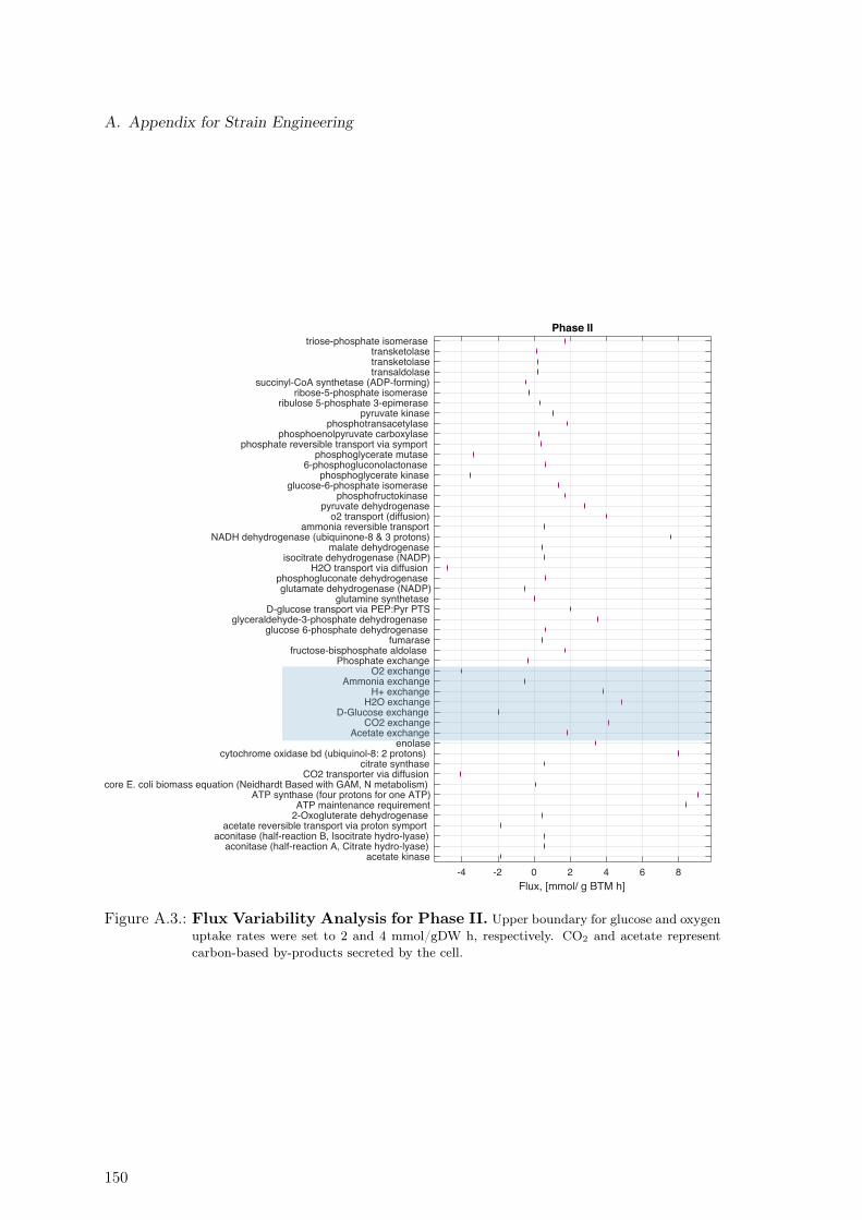
A. Appendix for Strain Engineering
-4 -2 0 2 4 6 8Flux, [mmol/ g BTM h]
acetate kinaseaconitase (half-reaction A, Citrate hydro-lyase)
aconitase (half-reaction B, Isocitrate hydro-lyase)acetate reversible transport via proton symport
2-Oxogluterate dehydrogenaseATP maintenance requirement
ATP synthase (four protons for one ATP)core E. coli biomass equation (Neidhardt Based with GAM, N metabolism)
CO2 transporter via diffusioncitrate synthase
cytochrome oxidase bd (ubiquinol-8: 2 protons)enolase
Acetate exchangeCO2 exchange
D-Glucose exchangeH2O exchange
H+ exchangeAmmonia exchange
O2 exchangePhosphate exchange
fructose-bisphosphate aldolasefumarase
glucose 6-phosphate dehydrogenaseglyceraldehyde-3-phosphate dehydrogenase
D-glucose transport via PEP:Pyr PTSglutamine synthetase
glutamate dehydrogenase (NADP)phosphogluconate dehydrogenase
H2O transport via diffusionisocitrate dehydrogenase (NADP)
malate dehydrogenaseNADH dehydrogenase (ubiquinone-8 & 3 protons)
ammonia reversible transporto2 transport (diffusion)
pyruvate dehydrogenasephosphofructokinase
glucose-6-phosphate isomerasephosphoglycerate kinase
6-phosphogluconolactonasephosphoglycerate mutase
phosphate reversible transport via symportphosphoenolpyruvate carboxylase
phosphotransacetylasepyruvate kinase
ribulose 5-phosphate 3-epimeraseribose-5-phosphate isomerase
succinyl-CoA synthetase (ADP-forming)transaldolasetransketolasetransketolase
triose-phosphate isomerasePhase II
Figure A.3.: Flux Variability Analysis for Phase II. Upper boundary for glucose and oxygenuptake rates were set to 2 and 4 mmol/gDW h, respectively. CO2 and acetate representcarbon-based by-products secreted by the cell.
150
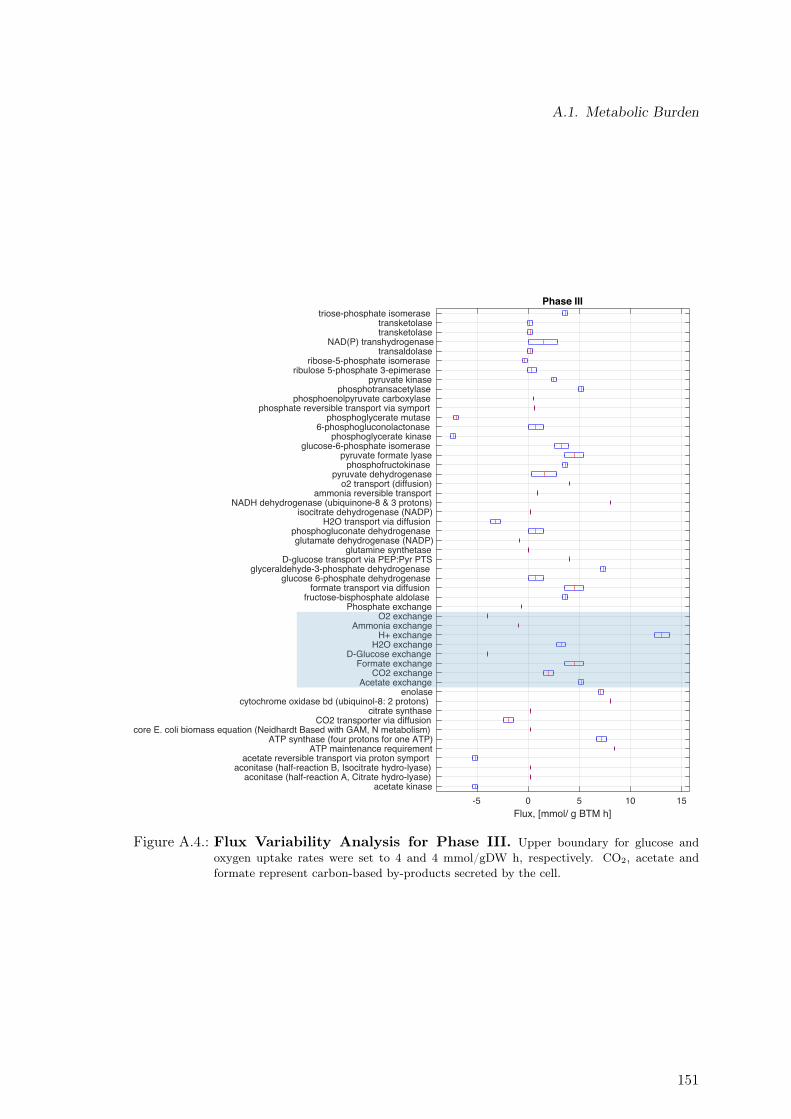
A.1. Metabolic Burden
-5 0 5 10 15Flux, [mmol/ g BTM h]
acetate kinaseaconitase (half-reaction A, Citrate hydro-lyase)
aconitase (half-reaction B, Isocitrate hydro-lyase)acetate reversible transport via proton symport
ATP maintenance requirementATP synthase (four protons for one ATP)
core E. coli biomass equation (Neidhardt Based with GAM, N metabolism)CO2 transporter via diffusion
citrate synthasecytochrome oxidase bd (ubiquinol-8: 2 protons)
enolaseAcetate exchange
CO2 exchangeFormate exchange
D-Glucose exchangeH2O exchange
H+ exchangeAmmonia exchange
O2 exchangePhosphate exchange
fructose-bisphosphate aldolaseformate transport via diffusion
glucose 6-phosphate dehydrogenaseglyceraldehyde-3-phosphate dehydrogenase
D-glucose transport via PEP:Pyr PTSglutamine synthetase
glutamate dehydrogenase (NADP)phosphogluconate dehydrogenase
H2O transport via diffusionisocitrate dehydrogenase (NADP)
NADH dehydrogenase (ubiquinone-8 & 3 protons)ammonia reversible transport
o2 transport (diffusion)pyruvate dehydrogenase
phosphofructokinasepyruvate formate lyase
glucose-6-phosphate isomerasephosphoglycerate kinase
6-phosphogluconolactonasephosphoglycerate mutase
phosphate reversible transport via symportphosphoenolpyruvate carboxylase
phosphotransacetylasepyruvate kinase
ribulose 5-phosphate 3-epimeraseribose-5-phosphate isomerase
transaldolaseNAD(P) transhydrogenase
transketolasetransketolase
triose-phosphate isomerasePhase III
Figure A.4.: Flux Variability Analysis for Phase III. Upper boundary for glucose andoxygen uptake rates were set to 4 and 4 mmol/gDW h, respectively. CO2, acetate andformate represent carbon-based by-products secreted by the cell.
151
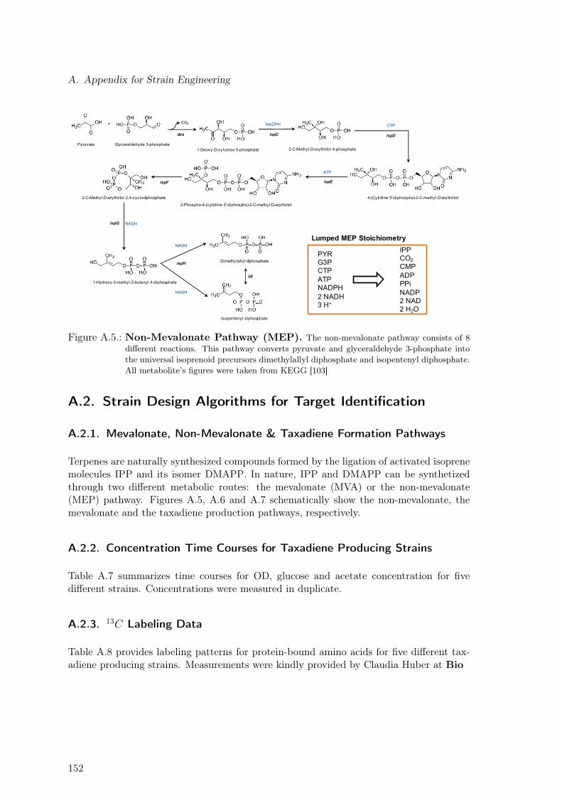
A. Appendix for Strain Engineering
Pyruvate Glyceraldehyde 3-phosphate
+
Isopentenyl diphosphate
4-(Cytidine 5'-diphospho)-2-C-methyl-D-erythritol
2-Phospho-4-(cytidine 5'-diphospho)-2-C-methyl-D-erythritol
2-C-Methyl-D-erythritol 2,4-cyclodiphosphate
1-Hydroxy-2-methyl-2-butenyl 4-diphosphate
Dimethylallyl diphosphate
ispD
ispEispF
ispG
ispH
idi
1-Deoxy-D-xylulose 5-phosphate
dxs ispC
NADPH CTP
ATP
NADH
NADH
NADH
2-C-Methyl-D-erythritol 4-phosphate
PYR G3PCTPATPNADPH2 NADH 3 H+
IPPCO2CMPADPPPiNADP2 NAD2 H2O
Lumped MEP Stoichiometry
CO2
Figure A.5.: Non-Mevalonate Pathway (MEP). The non-mevalonate pathway consists of 8different reactions. This pathway converts pyruvate and glyceraldehyde 3-phosphate intothe universal isoprenoid precursors dimethylallyl diphosphate and isopentenyl diphosphate.All metabolite’s figures were taken from KEGG [103]
A.2. Strain Design Algorithms for Target Identification
A.2.1. Mevalonate, Non-Mevalonate & Taxadiene Formation Pathways
Terpenes are naturally synthesized compounds formed by the ligation of activated isoprenemolecules IPP and its isomer DMAPP. In nature, IPP and DMAPP can be synthetizedthrough two different metabolic routes: the mevalonate (MVA) or the non-mevalonate(MEP) pathway. Figures A.5, A.6 and A.7 schematically show the non-mevalonate, themevalonate and the taxadiene production pathways, respectively.
A.2.2. Concentration Time Courses for Taxadiene Producing Strains
Table A.7 summarizes time courses for OD, glucose and acetate concentration for fivedifferent strains. Concentrations were measured in duplicate.
A.2.3. 13C Labeling Data
Table A.8 provides labeling patterns for protein-bound amino acids for five different tax-adiene producing strains. Measurements were kindly provided by Claudia Huber at Bio
152
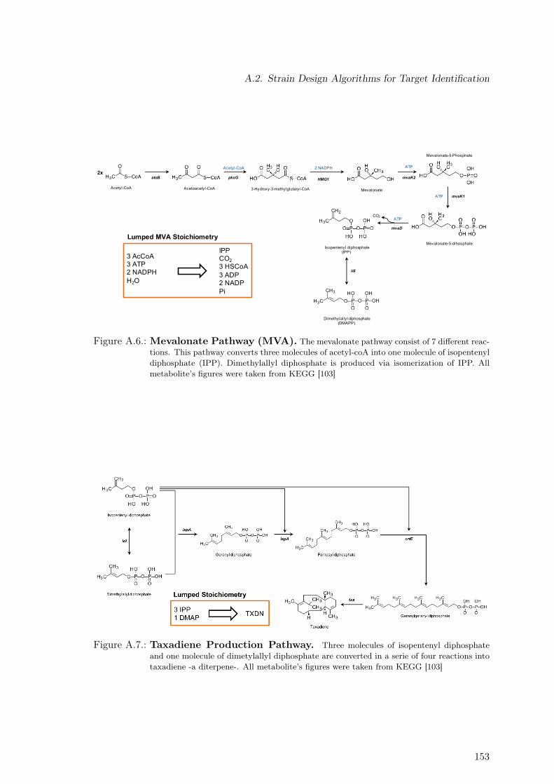
A.2. Strain Design Algorithms for Target Identification
Acetyl-CoA
2x
Dimethylallyl diphosphate(DMAPP)
idi
Acetoacetyl-CoA 3-Hydroxy-3-methylglutaryl-CoA
Mevalonate-5-Phosphate
Mevalonate-5-dihosphateIsopentenyl diphosphate
(IPP)
atoB pksG HMG1
mvaK1
mvaK2
mvaD
Acetyl-CoA 2 NADPH ATP
ATP
ATP
Mevalonate
3 AcCoA3 ATP2 NADPHH2O
IPPCO23 HSCoA3 ADP2 NADPPi
Lumped MVA Stoichiometry
CO2
Figure A.6.: Mevalonate Pathway (MVA). The mevalonate pathway consist of 7 different reac-tions. This pathway converts three molecules of acetyl-coA into one molecule of isopentenyldiphosphate (IPP). Dimethylallyl diphosphate is produced via isomerization of IPP. Allmetabolite’s figures were taken from KEGG [103]
Figure A.7.: Taxadiene Production Pathway. Three molecules of isopentenyl diphosphateand one molecule of dimetylallyl diphosphate are converted in a serie of four reactions intotaxadiene -a diterpene-. All metabolite’s figures were taken from KEGG [103]
153
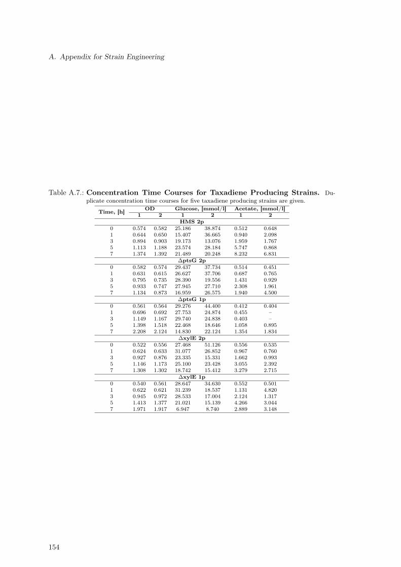
A. Appendix for Strain Engineering
Table A.7.: Concentration Time Courses for Taxadiene Producing Strains. Du-plicate concentration time courses for five taxadiene producing strains are given.
Time, [h] OD Glucose, [mmol/l] Acetate, [mmol/l]1 2 1 2 1 2
HMS 2p0 0.574 0.582 25.186 38.874 0.512 0.6481 0.644 0.650 15.407 36.665 0.940 2.0983 0.894 0.903 19.173 13.076 1.959 1.7675 1.113 1.188 23.574 28.184 5.747 0.8687 1.374 1.392 21.489 20.248 8.232 6.831
∆ptsG 2p0 0.582 0.574 29.437 37.734 0.514 0.4511 0.631 0.615 26.627 37.706 0.687 0.7653 0.795 0.735 28.390 19.556 1.431 0.9295 0.933 0.747 27.945 27.710 2.308 1.9617 1.134 0.873 16.959 26.575 1.940 4.500
∆ptsG 1p0 0.561 0.564 29.276 44.400 0.412 0.4041 0.696 0.692 27.753 24.874 0.455 –3 1.149 1.167 29.740 24.838 0.403 –5 1.398 1.518 22.468 18.646 1.058 0.8957 2.208 2.124 14.830 22.124 1.354 1.834
∆xylE 2p0 0.522 0.556 27.468 51.126 0.556 0.5351 0.624 0.633 31.077 26.852 0.967 0.7603 0.927 0.876 23.335 15.331 1.662 0.9935 1.146 1.173 25.100 23.428 3.055 2.3927 1.308 1.302 18.742 15.412 3.279 2.715
∆xylE 1p0 0.540 0.561 28.647 34.630 0.552 0.5011 0.622 0.621 31.239 18.537 1.131 4.8203 0.945 0.972 28.533 17.004 2.124 1.3175 1.413 1.377 21.021 15.139 4.266 3.0447 1.971 1.917 6.947 8.740 2.889 3.148
154
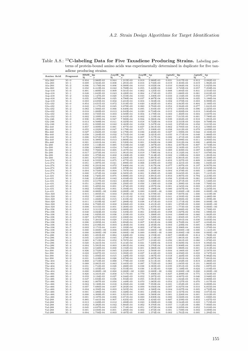
A.2. Strain Design Algorithms for Target Identification
Table A.8.: 13C-labeling Data for Five Taxadiene Producing Strains. Labeling pat-terns of protein-bound amino acids was experimentally determined in duplicate for five tax-adiene producing strains.
Amino Acid Fragment HMS_2p ∆xylE_2p ∆xylE_1p ∆ptsG_2p ∆ptsG_1p% σ % σ % σ % σ % σ
Ala-260 M+0 0.934 2.980E-03 0.944 1.315E-03 0.919 2.968E-03 0.931 3.617E-03 0.912 2.092E-03Ala-260 M+1 0.009 2.564E-03 0.008 1.291E-03 0.016 2.732E-03 0.019 3.303E-03 0.019 1.962E-03Ala-260 M+2 0.006 3.178E-04 0.006 6.089E-04 0.010 6.032E-04 0.010 6.044E-04 0.012 5.825E-04Ala-260 M+3 0.050 6.413E-04 0.042 6.788E-04 0.055 5.422E-04 0.040 3.745E-04 0.057 7.258E-04Asp-418 M+0 0.891 1.809E-03 0.909 9.501E-04 0.862 4.125E-03 0.888 1.894E-03 0.841 2.554E-03Asp-418 M+1 0.048 1.843E-03 0.043 8.426E-04 0.064 4.174E-03 0.055 1.680E-03 0.081 2.810E-03Asp-418 M+2 0.024 1.147E-03 0.020 5.316E-04 0.033 1.330E-03 0.033 2.134E-03 0.050 1.077E-03Asp-418 M+3 0.035 3.678E-04 0.025 4.796E-04 0.037 8.487E-04 0.022 5.565E-04 0.025 5.196E-04Asp-418 M+4 0.003 2.635E-04 0.002 3.231E-04 0.004 1.584E-04 0.002 3.570E-04 0.003 8.999E-05Glu-432 M+0 0.854 2.631E-03 0.872 3.018E-03 0.820 4.462E-03 0.854 4.843E-03 0.804 2.166E-03Glu-432 M+1 0.042 2.117E-03 0.045 3.079E-03 0.060 3.794E-03 0.054 3.564E-03 0.077 1.841E-03Glu-432 M+2 0.082 1.566E-03 0.066 6.649E-04 0.095 1.916E-03 0.073 1.695E-03 0.096 2.225E-03Glu-432 M+3 0.018 1.000E-03 0.013 6.943E-04 0.020 6.734E-04 0.015 6.820E-04 0.019 5.804E-04Glu-432 M+4 0.003 3.735E-04 0.003 2.509E-04 0.004 4.178E-04 0.003 1.360E-04 0.004 3.837E-04Glu-432 M+5 0.002 2.339E-04 0.001 6.043E-05 0.002 1.119E-04 0.001 7.015E-05 0.001 7.789E-05Gly-246 M+0 0.936 6.189E-04 0.947 7.906E-04 0.924 6.366E-04 0.939 2.662E-03 0.918 1.091E-03Gly-246 M+1 0.013 6.568E-04 0.011 6.325E-04 0.018 6.722E-04 0.019 2.531E-03 0.024 9.768E-04Gly-246 M+2 0.051 6.939E-04 0.042 2.483E-04 0.058 5.347E-04 0.043 3.970E-04 0.058 3.015E-04His-440 M+0 0.857 3.009E-03 0.881 1.877E-03 0.827 2.361E-03 0.862 2.795E-03 0.812 4.596E-03His-440 M+1 0.055 4.232E-03 0.047 9.179E-04 0.071 3.330E-03 0.058 3.612E-03 0.079 4.839E-03His-440 M+2 0.027 1.822E-03 0.022 2.179E-03 0.036 2.402E-03 0.027 1.590E-03 0.042 2.163E-03His-440 M+3 0.038 1.244E-03 0.032 9.731E-04 0.046 2.021E-03 0.035 8.171E-04 0.048 1.866E-03His-440 M+4 0.006 9.074E-04 0.005 7.217E-04 0.007 5.517E-04 0.006 1.471E-03 0.009 6.396E-04His-440 M+5 0.016 6.389E-04 0.013 3.869E-04 0.014 4.941E-04 0.012 8.099E-04 0.011 4.956E-04His-440 M+6 0.001 2.831E-04 0.001 2.520E-04 0.001 3.943E-04 0.000 3.612E-04 0.000 1.400E-04Ile-200 M+0 0.859 1.114E-03 0.885 9.018E-04 0.826 1.307E-03 0.864 2.857E-03 0.807 9.733E-04Ile-200 M+1 0.038 3.968E-04 0.034 5.744E-04 0.057 1.387E-03 0.050 2.182E-03 0.075 8.657E-04Ile-200 M+2 0.082 7.766E-04 0.065 3.457E-04 0.094 4.016E-04 0.069 6.309E-04 0.097 6.888E-04Ile-200 M+3 0.017 2.073E-04 0.013 1.061E-04 0.019 1.738E-04 0.014 3.132E-04 0.017 3.678E-04Ile-200 M+4 0.003 1.375E-04 0.002 6.190E-05 0.003 7.314E-05 0.002 1.139E-04 0.003 1.291E-04Ile-200 M+5 0.001 6.075E-05 0.001 4.236E-05 0.001 5.891E-05 0.001 6.891E-05 0.001 5.338E-05Leu-274 M+0 0.842 8.555E-04 0.875 1.677E-03 0.813 2.007E-03 0.852 5.227E-03 0.809 2.346E-03Leu-274 M+1 0.051 1.097E-03 0.041 1.899E-03 0.068 2.039E-03 0.056 4.421E-03 0.066 1.840E-03Leu-274 M+2 0.092 6.231E-04 0.072 7.846E-04 0.101 5.817E-04 0.077 1.007E-03 0.107 8.957E-04Leu-274 M+3 0.010 3.020E-04 0.009 1.679E-04 0.012 1.312E-04 0.010 4.354E-04 0.013 2.845E-04Leu-274 M+4 0.004 9.750E-05 0.004 1.787E-04 0.005 1.364E-04 0.004 8.379E-05 0.005 1.128E-04Leu-274 M+5 0.000 1.074E-04 0.000 6.585E-05 0.001 9.298E-05 0.000 9.645E-05 0.001 7.141E-05Lys-431 M+0 0.846 1.740E-03 0.875 3.888E-03 0.812 3.891E-03 0.853 3.967E-03 0.794 2.218E-03Lys-431 M+1 0.046 2.254E-03 0.042 4.034E-03 0.065 3.982E-03 0.056 5.255E-03 0.081 2.019E-03Lys-431 M+2 0.055 2.517E-03 0.044 1.603E-03 0.063 3.038E-03 0.052 3.271E-03 0.072 1.546E-03Lys-431 M+3 0.051 1.258E-03 0.039 1.256E-03 0.056 1.139E-03 0.038 1.399E-03 0.048 7.768E-04Lys-431 M+4 0.001 5.495E-04 0.001 1.074E-03 0.002 4.057E-04 0.001 4.545E-04 0.003 1.205E-03Lys-431 M+5 0.002 5.656E-04 0.001 5.356E-04 0.002 5.198E-04 0.000 2.647E-04 0.001 4.245E-04Lys-431 M+6 0.000 0.000E+00 0.000 0.000E+00 0.000 0.000E+00 0.000 0.000E+00 0.000 0.000E+00Met-320 M+0 0.915 1.005E-01 0.933 7.293E-02 0.814 6.578E-03 0.928 7.937E-02 1.000 4.419E-08Met-320 M+1 0.052 7.160E-02 0.041 4.511E-02 0.102 9.025E-03 0.041 4.593E-02 0.000 4.486E-08Met-320 M+2 0.010 1.222E-02 0.015 1.610E-02 0.040 6.690E-03 0.018 2.060E-02 0.000 1.359E-08Met-320 M+3 0.011 1.810E-02 0.007 1.206E-02 0.038 4.471E-03 0.010 1.171E-02 0.000 0.000E+00Met-320 M+4 0.004 6.758E-03 0.002 2.926E-03 0.004 3.451E-03 0.001 1.870E-03 0.000 0.000E+00Met-320 M+5 0.008 9.015E-03 0.001 3.268E-03 0.001 1.837E-03 0.001 1.773E-03 0.000 0.000E+00Phe-336 M+0 0.810 3.311E-03 0.850 2.089E-03 0.770 2.718E-03 0.807 1.068E-02 0.766 1.739E-03Phe-336 M+1 0.040 3.024E-03 0.032 1.535E-03 0.061 2.605E-03 0.058 1.027E-02 0.056 1.596E-03Phe-336 M+2 0.046 1.835E-03 0.036 1.319E-03 0.054 1.398E-03 0.044 1.098E-03 0.060 1.062E-03Phe-336 M+3 0.067 6.878E-04 0.053 4.226E-04 0.074 1.529E-03 0.061 1.856E-03 0.075 9.133E-04Phe-336 M+4 0.024 7.201E-04 0.020 7.191E-04 0.027 9.748E-04 0.020 5.691E-04 0.030 3.603E-04Phe-336 M+5 0.006 2.895E-04 0.005 3.894E-04 0.007 2.821E-04 0.006 4.702E-04 0.007 4.034E-04Phe-336 M+6 0.004 2.618E-04 0.003 2.484E-04 0.004 2.484E-04 0.003 1.238E-04 0.005 1.960E-04Phe-336 M+7 0.002 2.171E-04 0.001 1.332E-04 0.002 1.873E-04 0.001 2.396E-04 0.002 1.276E-04Phe-336 M+8 0.000 0.000E+00 0.000 0.000E+00 0.000 0.000E+00 0.000 0.000E+00 0.000 1.141E-05Phe-336 M+9 0.000 0.000E+00 0.000 0.000E+00 0.000 0.000E+00 0.000 0.000E+00 0.000 0.000E+00Pro-286 M+0 0.865 1.491E-03 0.884 1.626E-03 0.834 2.155E-03 0.867 1.683E-03 0.814 1.780E-03Pro-286 M+1 0.045 1.421E-03 0.045 1.278E-03 0.062 2.114E-03 0.057 1.881E-03 0.081 1.202E-03Pro-286 M+2 0.065 8.713E-04 0.052 9.787E-04 0.077 1.018E-03 0.056 1.961E-03 0.080 1.978E-03Pro-286 M+3 0.020 6.241E-04 0.015 6.414E-04 0.021 7.249E-04 0.016 6.849E-04 0.019 6.094E-04Pro-286 M+4 0.004 5.591E-04 0.003 3.881E-04 0.004 5.576E-04 0.003 5.908E-04 0.005 2.993E-04Pro-286 M+5 0.001 2.546E-04 0.000 3.194E-04 0.001 2.386E-04 0.000 1.980E-04 0.001 2.314E-04Ser-390 M+0 0.926 2.752E-03 0.945 2.232E-03 0.914 2.593E-03 0.934 4.186E-03 0.907 2.597E-03Ser-390 M+1 0.022 2.837E-03 0.013 3.392E-03 0.027 2.418E-03 0.022 4.058E-03 0.033 2.747E-03Ser-390 M+2 0.021 1.056E-03 0.015 1.349E-03 0.023 1.067E-03 0.018 1.440E-03 0.025 8.984E-04Ser-390 M+3 0.031 5.418E-04 0.026 3.878E-04 0.036 6.687E-04 0.026 7.491E-04 0.035 7.691E-04Thr-404 M+0 0.868 2.713E-03 0.888 1.778E-03 0.839 2.511E-03 0.861 8.432E-03 0.819 2.286E-03Thr-404 M+1 0.068 2.081E-03 0.063 2.445E-03 0.087 3.752E-03 0.083 1.045E-02 0.101 1.860E-03Thr-404 M+2 0.031 1.712E-03 0.028 1.288E-03 0.038 2.383E-03 0.035 2.951E-03 0.056 1.697E-03Thr-404 M+3 0.032 1.453E-03 0.021 4.553E-04 0.036 1.413E-03 0.020 1.148E-03 0.024 1.016E-03Thr-404 M+4 0.000 0.000E+00 0.000 0.000E+00 0.000 0.000E+00 0.000 0.000E+00 0.000 0.000E+00Tyr-466 M+0 0.820 4.341E-03 0.858 3.717E-03 0.779 7.490E-03 0.827 4.299E-03 0.775 3.563E-03Tyr-466 M+1 0.033 3.134E-03 0.027 4.244E-03 0.052 5.207E-03 0.045 4.067E-03 0.046 2.948E-03Tyr-466 M+2 0.047 1.833E-03 0.036 1.934E-03 0.055 3.081E-03 0.041 1.624E-03 0.061 2.868E-03Tyr-466 M+3 0.062 1.067E-03 0.050 1.449E-03 0.070 1.065E-03 0.054 2.127E-03 0.070 1.017E-03Tyr-466 M+4 0.024 9.120E-04 0.018 6.356E-04 0.028 7.953E-04 0.021 1.052E-03 0.031 9.899E-04Tyr-466 M+5 0.007 7.686E-04 0.007 8.202E-04 0.009 9.056E-04 0.007 6.027E-04 0.010 6.855E-04Tyr-466 M+6 0.004 4.356E-04 0.003 4.505E-04 0.005 4.586E-04 0.004 2.627E-04 0.005 4.722E-04Tyr-466 M+7 0.001 1.486E-04 0.001 3.328E-04 0.001 1.458E-04 0.001 4.547E-04 0.002 3.671E-04Tyr-466 M+8 0.000 4.309E-05 0.001 3.921E-04 0.000 3.580E-04 0.001 2.226E-04 0.001 9.012E-05Tyr-466 M+9 0.001 3.107E-04 0.000 3.071E-04 0.000 3.830E-04 0.000 3.040E-04 0.000 1.836E-04Val-288 M+0 0.885 7.441E-04 0.907 1.625E-03 0.858 2.424E-03 0.887 4.239E-03 0.852 1.627E-03Val-288 M+1 0.013 1.049E-03 0.012 1.206E-03 0.023 2.398E-03 0.026 3.544E-03 0.023 1.715E-03Val-288 M+2 0.052 8.292E-04 0.042 5.884E-04 0.062 8.376E-04 0.047 1.112E-03 0.066 7.956E-04Val-288 M+3 0.045 4.637E-04 0.035 1.714E-04 0.051 3.972E-04 0.036 3.035E-04 0.052 5.016E-04Val-288 M+4 0.001 2.030E-04 0.001 1.200E-04 0.002 1.872E-04 0.001 1.739E-04 0.002 3.099E-04Val-288 M+5 0.004 1.756E-04 0.003 9.497E-05 0.005 1.374E-04 0.003 1.761E-04 0.005 1.294E-04
155
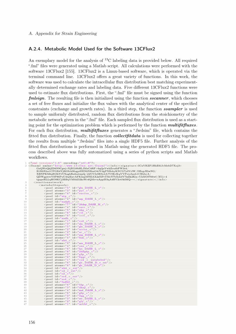
A. Appendix for Strain Engineering
A.2.4. Metabolic Model Used for the Software 13CFlux2
An exemplary model for the analysis of 13C labeling data is provided below. All required“.fml” files were generated using a Matlab script. All calculations were performed with thesoftware 13CFlux2 [155]. 13CFlux2 is a Linux-based software, which is operated via theterminal command line. 13CFlux2 offers a great variety of functions. In this work, thesoftware was used to calculate the intracellular flux distribution best matching experiment-ally determined exchange rates and labeling data. Five different 13CFlux2 functions wereused to estimate flux distributions. First, the “.fml” file must be signed using the functionfmlsign . The resulting file is then initialized using the function sscanner , which choosesa set of free fluxes and initialize the flux values with the analytical center of the specifiedconstraints (exchange and growth rates). In a third step, the function ssampler is usedto sample uniformly distributed, random flux distributions from the stoichiometry of themetabolic network given in the “.fml” file. Each sampled flux distribution is used as a start-ing point for the optimization problem which is performed by the function multifitfluxes.For each flux distribution, multifitfluxes generates a “.fwdsim” file, which contains thefitted flux distribution. Finally, the function collectfitdata is used for collecting togetherthe results from multiple “.fwdsim” files into a single HDF5 file. Further analysis of thefitted flux distributions is performed in Matlab using the generated HDF5 file. The pro-cess described above was fully automatized using a series of python scripts and Matlabworkflows.
1 <?xml ve r s i on=" 1 .0 " encoding="utf−8"?>2 <fluxml xmlns=" ht tp : //www.13 c f l ux . net / f luxml "><in f o><s igna tu r e>ICaVRZF1HhE6iJcMsbD7Xoj3+
GnQWeQkjZD6N9Cgwj+NjEGi9bHLJMxC4RF+6qQaVwhZru4bFW3s4/B1R8Xhn1CPGR4Yjf6OIck9fogptEEN6NRmO4JVdgPNBrkyKNCG7y0VrlW/DEopJZiwNG/XBNPKM6aH1IkYtVXxgbRnIestwpQ/d2UUfe9ESe4A7UIKrKqVVPeio5zsb1CEhbcA/QDWgpwwY0P86PuU4tpEnvAFK4apMNEAX2zSiPrTMcN7bXdidY7lzZk2Kia+UkMOf766wf/XUj+4tgapeRLLqHO9KCj3BBqVMbhD2ksWr4QMrvuAppIS3qA4RV2otf4dMQ==</ s i gna tu r e></ in f o>
3 <react ionnetwork>4 <metabo l i t epoo l s>5 <pool atoms="5" id="glu_DASH_L_c"/>6 <pool atoms="3" id="pyr_c"/>7 <pool atoms="4" id="succoa_c"/>8 <pool id="atp_c"/>9 <pool atoms="4" id="asp_DASH_L_c"/>
10 <pool id="nadph_c"/>11 <pool atoms="7" id="26dap_DASH_M_c"/>12 <pool atoms="4" id="succ_c"/>13 <pool atoms="5" id="akg_c"/>14 <pool atoms="6" id=" cit_c "/>15 <pool atoms="6" id=" i c i t_c "/>16 <pool id="nadh_c"/>17 <pool atoms="1" id="co2_c"/>18 <pool atoms="3" id="ala_DASH_L_c"/>19 <pool atoms="5" id="gln_DASH_L_c"/>20 <pool atoms="2" id="accoa_c"/>21 <pool atoms="2" id="ac_c"/>22 <pool atoms="6" id="arg_DASH_L_c"/>23 <pool atoms="4" id="fum_c"/>24 <pool id="nh4_c"/>25 <pool atoms="4" id="asn_DASH_L_c"/>26 <pool atoms="4" id="oaa_c"/>27 <pool atoms="6" id="lys_DASH_L_c"/>28 <pool atoms="6" id="2ddg6p_c"/>29 <pool atoms="3" id="g3p_c"/>30 <pool atoms="6" id="6pgc_c"/>31 <pool atoms="1" id="co2_c_unlabeled"/>32 <pool atoms="6" id="glc_DASH_D_e_ext"/>33 <pool atoms="6" id="glc_DASH_D_e"/>34 <pool id="nh4_c_ext"/>35 <pool id="o2_c_ext"/>36 <pool id="o2_c"/>37 <pool id="so4_c_ext"/>38 <pool id="so4_c"/>39 <pool id="fadh2_c"/>40 <pool atoms="6" id="fdp_c"/>41 <pool atoms="3" id="dhap_c"/>42 <pool atoms="4" id="mal_DASH_L_c"/>43 <pool atoms="6" id="g6p_c"/>44 <pool atoms="3" id="3pg_c"/>45 <pool atoms="3" id="ser_DASH_L_c"/>46 <pool atoms="2" id="gly_c"/>47 <pool atoms="1" id="mlthf_c"/>
156
A.2. Strain Design Algorithms for Target Identification
48 <pool atoms="3" id="pep_c"/>49 <pool atoms="6" id="glc_DASH_D_c"/>50 <pool atoms="5" id="ru5p_DASH_D_c"/>51 <pool atoms="1" id="10 fthf_c "/>52 <pool atoms="5" id="prpp_c"/>53 <pool atoms="6" id="his_DASH_L_c"/>54 <pool atoms="2" id="glx_c"/>55 <pool atoms="4" id="thr_DASH_L_c"/>56 <pool atoms="6" id="ile_DASH_L_c"/>57 <pool atoms="6" id="leu_DASH_L_c"/>58 <pool atoms="1" id="methf_c"/>59 <pool atoms="3" id="cys_DASH_L_c"/>60 <pool atoms="5" id="met_DASH_L_c"/>61 <pool atoms="6" id="f6p_c"/>62 <pool atoms="4" id="e4p_c"/>63 <pool atoms="9" id="phe_DASH_L_c"/>64 <pool atoms="5" id="pro_DASH_L_c"/>65 <pool atoms="5" id="r5p_c"/>66 <pool atoms="5" id="xu5p_DASH_D_c"/>67 <pool atoms="7" id="s7p_c"/>68 <pool atoms="3" id="TA_C3_c"/>69 <pool atoms="2" id="TK_C2_c"/>70 <pool atoms="11" id="trp_DASH_L_c"/>71 <pool atoms="9" id="tyr_DASH_L_c"/>72 <pool atoms="5" id="val_DASH_L_c"/>73 <pool atoms="6" id="glcU"/>74 <pool atoms="6" id=" g l c0 "/>75 <pool atoms="5" id="Xylose "/>76 <pool atoms="5" id="Xylose_c"/>77 </ metabo l i t epoo l s>78 <rea c t i on b i d i r e c t i o n a l=" f a l s e " id="26dap_DASH_MSYN">79 <reduct c f g="C#1@1 C#2@1 C#3@1 C#4@1 C#5@1" id="glu_DASH_L_c"/>80 <reduct c f g="C#1@2 C#2@2 C#3@2" id="pyr_c"/>81 <reduct c f g="C#1@3 C#2@3 C#3@3 C#4@3" id="succoa_c"/>82 <reduct id="atp_c"/>83 <reduct c f g="C#1@4 C#2@4 C#3@4 C#4@4" id="asp_DASH_L_c"/>84 <reduct id="nadph_c"/>85 <reduct id="nadph_c"/>86 <rproduct c f g="C#1@4 C#2@4 C#3@4 C#4@4 C#3@2 C#2@2 C#1@2" id="26dap_DASH_M_c"/>87 <rproduct c f g="C#1@3 C#2@3 C#3@3 C#4@3" id="succ_c"/>88 <rproduct c f g="C#1@1 C#2@1 C#3@1 C#4@1 C#5@1" id="akg_c"/>89 </ r ea c t i on>90 <rea c t i on b i d i r e c t i o n a l=" true " id="ACONTa_ACONTb">91 <reduct c f g="C#1@1 C#2@1 C#3@1 C#4@1 C#5@1 C#6@1" id=" cit_c "/>92 <rproduct c f g="C#1@1 C#2@1 C#3@1 C#4@1 C#5@1 C#6@1" id=" i c i t_c "/>93 </ r ea c t i on>94 <rea c t i on b i d i r e c t i o n a l=" f a l s e " id="AKGDH">95 <reduct c f g="C#1@1 C#2@1 C#3@1 C#4@1 C#5@1" id="akg_c"/>96 <rproduct id="nadh_c"/>97 <rproduct c f g="C#2@1 C#3@1 C#4@1 C#5@1" id="succoa_c"/>98 <rproduct c f g="C#1@1" id="co2_c"/>99 </ r ea c t i on>
100 <rea c t i on b i d i r e c t i o n a l=" f a l s e " id="ALATA_L">101 <reduct c f g="C#1@1 C#2@1 C#3@1 C#4@1 C#5@1" id="glu_DASH_L_c"/>102 <reduct c f g="C#1@2 C#2@2 C#3@2" id="pyr_c"/>103 <rproduct c f g="C#1@1 C#2@1 C#3@1 C#4@1 C#5@1" id="akg_c"/>104 <rproduct c f g="C#1@2 C#2@2 C#3@2" id="ala_DASH_L_c"/>105 </ r ea c t i on>106 <rea c t i on b i d i r e c t i o n a l=" f a l s e " id="ArgSYN">107 <reduct c f g="C#1@1 C#2@1 C#3@1 C#4@1 C#5@1" id="glu_DASH_L_c"/>108 <reduct c f g="C#1@2 C#2@2 C#3@2 C#4@2 C#5@2" id="gln_DASH_L_c"/>109 <reduct c f g="C#1@3" id="co2_c"/>110 <reduct id="atp_c"/>111 <reduct id="atp_c"/>112 <reduct id="atp_c"/>113 <reduct id="atp_c"/>114 <reduct id="atp_c"/>115 <reduct id="nadph_c"/>116 <reduct c f g="C#1@4 C#2@4" id="accoa_c"/>117 <reduct c f g="C#1@5 C#2@5 C#3@5 C#4@5" id="asp_DASH_L_c"/>118 <rproduct c f g="C#1@4 C#2@4" id="ac_c"/>119 <rproduct c f g="C#1@1 C#2@1 C#3@1 C#4@1 C#5@1 C#1@3" id="arg_DASH_L_c"/>120 <rproduct c f g="C#1@2 C#2@2 C#3@2 C#4@2 C#5@2" id="akg_c"/>121 <rproduct c f g="C#1@5 C#2@5 C#3@5 C#4@5" id="fum_c"/>122 </ r ea c t i on>123 <rea c t i on b i d i r e c t i o n a l=" f a l s e " id="ASNN">124 <reduct id="atp_c"/>125 <reduct id="atp_c"/>126 <reduct c f g="C#1@1 C#2@1 C#3@1 C#4@1" id="asp_DASH_L_c"/>127 <reduct id="nh4_c"/>128 <rproduct c f g="C#1@1 C#2@1 C#3@1 C#4@1" id="asn_DASH_L_c"/>129 </ r ea c t i on>130 <rea c t i on b i d i r e c t i o n a l=" f a l s e " id="ASPTA">131 <reduct c f g="C#1@1 C#2@1 C#3@1 C#4@1 C#5@1" id="glu_DASH_L_c"/>132 <reduct c f g="C#1@2 C#2@2 C#3@2 C#4@2" id="oaa_c"/>133 <rproduct c f g="C#1@1 C#2@1 C#3@1 C#4@1 C#5@1" id="akg_c"/>134 <rproduct c f g="C#1@2 C#2@2 C#3@2 C#4@2" id="asp_DASH_L_c"/>135 </ r ea c t i on>136 <rea c t i on b i d i r e c t i o n a l=" f a l s e " id="ATPM">137 <reduct id="atp_c"/>138 </ r ea c t i on>139 <rea c t i on b i d i r e c t i o n a l=" f a l s e " id="CS">
157
A. Appendix for Strain Engineering
140 <reduct c f g="C#1@1 C#2@1 C#3@1 C#4@1" id="oaa_c"/>141 <reduct c f g="C#1@2 C#2@2" id="accoa_c"/>142 <rproduct c f g="C#4@1 C#3@1 C#2@1 C#2@2 C#1@2 C#1@1" id=" cit_c "/>143 </ r ea c t i on>144 <rea c t i on b i d i r e c t i o n a l=" f a l s e " id="DAPDC">145 <reduct c f g="C#1@1 C#2@1 C#3@1 C#4@1 C#5@1 C#6@1 C#7@1" id="26dap_DASH_M_c"/>146 <rproduct c f g="C#1@1 C#2@1 C#3@1 C#4@1 C#5@1 C#6@1" id="lys_DASH_L_c"/>147 <rproduct c f g="C#7@1" id="co2_c"/>148 </ r ea c t i on>149 <rea c t i on b i d i r e c t i o n a l=" f a l s e " id="EDA">150 <reduct c f g="C#1@1 C#2@1 C#3@1 C#4@1 C#5@1 C#6@1" id="2ddg6p_c"/>151 <rproduct c f g="C#1@1 C#2@1 C#3@1" id="pyr_c"/>152 <rproduct c f g="C#4@1 C#5@1 C#6@1" id="g3p_c"/>153 </ r ea c t i on>154 <rea c t i on b i d i r e c t i o n a l=" f a l s e " id="EDD">155 <reduct c f g="C#1@1 C#2@1 C#3@1 C#4@1 C#5@1 C#6@1" id="6pgc_c"/>156 <rproduct c f g="C#1@1 C#2@1 C#3@1 C#4@1 C#5@1 C#6@1" id="2ddg6p_c"/>157 </ r ea c t i on>158 <rea c t i on b i d i r e c t i o n a l=" f a l s e " id="EX_ac_LPAREN_e_RPAREN_">159 <reduct c f g="C#1@1 C#2@1" id="ac_c"/>160 </ r ea c t i on>161 <rea c t i on b i d i r e c t i o n a l=" f a l s e " id="EX_co2_LPAREN_e_RPAREN_">162 <reduct c f g="C#1@1" id="co2_c"/>163 </ r ea c t i on>164 <rea c t i on b i d i r e c t i o n a l=" f a l s e " id="EX_co2_LPAREN_e_RPAREN__unlabeled">165 <reduct c f g="C#1@1" id="co2_c_unlabeled"/>166 <rproduct c f g="C#1@1" id="co2_c"/>167 </ r ea c t i on>168 <rea c t i on b i d i r e c t i o n a l=" f a l s e " id="EX_glc_LPAREN_e_RPAREN_">169 <reduct c f g="C#1@1 C#2@1 C#3@1 C#4@1 C#5@1 C#6@1" id="glc_DASH_D_e_ext"/>170 <rproduct c f g="C#1@1 C#2@1 C#3@1 C#4@1 C#5@1 C#6@1" id="glc_DASH_D_e"/>171 </ r ea c t i on>172 <rea c t i on b i d i r e c t i o n a l=" f a l s e " id="EX_nh4_LPAREN_e_RPAREN_">173 <reduct id="nh4_c_ext"/>174 <rproduct id="nh4_c"/>175 </ r ea c t i on>176 <rea c t i on b i d i r e c t i o n a l=" f a l s e " id="EX_o2_LPAREN_e_RPAREN_">177 <reduct id="o2_c_ext"/>178 <rproduct id="o2_c"/>179 </ r ea c t i on>180 <rea c t i on b i d i r e c t i o n a l=" f a l s e " id="EX_so4_LPAREN_e_RPAREN_">181 <reduct id="so4_c_ext"/>182 <rproduct id="so4_c"/>183 </ r ea c t i on>184 <rea c t i on b i d i r e c t i o n a l=" f a l s e " id="FADR_NADH_CYTBD_HYD_ATPS4r">185 <reduct id="fadh2_c"/>186 <reduct id="fadh2_c"/>187 <reduct id="o2_c"/>188 <rproduct id="atp_c"/>189 <rproduct id="atp_c"/>190 </ r ea c t i on>191 <rea c t i on b i d i r e c t i o n a l=" true " id="FBA">192 <reduct c f g="C#1@1 C#2@1 C#3@1 C#4@1 C#5@1 C#6@1" id="fdp_c"/>193 <rproduct c f g="C#3@1 C#2@1 C#1@1" id="dhap_c"/>194 <rproduct c f g="C#4@1 C#5@1 C#6@1" id="g3p_c"/>195 </ r ea c t i on>196 <rea c t i on b i d i r e c t i o n a l=" true " id="FUM">197 <reduct c f g="C#1@1 C#2@1 C#3@1 C#4@1" id="fum_c"/>198 <rproduct c f g="C#1@1 C#2@1 C#3@1 C#4@1" id="mal_DASH_L_c"/>199 </ r ea c t i on>200 <rea c t i on b i d i r e c t i o n a l=" f a l s e " id="G6PDH2r_PGL">201 <reduct c f g="C#1@1 C#2@1 C#3@1 C#4@1 C#5@1 C#6@1" id="g6p_c"/>202 <rproduct c f g="C#1@1 C#2@1 C#3@1 C#4@1 C#5@1 C#6@1" id="6pgc_c"/>203 <rproduct id="nadph_c"/>204 </ r ea c t i on>205 <rea c t i on b i d i r e c t i o n a l=" true " id="GAPD_PGK">206 <reduct c f g="C#1@1 C#2@1 C#3@1" id="g3p_c"/>207 <rproduct id="nadh_c"/>208 <rproduct id="atp_c"/>209 <rproduct c f g="C#1@1 C#2@1 C#3@1" id="3pg_c"/>210 </ r ea c t i on>211 <rea c t i on b i d i r e c t i o n a l=" true " id="GHMT2r">212 <reduct c f g="C#1@1 C#2@1 C#3@1" id="ser_DASH_L_c"/>213 <rproduct c f g="C#1@1 C#2@1" id="gly_c"/>214 <rproduct c f g="C#3@1" id="mlthf_c"/>215 </ r ea c t i on>216 <rea c t i on b i d i r e c t i o n a l=" f a l s e " id="GLCptspp">217 <reduct c f g="C#1@1 C#2@1 C#3@1" id="pep_c"/>218 <reduct c f g="C#1@2 C#2@2 C#3@2 C#4@2 C#5@2 C#6@2" id="glc_DASH_D_e"/>219 <rproduct c f g="C#1@1 C#2@1 C#3@1" id="pyr_c"/>220 <rproduct c f g="C#1@2 C#2@2 C#3@2 C#4@2 C#5@2 C#6@2" id="g6p_c"/>221 </ r ea c t i on>222 <rea c t i on b i d i r e c t i o n a l=" f a l s e " id="GLCt2pp">223 <reduct c f g="C#1@1 C#2@1 C#3@1 C#4@1 C#5@1 C#6@1" id="glc_DASH_D_e"/>224 <rproduct c f g="C#1@1 C#2@1 C#3@1 C#4@1 C#5@1 C#6@1" id="glc_DASH_D_c"/>225 </ r ea c t i on>226 <rea c t i on b i d i r e c t i o n a l=" f a l s e " id="GLNS">227 <reduct c f g="C#1@1 C#2@1 C#3@1 C#4@1 C#5@1" id="glu_DASH_L_c"/>228 <reduct id="atp_c"/>229 <reduct id="nh4_c"/>230 <rproduct c f g="C#1@1 C#2@1 C#3@1 C#4@1 C#5@1" id="gln_DASH_L_c"/>231 </ r ea c t i on>
158
A.2. Strain Design Algorithms for Target Identification
232 <rea c t i on b i d i r e c t i o n a l=" f a l s e " id="GluSYN">233 <reduct c f g="C#1@1 C#2@1 C#3@1 C#4@1 C#5@1" id="akg_c"/>234 <reduct id="nh4_c"/>235 <reduct id="nadph_c"/>236 <rproduct c f g="C#1@1 C#2@1 C#3@1 C#4@1 C#5@1" id="glu_DASH_L_c"/>237 </ r ea c t i on>238 <rea c t i on b i d i r e c t i o n a l=" f a l s e " id="GND">239 <reduct c f g="C#1@1 C#2@1 C#3@1 C#4@1 C#5@1 C#6@1" id="6pgc_c"/>240 <rproduct c f g="C#2@1 C#3@1 C#4@1 C#5@1 C#6@1" id="ru5p_DASH_D_c"/>241 <rproduct c f g="C#1@1" id="co2_c"/>242 <rproduct id="nadph_c"/>243 </ r ea c t i on>244 <rea c t i on b i d i r e c t i o n a l=" f a l s e " id="HEX1">245 <reduct c f g="C#1@1 C#2@1 C#3@1 C#4@1 C#5@1 C#6@1" id="glc_DASH_D_c"/>246 <reduct id="atp_c"/>247 <rproduct c f g="C#1@1 C#2@1 C#3@1 C#4@1 C#5@1 C#6@1" id="g6p_c"/>248 </ r ea c t i on>249 <rea c t i on b i d i r e c t i o n a l=" f a l s e " id="HisSYN">250 <reduct c f g="C#1@1" id="10 fthf_c "/>251 <reduct c f g="C#1@2 C#2@2 C#3@2 C#4@2 C#5@2" id="prpp_c"/>252 <reduct c f g="C#1@3 C#2@3 C#3@3 C#4@3 C#5@3" id="gln_DASH_L_c"/>253 <reduct id="atp_c"/>254 <reduct id="atp_c"/>255 <reduct id="atp_c"/>256 <reduct id="atp_c"/>257 <reduct c f g="C#1@4 C#2@4 C#3@4 C#4@4" id="asp_DASH_L_c"/>258 <rproduct id="nadh_c"/>259 <rproduct id="nadh_c"/>260 <rproduct c f g="C#5@2 C#4@2 C#3@2 C#2@2 C#1@2 C#1@1" id="his_DASH_L_c"/>261 <rproduct c f g="C#1@3 C#2@3 C#3@3 C#4@3 C#5@3" id="akg_c"/>262 <rproduct c f g="C#1@4 C#2@4 C#3@4 C#4@4" id="fum_c"/>263 </ r ea c t i on>264 <rea c t i on b i d i r e c t i o n a l=" true " id="ICDHyr">265 <reduct c f g="C#1@1 C#2@1 C#3@1 C#4@1 C#5@1 C#6@1" id=" i c i t_c "/>266 <rproduct c f g="C#1@1 C#2@1 C#3@1 C#4@1 C#5@1" id="akg_c"/>267 <rproduct id="nadph_c"/>268 <rproduct c f g="C#6@1" id="co2_c"/>269 </ r ea c t i on>270 <rea c t i on b i d i r e c t i o n a l=" f a l s e " id="ICL">271 <reduct c f g="C#1@1 C#2@1 C#3@1 C#4@1 C#5@1 C#6@1" id=" i c i t_c "/>272 <rproduct c f g="C#5@1 C#4@1 C#3@1 C#6@1" id="succ_c"/>273 <rproduct c f g="C#1@1 C#2@1" id="glx_c"/>274 </ r ea c t i on>275 <rea c t i on b i d i r e c t i o n a l=" f a l s e " id="IleSYN">276 <reduct c f g="C#1@1 C#2@1 C#3@1 C#4@1 C#5@1" id="glu_DASH_L_c"/>277 <reduct c f g="C#1@2 C#2@2 C#3@2" id="pyr_c"/>278 <reduct id="nadph_c"/>279 <reduct c f g="C#1@3 C#2@3 C#3@3 C#4@3" id="thr_DASH_L_c"/>280 <rproduct c f g="C#1@3 C#2@3 C#2@2 C#3@3 C#4@3 C#3@2" id="ile_DASH_L_c"/>281 <rproduct c f g="C#1@2" id="co2_c"/>282 <rproduct c f g="C#1@1 C#2@1 C#3@1 C#4@1 C#5@1" id="akg_c"/>283 <rproduct id="nh4_c"/>284 </ r ea c t i on>285 <rea c t i on b i d i r e c t i o n a l=" f a l s e " id="LeuSYN">286 <reduct c f g="C#1@1 C#2@1 C#3@1 C#4@1 C#5@1" id="glu_DASH_L_c"/>287 <reduct c f g="C#1@2 C#2@2 C#3@2" id="pyr_c"/>288 <reduct c f g="C#1@3 C#2@3 C#3@3" id="pyr_c"/>289 <reduct id="nadph_c"/>290 <reduct c f g="C#1@4 C#2@4" id="accoa_c"/>291 <rproduct id="nadh_c"/>292 <rproduct c f g="C#1@4 C#2@4 C#2@2 C#2@3 C#3@3 C#3@2" id="leu_DASH_L_c"/>293 <rproduct c f g="C#1@2" id="co2_c"/>294 <rproduct c f g="C#1@3" id="co2_c"/>295 <rproduct c f g="C#1@1 C#2@1 C#3@1 C#4@1 C#5@1" id="akg_c"/>296 </ r ea c t i on>297 <rea c t i on b i d i r e c t i o n a l=" f a l s e " id="MALS">298 <reduct c f g="C#1@1 C#2@1" id="glx_c"/>299 <reduct c f g="C#1@2 C#2@2" id="accoa_c"/>300 <rproduct c f g="C#1@1 C#2@1 C#2@2 C#1@2" id="mal_DASH_L_c"/>301 </ r ea c t i on>302 <rea c t i on b i d i r e c t i o n a l=" true " id="MDH">303 <reduct c f g="C#1@1 C#2@1 C#3@1 C#4@1" id="mal_DASH_L_c"/>304 <rproduct c f g="C#1@1 C#2@1 C#3@1 C#4@1" id="oaa_c"/>305 <rproduct id="nadh_c"/>306 </ r ea c t i on>307 <rea c t i on b i d i r e c t i o n a l=" f a l s e " id="ME1">308 <reduct c f g="C#1@1 C#2@1 C#3@1 C#4@1" id="mal_DASH_L_c"/>309 <rproduct c f g="C#1@1 C#2@1 C#3@1" id="pyr_c"/>310 <rproduct c f g="C#4@1" id="co2_c"/>311 <rproduct id="nadph_c"/>312 </ r ea c t i on>313 <rea c t i on b i d i r e c t i o n a l=" f a l s e " id="ME2">314 <reduct c f g="C#1@1 C#2@1 C#3@1 C#4@1" id="mal_DASH_L_c"/>315 <rproduct c f g="C#1@1 C#2@1 C#3@1" id="pyr_c"/>316 <rproduct id="nadh_c"/>317 <rproduct c f g="C#4@1" id="co2_c"/>318 </ r ea c t i on>319 <rea c t i on b i d i r e c t i o n a l=" f a l s e " id="MetSYN">320 <reduct c f g="C#1@1 C#2@1 C#3@1 C#4@1" id="succoa_c"/>321 <reduct id="atp_c"/>322 <reduct c f g="C#1@2" id="methf_c"/>323 <reduct c f g="C#1@3 C#2@3 C#3@3 C#4@3" id="asp_DASH_L_c"/>
159
A. Appendix for Strain Engineering
324 <reduct id="nadph_c"/>325 <reduct id="nadph_c"/>326 <reduct c f g="C#1@4 C#2@4 C#3@4" id="cys_DASH_L_c"/>327 <rproduct c f g="C#1@4 C#2@4 C#3@4" id="pyr_c"/>328 <rproduct c f g="C#1@1 C#2@1 C#3@1 C#4@1" id="succ_c"/>329 <rproduct c f g="C#1@3 C#2@3 C#3@3 C#4@3 C#1@2" id="met_DASH_L_c"/>330 <rproduct id="nh4_c"/>331 </ r ea c t i on>332 <rea c t i on b i d i r e c t i o n a l=" true " id="MlthfSYN">333 <reduct c f g="C#1@1 C#2@1" id="gly_c"/>334 <rproduct id="nadh_c"/>335 <rproduct c f g="C#1@1" id="co2_c"/>336 <rproduct c f g="C#2@1" id="mlthf_c"/>337 <rproduct id="nh4_c"/>338 </ r ea c t i on>339 <rea c t i on b i d i r e c t i o n a l=" f a l s e " id="MTHFC">340 <reduct c f g="C#1@1" id="mlthf_c"/>341 <rproduct c f g="C#1@1" id="10 fthf_c "/>342 <rproduct id="nadph_c"/>343 </ r ea c t i on>344 <rea c t i on b i d i r e c t i o n a l=" f a l s e " id="MTHFD">345 <reduct id="nadh_c"/>346 <reduct c f g="C#1@1" id="mlthf_c"/>347 <rproduct c f g="C#1@1" id="methf_c"/>348 </ r ea c t i on>349 <rea c t i on b i d i r e c t i o n a l=" f a l s e " id="NADH_CYTBD_HYD_ATPS4r">350 <reduct id="nadh_c"/>351 <reduct id="nadh_c"/>352 <reduct id="o2_c"/>353 <rproduct id="atp_c"/>354 <rproduct id="atp_c"/>355 <rproduct id="atp_c"/>356 <rproduct id="atp_c"/>357 </ r ea c t i on>358 <rea c t i on b i d i r e c t i o n a l=" true " id="NADTRHD_THD2pp">359 <reduct id="nadh_c"/>360 <rproduct id="nadph_c"/>361 </ r ea c t i on>362 <rea c t i on b i d i r e c t i o n a l=" f a l s e " id="PDH">363 <reduct c f g="C#1@1 C#2@1 C#3@1" id="pyr_c"/>364 <rproduct id="nadh_c"/>365 <rproduct c f g="C#2@1 C#3@1" id="accoa_c"/>366 <rproduct c f g="C#1@1" id="co2_c"/>367 </ r ea c t i on>368 <rea c t i on b i d i r e c t i o n a l=" f a l s e " id="PFK">369 <reduct c f g="C#1@1 C#2@1 C#3@1 C#4@1 C#5@1 C#6@1" id="f6p_c"/>370 <reduct id="atp_c"/>371 <rproduct c f g="C#1@1 C#2@1 C#3@1 C#4@1 C#5@1 C#6@1" id="fdp_c"/>372 </ r ea c t i on>373 <rea c t i on b i d i r e c t i o n a l=" true " id="PGI">374 <reduct c f g="C#1@1 C#2@1 C#3@1 C#4@1 C#5@1 C#6@1" id="g6p_c"/>375 <rproduct c f g="C#1@1 C#2@1 C#3@1 C#4@1 C#5@1 C#6@1" id="f6p_c"/>376 </ r ea c t i on>377 <rea c t i on b i d i r e c t i o n a l=" true " id="PGM">378 <reduct c f g="C#1@1 C#2@1 C#3@1" id="3pg_c"/>379 <rproduct c f g="C#1@1 C#2@1 C#3@1" id="pep_c"/>380 </ r ea c t i on>381 <rea c t i on b i d i r e c t i o n a l=" f a l s e " id="PheSYN">382 <reduct c f g="C#1@1 C#2@1 C#3@1 C#4@1" id="e4p_c"/>383 <reduct c f g="C#1@2 C#2@2 C#3@2 C#4@2 C#5@2" id="glu_DASH_L_c"/>384 <reduct id="nadph_c"/>385 <reduct id="atp_c"/>386 <reduct c f g="C#1@3 C#2@3 C#3@3" id="pep_c"/>387 <reduct c f g="C#1@4 C#2@4 C#3@4" id="pep_c"/>388 <rproduct c f g="C#1@3 C#2@3 C#3@3 C#2@4 C#3@4 C#1@1 C#2@1 C#3@1 C#4@1" id="phe_DASH_L_c"/
>389 <rproduct c f g="C#1@4" id="co2_c"/>390 <rproduct c f g="C#1@2 C#2@2 C#3@2 C#4@2 C#5@2" id="akg_c"/>391 </ r ea c t i on>392 <rea c t i on b i d i r e c t i o n a l=" f a l s e " id="PPC">393 <reduct c f g="C#1@1 C#2@1 C#3@1" id="pep_c"/>394 <reduct c f g="C#1@2" id="co2_c"/>395 <rproduct c f g="C#1@1 C#2@1 C#3@1 C#1@2" id="oaa_c"/>396 </ r ea c t i on>397 <rea c t i on b i d i r e c t i o n a l=" f a l s e " id="PPCK">398 <reduct c f g="C#1@1 C#2@1 C#3@1 C#4@1" id="oaa_c"/>399 <reduct id="atp_c"/>400 <rproduct c f g="C#1@1 C#2@1 C#3@1" id="pep_c"/>401 <rproduct c f g="C#4@1" id="co2_c"/>402 </ r ea c t i on>403 <rea c t i on b i d i r e c t i o n a l=" f a l s e " id="ProSYN">404 <reduct c f g="C#1@1 C#2@1 C#3@1 C#4@1 C#5@1" id="glu_DASH_L_c"/>405 <reduct id="atp_c"/>406 <reduct id="nadph_c"/>407 <reduct id="nadph_c"/>408 <rproduct c f g="C#1@1 C#2@1 C#3@1 C#4@1 C#5@1" id="pro_DASH_L_c"/>409 </ r ea c t i on>410 <rea c t i on b i d i r e c t i o n a l=" f a l s e " id="PRPPS">411 <reduct c f g="C#1@1 C#2@1 C#3@1 C#4@1 C#5@1" id="r5p_c"/>412 <reduct id="atp_c"/>413 <rproduct c f g="C#1@1 C#2@1 C#3@1 C#4@1 C#5@1" id="prpp_c"/>414 </ r ea c t i on>
160
A.2. Strain Design Algorithms for Target Identification
415 <rea c t i on b i d i r e c t i o n a l=" true " id="PTAr_ACKr_ACS">416 <reduct c f g="C#1@1 C#2@1" id="accoa_c"/>417 <rproduct id="atp_c"/>418 <rproduct c f g="C#1@1 C#2@1" id="ac_c"/>419 </ r ea c t i on>420 <rea c t i on b i d i r e c t i o n a l=" f a l s e " id="PYK">421 <reduct c f g="C#1@1 C#2@1 C#3@1" id="pep_c"/>422 <rproduct c f g="C#1@1 C#2@1 C#3@1" id="pyr_c"/>423 <rproduct id="atp_c"/>424 </ r ea c t i on>425 <rea c t i on b i d i r e c t i o n a l=" true " id="RPE">426 <reduct c f g="C#1@1 C#2@1 C#3@1 C#4@1 C#5@1" id="ru5p_DASH_D_c"/>427 <rproduct c f g="C#1@1 C#2@1 C#3@1 C#4@1 C#5@1" id="xu5p_DASH_D_c"/>428 </ r ea c t i on>429 <rea c t i on b i d i r e c t i o n a l=" true " id="RPI">430 <reduct c f g="C#1@1 C#2@1 C#3@1 C#4@1 C#5@1" id="ru5p_DASH_D_c"/>431 <rproduct c f g="C#1@1 C#2@1 C#3@1 C#4@1 C#5@1" id="r5p_c"/>432 </ r ea c t i on>433 <rea c t i on b i d i r e c t i o n a l=" f a l s e " id="SERAT_CYSS">434 <reduct id="atp_c"/>435 <reduct id="atp_c"/>436 <reduct id="atp_c"/>437 <reduct c f g="C#1@1 C#2@1 C#3@1" id="ser_DASH_L_c"/>438 <reduct id="so4_c"/>439 <reduct c f g="C#1@2 C#2@2" id="accoa_c"/>440 <reduct id="nadph_c"/>441 <reduct id="nadph_c"/>442 <reduct id="nadph_c"/>443 <reduct id="nadph_c"/>444 <rproduct c f g="C#1@2 C#2@2" id="ac_c"/>445 <rproduct c f g="C#1@1 C#2@1 C#3@1" id="cys_DASH_L_c"/>446 </ r ea c t i on>447 <rea c t i on b i d i r e c t i o n a l=" f a l s e " id="SerSYN">448 <reduct c f g="C#1@1 C#2@1 C#3@1 C#4@1 C#5@1" id="glu_DASH_L_c"/>449 <reduct c f g="C#1@2 C#2@2 C#3@2" id="3pg_c"/>450 <rproduct c f g="C#1@1 C#2@1 C#3@1 C#4@1 C#5@1" id="akg_c"/>451 <rproduct id="nadh_c"/>452 <rproduct c f g="C#1@2 C#2@2 C#3@2" id="ser_DASH_L_c"/>453 </ r ea c t i on>454 <rea c t i on b i d i r e c t i o n a l=" true " id="SUCCOAS">455 <reduct c f g="C#1@1 C#2@1 C#3@1 C#4@1" id="succoa_c"/>456 <rproduct c f g="C#1@1 C#2@1 C#3@1 C#4@1" id="succ_c"/>457 <rproduct id="atp_c"/>458 </ r ea c t i on>459 <rea c t i on b i d i r e c t i o n a l=" true " id="SUCDi">460 <reduct c f g="C#1@1 C#2@1 C#3@1 C#4@1" id="succ_c"/>461 <rproduct id="fadh2_c"/>462 <rproduct c f g="C#1@1 C#2@1 C#3@1 C#4@1" id="fum_c"/>463 </ r ea c t i on>464 <rea c t i on b i d i r e c t i o n a l=" true " id="TALA">465 <reduct c f g="C#1@1 C#2@1 C#3@1 C#4@1 C#5@1 C#6@1 C#7@1" id="s7p_c"/>466 <rproduct c f g="C#4@1 C#5@1 C#6@1 C#7@1" id="e4p_c"/>467 <rproduct c f g="C#1@1 C#2@1 C#3@1" id="TA_C3_c"/>468 </ r ea c t i on>469 <rea c t i on b i d i r e c t i o n a l=" f a l s e " id="THRD_GLYAT">470 <reduct c f g="C#1@1 C#2@1 C#3@1 C#4@1" id="thr_DASH_L_c"/>471 <rproduct id="nadh_c"/>472 <rproduct c f g="C#1@1 C#2@1" id="gly_c"/>473 <rproduct c f g="C#3@1 C#4@1" id="accoa_c"/>474 </ r ea c t i on>475 <rea c t i on b i d i r e c t i o n a l=" f a l s e " id="ThrSYN">476 <reduct id="atp_c"/>477 <reduct id="atp_c"/>478 <reduct c f g="C#1@1 C#2@1 C#3@1 C#4@1" id="asp_DASH_L_c"/>479 <reduct id="nadph_c"/>480 <reduct id="nadph_c"/>481 <rproduct c f g="C#1@1 C#2@1 C#3@1 C#4@1" id="thr_DASH_L_c"/>482 </ r ea c t i on>483 <rea c t i on b i d i r e c t i o n a l=" f a l s e " id="TKT1a">484 <reduct c f g="C#1@1 C#2@1 C#3@1 C#4@1 C#5@1 C#6@1 C#7@1" id="s7p_c"/>485 <rproduct c f g="C#1@1 C#2@1" id="TK_C2_c"/>486 <rproduct c f g="C#3@1 C#4@1 C#5@1 C#6@1 C#7@1" id="r5p_c"/>487 </ r ea c t i on>488 <rea c t i on b i d i r e c t i o n a l=" f a l s e " id="TKT1a1">489 <reduct c f g="C#1@1 C#2@1" id="TK_C2_c"/>490 <reduct c f g="C#1@2 C#2@2 C#3@2 C#4@2 C#5@2" id="r5p_c"/>491 <rproduct c f g="C#1@1 C#2@1 C#1@2 C#2@2 C#3@2 C#4@2 C#5@2" id="s7p_c"/>492 </ r ea c t i on>493 <rea c t i on b i d i r e c t i o n a l=" f a l s e " id="TKT1b">494 <reduct c f g="C#1@1 C#2@1 C#3@1 C#4@1 C#5@1 C#6@1" id="f6p_c"/>495 <rproduct c f g="C#1@1 C#2@1 C#3@1" id="TA_C3_c"/>496 <rproduct c f g="C#4@1 C#5@1 C#6@1" id="g3p_c"/>497 </ r ea c t i on>498 <rea c t i on b i d i r e c t i o n a l=" f a l s e " id="TKT1b1">499 <reduct c f g="C#1@1 C#2@1 C#3@1" id="TA_C3_c"/>500 <reduct c f g="C#1@2 C#2@2 C#3@2" id="g3p_c"/>501 <rproduct c f g="C#1@1 C#2@1 C#3@1 C#1@2 C#2@2 C#3@2" id="f6p_c"/>502 </ r ea c t i on>503 <rea c t i on b i d i r e c t i o n a l=" true " id="TKT2a">504 <reduct c f g="C#1@1 C#2@1 C#3@1 C#4@1 C#5@1" id="xu5p_DASH_D_c"/>505 <rproduct c f g="C#1@1 C#2@1" id="TK_C2_c"/>506 <rproduct c f g="C#3@1 C#4@1 C#5@1" id="g3p_c"/>
161
A. Appendix for Strain Engineering
507 </ r ea c t i on>508 <rea c t i on b i d i r e c t i o n a l=" true " id="TKT2b">509 <reduct c f g="C#1@1 C#2@1 C#3@1 C#4@1 C#5@1 C#6@1" id="f6p_c"/>510 <rproduct c f g="C#3@1 C#4@1 C#5@1 C#6@1" id="e4p_c"/>511 <rproduct c f g="C#1@1 C#2@1" id="TK_C2_c"/>512 </ r ea c t i on>513 <rea c t i on b i d i r e c t i o n a l=" true " id="TPI">514 <reduct c f g="C#1@1 C#2@1 C#3@1" id="dhap_c"/>515 <rproduct c f g="C#1@1 C#2@1 C#3@1" id="g3p_c"/>516 </ r ea c t i on>517 <rea c t i on b i d i r e c t i o n a l=" f a l s e " id="TrpSYN">518 <reduct c f g="C#1@1 C#2@1 C#3@1 C#4@1" id="e4p_c"/>519 <reduct c f g="C#1@2 C#2@2 C#3@2 C#4@2 C#5@2" id="gln_DASH_L_c"/>520 <reduct id="nadph_c"/>521 <reduct c f g="C#1@3 C#2@3 C#3@3 C#4@3 C#5@3" id="r5p_c"/>522 <reduct id="atp_c"/>523 <reduct id="atp_c"/>524 <reduct id="atp_c"/>525 <reduct c f g="C#1@4 C#2@4 C#3@4" id="ser_DASH_L_c"/>526 <reduct c f g="C#1@5 C#2@5 C#3@5" id="pep_c"/>527 <reduct c f g="C#1@6 C#2@6 C#3@6" id="pep_c"/>528 <rproduct c f g="C#1@6 C#2@6 C#3@6" id="pyr_c"/>529 <rproduct c f g="C#1@2 C#2@2 C#3@2 C#4@2 C#5@2" id="glu_DASH_L_c"/>530 <rproduct c f g="C#3@3 C#4@3 C#5@3" id="g3p_c"/>531 <rproduct c f g="C#1@5" id="co2_c"/>532 <rproduct c f g="C#1@4 C#2@4 C#3@4 C#2@3 C#1@3 C#3@5 C#1@1 C#2@1 C#3@1 C#4@1 C#2@5" id="
trp_DASH_L_c"/>533 </ r ea c t i on>534 <rea c t i on b i d i r e c t i o n a l=" f a l s e " id="TyrSYN">535 <reduct c f g="C#1@1 C#2@1 C#3@1 C#4@1" id="e4p_c"/>536 <reduct c f g="C#1@2 C#2@2 C#3@2 C#4@2 C#5@2" id="glu_DASH_L_c"/>537 <reduct id="nadph_c"/>538 <reduct id="atp_c"/>539 <reduct c f g="C#1@3 C#2@3 C#3@3" id="pep_c"/>540 <reduct c f g="C#1@4 C#2@4 C#3@4" id="pep_c"/>541 <rproduct id="nadh_c"/>542 <rproduct c f g="C#1@3 C#2@3 C#3@3 C#2@4 C#3@4 C#1@1 C#2@1 C#3@1 C#4@1" id="tyr_DASH_L_c"/
>543 <rproduct c f g="C#1@4" id="co2_c"/>544 <rproduct c f g="C#1@2 C#2@2 C#3@2 C#4@2 C#5@2" id="akg_c"/>545 </ r ea c t i on>546 <rea c t i on b i d i r e c t i o n a l=" f a l s e " id="ValSYN">547 <reduct c f g="C#1@1 C#2@1 C#3@1 C#4@1 C#5@1" id="glu_DASH_L_c"/>548 <reduct c f g="C#1@2 C#2@2 C#3@2" id="pyr_c"/>549 <reduct c f g="C#1@3 C#2@3 C#3@3" id="pyr_c"/>550 <reduct id="nadph_c"/>551 <rproduct c f g="C#1@3" id="co2_c"/>552 <rproduct c f g="C#1@1 C#2@1 C#3@1 C#4@1 C#5@1" id="akg_c"/>553 <rproduct c f g="C#1@2 C#2@2 C#3@2 C#2@3 C#3@3" id="val_DASH_L_c"/>554 </ r ea c t i on>555 <rea c t i on b i d i r e c t i o n a l=" f a l s e " id="uptU">556 <reduct c f g="C#1@1 C#2@1 C#3@1 C#4@1 C#5@1 C#6@1" id="glcU"/>557 <rproduct c f g="C#1@1 C#2@1 C#3@1 C#4@1 C#5@1 C#6@1" id="glc_DASH_D_e_ext"/>558 </ r ea c t i on>559 <rea c t i on b i d i r e c t i o n a l=" f a l s e " id="upt0">560 <reduct c f g="C#1@1 C#2@1 C#3@1 C#4@1 C#5@1 C#6@1" id=" g l c0 "/>561 <rproduct c f g="C#1@1 C#2@1 C#3@1 C#4@1 C#5@1 C#6@1" id="glc_DASH_D_e_ext"/>562 </ r ea c t i on>563 <rea c t i on b i d i r e c t i o n a l=" f a l s e " id="Pentose_Uptake">564 <reduct c f g="C#1@1 C#2@1 C#3@1 C#4@1 C#5@1" id="Xylose "/>565 <rproduct c f g="C#1@1 C#2@1 C#3@1 C#4@1 C#5@1" id="Xylose_c"/>566 </ r ea c t i on>567 <rea c t i on b i d i r e c t i o n a l=" f a l s e " id=" Xylu lok inase ">568 <reduct c f g="C#1@1 C#2@1 C#3@1 C#4@1 C#5@1" id="Xylose_c"/>569 <reduct id="atp_c"/>570 <rproduct c f g="C#1@1 C#2@1 C#3@1 C#4@1 C#5@1" id="xu5p_DASH_D_c"/>571 </ r ea c t i on>572 <rea c t i on id="BM_phe_DASH_L_c">573 <reduct c f g="C#1@1 C#2@1 C#3@1 C#4@1 C#5@1 C#6@1 C#7@1 C#8@1 C#9@1" id="phe_DASH_L_c"/>574 </ r ea c t i on>575 <rea c t i on id="BM_mlthf_c">576 <reduct c f g="C#1@2" id="mlthf_c"/>577 </ r ea c t i on>578 <rea c t i on id="BM_oaa_c">579 <reduct c f g="C#1@3 C#2@3 C#3@3 C#4@3" id="oaa_c"/>580 </ r ea c t i on>581 <rea c t i on id="BM_lys_DASH_L_c">582 <reduct c f g="C#1@4 C#2@4 C#3@4 C#4@4 C#5@4 C#6@4" id="lys_DASH_L_c"/>583 </ r ea c t i on>584 <rea c t i on id="BM_atp_c">585 <reduct id="atp_c"/>586 </ r ea c t i on>587 <rea c t i on id="BM_ser_DASH_L_c">588 <reduct c f g="C#1@5 C#2@5 C#3@5" id="ser_DASH_L_c"/>589 </ r ea c t i on>590 <rea c t i on id="BM_g3p_c">591 <reduct c f g="C#1@6 C#2@6 C#3@6" id="g3p_c"/>592 </ r ea c t i on>593 <rea c t i on id="BM_tyr_DASH_L_c">594 <reduct c f g="C#1@7 C#2@7 C#3@7 C#4@7 C#5@7 C#6@7 C#7@7 C#8@7 C#9@7" id="tyr_DASH_L_c"/>595 </ r ea c t i on>596 <rea c t i on id="BM_pep_c">
162
A.2. Strain Design Algorithms for Target Identification
597 <reduct c f g="C#1@8 C#2@8 C#3@8" id="pep_c"/>598 </ r ea c t i on>599 <rea c t i on id="BM_met_DASH_L_c">600 <reduct c f g="C#1@9 C#2@9 C#3@9 C#4@9 C#5@9" id="met_DASH_L_c"/>601 </ r ea c t i on>602 <rea c t i on id="BM_g6p_c">603 <reduct c f g="C#1@10 C#2@10 C#3@10 C#4@10 C#5@10 C#6@10" id="g6p_c"/>604 </ r ea c t i on>605 <rea c t i on id="BM_akg_c">606 <reduct c f g="C#1@11 C#2@11 C#3@11 C#4@11 C#5@11" id="akg_c"/>607 </ r ea c t i on>608 <rea c t i on id="BM_glu_DASH_L_c">609 <reduct c f g="C#1@12 C#2@12 C#3@12 C#4@12 C#5@12" id="glu_DASH_L_c"/>610 </ r ea c t i on>611 <rea c t i on id="BM_gln_DASH_L_c">612 <reduct c f g="C#1@13 C#2@13 C#3@13 C#4@13 C#5@13" id="gln_DASH_L_c"/>613 </ r ea c t i on>614 <rea c t i on id="BM_r5p_c">615 <reduct c f g="C#1@14 C#2@14 C#3@14 C#4@14 C#5@14" id="r5p_c"/>616 </ r ea c t i on>617 <rea c t i on id="BM_f6p_c">618 <reduct c f g="C#1@15 C#2@15 C#3@15 C#4@15 C#5@15 C#6@15" id="f6p_c"/>619 </ r ea c t i on>620 <rea c t i on id="BM_pyr_c">621 <reduct c f g="C#1@16 C#2@16 C#3@16" id="pyr_c"/>622 </ r ea c t i on>623 <rea c t i on id="BM_gly_c">624 <reduct c f g="C#1@17 C#2@17" id="gly_c"/>625 </ r ea c t i on>626 <rea c t i on id="BM_thr_DASH_L_c">627 <reduct c f g="C#1@18 C#2@18 C#3@18 C#4@18" id="thr_DASH_L_c"/>628 </ r ea c t i on>629 <rea c t i on id="BM_asp_DASH_L_c">630 <reduct c f g="C#1@19 C#2@19 C#3@19 C#4@19" id="asp_DASH_L_c"/>631 </ r ea c t i on>632 <rea c t i on id="BM_nadph_c">633 <reduct id="nadph_c"/>634 </ r ea c t i on>635 <rea c t i on id="BM_cys_DASH_L_c">636 <reduct c f g="C#1@20 C#2@20 C#3@20" id="cys_DASH_L_c"/>637 </ r ea c t i on>638 <rea c t i on id="BM_3pg_c">639 <reduct c f g="C#1@21 C#2@21 C#3@21" id="3pg_c"/>640 </ r ea c t i on>641 <rea c t i on id="BM_val_DASH_L_c">642 <reduct c f g="C#1@22 C#2@22 C#3@22 C#4@22 C#5@22" id="val_DASH_L_c"/>643 </ r ea c t i on>644 <rea c t i on id="BM_ala_DASH_L_c">645 <reduct c f g="C#1@23 C#2@23 C#3@23" id="ala_DASH_L_c"/>646 </ r ea c t i on>647 <rea c t i on id="BM_ile_DASH_L_c">648 <reduct c f g="C#1@24 C#2@24 C#3@24 C#4@24 C#5@24 C#6@24" id="ile_DASH_L_c"/>649 </ r ea c t i on>650 <rea c t i on id="BM_asn_DASH_L_c">651 <reduct c f g="C#1@25 C#2@25 C#3@25 C#4@25" id="asn_DASH_L_c"/>652 </ r ea c t i on>653 <rea c t i on id="BM_his_DASH_L_c">654 <reduct c f g="C#1@26 C#2@26 C#3@26 C#4@26 C#5@26 C#6@26" id="his_DASH_L_c"/>655 </ r ea c t i on>656 <rea c t i on id="BM_leu_DASH_L_c">657 <reduct c f g="C#1@27 C#2@27 C#3@27 C#4@27 C#5@27 C#6@27" id="leu_DASH_L_c"/>658 </ r ea c t i on>659 <rea c t i on id="BM_accoa_c">660 <reduct c f g="C#1@28 C#2@28" id="accoa_c"/>661 </ r ea c t i on>662 <rea c t i on id="BM_arg_DASH_L_c">663 <reduct c f g="C#1@29 C#2@29 C#3@29 C#4@29 C#5@29 C#6@29" id="arg_DASH_L_c"/>664 </ r ea c t i on>665 <rea c t i on id="BM_pro_DASH_L_c">666 <reduct c f g="C#1@30 C#2@30 C#3@30 C#4@30 C#5@30" id="pro_DASH_L_c"/>667 </ r ea c t i on>668 <rea c t i on id="BM_trp_DASH_L_c">669 <reduct c f g="C#1@31 C#2@31 C#3@31 C#4@31 C#5@31 C#6@31 C#7@31 C#8@31 C#9@31 C#10@31 C#11
@31" id="trp_DASH_L_c"/>670 </ r ea c t i on>671 </ react ionnetwork>672 <con s t r a i n t s>673 <net>674 <tex tua l>BM_phe_DASH_L_c=0.0882992;BM_mlthf_c=0.2222531;BM_oaa_c=0.170578;
BM_lys_DASH_L_c=0.1635542;BM_atp_c=16.6800199;BM_ser_DASH_L_c=0.1028485;BM_g3p_c=0.0647193;BM_tyr_DASH_L_c=0.0657227;BM_pep_c=0.0255867;BM_met_DASH_L_c=0.0732482;BM_g6p_c=0.1028485;BM_akg_c=0.0436479;BM_glu_DASH_L_c=0.125425;BM_gln_DASH_L_c=0.125425;BM_r5p_c=0.3782818;BM_f6p_c=0.0356207;BM_pyr_c=0.0416411;BM_gly_c=0.2919894;BM_thr_DASH_L_c=0.1209097;BM_asp_DASH_L_c=0.1148893;BM_nadph_c=2.6906171;BM_cys_DASH_L_c=0.0436479;BM_3pg_c=0.3105523;BM_val_DASH_L_c=0.2016834;BM_ala_DASH_L_c=0.2448296;BM_ile_DASH_L_c=0.1384692;BM_asn_DASH_L_c=0.1148893;BM_his_DASH_L_c=0.045153;BM_leu_DASH_L_c=0.2147276;BM_accoa_c=1.259267;BM_arg_DASH_L_c=0.1409777;BM_pro_DASH_L_c=0.105357;BM_trp_DASH_L_c=0.0270918;EX_co2_LPAREN_e_RPAREN__unlabeled &l t ;=20</ tex tua l>
675 </net>676 <xch>677 <tex tua l />678 </xch>
163
A. Appendix for Strain Engineering
679 </ con s t r a i n t s>680 <con f i gu r a t i on name=" de f au l t ">681 <comment>Eine Belegung bla bla</comment>682 <input pool=" g l c0 " type=" isotopomer ">683 <l ab e l c f g="110111">0.0016</ l a b e l>684 <l ab e l c f g="011111">0.0016</ l a b e l>685 <l ab e l c f g="101111">0.0016</ l a b e l>686 <l ab e l c f g="111101">0.0016</ l a b e l>687 <l ab e l c f g="111111">0.9904</ l a b e l>688 <l ab e l c f g="111110">0.0016</ l a b e l>689 <l ab e l c f g="111011">0.0016</ l a b e l>690 </ input>691 <input pool="glcU" type=" isotopomer ">692 <l ab e l c f g="000100">0.0107</ l a b e l>693 <l ab e l c f g="000000">0.9358</ l a b e l>694 <l ab e l c f g="000001">0.0107</ l a b e l>695 <l ab e l c f g="000010">0.0107</ l a b e l>696 <l ab e l c f g="001000">0.0107</ l a b e l>697 <l ab e l c f g="010000">0.0107</ l a b e l>698 <l ab e l c f g="100000">0.0107</ l a b e l>699 </ input>700 <input pool="Xylose " type=" isotopomer ">701 <l ab e l c f g="00000">0.9462</ l a b e l>702 <l ab e l c f g="10000">0.01076</ l a b e l>703 <l ab e l c f g="01000">0.01076</ l a b e l>704 <l ab e l c f g="00100">0.01076</ l a b e l>705 <l ab e l c f g="00010">0.01076</ l a b e l>706 <l ab e l c f g="00001">0.01076</ l a b e l>707 </ input>708 <input pool="co2_c_unlabeled" type=" isotopomer ">709 <l ab e l c f g="0">0.989</ l a b e l>710 <l ab e l c f g="1">0.011</ l a b e l>711 </ input>712 <input pool="so4_c_ext"/>713 <input pool="nh4_c_ext"/>714 <input pool="o2_c_ext"/>715 <measurement>716 <model>717 <label ingmeasurement>718 <group id="ms_group_1" s c a l e="auto">719 <tex tua l>ala_DASH_L_c[1 ,2 ,3 ]#M0,1 , 2 , 3</ tex tua l>720 </group>721 <group id="ms_group_2" s c a l e="auto">722 <tex tua l>asp_DASH_L_c[1 ,2 ,3 ,4 ]#M0,1 , 2 , 3 , 4</ tex tua l>723 </group>724 <group id="ms_group_3" s c a l e="auto">725 <tex tua l>glu_DASH_L_c[1 ,2 ,3 ,4 ,5 ]#M0,1 , 2 , 3 , 4 , 5</ tex tua l>726 </group>727 <group id="ms_group_4" s c a l e="auto">728 <tex tua l>gly_c [1 ,2 ]#M0,1 , 2</ tex tua l>729 </group>730 <group id="ms_group_5" s c a l e="auto">731 <tex tua l>his_DASH_L_c[1 ,2 ,3 ,4 ,5 ,6 ]#M0,1 , 2 , 3 , 4 , 5 , 6</ tex tua l>732 </group>733 <group id="ms_group_6" s c a l e="auto">734 <tex tua l>ile_DASH_L_c[2 ,3 ,4 ,5 ,6 ]#M0,1 , 2 , 3 , 4 , 5</ tex tua l>735 </group>736 <group id="ms_group_7" s c a l e="auto">737 <tex tua l>leu_DASH_L_c[2 ,3 ,4 ,5 ,6 ]#M0,1 , 2 , 3 , 4 , 5</ tex tua l>738 </group>739 <group id="ms_group_8" s c a l e="auto">740 <tex tua l>lys_DASH_L_c[1 ,2 ,3 ,4 ,5 ,6 ]#M0,1 , 2 , 3 , 4 , 5 , 6</ tex tua l>741 </group>742 <group id="ms_group_9" s c a l e="auto">743 <tex tua l>met_DASH_L_c[1 ,2 ,3 ,4 ,5 ]#M0,1 , 2 , 3 , 4 , 5</ tex tua l>744 </group>745 <group id="ms_group_10" s c a l e="auto">746 <tex tua l>phe_DASH_L_c[1 , 2 , 3 , 4 , 5 , 6 , 7 , 8 , 9 ]#M0,1 , 2 , 3 , 4 , 5 , 6 , 7 , 8 , 9</ tex tua l>747 </group>748 <group id="ms_group_11" s c a l e="auto">749 <tex tua l>pro_DASH_L_c[1 ,2 ,3 ,4 ,5 ]#M0,1 , 2 , 3 , 4 , 5</ tex tua l>750 </group>751 <group id="ms_group_12" s c a l e="auto">752 <tex tua l>ser_DASH_L_c[1 ,2 ,3 ]#M0,1 , 2 , 3</ tex tua l>753 </group>754 <group id="ms_group_13" s c a l e="auto">755 <tex tua l>thr_DASH_L_c[1 ,2 ,3 ,4 ]#M0,1 , 2 , 3 , 4</ tex tua l>756 </group>757 <group id="ms_group_14" s c a l e="auto">758 <tex tua l>tyr_DASH_L_c[1 ,2 , 3 , 4 , 5 , 6 , 7 , 8 , 9 ]#M0,1 , 2 , 3 , 4 , 5 , 6 , 7 , 8 , 9</ tex tua l>759 </group>760 <group id="ms_group_15" s c a l e="auto">761 <tex tua l>val_DASH_L_c[1 ,2 ,3 ,4 ,5 ]#M0,1 , 2 , 3 , 4 , 5</ tex tua l>762 </group>763 </ label ingmeasurement>764 <fluxmeasurement>765 <ne t f l ux id="fm_Glucose">766 <tex tua l>EX_glc_LPAREN_e_RPAREN_</ tex tua l>767 </ ne t f l ux>768 <ne t f l ux id="fm_Xylose">769 <tex tua l>Pentose_Uptake</ tex tua l>770 </ ne t f l ux>
164
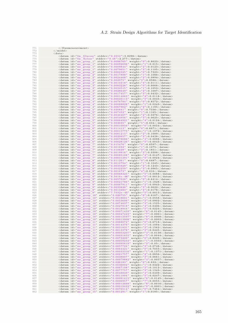
A.2. Strain Design Algorithms for Target Identification
771 </ fluxmeasurement>772 </model>773 <data>774 <datum id="fm_Glucose" stddev=" 0.2552 ">5.8296</datum>775 <datum id="fm_Xylose" stddev=" 0.48 ">2.277</datum>776 <datum id="ms_group_1" stddev=" 0.0098765 " weight="0">0.8623</datum>777 <datum id="ms_group_1" stddev="0.00092696 " weight="1">0.015</datum>778 <datum id="ms_group_1" stddev=" 0.0009844 " weight="2">0.0123</datum>779 <datum id="ms_group_1" stddev=" 0.0079651 " weight="3">0.1105</datum>780 <datum id="ms_group_2" stddev=" 0.0082325 " weight="0">0.7323</datum>781 <datum id="ms_group_2" stddev=" 0.0017888 " weight="1">0.1086</datum>782 <datum id="ms_group_2" stddev=" 0.0024468 " weight="2">0.0894</datum>783 <datum id="ms_group_2" stddev=" 0.002975 " weight="3">0.0586</datum>784 <datum id="ms_group_2" stddev=" 0.0010218 " weight="4">0.0111</datum>785 <datum id="ms_group_3" stddev=" 0.0083226 " weight="0">0.6666</datum>786 <datum id="ms_group_3" stddev=" 0.0034515 " weight="1">0.1053</datum>787 <datum id="ms_group_3" stddev=" 0.0028649 " weight="2">0.1687</datum>788 <datum id="ms_group_3" stddev=" 0.0017457 " weight="3">0.0432</datum>789 <datum id="ms_group_3" stddev="0.00014063 " weight="4">0.0118</datum>790 <datum id="ms_group_3" stddev="0.00040113 " weight="5">0.0045</datum>791 <datum id="ms_group_4" stddev=" 0.0076784 " weight="0">0.8572</datum>792 <datum id="ms_group_4" stddev="0.00088828 " weight="1">0.0243</datum>793 <datum id="ms_group_4" stddev=" 0.0067902 " weight="2">0.1185</datum>794 <datum id="ms_group_5" stddev=" 0.020841 " weight="0">0.7336</datum>795 <datum id="ms_group_5" stddev=" 0.007452 " weight="1">0.1165</datum>796 <datum id="ms_group_5" stddev=" 0.0040407 " weight="2">0.0376</datum>797 <datum id="ms_group_5" stddev=" 0.0054956 " weight="3">0.0625</datum>798 <datum id="ms_group_5" stddev="0.00064921 " weight="4">0.0124</datum>799 <datum id="ms_group_5" stddev=" 0.003035 " weight="5">0.034</datum>800 <datum id="ms_group_5" stddev="0.00016856 " weight="6">0.0034</datum>801 <datum id="ms_group_6" stddev=" 0.011413 " weight="0">0.6671</datum>802 <datum id="ms_group_6" stddev="0.00015775 " weight="1">0.1072</datum>803 <datum id="ms_group_6" stddev=" 0.0081215 " weight="2">0.1689</datum>804 <datum id="ms_group_6" stddev=" 0.0020657 " weight="3">0.0428</datum>805 <datum id="ms_group_6" stddev="0.00078686 " weight="4">0.0098</datum>806 <datum id="ms_group_6" stddev="0.00028126 " weight="5">0.0043</datum>807 <datum id="ms_group_7" stddev=" 0.015476 " weight="0">0.6597</datum>808 <datum id="ms_group_7" stddev=" 0.001692 " weight="1">0.1075</datum>809 <datum id="ms_group_7" stddev=" 0.010628 " weight="2">0.1851</datum>810 <datum id="ms_group_7" stddev=" 0.0019916 " weight="3">0.0306</datum>811 <datum id="ms_group_7" stddev="0.00085108 " weight="4">0.0147</datum>812 <datum id="ms_group_7" stddev="0.00031291 " weight="5">0.0024</datum>813 <datum id="ms_group_8" stddev=" 0.011261 " weight="0">0.6487</datum>814 <datum id="ms_group_8" stddev=" 0.0010794 " weight="1">0.1045</datum>815 <datum id="ms_group_8" stddev=" 0.0035929 " weight="2">0.1243</datum>816 <datum id="ms_group_8" stddev=" 0.0042259 " weight="3">0.0965</datum>817 <datum id="ms_group_8" stddev=" 0.001673 " weight="4">0.016</datum>818 <datum id="ms_group_8" stddev="0.00068325 " weight="5">0.0088</datum>819 <datum id="ms_group_8" stddev=" 6.5616 e−06" weight="6">0.0012</datum>820 <datum id="ms_group_9" stddev=" 0.0057048 " weight="0">0.6414</datum>821 <datum id="ms_group_9" stddev="0.00021786 " weight="1">0.1828</datum>822 <datum id="ms_group_9" stddev="0.00067911 " weight="2">0.0943</datum>823 <datum id="ms_group_9" stddev=" 0.0033826 " weight="3">0.0622</datum>824 <datum id="ms_group_9" stddev=" 0.0013483 " weight="4">0.0178</datum>825 <datum id="ms_group_9" stddev=" 7.7032 e−05" weight="5">0.0015</datum>826 <datum id="ms_group_10" stddev=" 0.020755 " weight="0">0.6167</datum>827 <datum id="ms_group_10" stddev=" 0.0018601 " weight="1">0.0558</datum>828 <datum id="ms_group_10" stddev=" 0.0053606 " weight="2">0.0902</datum>829 <datum id="ms_group_10" stddev=" 0.0074037 " weight="3">0.1525</datum>830 <datum id="ms_group_10" stddev=" 0.0027818 " weight="4">0.0406</datum>831 <datum id="ms_group_10" stddev=" 0.0018944 " weight="5">0.0224</datum>832 <datum id="ms_group_10" stddev="0.00071459 " weight="6">0.0145</datum>833 <datum id="ms_group_10" stddev="0.00047423 " weight="7">0.0061</datum>834 <datum id="ms_group_10" stddev="0.00012597 " weight="8">0.0008</datum>835 <datum id="ms_group_10" stddev="0.00013908 " weight="9">0.0003</datum>836 <datum id="ms_group_11" stddev=" 0.0068072 " weight="0">0.6718</datum>837 <datum id="ms_group_11" stddev=" 0.0014376 " weight="1">0.1094</datum>838 <datum id="ms_group_11" stddev=" 0.0031831 " weight="2">0.1562</datum>839 <datum id="ms_group_11" stddev=" 0.0013378 " weight="3">0.0445</datum>840 <datum id="ms_group_11" stddev="0.00053207 " weight="4">0.0138</datum>841 <datum id="ms_group_11" stddev="0.00031655 " weight="5">0.0044</datum>842 <datum id="ms_group_12" stddev=" 0.0073209 " weight="0">0.8249</datum>843 <datum id="ms_group_12" stddev="0.00059233 " weight="1">0.0503</datum>844 <datum id="ms_group_12" stddev="0.00095619 " weight="2">0.05</datum>845 <datum id="ms_group_12" stddev=" 0.0057724 " weight="3">0.0748</datum>846 <datum id="ms_group_13" stddev=" 0.0064421 " weight="0">0.7055</datum>847 <datum id="ms_group_13" stddev="0.00033316 " weight="1">0.1371</datum>848 <datum id="ms_group_13" stddev=" 0.0021757 " weight="2">0.0856</datum>849 <datum id="ms_group_13" stddev=" 0.0038007 " weight="3">0.0661</datum>850 <datum id="ms_group_13" stddev="0.00079882 " weight="4">0.0057</datum>851 <datum id="ms_group_14" stddev=" 0.026183 " weight="0">0.632</datum>852 <datum id="ms_group_14" stddev=" 0.0036002 " weight="1">0.0422</datum>853 <datum id="ms_group_14" stddev=" 0.0067108 " weight="2">0.1012</datum>854 <datum id="ms_group_14" stddev=" 0.0077757 " weight="3">0.1343</datum>855 <datum id="ms_group_14" stddev=" 0.0048849 " weight="4">0.0439</datum>856 <datum id="ms_group_14" stddev=" 0.0011994 " weight="5">0.0247</datum>857 <datum id="ms_group_14" stddev="0.00091415 " weight="6">0.0145</datum>858 <datum id="ms_group_14" stddev=" 0.0006957 " weight="7">0.0055</datum>859 <datum id="ms_group_14" stddev="0.00012668 " weight="8">0.0016</datum>860 <datum id="ms_group_14" stddev="0.00019422 " weight="9">0.0001</datum>861 <datum id="ms_group_15" stddev=" 0.0076514 " weight="0">0.7464</datum>862 <datum id="ms_group_15" stddev=" 0.001291 " weight="1">0.0185</datum>
165
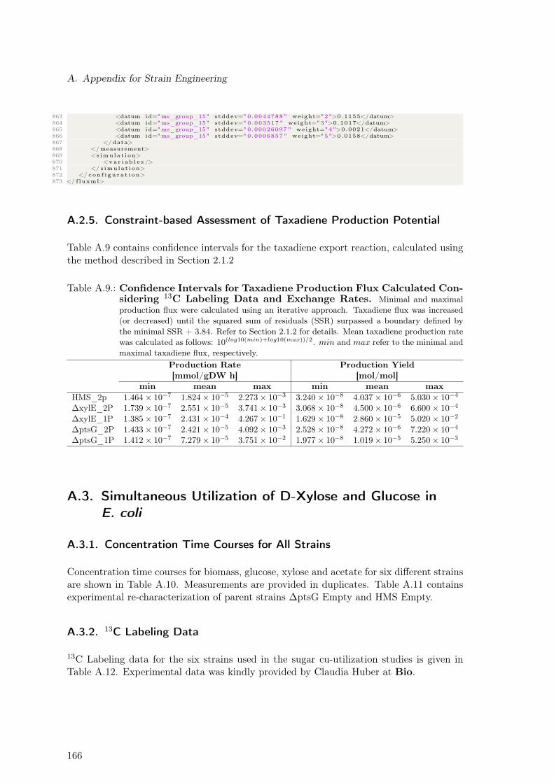
A. Appendix for Strain Engineering
863 <datum id="ms_group_15" stddev=" 0.0044788 " weight="2">0.1155</datum>864 <datum id="ms_group_15" stddev=" 0.003517 " weight="3">0.1017</datum>865 <datum id="ms_group_15" stddev=" 0.00026097 " weight="4">0.0021</datum>866 <datum id="ms_group_15" stddev=" 0.0006857 " weight="5">0.0158</datum>867 </data>868 </measurement>869 <s imula t i on>870 <va r i a b l e s />871 </ s imula t i on>872 </ con f i gu r a t i on>873 </ f luxml>
A.2.5. Constraint-based Assessment of Taxadiene Production Potential
Table A.9 contains confidence intervals for the taxadiene export reaction, calculated usingthe method described in Section 2.1.2
Table A.9.: Confidence Intervals for Taxadiene Production Flux Calculated Con-sidering 13C Labeling Data and Exchange Rates. Minimal and maximalproduction flux were calculated using an iterative approach. Taxadiene flux was increased(or decreased) until the squared sum of residuals (SSR) surpassed a boundary defined bythe minimal SSR + 3.84. Refer to Section 2.1.2 for details. Mean taxadiene production ratewas calculated as follows: 10(log10(min)+log10(max))/2. min and max refer to the minimal andmaximal taxadiene flux, respectively.
Production Rate[mmol/gDW h]
Production Yield[mol/mol]
min mean max min mean maxHMS_2p 1.464× 10⁻⁷ 1.824× 10⁻⁵ 2.273× 10⁻³ 3.240× 10⁻⁸ 4.037× 10⁻⁶ 5.030× 10⁻⁴
∆xylE_2P 1.739× 10⁻⁷ 2.551× 10⁻⁵ 3.741× 10⁻³ 3.068× 10⁻⁸ 4.500× 10⁻⁶ 6.600× 10⁻⁴
∆xylE_1P 1.385× 10⁻⁷ 2.431× 10⁻⁴ 4.267× 10⁻¹ 1.629× 10⁻⁸ 2.860× 10⁻⁵ 5.020× 10⁻²
∆ptsG_2P 1.433× 10⁻⁷ 2.421× 10⁻⁵ 4.092× 10⁻³ 2.528× 10⁻⁸ 4.272× 10⁻⁶ 7.220× 10⁻⁴
∆ptsG_1P 1.412× 10⁻⁷ 7.279× 10⁻⁵ 3.751× 10⁻² 1.977× 10⁻⁸ 1.019× 10⁻⁵ 5.250× 10⁻³
A.3. Simultaneous Utilization of D-Xylose and Glucose inE. coli
A.3.1. Concentration Time Courses for All Strains
Concentration time courses for biomass, glucose, xylose and acetate for six different strainsare shown in Table A.10. Measurements are provided in duplicates. Table A.11 containsexperimental re-characterization of parent strains ∆ptsG Empty and HMS Empty.
A.3.2. 13C Labeling Data
13C Labeling data for the six strains used in the sugar cu-utilization studies is given inTable A.12. Experimental data was kindly provided by Claudia Huber at Bio.
166
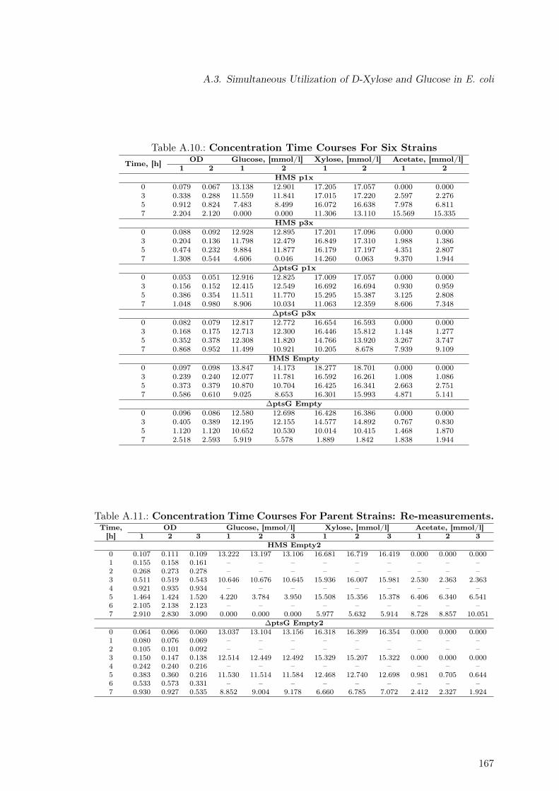
A.3. Simultaneous Utilization of D-Xylose and Glucose in E. coli
Table A.10.: Concentration Time Courses For Six StrainsTime, [h] OD Glucose, [mmol/l] Xylose, [mmol/l] Acetate, [mmol/l]
1 2 1 2 1 2 1 2HMS p1x
0 0.079 0.067 13.138 12.901 17.205 17.057 0.000 0.0003 0.338 0.288 11.559 11.841 17.015 17.220 2.597 2.2765 0.912 0.824 7.483 8.499 16.072 16.638 7.978 6.8117 2.204 2.120 0.000 0.000 11.306 13.110 15.569 15.335
HMS p3x0 0.088 0.092 12.928 12.895 17.201 17.096 0.000 0.0003 0.204 0.136 11.798 12.479 16.849 17.310 1.988 1.3865 0.474 0.232 9.884 11.877 16.179 17.197 4.351 2.8077 1.308 0.544 4.606 0.046 14.260 0.063 9.370 1.944
∆ptsG p1x0 0.053 0.051 12.916 12.825 17.009 17.057 0.000 0.0003 0.156 0.152 12.415 12.549 16.692 16.694 0.930 0.9595 0.386 0.354 11.511 11.770 15.295 15.387 3.125 2.8087 1.048 0.980 8.906 10.034 11.063 12.359 8.606 7.348
∆ptsG p3x0 0.082 0.079 12.817 12.772 16.654 16.593 0.000 0.0003 0.168 0.175 12.713 12.300 16.446 15.812 1.148 1.2775 0.352 0.378 12.308 11.820 14.766 13.920 3.267 3.7477 0.868 0.952 11.499 10.921 10.205 8.678 7.939 9.109
HMS Empty0 0.097 0.098 13.847 14.173 18.277 18.701 0.000 0.0003 0.239 0.240 12.077 11.781 16.592 16.261 1.008 1.0865 0.373 0.379 10.870 10.704 16.425 16.341 2.663 2.7517 0.586 0.610 9.025 8.653 16.301 15.993 4.871 5.141
∆ptsG Empty0 0.096 0.086 12.580 12.698 16.428 16.386 0.000 0.0003 0.405 0.389 12.195 12.155 14.577 14.892 0.767 0.8305 1.120 1.120 10.652 10.530 10.014 10.415 1.468 1.8707 2.518 2.593 5.919 5.578 1.889 1.842 1.838 1.944
Table A.11.: Concentration Time Courses For Parent Strains: Re-measurements.Time,
[h]OD Glucose, [mmol/l] Xylose, [mmol/l] Acetate, [mmol/l]
1 2 3 1 2 3 1 2 3 1 2 3HMS Empty2
0 0.107 0.111 0.109 13.222 13.197 13.106 16.681 16.719 16.419 0.000 0.000 0.0001 0.155 0.158 0.161 – – – – – – – – –2 0.268 0.273 0.278 – – – – – – – – –3 0.511 0.519 0.543 10.646 10.676 10.645 15.936 16.007 15.981 2.530 2.363 2.3634 0.921 0.935 0.934 – – – – – – – – –5 1.464 1.424 1.520 4.220 3.784 3.950 15.508 15.356 15.378 6.406 6.340 6.5416 2.105 2.138 2.123 – – – – – – – – –7 2.910 2.830 3.090 0.000 0.000 0.000 5.977 5.632 5.914 8.728 8.857 10.051
∆ptsG Empty20 0.064 0.066 0.060 13.037 13.104 13.156 16.318 16.399 16.354 0.000 0.000 0.0001 0.080 0.076 0.069 – – – – – – – – –2 0.105 0.101 0.092 – – – – – – – – –3 0.150 0.147 0.138 12.514 12.449 12.492 15.329 15.207 15.322 0.000 0.000 0.0004 0.242 0.240 0.216 – – – – – – – – –5 0.383 0.360 0.216 11.530 11.514 11.584 12.468 12.740 12.698 0.981 0.705 0.6446 0.533 0.573 0.331 – – – – – – – – –7 0.930 0.927 0.535 8.852 9.004 9.178 6.660 6.785 7.072 2.412 2.327 1.924
167
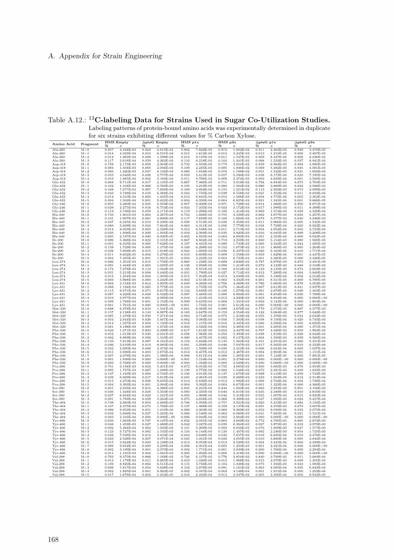
A. Appendix for Strain Engineering
Table A.12.: 13C-labeling Data for Strains Used in Sugar Co-Utilization Studies.Labeling patterns of protein-bound amino acids was experimentally determined in duplicatefor six strains exhibiting different values for % Carbon Xylose.
Amino Acid Fragment HMS Empty ∆ptsG Empty HMS p1x HMS p3x ∆ptsG p1x ∆ptsG p3x% σ % σ % σ % σ % σ % σ
Ala-260 M+0 0.857 4.434E-04 0.923 6.815E-04 0.862 7.822E-03 0.872 1.802E-02 0.911 2.463E-03 0.949 3.479E-03Ala-260 M+1 0.014 4.323E-04 0.010 8.531E-04 0.015 1.615E-03 0.014 3.245E-03 0.012 1.212E-03 0.008 2.467E-03Ala-260 M+2 0.012 1.982E-04 0.008 1.599E-04 0.012 9.147E-04 0.011 1.547E-03 0.009 8.427E-04 0.006 6.036E-04Ala-260 M+3 0.117 2.618E-04 0.059 4.262E-04 0.110 6.218E-03 0.104 1.341E-02 0.068 1.532E-03 0.037 6.941E-04Asp-418 M+0 0.759 2.173E-03 0.859 2.004E-03 0.732 6.553E-03 0.779 3.910E-02 0.839 6.984E-03 0.904 4.880E-03Asp-418 M+1 0.094 1.504E-03 0.065 2.056E-03 0.109 2.235E-03 0.085 1.946E-02 0.069 5.482E-03 0.045 4.081E-03Asp-418 M+2 0.085 1.220E-03 0.047 8.150E-04 0.089 1.916E-03 0.070 1.188E-02 0.051 1.532E-03 0.031 1.856E-03Asp-418 M+3 0.053 4.046E-04 0.026 2.757E-04 0.059 2.413E-03 0.057 5.596E-03 0.038 6.172E-04 0.020 7.195E-04Asp-418 M+4 0.010 1.885E-04 0.002 2.194E-04 0.011 9.798E-04 0.009 2.474E-03 0.003 4.629E-04 0.001 2.560E-04Glu-432 M+0 0.668 9.711E-04 0.817 2.135E-03 0.667 7.060E-03 0.711 3.916E-02 0.794 6.844E-03 0.873 4.763E-03Glu-432 M+1 0.102 1.104E-03 0.066 2.763E-03 0.105 3.219E-03 0.080 1.564E-02 0.066 3.889E-03 0.042 2.586E-03Glu-432 M+2 0.168 7.077E-04 0.097 7.856E-04 0.169 2.894E-03 0.155 1.501E-02 0.113 2.302E-03 0.073 2.099E-03Glu-432 M+3 0.043 3.788E-04 0.016 6.368E-04 0.043 1.735E-03 0.039 6.558E-03 0.021 1.352E-03 0.011 8.033E-04Glu-432 M+4 0.014 4.510E-04 0.003 1.425E-04 0.012 6.841E-04 0.010 1.588E-03 0.004 4.772E-04 0.002 2.362E-04Glu-432 M+5 0.004 1.502E-04 0.001 9.422E-05 0.004 4.350E-04 0.004 6.825E-04 0.001 1.345E-04 0.001 9.866E-05Gly-246 M+0 0.855 4.280E-04 0.925 6.503E-04 0.857 6.000E-03 0.871 1.728E-02 0.914 1.366E-03 0.950 8.671E-04Gly-246 M+1 0.029 2.275E-04 0.016 6.754E-04 0.024 7.335E-04 0.023 3.172E-03 0.017 1.098E-03 0.011 8.399E-04Gly-246 M+2 0.116 3.736E-04 0.059 3.171E-04 0.119 5.296E-03 0.106 1.414E-02 0.069 1.574E-03 0.039 4.329E-04His-440 M+0 0.733 1.901E-03 0.884 2.267E-03 0.734 1.688E-02 0.755 3.538E-02 0.862 4.877E-03 0.924 5.207E-03His-440 M+1 0.101 1.907E-03 0.061 2.900E-03 0.117 7.659E-03 0.100 1.684E-02 0.073 5.377E-03 0.040 4.246E-03His-440 M+2 0.047 6.245E-04 0.010 8.228E-04 0.038 3.513E-03 0.039 5.358E-03 0.011 3.966E-03 0.005 1.542E-03His-440 M+3 0.066 5.609E-04 0.034 7.664E-04 0.063 4.311E-03 0.056 7.779E-03 0.034 7.729E-04 0.020 8.922E-04His-440 M+4 0.014 8.053E-05 0.003 2.328E-04 0.012 6.548E-04 0.011 2.713E-03 0.004 4.954E-04 0.002 2.723E-04His-440 M+5 0.035 1.938E-04 0.009 1.505E-04 0.034 2.394E-03 0.035 3.920E-03 0.016 6.045E-04 0.009 3.208E-04His-440 M+6 0.005 2.197E-04 0.000 8.030E-05 0.003 4.935E-04 0.004 8.892E-04 0.001 2.352E-04 0.000 9.922E-05Ile-200 M+0 0.696 5.368E-04 0.822 2.101E-03 0.667 8.884E-03 0.718 4.259E-02 0.800 5.154E-03 0.880 1.920E-03Ile-200 M+1 0.091 6.325E-04 0.065 7.628E-04 0.107 8.431E-04 0.080 1.733E-02 0.065 2.342E-03 0.044 1.495E-03Ile-200 M+2 0.159 1.729E-04 0.095 1.175E-03 0.169 6.299E-03 0.152 1.673E-02 0.110 1.869E-03 0.065 1.264E-03Ile-200 M+3 0.038 7.809E-05 0.015 1.918E-04 0.043 1.695E-03 0.038 6.337E-03 0.020 9.163E-04 0.010 1.771E-04Ile-200 M+4 0.011 9.602E-05 0.002 5.270E-05 0.010 6.609E-04 0.009 1.558E-03 0.003 1.829E-04 0.001 4.447E-05Ile-200 M+5 0.004 7.405E-05 0.001 1.921E-05 0.004 2.223E-04 0.004 6.733E-04 0.001 4.360E-05 0.000 3.346E-05Leu-274 M+0 0.686 1.351E-03 0.815 1.756E-03 0.660 1.238E-02 0.699 3.836E-02 0.787 6.876E-03 0.872 2.491E-03Leu-274 M+1 0.091 1.444E-03 0.063 1.025E-03 0.108 2.958E-03 0.090 1.214E-02 0.072 4.123E-03 0.048 2.318E-03Leu-274 M+2 0.174 7.278E-04 0.110 1.024E-03 0.185 8.551E-03 0.168 2.012E-02 0.123 2.135E-03 0.074 2.662E-03Leu-274 M+3 0.031 5.213E-04 0.008 3.440E-04 0.031 1.790E-03 0.027 3.714E-03 0.012 7.280E-04 0.004 3.840E-04Leu-274 M+4 0.015 1.254E-04 0.004 1.005E-04 0.015 7.352E-04 0.013 2.049E-03 0.005 5.188E-04 0.002 2.012E-04Leu-274 M+5 0.003 5.968E-05 0.000 3.242E-05 0.002 2.514E-04 0.002 4.332E-04 0.001 8.311E-05 0.000 6.790E-05Lys-431 M+0 0.684 2.154E-03 0.814 3.905E-03 0.649 9.282E-03 0.706 4.289E-02 0.786 5.965E-03 0.878 4.303E-03Lys-431 M+1 0.088 1.194E-03 0.065 2.772E-03 0.104 3.735E-03 0.078 1.464E-02 0.067 3.613E-03 0.041 2.937E-03Lys-431 M+2 0.115 9.071E-04 0.071 8.617E-04 0.124 3.645E-03 0.106 1.270E-02 0.081 2.679E-03 0.049 1.403E-03Lys-431 M+3 0.087 4.226E-04 0.049 6.542E-04 0.097 3.485E-03 0.089 9.894E-03 0.061 8.854E-04 0.036 7.789E-04Lys-431 M+4 0.016 3.977E-04 0.001 2.095E-04 0.016 1.410E-03 0.013 4.230E-03 0.003 8.854E-04 0.000 0.000E+00Lys-431 M+5 0.009 1.788E-04 0.001 3.152E-04 0.009 6.625E-04 0.008 1.241E-03 0.002 3.143E-04 0.000 1.804E-04Lys-431 M+6 0.001 1.761E-04 0.000 0.000E+00 0.001 1.732E-04 0.001 5.612E-04 0.000 0.000E+00 0.000 0.000E+00Met-320 M+0 0.688 6.278E-03 0.810 1.531E-03 0.641 6.083E-03 0.699 4.676E-02 0.779 2.572E-03 0.867 4.377E-03Met-320 M+1 0.157 2.158E-03 0.110 8.997E-04 0.183 2.847E-03 0.153 2.554E-02 0.122 3.064E-03 0.077 3.042E-03Met-320 M+2 0.085 1.476E-03 0.050 7.271E-04 0.094 2.713E-03 0.075 1.216E-02 0.055 1.376E-03 0.034 2.034E-03Met-320 M+3 0.054 2.044E-03 0.026 5.467E-04 0.062 3.083E-03 0.056 7.303E-03 0.038 9.150E-04 0.020 6.745E-04Met-320 M+4 0.014 1.527E-03 0.004 1.150E-04 0.018 1.157E-03 0.016 3.445E-03 0.006 4.056E-04 0.002 6.650E-04Met-320 M+5 0.001 4.198E-04 0.000 1.472E-04 0.002 2.520E-04 0.003 3.385E-03 0.001 2.205E-04 0.000 1.371E-04Phe-336 M+0 0.642 1.271E-03 0.803 2.399E-03 0.617 1.612E-02 0.654 4.447E-02 0.767 4.030E-03 0.859 1.993E-03Phe-336 M+1 0.052 1.013E-03 0.030 2.031E-03 0.056 1.962E-03 0.050 5.393E-03 0.038 1.818E-03 0.029 8.042E-04Phe-336 M+2 0.082 8.989E-04 0.056 1.319E-03 0.090 4.457E-03 0.082 9.137E-03 0.064 1.558E-03 0.039 8.560E-04Phe-336 M+3 0.133 7.613E-04 0.087 8.181E-04 0.152 5.832E-03 0.135 1.564E-02 0.101 2.051E-03 0.060 5.451E-04Phe-336 M+4 0.046 3.019E-04 0.014 8.085E-04 0.041 2.258E-03 0.040 7.047E-03 0.017 6.505E-04 0.010 6.233E-04Phe-336 M+5 0.022 2.690E-04 0.006 2.474E-04 0.022 1.509E-03 0.020 3.410E-03 0.008 2.644E-04 0.003 1.027E-04Phe-336 M+6 0.015 2.696E-04 0.003 2.875E-04 0.014 6.457E-04 0.013 2.487E-03 0.004 2.963E-04 0.001 1.151E-04Phe-336 M+7 0.007 2.078E-04 0.001 1.386E-04 0.006 3.811E-04 0.006 1.305E-03 0.001 7.124E-05 0.000 7.881E-05Phe-336 M+8 0.001 1.836E-04 0.000 0.000E+00 0.001 1.154E-04 0.001 2.278E-04 0.000 0.000E+00 0.000 0.000E+00Phe-336 M+9 0.000 5.768E-05 0.000 0.000E+00 0.000 1.492E-04 0.000 2.029E-04 0.000 0.000E+00 0.000 0.000E+00Pro-286 M+0 0.701 3.194E-03 0.824 5.201E-03 0.672 6.054E-03 0.725 4.085E-02 0.800 5.682E-03 0.876 2.853E-03Pro-286 M+1 0.095 1.727E-03 0.067 1.498E-03 0.109 3.772E-03 0.083 1.548E-02 0.072 2.381E-03 0.049 1.832E-03Pro-286 M+2 0.147 1.163E-03 0.084 2.745E-03 0.156 3.015E-03 0.137 1.675E-02 0.098 3.110E-03 0.059 1.723E-03Pro-286 M+3 0.039 6.929E-04 0.017 5.813E-04 0.045 2.061E-03 0.039 6.088E-03 0.023 1.004E-03 0.012 2.514E-04Pro-286 M+4 0.015 4.270E-04 0.006 9.635E-04 0.014 6.830E-04 0.012 1.992E-03 0.006 2.702E-04 0.004 1.736E-04Pro-286 M+5 0.004 3.393E-04 0.001 2.084E-04 0.004 3.092E-04 0.004 6.673E-04 0.001 1.323E-04 0.000 4.366E-05Ser-390 M+0 0.851 2.035E-03 0.915 4.296E-03 0.825 6.231E-03 0.844 1.950E-02 0.903 2.932E-03 0.951 3.158E-03Ser-390 M+1 0.030 1.424E-03 0.024 3.353E-03 0.050 2.335E-03 0.044 6.015E-03 0.025 2.248E-03 0.010 2.810E-03Ser-390 M+2 0.027 6.824E-04 0.022 1.241E-03 0.050 1.969E-03 0.044 5.218E-03 0.025 1.007E-03 0.015 9.845E-04Ser-390 M+3 0.091 5.789E-04 0.039 3.264E-04 0.075 4.658E-03 0.068 9.498E-03 0.047 1.092E-03 0.024 9.457E-04Thr-404 M+0 0.748 2.060E-03 0.854 2.469E-03 0.706 5.359E-03 0.757 3.921E-02 0.820 5.313E-03 0.884 3.150E-03Thr-404 M+1 0.107 2.375E-03 0.075 1.708E-03 0.137 1.468E-03 0.109 2.137E-02 0.091 4.376E-03 0.070 3.007E-03Thr-404 M+2 0.086 9.052E-04 0.051 1.410E-03 0.086 2.303E-03 0.068 9.309E-03 0.052 9.058E-04 0.033 2.075E-03Thr-404 M+3 0.056 5.606E-04 0.027 5.265E-04 0.066 3.540E-03 0.063 6.060E-03 0.041 7.682E-04 0.021 5.521E-04Thr-404 M+4 0.003 2.105E-04 0.000 0.000E+00 0.006 9.944E-04 0.003 2.804E-03 0.000 0.000E+00 0.000 0.000E+00Tyr-466 M+0 0.633 1.863E-03 0.797 9.147E-04 0.632 2.031E-02 0.663 4.609E-02 0.772 4.795E-03 0.865 2.872E-03Tyr-466 M+1 0.046 1.459E-03 0.027 1.489E-03 0.042 3.027E-03 0.039 6.364E-03 0.027 3.973E-03 0.018 2.979E-03Tyr-466 M+2 0.092 5.484E-04 0.064 1.033E-03 0.101 5.269E-03 0.093 9.656E-03 0.076 1.009E-03 0.047 1.577E-03Tyr-466 M+3 0.123 5.727E-04 0.082 1.102E-03 0.134 6.144E-03 0.120 1.457E-02 0.092 2.246E-03 0.054 1.725E-03Tyr-466 M+4 0.048 7.538E-04 0.014 3.424E-04 0.044 3.848E-03 0.043 7.657E-03 0.018 6.630E-04 0.010 3.478E-04Tyr-466 M+5 0.023 2.528E-04 0.007 3.071E-04 0.025 1.051E-03 0.022 4.055E-03 0.010 3.860E-04 0.005 2.842E-04Tyr-466 M+6 0.015 3.942E-04 0.003 2.138E-04 0.014 8.053E-04 0.013 2.526E-03 0.004 3.445E-04 0.002 2.499E-04Tyr-466 M+7 0.006 9.654E-05 0.000 3.239E-04 0.006 6.301E-04 0.005 1.250E-03 0.001 2.321E-04 0.000 0.000E+00Tyr-466 M+8 0.002 3.199E-04 0.001 2.073E-04 0.002 1.771E-04 0.001 3.939E-04 0.000 1.766E-04 0.000 2.294E-04Tyr-466 M+9 0.011 1.191E-03 0.004 1.561E-03 0.000 1.992E-04 0.000 3.418E-04 0.000 0.000E+00 0.000 0.000E+00Val-288 M+0 0.762 9.275E-04 0.866 1.169E-03 0.746 6.127E-03 0.776 2.854E-02 0.840 3.709E-03 0.911 5.684E-04Val-288 M+1 0.012 1.179E-03 0.011 8.885E-04 0.019 1.040E-03 0.012 1.968E-03 0.015 2.079E-03 0.009 1.205E-03Val-288 M+2 0.109 8.820E-04 0.064 6.511E-04 0.115 3.756E-03 0.104 1.338E-02 0.075 1.592E-03 0.043 1.093E-03Val-288 M+3 0.098 7.817E-04 0.054 3.638E-04 0.102 2.878E-03 0.091 1.161E-02 0.063 8.085E-04 0.035 6.843E-04Val-288 M+4 0.002 1.895E-04 0.001 8.993E-05 0.002 6.047E-04 0.002 4.148E-04 0.001 1.915E-04 0.000 1.252E-04Val-288 M+5 0.017 1.678E-04 0.004 5.224E-05 0.016 6.222E-04 0.014 2.237E-03 0.005 2.256E-04 0.002 8.943E-05
168
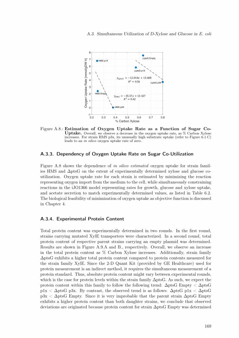
A.3. Simultaneous Utilization of D-Xylose and Glucose in E. coli
0.2 0.3 0.4 0.5 0.6 0.7 0.8% Carbon Xylose
-1
0
1
2
3
4
5
6
7
8
Oxy
gen
Upt
ake
Rat
e [m
mol
/gD
W h
]
HMS p1X
HMS p3X
ptsG p1X
ptsG p3X
HMS Empty
ptsG Empty
𝑦∆#$%& = −12.018𝑥 + 13.688𝑅3 = 0.56
𝑦567 = −35.57𝑥 + 13.427𝑅3 = 0.62
Figure A.8.: Estimation of Oxygen Uptake Rate as a Function of Sugar Co-Uptake. Overall, we observe a decrease in the oxygen uptake rate, as % Carbon Xyloseincreases. For strain HMS p3x, its unusually high substrate uptake (refer to Figure 6.1.C)leads to an in silico oxygen uptake rate of zero.
A.3.3. Dependency of Oxygen Uptake Rate on Sugar Co-Utilization
Figure A.8 shows the dependence of in silico estimated oxygen uptake for strain famil-ies HMS and ∆ptsG on the extent of experimentally determined xylose and glucose co-utilization. Oxygen uptake rate for each strain is estimated by minimizing the reactionrepresenting oxygen import from the medium to the cell, while simultaneously constrainingreactions in the iJO1366 model representing rates for growth, glucose and xylose uptake,and acetate secretion to match experimentally determined values, as listed in Table 6.2.The biological feasibility of minimization of oxygen uptake as objective function is discussedin Chapter 4.
A.3.4. Experimental Protein Content
Total protein content was experimentally determined in two rounds. In the first round,strains carrying mutated XylE transporters were characterized. In a second round, totalprotein content of respective parent strains carrying an empty plasmid was determined.Results are shown in Figure A.9.A and B., respectively. Overall, we observe an increasein the total protein content as % Carbon Xylose increases. Additionally, strain family∆ptsG exhibits a higher total protein content compared to protein contents measured forthe strain family XylE. Since the 2-D Quant Kit (provided by GE Healthcare) used forprotein measurement is an indirect method, it requires the simultaneous measurement of aprotein standard. Thus, absolute protein content might vary between experimental rounds,which is the case for protein levels within the strain family ∆ptsG. As such, we expect theprotein content within this family to follow the following trend: ∆ptsG Empty < ∆ptsGp1x < ∆ptsG p3x. By contrast, the observed trend is as follows: ∆ptsG p1x < ∆ptsGp3x < ∆ptsG Empty. Since it is very improbable that the parent strain ∆ptsG Emptyexhibits a higher protein content than both daughter strains, we conclude that observeddeviations are originated because protein content for strain ∆ptsG Empty was determined
169
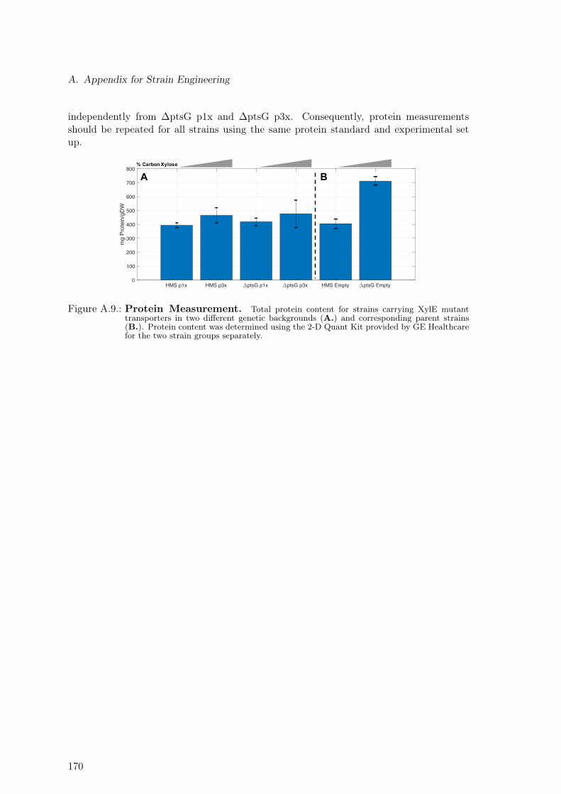
A. Appendix for Strain Engineering
independently from ∆ptsG p1x and ∆ptsG p3x. Consequently, protein measurementsshould be repeated for all strains using the same protein standard and experimental setup.
HMS p1x HMS p3x ptsG p1x ptsG p3x HMS Empty ptsG Empty0
100
200
300
400
500
600
700
800
mg
Prot
ein/
gDW
A B% Carbon Xylose
Figure A.9.: Protein Measurement. Total protein content for strains carrying XylE mutanttransporters in two different genetic backgrounds (A.) and corresponding parent strains(B.). Protein content was determined using the 2-D Quant Kit provided by GE Healthcarefor the two strain groups separately.
170
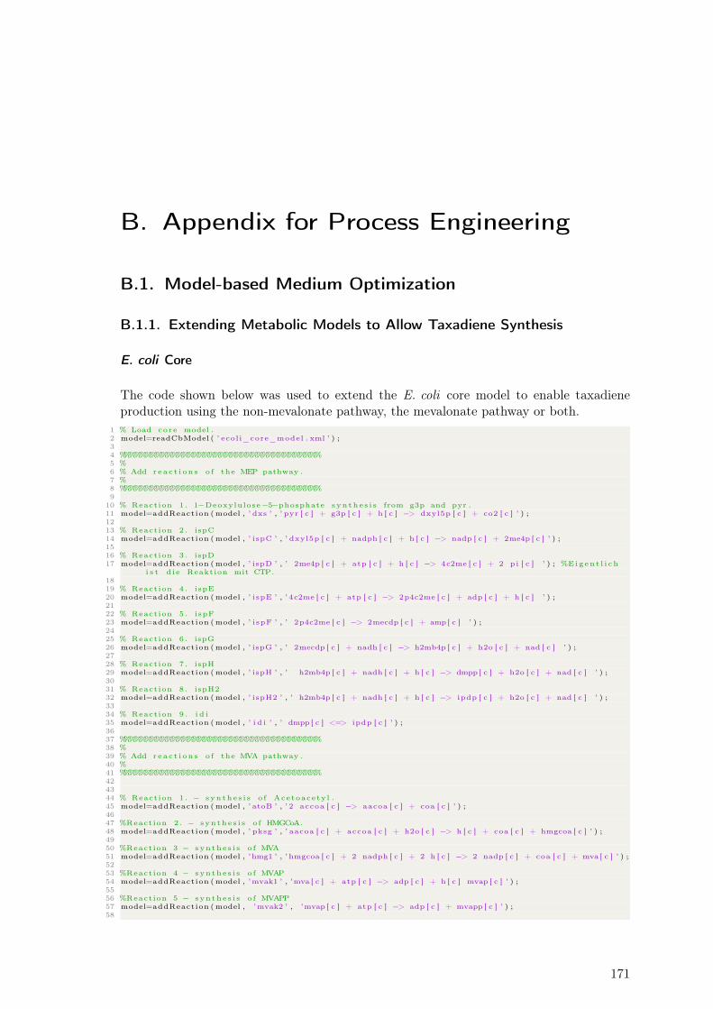
B. Appendix for Process Engineering
B.1. Model-based Medium Optimization
B.1.1. Extending Metabolic Models to Allow Taxadiene Synthesis
E. coli Core
The code shown below was used to extend the E. coli core model to enable taxadieneproduction using the non-mevalonate pathway, the mevalonate pathway or both.
1 % Load core model .2 model=readCbModel ( ’ ecol i_core_model . xml ’ ) ;34 %%%%%%%%%%%%%%%%%%%%%%%%%%%%%%%%%%%%%%5 %6 % Add r e a c t i on s o f the MEP pathway .7 %8 %%%%%%%%%%%%%%%%%%%%%%%%%%%%%%%%%%%%%%9
10 % Reaction 1 . 1−Deoxylulose−5−phosphate s yn th e s i s from g3p and pyr .11 model=addReaction (model , ’ dxs ’ , ’ pyr [ c ] + g3p [ c ] + h [ c ] −> dxyl5p [ c ] + co2 [ c ] ’ ) ;1213 % Reaction 2 . ispC14 model=addReaction (model , ’ ispC ’ , ’ dxyl5p [ c ] + nadph [ c ] + h [ c ] −> nadp [ c ] + 2me4p [ c ] ’ ) ;1516 % Reaction 3 . ispD17 model=addReaction (model , ’ ispD ’ , ’ 2me4p [ c ] + atp [ c ] + h [ c ] −> 4c2me [ c ] + 2 pi [ c ] ’ ) ; %E i g en t l i c h
i s t d i e Reaktion mit CTP.1819 % Reaction 4 . ispE20 model=addReaction (model , ’ ispE ’ , ’ 4c2me [ c ] + atp [ c ] −> 2p4c2me [ c ] + adp [ c ] + h [ c ] ’ ) ;2122 % Reaction 5 . ispF23 model=addReaction (model , ’ ispF ’ , ’ 2p4c2me [ c ] −> 2mecdp [ c ] + amp [ c ] ’ ) ;2425 % Reaction 6 . ispG26 model=addReaction (model , ’ ispG ’ , ’ 2mecdp [ c ] + nadh [ c ] −> h2mb4p [ c ] + h2o [ c ] + nad [ c ] ’ ) ;2728 % Reaction 7 . ispH29 model=addReaction (model , ’ ispH ’ , ’ h2mb4p [ c ] + nadh [ c ] + h [ c ] −> dmpp [ c ] + h2o [ c ] + nad [ c ] ’ ) ;3031 % Reaction 8 . ispH232 model=addReaction (model , ’ ispH2 ’ , ’ h2mb4p [ c ] + nadh [ c ] + h [ c ] −> ipdp [ c ] + h2o [ c ] + nad [ c ] ’ ) ;3334 % Reaction 9 . i d i35 model=addReaction (model , ’ i d i ’ , ’ dmpp [ c ] <=> ipdp [ c ] ’ ) ;3637 %%%%%%%%%%%%%%%%%%%%%%%%%%%%%%%%%%%%%%38 %39 % Add r e a c t i on s o f the MVA pathway .40 %41 %%%%%%%%%%%%%%%%%%%%%%%%%%%%%%%%%%%%%%424344 % Reaction 1 . − s yn th e s i s o f Acetoacety l .45 model=addReaction (model , ’ atoB ’ , ’ 2 accoa [ c ] −> aacoa [ c ] + coa [ c ] ’ ) ;4647 %Reaction 2 . − s yn th e s i s o f HMGCoA.48 model=addReaction (model , ’ pksg ’ , ’ aacoa [ c ] + accoa [ c ] + h2o [ c ] −> h [ c ] + coa [ c ] + hmgcoa [ c ] ’ ) ;4950 %Reaction 3 − s yn th e s i s o f MVA51 model=addReaction (model , ’hmg1 ’ , ’ hmgcoa [ c ] + 2 nadph [ c ] + 2 h [ c ] −> 2 nadp [ c ] + coa [ c ] + mva [ c ] ’ ) ;5253 %Reaction 4 − s yn th e s i s o f MVAP54 model=addReaction (model , ’mvak1 ’ , ’mva [ c ] + atp [ c ] −> adp [ c ] + h [ c ] mvap [ c ] ’ ) ;5556 %Reaction 5 − s yn th e s i s o f MVAPP57 model=addReaction (model , ’mvak2 ’ , ’mvap [ c ] + atp [ c ] −> adp [ c ] + mvapp [ c ] ’ ) ;58
171
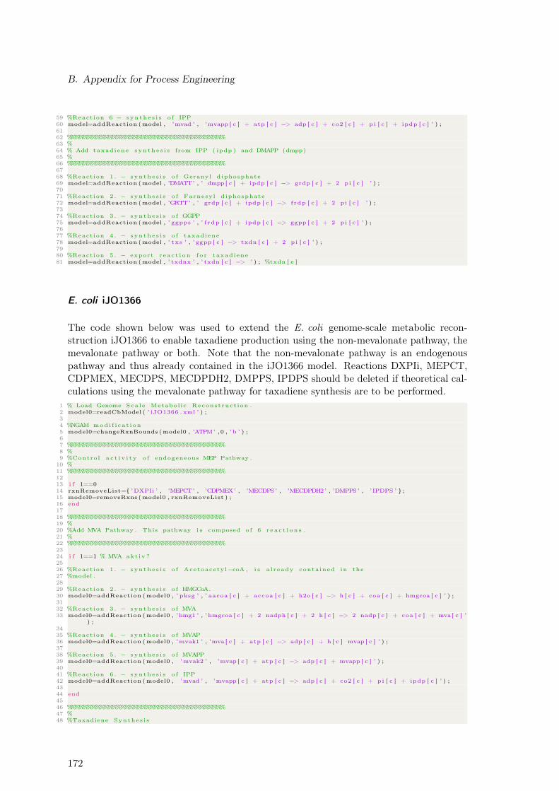
B. Appendix for Process Engineering
59 %Reaction 6 − s yn th e s i s o f IPP60 model=addReaction (model , ’mvad ’ , ’mvapp [ c ] + atp [ c ] −> adp [ c ] + co2 [ c ] + pi [ c ] + ipdp [ c ] ’ ) ;6162 %%%%%%%%%%%%%%%%%%%%%%%%%%%%%%%%%%%%%%63 %64 % Add taxadiene syn th e s i s from IPP ( ipdp ) and DMAPP (dmpp)65 %66 %%%%%%%%%%%%%%%%%%%%%%%%%%%%%%%%%%%%%%6768 %Reaction 1 . − s yn th e s i s o f Geranyl diphosphate69 model=addReaction (model , ’DMATT’ , ’ dmpp [ c ] + ipdp [ c ] −> grdp [ c ] + 2 pi [ c ] ’ ) ;7071 %Reaction 2 . − s yn th e s i s o f Farnesy l diphosphate72 model=addReaction (model , ’GRTT’ , ’ grdp [ c ] + ipdp [ c ] −> frdp [ c ] + 2 pi [ c ] ’ ) ;7374 %Reaction 3 . − s yn th e s i s o f GGPP75 model=addReaction (model , ’ ggpps ’ , ’ f rdp [ c ] + ipdp [ c ] −> ggpp [ c ] + 2 pi [ c ] ’ ) ;7677 %Reaction 4 . − s yn th e s i s o f taxadiene78 model=addReaction (model , ’ txs ’ , ’ ggpp [ c ] −> txdn [ c ] + 2 pi [ c ] ’ ) ;7980 %Reaction 5 . − export r e a c t i on f o r taxadiene81 model=addReaction (model , ’ txdnx ’ , ’ txdn [ c ] −> ’ ) ; %txdn [ e ]
E. coli iJO1366
The code shown below was used to extend the E. coli genome-scale metabolic recon-struction iJO1366 to enable taxadiene production using the non-mevalonate pathway, themevalonate pathway or both. Note that the non-mevalonate pathway is an endogenouspathway and thus already contained in the iJO1366 model. Reactions DXPIi, MEPCT,CDPMEX, MECDPS, MECDPDH2, DMPPS, IPDPS should be deleted if theoretical cal-culations using the mevalonate pathway for taxadiene synthesis are to be performed.
1 % Load Genome Sca l e Metabol ic Reconstruct ion .2 model0=readCbModel ( ’ iJO1366 . xml ’ ) ;34 %NGAM mod i f i c a t i on5 model0=changeRxnBounds (model0 , ’ATPM’ ,0 , ’b ’ ) ;67 %%%%%%%%%%%%%%%%%%%%%%%%%%%%%%%%%%%%%%8 %9 %Control a c t i v i t y o f endogeneous MEP Pathway .
10 %11 %%%%%%%%%%%%%%%%%%%%%%%%%%%%%%%%%%%%%%1213 i f 1==014 rxnRemoveList={ ’DXPIi ’ , ’MEPCT’ , ’CDPMEX’ , ’MECDPS’ , ’MECDPDH2’ , ’DMPPS’ , ’IPDPS ’ } ;15 model0=removeRxns (model0 , rxnRemoveList ) ;16 end1718 %%%%%%%%%%%%%%%%%%%%%%%%%%%%%%%%%%%%%%19 %20 %Add MVA Pathway . This pathway i s composed o f 6 r e a c t i o n s .21 %22 %%%%%%%%%%%%%%%%%%%%%%%%%%%%%%%%%%%%%%2324 i f 1==1 % MVA akt iv ?2526 %Reaction 1 . − s yn th e s i s o f Acetoacetyl−coA , i s a l ready conta ined in the27 %model .2829 %Reaction 2 . − s yn th e s i s o f HMGCoA.30 model0=addReaction (model0 , ’ pksg ’ , ’ aacoa [ c ] + accoa [ c ] + h2o [ c ] −> h [ c ] + coa [ c ] + hmgcoa [ c ] ’ ) ;3132 %Reaction 3 . − s yn th e s i s o f MVA33 model0=addReaction (model0 , ’hmg1 ’ , ’ hmgcoa [ c ] + 2 nadph [ c ] + 2 h [ c ] −> 2 nadp [ c ] + coa [ c ] + mva [ c ] ’
) ;3435 %Reaction 4 . − s yn th e s i s o f MVAP36 model0=addReaction (model0 , ’mvak1 ’ , ’mva [ c ] + atp [ c ] −> adp [ c ] + h [ c ] mvap [ c ] ’ ) ;3738 %Reaction 5 . − s yn th e s i s o f MVAPP39 model0=addReaction (model0 , ’mvak2 ’ , ’mvap [ c ] + atp [ c ] −> adp [ c ] + mvapp [ c ] ’ ) ;4041 %Reaction 6 . − s yn th e s i s o f IPP42 model0=addReaction (model0 , ’mvad ’ , ’mvapp [ c ] + atp [ c ] −> adp [ c ] + co2 [ c ] + pi [ c ] + ipdp [ c ] ’ ) ;4344 end4546 %%%%%%%%%%%%%%%%%%%%%%%%%%%%%%%%%%%%%%47 %48 %Taxadiene Synthes i s
172
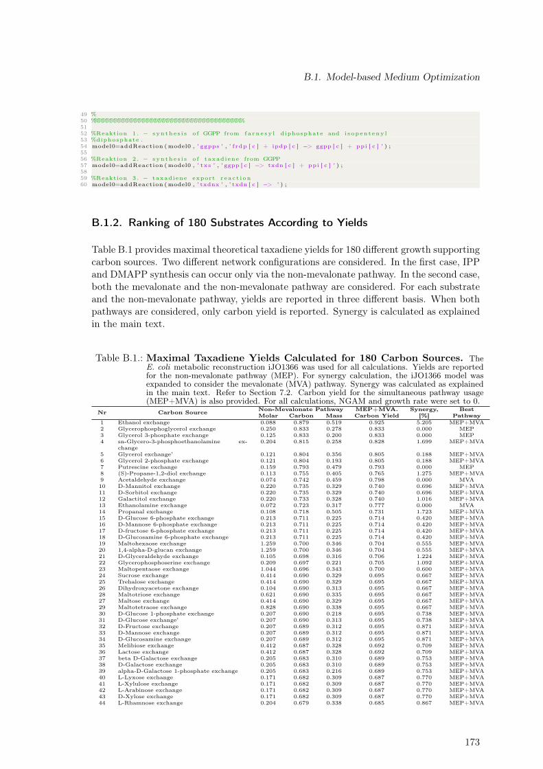
B.1. Model-based Medium Optimization
49 %50 %%%%%%%%%%%%%%%%%%%%%%%%%%%%%%%%%%%%%%5152 %Reaktion 1 . − s yn th e s i s o f GGPP from f a r n e s y l diphosphate and i s open t eny l53 %diphosphate .54 model0=addReaction (model0 , ’ ggpps ’ , ’ f rdp [ c ] + ipdp [ c ] −> ggpp [ c ] + ppi [ c ] ’ ) ;5556 %Reaktion 2 . − s yn th e s i s o f taxadiene from GGPP57 model0=addReaction (model0 , ’ txs ’ , ’ ggpp [ c ] −> txdn [ c ] + ppi [ c ] ’ ) ;5859 %Reaktion 3 . − taxadiene export r e a c t i on60 model0=addReaction (model0 , ’ txdnx ’ , ’ txdn [ c ] −> ’ ) ;
B.1.2. Ranking of 180 Substrates According to Yields
Table B.1 provides maximal theoretical taxadiene yields for 180 different growth supportingcarbon sources. Two different network configurations are considered. In the first case, IPPand DMAPP synthesis can occur only via the non-mevalonate pathway. In the second case,both the mevalonate and the non-mevalonate pathway are considered. For each substrateand the non-mevalonate pathway, yields are reported in three different basis. When bothpathways are considered, only carbon yield is reported. Synergy is calculated as explainedin the main text.
Table B.1.: Maximal Taxadiene Yields Calculated for 180 Carbon Sources. TheE. coli metabolic reconstruction iJO1366 was used for all calculations. Yields are reportedfor the non-mevalonate pathway (MEP). For synergy calculation, the iJO1366 model wasexpanded to consider the mevalonate (MVA) pathway. Synergy was calculated as explainedin the main text. Refer to Section 7.2. Carbon yield for the simultaneous pathway usage(MEP+MVA) is also provided. For all calculations, NGAM and growth rate were set to 0.
Nr Carbon Source Non-Mevalonate Pathway MEP+MVA.Carbon Yield
Synergy,[%]
BestPathwayMolar Carbon Mass
1 Ethanol exchange 0.088 0.879 0.519 0.925 5.205 MEP+MVA2 Glycerophosphoglycerol exchange 0.250 0.833 0.278 0.833 0.000 MEP3 Glycerol 3-phosphate exchange 0.125 0.833 0.200 0.833 0.000 MEP4 sn-Glycero-3-phosphoethanolamine ex-
change0.204 0.815 0.258 0.828 1.699 MEP+MVA
5 Glycerol exchange’ 0.121 0.804 0.356 0.805 0.188 MEP+MVA6 Glycerol 2-phosphate exchange 0.121 0.804 0.193 0.805 0.188 MEP+MVA7 Putrescine exchange 0.159 0.793 0.479 0.793 0.000 MEP8 (S)-Propane-1,2-diol exchange 0.113 0.755 0.405 0.765 1.275 MEP+MVA9 Acetaldehyde exchange 0.074 0.742 0.459 0.798 0.000 MVA10 D-Mannitol exchange 0.220 0.735 0.329 0.740 0.696 MEP+MVA11 D-Sorbitol exchange 0.220 0.735 0.329 0.740 0.696 MEP+MVA12 Galactitol exchange 0.220 0.733 0.328 0.740 1.016 MEP+MVA13 Ethanolamine exchange 0.072 0.723 0.317 0.777 0.000 MVA14 Propanal exchange 0.108 0.718 0.505 0.731 1.723 MEP+MVA15 D-Glucose 6-phosphate exchange 0.213 0.711 0.225 0.714 0.420 MEP+MVA16 D-Mannose 6-phosphate exchange 0.213 0.711 0.225 0.714 0.420 MEP+MVA17 D-fructose 6-phosphate exchange 0.213 0.711 0.225 0.714 0.420 MEP+MVA18 D-Glucosamine 6-phosphate exchange 0.213 0.711 0.225 0.714 0.420 MEP+MVA19 Maltohexaose exchange 1.259 0.700 0.346 0.704 0.555 MEP+MVA20 1,4-alpha-D-glucan exchange 1.259 0.700 0.346 0.704 0.555 MEP+MVA21 D-Glyceraldehyde exchange 0.105 0.698 0.316 0.706 1.224 MEP+MVA22 Glycerophosphoserine exchange 0.209 0.697 0.221 0.705 1.092 MEP+MVA23 Maltopentaose exchange 1.044 0.696 0.343 0.700 0.600 MEP+MVA24 Sucrose exchange 0.414 0.690 0.329 0.695 0.667 MEP+MVA25 Trehalose exchange 0.414 0.690 0.329 0.695 0.667 MEP+MVA26 Dihydroxyacetone exchange 0.104 0.690 0.313 0.695 0.667 MEP+MVA28 Maltotriose exchange 0.621 0.690 0.335 0.695 0.667 MEP+MVA27 Maltose exchange 0.414 0.690 0.329 0.695 0.667 MEP+MVA29 Maltotetraose exchange 0.828 0.690 0.338 0.695 0.667 MEP+MVA30 D-Glucose 1-phosphate exchange 0.207 0.690 0.218 0.695 0.738 MEP+MVA31 D-Glucose exchange’ 0.207 0.690 0.313 0.695 0.738 MEP+MVA32 D-Fructose exchange 0.207 0.689 0.312 0.695 0.871 MEP+MVA33 D-Mannose exchange 0.207 0.689 0.312 0.695 0.871 MEP+MVA34 D-Glucosamine exchange 0.207 0.689 0.312 0.695 0.871 MEP+MVA35 Melibiose exchange 0.412 0.687 0.328 0.692 0.709 MEP+MVA36 Lactose exchange 0.412 0.687 0.328 0.692 0.709 MEP+MVA37 beta D-Galactose exchange 0.205 0.683 0.310 0.689 0.753 MEP+MVA38 D-Galactose exchange 0.205 0.683 0.310 0.689 0.753 MEP+MVA39 alpha-D-Galactose 1-phosphate exchange 0.205 0.683 0.216 0.689 0.753 MEP+MVA40 L-Lyxose exchange 0.171 0.682 0.309 0.687 0.770 MEP+MVA41 L-Xylulose exchange 0.171 0.682 0.309 0.687 0.770 MEP+MVA42 L-Arabinose exchange 0.171 0.682 0.309 0.687 0.770 MEP+MVA43 D-Xylose exchange 0.171 0.682 0.309 0.687 0.770 MEP+MVA44 L-Rhamnose exchange 0.204 0.679 0.338 0.685 0.867 MEP+MVA
173
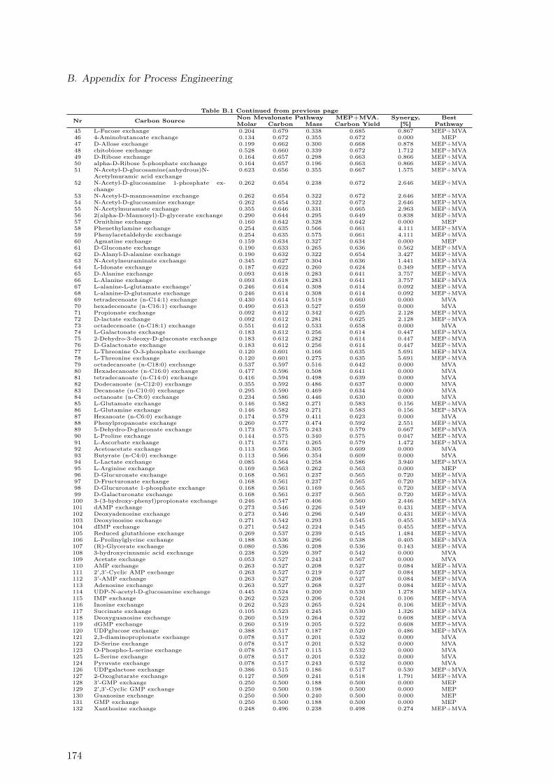
B. Appendix for Process Engineering
Table B.1 Continued from previous page
Nr Carbon Source Non Mevalonate Pathway MEP+MVA.Carbon Yield
Synergy,[%]
BestPathwayMolar Carbon Mass
45 L-Fucose exchange 0.204 0.679 0.338 0.685 0.867 MEP+MVA46 4-Aminobutanoate exchange 0.134 0.672 0.355 0.672 0.000 MEP47 D-Allose exchange 0.199 0.662 0.300 0.668 0.878 MEP+MVA48 chitobiose exchange 0.528 0.660 0.339 0.672 1.712 MEP+MVA49 D-Ribose exchange 0.164 0.657 0.298 0.663 0.866 MEP+MVA50 alpha-D-Ribose 5-phosphate exchange 0.164 0.657 0.196 0.663 0.866 MEP+MVA51 N-Acetyl-D-glucosamine(anhydrous)N-
Acetylmuramic acid exchange0.623 0.656 0.355 0.667 1.575 MEP+MVA
52 N-Acetyl-D-glucosamine 1-phosphate ex-change
0.262 0.654 0.238 0.672 2.646 MEP+MVA
53 N-Acetyl-D-mannosamine exchange 0.262 0.654 0.322 0.672 2.646 MEP+MVA54 N-Acetyl-D-glucosamine exchange 0.262 0.654 0.322 0.672 2.646 MEP+MVA55 N-Acetylmuramate exchange 0.355 0.646 0.331 0.665 2.963 MEP+MVA56 2(alpha-D-Mannosyl)-D-glycerate exchange 0.290 0.644 0.295 0.649 0.838 MEP+MVA57 Ornithine exchange 0.160 0.642 0.328 0.642 0.000 MEP58 Phenethylamine exchange 0.254 0.635 0.566 0.661 4.111 MEP+MVA59 Phenylacetaldehyde exchange 0.254 0.635 0.575 0.661 4.111 MEP+MVA60 Agmatine exchange 0.159 0.634 0.327 0.634 0.000 MEP61 D-Gluconate exchange 0.190 0.633 0.265 0.636 0.562 MEP+MVA62 D-Alanyl-D-alanine exchange 0.190 0.632 0.322 0.654 3.427 MEP+MVA63 N-Acetylneuraminate exchange 0.345 0.627 0.304 0.636 1.441 MEP+MVA64 L-Idonate exchange 0.187 0.622 0.260 0.624 0.349 MEP+MVA65 D-Alanine exchange 0.093 0.618 0.283 0.641 3.757 MEP+MVA66 L-Alanine exchange 0.093 0.618 0.283 0.641 3.757 MEP+MVA67 L-alanine-L-glutamate exchange’ 0.246 0.614 0.308 0.614 0.092 MEP+MVA68 L-alanine-D-glutamate exchange 0.246 0.614 0.308 0.614 0.092 MEP+MVA69 tetradecenoate (n-C14:1) exchange 0.430 0.614 0.519 0.660 0.000 MVA70 hexadecenoate (n-C16:1) exchange 0.490 0.613 0.527 0.659 0.000 MVA71 Propionate exchange 0.092 0.612 0.342 0.625 2.128 MEP+MVA72 D-lactate exchange 0.092 0.612 0.281 0.625 2.128 MEP+MVA73 octadecenoate (n-C18:1) exchange 0.551 0.612 0.533 0.658 0.000 MVA74 L-Galactonate exchange 0.183 0.612 0.256 0.614 0.447 MEP+MVA75 2-Dehydro-3-deoxy-D-gluconate exchange 0.183 0.612 0.282 0.614 0.447 MEP+MVA76 D-Galactonate exchange 0.183 0.612 0.256 0.614 0.447 MEP+MVA77 L-Threonine O-3-phosphate exchange 0.120 0.601 0.166 0.635 5.691 MEP+MVA78 L-Threonine exchange 0.120 0.601 0.275 0.635 5.691 MEP+MVA79 octadecanoate (n-C18:0) exchange 0.537 0.597 0.516 0.642 0.000 MVA80 Hexadecanoate (n-C16:0) exchange 0.477 0.596 0.508 0.641 0.000 MVA81 tetradecanoate (n-C14:0) exchange 0.416 0.594 0.498 0.639 0.000 MVA82 Dodecanoate (n-C12:0) exchange 0.355 0.592 0.486 0.637 0.000 MVA83 Decanoate (n-C10:0) exchange 0.295 0.590 0.469 0.634 0.000 MVA84 octanoate (n-C8:0) exchange 0.234 0.586 0.446 0.630 0.000 MVA85 L-Glutamate exchange 0.146 0.582 0.271 0.583 0.156 MEP+MVA86 L-Glutamine exchange 0.146 0.582 0.271 0.583 0.156 MEP+MVA87 Hexanoate (n-C6:0) exchange 0.174 0.579 0.411 0.623 0.000 MVA88 Phenylpropanoate exchange 0.260 0.577 0.474 0.592 2.551 MEP+MVA89 5-Dehydro-D-gluconate exchange 0.173 0.575 0.243 0.579 0.667 MEP+MVA90 L-Proline exchange 0.144 0.575 0.340 0.575 0.047 MEP+MVA91 L-Ascorbate exchange 0.171 0.571 0.265 0.579 1.472 MEP+MVA92 Acetoacetate exchange 0.113 0.566 0.305 0.609 0.000 MVA93 Butyrate (n-C4:0) exchange 0.113 0.566 0.354 0.609 0.000 MVA94 L-Lactate exchange 0.085 0.564 0.258 0.586 3.940 MEP+MVA95 L-Arginine exchange 0.169 0.563 0.262 0.563 0.000 MEP96 D-Glucuronate exchange 0.168 0.561 0.237 0.565 0.720 MEP+MVA97 D-Fructuronate exchange 0.168 0.561 0.237 0.565 0.720 MEP+MVA98 D-Glucuronate 1-phosphate exchange 0.168 0.561 0.169 0.565 0.720 MEP+MVA99 D-Galacturonate exchange 0.168 0.561 0.237 0.565 0.720 MEP+MVA100 3-(3-hydroxy-phenyl)propionate exchange 0.246 0.547 0.406 0.560 2.446 MEP+MVA101 dAMP exchange 0.273 0.546 0.226 0.549 0.431 MEP+MVA102 Deoxyadenosine exchange 0.273 0.546 0.296 0.549 0.431 MEP+MVA103 Deoxyinosine exchange 0.271 0.542 0.293 0.545 0.455 MEP+MVA104 dIMP exchange 0.271 0.542 0.224 0.545 0.455 MEP+MVA105 Reduced glutathione exchange 0.269 0.537 0.239 0.545 1.484 MEP+MVA106 L-Prolinylglycine exchange 0.188 0.536 0.296 0.538 0.405 MEP+MVA107 (R)-Glycerate exchange 0.080 0.536 0.208 0.536 0.143 MEP+MVA108 3-hydroxycinnamic acid exchange 0.238 0.529 0.397 0.542 0.000 MVA109 Acetate exchange 0.053 0.527 0.243 0.567 0.000 MVA110 AMP exchange 0.263 0.527 0.208 0.527 0.084 MEP+MVA111 2’,3’-Cyclic AMP exchange 0.263 0.527 0.219 0.527 0.084 MEP+MVA112 3’-AMP exchange 0.263 0.527 0.208 0.527 0.084 MEP+MVA113 Adenosine exchange 0.263 0.527 0.268 0.527 0.084 MEP+MVA114 UDP-N-acetyl-D-glucosamine exchange 0.445 0.524 0.200 0.530 1.278 MEP+MVA115 IMP exchange 0.262 0.523 0.206 0.524 0.106 MEP+MVA116 Inosine exchange 0.262 0.523 0.265 0.524 0.106 MEP+MVA117 Succinate exchange 0.105 0.523 0.245 0.530 1.326 MEP+MVA118 Deoxyguanosine exchange 0.260 0.519 0.264 0.522 0.608 MEP+MVA119 dGMP exchange 0.260 0.519 0.205 0.522 0.608 MEP+MVA120 UDPglucose exchange 0.388 0.517 0.187 0.520 0.486 MEP+MVA121 2,3-diaminopropionate exchange 0.078 0.517 0.201 0.532 0.000 MVA122 D-Serine exchange 0.078 0.517 0.201 0.532 0.000 MVA123 O-Phospho-L-serine exchange 0.078 0.517 0.115 0.532 0.000 MVA125 L-Serine exchange 0.078 0.517 0.201 0.532 0.000 MVA124 Pyruvate exchange 0.078 0.517 0.243 0.532 0.000 MVA126 UDPgalactose exchange 0.386 0.515 0.186 0.517 0.530 MEP+MVA127 2-Oxoglutarate exchange 0.127 0.509 0.241 0.518 1.791 MEP+MVA128 3’-GMP exchange 0.250 0.500 0.188 0.500 0.000 MEP129 2’,3’-Cyclic GMP exchange 0.250 0.500 0.198 0.500 0.000 MEP130 Guanosine exchange 0.250 0.500 0.240 0.500 0.000 MEP131 GMP exchange 0.250 0.500 0.188 0.500 0.000 MEP132 Xanthosine exchange 0.248 0.496 0.238 0.498 0.274 MEP+MVA
174
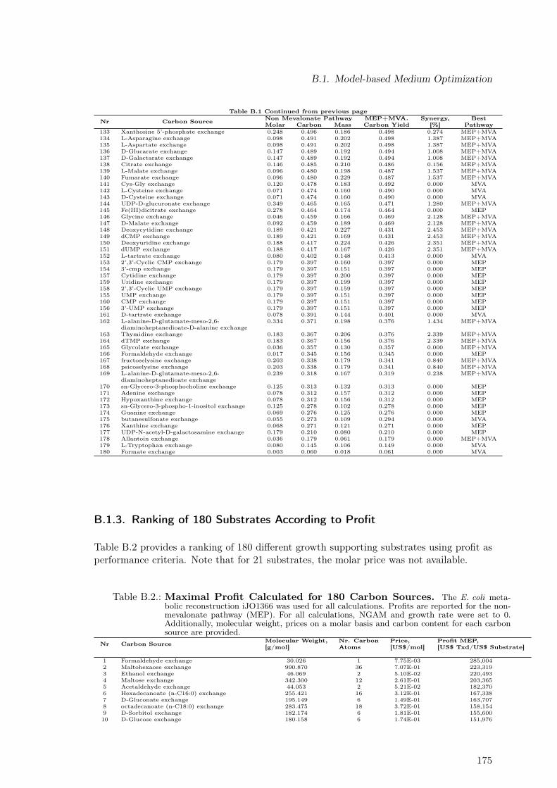
B.1. Model-based Medium Optimization
Table B.1 Continued from previous page
Nr Carbon Source Non Mevalonate Pathway MEP+MVA.Carbon Yield
Synergy,[%]
BestPathwayMolar Carbon Mass
133 Xanthosine 5’-phosphate exchange 0.248 0.496 0.186 0.498 0.274 MEP+MVA134 L-Asparagine exchange 0.098 0.491 0.202 0.498 1.387 MEP+MVA135 L-Aspartate exchange 0.098 0.491 0.202 0.498 1.387 MEP+MVA136 D-Glucarate exchange 0.147 0.489 0.192 0.494 1.008 MEP+MVA137 D-Galactarate exchange 0.147 0.489 0.192 0.494 1.008 MEP+MVA138 Citrate exchange 0.146 0.485 0.210 0.486 0.156 MEP+MVA139 L-Malate exchange 0.096 0.480 0.198 0.487 1.537 MEP+MVA140 Fumarate exchange 0.096 0.480 0.229 0.487 1.537 MEP+MVA141 Cys-Gly exchange 0.120 0.478 0.183 0.492 0.000 MVA142 L-Cysteine exchange 0.071 0.474 0.160 0.490 0.000 MVA143 D-Cysteine exchange 0.071 0.474 0.160 0.490 0.000 MVA144 UDP-D-glucuronate exchange 0.349 0.465 0.165 0.471 1.280 MEP+MVA145 Fe(III)dicitrate exchange 0.278 0.464 0.174 0.464 0.000 MEP146 Glycine exchange 0.046 0.459 0.166 0.469 2.128 MEP+MVA147 D-Malate exchange 0.092 0.459 0.189 0.469 2.128 MEP+MVA148 Deoxycytidine exchange 0.189 0.421 0.227 0.431 2.453 MEP+MVA149 dCMP exchange 0.189 0.421 0.169 0.431 2.453 MEP+MVA150 Deoxyuridine exchange 0.188 0.417 0.224 0.426 2.351 MEP+MVA151 dUMP exchange 0.188 0.417 0.167 0.426 2.351 MEP+MVA152 L-tartrate exchange 0.080 0.402 0.148 0.413 0.000 MVA153 2’,3’-Cyclic CMP exchange 0.179 0.397 0.160 0.397 0.000 MEP154 3’-cmp exchange 0.179 0.397 0.151 0.397 0.000 MEP157 Cytidine exchange 0.179 0.397 0.200 0.397 0.000 MEP159 Uridine exchange 0.179 0.397 0.199 0.397 0.000 MEP158 2’,3’-Cyclic UMP exchange 0.179 0.397 0.159 0.397 0.000 MEP155 UMP exchange 0.179 0.397 0.151 0.397 0.000 MEP160 CMP exchange 0.179 0.397 0.151 0.397 0.000 MEP156 3’-UMP exchange 0.179 0.397 0.151 0.397 0.000 MEP161 D-tartrate exchange 0.078 0.391 0.144 0.401 0.000 MVA162 L-alanine-D-glutamate-meso-2,6-
diaminoheptanedioate-D-alanine exchange0.334 0.371 0.198 0.376 1.434 MEP+MVA
163 Thymidine exchange 0.183 0.367 0.206 0.376 2.339 MEP+MVA164 dTMP exchange 0.183 0.367 0.156 0.376 2.339 MEP+MVA165 Glycolate exchange 0.036 0.357 0.130 0.357 0.000 MEP+MVA166 Formaldehyde exchange 0.017 0.345 0.156 0.345 0.000 MEP167 fructoselysine exchange 0.203 0.338 0.179 0.341 0.840 MEP+MVA168 psicoselysine exchange 0.203 0.338 0.179 0.341 0.840 MEP+MVA169 L-alanine-D-glutamate-meso-2,6-
diaminoheptanedioate exchange0.239 0.318 0.167 0.319 0.238 MEP+MVA
170 sn-Glycero-3-phosphocholine exchange 0.125 0.313 0.132 0.313 0.000 MEP171 Adenine exchange 0.078 0.312 0.157 0.312 0.000 MEP172 Hypoxanthine exchange 0.078 0.312 0.156 0.312 0.000 MEP173 sn-Glycero-3-phospho-1-inositol exchange 0.125 0.278 0.102 0.278 0.000 MEP174 Guanine exchange 0.069 0.276 0.125 0.276 0.000 MEP175 butanesulfonate exchange 0.055 0.273 0.109 0.294 0.000 MVA176 Xanthine exchange 0.068 0.271 0.121 0.271 0.000 MEP177 UDP-N-acetyl-D-galactosamine exchange 0.179 0.210 0.080 0.210 0.000 MEP178 Allantoin exchange 0.036 0.179 0.061 0.179 0.000 MEP+MVA179 L-Tryptophan exchange 0.080 0.145 0.106 0.149 0.000 MVA180 Formate exchange 0.003 0.060 0.018 0.061 0.000 MVA
B.1.3. Ranking of 180 Substrates According to Profit
Table B.2 provides a ranking of 180 different growth supporting substrates using profit asperformance criteria. Note that for 21 substrates, the molar price was not available.
Table B.2.: Maximal Profit Calculated for 180 Carbon Sources. The E. coli meta-bolic reconstruction iJO1366 was used for all calculations. Profits are reported for the non-mevalonate pathway (MEP). For all calculations, NGAM and growth rate were set to 0.Additionally, molecular weight, prices on a molar basis and carbon content for each carbonsource are provided.
Nr Carbon Source Molecular Weight,[g/mol]
Nr. CarbonAtoms
Price,[US$/mol]
Profit MEP,[US$ Txd/US$ Substrate]
1 Formaldehyde exchange 30.026 1 7.75E-03 285,0042 Maltohexaose exchange 990.870 36 7.07E-01 223,3193 Ethanol exchange 46.069 2 5.10E-02 220,4934 Maltose exchange 342.300 12 2.61E-01 203,3655 Acetaldehyde exchange 44.053 2 5.21E-02 182,3706 Hexadecanoate (n-C16:0) exchange 255.421 16 3.12E-01 167,3387 D-Gluconate exchange 195.149 6 1.49E-01 163,7078 octadecanoate (n-C18:0) exchange 283.475 18 3.72E-01 158,1549 D-Sorbitol exchange 182.174 6 1.81E-01 155,60010 D-Glucose exchange 180.158 6 1.74E-01 151,976
175
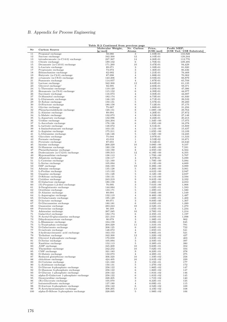
B. Appendix for Process Engineering
Table B.2 Continued from previous page
Nr Carbon Source Molecular Weight,[g/mol]
Nr. CarbonAtoms
Price,[US$/mol]
Profit MEP,[US$ Txd/ US$ Substrate]
11 Propanal exchange 58.080 3 1.03E-01 133,92812 Sucrose exchange 342.300 12 4.10E-01 129,24413 tetradecanoate (n-C14:0) exchange 227.367 14 4.06E-01 112,77614 Citrate exchange 189.102 6 1.70E-01 109,49515 Decanoate (n-C10:0) exchange 171.260 10 3.47E-01 94,42916 L-Lactate exchange 89.071 3 1.32E-01 81,92017 Propionate exchange 73.072 3 1.46E-01 80,43618 Ethanolamine exchange 62.092 2 1.21E-01 76,46919 Butyrate (n-C4:0) exchange 87.098 4 1.88E-01 70,36220 octanoate (n-C8:0) exchange 143.206 8 3.93E-01 66,87921 Fumarate exchange 114.057 4 1.87E-01 65,70922 Lactose exchange 342.300 12 8.63E-01 61,13523 Glycerol exchange’ 92.095 3 2.60E-01 59,37124 L-Threonine exchange 119.120 4 3.25E-01 47,38625 Hexanoate (n-C6:0) exchange 115.152 6 4.39E-01 44,97726 Succinate exchange 116.073 4 3.00E-01 44,68727 D-Mannitol exchange 182.174 6 6.73E-01 41,92028 L-Glutamate exchange 146.123 5 4.71E-01 39,53229 D-Xylose exchange 150.131 5 5.57E-01 39,20030 D-Fructose exchange 180.158 6 7.12E-01 37,17531 Glycine exchange 75.067 2 1.88E-01 31,25632 Phenylacetaldehyde exchange 120.151 8 1.08E+00 29,76433 L-Alanine exchange 89.094 3 4.26E-01 27,87234 L-Malate exchange 132.073 4 4.53E-01 27,14835 L-Aspartate exchange 132.096 4 6.22E-01 20,21536 Uridine exchange 244.204 9 1.34E+00 17,07537 L-Ascorbate exchange 176.126 6 1.35E+00 16,27838 L-tartrate exchange 148.072 4 6.51E-01 15,80939 4-Aminobutanoate exchange 103.121 4 1.11E+00 15,43740 L-Arginine exchange 175.211 6 1.65E+00 13,10941 L-Glutamine exchange 146.146 5 1.52E+00 12,22542 Glycolate exchange 75.044 2 3.97E-01 11,52343 Formate exchange 45.018 1 3.53E-02 10,87144 Pyruvate exchange 87.055 3 9.34E-01 10,64045 Inosine exchange 268.229 10 3.68E+00 9,10746 D-Mannose exchange 180.158 6 3.49E+00 7,59147 Phenethylamine exchange 122.190 8 4.95E+00 6,56448 Dodecanoate (n-C12:0) exchange 199.313 12 6.18E+00 6,35549 Hypoxanthine exchange 136.113 5 1.75E+00 5,70750 Allantoin exchange 158.117 4 8.97E-01 5,09951 L-Cysteine exchange 121.160 3 1.79E+00 5,08452 L-Serine exchange 105.094 3 2.13E+00 4,66953 IMP exchange 346.193 10 8.38E+00 3,99954 Adenine exchange 135.128 5 3.26E+00 3,06155 L-Proline exchange 115.132 5 4.61E+00 2,94756 Guanine exchange 151.128 5 3.12E+00 2,83757 D-Ribose exchange 150.131 5 8.11E+00 2,59458 Cytidine exchange 243.219 9 9.81E+00 2,33259 D-Galactose exchange 180.158 6 1.28E+01 2,05360 (S)-Propane-1,2-diol exchange 76.095 3 7.61E+00 1,90661 2-Oxoglutarate exchange 144.084 5 1.02E+01 1,59362 Ornithine exchange 133.171 5 1.29E+01 1,58063 D-Alanine exchange 89.094 3 7.66E+00 1,54964 L-Asparagine exchange 132.119 4 8.46E+00 1,48765 D-Galactonate exchange 195.149 6 1.68E+01 1,40066 D-lactate exchange 89.071 3 9.00E+00 1,30767 D-Glucosamine exchange 180.181 6 2.05E+01 1,28968 Guanosine exchange 283.244 10 2.52E+01 1,27069 Putrescine exchange 90.169 4 1.65E+01 1,23470 Adenosine exchange 267.245 10 2.78E+01 1,21471 Galactitol exchange 182.174 6 2.35E+01 1,19772 N-Acetyl-D-glucosamine exchange 221.210 8 3.05E+01 1,09873 Dihydroxyacetone exchange 90.079 3 1.38E+01 96274 L-Rhamnose exchange 164.158 6 3.09E+01 84575 L-Tryptophan exchange 204.229 11 1.31E+01 78176 D-Galactarate exchange 208.125 6 2.60E+01 72277 D-tartrate exchange 148.072 4 1.85E+01 54178 3-hydroxycinnamic acid exchange 163.153 9 5.86E+01 52179 Trehalose exchange 342.300 12 1.22E+02 43780 Glycerol 2-phosphate exchange 170.059 3 3.83E+01 40381 D-Serine exchange 105.094 3 2.50E+01 39782 Xanthine exchange 152.113 5 2.28E+01 38083 AMP exchange 345.209 10 9.60E+01 35284 Thymidine exchange 242.232 10 7.02E+01 33485 CMP exchange 321.183 9 8.22E+01 27886 D-Malate exchange 132.073 4 4.28E+01 27587 Reduced glutathione exchange 306.320 10 1.33E+02 25888 chitobiose exchange 424.405 16 2.81E+02 22989 D-Cysteine exchange 121.160 3 5.15E+01 17790 L-Arabinose exchange 150.131 5 1.27E+02 17291 D-Glucose 6-phosphate exchange 258.122 6 1.86E+02 14792 D-Mannose 6-phosphate exchange 258.122 6 1.86E+02 14793 D-Glucose 1-phosphate exchange 258.122 6 1.81E+02 14694 alpha-D-Galactose 1-phosphate exchange 258.122 6 1.81E+02 14595 Deoxyuridine exchange 228.205 9 1.71E+02 14096 (R)-Glycerate exchange 105.070 3 8.22E+01 12597 butanesulfonate exchange 137.180 4 6.09E+01 11598 D-fructose 6-phosphate exchange 258.122 6 2.52E+02 10999 N-Acetylneuraminate exchange 308.265 11 4.10E+02 108100 alpha-D-Ribose 5-phosphate exchange 228.095 5 1.98E+02 106
176
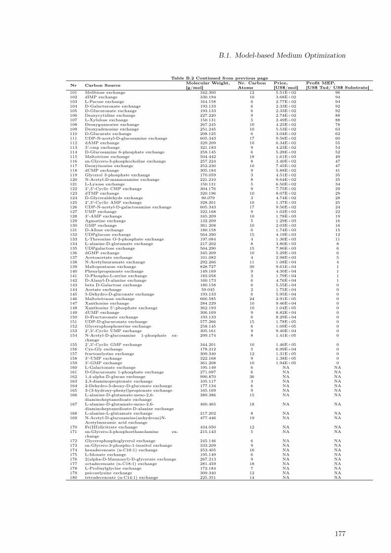
B.1. Model-based Medium Optimization
Table B.2 Continued from previous page
Nr Carbon Source Molecular Weight,[g/mol]
Nr. CarbonAtoms
Price,[US$/mol]
Profit MEP,[US$ Txd/ US$ Substrate]
101 Melibiose exchange 342.300 12 5.51E+02 96102 dIMP exchange 330.194 10 3.68E+02 94103 L-Fucose exchange 164.158 6 2.77E+02 94104 D-Galacturonate exchange 193.133 6 2.33E+02 92105 D-Glucuronate exchange 193.133 6 2.33E+02 92106 Deoxycytidine exchange 227.220 9 2.74E+02 88107 L-Xylulose exchange 150.131 5 2.49E+02 88108 Deoxyguanosine exchange 267.245 10 4.25E+02 78109 Deoxyadenosine exchange 251.245 10 5.53E+02 63110 D-Glucarate exchange 208.125 6 3.04E+02 62111 UDP-N-acetyl-D-glucosamine exchange 605.343 17 9.56E+02 60112 dAMP exchange 329.209 10 6.34E+02 55113 3’-cmp exchange 321.183 9 4.23E+02 54114 D-Glucosamine 6-phosphate exchange 258.145 6 5.28E+02 52115 Maltotriose exchange 504.442 18 1.61E+03 49116 sn-Glycero-3-phosphocholine exchange 257.224 8 3.40E+02 47117 Deoxyinosine exchange 252.230 10 7.45E+02 47118 dCMP exchange 305.184 9 5.88E+02 41119 Glycerol 3-phosphate exchange 170.059 3 4.51E+02 35120 N-Acetyl-D-mannosamine exchange 221.210 8 9.64E+02 35121 L-Lyxose exchange 150.131 5 6.50E+02 34122 2’,3’-Cyclic CMP exchange 304.176 9 7.75E+02 29123 dTMP exchange 320.196 10 8.07E+02 29124 D-Glyceraldehyde exchange 90.079 3 4.74E+02 28125 2’,3’-Cyclic AMP exchange 328.201 10 1.37E+03 25126 UDP-N-acetyl-D-galactosamine exchange 605.343 17 9.56E+02 24127 UMP exchange 322.168 9 1.02E+03 22128 3’-AMP exchange 345.209 10 1.78E+03 19129 Agmatine exchange 132.209 5 1.29E+03 16130 GMP exchange 361.208 10 2.03E+03 16131 D-Allose exchange 180.158 6 1.74E+03 15132 UDPglucose exchange 564.290 15 4.19E+03 12133 L-Threonine O-3-phosphate exchange 197.084 4 1.36E+03 11134 L-alanine-D-glutamate exchange 217.202 8 3.80E+03 8135 UDPgalactose exchange 564.290 15 7.86E+03 6136 dGMP exchange 345.209 10 5.29E+03 6137 Acetoacetate exchange 101.082 4 2.98E+03 5138 N-Acetylmuramate exchange 292.266 11 1.08E+04 4139 Maltopentaose exchange 828.727 30 9.61E+04 1140 Phenylpropanoate exchange 149.169 9 4.30E+04 1141 O-Phospho-L-serine exchange 183.058 3 1.79E+04 1142 D-Alanyl-D-alanine exchange 160.173 6 4.76E+04 1143 beta D-Galactose exchange 180.158 6 5.55E+04 0144 Acetate exchange 59.045 2 1.75E+04 0145 5-Dehydro-D-gluconate exchange 193.133 6 5.95E+04 0146 Maltotetraose exchange 666.585 24 2.91E+05 0147 Xanthosine exchange 284.229 10 9.46E+04 0148 Xanthosine 5’-phosphate exchange 362.193 10 1.04E+05 0149 dUMP exchange 306.169 9 8.82E+04 0150 D-Fructuronate exchange 193.133 6 8.29E+04 0151 UDP-D-glucuronate exchange 577.266 15 1.78E+05 0152 Glycerophosphoserine exchange 258.145 6 1.09E+05 0153 2’,3’-Cyclic UMP exchange 305.161 9 9.40E+04 0154 N-Acetyl-D-glucosamine 1-phosphate ex-
change299.174 8 1.41E+05 0
155 2’,3’-Cyclic GMP exchange 344.201 10 1.46E+05 0156 Cys-Gly exchange 178.212 5 6.99E+04 0157 fructoselysine exchange 309.340 12 1.31E+05 0158 3’-UMP exchange 322.168 9 1.38E+05 0159 3’-GMP exchange 361.208 10 1.94E+05 0160 L-Galactonate exchange 195.149 6 NA NA161 D-Glucuronate 1-phosphate exchange 271.097 6 NA NA162 1,4-alpha-D-glucan exchange 990.870 36 NA NA163 2,3-diaminopropionate exchange 105.117 3 NA NA164 2-Dehydro-3-deoxy-D-gluconate exchange 177.134 6 NA NA165 3-(3-hydroxy-phenyl)propionate exchange 165.169 9 NA NA166 L-alanine-D-glutamate-meso-2,6-
diaminoheptanedioate exchange389.386 15 NA NA
167 L-alanine-D-glutamate-meso-2,6-diaminoheptanedioate-D-alanine exchange
460.465 18 NA NA
168 L-alanine-L-glutamate exchange 217.202 8 NA NA169 N-Acetyl-D-glucosamine(anhydrous)N-
Acetylmuramic acid exchange477.446 19 NA NA
170 Fe(III)dicitrate exchange 434.050 12 NA NA171 sn-Glycero-3-phosphoethanolamine ex-
change215.143 5 NA NA
172 Glycerophosphoglycerol exchange 245.146 6 NA NA173 sn-Glycero-3-phospho-1-inositol exchange 333.209 9 NA NA174 hexadecenoate (n-C16:1) exchange 253.405 16 NA NA175 L-Idonate exchange 195.149 6 NA NA176 2(alpha-D-Mannosyl)-D-glycerate exchange 267.213 9 NA NA177 octadecenoate (n-C18:1) exchange 281.459 18 NA NA178 L-Prolinylglycine exchange 172.184 7 NA NA179 psicoselysine exchange 309.340 12 NA NA180 tetradecenoate (n-C14:1) exchange 225.351 14 NA NA
177
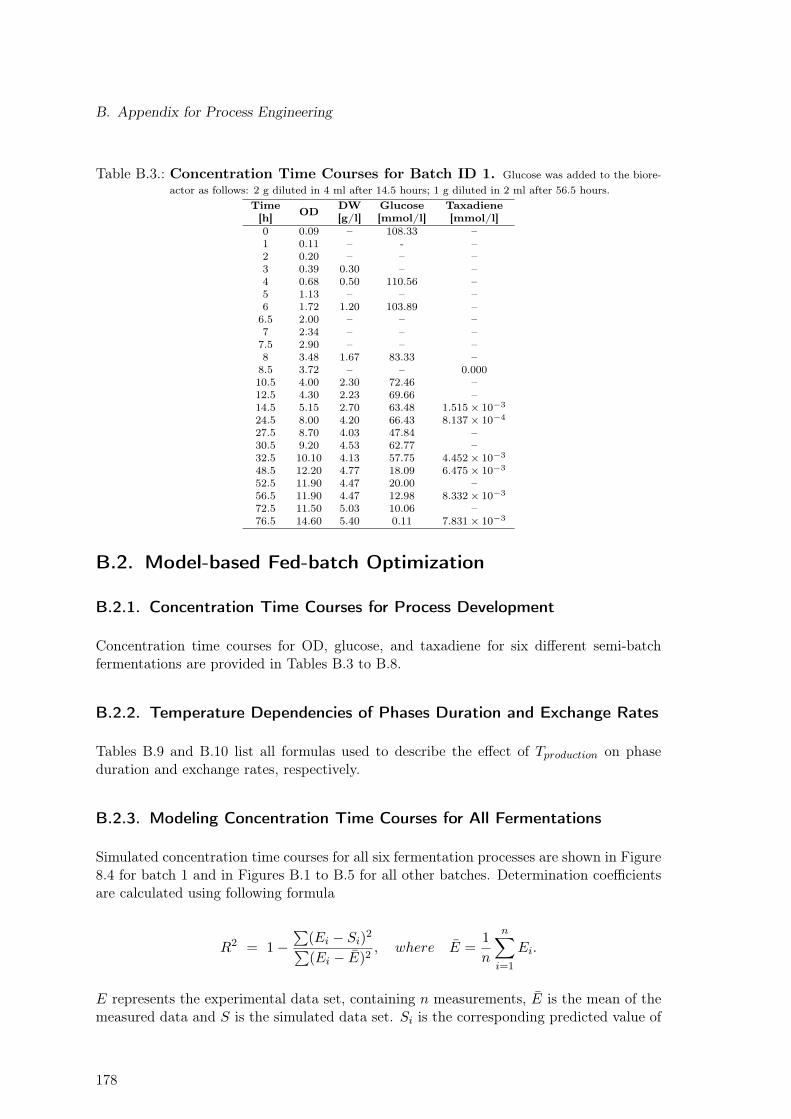
B. Appendix for Process Engineering
Table B.3.: Concentration Time Courses for Batch ID 1. Glucose was added to the biore-actor as follows: 2 g diluted in 4 ml after 14.5 hours; 1 g diluted in 2 ml after 56.5 hours.
Time[h] OD DW
[g/l]Glucose[mmol/l]
Taxadiene[mmol/l]
0 0.09 – 108.33 –1 0.11 – - –2 0.20 – – –3 0.39 0.30 – –4 0.68 0.50 110.56 –5 1.13 – – –6 1.72 1.20 103.89 –6.5 2.00 – – –7 2.34 – – –7.5 2.90 – – –8 3.48 1.67 83.33 –8.5 3.72 – – 0.00010.5 4.00 2.30 72.46 –12.5 4.30 2.23 69.66 –14.5 5.15 2.70 63.48 1.515 × 10⁻³
24.5 8.00 4.20 66.43 8.137 × 10⁻⁴
27.5 8.70 4.03 47.84 –30.5 9.20 4.53 62.77 –32.5 10.10 4.13 57.75 4.452 × 10⁻³
48.5 12.20 4.77 18.09 6.475 × 10⁻³
52.5 11.90 4.47 20.00 –56.5 11.90 4.47 12.98 8.332 × 10⁻³
72.5 11.50 5.03 10.06 –76.5 14.60 5.40 0.11 7.831 × 10⁻³
B.2. Model-based Fed-batch Optimization
B.2.1. Concentration Time Courses for Process Development
Concentration time courses for OD, glucose, and taxadiene for six different semi-batchfermentations are provided in Tables B.3 to B.8.
B.2.2. Temperature Dependencies of Phases Duration and Exchange Rates
Tables B.9 and B.10 list all formulas used to describe the effect of Tproduction on phaseduration and exchange rates, respectively.
B.2.3. Modeling Concentration Time Courses for All Fermentations
Simulated concentration time courses for all six fermentation processes are shown in Figure8.4 for batch 1 and in Figures B.1 to B.5 for all other batches. Determination coefficientsare calculated using following formula
R2 = 1−∑
(Ei − Si)2∑(Ei − E)2
, where E =1
n
n∑i=1
Ei.
E represents the experimental data set, containing n measurements, E is the mean of themeasured data and S is the simulated data set. Si is the corresponding predicted value of
178
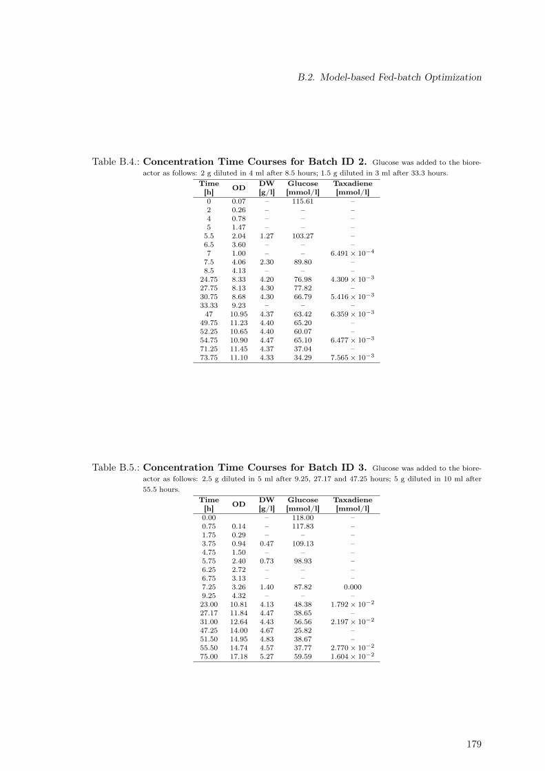
B.2. Model-based Fed-batch Optimization
Table B.4.: Concentration Time Courses for Batch ID 2. Glucose was added to the biore-actor as follows: 2 g diluted in 4 ml after 8.5 hours; 1.5 g diluted in 3 ml after 33.3 hours.
Time[h] OD DW
[g/l]Glucose[mmol/l]
Taxadiene[mmol/l]
0 0.07 – 115.61 –2 0.26 – – –4 0.78 – – –5 1.47 – – –5.5 2.04 1.27 103.27 –6.5 3.60 – – –7 1.00 – – 6.491 × 10⁻⁴
7.5 4.06 2.30 89.80 –8.5 4.13 – – –
24.75 8.33 4.20 76.98 4.309 × 10⁻³
27.75 8.13 4.30 77.82 –30.75 8.68 4.30 66.79 5.416 × 10⁻³
33.33 9.23 – – –47 10.95 4.37 63.42 6.359 × 10⁻³
49.75 11.23 4.40 65.20 –52.25 10.65 4.40 60.07 –54.75 10.90 4.47 65.10 6.477 × 10⁻³
71.25 11.45 4.37 37.04 –73.75 11.10 4.33 34.29 7.565 × 10⁻³
Table B.5.: Concentration Time Courses for Batch ID 3. Glucose was added to the biore-actor as follows: 2.5 g diluted in 5 ml after 9.25, 27.17 and 47.25 hours; 5 g diluted in 10 ml after55.5 hours.
Time[h] OD DW
[g/l]Glucose[mmol/l]
Taxadiene[mmol/l]
0.00 – 118.00 –0.75 0.14 – 117.83 –1.75 0.29 – – –3.75 0.94 0.47 109.13 –4.75 1.50 – – –5.75 2.40 0.73 98.93 –6.25 2.72 – – –6.75 3.13 – – –7.25 3.26 1.40 87.82 0.0009.25 4.32 – – –23.00 10.81 4.13 48.38 1.792 × 10⁻²
27.17 11.84 4.47 38.65 –31.00 12.64 4.43 56.56 2.197 × 10⁻²
47.25 14.00 4.67 25.82 –51.50 14.95 4.83 38.67 –55.50 14.74 4.57 37.77 2.770 × 10⁻²
75.00 17.18 5.27 59.59 1.604 × 10⁻²
179
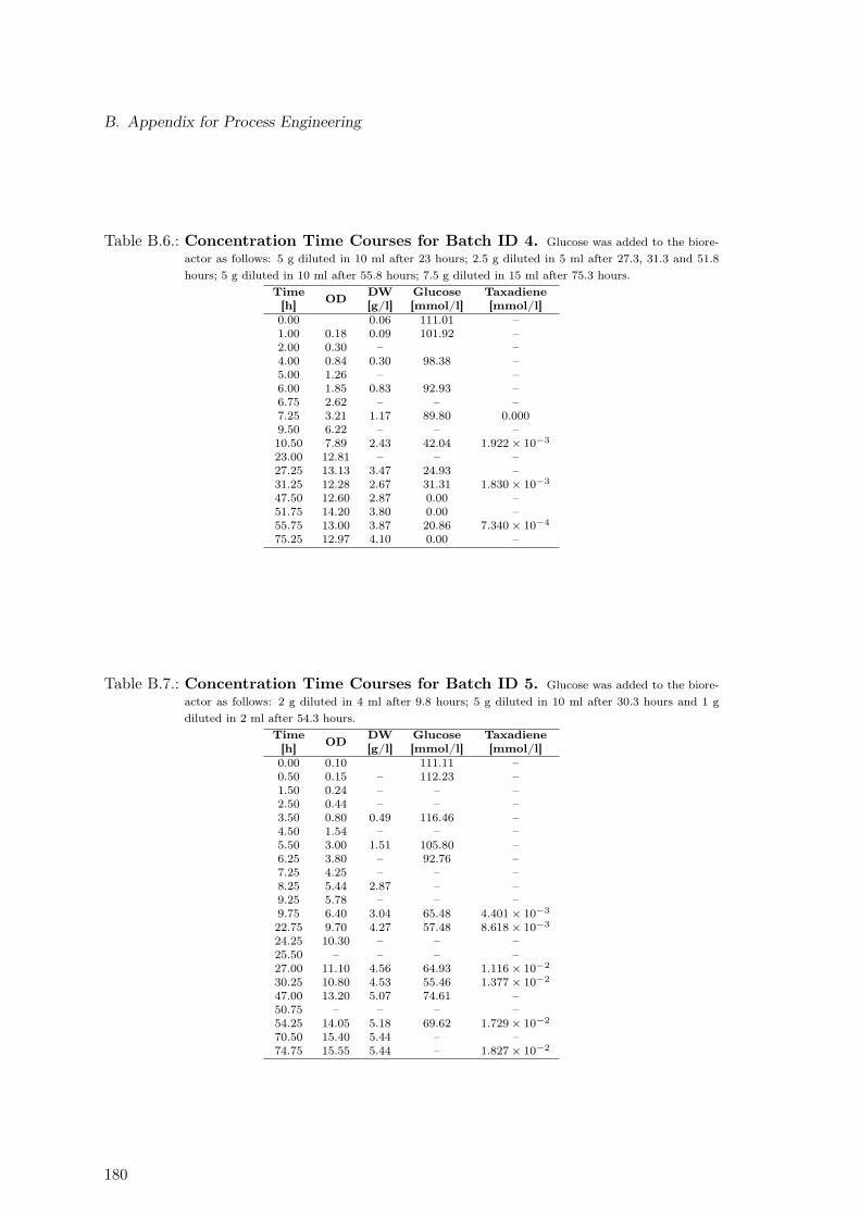
B. Appendix for Process Engineering
Table B.6.: Concentration Time Courses for Batch ID 4. Glucose was added to the biore-actor as follows: 5 g diluted in 10 ml after 23 hours; 2.5 g diluted in 5 ml after 27.3, 31.3 and 51.8hours; 5 g diluted in 10 ml after 55.8 hours; 7.5 g diluted in 15 ml after 75.3 hours.
Time[h] OD DW
[g/l]Glucose[mmol/l]
Taxadiene[mmol/l]
0.00 0.06 111.01 –1.00 0.18 0.09 101.92 –2.00 0.30 – –4.00 0.84 0.30 98.38 –5.00 1.26 – –6.00 1.85 0.83 92.93 –6.75 2.62 – – –7.25 3.21 1.17 89.80 0.0009.50 6.22 – – –10.50 7.89 2.43 42.04 1.922 × 10⁻³
23.00 12.81 – – –27.25 13.13 3.47 24.93 –31.25 12.28 2.67 31.31 1.830 × 10⁻³
47.50 12.60 2.87 0.00 –51.75 14.20 3.80 0.00 –55.75 13.00 3.87 20.86 7.340 × 10⁻⁴
75.25 12.97 4.10 0.00 –
Table B.7.: Concentration Time Courses for Batch ID 5. Glucose was added to the biore-actor as follows: 2 g diluted in 4 ml after 9.8 hours; 5 g diluted in 10 ml after 30.3 hours and 1 gdiluted in 2 ml after 54.3 hours.
Time[h] OD DW
[g/l]Glucose[mmol/l]
Taxadiene[mmol/l]
0.00 0.10 111.11 –0.50 0.15 – 112.23 –1.50 0.24 – – –2.50 0.44 – – –3.50 0.80 0.49 116.46 –4.50 1.54 – – –5.50 3.00 1.51 105.80 –6.25 3.80 – 92.76 –7.25 4.25 – – –8.25 5.44 2.87 – –9.25 5.78 – – –9.75 6.40 3.04 65.48 4.401 × 10⁻³
22.75 9.70 4.27 57.48 8.618 × 10⁻³
24.25 10.30 – – –25.50 – – – –27.00 11.10 4.56 64.93 1.116 × 10⁻²
30.25 10.80 4.53 55.46 1.377 × 10⁻²
47.00 13.20 5.07 74.61 –50.75 – – – –54.25 14.05 5.18 69.62 1.729 × 10⁻²
70.50 15.40 5.44 – –74.75 15.55 5.44 – 1.827 × 10⁻²
180
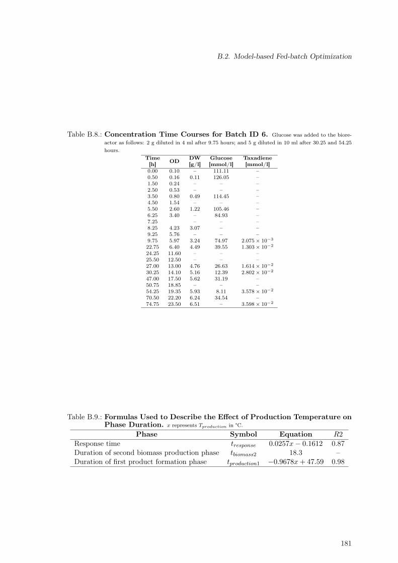
B.2. Model-based Fed-batch Optimization
Table B.8.: Concentration Time Courses for Batch ID 6. Glucose was added to the biore-actor as follows: 2 g diluted in 4 ml after 9.75 hours; and 5 g diluted in 10 ml after 30.25 and 54.25hours.
Time[h] OD DW
[g/l]Glucose[mmol/l]
Taxadiene[mmol/l]
0.00 0.10 – 111.11 –0.50 0.16 0.11 126.05 –1.50 0.24 – – –2.50 0.53 – – –3.50 0.80 0.49 114.45 –4.50 1.54 – – –5.50 2.60 1.22 105.46 –6.25 3.40 – 84.93 –7.25 – – –8.25 4.23 3.07 – –9.25 5.76 – – –9.75 5.97 3.24 74.97 2.075 × 10⁻³
22.75 6.40 4.49 39.55 1.303 × 10⁻²
24.25 11.60 – – –25.50 12.50 – – –27.00 13.00 4.76 26.63 1.614 × 10⁻²
30.25 14.10 5.16 12.39 2.802 × 10⁻²
47.00 17.50 5.62 31.19 –50.75 18.85 – – –54.25 19.35 5.93 8.11 3.578 × 10⁻²
70.50 22.20 6.24 34.54 –74.75 23.50 6.51 – 3.598 × 10⁻²
Table B.9.: Formulas Used to Describe the Effect of Production Temperature onPhase Duration. x represents Tproduction in °C.
Phase Symbol Equation R2
Response time tresponse 0.0257x− 0.1612 0.87Duration of second biomass production phase tbiomass2 18.3 –Duration of first product formation phase tproduction1 −0.9678x+ 47.59 0.98
181
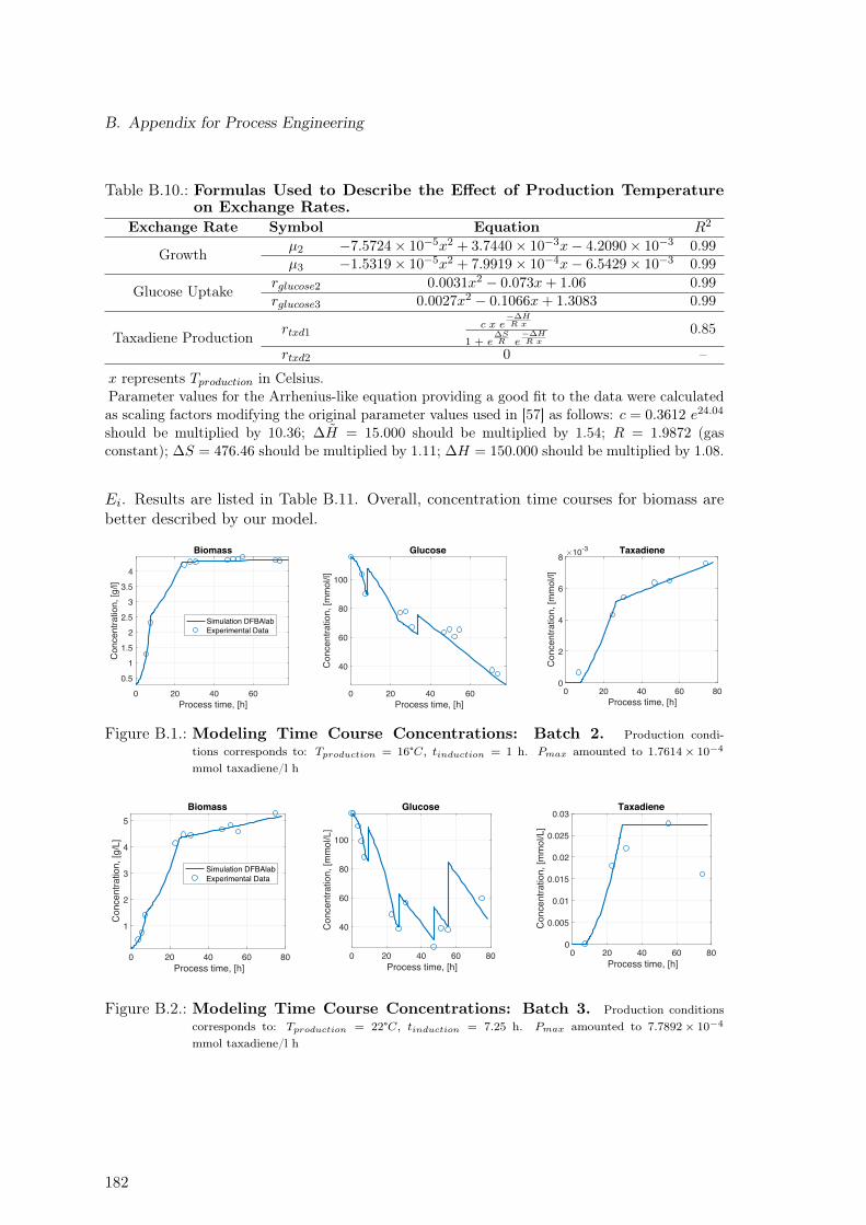
B. Appendix for Process Engineering
Table B.10.: Formulas Used to Describe the Effect of Production Temperatureon Exchange Rates.
Exchange Rate Symbol Equation R2
Growth µ2 −7.5724× 10−5x2 + 3.7440× 10⁻³x− 4.2090× 10⁻³ 0.99µ3 −1.5319× 10−5x2 + 7.9919× 10⁻⁴x− 6.5429× 10⁻³ 0.99
Glucose Uptake rglucose2 0.0031x2 − 0.073x+ 1.06 0.99rglucose3 0.0027x2 − 0.1066x+ 1.3083 0.99
Taxadiene Production rtxd1c x e
−∆HR x
1 + e∆SR e
−∆HR x
0.85
rtxd2 0 –
x represents Tproduction in Celsius.Parameter values for the Arrhenius-like equation providing a good fit to the data were calculatedas scaling factors modifying the original parameter values used in [57] as follows: c = 0.3612 e24.04
should be multiplied by 10.36; ∆H = 15.000 should be multiplied by 1.54; R = 1.9872 (gasconstant); ∆S = 476.46 should be multiplied by 1.11; ∆H = 150.000 should be multiplied by 1.08.
Ei. Results are listed in Table B.11. Overall, concentration time courses for biomass arebetter described by our model.
0 20 40 60Process time, [h]
0.5
1
1.5
2
2.5
3
3.5
4
Con
cent
ratio
n, [g
/l]
Biomass
Simulation DFBAlabExperimental Data
0 20 40 60Process time, [h]
40
60
80
100
Con
cent
ratio
n, [m
mol
/l]
Glucose
0 20 40 60 80Process time, [h]
0
2
4
6
8C
once
ntra
tion,
[mm
ol/l]
10-3 Taxadiene
Figure B.1.: Modeling Time Course Concentrations: Batch 2. Production condi-tions corresponds to: Tproduction = 16°C, tinduction = 1 h. Pmax amounted to 1.7614 × 10⁻⁴
mmol taxadiene/l h
0 20 40 60 80Process time, [h]
1
2
3
4
5
Con
cent
ratio
n, [g
/L]
Biomass
Simulation DFBAlabExperimental Data
0 20 40 60 80Process time, [h]
40
60
80
100
Con
cent
ratio
n, [m
mol
/L]
Glucose
0 20 40 60 80Process time, [h]
0
0.005
0.01
0.015
0.02
0.025
0.03
Con
cent
ratio
n, [m
mol
/L]
Taxadiene
Figure B.2.: Modeling Time Course Concentrations: Batch 3. Production conditionscorresponds to: Tproduction = 22°C, tinduction = 7.25 h. Pmax amounted to 7.7892 × 10⁻⁴
mmol taxadiene/l h
182
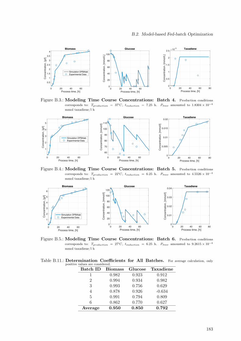
B.2. Model-based Fed-batch Optimization
0 20 40 60Process time, [h]
0.5
1
1.5
2
2.5
3
3.5
4
Con
cent
ratio
n, [g
/l]Biomass
Simulation DFBAlabExperimental Data
0 20 40 60Process time, [h]
0
20
40
60
80
100
Con
cent
ratio
n, [m
mol
/L]
Glucose
0 20 40 60 80Process time, [h]
0
0.5
1
1.5
2
2.5
Con
cent
ratio
n, [m
mol
/L]
10-3 Taxadiene
Figure B.3.: Modeling Time Course Concentrations: Batch 4. Production conditionscorresponds to: Tproduction = 37°C, tinduction = 7.25 h. Pmax amounted to 1.8304 × 10⁻⁴
mmol taxadiene/l h
0 20 40 60Process time, [h]
1
2
3
4
5
Con
cent
ratio
n, [g
/l]
Biomass
Simulation DFBAlabExperimental Data
0 20 40 60Process time, [h]
60
70
80
90
100
110
Con
cent
ratio
n, [m
mol
/l]
Glucose
0 20 40 60 80Process time, [h]
0
0.005
0.01
0.015
0.02
Con
cent
ratio
n, [m
mol
/l]
Taxadiene
Figure B.4.: Modeling Time Course Concentrations: Batch 5. Production conditionscorresponds to: Tproduction = 22°C, tinduction = 6.25 h. Pmax amounted to 4.5526 × 10⁻⁴
mmol taxadiene/l h
0 20 40 60Process time, [h]
1
2
3
4
5
6
Con
cent
ratio
n, [g
/l]
Biomass
Simulation DFBAlabExperimental Data
0 20 40 60Process time, [h]
0
20
40
60
80
100
120
Con
cent
ratio
n, [m
mol
/l]
Glucose
0 20 40 60 80Process time, [h]
0
0.01
0.02
0.03
0.04
Con
cent
ratio
n, [m
mol
/l]
Taxadiene
Figure B.5.: Modeling Time Course Concentrations: Batch 6. Production conditionscorresponds to: Tproduction = 27°C, tinduction = 6.25 h. Pmax amounted to 9.2615 × 10⁻⁴
mmol taxadiene/l h
Table B.11.: Determination Coefficients for All Batches. For average calculation, onlypositive values are considered.
Batch ID Biomass Glucose Taxadiene1 0.982 0.923 0.9122 0.994 0.934 0.9823 0.993 0.756 0.6294 0.878 0.926 -0.6345 0.991 0.794 0.8096 0.862 0.770 0.627
Average 0.950 0.850 0.792
183