University of Nebraska - LincolnDigitalCommons@University of Nebraska - Lincoln

USGS Staff -- Published Research US Geological Survey

1-1-1988

Determining the Distribution of HydraulicConductivity 1n a Fractured Limestone Aquifer bySimultaneous Injection and Geophysical LoggingRoger H. MorinDenver Federal Center, rhmorin@usgs.gov

Alfred E. HessDenver Federal Center

Frederick L. PailleeDenver Federal Center

This Article is brought to you for free and open access by the US Geological Survey at DigitalCommons@University of Nebraska - Lincoln. It has beenaccepted for inclusion in USGS Staff -- Published Research by an authorized administrator of DigitalCommons@University of Nebraska - Lincoln.

Morin, Roger H.; Hess, Alfred E.; and Paillee, Frederick L., "Determining the Distribution of Hydraulic Conductivity 1n a FracturedLimestone Aquifer by Simultaneous Injection and Geophysical Logging" (1988). USGS Staff -- Published Research. Paper 349.http://digitalcommons.unl.edu/usgsstaffpub/349

Determining the Distribution of Hydraulic

Conductivity 1n a Fractured Limestone Aquifer by

Simultaneous Injection and Geophysical Logging

by Roger H. Morin, Alfred E. Hess, and Frederick L. Paillee

ABSTRACT i\ field technique for assessing the vertical distribution

of hydraulic conductivity in an aquifer was applied to a fractured carbonate formation in southeastern Nevada. The technique combines the simultaneous usc of fluid injection and geophysical logging to measure in situ vertical distribu­tions of fluid velocity and hydraulic head down the bore­hole; these data subsequently are analyzed to arrive at quantitative estimates of hydraulic conductivity across discrete intervals in the aquifer. The diagnostic capabilities of the analysis were found to be constraincd by the accuracy and resolution of the logging tools as well as by the hydraulic characteristics of the formation. Despite thesc limitations, this injection/logging technique appears to be practical and effective under the conditions encountered in this application. The results of this analysis identified the contact margin between the Anchor and Dawn Members of the Monte Cristo Limestone as being the dominant trans­missive unit. This section is extensively fractured, and quantitative estimates of its hydraulic conductivity are at least two orders of magnitude larger than that of the surrounding competent roek matrix. This transmissive zone also correlates strongly with an interval where the drilling rate was reported to be quite rapid. Aquifer transmissivity was computed from the profile of hydraulic conductivity and found to be 7.6 X 10 5 ft 2 /day, a value that is in close agreement with that determined from a conventional constant-discharge test. Discrepancies between the two esti­mates may be scale-dependent, a function of the different formation volumes investigated by each method. The friction factor, a parameter derived from the differential pressure and velocity logs, appears to be a good indicator of borehole rugosity across intervals where fluid velocity remains virtually unchanged, and vertical flow is turbulent.

a U.S. Geological Survey, Box 25046, M.S. 403, Denver Federal Center, Denver, Colorado 80225-0046.

Received September 1987, revised January 1988, accepted January 1988.

Discussion open until March 1, 1989.

Vol. 26, No.5-GROUND WATER-September-October 1988

I NTRODUCTI ON A variety of hydrologic field techniques

involving the pumping or injection of test wells, along with the monitoring of observation wells, has been used commonly to arrive at estimates of aquifer transmissivity. Complementary straddle­packer tests have been performed to identify discrete production zones and quantify the vertical distri­bution of hydraulic conductivity (Zeigler, 1976; Davison and others, 1982). Characterization of the distribution of hydraulic conductivity in fractured rock also has been attempted through the applica­tion of various geophysical logging methods. The attenuation of tube-wave amplitude in full-wave­form acoustic logs has been used to estimate fracture permeability in crystalline rocks (Paillet, 1983; Mathieu and Toksoz, 1984). The interpreta­tion of tube waves generated during vertical seismic profiling also has provided information on fracture permeability (Paillet and others, 1986; Hardin and others, 1987).

This paper describes the application of a hybrid technique developed by Hufschmied (1984) that utilizes injection into a well and concurrent geo­physical logging to obtain a detailed profile of hydraulic conductivity. Logging is performed at quasi-steady state conditions and is designed to measure the vertical distributions of hydraulic head and fluid velocity in the well. In situ measurements of pressure perturbations and induced flows are obtained across arbitrary depth intervals from the digitized logs, and these data are processed to yield a quantitative vertical profile of hydraulic conduc­tivity. The capabilities and limitations of this method are assessed using the results of a field application conducted in a fractured carbonate aquifer.

587

( ) \ ) ~ )i

) ( \ ---. Fig. 1. Location of study site and test wells.

HYDROGEOLOGIC SETTING

Nevada

The study area is located in the Coyote Spring Valley north of Las Vegas in southeastern Nevada; the well of interest (test well CE-DT-4) is west of the White River Channel (Figure 1). The Coyote Spring Valley is underlain by a regional carbonate aquifer consisting primarily of fractured and faulted Paleozoic limestone and dolomite. Based on several surveys of the Paleozoic sequence in the area, the stratigraphic section may be divided into 10 hydrostratigraphic units consisting of discrete intervals of carbonate aquifers and shale aquitards (Ertec Western, Inc., 1981). The limestone matrix has a very low hydraulic conductivity, and water storage and transport are largely controlled by fractures and secondary dissolution (Eakin, 1966). At test well CE-DT-4, the carbonate aquifer units form an uninterrupted vertical sequence with none of the intervening shale confining units that are prevalent to the north (Longwell and others, 1979). A lithologic cross section of the site is presented in Figure 2, log A. A composite of all logs pertinent to this study is presented in Figure 2 ; these are displayed together for easy reference and companson.

588

Surficial alluvial deposits are 30 ft thick and overlay the Monte Cristo Limestone. This Mississippian formation extends to the total depth of the test well (669 ft), and the contact between its Anchor and Dawn Members occurs at about 580 ft (all de~ths are referenced to land surface). Well CE-DT-4 was drilled in 1981, and a driller's record of penetration rate is included in Figure 2 as log B; drilling rate is presented in units of time (minutes) required per 10-ft interval. The well has a 10-in. casing (inside diameter) to 50 ft, and the remainder of the borehole is open to the formation. Static water level is at 353 ft.

GEOPHYSICAL LOGGING PRIOR TO FLUID INJECTION

Some geophysical logs were obtained prior to injection in order to get fundamental information on the geometry and physical conditions of the borehole. A caliper log was used to measure bore­hole diameter and to identify fractured intervals and breakout zones (Figure 2, log C). An acoustic televiewer (Zemanek and others, 1969) provided an acoustic image of the borehole wall from which fractures in the carbonate aquifer could be identified. Whereas caliper arms detect fractures only where they can extend into gaps produced by erosion of altered rock or mechanical breakage, the televiewer records acoustic reflectivity and can detect finer fractures and lithologic contacts that intersect the borehole (Paillet and others, 1985). An analysis of fracture density based on the interpretation of the televiewer log yielded a distribution similar to that presented by Ertec Western, Inc. (1981) and derived from an analogous analysis of a videolog. This latter profile of fracture density obtained from the videolog is presented in Figure 2 as log D.

Several other logs were run to verify hydro­static conditions and to calibrate geophysical tools to be used later during the injection phase of the study. A heat-pulse flowmeter was used to monitor vertical water movement in the borehole. This tool releases a discrete heat pulse into the water column and operates on the principle of temperature tag­trace; the small packet of heated wate, is trans­ported with the surrounding velocity field and its progress is monitored by thermistors (Hess, 1986). The heat-pulse flowmeter is held stationary in the borehole, and both vertical flow velocity and direction are determined. The instrument has a sensitivity of ± 0.4 in./min., far better than con­ventional spinner-type flowmeters, and operates

over a velocity range of about 0.2 to 20 ft/min. The maximum velocity measured by this flowmeter in well CE-DT-4 before injection was approximately 0.5 ft/min. downward, a value near the low end of the detectable range for the tool. This su btle water movement could reflect somewhat larger heads in the shallow fractures, possibly due to slight seasonal fluctuations in the water level, or be generated by weak convection cells induced in the borehole by small variations in fluid density (Sammel, 1968; Urban and Diment, 1985). The temperature log depicted in Figure 2 as log E also indicates down­ward water movement. Although the temperature profile is close to linear below 400 ft, the gradient is suppressed due to cooler surface water slowly traveling down the borehole. Static temperature gradients in southern Nevada should be roughly 1. 5° F 11 00 ft (Lachenbruch and Sass, 1977), whereas the profile presented in Figure 2 has an average gradient of only about 0.15° 1"11 00 ft.

A pressure log was run to record the initial hydraulic-head distribution in the borehole, and the response of the pressure transducer was found to be sligh tly, but systematically, nonlinear with increasing depth. It is unlikely that this very gradual nonlinearity is caused by coincident nonlinear

Inverse Fracture

changes in head, either due to hydraulic conditions in the aquifer or to fluid density variations in the borehole. Rather, this behavior is probably a characteristic of the instrument itself. Actually, the cause of this nonlinearity is not really important in this application because the pressure log is obtained only for calibration purposes. This record will be compared directly to its dynamic counterpart obtained during fluid injection to accurately deter­mine the departures from initial conditions over the range of pressures encountered in this study (300 ft). Those initial conditions are not required to be static.

Finally, a spinner flowmeter was run in the test well at two different logging speeds, while trolling both up and down, to uniquely calibrate the tool to this well (Schimschal, 1981; Syms and others, 1982). This probe lacks the accuracy and sensitivity of the heat-pulse flowmeter, although recent versions have displayed improved perfor­mance (Rehfeldt and Gelhar, 1987). However, the spinner can operate within a greater velocity range than can the heat-pulse tool, and its accuracy improves at higher velocities (± 5 percent). The pressure and spinner-flowmeter logs were digitized at 0.5-ft intervals.

penetration Caliper, density, Temperature, Diff. pressure, inches H 20

Hydraulic conductivity, Itlmin Lithology rate. minI 10 It inches fractures/5 It OF Velocity. ft/min

10 12 o 10 20 9r--5 _-.:;96 0 10 20 30 0r--_'T--,---i4 0;..:..1_-;...._...:..;10,,--_1.:.:;00

A B C D E F G H

~ Limestone ~ Cherty limestone

~ Limestone witt, chert P±:§J Siliceous limestone

Fig. 2. Composite of logs ()btained from test well CE-DT-4.

589

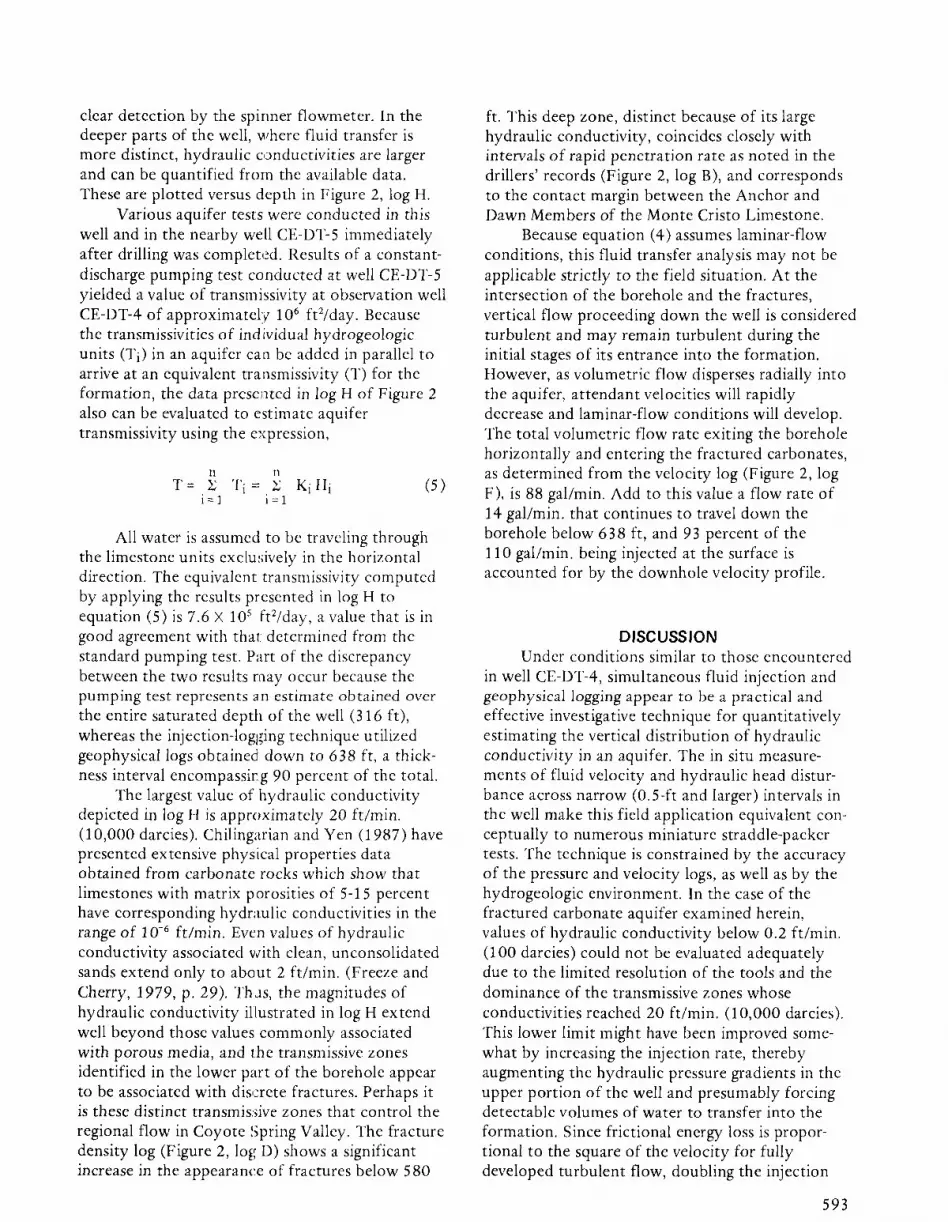
SIMULTANEOUS FLUID INJECTION AND GEOPHYSICAL LOGGING

Water was injected into well CE-DT-4 at the rate of 110 gal/min. after being pumped from well CE-DT- 5 located about 330 ft to the east (Figure 1). Hydraulic pressure buildup in test well CE-DT-4 was monitored with a stationary transducer placed 20 ft below static water level. The early time transient response due to factors such as wellbore storage and skin effects quickly dissipated, and pressure reached a quasi-steady state after only a few minutes. However, logging was not started for several hours to ensure the complete stabilization of the pressure and flow fields associated with this magnitude of injection. With the flow rate at land surface maintained at a constant 110 gal/min through the 10.4-in. diameter borehole, fluid velocity entering the well was anticipated to be approximately 25 ft/min. Because this speed is beyond the range of the heat-pulse flowmeter, a spinner flowmeter was used to obtain a continuous log of fluid velocity down the borehole. Logging speed was 30 ft/min., and logs were run while trolling both up and down the well. The resulting velocity log is shown in Figure 2 (log F), where values refer to downward fluid movement.

While injection continued and stable condi­tions persisted, a pressure log again was run in the well using the transducer that had been calibrated earlier. The rise in hydraulic head during injection was found to be approximately 3 in. The logs were digitized at 0.5-ft intervals, and the head differences between the dynamic and initial pressure profiles were computed. This differential pressure log is presented in Figure 2 as log G. Obtaining accurate differential pressure measurements over a 300-ft interval may be difficult when large absolute pressures and small differences are involved. How­ever, this can be achieved with a good calibration log at initial conditions and with an exact and repeatable depth-monitoring system connected to the logging tool.

Although downward flow was detected in the well with the heat-pulse flowmeter prior to injection and the disturbed temperature profile provided supporting evidence of dynamic conditions, the well was considered to be static before the onset of fluid injection for the purposes of this investigation. This is because: (1) the temperature log is highly sensitive to vertical fluid movement and can be significantly disturbed by slow velocities (Becker and others, 1985); and (2) the velocity values of 0.5 ft/min. or less initially measured with the heat­pulse flowmeter are within the limits of uncertainty

590

of the spinner tool. Thus, velocities of this magni­tude would have no recognizable impact on the velocity profile obtained during injection at the 110 gal/min. rate.

It should be noted that the nearby pumped well, CE-DT-5, experienced no discernible drawdown during this test. In an earlier constant­discharge test designed to measure aquifer transmissivity, 3,400 gal/min. were pumped from well CE-DT-5 for 8.3 days, and a maximum draw­down of 0.38 ft was recorded in observation well CE-DT-4 (Ertec Western, Inc., 1981). Given these magnitudes of pumping rate, pumping time, and resulting drawdown, it is unlikely that pumping well CE-DT-5 at only 11 0 gal/min. for several hours would significantly disturb the local flow field at well CE-DT-4.

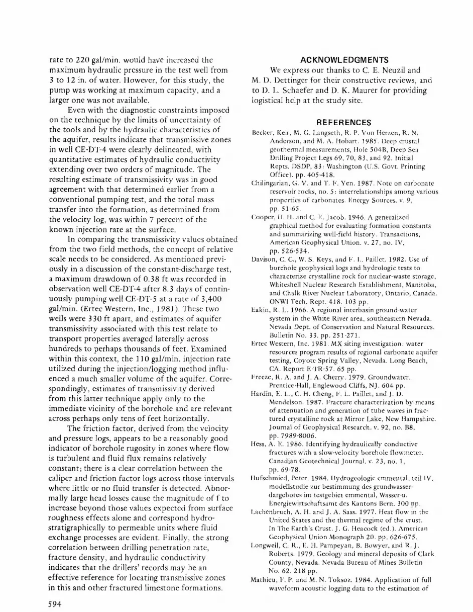
GEOPHYSICAL LOG ANALYSES AND RESULTS

Examination of the velocity log in Figure 2 (log F) shows that, across the interval between 355 and 580 ft, velocity remains relatively unchanged at approximately 24 ft/min. This is followed by sharp reductions in velocity at 580, 590, and 630 ft, where fluid exits the borehole. The differential pressure log depicts a nearly vertical profile from 355 to 480 ft, broken by two distinct offsets at 370 and 425 ft (shown by dashed lines on log). From 480 to 580 ft, a gradual decrease in differ­ential head occurs as frictional losses accumulate. At the 580 and 625-ft depths, more significant decreases in differential pressure are evident, each followed by an interval of little pressure change.

The decline in differential pressure with depth in the borehole represents a frictional energy loss that is a function of fluid velocity. This head loss can be expressed in terms of a proportionality constant known as the friction factor.

6h f=-----

(LID) (y2/2g)

where f = friction factor (dimensionless);

(1)

6h = hydraulic head loss (L); L = length of borehole interval (L); D = diameter of borehole (L); Y = fluid velocity (LIT); and g = gravitational constant (LlT2). The parameter f was developed by Moody (1944) to evaluate frictional energy losses in pipes. A Moody diagram (e.g., White, 1979, p. 333) presents the friction factor as a function of Reynolds number (Re) and surface roughness. The dimensionless Reynolds number is defined by: Re = YDlv, where v = kinematic viscosity of water (L 2/T).

For laminar flow (Re < 2,3 1)0), the friction factor is inversely proportional to the Reynolds number; specifically,

f = 64/Re.

Combining equations (1 ) and (2), one obtains,

(2 )

(3)

Equation (3) illustrates that frictlonal energy losses are proportional to the fluld velocity. This relation is true for laminar flow through pipes as well as through porous media, as represc nted by Darcy's law. For fully developed turbulnt flow, hydraulic­head decline becomes proportiolial to the square of the velocity [equation (l)[ . In tltis Nevada study, where 110 gal/min. was being injected into well CE-DT-4, a Reynolds number of 37,000 defined turbulent flow across the uppermost depth interval from 355 to 580 ft. Although bc,rehole velocities began to decrease below 580 ft, ]ow remained turbulent down to 635 ft where Re was 6,270.

Low-amplitude, high·frequency fluctuations in velocity were recorded when 1 he spinner tool remained stationary in the well, thereby indicating turbulent flow conditions; turbulent flow is charac­terized by temporal variatlons in velocity at a single point. Thus, the small, spa.tial-sc de fluctuations evident in the velocity log are probably the result of the turbulent nature of the local flow field as it responded to the substantial ngosity of the borehole wall. Had the injection rate been reduced sufficiently to permit lamlnar flow conditions to prevail, these oscillations would have been reduced or eliminated, and the high resolution heat-pulse flowmeter could have been used to obtain a velocity profile. However, the dist'lrbanc e in the hydraulic­pressure profile resulting from this lower injection rate would have been so small a~ to be below the sensitivity of the pressure tool and be almost indistinguishable from the initial profile. Thus, a trade-off had to be made becau5e the hydraulic characteristics of the aquifer cOllstrained the logging options. When formation transmissivity is large, the injection rate required to signifi :antly disturb the background pressure distribution induces turbulence and produces downhole velociti:s whose magni­tudes effectively prevent the usc: of the heat-pulse flowmeter.

Values of f can be comput ~d from the velocity and differential pressure logs by using equation (1). This was done usillg average values taken across individual 5-ft deph intervals, and the resulting profile of friction factIH-versus-depth is presented in Figure 3. The negative values of f need

Diameter, Inches

400

r:

~ 500

450

550

600

500 650

Fig. 3. Correlation of friction factor with caliper log. Peaks A are due to surface roughness; peak B is due to fluid exchange.

to be discounted since they correspond to small­scale variations in pressure, caused by turbulence, that erroneously indicate slight gains in hydraulic head with increasing depth for a few intervals. Examination of this log in conjunction with the caliper log shows a correlation between friction factor and borehole rugosity (Figure 3). The values of friction factor computed across relatively unfractured, competent sections of limestone are quite small « 0.2) when observed within the context of an open borehole environment. For comparison, values of f in the range of 0.2 are considered to be large in plumbing applications, where friction factors for pipes with a high surface roughness and a comparable Reynolds number are commonly less than 0.1 (see Moody diagram). This borehole, therefore, offers significantly more resistance to flow than does a "rough" pipe.

Su bstantial breakouts and fractures such as those seen at 365 ft and 425 ft produce sizeable pressure drops and correspondingly large increases in the values of f. The caliper log shown in Figure 3 is an analog record, included here because it shows more detail than does the digitized log (Figure 2, log C) that consists of values of diameter obtained every 6 in. As borehole rugosity becomes more severe in the interval between 480 and 580 ft, the value of f exhibits numerous positive deflections. Very large values of f also appear at 590 ft and 620 ft. Across these two zones, apparent frictional resistance acquires an additional component. Along with the pressure drop attributed to surface rough­ness of the borehole wall, a secondary head-loss effect is produced when some of the injected water exits the well and enters the formation, as can be observed from the velocity log.

591

The profile of friction factor provides an additional source of information from which to interpret the more conventional geophysical logs when vertical flow down the well is considered to be turbulent. When no water enters or leaves the formation, and fluid velocity in the borehole remains approximately constant, the computed value of friction factor is a measure of relative borehole rugosity. When fluid exchange occurs across the borehole-formation interface, frictional resistance becomes abnormally high. Corresponding values of friction factor reflect this condition and, as such, help identify transmissive zones. Note that when flow is laminar, the friction factor is a function of Re only [equation (2)] and is independent of surface roughness.

The differential pressure and velocity logs shown in Figure 2 can be analyzed further to arrive at estimates of hydraulic conductivity across arbitrary depth intervals in the aquifer. Because the logs were routinely digitized at o. 5-ft intervals, the formation can theoretically be divided into hori­zontallayers not less than 1 ft thick (Figure 4). However, the high-frequency, low-variance fluctua­tions in fluid velocity and pressure as a function of depth made the use of such thin intervals impractical. For the following analysis, mean values of velocity and hydraulic head were com­puted over 10-ft intervals (moving average) to smooth out the responses of the logging tools. Volumetric flow into or out of the formation at each interval (6Qj) is, from conservation of mass, the difference between the vertical flows

i-1

2----~

3-----f'

i+ 1

Fig. 4. Diagram of horizontally layered hydraulic conduc­tivity model [refer to equations (4) and (5)1.

592

traveling down the borehole measured above and below the zone of interest (Q2 - Q3). The pressure change required to induce this fluid transfer is obtained directly from the differential pressure log, since this is a record of the pressure disturbance above hydrostatic that was generated by the onset of injection. Hydraulic conductivity at each interval can be computed subsequently, assuming strictly horizontal flow, by using the transient expression developed by Cooper and] acob (1946).

6Q 2.25 KHt '12 (4) K = In [ 1

27TH (6 P ) R 2 S

where K = hydraulic conductivity (LIT); 6Q = horizontal volumetric flow across formation (L3/T); H = thickness of interval (L); 6p = change in head from static condition (L); t = time since onset of injection (T); R = borehole radius (L); and S = storativity (dimensionless).

Equation (4) is valid for large time t, or when R 2 S/4KHt < 0.01. In this case, t was roughly equal to 200 minutes, a value large enough to allow the ratio 6 Q/6 P to reach a quasi-steady state. The storativity of the limestone aquifer at this site, assuming a thickness of 1000 ft, is estimated to be on the order of 10-4 (Ertec Western, Inc., 1981). Proportionally, the storativity of each 10-ft thick layer is taken to be 10-6 . This value is not well constrained and likely can vary by ± an order of magnitude. Fortunately, the storativity appears in the logarithmic term of equation (4), thereby making the parameter of primary interest, the hydraulic conductivity, relatively insensitive to changes in S. Applying equation (4) to the velocity and pressure data depicted in the logs yields a series of hydraulic conductivity values across the formation in lO-ft sequences. Because K appears on both sides of this equation, values of hydraulic conductivity are computed iteratively.

In the uppermost part of the well, downhole fluid velocity remains virtually unchanged. There is, therefore, no detectable fluid exchange across the borehole-formation interface, even though differential heads are at their highest. According to equation (4), the corresponding values of hydraulic conductivity are too small to be resolved accurately given the limits of uncertainty in the in situ velocity and pressure measurements. The lower limit of hydraulic conductivity that can be evaluated under the conditions imposed by this field technique and by the particular hydrogeological characteristics of the study site seems to be about 0.2 ft/min. Hydraulic conductivities smaller than this prohibit the proper volume of fluid exchange necessary for

clear detection by the spinner flowmeter. In the deeper parts of the well, where fluid transfer is more distinct, hydraulic conductivities are larger and can be quantified from the available data. These are plotted versus depth in Figure 2, log H.

Various aquifer tests were conducted in this well and in the nearby well CE-DT-5 immediately after drilling was complet(~d. Results of a constant­discharge pumping test conducted at well CE-DT-5 yielded a value of transmissivity at observation well CE-DT-4 of approximately 106 ft 2/day. Because the transmissivities of ind ividual hydrogeologic units (Tj) in an aquifer can be added in parallel to arrive at an equivalent transmissivity ('1') for the formation, the data presented in log H of Figure 2 also can be evaluated to estimate aquifer transmissivity using the expression,

n n T = 1: Ti = 1: Ki Hi (5 )

j co 1 i = 1

All water is assumed to be traveling through the limestone units exclmivcly in the horizontal direction. The equivalent transmissivity computed by applying the results presented in log H to equation (5) is 7.6 X 105 fe/day, a value that is in good agreement with that determined from the standard pumping test. Part of the discrepancy between the two results may occur because the pumping test represents 3 n estimate obtained over the entire saturated depth of the well (316 ft), whereas the injection-logging technique utilized geophysical logs obtained down to 638 ft, a thick­ness interval encompassir g 90 percent of the total.

The largest value of hydraulic conductivity depicted in log H is approximately 20 ft/min. (10,000 darcies). Chilingarian and Yen (1987) have presented extensive physical properties data obtained from carbonate rocks which show that limestones with matrix porosities of 5-15 percent have corresponding hydraulic conductivities in the range of 10-6 ft/min. Even values of hydraulic conductivity associated with clean, unconsolidated sands extend only to about 2 ft/min. (Freeze and Cherry, 1979, p. 29). ThJs, the magnitudes of hydraulic conductivity illustrated in log H extend well beyond those values commonly associated with porous media, and the transmissive zones identified in the lower part of the borehole appear to be associated with discrete fractures. Perhaps it is these distinct transmissive zones that control the regional flow in Coyote ~;pring Valley. The fracture density log (Figure 2, log D) shows a significant increase in the appearance of fractures below 580

ft. This deep zone, distinct because of its large hydraulic conductivity, coincides closely with intervals of rapid penetration rate as noted in the drillers' records (Figure 2, log B), and corresponds to the contact margin between the Anchor and Dawn Members of the Monte Cristo Limestone.

Because equation (4) assumes laminar-flow conditions, this fluid transfer analysis may not be applicable strictly to the field situation. At the intersection of the borehole and the fractures, vertical flow proceeding down the well is considered turbulent and may remain turbulent during the initial stages of its entrance into the formation. However, as volumetric flow disperses radially into the aquifer, attendant velocities will rapidly decrease and laminar-flow conditions will develop. The total volumetric flow rate exiting the borehole horizontally and entering the fractured carbonates, as determined from the velocity log (Figure 2, log F), is 88 gal/min. Add to this value a flow rate of 14 gal/min. that continues to travel down the borehole below 638 ft, and 93 percent of the 110 gal/min. being injected at the surface is accounted for by the downhole velocity profile.

DISCUSSION Under conditions similar to those encountered

in well CE-DT-4, simultaneous fluid injection and geophysical logging appear to be a practical and effective investigative technique for quantitatively estimating the vertical distribution of hydraulic conductivity in an aquifer. The in situ measure­ments of fluid velocity and hydraulic head distur­bance across narrow (0.5-ft and larger) intervals in the well make this field application equivalent con­ceptually to numerous miniature straddle-packer tests. The technique is constrained by the accuracy of the pressure and velocity logs, as well as by the hydrogeologic environment. In the case of the fractured carbonate aquifer examined herein, values of hydraulic conductivity below 0.2 ft/min. (100 darcies) could not be evaluated adequately due to the limited resolu tion of the tools and the dominance of the transmissive zones whose conductivities reached 20 ft/min. (10,000 darcies). This lower limit might have been improved some­what by increasing the injection rate, thereby augmenting the hydraulic pressure gradients in the upper portion of the well and presumably forcing detectable volumes of water to transfer into the formation. Since frictional energy loss is propor­tional to the square of the velocity for fully developed turbulent flow, doubling the injection

593

rate to 220 gal/min. would have increased the maximum hydraulic pressure in the test well from 3 to 12 in. of water. However, for this study, the pump was working at maximum capacity, and a larger one was not available.

Even with the diagnostic constraints imposed on the technique by the limits of uncertainty of the tools and by the hydraulic characteristics of the aquifer, results indicate that transmissive zones in well CE-OT-4 were clearly delineated, with quantitative estimates of hydraulic conductivity extending over two orders of magnitude. The resulting estimate of transmissivity was in good agreement with that determined earlier from a conventional pumping test, and the total mass transfer into the formation, as determined from the velocity log, was within 7 percent of the known injection rate at the surface.

In comparing the transmissivity values obtained from the two field methods, the concept of relative scale needs to be considered. As mentioned previ­ously in a discussion of the constant-discharge test, a maximum drawdown of 0.38 ft was recorded in observation well CE-OT-4 after 8.3 days of contin­uously pumping well CE-D1'-5 at a rate of 3,400 gal/min. (Ertec Western, Inc., 1981). Thcse two wells were 330 ft apart, and estimates of aquifer transmissivity associated with this test relate to transport properties averaged laterally across hundreds to perhaps thousands of feet. Examined within this context, the 110 gal/min. injection rate utilized during the injection/logging method influ­enced a much smaller volume of the aquifer. Corre­spondingly, estimates of transmissivity derived from this latter technique apply only to the immediate vicinity of the borehole and are relevant across perhaps only tens of feet horizontally.

The friction factor, derived from thc velocity and pressure logs, appears to be a reasonably good indicator of borehole rugosity in zones where flow is turbulent and fluid flux remains relatively constant; there is a clear correlation between the caliper and friction factor logs across those intervals where little or no fluid transfer is detected. Abnor­mally large head losses cause the magnitude of f to increase beyond those values expected from surface roughness effects alone and correspond hydro­stratigraphically to permeable units where fluid exchange processes are evident. Finally, the strong correlation between drilling penetration rate, fracture density, and hydraulic conductivity indicates that the drillers' records may be an effective reference for locating transmissive zones in this and other fractured limestone formations.

594

ACKNOWLEDGMENTS We express our thanks to C. E. Neuzil and

M. D. Dettinger for their constructive reviews, and to D. L. Schaefer and O. K. Maurer for providing logistical help at the study site.

REFERENCES Becker, Keir, M. G. L.angseth, R. P. Von Herzen, R. N.

Anderson, and M. A. Hobart. 1985. Deep crustal geothermal measurements, Hole 504B, Deep Sea Drilling Project Legs 69,70,83, and 92. Initial Repts. DSDP, 83: Washington (U.S. Govt. Printing Office). pp. 405-418.

Chilingarian, G. V. and T. F. Yen. 1987. Note on carbonate reservoir rocks, no. 5: interrelationships among various properties of carbonates. Energy Sources. v. 9, pp.51-65.

Cooper, H. H. and C E. Jacob. 1946. A generalized graphical method for evaluating formation constants and summarizing well-field history. Transactions, American Geophysical Union. v. 27, no. IV, pp.526-534.

Davison, C C, W. S. Keys, and F. L. Paillet. 1982. Usc of borehole geophysical logs and hydrologic tests to characterize crystalline rock for nuclear-waste storage, Whiteshell Nuclear Research Establishment, Manitoba, and Chalk River Nuclear Laboratory, Ontario, Canada. ON WI Tech. Rept. 4]8.103 pp.

Eakin, R. L. 1966. A regional interbasin ground-water system in the White River area, southeastern Nevada. Nevada Dept. of Conservation and Natural Resources. Bulletin No. 33. pp. 251-271.

Ertec Western, Inc. 1981. MX siting investigation: water resources program results of regional carbonate aquifer testing, Coyote Spring Valley, Nevada. Long Beach, CA. Report E-TR-57. 65 pp.

Freeze, R. A. and J. A. Cherry. 1979. Groundwater. Prentice-Hall, Englewood Cliffs, NJ. 604 pp.

Hardin, E. L., C H. Cheng, F. L. Paillet, and]. D. Mendelson. 1987. Fracture characterization by means of attenuation and generation of tube waves in frac­tured crystalline rock at Mirror Lake, New Hampshire. Journal of Geophysical Research. v. 92, no. B8, pp. 7989-8006.

Hess, A. E. 1986. Identifying hydraulically conductive fractures with a slow-velocity borehole flowmeter. Canadian Geotechnical Journal. v. 23, no. 1, pp.69-78.

Hufschmied, Peter. 1984. Hydrogeologie emmcntal, teil IV, modellstudie zur bestimmung des grundwasser­dargebotes im testgebiet emmental, Wasser-u. Energiewirtschaftsamt des Kantons Bern. 300 pp.

Lachenbruch, A. H. and]. A. Sass. 1977. Heat flow in the United States and the thermal regime of the crust. In The Earth's Crust.]. G. Heacock (ed.). American Geophysical Union Monograph 20. pp. 626-675.

Longwell, C. R., E. H. Pampeyan, B. Bowyer, and R. J. Roberts. 1979. Geology and mineral deposits of Clark County, Nevada. Nevada Bureau of Mines Bulletin No. 62. 218 pp.

Mathieu, F. P. and M. N. Toksoz. 1984. Application of full waveform acoustic logging data to the estimation of

reservoir permeability. Proceedings, Soc. of Explora­tion Geophysicists 54th International Meeting, Atlanta, GA. pp. 9-12.

Moody, L. F. 1944. Friction flctors for pipe flow. Transac­tions, American Society of Mechanical Engineers. v. 66, pp. 671-684.

Paillet, F. L. 1983. Acoustic characterization of fracture permeability at Chalk River, Ontario. Canadian Geotechnical Journal. v. 20, no. 3, pp. 468-476.

Paillet, F. L., W. S. Keys, and A. E. Hess. 1985. Effects of lithology on acoustic televiewer log quality and fracture interpretation. Transactions, Soc. of Professional Well Log Analysts 26th Annual Logging Symposium, Dallas, TX. pp. J]]1-]]J31.

Paillet, F. L., C. H. Cheng, A. E. Hess, and E. L. Hardin. 1986. Comparison of fracture permeability estimates based on tube-wave generation in vertical seismic profiles, acoustic waveform-log attenuation, and pumping-test analysis. Pcoeeedings, National Water Well Association Confer,~nce on Borehole Geophysical Methods, Denver, CO. pp. 398-416.

Rehfeldt, K. R. and L. W. Gelhar. 1987. Measurements of the small scale hydraulic conductivity of heteroge­neous unconsolidated porous material in fully screened wells using a borehole fbwmeter. Abs. EOS, Trans., American Geophysical Union. v. 68, no. 16, p. 303.

Sam mel, E. A. 1968. Convective flow and its effect on temperature logging in small-diameter wells. Geophysics. v. 33, no. 6, pp. 1004-1012.

Schimschal, Ulrich. 1981. Flowmeter analysis at Raft River, Idaho. Ground Water. v. 19, no. 1, pp. 93-97.

Syms, M. c., P. H. Syms, and P. F. Bixley. 1982. Interpreta­tion of flow measurements in geothermal wells with­out caliper data. Log Analyst. v. 23, no. 2, pp. 34-45.

Urban, T. C. and W. H. Diment. 1985. Convection in bore­holes: limits on interpretation of temperature logs and methods for determining anomalous fluid-flow. Proceedings, National Water Well Association Confer­ence on Borehole Geophysical Methods, Worthington, OH. pp. 399-415.

White, F. M. 1979. Fluid Mechanics. McGraw-Hill Book Co., NY. 701 pp.

Zeigler, T. W. 1976. Determination of rock mass perme­ability. U.S. Army Corps of Engineers Waterways Experiment Station, Vicksburg, Miss. Tech. Rept. S-76-2. 112 pp.

Zemanek, J., R. L. Caldwell, E. E. Glenn, S. V. Halcomb, L. J. Norton, and A.J.D. Strauss. 1969. The borehole televiewer-a new logging concept for fracture location and other types of borehole inspection. Journal of Petroleum Technology. v. 21, no. 6, pp. 762-774.

* * * Roger JI. Morin is a Geophysicist with the Borehole

Geophysics Research Project, Water Resources J)ivision, Denver, Colorado. lIe obtained B.S'. and M,S, degrees in Mechanical Fngineering from the Universi~y afMaine and a Ph,D, in Ocean h'ngineering from the University of Rbode Island, where he studied marine soil mechanics. f Ie spent two years as a post-doctoral research scientist at the Massachusetts Institute of Tecbnology before joining the u.s. Geological Survey in 1984. lIis researcb interests include the physical properties of soil and rock, and their influence upon geologic processes,

Alfred F. Iless is an Wectronic h'Y/gineer with tbe Water Resources Division of the U.S. Geological Survey in Denver, Colorado, where he develops instruments and tecbniques for borehole geophysical investigations, After receiving a B,A. in Physics from Columbia Union College, Mr, Hess was employed as an engineering physicist for the Radio Standards Division of the National Bureau of Standards wbere be developed radio frequency standards and supporting instrumentation.

Frederick L. Paillet is Project Cbief: Borebole Geopbysics Researcb Project, Water Resources Division, Denver, Colorado. l/e obtained bis B.S, and M.S, degrees in Mecbanical h'ngineering at the Universi~y of R ocbester prior to entering active military service as a Civil L~'ngineer­ing Officer in 1970. He subsequently completed require­ments for a Pb. D, at the University of R ocbester in 1974 under a U.S'. A ir Force scbolarsbip. Paillet thcn .Ipent two years as a faculty member with tbe Department of Geology, Wright State University, Ohio, before joining the u.s. Geological Survey in 1978.

595