Designing Composites with Target Effective Young’s Modulususing Reinforcement Learning

Aldair E. Gongora∗Siddharth Mysore∗agongora@bu.edusidmys@bu.eduBoston University

Boston, Massachusetts, USA

Beichen Li∗Wan Shou

Wojciech MatusikMassachusetts Institute of Technology

Cambridge, Massachusetts, USA

Elise F. MorganKeith A. BrownBoston University

Boston, Massachusetts, USA

Emily WhitingBoston University

Boston, Massachusetts, USAwhiting@bu.edu

ABSTRACTAdvancements in additive manufacturing have enabled design andfabrication of materials and structures not previously realizable. Inparticular, the design space of composite materials and structureshas vastly expanded, and the resulting size and complexity haschallenged traditional design methodologies, such as brute forceexploration and one factor at a time (OFAT) exploration, to findoptimum or tailored designs. To address this challenge, supervisedmachine learning approaches have emerged to model the designspace using curated training data; however, the selection of thetraining data is often determined by the user. In this work, we de-velop and utilize a Reinforcement learning (RL)-based frameworkfor the design of composite structures which avoids the need foruser-selected training data. For a 5 × 5 composite design spacecomprised of soft and compliant blocks of constituent material,we find that using this approach, the model can be trained using2.78% of the total design space consists of 225 design possibilities.Additionally, the developed RL-based framework is capable of find-ing designs at a success rate exceeding 90%. The success of thisapproach motivates future learning frameworks to utilize RL forthe design of composites and other material systems.

1 INTRODUCTIONEngineered composite materials and structures are able to achievesuperior mechanical performance in comparison to their individ-ual constituents [Dimas et al. 2013; Ghiasi et al. 2010, 2009; Lakes1993; Wegst et al. 2015]. The ability to tailor their design to meetperformance requirements has resulted in their widespread applica-tion in the aerospace, automotive, and maritime industries [Fratzland Weinkamer 2007; Gu et al. 2016b; Guoxing and Tongxi 2004].While the design process has previously relied on domain expertise,bio-mimicry, brute force exhaustive search, or iterative trial anderror [Yeo et al. 2018], recent advancements in additive manufactur-ing (AM) have tremendously enhanced the realizable design spaceand challenged the conventional approaches to exploring designspaces [Gu et al. 2017a,b; Libonati et al. 2016]. The design freedomafforded by AM has significantly expanded the design space byenabling the fabrication of composites with arbitrary geometry and∗Authors contributed equally to this research.

material distributions spanning various length scales. With thisexpansion comes challenges such as how to rapidly and efficientlyexploring the vast and complex design space for optimal or targetedmechanical performance. While more traditional optimization tech-niques have been proposed, their robustness is often limited by thecomplexity of the design problems.

In order to overcome some of these design challenges, specifi-cally those pertaining to exploring and modeling the design space,we propose using reinforcement learning (RL). RL algorithms learnto model the problem space through interaction and can be opti-mized to solve specific controls problems. We present a designframework that utilizes RL to design and find composite designsthat meet a specified performance target (Figure 1 A). While themodels learned do not provide a general solution for arbitrary com-posite design problems, our work offers a guideline on successfullyframing design problems as RL problems. While learning-basedframeworks can be more data and computationally intensive thanany one optimization run using more traditional techniques, theyoffer potential benefits at scale, where inference after training canbe significantly less expensive.

In this work, we mainly consider a 2-material composite designproblem where we attempt to optimize the composite design inorder to achieve specific material properties. The RL-based designframework, takes an initial composite design and user-specifieddesired material properties, comprising of target elastic propertiesand material composition, and iteratively modifies the design untilthe desired properties are satisfied. The design is parameterized asa 2D grid of constituent materials and the learned policy adjuststhe design one grid cell at a time. This naturally upper-boundsthe number of required interactions by the number of cells in thedesign grid. We demonstrate that, despite only exploring less than5% of the design space for our design problem during training, thelearned RL policies are able to successfully solve over 95% of thedesign tasks in testing.

2 RELATEDWORKTo overcome the challenges of design optimization in additive man-ufacture, techniques combining computational methods and opti-mization algorithms, such as topology optimization, have enabled

arX

iv:2

110.

0526

0v1

[co

nd-m

at.m

trl-

sci]

7 O

ct 2

021

B C

L

L

xx

StiffCompliant

Alternative designs parallel

series

D

Ø <

0.5

Ø >

0.5

A

δ

StiffCompliant0 1

Agent

Environment

UserState

Reward

Egoal

FEA

Action

Design

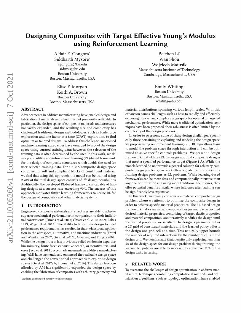
Figure 1: The Reinforcement Learning (RL) framework for the design of parametric composites consisting of stiff and compli-ant building blocks of constituent material to meet a specified target modulus 𝐸𝑔𝑜𝑎𝑙 (A). The design space considered in thiswork is built from a 5 by 5 arrangement of blocks of side length 𝑥 where the composite sample has side lengths 𝐿 (B). Thedesign space consists of parallel and series designs (C) with a volume fraction of stiff constituent material 𝜙 = 0.40. The designspace also consists of alternative designs where the majority of the compliant or stiff constituent material is concentrated atthe center, sparsely distributed along the edges, or randomly distributed (D).

the design of tailored composites with targeted structural and mate-rial design requirements such as elastic properties, Poisson’s ratio,and tunable stress-strain curves [Chen et al. 2018; Gu et al. 2016a;Sigmund and Maute 2013; Sigmund and Petersson 1998; Zhu et al.2017]. Although these approaches have achieved success in specificclasses of problems, they are often limited by the complexity of thedesign space and associated computational cost.

Recently, machine learning (ML) based design frameworks haveachieved success in the design and discovery of materials and struc-tures with optimal or targeted properties [Abueidda et al. 2019;Chen and Gu 2019; Gongora et al. 2021, 2020; Gu et al. 2018; Maoet al. 2020; Nikolaev et al. 2016]. Specifically in the field of compos-ite design, ML techniques utilizing artificial neural networks anddeep learning have been used in classification applications [Chenand Gu 2020] and in inverse design applications [Yang et al. 2020].These applications have demonstrated the ability to train ML-basedmodels with a fraction of observations from the design space to suc-cessfully assess or predict mechanical performance. A non-trivialchallenge that faces the development of accurate ML models isthe selection of appropriate training data, as inferior models canemerge from training on insufficient or poorly selected data. Inpractice, the training data is often selected using uniform randomsampling or a design of experiments approach, such as Latin hyper-cube sampling; however, the applicability of these approaches are

limited by the size of the design space and the computational orexperimental cost [Jin et al. 2020; Silver et al. 2017].

The dependence of the success of a ML model on appropriatelyselected training data motivates the development and applicationof an approach that automatically selects the training data. Anapproach that can address this challenge is reinforcement learning(RL) [Andrychowicz et al. 2017; Botvinick et al. 2019; Leinen et al.2020; Mnih et al. 2015; Popova et al. 2018]. RL models, also called RLagents, iteratively interact with a system in order to affect the stateof the system. In lieu of curating a dataset of behaviors, a rewardfunction can be defined to reflect the quality of actions taken byagents. The behavior of RL agents is conditioned to maximize the re-ceived reward. This shifts some of the burden from dataset curationto reward function engineering, but the latter can be significantlymore intuitive and tractable when dealing with large data-spaces.

3 DESIGN SPACE AND FINITE-ELEMENTANALYSIS

In order to frame composite design as a reinforcement learningproblem, we needed to establish a suitable state-space representa-tion and build an environment for the RL algorithm with whichto interact with. Training in simulation allows for faster feedbackthan fabrication and physical analysis, so we use finite elementanalysis (FEA) as our primary analytical tool for estimating design

2

CIncreasing E

0

0.5

1

2

1.5

E (GPa)

E (GPa

)

0 1.0 1.50.5 2

0.2

0.60.4

0.8

0

1

Ø

A B

0

0.5

1

2

1.5

0 0.6 0.80.2 10.4Ø

E (GPa

)

FEAExperimentAnalytical

series

0.6

RMSE = 98.7 MPa

D

parallel

series

0.2Ø

0.4 0.6 0.80 1

0.8

Ø

parallel~

1 cm

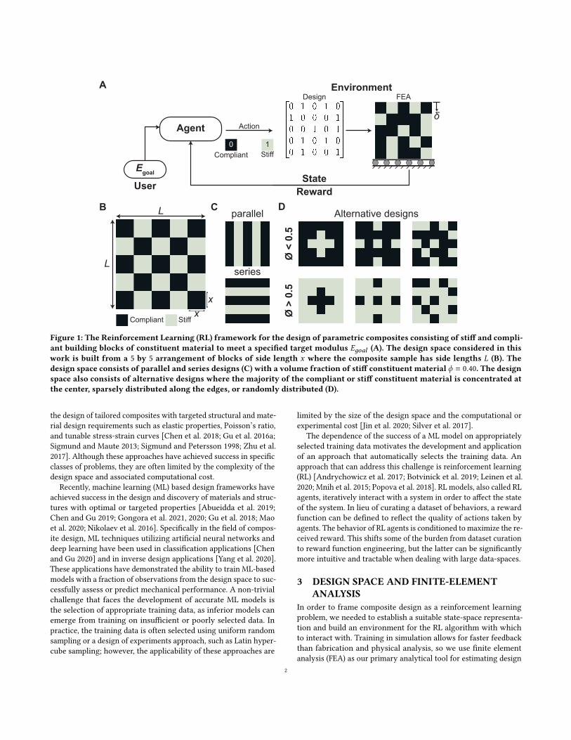
Figure 2: Fabricated composite designs with volume fraction between 𝜙 = 0 and 𝜙 = 1 with classical parallel and series com-posite designs with 𝜙 = 0.2, 0.4, 0.6, and 0.8 (A). Comparison of experimentally measured effective Young’s modulus 𝐸, FEApredicted effective Young’s modulus 𝐸, and analytical predictions of effective Young’s modulus for parallel and series com-posite designs with varying 𝜙 (B). Comparison of 𝐸 and 𝐸 for previously tested designs and five alternative designs for each𝜙 = 0.2, 0.4, 0.6, and 0.8 (C). Example designs with 𝜙 = 0.6 and 𝜙 = 0.8 in ascending order based on 𝐸 (D).

properties. Before employing the RL algorithm, it is imperative tovalidate the finite element predictions of Young’s modulus 𝐸. Thissection discusses the composite design space considered and thedevelopment and validation of FEA pipeline.

3.1 The Composite Design SpaceGiven that the set of all possible designs is large and intractable, weconsider here a more constrained problem amenable to experimen-tal validation so as to establish a viable framework for RL-automateddesign. We consider a composite design space built from a 5 × 5binary arrangement of material blocks where each block can becomposed of one of two materials that differ in their elastic mod-uli. The stiffer of these two materials we term "stiff" and the morecompliant of these materials we term "compliant". The materialblocks of the composite have a side length 𝑥 = 5mmwhile the totalcomposite has a side length 𝐿 = 25 mm and depth of 5 mm (Fig-ure 1 B). Without considering any geometric symmetries, a total of225 distinct designs exist in the composite design space. Classicalparallel and series composite designs can be found in the designspace by varying the volume fraction 𝜙 of stiff material (Figure 1 C).

Alternative designs also exist; for instance, designs where the ma-jority of the compliant or stiff constituent material is concentratedat the center, sparsely distributed along the edges, or randomlydistributed (Figure 1 D). With the ability to fabricate alternativedesigns, a range of Young’s modulus values can be achieved for agiven volume fraction.

3.2 Development and Validation of a PredictiveModel using Finite Element Analysis

The model we developed uses 2-D explicit FEA,which was imple-mented in C++ using the Taichi Graphics Library [Hu 2018], topredict the effective Young’s modulus of the composite in the 5 × 5design space. Here, we used a Neo-Hookean model for both thecompliant and stiff constituent materials and a static compressivestrain of 1e-4. The stiff and compliant constituent materials con-sidered in this work were VeroWhitePlus (VW+) and a volumepercentage mixture of 50% VW+ and 50% TangoBlackPlus (TB+),respectively. The effective Young’s modulus of the composite wasestimated from the predicted stress at a prescribed compressive

3

strain of 1e-4, which was kept constant for all simulations in thisstudy. The effective Young’s modulus was calculated by dividingthe predicted stress by the compressive strain. To simulate theuniaxial compression of the composite design, displacement bound-ary conditions were imposed on the nodes of the top surface ofthe composite. The coefficients of the Neo-Hookean model werecomputed from the Young’s modulus and Poisson’s ratio of theconstituent materials. The Young’s modulus and Poisson’s ratio ofthe stiff constituent material was 1818 MPa and 0.33, respectively,while the Young’s modulus and Poisson’s ratio of the compliant con-stituent material was 364 MPa and 0.49, respectively. Additionally,an explicit solver was selected over an implicit solver in the FEApipeline to avoid potential computational bottlenecks arising fromthe need to invert the stiffness matrix of the course of the applieddeformation in implicit analysis. In the explicit solver, the time stepwas set to 2.3e-7, which was sufficiently small to prevent numericalinstability in forward Euler integration. A fixed 2000 iterations wasused in the solver which was determined to be sufficiently large toguarantee convergence without compromising computational timebased on preliminary tests. Furthermore, the parameters used inthe solver were determined to be appropriate based on the reason-able agreement observed between Young modulus predictions andexperimental measurements.

The selected composite designs in this study were fabricatedfrom the aforementioned stiff and compliant constituent materialsand experimental measurements were taken in triplicate for eachcomposite design where 𝐸 is the mean effective Young’s modulusof the measurements. To assess the model using FEA, the predictedeffective Young’s modulus 𝐸 of selected composite designs werecompared to experimental measurements of the effective Young’smodulus 𝐸 from quasi-static uniaxial compression tests conductedon a universal testing machine (Instron 5984). The first set of se-lected composites designs were designs with only compliant con-stituent material 𝜙 = 0, only stiff constituent material 𝜙 = 1, andclassical parallel and series composite designs with 𝜙 = 0.2, 0.4, 0.6,and 0.8 (Figure 2 A). The absolute relative error between 𝐸 and 𝐸

for composite designs with 𝜙 = 0 and 𝜙 = 1 were 6.97% and 3.35%,respectively, while the average absolute relative error between 𝐸

and 𝐸 for the classical parallel and series composite designs with𝜙 = 0.2, 0.4, 0.6, and 0.8 was 12.10% (Figure 2 B). Evaluating theentire dataset with 𝜙 = 0, 0.2, 0.4, 0.6, 0.8, and 1.0, the root meansquared error (RMSE) was 101.79 MPa with an 𝑅2 = 0.96 where𝑅 is the Pearson correlation coefficient. For these composite de-signs, 𝐸 can also be analytically estimated via the Voigt and Reussapproximations for parallel and series designs, respectively. Theapproximations also yielded reasonable predictions of 𝐸 with anaverage absolute relative error of 9.07% when compared to experi-mental measurements. While the Voigt and Reuss approximationsenable rapid predictive approximations of 𝐸, the models are onlyexpected to be accurate for parallel and series composite designs.

To further assess the predictions using FEA, the 𝐸 of five alter-native designs for each 𝜙 = 0.2, 0.4, 0.6, and 0.8 were comparedto experimental measurements from uniaxial compression testing.Adding these results to the classical parallel and series dataset, theagreement between 𝐸 and 𝐸 was evaluated. The RMSE was com-puted to be 98.69 MPa with 𝑅2 = 0.97 and the average absolute

relative error between 𝐸 and 𝐸 of all the selected designs was calcu-lated to be 13.8% (Figure 2 C). Based on these results, we concludedthat the predictions of Young’s modulus from FEA were in goodagreement with experimental measurements. Interestingly, fromthe E of alternative designs with varying volume fraction, a broadrange of achievable modulus values with non-trivial designs wereobserved. Specifically, for 𝜙 = 0.6 the minimum 𝐸 was 792.3 MPaand the maximum 𝐸 was approximately 31% larger at 1.04 GPa.Additionally, for 𝜙 = 0.8, the minimum 𝐸 was 1.16 GPa and themaximum 𝐸 was approximately 24% larger at 1.44 GPa (Figure 2 D).While this range was observed for the experimental measurementsof alternative designs, brute-force evaluations of all the designssuggest that for a given𝜙 there is a range of achievable 𝐸 via alterna-tive designs. The overlap in ranges for varying 𝜙 demonstrates theability to vary performance for a given 𝜙 , which is a key factor indesigning composites to meet performance requirements. Note that𝐸 for a composite design only corresponds to quasi-static uniaxialcompression conditions. While designs such as the alternative com-posite designs may possess 𝐸 that depend on the loading direction,only quasi-static compression conditions as shown in Figure 1 Aare considered in this study.

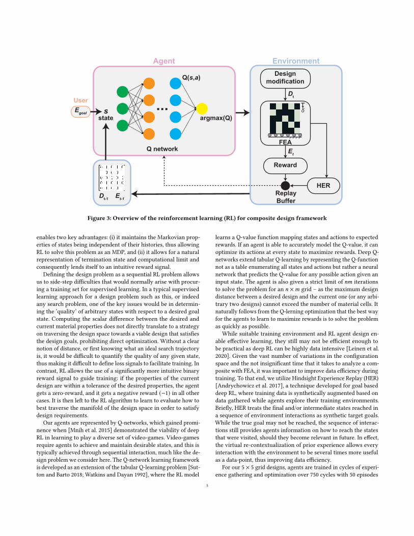
4 DEVELOPING THE REINFORCEMENTLEARNING (RL) FRAMEWORK FORCOMPOSITE DESIGN

Reinforcement learning (RL) algorithms seek to solve a sequen-tial decision-making problem, which are typically formulated as aMarkov decision process (MDP). There are two major componentsof any RL setup – (i) the training environments, and (ii) the agent(s),i.e., the learned behavior model. Agents take actions in responseto the current state, 𝑠𝑡 , of the environment and the state of theenvironment changes in response to the action taken. The agentdecides its actions by attempting to maximize the cumulative re-ward, received from the environment. In order to successfully trainan RL agent on a task, it is important to balance the complexitiesof the agent policy as well as the task environment. While morecomplex policy functions can have an increased modeling capacitywhich may allow learning of more complex tasks, this comes withincreased computational costs and training data requirements. Wedesigned our task environment with this in mind.

Figure 3 provides an overview of the RL framework developedto design composites with a target Young’s modulus 𝐸𝑔𝑜𝑎𝑙 andvolume fraction 𝜙𝑔𝑜𝑎𝑙 . We began by considering similar problemsalready solvable by RL and found close parallels with the problemof bit-flipping – i.e., modifying one binary string to match anothergiven one, one element at a time. Like in bit-flipping, our designproblem includes a current state and a desired future state, whereour 2-material design, 𝐷𝑡 , can be represented as a binary string(where an 𝑛 ×𝑚 grid can be represented by a nm-dimensional bi-nary vector). Unlike the bit-flipping problem; however, we do notknow the desired design ahead of time, only the desired proper-ties. By including the current (at iteration 𝑡 ) and desired materialproperties, 𝐸𝑡 and 𝐸𝑔𝑜𝑎𝑙 , respectively, in the state representationwe equivalently indicate necessary information about a goal stateto allow the agent to model and achieve desired material properties.Formulating the design problem as a sequential task in this way

4

Egoal

Q network

Q(s,a)

sstate

Agent

Reward

HER

argmax(Q)

Et

Dt-1

Dt

Environment

FEA

δ

Et-1ReplayBuffer

...

Designmodification

User

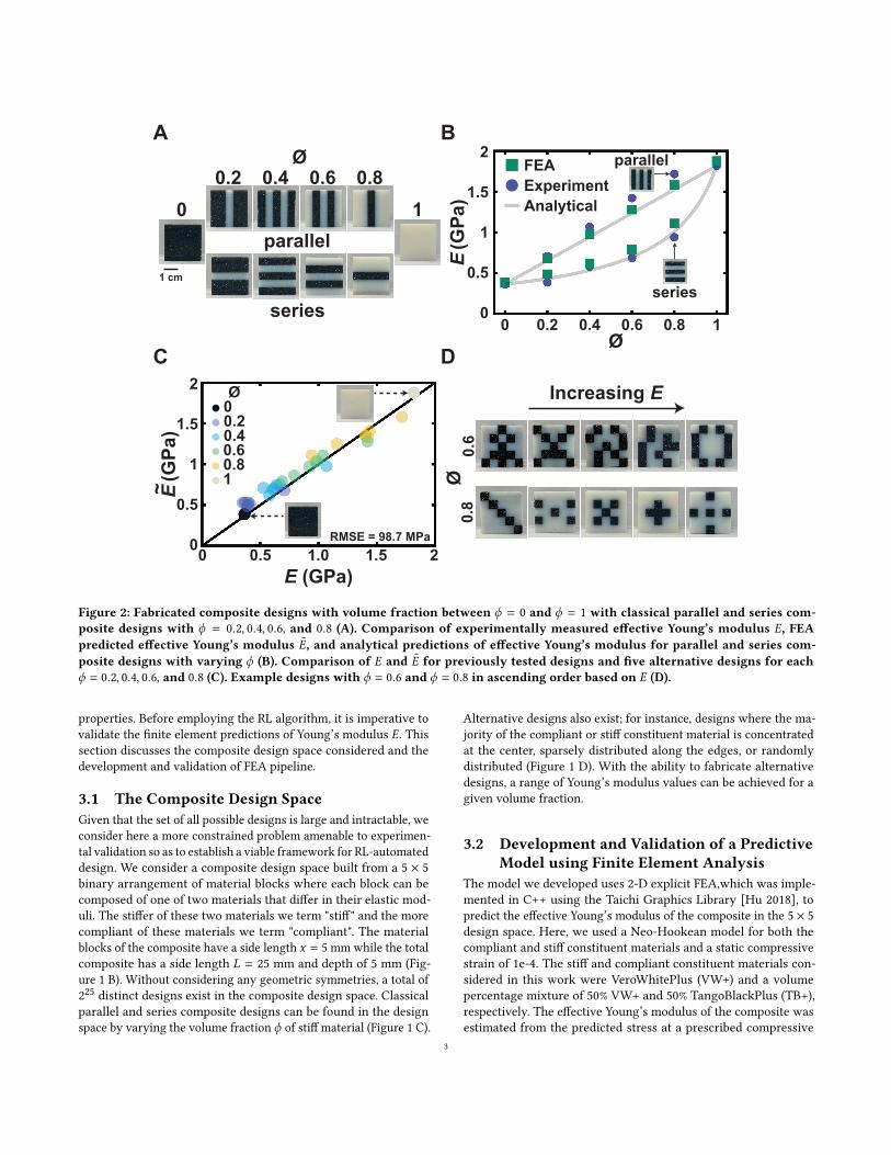
Figure 3: Overview of the reinforcement learning (RL) for composite design framework

enables two key advantages: (i) it maintains the Markovian prop-erties of states being independent of their histories, thus allowingRL to solve this problem as an MDP, and (ii) it allows for a naturalrepresentation of termination state and computational limit andconsequently lends itself to an intuitive reward signal.

Defining the design problem as a sequential RL problem allowsus to side-step difficulties that would normally arise with procur-ing a training set for supervised learning. In a typical supervisedlearning approach for a design problem such as this, or indeedany search problem, one of the key issues would be in determin-ing the ‘quality’ of arbitrary states with respect to a desired goalstate. Computing the scalar difference between the desired andcurrent material properties does not directly translate to a strategyon traversing the design space towards a viable design that satisfiesthe design goals, prohibiting direct optimization. Without a clearnotion of distance, or first knowing what an ideal search trajectoryis, it would be difficult to quantify the quality of any given state,thus making it difficult to define loss signals to facilitate training. Incontrast, RL allows the use of a significantly more intuitive binaryreward signal to guide training: if the properties of the currentdesign are within a tolerance of the desired properties, the agentgets a zero-reward, and it gets a negative reward (−1) in all othercases. It is then left to the RL algorithm to learn to evaluate how tobest traverse the manifold of the design space in order to satisfydesign requirements.

Our agents are represented by Q-networks, which gained promi-nence when [Mnih et al. 2015] demonstrated the viability of deepRL in learning to play a diverse set of video-games. Video-gamesrequire agents to achieve and maintain desirable states, and this istypically achieved through sequential interaction, much like the de-sign problem we consider here. The Q-network learning frameworkis developed as an extension of the tabular Q-learning problem [Sut-ton and Barto 2018; Watkins and Dayan 1992], where the RL model

learns a Q-value function mapping states and actions to expectedrewards. If an agent is able to accurately model the Q-value, it canoptimize its actions at every state to maximize rewards. Deep Q-networks extend tabular Q-learning by representing the Q-functionnot as a table enumerating all states and actions but rather a neuralnetwork that predicts the Q-value for any possible action given aninput state. The agent is also given a strict limit of 𝑛𝑚 iterationsto solve the problem for an 𝑛 ×𝑚 grid – as the maximum designdistance between a desired design and the current one (or any arbi-trary two designs) cannot exceed the number of material cells. Itnaturally follows from the Q-lerning optimization that the best wayfor the agents to learn to maximize rewards is to solve the problemas quickly as possible.

While suitable training environment and RL agent design en-able effective learning, they still may not be efficient enough tobe practical as deep RL can be highly data intensive [Leinen et al.2020]. Given the vast number of variations in the configurationspace and the not insignificant time that it takes to analyze a com-posite with FEA, it was important to improve data efficiency duringtraining. To that end, we utilize Hindsight Experience Replay (HER)[Andrychowicz et al. 2017], a technique developed for goal baseddeep RL, where training data is synthetically augmented based ondata gathered while agents explore their training environments.Briefly, HER treats the final and/or intermediate states reached ina sequence of environment interactions as synthetic target goals.While the true goal may not be reached, the sequence of interac-tions still provides agents information on how to reach the statesthat were visited, should they become relevant in future. In effect,the virtual re-contextualization of prior experience allows everyinteraction with the environment to be several times more usefulas a data-point, thus improving data efficiency.

For our 5 × 5 grid designs, agents are trained in cycles of experi-ence gathering and optimization over 750 cycles with 50 episodes

5

B

E (MPa)

start end

Goal: Ø = 0.40 , E = 600 MPaØ

9990.60

6300.40

Goal: Ø = 0.80 , E = 1300 MPa0.48754

0.801301

AInitial 1 2 3 4 5 6 Final

start end

Ø = 0.24E = 512 MPa

Ø = 0.52E = 808 MPa Goal: Ø = 0.20 , E = 500 MPa

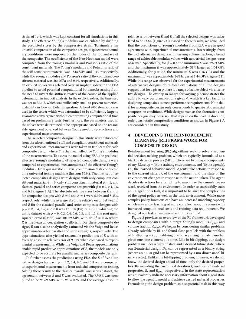
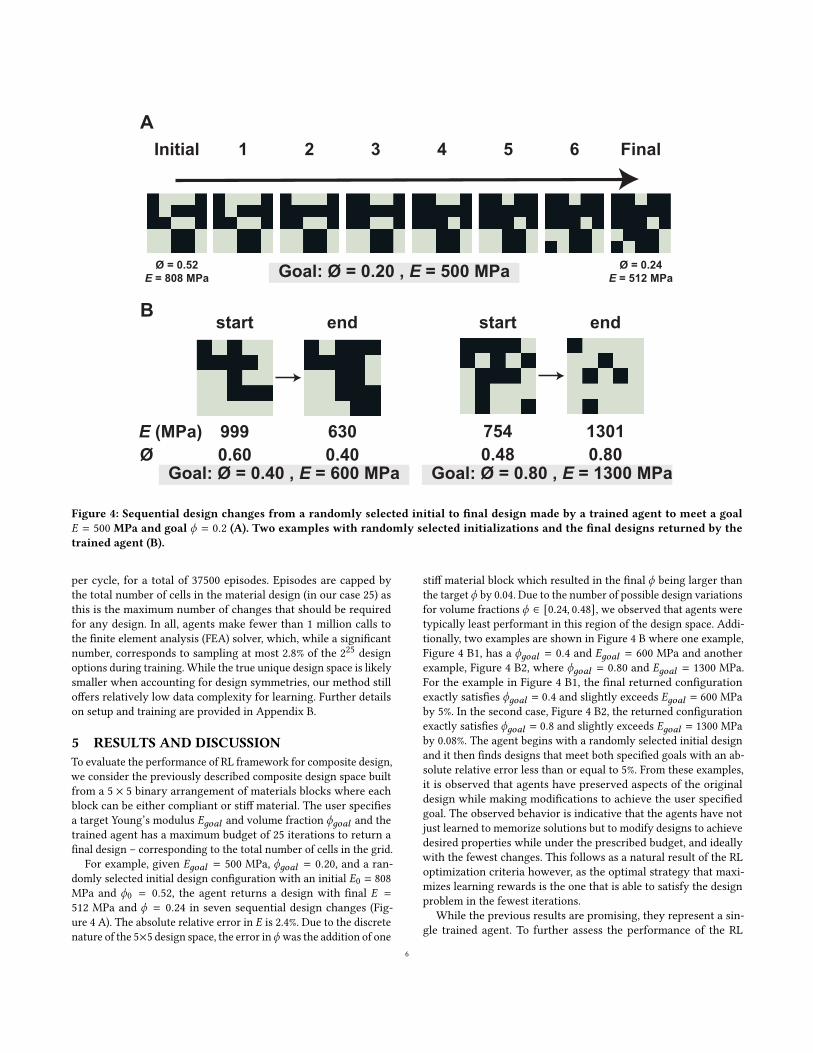
Figure 4: Sequential design changes from a randomly selected initial to final design made by a trained agent to meet a goal𝐸 = 500 MPa and goal 𝜙 = 0.2 (A). Two examples with randomly selected initializations and the final designs returned by thetrained agent (B).

per cycle, for a total of 37500 episodes. Episodes are capped bythe total number of cells in the material design (in our case 25) asthis is the maximum number of changes that should be requiredfor any design. In all, agents make fewer than 1 million calls tothe finite element analysis (FEA) solver, which, while a significantnumber, corresponds to sampling at most 2.8% of the 225 designoptions during training. While the true unique design space is likelysmaller when accounting for design symmetries, our method stilloffers relatively low data complexity for learning. Further detailson setup and training are provided in Appendix B.

5 RESULTS AND DISCUSSIONTo evaluate the performance of RL framework for composite design,we consider the previously described composite design space builtfrom a 5 × 5 binary arrangement of materials blocks where eachblock can be either compliant or stiff material. The user specifiesa target Young’s modulus 𝐸𝑔𝑜𝑎𝑙 and volume fraction 𝜙𝑔𝑜𝑎𝑙 and thetrained agent has a maximum budget of 25 iterations to return afinal design – corresponding to the total number of cells in the grid.

For example, given 𝐸𝑔𝑜𝑎𝑙 = 500 MPa, 𝜙𝑔𝑜𝑎𝑙 = 0.20, and a ran-domly selected initial design configuration with an initial 𝐸0 = 808MPa and 𝜙0 = 0.52, the agent returns a design with final 𝐸 =

512 MPa and 𝜙 = 0.24 in seven sequential design changes (Fig-ure 4 A). The absolute relative error in 𝐸 is 2.4%. Due to the discretenature of the 5×5 design space, the error in𝜙 was the addition of one

stiff material block which resulted in the final 𝜙 being larger thanthe target𝜙 by 0.04. Due to the number of possible design variationsfor volume fractions 𝜙 ∈ [0.24, 0.48], we observed that agents weretypically least performant in this region of the design space. Addi-tionally, two examples are shown in Figure 4 B where one example,Figure 4 B1, has a 𝜙𝑔𝑜𝑎𝑙 = 0.4 and 𝐸𝑔𝑜𝑎𝑙 = 600 MPa and anotherexample, Figure 4 B2, where 𝜙𝑔𝑜𝑎𝑙 = 0.80 and 𝐸𝑔𝑜𝑎𝑙 = 1300 MPa.For the example in Figure 4 B1, the final returned configurationexactly satisfies 𝜙𝑔𝑜𝑎𝑙 = 0.4 and slightly exceeds 𝐸𝑔𝑜𝑎𝑙 = 600MPaby 5%. In the second case, Figure 4 B2, the returned configurationexactly satisfies 𝜙𝑔𝑜𝑎𝑙 = 0.8 and slightly exceeds 𝐸𝑔𝑜𝑎𝑙 = 1300 MPaby 0.08%. The agent begins with a randomly selected initial designand it then finds designs that meet both specified goals with an ab-solute relative error less than or equal to 5%. From these examples,it is observed that agents have preserved aspects of the originaldesign while making modifications to achieve the user specifiedgoal. The observed behavior is indicative that the agents have notjust learned to memorize solutions but to modify designs to achievedesired properties while under the prescribed budget, and ideallywith the fewest changes. This follows as a natural result of the RLoptimization criteria however, as the optimal strategy that maxi-mizes learning rewards is the one that is able to satisfy the designproblem in the fewest iterations.

While the previous results are promising, they represent a sin-gle trained agent. To further assess the performance of the RL

6

A B

0

0.2

1

0.6

0.4

0.8

PP

i0 0.5 0.750.25 1

x106

P = 0.95

0 0.4 0.60.2 0.80

1500

500

1000

coun

t

0 800 1200400E (MPa) Ø

1

0.2

0.6

0.8

0.4

010.40.2 0.6 0.80

Ø

C

RL

Naive nearest neighborØ-biased nearest neighbor

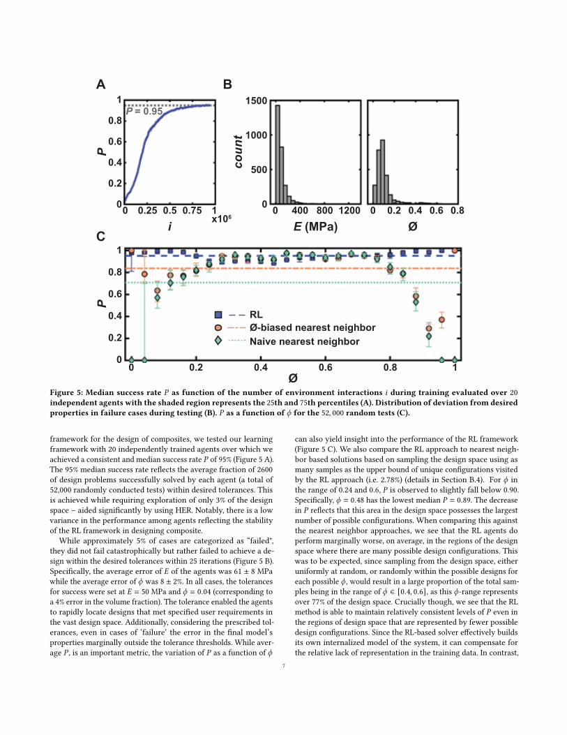
Figure 5: Median success rate 𝑃 as function of the number of environment interactions 𝑖 during training evaluated over 20independent agents with the shaded region represents the 25th and 75th percentiles (A). Distribution of deviation from desiredproperties in failure cases during testing (B). 𝑃 as a function of 𝜙 for the 52, 000 random tests (C).

framework for the design of composites, we tested our learningframework with 20 independently trained agents over which weachieved a consistent and median success rate 𝑃 of 95% (Figure 5 A).The 95% median success rate reflects the average fraction of 2600of design problems successfully solved by each agent (a total of52,000 randomly conducted tests) within desired tolerances. Thisis achieved while requiring exploration of only 3% of the designspace – aided significantly by using HER. Notably, there is a lowvariance in the performance among agents reflecting the stabilityof the RL framework in designing composite.

While approximately 5% of cases are categorized as “failed",they did not fail catastrophically but rather failed to achieve a de-sign within the desired tolerances within 25 iterations (Figure 5 B).Specifically, the average error of 𝐸 of the agents was 61 ± 8 MPawhile the average error of 𝜙 was 8 ± 2%. In all cases, the tolerancesfor success were set at 𝐸 = 50 MPa and 𝜙 = 0.04 (corresponding toa 4% error in the volume fraction). The tolerance enabled the agentsto rapidly locate designs that met specified user requirements inthe vast design space. Additionally, considering the prescribed tol-erances, even in cases of ‘failure’ the error in the final model’sproperties marginally outside the tolerance thresholds. While aver-age 𝑃 , is an important metric, the variation of 𝑃 as a function of 𝜙

can also yield insight into the performance of the RL framework(Figure 5 C). We also compare the RL approach to nearest neigh-bor based solutions based on sampling the design space using asmany samples as the upper bound of unique configurations visitedby the RL approach (i.e. 2.78%) (details in Section B.4). For 𝜙 inthe range of 0.24 and 0.6, 𝑃 is observed to slightly fall below 0.90.Specifically, 𝜙 = 0.48 has the lowest median 𝑃 = 0.89. The decreasein 𝑃 reflects that this area in the design space possesses the largestnumber of possible configurations. When comparing this againstthe nearest neighbor approaches, we see that the RL agents doperform marginally worse, on average, in the regions of the designspace where there are many possible design configurations. Thiswas to be expected, since sampling from the design space, eitheruniformly at random, or randomly within the possible designs foreach possible 𝜙 , would result in a large proportion of the total sam-ples being in the range of 𝜙 ∈ [0.4, 0.6], as this 𝜙-range representsover 77% of the design space. Crucially though, we see that the RLmethod is able to maintain relatively consistent levels of 𝑃 even inthe regions of design space that are represented by fewer possibledesign configurations. Since the RL-based solver effectively buildsits own internalized model of the system, it can compensate forthe relative lack of representation in the training data. In contrast,

7

highly data-dependent techniques, such as nearest neighbor search,would fail to generalize outside of the available data, allowing theRL approach to to achieve a higher average 𝑃 = 0.95 as comparedto 𝑃 = 0.84 and 𝑃 = 0.71 for the 𝜙-biased and naive nearest neigh-bor searches, respectively. Furthermore, the RL approach tries tomaintain design similarity to the original input, which would bedifficult to achieve through sampling-based approaches, given theirdata reliance.

6 CONCLUSIONIn this work, we developed and utilized a RL-based framework forthe design of composite structures to meet user-specified targetYoung’s modulus values E. The effectiveness of this approach wasevaluated using a 5 × 5 composite design space that was comprisedof stiff and compliant constituent materials. Using the RL-based ap-proach, the models were trained using approximately 2.78% of the225 design space. Tested on a total of 52000 test cases, 20 indepen-dently trained RL agents successfully solved the design optimizationproblem in 95% of the tests. In totality, this work demonstrated thepromise of RL in materials design since traditional design of exper-iment approaches are limited by the size of the design space andsupervised machine learning approaches are limited by the qualityof the training data. While we recognize that there are still openquestions on the extensibility of such an approach to more complexdesigns and design requirements, this work is meant to establisha framework and the viability of RL applied to automated design.Additionally, the results described in this work demonstrate theviability of RL for composite design motivating future work and ap-plications considering the distribution and arrangement of multipleconfigurations of composite designs composed of material blocks.Notably, in these cases, size and boundary effects become impera-tive to consider in tandem with designing the RL framework for alarger design space. An RL-based design framework circumventsthe challenges faced by traditional design of experiment approachand supervised ML approaches by being able to automatically gen-erate its own training set and solve subsequent design problems.This further motivates design approaches in materials design anddiscovery to focus on exploring larger design spaces.

ACKNOWLEDGMENTSThis material is based upon work supported by the National ScienceFoundation under Grant No. 1813319, the Alfred P. Sloan Founda-tion: Sloan Research Fellowship, Google LLC, the Boston UniversityRafik B. Hariri Institute for Computing and Computational Scienceand Engineering (2017-10-005), and the U.S. Army CCDC SoldierCenter (contract W911QY2020002).

REFERENCESDiabW. Abueidda, Mohammad Almasri, Rami Ammourah, Umberto Ravaioli, Iwona M.

Jasiuk, and Nahil A. Sobh. 2019. Prediction and optimization of mechanicalproperties of composites using convolutional neural networks. Composite Struc-tures 227, June (2019), 111264. https://doi.org/10.1016/j.compstruct.2019.111264arXiv:1906.00094

Marcin Andrychowicz, Filip Wolski, Alex Ray, Jonas Schneider, Rachel Fong, PeterWelinder, Bob McGrew, Josh Tobin, Pieter Abbeel, and Wojciech Zaremba. 2017.Hindsight experience replay. Advances in Neural Information Processing Systems2017-Decem, Nips (2017), 5049–5059. arXiv:1707.01495

Matthew Botvinick, Sam Ritter, Jane X. Wang, Zeb Kurth-Nelson, Charles Blundell, andDemis Hassabis. 2019. Reinforcement Learning, Fast and Slow. Trends in CognitiveSciences 23, 5 (2019), 408–422. https://doi.org/10.1016/j.tics.2019.02.006

Chun-Teh Chen and Grace X. Gu. 2019. Machine learning for composite materials.MRS Communications (2019), 1–11. https://doi.org/10.1557/mrc.2019.32

Chun Teh Chen and Grace X. Gu. 2020. Generative Deep Neural Networks for InverseMaterials Design Using Backpropagation and Active Learning. Advanced Science1902607 (2020). https://doi.org/10.1002/advs.201902607

Desai Chen, Mélina Skouras, Bo Zhu, and Wojciech Matusik. 2018. Computationaldiscovery of extremal microstructure families. Science Advances 4, 1 (jan 2018).https://doi.org/10.1126/sciadv.aao7005

Leon S. Dimas, Graham H. Bratzel, Ido Eylon, and Markus J. Buehler. 2013. Toughcomposites inspired by mineralized natural materials: Computation, 3D printing,and testing. Advanced Functional Materials 23, 36 (2013), 4629–4638. https://doi.org/10.1002/adfm.201300215 arXiv:9907039 [gr-qc]

Peter Fratzl and Richard Weinkamer. 2007. Nature’s hierarchical materials. Progress inMaterials Science 52, 8 (2007), 1263–1334. https://doi.org/10.1016/j.pmatsci.2007.06.001 arXiv:34548501731

Kunihiko Fukushima. 1980. Neocognitron: A self-organizing neural network modelfor a mechanism of pattern recognition unaffected by shift in position. BiologicalCybernetics 36, 4 (1980), 193–202. https://doi.org/10.1007/BF00344251

Hossein Ghiasi, Kazem Fayazbakhsh, Damiano Pasini, and Larry Lessard. 2010. Opti-mum stacking sequence design of composite materials Part II: Variable stiffnessdesign. Composite Structures 93, 1 (2010), 1–13. https://doi.org/10.1016/j.compstruct.2010.06.001

Hossein Ghiasi, Damiano Pasini, and Larry Lessard. 2009. Optimum stacking sequencedesign of composite materials Part I: Constant stiffness design. Composite Structures90, 1 (2009), 1–11. https://doi.org/10.1016/j.compstruct.2009.01.006

Aldair E Gongora, Kelsey L Snapp, Emily Whiting, Patrick Riley, Kristofer G Reyes,Elise F Morgan, and Keith A Brown. 2021. Using simulation to accelerate au-tonomous experimentation: A case study using mechanics. Iscience 24, 4 (2021),102262.

Aldair E Gongora, Bowen Xu, Wyatt Perry, Chika Okoye, Patrick Riley, Kristofer GReyes, Elise F Morgan, and Keith A Brown. 2020. A Bayesian experimentalautonomous researcher for mechanical design. Science Advances 6, 15 (2020).https://doi.org/10.1126/sciadv.aaz1708

Grace X. Gu, Chun Teh Chen, and Markus J. Buehler. 2018. De novo composite designbased on machine learning algorithm. Extreme Mechanics Letters 18 (2018), 19–28.https://doi.org/10.1016/j.eml.2017.10.001

Grace X. Gu, Leon Dimas, Zhao Qin, and Markus J. Buehler. 2016a. Optimization ofComposite Fracture Properties: Method, Validation, and Applications. Journal ofApplied Mechanics 83, 7 (2016), 071006. https://doi.org/10.1115/1.4033381

Grace X. Gu, Flavia Libonati, Susan D. Wettermark, and Markus J. Buehler. 2017a.Printing nature: Unraveling the role of nacre’s mineral bridges. Journal of theMechanical Behavior of Biomedical Materials 76, May (2017), 135–144. https://doi.org/10.1016/j.jmbbm.2017.05.007

Grace X. Gu, Mahdi Takaffoli, and Markus J. Buehler. 2017b. Hierarchically EnhancedImpact Resistance of Bioinspired Composites. Advanced Materials 29, 28 (2017),1–7. https://doi.org/10.1002/adma.201700060

Grace X. Gu, Mahdi Takaffoli, Alex J. Hsieh, and Markus J. Buehler. 2016b. Biomimeticadditivemanufactured polymer composites for improved impact resistance. ExtremeMechanics Letters 9 (2016), 317–323. https://doi.org/10.1016/j.eml.2016.09.006

Lu Guoxing and Yu Tongxi. 2004. Energy absorption of structures and materials.International Journal of Impact Engineering 30, 7 (2004), 881–882. https://doi.org/10.1016/j.ijimpeng.2003.12.004

Hado Hasselt. 2010. Double Q-learning. In Advances in Neural Information ProcessingSystems, J. Lafferty, C. Williams, J. Shawe-Taylor, R. Zemel, and A. Culotta (Eds.),Vol. 23. Curran Associates, Inc. https://proceedings.neurips.cc/paper/2010/file/091d584fced301b442654dd8c23b3fc9-Paper.pdf

Yuanming Hu. 2018. Taichi: An Open-Source Computer Graphics Library.arXiv:1804.09293 [cs.GR]

Zeqing Jin, Zhizhou Zhang, KahramanDemir, and Grace X. Gu. 2020. Machine Learningfor Advanced Additive Manufacturing. Matter 3, 5 (2020), 1541–1556. https://doi.org/10.1016/j.matt.2020.08.023

Piaras Kelly. 2013. Solid mechanics part I: An introduction to solid mechanics. Solidmechanics lecture notes (2013), 241–324.

Diederik P Kingma and Jimmy Ba. 2015. Adam: A Method for Stochastic Optimization.BT - 3rd International Conference on Learning Representations, ICLR 2015, SanDiego, CA, USA, May 7-9, 2015, Conference Track Proceedings. http://arxiv.org/abs/1412.6980

Roderic Lakes. 1993. Materials with structural hierarchy. Nature 361, 6412 (1993),511–515. https://doi.org/10.1038/361511a0

Philipp Leinen, Malte Esders, Kristof T. Schütt, Christian Wagner, Klaus Robert Müller,and F. Stefan Tautz. 2020. Autonomous robotic nanofabrication with reinforcementlearning. Science Advances 6, 36 (2020). https://doi.org/10.1126/sciadv.abb6987

Flavia Libonati, Grace X. Gu, Zhao Qin, Laura Vergani, and Markus J. Buehler. 2016.Bone-Inspired Materials by Design: Toughness Amplification Observed Using 3DPrinting and Testing. Advanced Engineering Materials 18, 8 (2016), 1354–1363.

8

https://doi.org/10.1002/adem.201600143Yunwei Mao, Qi He, and Xuanhe Zhao. 2020. Designing complex architectured

materials with generative adversarial networks. Science Advances 6, 17 (2020).https://doi.org/10.1126/sciadv.aaz4169

Volodymyr Mnih, Koray Kavukcuoglu, David Silver, Andrei A. Rusu, Joel Veness,Marc G. Bellemare, Alex Graves, Martin Riedmiller, Andreas K. Fidjeland, GeorgOstrovski, Stig Petersen, Charles Beattie, Amir Sadik, Ioannis Antonoglou, HelenKing, Dharshan Kumaran, Daan Wierstra, Shane Legg, and Demis Hassabis. 2015.Human-level control through deep reinforcement learning. Nature 518, 7540 (2015),529–533. https://doi.org/10.1038/nature14236

Vinod Nair and Geoffrey E Hinton. 2010. Rectified Linear Units Improve RestrictedBoltzmann Machines. In Proceedings of the 27th International Conference on Interna-tional Conference on Machine Learning (ICML’10). Omnipress, Madison, WI, USA,807–814.

Pavel Nikolaev, Daylond Hooper, Frederick Webber, Rahul Rao, Kevin Decker, MichaelKrein, Jason Poleski, Rick Barto, and Benji Maruyama. 2016. Autonomy in materialsresearch: A case study in carbon nanotube growth. npj Computational Materials 2,August (2016). https://doi.org/10.1038/npjcompumats.2016.31

Mariya Popova, Olexandr Isayev, and Alexander Tropsha. 2018. Deep reinforcementlearning for de novo drug design. Science Advances 4, 7 (2018), 1–15. https://doi.org/10.1126/sciadv.aap7885 arXiv:1711.10907

Eftychios Sifakis and Jernej Barbic. 2012. FEM simulation of 3D deformable solids:a practitioner’s guide to theory, discretization and model reduction. In ACMSIGGRAPH 2012 Courses. 1–50.

Ole Sigmund and Kurt Maute. 2013. Topology optimization approaches: A comparativereview. Structural and Multidisciplinary Optimization 48, 6 (2013), 1031–1055.https://doi.org/10.1007/s00158-013-0978-6

O. Sigmund and J. Petersson. 1998. Numerical instabilities in topology optimization: Asurvey on procedures dealing with checkerboards, mesh-dependencies and localminima. Structural Optimization 16, 1 (1998), 68–75. https://doi.org/10.1007/BF01214002

David Silver, Julian Schrittwieser, Karen Simonyan, Ioannis Antonoglou, Aja Huang,Arthur Guez, Thomas Hubert, Lucas Baker, Matthew Lai, Adrian Bolton, YutianChen, Timothy Lillicrap, Fan Hui, Laurent Sifre, George Van Den Driessche, ThoreGraepel, and Demis Hassabis. 2017. Mastering the game of Go without humanknowledge. Nature 550, 7676 (2017), 354–359. https://doi.org/10.1038/nature24270

Richard S Sutton and Andrew G Barto. 2018. Reinforcement Learning: An Introduction.A Bradford Book, Cambridge, MA, USA.

Hado van Hasselt, Arthur Guez, and David Silver. 2015. Deep Reinforcement Learningwith Double Q-learning. arXiv:1509.06461 [cs.LG]

Christopher J C H Watkins and Peter Dayan. 1992. Q-learning. Machine Learning 8, 3(1992), 279–292. https://doi.org/10.1007/BF00992698

Ulrike G.K. Wegst, Hao Bai, Eduardo Saiz, Antoni P. Tomsia, and Robert O. Ritchie.2015. Bioinspired structural materials. Nature Materials 14, 1 (2015), 23–36. https://doi.org/10.1038/nmat4089

Charles Yang, Youngsoo Kim, Seunghwa Ryu, and Grace X. Gu. 2020. Prediction ofcomposite microstructure stress-strain curves using convolutional neural networks.Materials and Design 189 (2020), 108509. https://doi.org/10.1016/j.matdes.2020.108509

Jingjie Yeo, Gang Seob Jung, Francisco J. Martín-Martínez, Shengjie Ling, Grace X.Gu, Zhao Qin, and Markus J. Buehler. 2018. Materials-by-design: Computation,synthesis, and characterization from atoms to structures. Physica Scripta 93, 5(2018). https://doi.org/10.1088/1402-4896/aab4e2

Bo Zhu, Mélina Skouras, Desai Chen, andWojciech Matusik. 2017. Two-Scale TopologyOptimization with Microstructures. 36, 5 (2017). arXiv:1706.03189 http://arxiv.org/abs/1706.03189

A MATERIALS MODELING, FABRICATIONAND ANALYSIS METHODS

A.1 Fabrication and Mechanical TestingAll composite specimens used in this study were printed usinga multi-material 3D printer (Objet260 Connex). The specimenswere printed using two constituent materials. The first constituentmaterial was VeroWhitePlus (VW+) and the second constituentmaterial was a volume percentage mixture of 50% VeroWhitePlusand 50% TangoBlackPlus (TB+). Compression tests were conductedusing a universal testing system (Instron 5984) at a loading rate of3 mm/min. Three samples for each selected composite design werefabricated and tested to obtain a mean measurement of Young’smodulus, which was measured as the slope of the linear portion ofthe tested specimen’s stress-strain curve.

A.2 Analytical analysisThe achievable range of Young’s moduli 𝐸 of a composite designcomprised of two constituent materials is bounded by the Voigt andReuss analytical models. The Voigt model assumes that compositedesigns in parallel can be modelled as springs acting in parallel andthe Reuss model assumes that the composite designs in series can bemodelled as springs in series. The models are a function of the stiffconstituent’s volume fraction𝜙𝑠 , themodulus of the stiff constituentmaterial 𝐸𝑠 and the modulus of the compliant constituent material𝐸𝑐 . The Voigt model can be expressed as 𝐸 = 𝜙𝑠𝐸𝑠 + (1−𝜙𝑠 )𝐸𝑐 . TheReuss model can be expressed as 𝐸 = (𝐸𝑐𝐸𝑠 )/(𝜙𝑠𝐸𝑐 + (1 − 𝜙𝑠 )𝐸𝑠 ).The modulus of the constituent materials 𝐸𝑠 and 𝐸𝑐 are 1,818 MPaand 364 MPa, respectively.

A.3 Finite-element analysisIn order to predict the 𝐸 of the composite designs, we performed2-D finite-element analysis (FEA). The 5 × 5 composite design wasrepresented using a 40 × 40 grid of quad-finite elements whereeach cell of the composite was represented by an 8 × 8 grid. Weadopted a Neo-Hookean material model to compute the hyper-elastic response of each element, where the strain energy densityfunction is given by [Sifakis and Barbic 2012].

𝑊 =`

2(𝐼1 − 2 − ln 𝐽 ) + _

2(ln 𝐽 )2 . (1)

Here, ` and _ are the Lamé parameters; 𝐼1 is the first invariant ofthe right Cauchy-Green deformation tensor; 𝐽 is the determinantof the deformation gradient. The material coefficients of the stiffand compliant base materials (`𝑠 , `𝑐 , _𝑠 , _𝑐 ) were computed fromYoung’s moduli (𝐸𝑠 , 𝐸𝑐 ) and Poisson’s ratios (𝑣𝑠 , 𝑣𝑐 ) as follows [Kelly2013].

` =𝐸 ′

2(1 + a ′) ,

_ =𝐸 ′a ′

(1 + a ′) (1 − 2a ′) ,

a ′ =a

1 + a ,

𝐸 ′ =𝐸 (1 + 2a)(1 + a)2

.

(2)

9

We set 𝐸𝑠 , 𝐸𝑐 the same as experimental measurements with 𝑣𝑠 =

0.33 and 𝑣𝑐 = 0.49. Additionally, we applied negative exponentialdamping to the nodal velocities (𝑣𝑖, 𝑗 ) to address material viscosityin the FEM.

𝑣 ′𝑖, 𝑗 = 𝑣𝑖, 𝑗𝑒−𝛾Δ𝑡sim . (3)

The damping constant (𝛾 ) was set to 1e5 which leads to desirabledamping effects in constituent material simulations. Based on thesesettings, the deformation was solved using an explicit solver underthe Dirichlet boundary constraint of a static compressive strainequal to 1e-4 on the displacement in the loading direction. The timestep (Δ𝑡sim) was set to 2.3e-7 which is sufficiently small to preventnumerical instability in forward Euler integration. Above all, weran a fixed 2,000 iterations to guarantee convergence. The estimatedYoung’s modulus was then derived from the gauge stress measuredat boundary nodes. The simulator was implemented in C++ withTaichi Graphics Library [Hu 2018]. Furthermore, we note that thesimulator is not the bottleneck of our computational pipeline, sinceeach simulation takes well less than a second on a single CPU core.

B REINFORCEMENT LEARNINGFRAMEWORK

B.1 Task Environment DesignAt design-step 𝑡 , the task environment state is represented numer-ically by a 29-dimensional 𝑠𝑡 ∈ 𝑆 where 𝑠𝑖𝑡 ∈ [0, 1] and 𝑆 ⊂ 𝑅29.The first 25 components capture the 5 × 5 material design grid,𝐷𝑡 . The 26th and 27th components capture the current Young’smodulus and volume fraction of material composition, while the28th and 29th components capture the desired modulus and volumefractions respectively. Neural networks are known to be sensitiveto the scale of the inputs, so we scale the Young’s moduli by di-viding it by the maximum value of the two materials’ moduli, i.e.𝑓 (𝐸) = 𝐸

max (𝐸1,𝐸2) . The action taken by the agent, 𝑎𝑡 , in effect,selects a material cell in the design grid to ‘flip’ between the twomaterials. The resultant design matrix is evaluated for its materialproperties and this, along with the modified design is returned asthe next state, 𝑠𝑡+1, to the agent. During training, 𝑠𝑡+1 is also usedto compute the binary reward of −1 or 0 depending on whether thestate is within tolerance of the desired properties. We use a Young’smodulus tolerance of 50 MPa and a volume fraction tolerance of4%, i.e. being one material cell off from the desired composition.

For each episode of the training run, which is limited to 25iterations as that is the maximum number of changes that couldtheoretically be required to achieve a goal for a 5 × 5 grid, a goalvolume fraction and desired Young’s modulus is selected randomlyfrom the range of possible volume fractions and Young’s modulias defined by the Voigt and Reuss approximations (as shown inFigure 2). A design, chosen uniformly at random, is also instantiatedand evaluated. If the design’s properties start too close to the goalproperties, the goals are reset until the desired Young’s modulus isat least 100 MPa away from the current design’s modulus.

B.2 Network Design and TrainingIn order to approximate the Q-function, we use a neural networkwith an input layer, 3 fully connected hidden layers and an out-put layer. The input layer has 29 input nodes to read in the 29-dimensional state provided by the training environment. The firstand second hidden layers have 128 and 64 neurons respectively withRectified Linear Unit (ReLU) activations [Fukushima 1980; Nair andHinton 2010]. These are passed to a 26-dimensional layer whichestimates the Q-value of 26 possible actions (one for each materialcell ‘flip’ and including a null action where the agent does nothing).The output action is determined by an argmax over the predictedQ-values to select action with the highest expected value. We use aQ-value discount factor of 𝛾 = 0.99 and the networks are trainedwith an Adam optimizer [Kingma and Ba 2015] with a learning rateof 10−3, a batch size of 320 and a training buffer size of 2 × 106.Training is run over 750 cycles with 50 episodes per cycle, with eachepisode consisting of 25 environment interactions (episodes are notterminated immediately upon success so that agents learn to notdeviate from a good design). 500 optimization steps are performedat the end of every cycle.

To mitigate over-fitting and over-estimation in the Q network,we employ Double Deep Q-learning. Double Q learning [Hasselt2010; van Hasselt et al. 2015] uses two networks in training insteadof just one. The networks start with equal weights but only one isupdated consistently during training (the ‘main’ or ‘live’ network)while the other (‘target’) network is held fixed for set intervals.When estimating Q-values for the training loss, the target networkis used to estimate the temporal difference error [Sutton and Barto2018] and is updated with weights from the live network onlyperiodically. During training, we update the target network onceper cycle with a 95% interpolation factor on the weights betweenthe target and live networks.

B.3 Developing an Exhaustive DatasetIn order to enable quick testing and iteration on experimental de-sign, we developed an exhaustive dataset of all with the 225 possibledesigns and their associated FEA values. While any individual agentrequires under 1 million data samples (less than 3% of the designspace), each agent may experience a different set of data, as is thenature of RL training. Each FEA call takes time however and, inan academic setting, this was found to limit early developmentof our RL framework. To mitigate this, we parallelized the FEAcomputation of every possible design to build a library of materialproperties for all the designs which could be looked up by the RLagents during training. This ensured that we were not re-computingthe FEA for any previously computed model and it also allowedus to massively parallelize the training of multiple agents whenverifying the efficacy of our method, to demonstrate that the per-formance was consistent and repeatable. We stress again that thiswas only done to facilitate the academic pursuit of a performanceanalysis of the method – any individual agent would only need tobe connected directly to the FEA solver during training and wouldonly need to be trained once.

10

B.4 Testing against brute-force methodsThe development of an exhaustive dataset also allowed us to com-pare our RL method against brute-force methods to solve a similardesign problem. A naive brute-force algorithm which keeps withthe bit-flipping inspired problem formulation would present withtoo much uncertainty in the run-time and could require a lot ofsampling from the dataset - which would, in a real application,correspond to significant time spent on the FEM solver. Instead, wecompare our method against a nearest-neighbor approach, wherea subset of designs are sampled from the full set of possible de-signs and given design requirements, the nearest neighbor from thesampled subset is used to present a possible solution. The nearest-neighbor solver is easily bounded to use a similar amount of totaldata as the RL algorithm by sampling 3% of the dataset.

We employed two sampling strategies for building the nearest-neighbor search subset: (i) Naive Nearest Neighbor: using 3% ofthe data, sampled uniformly from the full dataset, and (ii) 𝜙-biased

Nearest Neighbor: using 3%, of the possible samples for each of the26 possible volume fractions, totaling to 3% of the full design space;both cases are rounded up to their nearest integer. The formeris an admittedly naive approach but is likely more reflective ofthe sampling the RL agents might be expected to encounter, sincewe make no explicit attempt to condition how the RL algorithmsexplore the design space. The latter however is a minor changewhich uses a little bit of our prior knowledge of the design spaceto better shape the nearest-neighbor solution. Since we do nottrack the number of unique states visited by the RL agents duringtraining, a comparison of sampling strategies on strategy alone ismore difficult to judge, but we are able to compare the performanceson the design tasks. Given that the nearest-neighbor approachesdo not attempt to model the design space, we do not compare thesimilarity of the final solutions to any initial state, as that is notsomething this technique can be reasonably expected to accountfor in this particular design problem.

11