conformal dimension: cantor sets and fuglede modulus
TRANSCRIPT

Hakobyan, H. (2009) “Conformal Dimension: Cantor Sets and Fuglede Modulus,”International Mathematics Research Notices, Article ID rnp115, 25 pages.doi:10.1093/imrn/rnp115
Conformal Dimension: Cantor Sets and Fuglede Modulus
Hrant Hakobyan
Department of Mathematics, University of Toronto, Toronto, ON M5S2E4, Canada
Correspondence to be sent to: [email protected]
In this paper, we give several conditions for a space to be minimal for conformal
dimension. We show that there are sets of zero length and conformal dimension 1,
thus answering a question of Bishop and Tyson. Another sufficient condition for min-
imality is given in terms of a modulus of a system of measures in the sense of Fu-
glede [7]. It implies in particular that if E ⊂ R is minimal for conformal dimension and
supports a measure λ such that for every ε > 0 there is a constant 0 < C < ∞ such
that C −1r1+ε ≤ λ(E ∩ B(x, r)) ≤ Cr1−ε, then X × Y is minimal for conformal dimension for
every compact Y.
1 Introduction
Given a homeomorphism η : [0, ∞) → [0, ∞), a map f between metric spaces (X, dX) and
(Y, dY) is called η-quasisymmetric if for all distinct triples x, y, z ∈ X and t > 0,
dX(x, y)
dX(y, z)≤ t ⇒ dY( f (x), f (y))
dY( f (y), f (z))≤ η(t ). (1.1)
If η(t ) ≤ C max{t K , t1/K} for some K ≥ 1 and C > 0, then f is said to be power qua-
sisymmetric. We will denote by QS(X) the collection of all quasisymmetric maps defined
on X.
Received August 27, 2008; Revised June 29, 2009; Accepted June 30, 2009
Communicated by Prof. Nikolai Makarov
C© The Author 2009. Published by Oxford University Press. All rights reserved. For permissions,
please e-mail: [email protected].
International Mathematics Research Notices Advance Access published August 5, 2009

2 H. Hakobyan
Conformal dimension of a metric space, a concept introduced by Pansu in [14],
is the infimal Hausdorff dimension of quasisymmetric images of X,
C dim X = inff∈QS(X)
dimH f (X).
We say X is minimal for conformal dimension or just minimal if C dim X = dimH X.
Euclidean spaces with standard metric are the simplest examples of minimal spaces.
In [12], Kovalev proved a conjecture of Tyson that if dimH X < 1 then C dim X = 0.
In other words, a minimal space cannot have Hausdorff dimension strictly between 0
and 1.
When Hausdorff dimension of X is 1, its conformal dimension can be either 0
or 1. First, such examples of conformal dimension 0 were given by Tukia in [18]. On
the other hand, Staples and Ward showed in [17] the existence of (totally disconnected)
quasisymmetrically thick sets, i.e. sets E ⊂ R with the property that f (E ) has positive
Lebesgue measure for every quasisymmetric f : R → R. It is not known whether all
quasisymmetrically thick sets are minimal or not. In [3], Bishop and Tyson constructed
minimal Cantor sets of dimension α for every α ≥ 1. They also noticed that some of the
quasisymmetrically thick sets considered by Staples and Ward were in fact minimal. All
the sets considered in [3] were of positive Hausdorff 1-measure, and Bishop and Tyson
asked if there are sets of conformal dimension 1 which are not quasisymmetrically thick.
The following result gives an affirmative answer to the question above, by showing that
not only a minimal set E ⊂ R can be taken to be not quasisymmetrically thick but even
of zero Lebesgue measure.
Theorem 1.1. There is a set E ⊂ R of zero length and conformal dimension 1.
This result is a consequence of Theorem 3.2, which gives a sufficient condition
for a set E ⊂ R to have conformal dimension ≥ 1. Previously (see [8]), the present author
proved that all middle interval Cantor sets E ⊂ R of Hausdorff dimension 1 have the
property that dimH f (E ) = 1 for all quasisymmetric selfmaps f of the line R. In [11], Hu
and Wen generalized this result to include a larger class of uniform Cantor sets (see Sec-
tion 7 for the definitions). We remark that these results do not imply Theorem 1.1, since
in the definition of the conformal dimension of E ⊂ R one considers all quasisymmetric
mappings of E , which may have no quasisymmetric extension to R and the images f (E )
are not necessarily subsets of R. In fact, we do not know whether all middle interval
Cantor sets are minimal. However, Theorem 3.2 implies that all uniformly perfect exam-
ples considered in [8] and [11] are minimal not only for the selfmaps of the line but for

Conformal Dimension: Cantor Sets and Fuglede Modulus 3
arbitrary quasisymmetric homeomorphisms. It would be interesting to know if there are
subsets of the line which have conformal dimension 0 but are minimal for quasisymme-
tries of R. We refer to Section 7 and in particular to Corollary 7.1 for a further discussion
of uniform and more general Cantor sets and related problems.
Already in the works of Pansu and Bourdon, it was realized that the presence of
large families of curves gives lower bounds for the conformal dimension (see [5], [15]).
In [19], Tyson proved that if X is an Ahlfors Q-regular space then C dim X = Q if there is
a curve family � in X of positive Q modulus (see Section 5 for the definitions and precise
statement of Tyson’s theorem). In particular, (0, 1) × Y is minimal for every Borel metric
space Y. In [3], it was also shown that E × Y is minimal for every compact Y ⊂ Rn if the
Hausdorff 1-contents of quasisymmetric images of E are uniformly bounded away from
0. The second main results of this paper, Theorem 5.5, is a sufficient condition for a space
X to be minimal in terms of a certain modulus of a system of measures in the sense of
Fuglede [7]. The following result is a consequence of Theorem 5.5 and shows that even
sets of zero measure can have the property of having minimal products, provided they
are minimal themselves.
Theorem 1.2. If E ⊂ R is minimal and supports a measure λ s.t. for every ε > 0
r1+ε � λ(E ∩ Br(x)) � r1−ε (1.2)
for all x ∈ E and all r > 0, then E × Y is minimal for every nonempty compact Y.
Examples of sets E satisfying Theorems 1.1 and 1.2 are easily obtained. Consider
the so-called middle interval Cantor sets constructed as follows. Start from the unit
interval on the line. Remove its c1st middle part to obtain two intervals of equal length.
By induction, in the ith step, remove cith middle part of every remaining component
from the previous step to obtain 2i intervals of equal length. If ci → 0 and∑
i≥1 ci = ∞,
then the resulting Cantor set E would satisfy the conclusions of Theorems 1.1 and 1.2. In
fact, we will show that all uniformly perfect middle interval Cantor sets are minimal if
(and only if) they have Hausdorff dimension 1. If the sequence ci is a constant sequence,
ci = c, ∀i for some c ∈ [0, 1), we will denote the corresponding middle interval Cantor set
by Ec. The proof of Theorem 3.2 also proves the following result (see Remark 4.9).
Theorem 1.3. Let η be as in the definition of quasisymmetric maps. For every 0 < d < 1,
there is a c > 0 such that dimH f (Ec ′ ) ≥ d for every c ′ < c and f which is η-
quasisymmetric (note that dim Ec < 1 and therefore C dim Ec = 0).

4 H. Hakobyan
Theorem 1.3 gives other examples for Theorem 1.1.
Corollary 1.4. If ci > 0 and ci → 0 as i → ∞, then the set E = ⋃i Eci has zero length and
conformal dimension 1.
Proof. Since dimH Eci < 1 for every i ∈ N, it is clear that E has zero length. To show that
E is of conformal dimension 1, we suppose there is an η-quasisymmetric map f such
that dimH f (E ) < 1. By Theorem 1.3, we can choose d ∈ (dimH f (E ), 1) and i0 ∈ N so that
for every η-quasisymmetric map g we have dimH g(Eci ) ≥ d > dimH f (E ) for i > i0 since
ci → 0 as i → ∞. Hence, dimH f (E ) ≥ dimH f (Eci0+1 ) > dimH f (E ), a contradiction.
This paper is organized as follows. In Section 2, we provide some background
material and fix the notations. In section 3, we state Theorem 3.2 and explain how
Theorem 1.1 follows from it. In Section 4, we prove Theorems 3.2 and 1.3. In Section 5,
we recall the definitions of the modulus of a system of measures and discrete modulus
and deduce Theorem 1.2 from Theorem 5.5. We prove Theorem 5.5 in Section 6. Lastly,
Section 7 is devoted to some further remarks and open problems.
2 Background
Constants in this paper will be denoted by the letter C and can have different values
from line to line. The notation A � B means there is a constant C such that A ≤ C B.
Given r > 0, by Br we will denote any open ball in X of radius r and by B(x, r) the one
centered at x ∈ X. C B(x, r) will denote the ball B(x, Cr).
Recall that the Hausdorff t-measure of a metric space (X, dX) is defined as follows.
For every open cover of X by balls B(xi, ri), i ∈ N, let
H εt (X) = inf
{ ∞∑i=1
rti : X ⊂
∞⋃i=1
B(xi, ri), ri < ε
},
and
Ht (X) = limε→0
H εt (X).
The Hausdorff dimension of X is
dimH (X) = inf{t : Ht (X) = 0} = sup{t : Ht (X) = ∞}.

Conformal Dimension: Cantor Sets and Fuglede Modulus 5
One usually gives an upper bound for the Hausdorff dimension of a set by finding
explicit covers for it. Lower bounds can be obtained by finding a measure on X.
Lemma 2.1 (Mass distribution principle). If the metric space (X, dX) supports a positive
Borel measure μ satisfying μ(U ) ≤ C (diamU )d , for some fixed constant C > 0 and every
U ⊂ X, then dimH (E ) ≥ d.
Proof. For every cover {Ui}∞i=1 of X, we have∑
i (diamUi)d ≥ 1C
∑i μ(Ui) ≥ 1
C μ(X). There-
fore, Hd (X) ≥ μ(X)C > 0.
An important converse is the following lemma (see [13]).
Lemma 2.2 (Frostman’s lemma). If X is a metric space of Hausdorff dimension d and
0 < d ′ < d, then there is a finite and positive measure μ on X such that
μ(Br) � rd ′
for every ball Br ⊂ X.
3 Thick Cantor Sets
The next definition is similar to the one of thick sets of Staples and Ward from [17]. We
do not introduce new terminology since under the condition (3.2) of Theorem 3.2, the
following definition coincides with the one from [17].
Definition 3.1. Given a sequence {cn}∞n=0 such that 0 ≤ cn < 1, a set E ⊂ R is called {cn}-thick if it can be constructed as follows. Let E0,1 = [0, 1]. Remove an open interval J0,1
from E0,1 such that diamJ0,1/diamE0,1 ≤ c0 and denote the remaining intervals E1,1 and
E1,2. For n > 1, suppose the closed intervals En,1, . . . , En,2n have been constructed. Remove
and open interval Jn, j from En, j for every j = 1, . . . , 2n such that
diamJn, j
diamEn, j≤ cn
and denote the remaining intervals En+1,1, . . . , En+1,2n+1 . Let
E =∞⋂
n=0
2n⋃j=1
En, j.

6 H. Hakobyan
Clearly, E has a tree structure. We will use the following terminology. Every
interval En, j ∈ En has:
– two children intervals En+1,2 j−1, En+1,2 j ∈ En+1;
– one parent interval, containing En, j and denoted by En, j ∈ En−1;
– one sibling interval which has the same parent as En, j and denoted by E ′n, j ∈
En. We will denote by En the collection of intervals En, j, j = 1, . . . , 2n and will
refer to this collections as the generation n intervals.
Middle interval Cantor sets are examples of {cn}-thick sets. The more general
construction in the definition above allows one to remove the intervals not necessarily
from the middle. This flexibility allows one to include many more examples, for instance
the uniform Cantor sets discussed in Section 7.
If∑
i ci < ∞, then a {ci}-thick set has a positive Lebesgue measure on the line. It
was shown in [17] that if∑
i cpi < ∞ for every p > 0, then E is quasisymmetrically thick,
i.e. f (E ) has positive Lebesgue measure whenever f : R → R is a quasisymmetric map.
In the case of the middle interval Cantor sets, the condition was shown to be necessary
and sufficient for E to be quasisymmetrically thick (see [6]).
Theorem 3.2. Let E be a {ci}-thick set and f a power-quasisymmetric embedding of E
into some metric space. For every interval En, j ∈ En, let rn, j denote the ratio of the lengths
of the longer of the two components of En, j \ Jn, j to the shorter one. If
n
√√√√ n∏i=1
(1 − ci) → 1, and (3.1)
rn, j ≤ M, for some M < ∞, (3.2)
then dimH f (E ) ≥ 1.
Corollary 3.3. Suppose E ⊂ R is a middle interval Cantor set:
(i) If E is uniformly perfect, then it is minimal for conformal dimension if and
only if dimH E = 1.
(ii) If dimH E = 1, then dimH f (E ) ≥ 1 whenever f extends to a quasisymmetric
map of a uniformly perfect space.
Recall that a metric space is uniformly perfect if there is a constant C ≥ 1 so
that for each x ∈ X and for all r > 0
X \ B(x, r) = ∅ =⇒ B(x, r) \ B(
x,r
C
) = ∅.

Conformal Dimension: Cantor Sets and Fuglede Modulus 7
This condition in a sense rules out “large gaps” in the space. Examples of uniformly
perfect sets are connected sets as well as many totally disconnected sets, like middle
third Cantor set or many sets arising in conformal dynamics. The importance of uniform
perfectness in quasiconformal geometry comes from the following fact (see [9]).
Theorem 3.4. Any quasisymmetric embedding of a uniformly perfect space is power
quasisymmetric.
Proof of Corollary 3.3. By Kovalev’s theorem for (i), we only need to show that if
dimH E = 1 then E is minimal. Since every quasisymmetric map of a uniformly perfect
space is power quasisymmetric and in the case of middle interval Cantor sets rn, j = 1 to
prove (i) and (ii), we only need to show that dimH E = 1 implies (3.1).
Let N(X, ε) be the minimal number of ε balls needed to cover X. Recall that upper
and lower Minkowski dimensions of X are defined as
dimM(X) = lim supε→0
log N(X, ε)
log 1/εand dimM(X) = lim inf
ε→0
log N(X, ε)
log 1/ε,
respectively. When these two numbers are the same, the common value is called
Minkowski dimension of X and is denoted by dimM X. Generally, dimH (X) ≤ dimM(X) ≤dimM(X) (see [13]). Therefore, if X ⊂ R and dimH (X) = 1, then Minkowski dimension of X
exists is equal 1 and
dimM(E ) = limn→∞
log 2n
log 2n∏ni=1 (1−ci )
= limn→∞
1
1 − 1log 2 log n
√∏ni=1 (1 − ci)
= 1. (3.3)
Therefore, dimH E = 1 if and only if (3.1) holds.
4 Proof of Theorem 3.2.
We will need the following easy estimate in the proof of Theorem 3.2.
Remark 4.1. For a given a > 0, let S = Sa ({ci}) = {i ∈ N| ci < a} and sn = #(Sa ∩ {i ≤ n}). If
condition (3.1) holds, then
sn
n→ 1 as n → ∞. (4.1)
8 H. Hakobyan
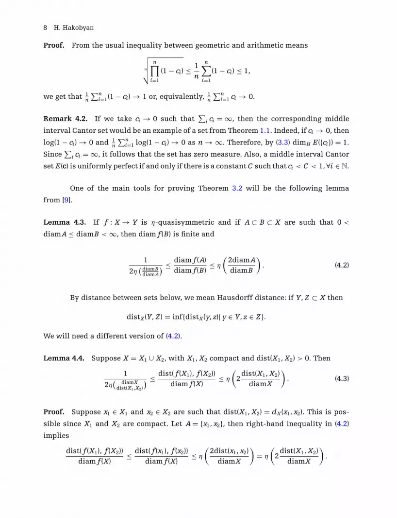
Proof. From the usual inequality between geometric and arithmetic means
n
√√√√ n∏i=1
(1 − ci) ≤ 1
n
n∑i=1
(1 − ci) ≤ 1,
we get that 1n
∑ni=1(1 − ci) → 1 or, equivalently, 1
n
∑ni=1 ci → 0.
Remark 4.2. If we take ci → 0 such that∑
i ci = ∞, then the corresponding middle
interval Cantor set would be an example of a set from Theorem 1.1. Indeed, if ci → 0, then
log(1 − ci) → 0 and 1n
∑ni=1 log(1 − ci) → 0 as n → ∞. Therefore, by (3.3) dimH E ({ci}) = 1.
Since∑
i ci = ∞, it follows that the set has zero measure. Also, a middle interval Cantor
set E (c) is uniformly perfect if and only if there is a constant C such that ci < C < 1, ∀i ∈ N.
One of the main tools for proving Theorem 3.2 will be the following lemma
from [9].
Lemma 4.3. If f : X → Y is η-quasisymmetric and if A ⊂ B ⊂ X are such that 0 <
diamA ≤ diamB < ∞, then diam f (B) is finite and
1
2η(
diamBdiamA
) ≤ diam f (A)
diam f (B)≤ η
(2diamA
diamB
). (4.2)
By distance between sets below, we mean Hausdorff distance: if Y, Z ⊂ X then
distX(Y, Z ) = inf{distX(y, z)| y ∈ Y, z ∈ Z}.
We will need a different version of (4.2).
Lemma 4.4. Suppose X = X1 ∪ X2, with X1, X2 compact and dist(X1, X2) > 0. Then
1
2η(
diamXdist(X1,X2)
) ≤ dist( f (X1), f (X2))
diam f (X)≤ η
(2
dist(X1, X2)
diamX
). (4.3)
Proof. Suppose x1 ∈ X1 and x2 ∈ X2 are such that dist(X1, X2) = dX(x1, x2). This is pos-
sible since X1 and X2 are compact. Let A = {x1, x2}, then right-hand inequality in (4.2)
implies
dist( f (X1), f (X2))
diam f (X)≤ dist( f (x1), f (x2))
diam f (X)≤ η
(2dist(x1, x2)
diamX
)= η
(2
dist(X1, X2)
diamX
).

Conformal Dimension: Cantor Sets and Fuglede Modulus 9
To obtain the other inequality of (4.3), take y1 ∈ f (X1), y2 ∈ f (X2) in such a way that
dist( f (X1), f (X2)) = dY(y1, y2). Let xi′ = f−1(yi). Now take A = {x1
′, x ′2}. Then again using
4.2, we get
dist( f (X1), f (X2))
diam f (X)≥ 1
2η(
diamXdist(x′
1,x′2)
) .
Since dX(x1′, x ′
2) ≥ dist(X1, X2) and since η is increasing, we obtain
1
2η(
diamXdist(x ′
1,x ′2)
) ≥ 1
2η(
diamXdist(X1,X2)
) .
Combining this with the previous inequality gives (4.3).
Theorem 3.2 follows from the following result and the mass distribution
principle.
Lemma 4.5. Let E be as in Theorem 3.2. If f : E → Y is a power-quasisymmetric home-
omorphism, then for every d < 1 there is a measure μ on Y satisfying
μ(B(y, r)) ≤ Crd
for some constant C > 0, all r > 0 and y ∈ Y. Constant C does not depend on y and r.
To simplify the notation below, we write f (En, j) for f (En, j ∩ E ) (we do not assume
that f extends to the real line). We will prove the lemma in several steps.
First, we will show that there is a measure μ on f (⋂
n
⋃En
En, j) ⊂ f (E ) such that
μ( f (En, j)) ≤ C diam f (En, j), (4.4)
for some nonzero finite constant C independent of n and j.
Proof of inequality 4.4. Since f is a homeomorphism, f (E ) has a tree structure just
like E . The notation of Definition 3.1 will also be used for f (E ). Namely, for an I ⊂ Y of
the form I = In, j = f (En, j), we will denote by In, j = f (En, j) and I ′n, j = f (E ′
n, j) the parent
and the sibling of I , respectively.
Construction of the measure. Now define μ as follows. Pick E0 ∈ E0 and let
μ( f (E0)) = 1.
10 H. Hakobyan
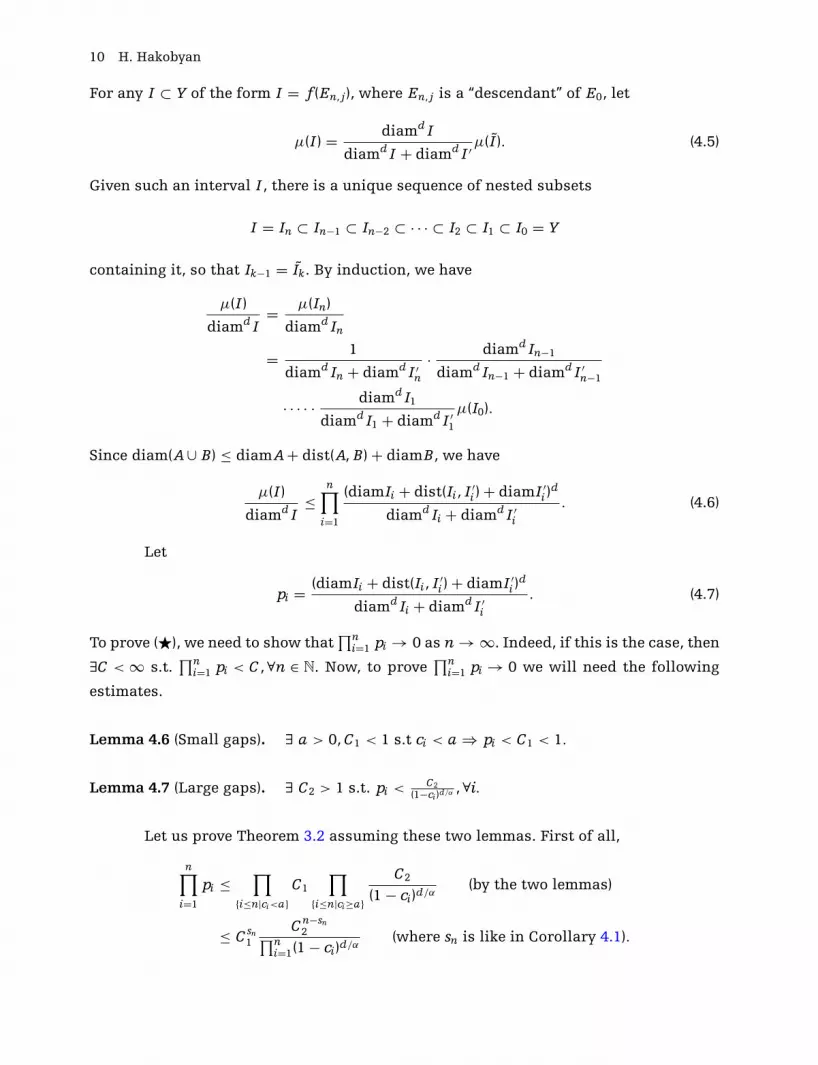
For any I ⊂ Y of the form I = f (En, j), where En, j is a “descendant” of E0, let
μ(I ) = diamd I
diamd I + diamd I ′ μ( I ). (4.5)
Given such an interval I , there is a unique sequence of nested subsets
I = In ⊂ In−1 ⊂ In−2 ⊂ · · · ⊂ I2 ⊂ I1 ⊂ I0 = Y
containing it, so that Ik−1 = Ik. By induction, we have
μ(I )
diamd I= μ(In)
diamd In
= 1
diamd In + diamd I ′n
· diamd In−1
diamd In−1 + diamd I ′n−1
· · · · · diamd I1
diamd I1 + diamd I ′1
μ(I0).
Since diam(A∪ B) ≤ diamA+ dist(A, B) + diamB, we have
μ(I )
diamd I≤
n∏i=1
(diamIi + dist(Ii, I ′i ) + diamI ′
i )d
diamd Ii + diamd I ′i
. (4.6)
Let
pi = (diamIi + dist(Ii, I ′i ) + diamI ′
i )d
diamd Ii + diamd I ′i
. (4.7)
To prove (�), we need to show that∏n
i=1 pi → 0 as n → ∞. Indeed, if this is the case, then
∃C < ∞ s.t.∏n
i=1 pi < C , ∀n ∈ N. Now, to prove∏n
i=1 pi → 0 we will need the following
estimates.
Lemma 4.6 (Small gaps). ∃ a > 0, C1 < 1 s.t ci < a ⇒ pi < C1 < 1.
Lemma 4.7 (Large gaps). ∃ C2 > 1 s.t. pi < C2(1−ci )d/α , ∀i.
Let us prove Theorem 3.2 assuming these two lemmas. First of all,
n∏i=1
pi ≤∏
{i≤n|ci<a}C1
∏{i≤n|ci≥a}
C2
(1 − ci)d/α(by the two lemmas)
≤ C sn1
C n−sn2∏n
i=1(1 − ci)d/α(where sn is like in Corollary 4.1).

Conformal Dimension: Cantor Sets and Fuglede Modulus 11
Now, if C1 < 1 and sn/n → 1, then for every number C2 < ∞ there is a C3 < 1 and N ∈ N
s.t. for n > N
C sn1 C n−sn
2 ≤ C n3 .
Hence,
n∏i=1
pi ≤⎛⎝ C3
n
√∏ni=1(1 − ci)d/α
⎞⎠
n
.
Since n
√∏ni=1(1 − ci) → 1 and C3 < 1, it follows that
∏ni=1 pi → 0.
Next, we prove Lemmas 4.6 and 4.7.
Proof of Lemma 4.6. Recall that for a given a > 0, we had
Sa = {i ∈ N| ci < a}, Sn = Sa ∩ {i ≤ n}, sn = card(Sn).
Without loss of generality, we can assume a < 1/2.
Suppose now i ∈ Sa . We find it easier to estimate p−1i from below:
p−1i = diamd Ii + diamd I ′
i
(diamIi + diamI ′i )
d· (diamIi + diamI ′
i )d
(diamIi + dist(Ii, I ′i ) + diamI ′
i )d
≥ diamd Ii + diamd I ′i
(diamIi + diamI ′i )
d·(
1 − dist(Ii, I ′i )
diamIi−1
)d
≥ diamd Ii + diamd I ′i
(diamIi + diamI ′i )
d· (1 − η(2ci))
d (by (4.3))
=1 + (diamI ′
idiamIi
)d
(1 + diamI ′
idiamIi
)d · (1 − η(2ci))d .
We will show that the the first term in this product is bounded below by a constant
strictly greater than 1. To do that, first note that there is a constant 1 < D(η, M) < ∞ so
that D−1 < diamIi/diamI ′i < D. Indeed,
diamIi
diamI ′i
≥ diamIi
diamIi−1≥ 1
2η(diamEi−1
diamEi
) . (by (4.3))
Since ci−1 < 1/2, it follows from (3.2) that
dist(Ei, E ′i) ≤ diamEi + diamE ′
i ≤ (1 + M)diamEi.
Therefore,
diamEi−1
diamEi≤ diamEi + dist(Ei, E ′
i) + diamE ′i
diamEi≤ 2(1 + M),
12 H. Hakobyan
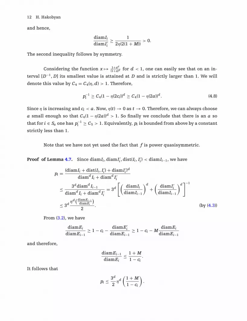
and hence,
diamIi
diamI ′i
≥ 1
2η(2(1 + M))> 0.
The second inequality follows by symmetry.
Considering the function x �→ 1+xd
(1+x)d for d < 1, one can easily see that on an in-
terval [D−1, D] its smallest value is attained at D and is strictly larger than 1. We will
denote this value by C4 = C4(η, d) > 1. Therefore,
p−1i ≥ C4(1 − η(2ci))
d ≥ C4(1 − η(2a))d . (4.8)
Since η is increasing and ci < a. Now, η(t ) → 0 as t → 0. Therefore, we can always choose
a small enough so that C4(1 − η(2a))d > 1. So finally we conclude that there is an a so
that for i ∈ Sa one has p−1i ≥ C5 > 1. Equivalently, pi is bounded from above by a constant
strictly less than 1.
Note that we have not yet used the fact that f is power quasisymmetric.
Proof of Lemma 4.7. Since diamIi, diamI ′i , dist(Ii, I ′
i ) < diamIi−1, we have
pi = (diamIi + dist(Ii, I ′i ) + diamI ′
i )d
diamd Ii + diamd I ′i
≤ 3ddiamd Ii−1
diamd Ii + diamd I ′i
= 3d
[(diamIi
diamIi−1
)d
+(
diamI ′i
diamIi−1
)d]−1
≤ 3dηd
(diamEi−1
diamEi
)2
. (by (4.3))
From (3.2), we have
diamEi
diamEi−1≥ 1 − ci − diamE ′
i
diamEi−1≥ 1 − ci − M
diamEi
diamEi−1
and therefore,
diamEi−1
diamEi≤ 1 + M
1 − ci.
It follows that
pi ≤ 3d
2ηd
(1 + M
1 − ci
).
Conformal Dimension: Cantor Sets and Fuglede Modulus 13
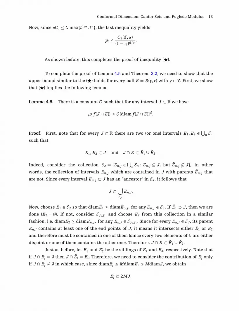
Now, since η(t ) ≤ C max{t1/α, tα}, the last inequality yields
pi ≤ C2(d, α)
(1 − ci)d/α.
As shown before, this completes the proof of inequality (�).
To complete the proof of Lemma 4.5 and Theorem 3.2, we need to show that the
upper bound similar to the (�) holds for every ball B = B(y, r) with y ∈ Y. First, we show
that (�) implies the following lemma.
Lemma 4.8. There is a constant C such that for any interval J ⊂ R we have
μ( f (J ∩ E )) ≤ C [diam f (J ∩ E )]d .
Proof. First, note that for every J ⊂ R there are two (or one) intervals E1, E2 ∈ ⋃n En
such that
E1, E2 ⊂ J and J ∩ E ⊂ E1 ∪ E2.
Indeed, consider the collection EJ = {En, j ∈ ⋃n En : En, j ⊆ J, but En, j � J}, in other
words, the collection of intervals En, j which are contained in J with parents En, j that
are not. Since every interval En, j ⊂ J has an “ancestor” in EJ , it follows that
J ⊂⋃EJ
En, j.
Now, choose E1 ∈ EJ so that diamE1 ≥ diamEn, j, for any En, j ∈ EJ . If E1 ⊃ J, then we are
done (E2 = ∅). If not, consider EJ\E1and choose E2 from this collection in a similar
fashion, i.e. diamE2 ≥ diamEn, j, for any En, j ∈ EJ\E1. Since for every En, j ∈ EJ , its parent
En, j contains at least one of the end points of J; it means it intersects either E1 or E2
and therefore must be contained in one of them (since every two elements of E are either
disjoint or one of them contains the other one). Therefore, J ∩ E ⊂ E1 ∪ E2.
Just as before, let E ′1 and E ′
2 be the siblings of E1 and E2, respectively. Note that
if J ∩ E ′i = ∅ then J ∩ Ei = Ei. Therefore, we need to consider the contribution of E ′
i only
if J ∩ E ′i = ∅ in which case, since diamE ′
i ≤ MdiamEi ≤ MdiamJ, we obtain
E ′i ⊂ 2MJ,

14 H. Hakobyan
where 2MJ is just the dilation of J by 2M. Now, from (�) it follows that
μ( f (J ∩ E )) =∑i=1,2
μ( f (Ei)) + μ( f (E ′i))
≤ C∑i=1,2
[diam f (Ei)]d + [diam f (E ′
i)]d .
Since
diam f (Ei), diam f (E ′i) ≤ diam f (2MJ ∩ E ),
and by (4.2), we have
diam f (2MJ ∩ E ) ≤ 2η(2M)diam f (J ∩ E ).
It follows that
μ( f (J ∩ E )) ≤ C [diam f (J ∩ E )]d
for some constant C and any interval J ⊂ R.
Proof of Lemma 4.5. By quasisymmetry there is a number 1 ≤ H < ∞ such that for
every y ∈ Y and r > 0
B(x, R) ⊂ f−1(B(y, r)) ⊂ B(x, H R),
where x = f−1(y). Therefore,
μ(B(y, r)) ≤ μ( f (B(x, H R)))
≤ C [diam f (B(x, H R))]d (by Lemma 4.8)
≤ C [diam f (B(x, R))]d (by (4.2))
≤ Crd . ( f (B(x, R)) ⊂ B(y, r))
As we noted before, it follows that dimH ( f (E )) ≥ 1 since d could be chosen as close to 1
as one would like.
Remark 4.9. Note that Ec is uniformly perfect for every c ∈ (0, 1] and therefore Theorem
1.3 is contained in the proof of Theorem 3.2 if we disregard Lemma 4.7.
Conformal Dimension: Cantor Sets and Fuglede Modulus 15
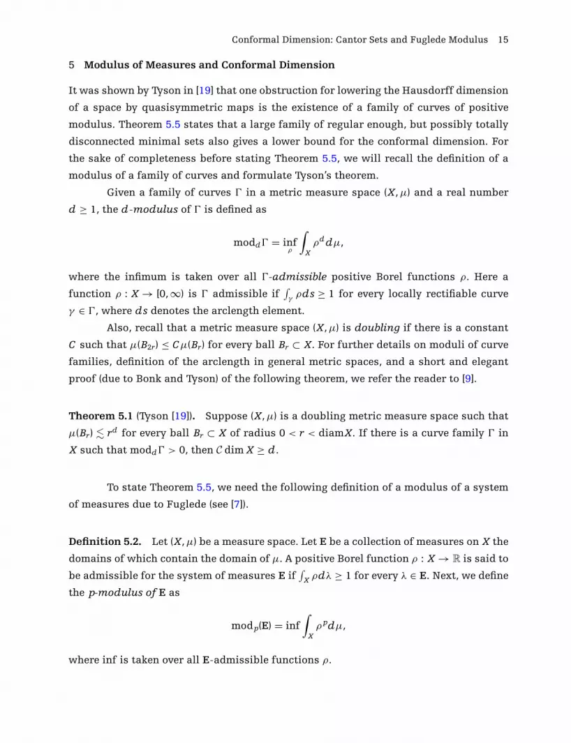
5 Modulus of Measures and Conformal Dimension
It was shown by Tyson in [19] that one obstruction for lowering the Hausdorff dimension
of a space by quasisymmetric maps is the existence of a family of curves of positive
modulus. Theorem 5.5 states that a large family of regular enough, but possibly totally
disconnected minimal sets also gives a lower bound for the conformal dimension. For
the sake of completeness before stating Theorem 5.5, we will recall the definition of a
modulus of a family of curves and formulate Tyson’s theorem.
Given a family of curves � in a metric measure space (X, μ) and a real number
d ≥ 1, the d-modulus of � is defined as
modd� = infρ
∫X
ρddμ,
where the infimum is taken over all �-admissible positive Borel functions ρ. Here a
function ρ : X → [0, ∞) is � admissible if∫γ
ρds ≥ 1 for every locally rectifiable curve
γ ∈ �, where ds denotes the arclength element.
Also, recall that a metric measure space (X, μ) is doubling if there is a constant
C such that μ(B2r) ≤ Cμ(Br) for every ball Br ⊂ X. For further details on moduli of curve
families, definition of the arclength in general metric spaces, and a short and elegant
proof (due to Bonk and Tyson) of the following theorem, we refer the reader to [9].
Theorem 5.1 (Tyson [19]). Suppose (X, μ) is a doubling metric measure space such that
μ(Br) � rd for every ball Br ⊂ X of radius 0 < r < diamX. If there is a curve family � in
X such that modd� > 0, then C dim X ≥ d.
To state Theorem 5.5, we need the following definition of a modulus of a system
of measures due to Fuglede (see [7]).
Definition 5.2. Let (X, μ) be a measure space. Let E be a collection of measures on X the
domains of which contain the domain of μ. A positive Borel function ρ : X → R is said to
be admissible for the system of measures E if∫
X ρdλ ≥ 1 for every λ ∈ E. Next, we define
the p-modulus of E as
modp(E) = inf∫
Xρ pdμ,
where inf is taken over all E-admissible functions ρ.

16 H. Hakobyan
Just like the usual modulus of a family of curves, the modulus of a system of
measures is monotone and subadditive (see [7]).
Lemma 5.3. The p-modulus is monotone and countably subadditive:
modpE ≤ modpE′, if E ⊂ E′, (5.1)
modpE ≤∑
i
modpEi, if E =∞⋃
i=1
Ei. (5.2)
We will also need the following property of modulus.
Lemma 5.4. Suppose μ(X) < ∞ and t > t ′ ≥ 1. If modt ′E > 0, then modtE > 0.
Proof. From Holder’s inequality, we obtain∫
X ρt ′dμ ≤ (
∫X ρt )
1t μ(X)1− t ′
t . Since μ(X) < ∞,
the lemma follows.
Theorem 5.5. Let p > 1 and (X, μ) be a compact, doubling metric measure space. Sup-
pose there is a constant 0 < C < ∞ such that for every ball Br ⊂ X
μ(Br) ≤ Cr p. (5.3)
Let E be a collection of subsets of X such that
C dim E ≥ 1, ∀E ∈ E , (5.4)
and there is a system of measures E = {λE }E∈E associated to E (λE is supported on E ) such
that for every s > 1 there are constants C1 = C1(s) and C2 = C2(s) such that ∀E ∈ E
λE (Br ∩ E ) ≥ C1rs, if1
C2Br ∩ E = ∅. (5.5)
If modp ′E > 0 for some 1 ≤ p′ < p, then C dim X ≥ p.
Theorem 5.5 is proved in Section 6. Here we show how Theorem 1.2 follows from
Theorem 5.5.
Corollary 5.6. Suppose E ⊂ R is a set of conformal dimension 1 which supports a mea-
sure λE such that for every ε > 0 there is a constant C so that whenever x ∈ E and
R < diamE
1
CR1+ε ≤ λE (B(x, R) ∩ E ) ≤ C R1−ε.
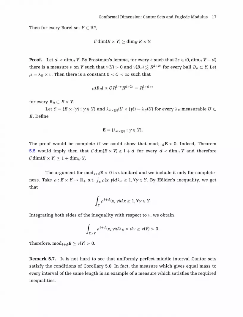
Conformal Dimension: Cantor Sets and Fuglede Modulus 17
Then for every Borel set Y ⊂ Rn,
C dim(E × Y) ≥ dimH E × Y.
Proof. Let d < dimH Y. By Frostman’s lemma, for every ε such that 2ε ∈ (0, dimH Y − d)
there is a measure ν on Y such that ν(Y) > 0 and ν(BR) � Rd+2ε for every ball BR ⊂ Y. Let
μ = λE × ν. Then there is a constant 0 < C < ∞ such that
μ(BR) ≤ C R1−ε Rd+2ε = R1+d+ε
for every BR ⊂ E × Y.
Let E = {E × {y} : y ∈ Y} and λE×{y}(U × {y}) = λE (U ) for every λE measurable U ⊂E . Define
E = {λE×{y} : y ∈ Y}.
The proof would be complete if we could show that mod1+dE > 0. Indeed, Theorem
5.5 would imply then that C dim(E × Y) ≥ 1 + d for every d < dimH Y and therefore
C dim(E × Y) ≥ 1 + dimH Y.
The argument for mod1+dE > 0 is standard and we include it only for complete-
ness. Take ρ : E × Y → R+ s.t.∫
E ρ(x, y)dλE ≥ 1, ∀y ∈ Y. By Holder’s inequality, we get
that
∫E
ρ1+d (x, y)dx ≥ 1, ∀y ∈ Y.
Integrating both sides of the inequality with respect to ν, we obtain
∫E×Y
ρ1+d (x, y)dλE × dν ≥ ν(Y) > 0.
Therefore, mod1+dE ≥ ν(Y) > 0.
Remark 5.7. It is not hard to see that uniformly perfect middle interval Cantor sets
satisfy the conditions of Corollary 5.6. In fact, the measure which gives equal mass to
every interval of the same length is an example of a measure which satisfies the required
inequalities.
18 H. Hakobyan
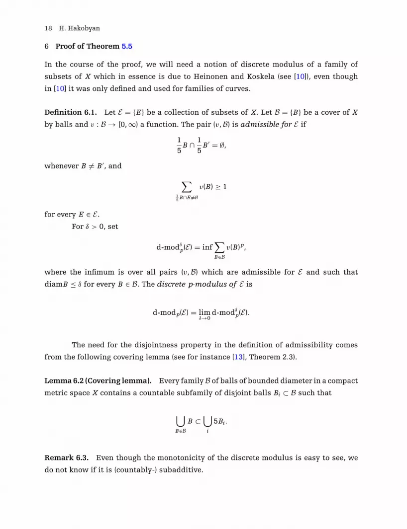
6 Proof of Theorem 5.5
In the course of the proof, we will need a notion of discrete modulus of a family of
subsets of X which in essence is due to Heinonen and Koskela (see [10]), even though
in [10] it was only defined and used for families of curves.
Definition 6.1. Let E = {E} be a collection of subsets of X. Let B = {B} be a cover of X
by balls and v : B → [0, ∞) a function. The pair (v,B) is admissible for E if
1
5B ∩ 1
5B ′ = ∅,
whenever B = B ′, and
∑15 B∩E =∅
v(B) ≥ 1
for every E ∈ E .
For δ > 0, set
d-modδp(E ) = inf
∑B∈B
v(B)p,
where the infimum is over all pairs (v,B) which are admissible for E and such that
diamB ≤ δ for every B ∈ B. The discrete p-modulus of E is
d-modp(E ) = limδ→0
d-modδp(E ).
The need for the disjointness property in the definition of admissibility comes
from the following covering lemma (see for instance [13], Theorem 2.3).
Lemma 6.2 (Covering lemma). Every familyB of balls of bounded diameter in a compact
metric space X contains a countable subfamily of disjoint balls Bi ⊂ B such that
⋃B∈B
B ⊂⋃
i
5Bi.
Remark 6.3. Even though the monotonicity of the discrete modulus is easy to see, we
do not know if it is (countably-) subadditive.

Conformal Dimension: Cantor Sets and Fuglede Modulus 19
Theorem 5.5 would follow from the following two lemmas.
Lemma 6.4. Let t > 0 and suppose E is a collection of subsets in X such that for some
δ > 0
H δt E ≥ c > 0, ∀E ∈ E .
Then d-modqE = 0 for every q > 1t dimH X.
Lemma 6.5. If conditions (5.3) and (5.5) of Theorem 5.5 are satisfied, then for every q < p
there is a constant C < ∞ such that
modqE ≤ C d-modq f (E ).
Before proving the lemmas, let us prove the theorem assuming they are true.
Proof of Theorem 5.5. Suppose f is a quasisymmetric map such that dimH f (X) < p.
Assume that q < p is chosen so that q > max(p′, dimH f (X)) and then choose t < 1 in
such a way that q > 1t dimH f (X). Since dimH f (E ) ≥ 1 for every E ∈ E , it follows that
H1/kt f (E ) → ∞ as k → ∞. Let kE ∈ N denote the smallest integer such that H1/kE
t f (E ) ≥ 1.
Let
E j = {E ∈ E : kE ≥ j}, and Ej = {λE ∈ E : E ∈ Ej}.
Then E = ⋃∞j=1 E j and therefore from (5.2) and from Lemma 6.5, it follows that
modqE ≤∞∑
i=1
modqEi ≤ C∞∑
i=1
d-modq f (Ei),
where f (Ei) is the image of the family Ei. Lemma 6.4 implies that d-modq f (E j) = 0 and
it follows that modqE = 0. Hence, Lemma 5.4 implies that modp′E = 0 which contradicts
our assumption.
Next, we prove Lemmas 6.4 and 6.5.
Proof of Lemma 6.4. Let q′ be such that dimH X < q′ < tq. For every δ > ε > 0, there is
a covering B of X by balls B1, B2, . . . with radii r1, r2, . . . such that 15 Bi ∩ 1
5 Bj = ∅, for i = j
and
∑i
rq′i < ε.

20 H. Hakobyan
Let v(Bi) = rti . Since ri < δ, it follows that for every E ∈ E we have∑
B∩E =∅v(B) ≥ H δ
t (E ) ≥ 1,
and so (v,B) is admissible for E . Now,∑i
v(Bi)q =
∑i
rtqi ≤
∑i
rq′i < ε.
Therefore, d-modqE < ε.
Proof of Lemma 6.5. Below we will need the following well-known inequality; see [9]
or [4] Lemma 4.2 in the case of Rn, which is a consequence of the boundedness of the
Hardy–Littlewood maximal operator.
Lemma 6.6. Suppose B = {Bi, B2, . . .} is a countable collection of balls in a doubling
metric measure space (X, μ) and ai ≥ 0 are real numbers. Then there is a positive constant
C such that ∫X
(∑B
aiχABi (x)
)p
dμ ≤ C (A, p, μ)∫
X
(∑B
aiχBi (x)
)p
dμ (†)
for every 1 < p < ∞ and A > 1.
It is clear that all we need to show is
modqE ≤ C d-modδq f (E )
for some δ ∈ (0, 1). For that suppose (v,B′) is an f (E )-admissible pair, where B′ = {B ′i}∞i=1
is a cover of f (X) by balls B ′i of radii r′
i < δ . Choose Bi ⊂ X with radius ri so that
1
HBi ⊂ f−1
(1
5B ′
i
)⊂ f−1(B ′
i) ⊂ Bi,
where H is constant depending on f (there is such a constant since f is quasisymmetric).
Note that since B′ is admissible, it follows that 1H Bi ∩ 1
H Bj = ∅ whenever i = j.
We want to construct an E-admissible function ρ such that∫X
ρqdμ ≤ C∑B∈B′
v(B ′)q.
Define
ρ(x) =∑
i
v(B ′i)
[diamBi]sχC2 Bi (x),

Conformal Dimension: Cantor Sets and Fuglede Modulus 21
where C2 is as in the formulation of Theorem 5.5. Then for every E ∈ E the following
holds: ∫E
ρdλE =∫
E
∑i
v(B ′i)
[diamBi]sχC2 Bi (x)dλE ≥
∫E
∑i: Bi∩E =∅
v(B ′i)
[diamBi]sχC2 Bi (x)dλE
=∑
i: Bi∩E =∅
v(B ′i)
[diamBi]s
∫E∩C2 Bi
dλE =∑
i: Bi∩E =∅
v(B ′i)
[diamBi]sλE (E ∩ C2 Bi)
≥ 1
C1
∑i: f (E )∩B ′
i =∅v(B ′
i) ≥ 1
C1.
It follows that
modq(E) ≤ C q1
∫X
ρqdμ.
Next, take s > 1 so that qs < p. Then we have
∫X
ρqdμ =∫
X
(∑i
v(B ′i)
[diamBi]sχ5Bi (x)
)q
dμ
≤ C (5H , q, μ)∫
X
(∑i
v(B ′i)
[diamBi]sχ 1
H Bi(x)
)q
dμ (by (†))
= C (5H , q, μ)∑
i
(v(B ′
i)
[diamBi]s
)q
μ
(1
HBi
)(6.1)
�∑
i
v(B ′i)
qr p−qsi (by (5.3))
�∑
i
v(B ′i)
q. (ri < δ < 1)
Taking infimum over all f (E )-admissible pairs (v′,B′), we obtain modqE ≤ C d-modδq f (E )
for some C independent of δ and hence
modqE ≤ C d-modq f (E ),
therefore completing the proof.
7 Remarks and Problems
In [1], Beurling and Ahlfors showed that there are full measure sets in [0, 1] (or R) which
can be mapped to a zero measure set by a quasisymmetry. Examples of sets which could
not be mapped to zero length sets by a quasisymmetries of a line were given in [17] and
[6]. The problem of characterization of such quasisymmetrically thick sets is well known
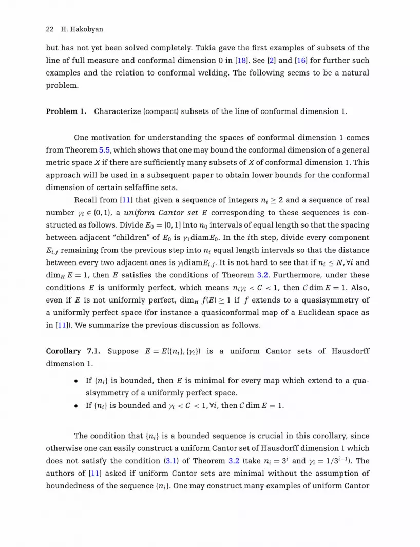
22 H. Hakobyan
but has not yet been solved completely. Tukia gave the first examples of subsets of the
line of full measure and conformal dimension 0 in [18]. See [2] and [16] for further such
examples and the relation to conformal welding. The following seems to be a natural
problem.
Problem 1. Characterize (compact) subsets of the line of conformal dimension 1.
One motivation for understanding the spaces of conformal dimension 1 comes
from Theorem 5.5, which shows that one may bound the conformal dimension of a general
metric space X if there are sufficiently many subsets of X of conformal dimension 1. This
approach will be used in a subsequent paper to obtain lower bounds for the conformal
dimension of certain selfaffine sets.
Recall from [11] that given a sequence of integers ni ≥ 2 and a sequence of real
number γi ∈ (0, 1), a uniform Cantor set E corresponding to these sequences is con-
structed as follows. Divide E0 = [0, 1] into n0 intervals of equal length so that the spacing
between adjacent “children” of E0 is γ1diamE0. In the ith step, divide every component
Ei, j remaining from the previous step into ni equal length intervals so that the distance
between every two adjacent ones is γidiamEi, j. It is not hard to see that if ni ≤ N, ∀i and
dimH E = 1, then E satisfies the conditions of Theorem 3.2. Furthermore, under these
conditions E is uniformly perfect, which means niγi < C < 1, then C dim E = 1. Also,
even if E is not uniformly perfect, dimH f (E ) ≥ 1 if f extends to a quasisymmetry of
a uniformly perfect space (for instance a quasiconformal map of a Euclidean space as
in [11]). We summarize the previous discussion as follows.
Corollary 7.1. Suppose E = E ({ni}, {γi}) is a uniform Cantor sets of Hausdorff
dimension 1.
• If {ni} is bounded, then E is minimal for every map which extend to a qua-
sisymmetry of a uniformly perfect space.
• If {ni} is bounded and γi < C < 1, ∀i, then C dim E = 1.
The condition that {ni} is a bounded sequence is crucial in this corollary, since
otherwise one can easily construct a uniform Cantor set of Hausdorff dimension 1 which
does not satisfy the condition (3.1) of Theorem 3.2 (take ni = 3i and γi = 1/3i−1). The
authors of [11] asked if uniform Cantor sets are minimal without the assumption of
boundedness of the sequence {ni}. One may construct many examples of uniform Cantor

Conformal Dimension: Cantor Sets and Fuglede Modulus 23
sets with unbounded {ni} which still satisfy the conditions of Theorem 3.2; however, the
answers to the following questions are not known to us.
Problem 2. Suppose E = E ({ni}, {γi}) is a uniform Cantor set.
• Obtain necessary and sufficient conditions for E to be minimal.
• Suppose E is uniformly perfect. Is it true that
C dim E = 1 if and only if dimH E = 1?
Here is a different construction of compact subsets of a line. Consider two
sequences {pi} and {qi} of integers with 1 ≤ qi < pi, ∀i ∈ N. Construct the compact set
F = F ({pi}, {qi}), corresponding to {pi} and {qi} as before but in the ith stage divide
each interval remaining from the previous stage into pi equal parts and remove any
qi out. The results of Staples and Ward [17] and Theorem 3.2 suggest the following
questions.
Problem 3. Let F = F ({pi}, {qi}) be constructed as above.
• Suppose∑
i(qi/pi)t < ∞, for every t > 0 and let F = F ({pi}, {qi}). Does F have
conformal dimension 1? Is it quasisymmetrically thick?
• Is there an example of F = F ({pi}, {qi}) of conformal dimension 0 and qi/pi → 0
as i → ∞?
In [3], Bishop and Tyson asked for a characterization of subsets E of the line such
that the products E × Y are minimal for every compact Y. Clearly, E would have to be
minimal itself to have that property.
Problem 4. Let E ⊂ R. Is E × Y minimal for every compact Y if (and only if) E ⊂ R is
minimal?
Theorem 1.2 does not answer this question since a lower bound on the Hausdorff
dimension does not in general imply that there is a measure λ satisfying the lower
estimate of (1.2). One may try to answer the last question by proving a result similar
to Theorem 5.5 but assuming positivity of the discrete modulus for a family of sets. In
fact, positive answers to the following two questions would imply a positive answer to
Problem 4.

24 H. Hakobyan
Problem 5. Let t > 1.
• Suppose E = {E} is a collection of minimal subsets of dimension 1 in a metric
space X. Is it true that if d-modt (E ) > 0 then C dim X ≥ t?
• Let E ⊂ R be minimal, Y be any metric space of positive Hausdorff di-
mension, and E = {E × {y} : y ∈ Y}. Is it true that d-modt (E ) > 0 for any
1 < t < dimH (E × Y)?
Acknowledgments
This paper is partly based on the author’s doctoral thesis at Stony Brook University. The author
would like to thank his advisor Christopher Bishop for constant support and encouragement.
He would also like to thank Ilia Binder, Saeed Zakeri, and the anonymous referees for numerous
helpful discussions and comments which made the paper more readable.
References[1] Beurling, A., and L. Ahlfors. “The boundary correspondence under quasiconformal map-
pings.” Acta Mathematica 96 (1956): 125–42.
[2] Bishop, C. J., and T. Steger. “Representation-theoretic rigidity in PSL(2, R).” Acta Mathemat-
ica 170, no. 1 (1993): 121–49.
[3] Bishop, C. J., and J. Tyson. “Locally minimal sets for conformal dimension.” Annales
Academia Scientiarum Fennica 26 (2001): 361–73.
[4] Bojarski, B. “Remarks on Sobolev imbedding inequalities.” In Complex Analysis (Joensuu
1987), 52–68. Lecture Notes in Mathematics 1351. Berlin: Springer, 1988.
[5] Bourdon, M. “Au bord de certains polyedres hyperboliques.” Annales de l’Institut Fourier
(Grenoble) 45, no. 1 (1995): 119–41.
[6] Buckley, S., B. Hanson, and P. Macmanus. “Doubling for general sets.” Mathematica Scandi-
navica 88, no. 2 (2001): 229–45.
[7] Fuglede, B. “Extremal length and functional completion.” Acta Mathematica 98 (1957): 171–
219.
[8] Hakobyan, H. “Cantor sets which are minimal for quasisymmetric maps.” Journal of Con-
temporary Mathematical Analysis 41, no. 2 (2006): 5–13.
[9] Heinonen, J. Lectures on Analysis in Metric Spaces. Universitext. New York: Springer, 2001.
[10] Heinonen, J., and P. Koskela. “Definitions of quasiconformality.” Inventiones Mathematicae
120, no. 1 (1995): 61–79.
[11] Hu, M., and S. Wen. “Quasisymmetrically minimal uniform Cantor sets.” Topology and Its
Applications 155, no. 6 (2008): 515–21.
[12] Kovalev, L. “Conformal dimension does not assume values between 0 and 1.” Duke Mathe-
matical Journal 134, no. 1 (2006): 1–13.

Conformal Dimension: Cantor Sets and Fuglede Modulus 25
[13] Mattila, P. “Geometry of sets and measures in Euclidean spaces.” Cambridge Studies in
Advanced Mathematics 44. Cambridge: Cambridge University Press, 1995.
[14] Pansu, P. “Dimension conforme et sphere a l’infini des varietes a courbure negative.” Annales
Academia Scientiarum Fennica 14, no. 2 (1989): 177–212.
[15] Pansu, P. “Metriques de Carnot–Caratheodory et quasiisometries des espaces symetriques
de rang un.” Annals of Mathematics 129, no. 2 (1989): 1–60.
[16] Rohde, S. “On conformal welding and quasicircles.” Michigan Mathematical Journal 38, no.
1 (1991): 111–6.
[17] Staples, S., and L. Ward. “Quasisymmetrically thick sets.” Annales Academia Scientiarum
Fennica Mathematica 23, no. 1 (1998): 151–68.
[18] Tukia, P. “Hausdorff dimension and quasisymmetric mappings.” Mathematica Scandinavica
65, no. 1 (1989): 152–60.
[19] Tyson, J. “Sets of minimal Hausdorff dimension for quasiconformal maps.” Proceedings of
the American Mathematical Society 128 (2000): 3361–7.