deriving in situ phytoplankton absorption for bio-optical productivity models in turbid waters

1 Deriving in situ phytoplankton absorption for bio-optical productivity

2 models in turbid waters

3 Matthew J. Oliver, Oscar Schofield, Trisha Bergmann, and Scott Glenn4 Institute of Marine and Coastal Sciences, Rutgers University, New Brunswick, New Jersey, USA

5 Cristina Orrico and Mark Moline6 Biological Sciences Department, California Polytechnic State University, San Luis Obispo, California, USA

7 Received 5 September 2002; revised 28 April 2003; accepted 25 July 2003; published XX Month 2004.

8 [1] As part of Hyperspectral Coupled Ocean Dynamics Experiment, a high-resolution9 hydrographic and bio-optical data set was collected from two cabled profilers at the Long-10 Term Ecosystem Observatory (LEO). Upwelling- and downwelling-favorable winds and a11 buoyant plume from the Hudson River induced large changes in hydrographic and optical12 structure of the water column. An absorption inversion model estimated the relative13 abundance of phytoplankton, colored dissolved organic matter (CDOM) and detritus, as14 well as the spectral exponential slopes of CDOM and detritus from in situ WET Labs nine-15 wavelength absorption/attenuation meter (ac-9) absorption data. Derived optical weights16 were proportional to the parameter concentrations and allowed for their absorptions to17 be calculated. Spectrally weighted phytoplankton absorption was estimated using modeled18 spectral irradiances and the phytoplankton absorption spectra inverted from an ac-9.19 Derived mean spectral absorption of phytoplankton was used in a bio-optical model20 estimating photosynthetic rates. Measured radiocarbon uptake productivity rates21 extrapolated with water mass analysis and the bio-optical modeled results agreed within22 20%. This approach is impacted by variability in the maximum quantum yield (fmax) and23 the irradiance light-saturation parameter (Ek(PAR)). An analysis of available data shows that24 fmax variability is relatively constrained in temperate waters. The variability of Ek(PAR)

25 is greater in temperate waters, but based on a sensitivity analysis, has an overall smaller26 impact on water-column-integrated productivity rates because of the exponential decay of27 light. This inversion approach illustrates the utility of bio-optical models in turbid coastal28 waters given the measurements of the bulk inherent optical properties. INDEX TERMS:

29 4853 Oceanography: Biological and Chemical: Photosynthesis; 4847 Oceanography: Biological and

30 Chemical: Optics; 4552 Oceanography: Physical: Ocean optics; 4842 Oceanography: Biological and

31 Chemical: Modeling; 4894 Oceanography: Biological and Chemical: Instruments and techniques; KEYWORDS:

32 coastal, productivity, optics

33 Citation: Oliver, M. J., O. Schofield, T. Bergmann, S. Glenn, C. Orrico, and M. Moline (2004), Deriving in situ phytoplankton

34 absorption for bio-optical productivity models in turbid waters, J. Geophys. Res., 109, C07S11, doi:10.1029/2002JC001627.

36 1. Introduction

37 [2] There is growing evidence that anthropogenic-38 induced changes to the coastal ocean are increasing and39 will continue to do so as coastal regions are developed40 worldwide [Hallegraeff, 1993]. This is significant as the41 coastal ocean represents a significant fraction of the total42 ocean productivity [Field et al., 1998; Bienfang and43 Ziemann, 1992], produces 90% of the global fish catch44 [Holligan and Reiners, 1992], and acts as a nutrient buffer45 between the terrestrial ecosystems and the open ocean46 [Biscaye et al., 1994; Falkowski et al., 1994]. Despite the47 functional importance of the coastal ocean, our understand-48 ing of physical and biological processes in nearshore coastal

49waters (<30 m deep) is severely limited due to its highly50turbulent nature [Brink, 1997]. Therefore there is a need to51develop effective means to map biological and chemical52processes in coastal ecosystems.53[3] Optical techniques are more commonly being used to54assess spatial and temporal phytoplankton dynamics of55offshore waters [cf. Advances in Ocean Optics, Journal56of Geophysical Research, 100(C7), 13,133–13,372, 1995];57however, these approaches are often compromised because58of the optical complexity of coastal waters. For example,59ocean color satellite chlorophyll algorithms are based on60ratios of remote sensing reflectance (Rrs) at different wave-61lengths. Most satellite algorithms assume that Rrs patterns62are based on case 1 waters where the in situ absorption63and water-leaving radiance (Lw) signal in the blue wave-64lengths are dominated by chlorophyll absorption while Lw65in the green wavelengths is relatively insensitive to chloro-

JOURNAL OF GEOPHYSICAL RESEARCH, VOL. 109, C07S11, doi:10.1029/2002JC001627, 2004

Copyright 2004 by the American Geophysical Union.0148-0227/04/2002JC001627$09.00

C07S11 1 of 12

66 phyll concentrations [Gordon and Morel, 1983]. Inaccura-67 cies in this approach arise in coastal waters that contain68 significant amounts of other absorbing/scattering com-69 pounds such as dissolved organics, detritus, and even70 variable phytoplankton communities [Morel and Prieur,71 1977; T. Bergmann et al., The impacts of a recurrent72 resuspension event and variable phytoplankton community73 composition on remote sensing reflectance, submitted to74 Journal of Geophysical Research, 2002]. These errors75 directly impact the utility of optical techniques for76 estimating primary production and in turn impacts our77 understanding of carbon flux and nutrient recycling in78 nearshore ecosystems and their relation to ecosystem79 function [Jickells, 1998; Cloern, 2001].80 [4] Resolving the impact of primary production on any81 oceanic system is ultimately a question of scale [Bidigare82 et al., 1992], which has been recently addressed with83 comparisons of local, regional, and global productivity84 models in ocean observatories. Comparisons of modeled85 and measured primary production in these observatories86 showed mixed results. For example, satellite-based depth-87 integrated models [see Behrenfeld and Falkowski, 1997 for88 review] performed well when integrated over long time89 periods (>200 days) but failed to resolve episodic production90 events on the order of days to months [Siegel et al., 2001].91 Failures in these satellite approaches on regional scales are92 probably related to the degree to which particular algorithms93 are ‘‘tuned’’ to a specific region and the resolution of the94 time step in which satellites sample regions because of95 orbital trajectories and the occurrence of cloudy weather.96 Ondrusek et al. [2001] also reported that satellite-based97 depth-integrated models also did not perform well; how-98 ever, estimates were improved using a wavelength-resolved99 model. This model was dependent on chlorophyll specific100 mean spectrally weighted absorption of phytoplankton (�aph* ),101 which explained 82% of the variance and was able to resolve102 small-timescale phytoplankton blooms. Productivity models103 that incorporate �aph* performed well in many different waters104 [Smith et al., 1989; Bidigare et al., 1992;Waters et al., 1994;105 Morel et al., 1996] because they describe the fraction of106 photosynthetically available radiation (PAR) that is107 absorbed, which is a function of phytoplankton abundance,108 distribution, community structure, and physiology. Most109 often studies using these models use chemical extraction110 [Kishino et al., 1985] or high-performance liquid chroma-111 tography (HPLC) to measure �aph* , which limits the amount of112 data that is available thus making comparisons to satellite113 data difficult [Siegel et al., 2001]. Secondarily, the presence114 of other compounds that absorb light in coastal waters can115 complicate these approaches.116 [5] Between the depth-integrated productivity models and117 the laboratory-dependent wavelength-resolved models there118 exists a gap in our ability to resolve and assess the episodic119 productivity events such as upwelling and river plumes in120 coastal systems that potentially account for a significant121 portion of the seasonal productivity signal [Walsh, 1978].122 Depth-integrated approaches are limited not only in algo-123 rithm development but also in the resolution of temporal124 coverage due to clouds, while the use of wavelength-125 resolved models derived from discrete water samples are126 limited to relatively short space and timescales because of127 sampling logistics. While there is progress being made in

128developing satellite productivity algorithms for coastal129turbid waters, the issues of cloud cover persist. Therefore130if we are to understand the episodic nature of coastal systems131on seasonal scales, there is a need to collect parameters for132wavelength-resolved models on high-resolution space and133timescales over broad regions to improve productivity esti-134mates in turbid coastal regions.135[6] Here we present a high-resolution time series of in-136water physical and optical data collected by two cabled137profilers as part of the Long-term Ecosystem Observatory138(LEO) [see Schofield et al., 2002] to demonstrate an139approach which can potentially ‘‘fill the gap’’ between140satellite-based depth-integrated productivity models and141productivity models dependent on discrete water samples142such as wavelength-resolved models. From this time series143we directly derive the spectral absorption of phytoplankton144in coastal waters from bulk optical parameters measured145with ‘‘off the shelf’’ technology and quantify its utility in146bio-optically estimating primary productivity in coastal147waters. We discuss assumptions and errors associated with148our approach. These absorption-based bio-optical model149estimates compared well with a physiology-based model150rooted in measured photosynthetic-irradiance (P-E) param-151eters. This technique represents a high-resolution approach152to calculating spectrally weighted phytoplankton absorption153independent of laboratory extractions. While the scope of154our study does not and cannot address the scope of the155variability in primary production in the coastal ocean, we156feel that automated optical approaches such as the one157presented here provide a link for wavelength-resolved158models to be applied on broad spatial scales through the159use of autonomous platforms.

1602. Methods

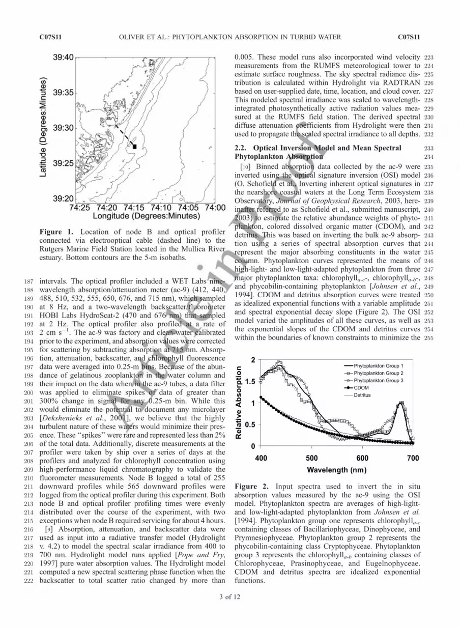
161[7] The 2000 Hyperspectral Coupled Ocean Dynamics162Experiment (HyCODE) conducted at LEO represents an163integrated coastal-ocean-observing network [Glenn et al.,1642000; Schofield et al., 2002]. As part of this experiment, in-165water physical and bio-optical time series data were col-166lected from two profiling instrument nodes linked to shore167via an electrooptical cable. These nodes were deployed168approximately 4 km offshore in 13 m of water at16939�27.410N, 74�14.750W (node B and the optical profiler,170Figure 1). This study represents data collected from calen-171dar days 202-215. Node B provided hydrographic data, and172the optical profiler provided optical data. These nodes were173separated by about 100 m.

1742.1. Profiler Data Sets

175[8] As opposed to traditional methods of water-column176profiling using lowered instrument packages from ships,177both the optical profiler and node B had frames anchored to178the seafloor with instrument packages attached to floating179drogues that were depth controlled by an underwater winch.180Data measured by these profilers streamed directly to the181Rutgers University Marine Field Station (RUMFS) in real182time via an electrooptical cable, where it was processed183and visualized. Node B included a Sea-Bird conductivity-184temperature-depth (CTD) mounted with a WET Labs185chlorophyll fluorometer, which was sampled at 2 Hz and186was profiled at a vertical rate of 2 cm s�1 at regular

C07S11 OLIVER ET AL.: PHYTOPLANKTON ABSORPTION IN TURBID WATER

2 of 12

C07S11

187 intervals. The optical profiler included a WET Labs nine-188 wavelength absorption/attenuation meter (ac-9) (412, 440,189 488, 510, 532, 555, 650, 676, and 715 nm), which sampled190 at 8 Hz, and a two-wavelength backscatter/fluorometer191 HOBI Labs HydroScat-2 (470 and 676 nm) that sampled192 at 2 Hz. The optical profiler also profiled at a rate of193 2 cm s�1. The ac-9 was factory and clean-water calibrated194 prior to the experiment, and absorption values were corrected195 for scattering by subtracting absorption at 715 nm. Absorp-196 tion, attenuation, backscatter, and chlorophyll fluorescence197 data were averaged into 0.25-m bins. Because of the abun-198 dance of gelatinous zooplankton in the water column and199 their impact on the data when in the ac-9 tubes, a data filter200 was applied to eliminate spikes of data of greater than201 300% change in signal for any 0.25-m bin. While this202 would eliminate the potential to document any microlayer203 [Dekshenieks et al., 2001], we believe that the highly204 turbulent nature of these waters would minimize their pres-205 ence. These ‘‘spikes’’ were rare and represented less than 2%206 of the total data. Additionally, discrete measurements at the207 profiler were taken by ship over a series of days at the208 profilers and analyzed for chlorophyll concentration using209 high-performance liquid chromatography to validate the210 fluorometer measurements. Node B logged a total of 255211 downward profiles while 565 downward profiles were212 logged from the optical profiler during this experiment. Both213 node B and optical profiler profiling times were evenly214 distributed over the course of the experiment, with two215 exceptions when node B required servicing for about 4 hours.216 [9] Absorption, attenuation, and backscatter data were217 used as input into a radiative transfer model (Hydrolight218 v. 4.2) to model the spectral scalar irradiance from 400 to219 700 nm. Hydrolight model runs applied [Pope and Fry,220 1997] pure water absorption values. The Hydrolight model221 computed a new spectral scattering phase function when the222 backscatter to total scatter ratio changed by more than

2230.005. These model runs also incorporated wind velocity224measurements from the RUMFS meteorological tower to225estimate surface roughness. The sky spectral radiance dis-226tribution is calculated within Hydrolight via RADTRAN227based on user-supplied date, time, location, and cloud cover.228This modeled spectral irradiance was scaled to wavelength-229integrated photosynthetically active radiation values mea-230sured at the RUMFS field station. The derived spectral231diffuse attenuation coefficients from Hydrolight were then232used to propagate the scaled spectral irradiance to all depths.

2332.2. Optical Inversion Model and Mean Spectral234Phytoplankton Absorption

235[10] Binned absorption data collected by the ac-9 were236inverted using the optical signature inversion (OSI) model237(O. Schofield et al., Inverting inherent optical signatures in238the nearshore coastal waters at the Long Term Ecosystem239Observatory, Journal of Geophysical Research, 2003, here-240inafter referred to as Schofield et al., submitted manuscript,2412003) to estimate the relative abundance weights of phyto-242plankton, colored dissolved organic matter (CDOM), and243detritus. This was based on inverting the bulk ac-9 absorp-244tion using a series of spectral absorption curves that245represent the major absorbing constituents in the water246column. Phytoplankton curves represented the means of247high-light- and low-light-adapted phytoplankton from three248major phytoplankton taxa: chlorophylla-c-, chlorophylla-b-,249and phycobilin-containing phytoplankton [Johnsen et al.,2501994]. CDOM and detritus absorption curves were treated251as idealized exponential functions with a variable amplitude252and spectral exponential decay slope (Figure 2). The OSI253model varied the amplitudes of all these curves, as well as254the exponential slopes of the CDOM and detritus curves255within the boundaries of known constraints to minimize the

Figure 1. Location of node B and optical profilerconnected via electrooptical cable (dashed line) to theRutgers Marine Field Station located in the Mullica Riverestuary. Bottom contours are the 5-m isobaths.

Figure 2. Input spectra used to invert the in situabsorption values measured by the ac-9 using the OSImodel. Phytoplankton spectra are averages of high-light-and low-light-adapted phytoplankton from Johnsen et al.[1994]. Phytoplankton group one represents chlorophylla-ccontaining classes of Bacillariophyceae, Dinophyceae, andPrymnesiophyceae. Phytoplankton group 2 represents thephycobilin-containing class Cryptophyceae. Phytoplanktongroup 3 represents the chlorophylla-b containing classes ofChlorophyceae, Prasinophyceae, and Eugelnophyceae.CDOM and detritus spectra are idealized exponentialfunctions.


3 of 12

C07S11

256 difference between the total modeled absorption (sum of all257 phytoplankton, CDOM, and detritus curves) and total ab-258 sorption measured by the ac-9. The OSI model returns the259 estimated weights of each phytoplankton group, and CDOM260 and detritus, as well as the spectral exponential slopes (or261 decay) of CDOM and detritus. These weights are analogous262 to the amplitude or abundance of their respective absorbing263 constituent.264 [11] Spectral absorption of phytoplankton (aph (l, z, t)265 m�1) was calculated by

aph l; z; tð Þ ¼X3n¼1

wn phð Þ z; tð Þan phð Þ lð Þ; ð1Þ

267 where n is the phytoplankton group number, wn(ph) (z, t) is268 the calibrated inverted scalar weight calculated by the OSI269 model of a specific group of phytoplankton (m�1), which is270 not spectrally dependent, and an(ph) (l) is the relative271 absorption of the input spectra of specific group of272 phytoplankton at a given wavelength. OSI calibration data273 showed that the amplitude of the phytoplankton spectra was274 generally underestimated due to the package effect of275 natural populations compared to the laboratory cultures276 from which the input spectra are derived. Although there277 was an underestimation, this underestimation was well278 quantified so that a calibration factor of 1.393 was applied

279to the relative weights of phytoplankton derived by the OSI280(Schofield et al., submitted manuscript, 2003). Modeled281spectral scalar irradiance values were combined with aph(l,282z, t) to calculate the mean spectral absorption of283phytoplankton �aph(l, z, t) (m

�1) using:

�aph z; tð Þ ¼

R700400

Eo l; z; tð Þaph l; z; tð Þdl

R700400

Eo l; z; tð Þdl; ð2Þ

285where Eo (l, z, t) is spectral scalar irradiance from 400 to286700 nm (W m�2) modeled by Hydrolight v. 4.2.

2872.3. Bio-Optical Modeling of Primary Production288From an ac-9

289[12] The bio-optical model used in this study to calculate290primary production was

PP z; tð Þ ¼ �aph z; tð ÞfmaxEk PARð Þ tanhEo PARð Þ z; tð ÞEk PARð Þ

� �; ð3Þ

292where PP(z, t) is primary production (mg C m�3 h�1), �aph293(z, t) is calculated from equation (2) and was based solely on294the optical inversion of ac-9 data, fmax is the maximum295quantum yield of carbon fixation (mol C mol photons296absorbed�1), Ek(PAR) is the irradiant flux at which photo-297synthesis becomes light saturated (mmol photons m�2 s�1),298and Eo(PAR) (z, t) is the PAR-integrated scalar irradiant flux299incident on the phytoplankton cells (mmol photons m�2 s�1)300modeled by Hydrolight v. 4.2. Eo(PAR) (z, t) was used for this301calculation because phytoplankton absorbs light from all302directions. Because our in situ optical data set did not303include measurements of fmax and Ek(PAR), we conducted a304literature survey to determine a mean for these waters305(Figure 3, see figure legend for references). The data in306Figure 3 represent the mean and standard deviation of the307water column measured in each study. The mean fmax and308Ek(PAR) value used in this study were calculated from all the309literature studies in temperate and tropical waters except310from those labeled ‘‘Antarctic’’ or ‘‘New Jersey Coastal311Region (LEO)’’ in Figure 3. We did not include values of312fmax and Ek(PAR) estimated by 14C incubations from the313LEO site in this mean because we wished to keep the bio-314optical method of estimating primary productivity and the315physiological method of estimating productivity as inde-316pendent as possible. The mean values used for fmax and317Ek(PAR) for this study were 0.025 mol C mol photons318absorbed�1 and 124.85 mmol photons m�2 s�1, respectively.319In this manuscript, this productivity model will be simply320referred to as the bio-optical model.

3212.4. Productivity Measurements of Phytoplankton

322[13] Discrete water samples were collected at the profilers323with Nisken bottles from the R/V Walford on calendar days324203, 208, and 212 at both the surface and at a depth of 8 m325(Table 1). These days coincided with major changes in326water-column structure that were observed from real-time327observation of profiler data, which allowed for adaptive328sampling. These samples were collected at approximately3291000 LT on these days and kept dark for 30 min while

Figure 3. Paired Ek(PAR) and fmax reported water columnmeans and standard deviations from various studies: 1–3,Sathyendranath et al. [1999]; 4–7, Figueiras et al. [1999];8–10, Lorenzo et al. [2002]; 11, Moline and Prezelin[1996]; 13–21, Kyewalyanga et al. [1998]; 22, Schofield etal. [1993]; and 23 New Jersey Coastal Region (LEO).Antarctic studies are characterized by low Ek(PAR) and highfmax, while the opposite trend is evident for tropical andtemperate waters. The mean values for this study for Ek(PAR)

and fmax were calculated from all the literature studies intemperate and tropical waters except those estimated at thestudy site using 14C incubations (all values not labeled‘‘Antarctic’’ or ‘‘New Jersey Coastal Region (LEO)’’).


4 of 12

C07S11

330 returning to the field station. Aliquots were then filtered331 onto 47-mm GF/F filters and stored in an �80�C freezer for332 phytoplankton pigment determination using HPLC analysis333 using the methods of Wright et al. [1991]. Photosynthetic-334 irradiance curves were measured using the methods of335 Prezelin et al. [1989]. Measured carbon uptake values for336 each of the P-E curves were curve fitted as a hyperbolic337 tangent function using the Simplex method of Caceci and338 Cacheris [1984] to estimate the chlorophyll-specific maxi-339 mum photosynthetic rate (Pmax, mol C m�3 h�1), the light-340 limited slope of photosynthesis (a), and the photosynthetic341 light-saturation parameter (Ek(PAR)). Error estimates were342 calculated using the methods of Zimmerman et al. [1987].343 [14] The general model used in this study to calculate344 physiology-based primary production is based on the work345 of Jassby and Platt [1976]:

PP z; tð Þ ¼ Pmax z; tð Þ tanhEo PARð Þ z; tð ÞEk PARð Þ z; tð Þ

� �; ð4Þ

347 where PP, Pmax, Eo(PAR), and Ek(PAR) are as described348 previously. To extrapolate physiological parameters (Pmax

349 and Ek(PAR)) measured at the profiler over the same depth-350 time area that the profilers were deployed (give them similar351 z and t distribution as equation (3)), multivariate cluster352 analysis of paired salinity and temperature observations353 from node B was used to define statistical boundaries on354 water masses. Salinity and temperature values were stan-355 dardized by subtracting the mean of the data set and356 dividing by the standard deviation of the data set. On the357 basis of Euclidian distance, a distance matrix was calculated358 for the data set and then hierarchically clustered according359 to Ward’s linkage [Ward, 1963]. The generated similarity360 index was used in conjunction with a multivariate analysis361 of variance (MANOVA) to define the major groupings of362 temperature and salinity observations (i.e., water masses).363 Physiological parameters were measured within each of the364 statistically distinct water masses except a water mass in the365 lower portion of the water column on days 213–215. This366 restricted physiology-based depth-integrated productivity367 calculations to days 202–212. In the case where a specific368 water mass was continuous throughout the depth of the369 water column, the water mass was subdivided at the 8-m370 mark, below the climatological depth of the thermocline in371 this area (7 m), so that the physiological parameters mea-372 sured at the surface and at 8-m depth in the water mass were373 separated. On the basis of this extrapolation method, the374 depth-integrated productivity was calculated.375 [15] The assumptions of this approach do not incorporate376 diel variation of physiological parameters, which have been377 shown to be important in calculating short-timescale pro-

378ductivity [Sournia, 1974; Prezelin et al., 1987; Prezelin,3791991]. To mediate these effects, measurements were made380at approximately the same time of day. However, these diel381cycles introduce errors into our comparison of physiology-382based and bio-optical calculations of primary production,383although not just our errors. In this manuscript, this pro-384ductivity model will be referred to as the physiology-based385model.

3873. Results

3883.1. Hydrographic and Optical Variability at the LEO389Profilers

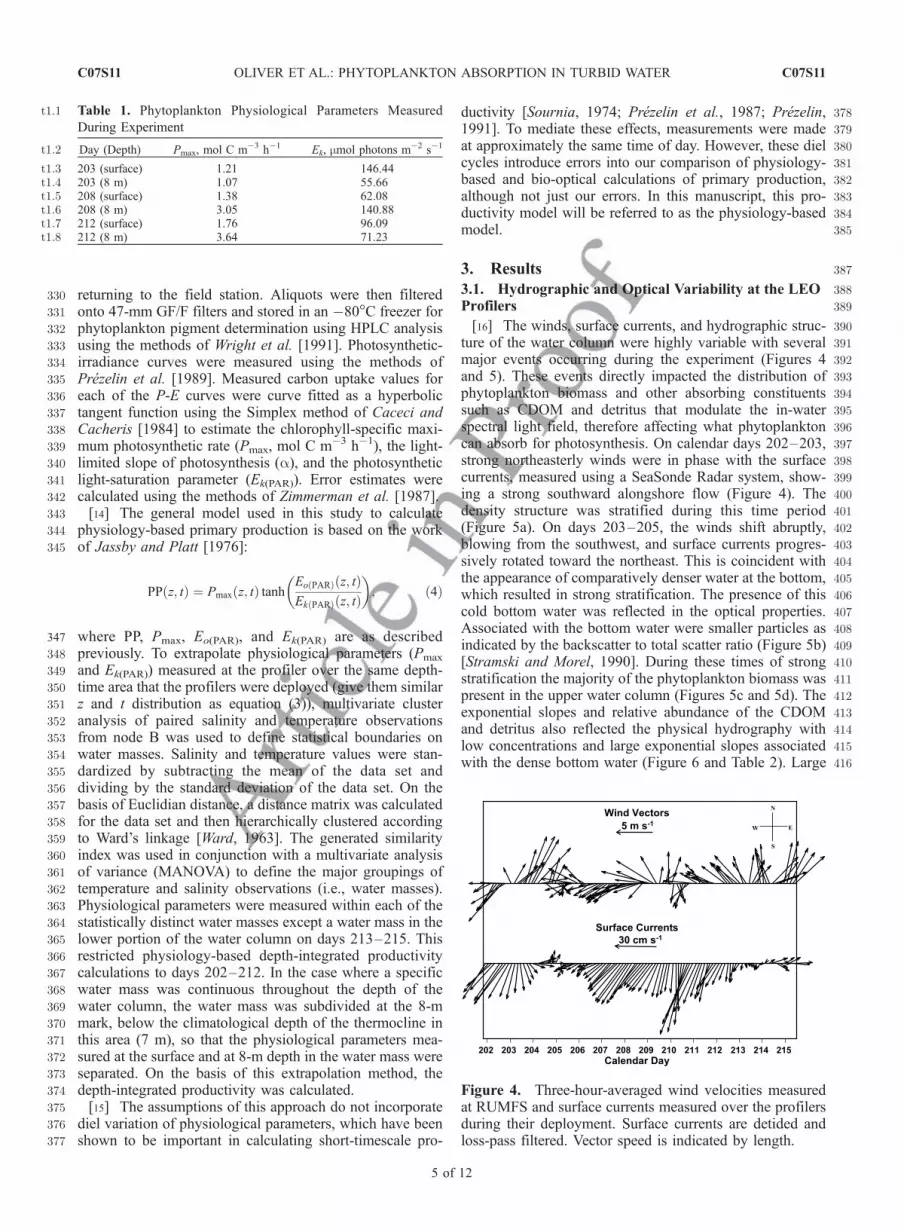
390[16] The winds, surface currents, and hydrographic struc-391ture of the water column were highly variable with several392major events occurring during the experiment (Figures 4393and 5). These events directly impacted the distribution of394phytoplankton biomass and other absorbing constituents395such as CDOM and detritus that modulate the in-water396spectral light field, therefore affecting what phytoplankton397can absorb for photosynthesis. On calendar days 202–203,398strong northeasterly winds were in phase with the surface399currents, measured using a SeaSonde Radar system, show-400ing a strong southward alongshore flow (Figure 4). The401density structure was stratified during this time period402(Figure 5a). On days 203–205, the winds shift abruptly,403blowing from the southwest, and surface currents progres-404sively rotated toward the northeast. This is coincident with405the appearance of comparatively denser water at the bottom,406which resulted in strong stratification. The presence of this407cold bottom water was reflected in the optical properties.408Associated with the bottom water were smaller particles as409indicated by the backscatter to total scatter ratio (Figure 5b)410[Stramski and Morel, 1990]. During these times of strong411stratification the majority of the phytoplankton biomass was412present in the upper water column (Figures 5c and 5d). The413exponential slopes and relative abundance of the CDOM414and detritus also reflected the physical hydrography with415low concentrations and large exponential slopes associated416with the dense bottom water (Figure 6 and Table 2). Large

t1.1 Table 1. Phytoplankton Physiological Parameters Measured

During Experiment

Day (Depth) Pmax, mol C m�3 h�1 Ek, mmol photons m�2 s�1t1.2

203 (surface) 1.21 146.44t1.3203 (8 m) 1.07 55.66t1.4208 (surface) 1.38 62.08t1.5208 (8 m) 3.05 140.88t1.6212 (surface) 1.76 96.09t1.7212 (8 m) 3.64 71.23t1.8

Figure 4. Three-hour-averaged wind velocities measuredat RUMFS and surface currents measured over the profilersduring their deployment. Surface currents are detided andloss-pass filtered. Vector speed is indicated by length.


5 of 12

C07S11

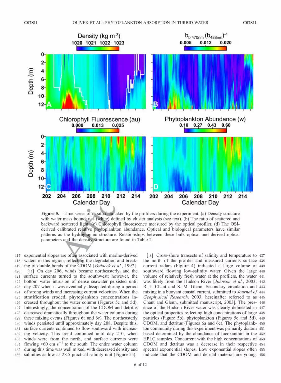
417 exponential slopes are often associated with marine-derived418 waters in this region, reflecting the degradation and break-419 ing of double bonds of the CDOM [Vodacek et al., 1997].420 [17] On day 206, winds became northeasterly, and the421 surface currents turned to the southwest; however, the422 bottom water intrusion of dense seawater persisted until423 day 207 when it was eventually dissipated during a period424 of strong winds and increasing current velocities. When the425 stratification eroded, phytoplankton concentrations in-426 creased throughout the water column (Figures 5c and 5d).427 Interestingly, the concentration of the CDOM and detritus428 decreased dramatically throughout the water column during429 these mixing events (Figures 6a and 6c). The northeasterly430 winds persisted until approximately day 208. Despite this,431 surface currents continued to flow southward with increas-432 ing velocity. This trend continued until day 210, when433 winds were from the north, and surface currents were434 flowing >60 cm s�1 to the south. The entire water column435 during this time was well mixed, with decreased density and436 salinities as low as 28.5 practical salinity unit (Figure 5a).

437[18] Cross-shore transects of salinity and temperature to438the north of the profiler and measured currents surface439current radars (Figure 4) indicated a large volume of440southward flowing low-salinity water. Given the large441volume of relatively fresh water at the profilers, the water442was likely from the Hudson River [Johnson et al., 2003;443R. J. Chant and S. M. Glenn, Secondary circulation and444mixing in a buoyant coastal current, submitted to Journal of445Geophysical Research, 2003, hereinafter referred to as446Chant and Glenn, submitted manuscript, 2003]. The pres-447ence of the Hudson River water was clearly delineated in448the optical properties reflecting high concentrations of large449particles (Figure 5b), phytoplankton (Figures 5c and 5d),450CDOM, and detritus (Figures 6a and 6c). The phytoplank-451ton community during this experiment was primarily diatom452based determined by the abundance of fucoxanthin in the453HPLC samples. Concurrent with the high concentrations of454CDOM and detritus was a decrease in their respective455spectral exponential slopes. Low exponential slopes often456indicate that the CDOM and detrital material are young.

Figure 5. Time series of in situ data taken by the profilers during the experiment. (a) Density structurewith water mass boundaries (white) defined by cluster analysis (see text). (b) The ratio of scattered andbackward scattered light. (c) Chlorophyll fluorescence measured by the optical profiler. (d) The OSI-derived calibrated relative phytoplankton abundance. Optical and biological parameters have similarpatterns as the hydrographic structure. Relationships between these bulk optical and derived opticalparameters and the density structure are found in Table 2.


6 of 12

C07S11

457 Local winds did not heavily influence the plume (Chant and458 Glenn, submitted manuscript, 2003) suggesting southward459 flow resulted from a buoyancy-derived pressure gradient.460 Alternating southeast and southwest winds blew from days461 211 to 215 while the surface currents weakened and462 eventually the currents veered offshore (Figure 4). Associ-463 ated with this was a restratification and intrusion of dense464 bottom waters. As before, the dense bottom waters were465 characterized by low concentrations of phytoplankton,466 CDOM, detritus, and small particles (Figures 5 and 6).467 [19] The clustering scheme applied to the hydrographic468 data suggests that at least three water masses were advected469 past and sampled by the profilers. A MANOVA showed that470 the three water masses defined by this clustering scheme471 were significantly different (Pillai Trace approximately F =472 2988.747, p = 0.000). The major features defined by cluster473 analysis as specific water mass types were the deep intru-474 sions on calendar days 202–207 and 212–215, intermediate475 mixed regime on calendar days 206–210, and the Hudson476 River Plume on calendar days 210–214 (Figure 5a). This477 clustering was also consistent with the major changes478 observed in the in situ optical properties and derived optical

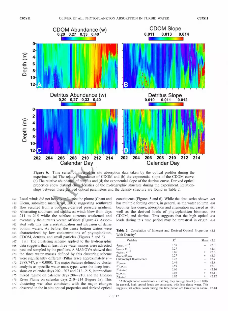
479constituents (Figures 5 and 6). While the time series shown480has multiple forcing events, in general, as the water column481becomes less dense, absorption and attenuation increased as482well as the derived loads of phytoplankton biomass,483CDOM, and detritus. This suggests that the high optical484loads during this time period may be terrestrial in origin.

Figure 6. Time series of inverted in situ absorption data taken by the optical profiler during theexperiment. (a) The relative abundance of CDOM and (b) the exponential slope of the CDOM curve.(c) The relative abundance of detritus and (d) the exponential slope of the detritus curve. Derived opticalproperties show distinct characteristics of the hydrographic structure during the experiment. Relation-ships between these derived optical parameters and the density structure are found in Table 2.

t2.1Table 2. Correlation of Inherent and Derived Optical Properties

With Densitya

Variable R2 Slope t2.2

A(488), m�1 0.58 � t2.3

C(488), m�1 0.27 � t2.4

Bb(470), m�1 0.06 + t2.5

Bb(470)/B(488) 0.27 + t2.6Chlorophyll fluorescence 0.22 � t2.7W(phyto) 0.46 � t2.8W(CDOM) 0.59 � t2.9W(detritus) 0.60 � t2.10S(CDOM) 0.03 + t2.11S(detritus) 0.02 + t2.12

aAlthough not all correlations are strong, they are significant (p = 0.000).In general, high optical loads are associated with less dense water. Thissuggests that optical loads during this time period are terrestrial in nature. t2.13


7 of 12

C07S11

485 Conversely, the particle size index (ratio of backscatter to486 total scatter), and the spectral exponential slopes of CDOM487 and detritus were positively correlated. This suggests that488 steeper slopes and smaller particles are coincident with489 marine waters during this time period (Table 2).

490 3.2. Spectrally Weighted Phytoplankton Absorption

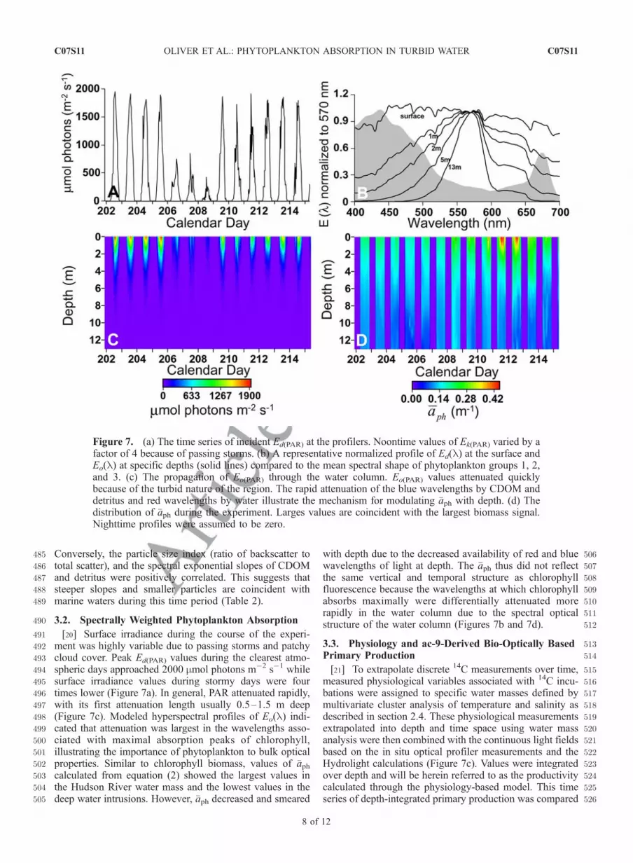
491 [20] Surface irradiance during the course of the experi-492 ment was highly variable due to passing storms and patchy493 cloud cover. Peak Ed(PAR) values during the clearest atmo-494 spheric days approached 2000 mmol photons m�2 s�1 while495 surface irradiance values during stormy days were four496 times lower (Figure 7a). In general, PAR attenuated rapidly,497 with its first attenuation length usually 0.5–1.5 m deep498 (Figure 7c). Modeled hyperspectral profiles of Eo(l) indi-499 cated that attenuation was largest in the wavelengths asso-500 ciated with maximal absorption peaks of chlorophyll,501 illustrating the importance of phytoplankton to bulk optical502 properties. Similar to chlorophyll biomass, values of �aph503 calculated from equation (2) showed the largest values in504 the Hudson River water mass and the lowest values in the505 deep water intrusions. However, �aph decreased and smeared

506with depth due to the decreased availability of red and blue507wavelengths of light at depth. The �aph thus did not reflect508the same vertical and temporal structure as chlorophyll509fluorescence because the wavelengths at which chlorophyll510absorbs maximally were differentially attenuated more511rapidly in the water column due to the spectral optical512structure of the water column (Figures 7b and 7d).

5133.3. Physiology and ac-9-Derived Bio-Optically Based514Primary Production

515[21] To extrapolate discrete 14C measurements over time,516measured physiological variables associated with 14C incu-517bations were assigned to specific water masses defined by518multivariate cluster analysis of temperature and salinity as519described in section 2.4. These physiological measurements520extrapolated into depth and time space using water mass521analysis were then combined with the continuous light fields522based on the in situ optical profiler measurements and the523Hydrolight calculations (Figure 7c). Values were integrated524over depth and will be herein referred to as the productivity525calculated through the physiology-based model. This time526series of depth-integrated primary production was compared

Figure 7. (a) The time series of incident Ed(PAR) at the profilers. Noontime values of Ek(PAR) varied by afactor of 4 because of passing storms. (b) A representative normalized profile of Ed(l) at the surface andEo(l) at specific depths (solid lines) compared to the mean spectral shape of phytoplankton groups 1, 2,and 3. (c) The propagation of Eo(PAR) through the water column. Eo(PAR) values attenuated quicklybecause of the turbid nature of the region. The rapid attenuation of the blue wavelengths by CDOM anddetritus and red wavelengths by water illustrate the mechanism for modulating �aph with depth. (d) Thedistribution of �aph during the experiment. Larges values are coincident with the largest biomass signal.Nighttime profiles were assumed to be zero.


8 of 12

C07S11

527 to the bio-optical model estimates using the ac-9-derived528 weighted phytoplankton absorption and equation (3).529 [22] To convert �aph into a productivity rate, we required530 estimates of fmax and Ek(PAR) which were taken from the531 literature (Figure 3). Using the mean values for fmax

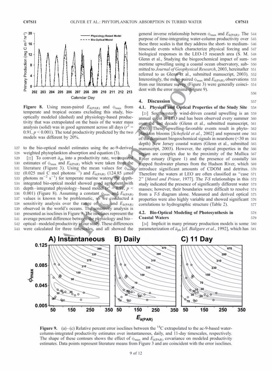
532 (0.025 mol C mol photons�1) and Ek(PAR) (124.85 mmol533 photons m�2 s�1) for temperate marine waters, the depth-534 integrated bio-optical model showed good agreement with535 depth–integrated physiology–based model (r2 = 0.91, p <536 0.001) (Figure 8). Assuming a constant fmax and Ek(PAR)

537 values is known to be problematic, so we conducted a538 sensitivity analysis over the range of fmax and Ek(PAR)

539 observed in the world’s oceans. The sensitivity analysis is540 presented as isoclines in Figure 9. The isoclines represent the541 average percent difference between the physiology and bio–542 optical–modeled productivity in our study. These differences543 were calculated for three timescales, and all showed the

544general inverse relationship between fmax and Ek(PAR). The545purpose of time-integrating water-column productivity over546these three scales is that they address the short- to medium-547timescale events which characterize physical forcing and548biological responses in the LEO-15 research area (S. M.549Glenn et al., Studying the biogeochemical impact of sum-550mertime upwelling using a coastal ocean observatory, sub-551mitted to Journal of Geophysical Research, 2003, hereinafter552referred to as Glenn et al., submitted manuscript, 2003).553Interestingly, the mean-paired fmax and Ek(PAR) observations554from our literature survey (Figure 3) were generally coinci-

dent with the error minima (Figure 9).556

5574. Discussion

5584.1. Physical and Optical Properties of the Study Site

559[23] Southwesterly wind-driven coastal upwelling is an560annual event at LEO and has been observed every summer561over the last decade (Glenn et al., submitted manuscript,5622003). These upwelling-favorable events result in phyto-563plankton blooms [Schofield et al., 2002] and represent one564of the dominant biogeochemical signals in nearshore (<30 m565depth) New Jersey coastal waters (Glenn et al., submitted566manuscript, 2003). However, the optical properties in the567region are complex due to the proximity of the Mullica568River estuary (Figure 1) and the presence of coastally569trapped freshwater plumes from the Hudson River, which570introduce significant amounts of CDOM and detritus.571Therefore the waters at LEO are often classified as ‘‘case5722’’ [Morel and Prieur, 1977]. The T-S relationships in this573study indicated the presence of significantly different water574masses; however, their boundaries were difficult to resolve575from a T-S diagram alone. Measured and derived optical576properties were also highly variable and showed significant577correlations to hydrographic structure (Table 2).

5784.2. Bio-Optical Modeling of Photosynthesis in579Coastal Waters

580[24] Implicit in many primary production models is some581parameterization of �aph [cf. Bidigare et al., 1992], which has

Figure 8. Using mean-paired Ek(PAR) and fmax fromtemperate and tropical oceans excluding this study, bio-optically modeled (dashed) and physiology-based produc-tivity that was extrapolated on the basis of the water massanalysis (solid) was in good agreement across all days (r2 =0.91, p < 0.001). The total productivity predicted by the twomodels was different by 20%.

Figure 9. (a)–(c) Relative percent error isoclines between the 14C extrapolated to the ac-9-based water-column-integrated productivity estimates over instantaneous, daily, and 11-day timescales, respectively.The shape of these contours shows the effect of fmax and Ek(PAR) covariance on modeled productivityestimates. Data points represent literature means from Figure 3 and are coincident with the error isoclines.


9 of 12

C07S11

582 traditionally been measured using discrete water samples or583 estimated empirically [Bricaud et al., 1995; Cleveland,584 1995]. Often �aph is derived from the product of biomass585 and biomass-normalized phytoplankton absorption (�aph* )586 [Sakshaug et al., 1997]. The utility of this approach is587 limited given the laboratory requirements for deriving �aph* ,588 and the well-documented variability in �aph* seasonally589 [Sathyendranath et al., 1999], regionally [Bricaud and590 Stramski, 1990; Hoepffner and Sathyendranath, 1992;591 Sosik, 1996; Arbones et al., 2000], and physiologically592 [Prezelin and Boczar, 1986; Lewis et al., 1988; Bricaud et593 al., 1995]. Ideally, the parameterization of �aph

* is not needed594 if �aph could easily be derived from in situ bulk optical595 measurements. Currently, off-the-shelf technology offers the596 potential to measure bulk optical properties [Dickey, 1991;597 Chang and Dickey, 1999].598 [25] High-resolution maps of �aph can be derived from an599 ac-9 (Figure 7d) allowing wavelength dependency of600 phytoplankton absorption and spectral light quality to be601 estimated. To first order �aph is described by chlorophyll602 biomass (r2 = 0.71, p = 0.000); however, �aph is a603 consistently decreasing function with depth. This decrease,604 a second-order effect, reflects the spectral skewing of light605 with depth. This spectral skewing of �aph was sensitive to606 the relative concentrations of the other in-water constitu-607 ents. For example, when CDOM and detritus signals were608 large (day 210) blue wavelengths (400–450 nm) of light609 were attenuated 30% faster than when CDOM and detritus610 signals were low (day 202). In contrast, the difference in611 red wavelength (650–700 nm) attenuation was approxi-612 mately 7%. The result of this variable skewing of the in613 situ light field accounts for the scatter between the614 phytoplankton fluorescence estimates and �aph. Given in615 situ �aph and Eo(PAR), the remaining difficulty for estimating616 photosynthesis is defining the magnitude of fmax and617 Ek(PAR) as these terms cannot currently be derived optically.618 While fmax has been related to fluorescence transients619 via fast repetition rate fluorometry [Kolber et al., 1988;620 Falkowski, 1992; Kolber and Falkowski, 1993], conversion621 of the electrons generated by photosystem II to carbon622 fixation is difficult [Kroon and Dijkman, 1996]. This con-623 version requires a thorough understanding of the environ-624 mental and physiological regulation of the photosynthetic625 quotient [Laws, 1991]. In nature, both fmax and Ek(PAR) are626 variable in time and space ranging from hours to seasons627 [Sournia, 1974; Prezelin, 1991; Kyewalyanga et al., 1998;628 Gong et al., 1999; Sathyendranath et al., 1999; Marra et629 al., 2000] and meters to kilometers [Schofield et al., 1993;630 Lindley et al., 1995; Sosik, 1996; Kyewalyanga et al., 1998].631 Over these scales, fmax and Ek(PAR) can vary by a factor632 of 10 and 5, respectively. To compensate for this effect,633 Ek(PAR) has been empirically or theoretically parameterized634 from underwater irradiance fields [Waters et al., 1994;635 Moline et al., 1998]. Parameterizations of fmax have636 proven difficult, and so is often assumed to be constant637 or is measured using radiolabel incubations [Marra, 1993;638 Waters et al., 1994; Ondrusek et al., 2001]. It was a639 pleasant surprise then that using temperate and tropical640 ocean means of fmax and Ek(PAR) from the literature641 resulted in such a good agreement of physiology-based642 productivity. Therefore we felt this serendipitous result643 merited further analysis.

644[26] The relationship between �aph, Ek(PAR), and fmax is645coupled via

Ek PARð Þ ¼Pmax

fmax�aph; ð5Þ

647which implies a general inverse, covariant relationship648between the product of fmax and �aph, and Ek(PAR). However,649sensitivity analyses of these terms in bio-optical productiv-650ity models [Sosik, 1996] suggest that �aph is not strongly651coupled to either Ek(PAR) or fmax. This effect is probably a652function of photoprotective pigments [Bidigare et al., 1989;653Schofield et al., 1996]. In contrast, Ek(PAR) and fmax appear654to be strongly coupled with each other [see Figure 6 in the655work of Sosik, 1996]. This is supported by the nonnormal656natural distribution of fmax and Ek(PAR) which shows an657inverse distribution suggesting that fmax and Ek(PAR) covary658in a nonlinear fashion (Figures 3 and 9). This implies that659their errors are not additive. Therefore determining the660sensitivity of an absorption-based bio-optical model without661considering this covariance would overestimate the im-662portance of the variability of fmax and Ek(PAR) to a663productivity estimate. Because of this we varied fmax and664Ek(PAR) over their natural ranges independent of other water-665column properties to quantify their impact on water-column666productivity. In addition, this error analysis assumed that667errors in the model related to the production of photo-668protective pigments were low because they were found in669negligible amounts in the HPLC analysis (zeaxanthin 0.1–6700.2 mg L�1) during the experiment and because of the highly671turbid nature of the water column.672[27] The net result of this analysis is that the variation in673fmax dominates the error in the productivity estimates over674hourly, daily, and 11-day timescales in temperate waters675(Figure 9). This is not surprising given past field results676in which fmax varied by a factor of 10 [Bannister and677Weidemann, 1984; Cleveland et al., 1989; Schofield et al.,6781993; Babin et al., 1996]. While the bio-optical model was679very sensitive to fmax, when considering literature values, the680variability in fmax is remarkably constrained temperate and681tropical waters ranging from �0.015 to 0.04 mol C mol682photons absorbed�1. Generally, the highest values are found683at depth, often near nutriclines [Cleveland et al., 1989],684where photosynthesis is light limited. Therefore the impact685on integrated water-column productivity is relatively small.686In these temperate waters, Ek(PAR) varies by a factor of 7 (50–687350 mmol photons m�2 s�1), reflecting photoacclimation688processes [Falkowski and LaRoche, 1991; Escoubas et al.,6891995]. However, the impact of Ek(PAR) variability is relatively690small in our analysis, as is evidenced by the elongation of the691error contours along the Ek(PAR) axis (Figure 9). This reflects692that a change in Ek(PAR) (especially when Ek(PAR) > 100) does693not dramatically impact the proportion of the total water-694column photosynthesis that is light-saturated as this is largely695determined by the exponential decay of light. It is the696combined effect of naturally constrained fmax values and697the rapid exponential decay of light in our system that allow698for our approach of bio-optically estimating productivity to699reasonably approximate the physiology-based model.700[28] While these general paradigms apply to temperate701and tropical waters, caution should be used, as this is not a702global phenomenon. In the Southern Ocean, discrete and


10 of 12

C07S11

703 water-column-averaged fmax values (Figures 3 and 9) are704 on average two times higher than that measured in tropical705 and temperate waters. The variance in fmax is also high. In706 these polar waters the Ek(PAR) magnitude (<100 mmol707 photons m�2 s�1) and variability (factor of 4) is low. Given708 equation (3) and that mean and variability of Ek(PAR) are709 relatively low, the light-saturated photosynthetic term is710 dominated by the product of fmax and �aph.711 [29] In contrast, the tropical and temperate oceans are712 generally stratified much of the year and have high-incident713 irradiance during the phytoplankton growing season. Be-714 cause of these factors, the euphotic zone is generally nutrient715 limited. The combination of low nutrient with high-light716 conditions can reduce the average water column, fmax. This717 decrease reflects the production of photoprotective pigments718 [Bidigare et al., 1989; Schofield et al., 1996; Fujita et al.,719 1994; Babin et al., 1996] and a decrease in functional720 photosynthetic reaction centers [Falkowski et al., 1989].721 The phytoplankton response to the high-light environment722 is an increase in Ek(PAR) given a sufficiently stable environ-

ment [Ryther and Menzel, 1959; Cote and Platt, 1983].724

725 5. Conclusions

726 [30] Bio-optical measurements show promise for map-727 ping phytoplankton; however, these techniques have often728 been compromised in turbid coastal waters. The bulk and729 derived optical parameters mimicked the hydrographic730 structure that was dominated by three distinct water masses731 advected through the study area. The correlations of density732 with bulk/derived optical properties suggest that much of733 the optical load is from terrestrial sources. Calculated �aph,734 from the relative phytoplankton weight and spectral irradi-735 ance showed that �aph was to first order a function of736 biomass but was modulated based on the spectral absorbing737 characteristics of in-water biotic and nonbiotic constituents.738 In addition, �aph could be used to initialize a bio-optical739 productivity model and calculate productivity within 20%740 given reasonable estimates of fmax and Ek(PAR). Sensitivity741 analysis of the bio-optical model indicated that most of the742 error is potentially associated with fmax; however, the743 natural range of water-column-averaged fmax is constrained.744 The bio-optical model was not as sensitive to Ek(PAR) when745 estimating water-column productivity because of the expo-746 nential decay of light in these turbid waters.

747 [31] Acknowledgments. Special thanks to two anonymous reviewers748 whose comments significantly improved the flow and content of this749 manuscript. Thanks and cold beer owed to Mike Crowley, Josh Kohut,750 Erica Heine, Mike Purcell, Christy Herren, Amanda Ashe, Dwight751 Peterson, Grace Chang, Sage Lichtenwalner, and Alan Weidmann. Support752 was provided by the Office of Naval Research’s COMOP and HyCODE753 programs (N00014-97-0767, N0014-99-0196), and the National Ocean754 Partnership Program (N00014-97-1-1019).

755 References756 Arbones, B., F. G. Figueiras, and R. Varela (2000), Action spectrum and757 maximum quantum yield of carbon fixation in natural phytoplankton758 populations: Implications for primary production estimates in the ocean,759 J. Mar. Syst., 26, 97–114.760 Babin, M., A. Morel, H. Claustre, A. Bricaud, Z. Kolber, and P. G. Falkowski761 (1996), Nitrogen-and irradiance-dependent variations of the maximum762 quantum yield of carbon fixation in eutrophic, mesotrophic, and oligo-763 trophic marine systems, Deep Sea Res., Part I, 43(8), 1241–1272.764 Bannister, T. T., and A. D. Weidemann (1984), The maximum quantum765 yield of phytoplankton photosynthesis in situ, J. Plankton Res., 6(2),766 275–294.

767Behrenfeld, M. J., and P. G. Falkowski (1997), A consumer’s guide to768phytoplankton productivity models, Limnol. Oceanogr., 42(7), 1479–7691491.770Bidigare, R. R., O. Schofield, and B. B. Prezelin (1989), Influence of771zeaxanthin on quantum yield of photosynthesis of Synechococcus clone772WH7803 (DC2), Mar. Ecol. Prog. Ser., 56, 177–188.773Bidigare, R. R., B. B. Prezelin, and R. C. Smith (1992), Bio-optical models774and the problems of scaling, in Primary Productivity and Biogeochemical775Cycles in the Sea, edited by P. G. Falkowski, pp. 175–212, Plenum, New776York.777Bienfang, P. K., and D. A. Ziemann (1992), The role of coastal high latitude778ecosystems in global export production, in Primary Productivity and779Biogeochemical Cycles in the Sea, edited by P. G. Falkowski, pp. 175–780212, Plenum, New York.781Biscaye, P. E., C. N. Flagg, and P. G. Falkowski (1994), The shelf edge782exchange experiment, Seep, II, An introduction to hypotheses, results and783conclusions, Deep Sea Res., Part II, 41(2), 231–253.784Bricaud, A., and D. Stramski (1990), Spectral absorption coefficients of785living phytoplankton and nonalgal biogenous matter: A comparison be-786tween the Peru upwelling area and the Sargasso Sea, Limnol. Oceanogr.,78735(3), 562–582.788Bricaud, A., M. Babin, A. Morel, and H. Claustre (1995), Variability in the789chlorophyll-specific absorption coefficients of natural phytoplankton:790Analysis and parameterization, J. Geophys. Res., 100(C7), 13,321–79113,332.792Brink, K. H. (1997), Observational coastal oceanography, paper presented793at National Science Foundation, paper presented at OCE Workshops,794Natl. Sci. Found., Monterey Bay, Calif.795Caceci, M. S., and W. P. Cacheris (1984), Fitting curves to data, Byte, 9,796340–362.797Chang, G. C., and T. D. Dickey (1999), Partitioning in situ spectral absorp-798tion by use of moored spectral absorption-attenuation meters, Appl. Opt.,79938(15), 3876–3887.800Cleveland, J. S. (1995), Regional models for phytoplankton absorption as a801function of chlorophyll a concentration, J. Geophys. Res., 100(C7),80213,333–13,344.803Cleveland, J. S., M. J. Perry, D. A. Kiefer, and M. C. Talbot (1989),804Maximal quantum yield of photosynthesis in the northwestern Sargasso805Sea, J. Mar. Res., 47, 869–886.806Cloern, J. E. (2001), Our evolving conceptual model of the coastal eutro-807phication problem, Mar. Ecol. Prog. Ser., 210, 223–253.808Cote, B., and T. Platt (1983), Day-to-day variations in the spring-summer809photosynthetic parameters of coastal marine phytoplankton, Limnol.810Oceanogr., 28(2), 320–344.811Dekshenieks, M. M., P. L. Donaghay, J. M. Sullivan, J. E. B. Rines, T. R.812Osborn, and M. S. Twardowski (2001), Temporal and spatial occurrence813of thin phytoplankton layers in relation to physical processes, Mar. Ecol.814Prog. Ser., 223, 61–71.815Dickey, T. D. (1991), The emergence of concurrent high-resolution physical816and bio-optical measurements in the upper ocean and their applications,817Rev. Geophys., 29(3), 383–413.818Escoubas, J. M., M. Lomas, J. LaRoche, and P. G. Falkowski (1995), Light819intensity regulation of cab gene transcription is signaled by the redox820state of the plastoquinone pool, Proc. Natl. Acad. Sci. U. S. A., 92,82110,237–10,241.822Falkowski, P. G. (1992), Molecular ecology of phytoplankton photosynth-823esis, in Primary Productivity and Biogeochemical Cycles in the Sea,824edited by P. G. Falkowski, pp. 47–67, Plenum, New York.825Falkowski, P. G., and J. LaRoche (1991), Acclimation to spectral irradiance826in algae, J. Phycol., 27, 8–14.827Falkowski, P. G., A. Sukenik, and R. Herzig (1989), Nitrogen limitation in828Isochrysis galbana (Haptophyceae), II, Relative abundance of chloroplast829proteins, J. Phycol., 25, 471–478.830Falkowski, P. G., P. E. Biscaye, and C. Sancetta (1994), The lateral flux of831biogenic particles from the eastern North American continental margin to832the North Atlantic Ocean, Deep Sea Res., Part II, 41(2), 583–602.833Field, C. B., M. J. Behrenfeld, J. T. Randerson, and P. Falkowski (1998),834Primary production of the biosphere: Integrating terrestrial and oceanic835components, Science, 281, 237–240.836Figueiras, F. G., B. Arbones, and M. Estrada (1999), Implications of bio-837optical modeling of phytoplankton photosynthesis in Antarctic waters:838Further evidence of no light limitation in the Bransfield Strait, Limnol.839Oceanogr., 44(7), 1599–1608.840Fujita, Y., A. Murakami, K. Aizawa, and K. Ohki (1994), Short-term and841long-term adaptation of the photosynthetic apparatus: Homeostatic prop-842erties of thylakoids, in The Molecular Biology of Cyanobacteria, edited843by D. A. Bryant, pp. 677–692, Kluwer Acad., Norwell, Mass.844Glenn, S. M., M. F. Crowley, D. B. Haidvogel, and Y. T. Song (1996),845Underwater observatory captures coastal upwelling events off New846Jersey, Eos Trans. AGU, 77, 233–236.


11 of 12

C07S11

847 Glenn, S. M., T. D. Dickey, W. P. Bisset, and O. Schofield (2000), Long-848 term real-time coastal ocean observation networks, Oceanography, 13,849 24–34.850 Gong, G., J. Chang, and Y. Wen (1999), Estimation of primary production851 in the Kuroshio waters northeast of Taiwan using a photosynthetic-852 irradiance model, Deep Sea Res., Part I, 46, 93–108.853 Gordon, H. R., and A. Morel (1983), Remote Sensing of Ocean Color for854 Interpretation of Satellite Visible Imagery: A Review, Springer-Verlag,855 New York.856 Hallegraeff, G. M. (1993), A review of harmful algal blooms and their857 apparent global increase, Phycology, 32, 79–99.858 Hoepffner, N., and S. Sathyendranath (1992), Bio-optical characteristics of859 coastal waters: Absorption spectra of phytoplankton and pigment distri-860 bution in the western North Atlantic, Limnol. Oceanogr., 37(8), 1660–861 1679.862 Holligan, P. M., and W. A. Reiners (1992), Predicting the responses of the863 coastal zone to global change, Adv. Ecol. Res., 22, 211–221.864 Jassby, A. D., and T. Platt (1976), Mathematical formulation of the relation-865 ship between photosynthesis and light for phytoplankton, Limnol.866 Oceanogr., 21, 540–547.867 Jickells, J. D. (1998), Nutrient biogeochemistry of the coastal zone,868 Science, 281, 217–222.869 Johnsen, G., O. Samset, L. Granskog, and E. Sakshaug (1994), In vivo870 absorption characteristics in 10 classes of bloom-forming phytoplankton:871 Taxonomic characteristics and responses to photoadaptation by means to872 discriminant and HPLC analysis, Mar. Ecol. Prog. Ser., 105, 149–157.873 Johnson, D. R., J. Miller, and O. Schofield (2003), Dynamics and optics of874 the Hudson River outflow plume, J. Geophys. Res., 108(C10), 3323,875 doi:10.1029/2002JC001485.876 Kishino, M., M. Takahashi, N. Okami, and S. Ichimura (1985), Estimation877 of the spectral absorption coefficients of phytoplankton in the sea, Bull.878 Mar. Sci., 37(2), 634–642.879 Kolber, Z. S., and P. G. Falkowski (1993), Use of active fluorescence to880 estimate phytoplankton photosynthesis in situ, Limnol. Oceanogr., 38,881 1646–1665.882 Kolber, Z. S., J. Zehr, and P. G. Falkowski (1988), Effects of growth883 irradiance and nitrogen limitation on photosynthetic energy conversion884 in photosystem II, Plant Physiol., 88, 923–929.885 Kroon, B. M. A., and N. A. Dijkman (1996), Photosystem II quantum886 yields, off-line measured P/I parameters and carbohydrate dynamics in887 Chlorella vulgaris grown under a fluctuating light regime and its888 application for optimizing mass cultures, J. Appl. Phycol., 8(4 –5),889 313–323.890 Kyewalyanga, M. N., T. Platt, S. Sathyendranath, V. A. Lutz, and V. Stuart891 (1998), Seasonal variations in physiological parameters of phytoplankton892 across the North Atlantic, J. Plankton Res., 20(1), 17–42.893 Laws, E. A. (1991), Photosynthetic quotients, new production and net894 community production in the open ocean, Deep Sea Res., Part A, 38,895 143–167.896 Lewis, M. R., O. Ulloa, and T. Platt (1988), Photosynthetic action, absorp-897 tion, and quantum yield spectra for a natural population of Oscillatoria in898 the North Atlantic, Limnol. Oceanogr., 33(1), 92–98.899 Lindley, S. T., R. R. Bidigare, and R. T. Barber (1995), Phytoplankton900 photosynthesis parameters along 140�W in the equatorial Pacific, Deep901 Sea Res., Part II, 42(2–3), 441–463.902 Lorenzo, L. M., B. Arbones, F. G. Figueiras, G. H. Tilstone, and F. L.903 Figueroa (2002), Photosynthesis, primary production and phytoplankton904 growth rates in Gerlache and Bransfield Straits during Austral summer:905 Cruise of FRUELA 95, Deep Sea Res., Part II, 49, 707–721.906 Marra, J. (1993), Proportionality between in situ carbon assimilation and907 bio-optical measures of primary production in the Gulf of Maine in908 summer, Limnol. Oceanogr., 38(1), 232–238.909 Marra, J., C. C. Trees, R. R. Bidigare, and R. T. Barber (2000), Pigment910 absorption and quantum yields in the Arabian Sea, Deep Sea Res., Part II,911 47, 1279–1299.912 Moline, M., and B. B. Prezelin (1996), Long-term monitoring and analy-913 sis of physical factors regulating variability in coastal Antarctic phyto-914 plankton biomass, in situ productivity and taxonomic composition over915 subseasonal, seasonal and interannual time scales, Mar. Ecol. Prog. Ser.,916 145, 143–160.917 Moline, M. A., O. Schofield, and N. P. Boucher (1998), Photosynthetic918 parameters and empirical modeling of primary production: A case study919 on the Antarctic Peninsula shelf, Antarct. Sci., 10(1), 45–54.920 Morel, A., and L. Prieur (1977), Analysis of variations in ocean color,921 Limnol. Oceanogr., 22, 709–722.922 Morel, A., D. Antoine, M. Babin, and Y. Dandonneau (1996), Measured923 and modeled primary production in the northeast Atlantic (EUMELI924 JGOFS program): The impact of natural variations in photosynthetic925 parameters in model predictive skill, Deep Sea Res., Part II, 43,926 1273–1304.

927Ondrusek, M. E., R. R. Bigidare, K. Waters, and D. M. Karl (2001), A928predictive model for estimating rates of primary production in the sub-929tropical North Pacific Ocean, Deep Sea Res., Part II, 48, 1837–1863.930Pope, R., and E. Fry (1997), Absorption spectrum (380–700 nm) of pure931water, II, Integrating cavity measurements, Appl. Opt., 36(33), 8710–9328723.933Prezelin, B. B. (1991), Diel periodicity in phytoplankton productivity,934Hydrobiology, 238, 1–35.935Prezelin, B. B., and B. A. Boczar (1986), Molecular bases of cell absorption936and fluorescence in phytoplankton: Potential applications to studies in937optical oceanography, Prog. Phycol. Res., 4, 349–464.938Prezelin, B. B., R. R. Bidigare, H. A. Matlick, M. Putt, and B. VerHoven939(1987), Diurnal patterns of size-fractioned primary productivity across a940coastal front, Biol. Morya Vladivostok., 96, 563–574.941Prezelin, B. B., H. E. Glover, B. VerHoeven, D. K. Steinberg, H. A.942Matlick, O. Schofield, N. B. Nelson, M. Wyamn, and L. Campbell943(1989), Blue-green light effects on light-limited rates of photosynthesis:944Relationship to pigmentation and productivity estimates from the Sargas-945so Sea, Mar. Ecol. Prog. Ser., 54, 121–136.946Ryther, J. H., and D. W. Menzel (1959), Light adaptation by marine phy-947toplankton, Limnol. Oceanogr., 4(4), 492–497.948Sakshaug, E., A. Bricaud, Y. Dandonneau, P. G. Falkowski, D. A. Kiefer,949L. Legendre, A. Morel, J. Parslow, and M. Takahashi (1997), Parameters950of photosynthesis: Definitions, theory and interpretation of results,951J. Plankton Res., 19(11), 1637–1670.952Sathyendranath, S., V. Stuart, B. D. Irwin, H. Maass, G. Savidge, L. Gilpin,953and T. Platt (1999), Seasonal variations in bio-optical properties of phy-954toplankton in the Arabian Sea, Deep Sea Res., Part II, 46, 633–653.955Schofield, O., B. B. Prezelin, R. R. Bidigare, and R. C. Smith (1993), In956situ photosynthetic quantum yield, correspondence to hydrographic and957optical variability within the southern California Bight, Mar. Ecol. Prog.958Ser., 93, 24–37.959Schofield, O., B. B. Prezelin, and G. Johnsen (1996), Wavelength depen-960dency in photosynthetic parameters for two dinoflagellate species961Heterocapsa pygmaea and Prorocentrum minimum: Implications for962the bio-optical modeling of photosynthetic rates, J. Phycol., 32, 574–583.963Schofield, O., T. Bergmann, W. P. Bisset, F. Grassle, D. Haidvogel,964J. Kohut, M. Moline, and S. Glenn (2002), The long term ecosystem965observatory: An integrated coastal observatory, IEEE J. Oceanic Eng.,96627(2), 146–154.967Siegel, D. A., et al. (2001), Bio-optical modeling of primary production on968regional scales: The Bermuda bio-optics project, Deep Sea Res., Part II,96948, 1865–1896.970Smith, R. C., B. B. Prezelin, R. R. Bidigare, and K. S. Baker (1989), Bio-971optical modeling of photosynthetic production in coastal waters, Limnol.972Oceanogr., 38(4), 1524–1544.973Sosik, H. M. (1996), Bio-optical modeling of primary production: Conse-974quences of variability in quantum yield and specific absorption, Mar.975Ecol. Prog. Ser., 143, 225–238.976Sournia, A. (1974), Circadian periodicities in natural populations of marine977phytoplankton: A review, Adv. Mar. Biol., 6, 325–389.978Stramski, D., and A. Morel (1990), Optical properties of photosynthetic979picoplankton in different physiological states as affected by growth irra-980diance, Deep Sea Res., 37, 245–266.981Vodacek, A., N. V. Blough, M. D. DeGrandpre, E. T. Peltzer, and R. K.982Nelson (1997), Seasonal variation of CDOM and DOC in the middle983Atlantic Bight: Terrestrial inputs and photooxidation, Limnol. Oceanogr.,98442(4), 674–686.985Walsh, J. J. (1978), Wind events and food chain dynamics within the New986York Bight, Limnol. Oceanogr., 23(4), 649–683.987Ward, J. H. (1963), Hierarchical grouping to optimize an objective function,988J. Am. Stat. Assoc., 58, 236–244.989Waters, K. J., R. C. Smith, and J. Marra (1994), Phytoplankton production990in the Sargasso Sea as determined using optical mooring data, J. Geo-991phys. Res., 99(C9), 18,385–18,402.992Wright, S. W., S. W. Jeffrey, R. F. C. Mantoura, C. A. Llewellyn,993T. Bjornland, D. Repeta, and N. Welschmeyer (1991), Improved HPLC994method for the analysis of chlorophylls and carotenoids from marine995phytoplankton, Mar. Ecol. Prog. Ser., 77, 183–196.996Zimmerman, R. C., J. B. SooHoo, J. N. Kremer, and D. Z. D’Argenio997(1987), Evaluation of variance approximation techniques of non-linear998photosynthetic-irradiance models, Biol. Morya Vladivostok, 95, 209–215.

��1000T. Bergmann, S. Glenn, M. J. Oliver, and O. Schofield, Institute of1001Marine and Coastal Sciences, Rutgers University, 71 Dudley Road, New1002Brunswick, NJ 08903, USA. ([email protected])1003M. Moline and C. Orrico, Biological Sciences Department, California1004Polytechnic State University, San Luis Obispo, CA 93407, USA.


12 of 12

C07S11

deriving in situ phytoplankton absorption for bio-optical productivity models in turbid waters

Documents