remote sensing

Article

Deriving Aerodynamic Roughness Length at Ultra-HighResolution in Agricultural Areas Using UAV-Borne LiDAR

Katerina Trepekli 1,2,* and Thomas Friborg 1

�����������������

Citation: Trepekli, K.; Friborg, T.

Deriving Aerodynamic Roughness

Length at Ultra-High Resolution in

Agricultural Areas Using UAV-Borne

LiDAR. Remote Sens. 2021, 13, 3538.

https://doi.org/10.3390/rs13173538

Academic Editor: Nicolas R. Dalezios

Received: 16 July 2021

Accepted: 2 September 2021

Published: 6 September 2021

Publisher’s Note: MDPI stays neutral

with regard to jurisdictional claims in

published maps and institutional affil-

iations.

Copyright: © 2021 by the authors.

Licensee MDPI, Basel, Switzerland.

This article is an open access article

distributed under the terms and

conditions of the Creative Commons

Attribution (CC BY) license (https://

creativecommons.org/licenses/by/

4.0/).

1 Department of Geosciences and Natural Resource Management, University of Copenhagen,Øster Voldgade 10, 1350 Copenhagen, Denmark; tfj@ign.ku.dk

2 Department of Computer Science, University of Copenhagen, Universitetsparken 1,2100 Copenhagen, Denmark

* Correspondence: atr@ign.ku.dk; Tel.: +45-353-267-98

Abstract: The aerodynamic roughness length (Z0) and surface geometry at ultra-high resolution inprecision agriculture and agroforestry have substantial potential to improve aerodynamic processmodeling for sustainable farming practices and recreational activities. We explored the potentialof unmanned aerial vehicle (UAV)-borne LiDAR systems to provide Z0 maps with the level ofspatiotemporal resolution demanded by precision agriculture by generating the 3D structure ofvegetated surfaces and linking the derived geometry with morphometric roughness models. Weevaluated the performance of three filtering algorithms to segment the LiDAR-derived point cloudsinto vegetation and ground points in order to obtain the vegetation height metrics and density ata 0.10 m resolution. The effectiveness of three morphometric models to determine the Z0 mapsof Danish cropland and the surrounding evergreen trees was assessed by comparing the resultswith corresponding Z0 values from a nearby eddy covariance tower (Z0_EC). A morphologicalfilter performed satisfactorily over a homogeneous surface, whereas the progressive triangulatedirregular network densification algorithm produced fewer errors with a heterogeneous surface. Z0

from UAV-LiDAR-driven models converged with Z0_EC at the source area scale. The Raupachroughness model appropriately simulated temporal variations in Z0 conditioned by vertical andhorizontal vegetation density. The Z0 calculated as a fraction of vegetation height or as a functionof vegetation height variability resulted in greater differences with the Z0_EC. Deriving Z0 in thismanner could be highly useful in the context of surface energy balance and wind profile estimationsfor micrometeorological, hydrologic, and ecologic applications in similar sites.

Keywords: unmanned aerial vehicles (UAVs); light detection and ranging (LiDAR); aerodynamicroughness length; point cloud classification; precision agriculture; morphometric roughness models

1. Introduction

To achieve more sustainable land and water-use management in precision agriculture,the serviceable description of the complex interactions between the vegetation growth,water availability, and aerodynamic characteristics of a canopy is pivotal. In this context,aerodynamic roughness length for momentum transfer (Z0) is a key factor in micrometeo-rological and hydrological applications, since it can elucidate how surface geometry maylead to alterations in energy, gas, and water exchanges surface friction; and the deflection ofairflow [1–3]. Many models have been developed to estimate the components of surface en-ergy balance and evapotranspiration (ET) [4–7] using passive remote sensing observationsand a set of algorithms to retrieve surface parameters such as the aerodynamic resistance toheat transfer (rah), which is a function of Z0 [8,9]. Obtaining an efficient parameterizationfor rah has been a challenging task, and there is no single method to accurately estimateZ0 over a wide range of land cover types [10,11], introducing further uncertainty in themodeling of energy fluxes and ET. As such, incremental advances in resolving Z0 usingcanopy structure data at ultra-high resolution from drone-borne instrumentation have the

Remote Sens. 2021, 13, 3538. https://doi.org/10.3390/rs13173538 https://www.mdpi.com/journal/remotesensing

Remote Sens. 2021, 13, 3538 2 of 21

potential to improve the accuracy of surface energy balance models in the context of energy,gas, and water exchange estimations in precision agriculture and related applications.

Two primary approaches exist in assigning Z0 values. The most commonly usedmethod is based on micrometeorological observations obtained by an eddy covariance (EC)system and the Monin–Obukhov similarity theory. A disadvantage of this approach is thatZ0 is restricted to single average values in the flux footprint of the EC system. Moreover,estimates of Z0 cannot always rely on field-based experiments due to practical limitationsand high costs. The second approach relies on the demarcation of surface objects usingremote sensing observations and the establishment of empirical relationships between Z0and measurable characteristics of site-specific roughness elements. In this morphometricmethod, theoretical models of the boundary layer are combined with more sophisticatedphysical models of vegetation canopy to determine Z0 (e.g., [12]). Following this approach,Z0 is often associated with the frontal area index (fai), which is the area of windwardvertical faces of the roughness elements to the total area under consideration, and the planarea index (pai), which equals the horizontal area occupied by roughness elements dividedby the total area [13]. For agricultural and natural sites without density information, Z0is often simply related to canopy height (h) [14]. However, this relation is not alwaysconstant, since the density, the type of vegetation, and the micro- or macrotopographiccharacteristics can affect Z0 variations as well [15].

Using remote sensing optical imagery and morphometric models, numerous re-searchers have developed semi-empirical formulas applicable to obtain fractional valuesof Z0/h of vegetation surfaces [16], and some of them have included the effects of veg-etation indices (VIs) [17]. However, precise observations of vegetation height or VI inboth high spatial and temporal resolution are difficult to obtain from publically availablesatellite datasets [18]. A major weakness of airborne/satellite imagery is its limitation inviewing beneath the canopy, leading to sparse points and low-density information on baresoil [19], whereas light detection and ranging (LiDAR) scanners can provide quantitativeinformation on the 3D structure of a canopy because the laser pulses can partly penetratevegetation cover. The technology of airborne LiDAR scanners (ALS) has now successfullybeen employed for the extraction of surface roughness characteristics in forests [20,21],urban areas [22], and low-vegetation areas [23]. The representation of a mixed grasslandprairie by ALS datasets revealed that up to 76% of the variation in Z0 was due to the heightvariability of vegetation and up to 65% of the variation could be explained by estimatesof vegetation height [24]. Li et al. [25] found that the accuracy of the estimated Z0 of asemi-arid shrubland using ALS data depends on the adopted morphometric models andthe precise representation of shrub height in these models. In short and dense canopies, theestimation of vegetation height using ALS is prone to errors [26], mainly due to the lack ofidentifiable referenced objects and of detectable differences between first (i.e., vegetation)and last (i.e., ground) LiDAR returns [27,28].

Given these challenges, the advantages conferred by unmanned aerial vehicle (UAV)-borne-LiDAR scanners may yield fine-grained spatiotemporal estimations of Z0 in agri-cultural areas. Compared to manned ALS, the comparatively cost-effective UAV-LiDARsystems are more flexible in data sampling and produce higher point cloud density dueto the larger field of view of the scanner and lower flight altitude and speed, allowing alarger number of LiDAR beams per scan [29]. These characteristics may limit the com-monly observed underestimation of canopy heights and mitigate difficulties in derivingindividual roughness element canopies from airborne LiDAR data [30]. Resop et al. [31]documented that higher-resolution UAV-LiDAR data facilitated the identification of smallvegetation and micro-alterations in a heterogeneous terrain that were not detectable byALS observations. In a similar study, the 3D characterization of individual plant species ofa shrubland area was achievable at the submeter scale using a UAV-LiDAR system [32].However, the technology of UAV-LiDAR is not currently used in precision farming, despiteits ability to effectively monitor canopy density [33] and fine-scale variations in crops

Remote Sens. 2021, 13, 3538 3 of 21

attributes compared to UAV-optical imagery [34–36], which is widely employed in suchapplications [37–40].

Most published methods for the estimation of crop height from LiDAR sensors arebased on the determination of the canopy height model (CHM), which is derived fromthe difference between rasterized ground elevation data (digital terrain model (DTM) andrasterized original point cloud elevation data (digital surface model (DSM)). A DTM of anagricultural field can be easily retrieved by scanning the bare soil before vegetation growth,but such data acquisitions are not always feasible due to land management practices,so a variety of filtering methods to generate DTMs and CHMs from airborne LiDARdata have been developed. As automatic separation of ground and non-ground pointsfrom LiDAR data has proved to be challenging and the filtering algorithms typicallyhave problems distinguishing ground returns and points reflecting vegetation [41], theadaptability of existing approaches for processing point cloud obtained by UAV-LiDAR iscurrently inadequate.

Poor filtering performance, particularly in areas of dense vegetation that hides under-lying terrain features, may result in erroneous surface morphologies or in sparse groundpoints, which, when interpolated, fail to reproduce surface morphology. In this framework,a detailed understanding of the errors associated with producing CHMs using UAV-LiDARtechnology and a context-specific approach to assess filtering algorithms and morphometricmethods to estimate surface characteristics are required.

We explored the potential of UAV-borne LiDAR in the estimation and mappingof surface roughness of a typical dense agricultural environment at very high spatialresolution. The major components of the project were as follows:

• An evaluation of the performance of three segmentation approaches (i.e., a morpholog-ical filter (MF), a progressive triangulated irregular network densification filter (TIN),and a combination of MF and TIN) to reliably partition the UAV-LiDAR-derived pointcloud data into bare earth and vegetation and, consequently, to generate CHMs atcentimeter resolution.

• An assessment for calculating Z0 values from UAV-LiDAR data using three dif-ferent morphometric methods (Kustas et al. [14], Raupach, [42], and Menenti andRitchie [43]), and a comparison of the respective results with the Z0 obtained from ECobservations.

• A discussion of the challenges and further potential of UAV-LiDAR in precisionagriculture and related applications.

2. Materials and Methods2.1. Site Description

The experimental site is part of the Integrated Carbon Observation System network(ICOS) located in Jutland, Denmark (56.037644◦ N, 9.159383◦ E). The site is a dense agricul-tural area with negligible topographic relief covered by potato plants with heights varyingfrom 0.3 to 1.7 m and sparse trees (Figure 1). The climate is humid temperate; during thesummer of 2019, the mean temperature was 18.54 ◦C and the mean relative humidity was66.65%. The site’s prevailing winds originated from the west (199◦) and the mean windspeed recorded was 2.83 m/s.

2.2. Data Collection

The aerial campaign was conducted on a monthly scale before and during the ger-mination of vegetation (14 May, 26 June, 14 July, and 12 August 2019). Point cloud datawere acquired using a UAV-LiDAR system (LidarSwiss GmbH, CH) onboard an octocopterMatrice 600 Pro drone (Figure 2). The LiDAR system included an internal navigationsystem (INS—Oxts Xnav 550 OEM IMU/GPS system) that fused data from an inertial mea-surement unit (Oxts micro electro-mechanical systems) and GPS data received by a GlobalNavigation Satellite System antenna, a beam LiDAR scanner (Quanergy M8), a 20 mpSONY RGB camera (16 mm lens), and an integrated data storage unit. A Trimble real-time

Remote Sens. 2021, 13, 3538 4 of 21

kinematic GNSS base station was used to provide additional overhead communicationwith the INS. The horizontal field of view (FOV) of the laser scanner was 360 degrees andthe vertical FOV was 20 degrees. The LiDAR data were recorded at 40 m above the ground,producing an average point density of 250 points/m2 (max 400 points/m2). The swathwidth of a single pass was 89 m, and the overlap between two adjacent swaths was greaterthan 25%. The raw GNSS data files obtained by the INS were converted to position data inpos format using trajectory software (RT Post-process of the NAVsuite software package).The laser scanner’s data were initially produced in bin format and were converted to pointclouds in las format using the position data (Geo-LAS software).

An EC system was installed at the western edge of a fenced measuring plot (80 × 20 m),approximately in the center of the agricultural field (orange point in Figure 1). The instru-mentation included a Gill R3-50 sonic anemometer (Gill Instruments Ltd., Lymingdon, UK)and a LI7000 closed-path infrared CO2/H2O gas analyzer (LI-COR, Lincoln, NE, USA).During the sampling period, EC data were recorded at a nominal sampling frequency of20 Hz and ancillary meteorological data at 1 Hz (for further details, see [44]).

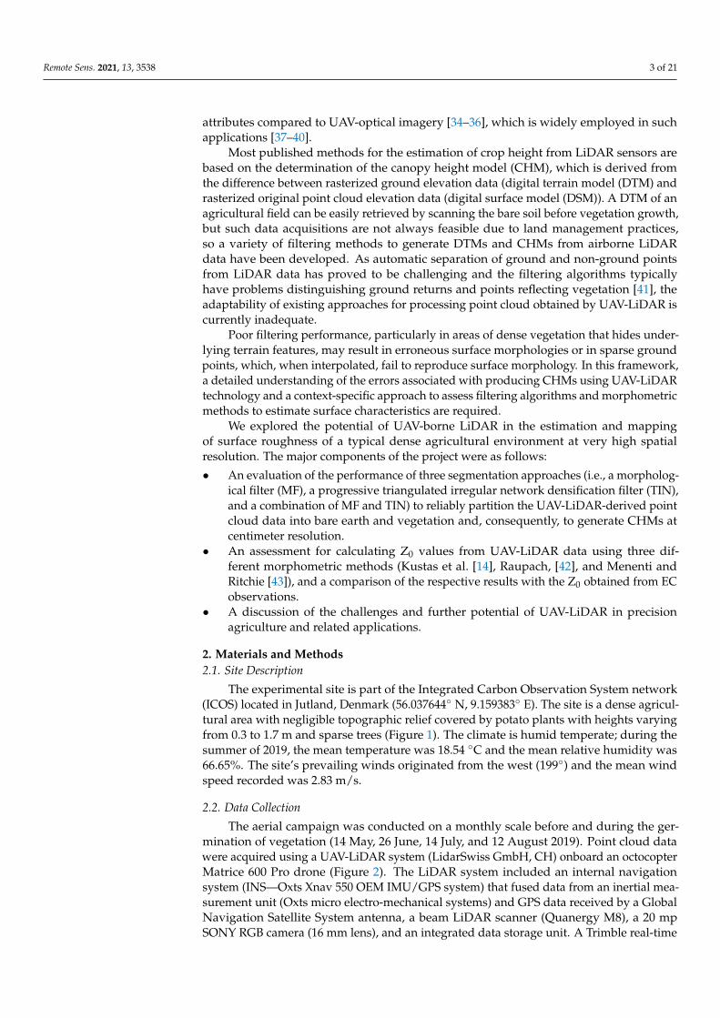
Figure 1. Illustration of the agricultural area (56.037644◦ N, 9.159383◦ E) surveyed by the Unmannedaerial vehicle-Light detection and ranging (UAV-LiDAR) system (30.68 ha), and the two subsceneswith a range of roughness element densities: Plot 1 with more homogeneous heights correspondingto the wind regime 190◦ to 347◦ (yellow, left rectangle), and Plot 2 with more heterogeneous heightscorresponding to the wind regime spanning from 90◦ to 190◦ (red, right rectangle). The orange labelindicates the location of the Eddy covariance tower.

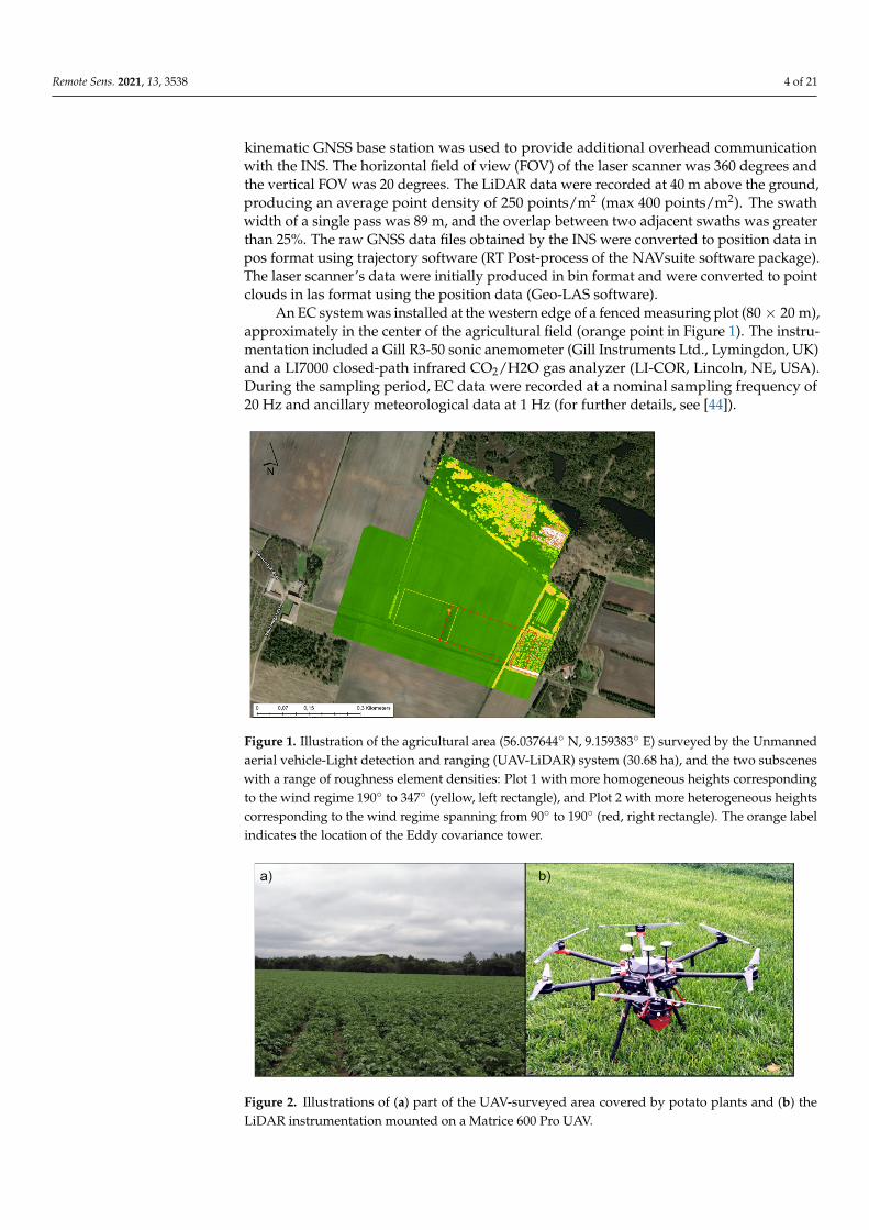
Figure 2. Illustrations of (a) part of the UAV-surveyed area covered by potato plants and (b) theLiDAR instrumentation mounted on a Matrice 600 Pro UAV.

Remote Sens. 2021, 13, 3538 5 of 21

2.3. Evaluation Procedure

A relative homogeneous subscene area of the agricultural field (100 × 150 m coveredarea) was used to evaluate the performance of the different filtering algorithms appliedto the LiDAR dataset retrieved in June (Plot 1 in Figure 1). The optimal set of parametersfor each filter was estimated by comparing their effectiveness in terms of the total errors(TEs) of misclassification. Each filter with the optimized parametrization was then appliedto the point cloud data, representing the subscene Plot 1 for July and August, and to asecond subscene (100 × 270 m) covered by low and high vegetation (Plot 2 in Figure 1).The manual classification of point clouds into terrain and vegetation cannot entirely beemployed in a GIS framework because filtering errors in such dense areas are not soobvious to interpret with the naked eye. Instead, bare earth elevation data, as resourcedin May before vegetation growth, were combined with the rest of the collected pointcloud data from June to August in order to manually label the non-ground points asreferenced data of vegetation. The plant heights, represented by the CHMs produced at0.10 m resolution, were compared with the plant heights that were manually measuredin randomly selected 1 × 1 m geolocated plots during the aerial campaign. Based on theCHMs’ various geometric parameters, we evaluated the effectiveness of the morphometricmodels to obtain Z0 values by comparing them with the anemometric-based method forspecific flux footprint areas.

2.4. Point Cloud Processing

Due to multi-path reflection, the pulses emitted from a LiDAR scanner may reachthe ground without returning directly to the instrument but rather reaching neighboringsurface points, creating noise data within the point clouds. By calculating the standarddeviation of each point’s surrounding fitting plane and by defining an expected relativeerror (RE = 2), a point was labeled as an outlier if its distance from the fitting plane wasgreater than the mean average distance plus the product of relative error and standarddeviation [45]. Additionally, low noise points that were close to the ground were excludedfrom further analysis by comparing the maximum height difference between each pointand their neighboring points with a height threshold (max height = 0.2 m).

The classification of the point cloud data to vegetation and bare earth was based onthe triangulated irregular network densification filter (TIN) [46], a morphological filter(MF) [47], and progressive triangulated irregular network densification (PTD), introducedby Zhao et al. [48]. The efficiency of a filtering algorithm depends on the choice of openingwindow/grid step and threshold used within each filter. These values are uncertain in allfilters and are expected to depend on the size of the objects and the land cover type [49].

The morphological filter (MF) is based on a progressively increasing window size inan iterative process. If the elevation difference between the original data and the data afterthe opening operation is higher than a user-defined elevation threshold (zthresh), the gridis labeled as a non-ground grid. A number of runs was conducted for the MF filter usinga maximum window size from 0.4 to 1 m with an increment of 0.2 m and an elevationthreshold from 0.25 to 1.5 m in 0.25 m intervals using a commercial software package [50].

To identify likely ground points in the TIN method, some of the terrain-local minimumpoints were used as the initial ground seed points to build an initial triangulated irregularnetwork. The sensitivity of the filter was tested by setting it in a software package [51]:a grid step of 0.2 to 1.6 m in 0.2 m intervals based on practical experience, and the spikeparameter to 0.10 m, 0.25 and 0.5 m considering the standard deviation for planar patchesequal to 1. The spike parameter describes the distance above the coarsest triangulatednetwork for which the points are classified as terrain.

In the PTD algorithm, ground seed points are acquired through a morphologicalopening operation instead of using the lowest points in user-defined grids. The parametersof iterative distance were set to vary from 0.2 to 1 m in an increment of 0.2 m, and an iterativeangle from 2◦ to 18◦ in an increment of 4◦, using a commercial software package [52].

Remote Sens. 2021, 13, 3538 6 of 21

To assess the performance of the three applied filtering methods, total error (TE) wascalculated according to the following equation [53]:

TE = (a + b)/e (1)

where a is the number of ground points that have been incorrectly classified as vegetationpoints, b is the number of vegetation points that have been incorrectly classified as groundpoints by comparing the processed point cloud datasets to the referenced data for Plot 1,and e is the total number of points tested.

Once vegetation was segmented from the LiDAR dataset, the resultant ground pointswere interpolated to replace non-ground points with an approximation of the correctsurface morphology. The inverse distance weighted method [54] was used to interpolatethe voids (Figure 3). The point clouds were converted to raster gridded elevation layersof 0.03–0.05 m resolution by connecting all the available point features into a network oftriangles and interpolating over the triangular faces using the feature elevation and slopevalues. To reduce the noise in the raster images by using all the point features, the pointcloud data were spatially binned into areas corresponding with the size of the output gridcells [50]. In our analysis, one elevation value from each of the spatial bins was used togenerate a gridded layer with a 0.10 m resolution.

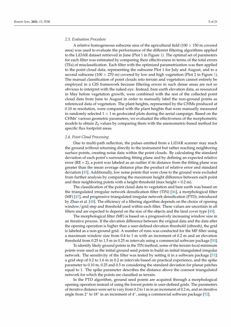
Figure 3. Example of rasterized point clouds after interpolation representing part of the agricultural field.

2.5. Description of Morphometric Methods

Three morphometric models were assessed to determine the Z0 of the subscenes, Plot1 and Plot 2, surrounding the EC tower through surface morphology.

2.5.1. Roughness Length Based on Vegetation Height

The rule of thumb (RT) method only requires the average roughness element height(h) per pixel, which is linearly related to Z0 [14] as follows:

Z0_RT = 0.1 h (2)

2.5.2. Roughness Length Based on Vegetation Geometry and Wind Conditions

In more advanced morphometric models, the alterations and resulting effects ofcanopy drag can be included by calculating the drag coefficient [55]. Raupach’s model(RAP), described in Equation (3a, 3b), includes the drag coefficient of an isolated roughnesselement (cs = 0.003); the drag coefficient for the substrate surface at h (cr = 0.3); theroughness sublayer influence function (ψh = 0.193, accounting for the correction to thelogarithmic wind profile); the wind speed (U), the friction velocity, u*, (u*/U)max = 0.3;and a free parameter (cd1 = 7.5). Zd (m) is the zero-plane displacement and k is the vonKarman’s constant (= 0.4).

Z0_RAP = h (1 − Zd/h) exp(−k U/u* + ψh) (3a)

Remote Sens. 2021, 13, 3538 7 of 21

Zd/h = 1 + {(exp [−(2cd1 fai)0.5] − 1)/(2cd1 fai)0.5}

u*/U = min [(cs + cr fai)0.5, (u*/U)max](3b)

The frontal area index (fai) can be defined by integrating positive height changes (∆y)over a cross-sectional line divided by the distance (∆x) in that section length, assuming anisotropic surface [25,56].

fai = (∑∆y)/(∑∆x) for ∆y > 0 (4)

The advantage of this technique is that we do not consider the precise shape of aplant but rather its cross-sectional area perpendicular to the wind [22]. In this analysis, weextracted cross-sections along 360/24 sectors reflecting different wind directions from eachgenerated CHM to derive the frontal area indexes. The associated morphometric Z0 fromall directions were averaged into one value at each grid cell.

The plan area index (pai), which equals the horizontal area occupied by roughnesselements divided by the total area under consideration, was also calculated since it can beassociated with Z0 and Zd [15]. For instance, it was observed that as surface cover increases,the magnitude of Zd/h produces a convex curve asymptotically increasing from zero tounity, which is the maximum possible value of pai. The pai and fai for each wind directionwere calculated using the UMEP plugin [57] in the open-source geographical informationsoftware QGIS [58].

2.5.3. Roughness Length Based on Vegetation Height Variability

This empirical model of Menethi and Ritchie [43] (MR) determines Z0 as a function ofvegetation height variability for each grid cell that is segmented by subcells following:

Z0_MR = (1/N) ∑ (σi,j/hi,j) havg (5)

where N is the number of subcells within each grid cell; σi,j is the standard deviation of theLiDAR-derived vegetation height (hi,j) per each subcell I; j. havg is the average vegetationheight calculated from the LiDAR’s CHM. It was documented that coarser grid cells reducethe standard deviation of height regardless of the size of the subcells, while larger subcellslead to higher values of Z0 [25]. Based on these observations, the size of each grid cell waschosen to be equal to 1 m and the segment size inside each grid was 0.25 m, reflectingthe maximum expected variance in plant height within a 1 × 1 m cell. All the geometricparameters of vegetation from the CHMs were retrieved using QGIS.

2.6. Description of the Anemometric Method

The raw data of wind, carbon dioxide, water vapor, and sonic temperature datawere processed using EddyPro 4.2.1 software (LI-COR, Lincoln, NE, USA) to estimatehalf-hourly turbulent scalar fluxes. The processing included statistical tests for raw datascreening [59], angle of attack correction [60], 2D coordinate rotation, block averaging, timelag optimization to maximize covariance between vertical wind speed and gas concen-trations, humidity corrections applied to the sonic temperature [61], and compensationfor density fluctuations [62]. Flux quality flags were assigned according to the test forsteady-state conditions and fully developed turbulence following Foken et al. [63] andsimplified by CarboEurope-IP.

From the EC micrometeorological data, the estimations of friction velocity, sensibleheat flux, and Obukhov length, as well as the meteorological data of wind speed anddirection, were used to calculate Z0 (Z0_EC) following the logarithmic wind law. For stableor unstable atmospheric conditions, the logarithmic wind profile [64] is given by:

Z0_EC = (z − Zd)/exp(kU/u* + ψm) (6)

Remote Sens. 2021, 13, 3538 8 of 21

where z is the measurement height (m). The stability correction for momentum ψm wascomputed using the parameterizations suggested by Högström [65]. Under neutral atmo-spheric conditions, ψm equals zero. Zd was considered here to be equal to 0.7 h [14].

Half-hourly estimations of Z0_EC from 25 to 27 June, from 13 to 15 July, from 12 to 13of August, and for daytime hours (from 9:00 to 19:00 local time) were used as referencevalues for validating the morphometric-derived Z0. This EC dataset was selected for thecomparison analysis of the different methods to calculate Z0 in order to minimize the effectof the differences in the temporal and spatial resolution of the remote sensing data acquiredon the 26 June, 14 July, and 12 August, and in situ EC data.

3. Results3.1. Segmentation of Point Cloud Data

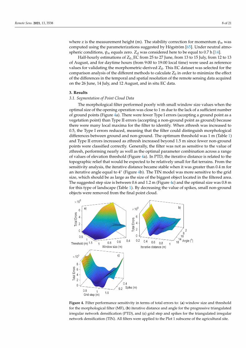
The morphological filter performed poorly with small window size values when theoptimal size of the opening operation was close to 1 m due to the lack of a sufficient numberof ground points (Figure 4a). There were fewer Type I errors (accepting a ground point as avegetation point) than Type II errors (accepting a non-ground point as ground) becausethere were many local maxima for the filter to identify. When zthresh was increased to0.5, the Type I errors reduced, meaning that the filter could distinguish morphologicaldifferences between ground and non-ground. The optimum threshold was 1 m (Table 1)and Type II errors increased as zthresh increased beyond 1.5 m since fewer non-groundpoints were classified correctly. Generally, the filter was not as sensitive to the value ofzthresh, performing nearly as well as the optimal parameter combination across a rangeof values of elevation threshold (Figure 4a). In PTD, the iterative distance is related to thetopographic relief that would be expected to be relatively small for flat terrains. From thesensitivity analysis, the iterative distance became stable when it was greater than 0.4 m foran iterative angle equal to 4◦ (Figure 4b). The TIN model was more sensitive to the gridsize, which should be as large as the size of the biggest object located in the filtered area.The suggested step size is between 0.6 and 1.2 m (Figure 4c) and the optimal size was 0.8 mfor this type of landscape (Table 1). By decreasing the value of spikes, small non-groundobjects were removed from the final point cloud.

Figure 4. Filter performance sensitivity in terms of total errors to: (a) window size and thresholdfor the morphological filter (MF), (b) iterative distance and angle for the progressive triangulatedirregular network densification (PTD), and (c) grid step and spikes for the triangulated irregularnetwork densification (TIN). All filters were applied to the Plot 1 subscene of the agricultural site.

Remote Sens. 2021, 13, 3538 9 of 21

Table 1. Optimized parameters of each filtering algorithm for the tested point cloud dataset.

Methods

Parameter Set

WindowSize (m)

ElevationThreshold (m)

IterativeDistance (m)

IterativeAngle (◦)

GridSize (m) Spike (m)

MF 1 1PTD 0.4 4TIN 0.8 0.2

Although the TE obtained at both sites was high because the referenced data includedthe ground elevation data collected in May, the MF and PTD filters performed satisfactorilycompared to TIN (Table 2). The MF achieved the minimum TE in Plot 1, which was ahomogeneous area, whereas PTD performed better in Plot 2, which consisted of low andhigh vegetation. The nature of the dense vegetation area resulted in a small number ofground points and, consequently, in fewer ground seeds for the interpolation-based filters(TIN and PTD), affecting the densifying process where the morphological filter couldprovide more ground seed points in general, enabling better coverage. The PTD probablyperformed better than TIN because TIN considers the lowest point in each grid with a fixedsize as ground seed points [48].

Table 2. Comparison of the ratio of incorrectly classified points to the total number of points tested(TE) of the filtering algorithms using their optimal set of parameters for the two subscenes, Plot 1and 2, monitored in June, July, and August.

Subscene/Date PTD TIN MF

Plot 1/26 June 15.57 26.38 9.27Plot 1/14 July 28.75 46.10 18.28

Plot 1/12 August 23.84 40.56 16.36Plot 2/26 June 14.75 34.73 19.62Plot 2/14 July 18.32 37.46 25.65

Plot 2/12 August 16.84 32.39 20.52

Mean Error 19.67 36.27 18.28

3.2. Validation of Canopy Height Models

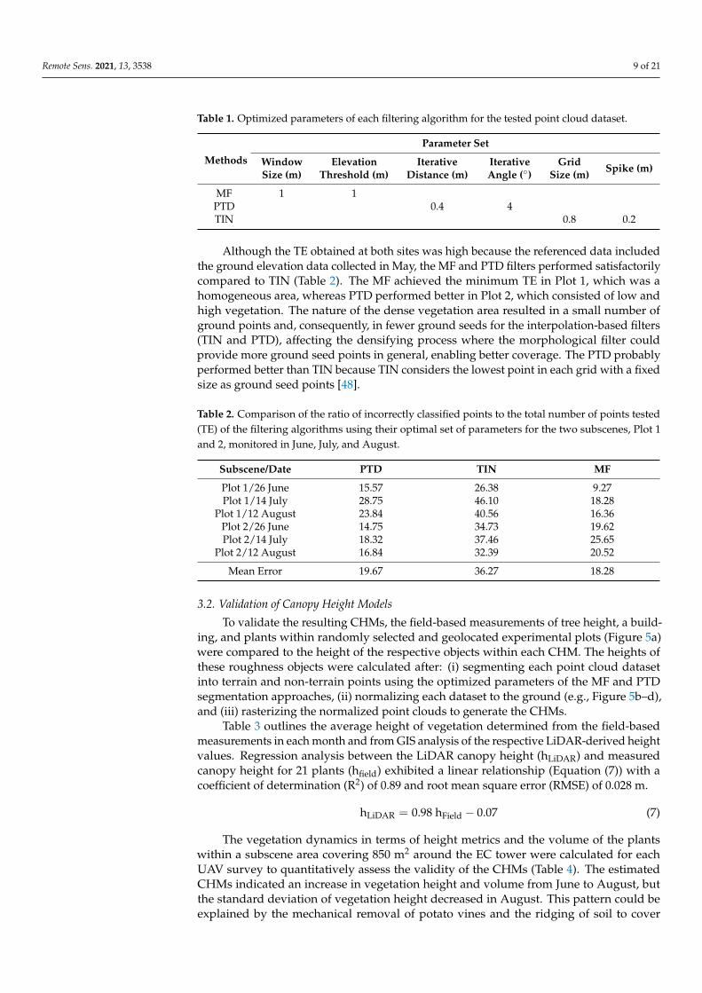
To validate the resulting CHMs, the field-based measurements of tree height, a build-ing, and plants within randomly selected and geolocated experimental plots (Figure 5a)were compared to the height of the respective objects within each CHM. The heights ofthese roughness objects were calculated after: (i) segmenting each point cloud datasetinto terrain and non-terrain points using the optimized parameters of the MF and PTDsegmentation approaches, (ii) normalizing each dataset to the ground (e.g., Figure 5b–d),and (iii) rasterizing the normalized point clouds to generate the CHMs.

Table 3 outlines the average height of vegetation determined from the field-basedmeasurements in each month and from GIS analysis of the respective LiDAR-derived heightvalues. Regression analysis between the LiDAR canopy height (hLiDAR) and measuredcanopy height for 21 plants (hfield) exhibited a linear relationship (Equation (7)) with acoefficient of determination (R2) of 0.89 and root mean square error (RMSE) of 0.028 m.

hLiDAR = 0.98 hField − 0.07 (7)

The vegetation dynamics in terms of height metrics and the volume of the plantswithin a subscene area covering 850 m2 around the EC tower were calculated for eachUAV survey to quantitatively assess the validity of the CHMs (Table 4). The estimatedCHMs indicated an increase in vegetation height and volume from June to August, butthe standard deviation of vegetation height decreased in August. This pattern could beexplained by the mechanical removal of potato vines and the ridging of soil to cover

Remote Sens. 2021, 13, 3538 10 of 21

growing tubers that both occurred at the end of July to facilitate the harvest of the potatoplants by the end of August.

Figure 5. (a) Canopy height model (CHM) of the agricultural field indicating the locations of theexperimental plots (yellow points), and profile view of point clouds normalized to the terrainillustrating the height of (b) vegetation in June (brown points), July (light green points), and August(dark green points), (c) a building, and (d) trees.

Table 3. Comparison between LiDAR-derived height of plants (h) and plants’ h measured manuallyin geolocated experimental plots. Number of plant samples = 21.

Date Field h (m) LiDAR h (m)

26 June 0.52 0.4414 July 0.71 0.56

12 August 0.78 0.72

Table 4. Vegetation dynamics as expressed by the statistics of height of plants (h) and the net volumeof a subscene of the CHMs around the EC tower covering 850 m2.

Date Mean h (m) Mode h (m) StandardDeviation h (m)

Increase inVegetation (%)

26 June 0.61 0.60 0.1114 July 0.76 0.75 0.16 30.25

12 August 0.91 1.00 0.15 44.36

3.3. Source Turbulent Areas Using Morphometric Models

The footprint model of Kljun et al. [66] is a parameterization of a Lagrangian stochasticparticle dispersion model and was applied to calculate the extent of turbulent source areasfor each 30-min period of the EC observations (Figure 6). For the comparison analysis,we used the morphometric Z0 values as calculated for the cross-sections of the CHM thatcoincided with the wind direction that was considered as the input for each run of thefootprint model. The footprint model requires the standard deviation of the lateral velocitycomponent, the measurement height, the Obukhov length, the friction velocity, and winddirection (all derived by the EC system), an estimation of the boundary-layer height, and aminimum fetch around the EC tower (approximately 100 m). The 80% cumulative sourcearea for each 30-min EC measurement was utilized to weight the fractional contribution of

Remote Sens. 2021, 13, 3538 11 of 21

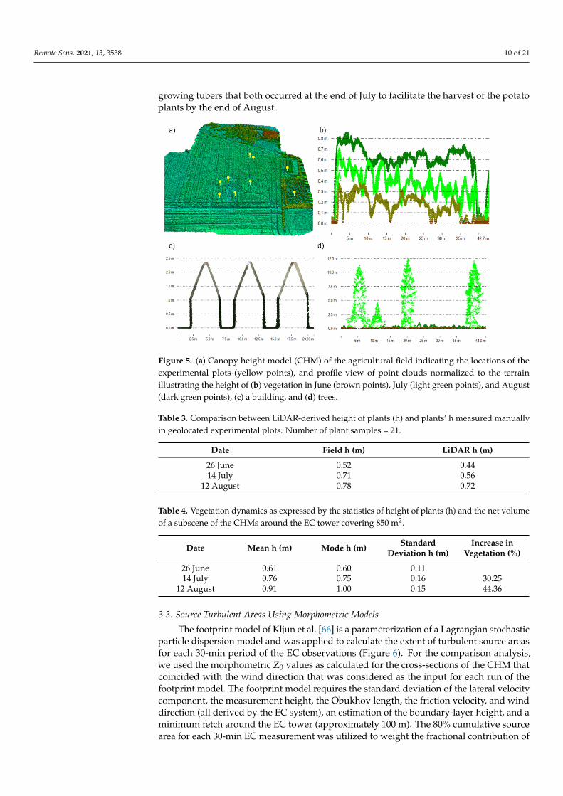
each grid square of the CHM. This allowed the calculation of a single value of Z0_EC (byweighting the values in the source area) and the calculation of the average morphometric-derived Z0 for each turbulent source area (Figure 7). Unstable atmospheric conditions weredefined as those corresponding to the ratio z/L < −0.032, while near-neutral atmosphericconditions reflected the relation −0.032 ≤ z/L ≤ 0.032 [67]. The source area climatologywas biased toward the dominant west-southerly wind direction, as in Plot 1. During theexperimental campaign, only in June did wind originate from the east-southerly direction,as in Plot 2.

Figure 6. Anemometric-derived roughness length Z0_EC, corresponding to different turbulent sourceareas from: 25 to 27 June; 13 to 15 July; 12 to 13 August. The central mark indicates the median of Z0,while the bottom and top edges of the box indicate the 25th and 75th percentiles, respectively. Thewhiskers represent the most extreme data points.

Figure 7. Canopy height model of the agricultural site as obtained by the UAV-LiDAR survey in June.The ellipsoid shapes indicate the probable surface areas contributing to turbulent flux measurementsimposing the respective prevailing meteorological conditions.

Remote Sens. 2021, 13, 3538 12 of 21

3.4. Comparison of Methods to Derive Roughness Length

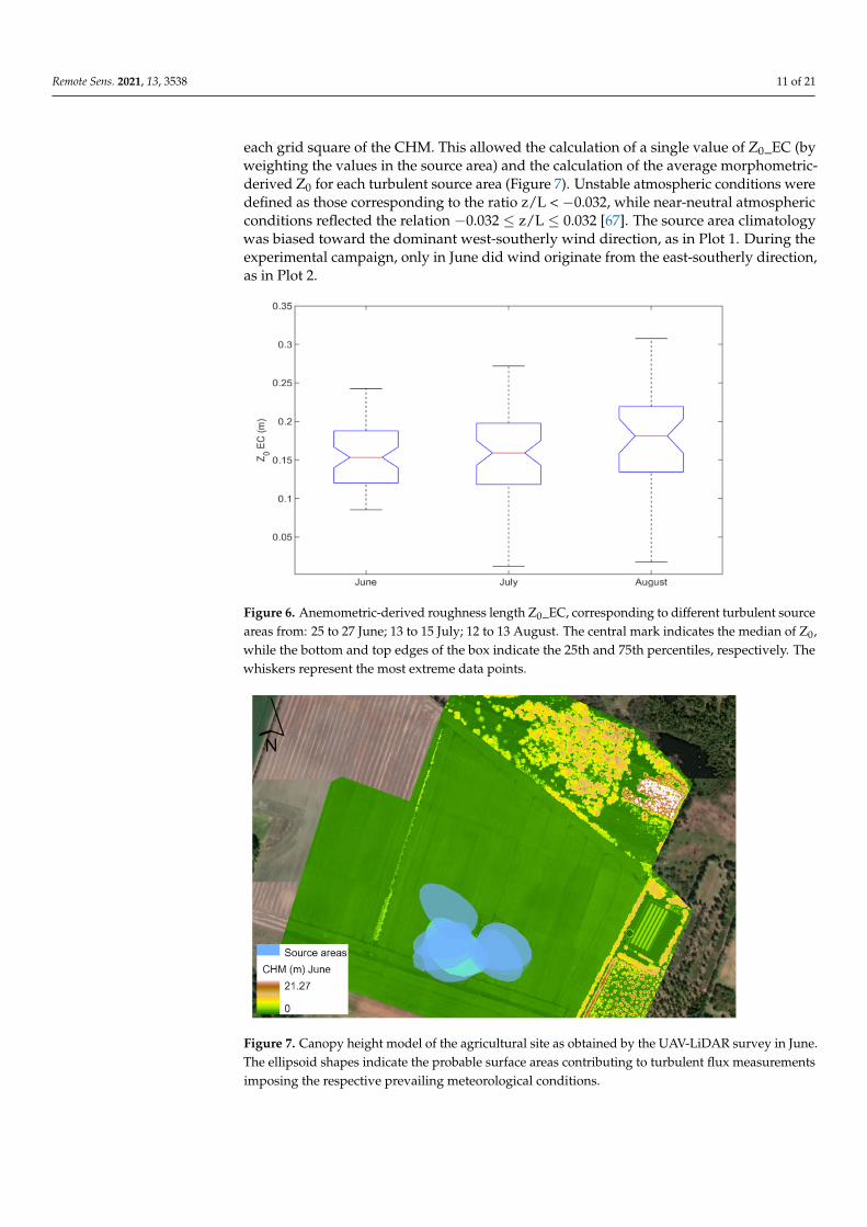
The mean values of Z0 as calculated by the anemometric and all morphometricmethods gradually increased from June to August, following the progression of vegetationgrowth resulting from the increases in fai and Zd due to the higher vegetation density andheight. On average, the morphometric-based Z0 presented strong linear correlations withZ0_EC (Figure 8), and a standard deviation of less than 4.2 cm with averages ranging froman underestimation of 1.3 cm (Z0_RT) to an overestimation of 1.9 cm (Z0_MR) (Table 5).

Figure 8. Scatterplots of the anemometric roughness length (Z0_EC) and the morphometric-derivedroughness length (Z0) using the Menethi and Ritchie (MR), Raupach (RAP), and the rule of thumb(RT) methods.

The observed positive correlation between the mean Z0 obtained by the EC methodand the mean Z0_RT (i.e., the height of the plants) during the vegetation-growing periodindicated that an accurate representation of vegetation height derived by a LiDAR systemcould be effective for estimating Z0 using the simple rule of thumb method (Figure 8).However, the correlations between Z0_RAP and Z0_MR with Z0_EC exhibited highercoefficients of determination (R2 = 0.96 and 0.93, respectively) and smaller RMSEs comparedto Z0_RT. Thus, the investigation of a suitable morphometric method may be crucial toimproving the accuracy of canopy aerodynamic characteristics estimations.

The overall difference in Z0 derived by RAP and the anemometric method was lessthan 10% for June, July, and August. The RT method had a similar performance to RAPfor July and August, while the estimated Z0_MR was 4% to 19% greater than the meanZ0_EC. The mean roughness length values under near-neutral conditions were higher thanthe Z0 calculated for unstable conditions (Table 5), since the extent of the turbulent sourceareas was typically larger in the former case with smaller values of friction velocity orwind speed. Perhaps the inclusion of the effect of frontal surface U and u* in the RAPmethod as well as the inclusion of vegetation height variability in the MR method enabledthe capture of Z0 amplification under near-neutral conditions, whereas the dependencyof Z0_RT to the averaged h per grid cell produced similar roughness lengths for unstableand near-neutral conditions. The mean Z0_EC, Z0_RAP, and Z0_MR in August and underunstable atmospheric conditions were smaller than the respective Z0 in July. This could beattributed to the decreased standard deviation of vegetation height within the cumulativesource areas observed in August (σh = 0.1 m), which may have translated to a higherdensity in foliage compared with the respective one for July (σh = 0.15 m).

Remote Sens. 2021, 13, 3538 13 of 21

Table 5. Comparison of Z0 (m) derived by the morphometric methods with the anemometric Z0

averaged over the source areas for daytime hours (from 9:00 to 19:00). The data were screened forwind speed higher than 2m/s and friction velocity higher than 0.2 m/s.

Z0_RAP Z0_RT Z0_MR Z0_EC fai

Differences to Z0_EC

June (n = 63) 0.009 0.037 −0.025 0.148 0.048July (n = 62) 0.018 0.008 −0.023 0.171 0.048

August (n = 36) 0.015 0.013 −0.006 0.200 0.058Average 0.014 0.013 −0.019

Standard deviation 0.031 0.042 0.022

Unstable conditions Plot 1

June (n = 8) 0.028 −0.003 −0.043 0.117 0.039July (n = 46) −0.016 −0.026 −0.042 0.137 0.045

August (n = 3) −0.022 −0.065 0.022 0.123 0.042

Neutral conditions Plot 1

June (n = 13) 0.078 0.05 0.006 0.171 0.041July (n = 16) 0.027 0.018 −0.053 0.182 0.042

August (n = 33) 0.018 0.02 −0.009 0.207 0.060

Unstable conditions Plot 2

June (n = 36) −0.020 0.036 −0.035 0.141 0.054

Neutral conditions Plot 2

June (n = 6) 0.017 0.077 −0.002 0.188 0.046

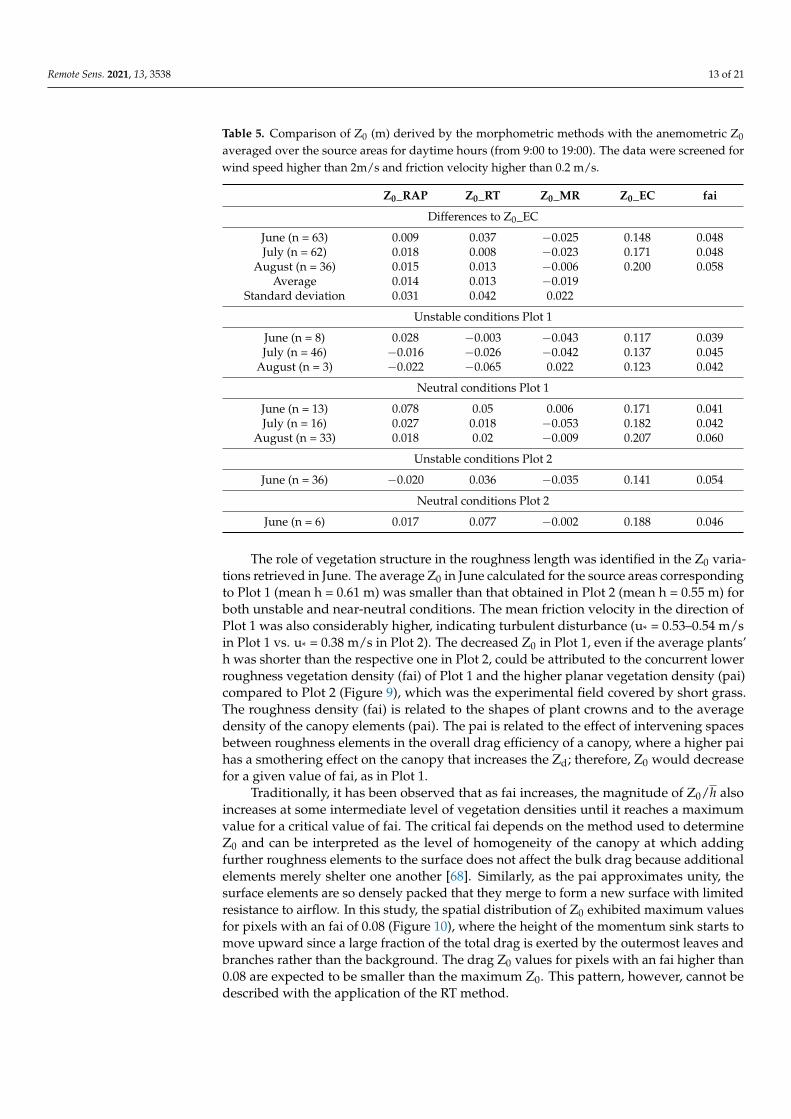
The role of vegetation structure in the roughness length was identified in the Z0 varia-tions retrieved in June. The average Z0 in June calculated for the source areas correspondingto Plot 1 (mean h = 0.61 m) was smaller than that obtained in Plot 2 (mean h = 0.55 m) forboth unstable and near-neutral conditions. The mean friction velocity in the direction ofPlot 1 was also considerably higher, indicating turbulent disturbance (u* = 0.53–0.54 m/sin Plot 1 vs. u* = 0.38 m/s in Plot 2). The decreased Z0 in Plot 1, even if the average plants’h was shorter than the respective one in Plot 2, could be attributed to the concurrent lowerroughness vegetation density (fai) of Plot 1 and the higher planar vegetation density (pai)compared to Plot 2 (Figure 9), which was the experimental field covered by short grass.The roughness density (fai) is related to the shapes of plant crowns and to the averagedensity of the canopy elements (pai). The pai is related to the effect of intervening spacesbetween roughness elements in the overall drag efficiency of a canopy, where a higher paihas a smothering effect on the canopy that increases the Zd; therefore, Z0 would decreasefor a given value of fai, as in Plot 1.

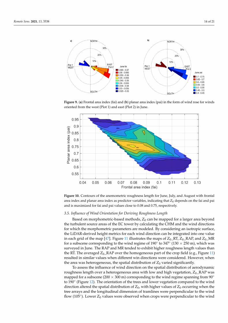
Traditionally, it has been observed that as fai increases, the magnitude of Z0/h alsoincreases at some intermediate level of vegetation densities until it reaches a maximumvalue for a critical value of fai. The critical fai depends on the method used to determineZ0 and can be interpreted as the level of homogeneity of the canopy at which addingfurther roughness elements to the surface does not affect the bulk drag because additionalelements merely shelter one another [68]. Similarly, as the pai approximates unity, thesurface elements are so densely packed that they merge to form a new surface with limitedresistance to airflow. In this study, the spatial distribution of Z0 exhibited maximum valuesfor pixels with an fai of 0.08 (Figure 10), where the height of the momentum sink starts tomove upward since a large fraction of the total drag is exerted by the outermost leaves andbranches rather than the background. The drag Z0 values for pixels with an fai higher than0.08 are expected to be smaller than the maximum Z0. This pattern, however, cannot bedescribed with the application of the RT method.

Remote Sens. 2021, 13, 3538 14 of 21

Figure 9. (a) Frontal area index (fai) and (b) planar area index (pai) in the form of wind rose for windsoriented from the west (Plot 1) and east (Plot 2) in June.

Figure 10. Contours of the anemometric roughness length for June, July, and August with frontalarea index and planar area index as predictor variables, indicating that Z0 depends on the fai and paiand is maximized for fai and pai values close to 0.08 and 0.75, respectively.

3.5. Influence of Wind Orientation for Deriving Roughness Length

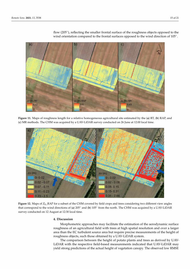
Based on morphometric-based methods, Z0 can be mapped for a larger area beyondthe turbulent source areas of the EC tower by calculating the CHM and the wind directionsfor which the morphometric parameters are modeled. By considering an isotropic surface,the LiDAR-derived height metrics for each wind direction can be integrated into one valuein each grid of the map [47]. Figure 11 illustrates the maps of Z0_RT, Z0_RAP, and Z0_MRfor a subscene corresponding to the wind regime of 190◦ to 347◦ (130 × 250 m), which wassurveyed in June. The RAP and MR tended to exhibit higher roughness length values thanthe RT. The averaged Z0_RAP over the homogeneous part of the crop field (e.g., Figure 11)resulted in similar values when different win directions were considered. However, whenthe area was heterogeneous, the spatial distribution of Z0 varied significantly.

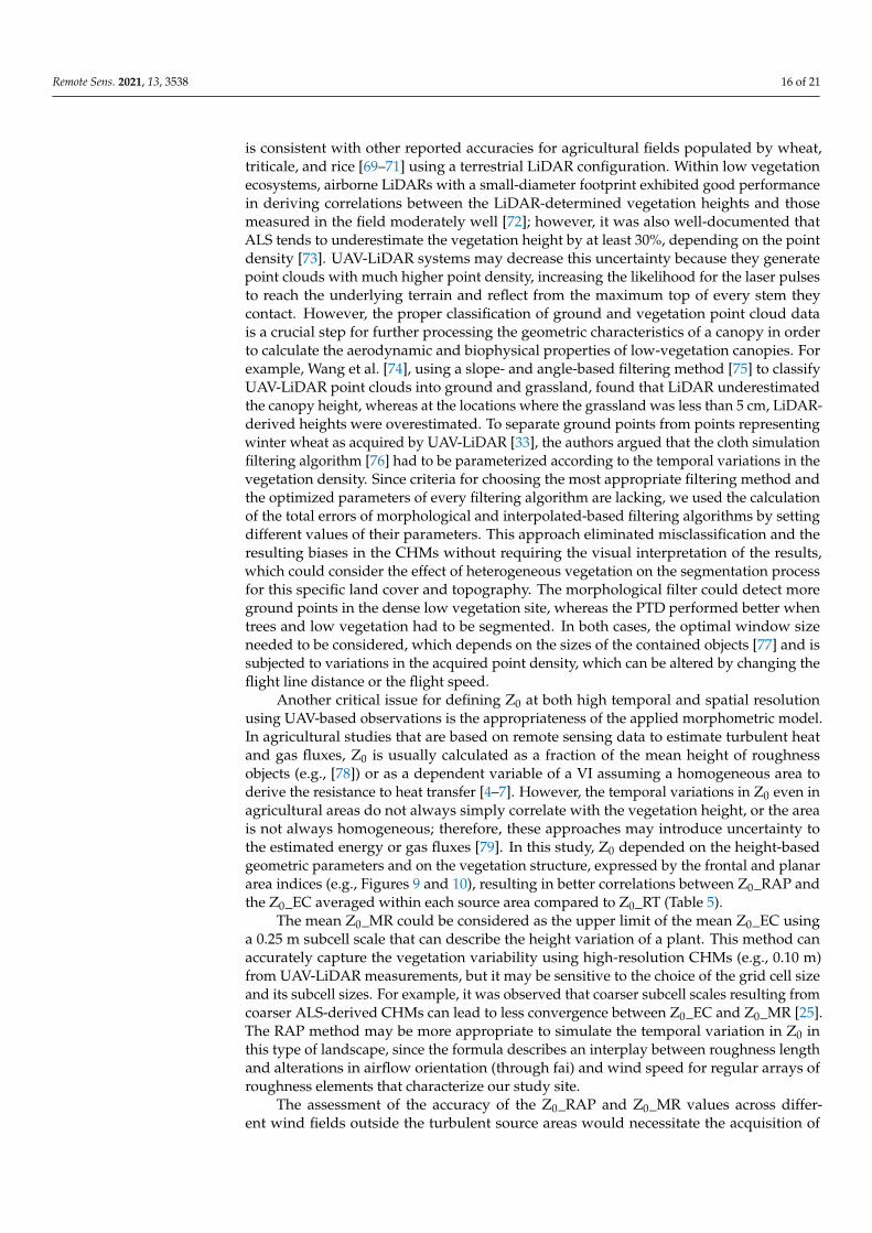
To assess the influence of wind direction on the spatial distribution of aerodynamicroughness length over a heterogeneous area with low and high vegetation, Z0_RAP wasmapped for a subscene (200 × 300 m) corresponding to the wind regime spanning from 90◦

to 190◦ (Figure 12). The orientation of the trees and lower vegetation compared to the winddirection altered the spatial distribution of Z0, with higher values of Z0 occurring when thetree arrays and the longitudinal dimension of tramlines were perpendicular to the windflow (105◦). Lower Z0 values were observed when crops were perpendicular to the wind

Remote Sens. 2021, 13, 3538 15 of 21

flow (205◦), reflecting the smaller frontal surface of the roughness objects opposed to thewind orientation compared to the frontal surfaces opposed to the wind direction of 105◦.

Figure 11. Maps of roughness length for a relative homogeneous agricultural site estimated by the (a) RT, (b) RAP, and(c) MR methods. The CHM was acquired by a UAV-LiDAR survey conducted on 26 June at 12:00 local time.

Figure 12. Maps of Z0_RAP for a subset of the CHM covered by field crops and trees considering two different view anglesthat correspond to the wind directions of (a) 205◦ and (b) 105◦ from the north. The CHM was acquired by a UAV-LiDARsurvey conducted on 12 August at 12:30 local time.

4. Discussion

Morphometric approaches may facilitate the estimation of the aerodynamic surfaceroughness of an agricultural field with trees at high spatial resolution and over a largerarea than the EC turbulent source area but require precise measurements of the height ofroughness objects, such those obtained by a UAV-LiDAR system.

The comparison between the height of potato plants and trees as derived by UAV-LiDAR with the respective field-based measurements indicated that UAV-LiDAR mayyield strong predictions of the actual height of vegetation canopy. The observed low RMSE

Remote Sens. 2021, 13, 3538 16 of 21

is consistent with other reported accuracies for agricultural fields populated by wheat,triticale, and rice [69–71] using a terrestrial LiDAR configuration. Within low vegetationecosystems, airborne LiDARs with a small-diameter footprint exhibited good performancein deriving correlations between the LiDAR-determined vegetation heights and thosemeasured in the field moderately well [72]; however, it was also well-documented thatALS tends to underestimate the vegetation height by at least 30%, depending on the pointdensity [73]. UAV-LiDAR systems may decrease this uncertainty because they generatepoint clouds with much higher point density, increasing the likelihood for the laser pulsesto reach the underlying terrain and reflect from the maximum top of every stem theycontact. However, the proper classification of ground and vegetation point cloud datais a crucial step for further processing the geometric characteristics of a canopy in orderto calculate the aerodynamic and biophysical properties of low-vegetation canopies. Forexample, Wang et al. [74], using a slope- and angle-based filtering method [75] to classifyUAV-LiDAR point clouds into ground and grassland, found that LiDAR underestimatedthe canopy height, whereas at the locations where the grassland was less than 5 cm, LiDAR-derived heights were overestimated. To separate ground points from points representingwinter wheat as acquired by UAV-LiDAR [33], the authors argued that the cloth simulationfiltering algorithm [76] had to be parameterized according to the temporal variations in thevegetation density. Since criteria for choosing the most appropriate filtering method andthe optimized parameters of every filtering algorithm are lacking, we used the calculationof the total errors of morphological and interpolated-based filtering algorithms by settingdifferent values of their parameters. This approach eliminated misclassification and theresulting biases in the CHMs without requiring the visual interpretation of the results,which could consider the effect of heterogeneous vegetation on the segmentation processfor this specific land cover and topography. The morphological filter could detect moreground points in the dense low vegetation site, whereas the PTD performed better whentrees and low vegetation had to be segmented. In both cases, the optimal window sizeneeded to be considered, which depends on the sizes of the contained objects [77] and issubjected to variations in the acquired point density, which can be altered by changing theflight line distance or the flight speed.

Another critical issue for defining Z0 at both high temporal and spatial resolutionusing UAV-based observations is the appropriateness of the applied morphometric model.In agricultural studies that are based on remote sensing data to estimate turbulent heatand gas fluxes, Z0 is usually calculated as a fraction of the mean height of roughnessobjects (e.g., [78]) or as a dependent variable of a VI assuming a homogeneous area toderive the resistance to heat transfer [4–7]. However, the temporal variations in Z0 even inagricultural areas do not always simply correlate with the vegetation height, or the areais not always homogeneous; therefore, these approaches may introduce uncertainty tothe estimated energy or gas fluxes [79]. In this study, Z0 depended on the height-basedgeometric parameters and on the vegetation structure, expressed by the frontal and planararea indices (e.g., Figures 9 and 10), resulting in better correlations between Z0_RAP andthe Z0_EC averaged within each source area compared to Z0_RT (Table 5).

The mean Z0_MR could be considered as the upper limit of the mean Z0_EC usinga 0.25 m subcell scale that can describe the height variation of a plant. This method canaccurately capture the vegetation variability using high-resolution CHMs (e.g., 0.10 m)from UAV-LiDAR measurements, but it may be sensitive to the choice of the grid cell sizeand its subcell sizes. For example, it was observed that coarser subcell scales resulting fromcoarser ALS-derived CHMs can lead to less convergence between Z0_EC and Z0_MR [25].The RAP method may be more appropriate to simulate the temporal variation in Z0 inthis type of landscape, since the formula describes an interplay between roughness lengthand alterations in airflow orientation (through fai) and wind speed for regular arrays ofroughness elements that characterize our study site.

The assessment of the accuracy of the Z0_RAP and Z0_MR values across differ-ent wind fields outside the turbulent source areas would necessitate the acquisition of

Remote Sens. 2021, 13, 3538 17 of 21

anemometric-derived Z0 across the whole field. Therefore, a precise statement abouthow these morphometric-based Z0 respond to vegetation variability is difficult. How-ever, differences in the spatial distribution of Z0 between crop fields, bare soil, and treeswere generated (e.g., Figure 11), and the effect of wind direction on the fai and Z0 forthe heterogeneous subscene of the agricultural site was evident using the RAP method(Figure 12). These observations are aligned with the findings of Colin and Faivere [23],who documented that the RAP approach could account for the heterogeneity of an areacovered by grassland with staggered arrays of trees.

The morphometric models, though, do not account directly for the potential effectof vegetation’s porosity on the amount of drag exerted on the flow [80]. Thus, it could beclaimed that the calculated aerodynamic resistance would be overestimated by consideringthe porosity of the foliage structures equal to one. That would probably be more effectivefor areas where the dominant roughness element is trees, which, in contrast to compactobstacles, mainly oppose a resistance to the airflow for tree heights with the highestfoliage density. Kent et al. [81] found that the effect of the porosity of low vegetation onthe roughness length compared to higher obstacles was negligible. For more complexcroplands, a sensitivity analysis of the drag coefficient used in various morphometricmodels may provide further information regarding the alterations in shear stress sourcedfrom the internal structure of high vegetation. Although we tested the applicability of theMacdonald [12] and Millward-Hopkins [82] morphometric models, which can account forthe differential drag imposed by different types of obstacles, the results were not exploitedin this study because they did not capture Z0 variations in low vegetation, probably becausethese models were designed to determine Z0 in urban areas.

The methods assessed here could generate the spatial distribution of Z0 at centimeter-level resolution for an agricultural site and for selected prevailing wind directions, but thecontribution of the upstream roughness elements cannot be quantified. The choice of anappropriate spatial scale of analysis for computing Z0 could be derived from a generalanalysis of the landscape characteristics along the prevailing airflows.

5. Conclusions

In this study, we explored a method of generating maps of roughness length at ultra-high spatial resolution (0.10 m) of a typical dense temperate agricultural field with sparsetrees using the newly developed UAV-LiDAR scanners and morphometric roughnessmodels without requiring any other data sources, such as optical photogrammetry or eddycovariance observations. This method is particularly useful for enhancing the sustainabilityof farming practices and recreation activities in agroforestry and agroecology applications,since the spatial distribution of Z0 can delineate how land cover alterations affect shearstress and turbulence, which, in turn, regulate the air–surface exchange of energy, water,and greenhouse gases.

For the determination of Z0, the selection of the appropriate morphometric methodand the effective classification of UAV-LiDAR-derived point clouds into vegetation andterrain that generates precise CHMs are both critical.

Overall, convergence was observed between the EC-derived Z0 values and thosefound through the UAV-LiDAR-driven models at the turbulent source area scale. Allmorphometric models showed a standard deviation of less than 4.2 cm with averagesranging from an underestimation of 1.3 cm (Z0_RT) to an overestimation of 1.9 cm (Z0_MR).The detailed comparison indicated that the Raupach roughness model is more suitablefor simulating the temporal variations in Z0. The spatial distribution of zo_RAP for aheterogeneous subscene beyond the turbulent source areas was conditioned by the shapeof the frontal surface opposed to wind direction, with a higher Z0 occurring when the treearrays were perpendicular to the wind flow.

A sensitivity analysis of three filtering approaches to segment the point cloud data tolow vegetation and ground highlighted the errors associated with CHM preparation. Themorphological filter performed satisfactorily over the more homogeneous area covered by

Remote Sens. 2021, 13, 3538 18 of 21

plants with a 1 m window size of the opening operation while the filter was not so sensitiveto elevation threshold due to the relative flat landscape. The PTD filter produced fewererrors in a subscene consisting of low and high vegetation for an iterative distance close to0.4 m and an iterative angle of 4◦. The TIN interpolation-based filter generated more errorsin detecting ground and non-ground points for this type of vegetation and landscape.

This technique may advance the establishment of more precise spatial representationof potentially nonlinear relationships between canopy structural characteristics and surfacewater and gas dynamics across heterogeneous land cover types. The application of all theelaborated approaches to derive precise CHMs and Z0 values in agricultural fields withother crop species and different climatic conditions could be used to assess their adequacyin other contexts. Further research is needed to improve the morphometric models for Z0in vegetated landscapes that can benefit from canopy height models of ultra-high spatialresolution to account for surface drag effects of upstream roughness elements.

Author Contributions: Conceptualization, T.F. and K.T.; UAV data collection, processing, andanalysis, K.T.; writing, K.T.; validation, K.T.; review and editing, T.F. All authors have read andagreed to the published version of the manuscript.

Funding: The remote sensing equipment purchased for this study was funded by the UAS-abilityDanish Drone Infrastructure (https://uas-ability.dk/ accessed on 2 August 2021) and the MapCland(Villum foundation Project no 00028314).

Data Availability Statement: The data presented in this study are available on request from thecorresponding author.

Acknowledgments: The authors would like to thank the field technicians Rasmus Jensen and LarsRasmussen who collect and maintained the daily operations of the eddy covariance data for theICOS network (https://www.icos-cp.eu/observations/national-networks/denmark accessed on12 August 2021). The source area calculations were based on the Urban Multi-scale EnvironmentalPredictor (https://plugins.qgis.org/plugins/UMEP/ accessed on 3 June 2021) climate service pluginfor the open-source software QGIS. The authors would also like to thank the anonymous reviewersfor their careful reading of the manuscript and their insightful comments and suggestions.

Conflicts of Interest: The authors declare no conflict of interest.

References1. Stull, R.B. An Introduction to Boundary Layer Meteorology; Kluwer Academic Publishers: Dordrecht, The Netherlands, 1988; p. 670.2. Minvielle, F.; Marticorena, B.; Gillette, D.A.; Lawson, R.E.; Thompson, R.; Bergametti, G. Relationship between the Aerodynamic

Roughness Length and the Roughness Density in Cases of Low Roughness Density. Environ. Fluid Mech. 2003, 3, 249–267.[CrossRef]

3. Dickinson, R.E. Land surface processes and climate surface albedos and energy balance. Adv. Geophys. 1983, 25, 305–353.4. Allen, R.G.; Tasumi, M.; Trezza, R. Satellite-based energy balance for mapping evapotranspiration with internalized calibration

(METRIC)–model. J. Irrig. Drain. Eng. ASCE 2007, 133, 380–394. [CrossRef]5. Bastiaanssen, W.; Menenti, M.; Feddes, R.; Holtslag, A.A.M. A remote sensing surface energy balance algorithm for land (SEBAL),

1. Formulation. J. Hydrol. 1998, 212–213, 198–212. [CrossRef]6. Roerink, G.; Su, Z.; Menenti, M. S-SEBI: A simple remote sensing algorithm to estimate the surface energy balance. Phys. Chem.

Earth. 2000, 25, 147–157. [CrossRef]7. Su, Z. The Surface Energy Balance System (SEBS) for estimation of turbulent heat fluxes at scales ranging from a point to a

continent. Hydrol. Earth Syst. Sci. 2002, 6, 85–99. [CrossRef]8. Massman, W.J. A model study of kBH-1 for vegetated surfaces using ‘localized near-field’ Lagrangian theory. J. Hydrol. 1999, 223,

27–43. [CrossRef]9. Blumel, K.B. A simple formula for estimation of the roughness length for heat transfer over partly vegetated surfaces. J. Appl.

Meteorol. 1999, 38, 814–829. [CrossRef]10. Su, Z.; Schmugge, T.; Kustas, W.P.; Massman, W.J. An evaluation of two models for estimation of the roughness height for heat

transfer between the land surface and the atmosphere. J. Appl. Meteorol. 2001, 40, 1933–1951. [CrossRef]11. Kustas, W.P.; Anderson, M.C.; Norman, J.M.; Li, F. Utility of radiometric–aerodynamic temperature relations for heat flux

estimation. Bound.-Layer Meteorol. 2007, 122, 167–187. [CrossRef]12. Macdonald, R.; Griffiths, R.; Hall, D. An improved method for the estimation of surface roughness of obstacle arrays. Atmos.

Environ. 1998, 32, 1857–1864. [CrossRef]

Remote Sens. 2021, 13, 3538 19 of 21

13. Grimmond, C.S.B.; Oke, T.R. Aerodynamic properties of urban areas derived from analysis of surface form. J. Appl. Meteorol.1999, 38, 1262–1292. [CrossRef]

14. Kustas, W.P.; Choudhury, B.J.; Moran, M.S.; Reginato, R.J.; Jackson, R.D.; Gay, L.W.; Weaver, H.L. Determination of sensible heatflux over sparse canopy using thermal infrared data. Agric. For. Meteorol. 1989, 44, 197–216. [CrossRef]

15. Garratt, J. The Atmospheric Boundary Layer; Cambridge University Press: Cambridge, UK, 1992; p. 336.16. Borak, J.S.; Jasinski, M.; Crago, R. Time series vegetation aerodynamic roughness fields estimated from modis observations. Agric.

For. Meteorol. 2005, 135, 252–268. [CrossRef]17. Schaudt, K.J.; Dickinson, R.E. An approach to deriving roughness length and zero-plane displacement height from satellite data,

prototyped with BOREAS data. Agric. For. Meteorol. 2000, 104, 143–155. [CrossRef]18. Tian, X.; Li, Z.Y.; Van der Tol, C.; Su, Z.; Li, X.; He, Q.; Bao, Y.; Chen, E.; Li, L. Estimating zero-plane displacement height and

aerodynamic roughness length using synthesis of LiDAR and SPOT-5 data. Remote Sens. Environ. 2011, 115, 2330–2341. [CrossRef]19. Yilmaz, V.; Konakoglu, B.; Serifoglu, C.; Gungor, O.; Gökalp, E. Image classification-based ground filtering of point clouds

extracted from UAV-based aerial photos. Geocarto Int. 2018, 33, 310–320. [CrossRef]20. Paul-Limoges, E.; Christen, A.; Coops, N.C.; Black, T.A.; Trofymow, J.A. Estimation of aerodynamic roughness of a harvested

Douglas-fir forest using airborne LiDAR. Remote Sens. Environ. 2013, 136, 225–233. [CrossRef]21. Floors, R.; Enevoldsen, P.; Davis, N.; Arnqvist, J.; Dellwik, E. From LiDAR scans to roughness maps for wind resource modelling

in forested areas. Wind Energ. Sci. 2018, 3, 353–370. [CrossRef]22. Holland, D.E.; Berglund, J.A.; Spruce, J.P.; McKellip, R.D. Derivation of effective aerodynamic surface roughness in urban areas

from airborne LiDAR terrain data. J. Appl. Meteorol. Clim. 2008, 47, 2614–2626. [CrossRef]23. Colin, J.; Faivre, R. Aerodynamic roughness length from very high-resolution LIDAR observation. Hydrol. Earth Syst. Sci. 2010,

14, 2661–2669. [CrossRef]24. Brown, O.W.; Hugenholtz, C.H. Estimating aerodynamic roughness (zo) in mixed grassland prairie with airborne LiDAR. Can. J.

Remote Sens. 2012, 37, 422–428. [CrossRef]25. Li, A.; Zhao, W.; Mitchell, J.J.; Glenn, N.F.; Germino, M.J.; Sankey, J.B.; Allen, R.G. Aerodynamic Roughness Length Estimation

with Lidar and Imaging Spectroscopy in a Shrub-Dominated Dryland. Photogramm. Eng. Remote S. 2017, 83, 415–427. [CrossRef]26. Hopkinson, C.; Chasmer, L.E.; Gabor, S.; Creed, I.F.; Sitar, M.; Kalbfleisch, W.; Treitz, P. Vegetation class dependent errors in

LiDAR ground elevation and canopy height estimates in a boreal wetland environment. Can. J. Remote Sens. 2005, 13, 191–206.[CrossRef]

27. Rosso, P.H.; Ustin, S.L.; Hastings, A. Use of LiDAR to study changes associated with Spartina invasion in San Francisco Baymarshes. Remote Sens. Environ. 2006, 100, 295–306. [CrossRef]

28. Wang, C.; Menenti, M.; Stoll, M.P.; Feola, A.; Belluco, E.; Marani, M. Separation of ground and low vegetation signatures inLiDAR measurements of salt-marsh environments. IEEE Trans. Geosci. Remote 2009, 47, 2014–2023. [CrossRef]

29. Kellner, J.R.; Armston, J.; Birrer, M.; Cushman, K.; Duncanson, L.; Eck, C.; Falleger, C.; Imbach, B.; Král, K.; Krucek, M.; et al. NewOpportunities for Forest Remote Sensing Through Ultra-High-Density Drone LiDAR. Surv. Geophys. 2019, 40, 959–977. [CrossRef][PubMed]

30. Mitchell, J.J.; Glenn, N.F.; Sankey, T.T.; Derryberry, D.R.; Anderson, M.O.; Hruska, R.C. Small-footprint LiDAR estimations ofsagebrush canopy characteristics. Photogramm. Eng. Remote S. 2011, 77, 521–530. [CrossRef]

31. Resop, J.P.; Lehmann, L.; Hession, W.C. Drone Laser Scanning for Modeling Riverscape Topography and Vegetation: Comparisonwith Traditional Aerial LiDAR. Drones 2019, 3, 35. [CrossRef]

32. Sankey, T.T.; McVay, J.; Swetnam, T.L.; McClaran, M.P.; Heilman, P.; Nichols, M. UAV hyperspectral and LiDAR data and theirfusion for arid and semi-arid land vegetation monitoring. Remote Sens. Ecol. Con. 2018, 4, 20–33. [CrossRef]

33. Bates, J.S.; Montzka, C.; Schmidt, M.; Jonard, F. Estimating Canopy Density Parameters Time-Series for Winter Wheat Using UASMounted LiDAR. Remote Sens. 2021, 13, 710. [CrossRef]

34. Rogers, S.R.; Manning, I.; Livingstone, W. Comparing the spatial accuracy of digital surface models from four unoccupied aerialsystems: Photogrammetry versus LiDAR. Remote Sens. 2020, 12, 2806. [CrossRef]

35. Cao, L.; Liu, H.; Fu, X.; Zhang, Z.; Shen, X.; Ruan, H. Comparison of UAV LiDAR and digital aerial photogrammetry point cloudsfor estimating forest structural attributes in subtropical planted forests. Forests 2019, 10, 145. [CrossRef]

36. Sofonia, J.; Shendryk, Y.; Phinn, S.; Roelfsema, C.; Kendoul, F.; Skocaj, D. Monitoring sugarcane growth response to varyingnitrogen application rates: A comparison of UAV SLAM LiDAR and photogrammetry. Int. J. Appl. Earth Observ. Geoinform. 2019,82, 101878. [CrossRef]

37. Duan, T.; Zheng, B.; Guo, W.; Ninomiya, S.; Guo, Y.; Chapman, S.C. Comparison of ground cover estimates from experiment plotsin cotton, sorghum and sugarcane based on images and ortho-mosaics captured by UAV. Funct. Plant. Biol. 2017, 44, 169–183.[CrossRef]

38. Shendryka, Y.; Sofonia, J.; Garrardc, R.; Rista, Y.; Skocajd, D.; Thorburn, P. Fine-scale prediction of biomass and leaf nitrogencontent in sugarcane using UAV LiDAR and multispectral imaging. Int. J. Appl. Earth Obs. Geoinf. 2020, 92, 102177. [CrossRef]

39. Adão, T.; Hruška, J.; Pádua, L.; Bessa, J.; Peres, E.; Morais, R.; Sousa, J. Hyperspectral imaging: A review on UAV-based sensors,data processing and applications for agriculture and forestry. Remote Sens. 2017, 9, 1110. [CrossRef]

Remote Sens. 2021, 13, 3538 20 of 21

40. Gano, B.; Dembele, J.S.B.; Ndour, A.; Luquet, D.; Beurier, G.; Diouf, D.; Audebert, A. Using UAV Borne, Multi-Spectral Imaging forthe Field Phenotyping of Shoot Biomass, Leaf Area Index and Height of West African Sorghum Varieties under Two ContrastedWater Conditions. Agronomy 2021, 11, 850. [CrossRef]

41. Chen, Q.; Gong, P.; Baldocchi, D.; Xie, G. Filtering airborne laser scanning data with morphological methods. Photogram. Eng.Remote Sens. 2007, 73, 175–185. [CrossRef]

42. Raupach, M.R. Simplified expressions for vegetation roughness length and zero-plane displacement as functions of canopy heightand area index. Bound.-Lay. Meteorol. 1994, 71, 211–216. [CrossRef]

43. Menenti, M.; Ritchie, J.C. Estimation of effective aerodynamic roughness of Walnet Gulch watershed with laser altimetermeasurements. Water Resour. Res. 1994, 5, 1329–1337. [CrossRef]

44. Jensen, R.; Herbst, M.; Friborg, T. Direct and indirect controls of the interannual variability in atmospheric CO2 exchange of threecontrasting ecosystems in Denmark. Agric. For. Meteor. 2017, 233, 12–31. [CrossRef]

45. Chang, C.; Habib, F.; Lee, C.; Yom, H. Automatic classification of lidar data into ground and nonground points. Int. Arch.Photogramm. Remote Sens. Spat. Inf. Sci. 2008, 37, 463–468.

46. Axelsson, P. DEM generation from laser scanner data using adaptive TIN models. Int. Arch. Photogram. Remote Sens. 2000, 33,111–118.

47. Zhang, K.; Chen, S.-C.; Whitman, D.; Shyu, M.-L.; Yan, J.; Zhang, C. A progressive morphological filter for removing non-groundmeasurements from airborne LIDAR data. IEEE Trans. Geosci. Remote Sens. 2003, 41, 872–882. [CrossRef]

48. Zhao, X.; Guo, Q.; Su, Y.; Xue, B. Improved progressive TIN densification filtering algorithm for airborne LiDAR data in forestedareas. ISPRS J. Photogramm. Remote Sens. 2016, 117, 79–91. [CrossRef]

49. Hutton, C.; Brazier, R. Quantifying riparian zone structure from airborne LiDAR: Vegetation filtering, anisotropic interpolation,and uncertainty propagation. J. Hydrol. 2012, 442–444, 36–45. [CrossRef]

50. Blue Marble Geographics. 2020. Available online: https://www.bluemarblegeo.com/ (accessed on 19 January 2021).51. LAStools. 2015. Available online: https://rapidlasso.com/lastools/ (accessed on 14 February 2021).52. GreenValley International Ltd. LiDAR360 Suite Software. 2019. Available online: https://greenvalleyintl.com (accessed on 7

April 2021).53. Sithole, G.; Vosselman, G. Experimental comparison of filter algorithms for bare-Earth extraction from airborne laser scanning

point clouds. ISPRS J. Photogram. Remote Sens. 2004, 59, 85–101. [CrossRef]54. Shepard, D. A two-dimensional interpolation function for irregularly-spaced data. In Proceedings of the 1968 23rd ACM National

Conference, New York, NY, USA; 1968; pp. 517–524.55. Krayenhoff, E.; Santiago, J.; Martilli, A.; Christen, A.; Oke, T. Parametrization of drag and turbulence for urban neighbourhoods

with trees. Bound.-Layer Meteorol. 2015, 156, 157–189. [CrossRef]56. De Vries, A.C.; Kustas, W.P.; Ritchie, J.C.; Klaassen, W.; Menenti, M.; Rango, A.; Prueger, J.H. Effective aerodynamic roughness

estimated from airborne laser altimeter measurements of surface features. Int. J. Remote Sens. 2003, 24, 1545–1558. [CrossRef]57. Lindberg, F.; Grimmond, C.S.B.; Gabey, A.; Huang, B.; Kent, C.W.; Sun, T.; Theeuwes, N.E.; Järvi, L.; Ward, H.C.;

Capel-Timms, I.; et al. Urban Multi-scale Environmental Predictor (UMEP): An integrated tool for city-based climate ser-vices. Environ. Model. Softw. 2018, 99, 70e87. [CrossRef]

58. QGIS Development Team. QGIS Geographic Information System. Open Source Geospatial Foundation Project. 2017. Availableonline: http://www.qgis.org/ (accessed on 23 May 2021).

59. Vickers, D.; Mahrt., L. Quality control and flux sampling problems for tower and aircraft data. J. Atmos. Ocean. Technol. 1997, 14,512–526. [CrossRef]

60. Nakai, T.; Van Der Molen, M.K.; Gash, J.H.C.; Kodama, Y. Correction of sonic anemometer angle of attack errors. Agric. For.Meteorol. 2006, 136, 19–30.

61. Schotanus, P.; Nieuwstadt, F.T.M.; De Bruin, H.A.R. Temperature measurement with a sonic anemometer and its application toheat and moisture fluxes. Bound.-Lay. Meteorol. 1983, 26, 81–93. [CrossRef]

62. Webb, E.K.; Pearman, G.A.; Leuning, R. Correction of flux measurements for density effects due to heat and water vapor transfer.Q. J. R. Meteorol. Soc. 1980, 106, 85–100. [CrossRef]

63. Foken, T.; Göockede, M.; Mauder, M.; Mahrt, L.; Amiro, B.; Munger, W. Post-field data quality control. In Handbook ofMicrometeorology; Lee, X., Massman, W., Law, B., Eds.; Atmospheric and Oceanographic Sciences Library, Springer: Dordrecht,The Netherlands, 2004.

64. Tennekes, H.; Lumley, J.L. Wall-bounded shear flows. In A First Course in Turbulence, 16th ed.; The MIT Press: Cambridge, MA,USA, 2018.

65. Högström, U. Review of some basic characteristics of the atmospheric surface € layer. Bound.-Layer Meteorol. 1996, 28, 215–246.[CrossRef]

66. Kljun, N.; Calanca, P.; Rotach, M.W.; Schmid, H.P. A simple two-dimensional parameterisation for Flux Footprint Prediction(FFP). Geosci. Model. Dev. 2015, 8, 3695–3713. [CrossRef]

67. Arya, P. Thermally stratified surface layer. In Introduction to Micrometeorology, 2nd ed.; Academic Press: San Diego, CA, USA,2001; p. 420.

68. Shaw, R.H.; Pereira, A.R. Aerodynamic roughness of a plant canopy: A numerical experiment. Agric. Meteorol. 1982, 26, 51–65.[CrossRef]

Remote Sens. 2021, 13, 3538 21 of 21

69. Tilly, N.; Hoffmeister, D.; Cao, Q.; Huang, S.; Lenz-Wiedemann, V.; Miao, Y.; Bareth, G. Multitemporal crop surface models:Accurate plant height measurement and biomass estimation with terrestrial laser scanning in paddy rice. J. Appl. Remote Sens.2014, 8, 083671. [CrossRef]

70. Jimenez-Berni, J.A.; Deery, D.M.; Rozas-Larraondo, P.; Condon, A.G.; Rebetzke, G.; James, R.; Bovill, W.; Furbank, R.; Sirault, X.High Throughput Determination of Plant Height, Ground Cover, and Above-Ground Biomass in Wheat with LiDAR. Front. Plant.Sci. 2018, 9, 237. [CrossRef]

71. Walter, J.D.C.; Edwards, J.; McDonald, G.; Kuchel, H. Estimating Biomass and Canopy Height with LiDAR for Field CropBreeding. Front. Plant. Sci. 2019, 10, 1145. [CrossRef] [PubMed]

72. Streutker, D.R.; Glenn, N.F. LiDAR measurement of sagebrush steppe vegetation heights. Remote Sens. Environ. 2006, 102, 135145.[CrossRef]

73. Su, J.G.; Bork, E.W. Characterization of diverse plant communities in Aspen Parkland rangeland using LiDAR data. Appl. Veg.Sci. 2007, 10, 407–416. [CrossRef]

74. Wang, D.; Xin, X.; Shao, Q.; Brolly, M.; Zhu, Z.; Chen, J. Modeling Aboveground Biomass in Hulunber Grassland Ecosystem byUsing Unmanned Aerial Vehicle Discrete Lidar. Sensors 2017, 17, 180. [CrossRef] [PubMed]

75. Maas, H.G.; Vosselman, G. Two algorithms for extracting building models from raw laser altimetry data. ISPRS J. Photogramm.Remote Sens. 1999, 54, 153–163. [CrossRef]

76. Zhang, W.; Qi, J.; Wan, P.; Wang, H.; Xie, D.; Wang, X.; Yan, G. An easy-to-use airborne LiDAR data filtering method based oncloth simulation. Remote Sens. 2016, 8, 501. [CrossRef]

77. Liu, X. Airborne LiDAR for DEM generation: Some critical issues. Prog. Phys. Geogr. 2008, 32, 31–49.78. Wang, S.; Garcia, M.; Bauer-Gottwein, P.; Jakobsen, J.; Zarco-Tejada, P.J.; Bandini, F.; Paz, V.S.; Ibrom, A. High spatial resolution

monitoring land surface energy, water and CO2 fluxes from an Unmanned Aerial System. Remote Sens. Environ. 2019, 229, 14–31.[CrossRef]

79. Colin, J.; Menenti, M.; Rubio, E.; Jochum, A. Accuracy vs. operability: A case study over barrax in the context of the idots. InProceedings of the AIP Conference Proceedings, Naples, Italy, 10–11 November 2005; Volume 852, pp. 75–83.

80. Yang, X.; Yu, Y.; Fan, W.A. A method to estimate the structural parameters of windbreaks using remote sensing. Agrofor. Syst.2017, 91, 37–49. [CrossRef]

81. Kent, C.W.; Grimmond, S.; Gatey, D. Aerodynamic roughness parameters in cities: Inclusion of vegetation. J. Wind Eng. Ind.Aerod. 2017, 169, 168176. [CrossRef]

82. Millward-Hopkins, J.; Tomlin, A.; Ma, L.; Ingham, D.; Pourkashanian, M. Estimating aerodynamic parameters of urban-likesurfaces with heterogeneous building heights. Bound.-Layer Meteorol. 2011, 141, 443–465. [CrossRef]