formula sae aerodynamic optimization - vut
TRANSCRIPT
BRNO UNIVERSITY OF TECHNOLOGYVYSOKÉ UČENÍ TECHNICKÉ V BRNĚ
FACULTY OF MECHANICAL ENGINEERINGFAKULTA STROJNÍHO INŽENÝRSTVÍ
INSTITUTE OF AEROSPACE ENGINEERINGLETECKÝ ÚSTAV
FORMULA SAE AERODYNAMIC OPTIMIZATIONAERODYNAMICKÁ OPTIMALIZACE MONOPOSTU FORMULE SAE
MASTER'S THESISDIPLOMOVÁ PRÁCE
AUTHORAUTOR PRÁCE
Bc. Lukáš Fryšták
SUPERVISORVEDOUCÍ PRÁCE
Ing. Robert Popela, Ph.D.
BRNO 2016

Master's Thesis Assignment
Institut: Institute of Aerospace Engineering
Be. Lukas Frystak
Mechanical Engineering
Aircraft Design
Ing. Robert Popela, Ph.D.
2015/16
Student:
Degree programm
Branch:
Supervisor:
Academic year:
As provided for by the Act No. 111/98 Coll. on higher education institutions and the BUT Study and
Examination Regulations, the director of the Institute hereby assigns the following topic of Master's
Thesis:
Brief description:
Performance of racing car is strongly determined by its aerodynamic characteristics. Aerodynamic
optimization is currently integral part of design of racing cars. TU Brno Racing team is for years
developing Formula Student cup vehicle. For further development there is necessary to perform testing
and aerodynamic optimization of car.
Master's Thesis goals:
Determine the basic aerodynamic characteristics of monopost in its current configuration. Perform
analysis, and identify gaps and determine areas for improvement in aerodynamic characteristics
(increase downforce, optimal distribution of downforce, reduce drag). Optimization by sophisticated
method using either the experimental or computational monopost model.
Bibliography:
Hucho, W. H.: Aerodynamics of Road Vehicles, ISBN: 978-0-7506-1267-8.
Barlow, J. B., Rae, W. H., Pope, A.: Low-Speed Wind Tunnel Testing, ISBN: 978-0-471-55774-6.
Katz, J.: Race Car Aerodynamics: Designing for Speed (Engineering and Performance), ISBN-13:
978-0837601427.
Faculty of Mechanical Engineering, Brno University of Technology / Technicka 2896/2 / 616 69 / Brno
Formula SAE aerodynamic optimization
Students are required to submit the thesis within the deadlines stated in the schedule of the academic
year 2015/16.
In Brno, 30. 11 . 2015
Faculty of Mechanical Engineering, Brno University of Technology / Technicka 2896/2 / 616 69 / Brno
ABSTRACTThis work focuses on wind tunnel testing of a 25% scale model of a Formula SAE racecar. In the first part, Formula SAE is introduced and role of aerodynamics within thiscompetition is described. That is followed by review of the theoretical background thatis relevant to the presented experiment. In the second part, the experiment itself isdescribed and results presented. As part of this work, a six component strain gaugeforce balance was designed, manufactured, and calibrated. Wind tunnel testing wasdone in four different configurations to determine the influence of inverted wings andfloor with diffuser on aerodynamic performance of the car.
KEYWORDSFormula SAE, Formula Student, Wind tunnel, aerodynamics, force balance
ABSTRAKTTato práce se zabývá měřením aerodynamických charakteristik modelu závodního vozuFormula SAE v aerodynamickém tunelu, v měřítku 1:4. V první části je představen projektFormula SAE a popsána role aerodynamiky v rámci této soutěže. Následuje přehledteoretického pozadí, které je relevantní k provedenému experimentu. Ve druhé částipráce je popsán samotný experiment a prezentovány jeho výsledky. Součástí je návrh,výroba a kalibrace šestikomponentní tenzometrické váhy pro měření aerodynamickéhozatížení. Testy v aerodynamickém tunelu byly provedeny ve čtyřech konfiguracích, abybylo možné určit vliv přítlačných křídel a podlahy s difuzorem na výsledné aerodynamickécharakteristiky vozu.
KLÍČOVÁ SLOVAFormula SAE, Formula Student, aerodynamický tunel, aerodynamika, tenzometrickáváha
FRYŠTÁK, Lukáš Formula SAE aerodynamic optimization: master’s thesis. Brno: BrnoUniversity of Technology, Faculty of Mechanical Engineering, Institute of AerospaceEngineering, 2016. 181 p. Supervised by Ing. Robert Popela, PhD.

DECLARATION
I declare that I have written my master’s thesis on the theme of “Formula SAE aerody-namic optimization” independently, under the guidance of the master’s thesis supervisorand using the technical literature and other sources of information which are all quotedin the thesis and detailed in the list of literature at the end of the thesis.
As the author of the master’s thesis I furthermore declare that, as regards the creationof this master’s thesis, I have not infringed any copyright. In particular, I have notunlawfully encroached on anyone’s personal and/or ownership rights and I am fully awareof the consequences in the case of breaking Regulation S 11 and the following of theCopyright Act No 121/2000 Sb., and of the rights related to intellectual property rightand changes in some Acts (Intellectual Property Act) and formulated in later regulations,inclusive of the possible consequences resulting from the provisions of Criminal ActNo 40/2009 Sb., Section 2, Head VI, Part 4.
Brno . . . . . . . . . . . . . . . . . . . . . . . . . . . . . . . . . . . . . . . . . . . . . . . . .author’s signature


ACKNOWLEDGEMENT
I would like to express a huge thank you to everyone that helped me with this work.Mainly, to my advisor, Ing. Robert Popela, PhD., whose help and guidance played anelemental role in the successful completion of this thesis.
Největší poděkování však patří mé rodině, za neúnavnou podporu během celého studia.
Brno . . . . . . . . . . . . . . . . . . . . . . . . . . . . . . . . . . . . . . . . . . . . . . . . .author’s signature

CONTENTS
Introduction 23
I Introduction, Theoretical background 24
1 Formula SAE 251.1 About FSAE . . . . . . . . . . . . . . . . . . . . . . . . . . . . . . . 251.2 Aerodynamics in FSAE . . . . . . . . . . . . . . . . . . . . . . . . . . 27
1.2.1 Wind tunnel tesing in FSAE . . . . . . . . . . . . . . . . . . . 271.3 Aerodynamics of Dragon cars . . . . . . . . . . . . . . . . . . . . . . 28
1.3.1 Dragon 4 . . . . . . . . . . . . . . . . . . . . . . . . . . . . . 291.3.2 Dragon 5 . . . . . . . . . . . . . . . . . . . . . . . . . . . . . 321.3.3 Dragon 6 . . . . . . . . . . . . . . . . . . . . . . . . . . . . . 33
2 Current State-of-the-art 352.1 Aerodynamics in automotive industry . . . . . . . . . . . . . . . . . . 352.2 Various aspects of on-road driving . . . . . . . . . . . . . . . . . . . . 372.3 Tools of the trade . . . . . . . . . . . . . . . . . . . . . . . . . . . . . 39
2.3.1 Road testing . . . . . . . . . . . . . . . . . . . . . . . . . . . . 392.3.2 Wind tunnel testing . . . . . . . . . . . . . . . . . . . . . . . 392.3.3 Computational methods . . . . . . . . . . . . . . . . . . . . . 40
3 Wind tunnel testing 413.1 Wind tunnel nomenclature . . . . . . . . . . . . . . . . . . . . . . . . 413.2 Types of wind tunnels . . . . . . . . . . . . . . . . . . . . . . . . . . 413.3 Types of test sections . . . . . . . . . . . . . . . . . . . . . . . . . . . 433.4 Facility characterization . . . . . . . . . . . . . . . . . . . . . . . . . 44
3.4.1 Flow uniformity . . . . . . . . . . . . . . . . . . . . . . . . . . 443.4.2 Longitudinal static pressure gradient . . . . . . . . . . . . . . 453.4.3 Angular flow variation in a jet . . . . . . . . . . . . . . . . . . 453.4.4 Turbulence . . . . . . . . . . . . . . . . . . . . . . . . . . . . 463.4.5 Surging . . . . . . . . . . . . . . . . . . . . . . . . . . . . . . 463.4.6 Acoustics . . . . . . . . . . . . . . . . . . . . . . . . . . . . . 46
3.5 Representation of the road . . . . . . . . . . . . . . . . . . . . . . . . 463.5.1 Wheel-road contact, wheel rotation . . . . . . . . . . . . . . . 48
3.6 Wind tunnel corrections . . . . . . . . . . . . . . . . . . . . . . . . . 503.6.1 Closed test section . . . . . . . . . . . . . . . . . . . . . . . . 523.6.2 Further comments on blockage . . . . . . . . . . . . . . . . . . 53
3.6.3 Boundary layer effects . . . . . . . . . . . . . . . . . . . . . . 553.7 Tests with reduced-scale models . . . . . . . . . . . . . . . . . . . . . 56
3.7.1 Details of model construction . . . . . . . . . . . . . . . . . . 563.7.2 Reynolds number effects . . . . . . . . . . . . . . . . . . . . . 56
3.8 Model mounting . . . . . . . . . . . . . . . . . . . . . . . . . . . . . . 593.9 Wind tunnel balances . . . . . . . . . . . . . . . . . . . . . . . . . . . 60
3.9.1 Deflections . . . . . . . . . . . . . . . . . . . . . . . . . . . . . 623.9.2 Measurement of the aerodynamic coefficients . . . . . . . . . . 62
II Experimental testing 66
4 Introduction to Part II 67
5 Experimental setup 695.1 Facility . . . . . . . . . . . . . . . . . . . . . . . . . . . . . . . . . . . 69
5.1.1 Wind tunnel . . . . . . . . . . . . . . . . . . . . . . . . . . . . 695.1.2 Test section and its equipment . . . . . . . . . . . . . . . . . . 69
5.2 Description of the experimental setup . . . . . . . . . . . . . . . . . . 715.2.1 Model scale . . . . . . . . . . . . . . . . . . . . . . . . . . . . 715.2.2 Measured quantities . . . . . . . . . . . . . . . . . . . . . . . 725.2.3 Model mounting . . . . . . . . . . . . . . . . . . . . . . . . . 725.2.4 Final experimental setup . . . . . . . . . . . . . . . . . . . . . 73
6 Model 75
7 Balance design and calibration 817.1 Basic definitions . . . . . . . . . . . . . . . . . . . . . . . . . . . . . . 81
7.1.1 Coordinate system . . . . . . . . . . . . . . . . . . . . . . . . 817.1.2 Aerodynamic loads . . . . . . . . . . . . . . . . . . . . . . . . 81
7.2 Balance design . . . . . . . . . . . . . . . . . . . . . . . . . . . . . . 837.3 Balance calibration . . . . . . . . . . . . . . . . . . . . . . . . . . . . 90
7.3.1 Test case . . . . . . . . . . . . . . . . . . . . . . . . . . . . . . 96
8 Experiment results 1018.1 Measurement procedure . . . . . . . . . . . . . . . . . . . . . . . . . 1018.2 Aerodynamic load . . . . . . . . . . . . . . . . . . . . . . . . . . . . . 103
8.2.1 Evaluation of acquired data . . . . . . . . . . . . . . . . . . . 1038.2.2 Results – Cases 1-4 . . . . . . . . . . . . . . . . . . . . . . . . 1058.2.3 Results – comparison of all cases . . . . . . . . . . . . . . . . 112
8.3 Pressure coefficient distribution . . . . . . . . . . . . . . . . . . . . . 113
8.3.1 Results – Cases 1-4 . . . . . . . . . . . . . . . . . . . . . . . . 1138.3.2 Results – comparison of all cases . . . . . . . . . . . . . . . . 119
8.4 Wake traversing . . . . . . . . . . . . . . . . . . . . . . . . . . . . . . 1198.4.1 Prandtl probe . . . . . . . . . . . . . . . . . . . . . . . . . . . 1198.4.2 Hot wire probe . . . . . . . . . . . . . . . . . . . . . . . . . . 122
8.5 Review of Reynolds number during the experiment . . . . . . . . . . 1228.6 Comparison with numerical simulations . . . . . . . . . . . . . . . . . 123
8.6.1 Aerodynamic coefficients . . . . . . . . . . . . . . . . . . . . . 1238.6.2 Wake . . . . . . . . . . . . . . . . . . . . . . . . . . . . . . . . 124
8.7 Load distribution . . . . . . . . . . . . . . . . . . . . . . . . . . . . . 124
9 Conclusion 127
Bibliography 129
List of symbols and abbreviations 133
List of appendices 137
A Reynolds number and blockage calculation 139
B Balance – further information 141B.1 Balance drawings . . . . . . . . . . . . . . . . . . . . . . . . . . . . . 141B.2 Balance – calibration graphs . . . . . . . . . . . . . . . . . . . . . . 150
C Aerodynamic load evaluation 157C.1 Loads on balance . . . . . . . . . . . . . . . . . . . . . . . . . . . . . 157C.2 Load on model . . . . . . . . . . . . . . . . . . . . . . . . . . . . . . 161


LIST OF FIGURES
1.1 Some aspects of Formula SAE project . . . . . . . . . . . . . . . . . . 261.2 Full scale symmetrical test, Monash Motorspors [27] . . . . . . . . . . 281.3 LUMotorsport scaled wind tunnel test [twitter.com/LUMotorsport] 291.4 Schematic sketch of G-G diagram [6] . . . . . . . . . . . . . . . . . . 301.5 Dragon 4 aerodynamic package [23] . . . . . . . . . . . . . . . . . . . 311.6 Comparison of CFD results and measured data [21] (modified) . . . . 321.7 Dragon 5 aerodynamic package [24] . . . . . . . . . . . . . . . . . . . 332.1 Aspects of vehicle aerodynamics [4] . . . . . . . . . . . . . . . . . . . 362.2 1996 Chaparral 2E Chevrolet (picture taken in 2005, Retrieved from:
http://www.ultimatecarpage.com/img/1553/Chaparral-2E-Chevrolet.html) . . . . . . . . . . . . . . . . . . . . . . . . . . . . . . . . . . . . 37
2.3 Real environment in which a vehicle operates [4] . . . . . . . . . . . . 382.4 Comparisson of various croswind profiles [4] . . . . . . . . . . . . . . 382.5 Illustrative picture – CFD. Total pressure coefficient displayed in sev-
eral planes along the car’s 𝑥 axis to trace vortices that are shed fromfront and rear wing’s end plates. . . . . . . . . . . . . . . . . . . . . . 40
3.1 Wind tunnel nomenclature [18] . . . . . . . . . . . . . . . . . . . . . 413.2 Types of wind tunnels [1] . . . . . . . . . . . . . . . . . . . . . . . . . 423.3 Main geometric characteristics of a wind tunnel test section [4] . . . . 433.4 The different types of wind tunnel test sections [5] . . . . . . . . . . . 443.5 Variation in the test section freestream velocity [6] . . . . . . . . . . . 453.6 Generic shape of the boundary layer [6] . . . . . . . . . . . . . . . . . 473.7 Various possibilities of road simulation [4] . . . . . . . . . . . . . . . 483.8 Drag and lift coefficients of isolated stationary and rotating wheel
versus ground clearance. The range of 𝐶𝐿 shown for zero groundclearance indicates the range of resutls obtained with a variety ofground-to-wheel seals. [6] . . . . . . . . . . . . . . . . . . . . . . . . . 49
3.9 Pressure distribution on the floor beneath a wheel for different groundclearances [4] . . . . . . . . . . . . . . . . . . . . . . . . . . . . . . . 50
3.10 Schematic sketch of flow separation and horseshoe vortex formingunder a stationary wheel [4] . . . . . . . . . . . . . . . . . . . . . . . 51
3.11 Wind tunnel testing of a passanger car, using flow visualisation paint.This test was conducted with stationary wheels. The horseshoe vortexis clearly visible. [17] . . . . . . . . . . . . . . . . . . . . . . . . . . . 51
3.12 Simulation of wheel rotation by attachment of trip molding[4] . . . . 513.13 Streamlines around a body in a closed test section [4] . . . . . . . . . 533.14 Wall effects in closed test section [4] . . . . . . . . . . . . . . . . . . . 54
3.15 Example of a detailed scaled model (1:4) of a passenger car [17] . . . 573.16 Drag coefficient versus Reynolds number for a 1:5 model and a real
car [4] . . . . . . . . . . . . . . . . . . . . . . . . . . . . . . . . . . . 583.17 Mounting a model through the tyre patches, while using elevated
ground plane [6] . . . . . . . . . . . . . . . . . . . . . . . . . . . . . . 593.18 Model mounted on a sting from behind [6] . . . . . . . . . . . . . . . 603.19 Sauber F1 Team – wind tunnel testing of 60% scale model mounted
from above [22] . . . . . . . . . . . . . . . . . . . . . . . . . . . . . . 613.20 Model mounted on a sting from below . . . . . . . . . . . . . . . . . 613.21 Overview of wind tunnel balance types after Hucho [4] . . . . . . . . 633.22 Internal balance schema [6] . . . . . . . . . . . . . . . . . . . . . . . . 643.23 Off-the-shelf internal balance, as sold by Aerolab [aerolab.com] . . . 645.1 Wind tunnel at the Institute of Aerospace Engineering (IAE) [9] . . . 695.2 Test section used for wind tunnel testing [9] . . . . . . . . . . . . . . 705.3 Wind tunnel freestream velocity and test section blockage versus
model scale. Based on Reynolds number calculation. . . . . . . . . . 725.4 Final experimental set up used for wind tunnel tests in this work . . . 746.1 Overall model dimensions . . . . . . . . . . . . . . . . . . . . . . . . 756.2 Geometry simplification – engine compartment; rear wing with the
additional fin in the symmetry plane . . . . . . . . . . . . . . . . . . 766.3 Geometry simplification – upright assembly, suspension . . . . . . . . 766.4 Detailed view of the pressure taps . . . . . . . . . . . . . . . . . . . . 776.5 Pressure taps connected to rubber hoses inside of the model . . . . . 786.6 Floor with diffuser . . . . . . . . . . . . . . . . . . . . . . . . . . . . 786.7 ’Simple’ floor – cut around sidepods, without a diffuser . . . . . . . . 796.8 Detailed view of the floor versions . . . . . . . . . . . . . . . . . . . . 796.9 Model used for the experiment . . . . . . . . . . . . . . . . . . . . . . 807.1 Aerodynamic loads on a vehicle acting in the reference coordinate
system [4] . . . . . . . . . . . . . . . . . . . . . . . . . . . . . . . . . 817.2 Sketch of the force balance in the test section with model – left view . 847.3 Sketch of the force balance in the test section with model – front view 857.4 Schematic picture of force balance . . . . . . . . . . . . . . . . . . . . 867.5 Sketch of balnce’s rectangular cross-section . . . . . . . . . . . . . . . 887.6 Data logger used to log strain gauge responses (during both calibra-
tion and wind tunnel testing) . . . . . . . . . . . . . . . . . . . . . . 917.7 Load cell used for applying load during calibration . . . . . . . . . . . 917.8 Schematic sketch of moment application on the balance . . . . . . . . 927.9 Moment application on balance (1) . . . . . . . . . . . . . . . . . . . 937.10 Moment application on balance (2) . . . . . . . . . . . . . . . . . . . 94

7.11 Data used for calibration of bridge B2, plotted with approximatedmoment . . . . . . . . . . . . . . . . . . . . . . . . . . . . . . . . . . 96
7.12 Balance calibration; test case – sketch . . . . . . . . . . . . . . . . . . 977.13 Balance calibration; test case. Comparison of values calculated based
on balance calibration and values based on load cell log – momentsat points of respective strain gauge bridges. . . . . . . . . . . . . . . 98
7.14 Balance calibration, test case. Comparison of values calculated basedon balance calibration and values based on load cell log – resultingload at the model attachment point . . . . . . . . . . . . . . . . . . . 99
8.1 Tyre contact patch treatment . . . . . . . . . . . . . . . . . . . . . . 1038.2 Case 1 – aerodynamic forces (left) and moments (right) versus velocity1078.3 Case 1 – aerodynamic coefficients versus velocity . . . . . . . . . . . . 1078.4 Case 2 – aerodynamic forces (left) and moments (right) versus velocity1088.5 Case 2 – aerodynamic coefficients versus velocity . . . . . . . . . . . . 1088.6 Case 3 – aerodynamic forces (left) and moments (right) versus velocity1098.7 Case 3 – aerodynamic coefficients versus velocity . . . . . . . . . . . . 1098.8 Case 4 – aerodynamic forces (left) and moments (right) versus velocity1108.9 Case 4 – aerodynamic coefficients versus velocity . . . . . . . . . . . . 1108.10 Positive rake angle [30] . . . . . . . . . . . . . . . . . . . . . . . . . . 1128.11 Resulting aerodynamic coefficients for all cases . . . . . . . . . . . . . 1148.12 Resulting aerodynamic coefficients for all cases, multiplied by models
reference area 𝐴 . . . . . . . . . . . . . . . . . . . . . . . . . . . . . . 1148.13 Pressure coefficient distribution, Case 1 – foam used to seal tyre con-
tact patch . . . . . . . . . . . . . . . . . . . . . . . . . . . . . . . . . 1168.14 Pressure coefficient distribution, Case 1 – rubber strip used to seal
tyre contact patch . . . . . . . . . . . . . . . . . . . . . . . . . . . . . 1168.15 Pressure coefficient distribution, Case 1. (a) stands for foam used to
seal tyre contact patch; (b) stands for rubber strip used to seal tyrecontact patch . . . . . . . . . . . . . . . . . . . . . . . . . . . . . . . 117
8.16 Pressure coefficient distribution, Case 2 . . . . . . . . . . . . . . . . . 1178.17 Pressure coefficient distribution, Case 3 . . . . . . . . . . . . . . . . . 1188.18 Pressure coefficient distribution, Case 4 . . . . . . . . . . . . . . . . . 1188.19 Pressure coefficient distribution, All cases, 30 m/s . . . . . . . . . . . 1208.20 Distance from the rearmost point of the model to the traversing plane 1208.21 Case 3, 𝑈∞ = 25 𝑚/𝑠. Velocity distribution behind a car – prandtl
probe traversing. . . . . . . . . . . . . . . . . . . . . . . . . . . . . . 1218.22 Case 4, 𝑈∞ = 25 𝑚/𝑠. Velocity distribution behind a car – prandtl
probe traversing. . . . . . . . . . . . . . . . . . . . . . . . . . . . . . 121

8.23 Case 3, 𝑈∞ = 25 𝑚/𝑠. Turbulence intensity distribution behind a car– hot wire probe traversing. . . . . . . . . . . . . . . . . . . . . . . . 122
8.24 CFD – full scale, 𝑈∞ = 16.7 𝑚/𝑠, velocity distribution behind a car [25]1248.25 Velocity contour plot – CFD . . . . . . . . . . . . . . . . . . . . . . . 1258.26 Velocity contour plot – experiment (case 3) . . . . . . . . . . . . . . . 1258.27 Load transfer vs. speed from Dragon 4 on track testing [21] . . . . . . 126B.1 Raw data recorded when a single component of load was applied – 𝐹𝑥 151B.2 Raw data recorded when a single component of load was applied – 𝐹𝑦 151B.3 Raw data recorded when a single component of load was applied – 𝐹𝑧 152B.4 Raw data recorded when a single component of load was applied –
𝑀𝑥 (after subtraction of zero values) . . . . . . . . . . . . . . . . . . 152B.5 Raw data recorded when a single component of load was applied –
𝑀𝑦 (after subtraction of zero values) . . . . . . . . . . . . . . . . . . 153B.6 Raw data recorded when a single component of load was applied –
𝑀𝑧 (after subtraction of zero values) . . . . . . . . . . . . . . . . . . 153B.7 Data used for calibration of bridge B1, plotted with approximated
moment . . . . . . . . . . . . . . . . . . . . . . . . . . . . . . . . . . 154B.8 Data used for calibration of bridge B2, plotted with approximated
moment . . . . . . . . . . . . . . . . . . . . . . . . . . . . . . . . . . 154B.9 Data used for calibration of bridge B3, plotted with approximated
moment . . . . . . . . . . . . . . . . . . . . . . . . . . . . . . . . . . 155B.10 Data used for calibration of bridge B4, plotted with approximated
moment . . . . . . . . . . . . . . . . . . . . . . . . . . . . . . . . . . 155B.11 Data used for calibration of bridge B5, plotted with approximated
moment . . . . . . . . . . . . . . . . . . . . . . . . . . . . . . . . . . 156B.12 Data used for calibration of bridge B6, plotted with approximated
moment . . . . . . . . . . . . . . . . . . . . . . . . . . . . . . . . . . 156C.1 Measurement of forces acting on balance, zero values . . . . . . . . . 157C.2 Measurement of forces acting on balance, strain gauge response to loads158C.3 Measurement of load acting on balance. Resulting forces on balance . 161C.4 Measurement of load acting on balance. Resulting moments on balance162C.5 Transformation of aerodynamic load to default coordinate system . . 163C.6 Case 1 – measured strain gauge responses for all measured velocities . 167C.7 Case 1 – measured strain gauge responses – zero values . . . . . . . . 168C.8 Case 1 – measured forces corrected – loads acting on the balance
subtracted . . . . . . . . . . . . . . . . . . . . . . . . . . . . . . . . . 168C.9 Case 1 – transformation of the reference coordinate system . . . . . . 169C.10 Case 1 – resulting forces acting on the model . . . . . . . . . . . . . . 169C.11 Case 1 – resulting moments acting on the model . . . . . . . . . . . . 170

C.12 Case 1 – resulting aerodynamic coefficients of the model . . . . . . . 170C.13 Case 2 – measured strain gauge responses – zero values . . . . . . . . 171C.14 Case 2 – measured strain gauge responses for all measured velocities . 171C.15 Case 2 – measured forces corrected – loads acting on the balance
subtracted . . . . . . . . . . . . . . . . . . . . . . . . . . . . . . . . . 172C.16 Case 2 – transformation of the reference coordinate system . . . . . . 172C.17 Case 2 – resulting forces acting on the model . . . . . . . . . . . . . . 173C.18 Case 2 – resulting moments acting on the model . . . . . . . . . . . . 173C.19 Case 2 – resulting aerodynamic coefficients of the model . . . . . . . 174C.20 Case 3 – measured strain gauge responses – zero values . . . . . . . . 174C.21 Case 3 – measured strain gauge responses for all measured velocities . 175C.22 Case 3 – measured forces corrected – loads acting on the balance
subtracted . . . . . . . . . . . . . . . . . . . . . . . . . . . . . . . . . 175C.23 Case 3 – transformation of the reference coordinate system . . . . . . 176C.24 Case 3 – resulting forces acting on the model . . . . . . . . . . . . . . 176C.25 Case 3 – resulting moments acting on the model . . . . . . . . . . . . 177C.26 Case 3 – resulting aerodynamic coefficients of the model . . . . . . . 177C.27 Case 4 – measured strain gauge responses – zero values . . . . . . . . 178C.28 Case 4 – measured strain gauge responses for all measured velocities . 178C.29 Case 4 – measured forces corrected – loads acting on the balance
subtracted . . . . . . . . . . . . . . . . . . . . . . . . . . . . . . . . . 179C.30 Case 4 – transformation of the reference coordinate system . . . . . . 179C.31 Case 4 – resulting forces acting on the model . . . . . . . . . . . . . . 180C.32 Case 4 – resulting moments acting on the model . . . . . . . . . . . . 180C.33 Case 4 – resulting aerodynamic coefficients of the model . . . . . . . 181


LIST OF TABLES1.1 Overall aerodynamic characteristics of Dragon 4 and Dragon 5, data
from CFD simulations . . . . . . . . . . . . . . . . . . . . . . . . . . 315.1 Wind tunnel parameters . . . . . . . . . . . . . . . . . . . . . . . . . 695.2 Test section parameters . . . . . . . . . . . . . . . . . . . . . . . . . . 707.1 Maximum estimated load on the force balance . . . . . . . . . . . . . 847.2 Balance geometry values . . . . . . . . . . . . . . . . . . . . . . . . . 877.3 Dimensions of balance’s cross-section at points of strain gauge bridges 908.1 Description of measured cases . . . . . . . . . . . . . . . . . . . . . . 1018.2 Maximum wind tunnel velocity achieved for all cases . . . . . . . . . 1028.3 Test cases measured – force balance . . . . . . . . . . . . . . . . . . . 1038.4 Test cases measured – pressure reading . . . . . . . . . . . . . . . . . 1038.5 Test cases measured – traverser . . . . . . . . . . . . . . . . . . . . . 1048.6 Case 1 – drag and lift forces, pitching moment and aerodynamic co-
efficients . . . . . . . . . . . . . . . . . . . . . . . . . . . . . . . . . . 1118.7 Case 2 – drag and lift forces, pitching moment and aerodynamic co-
efficients . . . . . . . . . . . . . . . . . . . . . . . . . . . . . . . . . . 1118.8 Case 3 – drag and lift forces, pitching moment and aerodynamic co-
efficients . . . . . . . . . . . . . . . . . . . . . . . . . . . . . . . . . . 1118.9 Case 4 – drag and lift forces, pitching moment and aerodynamic co-
efficients . . . . . . . . . . . . . . . . . . . . . . . . . . . . . . . . . . 1118.10 Resulting aerodynamic coefficient for all cases . . . . . . . . . . . . . 1138.11 Resulting aerodynamic coefficients for all cases, multiplied by models
reference area 𝐴 . . . . . . . . . . . . . . . . . . . . . . . . . . . . . . 1138.12 Comparison of experimental and numerical results – aerodynamic co-
efficients . . . . . . . . . . . . . . . . . . . . . . . . . . . . . . . . . . 1238.13 Load transfer based on measured aerodynamic load . . . . . . . . . . 126C.1 Density used for calculation of aerodynamic coefficients – case 1 . . . 165C.2 Density used for calculation of aerodynamic coefficients – case 2 . . . 165C.3 Density used for calculation of aerodynamic coefficients – case 3 . . . 165C.4 Density used for calculation of aerodynamic coefficients – case 4 . . . 165C.5 Model reference dimensions for dimensionless coefficient computation 165C.6 Forces and moment acting on the model – case 1 . . . . . . . . . . . . 166C.7 Forces and moment acting on the model – case 2 . . . . . . . . . . . . 166C.8 Forces and moment acting on the model – case 3 . . . . . . . . . . . . 166C.9 Forces and moment acting on the model – case 4 . . . . . . . . . . . . 166

INTRODUCTIONFormula SAE is a student design competition with a motorsport theme. As part ofthis project, a team of students is presented with a task – design and build a single-seat open-wheel racecar. The car has to comply with a given set of regulations.Since its inception in 1981 in the USA it has become a world wide competition,and arguably, the largest student project in the world. Teams are not judged onlyby the car’s performance but also in off-track, so called, static disciplines. In total,there are eight disciplines, for which points are awarded. In the end, a team withthe highest score wins the competition.
In the beginning of 2000s, some teams started to explore effects of downforceinducing devices, i.e. inverted wings and undertray with diffuser, with the aim oflowering lap times. Previously, inverted wings made an appearance around 1990.Although the two cars using them were extremely fast in the dynamic disciplines, itwas believed, that the benefits did not outweigh the negatives. [31] In 2006 Wordleyand Saunders published their four year work in this area. [26] [27] They mentiona considerable debate in the Formula SAE community as to the benefit of usingwings on FSAE cars with respect to the low speeds. Although they concluded that”the ’wing’ package described would significantly benefit the car’s dynamic eventperformance.”, the aforementioned debate went on for some more years. Ultimately,downforce inducing aerodynamic packages became a standard on FSAE cars.
Many papers, reports and theses were published in the last few years regardingaerodynamic development and performance of FSAE cars. However, most of thiswork relies on numerical simulations as a primary tool with little or no validation ofresults. Although it is known that both full scale and subscale wind tunnel exper-iments were conducted, there is not a lot of data available. Full scale wind tunneltest of two FSAE cars were described and results published in Racecar Engineeringmagazine. [11] – [15] In these articles, overall aerodynamic coefficients are measuredfor different wing setups and also for different yaw angles.
The presented study takes aim at conducting a subscale wind tunnel measure-ment and investigate if the data can be used to fill the gap between numericalsimulations and track testing. That is for two reasons. Firstly, CFD computa-tions, unless properly validated, give results with a high degree of uncertainty. Andsecondly, designing, manufacturing, building, testing and competing with a FSAEcar is a one year process. Therefore reducing the time requirement for specificallyaerodynamic on-track testing would be a considerable advantage.
Lukáš Fryšták 23

Part I
Introduction, Theoreticalbackground
24
1 Formula SAE
1 FORMULA SAE
Formula SAE was briefly described in the Introduction. This chapter aims to providemore detailed information on the competition, present what role does aerodynamicsplay in FSAE car development and introduce family of cars that is connected to thiswork.
1.1 About FSAE
Formula SAE is a student design competition. It is organized by SAE Internetional1
as one of its Collegiate Design Competitions2 . It was introduced in 1979 in the USto provide undergraduate and graduate engineering students a real-life engineeringchallenge. Since then it has spread into Australia, Asia, South America and in 1998the project got into Europe under a different name – Formula Student.
A team entering the competition is presented with a task to form a hypotheticalcompany. Such a company would operate on an amateur weekend racing market. Itwould develop, build and sell a single-seat open-wheel racecar.
In reality, every year a team has to design and build a racecar. With this racecarteams meet at competitions. There, a car is not only judged by its performance.A team also has to present its engineering design, cost analysis and a hypotheticalbusiness plan. These three areas form what is called static disciplines. Then thereare four so called dynamic disciplines, where cars are actually run on track. Foreach of these disciplines a team is awarded points, maximum being 1000. A teamwith highest cumulative total wins the competition.
For a given year there is a set of regulations that the car has to comply with.They define only basic specifications of a car and specifications to ensure safety ofeveryone involved. Other than that, it is specifically desired to give students asmuch freedom in their design as possible.
Formula SAE is a very complex (and demanding) project. It runs through all of anacademic year. In this time a team has to form itself, design a car, collect sufficient
1”SAE International is a global association of more than 138,000 engineers and related technicalexperts in the aerospace, automotive and commercial-vehicle industries. SAE International’s corecompetencies are life-long learning and voluntary consensus standards development. SAE Interna-tional’s charitable arm is the SAE Foundation, which supports many programs, including A WorldIn Motion and the Collegiate Design Series.” [28]
2Other student design competitions under the SAE Collegiate Series’s roof are SAE Baja (off-road vehicles), SAE Aero Design (radio-controlled airplanes), SAE Clean Snowmobile and SAESupermileage (single-person fuel-efficient vehicle). [28]
Lukáš Fryšták 25
Formula SAE aerodynamic optimization
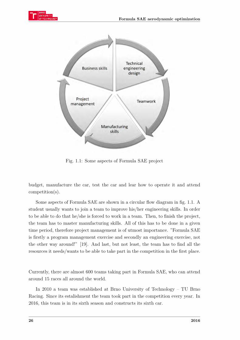
Fig. 1.1: Some aspects of Formula SAE project
budget, manufacture the car, test the car and lear how to operate it and attendcompetition(s).
Some aspects of Formula SAE are shown in a circular flow diagram in fig. 1.1. Astudent usually wants to join a team to improve his/her engineering skills. In orderto be able to do that he/she is forced to work in a team. Then, to finish the project,the team has to master manufacturing skills. All of this has to be done in a giventime period, therefore project management is of utmost importance. ”Formula SAEis firstly a program management exercise and secondly an engineering exercise, notthe other way around!” [19]. And last, but not least, the team has to find all theresources it needs/wants to be able to take part in the competition in the first place.
Currently, there are almost 600 teams taking part in Formula SAE, who can attendaround 15 races all around the world.
In 2010 a team was established at Brno University of Technology – TU BrnoRacing. Since its estalishment the team took part in the competition every year. In2016, this team is in its sixth season and constructs its sixth car.
26 2016
1 Formula SAE
1.2 Aerodynamics in FSAE
As was mentioned in the Introduction, first attempts to utilize inverted wings on aFSAE car were made in 1991. However, it was not until around 2005 that teamsstarted to seriously implement them into their design. In both 2010 and 2011,number of winged cars attending Formula Student Germany3 was still less than five.A significant turning point came in 2012. That year there were twelve winged carsand in 2013 there were thirty-seven of them [3]. In 2015 there were 70 winged cars,which makes it 76% of all cars.
With such a vast majority of teams spending time on aerodynamic develop-ment, a lot of publications on the topic can be found. Generally speaking, FormulaSAE teams usually have no or rare access to wind tunnels. Therefore, the bulkof aerodynamic development is done using numerical simulations. In the publica-tions available, there is usually not much information regarding validation of thesimulations. This can be perceived three ways – validation is done after the pub-lications (which can be the case for bachelor’s and master’s theses), or teams keepinformation about accuracy of their simulation to themselves (for engineering designpresentation purposes at competitions), or there is no validation done.
From experience, it can be anticipated, that at least half of the teams do notvalidate their numerical results. That is inconvenient for two reasons: (a) it leavesa high degree of uncertainty in the results, and (b) when a team presents numericalsimulation results without proper validation, it loses points at the engineering designpresentation.
1.2.1 Wind tunnel tesing in FSAE
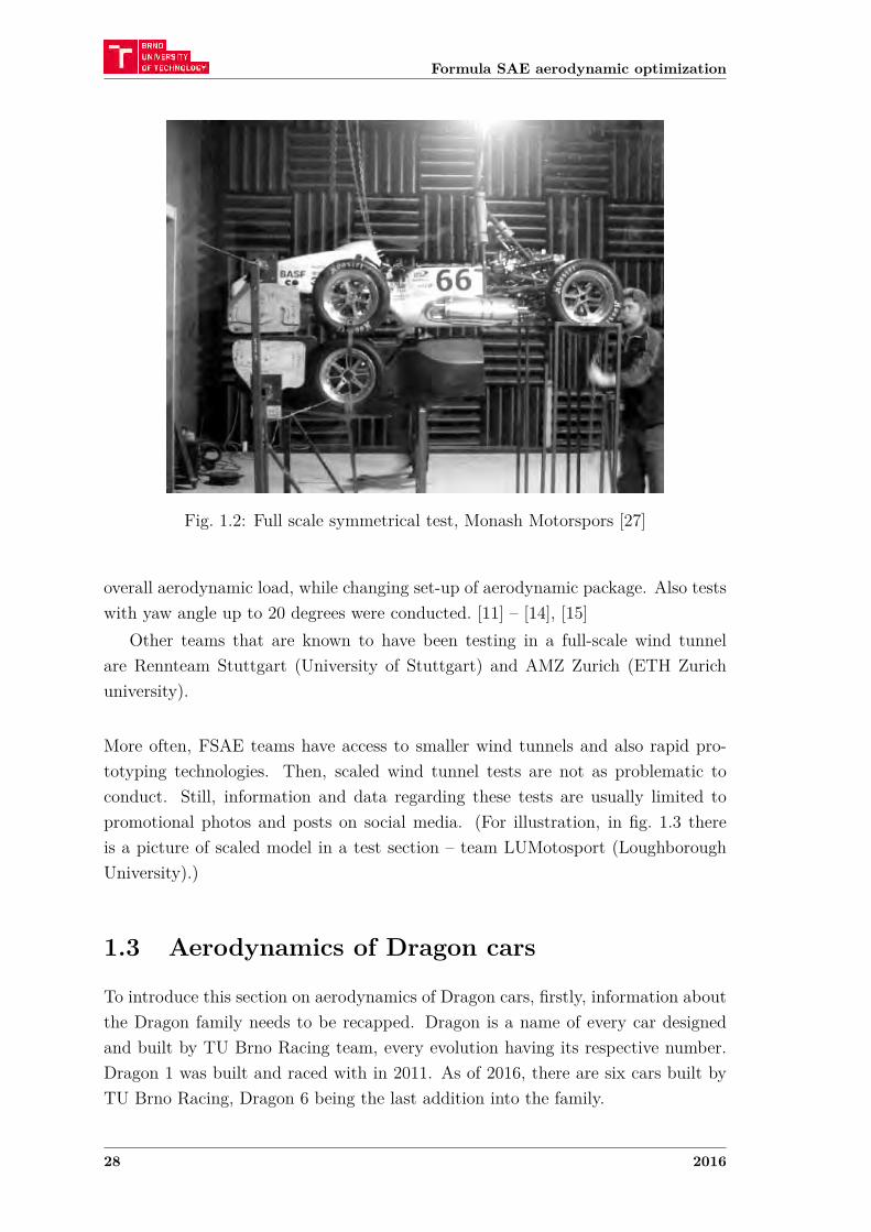
There are teams that have access to wind tunnels. Firstly, Monash Motorsport(University of Melbourne) – as pioneers of inverted wings in FSAE – were validat-ing their numerical simulations in a full scale wind tunnel from the beggining oftheir development. This work was later published by Wordley and Saunders in [26]and [27]. Their work included numerical simulations, wind tunnel testing and alsotrack testing. Interesting is their attempt to simulate ground motion by mountingsymmetrical models (see fig. 1.2)
Other well documented full-scale tests are those of UH Racing (University ofHertfordshire) and Bath Racing (University of Bath). Both of these teams gotaccess for half a day to MIRA wind tunnel4. These tests were focused on measuring
3Largest and most prestigious race in the world4 UK’s only full-scale wind tunnel facility [http://www.horiba-mira.com/our-services/
full-scale-wind-tunnel-(fswt)]
Lukáš Fryšták 27
Formula SAE aerodynamic optimization
Fig. 1.2: Full scale symmetrical test, Monash Motorspors [27]
overall aerodynamic load, while changing set-up of aerodynamic package. Also testswith yaw angle up to 20 degrees were conducted. [11] – [14], [15]
Other teams that are known to have been testing in a full-scale wind tunnelare Rennteam Stuttgart (University of Stuttgart) and AMZ Zurich (ETH Zurichuniversity).
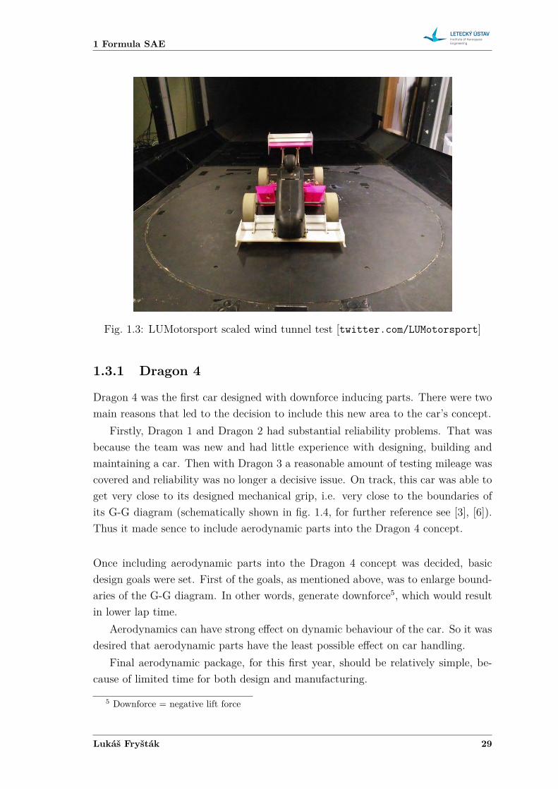
More often, FSAE teams have access to smaller wind tunnels and also rapid pro-totyping technologies. Then, scaled wind tunnel tests are not as problematic toconduct. Still, information and data regarding these tests are usually limited topromotional photos and posts on social media. (For illustration, in fig. 1.3 thereis a picture of scaled model in a test section – team LUMotosport (LoughboroughUniversity).)
1.3 Aerodynamics of Dragon cars
To introduce this section on aerodynamics of Dragon cars, firstly, information aboutthe Dragon family needs to be recapped. Dragon is a name of every car designedand built by TU Brno Racing team, every evolution having its respective number.Dragon 1 was built and raced with in 2011. As of 2016, there are six cars built byTU Brno Racing, Dragon 6 being the last addition into the family.
28 2016
1 Formula SAE
Fig. 1.3: LUMotorsport scaled wind tunnel test [twitter.com/LUMotorsport]
1.3.1 Dragon 4
Dragon 4 was the first car designed with downforce inducing parts. There were twomain reasons that led to the decision to include this new area to the car’s concept.
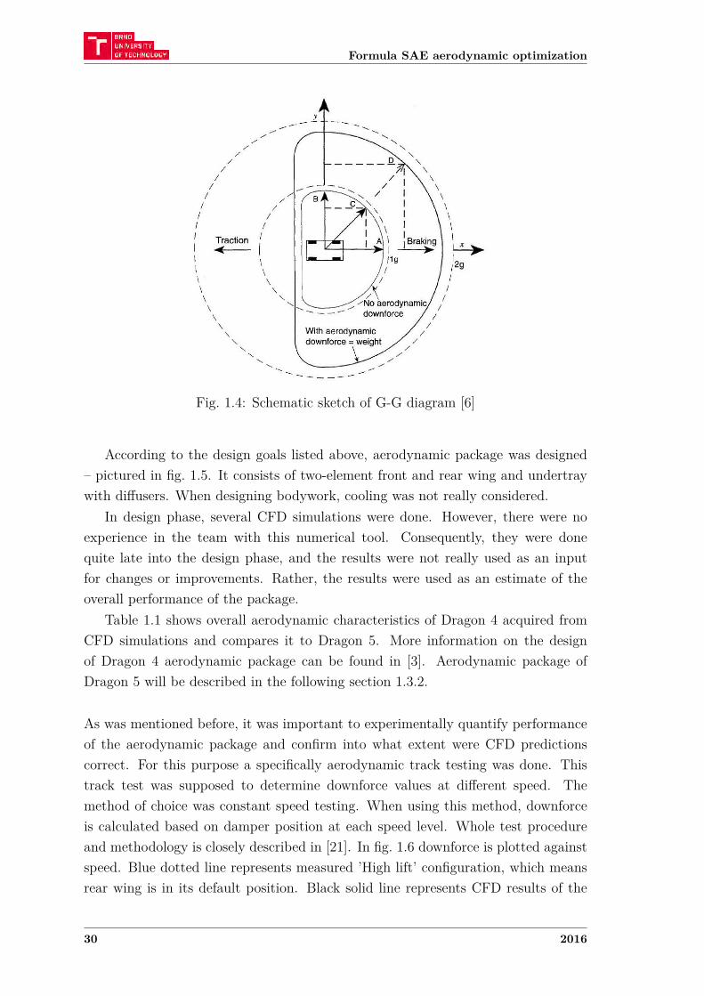
Firstly, Dragon 1 and Dragon 2 had substantial reliability problems. That wasbecause the team was new and had little experience with designing, building andmaintaining a car. Then with Dragon 3 a reasonable amount of testing mileage wascovered and reliability was no longer a decisive issue. On track, this car was able toget very close to its designed mechanical grip, i.e. very close to the boundaries ofits G-G diagram (schematically shown in fig. 1.4, for further reference see [3], [6]).Thus it made sence to include aerodynamic parts into the Dragon 4 concept.
Once including aerodynamic parts into the Dragon 4 concept was decided, basicdesign goals were set. First of the goals, as mentioned above, was to enlarge bound-aries of the G-G diagram. In other words, generate downforce5, which would resultin lower lap time.
Aerodynamics can have strong effect on dynamic behaviour of the car. So it wasdesired that aerodynamic parts have the least possible effect on car handling.
Final aerodynamic package, for this first year, should be relatively simple, be-cause of limited time for both design and manufacturing.
5 Downforce = negative lift force
Lukáš Fryšták 29
Formula SAE aerodynamic optimization
Fig. 1.4: Schematic sketch of G-G diagram [6]
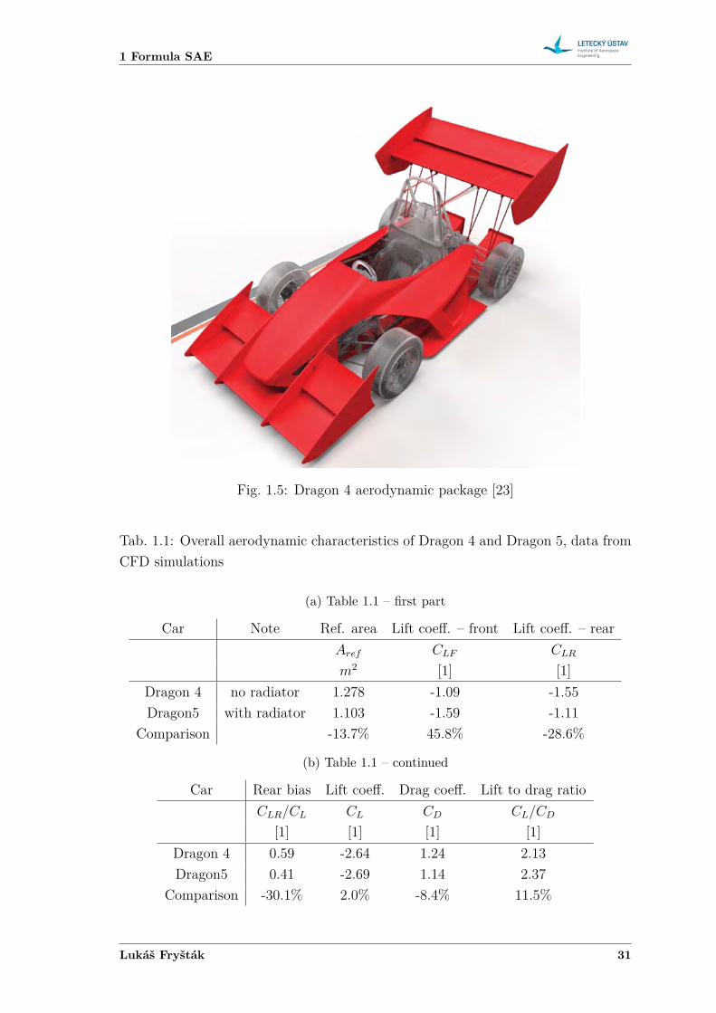
According to the design goals listed above, aerodynamic package was designed– pictured in fig. 1.5. It consists of two-element front and rear wing and undertraywith diffusers. When designing bodywork, cooling was not really considered.
In design phase, several CFD simulations were done. However, there were noexperience in the team with this numerical tool. Consequently, they were donequite late into the design phase, and the results were not really used as an inputfor changes or improvements. Rather, the results were used as an estimate of theoverall performance of the package.
Table 1.1 shows overall aerodynamic characteristics of Dragon 4 acquired fromCFD simulations and compares it to Dragon 5. More information on the designof Dragon 4 aerodynamic package can be found in [3]. Aerodynamic package ofDragon 5 will be described in the following section 1.3.2.
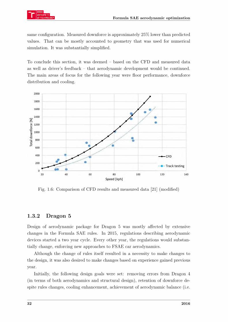
As was mentioned before, it was important to experimentally quantify performanceof the aerodynamic package and confirm into what extent were CFD predictionscorrect. For this purpose a specifically aerodynamic track testing was done. Thistrack test was supposed to determine downforce values at different speed. Themethod of choice was constant speed testing. When using this method, downforceis calculated based on damper position at each speed level. Whole test procedureand methodology is closely described in [21]. In fig. 1.6 downforce is plotted againstspeed. Blue dotted line represents measured ’High lift’ configuration, which meansrear wing is in its default position. Black solid line represents CFD results of the
30 2016
1 Formula SAE
Fig. 1.5: Dragon 4 aerodynamic package [23]
Tab. 1.1: Overall aerodynamic characteristics of Dragon 4 and Dragon 5, data fromCFD simulations
(a) Table 1.1 – first part
Car Note Ref. area Lift coeff. – front Lift coeff. – rear𝐴𝑟𝑒𝑓 𝐶𝐿𝐹 𝐶𝐿𝑅
𝑚2 [1] [1]Dragon 4 no radiator 1.278 -1.09 -1.55Dragon5 with radiator 1.103 -1.59 -1.11
Comparison -13.7% 45.8% -28.6%
(b) Table 1.1 – continued
Car Rear bias Lift coeff. Drag coeff. Lift to drag ratio𝐶𝐿𝑅/𝐶𝐿 𝐶𝐿 𝐶𝐷 𝐶𝐿/𝐶𝐷
[1] [1] [1] [1]Dragon 4 0.59 -2.64 1.24 2.13Dragon5 0.41 -2.69 1.14 2.37
Comparison -30.1% 2.0% -8.4% 11.5%
Lukáš Fryšták 31
Formula SAE aerodynamic optimization
same configuration. Measured downforce is approximately 25% lower than predictedvalues. That can be mostly accounted to geometry that was used for numericalsimulation. It was substantially simplified.
To conclude this section, it was deemed – based on the CFD and measured dataas well as driver’s feedback – that aerodynamic development would be continued.The main areas of focus for the following year were floor performance, downforcedistribution and cooling.
Fig. 1.6: Comparison of CFD results and measured data [21] (modified)
1.3.2 Dragon 5
Design of aerodynamic package for Dragon 5 was mostly affected by extensivechanges in the Formula SAE rules. In 2015, regulations describing aerodynamicdevices started a two year cycle. Every other year, the regulations would substan-tially change, enforcing new approaches to FSAE car aerodynamics.
Although the change of rules itself resulted in a necessity to make changes tothe design, it was also desired to make changes based on experience gained previousyear.
Initially, the following design goals were set: removing errors from Dragon 4(in terms of both aerodynamics and structural design), retention of downforce de-spite rules changes, cooling enhancement, achievement of aerodynamic balance (i.e.
32 2016
1 Formula SAE
achievement of neutral behaviour in terms of car handling) and last, but not least,revision/optimization of airfoil sections and floor.
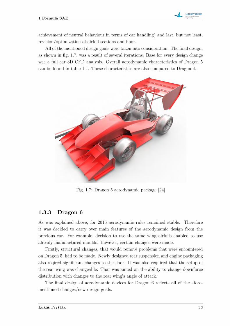
All of the mentioned design goals were taken into consideration. The final design,as shown in fig. 1.7, was a result of several iterations. Base for every design changewas a full car 3D CFD analysis. Overall aerodynamic characteristics of Dragon 5can be found in table 1.1. These characteristics are also compared to Dragon 4.
Fig. 1.7: Dragon 5 aerodynamic package [24]
1.3.3 Dragon 6
As was explained above, for 2016 aerodynamic rules remained stable. Thereforeit was decided to carry over main features of the aerodynamic design from theprevious car. For example, decision to use the same wing airfoils enabled to usealready manufactured moulds. However, certain changes were made.
Firstly, structural changes, that would remove problems that were encounteredon Dragon 5, had to be made. Newly designed rear suspension and engine packagingalso reqired significant changes to the floor. It was also required that the setup ofthe rear wing was changeable. That was aimed on the ability to change downforcedistribution with changes to the rear wing’s angle of attack.
The final design of aerodynamic devices for Dragon 6 reflects all of the afore-mentioned changes/new design goals.
Lukáš Fryšták 33

2 Current State-of-the-art
2 CURRENT STATE-OF-THE-ART
This chapter’s purpose is to provide a brief insight into road vehicle aerodynamicsand into current state-of-the-art aerodynamic development tools.
2.1 Aerodynamics in automotive industry
From the very beginning of road vehicle development, there were attempts to makethe vehicles ”aerodynamic”. These attempts were based on borrowing shapes fromnaval architecture and aeronautics. In the beginning of those respective fields, navaland aeronautical engineers had somewhat of an advantage, since they could findan inspiration for their designs in nature: fish and birds. From these naturalshapes, essential features could have been taken. Automobiles, however, have nosuch ”equivalent” in nature. These first aerodynamic vehicles did not meet withmuch appreciation, as they were done far too early. Automobiles were slow then.Streamlined bodies on the bad roads of those days would have looked ridiculous. [4]
When speed started to get higher, it became clear that aerodynamic drag reallyplays an important role in vehicle design. Either for economical reasons, or toachieve higher maximum speed.
It was in the late 1930’s, that importance of other components of aerodynamicload emerged, mainly lift force. Between years 1936-39, Daimler-Benz was doingspeed record-breaking trials with a special all-enclosed streamlined car. In speedin excess of 400 kph, the driver reported complete loss of steering and roadsideobservers had an impression that front wheels were off the ground. Such was theeffect of lift force acting on the front axle. [16]
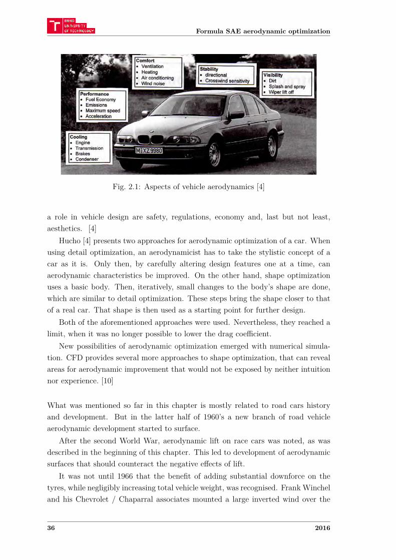
These days, aerodynamics plays much more important role in automobile develop-ment than that of the public interest, which is aerodynamic drag. Vehicle aerody-namics has to take into account a lot more aspects, as shown in fig. 2.1. Straightline stability, dynamic passive steering and crosswind sensitivity are all result ofexternal flow around a car. Moreover, external flow should also prevent droplets ofrain water from acumulating on windows and outside mirrors, keep headlights free ofdirt, prevent wind shield wipers from lifting off and cool the engine’s oil pan, mufflerand brakes. Reducing wind noise is also connected to flow around a vehicle. On theother hand, there is internal flow, which must ensure (with the aid of radiator) thatengine is cooled enough in all driving conditions. Other part of the internal flowsystem has to provide comfortable climate in the passenger compartment. [4]
Although aerodynamics does contribute to several important characteristics ofa car, overall shape is not primarily influenced by it. Other functions that play
Lukáš Fryšták 35
Formula SAE aerodynamic optimization2 Aerodynamics of Road Vehicles
Fig. 1.1 Spectrum of tasks for vehicle aerodynamics. (Courtesy BMW AG)
A l l in all, aerodynamics has a strong influence on the design of a vehicle. However, the aerodynamicist has to bear in mind that its overall shape and its many details are primarily determined by "other than aerodynamic" arguments. Among these are function, safety, regulations, economy and, last but not least, aesthetics. Only if he is ready to accept this, and only if he is able and willing to cooperate with the representatives of those "other" faculties, will he succeed in bringing his influence to bear. On the other hand, the opportunity to be closely included in the network of car design makes for the particular fascination of vehicle aerodynamics.
The main characteristics of the flow around a vehicle can be made visible. A l l that is needed is a wind tunnel and a smoke generator. Fig. 1.2 shows the streamlines in a car's plane of symmetry for symmetrical flow conditions, i.e., in the absence of side wind. Most significant is the flow separation at the rear of the car. While the streamlines follow the body contour over long stretches, even in regions of sharp curvature, the airflow finally separates at the trailing edge of the roof, forming a large wake. This wake, which sometimes is called a "dead water" region, can be observed by introducing smoke directly into it behind the vehicle (see Fig. 1.3) instead of into its oncoming flow in Fig. 1.2. Separations are typical of the flow around a vehicle. They, above all, cause drag, and the main task of the aerodynamic development of a car is to prevent or, where this is not possible, properly control them.
The aerodynamic drag D, as well as the other components of the resulting air force and moments, increases with the square of a vehicle's speed V:
D ~ V 2 0-1)
With a medium-sized car, aerodynamic drag typically accounts for about 75-80% of the total resistance to motion at 100 km/h (62 mph). Hence reducing aerodynamic drag contributes significantly to the fuel economy of a car. For this reason drag remains the focal point of vehicle aerodynamics. While for a long time, top speed was the motivation for reducing drag in many countries, today it is fuel economy and emissions.
Fig. 2.1: Aspects of vehicle aerodynamics [4]
a role in vehicle design are safety, regulations, economy and, last but not least,aesthetics. [4]
Hucho [4] presents two approaches for aerodynamic optimization of a car. Whenusing detail optimization, an aerodynamicist has to take the stylistic concept of acar as it is. Only then, by carefully altering design features one at a time, canaerodynamic characteristics be improved. On the other hand, shape optimizationuses a basic body. Then, iteratively, small changes to the body’s shape are done,which are similar to detail optimization. These steps bring the shape closer to thatof a real car. That shape is then used as a starting point for further design.
Both of the aforementioned approaches were used. Nevertheless, they reached alimit, when it was no longer possible to lower the drag coefficient.
New possibilities of aerodynamic optimization emerged with numerical simula-tion. CFD provides several more approaches to shape optimization, that can revealareas for aerodynamic improvement that would not be exposed by neither intuitionnor experience. [10]
What was mentioned so far in this chapter is mostly related to road cars historyand development. But in the latter half of 1960’s a new branch of road vehicleaerodynamic development started to surface.
After the second World War, aerodynamic lift on race cars was noted, as wasdescribed in the beginning of this chapter. This led to development of aerodynamicsurfaces that should counteract the negative effects of lift.
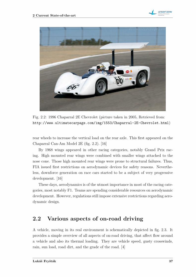
It was not until 1966 that the benefit of adding substantial downforce on thetyres, while negligibly increasing total vehicle weight, was recognised. Frank Wincheland his Chevrolet / Chaparral associates mounted a large inverted wind over the
36 2016
2 Current State-of-the-art
Fig. 2.2: 1996 Chaparral 2E Chevrolet (picture taken in 2005, Retrieved from:http://www.ultimatecarpage.com/img/1553/Chaparral-2E-Chevrolet.html)
rear wheels to increase the vertical load on the rear axle. This first appeared on theChaparral Can-Am Model 2E (fig. 2.2). [16]
By 1968 wings appeared in other racing categories, notably Grand Prix rac-ing. High mounted rear wings were combined with smaller wings attached to thenose cone. Those high mounted rear wings were prone to structural failures. Thus,FIA issued first restrictions on aerodynamic devices for safety reasons. Neverthe-less, downforce generation on race cars started to be a subject of very progressivedevelopment. [16]
These days, aerodynamics is of the utmost importance in most of the racing cate-gories, most notably F1. Teams are spending considerable resources on aerodynamicdevelopment. However, regulations still impose extensive restrictions regarding aero-dynamic design.
2.2 Various aspects of on-road driving
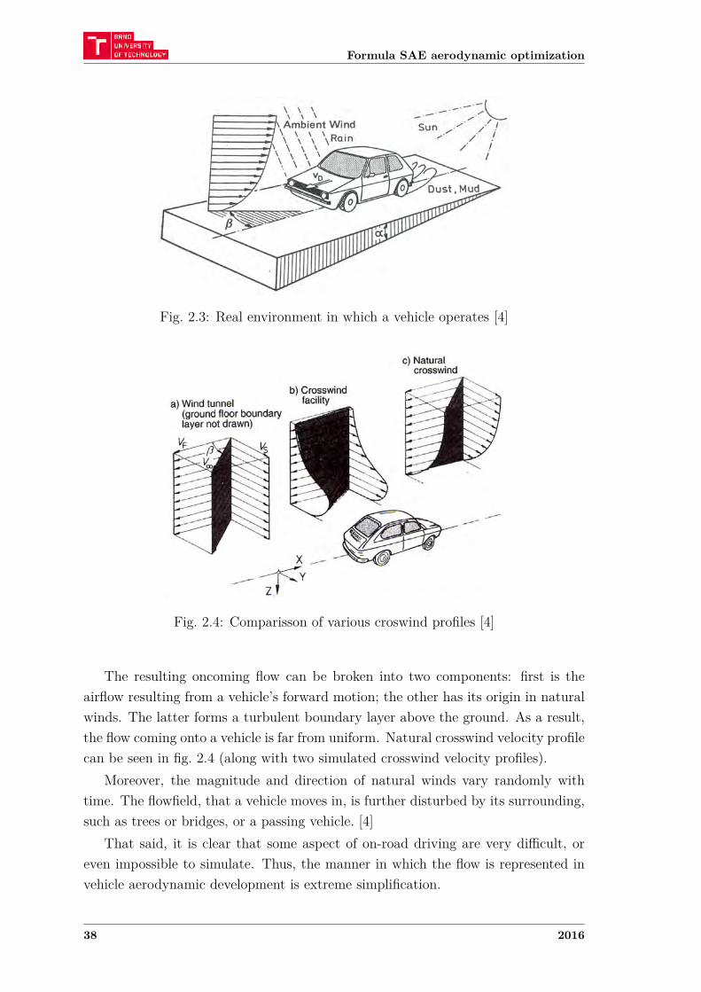
A vehicle, moving in its real environment is schematically depicted in fig. 2.3. Itprovides a simple overview of all aspects of on-road driving, that affect flow arounda vehicle and also its thermal loading. They are vehicle speed, gusty crosswinds,rain, sun load, road dirt, and the grade of the road. [4]
Lukáš Fryšták 37
Formula SAE aerodynamic optimization
Fig. 2.3: Real environment in which a vehicle operates [4]
Directional Stability 301
d assessment of anced numerical icle-road, can be
f the interaction be derived from
n exists between lal stability in a ride's center of
c) Natural crosswind
a) Wind tunnel (ground floor boundary layer not drawn)
b) Crosswind facility
Fig. 5.81 Comparison of various crosswind profiles, after W.-H. HUCHO [5.45].
'. subjective 'rating 1-10).
isonable accu-amics still are rhe advantage n a very early :fore driveable
ins. They are ipter 13. The are not taken
Si, A. COGOTTI sd turbulence
level by special elements built into the wind tunnel nozzle. Crosswind simulated by these means led to a more pronounced increase of side force, yawing moment, and rear lift with yawing angle than with a conventional flat profile of idealized flow.
5.6.2 Road Tests
Road tests for the evaluation of the impact of aerodynamics on directional stability are mostly conducted in closed proving grounds. This is advantageous with regard to safety, reproducibility, cost, and confidentiality, especially for development tasks performed on early workhorses and prototypes. Additional tests on public roads are used to gain ratings and standards for driving situations which cannot be simulated on the proving ground: stormy coastal roads, high bridges, passing maneuvers.
Measurements in crosswind facilities are of particular importance for evaluating the correlation between aerodynamics and directional stability (see also Section 14.4.2); a drastic example is shown in Fig. 5.82. In tests of this kind, a distinction is made between "open-loop" and "closed-loop" test methods; in Fig. 5.83 both methods are compared. In the open-loop test, no steering corrections are performed by the driver. Only the yawing reaction and the lateral course deviation of the vehicle under the effect of crosswind are measured.
Open-loop tests are generally conducted with the steering wheel held steady (fixed control). Comparative measurements byK. ROMPE and B. HEWING [5.31] (see Fig. 5.79) indicate that tests with a released steering wheel have a slight tendency toward more pronounced course deviations. However, major differences between "fixed control" and "free control" were measured on a car-trailer unit. With the steering wheel fixed, this vehicle combination showed only a minimum course deviation; with steering wheel released, on the other hand, almost the same course deviation was obtained as for a "solo" car. These opposed results led to the conclusion that open-loop tests are insufficient for the assessment of the directional stability of cars towing a trailer, and that closed-loop tests are necessary.
The closed-loop method also includes the driver's reaction. When passing a crosswind facility, the driver has the task of keeping his vehicle on track by means of corresponding steering corrections. His steering activity can be measured, and the directional stability can be subjectively evaluated and rated.
Fig. 2.4: Comparisson of various croswind profiles [4]
The resulting oncoming flow can be broken into two components: first is theairflow resulting from a vehicle’s forward motion; the other has its origin in naturalwinds. The latter forms a turbulent boundary layer above the ground. As a result,the flow coming onto a vehicle is far from uniform. Natural crosswind velocity profilecan be seen in fig. 2.4 (along with two simulated crosswind velocity profiles).
Moreover, the magnitude and direction of natural winds vary randomly withtime. The flowfield, that a vehicle moves in, is further disturbed by its surrounding,such as trees or bridges, or a passing vehicle. [4]
That said, it is clear that some aspect of on-road driving are very difficult, oreven impossible to simulate. Thus, the manner in which the flow is represented invehicle aerodynamic development is extreme simplification.
38 2016
2 Current State-of-the-art
2.3 Tools of the trade
There are three main tools, that are used for vehicle aerodynamic development.They are: wind tunnel testing, numerical simulations and on-track testing. Eachof these methods has its advantages and disadvantages. Often, main reasons indeciding what method in which design phase to use are also budget constraints andavailability of certain testing facilities.
According to Katz [6], aerodynamic information typically expected from theaforementioned methods are: total aerodynamic coefficients, surface pressure distri-bution and flow visualisation data (such as streamlines). Nevertheless, these remarksare in respect to racecar development. For road vehicles, further data may be col-lected, e.g. wind noise, etc.
2.3.1 Road testing
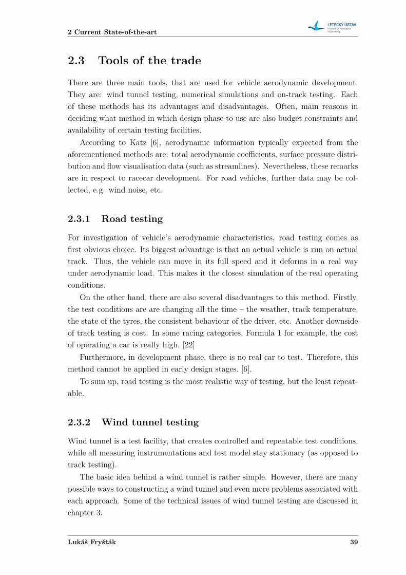
For investigation of vehicle’s aerodynamic characteristics, road testing comes asfirst obvious choice. Its biggest advantage is that an actual vehicle is run on actualtrack. Thus, the vehicle can move in its full speed and it deforms in a real wayunder aerodynamic load. This makes it the closest simulation of the real operatingconditions.
On the other hand, there are also several disadvantages to this method. Firstly,the test conditions are are changing all the time – the weather, track temperature,the state of the tyres, the consistent behaviour of the driver, etc. Another downsideof track testing is cost. In some racing categories, Formula 1 for example, the costof operating a car is really high. [22]
Furthermore, in development phase, there is no real car to test. Therefore, thismethod cannot be applied in early design stages. [6].
To sum up, road testing is the most realistic way of testing, but the least repeat-able.
2.3.2 Wind tunnel testing
Wind tunnel is a test facility, that creates controlled and repeatable test conditions,while all measuring instrumentations and test model stay stationary (as opposed totrack testing).
The basic idea behind a wind tunnel is rather simple. However, there are manypossible ways to constructing a wind tunnel and even more problems associated witheach approach. Some of the technical issues of wind tunnel testing are discussed inchapter 3.
Lukáš Fryšták 39
Formula SAE aerodynamic optimization
2.3.3 Computational methods
Computational fluid dynamics (CFD) is sometimes also called a virtual wind tun-nel. It enables to predict aerodynamic characteristics of a vehicle via a computersimulation – before a single part is manufactured. A strong emphasis is placedon development of this tool, due to the ever growing requirements on reducing de-velopment cycle times. Relative to road and wind tunnel testing, this method isconsiderably cheaper and quicker.
In the past 20 years, computational methods were evolving so rapidly, that itwas thought it would replace experiments altogether. This did not turn out tobe the case, though. But still, numerical simulations play an equally big part inaerodynamic development as experiments in these days. They complement oneanother.
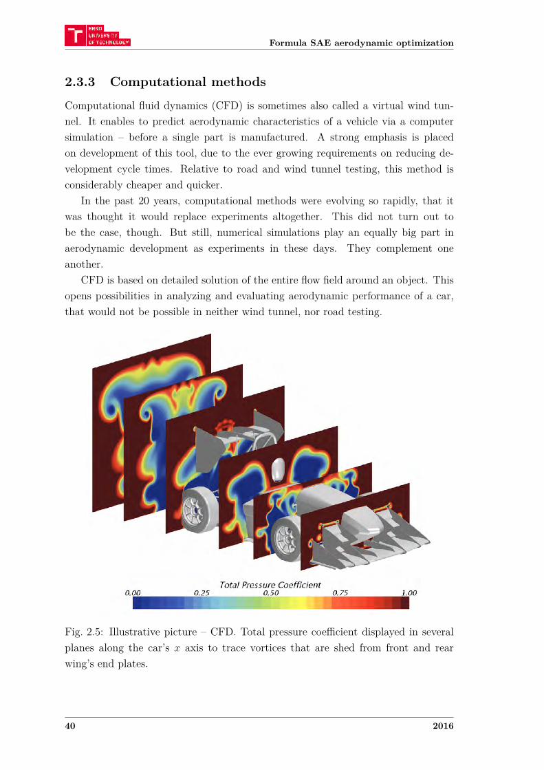
CFD is based on detailed solution of the entire flow field around an object. Thisopens possibilities in analyzing and evaluating aerodynamic performance of a car,that would not be possible in neither wind tunnel, nor road testing.
Fig. 2.5: Illustrative picture – CFD. Total pressure coefficient displayed in severalplanes along the car’s 𝑥 axis to trace vortices that are shed from front and rearwing’s end plates.
40 2016
3 Wind tunnel testing
3 WIND TUNNEL TESTING
As was mentioned in section 2.3.2, wind tunnel is a test facility, that creates con-trolled and repeatable test conditions. Nevertheless, it only simulates the conditionson a road. It does not reproduce them exactly.
There are many possible approaches to wind tunnel testing. For example, eitherfull scale or scaled tests can be conducted. With each different test layout, severalaspects have to be considered. An overview of these is described in the followingsections.
3.1 Wind tunnel nomenclature
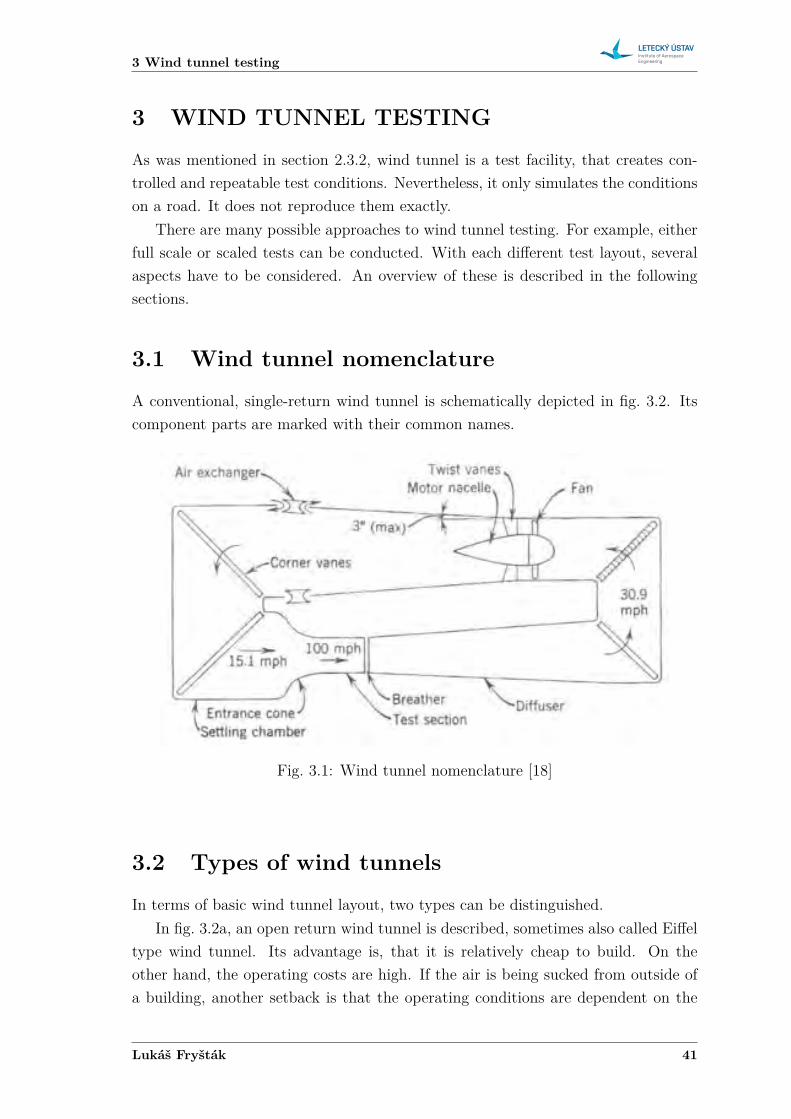
A conventional, single-return wind tunnel is schematically depicted in fig. 3.2. Itscomponent parts are marked with their common names.
Fig. 3.1: Wind tunnel nomenclature [18]
3.2 Types of wind tunnels
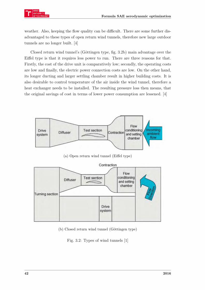
In terms of basic wind tunnel layout, two types can be distinguished.In fig. 3.2a, an open return wind tunnel is described, sometimes also called Eiffel
type wind tunnel. Its advantage is, that it is relatively cheap to build. On theother hand, the operating costs are high. If the air is being sucked from outside ofa building, another setback is that the operating conditions are dependent on the
Lukáš Fryšták 41
Formula SAE aerodynamic optimization
weather. Also, keeping the flow quality can be difficult. There are some further dis-advantaged to these types of open return wind tunnels, therefore new large outdoortunnels are no longer built. [4]
Closed return wind tunnel’s (Göttingen type, fig. 3.2b) main advantage over theEiffel type is that it requires less power to run. There are three reasons for that.Firstly, the cost of the drive unit is comparatively low; secondly, the operating costsare low and finally, the electric power connection costs are low. On the other hand,its longer ducting and larger settling chamber result in higher building costs. It isalso desirable to control temperature of the air inside the wind tunnel, therefore aheat exchanger needs to be installed. The resulting pressure loss then means, thatthe original savings of cost in terms of lower power consumption are lessened. [4]
(a) Open return wind tunnel (Eiffel type)
(b) Closed return wind tunnel (Göttingen type)
Fig. 3.2: Types of wind tunnels [1]
42 2016
3 Wind tunnel testing
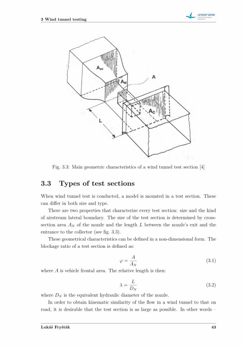
Fig. 3.3: Main geometric characteristics of a wind tunnel test section [4]
3.3 Types of test sectionsWhen wind tunnel test is conducted, a model is mounted in a test section. Thesecan differ in both size and type.
There are two properties that characterize every test section: size and the kindof airstream lateral boundary. The size of the test section is determined by cross-section area 𝐴𝑁 of the nozzle and the length 𝐿 between the nozzle’s exit and theentrance to the collector (see fig. 3.3).
These geometrical characteristics can be defined in a non-dimensional form. Theblockage ratio of a test section is defined as:
𝜙 = 𝐴
𝐴𝑁
(3.1)
where 𝐴 is vehicle frontal area. The relative length is then:
𝜆 = 𝐿
𝐷𝑁
(3.2)
where 𝐷𝑁 is the equivalent hydraulic diameter of the nozzle.In order to obtain kinematic similarity of the flow in a wind tunnel to that on
road, it is desirable that the test section is as large as possible. In other words –
Lukáš Fryšták 43
Formula SAE aerodynamic optimization
the blockage shoud be as low as possible. On the other hand, cost considerationsfor both construction and operation demand that the test section is as large as”feasible.” What does feasible mean in this sence is then a topic for discussion. [4]
The design of the test section should allow easy access and installation of testedmodel and wind tunnel instrumentation. [1]
Historically, many different test section shapes have been adopted: round, ellip-tical, square, rectangular, duplex, octagonal, rectangular with chamfered corners,round with flats on the sides and floor, elliptical with a floor flat, and several othershapes. [18]
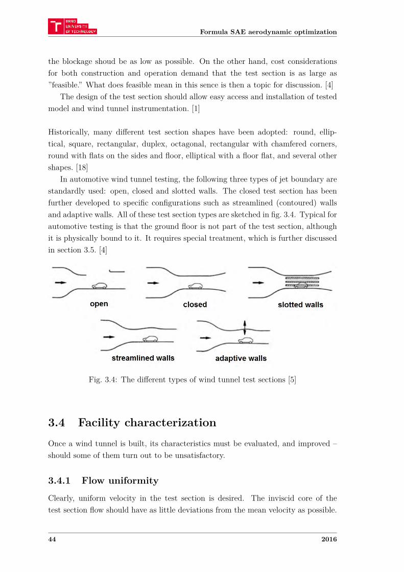
In automotive wind tunnel testing, the following three types of jet boundary arestandardly used: open, closed and slotted walls. The closed test section has beenfurther developed to specific configurations such as streamlined (contoured) wallsand adaptive walls. All of these test section types are sketched in fig. 3.4. Typical forautomotive testing is that the ground floor is not part of the test section, althoughit is physically bound to it. It requires special treatment, which is further discussedin section 3.5. [4]
Fig. 3.4: The different types of wind tunnel test sections [5]
3.4 Facility characterizationOnce a wind tunnel is built, its characteristics must be evaluated, and improved –should some of them turn out to be unsatisfactory.
3.4.1 Flow uniformity
Clearly, uniform velocity in the test section is desired. The inviscid core of thetest section flow should have as little deviations from the mean velocity as possible.
44 2016
3 Wind tunnel testing
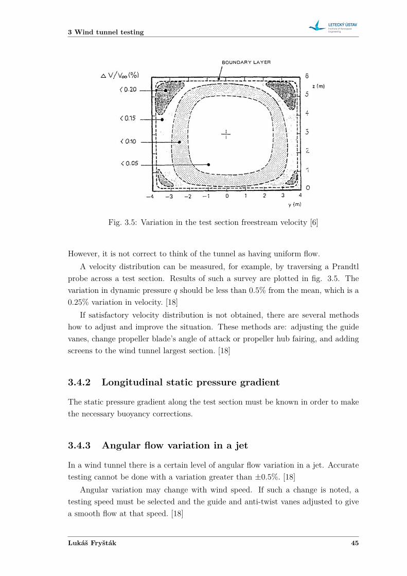
Fig. 3.5: Variation in the test section freestream velocity [6]
However, it is not correct to think of the tunnel as having uniform flow.A velocity distribution can be measured, for example, by traversing a Prandtl
probe across a test section. Results of such a survey are plotted in fig. 3.5. Thevariation in dynamic pressure 𝑞 should be less than 0.5% from the mean, which is a0.25% variation in velocity. [18]
If satisfactory velocity distribution is not obtained, there are several methodshow to adjust and improve the situation. These methods are: adjusting the guidevanes, change propeller blade’s angle of attack or propeller hub fairing, and addingscreens to the wind tunnel largest section. [18]
3.4.2 Longitudinal static pressure gradient
The static pressure gradient along the test section must be known in order to makethe necessary buoyancy corrections.
3.4.3 Angular flow variation in a jet
In a wind tunnel there is a certain level of angular flow variation in a jet. Accuratetesting cannot be done with a variation greater than ±0.5%. [18]
Angular variation may change with wind speed. If such a change is noted, atesting speed must be selected and the guide and anti-twist vanes adjusted to givea smooth flow at that speed. [18]
Lukáš Fryšták 45
Formula SAE aerodynamic optimization
3.4.4 Turbulence
While in real conditions turbulence is significant, in wind tunnel testing, it is desir-able to have low turbulence levels.
Turbulence intensity (𝑇𝐼) is typically computed from equation 3.3 and expressedas a percent of the local mean velocity. [1]
𝑇𝐼 = 𝑢′
𝑈∞(3.3)
Usually, turbulence intensity varies from 1.0 to 3.0. A value of 1.1 is not difficultto obtain, and values above 1.4 probably indicate, that the tunnel has too muchturbulence for reliable testing. [18]
3.4.5 Surging
Pope [18] calls surging ”the most vexatious problem a tunnel engineer may have toface.” It is a random low-frequency variation in velocity that may run as high as5% of dynamic pressure 𝑞. It makes trouble for all measurements, as it effects forcebalances, and pressure measurements. Doubts also arise, when assigning Reynoldsnumber to the test.
Surging is associated with separation and reattachment in the diffuser. Thereare methods how to cure this problem, but they have to be assessed individually. [18]
3.4.6 Acoustics
If the facility is used for acoustic measurements, background noise should be as-sessed. Ideally, an aeroacoustic flow facility sould have background noise levels atleast 10 dB below the acoustic source of interest in a test. [1]
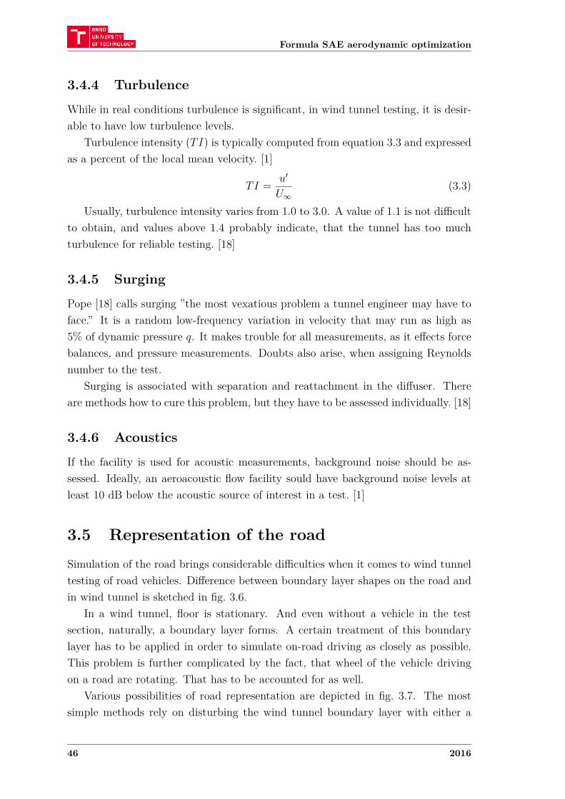
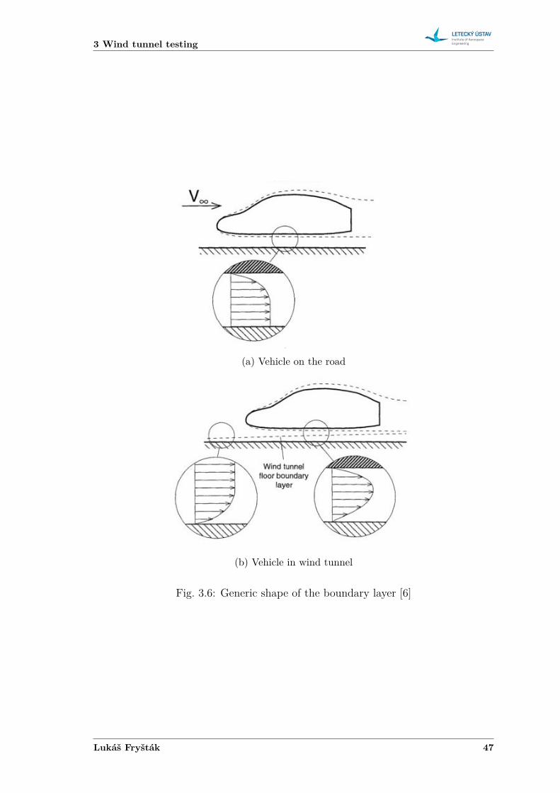
3.5 Representation of the roadSimulation of the road brings considerable difficulties when it comes to wind tunneltesting of road vehicles. Difference between boundary layer shapes on the road andin wind tunnel is sketched in fig. 3.6.
In a wind tunnel, floor is stationary. And even without a vehicle in the testsection, naturally, a boundary layer forms. A certain treatment of this boundarylayer has to be applied in order to simulate on-road driving as closely as possible.This problem is further complicated by the fact, that wheel of the vehicle drivingon a road are rotating. That has to be accounted for as well.
Various possibilities of road representation are depicted in fig. 3.7. The mostsimple methods rely on disturbing the wind tunnel boundary layer with either a
46 2016
3 Wind tunnel testing
(a) Vehicle on the road
(b) Vehicle in wind tunnel
Fig. 3.6: Generic shape of the boundary layer [6]
Lukáš Fryšták 47
Formula SAE aerodynamic optimization
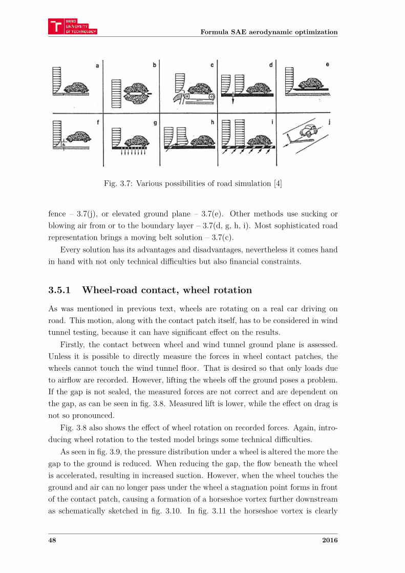
Fig. 3.7: Various possibilities of road simulation [4]
fence – 3.7(j), or elevated ground plane – 3.7(e). Other methods use sucking orblowing air from or to the boundary layer – 3.7(d, g, h, i). Most sophisticated roadrepresentation brings a moving belt solution – 3.7(c).
Every solution has its advantages and disadvantages, nevertheless it comes handin hand with not only technical difficulties but also financial constraints.
3.5.1 Wheel-road contact, wheel rotation
As was mentioned in previous text, wheels are rotating on a real car driving onroad. This motion, along with the contact patch itself, has to be considered in windtunnel testing, because it can have significant effect on the results.
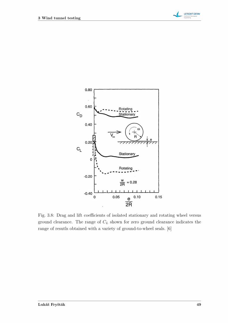
Firstly, the contact between wheel and wind tunnel ground plane is assessed.Unless it is possible to directly measure the forces in wheel contact patches, thewheels cannot touch the wind tunnel floor. That is desired so that only loads dueto airflow are recorded. However, lifting the wheels off the ground poses a problem.If the gap is not sealed, the measured forces are not correct and are dependent onthe gap, as can be seen in fig. 3.8. Measured lift is lower, while the effect on drag isnot so pronounced.
Fig. 3.8 also shows the effect of wheel rotation on recorded forces. Again, intro-ducing wheel rotation to the tested model brings some technical difficulties.
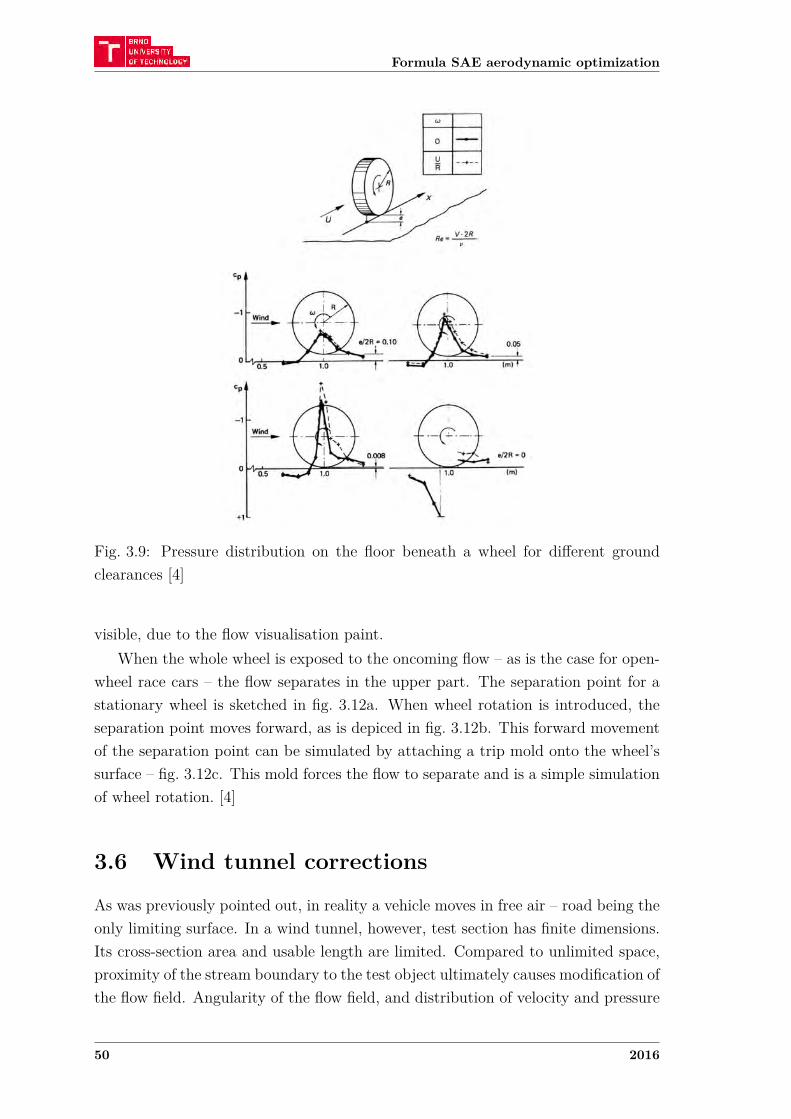
As seen in fig. 3.9, the pressure distribution under a wheel is altered the more thegap to the ground is reduced. When reducing the gap, the flow beneath the wheelis accelerated, resulting in increased suction. However, when the wheel touches theground and air can no longer pass under the wheel a stagnation point forms in frontof the contact patch, causing a formation of a horseshoe vortex further downstreamas schematically sketched in fig. 3.10. In fig. 3.11 the horseshoe vortex is clearly
48 2016
3 Wind tunnel testing
Fig. 3.8: Drag and lift coefficients of isolated stationary and rotating wheel versusground clearance. The range of 𝐶𝐿 shown for zero ground clearance indicates therange of resutls obtained with a variety of ground-to-wheel seals. [6]
Lukáš Fryšták 49
Formula SAE aerodynamic optimization
Fig. 3.9: Pressure distribution on the floor beneath a wheel for different groundclearances [4]
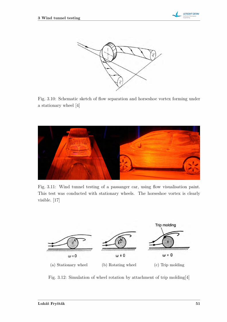
visible, due to the flow visualisation paint.When the whole wheel is exposed to the oncoming flow – as is the case for open-
wheel race cars – the flow separates in the upper part. The separation point for astationary wheel is sketched in fig. 3.12a. When wheel rotation is introduced, theseparation point moves forward, as is depiced in fig. 3.12b. This forward movementof the separation point can be simulated by attaching a trip mold onto the wheel’ssurface – fig. 3.12c. This mold forces the flow to separate and is a simple simulationof wheel rotation. [4]
3.6 Wind tunnel corrections
As was previously pointed out, in reality a vehicle moves in free air – road being theonly limiting surface. In a wind tunnel, however, test section has finite dimensions.Its cross-section area and usable length are limited. Compared to unlimited space,proximity of the stream boundary to the test object ultimately causes modification ofthe flow field. Angularity of the flow field, and distribution of velocity and pressure
50 2016
3 Wind tunnel testing
Fig. 3.10: Schematic sketch of flow separation and horseshoe vortex forming undera stationary wheel [4]
Fig. 3.11: Wind tunnel testing of a passanger car, using flow visualisation paint.This test was conducted with stationary wheels. The horseshoe vortex is clearlyvisible. [17]
(a) Stationary wheel (b) Rotating wheel (c) Trip molding
Fig. 3.12: Simulation of wheel rotation by attachment of trip molding[4]
Lukáš Fryšták 51
Formula SAE aerodynamic optimization
over a model is altered to a certain extent. Consequently, the measured forces andmoments are somewhat different than they would be in unlimited space. The smallerthe wind tunnel relative to the model, the higher are these discrepancies. [4]
When only relative results are sought, such as effect of shape modification ondrag force, these discrepancies might be tolerable – provided the wind tunnel’s sizeis reasonable. Nevertheless, it is absolute results that are usually desired. Then theresults are comparable to competing manufacturers, tests in different wind tunnels,or comparison of results with numerical computations. [4]
Corrections make allowances for the flow deviations in a wind tunnel. Originally,for automotive testing, these corrections were taken over from aeronautics. Overtime, though, doubts arose as to whether the aerospace corrections can be appliedto road vehicles, since there is substantial difference in their respective flow fileds.Cars are bluff bodies and their flow field has large areas of separation, while onaircraft, the flow is mostly attached. [4]
Eventually, methods for determining wind tunnel corrections for automotive test-ing were developed under the roof of the SAE. These methods are different for opentest section and closed test section. Only the methods for closed test section arediscussed furhter (section 3.6.1) as they are relevant to this work.
The basic premise of all wind tunnel corrections is that the flow pattern does notchange. That means that streamlines, pressure distribution and separation pointsall stay the same as in free air. Although, CFD methods enable this premise to berelaxed. [4]
Perturbations of the various stream boundaries result in two effects:• Velocity of the oncoming flow is altered.• An axial pressure gradient is superimposed on the flow field.
Then, linear approach can be applied. Effects of these perturbations are superim-posed by addition. [4]
This linear approach is only meaningful when each of the perturbations are smalland the resulting correction is small. This applies only if the wind tunnel’s testsection size is ”reasonable” relative to the test object. However, it is not possible toexactly determine the range in which this approach is valid. [4]
3.6.1 Closed test section
In a closed test section, three types of boundary perturbations can be distinguished:• Solid blockage• Wake blockage• Horizontal buoyancy
52 2016
3 Wind tunnel testing
In principle, each of these perturbations has the two aforementioned effects. Firstly,the oncoming flow is altered and secondly, pressure gradients along test section’saxis are introduced. [4]
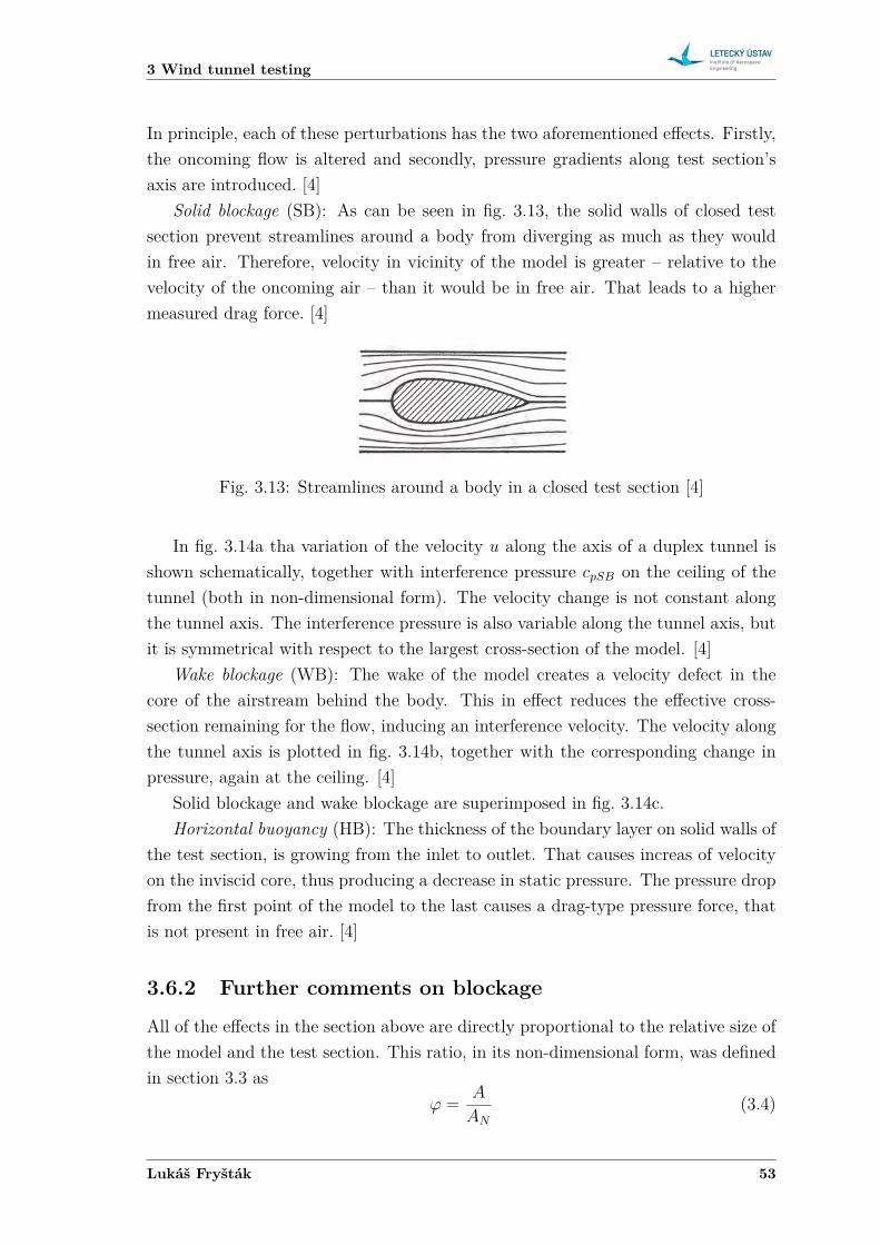
Solid blockage (SB): As can be seen in fig. 3.13, the solid walls of closed testsection prevent streamlines around a body from diverging as much as they wouldin free air. Therefore, velocity in vicinity of the model is greater – relative to thevelocity of the oncoming air – than it would be in free air. That leads to a highermeasured drag force. [4]
Fig. 3.13: Streamlines around a body in a closed test section [4]
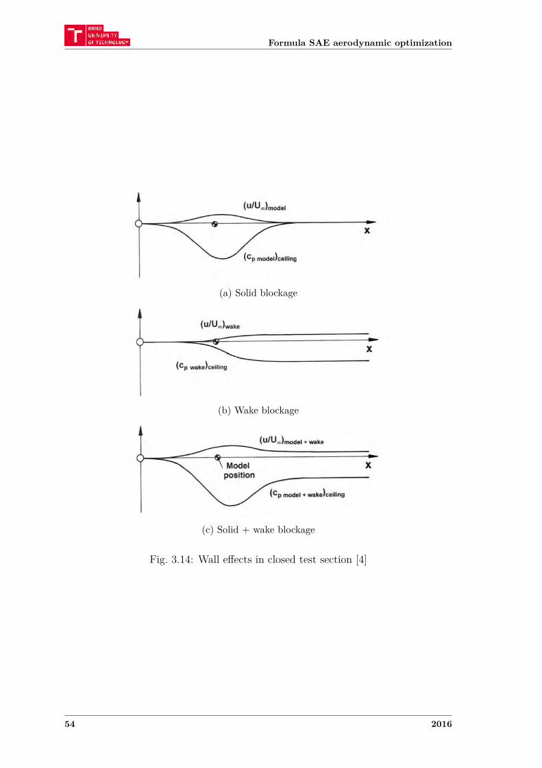
In fig. 3.14a tha variation of the velocity 𝑢 along the axis of a duplex tunnel isshown schematically, together with interference pressure 𝑐𝑝𝑆𝐵 on the ceiling of thetunnel (both in non-dimensional form). The velocity change is not constant alongthe tunnel axis. The interference pressure is also variable along the tunnel axis, butit is symmetrical with respect to the largest cross-section of the model. [4]
Wake blockage (WB): The wake of the model creates a velocity defect in thecore of the airstream behind the body. This in effect reduces the effective cross-section remaining for the flow, inducing an interference velocity. The velocity alongthe tunnel axis is plotted in fig. 3.14b, together with the corresponding change inpressure, again at the ceiling. [4]
Solid blockage and wake blockage are superimposed in fig. 3.14c.Horizontal buoyancy (HB): The thickness of the boundary layer on solid walls of
the test section, is growing from the inlet to outlet. That causes increas of velocityon the inviscid core, thus producing a decrease in static pressure. The pressure dropfrom the first point of the model to the last causes a drag-type pressure force, thatis not present in free air. [4]
3.6.2 Further comments on blockage
All of the effects in the section above are directly proportional to the relative size ofthe model and the test section. This ratio, in its non-dimensional form, was definedin section 3.3 as
𝜙 = 𝐴
𝐴𝑁
(3.4)
Lukáš Fryšták 53
Formula SAE aerodynamic optimization
(a) Solid blockage
(b) Wake blockage
(c) Solid + wake blockage
Fig. 3.14: Wall effects in closed test section [4]
54 2016
3 Wind tunnel testing
and was called blockage.For a long time 𝜙 = 0.05, the typical value in aeronautics, was used in auto-
motive wind tunnel testing. Today, automotive wind tunnels operate with blockage𝜙 ≈ 0.10. However, there are wind tunnel that operate with blockage ratio as highas 𝜙 ≈ 0.20.
Hucho states, that contoured wall test section and blockage ratio 𝜙 ≈ 0.20 canyield the same results as tests with 𝜙 ≈ 0.05. [4]. On the other hand, streamlined testsection also has its considerable disadvantages – it substantially limits the variatyof shapes, that can be tested and it also prevents yawing the model. [4][22]
Katz also presents experimental data from wind tunnel tests with rather highblockage. In [8] an investigation of wind tunnel wall effects in high blockage testingwas done. Four differently sized bluff bodies with blockage ranging from 5% to 20%were measured in a wind tunnel. The same cases were also numerically computed.It is concluded that ”As the blockage ratio increases, some effects may become quitelarge and simple corrections can not account for all the changes. Up to blockagevalues of 7% or even 10%, some of the traditional corrections can be applied sincethe effects are not very large. However at blockage values of near 20% the resultmay differ considerably. But valuable work is still possible in certain disciplines,when a single geometry is constantly being modified and the correlation betweenwind-tunnel and free-air data is constantly being verified. This is because the shapeof the pressure distribution is not changing in nature – but rather being magnifiedby the proximity of the walls.”. By ”traditional corrections”, those presented byPope and Harper in [18] are meant.
In another paper co-written by Katz [7] a 25% scaled model of generic Indy Car1 formula is tested in a wind tunnel. The tests are conducted with both wheelsand ground plane stationary (elevated ground plane is used). The blockage in theseexperiments was ”quite large” – 15% – and use of numerical corrections is suggested.With this experimental set up – high blockage, stationary groud plane and wheels– certain differences are stressed out, but it is deemed that such tests can be usedfor basic studies and can yield useful aerodynamic data.
3.6.3 Boundary layer effects
When measurements are made using a stationary floor, the drag force should be cor-rected for a boundary layer effect. Wheels of the tested vehicle are partly immersedin boundary layer. Therefore, the measured drag is too low. For cars, as an average,such a correction would be on the order of 𝐶𝐷 ≈ 0.01 on average. According toHucho [4], this correction is often being neglected.
1 Indy Car is a North American open-wheel racing series.
Lukáš Fryšták 55
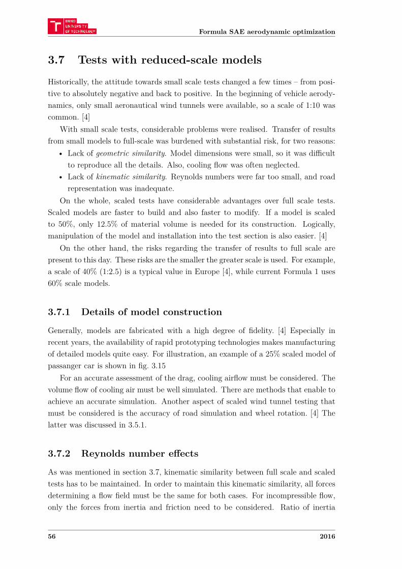
Formula SAE aerodynamic optimization
3.7 Tests with reduced-scale models
Historically, the attitude towards small scale tests changed a few times – from posi-tive to absolutely negative and back to positive. In the beginning of vehicle aerody-namics, only small aeronautical wind tunnels were available, so a scale of 1:10 wascommon. [4]
With small scale tests, considerable problems were realised. Transfer of resultsfrom small models to full-scale was burdened with substantial risk, for two reasons:
• Lack of geometric similarity. Model dimensions were small, so it was difficultto reproduce all the details. Also, cooling flow was often neglected.
• Lack of kinematic similarity. Reynolds numbers were far too small, and roadrepresentation was inadequate.
On the whole, scaled tests have considerable advantages over full scale tests.Scaled models are faster to build and also faster to modify. If a model is scaledto 50%, only 12.5% of material volume is needed for its construction. Logically,manipulation of the model and installation into the test section is also easier. [4]
On the other hand, the risks regarding the transfer of results to full scale arepresent to this day. These risks are the smaller the greater scale is used. For example,a scale of 40% (1:2.5) is a typical value in Europe [4], while current Formula 1 uses60% scale models.
3.7.1 Details of model construction
Generally, models are fabricated with a high degree of fidelity. [4] Especially inrecent years, the availability of rapid prototyping technologies makes manufacturingof detailed models quite easy. For illustration, an example of a 25% scaled model ofpassanger car is shown in fig. 3.15
For an accurate assessment of the drag, cooling airflow must be considered. Thevolume flow of cooling air must be well simulated. There are methods that enable toachieve an accurate simulation. Another aspect of scaled wind tunnel testing thatmust be considered is the accuracy of road simulation and wheel rotation. [4] Thelatter was discussed in 3.5.1.
3.7.2 Reynolds number effects
As was mentioned in section 3.7, kinematic similarity between full scale and scaledtests has to be maintained. In order to maintain this kinematic similarity, all forcesdetermining a flow field must be the same for both cases. For incompressible flow,only the forces from inertia and friction need to be considered. Ratio of inertia
56 2016
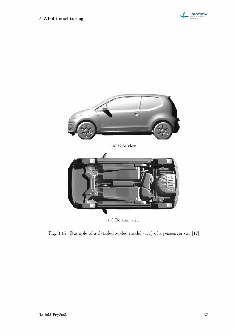
3 Wind tunnel testing
(a) Side view
(b) Bottom view
Fig. 3.15: Example of a detailed scaled model (1:4) of a passenger car [17]
Lukáš Fryšták 57
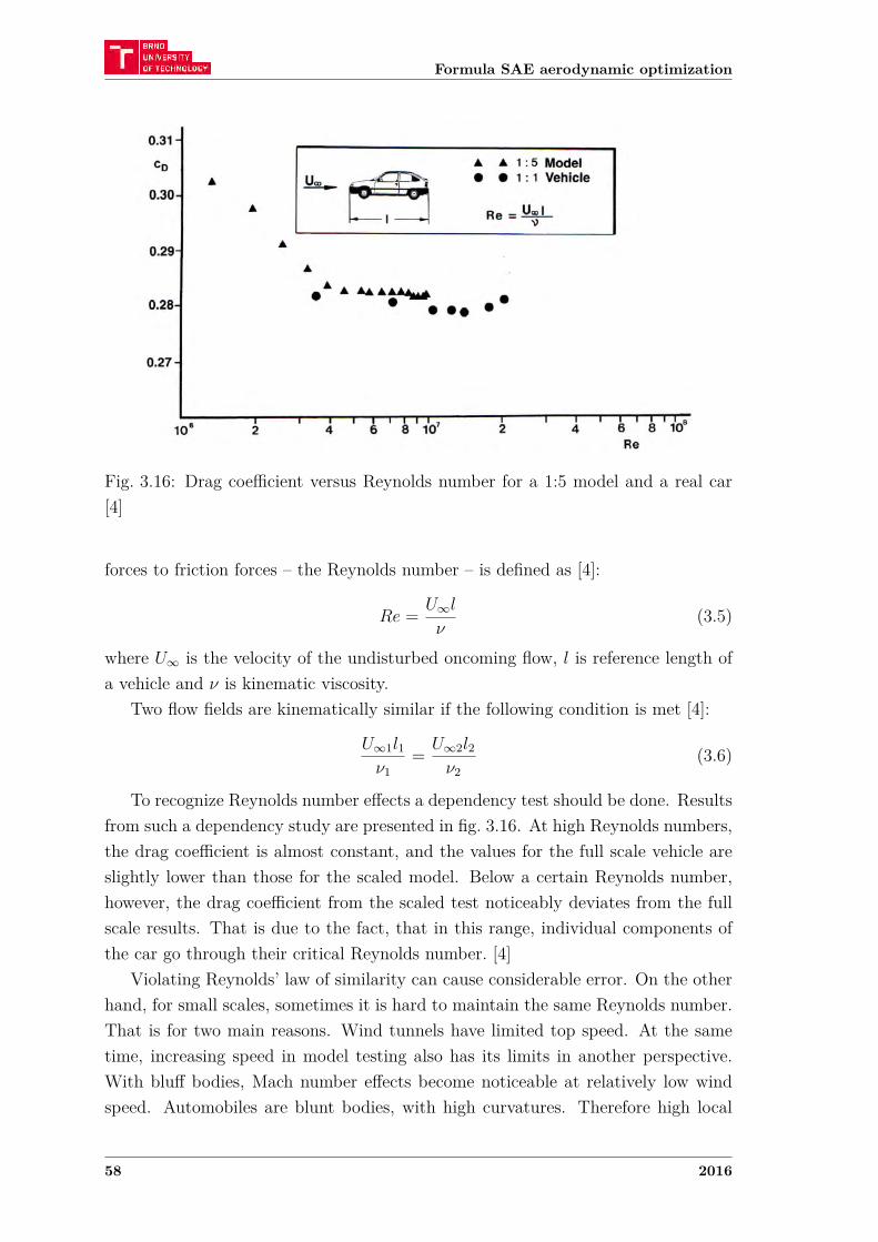
Formula SAE aerodynamic optimization<
o <
Wind Tunnels 687
0.31 H
0.30
0.29
0.28-
0.27-
106
A • 1:5 Model • • 1 : 1 Vehicle
Re =%i-
• •• •
i 1—i—i—ill, 4 6 8 10
"I 1 1 1 1 1 I I I 8
2 4 6 8 10 Re
Fig. 13.58 Drag coefficient cD versus Reynolds number Re for a 1:5 model and a real car, after H. -J. EMMELMANN [13.79]. Fig. 3.16: Drag coefficient versus Reynolds number for a 1:5 model and a real car
[4]
forces to friction forces – the Reynolds number – is defined as [4]:
𝑅𝑒 = 𝑈∞𝑙
𝜈(3.5)
where 𝑈∞ is the velocity of the undisturbed oncoming flow, 𝑙 is reference length ofa vehicle and 𝜈 is kinematic viscosity.
Two flow fields are kinematically similar if the following condition is met [4]:
𝑈∞1𝑙1𝜈1
= 𝑈∞2𝑙2𝜈2
(3.6)
To recognize Reynolds number effects a dependency test should be done. Resultsfrom such a dependency study are presented in fig. 3.16. At high Reynolds numbers,the drag coefficient is almost constant, and the values for the full scale vehicle areslightly lower than those for the scaled model. Below a certain Reynolds number,however, the drag coefficient from the scaled test noticeably deviates from the fullscale results. That is due to the fact, that in this range, individual components ofthe car go through their critical Reynolds number. [4]
Violating Reynolds’ law of similarity can cause considerable error. On the otherhand, for small scales, sometimes it is hard to maintain the same Reynolds number.That is for two main reasons. Wind tunnels have limited top speed. At the sametime, increasing speed in model testing also has its limits in another perspective.With bluff bodies, Mach number effects become noticeable at relatively low windspeed. Automobiles are blunt bodies, with high curvatures. Therefore high local
58 2016
3 Wind tunnel testing
Fig. 3.17: Mounting a model through the tyre patches, while using elevated groundplane [6]
values of 𝑢/𝑈∞ occur. The rule of thumb according to which compressibility effectscan be neglected up to 𝑀𝑎 = 0.3 does not apply to bodies as bluff as cars.𝑀𝑎 = 0.2 seems to be a more reasonable limit. Consequently, wind speed islimited to 𝑈∞ = 70 𝑚/𝑠. [4]
To conclude, the advantages of working with reduced scale models are realizedonly if the results achieved with them can reliably be transfered to full-scale. [4]
3.8 Model mountingGenerally, model mounting methods can be distinguished into two main approaches.They are: (a) mounting a model via the wheel-road contact, and (b) using a post –a sting – to mount the model.
Mounting a model in the tyre contact patches, as sketched in fig. 3.17, appearsto be the simplest method, especially for full scale vehicles. Wheels rest on smallpanels, that are separated from the rest of the floor (or the elevated ground plane)and must be kept as small as possible. These panels are then connected to a forcebalance with struts. The separated panels for wheels and shielding of the struts,provided elevated ground plane is used, must be included in order to measure forcesdue only to air flow. [6] With this solution, complications arise when a moving beltsystem is to be used to simulate the road. Then, only a narrow belt between thewheels can be used and the wheel supporting panels have to be equipped with motorsthat rotate the wheels.
The other method, that is attractive for light small-scale models, relies on mount-ing a model on a single sting. There are more options as to how exactly to do that.In fig. 3.18, model mounted on a sting from behind is shown. According to Katz [6]this creates less aerodynamic interference than mounting from above, as can be seen
Lukáš Fryšták 59
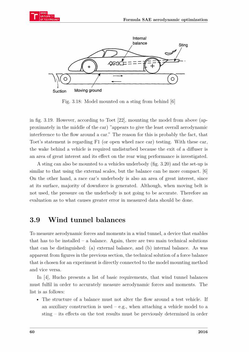
Formula SAE aerodynamic optimization
Fig. 3.18: Model mounted on a sting from behind [6]
in fig. 3.19. However, according to Toet [22], mounting the model from above (ap-proximately in the middle of the car) ”appears to give the least overall aerodynamicinterference to the flow around a car.” The reason for this is probably the fact, thatToet’s statement is regarding F1 (or open wheel race car) testing. With these car,the wake behind a vehicle is required undisturbed because the exit of a diffuser isan area of great interest and its effect on the rear wing performance is investigated.
A sting can also be mounted to a vehicles underbody (fig. 3.20) and the set-up issimilar to that using the external scales, but the balance can be more compact. [6]On the other hand, a race car’s underbody is also an area of great interest, sinceat its surface, majority of downforce is generated. Although, when moving belt isnot used, the pressure on the underbody is not going to be accurate. Therefore anevaluation as to what causes greater error in measured data should be done.
3.9 Wind tunnel balances
To measure aerodynamic forces and moments in a wind tunnel, a device that enablesthat has to be installed – a balance. Again, there are two main technical solutionsthat can be distinguished: (a) external balance, and (b) internal balance. As wasapparent from figures in the previous section, the technical solution of a force balancethat is chosen for an experiment is directly connected to the model mounting methodand vice versa.
In [4], Hucho presents a list of basic requirements, that wind tunnel balancesmust fulfil in order to accurately measure aerodynamic forces and moments. Thelist is as follows:
• The structure of a balance must not alter the flow around a test vehicle. Ifan auxiliary construction is used – e.g., when attaching a vehicle model to asting – its effects on the test results must be previously determined in order
60 2016
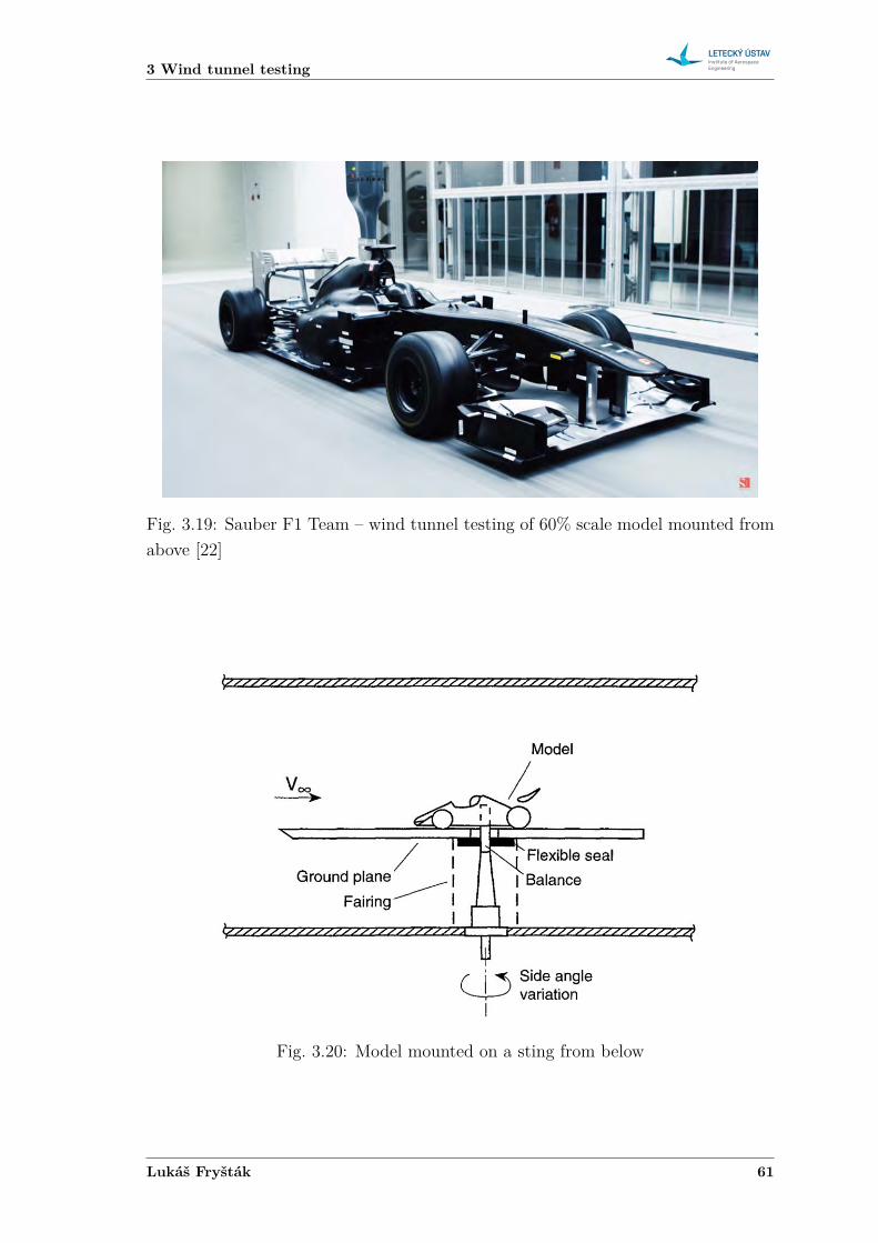
3 Wind tunnel testing
Fig. 3.19: Sauber F1 Team – wind tunnel testing of 60% scale model mounted fromabove [22]
Fig. 3.20: Model mounted on a sting from below
Lukáš Fryšták 61
Formula SAE aerodynamic optimization
to be able to correct the test values accordingly.• The vehicle position must not change uncontrolled during the measurement.• Since the aerodynamic lift forces to be measured are only fractions of the total
vehicle weight, the preloads of the 𝑧 axis must be compensated by correspond-ing tare weights for better accuracy.
• If measurements are to be performed under yaw, the balance must be rotatablearound the 𝑧 axis accordingly.
• The transmission of the forces between test object and force pick-up pointsmust occur free of friction and hysteresis. For this reason, the use of specialaccurate elements is essential, such as knife-edge and groove combinations,elastic hinges, or hydrostatic and pneumatic bearings, etc.
An overview of six-component balances developed for vehicle testing is shown infig. 3.21. Part of the figure is a brief description of every solution, with mainadvantages and disadvantages.
Internal balance is shown schematically in fig. 3.22. It is a very sophisticatedmeasuring element. By cutting holes and various shapes into the metal core of thisbalance, its structure becomes sensitive in particular spots to loads such as drag.At these spots, strain gauges are installed and the balance is calibrated for a certainrange. [6] These balances can be purchased off-the-shelf, an example being a balanceby Aerolab in fig. 3.23.
3.9.1 Deflections
One of the most troublesome problems of wind tunnel balances is their rigidity.Deflections of the balance may result in undesired movement of the test object. Itcan even lead to distortion of individual components of the aerodynamic loads (e.g.,part of lift appears as drag or side force). [18]
Solution to this problem seems obvious enough. Either keep the deflections solow, the can be rendered negligible, or they must be evaluated and accounted for inthe work-up. Keeping the deflections low is, of course, preferable.
The effects of deflections are evaluated during the calibration process, and cor-rections, if necessary, are included.
3.9.2 Measurement of the aerodynamic coefficients
As was described in the previous section (3.9), aerodynamic forces and moments aremeasured with a balance. To achieve more reliable data a few simple test detailsmust be observed to secure good test results, as presented by Hucho [4]:
62 2016
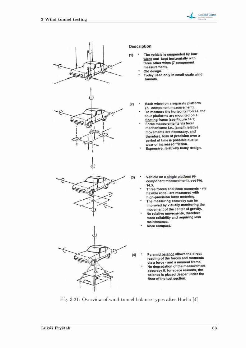
3 Wind tunnel testing
Measurement and Test Techniques
Description
(1) * The vehicle is suspended by four wires and kept horizontally with three other wires (7-component measurement).
* Old design. * Today used only in small-scale wind
tunnels.
(2)
(3)
Each wheel on a separate platform (7- component measurement). To measure the horizontal forces, the four platforms are mounted on a floating frame (see Figure 14.2). Force measurements via lever mechanisms; i.e., (small) relative movements are necessary, and therefore, loss of precision over a period of time is possible due to wear or increased friction. Expensive, relatively bulky design.
Vehicle on a single platform (6-component measurement), see Fig. 14.3. Three forces and three moments - via flexible rods - are measured with high-precision force metering. The measuring accuracy can be improved by visually monitoring the movement of the center of gravity. No relative movements, therefore more reliability and requiring less maintenance. More compact.
(4) * Pyramid balance allows the direct reading of the forces and moments via a force - and a moment frame.
* No degradation of the measurement accuracy if, for space reasons, the balance is placed deeper under the floor of the test section.
Fig. 14.1 Overview of various wind tunnel balance types.
Fig. 3.21: Overview of wind tunnel balance types after Hucho [4]
Lukáš Fryšták 63
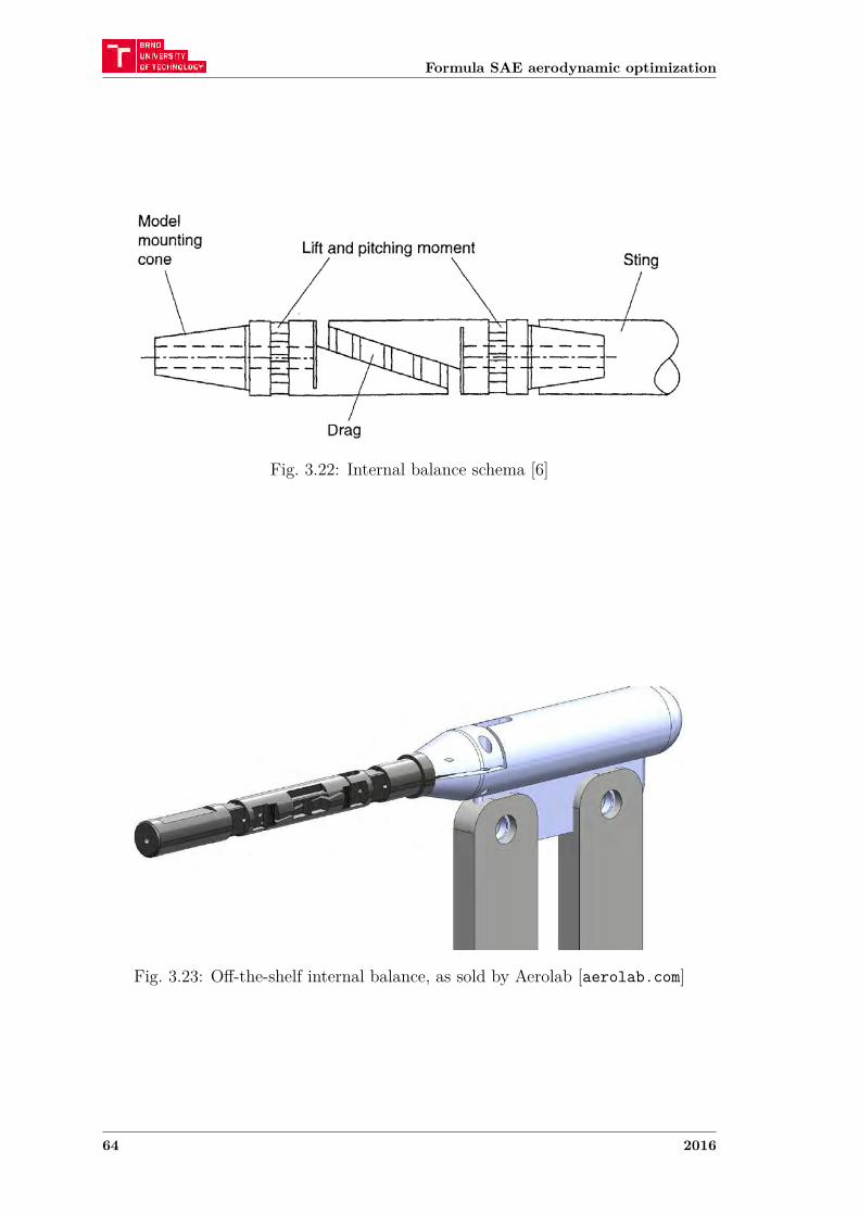
Formula SAE aerodynamic optimization
Fig. 3.22: Internal balance schema [6]
Fig. 3.23: Off-the-shelf internal balance, as sold by Aerolab [aerolab.com]
64 2016
3 Wind tunnel testing
• Correct loading of the vehicle should be checked – not only total weight butalso weight distribution between axles. Incorrect weight distribution mighthave an effect on ride height, thus also on the test results.
• Flow around a vehicle is unsteady – separations occur, vortices are shed.Therefore the model is exposed to vibrations and obtained test signals are notsteady. For this reason, data readings should be long enough to gain represen-tative mean value. The minimum time period required for the measurementmust be experimentally determined.
Lukáš Fryšták 65

Part II
Experimental testing
66
4 Introduction to Part II
4 INTRODUCTION TO PART IIThe second part of this work is focused on aerodynamic analysis of an FSAE car.There are two main goals that are to be accomplished. Firstly, it is determina-tion of basic aerodynamic characteristics of current configuration. The second partshould focus on determination of areas for improvements in aerodynamic character-istics. These areas for optimisation should be identified with respect to increasingdownforce, distribution of downforce and/or reducing drag.
There are two different methods that are accessible and would enable accom-plishing both of the aforementioned goals. First of them is numerical model, whilethe other is experimental model. Naturally, both bring their respective advantagesand disadvantages.
Should numerical model be employed, it would enable to determine overall aero-dynamic characteristics as well as detailed analysis of the entire flow field aroundthe car. Areas for improvement could be very well found due to the ability to reviewflow structures and interaction of specific parts on the car. This analysis was previ-ously done in the team and results are available for all the cars mentioned in chapter1.3. However, the CFD results themselves are not sufficient to really understand thereal on-track performance of the aerodynamic design. These results include a highdegree of uncertainty.
Employing experimental testing in this work would mean having relatively unre-stricted access to low-speed wind tunnel at the Institute of Aerospace Engineering(IAE). This would present an opportunity to obtain a different set of data that wouldcomplement the numerical results that are already available. It would not be donewith the aim to replace the numerical results altogether. Numerical model couldbe correlated with the experimental results. Consequently, this would considerablyreduce the uncertainty in the numerical model and enable detailed optimization inCFD.
Eventually, being able to use both CFD and wind tunnel results during designcould make the process more efficient and enable extraction of the best performancepossible.
All of the above being said, the method of choice for the aerodynamic analysis andoptimisation in this work is experimental model – wind tunnel testing.
Lukáš Fryšták 67

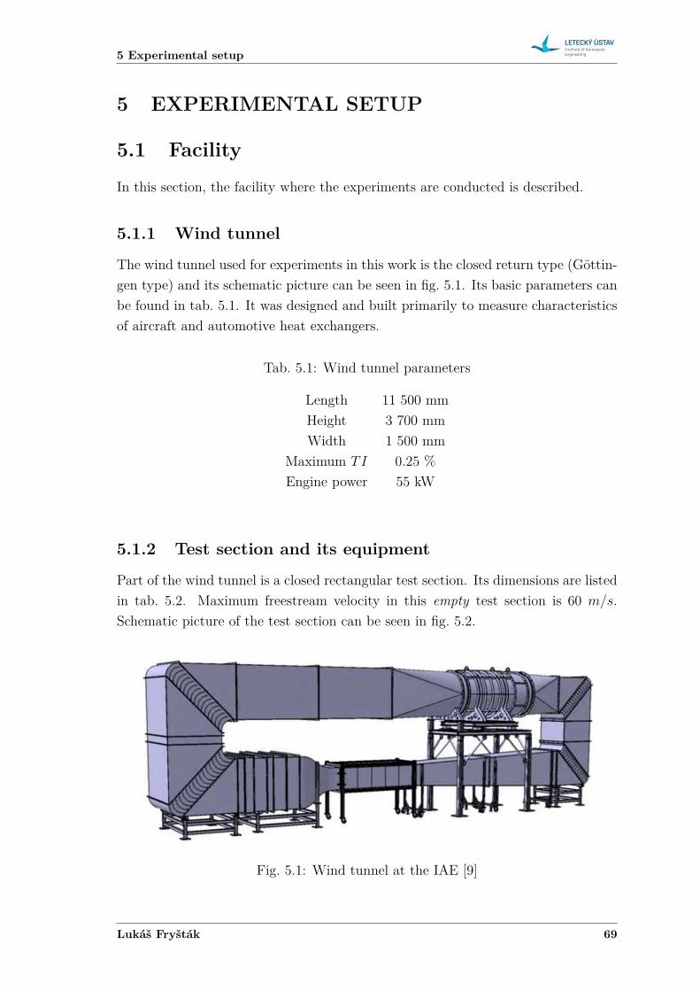
5 Experimental setup
5 EXPERIMENTAL SETUP
5.1 Facility
In this section, the facility where the experiments are conducted is described.
5.1.1 Wind tunnel
The wind tunnel used for experiments in this work is the closed return type (Göttin-gen type) and its schematic picture can be seen in fig. 5.1. Its basic parameters canbe found in tab. 5.1. It was designed and built primarily to measure characteristicsof aircraft and automotive heat exchangers.
Tab. 5.1: Wind tunnel parameters
Length 11 500 mmHeight 3 700 mmWidth 1 500 mm
Maximum 𝑇𝐼 0.25 %Engine power 55 kW
5.1.2 Test section and its equipment
Part of the wind tunnel is a closed rectangular test section. Its dimensions are listedin tab. 5.2. Maximum freestream velocity in this empty test section is 60 𝑚/𝑠.Schematic picture of the test section can be seen in fig. 5.2.
Fig. 5.1: Wind tunnel at the IAE [9]
Lukáš Fryšták 69
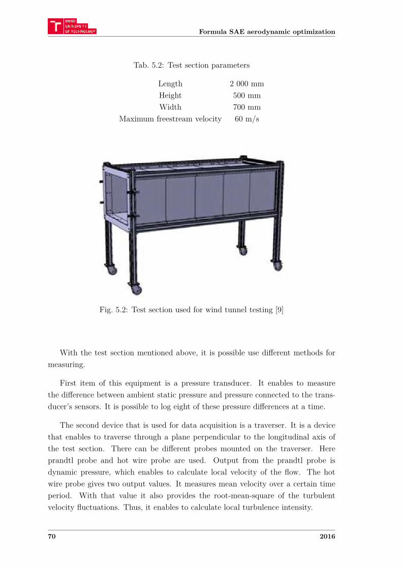
Formula SAE aerodynamic optimization
Tab. 5.2: Test section parameters
Length 2 000 mmHeight 500 mmWidth 700 mm
Maximum freestream velocity 60 m/s
Fig. 5.2: Test section used for wind tunnel testing [9]
With the test section mentioned above, it is possible use different methods formeasuring.
First item of this equipment is a pressure transducer. It enables to measurethe difference between ambient static pressure and pressure connected to the trans-ducer’s sensors. It is possible to log eight of these pressure differences at a time.
The second device that is used for data acquisition is a traverser. It is a devicethat enables to traverse through a plane perpendicular to the longitudinal axis ofthe test section. There can be different probes mounted on the traverser. Hereprandtl probe and hot wire probe are used. Output from the prandtl probe isdynamic pressure, which enables to calculate local velocity of the flow. The hotwire probe gives two output values. It measures mean velocity over a certain timeperiod. With that value it also provides the root-mean-square of the turbulentvelocity fluctuations. Thus, it enables to calculate local turbulence intensity.
70 2016
5 Experimental setup
5.2 Description of the experimental setup
Purpose of this section is to describe the experimental setup and the reasoning be-hind it. The main aspects that are considered here are model scale, model mountingand what is actually measured.
5.2.1 Model scale
Theoretically, the only parameter that influences the choice of the model’s scale isReynolds number. However, the scale based on Reynolds number similarity is oftenlimited by the wind tunnel’s maximum speed. Furthermore, test section blockageshould remain reasonably small. Usually a value of 5 − 10 % is said to be suitablefor automotive testing. [4] [6] On top of that, the scale should also take into accountthe fact, that if it was too small, it would not be possible to manufacture the modelwith appropriate geometric accuracy.
The scale that best fits the requirements mentioned above was chosen based onfig. 5.3. The diagram is based on the following condition.
𝑅𝑒𝑀 = 𝑅𝑒𝑅 (5.1)
In the equation above, 𝑅𝑒𝑀 stands for model Reynolds number and 𝑅𝑒𝑅 standsfor Reynolds number in real conditions. In real conditions, freestream velocity of50 𝑘𝑚/ℎ is used. That is the speed of interest when designing aerodynamic packagefor an FSAE car, because that is the average speed in corners.
In section 5.1.2 it is stated that maximum free stream velocity in an empty testsection is 60 𝑚/𝑠. However, when a model is placed in the test section, the sub-sequent pressure losses mean, that the maximum wind tunnel velocity is somewhatlower. It is expected, that the maximum velocity with model in the test section is55 𝑚/𝑠 – dashed line in fig. 5.3.
The blue and red solid lines represent how needed wind tunnel velocity and testsection blockage, respectively, depend on used model scale.
For 25 % scaled model the desired wind tunnel velocity is just the 55 𝑚/𝑠 –expected maximum achievable velocity. With this scale the blockage is 20 %. Suchblockage is quite substantial and it is certain that results would be influenced quiteconsiderably by this fact. But as was mentioned in section 3.6.2, testing with block-age up to 20 % can still yield useful aerodynamic data. [8]
Nevertheless, making the model smaller is not an option, because (a) it wouldcompromise the Reynolds number similarity, and (b) at 25 % scale some parts ofthe model are already really small and it would not be feasible to make them anysmaller.
Lukáš Fryšták 71
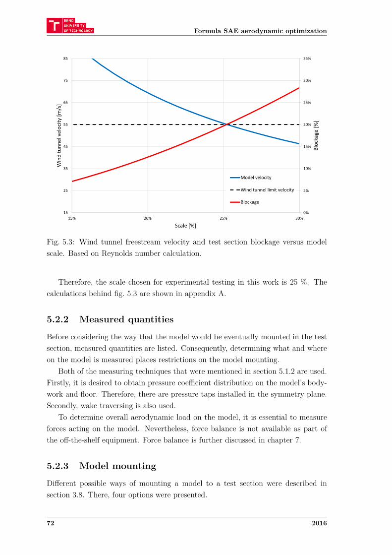
Formula SAE aerodynamic optimization
0%
5%
10%
15%
20%
25%
30%
35%
15
25
35
45
55
65
75
85
15% 20% 25% 30%
Blockage [%
]
Wind tunn
el velocity
[m/s]
Scale [%]
Model velocity
Wind tunnel limit velocity
Blockage
Fig. 5.3: Wind tunnel freestream velocity and test section blockage versus modelscale. Based on Reynolds number calculation.
Therefore, the scale chosen for experimental testing in this work is 25 %. Thecalculations behind fig. 5.3 are shown in appendix A.
5.2.2 Measured quantities
Before considering the way that the model would be eventually mounted in the testsection, measured quantities are listed. Consequently, determining what and whereon the model is measured places restrictions on the model mounting.
Both of the measuring techniques that were mentioned in section 5.1.2 are used.Firstly, it is desired to obtain pressure coefficient distribution on the model’s body-work and floor. Therefore, there are pressure taps installed in the symmetry plane.Secondly, wake traversing is also used.
To determine overall aerodynamic load on the model, it is essential to measureforces acting on the model. Nevertheless, force balance is not available as part ofthe off-the-shelf equipment. Force balance is further discussed in chapter 7.
5.2.3 Model mounting
Different possible ways of mounting a model to a test section were described insection 3.8. There, four options were presented.
72 2016
5 Experimental setup
In a more general way, the options could be divided into two categories. Firstly, itis mounting the model through struts directly connected to the wheels (see fig. 3.17).And a second option is using a sting mounting (see fig. 3.18, 3.19, and 3.20).
Connecting a model by its wheels directly to struts going through the groundplane offers the least flow disturbance of the surrounding flow field. However, thereare two reasons that render it inconvenient. The actual connection of the struts tothe wheels is rather complicated. There must be a gap between the struts and windtunnel floor, so that there is no contact. This gap has to be sealed to prevent anyflow alteration around the wheel contact patch. When this mounting solution isused, usually the entire force balance beneath the test section is hermetically closed.
If the model was placed on its wheels, it would mean that the wishbones wouldhave to support the entire model. With the 25 % scale, the wishbone diameter is4 𝑚𝑚. It is not believed that such a solution would be structurally sufficient.
Ruling out the first option leaves the choice to mounting the model on a sting. Itcan be mounted from behind, from below or from above. Sting introduced from everymentioned direction results in flow disturbance. But considering that introducingthe sting from below would alter the flow field in the vicinity of pressure taps andintroducing the sting from behind would bring disturbances to the wake – bothareas being of interest – it would consequently introduce an error in measured data.Therefore, mounting the model on a sting from above appears to be the best option.
5.2.4 Final experimental setup
Final experimental set up used for wind tunnel tests in this work can be seen infig. 5.4. In the picture the 25% scale model mounted on a sting balance from aboveis placed in a test section at the IAE wind tunnel facility.
Lukáš Fryšták 73
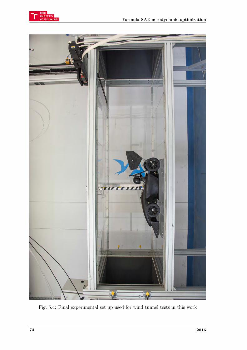
Formula SAE aerodynamic optimization
Fig. 5.4: Final experimental set up used for wind tunnel tests in this work
74 2016
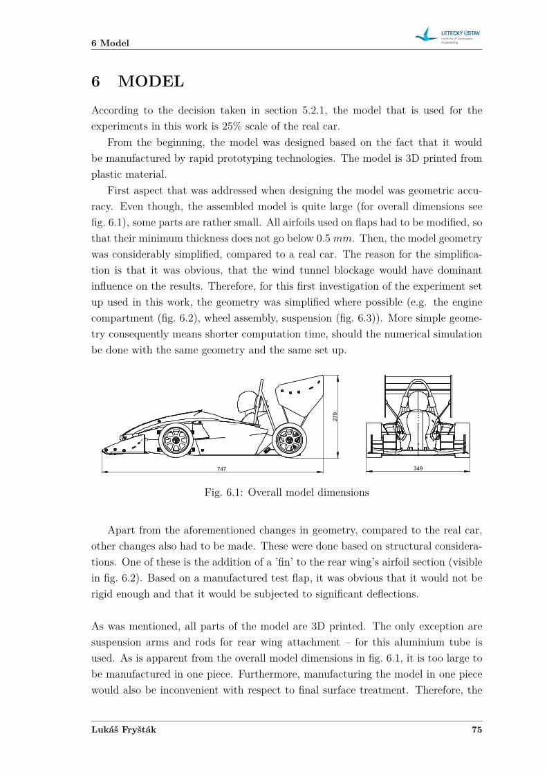
6 Model
6 MODEL
According to the decision taken in section 5.2.1, the model that is used for theexperiments in this work is 25% scale of the real car.
From the beginning, the model was designed based on the fact that it wouldbe manufactured by rapid prototyping technologies. The model is 3D printed fromplastic material.
First aspect that was addressed when designing the model was geometric accu-racy. Even though, the assembled model is quite large (for overall dimensions seefig. 6.1), some parts are rather small. All airfoils used on flaps had to be modified, sothat their minimum thickness does not go below 0.5 𝑚𝑚. Then, the model geometrywas considerably simplified, compared to a real car. The reason for the simplifica-tion is that it was obvious, that the wind tunnel blockage would have dominantinfluence on the results. Therefore, for this first investigation of the experiment setup used in this work, the geometry was simplified where possible (e.g. the enginecompartment (fig. 6.2), wheel assembly, suspension (fig. 6.3)). More simple geome-try consequently means shorter computation time, should the numerical simulationbe done with the same geometry and the same set up.
747
279
349
Fig. 6.1: Overall model dimensions
Apart from the aforementioned changes in geometry, compared to the real car,other changes also had to be made. These were done based on structural considera-tions. One of these is the addition of a ’fin’ to the rear wing’s airfoil section (visiblein fig. 6.2). Based on a manufactured test flap, it was obvious that it would not berigid enough and that it would be subjected to significant deflections.
As was mentioned, all parts of the model are 3D printed. The only exception aresuspension arms and rods for rear wing attachment – for this aluminium tube isused. As is apparent from the overall model dimensions in fig. 6.1, it is too large tobe manufactured in one piece. Furthermore, manufacturing the model in one piecewould also be inconvenient with respect to final surface treatment. Therefore, the
Lukáš Fryšták 75
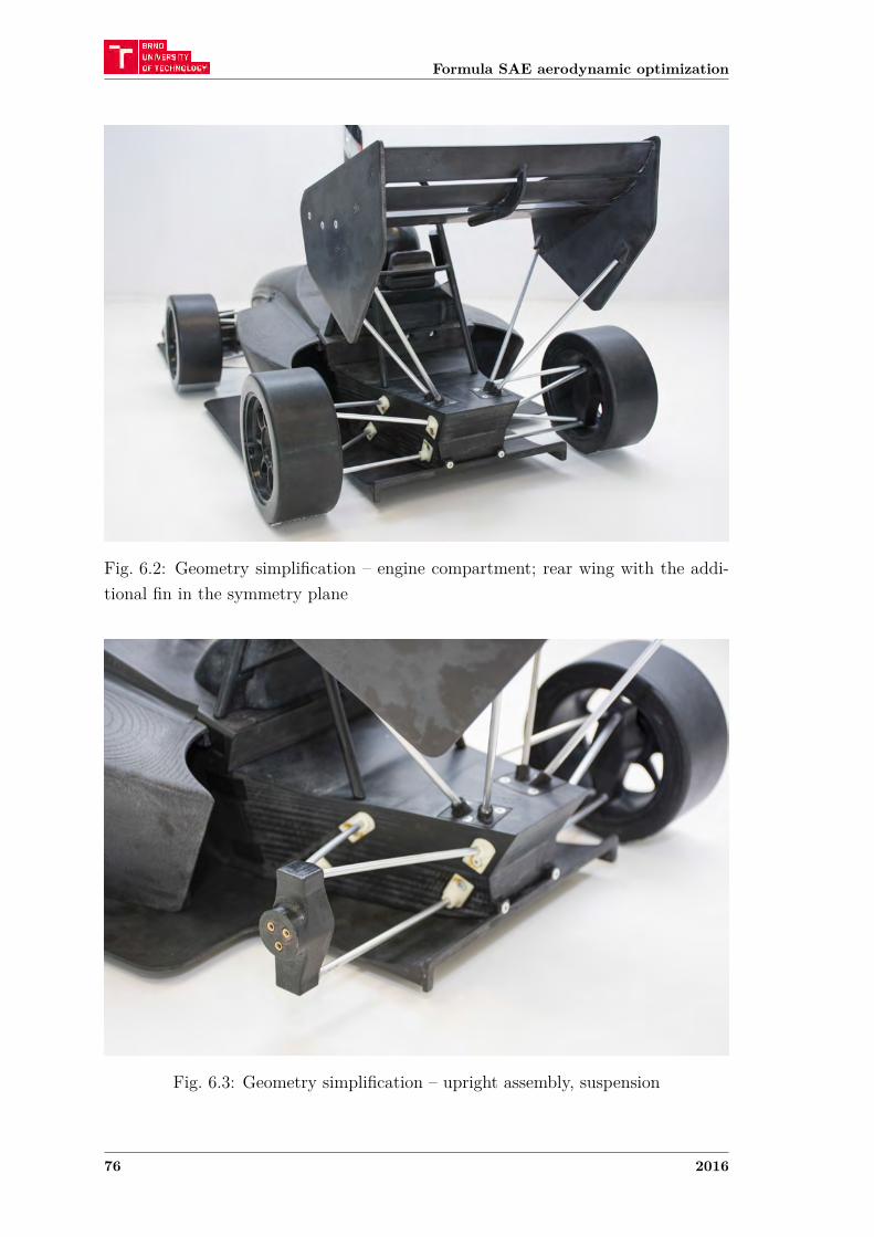
Formula SAE aerodynamic optimization
Fig. 6.2: Geometry simplification – engine compartment; rear wing with the addi-tional fin in the symmetry plane
Fig. 6.3: Geometry simplification – upright assembly, suspension
76 2016
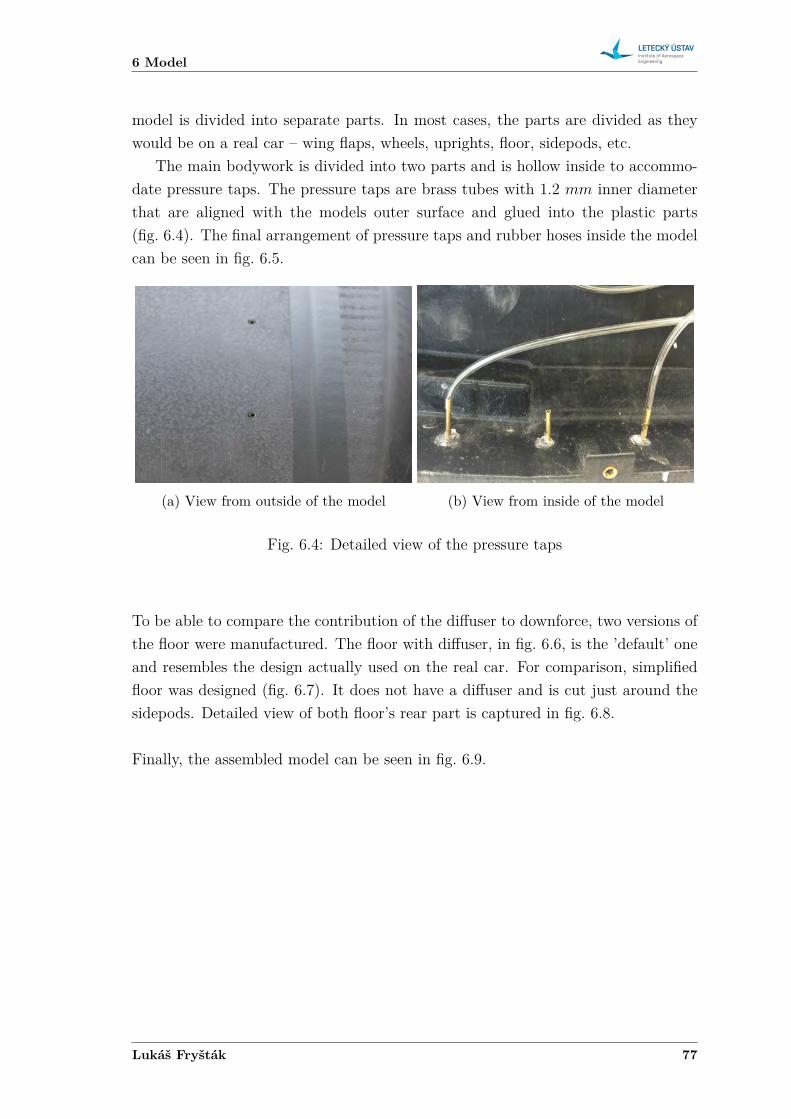
6 Model
model is divided into separate parts. In most cases, the parts are divided as theywould be on a real car – wing flaps, wheels, uprights, floor, sidepods, etc.
The main bodywork is divided into two parts and is hollow inside to accommo-date pressure taps. The pressure taps are brass tubes with 1.2 𝑚𝑚 inner diameterthat are aligned with the models outer surface and glued into the plastic parts(fig. 6.4). The final arrangement of pressure taps and rubber hoses inside the modelcan be seen in fig. 6.5.
(a) View from outside of the model (b) View from inside of the model
Fig. 6.4: Detailed view of the pressure taps
To be able to compare the contribution of the diffuser to downforce, two versions ofthe floor were manufactured. The floor with diffuser, in fig. 6.6, is the ’default’ oneand resembles the design actually used on the real car. For comparison, simplifiedfloor was designed (fig. 6.7). It does not have a diffuser and is cut just around thesidepods. Detailed view of both floor’s rear part is captured in fig. 6.8.
Finally, the assembled model can be seen in fig. 6.9.
Lukáš Fryšták 77
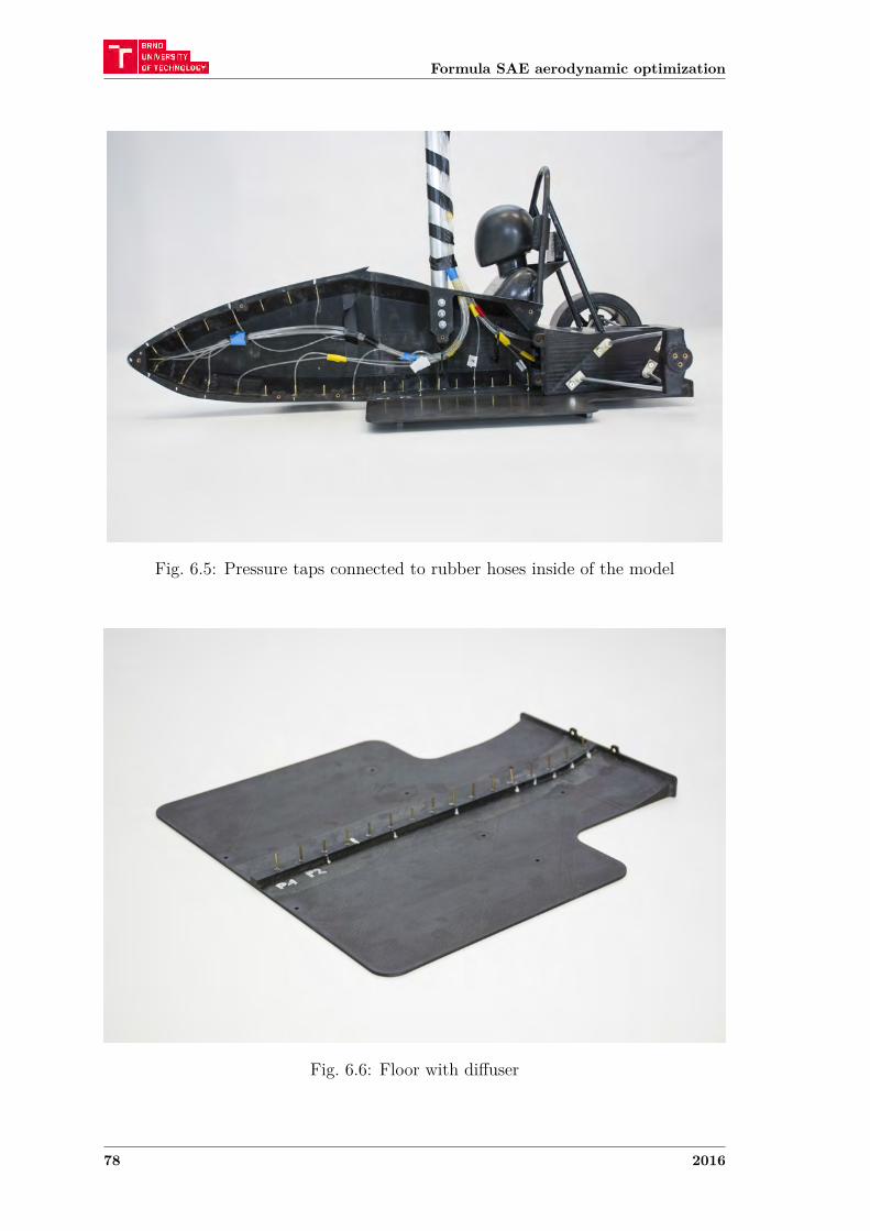
Formula SAE aerodynamic optimization
Fig. 6.5: Pressure taps connected to rubber hoses inside of the model
Fig. 6.6: Floor with diffuser
78 2016
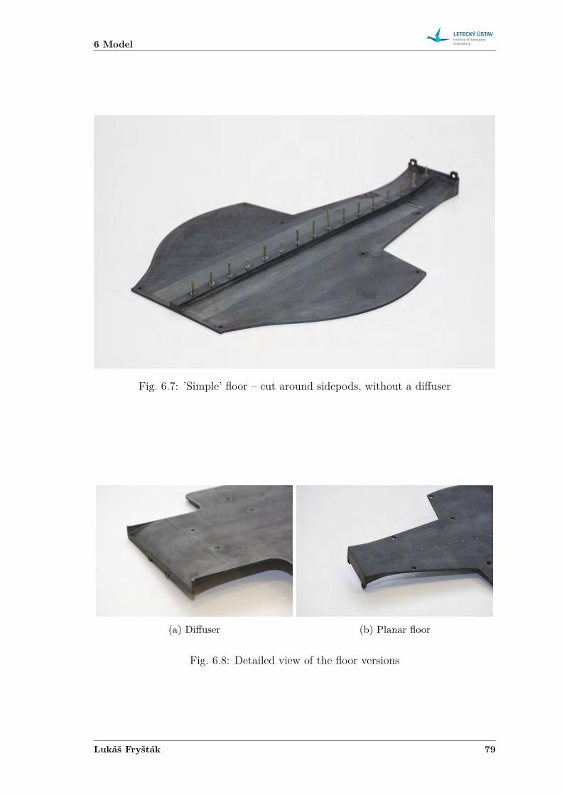
6 Model
Fig. 6.7: ’Simple’ floor – cut around sidepods, without a diffuser
(a) Diffuser (b) Planar floor
Fig. 6.8: Detailed view of the floor versions
Lukáš Fryšták 79
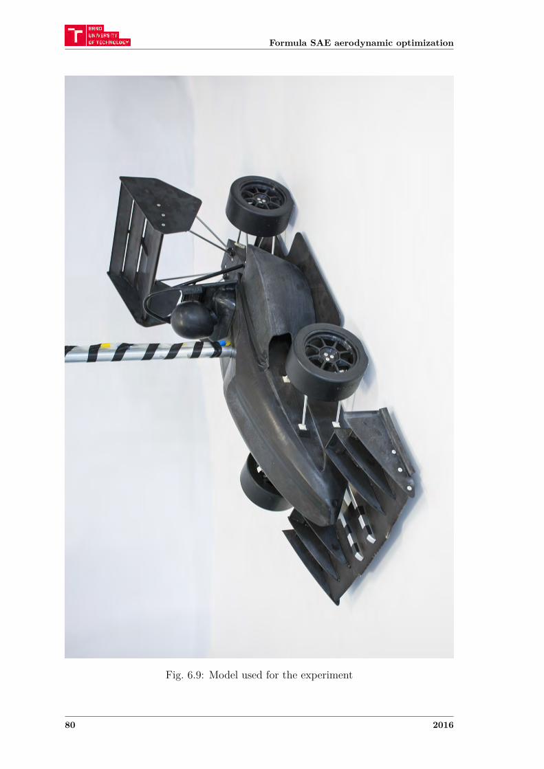
Formula SAE aerodynamic optimization
Fig. 6.9: Model used for the experiment
80 2016
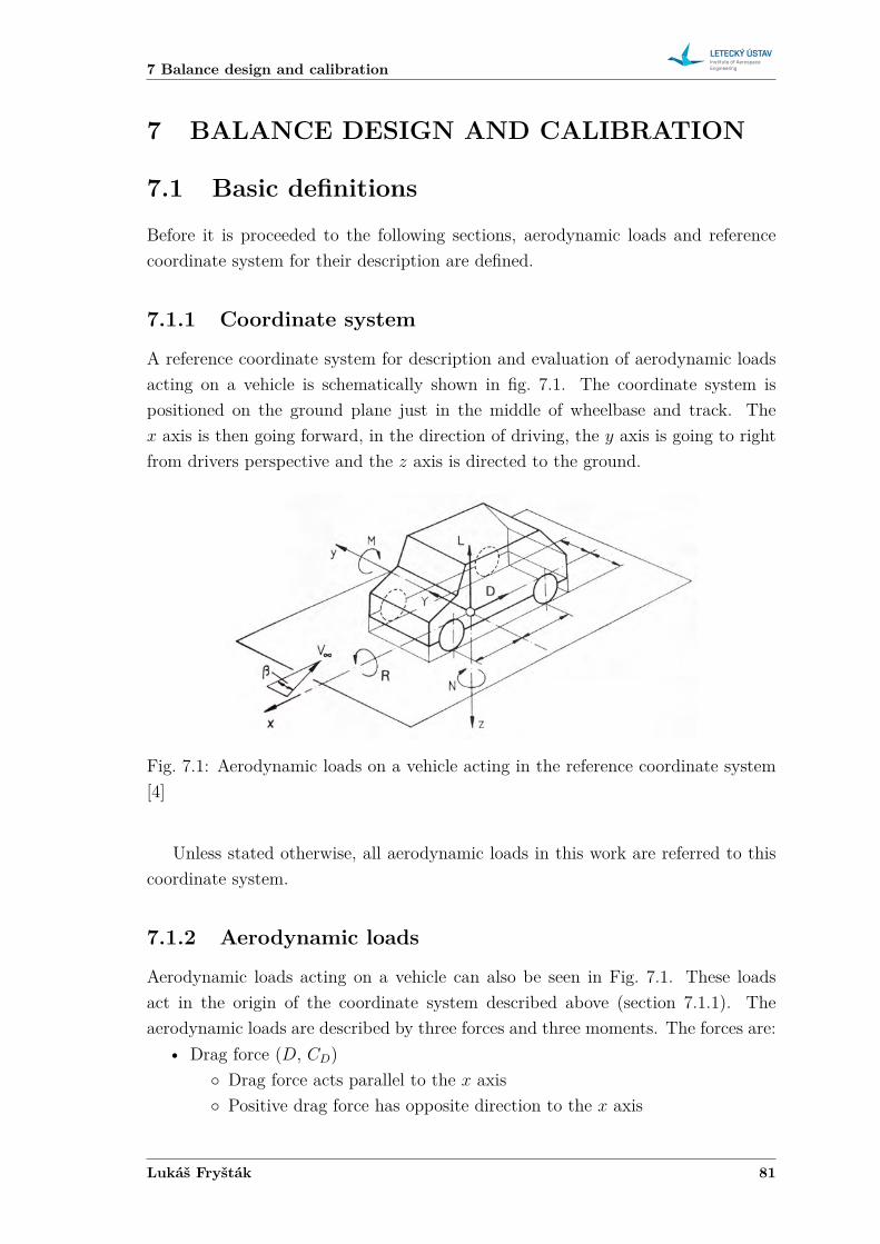
7 Balance design and calibration
7 BALANCE DESIGN AND CALIBRATION
7.1 Basic definitions
Before it is proceeded to the following sections, aerodynamic loads and referencecoordinate system for their description are defined.
7.1.1 Coordinate system
A reference coordinate system for description and evaluation of aerodynamic loadsacting on a vehicle is schematically shown in fig. 7.1. The coordinate system ispositioned on the ground plane just in the middle of wheelbase and track. The𝑥 axis is then going forward, in the direction of driving, the 𝑦 axis is going to rightfrom drivers perspective and the 𝑧 axis is directed to the ground.
Fig. 7.1: Aerodynamic loads on a vehicle acting in the reference coordinate system[4]
Unless stated otherwise, all aerodynamic loads in this work are referred to thiscoordinate system.
7.1.2 Aerodynamic loads
Aerodynamic loads acting on a vehicle can also be seen in Fig. 7.1. These loadsact in the origin of the coordinate system described above (section 7.1.1). Theaerodynamic loads are described by three forces and three moments. The forces are:
• Drag force (𝐷, 𝐶𝐷)∘ Drag force acts parallel to the 𝑥 axis∘ Positive drag force has opposite direction to the 𝑥 axis
Lukáš Fryšták 81
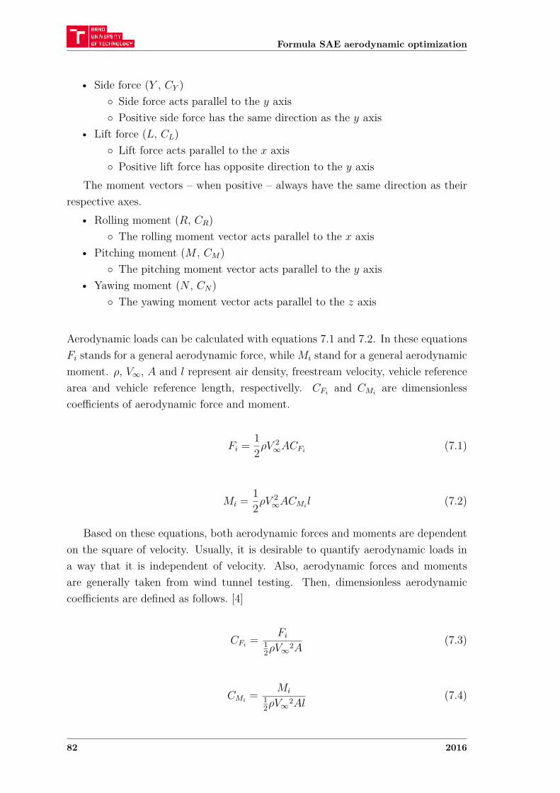
Formula SAE aerodynamic optimization
• Side force (𝑌 , 𝐶𝑌 )∘ Side force acts parallel to the 𝑦 axis∘ Positive side force has the same direction as the 𝑦 axis
• Lift force (𝐿, 𝐶𝐿)∘ Lift force acts parallel to the 𝑥 axis∘ Positive lift force has opposite direction to the 𝑦 axis
The moment vectors – when positive – always have the same direction as theirrespective axes.
• Rolling moment (𝑅, 𝐶𝑅)∘ The rolling moment vector acts parallel to the 𝑥 axis
• Pitching moment (𝑀 , 𝐶𝑀)∘ The pitching moment vector acts parallel to the 𝑦 axis
• Yawing moment (𝑁 , 𝐶𝑁)∘ The yawing moment vector acts parallel to the 𝑧 axis
Aerodynamic loads can be calculated with equations 7.1 and 7.2. In these equations𝐹𝑖 stands for a general aerodynamic force, while 𝑀𝑖 stand for a general aerodynamicmoment. 𝜌, 𝑉∞, 𝐴 and 𝑙 represent air density, freestream velocity, vehicle referencearea and vehicle reference length, respectivelly. 𝐶𝐹𝑖
and 𝐶𝑀𝑖are dimensionless
coefficients of aerodynamic force and moment.
𝐹𝑖 = 12𝜌𝑉 2
∞𝐴𝐶𝐹𝑖(7.1)
𝑀𝑖 = 12𝜌𝑉 2
∞𝐴𝐶𝑀𝑖𝑙 (7.2)
Based on these equations, both aerodynamic forces and moments are dependenton the square of velocity. Usually, it is desirable to quantify aerodynamic loads ina way that it is independent of velocity. Also, aerodynamic forces and momentsare generally taken from wind tunnel testing. Then, dimensionless aerodynamiccoefficients are defined as follows. [4]
𝐶𝐹𝑖= 𝐹𝑖
12𝜌𝑉∞2𝐴
(7.3)
𝐶𝑀𝑖= 𝑀𝑖
12𝜌𝑉∞2𝐴𝑙
(7.4)
82 2016
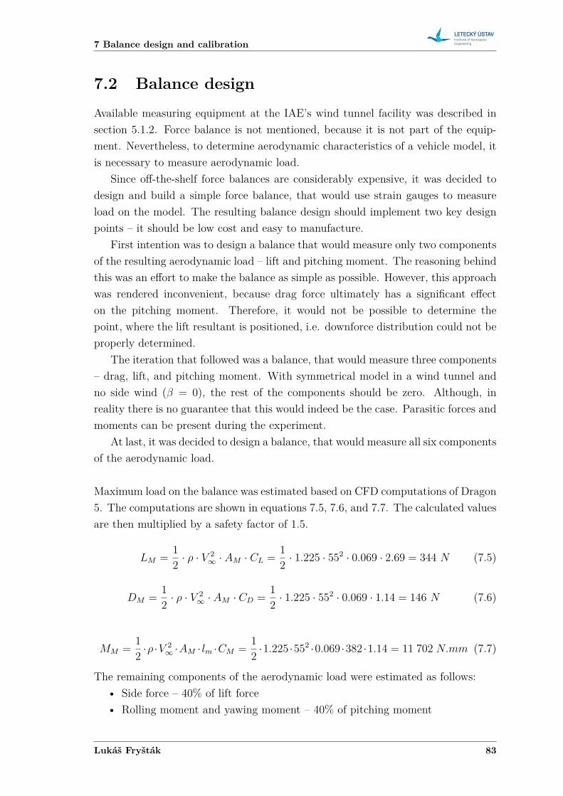
7 Balance design and calibration
7.2 Balance design
Available measuring equipment at the IAE’s wind tunnel facility was described insection 5.1.2. Force balance is not mentioned, because it is not part of the equip-ment. Nevertheless, to determine aerodynamic characteristics of a vehicle model, itis necessary to measure aerodynamic load.
Since off-the-shelf force balances are considerably expensive, it was decided todesign and build a simple force balance, that would use strain gauges to measureload on the model. The resulting balance design should implement two key designpoints – it should be low cost and easy to manufacture.
First intention was to design a balance that would measure only two componentsof the resulting aerodynamic load – lift and pitching moment. The reasoning behindthis was an effort to make the balance as simple as possible. However, this approachwas rendered inconvenient, because drag force ultimately has a significant effecton the pitching moment. Therefore, it would not be possible to determine thepoint, where the lift resultant is positioned, i.e. downforce distribution could not beproperly determined.
The iteration that followed was a balance, that would measure three components– drag, lift, and pitching moment. With symmetrical model in a wind tunnel andno side wind (𝛽 = 0), the rest of the components should be zero. Although, inreality there is no guarantee that this would indeed be the case. Parasitic forces andmoments can be present during the experiment.
At last, it was decided to design a balance, that would measure all six componentsof the aerodynamic load.
Maximum load on the balance was estimated based on CFD computations of Dragon5. The computations are shown in equations 7.5, 7.6, and 7.7. The calculated valuesare then multiplied by a safety factor of 1.5.
𝐿𝑀 = 12 · 𝜌 · 𝑉 2
∞ · 𝐴𝑀 · 𝐶𝐿 = 12 · 1.225 · 552 · 0.069 · 2.69 = 344 𝑁 (7.5)
𝐷𝑀 = 12 · 𝜌 · 𝑉 2
∞ · 𝐴𝑀 · 𝐶𝐷 = 12 · 1.225 · 552 · 0.069 · 1.14 = 146 𝑁 (7.6)
𝑀𝑀 = 12 ·𝜌 ·𝑉 2
∞ ·𝐴𝑀 · 𝑙𝑚 ·𝐶𝑀 = 12 ·1.225 ·552 ·0.069 ·382 ·1.14 = 11 702 𝑁.𝑚𝑚 (7.7)
The remaining components of the aerodynamic load were estimated as follows:• Side force – 40% of lift force• Rolling moment and yawing moment – 40% of pitching moment
Lukáš Fryšták 83
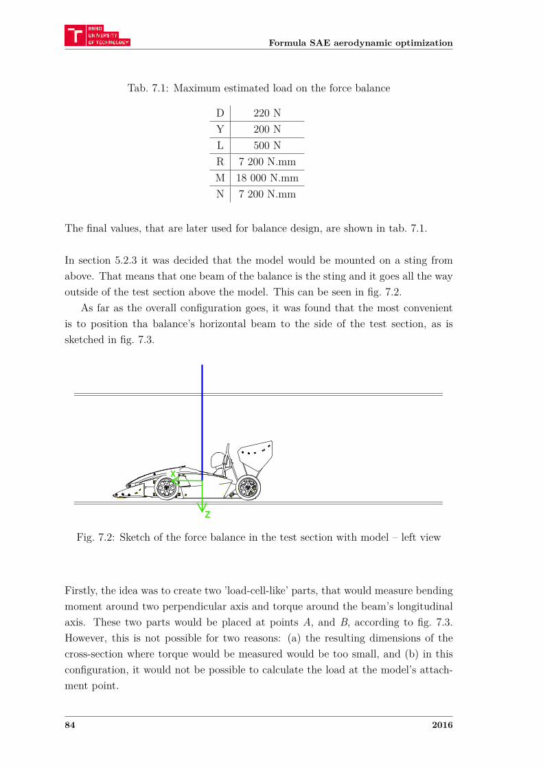
Formula SAE aerodynamic optimization
Tab. 7.1: Maximum estimated load on the force balance
D 220 NY 200 NL 500 NR 7 200 N.mmM 18 000 N.mmN 7 200 N.mm
The final values, that are later used for balance design, are shown in tab. 7.1.
In section 5.2.3 it was decided that the model would be mounted on a sting fromabove. That means that one beam of the balance is the sting and it goes all the wayoutside of the test section above the model. This can be seen in fig. 7.2.
As far as the overall configuration goes, it was found that the most convenientis to position tha balance’s horizontal beam to the side of the test section, as issketched in fig. 7.3.
Fig. 7.2: Sketch of the force balance in the test section with model – left view
Firstly, the idea was to create two ’load-cell-like’ parts, that would measure bendingmoment around two perpendicular axis and torque around the beam’s longitudinalaxis. These two parts would be placed at points A, and B, according to fig. 7.3.However, this is not possible for two reasons: (a) the resulting dimensions of thecross-section where torque would be measured would be too small, and (b) in thisconfiguration, it would not be possible to calculate the load at the model’s attach-ment point.
84 2016
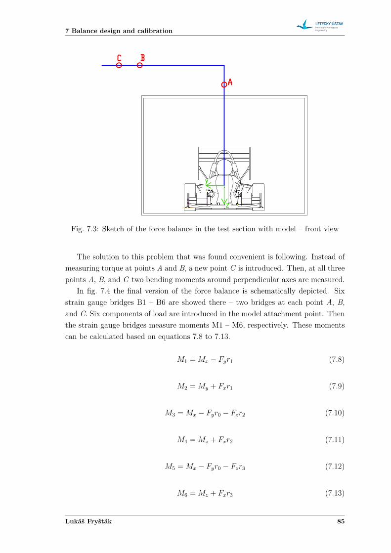
7 Balance design and calibration
Fig. 7.3: Sketch of the force balance in the test section with model – front view
The solution to this problem that was found convenient is following. Instead ofmeasuring torque at points A and B, a new point C is introduced. Then, at all threepoints A, B, and C two bending moments around perpendicular axes are measured.
In fig. 7.4 the final version of the force balance is schematically depicted. Sixstrain gauge bridges B1 – B6 are showed there – two bridges at each point A, B,and C. Six components of load are introduced in the model attachment point. Thenthe strain gauge bridges measure moments M1 – M6, respectively. These momentscan be calculated based on equations 7.8 to 7.13.
𝑀1 = 𝑀𝑥 − 𝐹𝑦𝑟1 (7.8)
𝑀2 = 𝑀𝑦 + 𝐹𝑥𝑟1 (7.9)
𝑀3 = 𝑀𝑥 − 𝐹𝑦𝑟0 − 𝐹𝑧𝑟2 (7.10)
𝑀4 = 𝑀𝑧 + 𝐹𝑥𝑟2 (7.11)
𝑀5 = 𝑀𝑥 − 𝐹𝑦𝑟0 − 𝐹𝑧𝑟3 (7.12)
𝑀6 = 𝑀𝑧 + 𝐹𝑥𝑟3 (7.13)
Lukáš Fryšták 85
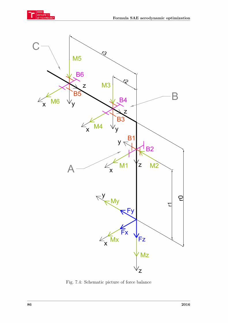
Formula SAE aerodynamic optimization
Fig. 7.4: Schematic picture of force balance
86 2016
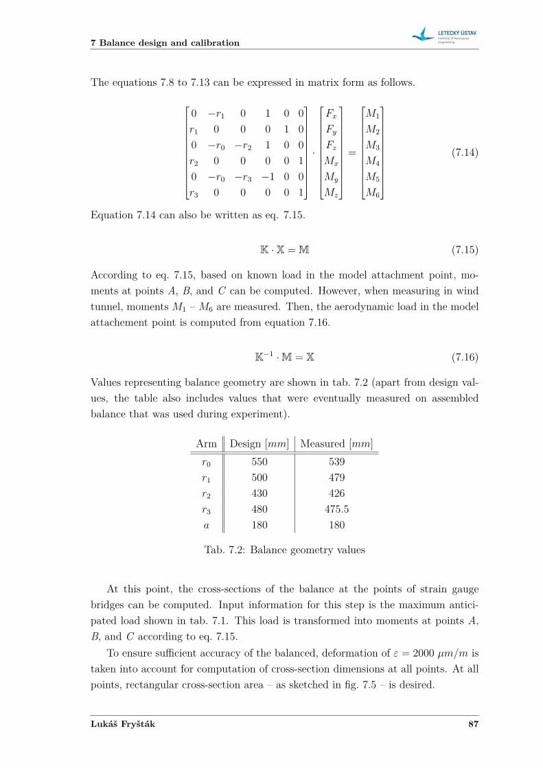
7 Balance design and calibration
The equations 7.8 to 7.13 can be expressed in matrix form as follows.
⎡⎢⎢⎢⎢⎢⎢⎢⎢⎢⎢⎢⎣
0 −𝑟1 0 1 0 0𝑟1 0 0 0 1 00 −𝑟0 −𝑟2 1 0 0𝑟2 0 0 0 0 10 −𝑟0 −𝑟3 −1 0 0𝑟3 0 0 0 0 1
⎤⎥⎥⎥⎥⎥⎥⎥⎥⎥⎥⎥⎦·
⎡⎢⎢⎢⎢⎢⎢⎢⎢⎢⎢⎢⎣
𝐹𝑥
𝐹𝑦
𝐹𝑧
𝑀𝑥
𝑀𝑦
𝑀𝑧
⎤⎥⎥⎥⎥⎥⎥⎥⎥⎥⎥⎥⎦=
⎡⎢⎢⎢⎢⎢⎢⎢⎢⎢⎢⎢⎣
𝑀1
𝑀2
𝑀3
𝑀4
𝑀5
𝑀6
⎤⎥⎥⎥⎥⎥⎥⎥⎥⎥⎥⎥⎦(7.14)
Equation 7.14 can also be written as eq. 7.15.
K · X = M (7.15)
According to eq. 7.15, based on known load in the model attachment point, mo-ments at points A, B, and C can be computed. However, when measuring in windtunnel, moments 𝑀1 – 𝑀6 are measured. Then, the aerodynamic load in the modelattachement point is computed from equation 7.16.
K−1 · M = X (7.16)
Values representing balance geometry are shown in tab. 7.2 (apart from design val-ues, the table also includes values that were eventually measured on assembledbalance that was used during experiment).
Arm Design [𝑚𝑚] Measured [𝑚𝑚]𝑟0 550 539𝑟1 500 479𝑟2 430 426𝑟3 480 475.5𝑎 180 180
Tab. 7.2: Balance geometry values
At this point, the cross-sections of the balance at the points of strain gaugebridges can be computed. Input information for this step is the maximum antici-pated load shown in tab. 7.1. This load is transformed into moments at points A,B, and C according to eq. 7.15.
To ensure sufficient accuracy of the balanced, deformation of 𝜀 = 2000 𝜇𝑚/𝑚 istaken into account for computation of cross-section dimensions at all points. At allpoints, rectangular cross-section area – as sketched in fig. 7.5 – is desired.
Lukáš Fryšták 87
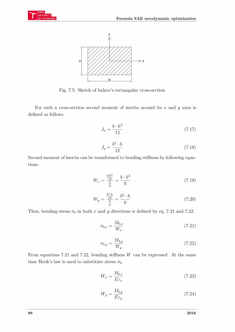
Formula SAE aerodynamic optimization
Fig. 7.5: Sketch of balnce’s rectangular cross-section
For such a cross-section second moment of inertia around its 𝑥 and 𝑦 axes isdefined as follows.
𝐽𝑥 = 𝑏 · ℎ3
12 (7.17)
𝐽𝑦 = 𝑏3 · ℎ
12 (7.18)
Second moment of inertia can be transformed to bending stiffness by following equa-tions.
𝑊𝑥 =𝑏·ℎ3
12ℎ2
= 𝑏 · ℎ2
6 (7.19)
𝑊𝑦 =𝑏3·ℎ12𝑏2
= 𝑏2 · ℎ
6 (7.20)
Then, bending stress 𝜎𝑏 in both 𝑥 and 𝑦 directions is defined by eq. 7.21 and 7.22.
𝜎𝑏,𝑥 = 𝑀𝑏,𝑥
𝑊𝑥
(7.21)
𝜎𝑏,𝑦 = 𝑀𝑏,𝑦
𝑊𝑦
(7.22)
From equations 7.21 and 7.22, bending stiffness 𝑊 can be expressed. At the sametime Hook’s law is used to substitute stress 𝜎𝑏.
𝑊𝑥 = 𝑀𝑏,𝑥
𝐸𝜀𝑥
(7.23)
𝑊𝑦 = 𝑀𝑏,𝑦
𝐸𝜀𝑦
(7.24)
88 2016
7 Balance design and calibration
In eq. 7.23 and 7.24, bending stiffness 𝑊 is substituted from eq. 7.19 and 7.20,respectively.
𝑏 · ℎ2
6 = 𝑀𝑏,𝑥
𝐸𝜀𝑥
(7.25)
𝑏2 · ℎ
6 = 𝑀𝑏,𝑦
𝐸𝜀𝑦
(7.26)
Then, dimension 𝑏 is expressed from eq. 7.25.
𝑏 = 6𝑀𝑏,𝑥
𝐸𝜀𝑥ℎ2 (7.27)
Dimension 𝑏 in eq. 7.26 is then substituted by eq. 7.27.
(︂ 6𝑀𝑏,𝑥
𝐸𝜀𝑥ℎ2
)︂2· ℎ
6 = 𝑀𝑏,𝑦
𝐸𝜀𝑦
(7.28)
Finally, from eq. 7.28, dimension ℎ can be expressed – eq. 7.29. In this equation,all variables are part of input information. Aluminum is used for balance manufac-turing, therefore young’s modulus is 𝐸 = 72 000 𝑀𝑃𝑎. As was mentioned before,deformation for all cross-sections is 𝜀 = 2000 𝜇𝑚/𝑚. Bending moments are calcu-lated according to eq. 7.14. So, for example, for cross-section at point A, bendingmoment around 𝑥 axis 𝑀𝑏,𝑥 is moment 𝑀1 and bending moment around 𝑦 axis 𝑀𝑏,𝑦
is moment 𝑀2.
ℎ = 3
⎯⎸⎸⎷(︂6𝑀𝑏,𝑥
𝐸𝜀𝑥
)︂2· 𝐸𝜀𝑦
6𝑀𝑏,𝑦
(7.29)
Equation 7.29 is retrospectively substituted into eq. 7.27 to enable calculation ofdimension 𝑏.
𝑏 = 6𝑀𝑏,𝑥
𝐸𝜀𝑥
(︃3
√︂(︁6𝑀𝑏,𝑥
𝐸𝜀𝑥
)︁2· 𝐸𝜀𝑦
6𝑀𝑏,𝑦
)︃2 (7.30)
Finally, computed dimensions of cross-section at all points A, B, and C are shownin tab. 7.3.
Final mechanical design of the balance can be seen from drawings that are shownin appendix B.1. The balance assembly – captured during calibration – can be seenin fig. 7.10.
Lukáš Fryšták 89
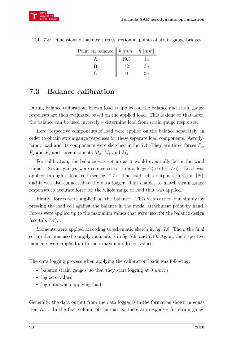
Formula SAE aerodynamic optimization
Tab. 7.3: Dimensions of balance’s cross-section at points of strain gauge bridges
Point on balance 𝑏 [𝑚𝑚] ℎ [𝑚𝑚]A 19.5 14B 12 35C 11 35
7.3 Balance calibration
During balance calibration, known load is applied on the balance and strain gaugeresponses are then evaluated based on the applied load. This is done so that later,the balance can be used inversely – determine load from strain gauge responses.
Here, respective components of load were applied on the balance separately, inorder to obtain strain gauge responses for these separate load components. Aerody-namic load and its components were sketched in fig. 7.4. They are three forces 𝐹𝑥,𝐹𝑦 and 𝐹𝑧 and three moments 𝑀𝑥, 𝑀𝑦 and 𝑀𝑧.
For calibration, the balance was set up as it would eventually be in the windtunnel. Strain gauges were connected to a data logger (see fig. 7.6). Load wasapplied through a load cell (see fig. 7.7). The load cell’s output is force in [𝑁 ],and it was also connected to the data logger. This enables to match strain gaugeresponses to accurate force for the whole range of load that was applied.
Firstly, forces were applied on the balance. This was carried out simply bypressing the load cell against the balance in the model attachment point by hand.Forces were applied up to the maximum values that were used for the balance design(see tab. 7.1).
Moments were applied according to schematic sketch in fig. 7.8. Then, the finalset up that was used to apply moments is in fig. 7.9, and 7.10. Again, the respectivemoments were applied up to their maximum design values.
The data logging process when applying the calibration loads was following:
• balance strain gauges, so that they start logging at 0 𝜇𝑚/𝑚
• log zero values• log data when applying load
Generally, the data output from the data logger is in the format as shown in equa-tion 7.31. In the first column of the matrix, there are responses for strain gauge
90 2016
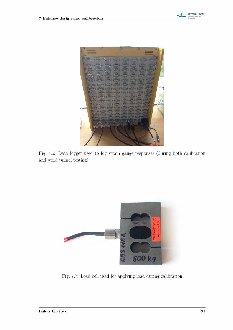
7 Balance design and calibration
Fig. 7.6: Data logger used to log strain gauge responses (during both calibrationand wind tunnel testing)
Fig. 7.7: Load cell used for applying load during calibration
Lukáš Fryšták 91
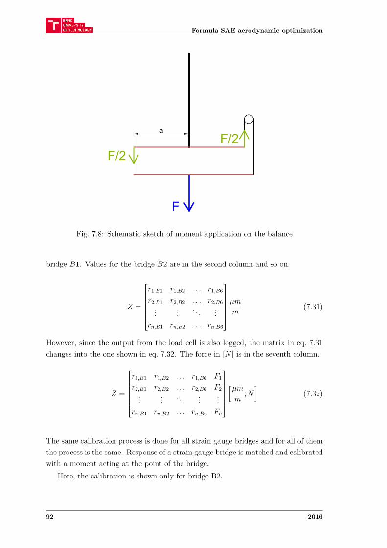
Formula SAE aerodynamic optimization
Fig. 7.8: Schematic sketch of moment application on the balance
bridge 𝐵1. Values for the bridge 𝐵2 are in the second column and so on.
𝑍 =
⎡⎢⎢⎢⎢⎢⎢⎣𝑟1,𝐵1 𝑟1,𝐵2 . . . 𝑟1,𝐵6
𝑟2,𝐵1 𝑟2,𝐵2 . . . 𝑟2,𝐵6... ... . . . ...
𝑟𝑛,𝐵1 𝑟𝑛,𝐵2 . . . 𝑟𝑛,𝐵6
⎤⎥⎥⎥⎥⎥⎥⎦𝜇𝑚
𝑚(7.31)
However, since the output from the load cell is also logged, the matrix in eq. 7.31changes into the one shown in eq. 7.32. The force in [𝑁 ] is in the seventh column.
𝑍 =
⎡⎢⎢⎢⎢⎢⎢⎣𝑟1,𝐵1 𝑟1,𝐵2 . . . 𝑟1,𝐵6 𝐹1
𝑟2,𝐵1 𝑟2,𝐵2 . . . 𝑟2,𝐵6 𝐹2... ... . . . ... ...
𝑟𝑛,𝐵1 𝑟𝑛,𝐵2 . . . 𝑟𝑛,𝐵6 𝐹𝑛
⎤⎥⎥⎥⎥⎥⎥⎦[︂𝜇𝑚
𝑚; 𝑁
]︂(7.32)
The same calibration process is done for all strain gauge bridges and for all of themthe process is the same. Response of a strain gauge bridge is matched and calibratedwith a moment acting at the point of the bridge.
Here, the calibration is shown only for bridge B2.
92 2016
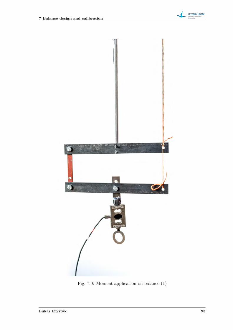
7 Balance design and calibration
Fig. 7.9: Moment application on balance (1)
Lukáš Fryšták 93
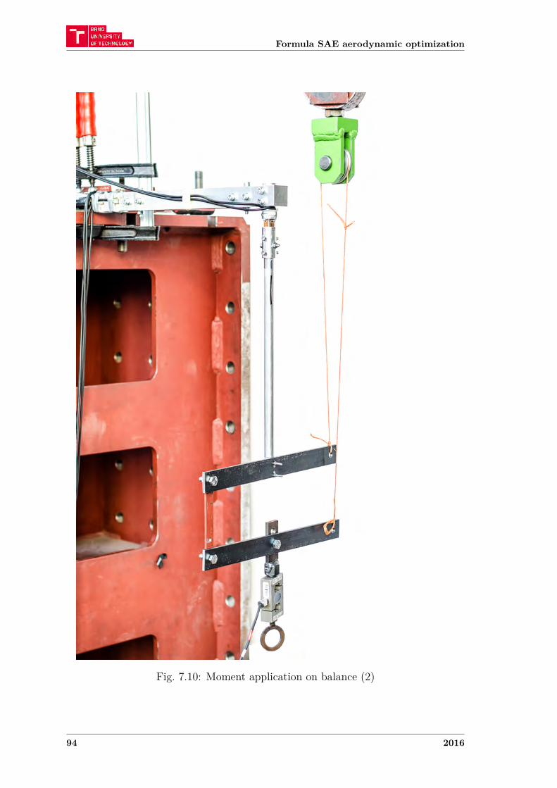
Formula SAE aerodynamic optimization
Fig. 7.10: Moment application on balance (2)
94 2016
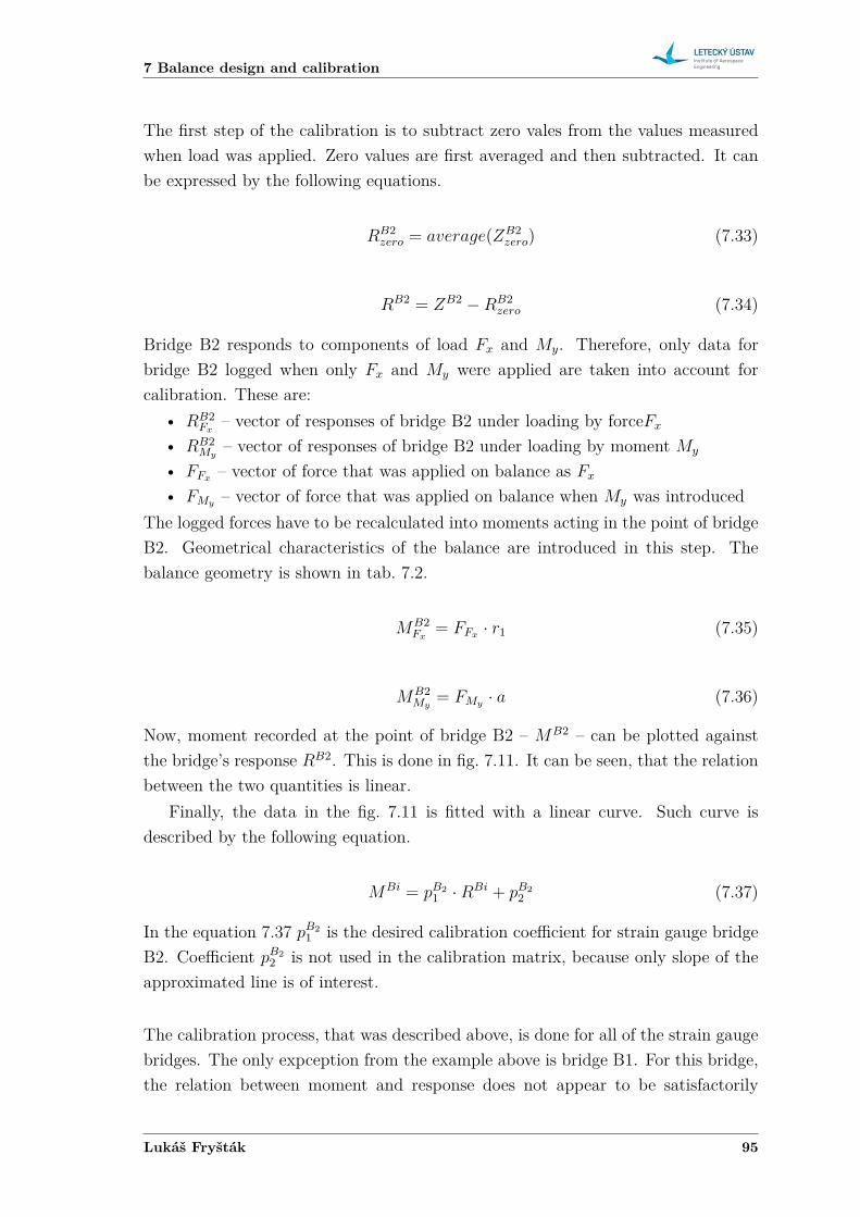
7 Balance design and calibration
The first step of the calibration is to subtract zero vales from the values measuredwhen load was applied. Zero values are first averaged and then subtracted. It canbe expressed by the following equations.
𝑅𝐵2𝑧𝑒𝑟𝑜 = 𝑎𝑣𝑒𝑟𝑎𝑔𝑒(𝑍𝐵2
𝑧𝑒𝑟𝑜) (7.33)
𝑅𝐵2 = 𝑍𝐵2 − 𝑅𝐵2𝑧𝑒𝑟𝑜 (7.34)
Bridge B2 responds to components of load 𝐹𝑥 and 𝑀𝑦. Therefore, only data forbridge B2 logged when only 𝐹𝑥 and 𝑀𝑦 were applied are taken into account forcalibration. These are:
• 𝑅𝐵2𝐹𝑥
– vector of responses of bridge B2 under loading by force𝐹𝑥
• 𝑅𝐵2𝑀𝑦
– vector of responses of bridge B2 under loading by moment 𝑀𝑦
• 𝐹𝐹𝑥 – vector of force that was applied on balance as 𝐹𝑥
• 𝐹𝑀𝑦 – vector of force that was applied on balance when 𝑀𝑦 was introducedThe logged forces have to be recalculated into moments acting in the point of bridgeB2. Geometrical characteristics of the balance are introduced in this step. Thebalance geometry is shown in tab. 7.2.
𝑀𝐵2𝐹𝑥
= 𝐹𝐹𝑥 · 𝑟1 (7.35)
𝑀𝐵2𝑀𝑦
= 𝐹𝑀𝑦 · 𝑎 (7.36)
Now, moment recorded at the point of bridge B2 – 𝑀𝐵2 – can be plotted againstthe bridge’s response 𝑅𝐵2. This is done in fig. 7.11. It can be seen, that the relationbetween the two quantities is linear.
Finally, the data in the fig. 7.11 is fitted with a linear curve. Such curve isdescribed by the following equation.
𝑀𝐵𝑖 = 𝑝𝐵21 · 𝑅𝐵𝑖 + 𝑝𝐵2
2 (7.37)
In the equation 7.37 𝑝𝐵21 is the desired calibration coefficient for strain gauge bridge
B2. Coefficient 𝑝𝐵22 is not used in the calibration matrix, because only slope of the
approximated line is of interest.
The calibration process, that was described above, is done for all of the strain gaugebridges. The only expception from the example above is bridge B1. For this bridge,the relation between moment and response does not appear to be satisfactorily
Lukáš Fryšták 95
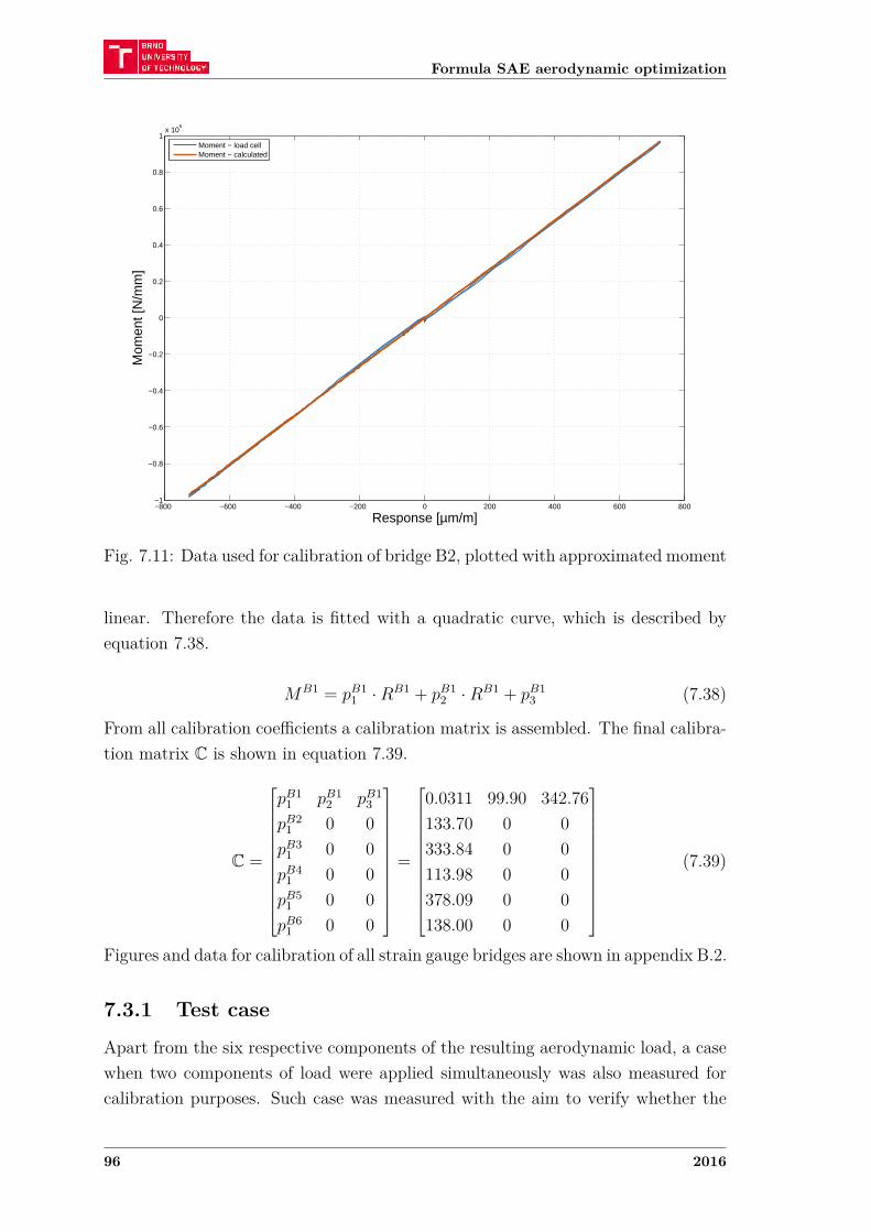
Formula SAE aerodynamic optimization
−800 −600 −400 −200 0 200 400 600 800−1
−0.8
−0.6
−0.4
−0.2
0
0.2
0.4
0.6
0.8
1x 10
5
Mom
ent [
N/m
m]
Response [µm/m]
Moment − load cellMoment − calculated
Fig. 7.11: Data used for calibration of bridge B2, plotted with approximated moment
linear. Therefore the data is fitted with a quadratic curve, which is described byequation 7.38.
𝑀𝐵1 = 𝑝𝐵11 · 𝑅𝐵1 + 𝑝𝐵1
2 · 𝑅𝐵1 + 𝑝𝐵13 (7.38)
From all calibration coefficients a calibration matrix is assembled. The final calibra-tion matrix C is shown in equation 7.39.
C =
⎡⎢⎢⎢⎢⎢⎢⎢⎢⎢⎢⎢⎣
𝑝𝐵11 𝑝𝐵1
2 𝑝𝐵13
𝑝𝐵21 0 0
𝑝𝐵31 0 0
𝑝𝐵41 0 0
𝑝𝐵51 0 0
𝑝𝐵61 0 0
⎤⎥⎥⎥⎥⎥⎥⎥⎥⎥⎥⎥⎦=
⎡⎢⎢⎢⎢⎢⎢⎢⎢⎢⎢⎢⎣
0.0311 99.90 342.76133.70 0 0333.84 0 0113.98 0 0378.09 0 0138.00 0 0
⎤⎥⎥⎥⎥⎥⎥⎥⎥⎥⎥⎥⎦(7.39)
Figures and data for calibration of all strain gauge bridges are shown in appendix B.2.
7.3.1 Test case
Apart from the six respective components of the resulting aerodynamic load, a casewhen two components of load were applied simultaneously was also measured forcalibration purposes. Such case was measured with the aim to verify whether the
96 2016
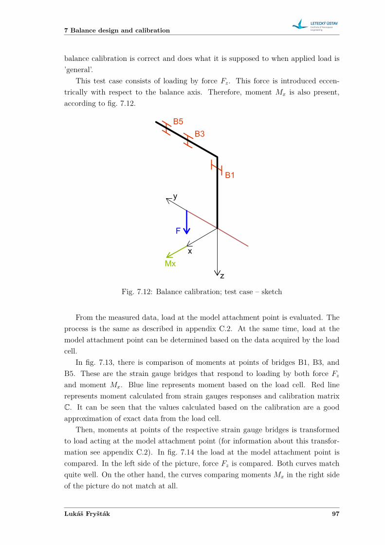
7 Balance design and calibration
balance calibration is correct and does what it is supposed to when applied load is’general’.
This test case consists of loading by force 𝐹𝑧. This force is introduced eccen-trically with respect to the balance axis. Therefore, moment 𝑀𝑥 is also present,according to fig. 7.12.
Fig. 7.12: Balance calibration; test case – sketch
From the measured data, load at the model attachment point is evaluated. Theprocess is the same as described in appendix C.2. At the same time, load at themodel attachment point can be determined based on the data acquired by the loadcell.
In fig. 7.13, there is comparison of moments at points of bridges B1, B3, andB5. These are the strain gauge bridges that respond to loading by both force 𝐹𝑧
and moment 𝑀𝑥. Blue line represents moment based on the load cell. Red linerepresents moment calculated from strain gauges responses and calibration matrixC. It can be seen that the values calculated based on the calibration are a goodapproximation of exact data from the load cell.
Then, moments at points of the respective strain gauge bridges is transformedto load acting at the model attachment point (for information about this transfor-mation see appendix C.2). In fig. 7.14 the load at the model attachment point iscompared. In the left side of the picture, force 𝐹𝑧 is compared. Both curves matchquite well. On the other hand, the curves comparing moments 𝑀𝑥 in the right sideof the picture do not match at all.
Lukáš Fryšták 97
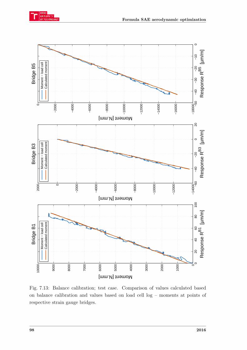
Formula SAE aerodynamic optimization
020
4060
8010
00
1000
2000
3000
4000
5000
6000
7000
8000
9000
1000
0B
ridge
B1
Res
pons
e R
B1 [
µm/m
]
Moment [N.mm]
M
omen
t − lo
ad c
ell
Cal
cula
ted
mom
ent
−60
−40
−20
020
−14
000
−12
000
−10
000
−80
00
−60
00
−40
00
−20
000
2000
Brid
ge B
3
Res
pons
e R
B3 [
µm/m
]
Moment [N.mm]
M
omen
t − lo
ad c
ell
Cal
cula
ted
mom
ent
−50
−40
−30
−20
−10
0−
1800
0
−16
000
−14
000
−12
000
−10
000
−80
00
−60
00
−40
00
−20
000B
ridge
B5
Res
pons
e R
B5 [
µm/m
]
Moment [N.mm]
M
omen
t − lo
ad c
ell
Cal
cula
ted
mom
ent
Fig. 7.13: Balance calibration; test case. Comparison of values calculated basedon balance calibration and values based on load cell log – moments at points ofrespective strain gauge bridges.
98 2016
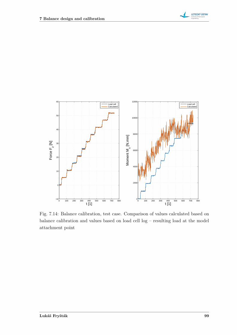
7 Balance design and calibration
0 100 200 300 400 500 600 700 800−10
0
10
20
30
40
50
60
t [1]
For
ce F
z [N]
0 100 200 300 400 500 600 700 8000
2000
4000
6000
8000
10000
12000
t [1]
Mom
ent M
x [N.m
m]
Load cellCalculated
Load cellCalculated
Fig. 7.14: Balance calibration, test case. Comparison of values calculated based onbalance calibration and values based on load cell log – resulting load at the modelattachment point
Lukáš Fryšták 99
Formula SAE aerodynamic optimization
The reason for the difference in the 𝑀𝑥 was not discovered. Moreover, when thesame process as in this test case was applied to all calibration logs, all values thattake into account responses from bridge B1 showed inaccurate results.
The components of aerodynamic load that use responses from bridge B1 are –side force 𝐹𝑦 and moment 𝑀𝑥. Moreover, when transforming load between the twocoordinate systems, moment 𝑀𝑧 also includes the inaccuracy from bridge B1 (seeapp. C.2).
For the reason mentioned above, in the following evaluation of aerodynamicload, components 𝐹𝑦, 𝑀𝑥, and 𝑀𝑧 are not taken into account. Furthermore, thesecomponents should all be zero when testing a symmetrical model with symmetricalflow (𝛽 = 0). Only components 𝐹𝑥, 𝐹𝑧, and 𝑀𝑦 are evaluated.
100 2016
8 Experiment results
8 EXPERIMENT RESULTS
This chapter presents the experiment and its results.
8.1 Measurement procedure
As part of the experimental testing, four different cases were measured. This wasdone to be able to compare different configurations and determine influence of dif-ferent parts.
Two different undertrays were manfactured, as mentioned in chapter 6. Onewith diffuser (cases 1 and 3) and one without diffuser (cases 2 and 4). Then, caseswithout wings (cases 1 and 2) and with wings (cases 3 and 4) were measured. Allcases are summed up in tab. 8.1. Numbers of the respective cases reflect the orderin which they were measured.
Tab. 8.1: Description of measured cases
Floor WingsCase 1 Floor with diffuser No wingsCase 2 Simple floor No wingsCase 3 Floor with diffuser Both wingsCase 4 Simple floor Both wings
Measurement was done in two basic steps. Firstly, each case was measured whilelogging data from force balance and pressure taps. Then, separately, the two wingedcases were measured with the traverser, with both Prandtl probe and hot wire probe.
As was previously mentioned, in an empty test section, the maximum velocityis 60 𝑚/𝑠. When choosing model scale and calculating Reynolds number, it wasexpected that with the model in the test section, the maximum velocity would be55 𝑚/𝑠 (see section 5.2.1). Nevertheless, that did not turn out to be the case.In the end, the maximum achievable velocity in the wind tunnel was much lower,different for all the cases. Unwinged cases – 1 and 2 – generate smaller pressurelosses, therefore the maximum speeds are higher, compared to winged cases.
However, for the winged cases, wind tunnel speed was no longer the limitingfactor. That turned out to be the model mounting. The model is mounted on astrain gauge balance, that is inherently not rigid. On top of that, the model itself isrelatively heavy. At speeds in excess of 30 𝑚/𝑠 whole model started to considerablyoscillate. A car is a bluff body, which means that the surrounding flow field isdominated by large areas of separated flow. It could be that the vibrations were
Lukáš Fryšták 101
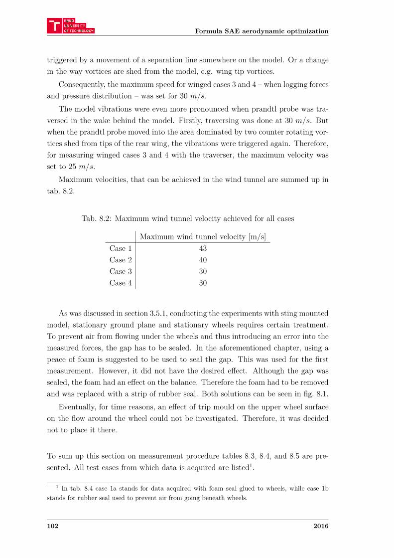
Formula SAE aerodynamic optimization
triggered by a movement of a separation line somewhere on the model. Or a changein the way vortices are shed from the model, e.g. wing tip vortices.
Consequently, the maximum speed for winged cases 3 and 4 – when logging forcesand pressure distribution – was set for 30 𝑚/𝑠.
The model vibrations were even more pronounced when prandtl probe was tra-versed in the wake behind the model. Firstly, traversing was done at 30 𝑚/𝑠. Butwhen the prandtl probe moved into the area dominated by two counter rotating vor-tices shed from tips of the rear wing, the vibrations were triggered again. Therefore,for measuring winged cases 3 and 4 with the traverser, the maximum velocity wasset to 25 𝑚/𝑠.
Maximum velocities, that can be achieved in the wind tunnel are summed up intab. 8.2.
Tab. 8.2: Maximum wind tunnel velocity achieved for all cases
Maximum wind tunnel velocity [m/s]Case 1 43Case 2 40Case 3 30Case 4 30
As was discussed in section 3.5.1, conducting the experiments with sting mountedmodel, stationary ground plane and stationary wheels requires certain treatment.To prevent air from flowing under the wheels and thus introducing an error into themeasured forces, the gap has to be sealed. In the aforementioned chapter, using apeace of foam is suggested to be used to seal the gap. This was used for the firstmeasurement. However, it did not have the desired effect. Although the gap wassealed, the foam had an effect on the balance. Therefore the foam had to be removedand was replaced with a strip of rubber seal. Both solutions can be seen in fig. 8.1.
Eventually, for time reasons, an effect of trip mould on the upper wheel surfaceon the flow around the wheel could not be investigated. Therefore, it was decidednot to place it there.
To sum up this section on measurement procedure tables 8.3, 8.4, and 8.5 are pre-sented. All test cases from which data is acquired are listed1.
1 In tab. 8.4 case 1a stands for data acquired with foam seal glued to wheels, while case 1bstands for rubber seal used to prevent air from going beneath wheels.
102 2016
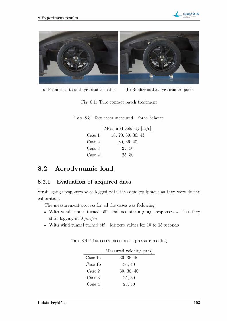
8 Experiment results
(a) Foam used to seal tyre contact patch (b) Rubber seal at tyre contact patch
Fig. 8.1: Tyre contact patch treatment
Tab. 8.3: Test cases measured – force balance
Measured velocity [m/s]Case 1 10, 20, 30, 36, 43Case 2 30, 36, 40Case 3 25, 30Case 4 25, 30
8.2 Aerodynamic load
8.2.1 Evaluation of acquired data
Strain gauge responses were logged with the same equipment as they were duringcalibration.
The measurement process for all the cases was following:• With wind tunnel turned off – balance strain gauge responses so that they
start logging at 0 𝜇𝑚/𝑚
• With wind tunnel turned off – log zero values for 10 to 15 seconds
Tab. 8.4: Test cases measured – pressure reading
Measured velocity [m/s]Case 1a 30, 36, 40Case 1b 36, 40Case 2 30, 36, 40Case 3 25, 30Case 4 25, 30
Lukáš Fryšták 103
Formula SAE aerodynamic optimization
Tab. 8.5: Test cases measured – traverser
Measured velocity [m/s]Case 3 – Prandtl probe 25Case 3 – Hot wire probe 25Case 4– Prandtl probe 25
• For a given speed – log strain gauge responses. Logging was done for abouttwo minutes on average. After logging is finished, increase wind tunnel speedand repeat logging.
• After wind tunnel speed dropped to 0 𝑚/𝑠, log zero values for 10 to 15 secondsLogging frequency was 100 Hz.As was described in the previous section four cases were measured. For every
case, at least two different velocities were measured (see tab. 8.3).
Loads acting on the balance were measured separately, so that it can be later sub-tracted from the loads measured with the model.
Load on balance was measured for five different speeds – 10, 20, 30, 35, and40 m/s. After calculation of all components of the load on balance, measured valueswere fitted with a quadratic curve. This enables to calculate load on balance ata given speed and subtract it from load on the model. The evaluation and curvefitting is described in appendix C.1.
When it comes to the final data evaluation of aerodynamic loads, for all the casesthe approach is the same. The only difference is in the number of measured points– different velocities measured.
As was mentioned above, the measuring process consists of: (a) zero values beforewind tunnel is turned on, (b) measured data for a given speed, and (c) zero valuesafter wind tunnel was turned off.
Here, only the general process is shown. More detailed information can be foundin appendix C.2.
First step of the evaluation is averaging measured values over the entire measur-ing period.
Next step is to subtract the average zero values from values at different velocities.After that, these values are multiplied by the balance’s calibration matrix. This stepyields moment values at points of strain gauge brides. These moments are multipliedagain by a transformation matrix, that transforms moments at strain gauge bridgesinto loads acting at the model attachment point.
104 2016
8 Experiment results
At this point, loads acting on a balance separately are subtracted. Then, the cal-culated values are components of aerodynamic load acting at the model attachmentpoint. This has to be transformed into loads acting at the origin of the coordinatesystem defined in section 7.1.
Last but not least, dimensionless coefficients as defined in section 7.1.2 can becalculated.
Again, for detailed description of the evaluation see appendix C.2.
8.2.2 Results – Cases 1-4
In this section, measured aerodynamic load acting on the model in respective casesis presented.
Case 1(Floor with diffuser, no wings)
Case 1 – as the first case measured – was measured for the largest range ofvelocities. The lowest measured velocity is 10 𝑚/𝑠 and it goes to 43 𝑚/𝑠, which isthe maximum wind tunnel speed, that can be achieved with this configuration.
In fig. 8.2 aerodynamic forces and moments are plotted as a function of speed.Unlike in appendix C.2, the forces are expressed in a more customary way – asdrag force 𝐷 and lift force 𝐿 (positive lift force acts upwards, while negative liftforce means that downforce is generated). All components appear to follow theexpected quadratic relation between the respective components of aerodynamic loadand velocity. In this case, lift is positive, which can be expected for an open wheelrace car without wings.
Aerodynamic coefficients are plotted against velocity in fig. 8.3. Theoretically,these values should be constant when plotted against speed. However, in the lowspeeds, the flow field around the car is not yet fully developed. Therefore, thevalues for 10 𝑚/𝑠 are considerably different compared to the higher velocities. Dragcoefficient and pitching moment coefficient are then relatively constant in the rangeof speeds from 20 to 43 𝑚/𝑠. Lift coefficient is increasing in the whole range,although the increment appears to be getting smaller between 36 and 43 𝑚/𝑠.
A possible explanation for the increasing lift coefficient could be behaviour of theflow around the wheels. With increasing velocity, the separation line on the uppersurface of the wheels may be moving aft, the result of which would be generation ofgreater lift force on the wheels.
Final aerodynamic characteristic for case 1 are taken following: for drag andpitching moment, values for 30, 36, and 43 𝑚/𝑠 are averaged. For lift coefficient,
Lukáš Fryšták 105
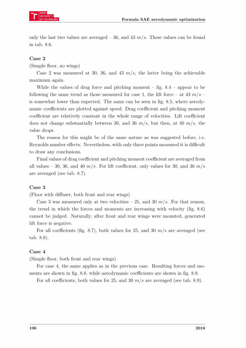
Formula SAE aerodynamic optimization
only the last two values are averaged – 36, and 43 𝑚/𝑠. These values can be foundin tab. 8.6.
Case 2(Simple floor, no wings)
Case 2 was measured at 30, 36, and 43 𝑚/𝑠, the latter being the achievablemaximum again.
While the values of drag force and pitching moment – fig. 8.4 – appear to befollowing the same trend as those measured for case 1, the lift force – at 43 𝑚/𝑠 –is somewhat lower than expected. The same can be seen in fig. 8.5, where aerody-namic coefficients are plotted against speed. Drag coefficient and pitching momentcoefficient are relatively constant in the whole range of velocities. Lift coefficientdoes not change substantially between 30, and 36 𝑚/𝑠, but then, at 40 𝑚/𝑠, thevalue drops.
The reason for this might be of the same nature as was suggested before, i.e.Reynolds number effects. Nevertheless, with only three points measured it is difficultto draw any conclusions.
Final values of drag coefficient and pitching moment coefficient are averaged fromall values – 30, 36, and 40 𝑚/𝑠. For lift coefficient, only values for 30, and 36 𝑚/𝑠
are averaged (see tab. 8.7).
Case 3(Floor with diffuser, both front and rear wings)
Case 3 was measured only at two velocities – 25, and 30 𝑚/𝑠. For that reason,the trend in which the forces and moments are increasing with velocity (fig. 8.6)cannot be judged. Naturally, after front and rear wings were mounted, generatedlift force is negative.
For all coefficients (fig. 8.7), both values for 25, and 30 𝑚/𝑠 are averaged (seetab. 8.8).
Case 4(Simple floor, both front and rear wings)
For case 4, the same applies as in the previous case. Resulting forces and mo-ments are shown in fig. 8.8, while aerodynamic coefficients are shown in fig. 8.9.
For all coefficients, both values for 25, and 30 𝑚/𝑠 are averaged (see tab. 8.9).
106 2016
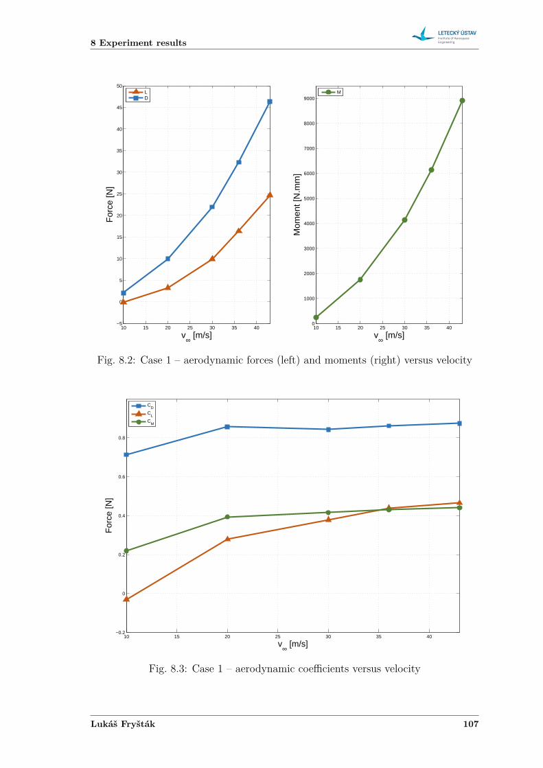
8 Experiment results
10 15 20 25 30 35 40−5
0
5
10
15
20
25
30
35
40
45
50
v∞ [m/s]
For
ce [N
]
LD
10 15 20 25 30 35 400
1000
2000
3000
4000
5000
6000
7000
8000
9000
v∞ [m/s]
Mom
ent [
N.m
m]
M
Fig. 8.2: Case 1 – aerodynamic forces (left) and moments (right) versus velocity
10 15 20 25 30 35 40−0.2
0
0.2
0.4
0.6
0.8
v∞ [m/s]
For
ce [N
]
C
D
CL
CM
Fig. 8.3: Case 1 – aerodynamic coefficients versus velocity
Lukáš Fryšták 107
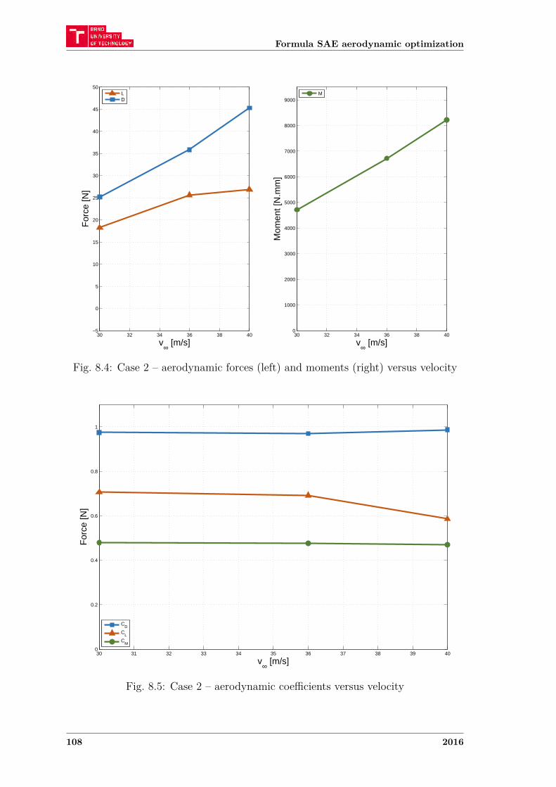
Formula SAE aerodynamic optimization
30 32 34 36 38 40−5
0
5
10
15
20
25
30
35
40
45
50
v∞ [m/s]
For
ce [N
]
LD
30 32 34 36 38 400
1000
2000
3000
4000
5000
6000
7000
8000
9000
v∞ [m/s]
Mom
ent [
N.m
m]
M
Fig. 8.4: Case 2 – aerodynamic forces (left) and moments (right) versus velocity
30 31 32 33 34 35 36 37 38 39 400
0.2
0.4
0.6
0.8
1
v∞ [m/s]
For
ce [N
]
CD
CL
CM
Fig. 8.5: Case 2 – aerodynamic coefficients versus velocity
108 2016
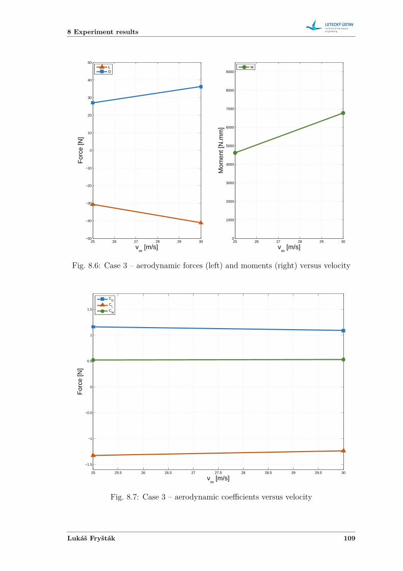
8 Experiment results
25 26 27 28 29 30−50
−40
−30
−20
−10
0
10
20
30
40
50
v∞ [m/s]
For
ce [N
]
L D
25 26 27 28 29 300
1000
2000
3000
4000
5000
6000
7000
8000
9000
v∞ [m/s]
Mom
ent [
N.m
m]
M
Fig. 8.6: Case 3 – aerodynamic forces (left) and moments (right) versus velocity
25 25.5 26 26.5 27 27.5 28 28.5 29 29.5 30
−1.5
−1
−0.5
0
0.5
1
1.5
v∞ [m/s]
For
ce [N
]
C
D
CL
CM
Fig. 8.7: Case 3 – aerodynamic coefficients versus velocity
Lukáš Fryšták 109
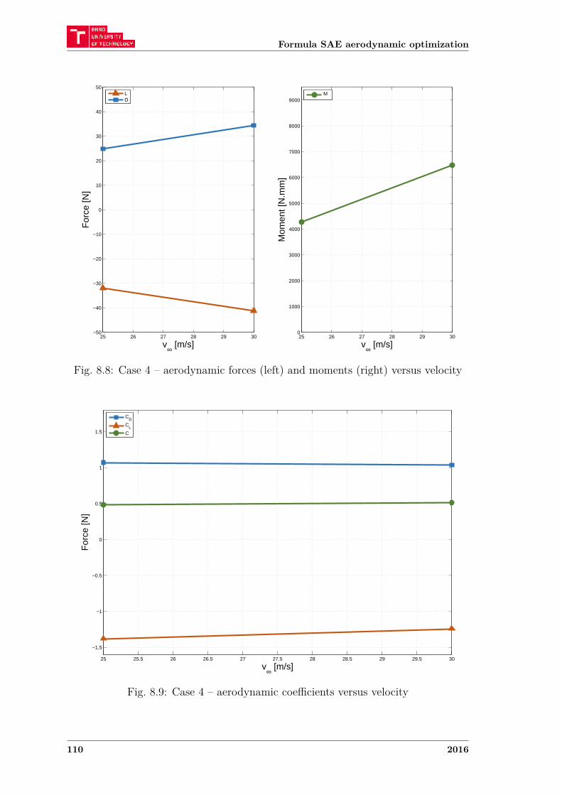
Formula SAE aerodynamic optimization
25 26 27 28 29 30−50
−40
−30
−20
−10
0
10
20
30
40
50
v∞ [m/s]
For
ce [N
]
LD
25 26 27 28 29 300
1000
2000
3000
4000
5000
6000
7000
8000
9000
v∞ [m/s]
Mom
ent [
N.m
m]
M
Fig. 8.8: Case 4 – aerodynamic forces (left) and moments (right) versus velocity
25 25.5 26 26.5 27 27.5 28 28.5 29 29.5 30
−1.5
−1
−0.5
0
0.5
1
1.5
v∞ [m/s]
For
ce [N
]
C
D
CL
C
Fig. 8.9: Case 4 – aerodynamic coefficients versus velocity
110 2016
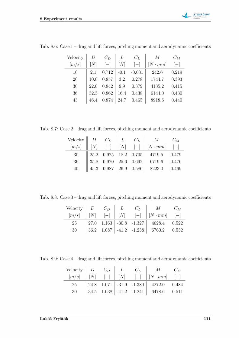
8 Experiment results
Tab. 8.6: Case 1 – drag and lift forces, pitching moment and aerodynamic coefficients
Velocity 𝐷 𝐶𝐷 𝐿 𝐶𝐿 𝑀 𝐶𝑀
[𝑚/𝑠] [𝑁 ] [−] [𝑁 ] [−] [𝑁 · 𝑚𝑚] [−]10 2.1 0.712 -0.1 -0.031 242.6 0.21920 10.0 0.857 3.2 0.278 1744.7 0.39330 22.0 0.842 9.9 0.379 4135.2 0.41536 32.3 0.862 16.4 0.438 6144.0 0.43043 46.4 0.874 24.7 0.465 8918.6 0.440
Tab. 8.7: Case 2 – drag and lift forces, pitching moment and aerodynamic coefficients
Velocity 𝐷 𝐶𝐷 𝐿 𝐶𝐿 𝑀 𝐶𝑀
[𝑚/𝑠] [𝑁 ] [−] [𝑁 ] [−] [𝑁 · 𝑚𝑚] [−]30 25.2 0.975 18.2 0.705 4719.5 0.47936 35.8 0.970 25.6 0.692 6719.6 0.47640 45.3 0.987 26.9 0.586 8223.0 0.469
Tab. 8.8: Case 3 – drag and lift forces, pitching moment and aerodynamic coefficients
Velocity 𝐷 𝐶𝐷 𝐿 𝐶𝐿 𝑀 𝐶𝑀
[𝑚/𝑠] [𝑁 ] [−] [𝑁 ] [−] [𝑁 · 𝑚𝑚] [−]25 27.0 1.163 -30.8 -1.327 4628.4 0.52230 36.2 1.087 -41.2 -1.238 6760.2 0.532
Tab. 8.9: Case 4 – drag and lift forces, pitching moment and aerodynamic coefficients
Velocity 𝐷 𝐶𝐷 𝐿 𝐶𝐿 𝑀 𝐶𝑀
[𝑚/𝑠] [𝑁 ] [−] [𝑁 ] [−] [𝑁 · 𝑚𝑚] [−]25 24.8 1.071 -31.9 -1.380 4272.0 0.48430 34.5 1.038 -41.2 -1.241 6478.6 0.511
Lukáš Fryšták 111
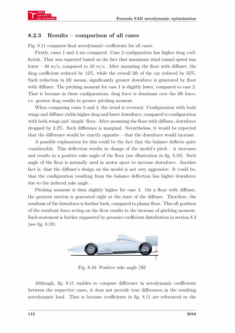
Formula SAE aerodynamic optimization
8.2.3 Results – comparison of all cases
Fig. 8.11 compares final aerodynamic coefficients for all cases.Firstly, cases 1 and 2 are compared. Case 2 configuration has higher drag coef-
ficient. That was expected based on the fact that maximum wind tunnel speed waslower – 40 𝑚/𝑠, compared to 43 𝑚/𝑠. After mounting the floor with diffuser, thedrag coefficient reduced by 12%, while the overall lift of the car reduced by 35%.Such reduction in lift means, significantly greater downforce is generated by floorwith diffuser. The pitching moment for case 1 is slightly lower, compared to case 2.That is because in these configurations, drag force is dominant over the lift force,i.e. greater drag results in greater pitching moment.
When comparing cases 3 and 4, the trend is reversed. Configuration with bothwings and diffuser yields higher drag and lower downforce, compared to configurationwith both wings and ’simple’ floor. After mounting the floor with diffuser, downforcedropped by 2.2%. Such difference is marginal. Nevertheless, it would be expectedthat the difference would be exactly opposite – that the downforce would increase.
A possible explanation for this could be the fact that the balance deflects quiteconsiderably. This deflection results in change of the model’s pitch – it increasesand results in a positive rake angle of the floor (see illustration in fig. 8.10). Suchangle of the floor is normally used in motor sport to increase downforce. Anotherfact is, that the diffuser’s design on the model is not very aggressive. It could be,that the configuration resulting from the balance deflection has higher downforcedue to the induced rake angle.
Pitching moment is then slightly higher for case 3. On a floor with diffuser,the greatest suction is generated right at the start of the diffuser. Therefore, theresultant of the downforce is further back, compared to planar floor. This aft positionof the resultant force acting on the floor results in the increase of pitching moment.Such statement is further supported by pressure coefficient distribution in section 8.3(see fig. 8.19).
Fig. 8.10: Positive rake angle [30]
Although, fig. 8.11 enables to compare difference in aerodynamic coefficientsbetween the respective cases, it does not provide true differences in the resultingaerodynamic load. That is because coefficients in fig. 8.11 are referenced to the
112 2016
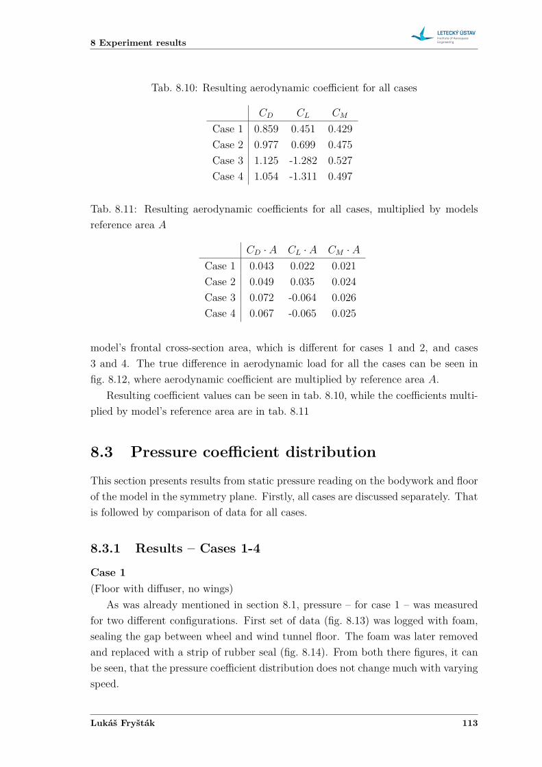
8 Experiment results
Tab. 8.10: Resulting aerodynamic coefficient for all cases
𝐶𝐷 𝐶𝐿 𝐶𝑀
Case 1 0.859 0.451 0.429Case 2 0.977 0.699 0.475Case 3 1.125 -1.282 0.527Case 4 1.054 -1.311 0.497
Tab. 8.11: Resulting aerodynamic coefficients for all cases, multiplied by modelsreference area 𝐴
𝐶𝐷 · 𝐴 𝐶𝐿 · 𝐴 𝐶𝑀 · 𝐴
Case 1 0.043 0.022 0.021Case 2 0.049 0.035 0.024Case 3 0.072 -0.064 0.026Case 4 0.067 -0.065 0.025
model’s frontal cross-section area, which is different for cases 1 and 2, and cases3 and 4. The true difference in aerodynamic load for all the cases can be seen infig. 8.12, where aerodynamic coefficient are multiplied by reference area 𝐴.
Resulting coefficient values can be seen in tab. 8.10, while the coefficients multi-plied by model’s reference area are in tab. 8.11
8.3 Pressure coefficient distribution
This section presents results from static pressure reading on the bodywork and floorof the model in the symmetry plane. Firstly, all cases are discussed separately. Thatis followed by comparison of data for all cases.
8.3.1 Results – Cases 1-4
Case 1(Floor with diffuser, no wings)
As was already mentioned in section 8.1, pressure – for case 1 – was measuredfor two different configurations. First set of data (fig. 8.13) was logged with foam,sealing the gap between wheel and wind tunnel floor. The foam was later removedand replaced with a strip of rubber seal (fig. 8.14). From both there figures, it canbe seen, that the pressure coefficient distribution does not change much with varyingspeed.
Lukáš Fryšták 113
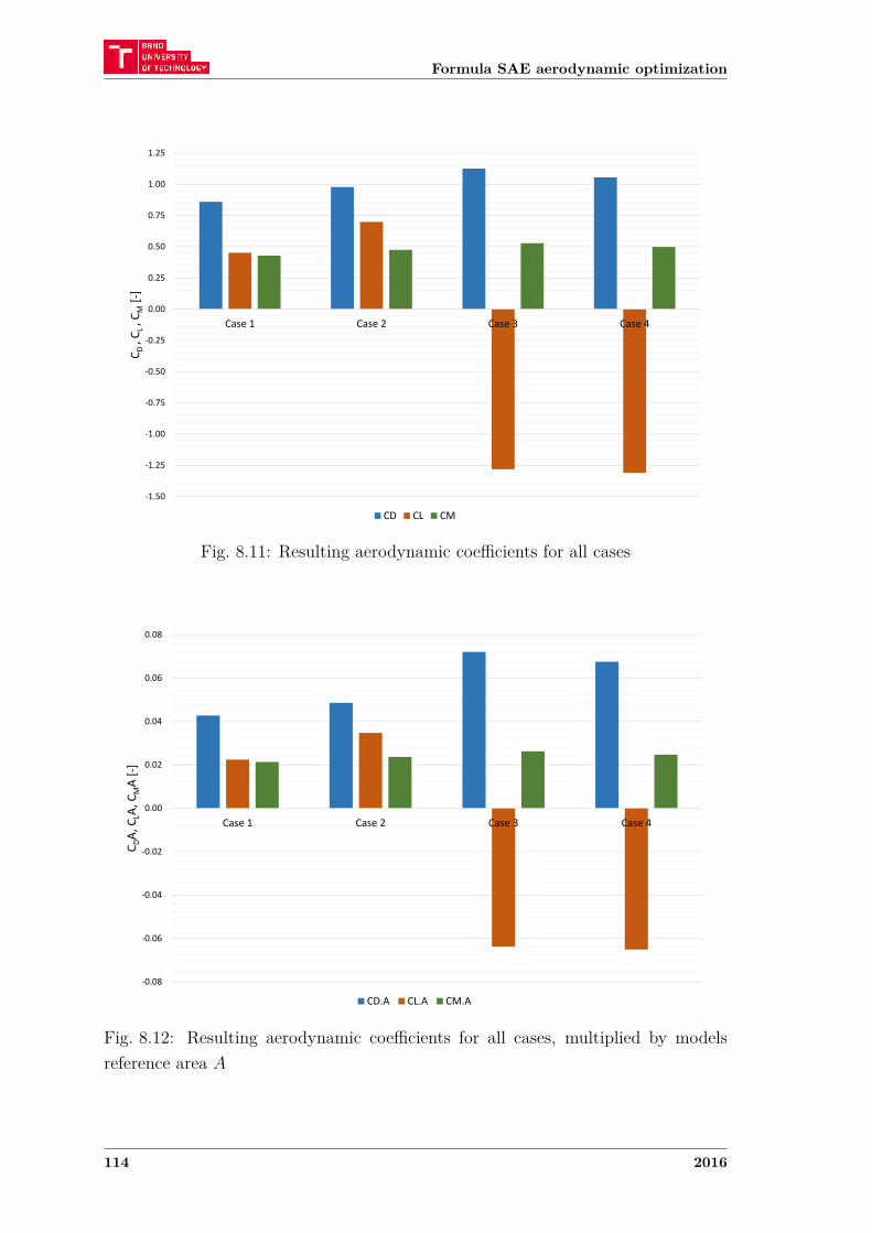
Formula SAE aerodynamic optimization
‐1.50
‐1.25
‐1.00
‐0.75
‐0.50
‐0.25
0.00
0.25
0.50
0.75
1.00
1.25
Case 1 Case 2 Case 3 Case 4
C D , C
L , C
M[‐]
CD CL CM
Fig. 8.11: Resulting aerodynamic coefficients for all cases
‐0.08
‐0.06
‐0.04
‐0.02
0.00
0.02
0.04
0.06
0.08
Case 1 Case 2 Case 3 Case 4
C DA, C
LA, C
MA[‐]
CD.A CL.A CM.A
Fig. 8.12: Resulting aerodynamic coefficients for all cases, multiplied by modelsreference area 𝐴
114 2016
8 Experiment results
Both of the two configurations are plotted together in fig. 8.15. The pressurecoefficient distribution matches in both cases, although there is one pressure tap,where there is noticeable difference.
On the upper surface of the bodywork, the pressure coefficient keeps getting lowertowards the cockpit. On the bodywork’s lower surface and floor, the pressure coeffi-cient decreases in a similar manner as on the upper surface. It keeps dropping untilthe airflow reaches area, where the ride height is constant, around 𝑥 = −120 𝑚𝑚.There, the pressure coefficient stays quite constant until it starts lowering again infront of the diffuser. At the start of the diffuser, the pressure reaches its minimumand in the diffuser, the air flow decelerates, resulting in increasing pressure.
Case 2(Simple floor, no wings)
For case 2, the pressure coefficient distribution is plotted in fig. 8.16. Comparedto case 1, there is no visible change in the pressure distribution on the upper surface.On the other hand, on the bodywork’s lower surface and floor, the difference is quitesubstantial. From the stagnation point, the pressure keeps decreasing until around𝑥 = −50 𝑚𝑚. There, the pressure reaches its minimum value, i.e. it is the placeof greatest suction. From there, the pressure gradient is adverse until 𝑥 = 140 𝑚𝑚,where the gradient changes and pressure coefficient starts decreasing again.
Case 3(Floor with diffuser, both front and rear wings)
For case 3 (fig. 8.17), the pressure coefficient distribution changes substantiallyin the area directly behind the front wing, compared to case 1. In the first part ofthe nose’s lower surface – between the nose cone and the front wing, the pressurecoefficient decreases at quite a steep gradient. Then in the area of the airfoil’swake, the pressure gradient changes. Pressure appears to be increasing for a shortdistance before it decreases again, but not at such a steep gradient. Then thepressure coefficient distribution towards the diffuser is similar to that in case 1.
Case 4(Simple floor, both front and rear wings)
Pressure coefficient distribution for case 4 is shown in fig. 8.18. The differencecaused by the front wing, compared to case 2 appears to be the same as was describedfor case 3.
Lukáš Fryšták 115
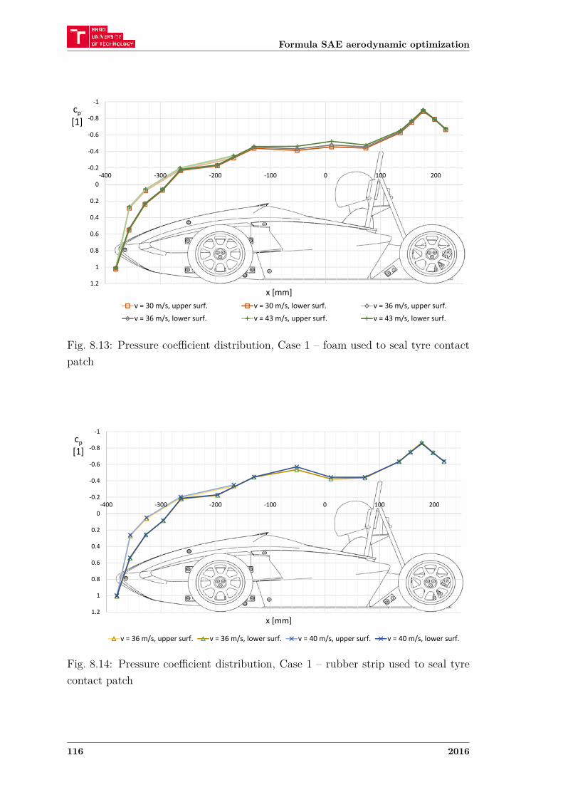
Formula SAE aerodynamic optimization
‐1
‐0.8
‐0.6
‐0.4
‐0.2
0
0.2
0.4
0.6
0.8
1
1.2
‐400 ‐300 ‐200 ‐100 0 100 200
cp[1]
x [mm]v = 30 m/s, upper surf. v = 30 m/s, lower surf. v = 36 m/s, upper surf.
v = 36 m/s, lower surf. v = 43 m/s, upper surf. v = 43 m/s, lower surf.
Fig. 8.13: Pressure coefficient distribution, Case 1 – foam used to seal tyre contactpatch
‐1
‐0.8
‐0.6
‐0.4
‐0.2
0
0.2
0.4
0.6
0.8
1
1.2
‐400 ‐300 ‐200 ‐100 0 100 200
cp[1]
x [mm]
v = 36 m/s, upper surf. v = 36 m/s, lower surf. v = 40 m/s, upper surf. v = 40 m/s, lower surf.
Fig. 8.14: Pressure coefficient distribution, Case 1 – rubber strip used to seal tyrecontact patch
116 2016
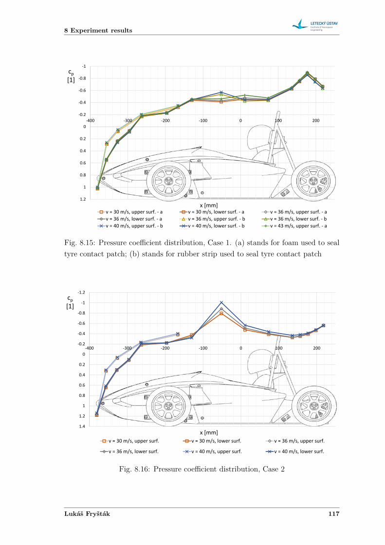
8 Experiment results
‐1
‐0.8
‐0.6
‐0.4
‐0.2
0
0.2
0.4
0.6
0.8
1
1.2
‐400 ‐300 ‐200 ‐100 0 100 200
cp[1]
x [mm]v = 30 m/s, upper surf. ‐ a v = 30 m/s, lower surf. ‐ a v = 36 m/s, upper surf. ‐ av = 36 m/s, lower surf. ‐ a v = 36 m/s, upper surf. ‐ b v = 36 m/s, lower surf. ‐ bv = 40 m/s, upper surf. ‐ b v = 40 m/s, lower surf. ‐ b v = 43 m/s, upper surf. ‐ a
Fig. 8.15: Pressure coefficient distribution, Case 1. (a) stands for foam used to sealtyre contact patch; (b) stands for rubber strip used to seal tyre contact patch
‐1.2
‐1
‐0.8
‐0.6
‐0.4
‐0.2
0
0.2
0.4
0.6
0.8
1
1.2
1.4
‐400 ‐300 ‐200 ‐100 0 100 200
cp[1]
x [mm]v = 30 m/s, upper surf. v = 30 m/s, lower surf. v = 36 m/s, upper surf.
v = 36 m/s, lower surf. v = 40 m/s, upper surf. v = 40 m/s, lower surf.
Fig. 8.16: Pressure coefficient distribution, Case 2
Lukáš Fryšták 117
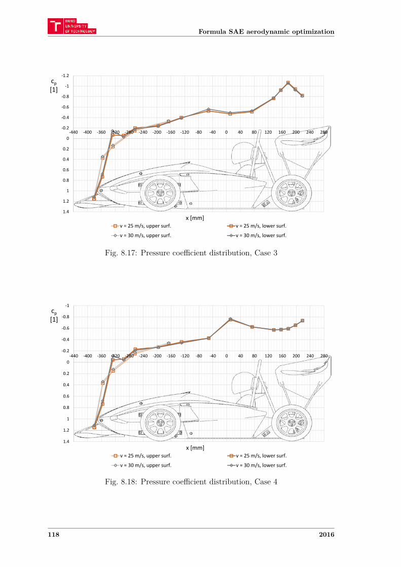
Formula SAE aerodynamic optimization
‐1.2
‐1
‐0.8
‐0.6
‐0.4
‐0.2
0
0.2
0.4
0.6
0.8
1
1.2
1.4
‐440 ‐400 ‐360 ‐320 ‐280 ‐240 ‐200 ‐160 ‐120 ‐80 ‐40 0 40 80 120 160 200 240 280
cp[1]
x [mm]v = 25 m/s, upper surf. v = 25 m/s, lower surf.
v = 30 m/s, upper surf. v = 30 m/s, lower surf.
Fig. 8.17: Pressure coefficient distribution, Case 3
‐1
‐0.8
‐0.6
‐0.4
‐0.2
0
0.2
0.4
0.6
0.8
1
1.2
1.4
‐440 ‐400 ‐360 ‐320 ‐280 ‐240 ‐200 ‐160 ‐120 ‐80 ‐40 0 40 80 120 160 200 240 280
cp[1]
x [mm]v = 25 m/s, upper surf. v = 25 m/s, lower surf.
v = 30 m/s, upper surf. v = 30 m/s, lower surf.
Fig. 8.18: Pressure coefficient distribution, Case 4
118 2016

8 Experiment results
8.3.2 Results – comparison of all cases
Pressure coefficient distribution for all cases is plotted in fig. 8.19. All curves arefor 30 𝑚/𝑠 velocity.
There is no significant change in the pressure distribution on the upper surface.In the front part of the lower surface, naturally, the effect of the front wing
is visible. However, downstream from the front wing – approximately from 𝑥 =−250 𝑚𝑚 to 𝑥 = −130 𝑚𝑚, the pressure coefficient appears to be quite similar forall the cases.
When comparing case 1 and case 3, the curves follow similar trend, with thecurve for case 3 shifted a bit into lower values.
For case 4, the minimum pressure shifted aft, compared to case 2, with theabsolute values being the same. Again, from the point of minimum pressure, thetrend is similar. However, configuration in case 4 in not subjected to such an adversepressure gradient as case 2, resulting in lower pressure coefficient values at the lastpart of the floor.
Conclusion from what was said above is that the rear wing contributes to gener-ate greater suction on the floor, resulting in greater downforce on the floor itself,compared to car without wings.
As was suggested in section 8.2.3, from the pressure coefficient distribution infig. 8.19, it can be estimated that the resultant of the force acting on the floor ismainly influenced by the position of the suction peak. Then the floor with diffuserwould have higher pitching moment compared to planar floor.
8.4 Wake traversing
8.4.1 Prandtl probe
Traverser with prandtl probe was used to measure velocity in a plane 410 𝑚𝑚 behindthe model (see fig. 8.20). The resulting velocity contour plots are shown in fig. 8.21and 8.22 for cases 3 and 4, respectively. Both cases were measured at 25 𝑚/𝑠. Therange of the axes in both plots determine the test section’s dimensions. The whitearea close to the borders of the graph is area, where measurement was not done.That is because the prandtl probe error is outside guaranteed range when proximityof a wall is less than five times the probe’s diameter.
In both pictures, it can seen that the wake behind the model is dominated by twolarge counter rotating vortices, that originate at the tips of the rear wing. Althoughit is obvious that the measurement is influenced by the large blockage, the fact that
Lukáš Fryšták 119
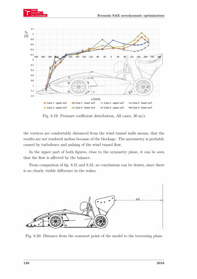
Formula SAE aerodynamic optimization
‐1.2
‐1
‐0.8
‐0.6
‐0.4
‐0.2
0
0.2
0.4
0.6
0.8
1
1.2
1.4
‐440 ‐400 ‐360 ‐320 ‐280 ‐240 ‐200 ‐160 ‐120 ‐80 ‐40 0 40 80 120 160 200 240 280
cp[1]
x [mm]Case 1 ‐ upper surf. Case 1 ‐ lower surf. Case 2 ‐ upper surf. Case 2 ‐ lower surf.
Case 3 ‐ upper surf. Case 3 ‐ lower surf. Case 4 ‐ upper surf. Case 4 ‐ lower surf.
Fig. 8.19: Pressure coefficient distribution, All cases, 30 m/s
the vortices are comfortably distanced from the wind tunnel walls means, that theresults are not rendered useless because of the blockage. The asymmetry is probablycaused by turbulence and pulsing of the wind tunnel flow.
In the upper part of both figures, close to the symmetry plane, it can be seenthat the flow is affected by the balance.
From comparison of fig. 8.21 and 8.22, no conclusions can be drawn, since thereis no clearly visible difference in the wakes.
Fig. 8.20: Distance from the rearmost point of the model to the traversing plane
120 2016
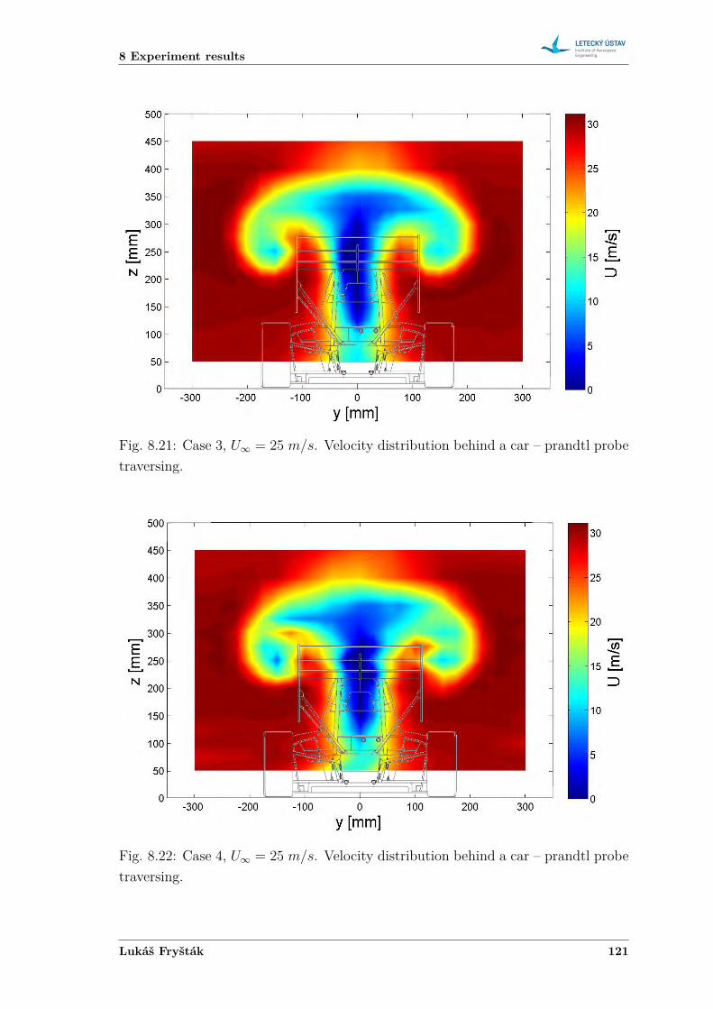
8 Experiment results
Fig. 8.21: Case 3, 𝑈∞ = 25 𝑚/𝑠. Velocity distribution behind a car – prandtl probetraversing.
Fig. 8.22: Case 4, 𝑈∞ = 25 𝑚/𝑠. Velocity distribution behind a car – prandtl probetraversing.
Lukáš Fryšták 121
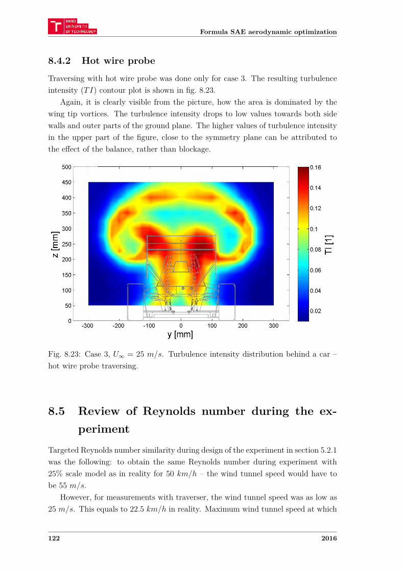
Formula SAE aerodynamic optimization
8.4.2 Hot wire probe
Traversing with hot wire probe was done only for case 3. The resulting turbulenceintensity (𝑇𝐼) contour plot is shown in fig. 8.23.
Again, it is clearly visible from the picture, how the area is dominated by thewing tip vortices. The turbulence intensity drops to low values towards both sidewalls and outer parts of the ground plane. The higher values of turbulence intensityin the upper part of the figure, close to the symmetry plane can be attributed tothe effect of the balance, rather than blockage.
Fig. 8.23: Case 3, 𝑈∞ = 25 𝑚/𝑠. Turbulence intensity distribution behind a car –hot wire probe traversing.
8.5 Review of Reynolds number during the ex-periment
Targeted Reynolds number similarity during design of the experiment in section 5.2.1was the following: to obtain the same Reynolds number during experiment with25% scale model as in reality for 50 𝑘𝑚/ℎ – the wind tunnel speed would have tobe 55 𝑚/𝑠.
However, for measurements with traverser, the wind tunnel speed was as low as25 𝑚/𝑠. This equals to 22.5 𝑘𝑚/ℎ in reality. Maximum wind tunnel speed at which
122 2016
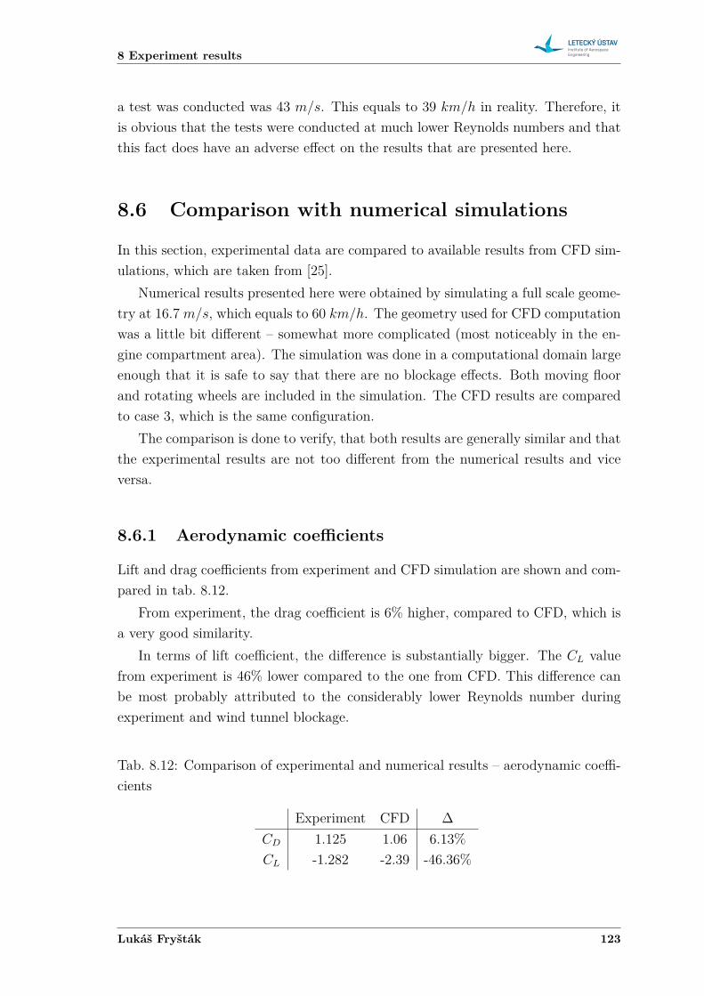
8 Experiment results
a test was conducted was 43 𝑚/𝑠. This equals to 39 𝑘𝑚/ℎ in reality. Therefore, itis obvious that the tests were conducted at much lower Reynolds numbers and thatthis fact does have an adverse effect on the results that are presented here.
8.6 Comparison with numerical simulations
In this section, experimental data are compared to available results from CFD sim-ulations, which are taken from [25].
Numerical results presented here were obtained by simulating a full scale geome-try at 16.7 𝑚/𝑠, which equals to 60 𝑘𝑚/ℎ. The geometry used for CFD computationwas a little bit different – somewhat more complicated (most noticeably in the en-gine compartment area). The simulation was done in a computational domain largeenough that it is safe to say that there are no blockage effects. Both moving floorand rotating wheels are included in the simulation. The CFD results are comparedto case 3, which is the same configuration.
The comparison is done to verify, that both results are generally similar and thatthe experimental results are not too different from the numerical results and viceversa.
8.6.1 Aerodynamic coefficients
Lift and drag coefficients from experiment and CFD simulation are shown and com-pared in tab. 8.12.
From experiment, the drag coefficient is 6% higher, compared to CFD, which isa very good similarity.
In terms of lift coefficient, the difference is substantially bigger. The 𝐶𝐿 valuefrom experiment is 46% lower compared to the one from CFD. This difference canbe most probably attributed to the considerably lower Reynolds number duringexperiment and wind tunnel blockage.
Tab. 8.12: Comparison of experimental and numerical results – aerodynamic coeffi-cients
Experiment CFD Δ𝐶𝐷 1.125 1.06 6.13%𝐶𝐿 -1.282 -2.39 -46.36%
Lukáš Fryšták 123
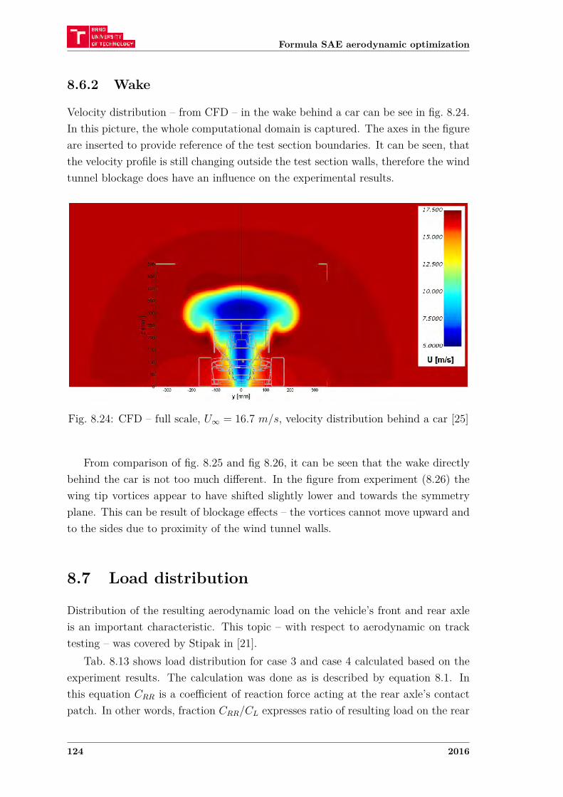
Formula SAE aerodynamic optimization
8.6.2 Wake
Velocity distribution – from CFD – in the wake behind a car can be see in fig. 8.24.In this picture, the whole computational domain is captured. The axes in the figureare inserted to provide reference of the test section boundaries. It can be seen, thatthe velocity profile is still changing outside the test section walls, therefore the windtunnel blockage does have an influence on the experimental results.
Fig. 8.24: CFD – full scale, 𝑈∞ = 16.7 𝑚/𝑠, velocity distribution behind a car [25]
From comparison of fig. 8.25 and fig 8.26, it can be seen that the wake directlybehind the car is not too much different. In the figure from experiment (8.26) thewing tip vortices appear to have shifted slightly lower and towards the symmetryplane. This can be result of blockage effects – the vortices cannot move upward andto the sides due to proximity of the wind tunnel walls.
8.7 Load distribution
Distribution of the resulting aerodynamic load on the vehicle’s front and rear axleis an important characteristic. This topic – with respect to aerodynamic on tracktesting – was covered by Stipak in [21].
Tab. 8.13 shows load distribution for case 3 and case 4 calculated based on theexperiment results. The calculation was done as is described by equation 8.1. Inthis equation 𝐶𝑅𝑅 is a coefficient of reaction force acting at the rear axle’s contactpatch. In other words, fraction 𝐶𝑅𝑅/𝐶𝐿 expresses ratio of resulting load on the rear
124 2016
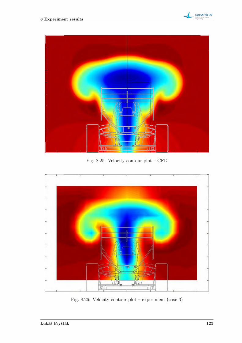
8 Experiment results
Fig. 8.25: Velocity contour plot – CFD
Fig. 8.26: Velocity contour plot – experiment (case 3)
Lukáš Fryšták 125
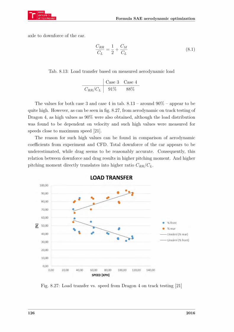
Formula SAE aerodynamic optimization
axle to downforce of the car.
𝐶𝑅𝑅
𝐶𝐿
= 12 + 𝐶𝑀
𝐶𝐿
(8.1)
Tab. 8.13: Load transfer based on measured aerodynamic load
Case 3 Case 4𝐶𝑅𝑅/𝐶𝐿 91% 88%
The values for both case 3 and case 4 in tab. 8.13 – around 90% – appear to bequite high. However, as can be seen in fig. 8.27, from aerodynamic on track testing ofDragon 4, as high values as 90% were also obtained, although the load distributionwas found to be dependent on velocity and such high values were measured forspeeds close to maximum speed [21].
The reason for such high values can be found in comparison of aerodynamiccoefficients from experiment and CFD. Total downforce of the car appears to beunderestimated, while drag seems to be reasonably accurate. Consequently, thisrelation between downforce and drag results in higher pitching moment. And higherpitching moment directly translates into higher ratio 𝐶𝑅𝑅/𝐶𝐿.
Fig. 8.27: Load transfer vs. speed from Dragon 4 on track testing [21]
126 2016
9 Conclusion
9 CONCLUSION
Over the recent years, aerodynamics became an integral part of car development inFormula SAE. In this work a study of a Formula SAE car’s aerodynamic character-istics was conducted, the method for aerodynamic analysis being subscale experi-mental testing. The goal was to determine aerodynamic characteristics of the modeland find areas from which improvement of these characteristics could be extracted.
The testing was done with a 25% scaled model of a Formula SAE race carderived from TU Brno Racing’s 2016 car – Dragon 6. Four different configurationswere measured, differing in usage of a floor with diffuser and inverted wings. Themodel was mounted on a sting balance and measurements were done with stationaryboth wheels and floor. The wind tunnel blockage in this configuration was quitehigh – approximately 20%.
The aforementioned force balance was initially not available as part of the windtunnel’s equipment. Therefore, part of this work focuses on design and calibrationof a six component balance, that uses strain gauges to measure the aerodynamicload.
From load measurement – for configurations without wings – it was found thatthe model produces lift. When using a floor with diffuser, the overall lift can bereduced. Here, the resulting difference is 35% reduction in the overall lift, whilereduction in drag is 12%. Configurations with wings produce downforce, but alsoconsiderably higher drag. However, the trend is different compared to configurationswithout wings. Although the difference is marginal – only 2% – with wings, theconfiguration with diffuser produces lower downforce, than the configuration withplanar floor. Probable cause for such unexpected behaviour is thought to be resultingfrom balance deflection. Such deflection consequently induces a rake angle of themodel, thus generating greater downforce.
Dominant source of downforce are the wings. However, pressure coefficient distri-bution on the floor showed, that the rear wing also contributes to higher downforcegeneration on the floor.
It is obvious that as high blockage as 20% must have a strong influence on theexperiment results. However, the fact that the two counter rotating vortices shedfrom tips of the rear wing were found to be comfortably distanced from the windtunnel walls means, that the results are not rendered useless because of the blockage.
It was desired to obtain Reynold number equivalent to full scale car’s velocityof 50 𝑘𝑚/ℎ. However, due to high blockage of the test section and the consequentpressure losses, the maximum speed that was achieved in the wind tunnel was equal
Lukáš Fryšták 127
Formula SAE aerodynamic optimization
to full scale velocity as low as 22.5 𝑘𝑚/ℎ. This fact also has an adverse effect onthe measured results.
Should the current car configuration be improved, either increasing downforce ordecreasing drag would be possible. However, it is more important to achieve areasonable aerodynamic balance. Therefore it is required to move the resultingcentre of pressure forward. That could be done in different ways. One of thembeing – as suggested above – using a rake angle instead of a diffuser to generatedownforce on the vehicle’s underbody
Even though conclusions can be drawn from the presented experimental data, furthereffort is required to make this experimental set up truly useful when designingaerodynamic parts for a Formula SAE car.
Effect of wind tunnel blockage on the results should be determined via numericalsimulations. Then, all three available design tools should also be correlated - CFD,wind tunnel testing, and track testing.
128 2016
BIBLIOGRAPHY[1] CATTAFESTA, Louis, BAHR, Chris and MATHEW, Jose, 2010, Funda-
mentals of Wind-Tunnel Design. Encyclopedia of Aerospace Engineering [on-line]. 15 December 2010. DOI 10.1002/9780470686652.eae532. Retrieved from:http://doi.wiley.com/10.1002/9780470686652.eae532
[2] CURTIS, Michael, 2016, Private communication. Loughborough University.
[3] FRYŠTÁK, Lukáš, 2013, Design of aerodynamic wings of Formula Student /SAE [online]. Bachelor’s Thesis. Brno. Retrieved from: https://www.vutbr.cz/www_base/zav_prace_soubor_verejne.php?file_id=84183
[4] HUCHO, Wolf-Heinrich, 1998, Aerodynamics of road vehicles: from fluid me-chanics to vehicle engineering. 4th ed. Warrendale, PA : Society of AutomotiveEngineers. ISBN 07-680-0029-7.
[5] HUCHO, Wolf-Heinrich, 2013, Aerodynamik des Automobils: Strö-mungsmechanik, Wärmetechnik, Fahrdynamik, Komfort ; mit 49 Tabellen. 6.Aufl. Wiesbaden : Vieweg. ISBN 978-383-4819-192.
[6] KATZ, Joseph, 1995, Race Car Aerodynamics: Designing for Speed. Cambridge,MA, USA : Bentley Publishers. ISBN 0-8376-0142-8.
[7] KATZ, Joseph and GARCIA, Darwin, 2002, Aerodynamic Effects of Indy CarComponents. Proceedings of the 2002 SAE Motorsports Engineering Conferenceand Exhibition [online]. 2002. No. 2002-01-3311p. 11. DOI 10.4271/2002-01-3311. Retrieved from: http://papers.sae.org/2002-01-3311/
[8] KATZ, Joseph and WALTERS, Robert, 1995, Investigation of wind-tunnel walleffects in high blockage testing. In : 33rd Aerospace Sciences Meeting and Ex-hibit [online]. Reston, Virigina : American Institute of Aeronautics and Astro-nautics. 09 January 1995. p. -. Retrieved from: http://arc.aiaa.org/doi/abs/10.2514/6.1995-438
[9] LAJZA, Ondřej, 2014, Aircraft engine cooling system testing. 2014.
[10] LYU, Zhoujie and MARTINS, Joaquim R. R. A., 2014, Aerodynamic DesignOptimization Studies of a Blended-Wing-Body Aircraft. In : Journal of Aircraft[online]. Grapevine, TX : AIAA. 2014. p. 1604-1617. Retrieved from: http://arc.aiaa.org/doi/10.2514/1.C032491
[11] MCBEATH, Simon, 2013, Aerobytes: Students unleashed. Racecar Engineer-ing. 01 December 2013. Vol. 2013, no. 12p. 57-59.
Lukáš Fryšták 129
Formula SAE aerodynamic optimization
[12] MCBEATH, Simon, 2014, Aerobytes: Further education. Racecar Engineering.01 January 2014. Vol. 2014, no. 1p. 53-54.
[13] MCBEATH, Simon, 2014, Aerobytes: Continuing studies. Racecar Engineering.01 February 2014. Vol. 2014, no. 2p. 45-46.
[14] MCBEATH, Simon, 2014, Aerobytes: Final examinations. Racecar Engineering.01 March 2014. Vol. 2014, no. 3p. 39-40.
[15] MCBEATH, Simon, 2014, Aerobytes: The flying limpet. Racecar Engineering:Fomula Student. 2014. No. 1p. 14-24.
[16] MILLIKEN, William F. and MILLIKEN, Douglas L., 1995, Race Car VehicleDynamics. Warrendale, PA, USA : SAE International. ISBN 1-56091-526-9.
[17] PLACZEK, Robin, SCHOLZ, Peter and OTHMER, Carsten, 2014, AnAnalysis of Drag Force Components and Structures in the Wake ofa Detailed Road Vehicle Model by Means of SPIV. 17 th Interna-tional Symposium on Applications of Laser Techniques to Fluid Mechan-ics [online]. 2014. Retrieved from: http://ltces.dem.ist.utl.pt/lxlaser/lxlaser2014/finalworks2014/papers/01.7_3_136paper.pdf
[18] POPE, Alan and HARPER, John J., 1966, Low-Speed Wind Tunnel Testing.New York : John Wiley & Sons, Inc. ISBN 978-0-471-55774-6.
[19] ROYCE, Michael and ROYCE, Suzanne, 2012, Learn and Compete: A primerfor Formula SAE, Formula Student and Formula Hybrid teams. ISBN 978-0953352470.
[20] ŠPIČÁK, Milan, 2015, Performance optimisation of turbocharged engine forFormula Student [online]. Master’s Thesis. Brno. Retrieved from: https://www.vutbr.cz/www_base/zav_prace_soubor_verejne.php?file_id=104750
[21] ŠTIPÁK, Patrik, 2015, Suspension Development of Formula Student Vehicle[online]. Master’s Thesis. Brno. Retrieved from: https://www.vutbr.cz/www_base/zav_prace_soubor_verejne.php?file_id=103919
[22] TOET, Willem, 2014, How WIND TUNNELS Work - F1 explained - Sauber F1Team [online]. Hinwil, Switzerland. [Accessed 25 March 2016]. Retrieved from:https://www.youtube.com/watch?v=KC0E0wU6inU. Sauber F1 Team; SauberMotorsport AG
[23] TU BRNO RACING, 2014, Dragon 4 - Design Book: Presentation materials.Brno : TU Brno Racing.
130 2016
[24] TU BRNO RACING, 2015, Dragon 5 - Design Book: Presentation materials.Brno : TU Brno Racing.
[25] TU BRNO RACING, 2016, Dragon 6 - Design Book: Presentation materials.Brno : TU Brno Racing.
[26] WORDLEY, Scott and SAUNDERS, Jeff, 2006, Aerodynamics for FormulaSAE: Initial Design and Performance Prediction. SAE Paper [online]. 2006. No.2006-01-0806. DOI 10.4271/2006-01-0806. Retrieved from: http://papers.sae.org/2006-01-0806/
[27] WORDLEY, Scott and SAUNDERS, Jeff, 2006, Aerodynamics for FormulaSAE: A Numerical, Wind Tunnel and On-Track Study. SAE Paper [online].2006. No. 2006-01-0806. DOI 10.4271/2006-01-0808. Retrieved from: http://papers.sae.org/2006-01-0808/
[28] SAE International, 2015. [online], 2015. [Accessed 30 December 2015]. Retrievedfrom: sae.org
[29] SAE J 1594: Vehicle Aerodynamics Terminology, 1987. , Warrendale : SAEInternational. SAE J 1594
[30] Rake Angle, In : Formula1-dictionary.net [online], [Accessed 22 May 2016].Retrieved from: http://www.formula1-dictionary.net/rake_angle.html
[31] Formula SAE: Competition History 1981-2004, In : SAE.org [online], [Ac-cessed 03 January 2016]. Retrieved from: http://www.sae.org/students/fsaehistory.pdf
Lukáš Fryšták 131


LIST OF SYMBOLS AND ABBREVIATIONS𝜀 Deformation
𝜙 Wind tunnel blockage
𝜆 Test section relative length
𝜈 Kinematic viscosity
𝜈𝑀 Kinematic viscosity for model
𝜈𝑅 Kinematic viscosity for real conditions
𝜌 Air density
𝜎𝑏 Bending stress
𝐴 Vehicle reference area
𝐴𝑁 Cross-section area of wind tunnel nozzle
𝐴𝑀 Model reference area
𝐴𝑅 Real car reference area
C Calibration matrix
𝐶𝐷 Drag coefficient
𝐶𝐿 Lift coefficient
𝐶𝑀 Pitching moment coefficient
𝐶𝑁 Yawing moment coefficient
𝑐𝑝 Pressure coefficient
𝐶𝑅 Rolling moment coefficient
𝐶𝑌 Side force coefficient
𝐶𝑅𝑅 Coefficient of reaction force acting at vehicle’s rear axle
CFD Computational fluid dynamics
𝐷 Drag force acting on a vehicle
𝐷𝑁 Equivalent (hydraulic) diameter of wind tunnel nozzle
Lukáš Fryšták 133
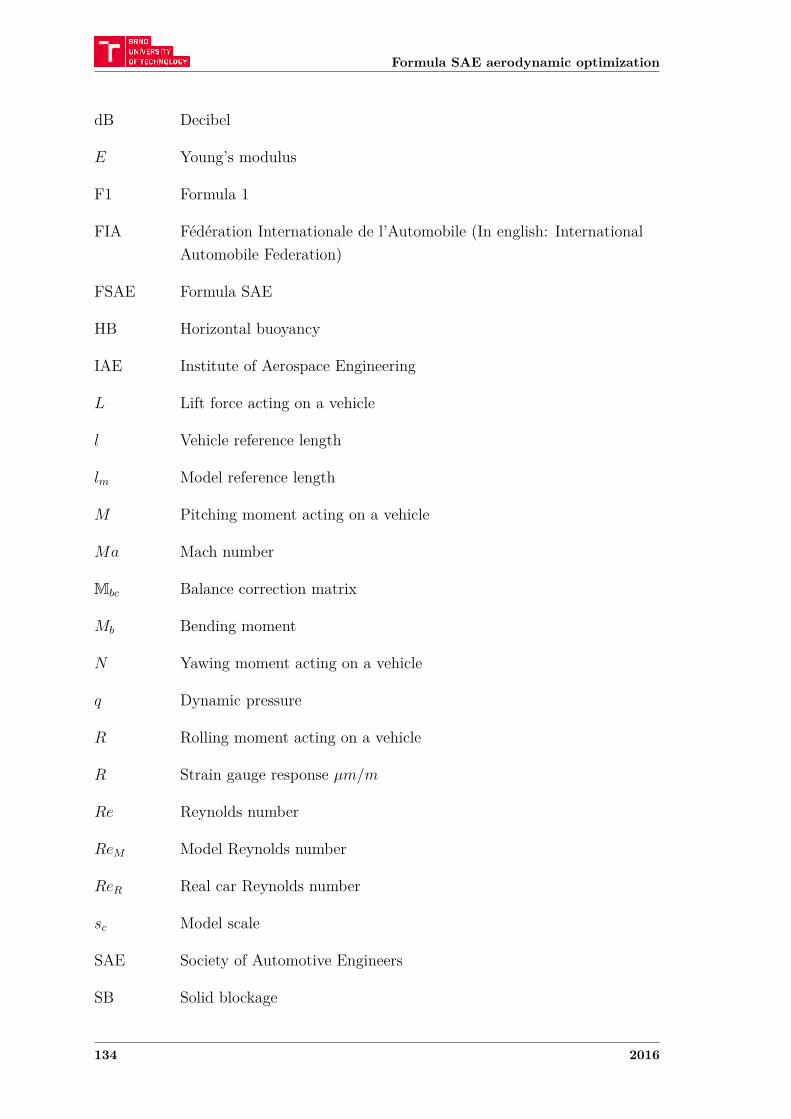
Formula SAE aerodynamic optimization
dB Decibel
𝐸 Young’s modulus
F1 Formula 1
FIA Fédération Internationale de l’Automobile (In english: InternationalAutomobile Federation)
FSAE Formula SAE
HB Horizontal buoyancy
IAE Institute of Aerospace Engineering
𝐿 Lift force acting on a vehicle
𝑙 Vehicle reference length
𝑙𝑚 Model reference length
𝑀 Pitching moment acting on a vehicle
𝑀𝑎 Mach number
M𝑏𝑐 Balance correction matrix
𝑀𝑏 Bending moment
𝑁 Yawing moment acting on a vehicle
𝑞 Dynamic pressure
𝑅 Rolling moment acting on a vehicle
𝑅 Strain gauge response 𝜇𝑚/𝑚
𝑅𝑒 Reynolds number
𝑅𝑒𝑀 Model Reynolds number
𝑅𝑒𝑅 Real car Reynolds number
𝑠𝑐 Model scale
SAE Society of Automotive Engineers
SB Solid blockage
134 2016
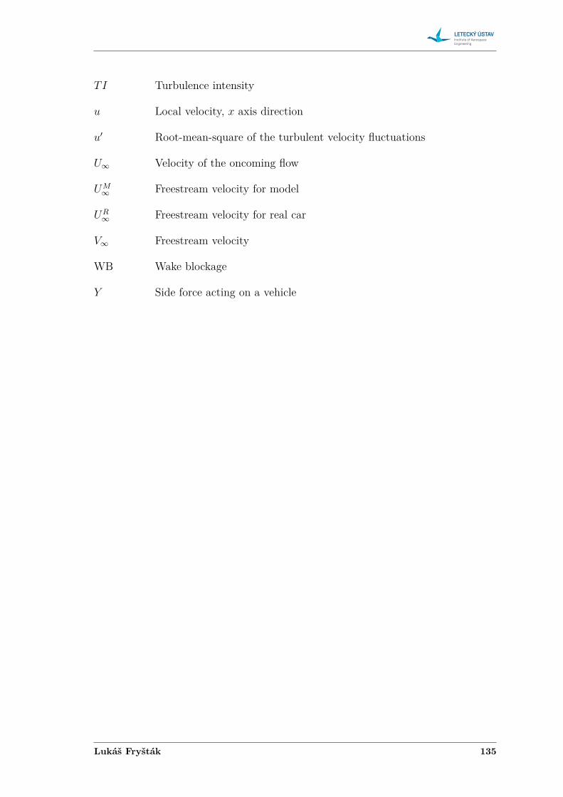
𝑇𝐼 Turbulence intensity
𝑢 Local velocity, 𝑥 axis direction
𝑢′ Root-mean-square of the turbulent velocity fluctuations
𝑈∞ Velocity of the oncoming flow
𝑈𝑀∞ Freestream velocity for model
𝑈𝑅∞ Freestream velocity for real car
𝑉∞ Freestream velocity
WB Wake blockage
𝑌 Side force acting on a vehicle
Lukáš Fryšták 135


LIST OF APPENDICES
LIST OF APPENDICES
A Reynolds number and blockage calculation 139
B Balance – further information 141B.1 Balance drawings . . . . . . . . . . . . . . . . . . . . . . . . . . . . . 141B.2 Balance – calibration graphs . . . . . . . . . . . . . . . . . . . . . . 150
C Aerodynamic load evaluation 157C.1 Loads on balance . . . . . . . . . . . . . . . . . . . . . . . . . . . . . 157C.2 Load on model . . . . . . . . . . . . . . . . . . . . . . . . . . . . . . 161
Lukáš Fryšták 137

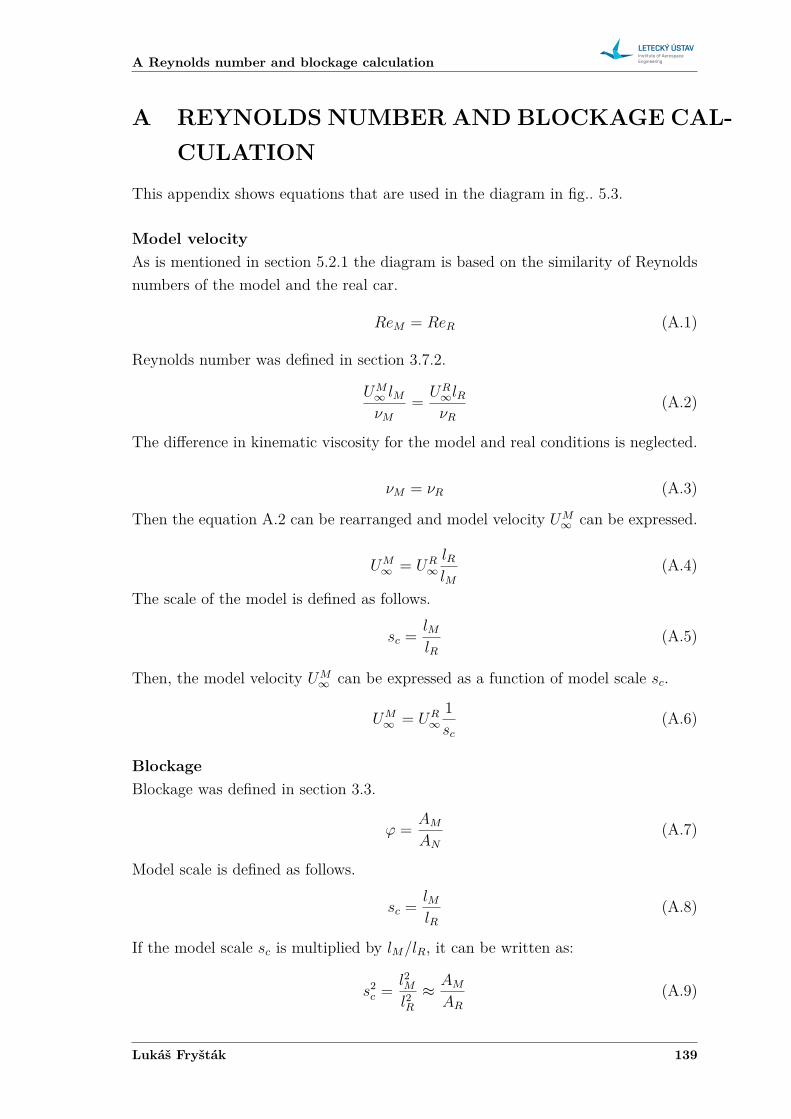
A Reynolds number and blockage calculation
A REYNOLDS NUMBER AND BLOCKAGE CAL-CULATION
This appendix shows equations that are used in the diagram in fig.. 5.3.
Model velocityAs is mentioned in section 5.2.1 the diagram is based on the similarity of Reynoldsnumbers of the model and the real car.
𝑅𝑒𝑀 = 𝑅𝑒𝑅 (A.1)
Reynolds number was defined in section 3.7.2.
𝑈𝑀∞ 𝑙𝑀𝜈𝑀
= 𝑈𝑅∞𝑙𝑅𝜈𝑅
(A.2)
The difference in kinematic viscosity for the model and real conditions is neglected.
𝜈𝑀 = 𝜈𝑅 (A.3)
Then the equation A.2 can be rearranged and model velocity 𝑈𝑀∞ can be expressed.
𝑈𝑀∞ = 𝑈𝑅
∞𝑙𝑅𝑙𝑀
(A.4)
The scale of the model is defined as follows.
𝑠𝑐 = 𝑙𝑀𝑙𝑅
(A.5)
Then, the model velocity 𝑈𝑀∞ can be expressed as a function of model scale 𝑠𝑐.
𝑈𝑀∞ = 𝑈𝑅
∞1𝑠𝑐
(A.6)
BlockageBlockage was defined in section 3.3.
𝜙 = 𝐴𝑀
𝐴𝑁
(A.7)
Model scale is defined as follows.
𝑠𝑐 = 𝑙𝑀𝑙𝑅
(A.8)
If the model scale 𝑠𝑐 is multiplied by 𝑙𝑀/𝑙𝑅, it can be written as:
𝑠2𝑐 = 𝑙2
𝑀
𝑙2𝑅
≈ 𝐴𝑀
𝐴𝑅
(A.9)
Lukáš Fryšták 139
Formula SAE aerodynamic optimization
𝑠2𝑐 = 𝐴𝑀
𝐴𝑅
(A.10)
Model reference area can be then expressed as follows.
𝐴𝑀 = 𝐴𝑅𝑠2𝑐 (A.11)
The model reference area is the substituted in the equation A.7, which gives blockage𝜙 as a function of model scale 𝑠𝑐.
𝜙 = 𝐴𝑅
𝐴𝑁
𝑠2𝑐 (A.12)
140 2016

B Balance – further information
B BALANCE – FURTHER INFORMATION
B.1 Balance drawingsOn the following pages, balance drawings are shown. First, there are drawings ofthe whole assembly and then, there are drawings of the respective parts.
Lukáš Fryšták 141
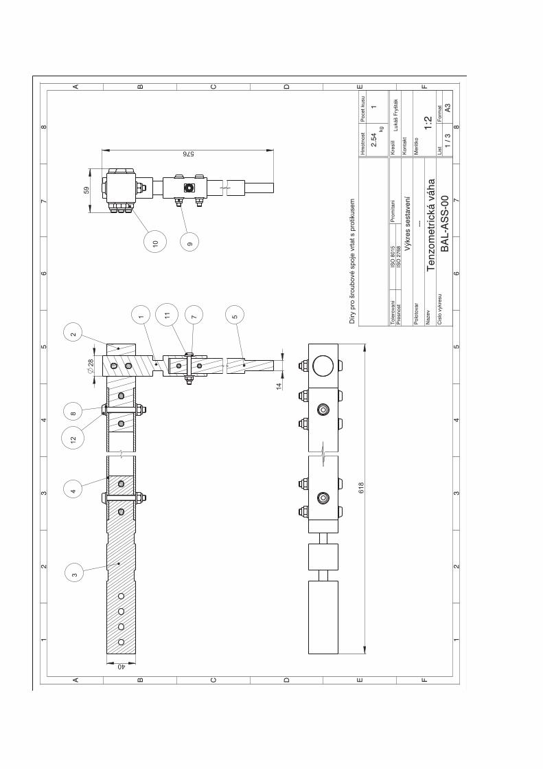
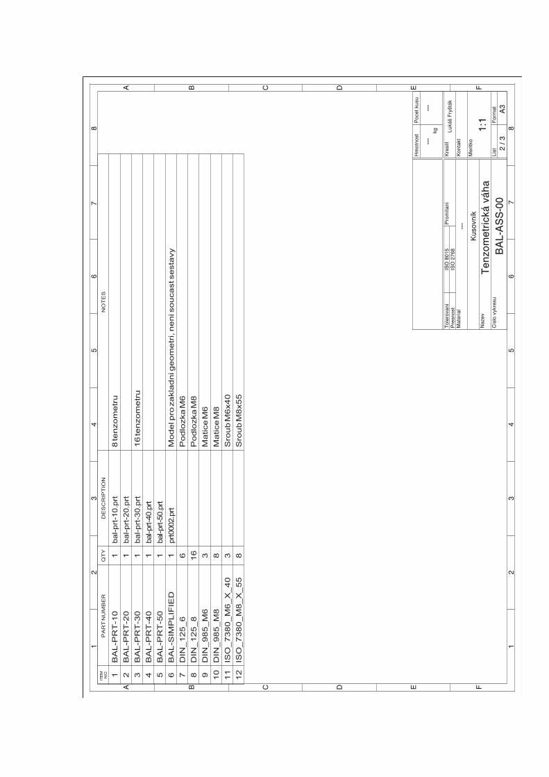
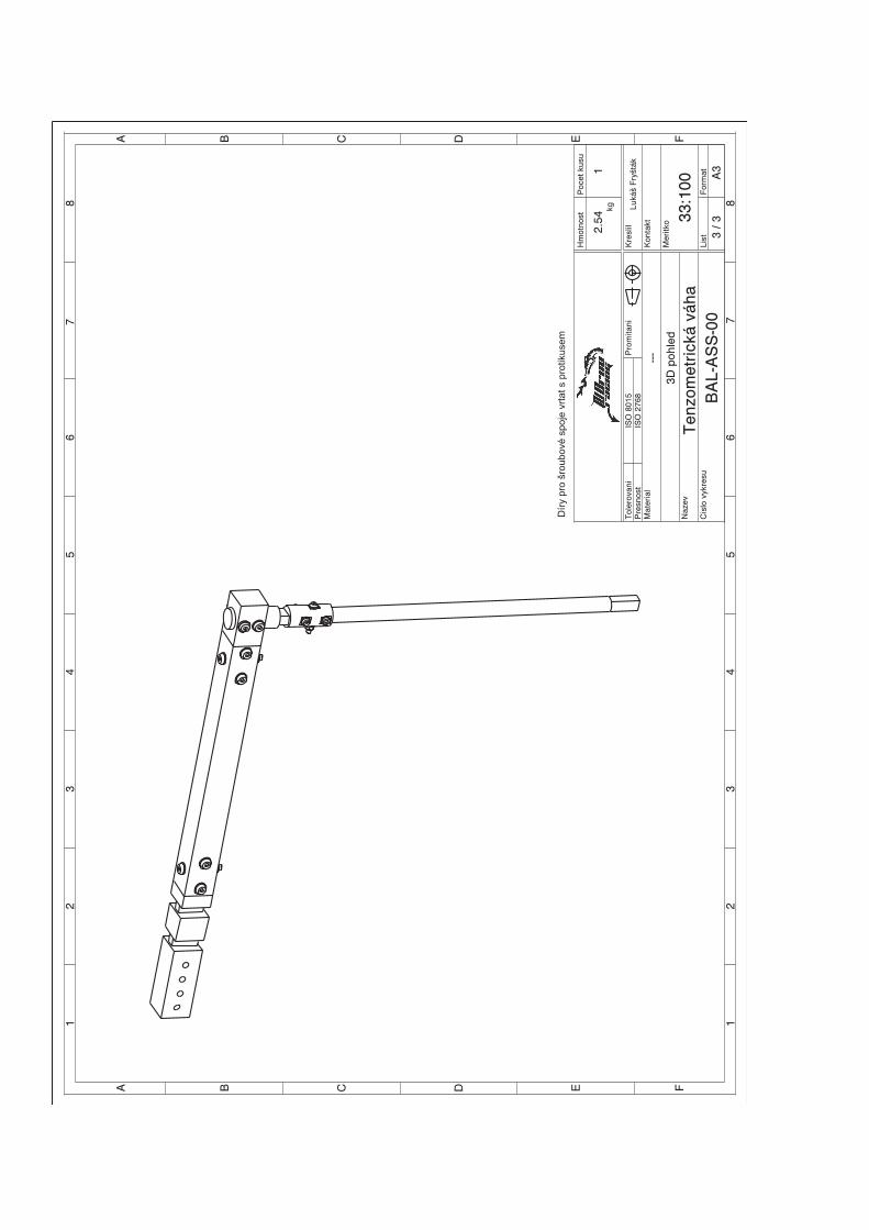

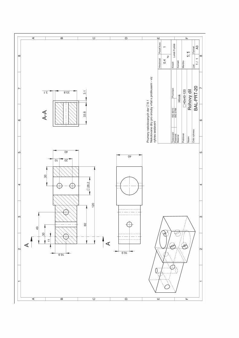
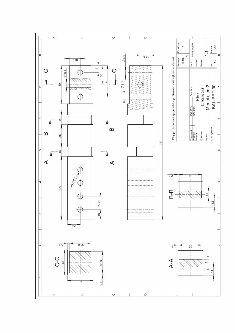
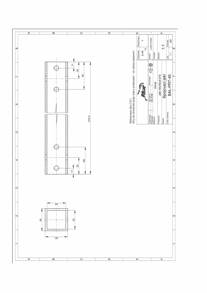
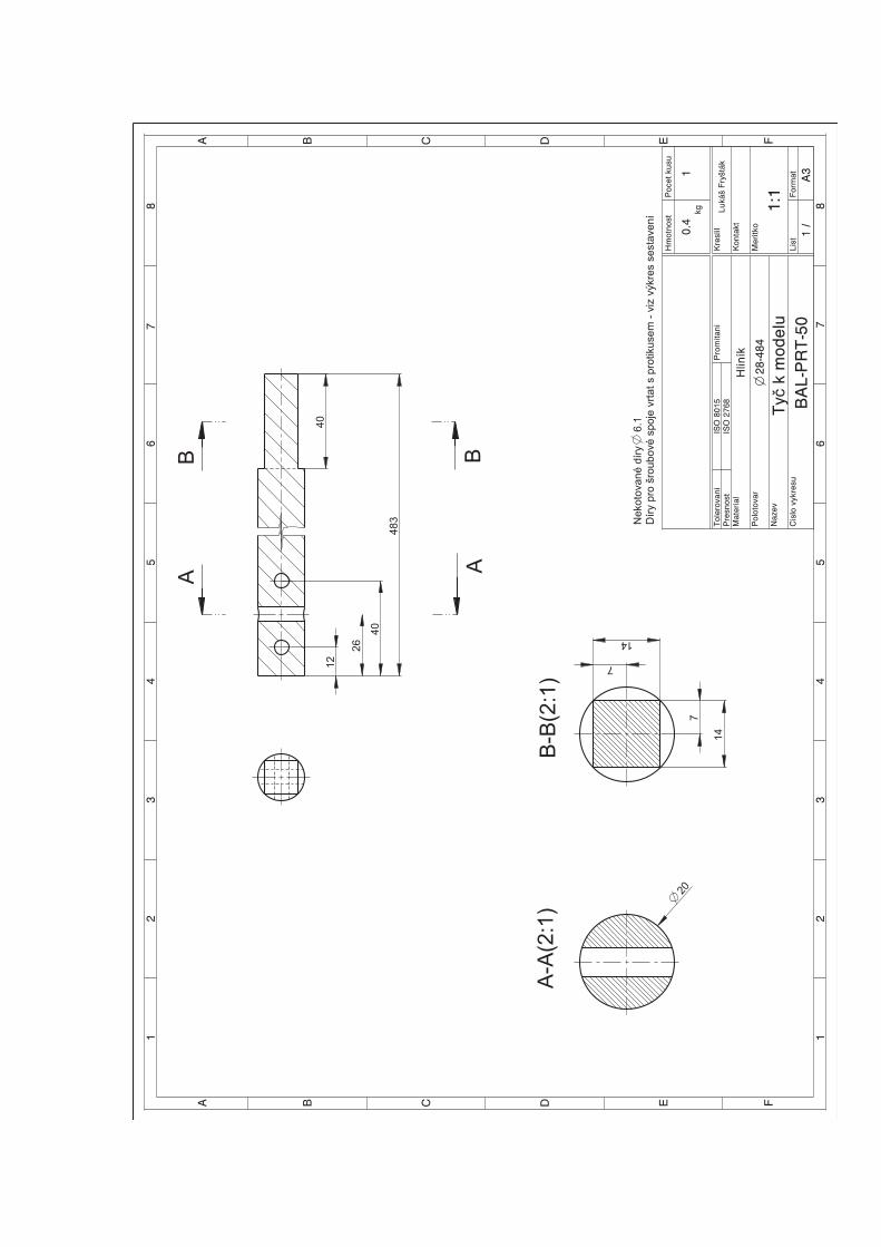
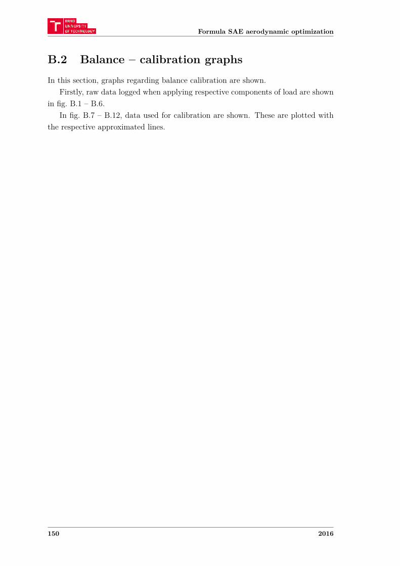
Formula SAE aerodynamic optimization
B.2 Balance – calibration graphsIn this section, graphs regarding balance calibration are shown.
Firstly, raw data logged when applying respective components of load are shownin fig. B.1 – B.6.
In fig. B.7 – B.12, data used for calibration are shown. These are plotted withthe respective approximated lines.
150 2016
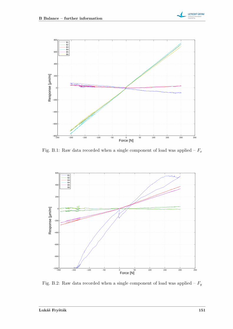
B Balance – further information
−250 −200 −150 −100 −50 0 50 100 150 200 250−800
−600
−400
−200
0
200
400
600
800
Force [N]
Res
pons
e [µ
m/m
]
B1B2B3B4B5B6
Fig. B.1: Raw data recorded when a single component of load was applied – 𝐹𝑥
−200 −150 −100 −50 0 50 100 150 200 250−1000
−800
−600
−400
−200
0
200
400
600
Force [N]
Res
pons
e [µ
m/m
]
B1B2B3B4B5B6
Fig. B.2: Raw data recorded when a single component of load was applied – 𝐹𝑦
Lukáš Fryšták 151
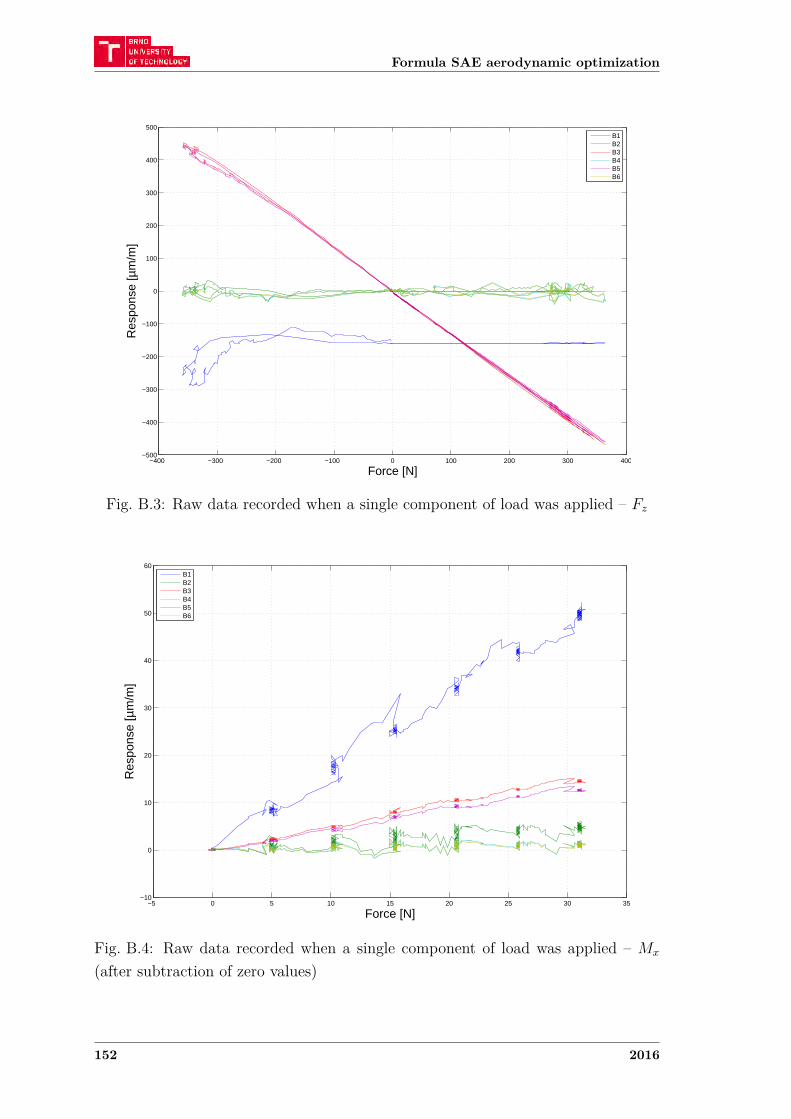
Formula SAE aerodynamic optimization
−400 −300 −200 −100 0 100 200 300 400−500
−400
−300
−200
−100
0
100
200
300
400
500
Force [N]
Res
pons
e [µ
m/m
]
B1B2B3B4B5B6
Fig. B.3: Raw data recorded when a single component of load was applied – 𝐹𝑧
−5 0 5 10 15 20 25 30 35−10
0
10
20
30
40
50
60
Force [N]
Res
pons
e [µ
m/m
]
B1B2B3B4B5B6
Fig. B.4: Raw data recorded when a single component of load was applied – 𝑀𝑥
(after subtraction of zero values)
152 2016
B Balance – further information
−10 0 10 20 30 40 50 60−80
−70
−60
−50
−40
−30
−20
−10
0
10
20
Force [N]
Res
pons
e [µ
m/m
]
B1B2B3B4B5B6
Fig. B.5: Raw data recorded when a single component of load was applied – 𝑀𝑦
(after subtraction of zero values)
−5 0 5 10 15 20 25 30 35−50
−40
−30
−20
−10
0
10
Force [N]
Res
pons
e [µ
m/m
]
B1B2B3B4B5B6
Fig. B.6: Raw data recorded when a single component of load was applied – 𝑀𝑧
(after subtraction of zero values)
Lukáš Fryšták 153
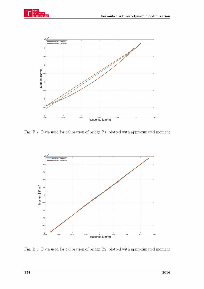
Formula SAE aerodynamic optimization
−1000 −800 −600 −400 −200 0 200−8
−7
−6
−5
−4
−3
−2
−1
0
1x 10
4
Mom
ent [
N/m
m]
Response [µm/m]
Moment − load cellMoment − calculated
Fig. B.7: Data used for calibration of bridge B1, plotted with approximated moment
−800 −600 −400 −200 0 200 400 600 800−1
−0.8
−0.6
−0.4
−0.2
0
0.2
0.4
0.6
0.8
1x 10
5
Mom
ent [
N/m
m]
Response [µm/m]
Moment − load cellMoment − calculated
Fig. B.8: Data used for calibration of bridge B2, plotted with approximated moment
154 2016
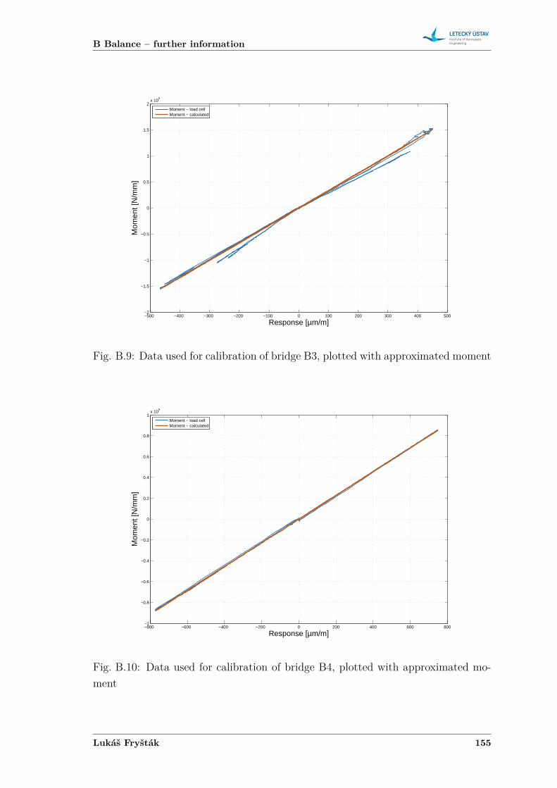
B Balance – further information
−500 −400 −300 −200 −100 0 100 200 300 400 500−2
−1.5
−1
−0.5
0
0.5
1
1.5
2x 10
5
Mom
ent [
N/m
m]
Response [µm/m]
Moment − load cellMoment − calculated
Fig. B.9: Data used for calibration of bridge B3, plotted with approximated moment
−800 −600 −400 −200 0 200 400 600 800−1
−0.8
−0.6
−0.4
−0.2
0
0.2
0.4
0.6
0.8
1x 10
5
Mom
ent [
N/m
m]
Response [µm/m]
Moment − load cellMoment − calculated
Fig. B.10: Data used for calibration of bridge B4, plotted with approximated mo-ment
Lukáš Fryšták 155
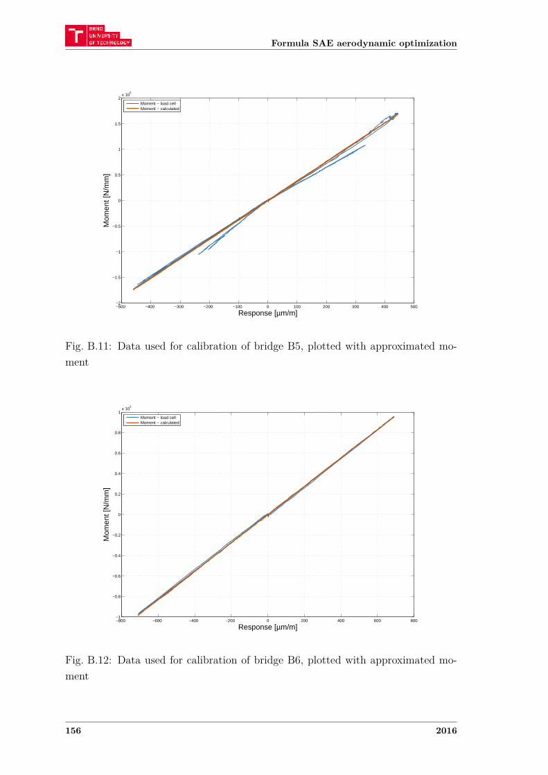
Formula SAE aerodynamic optimization
−500 −400 −300 −200 −100 0 100 200 300 400 500−2
−1.5
−1
−0.5
0
0.5
1
1.5
2x 10
5
Mom
ent [
N/m
m]
Response [µm/m]
Moment − load cellMoment − calculated
Fig. B.11: Data used for calibration of bridge B5, plotted with approximated mo-ment
−800 −600 −400 −200 0 200 400 600 800−1
−0.8
−0.6
−0.4
−0.2
0
0.2
0.4
0.6
0.8
1x 10
5
Mom
ent [
N/m
m]
Response [µm/m]
Moment − load cellMoment − calculated
Fig. B.12: Data used for calibration of bridge B6, plotted with approximated mo-ment
156 2016
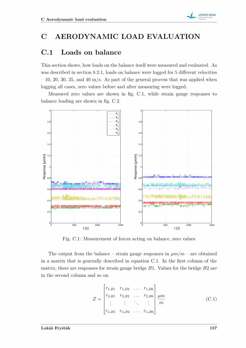
C Aerodynamic load evaluation
C AERODYNAMIC LOAD EVALUATION
C.1 Loads on balanceThis section shows, how loads on the balance itself were measured and evaluated. Aswas described in section 8.2.1, loads on balance were logged for 5 different velocities– 10, 20, 30, 35, and 40 m/s. As part of the general process that was applied whenlogging all cases, zero values before and after measuring were logged.
Measured zero values are shown in fig. C.1, while strain gauge responses tobalance loading are shown in fig. C.2.
0 500 1000 15000
0.2
0.4
0.6
0.8
1
1.2
1.4
1.6
1.8
2
t [1]
Res
pons
e [µ
m/m
]
B
1
B2
B3
B4
B5
B6
0 500 1000 15000
0.2
0.4
0.6
0.8
1
1.2
1.4
1.6
1.8
2
t [1]
Res
pons
e [µ
m/m
]
Fig. C.1: Measurement of forces acting on balance, zero values
The output from the balance – strain gauge responses in 𝜇𝑚/𝑚 – are obtainedin a matrix that is generally described in equation C.1. In the first column of thematrix, there are responses for strain gauge bridge 𝐵1. Values for the bridge 𝐵2 arein the second column and so on.
𝑍 =
⎡⎢⎢⎢⎢⎢⎢⎣𝑟1,𝐵1 𝑟1,𝐵2 . . . 𝑟1,𝐵6
𝑟2,𝐵1 𝑟2,𝐵2 . . . 𝑟2,𝐵6... ... . . . ...
𝑟𝑛,𝐵1 𝑟𝑛,𝐵2 . . . 𝑟𝑛,𝐵6
⎤⎥⎥⎥⎥⎥⎥⎦𝜇𝑚
𝑚(C.1)
Lukáš Fryšták 157
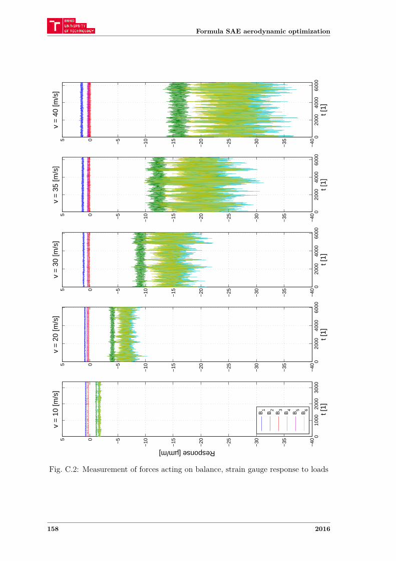
Formula SAE aerodynamic optimization
010
0020
0030
00−
40
−35
−30
−25
−20
−15
−10−
505v
= 1
0 [m
/s]
t [1]
Response [µm/m]
B1
B2
B3
B4
B5
B6
020
0040
0060
00−
40
−35
−30
−25
−20
−15
−10−
505v
= 2
0 [m
/s]
t [1]
020
0040
0060
00−
40
−35
−30
−25
−20
−15
−10−
505v
= 3
0 [m
/s]
t [1]
020
0040
0060
00−
40
−35
−30
−25
−20
−15
−10−
505v
= 3
5 [m
/s]
t [1]
020
0040
0060
00−
40
−35
−30
−25
−20
−15
−10−
505v
= 4
0 [m
/s]
t [1]
Fig. C.2: Measurement of forces acting on balance, strain gauge response to loads
158 2016
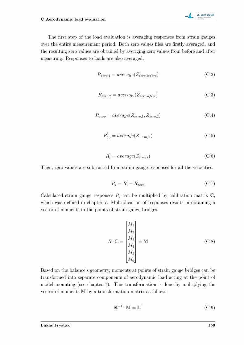
C Aerodynamic load evaluation
The first step of the load evaluation is averaging responses from strain gaugesover the entire measurement period. Both zero values files are firstly averaged, andthe resulting zero values are obtained by averiging zero values from before and aftermeasuring. Responses to loads are also averaged.
𝑅𝑧𝑒𝑟𝑜,1 = 𝑎𝑣𝑒𝑟𝑎𝑔𝑒(𝑍𝑧𝑒𝑟𝑜,𝑏𝑒𝑓𝑜𝑟𝑒) (C.2)
𝑅𝑧𝑒𝑟𝑜,2 = 𝑎𝑣𝑒𝑟𝑎𝑔𝑒(𝑍𝑧𝑒𝑟𝑜,𝑎𝑓𝑡𝑒𝑟) (C.3)
𝑅𝑧𝑒𝑟𝑜 = 𝑎𝑣𝑒𝑟𝑎𝑔𝑒(𝑍𝑧𝑒𝑟𝑜,1, 𝑍𝑧𝑒𝑟𝑜,2) (C.4)
𝑅′
10 = 𝑎𝑣𝑒𝑟𝑎𝑔𝑒(𝑍10 𝑚/𝑠) (C.5)
𝑅′
𝑖 = 𝑎𝑣𝑒𝑟𝑎𝑔𝑒(𝑍i 𝑚/𝑠) (C.6)
Then, zero values are subtracted from strain gauge responses for all the velocities.
𝑅𝑖 = 𝑅′
𝑖 − 𝑅𝑧𝑒𝑟𝑜 (C.7)
Calculated strain gauge responses 𝑅𝑖 can be multiplied by calibration matrix C,which was defined in chapter 7. Multiplication of responses results in obtaining avector of moments in the points of strain gauge bridges.
𝑅 · C =
⎡⎢⎢⎢⎢⎢⎢⎢⎢⎢⎢⎢⎣
𝑀1
𝑀2
𝑀3
𝑀4
𝑀5
𝑀6
⎤⎥⎥⎥⎥⎥⎥⎥⎥⎥⎥⎥⎦= M (C.8)
Based on the balance’s geometry, moments at points of strain gauge bridges can betransformed into separate components of aerodynamic load acting at the point ofmodel mounting (see chapter 7). This transformation is done by multiplying thevector of moments M by a transformation matrix as follows.
K−1 · M = L′ (C.9)
Lukáš Fryšták 159
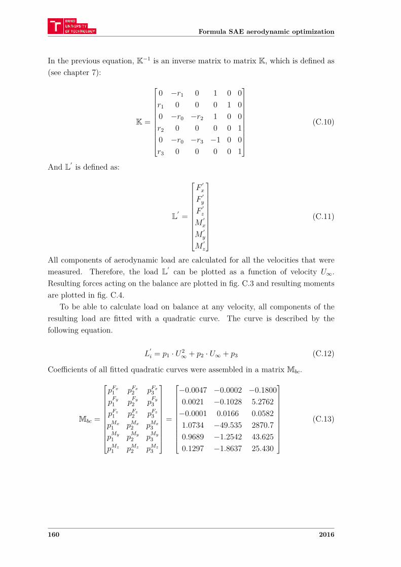
Formula SAE aerodynamic optimization
In the previous equation, K−1 is an inverse matrix to matrix K, which is defined as(see chapter 7):
K =
⎡⎢⎢⎢⎢⎢⎢⎢⎢⎢⎢⎢⎣
0 −𝑟1 0 1 0 0𝑟1 0 0 0 1 00 −𝑟0 −𝑟2 1 0 0𝑟2 0 0 0 0 10 −𝑟0 −𝑟3 −1 0 0𝑟3 0 0 0 0 1
⎤⎥⎥⎥⎥⎥⎥⎥⎥⎥⎥⎥⎦(C.10)
And L′ is defined as:
L′ =
⎡⎢⎢⎢⎢⎢⎢⎢⎢⎢⎢⎢⎣
𝐹′𝑥
𝐹′𝑦
𝐹′𝑧
𝑀′𝑥
𝑀′𝑦
𝑀′𝑧
⎤⎥⎥⎥⎥⎥⎥⎥⎥⎥⎥⎥⎦(C.11)
All components of aerodynamic load are calculated for all the velocities that weremeasured. Therefore, the load L′ can be plotted as a function of velocity 𝑈∞.Resulting forces acting on the balance are plotted in fig. C.3 and resulting momentsare plotted in fig. C.4.
To be able to calculate load on balance at any velocity, all components of theresulting load are fitted with a quadratic curve. The curve is described by thefollowing equation.
𝐿′
𝑖 = 𝑝1 · 𝑈2∞ + 𝑝2 · 𝑈∞ + 𝑝3 (C.12)
Coefficients of all fitted quadratic curves were assembled in a matrix M𝑏𝑐.
M𝑏𝑐 =
⎡⎢⎢⎢⎢⎢⎢⎢⎢⎢⎢⎢⎣
𝑝𝐹𝑥1 𝑝𝐹𝑥
2 𝑝𝐹𝑥3
𝑝𝐹𝑦
1 𝑝𝐹𝑦
2 𝑝𝐹𝑦
3
𝑝𝐹𝑧1 𝑝𝐹𝑧
2 𝑝𝐹𝑧3
𝑝𝑀𝑥1 𝑝𝑀𝑥
2 𝑝𝑀𝑥3
𝑝𝑀𝑦
1 𝑝𝑀𝑦
2 𝑝𝑀𝑦
3
𝑝𝑀𝑧1 𝑝𝑀𝑧
2 𝑝𝑀𝑧3
⎤⎥⎥⎥⎥⎥⎥⎥⎥⎥⎥⎥⎦=
⎡⎢⎢⎢⎢⎢⎢⎢⎢⎢⎢⎢⎣
−0.0047 −0.0002 −0.18000.0021 −0.1028 5.2762
−0.0001 0.0166 0.05821.0734 −49.535 2870.70.9689 −1.2542 43.6250.1297 −1.8637 25.430
⎤⎥⎥⎥⎥⎥⎥⎥⎥⎥⎥⎥⎦(C.13)
160 2016
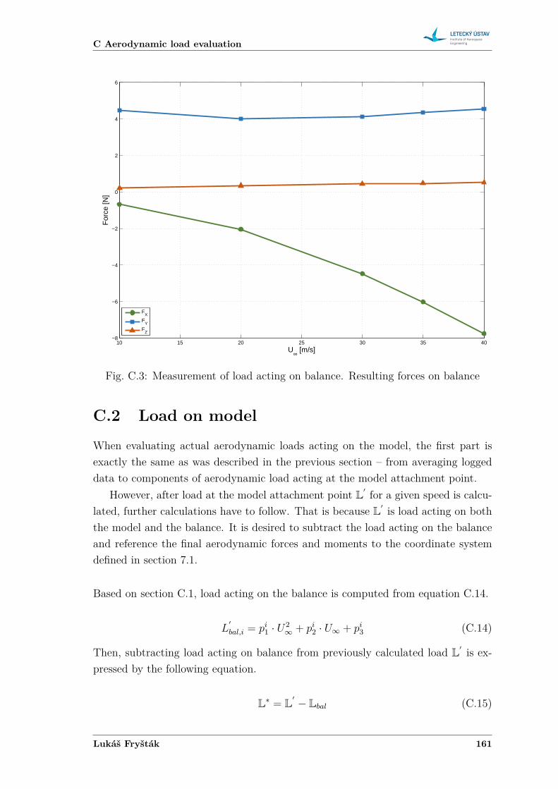
C Aerodynamic load evaluation
10 15 20 25 30 35 40−8
−6
−4
−2
0
2
4
6
U∞ [m/s]
For
ce [N
]
FX
FY
FZ
Fig. C.3: Measurement of load acting on balance. Resulting forces on balance
C.2 Load on model
When evaluating actual aerodynamic loads acting on the model, the first part isexactly the same as was described in the previous section – from averaging loggeddata to components of aerodynamic load acting at the model attachment point.
However, after load at the model attachment point L′ for a given speed is calcu-lated, further calculations have to follow. That is because L′ is load acting on boththe model and the balance. It is desired to subtract the load acting on the balanceand reference the final aerodynamic forces and moments to the coordinate systemdefined in section 7.1.
Based on section C.1, load acting on the balance is computed from equation C.14.
𝐿′
𝑏𝑎𝑙,𝑖 = 𝑝𝑖1 · 𝑈2
∞ + 𝑝𝑖2 · 𝑈∞ + 𝑝𝑖
3 (C.14)
Then, subtracting load acting on balance from previously calculated load L′ is ex-pressed by the following equation.
L* = L′ − L𝑏𝑎𝑙 (C.15)
Lukáš Fryšták 161

Formula SAE aerodynamic optimization
10 15 20 25 30 35 400
500
1000
1500
2000
2500
3000
U∞ [m/s]
Mom
ent [
N.m
m]
M
X
MY
MZ
Fig. C.4: Measurement of load acting on balance. Resulting moments on balance
Now, L* is vector of load components acting on the model (equation C.16), refer-enced to the coordinate system, which has origin point located on the balance at thepoint of model attachment. As was described before, it is customary to referencethe aerodynamic load to coordinate system defined in the section 7.1
L* =
⎡⎢⎢⎢⎢⎢⎢⎢⎢⎢⎢⎢⎣
𝐹 *𝑥
𝐹 *𝑦
𝐹 *𝑧
𝑀*𝑥
𝑀*𝑦
𝑀*𝑧
⎤⎥⎥⎥⎥⎥⎥⎥⎥⎥⎥⎥⎦(C.16)
The transformation between the two coordinate system is schematically depicted infig. C.5. Mathematically, it can be expressed by equation C.17.
L = T · L* (C.17)
It the equation above, T is transformation matrix derived from the geometrical
162 2016
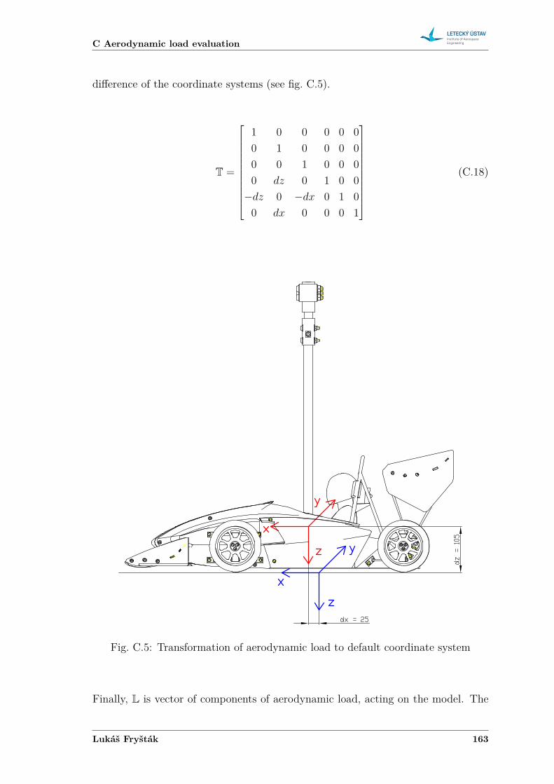
C Aerodynamic load evaluation
difference of the coordinate systems (see fig. C.5).
T =
⎡⎢⎢⎢⎢⎢⎢⎢⎢⎢⎢⎢⎣
1 0 0 0 0 00 1 0 0 0 00 0 1 0 0 00 𝑑𝑧 0 1 0 0
−𝑑𝑧 0 −𝑑𝑥 0 1 00 𝑑𝑥 0 0 0 1
⎤⎥⎥⎥⎥⎥⎥⎥⎥⎥⎥⎥⎦(C.18)
Fig. C.5: Transformation of aerodynamic load to default coordinate system
Finally, L is vector of components of aerodynamic load, acting on the model. The
Lukáš Fryšták 163
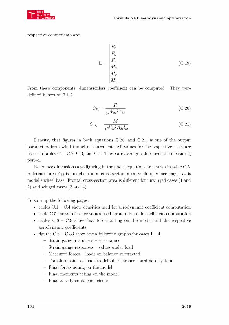
Formula SAE aerodynamic optimization
respective components are:
L =
⎡⎢⎢⎢⎢⎢⎢⎢⎢⎢⎢⎢⎣
𝐹𝑥
𝐹𝑦
𝐹𝑧
𝑀𝑥
𝑀𝑦
𝑀𝑧
⎤⎥⎥⎥⎥⎥⎥⎥⎥⎥⎥⎥⎦(C.19)
From these components, dimensionless coefficient can be computed. They weredefined in section 7.1.2.
𝐶𝐹𝑖= 𝐹𝑖
12𝜌𝑉∞2𝐴𝑀
(C.20)
𝐶𝑀𝑖= 𝑀𝑖
12𝜌𝑉∞2𝐴𝑀 𝑙𝑚
(C.21)
Density, that figures in both equations C.20, and C.21, is one of the outputparameters from wind tunnel measurement. All values for the respective cases arelisted in tables C.1, C.2, C.3, and C.4. These are average values over the measuringperiod.
Reference dimensions also figuring in the above equations are shown in table C.5.Reference area 𝐴𝑀 is model’s frontal cross-section area, while reference length 𝑙𝑚 ismodel’s wheel base. Frontal cross-section area is different for unwinged cases (1 and2) and winged cases (3 and 4).
To sum up the following pages:• tables C.1 – C.4 show densities used for aerodynamic coefficient computation• table C.5 shows reference values used for aerodynamic coefficient computation• tables C.6 – C.9 show final forces acting on the model and the respective
aerodynamic coefficients• figures C.6 – C.33 show seven following graphs for cases 1 – 4
– Strain gauge responses – zero values– Strain gauge responses – values under load– Measured forces – loads on balance subtracted– Transformation of loads to default reference coordinate system– Final forces acting on the model– Final moments acting on the model– Final aerodynamic coefficients
164 2016
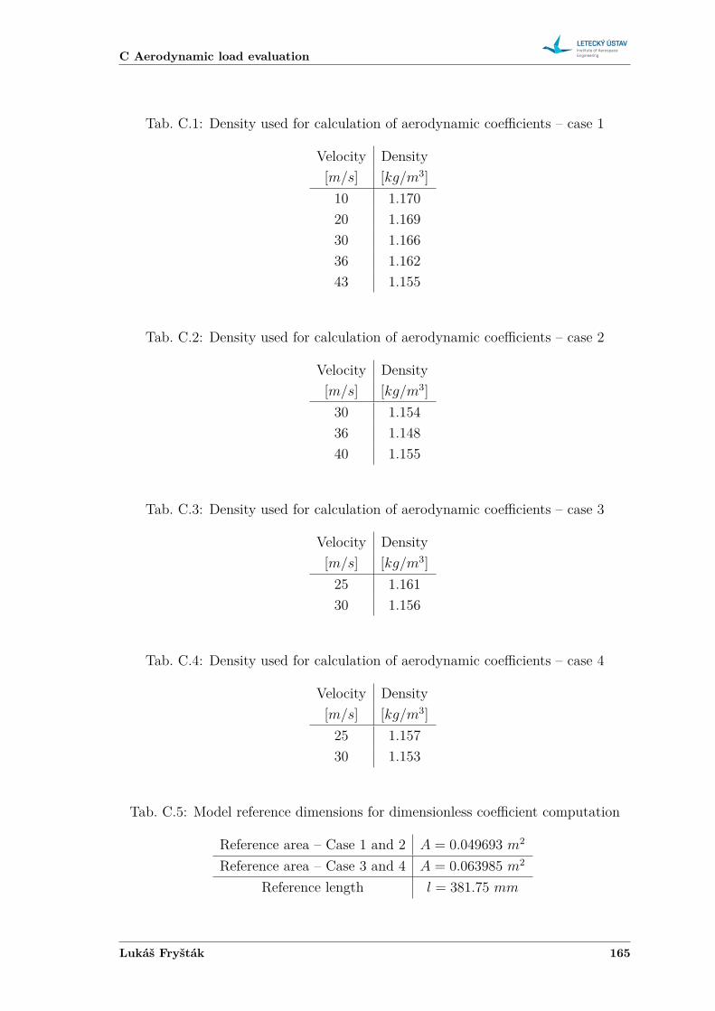
C Aerodynamic load evaluation
Tab. C.1: Density used for calculation of aerodynamic coefficients – case 1
Velocity Density[𝑚/𝑠] [𝑘𝑔/𝑚3]
10 1.17020 1.16930 1.16636 1.16243 1.155
Tab. C.2: Density used for calculation of aerodynamic coefficients – case 2
Velocity Density[𝑚/𝑠] [𝑘𝑔/𝑚3]
30 1.15436 1.14840 1.155
Tab. C.3: Density used for calculation of aerodynamic coefficients – case 3
Velocity Density[𝑚/𝑠] [𝑘𝑔/𝑚3]
25 1.16130 1.156
Tab. C.4: Density used for calculation of aerodynamic coefficients – case 4
Velocity Density[𝑚/𝑠] [𝑘𝑔/𝑚3]
25 1.15730 1.153
Tab. C.5: Model reference dimensions for dimensionless coefficient computation
Reference area – Case 1 and 2 𝐴 = 0.049693 𝑚2
Reference area – Case 3 and 4 𝐴 = 0.063985 𝑚2
Reference length 𝑙 = 381.75 𝑚𝑚
Lukáš Fryšták 165
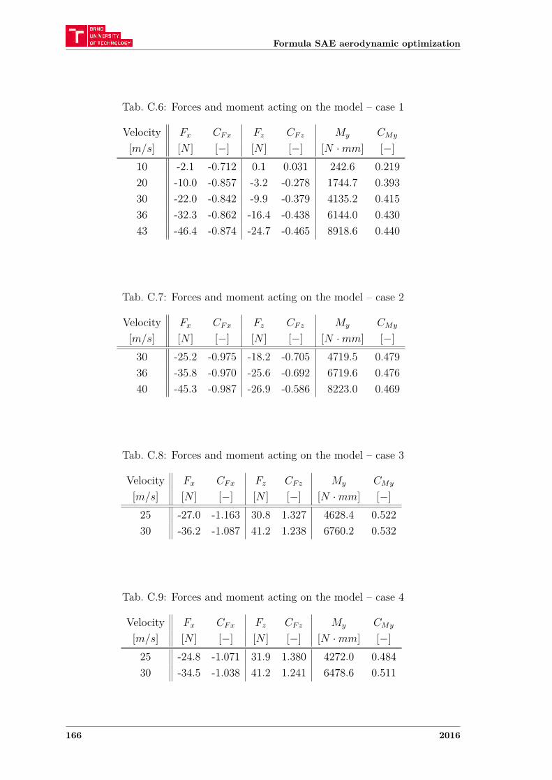
Formula SAE aerodynamic optimization
Tab. C.6: Forces and moment acting on the model – case 1
Velocity 𝐹𝑥 𝐶𝐹 𝑥 𝐹𝑧 𝐶𝐹 𝑧 𝑀𝑦 𝐶𝑀𝑦
[𝑚/𝑠] [𝑁 ] [−] [𝑁 ] [−] [𝑁 · 𝑚𝑚] [−]10 -2.1 -0.712 0.1 0.031 242.6 0.21920 -10.0 -0.857 -3.2 -0.278 1744.7 0.39330 -22.0 -0.842 -9.9 -0.379 4135.2 0.41536 -32.3 -0.862 -16.4 -0.438 6144.0 0.43043 -46.4 -0.874 -24.7 -0.465 8918.6 0.440
Tab. C.7: Forces and moment acting on the model – case 2
Velocity 𝐹𝑥 𝐶𝐹 𝑥 𝐹𝑧 𝐶𝐹 𝑧 𝑀𝑦 𝐶𝑀𝑦
[𝑚/𝑠] [𝑁 ] [−] [𝑁 ] [−] [𝑁 · 𝑚𝑚] [−]30 -25.2 -0.975 -18.2 -0.705 4719.5 0.47936 -35.8 -0.970 -25.6 -0.692 6719.6 0.47640 -45.3 -0.987 -26.9 -0.586 8223.0 0.469
Tab. C.8: Forces and moment acting on the model – case 3
Velocity 𝐹𝑥 𝐶𝐹 𝑥 𝐹𝑧 𝐶𝐹 𝑧 𝑀𝑦 𝐶𝑀𝑦
[𝑚/𝑠] [𝑁 ] [−] [𝑁 ] [−] [𝑁 · 𝑚𝑚] [−]25 -27.0 -1.163 30.8 1.327 4628.4 0.52230 -36.2 -1.087 41.2 1.238 6760.2 0.532
Tab. C.9: Forces and moment acting on the model – case 4
Velocity 𝐹𝑥 𝐶𝐹 𝑥 𝐹𝑧 𝐶𝐹 𝑧 𝑀𝑦 𝐶𝑀𝑦
[𝑚/𝑠] [𝑁 ] [−] [𝑁 ] [−] [𝑁 · 𝑚𝑚] [−]25 -24.8 -1.071 31.9 1.380 4272.0 0.48430 -34.5 -1.038 41.2 1.241 6478.6 0.511
166 2016
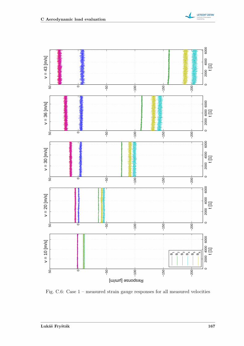
C Aerodynamic load evaluation
020
0040
0060
00
−20
0
−15
0
−10
0
−50050
v =
10
[m/s
]
t [1]
Response [µm/m]
B1
B2
B3
B4
B5
B6
020
0040
0060
00
−20
0
−15
0
−10
0
−50050
v =
20
[m/s
]
t [1]
020
0040
0060
00
−20
0
−15
0
−10
0
−50050
v =
30
[m/s
]
t [1]
020
0040
0060
00
−20
0
−15
0
−10
0
−50050
v =
36
[m/s
]
t [1]
020
0040
0060
00
−20
0
−15
0
−10
0
−50050
v =
43
[m/s
]
t [1]
Fig. C.6: Case 1 – measured strain gauge responses for all measured velocities
Lukáš Fryšták 167
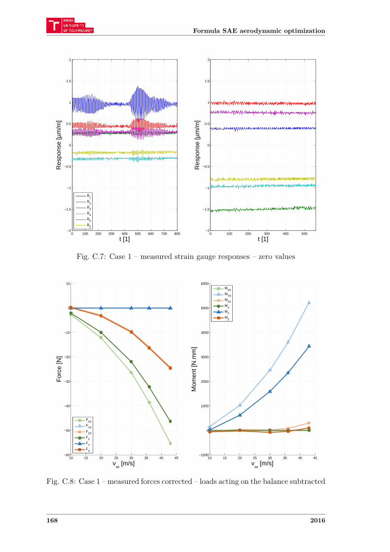
Formula SAE aerodynamic optimization
0 100 200 300 400 500 600 700 800−2
−1.5
−1
−0.5
0
0.5
1
1.5
2
t [1]
Res
pons
e [µ
m/m
]
B1
B2
B3
B4
B5
B6
0 100 200 300 400 500−2
−1.5
−1
−0.5
0
0.5
1
1.5
2
t [1]
Res
pons
e [µ
m/m
]
Fig. C.7: Case 1 – measured strain gauge responses – zero values
10 15 20 25 30 35 40 45−60
−50
−40
−30
−20
−10
0
10
v∞ [m/s]
For
ce [N
]
FX0
FY0
FZ0
FX
FY
FZ
10 15 20 25 30 35 40 45−1000
0
1000
2000
3000
4000
5000
6000
v∞ [m/s]
Mom
ent [
N.m
m]
M
X0
MY0
MZ0
MX
MY
MZ
Fig. C.8: Case 1 – measured forces corrected – loads acting on the balance subtracted
168 2016
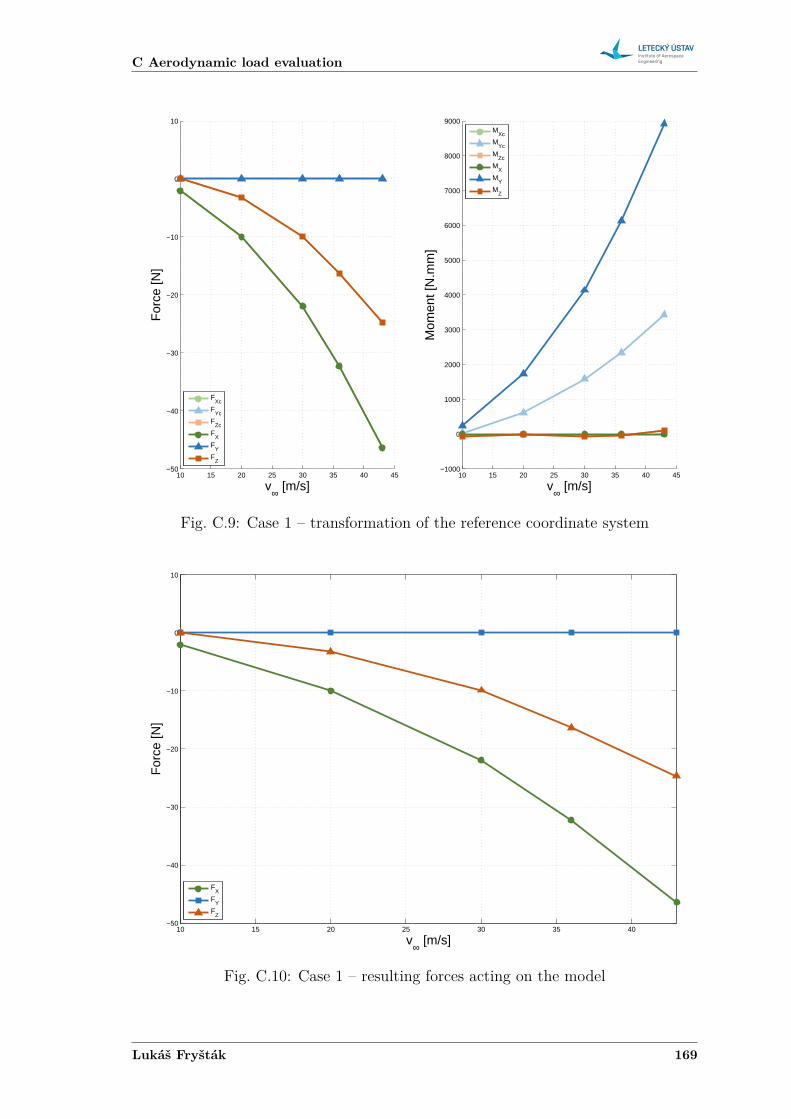
C Aerodynamic load evaluation
10 15 20 25 30 35 40 45−50
−40
−30
−20
−10
0
10
v∞ [m/s]
For
ce [N
]
FXc
FYc
FZc
FX
FY
FZ
10 15 20 25 30 35 40 45−1000
0
1000
2000
3000
4000
5000
6000
7000
8000
9000
v∞ [m/s]
Mom
ent [
N.m
m]
M
Xc
MYc
MZc
MX
MY
MZ
Fig. C.9: Case 1 – transformation of the reference coordinate system
10 15 20 25 30 35 40−50
−40
−30
−20
−10
0
10
v∞ [m/s]
For
ce [N
]
FX
FY
FZ
Fig. C.10: Case 1 – resulting forces acting on the model
Lukáš Fryšták 169
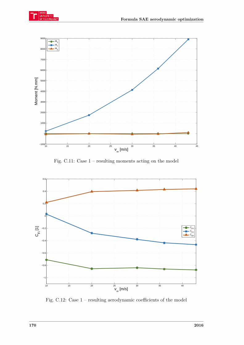
Formula SAE aerodynamic optimization
10 15 20 25 30 35 40 45−1000
0
1000
2000
3000
4000
5000
6000
7000
8000
9000
v∞ [m/s]
Mom
ent [
N.m
m]
M
X
MY
MZ
Fig. C.11: Case 1 – resulting moments acting on the model
10 15 20 25 30 35 40
−1
−0.8
−0.6
−0.4
−0.2
0
0.2
0.4
0.6
v∞ [m/s]
CF
i [1]
CFX
CFZ
CMY
Fig. C.12: Case 1 – resulting aerodynamic coefficients of the model
170 2016
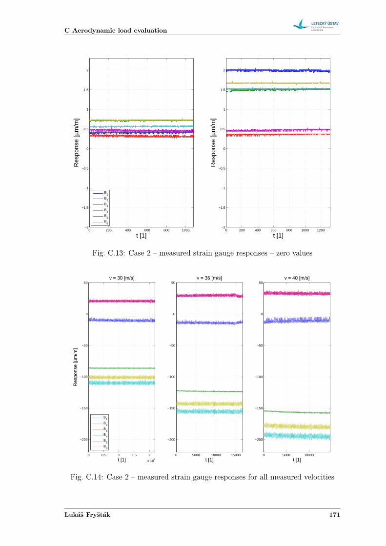
C Aerodynamic load evaluation
0 200 400 600 800 1000−2
−1.5
−1
−0.5
0
0.5
1
1.5
2
t [1]
Res
pons
e [µ
m/m
]
B1
B2
B3
B4
B5
B6
0 200 400 600 800 1000 1200−2
−1.5
−1
−0.5
0
0.5
1
1.5
2
t [1]
Res
pons
e [µ
m/m
]
Fig. C.13: Case 2 – measured strain gauge responses – zero values
0 0.5 1 1.5 2
x 104
−200
−150
−100
−50
0
50v = 30 [m/s]
t [1]
Res
pons
e [µ
m/m
]
B1
B2
B3
B4
B5
B6
0 5000 10000 15000
−200
−150
−100
−50
0
50v = 36 [m/s]
t [1]0 5000 10000
−200
−150
−100
−50
0
50v = 40 [m/s]
t [1]
Fig. C.14: Case 2 – measured strain gauge responses for all measured velocities
Lukáš Fryšták 171
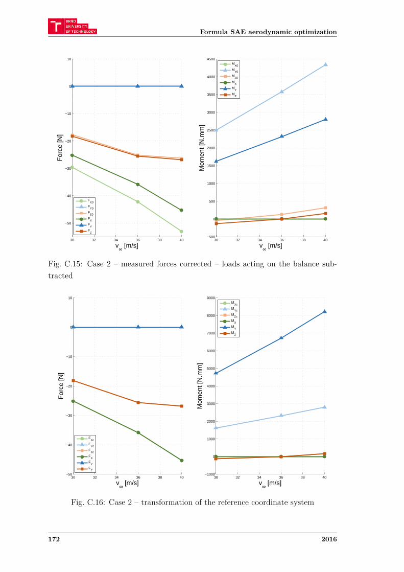
Formula SAE aerodynamic optimization
30 32 34 36 38 40
−50
−40
−30
−20
−10
0
10
v∞ [m/s]
For
ce [N
]
FX0
FY0
FZ0
FX
FY
FZ
30 32 34 36 38 40−500
0
500
1000
1500
2000
2500
3000
3500
4000
4500
v∞ [m/s]
Mom
ent [
N.m
m]
M
X0
MY0
MZ0
MX
MY
MZ
Fig. C.15: Case 2 – measured forces corrected – loads acting on the balance sub-tracted
30 32 34 36 38 40−50
−40
−30
−20
−10
0
10
v∞ [m/s]
For
ce [N
]
FXc
FYc
FZc
FX
FY
FZ
30 32 34 36 38 40−1000
0
1000
2000
3000
4000
5000
6000
7000
8000
9000
v∞ [m/s]
Mom
ent [
N.m
m]
M
Xc
MYc
MZc
MX
MY
MZ
Fig. C.16: Case 2 – transformation of the reference coordinate system
172 2016
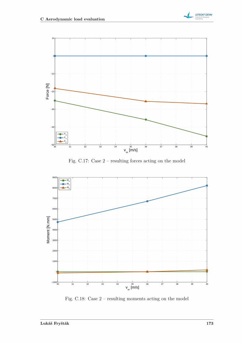
C Aerodynamic load evaluation
30 31 32 33 34 35 36 37 38 39 40−50
−40
−30
−20
−10
0
10
v∞ [m/s]
For
ce [N
]
FX
FY
FZ
Fig. C.17: Case 2 – resulting forces acting on the model
30 31 32 33 34 35 36 37 38 39 40−1000
0
1000
2000
3000
4000
5000
6000
7000
8000
9000
v∞ [m/s]
Mom
ent [
N.m
m]
M
X
MY
MZ
Fig. C.18: Case 2 – resulting moments acting on the model
Lukáš Fryšták 173
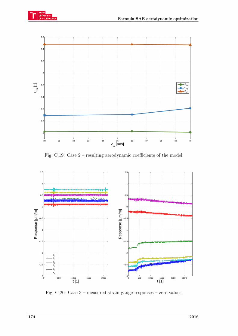
Formula SAE aerodynamic optimization
30 31 32 33 34 35 36 37 38 39 40
−1
−0.8
−0.6
−0.4
−0.2
0
0.2
0.4
0.6
v∞ [m/s]
CF
i [1]
CFX
CFZ
CMY
Fig. C.19: Case 2 – resulting aerodynamic coefficients of the model
0 500 1000 1500 2000−3
−2.5
−2
−1.5
−1
−0.5
0
0.5
1
1.5
t [1]
Res
pons
e [µ
m/m
]
B1
B2
B3
B4
B5
B6
0 500 1000 1500 2000 2500−3
−2.5
−2
−1.5
−1
−0.5
0
0.5
1
1.5
t [1]
Res
pons
e [µ
m/m
]
Fig. C.20: Case 3 – measured strain gauge responses – zero values
174 2016
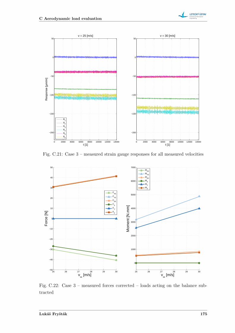
C Aerodynamic load evaluation
0 2000 4000 6000 8000 10000 12000 14000
−200
−150
−100
−50
0
50v = 25 [m/s]
t [1]
Res
pons
e [µ
m/m
]
B1
B2
B3
B4
B5
B6
0 2000 4000 6000 8000 10000 12000 14000
−200
−150
−100
−50
0
50v = 30 [m/s]
t [1]
Fig. C.21: Case 3 – measured strain gauge responses for all measured velocities
25 26 27 28 29 30−50
−40
−30
−20
−10
0
10
20
30
40
50
v∞ [m/s]
For
ce [N
]
FX0
FY0
FZ0
FX
FY
FZ
25 26 27 28 29 30
0
1000
2000
3000
4000
5000
6000
7000
v∞ [m/s]
Mom
ent [
N.m
m]
M
X0
MY0
MZ0
MX
MY
MZ
Fig. C.22: Case 3 – measured forces corrected – loads acting on the balance sub-tracted
Lukáš Fryšták 175
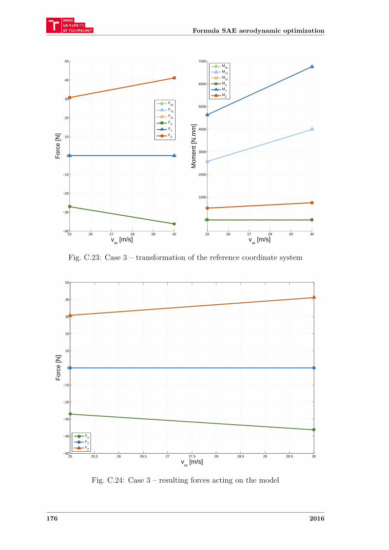
Formula SAE aerodynamic optimization
25 26 27 28 29 30−40
−30
−20
−10
0
10
20
30
40
50
v∞ [m/s]
For
ce [N
]
FXc
FYc
FZc
FX
FY
FZ
25 26 27 28 29 30
0
1000
2000
3000
4000
5000
6000
7000
v∞ [m/s]
Mom
ent [
N.m
m]
M
Xc
MYc
MZc
MX
MY
MZ
Fig. C.23: Case 3 – transformation of the reference coordinate system
25 25.5 26 26.5 27 27.5 28 28.5 29 29.5 30−50
−40
−30
−20
−10
0
10
20
30
40
50
v∞ [m/s]
For
ce [N
]
FX
FY
FZ
Fig. C.24: Case 3 – resulting forces acting on the model
176 2016
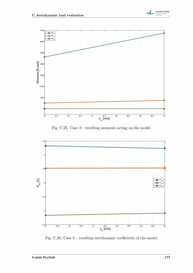
C Aerodynamic load evaluation
25 25.5 26 26.5 27 27.5 28 28.5 29 29.5 30
0
1000
2000
3000
4000
5000
6000
7000
v∞ [m/s]
Mom
ent [
N.m
m]
M
X
MY
MZ
Fig. C.25: Case 3 – resulting moments acting on the model
25 25.5 26 26.5 27 27.5 28 28.5 29 29.5 30−1.5
−1
−0.5
0
0.5
1
1.5
v∞ [m/s]
CF
i [1]
CFX
CFZ
CMY
Fig. C.26: Case 3 – resulting aerodynamic coefficients of the model
Lukáš Fryšták 177
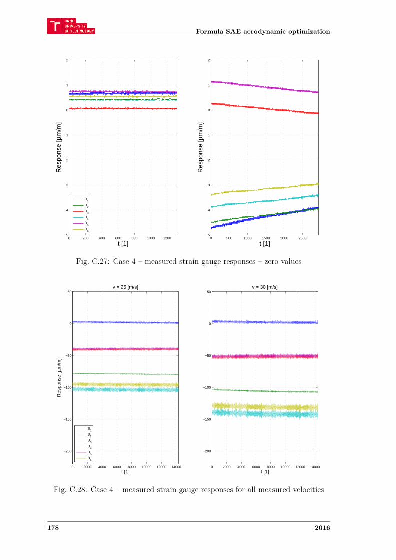
Formula SAE aerodynamic optimization
0 200 400 600 800 1000 1200−5
−4
−3
−2
−1
0
1
2
t [1]
Res
pons
e [µ
m/m
]
B1
B2
B3
B4
B5
B6
0 500 1000 1500 2000 2500−5
−4
−3
−2
−1
0
1
2
t [1]
Res
pons
e [µ
m/m
]
Fig. C.27: Case 4 – measured strain gauge responses – zero values
0 2000 4000 6000 8000 10000 12000 14000
−200
−150
−100
−50
0
50v = 25 [m/s]
t [1]
Res
pons
e [µ
m/m
]
B1
B2
B3
B4
B5
B6
0 2000 4000 6000 8000 10000 12000 14000
−200
−150
−100
−50
0
50v = 30 [m/s]
t [1]
Fig. C.28: Case 4 – measured strain gauge responses for all measured velocities
178 2016
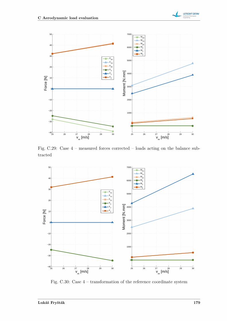
C Aerodynamic load evaluation
25 26 27 28 29 30−40
−30
−20
−10
0
10
20
30
40
50
v∞ [m/s]
For
ce [N
]
FX0
FY0
FZ0
FX
FY
FZ
25 26 27 28 29 30
0
1000
2000
3000
4000
5000
6000
7000
v∞ [m/s]
Mom
ent [
N.m
m]
M
X0
MY0
MZ0
MX
MY
MZ
Fig. C.29: Case 4 – measured forces corrected – loads acting on the balance sub-tracted
25 26 27 28 29 30−40
−30
−20
−10
0
10
20
30
40
50
v∞ [m/s]
For
ce [N
]
FXc
FYc
FZc
FX
FY
FZ
25 26 27 28 29 30
0
1000
2000
3000
4000
5000
6000
7000
v∞ [m/s]
Mom
ent [
N.m
m]
M
Xc
MYc
MZc
MX
MY
MZ
Fig. C.30: Case 4 – transformation of the reference coordinate system
Lukáš Fryšták 179

Formula SAE aerodynamic optimization
25 25.5 26 26.5 27 27.5 28 28.5 29 29.5 30−50
−40
−30
−20
−10
0
10
20
30
40
50
v∞ [m/s]
For
ce [N
]
FX
FY
FZ
Fig. C.31: Case 4 – resulting forces acting on the model
25 25.5 26 26.5 27 27.5 28 28.5 29 29.5 30
0
1000
2000
3000
4000
5000
6000
7000
v∞ [m/s]
Mom
ent [
N.m
m]
M
X
MY
MZ
Fig. C.32: Case 4 – resulting moments acting on the model
180 2016
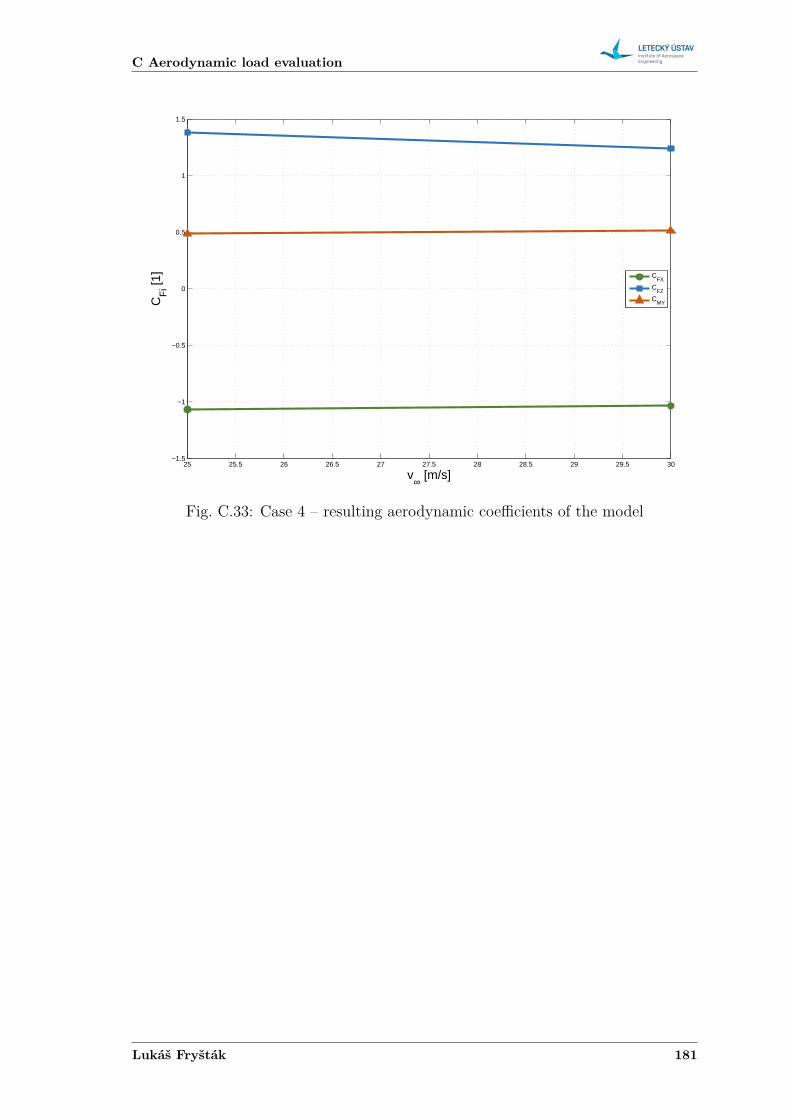
C Aerodynamic load evaluation
25 25.5 26 26.5 27 27.5 28 28.5 29 29.5 30−1.5
−1
−0.5
0
0.5
1
1.5
v∞ [m/s]
CF
i [1]
CFX
CFZ
CMY
Fig. C.33: Case 4 – resulting aerodynamic coefficients of the model
Lukáš Fryšták 181