deep generative models for natural language processing
TRANSCRIPT

Deep Generative Models
for Natural Language Processing
Yishu Miao
St Hugh’s College
University of Oxford
A thesis submitted for the degree of
Doctor of Philosophy
Michaelmas 2017

This thesis is dedicated to
my parents
for their persistent, unequivocal support
Acknowledgements
I am very grateful to many people at this point. My biggest gratitude certainlygoes to my supervisor Prof. Phil Blunsom, for advising me through my DPhilstudies. No matter how excited, agitated or helpless I was before I enteredhis office, there will be his sober voice waiting for me and encouraging me“sure go for it”. He usually describes his cool ideas with his unique calmnessand patience, which dispels the clouds and helps me see the key points behindeverything. I have learned so much from him, not only the way to carry outresearch work, but also the views on thinking and learning. Thus most of theideas related to my thesis were born in Phil’s office. I sincerely appreciate hishelp and supervision.
Second, I’d like to thank my managers Dani Yogatama and Edward Grefenstettefor hosting my internships at DeepMind in the years of 2017 and 2016, which arethe great memories that I will always remember. Many thanks to Wang Lingand other fellows in the NLP group, who shared so much their experiences withme (on research, engineering and also gaming), and eventually became my goodfriends. Thanks Karl Hermann for giving me great advice from time to time.Specifically, I want to thank Chris Dyer for helping me so much on organisingmy research proposals and presentations. He is always able to pinpoint outthe emphasis by a few words and share his comments at anytime. I believeeveryone around Chris is ready to learn from his passionate and professionalminds.
Next, I want to thank my colleagues in ML/CLG research group. I had a greatoffice shared with Jan Buys before we moved to the new one. I really enjoyedthe reading group for “deep learning beginners” held with Lei Yu and PengyuWang, and the nights we rushed for deadlines together. I also want to thankProf. Nando de Freitas, who gave me valuable comments on my thesis andeven helped me check every equation I listed in my reports. I always admire hispatience, enthusasm and meticulosity on research. In addition, I’d like to thankTsung-Hsien Wen from Cambridge for the great collaboration on the dialoguemodels.
I also want to thank my friends in Oxford, for all of the hotpot parties, beers andDotA games. No matter what ups and downs happened in my life or work, theywill always be there holding my back. I’m thankful to every one of them. Manythanks to my girlfriend for being with me through the bumpy thesis writingperiod, and my parents for their persistent and unequivocal support. I willalways miss the “Australian snakes” lying in the basement of CS departmentand the days I spent with them.
Last, many thanks to Prof. Yee Whye Teh and Prof. Noah Smith for being myexaminers and providing me lots of valuable comments to improve the thesis.
Abstract
Deep generative models are essential to Natural Language Processing (NLP)due to their outstanding ability to use unlabelled data, to incorporate abun-dant linguistic features, and to learn interpretable dependencies among data.As the structure becomes deeper and more complex, having an effective andefficient inference method becomes increasingly important. In this thesis, neu-ral variational inference is applied to carry out inference for deep generativemodels. While traditional variational methods derive an analytic approxima-tion for the intractable distributions over latent variables, here we construct aninference network conditioned on the discrete text input to provide the vari-ational distribution. The powerful neural networks are able to approximatecomplicated non-linear distributions and grant the possibilities for more inter-esting and complicated generative models. Therefore, we develop the potentialof neural variational inference and apply it to a variety of models for NLP withcontinuous or discrete latent variables.
This thesis is divided into three parts. Part I introduces a generic variationalinference framework for generative and conditional models of text. For con-tinuous or discrete latent variables, we apply a continuous reparameterisationtrick or the REINFORCE algorithm to build low-variance gradient estima-tors. To further explore Bayesian non-parametrics in deep neural networks,we propose a family of neural networks that parameterise categorical distribu-tions with continuous latent variables. Using the stick-breaking construction,an unbounded categorical distribution is incorporated into our deep generativemodels which can be optimised by stochastic gradient back-propagation with acontinuous reparameterisation.
Part II explores continuous latent variable models for NLP. Chapter 3discusses the Neural Variational Document Model (NVDM): an unsupervisedgenerative model of text which aims to extract a continuous semantic latentvariable for each document. In Chapter 4, the neural topic models modifythe neural document models by parameterising categorical distributions withcontinuous latent variables, where the topics are explicitly modelled by dis-crete latent variables. The models are further extended to neural unboundedtopic models with the help of stick-breaking construction, and a truncation-freevariational inference method is proposed based on a Recurrent Stick-breakingconstruction (RSB). Chapter 5 describes the Neural Answer Selection Model(NASM) for learning a latent stochastic attention mechanism to model thesemantics of question-answer pairs and predict their relatedness.
Part III discusses discrete latent variable models. Chapter 6 introduceslatent sentence compression models. The Auto-encoding Sentence Compression
Model (ASC), as a discrete variational auto-encoder, generates a sentence bya sequence of discrete latent variables representing explicit words. The ForcedAttention Sentence Compression Model (FSC) incorporates a combined pointernetwork biased towards the usage of words from source sentence, which signif-icantly improves the performance when jointly trained with the ASC model ina semi-supervised learning fashion. Chapter 7 describes the Latent IntentionDialogue Models (LIDM) that employ a discrete latent variable to learn under-lying dialogue intentions. Additionally, the latent intentions can be interpretedas actions guiding the generation of machine responses, which could be furtherrefined autonomously by reinforcement learning.
Finally, Chapter 8 summarizes our findings and directions for future work.
5
Contents
1 Introduction 2
1.1 Learning from Language . . . . . . . . . . . . . . . . . . . . . . . . . 2
1.2 Deep Generative Models . . . . . . . . . . . . . . . . . . . . . . . . . 3
1.3 Contributions . . . . . . . . . . . . . . . . . . . . . . . . . . . . . . . 5
1.4 Thesis Structure . . . . . . . . . . . . . . . . . . . . . . . . . . . . . . 7
I Neural Variational Inference 10
2 Neural Variational Inference 11
2.1 Continuous Latent Variables . . . . . . . . . . . . . . . . . . . . . . . 12
2.1.1 A Neural Variational Inference Framework . . . . . . . . . . . 12
2.1.2 Location Reparameterisable Distributions . . . . . . . . . . . 14
2.2 Discrete Latent Variables . . . . . . . . . . . . . . . . . . . . . . . . . 15
2.2.1 REINFORCE Algorithm . . . . . . . . . . . . . . . . . . . . . 15
2.2.2 Control Variates . . . . . . . . . . . . . . . . . . . . . . . . . 16
2.2.3 Advanced Sampling Schemes . . . . . . . . . . . . . . . . . . . 18
2.3 Parameterising Categorical Distribution . . . . . . . . . . . . . . . . . 18
2.3.1 Gaussian Softmax Construction . . . . . . . . . . . . . . . . . 19
2.3.2 Gaussian Stick-breaking Construction . . . . . . . . . . . . . . 19
2.3.3 Recurrent Stick-breaking Construction . . . . . . . . . . . . . 21
2.4 Summary . . . . . . . . . . . . . . . . . . . . . . . . . . . . . . . . . 22
II Continuous Latent Variable Models 24
3 Neural Document Models 25
3.1 Introduction . . . . . . . . . . . . . . . . . . . . . . . . . . . . . . . . 25
3.2 Neural Variational Document Model (NVDM) . . . . . . . . . . . . . 27
i
3.3 Experiments . . . . . . . . . . . . . . . . . . . . . . . . . . . . . . . . 28
3.3.1 Dataset & Setup . . . . . . . . . . . . . . . . . . . . . . . . . 28
3.3.2 Evaluation on Perplexity . . . . . . . . . . . . . . . . . . . . . 29
3.3.3 Interpreting Document Semantics . . . . . . . . . . . . . . . . 30
3.4 Summary . . . . . . . . . . . . . . . . . . . . . . . . . . . . . . . . . 32
4 Neural Topic Models 33
4.1 Introduction . . . . . . . . . . . . . . . . . . . . . . . . . . . . . . . . 33
4.2 Neural Finite Topic Model . . . . . . . . . . . . . . . . . . . . . . . . 34
4.2.1 Parameterising the Document-Topic Distribution . . . . . . . 35
4.2.2 Parameterising the Topic-Word Distribution . . . . . . . . . . 36
4.2.3 Integrating out Latent Topics . . . . . . . . . . . . . . . . . . 37
4.2.4 Topic Models vs. Document Models . . . . . . . . . . . . . . . 38
4.2.5 Topic Diversity . . . . . . . . . . . . . . . . . . . . . . . . . . 39
4.3 Neural Unbounded Topic Model . . . . . . . . . . . . . . . . . . . . . 39
4.3.1 Unbounded Topics . . . . . . . . . . . . . . . . . . . . . . . . 40
4.3.2 Truncation-free Neural Variational Inference . . . . . . . . . . 40
4.4 Experiments . . . . . . . . . . . . . . . . . . . . . . . . . . . . . . . . 42
4.5 Summary . . . . . . . . . . . . . . . . . . . . . . . . . . . . . . . . . 47
5 Neural Answer Selection Model 49
5.1 Introduction . . . . . . . . . . . . . . . . . . . . . . . . . . . . . . . . 49
5.2 Neural Answer Selection Model (NASM) . . . . . . . . . . . . . . . . 50
5.3 Experiments . . . . . . . . . . . . . . . . . . . . . . . . . . . . . . . . 53
5.3.1 Dataset & Setup . . . . . . . . . . . . . . . . . . . . . . . . . 53
5.3.2 Experimental Results . . . . . . . . . . . . . . . . . . . . . . . 55
5.3.3 Discussion . . . . . . . . . . . . . . . . . . . . . . . . . . . . . 56
5.4 Summary . . . . . . . . . . . . . . . . . . . . . . . . . . . . . . . . . 57
III Discrete Latent Variable Models 58
6 Latent Sentence Compression Models 59
6.1 Introduction . . . . . . . . . . . . . . . . . . . . . . . . . . . . . . . . 59
6.2 Related Work . . . . . . . . . . . . . . . . . . . . . . . . . . . . . . . 61
6.3 Auto-encoding Sentence Compression Model (ASC) . . . . . . . . . . 62
6.3.1 Compression . . . . . . . . . . . . . . . . . . . . . . . . . . . . 63
6.3.2 Reconstruction . . . . . . . . . . . . . . . . . . . . . . . . . . 64
ii
6.3.3 Inference . . . . . . . . . . . . . . . . . . . . . . . . . . . . . . 65
6.4 Forced Attention Sentence Compression Model (FSC) . . . . . . . . . 66
6.4.1 Semi-supervised Learning . . . . . . . . . . . . . . . . . . . . 69
6.4.2 Variance Reduction . . . . . . . . . . . . . . . . . . . . . . . . 69
6.5 Experiments . . . . . . . . . . . . . . . . . . . . . . . . . . . . . . . . 70
6.5.1 Extractive Summarisation . . . . . . . . . . . . . . . . . . . . 71
6.5.2 Abstractive Summarisation . . . . . . . . . . . . . . . . . . . 72
6.5.3 Discussion . . . . . . . . . . . . . . . . . . . . . . . . . . . . . 74
6.6 Summary . . . . . . . . . . . . . . . . . . . . . . . . . . . . . . . . . 75
7 Latent Intention Dialogue Models 77
7.1 Introduction . . . . . . . . . . . . . . . . . . . . . . . . . . . . . . . . 77
7.2 Related Work . . . . . . . . . . . . . . . . . . . . . . . . . . . . . . . 78
7.3 Latent Intention Dialogue Model (LIDM) . . . . . . . . . . . . . . . . 80
7.3.1 Model Description . . . . . . . . . . . . . . . . . . . . . . . . 80
7.3.2 Inference . . . . . . . . . . . . . . . . . . . . . . . . . . . . . . 82
7.3.3 Semi-Supervision . . . . . . . . . . . . . . . . . . . . . . . . . 84
7.3.4 Reinforcement Learning . . . . . . . . . . . . . . . . . . . . . 84
7.4 Experiments . . . . . . . . . . . . . . . . . . . . . . . . . . . . . . . . 85
7.4.1 Dataset & Setup . . . . . . . . . . . . . . . . . . . . . . . . . 85
7.4.2 Experimental Results . . . . . . . . . . . . . . . . . . . . . . . 87
7.5 Summary . . . . . . . . . . . . . . . . . . . . . . . . . . . . . . . . . 89
8 Conclusions and Further Work 90
A Details of Inference 93
A.1 Neural Variational Document Model . . . . . . . . . . . . . . . . . . 93
A.2 Neural Answer Selection Model . . . . . . . . . . . . . . . . . . . . . 94
B Discovered Topics 96
C Visualisation 98
D Sentence Compression Examples 99
E Goal Oriented Dialogue Examples 101
Bibliography 104
iii
List of Figures
2.1 Graphical Model of the Framework. . . . . . . . . . . . . . . . . . . . 13
2.2 Neural Stucture of GSM . . . . . . . . . . . . . . . . . . . . . . . . . 19
2.3 The Stick-breaking Construction. . . . . . . . . . . . . . . . . . . . . 20
2.4 Neural Stucture of GSB . . . . . . . . . . . . . . . . . . . . . . . . . 20
2.5 The unrolled RNN for breaking proportions η. . . . . . . . . . . . . . 22
2.6 Neural Stucture of RSB . . . . . . . . . . . . . . . . . . . . . . . . . 22
3.1 Neural Variational Document Model. . . . . . . . . . . . . . . . . . . 27
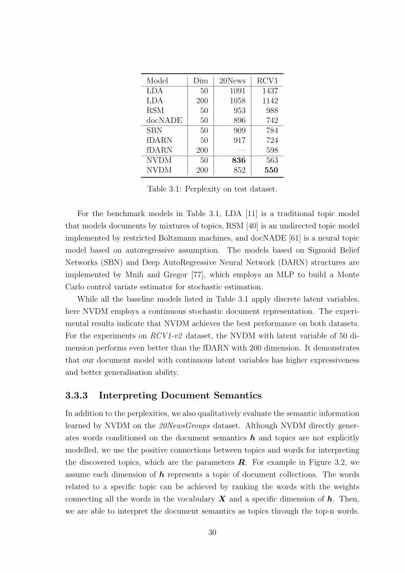
3.2 Interpreting document semantics as topics. . . . . . . . . . . . . . . . 31
4.1 Network structure of the inference model q(θ | d), and of the generative
model p(d | θ). . . . . . . . . . . . . . . . . . . . . . . . . . . . . . . . 37
4.2 The unrolled RNN that produces the topic-word distributions β. . . . 40
4.3 Corpus level topic probability distributions of GSM. . . . . . . . . . . 45
4.4 Corpus level topic probability distributions of GSB. . . . . . . . . . . 45
4.5 Test perplexities of the neural topic models with a varying maximum
number of topics on the 20NewsGroups dataset. . . . . . . . . . . . . 46
4.6 The convergence behavior of the truncation-free RSB model (RSB-TF)
with different initial active topics on 20NewsGroups. . . . . . . . . . 46
5.1 Neural Answer Selection Model. . . . . . . . . . . . . . . . . . . . . . 50
5.2 A visualisation of attention scores on answer sentences. . . . . . . . . 54
5.3 The standard deviations of MAP scores computed by running 10 NASM
models on WikiQA with different numbers of samples. . . . . . . . . 56
6.1 Auto-encoding Sentence Compression Model . . . . . . . . . . . . . . 62
6.2 Example of auto-encoding sentence compression. . . . . . . . . . . . . 63
6.3 Forced Attention Sentence Compression Model . . . . . . . . . . . . . 67
6.4 Example of forced-attention sentence compression. . . . . . . . . . . . 68
6.5 Perplexity on validation dataset. . . . . . . . . . . . . . . . . . . . . . 74
iv
7.1 LIDM for Goal-oriented Dialogue Modeling . . . . . . . . . . . . . . . 80
C.1 t-SNE projection of the estimated topic proportions of each document
(i.e. q(θ|d)) from 20NewsGroups. The vectors are learned by the GSM
model with 50 topics and each color represents one group from the 20
different groups of the dataset. . . . . . . . . . . . . . . . . . . . . . . 98
v
List of Tables
3.1 Perplexity on test dataset. . . . . . . . . . . . . . . . . . . . . . . . . 30
3.2 The topics learned by NVDM on 20News. . . . . . . . . . . . . . . . 31
3.3 The five nearest words in the semantic space. . . . . . . . . . . . . . 32
4.1 Perplexities of the topic models on the test datasets. . . . . . . . . . 43
4.2 Perplexities of document models on the test datasets. . . . . . . . . 43
4.3 Topic coherence on 20NewsGroups (higher is better). . . . . . . . . . 47
5.1 Statistics of QASent and WikiQA. Judgement denotes whether cor-
rectness was determined automatically or by human annotators. . . . 53
5.2 Results of our models (LSTM, LSTM + Att, NASM) in comparison
with other state of the art models on the QASent and WikiQA dataset. 54
6.1 Extractive Summarisation Performance. . . . . . . . . . . . . . . . . 71
6.2 Abstractive Summarisation Performance. . . . . . . . . . . . . . . . 72
6.3 Comparison on validation perplexity. . . . . . . . . . . . . . . . . . . 73
6.4 Comparison on test Rouge scores. . . . . . . . . . . . . . . . . . . . . 73
7.1 An example of the automatically labeled response seed set for semi-
supervised learning during variational inference. . . . . . . . . . . . . 86
7.2 Corpus-based Evaluation. . . . . . . . . . . . . . . . . . . . . . . . . 87
7.3 Human evaluation. The significance test is based on a two-tailed
student-t test, between NDM and LIDMs. . . . . . . . . . . . . . . . 88
B.1 Topics learned by GSM on 20NewsGroups dataset. . . . . . . . . . . 96
B.2 Topics learned by GSB on 20NewsGroups dataset. . . . . . . . . . . . 96
B.3 Topics learned by RSB on 20NewsGroups dataset. . . . . . . . . . . . 97
D.1 Examples of the compression sentences (Part I). . . . . . . . . . . . . 99
D.2 Examples of the compression sentences (Part II). . . . . . . . . . . . 100
vi
E.1 A sample dialogue from the LIDM, I=100 model, one exchange per
block. Each latent intention is shown by a tuple (index, probability),
followed by a decoded response. The sample dialogue was produced by
following the responses highlighted in bold. . . . . . . . . . . . . . . . 102
E.2 Two sample dialogues from the LIDM+RL, I=100 model, one exchange
per block. Comparing to Table E.1, the RL agent demonstrates a much
greedier behavior toward task success. This can be seen in block 2 &
block 4 in which the agent provides the address and phone number
even before the user asks. . . . . . . . . . . . . . . . . . . . . . . . . 103
vii
List of Related Publications
Yishu Miao, Lei Yu, Phil Blunsom. “Neural Variational Inference for Text Pro-
cessing”. In Proceedings of the 33rd International Conference on Machine Learn-
ing (ICML), 2016.
Yishu Miao, Phil Blunsom. “Language as a Latent Variable. Discrete Generative
Models for Sentence Compression”. In Proceedings of the 2016 Conference on
Empirical Methods in Natural Language Processing (EMNLP), 2016.
Tsung-Hsien Wen*, Yishu Miao*, Phil Blunsom, Steve J. Young. “Latent Inten-
tion Dialogue Models”. In Proceedings of the 34th International Conference on
Machine Learning (ICML), 2017. (*equal contribution)
Yishu Miao, Edward Grefenstette, Phil Blunsom. “Discovering Discrete Latent
Topics with Neural Variational Inference”. In Proceedings of the 34th Interna-
tional Conference on Machine Learning (ICML), 2017.
1
Chapter 1
Introduction
1.1 Learning from Language
Language is a complex system of communication. By speaking, reading, and writing
language we are able to communicate our intelligence with other people. It is natural
for human beings to learn and develop their language ability while using it in their
daily life, however, it is very challenging for a machine to learn both the underlying
complexities of a language system and the carried intelligence of a discourse at the
same time. Thus a lot of recent progress in Natural Language Processing (NLP) is
focused on employing large-scale of annotated corpora for solving specific problems,
for example machine translation, sentiment analysis, and linguistic analysis tasks
including parsing, part-of-speech tagging and named-entity-recognition. Especially
with the recent advances of deep learning, neural networks are widely used as dis-
criminative models to learn end-to-end systems specified for each different problem.
Whereas, due to the limitations of the existing labelled datasets, it is very difficult to
learn general knowledge and handle multiple different tasks at the same time. Hence,
to cope with the bottleneck we ought to explore the vast sea of unlabelled corpora
and teach the machine to learn from language by itself. Certainly, there is a long
way to go before we have an artificial general intelligence agent learning from lan-
guage, but to design unsupervised/semi-supervised models exploring unlabelled data
to further improve natural language understanding, natural language generation and
natural language grounding is a pressing necessity. The difficulty is how to introduce
inductive biases and proper priors to guide the models to learn on a mass of disor-
ganized textual corpora, and how to carry out effective and efficient inference for the
generative models.
This thesis discusses deep generative models that combine neural networks and
probabilistic models focused on unsupervised, semi-supervised or supervised learning
2
NLP tasks with small amounts of labelled data. With sufficient training data, neural
networks are able to fit complex distributions, as demonstrated by a variety of well-
developed discriminative models achieving state-of-the-art performance across many
fields. In contrast, deep generative models are more difficult to apply successfully due
to the fact that they are generally used in scenarios where labelled data is deficient or
inaccessible. Meanwhile, the deep neural structure of such generative models requires
more advanced inference methods to provide better gradient estimators. Therefore,
we choose neural variational inference as the major approach for inference in the deep
generative models proposed in this thesis.
What the chosen application scenarios have in common is that there are relatively
fewer labelled resources than the tasks well-explored by neural networks such as neural
machine translation. We demonstrate the effectiveness of deep generative models on
learning stochastic continuous representations of documents (document/topic mod-
elling), constructing discrete (sentence compression) or continuous (question answer
selection) representations of sentences, and modelling latent intentions in human ut-
terances (conversational dialogue). With the help of these neural models we are able
to better exploit the labelled/unlabelled data and to learn knowledge from language
directly.
1.2 Deep Generative Models
Probabilistic generative models underpin many successful applications within the field
of Natural Language Processing (NLP). Their popularity stems from their ability to
use unlabelled data effectively, to incorporate abundant linguistic features, and to
learn interpretable dependencies among data. However these successes are tempered
by the fact that as the structure of such generative models becomes deeper and more
complex, true Bayesian inference becomes intractable due to the high dimensional
integrals required. Hence, in this thesis, the neural variational inference approach
is applied to carry out inference in deep generative models. Instead of seeking an
analytic approximation, as in traditional variational Bayesian methods, neural vari-
ational inference directly applies neural networks to model the posterior probability.
Powerful neural networks are able to not only learn good representations, but also
approximate complicated non-linear distributions which affords the possibilities for
more interesting and complicated generative models applied in NLP. Generally, based
on the settings of the latent variables (continuous or discrete), we divide the models
into two folds: continuous generative models and discrete generative models.
3

For continuous latent variable models, an inference network is introduced to pa-
rameterise the latent distribution. Typically, a diagonal Gaussian is adopted as the
variational distribution, since the reparameterisation trick [84, 56] grants the abil-
ity to jointly update the inference networks and generative distributions by back-
propagating unbiased and low-variance gradients with a single sample from the vari-
ational distribution. For unsupervised learning, the models can be easily built in
the framework of variational auto-encoders, where the inference networks generate
powerful stochastic vector representations used for document modelling, topic mod-
elling and sentence modelling. For supervised learning, the inference networks are
able to be conditioned on all the observations and jointly updated with the model
parameters in a tight variational lower bound. Hence, with the help of the effective
amortised variational inference with Gaussian reparameterisation, the neural models
with continuous latent variables gain more capacity compared to the discriminative
counterparts.
For discrete latent variable models, instead, REINFORCE algorithm with con-
trol variates [77, 79] is employed due to the high variance issue of sampling-based
variational inference. Though the inference process becomes more complicated com-
pared to the continuous models, the discrete latent variables have more advantages
for developing the potential of deep neural networks. Generally, the introduction of
discrete latent variables allows for clustering, structure prediction and incorporating
an inductive bias into existing generative models. Moreover, discrete representations
have better interpretability and can be easily employed to incorporate labelled data
to carry out semi-supervised learning. In a different vein, the inference network can
also be considered as an agent and the samples are the actions made by the agent,
then the variational lower bound is the reward that provides the gradient to update
the inference networks and generative distributions. Hence, the connection between
neural variational inference and reinforcement learning would lead to the emergence
of a series of effective and interesting generative models that can be trained with only
a handful of labelled data.
In addition, there is a popular research direction in probabilistic models that has
been widely explored as Bayesian non-parametrics [103, 27]. Hence, in this thesis, we
also propose deep generative models with a stick-breaking construction to explore the
potential of non-parametrics in neural networks. By parameterising the categorical
distribution with a continuous latent variable, the generative model can be directly
trained by stochastic gradient back-propagation with continuous reparameterisation
in the neural variational inference. With the help of the recurrent stick-breaking
4

construction, a truncation-free algorithm can be applied to efficiently and effectively
carry out Bayesian non-parametric inference in a neural way.
1.3 Contributions
The contributions of this thesis can be summarised as following:
1. Generic Neural Variational Inference Framework for NLP. For both
continuous and discrete latent variable models for NLP, we propose a generic in-
ference framework – neural variational inference which constructs neural networks
conditioned on discrete text input to provide the variational distribution. We demon-
strate the effectiveness and efficiency of the framework by applying it to unsupervised
(neural variational document model), supervised (neural answer selection model) and
semi-supervised (auto-encoding sentence compression model) learning models. These
models are simple, expressive and can be trained efficiently with either the highly
scalable stochastic gradient back-propagation algorithm or the REINFORCE algo-
rithm with control variates. The neural variational framework can be generalised to
incorporate any type of neural networks e.g. multilayer perceptrons (MLP), convo-
lutional neural networks (CNN), and recurrent neural networks (RNN). The relevant
publication of this chapter is:
Yishu Miao, Lei Yu, Phil Blunsom. “Neural Variational Inference for Text Pro-
cessing”. In Proceedings of the 33rd International Conference on Machine Learn-
ing (ICML), 2016.
2. Discrete Representations of Language. Generally, the introduction of
discrete latent variables is motivated to improve clustering, structure prediction and
incorporate inductive biases into existing generative models. In deep neural networks,
they can also be used for modelling discrete interpretable representations other than
commonly applied continuous vector representations. Here, as language is naturally
discrete, we proposed a new perspective of learning language: modelling language
as a latent variable. A sequence of discrete latent variables (representing words)
are a employed to extract discrete representations of sentences which are language
as well. With the help of discrete variational auto-encoder, we are able to learn a
variable-length compact summary as the sentence compression. Integrated with a
combined pointer network model, we achieved good performance on both abstractive
and extractive sentence compression task. The relevant publication of this chapter is:
5
Yishu Miao, Phil Blunsom. “Language as a Latent Variable. Discrete Generative
Models for Sentence Compression”. In Proceedings of the 2016 Conference on
Empirical Methods in Natural Language Processing (EMNLP), 2016.
3. Bridging Generative Models and Reinforcement Learning. Learning
an end-to-end dialogue system is appealing but challenging because of insufficient
training data for goal-oriented dialogues results in over-fitting and produces less ef-
fective and scalable interactions. By introducing discrete latent variables into neural
dialogue systems we decompose the learning of language and the internal dialogue
decision-making, where a latent distribution as the policy network models an au-
tonomous decision-making agent for composing appropriate machine responses. In
variational inference, the generative model is updated by the learning signal from
the variational lower bound. While in reinforcement learning, the latent distribu-
tion as policy network is updated by the rewards from dialogue success and sentence
BLEU score. Hence, the latent variable bridges the different learning paradigms and
brings them together under the same framework, which allows the agent to directly
learn dialogue policies through interactions other than solely depending on supervised
sequence-to-sequence learning. The relevant publication of this chapter is:
Tsung-Hsien Wen*, Yishu Miao*, Phil Blunsom, Steve J. Young. “Latent Inten-
tion Dialogue Models”. In Proceedings of the 34th International Conference on
Machine Learning (ICML), 2017. (*equal contribution)
4. Bayesian Non-parametrics in Deep Neural Networks. To extend the
variational auto-encoder with Bayesian non-parametrics, we introduce a family of
neural networks for parameterising categorical distributions with continuous latent
variables, in which the parameterisation networks can be easily updated together
with the generative model by gradient back-propagation. More importantly, with
the help of a stick-breaking construction, we are free to choose the dimension of the
discrete latent space which yields to unbounded topics or vector representations for
learning documents or sentences. In addition, we propose a recurrent stick-breaking
construction for parameterising categorical distribution which allows truncation-free
variational inference so that we could dynamically choose the dimension of latent
space during the inference process. The relevant publication of this chapter is:
6
Yishu Miao, Edward Grefenstette, Phil Blunsom. “Discovering Discrete Latent
Topics with Neural Variational Inference”. In Proceedings of the 34th Interna-
tional Conference on Machine Learning (ICML), 2017.
1.4 Thesis Structure
This thesis is constructed into three different parts: Part I Neural Variational In-
ference, Part II Continuous Latent Variable Models and Part III Discrete Latent
Variable Models. Part I explains the main inference method applied in this thesis
which is neural variational inference including the continuous reparameterisation and
REINFORCE algorithms for both continuous and discrete latent variables. Part II
introduces the continuous latent variable models for NLP, including neural document
models, neural topic models and neural answer selection models. Part III discusses
the discrete latent variable models, which contains the latent sentence compression
models and latent intention dialogue models respectively. Abstracts of each chapters
are summarised as following:
Chapter 1 Introduction briefly summarises the intuitions about employing deep
generative models for NLP, the proposed continuous/discrete latent variable models
and their corresponding inference methods. The contributions and structure of the
thesis are also listed in this chapter.
Part I Neural Variational Inference
Chapter 2 Neural Variational Inference introduces a generic variational in-
ference framework for generative and conditional models of text, which is suitable for
both unsupervised and supervised learning tasks. For continuous or discrete latent
variables, we introduce the continuous reparameterisation trick or REINFORCE al-
gorithm with control variates to build low-variance gradient estimators. In addition,
we discuss the alternative location reparameterisable latent distributions for contin-
uous latent variables, and advanced sampling schemes for discrete latent variables.
To further explore Bayesian non-parametrics in deep neural networks, we propose a
families of neural networks that parameterise categorical distributions with continu-
ous latent variables, including the Gaussian softmax construction (GSM), Gaussian
stick-breaking construction (GSB) and recurrent stick-breaking construction (RSB).
Using these stick-breaking constructions, an unbounded categorical distribution is
7
able to be incorporated into the deep generative models, which can be easily updated
by stochastic gradient back-propagation with continuous reparameterisation.
Part II Continuous Latent Variable Models
Chapter 3 Neural Document Models discusses the neural variational docu-
ment model (NVDM), which is an unsupervised generative model of text aiming to
extract a continuous semantic latent variable for each document. This model can
be interpreted as a variational auto-encoder: an MLP encoder (inference network)
compresses the bag-of-words document representation into a continuous latent dis-
tribution, and a softmax decoder (generative model) reconstructs the document by
generating the words independently. A primary feature of NVDM is that each word
is generated directly from a dense continuous document representation instead of the
more common binary semantic vector.
Chapter 4 Neural Topic Models extend the neural document models to topic
models, where the ‘topics’ are modelled explicitly by parameterised categorical dis-
tributions with continuous latent variables. As the topic-word distribution can be
easily integrated out, we are able to directly apply continuous reparameterisation
trick for updating the inference networks. Moreover, the models are further extended
to neural unbounded topic models with the help of stick-breaking construction. In ad-
dition, we propose a truncation-free variational inference method using the recurrent
stick-breaking construction (RSB), where the categorical distribution is constructed
autoregressively by a recurrent neural network. Without pre-defining the number of
topics, the unbounded topic models are able to dynamically create new topics during
the inference process.
Chapter 5 Neural Answer Selection Models discuss supervised conditional
models which imbue LSTMs with a latent stochastic attention mechanism to model
the semantics of question-answer pairs and predict their relatedness. An attention
model is designed to focus on the phrases of an answer that are strongly connected
to the question semantics and is modelled by a latent distribution. This mechanism
allows the model to deal with the ambiguity inherent in the task and learns pair-
specific representations that are more effective at predicting answer matches, rather
than independent embeddings of question and answer sentences. Bayesian inference
provides a natural safeguard against overfitting, especially as the training sets avail-
able for this task are small. The experiments show that the LSTM with a latent
8
stochastic attention mechanism learns an effective attention model and outperforms
both previously published results, and our proposed strong non-stochastic attention
baselines.
Part III Discrete Latent Variable Models
Chapter 6 Latent Sentence Compression Models describes the applications
of discrete latent variable models on sentence compression and goal-oriented dialogue
systems. By introducing a sequence of discrete latent variables representing explicit
words, we are able to use language to model the discrete representations of sentences,
in which case the language is a latent variable that summarises meaning of the source
sentences. We construct this Auto-encoding Sentence Compression Model (ASC) in
the framework of variational auto-encoder, where the latent variables are discrete
rather than continuous. In order to further improve the performance of sentence
compression, we introduce a combined pointer network into the sequence-to-sequence
learning model, where it balances the probability of choosing a word from the source
sentence or generating a new word from the full vocabulary. The Forced Attention
Sentence Compression Model (FSC) can be trained together with ASC model in a
semi-supervised learning framework, and provide extra supervision as supplementary
to the unsupervised auto-encoding sentence compression. The models are able to be
applied to both extractive sentence summarisation and abstractive sentence summari-
sation.
Chapter 7 Latent Intention Dialogue Models introduces Latent Intention
Dialogue Models (LIDM) that employ a discrete latent variable to learn underlying
dialogue intentions in the framework of neural variational inference. Different from
the end-to-end discriminative models that directly learns to generate natural language
sentences as machine response, LIDM employs latent intentions as actions guiding the
generation of machine responses in the goal-oriented dialogue scenario. To further
improve the success rate of the dialogues, we incorporate semi-supervised learning
and reinforcement learning to refine the modelling of the latent distributions. The
experiments demonstrate the effectiveness of discrete latent variable models on learn-
ing goal-oriented dialogues, and the results outperform the published benchmarks on
both corpus-based evaluation and human evaluation.
Chapter 8 Conclusions and Further Work summarises the findings of this
thesis. We also discuss the works and directions to be explored in the future.
9

Part I
Neural Variational Inference
10
Chapter 2
Neural Variational Inference
Latent variable modelling is popular in many NLP problems, but it is non-trivial to
carry out effective and efficient inference for models with complex and deep structure.
True Bayesian inference becomes intractable due to the high dimensional integrals re-
quired. For example, Markov chain Monte Carlo (MCMC) [81, 1] and variational
inference [47, 2, 7] are the standard approaches for approximating these integrals.
However the computational cost of the former results in impractical training for the
large and deep neural networks which are now fashionable, and the latter is con-
ventionally confined due to the underestimation of posterior variance. The lack of
effective and efficient inference methods hinders our ability to create highly expressive
models of text, especially in the situation where the model is non-conjugate.
This chapter introduces a neural variational framework for generative models of
text processing, inspired by the variational auto-encoder [84, 56]. The principle idea is
to build an inference network, implemented by a deep neural network conditioned on
text, to approximate the distributions over the latent variables. Instead of providing
an analytic approximation, as in traditional variational Bayes, neural variational in-
ference learns to model the posterior probability, thus endowing the model with strong
generalisation abilities. Due to the flexibility of deep neural networks, the inference
network is capable of learning complicated non-linear distributions and processing
structured inputs such as word sequences. Inference networks can be designed as,
but not restricted to, multilayer perceptrons (MLP), convolutional neural networks
(CNN), and recurrent neural networks (RNN), approaches which are rarely used in
conventional generative models.
Training an inference network to approximate the variational distribution was
first proposed in the context of Helmholtz machines [42, 39, 21], but applications
of these directed generative models come up against the problem of establishing low
variance gradient estimators, especially when applied in deep neural networks. Recent
11
advances in neural variational inference mitigate this problem by reparameterising the
continuous random variables [84, 56], using control variates [77] or approximating the
posterior with importance sampling [13]. The instantiations of these ideas [28, 54, 4]
have demonstrated strong performance on the tasks of image processing. This chapter
discusses the neural variational inference methods for continuous latent variables,
discrete latent variables and non-parametric extensions.
2.1 Continuous Latent Variables
In traditional graphical models, continuous latent variables are usually applied for
factor analysis, where the latent distribution describes the correlations and joint
variations of the factors. In neural networks, however, we consider stochastic rep-
resentations as more powerful and expressive than their deterministic counterparts,
but generally do not model correlations directly via latent distributions. Hence, the
diagonal Gaussian is a default selection as the latent distribution. By using the repa-
rameterisation method [84, 56], the variational lower bound can be easily optimised
by back-propagating unbiased and low variance gradients w.r.t. the continuous latent
variables. The following contents focus on the inference method for generative models
with continuous latent variables, while the related applications in natural language
processing will be discussed in the next chapter.
2.1.1 A Neural Variational Inference Framework
Here we introduce a generic neural variational inference framework for continuous la-
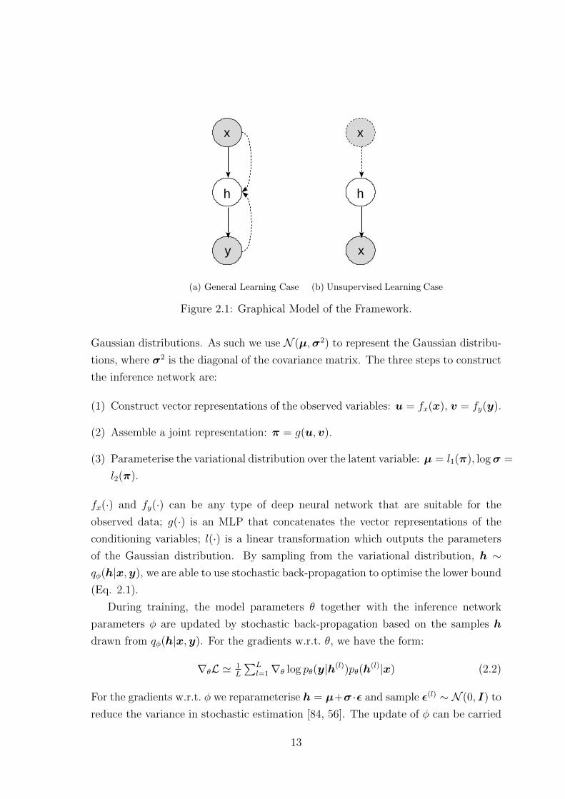
tent variable models. We define a generative model with a latent variable h, which can
be considered as the stochastic units in deep neural networks. We designate the ob-
served parent and child nodes of h as x and y respectively (e.g. Figure 2.1a). Hence,
the joint distribution of the generative model is pθ(x,y) =∑h pθ(y|h)pθ(h|x)p(x),
and the variational lower bound L is derived as:
L = Eq(h)[log pθ(y|h)pθ(h|x)p(x)− log q(h)] (2.1)
6 log
∫q(h)
q(h)pθ(y|h)pθ(h|x)p(x)dh = log pθ(x,y)
where θ parameterises the generative distributions pθ(y|h) and pθ(h|x). In or-
der to have a tight lower bound, the variational distribution q(h) should approach
the true posterior p(h|x,y). Here, we employ a parameterised diagonal Gaussian
N (h|µ(x,y),σ2(x,y)) as qφ(h|x,y). Throughout this thesis we employ diagonal
12
y
x
h
x
x
h
(a) General Learning Case
y
x
h
x
x
h
(b) Unsupervised Learning Case
Figure 2.1: Graphical Model of the Framework.
Gaussian distributions. As such we use N (µ,σ2) to represent the Gaussian distribu-
tions, where σ2 is the diagonal of the covariance matrix. The three steps to construct
the inference network are:
(1) Construct vector representations of the observed variables: u = fx(x), v = fy(y).
(2) Assemble a joint representation: π = g(u,v).
(3) Parameterise the variational distribution over the latent variable: µ = l1(π), logσ =
l2(π).
fx(·) and fy(·) can be any type of deep neural network that are suitable for the
observed data; g(·) is an MLP that concatenates the vector representations of the
conditioning variables; l(·) is a linear transformation which outputs the parameters
of the Gaussian distribution. By sampling from the variational distribution, h ∼qφ(h|x,y), we are able to use stochastic back-propagation to optimise the lower bound
(Eq. 2.1).
During training, the model parameters θ together with the inference network
parameters φ are updated by stochastic back-propagation based on the samples h
drawn from qφ(h|x,y). For the gradients w.r.t. θ, we have the form:
∇θL ' 1L
∑Ll=1∇θ log pθ(y|h(l))pθ(h
(l)|x) (2.2)
For the gradients w.r.t. φ we reparameterise h = µ+σ ·ε and sample ε(l) ∼ N (0, I) to
reduce the variance in stochastic estimation [84, 56]. The update of φ can be carried
13
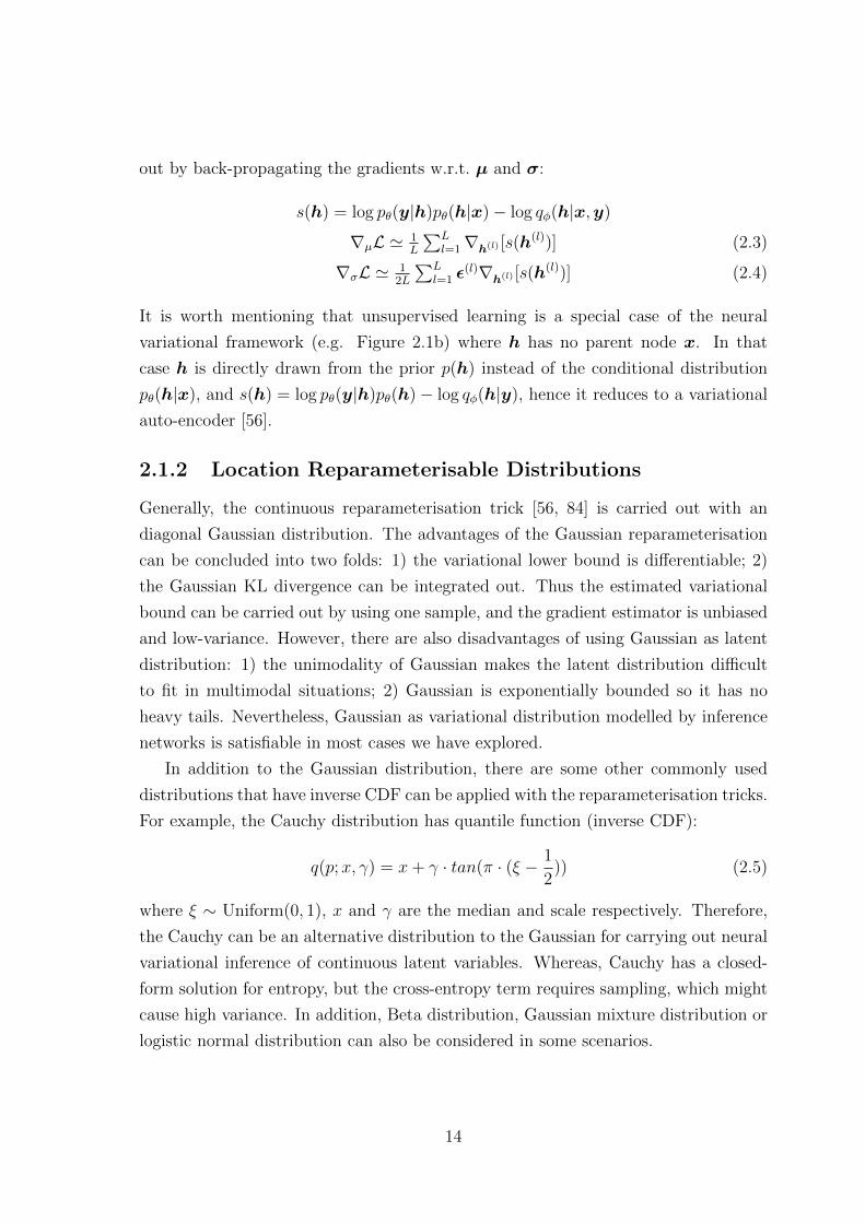
out by back-propagating the gradients w.r.t. µ and σ:
s(h) = log pθ(y|h)pθ(h|x)− log qφ(h|x,y)
∇µL ' 1L
∑Ll=1∇h(l) [s(h(l))] (2.3)
∇σL ' 12L
∑Ll=1 ε
(l)∇h(l) [s(h(l))] (2.4)
It is worth mentioning that unsupervised learning is a special case of the neural
variational framework (e.g. Figure 2.1b) where h has no parent node x. In that
case h is directly drawn from the prior p(h) instead of the conditional distribution
pθ(h|x), and s(h) = log pθ(y|h)pθ(h)− log qφ(h|y), hence it reduces to a variational
auto-encoder [56].
2.1.2 Location Reparameterisable Distributions
Generally, the continuous reparameterisation trick [56, 84] is carried out with an
diagonal Gaussian distribution. The advantages of the Gaussian reparameterisation
can be concluded into two folds: 1) the variational lower bound is differentiable; 2)
the Gaussian KL divergence can be integrated out. Thus the estimated variational
bound can be carried out by using one sample, and the gradient estimator is unbiased
and low-variance. However, there are also disadvantages of using Gaussian as latent
distribution: 1) the unimodality of Gaussian makes the latent distribution difficult
to fit in multimodal situations; 2) Gaussian is exponentially bounded so it has no
heavy tails. Nevertheless, Gaussian as variational distribution modelled by inference
networks is satisfiable in most cases we have explored.
In addition to the Gaussian distribution, there are some other commonly used
distributions that have inverse CDF can be applied with the reparameterisation tricks.
For example, the Cauchy distribution has quantile function (inverse CDF):
q(p;x, γ) = x+ γ · tan(π · (ξ − 1
2)) (2.5)
where ξ ∼ Uniform(0, 1), x and γ are the median and scale respectively. Therefore,
the Cauchy can be an alternative distribution to the Gaussian for carrying out neural
variational inference of continuous latent variables. Whereas, Cauchy has a closed-
form solution for entropy, but the cross-entropy term requires sampling, which might
cause high variance. In addition, Beta distribution, Gaussian mixture distribution or
logistic normal distribution can also be considered in some scenarios.
14
2.2 Discrete Latent Variables
The previous section discussed the scenario where the latent variables are contin-
uous and the parameterised diagonal Gaussian is generally employed as the latent
distribution. In fact, the aforementioned framework is also suitable for discrete la-
tent variables, and the only modification needed is to replace the Gaussian with a
multinomial distribution parameterised by the outputs of a softmax function. Com-
pared to generative models with continuous latent variables, models with discrete
ones are more suitable for building predictive systems. In addition, discrete repre-
sentations are easier to be interpreted, and it is more straightforward to incorporate
inductive biases to benefit the learning of deep neural networks. More importantly,
discrete latent variable models, provide a principled framework for semi-supervised
learning [54, 74, 115]. This is critical for NLP tasks, especially where additional
supervision and external knowledge can be utilized for bootstrapping. However, vari-
ational inference with discrete latent variables is relatively difficult due to intractable
marginalisation and the problem of high variance during sampling, because the Gaus-
sian reparameterisation trick for continuous variables is not applicable for this case.
Therefore, a policy gradient approach [77] can help to alleviate the high variance
problem during the sampling-based neural variational inference, which is also known
as REINFORCE algorithm. The recent works [71, 46] propose a categorical reparam-
eterization approach with the help of Gumbel-Softmax trick, which allows efficient
inference for discrete latent variables. Here, in this chapter, we discuss the general
REINFORCE Algorithm, which is the main approach applied for the discrete latent
variable models proposed in this thesis.
2.2.1 REINFORCE Algorithm
REINFORCE is a policy gradient method commonly used in reinforcement learning
problems. Here, we apply it to help construct an unbiased gradient estimator for
discrete latent distributions. Assume an unsupervised learning case, where z is the
discrete latent variable and x is the observation. The variational lower bound L is:
L = Eqφ(z|x)[log pθ(x|z)p(z)− log qφ(z|x)] (2.6)
= Eqφ(z|x)[log pθ(x|z)]−DKL[qφ(z|x)||p(z)]
6 log∑z
qφ(z|x)
qφ(z|x)pθ(x, z) = log p(x)
15
where θ parameterises the generative distributions pθ(z|x) and φ is the parameter set
of the inference network. As the continuous reparameterisation trick is not applicable,
we generate M samples z(m) ∼ qφ(z|x) for Monte Carlo estimation, and the estimated
variational lower bound is:
L ≈ 1
M
∑m
[log pθ(x, z(m))− log qφ(z(m)|x)] (2.7)
Therefore, for the parameters θ in the generative model, we directly update:
∂L
∂θ=
1
M
∑m
∂ log pθ(x, z(m))
∂θ(2.8)
and for the parameters φ in the recognition model, we update:
∂L
∂φ=
1
M
∑m
∂qφ(z(m)|x)
∂φ[log pθ(x, z
(m))− log qφ(z(m)|x)]
− 1
M
∑m
∂ log qφ(z(m)|x)
∂φ· qφ(z(m)|x)
=1
M
∑m
qφ(z(m)|x) · ∂ log qφ(z(m)|x)
∂φ[log pθ(x, z
(m))− log qφ(z(m)|x)]
− 1
M
∑m
∂qφ(z(m)|x)
∂φ· 1
qφ(z(m)|x)· qφ(z(m)|x)
=1
M
∑m
∂ log qφ(z(m)|x)
∂φ(log pθ(x, z
(m))− log qφ(z(m)|x)) (2.9)
Here, we achieve an unbiased gradient estimator, namely the likelihood ratio estimator
or REINFORCE estimator. Compared to Equation 2.8, the gradients w.r.t. φ contain
a potentially large scale term log pθ(x, z(m)) − log qφ(z(m)|x) which depends on the
samples of z. Since z(m) are discrete samples, the estimates can be very high due
to the scaling of the gradient inside the expectation, which results in a high-variance
gradient estimator and might cause slow convergence during training. Thus, in order
to mitigate the high-variance issue in this case, we introduce control variates method
in next section.
2.2.2 Control Variates
The main idea of a control variate is to introduce an extra term that is analytically
tractable in the expectation in Equation 2.6 and independent of the latent variable.
16
By subtracting the control variate c, the original expectation to be optimised remains
unchanged:
L = Eqφ(z|x)[log pθ(x, z)− log qφ(z|x)− c]
= Eqφ(z|x)[log pθ(x, z)− log qφ(z|x)]− Eqφ(z|x)[c]
= Eqφ(z|x)[log pθ(x, z)− log qφ(z|x)]− c (2.10)
but the variance of the gradients w.r.t. φ can be reduced:
∂L
∂φ=
1
M
∑m
∂qφ(z(m)|x)
∂φ[log pθ(x, z
(m))− log qφ(z(m)|x)− c]
− 1
M
∑m
∂ log qφ(z(m)|x)
∂φ· qφ(z(m)|x)
=1
M
∑m
qφ(z(m)|x) · ∂ log qφ(z(m)|x)
∂φ[log pθ(x, z
(m))− log qφ(z(m)|x)− c]
− 1
M
∑m
∂qφ(z(m)|x)
∂φ· 1
qφ(z(m)|x)· qφ(z(m)|x)
=1
M
∑m
∂ log qφ(z(m)|x)
∂φ(log pθ(x, z
(m))− log qφ(z(m)|x)− c) (2.11)
where the control variate c is directly added into the scaling term in the expecta-
tion. Compared to Equation 2.9, c is able to suppress the potentially large gradients,
which yields to a lower variance estimator. Generally, we could introduce a moving-
average baseline c0 as the simplest control variate. Since c0 is constant during every
epoch, its contribution to the gradient estimate is always zero in expectation. And
the original expectation to be optimised is unchanged, so it maintains an unbiased
gradient estimator.
A more effective control variate is the input-dependent baseline c(x) proposed
by Mnih & Gregor [77]. Since c(x) is only dependent on the input observation, it
is still analytically tractable from the expectation in the lower bound. In practice,
it can be implemented by a neural network and trained jointly with the model to
minimize the expected square of the moving-average baseline c:
Eqφ(z|x)[(l(z,x)− c0 − c(x))2] (2.12)
where l(z,x) = log pθ(x, z) − log qφ(z|x) is the original learning signal, c0 captures
the moving average and c(x) learns the systematic differences in the learning signal
17
for different observations. Hence, it makes the update more adapted to the input
observations x, and can be easily applied and customised for different discrete latent
variable models implemented by neural networks.
2.2.3 Advanced Sampling Schemes
In addition to the control variate approach, there are several other methods for miti-
gating the high-variance issue of sampling-based neural variational inference. MuProp
[31] extends the likelihood ratio estimator with control variates by first-order Tay-
lor expansion of a mean-field network, which is an unbiased gradient estimator for
stochastic networks and improves the performance of neural variational inference.
Intuitively, generating more samples for the gradient estimator is able to straight-
forwardly reduce the variance, but due to the computational expense we ought to
make full use of the limited number of samples. Importance weighted autoencoders
[15] provide a tighter log-likelihood lower bound for the continuous variational auto-
encoder derived from multi-sample importance weighting, and VIMCO (Variational
Inference for Monte Carlo Objectives) [78] further extends the importance sampling
approach to discrete latent variables and introduces an unbiased gradient estimator
designed for importance-sampled objectives.
2.3 Parameterising Categorical Distribution
Generally, the learning of continuous and discrete latent variables are separated since
variational inference applies different gradient estimators (e.g. Gaussian reparame-
terisation and REINFORCE algorithm). From the perspective of neural variational
inference, continuous latent variables are commonly preferred over discrete latent
variables since the Gaussian reparameterisation suffers less from the high-variance
problem than REINFORCE algorithm, though there exist a few techniques, e.g. con-
trol variate for mitigating the issue. However, we are able to parameterise the cat-
egorical distributions by continuous latent variables. Thus in some cases where the
computational expense allows integrating out discrete latent variables, we are able to
directly apply the Gaussian reparameterisation for carrying out the inference.
In this section, we are going to introduce several approaches for parameterising
categorical distributions, including Gaussian Softmax Construction (GSM), Gaus-
sian Stick-breaking Construction (GSB) and Recurrent Stick-breaking Construction
(RSB). It is worth mentioning that, by using the stick-breaking construction, we are
able to introduce Bayesian non-parametrics for deep neural networks.
18
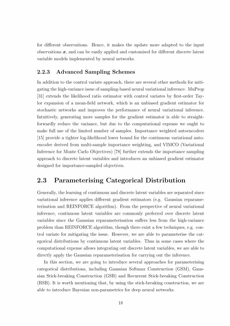
2.3.1 Gaussian Softmax Construction2.1 Gaussian Softmax (GSM)
Linear
Softmax
Gaussian Prior
Figure 2.2: Neural Stucture of GSM
In deep learning, an energy-based function is generally used to construct proba-
bility distributions [65]. Here we pass a Gaussian random vector through a softmax
function to parameterise the categorical distribution, and θ ∼ GGSM(µ0, σ20) is defined
as:
x ∼ N (µ0, σ20)
θ = softmax(W T1 x)
where W1 is a linear transformation, and we leave out the bias terms for brevity. µ0
and σ20 are hyper-parameters which we set for a zero mean and unit variance Gaussian.
Then, we easily construct a categorical distribution parameterised by a Gaussian, and
the neural structure is shown in Figure 2.2. Here, the Gaussian Softmax construction
can be considered as parameterised logistic normal distribution, which is similar to
the prior distribution applied in correlated topic models [10].
2.3.2 Gaussian Stick-breaking Construction
In Bayesian non-parametrics, the stick-breaking process [90] is used as a constructive
definition of the Dirichlet process, where sequentially drawn Beta random variables
define breaks from a unit stick. In our case, following [51], we transform the modelling
of multinomial probability parameters into the modelling of the logits of binomial
probability parameters using Gaussian latent variables. More specifically, conditioned
19
η1
η3(1−η2)(1−η1)
η2(1−η1)
θ1 θ2 θ3 θK
...
...
break1st
break2nd
break3rd
K-1 simplex
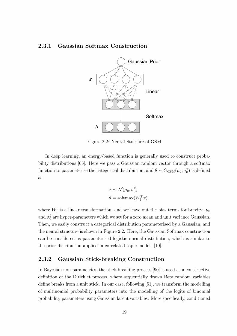
Figure 2.3: The Stick-breaking Construction.2.2 Gaussian Stick Breaking (GSB)
Stick Breaking
Sigmoid
Gaussian Prior
Figure 2.4: Neural Stucture of GSB
on a Gaussian sample x ∈ RH , the breaking proportions η ∈ RK−1 are generated by
applying the sigmoid function η = sigmoid(W T2 x) where W ∈ RH×K−1. Starting with
the first piece of the stick, the probability of the first category is modelled as a break of
proportion η1, while the length of the remainder of the stick is left for the next break.
Thus each dimension can be deterministically computed by θk = ηk∏k−1
i=1 (1−ηi) until
k=K−1, and the remaining length is taken as the probability of the Kth category
θK =∏K−1
i=1 (1− ηi).For instance assume K = 3, θ is generated by 2 breaks where θ1 = η1, θ2 =
η2(1 − η1) and the remaining stick θ3 = (1 − η2)(1 − η1). If the model proceeds
to break the stick for K = 4, the remaining stick θ3 is broken into (θ′3, θ′4), where
θ′3 = η3 · θ3, θ′4 = (1 − η3) · θ3 and θ3 = θ′3 + θ′4. Hence, for different values of K, it
always satisfies∑K
k=1 θk = 1. The stick-breaking construction fSB(η) is illustrated in
20

Figure 2.3 and the distribution θ ∼ GGSB(µ0, σ20) is defined as:
x ∼ N (µ0, σ20)
η = sigmoid(W T2 x)
θ = fSB(η)
Compared to the stick-breaking of Dirichlet process which has exchangeability
(viz. the probability of generating a sequence of draws θ1, θ2, ..., θk equals the proba-
bility of drawing them in any alternative order) and is invariant to size-biased permu-
tations (viz. the fragments η1, η2, ..., ηk for constructing θ are independent samples
from an identical distribution e.g. a Beta distribution), Gaussian stick-breaking con-
struction maintains exchangeability but is not invariant to size-biased permutations
due to that the parameters W2 of GGSB are attached to a fixed order of θ. Hence,
the fragments η1, η2, ..., ηk are not independent and identically distributed. Despite
of this, the Gaussian stick-breaking construction provides a more amenable form for
neural variational inference. More interestingly, this stick-breaking construction in-
troduces a non-parametric aspect to deep generative models with Gaussian as latent
distribution, and the neural structure is shown in Figure 2.4.
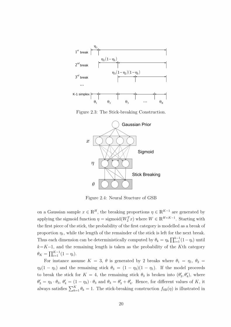
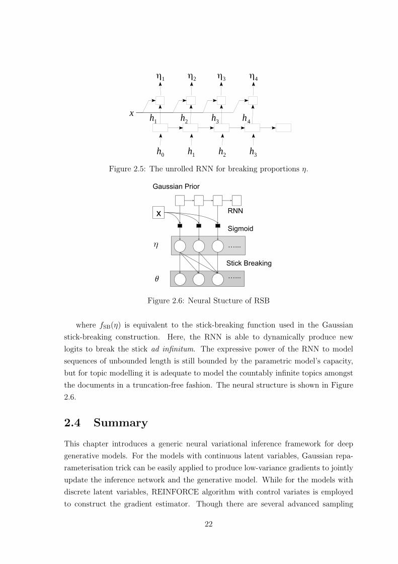
2.3.3 Recurrent Stick-breaking Construction
Recurrent Neural Networks (RNN) are commonly used for modelling sequences of
inputs in deep learning. Here we consider the stick-breaking construction as a se-
quential draw from an RNN, thus capturing an unbounded number of breaks with a
finite number of parameters. Conditioned on a Gaussian latent variable x, the recur-
rent neural network fSB(x) produces a sequence of binomial logits which are used to
break the stick sequentially. The fRNN(x) is decomposed as:
hk = RNNSB(hk−1)
ηk = sigmoid(hTk−1x)
where hk is the output of the kth state, which we feed into the next state of the
RNNSB as an input. Figure 2.5 shows the recurrent neural network structure. Now
θ ∼ GRSB(µ0, σ20) is defined as:
x ∼ N (µ0, σ20)
η = fRNN(x)
θ = fSB(η)
21
η1 η2 η3 η4
h0 h1 h2 h3
x h1 h2 h3 h4
Figure 2.5: The unrolled RNN for breaking proportions η.
x
2.3 Recurrent Stick Breaking (RSB)
…...
…...
Sigmoid
Stick Breaking
RNN
Gaussian Prior
Figure 2.6: Neural Stucture of RSB
where fSB(η) is equivalent to the stick-breaking function used in the Gaussian
stick-breaking construction. Here, the RNN is able to dynamically produce new
logits to break the stick ad infinitum. The expressive power of the RNN to model
sequences of unbounded length is still bounded by the parametric model’s capacity,
but for topic modelling it is adequate to model the countably infinite topics amongst
the documents in a truncation-free fashion. The neural structure is shown in Figure
2.6.
2.4 Summary
This chapter introduces a generic neural variational inference framework for deep
generative models. For the models with continuous latent variables, Gaussian repa-
rameterisation trick can be easily applied to produce low-variance gradients to jointly
update the inference network and the generative model. While for the models with
discrete latent variables, REINFORCE algorithm with control variates is employed
to construct the gradient estimator. Though there are several advanced sampling
22
schemes to further mitigate the high variance issue, it is still a major problem in
the neural variational inference for discrete variables. Therefore, continuous latent
variable models are generally more welcome than discrete ones from the perspective
of optimisation. However, despite of the high variance issue, discrete representation
is a natural fit for predictive systems with categorical properties, such as structure
prediction, planning and clustering. Thus we are interested in exploring the potential
of discrete latent variables and develop more sophisticated deep generative models
for NLP.
Alternatively, in some cases where the marginalisation of discrete latent variable
is tractable, we could use neural networks based on Gaussian draws to parameterise
the discrete latent distribution. Then the model is able to not only make use of
the discrete latent distribution, but also enjoy the efficiency and low-variance esti-
mators brought by Gaussian reparameterisation trick. Moreover, with the help of
the stick-breaking constructions, an unbounded categorical distribution is able to be
incorporated into the deep generative models, which brings Bayesian non-parametrics
and can easily updated by stochastic gradient back-propagation.
More details about the related deep generative models (continuous or discrete) for
NLP will be introduced in the following chapters of this thesis.
23
Part II
Continuous Latent Variable Models
24

Chapter 3
Neural Document Models
This chapter introduces the first application of this thesis, neural variational docu-
ment model (NVDM), which aims at learning continuous stochastic representations
of documents in unsupervised fashion. The model is an instantiation of variational
auto-encoders based on bag-of-words documents, which is simple, expressive and easy
to train. In the experiments section, we also show that the neural variational docu-
ment model is able to discover latent semantics of documents that can be interpreted
as topics.
3.1 Introduction
Document modelling is a classical NLP task, which is useful for document classifi-
cation, document clustering, information retrieval and knowledge discovery. Here,
we are interested in unsupervised document modelling, which requires no document
labels or categorical information. Generally, unsupervised document modelling is car-
ried out by language models or bag-of-words models. For the approach of language
modelling, a document is generated by autoregressively predicting the words as a long
sequence. While for bag-of-words models, a document is modelled as a collection of
words, where the syntactic information and grammars are not considered in this case.
Normally, documents are preprocessed by filtering “stopwords” (i.e. the most com-
mon words in a language that have little contribution to document modelling are
removed). In this chapter, the documents models discussed and compared are all
bag-of-words document models.
A simple and effective way to model documents is using term frequency-inverse
document frequency (tf-idf) score, which reflects how important a word is to a doc-
ument in a collection or corpus. However, tf-idf models have no interpretation on
topics and they are not scalable due to the sparse tf-idf matrix. In contrast, topic
25
models discovers the abstract topics that occur in a collection of documents so that
all the documents can be modelled as a mixture of topics. Starting with latent se-
mantic analysis (LSA [60]), models for uncovering the underlying semantic structure
of a document collection have been widely applied in data mining, text processing
and information retrieval. Probabilistic topic models (e.g. PLSA [45], LDA [11] and
HDPs [102]) provide a robust, scalable, and theoretically sound foundation for doc-
ument modelling by introducing latent variables for each token to topic assignment.
LDA, as the representative of probabilistic topic models, has been widely applied
for dimensionality reduction, text-mining and semantic interpretation. Beyond LDA,
significant extensions have sought to capture topic correlations [10], topic evolution
[9] and discover an unbounded number of topics [102]. Topic models have also been
extended to capture extra context information such as time [111], authorship [85], and
class labels [73]. Such extensions often require carefully tailored graphical models,
and associated inference algorithms, to capture the desired context.
With the recent advances of deep neural networks, neural document models be-
come more and more popular due to highly scalable vector representations and easy-
to-implement network structures. The simplest bag-of-words document model im-
plemented by neural networks is the bag-of-embeddings, which sums the word em-
beddings with semantic information rather than sparse one-hot word representations.
However, the off-the-shelf word representations limits the scalability of the model.
More recent neural document models are the Replicated Softmax [40]: an undirected
topic model implemented by restricted Boltzmann machines; and the Sigmoid Belief
Document Model [77] that applies sigmoid belief networks for modelling the semantics
of documents. DocNADE [61] extends the Replicated Softmax model and estimates
the probability of observing a new word in a given document given the previously ob-
served words. DARN [29] employs a similar assumption but applies neural variational
inference to infer the latent semantic information. Though these neural generative
models do not aim at modelling topic distributions directly, compared to conventional
probabilistic topic models [45, 11], they have achieved decent document perplexities.
While the Paragraph Vector model [63] implements the idea in an alternative deter-
ministic way, which directly concatenates the document/paragraph vector with the
word vector to model whole documents like a language model.
This chapter introduces our neural variational document model (NVDM). Differ-
ent from traditional probabilistic topic models, NVDM does not model topics explic-
itly, but it applies an easy-to-implement neural structure to discover continuous latent
semantics of documents as a generative model, where the stochastic vectors (latent
26
semantics) can be interpreted as topics. Compared to the neural models mentioned
above using binary vectors to model semantic, the continuous stochastic representa-
tions of documents are more expressive and easier to train.
3.2 Neural Variational Document Model (NVDM)
q (h∣X) (Inference Network)
X
p(X∣h)
h
X
Figure 3.1: Neural Variational Document Model.
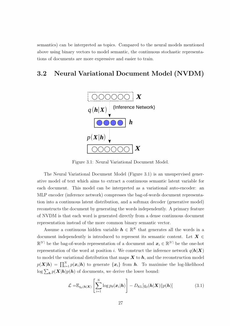
The Neural Variational Document Model (Figure 3.1) is an unsupervised gener-
ative model of text which aims to extract a continuous semantic latent variable for
each document. This model can be interpreted as a variational auto-encoder: an
MLP encoder (inference network) compresses the bag-of-words document representa-
tion into a continuous latent distribution, and a softmax decoder (generative model)
reconstructs the document by generating the words independently. A primary feature
of NVDM is that each word is generated directly from a dense continuous document
representation instead of the more common binary semantic vector.
Assume a continuous hidden variable h ∈ RK that generates all the words in a
document independently is introduced to represent its semantic content. Let X ∈R|V | be the bag-of-words representation of a document and xi ∈ R|V | be the one-hot
representation of the word at position i. We construct the inference network q(h|X)
to model the variational distribution that mapsX to h, and the reconstruction model
p(X|h) =∏N
i=1 p(xi|h) to generate {xi} from h. To maximise the log-likelihood
log∑h p(X|h)p(h) of documents, we derive the lower bound:
L =Eqφ(h|X)
[N∑i=1
log pθ(xi|h)
]−DKL[qφ(h|X)‖p(h)] (3.1)
27

where N is the number of words in the document and p(h) is a Gaussian prior for h.
Here, we consider N is observed for all the documents. The conditional probability
over words pθ(xi|h) (decoder) is modelled by multinomial logistic regression and
shared across documents:
pθ(xi|h) =exp{−E(xi;h, θ))}∑|V |j=1 exp{−E(xj;h, θ)}
(3.2)
E(xi;h, θ) = −hTRxi − bxi (3.3)
where R ∈ RK×|V | learns the semantic word embeddings and bxi represents the bias
term.
As there is no supervision information for the latent semantics, h, the poste-
rior approximation qφ(h|X) is only conditioned on the current document X. The
inference network qφ(h|X) = N (h|µ(X),σ2(X)) is modelled as:
π = g(fmlpX (X)) (3.4)
µ = l1(π), logσ = l2(π) (3.5)
For each document X, the neural network generates its own parameters µ and σ that
parameterise the latent distribution over document semantics h. Based on the sam-
ples h ∼ qφ(h|X), the lower bound (Eq. 3.1) can be optimised by back-propagating
the stochastic gradients w.r.t. θ and φ.
Since p(h) is a standard Gaussian prior, the Gaussian KL-Divergence between the
prior and variational distribution DKL[qφ(h|X)‖p(h)] can be computed analytically
to further lower the variance of the gradients:
DKL = −12(K − ‖µ‖2 − ‖σ‖2 + log |diag(σ2)|) (3.6)
Moreover, it also acts as a regulariser for updating the parameters of the inference
network qφ(h|X).
3.3 Experiments
3.3.1 Dataset & Setup
We experiment with NVDM on two standard news corpora: the 20NewsGroups1 and
the Reuters RCV1-v2 2. The former is a collection of newsgroup documents, consisting
1http://qwone.com/ jason/20Newsgroups2http://trec.nist.gov/data/reuters/reuters.html
28
of 11,314 training and 7,531 test articles. The latter is a large collection from Reuters
newswire stories with 794,414 training and 10,000 test cases. The vocabulary size of
these two datasets are set as 2,000 and 10,000.
To make a direct comparison with the prior work we follow the same preprocessing
procedure and setup as [40], [61], [97], and [77]. We train NVDM models with 50 and
200 dimensional document representations respectively. For the inference network,
we use an MLP (Eq. 3.4) with 2 layers and 500 dimension rectifier linear units, which
converts document representations into embeddings. During training we carry out
stochastic estimation by taking one sample for estimating the stochastic gradients,
while in prediction we use 20 samples for predicting document perplexity (see the
related discussion for Figure 5.3). The model is trained by Adam [53] and tuned by
hold-out validation perplexity.
We alternately optimise the generative model and the inference network by fixing
the parameters of one while updating the parameters of the other. This is an impor-
tant optimisation trick to achieving a good performance of a bag-of-words variational
auto-encoder. When the generative model is fixed, it focuses on learning the inference
network (encoder) for modelling stochastic document representations and fitting the
prior distribution. While when the inference network is fixed, it aims at learning
the generative model (decoder) to optimise the reconstruction error. In this way, the
model is encouraged to make use of the continuous latent variable for generating the
observations, which helps address the optimization challenge of VAEs. The sequence
VAE [14] applies KL cost annealing and word dropout for dealing with the similar
issue. However, sequence generation generally relies on powerful autoregressive de-
coders such as LSTMs, which are even more difficult to force the generative model to
use the latent variable compared to the simple softmax decoder applied in our case.
3.3.2 Evaluation on Perplexity
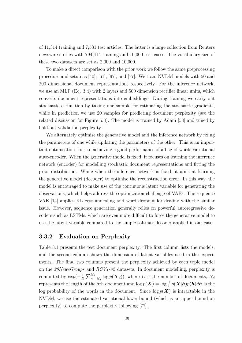
Table 3.1 presents the test document perplexity. The first column lists the models,
and the second column shows the dimension of latent variables used in the experi-
ments. The final two columns present the perplexity achieved by each topic model
on the 20NewsGroups and RCV1-v2 datasets. In document modelling, perplexity is
computed by exp(− 1D
∑Ndn
1Nd
log p(Xd)), where D is the number of documents, Nd
represents the length of the dth document and log p(X) = log∫p(X|h)p(h)dh is the
log probability of the words in the document. Since log p(X) is intractable in the
NVDM, we use the estimated variational lower bound (which is an upper bound on
perplexity) to compute the perplexity following [77].
29
Model Dim 20News RCV1LDA 50 1091 1437LDA 200 1058 1142RSM 50 953 988docNADE 50 896 742SBN 50 909 784fDARN 50 917 724fDARN 200 — 598NVDM 50 836 563NVDM 200 852 550
Table 3.1: Perplexity on test dataset.
For the benchmark models in Table 3.1, LDA [11] is a traditional topic model
that models documents by mixtures of topics, RSM [40] is an undirected topic model
implemented by restricted Boltzmann machines, and docNADE [61] is a neural topic
model based on autoregressive assumption. The models based on Sigmoid Belief
Networks (SBN) and Deep AutoRegressive Neural Network (DARN) structures are
implemented by Mnih and Gregor [77], which employs an MLP to build a Monte
Carlo control variate estimator for stochastic estimation.
While all the baseline models listed in Table 3.1 apply discrete latent variables,
here NVDM employs a continuous stochastic document representation. The experi-
mental results indicate that NVDM achieves the best performance on both datasets.
For the experiments on RCV1-v2 dataset, the NVDM with latent variable of 50 di-
mension performs even better than the fDARN with 200 dimension. It demonstrates
that our document model with continuous latent variables has higher expressiveness
and better generalisation ability.
3.3.3 Interpreting Document Semantics
In addition to the perplexities, we also qualitatively evaluate the semantic information
learned by NVDM on the 20NewsGroups dataset. Although NVDM directly gener-
ates words conditioned on the document semantics h and topics are not explicitly
modelled, we use the positive connections between topics and words for interpreting
the discovered topics, which are the parameters R. For example in Figure 3.2, we
assume each dimension of h represents a topic of document collections. The words
related to a specific topic can be achieved by ranking the words with the weights
connecting all the words in the vocabulary X and a specific dimension of h. Then,
we are able to interpret the document semantics as topics through the top-n words.
30
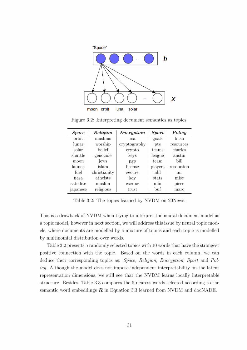
Figure 3.2: Interpreting document semantics as topics.
Space Religion Encryption Sport Policy
orbit muslims rsa goals bushlunar worship cryptography pts resourcessolar belief crypto teams charles
shuttle genocide keys league austinmoon jews pgp team billlaunch islam license players resolution
fuel christianity secure nhl mrnasa atheists key stats misc
satellite muslim escrow min piecejapanese religious trust buf marc
Table 3.2: The topics learned by NVDM on 20News.
This is a drawback of NVDM when trying to interpret the neural document model as
a topic model, however in next section, we will address this issue by neural topic mod-
els, where documents are modelled by a mixture of topics and each topic is modelled
by multinomial distribution over words.
Table 3.2 presents 5 randomly selected topics with 10 words that have the strongest
positive connection with the topic. Based on the words in each column, we can
deduce their corresponding topics as: Space, Religion, Encryption, Sport and Pol-
icy. Although the model does not impose independent interpretability on the latent
representation dimensions, we still see that the NVDM learns locally interpretable
structure. Besides, Table 3.3 compares the 5 nearest words selected according to the
semantic word embeddings R in Equation 3.3 learned from NVDM and docNADE.
31
Word weapons medical companies define israel book
guns medicine expensive defined israeli booksweapon health industry definition arab reference
NVDM gun treatment company printf arabs guidemilitia disease market int lebanon writingarmed patients buy sufficient lebanese pages
weapon treatment demand defined israeli readingshooting medecine commercial definition israelis read
NADE firearms patients agency refer arab booksassault process company make palestinian releventarmed studies credit examples arabs collection
Table 3.3: The five nearest words in the semantic space.
3.4 Summary
This chapter describes the proposed neural variational document model, which is
a simple, expressive and easy-to-train instantiation of variational auto-encoders for
NLP. Though NVDM only applies bag-of-words information to model documents,
both the quantitative and qualitative evaluation demonstrate the effectiveness and
efficiency of this deep generative model. Certainly, there is a drawback of interpret-
ing the latent semantics of documents as topics, which are not modelled explicitly
as distributions over words in NVDM. Thus, in the next chapter we are going to
introduce neural topic models where this issue will be addressed.
32
Chapter 4
Neural Topic Models
This chapter discusses the deep generative models for topic modelling. Different
from the NVDM introduced in the previous chapter, the neural topic models em-
ploy multinomial to model topic-word distributions explicitly, which is more similar
to the generative story of traditional probabilistic topic models. In this context,
we parameterise the categorical distributions by the Gaussian softmax construction
(GSM), Gaussian stick-breaking construction (GSB) and Recurrent stick-breaking
construction (RSB) that are introduced in Chapter 2. More interestingly, Bayesian
non-parametrics can be incorporated into the neural topic model with the help of
the stick-breaking constructions, and the inference can be easily carried out in the
framework of neural variational inference. The following contents will be divided into
neural finite topic models and neural unbounded topic models where the modelled
topics are bounded and unbounded respectively.
4.1 Introduction
For the traditional Dirichlet-Multinomial topic model, efficient inference is available
by exploiting conjugacy with either Monte Carlo or variational techniques [47, 2, 7]).
However, as topic models have grown more expressive, in order to capture topic
dependencies or exploit conditional information, inference methods have become in-
creasingly complex. This is especially apparent for non-conjugate models [17, 10, 107].
As mentioned in Chapter 2, deep neural networks are excellent function approxima-
tors and have shown great potential for learning complicated non-linear distributions
for unsupervised models. The inference network, as a black-box variational distribu-
tion parameterised by a neural network, approximates the posterior of a generative
model. This allows both the generative model and the variational network to be
jointly trained with backpropagation. Hence, in the framework of neural variational
33
inference, non-conjugacy is no longer a bottleneck for the probabilistic models, and
we are allowed to have more possibilities on designing complicated and interesting
deep generative models.
Here, we propose and evaluate a range of topic models parameterised with neu-
ral networks and trained with variational inference. We employ three different neural
structures for constructing topic distributions introduced in Chapter 2: Gaussian soft-
max construction (GSM), Gaussian stick-breaking distribution construction (GSB),
and recurrent stick-breaking construction (RSB), all of which are conditioned on a
draw from a multivariate Gaussian distribution. The Gaussian softmax topic model
constructs a finite topic distribution with a softmax function applied to the projection
of the Gaussian random vector. The Gaussian stick-breaking model also constructs a
discrete distribution from the Gaussian draw, but this time employing a stick-breaking
construction to provide a bias towards sparse topic distributions. And the recurrent
stick-breaking construction employs a recurrent neural network, again conditioned
on the Gaussian draw, to progressively break the stick, yielding a neural analog of a
Dirichlet Process topic model [102].
Our neural topic models combine the merits of both neural networks and tradi-
tional probabilistic topic models. They can be trained efficiently by backpropagation,
scaled to large data sets, and easily conditioned on any available contextual informa-
tion. Further, as probabilistic graphical models, they are interpretable and explicitly
representing the dependencies amongst the random variables. Previous neural doc-
ument models, such as the neural variational document model (NVDM) introduced
in the previous chapter, belief networks document model [77], neural auto-regressive
document model [61] and replicated softmax [40], have not explicitly modelled latent
topics. Through evaluations on a range of data sets we compare our models with pre-
viously proposed neural document models and traditional probabilistic topic models,
demonstrating their robustness and effectiveness.
4.2 Neural Finite Topic Model
This section discusses the neural finite topic model. Following the generative story
of topic model, we first describe the parameterisation of the document-topic distribu-
tion. Then, the neural networks for parametersing the topic-word distribution will be
introduced. Finally, we derive the variational lower bound that integrates out latent
topics. In addition, the connections and differences between neural topic models and
neural document models will be discussed.
34
4.2.1 Parameterising the Document-Topic Distribution
In probabilistic topic models, such as LDA [11], we use the latent variables θd and zn
for the topic proportion of document d, and the topic assignment for the observed word
wn, respectively. In order to facilitate efficient inference, the Dirichlet distribution
(or Dirichlet process [102]) is employed as the prior to generate the parameters of the
multinomial distribution θd for each document. The use of a conjugate prior allows the
tractable computation of the posterior distribution over the latent variables’ values.
While alternatives have been explored, such as log-normal topic distributions [9, 10],
extra approximation (e.g. the Laplace approximation [107]) is required for closed form
derivations. The generative process of LDA is:
θd ∼ Dir(α0), for d ∈ D
zn ∼ Multi(θd), for n ∈ [1, Nd]
wn ∼ Multi(βzn), for n ∈ [1, Nd]
where βzn represents the topic distribution over words given topic assignment zn and
Nd is the number of tokens in document d. βzn can be drawn from another Dirichlet
distribution, but here we consider it a model parameter. α0 is the hyper-parameter of
the Dirichlet prior and Nd is the total number of words in document d. The marginal
likelihood for a document in collection D is:
p(d|α0, β)=
∫θ
p(θ|α0)∏n
∑zn
p(wn|βzn)p(zn|θ)dθ. (4.1)
If we employ mean-field variational inference, the updates for the variational param-
eters q(θ) and q(zn) can be directly derived in closed form.
In contrast, our proposed models introduce a neural network to parameterise the
multinomial topic distribution. The generative process is:
θd ∼ G(µ0, σ20), for d ∈ D
zn ∼ Multi(θd), for n ∈ [1, Nd]
wn ∼ Multi(βzn), for n ∈ [1, Nd]
where G(µ0, σ20) is composed of a neural network θ = g(x) conditioned on a diagonal
Gaussian x ∼ N(µ0, σ20). The marginal likelihood is:
p(d|µ0, σ0, β) =
∫θ
p(θ|µ0, σ20)∏
n
∑znp(wn|βzn)p(zn|θ)dθ. (4.2)
35

Compared to Equation (4.1), here we parameterise the latent variable θ by a neural
network conditioned on a draw from a Gaussian distribution. To carry out neu-
ral variational inference [75], we construct an inference network q(θ|µ(d), σ(d)) to
approximate the posterior p(θ|d), where µ(d) and σ(d) are functions of d that are im-
plemented by multilayer perceptrons (MLP). By using a Gaussian prior distribution,
we are able to employ the re-parameterisation trick [56] to build an unbiased and low-
variance gradient estimator for the variational distribution. Without conjugacy, the
updates of the parameters can still be derived directly and easily from the variational
lower bound. We defer discussion of the inference process until the next section. Here
we introduce several alternative neural networks for g(x) which transform a Gaussian
sample x into the topic proportions θ.
4.2.2 Parameterising the Topic-Word Distribution
Assume we have finite number of topics K, the topic distribution over words given
a topic assignment zn is p(wn|β, zn) = Multi(βzn), and βzn is the zn topic-word dis-
tribution. Here we introduce topic vectors t ∈ RK×H , word vectors v ∈ RV×H and
generate the topic distributions over words by:
βk = softmax(v · tTk ). (4.3)
Therefore, β∈RK×V is a collection of simplexes achieved by computing the semantic
similarity between topics and words.
A related work Gaussian-LDA [20] also attempts to explicitly model the represen-
tations of topics. It applies multivariate Gaussian distributions as topics to generate
words, and each topics are drawn from conjugate priors, where a Gaussian centered at
zero for the mean and an inverse Wishart distribution for the covariance. Compared
to the topic-word distribution (Equation 4.3) that employs inner product distance,
the probability of generating a word from a topic in Gaussian-LDA is determined by
the Euclidean distance between the embeddings. The merit is that both topics and
words in Gaussian-LDA share the same semantic space and the correlations of words
are jointly modelled. While the drawback lies in the fact that the inference is difficult
due to the high sampling complexity, even if the word embeddings are pretrained.
On the contrary, in our models, the vector representations of both words and topics
can be directly and easily updated by gradient back-propagation.
Following the notation introduced in Chapter 2, the prior distribution is defined as
G(θ|µ0, σ20) in which x ∼ N (x|µ0, σ
20) and the projection network generates θ = g(x)
for each document. Here, g(x) can be the Gaussian Softmax gGSM(x), Gaussian
36
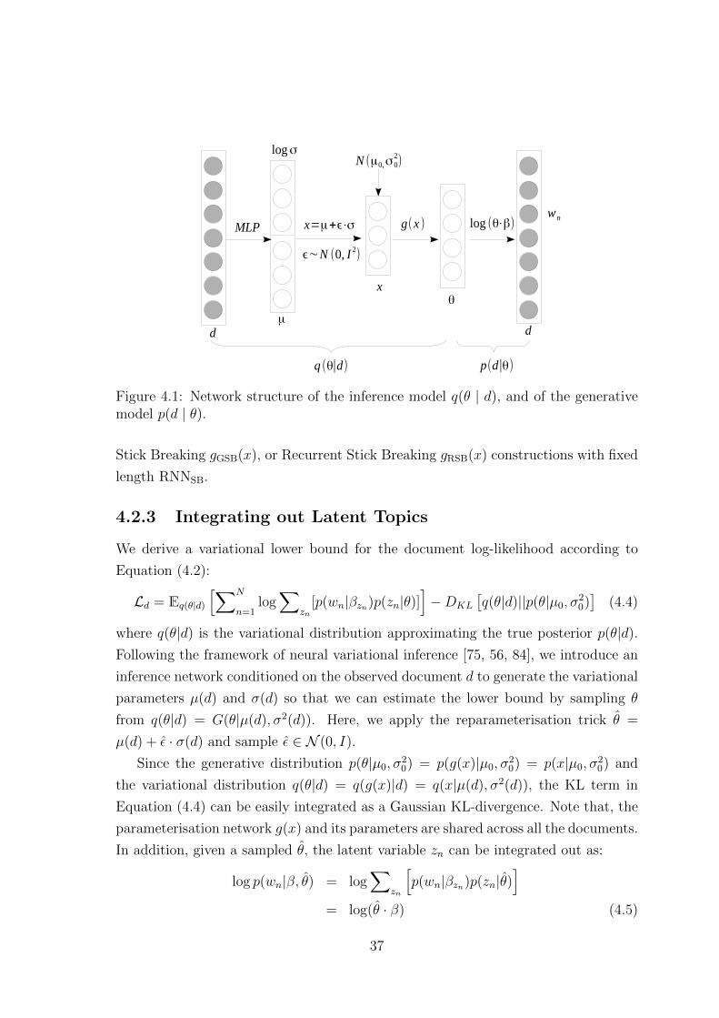
d
xθ
dμ
log σ
MLP
ϵ∼N (0, I 2)
N (μ0,σ02)
g(x ) log (θ⋅β)wn
q (θ∣d) p(d∣θ)
x=μ+ϵ⋅σ
Figure 4.1: Network structure of the inference model q(θ | d), and of the generativemodel p(d | θ).
Stick Breaking gGSB(x), or Recurrent Stick Breaking gRSB(x) constructions with fixed
length RNNSB.
4.2.3 Integrating out Latent Topics
We derive a variational lower bound for the document log-likelihood according to
Equation (4.2):
Ld = Eq(θ|d)
[∑N
n=1log∑
zn[p(wn|βzn)p(zn|θ)]
]−DKL
[q(θ|d)||p(θ|µ0, σ
20)]
(4.4)
where q(θ|d) is the variational distribution approximating the true posterior p(θ|d).
Following the framework of neural variational inference [75, 56, 84], we introduce an
inference network conditioned on the observed document d to generate the variational
parameters µ(d) and σ(d) so that we can estimate the lower bound by sampling θ
from q(θ|d) = G(θ|µ(d), σ2(d)). Here, we apply the reparameterisation trick θ =
µ(d) + ε · σ(d) and sample ε ∈ N (0, I).
Since the generative distribution p(θ|µ0, σ20) = p(g(x)|µ0, σ
20) = p(x|µ0, σ
20) and
the variational distribution q(θ|d) = q(g(x)|d) = q(x|µ(d), σ2(d)), the KL term in
Equation (4.4) can be easily integrated as a Gaussian KL-divergence. Note that, the
parameterisation network g(x) and its parameters are shared across all the documents.
In addition, given a sampled θ, the latent variable zn can be integrated out as:
log p(wn|β, θ) = log∑
zn
[p(wn|βzn)p(zn|θ)
]= log(θ · β) (4.5)
37

Thus there is no need to introduce another variational approximation for the topic
assignment z. The variational lower bound is therefore:
Ld ≈ Ld =∑N
n=1
[log p(wn|β, θ)
]−DKL [q(x|d)||p(x)]
We can directly derive the gradients of the generative parameters Θ, including t, v
and g(x). While for the variational parameters Φ, including µ(d) and σ(d), we use
the gradient estimators:
∇µ(d)Ld ≈ ∇θLd,
∇σ(d)Ld ≈ ε · ∇θLd.
Θ and Φ are jointly updated by stochastic gradient back-propagation. The structure
of this variational auto-encoder is illustrated in Figure 4.1.
4.2.4 Topic Models vs. Document Models
In most topic models, documents are modelled by a mixture of topics, and each word
is associated with a single topic latent variable, e.g. LDA and GSM. However, the
neural variational document model (NVDM) introduced in Chapter 3 is implemented
as a VAE [56] without modelling topics explicitly. The major difference is that NVDM
employs a softmax decoder (Equation 4.6) to generate all of the words of a document
conditioned on the document representation θ:
log p(wn|β, θ) = log softmax(θ · β). (4.6)
where both θ and β are unnormalised. Hence, it breaks the topic model assumption
that each document consists of a mixture of topics. Although the latent variables
can still be interpreted as topics, these topics are not modelled explicitly since there
is no actual topic distribution over words. [96] interprets the above decoder as a
weighted product of experts topic model, here however, we refer to such models that
do not directly assign topics to words as document models instead of topic models.
We can also convert our neural topic models to neural document models by replacing
the mixture decoder (Equation 4.5) with the softmax decoder (Equation 4.6). For
example in the GSM construction, if we remove the softmax function over θ, and
directly apply Equation 4.6 to generate the words, it reduces to a variant of the
NVDM model (GSM applies topic and word vectors to compute β, while NVDM
directly models a projection β from the latent variables to words). The experimental
evaluation in next section will have more detailed discussion comparing these models.
38

4.2.5 Topic Diversity
An issue that exists in both probabilistic and neural topic models is redundant topics.
In neural models, however, we are able to straightforwardly regularise the distance
between each of the topic vectors in order to diversify the topics. Following [120], we
apply such topic diversity regularisation during the inference process. We compute
the angles between each two topics a(ti, tj) = arccos(|ti·tj |||ti||·||tj ||). Then, the mean
angle of all pairs of K topics is ζ = 1K2
∑i
∑j a(ti, tj), and the variance is ν =
1K2
∑i
∑j(a(ti, tj) − ζ)2. We add the following topic diversity regularisation to the
variational objective:
J = L+ λ(ζ − ν),
where λ is a hyper-parameter for the regularisation that is set as 0.1 in the experi-
ments. During training, the mean angle is encouraged to be larger while the variance
is suppressed to be smaller so that all of the topics will be pushed away from each
other in the topic semantic space. Though in practice diversity regularisation does
not provide a significant improvement to perplexity (2∼5 in most cases), it helps
reduce topic redundancy and can be easily applied on topic vectors instead of the
simplex over the full vocabulary.
4.3 Neural Unbounded Topic Model
In this section, we further extend the neural topic model into neural unbounded
topic model, where Bayesian non-parametrics are introduced with the help of stick-
breaking construction. In this context, both Gaussian stick-breaking construction and
recurrent stick-breaking construction are able to provide non-parametrics into deep
generative models. As the recurrent stick-breaking construction applies recurrent
neural networks that dynamically produce new logits to break the stick ad infinitum, it
is able to model the countably infinite topics amongst the documents in a truncation-
free fashion. While for Gaussian stick-breaking construction, we have to predefine a
large enough number to be the threshold of generated topics during inference process,
which is a truncated variational inference. Therefore, the neural unbounded topic
model discussed in this chapter refers to the model implemented by the recurrent
stick-breaking construction with truncation-free neural variational inference.
39
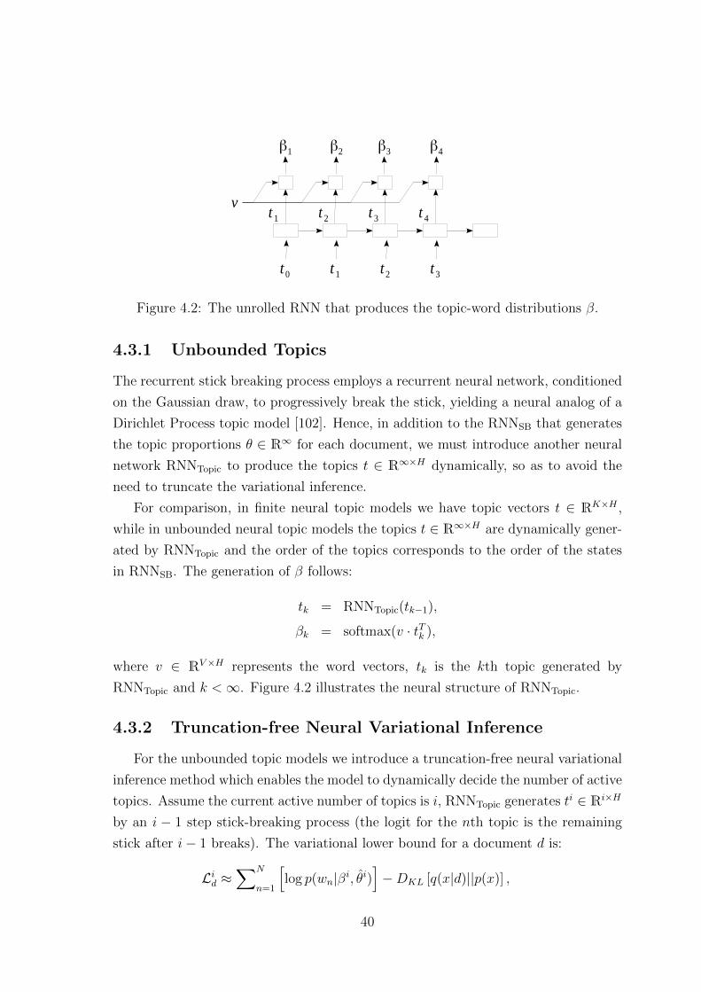
β1 β2 β3 β4
vt 1 t 2 t 3 t 4
t 0 t 1 t 2 t 3
Figure 4.2: The unrolled RNN that produces the topic-word distributions β.
4.3.1 Unbounded Topics
The recurrent stick breaking process employs a recurrent neural network, conditioned
on the Gaussian draw, to progressively break the stick, yielding a neural analog of a
Dirichlet Process topic model [102]. Hence, in addition to the RNNSB that generates
the topic proportions θ ∈ R∞ for each document, we must introduce another neural
network RNNTopic to produce the topics t ∈ R∞×H dynamically, so as to avoid the
need to truncate the variational inference.
For comparison, in finite neural topic models we have topic vectors t ∈ RK×H ,
while in unbounded neural topic models the topics t ∈ R∞×H are dynamically gener-
ated by RNNTopic and the order of the topics corresponds to the order of the states
in RNNSB. The generation of β follows:
tk = RNNTopic(tk−1),
βk = softmax(v · tTk ),
where v ∈ RV×H represents the word vectors, tk is the kth topic generated by
RNNTopic and k <∞. Figure 4.2 illustrates the neural structure of RNNTopic.
4.3.2 Truncation-free Neural Variational Inference
For the unbounded topic models we introduce a truncation-free neural variational
inference method which enables the model to dynamically decide the number of active
topics. Assume the current active number of topics is i, RNNTopic generates ti ∈ Ri×H
by an i − 1 step stick-breaking process (the logit for the nth topic is the remaining
stick after i− 1 breaks). The variational lower bound for a document d is:
Lid ≈∑N
n=1
[log p(wn|βi, θi)
]−DKL [q(x|d)||p(x)] ,
40

Algorithm 1 Unbounded Recurrent Neural Topic Model
0: Initialise Θ and Φ; Set active topic number i1: repeat2: for s ∈ minibatches S do3: for k ∈ [1, i] do4: Compute topic vector tk = RNNTopic(tk−1)5: Compute topic distribution βk = softmax(v · tTk )6: end for7: for d ∈ Ds do8: Sample topic proportion θ ∼ GRSB(θ|µ(d), σ2(d))9: for w ∈ document d do
10: Compute log-likelihood log p(w|θ, β)11: end for12: Compute lower bound Li−1
d and Lid13: Compute gradients ∇Θ,ΦLid and update14: end for15: Compute likelihood increase I16: if I > γ then17: Increase active topic number i = i+ 118: end if19: end for20: until Convergence
where θi corresponds to the topic distribution over words βt. In order to dynamically
increase the number of topics, the model proposes the ith break on the stick to split
the (i + 1)th topic. In this case, RNNTopic proceeds to the next state and generates
topic t(i+1) for β(i+1) and the RNNSB generates θ(i+1) by an extra break of the stick.
Firstly, we compute the likelihood increase brought by topic i across the documents
D:
I =∑D
d
[Lid − Li−1
d
]/∑D
d[Lid]
Then, we employ an acceptance hyper-parameter γ to decide whether to generate a
new topic. If I > γ, the previous proposed new topic (the ith topic) contributes to the
generation of words and we increase the active number of topics i by 1, otherwise we
keep the current i unchanged. Thus γ controls the rate at which the model generates
new topics. In practice, the increase of the lower bound is computed over mini-batches
so that the model is able to generate new topics before the current epoch is finished.
The details of the algorithm are described in Algorithm 1.
41
4.4 Experiments
We perform an experimental evaluation employing three datasets: MXM 1 song lyrics,
20NewsGroups2 and Reuters RCV1-v2 3 news. MXM is the official lyrics collection of
the Million Song Dataset with 210,519 training and 27,143 testing datapoints respec-
tively. The 20NewsGroups corpus is divided into 11,314 training and 7,531 testing
documents, while the RCV1-v2 corpus is a larger collection with 794,414 training
and 10,000 test cases from Reuters newswire stories. We employ the original 5,000
vocabulary provided for MXM, while the other two datasets are processed by stem-
ming, filtering stopwords and taking the most frequent 2,0004 and 10,000 words as
the vocabularies.
The hidden dimension of the MLP for constructing q(θ|d) is 256 for all the neural
topic models and the benchmarks that apply neural variational inference (e.g. NVDM,
proLDA, NVLDA), and 0.8 dropout is applied on the output of the MLP before
parameterising the diagonal Gaussian distribution. Grid search is carried out on
learning rate and batch size for achieving the held-out perplexity. For the recurrent
stick breaking construction we use a one layer LSTM cell (256 hidden units) for
constructing the recurrent neural network. For the finite topic models we set the
maximum number of topics K as 50 and 200. The models are trained by Adam
[53] and only one sample is used for neural variational inference. We follow the
optimisation strategy of NVDM by alternately updating the model parameters and
the inference network. To alleviate the redundant topics issue, we also apply topic
diversity regularisation [120] during the inference process.
We use Perplexity as the main metric for assessing the generalisation ability of our
generative models. Here we use the variational lower bound to estimate the document
perplexity: exp(− 1D
∑Dd
1Nd
log p(d)) following the setting of NVDM in Chapter 3.
Table 4.1 presents the test document perplexities of the topic models on the three
datasets. The upper section of the table lists the results for finite neural topic models,
with 50 or 200 topics, on the MXM, 20NewsGroups and RCV1 datasets. We compare
our neural topic models with the Gaussian Softmax (GSM), Gaussian Stick Breaking
(GSB) and Recurrent Stick Breaking (RSB) constructions to the online variational
LDA (onlineLDA) [44] and neural variational inference LDA (NVLDA) [96] models.
The lower section shows the results for the unbounded topic models, including our
1http://labrosa.ee.columbia.edu/millionsong/musixmatch [8]2http://qwone.com/ jason/20Newsgroups3http://trec.nist.gov/data/reuters/reuters.html4We use the vocabulary provided by Srivastava and Sutton [96] for direct comparison.
42
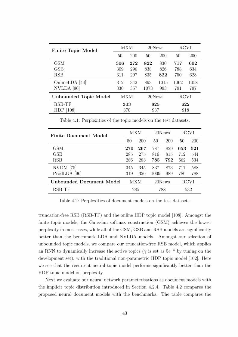
Finite Topic ModelMXM 20News RCV1
50 200 50 200 50 200
GSM 306 272 822 830 717 602GSB 309 296 838 826 788 634RSB 311 297 835 822 750 628
OnlineLDA [44] 312 342 893 1015 1062 1058NVLDA [96] 330 357 1073 993 791 797
Unbounded Topic Model MXM 20News RCV1
RSB-TF 303 825 622HDP [108] 370 937 918
Table 4.1: Perplexities of the topic models on the test datasets.
Finite Document ModelMXM 20News RCV1
50 200 50 200 50 200
GSM 270 267 787 829 653 521GSB 285 275 816 815 712 544RSB 286 283 785 792 662 534
NVDM [75] 345 345 837 873 717 588ProdLDA [96] 319 326 1009 989 780 788
Unbounded Document Model MXM 20News RCV1
RSB-TF 285 788 532
Table 4.2: Perplexities of document models on the test datasets.
truncation-free RSB (RSB-TF) and the online HDP topic model [108]. Amongst the
finite topic models, the Gaussian softmax construction (GSM) achieves the lowest
perplexity in most cases, while all of the GSM, GSB and RSB models are significantly
better than the benchmark LDA and NVLDA models. Amongst our selection of
unbounded topic models, we compare our truncation-free RSB model, which applies
an RNN to dynamically increase the active topics (γ is set as 5e−5 by tuning on the
development set), with the traditional non-parametric HDP topic model [102]. Here
we see that the recurrent neural topic model performs significantly better than the
HDP topic model on perplexity.
Next we evaluate our neural network parameterisations as document models with
the implicit topic distribution introduced in Section 4.2.4. Table 4.2 compares the
proposed neural document models with the benchmarks. The table compares the
43
results for a fixed dimension latent variable, 50 or 200, achieved by our neural docu-
ment models to Product of Experts LDA (prodLDA) [96] and the Neural Variational
Document Model (NVDM) [75]. According to our experimental results, the gener-
alisation abilities of the GSM, GSB and RSB models are all improved by switching
from the mixture decoder (Equation 4.5) to the softmax decoder (Equation 4.6), and
their performance is also significantly better than the NVDM and ProdLDA. We hy-
pothesise that this effect is due to the models not needing to infer the topic-word
assignments, which makes optimisation much easier. Interestingly, the RSB model
performs slightly better than the GSM and GSB on 20NewsGroups in both the 50 and
200 topic settings. As mentioned in Section 4.2.4, GSM is a variant of NVDM that
applies topic and word vectors to construct the topic distribution over words instead
of directly modelling a multinomial distribution by a softmax function, which further
simplifies optimisation. If it is not necessary to model the explicit topic distribution
over words, using an implicit topic distribution may lead to better generalisation.
To further demonstrate the effectiveness of the stick-breaking construction, Figure
4.3 and Figure 4.4 present the average probability of each topic of GSM model and
GSB model respectively, which are estimated by the posterior probability q(z|d) of
each document from 20NewsGroups. Here we set the number of topics to 400 that
is large enough for this dataset. Figure 4.3a shows that the topics with higher prob-
ability are evenly distributed. While in Figure 4.4a the higher probability ones are
placed in the front, and we can see a small tail on the topics after 300. Moreover,
Figure 4.3b and Figure 4.4b sort the average probability measures by decreasing or-
der, and as can be seen the overall distribution of GSB has slightly heavier tail than
GSM. Due to the sparsity inducing property of the stick-breaking construction, the
topics on the tail are less likely to be sampled. This is also the advantage of stick-
breaking construction when we apply the RSB-TF as a non-parametric topic model,
since the model activates the topics according to the knowledge learned from data
and it becomes less sensitive to the hyperparameter controlling the initial number of
topics.
Figure 4.5 shows the impact on test perplexity for the neural topic models when
the maximum number of topics is increased. The truncation-free RSB (RSB-TF)
dynamically increases the active topics, we use a dashed line to represent its test
perplexity for reference in the figure. We can see that the performance of the GSM
model gets worse if the maximum number of topics exceeds 400, but the GSB and
RSB are stable even though the number of topics far outstrips that which the model
requires. In addition, the RSB model performs better than GSB when the number of
44
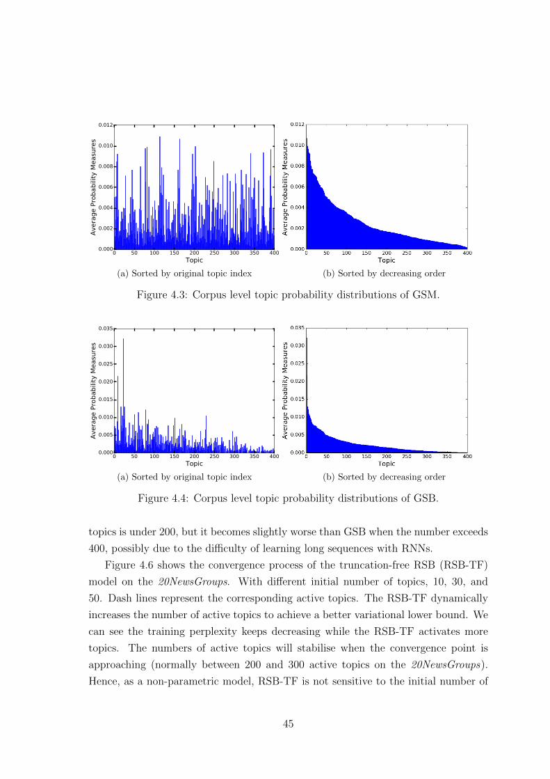
0 50 100 150 200 250 300 350 400
Topic
0.000
0.002
0.004
0.006
0.008
0.010
0.012
Avera
ge P
robabili
ty M
easu
res
(a) Sorted by original topic index (b) Sorted by decreasing order
Figure 4.3: Corpus level topic probability distributions of GSM.
0 50 100 150 200 250 300 350 400
Topic
0.000
0.005
0.010
0.015
0.020
0.025
0.030
0.035
Avera
ge P
robabili
ty M
easu
res
(a) Sorted by original topic index (b) Sorted by decreasing order
Figure 4.4: Corpus level topic probability distributions of GSB.
topics is under 200, but it becomes slightly worse than GSB when the number exceeds
400, possibly due to the difficulty of learning long sequences with RNNs.
Figure 4.6 shows the convergence process of the truncation-free RSB (RSB-TF)
model on the 20NewsGroups. With different initial number of topics, 10, 30, and
50. Dash lines represent the corresponding active topics. The RSB-TF dynamically
increases the number of active topics to achieve a better variational lower bound. We
can see the training perplexity keeps decreasing while the RSB-TF activates more
topics. The numbers of active topics will stabilise when the convergence point is
approaching (normally between 200 and 300 active topics on the 20NewsGroups).
Hence, as a non-parametric model, RSB-TF is not sensitive to the initial number of
45

0 200 400 600 800 1000
Topics
800
820
840
860
880
900
Test
Perp
lexit
y
GSMGSBRSBRSB-TF
Figure 4.5: Test perplexities of the neural topic models with a varying maximumnumber of topics on the 20NewsGroups dataset.
0 50 100 150 200 250 300 350 400 450
epoch (s)
800
1000
1200
1400
1600
Tra
inin
g P
erp
lexit
y
10 init topics30 init topics50 init topics
0
20
40
60
80
100
120
140
160
Act
ive T
opic
s
Figure 4.6: The convergence behavior of the truncation-free RSB model (RSB-TF)with different initial active topics on 20NewsGroups.
active topics.
In addition, since the quality of the discovered topics is not directly reflected
by perplexity (i.e. a function of log-likelihood), we evaluate the topic observed
coherence by normalised point-wise mutual information (NPMI) [62]. Table 4.3
shows the topic observed coherence achieved by the finite neural topic models. We
compute coherence over the top-5 words and top-10 words for all topics and then
take the mean of both values. According to these results, there does not appear to
be a significant difference in topic coherence amongst the neural topic models. We
observe that in both the GSB and RSB, the NPMI scores of the former topics in
46
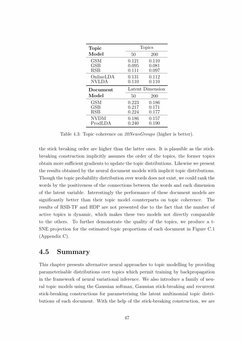
TopicModel
Topics
50 200
GSM 0.121 0.110GSB 0.095 0.081RSB 0.111 0.097
OnlineLDA 0.131 0.112NVLDA 0.110 0.110
DocumentModel
Latent Dimension
50 200
GSM 0.223 0.186GSB 0.217 0.171RSB 0.224 0.177
NVDM 0.186 0.157ProdLDA 0.240 0.190
Table 4.3: Topic coherence on 20NewsGroups (higher is better).
the stick breaking order are higher than the latter ones. It is plausible as the stick-
breaking construction implicitly assumes the order of the topics, the former topics
obtain more sufficient gradients to update the topic distributions. Likewise we present
the results obtained by the neural document models with implicit topic distributions.
Though the topic probability distribution over words does not exist, we could rank the
words by the positiveness of the connections between the words and each dimension
of the latent variable. Interestingly the performance of these document models are
significantly better than their topic model counterparts on topic coherence. The
results of RSB-TF and HDP are not presented due to the fact that the number of
active topics is dynamic, which makes these two models not directly comparable
to the others. To further demonstrate the quality of the topics, we produce a t-
SNE projection for the estimated topic proportions of each document in Figure C.1
(Appendix C).
4.5 Summary
This chapter presents alternative neural approaches to topic modelling by providing
parameterisable distributions over topics which permit training by backpropagation
in the framework of neural variational inference. We also introduce a family of neu-
ral topic models using the Gaussian softmax, Gaussian stick-breaking and recurrent
stick-breaking constructions for parameterising the latent multinomial topic distri-
butions of each document. With the help of the stick-breaking construction, we are
47
able to build neural topic models which exhibit similar sparse topic distributions
as found with traditional Dirichlet-Multinomial models. By exploiting the ability
of recurrent neural networks to model sequences of unbounded length, we further
present a truncation-free variational inference method that allows the number of top-
ics to dynamically increase, which is notionally neural unbounded topic model that is
analogous to Bayesian non-parametric topic model. The evaluation results show that
neural topic models achieve state-of-the-art performance on a range of standard docu-
ment corpora, which demonstrate more flexibility and effectiveness of deep generative
models than traditional probabilistic topic models. The experiments also compare the
neural topic models (with explicit topic distribution) and the neural document mod-
els (with implicit topic distribution) using different parameterisation networks. The
results show that if it is not necessary to model the explicit topic distribution over
words, using an implicit topic distribution may lead to better generalisation.
48
Chapter 5
Neural Answer Selection Model
Different from the deep generative models for unsupervised document and topic mod-
elling introduced in the previous contents, this chapter focuses on the generative
model for supervised question answer selection. One major difference of this task
from document/topic modelling is that there are a few labels available indicating
whether an answer is correct to a given question. Here, we are interested in how
is the performance of deep generative models applied on supervised learning tasks,
and whether the neural variational inference is effective on carrying out sequence
modelling.
5.1 Introduction
Question answer sentence selection is a task that selects the correct sentences an-
swering a factoid question from a set of candidate sentences. The key point is to
learn good representations of observed question and answer sequences. More specif-
ically, the representations need to contain both semantic and syntactic information
so that the model is able to figure out what information the question seeks to answer
and whether the answer contains correct information. Previous works have focused
on using only syntactic information to match questions and answers, for example
the generative models on aligning the dependency trees of question answer pairs
[110, 109, 33]. Then, the features are fed into a classifier for predicting correctness.
However, only syntactic information is not good enough to solve such a difficult NLP
task. Yih et al. [123] incorporates semantic information by using a combination
of lexical semantic resources such as WordNet. Severyn and Moschitti [92] employs
tree kernel SVMs to generate highly discriminative structural features that combine
syntactic and semantic information encoded in the input trees. Recently, Yu et al.
[125] directly applies a convolutional neural network over bigrams so that the model
49
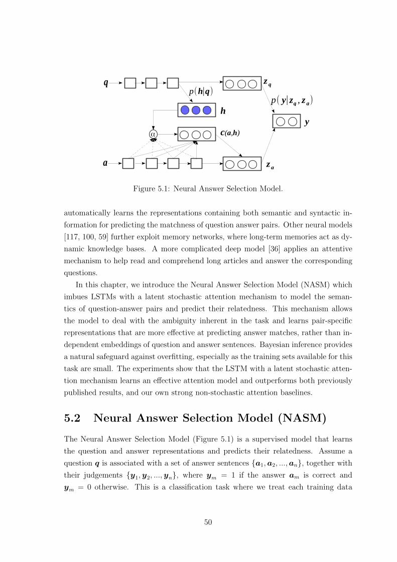
a
q
y
z q
c(a,h)
z a
h
p(h∣q)p( y∣zq , z a)
α
Figure 5.1: Neural Answer Selection Model.
automatically learns the representations containing both semantic and syntactic in-
formation for predicting the matchness of question answer pairs. Other neural models
[117, 100, 59] further exploit memory networks, where long-term memories act as dy-
namic knowledge bases. A more complicated deep model [36] applies an attentive
mechanism to help read and comprehend long articles and answer the corresponding
questions.
In this chapter, we introduce the Neural Answer Selection Model (NASM) which
imbues LSTMs with a latent stochastic attention mechanism to model the seman-
tics of question-answer pairs and predict their relatedness. This mechanism allows
the model to deal with the ambiguity inherent in the task and learns pair-specific
representations that are more effective at predicting answer matches, rather than in-
dependent embeddings of question and answer sentences. Bayesian inference provides
a natural safeguard against overfitting, especially as the training sets available for this
task are small. The experiments show that the LSTM with a latent stochastic atten-
tion mechanism learns an effective attention model and outperforms both previously
published results, and our own strong non-stochastic attention baselines.
5.2 Neural Answer Selection Model (NASM)
The Neural Answer Selection Model (Figure 5.1) is a supervised model that learns
the question and answer representations and predicts their relatedness. Assume a
question q is associated with a set of answer sentences {a1,a2, ...,an}, together with
their judgements {y1,y2, ...,yn}, where ym = 1 if the answer am is correct and
ym = 0 otherwise. This is a classification task where we treat each training data
50

point as a triple (q,a,y) while predicting y for the unlabelled question-answer pair
(q,a).
NASM employs two different LSTMs to embed raw question inputs q and answer
inputs a. Let sq(j) and sa(i) be the state outputs of the two LSTMs, and i, j be
the positions of the states. Conventionally, the last state outputs sq(|q|) and sa(|a|),as the independent question and answer representations, can be used for relatedness
prediction. In NASM, however, we aim to learn pair-specific representations through
a latent attention mechanism, which is more effective for pair relatedness prediction.
An attention model is applied in NASM to focus on the words in the answer sen-
tence that are prominent for predicting the answer matched to the current question.
Instead of using a deterministic question vector, such as sq(|q|), NASM employs a la-
tent distribution pθ(h|q) to model the question semantics, which is a parameterised di-
agonal GaussianN (h|µ(q),σ2(q)). Therefore, the attention model extracts a context
vector c(a,h) by iteratively attending to the answer tokens based on the stochastic
vector h ∼ pθ(h|q). In doing so the model is able to adapt to the ambiguity inher-
ent in questions and obtain salient information through attention. Compared to its
deterministic counterpart (applying sq(|q|) as the question semantics), the stochastic
units incorporated into NASM allow multi-modal attention distributions. Further,
NASM is more robust against overfitting due to that stochastic representations also
model the uncertainties. Hence, if we marginalise over the latent variable, the model
actually feeds a distribution to next layer instead of a deterministic vector. This is
analogous to the application of dropout in deep neural networks. [25] and [55] provide
more discussions about the connection between dropout and variational inference.
In this model, the conditional distribution pθ(h|q) is:
πθ = gθ(flstmq (q)) = gθ(sq(|q|)) (5.1)
µθ = l1(πθ), logσθ = l2(πθ) (5.2)
For each question q, the neural network generates the corresponding parameters µ
and σ that parameterise the latent distribution over question semantics h. Following
[6], the attention model is defined as:
α(i) ∝ exp(W Tα tanh(W hh+W ssa(i))) (5.3)
c(a,h) =∑
isa(i)α(i) (5.4)
za(a,h) = tanh (W ac(a,h) +W nsa(|a|)) (5.5)
where α(i) is the normalised attention score at answer token i, and the context vector
c(a,h) is the weighted sum of all the state outputs sa(i). We adopt zq(q), za(a,h)
51

as the question and answer representations for predicting their relatedness y. zq(q) is
a deterministic vector that is equal to sq(|q|), while za(a,h) is a combination of the
sequence output sa(|a|) and the context vector c(a,h) (Eq. 5.5). For the prediction
of pair relatedness y, we model the conditional probability distribution pθ(y|zq, za)by sigmoid function:
pθ(y = 1|zq, za) = σ(zTqMza + b
)(5.6)
To maximise the log-likelihood log p(y|q,a) we use the variational lower bound:
L =Eqφ(h)[log pθ(y|zq(q), za(a,h))]−DKL(qφ(h)||pθ(h|q))
6 log
∫pθ(y|zq(q), za(a,h))pθ(h|q)dh
= log p(y|q,a) (5.7)
Following the neural variational inference framework, we construct a deep neural
network as the inference network qφ(h|q,a,y) = N (h|µφ(q,a,y),σ2φ(q,a,y)):
πφ = gφ(f lstmq (q), f lstm
a (a), fy(y))
= gφ(sq(|q|), sa(|a|), sy) (5.8)
µφ = l3(πφ), logσφ = l4(πφ) (5.9)
where q and a are also modelled by LSTMs1, and the relatedness label y is mod-
elled by a simple linear transformation into the vector sy. According to the joint
representation πφ, we then generate the parameters µφ and σφ, which parameterise
the variational distribution over the question semantics h. To emphasise, though
both pθ(h|q) and qφ(h|q,a,y) are modelled as parameterised Gaussian distributions,
qφ(h|q,a,y) as an approximation only functions during inference by producing sam-
ples to compute the stochastic gradients, while pθ(h|q) is the generative distribution
that generates the samples for predicting the question-answer relatedness y.
Based on the samples h ∼ qφ(h|q,a,y), we use SGVB to optimise the lower
bound (Eq.5.7). The model parameters θ and the inference network parameters φ
are updated jointly using their stochastic gradients. In this case, similar to the
NVDM, the Gaussian KL divergence DKL[qφ(h|q,a,y))‖pθ(h|q)] can be analytically
computed during training process.
52
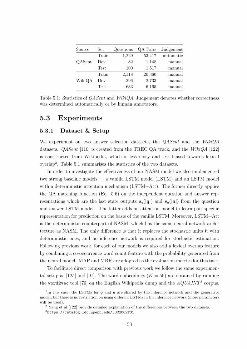
Source Set Questions QA Pairs Judgement
Train 1,229 53,417 automatic
QASent Dev 82 1,148 manual
Test 100 1,517 manual
Train 2,118 20,360 manual
WikiQA Dev 296 2,733 manual
Test 633 6,165 manual
Table 5.1: Statistics of QASent and WikiQA. Judgement denotes whether correctnesswas determined automatically or by human annotators.
5.3 Experiments
5.3.1 Dataset & Setup
We experiment on two answer selection datasets, the QASent and the WikiQA
datasets. QASent [110] is created from the TREC QA track, and the WikiQA [122]
is constructed from Wikipedia, which is less noisy and less biased towards lexical
overlap2. Table 5.1 summarises the statistics of the two datasets.
In order to investigate the effectiveness of our NASM model we also implemented
two strong baseline models — a vanilla LSTM model (LSTM) and an LSTM model
with a deterministic attention mechanism (LSTM+Att). The former directly applies
the QA matching function (Eq. 5.6) on the independent question and answer rep-
resentations which are the last state outputs sq(|q|) and sa(|a|) from the question
and answer LSTM models. The latter adds an attention model to learn pair-specific
representation for prediction on the basis of the vanilla LSTM. Moreover, LSTM+Att
is the deterministic counterpart of NASM, which has the same neural network archi-
tecture as NASM. The only difference is that it replaces the stochastic units h with
deterministic ones, and no inference network is required for stochastic estimation.
Following previous work, for each of our models we also add a lexical overlap feature
by combining a co-occurrence word count feature with the probability generated from
the neural model. MAP and MRR are adopted as the evaluation metrics for this task.
To facilitate direct comparison with previous work we follow the same experimen-
tal setup as [125] and [91]. The word embeddings (K = 50) are obtained by running
the word2vec tool [76] on the English Wikipedia dump and the AQUAINT 3 corpus.
1In this case, the LSTMs for q and a are shared by the inference network and the generativemodel, but there is no restriction on using different LSTMs in the inference network (more parameterswill be used).
2 Yang et al [122] provide detailed explanation of the differences between the two datasets.3https://catalog.ldc.upenn.edu/LDC2002T31
53
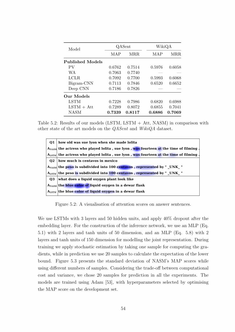
ModelQASent WikiQA
MAP MRR MAP MRR
Published ModelsPV 0.6762 0.7514 0.5976 0.6058WA 0.7063 0.7740 — —LCLR 0.7092 0.7700 0.5993 0.6068Bigram-CNN 0.7113 0.7846 0.6520 0.6652Deep CNN 0.7186 0.7826 — —
Our ModelsLSTM 0.7228 0.7986 0.6820 0.6988LSTM + Att 0.7289 0.8072 0.6855 0.7041NASM 0.7339 0.8117 0.6886 0.7069
Table 5.2: Results of our models (LSTM, LSTM + Att, NASM) in comparison withother state of the art models on the QASent and WikiQA dataset.
ALSTM the blue color of liquid oxygen in a dewar flask
ANASM the blue color of liquid oxygen in a dewar flask
Q3 what does a liquid oxygen plant look like
ALSTM the peso is subdivided into 100 centavos , represented by " _UNK_ "
ANASM the peso is subdivided into 100 centavos , represented by " _UNK_ "
Q2 how much is centavos in mexico
ALSTM the actress who played lolita , sue lyon , was fourteen at the time of filming .
ANASM the actress who played lolita , sue lyon , was fourteen at the time of filming .
Q1 how old was sue lyon when she made lolita
Figure 5.2: A visualisation of attention scores on answer sentences.
We use LSTMs with 3 layers and 50 hidden units, and apply 40% dropout after the
embedding layer. For the construction of the inference network, we use an MLP (Eq.
5.1) with 2 layers and tanh units of 50 dimension, and an MLP (Eq. 5.8) with 2
layers and tanh units of 150 dimension for modelling the joint representation. During
training we apply stochastic estimation by taking one sample for computing the gra-
dients, while in prediction we use 20 samples to calculate the expectation of the lower
bound. Figure 5.3 presents the standard deviation of NASM’s MAP scores while
using different numbers of samples. Considering the trade-off between computational
cost and variance, we chose 20 samples for prediction in all the experiments. The
models are trained using Adam [53], with hyperparameters selected by optimising
the MAP score on the development set.
54
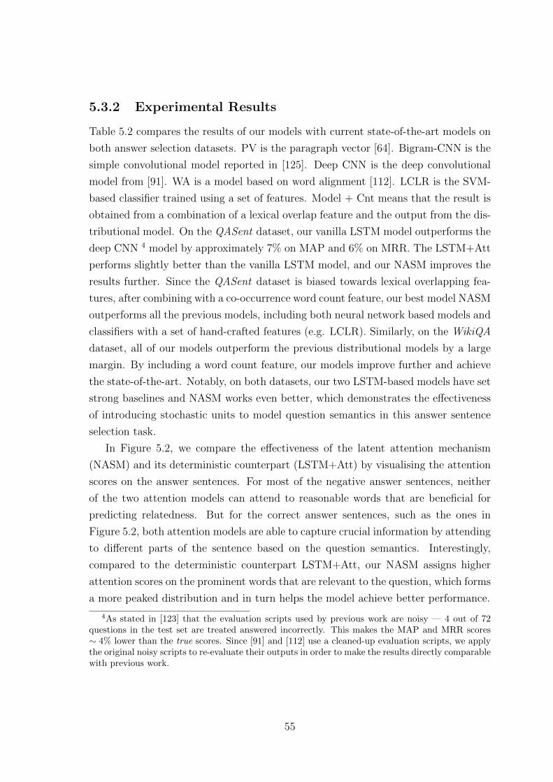
5.3.2 Experimental Results
Table 5.2 compares the results of our models with current state-of-the-art models on
both answer selection datasets. PV is the paragraph vector [64]. Bigram-CNN is the
simple convolutional model reported in [125]. Deep CNN is the deep convolutional
model from [91]. WA is a model based on word alignment [112]. LCLR is the SVM-
based classifier trained using a set of features. Model + Cnt means that the result is
obtained from a combination of a lexical overlap feature and the output from the dis-
tributional model. On the QASent dataset, our vanilla LSTM model outperforms the
deep CNN 4 model by approximately 7% on MAP and 6% on MRR. The LSTM+Att
performs slightly better than the vanilla LSTM model, and our NASM improves the
results further. Since the QASent dataset is biased towards lexical overlapping fea-
tures, after combining with a co-occurrence word count feature, our best model NASM
outperforms all the previous models, including both neural network based models and
classifiers with a set of hand-crafted features (e.g. LCLR). Similarly, on the WikiQA
dataset, all of our models outperform the previous distributional models by a large
margin. By including a word count feature, our models improve further and achieve
the state-of-the-art. Notably, on both datasets, our two LSTM-based models have set
strong baselines and NASM works even better, which demonstrates the effectiveness
of introducing stochastic units to model question semantics in this answer sentence
selection task.
In Figure 5.2, we compare the effectiveness of the latent attention mechanism
(NASM) and its deterministic counterpart (LSTM+Att) by visualising the attention
scores on the answer sentences. For most of the negative answer sentences, neither
of the two attention models can attend to reasonable words that are beneficial for
predicting relatedness. But for the correct answer sentences, such as the ones in
Figure 5.2, both attention models are able to capture crucial information by attending
to different parts of the sentence based on the question semantics. Interestingly,
compared to the deterministic counterpart LSTM+Att, our NASM assigns higher
attention scores on the prominent words that are relevant to the question, which forms
a more peaked distribution and in turn helps the model achieve better performance.
4As stated in [123] that the evaluation scripts used by previous work are noisy — 4 out of 72questions in the test set are treated answered incorrectly. This makes the MAP and MRR scores∼ 4% lower than the true scores. Since [91] and [112] use a cleaned-up evaluation scripts, we applythe original noisy scripts to re-evaluate their outputs in order to make the results directly comparablewith previous work.
55

1 10 20 50 100Samples
0.2
0.4
0.6
0.8
1.0
1.2
1.4
Sta
ndard
Devia
tion
1e−31.28
0.77
0.460.39
0.32
Figure 5.3: The standard deviations of MAP scores computed by running 10 NASMmodels on WikiQA with different numbers of samples.
5.3.3 Discussion
The basic intuition of applying deep generative models for learning language is that
the latent distributions grant the ability to sum over all the possibilities in terms of
semantics. As shown in the experiments, neural variational inference brings consistent
improvements on the performance of the NLP tasks including document/topic mod-
elling and question answer selection. Compared to the unsupervised learning model
NVDM, the supervised learning model NASM in this context enjoys more benefits
from the perspective of optimisation, since Bayesian learning naturally guards against
overfitting.
According to the variational lower bound (Eq. 3.1) of NVDM, we adopt p(h)
as a standard Gaussian prior, the KL divergence term DKL[qφ(h|X)‖p(h)] can be
analytically computed as 12(K − ‖µ‖2 − ‖σ‖2 + log |σ2|). It is not difficult to find
that it actually acts as L2 regulariser when we update the µ. Similarly, in NASM
(Eq. 5.7), we also have the KL divergence term DKL[qφ(h|q,a,y))‖pθ(h|q)]. Different
from NVDM, it attempts to minimise the distance between qφ(h|q,a,y)) and pθ(h|q)
that are both conditional distributions. Because pθ(h|q) as well as qφ(h|q,a,y)) are
learned during training, the two distributions are mutually restrained while being
updated. Therefore, NVDM simply penalises the large µ and encourages qφ(h|X)
to approach the prior p(h) for every document X, but in NASM, pθ(h|q) acts like a
moving baseline distribution which regularises the update of qφ(h|q,a,y)) for every
different condition. In practice, we use early stopping by observing the prediction
performance on development dataset for the question answer selection task. Using
the same learning rate and neural network structure, LSTM+Att reaches optimal
performance and starts to overfit on training dataset generally at the 20th iteration,
while NASM starts to overfit around the 35th iteration.
56
More interestingly, in the question answer selection experiments, NASM learns
more peaked attention scores than its deterministic counterpart LSTM+Att. For the
update process of LSTM+Att, we find there exists a relatively big variance in the
gradients w.r.t. question semantics (LSTM+Att applies deterministic sq(|q|) while
NASM applies stochastic h). This is because the training dataset is small and contains
many negative answer sentences that brings no benefit but noise to the learning of the
attention model. In contrast, for the update process of NASM, we observe more stable
gradients w.r.t. the parameters of latent distributions. The optimisation of the lower
bound on one hand maximises the conditional log-likelihood (that the deterministic
counterpart cares about) and on the other hand minimises the KL-divergence (that
regularises the gradients). Hence, each update of the lower bound actually keeps
the gradients w.r.t. µ from swinging heavily. Besides, since the values of σ are not
very significant in this case, the distribution of attention scores mainly depends on
µ. Therefore, the learning of the attention model benefits from the regularisation as
well, and it explains the fact that NASM learns more peaked attention scores which
in turn helps achieve a better prediction performance.
Certainly, the improvements of the performance in this question answer selection
task is more like icing on the cake. The fact of lacking training data makes the
deterministic counterpart easily overfit, which gives the opportunity to latent variable
models. However, if the labelled question answer pairs are sufficient enough, the
deterministic counterpart should be able to achieve adequate accuracy on predicting
question answer matchness.
5.4 Summary
This chapter discusses the neural answer selection model (NASM) which imbues
LSTMs with a latent stochastic attention mechanism to model the semantics of
question-answer pairs and predict their relatedness. Different from the unsupervised
generative models for document/topic modelling introduced in the previous chapters,
NASM is a supervised conditional model but its inference can also be carried out
in the same neural variational inference framework. These models are simple, ex-
pressive and can be trained efficiently with the highly scalable stochastic gradient
back-propagation. Hence, we show the effectiveness of the continuous latent variable
models for NLP, and the neural variational inference is capable of generalising to
incorporate any type of neural network for different application scenarios.
57
Part III
Discrete Latent Variable Models
58
Chapter 6
Latent Sentence CompressionModels
Compared to the continuous latent variables that commonly applied for learning
stochastic representations, discrete latent variables are more extensive on applica-
tions, for example structure prediction, planning and clustering. Since discrete rep-
resentation is a natural fit for predictive systems with categorical properties, it has
more advantages on developing the potential of deep neural networks. Language is
a straightforward case where each sentence is represented by a sequence of discrete
word symbols. However, variational inference on discrete latent variables is rela-
tively difficult due to intractable marginalisation and the high variance issue of the
sampling-based gradient estimators. Chapter 2 has introduced a few techniques to
mitigate the problem when the continuous reparameterisation trick is not applicable.
In this chapter, we are going to discuss the discrete latent variable models for mod-
elling language. We formulate a discrete variational auto-encoder and apply it to the
task of compressing long sentences into short ones.
6.1 Introduction
The recurrent sequence-to-sequence paradigm for natural language generation [48,
101] has achieved remarkable recent success and is now the approach of choice for
applications such as machine translation [6], caption generation [121] and speech
recognition [18]. While these models have developed sophisticated conditioning mech-
anisms, e.g. attention, fundamentally they are discriminative models trained only to
approximate the conditional output distribution of strings. In this chapter we explore
modelling the language sentences by a discrete variational auto-encoder (VAE).
59
Auto-encoder [86] is a typical neural network architecture for learning compact
data representations, with the general aim of performing dimensionality reduction
on embeddings [41]. In this context, rather than seeking to embed sentences as
points in a vector space, we model the representations with explicit natural language
sentences. This approach is a natural fit for summarisation tasks such as sentence
compression. According to this, we propose a generative auto-encoding sentence
compression (ASC) model, where we introduce a latent language model to provide
the variable-length compact summary. The objective is to perform Bayesian inference
for the posterior distribution of summaries conditioned on the observed utterances.
Hence, in the framework of VAE, we construct an inference network as the variational
approximation of the posterior, which generates compression samples to optimise the
variational lower bound.
The most common family of variational auto-encoders [56] relies on the repa-
rameterisation trick, which is not applicable for our discrete latent language model.
Instead, we employ the REINFORCE algorithm [79, 77] introduced in Chapter 2 to
mitigate the problem of high variance during sampling-based variational inference.
Nevertheless, when directly applying the RNN encoder-decoder to model the varia-
tional distribution it is very difficult to generate reasonable compression samples in
the early stages of training, since each hidden state of the sequence would have |V |possible words to be sampled from. To combat this we employ pointer networks [105]
to construct the variational distribution. This biases the latent space to sequences
composed of words only appearing in the source sentence (i.e. the size of softmax
output for each state becomes the length of current source sentence), which amounts
to applying an extractive compression model for the variational approximation.
In order to further boost the performance on sentence compression, we employ a
supervised forced-attention sentence compression model (FSC) trained on la-
belled data to teach the ASC model to generate compression sentences. The FSC
model shares the pointer network of the ASC model and combines a softmax out-
put layer over the whole vocabulary. Therefore, while training on the sentence-
compression pairs, it is able to balance copying a word from the source sentence
with generating it from the background distribution. More importantly, by jointly
training on the labelled and unlabelled datasets, this shared pointer network enables
the model to work in a semi-supervised scenario. In this case, the FSC teaches the
ASC to generate reasonable samples, while the pointer network trained on a large un-
labelled data set helps the FSC model to perform better abstractive summarisation.
60
In the experiment section, we evaluate the proposed model by jointly training
the generative (ASC) and discriminative (FSC) models on the standard Gigaword
sentence compression task with varying amounts of labelled and unlabelled data.
The results demonstrate that by introducing a latent language variable we are able to
match the previous benchmakers with small amount of the supervised data. When we
employ our mixed discriminative and generative objective with all of the supervised
data the model significantly outperforms all previously published results.
6.2 Related Work
As one of the typical sequence-to-sequence tasks, sentence-level summarisation has
been explored by a series of discriminative encoder-decoder neural models. Filippova
et al [24] carries out extractive summarisation via deletion with LSTMs, while Rush
et al [87] applies a convolutional encoder and an attentional feed-forward decoder
to generate abstractive summarises, which provides the benchmark for the Gigaword
dataset. Nallapati et al [80] further improves the performance by exploring multi-
ple variants of RNN encoder-decoder models. The recent works [32], [70], [80] and
[30] also apply the similar idea of combining pointer networks and softmax output.
However, different from all these discriminative models above, we explore generative
models for sentence compression. Instead of training the discriminative model on a
big labelled dataset, our original intuition of introducing a combined pointer networks
is to bridge the unsupervised generative model (ASC) and supervised model (FSC)
so that we could utilise a large additional dataset, either labelled or unlabelled, to
boost the compression performance. Dai and Le [19] also explored semi-supervised
sequence learning, but in a pure deterministic model focused on learning better vector
representations.
Recently variational auto-encoders have been applied in a variety of fields as deep
generative models. In computer vision Kingma and Welling [56], Rezende et al [84],
and Gregor et al [28] have demonstrated strong performance on the task of image
generation and Eslami et al [23] proposes variable-sized variational auto-encoders to
identify multiple objects in images. While in natural language processing, there are
variants of VAEs on modelling documents [75] (NVDM introduced in Chapter 3),
sentences [14] and discovery of relations [72]. Apart from the typical initiations of
VAEs, there are also a series of works that employs generative models for supervised
learning tasks. For instance, Ba et al [5] learns visual attention for multiple objects by
optimising a variational lower bound, Kingma et al [54] implements a semi-supervised
61

framework for image classification and Miao et al [75] (NASM introduced in Chapter
5) applies a conditional variational approximation in the task of factoid question an-
swering. Dyer et al [22] proposes a generative model that explicitly extracts syntactic
relationships among words and phrases which further supports the argument that
generative models can be a statistically efficient method for learning neural networks
from small data.
6.3 Auto-encoding Sentence Compression Model
(ASC)
s0
s1
s2
s1
s3
s2
s4
s3
h1
dh2
dh3
dh4
d
Decoder
s1
s2
s3
s4
h1
e
c1
c2
c3
c1 c
2c0
h1
c
h2
eh3
eh4
e
h2
ch3
c
Encoder Compressor
h0
c
Compression (Pointer Networks)
3α2α1α
h2
c
h3
ch1
c
Reconstruction (Soft Attention)
Figure 6.1: Auto-encoding Sentence Compression Model
In this section, we introduce the auto-encoding sentence compression model (Fig-
ure 6.1)1 in the framework of variational auto-encoders. The ASC model consists
of four recurrent neural networks – an encoder, a compressor, a decoder and a lan-
guage model. Let s be the source sentence, and c be the compression sentence.
The compression model (encoder-compressor) is the inference network qφ(c|s) that
takes source sentences s as inputs and generates extractive compressions c. The
reconstruction model (compressor-decoder) is the generative network pθ(s|c) that
reconstructs source sentences s based on the latent compressions c. Hence, the for-
ward pass starts from the encoder to the compressor and ends at the decoder. As
1The language model, layer connections and decoder soft attentions are omitted in Figure 6.1 forclarity.
62

there could
Source sentence: there could be a nasty surprise under the tree for the us economy this christmas
...this christmas
there could this christmas...
pessimistic for us economy
surprise for the christmas tree
grim tidings for us christmas shopping
happy christmas
the
Discrete Latent Variable Models
Source Compression Source
Figure 6.2: Example of auto-encoding sentence compression.
the prior distribution, a language model p(c) is pre-trained to regularise the latent
compressions so that the samples drawn from the compression model are likely to be
reasonable natural language sentences.
For example, in Figure 6.2, the compression model generates multiple possible
compressions for the source sentence “there could be a nasty surprise under the tree
for the us economy this christmas”, and the generated compression sentences will
be used to reconstruct the source sentence in the reconstruction model. All of the
possible sentence compressions are evaluated by the variational lower bound.
6.3.1 Compression
For the compression model (encoder-compressor), qφ(c|s), we employ a pointer net-
work consisting of a bidirectional LSTM encoder that processes the source sentences,
and an LSTM compressor that generates compressed sentences by attending to the
encoded source words.
Let si be the words in the source sentences, hei be the corresponding state outputs
of the encoder. hei are the concatenated hidden states from each direction:
hei = f−→enc(~hei−1, si)||f←−enc( ~hei+1, si) (6.1)
Further, let cj be the words in the compressed sentences, hcj be the state outputs of
the compressor. We construct the predictive distribution by attending to the words
63
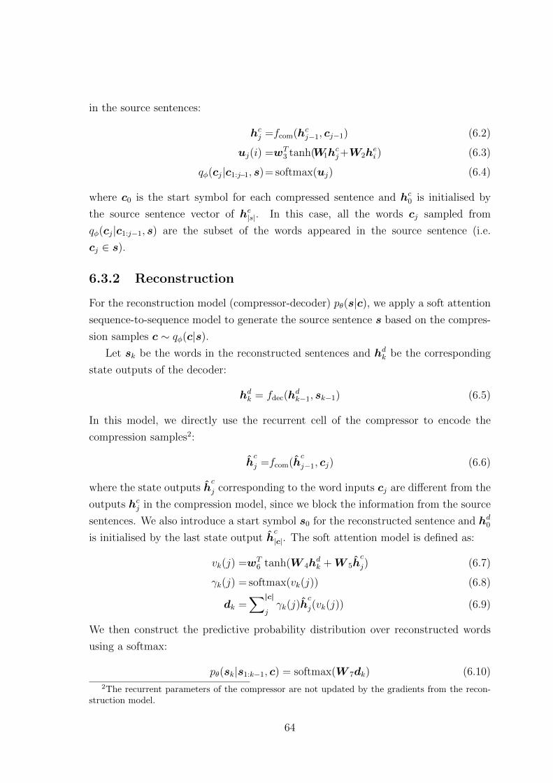
in the source sentences:
hcj =fcom(hcj−1, cj−1) (6.2)
uj(i) =wT3 tanh(W1h
cj+W2h
ei ) (6.3)
qφ(cj|c1:j−1, s)= softmax(uj) (6.4)
where c0 is the start symbol for each compressed sentence and hc0 is initialised by
the source sentence vector of he|s|. In this case, all the words cj sampled from
qφ(cj|c1:j−1, s) are the subset of the words appeared in the source sentence (i.e.
cj ∈ s).
6.3.2 Reconstruction
For the reconstruction model (compressor-decoder) pθ(s|c), we apply a soft attention
sequence-to-sequence model to generate the source sentence s based on the compres-
sion samples c ∼ qφ(c|s).
Let sk be the words in the reconstructed sentences and hdk be the corresponding
state outputs of the decoder:
hdk = fdec(hdk−1, sk−1) (6.5)
In this model, we directly use the recurrent cell of the compressor to encode the
compression samples2:
hc
j =fcom(hc
j−1, cj) (6.6)
where the state outputs hc
j corresponding to the word inputs cj are different from the
outputs hcj in the compression model, since we block the information from the source
sentences. We also introduce a start symbol s0 for the reconstructed sentence and hd0
is initialised by the last state output hc
|c|. The soft attention model is defined as:
vk(j) =wT6 tanh(W 4h
dk +W 5h
c
j) (6.7)
γk(j) = softmax(vk(j)) (6.8)
dk =∑|c|
jγk(j)h
c
j(vk(j)) (6.9)
We then construct the predictive probability distribution over reconstructed words
using a softmax:
pθ(sk|s1:k−1, c) = softmax(W 7dk) (6.10)2The recurrent parameters of the compressor are not updated by the gradients from the recon-
struction model.
64
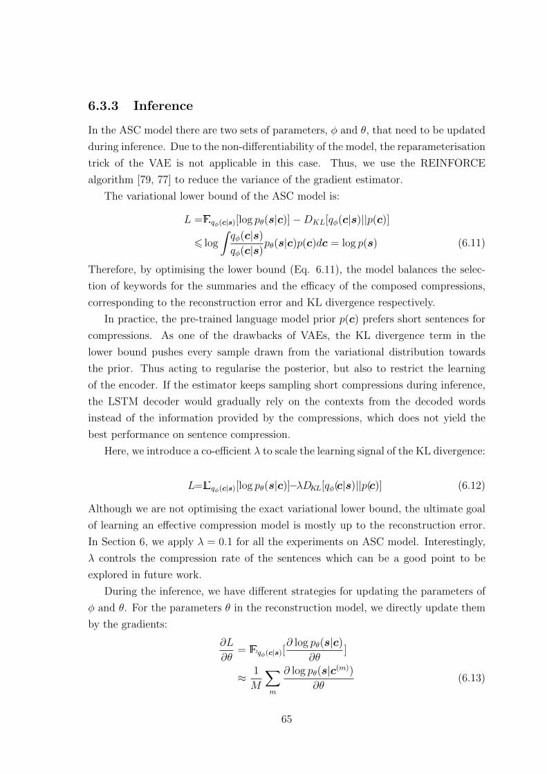
6.3.3 Inference
In the ASC model there are two sets of parameters, φ and θ, that need to be updated
during inference. Due to the non-differentiability of the model, the reparameterisation
trick of the VAE is not applicable in this case. Thus, we use the REINFORCE
algorithm [79, 77] to reduce the variance of the gradient estimator.
The variational lower bound of the ASC model is:
L =Eqφ(c|s)[log pθ(s|c)]−DKL[qφ(c|s)||p(c)]
6 log
∫qφ(c|s)
qφ(c|s)pθ(s|c)p(c)dc = log p(s) (6.11)
Therefore, by optimising the lower bound (Eq. 6.11), the model balances the selec-
tion of keywords for the summaries and the efficacy of the composed compressions,
corresponding to the reconstruction error and KL divergence respectively.
In practice, the pre-trained language model prior p(c) prefers short sentences for
compressions. As one of the drawbacks of VAEs, the KL divergence term in the
lower bound pushes every sample drawn from the variational distribution towards
the prior. Thus acting to regularise the posterior, but also to restrict the learning
of the encoder. If the estimator keeps sampling short compressions during inference,
the LSTM decoder would gradually rely on the contexts from the decoded words
instead of the information provided by the compressions, which does not yield the
best performance on sentence compression.
Here, we introduce a co-efficient λ to scale the learning signal of the KL divergence:
L=Eqφ(c|s)[log pθ(s|c)]−λDKL[qφ(c|s)||p(c)] (6.12)
Although we are not optimising the exact variational lower bound, the ultimate goal
of learning an effective compression model is mostly up to the reconstruction error.
In Section 6, we apply λ = 0.1 for all the experiments on ASC model. Interestingly,
λ controls the compression rate of the sentences which can be a good point to be
explored in future work.
During the inference, we have different strategies for updating the parameters of
φ and θ. For the parameters θ in the reconstruction model, we directly update them
by the gradients:
∂L
∂θ= Eqφ(c|s)[
∂ log pθ(s|c)∂θ
]
≈ 1
M
∑m
∂ log pθ(s|c(m))
∂θ(6.13)
65
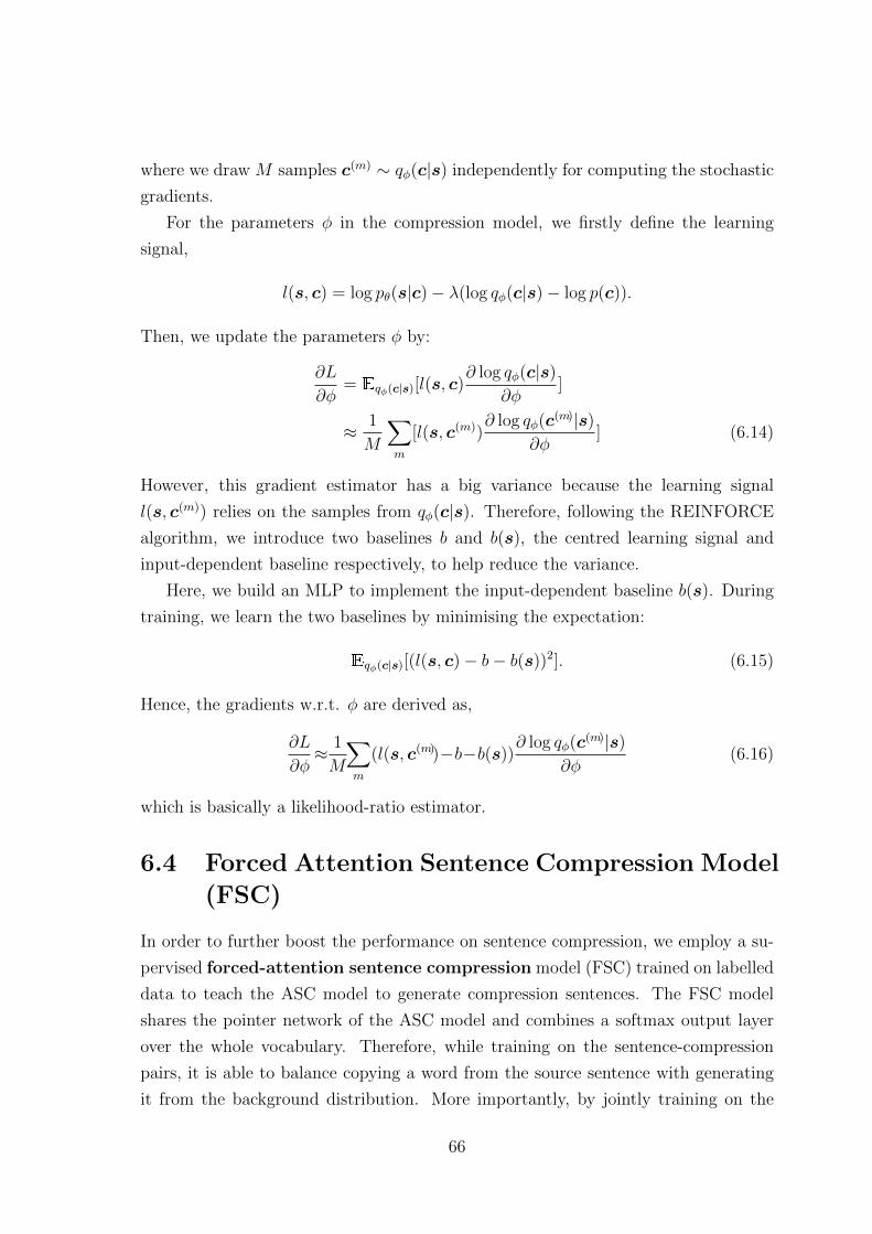
where we draw M samples c(m) ∼ qφ(c|s) independently for computing the stochastic
gradients.
For the parameters φ in the compression model, we firstly define the learning
signal,
l(s, c) = log pθ(s|c)− λ(log qφ(c|s)− log p(c)).
Then, we update the parameters φ by:
∂L
∂φ= Eqφ(c|s)[l(s, c)
∂ log qφ(c|s)
∂φ]
≈ 1
M
∑m
[l(s, c(m))∂ log qφ(c(m)|s)
∂φ] (6.14)
However, this gradient estimator has a big variance because the learning signal
l(s, c(m)) relies on the samples from qφ(c|s). Therefore, following the REINFORCE
algorithm, we introduce two baselines b and b(s), the centred learning signal and
input-dependent baseline respectively, to help reduce the variance.
Here, we build an MLP to implement the input-dependent baseline b(s). During
training, we learn the two baselines by minimising the expectation:
Eqφ(c|s)[(l(s, c)− b− b(s))2]. (6.15)
Hence, the gradients w.r.t. φ are derived as,
∂L
∂φ≈ 1
M
∑m
(l(s, c(m))−b−b(s))∂ log qφ(c(m)|s)
∂φ(6.16)
which is basically a likelihood-ratio estimator.
6.4 Forced Attention Sentence Compression Model
(FSC)
In order to further boost the performance on sentence compression, we employ a su-
pervised forced-attention sentence compression model (FSC) trained on labelled
data to teach the ASC model to generate compression sentences. The FSC model
shares the pointer network of the ASC model and combines a softmax output layer
over the whole vocabulary. Therefore, while training on the sentence-compression
pairs, it is able to balance copying a word from the source sentence with generating
it from the background distribution. More importantly, by jointly training on the
66
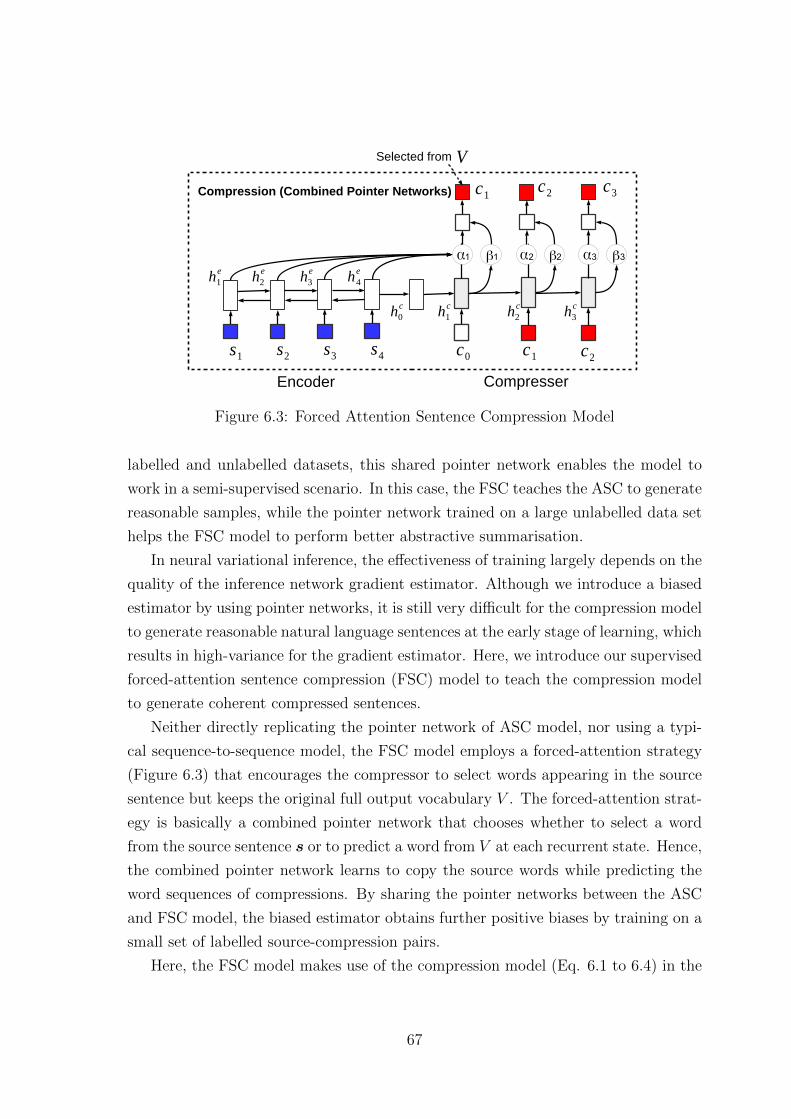
s1
s2
s3
s4
h1
e
c1
c2
c3
c1 c
2c0
h1
c
h2
eh3
eh4
e
h2
ch3
c
Encoder Compresser
h0
c
α β1 2 3α α1 β β2 3
Compression (Combined Pointer Networks)
Selected from V
Figure 6.3: Forced Attention Sentence Compression Model
labelled and unlabelled datasets, this shared pointer network enables the model to
work in a semi-supervised scenario. In this case, the FSC teaches the ASC to generate
reasonable samples, while the pointer network trained on a large unlabelled data set
helps the FSC model to perform better abstractive summarisation.
In neural variational inference, the effectiveness of training largely depends on the
quality of the inference network gradient estimator. Although we introduce a biased
estimator by using pointer networks, it is still very difficult for the compression model
to generate reasonable natural language sentences at the early stage of learning, which
results in high-variance for the gradient estimator. Here, we introduce our supervised
forced-attention sentence compression (FSC) model to teach the compression model
to generate coherent compressed sentences.
Neither directly replicating the pointer network of ASC model, nor using a typi-
cal sequence-to-sequence model, the FSC model employs a forced-attention strategy
(Figure 6.3) that encourages the compressor to select words appearing in the source
sentence but keeps the original full output vocabulary V . The forced-attention strat-
egy is basically a combined pointer network that chooses whether to select a word
from the source sentence s or to predict a word from V at each recurrent state. Hence,
the combined pointer network learns to copy the source words while predicting the
word sequences of compressions. By sharing the pointer networks between the ASC
and FSC model, the biased estimator obtains further positive biases by training on a
small set of labelled source-compression pairs.
Here, the FSC model makes use of the compression model (Eq. 6.1 to 6.4) in the
67

II. Force Attentioned Sentence Compression (FSC)
there could be a nasty surprise under the tree for the Source sentence:
<go> there is a
Pointer Network
surprise for us
Full vocab
surprise
t
...
Figure 6.4: Example of forced-attention sentence compression.
ASC model,
αj = softmax(uj), (6.17)
where αj(i), i ∈ (1, . . . , |s|) denotes the probability of selecting si as the prediction
for cj.
On the basis of the pointer network, we further introduce the probability of pre-
dicting cj that is selected from the full vocabulary,
βj = softmax(Whcj), (6.18)
where βj(w), w ∈ (1, . . . , |V |) denotes the probability of selecting the wth from V
as the prediction for cj. To combine these two probabilities in the RNN, we define
a selection factor t for each state output, which computes the semantic similarities
between the current state and the attention vector,
ηj =∑|s|
iαj(i)h
ei (6.19)
tj = σ(ηTjMhcj). (6.20)
Hence, the probability distribution over compressed words is defined as,
p(cj|c1:j−1, s) =
{tjαj(i) + (1− tj)βj(cj), cj = si(1− tj)βj(cj), cjs
(6.21)
Essentially, the FSC model is the extended compression model of ASC by incorpo-
rating the pointer network with a softmax output layer over the full vocabulary. So
68

we employ φ to denote the parameters of the FSC model pφ(c|s), which covers the
parameters of the variational distribution qφ(c|s).
For example, in Figure 6.4, every time when the model generates a word for
the sentence compression, the selection factor t balance the probability of directly
choosing a word that appeared in the source sentence and the probability of generating
the word from the full vocabulary.
6.4.1 Semi-supervised Learning
As the auto-encoding sentence compression (ASC) model grants the ability to make
use of an unlabelled dataset, we explore a semi-supervised training framework for
the ASC and FSC models. In this scenario we have a labelled dataset that contains
source-compression parallel sentences, (s, c) ∈ L, and an unlabelled dataset that
contains only source sentences s ∈ U. The FSC model is trained on L so that we are
able to learn the compression model by maximising the log-probability,
F =∑
(c,s)∈L
log pφ(c|s). (6.22)
While the ASC model is trained on U, where we maximise the modified variational
lower bound,
L=∑s∈U
(Eqφ(c|s)[log pθ(s|c)]−λDKL[qφ(c|s)||p(c)]). (6.23)
The joint objective function of the semi-supervised learning is,
J=∑s∈U
(Eqφ(c|s)[log pθ(s|c)]−λDKL[qφ(c|s)||p(c)])
+∑
(c,s)∈L
log pφ(c|s). (6.24)
Hence, the pointer network is trained on both unlabelled data, U, and labelled data,
L, by a mixed criterion of REINFORCE and cross-entropy.
6.4.2 Variance Reduction
From the perspective of generative models, a significant contribution of our work
is a process for reducing variance for discrete sampling-based variational inference.
The first step is to introduce two baselines in the control variates method due to the
fact that the reparameterisation trick is not applicable for discrete latent variables.
However it is the second step of using a pointer network as the biased estimator that
69
makes the key contribution. This results in a much smaller state space, bounded by
the length of the source sentence (mostly between 20 and 50 tokens), compared to the
full vocabulary. The final step is to apply the FSC model to transfer the knowledge
learned from the supervised data to the pointer network. This further reduces the
sampling variance by acting as a sort of bootstrap or constraint on the unsupervised
latent space which could encode almost anything but which thus becomes biased
towards matching the supervised distribution. By using these variance reduction
methods, the ASC model is able to carry out effective variational inference for the
latent language model so that it learns to summarise the sentences from the large
unlabelled training data.
In a different vein, according to the reinforcement learning interpretation of se-
quence level training [83], the compression model of the ASC model acts as an agent
which iteratively generates words (takes actions) to compose the compression sentence
and the reconstruction model acts as the reward function evaluating the quality of the
compressed sentence which is provided as a reward signal. [83] presents a thorough
empirical evaluation on three different NLP tasks by using additional sequence-level
reward (BLEU and Rouge-2) to train the models. In the context of this chapter,
we apply a variational lower bound (mixed reconstruction error and KL divergence
regularisation) instead of the explicit Rouge score. Thus the ASC model is granted
the ability to explore unlimited unlabelled data resources. In addition we introduce a
supervised FSC model to teach the compression model to generate stable sequences
instead of starting with a random policy. In this case, the pointer network that
bridges the supervised and unsupervised model is trained by a mixed criterion of
REINFORCE and cross-entropy in an incremental learning framework. Eventually,
according to the experimental results, the joint ASC and FSC model is able to learn
a robust compression model by exploring both labelled and unlabelled data, which
outperforms the other single discriminative compression models that are only trained
by cross-entropy reward signal.
6.5 Experiments
The proposed models are evaluated on the standard Gigaword3 sentence compression
dataset. This dataset was generated by pairing the headline of each article with its
first sentence to create a source-compression pair. [87] provided scripts4 to filter out
3https://catalog.ldc.upenn.edu/LDC2012T214https://github.com/facebook/NAMAS
70
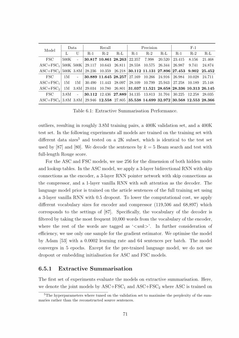
ModelData Recall Precision F-1
L U R-1 R-2 R-L R-1 R-2 R-L R-1 R-2 R-L
FSC 500K - 30.817 10.861 28.263 22.357 7.998 20.520 23.415 8.156 21.468
ASC+FSC1 500K 500K 29.117 10.643 26.811 28.558 10.575 26.344 26.987 9.741 24.874
ASC+FSC2 500K 3.8M 28.236 10.359 26.218 30.112 11.131 27.896 27.453 9.902 25.452
FSC 1M - 30.889 11.645 28.257 27.169 10.266 24.916 26.984 10.028 24.711
ASC+FSC1 1M 1M 30.490 11.443 28.097 28.109 10.799 25.943 27.258 10.189 25.148
ASC+FSC2 1M 3.8M 29.034 10.780 26.801 31.037 11.521 28.658 28.336 10.313 26.145
FSC 3.8M - 30.112 12.436 27.889 34.135 13.813 31.704 30.225 12.258 28.035
ASC+FSC2 3.8M 3.8M 29.946 12.558 27.805 35.538 14.699 32.972 30.568 12.553 28.366
Table 6.1: Extractive Summarisation Performance.
outliers, resulting in roughly 3.8M training pairs, a 400K validation set, and a 400K
test set. In the following experiments all models are trained on the training set with
different data sizes5 and tested on a 2K subset, which is identical to the test set
used by [87] and [80]. We decode the sentences by k = 5 Beam search and test with
full-length Rouge score.
For the ASC and FSC models, we use 256 for the dimension of both hidden units
and lookup tables. In the ASC model, we apply a 3-layer bidirectional RNN with skip
connections as the encoder, a 3-layer RNN pointer network with skip connections as
the compressor, and a 1-layer vanilla RNN with soft attention as the decoder. The
language model prior is trained on the article sentences of the full training set using
a 3-layer vanilla RNN with 0.5 dropout. To lower the computational cost, we apply
different vocabulary sizes for encoder and compressor (119,506 and 68,897) which
corresponds to the settings of [87]. Specifically, the vocabulary of the decoder is
filtered by taking the most frequent 10,000 words from the vocabulary of the encoder,
where the rest of the words are tagged as ‘<unk>’. In further consideration of
efficiency, we use only one sample for the gradient estimator. We optimise the model
by Adam [53] with a 0.0002 learning rate and 64 sentences per batch. The model
converges in 5 epochs. Except for the pre-trained language model, we do not use
dropout or embedding initialisation for ASC and FSC models.
6.5.1 Extractive Summarisation
The first set of experiments evaluate the models on extractive summarisation. Here,
we denote the joint models by ASC+FSC1 and ASC+FSC2 where ASC is trained on
5The hyperparameters where tuned on the validation set to maximise the perplexity of the sum-maries rather than the reconstructed source sentences.
71
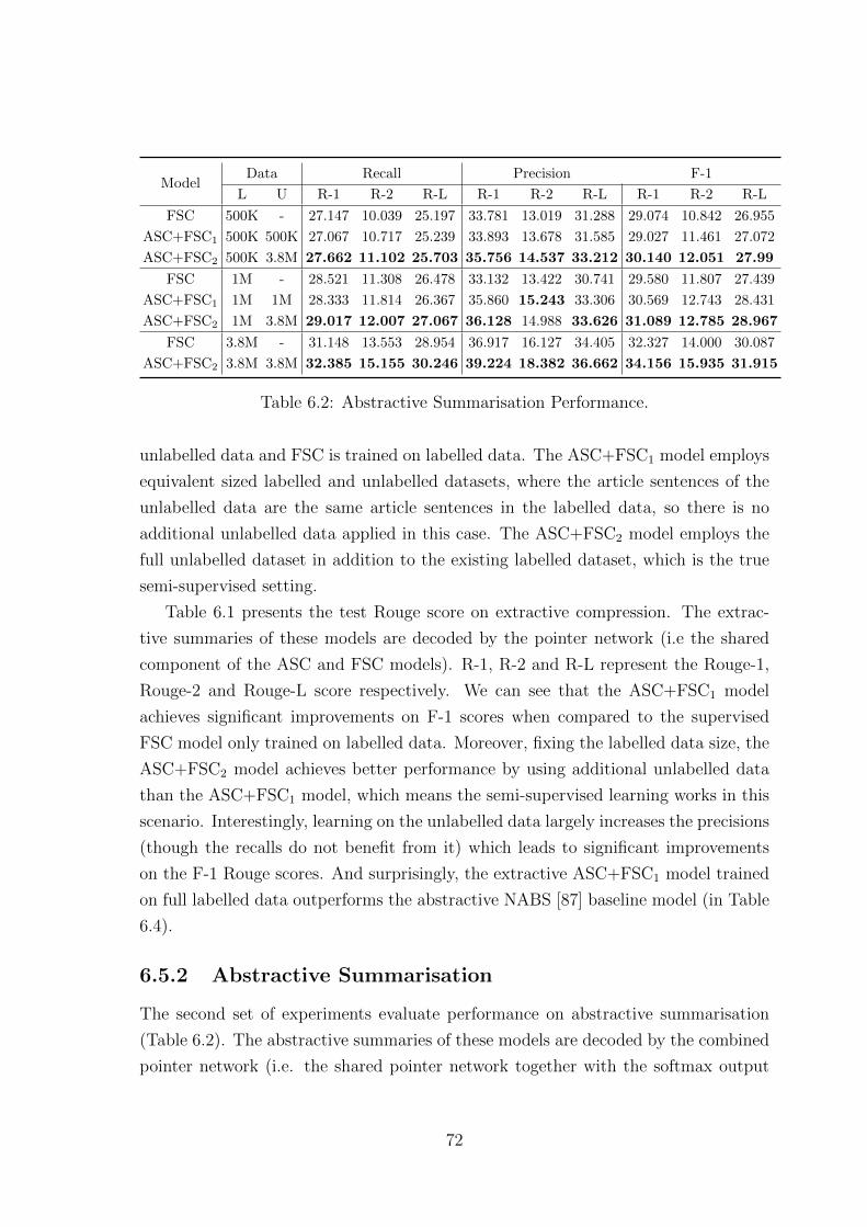
ModelData Recall Precision F-1
L U R-1 R-2 R-L R-1 R-2 R-L R-1 R-2 R-L
FSC 500K - 27.147 10.039 25.197 33.781 13.019 31.288 29.074 10.842 26.955
ASC+FSC1 500K 500K 27.067 10.717 25.239 33.893 13.678 31.585 29.027 11.461 27.072
ASC+FSC2 500K 3.8M 27.662 11.102 25.703 35.756 14.537 33.212 30.140 12.051 27.99
FSC 1M - 28.521 11.308 26.478 33.132 13.422 30.741 29.580 11.807 27.439
ASC+FSC1 1M 1M 28.333 11.814 26.367 35.860 15.243 33.306 30.569 12.743 28.431
ASC+FSC2 1M 3.8M 29.017 12.007 27.067 36.128 14.988 33.626 31.089 12.785 28.967
FSC 3.8M - 31.148 13.553 28.954 36.917 16.127 34.405 32.327 14.000 30.087
ASC+FSC2 3.8M 3.8M 32.385 15.155 30.246 39.224 18.382 36.662 34.156 15.935 31.915
Table 6.2: Abstractive Summarisation Performance.
unlabelled data and FSC is trained on labelled data. The ASC+FSC1 model employs
equivalent sized labelled and unlabelled datasets, where the article sentences of the
unlabelled data are the same article sentences in the labelled data, so there is no
additional unlabelled data applied in this case. The ASC+FSC2 model employs the
full unlabelled dataset in addition to the existing labelled dataset, which is the true
semi-supervised setting.
Table 6.1 presents the test Rouge score on extractive compression. The extrac-
tive summaries of these models are decoded by the pointer network (i.e the shared
component of the ASC and FSC models). R-1, R-2 and R-L represent the Rouge-1,
Rouge-2 and Rouge-L score respectively. We can see that the ASC+FSC1 model
achieves significant improvements on F-1 scores when compared to the supervised
FSC model only trained on labelled data. Moreover, fixing the labelled data size, the
ASC+FSC2 model achieves better performance by using additional unlabelled data
than the ASC+FSC1 model, which means the semi-supervised learning works in this
scenario. Interestingly, learning on the unlabelled data largely increases the precisions
(though the recalls do not benefit from it) which leads to significant improvements
on the F-1 Rouge scores. And surprisingly, the extractive ASC+FSC1 model trained
on full labelled data outperforms the abstractive NABS [87] baseline model (in Table
6.4).
6.5.2 Abstractive Summarisation
The second set of experiments evaluate performance on abstractive summarisation
(Table 6.2). The abstractive summaries of these models are decoded by the combined
pointer network (i.e. the shared pointer network together with the softmax output
72
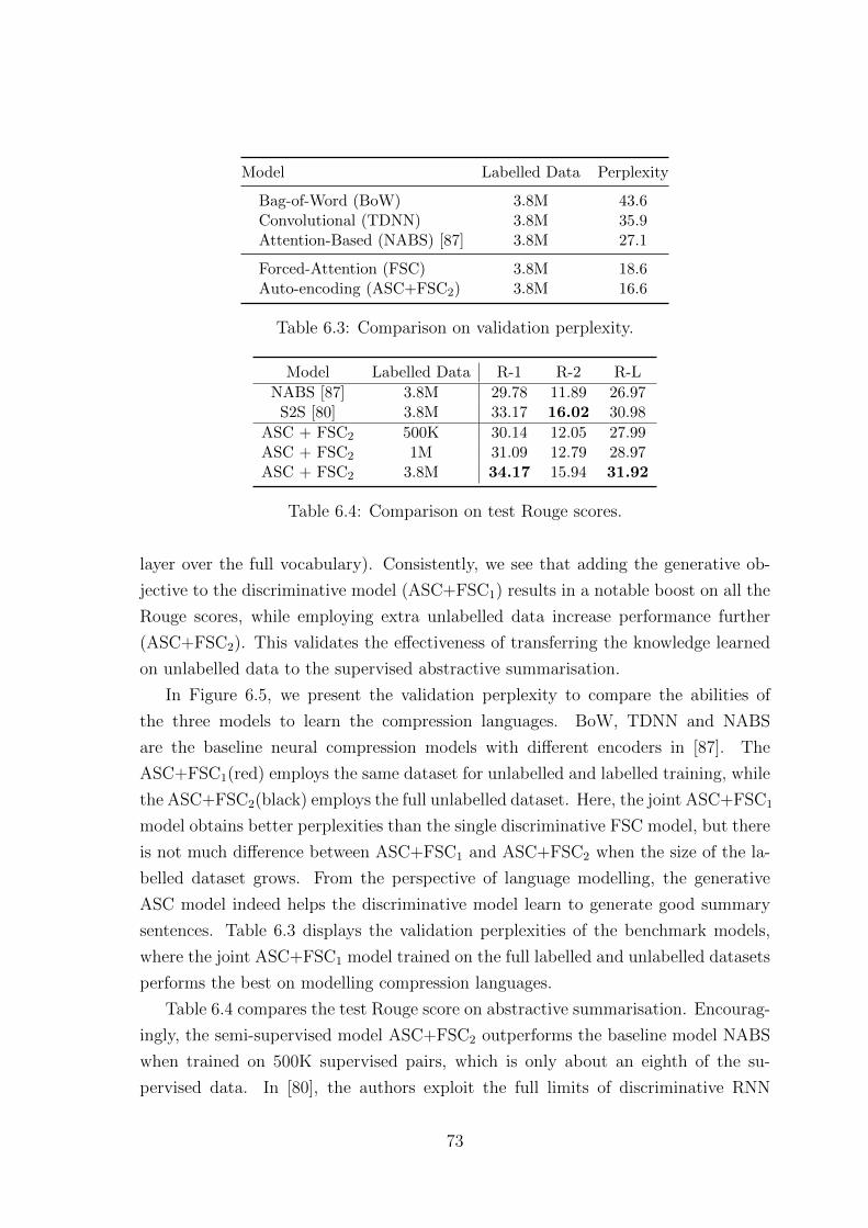
Model Labelled Data Perplexity
Bag-of-Word (BoW) 3.8M 43.6Convolutional (TDNN) 3.8M 35.9Attention-Based (NABS) [87] 3.8M 27.1
Forced-Attention (FSC) 3.8M 18.6Auto-encoding (ASC+FSC2) 3.8M 16.6
Table 6.3: Comparison on validation perplexity.
Model Labelled Data R-1 R-2 R-L
NABS [87] 3.8M 29.78 11.89 26.97S2S [80] 3.8M 33.17 16.02 30.98
ASC + FSC2 500K 30.14 12.05 27.99ASC + FSC2 1M 31.09 12.79 28.97ASC + FSC2 3.8M 34.17 15.94 31.92
Table 6.4: Comparison on test Rouge scores.
layer over the full vocabulary). Consistently, we see that adding the generative ob-
jective to the discriminative model (ASC+FSC1) results in a notable boost on all the
Rouge scores, while employing extra unlabelled data increase performance further
(ASC+FSC2). This validates the effectiveness of transferring the knowledge learned
on unlabelled data to the supervised abstractive summarisation.
In Figure 6.5, we present the validation perplexity to compare the abilities of
the three models to learn the compression languages. BoW, TDNN and NABS
are the baseline neural compression models with different encoders in [87]. The
ASC+FSC1(red) employs the same dataset for unlabelled and labelled training, while
the ASC+FSC2(black) employs the full unlabelled dataset. Here, the joint ASC+FSC1
model obtains better perplexities than the single discriminative FSC model, but there
is not much difference between ASC+FSC1 and ASC+FSC2 when the size of the la-
belled dataset grows. From the perspective of language modelling, the generative
ASC model indeed helps the discriminative model learn to generate good summary
sentences. Table 6.3 displays the validation perplexities of the benchmark models,
where the joint ASC+FSC1 model trained on the full labelled and unlabelled datasets
performs the best on modelling compression languages.
Table 6.4 compares the test Rouge score on abstractive summarisation. Encourag-
ingly, the semi-supervised model ASC+FSC2 outperforms the baseline model NABS
when trained on 500K supervised pairs, which is only about an eighth of the su-
pervised data. In [80], the authors exploit the full limits of discriminative RNN
73
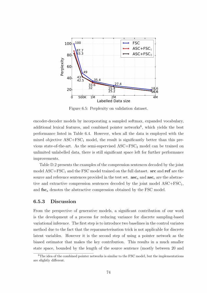
0 500K 1M 2M 4MLabelled Data size
20
40
60
80
100
Perp
lexit
y
100
49
35.427.4
18.6
87.7
43
3225.2 16.6
83.3
42.5
33.625.4
16.6
FSC
ASC+FSC1
ASC+FSC2
Figure 6.5: Perplexity on validation dataset.
encoder-decoder models by incorporating a sampled softmax, expanded vocabulary,
additional lexical features, and combined pointer networks6, which yields the best
performance listed in Table 6.4. However, when all the data is employed with the
mixed objective ASC+FSC1 model, the result is significantly better than this pre-
vious state-of-the-art. As the semi-supervised ASC+FSC2 model can be trained on
unlimited unlabelled data, there is still significant space left for further performance
improvements.
Table D.2 presents the examples of the compression sentences decoded by the joint
model ASC+FSC1 and the FSC model trained on the full dataset. src and ref are the
source and reference sentences provided in the test set. asca and asce are the abstrac-
tive and extractive compression sentences decoded by the joint model ASC+FSC1,
and fsca denotes the abstractive compression obtained by the FSC model.
6.5.3 Discussion
From the perspective of generative models, a significant contribution of our work
is the development of a process for reducing variance for discrete sampling-based
variational inference. The first step is to introduce two baselines in the control variates
method due to the fact that the reparameterisation trick is not applicable for discrete
latent variables. However it is the second step of using a pointer network as the
biased estimator that makes the key contribution. This results in a much smaller
state space, bounded by the length of the source sentence (mostly between 20 and
6The idea of the combined pointer networks is similar to the FSC model, but the implementationsare slightly different.
74
50 tokens), compared to the full vocabulary. The final step is to apply the FSC
model to transfer the knowledge learned from the supervised data to the pointer
network. This further reduces the sampling variance by acting as a sort of bootstrap
or constraint on the unsupervised latent space which could encode almost anything
but which thus becomes biased towards matching the supervised distribution. By
using these variance reduction methods, the ASC model is able to carry out effective
variational inference for the latent language model so that it learns to summarise the
sentences from the large unlabelled training data. However, without incorporating
the FSC model that provides explicit learning signals, the ASC model is unable to
learn effective summarisation by just learning in a unsupervised fashion, which is
basically due to high variance issue caused by the large vocabulary.
In a different vein, according to the reinforcement learning interpretation of se-
quence level training [83], the compression model of the ASC model acts as an agent
which iteratively generates words (takes actions) to compose the compression sentence
and the reconstruction model acts as the reward function evaluating the quality of the
compressed sentence which is provided as a reward signal. [83] presents a thorough
empirical evaluation on three different NLP tasks by using additional sequence-level
reward (BLEU and Rouge-2) to train the models. In the context of this paper, we
apply a variational lower bound (mixed reconstruction error and KL divergence reg-
ularisation) instead of the explicit Rouge score. Thus the ASC model is granted the
ability to explore unlimited unlabelled data resources. In addition we introduce a
supervised FSC model to teach the compression model to generate stable sequences
instead of starting with a random policy. In this case, the pointer network that
bridges the supervised and unsupervised model is trained by a mixed criterion of
REINFORCE and cross-entropy in an incremental learning framework. Eventually,
according to the experimental results, the joint ASC and FSC model is able to learn
a robust compression model by exploring both labelled and unlabelled data, which
outperforms the other single discriminative compression models that are only trained
by cross-entropy reward signal.
6.6 Summary
In this chapter, a generative model is introduced for jointly modelling pairs of se-
quences and evaluated its efficacy on the task of sentence compression. The neu-
ral variational inference framework provided an effective inference algorithm for this
approach and also allowed us to explore combinations of discriminative (FSC) and
75
generative (ASC) compression models. The evaluation results show that supervised
training of the combination of these models improves upon the state-of-the-art per-
formance for the Gigaword compression dataset. When we train the supervised FSC
model on a small amount of labelled data and the unsupervised ASC model on a large
set of unlabelled data the combined model is able to outperform previously reported
benchmarks trained on a great deal more supervised data. These results demonstrate
that we are able to model language as a discrete latent variable in the framework of
variational auto-encoders and that the resultant generative model is able to effectively
exploit both supervised and unsupervised data in sequence-to-sequence tasks.
76

Chapter 7
Latent Intention Dialogue Models
In this chapter, we present a Latent Intention Dialogue Model (LIDM) that employs
a discrete latent variable to learn underlying dialogue intentions in the framework of
neural variational inference. Different from the latent sentence compression model
introduced in the previous chapter, where the discrete latent variables represent ex-
plicit words from the full vocabulary, the discrete latent intention in this context is
interpreted as actions guiding the generation of machine responses and can be further
refined autonomously by reinforcement learning. Hence, by combining this latent in-
tention with the RNN decoder, we expect to decompose the learning of generating
natural language and the internal dialogue decision-making. The experimental eval-
uation of LIDM shows that the model out-performs published benchmarks for both
corpus-based and human evaluation, demonstrating the effectiveness of discrete latent
variable models for learning goal-oriented dialogues.
7.1 Introduction
Recurrent neural networks (RNNs) have shown impressive results in modeling gener-
ation tasks that have a sequential structured output form, such as machine transla-
tion [101, 6], caption generation [49, 121], and natural language generation [114, 52].
These discriminative models are trained to learn only a conditional output distribu-
tion over strings and despite the sophisticated architectures and conditioning mech-
anisms used to ensure salience, they are not able to model the underlying actions
needed to generate natural dialogues, which are the latent intentions in our case.
As a consequence, these sequence-to-sequence models are limited in their ability to
exhibit the intrinsic variability and stochasticity of natural dialogue. For example
both goal-oriented dialogue systems [116, 12] and sequence-to-sequence learning chat-
bots [106, 93, 89] struggle to generate diverse yet causal responses [66, 88]. Here, we
77

introduce a latent variable model – Latent Intention Dialogue Model (LIDM) – for
learning the complex distribution of communicative intentions in goal-oriented dia-
logues. The latent intentions are modelled as discrete latent variable, which can be
interpreted by using the content words in the generated machine responses (Table
7.1). In addition, an identical intention is able to generate multiple different machine
responses conditioned on different conversational contexts.
In this model, the latent variable representing dialogue intention can be considered
as the autonomous decision-making center of a dialogue agent for composing appro-
priate machine responses, which is inferred from user input utterances. Based on the
dialogue context, the agent draws a sample as the intention which then guides the
natural language response generation. Firstly, in the framework of neural variational
inference, we construct an inference network to approximate the posterior distribu-
tion over the latent intention. Then, by sampling the intentions for each response, we
are able to directly learn a basic intention distribution on a human-human dialogue
corpus by optimising the variational lower bound. To further reduce the variance, we
utilize a labeled subset of the corpus in which the labels of intentions are automati-
cally generated by clustering. Then, the latent intention distribution can be learned
in a semi-supervised fashion, where the learning signals are either from the direct
supervision (labeled set) or the variational lower bound (unlabeled set).
From the perspective of reinforcement learning, the latent intention distribution
can be interpreted as the intrinsic policy that reflects human decision-making under
a particular conversational scenario. Based on the initial policy (latent intention
distribution) learned from the semi-supervised variational inference framework, the
model can refine its strategy easily against alternative objectives using policy gradient-
based reinforcement learning. In some way, this is analagous to the training process
used in AlphaGo [94] for the game of Go. Based on LIDM, we show that different
learning paradigms can be brought together under the same framework to bootstrap
the development of a dialogue agent [69, 118].
7.2 Related Work
Modeling chat-based dialogues [89, 93] as a sequence-to-sequence learning [101] prob-
lem is a common theme in the deep learning community. Vinyals and Le [106] has
demonstrated a seq2seq-based model trained on a huge amount of conversation cor-
pora which learns interesting replies conditioned on different user queries. However,
due to an inability to model dialogue context, these models generally suffer from the
78
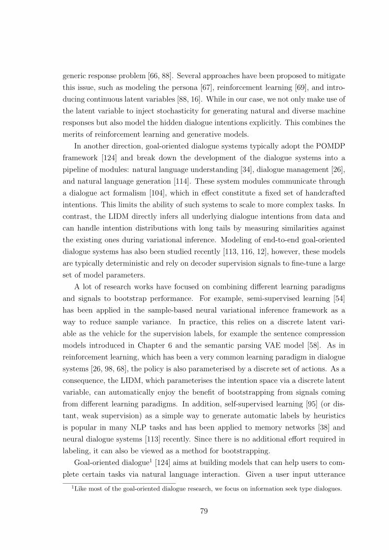
generic response problem [66, 88]. Several approaches have been proposed to mitigate
this issue, such as modeling the persona [67], reinforcement learning [69], and intro-
ducing continuous latent variables [88, 16]. While in our case, we not only make use of
the latent variable to inject stochasticity for generating natural and diverse machine
responses but also model the hidden dialogue intentions explicitly. This combines the
merits of reinforcement learning and generative models.
In another direction, goal-oriented dialogue systems typically adopt the POMDP
framework [124] and break down the development of the dialogue systems into a
pipeline of modules: natural language understanding [34], dialogue management [26],
and natural language generation [114]. These system modules communicate through
a dialogue act formalism [104], which in effect constitute a fixed set of handcrafted
intentions. This limits the ability of such systems to scale to more complex tasks. In
contrast, the LIDM directly infers all underlying dialogue intentions from data and
can handle intention distributions with long tails by measuring similarities against
the existing ones during variational inference. Modeling of end-to-end goal-oriented
dialogue systems has also been studied recently [113, 116, 12], however, these models
are typically deterministic and rely on decoder supervision signals to fine-tune a large
set of model parameters.
A lot of research works have focused on combining different learning paradigms
and signals to bootstrap performance. For example, semi-supervised learning [54]
has been applied in the sample-based neural variational inference framework as a
way to reduce sample variance. In practice, this relies on a discrete latent vari-
able as the vehicle for the supervision labels, for example the sentence compression
models introduced in Chapter 6 and the semantic parsing VAE model [58]. As in
reinforcement learning, which has been a very common learning paradigm in dialogue
systems [26, 98, 68], the policy is also parameterised by a discrete set of actions. As a
consequence, the LIDM, which parameterises the intention space via a discrete latent
variable, can automatically enjoy the benefit of bootstrapping from signals coming
from different learning paradigms. In addition, self-supervised learning [95] (or dis-
tant, weak supervision) as a simple way to generate automatic labels by heuristics
is popular in many NLP tasks and has been applied to memory networks [38] and
neural dialogue systems [113] recently. Since there is no additional effort required in
labeling, it can also be viewed as a method for bootstrapping.
Goal-oriented dialogue1 [124] aims at building models that can help users to com-
plete certain tasks via natural language interaction. Given a user input utterance
1Like most of the goal-oriented dialogue research, we focus on information seek type dialogues.
79
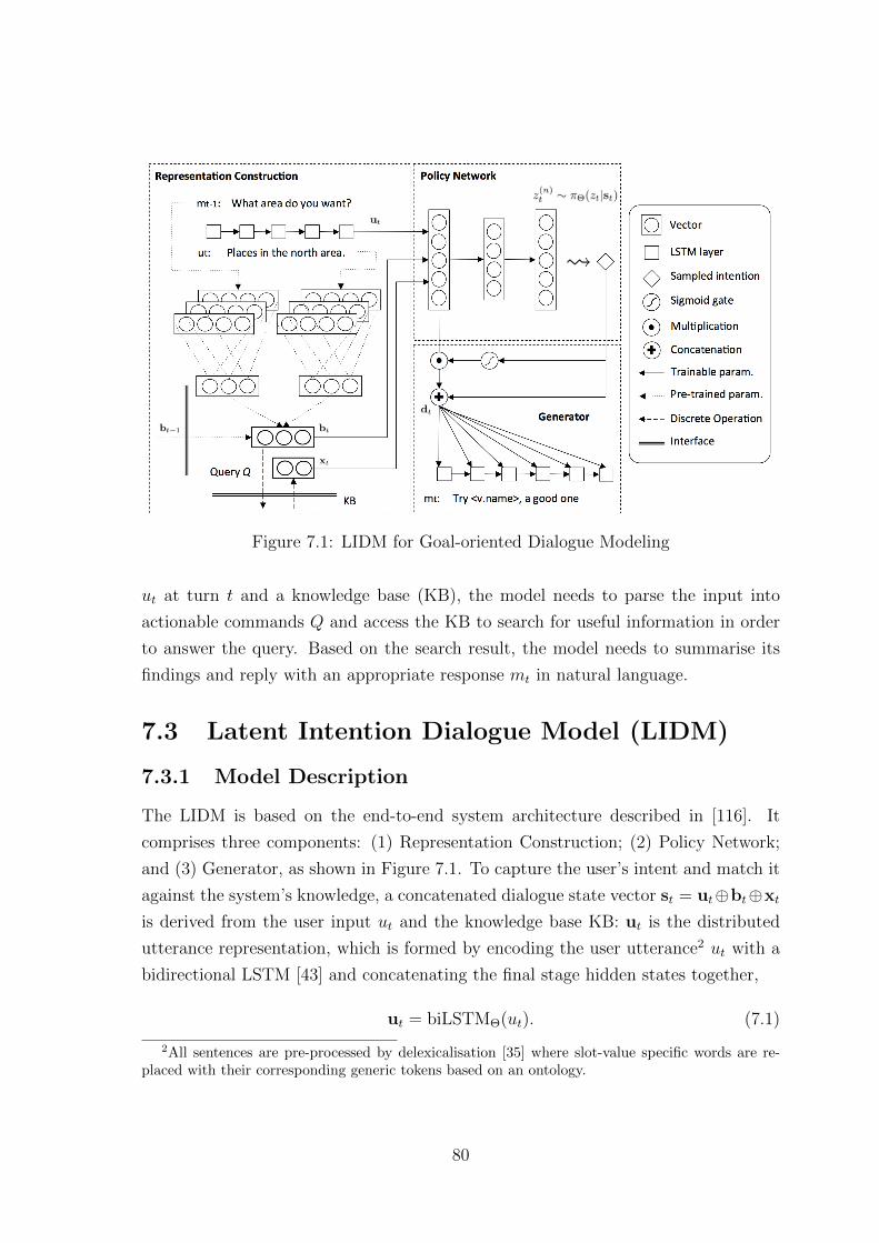
Figure 7.1: LIDM for Goal-oriented Dialogue Modeling
ut at turn t and a knowledge base (KB), the model needs to parse the input into
actionable commands Q and access the KB to search for useful information in order
to answer the query. Based on the search result, the model needs to summarise its
findings and reply with an appropriate response mt in natural language.
7.3 Latent Intention Dialogue Model (LIDM)
7.3.1 Model Description
The LIDM is based on the end-to-end system architecture described in [116]. It
comprises three components: (1) Representation Construction; (2) Policy Network;
and (3) Generator, as shown in Figure 7.1. To capture the user’s intent and match it
against the system’s knowledge, a concatenated dialogue state vector st = ut⊕bt⊕xt
is derived from the user input ut and the knowledge base KB: ut is the distributed
utterance representation, which is formed by encoding the user utterance2 ut with a
bidirectional LSTM [43] and concatenating the final stage hidden states together,
ut = biLSTMΘ(ut). (7.1)
2All sentences are pre-processed by delexicalisation [35] where slot-value specific words are re-placed with their corresponding generic tokens based on an ontology.
80
The belief vector bt, which is a concatenation of a set of probability distributions
over domain specific slot-value pairs, is extracted by a set of pre-trained RNN-CNN
belief trackers [116, 35], in which ut and mt−1 are processed by two different CNNs
as shown in Figure 7.1,
bt = RNN-CNN(ut,mt−1,bt−1) (7.2)
where mt−1 is the preceding machine response and bt−1 is the preceding belief vector.
They are included to model the current turn of the discourse and the long-term
dialogue context, respectively. Based on the belief vector, a query Q is formed by
taking the union of the maximum values of each slot. Q is then used to search the
internal KB and return a vector xt representing the degree of matching in the KB.
This is produced by counting all the matching values and re-structuring it into a
six-bin one-hot vector. Among the three vectors that comprise the dialogue state
st, ut is completely trainable from data, bt is pre-trained using a separate objective
function, and xt is produced by a discrete database accessing operation. For more
details about the belief trackers and database operation refer to Wen et al [113, 116].
Conditioning on the state st, the policy network parameterises the latent intention
zt by a single layer MLP,
πΘ(zt|st) = softmax(Wᵀ2 · tanh(Wᵀ
1st + b1) + b2) (7.3)
where W1, b1, W2, b2 are model parameters. Since πΘ(zt|st) is a discrete conditional
probability distribution based on dialogue state, we can also interpret the policy
network here as a latent dialogue management component in the traditional POMDP-
based framework [124, 26]. A latent intention z(n)t (or an action in the reinforcement
learning literature) can then be sampled from the conditional distribution,
z(n)t ∼ πΘ(zt|st). (7.4)
This sampled intention (or action) z(n)t and the state vector st can then be combined
into a control vector dt, which is used to govern the generation of the system response
based on a conditional LSTM language model,
dt = Wᵀ4zt ⊕ [sigmoid(Wᵀ
3zt + b3) ·Wᵀ5st] (7.5)
pΘ(mt|st, zt) =∏j
p(wtj+1|wtj,htj−1,dt) (7.6)
where b3 and W3∼5 are parameters, zt is the 1-hot representation of z(n)t , wtj is the
last output token (i.e. a word, a delexicalised2 slot name or a delexicalised2 slot
81
value), and htj−1 is the decoder’s last hidden state. Note in Equation 7.5 the degree
of information flow from the state vector is controlled by a sigmoid gate whose input
signal is the sampled intention z(n)t . This prevents the decoder from over-fitting to the
deterministic state information and forces it to take the sampled stochastic intention
into account. The LIDM can then be formally written down in its parameterised form
with parameter set Θ,
pΘ(mt|st) =∑zt
pΘ(mt|zt, st)πΘ(zt|st). (7.7)
7.3.2 Inference
To carry out inference for the LIDM, we apply an inference network qΦ(zt|st,mt)
to approximate the posterior distribution p(zt|st,mt) so that we can optimise the
variational lower bound of the joint probability in the neural variational inference
framework introduced in Chapter 2. We can then derive the modified variational
lower bound as,
L = EqΦ(zt)[log pΘ(mt|zt, st)]− λDKL(qΦ(zt)||πΘ(zt|st))
≤ log∑zt
pΘ(mt|zt, st)πΘ(zt|st)
= log pΘ(mt|st) (7.8)
where qΦ(zt) is a shorthand for qΦ(zt|st,mt). Note that we use a modified version
of the lower bound here by incorporating a trade-off factor λ [37]. The inference
network qΦ(zt|st,mt) is then constructed by
qΦ(zt|st,mt) = Multi(ot) = softmax(W6ot) (7.9)
ot = MLPΦ(bt,xt,ut,mt) (7.10)
ut = biLSTMΦ(ut),mt = biLSTMΦ(mt) (7.11)
where ot is the joint representation, and both ut and mt are modeled by a bidi-
rectional LSTM network. Although both qΦ(zt|st,mt) and πΘ(zt|st) are modelled as
parameterised multinomial distributions, the approximation qΦ(zt|st,mt) only func-
tions during inference by producing samples to compute the stochastic gradients,
while πΘ(zt|st) is the generative distribution that generates the required samples for
composing the machine response.
82
Based on the samples z(n)t ∼ qΦ(zt|st,mt), we use different strategies to alternately
optimise the parameters Θ and Φ against the variational lower bound (Equation 7.8).
To do this, we further divide Θ into two sets Θ = {Θ1,Θ2}. Parameters Θ1 on the
decoder side are directly updated by back-propagating the gradients,
∂L∂Θ1
= EqΦ(zt|st,mt)[∂ log pΘ1(mt|zt, st)
∂Θ1
]
≈ 1
N
∑n
∂ log pΘ1(mt|z(n)t , st)
∂Θ1
. (7.12)
Parameters Θ2 in the generative model, however, are updated by minimising the KL
divergence,
∂L∂Θ2
= −∂λDKL(qΦ(zt|st,mt)||πΘ2(zt|st))∂Θ2
= −λ∑zt
qΦ(zt|st,mt)∂ log πΘ2(zt|st)
∂Θ2
(7.13)
where the entropy derivative ∂H[qΦ(zt|st,mt)]/∂Θ2 = 0 and therefore can be ignored.
Finally, for the parameters Φ in the inference network, we firstly define the learning
signal r(mt, z(n)t , st),
r(mt,z(n)t , st) = log pΘ1(mt|z(n)
t , st)−
λ(log qΦ(z(n)t |st,mt)− log πΘ2(z
(n)t |st)). (7.14)
Then the parameters Φ are updated by,
∂L∂Φ
= EqΦ(at|st,mt)[r(mt, at, st)∂ log qΦ(at|st,mt)
∂Φ]
≈ 1
N
∑n
r(mt, z(n)t , st)
∂ log qΦ(z(n)t |st,mt)
∂Φ. (7.15)
However, this gradient estimator has a large variance because the learning signal
r(mt, z(n)t , st) relies on samples from the proposal distribution qΦ(zt|st,mt). To reduce
the variance during inference, we follow the REINFORCE algorithm introduced in
Chapter 2 and apply two baselines b and b(st), the centered learning signal and input
dependent baseline respectively to help reduce the variance. b is a learnable constant
and b(st) = MLP(st). During training, the two baselines are updated by minimising
the distance,
Lb =[r(mt, z
(n)t , st)− b− b(st)
]2
(7.16)
and the gradient w.r.t. Φ can be rewritten as
∂L∂Φ≈ 1
N
∑n
[r(mt, z(n)t , st)− b− b(st)]
∂ log qΦ(z(n)t |st,mt)
∂Φ. (7.17)
83
7.3.3 Semi-Supervision
Despite the steps described above for reducing the variance, there remain two major
difficulties in learning latent intentions in a completely unsupervised manner: (1) the
high variance of the inference network prevents it from generating sensible intention
samples in the early stages of training, and (2) the overly strong discriminative power
of the LSTM language model is prone to the disconnection phenomenon between the
LSTM decoder and the rest of the components whereby the decoder learns to ignore
the samples and focuses solely on optimising the language model. To ensure more
stable training and prevent disconnection, a semi-supervised learning technique is
introduced.
Inferring the latent intentions underlying utterances is similar to an unsuper-
vised clustering task. Standard clustering algorithms can therefore be used to pre-
process the corpus and generate automatic labels zt for part of the training exam-
ples (mt, st, zt) ∈ L. Then when the model is trained on the unlabeled examples
(mt, st) ∈ U, we optimise it against the modified variational lower bound given in
Equation 7.8,
L1 =∑
(mt,st)∈U
Eqφ(zt|st,mt) [log pθ(mt|zt, st)]
− λDKL(qφ(zt|st,mt)||πθ(zt|st)) (7.18)
However, when the model is updated based on examples from the labeled set (mt, st, zt) ∈L, we treat the labeled intention zt as an observed variable and train the model by
maximising the joint log-likelihood,
L2 =∑
(mt,zt,st)∈L
log [pΘ(mt|zt, st)πΘ(zt|st)] (7.19)
The final joint objective function can then be written as L′ = αL1 + L2, where α
controls the trade-off between the supervised and unsupervised examples.
7.3.4 Reinforcement Learning
One of the main purposes of learning interpretable, discrete latent intention inside
a dialogue system is to be able to control and refine the model’s behaviour with
operational experience. The learnt generative network πΘ(zt|st) encodes the policy
discovered from the underlying data distribution but this is not necessarily optimal
for any specific task. Since πΘ(zt|st) is a parameterised policy network itself, any
84
policy gradient-based reinforcement learning algorithm [119, 57] can be used to fine-
tune the initial policy against other objective functions that we are more interested
in.
Based on the initial policy πΘ(zt|st), we revisit the training dialogues and update
parameters based on the following strategy: when encountering unlabeled examples
U at turn t the system samples an action from the learnt policy z(n)t ∼ πΘ(zt|st) and
receives a reward r(n)t . Conditioning on these, we can directly fine-tune a subset of
the model parameters Θ′ by the policy gradient method,
∂J∂Θ′≈ 1
N
∑n
r(n)t
∂ log πΘ(z(n)t |st)
∂Θ′(7.20)
where Θ′ = {W1,b1,W2,b2} is the MLP that parameterises the policy network
(Equation 7.3). However, when a labeled example ∈ L is encountered we force the
model to take the labeled action z(n)t = zt and update the parameters by Equation 7.20
as well. Unlike Li et al [69] where the whole model is refined end-to-end using RL,
updating only Θ′ effectively allows us to refine only the decision-making of the system
and avoid the problem of over-fitting.
7.4 Experiments
7.4.1 Dataset & Setup
We explored the properties of the LIDM model3 using the CamRest676 corpus4 col-
lected by Wen et al [116], in which the task of the system is to assist users to find a
restaurant in the Cambridge, UK area. The corpus was collected based on a modified
Wizard of Oz [50] online data collection. Workers were recruited on Amazon Mechan-
ical Turk and asked to complete a task by carrying out a conversation, alternating
roles between a user and a wizard. There are three informable slots (food, pricerange,
area) that users can use to constrain the search and six requestable slots (address,
phone, postcode plus the three informable slots) that the user can ask a value for once
a restaurant has been offered. There are 676 dialogues in the dataset (including both
finished and unfinished dialogues) and approximately 2750 conversational turns in
total. The database contains 99 unique restaurants.
To make a direct comparison with prior work we follow the same experimental
setup as in Wen et al [113, 116]. The corpus was partitioned into training, validation,
3Will be available at https://github.com/shawnwun/NNDIAL4https://www.repository.cam.ac.uk/handle/1810/260970
85
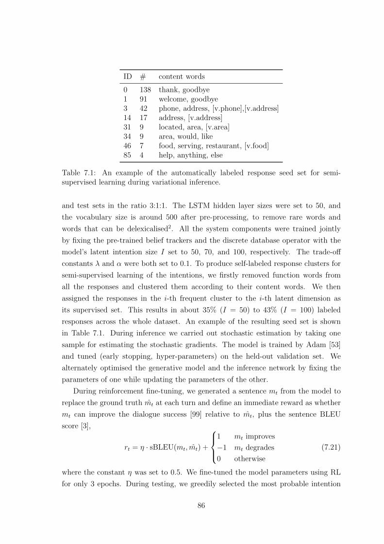
ID # content words
0 138 thank, goodbye1 91 welcome, goodbye3 42 phone, address, [v.phone],[v.address]14 17 address, [v.address]31 9 located, area, [v.area]34 9 area, would, like46 7 food, serving, restaurant, [v.food]85 4 help, anything, else
Table 7.1: An example of the automatically labeled response seed set for semi-supervised learning during variational inference.
and test sets in the ratio 3:1:1. The LSTM hidden layer sizes were set to 50, and
the vocabulary size is around 500 after pre-processing, to remove rare words and
words that can be delexicalised2. All the system components were trained jointly
by fixing the pre-trained belief trackers and the discrete database operator with the
model’s latent intention size I set to 50, 70, and 100, respectively. The trade-off
constants λ and α were both set to 0.1. To produce self-labeled response clusters for
semi-supervised learning of the intentions, we firstly removed function words from
all the responses and clustered them according to their content words. We then
assigned the responses in the i-th frequent cluster to the i-th latent dimension as
its supervised set. This results in about 35% (I = 50) to 43% (I = 100) labeled
responses across the whole dataset. An example of the resulting seed set is shown
in Table 7.1. During inference we carried out stochastic estimation by taking one
sample for estimating the stochastic gradients. The model is trained by Adam [53]
and tuned (early stopping, hyper-parameters) on the held-out validation set. We
alternately optimised the generative model and the inference network by fixing the
parameters of one while updating the parameters of the other.
During reinforcement fine-tuning, we generated a sentence mt from the model to
replace the ground truth mt at each turn and define an immediate reward as whether
mt can improve the dialogue success [99] relative to mt, plus the sentence BLEU
score [3],
rt = η · sBLEU(mt, mt) +
1 mt improves
−1 mt degrades
0 otherwise
(7.21)
where the constant η was set to 0.5. We fine-tuned the model parameters using RL
for only 3 epochs. During testing, we greedily selected the most probable intention
86
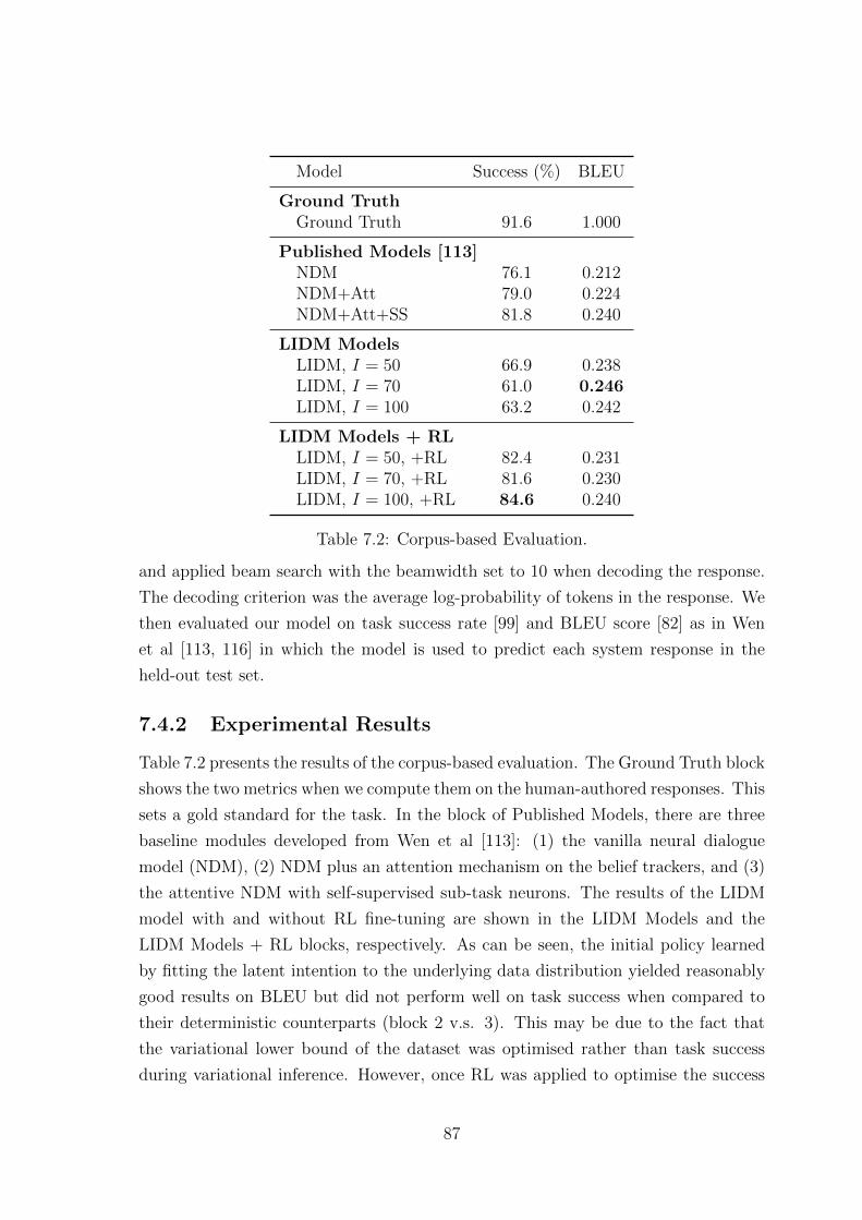
Model Success (%) BLEU
Ground TruthGround Truth 91.6 1.000
Published Models [113]NDM 76.1 0.212NDM+Att 79.0 0.224NDM+Att+SS 81.8 0.240
LIDM ModelsLIDM, I = 50 66.9 0.238LIDM, I = 70 61.0 0.246LIDM, I = 100 63.2 0.242
LIDM Models + RLLIDM, I = 50, +RL 82.4 0.231LIDM, I = 70, +RL 81.6 0.230LIDM, I = 100, +RL 84.6 0.240
Table 7.2: Corpus-based Evaluation.
and applied beam search with the beamwidth set to 10 when decoding the response.
The decoding criterion was the average log-probability of tokens in the response. We
then evaluated our model on task success rate [99] and BLEU score [82] as in Wen
et al [113, 116] in which the model is used to predict each system response in the
held-out test set.
7.4.2 Experimental Results
Table 7.2 presents the results of the corpus-based evaluation. The Ground Truth block
shows the two metrics when we compute them on the human-authored responses. This
sets a gold standard for the task. In the block of Published Models, there are three
baseline modules developed from Wen et al [113]: (1) the vanilla neural dialogue
model (NDM), (2) NDM plus an attention mechanism on the belief trackers, and (3)
the attentive NDM with self-supervised sub-task neurons. The results of the LIDM
model with and without RL fine-tuning are shown in the LIDM Models and the
LIDM Models + RL blocks, respectively. As can be seen, the initial policy learned
by fitting the latent intention to the underlying data distribution yielded reasonably
good results on BLEU but did not perform well on task success when compared to
their deterministic counterparts (block 2 v.s. 3). This may be due to the fact that
the variational lower bound of the dataset was optimised rather than task success
during variational inference. However, once RL was applied to optimise the success
87
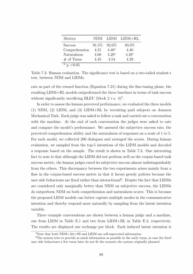
Metrics NDM LIDM LIDM+RL
Success 91.5% 92.0% 93.0%Comprehension 4.21 4.40∗ 4.40Naturalness 4.08 4.29∗ 4.28∗
# of Turns 4.45 4.54 4.29
* p <0.05
Table 7.3: Human evaluation. The significance test is based on a two-tailed student-ttest, between NDM and LIDMs.
rate as part of the reward function (Equation 7.21) during the fine-tuning phase, the
resulting LIDM+RL models outperformed the three baselines in terms of task success
without significantly sacrificing BLEU (block 2 v.s. 4)5.
In order to assess the human perceived performance, we evaluated the three models
(1) NDM, (2) LIDM, and (3) LIDM+RL by recruiting paid subjects on Amazon
Mechanical Turk. Each judge was asked to follow a task and carried out a conversation
with the machine. At the end of each conversation the judges were asked to rate
and compare the model’s performance. We assessed the subjective success rate, the
perceived comprehension ability and the naturalness of responses on a scale of 1 to 5.
For each model, we collected 200 dialogues and averaged the scores. During human
evaluation, we sampled from the top-5 intentions of the LIDM models and decoded
a response based on the sample. The result is shown in Table 7.3. One interesting
fact to note is that although the LIDM did not perform well on the corpus-based task
success metric, the human judges rated its subjective success almost indistinguishably
from the others. This discrepancy between the two experiments arises mainly from a
flaw in the corpus-based success metric in that it favors greedy policies because the
user side behaviours are fixed rather than interactional6. Despite the fact that LIDMs
are considered only marginally better than NDM on subjective success, the LIDMs
do outperform NDM on both comprehension and naturalness scores. This is because
the proposed LIDM models can better capture multiple modes in the communicative
intention and thereby respond more naturally by sampling from the latent intention
variable.
Three example conversations are shown between a human judge and a machine,
one from LIDM in Table E.1 and two from LIDM+RL in Table E.2, respectively.
The results are displayed one exchange per block. Each induced latent intention is
5Note that both NDM+Att+SS and LIDM use self-supervised information6The system tries to provide as much information as possible in the early turns, in case the fixed
user side behaviours a few turns later do not fit the scenario the system originally planned.
88
shown by a tuple (index, probability) followed by a decoded response, and the sample
dialogues were produced by following the responses highlighted in bold. As can be
seen, the LIDM shown in Table E.1 clearly has multiple modes in the distribution over
the learned intention latent variable, and what it represents can be easily interpreted
by the response generated. However, some intentions (such as intent 0) can result
in very different responses under different dialogue states even though they were
supervised by a small response set as shown in Table 7.1. This is mainly because of the
variance introduced during variational inference. Finally, when comparing Table E.1
and Table E.2, we can observe the difference between the two dialogue strategies:
the LIDM, by inferring its policy from the supervised dataset, reflects the diverse set
of modes in the underlying distribution; whereas the LIDM+RL, which refined its
strategy using RL, exhibits a much greedier behavior in achieving task success (e.g.
in Table E.2 in block 2 & 4 the LIDM+RL agent provides the address and phone
number even before the user asks). This is also supported by the human evaluation
in Table 7.3 where LIDM+RL has much shorter dialogues on average compared to
the other two models.
7.5 Summary
In this chapter, we propose a framework for learning dialogue intentions via discrete
latent variable models and introduced the Latent Intention Dialogue Model (LIDM)
for goal-oriented dialogue modeling. According to the experiments, the LIDM is able
discover an effective initial policy from the underlying data distribution and is capable
of revising its strategy based on an external reward using reinforcement learning. We
believe this is a promising step forward for building autonomous dialogue agents since
the learned discrete latent variable interface enables the agent to perform learning
using several differing paradigms. The experiments showed that the proposed LIDM
is able to communicate with human subjects and outperforms previous published
results.
89
Chapter 8
Conclusions and Further Work
This thesis has investigated deep generative models for NLP with neural variational
inference. The experiments on several different scenarios including document/topic
modelling, question answer selection, sentence compression and goal oriented dialogue
modelling have demonstrated the effectiveness and efficiency of our models on learning
stochastic representations, discovering topics and modelling latent intentions among
human utterances. We show that deep generative models are able to learn knowledge
from language and carry out a range of NLP tasks with unlabelled data or small
amounts of labelled data.
In this thesis, the deep generative models are divided into two folds by the set-
tings of the latent variables (continuous or discrete). However, the generic neural
variational inference framework is suitable for both continuous and discrete latent
variables, and is able to incorporate different kinds of deep neural networks. More
importantly, the inference networks acting as black-box functions are able to ap-
proximate multiplicate and complex distributions that can be jointly trained with
generative models, which provides efficient inference and grant the possibilities for
more interesting and sophisticated generative models.
In practice, both continuous and discrete latent variables have their own advan-
tages and disadvantages. Continuous variable is good at learning dense stochastic
representations. It is easy to generalise and fits the encoder-decoder structure very
well, especially in the unsupervised learning situation where the model can be built as
a continuous variational auto-encoder and easily trained with the help of continuous
reparameterisation trick. However, the KL divergence between the prior distribution
and the inference network acts as a strong regularisation for the learning of generative
model. If a powerful autoregressive neural network (e.g. LSTM) is employed as the
decoder, it has a chance to ignore the latent variable and generate the observations
as an unconditional model, which ends up with a trivial encoder. Hence, continuous
90

latent variables are preferred due to the simplicity of inference, but the decoders are
suggested to be built by simple and expressive neural networks to avoid the possible
failure from the perspective of optimisation.
Discrete latent variable, in contrast, is difficult to carry out inference due to the
high variance issue. In addition, as it lacks of smooth prior distribution, the dis-
crete latent variables are hard to be used directly in unsupervised learning models.
Nevertheless, discrete variables are good at constructing predictive models. By using
discrete latent distribution in the policy network, we are able to easily incorporate
semi-supervised and reinforcement learning to further improve the performance of
generative models. Moreover, in the context of language, discrete latent distribution
is more natural for the reasoning about complex semantics, incorporating structure
information and modelling interactive actions (e.g. dialogues). It generally has better
interpretability and easier to incorporate linguistic inductive biases. Therefore, it has
more potential in the field of natural language processing.
Introducing Bayesian non-parametrics in deep generative models is another inter-
esting part of this thesis. The complicated constructive process of Dirichlet process
yields to difficult inference in traditional probabilistic models. In the framework of
neural variational inference, however, we employ stick-breaking constructions param-
eterised by continuous latent variables to model categorical distributions. In this
case, the parameterisation networks can be easily updated together with the gener-
ative models by stochastic gradient back-propagation. With the help of recurrent
stick-breaking construction (RSB), a truncation-free variational inference can be im-
plemented to dynamically choose the dimension of latent space during the inference
process. This unbounded property is able to further extend the scalability of deep
generative models.
As of now, we have explored a few different kinds of deep generative models applied
for NLP and achieved good performance compared to other benchmark systems, but
there is still big space for further improvement due to the pressing requirement of
exploiting unlabelled data. Looking forward, the following topics can be further
studied in order to go deeper in the context of deep generative models:
1. Developing advanced inference algorithm and optimisation method for the neu-
ral variational inference framework. Variational auto-encoder (VAE) is an ef-
ficient framework of modeling natural images, but it is still not satisfiable on
generating natural language sentences due to the strong reliance on powerful
autoregressive neural networks. To develop more advanced inference algorithm
is able to further extend the capabilities of deep generative models for NLP.
91
2. Extending the proposed topic models into contextual neural topic models. Tra-
ditional probabilistic topic models achieved huge success owing to their flexibil-
ity of incorporating extra document information. Therefore time, authorship,
geo-location and categorical labels could all be integrated into the neural topic
models to further extend the vanilla neural topic models into contextual neural
topic models.
3. Discovering latent structures in language. The powerful recurrent neural net-
works are especially good at generating natural language sentences, generally by
the default left-to-right order. However, by using discrete variables representing
latent structures, we are able to incorporate grammars and logics in the natural
language generation rather than simply modelling language as plain sequences.
Hence, it is promising to develop more sophisticated and grammar-guided lan-
guage generation models with structural information.
4. Unsupervised language learning from multimodal resources. Human beings are
able to learn and develop language ability without supervision, since language is
grounded in daily life with the help of multiple input resources including vision,
voice, text and symbols. It is a challenging but worthwhile attempt to jointly
model multiple observations in the same deep generative model. In this context,
we expect the machine is able to learn knowledge from language, make sense
from surroundings and evolve without supervisions.
92
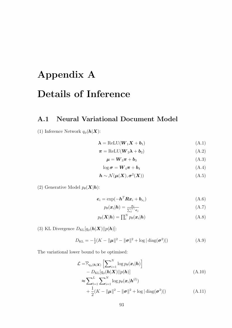
Appendix A
Details of Inference
A.1 Neural Variational Document Model
(1) Inference Network qφ(h|X):
λ = ReLU(W 1X + b1) (A.1)
π = ReLU(W 2λ + b2) (A.2)
µ = W 3π + b3 (A.3)
logσ = W 4π + b4 (A.4)
h ∼ N (µ(X),σ2(X)) (A.5)
(2) Generative Model pθ(X|h):
ei = exp(−hTRxi + bxi) (A.6)
pθ(xi|h) = ei∑|V |j ej
(A.7)
pθ(X|h) =∏N
i pθ(xi|h) (A.8)
(3) KL Divergence DKL[qφ(h|X)||p(h)]:
DKL = −12(K − ‖µ‖2 − ‖σ‖2 + log | diag(σ2)|) (A.9)
The variational lower bound to be optimised:
L =Eqφ(h|X)
[∑N
i=1log pθ(xi|h)
]−DKL[qφ(h|X)||p(h)] (A.10)
≈∑L
l=1
∑N
i=1log pθ(xi|h(l))
+1
2(K − ‖µ‖2 − ‖σ‖2 + log | diag(σ2)|) (A.11)
93
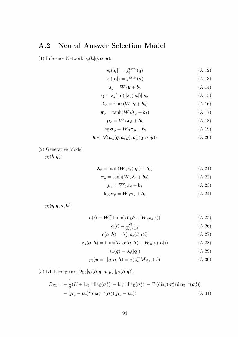
A.2 Neural Answer Selection Model
(1) Inference Network qφ(h|q,a,y):
sq(|q|) = f lstmq (q) (A.12)
sa(|a|) = f lstma (a) (A.13)
sy = W 5y + b5 (A.14)
γ = sq(|q|)||sa(|a|)||sy (A.15)
λφ = tanh(W 6γ + b6) (A.16)
πφ = tanh(W 7λφ + b7) (A.17)
µφ = W 8πφ + b8 (A.18)
logσφ = W 9πφ + b9 (A.19)
h ∼ N (µφ(q,a,y),σ2φ(q,a,y)) (A.20)
(2) Generative Model
pθ(h|q):
λθ = tanh(W 1sq(|q|) + b1) (A.21)
πθ = tanh(W 2λθ + b2) (A.22)
µθ = W 3πθ + b3 (A.23)
logσθ = W 4πθ + b4 (A.24)
pθ(y|q,a,h):
e(i) = W Tα tanh(W hh+W ssa(i)) (A.25)
α(i) = e(i)∑j e(j)
(A.26)
c(a,h) =∑
i sa(i)α(i) (A.27)
za(a,h) = tanh(W ac(a,h) +W nsa(|a|)) (A.28)
zq(q) = sq(|q|) (A.29)
pθ(y = 1|q,a,h) = σ(zTqMza + b) (A.30)
(3) KL Divergence DKL[qφ(h|q,a,y)||pθ(h|q)]:
DKL =− 1
2(K + log | diag(σ2
φ)| − log | diag(σ2θ)| − Tr(diag(σ2
φ) diag−1(σ2θ))
− (µφ − µθ)T diag−1(σ2θ)(µφ − µθ)) (A.31)
94
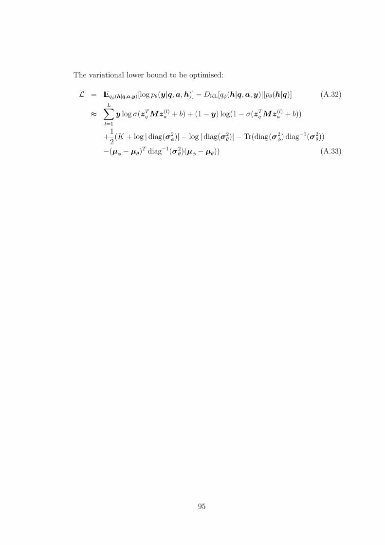
The variational lower bound to be optimised:
L = Eqφ(h|q,a,y)[log pθ(y|q,a,h)]−DKL[qφ(h|q,a,y)||pθ(h|q)] (A.32)
≈L∑l=1
y log σ(zTqMz(l)a + b) + (1− y) log(1− σ(zTqMz(l)
a + b))
+1
2(K + log | diag(σ2
φ)| − log | diag(σ2θ)| − Tr(diag(σ2
φ) diag−1(σ2θ))
−(µφ − µθ)T diag−1(σ2θ)(µφ − µθ)) (A.33)
95
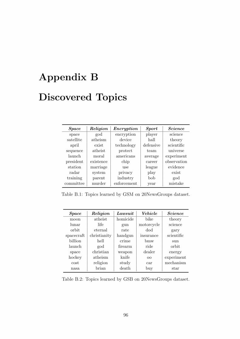
Appendix B
Discovered Topics
Space Religion Encryption Sport Science
space god encryption player sciencesatellite atheism device hall theory
april exist technology defensive scientificsequence atheist protect team universelaunch moral americans average experiment
president existence chip career observationstation marriage use league evidenceradar system privacy play exist
training parent industry bob godcommittee murder enforcement year mistake
Table B.1: Topics learned by GSM on 20NewsGroups dataset.
Space Religion Lawsuit Vehicle Science
moon atheist homicide bike theorylunar life gun motorcycle scienceorbit eternal rate dod gary
spacecraft christianity handgun insurance scientificbillion hell crime bmw sunlaunch god firearm ride orbitspace christian weapon dealer energy
hockey atheism knife oo experimentcost religion study car mechanismnasa brian death buy star
Table B.2: Topics learned by GSB on 20NewsGroups dataset.
96
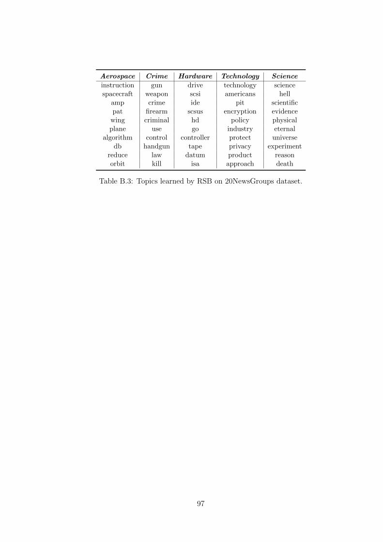
Aerospace Crime Hardware Technology Science
instruction gun drive technology sciencespacecraft weapon scsi americans hell
amp crime ide pit scientificpat firearm scsus encryption evidence
wing criminal hd policy physicalplane use go industry eternal
algorithm control controller protect universedb handgun tape privacy experiment
reduce law datum product reasonorbit kill isa approach death
Table B.3: Topics learned by RSB on 20NewsGroups dataset.
97
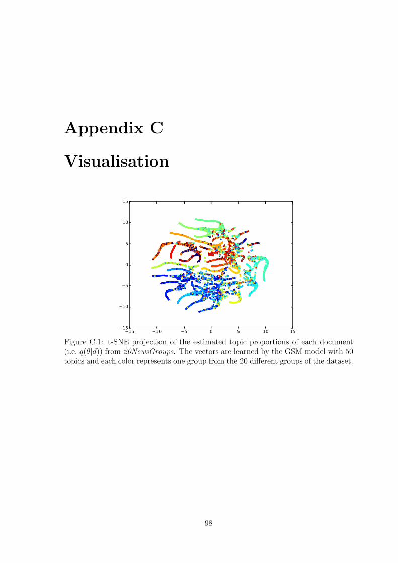
Appendix C
Visualisation
15 10 5 0 5 10 1515
10
5
0
5
10
15
Figure C.1: t-SNE projection of the estimated topic proportions of each document(i.e. q(θ|d)) from 20NewsGroups. The vectors are learned by the GSM model with 50topics and each color represents one group from the 20 different groups of the dataset.
98
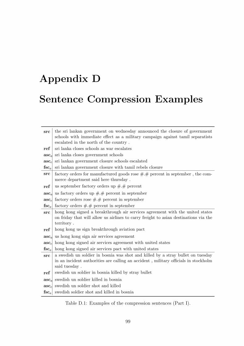
Appendix D
Sentence Compression Examples
src the sri lankan government on wednesday announced the closure of governmentschools with immediate effect as a military campaign against tamil separatistsescalated in the north of the country .
ref sri lanka closes schools as war escalates
asca sri lanka closes government schools
asce sri lankan government closure schools escalated
fsca sri lankan government closure with tamil rebels closure
src factory orders for manufactured goods rose #.# percent in september , the com-merce department said here thursday .
ref us september factory orders up #.# percent
asca us factory orders up #.# percent in september
asce factory orders rose #.# percent in september
fsca factory orders #.# percent in september
src hong kong signed a breakthrough air services agreement with the united stateson friday that will allow us airlines to carry freight to asian destinations via theterritory .
ref hong kong us sign breakthrough aviation pact
asca us hong kong sign air services agreement
asce hong kong signed air services agreement with united states
fsca hong kong signed air services pact with united states
src a swedish un soldier in bosnia was shot and killed by a stray bullet on tuesdayin an incident authorities are calling an accident , military officials in stockholmsaid tuesday .
ref swedish un soldier in bosnia killed by stray bullet
asca swedish un soldier killed in bosnia
asce swedish un soldier shot and killed
fsca swedish soldier shot and killed in bosnia
Table D.1: Examples of the compression sentences (Part I).
99
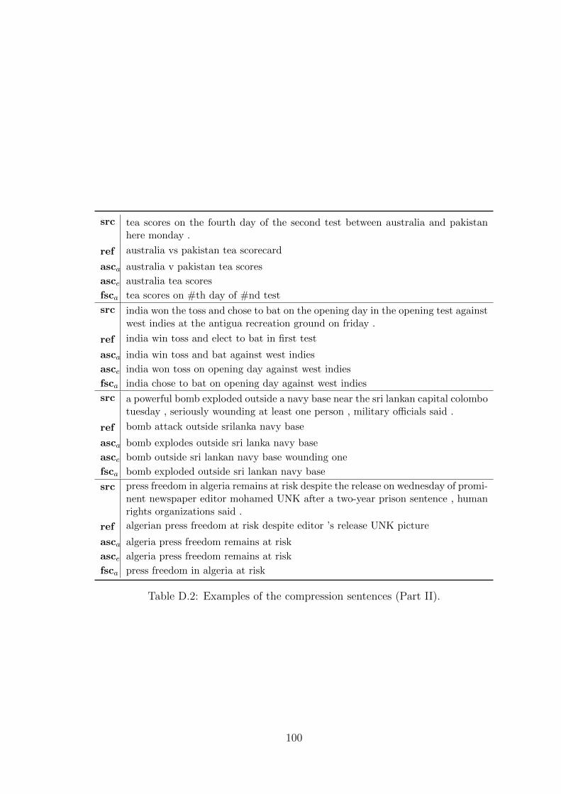
src tea scores on the fourth day of the second test between australia and pakistanhere monday .
ref australia vs pakistan tea scorecard
asca australia v pakistan tea scores
asce australia tea scores
fsca tea scores on #th day of #nd test
src india won the toss and chose to bat on the opening day in the opening test againstwest indies at the antigua recreation ground on friday .
ref india win toss and elect to bat in first test
asca india win toss and bat against west indies
asce india won toss on opening day against west indies
fsca india chose to bat on opening day against west indies
src a powerful bomb exploded outside a navy base near the sri lankan capital colombotuesday , seriously wounding at least one person , military officials said .
ref bomb attack outside srilanka navy base
asca bomb explodes outside sri lanka navy base
asce bomb outside sri lankan navy base wounding one
fsca bomb exploded outside sri lankan navy base
src press freedom in algeria remains at risk despite the release on wednesday of promi-nent newspaper editor mohamed UNK after a two-year prison sentence , humanrights organizations said .
ref algerian press freedom at risk despite editor ’s release UNK picture
asca algeria press freedom remains at risk
asce algeria press freedom remains at risk
fsca press freedom in algeria at risk
Table D.2: Examples of the compression sentences (Part II).
100
Appendix E
Goal Oriented Dialogue Examples
101
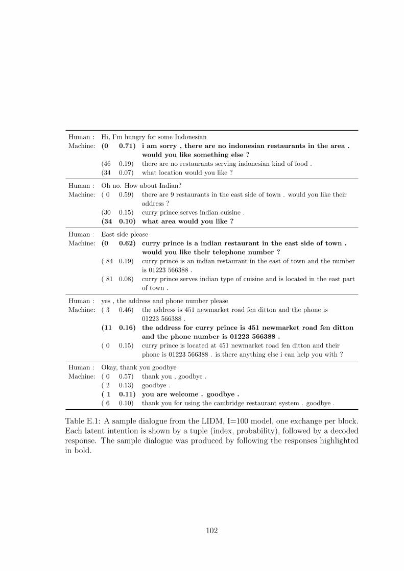
Human : Hi, I’m hungry for some Indonesian
Machine: (0 0.71) i am sorry , there are no indonesian restaurants in the area .
would you like something else ?
(46 0.19) there are no restaurants serving indonesian kind of food .
(34 0.07) what location would you like ?
Human : Oh no. How about Indian?
Machine: ( 0 0.59) there are 9 restaurants in the east side of town . would you like their
address ?
(30 0.15) curry prince serves indian cuisine .
(34 0.10) what area would you like ?
Human : East side please
Machine: (0 0.62) curry prince is a indian restaurant in the east side of town .
would you like their telephone number ?
( 84 0.19) curry prince is an indian restaurant in the east of town and the number
is 01223 566388 .
( 81 0.08) curry prince serves indian type of cuisine and is located in the east part
of town .
Human : yes , the address and phone number please
Machine: ( 3 0.46) the address is 451 newmarket road fen ditton and the phone is
01223 566388 .
(11 0.16) the address for curry prince is 451 newmarket road fen ditton
and the phone number is 01223 566388 .
( 0 0.15) curry prince is located at 451 newmarket road fen ditton and their
phone is 01223 566388 . is there anything else i can help you with ?
Human : Okay, thank you goodbye
Machine: ( 0 0.57) thank you , goodbye .
( 2 0.13) goodbye .
( 1 0.11) you are welcome . goodbye .
( 6 0.10) thank you for using the cambridge restaurant system . goodbye .
Table E.1: A sample dialogue from the LIDM, I=100 model, one exchange per block.Each latent intention is shown by a tuple (index, probability), followed by a decodedresponse. The sample dialogue was produced by following the responses highlightedin bold.
102
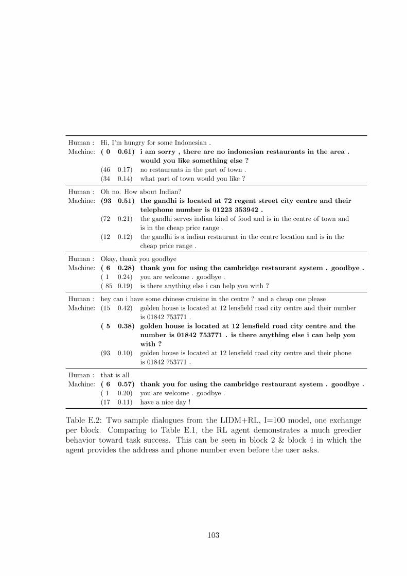
Human : Hi, I’m hungry for some Indonesian .
Machine: ( 0 0.61) i am sorry , there are no indonesian restaurants in the area .
would you like something else ?
(46 0.17) no restaurants in the part of town .
(34 0.14) what part of town would you like ?
Human : Oh no. How about Indian?
Machine: (93 0.51) the gandhi is located at 72 regent street city centre and their
telephone number is 01223 353942 .
(72 0.21) the gandhi serves indian kind of food and is in the centre of town and
is in the cheap price range .
(12 0.12) the gandhi is a indian restaurant in the centre location and is in the
cheap price range .
Human : Okay, thank you goodbye
Machine: ( 6 0.28) thank you for using the cambridge restaurant system . goodbye .
( 1 0.24) you are welcome . goodbye .
( 85 0.19) is there anything else i can help you with ?
Human : hey can i have some chinese cruisine in the centre ? and a cheap one please
Machine: (15 0.42) golden house is located at 12 lensfield road city centre and their number
is 01842 753771 .
( 5 0.38) golden house is located at 12 lensfield road city centre and the
number is 01842 753771 . is there anything else i can help you
with ?
(93 0.10) golden house is located at 12 lensfield road city centre and their phone
is 01842 753771 .
Human : that is all
Machine: ( 6 0.57) thank you for using the cambridge restaurant system . goodbye .
( 1 0.20) you are welcome . goodbye .
(17 0.11) have a nice day !
Table E.2: Two sample dialogues from the LIDM+RL, I=100 model, one exchangeper block. Comparing to Table E.1, the RL agent demonstrates a much greedierbehavior toward task success. This can be seen in block 2 & block 4 in which theagent provides the address and phone number even before the user asks.
103

Bibliography
[1] Christophe Andrieu, Nando De Freitas, Arnaud Doucet, and Michael I Jordan.
An introduction to mcmc for machine learning. Machine learning, 50(1-2):5–43,
2003.
[2] Hagai Attias. A variational bayesian framework for graphical models. In Pro-
ceedings of NIPS, 2000.
[3] Michael Auli and Jianfeng Gao. Decoder integration and expected bleu train-
ing for recurrent neural network language models. In ACL. Association for
Computational Linguistics, 2014.
[4] Jimmy Ba, Roger Grosse, Ruslan Salakhutdinov, and Brendan Frey. Learning
wake-sleep recurrent attention models. In Proceedings of NIPS, 2015.
[5] Jimmy Ba, Volodymyr Mnih, and Koray Kavukcuoglu. Multiple object recog-
nition with visual attention. In Proceedings of ICLR, 2015.
[6] Dzmitry Bahdanau, Kyunghyun Cho, and Yoshua Bengio. Neural machine
translation by jointly learning to align and translate. In Proceedings of ICLR,
2015.
[7] Matthew James Beal. Variational algorithms for approximate Bayesian infer-
ence. PhD thesis, University of London, 2003.
[8] Thierry Bertin-Mahieux, Daniel P.W. Ellis, Brian Whitman, and Paul Lamere.
The million song dataset. In Proceedings of ISMIR, 2011.
[9] David M Blei and John D Lafferty. Dynamic topic models. In Proceedings of
ICML, pages 113–120. ACM, 2006.
[10] David M Blei and John D Lafferty. A correlated topic model of science. The
Annals of Applied Statistics, 2007.
104

[11] David M Blei, Andrew Y Ng, and Michael I Jordan. Latent dirichlet allocation.
The Journal of Machine Learning Research, 3:993–1022, 2003.
[12] Antoine Bordes and Jason Weston. Learning end-to-end goal-oriented dialog.
In Proceedings of ICLR, 2017.
[13] Jorg Bornschein and Yoshua Bengio. Reweighted wake-sleep. In Proceedings of
ICLR, 2015.
[14] Samuel R Bowman, Luke Vilnis, Oriol Vinyals, Andrew M Dai, Rafal Jozefow-
icz, and Samy Bengio. Generating sentences from a continuous space. arXiv
preprint arXiv:1511.06349, 2015.
[15] Yuri Burda, Roger Grosse, and Ruslan Salakhutdinov. Importance weighted
autoencoders. In Proceedings of ICLR, 2016.
[16] Kris Cao and Stephen Clark. Latent variable dialogue models and their diver-
sity. In Proceedings of EACL, 2017.
[17] Bradley P Carlin and Nicholas G Polson. Inference for nonconjugate bayesian
models using the gibbs sampler. Canadian Journal of statistics, 19(4):399–405,
1991.
[18] Jan K Chorowski, Dzmitry Bahdanau, Dmitriy Serdyuk, Kyunghyun Cho, and
Yoshua Bengio. Attention-based models for speech recognition. In Proceedings
of NIPS, pages 577–585, 2015.
[19] Andrew M Dai and Quoc V Le. Semi-supervised sequence learning. In Proceed-
ings of NIPS, pages 3061–3069, 2015.
[20] Rajarshi Das, Manzil Zaheer, and Chris Dyer. Gaussian lda for topic models
with word embeddings. In Proceedings of ACL, volume 1, pages 795–804, 2015.
[21] Peter Dayan and Geoffrey E Hinton. Varieties of helmholtz machine. Neural
Networks, 9(8):1385–1403, 1996.
[22] Chris Dyer, Adhiguna Kuncoro, Miguel Ballesteros, and Noah A Smith. Recur-
rent neural network grammars. In Proceedings of NAACL, 2016.
[23] SM Eslami, Nicolas Heess, Theophane Weber, Yuval Tassa, Koray
Kavukcuoglu, and Geoffrey E Hinton. Attend, infer, repeat: Fast scene un-
derstanding with generative models. arXiv preprint arXiv:1603.08575, 2016.
105
[24] Katja Filippova, Enrique Alfonseca, Carlos A Colmenares, Lukasz Kaiser, and
Oriol Vinyals. Sentence compression by deletion with lstms. In Proceedings of
EMNLP, 2015.
[25] Yarin Gal and Zoubin Ghahramani. Dropout as a bayesian approximation:
Representing model uncertainty in deep learning. In Proceedings of ICML,
pages 1050–1059, 2016.
[26] Milica Gasic, Catherine Breslin, Matthew Henderson, Dongho Kim, Martin
Szummer, Blaise Thomson, Pirros Tsiakoulis, and Steve Young. On-line policy
optimisation of bayesian spoken dialogue systems via human interaction. In
Proceedings of ICASSP, 2013.
[27] Zoubin Ghahramani. Nonparametric bayesian methods. In Tutorial presenta-
tion at the UAI Conference, 2005.
[28] Karol Gregor, Ivo Danihelka, Alex Graves, and Daan Wierstra. Draw: A re-
current neural network for image generation. In Proceedings of ICML, 2015.
[29] Karol Gregor, Andriy Mnih, and Daan Wierstra. Deep autoregressive networks.
In Proceedings of ICML, 2014.
[30] Jiatao Gu, Zhengdong Lu, Hang Li, and Victor OK Li. Incorporating copying
mechanism in sequence-to-sequence learning. arXiv preprint arXiv:1603.06393,
2016.
[31] Shixiang Gu, Sergey Levine, Ilya Sutskever, and Andriy Mnih. Muprop: Unbi-
ased backpropagation for stochastic neural networks. In Proceedings of ICLR,
2016.
[32] Caglar Gulcehre, Sungjin Ahn, Ramesh Nallapati, Bowen Zhou, and Yoshua
Bengio. Pointing the unknown words. arXiv preprint arXiv:1603.08148, 2016.
[33] Michael Heilman and Noah A. Smith. Tree edit models for recognizing textual
entailments, paraphrases, and answers to questions. In Proceedings of NAACL,
2010.
[34] Matthew Henderson. Machine learning for dialog state tracking: A review. In
Machine Learning in Spoken Language Processing Workshop, 2015.
106
[35] Matthew Henderson, Blaise Thomson, and Steve Young. Word-based dialog
state tracking with recurrent neural networks. In Proceedings of SigDial, 2014.
[36] Karl Moritz Hermann, Tomas Kocisky, Edward Grefenstette, Lasse Espeholt,
Will Kay, Mustafa Suleyman, and Phil Blunsom. Teaching machines to read
and comprehend. In Proceedings of NIPS, 2015.
[37] Irina Higgins, Loic Matthey, Arka Pal, Christopher Burgess, Xavier Glorot,
Matthew Botvinick, Shakir Mohamed, and Alexander Lerchner. beta-vae:
Learning basic visual concepts with a constrained variational framework. In
Proceedings of ICLR, 2017.
[38] Felix Hill, Antoine Bordes, Sumit Chopra, and Jason Weston. The goldilocks
principle: Reading children’s books with explicit memory representations. In
Proceedings of ICLR, 2016.
[39] Geoffrey E Hinton, Peter Dayan, Brendan J Frey, and Radford M Neal.
The wake-sleep algorithm for unsupervised neural networks. Science,
268(5214):1158–1161, 1995.
[40] Geoffrey E Hinton and Ruslan Salakhutdinov. Replicated softmax: an undi-
rected topic model. In Proceedings of NIPS, 2009.
[41] Geoffrey E Hinton and Ruslan R Salakhutdinov. Reducing the dimensionality
of data with neural networks. Science, 313(5786):504–507, 2006.
[42] Geoffrey E Hinton and Richard S Zemel. Autoencoders, minimum description
length, and helmholtz free energy. In Proceedings of NIPS, 1994.
[43] Sepp Hochreiter and Jurgen Schmidhuber. Long short-term memory. Neural
Computation, 1997.
[44] Matthew Hoffman, Francis R Bach, and David M Blei. Online learning for
latent dirichlet allocation. In Proceedings of NIPS, pages 856–864, 2010.
[45] Thomas Hofmann. Probabilistic latent semantic indexing. In Proceedings of
SIGIR, 1999.
[46] Eric Jang, Shixiang Gu, and Ben Poole. Categorical reparameterization with
gumbel-softmax. arXiv preprint arXiv:1611.01144, 2016.
107

[47] Michael I Jordan, Zoubin Ghahramani, Tommi S Jaakkola, and Lawrence K
Saul. An introduction to variational methods for graphical models. Machine
learning, 37(2):183–233, 1999.
[48] Nal Kalchbrenner and Phil Blunsom. Recurrent continuous translation models.
In Proceedings of EMNLP, 2013.
[49] Andrej Karpathy and Li Fei-Fei. Deep visual-semantic alignments for generating
image descriptions. In Proceedings of CVPR, 2015.
[50] John F. Kelley. An iterative design methodology for user-friendly natural lan-
guage office information applications. ACM Transaction on Information Sys-
tems, 1984.
[51] Mohammad Emtiyaz Khan, Shakir Mohamed, Benjamin M Marlin, and Kevin P
Murphy. A stick-breaking likelihood for categorical data analysis with latent
gaussian models. In Proceedings of AISTATS, 2012.
[52] Chloe Kiddon, Luke Zettlemoyer, and Yejin Choi. Globally coherent text gen-
eration with neural checklist models. In Proceedings of EMNLP, 2016.
[53] Diederik P. Kingma and Jimmy Ba. Adam: A method for stochastic optimiza-
tion. In Proceedings of ICLR, 2015.
[54] Diederik P Kingma, Shakir Mohamed, Danilo Jimenez Rezende, and Max
Welling. Semi-supervised learning with deep generative models. In Proceed-
ings of NIPS, 2014.
[55] Diederik P Kingma, Tim Salimans, and Max Welling. Variational dropout and
the local reparameterization trick. In Proceedings of NIPS, pages 2575–2583,
2015.
[56] Diederik P Kingma and Max Welling. Auto-encoding variational bayes. In
Proceedings of ICLR, 2014.
[57] Vijay R. Konda and John N. Tsitsiklis. On actor-critic algorithms. SIAM J.
Control Optim., 42(4):1143–1166, April 2003.
[58] Tomas Kocisky, Gabor Melis, Edward Grefenstette, Chris Dyer, Wang Ling,
Phil Blunsom, and Karl Moritz Hermann. Semantic parsing with semi-
supervised sequential autoencoders. In Proceedings of EMNLP, 2016.
108
[59] Ankit Kumar, Ozan Irsoy, Jonathan Su, James Bradbury, Robert English,
Brian Pierce, Peter Ondruska, Ishaan Gulrajani, and Richard Socher. Ask me
anything: Dynamic memory networks for natural language processing. arXiv
preprint arXiv:1506.07285, 2015.
[60] Thomas K Landauer, Peter W Foltz, and Darrell Laham. An introduction to
latent semantic analysis. Discourse processes, 25(2-3):259–284, 1998.
[61] Hugo Larochelle and Stanislas Lauly. A neural autoregressive topic model. In
Proceedings of NIPS, 2012.
[62] Jey Han Lau, David Newman, and Timothy Baldwin. Machine reading tea
leaves: Automatically evaluating topic coherence and topic model quality. In
Proceedings of EACL, 2014.
[63] Quoc V Le and Tomas Mikolov. Distributed representations of sentences and
documents. In Proceedings of ICML, 2014.
[64] Quoc V. Le and Tomas Mikolov. Distributed representations of sentences and
documents. In Proceedings of ICML, 2014.
[65] Yann LeCun, Sumit Chopra, and Raia Hadsell. A tutorial on energy-based
learning. Predicting structured data, 2006.
[66] Jiwei Li, Michel Galley, Chris Brockett, Jianfeng Gao, and Bill Dolan. A
diversity-promoting objective function for neural conversation models. In Pro-
ceedings of NAACL-HLT, 2016.
[67] Jiwei Li, Michel Galley, Chris Brockett, Georgios Spithourakis, Jianfeng Gao,
and Bill Dolan. A persona-based neural conversation model. In Proceedings of
ACL, 2016.
[68] Jiwei Li, Alexander H. Miller, Sumit Chopra, Marc’Aurelio Ranzato, and Jason
Weston. Dialogue learning with human-in-the-loop. In Proceedings of ICLR,
2017.
[69] Jiwei Li, Will Monroe, Alan Ritter, Dan Jurafsky, Michel Galley, and Jianfeng
Gao. Deep reinforcement learning for dialogue generation. In Proceedings of
EMNLP, 2016.
109
[70] Wang Ling, Edward Grefenstette, Karl Moritz Hermann, Tomas Kocisky, An-
drew Senior, Fumin Wang, and Phil Blunsom. Latent predictor networks for
code generation. In Proceedings of ACL, 2016.
[71] Chris J Maddison, Andriy Mnih, and Yee Whye Teh. The concrete distri-
bution: A continuous relaxation of discrete random variables. arXiv preprint
arXiv:1611.00712, 2016.
[72] Diego Marcheggiani and Ivan Titov. Discrete-state variational autoencoders for
joint discovery and factorization of relations. Transactions of the Association
for Computational Linguistics, 4, 2016.
[73] Jon D McAuliffe and David M Blei. Supervised topic models. In Proceedings
of NIPS, pages 121–128, 2008.
[74] Yishu Miao and Phil Blunsom. Language as a latent variable: Discrete gener-
ative models for sentence compression. In Proceedings of EMNLP, 2016.
[75] Yishu Miao, Lei Yu, and Phil Blunsom. Neural variational inference for text
processing. In Proceedings of ICML, 2016.
[76] Tomas Mikolov, Ilya Sutskever, Kai Chen, Gregory S. Corrado, and Jeffrey
Dean. Distributed representations of words and phrases and their composition-
ality. In Proceedings of NIPS, 2013.
[77] Andriy Mnih and Karol Gregor. Neural variational inference and learning in
belief networks. In Proceedings of ICML, 2014.
[78] Andriy Mnih and Danilo Rezende. Variational inference for monte carlo objec-
tives. In Proceedings of ICML, 2016.
[79] Volodymyr Mnih, Nicolas Heess, and Alex Graves. Recurrent models of visual
attention. In Proceedings of NIPS, 2014.
[80] Ramesh Nallapati, Bowen Zhou, Ca glar Gulcehre, and Bing Xiang. Abstractive
text summarization using sequence-to-sequence rnns and beyond. arXiv preprint
arXiv:1602.06023, 2016.
[81] Radford M Neal. Probabilistic inference using markov chain monte carlo meth-
ods. Technical report: CRG-TR-93-1, 1993.
110
[82] Kishore Papineni, Salim Roukos, Todd Ward, and Wei-Jing Zhu. Bleu: a
method for automatic evaluation of machine translation. In Proceedings of
ACL.
[83] Marc’Aurelio Ranzato, Sumit Chopra, Michael Auli, and Wojciech Zaremba.
Sequence level training with recurrent neural networks. In Proceedings of ICLR,
2016.
[84] Danilo J Rezende, Shakir Mohamed, and Daan Wierstra. Stochastic backprop-
agation and approximate inference in deep generative models. In Proceedings
of ICML, 2014.
[85] Michal Rosen-Zvi, Thomas Griffiths, Mark Steyvers, and Padhraic Smyth. The
author-topic model for authors and documents. In Proceedings of UAI, 2004.
[86] David E Rumelhart, Geoffrey E Hinton, and Ronald J Williams. Learning in-
ternal representations by error propagation. Technical report, DTIC Document,
1985.
[87] Alexander M Rush, Sumit Chopra, and Jason Weston. A neural attention model
for abstractive sentence summarization. In Proceedings of EMNLP, 2015.
[88] Iulian V. Serban, Alessandro Sordoni, Ryan Lowe, Laurent Charlin, Joelle
Pineau, Aaron Courville, and Yoshua Bengio. A hierarchical latent variable
encoder-decoder model for generating dialogues. arXiv preprint: 1605.06069,
2016.
[89] Iulian Vlad Serban, Alessandro Sordoni, Yoshua Bengio, Aaron C. Courville,
and Joelle Pineau. Hierarchical neural network generative models for movie
dialogues. In Proceedings of AAAI, 2015.
[90] Jayaram Sethuraman. A constructive definition of dirichlet priors. Statistica
sinica, pages 639–650, 1994.
[91] Aliaksei Severyn. Modelling input texts: from Tree Kernels to Deep Learning.
PhD thesis, University of Trento, 2015.
[92] Aliaksei Severyn and Alessandro Moschitti. Automatic feature engineering for
answer selection and extraction. In Proceedings of EMNLP, 2013.
111
[93] Lifeng Shang, Zhengdong Lu, and Hang Li. Neural responding machine for
short-text conversation. In Proceedings of ACL, 2015.
[94] David Silver, Aja Huang, Chris J Maddison, Arthur Guez, Laurent Sifre, George
Van Den Driessche, Julian Schrittwieser, Ioannis Antonoglou, Veda Panneer-
shelvam, Marc Lanctot, et al. Mastering the game of go with deep neural
networks and tree search. Nature, 529(7587):484–489, 2016.
[95] Rion Snow, Daniel Jurafsky, and Andrew Y. Ng. Learning syntactic patterns
for automatic hypernym discovery. In Proceedings of NIPS, 2004.
[96] Akash Srivastava and Charles Sutton. Neural variational inference for topic
models. Bayesian deep learning workshop, NIPS, 2016.
[97] Nitish Srivastava, RR Salakhutdinov, and Geoffrey Hinton. Modeling docu-
ments with deep boltzmann machines. In Proceedings of UAI, 2013.
[98] Pei-Hao Su, Milica Gasic, Nikola Mrksic, Lina M. Rojas Barahona, Stefan Ultes,
David Vandyke, Tsung-Hsien Wen, and Steve Young. On-line active reward
learning for policy optimisation in spoken dialogue systems. In Proceedings of
ACL, 2016.
[99] Pei-Hao Su, David Vandyke, Milica Gasic, Dongho Kim, Nikola Mrksic, Tsung-
Hsien Wen, and Steve Young. Learning from real users: Rating dialogue success
with neural networks for reinforcement learning in spoken dialogue systems. In
Proceedings of Interspeech, 2015.
[100] Sainbayar Sukhbaatar, Arthur Szlam, Jason Weston, and Rob Fergus. End-to-
end memory networks. In Proceedings of NIPS, 2015.
[101] Ilya Sutskever, Oriol Vinyals, and Quoc VV Le. Sequence to sequence learning
with neural networks. In Proceedings of NIPS, 2014.
[102] Yee Whye Teh, Michael I Jordan, Matthew J Beal, and David M Blei. Hi-
erarchical dirichlet processes. Journal of the American Statistical Asociation,
101(476), 2006.
[103] Yee Whye Teh, Michael I Jordan, Matthew J Beal, and David M Blei. Hi-
erarchical dirichlet processes. Journal of the american statistical association,
2012.
112
[104] David R. Traum. Foundations of Rational Agency, chapter Speech Acts for
Dialogue Agents. Springer, 1999.
[105] Oriol Vinyals, Meire Fortunato, and Navdeep Jaitly. Pointer networks. In
Proceedings of NIPS, pages 2674–2682, 2015.
[106] Oriol Vinyals and Quoc V. Le. A neural conversational model. In ICML Deep
Learning Workshop, 2015.
[107] Chong Wang and David M Blei. Variational inference in nonconjugate models.
Journal of Machine Learning Research, 14(Apr):1005–1031, 2013.
[108] Chong Wang, John William Paisley, and David M Blei. Online variational
inference for the hierarchical dirichlet process. In Proceedings of AISTATS,
2011.
[109] Mengqiu Wang and Christopher D Manning. Probabilistic tree-edit models
with structured latent variables for textual entailment and question answering.
In Proceedings of COLING, 2010.
[110] Mengqiu Wang, Noah A Smith, and Teruko Mitamura. What is the jeop-
ardy model? a quasi-synchronous grammar for qa. In Proceedings of EMNLP-
CoNLL, 2007.
[111] Xuerui Wang and Andrew McCallum. Topics over time: a non-markov
continuous-time model of topical trends. In Proceedings of the 12th ACM
SIGKDD international conference on Knowledge discovery and data mining,
2006.
[112] Zhiguo Wang and Abraham Ittycheriah. Faq-based question answering via word
alignment. arXiv preprint arXiv:1507.02628, 2015.
[113] Tsung-Hsien Wen, Milica Gasic, Nikola Mrksic, Lina M. Rojas Barahona, Pei-
Hao Su, Stefan Ultes, David Vandyke, and Steve Young. Conditional generation
and snapshot learning in neural dialogue systems. In Proceedings of EMNLP,
November 2016.
[114] Tsung-Hsien Wen, Milica Gasic, Nikola Mrksic, Pei-Hao Su, David Vandyke,
and Steve Young. Semantically conditioned lstm-based natural language gen-
eration for spoken dialogue systems. In Proceedings of EMNLP, September
2015.
113
[115] Tsung-Hsien Wen, Yishu Miao, Phil Blunsom, and Steve Young. Latent inten-
tion dialogue models. In Proceedings of ICML, 2017.
[116] Tsung-Hsien Wen, David Vandyke, Nikola Mrksic, Milica Gasic, Lina M. Rojas-
Barahona, Pei-Hao Su, Stefan Ultes, and Steve Young. A network-based end-
to-end trainable task-oriented dialogue system. In Proceedings of EACL, 2017.
[117] Jason Weston, Sumit Chopra, and Antoine Bordes. Memory networks. In
Proceedings of ICLR, 2015.
[118] Jason E Weston. Dialog-based language learning. In Proceedings of NIPS, pages
829–837. Curran Associates, Inc., 2016.
[119] Ronald J. Williams. Simple statistical gradient-following algorithms for connec-
tionist reinforcement learning. Machine Learning, 8(3-4):229–256, May 1992.
[120] Pengtao Xie, Yuntian Deng, and Eric Xing. Diversifying restricted boltzmann
machine for document modeling. In Proceedings of KDD, pages 1315–1324.
ACM, 2015.
[121] Kelvin Xu, Jimmy Ba, Ryan Kiros, Aaron Courville, Ruslan Salakhutdinov,
Richard Zemel, and Yoshua Bengio. Show, attend and tell: Neural image cap-
tion generation with visual attention. In Proceedings of ICML, 2015.
[122] Yi Yang, Wen-tau Yih, and Christopher Meek. Wikiqa: A challenge dataset
for open-domain question answering. In Proceedings of EMNLP, 2015.
[123] Wen-tau Yih, Ming-Wei Chang, Christopher Meek, and Andrzej Pastusiak.
Question answering using enhanced lexical semantic models. In Proceedings of
ACL, 2013.
[124] Steve Young, Milica Gasic, Blaise Thomson, and Jason D. Williams. Pomdp-
based statistical spoken dialog systems: A review. In Proceedings of the IEEE,
2013.
[125] Lei Yu, Karl Moritz Hermann, Phil Blunsom, and Stephen Pulman. Deep
Learning for Answer Sentence Selection. In NIPS Deep Learning Workshop,
2014.
114