generative models for hep

Generative Models for HEP(Including a success story)

Fedor RatnikovNRU Higher School of Economics,

Yandex School of Data Analysis

[email protected] Generative Models

Approaches

2

mailto:[email protected]?subject=


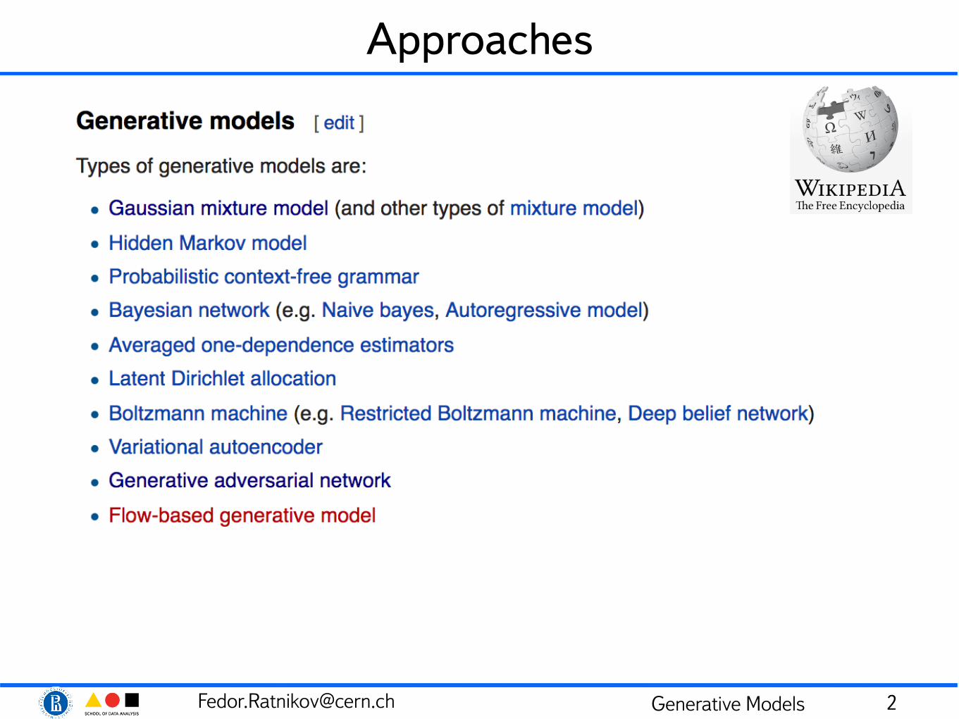
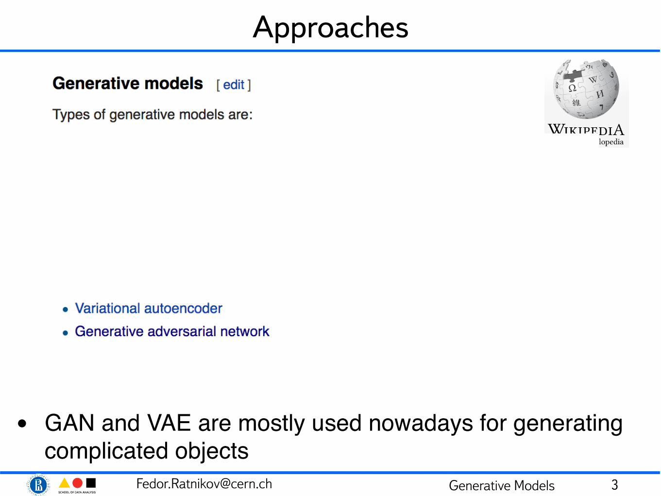
Approaches

• GAN and VAE are mostly used nowadays for generating complicated objects

3



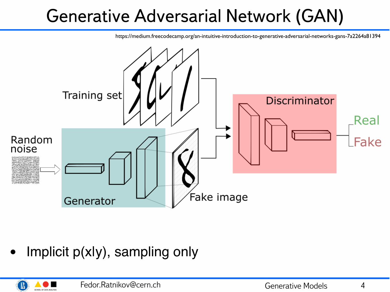
Generative Adversarial Network (GAN)

• Implicit p(x|y), sampling only

4

https://medium.freecodecamp.org/an-intuitive-introduction-to-generative-adversarial-networks-gans-7a2264a81394



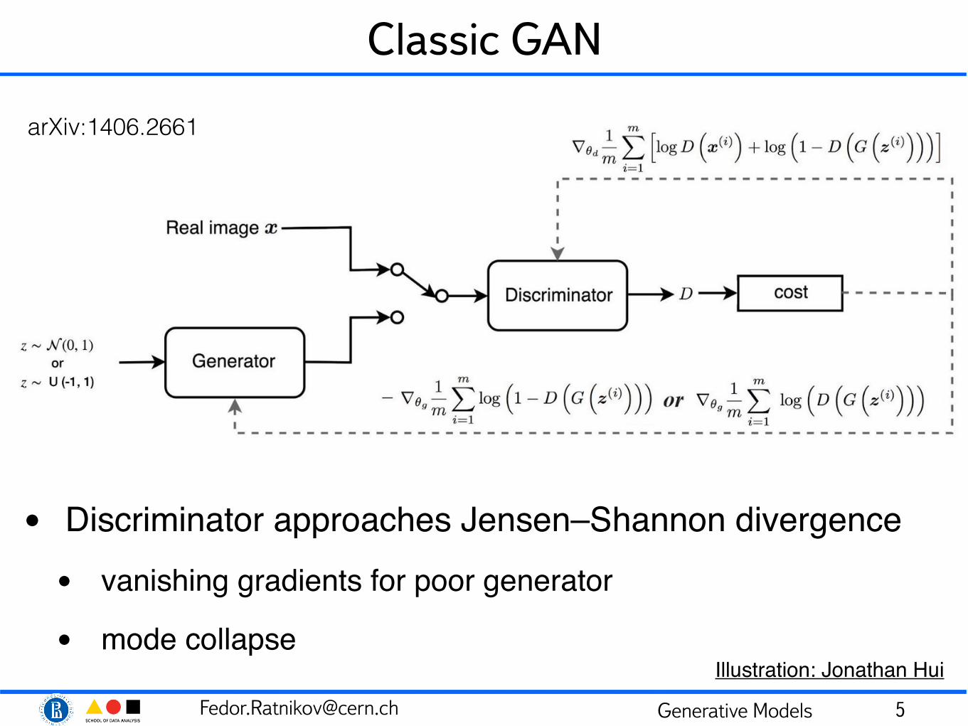
Classic GAN

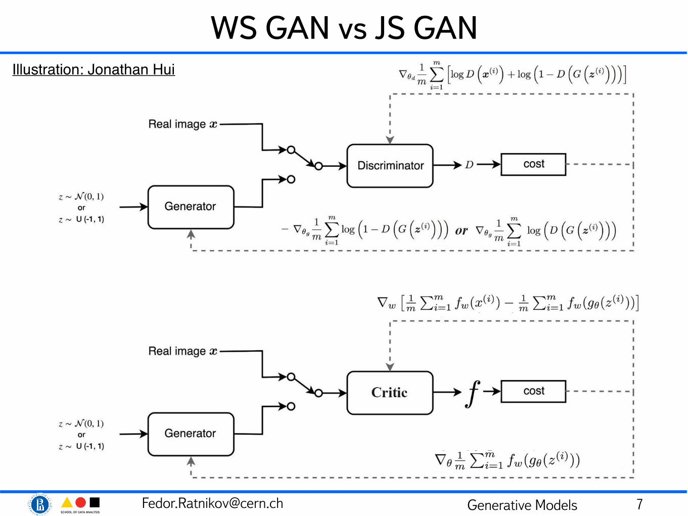
• Discriminator approaches Jensen–Shannon divergence• vanishing gradients for poor generator

• mode collapse

5

Illustration: Jonathan Hui

arXiv:1406.2661


https://medium.com/@jonathan_hui/gan-wasserstein-gan-wgan-gp-6a1a2aa1b490


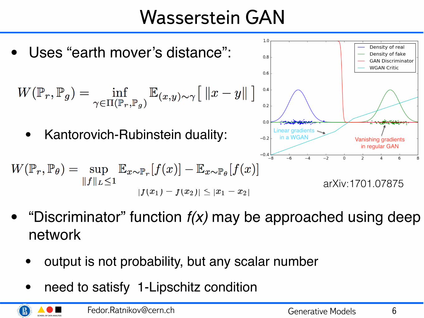
Wasserstein GAN

• Uses “earth mover’s distance”:

• Kantorovich-Rubinstein duality:

• “Discriminator” function f(x) may be approached using deep network• output is not probability, but any scalar number

• need to satisfy 1-Lipschitz condition 6

arXiv:1701.07875



WS GAN vs JS GAN

7

Illustration: Jonathan Hui


https://medium.com/@jonathan_hui/gan-wasserstein-gan-wgan-gp-6a1a2aa1b490


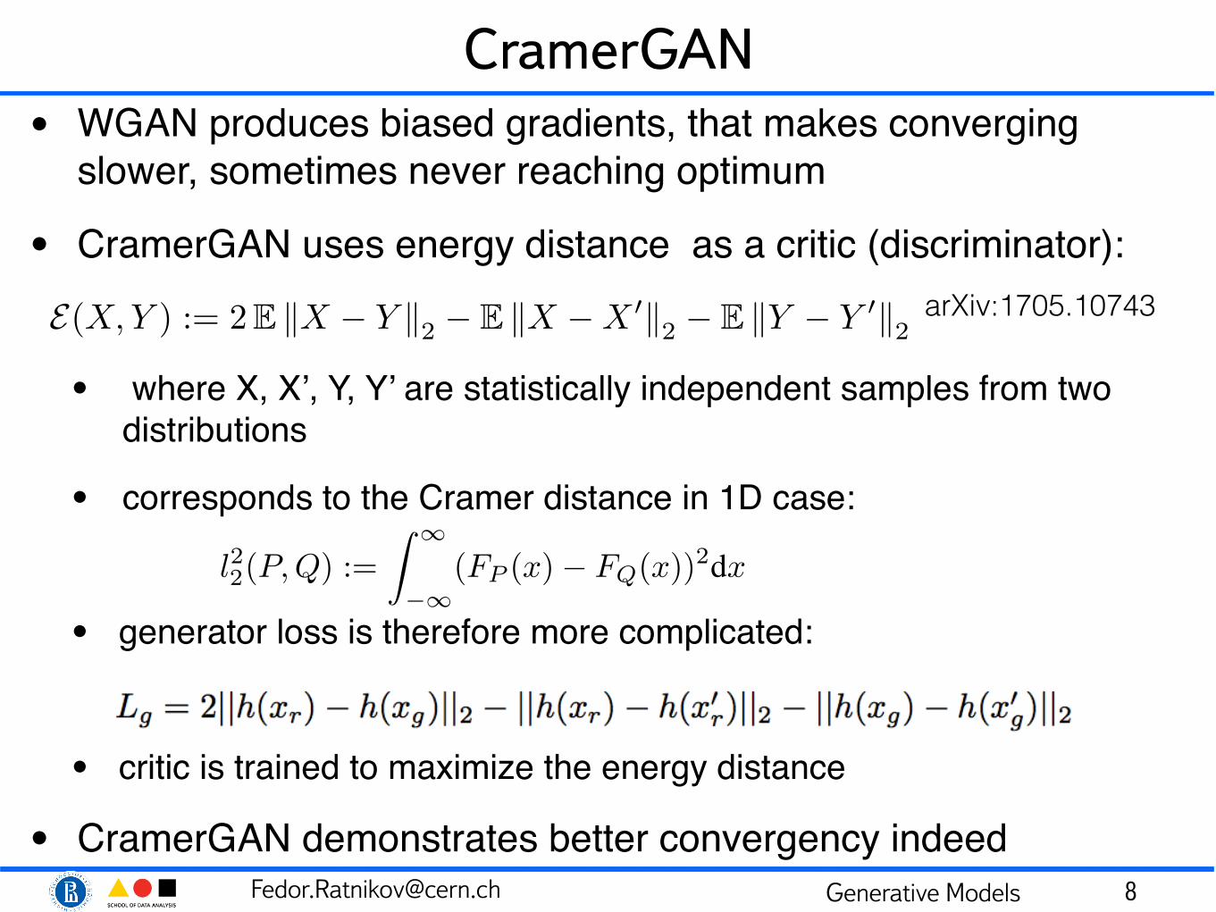
CramerGAN• WGAN produces biased gradients, that makes converging

slower, sometimes never reaching optimum

• CramerGAN uses energy distance as a critic (discriminator):

• where X, X’, Y, Y’ are statistically independent samples from two distributions

• corresponds to the Cramer distance in 1D case:

• generator loss is therefore more complicated:

• critic is trained to maximize the energy distance

• CramerGAN demonstrates better convergency indeed 8

4.1 Definition and Analysis

Recall that for two distributions P and Q over R, their (cumulative) distribution functions are re-spectively FP and FQ. The Cramér distance between P and Q is

l22(P, Q) :=

Z 1

�1(FP (x) � FQ(x))2dx.

Note that as written, the Cramér distance is not a metric proper. However, its square root is, and is amember of the lp family of metrics

lp(P, Q) :=

✓Z 1

�1|FP (x) � FQ(x)|pdx

◆1/p

.

The lp and Wasserstein metrics are identical at p = 1, but are otherwise distinct. Like the Wasser-stein metrics, the lp metrics have dual forms as integral probability metrics (see Dedecker and Mer-levède, 2007, for a proof):

lp(P, Q) = supf2Fq

�� Ex⇠P

f(x) � Ex⇠Q

f(x)��, (3)

where Fq := {f : f is absolutely continuous,�� df

dx

��q 1} and q is the conjugate exponent of p, i.e.

p�1 + q

�1 = 1.3 It is this dual form that we use to prove that the Cramér distance has property (S).Theorem 2. Consider two random variables X , Y , a random variable A independent of X, Y , and

a real value c > 0. Then for 1 p 1,

(I) lp(A + X,A + Y ) lp(X, Y ) (S) lp(cX, cY ) |c|1/plp(X, Y ).

Furthermore, the Cramér distance has unbiased sample gradients. That is, given Xm :=X1, . . . , Xm drawn from a distribution P , the empirical distribution P̂m := 1

m

Pmi=1 �Xi , and a

distribution Q✓,

EXm⇠P

r✓l22(P̂m, Q✓) = r✓l

22(P, Q✓),

and of all the lpp distances, only the Cramér (p = 2) has this property.

We conclude that the Cramér distance enjoys both the benefits of the Wasserstein metric and theSGD-friendliness of the KL divergence. Given the close similarity of the Wasserstein and lp metrics,it is truly remarkable that only the Cramér distance has unbiased sample gradients.

The energy distance (Székely, 2002) is a natural extension of the Cramér distance to the multivariatecase. Let P, Q be probability distributions over Rd and let X, X

0 and Y, Y0 be independent random

variables distributed according to P and Q, respectively. The energy distance (sometimes called thesquared energy distance, see e.g. Rizzo and Székely, 2016) is

E(P, Q) := E(X,Y ) := 2E kX � Y k2 � E kX � X0k2 � E kY � Y

0k2 . (4)

Székely showed that, in the univariate case, l22(P, Q) = 1

2E(P, Q). Interestingly enough, the energydistance can also be written in terms of a difference of expectations. For

f⇤(x) := E kx � Y

0k2 � E kx � X0k2 ,

we find thatE(X, Y ) = E f

⇤(X) � E f⇤(Y ). (5)

Note that this f⇤ is not the maximizer of the dual (3), since 1

2E is equal to the squared l2 metric (i.e.the Cramér distance).4 Finally, we remark that E also possesses properties (I), (S), and (U) (proof inthe appendix).

3This relationship is the reason for the notation F1 in the definition the dual of the 1-Wasserstein (2).4The maximizer of (3) is: g⇤(x) = f⇤(x)p

2(E f⇤(X)�E f⇤(Y ))(based on results by Gretton et al., 2012).

5

4.1 Definition and Analysis

Recall that for two distributions P and Q over R, their (cumulative) distribution functions are re-spectively FP and FQ. The Cramér distance between P and Q is

l22(P, Q) :=

Z 1

�1(FP (x) � FQ(x))2dx.

Note that as written, the Cramér distance is not a metric proper. However, its square root is, and is amember of the lp family of metrics

lp(P, Q) :=

✓Z 1

�1|FP (x) � FQ(x)|pdx

◆1/p

.

The lp and Wasserstein metrics are identical at p = 1, but are otherwise distinct. Like the Wasser-stein metrics, the lp metrics have dual forms as integral probability metrics (see Dedecker and Mer-levède, 2007, for a proof):

lp(P, Q) = supf2Fq

�� Ex⇠P

f(x) � Ex⇠Q

f(x)��, (3)

where Fq := {f : f is absolutely continuous,�� df

dx

��q 1} and q is the conjugate exponent of p, i.e.

p�1 + q

�1 = 1.3 It is this dual form that we use to prove that the Cramér distance has property (S).Theorem 2. Consider two random variables X , Y , a random variable A independent of X, Y , and

a real value c > 0. Then for 1 p 1,

(I) lp(A + X,A + Y ) lp(X, Y ) (S) lp(cX, cY ) |c|1/plp(X, Y ).

Furthermore, the Cramér distance has unbiased sample gradients. That is, given Xm :=X1, . . . , Xm drawn from a distribution P , the empirical distribution P̂m := 1

m

Pmi=1 �Xi , and a

distribution Q✓,

EXm⇠P

r✓l22(P̂m, Q✓) = r✓l

22(P, Q✓),

and of all the lpp distances, only the Cramér (p = 2) has this property.

We conclude that the Cramér distance enjoys both the benefits of the Wasserstein metric and theSGD-friendliness of the KL divergence. Given the close similarity of the Wasserstein and lp metrics,it is truly remarkable that only the Cramér distance has unbiased sample gradients.

The energy distance (Székely, 2002) is a natural extension of the Cramér distance to the multivariatecase. Let P, Q be probability distributions over Rd and let X, X

0 and Y, Y0 be independent random

variables distributed according to P and Q, respectively. The energy distance (sometimes called thesquared energy distance, see e.g. Rizzo and Székely, 2016) is

E(P, Q) := E(X,Y ) := 2E kX � Y k2 � E kX � X0k2 � E kY � Y

0k2 . (4)

Székely showed that, in the univariate case, l22(P, Q) = 1

2E(P, Q). Interestingly enough, the energydistance can also be written in terms of a difference of expectations. For

f⇤(x) := E kx � Y

0k2 � E kx � X0k2 ,

we find thatE(X, Y ) = E f

⇤(X) � E f⇤(Y ). (5)

Note that this f⇤ is not the maximizer of the dual (3), since 1

2E is equal to the squared l2 metric (i.e.the Cramér distance).4 Finally, we remark that E also possesses properties (I), (S), and (U) (proof inthe appendix).

3This relationship is the reason for the notation F1 in the definition the dual of the 1-Wasserstein (2).4The maximizer of (3) is: g⇤(x) = f⇤(x)p

2(E f⇤(X)�E f⇤(Y ))(based on results by Gretton et al., 2012).

5

arXiv:1705.10743



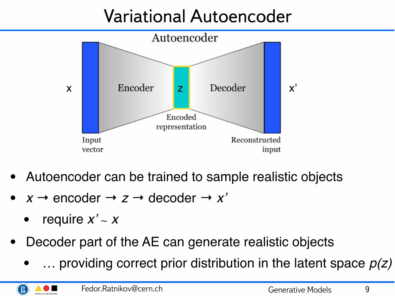
Variational Autoencoder

• Autoencoder can be trained to sample realistic objects• x → encoder → z → decoder → x’• require x’ ∼ x

• Decoder part of the AE can generate realistic objects• … providing correct prior distribution in the latent space p(z)

9

x z x’




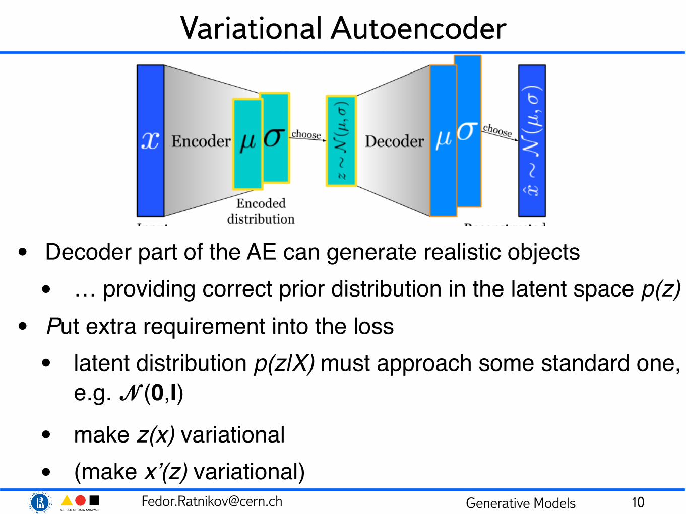
• Decoder part of the AE can generate realistic objects• … providing correct prior distribution in the latent space p(z)

• Put extra requirement into the loss• latent distribution p(z|X) must approach some standard one,

e.g. 𝓝(0,I)• make z(x) variational• (make x’(z) variational)

10




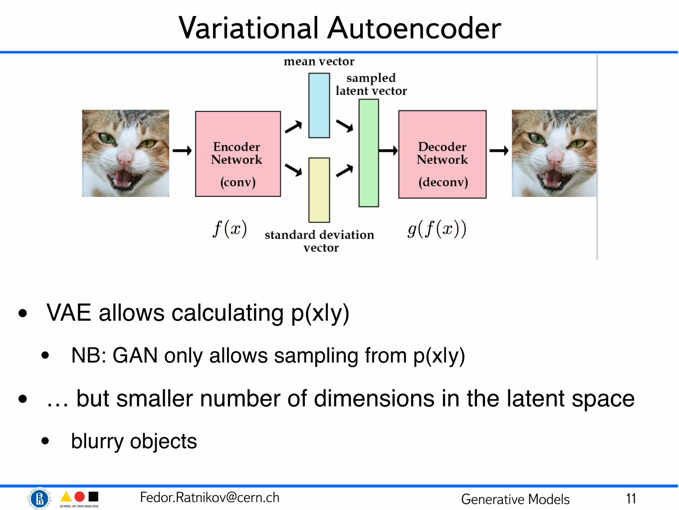
• VAE allows calculating p(x|y)• NB: GAN only allows sampling from p(x|y)

• … but smaller number of dimensions in the latent space• blurry objects

11



Library Approach• We have train sample for the generative model anyway• consistency with this train sample is a figure of merit for the

generative model

• Objects of the train sample may be used for generation directly• similar to KNN classification algorithm

• k=1: search for the object with appropriate conditions in the (presumably huge) data library

• k>1: need to interpolate between objects

• short distance objects interpolation, more robust than global generation

• NB: library approach by construction uses full information which is contained in the training sample

12



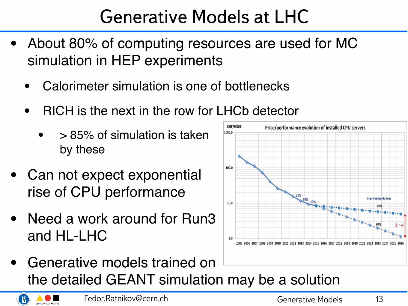
Generative Models at LHC• About 80% of computing resources are used for MC

simulation in HEP experiments• Calorimeter simulation is one of bottlenecks

• RICH is the next in the row for LHCb detector

• > 85% of simulation is taken by these

• Can not expect exponential rise of CPU performance

• Need a work around for Run3 and HL-LHC

• Generative models trained on the detailed GEANT simulation may be a solution

13



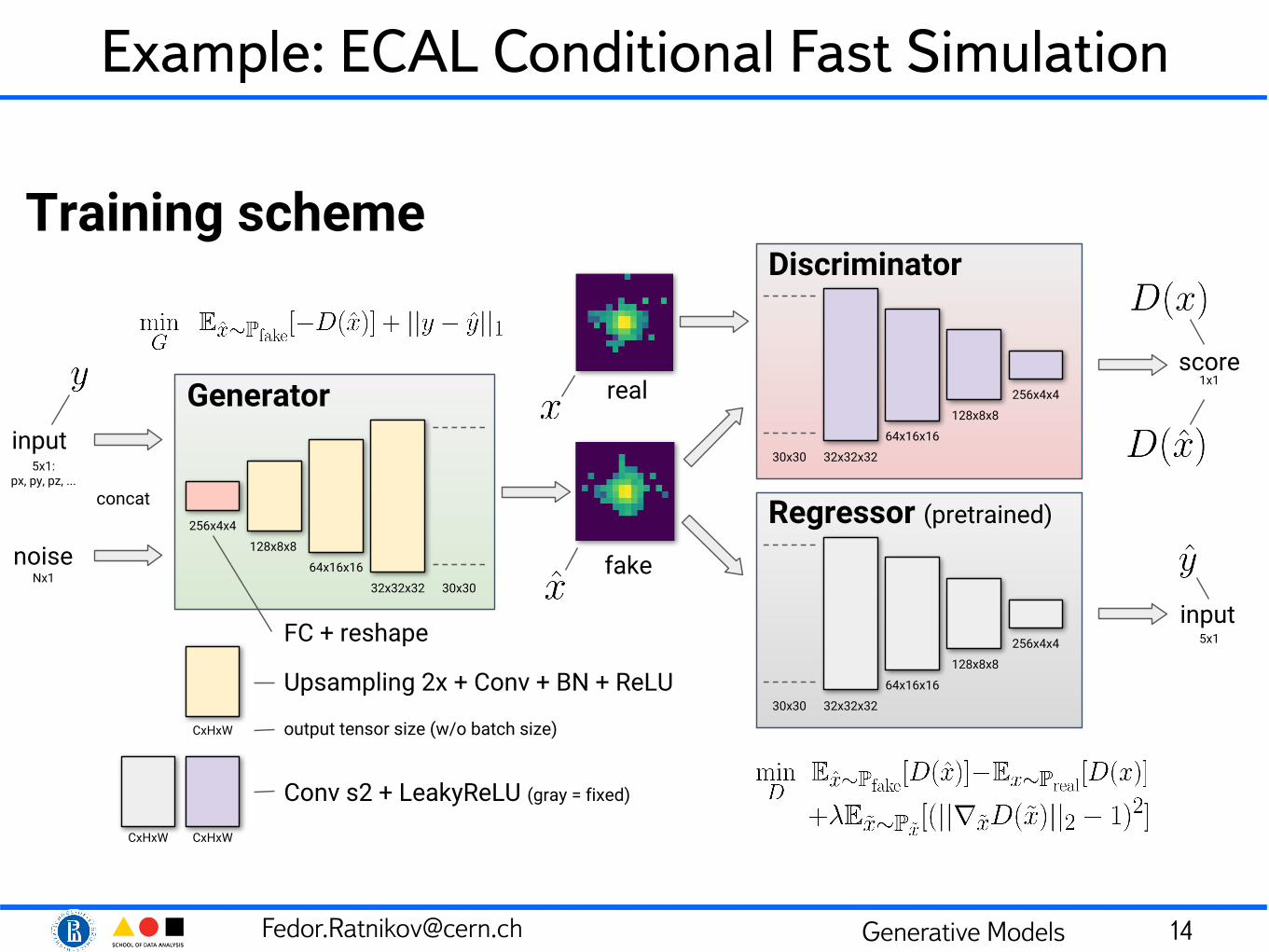
Example: ECAL Conditional Fast Simulation

14

Generatorinput

5x1: px, py, pz, ...

256x4x4

128x8x8

64x16x16

32x32x32 30x30

Discriminator

256x4x4

128x8x8

64x16x16

32x32x32

Regressor (pretrained)

256x4x4

128x8x8

64x16x16

32x32x32

real

fake

30x30

30x30

score

input

1x1

5x1

Upsampling 2x + Conv + BN + ReLU

Conv s2 + LeakyReLU (gray = fixed)

CxHxW output tensor size (w/o batch size)

CxHxWCxHxW

noiseNx1

Training scheme

FC + reshape

concat



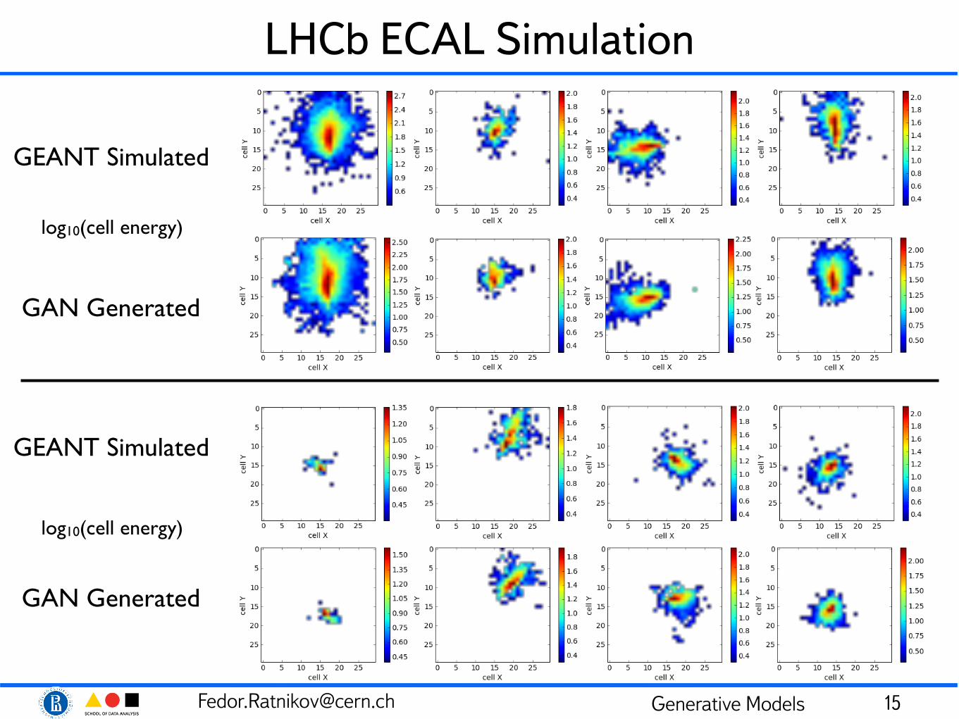
LHCb ECAL Simulation

15

GEANT Simulated

GAN Generated

GEANT Simulated

GAN Generated

log10(cell energy)

log10(cell energy)



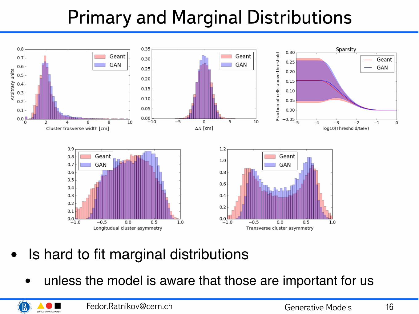
Primary and Marginal Distributions

• Is hard to fit marginal distributions• unless the model is aware that those are important for us

16



Scientific Requirements

• For image generation we are usually happy if the result looks like it is desired

• In science we need the result to reasonably well match the given set of requirements. Requirements are driven by scientific considerations closely connected to the ultimate scientific goal

17



Enforcing Important Statistics

• No generative model is ideal• some deviations from the original distribution remain

• Models tend to learn primary statistics of generated objects

• In physics applications, we often need for our model to learn particular statistics which are marginal for the generated object • e.g. cluster shape fluctuations for fast calorimeter simulation

• Can enforce these statistics by explicit adding them to the loss• can’t we?

18



Enforcing Important Statistics

• Can enforce statistics by explicit adding them to the loss• can’t we?

• By adding necessary statistics to the loss we do enforce match for these statistics• most likely by the price of overtraining these particular statistics• … and we lose handle to validate quality of generator on this

statistics

• Still can remove those statistics from loss, and see how far they would deviate

• this could be a figure of merit for generating this statistics

19



Generating Tails

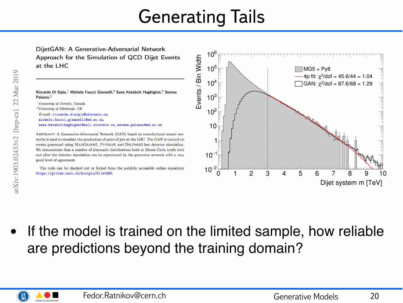
• If the model is trained on the limited sample, how reliable are predictions beyond the training domain?

20



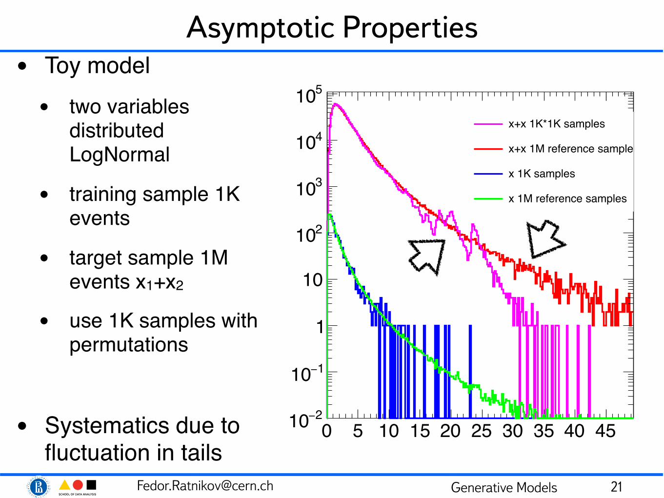
Asymptotic Properties• Toy model• two variables

distributed LogNormal

• training sample 1K events

• target sample 1M events x1+x2

• use 1K samples with permutations

• Systematics due to fluctuation in tails

21

0 5 10 15 20 25 30 35 40 452−10

1−10

1

10

210

310

410

510x+x 1K*1K samples

x+x 1M reference sample

x 1K samples

x 1M reference samples



0 5 10 15 20 25 30 35 40 452−10

1−10

1

10

210

310

410

510x+x 1K*1K samples

x+x 1M reference sample

x 1K samples

x 1M reference samples

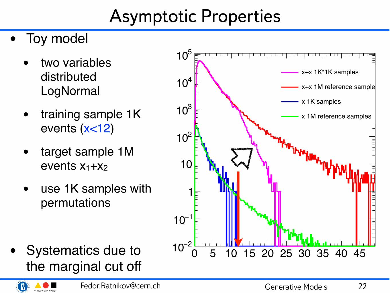
Asymptotic Properties• Toy model• two variables

distributed LogNormal

• training sample 1K events (x<12)

• target sample 1M events x1+x2

• use 1K samples with permutations

• Systematics due to the marginal cut off

22



0 5 10 15 20 25 30 35 40 45 50024681012141618202224

reference

σ/actual

σ

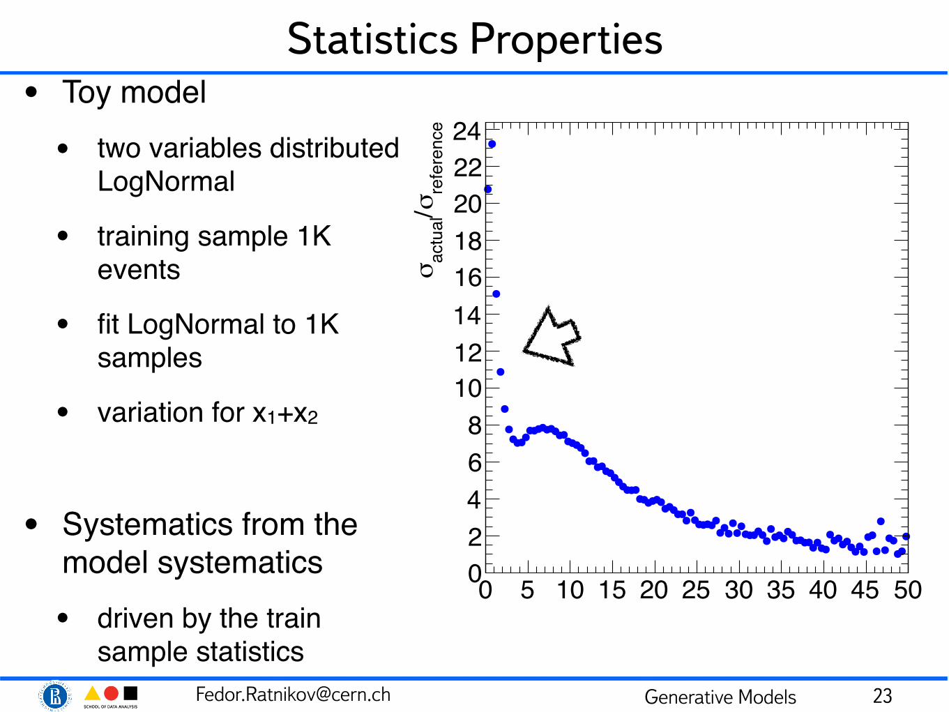
Statistics Properties• Toy model• two variables distributed

LogNormal

• training sample 1K events

• fit LogNormal to 1K samples

• variation for x1+x2

• Systematics from the model systematics• driven by the train

sample statistics 23



Decomposition

• Quality of the generative models is limited by the size of the train data sample• generative models may not give profit for producing statistically

correct big data sets

• no information beyond the train sample is available

• model systematics corresponds to the train sample statistics

24



Decomposition

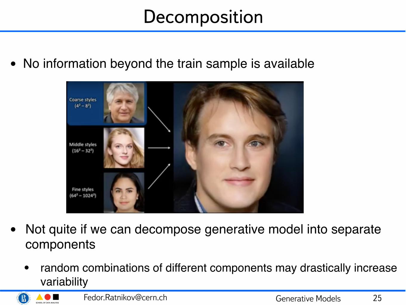
• No information beyond the train sample is available

• Not quite if we can decompose generative model into separate components• random combinations of different components may drastically increase

variability 25



Decomposition• Quality of the generative models is limited by the size of the

train data sample• generative models may not give profit for producing statistically

correct big data sets• no information beyond the train sample is available

• Not quite if we can decompose generative model into separate components• random combinations of different components may drastically

increase variativity• E.g. fast simulation of the calorimeter response• generator is trained on 106 incident particles• ∼50 particles in the calorimeter per event• total variability ∼(106)50 = 10300 ! (NB intrinsic correlation)

26



Quality Metric• No generative model is ideal• some deviations from the original distribution remain

• Minor deviations are not that important e.g. for image generation

• Minor deviations may be a big deal for generative models in physics• e.g. we could want E2-p2=m2 for generated particles to be

precise

• Ultimate generative model quality metric is a comparing the final physics result obtained using generative model with the one obtained using the test data• accuracy is limited by the size of the test data

27



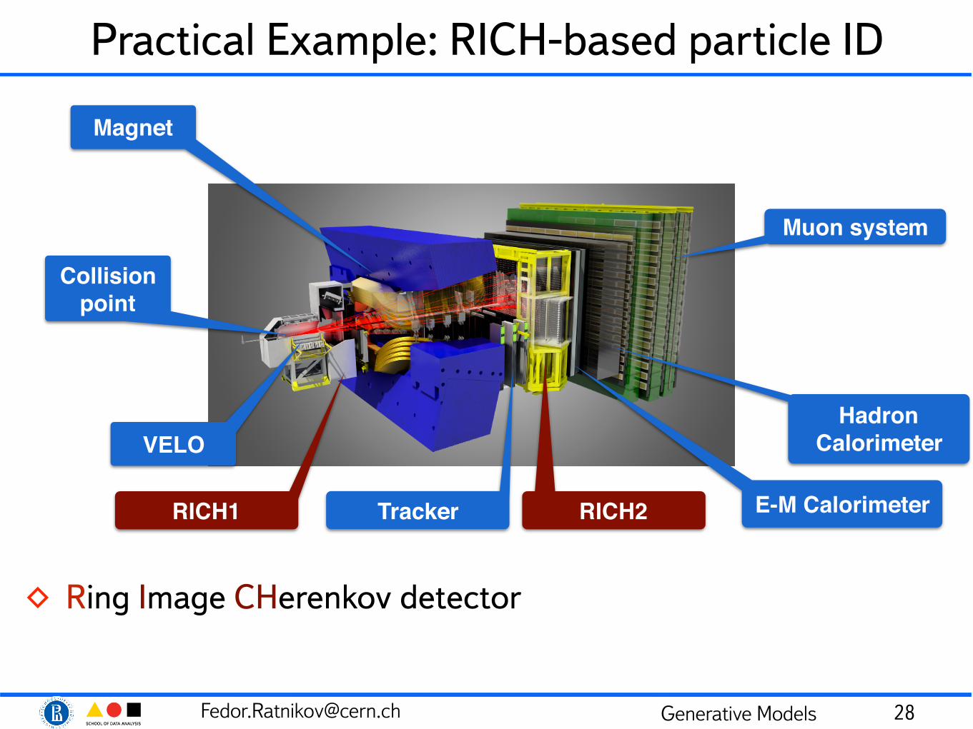
Practical Example: RICH-based particle ID

◊ Ring Image CHerenkov detector

28

Collision point

VELO

RICH1 Tracker RICH2

Magnet

E-M Calorimeter

Hadron Calorimeter

Muon system



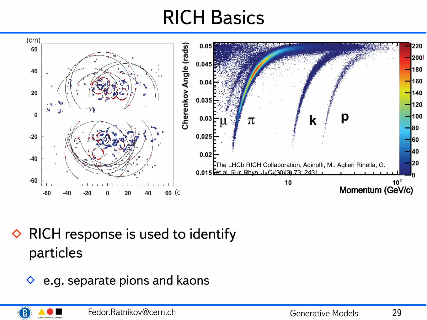
RICH Basics

◊ RICH response is used to identify particles

◊ e.g. separate pions and kaons

29

2008 JINST 3 S08005

θ C(m

rad)

250

200

150

100

50

0

1 10 100

Momentum (GeV/c)

Aerogel

C4F10 gas

CF4 gas

eµ

p

K

π

242 mrad

53 mrad

32 mrad

θC max

Kπ

Figure 6.1: Cherenkov angle versus particle momentum for the RICH radiators.

(a)

250 mrad

Track

Beam pipe

PhotonDetectors

Aerogel

VELOexit window

SphericalMirror

PlaneMirror

C4F10

0 100 200 z (cm)

MagneticShield

Carbon FiberExit Window

(b) (c)

Figure 6.2: (a) Side view schematic layout of the RICH 1 detector. (b) Cut-away 3D model of theRICH 1 detector, shown attached by its gas-tight seal to the VELO tank. (c) Photo of the RICH1gas enclosure containing the flat and spherical mirrors. Note that in (a) and (b) the interaction pointis on the left, while in (c) is on the right.

• minimizing the material budget within the particle acceptance of RICH 1 calls for lightweightspherical mirrors with all other components of the optical system located outside the accep-tance. The total radiation length of RICH 1, including the radiators, is ⇠8% X0.

• the low angle acceptance of RICH 1 is limited by the 25 mrad section of the LHCb berylliumbeampipe (see figure 3.1) which passes through the detector. The installation of the beampipeand the provision of access for its bakeout have motivated several features of the RICH 1design.

• the HPDs of the RICH detectors, described in section 6.1.5, need to be shielded from thefringe field of the LHCb dipole. Local shields of high-permeability alloy are not by them-selves sufficient so large iron shield boxes are also used.

– 73 –

2008 JINST 3 S08005

(cm)

(cm)

Figure 6.20: Display of a typical LHCb event in RICH 1.

Table 6.3: Single photoelectron resolutions for the three RICH radiators. All numbers are in mrad.Individual contributions from each source are given, together with the total.

Aerogel C4F10 CF4

Emission 0.4 0.8 0.2Chromatic 2.1 0.9 0.5HPD 0.5 0.6 0.2Track 0.4 0.4 0.4Total 2.6 1.5 0.7

6.2 Calorimeters

The calorimeter system performs several functions. It selects transverse energy hadron, electronand photon candidates for the first trigger level (L0), which makes a decision 4µs after the inter-action. It provides the identification of electrons, photons and hadrons as well as the measurementof their energies and positions. The reconstruction with good accuracy of p0 and prompt photonsis essential for flavour tagging and for the study of B-meson decays and therefore is important forthe physics program.

The set of constraints resulting from these functionalities defines the general structure andthe main characteristics of the calorimeter system and its associated electronics [1, 121]. Theultimate performance for hadron and electron identification will be obtained at the offline analysislevel. The requirement of a good background rejection and reasonable efficiency for B decays addsdemanding conditions on the detector performance in terms of resolution and shower separation.

– 96 –

Momentum (GeV/c)Momentum (GeV/c)2

The LHCb RICH Collaboration, Adinolfi, M., Aglieri Rinella, G. et al. Eur. Phys. J. C (2013) 73: 2431



RICH ID Simulation◊ Accurate RICH simulation involves:

◊ tracing the particles through the radiators

◊ Cherenkov light generation

◊ photon propagation, reflection, refraction and scattering

◊ Hybrid Photon Detector (photo-cathode + silicon pixel) simulation

◊ These require significant computing resources

◊ Besides:

◊ quality of obtained simulated ID variables is not satisfactory when comparing to calibration data samples

30

250 mrad

Track

Beam pipe

PhotonDetectors

VELO exit window

SphericalMirror

PlaneMirror

C4F10

0 100 200 z (cm)

MagneticShield



RICH ID Simulation◊ Accurate RICH simulation involves:

◊ tracing the particles through the radiators

◊ Cherenkov light generation

◊ photon propagation, reflection, refraction and scattering

◊ Hybrid Photon Detector (photo-cathode + silicon pixel) simulation

◊ These require significant computing resources

◊ Besides:

◊ quality of obtained simulated ID variables is not satisfactory when comparing to calibration data samples

◊ Let’s use ML:

◊ train generative model to directly convert track kinematics into ID variables

◊ can train directly on calibration data samples

31



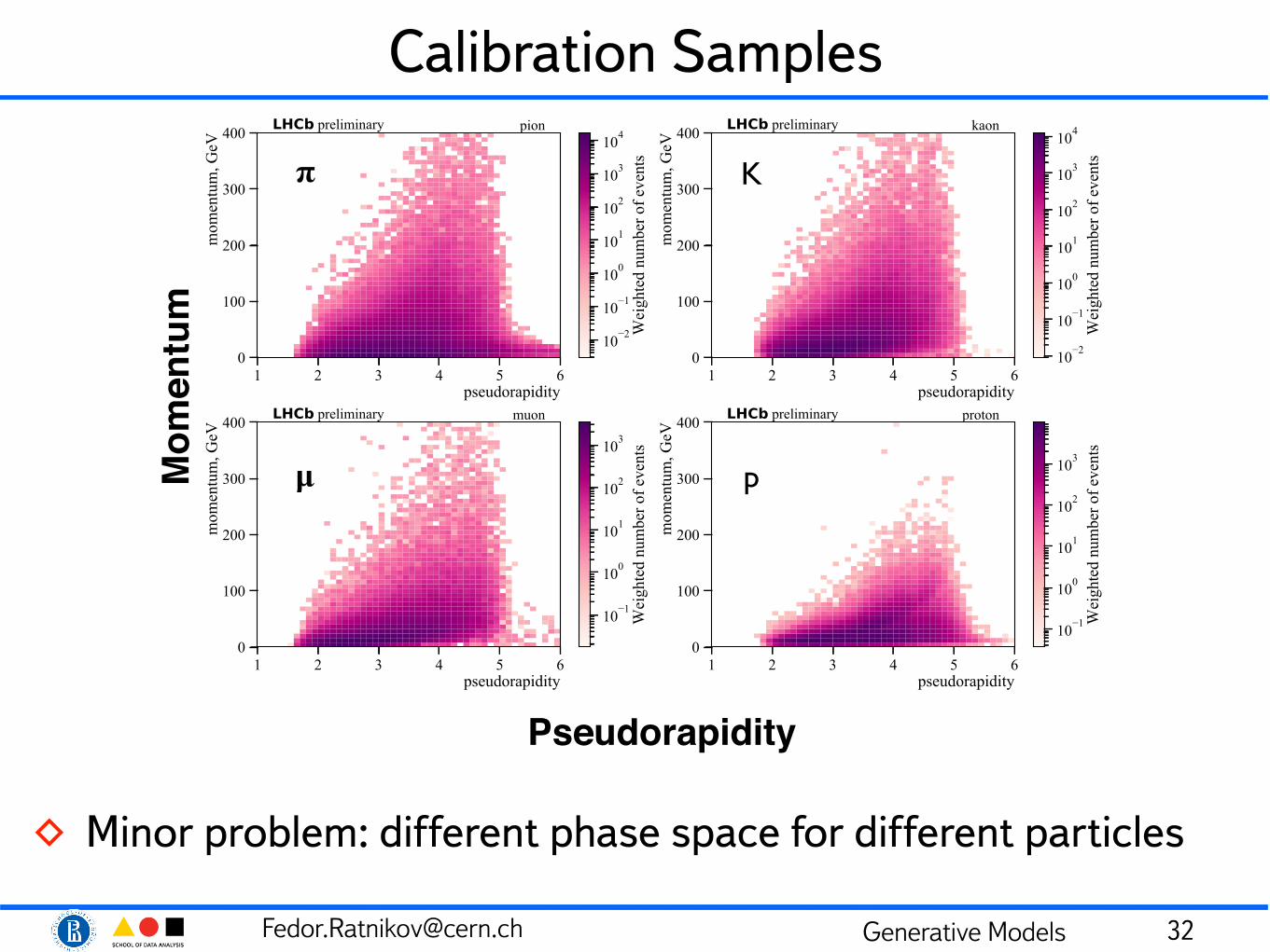
Calibration Samples

◊ Minor problem: different phase space for different particles

32

Pseudorapidity

Mom

entu

m𝛑

𝛍 p

K



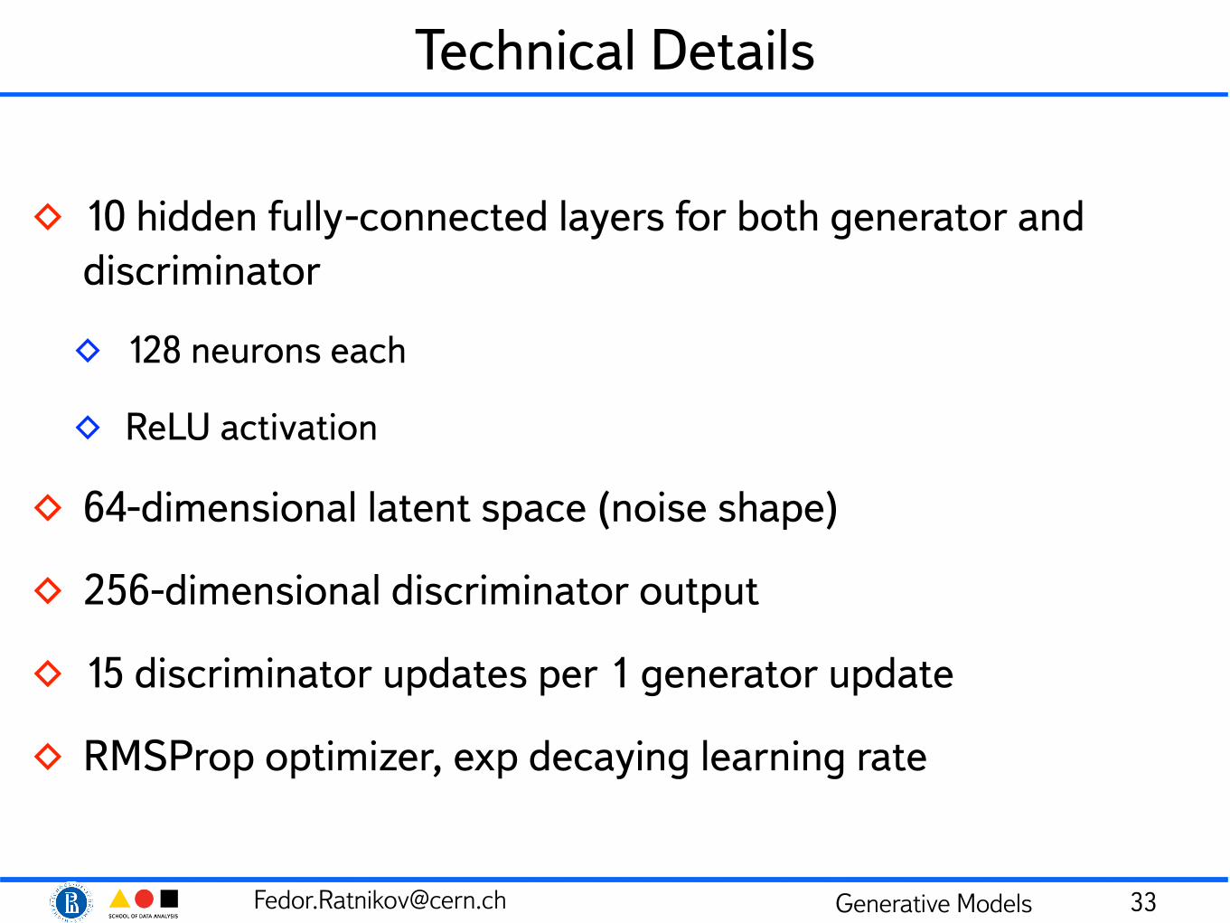
Technical Details

◊ 10 hidden fully-connected layers for both generator and discriminator

◊ 128 neurons each

◊ ReLU activation

◊ 64-dimensional latent space (noise shape)

◊ 256-dimensional discriminator output

◊ 15 discriminator updates per 1 generator update

◊ RMSProp optimizer, exp decaying learning rate

33



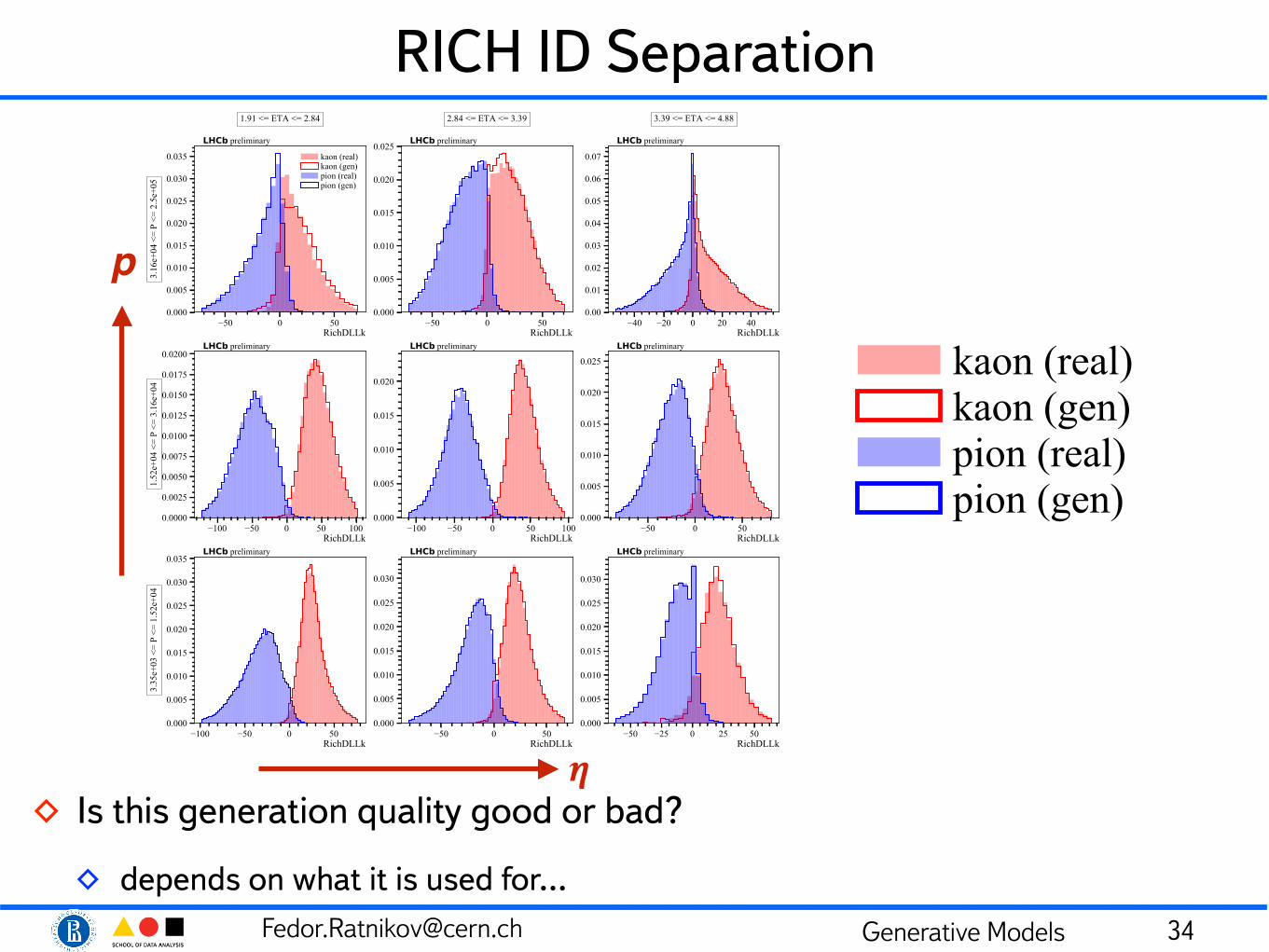
RICH ID Separation

◊ Is this generation quality good or bad?

◊ depends on what it is used for… 34

p

𝜼



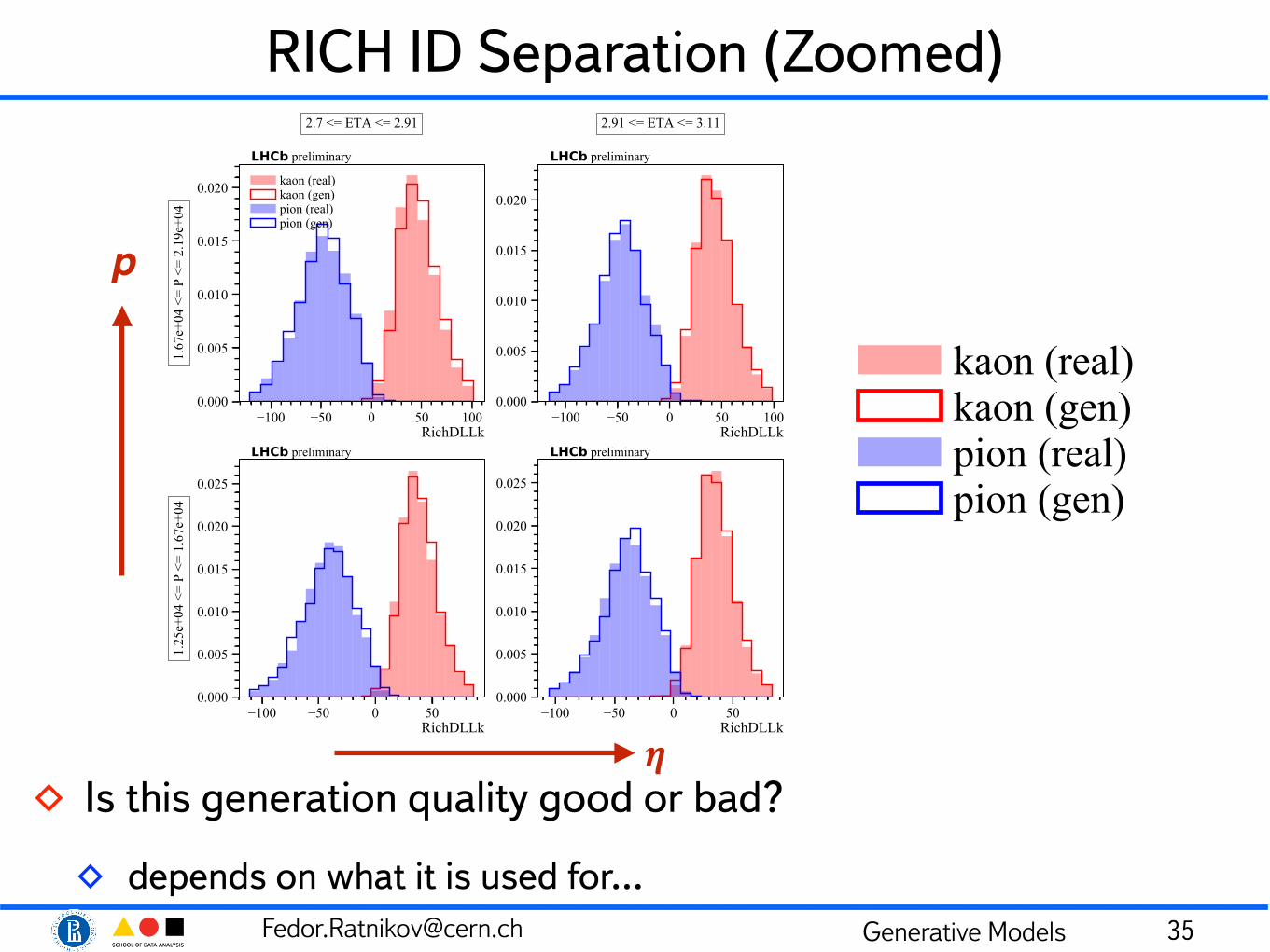
RICH ID Separation (Zoomed)

◊ Is this generation quality good or bad?

◊ depends on what it is used for… 35

p

𝜼



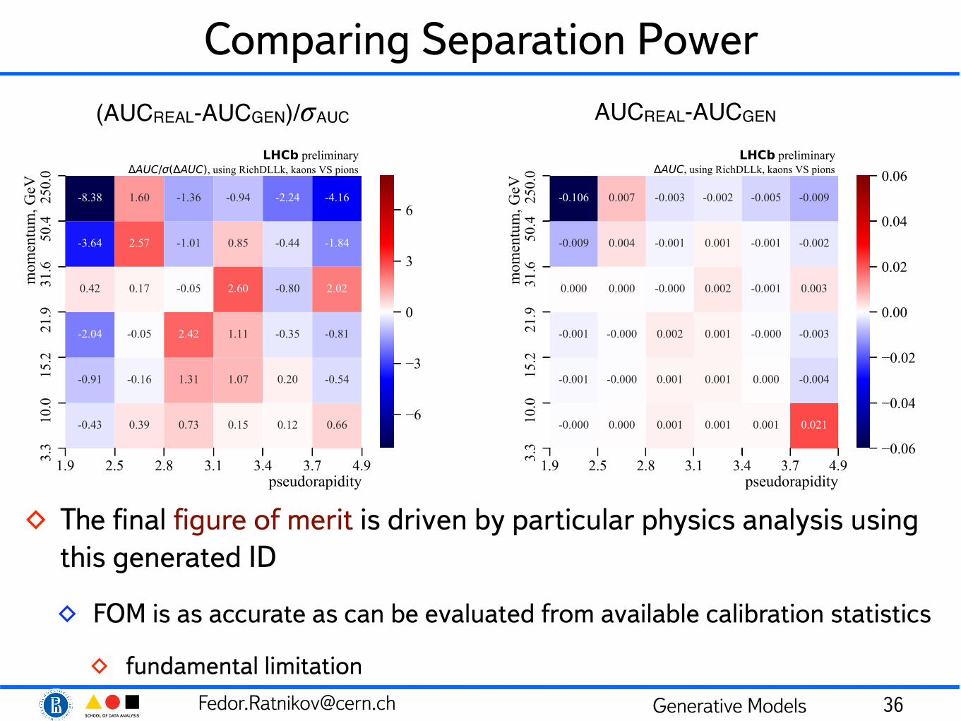
Comparing Separation Power

◊ The final figure of merit is driven by particular physics analysis using this generated ID

◊ FOM is as accurate as can be evaluated from available calibration statistics

◊ fundamental limitation 36

(AUCREAL-AUCGEN)/𝜎AUC AUCREAL-AUCGEN



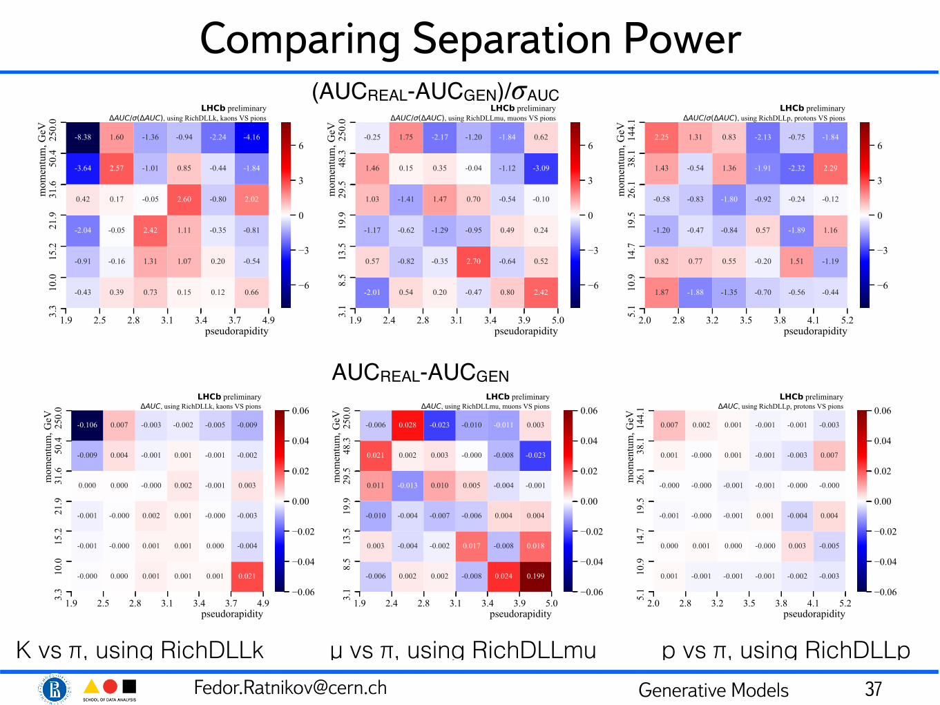
Comparing Separation Power

37

(AUCREAL-AUCGEN)/𝜎AUC

K vs π, using RichDLLk µ vs π, using RichDLLmu p vs π, using RichDLLp

AUCREAL-AUCGEN



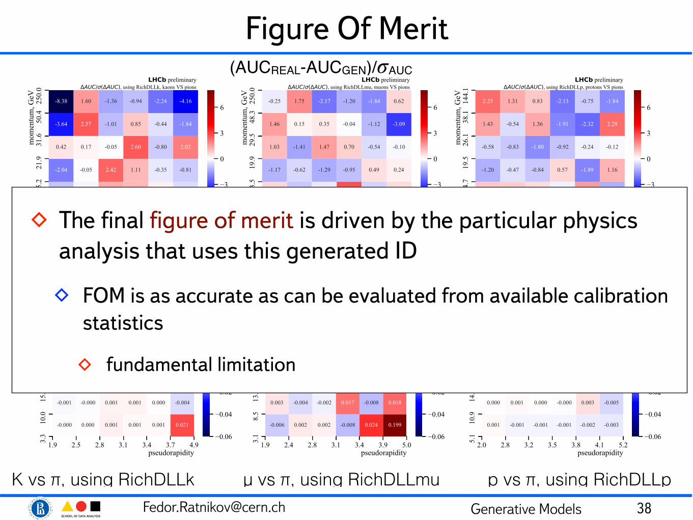
Figure Of Merit

38

(AUCREAL-AUCGEN)/𝜎AUC

K vs π, using RichDLLk µ vs π, using RichDLLmu p vs π, using RichDLLp

AUCREAL-AUCGEN

◊ The final figure of merit is driven by the particular physics analysis that uses this generated ID

◊ FOM is as accurate as can be evaluated from available calibration statistics

◊ fundamental limitation



Conclusions

• Surrogate generative models demonstrate extraordinary progress in current years

• There are many applications for use in HEP

• Generative models need attention to ensure scientifically solid results • satisfying boundary conditions, control of scientifically important

but marginal statistics

• appropriate evaluating the quality of the model

• propagating model intrinsic systematics to the systematic uncertainties of the final scientific result

• Success stories are available

39



Generative Model. ML Perspective• Generative models look very different from regression/classification

models• actually they are not that different

• Consider set of objects each of which is described by a vector of parameters• we arbitrary split this vector into “features” x and “labels” y

• For classification/regression problem we search for deterministic function f which approximates dependency y from x: y=f(x)• in probabilistic approach we search for probability p(y|x)

• For generation problem we want to sample objects for a given label• we search for probability p(x|y)• y for generative model is called “condition”• condition may be absent - unconditional generative model

40



Generative Model. ML Perspective• In both discriminative model and generative model we want to get

probability for subset of object parameters conditioned by another subset of object parameters

• Discriminative models:

• evaluate distributions for few, usually redundant, parameters conditioned by many features

• can discriminate basing on this parameters

• Generative models:

• evaluate many features conditioned by few parameters (conditions)

• can sample these features

• NB: logistic regression + binomial distribution = generative model

• for the binary objects

41


generative models for hep

Documents