university of cape town - inspire hep
TRANSCRIPT
Univers
ity of
Cap
e Tow
n
Topics in Relativistic CosmologyCosmology on the Past Lightcone and in Modified Gravitation
Maye Y.A. Elmardi
Thesis presented for the degree of
DOCTOR OF PHILOSOPHY
in the Department of Mathematics and Applied Mathematics
at the
University of Cape Town
Supervisors: Prof. Chris Clarkson, University of Cape TownDr. Julien Larena, University of Cape Town
Cape Town, South Africa, January 29, 2018
Univers
ity of
Cap
e Tow
n
The copyright of this thesis vests in the author. No quotation from it or information derived from it is to be published without full acknowledgement of the source. The thesis is to be used for private study or non-commercial research purposes only.
Published by the University of Cape Town (UCT) in terms of the non-exclusive license granted to UCT by the author.
ii
The research presented in this thesis is partially based on the following listed publications:
• Chapter 3, 4, 5Cosmological perturbation theory on the Past Lightcone.Maye Elmardi, Julien Larena and Chris Clarkson.Journal-ref: in preparation
• Chapter 6- Reconstructing f(R) Gravity from a Chaplygin Scalar Field in de Sitter Spacetimes.Heba Sami, Neo Namane, Joseph Ntahompagaze, Maye Elmardi and Amare Abebe.Journal-ref: Int. J. Geom. Methods Mod. Phys. 15 1850027 (2018).
• Chapter 7- Irrotational-fluid cosmologies in fourth-order gravity.Amare Abebe and Maye Elmardi.Journal-ref: Int. J. Geom. Methods Mod. Phys. 12 1550118 (2015).
- Integrability conditions for nonrotating solutions in f(R) gravity.Maye Elmardi and Amare Abebe.Journal-ref: J. Phys. Conf. Ser. SAIP2016 (Accepted).
•Chapter 8-Chaplygin-gas solutions of f(R) gravity.Maye Elmardi, Amare Abebe and Abiy Tekola.Journal-ref: Int. J. Geom. Methods Mod. Phys. 13 1650120 (2016).
-Cosmological Chaplygin gas as modified gravity.Maye Elmardi and Amare Abebe.Journal-ref: J. Phys. Conf. Ser. 905 012015 (2017).
vi
Topics in Relativistic CosmologyCosmology on the Past Lightcone and in Modified GravitationMaye ElmardiDepartment of Mathematics and Applied MathematicsUniversity of Cape Town
Abstract
The lightcone gauge is a set of what are called the observational coordinates adapted to ourpast lightcone. We develop this gauge by producing a perturbed spacetime metric that describesthe geometry of our past lightcone where observations are usually obtained. We then connect theproduced observational metric to the perturbed Friedmann-Lemaıtre-Robertson-Walker metric inthe standard general gauge or what is the so-called 1+3 gauge. We derive the relations betweenthese perturbations of spacetime in the observational coordinates and those perturbations in thestandard metric approach, as well as the dynamical equations for the perturbations in observationalcoordinates. We also calculate the observables in the lightcone gauge and re-derive them in termsof Bardeen potentials to first order. A verification is made of the observables in the perturbedlightcone gauge with those in the standard gauge. The advantage of the method developed is thatthe observable relations are simpler than in the standard formalism. We use the perturbed lightconegauge in galaxy surveys and galaxy number density contrast. The significance of the new gauge isthat by considering the null-like light propagations, the calculations are much simpler since angulardeviations are not considered.
Standard cosmology based on General Relativity is generally believed to have serious shortcom-ings, such as the unexplained issues of dark matter and dark energy. As a remedy, many alternativetheories of gravitation have been proposed over the years, one of which is f(R) gravity. We exploreclasses of irrotational-fluid cosmological models in the context of f(R) gravity in an attempt to putsome theoretical and mathematical restrictions on the form of the f(R) gravitational Lagrangian.In particular, we investigate the consistency of the linearised dust models for shear-free cases as wellas in the limiting cases when either the gravito-magnetic or gravito-electric components of the Weyltensor vanish. We also discuss the existence and consistency of classes of non-expanding irrotationalspacetimes in f(R)-gravity.
Furthermore, we explore exact f(R) gravity solutions that mimic Chaplygin-gas inspired ΛCDMcosmology. Starting with the original, generalized and modified Chaplygin gas equations of state,we reconstruct the forms of f(R) Lagrangians. The resulting solutions are generally quadratic in theRicci scalar, but have appropriate ΛCDM solutions in limiting cases. These solutions, given appro-priate initial conditions, can be potential candidates for scalar field-driven early universe expansion(inflation) and dark energy-driven late-time cosmic acceleration.
Keywords: General Relativity, Direct Observational Approach, Observables, Galaxy Surveys,Galaxy Number Count, Density Contrast, Cosmological Perturbations, Past Lightcone Gauge, f(R)Gravity, Modified Gravity, Cosmic Acceleration, Dark Energy, Irrotational Universe, Shear-free Uni-

vii
verse, Chaplygin Gas.

Contents
Abstract vi
List of Figures xiii
Part I 3
1 Introduction 41.1 Curved Spacetime . . . . . . . . . . . . . . . . . . . . . . . . . . . . . . . . . . . . . 41.2 The Friedmann-Lemaıtre-Robertson-Walker Models: the Background Geometry of
the Universe . . . . . . . . . . . . . . . . . . . . . . . . . . . . . . . . . . . . . . . . . 51.2.1 The Homogeneous Universe . . . . . . . . . . . . . . . . . . . . . . . . . . . . 51.2.2 Kinematics and Dynamics . . . . . . . . . . . . . . . . . . . . . . . . . . . . . 7
1.3 Some Observations . . . . . . . . . . . . . . . . . . . . . . . . . . . . . . . . . . . . . 81.3.1 Hubble Diagram . . . . . . . . . . . . . . . . . . . . . . . . . . . . . . . . . . 81.3.2 The Cosmic Microwave Background (CMB) . . . . . . . . . . . . . . . . . . . 91.3.3 Baryon Acoustic Oscillations (BAO) . . . . . . . . . . . . . . . . . . . . . . . 101.3.4 The Accelerating Universe . . . . . . . . . . . . . . . . . . . . . . . . . . . . . 111.3.5 Visible Matter and Dark Matter . . . . . . . . . . . . . . . . . . . . . . . . . 121.3.6 Large-scale Structure . . . . . . . . . . . . . . . . . . . . . . . . . . . . . . . . 14
1.4 The Cosmological Parameters . . . . . . . . . . . . . . . . . . . . . . . . . . . . . . . 181.4.1 The History of the Universe . . . . . . . . . . . . . . . . . . . . . . . . . . . . 18
1.5 Distances in Cosmology . . . . . . . . . . . . . . . . . . . . . . . . . . . . . . . . . . 211.5.1 Redshift . . . . . . . . . . . . . . . . . . . . . . . . . . . . . . . . . . . . . . . 211.5.2 Proper Distance . . . . . . . . . . . . . . . . . . . . . . . . . . . . . . . . . . 221.5.3 Comoving Distance (Line-of-Sight) . . . . . . . . . . . . . . . . . . . . . . . . 231.5.4 Transverse Comoving Distance . . . . . . . . . . . . . . . . . . . . . . . . . . 231.5.5 Area Distance . . . . . . . . . . . . . . . . . . . . . . . . . . . . . . . . . . . . 231.5.6 Luminosity Distance . . . . . . . . . . . . . . . . . . . . . . . . . . . . . . . . 24
1.6 Observations on the Past Lightcone . . . . . . . . . . . . . . . . . . . . . . . . . . . 251.7 The Scope of this Thesis . . . . . . . . . . . . . . . . . . . . . . . . . . . . . . . . . . 26
2 Perturbation Theory in Cosmology 282.1 The Inhomogeneous Universe: Gauge-invariant Cosmological Perturbation Theory . 28
2.1.1 The Metric of the Perturbed Spacetime . . . . . . . . . . . . . . . . . . . . . 282.1.2 Decomposition of the Perturbation Variables . . . . . . . . . . . . . . . . . . 292.1.3 The Gauge Problem . . . . . . . . . . . . . . . . . . . . . . . . . . . . . . . . 292.1.4 Gauge Transformation . . . . . . . . . . . . . . . . . . . . . . . . . . . . . . . 302.1.5 Gauge-invariant Variables . . . . . . . . . . . . . . . . . . . . . . . . . . . . . 312.1.6 The Four-velocity . . . . . . . . . . . . . . . . . . . . . . . . . . . . . . . . . . 32
2.2 Perturbations of Null Geodesics . . . . . . . . . . . . . . . . . . . . . . . . . . . . . . 332.2.1 Effects on Source Position . . . . . . . . . . . . . . . . . . . . . . . . . . . . . 332.2.2 Effects on Null-vector . . . . . . . . . . . . . . . . . . . . . . . . . . . . . . . 34
2.2.2.1 Conformal Trick . . . . . . . . . . . . . . . . . . . . . . . . . . . . . 34
viii
CONTENTS ix
2.2.3 Effect on Frequency . . . . . . . . . . . . . . . . . . . . . . . . . . . . . . . . 362.3 The Perturbative Cosmological Distances . . . . . . . . . . . . . . . . . . . . . . . . 38
2.3.1 Area Distance . . . . . . . . . . . . . . . . . . . . . . . . . . . . . . . . . . . . 382.3.2 Luminosity Distance . . . . . . . . . . . . . . . . . . . . . . . . . . . . . . . . 40
2.3.2.1 The Observed Luminosity Distance . . . . . . . . . . . . . . . . . . 41
Part II 44
3 Ideal Observational Cosmology 453.1 Observational Coordinates . . . . . . . . . . . . . . . . . . . . . . . . . . . . . . . . . 453.2 The Observational Metric . . . . . . . . . . . . . . . . . . . . . . . . . . . . . . . . . 473.3 The Perturbed Lightcone Gauge . . . . . . . . . . . . . . . . . . . . . . . . . . . . . 48
3.3.1 The PLG Coordinates Transformations . . . . . . . . . . . . . . . . . . . . . 493.3.2 The PLG Four-velocity . . . . . . . . . . . . . . . . . . . . . . . . . . . . . . 523.3.3 Connecting the Perturbations δµ with the Perturbed FLRW . . . . . . . . . . 53
3.4 Einstein Field Equations in the PLG . . . . . . . . . . . . . . . . . . . . . . . . . . . 543.5 The Geodesic Lightcone Gauge . . . . . . . . . . . . . . . . . . . . . . . . . . . . . . 583.6 Differences Between the PLG and the GLC . . . . . . . . . . . . . . . . . . . . . . . 59
4 Observables in the Past Lightcone Gauge 604.1 The Screen Space . . . . . . . . . . . . . . . . . . . . . . . . . . . . . . . . . . . . . . 60
4.1.1 Derivatives and Integrals in the Screen Space . . . . . . . . . . . . . . . . . . 604.1.2 Screen Space and SVT Decompositions . . . . . . . . . . . . . . . . . . . . . 61
4.2 The Redshift of Distant Galaxies in the PLG . . . . . . . . . . . . . . . . . . . . . . 624.2.1 Gauge Transformations of the Redshift . . . . . . . . . . . . . . . . . . . . . . 63
4.3 The Area Distance in the PLG . . . . . . . . . . . . . . . . . . . . . . . . . . . . . . 654.3.1 The Gauge Transformations of the Area Distance . . . . . . . . . . . . . . . . 66
4.4 The Luminosity Distance in the PLG . . . . . . . . . . . . . . . . . . . . . . . . . . . 684.4.1 The Gauge Transformations of the Luminosity Distance . . . . . . . . . . . . 684.4.2 The Luminosity Distance in the Longitudinal Gauge . . . . . . . . . . . . . . 694.4.3 Vector Contributions to the Luminosity Distance . . . . . . . . . . . . . . . . 714.4.4 Tensor Contributions to the Luminosity Distance . . . . . . . . . . . . . . . . 714.4.5 The Shear on the Lightcone . . . . . . . . . . . . . . . . . . . . . . . . . . . . 72
5 The Galaxy Number Count 735.1 The Galaxy Surveys . . . . . . . . . . . . . . . . . . . . . . . . . . . . . . . . . . . . 73
5.1.1 The Real Measure in Galaxy Surveys . . . . . . . . . . . . . . . . . . . . . . . 745.1.2 The Galaxy Bias . . . . . . . . . . . . . . . . . . . . . . . . . . . . . . . . . . 74
5.2 Galaxy Number Count . . . . . . . . . . . . . . . . . . . . . . . . . . . . . . . . . . . 755.2.1 Distortions in Galaxy Number Counts . . . . . . . . . . . . . . . . . . . . . . 765.2.2 The Galaxy Number Count on the Lightcone Gauge . . . . . . . . . . . . . . 77
5.3 The Perturbation of Galaxy Number Counts ∆ . . . . . . . . . . . . . . . . . . . . . 775.3.1 The ∆ Calculations in Redshift Space . . . . . . . . . . . . . . . . . . . . . . 775.3.2 The Computation of δz(n, z) . . . . . . . . . . . . . . . . . . . . . . . . . . . 785.3.3 The Volume Distortion . . . . . . . . . . . . . . . . . . . . . . . . . . . . . . . 80
5.4 Galaxy Number Counts Fluctuations with the PLG . . . . . . . . . . . . . . . . . . 815.4.1 Gauge Transformations of the Density Fluctuations . . . . . . . . . . . . . . 84
Part III 86
6 f(R) Theories of Gravity 876.1 Derivation of the f(R) Field Equations . . . . . . . . . . . . . . . . . . . . . . . . . . 87
6.1.1 The Metric Formalism . . . . . . . . . . . . . . . . . . . . . . . . . . . . . . . 88
CONTENTS x
6.1.2 The Palatini Formalism . . . . . . . . . . . . . . . . . . . . . . . . . . . . . . 896.1.3 The Metric-affine Formalism . . . . . . . . . . . . . . . . . . . . . . . . . . . 90
6.2 The Dynamics of f(R) Gravity . . . . . . . . . . . . . . . . . . . . . . . . . . . . . . 906.3 The Viability of f(R) Models . . . . . . . . . . . . . . . . . . . . . . . . . . . . . . . 916.4 Some f(R) Models . . . . . . . . . . . . . . . . . . . . . . . . . . . . . . . . . . . . . 92
6.4.1 R2 Model . . . . . . . . . . . . . . . . . . . . . . . . . . . . . . . . . . . . . . 926.4.2 1/Rn Model . . . . . . . . . . . . . . . . . . . . . . . . . . . . . . . . . . . . . 936.4.3 Rn Models . . . . . . . . . . . . . . . . . . . . . . . . . . . . . . . . . . . . . 936.4.4 αR+ βRn Model . . . . . . . . . . . . . . . . . . . . . . . . . . . . . . . . . . 936.4.5 Starobinsky Models . . . . . . . . . . . . . . . . . . . . . . . . . . . . . . . . 946.4.6 Hu-Sawicki Models . . . . . . . . . . . . . . . . . . . . . . . . . . . . . . . . . 946.4.7 Appleby-Battye Models . . . . . . . . . . . . . . . . . . . . . . . . . . . . . . 95
6.5 Scalar-Tensor Representation . . . . . . . . . . . . . . . . . . . . . . . . . . . . . . . 95
7 Irrotational-fluid Cosmologies in f(R) Gravity 977.1 The 1 + 3 Covariant Description . . . . . . . . . . . . . . . . . . . . . . . . . . . . . 977.2 Irrotational Spacetimes . . . . . . . . . . . . . . . . . . . . . . . . . . . . . . . . . . 99
7.2.1 Dust Spacetimes . . . . . . . . . . . . . . . . . . . . . . . . . . . . . . . . . . 1007.2.1.1 Shear-free Spacetimes . . . . . . . . . . . . . . . . . . . . . . . . . . 1017.2.1.2 Dust Solutions with divH = 0 . . . . . . . . . . . . . . . . . . . . . 1037.2.1.3 Purely Gravito-magnetic Spacetimes . . . . . . . . . . . . . . . . . . 103
7.2.2 Non-expanding Spacetimes . . . . . . . . . . . . . . . . . . . . . . . . . . . . 1037.2.2.1 Dust Solutions . . . . . . . . . . . . . . . . . . . . . . . . . . . . . . 1047.2.2.2 Shear-free Solutions . . . . . . . . . . . . . . . . . . . . . . . . . . . 104
8 Chaplygin-gas Solutions of f(R) Gravity 1068.1 Chaplygin Gas in FLRW Models . . . . . . . . . . . . . . . . . . . . . . . . . . . . . 106
8.1.1 Original and Generalised CG Model . . . . . . . . . . . . . . . . . . . . . . . 1068.1.2 Modified and Extended CG Models . . . . . . . . . . . . . . . . . . . . . . . . 1088.1.3 Generalised and Modified Cosmic Chaplygin Gas Models . . . . . . . . . . . 109
8.2 Chaplygin Gas as f(R) Gravity? . . . . . . . . . . . . . . . . . . . . . . . . . . . . . 1108.2.1 Constant Ricci-Curvature Scenarios . . . . . . . . . . . . . . . . . . . . . . . 1108.2.2 Chaplygin Gas Solutions in f(R) Gravity . . . . . . . . . . . . . . . . . . . . 111
8.2.2.1 Original and Generalized Chaplygin Gases . . . . . . . . . . . . . . 1118.2.2.2 Modified Chaplygin Gas . . . . . . . . . . . . . . . . . . . . . . . . . 1128.2.2.3 Modified Generalized Chaplygin Gas . . . . . . . . . . . . . . . . . . 113
9 Conclusions and Future Outlook 115
Appendices 118
A Some Useful Relations on Part I 119A.1 The Perturbed FLRW Metric . . . . . . . . . . . . . . . . . . . . . . . . . . . . . . . 119A.2 Spherical Harmonic Decomposition . . . . . . . . . . . . . . . . . . . . . . . . . . . . 119
A.2.1 Properties of the Harmonics Decomposition . . . . . . . . . . . . . . . . . . . 120A.2.1.1 Polar Decomposition . . . . . . . . . . . . . . . . . . . . . . . . . . . 120A.2.1.2 Axial Decomposition . . . . . . . . . . . . . . . . . . . . . . . . . . 121
B Some Useful Relations on Part II 123B.1 Zero-order Coordinates Transformation . . . . . . . . . . . . . . . . . . . . . . . . . 123
B.1.1 The Observables at Zeroth-order . . . . . . . . . . . . . . . . . . . . . . . . . 123B.2 Relations on the Observational Metric . . . . . . . . . . . . . . . . . . . . . . . . . . 124B.3 Derivatives and Integrals . . . . . . . . . . . . . . . . . . . . . . . . . . . . . . . . . . 125
B.3.1 Commuting Partial Derivatives . . . . . . . . . . . . . . . . . . . . . . . . . . 125B.3.2 Integration Formulae . . . . . . . . . . . . . . . . . . . . . . . . . . . . . . . . 126
CONTENTS xi
B.4 Some Useful Derivation for Sec. 4.4 . . . . . . . . . . . . . . . . . . . . . . . . . . . 127B.5 Some Useful Expressions for Computing HT . . . . . . . . . . . . . . . . . . . . . . . 128
C Some Useful Relations on Part III 130C.1 Linearised Differential Identities . . . . . . . . . . . . . . . . . . . . . . . . . . . . . . 130
List of Figures
1.1 The kinematics of the scale factor a in FLRW universe which satisfies the energycondition ρ+ 3p > 0. . . . . . . . . . . . . . . . . . . . . . . . . . . . . . . . . . . . . 6
1.2 The top panel depicts the Hubble diagram (Redshift-Distance Relation) with theΛCDM best fit; the bottom shows the residuals. This diagram is obtained by theanalysis of 740 SNeIa [1]. . . . . . . . . . . . . . . . . . . . . . . . . . . . . . . . . . 8
1.3 The black-body spectrum of the CMB radiation measured with COBE satellite [2]. . 91.4 The 4 years of data collection by Planck satellite. The colour code corresponds to
temperature fluctuations of a few micro-Kelvin [3]. . . . . . . . . . . . . . . . . . . . 101.5 The 2013 Planck CMB temperature angular power spectrum [3]. . . . . . . . . . . . 101.7 Rotation curves of typical spiral galaxy predicted, disk and extended dark matter
halo models and observed with error bars [4]. Best fit obtained for an exponentialdisk model with maximum mass. . . . . . . . . . . . . . . . . . . . . . . . . . . . . . 13
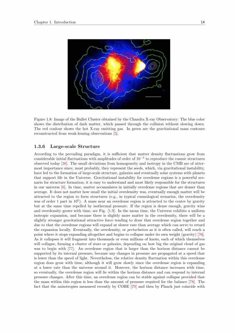
1.8 Image of the Bullet Cluster obtained by the Chandra X-ray Observatory: The bluecolor shows the distribution of dark matter, which passed through the collision withoutslowing down. The red coulour shows the hot X-ray emitting gas. In green are thegravitational mass contours reconstructed from weak-lensing observations [5]. . . . . 14
1.9 Gravitational instability: a nearby mass attracted to the center of an overdense regionby gravity and repelled by pressure [6]. . . . . . . . . . . . . . . . . . . . . . . . . . . 15
1.10 Slices through the SDSS 3-dimensional map of the distribution of galaxies and itcontains about 100 billion stars. Earth is at the center, and each point represents agalaxy. Galaxies are couloured according to the ages of their stars. The outer circleis at a distance of two billion light years. Both slices contain all galaxies within −1.25and 1.25 degrees declination [7]. . . . . . . . . . . . . . . . . . . . . . . . . . . . . . . 16
1.11 A galaxies survey power spectrum from PSCz and APM data survey 1 [8]. The biasis the square root of the ratio of power spectra. . . . . . . . . . . . . . . . . . . . . . 17
1.12 The history of the Universe [9]. . . . . . . . . . . . . . . . . . . . . . . . . . . . . . . 201.13 The proper distance between nearby events (A,B) connected by a unique geodesic G. 231.14 In a curved spacetime, light travels on null geodesics, and the area distance rA of the
source from the observer is r2A = dSo/dΩo. . . . . . . . . . . . . . . . . . . . . . . . . 24
1.15 Observations from the vertices of our past lightcone and future past lightcone. . . . 251.16 Observations of an event on the null cone. . . . . . . . . . . . . . . . . . . . . . . . . 26
2.1 Any perturbed quantity is defined by the mapping between the background universeFLRW, M, and the actual perturbed universe M [10]. . . . . . . . . . . . . . . . . . 30
2.2 The deviation of the angular coordinates θI of the source given an observationaldirection d. . . . . . . . . . . . . . . . . . . . . . . . . . . . . . . . . . . . . . . . . . 33
3.1 Observational coordinates w, y, θ, φ based on the event q on the worldline C. w is
the time of observation; θ, φ represent the direction of observation; and y is a measureof distance to the object observed. . . . . . . . . . . . . . . . . . . . . . . . . . . . . 46
3.2 Spacetime diagram showing the transformations between the observational coordi-nates into a spatial hypersurface in general coordinates. . . . . . . . . . . . . . . . . 49
3.3 Illustration of the GLC coordinates of an inhomogeneous lightcone parametrized byGLC coordinates: The observer sees the sky as the superposition of 2-spheres [11]. . 58
xii
List of Figures xiii
4.1 A time interval dτ at the observed galaxy is measured as a time interval dw by theobserver. . . . . . . . . . . . . . . . . . . . . . . . . . . . . . . . . . . . . . . . . . . . 62
5.1 The number count of galaxies per pixel at fixed redshift and solid angle. . . . . . . . 755.2 Same redshift bin different physical volume: Where in one of the pixel all the galaxies
moving toward the centre of the pixel. . . . . . . . . . . . . . . . . . . . . . . . . . 765.3 Same solid angle different physical volume: An overdensity cluster bending the light
beams emitted by the galaxies. . . . . . . . . . . . . . . . . . . . . . . . . . . 765.4 Same radial bin different distance: The whole galaxies in the pixel is moving toward
the observer. Credit: C. Bonvin. . . . . . . . . . . . . . . . . . . . . . . . . . 76
6.1 Scalar field rolling down to the minimum of the potential well equivalent2to the R+βR2. 93
Conventions and Abbreviations
Throughout this thesis (unless otherwise stated), the natural units (~ = c = kB = 8πG = 1) will beused, and Greek indices (α , β , µ , ν . . . ) and Latin indices a , b , c . . . run from 0 to 3 whereas Latinindices (i , j . . . ) run from 1 to 3. The symbols ∇ and ; represent the usual covariant derivativewhereas ∂ and , stand for partial derivatives; ∇ and the overdot . represent the spatial covariantderivative, and differentiation with respect to cosmic time, respectively. We use the (− + ++)spacetime signature and the Riemann tensor is defined by
Rµναβ = Γµνβ,α − Γµνα,β + ΓγνβΓµαγ − ΓσναΓµβσ , (1)
where the Γµνβ are the Christoffel symbols and they are symmetric in the lower indices, defined by
Γµνβ =1
2gµα(gνα,β + gαβ,ν − gνβ,α) . (2)
The Ricci tensor is obtained by contracting the first and the third indices of the Riemann tensor:
Rµν = gαβRαµβν , (3)
and the Ricci scalar is given asR = Rµµ . (4)
The following are standard notations used in the thesis:
g : det(gµν), the determinant of the metric gµν , (5)
(µν) : symmetrization over the indices µ and ν , (6)
[µν] : anti-symmetrization over the indices µ and ν . (7)
The 4-dimensional volume element ηµνγβ is defined such that
ηµνγβ = η[µνγβ], η0123 =√|det gµν | . (8)
The following are abbreviations frequently used in the thesis:
BBN: Big Bang NucleosynthesisCMB: Cosmic Microwave BackgroundEFEs: Einstein Field EquationsFLRW: Friedmann-Lemaıtre-Robertson-WalkerGI: Gauge-invariantGLC: Generalized Lightcone
1

2
GR: General RelativityLTB: Lemaıtre-Tolman-BondiWMAP: Wilkinson Microwave Anisotropy ProbeAPM: Automatic Plate MeasuringPSCz: Point Source Catalogue Redshift

Part I
3
Chapter 1
Introduction
Nothing exists except atoms andempty space; everything else isopinion.
Democritus
1.1 Curved Spacetime
Cosmology is the study of the origin, evolution, and the eventual fate of the Universe; points ofepistemological interest probably as old as human civilisation itself. Modern cosmology in the senseof ‘physical cosmology’ started with the publication of Einstein’s General Relativity (GR) in late1915 [12,13]. Einstein wrote down the now so-called Einstein-Hilbert action
SEH =1
2
∫all spacetime
d4x√−gR , (1.1)
from which we can derive the field equations:
Gµν + gµν = Tµν , (1.2)
whereGµν ≡ Rµν − 1
2gµνR (1.3)
is the Einstein tensor, gµν is the metric of the spacetime geometry, Rµν is the Ricci tensor, Ris the Ricci scalar and Tµν is the energy momentum tensor sourced by the presence of matter inspacetime [14]. In his formulation of GR, Einstein gave an entirely new and astounding explanationof energy, matter and gravity. He described gravity as the consequence of the bending of spacetimearound a massive body, i.e., it replaces Newtonian gravity with curved spacetime. In this view ofgravity, a test particle with velocity uν follows the geometry of space with a geodesic trajectorygiven by
uµ∇µuν = 0, (1.4)
where
uµ =dxµ
dτ, (1.5)
and τ is a proper time along the geodesic [10]. The idea of the geometry of the spacetime thatis curved by the existence of matter on it was a new way of understanding space and time, as a
4
Chapter 1. Introduction 5
spacetime dynamical continuum evolving according to the local content of energy and momentum.Astronomers have applied and tested these new scientific definitions to the extent that they havebecome the conceptual foundations of modern cosmology.
The model offered as a cosmological solution to Einstein’s equation was first suggested by himselfin 1917 [15]. In his solution Einstein held the idea of a static universe [16]. His theory was not basedon firm observational data, but rather on a mere theoretical simplification. Einstein mistakenlywanted to balance the self attraction of matter on the large scales by adding a new term (Λ) to hisequations such that Eq. (1.2) gets modified as
Gµν + Λgµν = Tµν , (1.6)
in order to keep the Universe static [17,18]. Einstein’s approach was then generalised independentlyby Friedmann in 1922 [19], where he did not try to balance the matter allowing the possibility of anexpanding or contracting universe, i .e., evolving cosmos, and by Lemaıtre in 1927 [20, 21] who alsopredicted the redshift1 of receding galaxies before its observation by Hubble [22] in 1929. The workof Friedmann and Lemaıtre was develpoed with geometric properties of spacetime by Robertson in1929 [23–26], followed by Walker [27].
1.2 The Friedmann-Lemaıtre-Robertson-Walker Models: theBackground Geometry of the Universe
The Friedmann-Lemaıtre-Robertson-Walker (FLRW) metric (also shortened as FRW or RW) is asolution to the EFEs with a homogeneous and isotropic universe. The cosmological models based onthis metric including perturbations are sometimes called the Standard Model of modern cosmologybecause they describe successfully the major features of the observed universe [28], its expansionfrom a hot Big Bang leading to the observed galactic redshifts and remnant black body radiation [29].These models, however, do not describe the real universe well in an essential way, in that the highlyidealised degree of symmetry does not correspond to the lumpy real universe [30].
The assumption of large-scale isotropy observed in particular through the Cosmic MicrowaveBackground (CMB), where it shows that our Universe properties are almost identical whatever thedirection we look at. The hypothesis of the so-called Copernican Principle: the Earth occupies nounique (or central) position in the Universe infer the homogeneity. These two facts are countedas a pillars of the Cosmological Principle: the Universe can be modeled as statistically spatiallyhomogeneous2 and isotropic. Therefore modern cosmology is based on this hypothesis that ouruniverse is to a good approximation homogeneous and isotropic on sufficiently large scales [31].
We know now the real universe is a perturbed one and there are inhomogeneities and anisotropiesarising during structure formation, that can be compared in detail with observations, but we canconsider it as almost FLRW at the same time. In this section we will strictly examine homogeneousand isotropic cosmologies.
1.2.1 The Homogeneous Universe
The Coordinate systems and metric
In order to explain a homogeneous and isotropic space one can admit a slicing of a maximallysymmetric space along a fixed time coordinate t, such that the 3-spaces-like hypersurfaces Σt aresurfaces of intrinsic geometry of homogeneity and isotropy with a spatial metric γij of constant timeand curvature
K =k
a2(t). (1.7)
1The redshift of an object is defined to be the fractional Doppler shift of its emitted light (photons) wavelength dueto its local peculiar motion. A cosmological redshift originates from the general relativistic effects of space expansionaffecting the wavelengths of cosmological events.
2From here onwards ‘homogeneous’ implies spatially homogeneous.
Chapter 1. Introduction 6
Here k denotes spacetime curvature and takes the values −1, 0 or +1 depending on whether theUniverse is open, flat or closed, respectively. The normalised metric dσ2 characterises a 3-space ofnormalised constant curvature whose spatial spherical comoving coordinates (χ, θ, φ) can be chosensuch that
dσ2 = γijdxidxj = dχ2 + S2(χ)(dθ2 + sin2 θdφ2) . (1.8)
The term γijdxidxj is a function of three spatial coordinates and it can describe an Euclidean space,
or hyperbolic space, whereas χ is a radial coordinate, φ and θ are two angles in the sky runningfrom 0 to 2π and from −π to π respectively. S(χ) depends on the curvature k, and it can be givenas [14]
S(χ) =
sin(χ) for k = +1,χ for k = 0,sinh(χ) for k = −1 .
(1.9)
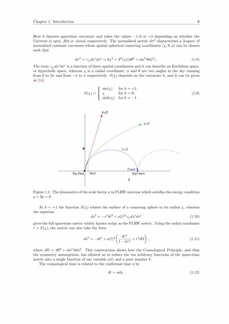
Figure 1.1: The kinematics of the scale factor a in FLRW universe which satisfies the energy conditionρ+ 3p > 0.
At k = +1 the function S(χ) relates the surface of a comoving sphere to its radius χ, whereasthe equation
ds2 = −c2dt2 + a(t)2γijdxidxj (1.10)
gives the full spacetime metric widely known today as the FLRW metric. Using the radial coordinater = S(χ), the metric can also take the form
ds2 = −dt2 + a(t)2
(dr2
1− kr2+ r2dΩ
), (1.11)
where dΩ = dθ2 + sin2 θdφ2. This construction shows how the Cosmological Principle, and thusthe symmetry assumptions, has allowed us to reduce the ten arbitrary functions of the space-timemetric into a single function of one variable a(t) and a pure number k.
The cosmological time is related to the conformal time η by
dt = adη . (1.12)
Chapter 1. Introduction 7
Then we can re-write Eq. (1.10) in the form of
ds2 = −a(η)2dη2 + a(η)2γijdxidxj . (1.13)
The FLRW solutions to the EFEs are the best fit to the observed universe so far [31].
1.2.2 Kinematics and Dynamics
For matter which respects the assumptions of homogeneity and isotropy, the stress-energy tensormust read
Tµν = ρ(t)uµuν + p(t)hµν , (1.14)
where ρ and p define the energy density and isotropic pressure (respectively) of all kinds of standardmatter, i .e., baryonic matter, dark matter, radiation. Each species is characterised by the equation-of-state parameter w, defined as
w =p
ρ, (1.15)
the ratio between its pressure and its energy density. hµν = gµν + uµuν is the projector on spatialsections t = const., hence hµ0 = 0 and hij = gij .
The EFEs (1.2) reduce to ordinary differential equations, known as Friedmann’s equations, forthe function a(η), with (′ = d/dη):
H2 =1
3a2ρ− k
a2+
1
3a2Λ , (1.16)
a′′
a= −1
6(1 + 3w)a2ρ+
1
3a2Λ . (1.17)
Here H is the conformal Hubble parameter related to H as follows:
H ≡ 1
a
da
dt=a
a, H ≡ 1
a
da
dη=a′
a= aH . (1.18)
The energy-momentum conservation equation is given by
ρ′ = −3
(a′
a
)(ρ+ p) = −3(1 + w)Hρ . (1.19)
Here ρ is a combination of cold non-relativistic matter with pm = 0, and radiation with pr = 1/3ρr.We can also define the fractional energy densities
Ωm ≡(ρa2
3H2
), (1.20)
Ωk ≡ − k
H2, (1.21)
ΩΛ ≡ Λa2
3H2, (1.22)
where Ωm, Ωk and ΩΛ are the fractional energy densities for matter, curvature and dark energydensity, respectively. The total energy density in the Universe can thus be given in a more compactform by virtue of Eq. (1.16) as
1 = Ωm + ΩΛ + Ωk , (1.23)
For Ωm Ωk,ΩΛ contributions to Eq. (1.19) the scale factor evolves as
a ∝ t2
3(1+w) ∝ η2
1+3w , (1.24)
Chapter 1. Introduction 8
when
w =
0 for nonrelativistic matter ,1/3 for ultrarelativistic component (radiation) .
(1.25)
When Ωk Ωm,ΩΛ > 0 with w = 0, we get [32]
a(t) ∝ sinh2/3
(√3Λ
2t
). (1.26)
When Λ = 0, it coincides with a ∝ t2/3, but when the cosmological constant is dominant over thecontribution of matter then we get a(t) ∝ exp(t
√Λ/3) = exp(tH) where the expansion rate will be
a constant in this case.
1.3 Some Observations
In this section we are going to discuss some cosmological observations. To measure the observables,we require a specific model, such as the FLRW model at a particular time.
1.3.1 Hubble Diagram
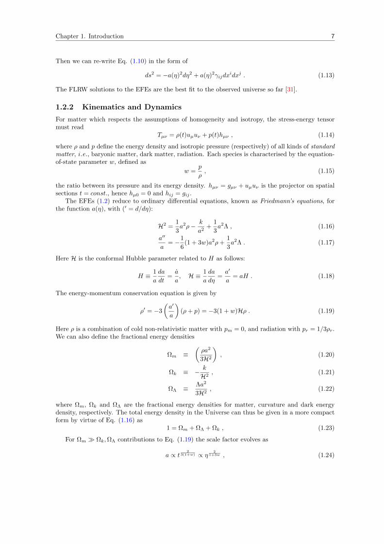
Figure 1.2: The top panel depicts the Hubble diagram (Redshift-Distance Relation) with the ΛCDMbest fit; the bottom shows the residuals. This diagram is obtained by the analysis of 740 SNeIa [1].
The diagram represents the plot of luminosity distance dL of objects with known intrinsic lu-minosity, i .e., the so-called standard candles where Supernovae type Ia (SNeIa) are the best can-didates, with their redshift, showing a redshift increasing with distance as a result of an expandinguniverse [22]. This recent Hubble diagram obtained by [1], where they plot the joint lightcurves,i .e., the evolution of the luminosity of the event with time, with the redshift (that is determined by
Chapter 1. Introduction 9
spectroscopic measurements), is interpreted assuming that light propagates through a smooth ho-mogeneous and isotropic universe, so that the redshift luminosity distance dL is measured assumingFLRW model [33].
The Hubble diagram obtained from SNeIa data was a good probe for investigating the existenceof dark energy at low redshift. That is how SNe provided the evidences of the accelerated cosmicexpansion discovered in the late 1990s.
1.3.2 The Cosmic Microwave Background (CMB)
The CMB is a thermal radiation imprint showing that the Universe was born about 13.81 billionyears ago with a Big Bang using the FLRW model. The COsmic Background Explorer (COBE)satellite [34] was the first space-based experiment dedicated to measure the CMB spectrum, thenby the Wilkinson Microwave Anisotropy Probe (WMAP) [35]. Recent precision observations of theCMB have been done by the Planck mission in 2013 [36].
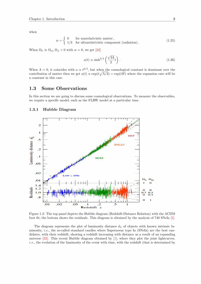
The Universe was in its early stages at high enough temperature to be fully ionised; then processessuch as Thompson scattering would thermalise the radiation field very efficiently. One would thenexpect to observe a radiation field which would have retained the black-body spectrum [2], see Fig.[1.3]. When the primordial plasma cooled enough, light thus suddenly stopped being scattered bycharged particles, and started propagating freely, following null geodesics. The spatial distributionfrom the CMB, showing that this happened everywhere at the same cosmic time. These findingswere rewarded with the 1978 and 2006 Nobel Prizes in Physics.
Figure 1.3: The black-body spectrum of the CMB radiation measured with COBE satellite [2].
As observers, we can measure three main things about this radiation: frequency spectrum,temperature and polarisation states. Each of these observables contains information about thecreation and evolution of the field and is packed with cosmological information. The observedaverage temperature is uniform across the sky of ∼ 2.72548±0.00057 K [37]. The CMB temperatureanisotropy δT/T ∼ 10 µK corresponds to regions of slightly different densities, representing the seedsof all future structure of the Universe; the galaxies of today. We see these temperature fluctuationsprojected in a 2D spherical sky, see Fig. [1.4]. This implies that, on the CMB temperature map,two points (hot or cold) on the last scattering surface are most likely to be separated by an angleθ∗ = rs/rA, where rs is the sound horizon and rA is the area distance measured by using thestandard choice of FLRW model. The analysis of the fluctuations of this thermal radiation hasgiven us valuable insights into our universe and its parameters; such as the rate of expansion, theHubble parameter, the mean matter density of the Universe.
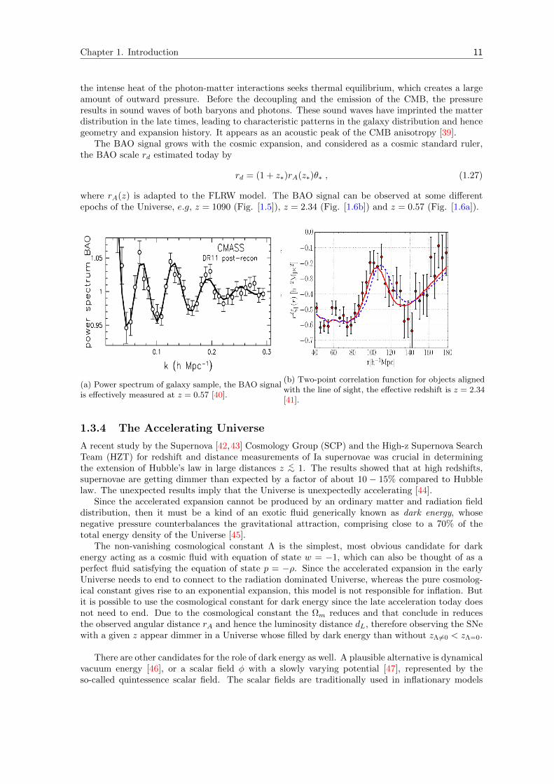
The resulting anisotropies spectrum of the CMB shows a series of acoustic oscillations as shownin Fig. [1.5], which present a snapshot of the CMB sky at the moment when photons decouple from
Chapter 1. Introduction 10
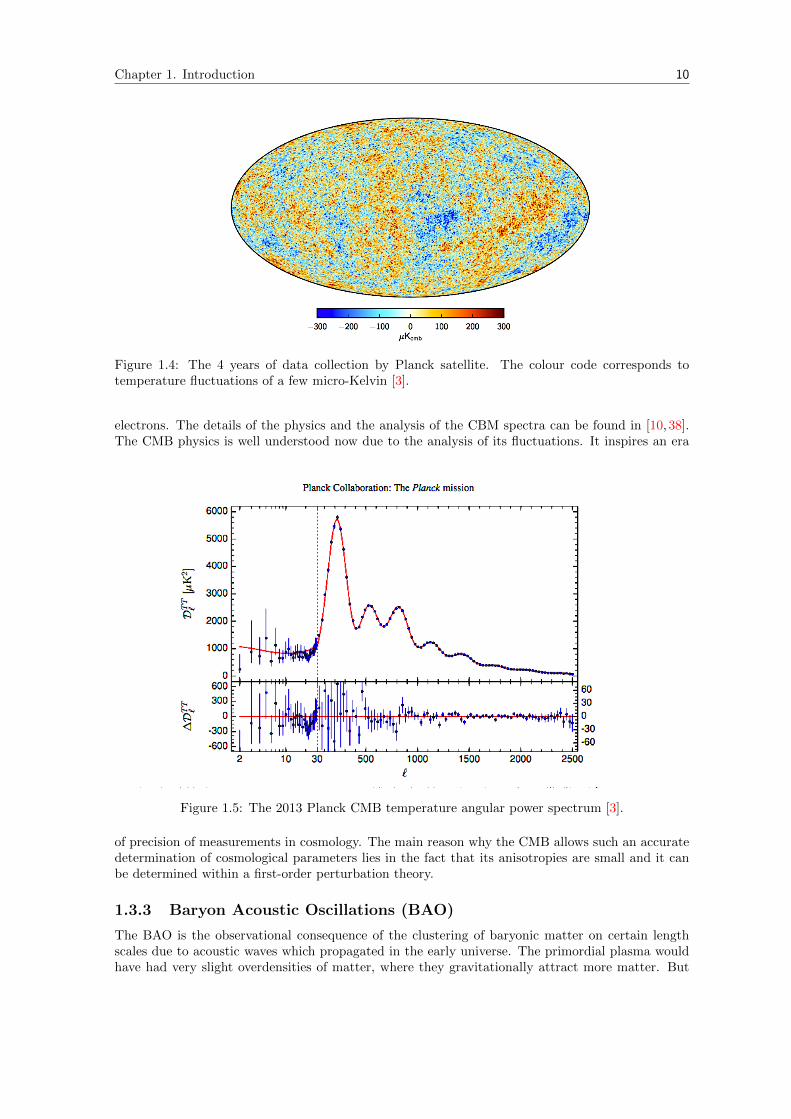
Figure 1.4: The 4 years of data collection by Planck satellite. The colour code corresponds totemperature fluctuations of a few micro-Kelvin [3].
electrons. The details of the physics and the analysis of the CBM spectra can be found in [10, 38].The CMB physics is well understood now due to the analysis of its fluctuations. It inspires an era
Figure 1.5: The 2013 Planck CMB temperature angular power spectrum [3].
of precision of measurements in cosmology. The main reason why the CMB allows such an accuratedetermination of cosmological parameters lies in the fact that its anisotropies are small and it canbe determined within a first-order perturbation theory.
1.3.3 Baryon Acoustic Oscillations (BAO)
The BAO is the observational consequence of the clustering of baryonic matter on certain lengthscales due to acoustic waves which propagated in the early universe. The primordial plasma wouldhave had very slight overdensities of matter, where they gravitationally attract more matter. But
Chapter 1. Introduction 11
the intense heat of the photon-matter interactions seeks thermal equilibrium, which creates a largeamount of outward pressure. Before the decoupling and the emission of the CMB, the pressureresults in sound waves of both baryons and photons. These sound waves have imprinted the matterdistribution in the late times, leading to characteristic patterns in the galaxy distribution and hencegeometry and expansion history. It appears as an acoustic peak of the CMB anisotropy [39].
The BAO signal grows with the cosmic expansion, and considered as a cosmic standard ruler,the BAO scale rd estimated today by
rd = (1 + z∗)rA(z∗)θ∗ , (1.27)
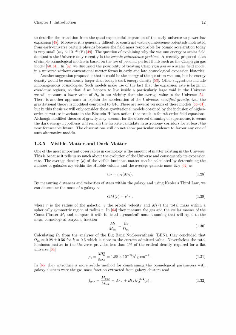
where rA(z) is adapted to the FLRW model. The BAO signal can be observed at some differentepochs of the Universe, e.g, z = 1090 (Fig. [1.5]), z = 2.34 (Fig. [1.6b]) and z = 0.57 (Fig. [1.6a]).
(a) Power spectrum of galaxy sample, the BAO signalis effectively measured at z = 0.57 [40].
(b) Two-point correlation function for objects alignedwith the line of sight, the effective redshift is z = 2.34[41].
1.3.4 The Accelerating Universe
A recent study by the Supernova [42,43] Cosmology Group (SCP) and the High-z Supernova SearchTeam (HZT) for redshift and distance measurements of Ia supernovae was crucial in determiningthe extension of Hubble’s law in large distances z <∼ 1. The results showed that at high redshifts,supernovae are getting dimmer than expected by a factor of about 10 − 15% compared to Hubblelaw. The unexpected results imply that the Universe is unexpectedly accelerating [44].
Since the accelerated expansion cannot be produced by an ordinary matter and radiation fielddistribution, then it must be a kind of an exotic fluid generically known as dark energy, whosenegative pressure counterbalances the gravitational attraction, comprising close to a 70% of thetotal energy density of the Universe [45].
The non-vanishing cosmological constant Λ is the simplest, most obvious candidate for darkenergy acting as a cosmic fluid with equation of state w = −1, which can also be thought of as aperfect fluid satisfying the equation of state p = −ρ. Since the accelerated expansion in the earlyUniverse needs to end to connect to the radiation dominated Universe, whereas the pure cosmolog-ical constant gives rise to an exponential expansion, this model is not responsible for inflation. Butit is possible to use the cosmological constant for dark energy since the late acceleration today doesnot need to end. Due to the cosmological constant the Ωm reduces and that conclude in reducesthe observed angular distance rA and hence the luminosity distance dL, therefore observing the SNewith a given z appear dimmer in a Universe whose filled by dark energy than without zΛ6=0 < zΛ=0.
There are other candidates for the role of dark energy as well. A plausible alternative is dynamicalvacuum energy [46], or a scalar field φ with a slowly varying potential [47], represented by theso-called quintessence scalar field. The scalar fields are traditionally used in inflationary models
Chapter 1. Introduction 12
to describe the transition from the quasi-exponential expansion of the early universe to power-lawexpansion [48]. Moreover it is generally difficult to construct viable quintessence potentials motivatedfrom early-universe particle physics because the field mass responsible for cosmic acceleration todayis very small (mφ ∼ 10−33eV) [49]. The question of explaining why the vacuum energy or scalar fielddominates the Universe only recently is the cosmic coincidence problem. A recently proposed classof simple cosmological models is based on the use of peculiar perfect fluids such as the Chaplygin gasmodel [50, 51]. In [52] we discussed the possibility of treating Chaplygin gas as a scalar field modelin a universe without conventional matter forms in early and late cosmological expansion histories.
Another suggestion proposed is that it could be the energy of the quantum vacuum, but its energydensity would be enormously larger than today’s dark energy density [53]. Other suggestions includeinhomogeneous cosmologies. Such models make use of the fact that the expansion rate is larger inoverdense regions, so that if we happen to live inside a particularly large void in the Universewe will measure a lower value of H0 in our vicinity than the average value in the Universe [54].There is another approach to explain the acceleration of the Universe: modified gravity, i .e., thegravitational theory is modified compared to GR. These are several versions of these models [55–61],but in this thesis we will only consider those gravitational models obtained by the inclusion of higher-order curvature invariants in the Einstein-Hilbert action that result in fourth-order field equations.Although modified theories of gravity may account for the observed dimming of supernovae, it seemsthe dark energy hypothesis will remain the favorite candidate in astronomy corridors for at least thenear foreseeable future. The observations still do not show particular evidence to favour any one ofsuch alternative models.
1.3.5 Visible Matter and Dark Matter
One of the most important observables in cosmology is the amount of matter existing in the Universe.This is because it tells us so much about the evolution of the Universe and consequently its expansionrate. The average density 〈ρ〉 of the visible luminous matter can be calculated by determining thenumber of galaxies nG within the Hubble volume and the average galactic mass MG [62] as
〈ρ〉 = nG〈MG〉. (1.28)
By measuring distances and velocities of stars within the galaxy and using Kepler’s Third Law, wecan determine the mass of a galaxy as
GM(r) = v2r , (1.29)
where r is the radius of the galactic, v the orbital velocity and M(r) the total mass within aspherically symmetric region of radius r. In [63] they measure the gas and the stellar masses of theComa Cluster Mb and compare it with its total ‘dynamical’ mass assuming that will equal to themean cosmological baryonic fraction
Mb
Mtot=
ΩbΩm
. (1.30)
Calculating Ωb from the analyses of the Big Bang Nucleosynthesis (BBN), they concluded thatΩm ≈ 0.28 ± 0.56 for h = 0.5 which is close to the current admitted value. Nevertheless the totalluminous matter in the Universe provides less than 1% of the critical density required for a flatuniverse [64]
ρc =3H2
0
8πG= 1.88× 10⁻²⁹h2g cm−3 . (1.31)
In [65] they introduce a more subtle method for constraining the cosmological parameters withgalaxy clusters were the gas mass fraction extracted from galaxy clusters read
fgas =Mgas
Mtot= ArA +B(z)r
3/2A (z) , (1.32)
Chapter 1. Introduction 13
where A and B are some cosmological parameters-independent values, and Mgas = Mb −MG [65],so that the area distance rA constrains all the cosmological dependence. Eq. (1.32) is a model-dependent formula because of the rA(z) term, in this case FLRW. The analysis of Planck datashows that normal matter, making up galaxies and stars, contributes only about 4.9% to the massand energy density of the Universe.
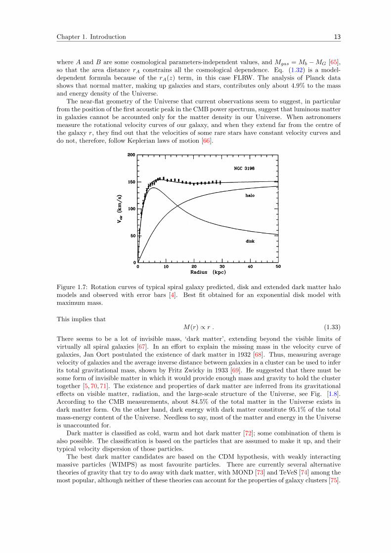
The near-flat geometry of the Universe that current observations seem to suggest, in particularfrom the position of the first acoustic peak in the CMB power spectrum, suggest that luminous matterin galaxies cannot be accounted only for the matter density in our Universe. When astronomersmeasure the rotational velocity curves of our galaxy, and when they extend far from the centre ofthe galaxy r, they find out that the velocities of some rare stars have constant velocity curves anddo not, therefore, follow Keplerian laws of motion [66].
Figure 1.7: Rotation curves of typical spiral galaxy predicted, disk and extended dark matter halomodels and observed with error bars [4]. Best fit obtained for an exponential disk model withmaximum mass.
This implies thatM(r) ∝ r . (1.33)
There seems to be a lot of invisible mass, ‘dark matter’, extending beyond the visible limits ofvirtually all spiral galaxies [67]. In an effort to explain the missing mass in the velocity curve ofgalaxies, Jan Oort postulated the existence of dark matter in 1932 [68]. Thus, measuring averagevelocity of galaxies and the average inverse distance between galaxies in a cluster can be used to inferits total gravitational mass, shown by Fritz Zwicky in 1933 [69]. He suggested that there must besome form of invisible matter in which it would provide enough mass and gravity to hold the clustertogether [5, 70, 71]. The existence and properties of dark matter are inferred from its gravitationaleffects on visible matter, radiation, and the large-scale structure of the Universe, see Fig. [1.8].According to the CMB measurements, about 84.5% of the total matter in the Universe exists indark matter form. On the other hand, dark energy with dark matter constitute 95.1% of the totalmass-energy content of the Universe. Needless to say, most of the matter and energy in the Universeis unaccounted for.
Dark matter is classified as cold, warm and hot dark matter [72]; some combination of them isalso possible. The classification is based on the particles that are assumed to make it up, and theirtypical velocity dispersion of those particles.
The best dark matter candidates are based on the CDM hypothesis, with weakly interactingmassive particles (WIMPS) as most favourite particles. There are currently several alternativetheories of gravity that try to do away with dark matter, with MOND [73] and TeVeS [74] among themost popular, although neither of these theories can account for the properties of galaxy clusters [75].
Chapter 1. Introduction 14
Figure 1.8: Image of the Bullet Cluster obtained by the Chandra X-ray Observatory: The blue colorshows the distribution of dark matter, which passed through the collision without slowing down.The red coulour shows the hot X-ray emitting gas. In green are the gravitational mass contoursreconstructed from weak-lensing observations [5].
1.3.6 Large-scale Structure
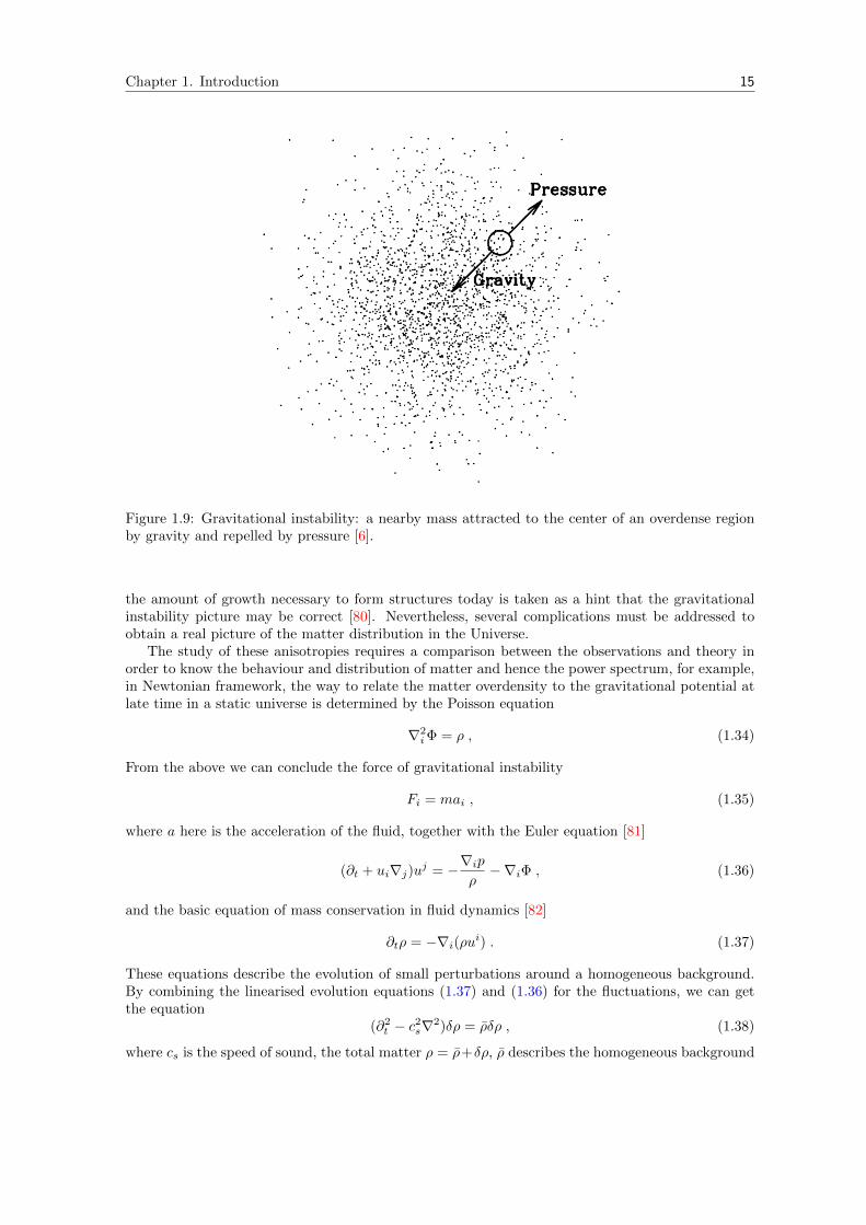
According to the prevailing paradigm, it is sufficient that matter density fluctuations grow fromconsiderable initial fluctuations with amplitudes of order of 10−5 to reproduce the cosmic structuresobserved today [38]. The small deviations from homogeneity and isotropy in the CMB are of utter-most importance since, most probably, they represent the seeds, which, via gravitational instability,have led to the formation of large-scale structure, galaxies and eventually solar systems with planetsthat support life in the Universe. Gravitational instability for overdense regions is a powerful sce-nario for structure formation; it is easy to understand and most likely responsible for the structuresin our universe [6]. In time, matter accumulates in initially overdense regions that are denser thanaverage. It does not matter how small the initial overdensity was, eventually enough matter will beattracted to the region to form structures (e.g., in typical cosmological scenarios, the overdensitywas of order 1 part in 105). A mass near an overdense region is attracted to the centre by gravitybut at the same time repelled by isothermal pressure. If the region is dense enough, gravity winsand overdensity grows with time, see Fig. [1.9]. In the mean time, the Universe exhibits a uniformisotropic expansion, and because there is slightly more matter in the overdensity, there will be aslightly stronger gravitational attractive force tending to draw that overdense region together anddue to that the overdense regions will expand at slower rate than average which can serve to retardthe expansion locally. Eventually, the overdensity, or perturbation as it is often called, will reach apoint where it stops expanding altogether and begins to collapse under its own weight (gravity) [76].As it collapses it will fragment into thousands or even millions of knots, each of which themselveswill collapse, forming a cluster of stars or galaxies, depending on how big the original cloud of gaswas to begin with [77]. An overdense region that is larger than the horizon distance cannot besupported by its internal pressure, because any changes in pressure are propagated at a speed thatis lower than the speed of light. Nevertheless, the relative density fluctuation within this overdenseregion does grow with time, although it will grow slowly since the overdense region is expandingat a lower rate than the universe around it. However, the horizon distance increases with time,so eventually, the overdense region will lie within the horizon distance and can respond to internalpressure changes. After this time, an overdense region can be stable against collapse provided thatthe mass within this region is less than the amount of pressure required for the balance [78]. Thefact that the anisotropies measured recently by COBE [79] and then by Planck just coincide with
Chapter 1. Introduction 15
Figure 1.9: Gravitational instability: a nearby mass attracted to the center of an overdense regionby gravity and repelled by pressure [6].
the amount of growth necessary to form structures today is taken as a hint that the gravitationalinstability picture may be correct [80]. Nevertheless, several complications must be addressed toobtain a real picture of the matter distribution in the Universe.
The study of these anisotropies requires a comparison between the observations and theory inorder to know the behaviour and distribution of matter and hence the power spectrum, for example,in Newtonian framework, the way to relate the matter overdensity to the gravitational potential atlate time in a static universe is determined by the Poisson equation
∇2iΦ = ρ , (1.34)
From the above we can conclude the force of gravitational instability
Fi = mai , (1.35)
where a here is the acceleration of the fluid, together with the Euler equation [81]
(∂t + ui∇j)uj = −∇ipρ−∇iΦ , (1.36)
and the basic equation of mass conservation in fluid dynamics [82]
∂tρ = −∇i(ρui) . (1.37)
These equations describe the evolution of small perturbations around a homogeneous background.By combining the linearised evolution equations (1.37) and (1.36) for the fluctuations, we can getthe equation
(∂2t − c2s∇2)δρ = ρδρ , (1.38)
where cs is the speed of sound, the total matter ρ = ρ+δρ, ρ describes the homogeneous background
Chapter 1. Introduction 16
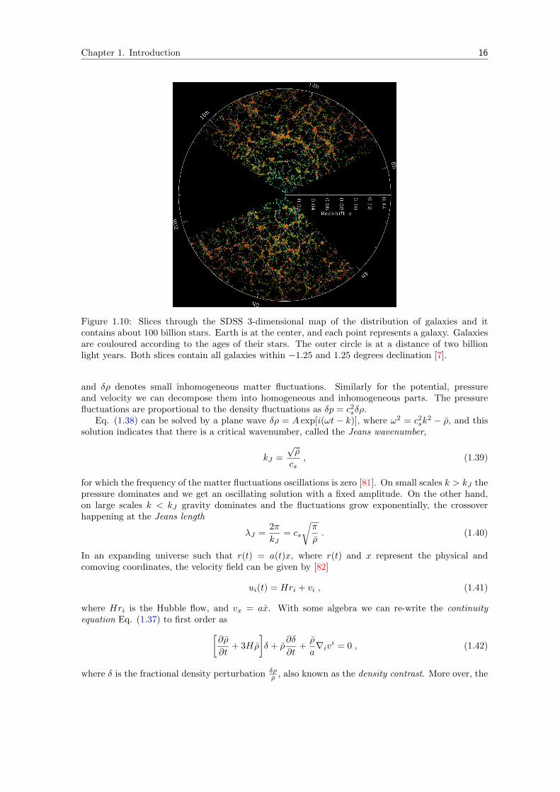
Figure 1.10: Slices through the SDSS 3-dimensional map of the distribution of galaxies and itcontains about 100 billion stars. Earth is at the center, and each point represents a galaxy. Galaxiesare couloured according to the ages of their stars. The outer circle is at a distance of two billionlight years. Both slices contain all galaxies within −1.25 and 1.25 degrees declination [7].
and δρ denotes small inhomogeneous matter fluctuations. Similarly for the potential, pressureand velocity we can decompose them into homogeneous and inhomogeneous parts. The pressurefluctuations are proportional to the density fluctuations as δp = c2sδρ.
Eq. (1.38) can be solved by a plane wave δρ = A exp[i(ωt − k)], where ω2 = c2sk2 − ρ, and this
solution indicates that there is a critical wavenumber, called the Jeans wavenumber,
kJ =
√ρ
cs, (1.39)
for which the frequency of the matter fluctuations oscillations is zero [81]. On small scales k > kJ thepressure dominates and we get an oscillating solution with a fixed amplitude. On the other hand,on large scales k < kJ gravity dominates and the fluctuations grow exponentially, the crossoverhappening at the Jeans length
λJ =2π
kJ= cs
√π
ρ. (1.40)
In an expanding universe such that r(t) = a(t)x, where r(t) and x represent the physical andcomoving coordinates, the velocity field can be given by [82]
ui(t) = Hri + vi , (1.41)
where Hri is the Hubble flow, and vx = ax. With some algebra we can re-write the continuityequation Eq. (1.37) to first order as[
∂ρ
∂t+ 3Hρ
]δ + ρ
∂δ
∂t+ρ
a∇ivi = 0 , (1.42)
where δ is the fractional density perturbation δρρ , also known as the density contrast. More over, the
Chapter 1. Introduction 17
Poisson and Euler equations (1.34) and (1.36) reduce to
∇2i δΦ = a2ρδ , (1.43)
vi +Hvi = − 1
aρ∇iδp−
1
a∇iδΦ . (1.44)
Using these equations together with Eq. (1.19) results in the Jeans’ instability equation 3
δ + 2Hδ − 1
a2∇2δ = ρδ . (1.45)
The second term on the LHS of the above equation of motion plays the role of a damping (friction)force term such that below the Jeans’ length the fluctuations oscillate with decreasing amplitudeand above the Jeans’ length the fluctuations experience power-law growth [81].
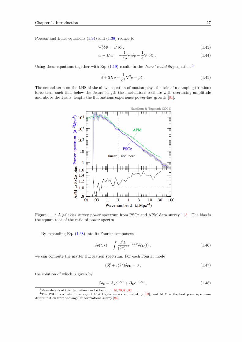
Figure 1.11: A galaxies survey power spectrum from PSCz and APM data survey 4 [8]. The bias isthe square root of the ratio of power spectra.
By expanding Eq. (1.38) into its Fourier components
δρ(t, r) =
∫d3k
(2π)3e−ik.rδρk(t) , (1.46)
we can compute the matter fluctuation spectrum. For each Fourier mode
(∂2t + c2sk
2)δρk = 0 , (1.47)
the solution of which is given by
δρk = Akeiωkt +Bke
−iωkt , (1.48)
3More details of this derivation can be found in [76,78,81,82].4The PSCz is a redshift survey of 15,411 galaxies accomplished by [83], and APM is the best power-spectrum
determination from the angular correlations survey [84].
Chapter 1. Introduction 18
where ωk = csk. Fourier modes evolve independently, and the power spectrum is sufficient tocompletely describe the density field.
1.4 The Cosmological Parameters
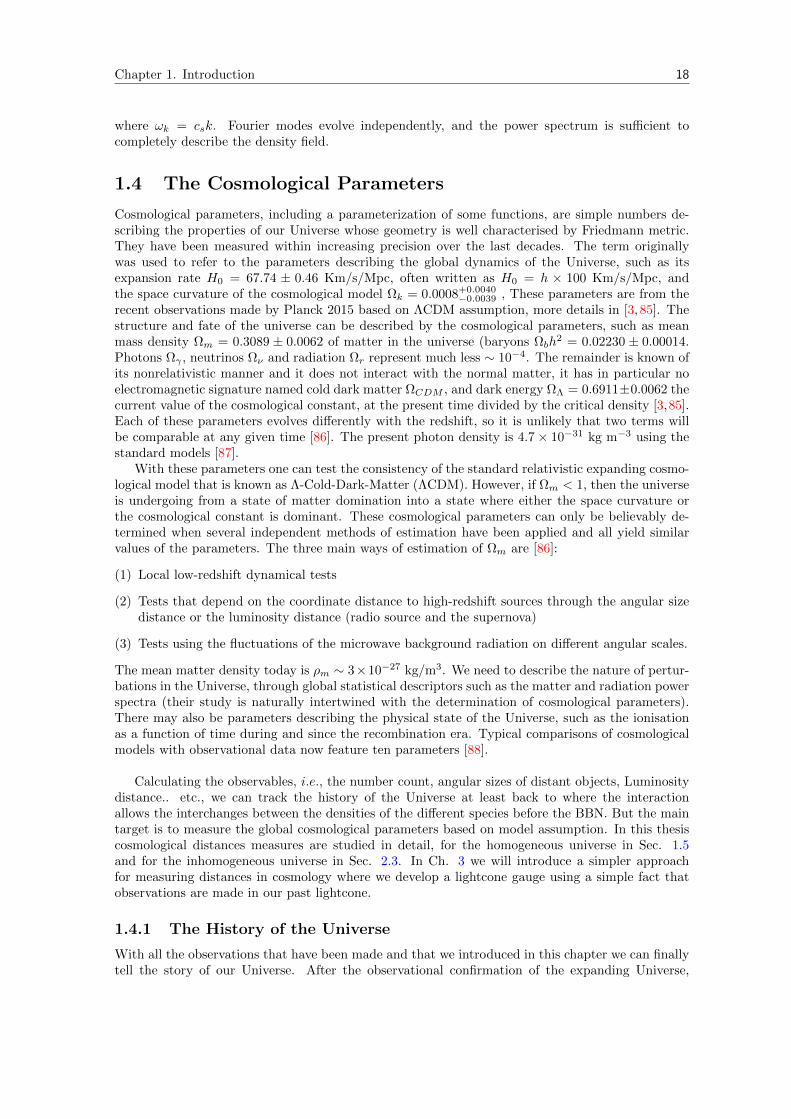
Cosmological parameters, including a parameterization of some functions, are simple numbers de-scribing the properties of our Universe whose geometry is well characterised by Friedmann metric.They have been measured within increasing precision over the last decades. The term originallywas used to refer to the parameters describing the global dynamics of the Universe, such as itsexpansion rate H0 = 67.74 ± 0.46 Km/s/Mpc, often written as H0 = h × 100 Km/s/Mpc, andthe space curvature of the cosmological model Ωk = 0.0008+0.0040
−0.0039 , These parameters are from therecent observations made by Planck 2015 based on ΛCDM assumption, more details in [3, 85]. Thestructure and fate of the universe can be described by the cosmological parameters, such as meanmass density Ωm = 0.3089 ± 0.0062 of matter in the universe (baryons Ωbh
2 = 0.02230 ± 0.00014.Photons Ωγ , neutrinos Ων and radiation Ωr represent much less ∼ 10−4. The remainder is known ofits nonrelativistic manner and it does not interact with the normal matter, it has in particular noelectromagnetic signature named cold dark matter ΩCDM , and dark energy ΩΛ = 0.6911±0.0062 thecurrent value of the cosmological constant, at the present time divided by the critical density [3,85].Each of these parameters evolves differently with the redshift, so it is unlikely that two terms willbe comparable at any given time [86]. The present photon density is 4.7× 10⁻³¹ kg m−3 using thestandard models [87].
With these parameters one can test the consistency of the standard relativistic expanding cosmo-logical model that is known as Λ-Cold-Dark-Matter (ΛCDM). However, if Ωm < 1, then the universeis undergoing from a state of matter domination into a state where either the space curvature orthe cosmological constant is dominant. These cosmological parameters can only be believably de-termined when several independent methods of estimation have been applied and all yield similarvalues of the parameters. The three main ways of estimation of Ωm are [86]:
(1) Local low-redshift dynamical tests
(2) Tests that depend on the coordinate distance to high-redshift sources through the angular sizedistance or the luminosity distance (radio source and the supernova)
(3) Tests using the fluctuations of the microwave background radiation on different angular scales.
The mean matter density today is ρm ∼ 3×10⁻²⁷ kg/m3. We need to describe the nature of pertur-bations in the Universe, through global statistical descriptors such as the matter and radiation powerspectra (their study is naturally intertwined with the determination of cosmological parameters).There may also be parameters describing the physical state of the Universe, such as the ionisationas a function of time during and since the recombination era. Typical comparisons of cosmologicalmodels with observational data now feature ten parameters [88].
Calculating the observables, i.e., the number count, angular sizes of distant objects, Luminositydistance.. etc., we can track the history of the Universe at least back to where the interactionallows the interchanges between the densities of the different species before the BBN. But the maintarget is to measure the global cosmological parameters based on model assumption. In this thesiscosmological distances measures are studied in detail, for the homogeneous universe in Sec. 1.5and for the inhomogeneous universe in Sec. 2.3. In Ch. 3 we will introduce a simpler approachfor measuring distances in cosmology where we develop a lightcone gauge using a simple fact thatobservations are made in our past lightcone.
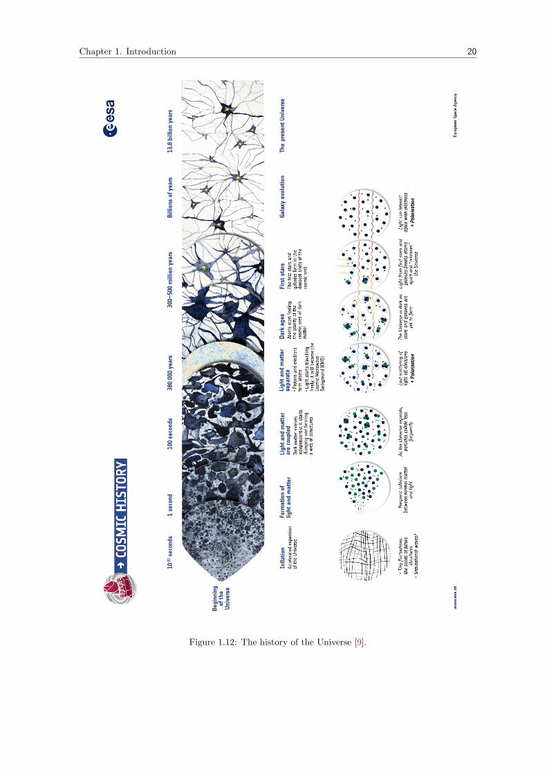
1.4.1 The History of the Universe
With all the observations that have been made and that we introduced in this chapter we can finallytell the story of our Universe. After the observational confirmation of the expanding Universe,

Chapter 1. Introduction 19
cosmologists concluded that the galaxies will be spread much farther apart in the far future andthat the Universe must have been much denser looking back in time. Therefore following theFriedmann dynamics back in time shows that there is a singularity, namely at a(t) = 0, we choosethe origin of the cosmic time t = 0 occurs at the big bang singularity, then present-day-value oft0 = 13.81 Gyr represent the age of the Universe [33]. This is generally taken to be the precursor ofthe current Big Bang model [89, 90]. After Planck era t ∼ 10−35 and within the first t ∼ 10−32 ourUniverse is thought to have experienced a first period of accelerated expansion, its called inflationintroduced by Guth (1981) [91, 92]. This sudden increase in the rate of expansion of the Universewould have increased the size of the Universe by an enormous factor. Prior to inflation the entireuniverse was small and causally connected; it was during this period that the physical propertiesevened out. Inflation resolves the horizon problem and the so-called flatness problem of the big bangmodel. It has therefore been accepted as part of the current concordance model of cosmology. Manyinflationary models have been proposed and tested with observations [93], but the most popularmodels of inflation that involves a single scalar field, the inflaton, whose slight inhomogeneities, anddue to quantum fluctuations, have been the seeds of the Universe structures that we observe today.
The so called the reheating phase [94] started after the end of inflation during which the inflatondecays into particles of the standard model of particle physics. The Universe was about 379000years old - much before the formation of stars and planets - it was denser, much hotter, and filledwith hydrogen plasma. As the Universe expanded further, both the plasma and the radiation fillingit grew cooler and at a temperature of about 3000K, it became favourable for protons and electronsto combine into hydrogen neutral atoms, and some stable nuclei (helium and lithium) could beformed from a primordial mixture of protons, neutrons and electrons [95,96].
This is the Primordial nucleosynthesis, or BBN as it is commonly called [97], is the earliestand one of the most stringent tests of Big Bang cosmology. The relevant BBN reactions thatplayed an important role in the history of the Universe took place in the first three minutes, notably(corresponding to temperatures of T ∼ 1 MeV to ∼ 109 KeV or higher [98]). At the end of this epochthe scale factor reads a0/aBBN = 5×10⁷ and dominated by radiation. From Friedmann equations weknow that radiation density Ωr decreases faster than the nonrelativistic matter density, at some pointthey become equal Ωm a0/aequ = Ωm/Ωr ∼ 3400. During the recombination epoch and at this pointatomic nuclei and electrons recombined into atoms, then photons stopped interacting with matterand became allowed to travel freely through space, and so the Universe became transparent [99].When light started to travel freely through space rather than constantly being scattered by electronsand protons in plasma, a photon decoupling of matter and radiation formed. The decoupled photonsreach present-day observers as the CMB, and they appear to come from a spherical surface aroundthe observer such that the radius of the shell is the distance each photon has travelled since it waslast scattered at the epoch of recombination. Such a surface is referred to as the last scatteringsurface (LSS).
Since light from this epoch has basically remained unaltered to the present day in the CMBimprint, that is what gives it the term relic radiation. The Universe remained basically neutral forfew hundreds of millions of years the dark ages, during this time structure form via gravitationalaccretion creating the first stars and their light broke some of the neutral atoms into hydrogenions in the interstellar medium during the epoch of reionization a0/are ∼ 12. The next billions ofyears the formation and evolution of galaxies took place and the large-scale-structure separated bywalls and filaments. The cosmological constant starts to dominate over matter density leading toan accelerated cosmic expansion a0/am ∼ 1.3 [33].
Chapter 1. Introduction 20
Figure 1.12: The history of the Universe [9].
Chapter 1. Introduction 21
1.5 Distances in Cosmology
We have shown in the previous sections a brief review of some current status of observationalcosmology that fits so well with ΛCDM model. We emphasize that for every observation that involvesthe relation between angular or luminous distance and redshift area distance, FLRW spacetime isassumed, i.e, light propagates through a homogeneous and isotropic universe.
Here we are going to show some theoretical derivations of these distances with standard cosmo-logical model. This will give a framework to interpret cosmological observations and to measure itsfree parameters. In particular we will show the crucial relation between cosmological distances andredshift for their correct interpretation. Over small distances, the relation between angular diameterdistance and redshift, or luminosity distance and redshift, does not depend on whether there is oris not a cosmological constant, or the total value of the matter density Ωm. These differences onlybecome apparent over much larger distances, which make these expressions sufficient when they arewritten as functions of redshift z.
In cosmology spatial distance and velocity measurements are important to determine the con-sistency of relativistic theories and to measure the cosmological parameters. Thus investigationsof spatial distance measurement arose from the fact that any specific astronomical measurement ofdistance carried out in any relativistic model of spacetime must lead to a result which depends uponthe particular operations of measurement, and not upon the particular coordinate system used to de-scribe the spacetime. Formulating invariant quantities corresponding to these various astronomicaldistances depends on the observations of apparent magnitude, apparent size, or apparent luminosityof distant light sources [100,101]. There are different ways to measure distances in cosmology all ofwhich give the same result in a Minkowski universe but differ in an expanding universe. They are,however, simply related as we shall see [38].
1.5.1 Redshift
A photons trajectory
We can define the four-vector kµ as the gradient of a wave phase
kµ = ∂µφ , (1.49)
which indicates the local direction of electromagnetic wave propagation through the spacetime. Thepropagation equation of the waves has to obey in the geometric optics
kµkµ = 0 . (1.50)
By taking the gradient of Eq. (1.50) and using Eq. (1.49), we can define the trajectory that followedby the electromagnetic waves
kµ∇µkν = 0 . (1.51)
The path where kµ is everywhere tangent are called null geodesics, and it can be interpreted as theworld lines of photons or light rays. The geodesic equation (1.51) can also be written.
dkµ
dv+ Γµναk
νkα = 0 , (1.52)
The momentum of the photon ispµ = ~kµ , (1.53)
where ~ = h/(2π) the reduced Planck constant. The affine parameter v along a given light ray isnaturally defined with its tangent vector
kµ =dxµ
dv, (1.54)
Chapter 1. Introduction 22
indicating that a small variation in v corresponds to a small displacement dxµ = kµdv along thelight ray. Then the geodesic equation becomes
kν∇νkµ =dkµ
dv+ Γµνρk
νkρ =d2xµ
dv2+ Γµνρ
dxν
dv
dxρ
dv, (1.55)
where ∇ν is the covariant derivative with respect to ν. τ denotes as the observer proper time, thenthe angular frequency is defined as
ω =
∣∣∣∣dφdτ∣∣∣∣ = |uµ∂µφ| = uµkµ . (1.56)
In order to detect the wave its propagations have to be in the direction opposite to the direction inwhich the observer is actually looking. This implies
kµ = ω(uµ + nµ) . (1.57)
Here nµ is a unit direction vector of the photons, and uµ their 4-velocity vector, defined more withthe orthonormality relations
uµuµ = −1, nµnµ = 1, uµnµ = 0 . (1.58)
The difference between the frequency emitted by a source ωs and the actual frequency measured byan observer ωo is quantified by the redshift z as
1 + z =ωsωo
=(uµkµ)s(uµkµ)o
. (1.59)
1.5.2 Proper Distance
If we place the galaxies at equal distance from each other and labelled them by a fixed coordinatex, and if space itself is expanding in time, the scale factor a will depend on time as well, and therelative velocity between two galaxies at distance
d = a∆x (1.60)
isv = a∆x , (1.61)
such that
v =da(t)/dt
a(t)d =
a
ad = H0d , (1.62)
where v is the recessional velocity, typically expressed in km/s, and d is the proper distance (whichcan change over time, unlike the comoving distance, which is constant) from the galaxy to theobserver, measured in megaparsecs (Mpc)5. Here H0 is the Hubble constant and corresponds to thevalue of the Hubble parameter H(t) at the time of observation. H(t) is a value that is time dependentand which can be expressed in terms of the scale factor.
It is convenient to normalise the scale factor such that a0 = 1, so that comoving scales becomephysical scales today. On the other hand, an object at z 1 at physical distance d away from us,recedes with speed v, then roughly d ≈ η0 − η is the time delay between the events (A,B) in thesame frame, and the positions of the two events will be changing over time due to the expansion,and therefore, a0 ≈ a(η) + a′(η0 − η), so that
1 + z ≈ 1 +a′
a(η0 − η) ≈ 1 +H0d . (1.63)
5 1 parsec = 3.2615638 light years = 3.0856776× 10¹⁶ metres.
Chapter 1. Introduction 23
Figure 1.13: The proper distance between nearby events (A,B) connected by a unique geodesic G.
Therefore we have v ≈ z, and H0 = v/z. The proper distance can be written as
d =
∫ z
0
dz′
(1 + z′)H(z′)=
1
H0
∫ z
0
dz′
(1 + z′)h(z′), (1.64)
where H(z) is the Hubble parameter as a function of redshift, and h(z) = H(z)/H0 is an expansionparameter normalized by the Hubble constant, given by
h(z) =√
Ωr(1 + z)4 + Ωd(1 + z)3 + Ωk(1 + z)2 + ΩΛ . (1.65)
1.5.3 Comoving Distance (Line-of-Sight)
A comoving distance between two events in the Universe, at a specific moment of the cosmologicaltime will remain constant, if the two objects are moving with the Hubble flow which will give distancethat does not change in time due to the expansion of space [102]. The total line-of-sight comovingdistance between two nearby objects along the radial lightray can be given by
dc =1
H0
∫ z
0
dz′
h(z′). (1.66)
The line-of-sight comoving distance is the fundamental distance measure for all other distance mea-sures [102].
1.5.4 Transverse Comoving Distance
The comoving distance between two objects on the sky that are at a constant redshift z, and theyare separated by an angle δθ is δθdm, where dm is the transverse comoving distance, i .e., the cross-sectional length of an object perpendicular to the light ray. It is related to the line-of-sight comovingdistance dc by [102]
dm =
dH√|Ωk|
sinh[√|Ωk|dc/dH
]if Ωk > 0 ,
dc if Ωk = 0 ,dH√|Ωk|
sin[√|Ωk|dc/dH
]if Ωk < 0 ,
(1.67)
where dH = 1/H0 is called Hubble distance.
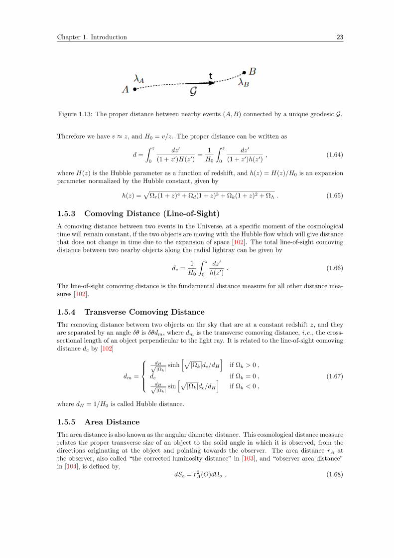
1.5.5 Area Distance
The area distance is also known as the angular diameter distance. This cosmological distance measurerelates the proper transverse size of an object to the solid angle in which it is observed, from thedirections originating at the object and pointing towards the observer. The area distance rA atthe observer, also called “the corrected luminosity distance” in [103], and “observer area distance”in [104], is defined by,
dSo = r2A(O)dΩo , (1.68)
Chapter 1. Introduction 24
Figure 1.14: In a curved spacetime, light travels on null geodesics, and the area distance rA of thesource from the observer is r2
A = dSo/dΩo.
where dΩo is the solid angle subtended by that object at the observer, and dSo is its cross-sectionalarea or the transverse size of the object at the observer, see Fig. [1.14]. The area distance measuredfrom the source would be defined using the geodesic bundle diverging from the source and the ratiobetween the physical transverse size of the source and the solid angle under which it would beobserved from the source
dSs = r2A(S)dΩs . (1.69)
From the above definition of the area distance at the source, one can say that it is not directlyobservable, i .e., an observer can measure dSs, then the observer cannot without knowing rA(S)determine the solid angle dΩs into which this radiation was emitted [105]. The relation betweenrA(O) and rA(S) is
rA(S) = (1 + z)rA(O) . (1.70)
From now on in our calculations of distances we will consider the area distance measured from theobserver rA. The area distance is related also to the transverse comoving distance measured inFLRW by
rA(z) =dm
1 + z. (1.71)
The difficulty of measuring angular distance in astronomy is that it requires standard rulers orsources of a known size or it can be calibrated by independent experiments. The angular diameterdistance is also naturally involved in strong gravitational lensing and time delays experiments.
1.5.6 Luminosity Distance
Distances can be inferred by measuring the flux from an object of known luminosity. In a nonrela-tivistic picture, the luminosity distance dL is defined by the relationship between the flux F of theluminosity, i .e., the rate at which radiation crosses a unit area of surface per unit time, and theintrinsic luminosity L of an object, i .e., energy per unit time, arriving at the observer [106]
dL =
√L
4πF. (1.72)
Chapter 1. Introduction 25
A light source not only appears smaller but also fainter as it lies farther from the observer. It isrelated to the transverse comoving distance and angular diameter distance by
dL(z) = (1 + z)dm = (1 + z)2rA . (1.73)
The factor (1 + z)2 can be interpreted as follows: the first (1 + z) comes from the shifted energies ofthe photons at the emission and reception and time dilation between the source and the observer, thesecond factor (1 + z) is due to the exchange of the roles of s and o Eq. (1.70). Because gravitationalwaves follow null geodesics just like electromagnetic waves, their detections are expected to usher inexcellent measurements of luminosity distance to their sources.
1.6 Observations on the Past Lightcone
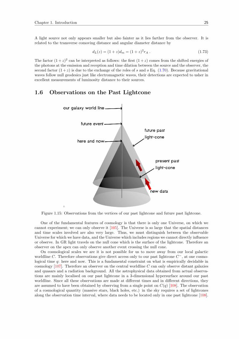
Figure 1.15: Observations from the vertices of our past lightcone and future past lightcone.
One of the fundamental features of cosmology is that there is only one Universe, on which wecannot experiment; we can only observe it [105]. The Universe is so large that the spatial distancesand time scales involved are also very large. Thus, we must distinguish between the observableUniverse for which we have data, and the Universe which includes regions we cannot directly influenceor observe. In GR light travels on the null cone which is the surface of the lightcone. Therefore anobserver on the apex can only observe another event crossing the null cone.
On cosmological scales we are it is not possible for us to move away from our local galacticworldline C. Therefore observations give direct access only to our past lightcone C−, at one cosmo-logical time q: here and now. This is a fundamental constraint on what is empirically decidable incosmology [107]. Therefore an observer on the central worldline C can only observe distant galaxiesand quasars and a radiation background. All the astrophysical data obtained from actual observa-tions are mainly localised on our past lightcone in a 3-dimensional hypersurface around our pastworldline. Since all these observations are made at different times and in different directions, theyare assumed to have been obtained by observing from a single point on C(q) [108]. The observationof a cosmological quantity (massive stars, black holes, etc.) in the sky requires a set of lightconesalong the observation time interval, where data needs to be located only in one past lightcone [108].
Chapter 1. Introduction 26
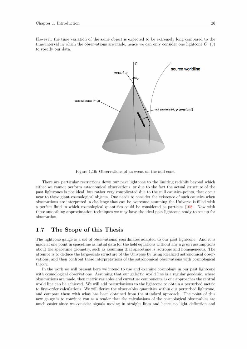
However, the time variation of the same object is expected to be extremely long compared to thetime interval in which the observations are made, hence we can only consider one lightcone C−(q)to specify our data.
Figure 1.16: Observations of an event on the null cone.
There are particular restrictions down our past lightcone to the limiting redshift beyond whicheither we cannot perform astronomical observations, or due to the fact the actual structure of thepast lightcones is not ideal, but rather very complicated due to the null caustics-points, that occurnear to these giant cosmological objects. One needs to consider the existence of such caustics whenobservations are interpreted, a challenge that can be overcome assuming the Universe is filled witha perfect fluid in which cosmological quantities could be considered as particles [108]. Now withthese smoothing approximation techniques we may have the ideal past lightcone ready to set up forobservation.
1.7 The Scope of this Thesis
The lightcone gauge is a set of observational coordinates adapted to our past lightcone. And it ismade at one point in spacetime as initial data for the field equations without any a priori assumptionsabout the spacetime geometry, such as assuming that spacetime is isotropic and homogeneous. Theattempt is to deduce the large-scale structure of the Universe by using idealized astronomical obser-vations, and then confront these interpretations of the astronomical observations with cosmologicaltheory.
In the work we will present here we intend to use and examine cosmology in our past lightconewith cosmological observations. Assuming that our galactic world line is a regular geodesic, whereobservations are made, then metric variables and curvature components as one approaches the centralworld line can be achieved. We will add perturbations to the lightcone to obtain a perturbed metricto first-order calculations. We will derive the observables quantities within our perturbed lightcone,and compare them with what has been obtained from the standard approach. The point of thisnew gauge is to convince you as a reader that the calculations of the cosmological observables aremuch easier since we consider signals moving in straight lines and hence no light deflection and
Chapter 1. Introduction 27
space distortion need to be worried about. We will also use the new gauge to calculate the densityfluctuations, then we will make gauge transformations to our result in the perturbed lightcone gaugeto the general gauge and see if our result is compatible with the results obtained in the standardgauge. We prove that our perturbed metric is genuine and it fulfills the EFE degrees of freedom.
The second topic is to address the recent observations of the accelerated cosmic expansion rateby using modified theories of gravity. We analyze models of f(R) gravity that allow non-rotatingfluid solutions, i .e., when the vorticity is zero. We consider several sub-cases, such as shear-freecases, non-expanding cosmologies, etc...
In the scramble for the understanding of the nature of dark matter and dark energy, it has recentlybeen suggested that the change of behavior of the missing energy density might be regulated by thechanges in the equation of state of the background fluid. Chaplygin gas models are based on theexistence of some kind of exotic fluids out there in the Universe. Our approach attempts to replacesuch exotic fluids with modification of gravity (geometry rather than extra fluid). We will attemptto produce f(R) models that replace Chaplygin gas solutions. This work aims to bring to light ageometric interpretation of the model by re-writing the different toy Chaplygin gas models in termsof exact f(R) gravity solutions that are generally quadratic in the Ricci scalar with appropriateΛCDM limiting solutions.
Chapter 2
Perturbation Theory in Cosmology
Nothing happens until somethingmoves.
Albert Einstein
2.1 The Inhomogeneous Universe: Gauge-invariant Cosmo-logical Perturbation Theory
The measurements of the anisotropies in the CMB of the Universe show only small initial fluctuationsfrom FLRW background. This spatial variation of the density growth in the actual universe is notquite uniform in all directions. The evolution of these fluctuations until the time when they becomeof order unity can be studied within linear perturbation theory [38].
2.1.1 The Metric of the Perturbed Spacetime
We shall now slightly perturb the FLRW model with the basic perturbation equations [10]
gµν = gµν + a2δgµν , (2.1)
where gµν represents the unperturbed Friedmann metric, and δgµν can be parametrised in terms ofits components respectively as
δgµνdxµdxν = −2φdη2 + 2Bidηdx
i + 2Cijdxidxj . (2.2)
Here Bi is a rank-1 tensor and Cij is a rank-2 tensor [10]. For linear perturbation theory, thespacetime metric is thus
ds2 = a2(η)[−(1 + 2φ)dη2 + 2Bidx
idη + (γij + 2Cij)dxidxj
]. (2.3)
The inverse components and the Christoffel symbols associated with this metric are given in Ap-pendix A.1.
28
Chapter 2. Perturbation Theory in Cosmology 29
2.1.2 Decomposition of the Perturbation Variables
The perturbation variables in Eq. (2.2) can be decomposed by splitting the vector field Bi as a sumof a gradient of a scalar and a divergenceless vector as [10]:
Bi ≡ ∇iB +Bi where ∇iBi = 0 . (2.4)
For a velocity field, B will be the potential, and Bi the vorticity. Here we can see that the 3-components of the vector have been split into 1 scalar (B) and 2 vector (Bi) components. Analo-gously, the symmetric rank-2 tensor Cij can be decomposed as
Cij ≡ −ψγij +∇i∇jE +∇iFj +1
2hij with ∇iFi = ∇ihij = hii = 0 . (2.5)
The 6 components of Cij have thus been split into 2 scalar (ψ and E), 2 vector (Fi) and 2 tensor(hij) components. Therefore, δgµν is decomposed into 10 components with 10 degrees of freedom ofthe metric. The advantages of this Scalar-Vector-Tensor (SVT) decomposition lies in the fact thatthe three types of perturbations are decoupled and can thus be studied separately.
2.1.3 The Gauge Problem
A problem in perturbation theory can be summarised in the ‘choice of gauge’. If coordinates arechosen in the background manifold s then the correspondence Ω introduces a coordinate system onthe physical manifold s. With tensor fields Q (e.g., the Ricci scalar, the energy density ρ, etc.) ons, and the corresponding physical quantity Q on s, then we define the perturbation δQ of Q at thepoint x ∈ s by [10]
δQ(x) = Q(x)−Q(x, t). (2.6)
It is usually understood that the perturbation δQ is small. However, δQ can be assigned at anypoint on the physical manifold s by simply altering the correspondence Ω.
In order to map between this two manifolds, we need to compare two different spacetimes. We willconsider for the physical observable universe s with a spacetime manifold M, metric g and energymomentum tensor T , which in some sense must be close to the FLRW universe, and a fictitiousbackground spacetime s with manifold M and metric g and energy momentum tensor T . Thisimplies that there exist some unphysical degrees of freedom related to the choice of the coordinatesystems on the two manifolds [10].
Similarly, ρ(x) describes the actual value of the energy density at point x, while ρ(x) describesthe fictitious background value there. The quantity δρ = ρ − ρ is the variation in density of thebackground model and the realistic lumpy model [109]. In general, the mapping is given as
Ω : gµν → gµν . (2.7)
An interesting and yet nontrivial problem is how to identify points in the background s withcorresponding points in the realistic spacetime s, in accord with
gµν → gµν = gµν + δgµν . (2.8)
This is related to the difficulties of the background choice. We will assume the existence of back-grounds that lead to the FLRW universe. There are may be many different ways to these differentbackgrounds leading to slightly different FLRW backgrounds. But since |g − g| is small, of order ε,the differences of FLRW backgrounds must also be small, of order ε, and can be regarded as part ofthe perturbations [38].
The only possibilities for gauge-invariant quantities are: a scalar or a tensor, which are constantin M. These quantities can be given any value we desire by altering that map; we can, e.g., setit to zero by choosing the real surfaces of constant energy density to be the background surfaces
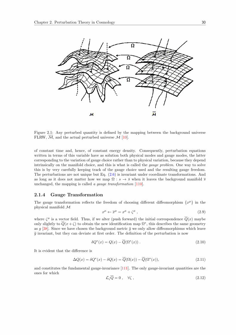
Chapter 2. Perturbation Theory in Cosmology 30
Figure 2.1: Any perturbed quantity is defined by the mapping between the background universeFLRW, M, and the actual perturbed universe M [10].
of constant time and, hence, of constant energy density. Consequently, perturbation equationswritten in terms of this variable have as solution both physical modes and gauge modes, the lattercorresponding to the variation of gauge choice rather than to physical variation, because they dependintrinsically on the manifold choice, and this is what is called the gauge problem. One way to solvethis is by very carefully keeping track of the gauge choice used and the resulting gauge freedom.The perturbations are not unique but Eq. (2.6) is invariant under coordinate transformations. Andas long as it does not matter how we map Ω : s → s when it leaves the background manifold sunchanged, the mapping is called a gauge transformation [110].
2.1.4 Gauge Transformation
The gauge transformation reflects the freedom of choosing different diffeomorphism xµ in thephysical manifold M
xµ ← xµ = xµ + ζµ , (2.9)
where ζµ is a vector field. Thus, if we alter (push forward) the initial correspondence Q(x) maybeonly slightly to Q(x+ ζ) to obtain the new identification map Ω∗, this describes the same geometryas g [38]. Since we have chosen the background metric g we only allow diffeomorphisms which leaveg invariant, but they can deviate at first order. The definition of the perturbation is now
δQ∗(x) = Q(x)−Q(Ω∗(x)) . (2.10)
It is evident that the difference is
∆Q(x) = δQ∗(x)− δQ(x) = Q(Ω(x))−Q(Ω∗(x)), (2.11)
and constitutes the fundamental gauge-invariance [111]. The only gauge-invariant quantities are theones for which
LζQ = 0 , ∀ζ , (2.12)
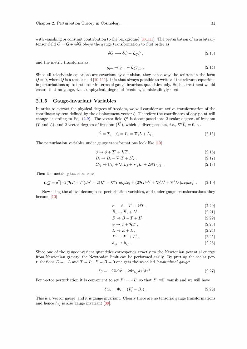
Chapter 2. Perturbation Theory in Cosmology 31
with vanishing or constant contribution to the background [38,111]. The perturbation of an arbitrarytensor field Q = Q+ εδQ obeys the gauge transformation to first order as
δQ −→ δQ+ LζQ , (2.13)
and the metric transforms asgµν → gµν + Lζgµν . (2.14)
Since all relativistic equations are covariant by definition, they can always be written in the formQ = 0, where Q is a tensor field [10,111]. It is thus always possible to write all the relevant equationsin perturbations up to first order in terms of gauge-invariant quantities only. Such a treatment wouldensure that no gauge, i .e.., unphysical, degree of freedom, is misleadingly used.
2.1.5 Gauge-invariant Variables
In order to extract the physical degrees of freedom, we will consider an active transformation of thecoordinate system defined by the displacement vector ζ. Therefore the coordinates of any point willchange according to Eq. (2.9). The vector field ζµ is decomposed into 2 scalar degrees of freedom
(T and L), and 2 vector degrees of freedom (Li), which is divergenceless, i.e., ∇iLi = 0, as
ζ0 = T, ζi = Li = ∇iL+ Li . (2.15)
The perturbation variables under gauge transformations look like [10]
φ→ φ+ T ′ +HT , (2.16)
Bi → Bi −∇iT + L′i , (2.17)
Cij → Cij +∇iLj +∇jLi + 2HTγij . (2.18)
Then the metric g transforms as
Lζg = a2[−2(HT + T ′)dη2 + 2(L′i −∇iT )dηdxi + (2HTγij +∇jLi +∇iLj)dxidxj ] . (2.19)
Now using the above decomposed perturbation variables, and under gauge transformations theybecome [10]
φ→ φ+ T ′ +HT , (2.20)
Bi → Bi + Li , (2.21)
B → B − T + L′ , (2.22)
ψ → ψ +HT , (2.23)
E → E + L , (2.24)
F i → F i + Li , (2.25)
hij → hij . (2.26)
Since one of the gauge-invariant quantities corresponds exactly to the Newtonian potential energyfrom Newtonian gravity, the Newtonian limit can be performed easily. By putting the scalar per-turbations E = −L and T = L′, E = B = 0 one gets the so-called longitudinal gauge:
δg = −2Φdη2 + 2Ψγijdxidxj . (2.27)
For vector perturbation it is convenient to set F i = −Li so that F i will vanish and we will have
δg0i = Φi = (F ′i −Bi) . (2.28)
This is a ‘vector gauge’ and it is gauge invariant. Clearly there are no tensorial gauge transformationsand hence hij is also gauge invariant [38].
Chapter 2. Perturbation Theory in Cosmology 32
The traditionally favoured choice for cosmological perturbations is the metric perturbation the-ory. In the so-called Bardeen’s approach [112] for metric perturbations, we can construct a set ofgauge-invariant independent quantities related to density perturbations, but these quantities are notperturbations themselves in terms of the background metric, i.e., they do not depend on Li and T .For instance
φ = Φ−H(B − E′)− (B − E′)′ , (2.29)
ψ = Ψ +H(B − E′) , (2.30)
where Φ and Ψ are called Bardeen potentials. The Bardeen approach to cosmological perturbationtheory is widely used and fundamentally important.
A new method developed by Ellis and Bruni (1989) [109] as an alternative description of spacetimein terms of scalars, 3-vectors and projected symmetric trace-free (PSTF) tensors is the so-called 1+3covariant approach [113], and the later is what we are going to use and call as standard gauge. Ithas the freedom of choosing a set of coordinates and transforming to another if wished. This work isbuilt on the work of Ehlers [114], Hawking (1966) [115], Olson [116] and Stewart and Walker [111],and does not use the metric directly but describes the spacetime instead by means of covariant andgauge-invariant quantities obtained by a local foliation of spacetime into ‘space’ and ‘time’.
2.1.6 The Four-velocity
A comoving observer’s trajectory along a worldline orthogonal to the hypersurfaces Σt is given by,uµ the four-velocity of the observer
uµ = uµ + δuµ , (2.31)
satisfying the condition given in Eqs. (1.58). With a time-like geodesic, the normalisation conditionof uµ to zeroth order provides the solution
uµ = a−1δµ0 , uµ = −aδ0µ , (2.32)
and hence ui = 0 at zeroth order. From Eqs. (1.58) we see that
gµνuµuν = −1 , (2.33)
and therefore− a2(1 + 2φ)u02
= −1 . (2.34)
This leads to
u0 =1
a
(1− φ
), (2.35)
andδu0 = −a−1φ . (2.36)
We then writeδui = a−1vi , (2.37)
where vi is the peculiar velocity of the object. It is also easy to show that
δu0 = −aφ, and δui = a(vi +Bi) . (2.38)
We can decompose vi into a scalar and a tensor part according to the form of Eq. (2.4):
vi = ∇iv + vi. (2.39)
And upon performing a gauge transformation on δuµ,
δuµ → δuµ + Lζuµ, (2.40)
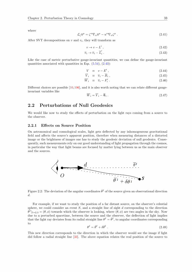
Chapter 2. Perturbation Theory in Cosmology 33
whereLζuµ = ζα∇αuµ − uα∇αζµ . (2.41)
After SVT decompositions on v and vi, they will transform as
v → v − L′ , (2.42)
vi → vi − L′i . (2.43)
Like the case of metric perturbative gauge-invariant quantities, we can define the gauge-invariantquantities associated with quantities in Eqs. (5.54), (2.43):
V ≡ v − E′ , (2.44)
V i ≡ vi −Bi , (2.45)
W i ≡ vi − F ′i . (2.46)
Different choices are possible [10,106], and it is also worth noting that we can relate different gauge-invariant variables like
W i = V i − Φi . (2.47)
2.2 Perturbations of Null Geodesics
We would like now to study the effects of perturbation on the light rays coming from a source tothe observer.
2.2.1 Effects on Source Position
On astronomical and cosmological scales, light gets deflected by any inhomogeneous gravitationalfield and affects the source’s apparent position, therefore when measuring distances of a distortedimage or the brightness of images one has to study the geodesic deviation of null geodesics. Conse-quently, such measurements rely on our good understanding of light propagation through the cosmos,in particular the way that light beams are focused by matter lying between us as the main observerand the sources.
Figure 2.2: The deviation of the angular coordinates θI of the source given an observational directiond.
For example, if we want to study the position of a far distant source, on the observer’s celestialsphere, we could consider an event S, and a straight line of sight d corresponding to the directionθI |I=2,3 = (θ, φ) towards which the observer is looking, where (θ, φ) are two angles in the sky. Nowdue to a perturbed spacetime, between the source and the observer, the deflection of light impliesthat the light ray deviates from its radial straight line θI = θI , to angular coordinates correspondingto
θI = θI + δθI . (2.48)
This new direction corresponds to the direction in which the observer would see the image if lightdid follow a radial straight line [33]. The above equation relates the real position of the source to
Chapter 2. Perturbation Theory in Cosmology 34
its observable position.
2.2.2 Effects on Null-vector
The geodesic of photons is a worldline xµ(λ) where λ is an affine parameter. Applying perturbationto the geodesic equation (1.52) to first order, we get
kµ = (kµ
+ δkµ) ,Γµνα = (Γµνα + δΓµνα) , (2.49)
d
dλδkµ + k
νkαδΓµνα + 2k
νΓµναδk
α = 0 . (2.50)
The tangent vector of the null geodesic satisfies the condition
gµνkµkν = 0 . (2.51)
Perturbing the above Eq. (2.51) also to first order, we will get
kµkνδgµν + k
µgµνδk
ν + kνgµνδk
µ = 0 . (2.52)
2.2.2.1 Conformal Trick
We can use the perturbed FLRW metric as in Eq. (2.2) and by connecting two metrics using Sachs’and Wolfe’s conformal techniques [117] such that
ds2 = a2ds2, (2.53)
whereds
2=[−(1 + 2φ)dη2 + 2Bidx
idη + (δij + 2Cij)dxidxj
]. (2.54)
ds2
is a conformal space metric, and it is called a perturbed Minkowski metric. It has all thegeometrical properties of the FLRW metric but its space is not expanding. The lightlike geodesics
of ds2 coincide with those of ds2. If k is a null geodesic for the metric ds
2with affine parameter λ,
thenkµ = a2kµ (2.55)
is a null geodesic for ds2 with affine parameter λ. However the affine parameters do not coincideand are related by
dλ = a−2dλ . (2.56)
In the following, we will first calculate kµ, and then we will use Eq. (2.55) to determine kµ. Lightlikegeodesics are invariant under conformal transformations; we are doing this to make our calculationseasier. We will drop the tilde ( ) and keep in mind the calculations are made on the conformalspace unless otherwise stated. The 0-components of the geodesic equation (2.50), with the use ofEq. (2.52), can be written as
d
dλδk0 + k
0k
0δΓ0
00 + 2k0Γ0
00δk0 + 2k
0kiδΓ0
0i + 2kiΓ0
0i
+δk0 + 2k0Γ0
0iδki + k
ikjδΓ0
ij + kjΓ0
ijδki + k
iΓ0
ijδkj = 0 , (2.57)
and with a conventional choice of kµ
= (1, ni) at the background, where ni is the unit vector, wehave
d
dλδk0 + φ′ + 2ni∇iφ+ ninj
(C ′ij −∇iBj
)= 0 . (2.58)
We also define the backward affine parameter along the past lightcone, such that
φ′ =dφ
dλ− ni∇iφ . (2.59)

Chapter 2. Perturbation Theory in Cosmology 35
Then we can rewrite Eq. (2.58) as
d
dλδk0 = φ′ − 2
d
dλφ− ninj
(C ′ij −∇iBj
). (2.60)
Integrating both sides of Eq. (2.60) yields
δk0o − δk0
s =
∫ o
s
[φ′ − 2
d
dλφ− ninj
(C ′ij −∇iBj
)]dλ . (2.61)
k0 is a component along the light trajectory between the observer o and the source s is given by
k0o − k0
s = k0
o + δk0o − k
0
s − δk0s . (2.62)
And since the background is Minkowski, the background term is the same both at the source andobserver points. Therefore
k0o − k0
s =
∫ o
s
[φ′ − 2
d
dλφ− ninj
(C ′ij −∇iBj
)]dλ . (2.63)
Now calculating the i-component of the null vector,
d
dλδki + k
0k
0δΓi00 + 2k
0Γi00δk
0 + 2k0kjδΓi0j + 2k
jΓi0jδk
0
+2k0Γi0jδk
j + kjkkδΓijk + k
jΓijkδk
k + kkΓijkδk
j = 0 , (2.64)
and hence
d
dλδki+Bi
′+∇iφ+2nj
(Ci′j +
1
2(∇jBi −∇iBj)
)+njnk
(∇kCij+∇jCik−∇iCjk
)= 0 , (2.65)
which we can rewrite after integrating both sides, as
δkio − δkis =
∫ o
s
[−Bi′ −∇iφ− 2nj
(Ci′j +
1
2(∇jBi −∇iBj)
)−njnk
(∇kCij +∇jCik −∇iCjk
)]dλ . (2.66)
ki is a vector along the path between the observer o and the source s
kio − kis = ki
o + δkio − ki
s − δkis . (2.67)
In the Minkowski background, this yields
kio − kis =
∫ o
s
[−Bi′ −∇iφ− 2nj
(Ci′j +
1
2(∇jBi −∇iBj)
)−njnk
(∇kCij +∇jCik −∇iCjk
)]dλ , (2.68)
and since we are dealing with a conformal space the background terms are constant.Now applying Eq. (2.55) and Eq. (2.56) to our null vector results Eqs. (2.63) and (2.68) to move
back from conformal space to FLRW space, then for the 0-components will get
k0s =
a2o
a2s
k0o −
1
a2s
∫ o
s
a−2
[φ′ − 2a2 d
dλφ− ninj
(C ′ij −∇iBj
)]dλ . (2.69)
Chapter 2. Perturbation Theory in Cosmology 36
In particular the observer sends a light ray of a past-pointed null cone vectors. Then this implies
−gabkaub < 0 . (2.70)
We can normalize the null vector k0o = −1 at the observer position
k0s = − 1
a2s
− 1
a2s
∫ o
s
a−2
[φ′ − 2a2 d
dλφ− ninj
(C ′ij −∇iBj
)]dλ . (2.71)
Applying the same conformal transformation to the i-components, we will get
kis =a2o
a2s
kio −1
a2s
∫ o
s
a−2
[−Bi′ −∇iφ− 2nj
(Ci′j +
1
2(∇jBi −∇iBj)
)−njnk
(∇kCij +∇jCik −∇iCjk
)]dλ , (2.72)
where kio = nio at the observer, then we get slightly simpler expression in the FLRW space
kis =nioa2s
− 1
a2s
∫ o
s
a−2
[−Bi′ −∇iφ− 2nj
(Ci′j +
1
2(∇jBi −∇iBj)
)−njnk
(∇kCij +∇jCik −∇iCjk
)]dλ . (2.73)
By lowering the indices, we obtain
ksη = 1 +
∫ o
s
a−2φ′dλ−∫ o
s
a−2[ninj(C ′ij −∇(jBi)
)]dλ−Bini , (2.74)
and
ksi = noi +
∫ o
s
a−2∇iφdλ+
∫ o
s
a−2B′idλ+ 2
∫ o
s
a−2
[nj(C ′ij +
1
2(∇jBi −∇iBj)
)]dλ
+
∫ o
s
a−2
[nlnj
(2∇jCil −∇iClj
)]dλ−Bi|os + 2njCij |os . (2.75)
2.2.3 Effect on Frequency
Now we can calculate the effect of perturbations on the observed frequency of the light signal byusing Eq. (1.59) to first-order perturbation along with the 4-velocity we define in Sec. 2.1.6 andEqs. (2.71), (2.73) we get
1 + z =ωs + δωsωo + δωo
=
[(gµν + δgµν)(k
µ+ δkµ)(uν + δuν)
]s[
(gγσ + δgγσ)(kγ
+ δkγ)(uσ + δuσ)]o
,
1 + z =1
a(ηs)
[[1− φ+ nivi − ni∇iB − niBi]os +
∫ o
s
(φ+ ψ)′dη
−∫ o
s
ninj(∇i∇jE′ +∇(iF
′j) +
1
2h′ij −
1
2(∇i∇jB +∇jBi +∇i∇jB +∇iBj)
)dη
],
(2.76)
where we have used a−2dλ = dη. Substituting for the Bardeen potentials quantities using Eqs. (2.29,2.30) and further simplify the term ∇i∇j(B − E′) as follows:
Chapter 2. Perturbation Theory in Cosmology 37
ninj∇i∇j(B − E′) = ni∇i(d
dη− ∂
∂η
)(B − E′) , (2.77)
= −(d
dη− ∂
∂η
)(B − E′)′ + ni∇i
d
dη(B − E′) , (2.78)
= (B − E′)′′ − d
dη(B − E′)′ + ni∇i
d
dη(B − E′) . (2.79)
Thus, integrating both sides leads to∫ o
s
ninj∇i∇j(B − E′)dη =
∫ o
s
(B − E′)′′dη − (B − E′)′|os + ni∇i(B − E′)|os . (2.80)
Moreover, let us decompose vi using Eq. (2.39) into scalar and tensor parts:
vi = [∇iv + vi] , (2.81)
= [∇i(V + E′) + (V i +Bi)] , (2.82)
= Vi + [∇iE′ +Bi] , (2.83)
where Vi is the gauge-invariant velocity perturbation of the baryon fluid, and now we can obtain
1 + z =1
a(η)s
[[1− Φ +H(B − E′) + Vin
i]os +
∫ o
s
(Φ + Ψ)′dη −∫ o
s
ninj(∇iF ′j +
1
2h′ij −∇iBj
)dη
].
(2.84)
Using (2.28) in the above equation results
1 + z =1
a(η)s
[[1− Φ +H(B − E′) + Vin
i]os +
∫ o
s
(Φ + Ψ)′dη −∫ o
s
ninj(∇iΦj +
1
2h′ij
)dη
].
(2.85)
This redshift relation is in a general gauge presentation, which we can reduce to any sort of gauge wewant. The redshifts calculated are gauge-invariant if and only if they relate to the observed redshiftof emission points on an invariantly specified surface in our past lightcone C−(q). This equationis known as the Sachs-Wolfe (SW) equation as well and it relates photons’ present potential andenergy to their potential and energy at the emission. The interpretation given the perturbationsconsidered is based on a splitting of perturbations into scalar, vector, and tensor parts [10]. Theordinary Sachs-Wolfe term,
ΘSW ≡ [−Φ +H(B − E′)]os (2.86)
is the scalar only contribution whereas the Doppler term
Θdop ≡ [Vini − Φin
i]os (2.87)
is the scalar-and- vector contribution and indicates that the emitter source and the observer do nothave the same velocity. Finally, the term
ΘISW ≡∫ o
s
((Φ + Ψ)′ − Φ′in
i +1
2h′ijn
inj)dη (2.88)
contains all three kinds of perturbations and is called the integrated Sachs-Wolfe term. The physicalmeaning of this splitting is non-local, and its implications depend on the details of the gauge choicemade. All terms in the above equation are gauge invariant. One may think the term H(B − E′) is

Chapter 2. Perturbation Theory in Cosmology 38
not gauge invariant under gauge transformation, but can proven to be so using the transformations;
η −→ η − T , (2.89)
xi −→ xi − Li , (2.90)
and thus
B − E′ −→ B − E′ − T, (2.91)
a(η) −→ a(η)[1−HT ]. (2.92)
Therefore, 1 + z is gauge invariant.
2.3 The Perturbative Cosmological Distances
We are going to calculate the cosmological distances in a perturbed FLRW space. The perturbeddistance is a gauge-invariant quantity. In any arbitrary geometry of spacetime it is easier to measurethe distance in a gauge of our choice.
A distance measure from a moving source with 4-velocity us and an observer moving with 4-velocity uo, can be obtained as a solution of the Sachs focusing equation [118, 119], which rulesthe relative acceleration between neighbouring geodesic motions, it represents the deviation of thegeodesic equation
d2D
dλ2= −
(R+ |Σ|2
)D , (2.93)
Σ is the complex shear of the light ray, this equation surely provides the best geometrical interpre-tation of curvature, where
R =1
2Rµνk
µkν , |Σ|2 = ΣµνΣµν . (2.94)
Σµν describes the shear
Σµν = Σ〈µν〉 ≡ N α(µN
σν)∇αkσ −
1
2θNµν , (2.95)
where Nµν is the screen space tensor given by Eq. (4.1), θ describes the expansion of a bundle oflight rays [120]. The shear related to the photon ray vector by
NαµN
βν∇αkβ =
1
2θNµν + Σµν . (2.96)
In perturbed FLRW metric to first order, the Sachs focusing equation reduces to [119]
d2D
dλ2= −RD (2.97)
since the complex scalar shear vanishes for a conformally flat spacetime and Σ2 contributes only atsecond order [119]. We consider a light bundle with vertex at the source; this leads to the followinginitial conditions:
D(λs) = 0,dD(λs)
dλ= ωs = −(gµνk
µuν)s . (2.98)
These are general initial conditions for an arbitrary affine parameter λ for distance measure. We cannormalise λ such that ωs = (1 + zs) then one could obtain the redshift luminosity distance, whileωs = (1 + zs)
−1 gives us the redshift angular diameter distance [119].
2.3.1 Area Distance
One considers a past-oriented lightlike geodesic, so we can normalise λ = λs such that ωs = 1. Thatwill ease the calculations for us for now. We will get the area distance in terms of the direction n
Chapter 2. Perturbation Theory in Cosmology 39
and the time of emission ηs. If we would like to obtain the real observed area distance simply weneed to measure the source redshift in the same direction n.The area distance will be given by
rA(λo) = (λo − λs)−∫ λo
λs
∫ λ
λs
R(λ− λs)dλ′dλ . (2.99)
Note that as we showed in Sec. 2.2.2.1, a perturbed FLRW universe is conformally related to aperturbed Minkowski spacetime by the scale factor a. The null geodesics are invariant under confor-mal transformations, therefore the distance D will not be affected by the conformal transformationthat we are going to apply. Then the effect of the expansion on the distance simply leads to arescaling [121]. The two conformally related area distances will be
rA = as rA . (2.100)
We will drop the tilde and bear in mind that the following calculations have been done inconformal space. From Eq. (2.99) we can calculate the area distance using the right initial conditionsof the Sachs focusing equation for an arbitrary affine parameter λ. At the source s it is useful toexpress the affine parameter in terms of the conformal time∫ o
s
kηdλ =
∫ o
s
dη , (2.101)
and from Eq. (2.63) we get
λo − λs = (ηo − ηs) +
∫ λo
λs
∫ λ
λs
[− d
dλ(Φ + Ψ) + ni∇i(Φ−Ψ)
−2ni∇iΦ− ninj [∇i∇jE′ +∇(iF′j) +
1
2h′ij −∇(iBj)]
]dλ′dλ . (2.102)
This leads to
λo − λs = (ηo − ηs)[1− (Φ + Ψ) + (B − E)′
]+
∫ ηo
ηs
(ηo − η)
[−ni∇i(Φ + Ψ)− ni∇i(B − E′)′
+ninj∇i∇j(B − E′)− ninj(∇(iF
′j) +
1
2h′ij +∇(iBj)
)]dη , (2.103)
where we have used the identity B.60. We need to calculate
R =1
2(R00 + 2R0in
i +Rijninj) . (2.104)
Using a Maple code, we have calculated the Ricci tensor components, and therefore
−∫ λo
λs
∫ λ
λs
(λ− λs)Rdλ′dλ = −1
2
∫ λo
λs
∫ λ
λs
(λ− λs)[−2
d2
dλ2[Φ−H(B − E′)− (B − E)′]
+(∇2 − ninj∇i∇j)(Φ + Ψ) + (∇2 − ninj∇i∇j)(B − E′)′
−∇2[ni(Bi − F ′i )] − ninj [∇(iB′j) −∇(iF
′′j)]− n
inj∇2hij
−2ninj∇i∇j(B − E′)]dλ′dλ , (2.105)
where ∇2 = ∇i∇i. By joining Eqs. (2.103) and (2.105), we can give the area distance in FLRWspace by
Chapter 2. Perturbation Theory in Cosmology 40
rA(n, ηs) = a(ηs)(ηo − ηs)[1−Ψs −H(B − E′)
+1
2
1
ηo − ηs
∫ ηo
ηs
(η − ηs)(ηo − η)
((∇2 − ninj∇i∇j −
2
ηo − ηni∇i)(Φ + Ψ)
−ni∇2(Bi − F ′i )− ninj(∇(iB′j) −∇(iF
′′j))− n
inj∇2hij −2
ηo − η(∇(iF
′j)
+1
2h′ij +∇(iBj))n
inj)dη
], (2.106)
where we have used the conformal transformation as mentioned in Eq. (2.56).
2.3.2 Luminosity Distance
For the perturbed luminosity distance we need
(1 + z)2 =1
a2(ηs)
[1− 2Φo + 2Φs + 2H(B − E′) + 2Vin
i
+2
∫ ηo
ηs
(Φ + Ψ)′dη − 2ninj∫ ηo
ηs
(∇iF ′j +
1
2h′ij −∇iBj
)dη
]. (2.107)
Using Eq. (2.106), the luminosity distance is given by
dL(n, ηs) = a(ηs)−1(ηo − ηs)
[1− 2Φo + 2Φs −Ψs +H(B − E′) + 2Vin
i + 2
∫ o
s
(Φ + Ψ)′dη
−2ninj∫ o
s
(∇iF ′j +
1
2h′ij −∇iBj
)dη
+1
2
1
ηo − ηs
∫ ηo
ηs
(η − ηs)(ηo − η)
([∇2 − ninj∇i∇j −
2
ηo − ηni∇i](Φ + Ψ)
−∇2ni(Bi − F ′i )− ninj [∇(iB′j) −∇(iF
′′j)]− n
inj∇2hij −2
ηo − η[∇(iF
′j) +
1
2h′ij
+∇(iBj)]ninj)dη
]. (2.108)
We can re-write the term∫
(Φ + Ψ)′dη as follows, with the use of Eq. (2.59) and Eq. (B.55):∫(Φ + Ψ)′dη =
∫ ηo
ηs
Φ′dη +
∫ ηo
ηs
Ψ′dη , (2.109)
=1
ηo − ηs
∫ ηo
ηs
(η − ηs)Φ′dη +1
ηo − ηs
∫ ηo
ηs
∫ η
ηs
Φ′dη′dη +
∫ ηo
ηs
Ψ′dη ,(2.110)
or ∫(Φ + Ψ)′dη =
1
ηo − ηs
∫ ηo
ηs
(η − ηs)d
dηΦdη − 1
ηo − ηs
∫ ηo
ηs
(η − ηs)ni∇iΦdη
+1
ηo − ηs
∫ ηo
ηs
∫ η
ηs
d
dη′Φdη′dη − 1
ηo − ηs
∫ ηo
ηs
∫ η
ηs
ni∇iΦdη′dη
+
∫ ηo
ηs
d
dηΨdη −
∫ ηo
ηs
ni∇iΨdη , (2.111)
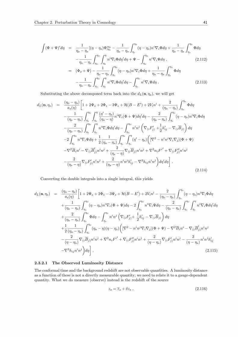
Chapter 2. Perturbation Theory in Cosmology 41
∫(Φ + Ψ)′dη =
1
ηo − ηs[(η − ηs)Φ]ηoηs −
1
ηo − ηs
∫ ηo
ηs
(η − ηs)ni∇iΦdη +1
ηo − ηs
∫ ηo
ηs
Φdη
− 1
ηo − ηs
∫ ηo
ηs
∫ η
ηs
ni∇iΦdη′dη + Ψ−∫ ηo
ηs
ni∇iΨdη , (2.112)
= (Φo + Ψ)− 1
ηo − ηs
∫ ηo
ηs
(η − ηs)ni∇iΦdη +1
ηo − ηs
∫ ηo
ηs
Φdη
− 1
ηo − ηs
∫ ηo
ηs
∫ η
ηs
ni∇iΦdη′dη −∫ ηo
ηs
ni∇iΨdη . (2.113)
Substituting the above decomposed term back into the dL(n, ηs), we will get
dL(n, ηs) =(ηo − ηs)as(η)
[1 + 2Ψo + 2Φs − 3Ψs +H(B − E′) + 2Vin
i +2
(ηo − ηs)
∫ ηo
ηs
Φdη
− 1
(ηo − ηs)
∫ ηo
ηs
∫ η
ηs
(η′ − ηs)(ηs − η)
ni∇i(Φ + Ψ)dη′dη − 2
(ηo − ηs)
∫ ηo
ηs
(η − ηs)ni∇iΦdη
− 2
(ηo − ηs)
∫ ηo
ηs
∫ η
ηs
ni∇iΦdη′dη −∫ ηo
ηs
ninj(∇(iF
′j) +
1
2h′ij −∇(iBj)
)dη
−2
∫ ηo
ηs
ni∇iΨdη +1
2
1
(ηo − ηs)
∫ ηo
ηs
∫ η
ηs
(η′ − ηs)(
[∇2 − ninj∇i∇j ](Φ + Ψ)
−∇2Bini −∇(iB
′j)n
inj +2
(ηs − η)∇(iBj)n
inj +∇2niFi′ +∇(iF
′′j)n
inj
− 2
(ηs − η)∇(iF
′j)n
inj +2
(ηs − η)ninjh′ij −∇2hijn
inj)dη′dη
].
(2.114)
Converting the double integrals into a single integral, this yields
dL(n, ηs) =(ηo − ηs)as(η)
[1 + 2Ψo + 2Φs − 3Ψs +H(B − E′) + 2Vin
i − 2
(ηo − ηs)
∫ ηo
ηs
(η − ηs)ni∇iΦdη
+1
(ηo − ηs)
∫ ηo
ηs
(η − ηs)ni∇i(Φ + Ψ)dη − 2
∫ ηo
ηs
ni∇iΨdη −2
(ηo − ηs)
∫ ηo
ηs
∫ η
ηs
ni∇iΦdη′dη
+2
(ηo − ηs)
∫ ηo
ηs
Φdη −∫ ηo
ηs
ninj(∇(iF
′j)+
1
2h′ij −∇(iBj)
)dη
+1
2
1
(ηo − ηs)
∫ ηo
ηs
(ηo − η)(η − ηs)(
[∇2 − ninj∇i∇j ](Φ + Ψ)−∇2Bini −∇(iB
′j)n
inj
− 2
(η − ηs)∇(iBj)n
inj +∇2niFi′ +∇(iF
′′j)n
inj +2
(η − ηs)∇(iF
′j)n
inj − 2
(η − ηs)ninjh′ij
−∇2hijninj)dη
]. (2.115)
2.3.2.1 The Observed Luminosity Distance
The conformal time and the background redshift are not observable quantities. A luminosity distanceas a function of these is not a directly measurable quantity; we need to relate it to a gauge-dependentquantity. What we do measure (observe) instead is the redshift of the source
zs = zs + δzs , (2.116)
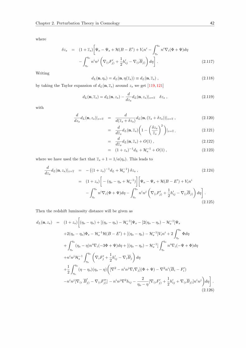
Chapter 2. Perturbation Theory in Cosmology 42
where
δzs = (1 + zs)
[Ψo −Ψs +H(B − E′) + Vin
i −∫ ηo
ηs
ni∇i(Φ + Ψ)dη
−∫ ηo
ηs
ninj(∇(iF
′j) +
1
2h′ij −∇(iBj)
)dη
]. (2.117)
WritingdL(n, ηs) = dL(n, η(zs)) ≡ dL(n, zs) , (2.118)
by taking the Taylor expansion of dL(n, zs) around zs we get [119,121]
dL(n, zs) = dL(n, zs)−d
dzsdL(n, zs)|z=z δzs , (2.119)
with
d
dzsdL(n, zs)|z=z =
d
d(zs + δzs)dL(n, (zs + δzs))|z=z , (2.120)
=d
dzsdL(n, zs)
(1−
(δzszs
)2)|z=z , (2.121)
=d
dzsdL(n, zs) +O(1) , (2.122)
= (1 + zs)−1dL +H−1
s +O(1) , (2.123)
where we have used the fact that zs + 1 = 1/a(ηs). This leads to
d
dzsdL(n, zs)|z=z = −
((1 + zs)
−1dL +H−1s
)δzs , (2.124)
= (1 + zs)
[− (ηo − ηs +H−1
s )
][Ψo −Ψs +H(B − E′) + Vin
i
−∫ ηo
ηs
ni∇i(Φ + Ψ)dη −∫ ηo
ηs
ninj(∇(iF
′j) +
1
2h′ij −∇(iBj)
)dη
].
(2.125)
Then the redshift luminosity distance will be given as
dL(n, zs) = (1 + zs)
[(ηo − ηs) + [(ηo − ηs)−H−1
s ]Ψo − [2(ηo − ηs)−H−1s ]Ψs
+2(ηo − ηs)Φs −H−1s H(B − E′) + [(ηo − ηs)−H−1
s ]Vini + 2
∫ ηo
ηs
Φdη
+
∫ ηo
ηs
(ηs − η)ni∇i(−3Φ + Ψ)dη + [(ηo − ηs)−H−1s ]
∫ ηo
ηs
ni∇i(−Ψ + Φ)dη
+ninjH−1s
∫ ηo
ηs
(∇iF ′j +
1
2h′ij −∇iBj
)dη
+1
2
∫ ηo
ηs
(η − ηs)(ηo − η)
([∇2 − ninj∇i∇j ](Φ + Ψ)−∇2ni(Bi − F ′i )
−ninj [∇(i B′j) −∇(iF
′′j)] − n
inj∇2hij −2
ηo − η[∇(iF
′j) +
1
2h′ij +∇(iBj)]n
inj)dη
].
(2.126)

Chapter 2. Perturbation Theory in Cosmology 43
This equation is the final expression we have got for the luminosity distance [122,123] in a perturbedFriedmann universe in general gauge, as a function of the measured source redshift zs and its directionn. This equation is complicated and contains the angular and redshift fluctuations of the luminositydistance, which may also contain important information about our universe. Nevertheless the matterdistribution and the geometry have fluctuations too, but to first order in perturbation theory thesefluctuations can average out in the mean and are therefore expected to be small.
Part II
44
Chapter 3
Ideal Observational Cosmology
Time is the true driving force ofthe Universe.
Khalid Masood
Cosmological observable quantities, henceforth simply referred to as observables, encode infor-mation about the state of the Universe at a particular cosmological redshift. In our past lightconewe can obtain these observables which can give us our connection to the rest of the Universe. Hencea precise measure of cosmological observables can directly determine the geometry of the observablepart of the spacetime, in the so-called observational approach [124]. Furthermore we can assume adynamical theory for the spacetime curvature of the past lightcone, i.e, GR.
The observations are taken so that we can discover what these observations imply about thelarge-scale structure of the Universe. The idea was first discussed in [103], and Refs. [108, 125–127]discussed the construction of the spacetime metric and ways to determine local matter densityin the Universe directly from astronomical observations on our past lightcone as initial data forthe field equations, and later to establish what is called now the lightcone gauge based on anobservational coordinates set. The main aim was to a great extent that cosmology rather be adirectly observational subject [108]. Therefore, they bring cosmologically interpretable astronomicalobservations into a confrontation with the cosmological theories, to reveal the structure of distantregions in the Universe.
3.1 Observational Coordinates
A lightcone gauge has been constructed and adapted to observations made on the null cone usingobservational coordinates as following. A spacetime consists of a manifold M with metric g. Weshall assume the spacetime filled with a perfect fluid of the form
Tµν = ρuµuν + p(gµν + uµuν) , (3.1)
where Tµν is the stress energy tensor. The first step in constructing a set of observational coordinatesis to identify fundamental observers. The integral curves of the velocity vector uµ and their nor-malised 4-velocity, represent the worldlines of these fundamental observers, i.e, they are comovingwith the galaxies. If τ is the proper time along these worldlines, then
uµ =dxµ
dτ, uµuµ = −1 . (3.2)
45
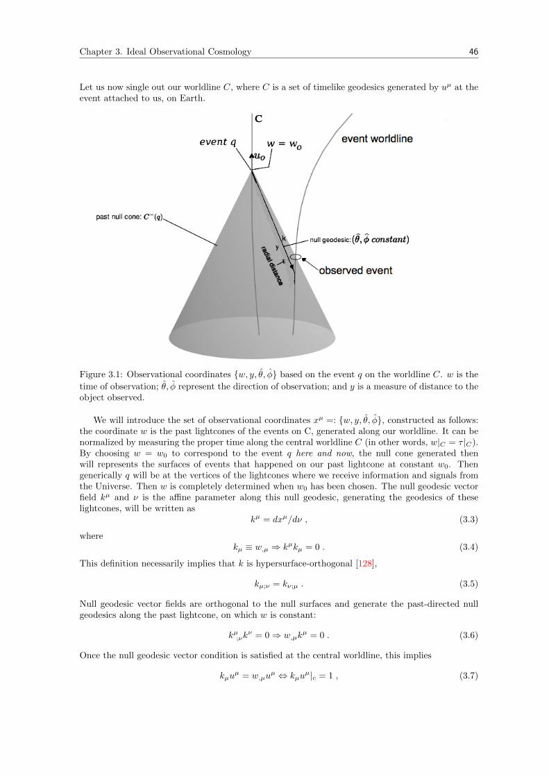
Chapter 3. Ideal Observational Cosmology 46
Let us now single out our worldline C, where C is a set of timelike geodesics generated by uµ at theevent attached to us, on Earth.
Figure 3.1: Observational coordinates w, y, θ, φ based on the event q on the worldline C. w is the
time of observation; θ, φ represent the direction of observation; and y is a measure of distance to theobject observed.
We will introduce the set of observational coordinates xµ =: w, y, θ, φ, constructed as follows:the coordinate w is the past lightcones of the events on C, generated along our worldline. It can benormalized by measuring the proper time along the central worldline C (in other words, w|C = τ |C).By choosing w = w0 to correspond to the event q here and now, the null cone generated thenwill represents the surfaces of events that happened on our past lightcone at constant w0. Thengenerically q will be at the vertices of the lightcones where we receive information and signals fromthe Universe. Then w is completely determined when w0 has been chosen. The null geodesic vectorfield kµ and ν is the affine parameter along this null geodesic, generating the geodesics of theselightcones, will be written as
kµ = dxµ/dν , (3.3)
wherekµ ≡ w,µ ⇒ kµkµ = 0 . (3.4)
This definition necessarily implies that k is hypersurface-orthogonal [128],
kµ;ν = kν;µ . (3.5)
Null geodesic vector fields are orthogonal to the null surfaces and generate the past-directed nullgeodesics along the past lightcone, on which w is constant:
kµ;νkν = 0⇒ w,µk
µ = 0 . (3.6)
Once the null geodesic vector condition is satisfied at the central worldline, this implies
kµuµ = w,µu
µ ⇔ kµuµ|c = 1 , (3.7)
Chapter 3. Ideal Observational Cosmology 47
and this shows that the affine parameter ν is uniquely defined geometrically on the null geodesics,and this defines the central condition. If we specify that ν = 0 on the worldline C, so the event “q”is given by
w = w0 , ν = 0 . (3.8)
The coordinate y measures distances down the null geodesics, and so represents spatial distancefrom “q” [108]. There are various choices of y that might be suitable for different purposes, forexample [108]:
(1) y = ν, the unique affine parameter down the null geodesics through C determined by the centralconditions on C (ν|c = 0, uµkµ|C = 1). The spacetime metric will be simplified, but one losesthe beautiful physical interpretation of observational coordinates;
(2) y = rA, the area distance down the null cones from C;
(3) y = z, galactic redshift observed from C, imposing y=cst along matter worldlines;
(4) y chosen as in one of (1)-(3) on the initial null cone w = w0, and then specified thereafter to becomoving with the fluid; y,µu
µ = 0.
When one of these specific choices has been made, y is uniquely defined on all the null cones. Wewill use such a choice of coordinate y as a coordinate comoving with the fluid, and determined by aunique specification on the initial null cone w = w0. From equations (3.3) and (3.4), and becausew,µk
µ = 0 we will have [108]
kµ = δ0µ , kµ = dxµ/dν = (1/β)δµ1 ⇒ (1/β) = dy/dν for β > 0 , (3.9)
where β is some function that determines the relation of the affine parameter ν to the coordinatey. Eq. (3.9) shows the rate of change of the coordinate y down the null geodesics relative to theaffine parameter ν. β = cst when y is affine parameter; and β → 1 when we choose y = rA asy → 0 [108]. Different values of y with constant values of ν represent an event at the same distance
from q down the null cone in different directions. The coordinates (θ, φ) are angles on the “physical”sky. The observer sees the sky as the superposition of 2-spheres embedded in the lightcone, thenwe can redefine θ, φ as spherical coordinates on the celestial sphere with respect to the (physicallynon-rotating) reference frame eµ
1. They label the geodesics generating the past lightcone (they areconstant along such geodesics) [108]. At a constant surface w, the null-cone geodesics are generated
by constant θ and φ, sokµθ,µ = kµφ,µ = 0 . (3.10)
They are based on a parallelly propagated orthonormal tetrad eµ [108] along C. Then at a constantw and ν,
limν→0
ds2
ν2
∣∣∣∣w=cstν=cst
= dΩ2 = dθ2 + sin2 θdφ2 . (3.11)
These coordinates do not necessarily cover all the spacetime, but they do cover that part which isobservable from the worldline C.
3.2 The Observational Metric
The metric components can be obtained from the previous discussions. From Eqs. (3.4) and (3.9)we see that
kµkµ = 0⇒ w,µgµνw,ν =⇒ g00 = 0 , (3.12)
kµ = gµνkν ⇒ gµ0 = (1/β)δµ1 , (3.13)
1These tetrad vectors eµ are defined through the conditions: (u = e0,u · ei = 0, eiej = δij), and thus satisfy theparallel propagation along C: ∇ueµ|c = 0, with u the velocity of the comoving geodesic observer.
Chapter 3. Ideal Observational Cosmology 48
and thusgµνgνγ = δµγ ⇒ g0νgνγ = δ0
γ ⇒ g1γ = βδ0γ . (3.14)
We can get the general expression for gµν and compute its inverse by introducing new functions forthe non-constrained components. We thus have [108],
gµν =
α β v2 v3
β 0 0 0v2 0 h22 h23
v3 0 h23 h33
, gνγ =
0 1/β 0 0
1/β δ σ2 σ3
0 σ2 h33/h −h23/h0 σ3 −h23/h h22/h
, (3.15)
where
h = det(hIJ) = h22h33 − (h23)2 , (3.16)
δ = −(α+ β(v2σ2 + v3σ3))/β2 . (3.17)
Here we have defined
σ2 = −(v2h33 − v3h23)/βh , (3.18)
σ3 = − (v3h22 − v2h23) /βh , (3.19)
where (I, J) ∈ 2, 32. The angular distance rA can be defined in terms of the proposed functionsabove,
r4A sin2 θ = h = det(hIJ) , fIJ = hIJ/r
2A ⇒ det(fIJ) = sin2 θ , (3.20)
where fIJ give an alternative representation of the quantities hIJ . The metric form above impliesthat the surface w|cst are null surfaces. But it does not, as it stands, guarantee that these nullsurfaces are the past lightcones of the geodesic worldline C. To set this feature, one has to imposesome limits on the behaviour of the metric tensor components near the worldline C [108]. When thecoordinate y is taken to be the affine parameter or the area distance, these essential limits are [108]:
limy→0
α = −1, limy→0
β = 1, limy→0
(vI/y2) = 0, lim
y→0hIJdx
IdxJ/y2 = dΩ2 . (3.21)
When this coordinate y is taken to be the last case (4), from what we obtained above, and by making
a coordinate transformation y′ = y′(w, y, θ, φ), w′ = w, θ′ = θ, φ′ = φ, as y → 0, one finds the limitsare found to be [108]
limy→0
α = −1 , limy→0
β = β0(w, xI) , limy→0
vI = 0 , limy→0
hIJdxIdxJ/y2 = β2
0dΩ2 . (3.22)
These limits we just introduced guarantee the necessary conditions to make the null hypersurfaces tobe the past lightcones of observer of the worldline C. Finally we can say that we have observationalcoordinates if and only if the metric tensor components obey Eqs. (3.15) and (3.21) [108].
Now we could characterise the cosmological quantities on the null cone at w = w0 down tosome distance y∗, and with the knowledge of the following: the metric tensor components gµν =α, β, vI , hIJ, the matter 4-velocity components uµ, the total number density n of the sources, andthe radiation density ρrad at each point of the null cone. Assuming the equation of state of thematter is known from local astronomical observations, knowledge of n will determine the local restmass density of matter ρm at each point and the isotropic pressure pm will be determined, and sothe matter contribution to the total stress tensor will be known [108].
3.3 The Perturbed Lightcone Gauge
The Perturbed Lightcone Gauge (PLG) is a gauge built on our understanding of the observationalcoordinates that we introduced in Sec. 3.1. The PLG links the perturbed variables (α, β, vI , hIJ)
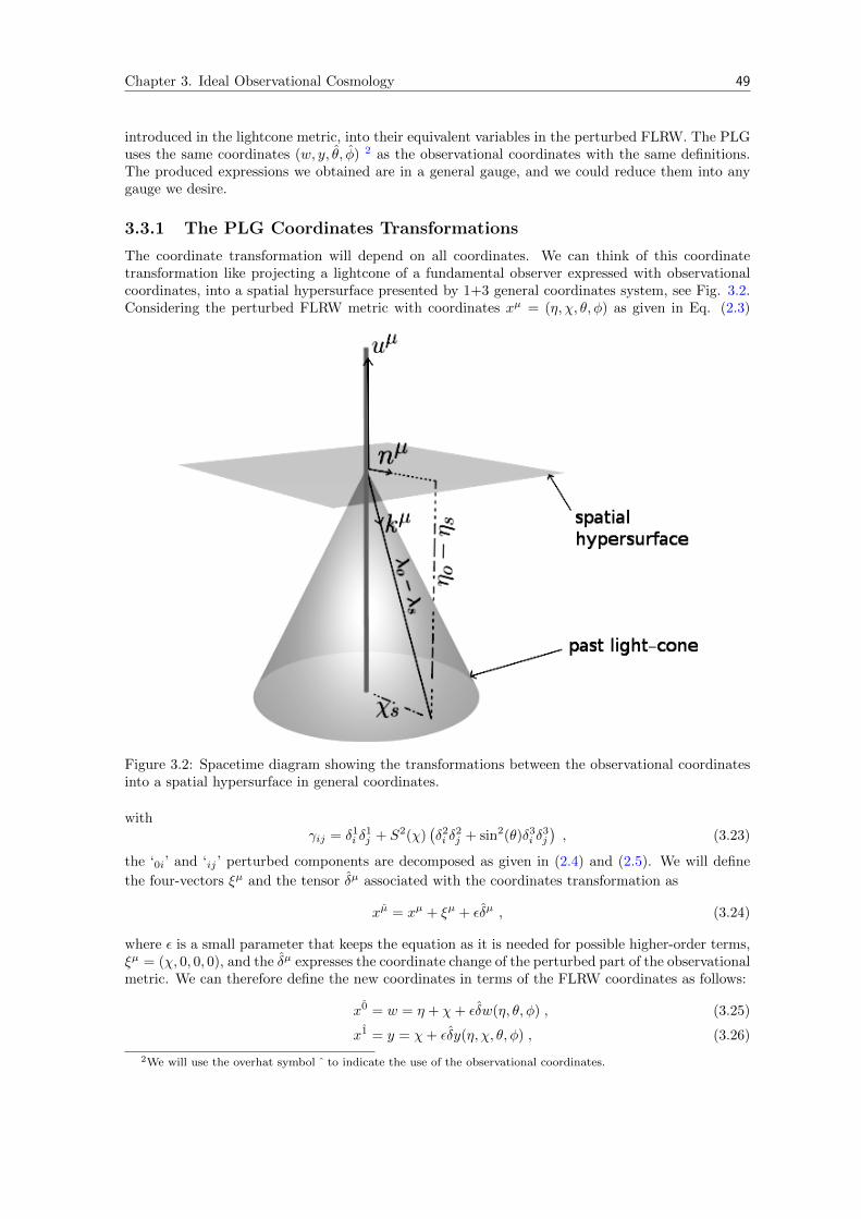
Chapter 3. Ideal Observational Cosmology 49
introduced in the lightcone metric, into their equivalent variables in the perturbed FLRW. The PLGuses the same coordinates (w, y, θ, φ) 2 as the observational coordinates with the same definitions.The produced expressions we obtained are in a general gauge, and we could reduce them into anygauge we desire.
3.3.1 The PLG Coordinates Transformations
The coordinate transformation will depend on all coordinates. We can think of this coordinatetransformation like projecting a lightcone of a fundamental observer expressed with observationalcoordinates, into a spatial hypersurface presented by 1+3 general coordinates system, see Fig. 3.2.Considering the perturbed FLRW metric with coordinates xµ = (η, χ, θ, φ) as given in Eq. (2.3)
Figure 3.2: Spacetime diagram showing the transformations between the observational coordinatesinto a spatial hypersurface in general coordinates.
withγij = δ1
i δ1j + S2(χ)
(δ2i δ
2j + sin2(θ)δ3
i δ3j
), (3.23)
the ‘0i’ and ‘ij ’ perturbed components are decomposed as given in (2.4) and (2.5). We will define
the four-vectors ξµ and the tensor δµ associated with the coordinates transformation as
xµ = xµ + ξµ + εδµ , (3.24)
where ε is a small parameter that keeps the equation as it is needed for possible higher-order terms,ξµ = (χ, 0, 0, 0), and the δµ expresses the coordinate change of the perturbed part of the observationalmetric. We can therefore define the new coordinates in terms of the FLRW coordinates as follows:
x0 = w = η + χ+ εδw(η, θ, φ) , (3.25)
x1 = y = χ+ εδy(η, χ, θ, φ) , (3.26)
2We will use the overhat symbol ˆ to indicate the use of the observational coordinates.
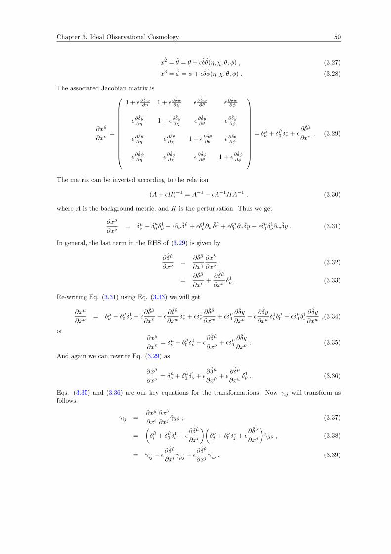
Chapter 3. Ideal Observational Cosmology 50
x2 = θ = θ + εδθ(η, χ, θ, φ) , (3.27)
x3 = φ = φ+ εδφ(η, χ, θ, φ) . (3.28)
The associated Jacobian matrix is
∂xµ
∂xν=
1 + ε∂δw∂η 1 + ε∂δw∂χ ε∂δw∂θ ε∂δw∂φ
ε∂δy∂η 1 + ε∂δy∂χ ε∂δy∂θ ε∂δy∂φ
ε∂δθ∂η ε∂δθ∂χ 1 + ε∂δθ∂θ ε∂δθ∂φ
ε∂δφ∂η ε∂δφ∂χ ε∂δφ∂θ 1 + ε∂δφ∂φ
= δµν + δµ0 δ
1ν + ε
∂δµ
∂xν. (3.29)
The matrix can be inverted according to the relation
(A+ εH)−1 = A−1 − εA−1HA−1 , (3.30)
where A is the background metric, and H is the perturbation. Thus we get
∂xµ
∂xν= δµν − δ
µ0 δ
1ν − ε∂ν δµ + εδ1
ν∂w δµ + εδµ0 ∂ν δy − εδ
µ0 δ
1ν∂w δy . (3.31)
In general, the last term in the RHS of (3.29) is given by
∂δµ
∂xν=
∂δµ
∂xγ∂xγ
∂xν, (3.32)
=∂δµ
∂xν+∂δµ
∂xwδ1ν . (3.33)
Re-writing Eq. (3.31) using Eq. (3.33) we will get
∂xµ
∂xν= δµν − δ
µ0 δ
1ν − ε
∂δµ
∂xν− ε ∂δ
µ
∂xwδ1ν + εδ1
ν
∂δµ
∂xw+ εδµ0
∂δy
∂xν+ ε
∂δy
∂xwδ1νδµ0 − εδ
µ0 δ
1ν
∂δy
∂xw,(3.34)
or∂xµ
∂xν= δµν − δ
µ0 δ
1ν − ε
∂δµ
∂xν+ εδµ0
∂δy
∂xν. (3.35)
And again we can rewrite Eq. (3.29) as
∂xµ
∂xν= δµν + δµ0 δ
1ν + ε
∂δµ
∂xν+ ε
∂δµ
∂xwδ1ν . (3.36)
Eqs. (3.35) and (3.36) are our key equations for the transformations. Now γij will transform asfollows:
γij =∂xµ
∂xi∂xν
∂xjγµν , (3.37)
=
(δµi + δµ0 δ
1i + ε
∂δµ
∂xi
)(δνj + δν0 δ
1j + ε
∂δν
∂xj
)γµν , (3.38)
= γij + ε∂δµ
∂xiγµj + ε
∂δν
∂xjγiν . (3.39)
Chapter 3. Ideal Observational Cosmology 51
Applying Eq. (3.33), one can rewrite this as
γij = γij + ε
(∂δµ
∂xi+∂δµ
∂xwδ1i
)γµj + ε
(∂δν
∂xj+∂δν
∂xwδ1j
)γiν . (3.40)
At the background we can writeξµ = xµ − xµ. (3.41)
Hence we have the following:
∂ξµ
∂xν=
∂ξµ
∂xγ∂xγ
∂xν, (3.42)
= δµ0 δ1γ
(δγν − δ
γ0 δ
1ν − ε
∂δγ
∂xν+ εδγ0
∂δy
∂xν
), (3.43)
= δµ0 δ1ν − δ
µ0 ε∂δy
∂xν. (3.44)
And finally, the metric tensor gµν transforms as
gµν =∂xγ
∂xµ∂xσ
∂xνgγσ . (3.45)
These transformations are valid up to first order. Note that γij is a zeroth-order term. The newmetric elements are then: (we will stop writing ε for simplicity)
gww = a2(w − y)
[− 1− 2
(φ− ∂w δw + ∂w δy
)], (3.46)
gwi = a2(w − y)
[δ1i + 2φδ1
i +Bi + ∂iδw − ∂iδy − δ1i ∂w δw + δ1
i ∂w δy − γij∂w δj
], (3.47)
gij = a2(w − y)
[γij − δ
1i δ
1j − 2φδ1
i δ1j − 2δ1
(i∂j)δw + 2δ1(j∂i)δy − 2B(iδ
1j) + 2Cij − 2γ
k(i∂j)δ
k
].
(3.48)
Let us now introduce the definitions for the perturbed metric elements:
δg00 = δα = −2(φ− ∂w δw + ∂w δy
), (3.49)
δg01 = δβ = 2φ+Bχ + ∂y δw − ∂y δy − ∂w δw , (3.50)
δg0I = vI = BI + ∂I δw − ∂I δy − γIJ∂w δJ , (3.51)
δg11 = 0 = −2φ− 2∂y δw − 2Bχ + 2Cχχ , (3.52)
δg1I = 0 = −∂I δw + ∂I δy −BI + 2C1I − 2γk(1∂I)δk , (3.53)
δgIJ = HIJ = 2CIJ − 2γK(I∂J)δK , (3.54)
with (I, J,K) ∈ 2, 32. The perturbed metric describes the past lightcone in the observational
coordinates xa = (w, y, θ, φ) given by
ds2 = a2(w − y)[(−1 + δα)dw2 + 2(1 + δβ)dwdy + 2vIdx
Idw + hIJdxIdxJ
]. (3.55)
The tensor hIJ =(ΩIJ +HIJ
), where ΩIJ = S2(y)
(δ2Iδ2J
+ sin2(θ)δ3Iδ3J
), is a spatial tensor given
by
hIJ =
(Ωθθ +Hθθ Hθφ
Hθφ Ωφφ +Hφφ
). (3.56)
Chapter 3. Ideal Observational Cosmology 52
We can further split the tensor hIJ into trace HT and traceless parts H, where
HT = Hθθ +1
sin2 θHφφ , (3.57)
is the trace of the perturbed hIJ on the 2-sphere. Eqs. (3.52) and (3.53) are constrains that definethe observational metric.
3.3.2 The PLG Four-velocity
We will use the uµ as the perturbed 4-velocity of a fundamental observer in the observationalcoordinates, which is defined by
uµ =(uw, ui
), (3.58)
where
ui =vi
a(w − y). (3.59)
The full perturbed 4-velocity is given by
uµ =1
a(w − y)
((1 + δuw), δuy, δuθ, δuφ
). (3.60)
Expanding terms out using the Einstein summation rule with Eq. (3.2), yields
g00u0u0 + 2g01u
0u1 + 2g0Iu0uI + gIJu
IuJ = −1 , (3.61)
and therefore, using the expressions for the components of the metric tensor from the precedingsection, we get
(−1 + δα)(1 + δu0)2 + 2(1 + δβ)(1 + δu0)δu1 +
2vI(1 + δu0)δuI + (ΩIJ +HIJ) δuIδuJ = −1 . (3.62)
Further simplifying gives− 2δu0 + δα+ 2δu1 = 0 , (3.63)
whence we can conclude
δu0 = δu1 +δα
2. (3.64)
It is now easy to see that using lowering operation on the indices uµ = gµνuν , the zeroth component
of the covariant 4-velocity is given by
u0 = g00u0 + g01u
1 + g0IuI , (3.65)
= a(−1 + δα− δu0 + δu0 − δα
2) , (3.66)
= a(−1 +δα
2) , (3.67)
where we have used Eq. (3.64) in the last two steps. Thus,
u0 =1
a(1 + δα/2) . (3.68)
Moreover,
u1 = g10u0 + g11u
1 + g1IuI , (3.69)
= a(1 + δβ + δu0) , (3.70)
Chapter 3. Ideal Observational Cosmology 53
and finally,
uI = gI0u0 + gI1u
1 + gIJuJ , (3.71)
= a(vI + ΩIJδuJ) . (3.72)
3.3.3 Connecting the Perturbations δµ with the Perturbed FLRW
To determine the local structure of the Universe, we wish to know the values of δµ, where it isalways labeled with the observation coordinates µ = w, y, θ, φ, and we can do that directly via thedefinition of the kµ in observational coordinates given by Eq. (3.9). The most important thing hereis that in order to calculate the null vector kµ in the observational coordinates, we do not have tofollow the long procedure we did in calculating the null vector kµ in 1+3 general coordinates systemin Sec. 2.2.2. However we can reach the same result if we do so. From Eq. (B.5) at the backgroundand Eq. (3.9), where we defined β = (1 + δβ) ,we can write
kµ = a−2(1− δβ)δµy . (3.73)
It is to be recalled that kµ = dxµ/dλ where λ is the affine parameter with dλ = a−2dη anda2 d
dλ = ∂∂η + ∂
∂χ . Thus we can write
kw = 0 =dw
dλ, (3.74)
=dη
dλ+dχ
dλ+dδw
dλ, (3.75)
= kη + kχ +dδw
dλ, (3.76)
from which
δw = −∫
(kη + kχ)dλ . (3.77)
Similarly,
ky = a−2(1− δβ) =dy
dλ, (3.78)
a−2(1− δβ) =dχ
dλ+dδy
dλ, (3.79)
and hence
−δβa2
=dδy
dλ. (3.80)
This leads to
δy = −∫ (
δβ
a2
)dλ = −
∫δβdη . (3.81)
And for δI ≡ (δθ, δφ), where I ∈ 2, 32,
kI = 0 =dI
dλ, (3.82)
=dI
dλ+dδI
dλ, (3.83)
and therefore
δI = −∫kIδIIdλ . (3.84)
Chapter 3. Ideal Observational Cosmology 54
Here we connected the perturbations of the observational metric with the perturbations of theperturbed FLRW metric. Applying all the above into the constrain Eq. (3.52) we get
0 = −φ−Bχ + Cχχ − ∂y δw , (3.85)
0 = −φ−Bχ + Cχχ + ∂y
∫(kη + kχ)dλ . (3.86)
We can use the facts that
∂
∂y|w=cst =
∂
∂η|χ=cst +
∂
∂χ|y=cst =
d
dη, (3.87)
∂
∂w|y=cst =
∂
∂η|χ=cst , (3.88)
which means that y mimics the behaviour of the affine parameter along the light ray. And we candefine also the identity
kη + kχ =1
a2
(nχ(φ+ ψ) +Bχ + nχ∂χ∂
χE + nχ∂χFχ + nχ
1
2h χχ
). (3.89)
This result makes use of the null geodesic equations (2.71) and (2.73). Therefore, we see that thevery definition of the observable coordinates via the relation ka = β−1δay ensures that the metrichas the correct form again.
3.4 Einstein Field Equations in the PLG
Using our observational metric (3.55) to calculate the 10 partial differential equations of the EFEs,we are going to consider a cosmological fluid with
∂wp ≡ ωρ⇒ ρ ≡ −3H(1 + ω)ρ ≡ −∂yp , (3.90)
where H = ∂wa/a and H = −∂ya/a. We also note the following useful relations:
∂2wa
a= −∂wH+H2 , (3.91)
∂2ya
a= ∂yH+H2. (3.92)
Then at the background the EFEs read:
E(0)ww = 3H2 + 3k − 8πGa2ρ− a2Λ = 0 , (3.93)
E(0)wy = −3H2 − 3k + 8πGa2ρ+ a2Λ = 0 , (3.94)
E(0)yy = −2Hp+ 2H2 − 8πGa2ρ+ 2k − 8πGa2p = 0 , (3.95)
E(0)θθ = S2H2 − S2k + a2ΛS2 − 2S2(Hp+H2)− 8πGa2S2p = 0 , (3.96)
E(0)φφ = S2 sin2(θ)H2 − S2 sin2(θ)k − 8πGa2S2 sin2(θ)p+ a2ΛS2 sin2(θ)
−2S2 sin2(θ)(Hp+H2) = 0 , (3.97)
andE
(0)wθ = E
(0)wφ = E
(0)θφ = E
(0)yθ = E
(0)yφ = 0 . (3.98)
We have calculated the 10 equations using the observational metric (3.55). As we can see, at thebackground the EFEs satisfy the observational metric justification.
We are going to derive the dynamical equations of the perturbations in observational coordinates.

Chapter 3. Ideal Observational Cosmology 55
In order to simplify the system we need to use the spherical decomposition dynamics, as follows:
δρ(w, y) =+∞∑l=0
l∑m=−l
[δρlm(w, y)Y lm(I)
], (3.99)
δu0(w, y) =+∞∑l=0
l∑m=−l
[δulm0 (w, y)Y lm(I)
], (3.100)
δα(w, y) =+∞∑l=0
l∑m=−l
[δαlm(w, y)Y lm(I)
], (3.101)
δβ(w, y) =+∞∑l=0
l∑m=−l
[δβlm(w, y)Y lm(I)
], (3.102)
vI(w, y, I) =+∞∑l=1
l∑m=−l
[vlm(w, y)Y lmI (I) + vlm(w, y)Y
lm
I (I)
], (3.103)
δuI(w, y, I) =+∞∑l=1
l∑m=−l
[δulm(w, y)Y lmI (I) + δu
lm(w, y)Y
lm
I (I)
], (3.104)
HIJ(w, y, I) =1
2
+∞∑l=0
l∑m=−l
HTlm(w, y)γIJY
lm(I) ++∞∑l=2
l∑m=−l
[H lm(w, y)Y lmIJ (I)
+Hlm
(w, y)Ylm
IJ (I)
], (3.105)
to enable us to decompose them harmonically and produce functions suitable for the extraction ofobservational quantities, see Sec. A.2 for more details. Using the above definitions and a Maplecode we calculated the 10 equations using the observation metric (3.55). The conservation equations∇µTµx , where x : w, y, I are given by
(1) ∇µTµw =
[− (1 + ω)ρ
(1
2∂wH
T + ∂wδu0 + ∂wβ − l(l + 1)δu
)− ∂wδρ
−3H(1 + ω)δρ
]Y = 0 , (3.106)
(2) ∇µTµy =
[− 2
3a(4− 3ω)ρδu0 − (1 + ω)ρ
(∂yδu
0 − 2∂wδu0
)+ a(−1
3+ ω)ρβ
+2(1 + ω)ρ∂wβ +1
2(1 + ω)ρ∂wH
T + (1 + ω)∂wδρ+ ω∂yδρ
+3H(1 + ω)δρ− ρ(1 + ω)l(l + 1)δu
]Y = 0 , (3.107)
(3) ∇µTµI =
[S2(1 + ω)ρ∂wδu+ S2
(ωρ− 16πGa2(1 +
1
3)ωρ+ 4Hρ
)δu
+(1 + ω)ρ∂wv +
(ωρ− 16πGa2(1 +
1
3)ωρ+ 4Hρ
)v
]Y I
+
[− (1 + ω)ρδu0 + S2(1 + ω)ρ∂wδu+ S2
(ωρ− 16πGa2(1 +
1
3)ωρ
)+4Hρδu+ (1 + ω)ρ∂wv +
(ωρ− 16πGa2(1 +
1
3)ωρ+ 4Hρ
)v
Chapter 3. Ideal Observational Cosmology 56
+ωδρ
]YI = 0 . (3.108)
We also substituted for the scalar δα by the vector δuw using Eq. (3.68). Since our observer iscomoving with the matter, we can consider u1 = dy
dτ = 0, where τ is the matter proper time. Andthe field equations are:
(4) EIJ =
[∂yv − 2Hv − 2S2∂2
wyH − S2∂2yH + 2(S2H− S(1− S2k)
12 )∂wH
−2S(1− S2k)12 ∂yH
]Y IJ +
[− 2β + 2∂yv − 4Hv − 2S2∂2
wyH − S2∂2yH
+2(S2H− S(1− S2k)12 )∂wH − 2S(1− S2k)
12 ∂yH
]YIJ = 0 , (3.109)
(5) EII =
[8S2
((1− S2k)
12
SH+ 4πGa2ωρ− 1
2Λa2
)δu0 + (8S2H− 4S(1− S2k)
12 )∂yδu
0
−2S2∂2yδu
0 + (4SH(1− S2k)12 + 4S2k)β + (4S2H− 2S(1− S2k)
12 )∂yβ
+2S2∂2wyβ + 2S2∂2
wyHT +
1
2S2∂2
yHT + 2(−S2H+ S(1− S2k)
12 )∂wH
T
+2S(1− S2k)12 ∂yH
T − 16πGa2S2ωδρ− l(l + 1)β + l(l + 1)∂yv
−2Hl(l + 1)v
]Y = 0 , (3.110)
(6) EwI =
[16πGS4a2(1 + ω)ρδu+ l(l + 1)v − S2∂2
wyv − S2∂2yv + 2S(1− S2k)
12 ∂wv
+(16πGS2(1 + ω)ρa2 − 4S2k)v + (2− l(l + 1))S2∂wH
]Y I
+
[2S2∂yδu
0 − 4HS2δu0 + 16πGS4a2(1 + ω)ρδu− S2∂wβ + S2∂yβ
−S2∂2wyv − S2∂2
yv + 2S(1− S2k)12 ∂wv +
(16πGS2(1 + ω)ρa2 − 4S2k
)v
−1
2S2∂wH
T +1
2S2∂wH(2− l(l + 1))
]YI = 0 , (3.111)
(7) EyI =
[− 2HS2∂yv +
(− 2 + 4SH(1− S2k)
12 − 16πGS2(1 + ω)ρa2
)v
+S2∂2yv − 16πGS4a2(1 + ω)ρδu+ (2− l(l + 1))S2∂yH
]Y I
+
[− 2HS2∂yv +
(− 2 + 4SH(1− S2k)
12 − 16πGS2(1 + ω)ρa2
)v
+S2∂2yv − 16πGS4a2(1 + ω)ρδu− S2∂yβ − 2S(SH− (1− S2k)
12 )β
−1
2S2∂yH
T +1
2(2− l(l + 1))S2∂yH
]YI = 0 , (3.112)
Chapter 3. Ideal Observational Cosmology 57
(8) Eyy =
[− 32πGSa2(1 + ω)ρδu0 − 32πGSa2(1 + ω)ρβ − 16πGa2S(1 + ω)δρ
−4(SH− (1− S2k)12 )∂yβ − S∂2
yHT − 2(1− S2k)
12 ∂yH
T
]Y = 0 , (3.113)
(9) Ewy =
[16πGS3a2(1 + ω)ρδu0 − 4S(1− 4SH(1− S2k)
12 + S2Λa2
−4S2k + 4πGS2(1 + ω)ρa2)δu0 + 4S2(SH− (1− S2k)12 )∂yδu
0
−4S(1− 2SH(1− S2k)12 − 2S2k)β − Sl(l + 1)β + 16πGS3a2(1 + ω)ρβ
+4S2(SH− (1− S2k)12 )∂yβ + 16πGS3a2δρ− Sl(l + 1)∂yv
−4(SH− 1
2(1− S2k)
12 )l(l + 1)v + S3∂2
yHT + S3∂2
wyHT
+SHT +9
2(1− S2k)
12S2∂yH
T − 2S2(SH− (1− S2k)12 )∂wH
T
−1
2Sl(l + 1)HT − S l
2(l + 1)2
2H + Sl(l + 1)H
]Y = 0 , (3.114)
(10) Eww =
[4S
(1− 4SH(1− S2k)
12 + (Λ + 8πGρ)S2a2 − 6S2k
)δu0
+2Sl(l + 1)δu0 − 4S2
(SH− (1− S2k)
12
)∂wδu
0
−4S2
(2SH− (1− S2k)
12
)∂yδu
0 − 16πGa3S2δρ+ 2Sl(l + 1)β
+4S2(1− S2k)12 ∂wβ − 4S2
(SH− (1− S2k)
12
)∂yβ
−4S
(3S2k + 2SH(1− S2k)
12 − 1
)β − 2Sl(l + 1)∂yv − 2Sl(l + 1)∂wv
+2(2SH− (1− S2k)12 )l(l + 1)v − S3∂2
wHT − S3∂2
yHT − 2S3∂2
wyHT
−SHT − 9
2S2(1− S2k)
12 ∂yH
T + 2S2(SH− (1− S2k)12 )∂wH
T
+1
2Sl(l + 1)HT + S
l2(l + 1)2
2H − Sl(l + 1)H
]Y = 0 . (3.115)
Here we have used ∂2yS(y) = −S(y)k, and
(∂yS(y))2
S(y)2=
1
S(y)2− k . (3.116)
The perturbed observational metric has the 10 degrees of freedom: 3 from the scalar (δβ, δρ, δu0), 2from the vector vI , 2 from the vector δuI and 3 from the tensor HIJ . More work in the future willbe added to the calculated first-order EFE in the PLG metric.

Chapter 3. Ideal Observational Cosmology 58
Figure 3.3: Illustration of the GLC coordinates of an inhomogeneous lightcone parametrized by GLCcoordinates: The observer sees the sky as the superposition of 2-spheres [11].
3.5 The Geodesic Lightcone Gauge
The Geodesic Lightcone Gauge (GLC) has been introduced and discussed in detail in [129–134],where they introduced a lightcone metric close to the observational coordinates and it has its dif-ferences from the observational coordinates as well. Their metric consists of 6 arbitrary functions(Υ, Ua, γab) [11]. It is totally gauge fixed, with a specially adapted coordinate system correspondingto constant-time hypersurfaces, xµ = (w, τ, θa) where a = 1 , 2, and τ is a coordinate to describethe proper time measured by an observer in geodesic motion. Its line element is given by
ds2GLC = Υ2dw2 − 2Υdwdτ + γab(dθ
a − Uadw)(dθb − U bdw) , (3.117)
w representing a null coordinate defining past light cones, where (∂µw∂µw = 0), with an observer
moving with a proper time τ along her geodesic. Υ is an inhomogeneous scale factor, Ua is a shift-vector, and the symmetric 2 × 2 matrix γab is the metric inside Σ(w, τ). The angles θa are theangles were the photons keep their path orthogonal to a 2-sphere Σ(w, τ) of constant time in ourpast lightcone. The ∂µτ defines a geodesic flow [129]
(∂ντ)∇ν(∂µτ) = 0 . (3.118)
Then we can obtain gττGLC=-1. The metric and its inverse will take the form
gGLCµν =
0 −Υ−→0
−Υ Υ2 + U2 −Ub−→0T
−UTa γab
, gνγGLC =
−1 −Υ−1 −U b/Υ−Υ−1 0 0
−(Ua)T /Υ−→0T
γab
, (3.119)
where−→0 = (0, 0) and Ub = (U1, U2). With g ≡ detgGLCµν , and γ ≡ detγab, we get
√−g = Υ
√|γ| . (3.120)
This GLC metric has the 6 degrees of freedom to describe the geometry of spacetime.For flat FLRW metric, the transformation into GLC coordinates and the meaning of the metric
Chapter 3. Ideal Observational Cosmology 59
components are easily obtained from Eq. (3.119):
τ = t , w = r + η , θ1 = θ , θ2 = φ , (3.121)
Υ = a(t) , Ua = 0 , γabdθadθb = a2(t)r2(dθ2 + sin2 θdφ2) , (3.122)
where r is defined from (1.11). The constant τ and constant w hypersurfaces intersect each otheron 2-dimensional surface (w0, τs), see Fig. [3.3]. Notice that this 2-sphere can be expressed in aconstant redshift hypersurface [129], where it corresponds to the constant Υ hypersurface on thepast lightcone.
To measure the distance from the observer down to the object in the GLC we need to calculatethe differences between the observer proper time and the object proper time.
τ =
∫ τo
τs
dτ ′ . (3.123)
To move from GLC gauge to the PLG gauge simply by applying the coordinates transformationsusing Eqs. (3.35) and (3.36) that we have mentioned earlier.
3.6 Differences Between the PLG and the GLC
We can summarise the differences between the PLG and the GLC as follows:
• The PLG uses the observational coordinates (w, y, θ, φ), whereas the GLC metric uses (τ, w, θa),the first two coordinates has created the main difference between the two gauges.
• The y coordinate in the PLG represents a spatial radial distance or a null distance down thelightcone. But in GLC the y coordinate has been replaced by the proper time coordinate τand the differences on the proper time of the event crossing the null cone and the fundamentalobserver moving along its worldline represent the distance down the null cone. And by thisdistance replacement definitions they will enhance the significance of the GLC gauge to havea coordinate system both adapted to the observations of the source and the proper time of theobserver [135].
• An important difference is that the GLC gauge corresponds to a complete ‘gauge fixing’ of theobservational coordinates. We can describe the GLC gauge as a ‘gauge fixing’ with 6 degreesof freedom, unlike the PLG gauge which is expressed in a general gauge with 10 degrees offreedom.
• The PLG gauge of the observational coordinates is set by the condition w = τ |C , where τ isthe proper time of the observer. On the other hand, in the GLC gauge the lightcone set byw =
∫dτ/a(τ) ≡ η, where a(τ) is defined as the homogeneous limit of the Υ function.
• Both gauges break down when caustics appear down on the past lightcone [108,135].
• The GLC is well adapted to computations of quantities related to light signals, to simplify theso-called averaging on the lightcone [135].
Chapter 4
Observables in the Past Lightcone Gauge
To go wrong in one’s own way isbetter than to go right insomeone else’s.
Fyodor Dostoyevsky
We are going to present here the observables that we can measure on our past lightcone. Byusing the observational coordinates (w, y, θ, φ) introduced in Ch 3, then we are going to get a setof observables defined by the PLG parameters, where they are more simple but different definitionsfrom what we introduced in Sec. 2.3. To justify our observables that can cover the perturbed FLRWlimits, we need to transfer them from the PLG gauge on the lightcone into 1+3 general gauge ona hypersurface that is orthogonal to the observer 4-velocity and described by a perturbed FLRWmetric. In order to do so we need to understand the screen space lying on the hypersurface.
4.1 The Screen Space
We are going to show how the covariant description of light beams, are naturally defined and theycan be turned to a more observation-oriented description. This requires to introduce a notion ofscreen, on which observers can project the beam and characterise its shape and extension. Thescreen space is orthogonal to the observer 4-velocity, and the tensor [120]
Nµν = gµν + uµuν − nµnν (4.1)
projects quantities into the screen space and satisfies the following conditions [120]:
Nµµ = 2, NµαN
αν = Nµν , Nµνk
µ = Nµνuµ = Nµνn
µ = 0 . (4.2)
4.1.1 Derivatives and Integrals in the Screen Space
We can isolate the components into parallel and orthogonal components to the light ray. We denotethe parts lying in the screen space by ⊥ and the parts parallel to it by ‖. Furthermore, let us definethe covariant angular derivative ∇⊥i on the screen space and the derivative ∇‖ along the directionof observations, respectively, as [120,136]
∇⊥iXj ≡ (γ ki − nink)(γ l
j − njnl)∇⊥kXl , (4.3)
60
Chapter 4. Observables in the Past Lightcone Gauge 61
∇‖ ≡ ni∇iX . (4.4)
The radial derivative can be interchanged with the derivative along a null geodesic using therelation
∇‖X = ∂ηX −d
dλX . (4.5)
At the background, one can switch the affine parameter λ with the conformal time η, and both arerelated to the radial distance along the past lightcone by χ = λo − λ = ηo − η = η− ηs. The spatialderivative is in general decomposed into parts along the null geodesic and in the screen space as
∇i = ni∇‖ +∇⊥i , (4.6)
= ni(∂η −d
dη) +∇⊥i . (4.7)
Then the 3-D Laplacian on the Minkowski background becomes
∇2 = γij [nj∇‖ +∇⊥j ][ni∇‖ +∇⊥i ] , (4.8)
= γij [ninj∇2‖ + nj∇‖∇⊥i +∇⊥j [ni∇‖] +∇⊥i∇⊥j ] , (4.9)
= γij [ninj∇2‖ + nj∇⊥i∇‖ +∇⊥jni∇‖ + ni∇⊥j∇‖ +∇⊥i∇⊥j ], (4.10)
= γij [ninj∇2‖ + n(i∇⊥j)∇‖ +∇⊥jni∇‖ +∇⊥i∇⊥j ] , (4.11)
= ∇2‖ + γij∇⊥jni∇‖ +∇2
⊥ , (4.12)
where [120]
∇⊥inj =1
λo − λ(γij − ninj) =
1
χ(γij − ninj) . (4.13)
This leads to the relation
∇2 = ∇2‖ +
2
χ∇‖ +∇2
⊥ , (4.14)
which can also be rewritten as
∇2⊥ = −ninj∇i∇j −
2
ηo − ηni∇i +∇2 . (4.15)
Since the radial derivative can be interchanged with the derivative along a null geodesic [120], onecan write
ni∇inj∇jX = ∇2‖ = ∇‖(∇‖X) , (4.16)
= (X ′′ − dηX ′)− dη(X ′ − dηX) , (4.17)
= X ′′ − 2dηX ′ − d2ηX , (4.18)
and we can conclude that
∇i∇j = ninj∇2‖ + 2n(i∇⊥j)∇‖ +
1
χ(γij − ninj)∇‖ +∇⊥i∇⊥j . (4.19)
4.1.2 Screen Space and SVT Decompositions
We can decompose a spatial vector vi that is orthogonal to the 4-velocity uµ on a perturbed spacetimeinto [120]
vi = niv‖ + vi⊥ , (4.20)
wherev‖ = njv
j , vi⊥ = N ijvj . (4.21)

Chapter 4. Observables in the Past Lightcone Gauge 62
And for a symmetric trace-free spatial tensor hij , the screen space decomposition will look like
hij = h‖(ninj −1
2Nij) + 2h⊥|(inj) + h⊥ij , (4.22)
whereh⊥ij = Nk
i Nljhkl, h⊥|(inj) = Nk
(inj)nlhkl , (4.23)
andhi⊥|ni = 0 = nih
ij⊥ = Nijh
ij⊥ . (4.24)
4.2 The Redshift of Distant Galaxies in the PLG
The distance-redshift relations for far-away cosmological objects play an important role in cosmology.It has led to the discovery of the expansion of the Universe [137] and later on to the discovery of itsaccelerated expansion [138].
Figure 4.1: A time interval dτ at the observed galaxy is measured as a time interval dw by theobserver.
The redshift of a source crossing the lightcone is the time dilation observed from C(w, y, θ, φ) ofa source of a proper time τ along its worldlines, crossing our past lightcone is determined by theratio dw/dτ along our worldline. Using the relations (3.4) and (4.25), then the observed redshift zof its emitted light is determined by
1 + z =λoλs
=ac(w)
a(w, y)=dw
dτ= uw , (4.25)
where ac(w) is the scale factor along the central worldline C at singular point w0|C (it can be taken
Chapter 4. Observables in the Past Lightcone Gauge 63
equal to 1 today). Or we can use the expression
1 + z =(kµuµ)s(kµuµ)o
, (4.26)
where we can normalise (kµuµ)o = 1, and we can re-write (4.26) as
1 + z = (kµuµ)s, (4.27)
using (3.4) again, we will get
1 + z = (δ0µu
µ)s , (4.28)
= (uw)s . (4.29)
This shows that in the lightcone gauge the redshift of the source is its 4-velocity. Where the 4-velocity of the source is directly observable because the redshift is directly measurable from theobserved source spectrum. Furthermore
ui =dxi
dτ= (1 + z)
dxi
dw. (4.30)
And we can obtain the velocity components uµ = gµνuν using (3.15) [108].
4.2.1 Gauge Transformations of the Redshift
To show that Eq. (4.29) is fulfilling the right form of redshift in the standard model we need totransform our result using the PLG to first-order perturbation. Using the coordinates transforma-tions mentioned in the previous chapter, we can transform the uη of Eq. (2.35) into uw using thecoordinate transformations given by Eq. (3.36), getting
1 + z = uw =dxw
dxaua , (4.31)
=dxw
dxηuη +
dxw
dxiui , (4.32)
=1
a(w − y)
(δ00 +
∂δw
∂xw
)(1− φ
)+
1
a(w − y)
(δ00δ
1i +
∂δw
∂xi+∂δw
∂xwδ1i
)vi ,
=1
a(w − y)
[1 + ∂w δw − φ+ viδ1
i
]. (4.33)
We can use the definition of the 4-velocity of Eq. (3.68) and substitute for δα by Eq. (3.49)
uw =1
a(1 + δα/2) =
1
a(1 + (∂w δw − φ− ∂w δy)) . (4.34)
Comparing the above with Eq. (4.33), we can conclude that
∂w δy = −viδ1i . (4.35)
We could decompose vi into scalar and tensor parts according to Eqs. (2.81, 2.83)
vi = V i + γij [∇jE′ +Bj ] . (4.36)
Chapter 4. Observables in the Past Lightcone Gauge 64
We need now to calculate ∂w δw, by using the fact that
kµ = ∂µw . (4.37)
Thus we getkη = ∂ηw = ∂η(η + χ+ δw) = 1 + ∂η δw . (4.38)
Applying Eq. (3.88) leads to
∂w δw = kη − 1 . (4.39)
We know that
kη = 1 +
∫ o
s
a−2φ′dλ−∫ o
s
a−2[ninj
(C ′ij −∇(iBj)
)]dλ−Bini , (4.40)
which, upon substituting for Bi and Cij by Eqs. (2.4, 2.5), becomes
kη = 1 +
∫ o
s
a−2φ′dλ
−∫ o
s
a−2
[ninj
(−ψ′δij +∇i∇jE′ +∇(iF
′j) +
1
2h′ij−
1
2(∇i∇jB −∇jBi +∇i∇jB −∇iBj)
)]dλ
−∇iBni −Bini . (4.41)
Further, we substitute for the gauge-invariant quantities and re-write Eq. (4.41) as
kη = 1 +
∫ o
s
a−2Φ′dλ
−∫ o
s
a−2(B − E′)′′dλ−∫ o
s
a−2[ninj (−Ψ′δij +∇i∇jE′ +∇(iF
′j) +
1
2h′ij −∇i∇jB −∇(iBj)
)]dλ
−∇iBni −Bini . (4.42)
Substituting Eq. (2.80) in Eq. (4.42), we then will get
kη = 1 +
∫ o
s
Φ′dη −∫ o
s
(B − E′)′′dη +
∫ o
s
(B − E′)′′dη − (B − E′)′|os + ni∇i(B − E′)|os
−∫ o
s
ninj(−Ψ′δij +∇(iF
′j) +
1
2h′ij −∇(iBj)
)dη − ni∇iB −Bini , (4.43)
= 1 +
∫ o
s
Φ′dη − (B − E′)′ − ni∇iE′ −∫ o
s
ninj(−Ψ′δij +∇(iF
′j) +
1
2h′ij −∇(iBj)
)dη
−Bini . (4.44)
We can therefore write
∂w δw =
∫ o
s
(Φ+Ψ)′dη−(B−E′)′−ni∇iE′−∫ o
s
ninj(∇(iF
′j) +
1
2h′ij −∇(iBj)
)dη−Bini . (4.45)
Now substituting the above equation and Eq. (4.36) in Eq. (4.33) yields
1 + z =1
a(η)
[1 +
∫ o
s
(Φ + Ψ)′dη − (B − E′)′ − ni∇iE′ − niBi
−∫ o
s
ninj(∇(iF
′j) +
1
2h′ij −∇(iBj)
)dη − Φ +H(B − E′) + (B − E′)′ + Vin
i + γij [∇jE′ +Bj ]δ1i
].
(4.46)
Chapter 4. Observables in the Past Lightcone Gauge 65
We can write the above as
1 + z =1
a(η)
[1− Φ +H(B − E′) + Vχ +
∫ o
s
(Φ + Ψ)′dη −∫ o
s
(∇χF ′χ +
1
2h′χχ −∇χBχ
)dη
].
(4.47)
Using the gauge-invariant variable of Eq. (2.28), the above result can be summarized as
1 + z =1
a(η)
[1−Φ +H(B −E′) + Vχ]os +
∫ o
s
(Φ + Ψ)′dη −∫ o
s
∇χΦχdη −1
2
∫ o
s
h′χχdη
. (4.48)
And this is the exact answer of the redshift in general coordinates system that we got earlier in Eq.(2.84), which makes the statement of our redshift in observational coordinates a correct statement,and the observational approach more trusted.
4.3 The Area Distance in the PLG
The shape and size of the image of the source depends on the path taken by the light rays from thesource to the observer through the spacetime by the null geodesics; i.e, it depends on the spacetimecurvature. In fact they are both represented by the metric components hIJ , which are in principle,directly measurable. For an object of known size and shape observed at time w0 and lying at distancey in the direction θ, φ one has [108]
dl2 = hIJ(w0, y, θ, φ)dxIdxJ , (4.49)
where dl represents distance of the object perpendicular to the line of sight, which are known if thesize, shape and orientation of the object are known. The term dxI represents the correspondingangular displacements at the image, which are directly measurable [108]. Comparing the angularmeasurements with the known dimensions, one can deduce hIJ . And directly from (4.49) and (3.21),we get the area distance rA given by (3.20) [108]
rA =
[det[hIJ ]
sin2 θ
] 14
, (4.50)
where
hIJ =
(a2S2(1 +Hθθ) a2S2Hθφ
a2S2Hθφ a2S2(sin2 θ +Hφφ)
). (4.51)
For simplicity we express the embedded S(y) in HIJ , thus defining the determinant as
det[h] = a4S4(sin2 θ +Hφφ + sin2 θHθθ)− a4S4H2
θφ, (4.52)
and therefore
rA =
(a4S4[1 +Hθθ +
1
sin2 θHφφ]
) 14
. (4.53)
This means the area distance using the PLG can be written in a very simple way as
rA = a((w − y), η)S(y)
[1 +
1
4HT
]. (4.54)
Nice and simple expression of area distance in the lightcone gauge, but we need to verify thisexpression with the one in the general gauge, therefore we need to do the gauge transformation.
Chapter 4. Observables in the Past Lightcone Gauge 66
4.3.1 The Gauge Transformations of the Area Distance
In the subsequent calculations, we need to justify whether our results are consistent with the onesin general 1 + 3 coordinates. Note that w|C θ, φ are constants at the surface. We recall that thearea distance for Eq. (4.54), and from Eq. (3.54) we have
HIJ = 2CIJ − 2γK(I∇J)δK ,
in observational coordinates, and since
γIJHIJ ≡ HII = HT , (4.55)
one can write
HT = 2γIJCIJ − γIJγKI∇J δK − γIJγKJ∇I δK , (4.56)
= 2CII − 2∇I δI , (4.57)
which, when substituting
δI = −∫ λ
λs
kIdλ′ (4.58)
yields
HT = 2CII + 2∇I∫ λ
λs
kIdλ′ , (4.59)
and according to Eq. (B.49), we have
HT = 2CII + 2
∫ λ
λs
∇IkIdλ′ . (4.60)
We will write the above equation in terms of the perpendicular and parallel components to the screenspace’s spatial tensor Nij , where
X⊥i = N ijX
j and n⊥i = 0 . (4.61)
We can think of it as a 2-sphere metric embedded in one higher dimension of Euclidean space withconstant radius, therefore
HT = 2C⊥i⊥i + 2
∫ λ
λs
∇⊥ik⊥idλ′ . (4.62)
Then the null vector from the source position at xs and along the light trajectory to the observerposition at xo as a function of the affine parameter λ is given by
k⊥i = − 1
a2
∫ λ
λs
a−2
[−B⊥i′ −∇⊥iφ− 2nj
(C⊥i
′j +
1
2(∇jB⊥i −∇⊥iBj)
)−njnk
(∇kC⊥ij +∇jC⊥ik −∇⊥iCjk
) ]dλ′ , (4.63)
= − 1
a2
1
(λo − λs)
∫ λo
λs
∫ λ
λs
a−2
[−B⊥i′ −∇⊥iφ− 2nj
(C⊥i
′j +
1
2(∇jB⊥i −∇⊥iBj)
)− njnk
(∇kC⊥ij +∇jC⊥ik −∇⊥iCjk
) ]dλ′dλ . (4.64)
One can expand further Eq. (4.62) using (4.63) to obtain
Chapter 4. Observables in the Past Lightcone Gauge 67
HT = 2C⊥i⊥i
+2
∫ λ
λs
a−2∇⊥in⊥i
a2− 1
a2
1
(λo − λs)
∫ λo
λs
∫ λ
λs
a−2
(−B⊥i′ −∇⊥iφ− 2nj
(C⊥i
′j +
1
2(∇jB⊥i −∇⊥iBj)
)−njnk
(∇kC⊥ij +∇jC⊥ik −∇⊥iCjk
) )dλ′dλ
dλ′ , (4.65)
where a−2dλ → dη in the perturbed spacetime, and (θ, φ) are constant angles along the light raybetween the source at ηs and the observer at ηo. We can therefore consider the unit radial vectorn⊥i = 0, reducing Eq. (4.65) to
HT = 2C⊥i⊥i + 2
∫ η
ηs
∇⊥i− 1
(ηo − ηs)
∫ ηo
ηs
(η′ − ηs)[−B⊥i′ −∇⊥iφ
− 2nj(C⊥i
′j +
1
2(∇jB⊥i −∇⊥iBj)
)− njnk
(∇kC⊥ij +∇jC⊥ik −∇⊥iCjk
) ]dη
dη′ ,
(4.66)
= 2C⊥i⊥i +2
(ηo − ηs)
∫ ηo
ηs
∫ η
ηs
(η′ − ηs)[∇⊥iB⊥i
′+∇⊥i∇⊥iφ −2∇⊥i njC⊥i
′j
+∇⊥inj∇jB⊥i −∇⊥i∇⊥iBjnj +∇⊥injnk∇kC⊥ij +∇⊥injnk∇jC⊥ik
−∇⊥i∇⊥iCjknjnk]dη′dη . (4.67)
Expanding more by substituting for Bi and Cij by Eqs. (2.4), (2.5), and applying the Bardeengauge-invariant potentials of Ch. 2 into Eq. (4.67), we get
HT = −4Ψs − 4H(B − E′) + 2∇⊥i∇⊥iE + 2∇⊥iF⊥i + h⊥i⊥i
+2
(ηo − ηs)
∫ ηo
ηs
∫ η
ηs
(η′ − ηs)[∇⊥i∇⊥iΦ +∇⊥i∇⊥iΨ−∇⊥i∇⊥i∇k∇jEnjnk
+∇⊥i∇⊥iE′′ +∇⊥injnk∇j∇⊥i∇kE + 2∇⊥i∇⊥i∇jE′nj +∇⊥injnk∇k∇⊥i∇jE
+∇⊥inj∇jB⊥i −∇⊥i∇⊥iBjnj +∇⊥iB
⊥i′+ 2∇⊥inj∇(jF
⊥i)′ +∇⊥injnk∇k∇(jF⊥i)
−∇⊥i∇⊥i∇(kFj)njnk +∇⊥injnk∇j∇(kF
⊥i) +1
2∇⊥injnk∇jh ⊥ik +
1
2∇⊥injnk∇kh ⊥ij
+∇⊥injh⊥i′j −
1
2∇⊥i∇⊥ihjknjnk
]dη′dη .
(4.68)
Now we will apply the relations from Sec. (4.1) on the terms above, and we will write each termderivations separately for simplicity, see B.4. Putting all the pieces together we will get
HT = −4Ψs − 4H(B − E′) +2
(ηo − ηs)
∫ ηo
ηs
∫ η
ηs
(η′ − ηs)[(∇2 −∇2
‖ −2
χ∇‖)(Φ + Ψ)
−∇2Bini −∇(iB
′j)n
inj +2
χ∇(iBj)n
inj +∇2njFj ′ +∇(iF
′′j)n
jni − 2
χ∇(iF
′j)n
jni
+2
χninj
1
2h′ij −∇2hijn
inj]dη′dη . (4.69)
Chapter 4. Observables in the Past Lightcone Gauge 68
Now substituting back in (4.54), the area distance is given by
rA(n, η) = a(ηs)(ηo − ηs)[1−Ψs −H(B − E′) +
1
2
1
(ηo − ηs)
∫ ηo
ηs
(η − ηs)(ηo − η)
×(
(∇2 − ninj∇i∇j −2
(ηo − η)ni∇i)(Φ + Ψ)− ni∇2Bi + ni∇2F ′i −∇(iB
′j)n
inj
+∇(iF′′j)n
jni −∇2hijninj − 2
(ηo − η)(∇(iF
′j)n
jni + ninj1
2h′ij +∇(iBj)n
inj)
)dη
],
(4.70)
where S(χ) = (ηo − ηs). This equation represents the area distance of an object in a general gaugeincluding the vector and tensor modes contributions in the Friedmann universe, see Eq. (2.106),and it is equivalent to the expression of the area distance in our PLG, see Eq. (4.54). The doubleintegrals term in Eq. (4.70) represents the integrated effects proportional to line-of-sight integralsof the scalar, vector and tensor modes and their time derivatives.
4.4 The Luminosity Distance in the PLG
The luminosity distance received from a source of area distance rA, observed at redshift z, is definedin the past-lightcone as
dL =(1 + z
)2rA , (4.71)
and is independent of other spacetime properties. This quantity is directly measurable. The lumi-nosity distance between a source at ηs along the way of sight of an observer at ηo, is given by usingthe PLG as
dL = a(w − y)S(y)(1 + z
)2[1 +
1
4HT
]. (4.72)
4.4.1 The Gauge Transformations of the Luminosity Distance
We are going now to transform the above-mentioned expression of the luminosity distance in PLGto the general gauge, and justify our Eq. (4.72). From Eq (4.70), we can write
dL(n, ηs) =S(χ)
as(η)
[1− 2Φo + 2Φs −Ψs +H(B − E′) + 2niVi
+2
∫(Φ + Ψ)′dη −
∫ninj
(∇(iF
′j) +
1
2h′ij −∇(iBj)
)dη
+1
2
1
(ηo − ηs)
∫ ηo
ηs
∫ η
ηs
(η′ − ηs)(
[∇2 − ninj∇i∇j −2
(ηs − η)ni∇i](Φ + Ψ)
−∇2Bini −∇(iB
′j)n
inj +2
(ηs − η)∇(iBj)n
inj +∇2njFj ′ + njni∇(iF
′′j)
− 2
(ηs − η)∇(iF
′j)n
jni +2
(ηs − η)ninjh′ij −∇2hijn
inj)dη′dη
]. (4.73)
Converting the double integrals into single integral with (ηo − η) = (ηs − η) results in
Chapter 4. Observables in the Past Lightcone Gauge 69
dL(n, ηs) =(ηo − ηs)as(η)
[1 + 2Ψo + 2Φs − 3Ψs +H(B − E′) + 2niVi −
2
ηo − ηs
∫ ηo
ηs
(η − ηs)ni∇iΦdη
+1
(ηo − ηs)
∫ ηo
ηs
(η − ηs)ni∇i(Φ + Ψ)dη − 2
∫ ηo
ηs
ni∇iΨdη −2
ηo − ηs
∫ ηo
ηs
∫ η
ηs
ni∇iΦdη′dη
+2
ηo − ηs
∫ ηo
ηs
Φdη −∫ninj
(∇(iF
′j) +
1
2h′ij −∇(iBj)
)dη
+1
2
1
(ηo − ηs)
∫ ηo
ηs
(ηo − η)(η − ηs)(
(∇2 − ninj∇i∇j)(Φ + Ψ)−∇2Bini −∇(iB
′j)n
inj
− 2
(η − ηs)∇(iBj)n
inj +∇2njFj ′ +∇(iF
′′j)n
jni +2
(η − ηs)∇(iF
′j)n
jni − 2
(η − ηs)ninjh′ij
−∇2hijninj)dη
], (4.74)
where we have used Eq (2.113) as well. We can relate the peculiar velocities of the source to theBardeen potential via the first-oder perturbations of Einstein’s equations using uµ = a−1(1−Φ, vi)where we can get
vi(η) = − 1
4πGa2(ρ+ p)
(a′
a∇iΦ +∇iΦ′
). (4.75)
Eq. (4.74) is the luminosity distance of a source in direction n at conformal time ηs. It is presentedin a general gauge, with the scalar, vector and tensor modes together. Then the real observedluminosity distance will be given as
dL(n, zs) = (1 + zs)
[(ηo − ηs) + (ηo − ηs −H−1
s )Ψo − (2(ηo − ηs)−H−1s )Ψs
+2(ηo − ηs)Φs −H−1s H(B − E′) + (ηo − ηs −H−1
s )niVi + 2
∫ ηo
ηs
Φdη
+
∫ ηo
ηs
(ηs − η)ni∇i(−3Φ + Ψ)dη + (ηo − ηs −H−1s )
∫ ηo
ηs
ni∇i(−Ψ + Φ)dη
+H−1s
∫ ηo
ηs
ninj(∇(iF
′j) +
1
2h′ij −∇(iBj)
)dη
+1
2
∫ ηo
ηs
(ηo − η)(η − ηs)(
[∇2 − ninj∇i∇j ](Φ + Ψ)−∇2ni(Bi + F ′j)− ninj(∇(iB′j) +∇(iF
′′j))
−∇2hijninj − 2
(η − ηs)[∇(iBj) +∇(iF
′j) +
1
2h′ij ]n
inj)dη
], (4.76)
where we have use Eq (2.125). It is equivalent to our expression of luminosity distance in PLG Eq.(4.72) which we expressed in one single line.
4.4.2 The Luminosity Distance in the Longitudinal Gauge
We are now going to rewrite an expression for the luminosity distance from Eq. (4.74) in longitudinalgauge, which it has been done in [121]. To do so, we will consider a perfect fluid where Φ = Ψ. Thisgives
Chapter 4. Observables in the Past Lightcone Gauge 70
dL(n, ηs) = (1 + zs)(ηo − ηs)[1 + 2Ψo −Ψs + 2niV oi + 2ni
(1
4πGa2s(ρ+ p)(ηs)
(H∇iΨ +∇iΨ′) (ηs)
)+2
∫ ηo
ηs
ni∇iΨdη −2
ηo − ηs
∫ ηo
ηs
Ψdη +2
ηo − ηs
∫ ηo
ηs
∫ η
ηs
ni∇iΨdη′dη
+1
(ηo − ηs)
∫ ηo
ηs
(ηo − η)(η − ηs)(
(∇2 − ninj∇i∇j)Ψ)dη
]. (4.77)
Using this and the expression for the redshift fluctuations
δzs = (1 + zs)
[Ψo −Ψs + ni(V oi − V si ) + 2
∫ ηo
ηs
ni∇iΨdη], (4.78)
where we have used Eq (2.59), then
((1 + zs)
−1dL +H−1s
)δzs = (1 + zs)[−(ηo − ηs)−H−1
s ]
[Ψo
−Ψs + ni(V oi − V si ) + 2
∫ ηo
ηs
ni∇iΨdη]. (4.79)
Then the redshift luminosity distance in the longitudinal gauge is
dL(n, zs) = (1 + zs)
[(ηo − ηs) + [(ηo − ηs)−H−1
s ]Ψo +H−1s Ψs
+[(ηo − ηs)−H−1s ]niV oi + ni
((ηo − ηs −H−1
s )
4πGa2s(ρ+ p)(ηs)
(H∇iΨ +∇iΨ′))
(ηs)
−2
∫ ηo
ηs
Ψdη + 2
∫ ηo
ηs
∫ η
ηs
ni∇iΨdη′dη − 2H−1s
∫ ηo
ηs
ni∇iΨdη
+
∫ ηo
ηs
(ηo − η)(η − ηs)(
(∇2 − ninj∇i∇j)Ψ)dη
]. (4.80)
We can re-write the above equation by substituting for each ni∇i the terms ( ddη − ∂η) and with
using of Eq. (4.75) again to obtain
dL(n, zs) = (1 + zs)(ηo − ηs)[1 + (1− 1
(ηo − ηs)Hs)Ψo +
1
(ηo − ηs)HsΨs
+(1− 1
(ηo − ηs)Hs)niV oi − (1− 1
(ηo − ηs)Hs)niV si −
2
(ηo − ηs)
∫ ηo
ηs
Ψdη
+2
(ηo − ηs)Hs
∫ ηo
ηs
Ψ′dη − 2
(ηo − ηs)
∫ ηo
ηs
∫ η
ηs
Ψ′dη′dη
− 1
(ηo − ηs)
∫ ηo
ηs
∫ η
ηs
(η′ − ηs)Ψ′′dη′dη +
∫ ηo
ηs
(ηo − η)(η − ηs)(ηo − ηs)
∇2Ψdη
]. (4.81)
In this equation the first line, apart from the background contribution, contains what can be identi-fied as “gravitational redshift”. This is, however, not entirely correct since this term does not vanisheven if Ψs = Ψo [121]. The second line can be the terms due to peculiar motion of the observer andemitter (Doppler terms). The third and fourth lines collect integrated effects proportional to line-of-sight integrals of Ψ and its time derivative, and the fifth and last line represents the lensing termwith ∇2Ψ ∝ δρ.
Chapter 4. Observables in the Past Lightcone Gauge 71
4.4.3 Vector Contributions to the Luminosity Distance
Vector perturbations they may serve as a source of cosmic strings or primordial magnetic fields[139, 140]. The vector contribution to the luminosity distance at ηs and from Eq. (4.74) we can bewritten as
dL(n, ηs) =(ηo − ηs)as(η)
[1−
∫ninj(∇(iF
′j) −∇(iBj))dη
+1
(ηo − ηs)
∫ ηo
ηs
ninj(ηo − η)(∇(iF′j) −∇(iBj))dη
+1
2
∫ ηo
ηs
(ηo − η)(η − ηs)(ηo − ηs)
(∇2(F ′i −Bi)ni +∇(iF
′′j)n
inj −∇(iB′j)n
inj)dη
].
(4.82)
Using
δzs = (1 + zs)
[−∫ninj
(∇(iF
′j) −∇(iBj)
)dη
], (4.83)
and
−((1 + zs)
−1dL +H−1s
)δzs = (1 + zs)
[(ηo − ηs +H−1
s )
][ ∫ninj
(∇(iF
′j) −∇(iBj)
)dη
], (4.84)
we can rewrite this contribution as
dL(n, zs) = (1 + zs)
[(ηo − ηs) +H−1
s
∫ninj
(∇(iF
′j) −∇(iBj)
)dη
+
∫ ηo
ηs
ninj(ηo − η)(∇(iF′j) −∇(iBj))dη
+1
2
∫ ηo
ηs
(ηo − η)(η − ηs)(
(∇2(F ′i −Bi)ni +∇(iF′′j)n
inj −∇(iB′j)n
inj)dη
].
(4.85)
This expression depends only on the gauge-invariant quantities Fi and Bi, and as expected it is acompletely geometrical equation.
4.4.4 Tensor Contributions to the Luminosity Distance
Tensor perturbations are generically produced during inflation, and hence their contribution has to beadded for completeness. A gravitational wave from a far away passing arbitrary object could generatea tensor perturbation added to the luminosity distance, and in principle could be detected [119].The tensor contributions for an object at ηs and from Eq. (4.74) are given by
dL(n, ηs) =(ηo − ηs)as(η)
[1− 1
2
∫ ηo
ηs
ninjh′ijdη −∫ ηo
ηs
ninj(ηo − η)
(ηo − ηs)h′ijdη
−1
2
∫ ηo
ηs
ninj(ηo − η)(η − ηs)
(ηo − ηs)∇2hijdη
]. (4.86)
And
δzs = (1 + zs)
[− 1
2
∫ ηo
ηs
ninjh′ijdη
], (4.87)
for a measurable relation
−((1 + zs)
−1dL +H−1s
)δzs = (1 + zs)
[(ηo − ηs +H−1
s )
][1
2
∫ ηo
ηs
ninjh′ijdη
], (4.88)
Chapter 4. Observables in the Past Lightcone Gauge 72
and hence
dL(n, zs) = (1 + zs)
[(ηo − ηs)−
1
2Hs
∫ ηo
ηs
ninjh′ijdη −∫ ηo
ηs
ninj(ηo − η)h′ijdη
−1
2
∫ ηo
ηs
ninj(ηo − η)(η − ηs)∇2hijdη
]. (4.89)
The origin of the different terms in this relation is as follows: the first term is the unperturbedexpression for the luminosity distance in a Friedmann-Lemaıtre universe at the observed redshift zs,the second term derives from the redshift correction, the third term from the relation between theconformal time η and the affine parameter λ, and the last one we can interpret as a lensing effect.The first two terms come from the perturbation of the redshift.
4.4.5 The Shear on the Lightcone
The shear σIJ of the null geodesics generating the null cone is a measure of the rate of distortiondown these geodesics. It is usually defined by projecting the covariant derivative of kµ down thenull geodesics into the “screen space” orthogonal to kµ and the 4-velocity uµ of the fundamentalobservers, and then subtracting off the trace [108]. The trace-free part is then the shear of the lightrays:
σIJ =
(r2A
2β
)δIi δ
Jj
∂fIJ∂y
. (4.90)
The magnitude of the shear is σ, determined by
σ2 =1
2σIJg
IKσKLgJL . (4.91)
Both rA and fIJ can, in principle, be directly observed, whereas the shear can only be determinedfrom the knowledge of hIJ [108]. From Eq. (4.90), where
fIJ = hIJ/r2A ⇒ det(fIJ) = sin2 θ, (4.92)
give an alternative representation of the quantities hIJ as its conformal two-structure. So
σθθ =S2
2
(∂yHθθ −
1
2∂yHT
), (4.93)
σφφ =S2
2
(∂yHφφ −
1
2∂yHT
), (4.94)
σθφ =S2
2
(∂yHθφ
). (4.95)
As the size and shape of the image are independent of the motion of the observer, one may carryout this calculation for the particular observer moving with zero proper motion and zero redshift;
the corresponding 4-velocity will then be uw = 1a(η)
[1 +∂w δw−φ+ vχ
], and the projection into the
screen space, defined by its components hIJ = δIi δJj gIJ . From these results it follows that while hIJ ,
and so both rA and fIJ , can in principle be directly observed, the null geodesic expansion θ andshear σab can only be determined from this knowledge of hIJ if the metric component β is known,
this implies that θ and shear σab are not directly observable.
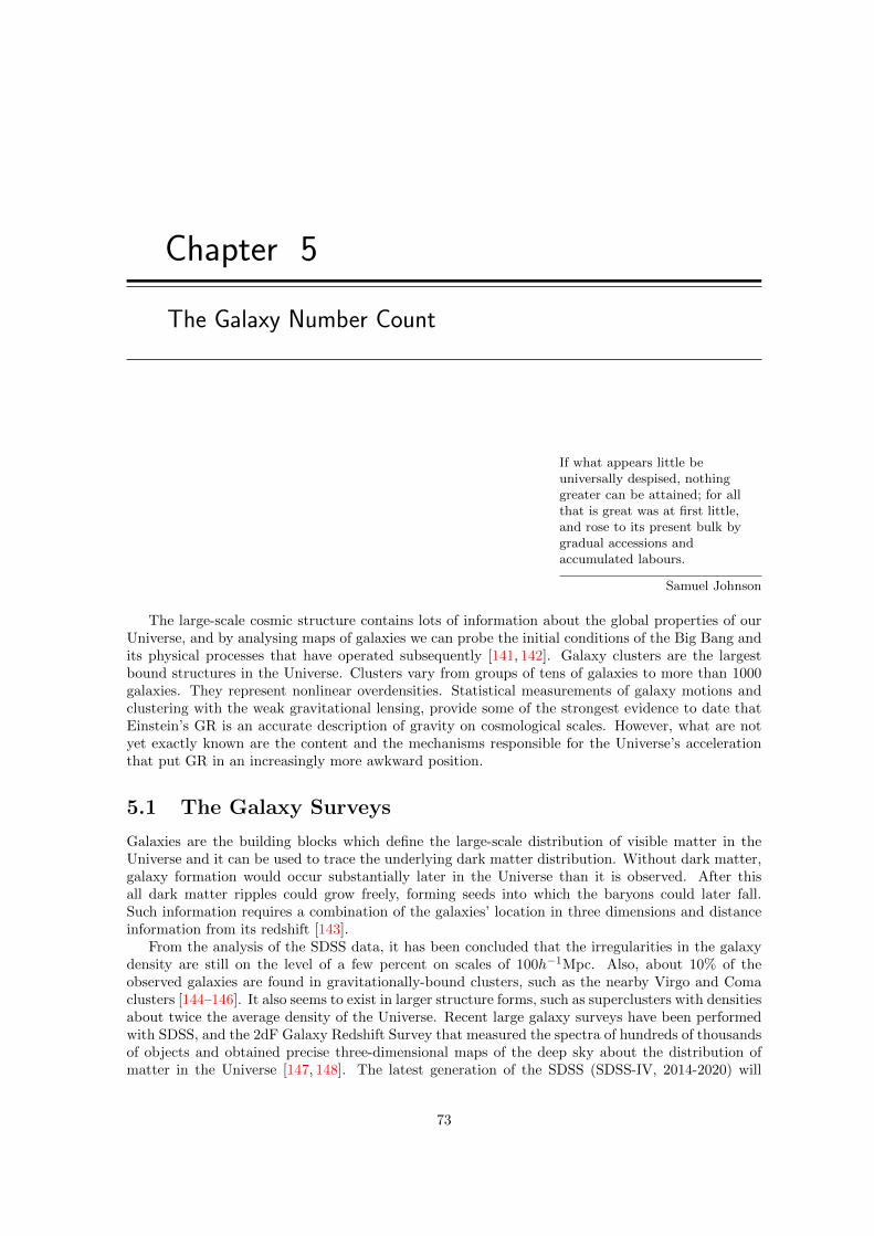
Chapter 5
The Galaxy Number Count
If what appears little beuniversally despised, nothinggreater can be attained; for allthat is great was at first little,and rose to its present bulk bygradual accessions andaccumulated labours.
Samuel Johnson
The large-scale cosmic structure contains lots of information about the global properties of ourUniverse, and by analysing maps of galaxies we can probe the initial conditions of the Big Bang andits physical processes that have operated subsequently [141, 142]. Galaxy clusters are the largestbound structures in the Universe. Clusters vary from groups of tens of galaxies to more than 1000galaxies. They represent nonlinear overdensities. Statistical measurements of galaxy motions andclustering with the weak gravitational lensing, provide some of the strongest evidence to date thatEinstein’s GR is an accurate description of gravity on cosmological scales. However, what are notyet exactly known are the content and the mechanisms responsible for the Universe’s accelerationthat put GR in an increasingly more awkward position.
5.1 The Galaxy Surveys
Galaxies are the building blocks which define the large-scale distribution of visible matter in theUniverse and it can be used to trace the underlying dark matter distribution. Without dark matter,galaxy formation would occur substantially later in the Universe than it is observed. After thisall dark matter ripples could grow freely, forming seeds into which the baryons could later fall.Such information requires a combination of the galaxies’ location in three dimensions and distanceinformation from its redshift [143].
From the analysis of the SDSS data, it has been concluded that the irregularities in the galaxydensity are still on the level of a few percent on scales of 100h−1Mpc. Also, about 10% of theobserved galaxies are found in gravitationally-bound clusters, such as the nearby Virgo and Comaclusters [144–146]. It also seems to exist in larger structure forms, such as superclusters with densitiesabout twice the average density of the Universe. Recent large galaxy surveys have been performedwith SDSS, and the 2dF Galaxy Redshift Survey that measured the spectra of hundreds of thousandsof objects and obtained precise three-dimensional maps of the deep sky about the distribution ofmatter in the Universe [147, 148]. The latest generation of the SDSS (SDSS-IV, 2014-2020) will
73
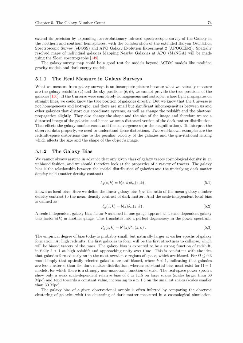
Chapter 5. The Galaxy Number Count 74
extend its precision by expanding its revolutionary infrared spectroscopic survey of the Galaxy inthe northern and southern hemispheres, with the collaboration of the extended Baryon OscillationSpectroscopic Survey (eBOSS) and APO Galaxy Evolution Experiment 2 (APOGEE-2). Spatiallyresolved maps of individual galaxies Mapping Nearby Galaxies at APO (MaNGA) will be madeusing the Sloan spectrographs [149].
The galaxy survey map could be a good test for models beyond ΛCDM models like modifiedgravity models and dark energy models.
5.1.1 The Real Measure in Galaxy Surveys
What we measure from galaxy surveys is an incomplete picture because what we actually measureare the galaxy redshifts (z) and the sky positions (θ, φ), we cannot provide the true positions of thegalaxies [150]. If the Universe were completely homogeneous and isotropic, where light propagates onstraight lines, we could know the true position of galaxies directly. But we know that the Universe isnot homogeneous and isotropic, and there are small but significant inhomogeneities between us andother galaxies that distort our coordinate systems, as well as change the redshift and the photons’propagation slightly. They also change the shape and the size of the image and therefore we see adistorted image of the galaxies and hence we see a distorted version of the dark matter distribution.That effects the galaxy number count and the convergence κ (or the magnification). To interpret theobserved data properly, we need to understand these distortions. Two well-known examples are theredshift-space distortions due to the peculiar velocity of the galaxies and the gravitational lensingwhich affects the size and the shape of the object’s image.
5.1.2 The Galaxy Bias
We cannot always assume in advance that any given class of galaxy traces cosmological density in anunbiased fashion, and we should therefore look at the properties of a variety of tracers. The galaxybias is the relationship between the spatial distribution of galaxies and the underlying dark matterdensity field (matter density contrast)
δg(z, k) = b(z, k)δm(z, k) , (5.1)
known as local bias. Here we define the linear galaxy bias b as the ratio of the mean galaxy numberdensity contrast to the mean density contrast of dark matter. And the scale-independent local biasis defined as
δg(z, k) = b(z)δm(z, k) . (5.2)
A scale independent galaxy bias factor b assumed in one gauge appears as a scale dependent galaxybias factor b(k) in another gauge. This translates into a perfect degeneracy in the power spectrum:
Pg(z, k) = b2(z)Pm(z, k) . (5.3)
The empirical degree of bias today is probably small, but naturally larger at earlier epochs of galaxyformation. At high redshifts, the first galaxies to form will be the first structures to collapse, whichwill be biased tracers of the mass. The galaxy bias is expected to be a strong function of redshift,initially b > 1 at high redshift and approaching unity over time. This is consistent with the ideathat galaxies formed early on in the most overdense regions of space, which are biased. For Ω ≤ 0.3would imply that optically-selected galaxies are anti-biased, where b < 1, indicating that galaxiesare less clustered than the dark matter distribution, whereas substantial bias must exist for Ω = 1models, for which there is a strongly non-monotonic function of scale. The real-space power spectrashow only a weak scale-dependent relative bias of b ' 1.15 on large scales (scales larger than 60Mpc) and tend towards a constant value, increasing to b ' 1.5 on the smallest scales (scales smallerthan 30 Mpc).
The galaxy bias of a given observational sample is often inferred by comparing the observedclustering of galaxies with the clustering of dark matter measured in a cosmological simulation.
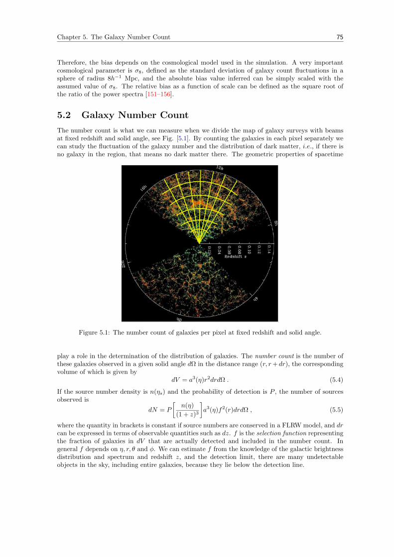
Chapter 5. The Galaxy Number Count 75
Therefore, the bias depends on the cosmological model used in the simulation. A very importantcosmological parameter is σ8, defined as the standard deviation of galaxy count fluctuations in asphere of radius 8h−1 Mpc, and the absolute bias value inferred can be simply scaled with theassumed value of σ8. The relative bias as a function of scale can be defined as the square root ofthe ratio of the power spectra [151–156].
5.2 Galaxy Number Count
The number count is what we can measure when we divide the map of galaxy surveys with beamsat fixed redshift and solid angle, see Fig. [5.1]. By counting the galaxies in each pixel separately wecan study the fluctuation of the galaxy number and the distribution of dark matter, i.e., if there isno galaxy in the region, that means no dark matter there. The geometric properties of spacetime
Figure 5.1: The number count of galaxies per pixel at fixed redshift and solid angle.
play a role in the determination of the distribution of galaxies. The number count is the number ofthese galaxies observed in a given solid angle dΩ in the distance range (r, r+ dr), the correspondingvolume of which is given by
dV = a3(η)r2drdΩ . (5.4)
If the source number density is n(ηs) and the probability of detection is P , the number of sourcesobserved is
dN = P
[n(η)
(1 + z)3
]a3(η)f2(r)drdΩ , (5.5)
where the quantity in brackets is constant if source numbers are conserved in a FLRW model, and drcan be expressed in terms of observable quantities such as dz. f is the selection function representingthe fraction of galaxies in dV that are actually detected and included in the number count. Ingeneral f depends on η, r, θ and φ. We can estimate f from the knowledge of the galactic brightnessdistribution and spectrum and redshift z, and the detection limit, there are many undetectableobjects in the sky, including entire galaxies, because they lie below the detection line.
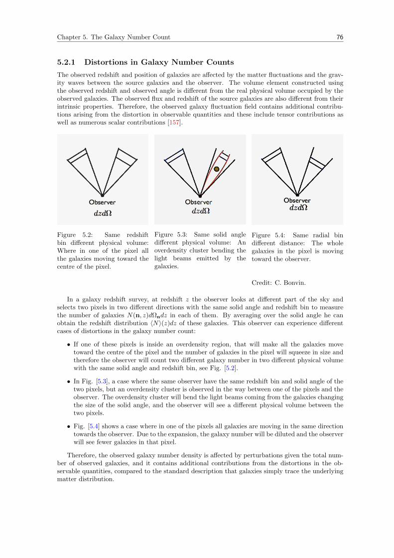
Chapter 5. The Galaxy Number Count 76
5.2.1 Distortions in Galaxy Number Counts
The observed redshift and position of galaxies are affected by the matter fluctuations and the grav-ity waves between the source galaxies and the observer. The volume element constructed usingthe observed redshift and observed angle is different from the real physical volume occupied by theobserved galaxies. The observed flux and redshift of the source galaxies are also different from theirintrinsic properties. Therefore, the observed galaxy fluctuation field contains additional contribu-tions arising from the distortion in observable quantities and these include tensor contributions aswell as numerous scalar contributions [157].
Figure 5.2: Same redshiftbin different physical volume:Where in one of the pixel allthe galaxies moving toward thecentre of the pixel.
Figure 5.3: Same solid angledifferent physical volume: Anoverdensity cluster bending thelight beams emitted by thegalaxies.
Figure 5.4: Same radial bindifferent distance: The wholegalaxies in the pixel is movingtoward the observer.
Credit: C. Bonvin.
In a galaxy redshift survey, at redshift z the observer looks at different part of the sky andselects two pixels in two different directions with the same solid angle and redshift bin to measurethe number of galaxies N(n, z)dΩndz in each of them. By averaging over the solid angle he canobtain the redshift distribution 〈N〉(z)dz of these galaxies. This observer can experience differentcases of distortions in the galaxy number count:
• If one of these pixels is inside an overdensity region, that will make all the galaxies movetoward the centre of the pixel and the number of galaxies in the pixel will squeeze in size andtherefore the observer will count two different galaxy number in two different physical volumewith the same solid angle and redshift bin, see Fig. [5.2].
• In Fig. [5.3], a case where the same observer have the same redshift bin and solid angle of thetwo pixels, but an overdensity cluster is observed in the way between one of the pixels and theobserver. The overdensity cluster will bend the light beams coming from the galaxies changingthe size of the solid angle, and the observer will see a different physical volume between thetwo pixels.
• Fig. [5.4] shows a case where in one of the pixels all galaxies are moving in the same directiontowards the observer. Due to the expansion, the galaxy number will be diluted and the observerwill see fewer galaxies in that pixel.
Therefore, the observed galaxy number density is affected by perturbations given the total num-ber of observed galaxies, and it contains additional contributions from the distortions in the ob-servable quantities, compared to the standard description that galaxies simply trace the underlyingmatter distribution.
Chapter 5. The Galaxy Number Count 77
5.2.2 The Galaxy Number Count on the Lightcone Gauge
Suppose one counts the galaxies seen in a solid angle dΩ0 around the direction of observation (θ, φ),down to a distance y. An increment from y −→ y + dy will result in including dN new galaxies inthe count, where dN is the number of galaxies detected in a volume of size as (dy, dθ, dφ) around apoint on our past lightcone
dV = (r2AdΩ)(uµkµdν) (5.6)
corresponding to the range (y −→ y + dy) in the coordinate y. If the number density of galaxiesat the position y is n, then (n dV ) is the number of galaxies that will be contained in this volume.However there is a chance that not all of the galaxies will be counted in dV , in general, for some willbe too faint to be detected, while others may not be selected for inclusion in the galactic numbercount because of various selection effects (e.g. they may be confused with stars if their images arevery small) [108]. We will write dN in the form
dN = fmdV , (5.7)
where fm is the selection function representing the fraction of galaxies in dV that are actuallydetected and included in the number count; one can estimate fm from knowledge of the galacticbrightness distribution and spectrum, the area distance rA and redshift z. In general, fm will dependon w, y, θ and φ. The number count of galaxies in a box of size (dy, dθ, dφ) around a point on ourpast lightcone can also be calculated as
dN = fmr2A(1 + z)dΩ0
βdy , (5.8)
where dν = βdy, and β = a2(1 + δβ). If y has been chosen to be an observable quantity, then dNis directly measurable. As z and rA are known, one can estimate the selection function fm, whichdepends on rA, z, the galaxy properties and the observational limits and selection effects. Therefore,in principle, one could determine the quantity β in terms of known quantities.
5.3 The Perturbation of Galaxy Number Counts ∆
The galaxy number density contrast in one pixel can be given by
∆ =N − NN
= b · δρρ
= b · δ . (5.9)
The number count ∆ is an observable quantity; it relates the number of the galaxies in each pixel tothe average numbers of the galaxies N , and the distribution of dark matter δ and its bias b. Sincethe density of the Universe is changing with time, it is useful to express the magnitude of densityvariation using the relative density fluctuation, which is defined as follows:
δρ
ρ=
density within a fluctuation−mean density of the Universe
mean density of the Universe. (5.10)
5.3.1 The ∆ Calculations in Redshift Space
Galaxy formation is a local process and its relation to the underlying matter density should be welldefined and gauge invariant. The observable quantities such as observed galaxy counting should beindependent of a choice of the gauge condition. The large-scale distribution of galaxies, the densityfluctuation δ(x, t) which we calculate in a given Friedmann background, is not a gauge invariant, thisis “the cosmological gauge problem” [38]. Since it depends on the background Friedmann universe

Chapter 5. The Galaxy Number Count 78
we compare the observed ρ(x, t) with [150].
δ(x, t) ≡ ρ(x, t)− ρ(t)
ρ(t). (5.11)
In order to fix this problem, one has to consider individual observational effects like the redshiftspace distortions [158,159], the Alcock-Pacinski [160] or lensing [150,161].
For unbiased distribution as we will consider for this section, ρ, is the mean galaxy density, i.e.,
ρ = 〈ρ〉 . (5.12)
The physical survey volume density per redshift bin per solid angle can be written as a backgroundpart in a homogeneous world and a fluctuated quantity, since the solid angle and the redshift binare distorted between the source and the observer:
V (n, z) = V (z) + δV (n, z) . (5.13)
Then following the discussion in [150], the redshift density perturbation can be written as
δz(n, z) =ρ(n, z)− 〈ρ〉(z)
〈ρ〉(z), (5.14)
=
N(n,z)V (n,z) −
〈N〉(z)V (z)
〈N〉(z)V (z)
, (5.15)
=
(N(n, z)V (z)
V (z) + δV (n, z)− 〈N〉(z)
)(1
〈N〉(z)
), (5.16)
=
(N(n, z)−N(n, z)
δV (n, z)
V (z)− 〈N〉(z)
)(1
〈N〉(z)
), (5.17)
=N(n, z)− 〈N〉(z)
〈N〉(z)− N(n, z)δV (n, z)
V (z)〈N〉(z), (5.18)
=N(n, z)− 〈N〉(z)
〈N〉(z)−
(〈N〉(z) + δN(n, z)
)δV (n, z)
V (z)〈N〉(z), (5.19)
=N(n, z)− 〈N〉(z)
〈N〉(z)− δV (n, z)
V (z). (5.20)
The perturbation in the number density of galaxies is an observed quantity, and the volume pertur-bation also can be measured with other tracers than galaxies, and it is therefore measurable by itselfand hence gauge invariant [150]. Therefore they are gauge-invariant quantities. And hence δz(n, z)is a gauge invariant. We can re-write the above expression as
∆(n, z) =N(n, z)− 〈N〉(z)
〈N〉(z)= δz(n, z) +
δV (n, z)
V (z), (5.21)
which is a gauge-invariant expression.
5.3.2 The Computation of δz(n, z)
We need to relate δz(n, z)→ δ(x, t) to a gauge-independent quantity. So to first order
δz(n, z) =ρ(n, z)− ρ(z)
ρ(z)=
(ρ(z) + δρ(n, z))− ρ(z)
ρ(z),
=(ρ(z − δz) + δρ(n, z))− ρ(z)
ρ(z). (5.22)
Chapter 5. The Galaxy Number Count 79
Taylor expansion of ρ(z) around z gives
ρ(z) = ρ(z + δz) , (5.23)
= ρ(z) +dρ
dzδz(n, z(η)) . (5.24)
Using the fact that z = z + δz and Eq. (5.23) in Eq. (5.22) yields
δz(n, z) =ρ(z) + δρ(n, z)− ρ(z)
ρ(z) + dρdz δz(n, z(η))
, (5.25)
=δρ(n, z)− dρ
dz δz(n, z(η))
ρ(z) + dρdz δz(n, z(η))
, (5.26)
=δρ(n, z)
ρ(z) + dρdz δz(n, z(η))
− dρ
dz
δz(n, z(η))
ρ(z) + dρdz δz(n, z(η))
, (5.27)
=δρ(n, z)
ρ(z)
(1− dρ
dz
δz(n, z(η))
ρ(z)
)− dρ
dz
δz(n, z(η))
ρ(z)
(1− dρ
dz
δz(n, z(η))
ρ(z)
).
(5.28)
Thus, to first order
δz(n, z) = δ(n, z)− dρ
dz
δz(n, z(η))
ρ(z), (5.29)
where δρ(n,z)ρ(z) = δ(n, z), and by using
dρ
dz= −3
ρ
1 + z, (5.30)
the matter fluctuation (at the observed redshift) is given by
δz(n, z) = δ(n, z) + 3δz(n, z(η))
(1 + z). (5.31)
Here we relate the perturbation variables in direction n at redshift z to their unperturbed positionand time η. z = z(η) is the redshift of the background universe that we measure on and δz is theredshift perturbation to this universe, δz(n, z) = δ(n, z) in a uniform-redshift frame δz = 0. It isgauge invariant since is defined by observable quantities, where the time slicing is set by the observedredshift z, rather than by an arbitrary choice of coordinate systems or gauge conditions as for δ(n, z)and differs in its value contingent upon the gauge choice [162].
Moreover, by solving the background relation z = z(η), we can write
ρ(n, z(η)) = ρ(η) + δρ(n, η) . (5.32)
Note that ρ(z) = ρ(z + δz) deviates to first order from ρ(z). Both δz and δρ depend on the chosenbackground and are, hence, gauge dependent; however their combination in Eq. (5.29) must turnout to be gauge invariant as it is in principle observable.Gauge-invariant density fluctuations and velocity perturbations can be found by combining δ, v andvi with metric perturbations. We shall use the Bardeen relations [112]
V ≡ v − E′ = vlong , (5.33)
Ds ≡ δ + 3(1 + w)H(E′ −B) ≡ δlong , (5.34)
D ≡ δlong + 3(1 + w)HV = δ + 3(1 + w)H(v −B)
= Ds + 3(1 + w)HV , (5.35)
Dg ≡ δ + 3(1 + w)(ψ) = δlong − 3(1 + w)Ψ
= Ds + 3(1 + w)Ψ . (5.36)
Chapter 5. The Galaxy Number Count 80
Here vlong and δlong are the velocity and density perturbations in the longitudinal gauge and Dg
is density fluctuation on the uniform curvature hypersurface. On sub-horizon scales the differencesbetween δ, δLong, Dg andD are negligible as are the differences between v and V . Since measurementsof density and velocity perturbations can only be made on sub-horizon scales, we may therefore useany of the gauge-invariant perturbation variables to compare with measurements [38].
If we want to introduce a bias between the matter density and the galaxy density, it would prob-ably be most physical to assume that both galaxies and dark matter follow the same velocity field, asthey experience the same gravitational acceleration. We then expect that biasing should be appliedto the density fluctuation in comoving gauge D and not to Dg. On small scales, such differencesare irrelevant, but on large scales they do become relevant, as becomes clear when considering the(linear) power spectra for the different density fluctuation variables [150].
5.3.3 The Volume Distortion
The volume perturbation δVV should be gauge invariant, because it is, in principle, a measurable
quantity given unbiased volume tracers. The differential volume element (seen by a source with4-velocity uµ) is given by
dV =√−gεµναβuµdxνdxαdxβ . (5.37)
In terms of the observed redshift z and sky position determined by the polar angles (θ, φ) at theobservation time,
dV =√−gεµναβuµ
∂xν
∂z
∂xα
∂θs
∂xβ
∂ϕs
∣∣∣∣∂(θs, ϕs)
∂(θo, ϕo)
∣∣∣∣ dzdθodϕo ,= v(z, θoϕo)dzdθodϕo , (5.38)
where v is a volume density, which determines the volume perturbation
δV
V=v(z)− v(z)
v(z)=δv
v. (5.39)
The determinant of the Jacobian matrix is
∣∣∣∂(θs, ϕs)
∂(θo, ϕo)
∣∣∣ = det J =
∂z∂z
∂z∂θo
∂z∂ϕo
∂θs∂z
∂θs∂θ0
∂θs∂ϕo
∂ϕs∂z
∂ϕs∂θo
∂ϕs∂ϕ0
, (5.40)
and gives the transformation matrix from the angles at the source to the angles at the observer. Inhomogeneous and isotropic backgrounds, the geodesics are straight lines, that is,
θs = θo , ϕs = ϕo . (5.41)
But in a perturbed universe, angles are perturbed with respect to
θs = θ0 + δθ , ϕs = ϕo + δϕ . (5.42)
Thus using (5.42) in the Jacobian expression given in (5.40), to first order of Taylor expansion, onegets ∣∣∣∂(θs, ϕs)
∂(θo, ϕo)
∣∣∣ = 1 +∂δθ
∂θ+∂δϕ
∂ϕ. (5.43)
We discussed in the last two subsections a general simplification steps for computing the twoterms of Eq. (5.21). We can apply them to any spacetime metric. In [150] they calculated theperturbed galaxy number counts using the perturbed FLRW metric. In the up coming section weare going to compute the perturbed galaxy number counts using our perturbed PLG metric and usethe simplified steps we just introduced above. Then we will do a coordinate transformation to our
Chapter 5. The Galaxy Number Count 81
final answer to the perturbed FLRW space and compare it with what [150] obtained.
5.4 Galaxy Number Counts Fluctuations with the PLG
Let us now consider the geodesic of a photon emitted from a galaxy in our lightcone backgroundwhich arrives to us at the vertex of our lightcone, moving in straight null-like vectors pointed indirection n (hence, to lowest order, it is seen under the direction −n from the observer). Theobserver receives the photon redshifted by
1 + z = uw =1
a(1 +
δα
2) = (1 + z)(1 +
δα
2) . (5.44)
Sinceδz = z − z (5.45)
and
δz =1
2(1 + z)δα , (5.46)
we have
δz(n, z) = δm(n, z) +3
2δα . (5.47)
The volume perturbation in terms of redshift and sky position is determined by our observationcoordinates (w, y, θ, φ), and therefore
v =√−gε0123u
w ∂y
∂z
∂θ
∂θs
∂φ
∂φs+√−gε1230u
y ∂w
∂z
∂θ
∂θs
∂φ
∂φs, (5.48)
where the components of ε satisfy
ε0321 = ε0231 = ε0312 = ε0132 = ε0213 = ε0123 = 1, (5.49)
ε1320 = ε1230 = ε1302 = ε1203 = ε1023 = ε1032 = −1 , (5.50)
and the angles between the source and the observer are fixed, it can be shown that there is noangular displacement
δθ = δφ = 0 . (5.51)
That will lead to the volume perturbation being given as
v =√−guw ∂y
∂z−√−guy ∂w
∂z. (5.52)
(5.53)
With constant light cone w|cst, we get
v =√−guw ∂y
∂z. (5.54)
Furthermore√−g = a4S2 sin(θ)
(1 +
HT
2+ δβ
), (5.55)
and the 4-velocity of the source according to the observational coordinates
u = (1 + z), nivi , (5.56)
Chapter 5. The Galaxy Number Count 82
where vi ≡ vy, vθ and vφ. Since dydz is the change in comoving distance y with redshift along the
photon geodesic, we can re-write it as
dy
dz=
d(y + δy)
d(z + δz)=d[y(1 + δy
y )]
d[z(1 + δzz )]
,
=dy(1 + δy
y ) + yd(1 + δyy )
dz(1 + δzz ) + zd(1 + δz
z ),
=dy
dz + dδz+
dδy
dz + dδz,
=dy
dz(1− dδz
dz) +
dδy
dz(1− dδz
dz) ,
=dy
dz− dy
dz
dδz
dz+dδy
dz. (5.57)
Using the fact that y = χ, we can rewrite the above result as
dy
dz=
dχ
dz− dχ
dz
dδz
dz+dδy
dz=
(dχ
dη− dχ
dz
dδz
dη+dδy
dη
)dη
dz. (5.58)
Here dy/dz is to be understood as the change in comoving distance y with respect to the redshift alongthe photon geodesic. The distinction between z and z is only relevant for background quantities.
Appling our reslut above to Eq. (5.54), then it will look like
v(z) = a4S2 sin(θ)
(1 +
HT
2+ δβ
)(1 + z)
(dχ
dη− dχ
dz
dδz
dη+dδy
dη
)dη
dz. (5.59)
In Eq. (5.58)), the last term contains the redshift-space distortion, which will turn out to be thebiggest correction to the power spectrum [150]. To lowest order along the photon geodesic, with1 + z = a0
a = 1a , we have
dη
dz=
dη
dz
da
da, (5.60)
=dη
da
da
dz=dη
da
d
dz
(1
1 + z
), (5.61)
= − 1
a′(1 + z)
−2= − a
a′(1 + z)
−1, (5.62)
= −aH−1 = −H−1 . (5.63)
With all the above taken into account, the volume element becomes
v(z) = −a4S(y)2 sin(θ)
(1 +
HT
2+ δβ
)(1 +
1
2δα
)(dχ
dη− 1
H(1 + z)
dδz
dη+dδy
dη
)H−1 , (5.64)
or
v(z) =a4S(y)2 sin(θ)
H
(−1 +
1
H(1 + z)
∂δz
∂y− ∂δy
∂y− HT
2− δβ − 1
2δα
), (5.65)
where we have used the relations (3.87). Furthermore, if we introduce the volume density as
δv
v=v(z)− v(z)
v(z), (5.66)
and v(z) is given by the Taylor expansion of v(z) around z, we get
Chapter 5. The Galaxy Number Count 83
v(z) = v(z + δz) , (5.67)
= v(z) +dv
dzδz , (5.68)
v(z) = v(z) +dv(z)
dzδz(n, z) . (5.69)
To obtain the fluctuation of v just subtract the unperturbed part v(z) from v of Eq.(5.65) (andadditional 1/a factor coming from the background part of [1+z] term), using a = 1/(z + 1)
v(z) =S(y)2 sin(θ)
(1 + z)4H, (5.70)
obtaining
dv(z)
dz= sin θ
d
dz
[S(y)2
(1 + z)4H
],
= sin θ
[2S(y)dS(y)/dz(1 + z)4H− S(y)2[4(1 + z)3H+ (1 + z)4 dH
dz
(1 + z)8H2
],
= sin θ
[2S(y)(dS(y)/dχ).(dχ/dz)(1 + z)4H− S(y)2[4(1 + z)3H+ (1 + z)4 dH
dηdηdz ]
(1 + z)8H2
],
= sin θ
[2S(y) aH (1 + z)4H− S(y)2[4(1 + z)3H+ (1 + z)4H′(−aH−1)]
(1 + z)8H2
],
= sin θ
[2S(y)a(1 + z)−4H−2 − S(y)2[4(1 + z)−5H−1 − (1 + z)−4aH′H−3]
], (5.71)
= v(z)
[2
S(y)H− 4 +
H′
H2
](1 + z)−1 . (5.72)
Thus,
v(z) = v(z)
(1 +
[2
S(y)H− 4 +
H′
H2
]δz
1 + z
), (5.73)
and
δv
v=
(1
H(1 + z)
∂δz
∂y− ∂δy
∂y− HT
2− δβ +
[2
S(y)H+H′
H2− 1
]δα
2
). (5.74)
And since from Eq. (3.81) we can conclude
∂δy
∂y=dδy
dη= −δβ , (5.75)
then
δv
v=
(1
H(1 + z)
∂δz
∂y− HT
2+
[2
S(y)H+H′
H2− 1
]δα
2
). (5.76)
With S(y) = y = (ηo − ηs) in flat space, and δz = 12 (1 + z)δα, one can then write
∆(n, z) = δ(n, z) +1
2H∂δα
∂y− HT
2+
[2
yH+H′
H2− 1
]δα
2. (5.77)
This is the expression for the density redshift perturbation in observational coordinates using theobservational metric, and as indicated does not include unmeasurable monopole terms or a dipole
Chapter 5. The Galaxy Number Count 84
term (niVi)o that usually arises by the perturbation at the observer position. Moreover it doesnot depend on the peculiar velocity of observer and emitter, and we do not need to compute thedeviation vectors that relate the perturbed geodesic to the unperturbed one. It only depends onquantities in terms of the perturbed metric and in principle all measurable.
Eq. (5.77) is gauge-invariant expression, the first term we have discussed it earlier, the sec-ond term contains the Doppler term, the integrated sachs-wolfe, the gravitational redshift and theredshift-space distortion. The third term contains the lensing distortion and time delay, and the lastterm contains the redshift perturbation of the volume.
5.4.1 Gauge Transformations of the Density Fluctuations
We need now to convert our result in Eq. (5.77) from the PLG into its equivalent expression inthe general coordinates and then we will contrast the outcomes. The upcoming result is alreadyobtained in [150,157,162]. Now we will convert each term one by one:
1
2H∂δα
∂y=
1
H(1 + z)
∂δz
∂y=
1
H(1 + z)
dδz
dη, (5.78)
= −Φ +H(B − E′) + Vχ +
∫ ηo
ηs
(Φ + Ψ)′dη −∫ ηo
ηs
(∂(χF
′χ) +
1
2h′χχ − ∂(χBχ)
)dη
+1
Hd
dη
[− Φ +H(B − E′) + Vχ +
∫ ηo
ηs
(Φ + Ψ)′dη −∫ ηo
ηs
(∂χF
′χ +
1
2h′χχ −∂χBχ
)dη
],
(5.79)
= −Φ +H(B − E′) + Vχ +
∫ ηo
ηs
(Φ + Ψ)′dη −∫ ηo
ηs
(∂(χF
′χ) +
1
2h′χχ − ∂(χBχ)
)dη
+1
H
[∂χVχ + Ψ′ −
(∂χF
′χ+
1
2h′χχ − ∂χBχ
)], (5.80)
where for a pressureless matter moving along the geodesics, we know that
Vχ −HVχ − ∂χΨ = 0 . (5.81)
and for
δα
2=
δz
(1 + z), (5.82)
=
[− Φ +H(B − E′) + Vχ +
∫ ηo
ηs
(Φ + Ψ)′dη
−∫ ηo
ηs
(∂χF
′χ +
1
2h′χχ − ∂(χBχ)
)dη
]. (5.83)
Finally, the HT term, you may see B.5 for more detailed derivation. Using the definition of ∆Ω
as the angular part of the Laplacian, which is denoted as
∆Ω = (∂2θ + cot θ∂θ +
1
sin2 θ∂2φ) ≡ ∇⊥i∇⊥i , (5.84)
we can show that
HT =
[− 2Ψ− 2H(B − E′)
+1
ηo − ηs
∫ ηo
ηs
∫ η
ηs
(∆Ω
[(Φ + Ψ)−Bχ + F ′χ −
1
2hχχ
])dη′dη
]. (5.85)
Chapter 5. The Galaxy Number Count 85
Now using Eqs. (5.34) and (5.36) together with the above expressions, we get
∆(n, z) = Dg −Ψ−H(B − E′) +1
H
[Ψ′ + ∂χVχ −
(∂χF
′χ +
1
2h′χχ −∂χBχ
) ]+
[2
yH+H′
H2
][− Φ +H(B − E′) + Vχ +
∫ ηo
ηs
(Φ + Ψ)′dη −∫ ηo
ηs
(∂χF
′χ +
1
2h′χχ − ∂(χBχ)
)dη
]− 1
ηo − ηs
∫ ηo
ηs
(η′ − ηs)∆Ω
((Φ + Ψ)−Bχ + F ′χ −
1
2hχχ
)dη′ . (5.86)
For only scalars we have
∆(n, z) = Dg −Ψ−H(B − E′) +1
H
[Ψ′ + ∂χVχ
]+
[2
yH+H′
H2
][− Φ +H(B − E′) + Vχ +
∫ ηo
ηs
(Φ + Ψ)′dη
]− 1
ηo − ηs
∫ ηo
ηs
(η′ − ηs)∆Ω(Φ + Ψ)dη′ . (5.87)
Eq. (5.87) represents the gauge-invariant redshift density fluctuation using a FLRW metric.The H−1∂χΨ term is the gravitational redshift. The light emitted from a galaxy has to pass viathat potential field and reach the observer. In so doing, the photon has to lose some of its ownenergy and hence become redshifted. That will result in changing the redshift of the beam. Theterm H−1∂χ(Vχ) is the redshift space distortion due to the galaxies’ peculiar velocity relative tothe observer line of sight, and this is considered the largest signal correction on the intermediatescales [150]. The middle line comes from the redshift perturbation of the volume, and it contains aDoppler term; it also contains the ordinary and integrated Sachs-Wolfe terms. The third line (theintegral) is the lensing distortion which corresponds to the change in the solid angle causing radialand angular volume distortions and time delay [163–165]; it is relevant especially on large scales.The rest of the terms have very small relativistic effects.
The standard Newtonian description of the galaxy power spectrum breaks down and the generalrelativistic description is therefore essential for understanding the observed galaxy power spectrumand deriving correct constraints from these measurements. The relativistic effects progressivelybecome significant at low angular multipoles at high redshifts z ≥ 2, where the relativistic effectsare dominant and significant on the horizon scale but they break the symmetry of the correlationfunction [166]. Due to these effects ∆ contains additional information δ, V,Φ,Ψ, this can helptesting gravity by probing the relation between density, velocity and gravitational potentials. Theydo affect our observables and by measuring these effects we can use them to test the relations betweenthe density, velocity and gravitational potentials. Using the PLG gauge was an attempt to makethe measuring of these relativistic effects achievable in most simple way. Our results will be mostsignificant for future galaxy survey catalogs like BOSS, DES, Euclid, and of significance to SLOAN-7data analysis.
Part III
86
Chapter 6
f (R) Theories of Gravity
The great tragedy of science - theslaying of a beautiful hypothesisby an ugly fact.
Thomas Huxley
Relativistic cosmology based on Einstein’s Field Equations (1.2) describes a universe with itsgeometric properties. It is derived from a density variational principle Lagrangian (L) of the EHaction with scalar curvature R.
If L is chosen to be a function of R, we can consider that as an Extended Theory of Gravity [58].This approach is aimed to address problems and shortcomings from the standard cosmological model,such as the recently discovered, arguably not yet explained, phenomenon of cosmic accelerationand the lack of a final theory of quantum gravity. It is also important to point out that anyextended theory also has to address where GR’s positive results had been obtained, i.e., such as BigBang cosmology, inflation, dark energy, local gravity constraints, cosmological perturbations, andspherically symmetric solutions in weak and strong gravitational backgrounds.
The f(R) model of gravity is a family of theories, each one defined by a different function ofthe Ricci scalar. Via the arbitrary function introduced in L, we have the freedom to explain theaccelerated expansion and the structure formation of the Universe without adding unknown forms ofenergy or exotic matter. However, not all functional forms of these models can be accepted as viablecosmological models; a wide range of them can be ruled out based on observations, cosmological andastrophysical principles, while others can be rejected because of theoretical pathologies.
f(R) theories were first speculated on by Buchdahl [167] in 1970, but it gained more popularity incosmology after further developments by Starobinsky [168]. The recent interest has centred on theirpotential candidacy as possible infrared (IR) and ultraviolet (UV) completions of GR [59, 60, 169–172]. More recently, these gravitational alternative theories have found cosmological applications in,inter alia, the dynamical study of homogeneous cosmological models [173–180, 180–188], the lineargrowth of large-scale structures [189–197] and astrophysics [198–202].
6.1 Derivation of the f(R) Field Equations
There are three ways in deriving the field equations from the action in f(R) gravity. From the EHaction in Eq. (1.1), with some function of R, we get
S =1
2
∫d4x√−g [f(R) + 2Lm(gab,Ψm)] , (6.1)
87
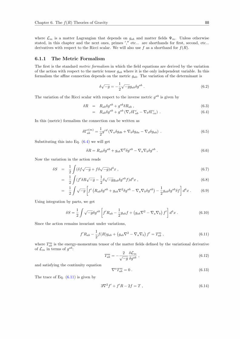
Chapter 6. The f(R) Theories of Gravity 88
where Lm is a matter Lagrangian that depends on gab and matter fields Ψm. Unless otherwisestated, in this chapter and the next ones, primes ′,′′ etc... are shorthands for first, second, etc...derivatives with respect to the Ricci scalar. We will also use f as a shorthand for f(R).
6.1.1 The Metric Formalism
The first is the standard metric formalism in which the field equations are derived by the variationof the action with respect to the metric tensor gab where it is the only independent variable. In thisformalism the affine connection depends on the metric gab. The variation of the determinant is
δ√−g = −1
2
√−ggabδgab . (6.2)
The variation of the Ricci scalar with respect to the inverse metric gab is given by
δR = Rabδgab + gabδRab , (6.3)
= Rabδgab + gab (∇cδΓcab −∇bδΓcca) . (6.4)
In this (metric) formalism the connection can be written as
δΓc(m)ab =
1
2gcd (∇aδgdb +∇bδgda −∇dδgab) . (6.5)
Substituting this into Eq. (6.4) we will get
δR = Rabδgab + gab∇2δgab −∇a∇bδgab . (6.6)
Now the variation in the action reads
δS =1
2
∫(δf√−g + fδ
√−g)d4x , (6.7)
=1
2
∫(f ′δR
√−g − 1
2δ√−ggabδgabf)d4x , (6.8)
=1
2
∫ √−g[f ′(Rabδg
ab + gab∇2δgab −∇a∇bδgab)− 1
2gabδg
abδf
]d4x . (6.9)
Using integration by parts, we get
δS =1
2
∫ √−gδgab
[f ′Rab −
1
2gabf +
(gab∇2 −∇a∇b
)f ′]d4x . (6.10)
Since the action remains invariant under variations,
f ′Rab −1
2f(R)gab +
(gab∇2 −∇a∇b
)f ′ = Tmab , (6.11)
where Tmab is the energy-momentum tensor of the matter fields defined by the variational derivativeof Lm in terms of gab:
Tmab = − 2√−g
δLmδgab
, (6.12)
and satisfying the continuity equation∇aTmab = 0 . (6.13)
The trace of Eq. (6.11) is given by
3∇2f ′ + f ′R− 2f = T , (6.14)
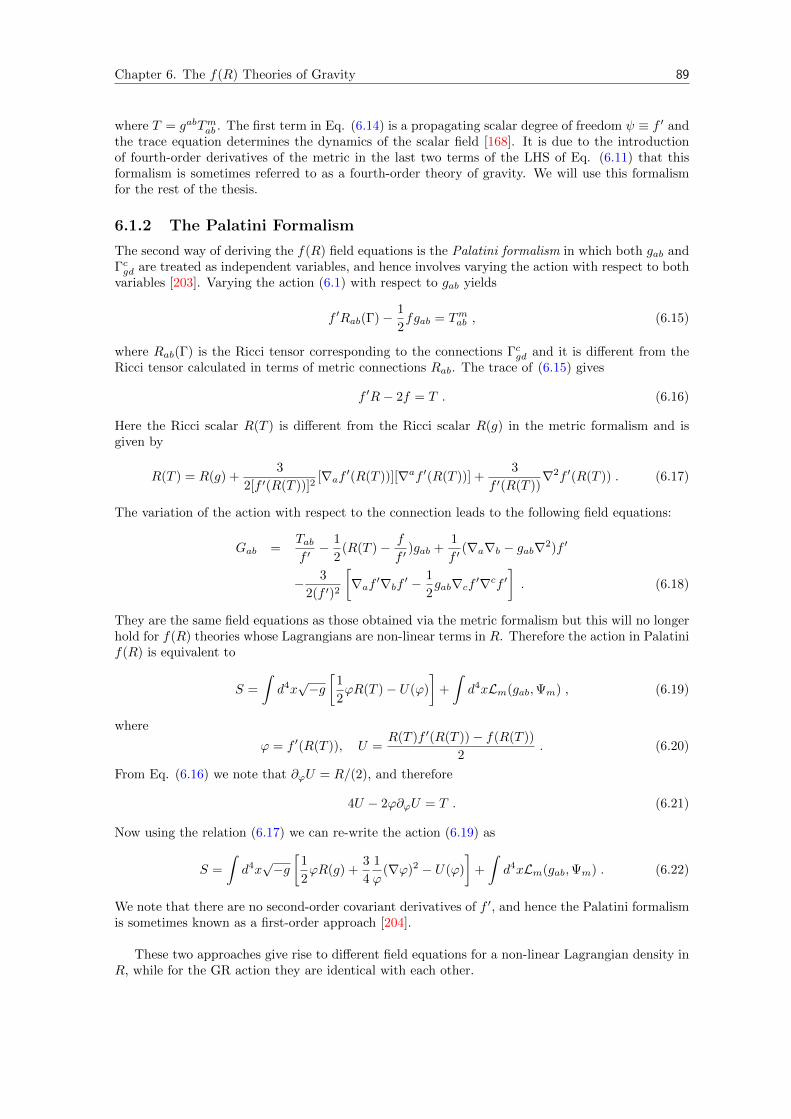
Chapter 6. The f(R) Theories of Gravity 89
where T = gabTmab . The first term in Eq. (6.14) is a propagating scalar degree of freedom ψ ≡ f ′ andthe trace equation determines the dynamics of the scalar field [168]. It is due to the introductionof fourth-order derivatives of the metric in the last two terms of the LHS of Eq. (6.11) that thisformalism is sometimes referred to as a fourth-order theory of gravity. We will use this formalismfor the rest of the thesis.
6.1.2 The Palatini Formalism
The second way of deriving the f(R) field equations is the Palatini formalism in which both gab andΓcgd are treated as independent variables, and hence involves varying the action with respect to bothvariables [203]. Varying the action (6.1) with respect to gab yields
f ′Rab(Γ)− 1
2fgab = Tmab , (6.15)
where Rab(Γ) is the Ricci tensor corresponding to the connections Γcgd and it is different from theRicci tensor calculated in terms of metric connections Rab. The trace of (6.15) gives
f ′R− 2f = T . (6.16)
Here the Ricci scalar R(T ) is different from the Ricci scalar R(g) in the metric formalism and isgiven by
R(T ) = R(g) +3
2[f ′(R(T ))]2[∇af ′(R(T ))][∇af ′(R(T ))] +
3
f ′(R(T ))∇2f ′(R(T )) . (6.17)
The variation of the action with respect to the connection leads to the following field equations:
Gab =Tabf ′− 1
2(R(T )− f
f ′)gab +
1
f ′(∇a∇b − gab∇2)f ′
− 3
2(f ′)2
[∇af ′∇bf ′ −
1
2gab∇cf ′∇cf ′
]. (6.18)
They are the same field equations as those obtained via the metric formalism but this will no longerhold for f(R) theories whose Lagrangians are non-linear terms in R. Therefore the action in Palatinif(R) is equivalent to
S =
∫d4x√−g[
1
2ϕR(T )− U(ϕ)
]+
∫d4xLm(gab,Ψm) , (6.19)
where
ϕ = f ′(R(T )), U =R(T )f ′(R(T ))− f(R(T ))
2. (6.20)
From Eq. (6.16) we note that ∂ϕU = R/(2), and therefore
4U − 2ϕ∂ϕU = T . (6.21)
Now using the relation (6.17) we can re-write the action (6.19) as
S =
∫d4x√−g[
1
2ϕR(g) +
3
4
1
ϕ(∇ϕ)2 − U(ϕ)
]+
∫d4xLm(gab,Ψm) . (6.22)
We note that there are no second-order covariant derivatives of f ′, and hence the Palatini formalismis sometimes known as a first-order approach [204].
These two approaches give rise to different field equations for a non-linear Lagrangian density inR, while for the GR action they are identical with each other.
Chapter 6. The f(R) Theories of Gravity 90
6.1.3 The Metric-affine Formalism
The matter part of the action (6.15) depends on the affine connection and hence introduces a torsionassociated with matter. If this connection has its standard geometrical meaning the resulting theorywill be a metric-affine theory of gravity [205]. The field equations (6.11) can be written in thefollowing form:
Gab = Tmab + TRab = Tab , (6.23)
where the effective EMT of standard matter is given by
Tmab ≡Tmabf ′
, (6.24)
and the curvature fluid contribution to the total EMT is
TRab ≡1
f ′[gab(f −Rf ′)/2 +∇a∇bf ′ − gab∇2f ′
]. (6.25)
Since ∇aGab = 0 for the total fluid, it follows that the total energy-momentum is also conserved:
∇aTab = 0 and for the standard matter ∇aT (m)ab = 0. It is straightforward to see that
∇aTRab =f ′′
f ′2Tmab∇aR , (6.26)
∇aTmab =∇aT (m)
ab
f ′− f ′′
f ′2T
(m)ab ∇
aR . (6.27)
This theory is not yet a well explored one. But it is important to note once more that metric-affine gravity is a modification of GR that follows its geometrical spirit but relaxes its simplifyingassumptions [205].
6.2 The Dynamics of f(R) Gravity
The effective total energy-momentum tensor described by
Tab = ρuaub + phab + 2q(aub) + πab (6.28)
sources the following thermodynamical quantities:
ρ = ρm + ρR ,
p = pm + pR ,
qa = qma + qRa ,
πab = πmab + πRab, (6.29)
with
ρm =ρmf ′, pm =
pmf ′, qma =
qaf ′, πmab =
πmabf ′
(6.30)
representing the effective energy density, isotropic pressure, heat flux and anisotropic pressure termsfor standard matter. In a perfect fluid the quantities qma and πmab both vanish in an FLRW backgroundand the effective background energy density and isotropic pressure of the curvature fluid are givenby
ρR =1
f ′
[1
2(Rf ′ − f)−Θf ′′R
], (6.31)
pR =1
f ′
[1
2(f −Rf ′) + f ′′R+ f ′′′R2 +
2
3Θf ′′R
], (6.32)
Chapter 6. The f(R) Theories of Gravity 91
with an effective equation of state [199]
wR ≡ −3f − 3Rf ′ + 6f ′′R+ 6f ′′R2 + 4Θf ′′R
3f − 3Rf ′ + 6Θf ′′R. (6.33)
There are also other ways of defining the effective equation of state wR in a way that it mimics theequation of state of dark energy [206–210]. The energy conservation equations for the matter andcurvature-fluid components read
ρm = −Θ(ρm + pm), (6.34)
ρR = −Θ(ρR + pR) + ρmf ′′R
f ′2, (6.35)
thus showing energy exchange between the two components due to the coupling between theseequations. The Friedmann and Raychaudhuri equations for these theories are generalised as
Θ2 = 3(ρm + ρR)− 32 R = 3
ρmf ′
+3
2
(R− f
f ′
)− 3ΘR
f ′′
f ′− 9k
a2, (6.36)
Θ = − 13Θ2 − 1
2 (ρm + 3pm)− 12 (ρR + 3pR) , (6.37)
= −1
3Θ2 − 1
2f ′
(2ρm − f − 2ΘRf ′′
). (6.38)
The generalised Friedmann equations in a flat FLRW read
3f ′H2 = (ρ+ 3p) +1
2(f ′R− f)− 3Hf ′ , (6.39)
−2f ′H = (ρ+ 4p) + f ′ −Hf ′ . (6.40)
The Ricci scalar is given by
R = 6
(a
a+a2
a2+
k
a2
)= 6
(H + 2H2 +
k
a2
), (6.41)
whereas the 3-Ricci curvature scalar is
R = 2
(ρ− 1
3Θ2
)= 6k/a2 . (6.42)
6.3 The Viability of f(R) Models
Over the last few decades, several models of f(R) gravitation have been proposed [174,200,211–217].However, most of these models suffer from a number of problems such as matter instability [218–220],the instability of cosmological perturbations [189,190,221], the absence of the matter era [222], andthe inability to satisfy local gravity constraints [55]. Amendola et al [223] derived some conditionsfor cosmological viability of f(R) models. Viable f(R) dark energy models need to satisfy [200,204,215,224]:
1. Avoiding the appearance of ghost particles. This corresponds to putting the constraint
f ′ > 0 ∀R (6.43)
to the f(R) model in question. This ensures that the graviton energy is positive and hencethat gravity remain attractive [215].
Chapter 6. The f(R) Theories of Gravity 92
2. Avoiding the matter instability. This requires the condition
f ′′ > 0 ∀R f ′′ . (6.44)
Any violation of this condition gives rise to the negative mass squared (M2 < 0, M being acharacteristic mass scale) and tachyonic scalaron field.
3. The early universe was governed by a GR-like law of gravitation (as evidenced by BBN andCMB constraints), i.e.,
limR→∞
f
R= 1⇒ f ′ < 1 , (6.45)
implying together with Condition (2) that f ′ must monotonically asymptote to 1 from below.
4. A less stringent condition is also that
|f ′ − 1| 1 , (6.46)
at recent epochs but this is not a necessary condition for the ongoing cosmic acceleration.
5. For a stable late-time de Sitter-type expansion
f ′
f ′′> R ∀R > 0 . (6.47)
6.4 Some f(R) Models
In this section we briefly discuss some of the most common models of f(R) gravitation that havegained some level of attention in recent years.
6.4.1 R2 Model
The first model of inflation proposed by Starobinsky [225] showed that R2 corrections in the standardGR gravitational action of the form
f = R+ βR2, (β > 0) (6.48)
where β ≡ 16M2 can lead to accelerated expansion. In the slow-roll approximation for inflation, the
the inflaton field φM and the slow-roll parameter is given by
ε ≡ − H
H2' 1
36βH2. (6.49)
The number of e-foldings in this model can be given by
N ' 1
2ε, (6.50)
whereas reheating around φ ' 0 results in the inflaton potential
V (φ) ' 1
12βφ2 . (6.51)
This model is very consistent with the thermal temperature anisotropies observed in the CMBand thus it can be an alternative to the scalar field models of inflation [226].
1β = 1 has been used for this figure.
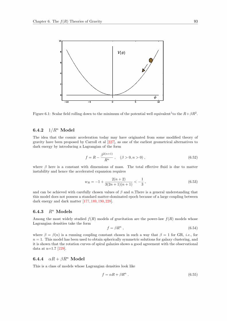
Chapter 6. The f(R) Theories of Gravity 93
Figure 6.1: Scalar field rolling down to the minimum of the potential well equivalent1to the R+βR2.
6.4.2 1/Rn Model
The idea that the cosmic acceleration today may have originated from some modified theory ofgravity have been proposed by Carroll et al [227], as one of the earliest geometrical alternatives todark energy by introducing a Lagrangian of the form
f = R− β2(n+1)
Rn, (β > 0, n > 0) , (6.52)
where β here is a constant with dimensions of mass. The total effective fluid is due to matterinstability and hence the accelerated expansion requires
wR = −1 +2(n+ 2)
3(2n+ 1)(n+ 1)< −1
3, (6.53)
and can be achieved with carefully chosen values of β and n.There is a general understanding thatthis model does not possess a standard matter-dominated epoch because of a large coupling betweendark energy and dark matter [177,189,190,228].
6.4.3 Rn Models
Among the most widely studied f(R) models of gravitation are the power-law f(R) models whoseLagrangian densities take the form
f = βRn , (6.54)
where β = β(n) is a running coupling constant chosen in such a way that β = 1 for GR, i.e., forn = 1. This model has been used to obtain spherically symmetric solutions for galaxy clustering, andit is shown that the rotation curves of spiral galaxies shows a good agreement with the observationaldata at n=1.7 [229].
6.4.4 αR + βRn Model
This is a class of models whose Lagrangian densities look like
f = αR+ βRn . (6.55)
Chapter 6. The f(R) Theories of Gravity 94
It is considered as a generalisation of both the Rn and the GR actions since α = 0 reduces to the Rn
and α = 1, β = 0 reduces to GR. Although this toy model is currently used a lot as an alternativesolution to inflationary and dark energy cosmology, it is known to violate the f ′′ > 0 condition, andis not considered a viable candidate [55,227].
6.4.5 Starobinsky Models
These are models of the form [230]
f = R+ βRc
[(1 +R2/R2
c
)−n − 1], (β > 0, n > 0) , (6.56)
with positive free parameters β, n. Rc roughly corresponding to the order of the curvature scaleof the present-day value, R0. An interesting aspect of these models is that in the limiting extremecurvature regimes,
limR/Rc→0
f = R , (6.57)
limR/Rc→∞
f ' R− βRc ≡ R− 2Λ . (6.58)
Thus at low-curvature regimes, there is no existence of the cosmological constant in the modelwhereas there is an effective cosmological constant term Λ ≡ βRc/2 that can mimic dark energy atlate times.
Starobinsky shows that for some limiting values of n and R/Rc 1 in the de Sitter solutionR = const., one can obtain a cosmic expansion history indistinguishable from that can be obtainedin the Concordance Model.
6.4.6 Hu-Sawicki Models
Hu and Sawicki [231] proposed a Lagrangian density of the form
f = R−β1m
2(R/m2
)n1 + β2 (R/m2)
n , (6.59)
where β1, β2 and n are the free parameters of the model and
m2 =ρm3, (6.60)
is a curvature scale that depends on the value of the matter energy density. It is interesting to notethat this model also introduces no cosmological constant term for low-curvature regimes, since
limR/m2→0
f = R ,
whereas for high curvature regimes, one can recover an effective cosmological constant at presentepoch because in this limiting case
limR/m2→∞
f ' R− β1
β2m2 +
β1
β22
m2
(R
m2
)−n.
These models have more recently shown growing popularity as viable f(R) gravitational solutions.
Chapter 6. The f(R) Theories of Gravity 95
6.4.7 Appleby-Battye Models
These are models that can be parametrised as [232,233]
f = R+Rc log[e−β +
(1− e−β
)e−R/Rc
], (6.61)
where β > 0 is a dimensionless constant and Rc scales as the present-day value of Λ. These models,like the Starobinsky and Hu-Sawicki models, can be shown to mimic ΛCDM for large R and avoidthe cosmological constant in the limiting R = 0 regime
limR/Rc→0
f = R , (6.62)
limR/Rc→∞
f ' R− βRc . (6.63)
6.5 Scalar-Tensor Representation
Before we close this review chapter, it is worth pointing out that there exists an equivalence betweenf(R) and Scalar-Tensor theories of gravity [204, 234–237]. If one replaces the f(R) action with onecontaining a standard matter non-minimally coupled with a classical scalar field φ defined as
φ ≡ f ′ − 1 , (6.64)
the resulting action can be written as
Aφ =1
2
∫d4x√−g [f(φ(R)) + Lm], (6.65)
and the corresponding field equations can be thought of as the field equations of a classical canonicalscalar field φ with a potential V (φ) given by
(1 + φ)Gab = Tmab +1
2gab(f − (1 + φ)R) +∇b∇aφ− gab∇c∇cφ . (6.66)
In this representation, the scalar field φ will have an EMT given by
Tφab =1
1 + φ
[1
2gab(f − (1 + φ)R) +∇b∇aφ− gab∇c∇cφ
], (6.67)
and satisfies the Klein-Gordon equation (KGE)
∇a∇aφ−1
3[2f − (1 + φ)R+ (ρm − 3pm)] = 0 . (6.68)
Defining the scalar field potential via the equation
dV
dφ≡ 1
3[2f − (1 + φ)R] =
dV
dR
dR
dφ, (6.69)
and using the trace equation1
3T aa =
T
3=
1
3(ρm − 3pm) , (6.70)
the KGE can be rewritten as
∇a∇aφ−dV
dφ− 1
3(ρm − 3pm) = 0 . (6.71)
Chapter 6. The f(R) Theories of Gravity 96
The scalar potential evolves according to
dV
dR=
1
3[2f − (1 + φ)R] f ′′ . (6.72)
Using this correspondence, one can recast the evolution equations in f(R) gravity into respectivecosmological equations in Scalar-Tensor theories, and vice versa. For example, in [52], we usedthe equivalence between f(R) gravity and the Brans-Dicke subclass of scalar-tensor theories, andtreating the Chaplygin gas as a scalar field model in a universe without conventional matter forms,we reconstructed the Lagrangian densities for the f(R) gravitational action.
Chapter 7
Irrotational-fluid Cosmologies in f (R) Gravity
Consistency is contrary to nature,contrary to life. The onlycompletely consistent people aredead.
Aldous Huxley
As an application of the preceding chapter, several classes of cosmological models with irrota-tional fluid flows and where the underlying theory of gravitation is f(R)-gravity are investigatedin this chapter. Using the 1 + 3 covariant decomposition formalism, the integrability conditionsdescribing a consistent evolution of the linearized field equations of shear-free dust universes arepresented. We also derive consistency relations of models with more severe constraints, such as non-expanding spacetimes as well as those spacetimes with vanishing gravito-magnetic or gravito-electriccomponents of the Weyl tensor.
In order to understand the dynamics of nonlinear fluid flows in f(R) theories, it is importantto understand the relationship between their Newtonian and general relativistic limits. This is rele-vant both in the physics of gravitational collapse and the late nonlinear stages of cosmic structureformation [108, 238–242]. The differential properties of time-like geodesics describe the fluid flowsin cosmology [31, 191, 243]. The expansion Θ, shear (distortion) σab, rotation (vorticity) ωa, andacceleration Aa of the four-velocity field ua tangent to the fluid flowlines describe kinematics of suchfluid flows. The generalised field equations, i.e, governing the fluid flows, are obtained by contractingthe Ricci identities along and orthogonal to ua.
7.1 The 1 + 3 Covariant Description
The covariant approach in cosmology is an excellent framework for studying cosmological per-turbations, and has been primarily developed to analyze the evolution of linear perturbations ofFriedmann-Lemaıtre-Robertson-Walker (FLRW) models in general relativity (GR) [244–246]. Theformalism is based on threading spacetimes via covariantly defined variables with respect to par-tial frames. A fundamental observer slices spacetime into time and space. Unlike in the standardgauge-invariant perturbation formalism (based on the foliation of a background spacetime with hy-persurfaces and perturbing away from it), the covariant approach starts from the theory and reducesto linearities in a particular background and has the main advantage that no unphysical gauge modesappear here.
97
Chapter 7. Irrotational-fluid Cosmologies in f(R) Gravity 98
In the 1 + 3 covariant decomposition, the four-velocity ua defines the covariant time derivativefor any tensor Sa..bc..d along an observer’s worldlines:
Sa..bc..d = ue∇eSa..bc..d . (7.1)
The projection tensor into the tangent 3-spaces orthogonal to ua is given by
hab ≡ gab + uaub , (7.2)
and is used to define the fully orthogonally projected covariant derivative for any tensor Sa..bc..d:
∇eSa..bc..d = hafhpc...h
bghqdhre∇rSf..gp..q , (7.3)
with total projection on all the free indices. The orthogonally projected symmetric trace-free (PSTF)part of vectors and rank-2 tensors is defined as
V 〈a〉 = habVb , S〈ab〉 =
[h(a
chb)d − 1
3habhcd
]Scd , (7.4)
and the volume element for the rest spaces orthogonal to ua is given by [31,247,248]
εabc = udηdabc = −√|g|δ0
[a δ1bδ
2cδ
3d]u
d ⇒ εabc = ε[abc], εabcuc = 0, (7.5)
where ηabcd is the 4-dimensional volume element with the properties
ηabcd = η[abcd] = 2εab[cud] − 2u[aεb]cd. (7.6)
We define the covariant spatial divergence and curl of vectors and rank-2 tensors as [249]
divV = ∇aVa , (divS)a = ∇bSab , (7.7)
curlVa = εabc∇bV c , curlSab = εcd(a∇cSb)d . (7.8)
The first covariant derivative of ua can be split into its irreducible parts as
∇aub = −Aaub + 13habΘ + σab + εabcω
c, (7.9)
where Aa ≡ ua, Θ ≡ ∇aua, σab ≡ ∇〈aub〉 and ωa ≡ εabc∇buc. The Weyl conformal curvature tensorCabcd is defined as [31,248]
Cabcd = Rabcd − 2g[a[cR
b]d] +
R
3g[a
[cgb]d] (7.10)
and can be split into its “electric” and “magnetic” parts, respectively, as
Eab ≡ Cagbhuguh, Hab = 12ηae
ghCghbdueud. (7.11)
Eab and Hab represent the free gravitational field [31], enabling gravitational action at a distance,i.e, tidal forces and gravitational waves, and influence the motion of matter and radiation throughthe geodesic deviation for timelike and null vector fields, respectively.
Cosmological quantities that vanish in the background spacetime are considered to be first-order and gauge-invariant by virtue of the Stewart-Walker lemma [111]. In a multi-component fluiduniverse filled with standard matter fields (dust, radiation, etc) and curvature contributions, the totalenergy density, isotropic and anisotropic pressures and heat flux are as given in Eq. (6.29) [192]where the linearised thermodynamic quantities for the curvature fluid component are defined as
ρR =1
f ′
[12 (Rf ′ − f)−Θf ′′R+ f ′′∇2R
], (7.12)
Chapter 7. Irrotational-fluid Cosmologies in f(R) Gravity 99
pR =1
f ′
[12 (f −Rf ′) + f ′′R+ f ′′′R2 + 2
3
(Θf ′′R− f ′′∇2R
)], (7.13)
qRa = − 1
f ′
[f ′′′R∇aR+ f ′′∇aR− 1
3f′′Θ∇aR
], (7.14)
πRab =f ′′
f ′
[∇〈a∇b〉R− σabR
]. (7.15)
Applying the 1 + 3 covariant decomposition on the Bianchi and Ricci identities
∇[aRbc]de = 0 , (∇a∇b −∇b∇a)uc = Rabc
dud (7.16)
for the total fluid 4-velocity ua, the following linearised propagation (evolution) and constraintequations are obtained [192,240]:
ρm = −(ρm + pm)Θ− ∇aqma , (7.17)
ρR = −(ρR + pR)Θ +ρmf
′′
f ′2R− ∇aqRa , (7.18)
Θ = − 13Θ2 − 1
2 (ρ+ 3p) + ∇aAa , (7.19)
qma = − 43Θqma − ρmAa , (7.20)
qRa = − 43ΘqRa +
ρmf′′
f ′2∇aR− ∇apR − ∇bπRab , (7.21)
ωa = − 23Θωa − 1
2εabc∇bAc , (7.22)
σab = − 23Θσab − Eab + 1
2πab + ∇〈aAb〉 , (7.23)
Eab + 12 πab = εcd〈a∇cHd
b〉 −ΘEab − 12 (ρ+ p)σab − 1
2∇〈aqb〉 −16Θπab , (7.24)
Hab = −ΘHab − εcd〈a∇cEdb〉 + 12εcd〈a∇
cπ db〉 , (7.25)
(C1)a := ∇bσab − 23∇aΘ + εabc∇bωc + qa = 0 , (7.26)
(C2)ab := εcd(a∇cσb)d + ∇〈aωb〉 −Hab = 0 , (7.27)
(C3)a := ∇bHab + (ρ+ p)ωa + 12εabc∇
bqc = 0 , (7.28)
(C4)a := ∇bEab + 12∇
bπab − 13∇aρ+ 1
3Θqa = 0 , (7.29)
(C5) := ∇aωa = 0 , (7.30)
(C6)a := ∇apm + (ρm + pm)Aa = 0 . (7.31)
The evolution equations propagate consistent initial data on some initial (t = t0) hypersurface S0
uniquely along the (generally future-directed) reference timelike congruence whereas the constraintsrestrict the initial data to be specified. For consistency, the constraint equations must remainsatisfied on any hypersurface St for all comoving time t .
7.2 Irrotational Spacetimes
Consistency analyses of the field equations for different models where integrability conditions, com-binations of the Bianchi identities and their consequences, arise from imposing external restrictionshave been made over the years [240, 241, 249–253]. We are going to explore some [sub]classes ofirrotational cosmological models and show how these models put restrictions on the possible formsof the underlying f(R) gravitational theory.
Chapter 7. Irrotational-fluid Cosmologies in f(R) Gravity 100
Irrotational fluid flows admit geodesic timelike congruences with vanishing vorticity
ωa = 0 (7.32)
and characterise potential cosmological models for the late universe and gravitational collapse. Fora barotropic irrotational matter fluid with the equation of state pm = wρm, the evolution equa-tions(7.17)-(7.25) for this class of spacetimes can be rewritten as:
ρm = −(1 + w)ρmΘ− ∇aqma , (7.33)
ρR = −(ρR + pR)Θ +ρmf
′′
f ′2R− ∇aqRa , (7.34)
Θ = − 13Θ2 − 1
2f ′ (1 + 3w)ρm − 12 (ρR + 3pR) + ∇aAa , (7.35)
qma = − 43Θqma − ρmAa , (7.36)
qRa = − 43ΘqRa +
ρmf′′
f ′2∇aR− ∇apR − ∇bπRab , (7.37)
σab = − 23Θσab − Eab + 1
2πab + ∇〈aAb〉 , (7.38)
Eab + 12 πab = εcd〈a∇cHd
b〉 −ΘEab − 12 (ρ+ p)σab − 1
2∇〈aqb〉 −16Θπab , (7.39)
Hab = −ΘHab − εcd〈a∇cEdb〉 + 12εcd〈a∇
cπ db〉 , (7.40)
and are constrained by the following equations:
(C1∗)a := ∇bσab − 23∇aΘ + qa = 0 , (7.41)
(C2∗)ab := εcd(a∇cσb)d −Hab = 0 , (7.42)
(C3∗)a := ∇bHab + 12εabc∇
bqc = 0 , (7.43)
(C4∗)a := ∇bEab + 12∇
bπab − 13∇aρ+ 1
3Θqa = 0 , (7.44)
(C5∗)a := w∇aρm + (1 + w)ρmAa = 0 , (7.45)
(C6∗)a := εabc∇bAc = 0 =⇒ Aa = ∇aψ for some scalar ψ . (7.46)
The new constraint(7.46) arises as a result of our irrotational restriction. To check for temporalconsistency, we propagate this constraint to obtain(
εabc∇bAc).
= 0 , (7.47)
which is an identity. On the other hand, taking the curl of this constraint, one obtains
curl(curl(Aa)) = ∇a(∇bAb
)− ∇2Aa + 2
3
(ρ− 1
3Θ2)Aa (7.48)
= ∇a(∇b∇bψ
)− ∇2∇aψ + 2
3
(ρ− 1
3Θ2)∇aψ (7.49)
= ∇a(∇2ψ
)− ∇2
(∇aψ
)+ 2
3
(ρ− 1
3Θ2)∇aψ = 0 , (7.50)
which is another identity by virtue of Eq’s. (C.4) and(C.12).
7.2.1 Dust Spacetimes
Pure dust spacetimes are characterised by
w = 0 = pm , qma = 0 = Aa , πmab = 0 , (7.51)
Chapter 7. Irrotational-fluid Cosmologies in f(R) Gravity 101
and the linearised evolution and constraint equations read:
ρd = −ρdΘ , (7.52)
ρR = −(ρR + pR)Θ +ρdf′′
f ′2R− ∇aqRa , (7.53)
Θ = − 13Θ2 − 1
2f ′ ρd − 12 (ρR + 3pR) , (7.54)
qRa = − 43ΘqRa +
ρdf′′
f ′2∇aR− ∇apR − ∇bπRab , (7.55)
σab = − 23Θσab − Eab + 1
2πRab , (7.56)
Eab + 12 π
Rab = εcd〈a∇cHd
b〉 −ΘEab − 12
(ρdf ′
+ ρR + pR
)σab − 1
2∇〈aqRb〉 − 1
6ΘπRab , (7.57)
Hab = −ΘHab − εcd〈a∇cEdb〉 + 12εcd〈a∇
cπR db〉 , (7.58)
(C1d)a := ∇bσab − 23∇aΘ + qRa = 0 , (7.59)
(C2d)ab := εcd(a∇cσb)d −Hab = 0 , (7.60)
(C3d)a := ∇bHab + 12εabc∇
bqcR = 0 , (7.61)
(C4d)a := ∇bEab + 12∇
bπRab − 13f ′ ∇aρm − 1
3∇aρR + 13ΘqRa = 0 . (7.62)
Notice here that no new constraints appear.
7.2.1.1 Shear-free Spacetimes
Over the years, the role of shear in GR and the special nature of shear-free cases in particular havebeen studied [204, 243, 254–256]. Godel showed [254] that shear-free time-like geodesics of somespatially homogeneous universes cannot expand and rotate simultaneously and this result was latergeneralized by Ellis [243] to include inhomogeneous cases of shear-free time-like geodesics. Goldbergand Sachs, on the other hand, showed [255] that shear-free null geodesic congruences in vacuo re-quire an algebraically special Weyl tensor, a result later generalized by Robinson and Schild [256]to include non-vanishing, but special, forms of the Ricci tensor.
An interesting aspect of these shear-free solutions is that they do not hold in Newtonian grav-itation theory [257–259], although Newtonian theory is a limiting case of GR under special cir-cumstances, namely at low-speed relative motion of matter with no gravito-magnetic effects, i.e,vanishing magnetic part of the Weyl tensor, and hence no gravitational waves. Now if we turn offthe shear, i.e., if we set
σab = 0 (7.63)
in the above propagation equations, we get Eq.(7.56) turning into a new constraint
(C5d)ab := Eab − 12π
Rab = 0 , (7.64)
the temporal and spatial consistencies of which have to be checked. It is interesting to note herethat, unlike for shear-free dust spacetimes in GR, the electric component of the Weyl tensor does notvanish because of the non-vanishing contribution of the anisotropic pressure πRab. However, we seefrom Eq. (7.60) that Hab identically vanishes, thus resulting in another constraint from Eq. (7.58):
(C6d)ab := εcd〈a∇cEdb〉 − 12εcd〈a∇
cπd db〉 = 0 , (7.65)
which is an identity by virtue of Eq. (7.64). From(7.61), we see that qRa is irrotational, and therefore
Chapter 7. Irrotational-fluid Cosmologies in f(R) Gravity 102
can be written as the gradient of a scalar:
qRa = ∇aφ . (7.66)
However, we already know from Eq. (7.59) that qRa = 23∇aΘ. One can therefore conclude that in
irrotational and shear-free dust spacetimes,
φ = 23Θ + C , (7.67)
for some spatially constant scalar C. We can rewrite this dynamical constraint on the expansionhistory, using Eq. (7.14) in (7.66), as
23f′∇aΘ +
(f ′′R− 1
3Θf ′′)∇aR+ f ′′∇aR = 0 . (7.68)
For GR, i.e., f = R , f ′ = 1 , f ′′ = f ′′′ = 0 , we obtain a spatially constant expansion since
∇aΘ = 0 , (7.69)
which is trivially true for the class of models under consideration. Now to check for temporalconsistency of Eq. (7.64), we take the time derivative of both sides of this equation to obtain therelation
πRab + 23ΘπRab − 1
2∇〈aqRb〉 = 0 , (7.70)
which, using qRa and πRab as defined by Eq’s. (7.14) and(7.15), can be rewritten as[3
2
(f ′′′
f ′− f ′′2
f ′2
)R− Θf ′′
6f ′
]∇〈a∇b〉R+ 3f ′′
2f ′ ∇〈a∇b〉R = 0 . (7.71)
Thus irrotational shear-free dust spacetimes governed by f(R) gravitational physics evolve consis-tently if Eq. (7.71) is satisfied. Note that Eq. (7.71) becomes an identity in the GR limit. Now bytaking the curl of the above equation, we obtain[
3
2
(f ′′′
f ′− f ′′2
f ′2
)R− Θf ′′
6f ′
]εcda∇c∇〈b∇d〉R+ 3f ′′
2f ′ εcda∇c∇〈b∇d〉R = 0 , (7.72)
which is an identity by virtue of Eq. (C.3). Thus the temporal consistency condition given byEq. (7.71) is satisfied on any initial hypersurface. Moreover, from Eq’s. (7.65) and (7.72), we canconclude that all irrotational shear-free dust spacetimes in f(R)-gravity are spatially consistent.
A further restriction one can make for such shear-free spacetimes is turning off Eab. This is a caseof vanishing Weyl tensor (since Hab = 0 by virtue of Eq. (7.60)), resulting in a locally conformallyflat metric. For such a class of cosmological models Eq. (7.57) changes to the (linearised) constraint
∇〈aqRb〉 = 0 =1
f ′
[(Rf ′′′ − 1
3Θf ′′)∇〈a∇b〉R+ f ′′∇〈a∇b〉R
]. (7.73)
Eq. (7.56) implies
πRab = 0 =f ′′
f ′∇〈a∇b〉R , (7.74)
which, for f ′′ 6= 0, leads to the conclusion that
∇〈a∇b〉R = 0 . (7.75)
Using this and the relation (C.1), we see that Eq. (7.73) becomes an identity. Thus the linearisedf(R) field equations in irrotational and shear-free dust spacetimes with vanishing Weyl tensor areconsistent.
Chapter 7. Irrotational-fluid Cosmologies in f(R) Gravity 103
7.2.1.2 Dust Solutions with divH = 0
The vanishing of the divergence of a non-zero Hab is a necessary condition for gravitational radiation[260–262]. Here we analyse the consistency of divergence-free GM (∇bHab = 0) scenarios in an effortto understand the nature of gravitationally radiating irrotational dust spacetimes. We see that thereare no new constraints arising as a result of imposing a divergence-free Hab to the field equations,but as in the shear-free case discussed above, Eq. (7.61) implies that qRa satisfies Eq. (7.66) whereasEq. (7.67) generalises to
∇aφ = 23∇aΘ− ∇bσab . (7.76)
Another interesting subclass of these models arises if both Hab and Eab are divergence-free.Described as “purely radiative” dust spacetimes [263], such models should satisfy the additionalmodified constraint
∇aρm + f ′∇aρR + f ′ΘqRa −3f ′
2 ∇bπRab = 0 (7.77)
as a result of Eq. (7.62). One can see from this result that purely radiative irrotational dust space-times in GR where f = R should be spatially homogeneous with ∇aρm = 0.
The so-called Newtonian-like spacetimes are described by the vanishing of the GM componentof the Weyl tensor [264]. Thus if the Weyl tensor is to have a purely GE component, then we noticefrom Eq. (7.60) that a curl-free shear is required, i.e.,
Hab = 0 =⇒ εcd(a∇cσb)d = 0 , (7.78)
and the constraint(7.65) is obtained from Eq. (7.58). Although such models are known to be oflimited applicability in GR-based cosmology, there are some interesting features in f(R) cosmologies.
7.2.1.3 Purely Gravito-magnetic Spacetimes
These are models with vanishing gravito-electric component of the Weyl tensor and are referred toas anti-Newtonian1 models because they are considered to be the most extreme of non-Newtoniangravitational models [264]. The only anti-Newtonian solutions in GR are the FLRW spacetimes[241,264], but a recent covariant consistency analysis [267] has shown that linearised anti-Newtonianuniverses are permitted by some models of f(R) gravity.
As can be seen from the set of equations(7.52)-(7.62), no new constraint equations arise as aresult of vanishing Eab. This is because of the non-vanishing of πRab for generic f(R) models; but inthe GR limiting case Eq. (7.57) would have turned into a new constraint since πRab = 0.
7.2.2 Non-expanding Spacetimes
In this section we explore theoretical cases where the background spacetime is not expanding, i.e.,Θ = 0 to analyse the kind of [in]consistencies one would obtain if a universe with such propertiesexisted. In this very special case, the linearised evolution equations (7.33)-(7.40) become
ρm = −∇aqma , (7.79)
qma =w
1 + w∇aρm , (7.80)
ρR =ρmf
′′
f ′2R− ∇aqRa , (7.81)
qRa =ρmf
′′
f ′2∇aR− ∇apR − ∇bπRab , (7.82)
σab = −Eab + 12πab + ∇〈aAb〉 , (7.83)
Eab + 12 πab = εcd〈a∇cHd
b〉 − 12 (ρ+ p)σab − 1
2∇〈aqb〉 , (7.84)
1An earlier use of the word ‘anti-Newtonian’ exists [265,266], where the word is used to refer to an earlier stage ofthe Universe when the dimension of irregularity exceeds the cosmological (Hubble) horizon.
Chapter 7. Irrotational-fluid Cosmologies in f(R) Gravity 104
Hab = −εcd〈a∇cEdb〉 + 12εcd〈a∇
cπ db〉 , (7.85)
whereas the revised constraint equations are given by
(C1s)a := ∇bσab + qa = 0 , (7.86)
(C2s)ab := εcd(a∇cσb)d −Hab = 0 , (7.87)
(C3s)a := ∇bHab + 12εabc∇
bqc = 0 , (7.88)
(C4s)a := ∇bEab + 12∇
bπab − 13∇aρ = 0 , (7.89)
(C5s)a := w∇aρm + (1 + w)ρmAa = 0 , (7.90)
(C6s) := ∇aAa − 12f ′ (1 + 3w)ρm − 1
2 (ρR + 3pR) = 0 . (7.91)
Eq. (7.80) has been obtained by using Eq. (7.45) into Eq. (7.36) whereas Eq. (7.91) arises from Eq.(7.35), showing that in the non-expanding case the Raychaudhuri (acceleration) equation changesinto a constraint.
7.2.2.1 Dust Solutions
In the case of dustAa = 0 = qma , (7.92)
the active gravitational mass ρ + 3p = 0, because of Eq. (7.91). Since Eq. (7.79) implies ρd(t) =constant, we notice that
ρR + 3pR = const (7.93)
as well. From the definitions of Eqs. (7.12) and (7.13) for ρR and pR and the trace equation
3f ′′R+ 3R2f ′′′ + 3ΘRf ′′ − 3f ′′∇2R−Rf ′ + 2f − ρm + 3pm = 0 , (7.94)
we conclude that Eq. (7.93) implies2
f − 2f ′′∇2R = const . (7.95)
Thus any nonrotating and noexpanding dust spacetime in f(R) cosmology should have a gravita-tional Lagrangian that satisfies Eq. (7.95).
7.2.2.2 Shear-free Solutions
As mentioned in the previous subsection, shear-free assumptions in cosmology result in many inter-esting and at times intriguing properties. Despite the limited applicability of such assumptions instandard cosmology - not least because the Universe is known, beyond any reasonable doubt, to beexpanding - it is interesting to explore the different mathematical constraints one obtains if f(R) isthe basic gravitational physics behind such cosmology. If we make the shear-free assumption, thepropagation equation (7.83) turns into the constraint
(C7s)ab := Eab − 12πab − ∇〈aAb〉 , (7.96)
whereas the constraint equations Eqs. (7.86) and(7.87) imply qa = 0 and Hab = 0. This means thatEq. (7.84) reduces to
Eab + 12 πab = 0 . (7.97)
2In GR, where f(R) = R, this translates into stating the obvious result that a constant ρd implies a constant Rsince f ′′ = 0.
Chapter 7. Irrotational-fluid Cosmologies in f(R) Gravity 105
If we differentiate the new constraint equation (7.96) with respect to cosmic time, and solve simul-taneously with Eq. (7.97) we obtain
Eab − (∇〈aAb〉). = 0 . (7.98)
On the other hand, if we take the gradient of Eq. (7.96) and solve simultaneously with Eq. (7.89),we obtain
∇bEab − 16∇aρ−
12∇
b∇〈aAb〉 = 0 . (7.99)
Moreover, the curl condition of Eq. (7.96) is identically satisfied by virtue of Eq’s. (7.85),(7.46)and(C.3).
If we consider the special case of dust
Aa = 0 = qma , πmab = 0 , (7.100)
in this shear-free setting, then Eq. (7.98) implies Eab = const in time. However, since Eab is relatedto πRab via Eq. (7.96), then πRab = const as well. This dictates that, because of Eq. (7.15), the
term f ′′
f ′ ∇〈a∇b〉R, be constant in cosmic time. It is also no coincidence that Eq. (7.95) is recovered
for this subclass as a result of Eq. (7.91). Another interesting point to note about non-expanding,shear-free dust spacetimes is that since qa = 0 =⇒ qRa = 0, we are dictated by Eq. (7.14) toconclude (
f ′′∇aR).
= 0 , (7.101)
thus putting a constraint on the form of the viable f(R) gravitational action that describes suchspacetimes. We notice that Eq. (7.101) is an identity in GR.
A completely general covariant analysis of irrotational fluids in f(R) cosmology requires takingnonlinear effects into account. In the case of purely radiative irrotational dust spacetimes, the consis-tency requirement implies that such models need not be homogeneous, unlike their GR counterparts.
The introduction of integrability conditions in f(R) gravitational models, and their conservationsshould these conditions be constraints, provides useful insight into the forms of the f(R) action. Italso helps us explore the existence and nature of some universe models that would otherwise notexist under the stricter requirement of the action involving the EH Lagrangian of GR.
Chapter 8
Chaplygin-gas Solutions of f (R) Gravity
You cannot apply mathematics aslong as words still becloud reality.
Hermann Weyl
In the scramble for the understanding of the nature of dark matter and dark energy, it has recentlybeen suggested that the change of behavior of the missing energy density might be regulated by thechange in the equation of state of the background fluid instead of the form of the potential [268,269].The Chaplygin Gas (CG) model in cosmology is one of the most profound candidates for thissuggestion. For quite sometime now, the CG model has been considered as another alternative to thecosmological FLRW universe models with a perfect fluid equation of state with a negative pressure[270, 271]. The model provides an interesting features of the cosmic expansion history consistentwith a smooth transition between an inflationary phase, the matter-dominated decelerating era, andthen late-time accelerated de Sitter phase of cosmic expansion can be achieved [50, 272, 273]; theexpansion of the Universe as alternative to the cosmological constant [274]. It predicts also that theexpanding universe will continue expanding and this could in principle be observed.
8.1 Chaplygin Gas in FLRW Models
The Chaplygin gas model in FLRW background provides a cosmic expansion history with a universefilled with an exotic background fluid: the Chaplygin gas. The model consists of a universe thattransits from a decelerating matter-dominated phase to a late-time accelerated one. However, in itsintermediate stages, it behaves as a mixture of a cosmological constant and a perfect fluid obeyingthe p = wρ equation of state. The resulting evolution of the Universe is not in disagreement withthe current observation of cosmic acceleration [50,270,272,273].
8.1.1 Original and Generalised CG Model
The CG model was introduced first by Chaplygin [275] as a model for aerodynamical studies. Chap-lygin assumed an ideal fluid of gas in stabilised motion where all effects of external forces are beneglected in order to get a steady irrotational flow of the gas, where vorticity formation is avoidable.It is necessary to consider the pressure as a function of the density. So it is convenient to take theequation of state in the form
p = − A
ρα, (8.1)
106
Chapter 8. Chaplygin-gas Solutions of f(R) Gravity 107
where p and ρ are respectively pressure and energy density in a comoving reference frame withρ > 0, and A and α are positive constants. α = 1 is constant of the ratio of specific fluctuation,i.e, heat1. A more generalised CG equation of state is obtained when 0 ≤ α ≤ 1 [276–278]. Thenunder homogeneity considerations, the relativistic energy conservation equation in the context ofFRW cosmology substituting for the equation of state yields an expression for the density in termsof the scale factor a given as
ρ =
(A+
B
a3(1+α)
) 11+α
, (8.2)
where B here is a positive integration constant. When α = 1 this solution takes us back to theoriginal Chaplygin gas. This simple and elegant model smoothly interpolates between matter phase,for small value of a (a6 B/A) the energy density is approximated by
ρ ∼√B
a3, (8.3)
which clearly corresponds to a dust-like dominated phase. For large values of the cosmological radiusa, it follows that
p ' −ρ⇒ ρ ∼√A⇒ p ∼ −
√A , (8.4)
which corresponds to an empty universe with a cosmological constant√A and that is a de Sitter
universe, through an intermediate regime described by the equation of state for stiff matter p = ρ.The interesting point, however, is that such an evolution is accounted by using only one fluid. Thereis a possibility of interpreting the model as a “quintessential” model [50, 269, 279]2 The criticaldensity for such model is
ρc = (A+B)1
1+α , (8.5)
whereas the Hubble parameter given through the Friedmann equation by
H2 =
(a
a
)2
=1
3ρ =
1
3
(A+
B
a3(1+α)
) 11+α
. (8.6)
This model automatically leads to an asymptotic phase where the equation of state is dominatedby a cosmological constant
√A. Subsequently, it has been shown that this model admits, under
conditions, an inhomogeneous generalisation, which can be regarded as a unification of dark matterand dark energy models [272].
We can express the perturbed pressure as
δp =A
ρ2δρ , (8.7)
and for the density contrast we have
δ =δρ
ρ∝ t2/3 . (8.8)
The most important point of the evolution of density perturbations in a universe dominated bythe Chaplygin gas is that a universe dominated by the Chaplygin gas admits an initial phase ofgrowing perturbations, with the same rate as in the dust case of the cosmological standard model,from which it follows decreasing oscillations, which asymptotically go to zero [280]. Furthermore,the model predicts an increasing value for the effective cosmological constant [50], i.e, in the contextof a Chaplygin cosmology, once an expanding universe starts accelerating it cannot decelerate anymore, a fact that we seem to be observing today.
For open or flat Chaplygin cosmologies (k = −1, 0), the Universe always evolves from a decel-erating to an accelerating epoch. For the closed Chaplygin cosmological models (k = 1), for static
1The CG equation of state (EoS) its also obtainable from Nambu-Goto action for d-branes moving in a (d+2)-dimensional spacetime and that by using the observational coordinates in the light-cone gauge [270].
2A quintessence field is a scalar field with standard kinetic term, which is minimally coupled to gravity.
Chapter 8. Chaplygin-gas Solutions of f(R) Gravity 108
Einstein universes, the solution yields
B =2
3√
3A. (8.9)
The generalised Chaplygin gas cosmological model, with no additional fluid components, is compat-ible with structure formation and large scale structure only for α sufficiently small (α < 10−5), inwhich case it is indistinguishable from the ΛCDM model.
The GCG of Eq. (8.1) is important to cosmology and it is one of the promising candidates toexplain the present accelerated expansion of the universe with simple model unifying dark matterand dark energy [272,274,280] as manifestations of a single cosmic fluid [281–284].
8.1.2 Modified and Extended CG Models
The modified Chaplygin gas (MCG) model is often used often to describe the acceleration phase ofthe Universe from the radiation era to the ΛCDM model. It includes a matter term [276,285]
p = Aρ− B
ρα, 0 ≤ α ≤ 1 , (8.10)
where 0 < A < 1/3 , 0 < α < 1 and B is a positive constant. It has been shown that A = 1/3 isthe best fitted value to describe evolution of the Universe from radiation regime to the Λ-cold darkmatter regime [286]. The energy density for such a model is given by
ρ =
[B
1 +A+
C
a3(1+A)(1+α)
] 11+α
, (8.11)
where C is an arbitrary integration constant. This model is a more appropriate choice to haveconstant negative pressure at low energy density and high pressure at high energy density. Wecan use this equation of state to describe low-surface brightness galaxies which are supposed to bedominated by dark matter [287]. The MCG equation of state is a suitable description for an ordinarylinear barotropic fluid [288]. While there are other barotropic fluids with equation of state beingquadratic and higher orders. For example, recently the model has been extended [289–291] so thatthe resulting equation of state can also recover a barotropic fluids with higher orders
pc =
n∑i=1
Aiρic −
B
ρα, (8.12)
where pc and ρc are the pressure and energy density of the extended Chaplygin gas which is theunification of the dark matter and dark energy. There is no general solution to this approach. But ifwe reduce n = 1 the above expression recovers the standard MCG. Barotropic fluids with quadraticequation of state can be recovered by setting n = 2, reducing Eq. (8.12) to
pc = A1ρc +A2ρ2c −
B
ραc, (8.13)
where A1, A2, B and α are positive constants [292]. These models give us the second-order solution[293]
ρc =
[B
1 +A1+
C
a3(1+A1)(1+α)e−(1+α)(1+A1)f(ρc)
] 11+α
, (8.14)
where C = (1 +A1)−1 and f(ρc) is a function of the critical energy density ρc given by [293]
Chapter 8. Chaplygin-gas Solutions of f(R) Gravity 109
f(ρc) =A2ρc
(1 +A1)2− BA2ρc
(1 + α)(1 +A1)2((1 +A1)ρ1+αc −B)
+A2
∫B(2 + α)
(1 + α)(1 +A1)2((1 +A1)ρ1+αc −B)
dρc . (8.15)
Note that in case of A2 = 0, we have a vanishing f(ρc). With higher order n, we will recover ahigher-order barotropic fluid. From this model numerically, increasing n decreases the value of thescale factor a and hence decreases the value of the energy density. The evolution of the scale factorcorresponding to n = 1 is faster than the case with n = 2, and the Hubble expansion parameter anddark energy density are decreasing with n. Different orders of n have been studied in [293–295], andit has been shown that by choosing appropriate values of constant parameters, the model has moreagreement with observational data than ΛCDM.
8.1.3 Generalised and Modified Cosmic Chaplygin Gas Models
The generalized cosmic Chaplygin gas (GCCG) models are those Chaplyging gas models that admitthe equation of state given by [296]
p = −ρ−α[C + (ρ1+α − C)−ω
], (8.16)
where
C =A
1 + ω− 1 , (8.17)
with A a constant which now can take on both positive and negative values, and 0 > ω > −l, l beinga positive definite constant which can take on values larger than unity. In the special case whenω = 0 one can write that C = A − 1. The speciality of this model is stability so the theory is freefrom unphysical behaviours even when the vacuum fluid satisfies the phantom energy condition [286].The above equation satisfies the following conditions:
i) it becomes a de Sitter fluid at late time and when ω = −1,
ii) it reduces to p = ωρ in the limit that the Chaplygin parameter A→ 0,
iii) it reduces to the equation of state of current Chaplygin unified dark matter models at highenergy density,
iv) the evolution of density perturbations becomes free from any pathological behaviour of thematter power spectrum for physically reasonable values of the involved parameters at latetimes.
By integrating the cosmic conservation law for energy we get for the energy density
ρ(a) =
[C +
(1 +
B
a3(1+α)(1+ω)
) 11+ω
] 11+α
, (8.18)
where B is a positive integration constant. B shows the effect of Chaplygin gas, and the cosmiceffect represented by ω. A further extension of the CG model is called modified cosmic Chaplygingas (MCCG) [286,297], where the EOS is further generalized to
p = γρ− 1
ρα
[B
1 + ω− 1 +
(ρ1+α − B
1 + ω+ 1
)−ω]. (8.19)
Here B and γ could be both positive or negative constants, and −l < ω < 0 where l is a positivedefinite constant with values larger than unity. Here also, 0 < α ≤ 1, and the case where ω = 0
Chapter 8. Chaplygin-gas Solutions of f(R) Gravity 110
gives the equation of state corresponding to the MCG. If we then put γ = 0, the equation of statecorresponding to the GCG is recovered. We can also reach back to the simplest case where α = 1,the Chaplygin gas’s original equation of state.
Chaplygin gas models have been studied in flat Friedmann models, in terms of the recentlyproposed “statefinder 3” parameters [298], dimensionless parameters that allow us to characterisethe properties of dark energy in a model-independent manner. It has also been shown that the simpleflat Friedmann model with Chaplygin gas can equivalently be described in terms of a homogeneousminimally coupled scalar field φ, which has been used in a variety of inflationary models in describingthe transition from the quasi-exponential expansion of the early universe to a power law expansionin order to understand the present acceleration of the Universe [50,51].
The model can be re-expressed as flat Friedman universes containing a scalar field with particularself-interaction potentials [299,300]; in other words, a very light scalar field φ whose effective potentialV (φ) leads to an accelerated phase at the late stages of the Universe [271] by constructing modelswhere the matter responsible for such behaviour is also represented by a scalar field [301,302].
In [50, 303]a homogeneous scalar field φ(t) and a potential V (φ) have been shown to describeChaplygin cosmology. An extended work is done by [304] with a modified CG. Moreover, theChaplygin gas is the only gas known to admit a supersymmetric generalisation [305].
8.2 Chaplygin Gas as f(R) Gravity?
In the remainder of the chapter, we are going to study models of f(R) gravity which, when weimpose the Chaplygin gas equations of state (EoS) to their effective pressure and energy density,produce viable exact solutions that reduce to the ΛCDM scenario in the approximate cosmologicallimits.
8.2.1 Constant Ricci-Curvature Scenarios
Analogous to the matter EoS pm = wmρm, where wm is the matter EoS parameter, we can definethe EoS for the curvature fluid as pR = wRρR.
For FLRW spacetimes, the Ricci scalar R is given by
R = 2Θ +4
3Θ2 , (8.20)
where Θ is the cosmic expansion parameter related to the cosmological scale factor a(t) and theHubble parameter H(t) via the equations
Θ ≡ 3a(t)
a(t)= 3H(t) . (8.21)
Solving for Θ one can rewrite the above equation as
Θ =R
2
(1− 4
3RΘ2
). (8.22)
If the Ricci scalar varies slowly, i.e., if R is almost constant, the solution of this ordinary differential
3The statefinder diagnostic trajectories in the plane s,r are constructed from the scale factor a(t) and theirderivatives up to third order as
r =
...a
aH3and s = −
r − 1
3(aaa2− 1
2).
Chapter 8. Chaplygin-gas Solutions of f(R) Gravity 111
equation (o.d.e) takes the form
Θ =1
2
√3R tanh
[√R
3(t− t0)
], (8.23)
for some constant of integration t0 that can be taken to be the time at the commencement of theinflationary phase of expansion. Solving for the cosmological scale factor gives
a(t) = a0
√√√√cosh
[√R
3(t0 − t)
]. (8.24)
For simplicity we set t0 ' 0. During steady-state exponential expansion in a de Sitter spacetime(such as during inflation or late-time evolution), the approximation Θ→ 0 results in
R =4
3Θ2 = const , a(t) = a0e
13 Θt , (8.25)
and the matter content evolves according to
ρm = ρ0
(a(t)
a0
)−3(1+wm)
. (8.26)
During such an exponentially expanding cosmic evolution phase, for an initial energy density ρ0, wesee that the matter energy density decays exponentially:
ρm = ρ0e−(1+wm)Θt . (8.27)
8.2.2 Chaplygin Gas Solutions in f(R) Gravity
8.2.2.1 Original and Generalized Chaplygin Gases
In the original treatment, the negative pressure associated with the Chaplygin gas models is relatedto the (positive) energy density through the EoS
p = − A
ρα(8.28)
for positive constant A and α = 1. But this was later generalized [50, 306] to include 0 ≤ α ≤ 1.One of the first cosmological interpretations of such a fluid model was given in [302] where for flatuniverses, Eq. (8.28) corresponds to a viscosity term that is inversely proportional to dust energydensity. Ever since the discovery of cosmic acceleration, however, both the original and generalizedChaplygin gas models have been extensively studied as alternatives to dark energy and/or unifieddark energy and dark matter models (see, e.g., [50,269,272,274,307,308]).
Now if we consider the background curvature energy density and isotropic pressure terms definedin Eqs. (7.12) and (7.13) above, in the constant-curvature limiting case, we have
ρR =1
4[R(f ′ + 1)− 2f ] = −pR . (8.29)
This equation of state, with an effective EoS parameter wR = −1, provides the condition for anexponential (accelerated) expansion with a constant Hubble parameter. The energy density ρR(with its negative pressure pR) remains constant and can be interpreted as playing the role of thecosmological constant Λ.
Considering the curvature fluid as a manifestation of the Chaplygin gas with the EoS (8.28), we
Chapter 8. Chaplygin-gas Solutions of f(R) Gravity 112
obtain
pR = −ρR = − A
ραR, (8.30)
which, using Eq. (8.29), leads to the o.d.e
Rf(R)
dR− 2f(R) +R = 4A
1α+1 . (8.31)
Solving this ordinary differential equation yields
f(R) = R+ C1R2 − 2A
1α+1 (8.32)
for an arbitrary (integration) constant C1. We note that the ΛCDM solution f(R) = R − 2Λ isalready a particular solution with C1 = 0 and A = Λα+1. In particular, if α = 0, then A = Λ, fromwhich, going back to Eq. (8.30), one concludes ρR = Λ.
If we include the linearized Laplacian term in Eqs. (7.12) and (7.13) and use the eigenvalue −k2
a2
of the covariantly defined Laplace-Beltrami operator ∇2 on (almost) FLRW spacetimes
∇2R = −k2
a2R (8.33)
for a comoving wavenumber k, we obtain the second-order o.d.e
B2Rf ′′(R)−Rf ′(R) + 2f(R)−R+ 4A1
α+1 = 0 , (8.34)
where here we have defined
B2 ≡ 4(2 + 3α)
3(1 + α)
k2
a2. (8.35)
The solution of Eq. (8.34) is given, for arbitrary constants C2, C3, by
f(R) = R+C2
[R2 − 2RB2
]+C3
[(R2 − 2RB2)Ei
(1,− R
B2
)+ (R−B2)B2e
RB2
]−2A
1α+1 , (8.36)
which should reduce to the quadratic solution (8.32) for negligible values of B2, i.e., for smallfirst-order contributions to the energy density and pressure terms.
8.2.2.2 Modified Chaplygin Gas
On the other hand, if one considers the modified Chaplygin gas (MCG) EoS [51, 131, 286, 289, 290,306,309,310]
pR = γρR −A
ραR, (8.37)
then the resulting f(R) model generalizes to
f(R) = R+ C4R2 − 2
(A
γ + 1
) 1α+1
, (8.38)
where C4 is an arbitrary integration constant.The ΛCDM solution is a limiting case of this generalized model when C4 = 0 and A = (γ+1)Λα+1.
In particular, if α = 0 = γ, then A = Λ.Following similar arguments as in the preceding subsection, if we include the linearized Laplacian
contributions to the energy density and pressure, we get Eq. (8.34) generalized to
B2Rf ′′(R)−Rf ′(R) + 2f(R)−R+ 4
(A
γ + 1
) 1α+1
= 0 , (8.39)
Chapter 8. Chaplygin-gas Solutions of f(R) Gravity 113
the solution of which can be given by
f(R) = R+C5
[R2 − 2RB2
]+C6
[(R2 − 2RB2)Ei
(1,− R
B2
)+ (R−B2)B2e
RB2
]−2
(A
γ + 1
) 1α+1
,
(8.40)for an arbitrary integration constants C5 and C6. This solution obviously generalizes Solutions(8.32),(8.36) and (8.38) and should reduce to the quadratic solution (8.32) for vanishingly smallB2 values. In [311], it has been shown that any quadratic Lagrangian leading to an isotropic,homogeneous cosmological model takes the form
f(R) = R− 2Λ− 1
6βR2 , (8.41)
where β is an arbitrary, real constant. If we keep only the quadratic solution in (8.40), i.e., if we setC6 = 0, the Lagrangian (8.41) corresponds to the choice
C5 = −1
6β ,B = 0 , A = (γ + 1)Λα+1 . (8.42)
Another interesting fact worth pointing out here is that the condition for the existence of a maximallysymmetric vacuum solution in f(R) gravity [311]
R0f′(R0) = 2f(R0) (8.43)
leads to the quadratic solution resulting in the constraint
R0
(1− 2C5B
2)− 4
(A
γ + 1
) 1α+1
= 0 . (8.44)
The corresponding GR de Sitter, anti-de Sitter and Minkowski solutions R0 = 4Λ (respectively forΛ > 0 ,Λ < 0 and Λ = 0) are obtained when C5B
2 = 0 and A = (γ + 1)Λα+1.
The resulting solutions are generally quadratic in the Ricci scalar, but have appropriate ΛCDMsolutions in limiting cases. These solutions, given appropriate initial conditions, can be potentialcandidates for scalar field-driven early universe expansion, i.e., inflation, and dark energy-drivenlate-time cosmic acceleration. Of course, to take this model seriously one should have a goodfundamental reason to believe such fluid exists in the real universe.
8.2.2.3 Modified Generalized Chaplygin Gas
The so-called modified generalized Chaplygin gas (mGCG) model is described by a barotropic equa-tion of state of the form [312,313]
p = βρ− (1 + β)A
ρα. (8.45)
Models of f(R) gravity that satisfy the condition (8.29), at the same time mimicking the mGCG, canbe shown to be governed by the same equation as (8.31) and admit the same solutions (8.32), providedβ 6= −1. On the other hand, if linearized Laplacian terms are included, then the correspondingdifferential equation in f(R) generalizes to
D2Rf ′′(R)−Rf ′(R) + 2f(R)−R+ 4A1
α+1 = 0 , (8.46)
where we have defined
D2 ≡ 4 [2 + 3α+ 3β(1 + α)]
3(1 + α)(1 + β)
k2
a2. (8.47)
Chapter 8. Chaplygin-gas Solutions of f(R) Gravity 114
Worthy of note is that this equation and its solution
f(R) = R+ C7
[R2 − 2RD2
]+ C8
[(R2 − 2RD2)Ei
(1,− R
D2
)+ (R−D2)D2e
RD2
]−2
(A
γ + 1
) 1α+1
, (8.48)
reduce to their generalized counterparts of Eqs. (8.34) and (8.36) when β = 0.
Chapter 9
Conclusions and Future Outlook
It would be interesting to find outwhat goes on in that momentwhen someone looks at you anddraws all sorts of conclusions.
Malcolm Gladwell
We humans are very eager to observe and understand what is in the Universe, and that is ex-actly what makes the study of our cosmos very interesting. In cosmology, we distinguish betweenthe observable universe for which by definition we have data and a universe which includes regionswe cannot directly influence or experiment on. The inference of the geometrical properties of theuniverse from the observable universe cannot be achieved without hypothesis and philosophical prej-udices.
The accurate determination of cosmological distances is the most important probe in cosmol-ogy. Observing the Universe and measuring many of the cosmological observables can allow us todetermine the cosmological parameters which, in turn, allow us to study and track the history ofthe whole Universe and predict its future and in between study its evolution. In this thesis wecalculated the observables in the so-called lightcone gauge adapted to the observational coordinates.We developed this gauge by perturbing the lightcone, and reproducing a new linear perturbed gaugeto satisfy us up to first-order calculations of the observables. The calculations of the observables inthe new gauge introduced was much easier than the ones we usually obtain in the standard gauge.We then used this perturbed gauge to compute the fractional perturbation of galaxy number counts,which is truly measured in large galaxy surveys. In the later calculation we did not have to worryabout the spatial positions of the galaxy because we only observe galaxy redshifts and sky positionson the lightcone background.
Ever since Hubble’s observations of the 1920s that changed our worldview once and for all, ithas become a textbook fact that the Universe is expanding. One of the important observables incosmology is the measure of the rate of this expansion of the Universe. Towards the turn of thiscentury, a totally unexpected discovery challenged our worldview once again: the Universe is notonly expanding but this expansion happens at an accelerated rate. Since Einstein’s field equationsbased on General Relativity do not predict this (in fact the expansion should have been slowing downat the present epoch due to matter domination), this discovery came as a surprise and left manyrushing to find possible hypotheses. One of such hypotheses is that the Universe is filled with aninvisible form of energy called dark energy. Other propositions came in the form of modifications to
115
Chapter 9. Conclusions and Future Outlook 116
the underlying theory of gravity. In this thesis we discussed one of such possible modifications, f(R)gravity. This theory of gravity is one of many candidates studied to solve the current accelerated rateof expansion. The theory has its gravitational action chosen to include generic functions of the Ricciscalar, and therefore comes with an the extra degree of freedom that can explain different cosmicexpansion scenarios, including accelerated ones. In particular, we studied f(R) gravitational modelsthat allow irrotational fluid flows. The integrability conditions describing a consistent evolution ofthe linearized field equations of shear-free dust universes were studied, as well as the consistencyrelations of models with more severe constraints, such as non-expanding spacetimes as well as thosespacetimes with vanishing gravito-magnetic or gravito-electric components of the Weyl tensor.
We also studied the possibility of the f(R) theory of gravity acting as an exotic curvature fluidwith negative pressure such as a Chaplygin gas. Assuming a temporally constant Ricci scalar, theresulting f(R) solutions mimicking the Chaplygin gas equations of state are generally quadratic inthe Ricci scalar, but have appropriate ΛCDM solutions as their limiting cases. These solutions,given appropriate initial conditions, can be potential candidates for scalar field-driven early universeexpansion (inflation) and dark energy-driven late-time cosmic acceleration.
The whole thesis was divided into three parts. Part I covered the literature review and thegeneral theoretical foundation of what would follow as calculations of the cosmological observablesin Part II. Part III focused on a class of alternative cosmological models, f(R) theories of gravity,and their cosmological underpinnings.
In Chapter 1, we introduced the literature review on General Relativity and some cosmologicalobservables that are of importance to the development of the thesis.
In Chapter 2, we presented some basic background information about the GR solution and therelation to the standard models of the Universe. We explained the perturbation theory and its ne-cessity to the evolution of the Universe, and we calculated the observables in light of the perturbedfirst-order FLRW models.
In Chapter 3, we introduced the observational coordinates set that is adapted to our past-lightcone. Since we are the only observers in the Universe, we do our observation from one pointat the vertices of our lightcone. We derived the observational spacetime metric. In particular, wewere able to identify the way to fix the gauge properly, by showing the relations between the per-turbations of spacetime in observational coordinates and those perturbations in the standard metricapproach. We derived its dynamical equations for the perturbations in observational coordinates.We decomposed the equations into spherical harmonics in order to simplify the system and producefunctions suitable for the extraction of observational quantities, and checked for consistency with theEinstein field equations degrees of freedom. We introduced the GLC gauge and presented the key dif-ferences between the GLC gauge and the observational coordinates gauge and hence the PLG gauge.
In Chapter 4, we presented the observables of spacetime in the lightcone gauge using the ob-servational coordinates. We verified the observables on the perturbed lightcone gauge with thoseobtained in the standard perturbed gauge. The result was accurate and satisfactory to our expec-tations. We showed the advantage of the method developed in our PLG gauge, namely that theobservable relations are simpler than in the standard formalism (not involving integro-differentialequations) and it can be extended to second order more easily.
In Chapter 5, we calculated the overdensity regions using the PLG gauge and the results wereremarkable. We did a verification with the standard gauge as well.
After introducing the rationale for considering alternative gravitational models, we presented thegeneralized forms of the field equations of f(R) gravity in Chapter 6. We gave an overview of the1 + 3 covariant spacetime splitting formalism as applied to f(R) theories and gave the propagationand constraint equations relating the kinematical quantities arising from the covariant decomposi-tion, first for the full nonlinear case and then in the linearised regime.
Chapter 9. Conclusions and Future Outlook 117
In Chapter 7, in the framework of these new gravitational theories, we outlined the general con-ditions that any f(R) model should satisfy for non-rotational dust universes for it to be a viablecandidate for explaining observations on all cosmological scales. We looked at the consistency rela-tions of linearized perturbations of FLRW universes with irrotational fluid flows arising as a resultof imposing special restrictions to the field equations. We showed that linearized shear-free dustmodels have a vanishing gravito-magnetic component of the Weyl tensor. The case of vanishingfull Weyl tensor in linearised f(R) field equations was also explored, as well as those models withpurely gravito-magnetic spacetimes. A subclass of gravito-magnetic models are those in which thedivergence of Hab is zero, a necessary condition for emission of gravitational waves. In GR, it isknown that these models are homogeneous dust FLRW universes. We showed that the homogeneitycondition is not necessary in f(R) gravity. Lastly, we derived an integrability condition for non-rotating and no-expanding dust spacetimes in f(R) gravity.
In Chapter 8, we explored exact f(R) gravity solutions that mimic Chaplygin-gas inspired ΛCDMcosmology for the so-called original, generalized, modified and generalized modified Chaplygin gasequations of state. The resulting solutions are generally quadratic in the Ricci scalar, but haveappropriate ΛCDM solutions as their limiting cases. These solutions, given appropriate initialconditions, can be potential candidates for scalar field-driven early universe expansion (inflation) anddark energy-driven late-time cosmic acceleration. The solutions discussed here are based on a slowly-changing Ricci curvature assumption. For future work more realistic solutions should relax thisassumption, and consider higher-order corrections. Numerical computations require more physicallymotivated initial conditions, currently not fully understood.
Appendices
118
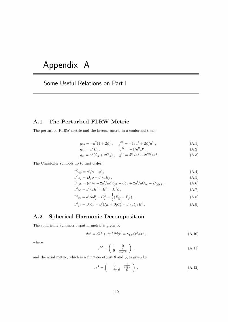
Appendix A
Some Useful Relations on Part I
A.1 The Perturbed FLRW Metric
The perturbed FLRW metric and the inverse metric in a conformal time:
g00 = −a2(1 + 2φ) , g00 = −1/a2 + 2φ/a2 , (A.1)
g0i = a2Bi , g0i = −1/a2Bi , (A.2)
gij = a2(δij + 2Cij) , gij = δij/a2 − 2Cij/a2 . (A.3)
The Christoffer symbols up to first order:
Γ000 = a′/a+ φ′ , (A.4)
Γ00j = Djφ+ a′/aBj , (A.5)
Γ0jk = (a′/a− 2a′/aφ)δjk + C ′jk + 2a′/aCjk −B(j|k) , (A.6)
Γi00 = a′/aBi +B′i +Diφ , (A.7)
Γi0j = a′/aδij + C ′ij +1
2(Bi|j −B
|ij ) , (A.8)
Γijk = ∂kCij − ∂iCjk + ∂jC
ik − a′/aδjkBi . (A.9)
A.2 Spherical Harmonic Decomposition
The spherically symmetric spatial metric is given by
ds2 = dθ2 + sin2 θdφ2 = γIJdxIdxJ , (A.10)
where
γIJ =
(1 00 1
sin2 θ
), (A.11)
and the axial metric, which is a function of just θ and φ, is given by
εIJ =
(0 1
sin θ− sin θ 0
), (A.12)
119
Appendix 120
whereεIJ = γIkγJlεk
l, and εIJεJ
K = −γIk . (A.13)
A.2.1 Properties of the Harmonics Decomposition
The spherical harmonic decomposition is a conventional way to decompose a spatial tensor field δQinto components which transform irreducibly under translations and rotation components, wherethese components evolve independently. This is achieved by splitting the spacetime into a 2 ×2 manifold, indicating 2-dimensional spherically symmetric surfaces and 2-dimensional sphericalharmonic functions Y lm(φ, θ).
Scalars : X(w, y,Xk) =+∞∑l=0
l∑m=−l
[X lm(w, y)Y lm(Xk)
], (A.14)
Vectors : XI(w, y,Xk) =
+∞∑l=1
l∑m=−l
[X lm(w, y)Y lmI (Xk) +X
lm(w, y)Y
lm
I (Xk)
], (A.15)
Tensors : XIJ(w, y,Xk) =1
2
+∞∑l=0
l∑m=−l
XTlm(w, y)γIJY
lm(Xk)
++∞∑l=2
l∑m=−l
[X lm(w, y)Y lmIJ (Xk) +X
lm(w, y)Y
lm
IJ (Xk)
]. (A.16)
A.2.1.1 Polar Decomposition
The (Y lm, Y lmI , Y lmIJ ) represent the polar parts; for scalar, vector and tensor respectively. For thescalar polar part we get
∇2Y lm = γIJ∇
I∇JY lm = −l(l + 1)Y lm , (A.17)
εIJ∇I∇JY lm = 0 . (A.18)
We can re-write the polar vector part as
Y lmI = ∂IYlm , (A.19)
where we can say
Y lmθ = ∂θYlm , (A.20)
Y lmφ = ∂φYlm . (A.21)
The polar vector divergence can be given as
∇IY lmI = ∆Y lm = −l(l + 1)Y lm . (A.22)
Then for the polar tensor part we have
Y lmIJ = ∇I∂JY lm +l(l + 1)
2γIJY
lm , (A.23)
this means
Y lmθθ = ∂2θY
lm +l(l + 1)
2Y lm , (A.24)
Y lmφφ = ∂2φY
lm + sin θ cos θ∂θYlm +
l(l + 1)
2sin2 θY lm , (A.25)
Appendix 121
Y lmθφ = ∂2θφY
lm − cos θ
sin θ∂φY
lm . (A.26)
The polar tensor part is trace-freeγIJY lmIJ = 0 , (A.27)
and given this fact we can have
Y lmI
I = γθθY lmθθ + γφφY lmφφ = 0 , (A.28)[∂2θY
lm +1
sin2 θ∂2φY
lm +l(l + 1)
2Y lm +
l(l + 1)
2Y lm +
cos θ
sin θ∂θY
lm
]= 0 , (A.29)[
∂2θY
lm +1
sin2 θ∂2φY
lm +cos θ
sin θ∂θY
lm
]= −l(l + 1)Y lm . (A.30)
Also note the polar tensor divergence
∇IY lmIJ = ∇2Y lmJ +
l(l + 1)
2∇JY lm =
2− l(l + 1)
2Y lmJ , (A.31)
whereas∆Y lmI = ∇2
Y lmI = (1− l(l + 1))Y lmI , (A.32)
from which one gets
∆Yφ =
[∂2θY
lmφ +
1
sin2 θ∂2φY
lmφ +
cos θ
sin θ∂θY
lmφ
]= (1− l(l + 1))Y lmφ , (A.33)
∆Yθ =
[∂2θY
lmθ +
1
sin2 θ∂2φY
lmθ +
cos θ
sin θ∂θY
lmθ
]= (1− l(l + 1))Y lmθ , (A.34)
and for polar tensor∆Y lmIJ = (4− l(l + 1))Y lmIJ . (A.35)
A.2.1.2 Axial Decomposition
The (Ylm
I , Ylm
IJ ) represent the axial part for vectors and tensors respectively and there is no axialpart for scalars. We can re-define the axial vector part as
Ylm
I = εIJ∂JY
lm , (A.36)
where
Ylm
θ =1
sin θ∂φY
lm , (A.37)
Ylm
φ = − sin θ∂θYlm . (A.38)
The axial vector divergence is given as
∇IY lmI = ∇IεIJY lmJ = γIm∇mεIJ∇JY lm , (A.39)
=1
sin θ
[∂2θφY
lm − cos θ
sin θ∂φY
lm
]− 1
sin θ
[∂2θφY
lm − cos θ
sin θ∂φY
lm
]= 0 . (A.40)
For axial tensors we getY IJ = 2∇(IY J) = −2εk(I∇J)∇kY , (A.41)
Appendix 122
where
Y θθ =2
sin θ
[∂2θφY −
cos θ
sin θ∂φY
], (A.42)
Y φφ = −2 sin θ
[∂2θφY −
cos θ
sin θ∂φY
], (A.43)
Y θφ = − sin θ
[∂2θY −
1
sin2 θ∂2φY −
cos θ
sin θ∂θY
]. (A.44)
The axial tensor is also trace-freeγIJY
lm
IJ = 0 , (A.45)
which implies that
∂θYlm
θ +1
sin2 θ∂φY
lm
φ +cos θ
sin θYlm
θ = 0 . (A.46)
The axial tensor divergence is
DIYlm
IJ = −2DIεk(IDJ)Ylmk = −[1− l(l + 1)][γθθ∇θY δφJ − γ
φφ∇φY δθJ ] . (A.47)
The axial vector harmonics also obey
∆Ylm
I = ∇2Ylm
I = (1− l(l + 1))Ylm
I , (A.48)
from which one gets
∆Y φ =
[∂2θY
lm
φ +1
sin2 θ∂2φY
lm
φ +cos θ
sin θ∂θY
lm
φ
]= (1− l(l + 1))Y
lm
φ , (A.49)
∆Y θ =
[∂2θY
lm
θ +1
sin2 θ∂2φY
lm
θ +cos θ
sin θ∂θY
lm
θ
]= (1− l(l + 1))Y
lm
θ , (A.50)
and for tensors∆Y
lm
IJ = (4− l(l + 1))Ylm
IJ . (A.51)
Appendix B
Some Useful Relations on Part II
B.1 Zero-order Coordinates Transformation
We can see now how the background changes under the PLG transformation. The Jacobian mapwill look like
∂xµ
∂xν=
1 1 0 00 1 0 00 0 1 00 0 0 1
= δµν + δµ0 δ1ν , (B.1)
whereas the inverse matrix is given by
∂xµ
∂xν=
1 −1 0 00 1 0 00 0 1 00 0 0 1
= δµν − δµ0 δ
1ν . (B.2)
Then at the background level, the line element becomes,
ds2 = a2(w − y)(−dw2 + 2dwdy + S2(y)dΩ2) , (B.3)
and the 4-velocity is given by
uµ =1
a(w − y)δµ0 . (B.4)
The scale factor a(η) transforms as a(η) = a(w − y), and S(χ) = S(y), i.e, they are the samespacetime functions but expressed in the new coordinates. The vector field k is given by
kµ = a(w)δ0µ , kν = (a(w)/a2(w − y))δν1 . (B.5)
Thereforedy
dν= a(w)/a2(w − y)→ 1/a(w), at C . (B.6)
B.1.1 The Observables at Zeroth-order
The observable quantities are given by the relations
123

Appendix 124
1. The Redshift:1 + z = a(w)/a(w − y) . (B.7)
2. The Area Distance:
r2A = S2(y)a2(w)/(1 + z)2 = a2(w − y)S2(y) . (B.8)
3. The Luminosity Distance:dL = (1 + z)2r2
A = a2(w)S2(y) . (B.9)
4. The Number Count
dN = fmn(w − y)r2A dΩ a(w)(1 + z)−1dy = fmn(w − y)a3(w − y)S2(y) dΩdy . (B.10)
B.2 Relations on the Observational Metric
From the observational metric we can write the complete perturbed metric components to first orderas:
gww = −a2(w − y) (1− δα) , (B.11)
gwy = a2(w − y) (1 + δβ) , (B.12)
gyy = 0 , (B.13)
gwI = a2(w − y) (vI) , (B.14)
gIJ = a2(w − y) (ΩIJ +HIJ) , (B.15)
gyI = 0 . (B.16)
The contravariant metric tensor follows from the constraint to the required order:
gµνgνλ = δλµ , (B.17)
and that gives
gww = 0 , (B.18)
gwy = a−2(w − y)−1 (1− δβ) , (B.19)
gwI = 0 , (B.20)
gyy = a−2(w − y)−1 (1− (δα+ 2δβ)) , (B.21)
gIJ = a−2(w − y)−1(ΩIJ −HIJ
), (B.22)
gyI = −a−2(w − y)−1ΩIJvJ . (B.23)
Using the definition of the Christoffel symbols given by Eq. (2) we can have the components of theaffine connection coefficients calculated to first order as
Γwww = 2∂wa
a+∂ya
a(1− δβ − δα) + ∂wδβ −
1
2∂yδα , (B.24)
ΓwwI = −a′
avI −
1
2∂yvI +
1
2∂Iδβ , (B.25)
ΓwIJ =∂ya
a(−ΩIJ −HIJ + ΩIJδβ)− 1
2∂yΩIJ −
1
2∂yHIJ +
1
2εδβ∂yΩIJ , (B.26)
Γyyy = 2∂ya
a+ ∂yδβ , (B.27)
Γywy =∂ya
a(−1 + δα+ δβ) +
1
2∂yδα , (B.28)

Appendix 125
ΓyIy =∂ya
a(vI − ΩJkΩIkvJ) +
1
2∂yvI −
1
2ΩJk∂yΩIkvJ +
1
2∂Iδβ , (B.29)
ΓyIw = −∂waa
ΩIJΩIJvI −∂ya
avI −
1
2∂yvI +
1
2∂Iδα+
1
2∂Iδβ , (B.30)
Γyww =∂wa
a(1− δα− δβ) +
∂ya
a(1− 2δα− 2δβ) +
1
2∂wδα+ ∂wδβ −
1
2∂yδα , (B.31)
ΓyIJ =1
2∂IvJ +
1
2∂JvI −
∂wa
a(ΩIJ + εHIJ − ΩIJδβ)− ∂ya
a(ΩIJ +HIJ − ΩIJ
δα− 2ΩIJδβ)− 1
2∂wHIJ −
1
2∂yHIJ −
1
2∂yΩIJ +
1
2∂yΩIJδα
+∂yΩIJδβ +1
2ΩkJvJ∂IΩkJ , (B.32)
ΓIkJ =∂ya
aΩImΩkJvm +
1
2ΩImvm∂yΩkJ +
1
2ΩmI∂kΩmJ +
1
2ΩmI∂kHmJ
+1
2ΩmI∂JΩmk +
1
2ΩmI∂JHmk −
1
2ΩmI∂mΩkJ −
1
2ΩmI∂mHkJ
−1
2HmI∂kΩmJ −
1
2HmI∂JΩmk +
1
2HmI∂mΩkJ , (B.33)
ΓIww = −∂yaa
ΩIJvJ + ΩIJ∂wvJ −1
2ΩIJ∂Jδα , (B.34)
ΓIwy =∂ya
aΩIJvJ +
1
2ΩIJ∂yvJ −
1
2ΩIJ∂Jδβ , (B.35)
ΓIwJ =∂wa
a(ΩkIΩkJ + ΩkIHkJ − ΩkJH
kI) +1
2ΩkI∂wHkJ +
1
2ΩkI∂Jvk
−1
2ΩkI∂kvJ , (B.36)
ΓIyJ =∂ya
a(ΩkIΩkJ + ΩkIHkJ − ΩkJH
kI) +1
2ΩkI∂yΩkJ +
1
2ΩkI∂yHkJ
−1
2HkI∂yΩkJ , (B.37)
whereΓwwy = ΓwIy = Γwyy = ΓIyy = 0 . (B.38)
The Riemann tensor is defined by
Rµνγβ = Γµνβ,γ − Γµνγ,β + ΓανβΓµγα − ΓδνγΓµβδ , (B.39)
whereas the Ricci tensor is obtained by contracting the first and the third indices of the Riemanntensor:
Rµν = gγβRγµβν , (B.40)
and the Ricci scalar is given asR = Rµµ . (B.41)
B.3 Derivatives and Integrals
B.3.1 Commuting Partial Derivatives
Here is an attempt at finding a way to commute partial derivatives and integrals that we used inour calculations. Assume we want to calculate ∂ηX where X is first order and is written:
X =
∫Y dλ . (B.42)
Appendix 126
Then we haved
dλX = Y ⇔ (∂χ + ∂η)X = a2Y . (B.43)
Therefore,(∂χ + ∂η) ∂ηX = a2∂ηY + 2a2HY , (B.44)
or equivalently,d
dλ∂ηX = ∂ηY + 2HY . (B.45)
Hence,
∂η
∫Y dλ =
∫[∂ηY + 2HY ] dλ . (B.46)
Similarly:
∂χ
∫Y dλ =
∫[∂χY ] dλ . (B.47)
Using these two relations and integrating by parts, we recover∫d
dλY dλ = Y . (B.48)
Finally,
∂I
∫Y dλ =
∫∂IY dλ . (B.49)
B.3.2 Integration Formulae
Using integration by parts we can convert the double integrals over time into a single integral, usinga regular function f(η). We are going to integrate by parts the following function:∫ ηo
ηs
(η − ηs)f(η)dη, (B.50)
Choosing the auxiliary functions
u = η − ηs , dv = f(η)dη, (B.51)
du = dη , v =
∫ η
ηs
f(η′)dη′ (B.52)
then we can write
∫ ηo
ηs
(η − ηs)f(η)dη =
((η − ηs)
∫ η
ηs
f(η)dη
)nons
−∫ ηo
ηs
dη
∫ η
ηs
f(η′)dη′, (B.53)
= (ηo − ηs)∫ ηo
ηs
f(η)dη −∫ ηo
ηs
dη
∫ η
ηs
f(η′)dη′, (B.54)
=
∫ ηo
ηs
dη
[ ∫ η
ηs
f(η)dη +
∫ ηo
η
f(η)dη
]−∫ ηo
ηs
dη
∫ η
ηs
f(η′)dη′, (B.55)
=
∫ ηo
ηs
dη(η − ηs)f(η) +
∫ ηo
ηs
dη(ηo − η)f(η)dη −∫ ηo
ηs
dη
∫ η
ηs
f(η′)dη′,
(B.56)
0 =
∫ ηo
ηs
dη(ηo − η)f(η)−∫ ηo
ηs
dη
∫ η
ηs
f(η′)dη′ . (B.57)
Appendix 127
Thus ∫ ηo
ηs
dη(ηo − η)f(η) =
∫ ηo
ηs
dη
∫ η
ηs
f(η′)dη′. (B.58)
or ∫ ηo
ηs
dη(η − ηs)f(η) =
∫ ηo
ηs
dη
∫ η
ηs
f(η′)dη′. (B.59)
We can also use the following from Eq. (B.55):∫ ηo
ηs
f(η)dη =1
ηo − ηs
[ ∫ ηo
ηs
dη(η − ηs)f(η) +
∫ ηo
ηs
dη
∫ η
ηs
f(η′)dη′]. (B.60)
B.4 Some Useful Derivation for Sec. 4.4
Using Eq. (4.12) we have
∇⊥i∇⊥iE = (−ninj∇i∇j − γij∇⊥inj∇‖ + γij∇i∇j)E , (B.61)
= (−ninj∇i∇j − γij(∇i − ni∇‖)nj∇‖ + γij∇i∇j)E , (B.62)
= (−ninj∇i∇j − γij∇injnj∇j + γijni(ni∇i)nj(nj∇j) + γij∇i∇j)E = 0 , (B.63)
and
∇⊥iF⊥i = (∇i − ni∇‖)(F i − niF‖) , (B.64)
= ∇iF i −∇iniF‖ − ni∇‖F i + ni∇‖niF‖ = 0 . (B.65)
From Eq. (4.22) and Eq. (4.24) we can write
h⊥i⊥i = hii − h‖(nini −1
2N i
i)− 2h⊥|(ini) = 0 . (B.66)
We can also simplify and write
1
2∇⊥injnk∇jh ⊥ik +
1
2∇⊥injnk∇kh ⊥ij +∇⊥injh′ ⊥ij − 1
2∇⊥i∇⊥ihjknjnk
= ∇⊥injnk∇kh ⊥ij + (∇⊥inj)h′ ⊥ij − 1
2(∇2 − ninj∇i∇j − γij∇⊥inj∇‖)hlknlnk , (B.67)
= ∇⊥injnk∇k1
2(hij − h‖(
*0ninj − 1/2
0
N ij)−
>0
h⊥i⊥j) +1
χnin
jγij(γji − nin
j)h′ lj Nil
− 1
2(∇2 − ninj∇i∇j − γij(∇i − ni∇‖)nj∇‖)hlknlnk , (B.68)
=1
2(∇i − ni∇‖)njnk∇khij +
2
χnin
jh′ lj Nil −
1
2(∇2 − ninj∇i∇j − γij∇inj∇‖
+ γijni∇‖nj∇‖)hlknlnk ,(B.69)
= −
:
1
2ninj∇lnlnk∇khij +
2
χnln
jh′ lj −1
2
(2∇2 −
:2ninj∇i∇j)hlkn
lnk , (B.70)
=2
χninjh′ij −∇2hijn
inj , (B.71)
and the following terms can be re-written as
:0∇⊥inj∇jB
⊥i −∇⊥i∇⊥iBjnj +:
0∇⊥iB
⊥i′= −(∇2 −∇2
‖ −2
χ∇‖)Bjnj , (B.72)
Appendix 128
= −∇2Bjnj +∇‖(
d
dη−∇η)Bjn
j +1
χ∇‖)Bjnj +
1
χ∇‖)Bini , (B.73)
= −∇2Bjnj +
*0
d
dη∇‖B
‖ −∇‖B′jnj +
1
χ∇‖Bjnj +
1
χ∇‖Bini , (B.74)
= −∇2Bini − 1
2∇iniB
′‖ −
1
2∇jnjB
′‖ +
2
χ∇(jBi)n
inj , (B.75)
= −∇2Bini −∇(iB
′j)n
inj +2
χ∇(iBj)n
inj . (B.76)
Moreover, we note
2∇⊥inj∇(jF⊥i)′ +∇⊥injnk∇k∇(jF
⊥i) −∇⊥i∇⊥i∇(kFj)njnk +∇⊥injnk∇j∇(kF
⊥i)
=
:0∇⊥inj∇jF⊥i
′+∇⊥inj∇⊥iF j
′+
:0
∇⊥injnk∇k∇jF⊥i −
:
∇⊥i∇⊥i∇kFjnjnk
+
:
∇⊥i∇⊥i∇kFjnjnk ,(B.77)
= ∇⊥inj∇⊥iF j′, (B.78)
= (∇2 −∇2‖ −
2
χ∇‖)njF j
′, (B.79)
= ∇2njFj ′ −∇‖(
d
dη−∇η)njF
j ′ − 2
χ∇‖njF j
′, (B.80)
= ∇2njFj ′ −*
0
∇‖d
dηF ‖′+∇‖∇ηF j
′nj −
2
χ∇‖njF j
′, (B.81)
= ∇2njFj ′ +∇‖F j
′′nj −
2
χ∇‖njF j
′, (B.82)
= ∇2njFj ′ +
1
2∇‖F j
′′nj +
1
2∇‖F i
′′ni −
1
χ∇‖njF j
′ − 1
χ∇‖niF i
′, (B.83)
= ∇2njFj ′ +∇(iFj)
′′njni − 2
χ∇(iFj)
′njni , (B.84)
where Eq. (4.5) has been made use of.
B.5 Some Useful Expressions for Computing HT
The following facts/relations have been used in our calculations of Chapter 5:
1
2∇⊥injnk∂jh ⊥ik +
1
2∇⊥injnk∂kh ⊥ij +∇⊥injh′ ⊥ij − 1
2∇⊥i∇⊥ihjknjnk
= ∇⊥injnk∇kh ⊥ij +∇⊥injh′ ⊥ij − 1
2∇⊥i∇⊥ihjknjnk , (B.85)
=
:
0
(∇i + ni∇‖)[njnk∇kh ⊥ij + njh′ ⊥ij ]− 1
2∇⊥i∇⊥ihjknjnk , (B.86)
= −1
2∇⊥i∇⊥ihjknjnk , (B.87)
≡ −1
2(∂2θ + cot θ∂θ + 1/ sin2 θ∂2
φ)hχχnχnχ , (B.88)
Appendix 129
2∇⊥inj∇(jF⊥i)′ +∇⊥injnk∂k∂(jF
⊥i) −∇⊥i∇⊥i∂(kFj)njnk +∇⊥injnk∂j∂(kF
⊥i)
=
:0∇⊥inj∇jF⊥i
′+∇⊥inj∇⊥iF j
′+
:
0
∇⊥injnk∇k∇jF⊥i −
:
∇⊥i∇⊥i∂kFjnjnk
+
:
∇⊥i∇⊥i∇kFjnjnk , (B.89)
= ∇⊥i∇⊥iF j′nj , (B.90)
Or we can say (B.91)
≡ (∂2θ + cot θ∂θ + 1/ sin2 θ∂2
φ)nχF ′χ , (B.92)
:0∇⊥inj∇jB
⊥i −∇⊥i∇⊥iBjnj +:
0∇⊥iB
⊥i′= −∇⊥i∇⊥iBjnj , (B.93)
≡ −(∂2θ + cot θ∂θ + 1/ sin2 θ∂2
φ)Bχnχ . (B.94)
Appendix C
Some Useful Relations on Part III
C.1 Linearised Differential Identities
For all scalars f , vectors Va and tensors that vanish in the background, Sab = S〈ab〉, the followinglinearised identities hold [192,240,249]:(
∇〈a∇b〉f).
= ∇〈a∇b〉f − 23Θ∇〈a∇b〉f + f∇〈aAb〉 , (C.1)
εabc∇b∇cf = 0 , (C.2)
εcda∇c∇〈b∇d〉f = εcda∇c∇(b∇d)f = εcda∇c∇b∇df = 0 , (C.3)
∇2(∇af
)= ∇a
(∇2f
)+ 1
3 R∇af , (C.4)(∇af
)·= ∇af − 1
3Θ∇af + fAa , (C.5)(∇aSb···
)·= ∇aSb··· − 1
3Θ∇aSb··· , (C.6)(∇2f
)·= ∇2f − 2
3Θ∇2f + f∇aAa , (C.7)
∇[a∇b]Vc = − 16 RV[ahb]c , (C.8)
∇[a∇b]Scd = − 13 RS[a
(chb]d) , (C.9)
∇a(εabc∇bV c
)= 0 , (C.10)
∇b(εcd〈a∇cSb〉d
)= 1
2εabc∇b
(∇dSdc
), (C.11)
curlcurlVa = ∇a(∇bVb
)− ∇2Va + 2
3
(µ− 1
3Θ2)Va , (C.12)
where R ≡ 2(µ− 1
3Θ2)
is the 3-curvature scalar.
130
Bibliography
[1] M. Betoule, R. Kessler, J. Guy, J. Mosher, D. Hardin, R. Biswas, P. Astier, P. El-Hage,M. Konig, S. Kuhlmann, et al., “Improved cosmological constraints from a joint analysis ofthe SDSS-II and SNLS supernova samples,” Astronomy & Astrophysics, vol. 568, p. A22, 2014.
[2] J. C. Mather, E. Cheng, R. Eplee Jr, R. Isaacman, S. Meyer, R. Shafer, R. Weiss, E. Wright,C. Bennett, N. Boggess, et al., “A preliminary measurement of the cosmic microwave back-ground spectrum by the cosmic background explorer (COBE) satellite,” The AstrophysicalJournal, vol. 354, pp. L37–L40, 1990.
[3] R. Adam, P. Ade, N. Aghanim, Y. Akrami, M. Alves, F. Argueso, M. Arnaud, F. Arroja,M. Ashdown, J. Aumont, et al., “Planck 2015 results-i. overview of products and scientificresults,” Astronomy & Astrophysics, vol. 594, p. A1, 2016.
[4] T. V. Albada et al., “Distribution of dark matter in the spiral galaxy NGC 3198,” Astrophys.J., vol. 295, pp. 305–313, 1985.
[5] D. Clowe, M. Bradac, A. H. Gonzalez, M. Markevitch, S. W. Randall, C. Jones, and D. Zarit-sky, “A direct empirical proof of the existence of dark matter,” The Astrophysical JournalLetters, vol. 648, no. 2, p. L109, 2006.
[6] S. Dodelson, Modern Cosmology. Academic Press, 2003.
[7] M. Blanton and S. D. S. Survey, “Lecture notes on Introduction to Cosmology,” February2013. Accessed: 10-07-2016.
[8] A. Hamilton, “Lecture notes on Introduction to Cosmology,” 2002. Accessed: 17-02-2015.
[9] e.s.a., “Planck and the Cosmic Microwave Background,” March 2013. Accessed: 19-12-2016.
[10] P. Peter and J. P. Uzan, Primordial Cosmology. Oxford University Press, 2013.
[11] F. Nugier, “The geodesic light-cone coordinates, an adapted system for light-signal-basedcosmology,” arXiv preprint arXiv:1508.07464, 2015.
[12] A. Einstein, Allgemeine Relativitatstheorie. Wiley Online Library, 1915.
[13] S. Weinberg, Gravitation and cosmology: principles and applications of the general theory ofrelativity, vol. 1. Wiley New York, 1972.
[14] H. Stephani, General Relativity an introduction to the theory of gravitational fields. CambridgeUniversity Press, Cambridge, 1990.
131
Bibliography 132
[15] A. Einstein, “Kosmologische Betrachtungen zur allgemeinen Relativitatstheorie, Sitzungs-berichte der Kniglich Preußischen Akademie der Wissenschaften (Berlin), Seite 142-152,” 1917.
[16] H. Nussbaumer, “Einstein’s conversion from his static to an expanding universe,” The Euro-pean Physical Journal H, vol. 39, no. 1, pp. 37–62, 2014.
[17] C. W. Misner, K. S. Thorne, and J. A. Wheeler, Gravitation. Macmillan, 1973.
[18] L. M. Krauss and M. S. Turner, “The cosmological constant is back,” General Relativity andGravitation, vol. 27, no. 11, pp. 1137–1144, 1995.
[19] A. Friedman, “Uber die krummung des Raumes,” Zeitschrift fur Physik A Hadrons and Nuclei,vol. 10, no. 1, pp. 377–386, 1922.
[20] G. Lemaıtre, “Un univers homogene de masse constante et de rayon croissant rendant comptede la vitesse radiale des nebuleuses extra-galactiques,” in Annales de la Societe scientifique deBruxelles, vol. 47, pp. 49–59, 1927.
[21] G. Lemaıtre, A, “A homogeneous universe of constant mass and increasing radius accountingfor the radial velocity of extra-galactic nebulae,” Monthly Notices of the Royal AstronomicalSociety, vol. 91, no. 5, pp. 483–490, 1931.
[22] E. Hubble, “A relation between distance and radial velocity among extra-galactic nebulae,”Proceedings of the National Academy of Sciences, vol. 15, no. 3, pp. 168–173, 1929.
[23] H. P. Robertson, “On the foundations of relativistic cosmology,” Proceedings of the NationalAcademy of Sciences, vol. 15, no. 11, pp. 822–829, 1929.
[24] H. P. Robertson, “Kinematics and World-Structure,” The Astrophysical Journal, vol. 82,p. 284, 1935.
[25] H. P. Robertson, “Kinematics and World-Structure II.,” The Astrophysical Journal, vol. 83,p. 187, 1936.
[26] H. P. Robertson, “Kinematics and World-Structure III.,” The Astrophysical Journal, vol. 83,p. 257, 1936.
[27] A. G. Walker, “On Milne’s theory of world-structure,” Proceedings of the London MathematicalSociety, vol. 2, no. 1, pp. 90–127, 1937.
[28] G. Ellis, “Limits to verification in cosmology,” Annals of the New York Academy of Sciences,vol. 336, no. 1, pp. 130–160, 1980.
[29] P. J. E. Peebles, D. Schramm, E. Turner, and R. Kron, “The case for the relativistic hot bigbang cosmology,” Nature, vol. 352, no. 6338, pp. 769–776, 1991.
[30] P. Peebles, “Large-scale background temperature and mass fluctuations due to scale-invariantprimeval perturbations,” Astrophys. J, vol. 263, pp. L1–L5, 1982.
[31] G. F. Ellis and H. Van Elst, “Cosmological models,” in Theoretical and Observational Cos-mology, pp. 1–116, Springer, 1999.
[32] A. De Simone, A. H. Guth, M. P. Salem, and A. Vilenkin, “Predicting the cosmologicalconstant with the scale-factor cutoff measure,” Physical Review D, vol. 78, no. 6, p. 063520,2008.
[33] P. Fleury, “Light propagation in inhomogeneous and anisotropic cosmologies,” arXiv preprintarXiv:1511.03702, 2015.
Bibliography 133
[34] C. Bennett, N. Boggess, E. Cheng, M. Hauser, T. Kelsall, J. Mather, S. Moseley, T. Mur-dock, R. Shafer, R. Silverberg, et al., “Scientific results from the cosmic background explorer(COBE)(microwave/infrared),” Proceedings of the National Academy of Sciences, vol. 90,no. 11, pp. 4766–4773, 1993.
[35] “NASA/WMAP Science Team: Wilkinson Microwave Anisotropy Probe,” 2013. Accessed:26-06-2016.
[36] P. Ade, N. Aghanim, M. Alves, C. Armitage-Caplan, M. Arnaud, M. Ashdown, F. Atrio-Barandela, J. Aumont, H. Aussel, C. Baccigalupi, et al., “Planck 2013 results. I. overview ofproducts and scientific results,” Astronomy & Astrophysics, vol. 571, p. A1, 2014.
[37] D. Fixsen, “The temperature of the cosmic microwave background,” The Astrophysical Jour-nal, vol. 707, no. 2, p. 916, 2009.
[38] R. Durrer, The cosmic microwave background, vol. 140. Cambridge University Press Cam-bridge, 2008.
[39] D. J. Eisenstein, I. Zehavi, D. W. Hogg, R. Scoccimarro, M. R. Blanton, R. C. Nichol, R. Scran-ton, H.-J. Seo, M. Tegmark, Z. Zheng, et al., “Detection of the baryon acoustic peak in thelarge-scale correlation function of SDSS luminous red galaxies,” The Astrophysical Journal,vol. 633, no. 2, p. 560, 2005.
[40] L. Anderson, E. Aubourg, S. Bailey, F. Beutler, V. Bhardwaj, M. Blanton, A. S. Bolton,J. Brinkmann, J. R. Brownstein, A. Burden, et al., “The clustering of galaxies in the SDSS-IIIbaryon oscillation spectroscopic survey: baryon acoustic oscillations in the data releases 10and 11 galaxy samples,” Monthly Notices of the Royal Astronomical Society, vol. 441, no. 1,pp. 24–62, 2014.
[41] T. Delubac, J. E. Bautista, J. Rich, D. Kirkby, S. Bailey, A. Font-Ribera, A. Slosar, K.-G. Lee,M. M. Pieri, J.-C. Hamilton, et al., “Baryon acoustic oscillations in the Lyα forest of BOSSDR11 quasars,” Astronomy & Astrophysics, vol. 574, p. A59, 2015.
[42] W. Baade and F. Zwicky, “On super-novae,” Proceedings of the National Academy of Sciences,vol. 20, no. 5, pp. 254–259, 1934.
[43] W. Baade and F. Zwicky, “Cosmic rays from super-novae,” Proceedings of the NationalAcademy of Sciences, vol. 20, no. 5, pp. 259–263, 1934.
[44] A. G. Riess, A. V. Filippenko, P. Challis, A. Clocchiatti, A. Diercks, P. M. Garnavich, R. L.Gilliland, C. J. Hogan, S. Jha, R. P. Kirshner, et al., “Observational evidence from supernovaefor an accelerating universe and a cosmological constant,” The Astronomical Journal, vol. 116,no. 3, p. 1009, 1998.
[45] E. Elizalde, S. Nojiri, and S. D. Odintsov, “Late-time cosmology in a (phantom) scalar-tensortheory: dark energy and the cosmic speed-up,” Physical Review D, vol. 70, no. 4, p. 043539,2004.
[46] M. S. Turner and M. White, “CDM models with a smooth component,” Physical Review D,vol. 56, no. 8, p. R4439, 1997.
[47] R. R. Caldwell, R. Dave, and P. J. Steinhardt, “Cosmological imprint of an energy componentwith general equation of state,” Physical Review Letters, vol. 80, no. 8, p. 1582, 1998.
[48] P. Peebles and B. Ratra, “Cosmology with a time-variable cosmological ’constant’,” The As-trophysical Journal, vol. 325, pp. L17–L20, 1988.
[49] J. Yoo and Y. Watanabe, “Theoretical models of dark energy,” International Journal of Mod-ern Physics D, vol. 21, no. 12, p. 1230002, 2012.
Bibliography 134
[50] A. Kamenshchik, U. Moschella, and V. Pasquier, “An alternative to quintessence,” PhysicsLetters B, vol. 511, no. 2.
[51] E. Kahya, B. Pourhassan, and S. Uraz, “Constructing an inflaton potential by mimickingmodified Chaplygin gas,” Physical Review D, vol. 92, no. 10, p. 103511, 2015.
[52] H. Sami, N. Namane, J. Ntahompagaze, M. Elmardi, and A. Abebe, “Reconstructing f(R)gravity from a Chaplygin scalar field in de Sitter spacetimes,” International Journal of Geo-metric Methods in Modern Physics, vol. 15, p. 1850027, 2018.
[53] T.-P. Cheng and B. H. Benedict, A college course on relativity and cosmology. Oxford Uni-versity Press, 2015.
[54] S. Nadathur and S. Sarkar, “Reconciling the local void with the CMB,” Physical Review D,vol. 83, no. 6, p. 063506, 2011.
[55] A. De Felice and S. Tsujikawa, “f(R) theories,” Living Rev. Rel, vol. 13, no. 3, pp. 1002–4928,2010.
[56] T. P. Sotiriou and V. Faraoni, “f(R) theories of gravity,” Reviews of Modern Physics, vol. 82,no. 1, p. 451, 2010.
[57] T. Clifton, P. G. Ferreira, A. Padilla, and C. Skordis, “Modified gravity and cosmology,”Physics Reports, vol. 513, no. 1, pp. 1–189, 2012.
[58] S. Capozziello and M. De Laurentis, “Extended theories of gravity,” Physics Reports, vol. 509,no. 4, pp. 167–321, 2011.
[59] L. Modesto, “Super-renormalizable quantum gravity,” Phys. Rev. D, vol. 86, p. 044005, Aug2012.
[60] T. Biswas, E. Gerwick, T. Koivisto, and A. Mazumdar, “Towards singularity and ghost freetheories of gravity,” Phys.Rev.Lett., vol. 108, p. 031101, 2012.
[61] S. Nojiri and S. D. Odintsov, “Modified gravity with negative and positive powers of curvature:Unification of inflation and cosmic acceleration,” Physical Review D, vol. 68, no. 12, p. 123512,2003.
[62] J. Rosa, “Lecture notes on Introduction to Cosmology,” February 2013. Accessed: 23-12-2015.
[63] S. D. White, J. F. Navarro, A. E. Evrard, and C. S. Frenk, “The baryon content of galaxyclusters-a challenge to cosmological orthodoxy,” 1993.
[64] R. Peccei and D. Cline, Trends in Astroparticle Physics: Proceedings of the UCLA Interna-tional Conference. World Scientific, 1991.
[65] S. Sasaki, “A new method to estimate cosmological parameters using the baryon fractionof clusters of galaxies,” Publications of the Astronomical Society of Japan, vol. 48, no. 6,pp. L119–L122, 1996.
[66] C. Faure, A. Siebert, and B. Famaey, “Radial and vertical flows induced by galactic spiralarms: likely contributors to our wobbly galaxy,” Monthly Notices of the Royal AstronomicalSociety, vol. 440, no. 3, pp. 2564–2575, 2014.
[67] M. Roos, “Dark matter: The evidence from astronomy, astrophysics and cosmology,” arXivpreprint arXiv:1001.0316, 2010.
[68] J. H. Oort, “The force exerted by the stellar system in the direction perpendicular to thegalactic plane and some related problems,” Bulletin of the Astronomical Institutes of theNetherlands, vol. 6, p. 249, 1932.
Bibliography 135
[69] F. Zwicky, “Die Rotverschiebung von extragalaktischen Nebeln,” Helvetica Physica Acta,vol. 6, pp. 110–127, 1933.
[70] F. Zwicky, “On the masses of nebulae and of clusters of nebulae,” The Astrophysical Journal,vol. 86, p. 217, 1937.
[71] G. Bertone, D. Hooper, and J. Silk, “Particle dark matter: Evidence, candidates and con-straints,” Physics Reports, vol. 405, no. 5, pp. 279–390, 2005.
[72] R. Durrer, “Gauge invariant cosmological perturbation theory: A general study and its ap-plication to the texture scenario of structure formation,” Fundamentals of Cosmic Physics,vol. 15, no. 3, pp. 209–339, 1994.
[73] M. Milgrom, “A modification of the Newtonian dynamics as a possible alternative to thehidden mass hypothesis,” The Astrophysical Journal, vol. 270, pp. 365–370, 1983.
[74] J. D. Bekenstein, “Relativistic gravitation theory for the modified Newtonian dynamicsparadigm,” Physical Review D, vol. 70, no. 8, p. 083509, 2004.
[75] G. W. Angus, A. Diaferio, B. Famaey, and K. J. van der Heyden, “Cosmological simulationsin MOND: the cluster scale halo mass function with light sterile neutrinos,” Monthly Noticesof the Royal Astronomical Society, vol. 436, no. 1, pp. 202–211, 2013.
[76] P. J. E. Peebles, Principles of physical cosmology. Princeton University Press, 1993.
[77] W. Stoeger, “Cosmology,” 2009. Accessed: 28-12-2015.
[78] H. J. Mark and J. L. Robert, An introduction to galaxies and cosmology. Cambridge UniversityPress, 2004.
[79] C. Bennett, N. Boggess, M. Hauser, J. Mather, G. Smoot, and E. Wright, “Recent results fromCOBE,” in The Environment and Evolution of Galaxies, pp. 27–58, Springer, 1993.
[80] R. Durrer, “Gauge invariant cosmological perturbation theory,” arXiv preprint astro-ph/9311041, 1993.
[81] D. D. Baumann, “Lecture notes on Cosmology,” Novamber 2014. Department of AppliedMathematics and Theoretical Physics-CAMBRIDGE UNIVERSITY.
[82] J. Bahcall, T. Piran, and S. Weinberg, “Dark matter in the universe: Jerusalem winter schoolfor theoretical physics,” in Dark Matter in the Universe: Jerusalem Winter School for Theo-retical Physics, pp. 1–266, World Scientific, 1987.
[83] W. Saunders, W. Sutherland, S. Maddox, O. Keeble, S. Oliver, M. Rowan-Robinson, R. McMa-hon, G. Efstathiou, H. Tadros, S. White, et al., “The PSCz catalogue,” Monthly Notices ofthe Royal Astronomical Society, vol. 317, no. 1, pp. 55–63, 2000.
[84] S. Maddox, G. Efstathiou, W. Sutherland, and J. Loveday, “Galaxy correlations on largescales,” Monthly Notices of the Royal Astronomical Society, vol. 242, no. 1, pp. 43P–47P,1990.
[85] P. Ade, N. Aghanim, C. Armitage-Caplan, M. Arnaud, M. Ashdown, F. Atrio-Barandela,J. Aumont, C. Baccigalupi, A. J. Banday, R. Barreiro, et al., “Planck 2013 results. XVI.cosmological parameters,” Astronomy & Astrophysics, vol. 571, p. A16, 2014.
[86] R. A. Daly, E. J. Guerra, and L. Wan, “Global cosmological parameters measured usingclassical double radio sources,” arXiv preprint astro-ph/9803265, 1998.
[87] A. Unsold and B. Baschek, The new cosmos: an introduction to astronomy and astrophysics.Springer Science & Business Media, 2013.
Bibliography 136
[88] O. Lahav and A. R. Liddle, “The cosmological parameters,” arXiv preprint astro-ph/0406681,2004.
[89] G. Lemaıtre, A, “The beginning of the world from the point of view of quantum theory,”Nature, vol. 127, no. 3210, p. 706, 1931.
[90] H. Kragh, “The beginning of the world: Georges Lemaıtre and the expanding universe,”Centaurus, vol. 30, no. 2, pp. 114–139, 1987.
[91] A. H. Guth, “Inflationary universe: A possible solution to the horizon and flatness problems,”Physical Review D, vol. 23, no. 2, p. 347, 1981.
[92] A. H. Guth and P. J. Steinhardt, “The inflationary universe,” Scientific American, vol. 250,no. 5, pp. 116–128, 1984.
[93] J. Martin, C. Ringeval, and V. Vennin, “Encyclopædia inflationaris,” Physics of the DarkUniverse, vol. 5, pp. 75–235, 2014.
[94] J. Martin, C. Ringeval, and V. Vennin, “Observing inflationary reheating,” Physical reviewletters, vol. 114, no. 8, p. 081303, 2015.
[95] R. A. Alpher, R. Herman, and G. A. Gamow, “Thermonuclear reactions in the expandinguniverse,” Physical Review, vol. 74, no. 9, p. 1198, 1948.
[96] J. Beringer, J. Arguin, R. Barnett, K. Copic, O. Dahl, D. Groom, C. Lin, J. Lys, H. Murayama,C. Wohl, et al., “Review of particle physics,” Physical Review D, vol. 86, no. 1, 2012.
[97] A. Coc and E. Vangioni, “Big-bang nucleosynthesis with updated nuclear data,” in Journal ofPhysics: Conference Series, vol. 202, p. 012001, IOP Publishing, 2010.
[98] T. P. Walker, G. Steigman, D. N. Schramm, K. A. Olive, and H.-S. Kang, “Primordial nu-cleosynthesis redux,” in The Big Bang And Other Explosions In Nuclear And Particle Astro-physics, pp. 43–61, World Scientific, 1996.
[99] R. A. Sunyaev and Y. B. Zeldovich, “Small-scale fluctuations of relic radiation,” Astrophysicsand Space Science, vol. 7, no. 1, pp. 3–19, 1970.
[100] W. McCrea, “Observable relations in relativistic cosmology,” Zeitschrift fur Astrophysik, vol. 9,p. 290, 1935.
[101] A. Walker, “Distance in an expanding universe,” Monthly Notices of the Royal AstronomicalSociety, vol. 94, p. 159, 1933.
[102] D. W. Hogg, “Distance measures in cosmology,” arXiv preprint astro-ph/9905116, 1999.
[103] J. Kristian and R. Sachs, “Observations in cosmology,” The Astrophysical Journal, vol. 143,p. 379, 1966.
[104] G. Ellis, “Relativistic Cosmology in: Proceedings of the International School of Physics ”EnricoFermi”, Course 47: General Relativity and Cosmology. Ed. RK Sachs,” 1971.
[105] G. F. Ellis, R. Maartens, and M. A. MacCallum, Relativistic cosmology. Cambridge UniversityPress, 2012.
[106] R. Durrer, “The theory of CMB anisotropies,” arXiv preprint astro-ph/0109522, 2001.
[107] G. F. Ellis, “Cosmology and verifiability,” Quarterly Journal of the Royal Astronomical Society,vol. 16, pp. 245–264, 1975.
[108] G. F. R. Ellis, S. Nel, R. Maartens, W. Stoeger, and A. Whitman, “Ideal observational cos-mology,” Physics Reports, vol. 124, no. 5, pp. 315–417, 1985.
Bibliography 137
[109] C. F. R. Elis and M. Bruni, “Covariant and guage-invariant approach to cosmological densityfluctuations,” Phys. Rev. D 40 1804, 1989.
[110] M. Elmardi, Magnetogenesis from Cosmological Velocity Perturbations. Lap Lambert Aca-demic Publishing GmbH KG, 2011.
[111] M. J. Stewart and M. Walker, “Perturbations of space-times in general relativity,” Proc. R.Soc. London A 341 49, 1974.
[112] J. M. Bardeen, “Gauge-invariant cosmological perturbations,” Physical Review D, vol. 22,no. 8, p. 1882, 1980.
[113] M. Bruni, P. Dunsby, and G. Ellis, “Cosmological perturbations and the physical meaning ofgauge-invariant variables,” The Astrophysical Journal, vol. 395:34-53, 1992.
[114] J. Ehlers, “Beitrage zur relativistischen Mechanik kontinuierlicher Medien,” Mainz AkademieWissenschaften Mathematisch Naturwissenschaftliche Klasse, vol. 11, pp. 792–837, 1961.
[115] S. W. Hawking, “Perturbations of an expanding universe,” Astrophys. J. 145 544, 1966.
[116] D. W. Olson, “Density perturbations in cosmological models,” Phys. Rev. D 14 327, 1976.
[117] R. K. Sachs and A. M. Wolfe, “Perturbations of a cosmological model and angular variationsof the microwave background,” The Astrophysical Journal, vol. 147, no. 1, pp. 73–90, 1967.
[118] O. Umeh, C. Clarkson, and R. Maartens, “Nonlinear relativistic corrections to cosmologi-cal distances, redshift and gravitational lensing magnification: I. key results,” Classical andQuantum Gravity, vol. 31, no. 20, p. 202001, 2014.
[119] E. Di Dio and R. Durrer, “Vector and tensor contributions to the luminosity distance,” PhysicalReview D, vol. 86, no. 2, p. 023510, 2012.
[120] O. Umeh, C. Clarkson, and R. Maartens, “Nonlinear relativistic corrections to cosmologi-cal distances, redshift and gravitational lensing magnification: II. derivation,” Classical andQuantum Gravity, vol. 31, no. 20, p. 205001, 2014.
[121] C. Bonvin, R. Durrer, and M. A. Gasparini, “Fluctuations of the luminosity distance,” PhysicalReview D, vol. 73, no. 2, p. 023523, 2006.
[122] L. Hui and P. B. Greene, “Correlated fluctuations in luminosity distance and the importanceof peculiar motion in supernova surveys,” Physical Review D, vol. 73, no. 12, p. 123526, 2006.
[123] C. Bonvin, R. Durrer, and M. Kunz, “Dipole of the luminosity distance: a direct measure ofh (z),” Physical Review Letters, vol. 96, no. 19, p. 191302, 2006.
[124] M. McClure and C. Hellaby, “Determining the metric of the cosmos: stability, accuracy, andconsistency,” Physical Review D, vol. 78, no. 4, p. 044005, 2008.
[125] R. Maartens, Idealized observations in relativistic cosmology. PhD thesis, University of CapeTown, 1980.
[126] S. D. Nel, Observational space-times. PhD thesis, University of Cape Town, 1980.
[127] G. Ellis, R. Maartens, and S. Nel, “Observational cosmology i: Ideal cosmographic observa-tions,” University of Cape Town preprint, 1980.
[128] R. Sachs, “Propagation laws for null and type III gravitational waves,” Zeitschrift fur Physik,vol. 157, no. 4, pp. 462–477, 1960.
[129] F. Nugier, “Lightcone averaging and precision cosmology,” arXiv preprint arXiv:1309.6542,2013.
Bibliography 138
[130] M. Gasperini, G. Marozzi, F. Nugier, and G. Veneziano, “Light-cone averaging in cosmology:formalism and applications,” Journal of Cosmology and Astroparticle Physics, vol. 2011, no. 07,p. 008, 2011.
[131] I. Ben-Dayan, M. Gasperini, G. Marozzi, F. Nugier, and G. Veneziano, “Backreaction on theluminosity-redshift relation from gauge invariant light-cone averaging,” Journal of Cosmologyand Astroparticle Physics, vol. 2012, no. 04, p. 036, 2012.
[132] I. Ben-Dayan, G. Marozzi, F. Nugier, and G. Veneziano, “The second-order luminosity-redshiftrelation in a generic inhomogeneous cosmology,” Journal of Cosmology and AstroparticlePhysics, vol. 2012, no. 11, p. 045, 2012.
[133] I. Ben-Dayan, M. Gasperini, G. Marozzi, F. Nugier, and G. Veneziano, “Average and disper-sion of the luminosity-redshift relation in the concordance model,” Journal of Cosmology andAstroparticle Physics, vol. 2013, no. 06, p. 002, 2013.
[134] P. Fleury, F. Nugier, and G. Fanizza, “Geodesic-light-cone coordinates and the Bianchi Ispacetime,” J. Cosmol. Astropart. Phys., vol. 2016, p. 008, 2016.
[135] F. Nugier, “Lightcone averaging and precision cosmology,” arXiv preprint arXiv:1309.6542,2013.
[136] F. Schmidt and D. Jeong, “Cosmic rulers,” Physical Review D, vol. 86, no. 8, p. 083527, 2012.
[137] H. Nussbaumer, L. Bieri, et al., “Discovering the expanding universe,” Discovering the Ex-panding Universe, by Harry Nussbaumer, Lydia Bieri, Foreword by Allan Sandage, Cambridge,UK: Cambridge University Press, 2009, vol. 1, 2009.
[138] R. Amanullah, C. Lidman, D. Rubin, G. Aldering, P. Astier, K. Barbary, M. Burns, A. Conley,K. Dawson, S. Deustua, et al., “Spectra and Hubble space telescope light curves of six TypeIa supernovae at 0.511 < z < 1.12 and the Union2 compilation.,” The Astrophysical Journal,vol. 716, no. 1, p. 712, 2010.
[139] K. Horiguchi, K. Ichiki, T. Sekiguchi, and N. Sugiyama, “Primordial magnetic fields fromself-ordering scalar fields,” Journal of Cosmology and Astroparticle Physics, vol. 2015, no. 04,p. 007, 2015.
[140] K. Horiguchi, K. Ichiki, and N. Sugiyama, “Primordial magnetic fields from the string net-work,” Progress of Theoretical and Experimental Physics, vol. 2016, no. 8, 2016.
[141] S. Ho, N. Agarwal, A. D. Myers, R. Lyons, A. Disbrow, H.-J. Seo, A. Ross, C. Hirata, N. Pad-manabhan, R. O’Connell, et al., “Sloan Digital Sky Survey III photometric quasar clustering:probing the initial conditions of the Universe,” Journal of Cosmology and Astroparticle Physics,vol. 2015, no. 05, p. 040, 2015.
[142] F. S. Kitaura, “The initial conditions of the universe from constrained simulations,” MonthlyNotices of the Royal Astronomical Society: Letters, vol. 429, no. 1, pp. L84–L88, 2013.
[143] M. J. L. P. Andrea Gabrielli, F. Sylos Labini, Statistical Physics for Cosmic Structures.Springer, 2006.
[144] K. N. Abazajian, J. K. Adelman-McCarthy, M. A. Agueros, S. S. Allam, C. A. Prieto, D. An,K. S. Anderson, S. F. Anderson, J. Annis, N. A. Bahcall, et al., “The seventh data release ofthe Sloan Digital Sky Survey,” The Astrophysical Journal Supplement Series, vol. 182, no. 2,p. 543, 2009.
[145] D. W. Hogg, D. J. Eisenstein, M. R. Blanton, N. A. Bahcall, J. Brinkmann, J. E. Gunn,and D. P. Schneider, “Cosmic homogeneity demonstrated with luminous red galaxies,” TheAstrophysical Journal, vol. 624, no. 1, p. 54, 2005.
Bibliography 139
[146] K. K. Wu, O. Lahav, and M. J. Rees, “The large-scale smoothness of the universe,” Nature,vol. 397, no. 6716, pp. 225–230, 1999.
[147] M. Colless, G. Dalton, S. Maddox, W. Sutherland, P. Norberg, S. Cole, J. Bland-Hawthorn,T. Bridges, R. Cannon, C. Collins, et al., “The 2dF galaxy redshift survey: spectra andredshifts,” Monthly Notices of the Royal Astronomical Society, vol. 328, no. 4, pp. 1039–1063,2001.
[148] S. Cole, W. J. Percival, J. A. Peacock, P. Norberg, C. M. Baugh, C. S. Frenk, I. Baldry,J. Bland-Hawthorn, T. Bridges, R. Cannon, et al., “The 2dF galaxy redshift survey: power-spectrum analysis of the final data set and cosmological implications,” Monthly Notices of theRoyal Astronomical Society, vol. 362, no. 2, pp. 505–534, 2005.
[149] “Sloan Digital Sky Surveys- Current Surveys (2014-2020),” 2017.
[150] C. Bonvin and R. Durrer, “What galaxy surveys really measure,” Physical Review D, vol. 84,no. 6, p. 063505, 2011.
[151] J. Peacock, “The evolution of galaxy clustering,” Monthly Notices of the Royal AstronomicalSociety, vol. 284, no. 4, pp. 885–898, 1997.
[152] R. Mann, J. Peacock, and A. Heavens, “Eulerian bias and the galaxy density field,” MonthlyNotices of the Royal Astronomical Society, vol. 293, no. 3, pp. 209–221, 1998.
[153] M. Tegmark, M. R. Blanton, M. A. Strauss, F. Hoyle, D. Schlegel, R. Scoccimarro, M. S.Vogeley, D. H. Weinberg, I. Zehavi, A. Berlind, et al., “The three-dimensional power spectrumof galaxies from the Sloan Digital Sky Survey,” The Astrophysical Journal, vol. 606, no. 2,p. 702, 2004.
[154] P. Coles, “Galaxy formation with a local bias,” Monthly Notices of the Royal AstronomicalSociety, vol. 262, no. 4, pp. 1065–1075, 1993.
[155] S. D. White, R. B. Tully, and M. Davis, “Clustering bias in the nearby galaxies catalog andin cold dark matter models,” The Astrophysical Journal, vol. 333, pp. L45–L49, 1988.
[156] A. L. Coil, “The large-scale structure of the universe,” in Planets, Stars and Stellar Systems,pp. 387–421, Springer, 2013.
[157] J. Yoo, A. L. Fitzpatrick, and M. Zaldarriaga, “New perspective on galaxy clustering as acosmological probe: General relativistic effects,” Physical Review D, vol. 80, no. 8, p. 083514,2009.
[158] H. Tadros, W. Ballinger, A. Taylor, A. Heavens, G. Efstathiou, W. Saunders, C. Frenk, O. Kee-ble, R. McMahon, S. Maddox, et al., “Spherical harmonic analysis of the PSCz galaxy cata-logue: redshift distortions and the real-space power spectrum,” Monthly Notices of the RoyalAstronomical Society, vol. 305, no. 3, pp. 527–546, 1999.
[159] L. Samushia, W. J. Percival, and A. Raccanelli, “Interpreting large-scale redshift-space dis-tortion measurements,” Monthly Notices of the Royal Astronomical Society, vol. 420, no. 3,pp. 2102–2119, 2012.
[160] C. Alcock and B. Paczynski, “An evolution free test for non-zero cosmological constant,”Nature, vol. 281, p. 358, 1979.
[161] J. Yoo, M. Zaldarriaga, and L. Hernquist, “Lensing reconstruction of cluster-mass cross cor-relation with cosmic microwave background polarization,” Physical Review D, vol. 81, no. 12,p. 123006, 2010.
[162] J. Yoo, “General relativistic description of the observed galaxy power spectrum: do we under-stand what we measure?,” Physical Review D, vol. 82, no. 8, p. 083508, 2010.
Bibliography 140
[163] F. Montanari and R. Durrer, “Measuring the lensing potential with tomographic galaxy num-ber counts,” Journal of Cosmology and Astroparticle Physics, vol. 2015, no. 10, p. 070, 2015.
[164] D. Jeong, F. Schmidt, and C. M. Hirata, “Large-scale clustering of galaxies in general relativ-ity,” Physical Review D, vol. 85, no. 2, p. 023504, 2012.
[165] A. Raccanelli, D. Bertacca, R. Maartens, C. Clarkson, and O. Dore, “Lensing and time-delaycontributions to galaxy correlations,” General Relativity and Gravitation, vol. 48, no. 7, p. 84,2016.
[166] C. Bonvin, “Isolating relativistic effects in large-scale structure,” Classical and Quantum Grav-ity, vol. 31, no. 23, p. 234002, 2014.
[167] H. A. Buchdahl, “Non-linear lagrangians and cosmological theory,” Monthly Notices of theRoyal Astronomical Society, vol. 150, no. 1, pp. 1–8, 1970.
[168] A. A. Starobinsky, “A new type of isotropic cosmological models without singularity,” PhysicsLetters B, vol. 91, no. 1, pp. 99–102, 1980.
[169] L. Modesto and L. Rachwal, “Super-renormalizable and finite gravitational theories,” NuclearPhysics B, vol. 889, pp. 228–248, 2014.
[170] S. Nojiri and S. D. Odintsov, “Introduction to modified gravity and gravitational alternative fordark energy,” International Journal of Geometric Methods in Modern Physics, vol. 4, no. 01,pp. 115–145, 2007.
[171] S. Nojiri and S. D. Odintsov, “Unified cosmic history in modified gravity: from f(R) theoryto Lorentz non-invariant models,” Physics Reports, vol. 505, no. 2, pp. 59–144, 2011.
[172] S. Nojiri, S. Odintsov, and D. Saez-Gomez, “Cyclic, ekpyrotic and little rip universe in modi-fied gravity,” in Towards New Paradigms: Proceeding of the Spanish Relativity Meeting 2011,vol. 1458, pp. 207–221, AIP Publishing, 2012.
[173] S. Rippl, H. van Elst, R. Tavakol, and D. Taylor, “Kinematics and dynamics of f(R) theoriesof gravity,” General Relativity and Gravitation, vol. 28, no. 2, pp. 193–205, 1996.
[174] S. Nojiri and S. D. Odintsov, “Modified f(R) gravity consistent with realistic cosmology:From a matter dominated epoch to a dark energy universe,” Physical Review D, vol. 74, no. 8,p. 086005, 2006.
[175] K. Bamba, S. D. Odintsov, et al., “The future of the universe in modified gravitational theories:approaching a finite-time future singularity,” Journal of Cosmology and Astroparticle Physics,vol. 2008, no. 10, p. 045, 2008.
[176] K. Bamba, C.-Q. Geng, S. Nojiri, and S. D. Odintsov, “Crossing of the phantom divide inmodified gravity,” Physical Review D, vol. 79, no. 8, p. 083014, 2009.
[177] L. Amendola, D. Polarski, and S. Tsujikawa, “Are f(R) dark energy models cosmologicallyviable?,” Physical Review Letters, vol. 98, no. 13, p. 131302, 2007.
[178] S. Nojiri and S. D. Odintsov, “Modified gravity and its reconstruction from the universe ex-pansion history,” in Journal of Physics: Conference Series, vol. 66, p. 012005, IOP Publishing,2007.
[179] S. Carloni, P. K. Dunsby, S. Capozziello, and A. Troisi, “Cosmological dynamics of Rn gravity,”Classical and Quantum Gravity, vol. 22, no. 22, p. 4839, 2005.
[180] S. Capozziello, S. Nojiri, S. Odintsov, and A. Troisi, “Cosmological viability of f(R)-gravityas an ideal fluid and its compatibility with a matter dominated phase,” Physics Letters B,vol. 639, no. 3, pp. 135–143, 2006.
Bibliography 141
[181] S. Carloni, A. Troisi, and P. Dunsby, “Some remarks on the dynamical systems approach tofourth order gravity,” General Relativity and Gravitation, vol. 41, no. 8, pp. 1757–1776, 2009.
[182] J. A. Leach, S. Carloni, and P. K. Dunsby, “Shear dynamics in Bianchi I cosmologies withRn-gravity,” Classical and Quantum Gravity, vol. 23, no. 15, p. 4915, 2006.
[183] N. Goheer, J. Larena, and P. K. Dunsby, “Power-law cosmic expansion in f(R) gravity models,”Physical Review D, vol. 80, no. 6, p. 61301, 2009.
[184] S. Nojiri, S. D. Odintsov, and D. Saez-Gomez, “Cosmological reconstruction of realistic mod-ified f(R) gravities,” Physics Letters B, vol. 681, no. 1, pp. 74–80, 2009.
[185] P. K. Dunsby, E. Elizalde, R. Goswami, S. Odintsov, and D. Saez-Gomez, “ΛCDM universein f(R) gravity,” Physical Review D, vol. 82, no. 2, p. 023519, 2010.
[186] A. Abebe, “Anti-Newtonian cosmologies in f(R) gravity,” Classical and Quantum Gravity,vol. 31, no. 11, p. 115011, 2014.
[187] A. Abebe and M. Elmardi, “Irrotational-fluid cosmologies in fourth-order gravity,” Interna-tional Journal of Geometric Methods in Modern Physics, vol. 12, no. 10, p. 1550118, 2015.
[188] A. Abebe, D. Momeni, and R. Myrzakulov, “Shear-free anisotropic cosmological models inf(R) gravity,” General Relativity and Gravitation, vol. 48, no. 4, pp. 1–17, 2016.
[189] R. Bean, D. Bernat, L. Pogosian, A. Silvestri, and M. Trodden, “Dynamics of linear pertur-bations in f(R) gravity,” Physical Review D, vol. 75, no. 6, p. 064020, 2007.
[190] Y.-S. Song, W. Hu, and I. Sawicki, “Large scale structure of f(R) gravity,” Physical ReviewD, vol. 75, no. 4, p. 044004, 2007.
[191] A. Abebe, M. Abdelwahab, A. de la Cruz-Dombriz, and P. K. Dunsby, “Covariant gauge-invariant perturbations in multifluid f(R) gravity,” Classical and Quantum Gravity, vol. 29,no. 13, p. 135011, 2012.
[192] S. Carloni, P. Dunsby, and A. Troisi, “Evolution of density perturbations in f(R) gravity,”Physical Review D, vol. 77, no. 2, p. 024024, 2008.
[193] K. N. Ananda, S. Carloni, and P. K. Dunsby, “Structure growth in f(R) theories of gravitywith a dust equation of state,” Classical and Quantum Gravity, vol. 26, no. 23, p. 235018,2009.
[194] A. Abebe, A. de la Cruz-Dombriz, and P. K. Dunsby, “Large scale structure constraints for aclass of f(R) theories of gravity,” Physical Review D, vol. 88, no. 4, p. 044050, 2013.
[195] K. N. Ananda, S. Carloni, and P. K. Dunsby, “A detailed analysis of structure growth in f(R)theories of gravity,” arXiv preprint arXiv:0809.3673, 2008.
[196] A. Abebe, “Breaking the cosmological background degeneracy by two-fluid perturbations inf(R) gravity,” International Journal of Modern Physics D, vol. 24, p. 1550053.
[197] A. de La Cruz-Dombriz, A. Dobado, and A. Maroto, “Evolution of density perturbations inf(R) theories of gravity,” Physical Review D, vol. 77, no. 12, p. 123515, 2008.
[198] P. Canate, L. G. Jaime, and M. Salgado, “Spherically symmetric black holes in f(R) gravity: isgeometric scalar hair supported?,” Classical and Quantum Gravity, vol. 33, no. 15, p. 155005,2016.
[199] S. Capozziello and M. Francaviglia, “Extended theories of gravity and their cosmological andastrophysical applications,” General Relativity and Gravitation, vol. 40, no. 2, pp. 357–420,2008.
Bibliography 142
[200] A. de la Cruz-Dombriz, “Some cosmological and astrophysical aspects of modified gravitytheories,” arXiv preprint arXiv:1004.5052, 2010.
[201] T. Chiba, T. L. Smith, and A. L. Erickcek, “Solar system constraints to general f(R) gravity,”Physical Review D, vol. 75, no. 12, p. 124014, 2007.
[202] M. A. Resco, A. de la Cruz-Dombriz, F. J. L. Estrada, and V. Z. Castrillo, “On neutron starsin f(R) theories: small radii, large masses and large energy emitted in a merger,” Physics ofthe Dark Universe, vol. 13, pp. 147–161, 2016.
[203] A. Palatini, “Deduzione invariantiva delle equazioni gravitazionali dal principio di hamilton,”Rendiconti del Circolo Matematico di Palermo (1884-1940), vol. 43, no. 1, pp. 203–212, 1919.
[204] A. Abebe, Beyond concordance cosmology. PhD thesis, UCT (University of Cape Town), 2013.
[205] T. P. Sotiriou and S. Liberati, “The metric-affine formalism of f(R) gravity,” in Journal ofPhysics: Conference Series, vol. 68, p. 012022, IOP Publishing, 2007.
[206] H. W. Lee, K. Y. Kim, and Y. S. Myung, “Future cosmological evolution in f(R) gravity usingtwo equations of state parameters,” The European Physical Journal C, vol. 71, no. 9, pp. 1–10,2011.
[207] S. Nojiri and S. D. Odintsov, “Modified non-local-f(R) gravity as the key for the inflation anddark energy,” Physics Letters B, vol. 659, no. 4, pp. 821–826, 2008.
[208] H. Motohashi, A. A. Starobinsky, and J. Yokoyama, “Future oscillations around phantomdivide in f(R) gravity,” Journal of Cosmology and Astroparticle Physics, vol. 2011, no. 06,p. 006, 2011.
[209] M. Martinelli, “Cosmological constraints on the hu-sawicki modified gravity scenario,” NuclearPhysics B-Proceedings Supplements, vol. 194, pp. 266–271, 2009.
[210] L. G. Jaime, L. Patino, and M. Salgado, “Note on the equation of state of geometric darkenergy in f(R) gravity,” Physical Review D, vol. 89, no. 8, p. 084010, 2014.
[211] T. P. Sotiriou, “The nearly Newtonian regime in non-linear theories of gravity,” General Rel-ativity and Gravitation, vol. 38, no. 9, pp. 1407–1417, 2006.
[212] S. Tsujikawa, “Observational signatures of f(R) dark energy models that satisfy cosmologicaland local gravity constraints,” Physical Review D, vol. 77, no. 2, p. 023507, 2008.
[213] O. Mena, J. Santiago, and J. Weller, “Constraining inverse-curvature gravity with supernovae,”Physical Review Letters, vol. 96, no. 4, p. 041103, 2006.
[214] L. Amendola, R. Gannouji, D. Polarski, and S. Tsujikawa, “Conditions for the cosmologicalviability of f(R) dark energy models,” Physical Review D, vol. 75, no. 8, p. 083504, 2007.
[215] L. Pogosian and A. Silvestri, “Pattern of growth in viable f(R) cosmologies,” Physical ReviewD, vol. 77, no. 2, p. 023503, 2008.
[216] V. Faraoni, “f(R) gravity: successes and challenges,” arXiv preprint arXiv:0810.2602, 2008.
[217] S. Capozziello, M. De Laurentis, and V. Faraoni, “A bird’s eye view of f(R)-gravity,” arXivpreprint arXiv:0909.4672, 2009.
[218] A. D. Dolgov and M. Kawasaki, “Can modified gravity explain accelerated cosmic expansion?,”Physics Letters B, vol. 573, pp. 1–4, 2003.
[219] V. Faraoni, “Matter instability in modified gravity,” Physical Review D, vol. 74, no. 10,p. 104017, 2006.
Bibliography 143
[220] L. G. Jaime, L. Patino, and M. Salgado, “About matter and dark-energy domination eras inRn gravity or lack thereof,” Physical Review D, vol. 87, no. 2, p. 024029, 2013.
[221] S. M. Carroll, I. Sawicki, A. Silvestri, and M. Trodden, “Modified-source gravity and cosmo-logical structure formation,” New Journal of Physics, vol. 8, no. 12, p. 323, 2006.
[222] L. Amendola, D. Polarski, and S. Tsujikawa, “Power-laws f(R) theories are cosmologicallyunacceptable,” International Journal of Modern Physics D, vol. 16, no. 10, pp. 1555–1561,2007.
[223] L. Amendola, R. Gannouji, D. Polarski, and S. Tsujikawa, “Conditions for the cosmologicalviability of f(R) dark energy models,” Physical Review D, vol. 75, no. 8, p. 083504, 2007.
[224] V. Muller, H.-J. Schmidt, and A. A. Starobinsky, “The stability of the de sitter space-time infourth order gravity,” Physics Letters B, vol. 202, no. 2, pp. 198–200, 1988.
[225] A. Starobinsky, “A new type of isotropic cosmological models without singularity,” WorldScientific Series in 20th Century Physics, vol. 11, pp. 771–774, 1995.
[226] A. Starobinsky, “Nonsingular model of the universe with the quantum-gravitational de sitterstage and its observational consequences,” in Quantum Gravity, pp. 103–128, Springer, 1984.
[227] S. Carroll, V. Duvvuri, M. Turner, and M. Trodden, “Is cosmic speed-up due to new gravita-tional physics?,” Physical Review D, vol. 70, no. 4, p. 043528.
[228] L. Amendola, D. Polarski, and S. Tsujikawa, “Are f(R) dark energy models cosmologicallyviable?,” Physical Review Letters, vol. 98, no. 13, p. 131302, 2007.
[229] S. Capozziello, V. Cardone, and A. Troisi, “Dark energy and dark matter as curvature effects?,”Journal of Cosmology and Astroparticle Physics, vol. 2006, no. 08, p. 001, 2006.
[230] A. A. Starobinsky, “Disappearing cosmological constant in f(R) gravity,” JETP Letters,vol. 86, no. 3, pp. 157–163, 2007.
[231] W. Hu and I. Sawicki, “Models of f(R) cosmic acceleration that evade solar system tests,”Physical Review D, vol. 76, no. 6, p. 064004, 2007.
[232] S. A. Appleby and R. A. Battye, “Do consistent f(R) models mimic general relativity plusΛ,” Physics Letters B, vol. 654, no. 1, pp. 7–12, 2007.
[233] S. A. Appleby, R. A. Battye, and A. A. Starobinsky, “Curing singularities in cosmologicalevolution of F (R) gravity,” Journal of Cosmology and Astroparticle Physics, vol. 2010, no. 06,p. 005, 2010.
[234] T. P. Sotiriou, “f(R) gravity and scalar–tensor theory,” Classical and Quantum Gravity,vol. 23, no. 17, p. 5117, 2006.
[235] A. V. Frolov, “Singularity problem with f(R) models for dark energy,” Physical Review Letters,vol. 101, no. 6, p. 061103, 2008.
[236] L. G. Jaime, L. Patino, and M. Salgado, “Robust approach to f(R) gravity,” Physical ReviewD, vol. 83, no. 2, p. 024039, 2011.
[237] L. Jaime, M. Salgado, and L. Patino, “Cosmology in f(R) exponential gravity,” in Relativityand Gravitation, pp. 363–371, Springer, 2014.
[238] S. Matarrese, O. Pantano, and D. Saez, “General relativistic dynamics of irrotational dust:Cosmological implications,” Physical Review Letters, vol. 72, no. 3, pp. 320–323, 1994.
[239] E. Bertschinger and B. Jain, “Gravitational instability of cold matter,” The AstrophysicalJournal, vol. 431, no. 2, pp. 486–494, 1994.
Bibliography 144
[240] R. Maartens, “Covariant velocity and density perturbations in quasi-Newtonian cosmologies,”Physical Review D, vol. 58, no. 12, p. 124006, 1998.
[241] L. Wylleman, “Anti-Newtonian universes do not exist,” Classical and Quantum Gravity,vol. 23, no. 7, p. 2727, 2006.
[242] R. Maartens and D. Matravers, “Isotropic and semi-isotropic observations in cosmology,” Clas-sical and Quantum Gravity, vol. 11, no. 11, p. 2693, 1994.
[243] G. Ellis, “Dynamics of pressure-free matter in general relativity,” Journal of MathematicalPhysics, vol. 8, p. 1171, 1967.
[244] G. Ellis and M. Bruni, “Covariant and gauge-invariant approach to cosmological density fluc-tuations,” Physical Review D, vol. 40, no. 6, p. 1804, 1989.
[245] H. P. Robertson, “Relativistic cosmology,” Reviews of Modern Physics, vol. 5, no. 1, p. 62,1933.
[246] C. Clarkson, “Covariant approach for perturbations of rotationally symmetric spacetimes,”Physical Review D, vol. 76, no. 10, p. 104034, 2007.
[247] A. Abebe, R. Goswami, and P. Dunsby, “Shear-free perturbations of f(R) gravity,” PhysicalReview D, pp. 1–7, Dec.
[248] G. Betschart, General relativistic electrodynamics with applicantions in cosmology and astro-physics. PhD thesis, University of Cape Town, 2005.
[249] R. Maartens and J. Triginer, “Density perturbations with relativistic thermodynamics,” Phys-ical Review D, vol. 56, no. 8, p. 4640, 1997.
[250] H. van Elst, C. Uggla, W. M. Lesame, G. Ellis, and R. Maartens, “Integrability of irrotationalsilent cosmological models,” Classical and Quantum Gravity, vol. 14, no. 5, p. 1151, 1997.
[251] W. Lesame, P. Dunsby, and G. Ellis, “Integrability conditions for irrotational dust with apurely electric Weyl tensor: A Tetrad analysis,” Physical Review D, vol. 52, no. 6, p. 3406,1995.
[252] H. van Elst and G. Ellis, “Quasi-Newtonian dust cosmologies,” Classical and Quantum Gravity,vol. 15, no. 11, p. 3545, 1998.
[253] M. MacCallum, “Integrability in tetrad formalisms and conservation in cosmology,” arXivpreprint gr-qc/9806003, 1998.
[254] K. Godel, “Rotating universes in general relativity theory,” in Proceedings of the InternationalCongress of Mathematicians Edited by LM Graves et al., Cambridge, Mass. 1952, vol. 1, p.175., vol. 1, p. 175, 1952.
[255] J. Goldberg and R. Sachs, “Field equations for proving theorem identifying geometrical prop-erties of null congruence with existence of algebraically special Riemann tensor,” Acta PhysicaPolonica, vol. 22, pp. 13–23, 1962.
[256] I. Robinson and A. Schild, “Generalization of a theorem by goldberg and sachs,” Journal ofMathematical Physics, vol. 4, p. 484, 1963.
[257] G. Ellis, “Shear free solutions in general relativity theory,” General Relativity and Gravitation,vol. 43, no. 12, pp. 3253–3268, 2011.
[258] J. V. Narlikar, “Spinning universes in Newtonian cosmology,” in On Einstein’s Path, pp. 319–327, Springer, 1999.
Bibliography 145
[259] J. Narlikar, “Newtonian universes with shear and rotation,” Monthly Notices of the RoyalAstronomical Society, vol. 126, p. 203, 1963.
[260] W. Lesame, G. Ellis, and P. Dunsby, “Irrotational dust with divH= 0,” Physical Review D,vol. 53, no. 2, p. 738, 1996.
[261] R. Maartens, W. M. Lesame, and G. Ellis, “Consistency of dust solutions with div H= 0,”Physical Review D, vol. 55, no. 8, p. 5219, 1997.
[262] R. Maartens, “Linearization instability of gravity waves?,” Physical Review D, vol. 55, no. 2,p. 463, 1997.
[263] N. Van den Bergh, B. Bastiaensen, H. Karimian, and L. Wylleman, “Purely radiative irro-tational dust spacetimes,” in Journal of Physics: Conference Series, vol. 66, p. 012023, IOPPublishing, 2007.
[264] R. Maartens, W. M. Lesame, and G. Ellis, “Newtonian-like and anti-Newtonian universes,”Classical and Quantum Gravity, vol. 15, no. 4, p. 1005, 1998.
[265] K. Tomita, “Primordial irregularities in the early universe,” Progress of Theoretical Physics,vol. 48, no. 5, pp. 1503–1516, 1972.
[266] K. Tomita, “Evolution of irregularities in a chaotic early universe,” Progress of TheoreticalPhysics, vol. 54, no. 3, pp. 730–739, 1975.
[267] A. Abebe, “Anti-Newtonian cosmologies in f(R) gravity,” Classical and Quantum Gravity,vol. 31, no. 11, p. 115011, 2014.
[268] S. Chattopadhyay and U. Debnath, “Interaction between phantom field and modified Chap-lygin gas,” Astrophysics and Space Science, vol. 326, no. 2, pp. 155–158, 2010.
[269] M. Bento, O. Bertolami, and A. Sen, “Generalized Chaplygin gas, accelerated expansion, anddark-energy-matter unification,” Physical Review D, vol. 66, no. 4, p. 043507, 2002.
[270] V. Gorini, A. Kamenshchik, U. Moschella, and V. Pasquier, “The Chaplygin gas as a modelfor dark energy,” vol. 20, p. 26, 2003.
[271] A. Dev, J. Alcaniz, and D. Jain, “Cosmological consequences of a Chaplygin gas dark energy,”Physical Review D, vol. 67, no. 2, p. 023515, 2003.
[272] N. Bilic, G. B. Tupper, and R. D. Viollier, “Unification of dark matter and dark energy: theinhomogeneous Chaplygin gas,” Physics Letters B, vol. 535, no. 1, pp. 17–21, 2002.
[273] V. Gorini, A. Kamenshchik, and U. Moschella, “Can the Chaplygin gas be a plausible modelfor dark energy?,” Physical Review D, vol. 67, no. 6, p. 063509, 2003.
[274] R. Bean and O. Dore, “Are Chaplygin gases serious contenders for the dark energy?,” PhysicalReview D, vol. 68, no. 2, p. 023515, 2003.
[275] S. Chaplygin, “On gas jets, Sci. Mem., Moscow Univ. Phys-Math. 21 (1904) pp. 1-127,” Trans.by M. Slud, Brown University, 1944.
[276] L. Xu, J. Lu, and Y. Wang, “Revisiting generalized Chaplygin gas as a unified dark matterand dark energy model,” The European Physical Journal C, vol. 72, no. 2, pp. 1–6, 2012.
[277] J. Lu, L. Xu, Y. Wu, and M. Liu, “Combined constraints on modified Chaplygin gas modelfrom cosmological observed data: Markov chain monte carlo approach,” General Relativityand Gravitation, vol. 43, no. 3, pp. 819–832, 2011.
[278] X. H. Meng, M. G. Hu, and J. Ren, “Cosmology with extended Chaplygin gas media andw = −1 crossing,” arXiv preprint astro-ph/0510357, 2005.
Bibliography 146
[279] L. Parker and A. Raval, “Nonperturbative effects of vacuum energy on the recent expansionof the universe,” Physical Review D, vol. 60, no. 6, p. 063512, 1999.
[280] J. C. Fabris, S. V. Goncurlcalves, and P. E. de Souza, “Letter: density perturbations in auniverse dominated by the Chaplygin gas,” General Relativity and Gravitation, vol. 34, no. 1,pp. 53–63, 2002.
[281] A. Davidson, D. Karasik, and Y. Lederer, “Cold dark matter from dark energy,” arXiv preprintgr-qc/0111107, 2001.
[282] S. Kasuya, “Difficulty of a spinning complex scalar field to be dark energy,” Physics LettersB, vol. 515, no. 1, pp. 121–124, 2001.
[283] C. Wetterich, “Cosmon dark matter?,” Physical Review D, vol. 65, no. 12, p. 123512, 2002.
[284] T. Matos and L. A. Urena-Lopez, “Further analysis of a cosmological model with quintessenceand scalar dark matter,” Physical Review D, vol. 63, no. 6, p. 063506, 2001.
[285] L. Dao-Jun and L. Xin-Zhou, “Cosmic microwave background radiation constraints on a mod-ified Chaplygin gas model,” Chinese Physics Letters, vol. 22, no. 7, p. 1600, 2005.
[286] B. Pourhassan, “Viscous modified cosmic Chaplygin gas cosmology,” International Journal ofModern Physics D, vol. 22, no. 09, p. 1350061, 2013.
[287] O. Bertolami and J. Paramos, “Chaplygin dark star,” Physical Review D, vol. 72, no. 12,p. 123512, 2005.
[288] J. Naji, B. Pourhassan, and A. R. Amani, “Effect of shear and bulk viscosities on interactingmodified Chaplygin gas cosmology,” International Journal of Modern Physics D, vol. 23, no. 02,p. 1450020, 2014.
[289] B. Pourhassan and E. Kahya, “Extended Chaplygin gas model,” Results in Physics, vol. 4,pp. 101–102, 2014.
[290] E. Kahya and B. Pourhassan, “The universe dominated by the extended Chaplygin gas,”Modern Physics Letters A, vol. 30, no. 13, p. 1550070, 2015.
[291] J. Sadeghi, H. Farahani, and B. Pourhassan, “Interacting holographic extended Chaplygin gasand phantom cosmology in the light of bicep2,” The European Physical Journal Plus, vol. 130,no. 4, pp. 1–9, 2015.
[292] E. Kahya and B. Pourhassan, “Observational constraints on the extended Chaplygin gas in-flation,” Astrophysics and Space Science, vol. 353, no. 2, pp. 677–682, 2014.
[293] B. Pourhassan, “Extended Chaplygin gas in Horava-Lifshitz Gravity,” arXiv preprintarXiv:1412.2605, 2014.
[294] B. Pourhassan and E. Kahya, “FRW cosmology with the extended Chaplygin gas,” Advancesin High Energy Physics, vol. 2014, 2014.
[295] B. Pourhassan, “Unified universe history through phantom extended Chaplygin gas,” arXivpreprint arXiv:1504.04173, 2015.
[296] P. F. Gonzalez-Dıaz, “You need not be afraid of phantom energy,” Physical Review D, vol. 68,no. 2, p. 021303, 2003.
[297] H. Saadat and B. Pourhassan, “FRW bulk viscous cosmology with modified cosmic Chaplygingas,” Astrophysics and Space Science, vol. 344, no. 1, pp. 237–241, 2013.
Bibliography 147
[298] V. Sahni, T. D. Saini, A. A. Starobinsky, and U. Alam, “Statefinder - a new geometricaldiagnostic of dark energy,” Journal of Experimental and Theoretical Physics Letters, vol. 77,no. 5, pp. 201–206, 2003.
[299] J. D. Barrow, “String-driven inflationary and deflationary cosmological models,” NuclearPhysics B, vol. 310, no. 3, pp. 743–763, 1988.
[300] J. D. Barrow, “Graduated inflationary universes,” Physics Letters B, vol. 235, no. 1, pp. 40–43,1990.
[301] T. D. Saini, S. Raychaudhury, V. Sahni, and A. A. Starobinsky, “Reconstructing the cosmicequation of state from supernova distances,” Physical Review Letters, vol. 85, no. 6, p. 1162,2000.
[302] J. D. Barrow, “Deflationary universes with quadratic lagrangians,” Physics Letters B, vol. 183,no. 3, pp. 285–288, 1987.
[303] V. Gorini, A. Kamenshchik, U. Moschella, and V. Pasquier, “Tachyons, scalar fields, andcosmology,” Physical Review D, vol. 69, no. 12, p. 123512, 2004.
[304] U. Debnath, A. Banerjee, and S. Chakraborty, “Role of modified Chaplygin gas in accelerateduniverse,” Classical and Quantum Gravity, vol. 21, no. 23, p. 5609, 2004.
[305] R. Jackiw, “A particle field theorist’s lectures on supersymmetric, non-abelian fluid mechanicsand d-branes,” arXiv preprint physics/0010042, 2000.
[306] H. Saadat and B. Pourhassan, “Effect of varying bulk viscosity on generalized Chaplygin gas,”International Journal of Theoretical Physics, vol. 53, no. 4, pp. 1168–1173, 2014.
[307] M. Makler, S. Q. de Oliveira, and I. Waga, “Constraints on the generalized Chaplygin gasfrom supernovae observations,” Physics Letters B, vol. 555, no. 1, pp. 1–6, 2003.
[308] M. Setare, “Interacting generalized Chaplygin gas model in non-flat universe,” The EuropeanPhysical Journal C, vol. 52, no. 3, pp. 689–692, 2007.
[309] H. Benaoum, “Accelerated universe from modified Chaplygin gas and tachyonic fluid,” arXivpreprint hep-th/0205140, 2002.
[310] E. Kahya, M. Khurshudyan, B. Pourhassan, R. Myrzakulov, and A. Pasqua, “Higher ordercorrections of the extended Chaplygin gas cosmology with varying G and Λ,” The EuropeanPhysical Journal C, vol. 75, no. 2, pp. 1–12, 2015.
[311] J. D. Barrow and A. C. Ottewill, “The stability of general relativistic cosmological theory,”Journal of Physics A: Mathematical and General, vol. 16, no. 12, p. 2757, 1983.
[312] M. Bouhmadi-Lopez, M. Brilenkov, R. Brilenkov, J. Morais, and A. Zhuk, “Scalar perturba-tions in the late universe: viability of the Chaplygin gas models,” Journal of Cosmology andAstroparticle Physics, vol. 2015, no. 12, p. 037, 2015.
[313] J. Morais, M. Bouhmadi-Lopez, and S. Capozziello, “Can f(R) gravity contribute to (dark)radiation?,” Journal of Cosmology and Astroparticle Physics, vol. 2015, no. 09, p. 041, 2015.