jhep01(2021)028 - inspire hep
TRANSCRIPT
JHEP01(2021)028
Published for SISSA by Springer
Received: September 2, 2020Accepted: November 8, 2020
Published: January 7, 2021
Effective operator bases for beyond Standard Modelscenarios: an EFT compendium for discoveries
Upalaparna Banerjee,a Joydeep Chakrabortty,a Suraj Prakash,a Shakeel Ur Rahamanaand Michael SpannowskybaIndian Institute of Technology Kanpur,Kalyanpur, Kanpur 208016, Uttar Pradesh, IndiabInstitute for Particle Physics Phenomenology, Department of Physics, Durham University,Durham DH1 3LE, U.K.E-mail: [email protected], [email protected], [email protected],[email protected], [email protected]
Abstract: It is not only conceivable but likely that the spectrum of physics beyondthe Standard Model (SM) is non-degenerate. The lightest non-SM particle may resideclose enough to the electroweak scale that it can be kinematically probed at high-energyexperiments and on account of this, it must be included as an infrared (IR) degree offreedom (DOF) along with the SM ones. The rest of the non-SM particles are heavy enoughto be directly experimentally inaccessible and can be integrated out. Now, to capture theeffects of the complete theory, one must take into account the higher dimensional operatorsconstituted of the SM DOFs and the minimal extension. This construction, BSMEFT, isin the same spirit as SMEFT but now with extra IR DOFs. Constructing a BSMEFT is ingeneral the first step after establishing experimental evidence for a new particle. We haveinvestigated three different scenarios where the SM is extended by additional (i) uncolored,(ii) colored particles, and (iii) abelian gauge symmetries. For each such scenario, we haveincluded the most-anticipated and phenomenologically motivated models to demonstratethe concept of BSMEFT. In this paper, we have provided the full EFT Lagrangian for eachsuch model up to mass dimension 6. We have also identified the CP , baryon (B), andlepton (L) number violating effective operators.
Keywords: Beyond Standard Model, Effective Field Theories, Gauge Symmetry
ArXiv ePrint: 2008.11512
Open Access, c© The Authors.Article funded by SCOAP3. https://doi.org/10.1007/JHEP01(2021)028
JHEP01(2021)028
Contents
1 Introduction 1
2 Roadmap of invariant operator construction 42.1 Tackling space-time symmetry: Lorentz invariance 42.2 Role of gauge symmetry 82.3 Removal of redundancies and forming operator basis 92.4 Additional impacts of the global (accidental) symmetries 15
3 BSMEFT operator bases 163.1 Standard Model extended by uncolored particles 173.2 Standard Model extended by colored particles 313.3 Standard Model extended by abelian gauge symmetries 343.4 Flavour (Nf ) dependence and B, L, CP violating operators 37
4 Conclusions and remarks 38
A The SMEFT effective operator basis 41
B BSMEFT: a few more popular scenarios 41B.1 The operator bases 41B.2 Flavour (Nf ) dependence and B, L, CP violating operators 43
1 Introduction
The Standard Model (SM) of particle physics has been the most successful theory todescribe the dynamics and interactions of sub-atomic particles. Every prediction that couldbe made based on the SM Lagrangian has been substantiated by different experiments,while the converse is not true. Several observations can not be satisfactorily explainedwithin the Standard Model framework. Thus, the SM appears to be a theory of fundamentalparticles — but not the complete one, i.e. its validity does not extend to arbitrarily highenergy scales. There have been several efforts to extend the SM by extending its gaugegroups and (or) by adding new particles. It is believed that at very high energies, nearthe Planck scale, there is a unified gauge group from where all the low energy physics,including the SM, have descended. The region between the unified and electroweak scalesis potentially populated with many particles of different mass scales. However, to this day,we are not confident about the exact nature of the theories beyond the SM (BSM), as wedo not have sufficient experimental data that can help us to isolate a specific BSM scenario.A plethora of BSM proposals [1, 2] exist and each of them has its own merits.
– 1 –
JHEP01(2021)028
For future and ongoing searches of new physics, for example at the LHC, an importantquestion is whether it is possible to capture the essence of the new unknown physics usingour knowledge about the symmetries and the particle content. Indeed, this is the underlyingidea of an Effective Field theory (EFT) where the complete Lagrangian is written as:
L = Lrenorm +n∑i=5
Ni∑j=1
C(i)j
Λi−4O(i)j . (1.1)
Here, (∑j) denotes the sum over effective operators (Ni) each having mass dimension
i. Λ is the scale of new physics and thus possesses mass dimension 1. The dimensionlesscoefficients C(i)
j are the so-called Wilson coefficients. The second term in the above equationis the effective Lagrangian (LEFT) [3–9]. The origin of these effective operators can beunderstood through two possible mechanisms. First, if we have prior knowledge about thenew physics Lagrangian then we can suitably integrate out the heavy modes from the UVtheory while retaining the light ones, i.e. infrared (IR) degrees of freedom (DOF). Theimpact of heavy DOFs is captured by the effective interactions and their respective WCs.Second, to capture their effects, we can add the gauge invariant effective operators in aconsistent way. In this case we need to rely only on the on-shell DOFs and the associatedsymmetries. It is interesting to note that even when the exact nature of the UV theory isunknown, this formalism can be very useful in sensing the integrated out new physics. Inthis work, we will focus on this aspect of EFTs [3–9].
Recognising that the SM may only be valid up to a certain high energy scale beyondwhich the effects of new physics may become noticeable, the last decade has seen tremen-dous progress towards the study of SM physics as an EFT (or SMEFT) [10–15]. More pre-cisely, the study of higher dimensional operators (of mass dimension ≥ 5) has attracted a lotof attention. And these operators have been found to introduce many novel and interestingpredictions. For instance, the only dimension 5 operator shows lepton number violationand generates a Majorana mass term for the neutrino. Going to even higher dimensionswe even come across predictions of processes as rare as proton decay [16, 17]. SMEFT alsoencompasses the two paradigms of EFT — the first being the top-down approach whichactually comes about through an interplay of a particular minimal extension of the SMand through a subset of higher dimension SMEFT operators. These assume the existenceof the minimal extension at some high energy scale and after integrating out the heavydegree of freedom yields SMEFT effective operators [18–23]. A number of computationaltools such as CoDeX [24], Wilson [25], DsixTools [26], WCxf [27], MatchingTools [28] havebeen developed to automatise this procedure. The second one, i.e., the bottom-up approachis concerned with the construction of complete and independent operator sets at variousmass dimensions based on group-theoretic ideas [29–33]. Complete and independent setsof SMEFT operators have been constructed for mass dimensions 6 [34], 7 [35], 8 [36, 37],and 9 [38, 39]. Several ingeniously built modern tools such as GrIP [40], BasisGen [41],Sym2Int [42], ECO [43], and DEFT [44] have made the construction of higher dimensionaloperators straightforward and convenient. The operators obtained by integrating out theheavy fields from several different SM extensions turn out to be overlapping subsets of this
– 2 –
JHEP01(2021)028
complete set. Thus, SMEFT provides a common ground to encode the predictions of differ-ent new physics models. At the same time, some of the higher dimensional operators alsoprovide non-leading order contributions to the predictions of the SM itself, thus enhancingthe precision of theoretical calculations [45–47].
It is worth noting that the SMEFT construction assumes that new physics appears ata particular scale and all the non-SM particles are degenerate. A completely degeneratespectrum in the UV regime of a new theory, however, is very unlikely. Instead, for anon-degenerate spectrum, there will be a non-SM degree of freedom with a small mass. Ifsuch a BSM particle is light enough to be kinematically accessible, and couples stronglyto the SM DOFs, it may be counted as an IR DOF along with the SM ones, while therest of the new particles would be heavy enough to be integrated out. SMEFT is notdesigned to capture such a scenario. As the on-shell IR DOFs are now extended, one hasto compute the new set of effective operators in addition to the SMEFT ones, thus leading toa new effective operator basis which can be referred to as BSMEFT. This is the underlyingprinciple behind the Effective Field Theoretic reformulation of several popular scenarios.Higher mass dimension operators have been constructed for diverse scenarios such as theextension of SM by a doubly charged scalar [48], the Two Higgs Doublet Model [49–53],and the Minimal Left Right Symmetric Model [49]. Neutrino mass models are now beingstudied under the framework of νSMEFT and operators of mass dimensions 6 [54, 55] and7 [56, 57] have been constructed for the same. The same ideas have also been applied tolow energy (below electroweak scale) models within the framework of LEFT [58–60] whereoperators up to mass dimension 7 have been constructed [61]. These find great utility inB-physics [62] and dark matter studies [63].
To conduct a procedural analysis we must start by investigating possible minimalextensions of the SM, which are mostly phenomenologically motivated. To capture theinterplay of the SM electroweak sector with the new physics models, one must address avariety of scenarios starting from SM-singlet real scalar fields [64–66] to higher dimensionalcolor singlet multiplets. One must also consider the extensions of the strong sector usingcolored scalars and fermions [67]. These minimal extensions have been introduced in anattempt to rationalize very specific observations. It is worth mentioning that there existmultiple UV complete theories that may end up leading to the same set of IR DOFsafter suitably and partially integrating out heavy DOFs. So, looking into these minimalextensions, it is indeed difficult to identify the unique parent theory. For example, if theSM spectrum is extended by a doubly charged scalar then its UV root will be difficult toascertain. It can appear either as an SU(2)L singlet but non-zero hyper-charged complexscalar field or as a part of higher dimensional representations of the electroweak gauge groupSU(2)L ⊗ U(1)Y . In such cases, the natural possibility is that there exists a hierarchy ofmasses between the doubly charged scalar and the other components of the multiplet. Itis also possible that the whole multiplet is lighter than the other non-SM fields. Then thatshould be counted as the IR DOF while constructing the effective operators.
BSMEFT can be considered to be the first stride in the step by step process of unrav-eling a full BSM model. Collision experiments are expected to detect few non-SM particlesfirst, rather than unveiling the complete spectrum of an extension to the SM at once. The
– 3 –
JHEP01(2021)028
first reaction after observing a new resonance will be to build a BSMEFT theory aroundthis particle — as evidenced in previous occasions of eventually unconfirmed experimentalexcesses (see e.g. [68–70]). Thus, the BSMEFT models we provide can serve as a com-pendium for complete operator bases after a new resonance is observed.
To promulgate the idea of BSMEFT our study must encompass several varieties ofmodels, which is precisely the purpose of this work. We have organized the paper as fol-lows. First, we have meticulously described a general procedure to construct invariantoperators in section 2. We have highlighted the various subtleties associated with it bygiving suitable example operators. In this work, we have carefully selected the BSM scenar-ios to capture the possible impact of the effective operators on the electroweak and strongsectors. Thus we have worked with models where SM is extended by additional color sin-glet complex scalars and fermions that transform as different SU(2)L representations andalso phenomenologically motivated Lepto-Quark scenarios. We have further adopted anabelian extension of the gauge sector of the SM, motivated by a gauge-boson dark matterscenario. In section 3 we have enlisted the complete and independent sets of operators ofmass dimensions 5 and 6 for all these models. We have arranged the operators on the basisof their constituents and we have specifically highlighted the operators that violate baryonand lepton numbers. This will help to analyze and pin down which of the rare processes aremore likely to occur for a given BSM scenario. We have showcased the flavour structuresof each class of operators for each such model.
2 Roadmap of invariant operator construction
In calculating the invariant operators, underlying symmetries play a crucial role. Thequantum fields transform under these symmetries according to their assigned charges. Thegoal is to find all invariants under these symmetries, i.e., singlet configurations containingany number of those quantum fields. The Lagrangian consists of all such configurations.We classify the symmetries as follows: (i) space-time and (ii) gauge symmetries. In additionto that we can have certain kinds of imposed and (or) accidental global symmetries. Therequirement of their violation or conservation driven by phenomenological needs determinesthe presence or absence of rare operators. In principle, the Lagrangian (L) can containan infinite number of such singlet terms. But not all of them are phenomenologicallyimportant. Thus it is preferred to write down L as a polynomial of the invariant operatorsand the mass dimension is chosen to be the order of that polynomial. This allows oneto keep the terms up to a mass dimension based on the experimental precision possiblyachieved in the ongoing and (or) future experiments. In the following subsections we willdemonstrate the role of individual symmetries and the issues related to the dynamicalnature of these fields, e.g., equation of motions and integration by parts.
2.1 Tackling space-time symmetry: Lorentz invariance
The quantum fields under consideration have different spins, which are determined by theirtransformation properties under the (3+1)-dimensional space-time symmetry, dictated hereby the Lorentz group SO(3, 1). In this work, our primary focus is on the scalar, vector and
– 4 –
JHEP01(2021)028
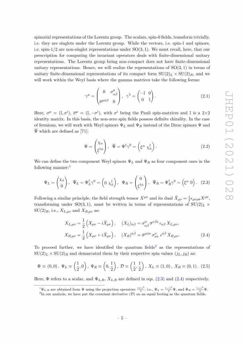
spinorial representations of the Lorentz group. The scalars, spin-0 fields, transform trivially,i.e. they are singlets under the Lorentz group. While the vectors, i.e. spin-1 and spinors,i.e. spin-1/2 are non-singlet representations under SO(3, 1). We must recall, here, that ourprescription for computing the invariant operators deals with finite-dimensional unitaryrepresentations. The Lorentz group being non-compact does not have finite-dimensionalunitary representations. Hence, we will realize the representations of SO(3, 1) in terms ofunitary finite-dimensional representations of its compact form SU(2)L × SU(2)R, and wewill work within the Weyl basis where the gamma matrices take the following forms:
γµ =
0 σµαβ
σµαβ 0
, γ5 =(−I 00 I
). (2.1)
Here, σµ = (I, σi), σµ = (I,−σi), with σi being the Pauli spin-matrices and I is a 2×2identity matrix. In this basis, the non-zero spin fields possess definite chirality. In the caseof fermions, we will work with Weyl spinors ΨL and ΨR instead of the Dirac spinors Ψ andΨ which are defined as [71]:
Ψ =
χαξ†α
, Ψ = Ψ†γ0 =(ξα χ†α
). (2.2)
We can define the two component Weyl spinors ΨL and ΨR as four component ones in thefollowing manner:1
ΨL =(χα
0
), ΨL = Ψ†Lγ
0 =(
0 χ†α), ΨR =
0ξ†α
, ΨR = Ψ†Rγ0 =
(ξα 0
). (2.3)
Following a similar principle, the field strength tensor Xµν and its dual Xµν = 12εµνρσX
ρσ,transforming under SO(3, 1), must be written in terms of representations of SU(2)L ×SU(2)R, i.e., XL,µν and XR,µν as:
XL,µν = 12(Xµν − iXµν
), (XL)αβ = σµ
αβσνβκ εκβ XL,µν ,
XR,µν = 12(Xµν + iXµν
), (XR)αβ = σµακ σνκκ ε
κβ XR,µν . (2.4)
To proceed further, we have identified the quantum fields2 as the representations ofSU(2)L × SU(2)R and demarcated them by their respective spin values (jL, jR) as:
Φ ≡ (0, 0) , ΨL ≡(1
2 , 0), ΨR ≡
(0, 1
2
), D ≡
(12 ,
12
), XL ≡ (1, 0) , XR ≡ (0, 1) . (2.5)
Here, Φ refers to a scalar, and ΨL,R, XL,R are defined in eqs. (2.3) and (2.4) respectively.
1ΨL,R are obtained from Ψ using the projection operators 1∓γ5
2 , i.e., ΨL = 1−γ5
2 Ψ, and ΨR = 1+γ5
2 Ψ.2In our analysis, we have put the covariant derivative (D) on an equal footing as the quantum fields.
– 5 –
JHEP01(2021)028
As mentioned earlier, our primary aim is to construct a set of Lorentz invariant oper-ators (O) using these fields and that can be mathematically framed as follows:
O ≡ Φp ×Ψq1L ×Ψq2
R ×Dr ×Xs1
L ×Xs2R , (2.6)
=⇒ (0, 0) ≡ (0, 0)p ×(1
2 , 0)q1
×(
0, 12
)q2
×(1
2 ,12
)r× (1, 0)s1 × (0, 1)s2 . (2.7)
Here p, q1, q2, r, s1, s2 are the number of times the different fields appear in the operator.All these are non-negative integers. The equivalent relation in terms of mass dimensioncan be written as:
[M ]d ≡ [M ]p × [M ]3q1/2 × [M ]3q2/2 × [M ]r × [M ]2s1 × [M ]2s2 , (2.8)
and equating mass dimensions on both sides we find
d = p+ 32(q1 + q2) + r + 2(s1 + s2). (2.9)
Here, d is the mass dimension of the Lorentz invariant operator and that for fermionicand bosonic fields, and field strength tensors are 3/2, 1, and 2 respectively.3 Similarly, therelation derived from eq. (2.7) can be expressed in terms of the spin (j) as:
0 ≡ [0]p ⊕ [1/2]q1 ⊕ [0]q2 ⊕ [1/2]r ⊕ [1]s1 ⊕ [0]s2 ,
0 ≡ [0]p ⊕ [0]q1 ⊕ [1/2]q2 ⊕ [1/2]r ⊕ [0]s1 ⊕ [1]s2 , (2.10)
or equivalently in terms of SU(2) representations (2j + 1) as:
1 ≡ [1]p ⊗ [2]q1 ⊗ [1]q2 ⊗ [2]r ⊗ [3]s1 ⊗ [1]s2 ,
1 ≡ [1]p ⊗ [1]q1 ⊗ [2]q2 ⊗ [2]r ⊗ [1]s1 ⊗ [3]s2 . (2.11)
Here, [1/2]q in eq. (2.10) and [2]q in eq. (2.11) imply ~12 + · · ·+ ~12︸ ︷︷ ︸
q
and 2⊗ · · · ⊗ 2︸ ︷︷ ︸q
respec-
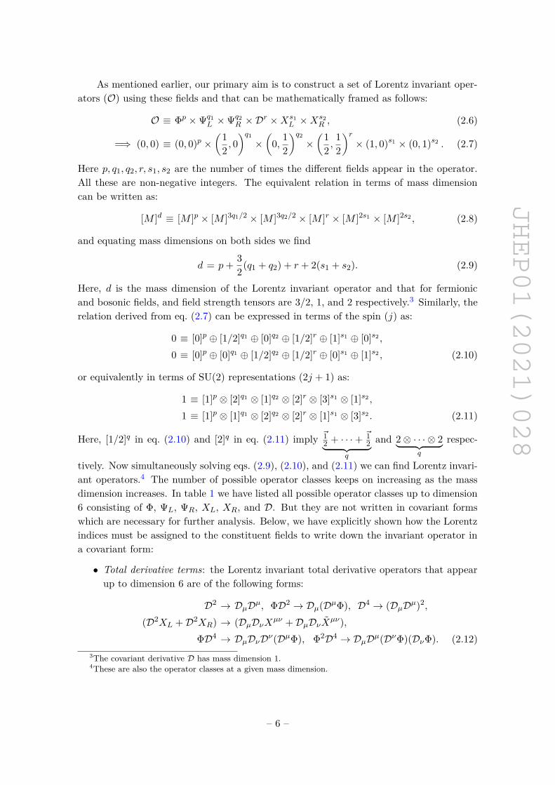
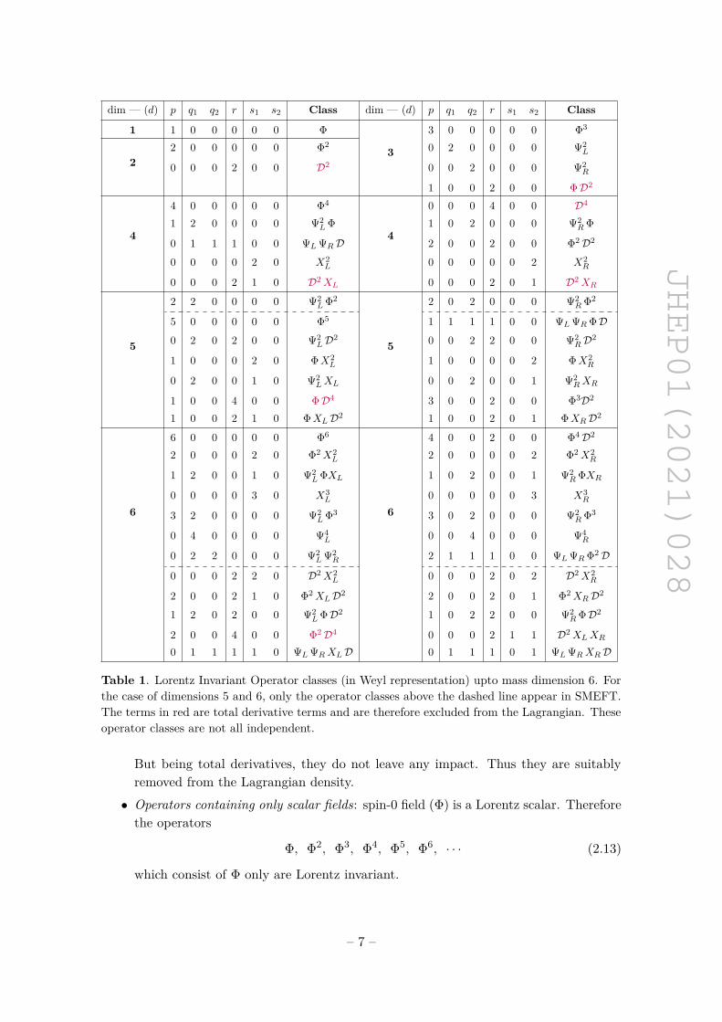
tively. Now simultaneously solving eqs. (2.9), (2.10), and (2.11) we can find Lorentz invari-ant operators.4 The number of possible operator classes keeps on increasing as the massdimension increases. In table 1 we have listed all possible operator classes up to dimension6 consisting of Φ, ΨL, ΨR, XL, XR, and D. But they are not written in covariant formswhich are necessary for further analysis. Below, we have explicitly shown how the Lorentzindices must be assigned to the constituent fields to write down the invariant operator ina covariant form:
• Total derivative terms: the Lorentz invariant total derivative operators that appearup to dimension 6 are of the following forms:
D2 → DµDµ, ΦD2 → Dµ(DµΦ), D4 → (DµDµ)2,
(D2XL +D2XR) → (DµDνXµν +DµDνXµν),ΦD4 → DµDνDν(DµΦ), Φ2D4 → DµDµ(DνΦ)(DνΦ). (2.12)
3The covariant derivative D has mass dimension 1.4These are also the operator classes at a given mass dimension.
– 6 –
JHEP01(2021)028
dim — (d) p q1 q2 r s1 s2 Class dim — (d) p q1 q2 r s1 s2 Class
1 1 0 0 0 0 0 Φ
3
3 0 0 0 0 0 Φ3
22 0 0 0 0 0 Φ2 0 2 0 0 0 0 Ψ2
L
0 0 0 2 0 0 D2 0 0 2 0 0 0 Ψ2R
1 0 0 2 0 0 ΦD2
4
4 0 0 0 0 0 Φ4
4
0 0 0 4 0 0 D4
1 2 0 0 0 0 Ψ2L Φ 1 0 2 0 0 0 Ψ2
R Φ
0 1 1 1 0 0 ΨL ΨRD 2 0 0 2 0 0 Φ2D2
0 0 0 0 2 0 X2L 0 0 0 0 0 2 X2
R
0 0 0 2 1 0 D2XL 0 0 0 2 0 1 D2XR
5
2 2 0 0 0 0 Ψ2L Φ2
5
2 0 2 0 0 0 Ψ2R Φ2
5 0 0 0 0 0 Φ5 1 1 1 1 0 0 ΨL ΨR ΦD0 2 0 2 0 0 Ψ2
LD2 0 0 2 2 0 0 Ψ2RD2
1 0 0 0 2 0 ΦX2L 1 0 0 0 0 2 ΦX2
R
0 2 0 0 1 0 Ψ2LXL 0 0 2 0 0 1 Ψ2
RXR
1 0 0 4 0 0 ΦD4 3 0 0 2 0 0 Φ3D2
1 0 0 2 1 0 ΦXLD2 1 0 0 2 0 1 ΦXRD2
6
6 0 0 0 0 0 Φ6
6
4 0 0 2 0 0 Φ4D2
2 0 0 0 2 0 Φ2X2L 2 0 0 0 0 2 Φ2X2
R
1 2 0 0 1 0 Ψ2L ΦXL 1 0 2 0 0 1 Ψ2
R ΦXR
0 0 0 0 3 0 X3L 0 0 0 0 0 3 X3
R
3 2 0 0 0 0 Ψ2L Φ3 3 0 2 0 0 0 Ψ2
R Φ3
0 4 0 0 0 0 Ψ4L 0 0 4 0 0 0 Ψ4
R
0 2 2 0 0 0 Ψ2L Ψ2
R 2 1 1 1 0 0 ΨL ΨR Φ2D
0 0 0 2 2 0 D2X2L 0 0 0 2 0 2 D2X2
R
2 0 0 2 1 0 Φ2XLD2 2 0 0 2 0 1 Φ2XRD2
1 2 0 2 0 0 Ψ2L ΦD2 1 0 2 2 0 0 Ψ2
R ΦD2
2 0 0 4 0 0 Φ2D4 0 0 0 2 1 1 D2XLXR
0 1 1 1 1 0 ΨL ΨRXLD 0 1 1 1 0 1 ΨL ΨRXRD
Table 1. Lorentz Invariant Operator classes (in Weyl representation) upto mass dimension 6. Forthe case of dimensions 5 and 6, only the operator classes above the dashed line appear in SMEFT.The terms in red are total derivative terms and are therefore excluded from the Lagrangian. Theseoperator classes are not all independent.
But being total derivatives, they do not leave any impact. Thus they are suitablyremoved from the Lagrangian density.• Operators containing only scalar fields: spin-0 field (Φ) is a Lorentz scalar. Thereforethe operators
Φ, Φ2, Φ3, Φ4, Φ5, Φ6, · · · (2.13)
which consist of Φ only are Lorentz invariant.
– 7 –
JHEP01(2021)028
• Operators containing fermion bi-linears: in the Weyl basis, there exist three differentfermion bi-linears: Ψ2
L, Ψ2R, ΨLΨR. The first two terms can form Lorentz invariant
operators of mass dimension three. The last one appears only as a constituent ofhigher dimensional operators, since it transforms as the
(12 ,
12
)representation of
SU(2)L × SU(2)R. These fermion bi-linears can be written in multiple covariantforms:
Ψ2L,R → ΨT
L,R C ΨL,R, ΨR,L ΨL,R, ΨTL,R C σ
µν ΨL,R, ΨR,L σµν ΨL,R,
ΨLΨR → ΨL γµ ΨL, ΨR γ
µ ΨR. (2.14)
Here, σµν = i4 [γµ, γν ] and C is the charge conjugation operator. In the above equation
only underlined terms are Lorentz invariant. The remaining structures combine withother Lorentz non-singlet terms to form higher dimensional operators. Some of thoseinvariant structures have been listed below:
ΨL γµ ΨL × Dµ ≡ ΨLΨRD, ΨL γ
µ ΨL × ΦDµ Φ ≡ ΨLΨR Φ2D,ΨL γ
µ ΨL × ΨR γµ ΨR ≡ Ψ2
LΨ2R, ΨR σ
µν ΨL × Xµν ≡ Ψ2LXL,
ΨR ΨL × Φ ≡ Ψ2LΦ, ΨR ΨL × ΨR ΨL ≡ Ψ4
L. (2.15)
• Operators containing Field strength tensors: as XL, XR transform as (1, 0), (0, 1)respectively under SU(2)L × SU(2)R, they form the following Lorentz scalars: X2
L,X2R, X
3L, X
3R up to dimension 6. They can be expressed in terms of Xµν , Xµν ∈
SO(3, 1) as:
X2L + X2
R → XµνXµν + XµνX
µν ,
X3L + X3
R → XµνX
νκX
κµ + Xµ
νXνκX
κµ. (2.16)
The tri-linear terms being overall traces of the combination of three antisymmet-ric tensors vanish. This method can be adopted to construct higher dimensionaloperators, e.g., at dimension 8 we will have:
X4L+X2
LX2R+X4
R → (XµνXµν) (XκλX
κλ)+(XµνXµν) (XκλX
κλ)+(XµνXµν) (XκλX
κλ).
The field strength tensor XL/R may combine with other Lorentz non-singlet objectsto form an invariant operator class, e.g.,
D2X2L,R ≡ (DµXµν)2, XL,RΦ2D2 ≡ (DµXµν)(ΦDνΦ), D2XLXR ≡ (DνDµXµκXν
κ).
2.2 Role of gauge symmetry
So far we have discussed the possible structures of the operators which are constitutedof quantum fields with spin 0, 1/2, 1 only and taking only the space-time symmetry intoaccount. In a realistic particle physics model, there are additional local and (or) globalinternal symmetries. As a result of this, there could be particles of different internalquantum numbers but possessing the same spin. Such fields will be equivalent to each otherwith respect to the Lorentz symmetry. But based on their internal charges, these fields
– 8 –
JHEP01(2021)028
will combine in a variety of ways leading to different sub-categories of operators within thesame class. Thus, while Lorentz invariance provides us a list of possible operator classes,it is the internal symmetry which ultimately decides which combinations are permittedand which ones are not. This can be elucidated through the most popular example: theStandard Model gauge symmetry. Looking into its particle content and their quantumnumbers in table 29, it is evident that many of the operator classes in table 1 do notrespect the SM gauge symmetry. Thus they are excluded from the operator basis. Here,we have systematically explained the impact of internal gauge symmetries:
• Φn operator class with integer n: the SM Higgs transforms under SU(3)C ⊗SU(2)L⊗U(1)Y as (1, 2, 1/2). Thus, the operators containing an odd number of H fields violateboth SU(2) and U(1) symmetries. If n is an even integer then all the operators of theforms Hn, (H†)n, and H
n2 (H†)
n2 are SU(2) invariant. But only the (H†H) and its
powers are SM singlets. In BSM scenarios that contain multiple scalars, we may endup with more intricate structures. For example, if we add an SU(2) triplet scalar ∆with hypercharge of +1, there will be an invariant operator HT ∆†H ∈ Φ3-class.
• Operators involving field strength tensors: lorentz invariance allows us to constructterms containing an even number of field strength tensors. But the internal symmetryprevents their mixing, e.g., in SM there are no cross-terms between Bµν ,W I
µν andGAµν .But this need not be true for certain BSM scenarios. For example, if there are multi-ple abelian symmetries, then we can expect some mixing in the gauge kinetic sector.Looking into the Lorentz symmetry only, the term involving tri-linear field strengthsvanishes due to its anti-symmetric structure. But internal non-abelian gauge sym-metries allow such terms at the dimension 6 level. Within the SM, Bµ
νBνκB
κµ is
absent but fABC GAµν GBνκ GCκµ and εIJKW Iµν W Jν
κ WKκµ possess non-vanishing con-
tributions. Here, the anti-symmetric tensors fABC and εIJK are SU(3) and SU(2)structure constants respectively.
• Operators containing of bi-linear fermion fields: Lorentz invariance allows fermionmass terms of the forms Ψ2
L (Majorana) and ΨL ΨR (Dirac). But in the SM, leftand right chiral fermions are on a different footing. Hence, these terms are for-bidden by the internal symmetries. Further, the quantum numbers of the fieldsallow the couplings of fermion bi-linears with the Higgs scalar in the form of theYukawa interactions — LeH, QdH and Qu iτ2H
∗. In addition, the SU(3) symme-try prevents the appearance of terms like Lu, Ld and Qe.5 Also, the operator class(ΨL σµν ΨR) ΦXµν appears at mass dimension 6. The choice of Xµν and Ψ’s is fixedby the internal symmetries. There are fermion bi-linears which are not Lorentz scalarbut may appear in higher mass dimensional operator class (Ψ γµ Ψ) (Ψ′ γµ Ψ′).6
2.3 Removal of redundancies and forming operator basis
So far we have learnt how to compute the invariant operators of any mass dimensionbased on the space-time and internal symmetries. But we must keep in mind the fact
5These terms appear as constituents of certain dimension 9 operators.6The fermion fields Ψ and Ψ′ need not be same always.
– 9 –
JHEP01(2021)028
that these operators need to satisfy another criteria to be phenomenologically relevant.The operators at each mass dimension must form a basis, i.e., they must be mutuallyindependent. Thus it is necessary to remove all the redundancies, if any, to computethe operator basis. In this construction, we have noted three different ways in whichthe operators can be interrelated: (i) integration by parts (IBP), (ii) equation of motion(EOM), and (iii) identities of symmetry generators. Here, we have discussed these sourcesof redundancies briefly with examples based on SMEFT and beyond.
Integration by parts (IBP): in our prescription, the covariant derivative (Dµ) par-ticipates in the operator construction in a similar way as the quantum fields. Due to thedistributive property of Dµ and incorporating integration by parts (IBPs), two or moreinvariant operators may be related to each other by a total derivative. As we know such aterm in the Lagrangian has no role to play, thus it can be removed. Therefore the multipleoperators can not be treated independently and only one of them should be included in theoperator basis. This duplication due to IBP occurs among different operators belonging tothe same operator class. For example, at mass dimension 6, the operator ΨLΨR Φ2D canbe recast in the following form:
iDµ (ΨL,R γµ ΨL,R Φ†Φ) = ΨL,R γ
µiDµ ΨL,R Φ†Φ−ΨL,R γµi←−Dµ ΨL,R Φ†Φ
+ΨL,R γµ ΨL,R Φ†iDµΦ−ΨL,R γ
µ ΨL,R Φ†i←−DµΦ= (ΨL,R γ
µi←→D µ ΨL,R) Φ†Φ + ΨL,R γ
µ ΨL,R (Φ†i←→D µ Φ).(2.17)
Here, i←→D µ ≡ iDµ − i←−Dµ has been introduced to combine the first two and the last two
operators to form (ΨL,R γµi←→D µ ΨL,R) Φ†Φ and ΨL,R γ
µ ΨL,R (Φ†i←→D µ Φ) which are self-hermitian. It is evident from eq. (2.17), that these operators are related to each other bya total derivative term Dµ (ΨL,R γ
µ ΨL,R Φ†Φ). So, in the operator basis we will includeonly one of them. Here, our choice of the independent operator will be the one where thederivative acts on the scalar field. This is because the latter structure where the derivativeacts on the fermions is related to other operators through equations of motion. We willjustify this choice in the following section.
Equation of motion (EOM): the quantum fields representing the particles are dynam-ical in nature and each of them satisfies their respective equation of motion. It has beennoted that two or more operators may be related to each other through the EOMs of theinvolved fields along with the IBPs [30, 34]. Unlike the previous case, the EOMs can relateoperators belonging to different classes. We have explained how EOM leads to redundancyusing a few examples:
• ΨLΨR Φ2D : in the Weyl basis we can have two possible covariant structures for thisoperator: (ΨL,R γ
µi←→D µ ΨL,R) Φ†Φ and ΨL,R γ
µ ΨL,R (Φ†i←→D µ Φ). We have alreadynoted that these two operators differ from each other by a total derivative. Therewe have further mentioned that we have selected the operator where the derivativeis acting on the scalars. The reason behind that choice is that after incorporating
– 10 –
JHEP01(2021)028
the EOMs of Ψ or its conjugate Ψ, this operator reduces to an operator belonging toΨ2L,RΦ3 class:
(ΨL,R γµi←→D µ ΨL,R) Φ†Φ ∝ ΨL,R ΨR,L Φ (Φ†Φ) ≡ Ψ2
L,R Φ3. (2.18)
• Ψ2L,R ΦD2 : the unique covariant form of this operator is (ΨL ΨR)D2 Φ. After im-
plementing the EOM of the scalar field: D2 Φ = c1 Φ + c2 Φ (Φ†Φ) + c3 ΨR ΨL, thisoperator can be reduced in the following form:
(ΨLΨR)D2 Φ = c1 (ΨLΨR Φ)︸ ︷︷ ︸dim-4 term
+c2 (ΨLΨR Φ) (Φ†Φ) + c3 (ΨLΨR) (ΨRΨL), (2.19)
with c1, c2 and c3 being complex numbers. Thus, the operator class Ψ2L,R ΦD2 can
be expressed as a linear combination of two other dimension 6 classes Ψ2L,RΦ3 and
Ψ2LΨ2
R, and therefore is excluded from the set of independent operators.
• D2X2L,R, D2XLXR : the possible covariant form of the operators are (i) (DµXµν)2,
(ii) (DµXµν)(DµXµν), and (iii) (DµXµν)2. It is interesting to note that after imple-menting the EOM of field strength tensors:
DµXµν = 0, DµXµν = ΨL,Rγν ΨL,R + Φ†i←→D νΦ, (2.20)
the last two structures (ii) and (iii) identically vanish. The very first operator can berewritten either as:
(DµXµν)2 = a1(ΨL,R γν ΨL,R)(DµXµν) + a2(Φ†i←→D νΦ)(DµXµν), (2.21)
or as:
(DµXµν)2 = b1 (ΨL,R γν ΨL,R)2 + b2 (Φ†i←→D νΦ)2 + b3(Φ†i←→D νΦ)(ΨL,R γ
ν ΨL,R).(2.22)
Here, ai, bi are complex numbers. Thus we can generate operators belonging toΦ4D2, Ψ4, Φ2Ψ2D starting from D2X2 class of operators and thus it is redundantand can not be a part of the operator basis.
Alternatively, using the notion of integration by parts (IBP) we have the followingrelation:
(DµXµν)2, (DµXµν)(Dµ Xµν) IBP==⇒ [Dµ, Dν ]X [µκXν]κ , [Dµ, Dν ]X [µκ Xν]
κ
≡ XµνXµκXν
κ , XµνXµκXν
κ . (2.23)
Here, [Dµ, Dν ] is suitably replaced byXµν and we have obtainedX3 class of operators.So, we conclude that with the help of EOMs and IBPs, the operators belonging toD2X2
L,R and D2XLXR classes can always be recast into operators of other classes.Thus these two are excluded from the operator basis.
– 11 –
JHEP01(2021)028
• Φ2XL,RD2 : the covariant form of this operator (Φ†i←→D ν Φ)DµXµν can be rewrittenusing eq. (2.20) as:
(Φ†i←→D ν Φ)DµXµν = a′ (ΨL,R γν ΨL,R)(Φ† i←→D ν Φ) + b′ (Φ† i←→D ν Φ)(Φ† i←→D ν Φ),(2.24)
where a′, b′ are complex numbers. Similar to the previous case, Φ2X D2 can berewritten in terms of operator classes ΨLΨR Φ2D and Φ4D2. This justifies the absenceof Φ2XL,RD2 class from the independent operator set.
• ΨL ΨRXL,RD : we find two different covariant forms Xµν (ΨL,R γµDν ΨL,R) and(DµXµν)(ΨL,R γν ΨL,R). These operators can be further reduced with the help ofsuitable EOMs as:
Xµν (ΨL,R γµDν ΨL,R) = Xµν (ΨL,R γµ γν /DΨL,R) = Xµν (ΨL,R γ[µ γν] /DΨL,R)= Xµν (ΨL,R σµν ΨR,L) Φ ≡ Ψ2 ΦX, (2.25)
(DµXµν)(ΨL,R γν ΨL,R) = c′1 (Ψ γν Ψ) (ΨL,R γν ΨL,R)+c′2 (Φ† i←→D ν Φ) (ΨL,R γν ΨL,R)≡ Ψ4
L,R /Ψ2L Ψ2
R+ΨL ΨR Φ2D. (2.26)
Thus it is quite evident why this class is also counted as redundant.
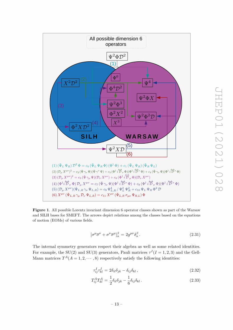
In summary, the symmetries of the theory play a crucial role in constructing theinvariant operator set. But it is not guaranteed that all of them are independent and thusthe set of operators is always over-complete. To be a part of the Lagrangian the operators ofany mass dimension must form a basis, i.e., the operators should be independent. To ensurethat we have shown through some toy examples how the EOMs and IBPs relate differentoperators and thus can be used as constraints in this computation. In the latter part ofthis paper, we have computed the dimension 6 operator basis for a plethora of models. Asthe “Warsaw” is the only known complete operator basis, we have tabulated our results inthis basis only. There is another popular choice — the SILH (Strongly Interacting LightHiggs) basis which trades away the fermion rich operator classes Ψ4, Ψ2ΦX, Ψ2Φ2D fromthe Warsaw one and includes D2X2, Φ2XD2, see figure 1.
Symmetry generators and their identities: the quantum fields that are the buildingblocks of the operators transform under the assigned space-time and internal symmetries.The symmetry generators (specifically for the non-abelian case) respect the pre-fixed al-gebras and satisfy a few identities. For example, the Lorentz symmetry generators σµ, σµ
together form the σµν , σµν matrices, defined in eq. (2.27):
(σµν)βα = (σµ)αβ(σν)ββ , (σµν)βα = (σµ)ββ(σν)βα . (2.27)
They also satisfy the following identities [71]:
(σµ)αα(σµ)ββ = 2εαβεαβ , (2.28)
(σµ)αα(σµ)ββ = 2δβαδβα , (2.29)
(σµ)αα(σµ)ββ = 2εαβεαβ , (2.30)
– 12 –
JHEP01(2021)028
S ILH WARSAW
All possible dimension 6 operators
(3)
(1)
(2)
(4)
(5)
(6)
Figure 1. All possible Lorentz invariant dimension 6 operator classes shown as part of the Warsawand SILH bases for SMEFT. The arrows depict relations among the classes based on the equationsof motion (EOMs) of various fields.
[σµσν + σνσµ]βα = 2gµνδβα . (2.31)
The internal symmetry generators respect their algebra as well as some related identities.For example, the SU(2) and SU(3) generators, Pauli matrices τ I(I = 1, 2, 3) and the Gell-Mann matrices TA(A = 1, 2, · · · , 8) respectively satisfy the following identities:
τ IijτIkl = 2δilδjk − δijδkl , (2.32)
TAij TAkl = 1
2δilδjk −16δijδkl . (2.33)
– 13 –
JHEP01(2021)028
While constructing the covariant form of the operators we may encounter two differentstructures with the same field content. But they need not be two independent operatorsand may be related to each other through these identities eqs. (2.28)–(2.33). Here, wehave demonstrated how the utilisation of these identities could help us to relate differentcovariant-structured dimension 6 operators with a few examples.7
• Ψ4 : we have considered two dimension 6 operators (d γµ TA d)(Qγµ TAQ) and(d γµ d)(QγµQ) from this class. Using the identities in eqs. (2.28)–(2.32), theseoperators can be expressed as:
(dγµTAd)(QTAγµQ) = (dασµααTAdα)(QβTAσµββQβ) = 2dαTAQβQβT
Adαδβαδβα
= 2(d TAQ) (QTA d) = 2(da [TA]ab Qb)(Qc [TA]ce de)
= (d d) (QQ)− 13(dQ)(Qd) . (2.34)
(dγµd)(QγµQ) = (dασµααdα)(QβσµββQβ) = 2dαQβQβd
αδβαδβα
= 2(dQ)(Qd). (2.35)
It is quite evident from eqs. (2.34) and (2.35), that with the fields d, d, Q, and Q
we can only have two independent operators that should be included in SMEFTdimension 6 operator basis. Similarly, with fields e, L, u, and Q we have followingrelation
(Lσµνe)(Qσµνu) = ((L)α(σµν)βα(e)β)((Q)ρ(σµν)θρ(u)θ)
= ((L)α(σµ)αβ(σν)ββ(e)β)((L)ρ(σµ)ρθ(σν)θθ(u)θ)
= 4(Le)(Qu)− 8(Lu)(Qe) . (2.36)
Thus, only (Lσµνe)(Qσµνu) and (L e)(Q u) are included in the operator set.
• Φ6 : here, we are looking into the quartic subpart of the dimension 6 operator(H†H)3. It is interesting to note using eq. (2.32) that inclusion of SU(2) genera-tors does not lead to an independent operator in the SMEFT basis [34]:
(H†τ IH)(H†τ IH) = (H†i τIijHj)(H†kτ
IklHl) = H†iHjH
†kHl(2δilδjk − δijδkl)
= 2(H†H)2 − (H†H)2 = (H†H)2 . (2.37)
• Φ4D2 : to illustrate the redundancy in this class of operators, we have considered anoperator involving a scalar Lepto-Quark (χ1) transforming as (3, 2, 1/6) under theSM gauge group.
(H†i←→D IµH)(χ†1i
←→D µIχ1) = (H†(τ I iDµ−i
←−Dµτ I)H)(χ†1(τ I iDµ−i←−Dµτ I)χ1)
= (H†i τIij(iDµH)j−(iDµH)†kτ
IklHl)(χ†1aτ
Iab(iDµχ1)b−(iDµχ1)†cτ Icdχ1d)
= −(H†i←→D µH)(χ1†i←→D µχ1)+2 (H†b i
←→D µH
a)(χ†1ai←→D µχb1). (2.38)
7Here, we work with four component Weyl-spinors.
– 14 –
JHEP01(2021)028
As three operators are related through the above relation, only two of these can beindependent and we may include (H†i←→D I
µH)(χ†1i←→D µIχ1) and (H†i←→D µH)(χ†1i
←→D µχ1)
in the operator basis for this scenario.
• Ψ2Φ2D : in this class we can have following three operators involving the Lepto-Quark χ1:
(Qτ IγµQ) (χ†1i←→D Iµχ1) = (Qτ IγµQ)[χ†1τ
I(iDµχ1)+(iDµχ1)†τ Iχ1]
= 2(Qγµ(iDµχ1))(Qχ†1)−(QγµQ)(χ†1(iDµχ1))
+2(Qγµχ1)(Q(iDµχ1)†)−(QγµQ)((iDµχ1)†χ1), (2.39)
(QTAγµQ) (χ†1i←→D Aµχ1) = (QTAγµQ)[χ†1T
A(iDµχ1)+(iDµχ1)†TAχ1]
= 12(Qγµ(iDµχ1))(Qχ†1)−1
6(QγµQ)(χ†1(iDµχ1))
+12(Qγµχ1)(Q(iDµχ1)†)−1
6(QγµQ)((iDµχ1)†χ1), (2.40)
(QTA τ I γµQ) (χ†1 TA i←→D Iµ χ1) = (QTAτ IγµQ)[χ†1T
Aτ I(iDµχ1)+(iDµχ1)†TAτ Iχ1]
= 12 [(Qτ Iγµ(iDµχ1))(Qτ Iχ†1)]−1
6 [(Qτ IγµQ)(χ†1τI(iDµχ1))]
+12 [(Qτ Iγµχ1)(Qτ I(iDµχ1)†)]−1
6 [(Qτ IγµQ)((iDµχ1)†τ Iχ1)]
= [(Qγµχ†1)((iDµχ1)Q)−12((Qγµ(iDµχ1))(Qχ†1))]
−16 [(Qγµ(iDµχ1))(Qχ†1)−(QγµQ)(χ†1(iDµχ1))]
+[(Qγµ(iDµχ1)†)(χ1Q)−12(Qγµχ1)(Q(iDµχ1)†)]
−16 [(Qγµχ1)(Q(iDµχ1)†)−(QγµQ)((iDµχ1)†χ1)]. (2.41)
Thus, it is evident that the three operators in the l.h.s. of the above equation alongwith (QγµQ) (χ†1i
←→D µχ1), comprise a set of four independent operators and qualify
to be in the operator basis.
2.4 Additional impacts of the global (accidental) symmetries
The effect of global symmetries is very similar to the gauge ones in the construction ofinvariant operators. But, unlike the gauge symmetry, the global symmetry need not bestrictly imposed and it may be allowed to be broken softly in specific interactions as de-manded by the phenomenology. This leads to the appearance of global charge violatingeffective operators that induce rare processes.
Baryon (B) and lepton (L) numbers appear as accidental global symmetries in the tree-level SM Lagrangian, see eq. (A.1). But they may be violated through higher dimensionaloperators. If we assign the leptons an L charge of −1 unit and the quarks a B charge of 1/3units respectively, then we can generate a Majorana neutrino mass for the SM neutrinosthrough dimension 5 H2L2 operator. As this operator is suppressed by a high scale, thesmallness of neutrino masses can be explained. Similarly within the SMEFT framework,we find operators violating B and L by (0,−2), (1,−1), (1, 1) units at mass dimensions 5,
– 15 –
JHEP01(2021)028
6 and 7. Recently it has been noted [72] that a similar violation by (1,−3) units appears atdimension 9 and this can induce a new decay mode of the proton to three charged leptons.
In the case of BSM scenarios, there could be additional global symmetries and theamount of their breaking would be completely phenomenologically driven. This controlsthe appearance of certain kinds of operators at different mass dimensions.
3 BSMEFT operator bases
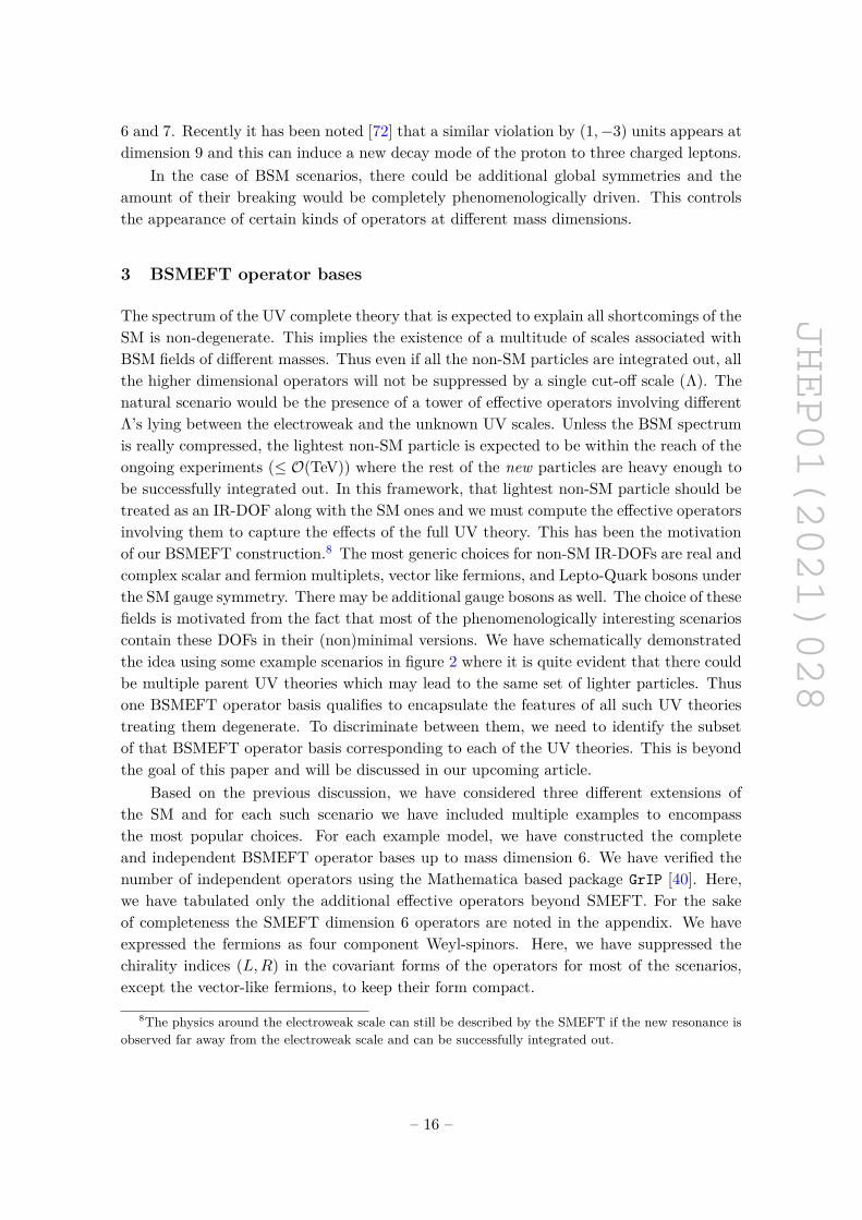
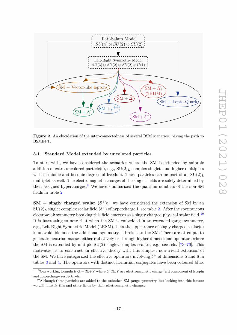
The spectrum of the UV complete theory that is expected to explain all shortcomings of theSM is non-degenerate. This implies the existence of a multitude of scales associated withBSM fields of different masses. Thus even if all the non-SM particles are integrated out, allthe higher dimensional operators will not be suppressed by a single cut-off scale (Λ). Thenatural scenario would be the presence of a tower of effective operators involving differentΛ’s lying between the electroweak and the unknown UV scales. Unless the BSM spectrumis really compressed, the lightest non-SM particle is expected to be within the reach of theongoing experiments (≤ O(TeV)) where the rest of the new particles are heavy enough tobe successfully integrated out. In this framework, that lightest non-SM particle should betreated as an IR-DOF along with the SM ones and we must compute the effective operatorsinvolving them to capture the effects of the full UV theory. This has been the motivationof our BSMEFT construction.8 The most generic choices for non-SM IR-DOFs are real andcomplex scalar and fermion multiplets, vector like fermions, and Lepto-Quark bosons underthe SM gauge symmetry. There may be additional gauge bosons as well. The choice of thesefields is motivated from the fact that most of the phenomenologically interesting scenarioscontain these DOFs in their (non)minimal versions. We have schematically demonstratedthe idea using some example scenarios in figure 2 where it is quite evident that there couldbe multiple parent UV theories which may lead to the same set of lighter particles. Thusone BSMEFT operator basis qualifies to encapsulate the features of all such UV theoriestreating them degenerate. To discriminate between them, we need to identify the subsetof that BSMEFT operator basis corresponding to each of the UV theories. This is beyondthe goal of this paper and will be discussed in our upcoming article.
Based on the previous discussion, we have considered three different extensions ofthe SM and for each such scenario we have included multiple examples to encompassthe most popular choices. For each example model, we have constructed the completeand independent BSMEFT operator bases up to mass dimension 6. We have verified thenumber of independent operators using the Mathematica based package GrIP [40]. Here,we have tabulated only the additional effective operators beyond SMEFT. For the sakeof completeness the SMEFT dimension 6 operators are noted in the appendix. We haveexpressed the fermions as four component Weyl-spinors. Here, we have suppressed thechirality indices (L,R) in the covariant forms of the operators for most of the scenarios,except the vector-like fermions, to keep their form compact.
8The physics around the electroweak scale can still be described by the SMEFT if the new resonance isobserved far away from the electroweak scale and can be successfully integrated out.
– 16 –
JHEP01(2021)028
Figure 2. An elucidation of the inter-connectedness of several BSM scenarios: paving the path toBSMEFT.
3.1 Standard Model extended by uncolored particles
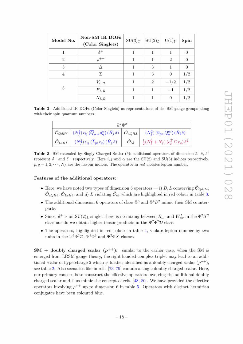
To start with, we have considered the scenarios where the SM is extended by suitableaddition of extra uncolored particle(s), e.g., SU(2)L complex singlets and higher multipletswith fermionic and bosonic degrees of freedom. These particles can be part of an SU(2)Lmultiplet as well. The electromagnetic charges of the singlet fields are solely determined bytheir assigned hypercharges.9 We have summarized the quantum numbers of the non-SMfields in table 2.
SM + singly charged scalar (δ+): we have considered the extension of SM by anSU(2)L singlet complex scalar field (δ+) of hypercharge 1, see table 2. After the spontaneouselectroweak symmetry breaking this field emerges as a singly charged physical scalar field.10
It is interesting to note that when the SM is embedded in an extended gauge symmetry,e.g., Left Right Symmetric Model (LRSM), then the appearance of singly charged scalar(s)is unavoidable once the additional symmetry is broken to the SM. There are attempts togenerate neutrino masses either radiatively or through higher dimensional operators wherethe SM is extended by mutiple SU(2) singlet complex scalars, e.g., see refs. [73–76]. Thismotivates us to construct an effective theory with this simplest non-trivial extension ofthe SM. We have categorized the effective operators involving δ+ of dimensions 5 and 6 intables 3 and 4. The operators with distinct hermitian conjugates have been coloured blue.
9Our working formula is Q = T3 +Y where Q,T3, Y are electromagnetic charge, 3rd component of isospinand hypercharge respectively.
10Although these particles are added to the unbroken SM gauge symmetry, but looking into this featurewe will identify this and other fields by their electromagnetic charges.
– 17 –
JHEP01(2021)028
Model No. Non-SM IR DOFs SU(3)C SU(2)L U(1)Y Spin(Color Singlets)
1 δ+ 1 1 1 02 ρ++ 1 1 2 03 ∆ 1 3 1 04 Σ 1 3 0 1/2
5VL,R 1 2 −1/2 1/2
EL,R 1 1 −1 1/2
NL,R 1 1 0 1/2
Table 2. Additional IR DOFs (Color Singlets) as representations of the SM gauge groups alongwith their spin quantum numbers.
Ψ2Φ2
OQdHδ (N2f ) εij (Qpαi dαq ) (Hj δ) OuQHδ (N2
f ) (upαQαiq ) (Hi δ)
OLeHδ (N2f ) εij (Lpi eq) (Hj δ) Oeδ 1
2(N2f +Nf ) (eTp C eq) δ2
Table 3. SM extended by Singly Charged Scalar (δ): additional operators of dimension 5. δ, δ†represent δ+ and δ− respectively. Here i, j and α are the SU(2) and SU(3) indices respectively.p, q = 1, 2, · · · , Nf are the flavour indices. The operator in red violates lepton number.
Features of the additional operators:
• Here, we have noted two types of dimension 5 operators — i) B,L conserving OQdHδ,OuQHδ, OLeHδ, and ii) L violating Oeδ which are highlighted in red colour in table 3.
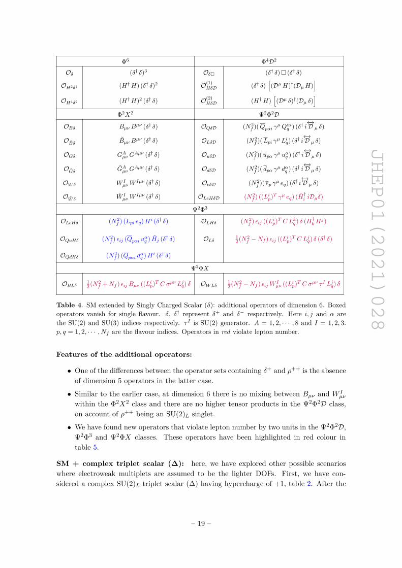
• The additional dimension 6 operators of class Φ6 and Φ4D2 mimic their SM counter-parts.
• Since, δ+ is an SU(2)L singlet there is no mixing between Bµν and W Iµν in the Φ2X2
class nor do we obtain higher tensor products in the Ψ2Φ2D class.
• The operators, highlighted in red colour in table 4, violate lepton number by twounits in the Ψ2Φ2D, Ψ2Φ3 and Ψ2ΦX classes.
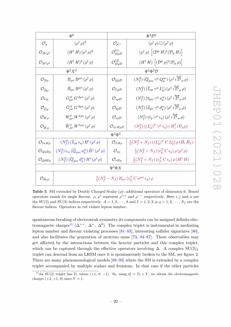
SM + doubly charged scalar (ρ++): similar to the earlier case, when the SM isemerged from LRSM gauge theory, the right handed complex triplet may lead to an addi-tional scalar of hypercharge 2 which is further identified as a doubly charged scalar (ρ++),see table 2. Also scenarios like in refs. [73–79] contain a single doubly charged scalar. Here,our primary concern is to construct the effective operators involving the additional doublycharged scalar and thus mimic the concept of refs. [48, 80]. We have provided the effectiveoperators involving ρ++ up to dimension 6 in table 5. Operators with distinct hermitianconjugates have been coloured blue.
– 18 –
JHEP01(2021)028
Φ6 Φ4D2
Oδ (δ† δ)3 Oδ� (δ† δ)� (δ† δ)
OH2δ4 (H†H) (δ† δ)2 O(1)HδD (δ† δ)
[(DµH)†(DµH)
]OH4δ2 (H†H)2 (δ† δ) O(2)
HδD (H†H)[(Dµ δ)†(Dµ δ)
]Φ2X2 Ψ2Φ2D
OBδ Bµν Bµν (δ† δ) OQδD (N2
f )(Qpαi γµQαiq ) (δ† i←→D µ δ)
OBδ Bµν Bµν (δ† δ) OLδD (N2
f )(Lpi γµ Liq) (δ† i←→D µ δ)
OGδ GAµν GAµν (δ† δ) OuδD (N2
f )(upα γµ uαq ) (δ† i←→D µ δ)
OGδ GAµν GAµν (δ† δ) OdδD (N2
f )( dpα γµ dαq ) (δ† i←→D µ δ)
OWδ W IµνW
Iµν (δ† δ) OeδD (N2f )( ep γµ eq) (δ† i←→D µ δ)
OW δ W IµνW
Iµν (δ† δ) OLeHδD (N2f ) ((Lip)T γµ eq) (H†i iDµδ)
Ψ2Φ3
OLeHδ (N2f ) (Lpi eq)H i (δ† δ) OLHδ (N2
f ) εij ((Lip)T C Lkq ) δ (H†kHj)
OQuHδ (N2f ) εij (Qpαi uαq ) Hj (δ† δ) OLδ 1
2(N2f −Nf ) εij ((Lip)T C Ljq) δ (δ† δ)
OQdHδ (N2f ) (Qpαi dαq )H i (δ† δ)
Ψ2ΦX
OBLδ 12(N2
f +Nf ) εij Bµν ((Lip)T C σµν Ljq) δ OWLδ12(N2
f −Nf ) εijW Iµν ((Lip)T C σµν τ I Ljq) δ
Table 4. SM extended by Singly Charged Scalar (δ): additional operators of dimension 6. Boxedoperators vanish for single flavour. δ, δ† represent δ+ and δ− respectively. Here i, j and α arethe SU(2) and SU(3) indices respectively. τ I is SU(2) generator. A = 1, 2, · · · , 8 and I = 1, 2, 3.p, q = 1, 2, · · · , Nf are the flavour indices. Operators in red violate lepton number.
Features of the additional operators:
• One of the differences between the operator sets containing δ+ and ρ++ is the absenceof dimension 5 operators in the latter case.
• Similar to the earlier case, at dimension 6 there is no mixing between Bµν and W Iµν
within the Φ2X2 class and there are no higher tensor products in the Ψ2Φ2D class,on account of ρ++ being an SU(2)L singlet.
• We have found new operators that violate lepton number by two units in the Ψ2Φ2D,Ψ2Φ3 and Ψ2ΦX classes. These operators have been highlighted in red colour intable 5.
SM + complex triplet scalar (∆): here, we have explored other possible scenarioswhere electroweak multiplets are assumed to be the lighter DOFs. First, we have con-sidered a complex SU(2)L triplet scalar (∆) having hypercharge of +1, table 2. After the
– 19 –
JHEP01(2021)028
Φ6 Φ4D2
Oρ (ρ† ρ)3 Oρ� (ρ† ρ)� (ρ† ρ)
OH2ρ4 (H†H) (ρ† ρ)2 O(1)HρD (ρ† ρ)
[(DµH)†(DµH)
]OH4ρ2 (H†H)2 (ρ† ρ) O(2)
HρD (H†H)[(Dµ ρ)†(Dµ ρ)
]Φ2X2 Ψ2Φ2D
OBρ Bµν Bµν (ρ† ρ) OQρD (N2
f ) (Qpαi γµQαiq ) (ρ† i←→D µ ρ)
OBρ Bµν Bµν (ρ† ρ) OLρD (N2
f ) (Lpi γµ Liq) (ρ† i←→D µ ρ)
OGρ GAµν GAµν (ρ† ρ) OuρD (N2
f ) (upα γµ uαq ) (ρ† i←→D µ ρ)
OGρ GAµν GAµν (ρ† ρ) OdρD (N2
f ) (dpα γµ dαq ) (ρ† i←→D µ ρ)
OWρ W IµνW
Iµν (ρ† ρ) OeρD (N2f ) (ep γµ eq) (ρ† i←→D µ ρ)
OWρ W IµνW
Iµν (ρ† ρ) OLeHρD (N2f ) ((Lip)T γµ eq) (H†i iDµρ)
Ψ2Φ3
OLeHρ (N2f ) (Lpi eq)H i (ρ† ρ) OLHρ 1
2(N2f +Nf ) ((Lip)T C Ljq) ρ (Hi Hj)
OQuHρ (N2f ) εij (Qpαi uαq ) Hj (ρ† ρ) Oeρ 1
2(N2f +Nf ) (eTp C eq) ρ (ρ† ρ)
OQdHρ (N2f ) (Qpαi dαq )H i (ρ† ρ) OeHρ 1
2(N2f +Nf ) (eTp C eq) ρ (H†H)
Ψ2ΦX
OBeρ 12(N2
f −Nf )Bµν (eTp C σµν eq) ρ
Table 5. SM extended by Doubly Charged Scalar (ρ): additional operators of dimension 6. Boxedoperators vanish for single flavour. ρ, ρ† represent ρ++ and ρ−− respectively. Here i, j and α arethe SU(2) and SU(3) indices respectively. A = 1, 2, · · · , 8 and I = 1, 2, 3. p, q = 1, 2, · · · , Nf are theflavour indices. Operators in red violate lepton number.
spontaneous breaking of electroweak symmetry its components can be assigned definite elec-tromagnetic charges11 (∆++, ∆+, ∆0). The complex triplet is instrumental in mediatinglepton number and flavour violating processes [81–83], interesting collider signatures [80],and also facilitates the generation of neutrino mass [73, 84–87]. These observables mayget affected by the interactions between the heavier particles and this complex triplet,which can be captured through the effective operators involving ∆. A complex SU(2)Ltriplet can descend from an LRSM once it is spontaneously broken to the SM, see figure 2.There are many phenomenological models [88–93] where the SM is extended by a complextriplet accompanied by multiple scalars and fermions. In that case if the other particles
11An SU(2) triplet has T3 values (+1, 0, −1). So, using Q = T3 + Y , we obtain the electromagneticcharges (+2, +1, 0) since Y = 1.
– 20 –
JHEP01(2021)028
Ψ2Φ2 Φ5
OLeH∆ N2f (Lpi eq ∆ Hi) O(1)
H2∆3 (HT∆†H) Tr[(∆†∆)]
OQdH∆ N2f (Qpαi dαq ∆ Hi) O(2)
H2∆3 (HT∆†∆†∆H)
OQuH∆ N2f (Qpαi uαq ∆† Hi) OH4∆ (HT ∆†H) (H†H)
Oe∆ 12(N2
f +Nf ) (eTp C eq) Tr[ ∆ ∆]
Table 6. SM extended by Complex Triplet Scalar (∆): additional operators of dimension 5. Herei and α are SU(2) and SU(3) indices respectively. p, q = 1, 2, · · · , Nf are the flavour indices. Theoperator in red violates lepton number.
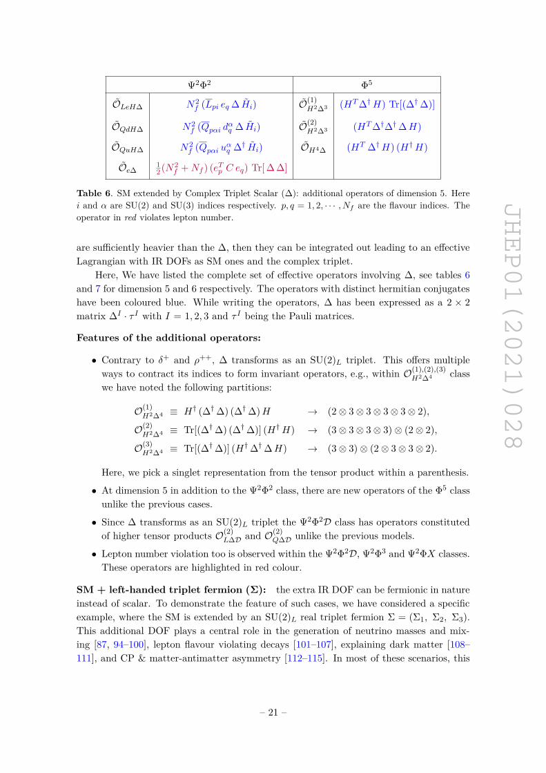
are sufficiently heavier than the ∆, then they can be integrated out leading to an effectiveLagrangian with IR DOFs as SM ones and the complex triplet.
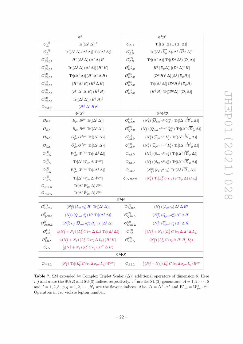
Here, We have listed the complete set of effective operators involving ∆, see tables 6and 7 for dimension 5 and 6 respectively. The operators with distinct hermitian conjugateshave been coloured blue. While writing the operators, ∆ has been expressed as a 2 × 2matrix ∆I · τ I with I = 1, 2, 3 and τ I being the Pauli matrices.
Features of the additional operators:
• Contrary to δ+ and ρ++, ∆ transforms as an SU(2)L triplet. This offers multipleways to contract its indices to form invariant operators, e.g., within O(1),(2),(3)
H2∆4 classwe have noted the following partitions:
O(1)H2∆4 ≡ H† (∆†∆) (∆†∆)H → (2⊗ 3⊗ 3⊗ 3⊗ 3⊗ 2),
O(2)H2∆4 ≡ Tr[(∆†∆) (∆†∆)] (H†H) → (3⊗ 3⊗ 3⊗ 3)⊗ (2⊗ 2),
O(3)H2∆4 ≡ Tr[(∆†∆)] (H†∆†∆H) → (3⊗ 3)⊗ (2⊗ 3⊗ 3⊗ 2).
Here, we pick a singlet representation from the tensor product within a parenthesis.
• At dimension 5 in addition to the Ψ2Φ2 class, there are new operators of the Φ5 classunlike the previous cases.
• Since ∆ transforms as an SU(2)L triplet the Ψ2Φ2D class has operators constitutedof higher tensor products O(2)
L∆D and O(2)Q∆D unlike the previous models.
• Lepton number violation too is observed within the Ψ2Φ2D, Ψ2Φ3 and Ψ2ΦX classes.These operators are highlighted in red colour.
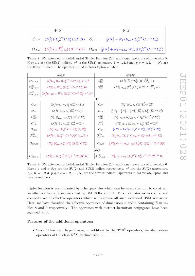
SM + left-handed triplet fermion (Σ): the extra IR DOF can be fermionic in natureinstead of scalar. To demonstrate the feature of such cases, we have considered a specificexample, where the SM is extended by an SU(2)L real triplet fermion Σ = (Σ1, Σ2, Σ3).This additional DOF plays a central role in the generation of neutrino masses and mix-ing [87, 94–100], lepton flavour violating decays [101–107], explaining dark matter [108–111], and CP & matter-antimatter asymmetry [112–115]. In most of these scenarios, this
– 21 –
JHEP01(2021)028
Φ6 Φ4D2
O(1)∆ Tr[(∆†∆)]3 O∆� Tr[(∆†∆)� (∆†∆)]
O(2)∆ Tr[(∆†∆) (∆†∆)] Tr[(∆†∆)] O(1)
∆D Tr[(∆† i←→Dµ ∆)(∆† i←→D µ ∆)]
O(1)H2∆4 H† (∆†∆) (∆†∆)H O(2)
∆D Tr[(∆†∆)] Tr[(Dµ ∆†) (Dµ∆)]
O(2)H2∆4 Tr[(∆†∆) (∆†∆)] (H†H) O(1)
H∆D [H† (Dµ∆)] [(Dµ ∆)†H]
O(3)H2∆4 Tr[(∆†∆)] (H†∆†∆H) O(2)
H∆D [(DµH)†∆] [∆† (DµH)]
O(1)H4∆2 (H†∆†H) (H†∆H) O(3)
H∆D Tr[(∆†∆)] (DµH)† (DµH)
O(2)H4∆2 (H†∆†∆ H) (H†H) O(4)
H∆D (H†H) Tr[(Dµ∆)† (Dµ∆)]
O(3)H4∆2 Tr[(∆†∆)] (H†H)2
OH∆H (HT ∆†H)2
Φ2X2 Ψ2Φ2D
OB∆ Bµν Bµν Tr[(∆†∆)] O(1)
Q∆D (N2f ) (Qpαi γµQαiq ) Tr[(∆† i←→D µ ∆)]
OB∆ Bµν Bµν Tr[(∆†∆)] O(2)
Q∆D (N2f ) (Qpαi γµ τ I Qαiq ) Tr[(∆† i←→D I
µ ∆)]
OG∆ GAµν GAµν Tr[(∆†∆)] O(1)
L∆D (N2f ) (Lpi γµ Liq) Tr[(∆† i←→D µ ∆)]
OG∆ GAµν GAµν Tr[(∆†∆)] O(2)
L∆D (N2f ) (Lpi γµ τ I Liq) Tr[(∆† i←→D I
µ ∆)]
O(1)W∆ W I
µνWIµν Tr[(∆†∆)] Ou∆D (N2
f ) (upα γµ uαq ) Tr[(∆† i←→D µ ∆)]
O(2)W∆ Tr[∆†Wµν ∆Wµν ] Od∆D (N2
f ) (dpα γµ dαq ) Tr[(∆† i←→D µ ∆)]
O(1)W∆ W I
µνWIµν Tr[(∆†∆)] Oe∆D (N2
f ) (ep γµ eq) Tr[(∆† i←→D µ ∆)]
O(2)W∆ Tr[∆†Wµν ∆ Wµν ] OLeH∆D (N2
f ) Tr[LTp C iτ2 (γµDµ ∆)H eq]
OBW∆ Tr[∆†Wµν ∆]Bµν
OBW∆ Tr[∆† Wµν ∆]Bµν
Ψ2Φ3
O(1)LeH∆ (N2
f ) (Lpi eq)H i Tr[(∆†∆)] O(2)LeH∆ (N2
f ) (Lpi eq) ∆†∆H i
O(1)QdH∆ (N2
f ) (Qpαi dαq )H i Tr[(∆†∆)] O(2)QdH∆ (N2
f ) (Qpαi dαq ) ∆†∆H i
O(1)QuH∆ (N2
f ) εij (Qpαi uαq ) Hj Tr[(∆†∆)] O(2)QuH∆ (N2
f ) (Qpαi uαq ) ∆†∆ Hi
O(1)L∆
12(N2
f +Nf ) (LTp C iτ2 ∆Lq) Tr[(∆†∆)] O(2)L∆
12(N2
f +Nf ) (LTp C iτ2 ∆ ∆†∆Lq)
O(1)LH∆
12(N2
f +Nf ) (LTp C iτ2 ∆Lq) (H†H) O(2)LH∆ (N2
f ) (LTpiC iτ2 ∆H iH†j Ljq)
Oe∆ 12(N2
f +Nf ) (eTp C eq) (HT ∆H)
Ψ2ΦX
OWL∆ (N2f ) Tr[(LTp C iτ2 ∆σµν Lq)Wµν ] OBL∆
12(N2
f −Nf ) (LTp C iτ2 ∆σµν Lq)Bµν
Table 7. SM extended by Complex Triplet Scalar (∆): additional operators of dimension 6. Herei, j and α are the SU(2) and SU(3) indices respectively. τ I are the SU(2) generators. A = 1, 2, · · · , 8and I = 1, 2, 3. p, q = 1, 2, · · · , Nf are the flavour indices. Also, ∆ = ∆I · τ I and Wµν = W I
µν · τ I .Operators in red violate lepton number.
– 22 –
JHEP01(2021)028
Ψ2Φ2 Ψ2X
OΣH (N2f ) ((ΣI
p)T C ΣIq) (H†H) OBΣ
12(N2
f −Nf )Bµν ((ΣIp)T C σµν ΣI
q)
OeΣH (N2f ) εij (ΣI
p eq) (H i τ IHj) OWΣ12(N2
f +Nf ) εIJKW Iµν ((ΣJ
p )T C σµν ΣKq )
Table 8. SM extended by Left-Handed Triplet Fermion (Σ): additional operators of dimension 5.Here i, j are the SU(2) indices. τ I is the SU(2) generator. I = 1, 2, 3 and p, q = 1, 2, · · · , Nf arethe flavour indices. The operator in red violates lepton number.
Ψ2ΦX Ψ2Φ2D
OBLΣH (N2f ) εij Bµν ((Lip)T C σµν ΣI
q) τ I Hj O(1)ΣH (N2
f ) (ΣIpγµΣI
q) (H† i←→D µH)
O(1)WLΣH (N2
f ) εijW Iµν ((Lip)T C σµν ΣI
q)Hj O(2)ΣH (N2
f ) εIJK (ΣIp γ
µ ΣJq ) (H† τK i←→D µH)
O(2)WLΣH (N2
f ) εIJK εijW Iµν ((Lip)T C σµν ΣJ
q ) τK Hj
Ψ4
OuΣ (N4f ) (upα γµ uαq ) (ΣI
r γµ ΣI
s) OdΣ (N4f ) (dpα γµ dαq ) (ΣI
r γµ ΣI
s)
OeΣ (N4f ) (ep γµ eq) (ΣI
r γµ ΣI
s) OΣΣ (34N
4f + 1
2N3f + 3
4N2f ) (ΣI
p γµ ΣIq) (ΣJ
r γµ ΣJ
s )
O(1)QΣ (N4
f ) (Qpαi γµQαiq ) (ΣIr γ
µ ΣIs) O(2)
QΣ (N4f ) εIJK (Qpαi γµ τ I Qjαq ) (ΣJ
r γµ ΣK
s )
O(1)LΣ (N4
f ) (Lpi γµ Liq) (ΣIr γ
µ ΣIs) O(2)
LΣ (N4f ) εIJK (Lpi γµ τ I Liq) (ΣJ
r γµ ΣK
s )
OeLΣ (N4f ) εij ((Lip)T C τ I Ljq) (er ΣI
s) OΣ214(N4
f + 3N2f ) ((ΣI
p)T C ΣIq) ((ΣI
r)T C ΣIs)
O(1)QLdΣ (N4
f ) εij ((Lip)T C τ I Qαjq ) (drα ΣIs) O(2)
QLdΣ (N4f ) εij ((Lip)T C σµν τ I Qαjq ) (drα σµν ΣI
s)
OQLuΣ (N4f ) (Qpαi uαq ) [τ I ]ij ((Ljr)T C ΣI
s) OQdΣ12N
3f (Nf − 1) εαβγ εij (ΣI
p dαq ) ((Qβir )T C τ I Qγjs )
Ψ2Φ3
O(1)LΣHH (N2
f ) εij ((Lip)T C ΣIq) τ I Hj (H†H) O(2)
LΣHH (N2f ) εIJK εij ((Lip)T C ΣI
q) τJ Hj (H† τK H)
Table 9. SM extended by Left-Handed Triplet Fermion (Σ): additional operators of dimension 6.Here i, j and α, β, γ are the SU(2) and SU(3) indices respectively. τ I are the SU(2) generators.I, J,K = 1, 2, 3. p, q, r, s = 1, 2, · · · , Nf are the flavour indices. Operators in red violate lepton andbaryon numbers.
triplet fermion is accompanied by other particles which can be integrated out to constructan effective Lagrangian described by SM DOFs and Σ. This motivates us to compute acomplete set of effective operators which will capture all such extended BSM scenarios.Here, we have classified the effective operators of dimensions 5 and 6 containing Σ in ta-bles 8 and 9 respectively. The operators with distinct hermitian conjugates have beencoloured blue.
Features of the additional operators:
• Since Σ has zero hypercharge, in addition to the Ψ2Φ2 operators, we also obtainoperators of the class Ψ2X at dimension 5.
– 23 –
JHEP01(2021)028
Ψ2Φ2
OHELER (N2f ) (H†i H i) (ERpELq) OHNLNR (N2
f ) (H†i H i) (NLpNRq)
O(1)HLVR
(N2f ) (H†i H i) (Lpj V j
Rq) O(1)HVLVR
(N2f ) (H†i H i) (V Lpj V
jRq)
O(2)HLVR
(N2f ) (H†i τ I H i) (Lpj τ I V j
Rq) O(2)HVLVR
(N2f ) (H†i τ I H i) (V Lpj τ
I V jRq)
OHeEL (N2f ) (H†i H i) (epELq) OHNR 1
2Nf (Nf + 1) (H†i H i) (NTRpC NRq)
OHVL 12Nf (Nf + 1)εij εmnH iHm (V j
Lp)TC V nLq OHVR 1
2Nf (Nf + 1)εij εmnH iHm (V jRp)TC V n
Rq
OHLVL (N2f )εij εmnH iHm (Ljp)TC V n
Lq OHNL 12Nf (Nf + 1) (H†i H i) (NT
LpC NLq)
Ψ2X
OBeEL (N2f )Bµν(ep σµν ELq) OBELER (N2
f )Bµν(ERp σµν ELq)
OBLVR (N2f )Bµν(V Rpi σµν L
iq) OWLVR (N2
f )W Iµν (V Rpi τ
Iσµν Liq)
OBVLVR (N2f )Bµν(V Rpi σµν V
iLq) OWVLVR (N2
f )W Iµν (V Rpi τ
Iσµν V iLq)
OBNLNR (N2f )Bµν(NRp σµν NLq) OBNR 1
2Nf (Nf − 1)Bµν (NTRpC σ
µνNRq)
OBNL 12Nf (Nf − 1)Bµν (NT
LpC σµνNLq)
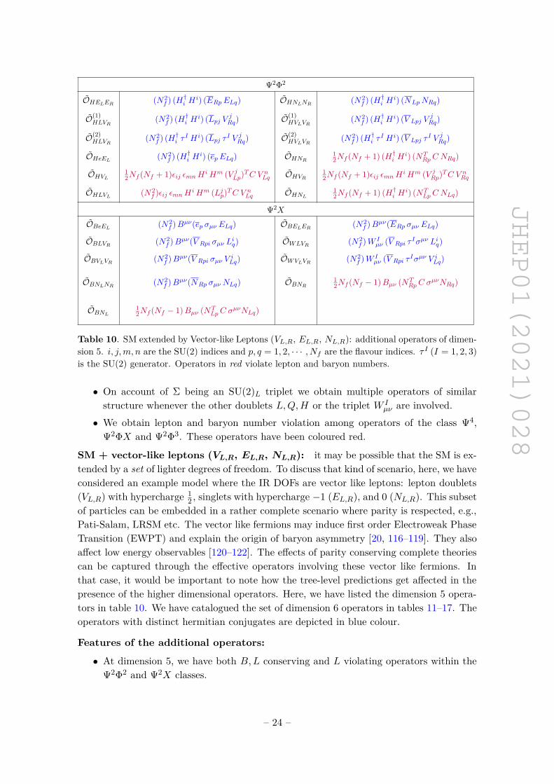
Table 10. SM extended by Vector-like Leptons (VL,R, EL,R, NL,R): additional operators of dimen-sion 5. i, j,m, n are the SU(2) indices and p, q = 1, 2, · · · , Nf are the flavour indices. τ I (I = 1, 2, 3)is the SU(2) generator. Operators in red violate lepton and baryon numbers.
• On account of Σ being an SU(2)L triplet we obtain multiple operators of similarstructure whenever the other doublets L,Q,H or the triplet W I
µν are involved.• We obtain lepton and baryon number violation among operators of the class Ψ4,
Ψ2ΦX and Ψ2Φ3. These operators have been coloured red.
SM + vector-like leptons (VL,R, EL,R, NL,R): it may be possible that the SM is ex-tended by a set of lighter degrees of freedom. To discuss that kind of scenario, here, we haveconsidered an example model where the IR DOFs are vector like leptons: lepton doublets(VL,R) with hypercharge 1
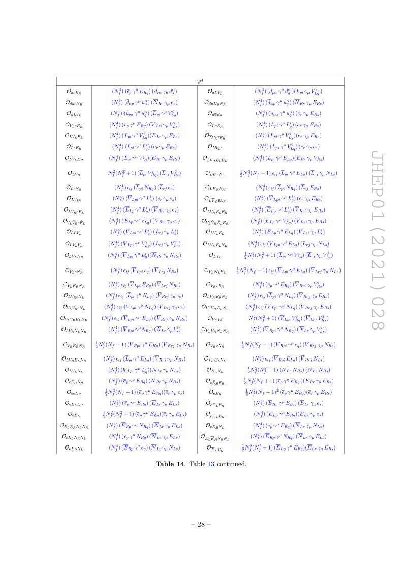
2 , singlets with hypercharge −1 (EL,R), and 0 (NL,R). This subsetof particles can be embedded in a rather complete scenario where parity is respected, e.g.,Pati-Salam, LRSM etc. The vector like fermions may induce first order Electroweak PhaseTransition (EWPT) and explain the origin of baryon asymmetry [20, 116–119]. They alsoaffect low energy observables [120–122]. The effects of parity conserving complete theoriescan be captured through the effective operators involving these vector like fermions. Inthat case, it would be important to note how the tree-level predictions get affected in thepresence of the higher dimensional operators. Here, we have listed the dimension 5 opera-tors in table 10. We have catalogued the set of dimension 6 operators in tables 11–17. Theoperators with distinct hermitian conjugates are depicted in blue colour.
Features of the additional operators:
• At dimension 5, we have both B,L conserving and L violating operators within theΨ2Φ2 and Ψ2X classes.
– 24 –
JHEP01(2021)028
Ψ2Φ3
OHVLe (N2f ) (V Lpi eqH
i) (H†j Hj) OHVREL (N2f )(V RpiELqH
i) (H†j Hj)
OHVLER (N2f ) (V LpiERqH
i) (H†j Hj) OHLER (N2f ) (LpiERqH i) (H†j Hj)
OHVLNR (N2f ) εij (NRp V
iLqH
j) (H†kHk) OHLNR (N2f ) εij (NRp L
iqH
j) (H†kHk)
OHVRNL (N2f ) εij (NLp V
iRqH
j) (H†kHk) OHLNL (N2f ) εij ((Lip)T C NLqH
j) (H†kHk)
OHVLNL (N2f ) εij ((V i
Lp)T C NLqHj) (H†kHk) OHVRNR (N2
f ) εij ((V iRp)T C NRqH
j) (H†kHk)
Ψ2ΦXOBHVLe (N2
f )Bµν (V Lpi σµν eq)H i OWHVLe (N2
f )W Iµν (V Lpi σ
µν eq) τ I H i
OBHLER (N2f )Bµν (Lpi σµν ERq)H i OWHLER (N2
f )W Iµν (Lpi σµν ERq) τ I H i
OBHLNR (N2f )Bµν (Lpi σµν NRq) Hi OWHLNR (N2
f )W Iµν (Lpi σµν NRq) τ I Hi
OBHVLER (N2f )Bµν (V Lpi σ
µν ERq)H i OWHVLER (N2f )W I
µν (V Lpi σµν ERq) τ I H i
OBHVLNR (N2f ) εij Bµν (NRpi σ
µν V iLq)Hj OWHVLe (N2
f )W Iµν (V Lpi σ
µν eq) τ I H i
OWHVLNR (N2f ) εijW I
µν (NRpi σµν V i
Lq) τ I Hj OBHVLER (N2f )Bµν (V Lpi σ
µν ERq)H i
OWHVREL (N2f )W I
µν (V Rpi σµν ELq) τ I H i OBHVRNL (N2
f )Bµν (V Rpi σµν NLq) Hi
OWHVRNL (N2f )W I
µν (V Rpi σµν NLq) τ I Hi OBHVREL (N2
f ) εij Bµν (V Rpi σµν ELq)H i
OBHLNL (N2f ) εij Bµν (NT
LpC σµν Liq)Hj OBHVLNL (N2
f ) εij Bµν (NTLpC σ
µν V iLq)Hj
OBHVRNR (N2f ) εij Bµν (NT
RpC σµν V i
Rq)Hj OWHLNL (N2f ) εijW I
µν (NTLpC σ
µν Liq) τ I Hj
OWHVRNR (N2f ) εijW I
µν (NTRpC σ
µν V iRq) τ I Hj OWHVLNL (N2
f ) εijW Iµν (NT
LpC σµν V i
Lq) τ I Hj
Ψ2Φ2D
O(1)HVRD (N2
f ) (V Rpi γµ V i
Rq) (H†i i←→D µH
i) O(1)HVLD (N2
f ) (V Lpi γµ V i
Lq) (H†j i←→D µH
j)
O(2)HVRD (N2
f ) (V Rpi γµ τ IV i
Rq) (H†i i←→D IµH
i) O(2)HVLiD (N2
f ) (V Lpi γµ τ IV i
Lq) (H†j i←→D µH
j)
OHNLD (N2f ) (NLp γ
µNLq) (H†i i←→D µH
i) OHNRD (N2f ) (NRp γ
µNRq) (H†i i←→D µH
i)
OHELD (N2f ) (ELp γµELq) (H†i i
←→D µH
i) OHERD (N2f ) (ERp γµERq) (H†i i
←→D µH
i)
OHeERD (N2f ) (ep γµERq) (H†i iDµH i) OHeNRD (N2
f ) (NRp γµ eq) (H†i iDµH i)
OHELNLD (N2f ) εij (NLp γ
µELq) (H†i iDµH i) O(1)HLVLD (N2
f ) (Lpi γµ V iLq) (H†j iDµHj)
OHERNRD (N2f ) (NRp γ
µERq) (H†i iDµH i) O(2)HLVLD (N2
f ) (Lpi γµ τ IV iLq) (H†j iDIµHj)
OHLVRD (N2f ) εij εmn ((V i
Rp)T C γµ Lmq ) (H†n iDµHj) OHVLVRD (N2f ) εij εmn ((V i
Rp)T C γµ V mLq) (H†n iDµHj)
OHeNLD (N2f ) (eTp C γµNLq) (H†i iDµH i) OHERNLD (N2
f ) (ETRpC γµNLq) (H†i iDµH i)
OHELNRD (N2f ) (ETLpC γµNRq) (H†i iDµH i) OHNLNRD (N2
f ) (NTLpC γ
µNRq) (H†i iDµH i)
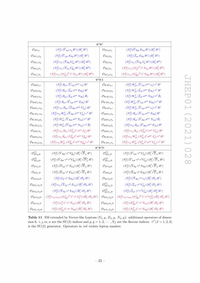
Table 11. SM extended by Vector-like Leptons (VL,R, EL,R, NL,R): additional operators of dimen-sion 6. i, j,m, n are the SU(2) indices and p, q = 1, 2, · · · , Nf are the flavour indices. τ I (I = 1, 2, 3)is the SU(2) generator. Operators in red violate lepton number.
– 25 –
JHEP01(2021)028
Ψ4
OdEL (N4f ) (ELp γµELq) (drα γµ dαs ) OeEL (N4
f ) (ELp γµELq) (er γµ es)
OeER (N4f ) (ep γµ eq) (ERr γµERs) OELER (N4
f ) (ELp γµELq) (ERr γµERs)
OER 14N
2f (Nf + 1)2 (ERp γµERq)(ERr γµERs) OEL 1
4N2f (Nf + 1)2 (ELp γµELq)(ELr γµELs)
OLEL (N4f ) (Lpi γµ Liq)(ELr γµELs) OLER (N4
f ) (Lpi γµ Liq)(ERr γµERs)
O(1)LVL
(N4f ) (V Lpi γ
µ V iLq) (Lrj γµLjs) OVLEL (N4
f ) (ELp γµELq) (V Lri γµ ViLs)
O(2)LVL
(N4f ) (V Lpi γ
µ τ I V iLq) (Lrj γµ τ I Ljs) OVLER (N4
f ) (ERp γµERq) (V Lri γµ ViLs)
OdVL (N4f ) (dpα γµ dαq )(V Lri γµ V
iLs) OVLe (N4
f )(ep γµ eq) (V Lri γµ ViLs)
OVL 12N
2f (N2
f + 1) (V Lpi γµ V i
Lq )(V Lrj γµ VjLs) OdVR (N4
f ) (dpα γµ dαq )(V Rri γµ ViRs)
OVREL (N4f ) (ELp γµELq) (V Rri γµ V
iRs) OeVR (N4
f ) (ep γµ eq) (V Rri γµ ViRs)
OVRER (N4f ) (ERp γµERq) (V Rri γµ V
iRs) OVR 1
2N2f (N2
f + 1) (V Rpi γµ V i
Rq )(V Rrj γµ VjRs)
O(1)LVR
(N4f ) (V Rpi γ
µ V iRq) (Lrj γµ Ljs) O(1)
VLVR(N4
f ) (V Rpi γµ V i
Rq) (V Lrj γµ VjLs)
O(2)LVR
(N4f ) (V Rpi γ
µ τ I V iRq) (Lrj γµ τ I Ljs) O(2)
VLVR(N4
f ) (V Rpi γµ τ I V i
Rq) (V Lrj γµ τ I V j
Ls)
OdNL (N4f ) (dpα γµ dαq )(NLr γµNLs) OeNL (N4
f ) (ep γµ eq) (NLr γµNLs)
OELNL (N4f ) (ELp γµELq) (NLr γµNLs) OERNL (N4
f ) (ERp γµERq) (NLr γµNLs)
OLNL (N4f ) (Lpi γµ Liq)(NLr γµNLs) OVLNL (N4
f ) (V Lpi γµ V i
Lq)(NLr γµNLs)
OVRNL (N4f ) (V Rpi γ
µ V iRq)(NLr γµNLs) ONL 1
4N2f (Nf + 1)2 (NLp γ
µNLq)(NLr γµNLs)
OdNR (N4f ) (dpα γµ dαq )(NRr γµNRs) OeNR (N4
f ) (ep γµ eq) (NRr γµNRs)
OELNR (N4f ) (ELp γµELq) (NRr γµNRs) OERNR (N4
f ) (ERp γµERq) (NRr γµNRs)
OLNR (N4f ) (Lpi γµ Liq)(NRr γµNRs) OVLNR (N4
f ) (V Lpi γµ V i
Lq)(NRr γµNRs)
OVRNR (N4f ) (V Rpi γ
µ V iRq)(NRr γµNRs) ONLNR (N4
f ) (NLp γµNLq) (NRr γµNRs)
ONR 14N
2f (Nf + 1)2(NRp γ
µNRq)(NRr γµNRs) OQEL (N4f ) (Qαp γµQαq )(ELr γµELs)
OQNL (N4f ) (Qαp γµQαq )(NLr γµNLs) OQER (N4
f ) (Qαp γµQαq )(ERr γµERs)
O(1)QVL
(N4f ) (V Lpi γµ V
iLq) (Qrαj γµQαjs ) O(1)
QVR(N4
f ) (V Rpi γµ ViRq) (Qrjα γµQjαs )
O(2)QVL
(N4f ) (V Lpi γµ τ
I V iLq) (Qrjα γµ τ I Qjαs ) O(2)
QVR(N4
f ) (V Rpi γµ τI V i
Rq) (Qrjα γµ τ I Qjαs )
OQNR (N4f ) (Qpα γµQαq )(NRr γµNRs) OuEL (N4
f ) (upα γµ uαq ) (ELr γµELs)
OuVL (N4f ) (upα γµ uαq ) (V Lr γµ VLs) OuER (N4
f ) (upα γµ uαq ) (ERr γµERs)
OuVR (N4f ) (upα γµ uαq ) (V Rri γµ V
iRs) OuNR (N4
f ) (upα γµ uαq ) (NRr γµNRs)
OuNL (N4f ) (upα γµ uαq ) (NLr γµNLs) OdER (N4
f ) (dpα γµ dαq )(ERr γµERs)
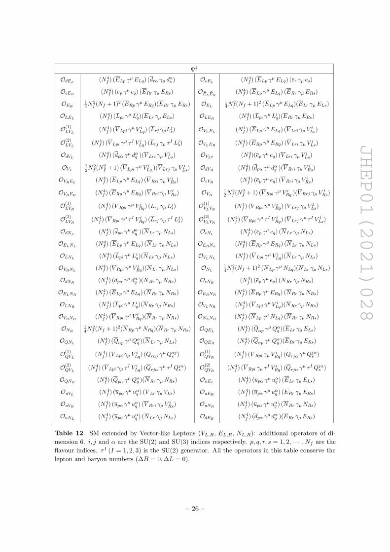
Table 12. SM extended by Vector-like Leptons (VL,R, EL,R, NL,R): additional operators of di-mension 6. i, j and α are the SU(2) and SU(3) indices respectively. p, q, r, s = 1, 2, · · · , Nf are theflavour indices. τ I (I = 1, 2, 3) is the SU(2) generator. All the operators in this table conserve thelepton and baryon numbers (∆B = 0,∆L = 0).
– 26 –
JHEP01(2021)028
Ψ4
O(1)VLVReEL
(N4f ) (V Lpi V
iRq) (ELr es) O(1)
VLVRELER(N4
f ) (V Lpi ViRq) (ELr ERs)
O(2)VLVReEL
(N4f ) (V Lpi σ
µν V iRq) (ELr σµν es) O(2)
VLVRELER(N4
f ) (V Lpi σµν V i
Rq) (ELr σµν ERs)
O(1)LVLeNR
(N4f ) εij (V Lpi eq) (Lrj γµNRs) O(1)
LVLERNR(N4
f ) εij (V LpiERq) (Lrj NRs)
O(2)LVLeNR
(N4f ) εij (V Lpi σ
µν eq) (Lrj σµν NRs) O(2)LVLERNR
(N4f ) εij (V Lpi σ
µν ERq) (Lrj σµν NRs)
O(1)LVReEL
(N4f ) (Lpi V i
Rq) (ELr es) O(1)LVRELER
(N4f ) (Lpi V i
Rq) (ELr ERs)
O(2)LVReEL
(N4f ) (Lpi σµν V i
Rq) (ELr σµν es) O(2)LVRELER
(N4f ) (Lpi σµν V i
Rq) (ELr σµν ERs)
O(1)LVLVR
(N4f ) (V Lpi V
iRq) (Lrj V j
Rs) O(1)QdVREL
(N4f ) (dαpQiαq) (V RriELs)
O(2)LVLVR
(N4f ) (V Lpi σ
µν V iRq) (Lrj σµν V j
Rs) O(2)QdVREL
(N4f ) (dαp σµν Qiαq) (V Rri σµν ELs)
O(1)LVRNLNR
(N4f ) (Lpi V i
Rq) (NLrNRs) O(1)LVLV R
(N4f ) (V Rpi V
iLq) (Lrj V j
Rs)
O(2)LVRNLNR
(N4f ) (Lpi σµν V i
Rq) (NLr σµν NRs) O(2)LVLV R
(N4f ) (V Rpi σ
µν V iLq) (Lrj σµν V j
Rs)
O(1)eELNLNR
(N4f ) (NLpNRq) (ELr es) O(1)
NLVRELER(N4
f ) (NLpNRq) (ELr ERs)
O(2)eELNLNR
(N4f ) (NLp σ
µν N iRq) (ELr σµν es) O(2)
NLNRELER(N4
f ) (NLpi σµν N i
Rq) (ELr σµν ERs)
O(1)VLVRNLNR
(N4f ) (V Lpi V
iRq) (NLrNRs) O(1)
QdLNR(N4
f ) εij (Qαpi dαq) (Lrj NRs)
O(2)VLVRNLNR
(N4f ) (V Lpi σ
µν V iRq) (NLr σµν NRs) O(2)
QdLNR(N4
f ) εij (Qαpi σµν dαq) (Lrj σµν NRs)
O(1)QLVL
(N4f ) (Qαpi γµQiαq) (Lrj γµ V j
Ls) O(1)QdVLNR
(N4f ) εij (Qαpi dαq) (V Lrj NRs)
O(2)QLVL
(N4f ) (Qαpi γµ τ I Qiαq) (Lrj γµ τ I V j
Ls) O(2)QdVLNR
(N4f ) εij (Qαpi σµν dαq) (V Lrj σµν NRs)
O(1)QuLER
(N4f ) εij (QαpERq) (Lrj uαs) O(1)
QuVLER(N4
f ) εij (QαpERq) (V Lrj uαs)
O(2)QuLER
(N4f ) εij (Qαp σµν ERq) (Lrj σµν uαs) O(2)
QuVLER(N4
f ) εij (Qαp σµν ERq) (V Lrj σµν uαs)
O(1)QuVLe
(N4f ) εij (Qαp uαq) (V Lrj es) O(1)
QuVRNL(N4
f ) (Qαpi uαq ) (NLr ViRs)
O(2)QuVLe
(N4f ) εij (Qαp σµν uαq) (V Lrj σµν es) O(2)
QuVRNL(N4
f ) (Qαpi σµν uαq ) (NLr σµν ViRs)
OQdVLe (N4f ) (dpα γµ eq )(V Lir γµQ
αis ) OQdLER (N4
f ) (Lpi γµQαiq ) (dirα γµERs)
OQeER (N4f ) (Qαpi γµQαiq ) (er γµERs) OQdVLER (N4
f ) (dαp γµERq) (V Lir γµQαiRs)
OQuVREL (N4f ) εij (Qαpi γµELq) (V Rir γµ u
αs ) OQeER (N4
f ) (Qαpi γµQαiq ) (ERr γµ es)
OQuLNR (N4f ) (Qαpi γµ Liq) (NRr γµ u
αs ) OQuVLNR (N4
f ) (Qαpi γµ V iLq) (NRr γµ u
αs )
OQdVRNL (N4f ) εij (Qαpi γµ dαq ) (V Rrj γµNLs) OudELNL (N4
f ) (dαp γµ uαq ) (NLr γµELs)
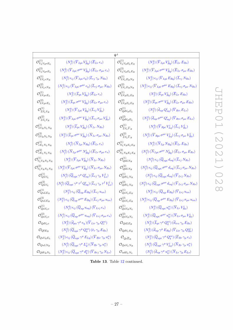
Table 13. Table 12 continued.
– 27 –
JHEP01(2021)028
Ψ4
OdeER (N4f ) (ep γµERq) (drα γµ dαs ) OdLVL (N4
f ) (dpα γµ dαq )(Lpi γµ V iLq )
OdueNR (N4f ) (dαp γµ uαq ) (NRr γµ es) OduERNR (N4
f ) (dαp γµ uαq ) (NRr γµERs)
OuLVL (N4f ) (upα γµ uαq ) (Lpi γµ V i
Lq) OueER (N4f ) (upα γµ uαq ) (er γµERs)
OVLeER (N4f ) (ep γµERq) (V Lri γµ V
iLs) OLeER (N4
f ) (Lpi γµ Liq) (er γµERs)
OLVLEL (N4f ) (Lpi γµ V i
Lq)(ELr γµELs) OLVLeER (N4f ) (Lpi γµ V i
Lq)(er γµERs)
OLeER (N4f ) (Lpi γµ Liq) (er γµERs) OLVLe (N4
f ) (Lpi γµ V iLq) (er γµ es)
OLVLER (N4f ) (Lpi γµ V i
Lq)(ERr γµERs) OLVRELER (N4f ) (Lpi γµELq)(ERr γµ V i
Rs)
OLVR N2f (N2
f + 1) (Lpi V iRq) (Lrj V j
Rs) OLELNL 12N
3f (Nf − 1) εij (Lpi γµELq) (Lrj γµNLs)
OLeNR (N4f ) εij (LpiNRq) (Lrj es) OLERNR (N4
f ) εij (LpiNRq) (Lrj ERs)
OLVLe (N4f ) (V Lpi γ
µ Liq) (er γµ es) OLV LeER (N4f ) (V Lpi γ
µ Liq) (er γµERs)
OLVReEL (N4f ) (ELp γµ Liq) (V Rri γµ es) OLVRELER (N4
f ) (ELp γµ Liq) (V Rri γµERs)
OVLVReEL (N4f ) (ELp γµ V i
Lq) (V Rri γµ es) OVLVRELER (N4f ) (ELp γµ V i
Lq) (V Rri γµERs)
OLLVL (N4f ) (V Lpi γ
µ Liq) (Lrj γµ Ljs) OLVLEL (N4f ) (ELp γµELq) (V Lri γµ L
is)
OLVLVL (N4f ) (V Lpi γ
µ V iLq) (Lrj γµ V j
Ls) OLVLELNL (N4f ) εij (V Lpi γ
µELq) (Lrj γµNLs)
OLVLNR (N4f ) (V Lpi γ
µ Liq)(NRr γµNRs) OLVL 12N
2f (N2
f + 1) (Lpi γµ V iLq) (Lrj γµ V j
Ls)
OVLeNR (N4f ) εij (V Lpi eq) (V Lrj NRs) OVLNLEL 1
2N3f (Nf − 1) εij (V Lpi γ
µELq) (V Lrj γµNLs)
OVLERNR (N4f ) εij (V LpiERq) (V Lrj NRs) OVReER (N4
f ) (ep γµERq) (V Rri γµ ViRs)
OLVReNL (N4f ) εij (Lpi γµNLq) (V Rrj γµ es) OLVRERNL (N4
f ) εij (Lpi γµNLq) (V Rrj γµERs)
OVLVReNL (N4f ) εij (V Lpi γ
µNLq) (V Rrj γµ es) OVLVRERNL (N4f ) εij (V Lpi γ
µNLq) (V Rrj γµERs)
OVLVRELNR (N4f ) εij (V Lpi γ
µELq) (V Rrj γµNRs) OVLVR N2f (N2
f + 1) (V Lpi ViRq) (V Lrj V
jRs)
OLVRNLNR (N4f ) (V Rpi γ
µNRq) (NLr γµLis) OVLVRNLNR (N4
f ) (V Rpi γµNRq) (NLr γµ V
iLs)
OVRERNR 12N
3f (Nf − 1) (V Rpi γ
µERq) (V Rrj γµNRs) OVReNR 12N
3f (Nf − 1) (V Rpi γ
µ eq) (V Rrj γµNRs)
OLVRELNR (N4f ) εij (Lpi γµELq) (V Rrj γµNRs) OVRELNL (N4
f ) εij (V RpiELq) (V Rrj NLs)
OLVLNL (N4f ) (V Lpi γ
µ Liq)(NLr γµNLs) ONLNR 12N
2f (N2
f + 1) (NLrNRs) (NLrNRs)
OeERNR (N4f ) (ep γµERq) (NRr γµNRs) OeERER
12N
3f (Nf + 1) (ep γµERq )(ERr γµERs)
OeeER 12N
3f (Nf + 1) (ep γµERq)(er γµ es) OeER 1
4N2f (Nf + 1)2 (ep γµERq)(er γµERs)
OeELER (N4f ) (ep γµERq) (ELr γµELs) OeELER (N4
f ) (ERp γµELq) (ELr γµ es)
OeEL 12N
2f (N2
f + 1) (ep γµELq)(er γµELs) OeELER (N4f ) (ELp γµERq)(ELr γµ es)
OELERNLNR (N4f ) (ERp γµNRq) (NLr γµELs) OeERNL (N4
f ) (ep γµERq) (NLr γµNLs)
OeELNRNL (N4f ) (ep γµNRq) (NLr γµELs) OELERNRNL (N4
f ) (ERp γµNRq) (NLr γµELs)
OeERNL (N4f ) (ERp γµ eq) (NLr γµNLs) OELER
12N
2f (N2
f + 1) (ELp γµERq)(ELr γµERs)
Table 14. Table 13 continued.
– 28 –
JHEP01(2021)028
Ψ4
OduNR (N4f ) εαβγ [(dαp )T C dβq ] [(uγr )T C NRs] OQdNR 1
2N3f (Nf + 1)εαβγ εij [(Qiαp )T C Qjγq ] [(dβr )T C NRs]
OQduVL (N4f ) εαβγ εij [(Qiαp )T C V j
Lq] [(dβr )T C uγs ] OQVL 13N
2f (2N2
f + 1)εαβγ εjn εkm [(Qjαp )T C Qkβq ] [(Qmγr )T C V nLs]
OuddNL (N4f ) εαβγ [NLp u
αq ] [(dβr )T C dγs ] OQuER 1
2N3f (Nf + 1) εαβγ εij [(Qiαp )T C Qjβq ] [(uγr )T C ERs]
OuudER (N4f ) εαβγ [(uαp )T C uβq ] [(dγr )T C ERs] OdEL 1
3N2f (N2
f − 1) εαβγ ((dαp )T C dβq ) (ELr dγs )
OQdVR 12N
3f (Nf − 1)εαβγ [V RpiQ
iαq ] [(dβr )T C dγr ] OQdNL 1
2N3f (Nf + 1)εαβγ εij [NLp d
αq ] [(Qiβr )T C Qjγr ]
ONL 112N
2f (N2
f − 1)(NTLpC NLq) (NT
Lr C NLs) ONLNR 14N
2f (Nf + 1)2(NT
LpC NLq) (NTRr C NRs)
ONR 112N
2f (N2
f − 1)(NTRpC NRq) (NT
Rr C NRs)
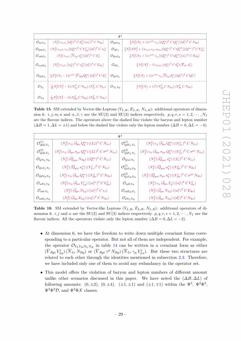
Table 15. SM extended by Vector-like Leptons (VL,R, EL,R, NL,R): additional operators of dimen-sion 6. i, j,m, n and α, β, γ are the SU(2) and SU(3) indices respectively. p, q, r, s = 1, 2, · · · , Nfare the flavour indices. The operators above the dashed line violate the baryon and lepton number(∆B = 1,∆L = ±1) and below the dashed line violate only the lepton number (∆B = 0,∆L = −4).
Ψ4
O(1)QdLNL
(N4f ) εij (dpαQiαq ) ((Ljr)T C NLs) O(1)
QdVLNL(N4
f ) εij (dpαQiαq ) ((V jLr)T C NLs)
O(2)QdLNL
(N4f ) εij (dpα σµν Qiαq ) ((Ljr)T C σµν NLs) O(2)
QdVLNL(N4
f ) εij (dpα σµν Qiαq ) ((V jLr)T C σµν NLs)
OQNLNR (N4f ) (QpαiNRq) ((Qiαr )T C NLs) OQuLNL (N4
f ) (Qpαi uαq ) ((Lir)T C NLs)
OQuVLNL (N4f ) (Qpαi uαq ) ((V i
Lr)T C NLs) O(1)QuVRNR
(N4f ) (Qpαi uαq ) ((V i
Rr)T C NRs)
OQdVRNR (N4f ) εij (dpαQiαq ) ((V j
Rr)T C NRs) O(2)QuVRNR
(N4f ) (Qpαi σµν uαq ) ((V i
Rr)T C σµν NRs)
OudVLVR (N4f ) εij (dpα V i
Lq) ((ujαr )T C V jRs) OudLVR (N4
f ) εij (dpα Liq) ((uαr )T C V jRs)
OudeNL (N4f ) (dpαNLq) ((uαr )T C es) OudERNL (N4
f ) (dpαNLq) ((uαr )T C ERs)
OudELNR (N4f ) (dpαELq) ((uαr )T C NRs) OdNLNR (N4
f ) (dpαNLq) ((dαr )T C NRs)
Table 16. SM extended by Vector-like Leptons (VL,R, EL,R, NL,R): additional operators of di-mension 6. i, j and α are the SU(2) and SU(3) indices respectively. p, q, r, s = 1, 2, · · · , Nf are theflavour indices. All the operators violate only the lepton number (∆B = 0,∆L = −2).
• At dimension 6, we have the freedom to write down multiple covariant forms corre-sponding to a particular operator. But not all of them are independent. For example,the operator OVLVRNLNR in table 14 can be written in a covariant form as either(V Rpi V
iLq) (NLrNRq) or (V Rpi γ
µNRq) (NLr γµ ViLs). But these two structures are
related to each other through the identities mentioned in subsection 2.3. Therefore,we have included only one of them to avoid any redundancy in the operator set.
• This model offers the violation of baryon and lepton numbers of different amountunlike other scenarios discussed in this paper. We have noted the (∆B,∆L) offollowing amounts: (0,±2), (0,±4). (±1,±1) and (±1,∓1) within the Ψ4, Ψ2Φ3,Ψ2Φ2D, and Ψ2ΦX classes.
– 29 –
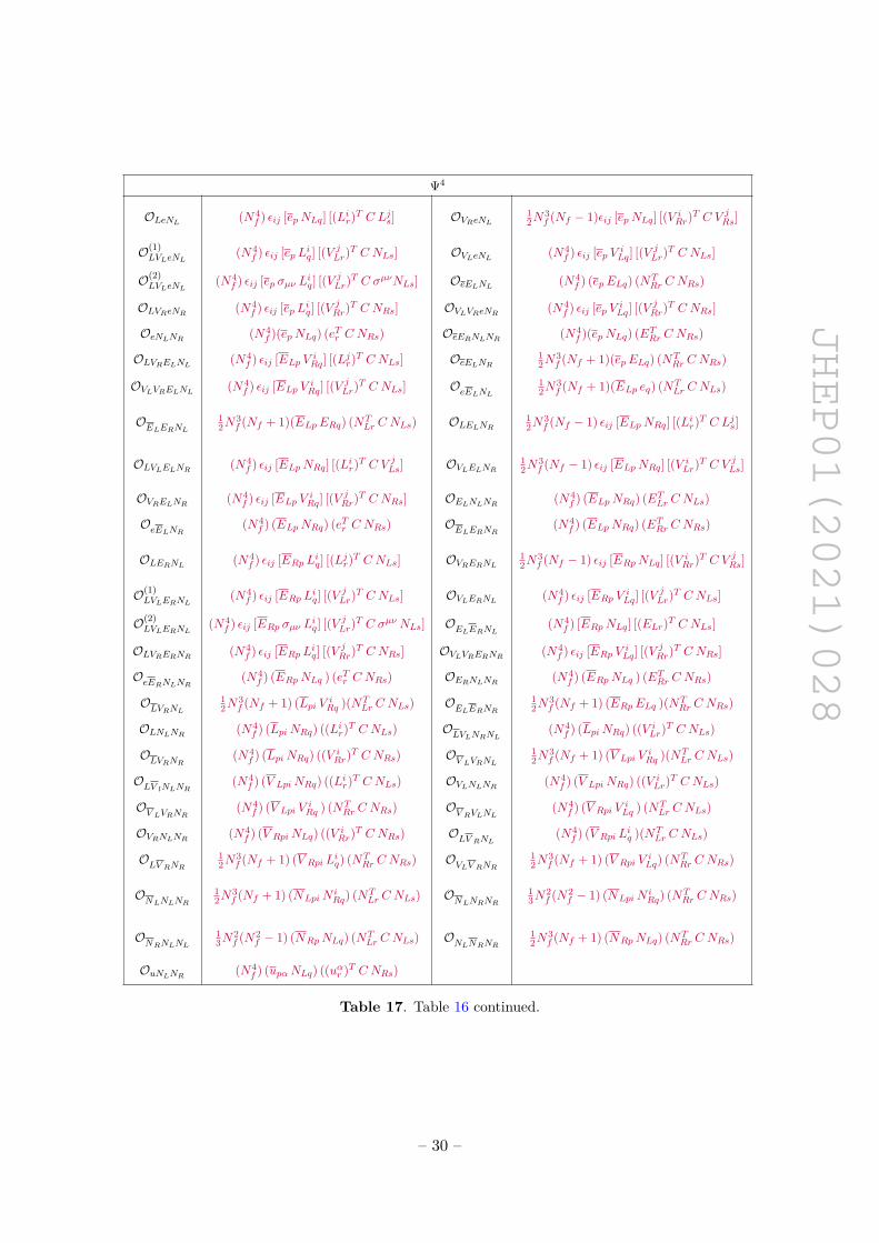
JHEP01(2021)028
Ψ4
OLeNL (N4f ) εij [epNLq] [(Lir)T C Ljs] OVReNL 1
2N3f (Nf − 1)εij [epNLq] [(V i
Rr)T C VjRs]
O(1)LVLeNL
(N4f ) εij [ep Liq] [(V j
Lr)T C NLs] OVLeNL (N4f ) εij [ep V i
Lq] [(V jLr)T C NLs]
O(2)LVLeNL
(N4f ) εij [ep σµν Liq] [(V j
Lr)T C σµνNLs] OeELNL (N4f ) (epELq) (NT
Rr C NRs)
OLVReNR (N4f ) εij [ep Liq] [(V j
Rr)T C NRs] OVLVReNR (N4f ) εij [ep V i
Lq] [(V jRr)T C NRs]
OeNLNR (N4f )(epNLq) (eTr C NRs) OeERNLNR (N4
f )(epNLq) (ETRr C NRs)
OLVRELNL (N4f ) εij [ELp V i
Rq] [(Ljr)T C NLs] OeELNR 12N
3f (Nf + 1)(epELq) (NT
Rr C NRs)
OVLVRELNL (N4f ) εij [ELp V i
Rq] [(V jLr)T C NLs] OeELNL
12N
3f (Nf + 1)(ELp eq) (NT
Lr C NLs)
OELERNL12N
3f (Nf + 1)(ELpERq) (NT
Lr C NLs) OLELNR 12N
3f (Nf − 1) εij [ELpNRq] [(Lir)T C Ljs]
OLVLELNR (N4f ) εij [ELpNRq] [(Lir)T C V
jLs] OVLELNR 1
2N3f (Nf − 1) εij [ELpNRq] [(V i
Lr)T C VjLs]
OVRELNR (N4f ) εij [ELp V i
Rq] [(V jRr)T C NRs] OELNLNR (N4
f ) (ELpNRq) (ETLr C NLs)
OeELNR (N4f ) (ELpNRq) (eTr C NRs) OELERNR (N4
f ) (ELpNRq) (ETRr C NRs)
OLERNL (N4f ) εij [ERp Liq] [(Ljr)T C NLs] OVRERNL 1
2N3f (Nf − 1) εij [ERpNLq] [(V i
Rr)T C VjRs]
O(1)LVLERNL
(N4f ) εij [ERp Liq] [(V j
Lr)T C NLs] OVLERNL (N4f ) εij [ERp V i
Lq] [(V jLr)T C NLs]
O(2)LVLERNL
(N4f ) εij [ERp σµν Liq] [(V j
Lr)T C σµν NLs] OELERNL (N4f ) [ERpNLq] [(ELr)T C NLs]
OLVRERNR (N4f ) εij [ERp Liq] [(V j
Rr)T C NRs] OVLVRERNR (N4f ) εij [ERp V i
Lq] [(V jRr)T C NRs]
OeERNLNR (N4f ) (ERpNLq ) (eTr C NRs) OERNLNR (N4
f ) (ERpNLq ) (ETRr C NRs)
OLVRNL12N
3f (Nf + 1) (Lpi V i
Rq )(NTLr C NLs) OELERNR
12N
3f (Nf + 1) (ERpELq )(NT
Rr C NRs)
OLNLNR (N4f ) (LpiNRq) ((Lir)T C NLs) OLVLNRNL (N4
f ) (LpiNRq) ((V iLr)T C NLs)
OLVRNR (N4f ) (LpiNRq) ((V i
Rr)T C NRs) OV LVRNL12N
3f (Nf + 1) (V Lpi V
iRq )(NT
Lr C NLs)
OLV lNLNR (N4f ) (V LpiNRq) ((Lir)T C NLs) OVLNLNR (N4
f ) (V LpiNRq) ((V iLr)T C NLs)
OV LVRNR (N4f ) (V Lpi V
iRq ) (NT
Rr C NRs) OV RVLNL (N4f ) (V Rpi V
iLq ) (NT
Lr C NLs)
OVRNLNR (N4f ) (V RpiNLq) ((V i
Rr)T C NRs) OLV RNL (N4f ) (V Rpi L
iq )(NT
Lr C NLs)
OLV RNR12N
3f (Nf + 1) (V Rpi L
iq) (NT
Rr C NRs) OVLV RNR12N
3f (Nf + 1) (V Rpi V
iLq) (NT
Rr C NRs)
ONLNLNR12N
3f (Nf + 1) (NLpiN
iRq) (NT
Lr C NLs) ONLNRNR13N
2f (N2
f − 1) (NLpiNiRq) (NT
Rr C NRs)
ONRNLNL13N
2f (N2
f − 1) (NRpNLq) (NTLr C NLs) ONLNRNR
12N
3f (Nf + 1) (NRpNLq) (NT
Rr C NRs)
OuNLNR (N4f ) (upαNLq) ((uαr )T C NRs)
Table 17. Table 16 continued.
– 30 –
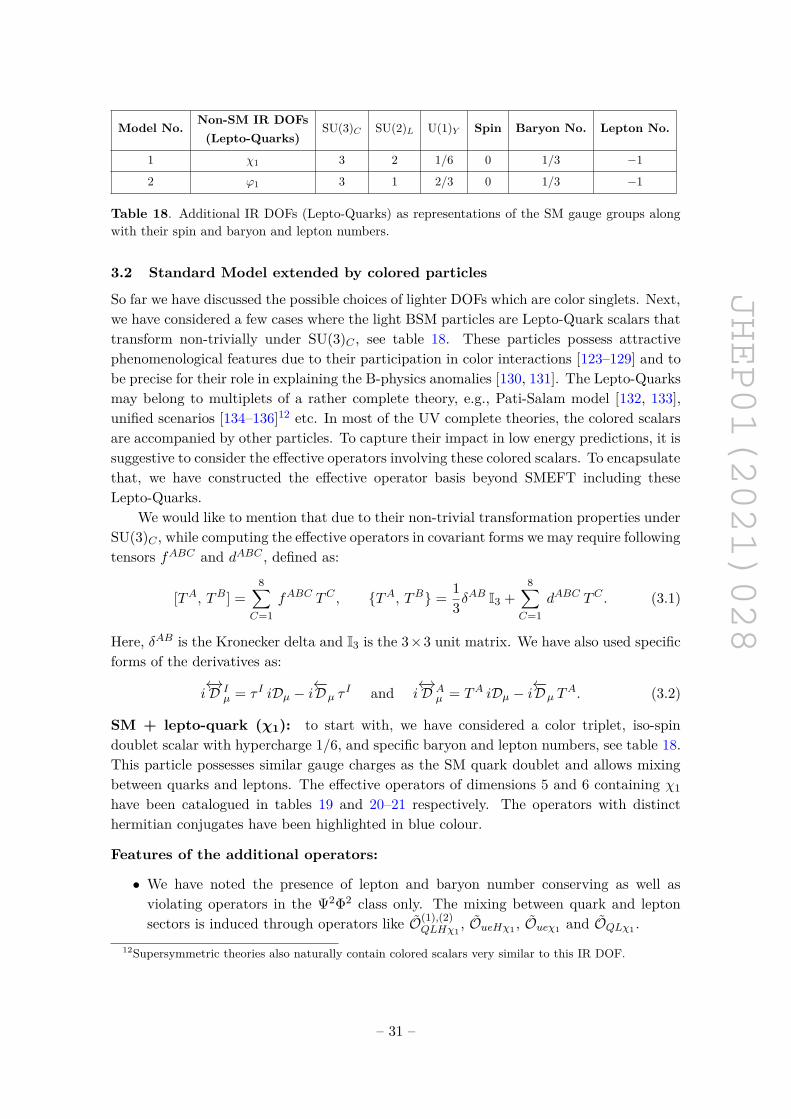
JHEP01(2021)028
Model No. Non-SM IR DOFs SU(3)C SU(2)L U(1)Y Spin Baryon No. Lepton No.(Lepto-Quarks)
1 χ1 3 2 1/6 0 1/3 −1
2 ϕ1 3 1 2/3 0 1/3 −1
Table 18. Additional IR DOFs (Lepto-Quarks) as representations of the SM gauge groups alongwith their spin and baryon and lepton numbers.
3.2 Standard Model extended by colored particles
So far we have discussed the possible choices of lighter DOFs which are color singlets. Next,we have considered a few cases where the light BSM particles are Lepto-Quark scalars thattransform non-trivially under SU(3)C , see table 18. These particles possess attractivephenomenological features due to their participation in color interactions [123–129] and tobe precise for their role in explaining the B-physics anomalies [130, 131]. The Lepto-Quarksmay belong to multiplets of a rather complete theory, e.g., Pati-Salam model [132, 133],unified scenarios [134–136]12 etc. In most of the UV complete theories, the colored scalarsare accompanied by other particles. To capture their impact in low energy predictions, it issuggestive to consider the effective operators involving these colored scalars. To encapsulatethat, we have constructed the effective operator basis beyond SMEFT including theseLepto-Quarks.
We would like to mention that due to their non-trivial transformation properties underSU(3)C , while computing the effective operators in covariant forms we may require followingtensors fABC and dABC , defined as:
[TA, TB] =8∑
C=1fABC TC , {TA, TB} = 1
3δAB I3 +
8∑C=1
dABC TC . (3.1)
Here, δAB is the Kronecker delta and I3 is the 3×3 unit matrix. We have also used specificforms of the derivatives as:
i←→D Iµ = τ I iDµ − i
←−Dµ τ
I and i←→D Aµ = TA iDµ − i
←−Dµ T
A. (3.2)
SM + lepto-quark (χ1): to start with, we have considered a color triplet, iso-spindoublet scalar with hypercharge 1/6, and specific baryon and lepton numbers, see table 18.This particle possesses similar gauge charges as the SM quark doublet and allows mixingbetween quarks and leptons. The effective operators of dimensions 5 and 6 containing χ1have been catalogued in tables 19 and 20–21 respectively. The operators with distincthermitian conjugates have been highlighted in blue colour.
Features of the additional operators:
• We have noted the presence of lepton and baryon number conserving as well asviolating operators in the Ψ2Φ2 class only. The mixing between quark and leptonsectors is induced through operators like O(1),(2)
QLHχ1, OueHχ1 , Oueχ1 and OQLχ1 .
12Supersymmetric theories also naturally contain colored scalars very similar to this IR DOF.
– 31 –
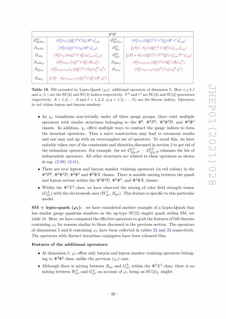
JHEP01(2021)028
Ψ2Φ2
O(1)QLHχ1
(N2f ) εij ((Qαip )T C Ljq)Hk χ†1,αk O(2)
QLHχ1(N2
f ) εij ((Qαip )T C τ I Ljq) (Hk τ I χ†1,αk)
OueHχ1 (N2f ) ((uαp )T C eq) (H i χ†1,αi) O(1)
Qχ112(N2
f +Nf ) ((Qαip )T C Qβjq ) (χ†1,αi χ†1,βj)
Oudχ1 (N2f ) εij (I(uαp )T C dβq ) (χ†1,αi χ
†1,βj) O(2)
Qχ112(N2
f +Nf ) ((Qαip )T C TAQβjq ) (χ†1,αi TA χ†1,βj)
OudHχ1 (N2f ) εαβγ ((uαp )T C dβq ) (Hi χ
γi1 ) OQHχ1 (N2
f ) εαβγ εij ((Qαip )T C Qβjq ) (Hk χγk1 )
OQLχ1 (N2f ) εαβγ εij εkl ((Qαip )T C Ljq) (χβk1 χγl1 ) Oueχ1 (N2
f ) εαβγ εij ((uαp )T C eq) (χβi1 χγj1 )
OdHχ112(N2
f −Nf ) εαβγ εij ((dαp )T C dβq ) (H i χγj1 )
Table 19. SM extended by Lepto-Quark (χ1): additional operators of dimension 5. Here i, j, k, land α, β, γ are the SU(2) and SU(3) indices respectively. TA and τ I are SU(3) and SU(2) generatorsrespectively. A = 1, 2, · · · , 8 and I = 1, 2, 3. p, q = 1, 2, · · · , Nf are the flavour indices. Operatorsin red violate lepton and baryon numbers.
• As χ1 transforms non-trivially under all three gauge groups, there exist multipleoperators with similar structures belonging to the Φ6, Φ4D2, Ψ2Φ2D, and Ψ2Φ3
classes. In addition, χ1 offers multiple ways to contract the gauge indices to formthe invariant operators. Thus a naive construction may lead to erroneous resultsand one may end up with an overcomplete set of operators. To avoid this, we havesuitably taken care of the constraints and identities discussed in section 2 to get rid ofthe redundant operators. For example, the set O(1)
Qχ1D — O(4)Qχ1D exhausts the list of
independent operators. All other structures are related to these operators as shownin eqs. (2.39)–(2.41).
• There are new lepton and baryon number violating operators (in red colour) in theΦ4D2, Ψ2Φ2D, Ψ2Φ3 and Ψ2ΦX classes. There is notable mixing between the quarkand lepton sectors within the Ψ2Φ2D, Ψ2Φ3, and Ψ2ΦX classes.
• Within the Φ2X2 class, we have observed the mixing of color field strength tensor(GAµν) with the electroweak ones (W I
µν , Bµν). This feature is specific to this particularmodel.
SM + lepto-quark (ϕ1): we have considered another example of a Lepto-Quark thathas similar gauge quantum numbers as the up-type SU(2) singlet quark within SM, seetable 18. Here, we have computed the effective operators to grab the features of full theoriescontaining ϕ1 for reasons similar to those discussed in the previous section. The operatorsof dimensions 5 and 6 containing ϕ1 have been collected in tables 22 and 23 respectively.The operators with distinct hermitian conjugates have been coloured blue.
Features of the additional operators:
• At dimension 5, ϕ1 offers only baryon and lepton number violating operators belong-ing to Ψ2Φ2 class, unlike the previous (χ1) case.
• Although there is mixing between Bµν and GAµν within the Φ2X2 class, there is nomixing between W I
µν and GAµν on account of ϕ1 being an SU(2)L singlet.
– 32 –
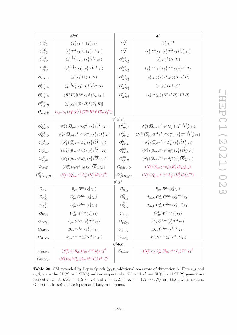
JHEP01(2021)028
Φ4D2 Φ6
O(1)χ1� (χ†1 χ1)� (χ†1 χ1) O(1)
χ1 (χ†1 χ1)3
O(2)χ1� (χ†1 TA χ1)� (χ†1 TA χ1) O(2)
χ1 (χ†1 TA χ1) (χ†1 TA χ1) (χ†1 χ1)
O(1)χ1D (χ†1
←→D µ χ1) (χ†1
←→D µ χ1) O(1)
H2χ41
(χ†1 χ1)2 (H†H)
O(2)χ1D (χ†1
←→D Aµ χ1) (χ†1
←→D µA χ1) O(2)
H2χ41
(χ†1 TA χ1) (χ†1 TA χ1) (H†H)
OHχ1� (χ†1 χ1)� (H†H) O(3)H2χ4
1(χ†1 χ1) (χ†1 τ I χ1) (H† τ I H)
O(1)Hχ1D (χ†1
←→D Iµ χ1) (H†←→D µI H) O(1)
H4χ21
(χ†1 χ1) (H†H)2
O(2)Hχ1D (H†H) [(Dµ χ1)† (Dµ χ1)] O(2)
H4χ21
(χ†1 τ I χ1) (H† τ I H) (H†H)
O(3)Hχ1D (χ†1 χ1) [(DµH)† (DµH)]
OHχ31D
εαβγ εij (χαi1 χβj1 ) [(DµHk)† (Dµ χγk1 )]
Ψ2Φ2D
O(1)Qχ1D (N2
f ) (Qpαi γµQαiq ) (χ†1 i←→D µ χ1) O(2)
Qχ1D (N2f ) (Qpαi TA γµQαiq ) (χ†1 i
←→D Aµ χ1)
O(3)Qχ1D (N2
f ) (Qpαi τ I γµQαiq ) (χ†1 i←→D Iµ χ1) O(4)
Qχ1D (N2f ) (Qpαi TA τ I γµQαii ) (χ†1 TA i
←→D Iµ χ1)
O(1)Lχ1D (N2
f ) (Lpi γµ Liq) (χ†1 i←→D µ χ1) O(2)
Lχ1D (N2f ) (Lpi τ I γµ Liq) (χ†1 i
←→D Iµ χ1)
O(1)uχ1D (N2
f ) (upα γµ uαq ) (χ†1 i←→D µ χ1) O(2)
uχ1D (N2f ) (upα TA γµ uαq ) (χ†1 i
←→D Aµ χ1)
O(1)dχ1D (N2
f ) (dpα γµ dαq ) (χ†1 i←→D µ χ1) O(2)
dχ1D (N2f ) (dpα TA γµ dαq ) (χ†1 i
←→D Aµ χ1)
Oeχ1D (N2f ) (ep γµ eq) (χ†1 i
←→D µ χ1) OdeHχ1D (N2
f ) (dpα γµ eq) (H†i iDµχi1,α)
O(1)QLHχ1D (N2
f ) (Qpαi γµ Liq) (H†j iDµχαj1 ) O(2)
QLHχ1D (N2f ) (Qpαi τ I γµ Liq) (H†j iDIµχ
αj1 )
Φ2X2
OBχ1 Bµν Bµν (χ†1 χ1) OBχ1
Bµν Bµν (χ†1 χ1)
O(1)Gχ1
GAµν GAµν (χ†1 χ1) O(2)
Gχ1dABC G
Aµν G
Bµν (χ†1 TC χ1)
O(1)Gχ1
GAµν GAµν (χ†1 χ1) O(2)
Gχ1dABC G
Aµν G
Bµν (χ†1 TC χ1)
OWχ1 W IµνW
Iµν (χ†1 χ1) OWχ1W IµνW
Iµν (χ†1 χ1)
OBGχ1 Bµν GAµν (χ†1 TA χ1) OBGχ1
Bµν GAµν (χ†1 TA χ1)
OBWχ1 BµνWIµν (χ†1 τ I χ1) OBWχ1
Bµν WIµν (χ†1 τ I χ1)
OWGχ1 W Iµν G
Aµν (χ†1 TA τ I χ1) OWGχ1W Iµν G
Aµν (χ†1 TA τ I χ1)
Ψ2ΦX
OBLdχ1 (N2f ) εij Bµν (dpα σµν Liq)χ
αj1 OGLdχ1 (N2
f ) εij GAµν (dpα σµν Liq)TA χαj1
OWLdχ1 (N2f ) εijW I
µν (dpα σµν Liq) τ I χαj1
Table 20. SM extended by Lepto-Quark (χ1): additional operators of dimension 6. Here i, j andα, β, γ are the SU(2) and SU(3) indices respectively. TA and τ I are SU(3) and SU(2) generatorsrespectively. A,B,C = 1, 2, · · · , 8 and I = 1, 2, 3. p, q = 1, 2, · · · , Nf are the flavour indices.Operators in red violate lepton and baryon numbers.
– 33 –
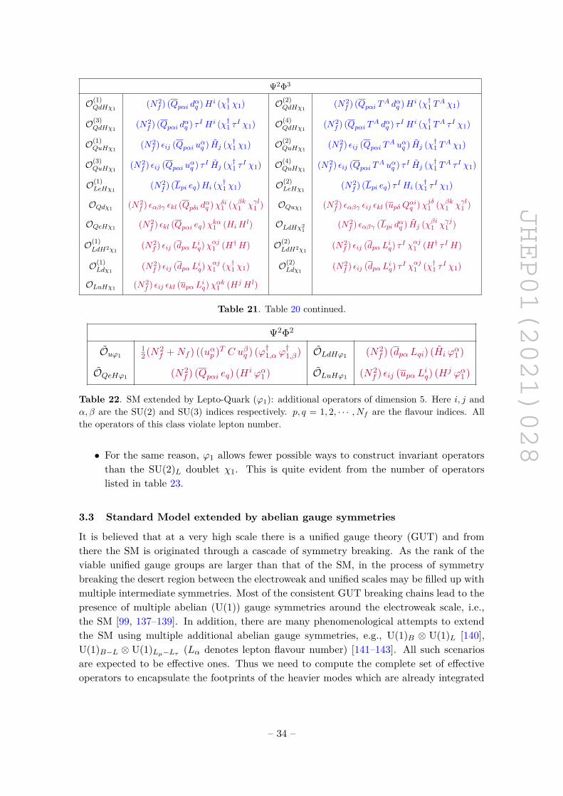
JHEP01(2021)028
Ψ2Φ3
O(1)QdHχ1
(N2f ) (Qpαi dαq )H i (χ†1 χ1) O(2)
QdHχ1(N2
f ) (Qpαi TA dαq )H i (χ†1 TA χ1)
O(3)QdHχ1
(N2f ) (Qpαi dαq ) τ I H i (χ†1 τ I χ1) O(4)
QdHχ1(N2
f ) (Qpαi TA dαq ) τ I H i (χ†1 TA τ I χ1)
O(1)QuHχ1
(N2f ) εij (Qpαi uαq ) Hj (χ†1 χ1) O(2)
QuHχ1(N2
f ) εij (Qpαi TA uαq ) Hj (χ†1 TA χ1)
O(3)QuHχ1
(N2f ) εij (Qpαi uαq ) τ I Hj (χ†1 τ I χ1) O(4)
QuHχ1(N2
f ) εij (Qpαi TA uαq ) τ I Hj (χ†1 TA τ I χ1)
O(1)LeHχ1
(N2f ) (Lpi eq)Hi (χ†1 χ1) O(2)
LeHχ1(N2
f ) (Lpi eq) τ I Hi (χ†1 τ I χ1)
OQdχ1 (N2f ) εαβγ εkl (Qpδi dαq )χδi1 (χβk1 χγl1 ) OQuχ1 (N2
f ) εαβγ εij εkl (upδ Qαiq )χjδ1 (χβk1 χγl1 )
OQeHχ1 (N2f ) εkl (Qpαi eq)χkα1 (HiH
l) OLdHχ21
(N2f ) εαβγ (Lpi dαq ) Hj (χβi1 χγj1 )
O(1)LdH2χ1
(N2f ) εij (dpα Liq)χ
αj1 (H†H) O(2)
LdH2χ1(N2
f ) εij (dpα Liq) τ I χαj1 (H† τ I H)
O(1)Ldχ1
(N2f ) εij (dpα Liq)χ
αj1 (χ†1 χ1) O(2)
Ldχ1(N2
f ) εij (dpα Liq) τ I χαj1 (χ†1 τ I χ1)
OLuHχ1 (N2f ) εij εkl (upα Liq)χαk1 (Hj H l)
Table 21. Table 20 continued.
Ψ2Φ2
Ouϕ112(N2
f +Nf ) ((uαp )T C uβq ) (ϕ†1,α ϕ†1,β) OLdHϕ1 (N2
f ) (dpα Lqi) (Hi ϕα1 )
OQeHϕ1 (N2f ) (Qpαi eq) (H i ϕα1 ) OLuHϕ1 (N2
f ) εij (upα Liq) (Hj ϕα1 )
Table 22. SM extended by Lepto-Quark (ϕ1): additional operators of dimension 5. Here i, j andα, β are the SU(2) and SU(3) indices respectively. p, q = 1, 2, · · · , Nf are the flavour indices. Allthe operators of this class violate lepton number.
• For the same reason, ϕ1 allows fewer possible ways to construct invariant operatorsthan the SU(2)L doublet χ1. This is quite evident from the number of operatorslisted in table 23.
3.3 Standard Model extended by abelian gauge symmetries
It is believed that at a very high scale there is a unified gauge theory (GUT) and fromthere the SM is originated through a cascade of symmetry breaking. As the rank of theviable unified gauge groups are larger than that of the SM, in the process of symmetrybreaking the desert region between the electroweak and unified scales may be filled up withmultiple intermediate symmetries. Most of the consistent GUT breaking chains lead to thepresence of multiple abelian (U(1)) gauge symmetries around the electroweak scale, i.e.,the SM [99, 137–139]. In addition, there are many phenomenological attempts to extendthe SM using multiple additional abelian gauge symmetries, e.g., U(1)B ⊗ U(1)L [140],U(1)B−L ⊗ U(1)Lµ−Lτ (Lα denotes lepton flavour number) [141–143]. All such scenariosare expected to be effective ones. Thus we need to compute the complete set of effectiveoperators to encapsulate the footprints of the heavier modes which are already integrated
– 34 –
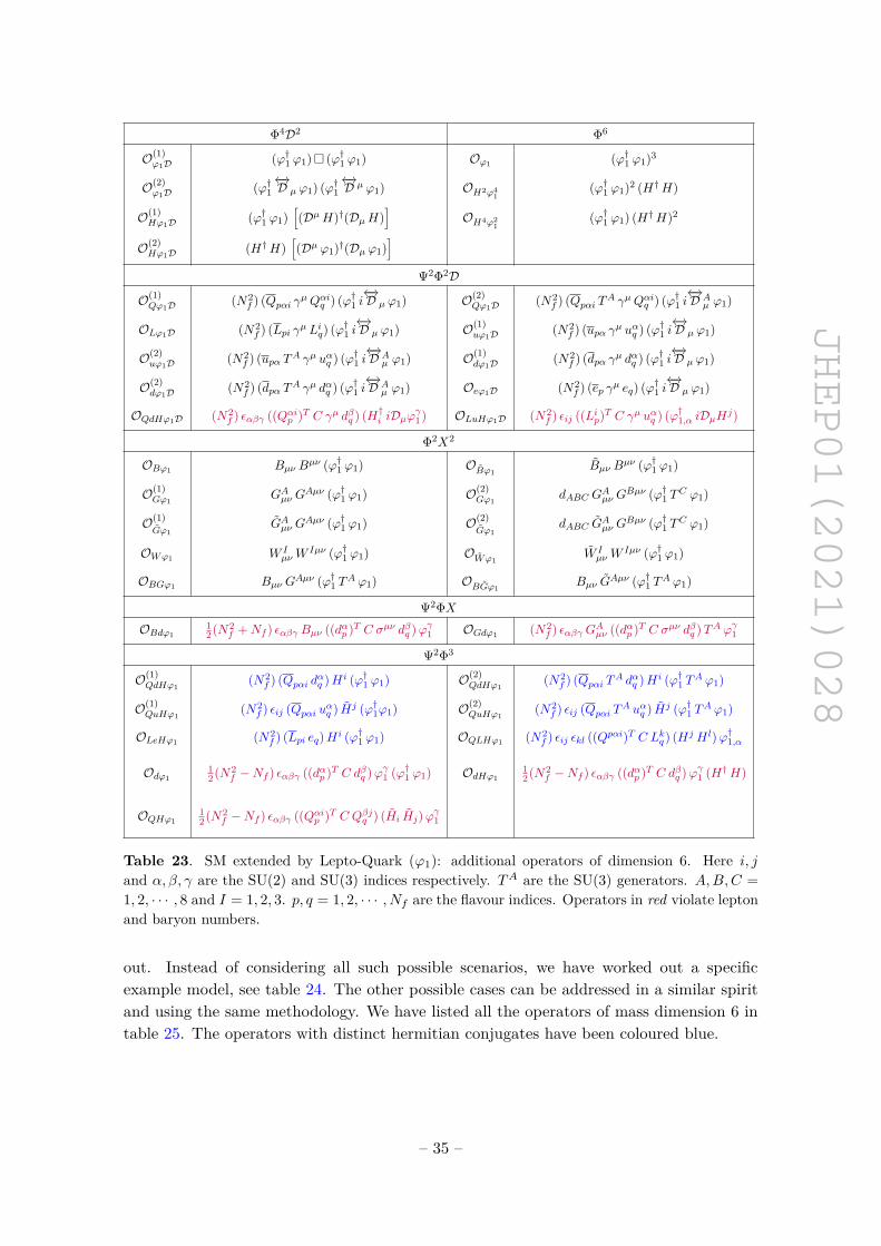
JHEP01(2021)028
Φ4D2 Φ6
O(1)ϕ1D (ϕ†1 ϕ1)� (ϕ†1 ϕ1) Oϕ1 (ϕ†1 ϕ1)3
O(2)ϕ1D (ϕ†1
←→D µ ϕ1) (ϕ†1
←→D µ ϕ1) OH2ϕ4
1(ϕ†1 ϕ1)2 (H†H)
O(1)Hϕ1D (ϕ†1 ϕ1)
[(DµH)†(DµH)
]OH4ϕ2
1(ϕ†1 ϕ1) (H†H)2
O(2)Hϕ1D (H†H)
[(Dµ ϕ1)†(Dµ ϕ1)
]Ψ2Φ2D
O(1)Qϕ1D (N2
f ) (Qpαi γµQαiq ) (ϕ†1 i←→D µ ϕ1) O(2)
Qϕ1D (N2f ) (Qpαi TA γµQαiq ) (ϕ†1 i
←→D Aµ ϕ1)
OLϕ1D (N2f ) (Lpi γµ Liq) (ϕ†1 i
←→D µ ϕ1) O(1)
uϕ1D (N2f ) (upα γµ uαq ) (ϕ†1 i
←→D µ ϕ1)
O(2)uϕ1D (N2
f ) (upα TA γµ uαq ) (ϕ†1 i←→D Aµ ϕ1) O(1)
dϕ1D (N2f ) (dpα γµ dαq ) (ϕ†1 i
←→D µ ϕ1)
O(2)dϕ1D (N2
f ) (dpα TA γµ dαq ) (ϕ†1 i←→D Aµ ϕ1) Oeϕ1D (N2
f ) (ep γµ eq) (ϕ†1 i←→D µ ϕ1)
OQdHϕ1D (N2f ) εαβγ ((Qαip )T C γµ dβq ) (H†i iDµϕ
γ1) OLuHϕ1D (N2
f ) εij ((Lip)T C γµ uαq ) (ϕ†1,α iDµHj)
Φ2X2
OBϕ1 Bµν Bµν (ϕ†1 ϕ1) OBϕ1
Bµν Bµν (ϕ†1 ϕ1)
O(1)Gϕ1
GAµν GAµν (ϕ†1 ϕ1) O(2)
Gϕ1dABC G
Aµν G
Bµν (ϕ†1 TC ϕ1)
O(1)Gϕ1
GAµν GAµν (ϕ†1 ϕ1) O(2)
Gϕ1dABC G
Aµν G
Bµν (ϕ†1 TC ϕ1)
OWϕ1 W IµνW
Iµν (ϕ†1 ϕ1) OWϕ1W IµνW
Iµν (ϕ†1 ϕ1)
OBGϕ1 Bµν GAµν (ϕ†1 TA ϕ1) OBGϕ1
Bµν GAµν (ϕ†1 TA ϕ1)
Ψ2ΦXOBdϕ1
12(N2
f +Nf ) εαβγ Bµν ((dαp )T C σµν dβq )ϕγ1 OGdϕ1 (N2f ) εαβγ GAµν ((dαp )T C σµν dβq )TA ϕγ1
Ψ2Φ3
O(1)QdHϕ1
(N2f ) (Qpαi dαq )H i (ϕ†1 ϕ1) O(2)
QdHϕ1(N2
f ) (Qpαi TA dαq )H i (ϕ†1 TA ϕ1)
O(1)QuHϕ1
(N2f ) εij (Qpαi uαq ) Hj (ϕ†1ϕ1) O(2)
QuHϕ1(N2
f ) εij (Qpαi TA uαq ) Hj (ϕ†1 TA ϕ1)
OLeHϕ1 (N2f ) (Lpi eq)H i (ϕ†1 ϕ1) OQLHϕ1 (N2
f ) εij εkl ((Qpαi)T C Lkq ) (Hj H l)ϕ†1,α
Odϕ112(N2
f −Nf ) εαβγ ((dαp )T C dβq )ϕγ1 (ϕ†1 ϕ1) OdHϕ112(N2
f −Nf ) εαβγ ((dαp )T C dβq )ϕγ1 (H†H)
OQHϕ112(N2
f −Nf ) εαβγ ((Qαip )T C Qβjq ) (Hi Hj)ϕγ1
Table 23. SM extended by Lepto-Quark (ϕ1): additional operators of dimension 6. Here i, jand α, β, γ are the SU(2) and SU(3) indices respectively. TA are the SU(3) generators. A,B,C =1, 2, · · · , 8 and I = 1, 2, 3. p, q = 1, 2, · · · , Nf are the flavour indices. Operators in red violate leptonand baryon numbers.
out. Instead of considering all such possible scenarios, we have worked out a specificexample model, see table 24. The other possible cases can be addressed in a similar spiritand using the same methodology. We have listed all the operators of mass dimension 6 intable 25. The operators with distinct hermitian conjugates have been coloured blue.
– 35 –
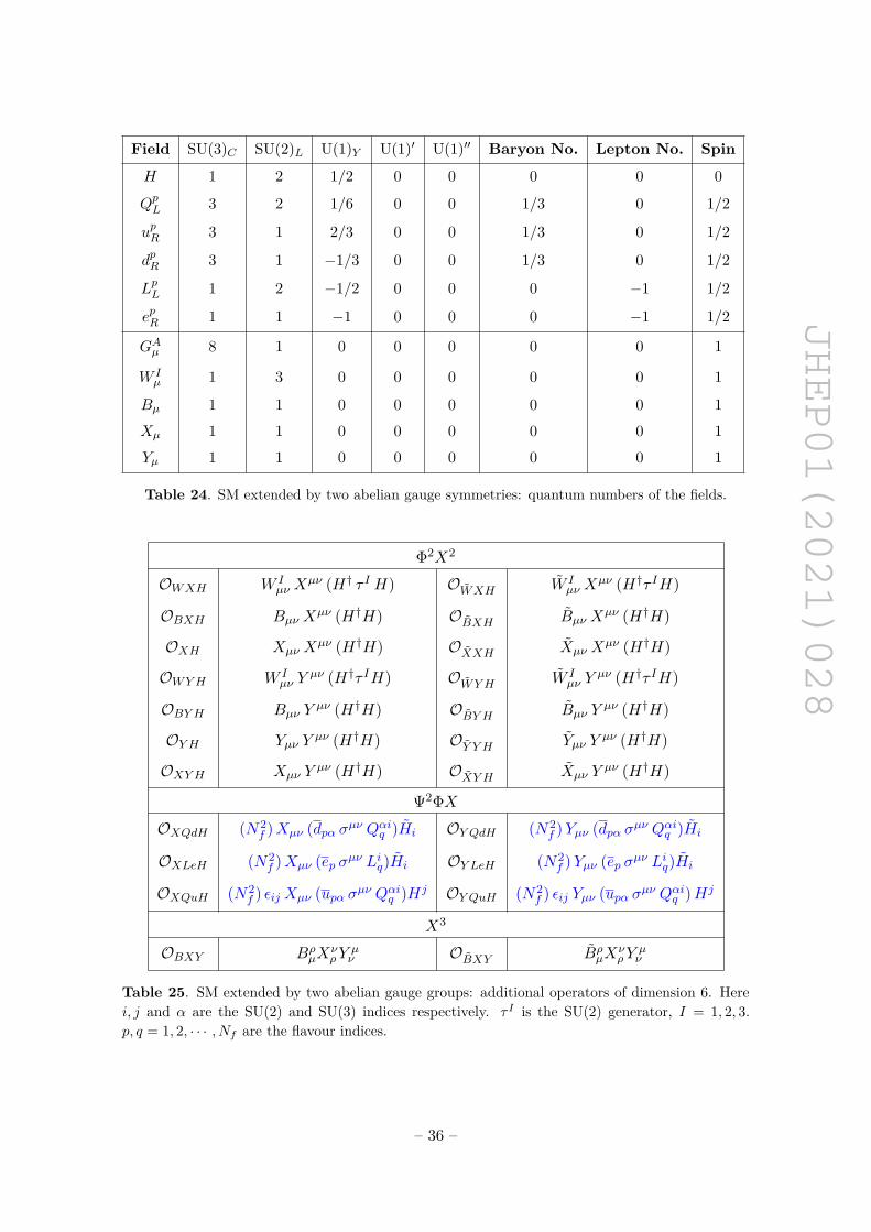
JHEP01(2021)028
Field SU(3)C SU(2)L U(1)Y U(1)′ U(1)′′ Baryon No. Lepton No. Spin
H 1 2 1/2 0 0 0 0 0
QpL 3 2 1/6 0 0 1/3 0 1/2
upR 3 1 2/3 0 0 1/3 0 1/2
dpR 3 1 −1/3 0 0 1/3 0 1/2
LpL 1 2 −1/2 0 0 0 −1 1/2
epR 1 1 −1 0 0 0 −1 1/2
GAµ 8 1 0 0 0 0 0 1
W Iµ 1 3 0 0 0 0 0 1
Bµ 1 1 0 0 0 0 0 1Xµ 1 1 0 0 0 0 0 1Yµ 1 1 0 0 0 0 0 1
Table 24. SM extended by two abelian gauge symmetries: quantum numbers of the fields.
Φ2X2
OWXH W Iµν X
µν (H† τ I H) OWXH W Iµν X
µν (H†τ IH)
OBXH Bµν Xµν (H†H) OBXH Bµν X
µν (H†H)
OXH Xµν Xµν (H†H) OXXH Xµν X
µν (H†H)
OWYH W Iµν Y
µν (H†τ IH) OWY H W Iµν Y
µν (H†τ IH)
OBYH Bµν Yµν (H†H) OBY H Bµν Y
µν (H†H)
OY H Yµν Yµν (H†H) OY Y H Yµν Y
µν (H†H)
OXYH Xµν Yµν (H†H) OXY H Xµν Y
µν (H†H)
Ψ2ΦXOXQdH (N2
f )Xµν (dpα σµν Qαiq )Hi OY QdH (N2f )Yµν (dpα σµν Qαiq )Hi
OXLeH (N2f )Xµν (ep σµν Liq)Hi OY LeH (N2
f )Yµν (ep σµν Liq)Hi
OXQuH (N2f ) εij Xµν (upα σµν Qαiq )Hj OY QuH (N2
f ) εij Yµν (upα σµν Qαiq )Hj
X3
OBXY BρµX
νρY
µν OBXY Bρ
µXνρY
µν
Table 25. SM extended by two abelian gauge groups: additional operators of dimension 6. Herei, j and α are the SU(2) and SU(3) indices respectively. τ I is the SU(2) generator, I = 1, 2, 3.p, q = 1, 2, · · · , Nf are the flavour indices.
– 36 –
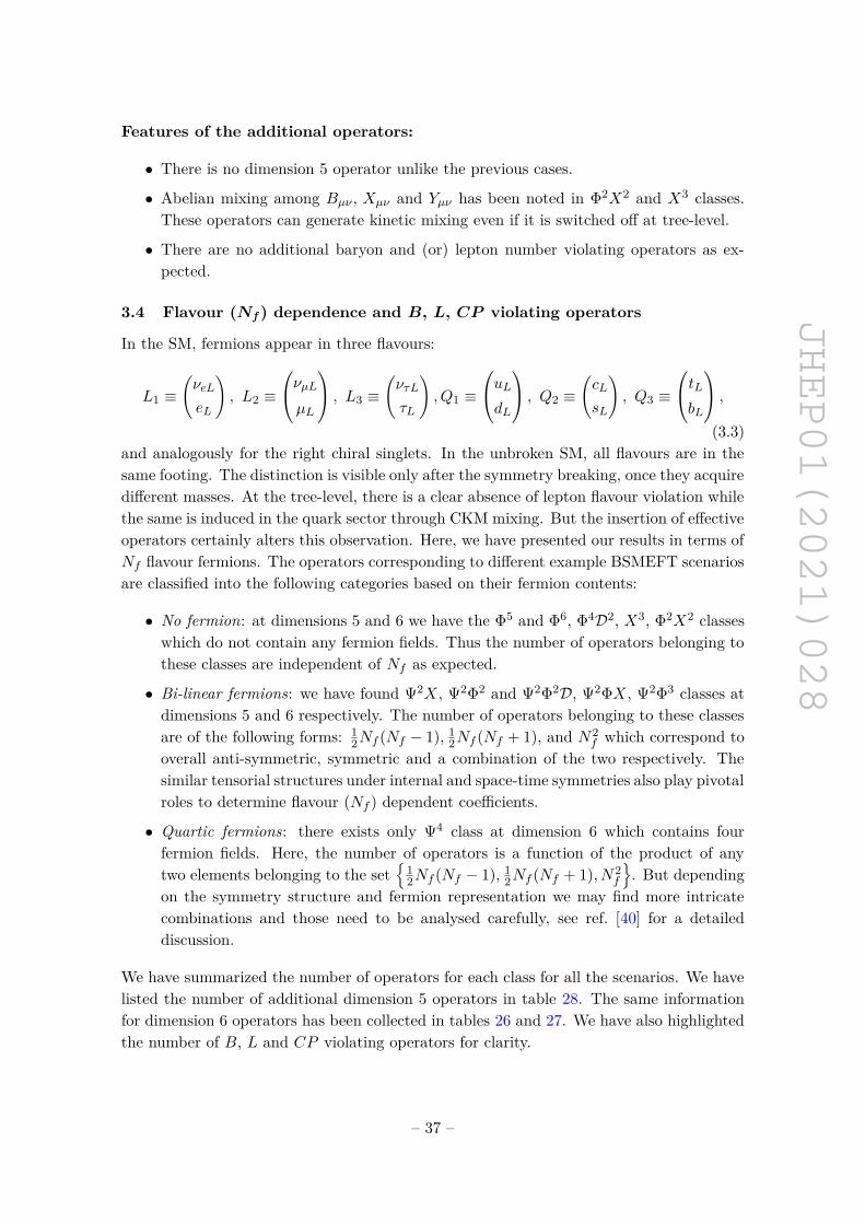
JHEP01(2021)028
Features of the additional operators:
• There is no dimension 5 operator unlike the previous cases.
• Abelian mixing among Bµν , Xµν and Yµν has been noted in Φ2X2 and X3 classes.These operators can generate kinetic mixing even if it is switched off at tree-level.
• There are no additional baryon and (or) lepton number violating operators as ex-pected.
3.4 Flavour (Nf) dependence and B, L, CP violating operators
In the SM, fermions appear in three flavours:
L1 ≡(νeL
eL
), L2 ≡
νµLµL
, L3 ≡(ντL
τL
), Q1 ≡
uLdL
, Q2 ≡(cL
sL
), Q3 ≡
tLbL
,(3.3)
and analogously for the right chiral singlets. In the unbroken SM, all flavours are in thesame footing. The distinction is visible only after the symmetry breaking, once they acquiredifferent masses. At the tree-level, there is a clear absence of lepton flavour violation whilethe same is induced in the quark sector through CKM mixing. But the insertion of effectiveoperators certainly alters this observation. Here, we have presented our results in terms ofNf flavour fermions. The operators corresponding to different example BSMEFT scenariosare classified into the following categories based on their fermion contents:
• No fermion: at dimensions 5 and 6 we have the Φ5 and Φ6, Φ4D2, X3, Φ2X2 classeswhich do not contain any fermion fields. Thus the number of operators belonging tothese classes are independent of Nf as expected.
• Bi-linear fermions: we have found Ψ2X, Ψ2Φ2 and Ψ2Φ2D, Ψ2ΦX, Ψ2Φ3 classes atdimensions 5 and 6 respectively. The number of operators belonging to these classesare of the following forms: 1
2Nf (Nf − 1), 12Nf (Nf + 1), and N2
f which correspond tooverall anti-symmetric, symmetric and a combination of the two respectively. Thesimilar tensorial structures under internal and space-time symmetries also play pivotalroles to determine flavour (Nf ) dependent coefficients.
• Quartic fermions: there exists only Ψ4 class at dimension 6 which contains fourfermion fields. Here, the number of operators is a function of the product of anytwo elements belonging to the set
{12Nf (Nf − 1), 1
2Nf (Nf + 1), N2f
}. But depending
on the symmetry structure and fermion representation we may find more intricatecombinations and those need to be analysed carefully, see ref. [40] for a detaileddiscussion.
We have summarized the number of operators for each class for all the scenarios. We havelisted the number of additional dimension 5 operators in table 28. The same informationfor dimension 6 operators has been collected in tables 26 and 27. We have also highlightedthe number of B, L and CP violating operators for clarity.
– 37 –
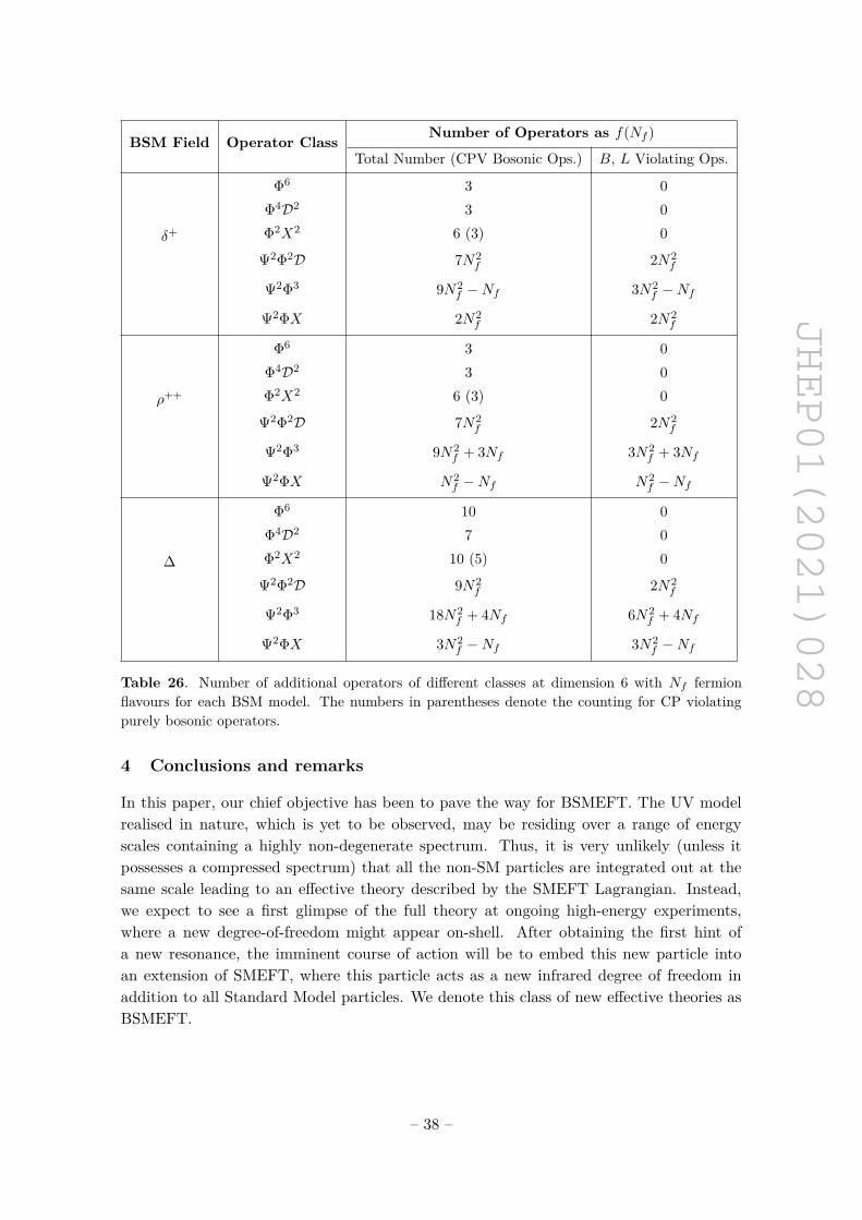
JHEP01(2021)028
BSM Field Operator Class Number of Operators as f(Nf )
Total Number (CPV Bosonic Ops.) B, L Violating Ops.
δ+
Φ6 3 0Φ4D2 3 0Φ2X2 6 (3) 0
Ψ2Φ2D 7N2f 2N2
f
Ψ2Φ3 9N2f −Nf 3N2
f −Nf
Ψ2ΦX 2N2f 2N2
f
ρ++
Φ6 3 0Φ4D2 3 0Φ2X2 6 (3) 0
Ψ2Φ2D 7N2f 2N2
f
Ψ2Φ3 9N2f + 3Nf 3N2
f + 3Nf
Ψ2ΦX N2f −Nf N2
f −Nf
∆
Φ6 10 0Φ4D2 7 0Φ2X2 10 (5) 0
Ψ2Φ2D 9N2f 2N2
f
Ψ2Φ3 18N2f + 4Nf 6N2
f + 4Nf
Ψ2ΦX 3N2f −Nf 3N2
f −Nf
Table 26. Number of additional operators of different classes at dimension 6 with Nf fermionflavours for each BSM model. The numbers in parentheses denote the counting for CP violatingpurely bosonic operators.
4 Conclusions and remarks
In this paper, our chief objective has been to pave the way for BSMEFT. The UV modelrealised in nature, which is yet to be observed, may be residing over a range of energyscales containing a highly non-degenerate spectrum. Thus, it is very unlikely (unless itpossesses a compressed spectrum) that all the non-SM particles are integrated out at thesame scale leading to an effective theory described by the SMEFT Lagrangian. Instead,we expect to see a first glimpse of the full theory at ongoing high-energy experiments,where a new degree-of-freedom might appear on-shell. After obtaining the first hint ofa new resonance, the imminent course of action will be to embed this new particle intoan extension of SMEFT, where this particle acts as a new infrared degree of freedom inaddition to all Standard Model particles. We denote this class of new effective theories asBSMEFT.
– 38 –
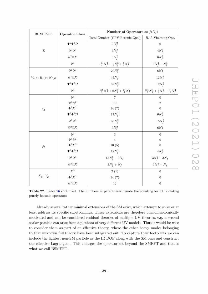
JHEP01(2021)028
BSM Field Operator Class Number of Operators as f(Nf )
Total Number (CPV Bosonic Ops.) B, L Violating Ops.
Σ
Ψ2Φ2D 2N2f 0
Ψ2Φ3 4N2f 4N2
f
Ψ2ΦX 6N2f 6N2
f
Ψ4 694 N
4f −
12N
3f + 9
4N2f 9N4
f −N3f
VL,R; EL,R; NL,R
Ψ2Φ3 20N2f 6N2
f
Ψ2ΦX 44N2f 12N2
f
Ψ2Φ2D 32N2f 12N2
f
Ψ4 6763 N4
f + 6N3f + 17
3 N2f
80512 N
4f + 9
2N3f −
712N
2f
χ1
Φ6 7 0Φ4D2 10 2Φ2X2 14 (7) 0
Ψ2Φ2D 17N2f 6N2
f
Ψ2Φ3 38N2f 18N2
f
Ψ2ΦX 6N2f 6N2
f
ϕ1
Φ6 3 0Φ4D2 4 0Φ2X2 10 (5) 0
Ψ2Φ2D 12N2f 4N2
f
Ψ2Φ3 15N2f − 3Nf 3N2
f − 3Nf
Ψ2ΦX 3N2f +Nf 3N2
f +Nf
Xµ, Yµ
X3 2 (1) 0
Φ2X2 14 (7) 0
Ψ2ΦX 12 0
Table 27. Table 26 continued. The numbers in parentheses denote the counting for CP violatingpurely bosonic operators.
Already several rather minimal extensions of the SM exist, which attempt to solve or atleast address its specific shortcomings. These extensions are therefore phenomenologicallymotivated and can be considered residual theories of multiple UV theories, e.g. a secondscalar particle can arise from a plethora of very different UV models. Thus it would be wiseto consider them as part of an effective theory, where the other heavy modes belongingto that unknown full theory have been integrated out. To capture their footprints we caninclude the lightest non-SM particle as the IR DOF along with the SM ones and constructthe effective Lagrangian. This enlarges the operator set beyond the SMEFT and that iswhat we call BSMEFT.
– 39 –
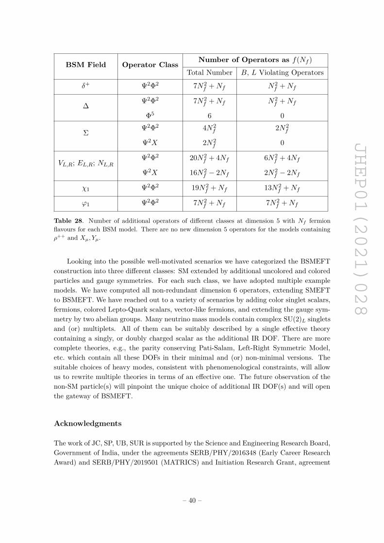
JHEP01(2021)028
BSM Field Operator Class Number of Operators as f(Nf )
Total Number B, L Violating Operators
δ+ Ψ2Φ2 7N2f +Nf N2
f +Nf
∆ Ψ2Φ2 7N2f +Nf N2
f +Nf
Φ5 6 0
Σ Ψ2Φ2 4N2f 2N2
f
Ψ2X 2N2f 0
VL,R; EL,R; NL,RΨ2Φ2 20N2
f + 4Nf 6N2f + 4Nf
Ψ2X 16N2f − 2Nf 2N2
f − 2Nf
χ1 Ψ2Φ2 19N2f +Nf 13N2
f +Nf
ϕ1 Ψ2Φ2 7N2f +Nf 7N2
f +Nf
Table 28. Number of additional operators of different classes at dimension 5 with Nf fermionflavours for each BSM model. There are no new dimension 5 operators for the models containingρ++ and Xµ, Yµ.
Looking into the possible well-motivated scenarios we have categorized the BSMEFTconstruction into three different classes: SM extended by additional uncolored and coloredparticles and gauge symmetries. For each such class, we have adopted multiple examplemodels. We have computed all non-redundant dimension 6 operators, extending SMEFTto BSMEFT. We have reached out to a variety of scenarios by adding color singlet scalars,fermions, colored Lepto-Quark scalars, vector-like fermions, and extending the gauge sym-metry by two abelian groups. Many neutrino mass models contain complex SU(2)L singletsand (or) multiplets. All of them can be suitably described by a single effective theorycontaining a singly, or doubly charged scalar as the additional IR DOF. There are morecomplete theories, e.g., the parity conserving Pati-Salam, Left-Right Symmetric Model,etc. which contain all these DOFs in their minimal and (or) non-minimal versions. Thesuitable choices of heavy modes, consistent with phenomenological constraints, will allowus to rewrite multiple theories in terms of an effective one. The future observation of thenon-SM particle(s) will pinpoint the unique choice of additional IR DOF(s) and will openthe gateway of BSMEFT.
Acknowledgments
The work of JC, SP, UB, SUR is supported by the Science and Engineering Research Board,Government of India, under the agreements SERB/PHY/2016348 (Early Career ResearchAward) and SERB/PHY/2019501 (MATRICS) and Initiation Research Grant, agreement
– 40 –
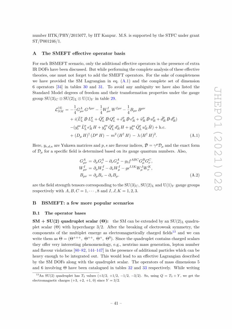
JHEP01(2021)028
number IITK/PHY/2015077, by IIT Kanpur. M.S. is supported by the STFC under grantST/P001246/1.
A The SMEFT effective operator basis
For each BSMEFT scenario, only the additional effective operators in the presence of extraIR DOFs have been discussed. But while performing the complete analysis of these effectivetheories, one must not forget to add the SMEFT operators. For the sake of completenesswe have provided the SM Lagrangian in eq. (A.1) and the complete set of dimension6 operators [34] in tables 30 and 31. To avoid any ambiguity we have also listed theStandard Model degrees of freedom and their transformation properties under the gaugegroup SU(3)C ⊗ SU(2)L ⊗U(1)Y in table 29.
L(4)SM = −1
4GAµν G
Aµν − 14W
IµνW
Iµν − 14Bµν B
µν
+ i(LpL /DLpL + QpL /DQpL + epR /D epR + upR /D upR + dpR /D dpR)
−(ypse LpL esRH + ypsd QpL d
sRH + ypsu QpL u
sR H) + h.c.
+ (DµH)† (DµH) − m2 (H†H) − λ (H†H)2. (A.1)
Here, ye,d,u are Yukawa matrices and p, s are flavour indices, /D = γµDµ and the exact formof Dµ for a specific field is determined based on its gauge quantum numbers. Also,
GAµν = ∂µGAν − ∂νGAµ − g3f
ABCGBµGCν ,
W Iµν = ∂µW
Iν − ∂νW I
µ − gεIJKW JµW
Kν ,
Bµν = ∂µBν − ∂νBµ. (A.2)
are the field strength tensors corresponding to the SU(3)C , SU(2)L and U(1)Y gauge groupsrespectively with A,B,C = 1, · · · , 8 and I, J,K = 1, 2, 3.
B BSMEFT: a few more popular scenarios
B.1 The operator bases
SM + SU(2) quadruplet scalar (Θ): the SM can be extended by an SU(2)L quadru-plet scalar (Θ) with hypercharge 3/2. After the breaking of electroweak symmetry, thecomponents of the multiplet emerge as electromagnetically charged fields13 and we canwrite them as Θ = (Θ+++, Θ++, Θ+, Θ0). Since the quadruplet contains charged scalarsthey offer very interesting phenomenology, e.g., neutrino mass generation, lepton numberand flavour violations [80–82, 144–147] in the presence of additional particles which can beheavy enough to be integrated out. This would lead to an effective Lagrangian describedby the SM DOFs along with the quadruplet scalar. The operators of mass dimensions 5and 6 involving Θ have been catalogued in tables 32 and 33 respectively. While writing
13An SU(2) quadruplet has T3 values (+3/2, +1/2, −1/2, −3/2). So, using Q = T3 + Y , we get theelectromagnetic charges (+3, +2, +1, 0) since Y = 3/2.
– 41 –
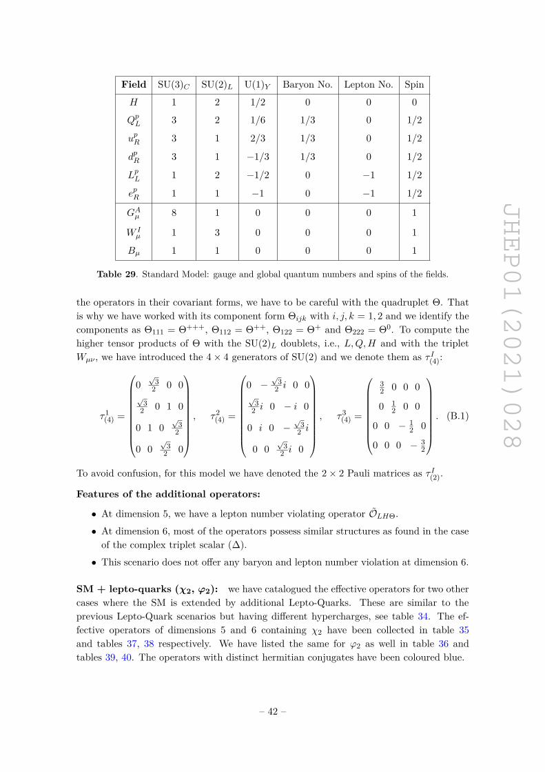
JHEP01(2021)028
Field SU(3)C SU(2)L U(1)Y Baryon No. Lepton No. Spin
H 1 2 1/2 0 0 0
QpL 3 2 1/6 1/3 0 1/2
upR 3 1 2/3 1/3 0 1/2
dpR 3 1 −1/3 1/3 0 1/2
LpL 1 2 −1/2 0 −1 1/2
epR 1 1 −1 0 −1 1/2
GAµ 8 1 0 0 0 1
W Iµ 1 3 0 0 0 1
Bµ 1 1 0 0 0 1
Table 29. Standard Model: gauge and global quantum numbers and spins of the fields.
the operators in their covariant forms, we have to be careful with the quadruplet Θ. Thatis why we have worked with its component form Θijk with i, j, k = 1, 2 and we identify thecomponents as Θ111 = Θ+++, Θ112 = Θ++, Θ122 = Θ+ and Θ222 = Θ0. To compute thehigher tensor products of Θ with the SU(2)L doublets, i.e., L,Q,H and with the tripletWµν , we have introduced the 4× 4 generators of SU(2) and we denote them as τ I(4):
τ1(4) =
0√
32 0 0
√3
2 0 1 0
0 1 0√
32
0 0√
32 0
, τ2
(4) =
0 −√
32 i 0 0
√3
2 i 0 − i 0
0 i 0 −√
32 i
0 0√
32 i 0
, τ3
(4) =
32 0 0 0
0 12 0 0
0 0 − 12 0
0 0 0 − 32
. (B.1)
To avoid confusion, for this model we have denoted the 2× 2 Pauli matrices as τ I(2).
Features of the additional operators:
• At dimension 5, we have a lepton number violating operator OLHΘ.
• At dimension 6, most of the operators possess similar structures as found in the caseof the complex triplet scalar (∆).
• This scenario does not offer any baryon and lepton number violation at dimension 6.
SM + lepto-quarks (χ2, ϕ2): we have catalogued the effective operators for two othercases where the SM is extended by additional Lepto-Quarks. These are similar to theprevious Lepto-Quark scenarios but having different hypercharges, see table 34. The ef-fective operators of dimensions 5 and 6 containing χ2 have been collected in table 35and tables 37, 38 respectively. We have listed the same for ϕ2 as well in table 36 andtables 39, 40. The operators with distinct hermitian conjugates have been coloured blue.
– 42 –
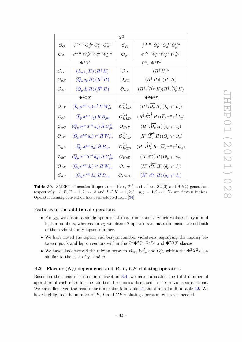
JHEP01(2021)028
X3
OG fABC GAµν GBνρ GCρµ OG fABC GAµν GBνρ GCρµ
OW εIJKW Iµν W Jν
ρ WKρµ OW εIJK W Iµ
ν W Jνρ WKρ
µ
Ψ2Φ3 Φ6, Φ4D2
OeH (Lp eqH) (H†H) OH (H†H)6
OuH (Qp uq H) (H†H) OH� (H†H)�(H†H)
OdH (Qp dqH) (H†H) OHD (H† i←→D µH)(H† i←→DµH)
Ψ2ΦX Ψ2Φ2D
OeW (Lp σµν eq) τ I HW Iµν O(1)
HLD (H† i←→DµH) (Lp γµ Lq)
OeB (Lp σµν eq)H Bµν O(3)HLD (H† i
←→DIµH) (Lp γµ τ I Lq)
OuG (Qp σµν TA uq) H GAµν OHeD (H† i←→DµH) (ep γµ eq)
OuW (Qp σµν uq) τ I H W Iµν O(1)
HQD (H† i←→DµH) (Qp γµQq)
OuB (Qp σµν uq) H Bµν O(3)HQD (H† i
←→DIµH) (Qp γµ τ I Qq)
OdG (Qp σµν TA dq)H GAµν OHuD (H† i←→DµH) (up γµ uq)
OdW (Qp σµν dq) τ I HW Iµν OHdD (H† i←→DµH) (dp γµ dq)
OdB (Qp σµν dq)H Bµν OHudD (H† iDµH) (up γµ dq)
Table 30. SMEFT dimension 6 operators. Here, TA and τ I are SU(3) and SU(2) generatorsrespectively. A,B,C = 1, 2, · · · , 8 and I, J,K = 1, 2, 3. p, q = 1, 2, · · · , Nf are flavour indices.Operator naming convention has been adopted from [34].
Features of the additional operators:
• For χ2, we obtain a single operator at mass dimension 5 which violates baryon andlepton numbers, whereas for ϕ2 we obtain 2 operators at mass dimension 5 and bothof them violate only lepton number.• We have noted the lepton and baryon number violations, signifying the mixing be-tween quark and lepton sectors within the Ψ2Φ2D, Ψ2Φ3 and Ψ2ΦX classes.• We have also observed the mixing between Bµν , W I
µν and GAµν within the Φ2X2 classsimilar to the case of χ1 and ϕ1.
B.2 Flavour (Nf) dependence and B, L, CP violating operators
Based on the ideas discussed in subsection 3.4, we have tabulated the total number ofoperators of each class for the additional scenarios discussed in the previous subsections.We have displayed the results for dimension 5 in table 41 and dimension 6 in table 42. Wehave highlighted the number of B, L and CP violating operators wherever needed.
– 43 –
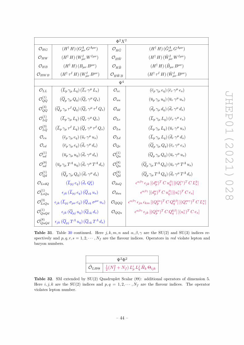
JHEP01(2021)028
Φ2X2
OHG (H†H) (GAµν GAµν) OHG (H†H) (GAµν GAµν)
OHW (H†H) (W IµνW
Iµν) OHW (H†H) (W IµνW
Iµν)
OHB (H†H) (Bµν Bµν) OHB (H†H) (Bµν Bµν)
OHWB (H† τ I H) (W Iµν B
µν) OHWB (H† τ I H) (W Iµν B
µν)
Ψ4
OLL (Lp γµ Lq) (Lr γµ Ls) Oee (ep γµ eq) (er γµ es)
O(1)QQ (Qp γµQq) (Qr γµQs) Ouu (up γµ uq) (ur γµ us)
O(3)QQ (Qp γµ τ I Qq) (Qr γµ τ I Qs) Odd (dp γµ dq) (dr γµ ds)
O(1)LQ (Lp γµ Lq) (Qr γµQs) OLe (Lp γµ Lq) (er γµ es)
O(3)LQ (Lp γµ τ I Lq) (Qr γµ τ I Qs) OLu (Lp γµ Lq) (ur γµ us)
Oeu (ep γµ eq) (ur γµ us) OLd (Lp γµ Lq) (dr γµ ds)
Oed (ep γµ eq) (dr γµ ds) OQe (Qp γµQq) (er γµ es)
O(1)ud (up γµ uq) (dr γµ ds) O(1)
Qu (Qp γµQq) (ur γµ us)
O(8)ud (up γµ TA uq) (dr γµ TA ds) O(8)
Qu (Qp γµ TAQq) (ur γµ TA us)
O(1)Qd (Qp γµQq) (dr γµ ds) O(8)
Qd (Qp γµ TAQq) (dr γµ TA ds)
OLedQ (Lpj eq) (drQjs) OduQ εαβγ εjk [(dαp )T C uβq ] [(Qjγr )T C Lks ]
O(1)LeQu εjk (Lpj eq) (Qrk us) Oduu εαβγ [(dαp )T C uβq ] [(uγr )T C es]
O(3)LeQu εjk (Lpj σµν eq) (Qrk σµν us) OQQQ εαβγ εjn εkm [(Qjαp )T C Qkβq ] [(Qmγr )T C Lns ]
O(1)QuQd εjk (Qpj uq) (Qrk ds) OQQu εαβγ εjk [(Qjαp )T C Qkβq ] [(uγr )T C es]
O(8)QuQd εjk (Qpj TA uq) (Qrk TA ds)
Table 31. Table 30 continued. Here j, k,m, n and α, β, γ are the SU(2) and SU(3) indices re-spectively and p, q, r, s = 1, 2, · · · , Nf are the flavour indices. Operators in red violate lepton andbaryon numbers.
Ψ2Φ2
OLHΘ12(N2
f +Nf )Lip Ljq Hk Θijk
Table 32. SM extended by SU(2) Quadruplet Scalar (Θ): additional operators of dimension 5.Here i, j, k are the SU(2) indices and p, q = 1, 2, · · · , Nf are the flavour indices. The operatorviolates lepton number.
– 44 –
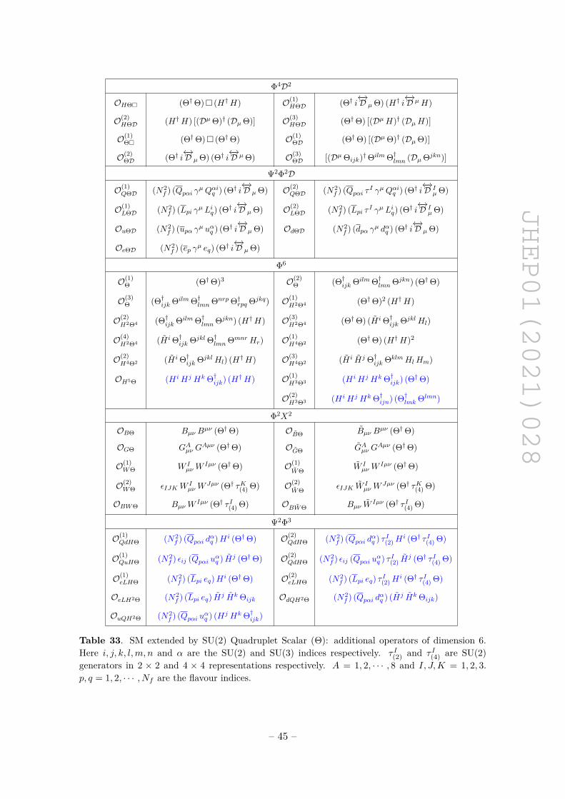
JHEP01(2021)028
Φ4D2
OHΘ� (Θ†Θ)� (H†H) O(1)HΘD (Θ† i←→D µ Θ) (H† i←→D µH)
O(2)HΘD (H†H) [(Dµ Θ)† (Dµ Θ)] O(3)
HΘD (Θ†Θ) [(DµH)† (DµH)]
O(1)Θ� (Θ†Θ)� (Θ†Θ) O(1)
ΘD (Θ†Θ) [(Dµ Θ)† (Dµ Θ)]
O(2)ΘD (Θ† i←→D µ Θ) (Θ† i←→D µ Θ) O(3)
ΘD [(Dµ Θijk)†Θilm Θ†lmn (Dµ Θjkn)]
Ψ2Φ2D
O(1)QΘD (N2
f ) (Qpαi γµQαiq ) (Θ† i←→D µ Θ) O(2)QΘD (N2
f ) (Qpαi τ I γµQαiq ) (Θ† i←→D Iµ Θ)
O(1)LΘD (N2
f ) (Lpi γµ Liq) (Θ† i←→D µ Θ) O(2)LΘD (N2
f ) (Lpi τ I γµ Liq) (Θ† i←→D Iµ Θ)
OuΘD (N2f ) (upα γµ uαq ) (Θ† i←→D µ Θ) OdΘD (N2
f ) (dpα γµ dαq ) (Θ† i←→D µ Θ)
OeΘD (N2f ) (ep γµ eq) (Θ† i←→D µ Θ)
Φ6
O(1)Θ (Θ†Θ)3 O(2)
Θ (Θ†ijk Θilm Θ†lmn Θjkn) (Θ†Θ)
O(3)Θ (Θ†ijk Θilm Θ†lmn Θnrp Θ†rpq Θjkq) O(1)
H2Θ4 (Θ†Θ)2 (H†H)
O(2)H2Θ4 (Θ†ijk Θilm Θ†lmn Θjkn) (H†H) O(3)
H2Θ4 (Θ†Θ) (H i Θ†ijk ΘjklHl)
O(4)H2Θ4 (H i Θ†ijk Θjkl Θ†lmn ΘmnrHr) O(1)
H4Θ2 (Θ†Θ) (H†H)2
O(2)H4Θ2 (H i Θ†ijk ΘjklHl) (H†H) O(3)
H4Θ2 (H i Hj Θ†ijk ΘklmHlHm)
OH5Θ (H iHj Hk Θ†ijk) (H†H) O(1)H3Θ3 (H iHj Hk Θ†ijk) (Θ†Θ)
O(2)H3Θ3 (H iHj Hk Θ†ijn) (Θ†lmk Θlmn)
Φ2X2
OBΘ Bµν Bµν (Θ†Θ) OBΘ Bµν B
µν (Θ†Θ)
OGΘ GAµν GAµν (Θ†Θ) OGΘ GAµν G
Aµν (Θ†Θ)
O(1)WΘ W I
µνWIµν (Θ†Θ) O(1)
WΘ W IµνW
Iµν (Θ†Θ)
O(2)WΘ εIJKW
IµνW
Jµν (Θ† τK(4) Θ) O(2)WΘ εIJK W
IµνW
Jµν (Θ† τK(4) Θ)
OBWΘ BµνWIµν (Θ† τ I(4) Θ) OBWΘ Bµν W
Iµν (Θ† τ I(4) Θ)
Ψ2Φ3
O(1)QdHΘ (N2
f ) (Qpαi dαq )H i (Θ†Θ) O(2)QdHΘ (N2
f ) (Qpαi dαq ) τ I(2)Hi (Θ† τ I(4) Θ)
O(1)QuHΘ (N2
f ) εij (Qpαi uαq ) Hj (Θ†Θ) O(2)QdHΘ (N2
f ) εij (Qpαi uαq ) τ I(2) Hj (Θ† τ I(4) Θ)
O(1)eLHΘ (N2
f ) (Lpi eq)H i (Θ†Θ) O(2)eLHΘ (N2
f ) (Lpi eq) τ I(2)Hi (Θ† τ I(4) Θ)
OeLH2Θ (N2f ) (Lpi eq) Hj Hk Θijk OdQH2Θ (N2
f ) (Qpαi dαq ) (Hj Hk Θijk)
OuQH2Θ (N2f ) (Qpαi uαq ) (Hj Hk Θ†ijk)
Table 33. SM extended by SU(2) Quadruplet Scalar (Θ): additional operators of dimension 6.Here i, j, k, l,m, n and α are the SU(2) and SU(3) indices respectively. τ I(2) and τ I(4) are SU(2)generators in 2 × 2 and 4 × 4 representations respectively. A = 1, 2, · · · , 8 and I, J,K = 1, 2, 3.p, q = 1, 2, · · · , Nf are the flavour indices.
– 45 –
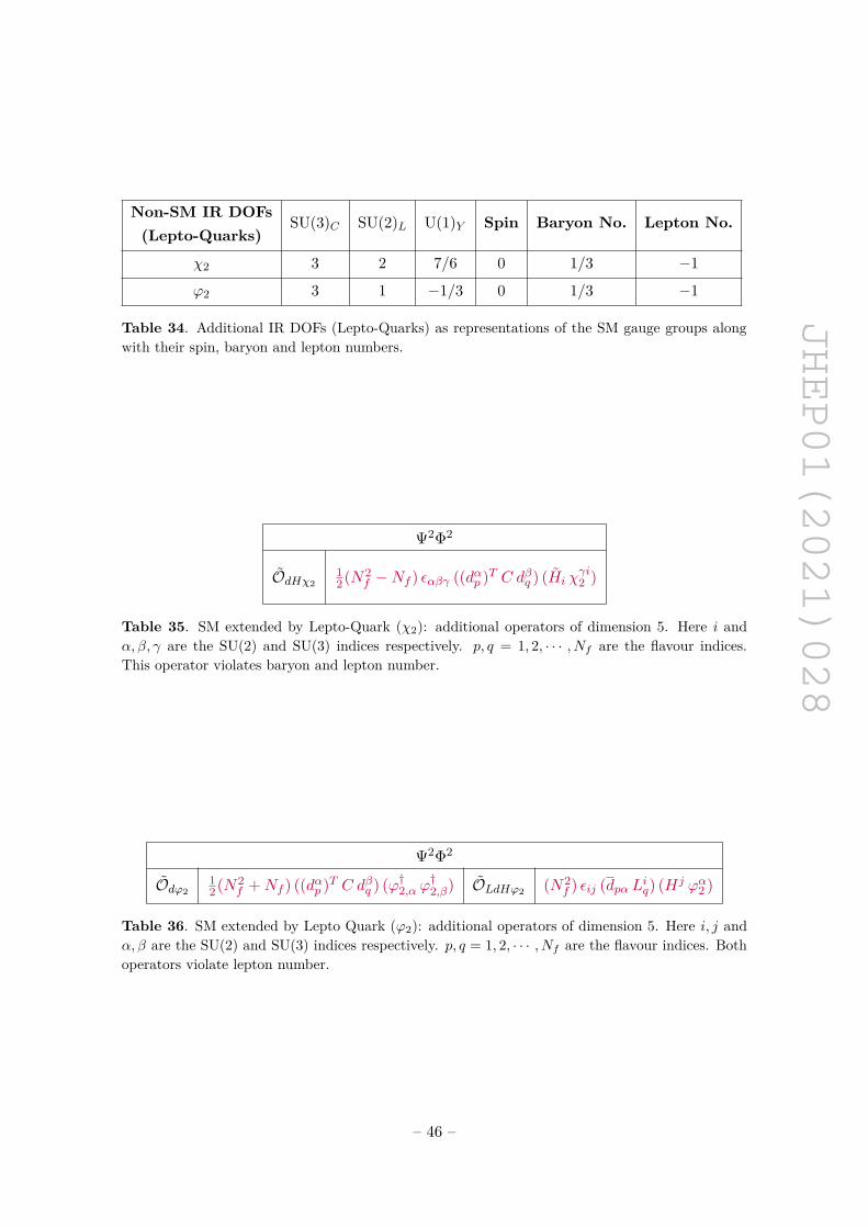
JHEP01(2021)028
Non-SM IR DOFs SU(3)C SU(2)L U(1)Y Spin Baryon No. Lepton No.(Lepto-Quarks)
χ2 3 2 7/6 0 1/3 −1
ϕ2 3 1 −1/3 0 1/3 −1
Table 34. Additional IR DOFs (Lepto-Quarks) as representations of the SM gauge groups alongwith their spin, baryon and lepton numbers.
Ψ2Φ2
OdHχ212(N2
f −Nf ) εαβγ ((dαp )T C dβq ) (Hi χγi2 )
Table 35. SM extended by Lepto-Quark (χ2): additional operators of dimension 5. Here i andα, β, γ are the SU(2) and SU(3) indices respectively. p, q = 1, 2, · · · , Nf are the flavour indices.This operator violates baryon and lepton number.
Ψ2Φ2
Odϕ212(N2
f +Nf ) ((dαp )T C dβq ) (ϕ†2,α ϕ†2,β) OLdHϕ2 (N2
f ) εij (dpα Liq) (Hj ϕα2 )
Table 36. SM extended by Lepto Quark (ϕ2): additional operators of dimension 5. Here i, j andα, β are the SU(2) and SU(3) indices respectively. p, q = 1, 2, · · · , Nf are the flavour indices. Bothoperators violate lepton number.
– 46 –
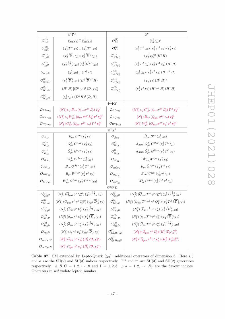
JHEP01(2021)028
Φ4D2 Φ6
O(1)χ2� (χ†2 χ2)� (χ†2 χ2) O(1)
χ2 (χ†2 χ2)3
O(2)χ2� (χ†2 TA χ2)� (χ†2 TA χ2) O(2)
χ2 (χ†2 TA χ2) (χ†2 TA χ2) (χ†2 χ2)
O(1)χ2D (χ†2
←→D µ χ2) (χ†2
←→D µ χ2) O(1)
H2χ42
(χ†2 χ2)2 (H†H)
O(2)χ2D (χ†2
←→D Aµ χ2) (χ†2
←→D µA χ2) O(2)
H2χ42
(χ†2 TA χ2) (χ†2 TA χ2) (H†H)
OHχ2� (χ†2 χ2)� (H†H) O(3)H2χ4
2(χ†2 χ2) (χ†2 τ I χ2) (H† τ I H)
O(2)Hχ2D (χ†2
←→D Iµ χ2) (H†←→D µI H) O(1)
H4χ22
(χ†2 χ2) (H†H)2
O(3)Hχ2D (H†H) [(Dµ χ2)† (Dµχ2)] O(2)
H4χ22
(χ†2 τ I χ2) (H† τ I H) (H†H)
O(4)Hχ2D (χ†2 χ2) [(DµH)† (DµH)]
Ψ2ΦX
OBLuχ2 (N2f ) εij Bµν (upα σµν Liq)χ
αj2 OGLuχ2 (N2
f ) εij GAµν (upα σµν Liq)TA χαj2
OWLuχ2 (N2f ) εijW I
µν (upα σµν Liq) τ I χαj2 OBQeχ2 (N2
f )Bµν (Qpαi σµν eq)χαi2
OGQeχ2 (N2f )GAµν (Qpαi σµν eq)TA χαi2 OWQeχ2 (N2
f )W Iµν (Qpαi σµν eq) τ I χαi2
Φ2X2
OBχ2 Bµν Bµν (χ†2 χ2) OBχ2
Bµν Bµν (χ†2 χ2)
O(2)Gχ2
GAµν GAµν (χ†2 χ2) O(2)
Gχ2dABC G
Aµν G
Bµν (χ†2 TC χ2)
O(1)Gχ2
GAµν GAµν (χ†2 χ2) O(2)
Gχ2dABC G
Aµν G
Bµν (χ†2 TC χ2)
OWχ2 W IµνW
Iµν (χ†2 χ2) OWχ2W IµνW
Iµν (χ†2 χ2)
OBGχ2 Bµν GAµν (χ†2 TA χ2) OBGχ2
Bµν GAµν (χ†2 TA χ2)
OBWχ2 BµνWIµν (χ†2 τ I χ2) OBWχ2
Bµν WIµν (χ†2 τ I χ2)
OWGχ2 W Iµν G
Aµν (χ†2 TA τ I χ2) OWGχ2W Iµν G
Aµν (χ†2 TA τ I χ2)
Ψ2Φ2D
O(1)Qχ2D (N2
f ) (Qpαi γµQαiq ) (χ†2 i←→D µ χ2) O(2)
Qχ2D (N2f ) (Qpαi TA γµQαiq ) (χ†2 i
←→D Aµ χ2)
O(3)Qχ2D (N2
f ) (Qpαi τ I γµQαiq ) (χ†2 i←→D Iµ χ2) O(4)
Qχ2D (N2f ) (Qpαi TA τ I γµQαiq ) (χ†2 TA i
←→D Iµ χ2)
O(1)Lχ2D (N2
f ) (Lpi γµ Liq) (χ†2 i←→D µ χ2) O(2)
Lχ2D (N2f ) (Lpi τ I γµ Liq) (χ†2 i
←→D Iµ χ2)
O(1)uχ2D (N2
f ) (upα γµ uαq ) (χ†2 i←→D µ χ2) O(2)
uχ2D (N2f ) (upα TA γµ uαq ) (χ†2 i
←→D Aµ χ2)
O(1)dχ2D (N2
f ) (dpα γµ dαq ) (χ†2 i←→D µ χ2) O(2)
dχ2D (N2f ) (dpα TA γµ dαq ) (χ†2 i
←→D Aµ χ2)
Oeχ2D (N2f ) (ep γµ eq) (χ†2 i
←→D µ χ2) O(1)
QLHχ2D (N2f ) (Qpαi γµ Liq) (H†j iDµχ
αj2 )
OdeHχ2D (N2f ) (dpα γµ eq) (H†i iDµχαi2 ) O(2)
QLHχ2D (N2f ) (Qpαi τ I γµ Liq) (H†j iDIµχ
αj2 )
OueHχ2D (N2f ) (upα γµ eq) (H†i iDµχαi2 )
Table 37. SM extended by Lepto-Quark (χ2): additional operators of dimension 6. Here i, jand α are the SU(2) and SU(3) indices respectively. TA and τ I are SU(3) and SU(2) generatorsrespectively. A,B,C = 1, 2, · · · , 8 and I = 1, 2, 3. p, q = 1, 2, · · · , Nf are the flavour indices.Operators in red violate lepton number.
– 47 –
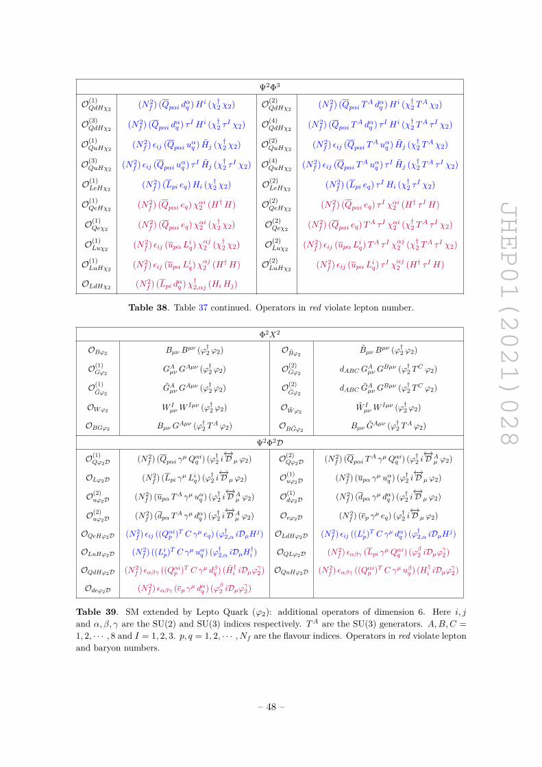
JHEP01(2021)028
Ψ2Φ3
O(1)QdHχ2
(N2f ) (Qpαi dαq )H i (χ†2 χ2) O(2)
QdHχ2(N2
f ) (Qpαi TA dαq )H i (χ†2 TA χ2)
O(3)QdHχ2
(N2f ) (Qpαi dαq ) τ I H i (χ†2 τ I χ2) O(4)
QdHχ2(N2
f ) (Qpαi TA dαq ) τ I H i (χ†2 TA τ I χ2)
O(1)QuHχ2
(N2f ) εij (Qpαi uαq ) Hj (χ†2 χ2) O(2)
QuHχ2(N2
f ) εij (Qpαi TA uαq ) Hj (χ†2 TA χ2)
O(3)QuHχ2
(N2f ) εij (Qpαi uαq ) τ I Hj (χ†2 τ I χ2) O(4)
QuHχ2(N2
f ) εij (Qpαi TA uαq ) τ I Hj (χ†2 TA τ I χ2)
O(1)LeHχ2
(N2f ) (Lpi eq)Hi (χ†2 χ2) O(2)
LeHχ2(N2
f ) (Lpi eq) τ I Hi (χ†2 τ I χ2)
O(1)QeHχ2
(N2f ) (Qpαi eq)χαi2 (H†H) O(2)
QeHχ2(N2
f ) (Qpαi eq) τ I χαi2 (H† τ I H)
O(1)Qeχ2
(N2f ) (Qpαi eq)χαi2 (χ†2 χ2) O(2)
Qeχ2(N2
f ) (Qpαi eq)TA τ I χαi2 (χ†2 TA τ I χ2)
O(1)Luχ2
(N2f ) εij (upα Liq)χ
αj2 (χ†2 χ2) O(2)
Luχ2(N2
f ) εij (upα Liq)TA τ I χαj2 (χ†2 TA τ I χ2)
O(1)LuHχ2
(N2f ) εij (upα Liq)χ
αj2 (H†H) O(2)
LuHχ2(N2
f ) εij (upα Liq) τ I χαj2 (H† τ I H)
OLdHχ2 (N2f ) (Lpi dαq )χ†2,αj (HiHj)
Table 38. Table 37 continued. Operators in red violate lepton number.
Φ2X2
OBϕ2 Bµν Bµν (ϕ†2 ϕ2) OBϕ2
Bµν Bµν (ϕ†2 ϕ2)
O(1)Gϕ2
GAµν GAµν (ϕ†2 ϕ2) O(2)
Gϕ2dABC G
Aµν G
Bµν (ϕ†2 TC ϕ2)
O(1)Gϕ2
GAµν GAµν (ϕ†2 ϕ2) O(2)
Gϕ2dABC G
Aµν G
Bµν (ϕ†2 TC ϕ2)
OWϕ2 W IµνW
Iµν (ϕ†2 ϕ2) OWϕ2W IµνW
Iµν (ϕ†2 ϕ2)
OBGϕ2 Bµν GAµν (ϕ†2 TA ϕ2) OBGϕ2
Bµν GAµν (ϕ†2 TA ϕ2)
Ψ2Φ2D
O(1)Qϕ2D (N2
f ) (Qpαi γµQαiq ) (ϕ†2 i←→D µ ϕ2) O(2)
Qϕ2D (N2f ) (Qpαi TA γµQαiq ) (ϕ†2 i
←→D Aµ ϕ2)
OLϕ2D (N2f ) (Lpi γµ Liq) (ϕ†2 i
←→D µ ϕ2) O(1)
uϕ2D (N2f ) (upα γµ uαq ) (ϕ†2 i
←→D µ ϕ2)
O(2)uϕ2D (N2
f ) (upα TA γµ uαq ) (ϕ†2 i←→D Aµ ϕ2) O(1)
dϕ2D (N2f ) (dpα γµ dαq ) (ϕ†2 i
←→D µ ϕ2)
O(2)uϕ2D (N2
f ) (dpα TA γµ dαq ) (ϕ†2 i←→D Aµ ϕ2) Oeϕ2D (N2
f ) (ep γµ eq) (ϕ†2 i←→D µ ϕ2)
OQeHϕ2D (N2f ) εij ((Qαip )T C γµ eq) (ϕ†2,α iDµHj) OLdHϕ2D (N2
f ) εij ((Lip)T C γµ dαq ) (ϕ†2,α iDµHj)
OLuHϕ2D (N2f ) ((Lip)T C γµ uαq ) (ϕ†2,α iDµH
†i ) OQLϕ2D (N2
f ) εαβγ (Lpi γµQαiq ) (ϕβ2 iDµϕγ2)
OQdHϕ2D (N2f ) εαβγ ((Qαip )T C γµ dβq ) (H†i iDµϕ
γ2) OQuHϕ2D (N2
f ) εαβγ ((Qαip )T C γµ uβq ) (H†i iDµϕγ2)
Odeϕ2D (N2f ) εαβγ (ep γµ dαq ) (ϕβ2 iDµϕ
γ2)
Table 39. SM extended by Lepto Quark (ϕ2): additional operators of dimension 6. Here i, jand α, β, γ are the SU(2) and SU(3) indices respectively. TA are the SU(3) generators. A,B,C =1, 2, · · · , 8 and I = 1, 2, 3. p, q = 1, 2, · · · , Nf are the flavour indices. Operators in red violate leptonand baryon numbers.
– 48 –
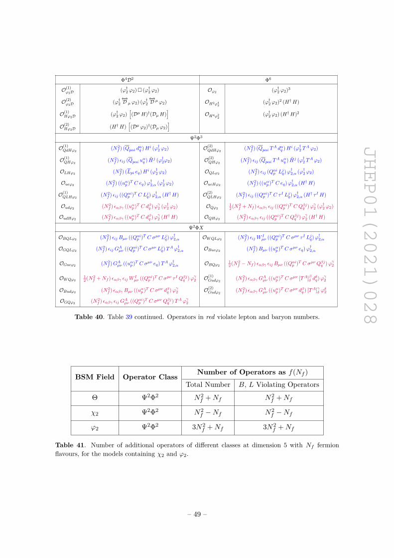
JHEP01(2021)028
Φ4D2 Φ6
O(1)ϕ2D (ϕ†2 ϕ2)� (ϕ†2 ϕ2) Oϕ2 (ϕ†2 ϕ2)3
O(2)ϕ2D (ϕ†2
←→D µ ϕ2) (ϕ†2
←→D µ ϕ2) OH2ϕ4
2(ϕ†2 ϕ2)2 (H†H)
O(1)Hϕ2D (ϕ†2 ϕ2)
[(DµH)†(DµH)
]OH4ϕ2
2(ϕ†2 ϕ2) (H†H)2
O(2)Hϕ2D (H†H)
[(Dµ ϕ2)†(Dµ ϕ2)
]Ψ2Φ3
O(1)QdHϕ2
(N2f ) (Qpαi dαq )H i (ϕ†2 ϕ2) O(2)
QdHϕ2(N2
f ) (Qpαi TA dαq )H i (ϕ†2 TA ϕ2)
O(1)QHϕ2
(N2f ) εij (Qpαi uαq ) Hj (ϕ†2ϕ2) O(2)
QHϕ2(N2
f ) εij (Qpαi TA uαq ) Hj (ϕ†2 TA ϕ2)
OLHϕ2 (N2f ) (Lpi eq)H i (ϕ†2 ϕ2) OQLϕ2 (N2
f ) εij (Qαip Ljq)ϕ†2,α (ϕ†2 ϕ2)
Oueϕ2 (N2f ) ((uαp )T C eq)ϕ†2,α (ϕ†2 ϕ2) OueHϕ2 (N2
f ) ((uαp )T C eq)ϕ†2,α (H†H)
O(1)QLHϕ2
(N2f ) εij ((Qαip )T C Ljq)ϕ
†2,α (H†H) O(2)
QLHϕ2(N2
f ) εij ((Qαip )T C τ I Ljq)ϕ†2,α (H† τ I H)
Oudϕ2 (N2f ) εαβγ ((uαp )T C dβq )ϕγ2 (ϕ†2 ϕ2) OQϕ2
12(N2
f +Nf ) εαβγ εij ((Qαip )T C Qβjq )ϕγ2 (ϕ†2 ϕ2)
OudHϕ2 (N2f ) εαβγ ((uαp )T C dβq )ϕγ2 (H†H) OQHϕ2 (N2
f ) εαβγ εij ((Qαip )T C Qβjq )ϕγ2 (H†H)
Ψ2ΦX
OBQLϕ2 (N2f ) εij Bµν ((Qαip )T C σµν Ljq)ϕ
†2,α OWQLϕ2 (N2
f ) εijW Iµν ((Qαip )T C σµν τ I Ljq)ϕ
†2,α
OGQLϕ2 (N2f ) εij GAµν ((Qαip )T C σµν Ljq)TA ϕ
†2,α OBueϕ2 (N2
f )Bµν ((uαp )T C σµν eq)ϕ†2,α
OGueϕ2 (N2f )GAµν ((uαp )T C σµν eq)TA ϕ†2,α OBQϕ2
12(N2
f −Nf ) εαβγ εij Bµν ((Qαip )T C σµν Qβjq )ϕγ2
OWQϕ212(N2
f +Nf ) εαβγ εijW Iµν ((Qαip )T C σµν τ I Qβjq )ϕγ2 O(1)
Gudϕ2(N2
f ) εαβγ GAµν ((uαp )T C σµν [TA]βδ dδq)ϕγ2
OBudϕ2 (N2f ) εαβγ Bµν ((uαp )T C σµν dβq )ϕγ2 O(2)
Gudϕ2(N2
f ) εαβγ GAµν ((uαp )T C σµν dβq ) [TA]γδ ϕδ2
OGQϕ2 (N2f ) εαβγ εij GAµν ((Qαip )T C σµν Qβjq )TA ϕγ2
Table 40. Table 39 continued. Operators in red violate lepton and baryon numbers.
BSM Field Operator Class Number of Operators as f(Nf )
Total Number B, L Violating Operators
Θ Ψ2Φ2 N2f +Nf N2
f +Nf
χ2 Ψ2Φ2 N2f −Nf N2
f −Nf
ϕ2 Ψ2Φ2 3N2f +Nf 3N2
f +Nf
Table 41. Number of additional operators of different classes at dimension 5 with Nf fermionflavours, for the models containing χ2 and ϕ2.
– 49 –
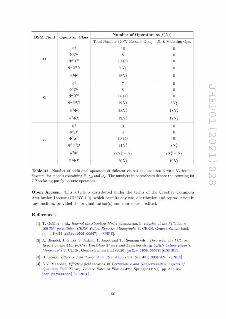
JHEP01(2021)028
BSM Field Operator Class Number of Operators as f(Nf )
Total Number (CPV Bosonic Ops.) B, L Violating Ops.
Θ
Φ6 16 0Φ4D2 8 0Φ2X2 10 (5) 0
Ψ2Φ2D 7N2f 0
Ψ2Φ3 18N2f 0
χ2
Φ6 7 0Φ4D2 8 0Φ2X2 14 (7) 0
Ψ2Φ2D 19N2f 8N2
f
Ψ2Φ3 38N2f 18N2
f
Ψ2ΦX 12N2f 12N2
f
ϕ2
Φ6 3 0Φ4D2 4 0Φ2X2 10 (5) 0
Ψ2Φ2D 14N2f 8N2
f
Ψ2Φ3 27N2f +Nf 7N2
f +Nf
Ψ2ΦX 20N2f 10N2
f
Table 42. Number of additional operators of different classes at dimension 6 with Nf fermionflavours, for models containing Θ, χ2 and ϕ2. The numbers in parentheses denote the counting forCP violating purely bosonic operators.
Open Access. This article is distributed under the terms of the Creative CommonsAttribution License (CC-BY 4.0), which permits any use, distribution and reproduction inany medium, provided the original author(s) and source are credited.
References
[1] T. Golling et al., Beyond the Standard Model phenomena, in Physics at the FCC-hh, a100TeV pp collider , CERN Yellow Reports: Monographs 3, CERN, Geneva Switzerland,pp. 441–634 [arXiv:1606.00947] [INSPIRE].
[2] A. Blondel, J. Gluza, S. Jadach, P. Janot and T. Riemann eds., Theory for the FCC-ee:Report on the 11th FCC-ee Workshop Theory and Experiments, in CERN Yellow Reports:Monographs 3, CERN, Geneva Switzerland (2020) [arXiv:1905.05078] [INSPIRE].
[3] H. Georgi, Effective field theory, Ann. Rev. Nucl. Part. Sci. 43 (1993) 209 [INSPIRE].
[4] A.V. Manohar, Effective field theories, in Perturbative and Nonperturbative Aspects ofQuantum Field Theory, Lecture Notes in Physics 479, Springer (1997), pp. 311–362[hep-ph/9606222] [INSPIRE].
– 50 –
JHEP01(2021)028
[5] D.B. Kaplan, Effective field theories, in proceedings of the 5th International Conference onPhysics Beyond the Standard Model, Balholm, Norway, 29 April–4 May 1997,nucl-th/9506035 [INSPIRE].
[6] D.B. Kaplan, Five lectures on effective field theory, nucl-th/0510023 [INSPIRE].
[7] C.P. Burgess, Introduction to Effective Field Theory, Ann. Rev. Nucl. Part. Sci. 57 (2007)329 [hep-th/0701053] [INSPIRE].
[8] I.Z. Rothstein, TASI lectures on effective field theories, hep-ph/0308266 [INSPIRE].
[9] T. Cohen, As Scales Become Separated: Lectures on Effective Field Theory, PoSTASI2018 (2019) 011 [arXiv:1903.03622] [INSPIRE].
[10] B. Henning, X. Lu and H. Murayama, How to use the Standard Model effective field theory,JHEP 01 (2016) 023 [arXiv:1412.1837] [INSPIRE].
[11] F. Jegerlehner, The Standard model as a low-energy effective theory: what is triggering theHiggs mechanism?, Acta Phys. Polon. B 45 (2014) 1167 [arXiv:1304.7813] [INSPIRE].
[12] R. Contino, A. Falkowski, F. Goertz, C. Grojean and F. Riva, On the Validity of theEffective Field Theory Approach to SM Precision Tests, JHEP 07 (2016) 144[arXiv:1604.06444] [INSPIRE].
[13] J. Ellis, V. Sanz and T. You, The Effective Standard Model after LHC Run I, JHEP 03(2015) 157 [arXiv:1410.7703] [INSPIRE].
[14] L. Berthier and M. Trott, Consistent constraints on the Standard Model Effective FieldTheory, JHEP 02 (2016) 069 [arXiv:1508.05060] [INSPIRE].
[15] I. Brivio and M. Trott, The Standard Model as an Effective Field Theory, Phys. Rept. 793(2019) 1 [arXiv:1706.08945] [INSPIRE].
[16] T. Hambye and J. Heeck, Proton decay into charged leptons, Phys. Rev. Lett. 120 (2018)171801 [arXiv:1712.04871] [INSPIRE].
[17] R.M. Fonseca, M. Hirsch and R. Srivastava, ∆L = 3 processes: Proton decay and the LHC,Phys. Rev. D 97 (2018) 075026 [arXiv:1802.04814] [INSPIRE].
[18] B. Henning, X. Lu and H. Murayama, One-loop Matching and Running with CovariantDerivative Expansion, JHEP 01 (2018) 123 [arXiv:1604.01019] [INSPIRE].
[19] J.C. Criado Álamo, Effective field theories for general extensions of the Standard Modelwith new particles, Ph.D. Thesis, University of Granada, Granada Spain (2019).
[20] R. Huo, Standard Model Effective Field Theory: Integrating out Vector-Like Fermions,JHEP 09 (2015) 037 [arXiv:1506.00840] [INSPIRE].
[21] C.-W. Chiang and R. Huo, Standard Model Effective Field Theory: Integrating out aGeneric Scalar, JHEP 09 (2015) 152 [arXiv:1505.06334] [INSPIRE].
[22] S.A.R. Ellis, J. Quevillon, T. You and Z. Zhang, Mixed heavy-light matching in theUniversal One-Loop Effective Action, Phys. Lett. B 762 (2016) 166 [arXiv:1604.02445][INSPIRE].
[23] J. Fuentes-Martin, J. Portoles and P. Ruiz-Femenia, Integrating out heavy particles withfunctional methods: a simplified framework, JHEP 09 (2016) 156 [arXiv:1607.02142][INSPIRE].
– 51 –
JHEP01(2021)028
[24] S. Das Bakshi, J. Chakrabortty and S.K. Patra, CoDEx: Wilson coefficient calculatorconnecting SMEFT to UV theory, Eur. Phys. J. C 79 (2019) 21 [arXiv:1808.04403][INSPIRE].
[25] J. Aebischer, J. Kumar and D.M. Straub, Wilson: a Python package for the running andmatching of Wilson coefficients above and below the electroweak scale, Eur. Phys. J. C 78(2018) 1026 [arXiv:1804.05033] [INSPIRE].
[26] A. Celis, J. Fuentes-Martin, A. Vicente and J. Virto, DsixTools: The Standard ModelEffective Field Theory Toolkit, Eur. Phys. J. C 77 (2017) 405 [arXiv:1704.04504][INSPIRE].
[27] J. Aebischer et al., WCxf: an exchange format for Wilson coefficients beyond the StandardModel, Comput. Phys. Commun. 232 (2018) 71 [arXiv:1712.05298] [INSPIRE].
[28] J.C. Criado, MatchingTools: a Python library for symbolic effective field theory calculations,Comput. Phys. Commun. 227 (2018) 42 [arXiv:1710.06445] [INSPIRE].
[29] B. Henning, X. Lu, T. Melia and H. Murayama, 2, 84, 30, 993, 560, 15456, 11962, 261485,. . . : Higher dimension operators in the SM EFT, JHEP 08 (2017) 016 [Erratum JHEP 09(2019) 019] [arXiv:1512.03433] [INSPIRE].
[30] B. Henning, X. Lu, T. Melia and H. Murayama, Operator bases, S-matrices, and theirpartition functions, JHEP 10 (2017) 199 [arXiv:1706.08520] [INSPIRE].
[31] L. Lehman and A. Martin, Hilbert Series for Constructing Lagrangians: expanding thephenomenologist’s toolbox, Phys. Rev. D 91 (2015) 105014 [arXiv:1503.07537] [INSPIRE].
[32] L. Lehman and A. Martin, Low-derivative operators of the Standard Model effective fieldtheory via Hilbert series methods, JHEP 02 (2016) 081 [arXiv:1510.00372] [INSPIRE].
[33] R.M. Fonseca, Enumerating the operators of an effective field theory, Phys. Rev. D 101(2020) 035040 [arXiv:1907.12584] [INSPIRE].
[34] B. Grzadkowski, M. Iskrzynski, M. Misiak and J. Rosiek, Dimension-Six Terms in theStandard Model Lagrangian, JHEP 10 (2010) 085 [arXiv:1008.4884] [INSPIRE].
[35] L. Lehman, Extending the Standard Model Effective Field Theory with the Complete Set ofDimension-7 Operators, Phys. Rev. D 90 (2014) 125023 [arXiv:1410.4193] [INSPIRE].
[36] C.W. Murphy, Dimension-8 operators in the Standard Model Eective Field Theory, JHEP10 (2020) 174 [arXiv:2005.00059] [INSPIRE].
[37] H.-L. Li, Z. Ren, J. Shu, M.-L. Xiao, J.-H. Yu and Y.-H. Zheng, Complete Set ofDimension-8 Operators in the Standard Model Effective Field Theory, arXiv:2005.00008[INSPIRE].
[38] H.-L. Li, Z. Ren, M.-L. Xiao, J.-H. Yu and Y.-H. Zheng, Complete Set of Dimension-9Operators in the Standard Model Effective Field Theory, arXiv:2007.07899 [INSPIRE].
[39] Y. Liao and X.-D. Ma, An explicit construction of the dimension-9 operator basis in thestandard model effective field theory, JHEP 11 (2020) 152 [arXiv:2007.08125] [INSPIRE].
[40] U. Banerjee, J. Chakrabortty, S. Prakash and S.U. Rahaman, Characters and groupinvariant polynomials of (super)fields: road to “Lagrangian”, Eur. Phys. J. C 80 (2020) 938[arXiv:2004.12830] [INSPIRE].
[41] J.C. Criado, BasisGen: automatic generation of operator bases, Eur. Phys. J. C 79 (2019)256 [arXiv:1901.03501] [INSPIRE].
– 52 –
JHEP01(2021)028
[42] R.M. Fonseca, The Sym2Int program: going from symmetries to interactions, J. Phys.Conf. Ser. 873 (2017) 012045 [arXiv:1703.05221] [INSPIRE].
[43] C.B. Marinissen, R. Rahn and W.J. Waalewijn, . . . , 83106786, 114382724, 1509048322,2343463290, 27410087742, . . . efficient Hilbert series for effective theories, Phys. Lett. B808 (2020) 135632 [arXiv:2004.09521] [INSPIRE].
[44] B. Gripaios and D. Sutherland, DEFT: A program for operators in EFT, JHEP 01 (2019)128 [arXiv:1807.07546] [INSPIRE].
[45] S. Banerjee, S. Mukhopadhyay and B. Mukhopadhyaya, Higher dimensional operators andthe LHC Higgs data: The role of modified kinematics, Phys. Rev. D 89 (2014) 053010[arXiv:1308.4860] [INSPIRE].
[46] C. Hays, A. Martin, V. Sanz and J. Setford, On the impact of dimension-eight SMEFToperators on Higgs measurements, JHEP 02 (2019) 123 [arXiv:1808.00442] [INSPIRE].
[47] A. Dedes, M. Paraskevas, J. Rosiek, K. Suxho and L. Trifyllis, The decay h→ γγ in theStandard-Model Effective Field Theory, JHEP 08 (2018) 103 [arXiv:1805.00302][INSPIRE].
[48] S.F. King, A. Merle and L. Panizzi, Effective theory of a doubly charged singlet scalar:complementarity of neutrino physics and the LHC, JHEP 11 (2014) 124[arXiv:1406.4137] [INSPIRE].
[49] Anisha, S. Das Bakshi, J. Chakrabortty and S. Prakash, Hilbert Series and Plethystics:Paving the path towards 2HDM- and MLRSM-EFT, JHEP 09 (2019) 035[arXiv:1905.11047] [INSPIRE].
[50] A. Trautner, Systematic construction of basis invariants in the 2HDM, JHEP 05 (2019) 208[arXiv:1812.02614] [INSPIRE].
[51] A. Crivellin, M. Ghezzi and M. Procura, Effective Field Theory with Two Higgs Doublets,JHEP 09 (2016) 160 [arXiv:1608.00975] [INSPIRE].
[52] S. Karmakar and S. Rakshit, Higher dimensional operators in 2HDM, JHEP 10 (2017) 048[arXiv:1707.00716] [INSPIRE].
[53] C. Birch-Sykes, N. Darvishi, Y. Peters and A. Pilaftsis, Accidental symmetries in the2HDMEFT, Nucl. Phys. B 960 (2020) 115171 [arXiv:2007.15599] [INSPIRE].
[54] G. Elgaard-Clausen and M. Trott, On expansions in neutrino effective field theory, JHEP11 (2017) 088 [arXiv:1703.04415] [INSPIRE].
[55] M. Chala and A. Titov, One-loop matching in the SMEFT extended with a sterile neutrino,JHEP 05 (2020) 139 [arXiv:2001.07732] [INSPIRE].
[56] S. Bhattacharya and J. Wudka, Dimension-seven operators in the standard model with righthanded neutrinos, Phys. Rev. D 94 (2016) 055022 [Erratum ibid. 95 (2017) 039904][arXiv:1505.05264] [INSPIRE].
[57] Y. Liao and X.-D. Ma, Operators up to Dimension Seven in Standard Model Effective FieldTheory Extended with Sterile Neutrinos, Phys. Rev. D 96 (2017) 015012[arXiv:1612.04527] [INSPIRE].
[58] E.E. Jenkins, A.V. Manohar and P. Stoffer, Low-Energy Effective Field Theory below theElectroweak Scale: Operators and Matching, JHEP 03 (2018) 016 [arXiv:1709.04486][INSPIRE].
– 53 –
JHEP01(2021)028
[59] E.E. Jenkins, A.V. Manohar and P. Stoffer, Low-Energy Effective Field Theory below theElectroweak Scale: Anomalous Dimensions, JHEP 01 (2018) 084 [arXiv:1711.05270][INSPIRE].
[60] W. Dekens and P. Stoffer, Low-energy effective field theory below the electroweak scale:matching at one loop, JHEP 10 (2019) 197 [arXiv:1908.05295] [INSPIRE].
[61] Y. Liao, X.-D. Ma and Q.-Y. Wang, Extending low energy effective field theory with acomplete set of dimension-7 operators, JHEP 08 (2020) 162 [arXiv:2005.08013] [INSPIRE].
[62] J. Aebischer, M. Fael, C. Greub and J. Virto, B physics Beyond the Standard Model at OneLoop: Complete Renormalization Group Evolution below the Electroweak Scale, JHEP 09(2017) 158 [arXiv:1704.06639] [INSPIRE].
[63] J. Brod, A. Gootjes-Dreesbach, M. Tammaro and J. Zupan, Effective Field Theory for DarkMatter Direct Detection up to Dimension Seven, JHEP 10 (2018) 065 [arXiv:1710.10218][INSPIRE].
[64] S. Adhikari, I.M. Lewis and M. Sullivan, Beyond the Standard Model Effective FieldTheory: The Singlet Extended Standard Model, arXiv:2003.10449 [INSPIRE].
[65] D. O’Connell, M.J. Ramsey-Musolf and M.B. Wise, Minimal Extension of the StandardModel Scalar Sector, Phys. Rev. D 75 (2007) 037701 [hep-ph/0611014] [INSPIRE].
[66] V. Barger, P. Langacker, M. McCaskey, M.J. Ramsey-Musolf and G. Shaughnessy, CERNLHC phenomenology of an extended standard model with a real scalar singlet, Phys. Rev. D77 (2008) 035005.
[67] W. Buchmüller, R. Ruckl and D. Wyler, Leptoquarks in Lepton-Quark Collisions, Phys.Lett. B 191 (1987) 442 [Erratum ibid. 448 (1999) 320] [INSPIRE].
[68] R. Franceschini et al., What is the γγ resonance at 750GeV?, JHEP 03 (2016) 144[arXiv:1512.04933] [INSPIRE].
[69] M. Backovic, A. Mariotti and D. Redigolo, Di-photon excess illuminates Dark Matter,JHEP 03 (2016) 157 [arXiv:1512.04917] [INSPIRE].
[70] A. Strumia, Interpreting the 750GeV digamma excess: a review, in proceedings of the 51stRencontres de Moriond on EW Interactions and Unified Theories, La Thuile, Italy, 12–19March 2016, pp. 407–426 [arXiv:1605.09401] [INSPIRE].
[71] H.K. Dreiner, H.E. Haber and S.P. Martin, Two-component spinor techniques and Feynmanrules for quantum field theory and supersymmetry, Phys. Rept. 494 (2010) 1[arXiv:0812.1594] [INSPIRE].
[72] T. Hambye, CLFV and the origin of neutrino masses, Nucl. Phys. B Proc. Suppl. 248–250(2014) 13 [arXiv:1312.5214] [INSPIRE].
[73] T.P. Cheng and L.-F. Li, Neutrino Masses, Mixings and Oscillations in SU(2)×U(1)Models of Electroweak Interactions, Phys. Rev. D 22 (1980) 2860 [INSPIRE].
[74] K.S. Babu, Model of ‘Calculable’ Majorana Neutrino Masses, Phys. Lett. B 203 (1988) 132[INSPIRE].
[75] K.S. Babu and C. Macesanu, Two loop neutrino mass generation and its experimentalconsequences, Phys. Rev. D 67 (2003) 073010 [hep-ph/0212058] [INSPIRE].
[76] D. Aristizabal Sierra and M. Hirsch, Experimental tests for the Babu-Zee two-loop model ofMajorana neutrino masses, JHEP 12 (2006) 052 [hep-ph/0609307] [INSPIRE].
– 54 –
JHEP01(2021)028
[77] T.G. Rizzo, Doubly Charged Higgs Bosons and Lepton Number Violating Processes, Phys.Rev. D 25 (1982) 1355 [Addendum ibid. 27 (1983) 657] [INSPIRE].
[78] A.G. Akeroyd and M. Aoki, Single and pair production of doubly charged Higgs bosons athadron colliders, Phys. Rev. D 72 (2005) 035011 [hep-ph/0506176] [INSPIRE].
[79] J. Maalampi and N. Romanenko, Single production of doubly charged Higgs bosons athadron colliders, Phys. Lett. B 532 (2002) 202 [hep-ph/0201196] [INSPIRE].
[80] J. Chakrabortty, P. Ghosh, S. Mondal and T. Srivastava, Reconciling (g − 2)µ and chargedlepton flavor violating processes through a doubly charged scalar, Phys. Rev. D 93 (2016)115004 [arXiv:1512.03581] [INSPIRE].
[81] F. del Aguila, M. Chala, A. Santamaria and J. Wudka, Discriminating between leptonnumber violating scalars using events with four and three charged leptons at the LHC, Phys.Lett. B 725 (2013) 310 [arXiv:1305.3904] [INSPIRE].
[82] F. del Aguila, M. Chala, A. Santamaria and J. Wudka, Distinguishing between leptonnumber violating scalars at the LHC, EPJ Web Conf. 60 (2013) 17002 [arXiv:1307.0510][INSPIRE].
[83] R.M. Fonseca and M. Hirsch, ∆L ≥ 4 lepton number violating processes, Phys. Rev. D 98(2018) 015035 [arXiv:1804.10545] [INSPIRE].
[84] W. Konetschny and W. Kummer, Nonconservation of Total Lepton Number with ScalarBosons, Phys. Lett. B 70 (1977) 433 [INSPIRE].
[85] J. Schechter and J.W.F. Valle, Neutrino Masses in SU(2)×U(1) Theories, Phys. Rev. D 22(1980) 2227 [INSPIRE].
[86] P.-H. Gu, H. Zhang and S. Zhou, A Minimal Type II Seesaw Model, Phys. Rev. D 74 (2006)076002 [hep-ph/0606302] [INSPIRE].
[87] Y. Cai, T. Han, T. Li and R. Ruiz, Lepton Number Violation: Seesaw Models and TheirCollider Tests, Front. Phys. 6 (2018) 40 [arXiv:1711.02180] [INSPIRE].
[88] H. Georgi and M. Machacek, Doubly Charged Higgs Bosons, Nucl. Phys. B 262 (1985) 463[INSPIRE].
[89] C.-W. Chiang and K. Tsumura, Properties and searches of the exotic neutral Higgs bosonsin the Georgi-Machacek model, JHEP 04 (2015) 113 [arXiv:1501.04257] [INSPIRE].
[90] H.E. Logan and V. Rentala, All the generalized Georgi-Machacek models, Phys. Rev. D 92(2015) 075011 [arXiv:1502.01275] [INSPIRE].
[91] C.-W. Chiang, G. Cottin and O. Eberhardt, Global fits in the Georgi-Machacek model,Phys. Rev. D 99 (2019) 015001 [arXiv:1807.10660] [INSPIRE].
[92] C.-W. Chiang, A.-L. Kuo and T. Yamada, Searches of exotic Higgs bosons in general massspectra of the Georgi-Machacek model at the LHC, JHEP 01 (2016) 120[arXiv:1511.00865] [INSPIRE].
[93] C.-W. Chiang and K. Yagyu, Testing the custodial symmetry in the Higgs sector of theGeorgi-Machacek model, JHEP 01 (2013) 026 [arXiv:1211.2658] [INSPIRE].
[94] R. Foot, H. Lew, X.G. He and G.C. Joshi, Seesaw Neutrino Masses Induced by a Triplet ofLeptons, Z. Phys. C 44 (1989) 441 [INSPIRE].
– 55 –
JHEP01(2021)028
[95] J. Chakrabortty, A. Dighe, S. Goswami and S. Ray, Renormalization group evolution ofneutrino masses and mixing in the Type-III seesaw mechanism, Nucl. Phys. B 820 (2009)116 [arXiv:0812.2776] [INSPIRE].
[96] R. Franceschini, T. Hambye and A. Strumia, Type-III seesaw mechanism at CERN LHC,Phys. Rev. D 78 (2008) 033002.
[97] M.-C. Chen and J. Huang, TeV Scale Models of Neutrino Masses and TheirPhenomenology, Mod. Phys. Lett. A 26 (2011) 1147 [arXiv:1105.3188] [INSPIRE].
[98] J. Chakrabortty, TeV Scale Double Seesaw in Left-Right Symmetric Theories,arXiv:1003.3154 [INSPIRE].
[99] J. Chakrabortty, S. Goswami and A. Raychaudhuri, An SO(10) model with adjoint fermionsfor double seesaw neutrino masses, Phys. Lett. B 698 (2011) 265 [arXiv:1012.2715][INSPIRE].
[100] P.-H. Gu, A left-right symmetric model with SU(2)-triplet fermions, Phys. Rev. D 84 (2011)097301 [arXiv:1110.6049] [INSPIRE].
[101] A. Abada, C. Biggio, F. Bonnet, M.B. Gavela and T. Hambye, µ→ eγ and τ → lγ decaysin the fermion triplet seesaw model, Phys. Rev. D 78 (2008) 033007 [arXiv:0803.0481][INSPIRE].
[102] T.P. Cheng and L.-F. Li, µ→ eγ in Theories With Dirac and Majorana Neutrino MassTerms, Phys. Rev. Lett. 45 (1980) 1908 [INSPIRE].
[103] W.J. Marciano and A.I. Sanda, Exotic Decays of the Muon and Heavy Leptons in GaugeTheories, Phys. Lett. B 67 (1977) 303 [INSPIRE].
[104] O.J.P. Eboli, J. Gonzalez-Fraile and M.C. Gonzalez-Garcia, Neutrino Masses at LHC:Minimal Lepton Flavour Violation in Type-III See-saw, JHEP 12 (2011) 009[arXiv:1108.0661] [INSPIRE].
[105] CMS collaboration, Search for Evidence of the Type-III Seesaw Mechanism in MultileptonFinal States in Proton-Proton Collisions at
√s = 13TeV, Phys. Rev. Lett. 119 (2017)
221802 [arXiv:1708.07962] [INSPIRE].
[106] ATLAS collaboration, Search for type-III seesaw heavy leptons in proton-proton collisionsat√s = 13TeV with the ATLAS detector, ATLAS-CONF-2018-020 (2018) [INSPIRE].
[107] S. Goswami, K.N. Vishnudath and N. Khan, Constraining the minimal type-III seesawmodel with naturalness, lepton flavor violation, and electroweak vacuum stability, Phys. Rev.D 99 (2019) 075012 [arXiv:1810.11687] [INSPIRE].
[108] A. Chaudhuri, N. Khan, B. Mukhopadhyaya and S. Rakshit, Dark matter candidate in anextended type-III seesaw scenario, Phys. Rev. D 91 (2015) 055024 [arXiv:1501.05885][INSPIRE].
[109] S. Choubey, S. Khan, M. Mitra and S. Mondal, Singlet-Triplet Fermionic Dark Matter andLHC Phenomenology, Eur. Phys. J. C 78 (2018) 302 [arXiv:1711.08888] [INSPIRE].
[110] D. Restrepo and A. Rivera, Phenomenological consistency of the singlet-triplet scotogenicmodel, JHEP 04 (2020) 134 [arXiv:1907.11938] [INSPIRE].
[111] P. Fileviez Perez, Type III Seesaw and Left-Right Symmetry, JHEP 03 (2009) 142[arXiv:0809.1202] [INSPIRE].
– 56 –
JHEP01(2021)028
[112] B. Bajc, M. Nemevšek and G. Senjanović, Probing seesaw at LHC, Phys. Rev. D 76 (2007)055011 [hep-ph/0703080] [INSPIRE].
[113] E.T. Franco, Type I+ III seesaw mechanism and CP-violation for leptogenesis, Phys. Rev.D 92 (2015) 113010 [arXiv:1510.06240] [INSPIRE].
[114] G.C. Branco, R. Felipe and F.R. Joaquim, Leptonic CP-violation, Rev. Mod. Phys. 84(2012) 515 [arXiv:1111.5332] [INSPIRE].
[115] T. Hambye, Leptogenesis: beyond the minimal type-I seesaw scenario, New J. Phys. 14(2012) 125014 [arXiv:1212.2888] [INSPIRE].
[116] A. Angelescu and P. Huang, Integrating Out New Fermions at One Loop,arXiv:2006.16532 [INSPIRE].
[117] A. Angelescu and P. Huang, Multistep Strongly First Order Phase Transitions from NewFermions at the TeV Scale, Phys. Rev. D 99 (2019) 055023 [arXiv:1812.08293] [INSPIRE].
[118] K. Ishiwata, Z. Ligeti and M.B. Wise, New Vector-Like Fermions and Flavor Physics,JHEP 10 (2015) 027 [arXiv:1506.03484] [INSPIRE].
[119] D. Borah, R. Roshan and A. Sil, Sub-TeV singlet scalar dark matter and electroweakvacuum stability with vectorlike fermions, Phys. Rev. D 102 (2020) 075034[arXiv:2007.14904] [INSPIRE].
[120] A. Falkowski, D.M. Straub and A. Vicente, Vector-like leptons: Higgs decays and colliderphenomenology, JHEP 05 (2014) 092 [arXiv:1312.5329] [INSPIRE].
[121] S.A.R. Ellis, R.M. Godbole, S. Gopalakrishna and J.D. Wells, Survey of vector-like fermionextensions of the Standard Model and their phenomenological implications, JHEP 09 (2014)130 [arXiv:1404.4398] [INSPIRE].
[122] A. Crivellin, F. Kirk, C.A. Manzari and M. Montull, Global Electroweak Fit and Vector-LikeLeptons in Light of the Cabibbo Angle Anomaly, arXiv:2008.01113 [INSPIRE].
[123] U.K. Dey, D. Kar, M. Mitra, M. Spannowsky and A.C. Vincent, Searching for Leptoquarksat IceCube and the LHC, Phys. Rev. D 98 (2018) 035014 [arXiv:1709.02009] [INSPIRE].
[124] P. Bandyopadhyay and R. Mandal, Revisiting scalar leptoquark at the LHC, Eur. Phys. J.C 78 (2018) 491 [arXiv:1801.04253] [INSPIRE].
[125] D. Das, K. Ghosh, M. Mitra and S. Mondal, Probing sterile neutrinos in the framework ofinverse seesaw mechanism through leptoquark productions, Phys. Rev. D 97 (2018) 015024[arXiv:1708.06206] [INSPIRE].
[126] J.M. Arnold, B. Fornal and M.B. Wise, Phenomenology of scalar leptoquarks, Phys. Rev. D88 (2013) 035009 [arXiv:1304.6119] [INSPIRE].
[127] I. Dorsner, S. Fajfer and A. Greljo, Cornering Scalar Leptoquarks at LHC, JHEP 10 (2014)154 [arXiv:1406.4831] [INSPIRE].
[128] M. Kohda, H. Sugiyama and K. Tsumura, Lepton number violation at the LHC withleptoquark and diquark, Phys. Lett. B 718 (2013) 1436 [arXiv:1210.5622] [INSPIRE].
[129] I. Doršner, S. Fajfer, A. Greljo, J.F. Kamenik and N. Košnik, Physics of leptoquarks inprecision experiments and at particle colliders, Phys. Rept. 641 (2016) 1[arXiv:1603.04993] [INSPIRE].
[130] A. Monteux and A. Rajaraman, B Anomalies and Leptoquarks at the LHC: Beyond theLepton-Quark Final State, Phys. Rev. D 98 (2018) 115032 [arXiv:1803.05962] [INSPIRE].
– 57 –
JHEP01(2021)028
[131] M. Bauer and M. Neubert, Minimal Leptoquark Explanation for the RD(∗) , RK , and(g − 2)g Anomalies, Phys. Rev. Lett. 116 (2016) 141802 [arXiv:1511.01900] [INSPIRE].
[132] J.C. Pati and A. Salam, Lepton Number as the Fourth Color, Phys. Rev. D 10 (1974) 275[Erratum ibid. 11 (1975) 703] [INSPIRE].
[133] J.C. Pati and A. Salam, Unified Lepton-Hadron Symmetry and a Gauge Theory of theBasic Interactions, Phys. Rev. D 8 (1973) 1240 [INSPIRE].
[134] P. Fileviez Perez, T. Han, T. Li and M.J. Ramsey-Musolf, Leptoquarks and NeutrinoMasses at the LHC, Nucl. Phys. B 819 (2009) 139 [arXiv:0810.4138] [INSPIRE].
[135] I. Dorsner and P. Fileviez Perez, Unification without supersymmetry: Neutrino mass, protondecay and light leptoquarks, Nucl. Phys. B 723 (2005) 53 [hep-ph/0504276] [INSPIRE].
[136] W. Buchmüller and D. Wyler, Constraints on SU(5) Type Leptoquarks, Phys. Lett. B 177(1986) 377 [INSPIRE].
[137] J. Chakrabortty and A. Raychaudhuri, GUTs with dim-5 interactions: Gauge Unificationand Intermediate Scales, Phys. Rev. D 81 (2010) 055004 [arXiv:0909.3905] [INSPIRE].
[138] J. Chakrabortty, R. Maji, S.K. Patra, T. Srivastava and S. Mohanty, Roadmap of left-rightmodels based on GUTs, Phys. Rev. D 97 (2018) 095010 [arXiv:1711.11391] [INSPIRE].
[139] J. Chakrabortty, R. Maji and S.F. King, Unification, Proton Decay and Topological Defectsin non-SUSY GUTs with Thresholds, Phys. Rev. D 99 (2019) 095008 [arXiv:1901.05867][INSPIRE].
[140] P. Fileviez Perez and M.B. Wise, Baryon and lepton number as local gauge symmetries,Phys. Rev. D 82 (2010) 011901 [Erratum ibid. 82 (2010) 079901] [arXiv:1002.1754][INSPIRE].
[141] J. Heeck and W. Rodejohann, Kinetic and mass mixing with three abelian groups, Phys.Lett. B 705 (2011) 369 [arXiv:1109.1508] [INSPIRE].
[142] J. Heeck, M. Lindner, W. Rodejohann and S. Vogl, Non-Standard Neutrino Interactionsand Neutral Gauge Bosons, SciPost Phys. 6 (2019) 038 [arXiv:1812.04067] [INSPIRE].
[143] Y. Kahn, G. Krnjaic, N. Tran and A. Whitbeck, M3: a new muon missing momentumexperiment to probe (g − 2)µ and dark matter at Fermilab, JHEP 09 (2018) 153[arXiv:1804.03144] [INSPIRE].
[144] K.S. Babu, S. Nandi and Z. Tavartkiladze, New Mechanism for Neutrino Mass Generationand Triply Charged Higgs Bosons at the LHC, Phys. Rev. D 80 (2009) 071702[arXiv:0905.2710] [INSPIRE].
[145] K. Kumericki, I. Picek and B. Radovcic, TeV-scale Seesaw with Quintuplet Fermions, Phys.Rev. D 86 (2012) 013006 [arXiv:1204.6599] [INSPIRE].
[146] K.L. McDonald, Probing Exotic Fermions from a Seesaw/Radiative Model at the LHC,JHEP 11 (2013) 131 [arXiv:1310.0609] [INSPIRE].
[147] G. Bambhaniya, J. Chakrabortty, S. Goswami and P. Konar, Generation of neutrino massfrom new physics at TeV scale and multilepton signatures at the LHC, Phys. Rev. D 88(2013) 075006 [arXiv:1305.2795] [INSPIRE].
– 58 –