proceedings of the eighteenth workshop - inspire hep
TRANSCRIPT
PROCEEDINGS OF THE EIGHTEENTH WORKSHOPON
GENERAL RELATIVITY AND GRAVITATION IN JAPAN
FACULTY CLUB, HIROSHIMA UNIVERSITY,
HIGASHI-HIROSHIMA, JAPAN
NOVEMBER 17-21, 2008
Edited byYasufumi Kojima, Kazuhiro Yamamoto, Ryo Yamazaki, Misao Sasaki
Preface
The eighteenth workshop on General Relativity and Gravitation (the 18th JGRG meeting) was held atthe faculty club in the campus of Hiroshima University from 17 to 21 November 2008.
There has been impressive progress in astrophysical/cosmological observations in recent years. Cos-mology has entered an era of precision science. Astrophysical black holes have been observed in manyfrequency bands with better resolutions and sensitivities. Observations of gamma-ray bursts have addeda new mystery to relativistic astrophysics. And, a new frontier is waiting to be explored by gravitationalwave interferometers. On the theoretical side, motivated by unified theories of fundamental interactions,especially string theory, many efforts have been made for studies of physics in 5-dimensional or higherdimensional spacetimes, and there is a growing interest in experimental verifications of extra dimensions.There have been also important and interesting developments in various other areas, including alternativetheories of gravity, quantum gravity, and spacetime singularities, to mention a few.
This year, we invited eight speakers from various countries, who gave us clear overviews of recentdevelopments and future perspectives. We witnessed active discussions among the participants duringthe meeting. We would like to thank all the participants for their earnest participation. This workshopwas supported in part by JSPS Grant-in-Aid for Scientific Research (B) No. 17340075, JSPS Grant-in-Aidfor Creative Scientific Research No. 19GS0219, and Satake memorial foundation.
Yasufumi Kojima, Kazuhiro Yamamoto, Ryo Yamazaki, Misao Sasaki March 2009
Organizing Committee
Hideki Asada (Hirosaki Univ.), Takeshi Chiba (Nihon Univ.), Akio Hosoya (Tokyo Inst. Univ.), KunihitoIoka (KEK), Hideki Ishihara (Osaka City Univ.), Hideo Kodama (KEK), Yasufumi Kojima (HiroshimaUniv.), Kei-ichi Maeda (Waseda Univ.), Shinji Mukohyama (IPMU), Takashi Nakamura (Kyoto Univ.),Ken’ichi Nakao (Osaka City Univ.), Yasusada Nambu (Nagoya Univ.), Ken-ichi Oohara (Niigata Univ.),Misao Sasaki (YITP), Masaru Shibata (Univ. of Tokyo), Tetsuya Shiromizu (Kyoto Univ.), Jiro Soda(Kyoto Univ.), Naoshi Sugiyama (Nagoya Univ.), Takahiro Tanaka (YITP), Jun’ichi Yokoyama (Univ.of Tokyo)
TABLE OF CONTENTS1
Invited talks
∗Markus Ackermann (SLAC, USA)“First results and future prospects of the Fermi Large Area Telescope”
Roverto Emparan (Barcelona Spain)“New phases of black holes in higher dimensions”
∗Yasushi Fukazawa (Hiroshima Univ.)“Current status of Fermi Gamma-ray Space Telescope”
∗Kazunori Kohri (Lancaster, UK)“Long-lived particles and cosmology in supergravity”
Kazuya Koyama (Portsmouth, UK)“Modified gravity as an alternative to dark energy”
∗Luciano Rezzolla (AEI, Germany)“Modeling black holes and neutron stars as sources of gravitational waves”
∗Gary Shiu (Wisconsin-Madison, USA)“String Inflation: an Update”
∗Koji Yoshimura (KEK, Japan)“Cosmic-ray antiparticles as a probe of early universe”
Oral Presentation
Hideki Asada (Hirosaki University)“Perturbation theory of N point-mass gravitational lens”
∗Luca Baiotti (University of Tokyo)“Inspiralling neutron-star binaries”
Antonino Flachi (YITP, Kyoto University)“Signatures of spinning evaporating micro black holes”
Jakob Hansen (Waseda University)“Numerical performance of the parabolized ADM (PADM) formulation in general relativity”
Tomohiro Harada (Rikkyo University)“Gravitational collapse of a dust ball from the perspective of loop quantum gravity: an application”
Kenta Hioki (Waseda University)“Measuring the spin parameter of Kerr black holes and naked singularities”
Takashi Hiramatsu (ICRR, University of Tokyo)“Non-linear evolution of density power spectrum in a closure theory”
∗Peter Hogan (Tohoku University)“On The Motion of a Small Charged Black Hole in General Relativity”
Takamitsu Horiguchi (Nagoya University)“Particle acceleration in force-free magnetospheres around rotating black holes – the outer gapmodels –”
1The asterisk (∗) denotes not being contained in this proceedings
∗Takahisa Igata (Osaka City University)“Killing Tensors and Constants of Motion of a Charged Particle”
Akihiro Ishibashi (KEK)“Extremal Black Holes in Higher Dimensions and Symmetries”
Keisuke Izumi (Kyoto University)“Massive spin-2 ghost in de Sitter spacetime”
Kohei Kamada (RESCEU, The University of Tokyo)“Can dissipative effects help the MSSM inflation?”
∗Masumi Kasai (Hirosaki University)“Inhomogeneous Interpretation on The Supernova Legacy Survey Data”
∗Kazumi Kashiyama (Kyoto University)“Analytic approach to the Hawking Page transition”
Masashi Kimura (Osaka City University)“Anisotropic inflation from vector impurity”
Shunichiro Kinoshita (The University of Tokyo)“Thermodynamic and dynamical stability of Freund-Rubin compactification”
Kenta Kiuchi (Waseda University)“Long term simulation of binary neutron star merger”
Taichi Kobayashi (Nagoya University)“Super-radiance of electromagnetic radiation from disk surface around Kerr black hole”
Takeshi Kobayashi (The University of Tokyo)“Conformal Inflation, Modulated Reheating, and WMAP5”
Tsutomu Kobayashi (Waseda University)“Relativistic stars in f(R) gravity, and absence thereof”
Hideo Kodama (IPNS, KEK)“Repulsons in the 5D Myers-Perry family”
∗Tatsuhiko Koike (Keio University)“Systematic construction of classical string solutions”
∗Roman Konoplya (Kyoto University)“Particles motion near the magnetized black hole surrounded by a toroidal distribution of matter”
∗Amitabha Lahiri (S.N.Bose National Centre for Basic Sciences)“Black hole no-hair theorems for positive Lambda”
Wonwoo Lee (CQUeST, Sogang University)“The vacuum bubble and black hole pair creation”
Shuntaro Mizuno (RESCEU)“Non-gaussianity from the bispectrum in general multiple field inflation”
Keiju Murata (Kyoto University)“Phase Transitions of Charged Kerr-AdS Black Holes from Gauge Theories”
Masahiro Nakashima (RESCEU)“WMAP-5yr Constraint on the Varying Fine Structure Constant”
Kazunori Nakayama (ICRR, University of Tokyo)“Non-Gaussianity from Isocurvature Perturbations”
Atsushi Naruko (Kyoto University)“Large non-Gaussianity from multi-brid inflation”
Ishwaree Neupane (University of Canterbury)“Viscosity and Entropy Bounds from Black Hole Physics”
∗Masashi Oasa (Waseda University)“Post-Newtonian parameters and constraints on TeVeS theory”
Hiromi Saida (Daido Inst. of Tech.)“Does the Entropy-Area law hold for Schwarzschild-de Sitter spacetime ? ”
Motoyuki Saijo (Rikkyo University)“Faraday Resonance in Dynamically Bar Unstable Stars”
Ryo Saito (RESCEU)“Gravitational-Wave Constraints on Abundance of Primordial Black Holes”
Masakazu Sano (Hokkaido University)“Moduli fixing in Brane gas cosmology”
Masaki Satoh (Kyoto University)“Higher Curvature Corrections to Primordial Fluctuations in Slow-roll Inflation”
Shintaro Sawayama (Sawayama Cram School of Physics)“Entanglement of universe”
Fabio Scardigli (National Taiwan University)“Invariances of generalized uncertainty principles”
Yuichiro Sekiguchi (National Astronomical Observatory of Japan)“Towards clarifying the central engine of long gamma-ray bursts”
∗Naoki Seto (NAOJ)“Science with space gravitational wave detectors”
Masahiro Shimano (Rikkyo University)“The scalar field potential of the super-inflation in Loop Quantum Cosmology”
∗Ryotaku Suzuki (Kyoto University)“Phase transition on AdS Kerr-Newman Black holes”
Tomo Takahashi (Saga University)“Non-Gaussianity in the Curvaton Scenario”
Yuichi Takamizu (Waseda University)“Nonlinear superhorizon perturbations of non-canonical scalar”
∗Yosuke Takamori (Osaka City University)“Can the Blandford-Znajek monopole solution extend beyond the inner light surface?”
Takashi Tamaki (Waseda University)“Gravitating Q-balls and their stabilities”
Makoto Tanabe (Waseda University)“Non-BPS Rotating Black Hole and Black String by Intersecting M-branes”
Norihiro Tanahashi (Kyoto University)“Initial data of black hole localized on Karch-Randall brane”
Tomo Tanaka (Waseda University)“Black hole entropy for the general area spectrum”
∗Yuji Torigoe (Hirosaki University)“Gravitational radiation by celestial bodies in various orbits”
Motomu Tsuda (Saitama Institute of Technology)“Nonlinear supersymmetric general relativity and origin of mass”
Yuko Urakawa (Waseda University)“Solution to IR divergence problem of interacting inflaton field”
Kunihito Uzawa (Osaka City University)“Classification of dynamical intersecting brane solutions”
Babak Vakili (IAU, Iran)“Deformed phase space and canonical quantum cosmology”
Kent Yagi (Kyoto University)“Stringent Constraints on Brans-Dicke Parameter using 0.1Hz Gravitational Wave Interferometers”
Daisuke Yamauchi (YITP, Kyoto University)“Open inflation in string landscape”
∗Shuichiro Yokoyama (Nagoya University)“Primordial Trispectrum in Multi-Scalar Inflation”
Chul-Moon Yoo (Asia Pacific Center for Theoretical Physics)“Solving the Inverse Problem with Inhomogeneous Universes
—Toward a test of the Copernican principle—”
Olexandr Zhydenko (Universidade de Sao Paulo)“Black string perturbations and the Gregory-Laflamme instability”
Poster Presentation
∗Masaru Adachi (Hirosaki University)“Inhomogeneous interpretation on the m-z relation of the type Ia supernovae”
Fumitoshi Amemiya (Keio University)“Deparametrised quantum cosmology with Phantom dust”
Hideyoshi Arakida (Waseda University)“Influence of Dark Matter on Light Propagation in Solar System Experiment”
∗Frederico Arroja (University of Portsmouth)“Second order gravitational waves”
Ryuichi Fujita (Raman Research Institute)“Bound geodesics in Kerr space time”
Teruki Hanada (Yamaguchi University)“Cosmology of multigravity”
Kazuhiro Iwata (Nagoya University)“The distance-redshift relation for the inhomogeneous and anisotropic universe”
Nahomi Kan (Yamaguchi Junior College)“Cancellation of long-range forces in Einstein-Maxwell-dilaton system”
Shota Kisaka (Hiroshima University)“The correlation of black hole mass with metallicity index of host spheroid”
Hiroshi Kozaki (Ishikawa National College of Technology)“Integrability of strings with a symmetry in the Minkowski spacetime”
Satoshi Maeda (Tokyo Institute of Technology)“Primordial magnetic fields from second-order cosmological perturbations: Tight coupling approx-imation”
Takuya Maki (Japan Woman’s College of Physical Education)“Dilatonic Universe in Arbitrary Dimensions”
Masato Minamitsuji (CQUeST, Sogang University)“Thick de Sitter brane solutions in higher dimensions”
Yoshiyuki Morisawa (Osaka University of Economics and Law)“Informational interpretation on volume operator and physical bound on information”
Kouji Nakamura (the Grad. Univ. for Adv. Studies, NAOJ)“Second-order gauge-invariant cosmological perturbation theory 3 : — Consistency of equations—”
Hiroyuki Nakano (Rochester Institute of Technology)“Comparison of Post-Newtonian and Numerical Evolutions of Black-Hole Binaries”
Hidenori Nomura (Hiroshima University)“Damping of the baryon acoustic oscillations in the matter power spectrum as a probe of the growthfactor”
Masato Nozawa (Waseda University)“Quasinormal modes of black holes localized on the Randall-Sundrum 2-branes”
Yuji Ohsumi (Nagoya University)“Classicality of the stochastic approach to inflation”
Takahiro Sato (Hiroshima University)“Testing general relativity on the scales of cosmology using the redshift-space distortion”
Yuuiti Sendouda (YITP, Kyoto University)“Higher curvature theories of gravity in the ADM canonical formalism”
Hisa-aki Shinkai (Osaka Institute of Technology)“Towards the dynamics in Einstein-Gauss-Bonnet gravity: Initial Value Problem”
∗Takeshi Suehiro (Keio University)“Gravitational radiation from a stationary cosmic string”
∗Hideyuki Tagoshi (Osaka University)“Detecting gravitational waves from inspiraling binaries with a network of geographically separateddetectors”
Takashi Tamaki (Waseda University)“Revisiting chameleon gravity–thin-shells and no-shells with appropriate boundary conditions”
Shinya Tomizawa (KEK)“Kaluza-Klein-Kerr-Godel Black Holes”
Takashi Torii (Osaka Institute of Technology)“Dilatonic Black Holes in Gauss-Bonnet Gravity in Various Dimensions”
Yuta Yamada (Osaka Institute of Technology)“Apparent horizon formation in higher dimensional spacetime”
New phases of black holes in higher dimensions
Roberto Emparan1
Institucio Catalana de Recerca i Estudis Avancats (ICREA), andDepartament de Fısica Fonamental, Universitat de Barcelona
Marti i Franques 1, E-08028 Barcelona, Spain
AbstractI review recent progress in understanding black hole solutions of higher-dimensionalvacuum gravity.
1 Introduction
Classical General Relativity in more than four spacetime dimensions has been the subject of increas-ing attention in recent years. Reasons for this interest include its application to string/M-theory, theAdS/CFT correspondence (and its recent derivatives: AdS/QGP, AdS/cond-mat etc), the possible pro-duction of higher-dimensional black holes in future colliders, and the mathematics of Lorentzian Ricci-flatmanifolds.
But higher-dimensional gravity is also of intrinsic interest. Just like we study quantum field theorieswith a field content different than what might be directly relevant to Nature (e.g., SU(N) gauge theorieswith large N), we may gain insight into the General Theory of Relativity, and its most fundamentalsolutions: black holes, by studying it at different values of some adjustable parameter. The equations ofGeneral Relativity in vacuum, Rµν = 0, appear to possess only one such tunable parameter: the numberof spacetime dimensions D. Thus, we would like to know which properties of black holes are peculiarto four-dimensions, and which hold more generally. At the very least, this study will lead to a deeperunderstanding of classical black holes and of what spacetime can do at its most extreme.
This contribution to the proceedings of the JGRG18 workshop consists mostly of excerpts from anextensive review on the subject written in collaboration with Harvey Reall [1], to which interested readersare directed for a more complete coverage.
2 Frequently asked questions
I will begin by trying to give simple answers to two frequently asked questions: 1) why should oneexpect any interesting new dynamics in higher-dimensional General Relativity, and 2) what are the mainobstacles to a direct generalization of the four-dimensional techniques and results. A straightforwardanswer to both questions is to simply say that as the number of dimensions grows, the number of degreesof freedom of the gravitational field also increases, but more specific yet intuitive answers are possible.
2.1 Why gravity is richer in d > 4
The novel features of higher-dimensional black holes that have been identified so far can be understoodin physical terms as due to the combination of two main ingredients: different rotation dynamics, andthe appearance of extended black objects.
There are two aspects of rotation that change significantly when spacetime has more than four dimen-sions. First, there is the possibility of rotation in several independent rotation planes [2]. The rotationgroup SO(d− 1) has Cartan subgroup U(1)N , with
N ≡⌊
d− 12
⌋, (1)
1E-mail: [email protected]
1
hence there is the possibility of N independent angular momenta. In simpler and more explicit terms,group the d−1 spatial dimensions (say, at asymptotically flat infinity) in pairs (x1, x2), (x3, x4),. . . , eachpair defining a plane, and choose polar coordinates in each plane, (r1, φ1), (r2, φ2),. . . . Here we see thepossibility of having N independent (commuting) rotations associated to the vectors ∂φ1 , ∂φ2 . . . . Toeach of these rotations we associate an angular momentum component Ji.
The other aspect of rotation that changes qualitatively as the number of dimensions increases isthe relative competition between the gravitational and centrifugal potentials. The radial fall-off of theNewtonian potential
−GM
rd−3(2)
depends on the number of dimensions, whereas the centrifugal barrier
J2
M2r2(3)
does not, since rotation is confined to a plane. We see that the competition between (2) and (3) isdifferent in d = 4, d = 5, and d ≥ 6. In Newtonian physics this is well-known to result in a differentstability of Keplerian orbits, but this precise effect is not directly relevant to the black hole dynamics weare interested in. Still, the same kind of dimension-dependence will have rather dramatic consequencesfor the behavior of black holes.
The other novel ingredient that appears in d > 4 but is absent in lower dimensions (at least invacuum gravity) is the presence of black objects with extended horizons, i.e., black strings and in generalblack p-branes. Although these are not asymptotically flat solutions, they provide the basic intuition forunderstanding novel kinds of asymptotically flat black holes.
Let us begin from the simple observation that, given a black hole solution of the vacuum Einsteinequations in d dimensions, with horizon geometry ΣH , then we can immediately construct a vacuumsolution in d+1 dimensions by simply adding a flat spatial direction2. The new horizon geometry is thena black string with horizon ΣH ×R. Since the Schwarzschild solution is easily generalized to any d ≥ 4,it follows that black strings exist in any d ≥ 5. In general, adding p flat directions we find that blackp-branes with horizon Sq ×Rp (with q ≥ 2) exist in any d ≥ 6 + p− q.
How are these related to new kinds of asymptotically flat black holes? Heuristically, take a piece ofblack string, with Sq×R horizon, and curve it to form a black ring with horizon topology Sq×S1. Sincethe black string has a tension, then the S1, being contractible, will tend to collapse. But we may try toset the ring into rotation and in this way provide a centrifugal repulsion that balances the tension. Thisturns out to be possible in any d ≥ 5, so we expect that non-spherical horizon topologies are a genericfeature of higher-dimensional General Relativity.
It is also natural to try to apply this heuristic construction to black p-branes with p > 1, namely, tobend the worldvolume spatial directions into a compact manifold, and balance the tension by introducingsuitable rotations. The possibilities are still under investigation, but it is clear that an increasing varietyof black holes should be expected as d grows. Observe again that the underlying reason is a combinationof extended horizons with rotation.
Horizon topologies other than spherical are forbidden in d = 4 by well-known theorems [3]. Theseare rigorous, but also rather technical and formal results. Can we find a simple, intuitive explanation forthe absence of vacuum black rings in d = 4? The previous argument would trace this fact back to theabsence of asymptotically flat vacuum black holes in d = 3. This is often attributed to the absence ofpropagating degrees of freedom for the three-dimensional graviton (or one of its paraphrases: 2+1-gravityis topological, the Weyl tensor vanishes identically, etc), but here we shall use the simple observation thatthe quantity GM is dimensionless in d = 3. Hence, given any amount of mass, there is no length scaleto tell us where the black hole horizon could be3. So we would attribute the absence of black strings ind = 4 to the lack of such a scale. This observation goes some way towards understanding the absenceof vacuum black rings with horizon topology S1 × S1 in four dimensions: it implies that there cannot
2This is no longer true if the field equations involve not only the Ricci tensor but also the Weyl tensor, such as inLovelock theories.
3It follows that the introduction of a length scale, for instance in the form of a (negative) cosmological constant, is anecessary condition for the existence of a black hole in 2 + 1 dimensions. But gravity may still remain topological.
2
exist black ring solutions with different scales for each of the two circles, and in particular one couldnot make one radius arbitrarily larger than the other. This argument, though, could still allow for blackrings where the radii of the two S1 are set by the same scale, i.e., the black rings should be plump. Thehorizon topology theorems then tell us that plump black rings do not exist: they would actually be withina spherical horizon.
Extended horizons also introduce a feature absent in d = 4: dynamical horizon instabilities [4].Again, this is to some extent an issue of scales. Black brane horizons can be much larger in some oftheir directions than in others, and so perturbations with wavelength of the order of the ‘short’ horizonlength can fit several times along the ‘long’ extended directions. Since the horizon area tends to increaseby dividing up the extended horizon into black holes of roughly the same size in all its dimensions,this provides grounds to expect an instability of the extended horizon (however, when other scales arepresent, as in charged solutions, the situation can become quite more complicated). It turns out thathigher-dimensional rotation can make the horizon much more extended in some directions than in others,which is expected to trigger this kind of instability [5]. At the threshold of the instability, a zero-modedeformation of the horizon has been conjectured to lead to new ‘pinched’ black holes that do not havefour-dimensional counterparts.
Finally, an important question raised in higher dimensions refers to the rigidity of the horizon. Infour dimensions, stationarity implies the existence of a U(1) rotational isometry [3]. In higher dimensionsstationarity has been proven to imply one rigid rotation symmetry too [6], but not (yet?) more thanone. However, all known higher-dimensional black holes have multiple rotational symmetries. Are therestationary black holes with less symmetry, for example just the single U(1) isometry guaranteed ingeneral? Or are black holes always as rigid as can be? This is, in our opinion, the main unsolvedproblem on the way to a complete classification of five-dimensional black holes, and an important issuein understanding the possibilities for black holes in higher dimensions.
2.2 Why gravity is more difficult in d > 4
Again, the simple answer to this question is the larger number of degrees of freedom. However, this cannot be an entirely satisfactory reply, since one often restricts to solutions with a large degree of symmetryfor which the number of actual degrees of freedom may not depend on the dimensionality of spacetime.A more satisfying answer should explain why the methods that are so successful in d = 4 become harder,less useful, or even inapplicable, in higher dimensions.
Still, the larger number of metric components and of equations determining them is the main reasonfor the failure so far to find a useful extension of the Newman-Penrose (NP) formalism to d > 4. Thisformalism, in which all the Einstein equations and Bianchi identities are written out explicitly, wasinstrumental in deriving the Kerr solution and analyzing its perturbations. The formalism is tailoredto deal with algebraically special solutions, but even if algebraic classifications have been developedfor higher dimensions [7], and applied to known black hole solutions, no practical extension of the NPformalism has appeared yet that can be used to derive the solutions nor to study their perturbations.
Then, it seems natural to restrict to solutions with a high degree of symmetry. Spherical symmetryyields easily by force of Birkhoff’s theorem. The next simplest possibility is to impose stationarity andaxial symmetry. In four dimensions this implies the existence of two commuting abelian isometries–time translation and axial rotation–, which is extremely powerful: by integrating out the two isometriesfrom the theory we obtain an integrable two-dimensional GL(2,R) sigma-model. The literature on thesetheories is enormous and many solution-generating techniques are available, which provide a variety ofderivations of the Kerr solution.
There are two natural ways of extending axial symmetry to higher dimensions. We may look forsolutions invariant under the group O(d − 2) of spatial rotations around a given line axis, where theorbits of O(d − 2) are (d − 3)-spheres. However, in more than four dimensions these orbits have non-zero curvature. As a consequence, after dimensional reduction on these orbits, the sigma-model acquiresterms (of exponential type) that prevent a straightforward integration of the equations (see [8, 9] for aninvestigation of these equations).
This suggests looking for a different higher-dimensional extension of the four-dimensional axial symme-try. Instead of rotations around a line, consider rotations around (spatial) codimension-2 hypersurfaces.
3
These are U(1) symmetries. If we assume d − 3 commuting U(1) symmetries, so that we have a spatialU(1)d−3 symmetry in addition to the timelike symmetry R, then the vacuum Einstein equations againreduce to an integrable two-dimensional GL(d − 2,R) sigma-model with powerful solution-generatingtechniques.
However, there is an important limitation: only in d = 4, 5 can these geometries be globally asymptot-ically flat. Global asymptotic flatness implies an asymptotic factor Sd−2 in the spatial geometry, whoseisometry group O(d− 1) has a Cartan subgroup U(1)N . If, as above, we demand d− 3 axial isometries,then, asymptotically, these symmetries must approach elements of O(d−1), so we need U(1)d−3 ⊂ U(1)N ,i.e.,
d− 3 ≤ N =⌊
d− 12
⌋, (4)
which is only possible in d = 4, 5. This is the main reason for the recent great progress in the constructionof exact five-dimensional black holes, and the failure to extend it to d > 5.
Finally, the classification of possible horizon topologies becomes increasingly complicated in higherdimensions [10]. In four spacetime dimensions the (spatial section of the) horizon is a two-dimensionalsurface, so the possible topologies can be easily characterized and restricted. Much less restriction ispossible as d is increased.
3 The Schwarzschild-Tangherlini solution and black p-branes
The linearized approximation to the field of a static pointlike source in higher-dimensions is easily foundto be
ds2(lin) = −
(1− µ
rd−3
)dt2 +
(1 +
µ
rd−3
)dr2 + r2dΩ2
d−2, (5)
where, to lighten the notation, we have introduced the ‘mass parameter’
µ =16πGM
(d− 2)Ωd−2. (6)
This suggests that the Schwarzschild solution generalizes to higher dimensions in the form
ds2 = −(1− µ
rd−3
)dt2 +
dr2
1− µrd−3
+ r2dΩ2d−2 . (7)
In essence, all we have done is change the radial fall-off 1/r of the Newtonian potential to the d-dimensionalone, 1/rd−3. As Tangherlini found in 1963 [11], this turns out to give the correct solution: it is straight-forward to check that this metric is indeed Ricci-flat. It is apparent that there is an event horizon atr0 = µ1/(d−3).
Having this elementary class of black hole solutions, it is easy to construct other vacuum solutionswith event horizons in d ≥ 5. The direct product of two Ricci-flat manifolds is itself a Ricci-flat manifold.So, given any vacuum black hole solution B of the Einstein equations in d dimensions, the metric
ds2d+p = ds2
d(B) +p∑
i=1
dxidxi (8)
describes a black p-brane, in which the black hole horizon H ⊂ B is extended to a horizon H ×Rp, orH × Tp if we identify periodically xi ∼ xi + Li. A simple way of obtaining another kind of vacuumsolutions is the following: unwrap one of the directions xi; perform a boost t → cosh αt + sinh αxi,xi → sinhαt+cosh αxi, and re-identify points periodically along the new coordinate xi. Although locallyequivalent to the static black brane, the new boosted black brane solution is globally different from it.
4 Myers-Perry solutions
The generalization of the Schwarzschild solution to d > 4 is, as we have seen, a rather straightforwardproblem. However, in General Relativity it is often very difficult to extend a solution from the static
4
case to the stationary one (as exemplified by the Kerr solution). Impressively, in 1986 Myers and Perry(MP) managed to find exact solutions for black holes in any dimension d > 4, rotating in all possibleindependent rotation planes [2]. The feat was possible since the solutions belong in the Kerr-Schild class
gµν = ηµν + 2H(xρ)kµkν (9)
where kµ is a null vector with respect to both gµν and the Minkowski metric ηµν . This entails a sortof linearization of the problem, which facilitates greatly the resolution of the equations. Of all knownvacuum black holes in d > 4, only the Myers-Perry solutions seem to have this property.
In this section I review these solutions and their properties, focusing on black holes with a singlerotation. The existence of ultra-spinning regimes in d ≥ 6 is emphasized.
4.1 Rotation in a single plane
Black holes that rotate in a single plane are not only simpler, but they also exhibit more clearly thequalitatively new physics afforded by the additional dimensions.
The metric takes the form
ds2 = −dt2 +µ
rd−5Σ(dt− a sin2 θ dφ
)2+
Σ∆
dr2 + Σdθ2 + (r2 + a2) sin2 θ dφ2
+r2 cos2 θ dΩ2(d−4) , (10)
whereΣ = r2 + a2 cos2 θ , ∆ = r2 + a2 − µ
rd−5. (11)
The physical mass and angular momentum are easily obtained and are given in terms of the parametersµ and a by
M =(d− 2)Ωd−2
16πGµ , J =
2d− 2
Ma . (12)
Hence one can think of a as essentially the angular momentum per unit mass. We can choose a ≥ 0without loss of generality.4
As in Tangherlini’s solution, this metric seems to follow from a rather straightforward extension ofthe Kerr solution, which is recovered when d = 4. The first line in eq. (10) looks indeed like the Kerrsolution, with the 1/r fall-off replaced, in appropriate places, by 1/rd−3. The second line contains theline element on a (d− 4)-sphere which accounts for the additional spatial dimensions. It might thereforeseem that, again, the properties of these black holes should not differ much from their four-dimensionalcounterparts.
However, this is not the case. Heuristically, we can see the competition between gravitational attrac-tion and centrifugal repulsion in the expression
∆r2− 1 = − µ
rd−3+
a2
r2. (13)
Roughly, the first term on the right-hand side corresponds to the attractive gravitational potential andfalls off in a dimension-dependent fashion. In contrast, the repulsive centrifugal barrier described by thesecond term does not depend on the total number of dimensions, since rotations always refer to motionsin a plane.
Given the similarities between (10) and the Kerr solution it is clear that the outer event horizon liesat the largest (real) root r0 of g−1
rr = 0, i.e., ∆(r) = 0. Thus, we expect that the features of the eventhorizons will be strongly dimension-dependent, and this is indeed the case. If there is an event horizonat r = r0,
r20 + a2 − µ
rd−50
= 0 , (14)
its area will beAH = rd−4
0 (r20 + a2)Ωd−2 . (15)
4This choice corresponds to rotation in the positive sense (i.e. increasing φ). The solution presented in [2] is obtainedby φ → −φ, which gives rotation in a negative sense.
5
For d = 4, a regular horizon is present for values of the spin parameter a up to the Kerr bound: a = µ/2(or a = GM), which corresponds to an extremal black hole with a single degenerate horizon (withvanishing surface gravity). Solutions with a > GM correspond to naked singularities. In d = 5, thesituation is apparently quite similar since the real root at r0 =
√µ− a2 exists only up to the extremal
limit µ = a2. However, this extremal solution has zero area, and in fact, has a naked ring singularity.For d ≥ 6, ∆(r) is always positive at large values of r, but the term −µ/rd−5 makes it negative at small
r (we are assuming positive mass). Therefore ∆ always has a (single) positive real root independentlyof the value of a. Hence regular black hole solutions exist with arbitrarily large a. Solutions with largeangular momentum per unit mass are referred to as “ultra-spinning”.
An analysis of the shape of the horizon in the ultra-spinning regime a À r0 shows that the black holesflatten along the plane of rotation [5]: the extent of the horizon along this plane is ∼ a, while in directionstransverse to this plane its size is ∼ r0. In fact, a limit can be taken in which the ultraspinning blackhole becomes a black membrane with horizon geometry R2 × Sd−4. This turns out to have importantconsequences for black holes in d ≥ 6, as we will discuss later. The transition between the regime inwhich the black hole behaves like a fairly compact, Kerr-like object, and the regime in which it is bettercharacterized as a membrane, is most clearly seen by analyzing the black hole temperature
TH =14π
(2r0
r20 + a2
+d− 5
r0
). (16)
At (a
r0
)
mem
=
√d− 3d− 5
, (17)
this temperature reaches a minimum. For a/r0 smaller than this value, quantities like TH and AH
decrease, in a manner similar to the Kerr solution. However, past this point they rapidly approach theblack membrane results in which TH ∼ 1/r0 and AH ∼ a2rd−4
0 , with a2 characterizing the area of themembrane worldvolume.
The properties of the solutions are conveniently encoded using the dimensionless variables aH , jintroduced in [12]. For the solutions (10) the curve aH(j) can be found in parametric form, in terms ofthe dimensionless ‘shape’ parameter ν = r0
a , as
jd−3 =π
(d− 3)d−32
Ωd−3
Ωd−2
ν5−d
1 + ν2, (18)
ad−3H = 8π
(d− 4d− 3
) d−32 Ωd−3
Ωd−2
ν2
1 + ν2. (19)
The static and ultra-spinning limits correspond to ν →∞ and ν → 0, respectively. The inflection pointwhere d2aH/dj2 changes sign when d ≥ 6, occurs at the value (17).
5 Black rings
Five-dimensional black rings are black holes with horizon topology S1 × S2 in asymptotically flat space-time. The S1 describes a contractible circle, not stabilized by topology but by the centrifugal forceprovided by rotation. An exact solution for a black ring with rotation along this S1 was presented in[13]. Its most convenient form was given in [14] as5
ds2 = −F (y)F (x)
(dt− C R
1 + y
F (y)dψ
)2
+R2
(x− y)2F (x)
[−G(y)
F (y)dψ2 − dy2
G(y)+
dx2
G(x)+
G(x)F (x)
dφ2
], (20)
5An alternative form was found in [15, 16]. The relation between the two is given in [17].
6
whereF (ξ) = 1 + λξ, G(ξ) = (1− ξ2)(1 + νξ) , (21)
and
C =
√λ(λ− ν)
1 + λ
1− λ. (22)
The dimensionless parameters λ and ν must lie in the range
0 < ν ≤ λ < 1 . (23)
The coordinates vary in the ranges −∞ ≤ y ≤ −1 and −1 ≤ x ≤ 1, with asymptotic infinity recovered asx → y → −1. The axis of rotation around the ψ direction is at y = −1, and the axis of rotation around φis divided into two pieces: x = 1 is the disk bounded by the ring, and x = −1 is its complement from thering to infinity. The horizon lies at y = −1/ν. Outside it, at y = −1/λ, lies an ergosurface. A detailedanalysis of this solution and its properties can be found in [17] and [18], so we shall only discuss it briefly.
In the form given above the solution possesses three independent parameters: λ, ν, and R. Physically,this sounds like one too many: given a ring with mass M and angular momentum J , we expect its radiusto be dynamically fixed by the balance between the centrifugal and tensional forces. This is also the casefor the black ring (20): in general it has a conical defect on the plane of the ring, x = ±1. In order toavoid it, the angular variables must be identified with periodicity
∆ψ = ∆φ = 4π
√F (−1)
|G′(−1)| = 2π
√1− λ
1− ν(24)
and the two parameters λ, ν must satisfy
λ =2ν
1 + ν2. (25)
This eliminates one parameter, and leaves the expected two-parameter (ν, R) family of solutions. Themechanical interpretation of this balance of forces for thin rings is discussed in [12]. The Myers-Perrysolution with a single rotation is obtained as a limit of the general solution (20) [14], but cannot berecovered if λ is eliminated through (25).
The physical parameters of the solution (mass, angular momentum, area, angular velocity, surfacegravity) in terms of ν and R can be found in [17]. It can be seen that while R provides a measure of theradius of the ring’s S1, the parameter ν can be interpreted as a ‘thickness’ parameter characterizing itsshape, corresponding roughly to the ratio between the S2 radius and the S1 radius.
More precisely, one finds two branches of solutions, whose physical differences are seen most clearlyin terms of the dimensionless variables j and aH introduced above. For a black ring in equilibrium, thephase curve aH(j) can be expressed in parametric form as
aH = 2√
ν(1− ν) , j =
√(1 + ν)3
8ν. (26)
This curve is easily seen to have a cusp at ν = 1/2, which corresponds to a minimum value of j =√
27/32and a maximum aH = 1. Branching off from this cusp, the thin black ring solutions (0 < ν < 1/2) extendto j → ∞ as ν → 0, with asymptotic aH → 0. The fat black ring branch (1/2 ≤ ν < 1) has lower areaand extends only to j → 1, ending at ν → 1 at the same zero-area singularity as the MP solution. Thisimplies that in the range
√27/32 ≤ j < 1 there exist three different solutions (thin and fat black rings,
and MP black hole) with the same value of j. The notion of black hole uniqueness that was proven tohold in four dimensions does not extend to five dimensions.
A remarkable vacuum black ring solution with rotation along both the S1 and the S2 was presentedin [19].
6 Vacuum solutions in more than five dimensions
With no available techniques to construct asymptotically flat exact solutions beyond those found byMyers and Perry, the situation in d ≥ 6 is much less developed than in d = 5.
7
However, despite the paucity of exact solutions, there are strong indications that the variety of blackholes that populate General Relativity in d ≥ 6 is vastly larger than in d = 4, 5. A first indication camefrom the conjecture in ref. [5] about the existence of black holes with spherical horizon topology but withaxially symmetric ‘ripples’ (or ‘pinches’). The plausible existence of black rings in any d ≥ 5 was arguedin [20, 18]. More recently, ref. [12] has constructed approximate solutions for black rings in any d ≥ 5and then exploited the conjecture of [5] to try to draw a phase diagram with connections and mergersbetween the different expected phases. In the following I summarize these results.
6.1 Approximate solutions from curved thin branes
In the absence of exact techniques, ref. [12] resorted to approximate constructions, in particular to themethod of matched asymptotic expansions previously used in the context of black holes localized inKaluza-Klein circles in [21, 22, 23, 24]6. The basic idea is to find two widely separated scales in theproblem, call them R1 and R2, with R2 ¿ R1. Then try to solve the equations in two limits: first, as aperturbative expansion for small R2, and then in an expansion in 1/R1. The former solves the equationsin the far-region r À R2, in which the boundary conditions, e.g., asymptotic flatness, fix the integrationconstants. The second expansion is valid in a near-region r ¿ R1. In order to fix the integrationconstants in this case, one matches the two expansions in the overlap region R2 ¿ r ¿ R1 in which bothapproximations are valid. The process can then be iterated to higher orders in the expansion, see [22] foran explanation of the systematics involved.
In order to construct a black ring with horizon topology S1 × Sd−3, we take the scales R1, R2 to bethe radii of the S1 and Sd−3 respectively7. To implement the above procedure, we take R2 = r0, thehorizon radius of the Sd−3 of a straight boosted black string, and R1 = R the large circle radius of a verythin circular string. Thus, in effect, to first order in the expansion what one does is: (i) find the solutionwithin linearized approximation, i.e., for small r0/r, around a Minkowski background for an infinitelythin circular string with momentum along the circle; (ii) perturb a straight boosted black string so asto bend it into an arc of circle of very large radius 1/R. The latter step not only requires matching tothe previous solution in order to provide boundary conditions for the homogeneous differential equations:one also needs to check that the perturbations can be made compatible with regularity of the horizon.
It is worth noting that the form of the solution thus found exhibits a considerable increase in com-plexity when going from d = 5, where an exact solution is available, to d > 5: simple linear functions ofr in d = 5 change to hypergeometric functions in d > 5. We take this as an indication that exact closedanalytical forms for these solutions may not exist in d > 5.
We will not dwell here on the details of the perturbative construction of the solution –see [12] forthis–, but instead we shall emphasize that adopting the view that a black object is approximated by acertain very thin black brane curved into a given shape can easily yield non-trivial information aboutnew kinds of black holes. Eventually, of course, the assumption that the horizon remains regular aftercurving needs to be checked.
Consider then a stationary black brane, possibly with some momentum along its worldvolume, withhorizon topology Rp+1×Sq, with q = d−p−2. When viewed at distances much larger than the size r0 ofthe Sq, we can approximate the metric of the black brane spacetime by the gravitational field created byan ‘equivalent source’ with distributional energy tensor T ν
µ ∝ rq−10 δ(q+1)(r), with non-zero components
only along directions tangent to the worldvolume, and where r = 0 corresponds to the location of thebrane. Now we want to put this same source on a curved, compact p-dimensional spatial surface in agiven background spacetime (e.g., Minkowski, but possibly (Anti-)deSitter or others, too). In principlewe can obtain the mass M and angular momenta Ji of the new object by integrating T t
t and T it over
the entire spatial section of the brane worldvolume. Moreover, the total area AH is similarly obtainedby replacing the volume of Rp with the volume of the new surface. Thus, it appears that we can easilyobtain the relation AH(M,Ji) in this manner.
There is, however, the problem that having changed the embedding geometry of the brane, it is notguaranteed that the brane will remain stationary. Moreover, AH will be a function not only of (M,Ji),
6The classical effective field theory of [25, 26] is an alternative to matched asymptotic expansions which presumablyshould be useful as well in the context discussed in this section.
7The Sd−3 is not round for known solutions, but one can define an effective scale R2 as the radius of a round Sd−3 withthe same area.
8
but it will also depend explicitly on geometrical parameters of the surface. However, we would expectthan in a situation of equilibrium some of these geometrical parameters should be fixed dynamically bythe mechanical parameters (M, Ji) of the brane. For instance, take a boosted string and curve it into acircular ring so the linear velocity turns into angular rotation. If we fix the mass and the radius then thering will not be in equilibrium for every value of the boost, i.e., of the angular momentum, so there mustexist a fixed relation R = f(M,J). This is reflected in the fact that in the new situation the stress-energytensor is in general not conserved, ∇µTµν 6= 0: additional stresses would be required to keep the branein place. An efficient way of imposing the brane equations of motion is in fact to demand conservation ofthe stress-energy tensor. In the absence of external forces, the classical equations of motion of the branederived in this way are [27]
KρµνTµν = 0 , (27)
where Kρµν is the second-fundamental tensor, characterizing the extrinsic curvature of the embedding
surface spanned by the brane worldvolume. For a string on a circle of radius R in flat space, parametrizedby a coordinate z ∼ z + 2πR, this equation becomes
Tzz
R= 0 . (28)
In d = 5, this can be seen to correspond to the condition of absence of conical singularities in the solution(20), in the limit of a very thin black ring [16]. Ref. [12] showed that this condition is also required ind ≥ 6 in order to avoid curvature singularities on the plane of the ring.
In general, eq. (27) constrains the allowed values of parameters of a black brane that can be put ona given surface. Ref. [12] easily derived, for any d ≥ 5, that the radius R of thin rotating black rings ofgiven M and J is fixed to
R =d− 2√d− 3
J
M(29)
so large R corresponds to large spin for fixed mass. The horizon area of these thin black rings goes like
AH(M, J) ∝ J−1
d−4 Md−2d−4 . (30)
This is to be compared to the value for ultra-spinning MP black holes in d ≥ 6 (cf. eqs. (18), (19) asν → 0),
AH(M, J) ∝ J−2
d−5 Md−2d−5 . (31)
This shows that in the ultra-spinning regime the rotating black ring has larger area than the MP blackhole.
6.2 Phase diagram
Equation (30) allows to compute the asymptotic form of the curve aH(j) in the phase diagram at large jfor black rings. However, when j is of order one the approximations in the matched asymptotic expansionbreak down, and the gravitational interaction of the ring with itself becomes important. At present wehave no analytical tools to deal with this regime for generic solutions. In most cases, numerical analysismay be needed to obtain precise information.
Nevertheless, ref. [12] has advanced heuristic arguments to propose a completion of the curves that isqualitatively consistent with all the information available at present. A basic ingredient is the observationin [5], discussed in section 4.1, that in the ultraspinning regime in d ≥ 6, MP black holes approach thegeometry of a black membrane ≈ R2 × Sd−4 spread out along the plane of rotation.
We already discussed how using this analogy, ref. [5] argued that ultra-spinning MP black holes shouldexhibit a Gregory-Laflamme-type of instability [28]. Since the threshold mode of the GL instability givesrise to a new branch of static non-uniform black strings and branes [29, 30, 31], ref. [5] argued that it isnatural to conjecture the existence of new branches of axisymmetric ‘lumpy’ (or ‘pinched’) black holes,branching off from the MP solutions along the stationary axisymmetric zero-mode perturbation of theGL-like instability.
Ref. [12] developed further this analogy, and drew a correspondence between the phases of black mem-branes and the phases of higher-dimensional black holes. Although the analogy has several limitations,
9
it allows to propose a phase diagram in d ≥ 6, see [12], which should be compared to the much simplerdiagram in five dimensions. It includes the presence of an infinite number of black holes with sphericaltopology, connected via merger transitions to MP black holes, black rings, and black Saturns. Of allmulti-black hole configurations, the diagram only includes those phases in which all components of thehorizon have the same surface gravity and angular velocity: presumably, these are the only ones that canmerge to a phase with connected horizon. Even within this class of solutions, the diagram is not expectedto contain all possible phases with a single angular momentum: blackfolds with other topologies mustlikely be included too. The extension to phases with several angular momenta also remains to be done.
Indirect evidence for the existence of black holes with pinched horizons is provided by the results of[32], which finds ‘pinched plasma ball’ solutions of fluid dynamics that are CFT duals of pinched blackholes in six-dimensional AdS space. The approximations involved in the construction require that thehorizon size of the dual black holes be larger than the AdS curvature radius, so they do not admit a limitto flat space space. Nevertheless, their existence provides an example, if indirect, that pinched horizonsmake appearance in d = 6 (and not in d = 5).
Acknowledgements
I would like to express my gratitude to the organizers of the JGRG18 workshop for their invitation todeliver this talk, and for their successful efforts at running an estimulating and enjoyable conference. Iwould like to thank Harvey Reall for his collaboration in the review article that this contribution is basedon. This work has been supported in part by DURSI 2005 SGR 00082 and CICYT FPA 2004-04582-C02-02 and FPA 2007-66665C02-02.
References
[1] R. Emparan and H. S. Reall, “Black Holes in Higher Dimensions,” submitted to Living Rev. Rel.arXiv:0801.3471 [hep-th].
[2] R. C. Myers and M. J. Perry, “Black Holes In Higher Dimensional Space-Times,” Annals Phys. 172,304 (1986).
[3] S. W. Hawking and G. F. R. Ellis, “The Large scale structure of space-time,” Cambridge UniversityPress, Cambridge, 1973
[4] R. Gregory and R. Laflamme, “Black strings and p-branes are unstable,” Phys. Rev. Lett. 70 (1993)2837 [arXiv:hep-th/9301052].
[5] R. Emparan and R. C. Myers, “Instability of ultra-spinning black holes,” JHEP 0309, 025 (2003)[arXiv:hep-th/0308056].
[6] S. Hollands, A. Ishibashi and R. M. Wald, “A higher dimensional stationary rotating black hole mustbe axisymmetric,” Commun. Math. Phys. 271, 699 (2007) [arXiv:gr-qc/0605106].
[7] A. A. Coley, “Classification of the Weyl Tensor in Higher Dimensions and Applications,”arXiv:0710.1598 [gr-qc].
[8] C. Charmousis and R. Gregory, “Axisymmetric metrics in arbitrary dimensions,” Class. Quant.Grav. 21 (2004) 527 [arXiv:gr-qc/0306069].
[9] C. Charmousis, D. Langlois, D. Steer and R. Zegers, “Rotating spacetimes with a cosmologicalconstant,” JHEP 0702 (2007) 064 [arXiv:gr-qc/0610091].
[10] G. J. Galloway and R. Schoen, “A generalization of Hawking’s black hole topology theorem to higherdimensions,” Commun. Math. Phys. 266, 571 (2006) [arXiv:gr-qc/0509107].
[11] F. R. Tangherlini, “Schwarzschild field in n dimensions and the dimensionality of space problem,”Nuovo Cim. 27, 636 (1963).
10
[12] R. Emparan, T. Harmark, V. Niarchos, N. A. Obers and M. J. Rodriguez, “The Phase Structure ofHigher-Dimensional Black Rings and Black Holes,” JHEP 0710 (2007) 110 [arXiv:0708.2181 [hep-th]].
[13] R. Emparan and H. S. Reall, “A rotating black ring in five dimensions,” Phys. Rev. Lett. 88 (2002)101101 [arXiv:hep-th/0110260].
[14] R. Emparan, “Rotating circular strings, and infinite non-uniqueness of black rings,” JHEP 0403(2004) 064 [arXiv:hep-th/0402149].
[15] K. Hong and E. Teo, “A new form of the C-metric,” Class. Quant. Grav. 20 (2003) 3269 [arXiv:gr-qc/0305089].
[16] H. Elvang and R. Emparan, “Black rings, supertubes, and a stringy resolution of black hole non-uniqueness,” JHEP 0311, 035 (2003) [arXiv:hep-th/0310008].
[17] R. Emparan and H. S. Reall, “Black rings,” Class. Quant. Grav. 23 (2006) R169 [arXiv:hep-th/0608012].
[18] H. Elvang, R. Emparan and A. Virmani, “Dynamics and stability of black rings,” JHEP 0612 (2006)074 [arXiv:hep-th/0608076].
[19] A. A. Pomeransky and R. A. Sen’kov, “Black ring with two angular momenta,” arXiv:hep-th/0612005.
[20] J. L. Hovdebo and R. C. Myers, “Black rings, boosted strings and Gregory-Laflamme,” Phys. Rev.D 73, 084013 (2006) [arXiv:hep-th/0601079].
[21] T. Harmark, “Small black holes on cylinders,” Phys. Rev. D 69, 104015 (2004) [arXiv:hep-th/0310259].
[22] D. Gorbonos and B. Kol, “A dialogue of multipoles: Matched asymptotic expansion for caged blackholes,” JHEP 0406, 053 (2004) [arXiv:hep-th/0406002].
[23] D. Karasik, C. Sahabandu, P. Suranyi and L. C. R. Wijewardhana, “Analytic approximation to 5dimensional black holes with one compact dimension,” Phys. Rev. D 71, 024024 (2005) [arXiv:hep-th/0410078].
[24] D. Gorbonos and B. Kol, “Matched asymptotic expansion for caged black holes: Regularization ofthe post-Newtonian order,” Class. Quant. Grav. 22, 3935 (2005) [arXiv:hep-th/0505009].
[25] Y. Z. Chu, W. D. Goldberger and I. Z. Rothstein, “Asymptotics of d-dimensional Kaluza-Klein blackholes: Beyond the newtonian approximation,” JHEP 0603 (2006) 013 [arXiv:hep-th/0602016].
[26] B. Kol and M. Smolkin, “Classical Effective Field Theory and Caged Black Holes,” arXiv:0712.2822[hep-th].
[27] B. Carter, “Essentials of classical brane dynamics,” Int. J. Theor. Phys. 40, 2099 (2001) [arXiv:gr-qc/0012036].
[28] R. Gregory and R. Laflamme, “The Instability of charged black strings and p-branes,” Nucl. Phys.B 428 (1994) 399 [arXiv:hep-th/9404071].
[29] R. Gregory and R. Laflamme, “Hypercylindrical black holes,” Phys. Rev. D 37 (1988) 305.
[30] S. S. Gubser, “On non-uniform black branes,” Class. Quant. Grav. 19, 4825 (2002) [arXiv:hep-th/0110193].
[31] T. Wiseman, “Static axisymmetric vacuum solutions and non-uniform black strings,” Class. Quant.Grav. 20 (2003) 1137 [arXiv:hep-th/0209051].
[32] S. Lahiri and S. Minwalla, “Plasmarings as dual black rings,” arXiv:0705.3404 [hep-th].
11
Modified Gravity as an Alternative to Dark Energy
Kazuya Koyama1
1 Institute of Cosmology & Gravitation, University of Portsmouth, Portsmouth, Hampshire, PO1 3FX,UK
AbstractThe late time accelerated expansion of the Universe may indicate that General Rela-tivity (GR) fails on cosmological scales. In this review, we study structure formationin modified gravity models and explain how large scale structure of the Universe canbe used to distinguish between modified gravity models and dark energy models inGR. An emphasize is made on the necessity to obtain the non-linear power spectrumof dark matter perturbations by properly taking into a mechanism to recover GR onsmall scales, which is essential to evade stringent constraints on deviations from GRat solar system scales.
1 Introduction
The late-time acceleration of the Universe is surely the most challenging problem in cosmology. Withinthe framework of general relativity (GR), the acceleration originates from dark energy. The simplestoption is the cosmological constat. However, in order to explain the current acceleration of the Universe,the required value of the cosmological constant must be incredibly small. Alternatively, there could beno dark energy, but a large distance modification of GR may account for the late-time acceleration ofthe Unverse. Recently considerable efforts have been made to construct models for modified gravity asan alternative to dark energy and distinguish them from dark energy models by observations (see [1–4]for reviews). Although fully consistent models have not been constructed yet, some indications of thenature of the modified gravity models have been obtained. In general, there are three regimes of gravityin modified gravity models [2, 5]. On the largest scales, gravity must be modified significantly in orderto explain the late time acceleration without introducing dark energy. On the smallest scales, the theorymust approach GR because there exist stringent constraints on the deviation from GR at solar systemscales. On intermediate scales between the cosmological horizon scales and the solar system scales, therecan be still a deviation from GR. In fact, it is a very common feature in modified gravity models thatthere is a significant deviation from GR on large scale structure scales. This is due to the fact that, oncewe modify GR, there arises a new scalar degree of freedom in gravity. This scalar mode changes gravityeven below the length scale where the modification of the tensor sector of gravity becomes significant,which causes the cosmic acceleration.
Therefore, large scale structure of the Universe offers the best opportunity to distinguish betweenmodified gravity models and dark energy models in GR. [6–19]. The expansion history of the Universedetermined by the Friedman equation can be completely the same in modified gravity models and darkenergy models. In fact, it is always possible to find a dark energy model that can mimic the expansionhistory of the Universe in a given modified gravity model by tuning the equation of state of dark energy.However, this degeneracy can be broken by the growth rate of structure formation. This is becausethe scalar degree of freedom in modified gravity models changes the strength of gravity on sub-horizonscales and thus changes the growth rate of structure formation. Thus combining the geometrical test andstructure formation test, one can distinguish between dark energy models and modified gravity models.
However, there is a subtlety in testing modified gravity models using large scale structure of theUniverse. In any successful modified gravity models, we should recover GR on small scales. Indeed,unless there is an additional mechanism to screen the scalar interaction which changes the growth rate ofstructure formation, the modification of gravity contradicts to the stringent constraints on the deviationfrom GR at solar system scales. This mechanism affects the non-linear clustering of dark matter. We
1E-mail:[email protected]
1
expect that the power-spectrum of dark matter perturbations approaches the one in the GR dark energymodel with the same expansion history of the Universe because the modification of gravity disappears onsmall scales. Then the difference between a modified gravity model and a dark energy model with the sameexpansion history becomes smaller on smaller scales. This recovery of GR has important implicationsfor weak lensing measurements because the strongest signals in weak lensing measurements come fromnon-linear scales.
In this review, we use two examples, branewrold models and f(R) gravity models to explain howlarge scale structure of the Universe can be used to distinguish between modified gravity models fromdark energy models in GR. For this purpose, a general framework based on Brans-Dicke (BD) gravityis introduced to describe inhomogeneities under horizon scales. The two examples are included in thisgeneral framework. Then the mechanisms to recover GR is introduced and we study their effects on thenon-linear clustering of dark matter.
2 Quasi-static perturbations in modified gravity models
We consider perturbations around the Friedman-Robertson-Walker universe described in the Newtoniangauge:
ds2 = −(1 + 2ψ)dt2 + a2(1 + 2φ)δijdxidxj . (1)
We will work on the evolution of matter fluctuations inside the Hubble horizon. Then we can use thequasi-static approximation and neglect the time derivatives of the perturbed quantities compared withthe spatial derivatives. As mentioned in the introduction, the large distance modification of gravity whichis necessary to explain the late-time acceleration generally modifies gravity even on sub-horizon scalesdue to the introduction of a new scalar degree of freedom. This modification of gravity due to the scalarmode can be described by the Brans-Dicke (BD) gravity. The action of the BD theory is given by
S =1
16π
∫d4x
√−g4
(ϕR− ωBD
ϕ(∇ϕ)2
). (2)
Under the quasi-static approximations, perturbed modified Einstein equations give
φ + ψ = −ϕ, (3)1a2∇2ψ = 4πGρmδ − 1
2a2∇2ϕ, (4)
(3 + 2ωBD)1a2∇2ϕ = −8πGρmδ, (5)
where we expanded the BD scalar as ϕ = ϕ0 + ϕ(x, t), G = 1/ϕ0, ρm is the background dark matterenergy density and δ is dark matter density perturbations. In general, modified gravity models thatexplain the late time acceleration have ωBD ∼ O(1) on sub-horizon scales today. This would contradictto the solar system constraints which require ωBD > 40000. However, this constraint can be applied onlywhen the BD scalar has no potential and no self-interactions. Thus, in order to avoid this constraint,the BD scalar should acquire some interaction terms on small scales. In general we expect that the BDscalar field equation is given by
(3 + 2ωBD)1a2
k2ϕ = 8πGρmδ − I(ϕ), (6)
in a Fourier space. Here the interaction term I can be expanded as
I(ϕ) = M1(k)ϕ +12
∫d3k1d
3k2
(2π)3δD(k − k12)M2(k1, k2)ϕ(k1)ϕ(k2)
+16
∫d3k1d
3k2d3k3
(2π)6δD(k − k123)M3(k1, k2,k3)ϕ(k1)ϕ(k2)ϕ(k3) + ..., (7)
where kij = ki + kj and kijk = ki + kj + kk.
2
There are two known mechanisms where the non-linear interaction terms I are responsible for therecovery of GR on small scales. One is the chameleon mechanism [20]. In this case, the BD scalar hasa non-trivial potential. The potential gives a mass to the BD scalar. Then the BD scalar mediates theYukawa-type force and the interaction decays exponentially beyond the length scale determined by theinverse of mass, the compton wavelength. Then the scalar interaction is hidden beyond the comptonwavelength and GR is recovered. The BD scalar is coupled to the trace of the energy momentum tensor.Thus the effective potential depends on the energy density of the environment. The potential is tuned sothat the mass of the BD scalar becomes large for a dense environment such as the solar system. Thenthe compton wavelength becomes very short for a dense environment and the scalar mode is effectivelyhidden. In this paper, we deal with this mechanism perturbatively. M1 determines the mass term in thecosmological background. The higher order terms Mi, (i > 1) describe the change of the mass term dueto the change of the energy density. If the chameleon mechanism is at work, the effective mass becomeslarger when the density fluctuations become non-linear.
The other mechanism relies on the existence of the non-linear derivative interactions. A typicalexample is the Dvali-Gabadadze-Porratti (DGP) model where we are supposed to be living on a 4Dbrane in a 5D Minkowski spacetime [21]. In this model, the BD scalar is identified as the brane bendingmode which describes the deformation of the 4D brane in the 5D bulk spacetime. The brane bendingmode has a large second-order term in the equation of motion which cannot be neglected even when themetric perturbations remain linear [22–24]. This corresponds to the existence of a large M2(k) term. ithas been shown that once this second order term dominates over the linear term, the scalar mode is hiddenand the solutions for metric perturbations approach GR solutions. For a static spherically symmetricsource, we can identify the length scale below which the second order interaction becomes important.This length scale is known as the Vainshtein radius [25]. In the cosmological situation, it is expectedthat once the density perturbations become non-linear, the second order term becomes important andwe recover GR. In the next section, we apply the perturbation theory to solve the equations. Thus weonly keep up to the third order in the expansion of I which is necessary to calculate the quasi non-linearpower spectrum.
The evolution equations for matter perturbations are obtained from the conservation of energy mo-mentum tensor, the continuity equation and the Euler equation:
∂δ
∂t+
1a∇ · [(1 + δ)v] = 0, (8)
∂v
∂t+ Hv +
1a(v · ∇)v = −1
a∇ψ. (9)
Eqs. (4), (6), (8) and (9) are the basic equations that have to be solved.
3 Linear regime
In this section, we study the behaviour of perturbations on linear scales under horizon. First we studytwo explicit examples and then discuss the possibility to distinguish between modified gravity modelsand dark energy models.
3.1 Linear growth rate
By linearizing Eqs. (4), (6), the solutions for metric perturbations are given by
k2
a2Φ = 4πG
(2(1 + ωBD) + M1a
2/k2
3 + 2ωBD + M1a2/k2
)ρmδm, (10)
k2
a2Ψ = −4πG
(2(2 + ωBD) + M1a
2/k2
3 + 2ωBD + M1a2/k2
)ρmδm, (11)
where we only keep the linear order in I. There are two ways to recover GR solutions at linearizedlevel. One is to take ωBD → ∞. The other is to consider a large mass for the BD scalar which satisfiesM1 À k/a. However, modified gravity models that explain the late time acceleration do not satisfy
3
these conditions in general and linearized gravity under horizon scales deviates from GR. The evolutionequation for density perturbations is obtained by Eq. (8) and (9) using the solutions (10) and (11):
Lδm = 0, (12)
where the linear operator L is given by
L ≡ d2
dt2+ 2H
d
dt− κ2
2ρm
(2(2 + ωBD) + M1a
2/k2
3 + 2ωBD + M1a2/k2
), (13)
and we assumed the irrotationality of the fluid. In the following, we consider two explicit examples andstudy the behaviour of density perturbations.
3.2 DGP models
In DGP models, we are supposed to be living in a 4D brane in a 5D spacetime. The model is describedby the action given by
S =1
4κ2rc
∫d4x
√−g5R5 +1
2κ2
∫d4x
√−g(R + Lm), (14)
where κ2 = 8πG, R5 is the Ricci scalar in 5D and Lm stands for the matter lagrangian confined to abrane. The cross over scale rc is the parameter in this model which is a ratio between the 5D Newtonconstant and the 4D Newton constant. The modified Friedman equation is given by
εH
rc= H2 − κ2
3ρ, (15)
where ε = ±1 represents two distinct branches of the solutions [26]. From this modified Friedmanequation, we find that the cross-over scale rc must be fine-tuned to be the present-day horizon scales inorder to modify gravity only at late times. The solution with ε = +1 is known as the self-acceleratingbranch because even without the cosmological constant, the expansion of the Universe is accelerating asthe Hubble parameter is constant, H = 1/rc. On the other hand ε = −1 corresponds to the normalbranch. In this branch, we need a cosmological constant to realize the cosmic acceleration. However, dueto the modified gravity effects, the Universe behaves as if it were filled with the Phantom dark energywith the equation of state w smaller than −1. It is known that the self-accelerating solution is plaguedby the ghost instabilities (see [27] for a review). Also it gives a poor fit to the observations such assupernovae and cosmic microwave background anisotropies [28]. However, as we will see later, this modelis the simplest modified gravity model where the mechanism of the recovery of GR on small scales isnaturally encoded and it can be used to get insights into the effect of this mechanism on the non-linearpower spectrum.
In this model, gravity becomes 5D on large scales larger than rc. On small scales, gravity becomes4D but it is not described by GR. The quasi-static perturbations are described by the BD theory wherethe BD parameter is given by
ωBD(t) =32
(β(t)− 1
), β(t) = 1− 2εHrc
(1 +
H
3H2
), (16)
where H is a cosmic time derivative of the Hubble parameter H. Note that the BD parameter depends ontime in this model. The BD scalar is massless M1 = 0. Then the solutions for the metric perturbationsare given by [29,30]
k2
a2Φ = 4πG
(1− 1
3β
)ρmδm, (17)
k2
a2Ψ = 4πG
(1 +
13β
)ρmδm, (18)
4
and the linear growth rate is determined as
Lδm = 0, L ≡ d2
dt2+ 2H
d
dt− κ2
2ρm
(1− 1
3β
). (19)
In the self-accelerating branch, β < 0 and the BD parameter is negative which makes the Newton constanteffectively smaller than GR. Thus the growth rate receives additional suppressions compared with darkenergy models in GR. On the other hand, in the normal branch, β > 0 and the BD parameter is positivewhich makes the Newton constant larger than GR. Then the growth rate is enhanced. In order todemonstrate the effect of this modification, it is instructive to consider a dark energy model in GR whichfollows the same expansion history of the Universe in the self-accelerating universe:
H2 =8πG
3(ρm + ρde), (20)
where ρde = H/rc. The equation of state of dark energy wde = pde/ρde is given by wde = −1/(1 + Ωm)where Ωm = 8πGρm/3H2 [29]. Now let us consider the linear growth rate in this dark energy mode.Since gravity is not modified, the linear growth rate is given by
Lδm = 0, L ≡ d2
dt2+ 2H
d
dt− κ2
2ρm. (21)
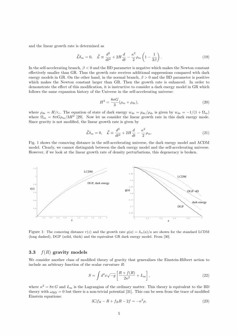
Fig. 1 shows the comoving distance in the self-accelerating universe, the dark energy model and ΛCDMmodel. Clearly, we cannot distinguish between the dark energy model and the self-accelerating universe.However, if we look at the linear growth rate of density perturbations, this degeneracy is broken.
0
0.2
0.4
0.6
0.8
1
1.2
0.2 0.4 0.6 0.8 1 1.2 1.4 1.6 1.8 2
z
LCDM
DGP, dark energy
z
r(z)
0.65
0.7
0.75
0.8
0.85
0.9
0.95
1
y
0 0.2 0.4 0.6 0.8 1
x
DGP
LCDM
DGP−4D
dark energy
a
g(a)
Figure 1: The comoving distance r(z) and the growth rate g(a) = δm(a)/a are shown for the standard LCDM
(long dashed), DGP (solid, thick) and the equivalent GR dark energy model. From [30].
3.3 f(R) gravity models
We consider another class of modified theory of gravity that generalizes the Einstein-Hilbert action toinclude an arbitrary function of the scalar curvature R:
S =∫
d4x√−g
[R + f(R)
2κ2+ Lm
], (22)
where κ2 = 8π G and Lm is the Lagrangian of the ordinary matter. This theory is equivalent to the BDtheory with ωBD = 0 but there is a non-trivial potential [31]. This can be seen from the trace of modifiedEinstein equations:
3¤fR −R + fRR− 2f = −κ2ρ, (23)
5
where fR = df/dR and ¤ is a Laplacian operator and we assumed matter dominated universe. We canidentify fR as the BD scalar field and its perturbations are defined as
ϕ = δfR ≡ fR − fR, (24)
where the bar indicates that the quantity is evaluated on the cosmological background. In this paper, weassume |fR| ¿ 1 and |f/R| ¿ 1. These conditions are necessary to have the background which is closeto ΛCDM cosmology. Then the BD scalar perturbations satisfy
31a2∇2ϕ = −κ2ρmδ + δR, δR ≡ R(fR)−R(fR). (25)
This is noting but the equation for the BD scalar perturbations with ωBD = 0 and the potential givesthe non-linear interaction term
I(ϕ) = δR(ϕ). (26)
By linearizing the potential we find
M1 = Rf (t) ≡ dR(fR)dfR
. (27)
The solutions for the metric perturbations are then given by
k2
a2Φ = 4πG
(2 + M1a
2/k2
3 + M1a2/k2
)ρmδm, (28)
k2
a2Ψ = 4πG
(4 + M1a
2/k2
3 + M1a2/k2
)ρmδm, (29)
and the liner growth rate is given by
Lδm = 0, L ≡ d2
dt2+ 2H
d
dt− κ2
2
(4 + M1a
2/k2
3 + M1a2/k2
)ρm. (30)
In this paper, we consider a function f(R) of the form [32]
f(R) ∝ Rn
ARn + 1, (31)
where A is a constant with dimensions of length squared and n is an integer. In the following we taken = 1. In the limit R → 0, f(R) → 0 and there is no cosmological constant. For high curvature AR À 1,f(R) can be expanded as
f(R) = −2κ2ρΛ − fR0R0
R, (32)
where ρΛ is determined by A, R0 is the background curvature today and we defined fR0 as fR0 = fR(R0).As we mentioned before, we take |fR0| ¿ 1 and assume that the background expansion follows the ΛCDMhistory with the same ρΛ. The M1 term determines the mass of the BD field mBD = (M1/3)1/2 as
mBD(t) ≡√
Rf
3=
(R0
6|fR|
√fR0
fR
)1/2
. (33)
Above the compton length m−1BD, the BD scalar interaction decays exponentially and we recover GR. On
small scales, we recover the BD theory with ωBD = 0. Then the Newton constant is 4/3 times large thanGR. Thus the linear power spectrum acquires a scale dependent enhancement on small scales (Fig. 2).
6
0.01
0.01
0.03
0.03
0.1= | fR0|
0.1=| fR0|
z
wef
fw
eff
2
-0.95
-0.9
-1
-1.1
-1
-1.05
4 6 8
(b) n=4
(a) n=1
k (h Mpc-1)
∆P/P
∆P/P
0.001 0.01 0.1
0
0.1
0.2
0
0.1
0.2
(b) n=4
(a) n=1| fR0| =0.1
| fR0| =0.1
0.01
0.01
10-7
10-7
10-6
10-6
10-5
10-5
10-4
10-4
10-3
10-3
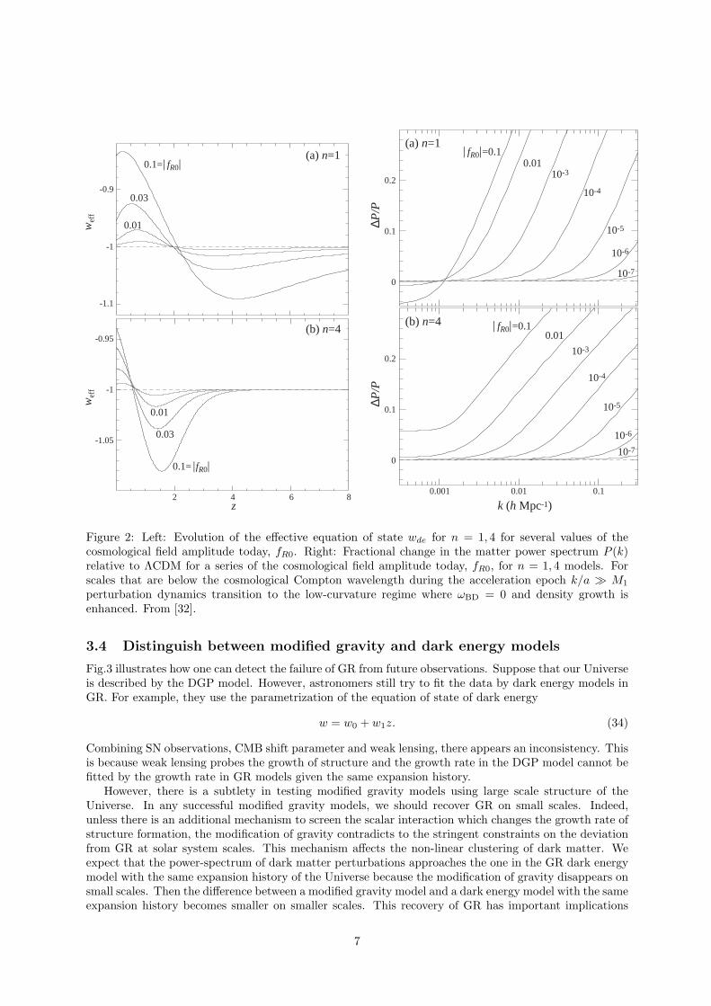
Figure 2: Left: Evolution of the effective equation of state wde for n = 1, 4 for several values of thecosmological field amplitude today, fR0. Right: Fractional change in the matter power spectrum P (k)relative to ΛCDM for a series of the cosmological field amplitude today, fR0, for n = 1, 4 models. Forscales that are below the cosmological Compton wavelength during the acceleration epoch k/a À M1
perturbation dynamics transition to the low-curvature regime where ωBD = 0 and density growth isenhanced. From [32].
3.4 Distinguish between modified gravity and dark energy models
Fig.3 illustrates how one can detect the failure of GR from future observations. Suppose that our Universeis described by the DGP model. However, astronomers still try to fit the data by dark energy models inGR. For example, they use the parametrization of the equation of state of dark energy
w = w0 + w1z. (34)
Combining SN observations, CMB shift parameter and weak lensing, there appears an inconsistency. Thisis because weak lensing probes the growth of structure and the growth rate in the DGP model cannot befitted by the growth rate in GR models given the same expansion history.
However, there is a subtlety in testing modified gravity models using large scale structure of theUniverse. In any successful modified gravity models, we should recover GR on small scales. Indeed,unless there is an additional mechanism to screen the scalar interaction which changes the growth rate ofstructure formation, the modification of gravity contradicts to the stringent constraints on the deviationfrom GR at solar system scales. This mechanism affects the non-linear clustering of dark matter. Weexpect that the power-spectrum of dark matter perturbations approaches the one in the GR dark energymodel with the same expansion history of the Universe because the modification of gravity disappears onsmall scales. Then the difference between a modified gravity model and a dark energy model with the sameexpansion history becomes smaller on smaller scales. This recovery of GR has important implications
7
-0.2
0
0.2
0.4
0.6
0.8
-1.1 -1 -0.9 -0.8 -0.7 -0.6
w1
w0
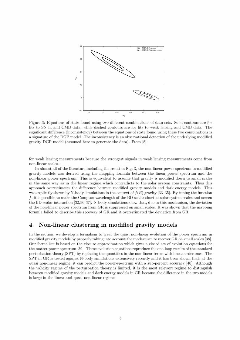
SN + CMB (1,2 sigma)WL + CMB (1,2 sigma)
Figure 3: Equations of state found using two different combinations of data sets. Solid contours are forfits to SN Ia and CMB data, while dashed contours are for fits to weak lensing and CMB data. Thesignificant difference (inconsistency) between the equations of state found using these two combinations isa signature of the DGP model. The inconsistency is an observational detection of the underlying modifiedgravity DGP model (assumed here to generate the data). From [8].
for weak lensing measurements because the strongest signals in weak lensing measurements come fromnon-linear scales.
In almost all of the literature including the result in Fig. 3, the non-linear power spectrum in modifiedgravity models was derived using the mapping formula between the linear power spectrum and thenon-linear power spectrum. This is equivalent to assume that gravity is modified down to small scalesin the same way as in the linear regime which contradicts to the solar system constraints. Thus thisapproach overestimates the difference between modified gravity models and dark energy models. Thiswas explicitly shown by N-body simulations in the context of f(R) gravity [33–35]. By tuning the functionf , it is possible to make the Compton wavelength of the BD scalar short at solar system scales and screenthe BD scalar interaction [32,36,37]. N-body simulations show that, due to this mechanism, the deviationof the non-linear power spectrum from GR is suppressed on small scales. It was shown that the mappingformula failed to describe this recovery of GR and it overestimated the deviation from GR.
4 Non-linear clustering in modified gravity models
In the section, we develop a formalism to treat the quasi non-linear evolution of the power spectrum inmodified gravity models by properly taking into account the mechanism to recover GR on small scales [38].Our formalism is based on the closure approximation which gives a closed set of evolution equations forthe matter power spectrum [39]. These evolution equations reproduce the one-loop results of the standardperturbation theory (SPT) by replacing the quantities in the non-linear terms with linear-order ones. TheSPT in GR is tested against N-body simulations extensively recently and it has been shown that, at thequasi non-linear regime, it can predict the power-spectrum with a sub-percent accuracy [40]. Althoughthe validity regime of the perturbation theory is limited, it is the most relevant regime to distinguishbetween modified gravity models and dark energy models in GR because the difference in the two modelsis large in the linear and quasi-non-linear regime.
8
4.1 Evolution equations for perturbations
The Fourier transform of the fluid equations (8) and (9) become
H−1 ∂δ(k)∂t
+ θ(k) = −∫
d3k1d3k2
(2π)3δD(k − k1 − k2)α(k1, k2) θ(k1)δ(k2), (35)
H−1 ∂θ(k)∂t
+
(2 +
H
H2
)θ(k)−
(k
aH
)2
ψ(k) = −12
∫d3k1d
3k2
(2π)3δD(k − k1 − k2)β(k1,k2) θ(k1)θ(k2),
(36)
where the kernels in the Fourier integrals, α and β, are given by
α(k1,k2) = 1 +k1 · k2
|k1|2 , β(k1, k2) =(k1 · k2) |k1 + k2|2
|k1|2|k2|2 . (37)
We take into account the non-linear interaction terms I in the BD scalar equation. Due to the non-linearinteractions, the potential ψ is couples to δ through the BD scalar ϕ in a fully non-linear way. To deriveclosed equations for δ and θ, we must employ the perturbative approach to Eq. (6). By solving Eq. (6)perturbatively assuming ϕ < 1, ψ can be expressed in terms of δ as
−(
k
a
)2
ψ =12
κ2 ρm
[1 +
13
(k/a)2
Π(k)
]δ(k) +
12
(k
a
)2
S(k), (38)
where
Π(k) =13
((3 + 2ωBD)
k2
a2+ M1
), (39)
and κ2 = 8πG. The function S(k) is the non-linear source term which is obtained perturbatively using(4) as
S(k) = − 16Π(k)
(κ2 ρm
3
)2 ∫d3k1d
3k2
(2π)3δD(k − k12)M2(k1, k2)
δ(k1) δ(k2)Π(k1)Π(k2)
− 118Π(k)
(κ2 ρm
3
)3 ∫d3k1d
3k2d3k3
(2π)6δD(k − k123)
M3(k1,k2,k3)− M2(k1, k2 + k3)M2(k2, k3)
Π(k23)
× δ(k1) δ(k2), δ(k3)Π(k1)Π(k2)Π(k3)
, (40)
The expression (40) is valid up to the third-order in δ.The perturbation equations (35), (36) and (40) can be further reduced to a compact form by intro-
ducing the following quantity:
Φa(k) =(
δ(k)−θ(k)
). (41)
We can write down the basic equations in a single form as
∂Φa(k; η)∂η
+ Ωab(k; η) Φb(k; η) =∫
d3k1d3k2
(2π)3δD(k − k12) γabc(k1,k2; η)Φb(k1; η)Φc(k2; η)
+∫
d3k1d3k2d
3k3
(2π)6δD(k − k123)σabcd(k1,k2, k3; η)Φb(k1; η)Φc(k2η)Φd(k3; η),(42)
where the time variable η is defined by η = ln a(t). The matrix Ωab is given by
Ωab(k; η) =
0 −1
−κ2
2ρm
H2
[1 +
13
(k/a)2
Π(k)
]2 +
H
H2
. (43)
9
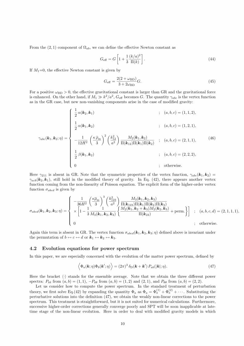
From the (2, 1) component of Ωab, we can define the effective Newton constant as
Geff = G
[1 +
13
(k/a)2
Π(k)
]. (44)
If M1=0, the effective Newton constant is given by
Geff =2(2 + ωBD)3 + 2ωBD
G. (45)
For a positive ωBD > 0, the effective gravitational constant is larger than GR and the gravitational forceis enhanced. On the other hand, if M1 À k2/a2, Geff becomes G. The quantity γabc is the vertex functionas in the GR case, but new non-vanishing components arise in the case of modified gravity:
γabc(k1, k2; η) =
12
α(k2,k1) ; (a, b, c) = (1, 1, 2),
12
α(k1,k2) ; (a, b, c) = (1, 2, 1),
− 112H2
(κ ρm
3
)2 (k212
a2
)M2(k1, k2)
Π(k12)Π(k1)Π(k2); (a, b, c) = (2, 1, 1),
12
β(k1,k2) ; (a, b, c) = (2, 2, 2),
0 ; otherwise.
(46)
Here γ211 is absent in GR. Note that the symmetric properties of the vertex function, γabc(k1, k2) =γacb(k2,k1), still hold in the modified theory of gravity. In Eq. (42), there appears another vertexfunction coming from the non-linearity of Poisson equation. The explicit form of the higher-order vertexfunction σabcd is given by
σabcd(k1,k2,k3; η) =
− 136H2
(κρm
3
)3 (k2123
a2
)M3(k1, k2, k3)
Π(k123)Π(k1)Π(k2)Π(k3)
×[1− 1
31
M3(k1,k2, k3)
M2(k1, k2 + k3)M2(k2,k3)
Π(k23)+ perm.
]; (a, b, c, d) = (2, 1, 1, 1),
0 ; otherwise.
Again this term is absent in GR. The vertex function σabcd(k1,k2, k3; η) defined above is invariant underthe permutation of b ↔ c ↔ d or k1 ↔ k2 ↔ k3.
4.2 Evolution equations for power spectrum
In this paper, we are especially concerned with the evolution of the matter power spectrum, defined by⟨Φa(k; η)Φb(k′; η)
⟩= (2π)3 δD(k + k′)Pab(|k|; η). (47)
Here the bracket 〈·〉 stands for the ensemble average. Note that we obtain the three different powerspectra: Pδδ from (a, b) = (1, 1), −Pδθ from (a, b) = (1, 2) and (2, 1), and Pθθ from (a, b) = (2, 2).
Let us consider how to compute the power spectrum. In the standard treatment of perturbationtheory, we first solve Eq.(42) by expanding the quantity Φa as Φa = Φ(1)
a + Φ(2)a + · · · . Substituting the
perturbative solutions into the definition (47), we obtain the weakly non-linear corrections to the powerspectrum. This treatment is straightforward, but it is not suited for numerical calculations. Furthermore,successive higher-order corrections generally converge poorly and SPT will be soon inapplicable at late-time stage of the non-linear evolution. Here in order to deal with modified gravity models in which
10
analytical calculations are intractable in many cases, we take another approach. Our approach is basedon the closure approximation proposed by Ref. [39], in which the evolution of power spectrum is obtainednumerically by solving a closed set of evolution equations.
Provided the basic equation (42), the evolution equation for power spectrum can be derived bytruncating the infinite chain of the moment equations with a help of perturbative calculation, calledclosure approximation. We skip the details of the derivation and present the final results. Readersinterested in the derivation can refer to Ref. [39]. The resultant evolution equations are the coupledequations characterized by the three statistical quantities including the power spectrum. We define
⟨Φa(k; η)Φb(k′; η′)
⟩= (2π)3 δD(k + k′)Rab(|k|; η, η′) ; η > η′,
⟨ δΦa(k; η)δΦb(k′; η′)
⟩= δD(k − k′)Gab(|k|; η, η′) ; η ≥ η′. (48)
The quantities Rab and Gab respectively denote the cross spectra between different times and the non-linear propagator. Note that Rab 6= Rba, in general. Then, the closure equations become
Σabcd(k; η)Pcd(k; η) =∫
d3q
(2π)3[γapq(q, k − q; η)Fbpq(−k, q,k − q; η) + γbpq(q,−k − q; η) Fapq(k, q,−k − q; η)
]
+3∫
d3q
(2π)3[σapqr(q,−q, k; η)Ppq(q; η)Prb(k; η) + σbpqr(q,−q,−k; η) Ppq(q; η)Pra(k; η)
],
(49)
Λab(k; η)Rbc(k; η, η′) =∫
d3q
(2π)3γapq(q, k − q; η)Kcpq(−k, q, k − q; η, η′)
+3∫
d3q
(2π)3σapqr(q,−q,k; η)Ppq(q; η)Rrc(k; η, η′), (50)
Λab(k; η)Gbc(k|η, η′) = 4∫ η
η′dη′′
∫d3q
(2π)3γapq(q, k − q; η) γlrs(−q, k; η′′)Gql(|k − q||η, η′′)Rpr(q; η, η′′)Gsc(k|η′′, η′),
+3∫
d3q
(2π)3σapqr(q,−q,k; η)Ppq(q; η)Grc(k|η, η′), (51)
where the operators Σabcd and Λab are defined as
Σabcd(k; η) = δacδbd∂
∂η+ δacΩbd(k; η) + δbdΩac(k; η), Λab(k; η) = δab
∂
∂η+ Ωab(k; η), (52)
The explicit expressions for the kernels Fapq and Kcpq are summarized as
Fapq(k, p, q; η) = 2∫ η
η0
dη′′[2 Gql(q|η, η′′) γlrs(k, p; η′′)Rar(k; η, η′′)Rps(p; η, η′′)
+ Gal(k|η, η′′) γlrs(p, q; η′′)Rpr(p; η, η′′)Rqs(q; η, η′′)], (53)
Kcpq(k′, p, q; η, η′)
= 4∫ η
η0
dη′′ Gql(q|η, η′′) γlrs(k′, p; η′′)Rps(p; η, η′′)
×
Rcr(k′; η′, η′′)Θ(η′ − η′′) + Rrc(k′; η′′, η′)Θ(η′′ − η′)
+ 2∫ η′
η0
dη′′Gcl(k′|η′, η′′) γlrs(p, q; η′′) Rpr(p; η, η′′)Rqs(q; η, η′′). (54)
The closure equations (50)–(51) are the integro-differential equations involving several non-linearterms, in which the information of the higher-order corrections in SPT is encoded. Thus, replacing allstatistical quantities in these non-linear terms with linear-order ones, the solutions of closure equationsautomatically reproduce the leading-order results of SPT, called one-loop power spectra. Further, fully
11
non-linear treatment of the closure equations is a non-perturbative description of the power spectra, andhave an ability to predict the matter power spectra accurately, beyond one-loop SPT. Strictly speaking,the non-linear terms in the right-hand side of Eqs. (50)–(51) have only the information of the one-loopcorrections. However, it has been shown in Ref. [39] that the present formulation is equivalent to theone-loop level of renormalized perturbation theory [41], and even the leading-order approximation stillcontain some non-perturbative effects. The application of the closure approximation, together with thedetailed comparison with N-body simulations, is presented in Refs. [40, 42].
In this paper, we mainly use the closure equations for the purpose of computing the one-loop powerspectra. The results for fully non-linear treatment of the closure equations will be presented elsewhere.The numerical scheme to solve the closure equations is basically the same as described in Ref. [39]. InAppendix A, we briefly review the numerical scheme and summarize several modifications.
Before closing this section, we note here that the resultant equations (50)–(51) contain the additionalnon-linear terms originating from the modification of the Poisson equation (see Eq.(38)). In particular,for the terms containing the higher-order vertex function σabcd can be effectively absorbed into the matrixΩab. Since the non-vanishing contribution of the higher-order vertex function only comes from σ2111, thismeans that the effective Newton constant Geff defined by (44) is renormalized as Geff → Geff + δGeff ,with δGeff given by
δGeff =3H2
4π ρm
∫d3q
(2π)3σ2111(q,−q, k; η) P11(q; η). (55)
This is a clear manifestation of the mechanism that non-linear clustering does generically alter the growthrate of the structure formation through the renormalisation of the Newton constant and, due to thismechanism, successful modified gravity models are expected to recover GR on small scales.
5 Non-linear power spectrum in modified gravity models
In this section, we show solutions for the non-lienar power spectrum in two examples, DGP modelsand f(R) gravity models. We also extend these results to fully non-linear scales using the so-calledParametrized Post Friedmann (PPF) framework.
5.1 PPF formalism
Sawicki and Hu proposed a fitting formula for the non-linear power spectrum in modified gravity models[5]. The fitting formula based on the observation that the non-linear power spectrum should approachthe one in the GR model that follows the same expansion history of the Universe due to the recovery ofGR on small scales. They postulate that the full non-linear power spectrum in a modified gravity modelis given by the formula
P (k, z) =Pnon−GR(k, z) + cnlΣ2(k, z)PGR(k, z)
1 + cnlΣ2(k, z), (56)
where z is a red-shift. Here Pnon−GR(k, z) is the non-linear power spectrum which is obtained withoutthe non-linear interactions that are responsible for the recovery of GR. This is equivalent to assumethat gravity is modified down to the small scales in the same way as in the linear regime. PGR(k, z) isthe non-linear power spectrum obtained in the GR dark energy model that follows the same expansionhistory of the Universe as in the modified gravity model. The function Σ2(k, z) determines the degreeof non-linearity at a relevant wavenumber k. They propose to take Σ2(k) = k3Plin(k, z)/2π2, wherePlin(k, z) is the linear power spectrum in the modified gravity model. Finally, cnl is a parameter in thisframework which controls the scale at which the theory approaches GR.
Once we obtain the quasi non-linear power spectrum, we can check whether the PPF frameworkworks and determines cnl in the quasi non-linear regime. In our formalism, Pnon−GR(k, z) is obtained byneglecting the non-linear interaction I. PGR(k, z) can be obtained by taking ωBD → ∞ limit and alsoneglecting I. We again consider two explicit examples.
12
5.2 DGP models
In DGP models, the BD scalar acquires a large second order interaction given by
I(ϕ) =r2c
a4
[(∇2ϕ)2 − (∇i∇jϕ)2
]. (57)
Note that rc is tuned to be the present-day horizon scale. Thus this second order term has a large effect.The higher order terms than the second order are suppressed by the additional powers of the 4D Planckscale and, in the Newtonian limit, we can safely ignore them. Therefore, in this model, we have
M1 = 0, M2(k1,k2) = 2r2c
a4
[k21k
22 − (k1 · k2)2
], M3 = 0, (58)
Π(k, η) = β(η)k2
a2. (59)
In this paper, we only consider the self-accelerating branch solutions and use the best-fit cosmologicalparameters for the flat self-accelerating universe: Ωm = 0.257,Ωb = 0.0544, h = 0.66, ns = 0.998 [28]. Inthe left panel of Fig. 4, the solid (black) line shows the fractional difference between the power spectrumin DGP models and dark energy models that follow the same expansion history obtained by solving thelinearized closure equation numerically. The dashed (red) line shows the result obtained by neglecting thenon-linear term M2, Pnon−GR. we can see that the non-linear interaction enhances the non-linear powerspectrum. This is natural because in the self-accelerating branch, the linear growth rate is suppressedcompared to the GR model that follows the same expansion history due to the negative BD parameterωBD < 0 which makes the Newton constant smaller than GR. This is closely related to the fact thatthe BD scalar becomes a ghost in this model. Classically, the ghost mediates a repulsive force andsuppresses the gravitational collapse. The non-linear interaction makes the theory approach GR. Thus iteffectively increases the Newton constant by screening the BD scalar. Then the power-spectrum receivesan enhancement compared with the case without the non-linear interaction.
For DGP models, we find that the PPF formalism with
Σ2(k, z) =k3
2π2Plin(k, z) (60)
as proposed by Sawicki and Hu gives a nice fit to the results obtained in the perturbation theory. Wefind that by allowing the time dependence in cnl, it is possible to recover the solutions for t he non-linearpower spectrum very well within the validity regime of the perturbation theory. At z = 0, cnl is given by0.3 and there is a slight redshift dependence (the dotted (blue) line in the left panel of Fig. 4).
Armed with this result, it is tempting to extend our analysis to the fully non-linear regime. In GR,there are several fitting formulae which provide the mapping between the linear power spectrum andnon-linear power spectrum. It is impossible to apply these mapping formulae to modified gravity modelsas the mapping does not take into account the non-linear interaction terms in the Poisson equation I.If we apply the GR mapping formula to the linear power spectrum, we would get the non-linear powerspectrum without I, Pnon−GR(k). In fact, there exist N-body simulations in DGP models performed byneglecting the non-linear interaction terms [43]. It was shown that the power spectrum obtained in theseN-body simulations can be fitted well by the mapping formulae in GR. The mapping formulae should bevalid in GR models, so we can also predict PGR(k). Then using the PPF formalism (56), we can predictthe non-linear power spectrum if cnl is known. In the right panel of Fig. 4, we plotted the fractionaldifference between the power spectrum in the DGP model and the GR model with the same expansionhistory. We used the fitting formula developed by Smith et.al. [44]. If we could extrapolate the resultin the quasi non-linear regime, we would have cnl = 0.3 at z = 0. If this is correct, we find that evenat k = 10Mpc h−1, the difference between the power spectrum in DGP and that in the equivalent GRmodel remains at 7% level. This is crucial to distinguish between the two models using weak lensingas the signal to noise ratio is larger on smaller scales. Of course, we should emphasize that there is noguarantee that cnl measured in the quasi non-linear regime is valid down to the fully non-linear scalesand this should be tested using N-body simulations. Still there is no N-body simulation available in DGPmodels and it would be important to test the prediction against N-body simulations.
13
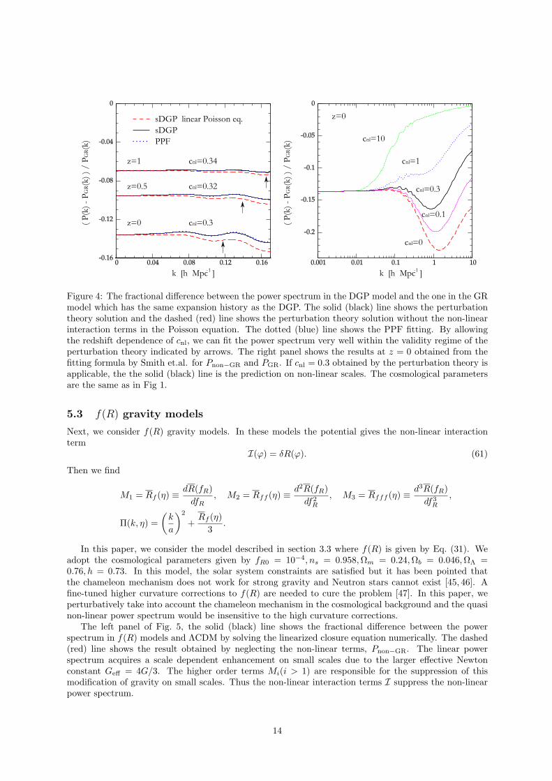
Figure 4: The fractional difference between the power spectrum in the DGP model and the one in the GRmodel which has the same expansion history as the DGP. The solid (black) line shows the perturbationtheory solution and the dashed (red) line shows the perturbation theory solution without the non-linearinteraction terms in the Poisson equation. The dotted (blue) line shows the PPF fitting. By allowingthe redshift dependence of cnl, we can fit the power spectrum very well within the validity regime of theperturbation theory indicated by arrows. The right panel shows the results at z = 0 obtained from thefitting formula by Smith et.al. for Pnon−GR and PGR. If cnl = 0.3 obtained by the perturbation theory isapplicable, the the solid (black) line is the prediction on non-linear scales. The cosmological parametersare the same as in Fig 1.
5.3 f(R) gravity models
Next, we consider f(R) gravity models. In these models the potential gives the non-linear interactionterm
I(ϕ) = δR(ϕ). (61)
Then we find
M1 = Rf (η) ≡ dR(fR)dfR
, M2 = Rff (η) ≡ d2R(fR)df2
R
, M3 = Rfff (η) ≡ d3R(fR)df3
R
,
Π(k, η) =(
k
a
)2
+Rf (η)
3.
In this paper, we consider the model described in section 3.3 where f(R) is given by Eq. (31). Weadopt the cosmological parameters given by fR0 = 10−4, ns = 0.958, Ωm = 0.24,Ωb = 0.046, ΩΛ =0.76, h = 0.73. In this model, the solar system constraints are satisfied but it has been pointed thatthe chameleon mechanism does not work for strong gravity and Neutron stars cannot exist [45, 46]. Afine-tuned higher curvature corrections to f(R) are needed to cure the problem [47]. In this paper, weperturbatively take into account the chameleon mechanism in the cosmological background and the quasinon-linear power spectrum would be insensitive to the high curvature corrections.
The left panel of Fig. 5, the solid (black) line shows the fractional difference between the powerspectrum in f(R) models and ΛCDM by solving the linearized closure equation numerically. The dashed(red) line shows the result obtained by neglecting the non-linear terms, Pnon−GR. The linear powerspectrum acquires a scale dependent enhancement on small scales due to the larger effective Newtonconstant Geff = 4G/3. The higher order terms Mi(i > 1) are responsible for the suppression of thismodification of gravity on small scales. Thus the non-linear interaction terms I suppress the non-linearpower spectrum.
14
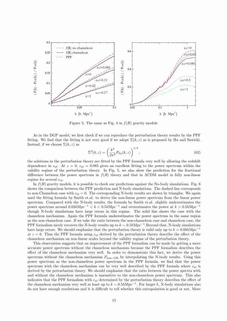
Figure 5: The same as Fig. 4 in f(R) gravity models
As in the DGP model, we first check if we can reproduce the perturbation theory results by the PPFfitting. We find that the fitting is not very good if we adopt Σ(k, z) as is proposed by Hu and Sawicki.Instead, if we choose Σ(k, z) as
Σ2(k, z) =(
k3
2π2Plin(k, z)
)1/3
, (62)
the solutions in the perturbation theory are fitted by the PPF formula very well by allowing the redshiftdependence in cnl. At z = 0, cnl = 0.085 gives an excellent fitting to the power spectrum within thevalidity regime of the perturbation theory. In Fig. 5, we also show the prediction for the fractionaldifference between the power spectrum in f(R) theory and that in ΛCDM model in fully non-linearregime for several cnl.
In f(R) gravity models, it is possible to check our predictions against the No-body simulations. Fig. 6shows the comparison between the PPF prediction and N-body simulations. The dashed line correspondsto non-Chameleon case with cnl = 0. The corresponding N-body results are shown by triangles. We againused the fitting formula by Smith et.al. to derive the non-linear power spectrum from the linear powerspectrum. Compared with the N-body results, the formula by Smith et.al. slightly underestimates thepower spectrum around 0.03hMpc−1 < k < 0.5hMpc−1 and overestimates the power at k > 0.5hMpc−1
though N-body simulations have large errors in this regime. The solid line shows the case with thechameleon mechanism. Again the PPF formula underestimates the power spectrum in the same regionas the non-chameleon case. If we take the ratio between the non-chameleon case and chameleon case, thePPF formalism nicely recovers the N-body results up to k ∼ 0.5hMpc−1.Beyond that, N-body simulationshave large errors. We should emphasize that the perturbation theory is valid only up to k = 0.08hMpc−1
at z = 0. Thus the PPF formula using cnl derived by the perturbation theory describe the effect of thechameleon mechanism on non-linear scales beyond the validity regime of the perturbation theory.
This observation suggests that an improvement of the PPF formalism can be made by getting a moreaccurate power spectrum without the chameleon mechanism because the PPF formalism describes theeffect of the chameleon mechanism very well. In order to demonstrate this fact, we derive the powerspectrum without the chameleon mechanism Pnon−GR by interpolating the N-body results. Using thispower spectrum as the non-chameleon power spectrum in the PPF formula, we find that the powerspectrum with the chameleon mechanism can be very well described by the PPF formula where cnl isderived by the perturbation theory. We should emphasize that the ratio between the power spectra withand without the chameleon mechanism is insensitive to the non-chameleon power spectrum. This alsoindicates that the PPF formalism with cnl determined by the perturbation theory describes the effect ofthe chameleon mechanism very well at least up to k ∼ 0.5hMpc−1. For larger k, N-body simulations alsodo not have enough resolutions and it is difficult to tell whether this extrapolation is good or not. More
15
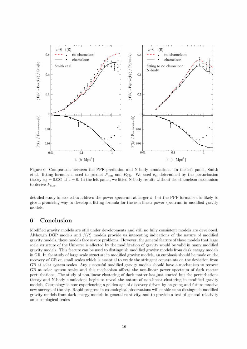
Figure 6: Comparison between the PPF prediction and N-body simulations. In the left panel, Smithet.al. fitting formula is used to predict Pnon and PGR. We used cnl determined by the perturbationtheory cnl = 0.085 at z = 0. In the left panel, we fitted N-body results without the chameleon mechanismto derive Pnon.
detailed study is needed to address the power spectrum at larger k, but the PPF formalism is likely togive a promising way to develop a fitting formula for the non-linear power spectrum in modified gravitymodels.
6 Conclusion
Modified gravity models are still under developments and still no fully consistent models are developed.Although DGP models and f(R) models provide us interesting indications of the nature of modifiedgravity models, these models face severe problems. However, the general feature of these models that largescale structure of the Universe is affected by the modification of gravity would be valid in many modifiedgravity models. This feature can be used to distinguish modified gravity models from dark energy modelsin GR. In the study of large scale structure in modified gravity models, an emphasis should be made on therecovery of GR on small scales which is essential to evade the stringent constraints on the deviation fromGR at solar system scales. Any successful modified gravity models should have a mechanism to recoverGR at solar system scales and this mechanism affects the non-linear power spectrum of dark matterperturbations. The study of non-linear clustering of dark matter has just started but the perturbationstheory and N-body simulations begin to reveal the nature of non-linear clustering in modified gravitymodels. Cosmology is now experiencing a golden age of discovery driven by on-going and future massivenew surveys of the sky. Rapid progress in cosmological observations will enable us to distinguish modifiedgravity models from dark energy models in general relativity, and to provide a test of general relativityon cosmological scales
16
Acknowledgement
I would like to thank my collaborators in this subject. This review is mainly based on a paper withTakashi Hiramatsu and Atsushi Taruya [38]. KK is supported by ERC, RCUK and STFC.
References
[1] S. Nojiri and S. D. Odintsov, ECONF C0602061, 06 (2006), hep-th/0601213.
[2] K. Koyama, Gen. Rel. Grav. 40, 421 (2008), 0706.1557.
[3] R. Durrer and R. Maartens, (2008), 0811.4132.
[4] R. Durrer and R. Maartens, Gen. Rel. Grav. 40, 301 (2008), 0711.0077.
[5] W. Hu and I. Sawicki, (2007), arXiv:0708.1190 [astro-ph].
[6] J.-P. Uzan and F. Bernardeau, Phys. Rev. D64, 083004 (2001), hep-ph/0012011.
[7] A. Lue, R. Scoccimarro, and G. Starkman, Phys. Rev. D69, 044005 (2004), astro-ph/0307034.
[8] M. Ishak, A. Upadhye, and D. N. Spergel, Phys. Rev. D74, 043513 (2006), astro-ph/0507184.
[9] L. Knox, Y.-S. Song, and J. A. Tyson, Phys. Rev. D74, 023512 (2006).
[10] K. Koyama, JCAP 0603, 017 (2006), astro-ph/0601220.
[11] T. Chiba and R. Takahashi, Phys. Rev. D75, 101301 (2007), astro-ph/0703347.
[12] L. Amendola, M. Kunz, and D. Sapone, JCAP 0804, 013 (2008), 0704.2421.
[13] K. Yamamoto, D. Parkinson, T. Hamana, R. C. Nichol, and Y. Suto, Phys. Rev. D76, 023504(2007), 0704.2949.
[14] K. Yamamoto, T. Sato, and G. Huetsi, Prog. Theor. Phys. 120, 609 (2008), 0805.4789.
[15] Y.-S. Song and W. J. Percival, (2008), 0807.0810.
[16] M. Kunz and D. Sapone, Phys. Rev. Lett. 98, 121301 (2007), astro-ph/0612452.
[17] B. Jain and P. Zhang, (2007), 0709.2375.
[18] Y.-S. Song and K. Koyama, JCAP 01, 048 (2009), 0802.3897.
[19] Y.-S. Song and O. Dore, (2008), 0812.0002.
[20] J. Khoury and A. Weltman, Phys. Rev. D69, 044026 (2004), astro-ph/0309411.
[21] G. R. Dvali, G. Gabadadze, and M. Porrati, Phys. Lett. B485, 208 (2000), hep-th/0005016.
[22] M. A. Luty, M. Porrati, and R. Rattazzi, JHEP 09, 029 (2003), hep-th/0303116.
[23] T. Tanaka, Phys. Rev. D69, 024001 (2004), gr-qc/0305031.
[24] K. Koyama and F. P. Silva, Phys. Rev. D75, 084040 (2007), hep-th/0702169.
[25] C. Deffayet, G. R. Dvali, G. Gabadadze, and A. I. Vainshtein, Phys. Rev. D65, 044026 (2002),hep-th/0106001.
[26] C. Deffayet, Phys. Lett. B502, 199 (2001), hep-th/0010186.
[27] K. Koyama, Class. Quant. Grav. 24, R231 (2007), 0709.2399.
[28] W. Fang et al., Phys. Rev. D78, 103509 (2008), 0808.2208.
17
[29] A. Lue, R. Scoccimarro, and G. D. Starkman, Phys. Rev. D69, 124015 (2004), astro-ph/0401515.
[30] K. Koyama and R. Maartens, JCAP 0601, 016 (2006), astro-ph/0511634.
[31] T. Chiba, Phys. Lett. B575, 1 (2003), astro-ph/0307338.
[32] W. Hu and I. Sawicki, Phys. Rev. D76, 064004 (2007), 0705.1158.
[33] H. Oyaizu, Phys. Rev. D78, 123523 (2008), 0807.2449.
[34] H. Oyaizu, M. Lima, and W. Hu, Phys. Rev. D78, 123524 (2008), 0807.2462.
[35] F. Schmidt, M. V. Lima, H. Oyaizu, and W. Hu, (2008), 0812.0545.
[36] A. A. Starobinsky, JETP Lett. 86, 157 (2007), 0706.2041.
[37] S. A. Appleby and R. A. Battye, Phys. Lett. B654, 7 (2007), 0705.3199.
[38] K. Koyama, A. Taruya, and T. Hiramatsu, (2009), in preparation.
[39] A. Taruya and T. Hiramatsu, (2007), 0708.1367.
[40] T. Nishimichi et al., (2008), 0810.0813.
[41] M. Crocce and R. Scoccimarro, Phys. Rev. D73, 063519 (2006), astro-ph/0509418.
[42] A. Taruya, T. Nishimichi, S. Saito, and T. Hiramatsu, (2009), in preparation.
[43] I. Laszlo and R. Bean, Phys. Rev. D77, 024048 (2008), 0709.0307.
[44] The Virgo Consortium, R. E. Smith et al., Mon. Not. Roy. Astron. Soc. 341, 1311 (2003), astro-ph/0207664.
[45] A. V. Frolov, Phys. Rev. Lett. 101, 061103 (2008), 0803.2500.
[46] T. Kobayashi and K.-i. Maeda, (2008), 0807.2503.
[47] T. Kobayashi and K.-i. Maeda, Phys. Rev. D79, 024009 (2009), 0810.5664.
18
Perturbation theory of N point mass gravitational lens
Hideki Asada1
Faculty of Science and Technology, Hirosaki University, Hirosaki 036-8561, Japan
AbstractWe make the first systematic attempt to determine using perturbation theory thepositions of images by gravitational lensing due to arbitrary number of coplanarmasses without any symmetry on a plane, as a function of lens and source parameters.We present a method of Taylor-series expansion to solve the lens equation under asmall mass-ratio approximation. The advantage of our method is that it allows asystematic iterative analysis. We determine image positions for binary lens systemsup to the third order in mass ratios and for arbitrary N point masses up to thesecond order. The number of the images that admit a small mass-ratio limit is lessthan the maximum number. It is suggested that positions of extra images could notbe expressed as Maclaurin series in mass ratios. Magnifications are finally discussed.
1 Introduction
Gravitational lensing has become one of important subjects in modern astronomy and cosmology. It playscrucial roles as gravitational telescopes in various fields ranging from extra-solar planets to dark matterand dark energy at cosmological scales. This work focuses on gravitational lensing due to a N-point masssystem. Definitely it is a challenging problem to express the image positions as functions of lens andsource parameters.
There are several motivations for this work. One is that gravitational lensing offers a tool of discoveriesand measurements of planetary systems (Schneider and Weiss 1986, Mao and Paczynski 1991, Gould andLoeb 1992, Bond et al. 2004, Beaulieu et al. 2006), compact stars, or a cluster of dark objects, whichare difficult to probe with other methods. Gaudi et al. (2008) have recently found an analogy of theSun-Jupiter-Saturn system by lensing. Efficient methods for producing light curves beyond binary casesare preferred.
Another motivation is to pursue a transit between a particle method and a fluid (mean field) one.For microlensing studies, particle methods are employed, because the systems consist of stars, planets orMACHOs. In cosmological lensing, on the other hand, light propagation is considered for the gravitationalfield produced by inhomogeneities of cosmic fluids, say galaxies or large scale structures of our Universe. Itseems natural, though no explicit proof has been given, that observed quantities computed by continuumfluid methods will agree with those by discrete particle ones in the limit N → ∞, at least on average,where N is the number of particles.
Galois showed that the fifth-order and higher polynomials cannot be solved algebraically. Hence, noformula for quintic equations is known.
In this work, we present a method of Taylor-series expansion to solve the lens equation under a smallmass-ratio approximation.
2 Complex Formalism
We consider a lens system with N point masses. The mass and two-dimensional location of each body isdenoted as Mi and the vector Ei, respectively. For the later convenience, let us define the angular sizeof the Einstein ring as
θE =
√4GMtotDLS
c2DLDS, (1)
1E-mail: [email protected]
1
where G is the gravitational constant, c is the light speed, Mtot is the total mass∑N
i=1 Mi and DL, DSand DLS denote distances between the observer and the lens, between the observer and the source, andbetween the lens and the source, respectively. In the unit normalised by the angular size of the Einsteinring, the lens equation becomes
β = θ −N∑i
νiθ − ei
|θ − ei|2, (2)
where β = (βx, βy) and θ = (θx, θy) denote the vectors for the position of the source and image,respectively and we defined the mass ratio and the angular separation vector as νi = Mi/Mtot andei = Ei/θE = (eix, eiy).
Bourassa, Kantowski and Norton (1973), Bourassa and Kantowski (1975) introduced a complex nota-tion to describe gravitational lensing. In a formalism based on complex variables, two-dimensional vectorsfor the source, lens and image positions are denoted as w = βx + iβy, z = θx + iθy, and εi = eix + ieiy,respectively. By employing this formalism, the lens equation is rewritten as
w = z −N∑i
νi
z∗ − ε∗i, (3)
where the asterisk ∗ means the complex conjugate. The lens equation is non-analytic because it containsboth z and z∗.
3 Perturbation
The lens equation is written as
C(z, z∗) =N∑
k=2
νkDk(z∗), (4)
where C(z, z∗) was defined by Eq. (5) and we defined
C(z, z∗) = w − z +1z∗
, (5)
Dk(z∗) =1z∗
− 1z∗ − ε∗k
. (6)
We seek a solution in expansion series as
z =∞∑
p2=0
∞∑p3=0
· · ·∞∑
pN=0
(ν2)p2(ν3)p3 · · · (νN )pN z(p2)(p3)···(pN ), (7)
where z(p2)(p3)···(pN ) is a constant to be determined iteratively.It is convenient to normalise the perturbed roots in the units of the zeroth-order one as
σ(p2)(p3)···(pN ) =z(p2)(p3)···(pN )
z(0)···(0). (8)
Here, we shall give perturbative roots when the zeroth order roots are not located at the lens position.Please see Asada (2009) for the special case when the zeroth order roots are located at the lens position.
3.1 0th order (z(0)···(0) 6= εi for i = 1, · · · , N)
Zeroth-order solution is given asz(0)···(0) = Aw, (9)
where, we defined
A =12
(1 ±
√1 +
4ww∗
). (10)
2
3.2 1st order (z(0)···(0) 6= εi for i = 1, · · · , N)
We obtain the first order solution as
z(0)···(1k)···(0)
=b(0)···(1k)···(0) − a(0)···(1k)···(0)b
∗(0)···(1k)···(0)
1 − a(0)···(1k)···(0)a∗(0)···(1k)···(0)
. (11)
Here, we defined
a(0)···(1k)···(0) =1
(z∗(0)···(0))2, (12)
b(0)···(1k)···(0) =ε∗k
z∗(0)···(0)(z∗(0)···(0) − ε∗k)
. (13)
3.3 2nd order (z(0)···(0) 6= εi for i = 1, · · · , N)
There are two types of second-order solutions as shown below. First, we obtain
z(0)···(2k)···(0)
=b(0)···(2k)···(0) − a(0)···(2k)···(0)b
∗(0)···(2k)···(0)
1 − a(0)···(2k)···(0)a∗(0)···(2k)···(0)
. (14)
Here, we defined
a(0)···(2k)···(0) =1
(z∗(0)···(0))2, (15)
b(0)···(2k)···(0) = −Dk(0)···(1k)···(0) +(σ∗
(0)···(1k)···(0))2
z∗(0)···(0). (16)
Next, let us assume k < `. We obtain
z(0)···(1k)···(1`)···(0)
=b(0)···(1k)···(1`)···(0) − a(0)···(1k)···(1`)···(0)b
∗(0)···(1k)···(1`)···(0)
1 − a(0)···(1k)···(1`)···(0)a∗(0)···(1k)···(1`)···(0)
.
(17)
Here, we defined
a(0)···(1k)···(1`)···(0) =1
(z∗(0)···(0))2, (18)
b(0)···(1k)···(1`)···(0) = −Dk(0)···(1`)···(0) − D`(0)···(1k)···(0)
+2σ∗
(0)···(1k)···(0)σ∗(0)···(1`)···(0)
z∗(0)···(0). (19)
4 Conclusion
Under a small mass-ratio approximation, we have developed a perturbation theory of N coplanar (inthe thin lens approximation) point-mass gravitational lens systems without symmetries on a plane. Thesystem can be separated into a single mass lens as a background and its perturbation due to the remainingpoint masses.
The number of the images that admit the small mass-ratio limit is less than the maximum number.This suggests that the other images do not have the small mass limit. Therefore, it is conjectured that
3
positions of the extra images could not be expressed as Maclaurin series in mass ratios. This is a topicof future work.
There are possible applications along the course of the perturbation theory of N point-mass gravita-tional lens systems. For instance, it will be interesting to study lensing properties such as magnificationsby using the functional form of image positions. Furthermore, the validity of the present result may belimited in the weak field regions. It is important also to extend the perturbation theory to a domain nearthe strong field.
References
[1] Asada H., 2009, MNRAS, in press (ArXiv:0809.4122)
[2] Beaulieu J. P., et al., 2006, Nature, 439, 437
[3] Bond I. A., et al., 2004, ApJ, 606, L155
[4] Bourassa R. R., Kantowski R., Norton T. D., 1973, ApJ, 185, 747
[5] Bourassa R. R., Kantowski R., 1975, ApJ, 195, 13
[6] Gaudi B. S., et al., 2008, Science, 319, 927
[7] Gould A., Loeb A., 1992, ApJ, 396, 104
[8] Mao S., Paczynski B., 1991, ApJ, 374, 37L
[9] Schneider P., Weiss A., 1986, A&A. 164, 237
4
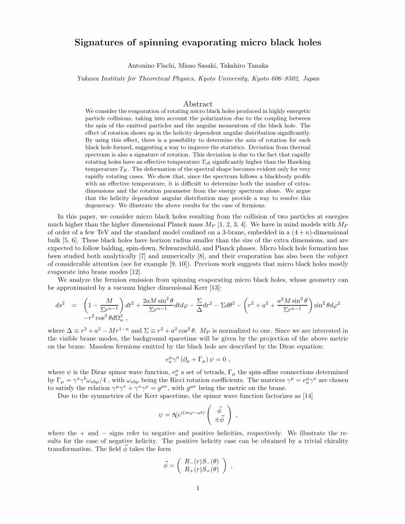
Signatures of spinning evaporating micro black holes
Antonino Flachi, Misao Sasaki, Takahiro Tanaka
Yukawa Institute for Theoretical Physics, Kyoto University, Kyoto 606–8502, Japan
AbstractWe consider the evaporation of rotating micro black holes produced in highly energetic
particle collisions, taking into account the polarization due to the coupling between
the spin of the emitted particles and the angular momentum of the black hole. The
effect of rotation shows up in the helicity dependent angular distribution significantly.
By using this effect, there is a possibility to determine the axis of rotation for each
black hole formed, suggesting a way to improve the statistics. Deviation from thermal
spectrum is also a signature of rotation. This deviation is due to the fact that rapidly
rotating holes have an effective temperature Teff significantly higher than the Hawking
temperature TH . The deformation of the spectral shape becomes evident only for very
rapidly rotating cases. We show that, since the spectrum follows a blackbody profile
with an effective temperature, it is difficult to determine both the number of extra-
dimensions and the rotation parameter from the energy spectrum alone. We argue
that the helicity dependent angular distribution may provide a way to resolve this
degeneracy. We illustrate the above results for the case of fermions.
In this paper, we consider micro black holes resulting from the collision of two particles at energiesmuch higher than the higher dimensional Planck mass MP [1, 2, 3, 4]. We have in mind models with MP
of order of a few TeV and the standard model confined on a 3-brane, embedded in a (4 + n)-dimensionalbulk [5, 6]. These black holes have horizon radius smaller than the size of the extra dimensions, and areexpected to follow balding, spin-down, Schwarzschild, and Planck phases. Micro black hole formation hasbeen studied both analytically [7] and numerically [8], and their evaporation has also been the subjectof considerable attention (see for example [9, 10]). Previous work suggests that micro black holes mostlyevaporate into brane modes [12].
We analyze the fermion emission from spinning evaporating micro black holes, whose geometry canbe approximated by a vacuum higher dimensional Kerr [13]:
ds2 =
(
1 −M
Σrn−1
)
dt2 +2aM sin2 θ
Σrn−1dtdϕ−
Σ
∆dr2 − Σdθ2 −
(
r2 + a2 +a2M sin2 θ
Σrn−1
)
sin2 θdϕ2
−r2 cos2 θdΩ2n ,
where ∆ ≡ r2 + a2 −Mr1−n and Σ ≡ r2 + a2 cos2 θ. MP is normalized to one. Since we are interested inthe visible brane modes, the background spacetime will be given by the projection of the above metricon the brane. Massless fermions emitted by the black hole are described by the Dirac equation:
eµaγ
a (∂µ + Γµ)ψ = 0 ,
where ψ is the Dirac spinor wave function, eµa a set of tetrads, Γµ the spin-affine connections determined
by Γµ = γaγbωabµ/4 , with ωabµ being the Ricci rotation coefficients. The matrices γµ = eµaγ
a are chosento satisfy the relation γµγν + γνγµ = gµν , with gµν being the metric on the brane.
Due to the symmetries of the Kerr spacetime, the spinor wave function factorizes as [14]
ψ = N ei(mϕ−ωt)
(
~φ
±~φ
)
,
where the + and − signs refer to negative and positive helicities, respectively. We illustrate the re-sults for the case of negative helicity. The positive helicity case can be obtained by a trivial chiralitytransformation. The field ~φ takes the form
~φ =
(
R−(r)S−(θ)R+(r)S+(θ)
)
,
1
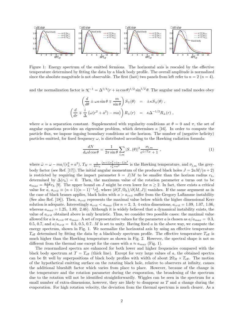
2.0
1.5
1.0
0.5
2 4 6 8 10 12 14
a=0.3acrita=0.5acrita=0.7acrit
ω/Teff
∝dE/dωblack body 2.0
1.5
1.0
0.5
2 4 6 8 10 12 14
a=0.3amaxa=0.5amaxa=0.7amax
ω/Teff
∝dE/dωblack body
2.0
1.5
1.0
0.5
2 4 6 8 10 12 14
a=0.3acrita=0.5acrita=0.7acrit
ω/Teff
∝dE/dωblack body
2.0
1.5
1.0
0.5
2 4 6 8 10 12 14
a=0.3amaxa=0.5amaxa=0.7amax
ω/Teff
∝dE/dω
black body
Figure 1: Energy spectrum of the emitted fermions. The horizontal axis is rescaled by the effectivetemperature determined by fitting the data by a black body profile. The overall amplitude is normalizedsince the absolute magnitude is not observable. The first (last) two panels from left refer to n = 2 (n = 4).
and the normalization factor is N −1 = ∆1/4(r + ia cos θ)1/2 sin1/2 θ. The angular and radial modes obey
(
d
dθ± ωa sin θ ∓
m
sin θ
)
S∓(θ) = ±κS±(θ) ,
(
d
dr∓
i
∆
(
ω(r2 + a2) −ma)
)
R∓(r) = κ∆−1/2R±(r) ,
where κ is a separation constant. Supplemented with regularity conditions at θ = 0 and π, the set ofangular equations provides an eigenvalue problem, which determines κ [16]. In order to compute theparticle flux, we impose ingoing boundary conditions at the horizon. The number of (negative helicity)particles emitted, for fixed frequency ω, is distributed according to the Hawking radiation formula:
dN
dωd cos θ=
1
2π sin θ
∑
l,m
|S−(θ)|2σl,m
eω/TH + 1, (1)
where ω = ω−ma/(r2h + a2), TH = 14πrh
(n+1)r2
h+(n−1)a2
r2
h+a2
is the Hawking temperature, and σl,m the grey-
body factor (see Ref. [17]). The initial angular momentum of the produced black holes J = 2aM/(n+ 2)is restricted by requiring the impact parameter b = J/M to be smaller than the horizon radius rh,determined by ∆(rh) = 0. Then, the maximum value of the rotation parameter a turns out to beamax = n+2
2 rh [9]. The upper bound on J might be even lower for n ≥ 2. In fact, there exists a criticalvalue for a, acrit ≡ (n + 1)(n − 1)−1r2h, where |∂(T,Ωh)/∂(M,J)| vanishes. If the same argument as inthe case of black branes applies, black holes with a > acrit suffer from the Gregory Laflamme instability(See also Ref. [18]). Then, acrit represents the maximal value below which the higher dimensional Kerrsolution is adequate. Interestingly acrit < amax (for n = 2, 3, 4 extra dimensions, acrit = 1.09, 1.07, 1.06,whereas amax = 1.25, 1.89, 2.46). Although it is widely believed that a dynamical instability exists, thevalue of acrit obtained above is only heuristic. Thus, we consider two possible cases: the maximal valueallowed for a is acrit or amax. A set of representative values for the parameter a is chosen as a/amax = 0.3,0.5, 0.7, and a/acrit = 0.3, 0.5, 0.7. M is set to unity. Having fixed a in the above way, we compute theenergy spectrum, shown in Fig. 1. We normalize the horizontal axis by using an effective temperatureTeff determined by fitting the data by a blackbody spectrum profile. The effective temperature Teff ismuch higher than the Hawking temperature as shown in Fig. 2. However, the spectral shape is not sodifferent from the thermal one except for the cases with a ≈ amax (Fig. 1).
The renormalized spectra are enhanced for both lower and higher frequencies compared with theblack body spectrum at T = Teff (thick line). Except for very large values of a, the obtained spectracan be fit well by superpositions of black body profiles with width of about 2ΩH × Teff . The motionof the hypothetical emitting surface on the rotating black hole, relative to observers at infinity, causesthe additional blueshift factor which varies from place to place. However, because of the change inthe temperature and the rotation parameter during the evaporation, the broadening of the spectrumdue to the rotation will not be identified straightforwardly. Wiggles can be seen in the spectrum for asmall number of extra-dimensions, however, they are likely to disappear as T and a change during theevaporation. For high rotation velocity, the deviation from the thermal spectrum is much clearer. As a
2
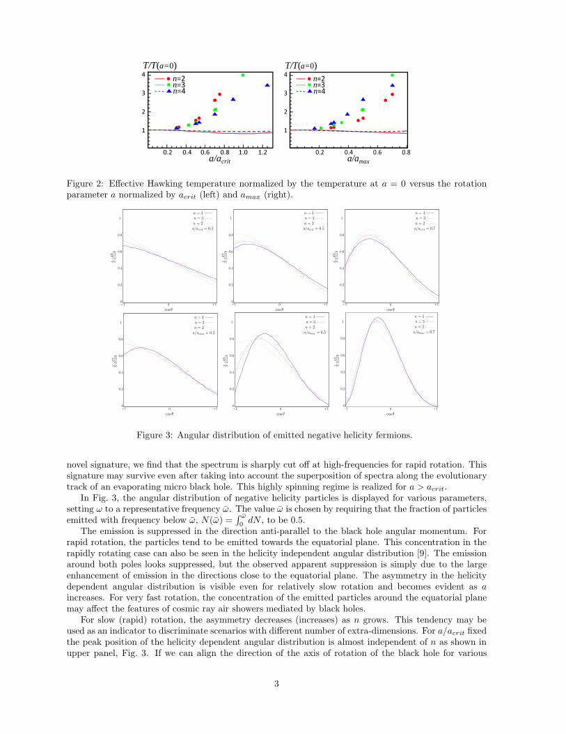
4
3
2
1
0.2 0.4 0.6 0.8 1.0 1.2
n=2n=3n=4
a/acrit
T/T(a=0)4
3
2
1
0.2 0.4 0.6 0.8 a/amax
T/T(a=0)n=2n=3n=4
Figure 2: Effective Hawking temperature normalized by the temperature at a = 0 versus the rotationparameter a normalized by acrit (left) and amax (right).
a/acrit = 0.3
1 N
dN
dcosθ
cos θ
n = 4
n = 3
n = 2
−1 0 +10
0.2
0.4
0.6
0.8
1
a/acrit = 0.5
1 N
dN
dcosθ
cos θ
n = 4
n = 3
n = 2
−1 0 +10
0.2
0.4
0.6
0.8
1
a/acrit = 0.7
1 N
dN
dcosθ
cos θ
n = 4
n = 3
n = 2
−1 0 +10
0.2
0.4
0.6
0.8
1
a/amax = 0.3
1 N
dN
dcosθ
cos θ
n = 4
n = 3
n = 2
−1 0 +10
0.2
0.4
0.6
0.8
1
a/amax = 0.5
1 N
dN
dcosθ
cos θ
n = 4
n = 3
n = 2
−1 0 +10
0.2
0.4
0.6
0.8
1
a/amax = 0.71 N
dN
dcosθ
cos θ
n = 4
n = 3
n = 2
−1 0 +10
0.2
0.4
0.6
0.8
1
Figure 3: Angular distribution of emitted negative helicity fermions.
novel signature, we find that the spectrum is sharply cut off at high-frequencies for rapid rotation. Thissignature may survive even after taking into account the superposition of spectra along the evolutionarytrack of an evaporating micro black hole. This highly spinning regime is realized for a > acrit.
In Fig. 3, the angular distribution of negative helicity particles is displayed for various parameters,setting ω to a representative frequency ω. The value ω is chosen by requiring that the fraction of particlesemitted with frequency below ω, N(ω) =
∫ ω
0dN , to be 0.5.
The emission is suppressed in the direction anti-parallel to the black hole angular momentum. Forrapid rotation, the particles tend to be emitted towards the equatorial plane. This concentration in therapidly rotating case can also be seen in the helicity independent angular distribution [9]. The emissionaround both poles looks suppressed, but the observed apparent suppression is simply due to the largeenhancement of emission in the directions close to the equatorial plane. The asymmetry in the helicitydependent angular distribution is visible even for relatively slow rotation and becomes evident as aincreases. For very fast rotation, the concentration of the emitted particles around the equatorial planemay affect the features of cosmic ray air showers mediated by black holes.
For slow (rapid) rotation, the asymmetry decreases (increases) as n grows. This tendency may beused as an indicator to discriminate scenarios with different number of extra-dimensions. For a/acrit fixedthe peak position of the helicity dependent angular distribution is almost independent of n as shown inupper panel, Fig. 3. If we can align the direction of the axis of rotation of the black hole for various
3
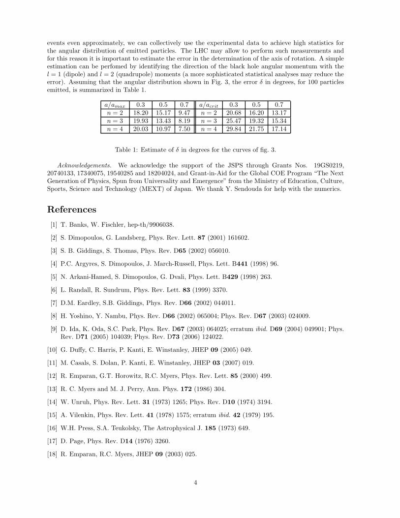
events even approximately, we can collectively use the experimental data to achieve high statistics forthe angular distribution of emitted particles. The LHC may allow to perform such measurements andfor this reason it is important to estimate the error in the determination of the axis of rotation. A simpleestimation can be perfomed by identifying the direction of the black hole angular momentum with thel = 1 (dipole) and l = 2 (quadrupole) moments (a more sophisticated statistical analyses may reduce theerror). Assuming that the angular distribution shown in Fig. 3, the error δ in degrees, for 100 particlesemitted, is summarized in Table 1.
a/amax 0.3 0.5 0.7 a/acrit 0.3 0.5 0.7n = 2 18.20 15.17 9.47 n = 2 20.68 16.20 13.17n = 3 19.93 13.43 8.19 n = 3 25.47 19.32 15.34n = 4 20.03 10.97 7.50 n = 4 29.84 21.75 17.14
Table 1: Estimate of δ in degrees for the curves of fig. 3.
Acknowledgements. We acknowledge the support of the JSPS through Grants Nos. 19GS0219,20740133, 17340075, 19540285 and 18204024, and Grant-in-Aid for the Global COE Program “The NextGeneration of Physics, Spun from Universality and Emergence” from the Ministry of Education, Culture,Sports, Science and Technology (MEXT) of Japan. We thank Y. Sendouda for help with the numerics.
References
[1] T. Banks, W. Fischler, hep-th/9906038.
[2] S. Dimopoulos, G. Landsberg, Phys. Rev. Lett. 87 (2001) 161602.
[3] S. B. Giddings, S. Thomas, Phys. Rev. D65 (2002) 056010.
[4] P.C. Argyres, S. Dimopoulos, J. March-Russell, Phys. Lett. B441 (1998) 96.
[5] N. Arkani-Hamed, S. Dimopoulos, G. Dvali, Phys. Lett. B429 (1998) 263.
[6] L. Randall, R. Sundrum, Phys. Rev. Lett. 83 (1999) 3370.
[7] D.M. Eardley, S.B. Giddings, Phys. Rev. D66 (2002) 044011.
[8] H. Yoshino, Y. Nambu, Phys. Rev. D66 (2002) 065004; Phys. Rev. D67 (2003) 024009.
[9] D. Ida, K. Oda, S.C. Park, Phys. Rev. D67 (2003) 064025; erratum ibid. D69 (2004) 049901; Phys.Rev. D71 (2005) 104039; Phys. Rev. D73 (2006) 124022.
[10] G. Duffy, C. Harris, P. Kanti, E. Winstanley, JHEP 09 (2005) 049.
[11] M. Casals, S. Dolan, P. Kanti, E. Winstanley, JHEP 03 (2007) 019.
[12] R. Emparan, G.T. Horowitz, R.C. Myers, Phys. Rev. Lett. 85 (2000) 499.
[13] R. C. Myers and M. J. Perry, Ann. Phys. 172 (1986) 304.
[14] W. Unruh, Phys. Rev. Lett. 31 (1973) 1265; Phys. Rev. D10 (1974) 3194.
[15] A. Vilenkin, Phys. Rev. Lett. 41 (1978) 1575; erratum ibid. 42 (1979) 195.
[16] W.H. Press, S.A. Teukolsky, The Astrophysical J. 185 (1973) 649.
[17] D. Page, Phys. Rev. D14 (1976) 3260.
[18] R. Emparan, R.C. Myers, JHEP 09 (2003) 025.
4
1
Numerical performance of the Parabolized ADM (PADM)formulation of General Relativity
Jakob Hansen[22]
1Department of Physics, Waseda University, 55N-307, Okubo 3-4-1, Shinjuku-ku, Tokyo 169-8555,
Japan
AbstractA new parabolic extension (PADM) of the standard 3+1 Arnowitt, Deser, Misner(ADM) formulation of the equations of general relativity is presented. By paraboliz-ing first-order ADM in a certain way, the PADM formulation turns it into a mixedhyperbolic - second-order parabolic, well-posed system. The surface of constraints ofPADM becomes a local attractor for all solutions and all possible well-posed gaugeconditions. Numerical properties of PADM are compared with those of standardADM and its hyperbolic Kidder, Scheel, Teukolsky (KST) extension in a series ofstandard tests. The PADM scheme is numerically stable, convergent and second-order accurate. The new formulation has better control of the constraint-violatingmodes than ADM and KST. Full details can be found in [1] and [2].
I. INTRODUCTION
For years people have tried to obtain analytic solutions of the complex field equations of Einstein’sgeneral theory of relativity (GR). Approximation methods have been developed over the course of time,but the most promising tool for tackling problems such as gravitational waves arising from binary blackhole (BBH) or binary neutron star mergers, gravitational collapse etc., is numerical relativity.
The numerical integration of the Einstein equations is not an easy task because the computations canbecome unstable and an exponential blow up of the numerical error may occur, even when the formulationemployed admits a well-posed initial value problem. If the numerical techniques employed and gauge andboundary conditions chosen do not suffer from pathologies, perhaps the most important source that canpotentially lead to instabilities during a free evolution is the growth of the constraint violating modes.Over the years, several methods have been proposed to deal with this type of instability [3–15].
The approach which has attracted most attention in recent years takes advantage of the fact that inthe ideal case where the constraint equations are satisfied, one has the freedom to add combinations ofthe constraint equations to the right-hand-side (RHS) of the evolution equations of a given formulation.By virtue of this freedom, it is also possible to introduce in the system of evolution equations terms whichact as “constraint drivers” and turn the constraint surface into an attractor. This technique is usuallytermed as “constraint damping”.
One way to achieve efficient damping is to construct formulations of GR that under free evolutionforce all constraint violating modes to evolve according to parabolic equations, which are known for theirdamping and smoothing properties [16]. In [1] this goal was achieved by the construction of an evolutionsystem based on the first-order form of the standard Arnowitt, Deser, Misner (ADM) formulation [17],through the addition of appropriate combinations of the derivatives of the constraints and the constraintsthemselves at the RHS of the ADM evolution equations. We call this evolution system the ParabolizedADM (PADM) formulation throughout this work. It was shown in [1] that the evolution of the constraintequations with the PADM formulation are second-order parabolic, independently of the gauge conditionsemployed. This in turn implies that the constraint surface becomes a local attractor. Finally, it wasproved, that the PADM system satisfies the necessary conditions for well-posedness and based on theresults of [18] an argument, which indicates strong evidence that the PADM system admits a well-posedinitial value problem, was given.
The purpose of this work is to test the numerical accuracy and stability of the PADM system, andcompare the PADM formulation with the first-order ADM and the Kidder, Scheel, Teukolsky (KST) [19]formulations. The comparison between the three formulations is carried out in a series of standard one-and two-dimensional tests, usually referred to as the “Apples with Apples” tests or the “Mexico City”tests [20].
2
II. THE PADM FORMULATION
The PADM system is obtained from the first-order ADM formulation [17] by addition of constraintsand their derivatives to the RHS of the ADM evolution equations. The PADM formulation is given by(see [18] for details):
∂tγij = (ADM) + λγab∂bCaij , (1)
∂tKij = (ADM) + φγijγab∂aMb + θ∂(iMj), (2)
∂tDkij = (ADM) + ǫγab∂aCbkij + ξγij∂kH + ζCkij , (3)
where λ, φ, θ, ǫ, ξ, ζ are the six parameters of the formulation and where H,Mb, Caij and Cbkij are theconstraint equations of the first order ADM formulation. We refer to the added terms of the PADMformulation as the constraint driver. It was shown in [1] that for gauges which do not introduce second-order derivatives of the dynamical variables in the evolution equations the PADM system satisfies thePetrovskii condition for well-posedness [21], provided that
λ > 0, ǫ > 0, ξ < 0, φ < 0, θ > 0. (4)
Therefore, in this work we use the PADM equations in conjunction with the algebraic gauge conditionα = α(γ), βi = 0.
When the aforementioned conditions are satisfied, the PADM system has the following properties:a) The PADM evolution equations can be classified as a set of mixed hyperbolic - second-order parabolic
quasi-linear partial differential equations.b) The evolution equations of the constraint variables become second-order parabolic partial differ-
ential equations (PDEs) independently of the spacetime geometry and the gauge conditions employed.Therefore, the constraint propagation equations admit a well-posed Cauchy problem themselves.
c) Because of the parabolic structure of the evolution equations of the constraints, the constraintsurface becomes a local attractor. All small amplitude, high-frequency constraint-violating perturbationsare exponentially damped in time as exp(−λκ2t), where κ is the magnitude of the wavevector of theperturbations. This in turn implies that the hazardous high frequency perturbations will be dampedvery efficiently. This is espcially of importance in numerical simulations since it is most often the highfrequency perturbations that kills a simulation.
III. NUMERICAL TESTS
To test the numerical performance of the PADM formulation, we used the so-called ”Apples WithApples“ [20] tests, which were designed to provide the numerical relativity community with a set of stan-dard tests that could be use to, quantitatively, compare different numerical implementations of differentformulations of GR.
The tests are briefly described below, for in-detail descriptions of the tests and their results, see [2].The tests include both one- and two-dimensional solutions. For 1D tests the simulations are run for1000 light crossings (or until the code crash) and for 2D tests, the simulations are run for 100 lightcrossings (or until the code crash). Note that the dimensionality of the tests refers to the dimensionaltyof the solutions, not the grid, i.e. for a 1D test, the wave travels parallel to the computational mesh,for a 2D test, the solution wave travels diagonally. However, all tests are carried out in a 3 dimensionalcomputational mesh, such that all cross derivatives are evaluated and the full Einstein equations are thusevolved. The tests are :
• Standard Robust Stability Test : The standard robust stability test is based on small randomperturbations about Minkowski spacetime. In this test, all the dynamic variables are set equal totheir Minkowski space values and the initial data are then perturbed by random noise of sufficientlysmall amplitude such that the evolution remains in the linearized regime unless any instabilitiesarise. The perturbed initial data is then evolved for 1000 light crossing (or until the simulation
3
crashes) Although being a very simple test, it is naturally a very important one since all codes willexperience such random perturbations due to numerical roundoff and truncation errors, hence allcodes must be able to pass this test sucessfully.
The main outcome of this test was that 1) ADM fails miserably due to the illposed nature of thisformulation, 2) KST pass this test, but the constraint violations are seen to grow linearly in timesince this formulation has no mechanism of dissipating constraint violations. 3) In strong contrastto this, the PADM formulation not only pass this test perfectly, but the constraint violations areseen to be quickly damped away. In particular, it is shown that high frequency perturbations aredamped away extremely quickly.
• Strong Robust Stability Test : Another version of the robust test (not included in the standard”Apples With Apples“ testbed) requires perturbation by random noise not only at the initial time-step, but at every time-step throughout the entire simulation. We call this test the “strong” robuststability test. This test is much more challenging than the standard robust test and is much closerto reality because in numerical simulations, truncation and round-off errors will unavoidably beintroduced into the solution of the PDE system at every time-step.
The result of this test is again that 1) ADM fails, 2) KST pass this test if the amplitude of the noiseis sufficiently small or if the simulation is run for only a short time. But since KST has no wayof dissipating the introduced noise, eventually KST will crash. 3) In contrast to this, PADM passthis test for even high amplitude noise and show no indications of any instabilities or growth of theconstraint violations due to the PADM formulations unique ability to damp constraint violations.
• Gauge Wave Test : In the gauge wave test, a gauge wave is evolved in both a one-dimensionaland two-dimensional form. Both 1D and 2D tests are carried out for gauge waves with differentamplitudes. The gauge wave stability test has proven to be one of the most challenging testsfor most evolution schemes mainly due to the existence of a one-parameter family of exponential,harmonic gauge solutions that is excited by truncation errors during numerical solutions. Thiseventually causes the numerical solution to veer off the analytic one.
The result of this test is that PADM performs better than both ADM and KST. In particular it isshown that PADM can pass the two-dimensional, high amplitude gauge wave test. We know of noother formulations which can do this, including BSSN.
• Linear Weak Wave Test : The linear wave test evolves a traveling gravitational wave ofamplitude small enough so the evolution remains in the linear regime. This test is carried out inboth a one-dimensional and two-dimensional form.
This test pose no particular problems for most formulations and both ADM, KST and PADM canpass this test. However, PADM is still seen to have better control of the constraint violations thanthe other two formulations.
• Gowdy Wave Test : The polarized Gowdy T3 spacetimes are solutions of the Einstein equa-tions which describe an expanding (or contracting) universe containing plane polarized gravitationalwaves, see for example [20] and references therein. The previous tests can be considered as pertur-bations about flat spacetime, so they probe the weak field limit of the Einstein equations, whereasthe Gowdy test probes the strong field regime of GR.
– The expanding Gowdy wave test has proved to be one of the most challenging problemsin numerical relativity. This is because the metric components grow exponentially with timeand hence the truncation errors introduced in the numerical solution grow with time, if theresolution is fixed. Consequently, the numerical solution soon veers off the analytical one. An-other result of the exponential growth is that the dynamical variables eventually grow so largethat the computations cannot be handled by using standard 64-bit floating-point arithmetic.Therefore, all simulations of the expanding Gowdy solution will eventually terminate [20].
Our results for the expanding Gowdy wave test is that KST performs particularly bad in thistest and crash after just 20 lightcrossing times. The ADM formulation performs suprisinglywell and can do roughly 260 light crossings before accuracy is completely lost, but the winneris still the PADM formulation which does not terminate until 275 light crossing times has
4
passed. The reason why ADM performs relatively well in this test is that the solution is one-dimensional and in the particular case of one-dimensional solutions, the ADM formulation canbe shown to be well posed [1].
– The collapsing Gowdy wave test is less challenging and all the formulations are able topass this test. However, still we see that PADM performs (marinally) better than the othertwo formulations.
For all tests we thus find that PADM behaves better than the ADM and KST formulations. Inparticular, PADM can pass the high amplitude gauge wave test and performs better in the expandinggowdy wave test than any other formulations know to the authors.
The most important feature of the PADM formulation is that it damps away constraint violatingperturbations and thus drive the solution back to the surface of constraints. High frequency constraintviolations are damped away the most effectively, which is important for ensuring the numerical stabilityof PADM implementations.
IV. CONCLUSIONS
In [1] is presented the PADM formulation of GR and in [2] we have described a stable, convergent andsecond-order accurate numerical scheme for solving the equations of the PADM system. Also in [2] wehave tested the accuracy and stability of the PADM system and compared it with the first-order ADMand KST evolution systems using the ”Apples with Apples” tests.
For all tests we find that PADM behaves significantly better than the ADM and KST formulations.In particular, the PADM formulation damps away constraint violating perturbations and thus drive thesolution back to the surface of constraints. High frequency violations are damped away most effectively.
We conclude that PADM successfully passes the standard tests of numerical relativity and works equallywell with a variety of algebraic gauges. Via the comparison of the numerical performance of the PADMformulation and those of the ADM and the KST formulations, we conclude that PADM has better controlof the constraint violations than both ADM and KST. This leads to hope that the PADM formulationcan lead to new advances in numerical relativity.
[1] V. Paschalidis, Phys.Rev.D 78, 024002 (2008), gr-qc/0704.2861.[2] V. Paschalidis, J. Hansen, and A. Khokhlow, Phys. Rev. D 78, 064048 (2008), gr-qc/0712.1258.[3] R. F. Stark and T. Piran, Phys. Rev. Lett 55, 891 (1985).[4] A. M. Abrahams and C. R. Evans, Phys. Rev. D 46, R4117 (1992).[5] M. W. Choptuik, Phys. Rev. Lett. 70, 9 (1993).[6] A. M. Abrahams and C. R. Evans, Phys. Rev. Lett 70, 2980 (1993).[7] A. M. A. et al., Phys. Rev. D 49, 5153 (1994).[8] M. W. C. et al., Class. Quantum Grav. 20, 1857 (2003).[9] M. W. C. et al., Phys. Rev. D2 68, 044007 (2003).
[10] O. Brodbeck, S. Frittelli, P. Haubner, and O. A. Reula, J. Math. Phys. 40, 909 (1999).[11] C. Gundlach, G. Calabrese, I. Hinder, and J. M. Martın-Garcıa, Class. Quantum Grav. 22, 3767 (2005).[12] G. Yoneda and H. aki Shinkai (2001).[13] M. H. et al., Phys. Rev. D, (2004).[14] M. Anderson and R. A. Matzner, Found. Phys 35, 1477 (2005).[15] D. R. Fiske, Phys. Rev. D 69, 047501 (2004).[16] H.-O. Kreiss and J. Lorenz, Initial-Boundary Value Problems and the Navier-Stokes Equations (Academic
Press Inc., 1989).[17] R. Arnowitt, S. Deser, and C. W. Misner, Gravitation: An Introduction to Current research (Wiley, 1962),
gr-qc/0405109.[18] V. Paschalidis, A. M. Khokhlov, and I. D. Novikov, Phys. Rev. D 75, 024026 (2007).[19] L. E. Kidder, M. A. Scheel, and S. A. Teukolsky, Phys. Rev. D 64, 064017 (2001).[20] M. A. et al., Class. Quant. Grav. 21, 589 (2004).[21] B. Gustafsson, H. Kreiss, and J. Oliger, Time dependent problems and difference methods (John Willey &
Sons, 1995).[22] E-mail:[email protected]
Gravitational collapse of a dust ball from the perspective ofloop quantum gravity: an application
Tomohiro Harada1
Department of Physics, Rikkyo University, Toshima, Tokyo 171–8501, Japan
AbstractAt an effective level, consistent versions of dynamics with corrections from loop quan-
tum gravity are presented which implement the conditions together with the dynami-
cal constraints of gravity in an anomaly-free manner. These are then used for analyt-
ical as well as numerical investigations of the fate of classical singularities, including
non-spacelike ones, as they generically develop in these models. None of the correc-
tions used here resolve those singularities by regular effective geometries. However,
there are numerical indications that the collapse ends in a tamer shell-crossing singu-
larity prior to the formation of central singularities for mass functions giving a regular
conserved mass density. Moreover, we find quantum gravitational obstructions to the
existence of exactly homogeneous solutions within this class of models. This indicates
that homogeneous models must be seen in a wider context of inhomogeneous solutions
and their reduction in order to provide reliable dynamical conclusions.
1 Introduction
Quantum gravity is supposed to solve the problems, such as, how we can deal with spacetime singularitieswhich appear in big bang and in gravitational collapse in classical general relativity, how black holeentropy is related to the microscopic degrees of freedom, whether a black hole evaporates away completelyor leaves a Planck mass relic and how gravitational force behaves from low-energy scale to the Planckscale? We here focus on the problem how loop quantum gravity (LQG) affects the scenario of spacetimesingularities in gravitational collapse. LQG is nonperturbative, background-independent quantum gravitywith no ultraviolet divergence. This is based on a canonical quantisation approach. LQG has inspiredloop quantum cosmology (LQC), which successfully avoids big bang singularity and predicts a bouncinguniverse
This article is based on the collaboration with M. Bojowald and R. Tibrewala. Details of the presentanalysis is given in Ref [1]. We use the unit in which c = 1.
2 Lemaitre-Tolman-Bondi spacetime in classical theory
The Lemaitre-Tolman-Bondi (LTB) solution is an exact solution to Einstein’s field equations, whichdescribes the evolution of a spherically symmetric inhomogeneous dust cloud. Here, we focus on themarginally bound case, in which the energy function, which is the sum of kinetic energy and potentialenergy, vanishes identically. The line element in this solution is given by
ds2 = −dt2 + R′2dx2 + R2(dθ2 + sin2 θdφ2), (1)
R(t, x) =
(
x3/2 − 3
2
√
F (x)t
)2/3
, (2)
where F (x) is an arbitrary function, which is twice the conserved dust mass, and the prime denotes thederivative with respect to x. The density of the dust is given by
ε =F ′
8πGR2R′, (3)
1E-mail:[email protected]
1
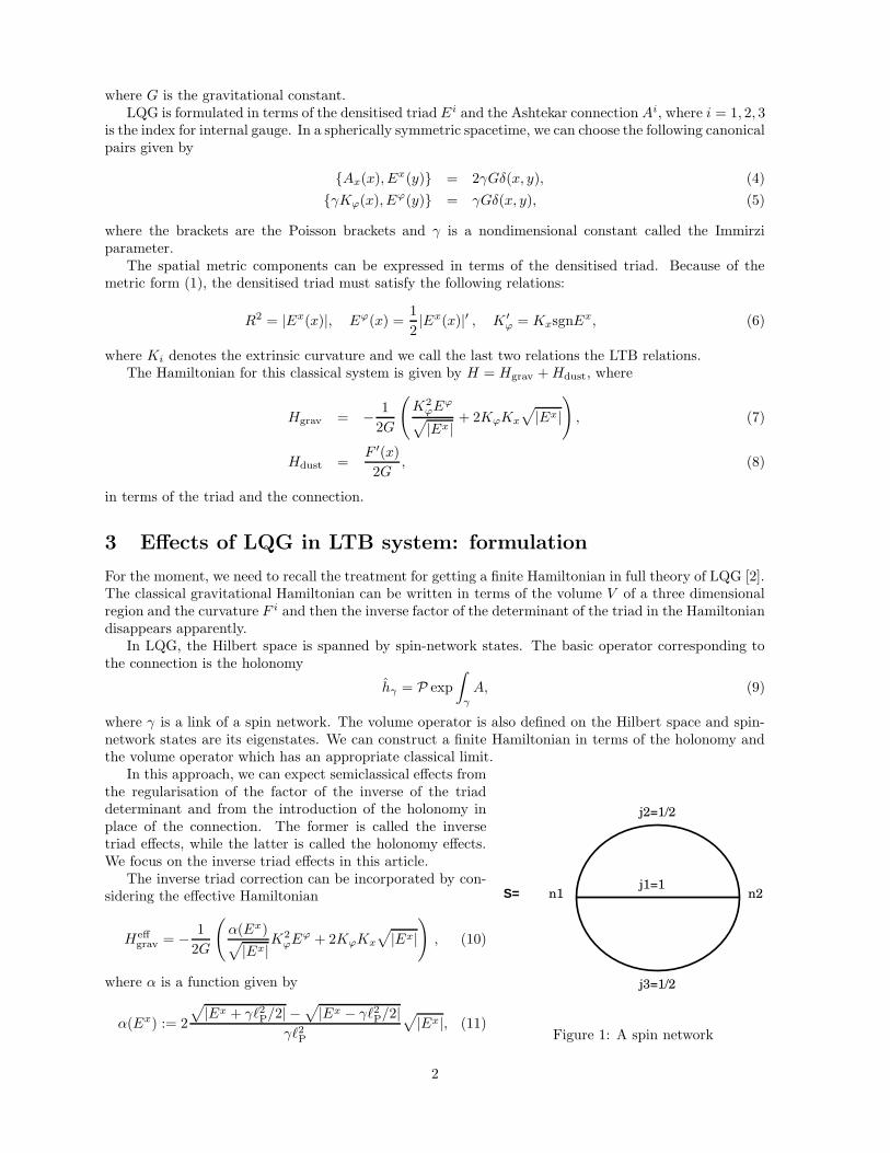
where G is the gravitational constant.LQG is formulated in terms of the densitised triad Ei and the Ashtekar connection Ai, where i = 1, 2, 3
is the index for internal gauge. In a spherically symmetric spacetime, we can choose the following canonicalpairs given by
Ax(x), Ex(y) = 2γGδ(x, y), (4)
γKϕ(x), Eϕ(y) = γGδ(x, y), (5)
where the brackets are the Poisson brackets and γ is a nondimensional constant called the Immirziparameter.
The spatial metric components can be expressed in terms of the densitised triad. Because of themetric form (1), the densitised triad must satisfy the following relations:
R2 = |Ex(x)|, Eϕ(x) =1
2|Ex(x)|′ , K ′
ϕ = KxsgnEx, (6)
where Ki denotes the extrinsic curvature and we call the last two relations the LTB relations.The Hamiltonian for this classical system is given by H = Hgrav + Hdust, where
Hgrav = − 1
2G
(
K2ϕEϕ
√
|Ex|+ 2KϕKx
√
|Ex|)
, (7)
Hdust =F ′(x)
2G, (8)
in terms of the triad and the connection.
3 Effects of LQG in LTB system: formulation
For the moment, we need to recall the treatment for getting a finite Hamiltonian in full theory of LQG [2].The classical gravitational Hamiltonian can be written in terms of the volume V of a three dimensionalregion and the curvature F i and then the inverse factor of the determinant of the triad in the Hamiltoniandisappears apparently.
In LQG, the Hilbert space is spanned by spin-network states. The basic operator corresponding tothe connection is the holonomy
hγ = P exp
∫
γ
A, (9)
where γ is a link of a spin network. The volume operator is also defined on the Hilbert space and spin-network states are its eigenstates. We can construct a finite Hamiltonian in terms of the holonomy andthe volume operator which has an appropriate classical limit.
n1 n2
j2=1/2
j1=1
j3=1/2
S=
Figure 1: A spin network
In this approach, we can expect semiclassical effects fromthe regularisation of the factor of the inverse of the triaddeterminant and from the introduction of the holonomy inplace of the connection. The former is called the inversetriad effects, while the latter is called the holonomy effects.We focus on the inverse triad effects in this article.
The inverse triad correction can be incorporated by con-sidering the effective Hamiltonian
Heffgrav = − 1
2G
(
α(Ex)√
|Ex|K2
ϕEϕ + 2KϕKx
√
|Ex|)
, (10)
where α is a function given by
α(Ex) := 2
√
|Ex + γ`2P/2| −
√
|Ex − γ`2P/2|
γ`2P
√
|Ex|, (11)
2
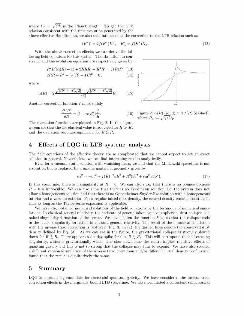
where `P =√
Gh is the Planck length. To get the LTBrelation consistent with the time evolution generated by theabove effective Hamiltonian, we also take into account the correction to the LTB relation such as
(Ex)′ = 2f(Ex)Eϕ, K ′
ϕ = f(Ex)Kx. (12)
1R/R*
0
1
α(R
/R*)
, f(R
/R*)
Figure 2: α(R) (solid) and f(R) (dashed),where R∗ :=
√
γ/2`P.
With the above correction effects, we can derive the fol-lowing field equations for this system. The Hamiltonian con-straint and the evolution equation are respectively given by
R2R′(α(R) − 1) + 2RRR′ + R2R′ = f(R)F ′ (13)
2RR + R2 + (α(R) − 1)R2 = 0 , (14)
where
α(R) = 2
√
|R2 + γ`2P/2| −
√
|R2 − γ`2P/2|
γ`2P
R. (15)
Another correction function f must satisfy
df(R)
dR= (1 − α(R))
f
R. (16)
The correction functions are plotted in Fig. 2. In this figure,we can see that the the classical value is recovered for R R∗
and the deviation becomes significant for R <∼ R∗.
4 Effects of LQG in LTB system: analysis
The field equations of the effective theory are so complicated that we cannot expect to get an exactsolution in general. Nevertheless, we can find interesting results analytically.
Even for a vacuum static solution with vanishing mass, we find that the Minkowski spacetime is nota solution but is replaced by a unique nontrivial geometry given by
ds2 = −dt2 + f(R)−2dR2 + R2(dθ2 + sin2 θdφ2). (17)
In this spacetime, there is a singularity at R = 0. We can also show that there is no bounce becauseR = 0 is impossible. We can also show that there is no Friedmann solution, i.e, the system does notallow a homogeneous solution and that there is no Oppenheimer-Snyder-like solution with a homogeneousinterior and a vacuum exterior. For a regular initial dust density, the central density remains constant intime as long as the Taylor-series expansion is applicable.
We have also obtained numerical solutions of the field equations by the technique of numerical simu-lations. In classical general relativity, the endstate of generic inhomogeneous spherical dust collapse is anaked singularity formation at the centre. We have chosen the function F (x) so that the collapse endsin the naked singularity formation in classical general relativity. The result of the numerical simulationwith the inverse triad correction is plotted in Fig. 3. In (a), the dashed lines denote the conserved dustdensity defined by Eq. (3). As we can see in the figure, the gravitational collapse is strongly sloweddown for R <∼ R∗ There appears a density spike for 0 < R <∼ R∗. This will correspond to shell-crossingsingularity, which is gravitationally weak. The slow down near the centre implies repulsive effects ofquantum gravity but this is not so strong that the collapse may turn to expand. We have also studieda different version formulation of the inverse triad correction and/or different initial density profiles andfound that the result is qualitatively the same.
5 Summary
LQG is a promising candidate for successful quantum gravity. We have considered the inverse triadcorrection effects in the marginally bound LTB spacetime. We have formulated a consistent semiclassical
3
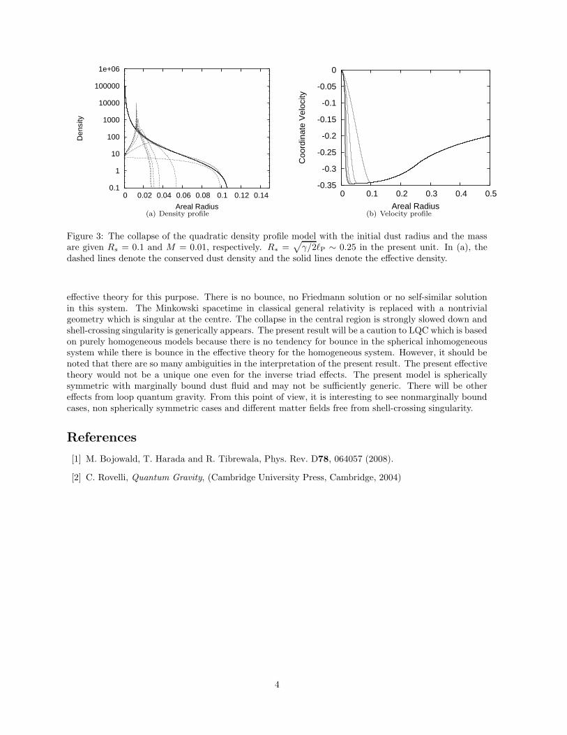
0.1
1
10
100
1000
10000
100000
1e+06
0 0.02 0.04 0.06 0.08 0.1 0.12 0.14
Den
sity
Areal Radius(a) Density profile
-0.35
-0.3
-0.25
-0.2
-0.15
-0.1
-0.05
0
0 0.1 0.2 0.3 0.4 0.5
Coo
rdin
ate
Vel
ocity
Areal Radius(b) Velocity profile
Figure 3: The collapse of the quadratic density profile model with the initial dust radius and the massare given Rs = 0.1 and M = 0.01, respectively. R∗ =
√
γ/2`P ∼ 0.25 in the present unit. In (a), thedashed lines denote the conserved dust density and the solid lines denote the effective density.
effective theory for this purpose. There is no bounce, no Friedmann solution or no self-similar solutionin this system. The Minkowski spacetime in classical general relativity is replaced with a nontrivialgeometry which is singular at the centre. The collapse in the central region is strongly slowed down andshell-crossing singularity is generically appears. The present result will be a caution to LQC which is basedon purely homogeneous models because there is no tendency for bounce in the spherical inhomogeneoussystem while there is bounce in the effective theory for the homogeneous system. However, it should benoted that there are so many ambiguities in the interpretation of the present result. The present effectivetheory would not be a unique one even for the inverse triad effects. The present model is sphericallysymmetric with marginally bound dust fluid and may not be sufficiently generic. There will be othereffects from loop quantum gravity. From this point of view, it is interesting to see nonmarginally boundcases, non spherically symmetric cases and different matter fields free from shell-crossing singularity.
References
[1] M. Bojowald, T. Harada and R. Tibrewala, Phys. Rev. D78, 064057 (2008).
[2] C. Rovelli, Quantum Gravity, (Cambridge University Press, Cambridge, 2004)
4
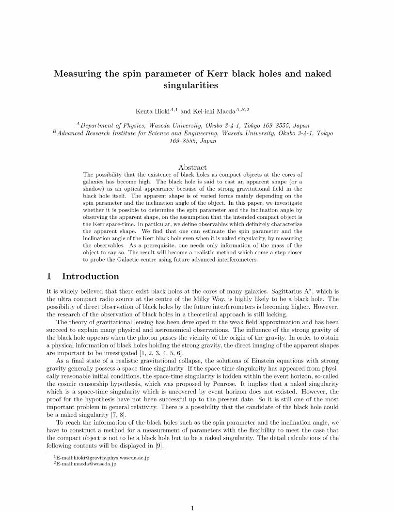
Measuring the spin parameter of Kerr black holes and nakedsingularities
Kenta HiokiA,1 and Kei-ichi MaedaA,B,2
ADepartment of Physics, Waseda University, Okubo 3-4-1, Tokyo 169–8555, JapanBAdvanced Research Institute for Science and Engineering, Waseda University, Okubo 3-4-1, Tokyo
169–8555, Japan
AbstractThe possibility that the existence of black holes as compact objects at the cores ofgalaxies has become high. The black hole is said to cast an apparent shape (or ashadow) as an optical appearance because of the strong gravitational field in theblack hole itself. The apparent shape is of varied forms mainly depending on thespin parameter and the inclination angle of the object. In this paper, we investigatewhether it is possible to determine the spin parameter and the inclination angle byobserving the apparent shape, on the assumption that the intended compact object isthe Kerr space-time. In particular, we define observables which definitely characterizethe apparent shape. We find that one can estimate the spin parameter and theinclination angle of the Kerr black hole even when it is naked singularity, by measuringthe observables. As a prerequisite, one needs only information of the mass of theobject to say so. The result will become a realistic method which come a step closerto probe the Galactic centre using future advanced interferometers.
1 Introduction
It is widely believed that there exist black holes at the cores of many galaxies. Sagittarius A∗, which isthe ultra compact radio source at the centre of the Milky Way, is highly likely to be a black hole. Thepossibility of direct observation of black holes by the future interferometers is becoming higher. However,the research of the observation of black holes in a theoretical approach is still lacking.
The theory of gravitational lensing has been developed in the weak field approximation and has beensucceed to explain many physical and astronomical observations. The influence of the strong gravity ofthe black hole appears when the photon passes the vicinity of the origin of the gravity. In order to obtaina physical information of black holes holding the strong gravity, the direct imaging of the apparent shapesare important to be investigated [1, 2, 3, 4, 5, 6].
As a final state of a realistic gravitational collapse, the solutions of Einstein equations with stronggravity generally possess a space-time singularity. If the space-time singularity has appeared from physi-cally reasonable initial conditions, the space-time singularity is hidden within the event horizon, so-calledthe cosmic censorship hypothesis, which was proposed by Penrose. It implies that a naked singularitywhich is a space-time singularity which is uncovered by event horizon does not existed. However, theproof for the hypothesis have not been successful up to the present date. So it is still one of the mostimportant problem in general relativity. There is a possibility that the candidate of the black hole couldbe a naked singularity [7, 8].
To reach the information of the black holes such as the spin parameter and the inclination angle, wehave to construct a method for a measurement of parameters with the flexibility to meet the case thatthe compact object is not to be a black hole but to be a naked singularity. The detail calculations of thefollowing contents will be displayed in [9].
1E-mail:[email protected]:[email protected]
1
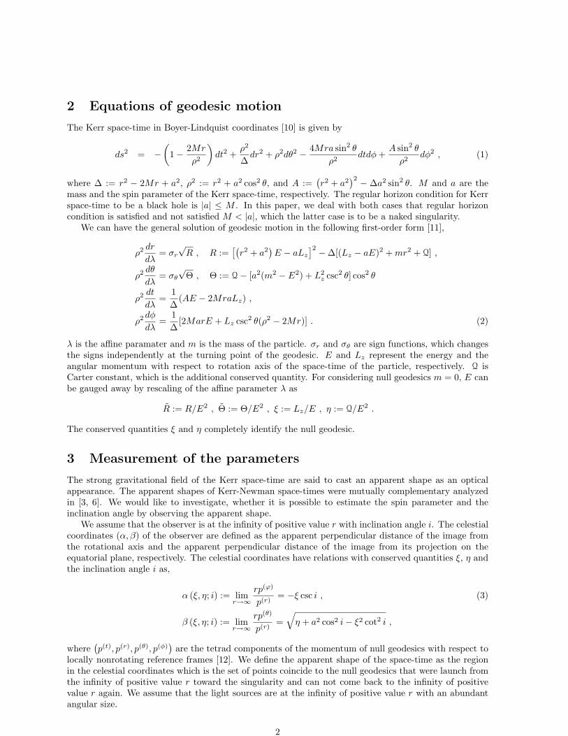
2 Equations of geodesic motion
The Kerr space-time in Boyer-Lindquist coordinates [10] is given by
ds2 = −(
1− 2Mr
ρ2
)dt2 +
ρ2
∆dr2 + ρ2dθ2 − 4Mra sin2 θ
ρ2dtdφ +
A sin2 θ
ρ2dφ2 , (1)
where ∆ := r2 − 2Mr + a2, ρ2 := r2 + a2 cos2 θ, and A :=(r2 + a2
)2 − ∆a2 sin2 θ. M and a are themass and the spin parameter of the Kerr space-time, respectively. The regular horizon condition for Kerrspace-time to be a black hole is |a| ≤ M . In this paper, we deal with both cases that regular horizoncondition is satisfied and not satisfied M < |a|, which the latter case is to be a naked singularity.
We can have the general solution of geodesic motion in the following first-order form [11],
ρ2 dr
dλ= σr
√R , R :=
[(r2 + a2
)E − aLz
]2 −∆[(Lz − aE)2 + mr2 + Q] ,
ρ2 dθ
dλ= σθ
√Θ , Θ := Q− [a2(m2 − E2) + L2
z csc2 θ] cos2 θ
ρ2 dt
dλ=
1∆
(AE − 2MraLz) ,
ρ2 dφ
dλ=
1∆
[2MarE + Lz csc2 θ(ρ2 − 2Mr)] . (2)
λ is the affine paramater and m is the mass of the particle. σr and σθ are sign functions, which changesthe signs independently at the turning point of the geodesic. E and Lz represent the energy and theangular momentum with respect to rotation axis of the space-time of the particle, respectively. Q isCarter constant, which is the additional conserved quantity. For considering null geodesics m = 0, E canbe gauged away by rescaling of the affine parameter λ as
R := R/E2 , Θ := Θ/E2 , ξ := Lz/E , η := Q/E2 .
The conserved quantities ξ and η completely identify the null geodesic.
3 Measurement of the parameters
The strong gravitational field of the Kerr space-time are said to cast an apparent shape as an opticalappearance. The apparent shapes of Kerr-Newman space-times were mutually complementary analyzedin [3, 6]. We would like to investigate, whether it is possible to estimate the spin parameter and theinclination angle by observing the apparent shape.
We assume that the observer is at the infinity of positive value r with inclination angle i. The celestialcoordinates (α, β) of the observer are defined as the apparent perpendicular distance of the image fromthe rotational axis and the apparent perpendicular distance of the image from its projection on theequatorial plane, respectively. The celestial coordinates have relations with conserved quantities ξ, η andthe inclination angle i as,
α (ξ, η; i) := limr→∞
rp(ϕ)
p(r)= −ξ csc i , (3)
β (ξ, η; i) := limr→∞
rp(θ)
p(r)=
√η + a2 cos2 i− ξ2 cot2 i ,
where(p(t), p(r), p(θ), p(φ)
)are the tetrad components of the momentum of null geodesics with respect to
locally nonrotating reference frames [12]. We define the apparent shape of the space-time as the regionin the celestial coordinates which is the set of points coincide to the null geodesics that were launch fromthe infinity of positive value r toward the singularity and can not come back to the infinity of positivevalue r again. We assume that the light sources are at the infinity of positive value r with an abundantangular size.
2
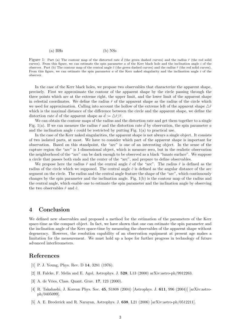
(a) BHs (b) NSs
Figure 1: Part (a) The contour map of the distorted rate d (the green dashed curves) and the radius r (the red solidcurves). From this figure, we can estimate the spin parameter a of the Kerr black hole and the inclination angle i of theobserver. Part (b) The contour map of the central angle c (the green dashed curves) and the radius r (the red solid curves).From this figure, we can estimate the spin parameter a of the Kerr naked singularity and the inclination angle i of theobserver.
In the case of the Kerr black holes, we propose two observables that characterize the apparent shape,precisely. First we approximate the contour of the apparent shape by the circle passing through thethree points which are at the extreme right, the upper limit, and the lower limit of the apparent shapein celestial coordinates. We define the radius r of the apparent shape as the radius of the circle whichwe used for approximation. Calling into account the hollow of the extreme left of the apparent shape 4rwhich is the maximal distance of the difference between the circle and the apparent shape, we define thedistortion rate d of the apparent shape as d := 4r/r.
We can obtain the contour maps of the radius and the distortion rate and get them together to a singleFig. 1(a). If we can measure the radius r and the distortion rate d by observation, the spin parameter aand the inclination angle i could be restricted by putting Fig. 1(a) to practical use.
In the case of the Kerr naked singularities, the apparent shape is not always a single object. It consistsof two isolated parts, at most. We have to consider which part of the apparent shape is important forobservation. Based on this standpoint, the “arc” is one of an interesting object. In the sense of thecapture region the “arc” is 1-dimensional object, which is measure zero, but in the realistic observationthe neighborhood of the “arc” can be dark enough to be observed as a black “lunate surface”. We supposea circle that passes both ends and the center of the “arc”, and prepare to define observables.
We propose here the radius r and the central angle c of the “arc”. The radius r is defined as theradius of the circle which we supposed. The central angle c is defined as the angular distance of the arcsegment on the circle. The radius and the central angle feature the shape of the “arc”, which continuouslychanges by the spin parameter and the inclination angle. Fig. 1(b) is the contour map of the radius andthe central angle, which enable one to estimate the spin parameter and the inclination angle by observingthe two observables r and c.
4 Conclusion
We defined new observables and proposed a method for the estimation of the parameters of the Kerrspace-time as the compact object. In fact, we have shown that one can estimate the spin parameter andthe inclination angle of the Kerr space-time by measuring the observables of the apparent shape withoutdegeneracy. However, the resolution capability of an observation equipment at present age makes alimitation for the measurement. We must hold up a hope for further progress in technology of futureadvanced interferometers.
References
[1] P. J. Young, Phys. Rev. D 14, 3281 (1976).
[2] H. Falcke, F. Melia and E. Agol, Astrophys. J. 528, L13 (2000) arXiv:astro-ph/9912263.
[3] A. de Vries, Class. Quant. Grav. 17, 123 (2000).
[4] R. Takahashi, J. Korean Phys. Soc. 45, S1808 (2004) [Astrophys. J. 611, 996 (2004)] [arXiv:astro-ph/0405099].
[5] A. E. Broderick and R. Narayan, Astrophys. J. 638, L21 (2006) [arXiv:astro-ph/0512211].
3
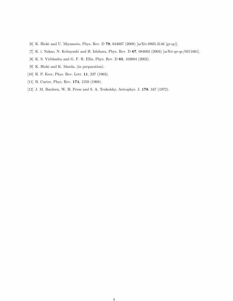
[6] K. Hioki and U. Miyamoto, Phys. Rev. D 78, 044007 (2008) [arXiv:0805.3146 [gr-qc]].
[7] K. i. Nakao, N. Kobayashi and H. Ishihara, Phys. Rev. D 67, 084002 (2003) [arXiv:gr-qc/0211061].
[8] K. S. Virbhadra and G. F. R. Ellis, Phys. Rev. D 65, 103004 (2002).
[9] K. Hioki and K. Maeda, (in preparation).
[10] R. P. Kerr, Phys. Rev. Lett. 11, 237 (1963).
[11] B. Carter, Phys. Rev. 174, 1559 (1968).
[12] J. M. Bardeen, W. H. Press and S. A. Teukolsky, Astrophys. J. 178, 347 (1972).
4
Non-linear evolution of matter power spectrum in a closuretheory
Takashi Hiramatsu1, Kazuya Koyama2 and Atsushi Taruya3
1Institute for Cosmic Ray Research (ICRR), The University of Tokyo, Chiba 277–8582, Japan2Institute of Cosmology & Gravitation, University of Portsmouth, Portsmouth, Hampshire, PO1 2EG,
UK3Research Center for the Early Universe (RESCEU), The University of Tokyo, Tokyo 113–0033, Japan
AbstractWe study the non-linear evolution of cosmological power spectra in a closure the-ory. Governing equations for matter power spectra have been previously derived bya non-perturbative technique with closure approximation. Solutions of the resultantclosure equations just correspond to the resummation of an infinite class of pertur-bation corrections, and they consistently reproduce the one-loop results of standardperturbation theory. We develop a numerical algorithm to solve closure evolutionsin both perturbative and non-perturbative regimes. The present numerical scheme isparticularly suited for examining non-linear matter power spectrum in general cos-mological models, including modified theory of gravity. As a demonstration, we applyour numerical scheme to the Dvali-Gabadadze-Porrati braneworld model.
1 Introduction
Probing the nature of dark energy, accelerating the late-time universe, is one of the most tough issuesin cosmology and astrophysics. So far it remains to be clarified what the dark energy really is. Asimple solution is that it is the cosmological constant, or described by dynamics of unknown scalar fields.Another solution may lie in the sector of gravity. The attention has been focused on the test of generalrelativity (GR) in both solar system experiments and cosmological contexts. Several modified theoriesof gravity beyond GR have passed these tests and been viable. A key to distinguish these possibilities isto precisely predict the matter power spectrum considering non-linear dynamics of matter perturbations.This situation motivates to develop a framework to compute the non-linear matter power spectrum in avariety of cosmological models.
The naive perturbative approach (see [1] for a review) has been frequently used for predictions ofthe power spectra, as well as fully numerical approach such as N-body simulations. Recently, alternativeto perturbation theory, several authors have recently proposed the renormalisation/resummation tech-nique for the infinite series of the loop calculation appeared in the naive expansion of the perturbativequantities. In those treatments, the fundamental quantities are not the density/velocity perturbationsbut propagators, power spectra and vertex functions of density and velocity divergence [2]. In our previ-ous paper [3], we have derived evolution equations of the non-perturbative quantities, power spectra andpropagators of matter fluctuations on the basis of the closure approximation used in the statistical theoryof turbulence [4]. This approach is suited for numerical purpose where we set the initial conditions andtrack the time evolution of those quantities.
In this paper, we demonstrate the closure equations in the case of Dvali-Gabadadze-Poratti (DGP)braneworld model. For the numerical scheme, please see [5] and, for the numerical analysis, [6].
2 Evolution equations for perturbations
We consider the cold dark matter plus baryon system as a pressureless perfect (irrotational) fluid neglect-ing the contribution from massive neutrinos. The density contrast, δ ≡ δρ/ρ, and the velocity divergence,
1E-mail:[email protected]:[email protected]:[email protected]
1
θ ≡ ∇·u, are governed by the Euler and the continuity equations. The Newton potential, ϕ, satisfies thePoisson equation with non-linear source terms, if exists,
−k2
a2ϕ(k, τ) = 4πGeff(k, τ)ρmδ(k, τ) + (nonlinear terms), Geff = G
[1 +
13
(k/a)2
Π(k)
], (1)
where we take the time coordinate as τ = log(a/a0), and Geff represents the effective gravity constantgeneralising the Newton constant G in GR with a model-dependent function, Π(k).
For the purpose of quantitative estimation of the density/velocity perturbations, we consider theirstatistical quantities, namely, power spectra. The perturbations are recasted in a vector form, Φa(k, τ) =(δ(k, τ),−θ(k, τ))T. The standard approach of perturbative estimation of power spectra is then to expandΦa = Φ(0)
a + Φ(1)a + · · · , where Φ(i≥1)
a is iteratively obtained from the Euler and the continuity equations,and to substitute it into the definition of the power spectra,
⟨Φa(k, τ)Φb(k′, τ)⟩ = (2π)3δD(k + k′)Pab(|k|; τ). (2)
In addition to this quantity, we here introduce the propagator, Gab(k|τ, τ ′), and the power spectra betweendifferent times, Rab(k; τ, τ ′), defined as [2, 3]⟨
δΦa(k, τ)δΦb(k′, τ ′)
⟩= Gab(k|τ, τ ′)δD(k − k′), ⟨Φa(k, τ)Φb(k′, τ ′)⟩ = (2π)3δD(k + k′)Rab(|k|; τ, τ ′), (τ > τ ′).
(3)
Then using those quantities, the above naıve expansion is re-organised in a non-perturbative way.In the closure theory, we truncate the non-perturbative expansions of the power spectra and the
propagator up to the one-loop level, and make them close. The resultant equations are [3, 5, 6]
ΛabGbc(k|τ, τ ′) =∫ τ
τ ′dτ ′′ Mas(k; τ, τ ′′)Gsc(k|τ ′′, τ ′) + Sar(k; τ)Grc(k|τ, τ ′), (4)
ΛabRbc(k; τ, τ ′) =∫ τ
τ0
dτ ′′ Mas(k; τ, τ ′′)Rsc(k; τ ′′, τ ′) +∫ τ ′
τ0
dτ ′′ Naℓ(k; τ, τ ′′)Gcℓ(k|τ ′, τ ′′) + Sar(k; τ)Rrc(k; τ, τ ′),
(5)
where we defined k = |k| and k′ = |k′|, and
Mas(k; τ, τ ′′) = 4∫
d3k′
(2π)3γapq(k − k′,k′)γℓrs(k′ − k,k)Gqℓ(k′|τ, τ ′′)Rpr(|k − k′|; τ, τ ′′), (6)
Naℓ(k; τ, τ ′′) = 2∫
d3k′
(2π)3γapq(k − k′,k′)γℓrs(k − k′,k′)Rqs(k′; τ, τ ′′)Rpr(|k − k′|; τ, τ ′′), (7)
Sar(k; τ) = 3∫
d3k′
(2π)3σapqr(k′,−k′,k; τ)Ppq(k′; τ). (8)
Here the functions γacd and σabcd are called as the vertex functions described as a simple function ofwavenumber. The non-linear terms in the Euler and continuity equations give rise to three non-vanishingcomponents, γ112, γ121 and γ222. In the case where the Poisson equation has non-linear source terms,the components, γ211 and σ2111, become non-zero, while the other components remain to be zero. Theoperator Λab is defined by
Λab = δab∂
∂τ+ Ωab(τ), Ωab(τ) =
(0 −1
−4πGeffρmH2 2 + H
H2
). (9)
Eqs. (4)(5) contain the non-linear quantities in those source terms. Since we truncated at the one-looplevel when the equations were derived, it is easy to see the recovery of the one-loop power spectrum in theSPT by replacing all power spectra, Rab, and propagators, Gab, in the source terms with those calculatedin the linear theory, RL
ab, and GLab [3]. Here the linear quantities are given by Eqs. (4)(5) with neglecting
all of right-hand sides. Furthermore, it needs to be emphasised that, the formal solution of the closureequations has been confirmed to coincide with the renormalised one-loop results presented by Crocce andScoccimarro apart from the vertex renormalisation [2]. Hence, the closure equation is basically equivalentto the RPT truncated at the one-loop level.
2
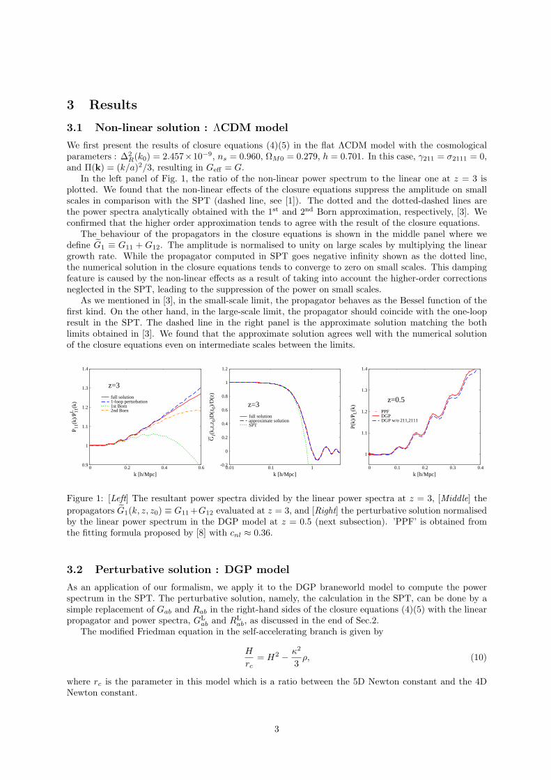
3 Results
3.1 Non-linear solution : ΛCDM model
We first present the results of closure equations (4)(5) in the flat ΛCDM model with the cosmologicalparameters : ∆2
R(k0) = 2.457×10⁻⁹, ns = 0.960, ΩM0 = 0.279, h = 0.701. In this case, γ211 = σ2111 = 0,and Π(k) = (k/a)2/3, resulting in Geff = G.
In the left panel of Fig. 1, the ratio of the non-linear power spectrum to the linear one at z = 3 isplotted. We found that the non-linear effects of the closure equations suppress the amplitude on smallscales in comparison with the SPT (dashed line, see [1]). The dotted and the dotted-dashed lines arethe power spectra analytically obtained with the 1st and 2nd Born approximation, respectively, [3]. Weconfirmed that the higher order approximation tends to agree with the result of the closure equations.
The behaviour of the propagators in the closure equations is shown in the middle panel where wedefine G1 ≡ G11 + G12. The amplitude is normalised to unity on large scales by multiplying the lineargrowth rate. While the propagator computed in SPT goes negative infinity shown as the dotted line,the numerical solution in the closure equations tends to converge to zero on small scales. This dampingfeature is caused by the non-linear effects as a result of taking into account the higher-order correctionsneglected in the SPT, leading to the suppression of the power on small scales.
As we mentioned in [3], in the small-scale limit, the propagator behaves as the Bessel function of thefirst kind. On the other hand, in the large-scale limit, the propagator should coincide with the one-loopresult in the SPT. The dashed line in the right panel is the approximate solution matching the bothlimits obtained in [3]. We found that the approximate solution agrees well with the numerical solutionof the closure equations even on intermediate scales between the limits.
0.9
1
1.1
1.2
1.3
1.4
0 0.2 0.4 0.6
P 11(
k)/P
L 11(k
)
k [h/Mpc]
z=3
full solution1-loop perturbation1st Born2nd Born
-0.2
0
0.2
0.4
0.6
0.8
1
1.2
0.01 0.1 1
G1(
k,z,
z 0)D
(z0)
/D(z
)
k [h/Mpc]
z=3
()
full solutionapproximate solutionSPT
1
1.1
1.2
1.3
1.4
0 0.1 0.2 0.3 0.4
P(k)
/PL(k
)
k [h/Mpc]
z=0.5
PPFDGPDGP w/o 211,2111
Figure 1: [Left] The resultant power spectra divided by the linear power spectra at z = 3, [Middle] thepropagators G1(k, z, z0) ≡ G11 +G12 evaluated at z = 3, and [Right] the perturbative solution normalisedby the linear power spectrum in the DGP model at z = 0.5 (next subsection). ’PPF’ is obtained fromthe fitting formula proposed by [8] with cnl ≈ 0.36.
3.2 Perturbative solution : DGP model
As an application of our formalism, we apply it to the DGP braneworld model to compute the powerspectrum in the SPT. The perturbative solution, namely, the calculation in the SPT, can be done by asimple replacement of Gab and Rab in the right-hand sides of the closure equations (4)(5) with the linearpropagator and power spectra, GL
ab and RLab, as discussed in the end of Sec.2.
The modified Friedman equation in the self-accelerating branch is given by
H
rc= H2 − κ2
3ρ, (10)
where rc is the parameter in this model which is a ratio between the 5D Newton constant and the 4DNewton constant.
3
In this model, gravity becomes 5D on large scales larger than rc. On small scales, gravity becomes 4Dbut it is not described by GR. According to the quasi-static perturbations [7], the brane-bending modecouples to the Newton potential on the brane. Therefore we have
γ211(k1,k2; τ) = − 112H2
(8πGρm
3
)2 (k212
a2
)M(k1,k2)
Π(k12)Π(k1)Π(k2)(11)
σ2111(k1,k2,k3; τ) =8πGρm
324H2
(k2123/a2
Π(k123)Π(k1)Π(k2)Π(k3)
)(M(k1,k2 + k3)M(k2,k3)
Π(k23)+ perm.
)(12)
where
M(k1,k2) = 2r2c
a4[k2
1k22 − (k1 · k2)2], β(τ) = 1 − 2Hrc
(1 +
H
3H2
)(13)
For the numerical calculation, we use the best fit parameters for the flat self-accelerating universeΩm = 0.257, Ωr = 0.138, h = 0.66, ns = 0.998. The resultant power spectrum normalised by the linearone is presented as the solid line in the right panel of Fig. (1). The dashed line is the same calculationneglecting the extra functions, γ211 and σ2111. From this figure, we found that γ211 gives a positivecontribution to the mode coupling, while σ2111 gives a negative and smaller contribution. Therefore theresultant power is enhanced on small scales.
We also plotted the prediction in the Parameterised Post-Friedmann (PPF) framework proposed in[8] as ’PPF’ in the right panel. It is possible to recover the numerical solution for the non-linear powerspectrum very well with the non-linear parameter cnl ≈ 0.36 introduced in [8].
4 Summary
In this paper, we showed the non-linear matter power spectra as a demonstration of our numerical schemefor the closure equations derived in [3]. From the calculation in the ΛCDM model, we observed the extrasuppression of the power on small scales due to the non-linear effects which are neglected in the SPT,as shown in the left panel of Fig (1). Moreover, the middle panel shows that the resultant propagatorconverges to zero on small scales, and coincides with the approximate solution obtained in an analyticway in [3]. These facts confirm that the closure equations contain non-linear contributions more than theSPT, and that our numerical scheme works well from the qualitative viewpoint.
As an application, we applied the closure equations to compute the perturbative prediction of thematter power spectrum in the DGP model. The perturbative calculation, namely, the calculation in theSPT can be performed by the replacement of the right-hand sides of the closure equations (4)(5) withthe linear propagator and power spectra, GL
ab and RLab. As as result, the extra vertex function, γ211, gives
a positive, and large, contribution to the mode coupling, enhancing the power on small scales.More detailed analysis can be seen in [6] together with the application to a f(R) gravity model.
References
[1] F. Bernardeau, S. Colombi, E. Gaztanaga and R. Scoccimarro, Phys. Rept. 367 (2002) 1
[2] M. Crocce and R. Scoccimarro, Phys. Rev. D 73, 063519 (2006) [arXiv:astro-ph/0509418] ;M. Crocceand R. Scoccimarro, Phys. Rev. D 73, 063520 (2006) [arXiv:astro-ph/0509419].
[3] A. Taruya and T. Hiramatsu, arXiv:0708.1367 [astro-ph].
[4] R. H. Kraichnan, J. of Fluid Mechanics 5, 497 (1959)
[5] T. Hiramatsu and A. Taruya, in preparation.
[6] K. Koyama, A. Taruya and T. Hiramatsu, in preparation.
[7] K. Koyama and F. P. Silva, Phys. Rev. D 75, 084040 (2007) [arXiv:hep-th/0702169].
[8] W. Hu, Phys. Rev. D 77, 103524 (2008) [arXiv:0801.2433 [astro-ph]].
4
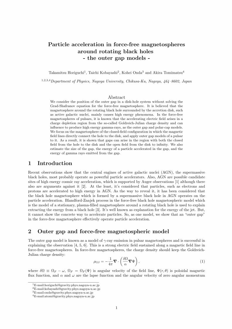
Particle acceleration in force-free magnetospheresaround rotating black holes
- the outer gap models -
Takamitsu Horiguchi1, Taichi Kobayashi2, Kohei Onda3 and Akira Tomimatsu4
1,2,3,4Department of Physics, Nagoya University, Chikusa-Ku, Nagoya, 464–8602, Japan
AbstractWe consider the position of the outer gap in a disk-hole system without solving theGrad-Shafranov equation for the force-free magnetosphere. It is believed that themagnetosphere around the rotating black hole surrounded by the accretion disk, suchas active galactic nuclei, mainly causes high energy phenomena. In the force-freemagnetospheres of pulsars, it is known that the accelerating electric field arises in acharge depletion region from the so-called Goldreich-Julian charge density and caninfluence to produce high energy gamma-rays, as the outer gap and polar-cap models.We focus on the magnetosphere of the closed-field configuration in which the magneticfield lines directly connect the hole to the disk, and apply outer gap models of a pulsarto it. As a result, it is shown that gaps can arise in the region with both the closedfield from the hole to the disk and the open field from the disk to infinity. We alsoestimate the size of the gap, the energy of a particle accelerated in the gap, and theenergy of gamma rays emitted from the gap.
1 Introduction
Recent observations show that the central engines of active galactic nuclei (AGN), the supermassiveblack holes, most probably operate as powerful particle accelerators. Also, AGN are possible candidatesites of high energy cosmic ray acceleration, which is supported by Auger observations [1] although therealso are arguments against it [2]. At the least, it’s considered that particles, such as electrons andprotons are accelerated to high energy in AGN. As the way to reveal it, it has been considered thatthe black hole magnetosphere which is formed by a supermassive black hole in AGN operates on theparticle acceleration. Blandford-Znajek process in the force-free black hole magnetospheric model whichis the model of a stationary, plasma-filled magnetosphere around a rotating black hole is used to explainextracting the energy from a black hole [3]. It’s well known as explanation for the energy of the jet. But,it cannot show the concrete way to accelerate particles. So, as one model, we show that an “outer gap”in the force-free magnetosphere effectively operate particle acceleration.
2 Outer gap and force-free magnetospheric model
The outer gap model is known as a model of γ-ray emission in pulsar magnetospheres and is successful inexplaining the observation [4, 5, 6]. This is a strong electric field sustained along a magnetic field line inforce-free magnetospheres. In force-free magnetospheres, the charge density should keep the Goldreich-Julian charge density:
ρGJ = − 14π
∇ ·(
δΩα
∇Ψ)
, (1)
where δΩ ≡ ΩF − ω, ΩF = ΩF (Ψ) is angular velocity of the field line, Ψ(r, θ) is poloidal magneticflux function, and α and ω are the lapse function and the angular velocity of zero angular momentum
1E-mail:[email protected]:[email protected]:[email protected]:[email protected]
1
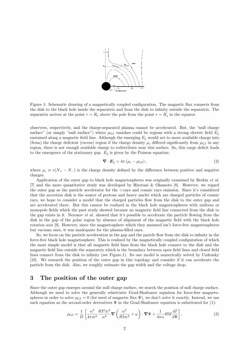
Figure 1: Schematic drawing of a magnetically coupled configuration. The magnetic flux connects fromthe disk to the black hole inside the separatrix and from the disk to infinity outside the separatrix. Theseparatrix arrives at the point r = Rs above the pole from the point r = R
′
s in the equator.
observers, respectively, and the charge-separated plasma cannot be accelerated. But, the “null chargesurface” (or simply “null surface”) where ρGJ vanishes could be regions with a strong electric field E‖sustained along a magnetic field line. Although the emerging E‖ would act to move available charge into(from) the charge deficient (excess) region if the charge density ρe differed significantly from ρGJ in anyregion, there is not enough available charge to redistribute near this surface. So, this carge deficit leadsto the emergence of the stationary gap. E‖ is given by the Poisson equation:
∇ · E‖ = 4π (ρe − ρGJ) , (2)
where ρe ≡ e(N+ − N−) is the charge density defined by the difference between positive and negativecharges.
Application of the outer gap to black hole magnetospheres was originally examined by Beskin et al.[7] and the more quantitative study was developed by Hirotani & Okamoto [8]. However, we regardthe outer gap as the particle accelerator for the γ-rays and cosmic rays emission. Since it’s consideredthat the accretion disk is the source of protons and heavy nuclei which are charged particles of cosmicrays, we hope to consider a model that the charged particles flow from the disk to the outer gap andare accelerated there. But this cannot be realized in the black hole magnetospheres with uniform ormonopole fields which the past study showed because no magnetic field line connected from the disk tothe gap exists in it. Neronov et al. showed that it’s possible to accelerate the particle flowing from thedisk in the gap of the polar region by absence of alignment of the magnetic field with the black holerotation axis [9]. However, since the magnetosphere which they assumed isn’t force-free magnetospheresbut vacuum ones, it was inadequate for the plasma-filled ones.
So, we focus on the particle acceleration in the gap and the paricle flow from the disk to infinity in theforce-free black hole magnetosphere. This is realized by the magnetically coupled configuration of whichthe most simple model is that all magnetic field lines from the black hole connect to the disk and themagnetic field line outside the separatrix which is the boundary between open field lines and closed fieldlines connect from the disk to infinity (see Figure.1). Its one model is numerically solved by Uzdensky[10]. We research the position of the outer gap in this topology and consider if it can accelerate theparticle from the disk. Also, we roughly estimate the gap width and the voltage drop.
3 The position of the outer gap
Since the outer gap emerges around the null charge surface, we search the position of null charge surface.Although we need to solve the generally relativistic Grad-Shafranov equation for force-free magneto-spheres in order to solve ρGJ = 0 (for need of magnetic flux Ψ), we don’t solve it exactly. Instead, we usesuch equation as the second-order derivatives Ψ in the Grad-Shafranov equation is substituted for (1):
ρGJ =1D
[α3
4π$2
δΩ2$4
α4∇
(α2
δΩ$2+ ω
)· ∇Ψ +
14πα
δΩIdI
dΨ
], (3)
2
(a) (b)
Figure 2: The possible configuration of null charge surfaces to eject from the disk to infinity. Bothconfigurations can accelerate the charged particle flowing along the field to infinity in polar region.Directing our attention to the magnetic flux right outside the separatrix, the region of the gap is the grayregion.
where D ≡ α2− δΩ2$2, $ ≡ √gϕϕ in Boyer-Lindquist coordinate and I = I(Ψ) is 2/c times the poloidal
electric current flowing through the circular loop r = const, θ = const. Of cource, it is difficult to solvethis equation. So, we expect the position of ρGJ = 0 by finding it in the polar region, on the equator,and on the vent horizon.
As a result, we found that two surfaces are in the polar region, one surface is near the horizon andone surface is on the equator. One surface in the polar region is on the separatrix and the other is onthe corotation point (δΩ = 0). The surface on the horizon is on the magnetic field line with the maximalcurrent (I(dI/dΨ) = 0). And, The surface on the equator is on the corotation surface if its surface ison the plunging region which is between the black hole and the disk or between the magnetic field linewith the maximal current and the separatrix (r = R′
s in Figure.1) if the corotation surface is on the disk.We can expect the configuration of the null charge surface by connecting their four boundaries. In theexpected configurations, the model where particles flowing from the disk are accelerated to infinity isrealized in the case where the gap emerges in the open field region near the polar axis (Figure.2). Thecondition of this model is that the corotation surface in the polar region is outside the separatrix. Thedifference between two configurations of Figure.2 is a difference of the position between the corotationsurface r = R0 and the separatrix r = Rs on the polar axis. They tend to select (b) in Figure.2 if thereis the corotation surface near the separatrix or the configuration of the separatrix is oblate (Rs < R′
s).Since the inner null charge surface in (a) in Figure.2 always crosses to the inner light surface (which isthe surface of D = 0 and the singular surface of the Grad-Shafranov equation), appropriate regularityconditions may be selected on this light surface in order to select (a).
Directing our attention to the magnetic field line in the open field region near the separatrix, chargedparticles moving along this can be accelerated in the gap near the polar axis (gray color region in Figure.2)and can be ejected to infinity. This field line crosses the null charge surface twice, but it’s thought thatthe gap cannot grow around the inside null charge surface (around the point Q), because the directionof the electric field is opposite and the global electric current is interfered. Such region is filled to theGoldreich-Julian charge density with the charge from the disk or the other gap.
4 Rough estimation of the gap width and the voltage drop
We roughly estimate the gap width and the voltage drop by using one-dimensional equations along themagnetic field lines. In particular, high energy γ-rays are observed not only from luminous AGN, suchas quasars and blazars (its luminosity is >∼ 1043 [ergs s−1]), but also from low luminosity AGN, such asweak Seyfert (its luminosity is 1040-1043 [ergs s−1]). So, we show the luminosity dependence of them.
3
The following static physical process is considered in the gap. First, the electric field emerges aroundthe null charge surface because of the charge depletions. Secondly, it accelerates the charged particles inthe gap and they emits the γ-ray photons by the curvature radiation or the inverse Compton scattering.Finally, the emitted photons generate electrons & positrons with soft background photons by the pairproduction and are reduced, whereas the charged particles increase. These processes is showed by self-consistently solving the Poisson equation (2), the kinetic equation with the reaction force for γ-rayemission, and the Boltzmann equation of particles and photons. We roughly estimate these equation andget the gap width H and the voltage drop Vgap:
H ≈ 1011
(M
108M¯
)0.79 (L
LEdd
)−0.07
[cm], (4)
Vgap ≈ 1012
(M
108M¯
)0.36 (L
LEdd
)−0.21
[V], (5)
in the case where curvature radiation is dominant and
H ≈ 109
(M
108M¯
)0.80 (L
LEdd
)−0.40
[cm], (6)
Vgap ≈ 107
(M
108M¯
)0.40 (L
LEdd
)−1.20
[V], (7)
in the case where inverse Compton is dominant. Here, M is the black hole mass, and L is the luminosityof the soft background photon emitted from the disk and is represented by the ratio of the Eddingtonluminosity. We found that the curvature radiation is dominant because of the gap width being shorterthan the width by inverse Compton scattering if L is less than 10−5−10−6LEdd. Its width is 1012 [cm] andthe energy gained the proton, electron and so on is 1015 [eV]. Also, we found that the more luminositylowers, the more energy is high.
5 Summary
We considered the outer gap in the force-free magnetosphere with separatrix. We showed the configurationof the outer gap in it and found that the separatrix formed the gap in the polar retion which can ejectthe particle flowing from the disk to infinity. Also, we estimated the gap width and the energy gainedparticles by roughly estimation. We found that curvature radiation is dominant and the high energy overTeV is got if the Eddington ratio for accretion is low. So, it’s thought that the outer gap is expected asthe source of the high energy γ-ray and cosmic ray emission.
References
[1] Abraham, J., et al. 2007, Science, 318, 939
[2] Gorbunov, D. S., Tinyakov, P. G., Tkachev, I. I., & Troitsky, S. V. 2008, arXiv:astro-ph/08041088
[3] Blandford, R. D., & Znajek, R. L. 1977, MNRAS, 179, 433
[4] Hirotani, K., & Shibata, S. 1999a, MNRAS, 308, 54
[5] Hirotani, K., & Shibata, S. 1999b, MNRAS, 308, 67
[6] Romani, R. W., & Yadigaroglu, I. -A. 1995, ApJ, 438, 314
[7] Beskin, V. S., Istomin, Ya. N., & Par’ev, V. I. 1992, Soviet Ast., 36, 642
[8] Hirotani, K., & Okamoto, I. 1998, ApJ, 497, 563
[9] Neronov, A. Yu., Semikoz, D. V., & Tkachev, I. I. 2007, arXiv:astro-ph/0712.1737v1
[10] Uzdensky, D. A. 2005, ApJ, 620, 889
4
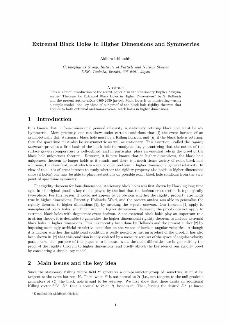
Extremal Black Holes in Higher Dimensions and Symmetries
Akihiro Ishibashi1
Cosmophysics Group, Institute of Particle and Nuclear StudiesKEK, Tsukuba, Ibaraki, 305-0801, Japan
AbstractThis is a brief introduction of the recent paper “On the ‘Stationary Implies Axisym-metric’ Theorem for Extremal Black Holes in Higher Dimensions” by S. Hollandsand the present author arXiv:0809.2659 [gr-qc]. Main focus is on illustrating—usinga simple model—the key ideas of our proof of the black hole rigidity theorem thatapplies to both extremal and non-extremal black holes in higher dimensions.
1 Introduction
It is known that in four-dimensional general relativity, a stationary rotating black hole must be ax-isymmetric. More precisely, one can show under certain conditions that (i) the event horizon of anasymptotically flat, stationary black hole must be a Killing horizon, and (ii) if the black hole is rotating,then the spacetime must also be axisymmetric as well as stationary. This assertion—called the rigiditytheorem—provides a firm basis of the black hole thermodynamics, guaranteeing that the notion of thesurface gravity/temperature is well-defined, and in particular, plays an essential role in the proof of theblack hole uniqueness theorem. However, it is now known that in higher dimensions, the black holeuniqueness theorem no longer holds as it stands, and there is a much richer variety of exact black holesolutions, the classification of which is a major open problem in higher dimensional general relativity. Inview of this, it is of great interest to study whether the rigidity property also holds in higher dimensionssince (if holds) one may be able to place restrictions on possible exact black hole solutions from the viewpoint of spacetime symmetry.
The rigidity theorem for four-dimensional stationary black holes was first shown by Hawking long timeago. In his original proof, a key role is played by the fact that the horizon cross section is topologicallytwo-sphere. For this reason, it would not appear to be obvious whether the rigidity property also holdstrue in higher dimensions. Recently, Hollands, Wald, and the present author was able to generalise therigidity theorem to higher dimensions [1], by invoking the ergodic theorem. Our theorem [1] apply tonon-spherical black holes, which can occur in higher dimensions. However, the proof does not apply toextremal black holes with degenerate event horizon. Since extremal black holes play an important rolein string theory, it is desirable to generalise the higher dimensional rigidity theorem to include extremalblack holes in higher dimensions. This has recently been done by Hollands and the present author [2] byimposing seemingly artificial restrictive condition on the vector of horizon angular velocities. Althoughit is unclear whether this additional condition is really needed or just an artefact of the proof, it has alsobeen shown in [2] that this condition is only violated by a measure zero set of the space of angular velocityparameters. The purpose of this paper is to illustrate what the main difficulties are in generalising theproof of the rigidity theorem to higher dimensions, and briefly sketch the key idea of our rigidity proofby considering a simple, toy model.
2 Main issues and the key idea
Since the stationary Killing vector field ta generates a one-parameter group of isometries, it must betangent to the event horizon, H. Then, when ta is not normal to H (i.e., not tangent to the null geodesicgenerators of H), the black hole is said to be rotating. We first show that there exists an additionalKilling vector field, Ka, that is normal to H on H, besides ta. Then, having the desired Ka, (a linear
1E-mail:[email protected]
1
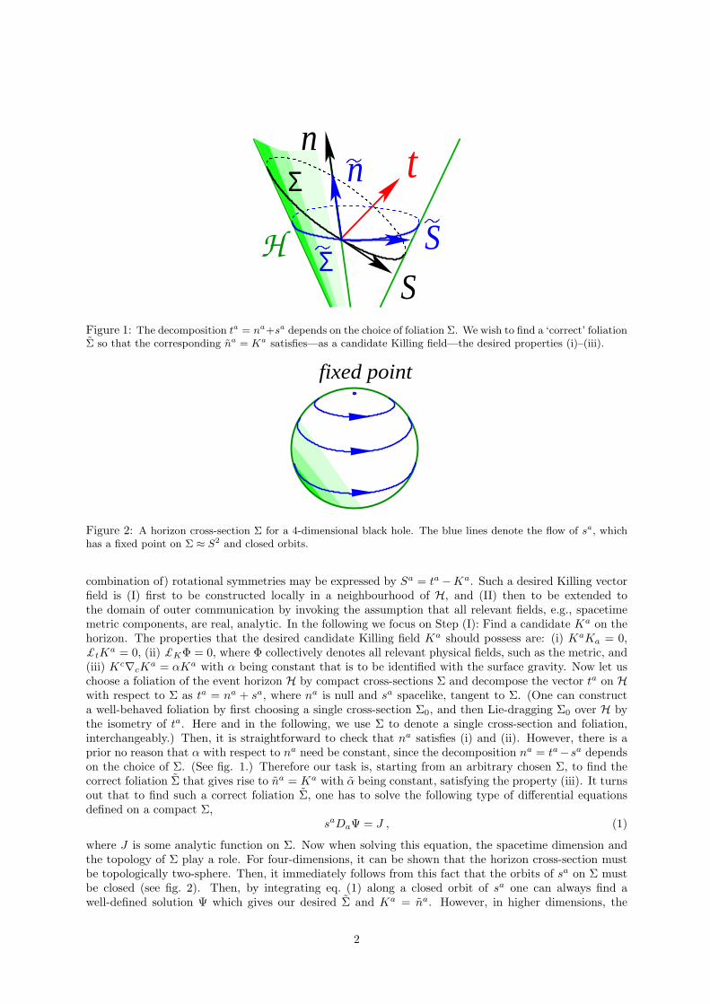
tΣ
ΣS
n
SH
n
Figure 1: The decomposition ta = na+sa depends on the choice of foliation Σ. We wish to find a ‘correct’ foliationΣ so that the corresponding na = Ka satisfies—as a candidate Killing field—the desired properties (i)–(iii).
fixed point
Figure 2: A horizon cross-section Σ for a 4-dimensional black hole. The blue lines denote the flow of sa, whichhas a fixed point on Σ ≈ S2 and closed orbits.
combination of) rotational symmetries may be expressed by Sa = ta−Ka. Such a desired Killing vectorfield is (I) first to be constructed locally in a neighbourhood of H, and (II) then to be extended tothe domain of outer communication by invoking the assumption that all relevant fields, e.g., spacetimemetric components, are real, analytic. In the following we focus on Step (I): Find a candidate Ka on thehorizon. The properties that the desired candidate Killing field Ka should possess are: (i) KaKa = 0,£tK
a = 0, (ii) £KΦ = 0, where Φ collectively denotes all relevant physical fields, such as the metric, and(iii) Kc∇cK
a = αKa with α being constant that is to be identified with the surface gravity. Now let uschoose a foliation of the event horizon H by compact cross-sections Σ and decompose the vector ta on Hwith respect to Σ as ta = na + sa, where na is null and sa spacelike, tangent to Σ. (One can constructa well-behaved foliation by first choosing a single cross-section Σ0, and then Lie-dragging Σ0 over H bythe isometry of ta. Here and in the following, we use Σ to denote a single cross-section and foliation,interchangeably.) Then, it is straightforward to check that na satisfies (i) and (ii). However, there is aprior no reason that α with respect to na need be constant, since the decomposition na = ta−sa dependson the choice of Σ. (See fig. 1.) Therefore our task is, starting from an arbitrary chosen Σ, to find thecorrect foliation Σ that gives rise to na = Ka with α being constant, satisfying the property (iii). It turnsout that to find such a correct foliation Σ, one has to solve the following type of differential equationsdefined on a compact Σ,
saDaΨ = J , (1)
where J is some analytic function on Σ. Now when solving this equation, the spacetime dimension andthe topology of Σ play a role. For four-dimensions, it can be shown that the horizon cross-section mustbe topologically two-sphere. Then, it immediately follows from this fact that the orbits of sa on Σ mustbe closed (see fig. 2). Then, by integrating eq. (1) along a closed orbit of sa one can always find awell-defined solution Ψ which gives our desired Σ and Ka = na. However, in higher dimensions, the
2
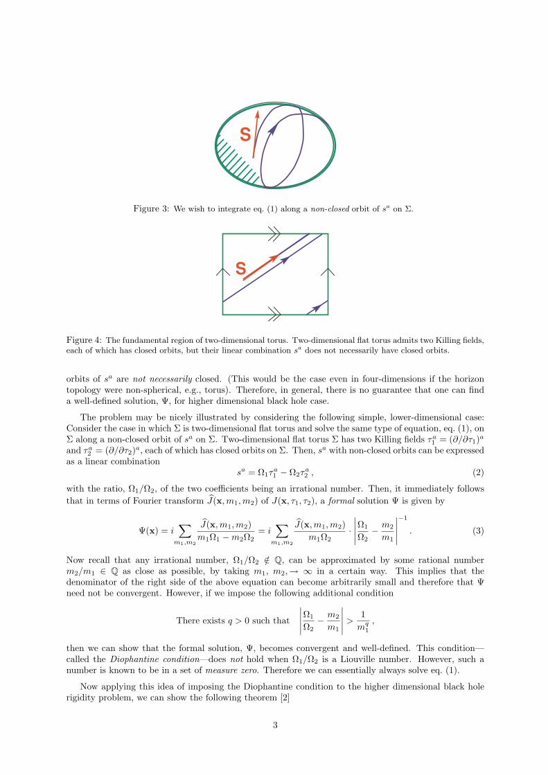
S
Figure 3: We wish to integrate eq. (1) along a non-closed orbit of sa on Σ.
S
Figure 4: The fundamental region of two-dimensional torus. Two-dimensional flat torus admits two Killing fields,each of which has closed orbits, but their linear combination sa does not necessarily have closed orbits.
orbits of sa are not necessarily closed. (This would be the case even in four-dimensions if the horizontopology were non-spherical, e.g., torus). Therefore, in general, there is no guarantee that one can finda well-defined solution, Ψ, for higher dimensional black hole case.
The problem may be nicely illustrated by considering the following simple, lower-dimensional case:Consider the case in which Σ is two-dimensional flat torus and solve the same type of equation, eq. (1), onΣ along a non-closed orbit of sa on Σ. Two-dimensional flat torus Σ has two Killing fields τa
1 = (∂/∂τ1)a
and τa2 = (∂/∂τ2)a, each of which has closed orbits on Σ. Then, sa with non-closed orbits can be expressed
as a linear combinationsa = Ω1τ
a1 − Ω2τ
a2 , (2)
with the ratio, Ω1/Ω2, of the two coefficients being an irrational number. Then, it immediately followsthat in terms of Fourier transform J(x,m1,m2) of J(x, τ1, τ2), a formal solution Ψ is given by
Ψ(x) = i∑
m1,m2
J(x,m1,m2)m1Ω1 −m2Ω2
= i∑
m1,m2
J(x,m1,m2)m1Ω2
·∣∣∣∣∣Ω1
Ω2− m2
m1
∣∣∣∣∣
−1
. (3)
Now recall that any irrational number, Ω1/Ω2 /∈ Q, can be approximated by some rational numberm2/m1 ∈ Q as close as possible, by taking m1, m2,→ ∞ in a certain way. This implies that thedenominator of the right side of the above equation can become arbitrarily small and therefore that Ψneed not be convergent. However, if we impose the following additional condition
There exists q > 0 such that
∣∣∣∣∣Ω1
Ω2− m2
m1
∣∣∣∣∣ >1
mq1
,
then we can show that the formal solution, Ψ, becomes convergent and well-defined. This condition—called the Diophantine condition—does not hold when Ω1/Ω2 is a Liouville number. However, such anumber is known to be in a set of measure zero. Therefore we can essentially always solve eq. (1).
Now applying this idea of imposing the Diophantine condition to the higher dimensional black holerigidity problem, we can show the following theorem [2]
3
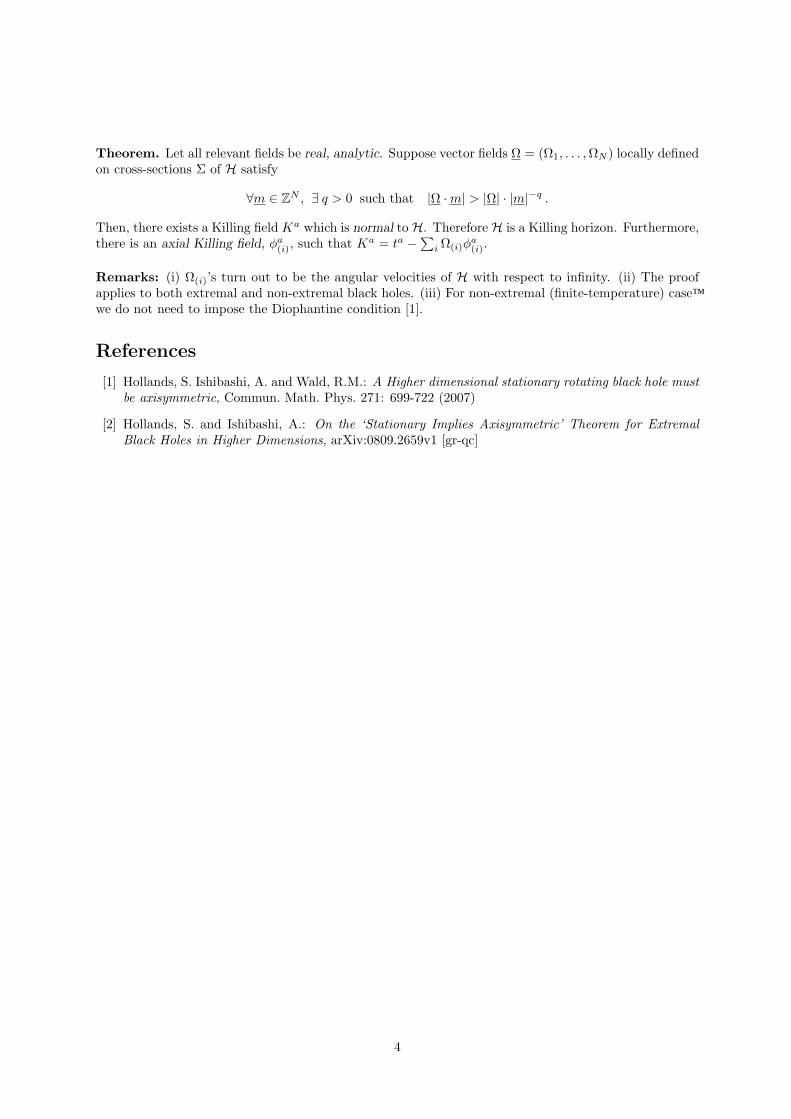
Theorem. Let all relevant fields be real, analytic. Suppose vector fields Ω = (Ω1, . . . , ΩN ) locally definedon cross-sections Σ of H satisfy
∀m ∈ ZN , ∃ q > 0 such that |Ω ·m| > |Ω| · |m|−q .
Then, there exists a Killing field Ka which is normal to H. Therefore H is a Killing horizon. Furthermore,there is an axial Killing field, φa
(i), such that Ka = ta −∑i Ω(i)φ
a(i).
Remarks: (i) Ω(i)’s turn out to be the angular velocities of H with respect to infinity. (ii) The proofapplies to both extremal and non-extremal black holes. (iii) For non-extremal (finite-temperature) case、we do not need to impose the Diophantine condition [1].
References
[1] Hollands, S. Ishibashi, A. and Wald, R.M.: A Higher dimensional stationary rotating black hole mustbe axisymmetric, Commun. Math. Phys. 271: 699-722 (2007)
[2] Hollands, S. and Ishibashi, A.: On the ‘Stationary Implies Axisymmetric’ Theorem for ExtremalBlack Holes in Higher Dimensions, arXiv:0809.2659v1 [gr-qc]
4
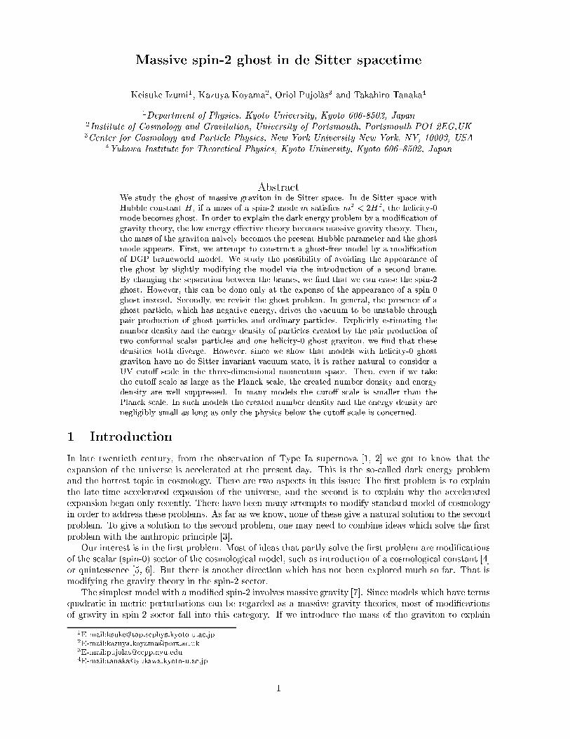
! " #$ %" ! &' () &' () &( $* +,
()' - .
!
" #
$
%&'
(
)
*+ " # !
" ' !
"
' !
"
!" # $ % & # #% ' ( $ & $ $ $ # % # % ) # % # ( *"%
( % + ( ( ,&-. # # /" 0 1 2"% 3 $ % # # &! %
( &! # 4"% 5 0 # # ( # &! # % # $
$ 6 % 6 &! # #- ! 5 # # $ &- 7"% 6 # % 6 Æ # # $ & $ % 6 0 % 0 89 # ( &! $ # &:; 0 8 # :;
( 0 <&=& ,<=. >"% ( % ( # # % <= ? 6 % <= $ ( # % -"% + + % # # $ $ # # -"% #% 6 # 0 ! * / 1 2 4" % # <= & # @ % & ( ! 0 % ) # 7"% # & % 5 & $ $ % 3 ( # & # % 6 # % ) # # ( ( # %
# # & & : % A # >"% $ $% 6 # ( # %
B$ 0 % # 0 # #% # $# !- ! "% ) $ # # #% ?$ # # #%#% % ) ## # # # # # # % + # $ # & # # # % # # C % # # # % A ( % #
!
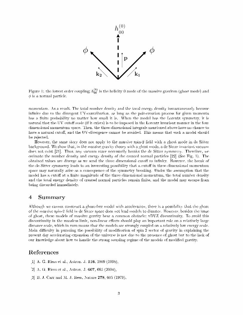
h(0)
00
þp
k1k2
þ
D# ' #E &- # ,# .
%
% ) # ( # FG& # & # ( % A C FG& @ , $. C % # @ FG&# % %
6 &! ( # 5# % A # # 5 $ ! "% 5 % # !!" ,5 D#% .% # @ (% 6 5 # @ 0 #% F @ ( # # ( # %
) # # & # &! ( 5 % 6 # # E <GH % & @ # # # %+ Æ # ( &! # $# & # $ # # # # # ( #%
" )% =% I % ) % J% --> , >>7.
!" )% =% I % ) % J% 221 ,!--/.
*" 3% J% 9 +% J% I B 2-1 , >4>.
*
/" 5% A# I% + % % , >7>.
1" 9% A B% % 3 227 , >77.
2" 3% I % J% ?% % I% < */-2 , >77.
4" +% D A% % I % 5 % C % ) ! , >*>.
7" )% 6# B% % 3 *>4 , >74.
>" =% I% < =% = +% % C% 3 ! ,!---.
-" 9% <@ % C% 3 >> ,!-- .
" +% )% C +% I% I J6? -!> ,!--*.
!" )% B I% I J6? -1> ,!--/.
*" % % % I% < -/*1 ,!--1.
/" % % I% < !*1 ,!--1.
1" 9% 9 I% =# B% )% J6? -22 ,!--2.
2" +% 9 J% C +% J% 5# % I% < -!2--> ,!--4.
4" % % % J6? -1* ,!--4.
7" <% = % 5% 5 % I% < -//- 2 ,!--2.
>" % % % % % I% < -/-/ ,!--4.
!-" J% +% 9 5% J =% <% + % I% < -/*1/* ,!--/.
! " % % #% % % / /! K'-4->%- >>
!!" % % #% % % / /! K'-7 -%/7
/
Can dissipative ee ts help the MSSM in ation?Kohei Kamada1;2 and Jun'i hi Yokoyama2;31Department of Physi s, Graduate S hool of S ien e, The University of Tokyo, Tokyo 113-0033, Japan2Resear h Center for the Early Universe (RESCEU), Graduate S hool of S ien e, The University ofTokyo, Tokyo 113-0033, Japan3Institute for the Physi s and Mathemati s of the Universe,The University of Tokyo, Chiba 277-8582, JapanAbstra tWe study the dissipative ee ts on the MSSM in ation, whi h suers from severe ne-tuning problems on potential parameters and initial onditions. Dissipative ee tsappear as a onsequen e of intera tions between an in aton and other elds and theya t as a fri tion term in its equation of motion. Of ourse it also an emerge inthe ase of MSSM in ation. However, we nd that in the in ationary stage it anneither overwhelm the fri tion term that is due to the osmi expansion nor ae tthe primordial u tuations. Therefore it annot relax the ne-tuning problem of theMSSM in ation.1 Introdu tionMSSM in ation [1 is a model of in ation that is based on an extension of the Standard Model (SM) thatis motivated by the supersymmetry (SUSY), the Minimal Supersymmetri Standard Model (MSSM). Inthis model, the in aton is the at dire tion in the MSSM, a gauge invariant ombination of either squarkor slepton elds. Flat dire tions an be lifted by the SUSY-breaking ee t and the non-renormalizablepotential. If a ne-tuning of the potential parameters is realized, the potential for the at dire tion hasa saddle point and in ation an o ur near the point. If we take the in aton as the u d d or the LLe atdire tion, the saddle point lo ates at ' 1014 GeV and the Hubble parameter during in ation is about1 10 GeV. Here ' is the in aton. Its most interesting feature is that the in aton ouplings to parti lesin the SM are known and, at least in prin iple, measurable in laboratory experiments su h as the LargeHadron Collider or a future Linear Collider. We do not need new physi s beyond the MSSM.Despite these attra tive features des ribed above, the MSSM in ation has some drawba ks, su h as thene-tuning of the potential parameters and worse, the ne-tuning of the initial ondition. In parti ular,the latter is a very diÆ ult problem. Be ause the slow-roll region for the MSSM in ation is extremelynarrow, if the former is solved by some me hanism, the in aton must rea h the slow-roll region with anextremely small velo ity in order to expand the Universe exponentially.However, previous analyses have been negle ted the intera tions between the in aton and other MSSMparti les, whi h we know well, when they onsider the dynami s of the in aton. In general, intera tionsof the s alar elds with other elds an ause the dissipative ee t. This phenomenon has been dis ussedin the high temperature regime [2, 3, in parti ular, in the ontext of the warm in ation [4. It a ts as afri tion term in the equation of motion of the in aton and an ae ts its dynami s. Therefore it has apossibility of relaxation of the ne-tuning of the MSSM in ation.We investigate the intera tion between the MSSM in aton and other elds and the resultant dissipativeee t arefully. As a onsequen e, dissipative ee ts arise but annot hange the dynami s of the MSSMin aton in the in ationary stage. Moreover, it does not ae t the primordial u tuations. Thereforedissipative ee ts annot relax the ne-tuning problem of the MSSM in ation.2 MSSM in ationLet us summarize the main features of the MSSM in ation [1 brie y. We adopt a non-renormalizablesuperpotential of the form Wnon = 6M3G6: (1)1
HereMG is the redu ed Plan k mass and is a supermultuplet whose s alar omponent parameterizesthe at dire tion. in the ase where the u d d at dire tion a ts as an in aton, represents the followingeld onguration. ~ui = ~dj = ~d k = 1p3; (j 6= k; 6= 6= ); (2)where i; j and k are the family indi es and ; and are the olor indi es. We assume that is parameterof order unity. The at dire tion is lifted by the superpotential (1). Hereafter we onsider the ase whenthe s alar omponent of a quires a large expe tation value.In luding the SUSY breaking ee t from the hidden se tor, the s alar potential is found to beV (') = 12m2'2 A24M3G'6 + 232M6G'10; (3)where m 100 GeV - 1 TeV is the soft-breaking mass of and A is a parameter whose amplitude is alsojaj ' O(100) GeV - 1 TeV. This is justied when SUSY-breaking is gravity-mediated. Here we minimizedthe potential along the angular dire tion of , and rewriting the at dire tion as = 1p2'ei, with 'being a real quantity,If A is ne-tuned as A2 = 20m2(1 + 2=4), with 2 1, V (') has a in e tion point '0 at'0 = 2AM3G5 1=4 (1 +O(2)); V 00('0) = 0; (4)where V ('0) = 415m2'20(1 +O(2)): V 0('0) = m2'0 O(2); (5)Therefore in ation an o ur near the in e tion point and its Hubble parameter isHMSSM ' 2m3p5MG'0 ' 1016 m103GeV'0: (6)The potential for MSSM in ation V (') an be expanded around the in e tion point asV (') = 415m2'20 + 83m2'0 (' '0)3: (7)The slow-roll parameters, (M2G=2)(V 0=V )2 and M2G(V 00=V ), an be al ulated from Eq. (7).We nd that the required degree of ne-tuning isjj 109 (8)in order to generate the orre t primordial perturbations [1.Moreover we nd that slow roll region is very narrow, j' '0j='0 1010 even if the above ne-tuning is a omplished by some unknown me hanism. Therefore the in aton must rea h the slow-rollregion with an extremely small velo ity, H1d(log')=dtj'=' + < '20=20M2G. Otherwise the in atonpasses through the slow-roll region within a time interval of H1 be ause the time interval of passing isshorter than the time s ale of de eleration of the in aton. If the above ondition is a omplished, theUniverse goes through the self-reprodu ing regime when exa tly ' = '0 and we have enough number ofe-folds and orre t primordial perturbations.3 Dissipative ee tNext, we onsider the dissipative ee ts. So far, we have not onsidered the intera tions between thein aton and other elds, whi h might ause dissipative ee ts and modify the dynami s of the in aton.As a onsequen e, the narrowness of the slow-roll region ould be relaxed if dissipative ee ts turned outto be strong enough. Here, we see whether it an relax the problems of the MSSM in ation or not.2
3.1 Modi ation to in ationWhen an in aton has intera tion with other elds, espe ially when they are in thermal bath, a dissipa-tive phenomenon takes pla e and the in aton feels a damping for e. Although often a thermal orre tionto the potential also auses and might ae t the slow-roll onditions, in the ontext of the MSSM in ation,it is diÆ ult to onsider su h a ase. For the elds that ouple to the in aton a quire large mass fromthe va uum expe tation value of the in aton. Su h elds are hard to be in thermal bath. Moreover, ifthey are in thermal bath, their energy density will overwhelm that of the in aton. Consequently, in atondoes not o ur. Instead, we onsider the ase where the in aton ouples to the radiation atalyzed byheavy elds [5. In su h a ase, we do not have to worry about the thermal orre tion to the potential.A ording to the dis ussion above, we take into a ount dissipative ee ts and write down the equationof motion for the in aton approximately as+ (3H + Fr) _+ V = 0: (9)Here Fr is the dissipative oeÆ ient representing the dissipative ee t, whi h may enhan e in ation [6anddepends on and the temperature of radiation T . We estimate the value of Fr in the next subse tion.The relative strength of the dissipative ee t ompared to the fri tion term from the expansion an bedes ribed by a parameter r, r FrH : (10)If r is mu h larger than unity, the dynami s of in aton would be modied. In order to estimate itquantitatively, we evaluate the dynami s of the in aton and other omponents of the Universe further.Other equations that governs the universe are,3M2GH2 = V () + ; (11)_ + 4H = Fr _2; (12)where is the energy density of the radiation, that is, = (2=30)gT 4. Here g is the ee tive numberof relativisti degree of freedom. (11) is the Friedman equation and (12) is the Boltzmann equation forthe radiation.The slow-roll onditions in this ase are, then, the onditions that the time variations of H , _ and Tis negligible in omparison to the time s ale of the osmi expansion. Using equations (9), (11) and (12),if r 1, the slow-roll ondition hanges as [7 r; r; r: (13)Here is the new slow-roll parameter introdu ed in order to take into a ount the time variation of Fr, M2GV;Fr;V Fr : (14)We an see from (13) that slow-roll ondition is relaxed by the fa tor of r. 1If we apply this ee t to the MSSM in ation, the slow-roll region is determined by the ondition r. As a onsequen e, the slow-roll region will be enhan ed,j' '0j'0 1010r: (15)3.2 Dissipative oeÆ ients for the MSSM in atonThen, we estimate the dissipative oeÆ ients of the MSSM in aton. The relevant part of the potentialis, then, Vint =h21(jj2j1j2 + jj2j2j2 + j1j2j2j2) + h1h2(2y1y2 +H: :)+ h2(j1j2jy1j2 + j1j2jy2j2 + jy1j2jy2j2)+ h1 PL + PR + h2 1 yPL y + 1 yPR y ; (16)1Stri tly speaking, the degree of relaxation is dependent on the form of the potential V and the dissipative oeÆ ientFr. 3
Here ; and y are the s alar elds. PL(PR) = 1 5(1+ 5) is left-(right-)handed proje tion operators. and y are the four- omponent Dira spinor . As derived in [2, the dissipative oeÆ ients are al ulated using the in-in or the losed time-path formalism,Fr = h41' (t)2 Z t1 dt0(t0 t) Z d3q(2)3 Im G++i (q; t t0)G++i (q; t0 t) ; (17)where G++ (k; t) is the Fourier transform of the Feynman propagator of [2In order to in lude the dissipative pro ess, we dress the propagator with loop. The imaginarypart of its self energy generate non-zero value of Fr. At zero temperature, although there exists animaginary part of its self energy, its ontribution an els out. At non-zero temperature non-zero value ofthe dissipative oeÆ ient appears[5, Fr = CgT 3'2 : (18)Here C is a numeri al onstant of O(10) and g ' O(102) is the relativisti degree of freedom. However,the radiation must not overwhelm the va uum energy, (2=30)gT 4 < (4=15)m2'20. As a result, thedissipative oeÆ ient Fr is smaller than 3H , the fri tion oeÆ ient from osmi expansion unless g isextremely large. 2 Therefore, dissipative ee ts annot relax the ne-tuning problem or the problem ofnarrowness of the slow-roll region.4 Con lusionWe have studied the ee t of the intera tion of the MSSM in aton. The intera tion between the MSSMin aton and the other elds an ause the dissipative ee t. However, this ee t is very weak and annot hange the dynami s of the MSSM in aton. It also does not hange the primordial perturbations that theMSSM in aton generates. Therefore, there still remains the problem of the narrowness of the slow-rollregion of the MSSM in aton. The ne-tuning problem of the MSSM in ation must be solved by otherme hanisms.Referen es[1 R. Allahverdi, K. Enqvist, J. Gar ia-Bellido and A. Mazumdar, Phys. Rev. Lett. 97, 191304 (2006)[arXiv:hep-ph/0605035; R. Allahverdi, K. Enqvist, J. Gar ia-Bellido, A. Jokinen and A. Mazumdar,JCAP 0706, 019 (2007) [arXiv:hep-ph/0610134; J. C. Bueno San hez, K. Dimopoulos and D. H. Lyth,JCAP 0701, 015 (2007) [arXiv:hep-ph/0608299.[2 M. Gleiser and R. O. Ramos, Phys. Rev. D 50, 2441 (1994) [arXiv:hep-ph/9311278;[3 M. Morikawa and M. Sasaki, Prog. Theor. Phys. 72, 782 (1984). A. Hosoya and M. a. Sakagami,Phys. Rev. D 29, 2228 (1984); M. Morikawa, Phys. Rev. D 33, 3607 (1986); J. Yokoyama, Phys. Rev.D 70, 103511 (2004) [arXiv:hep-ph/0406072;[4 A. Berera, Phys. Rev. Lett. 75, 3218 (1995) [arXiv:astro-ph/9509049; J. Yokoyama and A. D. Linde,Phys. Rev. D 60, 083509 (1999) [arXiv:hep-ph/9809409.[5 I. G. Moss and C. Xiong, arXiv:hep-ph/0603266; A. Berera, I. G. Moss and R. O. Ramos,arXiv:0808.1855 [hep-ph.[6 J. Yokoyama and K. Maeda, Phys. Lett. B 207, 31 (1988).[7 L. M. H. Hall, I. G. Moss and A. Berera, Phys. Rev. D 69, 083525 (2004) [arXiv:astro-ph/0305015.2Even if g is extremely large, the warm in ationary solution requires extremely small temperature, whi h is in onsistentwith the assumption that g is large. 4
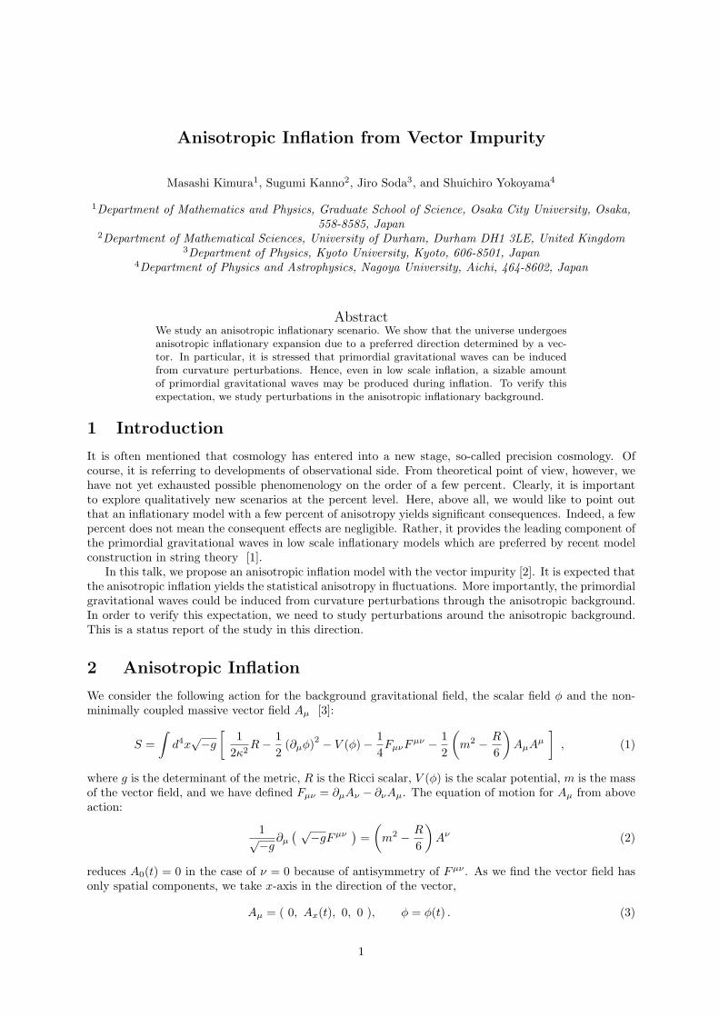
Anisotropic Inflation from Vector Impurity
Masashi Kimura1, Sugumi Kanno2, Jiro Soda3, and Shuichiro Yokoyama4
1Department of Mathematics and Physics, Graduate School of Science, Osaka City University, Osaka,558-8585, Japan
2Department of Mathematical Sciences, University of Durham, Durham DH1 3LE, United Kingdom3Department of Physics, Kyoto University, Kyoto, 606-8501, Japan
4Department of Physics and Astrophysics, Nagoya University, Aichi, 464-8602, Japan
AbstractWe study an anisotropic inflationary scenario. We show that the universe undergoesanisotropic inflationary expansion due to a preferred direction determined by a vec-tor. In particular, it is stressed that primordial gravitational waves can be inducedfrom curvature perturbations. Hence, even in low scale inflation, a sizable amountof primordial gravitational waves may be produced during inflation. To verify thisexpectation, we study perturbations in the anisotropic inflationary background.
1 Introduction
It is often mentioned that cosmology has entered into a new stage, so-called precision cosmology. Ofcourse, it is referring to developments of observational side. From theoretical point of view, however, wehave not yet exhausted possible phenomenology on the order of a few percent. Clearly, it is importantto explore qualitatively new scenarios at the percent level. Here, above all, we would like to point outthat an inflationary model with a few percent of anisotropy yields significant consequences. Indeed, a fewpercent does not mean the consequent effects are negligible. Rather, it provides the leading component ofthe primordial gravitational waves in low scale inflationary models which are preferred by recent modelconstruction in string theory [1].
In this talk, we propose an anisotropic inflation model with the vector impurity [2]. It is expected thatthe anisotropic inflation yields the statistical anisotropy in fluctuations. More importantly, the primordialgravitational waves could be induced from curvature perturbations through the anisotropic background.In order to verify this expectation, we need to study perturbations around the anisotropic background.This is a status report of the study in this direction.
2 Anisotropic Inflation
We consider the following action for the background gravitational field, the scalar field φ and the non-minimally coupled massive vector field Aµ [3]:
S =∫
d4x√−g
[1
2κ2R− 1
2(∂µφ)2 − V (φ)− 1
4FµνFµν − 1
2
(m2 − R
6
)AµAµ
], (1)
where g is the determinant of the metric, R is the Ricci scalar, V (φ) is the scalar potential, m is the massof the vector field, and we have defined Fµν = ∂µAν − ∂νAµ. The equation of motion for Aµ from aboveaction:
1√−g∂µ
( √−gFµν)
=(
m2 − R
6
)Aν (2)
reduces A0(t) = 0 in the case of ν = 0 because of antisymmetry of Fµν . As we find the vector field hasonly spatial components, we take x-axis in the direction of the vector,
Aµ = ( 0, Ax(t), 0, 0 ), φ = φ(t) . (3)
1
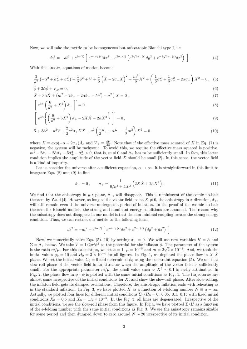
Now, we will take the metric to be homogeneous but anisotropic Bianchi type-I, i.e.
ds2 = −dt2 + e2α(t)[
e−4σ+(t)dx2 + e2σ+(t)(e2√
3σ−(t)dy2 + e−2√
3σ−(t)dz2) ]
. (4)
With this ansatz, equations of motion become:
3κ2
(−α2 + σ2+ + σ2
−)
+12φ2 + V +
12
(X − 2σ+X
)2
+m2
2X2 +
(12σ2
+ +12σ2− − 2ασ+
)X2 = 0 , (5)
φ + 3αφ + V,φ = 0 , (6)
X + 3αX +(m2 − 2σ+ − 2ασ+ − 5σ2
+ − σ2−
)X = 0 , (7)
[e3α
(6κ2
+ X2
)σ−
]·= 0 , (8)
[e3α
(6κ2
+ 5X2
)σ+ − 2XX − 2αX2
]·= 0 , (9)
α + 3α2 − κ2V +23κ2σ+XX + κ2
(13σ+ + ασ+ − 1
2m2
)X2 = 0 . (10)
where X ≡ exp(−α + 2σ+)Ax and V,φ ≡ dVdφ . Note that if the effective mass squared of X in Eq. (7) is
negative, the system will be tachyonic. To avoid this, we require the effective mass squared is positive,m2 − 2σ+ − 2ασ+ − 5σ2
+ − σ2− > 0, that is, m 6= 0 and σ± has to be sufficiently small. In fact, this latter
condition implies the amplitude of the vector field X should be small [2]. In this sense, the vector fieldis a kind of impurity.
Let us consider the universe after a sufficient expansion, α →∞. It is straightforward in this limit tointegrate Eqs. (8) and (9) to find
σ− = 0 , σ+ =1
6/κ2 + 5X2
(2XX + 2αX2
). (11)
We find that the anisotropy in y-z plane, σ−, will disappear. This is reminiscent of the comic no-hairtheorem by Wald [4]. However, as long as the vector field exists X 6= 0, the anisotropy in x direction, σ+,will still remain even if the universe undergoes a period of inflation. In the proof of the cosmic no-hairtheorem for Bianchi models, the strong and dominant energy conditions are assumed. The reason whythe anisotropy does not disappear in our model is that the non-minimal coupling breaks the strong energycondition. Thus, we can restrict our metric to the following form:
ds2 = −dt2 + e2α(t)[
e−4σ+(t)dx2 + e2σ+(t)(dy2 + dz2
) ]. (12)
Now, we numerically solve Eqs. (5)-(10) by setting σ− = 0. We will use new variables H = α andΣ = σ+ below. We take V = 1/2µ2φ2 as the potential for the inflaton φ. The parameter of the systemis the ratio m/µ. For this calculation, we set κ = 1, µ = 10−5 and m = 2
√2 × 10⁻⁵. And, we took the
initial values φ0 = 10 and H0 = 3 × 10⁻⁴ for all figures. In Fig. 1, we depicted the phase flow in X-Xplane. We set the initial value Σ0 = 0 and determined φ0 using the constraint equation (5). We see thatslow-roll phase of the vector field is an attractor when the amplitude of the vector field is sufficientlysmall. For the appropriate parameter m/µ, the small value such as X2 ∼ 0.1 is easily attainable. InFig. 2, the phase flow in φ - φ is plotted with the same initial conditions as Fig. 1. The trajectories arealmost same irrespective of the initial conditions for X, and show the slow-roll phase. After slow-rolling,the inflaton field gets its damped oscillations. Therefore, the anisotropic inflation ends with reheating asin the standard inflation. In Fig. 3, we have plotted H as a function of e-folding number N ≡ α − α0.Actually, we plotted four lines for different initial conditions Σ0/H0 = 0, 0.05, 0.1, 0.15 with fixed initialconditions X0 = 0.5 and X0 = 1.5 × 10⁻⁵. In the Fig. 3, all lines are degenerated. Irrespective of theinitial conditions, we see the slow-roll phase from this figure. In Fig.4, we have plotted Σ/H as a functionof the e-folding number with the same initial conditions as Fig. 3. We see the anisotropy remains sizablefor some period and then dumped down to zero around N ∼ 20 irrespective of its initial condition.
2
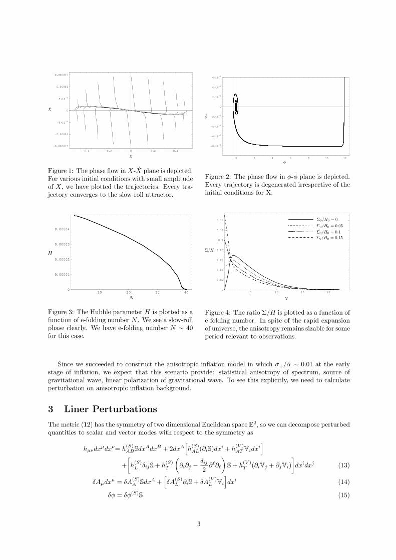
Figure 1: The phase flow in X-X plane is depicted.For various initial conditions with small amplitudeof X, we have plotted the trajectories. Every tra-jectory converges to the slow roll attractor.
Figure 2: The phase flow in φ-φ plane is depicted.Every trajectory is degenerated irrespective of theinitial conditions for X.
Figure 3: The Hubble parameter H is plotted as afunction of e-folding number N . We see a slow-rollphase clearly. We have e-folding number N ∼ 40for this case.
Figure 4: The ratio Σ/H is plotted as a function ofe-folding number. In spite of the rapid expansionof universe, the anisotropy remains sizable for someperiod relevant to observations.
Since we succeeded to construct the anisotropic inflation model in which σ+/α ∼ 0.01 at the earlystage of inflation, we expect that this scenario provide: statistical anisotropy of spectrum, source ofgravitational wave, linear polarization of gravitational wave. To see this explicitly, we need to calculateperturbation on anisotropic inflation background.
3 Liner Perturbations
The metric (12) has the symmetry of two dimensional Euclidean space E2, so we can decompose perturbedquantities to scalar and vector modes with respect to the symmetry as
hµνdxµdxν= h(S)ABSdxAdxB + 2dxA
[h
(S)AL(∂iS)dxi + h
(V )AT Vidxi
]
+[h
(S)L δijS+ h
(S)T
(∂i∂j − δij
2∂`∂`
)S+ h
(V )T (∂iVj + ∂jVi)
]dxidxj (13)
δAµdxµ = δA(S)A SdxA +
[δA
(S)L ∂iS+ δA
(V )L Vi
]dxi (14)
δφ = δφ(S)S (15)
3
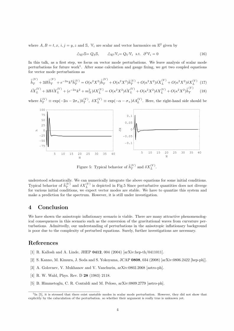
where A,B = t, x, i, j = y, z and S, Vi are scalar and vector harmonics on E2 given by
4E2S= QSS, 4E2Vi= QV Vi s.t. ∂iVi = 0 (16)
In this talk, as a first step, we focus on vector mode perturbations. We leave analysis of scalar modeperturbations for future work1. After some calculation and gauge fixing, we get two coupled equationsfor vector mode perturbations as
¨h
(V )
T + 3H˙h
(V )
T + e−2αk2h(V )T = O(κ2X2) ˙
h(V )
T + O(κ2X2)h(V )T + O(κ2X2) ˙δX
(V )
L + O(κ2X2)δX(V )L (17)
¨δX(V )
L + 3H ˙δX(V )
L + (e−2αk2 + m2X)δX(V )
L = O(κ2X2) ˙δX(V )
L + O(κ2X2)δX(V )L + O(κ2X2) ˙
h(V )
T (18)
where h(V )T ≡ exp(−2α − 2σ+)h(V )
T , δX(V )L ≡ exp(−α − σ+)δA(V )
L . Here, the right-hand side should be
5 10 15 20 25 30 35 40N
-75
-50
-25
0
25
50
75
100
h
5 10 15 20 25 30 35 40N
-0.1
-0.05
0
0.05
0.1∆X
Figure 5: Typical behavior of h(V )T and δX
(V )L .
understood schematically. We can numerically integrate the above equations for some initial conditions.Typical behavior of h
(V )T and δX
(V )L is depicted in Fig.5 Since perturbative quantities does not diverge
for various initial conditions, we expect vector modes are stable. We have to quantize this system andmake a prediction for the spectrum. However, it is still under investigation.
4 Conclusion
We have shown the anisotropic inflationary scenario is viable. There are many attractive phenomenolog-ical consequences in this scenario such as the conversion of the gravitational waves from curvature per-turbations. Admittedly, our understanding of perturbations in the anisotropic inflationary backgroundis poor due to the complexity of perturbed equations. Surely, further investigations are necessary.
References
[1] R. Kallosh and A. Linde, JHEP 0412, 004 (2004) [arXiv:hep-th/0411011].
[2] S. Kanno, M. Kimura, J. Soda and S. Yokoyama, JCAP 0808, 034 (2008) [arXiv:0806.2422 [hep-ph]].
[3] A. Golovnev, V. Mukhanov and V. Vanchurin, arXiv:0802.2068 [astro-ph].
[4] R. W. Wald, Phys. Rev. D 28 (1983) 2118.
[5] B. Himmetoglu, C. R. Contaldi and M. Peloso, arXiv:0809.2779 [astro-ph].
1In [5], it is stressed that there exist unstable modes in scalar mode perturbation. However, they did not show thatexplicitly by the caluculation of the perturbation. so whether their argument is really true is unknown yet.
4
Thermodynamic and dynamical stability of Freund–Rubincompactification
Shunichiro Kinoshita1 and Shinji Mukohyama2
1Department of Physics, The University of Tokyo, Hongo 7-3-1, Bunkyo-ku, Tokyo 113-0033, Japan2Institute for the Physics and Mathematics of the Universe (IPMU), The University of Tokyo, 5-1-5
Kashiwanoha, Kashiwa, Chiba 277-8582, Japan
AbstractWe investigate stability of Freund–Rubin compactication from both thermodynamicand dynamical perspectives. Freund–Rubin compactication not only has trivialFreund–Rubin solutions but also deformed solutions which are described as warpedproduct of external de Sitter space and internal deformed sphere. We study dynamicalstability by analyzing linear perturbations around the deformed solutions. Also westudy thermodynamic stability between the Freund–Rubin solutions and the deformedsolutions based on de Sitter entropy. We show close relations between thermodynamicand dynamical stability exist in this system.
1 Introduction
The Freund–Rubin compactication is a simple model with a stabilization mechanism by ux [1]. Inthis model, considering (p + q)-dimensional spacetime, there is a q-form ux eld for stabilizing the q-dimensional compact space. Moreover, introducing a bulk cosmological constant allows an external deSitter space and an internal manifold with positive curvature. We obtain a (p + q)-dimensional productspacetime of p-dimensional de Sitter space dSp and q-dimensional sphere Sq.
It has been shown that the Freund–Rubin solution has dynamical instabilities that are divided intotwo classes [3, 4]; one is attributed to homogeneous excitation (l = 0 mode) in the internal space, whichcorresponds to a change of the radius of the extra dimensions, and the other is inhomogeneous excitationwith quadrupole moment and higher multi-pole moments (l ≥ 2 modes), which represents the deformationof the internal space. The l = 0 mode is a so-called volume modulus or radion, and becomes tachyonicwhen the Hubble parameter of the external de Sitter space is too large (in other words, the ux densityon the internal space is small). This fact implies that if the energy scale of the in ationary externalspacetime is sufficiently larger than the compactication scale of the internal space, stabilization by uxwill be broken. In order to avoid the emergence of this instability, congurations with small Hubbleparameters would be preferable. On the other hand, instabilities arising from inhomogeneous excitationswill emerge only if the number of extra dimensions is larger than or equal to four. In the unstable region,in which the l ≥ 2 modes are tachyonic, the external spacetime has small Hubble parameters includingthe Minkowski spacetime. It means that the ux densities are very large. It should also be added thatfor more than four extra dimensions, the two unstable regions overlap so that stable congurations forthe FR solution no longer exist.
Little has been known about the non-perturbative nature of the instability from higher multi-polemodes; how it turns out after the onset of this instability and whether any stable conguration as apossible end-state exists in this model, and so on. In [2] we have shown that in the Freund–Rubincompactication there is a new branch of different solutions other than the FR solutions. Those solutionsare described as the warped product of an external de Sitter space and an internal deformed sphere.It has been found that the branch of the FR solutions and that of the deformed solutions intersect atone point where the FR solution becomes marginally stable for the l = 2 mode. Although we have seenexistence of solution other than the FR solution, its stability remains unanswered.
1E-mail:[email protected]:[email protected]
1
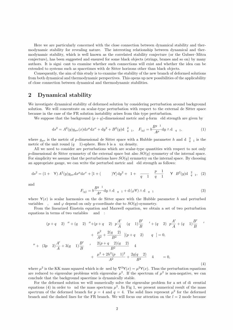
Here we are particularly concerned with the close connection between dynamical stability and ther-modynamic stability for revealing nature. The interesting relationship between dynamical and ther-modynamic stability, which is well known as the correlated stability conjecture (or the Gubser–Mitraconjecture), has been suggested and ensured for some black objects (strings, branes and so on) by manyauthors. It is signicant to examine whether such connections will exist and whether the idea can beextended to systems such as spacetimes with de Sitter horizons other than black objects.
Consequently, the aim of this study is to examine the stability of the new branch of deformed solutionsfrom both dynamical and thermodynamic perspectives. This opens up new possibilities of the applicabilityof close connection between dynamical and thermodynamic stabilities.
2 Dynamical stability
We investigate dynamical stability of deformed solution by considering perturbation around backgroundsolution. We will concentrate on scalar-type perturbation with respect to the external de Sitter spacebecause in the case of the FR solution instability arises from this type perturbation.
We suppose that the background (p + q)-dimensional metric and q-form eld strength are given by
ds2 = A2(y)gµν(x)dxµdxν + dy2 + B2(y)dΩ2q1, F(q) = b
Bq1
Apdy ∧ dΩq1, (1)
where gµν is the metric of p-dimensional de Sitter space with a Hubble parameter h and dΩ2q1 is the
metric of the unit round (q 1)-sphere. Here b is a ux density.All we need to consider are perturbations which are scalar-type quantities with respect to not only
p-dimensional de Sitter symmetry of the external space but also SO(q) symmetry of the internal space.For simplicity we assume that the perturbations have SO(q) symmetry on the internal space. By choosingan appropriate gauge, we can write the perturbed metric and eld strength as follows:
ds2 = (1 + Y) A2(y)gµνdxµdxν + [1 + ( Ω)Y] dy2 +[1 +
(Ω
q 1 p 1
q 1
)Y
]B2(y)dΩ2
q1, (2)
and
F(q) = bBq1
Apdy ∧ dΩq1 + d (φY) ∧ dΩq1 (3)
where Y(x) is scalar harmonics on the de Sitter space with the Hubble parameter h and perturbedvariables , Ω and φ depend on only y-coordinate due to SO(q)-symmetry.
From the linearized Einstein equation and Maxwell equation, we obtain a set of two perturbationequations in terms of two variables and Ω:
(p + q 2)′′ + (q 2)Ω′′+(p + q 2)[pA′
A (q 1)
B′
B
]′ + (q 2)
[pA′
A+ (q 1)
B′
B
]Ω′
+[
µ2
A2+
2(q 2)B2
][(p + q 2) qΩ] = 0,
Ω′′ +[(3p 2)
A′
A+ 3(q 1)
B′
B
]Ω′
[2(p + q 2)(q 2)
B2 4
]
+[µ2 + 2h2(p 1)2
A2+
2q(q 2)B2
4]
Ω = 0,
(4)where µ2 is the KK mass squared which is dened by ∇2Y(x) = µ2Y(x). Thus the perturbation equationsare reduced to eigenvalue problems with eigenvalue µ2. If the spectrum of µ2 is non-negative, we canconclude that the background spacetime is dynamically stable.
For the deformed solution we will numerically solve the eigenvalue problem for a set of differentialequations (4) in order to nd the mass spectrum µ2. In Fig 1, we present numerical result of the massspectrum of the deformed branch for p = 4 and q = 4. The solid lines represent µ2 for the deformedbranch and the dashed lines for the FR branch. We will focus our attention on the l = 2 mode because
2
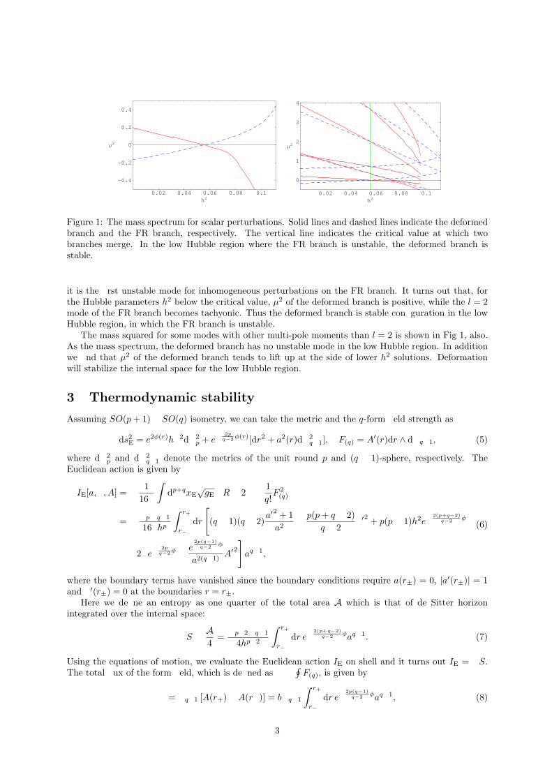
0.02 0.04 0.06 0.08 0.1h2
-0.4
-0.2
0
0.2
0.4
Μ2
0.02 0.04 0.06 0.08 0.1h2
0
1
2
3
4
Μ2
Figure 1: The mass spectrum for scalar perturbations. Solid lines and dashed lines indicate the deformedbranch and the FR branch, respectively. The vertical line indicates the critical value at which twobranches merge. In the low Hubble region where the FR branch is unstable, the deformed branch isstable.
it is the rst unstable mode for inhomogeneous perturbations on the FR branch. It turns out that, forthe Hubble parameters h2 below the critical value, µ2 of the deformed branch is positive, while the l = 2mode of the FR branch becomes tachyonic. Thus the deformed branch is stable conguration in the lowHubble region, in which the FR branch is unstable.
The mass squared for some modes with other multi-pole moments than l = 2 is shown in Fig 1, also.As the mass spectrum, the deformed branch has no unstable mode in the low Hubble region. In additionwe nd that µ2 of the deformed branch tends to lift up at the side of lower h2 solutions. Deformationwill stabilize the internal space for the low Hubble region.
3 Thermodynamic stability
Assuming SO(p + 1) SO(q) isometry, we can take the metric and the q-form eld strength as
ds2E = e2ϕ(r)h2dΩ2
p + e2p
q−2 ϕ(r)[dr2 + a2(r)dΩ2q1], F(q) = A′(r)dr ∧ dΩq1, (5)
where dΩ2p and dΩ2
q1 denote the metrics of the unit round p and (q 1)-sphere, respectively. TheEuclidean action is given by
IE[a, ϕ, A] = 116
∫dp+qxE
√gE
(R 2 1
q!F 2
(q)
)= ΩpΩq1
16hp
∫ r+
r−
dr
[(q 1)(q 2)
a′2 + 1a2
p(p + q 2)q 2
ϕ′2 + p(p 1)h2e2(p+q−2)
q−2 ϕ
2e2p
q−2 ϕ e2p(q−1)
q−2 ϕ
a2(q1)A′2
]aq1,
(6)
where the boundary terms have vanished since the boundary conditions require a(r±) = 0, |a′(r±)| = 1and ϕ′(r±) = 0 at the boundaries r = r±.
Here we dene an entropy as one quarter of the total area A which is that of de Sitter horizonintegrated over the internal space:
S A4
=Ωp2Ωq1
4hp2
∫ r+
r−
dr e2(p+q−2)
q−2 ϕaq1. (7)
Using the equations of motion, we evaluate the Euclidean action IE on shell and it turns out IE = S.The total ux of the form eld, which is dened as
∮F(q), is given by
= Ωq1 [A(r+) A(r)] = bΩq1
∫ r+
r−
dr e2p(q−1)
q−2 ϕaq1, (8)
3
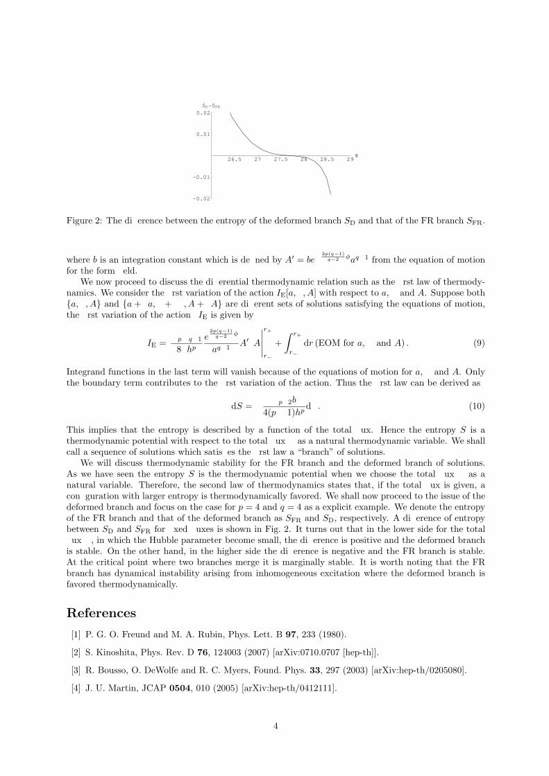
26.5 27 27.5 28 28.5 29F
-0.02
-0.01
0.01
0.02SD-SFR
Figure 2: The difference between the entropy of the deformed branch SD and that of the FR branch SFR.
where b is an integration constant which is dened by A′ = be2p(q−1)
q−2 ϕaq1 from the equation of motionfor the form eld.
We now proceed to discuss the differential thermodynamic relation such as the rst law of thermody-namics. We consider the rst variation of the action IE[a, ϕ,A] with respect to a, ϕ and A. Suppose botha, ϕ, A and a + a, ϕ + ϕ, A + A are different sets of solutions satisfying the equations of motion,the rst variation of the action IE is given by
IE =ΩpΩq1
8hp
e2p(q−1)
q−2 ϕ
aq1A′A
∣∣∣∣∣r+
r−
+∫ r+
r−
dr (EOM for a, ϕ and A) . (9)
Integrand functions in the last term will vanish because of the equations of motion for a, ϕ and A. Onlythe boundary term contributes to the rst variation of the action. Thus the rst law can be derived as
dS = Ωp2b
4(p 1)hpd. (10)
This implies that the entropy is described by a function of the total ux. Hence the entropy S is athermodynamic potential with respect to the total ux as a natural thermodynamic variable. We shallcall a sequence of solutions which satises the rst law a “branch” of solutions.
We will discuss thermodynamic stability for the FR branch and the deformed branch of solutions.As we have seen the entropy S is the thermodynamic potential when we choose the total ux as anatural variable. Therefore, the second law of thermodynamics states that, if the total ux is given, aconguration with larger entropy is thermodynamically favored. We shall now proceed to the issue of thedeformed branch and focus on the case for p = 4 and q = 4 as a explicit example. We denote the entropyof the FR branch and that of the deformed branch as SFR and SD, respectively. A difference of entropybetween SD and SFR for xed uxes is shown in Fig. 2. It turns out that in the lower side for the total ux , in which the Hubble parameter become small, the difference is positive and the deformed branchis stable. On the other hand, in the higher side the difference is negative and the FR branch is stable.At the critical point where two branches merge it is marginally stable. It is worth noting that the FRbranch has dynamical instability arising from inhomogeneous excitation where the deformed branch isfavored thermodynamically.
References
[1] P. G. O. Freund and M. A. Rubin, Phys. Lett. B 97, 233 (1980).
[2] S. Kinoshita, Phys. Rev. D 76, 124003 (2007) [arXiv:0710.0707 [hep-th]].
[3] R. Bousso, O. DeWolfe and R. C. Myers, Found. Phys. 33, 297 (2003) [arXiv:hep-th/0205080].
[4] J. U. Martin, JCAP 0504, 010 (2005) [arXiv:hep-th/0412111].
4
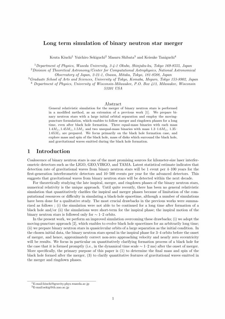
Long term simulation of binary neutron star merger
Kenta Kiuchi1 Yuichiro Sekiguchi2 Masaru Shibata3 and Keisuke Taniguchi4
1Department of Physics, Waseda University, 3-4-1 Okubo, Shinjuku-ku, Tokyo 169-8555, Japan2Division of Theoretical Astronomy/Center for Computational Astrophysics, National Astronomical
Observatory of Japan, 2-21-1, Osawa, Mitaka, Tokyo, 181-8588, Japan3Graduate School of Arts and Sciences, University of Tokyo, Komaba, Meguro, Tokyo 153-8902, Japan
4 Department of Physics, University of Wisconsin-Milwaukee, P.O. Box 413, Milwaukee, Wisconsin53201 USA
AbstractGeneral relativistic simulation for the merger of binary neutron stars is performedin a modified method, as an extension of a previous work [1]. We prepare bi-nary neutron stars with a large initial orbital separation and employ the moving-puncture formulation, which enables to follow merger and ringdown phases for a longtime, even after black hole formation. Three equal-mass binaries with each mass1.4M¯, 1.45M¯, 1.5M¯ and two unequal-mass binaries with mass 1.3–1.6M¯, 1.35–1.65M¯ are prepared. We focus primarily on the black hole formation case, andexplore mass and spin of the black hole, mass of disks which surround the black hole,and gravitational waves emitted during the black hole formation.
1 Introduction
Coalescence of binary neutron stars is one of the most promising sources for kilometer-size laser interfer-ometric detectors such as the LIGO, GEO,VIRGO, and TAMA. Latest statistical estimate indicates thatdetection rate of gravitational waves from binary neutron stars will be 1 event per 4–100 years for thefirst-generation interferometric detectors and 10–500 events per year for the advanced detectors. Thissuggests that gravitational waves from binary neutron stars will be detected within the next decade.
For theoretically studying the late inspiral, merger, and ringdown phases of the binary neutron stars,numerical relativity is the unique approach. Until quite recently, there has been no general relativisticsimulation that quantitatively clarifies the inspiral and merger phases because of limitation of the com-putational resources or difficulty in simulating a black-hole spacetime, although a number of simulationshave been done for a qualitative study. The most crucial drawbacks in the previous works were summa-rized as follows ; (i) the simulation were not able to be continued for a long time after formation of ablack hole and/or (ii) the simulations were short-term for the inspiral phase; the inspiral motion of thebinary neutron stars is followed only for ∼ 1–2 orbits.
In the present work, we perform an improved simulation overcoming these drawbacks; (i) we adopt themoving-puncture approach [2], which enables to evolve black hole spacetimes for an arbitrarily long time;(ii) we prepare binary neutron stars in quasicircular orbits of a large separation as the initial condition. Inthe chosen initial data, the binary neutron stars spend in the inspiral phase for 3–4 orbits before the onsetof merger, and hence, approximately correct non-zero approaching velocity and nearly zero eccentricitywill be results. We focus in particular on quantitatively clarifying formation process of a black hole forthe case that it is formed promptly (i.e., in the dynamical time scale ∼ 1–2 ms) after the onset of merger.More specifically, the primary purpose of this paper is (1) to determine the final mass and spin of theblack hole formed after the merger, (3) to clarify quantitative features of gravitational waves emitted inthe merger and ringdown phases.
1E-mail:[email protected]:[email protected]
1
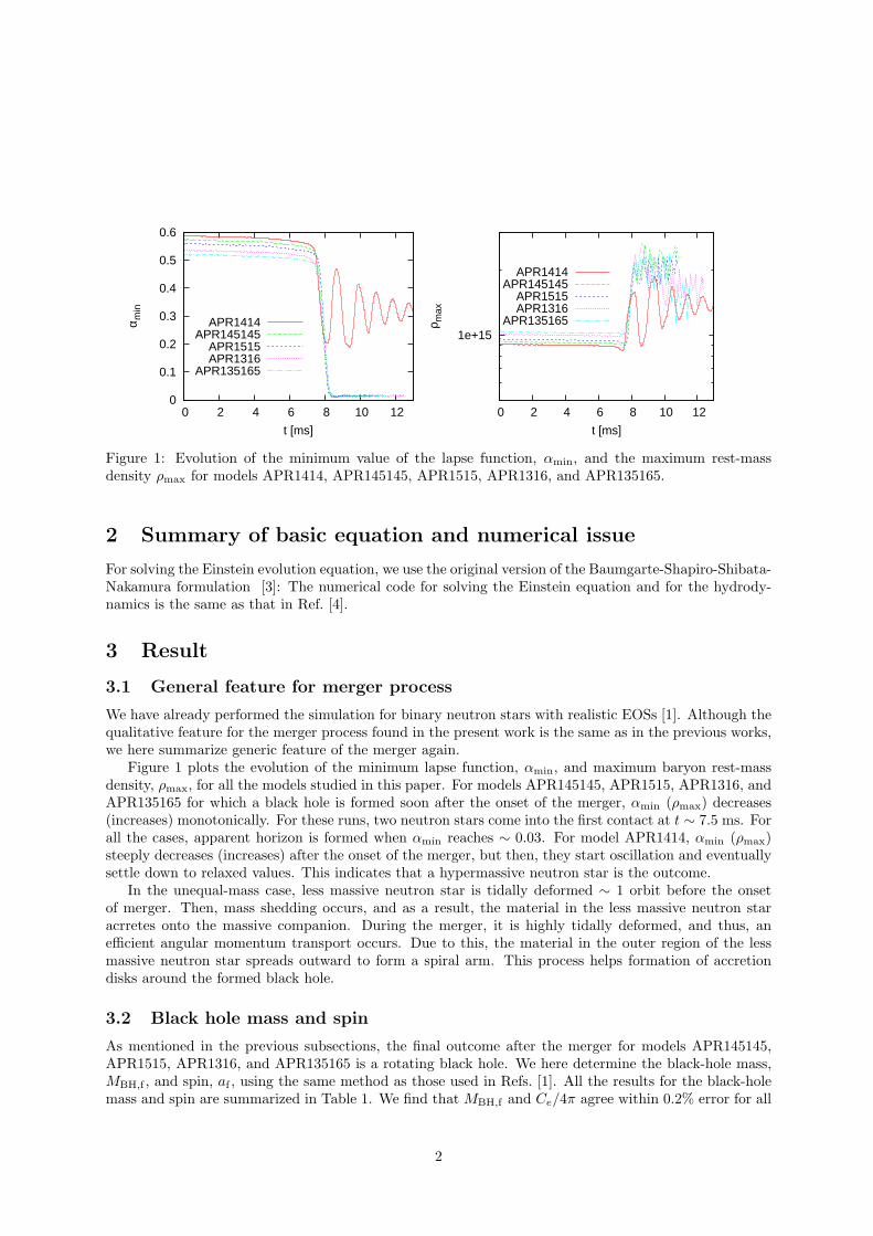
0
0.1
0.2
0.3
0.4
0.5
0.6
0 2 4 6 8 10 12
α min
t [ms]
APR1414APR145145
APR1515APR1316
APR135165
1e+15
0 2 4 6 8 10 12
ρ max
t [ms]
APR1414APR145145
APR1515APR1316
APR135165
Figure 1: Evolution of the minimum value of the lapse function, αmin, and the maximum rest-massdensity ρmax for models APR1414, APR145145, APR1515, APR1316, and APR135165.
2 Summary of basic equation and numerical issue
For solving the Einstein evolution equation, we use the original version of the Baumgarte-Shapiro-Shibata-Nakamura formulation [3]: The numerical code for solving the Einstein equation and for the hydrody-namics is the same as that in Ref. [4].
3 Result
3.1 General feature for merger process
We have already performed the simulation for binary neutron stars with realistic EOSs [1]. Although thequalitative feature for the merger process found in the present work is the same as in the previous works,we here summarize generic feature of the merger again.
Figure 1 plots the evolution of the minimum lapse function, αmin, and maximum baryon rest-massdensity, ρmax, for all the models studied in this paper. For models APR145145, APR1515, APR1316, andAPR135165 for which a black hole is formed soon after the onset of the merger, αmin (ρmax) decreases(increases) monotonically. For these runs, two neutron stars come into the first contact at t ∼ 7.5 ms. Forall the cases, apparent horizon is formed when αmin reaches ∼ 0.03. For model APR1414, αmin (ρmax)steeply decreases (increases) after the onset of the merger, but then, they start oscillation and eventuallysettle down to relaxed values. This indicates that a hypermassive neutron star is the outcome.
In the unequal-mass case, less massive neutron star is tidally deformed ∼ 1 orbit before the onsetof merger. Then, mass shedding occurs, and as a result, the material in the less massive neutron staracrretes onto the massive companion. During the merger, it is highly tidally deformed, and thus, anefficient angular momentum transport occurs. Due to this, the material in the outer region of the lessmassive neutron star spreads outward to form a spiral arm. This process helps formation of accretiondisks around the formed black hole.
3.2 Black hole mass and spin
As mentioned in the previous subsections, the final outcome after the merger for models APR145145,APR1515, APR1316, and APR135165 is a rotating black hole. We here determine the black-hole mass,MBH,f , and spin, af , using the same method as those used in Refs. [1]. All the results for the black-holemass and spin are summarized in Table 1. We find that MBH,f and Ce/4π agree within 0.2% error for all
2
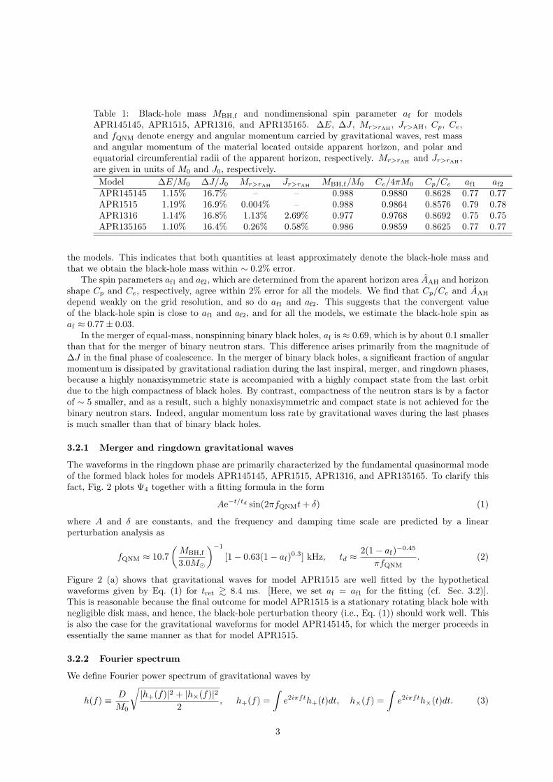
Table 1: Black-hole mass MBH,f and nondimensional spin parameter af for modelsAPR145145, APR1515, APR1316, and APR135165. ∆E, ∆J , Mr>rAH , Jr>AH, Cp, Ce,and fQNM denote energy and angular momentum carried by gravitational waves, rest massand angular momentum of the material located outside apparent horizon, and polar andequatorial circumferential radii of the apparent horizon, respectively. Mr>rAH and Jr>rAH ,are given in units of M0 and J0, respectively.Model ∆E/M0 ∆J/J0 Mr>rAH Jr>rAH MBH,f/M0 Ce/4πM0 Cp/Ce af1 af2
APR145145 1.15% 16.7% – – 0.988 0.9880 0.8628 0.77 0.77APR1515 1.19% 16.9% 0.004% – 0.988 0.9864 0.8576 0.79 0.78APR1316 1.14% 16.8% 1.13% 2.69% 0.977 0.9768 0.8692 0.75 0.75APR135165 1.10% 16.4% 0.26% 0.58% 0.986 0.9859 0.8625 0.77 0.77
the models. This indicates that both quantities at least approximately denote the black-hole mass andthat we obtain the black-hole mass within ∼ 0.2% error.
The spin parameters af1 and af2, which are determined from the aparent horizon area AAH and horizonshape Cp and Ce, respectively, agree within 2% error for all the models. We find that Cp/Ce and AAH
depend weakly on the grid resolution, and so do af1 and af2. This suggests that the convergent valueof the black-hole spin is close to af1 and af2, and for all the models, we estimate the black-hole spin asaf ≈ 0.77± 0.03.
In the merger of equal-mass, nonspinning binary black holes, af is ≈ 0.69, which is by about 0.1 smallerthan that for the merger of binary neutron stars. This difference arises primarily from the magnitude of∆J in the final phase of coalescence. In the merger of binary black holes, a significant fraction of angularmomentum is dissipated by gravitational radiation during the last inspiral, merger, and ringdown phases,because a highly nonaxisymmetric state is accompanied with a highly compact state from the last orbitdue to the high compactness of black holes. By contrast, compactness of the neutron stars is by a factorof ∼ 5 smaller, and as a result, such a highly nonaxisymmetric and compact state is not achieved for thebinary neutron stars. Indeed, angular momentum loss rate by gravitational waves during the last phasesis much smaller than that of binary black holes.
3.2.1 Merger and ringdown gravitational waves
The waveforms in the ringdown phase are primarily characterized by the fundamental quasinormal modeof the formed black holes for models APR145145, APR1515, APR1316, and APR135165. To clarify thisfact, Fig. 2 plots Ψ4 together with a fitting formula in the form
Ae−t/td sin(2πfQNMt + δ) (1)
where A and δ are constants, and the frequency and damping time scale are predicted by a linearperturbation analysis as
fQNM ≈ 10.7(
MBH,f
3.0M¯
)−1
[1− 0.63(1− af)0.3] kHz, td ≈ 2(1− af)−0.45
πfQNM. (2)
Figure 2 (a) shows that gravitational waves for model APR1515 are well fitted by the hypotheticalwaveforms given by Eq. (1) for tret & 8.4 ms. [Here, we set af = af1 for the fitting (cf. Sec. 3.2)].This is reasonable because the final outcome for model APR1515 is a stationary rotating black hole withnegligible disk mass, and hence, the black-hole perturbation theory (i.e., Eq. (1)) should work well. Thisis also the case for the gravitational waveforms for model APR145145, for which the merger proceeds inessentially the same manner as that for model APR1515.
3.2.2 Fourier spectrum
We define Fourier power spectrum of gravitational waves by
h(f) ≡ D
M0
√|h+(f)|2 + |h×(f)|2
2, h+(f) =
∫e2iπfth+(t)dt, h×(f) =
∫e2iπfth×(t)dt. (3)
3
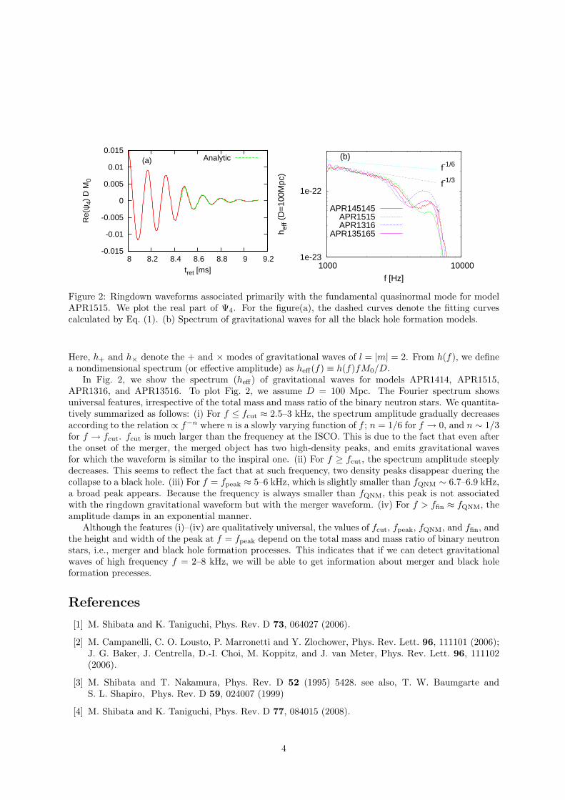
-0.015
-0.01
-0.005
0
0.005
0.01
0.015
8 8.2 8.4 8.6 8.8 9 9.2
Re(
ψ4)
D M
0
tret [ms]
(a) Analytic
1e-23
1e-22
1000 10000
h eff
(D=
100M
pc)
f [Hz]
(b)f-1/6
f-1/3
APR145145APR1515APR1316
APR135165
Figure 2: Ringdown waveforms associated primarily with the fundamental quasinormal mode for modelAPR1515. We plot the real part of Ψ4. For the figure(a), the dashed curves denote the fitting curvescalculated by Eq. (1). (b) Spectrum of gravitational waves for all the black hole formation models.
Here, h+ and h× denote the + and × modes of gravitational waves of l = |m| = 2. From h(f), we definea nondimensional spectrum (or effective amplitude) as heff(f) ≡ h(f)fM0/D.
In Fig. 2, we show the spectrum (heff) of gravitational waves for models APR1414, APR1515,APR1316, and APR13516. To plot Fig. 2, we assume D = 100 Mpc. The Fourier spectrum showsuniversal features, irrespective of the total mass and mass ratio of the binary neutron stars. We quantita-tively summarized as follows: (i) For f ≤ fcut ≈ 2.5–3 kHz, the spectrum amplitude gradually decreasesaccording to the relation ∝ f−n where n is a slowly varying function of f ; n = 1/6 for f → 0, and n ∼ 1/3for f → fcut. fcut is much larger than the frequency at the ISCO. This is due to the fact that even afterthe onset of the merger, the merged object has two high-density peaks, and emits gravitational wavesfor which the waveform is similar to the inspiral one. (ii) For f ≥ fcut, the spectrum amplitude steeplydecreases. This seems to reflect the fact that at such frequency, two density peaks disappear duering thecollapse to a black hole. (iii) For f = fpeak ≈ 5–6 kHz, which is slightly smaller than fQNM ∼ 6.7–6.9 kHz,a broad peak appears. Because the frequency is always smaller than fQNM, this peak is not associatedwith the ringdown gravitational waveform but with the merger waveform. (iv) For f > ffin ≈ fQNM, theamplitude damps in an exponential manner.
Although the features (i)–(iv) are qualitatively universal, the values of fcut, fpeak, fQNM, and ffin, andthe height and width of the peak at f = fpeak depend on the total mass and mass ratio of binary neutronstars, i.e., merger and black hole formation processes. This indicates that if we can detect gravitationalwaves of high frequency f = 2–8 kHz, we will be able to get information about merger and black holeformation precesses.
References
[1] M. Shibata and K. Taniguchi, Phys. Rev. D 73, 064027 (2006).
[2] M. Campanelli, C. O. Lousto, P. Marronetti and Y. Zlochower, Phys. Rev. Lett. 96, 111101 (2006);J. G. Baker, J. Centrella, D.-I. Choi, M. Koppitz, and J. van Meter, Phys. Rev. Lett. 96, 111102(2006).
[3] M. Shibata and T. Nakamura, Phys. Rev. D 52 (1995) 5428. see also, T. W. Baumgarte andS. L. Shapiro, Phys. Rev. D 59, 024007 (1999)
[4] M. Shibata and K. Taniguchi, Phys. Rev. D 77, 084015 (2008).
4
Super-radiance of electromagnetic radiation from disk surfacearound Kerr black hole
Taichi Kobayashi1, Kohei Onda2 and Akira Tomimatsu3
Department of Physics, Nagoya University, Nagoya , 464-8602, Japan
AbstractAccording to recent observation, it is possible to see the event-horizon-scale struc-ture in the supermassive black hole candidate at the Galactic Centre. Therefore, itis important to consider the electromagnetic waves emitted by disk surface near theblack hole horizon. In general, the electromagnetic waves are essentially influencedby gravitation around the black hole (cf. doppler shift, lensing effects, and super-radiance). Using ray-tracing, there is the study of black hole shadow, which is theimage of disk configuration influenced by black hole. However, in ray-tracing, theinfluence of waves (cf. superradiance) is not treated. We focus on the superradianceof electromagnetic waves emitted from disk surface around Kerr black hole. Thenit is interesting to see the amplification of disk radiation, and estimate the energyradiated away to infinity.
1 Introduction
It is widely believed that there exists a rotating black hole surrounded by a disk in the central regionof highly energetic astrophysical objects, such as active galactic nuclei (AGNs), x-ray binary systems,and gamma-ray bursts (GRBs). Because the electromagnetic waves cannot be emitted from horizon ofblack hole, the electromagnetic waves emitted from disk surface are observed in the observation of blackhole candidates. Then the electromagnetic waves near the horizon are influenced by strong gravitationalfield. Furthermore, according to recent observation, it is possible to see the event-horizon-scale structurein the supermassive black hole candidate at the galactic centre[1]. In these situations, it is important toconsider the behavior of electromagnetic waves around Kerr black holes.
On the other hand, there is the study of radiation from disk around Kerr black holes, called by“Ray-tracing” method[2]. In this method, the effects of gravitation, such as the bending of light andgravitational red shift, are considered. However, the interaction between wave and black hole, is nottreated. One of effect is super-radiance which is energy extraction process from black hole due to elec-tromagnetic waves.
In a previous study of well-known super-radiance scattering[3], an disk boundary condition is notconsidered. Therefore we consider the vacuum electromagnetic fields with a disk boundary condition onthe equatorial plane around Kerr black holes. Then we focus on super-radiance and energy transport dueto electromagnetic waves.
2 Formalism
To treat vacuum electromagnetic fields in the disk-black hole system, it is convenient to use the Kerr-Schild formalism for solving the Einstein-Maxwell equation[4]. If this formalism is applied to obtainelectromagnetic perturbations on Kerr background, it is known that all the field components are simplyderived by two arbitrary complex functions ψ and φ, which can be appropriately chosen according to thedisk boundary condition. Here, we put a branch cut in arbitrary complex function ψ on the equatorialplane. Then, the component of Ftθ, Fθϕ and Frθ become discontinuous at θ = π/2. This discontinutiescorrespond to the existence of disk current on the equator[5].
1E-mail:[email protected]:[email protected]:[email protected]
1
Using Newman-Penrose formalism[6], the electromagnetic fields derived from Kerr-Schild formalism(called by KS solution) are described as
φKS0 = 0, (1)
(r − ia cos θ)2φKS1 = ψ(X)/2, (2)
(r − ia cos θ)φKS2 =
eiϕφ(Y, τ)2√
2 cos2(θ/2)+
XψX√2(r + ia cos θ) sin θ
[(r − ia)2iσ cos2(θ/2) − 1
]. (3)
Here, Y = eiϕ tan(θ/2), τ = −t + r + ia cos θ, X = eiστY , σ is corresponding to frequency, and t and ϕare Kerr-Schild coordinates which remain finite even on the horizon. Here we consider the expansion ofarbitrary complex function ψ. By using the expansion form, for example, we obtain
Xψ,X =∑m
mamXm. (4)
As a result, we choose an azimuthal mode m. Then the electromagnetic field is described as
φKS0 m = 0, (5)
(r − ia cos θ)2φKS1 m = ame−iωt+imϕe
iωr∗+i∫
mar2+a2 dr∗ tanm(θ/2)/2, (6)
(r − ia cos θ)φKS2 m =
eiϕφ(Y, τ)2√
2 cos2(θ/2)
+ame−iωt+imϕe
iωr∗+i∫
mar2+a2 dr∗ tanm(θ/2)√
2(r + ia cos θ) sin θ
[(r − ia)2iω cos2(θ/2) − m
], (7)
in Boyer-Lindquist coordinates, where we define ω ≡ mσ and dr∗/dr = 2mr/(r2 + a2). However, ifthe Kerr-Schild formalism is applied to the radiation from disk, the pure outgoing waves are emittedon the horizon. Therefore to require the elimination of outgoing wave on the horizon, we consider thesuperposition between Kerr-Schild solution and well-known electromagnetic perturbations (called by TPsolution)[3]. The electromagnetic fields are described as
φa = φKSa + φTP
a , [a = 0, 1, 2]. (8)
Then, we consider the boundary conditions as follows: ingoing waves on the horizon and outgoing wavesat infinity. Our model differ from the “well-known” perturbations, such as analysis of quasi-normal mode,because on the disk boundary there are emission and absorption of electromagnetic waves.
3 Energy flux in each regions
In this section, we consider the distribution of the energy flux. The energy flux is written by
E¹ = −T¹t, (9)
where
T¹º =14π
[φ0φ0n¹nº + φ2φ2l¹lº2φ1φ1(l(¹nº) + m(¹mº))
−4φ0φ1n(¹mº) − 4φ1φ2l(¹mº) + 2φ2φ0m¹mº
]+ C.C., (10)
and, l¹, n¹ and m¹ are Kinnersley’s tetrad written by
l¹ =[1, −Σ/∆, 0, −a sin2 θ
], (11)
n¹ = (∆/2Σ)[1, Σ/∆, 0, −a sin2 θ
], (12)
m¹ =[ia sin θ, 0, −Σ, −i(r2 + a2) sin θ
]/√
2(r + ia cos θ), (13)
2
in Boyer-Lindquist coordinates. In particular, the radial and angular components of energy flux aredescribed as
Er =14π
[− ∆2
4Σ2φ0φ0 + φ2φ2 +
ia sin θ√2(r + ia cos θ)
∆Σ
φ0φ1 −2ia sin θ√
2(r + ia cos θ)φ1φ2
]+ C.C., (14)
Eθ = − 14πΣ
[∆√
2(r + ia cos θ)φ0φ1 +
2Σ√2(r + ia cos θ)
φ1φ2 −Σia sin θ
(r + ia cos θ)2φ0φ2
]+ C.C., (15)
where ∆ = r2 + a2 − 2Mr, Σ = r2 + a2 cos2 θ.First we see the total energy on the horizon written by
EH =∫ π
0
ErHΣH sin θdθ. (16)
Using Maxwell equations, the total energy is described as
EH ∝ −(ω
kA +
ωH
kB
), (17)
where ω and ωH are frequency of wave and angular velocity of black hole, respectively, and k = ω−mωH.Here, if superradiant condition (0 < ω < ωH) is filled, the rotational energy is extracted due to theelectromagnetic waves.
Secondly, to see the energy transport, we consider the low-frequency limit (aω ¿ 1). In this limit,we can solve the radial equation of electromagnetic field. As a result, we get the relations between eachcoefficients of waves, which is corresponding to amplitude. This relations are written by
(out)∞s(out)Hs
= (−1)−l(r1 − r2)2s+1(2κ)l−s (l + s)!(l − s)!(2l)!(2l + 1)!
Γ(l + 1 + 2iQ)Γ(−s + 2iQ)
, (18)
(In)Hs(out)Hs
=(−1)−s+1
(r1 − r2)−2s
(l − s)!(l + s)!
Γ(s + 1 − 2iQ)Γ(l + 1 + 2iQ)Γ(l + 1 − 2iQ)(Γ(1 − s + 2iQ)
, (19)
where κ = −i(r1−r2)ω, Q = (r 21 +a2)(ωH−ω)/(r1−r2), r1 and r2 are distance of outer and inner horizon,
respectively, the electromagnetic field is described as s = ±1, and s = 1 and s = −1 are correspondingto coefficients of φ0 and φ2, respectively. Then we can see the dependence on frequency in the energyfluxes. As a result, it is easy to see that the extracted energy is transported to disk region.
4 Summary
We consider the electromagnetic perturbations considered by disk boundary. Then we put the boundaryconditions as follows: ingoing waves on the horizon and outgoing waves at infinity. However, becausethe source of radiation exist, Our model differ from the “well-known” perturbations, such as analysis ofquasi-normal mode. As a result, we find the energy extracted from black hole due to super-radiance, andthe extracted energy is transported to disk regions.
References
[1] S. S. Doelema et al., ”Event-horizon-scale structure in the supermassive black hole candidate at theGalactic Centre”, Nature, 455, 78 (2008)
[2] A. Muler, & M. Camenzind, ”Relativistic emission lines from accretion black holes: The effect ofdisk truncation on line profiles”, A&A, 413, 861(2004)
[3] W. H. Press, & S. A. Teukolsky, Perturbations of Rotating Black hole. III. Interaction of the Holewith Gravitational and Electromagnetic Radiation”, ApJ, 193, 443(1974)
[4] G. C. Debney, R. P. Kerr, & A. Schild, ”Solutions of the Einstein and Einstein-Maxwell Equations”,J. Math. Phys., 10, 1842(1969)
3
[5] T. Kobayashi et al., ”Disk illumination by black hole superradiance of electromagnetic perturba-tions”, Phys. Rev. D, 77, 064011(2008)
[6] E. T. Newman & R. Penrose, ”An Approach to Gravitational Radiation by a Method of SpinCoefficients”. J. Math. Phys., 6, 566(1962)
4
Conformal Inflation, Modulated Reheating, and WMAP5
Takeshi Kobayashi1 and Shinji Mukohyama2
1Department of Physics, School of Science, The University of Tokyo, Hongo 7-3-1, Bunkyo-ku, Tokyo113-0033, Japan
2Institute for the Physics and Mathematics of the Universe (IPMU), The University of Tokyo, 5-1-5Kashiwanoha, Kashiwa, Chiba 277-8582, Japan
AbstractWe investigate density perturbations generated through modulated reheating whileinflation is driven by a conformally coupled scalar field. A large running of the spec-tral index is obtained, which reflects the basic nature of conformal inflation thathigher-order time derivatives of the Hubble parameter during inflation are not nec-essarily small. This feature may allow us to distinguish between conformal inflationmodels and standard minimally coupled ones. We also investigate how the resultingfluctuations are modified when there is a deviation from an exact conformal couplingbetween the inflaton and gravity. Finally, we apply our results to the warped braneinflation model and see that observational bounds from the WMAP5 data suggesta blue tilted density perturbation spectrum. The discussion here is based on thepaper [1].
1 Introduction
Ever since the idea of cosmic inflation was proposed, inflationary model building has largely focused onslow-rolling scalar fields minimally coupled to gravity as candidate inflatons. However, recently it waspointed out in [2] that conformally coupled scalar fields are also capable of accelerating the universe.Since the existence of such conformally coupled fields are rather common in models from string theory, itis of great interest to explore the possibility of conformally coupled fields driving inflation. In this light,we also come up with a new question of how we can distinguish between these “conformal inflation”models and standard minimally coupled ones.
The aim of our work is to focus on density perturbations and seek for distinctive features confor-mal inflation might have left. A conformally coupled inflaton itself cannot be responsible for generatingprimordial fluctuations, but instead string theory suggests alternative scenarios such as modulated re-heating [3, 4]. Thence, we consider the case where modulated reheating generates density perturbationswhile inflation is driven by an almost conformally coupled inflaton. We study the scale dependence ofthe generated density perturbations.
We also investigate how the resulting density perturbations are modified when there is a deviationfrom an exact conformal coupling between the inflaton and gravity. The result will allow us to imposeconstraints on the inflaton’s coupling from observational data. As a concrete example, our generic resultsare applied to the well-studied warped brane inflation model [5].
2 Review of Conformal Inflation
Here we give a brief review of conformal inflation. Consider the action
S =∫
dx4√−g
[M2
p
2R− 1
2gµν∂µφ∂νφ− V (φ)− ξ
2Rφ2
](1)
[email protected]:[email protected]
1
where R is the scalar curvature and ξ is the non-minimal coupling to gravity. Choosing a flat FRWbackground ds2 = −dt2 + a(t)2dx2 and also introducing π ≡ φ + Hφ, the Friedmann equation is
M2p H2 =
13V +
16π2 +
(ξ − 1
6
)(2Hφπ −H2φ2), (2)
and the equation of motion of φ is
π + 2Hπ + V ′ + 6(
ξ − 16
)(H + 2H2)φ = 0. (3)
The conformal case ξ = 1/6 was investigated in [2], where inflation was realized while the equations(2) and (3) could be approximated to
M2p H2 ' 1
3V, cHπ ' −V ′. (4)
Here, c is a dimensionless constant3. Let us define three “flatness parameters” as
ε ≡M2
p
2
(V ′
V
)2
, ε ≡ φV ′
2V, ηc ≡ η +
c
3
(V ′′φ
V ′ + c− 2)
, (5)
where η ≡ M2p V ′′/V . When |c| ∼ O(1), one can check that the necessary conditions for (4) and |H/H2|
1 are simplyε 1, |ε| 1, |ηc| 1. (6)
The proportionality constant c is chosen such that it is the largest constant to minimize |ηc|/c2 [1].It is clear from (2) and (4) that π2/V is small during inflation. Especially when the potential is flat
enough to satisfy |M2p V ′| |cφV |, then φ ≈ −Hφ, which suggests that the inflaton is rapidly rolling
towards its origin.
3 Density Perturbations from Modulated Reheating
We analyze the case where density perturbations are generated through modulated reheating [3, 4] afterconformal inflation. The scale dependence of the perturbations can be expressed by expansion in terms ofthe flatness parameters. Furthermore, we take account of the inflaton’s slight deviation from a conformalcoupling (ξ − 1/6). This procedure allows us to deal with a wide variety of situations, e.g., when thereexists additional corrections to the action which ruins the exact conformal coupling, when the framewhere the inflaton φ is conformally coupled to gravity differs from the frame where the light modulus χis minimally coupled. In [1] the resulting spectral index and its running were shown to take the form,
ns − 1 =d lnH2
d ln k= 2
H
H2
(1 +
H
H2
)−1
= −2ε−(
12c2
+ κ2
)ε +O(ε3/2, εηc) +
(ξ − 1
6
)2κ2 +O(ε1/2)
+O
((ξ − 1
6
)2)
, (7)
dns
d ln k= 2
(1 +
H
H2
)−31H
(H
H2
)·
= 2(
3− c +3cηc
)ε +
(6(8− 3c)
c2+ (7− 3c)κ2
)ε +O(ε3/2, εηc)
+(
ξ − 16
)−4κ2 +O(ε1/2)
+O
((ξ − 1
6
)2)
, (8)
3Our parameterization of c differs from that of [2] by cours = c[2] + 2.
2
where the right hand sides should be estimated at the moment of horizon crossing k = aH. We imme-diately see that |dns/d ln k| can become large, comparable to |ns − 1|. This is due to the fact that thederivatives of the flatness parameters do not necessarily become smaller than the parameters themselves.Since this is a generic feature of conformal inflation, a large running is expected even if we considermechanisms other than modulated reheating for generating fluctuations (e.g. curvaton models). Also,our results indicate that (ξ−1/6)-corrections can dominantly determine the values of the cosmologicalobservables unless |ξ−1/6| is smaller than the flatness parameters.
4 Application to Warped Brane Inflation
Let us now apply the results obtained in the previous section to a specific model. Here we considerthe warped brane inflation model [5], where the universe experiences inflation while a D3-brane movestowards the tip of a flux compactified warped throat. The D3-brane is pulled by a stack of D3-branessitting at the tip. If the position of the D3-brane is a conformally coupled scalar (for a discussion on thisissue, see e.g. [7]), then this model serves as a realization of conformal inflation.
Considering a throat whose geometry is AdS5 ×X5, the potential of the inflaton takes the form
V (φ) = 2ph40T3
(1− h4
0T23 R4
Nφ4
). (9)
Here, the inflaton is related to the radial position ρ of the D3 through φ =√
T3ρ, p is the numberof D3s at the tip, h0 = ρ0/R is the warping at the tip, T3 = 1/(2π)3gs(α′)2 is the D3 tension, R4 =22π4gs(α′)2N/Vol(X5) is the AdS radius of the throat, Vol(X5) is the dimensionless volume of the basespace X5, and N(> 1) is the 5-form charge.
The conformally coupled inflaton satisfies φ ≈ −φH during inflation, hence the number of e-foldingsgenerated is N ≈ log (ρi/ρf ) ≈ − log (h0/λi) , where we have set the initial position of the D3 by adimensionless constant λi as ρi = λiR, and assumed inflation to end when the D3 approaches the tipρf ≈ ρ0. This shows that in order to obtain enough e-foldings, the throat should be strongly warpedh0/λi 1.
The scale dependence of the perturbations can be computed by (7) and (8). We parametrize the posi-tion of the D3 when the CMB scale was originally produced by ρCMB = λR. Furthermore, for simplicity,we ignore the compactified bulk to which the throat is glued, hence M2
p ' 2(2π)7g2
s(α′)4
∫ R
ρ0dρ Vol(X5) ρ5
h4 'Vol(X5)R
6
(2π)7g2s(α′)4 . Then under the assumption h0/λ 1, the flatness parameters and κ can be calculated (note
that c = 7)
ε ' 2h80
λ10N, ε ' 2h4
0
λ4N, ηc = η ' −5h4
0
λ6, κ2 ' 4λ2
N. (10)
Since ε is extremely small compared to the other flatness parameters, the cosmological observables canbe estimated as follows:
ns − 1 ' − 4N
h4
0
λ4− 2λ2
(ξ − 1
6
),
dns
d ln k' −16
N
h4
0
λ4+ λ2
(ξ − 1
6
). (11)
The 5-year WMAP+BAO+SN data gives bounds ns = 1.022+0.043−0.042 (68% CL) and dns/d ln k =
−0.032+0.021−0.020 (68% CL) when tensor mode perturbations are negligible [6]. Since the h4
0/λ4 terms aretoo small to be constrained by the observational bounds, we ignore them. Then the observables aredetermined only by the inflaton’s deviation from an exact conformal coupling,
ns − 1 ' 8λ2
N
(ξ − 1
6
),
dns
d ln k' −16
λ2
N
(ξ − 1
6
). (12)
It is easy to see that the spectral index and its running are related by
dns
d ln k' −2(ns − 1). (13)
3
Using the observational bound on dns/d ln k to constrain λ2(ξ−1/6)/N ,
0.001 .λ2
N
(ξ − 1
6
). 0.003. (14)
If we further make use of this bound to constrain the spectral index, we obtain
0.006 . ns − 1 . 0.026. (15)
Thus the 1σ observational bound on the running allows us to predict a blue tilt for the warped braneinflation model. Moreover, the values of the observables were dominantly determined by the inflaton’sdeviation from a conformal coupling. The bound (14) suggests that this deviation can be fairly large,e.g., (ξ−1/6) ∼ 10−1 when λ ∼ 1, N ∼ 102.
5 Conclusion
We have investigated the scale dependence of the density perturbations that are generated throughmodulated reheating after conformal inflation. We have written down the spectral index and its runningin terms of the flatness parameters and the inflaton’s deviation from an exact conformal coupling. Thegeneral results we have obtained are that (i) modulated reheating together with conformal inflation canproduce a nearly scale-invariant spectrum, (ii) the running of the spectral index |dns/d ln k| turns outto be as large as |ns − 1|. The latter result reflects the nonexistence of hierarchy among higher-ordertime derivatives of the Hubble parameter dn lnH2/dtnHn during conformal inflation. This is in strongcontrast to standard minimal models where higher-order derivatives are suppressed by higher orders of theslow-roll parameters (and their derivatives). Hence this feature offers a chance of obtaining a smoking-gunsignal for non-minimally coupled inflation models.
We also applied our results to the warped brane inflation model, where it was shown that observableswere dominantly determined by the deviation from the conformal coupling. We have shown that thespectral index and its running are related by (13) for this model. Since the running is highly constrainedby the WMAP5 data, a stringent bound on the coupling of the inflaton to gravity was obtained. Also,comparison with the WMAP5 data suggested a blue tilt of the spectrum.
While our analysis focused on general aspects of modulated reheating after conformal inflation, wehave not presented the light modulus responsible for generating fluctuations in a concrete setup. Inthe warped brane inflation case, potential candidates for such light fields are angular positions of theD3(D3)-branes sitting in throats with angular isometries, and/or axions associated with shift symmetriesof the Kahler potential. For further study, it is important to come up with an explicit realization of ourmechanism based on fundamental theories. We leave this for future work.
One of the general lessons of our work is that a non-minimal coupling with gravity can drasticallychange the behavior of inflation. Large values for higher-order time derivatives of the Hubble parameteris a special nature of conformal inflation. Cosmological observations are imposing (not necessarily directbut) important constraints on such features even at the present stage.
References
[1] T. Kobayashi and S. Mukohyama, arXiv:0810.0810 [hep-th].
[2] L. Kofman and S. Mukohyama, Phys. Rev. D 77, 043519 (2008) [arXiv:0709.1952 [hep-th]].
[3] G. Dvali, A. Gruzinov and M. Zaldarriaga, Phys. Rev. D 69, 023505 (2004) [arXiv:astro-ph/0303591].
[4] L. Kofman, arXiv:astro-ph/0303614.
[5] S. Kachru, R. Kallosh, A. Linde, J. M. Maldacena, L. P. McAllister and S. P. Trivedi, JCAP 0310,013 (2003) [arXiv:hep-th/0308055].
[6] E. Komatsu et al. [WMAP Collaboration], arXiv:0803.0547 [astro-ph].
[7] N. Seiberg and E. Witten, JHEP 9904, 017 (1999) [arXiv:hep-th/9903224].
4
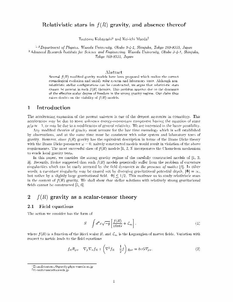
!"#$$$ %& ' ( )**
!"#$$$ %
!
!
" # $% & ' & ' ( ) $% * + ,- .
/ * +,- 0 1 $% 2 *3- / 4 ( 4 + $% ! *5 6-
(
$%
67
$%
$% 0 8 9
7
+
( : $+%
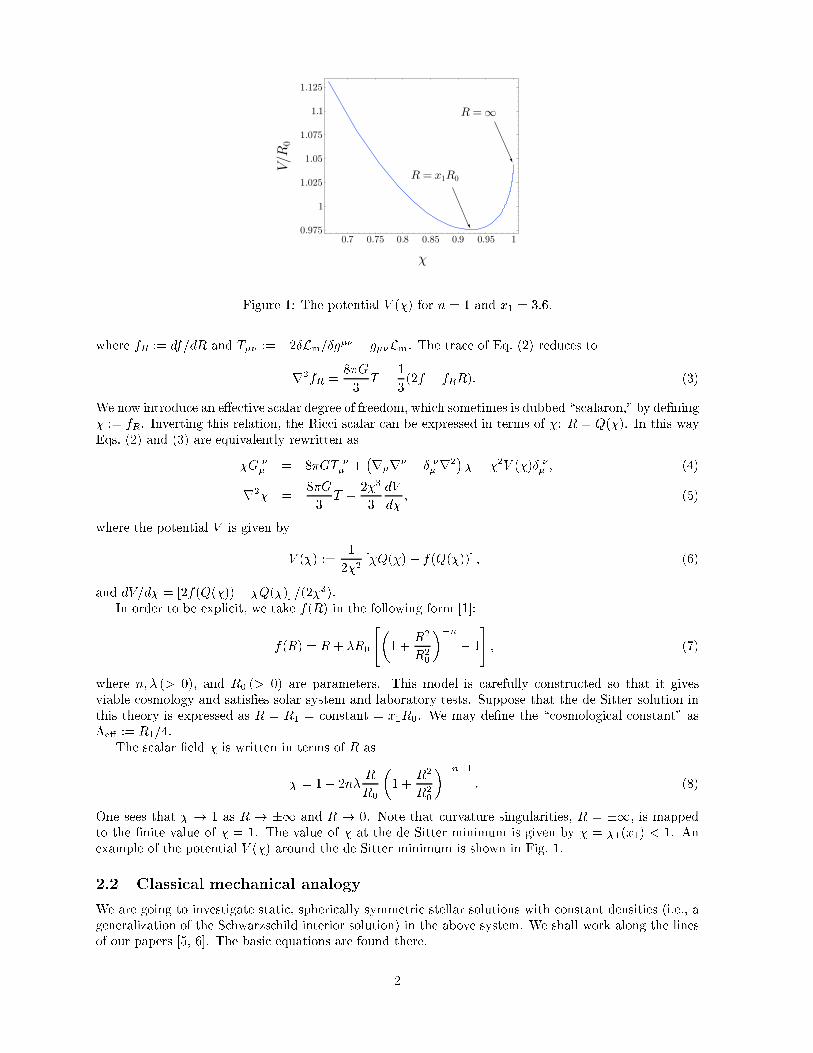
1 ; $% ( ( ,6
;( ;( +ÆÆ 7 < $+%
(:
, 7
,$+ % $,%
! 2 = > ;( / 0 ; ( $% / < $+% $,%
( :
7 Æ
$%Æ
$3%
(:
, 7
+
,
$5%
$% ;(
+*$% $$%%- $6%
( *+$$%% $%- $+%/ $% *-;
$% ( 7
7
$?%
$ )% $ )% @ @ ( ( ( ! = > A ;( 3
( +
7
$:%
B ) C ( ( @ ( $% " $% @ 1
! $ D @D % ! *5 6-
+
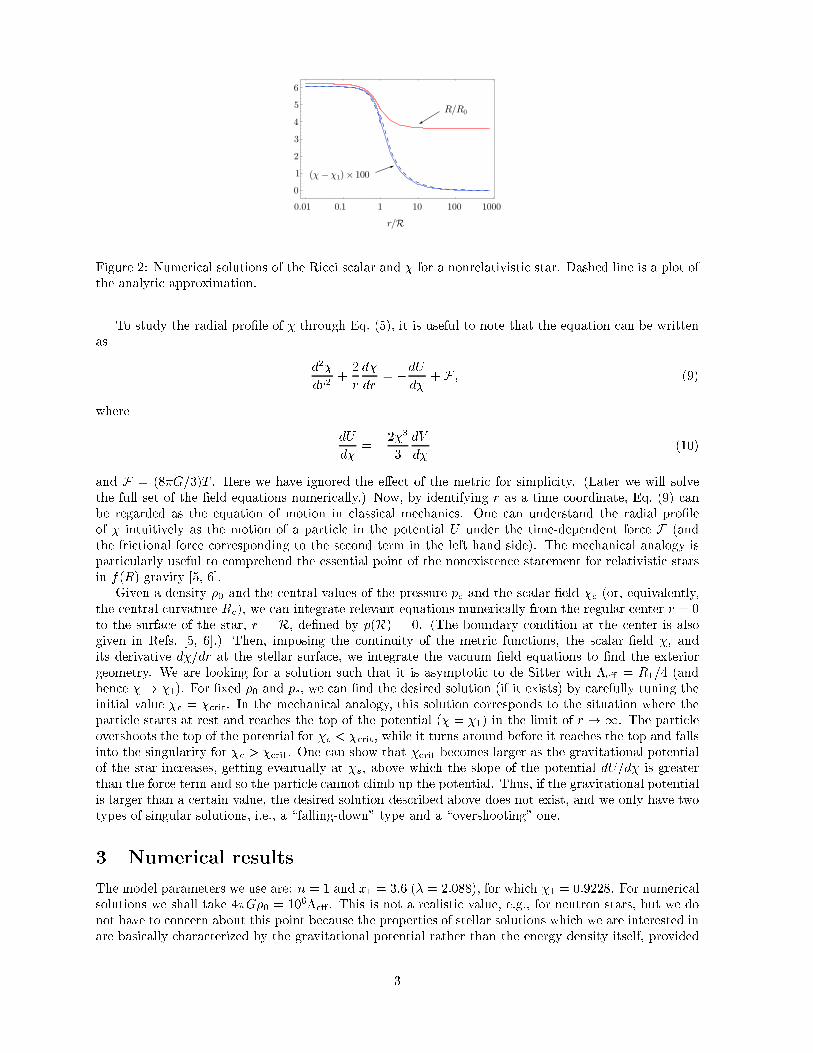
1 +; C 0 '
< $5%
7
+
(
7 $E%
( +
,
$)%
( $:,% # 2 $8 % C < $E% B $ % $% *5 6-
F $ % ( ) ( $% ( ) $ 0 *5 6-% ! @ A ( 3 $ % 1 $ % ( / $ ( % B = > = >
; ( ( ,6 $ ( +)::% ( )E++: 1 3 ( ) A D
,
1 ,; "
A
3 ( ) A ( ) @ ( +)) ) :
" 3 ( ) A ( 5 ) ! ( ,36+ ) : $ ( )E:,6% G ))66:?B 1 + , B 1 +
G 3 ( ) A ( ) " ( )?))) : $ 1 ,% $$% ) $% % / => G )+), ( )?)) : 0 (
/ $% * + ,- ! $% *- D ; @ ! 1 ( + 4 ) $%
*- " " @ H<I 8 5? $+))?% *J;)?)6+)3 *--
*+- ! # / @ I 0 ' )63))3 $+))?% *J;)?)55: *--
*,- @ " " 0 " & I 8 & ? $+))?% *J;)?)5,EE *--
*3- " 9 1 I 0 8 )6), $+)):% *J;):),+5)) *--
*5- I 0 ' )63)E $+)):% *J;):)?+5), *--
*6- I 0 ' )+3))E $+))E% *J;):)5663 *--
3
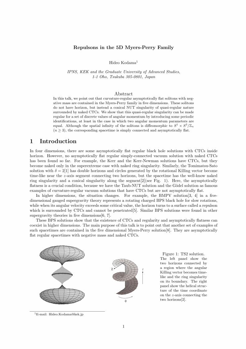
Repulsons in the 5D Myers-Perry Family
Hideo Kodama1
IPNS, KEK and the Graduate University of Advanced Studies,1-1 Oho, Tsukuba 305-0801, Japan
AbstractIn this talk, we point out that curvature-regular asymptotically flat solitons with neg-ative mass are contained in the Myers-Perry family in five dimensions. These solitonsdo not have horizon, but instead a conical NUT singularity of quasi-regular naturesurrounded by naked CTCs. We show that this quasi-regular singularity can be maderegular for a set of discrete values of angular momentum by introducing some periodicidentifications, at least in the case in which two angular momentum parameters areequal. Although the spatial infinity of the solitons is diffeomorphic to S1 × S3/Zn
(n ≥ 3), the corresponding spacetime is simply connected and asymptotically flat.
1 Introduction
In four dimensions, there are some asymptotically flat regular black hole solutions with CTCs insidehorizon. However, no asymptotically flat regular simply-connected vacuum solution with naked CTCshas been found so far. For example, the Kerr and the Kerr-Newman solutions have CTCs, but theybecome naked only in the superextreme case with naked ring singularity. Similarly, the Tomimatsu-Satosolution with δ = 2[1] has double horizons and circles generated by the rotational Killing vector becometime-like near the z-axis segment connecting two horizons, but the spacetime has the well-know nakedring singularity and a conical singularity along the segment[2](see Fig. 1). Here, the asymptoticallyflatness is a crucial condition, because we have the Taub-NUT solution and the Godel solution as famousexamples of curvature-regular vacuum solutions that have CTCs but are not asymptotically flat.
In higher dimensions, the situation changes. For example, the BMPV solution[3, 4] in a five-dimensional gauged supergravity theory represents a rotating charged BPS black hole for slow rotations,while when its angular velocity exceeds some critical value, the horizon turns to a surface called a repulsonwhich is surrounded by CTCs and cannot be penetrated[5]. Similar BPS solutions were found in othersupergravity theories in five dimensions[6, 7].
These BPS solutions show that the existence of CTCs and regularity and asymptotically flatness cancoexist in higher dimensions. The main purpose of this talk is to point out that another set of examples ofsuch spacetimes are contained in the five dimensional Myers-Perry solution[8]. They are asymptoticallyflat regular spacetimes with negative mass and naked CTCs.
χ
φ
t
Figure 1: TS2 solution.The left panel show thetwo horizons connected bya region where the angularKilling vector becomes time-like and the ring singularityon its boundary. The rightpanel show the helical struc-ture of the time coordinateon the z-axis connecting thetwo horizons[2].
1E-mail: [email protected]
1
2 Internal Structure of the 5D Myers-Perry Solution
2.1 Metric and regularity
In terms of the Boyer-Lindquist coordinates (t, φ1, φ2, r, θ), the 5D Myers-Perry solution can be writtenas[8]
ds2 =r2ρ2
∆dr2 + ρ2dθ2 + (r2 + a2) sin2 θdφ1
2 + (r2 + b2) cos2 θdφ22
−dt2 +µ
ρ2
[dt + a sin2 θdφ1 + b cos2 θdφ2
]2, (1)
where ∆ := (r2 + a2)(r2 + b2) − µr2.Because the determinant of the metric is given by −g = r2ρ4 sin2 θ cos2 θ, apart from the angular
coordinate singularities at θ = 0, π/2, the metric (1) is apparently singular at r = 0 and at ∆ = 0 inaddition to ρ = 0, which is curvature singularity from the expression for the Kretchman invariant,
RµνλσRµνλσ = 24µ2 (3r2 − a2 cos2 θ − b2 sin2 θ)(r2 − 3a2 cos2 θ − 3b2 sin2 θ)ρ12
. (2)
Among these apparent singularities, we can confirm that the points with r = 0 are not real singularityby expressing the metric in terms of x = r2 as[8]
ds2 =ρ2
4∆dx2 + ρ2dθ2 + (x + a2) sin2 θdφ1
2 + (x + b2) cos2 θdφ22
−dt2 +µ
ρ2
[dt + a sin2 θdφ1 + b cos2 θdφ2
]2. (3)
Now, ∆ and ρ2 become polynomials in x as
∆ = (x + a2)(x + b2) − µx, ρ2 = x + a2 cos2 θ + b2 sin2 θ, (4)
and −g is expressed as −g = ρ4 sin2 θ cos2 θ/4.
2.2 Structure of Killing orbits
On a Killing horizon, the induced metric on the orbit space of the Killing vectors ∂t, ∂φ1 and ∂φ2 becomesdegenerate. From |gab|a,b=t,φ2,φ1
= −∆sin2 θ cos2 θ, this condition can be written ∆ = 0. When ab 6= 0and µ > 0, this equation for x has a root in the region ρ2 > 0 iff µ > (|a| + |b|)2. In this case, thereactually exist two positive roots, which are both regular horizons.
In contrast, when µ < 0, we have only negative roots, but one of them, x = xh, is larger than −b2 andin the region with ρ2 > 0. This apparently indicates that even in the negative mass case, the spacetimehas a regular horizon and a regular domain of outer communication. However, this is not the case. Infact, the spacetime has pathological features around x = xh, when xh 6= 0. For example, the Killingvector k whose norm vanishes at x = xh becomes spacelike outside the horizon. Further, the norm of theKilling vector ∂t is negative definite for x ¸ xh.
2.3 CTCs
Let Φ be the symmetric matrix of degree 2 defined by Φ := (gij)i,j=φ1.φ2. Then, we can show that
detΦ = D1 sin2 θ cos2 θ/ρ2 is non-negative in x > 0 for µ > 0, and therefore that there occurs nocausality violation at or outside the outer horizon for µ > (|a| + |b|)2.
In contrast, for µ < 0, causality violation occurs in the region x ¸ xh. In fact, D1 can be written as
D1 = ∆(x + a2 sin2 θ + b2 cos2 θ + µ) + µ2x. (5)
From this, around x = xh at which ∆ = 0, the sign of D1 is determined by the sign of xh. Hence, whenxh < 0, 2-tori generated by ∂φ1 and ∂φ2 become timelike surfaces around x = xh, which always contain
2
CTCs. As we show in the next section, this feature together with the fact that gtt is netative and Φ hasa finite non-degenerate limit at x = xh implies that x = xh is not a horizon but rather something like arepulson, which was first found by Gibbons and Herdeiro for supersymmetric rotating black holes in fivedimensions[5, 6].
3 Repulson
3.1 U(2) MP solution
In the case a = b 6= 0, the metric in the Boyer-Lindquist coordinates reads
ds2 =ydy2
4(y2 − µy + a2µ)+ yds2(S3) − dt2 +
µ
y
(dt + aχ3
)2, (6)
where y = ρ2 = x + a2, and χ3 is the 1-form on S3 invariant under the action of SU(2)
χ3 = sin2 θdφ1 + cos2 θdφ2. (7)
3.2 Negative mass soliton
Now, we show that the surface corresponding to the root x = xh(> −a2) of ∆ = 0 for µ < 0, which isintrinsically S2, is not a regular submanifold of the spacetime, but rather a quasi-regular singularity. Forthat purpose, let us introduce the coordinate
ξ =(
a2 − yh
2a2 − yh(y − yh)
)1/2
, (8)
where yh = xh + a2 > 0. Then, in terms of the 1-forms
τ = − a
yhdt + χ3, χ = χ3 +
yh
2a2 − yhτ , (9)
the metric can be written near the locus y = yh as
ds2 ' − y2h
(a2 − yh)τ2 + dξ2 + c2ξ2χ2
3 + yhds2(S2), (10)
wherec =
2a
(a2 − yh)1/2
(1 − yh
2a2
). (11)
The curvature tensor of this metric is bounded everywhere. However, it has a kind of conical singularityat ξ = 0 because c > 2 and t is not a periodic coordinate. This conical singularity cannot be removedeven by a periodic identification of t in general. For some discrete values of yh, however, the spacetimecan be made regular by such an identification. To see this, we utilise the local charts, (z+, w+, t+) forθ 6= π/2 and (z−, w−, t−) for θ 6= 0 defined by
z± := (tan θ)±1e±iφ, w± := ξeic(ψ±φ)/2, t± := t − yh
4a(ψ ± φ). (12)
It is easy to see that in each of these coordinate system, the metric (10) has regular expressions.In the region 0 < θ < π/2 covered by both charts, the two set of coordinates are related by
z− =1z+
, w− = w+
(z+
|z+|
)−c
, t− = t+ + iyh
aln
z+
|z+|. (13)
From the relation for w±, we find that c must be an integer n > 2 for the coordinate transformation tobe well-defined. Further, because the ln-term in the relation for t± produces ambiguity in the values of
3
t± written as an integer multiple of 2πyh/a, these two charts are consistent only when we identify t±periodically with a period 2πyh/(ma) where m is some positive integer.
For ξ 6= 0, by this identification, each ξ = const surface becomes a S1 bundle over S3/Zn. However,since we can easily show that the regular manifold constructed above from the region around ξ = 0 issimply connected for m = 1, the whole spacetime is also simply connected for m = 1. In that case, CTCsalong S1 produced by the above identification at ξ 6= 0 cannot be removed by taking a covering space.
4 Summary and Discussion
In the present paper, we have shown that the five-dimensional Myers-Perry solution with negative massdescribes an asymptotically flat rotating spacetime with naked CTCs, no horizon and no curvaturesingularity. We further pointed out that we can construct a regular repulson-type asymptotically flatsoliton from them for a discrete set of values of the angular momentum for a fixed mass parameter µ.
Although the structure of the original metric when the repulson appears is similar to that of BPSsolutions with repulsons, there exist several big differences between our family and the BPS families. Inparticular, our solutions are non-BPS solution to the purely vacuum Einstein equations, and the repulsonis a regular submanifold of the whole spacetime. This should be contrasted to the BPS case in whichthe repulson is at spatially infinite distance. Further, the soliton spacetime obtained after regularisationis not asymptotically flat in the standard sense because it has some time periodicity at spatial infinityand its spatial infinity is S3/Zn with n ¸ 3, although it is topologically simply connected. Finally, therepulson appears only for negative mass. This is rather striking because a regular soliton spacetime withnegative mass can exist in higher dimensions.
Finally, we note that our analysis can be extended to the U(N) symmetry Myers-Perry solutions in2N +1 dimensions[9]. It can be also extended to the rotating black-hole type solutions with cosmologicalconstant[10] and to the black holes with generic angular momentum parameters. These extensions areunder investigation.
Acknowledgement
This talk is based on the work in collaboration with G.W. Gibbons. The author would like to thank HidekiMaeda, Akihiro Ishibashi, Shinya Tomizawa and Andres Anabalon for discussions and useful comments.This work was supported in part by Grants-in-Aids for Scientific Research from JSPS (No. 18540265)and for the Japan-U.K. Research Cooperative Program.
References
[1] Tomimatsu, A. and Sato, H.: Phys. Rev. Lett. 29, 1344 (1972).
[2] Kodama, H. and Hikida, W.: Class. Quant. Grav. 20, 5121–40 (2003).
[3] Breckenridge, J., Myers, R., Peet, A. and Vafa, C.: Phys. Lett. B 391, 93–98 (1997).
[4] Kallosh, R., Rajaraman, A. and Wong, W.: Phys. Rev. D 55, R3246–9 (1997).
[5] Gibbons, G. and Herdeiro, C.: Class. Quantum Grav. 16, 3619–52 (1999).
[6] Cvetic, M., Gibbons, G., Lu, H. and Pope, C.: hep-th0504080 (2005).
[7] Gauntlett, J., Gutowski, J., Hull, C., Pakis, S. and Reall, H.: Class. Quant. Grav. 20, 4587–4634(2003).
[8] Myers, R. and Perry, M.: Ann. Phys. 172, 304–347 (1986).
[9] Gibbons, G. and Kodama, H.: arXiv:0910.1203 (2009).
[10] Gibbons, G. W., Lu, H., Page, D. N. and Pope, C. N.: J. Geom. Phys. 53, 49–73 (2005).
4
Vacuum Bubble Nucleation and Black Hole Pair Creation
Bum-Hoon Lee1 and Wonwoo Lee2
1Department of Physics and Center for Quantum Spacetime, Sogang University, Seoul 121-742, Korea2Center for Quantum Spacetime, Sogang University, Seoul 121-742, Korea
AbstractWe study the nucleation of a vacuum bubble in the presence of gravity and considerthe pair production of blak holes in the background of bubble solutions. This articleis prepared for the proceedings of The 18th Workshop on General Relativity andGravitation in Japan (JGRG18) in Hiroshima, Japan, 17-21 Nov 2008.
1 Introduction
Recently, we have investigated the possible types of the nucleation of vacuum bubbles [1]. We classifiedtrue vacuum bubbles in de Sitter background and present some numerical solutions. The nucleationrate and the radius of true and false vacuum bubbles are analytically computed using the thin-wallapproximation. We obtained static bubble wall solutions of junction equation with black hole pair. Inthis article, we will summarize our results.
It has been shown that the first-order vacuum phase transitions occur via the nucleation of truevacuum bubble at zero temperature both in the absence of gravity [2] and in the presence of gravity [3].This result was extended by Parke [4] to the case of arbitrary vacuum energy densities. An extension ofthis theory to the case of non-zero temperatures has been found by Linde [5] in the absence of gravity,where one should look for the O(3)-symmetric solution due to periodicity in the time direction β withperiod T−1 unlike the O(4)-symmetric solution in the zero temperature. These processes as cosmologicalapplications of false vacuum decay have been applied to various inflationary universe scenarios by manyauthors [6]. The Hawking-Moss transition describes the scalar field jumping simultaneously at the top ofthe potential barrier [7]. A new method to calculate the tunneling wave function that describes vacuumdecay was studied by Gen and Sasaki [8]. The effect of the Gauss-Bonnet term on vacuum decay was alsostudied [9]. Marvel and Wesley studied thin-wall instanton with negative tension wall and its relation toWitten’s bubble of nothing [10]. In Ref. [11], the authors discussed the possible four different instantonsin Euclidean de Sitter space.
As for the false vacuum bubble formation, Lee and Weinberg [12] have shown that if the vacuumenergies are greater than zero, gravitational effects make it possible for bubbles of a higher-energy falsevacuum to nucleate and expand within the true vacuum bubble in the de Sitter space which has a topologyof 4-sphere. The false vacuum bubble nucleation is described as the inverse process of the true vacuumbubble nucleation. However, their solution is larger than the true vacuum horizon [13]. The oscillatingbounce solutions, another type of Euclidean solutions, have been studied in detail by Hackworth andWeinberg [14]. On the other hand Kim et al. [15] have shown that false vacuum region may nucleatewithin the true vacuum bubble as global monopole bubble in the high temperature limit.
Next, we will consider black hole pair creation. Caldwell et al. studied black hole pair creation in thepresence of a domain wall [16] using the cut-and-paste procedure, where the background has vanishingcosmological constant and the probability was obtained. The repulsive property of the domain wall giverise to black hole pair creation. However, our solutions give rise to the background for the black hole paircreation with a bubble wall more naturally.
1E-mail:[email protected]:[email protected]
1
2 The vacuum bubble
The bubble nucleation rate or the decay rate of background vacuum is semiclassically given by
Γ/V = Ae−B/h, (1)
where B is the difference between Euclidean action corresponding to bubble solution and that of thebackground and the prefactor A is discussed in Ref. [17], that with some gravitational corrections in Ref.[18]. We are interested in finding the coefficient B.
Let us consider the action
S =∫
M
√−gd4x
[R
2κ− 1
2∇αΦ∇αΦ− U(Φ)
]+
∮
∂M
√−hd3x
K
κ, (2)
where κ ≡ 8πG, g ≡ detgµν , and the second term on the right-hand side is the boundary term. U(Φ) isthe scalar field potential with two non-degenerate minima with lower minima at ΦT and higher minimaat ΦF , R denotes the Ricci curvature of spacetime M, and K is the trace of the extrinsic curvature ofthe boundary ∂M.
We will take O(4) symmetry for both Φ and the spacetime metric gµν , expecting its dominant con-tribution [19].
The Euclidean field equations for Φ and ρ have the form
Φ′′ +3ρ′
ρΦ′ =
dU
dΦ, (3)
ρ′′ = −κ
3ρ(Φ′2 + U), (4)
respectively and the Hamiltonian constraint is given by
ρ′2 − 1− κρ2
3
(12Φ′2 − U
)= 0. (5)
We will consider only the case with initial de Sitter space. The boundary conditions for the bounce are
dΦdη
∣∣∣η=0
= 0,dΦdη
∣∣∣η=ηmax
= 0, ρη=0 = 0, and ρη=ηmax = 0, (6)
where ηmax is a finite value in Euclidean de Sitter space.In this article, we consider only several cases including true, false, and degenerate vacua. Firstly, we
consider the large true anti-de Sitter bubble with small false de Sitter background. The size of the bubbleand the nucleation rate are evaluated to be
ρ2 =ρ2
o
Dand B =
2Bo(λ2λ1
)2[1 + (λ1λ2
)2( ρo
2λ2)2 − (λ1
λ2)2D1/2 + E]
[( ρo
2λ2)4(λ2
λ1)4 − 1D1/2]
, (7)
where D =[1 + 2( ρo
2λ1)2 + ( ρo
2λ2)4
], λ2
1 = [3/κ(UF + UT )], λ22 = [3/κ(UF − UT )], UT < 0, and E =
2(λ2λ1
)4 − 1( ρo
2λ1)2[1− ( ρo
2λ2)2]D−1.
Secondly, we consider the large false de Sitter bubble with the small true de Sitter background. Thesize of the bubble has the same as above case. The nucleation rate is given by
B =2Bo[1 + ( ρo
2λ1)2+ 1 + 2( ρo
2λ1)2 + ( ρo
2λ2)41/2]
[( ρo
2λ2)4(λ2
λ1)4 − 11 + 2( ρo
2λ1)2 + ( ρo
2λ2)41/2]
. (8)
Thirdly, we consider the transition between degenerate vacua in de Sitter space. The critical radiusof the wall is given by
ρ =2
κ√
S2o
4 + 43κUo
. (9)
The nucleation rate is given by
B =12π2So
κ2Uo
√S2
o
4 + 43κUo
. (10)
2
3 Black hole pair creation
We consider several types of the configuration as the background space for black hole pair creation. Inthis work the general Euclidean junction condition becomes
√1− 2GM
r± Λ−
3r2 − r2 +
√1− 2GM
r− Λ+
3r2 − r2 = 4πGσr, (11)
where So = σ and · denotes the differentiation with respect to the proper time measured by the observermoving along with the wall. The signs (−) and (+) as a subscript of Λ represent left and right spacetime,respectively. After squaring twice, we define the effective potential for Euclidean junction equation to be
Veff =12− 1
2
[(2πGσ +
(Λ+ − Λ−)24πGσ
)2
+Λ−3
]r2 − GM
r, (12)
with total energy is 0. The static bubble wall solution satisfies the following conditions
Veff (rb) = 0, anddVeff
dr
∣∣rb
= 0. (13)
The solution can exist at rb = 3GM . The masses of created black holes are uniquely determined by thegiven cosmological constant and surface tension on the wall:
M =1
3G
√3
[(2πGσ + (Λ+−Λ−)
24πGσ
)2
+ Λ−3
] . (14)
In this process the location of the wall with black holes is given by
rb = 3GM or rb =1√
3[(
2πGσ + (Λ+−Λ−)24πGσ
)2
+ Λ−3
] . (15)
This case is that the left of the wall corresponds to flat space and the right corresponds to de Sitterspace. The action turns out to be
SE = SCE − σ
4
(√1− 2GM
r
∫ τ−
0
dτ− +
√1− 2GM
r− Λ+
3r2
∫ τ+
0
dτ+
) ∫ π
0
dθ
∫ 2π
0
dφr2 sin θ
− SE(bulk)− SBE
= SCE − πσr2
b
(8πGM√
3+
(4πGσrb − 1√
3
)2πrh
√1− (9Λ+G2M2)1/3
1− Λ+r2h
)
− 2πU+
3r3b
(2πrh
√1− (9Λ+G2M2)1/3
1− Λ+r2h
)+
2π2U+√3Λ+
r3wob
+ σπr2wob
(πr
2+ 2
√3
Λ+(4πGσr − 1)
), (16)
where U+ > 0 and we use the Bousso-Hawking normalization for Schwarzschild-de Sitter space.
4 Summary and Discussions
In this paper we classified the possible types of vacuum bubbles and calculated the radius and thenucleation rate. We present analytic computation using the thin-wall approximation. There are ninetypes of true vacuum bubbles, three false vacuum bubbles, and Hawking-Moss transition in which the
3
thin-wall approximation is not considered. Our results, including the half sized and the large bubble fortrue vacuum bubbles, false vacuum bubbles, and degenerate case, extend Parke’s results. We consideredthe pair creation of black holes in some of these vacuum bubble backgrounds. These solutions give riseto the background for the black hole pair creation more naturally.
Our solutions, even if it has simple structure, can be used to understand the mechanism how thecomplicated spacetime structure could be created in the early universe as well as tunneling phenomenaoccur in the string landscape and eternal inflation.
Acknowledgements
We would like to thank Misao Sasaki for his hospitality at the 18th Workshop on General Relativityand Gravitation in Japan (JGRG18) in Hiroshima. We would like to thank Kei-ichi Maeda for helpfuldiscussions. This work was supported by the Korea Science and Engineering Foundation (KOSEF)grant funded by the Korea government(MEST) through the Center for Quantum Spacetime(CQUeST)of Sogang University with grant number R11 - 2005 - 021. W.L. was supported by the Korea ResearchFoundation Grant funded by the Korean Government(MOEHRD)(KRF-2007-355-C00014).
References
[1] B.-H. Lee and W. Lee, arXiv:0809.4907.
[2] S. Coleman, Phys. Rev. D 15, 2929 (1977); ibid. D 16, 1248(E) (1977).
[3] S. Coleman and F. De Luccia, Phys. Rev. D 21, 3305 (1980).
[4] S. Parke, Phys. Lett. B 121, 313 (1983).
[5] A. D. Linde, Phys. Lett. B 100, 37 (1981); Nucl. Phys. B 216, 421 (1983).
[6] A. H. Guth, Phys. Rev. D 23, 347 (1981); K. Sato, Mon. Not. R. Astron. Soc. 195, 467 (1981); J.R. Gott, Nature 295, 304 (1982); J. R. Gott and T. S. Statler, Phys. Lett. B 136, 157 (1984); M.Bucher, A. S. Goldhaber, and N. Turok, Phys. Rev. D 52, 3314 (1995).
[7] S. W. Hawking and I. G. Moss, Phys. Lett. B 110, 35 (1982).
[8] U. Gen and M. Sasaki, Phys. Rev. D 61, 103508 (2000).
[9] R.-G. Cai, B. Hu, and S. Koh, arXiv:0806.2508.
[10] K. Marvel and D. Wesley, arXiv:0808.3186.
[11] K. Marvel and N. Turok, arXiv:0712.2719.
[12] K. Lee and E. J. Weinberg, Phys. Rev. D 36, 1088 (1987).
[13] R. Basu, A. H. Guth, and A. Vilenkin, Phys. Rev. D 44, 340 (1991); J. Garriga, Phys. Rev. D 49,6327 (1994).
[14] J. C. Hackworth and E. J. Weinberg, Phys. Rev. D 71, 044014 (2005).
[15] Y. Kim, K. Maeda, and N. Sakai, Nucl. Phys. B 481, 453 (1996); Y. Kim, S. J. Lee, K. Maeda, andN. Sakai, Phys. Lett. B 452, 214 (1999).
[16] R. R. Caldwell, H. A. Chamblin, and G. W. Gibbons, Phys. Rev. D 53, 7103 (1996).
[17] C. G. Callan and S. Coleman, Phys. Rev. D 16, 1762 (1977); E. J. Weinberg, Phys. Rev. D 47, 4614(1993); G. V. Dunne and H. Min, Phys. Rev. D 72, 125004 (2005).
[18] D. Metaxas, arXiv:0804.1045.
[19] S. Coleman, V. Glaser, and A. Martin, Commun. Math. Phys. 58, 211 (1978).
4
Non-gaussianity from the bispectrum in general multiple fieldinflation
Shuntaro Mizuno1 , Frederico Arroja2 and Kazuya Koyama3
1Research Center for the Early Universe (RESCEU), School of Science, University of Tokyo, 7-3-1Hongo, Bunkyo, Tokyo 113-0033, Japan
2,3Institute of Cosmology and Gravitation, University of Portsmouth, Portsmouth PO1 2EG, UK
AbstractWe study the non-gaussianity from the bispectrum in multi-field inflation modelswith a general kinetic term. The models include the multi-field K-inflation and themulti-field Dirac-Born-Infeld (DBI) inflation as special cases. We derive the threepoint function for the curvature perturbation which depends on both adiabatic andentropy perturbations, in the small sound speed limit and at leading order in theslow-roll expansion. The contribution from the entropy perturbations has a differentmomentum dependence if the sound speed for the entropy perturbations is differentfrom the adiabatic one, which provides a possibility to distinguish the multi-fieldmodels from single field models.
1 Introduction
The non-gaussianity of the primordial fluctuations will provide powerful ways to constrain models (seee.g. [1] for a review). The simplest single field inflation models predict that the non-gaussianity of thefluctuations should be very difficult to be detected even in the future experiments such as Planck. If wedetect large non-gaussianity, this means that the simplest model of inflation would be rejected.
There are a few models where the primordial fluctuations generated during inflation have a large non-gaussianity. One way to obtain the large primordial non-gaussianity is to consider Multi-field inflationmodels where the curvature perturbation is modified on large scales due to the entropy perturbations[2]. Since it is shown that in the case of the standard kinetic term, it is not easy to generate largenon-gaussianity from multi-field dynamics, it is interesting to consider the multi-field generalization tothe models with non-canonical kinetic term like K-inflation [3, 4] and Dirac-Born-Infeld (DBI) inflation[5, 6], motivated by string theory. Especially, since in the DBI-inflation, the inflaton is identified withthe position of a moving D3 brane where each compact direction is described by a scalar field, theDBI-inflation is naturally a multi-field model [7].
In this paper, based on [8], we study a fairly general class of multi-field inflation models with a generalkinetic term which includes K-inflation [9] and DBI-inflation [10, 11]. We study the sound speeds of theadiabatic perturbations and entropy perturbations and clarify the difference between K-inflation andDBI-inflation. Then we calculate the third order action by properly taking into account the effect ofgravity. Then three point functions at the leading order in slow-roll and in the small sound speed limitare obtained. We can recover the results for K-inflation and DBI-inflation easily from this general result.
2 The model
We consider a very general class of models described by the following action
S =12
∫d4x
√−g[M2
PlR + 2P (XIJ , φI)], (1)
1E-mail:[email protected]:[email protected]:[email protected]
1
where φI are the scalar fields (I = 1, 2, ..., N), MPl is the Planck mass that we will set to unity hereafter,R is the Ricci scalar and
XIJ ≡ −12gµν∂µφI∂νφJ , (2)
is the kinetic term, gµν is the metric tensor. We label the fields’ Lagrangian by P and we assume that itis a well behaved function. Greek indices run from 0 to 3. Lower case Latin letters denote spatial indices.Upper case Latin letters denote field indices.
In the background, we are interested in flat, homogeneous and isotropic Friedmann-Robertson-Walkeruniverses. For this background, we consider perturbations beyond linear order. For this purpose, we willconstruct the action at second and third order in the perturbations and it is convenient to use the ADMmetric formalism where the ADM line element reads
ds2 = −N2dt2 + hij
(dxi + N idt
) (dxj + N jdt
), (3)
where N is the lapse function, N i is the shift vector and hij is the 3D metric. For convenience, we definebackground scalar fields φI
0 and scalar field perturbations QI in the flat hypersurface as
φI(x, t) = φI0(t) + QI(x, t). (4)
Furthermore, we decompose the perturbations into the instantaneous adiabatic and entropy pertur-bations, where the adiabatic direction corresponds to the direction of the background fields’ evolutionwhile the entropy directions are orthogonal to this. Similar to [8], we introduce an orthogonal basiseIn(n = 1, 2, ..., N) in the field space so that the orthonormalily condition and the adiabatic basis are
given by
P,XIJ eIneJ
m = δnm , eI1 =
φI
√P,XJK φJ φK
. (5)
Furthermore, for simplicity, let us consider models described by
P (XIJ , φI) = P (Y, φI) , where Y = GIJ (φK)XIJ +b(φK)
2(X2 −XJ
I XIJ) . (6)
The functional form of Y is chosen so that Y = X ≡ GIJXIJ in the background as in the DBI-inflationmodel. This model includes as particular cases the K-inflation model for b = 0 and the DBI-inflation forb = −2f and if P has the DBI form. This might be surprising as the DBI action contains additionalterms of order f2, f3 and f4, but it turn out that these terms do not contribute to the leading orderthird order action.
3 Second and Third-order actions
The second order action can be written in terms of the decomposed perturbations as
S(2) =12
∫dtd3xa3
[δmn +
2XP,Y Y
P,Y
δ1mδ1n +bX
1 + bX(δn1δm1 − δmn)
(DtQm)(DtQn)
− 1a2
δmn∂iQm∂iQn − MmnQmQn + NmnQn(DtQm)]
, (7)
From this, we can see that the sound speed for adiabatic perturbations c2ad and for entropy perturbations
c2en are given by
c2ad =
P,Y
P,Y + 2XP,Y Y
, c2en = 1 + bX . (8)
Similarly, at the leading order in slow-roll approximation where the following parameters are small,
ε = − H
H2=
XP,Y
H2, η =
ε
εH, χad =
cad
cadH, χen =
cen
cenH, (9)
2
the third-order action can be written as
S(3) =∫
dx3dta3
[12ΞnmlQnQmQl − 1
2a2ΥnmlQn(∂iQm)(∂iQl)
], (10)
where we define the coefficients Ξnml and Υnml as
Ξnml = (2XP,Y )−12
[(1− c2
ad)c2adc
2en
δ1(nδml) +
(43
X2P,Y Y Y
P,Y
− (1− c2ad)(1− c2
en)c2adc
2en
)δn1δm1δl1
], (11)
Υnml = (2XP,Y )−12
(1− c2
ad
c2ad
δn1δml − 2(1− c2en)
c2en
(δn1δml − δn(mδl)1
)), (12)
and it is obvious that the DBI-inflation is a specific case of the general model with c2ad = c2
en = c2s.
4 Three-point functions
We derive the three point functions of the adiabatic and entropy fields in the generalized case and atleading order in slow-roll and in the small sound speeds limit. We consider the two-field case with theadiabatic field σ and the entropy field s.
The vacuum expectation value of the three point operator in the interaction picture is
〈Ω|Ql(t,k1)Qm(t,k2)Qn(t,k3)|Ω〉 = −i
∫ t
t0
dt〈0| [Ql(t,k1)Qm(t,k2)Qn(t,k3),HI(t)] |0〉, (13)
where t0 is some early time during inflation when the field’s vacuum fluctuation are deep inside thehorizons, t is some time after horizon exit. |Ω〉 is the interacting vacuum which is different from the freetheory vacuum |0〉. At this order, the only non-zero three point functions are
〈Ω|Qσ(0,k1)Qσ(0,k2)Qσ(0,k3)|Ω〉 = (2π)3δ(3)(k1 + k2 + k3)2cad|Aσ|6
H
1Π3
i=1k3i
1K
×[6c2
ad(C3 + C4)k21k
22k
23
K2− C1k
21k2 · k3
(1 +
k2 + k3
K+ 2
k2k3
K2
)+ 2 cyclic terms
], (14)
〈Ω|Qσ(0,k1)Qs(0,k2)Qs(0,k3)|Ω〉 = (2π)3δ(3)(k1 + k2 + k3)|Aσ|2|As|4
H
1Π3
i=1k3i
1K
×[C2c
2enk2
3k1 · k2
(1 +
cadk1 + cenk2
K+
2cadcenk1k2
K2
)+ (k2 ↔ k3)
+4C3c2adc
4en
k21k
22k
23
K2− 2(C1 + C2)c2
adk21k2 · k3
(1 + cen
k2 + k3
K+ 2c2
en
k2k3
K2
)], (15)
where K = k1 + k2 + k3, K = cadk1 + cen(k2 + k3), cyclic terms means cyclic permutations of the threewave vectors and (k2 ↔ k3) denotes a term like the preceding one but with k2 and k3 interchanged.
Then, we calculate the leading order in slow-roll three point function of the comoving curvatureperturbation. In this work we will ignore the possibility that the entropy perturbations during inflationcan lead to primordial entropy perturbations that could be observable in the CMB. But we shall considerthe effect of entropy perturbations on the final curvature perturbation. We will follow the analysis, whereit has been shown that even on large scales the curvature perturbation can change in time because ofthe presence of entropy perturbations. The way the entropy perturbations are converted to curvatureperturbations is model dependent but it was shown that this model dependence can be parameterized bya transfer coefficient TRS like
R = AσQσ∗ + TRSAsQs∗, (16)
with
Aσ =
H
σ√
P,Y
∗
, As =
H
σ√
P,Y
√cen
cad
∗
. (17)
3
Using the previous expressions we can now relate the three point function of the curvature perturbationto the three point functions of the fields obtained in the previous subsection. The three point functionof the curvature perturbation is given by
〈R(k1)R(k2)R(k3)〉 = A3σ〈Qσ(k1)Qσ(k2)Qσ(k3)〉+AσA2
s (〈Qσ(k1)Qs(k2)Qs(k3)〉+ 2 perms.) . (18)
For the DBI-inflation case the previous equation can be simplified and the total momentum dependenceof the three point function of the comoving curvature perturbation is the same as in single field DBI.For our general model this is no longer the case, i.e., the different terms of the previous equation havedifferent momentum dependence. Once again one can see that DBI-inflation is a very particular caseand more importantly it provides a distinct signature that enables us to distinguish it from other moregeneral models.
5 Conclusions
In this paper, we studied the non-gaussianity from the bispectrum in general multi-field inflation modelswith a generic kinetic term. We derived the second and third order action for the perturbations includingthe effect of gravity. The second order action is written in terms of adiabatic and entropy perturbations.It was shown that the sound speeds for these perturbations are in general different. The K-inflation andthe DBI-inflation are special cases where the sound speed for entropy perturbations is one and the sameas the adiabatic perturbations, respectively.
Then we derive the three point function in the small sound speeds limit at the leading order in slow-rollexpansion. In these approximations there exists a three point function between adiabatic perturbationsQσ and entropy perturbations Qs, 〈Qσ(k1)Qs(k2)Qs(k3)〉, in addition to the pure adiabatic three pointfunction. This mixed contribution has a different momentum dependence if the sound speed for theentropy perturbations is different from the adiabatic one. This provides a possibility to distinguishbetween the multi-field models and the single field models. Unfortunately, in the multi-field DBI case,the sound speed for the entropy perturbation is the same as the adiabatic one and the mixed contributiononly changes the amplitude of the three point function. This could help to ease the constraints on DBI-inflation. For the specialty of the DBI inflation model, we can see that the trispectrum can distinguishthe multi-field inflation from the single field DBI inflation model [12].
References
[1] N. Bartolo, E. Komatsu, S. Matarrese and A. Riotto, Phys. Rept. 402, 103 (2004).
[2] A. A. Starobinsky and J. Yokoyama, arXiv:gr-qc/9502002.
[3] C. Armendariz-Picon, T. Damour and V. F. Mukhanov, Phys. Lett. B 458 (1999) 209.
[4] J. Garriga and V. F. Mukhanov, Phys. Lett. B 458 (1999) 219.
[5] E. Silverstein and D. Tong, Phys. Rev. D 70 (2004) 103505.
[6] M. Alishahiha, E. Silverstein and D. Tong, Phys. Rev. D 70 (2004) 123505.
[7] D. A. Easson, R. Gregory, D. F. Mota, G. Tasinato and I. Zavala, JCAP 0802 (2008) 010.
[8] F. Arroja, S. Mizuno and K. Koyama, JCAP 0808, 015 (2008).
[9] D. Langlois and S. Renaux-Petel, JCAP 0804 (2008) 017.
[10] D. Langlois, S. Renaux-Petel, D. A. Steer and T. Tanaka, Phys. Rev. Lett. 101, 061301 (2008).
[11] D. Langlois, S. Renaux-Petel, D. A. Steer and T. Tanaka, Phys. Rev. D 78, 063523 (2008).
[12] S. Mizuno, F. Arroja and K. Koyama, in preparation
4
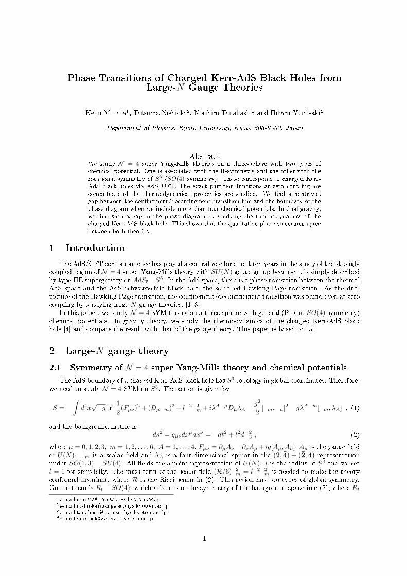
Phase Transitions of Charged Kerr-AdS Black Holes fromLarge-N Gauge Theories
Keiju Murata1, Tatsuma Nishioka2, Norihiro Tanahashi3 and Hikaru Yumisaki4
Department of Physics, Kyoto University, Kyoto 606-8502, Japan
AbstractWe study N = 4 super Yang-Mills theories on a three-sphere with two types ofchemical potential. One is associated with the R-symmetry and the other with therotational symmetry of S3 (SO(4) symmetry). These correspond to charged Kerr-AdS black holes via AdS/CFT. The exact partition functions at zero coupling arecomputed and the thermodynamical properties are studied. We nd a nontrivialgap between the connement/deconnement transition line and the boundary of thephase diagram when we include more than four chemical potentials. In dual gravity,we nd such a gap in the phase diagram by studying the thermodynamics of thecharged Kerr-AdS black hole. This shows that the qualitative phase structures agreebetween both theories.
1 Introduction
The AdS/CFT correspondence has played a central role for about ten years in the study of the stronglycoupled region of N = 4 super Yang-Mills theory with SU(N) gauge group because it is simply describedby type IIB supergravity on AdS5S5. In the AdS space, there is a phase transition between the thermalAdS space and the AdS-Schwarzschild black hole, the so-called Hawking-Page transition. As the dualpicture of the Hawking-Page transition, the connement/deconnement transition was found even at zerocoupling by studying large-N gauge theories. [13]
In this paper, we study N = 4 SYM theory on a three-sphere with general (R- and SO(4) symmetry)chemical potentials. In gravity theory, we study the thermodynamics of the charged Kerr-AdS blackhole [4] and compare the result with that of the gauge theory. This paper is based on [5].
2 Large-N gauge theory
2.1 Symmetry of N = 4 super Yang-Mills theory and chemical potentials
The AdS boundary of a charged Kerr-AdS black hole has S3 topology in global coordinates. Therefore,we need to study N = 4 SYM on S3. The action is given by
S = ∫
d4x√g tr
[12(Fµν)2 + (Dµm)2 + l22
m + iλAµDµλA g2
2[m, n]2 gλAm[m, λA]
], (1)
and the background metric isds2 = gµνdxµdxν = dt2 + l2d2
3 , (2)
where µ = 0, 1, 2, 3, m = 1, 2, . . . , 6, A = 1, . . . , 4, Fµν = ∂µAν ∂νAµ + ig[Aµ, Aν ], Aµ is the gauge eldof U(N). m is a scalar eld and λA is a four-dimensional spinor in the (2, 4) + (2,4) representationunder SO(1, 3) SU(4). All elds are adjoint representation of U(N). l is the radius of S3 and we setl = 1 for simplicity. The mass term of the scalar eld (R/6)2
m = l22m is needed to make the theory
conformal invariant, where R is the Ricci scalar in (2). This action has two types of global symmetry.One of them is Rt SO(4), which arises from the symmetry of the background spacetime (2), where Rt
1e-mail:[email protected]:[email protected]:[email protected]:[email protected]
1
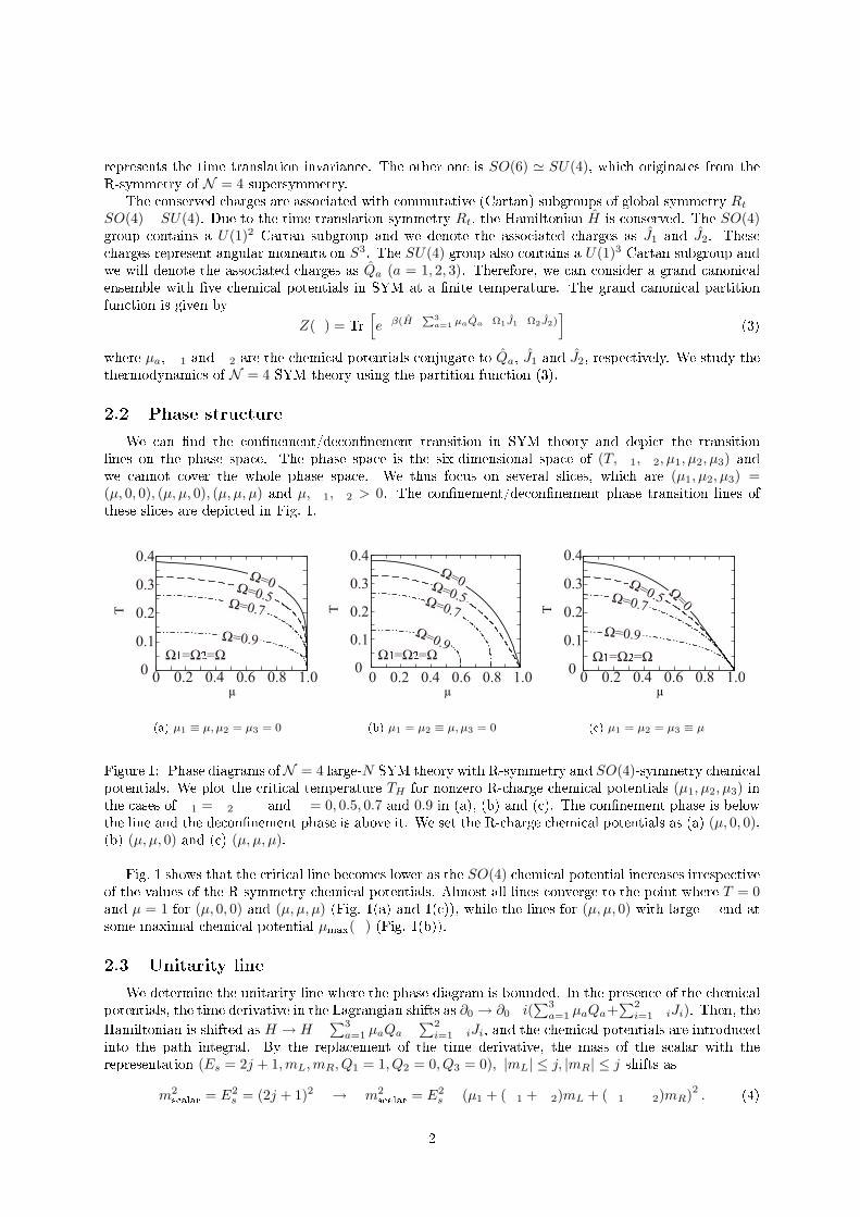
represents the time translation invariance. The other one is SO(6) ' SU(4), which originates from theR-symmetry of N = 4 supersymmetry.
The conserved charges are associated with commutative (Cartan) subgroups of global symmetry Rt SO(4) SU(4). Due to the time translation symmetry Rt, the Hamiltonian H is conserved. The SO(4)group contains a U(1)2 Cartan subgroup and we denote the associated charges as J1 and J2. Thesecharges represent angular momenta on S3. The SU(4) group also contains a U(1)3 Cartan subgroup andwe will denote the associated charges as Qa (a = 1, 2, 3). Therefore, we can consider a grand canonicalensemble with ve chemical potentials in SYM at a nite temperature. The grand canonical partitionfunction is given by
Z() = Tr[eβ(H
∑3a=1 µaQaΩ1J1Ω2J2)
](3)
where µa, 1 and 2 are the chemical potentials conjugate to Qa, J1 and J2, respectively. We study thethermodynamics of N = 4 SYM theory using the partition function (3).
2.2 Phase structure
We can nd the connement/deconnement transition in SYM theory and depict the transitionlines on the phase space. The phase space is the six-dimensional space of (T, 1, 2, µ1, µ2, µ3) andwe cannot cover the whole phase space. We thus focus on several slices, which are (µ1, µ2, µ3) =(µ, 0, 0), (µ, µ, 0), (µ, µ, µ) and µ,1, 2 > 0. The connement/deconnement phase transition lines ofthese slices are depicted in Fig. 1.
(a) µ1 ≡ µ, µ2 = µ3 = 0 (b) µ1 = µ2 ≡ µ, µ3 = 0 (c) µ1 = µ2 = µ3 ≡ µ
Figure 1: Phase diagrams ofN = 4 large-N SYM theory with R-symmetry and SO(4)-symmetry chemicalpotentials. We plot the critical temperature TH for nonzero R-charge chemical potentials (µ1, µ2, µ3) inthe cases of 1 = 2 and = 0, 0.5, 0.7 and 0.9 in (a), (b) and (c). The connement phase is belowthe line and the deconnement phase is above it. We set the R-charge chemical potentials as (a) (µ, 0, 0),(b) (µ, µ, 0) and (c) (µ, µ, µ).
Fig. 1 shows that the critical line becomes lower as the SO(4) chemical potential increases irrespectiveof the values of the R-symmetry chemical potentials. Almost all lines converge to the point where T = 0and µ = 1 for (µ, 0, 0) and (µ, µ, µ) (Fig. 1(a) and 1(c)), while the lines for (µ, µ, 0) with large end atsome maximal chemical potential µmax() (Fig. 1(b)).
2.3 Unitarity line
We determine the unitarity line where the phase diagram is bounded. In the presence of the chemicalpotentials, the time derivative in the Lagrangian shifts as ∂0 → ∂0i(
∑3a=1 µaQa+
∑2i=1 iJi). Then, the
Hamiltonian is shifted as H → H ∑3
a=1 µaQa ∑2
i=1 iJi, and the chemical potentials are introducedinto the path integral. By the replacement of the time derivative, the mass of the scalar with therepresentation (Es = 2j + 1,mL,mR, Q1 = 1, Q2 = 0, Q3 = 0), |mL| ≤ j, |mR| ≤ j shifts as
m2scalar = E2
s = (2j + 1)2 → m2scalar = E2
s (µ1 + (1 + 2)mL + (1 2)mR)2 . (4)
2
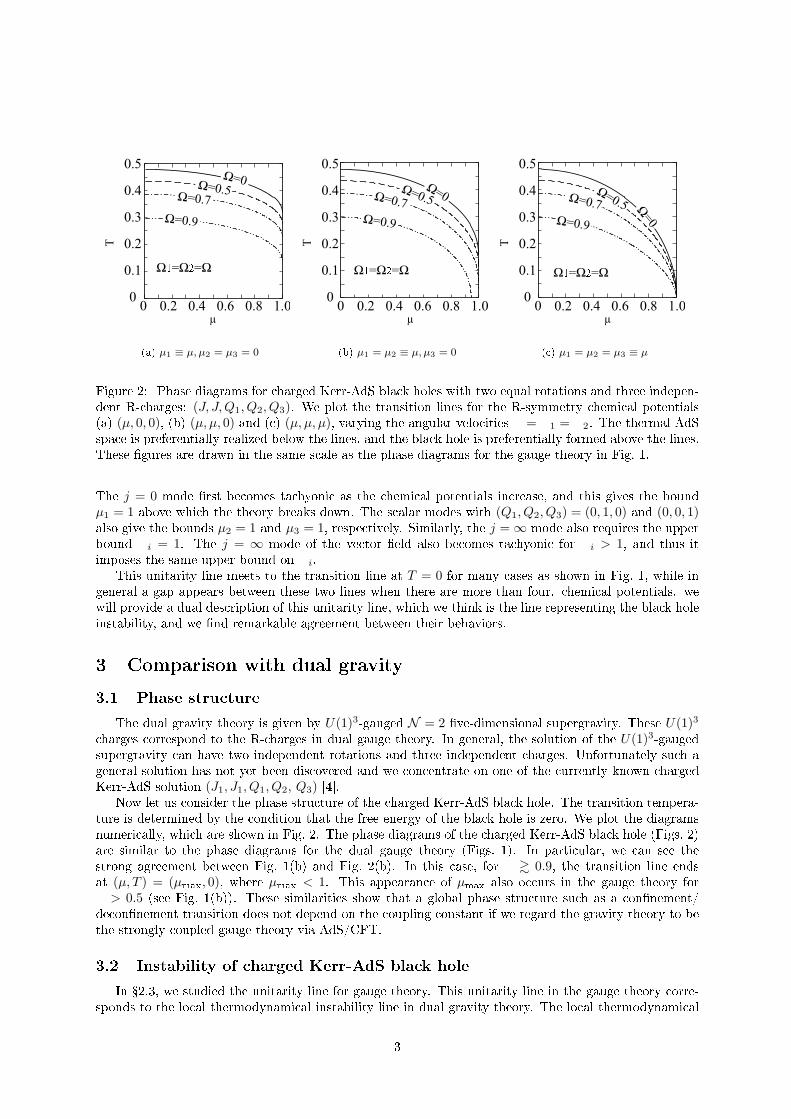
(a) µ1 ≡ µ, µ2 = µ3 = 0 (b) µ1 = µ2 ≡ µ, µ3 = 0 (c) µ1 = µ2 = µ3 ≡ µ
Figure 2: Phase diagrams for charged Kerr-AdS black holes with two equal rotations and three indepen-dent R-charges: (J, J,Q1, Q2, Q3). We plot the transition lines for the R-symmetry chemical potentials(a) (µ, 0, 0), (b) (µ, µ, 0) and (c) (µ, µ, µ), varying the angular velocities = 1 = 2. The thermal AdSspace is preferentially realized below the lines, and the black hole is preferentially formed above the lines.These gures are drawn in the same scale as the phase diagrams for the gauge theory in Fig. 1.
The j = 0 mode rst becomes tachyonic as the chemical potentials increase, and this gives the boundµ1 = 1 above which the theory breaks down. The scalar modes with (Q1, Q2, Q3) = (0, 1, 0) and (0, 0, 1)also give the bounds µ2 = 1 and µ3 = 1, respectively. Similarly, the j = ∞ mode also requires the upperbound i = 1. The j = ∞ mode of the vector eld also becomes tachyonic for i > 1, and thus itimposes the same upper bound on i.
This unitarity line meets to the transition line at T = 0 for many cases as shown in Fig. 1, while ingeneral a gap appears between these two lines when there are more than four. chemical potentials. wewill provide a dual description of this unitarity line, which we think is the line representing the black holeinstability, and we nd remarkable agreement between their behaviors.
3 Comparison with dual gravity
3.1 Phase structure
The dual gravity theory is given by U(1)3-gauged N = 2 ve-dimensional supergravity. These U(1)3
charges correspond to the R-charges in dual gauge theory. In general, the solution of the U(1)3-gaugedsupergravity can have two independent rotations and three independent charges. Unfortunately such ageneral solution has not yet been discovered and we concentrate on one of the currently known chargedKerr-AdS solution (J1, J1, Q1, Q2, Q3) [4].
Now let us consider the phase structure of the charged Kerr-AdS black hole. The transition tempera-ture is determined by the condition that the free energy of the black hole is zero. We plot the diagramsnumerically, which are shown in Fig. 2. The phase diagrams of the charged Kerr-AdS black hole (Figs. 2)are similar to the phase diagrams for the dual gauge theory (Figs. 1). In particular, we can see thestrong agreement between Fig. 1(b) and Fig. 2(b). In this case, for & 0.9, the transition line endsat (µ, T ) = (µmax, 0), where µmax < 1. This appearance of µmax also occurs in the gauge theory for > 0.5 (see Fig. 1(b)). These similarities show that a global phase structure such as a connement/deconnement transition does not depend on the coupling constant if we regard the gravity theory to bethe strongly coupled gauge theory via AdS/CFT.
3.2 Instability of charged Kerr-AdS black hole
In 2.3, we studied the unitarity line for gauge theory. This unitarity line in the gauge theory corre-sponds to the local thermodynamical instability line in dual gravity theory. The local thermodynamical
3
instability means that the Hessian matrix of second derivatives of the mass with respect to the entropyand the conserved charges has a negative eigenvalue. Fig. 3 shows the resultant instability lines on whichthe Hessian matrix has zero eigenvalue, along with the Hawking-Page transition lines. We also depict theconnement/deconnement transition lines and the unitarity lines of the dual gauge theory.
In Fig. 3, we can see qualitative similarities between the instability line of the gravity theory and theunitarity line of the dual gauge theory. In particular, in Fig. 3(b) for the case (µ1, µ2, µ3) = (µ, µ, 0), agap appeared between the Hawking-Page line and the instability line. We found such a gap in the dualgauge theory in 2.3.
(a) µ1 ≡ µ, µ2 = µ3 = 0 (b) µ1 = µ2 ≡ µ, µ3 = 0 (c) µ1 = µ2 = µ3 ≡ µ
Figure 3: Phase diagrams for = 0.9 including the unitarity lines. The solid lines are the Hawking-Page transition line and the instability line of a charged Kerr-AdS black hole. The dashed lines are theconnement/deconnement transition line and the unitarity line of the dual gauge theory.
4 Conclusion
We have studied the free N = 4 SYM theory dual to the charged Kerr-AdS black hole. We foundthe connement/deconnement transition and specied the unitarity bound for this theory. In the dualgravity theory, the Hawking-Page transition and the thermodynamical instability of charged Kerr-AdSblack holes have been investigated. The resulting phase diagrams for gauge theory and charged Kerr-AdSblack holes resemble each other, and, in particular, we have found that the connement/deconnementtransition line and the unitarity line of gauge theory correspond to the Hawking-Page transition line andthe instability line in dual gravity theory, respectively.
References
[1] B. Sundborg, Nucl. Phys. B 573, 349 (2000) [arXiv:hep-th/9908001].
[2] O. Aharony, J. Marsano, S. Minwalla, K. Papadodimas and M. Van Raamsdonk, Adv. Theor. Math.Phys. 8, 603 (2004) [arXiv:hep-th/0310285].
[3] D. Yamada and L. G. Yae, JHEP 0609, 027 (2006) [arXiv:hep-th/0602074].
[4] M. Cvetic, H. Lu and C. N. Pope, Phys. Rev. D 70, 081502 (2004) [arXiv:hep-th/0407058].
[5] K. Murata, T. Nishioka, N. Tanahashi and H. Yumisaki, Prog. Theor. Phys. 120, 473 (2008)[arXiv:0806.2314 [hep-th]].
4
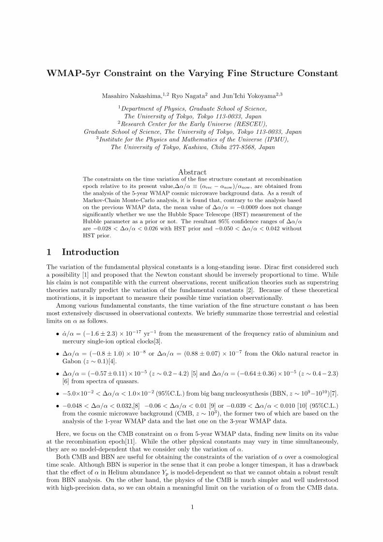
WMAP-5yr Constraint on the Varying Fine Structure Constant
Masahiro Nakashima,1,2 Ryo Nagata2 and Jun’Ichi Yokoyama2,3
1Department of Physics, Graduate School of Science,The University of Tokyo, Tokyo 113-0033, Japan
2Research Center for the Early Universe (RESCEU),Graduate School of Science, The University of Tokyo, Tokyo 113-0033, Japan
3Institute for the Physics and Mathematics of the Universe (IPMU),The University of Tokyo, Kashiwa, Chiba 277-8568, Japan
AbstractThe constraints on the time variation of the fine structure constant at recombinationepoch relative to its present value,∆α/α ≡ (αrec − αnow)/αnow, are obtained fromthe analysis of the 5-year WMAP cosmic microwave background data. As a result ofMarkov-Chain Monte-Carlo analysis, it is found that, contrary to the analysis basedon the previous WMAP data, the mean value of ∆α/α = −0.0009 does not changesignificantly whether we use the Hubble Space Telescope (HST) measurement of theHubble parameter as a prior or not. The resultant 95% confidence ranges of ∆α/αare −0.028 < ∆α/α < 0.026 with HST prior and −0.050 < ∆α/α < 0.042 withoutHST prior.
1 Introduction
The variation of the fundamental physical constants is a long-standing issue. Dirac first considered sucha possibility [1] and proposed that the Newton constant should be inversely proportional to time. Whilehis claim is not compatible with the current observations, recent unification theories such as superstringtheories naturally predict the variation of the fundamental constants [2]. Because of these theoreticalmotivations, it is important to measure their possible time variation observationally.
Among various fundamental constants, the time variation of the fine structure constant α has beenmost extensively discussed in observational contexts. We briefly summarize those terrestrial and celestiallimits on α as follows.
• α/α = (−1.6 ± 2.3) × 10−17 yr−1 from the measurement of the frequency ratio of aluminium andmercury single-ion optical clocks[3].
• ∆α/α = (−0.8 ± 1.0) × 10−8 or ∆α/α = (0.88 ± 0.07) × 10−7 from the Oklo natural reactor inGabon (z ∼ 0.1)[4].
• ∆α/α = (−0.57±0.11)×10−5 (z ∼ 0.2−4.2) [5] and ∆α/α = (−0.64±0.36)×10−5 (z ∼ 0.4−2.3)[6] from spectra of quasars.
• −5.0×10⁻² < ∆α/α < 1.0×10⁻² (95%C.L.) from big bang nucleosynthesis (BBN, z ∼ 109−1010)[7].
• −0.048 < ∆α/α < 0.032,[8] −0.06 < ∆α/α < 0.01 [9] or −0.039 < ∆α/α < 0.010 [10] (95%C.L.)from the cosmic microwave background (CMB, z ∼ 103), the former two of which are based on theanalysis of the 1-year WMAP data and the last one on the 3-year WMAP data.
Here, we focus on the CMB constraint on α from 5-year WMAP data, finding new limits on its valueat the recombination epoch[11]. While the other physical constants may vary in time simultaneously,they are so model-dependent that we consider only the variation of α.
Both CMB and BBN are useful for obtaining the constraints of the variation of α over a cosmologicaltime scale. Although BBN is superior in the sense that it can probe a longer timespan, it has a drawbackthat the effect of α in Helium abundance Yp is model-dependent so that we cannot obtain a robust resultfrom BBN analysis. On the other hand, the physics of the CMB is much simpler and well understoodwith high-precision data, so we can obtain a meaningful limit on the variation of α from the CMB data.
1
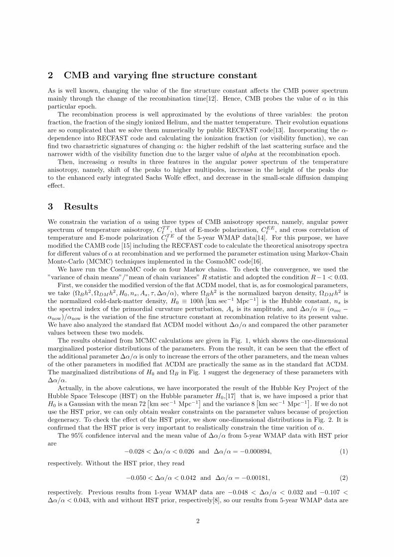
2 CMB and varying fine structure constant
As is well known, changing the value of the fine structure constant affects the CMB power spectrummainly through the change of the recombination time[12]. Hence, CMB probes the value of α in thisparticular epoch.
The recombination process is well approximated by the evolutions of three variables: the protonfraction, the fraction of the singly ionized Helium, and the matter temperature. Their evolution equationsare so complicated that we solve them numerically by public RECFAST code[13]. Incorporating the α-dependence into RECFAST code and calculating the ionization fraction (or visibility function), we canfind two charastrictic signatures of changing α: the higher redshift of the last scattering surface and thenarrower width of the visibility function due to the larger value of alpha at the recombination epoch.
Then, increasing α results in three features in the angular power spectrum of the temperatureanisotropy, namely, shift of the peaks to higher multipoles, increase in the height of the peaks dueto the enhanced early integrated Sachs Wolfe effect, and decrease in the small-scale diffusion dampingeffect.
3 Results
We constrain the variation of α using three types of CMB anisotropy spectra, namely, angular powerspectrum of temperature anisotropy, CTT
ℓ , that of E-mode polarization, CEEℓ , and cross correlation of
temperature and E-mode polarization CTEl of the 5-year WMAP data[14]. For this purpose, we have
modified the CAMB code [15] including the RECFAST code to calculate the theoretical anisotropy spectrafor different values of α at recombination and we performed the parameter estimation using Markov-ChainMonte-Carlo (MCMC) techniques implemented in the CosmoMC code[16].
We have run the CosmoMC code on four Markov chains. To check the convergence, we used the”variance of chain means”/”mean of chain variances” R statistic and adopted the condition R−1 < 0.03.
First, we consider the modified version of the flat ΛCDM model, that is, as for cosmological parameters,we take (ΩBh2, ΩDMh2, H0, ns, As, τ, ∆α/α), where ΩBh2 is the normalized baryon density, ΩDMh2 isthe normalized cold-dark-matter density, H0 ≡ 100h
[km sec−1 Mpc−1
]is the Hubble constant, ns is
the spectral index of the primordial curvature perturbation, As is its amplitude, and ∆α/α ≡ (αrec −αnow)/αnow is the variation of the fine structure constant at recombination relative to its present value.We have also analyzed the standard flat ΛCDM model without ∆α/α and compared the other parametervalues between these two models.
The results obtained from MCMC calculations are given in Fig. 1, which shows the one-dimensionalmarginalized posterior distributions of the parameters. From the result, it can be seen that the effect ofthe additional parameter ∆α/α is only to increase the errors of the other parameters, and the mean valuesof the other parameters in modified flat ΛCDM are practically the same as in the standard flat ΛCDM.The marginalized distributions of H0 and ΩB in Fig. 1 suggest the degeneracy of these parameters with∆α/α.
Actually, in the above calcutions, we have incorporated the result of the Hubble Key Project of theHubble Space Telescope (HST) on the Hubble parameter H0,[17] that is, we have imposed a prior thatH0 is a Gaussian with the mean 72
[km sec−1 Mpc−1
]and the variance 8
[km sec−1 Mpc−1
]. If we do not
use the HST prior, we can only obtain weaker constraints on the parameter values because of projectiondegeneracy. To check the effect of the HST prior, we show one-dimensional distributions in Fig. 2. It isconfirmed that the HST prior is very important to realistically constrain the time varition of α.
The 95% confidence interval and the mean value of ∆α/α from 5-year WMAP data with HST priorare
−0.028 < ∆α/α < 0.026 and ∆α/α = −0.000894, (1)
respectively. Without the HST prior, they read
−0.050 < ∆α/α < 0.042 and ∆α/α = −0.00181, (2)
respectively. Previous results from 1-year WMAP data are −0.048 < ∆α/α < 0.032 and −0.107 <∆α/α < 0.043, with and without HST prior, respectively[8], so our results from 5-year WMAP data are
2
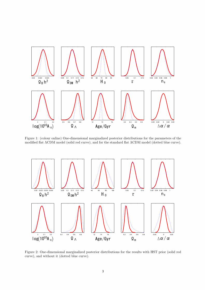
Figure 1: (colour online) One-dimensional marginalized posterior distributions for the parameters of themodified flat ΛCDM model (solid red curve), and for the standard flat ΛCDM model (dotted blue curve).
Figure 2: One-dimensional marginalized posterior distributions for the results with HST prior (solid redcurve), and without it (dotted blue curve).
3
about 30% tighter than those from the 1-year WMAP data. We also note that for the 1-year data, themean value of ∆α/α was found to be ∆α/α = −0.04 without the HST prior although it was practicallyequal to 0 with it. For the 5-year data, we have found that the mean value remains practically intactwhether we use the HST prior or not. This may be interpreted as an indication that the observationalcosmology has made a step forward to the concordance at an even higher level.
4 Conclusion
In terms of the MCMC analysis using CosmoMC code, we have updated constraints on the time variationof the fine structure constant α based on 5-year WMAP data. We obtained tighter constraints comparedwith previous results from 1-year WMAP data owing to the inclusion of the polarization data and thedecrease in the statistical errors. Compared with the result based on the 3-year WMAP data[10], whereno comparison between the cases with and without HST prior has been made, the resultant limit is almostof the same order of magnitude but the mean value of ours is closer to 0. We have verified that the nullresult is favored concerning the variation of α, and the addition of this new parameter ∆α/α does notessentially affect the determinations of the other standard parameters contrary to the case of the analysisbased on the 1-year WMAP data[8].
References
[1] P. A. M. Dirac, Nature 139 (1937), 323 , P. A. M. Dirac, Proc. R. Soc. London A 165 (1938), 199.
[2] J. P. Uzan, Rev. Mod. Phys. 75 (2003), 403, hep-ph/0205340.
[3] T. Rosenband et al., Science 319 (2008), 1808.
[4] Y. Fujii et al., in Proc. Int. Conf. on Nuclear Data for Science and Technology, 2001, hep-ph/0205206.
[5] M. T. Murphy et al., Lecture Notes in Phys., 131 (2004), 648.
[6] M. T. Murphy, J. K. Webb and V. V. Flambaum, Mon. Not. R. Astron. Soc. 384 (2008), 1053,astro-ph/0612407.
[7] K. Ichikawa and M. Kawasaki, Phys. Rev. D 65 (2002), 123511, hep-ph/0203006.
[8] K. Ichikawa, T. Kanzaki and M. Kawasaki, Phys. Rev. D 74 (2006), 023515, astro-ph/0602577.
[9] G. Rocha, R. Trotta, C. J. A. Martins, A. Melchiorri, P. P. Avelino, R. Bean and P. T. P. Viana,Mon. Not. R. Astron. Soc. 352 (2004), 20, astro-ph/0309211.
[10] P. Stefanescu, New Astron. 12 (2007), 635, arXiv:0707.0190.
[11] M. Nakashima, R. Nagata and J. Yokoyama, Prog. Theor. Phys. 120, 1207 (2008) [arXiv:0810.1098[astro-ph]].
[12] S. Hannestad, Phys. Rev. D 60 (1999), 023515, astro-ph/9810102 , M. Kaplinghat, R. J. Scherrerand M. S. Turner, Phys. Rev. D 60 (1999), 023516, astro-ph/9810133.
[13] http://www.astro.ubc.ca/people/scott/recfast.html
[14] M. R. Nolta et al. (WMAP Collaboration), arXiv:0803.0593, J. Dunkley et al. (WMAP Collabora-tion), arXiv:0803.0586, E. Komatsu et al. (WMAP Collaboration), arXiv:0803.0547.
[15] A. Lewis, A. Challinor and A. Lasenby, Astrophys. J. 538 (2000), 473, astro-ph/9911177 ,http://camb.info/
[16] A. Lewis and S. Bridle, Phys. Rev. D 66 (2002), 103511, astro-ph/0205436,http://cosmologist.info/cosmomc/
[17] W. L. Freedman et al. (HST Collaboration), Astrophys. J. 553 (2001), 47, astro-ph/0012376.
4
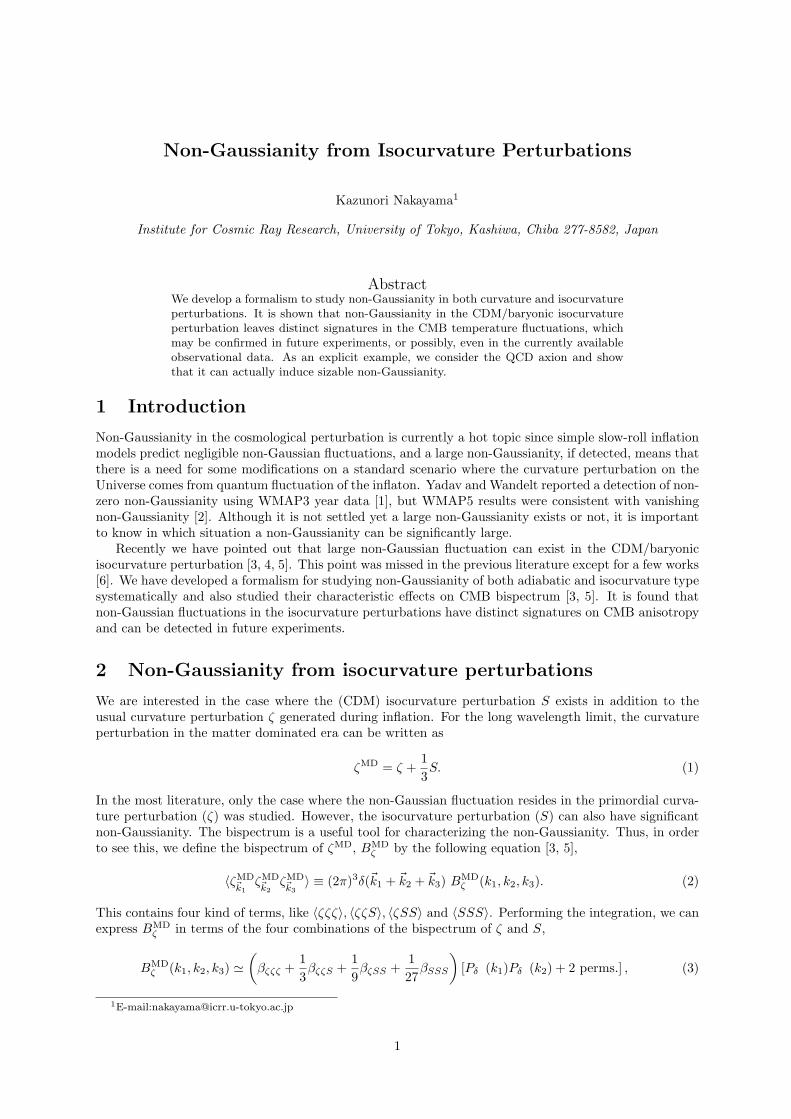
Non-Gaussianity from Isocurvature Perturbations
Kazunori Nakayama1
Institute for Cosmic Ray Research, University of Tokyo, Kashiwa, Chiba 277-8582, Japan
AbstractWe develop a formalism to study non-Gaussianity in both curvature and isocurvatureperturbations. It is shown that non-Gaussianity in the CDM/baryonic isocurvatureperturbation leaves distinct signatures in the CMB temperature fluctuations, whichmay be confirmed in future experiments, or possibly, even in the currently availableobservational data. As an explicit example, we consider the QCD axion and showthat it can actually induce sizable non-Gaussianity.
1 Introduction
Non-Gaussianity in the cosmological perturbation is currently a hot topic since simple slow-roll inflationmodels predict negligible non-Gaussian fluctuations, and a large non-Gaussianity, if detected, means thatthere is a need for some modifications on a standard scenario where the curvature perturbation on theUniverse comes from quantum fluctuation of the inflaton. Yadav and Wandelt reported a detection of non-zero non-Gaussianity using WMAP3 year data [1], but WMAP5 results were consistent with vanishingnon-Gaussianity [2]. Although it is not settled yet a large non-Gaussianity exists or not, it is importantto know in which situation a non-Gaussianity can be significantly large.
Recently we have pointed out that large non-Gaussian fluctuation can exist in the CDM/baryonicisocurvature perturbation [3, 4, 5]. This point was missed in the previous literature except for a few works[6]. We have developed a formalism for studying non-Gaussianity of both adiabatic and isocurvature typesystematically and also studied their characteristic effects on CMB bispectrum [3, 5]. It is found thatnon-Gaussian fluctuations in the isocurvature perturbations have distinct signatures on CMB anisotropyand can be detected in future experiments.
2 Non-Gaussianity from isocurvature perturbations
We are interested in the case where the (CDM) isocurvature perturbation S exists in addition to theusual curvature perturbation ζ generated during inflation. For the long wavelength limit, the curvatureperturbation in the matter dominated era can be written as
ζMD = ζ +13S. (1)
In the most literature, only the case where the non-Gaussian fluctuation resides in the primordial curva-ture perturbation (ζ) was studied. However, the isocurvature perturbation (S) can also have significantnon-Gaussianity. The bispectrum is a useful tool for characterizing the non-Gaussianity. Thus, in orderto see this, we define the bispectrum of ζMD, BMD
ζ by the following equation [3, 5],
⟨ζMDk1
ζMDk2
ζMDk3
⟩ ≡ (2π)3δ(k1 + k2 + k3) BMDζ (k1, k2, k3). (2)
This contains four kind of terms, like ⟨ζζζ⟩, ⟨ζζS⟩, ⟨ζSS⟩ and ⟨SSS⟩. Performing the integration, we canexpress BMD
ζ in terms of the four combinations of the bispectrum of ζ and S,
BMDζ (k1, k2, k3) ≅
(βζζζ +
13βζζS +
19βζSS +
127
βSSS
)[Pδφ(k1)Pδφ(k2) + 2 perms.] , (3)
1E-mail:[email protected]
1
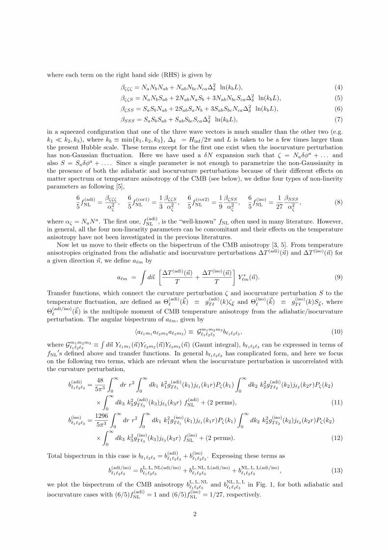
where each term on the right hand side (RHS) is given by
βζζζ = NaNbNab + NabNbcNca∆2δφ ln(kbL), (4)
βζζS = NaNbSab + 2NabNaSb + 3NabNbcSca∆2δφ ln(kbL), (5)
βζSS = SaSbNab + 2SabSaNb + 3SabSbcNca∆2δφ ln(kbL), (6)
βSSS = SaSbSab + SabSbcSca∆2δφ ln(kbL), (7)
in a squeezed configuration that one of the three wave vectors is much smaller than the other two (e.g.k1 ≪ k2, k3), where kb ≡ mink1, k2, k3, ∆δφ = Hinf/2π and L is taken to be a few times larger thanthe present Hubble scale. These terms except for the first one exist when the isocurvature perturbationhas non-Gaussian fluctuation. Here we have used a δN expansion such that ζ = Naδφa + . . . andalso S = Saδφa + . . . . Since a single parameter is not enough to parametrize the non-Gaussianity inthe presence of both the adiabatic and isocurvature perturbations because of their different effects onmatter spectrum or temperature anisotropy of the CMB (see below), we define four types of non-linerityparameters as following [5],
65f
(adi)NL =
βζζζ
α2ζ
,65f
(cor1)NL =
13
βζζS
α2ζ
,65f
(cor2)NL =
19
βζSS
α2ζ
,65f
(iso)NL =
127
βSSS
α2ζ
, (8)
where αζ = NaNa. The first one, f(adi)NL , is the “well-known” fNL often used in many literature. However,
in general, all the four non-linearity parameters can be concomitant and their effects on the temperatureanisotropy have not been investigated in the previous literatures.
Now let us move to their effects on the bispectrum of the CMB anisotropy [3, 5]. From temperatureanisotropies originated from the adiabatic and isocurvature perturbations ∆T (adi)(n) and ∆T (iso)(n) fora given direction n, we define aℓm by
aℓm =∫
dn
[∆T (adi)(n)
T+
∆T (iso)(n)T
]Y ∗
ℓm(n). (9)
Transfer functions, which connect the curvature perturbation ζ and isocurvature perturbation S to thetemperature fluctuation, are defined as Θ(adi)
ℓ (k) ≡ g(adi)Tℓ (k)ζk and Θ(iso)
ℓ (k) ≡ g(iso)Tℓ (k)Sk, where
Θ(adi/iso)ℓ (k) is the multipole moment of CMB temperature anisotropy from the adiabatic/isocurvature
perturbation. The angular bispectrum of aℓm, given by
⟨aℓ1m1aℓ2m2aℓ3m3⟩ ≡ Gm1m2m3ℓ1ℓ2ℓ3
bℓ1ℓ2ℓ3 , (10)
where Gm1m2m3ℓ1ℓ2ℓ3
≡∫
dn Yℓ1m1(n)Yℓ2m2(n)Yℓ3m3(n) (Gaunt integral), bℓ1ℓ2ℓ3 can be expressed in terms offNL
′s defined above and transfer functions. In general bℓ1ℓ2ℓ3 has complicated form, and here we focuson the following two terms, which are relevant when the isocurvature perturbation is uncorrelated withthe curvature perturbation,
b(adi)ℓ1ℓ2ℓ3
=485π3
∫ ∞
0
dr r2
∫ ∞
0
dk1 k21g
(adi)Tℓ1
(k1)jℓ1(k1r)Pζ(k1)∫ ∞
0
dk2 k22g
(adi)Tℓ2
(k2)jℓ2(k2r)Pζ(k2)
×∫ ∞
0
dk3 k23g
(adi)Tℓ3
(k3)jℓ3(k3r) f(adi)NL + (2 perms), (11)
b(iso)ℓ1ℓ2ℓ3
=12965π3
∫ ∞
0
dr r2
∫ ∞
0
dk1 k21g
(iso)Tℓ1
(k1)jℓ1(k1r)Pζ(k1)∫ ∞
0
dk2 k22g
(iso)Tℓ2
(k2)jℓ2(k2r)Pζ(k2)
×∫ ∞
0
dk3 k23g
(iso)Tℓ3
(k3)jℓ3(k3r) f(iso)NL + (2 perms). (12)
Total bispectrum in this case is bℓ1ℓ2ℓ3 = b(adi)ℓ1ℓ2ℓ3
+ b(iso)ℓ1ℓ2ℓ3
. Expressing these terms as
b(adi/iso)ℓ1ℓ2ℓ3
= bL, L, NL(adi/iso)ℓ1ℓ2ℓ3
+ bL, NL, L(adi/iso)ℓ1ℓ2ℓ3
+ bNL, L, L(adi/iso)ℓ1ℓ2ℓ3
, (13)
we plot the bispectrum of the CMB anisotropy bL, L, NLℓ1ℓ2ℓ3
and bNL, L, Lℓ1ℓ2ℓ3
in Fig. 1, for both adiabatic and
isocurvature cases with (6/5)f (adi)NL = 1 and (6/5)f (iso)
NL = 1/27, respectively.
2
Figure 1: Bispectrum of the CMB anisotropy bNL, L, Lℓ1ℓ2ℓ3
and bL, L, NLℓ1ℓ2ℓ3
for (6/5)f (adi)NL = 1 and (6/5)f (iso)
NL =1/27. Shaded regions are unphysical. (Courtesy of T. Sekiguchi.)
3 Application to the axion
In this section we apply our formulation to the axion as a concrete example [3]. The axion, a, is a pseudoNambu-Goldstone boson associated with the spontaneous breaking of the PQ symmetry. The existenceof the axion is strongly motivated, since it naturally solves the strong CP problem in QCD. Let us denotethe breaking scale by Fa, whose magnitude is constrained from various experiments, astrophysical andcosmological considerations. The most strict lower bound on Fa comes from the observation of 1987A. Inorder to prevent too fast cooling by the axion emission, Fa
>∼ 1010 GeV is required. On the other hand,the upper bound is provided by the cosmological argument. The axion obtains a tiny mass after the QCDphase transition due to the anomaly effect which explicitly breaks the PQ symmetry. The axion beginsto oscillate coherently after that. Since the lifetime of the axion is very long, it survives until now andcontributes to DM of the universe. The abundance is estimated as
Ωah2 ≅ 0.2(
Fa
1012 GeV
)−0.82 ( a∗
1012 GeV
)2
, (14)
where a∗ = maxFaθ, Hinf/2π and θ denotes the initial misalignment angle of the axion.If the PQ symmetry is already broken before or during inflation and if it is never restored after inflation,
the axion has unsuppressed quantum fluctuations during inflation because it remains practically masslessduring inflation. Since the axion contributes to some fraction of DM, such an axionic isocurvaturefluctuation is converted to the CDM isocurvature fluctuation. Thus the axion is a plausible candidatefor generating the non-Gaussianity from the isocurvature perturbation. The isocurvature perturbation isgiven by
S ≅(
Ωa
ΩCDM
)[2aiδa
a2∗
+(
δa
a∗
)2], (15)
where ai = Faθ. The second term denotes the non-Gaussian isocurvature fluctuation. In Fig. 2, f(iso)NL
is shown for Fa = 1012 GeV. Constraint on the uncorrelated isocurvaure perturbation from CMB powerspectrum [2] is also shown. Thus we can see that large enough f
(iso)NL can be obtained with satisfying the
isocurvature constraint.22In the case where the axion rolls down from the top of the cosine-type potential, see Ref. [7].
3
Figure 2: Contours of f(iso)NL (= 1, 10 and 100) and r ≡ Ωa/ΩCDM for Fa = 1012 GeV.
4 Conclusions
We have investigated a possibility that large non-Gaussianity is generated by isocurvature fluctuations.One interesting feature of this scenario is that the bispectrum and the power spectrum of the CMBtemperature fluctuations exhibit characteristic scale dependence. Furthermore, our results indicate thatlarge non-Gaussianity may be accompanied with an observable fraction of the isocurvature perturbation.If future observations confirm both large non-Gaussianity and a certain amount of isocurvature fluctuationcomponent, our scenario will become very attractive. Although we have restricted ourselves to theCDM isocurvature perturbation, the baryonic isocurvature perturbation can also generate large non-Gaussianity in a similar fashion [4]. Another example is a curvaton scenario with correlated CDM(baryonic) isocurvature perturbations [5]. For some recent related works see Refs. [8, 9, 10].
References
[1] A. P. S. Yadav and B. D. Wandelt, Phys. Rev. Lett. 100, 181301 (2008) [arXiv:0712.1148 [astro-ph]].
[2] E. Komatsu et al. [WMAP Collaboration], arXiv:0803.0547 [astro-ph].
[3] M. Kawasaki, K. Nakayama, T. Sekiguchi, T. Suyama and F. Takahashi, JCAP 0811, 019 (2008)[arXiv:0808.0009 [astro-ph]].
[4] M. Kawasaki, K. Nakayama and F. Takahashi, JCAP 0901, 002 (2009) [arXiv:0809.2242 [hep-ph]].
[5] M. Kawasaki, K. Nakayama, T. Sekiguchi, T. Suyama and F. Takahashi, arXiv:0810.0208 [astro-ph],to appear in JCAP.
[6] A. D. Linde and V. F. Mukhanov, Phys. Rev. D 56, 535 (1997) [arXiv:astro-ph/9610219]; N. Bartolo,S. Matarrese and A. Riotto, Phys. Rev. D 65, 103505 (2002) [arXiv:hep-ph/0112261]; L. Boubekeurand D. H. Lyth, Phys. Rev. D 73, 021301 (2006) [arXiv:astro-ph/0504046].
[7] M. Kawasaki, K. Nakayama and F. Takahashi, JCAP 0901, 026 (2009) [arXiv:0810.1585 [hep-ph]].
[8] D. Langlois, F. Vernizzi and D. Wands, JCAP 0812, 004 (2008) [arXiv:0809.4646 [astro-ph]].
[9] T. Moroi and T. Takahashi, arXiv:0810.0189 [hep-ph].
[10] C. Hikage, K. Koyama, T. Matsubara, T. Takahashi and M. Yamaguchi, arXiv:0812.3500 [astro-ph].
4
Large non-Gaussianity from multi-brid in ation
Atsushi Naruko 1 and Misao Sasaki2
Yukawa Institute for Theoretical Physics, Kyoto University, Kyoto 606–8502, Japan
AbstractA model of multi-component hybrid in ation, dubbed multi-brid in ation, which mayyield a large non-Gaussian paramter fNL, was proposed recently. In particular, fora two-brid in ation model with an exponential potential and the condition that theend of in ation is an ellipse in the eld space, it was found that, while keeping theother observational quantities within the range consistent with observations, largenon-Gaussianity is possible for certain in ationary trajectories. In this talk, in orderto see if this result is a general feature of multi-brid in ation, we consider a modelwith a potential with an exponent quadratic in the scalar eld components. We alsoconsider a more general class of ellipses for the end of in ation. Focusing on the caseof two-brid in ation, we nd that large non-Gaussianity is also possible in the presentmodel. Then by tuning the model parameters, we nd that there exist models forwhich both the non-Gaussianity and the tensor-to-scalar ratio are large enough to bedetected in the very near future.
1 Introduction
The primordial non-Gaussianity has been one of the hottest topics in cosmology in recent years. Theconventional, single-field slow-roll inflation predicts that the curvature perturbation is Gaussian to anextremely high accuracy. In other words, if any primordial non-Gaussianity is detected, it stronglyindicates that the dynamics of inflation is not as simple as we thought it to be.
The primordial non-Gaussianity is conveniently represented by a parameter denoted by fNL [1].Roughly, it is the ratio of the 3-point correlation function (or the bispectrum) to the square of the 2-point correlation function (or the square of the spectrum). It is expected that near-future experimentssuch as those of PLANCK will be able to detect fNL at a level as small as 5 [2].
Finding even a small deviation from Gaussianity will have profound implications on the theory ofthe early universe. Consequently, numerous types of inflationary models that produce detectable non-Gaussianity have been proposed and studied. In terms of the nature of non-Gaussianities, most ofthese models can be classified into two categories; those with non-Gaussianities arising intrinsically fromthe quantum fluctuations, and those with non-Gaussianities due to nontrivial classical dynamics onsuperhorizon scales. A typical example of the former is the DBI inflation, in which the slow-roll conditioncan be fully violated. In this case, the equilateral fNL (denoted by f equil
NL ) representing the amplitudeof the bispectrum of the equilateral configurations, is found to play an important role. On the otherhand, in the latter case where non-Gaussianities are produced on superhorizon scales, by causality thelocal fNL (denoted by f local
NL ) characterizes the level of the non-Gaussianity. It is defined in terms of thecoefficient in front of the second order curvature perturbation [1],
Φ = ΦL + f localNL Φ2
L , (1)
where Φ is the curvature perturbation on the Newtonian slice and ΦL is its linear, Gaussian part.In this paper, we focus on the latter case, that is, we consider models that may produce a large
value of f localNL , for example 10–100. More specifically, we consider hybrid inflation with multiple inflaton
fields, dubbed multi-brid inflation [3]. The inflaton fields are assumed to follow the slow-roll equations ofmotion, and their fluctuations are assumed to be Gaussian. In this case, the δN formalism is most usefulfor the evaluation of the curvature perturbation and non-Gaussianity [4].
1E-mail:[email protected]:[email protected]
1
As in the conventional hybrid inflation, the inflaton fields are coupled to a water-fall field, and inflationends when the inflaton fields satisfy a certain condition that triggers the instability of the water-fall field.However, unlike the case of a single inflaton field in which there is essentially no degree of freedom in thecondition for the end of inflation, there is a substantial increase in the degree of freedom at the end ofinflation in multi-brid inflation and it widens the viable range of the parameter space considerably andleads to the possibility of generating large non-Gaussianity.
As a model of multi-brid inflation, an analytically solvable two-brid inflation model was recentlyinvestigated in detail [3], where the potential was assumed to be exponential with the exponent givenby a linear combination of the inflaton fields. In this paper, we consider a two-brid model with againan exponential potential but with the exponent given by a quadratic function of the inflaton fields. Thepotential has point symmetry about the origin of the field space, in contrast to the case of the linearexponent which has no symmetry. Thus by investigating the quadratic case, we will be able to see if thegeneration of large non-Gaussianity is a generic feature of multi-brid inflation or if it is due to the lackof symmetry that leads to large non-Gaussianity in the linear exponent case.
2 Two-brid in ation
We consider a two-component scalar field whose action is given by
S = −∫
d4x√−g
12gµν
∑A=1,2
∂µϕA∂νϕA + V (ϕ)
, (2)
where the potential is given by
V = V0(χ, ϕ1, ϕ2) exp[12
(m2
1ϕ21 + m2
2ϕ22
)], (3)
with V0 being a function of a water-fall field χ as well as of ϕ1 and ϕ2, but is assumed to be constant intime during inflation.
The slow-roll equations of motion are obtained by neglecting the kinetic term in the Friedmannequation and the second time derivative in the field equations. Thus the slow-roll equations of motionare
3H2 = V ,dϕA
dN=
1V
∂V
∂ϕA= m2
AϕA , (4)
where H = a/a and the dot ˙ denotes a derivative with respect to the cosmic proper time. The numberof e-folds counted backwards in time, dN = −Hdt, is used as the time variable for later convenience.Hence we immediately obtain
N =12
ln[ϕ
2/m21
1 + ϕ2/m2
22
]− 1
2ln
[ϕ
2/m21
1,f + ϕ2/m2
22,f
], (5)
where the number of e-folds is set to zero at the end of inflation and ϕA,f is the final value of the inflatonfields.
We assume that inflation ends at
σ2 = G(ϕ1, ϕ2) ≡ g21(ϕ1 cos α + ϕ2 sinα)2 + g2
2(−ϕ1 sin α + ϕ2 cos α)2 , (6)
which is realized by the potential V0 given by
V0 =12G(ϕ1, ϕ2)χ2 +
λ
4
(χ2 − σ2
λ
)2
. (7)
We parametrize the scalar fields at the end of inflation as
σ
g1cos γ = ϕ1,f cos α + ϕ2,f sinα ,
σ
g2sin γ = −ϕ1,f sinα + ϕ2,f cos α , (8)
2
The angle α describes the amount of rotation of the ellipse relative to the ϕ1 and ϕ2 axes. The angle γdescribes the position of the inflaton trajectory at the end of inflation.
Since there is a constant of motion from Eq.(4), we have
lnϕ1
m21
− lnϕ2
m22
=1
m21
lnσ
g1g2(g2 cos α cos γ − g1 sinα sin γ) − 1
m22
lnσ
g1g2(g2 sin α cos γ − g1 cos α sin γ). (9)
This equation determines the parameter γ in terms of ϕ1 and ϕ2: γ = γ(ϕ1, ϕ2). Hence, from Eq. (8),ϕ1,f and ϕ2,f become functions of ϕ1 and ϕ2,
ϕ1,f = ϕ1,f (ϕ1, ϕ2) , ϕ2,f = ϕ2,f (ϕ1, ϕ2) . (10)
With this understanding, the number of e-folds given by Eq. (5) becomes a function of (ϕ1, ϕ2). It isthen straightforward to obtain δN to full nonlinear order. It can be straightforwardly calculated as
δN = N(ϕ1 + δϕ1, ϕ2 + δϕ2) − N(ϕ1, ϕ2) . (11)
3 Case for large non-Gaussianity
In this section, we compute the curvature perturbation of our model explicitly, and evaluate the curvatureperturbation spectrum PS , the spectral index nS , the tensor-to-scalar ratio r, and the non-Gaussianityparameter f local
NL . But, because these expressions are very complicated, it is not easy to study all possiblecases in detail. However, there are some limiting cases in which we have a substantially simplifiedexpression for PS , nS , r and f local
NL , but which are yet sufficiently of interest.One case of interest is when the two masses are equal, m1 = m2. In this case, the potential during
inflation is O(2) symmetric. This symmetry is broken at the end of inflation because of condition (6),unless g1 = g2. This model was discussed by Alabidi and Lyth [5] as a new mechanism of generatingcurvature perturbations. Another case of interest is when the ratio of the mass parameters are large, forexample, m1 ≫ m2.
Using δN -formalism, the expressions of PS , nS , r and f localNL are given. In equal mass case, the formulas
simplify considerably to
PS =( g
σm2em2Nk
)2 1 + cos 2β cos 2γ
2
(H
2π
)2
tk
=8r
(H
2π
)2
tk
, (12)
nS − 1 = 2m2 − 2
(σm2em2Nk
g
)21 − cos 2β cos 2γ
sin2 2β= 2m2 − r
81 − cos2 2β cos2 2γ
sin2 2β, (13)
r = 8
(σm2em2Nk
g
)22
1 + cos 2β cos 2γ, (14)
f localNL =
5m2
6
(cos 2β sin 2γ
1 + cos 2β cos 2γ
)2
− 1
, (15)
here g and β is giben by g =√
g21 + g2
2 and tanβ = g2/g1 respectively. Note that the α-dependence hasdisappeared because of the symmetry.
As is clear from Eq. (15) for f localNL , in order to obtain large non-Gaussianity, it is necessary for the
factor in the curly brackets to become large, that is, cos 2β sin 2γ/(1+cos 2β cos 2γ) ≫ 1. This is possibleeither in the limit (β, γ) → (0, π/2) or (β, γ) → (π/2, 0). Since these two limits are equivalent, let us takethe limit (β, γ) → (0, π/2). This corresponds to the situation in which the ellipse is highly elongated andthe inflaton trajectory hits the ellipse close to one of the tips of the majoraxis.
To investigate in more detail the theoretical predictions of this model, let us derive expressions for rand f local
NL in terms of the observational data as much as possible. We fix the amplitude of the spectrumPS and the spectral index nS . The WMAP normalization at the present Hubble horizon scale and the
3
WMAP 5-year analysis [6] gives
PS =8r
(H
2π
)2
tk
= 2.5 × 10⁹ , nS = 0.96 +0.014−0.015 . (16)
Below we replace PS and nS by these observed values.The useful expression may be obtained by combining the two expressions of r and f local
NL :
f localNL ∼ 52
( r
0.1
) (104
β2
)m2
m2 + 0.02. (17)
This tells us that for m2 >∼ 0.02, in the very near future, both r and f localNL may be large enough to be
detected upon tuning the model parameters to some extent. As we can see, although the values of f localNL
and r are relatively sensitive to the values of m2 and β, there indeed exist models with large f localNL and
r simultaneously.
4 conclusion
We analytically investigated the curvature perturbation and its non-Gaussianity in a model of multi-fieldhybrid inflation, dubbed multi-brid inflation. The model we considered is a two-field hybrid inflation(two-brid inflation) model with the potential mimicking conventional quadratic potentials. The newingredient of the model is the generalization of the condition for the end of inflation. We considered avery general coupling of the two inflaton fields to a water-fall field.
Then, using the δN formula, we derived an analytical expression for the curvature perturbation.Based on this expression, we obtained the curvature perturbation spectrum PS , the spectral index nS ,the tensor-to-scalar ratio r, and the non-Gaussian parameter f local
NL . We found that a large positive f localNL
is possible in this model. Then, at least for a certain limited range of the parameters, we explicitlyshowed that it is possible to have large non-Gaussianity while keeping the values of the other quantitiesconsistent with those of the observation. In particular, we showed that when the two inflaton masses areequal, the parameters can be tuned so that they lead to a fairly large tensor-to-scalar ratio, r ∼ 0.1, aswell as a large non-Gaussian parameter, f local
NL ∼ 50. These values will be at a detectable level in the verynear future. On the other hand, interestingly, we found that having a large mass ratio in the presentmodel does not help in producing both r and f local
NL large enough to be detected. This is in contrast tothe model studied in [3].
The standard lore has been that f localNL is too small for models with large r or vice versa. We have
shown, in this paper, not be the case, particularly in this model of spontaneously symmetry breaking atthe end of inflation. This may be the most important conclusion of this work. At the moment, we haveno clear physical explanation for this result. We hope we will be able to answer this question in the nearfuture.
References
[1] E. Komatsu and D. N. Spergel, Phys. Rev. D 63 (2001), 063002; astro-ph/0005036.
[2] D. Babich and M. Zaldarriaga, Phys. Rev. D 70 (2004), 083005; astro-ph/0408455.
[3] M. Sasaki, Prog. Theor. Phys. 120 (2008), 159; arXiv:0805.0974 .
[4] D. H. Lyth, K. A. Malik and M. Sasaki, J. Cosmol. Astropart 0505 (2005), 004; astro-ph/0411220.
[5] L. Alabidi and D. Lyth, JCAP 0608, 006 (2006) [arXiv:astro-ph/0604569].
[6] E. Komatsu et al. (WMAP Collaboration), arXiv:0803.0547.
4
Viscosity and Entropy Bounds from Black Hole Physics
Ishwaree P. Neupane 1
Department of Physics and Astronomy, Rutherford Building, University of CanterburyPrivate Bag 4800, Christchurch 8041, New Zealand
AbstractThe gauge theory - gravity duality has provided us a way of studying QCD at highenergies or short distances from straightforward calculations in classical general rel-ativity. Among numerous results obtained so far, one of the most striking is theuniversality of the ratio of the shear viscosity to the entropy density. For all gaugetheories with Einstein gravity dual this ratio has been found to be η/s = 1/4π. Inthis talk, we consider higher curvature-corrected black hole solutions for which η/scan be smaller than 1/4π, thus violating the conjecture bound. Here we shall arguethat the Gauss-Bonnet and (Riemann)2 gravities, in particular, provide concrete ex-amples in which inconsistency of a theory, such as, a violation of microcausality atshort distances, and a classical limit on black hole entropy are correlated.
1 Introduction
Anti de Sitter conformal field theory (CFT) correspondence [1] has proven an excellent tool to studystrongly coupled gauge theories. Through AdS holography one can also study hydrodynamic propertiesof a certain class of boundary CFTs. Indeed, for a large class of four-dimensional CFTs, the ratio of theshear viscosity η to the entropy density s is (in units where h = kB = 1) given by [2],
η
s=
14π
. (1)
This result is universal for all theories with Einstein gravity dual. The reason of this uniqueness is dueto the fact that in pure Einstein gravity all black holes satisfy the Bekenstein-Hawking entropy law
S =kBc3
h
A
4GN, (2)
where h is the Planck’s constant, A is the area of the horizon corresponding to the surface at r = r+
and GN is the Newton’s constant. However, the ratio η/s can be different from 1/4π in general gravitytheories (with higher derivative or higher-curvature corrections). A violation of causality may occur inthe boundary CFT when η/s is too low. This violation can be related to black hole entropy bounds.
To establish better contact with QCD via AdS holography, it is essential to understand the effectof curvature corrections to Einstein-Hilbert action in the holographic framework, see [3] and referencestherein. As the simplest modification to Einstein gravity, we consider the following quadratic action
I =1
16πGN
∫ddx
√−g[R− 2Λ + α′L2
(aR2 + bRµνRµν + cRµνλρR
µνλρ)]
, (3)
where α′ is a dimensionless coupling and the bulk cosmological term Λ = −(d − 1)(d − 2)/2L2. Wewill focus our discussion to the gravity sector in AdS5, for which we have from AdS/CFT dictionary,GN ≡ (πL3/4N2
c ) and L = (4πgsNc)1/4`s, where `s is the string scale and gs the string coupling and Nc
is the number of color charges or rank of the gauge group. Since α′ ∼ 1/√
λ, in the dual supergravitydescription, a small α′ corresponds to the strong coupling limit, λ ≡ g2
Y MNc À 1. The Gauss-Bonnet(GB) term obtained by setting a = c = 1 and b = −4 in (3), in which case the equations of motion are
1E-mail:[email protected]
1
second order in the metric and there would be no need to treat α′ as small. For a class of CFTs in flatspace with Gauss-Bonnet gravity dual, we find [4]
η
s=
14π
(1− 2(d− 1)λGB
(d− 3)
), (4)
where λGB ≡ (d − 3)(d − 4)α′, which is smaller than 1/4π with λGB > 0. Based on the bulk causalstructure of an AdS5 black brane solution, the authors of [4] found a more stronger bound for λGB, i.e.
λGB <9
100, or, equivalently,
η
s≥ 16
25
(14π
), (5)
which otherwise violates a microcausality in the dual CFT defined on a flat hypersurface. Here we arguethat the critical value of λGB beyond which the theory becomes inconsistent is related to the entropybound for a large class of AdS black holes. Further, in the holographic context, we find that the AdS blackhole solutions with spherical and hyperbolic event horizons allow much wider possibilities for η/s [5].
2 Entropy and Viscosity Bounds
For pure AdS GB black hole solutions, the entropy and Hawking temperature are given by [6]
S =A
4GN
(1 +
2(d− 2)kλGB
(d− 4)x2
), T =
(d− 1)x4 + k(d− 3)x2 + (d− 5)k2λGB
4πLx(x2 + 2kλGB)(6)
(in units c = h = kB = 1) where x ≡ r+/L, A ≡ Vd−2rd−2+ , with Vd−2 being the unit volume of the
base manifold or hypersurface M. The entropy of a GB black hole depends on the curvature constantk, whose value determines the geometry of event horizon M = Sd−2, IRd−2 and Hd−2, respectively, fork = +1, k = 0 and k = −1 2. Especially, at the k = −1 extremal state with zero Hawking temperature,
S|T→0 =V3
GN
L3
27/2(1− 12λGB) , E|T→0 = 0. (7)
Thus, beyond a critical coupling λGB > λcrit, the entropy S becomes negative, which indicates a violationof cosmic censorship or the second law of the thermodynamics. In the AdS5 case, λcrit = 1/12. Thiscritical value of λGB above which the theory is inconsistent nearly coincides with the bound λGB < 9/100required for a consistent formulation of a class of CFTs with Gauss-Bonnet gravity dual.
Next let us consider small metric fluctuations φ = h12 around an AdS GB black hole metric
ds2 = −r2+
L2f(z)N2
∗dt2 +L2
f(z)dz2 +
r2+z2
L2
(dx2
3
1− kx23
+ x23
2∑
i=1
dx2i + 2φ(t, x3, z)dx1dx2
), (8)
where k = 0,±1 and N∗ ≡ a = [(1 +√
1− 4λGB)/2]1/2. The scalar metric fluctuation
φ(t, x3, z) =∫
dwdq
(2π)3φ(z; k) e−iwt+iqx3 , φ(z;−k) = φ∗(z, k), (9)
(where k = (w, 0, 0, q)) satisfies the following (linearized) equation of motion
K∂2zφ + ∂zK∂zφ + K2φ = 0. (10)
This structure is not affected by Maxwell type charges but can be affected by scalar charges. In pure GBgravity, K = z2f (z − λGB∂zf) , K2 = (z2w2/N2
∗ f) (z − λGB∂zf)− z(1− λGB∂2z f)
(q2 + 2k
),
f(z) = k +z2
2λGB
[1−
√1− 4λGB +
4λGB
z4
(1 +
k
x2+
λGBk2
x4
)],
2The GB term is topological in d = 4, especially, with a constant coupling, α′L2 = const, so we shall take d ≥ 5.
2
where z ≡ r/r+, x ≡ r+/L, k = k/x2, w ≡ wL/x and q ≡ qL/x. Equation (10) may be solved withthe following incoming boundary conditions at the horizon: φ(z; k) = ain(k)φin(z; k) + aout(k)φout(z; k),aout ≡ 0 and ain ≡ J(k), where J(k) is an infinitesimal boundary source for the fluctuating field φ. Tothe leading order in w, and in the limit q → 0, the solution is given by [5]
φ(z; k) = J(k)
[1 +
iw
4N∗a2
√1− 4λGB
(1z4− 4λGBk
3(1 +√
1− 4λGB)1z6
+O(z−8)
)+O(w2)
]. (11)
By identifying φ ∼ T 21 , one obtains the retarded two-point Green’s function
GR12,12(w, 0) = −i
∫d4xeiwtθ(t)〈[T12(t, ~x), T12(0,~0)]〉, (12)
which satisfies GA(w, ~q) ≡ GR(w, ~q)∗. The shear viscosity η is obtained by using the Kubo formula
η = limw→0
12iw
[GA
12,12(w, 0)−GR12,12(w, 0)
] ≡ limw→0
1w
ImGR12,12(w, 0). (13)
It is not difficult to see that the curvature on a boundary does not affect the result on a flat hypersurface,namely η = 1
16πGN
(r3+
L3
)(1− 4λGB). However, the ratio η/s is modified to be
η
s=
14π
(1− 4λGB)(1 + 6kλGB)
. (14)
One obtains the standard result in Einstein gravity, i.e. η/s = 1/4π, only at a fixed k, i.e. when k = −1and x = r+/L =
√3/2. The minimum of entropy density occurs at x =
√1/2, implying that
s =1
GN
127/2
(1− 12λGB) , η =1
4πGN
127/2
(1− 4λGB) . (15)
The positivity of extremal entropy density implies λGB ≤ 1/12 and hence η/s ≥ 1/6π for k = 0 andη/s ≤ 5/12π for k = −1. Quite remarkably, the lower bound η/s ≈ 0.66/4π is similar to a lower value ofη/s anticipated at relativistic heavy ion collision experiments [7]. In the k = +1 case, the lower bound onη/s could be very close to that in flat space which however arises as a consequence of boundary causality,which requires that the square of local speed of graviton on a constant z-hypersurface is less than unity,
c2g = 1−
(52− 2
1− 4λGB+
12√
1− 4λGB
)1z4
+O(z−8) < 1
or λGB < 0.09. This limit is only very weakly affected by the Maxwell term FµνFµν and the possible F 4
type corrections to Maxwell field [8, 9]. In d = 6 and d = 7, the consistency of GB gravity requires
λd=6GB
<∼ 0.1380, λd=7GB
<∼ 0.1905. (16)
Next consider the (Riemann)2 gravity which is obtained by setting a = b = 0 in eq. (3), for which [5]
η =r3+N2
c
4π2L3
(1− 4λRiem +O(λ2
Riem)), s =
r3+N2
c
πL3
(1 + 4λRiem
(1 +
32k
)+O(λ2
Riem))
. (17)
For a class of boundary field theories with (Riemann)2 gravity dual in flat space (k = 0), this yields
η
s=
14π
(1− 4λRiem
1 + 4λRiem
)≈ 1
4π(1− 8λRiem) =
14π
(1− 1
Nc
). (18)
The limit λRiem > 1/8 is the same as implied by the positivity of extremal entropy of a (Riemann)2 blackhole. Taking into account all three possibilities for the boundary topology that k = 0 or k = ±1, we find
0 <η
s≤ 3
2
(14π
). (19)
It would be interesting to know whether either of these limits applies to nuclear matter at extremedensities and temperatures, or heavy ion collision experiments and study further a universality of theresult η/s ≈ 1/4π through numerical hydrodynamic simulations of data from RHIC and LHC.
3
3 Conclusion
The Gauss-Bonnet gravity with a coupling λGB < 1/4 could be viewed as a classical limit of a consistenttheory of quantum gravity. It is conceivable that the bound on the shear viscosity of any fluid interms of its entropy density is saturated, η/s = 1/4π, for gauge theories at large ’t Hooft coupling,which correspond to the cases where all higher-order curvature contributions are absent. But this boundis naturally in immediate threat of being violated in the presence of generic higher-order curvaturecorrections to the Einstein-Hilbert action. It is remarkable that by tuning of the Gauss-Bonnet and/orgeneric higher curvature couplings, the ratio η/s can be adjusted to a small positive value.
In this note, the limits on GB coupling are imposed by demanding the positivity of extremal black holeentropy and non-violation of boundary causality. We have not found any obvious explicit bound on λGB
from the thermodynamics of spherically symmetric AdS Gauss-Bonnet black holes, which could howeverarise as a consequence of causality violation of a boundary CFT. The critical value of λGB beyond whichthe theory becomes inconsistent is found to be related to the entropy bound for an AdS GB black holewith a hyperbolic or Euclidean anti-de Sitter event horizon. This remark applies also to the (Riemann)2
gravity. Some other inconsistencies of higher-derivative gravity, such as an appearance of tacyonic mode,or semi-classical instability at short distances, are often related to a classical limit on black hole entropy.
Finally, we make the following remark. In the presence of a Maxwell type charge q, the ratio η/s isgenerally modified, which is given by 4π(η/s) = 1− 4λGB(1− a/2), where a ≡ q2L6/r2
+. In the extremallimit (a → 2), one may restrict the coupling λGB such that λGB ≤ 1/24. The latter ensures that thegravitational potential of a black brane is positive and bounded. The conjecture bound η/s ≥ 1/4π issaturated only in the extremal limit, while in general it is violated also by charged Gauss-Bonnet blackbrane solutions. The bound 4π(η/s) ≥ 5/6 found in [8] with a nonzero charge is stronger than for pureEGB gravity in flat space, namely 4π(η/s) ≥ 2/3. In d = 5 dimensions, the entropy of a GB black holecould be negative for 1
12 < λGB < 1/4, leading to a possible violation of unitarity in this range. Thissuggests some deeper connections between bulk causality violation and limits on black hole entropy.
Acknowledgments
This talk is based on a published work in collaboration with Naresh Dadhich. This work is supportedby the New Zealand Foundation for Research, Science and Technology Grant No. E5229 and also byElizabeth Ellen Dalton Grant No. 5393.
References
[1] O. Aharony, S. S. Gubser, J. M. Maldacena, H. Ooguri and Y. Oz, Phys. Rept. 323, 183 (2000).
[2] P. Kovtun, D. T. Son and A. O. Starinets, Phys. Rev. Lett. 94, 111601 (2005); D. T. Son andA. O. Starinets, Ann. Rev. Nucl. Part. Sci. 57, 95 (2007).
[3] Y. M. Cho and I. P. Neupane, Phys. Rev. D 66, 024044 (2002). R.-G. Cai, Phys. Rev. D 65, 084014(2002); M. Cvetic, S. Nojiri and S. D. Odintsov, Nucl. Phys. B 628, 295 (2002).
[4] M. Brigante, H. Liu, R. C. Myers, S. Shenker and S. Yaida, Phys. Rev. Lett. 100, 191601 (2008);ibid, Phys. Rev. D 77, 126006 (2008); Y. Kats and P. Petrov, arXiv:0712.0743 [hep-th].
[5] I. P. Neupane and N. Dadhich, Class. Quant. Grav. 26, 015013 (2009).
[6] I. P. Neupane, Phys. Rev. D 67, 061501 (2003); Phys. Rev. D 69, 084011 (2004).
[7] D. Molnar and P. Huovinen, Phys. Rev. Lett. 94, 012302 (2005); P. Romatschke and U. Romatschke,Phys. Rev. Lett. 99, 172301 (2007).
[8] X. H. Ge, Y. Matsuo, F. W. Shu, S. J. Sin and T. Tsukioka, arXiv:0808.2354 [hep-th].
[9] R. G. Cai, Z. Y. Nie and Y. W. Sun, Phys. Rev. D 78, 126007 (2008).
4
Does the Entropy-Area Law hold
for Schwarzschild-de Sitter spacetime ?
Hiromi Saida1
Department of Physics, Daido Institute of Technology, Minami-ku, Nagoya 457–8530, Japan
AbstractMulti-horizon means multi-temperature unless all of the Hawking temperatures ofhorizons coincide. Multi-temperature system is a nonequilibrium system, and gener-ally the equation of state in nonequilibrium is different form that in equilibrium. Thismay imply that the horizon entropies in multi-horizon spacetime do not satisfy theentropy-area law which is an equation of state of a horizon in thermal equilibrium.This report examines whether the entropy-area law holds for Schwarzschild-de Sitter(SdS) spacetime, which is two-temperature system due to the difference of Hawk-ing temperatures of black hole event horizon (BEH) and cosmological event horizon(CEH). We propose a reasonable evidence of breakdown of entropy-area law for CEHin SdS spacetime. The validity of the law for BEH in SdS spacetime can not bejudged, but we point out the key issue for BEH’s entropy.
1 Simple question from the Nonequilibrium viewpoint
Entropy-area law, which claims the entropy of horizon is equal to one quarter of its spatial area, is theequation of state for equilibrium systems which consist of horizons and matter fields. Now this law seemsaccepted as the universal law of thermodynamic aspects of any horizon in thermal equilibrium. Howevernothing is known about nonequilibrium situations of horizons.
On the other hand, generally in nonequilibrium physics, once the system under consideration comes ina nonequilibrium state, the equation of state for nonequilibrium case takes different form in comparisonwith that for equilibrium case. Especially the nonequilibrium entropy deviates from the equilibriumentropy (when a nonequilibrium entropy is well defined). Indeed, although a quite general formulation ofnonequilibrium thermodynamics remains unknown at present 2, the differences of nonequilibrium entropyfrom equilibrium one are already revealed for some restricted class of nonequilibrium systems [1].
Then, for horizon systems, a simple question arises; does the entropy-area law of horizons hold forhorizon systems in nonequilibrium states? We try to resolve this question and discuss to what extentthe entropy-area law is universal. The representative nonequilibrium system of horizons may be multi-horizon spacetimes whose horizons have different Hawking temperatures. As a simple example of suchsystem, we focus our discussion on Schwarzschild-de Sitter (SdS) spacetime, which is in two-temperaturenonequilibrium state due to the difference of Hawking temperatures of black hole event horizon (BEH)and cosmological event horizon (CEH). We examine the entropy-area law for SdS spacetime.
However, applying some existing nonequilibrium thermodynamics to SdS spacetime is difficult atpresent. Then as one trial to search for SdS horizon entropy, we make a good strategy: We constructcarefully two thermal EQUILIBRIUM systems separately for BEH and CEH which are designed so thatthe origin of nonequilibrium effect of CEH (BEH) on thermodynamic state of BEH (CEH) is retainedand the Euclidean action method is applicable (see next section for a more concrete explanation). Thesubtraction term in Euclidean action is determined with referring to Schwarzschild thermodynamics forBEH and de Sitter thermodynamics for CEH. Although our systems are in thermal equilibrium states,some implication for nonequilibrium states of SdS horizons can be extracted, because the thermal statesare “fine tuned” to include the origin of nonequilibrium nature of SdS spacetime. In this report, we willpropose a reasonable evidence of breakdown of entropy-area law for CEH. The validity of the law forBEH can not be judged, but we will point out the key issue for BEH’s entropy.
Recall that every existing verification of entropy-area law requires the thermal equilibrium of horizons.However, strictly speaking, it is not clear whether the thermal equilibrium is the necessary and sufficient
1E-mail: [email protected], a completely general formulation of nonequilibrium thermodynamics may not exist in our physical world.
1
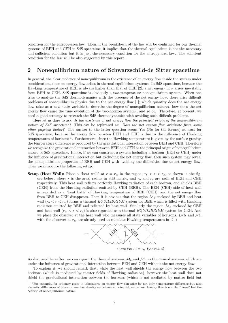
condition for the entropy-area law. Then, if the breakdown of the law will be confirmed for our thermalsystems of BEH and CEH in SdS spacetime, it implies that the thermal equilibrium is not the necessaryand sufficient condition but it is just the necessary condition for the entropy-area law. The sufficientcondition for the law will be also suggested by this report.
2 Nonequilibrium nature of Schwarzschild-de Sitter spacetime
In general, the clear evidence of nonequilibrium is the existence of an energy flow inside the system underconsideration, since no energy flow arises in thermal equilibrium systems. In SdS spacetime, because theHawking temperature of BEH is always higher than that of CEH [2], a net energy flow arises inevitablyfrom BEH to CEH. SdS spacetime is obviously a two-temperature nonequilibrium system. When onetries to analyze the SdS thermodynamics with the presence of the net energy flow, there arise difficultproblems of nonequilibrium physics due to the net energy flow [1]; which quantity does the net energyflow raise as a new state variable to describe the degree of nonequilibrium nature?, how does the netenergy flow cause the time evolution of the two-horizon system?, and so on. Therefore, at present, weneed a good strategy to research the SdS thermodynamics with avoiding such difficult problems.
Here let us dare to ask: Is the existence of net energy flow the principal origin of the nonequilibriumnature of SdS spacetime? This can be rephrased as: Does the net energy flow originate from someother physical factor? The answer to the latter question seems Yes (No for the former) at least forSdS spacetime, because the energy flow between BEH and CEH is due to the difference of Hawkingtemperatures of horizons 3. Furthermore, since the Hawking temperature is given by the surface gravity,the temperature difference is produced by the gravitational interaction between BEH and CEH. Thereforewe recognize the gravitational interaction between BEH and CEH as the principal origin of nonequilibriumnature of SdS spacetime. Hence, if we can construct a system including a horizon (BEH or CEH) underthe influence of gravitational interaction but excluding the net energy flow, then such system may revealthe nonequilibrium properties of BEH and CEH with avoiding the difficulties due to net energy flow.Then we introduce the following setup:
Setup (Heat Wall): Place a “heat wall” at r = rw in the region, rb < r < rc, as shown in the fig-ure below, where r is the areal radius in SdS metric, and rb and rc are radii of BEH and CEHrespectively. This heat wall reflects perfectly Hawking radiation of each horizon, and shields BEH(CEH) from the Hawking radiation emitted by CEH (BEH). The BEH (CEH) side of heat wallis regarded as a “heat bath” of Hawking temperature of BEH (CEH), and the net energy flowfrom BEH to CEH disappears. Then it is obvious that the region Mb enclosed by BEH and heatwall (rb < r < rw) forms a thermal EQUILIBRIUM system for BEH which is filled with Hawkingradiation emitted by BEH and reflected by heat wall. Similarly the region Mc enclosed by CEHand heat wall (rw < r < rc) is also regarded as a thermal EQUILIBRIUM system for CEH. Andwe place the observer at the heat wall who measures all state variables of horizons. (Mb and Mc
with the observer at rw are already used to calculate Hawking temperatures in [2].)
..... .....BEH CEH
observer : r = rw (constant)
As discussed hereafter, we can regard the thermal systems Mb and Mc as the desired systems which areunder the influence of gravitational interaction between BEH and CEH without the net energy flow:
To explain it, we should remark that, while the heat wall shields the energy flow between the twohorizons (which is mediated by matter fields of Hawking radiation), however the heat wall does notshield the gravitational interaction between the horizons (which is not mediated by matter field but
3For example, for ordinary gases in laboratory, an energy flow can arise by not only temperature difference but alsoviscosity, differences of pressure, number density and chemical potential, and so on. Energy flow is not the “cause” but the“effect” of nonequilibrium nature.
2
by gravitational field). This means the following; if we find that all state variables of thermal systemMb depend on a parameter of such gravitational interaction, then it is reasonable to regard the systemMb as a thermal equilibrium system for BEH under the influence of gravitational interaction of twohorizons but excluding net energy flow, and similarly for Mc as a thermal system for CEH. Here itseems natural that the control parameter of the gravitational interaction between BEH and CEH are themass parameter M and the cosmological constant Λ. Furthermore, concerning the state variables, wecan assume very reasonably that every state variable of BEH depends on horizon radius rb or its surfacegravity κb, and similarly for CEH. Here the radii rb, rc and surface gravities κb, κc depend on M and Λ,because, for example, rb(M, Λ) and rc(M, Λ) are the positive roots of algebraic equation f(r) = 0, wheref(r) := −gtt = 1−2M/r−Λ r2/3 and t is the time coordinate in the static chart of SdS metric gµν . Then,obviously, every state variable of BEH (CEH) is under the influence of CEH’s (BEH’s) gravity throughits dependence on horizon radii and surface gravities. Consequently, as mentioned above, we can regardthe thermal systems Mb and Mc as the desired systems which are under the influence of gravitationalinteraction between the two horizons without the net energy flow.
Here note that the gravitational interaction on Mb is expressed as an external gravitational fieldproduced by CEH which acts on BEH, and that on Mc is an external field by BEH acting on CEH.This situation is analogous to a magnetized gas under the influence of an external magnetic field. Themagnetized gas consists of molecules possessing magnetic moment, and its thermodynamic state is charac-terized by three independent state variables; for example, temperature, volume and magnetization vector(response of the gas to external field), where the temperature and volume are variables required even forordinary non-magnetized gas, and the magnetization vector is responsible for the magnetic property ofthe gas. The existence of three independent variables is mandatory for thermodynamic consistency ofthe magnetized gas. Then, as a strict thermodynamic requirement, our thermal systems Mb and Mc
should also have three independent state variables to ensure thermodynamic consistency. This impliesthat every state variable of Mb and Mc is a function of three independent variables. Consequently, as aworking hypothesis, we have to require that three parameters M , rw and Λ are independent variables:
Working Hypothesis (three independent variables): To ensure thermodynamic consistency of ourthermal systems Mb and Mc, the radius of heat wall rw, the mass parameter M and the cosmo-logical constant Λ are regarded as three independent variables.
When one consider a non-variable Λ as a physical situation, it is obtained by setting the variation of Λzero (δΛ = 0) in thermodynamics of Mb and Mc after constructing them with regarding Λ as anindependent variable. In such case, the variable Λ is interpreted as a “working variable” to obtain SdSthermodynamics.
3 Entropies of horizons in Schwarzschild-de Sitter spacetime
As page space is limited, this section gives only a brief sketch of discussion of entropy-area law.As a technique to obtain the state variables of Mb and Mc, we make use of the Euclidean action
method [3] which is applicable for any thermal equilibrium systems. The Euclidean action IE is obtainedby the imaginary unit i times the Wick rotation t → −iτ of Lorentzian Einstein-Hilbert action,
IE =1
16π
∫
Mdx4√gE (RE − 2Λ) +
18π
∫
∂Mdx3
√hE KE − I0 , (1)
where RE is the scalar curvature of Euclidean spacetime region M, ∂M is the boundary of M, KE is thetrace of the extrinsic curvature of ∂M, gE is the determinant of Euclidean metric, hE is the determinantof metric on ∂M, and I0 is the so-called subtraction term. I0 is independent of the bulk metric gEµν ofM and determines the integration constant of action integral with eliminating unexpected divergencesof the other two integral terms. For our thermal systems for BEH and CEH in SdS spacetime, M = Mb
for BEH, M = Mc for CEH, and ∂M is the heat wall for both horizons. (I0 is determined later.)The Euclidean spaces of Mb and Mc respectively have topology D2 × S2, where D2 is the time-
radial part and S2 reflects the spherical symmetry of Lorentzian SdS spacetime. The event horizonin Euclidean space is the center of D2 and the boundary of D2 has radius rw. The regularity at the
3
center of D2 (excluding a conical singularity) determines the temperatures Tb of BEH and Tc of CEH,Tb = κb/(2π
√fw) and Tc = κc/(2π
√fw), where fw = f(rw) and f(r) = −gtt. The factor
√f(rw) is
equal to the so-called Toleman factor which expresses the gravitational redshift on the Hawking radiationpropagating from horizon to observer. Therefore, these temperatures are consistent with our setting thatthe observer is at the heat wall.
We determine the subtraction term I0 to match with Schwarzschild thermodynamics for BEH andde Sitter thermodynamics for CEH. Referring to [4] which established precisely the Schwarzschild thermo-dynamics, it is natural to set I0 = Iflat, where Iflat is the Euclidean action for Minkowski spacetime. Onthe other hand, the existing formulation of de Sitter thermodynamics does not introduce any boundary,since the spacetime is closed [5]. This corresponds to considering the micro-canonical ensemble, whilethe introduction of the boundary (heat wall) corresponds to the canonical ensemble. We can constructthe canonical ensemble for de Sitter thermodynamics with introducing an appropriate boundary term inIE to reproduce the same equations of state which the micro-canonical ensemble gives. Then, referringto the de Sitter’s canonical ensemble, we find it is natural to set I0 = (1 − rc/rw)
√fw Iflat. With these
subtraction terms, the Euclidean actions Ib for Mb and Ic for Mc are
Ib =π
κb
[3M − rb + 2rw
(fw −
√fw
) ], Ic =
π
κb[ 3M − rc + 2rcfw ] . (2)
Hence, following the argument of Euclidean action method [3], the free energies Fb for BEH and Fc forCEH are given by Fb(Tb, Aw, Xb) := −Tb Ib and Fb(Tc, Aw, Xc) := −Tc Ic, where Aw := 4πr2
w is theextensive state variable of system size which mimics the volume of ordinary gases (see [4] for detail of thisvariable), and Xb and Xc are respectively the response of thermal systems Mb and Mc to the externalgravitational field. These free energies are functions of three independent state variables as discussed atthe working hypothesis in previous section.
Since Xb is the response of Mb to the external gravitational field by CEH, Xb should be a function ofthe quantity which characterizes the gravity of CEH and is measured by the observer at rw. This implies,
Xb = r2w Ψb(Λ r2
w) or Xb = r2w Ψb(κc rw) , (3)
where Ψb is an arbitrary function of single argument, and the factor r2w is due to the detail of extensive
nature of state variable [4] but not an essence of present discussion. Here we can not judge which of Λand κc is appropriate as the characteristic quantity of CEH’s gravity. Similarly, it is natural for Xc torequire Xc = r2
w Ψc(M/rw) or Xc = r2w Ψc(κb rw), where Ψc is an arbitrary function. Then, following
the argument of thermodynamics, the entropy of BEH Sb and that of CEH Sc are define by the partialderivatives; Sb := −∂Fb(Tb, Aw, Xb)/∂Tb and Sb := −∂Fc(Tc, Aw, Xc)/∂Tc, which are rearranged to befirst order partial differential equations of Ψb and Ψc. We can find these differential equations imply:
Result for BEH: BEH’s entropy Sb = π r2b for the choice Xb = r2
w Ψb(Λ r2w), but Sb 6= π r2
b for thechoice Xb = r2
w Ψb(κc rw). The entropy-area law for BEH holds if ∂MXb = 0, but breaks down if∂MXb 6= 0. This denotes that the sufficient condition of entropy-area law for BEH is ∂MXb = 0.Hence it is the dependence of Xb on M that determines the validity of entropy-area law for BEH.
Result for CEH: CEH’s entropy Sc 6= π r2c for either choice Xc = r2
w Ψc(M/rw) and Xc = r2w Ψc(κb rw).
The entropy-area law seems break down for CEH in SdS spacetime.
References
[1] For example, see the list of references in; H. Saida, Chapter 8 “Black hole evaporation as a nonequi-librium process” ( arXiv:0811.1622[gr-qc] ) in the edited book by M.N. Christiansen and T.K. Ras-mussen, Classical and Quantum Gravity Research, Nova Science Publ., 2008.
[2] G.W. Gibbons and S.W. Hawking, Phys.Rev.D15 (1977) 2738.
[3] See chapter 12 in: V.P. Frolov and I.D. Novikov, Black Hole Physics, Kluwer Academic Publ., 1998.
[4] J.W. York,Jr., Phys.Rev.D33 (1986) 2092.
[5] S.W. Hawking and S.F. Ross, Phys.Rev.D52 (1995) 5865.
4
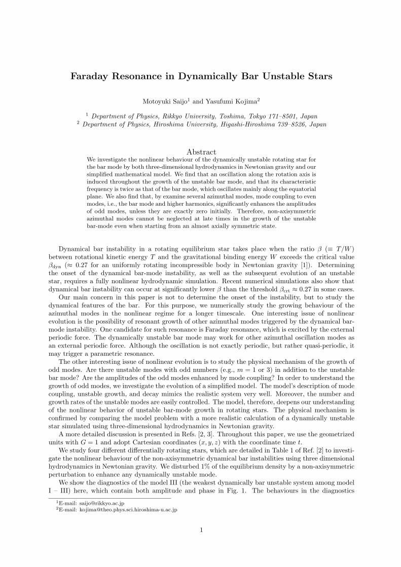
Faraday Resonance in Dynamically Bar Unstable Stars
Motoyuki Saijo1 and Yasufumi Kojima2
1 Department of Physics, Rikkyo University, Toshima, Tokyo 171–8501, Japan2 Department of Physics, Hiroshima University, Higashi-Hiroshima 739–8526, Japan
AbstractWe investigate the nonlinear behaviour of the dynamically unstable rotating star forthe bar mode by both three-dimensional hydrodynamics in Newtonian gravity and oursimplified mathematical model. We find that an oscillation along the rotation axis isinduced throughout the growth of the unstable bar mode, and that its characteristicfrequency is twice as that of the bar mode, which oscillates mainly along the equatorialplane. We also find that, by examine several azimuthal modes, mode coupling to evenmodes, i.e., the bar mode and higher harmonics, significantly enhances the amplitudesof odd modes, unless they are exactly zero initially. Therefore, non-axisymmetricazimuthal modes cannot be neglected at late times in the growth of the unstablebar-mode even when starting from an almost axially symmetric state.
Dynamical bar instability in a rotating equilibrium star takes place when the ratio β (≡ T/W )between rotational kinetic energy T and the gravitational binding energy W exceeds the critical valueβdyn (≈ 0.27 for an uniformly rotating incompressible body in Newtonian gravity [1]). Determiningthe onset of the dynamical bar-mode instability, as well as the subsequent evolution of an unstablestar, requires a fully nonlinear hydrodynamic simulation. Recent numerical simulations also show thatdynamical bar instability can occur at significantly lower β than the threshold βcrt ≈ 0.27 in some cases.
Our main concern in this paper is not to determine the onset of the instability, but to study thedynamical features of the bar. For this purpose, we numerically study the growing behaviour of theazimuthal modes in the nonlinear regime for a longer timescale. One interesting issue of nonlinearevolution is the possibility of resonant growth of other azimuthal modes triggered by the dynamical bar-mode instability. One candidate for such resonance is Faraday resonance, which is excited by the externalperiodic force. The dynamically unstable bar mode may work for other azimuthal oscillation modes asan external periodic force. Although the oscillation is not exactly periodic, but rather quasi-periodic, itmay trigger a parametric resonance.
The other interesting issue of nonlinear evolution is to study the physical mechanism of the growth ofodd modes. Are there unstable modes with odd numbers (e.g., m = 1 or 3) in addition to the unstablebar mode? Are the amplitudes of the odd modes enhanced by mode coupling? In order to understand thegrowth of odd modes, we investigate the evolution of a simplified model. The model’s description of modecoupling, unstable growth, and decay mimics the realistic system very well. Moreover, the number andgrowth rates of the unstable modes are easily controlled. The model, therefore, deepens our understandingof the nonlinear behavior of unstable bar-mode growth in rotating stars. The physical mechanism isconfirmed by comparing the model problem with a more realistic calculation of a dynamically unstablestar simulated using three-dimensional hydrodynamics in Newtonian gravity.
A more detailed discussion is presented in Refs. [2, 3]. Throughout this paper, we use the geometrizedunits with G = 1 and adopt Cartesian coordinates (x, y, z) with the coordinate time t.
We study four different differentially rotating stars, which are detailed in Table 1 of Ref. [2] to investi-gate the nonlinear behaviour of the non-axisymmetric dynamical bar instabilities using three dimensionalhydrodynamics in Newtonian gravity. We disturbed 1% of the equilibrium density by a non-axisymmetricperturbation to enhance any dynamically unstable mode.
We show the diagnostics of the model III (the weakest dynamically bar unstable system among modelI – III) here, which contain both amplitude and phase in Fig. 1. The behaviours in the diagnostics
1E-mail: [email protected]: [email protected]
1
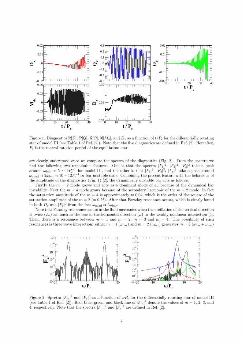
-0.02
-0.01
0
0.01
0.02
Dx
-0.3
-0.2
-0.1
0
0.1
0.2
0.3
Qx
0 10 20 30 40
t / Pc
-0.02
-0.01
0
0.01
0.02
Ox
0 10 20 30 40
t / Pc
-0.06
-0.03
0
0.03
0.06
M4x
0 10 20 30 40
t / Pc
0.37
0.38
0.39
Dz
Figure 1: Diagnostics <[D], <[Q], <[O], <[M4], and Dz as a function of t/Pc for the differentially rotatingstar of model III (see Table 1 of Ref. [2]). Note that the five diagnostics are defined in Ref. [2]. Hereafter,Pc is the central rotation period of the equilibrium star.
are clearly understood once we compute the spectra of the diagnostics (Fig. 2). From the spectra wefind the following two remarkable features. One is that the spectra |F1|2, |F2|2, |F3|2 take a peakaround ωbar ≈ 5 ∼ 6P−1
c for model III, and the other is that |F3|2, |F4|2, |Fz|2 take a peak aroundωquad ≈ 2ωbar ≈ 10 – 12P−1
c for bar unstable stars. Combining the present feature with the behaviour ofthe amplitude of the diagnostics (Fig. 1) [2], the dynamically unstable bar acts as follows.
Firstly the m = 2 mode grows and acts as a dominant mode of all because of the dynamical barinstability. Next the m = 4 mode grows because of the secondary harmonic of the m = 2 mode. In factthe saturation amplitude of the m = 4 is approximately ≈ 0.04, which is the order of the square of thesaturation amplitude of the m = 2 (≈ 0.22). After that Faraday resonance occurs, which is clearly foundin both Dz and |Fz|2 from the fact ωquad ≈ 2ωbar.
Note that Faraday resonance occurs in the fluid mechanics when the oscillation of the vertical directionis twice (2ω) as much as the one in the horizontal direction (ω) in the weakly nonlinear interaction [4].Then, there is a resonance between m = 1 and m = 2, m = 3 and m = 4. The possibility of suchresonances is three wave interaction: either m = 1 (ωbar) and m = 2 (ωbar) generates m = 3 (ωbar +ωbar)
-20 -10 0 10 20ω Pc
10-5
10-4
10-3
10-2
10-1
100
101
|Fz|2
-20 -10 0 10 20ω Pc
10-2
10-1
100
101
102
103
104
105
106
|Fm
|2
Figure 2: Spectra |Fm|2 and |Fz|2 as a function of ωPc for the differentially rotating star of model III(see Table 1 of Ref. [2]). Red, blue, green, and black line of |Fm|2 denote the values of m = 1, 2, 3, and4, respectively. Note that the spectra |Fm|2 and |Fz|2 are defined in Ref. [2].
2
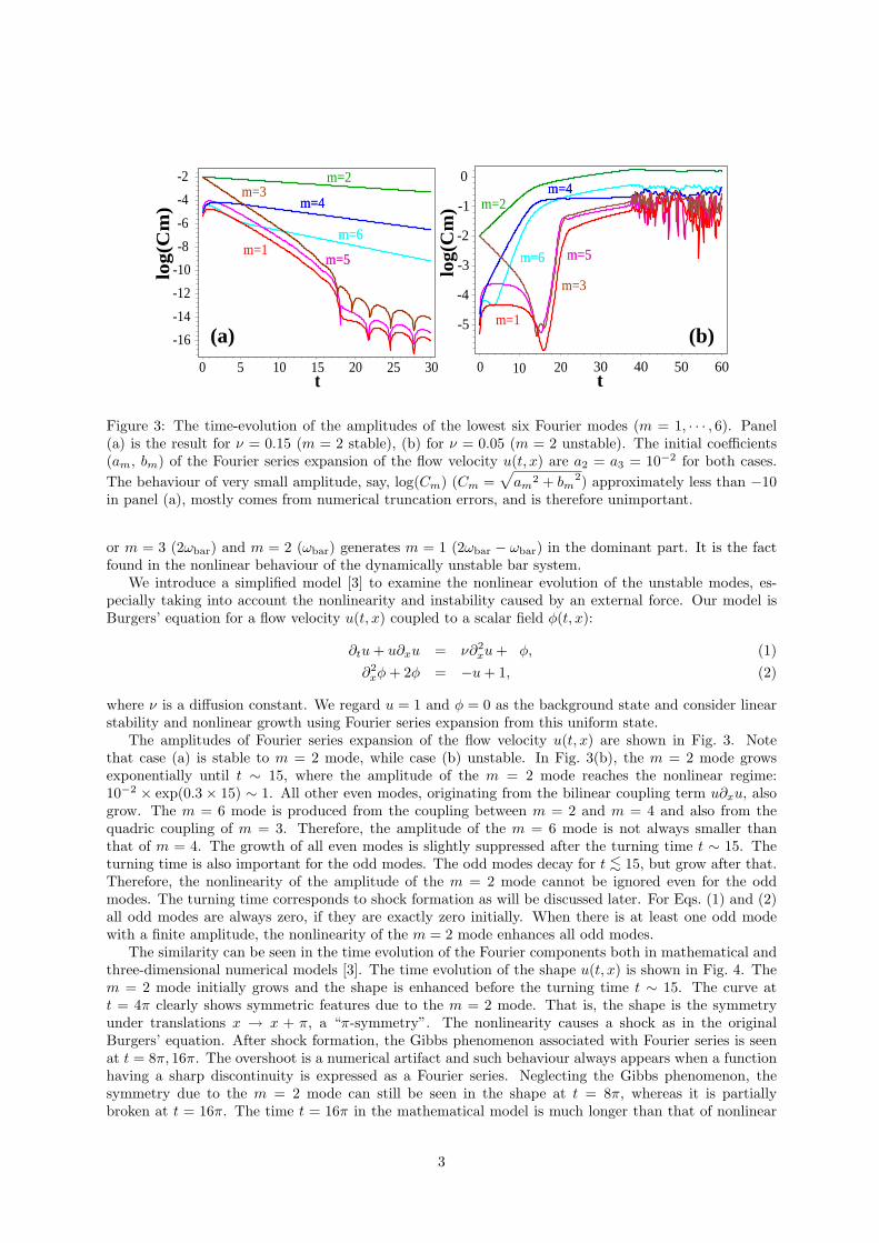
m=6m=6
m=5m=5
m=4m=4
m=2
m=1
-16
-14
-12
-10
-8
-6
-4
-2lo
g(C
m)
0 5 10 15 20 25 30t
-5
-4
-3
-2
-1
0
log(
Cm
)
30 40 50 60t
m=2
m=3
m=1
m=5m=5m=6m=6
m=4m=4
0 10 20
m=3
(a) (b)
Figure 3: The time-evolution of the amplitudes of the lowest six Fourier modes (m = 1, · · · , 6). Panel(a) is the result for ν = 0.15 (m = 2 stable), (b) for ν = 0.05 (m = 2 unstable). The initial coefficients(am, bm) of the Fourier series expansion of the flow velocity u(t, x) are a2 = a3 = 10−2 for both cases.The behaviour of very small amplitude, say, log(Cm) (Cm =
√am
2 + bm2) approximately less than −10
in panel (a), mostly comes from numerical truncation errors, and is therefore unimportant.
or m = 3 (2ωbar) and m = 2 (ωbar) generates m = 1 (2ωbar − ωbar) in the dominant part. It is the factfound in the nonlinear behaviour of the dynamically unstable bar system.
We introduce a simplified model [3] to examine the nonlinear evolution of the unstable modes, es-pecially taking into account the nonlinearity and instability caused by an external force. Our model isBurgers’ equation for a flow velocity u(t, x) coupled to a scalar field φ(t, x):
∂tu + u∂xu = ν∂2xu + ¸φ, (1)
∂2xφ + 2φ = −u + 1, (2)
where ν is a diffusion constant. We regard u = 1 and φ = 0 as the background state and consider linearstability and nonlinear growth using Fourier series expansion from this uniform state.
The amplitudes of Fourier series expansion of the flow velocity u(t, x) are shown in Fig. 3. Notethat case (a) is stable to m = 2 mode, while case (b) unstable. In Fig. 3(b), the m = 2 mode growsexponentially until t ∼ 15, where the amplitude of the m = 2 mode reaches the nonlinear regime:10−2 × exp(0.3 × 15) ∼ 1. All other even modes, originating from the bilinear coupling term u∂xu, alsogrow. The m = 6 mode is produced from the coupling between m = 2 and m = 4 and also from thequadric coupling of m = 3. Therefore, the amplitude of the m = 6 mode is not always smaller thanthat of m = 4. The growth of all even modes is slightly suppressed after the turning time t ∼ 15. Theturning time is also important for the odd modes. The odd modes decay for t <∼ 15, but grow after that.Therefore, the nonlinearity of the amplitude of the m = 2 mode cannot be ignored even for the oddmodes. The turning time corresponds to shock formation as will be discussed later. For Eqs. (1) and (2)all odd modes are always zero, if they are exactly zero initially. When there is at least one odd modewith a finite amplitude, the nonlinearity of the m = 2 mode enhances all odd modes.
The similarity can be seen in the time evolution of the Fourier components both in mathematical andthree-dimensional numerical models [3]. The time evolution of the shape u(t, x) is shown in Fig. 4. Them = 2 mode initially grows and the shape is enhanced before the turning time t ∼ 15. The curve att = 4π clearly shows symmetric features due to the m = 2 mode. That is, the shape is the symmetryunder translations x → x + π, a “π-symmetry”. The nonlinearity causes a shock as in the originalBurgers’ equation. After shock formation, the Gibbs phenomenon associated with Fourier series is seenat t = 8π, 16π. The overshoot is a numerical artifact and such behaviour always appears when a functionhaving a sharp discontinuity is expressed as a Fourier series. Neglecting the Gibbs phenomenon, thesymmetry due to the m = 2 mode can still be seen in the shape at t = 8π, whereas it is partiallybroken at t = 16π. The time t = 16π in the mathematical model is much longer than that of nonlinear
3
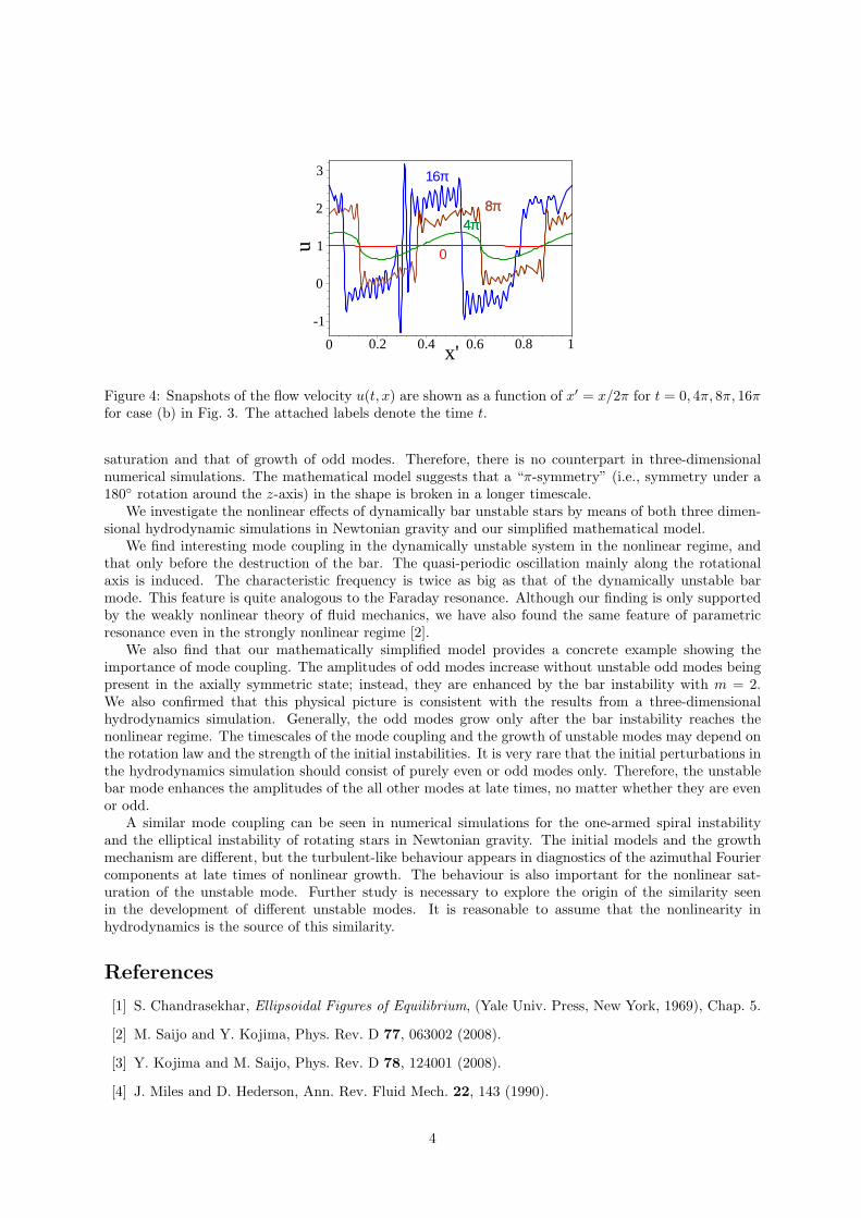
16π
8π8π4π4π
0
-1
0
1
2
3
u
0.2 0.4 0.6 0.8 1x'0
Figure 4: Snapshots of the flow velocity u(t, x) are shown as a function of x′ = x/2π for t = 0, 4π, 8π, 16πfor case (b) in Fig. 3. The attached labels denote the time t.
saturation and that of growth of odd modes. Therefore, there is no counterpart in three-dimensionalnumerical simulations. The mathematical model suggests that a “π-symmetry” (i.e., symmetry under a180 rotation around the z-axis) in the shape is broken in a longer timescale.
We investigate the nonlinear effects of dynamically bar unstable stars by means of both three dimen-sional hydrodynamic simulations in Newtonian gravity and our simplified mathematical model.
We find interesting mode coupling in the dynamically unstable system in the nonlinear regime, andthat only before the destruction of the bar. The quasi-periodic oscillation mainly along the rotationalaxis is induced. The characteristic frequency is twice as big as that of the dynamically unstable barmode. This feature is quite analogous to the Faraday resonance. Although our finding is only supportedby the weakly nonlinear theory of fluid mechanics, we have also found the same feature of parametricresonance even in the strongly nonlinear regime [2].
We also find that our mathematically simplified model provides a concrete example showing theimportance of mode coupling. The amplitudes of odd modes increase without unstable odd modes beingpresent in the axially symmetric state; instead, they are enhanced by the bar instability with m = 2.We also confirmed that this physical picture is consistent with the results from a three-dimensionalhydrodynamics simulation. Generally, the odd modes grow only after the bar instability reaches thenonlinear regime. The timescales of the mode coupling and the growth of unstable modes may depend onthe rotation law and the strength of the initial instabilities. It is very rare that the initial perturbations inthe hydrodynamics simulation should consist of purely even or odd modes only. Therefore, the unstablebar mode enhances the amplitudes of the all other modes at late times, no matter whether they are evenor odd.
A similar mode coupling can be seen in numerical simulations for the one-armed spiral instabilityand the elliptical instability of rotating stars in Newtonian gravity. The initial models and the growthmechanism are different, but the turbulent-like behaviour appears in diagnostics of the azimuthal Fouriercomponents at late times of nonlinear growth. The behaviour is also important for the nonlinear sat-uration of the unstable mode. Further study is necessary to explore the origin of the similarity seenin the development of different unstable modes. It is reasonable to assume that the nonlinearity inhydrodynamics is the source of this similarity.
References
[1] S. Chandrasekhar, Ellipsoidal Figures of Equilibrium, (Yale Univ. Press, New York, 1969), Chap. 5.
[2] M. Saijo and Y. Kojima, Phys. Rev. D 77, 063002 (2008).
[3] Y. Kojima and M. Saijo, Phys. Rev. D 78, 124001 (2008).
[4] J. Miles and D. Hederson, Ann. Rev. Fluid Mech. 22, 143 (1990).
4
Gravitational-Wave Constraintson Abundance of Primordial Black Holes
Ryo Saito1 and Jun’ichi Yokoyama2
1Department of Physics, Graduate School of Science, The University of Tokyo, Tokyo 113-0033, Japan2Research Center for the Early Universe, Graduate School of Science, The University of Tokyo,Tokyo
113-0033, Japan3Institute for the Physics and Mathematics of the Universe, University of Tokyo, Chiba 277-8568, Japan
AbstractFormation of primordial black holes (PBHs) requires a large root-mean-square ampli-tude of density fluctuations, which generate second-order tensor perturbations thatcan be compared with observational constraints. We show that pulsar timing dataessentially rules out PBHs with 102−4M¯ which were previously considered as a can-didate of intermediate-mass black hoes and that PBHs with mass range 1020−25 gwhich provide an astrophysical candidate for dark matter may be probed by futurespace-based laser interferometers.
1 Introduction
Primordial black holes (PBHs) are produced when density fluctuations with a large amplitude enters thehorizon in the radiation dominated stage of the early universe with their typical mass given by the horizonmass at that epoch [1, 2]. PBHs with their mass smaller than 1015g would have been evaporated awayby now due to the Hawking radiation and a number of cosmological constraints have been imposed onthe abundance of these light holes by big-bang nucleosynthesis (BBN) and gamma-ray background etc.Heavier PBHs can play some astrophysical roles today. For example, they may serve as the origin of theintermediate-mass black holes (IMBHs), which are considered to be the observed ultra-luminous X-raysources, if their mass and abundance lie in the range MPBH ∼ 102M¯−104M¯ and ΩPBHh2 ∼ 10−5−10−2,respectively [3], while PBHs with mass MPBH ∼ 1020g−1026g (10−13M¯−10−7M¯) [2] and the abundanceΩPBHh2 = 0.1 can provide astrophysical origin of dark matter (DM) which is yet free from the constraintimposed by gravitational lensing experiments [4]. In order to produce the relevant density of PBHs, itis necessary to produce density fluctuations whose power spectrum has a high peak with an amplitude10−2 − 10−1 on the corresponding scales.
Second-order effects also generate tensor fluctuations to produce stochastic background of gravi-tational waves (GWs) from scalar-tensor mode coupling [6, 7], whose amplitude may well exceed thefirst-order tensor perturbation generated by quantum effect during inflation in the current set up sincethe amplitude of density fluctuations required for a substantial density of PBHs is so large.
In the following sections, we show the GWs induced by scalar fluctuations as a second-order effect[6, 7] is a useful probe to investigate the abundance of the PBHs. We calculate spectrum of thesesecond-order GWs in the case scalar fluctuations have a sufficiently large peak to realize formation ofrelevant numbers of PBHs. As a natural consequence we find that the spectrum of GWs has a peak ona scale approximately equal to the scale of the peak of the scalar fluctuations. We can therefore obtaininformation on the abundance of PBHs with the horizon mass when the scale of the peak entered theHubble radius by observing GWs with the frequency corresponding to the same comoving scale, namely,10−9Hz − 10−8Hz for IMBHs and 10−3Hz − 1Hz for dark-matter PBHs. Fortunately, the former band isprobed by the pulsar timing observations [8, 9] while the latter band can be observed in future by thespace-based interferometers for dark matter PBHs.
1E-mail:[email protected]:[email protected]
1
2 The induced gravitational waves
We write the perturbed metric as
ds2 = a(η)2[−e2Φdη2 + e−2Ψ(δij + hij)dxidxj
], (1)
including both scalar perturbations, Φ and Ψ, and tensor perturbation, hij , which satisfies ∂ihij =
hii = 0 with hi
j ≡ δikhkj . We assume the lowest-order tensor perturbation is negligible and considerthat generated by the scalar mode as a second-order effect. The relevant part of the Einstein equationtherefore reads
hij
′′+ 2Hhi
j
′ − ∂2hij = 2Pis
rjSrs , (2)
where a prime denotes differentiation with respect to the conformal time, Pisrj represents the projection
operator to the transverse, traceless part, and H ≡ a′/a [6, 7]. The source term reads
Srs = 2∂rΨ∂sΨ − 4
3(1 + w)∂r(Ψ + H−1Ψ′)∂s(Ψ + H−1Ψ′), (3)
with w ≡ ρ/p being the equation-of-state parameter of the background fluid. In practice, only theradiation dominated era is relevant, so we take w = 1/3 hereafter. We also neglect anisotropic stress,which is expected to give only a small correction [7], and set Φ = Ψ at linear order. In order to calculatethe induced GWs up to second order, it is sufficient to use the linear scalar modes. Hence, we only needto solve the linear evolution equation,
Ψ′′k(η) +
4ηΨ′
k(η) +k2
3Ψk(η) = 0, (4)
for the scalar modes where Ψk represents a Fourier mode.For our purpose we assume the following approximate form of the power spectrum of the initial
fluctuations,
PΨ(k) ≡ k3
2π2〈|Ψk(0)|2〉 = A2δ(ln(k/kp)), (5)
where kp and A2 represent the wavenumber of the peak and (amplitude)2× ln(peak width) of the originalspectrum, respectively. With this power spectrum the fractional energy density of the region collapsinginto PBHs at their formation time is estimated as
β(MPBH) ∼ 0.1 exp(− Ψ2
c
2A2
), (6)
where MPBH is of the order of the horizon mass when the comoving scale k−1p enters the Hubble radius
and Ψc is the threshold value of PBH formation. Carr [5] takes the threshold value of the density contrastto be δc = 1/3 corresponding to Ψc = 1/2. One can express the current value of the density parameterof PBHs in terms of β(MPBH) as
ΩPBH,0h2 = 2 × 10⁶β(MPBH)
(MPBH
1036 g
)−1/2 ( g∗p
10.75
)−1/3
, (7)
where g∗p is the effective number of the relativistic degrees of freedom when kp entered the Hubble radius.We define the Fourier modes hk as
hij(x, η) =∫
d3k
(2π)3/2eik·x [
h+k (η)e+
ij(k) + h×k (η)e×ij(k)
], (8)
where e+ij(k), e×ij(k) are polarization tensors which are normalized as
∑i,j eα
ij(k)eβij(−k) = 2δαβ . The
Fourier transform of the source term (3) is also defined similarly. We find the source term is constantwhen kpη/
√3 ¿ 1, while it decreases in proportion to η−2 for kpη/
√3 À 1. As a result the production
of scalar-induced GWs mostly occurs around the time when kp crosses the sound horizon. In the mass
2
range of the PBHs of our interest, creation of scalar-induced GWs is terminated well before the equalitytime. After that the energy density of GWs decreases in proportion to a−4. Using the Green functionmethod one can easily find a formal solution to (2) from which we can evaluate the density parameter ofGWs contributed by a logarithmic interval of the wavenumber around k. It is formally expressed as
ΩGW(k, η) =k3
12π2H2
(|h+
k
′|2
+ |h×k
′|2)
, (9)
when k-mode is well inside the horizon. The overall feature of the spectrum of ΩGW(f, η0) today can beestimated to be
ΩGW(f)h2 = 7 × 10⁻⁹( g∗p
10.75
)−1/3(
A2
10−3
)2 (Ωradh2
4 × 10⁻⁵
) (f
fp
)2[1 −
(f
2fp
)2]2
θ
(1 − f
2fp
)(10)
≡ AGW
(f
fp
)2[1 −
(f
2fp
)2]2
θ
(1 − f
2fp
),
for f . fGW ≡ 2fp/√
3 where we have used the frequency f ≡ 2πk/a0 instead of the wavenumber. Theabove expression has the peak value ΩGW(fGW)h2 = (16/27)AGW at fGW.
3 Constraints on the PBH abundance
We now compare our results with observational constraints. For definiteness we identify MPBH with thehorizon mass when the peak scale k−1
p entered the Hubble radius. Then MPBH is related with the peakfrequency of GWs as
fGW = 1 × 10⁻⁸ Hz(
MPBH
1036 g
)−1/2( g∗p
10.75
)−1/12
. (11)
The pulsar timing observations are sensitive to GWs with f > 1/T where T is the data span. The 7-yeardata of observation of PSR B1855+09 gives an upper limit
ΩGW(f)h2 < 4.8 × 10⁻⁹
(f
4.4 × 10⁻⁹Hz
)2
, (12)
for f > 4.4× 10⁻⁹Hz at 90% confidence level [8]. By using this limit, we can constrain the abundance ofPBHs with mass MPBH . 1 × 1037 g = 5 × 10³M¯.
The space-based interferometers are sensitive to GWs with 10−5Hz . f . 10Hz [10, 11], which coversthe entire mass range of the PBHs which are allowed to be DM, 1020g < MPBH < 1026g. LISA willhave its best sensitivity ΩGWh2 ∼ 10−11 at f ∼ 10−2Hz (MPBH ∼ 1024g), BBO and the ultimate-DECIGO are planned to have sensitivity to ΩGWh2 ∼ 10−13 and ΩGWh2 ∼ 10−17, respectively atf ∼ 10−1Hz (MPBH ∼ 1022g).
Figure 1 shows the energy density of the induced GWs, whose approximate form is given by (10).As is seen in the figure the pulsar timing constraint is so stringent that one cannot achieve ΩPBHh2 ¸
10−5 for PBHs with 4 × 10²M¯ . MPBH . 5 × 10³M¯, ruling out the major mass range of IMBHs.On the other hand, if pulsar timing experiments should find any nontrivial modulation in near future, itmight be due to the PBHs with mass around 102M¯ [9].
It is clear from Fig. 1 that the future space-based interferometers can test the feasibility of PBHs asthe dominant constituent of the DM. The ground-based interferometers, on the other hand, have goodsensitivity at f ∼ 10−102Hz [12]. This frequency band corresponds to mass scale MPBH ∼ 1016g−1018g.Though the sensitivity of LIGO is too low now and in near future to detect GWs from the second-ordereffect associated with PBH formation, we could improve the sensitivity by correlation analysis to reach thedesired level to probe PBHs. Because the spectrum has a tail to lower frequencies, it may be possible toconstrain the abundance of the PBHs with MPBH < 7×10¹⁴g (fGW > 6×10²Hz), which have evaporatedby the present epoch and could contribute to cosmic rays. Further study, however, is necessary in orderto obtain the conclusion because there are astronomical sources of GWs in this frequency band, too.
3
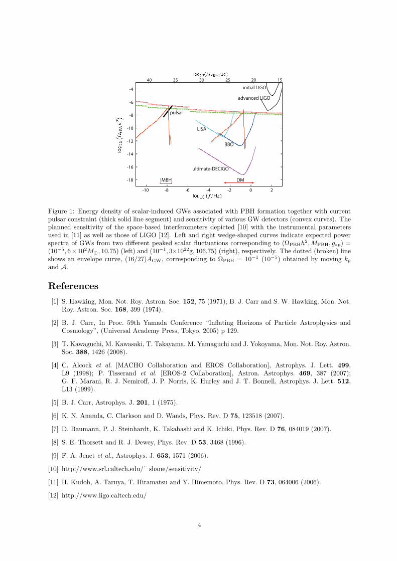
-18
-16
-14
-12
-10
-8
-6
-4
-10 -8 -6 -4 -2 0 2
LISA
BBO
ultimate-DECIGO
pulsar
initial LIGO
advanced LIGO
IMBH DM
15 20 25 30 35 40
Figure 1: Energy density of scalar-induced GWs associated with PBH formation together with currentpulsar constraint (thick solid line segment) and sensitivity of various GW detectors (convex curves). Theplanned sensitivity of the space-based interferometers depicted [10] with the instrumental parametersused in [11] as well as those of LIGO [12]. Left and right wedge-shaped curves indicate expected powerspectra of GWs from two different peaked scalar fluctuations corresponding to (ΩPBHh2, MPBH, g∗p) =(10−5, 6×10²M¯, 10.75) (left) and (10−1, 3×10²²g, 106.75) (right), respectively. The dotted (broken) lineshows an envelope curve, (16/27)AGW, corresponding to ΩPBH = 10−1 (10−5) obtained by moving kp
and A.
References
[1] S. Hawking, Mon. Not. Roy. Astron. Soc. 152, 75 (1971); B. J. Carr and S. W. Hawking, Mon. Not.Roy. Astron. Soc. 168, 399 (1974).
[2] B. J. Carr, In Proc. 59th Yamada Conference “Inflating Horizons of Particle Astrophysics andCosmology”, (Universal Academy Press, Tokyo, 2005) p 129.
[3] T. Kawaguchi, M. Kawasaki, T. Takayama, M. Yamaguchi and J. Yokoyama, Mon. Not. Roy. Astron.Soc. 388, 1426 (2008).
[4] C. Alcock et al. [MACHO Collaboration and EROS Collaboration], Astrophys. J. Lett. 499,L9 (1998); P. Tisserand et al. [EROS-2 Collaboration], Astron. Astrophys. 469, 387 (2007);G. F. Marani, R. J. Nemiroff, J. P. Norris, K. Hurley and J. T. Bonnell, Astrophys. J. Lett. 512,L13 (1999).
[5] B. J. Carr, Astrophys. J. 201, 1 (1975).
[6] K. N. Ananda, C. Clarkson and D. Wands, Phys. Rev. D 75, 123518 (2007).
[7] D. Baumann, P. J. Steinhardt, K. Takahashi and K. Ichiki, Phys. Rev. D 76, 084019 (2007).
[8] S. E. Thorsett and R. J. Dewey, Phys. Rev. D 53, 3468 (1996).
[9] F. A. Jenet et al., Astrophys. J. 653, 1571 (2006).
[10] http://www.srl.caltech.edu/˜ shane/sensitivity/
[11] H. Kudoh, A. Taruya, T. Hiramatsu and Y. Himemoto, Phys. Rev. D 73, 064006 (2006).
[12] http://www.ligo.caltech.edu/
4
Moduli fixing in Brane gas cosmology
Masakazu Sano 1
1Department of Physics, Hokkaido University, Sapporo, Hokkaido , 060–0810, Japan
AbstractWe consider a moduli stabilization in a brane gas model based on Type II stringtheories. We show that gauge fields on D-branes, NS5-branes and KK5-monopolesare required in order to stabilize radial moduli fields of a six-dimensional torus as aninternal space and dilaton, simultaneously.
1 Introduction
One of most interesting problems in string theories is to reveal a mechanism of a moduli fixing of higherdimensions and a dilaton field. In a higher dimensional theory like the string theories, the scales ofa compactified space and the dilaton are dynamical variables. Those variables are related to gaugecouplings of the theories by a Kaluza-Klein reduction. We should stabilize the moduli fields to obtain afour-dimensional theory describing a realistic universe, because the gauge coupling has a fixed value.
Brandenberger and Vafa proposed the string gas model [1]. According to this model, at a very earlyuniverse, It was assumed that fundamental strings fill the universe which has T 9 as the spatial part.In this setup, they considered an interesting mechanism of compactifications. If strings remain withoutannihilations in the 6-dimensions of T 9, it is expected that the internal space is stabilized by the tensionof the strings. On the other hand, the 3-dimensional space decompactifies from T 9, because strings easilyannihilate each other in the 3-dimensional space.
A lot of models on the moduli stabilizations have been proposed, using brane gas models [2] as wellas string gas models [3, 4, 5, 6, 7, 8, 9, 10, 11, 12, 13, 14, 15, 16], since string theories neutrally includebranes. However, it has been known that a simple compactification with only winding modes of branesor strings cannot stabilize radial moduli fields and the dilaton field, simultaneously [15].
The purpose of this work is to construct brane gas models with stabilized moduli fields in Type IIstring theories. We consider gauge fields on D-branes, NS5-branes and Kaluza-Klein monopoles (KK5)as new ingredients. It will be found that those objects are required for the stabilization of the dilatonfield. This talk is based on the work in collaboration with Hisao Suzuki [17].
2 Moduli fixing with D-brane, KK5-monopole and NS5-branein Brane gas model
2.1 Preliminaries
Before discussing a detail of the moduli stabilization in brane gas models, we give a setup of the 10-dimensional metric, the 4-dimensional Einstein frame and a bulk action. In this talk, we do not take avarying Newton constant, therefore the 4-dimensional Einstein frame is required when the Kaluza-Kleinreduction is performed.
We consider a case where the 3-dimensional space has already been large and take the followinghomogeneous metric:
ds210 = −e2λ0(t)dt2 + e2λ(t)dx2 +
9∑m=4
e2λm(t)(dym)2. (1)
The 3-dimensional space is R3 and the internal space is T 6. The coordinate of a cycle ym is defined as0 ≤ ym ≤ 2π
√α′ where
√α′ is related to the string length, ls =
√α′. We assume that all fields depend
1E-mail:sano [email protected]
1
only on time and fluxes are canceled each other. This assumption implies that the dynamics of the branegas models are decided by gases of world volume action of branes. In the system, a total action is givenby S0 + Sbrane gases. S0 is the 10-dimensional action which gives the following 4-dimensional effectiveaction:
S0 =1
16πG10
∫
M10d10X
√−Ge−2φ(t)(R + 4(∇φ)2)
=1
16πG4
∫
M4d4xen(t)+3A(t) × e−2n(t)
(−6A2(t) + 2β2(t) +
9∑m=4
λ2m(t)
)(2)
where we have defined the 4-dimensional Einstein frame as follows (G(4) = G(10)(2π√
α′)−6):
λ0(t) = n(t) + β(t), λ(t) = A(t) + β(t), β(t) ≡ φ(t)− 12λ(t), λ(t) ≡
9∑m=4
λm(t). (3)
The new variable β(t) is useful in order to obtain the diagonal kinetic term. Then, we can analyze aminimum condition of a potential given by the energy-momentum tensor in term of brane gases:
u(m1···mp)
Dp/KK5/NS5 ≡ −T 00 =
2g00
√−g4(x)
δL(m1···mp)
Dp/KK5/NS5
δg00= −e−n(t)−3A(t)
δL(m1···mp)
Dp/KK5/NS5
δn(t). (4)
2.2 Brane gas
We will consider a Dp-brane which wraps over a cycle of T 6. It is known that gauge fields can be generatedon the Dp-brane whose action is
S(m1···mp)Dp = −Tp
∫
R×Σp
dp+1ξe−φ(t)√− det(γab + 2πα′Fab) (5)
where Σp ⊂ T 6. We have assumed the homogeneous metric and fields, and then the electric fields F0i =Ai(t) flow on the Dp-brane. If fluxes are canceled each other and only brane gases dominate as ideal gases,the electric fields, Am(t) and velocity along the internal space, Xm(t) are free. Then, we can integratethose variables once and, by Eq.(4), we obtain the potentials of brane gases (Tp = (2π)−p(α′)−(p+1)/2):
u(m1···mp)Dp =e−3A(t)(2π
√α′)pTp ×
e−λ(t)+2
Ppa=1 λma (t) + A(t)
12
(6)
where
A(t) ≡p∑
a=1
e2β(t)+2λma (t)
(fma
2πα′
)2
+6∑
b=p+1
e2β(t)−2λmb(t)(vmb)2. (7)
fma and vmb are constants of integration of equations of motion on A(t) and Xm(t). Similarly, thepotential of gases of NS5 and KK5 [18, 19, 20] whose action is
S(m1···m5)NS5 = −TNS5
∫
R×Σ5
d6ξe−2φ(t)√− det γab, (8)
S(m1···m5)KK5 = −TKK5
∫
R×Σ5
d6ξe−2φ(t)k2√− det γab, γab ≡ ∂Xm
∂ξa
∂Xm
∂ξa(Gmn − k−2kmkn), (9)
(km ≡ δmm6 is the killing vector of the S1 isometry of the (m6)-cycle) are given by
u(m1···m5)NS5 = e−3A(t)(2π
√α′)5TNS5 × e−β(t)−λ(t)+
P5a=1 λma (t), (10)
u(m1···m5)KK5 = e−3A(t)(2π
√α′)5TKK5 × e−β(t)−λ(t)+2λm6+
P5a=1 λma (t) (11)
2
where TNS5 = TKK5 = TD5.We find two important facts from (6), (10) and (11). First, the energy density is proportional to
e−3A(t) where eA(t) is the scale factor of the three dimensions in the 4-dimensional Einstein frame. Ifall moduli fields are fixed, this gives the energy density of a pressureless dust. This property resultfrom brane gases whose all spatial parts wrap over cycles of T 6. We see those branes as gases of pointparticles on the 3-dimensional space. Second, It is found that the the potential of the Dp-brane cannotstabilize the dilaton field. The winding mode of the world volume action has no dilaton dependence inthe 4-dimensional Einstein frame. The terms derived by electric fields and velocities have the dilatondependence of e+2β(t) in (7). On the other hand, the potential of NS5 and KK5 has the inverse dependenceof the dilaton field like Eq.(10) and Eq.(11). Therefore, It is expected that the dilaton field is stabilizedby the electric fields and NS5/KK5.
2.3 D1-brane(+gauge field), KK5-monopole(IIB)
We will investigate an explicit brane gas model in Type IIB theory. This model is constructed by D1-branes wrapping over each cycle and KK5 wrapping over (45678)-cycle and its cyclic permutations. UsingT-duality [17], we are able to map this system to a dual model including NS5-branes. We take the initialconditions as vm = 0 and fm = 2πα′f . Then, the energy density of this system is given by
U IIB =ND1
e3A(t)(2π
√α′)T1
9∑a=4
e−12 λ(t)+λa(t)(1 + f2e2β(t)+λ(t))
12 +
NKK5
e3A(t)(2π
√α′)5TKK5
9∑a=4
e−β(t)+λa(t)
(12)
where ND1 and NKK5 are constants and indicate the number density of the pressureless dust at present,eA(t=t0) = 1. The condition of a minimum of U IIB is given by ∂U IIB/∂β = ∂U IIB/λm = 0. The solutionof this condition is
e2φmin. =1f2
, e2λ′min. =( ND1
NKK5
)1/3( 12f2
)1/6
. (13)
This condition shows eλm = eλ′min. (m = 4, 5, · · · , 9), because of the isotropic initial condition for theelectric fields like fm = 2πα′f .
This mechanism of the moduli stabilization is intuitively understood as follows. For example, in the4-dimensional Einstein frame, one of the winding modes of D1-brane and KK5-monopole are exp[(λ4 −λ5 − · · · − λ9)/2] and exp[−β + λ4], respectively. Those windings bind a cycle where the branes wraparound. The expanding directions are bound by another brane. The electric fields on D1-brane andKK5-monopoles stabilize the dilaton field. All forces are canceled each other, and then the radial modulifields of T 6 and the dilaton field are stabilized, simultaneously. After the moduli stabilization, it is foundthat this potential gives the energy density of the pressureless dust like U IIB ∝ e−3A(t).
3 Conclusions and Discussions
We have considered the mechanism of the moduli stabilization in the brane gas model based on Type IIstring theories. It has been found that the gauge fields on D-branes, NS5-branes and KK5-monopole arerequired in order to stabilize the radial moduli fields of T 6 and the dilaton, simultaneously.
Once all moduli fields are stabilized, it is expected that there is a possibility of a dark matter candidatefor this wrapped brane gases, because the energy density with fixed moduli fields gives rise to ρ ∼ e−3A
which is the energy density of a pressureless dust. To realize this statement, we have to check a massscale of wrapped branes and interactions in term of RR-flux in the 4-dimensional Einstein frame.
Acknowledgments
I would like to express my gratitude to the organizers of the JGRG18 for giving me an opportunity ofthis presentation. I would like to thank Hideo Kodama, Shinji Mukohyama and Misao Sasaki for usefulcomments and discussions.
3
References
[1] R. H. Brandenberger and C. Vafa: Superstrings in the Early Universe: Nucl. Phys. B316 391 (1989)
[2] S. Alexander, R. H. Brandenberger and D. Easson: Brane gases in the early universe:Phys.Rev.D62(2000) 103509: hep-th/0005212
[3] S. Watson and R. Brandenberger: Stabilization of extra dimensions at tree level: JCAP0311(2003)008:hep-th/0307044
[4] A. Kaya and T. Rador: Wrapped branes and compact extra dimensions in cosmology: Phys. Lett.B565: 19-26, (2003): hep-th/0301031
[5] B. Bassett, M. Borunda, M. Serone and S. Tsujikawa: Aspects of String-Gas Cosmology at FiniteTemperature: Phys.Rev. D67 (2003) 123506: hep-th/0301180
[6] T Batterfeld and S. Watson: Effective field theory approach to string gas cosmlogy: JCAP 0406001 (2004): hep-th/0403075
[7] S. Watson: Moduli Stabilization with the String Higgs Effect: Phys.Rev. D70 (2004) 066005: hep-th/0404177
[8] S. P. Patil and R. Brandenberger: Radion stabilization by stringy effects in general relativity:Phys.Rev. D71 (2005) 103522:hep-th/0401037
[9] S. P. Patil and R. Brandenberger: The Cosmology of massless string modes: JCAP 0601 (2006)005:hep-th/0502069
[10] S. P. Patil: Moduli (dilaton, volume and shape) stabilization via massless F and D string modes:hep-th/0504145
[11] S. Kanno and J. Soda: Moduli Stabilization in String Gas Compactification : Phys.Rev. D72 (2005)104023: hep-th/0509074
[12] R. Brandenberger, Y. K. Cheung and S. Watson: Moduli stabilization with string gases and fluxes:JHEP 0605 (2006) 025: hep-th/0501032
[13] A. Chatrabhuti: Target space duality and moduli stabilization in String Gas Cosmology:Int.J.Mod.Phys. A22 (2007) 165-180:hep-th/0602031
[14] A. J. Berndsen and J. M. Cline: Dilaton stabilization in brane gas cosmology: Int. J. Mod. Phys.A19 (2004) 5311: hep-th/0408185
[15] A. Berndsen, T. Biswas, J. M. Cline: Moduli stabilization in brane gas cosmology with superpoten-tials: JCAP 0508 012 (2005):hep-th/0505151
[16] R. J. Danos, A. R. Frey and R. H. Brandenberger: Stabilizing moduli with thermal matter andnonperturbative effects: arXiv:0802.1557
[17] M. Sano and H. Suzuki: Moduli fixing and T-duality in Type II brane gas models: Phys.Rev.D78(2008) 064045: arXiv:0804.0176
[18] E. Bergshoeff, B. Janssen and T. Ortin: Kaluza-Klein monopoles and gauged sigma models: Phys.Lett. B410: 131-141, (1997): hep-th/9706117
[19] E. Eyras, B. Janssen and Y. Lozano: 5-branes, KK-monopoles and T-duality: Nucl. Phys. B531(1998) 275-301: hep-th/9806169
[20] E. Bergshoeff, Y. Lozano and T. Ortin: Massive Branes: Nucl.Phys. B518 (1998) 363-423:hep-th/9712115
4
Higher Curvature Corrections to Primordial Fluctuations inSlow-roll Inflation
Masaki Satoh1 and Jiro Soda2
1,2Department of Physics, Kyoto University, Kyoto 606–8501, Japan
AbstractWe study higher curvature corrections to the scalar spectral index, the tensor spectralindex, the tensor-to-scalar ratio, and the polarization of gravitational waves. We findthat there are cases where the higher curvature corrections can not be negligible. Itturns out that the tensor-to-scalar ratio could be enhanced and the tensor spectralindex could be blue due to the Gauss-Bonnet term.
1 Introduction
According to the Wilkinson Microwave Anisotropy Probe (WMAP) data [1] and other observations, itseems plausible that the large scale structure of the universe stems from quantum fluctuations duringthe slow-roll inflation. Considering the accuracy of future observations, it would be worth to study thecorrections due to higher curvature terms to the slow-roll inflation. To the leading order, the correctionscome from the Gauss-Bonnet and the axion-like parity violating coupling terms [2]. In fact, the same typeof corrections can be derived from a particular superstring theory [3]. Hence, we hope the understandingof such corrections to the inflationary scenario provides a clue to the study of superstring theory.
There have been many works concerning the Gauss-Bonnet and the parity violating corrections to theEinstein gravity [3, 4, 5]. However, since no one has systematically investigated both terms simultaneouslyin the context of the slow-roll inflation, the combined effect on the slow-roll inflation is not so clear.Hence, we study the slow-roll inflation with higher curvature corrections and derive the formula for theobservables in terms of slow-roll parameters.
The organization of the paper is as follows: In section 2, we define slow-roll parameters in the infla-tionary scenario with higher curvature corrections. In section 3, we obtain the scalar and tensor spectralindex and the tensor-to-scalar ratio. In section 4, the concrete example is presented as an illustration.The final section is devoted to the conclusion.
2 Slow-roll inflation
We consider the gravitational action with the Gauss-Bonnet and the parity violating terms
S =M2
Pl
2
∫d4x
√−gR −
∫d4x
√−g
[12∇µφ∇µφ + V (φ)
]− 1
16
∫d4x
√−gξ(φ)R2
GB +116
∫d4x
√−gω(φ)RR , (1)
where M2Pl ≡ 1/8πG denotes the reduced Planck mass and gµν is the metric tensor. The Gauss-Bonnet
term RGB and the parity violating term RR are defined by
R2GB ≡ RαβγδRαβγδ − 4RαβRαβ + R2 , RR ≡ 1
2εαβγδRαβρσRγδ
ρσ . (2)
The inflaton field φ has the potential V (φ). We have introduced coupling functions ξ(φ) and ω(φ). Inprinciple, these functions should be calculated from the fundamental theory, such as superstring theory.Hence, it might be important to put constraints on these functions through observations.
1E-mail:[email protected]:[email protected]
1
Let us take the flat Friedmann-Robertson-Walker(FRW) metric
ds2 = −dt2 + a2(t)δijdxidxj , (3)
where a is the scale factor. From the action (1), we obtain following background equations
3M2PlH
2 =12φ2 + V +
32H3ξ , φ + 3Hφ +
32H2(H + H2)ξ,φ + V,φ = 0 , (4)
where a dot denotes the derivative with respect to the cosmic time, and H is the Hubble parameterdefined by H ≡ a/a. Note that coupling function ξ works as the effective potential for the inflaton φ.
We consider the friction-dominated slow-roll inflation phase where the following inequalities hold:
φ2
M2PlH
2¿ 1 ,
H3ξ
M2PlH
2=
Hξ
M2Pl
¿ 1 ,H
H2¿ 1 ,
φ
Hφ¿ 1 . (5)
Under these circumstances, Eqs.(4) read
H2 =V
3M2Pl
, φ = −V,φ
3H− 1
2H3ξ,φ . (6)
The inflation is driven by the potential V , whereas the dynamics of the scalar field is also determinedby the Gauss-Bonnet term.
From consistency conditions, we define five slow-roll parameters,
ε ≡ M2Pl
2V 2
,φ
V 2, η ≡ M2
Pl
V,φφ
V, α ≡ V,φξ,φ
4M2Pl
, β ≡ V ξ,φφ
6M2Pl
, γ ≡V 2ξ2
,φ
18M6Pl
=49
α2
ε, (7)
and impose that ε, |η|, |α|, |β|, γ ¿ 1. Note that, due to the Gauss-Bonnet term, the number of parametersand accompanying conditions increased. What we want to know is the effect of new parameters α, β, γon the cosmological fluctuations.
3 Perturbations
In this section, we show the higher curvature corrections to the scalar and tensor perturbations. Weconsider the scalar perturbations A,B,ψ,E and tensor perturbations hij defined by the perturbed metric
ds2 = a2(τ)[−(1 + 2A)dτ2 + B|idηdxi + (δij + 2ψδij + 2E|ij + hij)dxidxj
], (8)
where τ is conformal time defined by a(t)dτ = dt, the bar denotes the spatial derivative and the primerepresents the derivative with respect to the conformal time. We take the gauge, E = δφ = 0.
We can calculate perturbation quantities following same procedures in the case of ordinary slow-rollinflation. Hence we skip tedious but straightforward calculations. We define power spectrum as
〈0|ψ†ψ|0〉 =∫
d(logk)Pψ(k) , 〈0|hij hij |0〉 =
∑±
∫d(log k)P±
T =∫
d(log k)PT , (9)
where ± denotes helicity of gravitational waves. The results are
Pψ(k) =1
2ε + 4α/3 + γ/2
(H
2π
Γ(νψ)Γ(3/2)
)2 (−kτ
2
)3−2νψ
(10)
P±T (k) =
41 + ε − α − γ
(H
2π
Γ(νT)Γ(3/2)
)2 (−CTkτ
2
)3−2νT(
1 ± π
2H
McΩ
), (11)
where we defined νψ ≡ 3/2 + 3ε− η − α/3− β and νT ≡ 3/2 + ε + α/3, and Ω is another small quantity,representing effect of parity violating term, defined by
Ω ≡ 12
Mc
MPl
ω
MPl' const. , (12)
2
where Mc is the physical wave-number corresponding to the cut-off scale, e.g. string scale. We can readthe scalar and tensor spectral indices nψ, nT
nψ − 1 = 3 − 2νψ = −6ε + 2η +23α + 2β , nT = 3 − 2νT = −2ε − 2
3α . (13)
Of course, in the absence of the Gauss-Bonnet term, α = β = 0, we recover the conventional formula.The most impressive result is shown in Eq.(13). In the usual case, because ε > 0, nT takes a negative
value, namely, the tensor spectrum is red. However, if we incorporate the effect of the Gauss-Bonnetterm, tensor spectrum could be blue, because α takes either positive or negative value. Hence, detectionof the blue spectrum in the gravitational waves through the observation of B-mode polarization mightindicate the existence of the Gauss-Bonnet term.
From the scalar and tensor spectrum, we can deduce the tensor-to-scalar ratio r:
r ≡ PT
Pψ∼ 16ε +
323
α + 4γ = 16ε +323
α +169
α2
ε¸ 32
3(α + |α|) . (14)
For a negative α, we have the minimum, that is, r = 0. In the case 1 ¸ α ¸ ε, the last term dominatesand give rise to the sizable tensor-to-scalar ratio even if ε is extremely small.
Another interesting observable is the circular polarization Π, which is defined as difference betweenleft and right helicity modes
Π ≡P+
T − P−T
P+T + P−
T
=π
2H
McΩ . (15)
This result for circular polarization is the same as the previous work [5], although they considered onlyparity violating term. Let us consider some extreme case, H = 10−4MPl, Mc = 10−3MPl, Ω = 0.1, then,the ratio becomes Π ' 0.015. This means we have a hope to measure the sub-percent order of polarizationdue to the parity violating term [6]. It should be stressed that the effect of the Gauss-Bonnet term couldenhance the amplitude of the primordial gravitational waves. That also enhances the detectability.
4 Observational implications
In the previous sections, we have derived general formula for observables in slow-roll inflation with highercurvature corrections. Here, we will discuss one model as an illustration. Let us consider chaotic inflationmodels with higher curvature corrections. We take the functions as
V =12m2φ2 , ξ = λe−κφ/MPl , (16)
where m is the mass of the inflaton and λ, κ are parameters of the coupling function ξ. Then, the slow-rollparameters can be calculated as
ε = η = 2M2
Pl
φ2, α = −κλ
4m2φ
M3Pl
e−κφ/MPl , β =κ2λ
12m2φ2
M4Pl
e−κφ/MPl , γ =κ2λ2
72m4φ4
M8Pl
e−2κφ/MPl . (17)
We can evaluate the spectral index and the tensor-to-scalar ratio. The results are shown in FIG.1.We have also plotted constraints from WMAP 5-year result, combined with baryon acoustic oscillations(BAO) and Type I supernova (SN). We see these observables are sensitive to higher curvature corrections.Hence, it implies that the higher curvature corrections are relevant to precision cosmology. Here, we noticethat there exist parameter regions represented by blue lines which leads to the blue spectrum in tensormodes. We plotted some typical values of nT in Fig.1.
5 Conclusion
We have studied the slow-roll inflationary scenario with the leading corrections, namely, the Gauss-Bonnetand the parity violating terms. We have obtained the higher curvature corrections to the scalar spectral
3
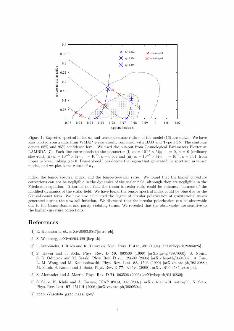
0
0.05
0.1
0.15
0.2
0.25
0.3
0.35
0.4
0.92 0.93 0.94 0.95 0.96 0.97 0.98 0.99 1 1.01 1.02
tens
or-to
-sca
lar r
atio
r
spectral index n
e-folding 50
e-folding 60
n =0.002
n =0.004
n =0.015
T
T
T
Figure 1: Expected spectral index nψ and tensor-to-scalar ratio r of the model (16) are shown. We havealso plotted constraints from WMAP 5-year result, combined with BAO and Type I SN. The contoursdenote 68% and 95% confidence level. We used the out-put from Cosmological Parameters Plotter atLAMBDA [7]. Each line corresponds to the parameter (i) m = 10−5 × MPl, λ = 0, κ = 0 (ordinaryslow-roll), (ii) m = 10−5 × MPl, λ = 1010, κ = 0.003 and (iii) m = 10−5 × MPl, λ = 1010, κ = 0.01, fromupper to lower, taking φ > 0. Blue-colored lines denote the region that generate blue spectrum in tensormodes, and we plot some values of nT.
index, the tensor spectral index, and the tensor-to-scalar ratio. We found that the higher curvaturecorrections can not be negligible in the dynamics of the scalar field, although they are negligible in theFriedmann equation. It turned out that the tensor-to-scalar ratio could be enhanced because of themodified dynamics of the scalar field. We have found the tensor spectral index could be blue due to theGauss-Bonnet term. We have also calculated the degree of circular polarization of gravitational wavesgenerated during the slow-roll inflation. We discussed that the circular polarization can be observabledue to the Gauss-Bonnet and parity violating terms. We revealed that the observables are sensitive tothe higher curvature corrections.
References
[1] E. Komatsu et al., arXiv:0803.0547[astro-ph].
[2] S. Weinberg, arXiv:0804.4291[hep-th].
[3] I. Antoniadis, J. Rizos and K. Tamvakis, Nucl. Phys. B 415, 497 (1994) [arXiv:hep-th/9305025].
[4] S. Kawai and J. Soda, Phys. Rev. D 59, 063506 (1999) [arXiv:gr-qc/9807060]; S. Nojiri,S. D. Odintsov and M. Sasaki, Phys. Rev. D 71, 123509 (2005) [arXiv:hep-th/0504052]; A. Lue,L. M. Wang and M. Kamionkowski, Phys. Rev. Lett. 83, 1506 (1999) [arXiv:astro-ph/9812088];M. Satoh, S. Kanno and J. Soda, Phys. Rev. D 77, 023526 (2008), arXiv:0706.3585[astro-ph].
[5] S. Alexander and J. Martin, Phys. Rev. D 71, 063526 (2005) [arXiv:hep-th/0410230];
[6] S. Saito, K. Ichiki and A. Taruya, JCAP 0709, 002 (2007), arXiv:0705.3701 [astro-ph]; N. Seto,Phys. Rev. Lett. 97, 151101 (2006) [arXiv:astro-ph/0609504].
[7] http://lambda.gsfc.nasa.gov/
4
Entanglement of Universe
Shintaro Sawayama1
1Sawayama cram school of physics, Atsuhara 328,Fuji-shi,Shizuoka-ken, 419-0201, Japan
AbstractBy the recent study of the quantum gravity, we can solved the inhomogeneous space-time. And we quantized the enlarged Bianch I universe. As a result of quantization,we know the universe are entangled. The x,y, and z direction are entangled. So if wemeasure the x direction we know the information of the y and z directions.
1 Introduction
In the quantum gravity there are many difficulties i.e. problem of the time and problem of the norm andinterpretation problem and problem of the inhomogeneous spacetime. One of the main difficulty comesform the Wheeler-DeWitt equation. The difficulty of the Wheeler-DeWitt still remain the Hamiltonianconstraint of the loop quantum gravity. So we should remove the difficulty of the Wheeler-DeWittequation.
So we construct the one method which called the up-to-down method. We explain what is the up-to-down method simply. Once we add an additional dimension to the usual 4-dimensional gravity. Andwe remove the additional dimension by using the problem of the time inversely. Then there appear theadditional constraint equation. This is the up-to-down methodl.
The up-to-down method comes from the Isham’s idea, that is quantum category. Imagine many worldinterpretation, and we assume may world is the infinitely many brane. We quantize the many brane atthe same time.
In section II we write the result of the up-to-down method. In section III we quantize the enlargedBianch I universe. And in section IV we discuss and conclude the presentation.
2 Up-to-down method
We skip the up-to-down method, because it is long. We cite the paper [5]. We start from 5-dimensionalspacetime. There appear one additional constraint equation as,
HS → −mHS := −K2 + KabKab −12P . (1)
Here, HS is the Hamiltonian constraint of the 4+1 decomposition, and Kab is the 4+1 extrinsic curvatureand K is the it’s trace and P is the 3+1 momentum. Now 4+1 decomposition is carried on the additionaldimension s. This is the not usual decomposition. However, because we use the problem of the timeinversely, the s direction vanished. We only consider the 4-dimensional quantum gravity. We obtain thenext theorem.
Theorem 1. In this method, in the H4 additional constraint mHSΠ3 = 0 appears which we call staticrestriction, if there is no time evolution and the projection is defined by the difinition 3.
Here, Π3 is the projection defined by Π3|gµν⟩ = |gsµ = constgij⟩.For example we first consider the Freedman universe as
gab :=
b 0 0 00 a 0 00 0 a 00 0 0 a
. (2)
1E-mail:[email protected]
1
The modified Hamiltonian constraint becomes as
mHS = 6ab∂
∂a
∂
∂b+ a2 ∂2
∂a2(3)
= 6∂
∂η
∂
∂ηb+
∂2
∂η2= 0, (4)
And the Hamiltonian constraint becomes as well known,
HS =92a2 ∂
∂a2+ Λ (5)
=92
∂
∂η2+ Λ = 0. (6)
The 4-dimensional state becomes as
|Ψ4(η)⟩ = exp(i√
23
Λ1/2η). (7)
And it’s enlargement of 4+1 is
|Ψ5(4)(ηb, η)⟩ = exp(− i
√2
3Λ1/2ηb
)exp(i
√2
3Λ1/2η). (8)
We can proof the one of the universe are appropriated to the up-to-down method. There is one enlarge-ment and measure of the projection is not zero.
Secondary, we think about the off-diagonal metric case.
gab =
−c 0 0 00 a b 00 b a 00 0 0 a
. (9)
The modified Hamiltonian constraint become,
mHS = −6ac∂
∂a
∂
∂c+ (6a2 − 2b2)
∂2
∂a2+ 2(b2 − a2)
∂2
∂b2= 0, (10)
And the Hamiltonian constraint becomes as,
HS = −(5a2 − b2)∂
∂a2− (2b2 − a2)
∂2
∂b2= 0. (11)
This Hamiltonian constraint can not solved simply because this is the elliptic differential equation. How-ever, if we use additional constraint as,
mHSΠ3 = (6a2 − 2b2)∂2
∂a2+ 2(b2 − a2)
∂2
∂b2= 0, (12)
The Hamiltonian constraint can be solved.
|Ψ4(5)(a, b)⟩ = E1ab + E2a + E3b + E4. (13)
And the enlargement is
|Ψ5(4)(a, b, c)⟩ = F1ab + F2a + F3bc + F4c + F5. (14)
This enlargement has also non zero measure of the projection.Next we consider the Schwarzchild black holes as
gab =
−f 0 0 00 f−1 00 0 A 00 0 0 A sin2 θ
. (15)
2
The Hamiltonian constraint becomes as
HS =12
(− f2 ∂2
∂f2+ Af
∂
∂f
∂
∂A− 2A2 ∂2
∂A2
)+ R = 0, (16)
Usually this Hamiltonian constraint does not solved. However, if we think the additional constraintequation as,
mHSΠ3 = −2fA∂
∂f
∂
∂A+ A2 ∂2
∂A2(17)
= A∂
∂A
(− 2f
∂
∂f+ A
∂
∂A
)= 0, (18)
we can solve the Hamiltonian constraint equation. Although the Hamiltonian and the additional con-straint equation does not commute, if we make additional constraint parameter relations, we can solvethe Hamiltonian constraint. The Hamiltonian constraint become simple second order ordinal functionalequations.
HS = −78A2 ∂2
∂A2+
1 − c2A2
2A= 0. (19)
And this equation is solved easily by numerical method. The additional constraint or the enlargement isgiven by next formula.
mHS = −f2 ∂2
∂f2+
47
c − cf
f1/2= 0. (20)
In this case the enlargement be able and measure of the projection does not zero.
3 Enlarged Bianchi I universe
Now we consider the metric diagonal case. In this case the Hamiltonian constraint becomes as,
HS =∑ij
δ2
δϕiδϕj+
∑i =j
(ϕi,jj + ϕi,iϕj,i)eϕi . (21)
Here, gii = eϕi . And the commutation relation of the additional and the Hamiltonian constraint becomesas
[mHS ,H4] = δ2∑i =j
(ϕi,ii + ϕ2i,i +
12ϕi,iϕj,i)eϕi − 1
2δ2
∑i =j
ϕi,0(ϕj,ii − 2ϕi,ij − ϕi,jϕi,i)eϕi
−12δ2
∑i =j
(ϕi,0jj + ϕi,0jϕj,j − ϕi,0ji − ϕi,0iϕi,j)eϕi . (22)
We know there are two case whose commutation relation is always zero. Such spacetime is following,g00 0 0 00 q11(x1) 0 00 0 q22(x2) 00 0 0 q33(x3)
. (23)
and g00 0 0 00 q11(x2, x3) 0 00 0 q22(x1, x3) 00 0 0 q33(x1, x2)
. (24)
3
If we treat first metric, the Hamiltonian constraint become,
HS =∑
i
δ2
δϕ2i
= 0. (25)
And the additional constraint with cosmological constant becomes as
S =∑i =j
δ2
δϕiδϕj= Λ (26)
The solution of the usual Hamilton constraint is,
|Ψ4(ϕ)⟩ =∏
exp(aiΛ1/2
∫ϕiδϕi(xi)). (27)
In the ai there are two equation as
a1a2 + a1a3 + a2a3 = 1 (28)a21 + a2
2 + a23 = 1. (29)
Because there are two equation and three parameter, there are infinitely many basis. However, if weassume the one of the norm of ai is one, we can obtain 12 basis as follows
a1 = ±√
3, a2 = ±i, a3 = ∓i (30)
a1 = ±i, a2 = ±√
3, a3 = ∓i (31)
a1 = ±i, a2 = ∓i, a3 = ±√
3. (32)
Looking these basis we can easily know that the state is entangled.
4 Conclusion and Discussions
If we only solve the usual Bianch I universe, the spacetime are entangled. The difference of the enlargedBianch I and usual Bianch I universe are eta square or only eta. Because three direction are entangled,by the measurement of the x direction, we know y direction and z direction. And we justify the up-to-down method. the measure of the all the projection treated here has non zero measure. In this casewe only consider the cosmological constant. But we can consider the Schrodinger or the Krein-Gordonfield instead of the cosmological constant. Then we can know the information of the spacetime by themeasurement of the field. We can answer the philosophical problem“what is existence”by the physics.
References
[1] C.J.Isham and A.Ashtekar Class. Quant. Grav. 9 1433 (1992)
[2] C.Rovelli Quantum Gravity; Cambridge monographs on mathematical physics (2004)
[3] T.Thiemann gr-qc/0110034 (2001)
[4] C.J.Isham Adv.Theor.Math.Phys. 7 331 (2003)
[5] S.Sawayama gr-qc/0604007 (2006)
[6] B.S.DeWitt Phys. Rev. 160 1113 (1967)
[7] J.J.Halliwell and J.B.Hartle Phys. Rev. D 43 1170 (1991)
[8] Quantum computation and quantum information, M.A.Nielsen and I.L.Chang, Cambridge, (2000)
[9] A.Hosoya, privet discussions
4
Invariances of generalized uncertainty principles
Fabio Scardigli1
Leung Center for Cosmology and Particle Astrophysics (LeCosPA),Department of Physics, National Taiwan University, Taipei 106, Taiwan
AbstractIn Ref.[1] we use two different generalized uncertainty principles to compute massthresholds and lifetimes for micro black holes close to their Planck phase. Motivatedby that paper, we study here in detail the conditions for the translation and rotationinvariance of these two different kinds of deformed commutation relations.
1 Introduction
When we consider a high energy collision, we know that Heisenberg principle ∆p∆x ≥ h/2 can be castedin the form ∆E∆x ≥ hc/2 (since ∆E ' c∆p). Actually, the main reason since larger and larger energiesare required to explore smaller and smaller details is that the size of the smallest detail theoreticallydetectable with a beam of energy E is δx = hc/(2E). An equivalent argument comes from consideringthe resolving power of a ”microscope”: the smallest resolvable detail goes roughly as the wavelength ofthe employed photons, and therefore δx ' λ = c
ν = hcε .
The research on viable generalizations of the Heisenberg uncertainty principle traces back to manydecades (see for early approaches [2], etc. See for a review [3] and for more recent approaches [4]). In thelast 20 years, there have been seminal studies in string theory [5] suggesting that for very high energyscattering the uncertainty relation (ST GUP) should be written (in 4 + n dimensions) as
δx ≥ hc
2E+ β`4n
E
E4n, (1)
where `4n is the 4 + n dimensional Planck length and E is the energy of the colliding beams (we use therelation E4n`4n = hc/2). If however we take into account the possibility of a formation of micro blackholes in the scattering, with a gravitational radius of RS ∼ (E)1/(n+1), then we easily see that in 4 + ndimensions (and n ≥ 1) the stringy principle seems to forbid the very observation of the micro hole itself.In fact, at high energy the error predicted by the stringy GUP goes like δx ∼ E, while the size of thehole goes like RS ∼ (E)1/(n+1). For E large enough and n ≥ 1, we always have E > (E)1/(n+1), therebyloosing the possibility of observing micro black holes, just when they become massive (that is, whenthey should approach the classicality). Also to avoid this state of affairs, and on the ground of gedankenexperiments involving the formation of micro black holes, it has been proposed [6] a modification of theuncertainty principle, that in 4 + n dimensions reads
δx ≥ hc
2E+ βR4n(E) , (2)
where R4n is the 4 + n dimensional Schwarzschild radius associated with the energy E (see [7])
R4n =[
16πG4nE
(N − 1)ΩN−1c4
] 1N−2
= `4n
(ωn
E
E4n
) 1n+1
(3)
and N = 3+n is the number of space-like dimensions, ωn = 8π/((N−1)ΩN−1), ΩN−1 = 2πN/2/Γ(N/2) =area of the unit SN−1 sphere. Thus, the GUP originating from micro black hole gedanken experiments(MBH GUP) can be written as
δx ≥ hc
2E+ β`4n
(ωn
E
E4n
) 1n+1
, (4)
1E-mail: [email protected]
1
where β is the deformation parameter, generally believed of O(1). Remarkably, in 4 dimensions (N = 3,n = 0) the two principles coincide. The deformation parameter β, supposed independent from thedimensions N , can be therefore chosen as the same for both principles.
2 Translation and rotation invariance of the GUPs
In this section we shall prove that the GUPs previously introduced do respect the constraints posedby requiring the conventional translation and rotation invariance of the commutation relations. First,we show what these kinematic constraints imply about the structure, in 4 + n dimensions, of the [x, p]commutations relations. In this, we follow closely Ref. [8]. As a general ansatz for the x, p commutationrelation in 4 + n dimensions we take
[xi, pj ] = i h Θij(p) (5)
and we require that Θij(p) differs significantly from δij only for large momenta. We assume also [pi, pj ] = 0and we compute the remaining commutation relation through the Jacobi identities, obtaining
[xi, xj ] = ihxa, Θ−1ar Θs[iΘj]r,s (6)
where are the anti-commutators and Q,s := ∂Q/∂s. The commutation relations (5) are translationinvariant (they are preserved under the transformations xi → xi + di, pi → pi). However, the com-mutation relations (6) are not invariant under translation, unless we require Θij(p) to be such that ityields [xi, xj ] = 0. Thus, in order to implement translation invariance, Θij must satisfy the necessaryand sufficient condition (read off from the (6))
Θia∂piΘbc = Θib∂piΘac (7)
where sum over i is understood. The rotation invariance can be implemented by requiring Θij to havethe form
Θij(p) = f(p2)δij + g(p2)pipj . (8)
Together, conditions (7) and (8) imply that f and g must satisfy the differential equation
2f ′f + (2p2f ′ − f)g = 0 (9)
where f ′(p2) = df/d(p2). Under these conditions, commutation relations do obey translation and rotationinvariance. Considering, for sake of simplicity, the mono-dimensional case i = j, we write for the maincommutator
[x, p] = ih(f(p2) + g(p2)p2) . (10)
The usual Heisenberg commutator is recovered by choosing, for example, f(p2) = 1. Then Eq.(9) impliesg(p2) = 0 and [x, p] = ih. The stringy inspired commutator is obtained, to the first order in β, bychoosing g(p2) = β (see [8]). Then, in fact, solving (9) (a Manfredi equation, in such case), we find
f(p2) =βp2
√1 + 2βp2 − 1
' 1 +β
2p2 + O((βp2)2) (11)
and, to the first order in β (or, equivalently, for small p) we have
[x, p] = ih
(1 +
32βp2 + O(β2)
). (12)
The MBH GUP (4) can be written in terms of momentum transferred as p δx >∼ h2
(1 + γp
n+2n+1
)where
γ = β(ωn)1
n+1(
2`4n
h
)n+2n+1 and this in terms of commutators becomes
[x, p] = ih(1 + γp
n+2n+1
). (13)
2
To show that MBH GUP is translation and rotation invariant we must show that the commutator (13)is of the same form of commutator (10) (when p → 0), with f and g satisfying (9) (in particular wewould like to have f(p2) → 1 for p → 0). However, the previous strategy, namely to fix a priori agiven form for g(p2) and then to compute f(p2) by solving (9) (as we did for HUP, g(p2) = 0, and forstringy GUP, g(p2) = β), in this case does not work. Even if one puts p2g(p2) = γp(n+2)/(n+1), Eq.(9)becomes however rather complicated (it is an Abel equation of 2nd kind), and hardly we can hope itgives f(p2) → 1 for p → 0. Moreover, an explicit solution could not be so useful, since we are mainlyinterested in an asymptotic behaviour. Therefore we ask the following general properties to be satisfiedby the functions f and g
[f(p2) + g(p2)p2] → [1 + γpn+2n+1 ] for p → 0
2f ′f + (2f ′p2 − f)g = 0 ,
(14)
We shall look if there actually exist f and g such that the above two properties can be simultaneouslysatisfied. In this way the rotational and translational invariance of GUP (4) will result proved. In whatfollows such solutions are proved to exist, provided we allow g to develop poles (of course, the functionf and the whole function f + gp2 remain perfectly finite).
In the differential equation (9) everything is function of p2 and f ′(p2) = df/d(p2). So, let’s sety := p2 (y > 0, p = y1/2) and, to avoid fractionary powers, set also y
12(n+1) =: λ, y = λ2(n+1). Then
f ′(y) = 12(n+1)λ
−(2n+1)F ′(λ) , and the system (14) becomes
[F (λ) + G(λ)λ2(n+1)] → [1 + γλn+2] for λ → 0
F ′(λ)F (λ) + [λF ′(λ)− (n + 1)F (λ)]G(λ)λ2n+1 = 0 .(15)
We have to see if the two conditions are compatible, and what this implies for f and g. To check thiscompatibility we can use power series representations of the functions F (λ), G(λ). We allow G(λ) todevelop poles. Since the factor λ2(n+1) multiplies G(λ) in the boundary condition, we could allow polesuntil λ−2(n+1) and still the combination [F + Gλ2(n+1)] would remain analytical. However, we’ll showthat the result can be obtained by allowing poles just until λ−n only. So we write
F (λ) =∞∑
k=0
akλk and G(λ) =∞∑
k=−n
bkλk . (16)
and we look for what the two conditions imply on the coefficients ak, bk. We have
F (λ) + G(λ)λ2(n+1) =∞∑
k=0
(ak + bk−2(n+1))λk (17)
where bk−2(n+1) = 0 for k = 0, 1, 2, ..., n + 1 and b−n 6= 0, b−n+1 6= 0, etc.At small λ we should have the matching, for λ → 0,
∞∑
k=0
(ak + bk−2(n+1))λk −→ 1 + γλn+2 . (18)
This means
k = 0; [a0 + b−2(n+1)] = 1 ⇒ a0 = 1k = 1; [a1 + b1−2(n+1)] = 0 ⇒ a1 = 0k = 2; [a2 + b2−2(n+1)] = 0 ⇒ a2 = 0
... ... ...
k = n + 2; [an+2 + b−n] = γ ⇒ (∗)k = n + 3; [an+3 + b−n+1] = any quantity
... ... ... (19)
3
(*) here at least b−n is 6= 0, therefore at least b−n can be chosen equal to γ.Now let’s see if the conditions on ak, bk just found above, required by the first of Eqs.(15), are com-patible with those required by the differential equation (15). Since F ′(λ) =
∑∞k=0(k + 1)ak+1λ
k,G(λ) =
∑∞k=−n bkλk =
∑∞k=0 bk−nλk−n (with b−n 6= 0, b−n+1 6= 0,..., b0 6= 0), we have F (λ)F ′(λ) =∑∞
k=0 Ckλk, G(λ)F ′(λ) =∑∞
k=0 Dkλk−n, F (λ)G(λ) =∑∞
k=0 Ekλk−n, where Ck =∑k
q=0(q+1)ak−qaq+1,
Dk =∑k
q=0(q + 1)bk−n−qaq+1, Ek =∑k
q=0 ak−qbq−n and the differential equation (15) becomes
∞∑
k=0
[Ckλk + Dkλk+n+2 − (n + 1)Ekλk+n+1
]= 0 (20)
Reshuffling indexes a bit in Eq.(20) we get∞∑
k=0
[Ck + Dk−n−2 − (n + 1)Ek−n−1] λk = 0 (21)
where D−n−2 = 0, D1−n−2 = 0, ..., D−1 = 0, and E−n−1 = 0, E1−n−1 = 0, ..., E−1 = 0, andit is easy to see that these relations are direct consequences of the definitions for bk in Eq.(17) andof relations (19). Equation (21) can be satisfied only if all the coefficients of λk are identically zero.We can now check explicitly that this requirement is in full agreement with conditions (19). In fact:k = 0; C0 + D−n−2 − (n + 1)E−n−1 = a0a1 = 0 ⇒ a1 = 0 (since a0 = 1) and this agrees with (19).And then k = 1; C1 + D1−n−2 − (n + 1)E1−n−1 = a1a1 + 2a0a2 = 0 ⇒ a2 = 0 (since a0 = 1) and thisagrees with (19). Again, for k = 2 we have C2 + D2−n−2 − (n + 1)E2−n−1 = 0 ⇒ a3 = 0 and so on fork = 3, 4, .... For k = n we find an+1 = 0 in agreement with (19). For k = n + 1 we have
Cn+1 + D−1 − (n + 1)E0 =n+1∑q=0
(q + 1)an+1−qaq+1 − (n + 1)0∑
q=0
a0−qbq−n = (n + 2)a0an+2 − (n + 1)a0b−n = 0
Since a0 = 1, then (n + 2)an+2 − (n + 1)b−n = 0 and this equation is compatible with the ”k = n + 2”condition of (19). In fact, we have two equations in two unknowns
(n + 2)an+2 − (n + 1)b−n = 0 and an+2 + b−n = γ , (22)
which allow us to compute an+2 (the first non zero coefficient for F (λ), after a0 = 1) and b−n (pole oforder n of G(λ)). For the next case, k = n + 2, we don’t have evidently any problem, since Eq.(19)simply gives (an+3 + b−n+1) =any quantity. Therefore any relation between an+3, b−n+1 required by thedifferential equation in (15) is acceptable. Note moreover that if we allowed poles for G(λ) with a degreeless than n, we would find contradiction between the conditions (18)-(19), and the differential equationin (15). Thus, we conclude that the two conditions (15) are compatible (if we allow G(λ) to developpoles). So the MBH GUP, as well as the ST GUP, are translational and rotational invariant. Q.E.D.
References
[1] F. Scardigli, Glimpses on the micro black hole Planck phase, [arXiv:0809.1832 (hep-th)]
[2] C.N. Yang, Phys. Rev. 72, 874 (1947); F. Karolyhazy, Nuovo Cim. A 42, 390 (1966).
[3] L.J. Garay, Int. J. Mod. Phys. A 10, 145 (1995).
[4] M.Maggiore, Phys. Lett. B 304, 65 (1993); F. Scardigli, Phys. Lett. B 452, 39 (1999).
[5] D.Amati, M.Ciafaloni, G.Veneziano, Phys. Lett. B 197, 81 (1987); D.J.Gross, P.F.Mende, Phys. Lett. B197, 129 (1987); K.Konishi, G.Paffuti, P.Provero, Phys. Lett. B 234, 276 (1990).
[6] F. Scardigli, Phys. Lett. B 452, 39 (1999); F.Scardigli, R.Casadio, Class. Quant. Grav. 20, 3915 (2003).
[7] R.C.Myers, M.J.Perry, Annals of Physics 172, 304 (1987).
[8] A.Kempf, J. Phys. A Math. Gen.30, 2093 (1997); A.Kempf, G.Mangano, Phys. Rev. D 55, 7909 (1997).
[9] A.Kempf, G.Mangano, R.B.Mann, Phys. Rev. D 52, 1108 (1995); Y.Himemoto, T.Tanaka, Phys. Rev. D61, 064004 (2000); G.Amelino-Camelia, Quantum Gravity Phenomenology, [arXiv:0806.0339]; G.Amelino-Camelia, M.Arzano, Y.Ling, G.Mandanici, Class. Quant. Grav. 23, 2585 (2006); N.Sasakura, JHEP 05 015(2000); G.L. Alberghi, R. Casadio, A. Tronconi, Phys. Lett. B 579, 1 (2004).
4
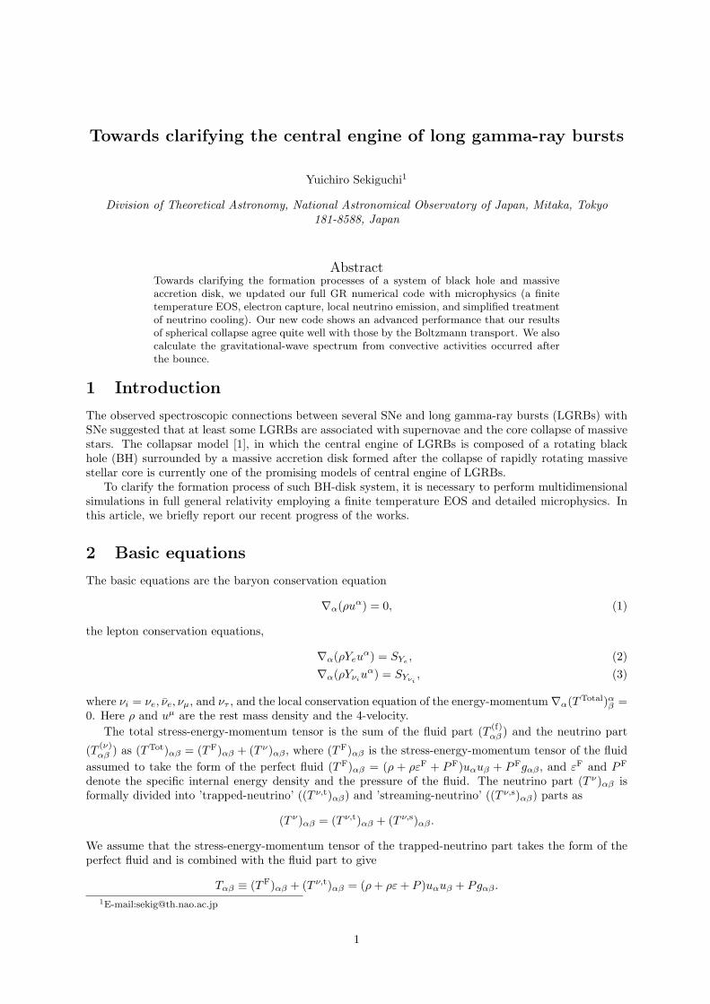
Towards clarifying the central engine of long gamma-ray bursts
Yuichiro Sekiguchi1
Division of Theoretical Astronomy, National Astronomical Observatory of Japan, Mitaka, Tokyo181-8588, Japan
AbstractTowards clarifying the formation processes of a system of black hole and massiveaccretion disk, we updated our full GR numerical code with microphysics (a finitetemperature EOS, electron capture, local neutrino emission, and simplified treatmentof neutrino cooling). Our new code shows an advanced performance that our resultsof spherical collapse agree quite well with those by the Boltzmann transport. We alsocalculate the gravitational-wave spectrum from convective activities occurred afterthe bounce.
1 Introduction
The observed spectroscopic connections between several SNe and long gamma-ray bursts (LGRBs) withSNe suggested that at least some LGRBs are associated with supernovae and the core collapse of massivestars. The collapsar model [1], in which the central engine of LGRBs is composed of a rotating blackhole (BH) surrounded by a massive accretion disk formed after the collapse of rapidly rotating massivestellar core is currently one of the promising models of central engine of LGRBs.
To clarify the formation process of such BH-disk system, it is necessary to perform multidimensionalsimulations in full general relativity employing a finite temperature EOS and detailed microphysics. Inthis article, we briefly report our recent progress of the works.
2 Basic equations
The basic equations are the baryon conservation equation
∇α(ρuα) = 0, (1)
the lepton conservation equations,
∇α(ρYeuα) = SYe , (2)
∇α(ρYνiuα) = SYνi
, (3)
where νi = νe, νe, νµ, and ντ , and the local conservation equation of the energy-momentum∇α(TTotal)αβ =
0. Here ρ and uµ are the rest mass density and the 4-velocity.The total stress-energy-momentum tensor is the sum of the fluid part (T (f)
αβ ) and the neutrino part
(T (ν)αβ ) as (TTot)αβ = (TF)αβ + (T ν)αβ , where (TF)αβ is the stress-energy-momentum tensor of the fluid
assumed to take the form of the perfect fluid (TF)αβ = (ρ + ρεF + PF)uαuβ + PFgαβ , and εF and PF
denote the specific internal energy density and the pressure of the fluid. The neutrino part (T ν)αβ isformally divided into ’trapped-neutrino’ ((T ν,t)αβ) and ’streaming-neutrino’ ((T ν,s)αβ) parts as
(T ν)αβ = (T ν,t)αβ + (T ν,s)αβ .
We assume that the stress-energy-momentum tensor of the trapped-neutrino part takes the form of theperfect fluid and is combined with the fluid part to give
Tαβ ≡ (TF)αβ + (T ν,t)αβ = (ρ + ρε + P )uαuβ + Pgαβ .
1E-mail:[email protected]
1
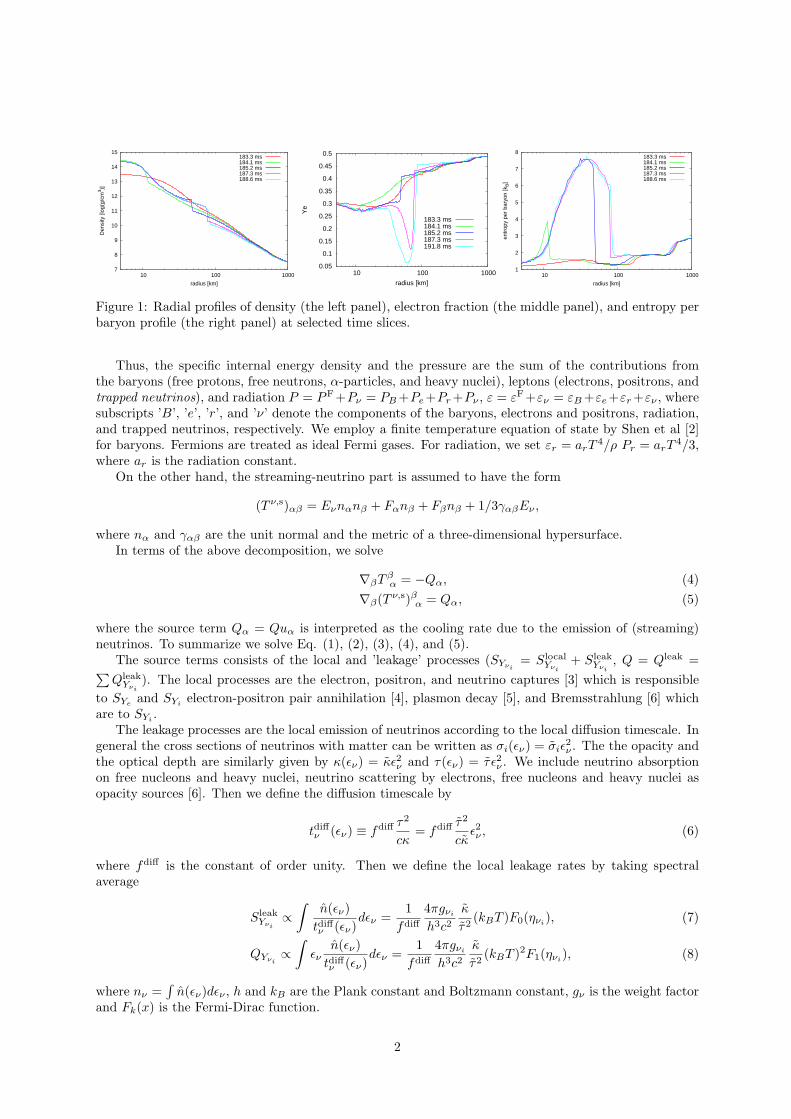
7
8
9
10
11
12
13
14
15
10 100 1000
Den
sity
[log
(g/c
m3 )]
radius [km]
183.3 ms184.1 ms185.2 ms187.3 ms188.6 ms
0.05
0.1
0.15
0.2
0.25
0.3
0.35
0.4
0.45
0.5
10 100 1000
Ye
radius [km]
183.3 ms184.1 ms185.2 ms187.3 ms191.8 ms
1
2
3
4
5
6
7
8
10 100 1000
entr
opy
per
bary
on [k
B]
radius [km]
183.3 ms184.1 ms185.2 ms187.3 ms188.6 ms
Figure 1: Radial profiles of density (the left panel), electron fraction (the middle panel), and entropy perbaryon profile (the right panel) at selected time slices.
Thus, the specific internal energy density and the pressure are the sum of the contributions fromthe baryons (free protons, free neutrons, α-particles, and heavy nuclei), leptons (electrons, positrons, andtrapped neutrinos), and radiation P = PF+Pν = PB +Pe +Pr +Pν , ε = εF+εν = εB +εe +εr +εν , wheresubscripts ’B’, ’e’, ’r’, and ’ν’ denote the components of the baryons, electrons and positrons, radiation,and trapped neutrinos, respectively. We employ a finite temperature equation of state by Shen et al [2]for baryons. Fermions are treated as ideal Fermi gases. For radiation, we set εr = arT
4/ρ Pr = arT4/3,
where ar is the radiation constant.On the other hand, the streaming-neutrino part is assumed to have the form
(T ν,s)αβ = Eνnαnβ + Fαnβ + Fβnβ + 1/3γαβEν ,
where nα and γαβ are the unit normal and the metric of a three-dimensional hypersurface.In terms of the above decomposition, we solve
∇βT βα = −Qα, (4)
∇β(T ν,s)βα = Qα, (5)
where the source term Qα = Quα is interpreted as the cooling rate due to the emission of (streaming)neutrinos. To summarize we solve Eq. (1), (2), (3), (4), and (5).
The source terms consists of the local and ’leakage’ processes (SYνi= Slocal
Yνi+ Sleak
Yνi, Q = Qleak =∑
QleakYνi
). The local processes are the electron, positron, and neutrino captures [3] which is responsibleto SYe and SYi electron-positron pair annihilation [4], plasmon decay [5], and Bremsstrahlung [6] whichare to SYi .
The leakage processes are the local emission of neutrinos according to the local diffusion timescale. Ingeneral the cross sections of neutrinos with matter can be written as σi(εν) = σiε
2ν . The the opacity and
the optical depth are similarly given by κ(εν) = κε2ν and τ(εν) = τ ε2ν . We include neutrino absorptionon free nucleons and heavy nuclei, neutrino scattering by electrons, free nucleons and heavy nuclei asopacity sources [6]. Then we define the diffusion timescale by
tdiffν (εν) ≡ fdiff τ2
cκ= fdiff τ2
cκε2ν , (6)
where fdiff is the constant of order unity. Then we define the local leakage rates by taking spectralaverage
SleakYνi
∝∫
n(εν)tdiffν (εν)
dεν =1
fdiff
4πgνi
h3c2
κ
τ2(kBT )F0(ηνi), (7)
QYνi∝
∫εν
n(εν)tdiffν (εν)
dεν =1
fdiff
4πgνi
h3c2
κ
τ2(kBT )2F1(ηνi), (8)
where nν =∫
n(εν)dεν , h and kB are the Plank constant and Boltzmann constant, gν is the weight factorand Fk(x) is the Fermi-Dirac function.
2
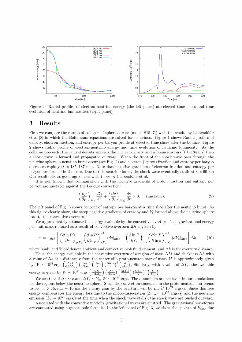
0
20
40
60
80
100
120
140
160
10 100 1000
neut
rino
ener
gy [M
eV]
radius [km]
183.3 ms184.1 ms185.2 ms187.3 ms188.6 ms
0
0.5
1
1.5
2
2.5
3
3.5
4
170 180 190 200 210 220
Lum
inos
ity [1
053 e
rg/s
]
Time [ms]
e neutrinoe antineutrinoµ, τ neutrinos
Figure 2: Radial profiles of electron-neutrino energy (the left panel) at selected time slices and timeevolution of neutrino luminosities (right panel).
3 Results
First we compare the results of collapse of spherical core (model S15 [7]) with the results by Liebendoferet al [8] in which the Boltzmann equations are solved for neutrinos. Figure 1 shows Radial profiles ofdensity, electron fraction, and entropy per baryon profile at selected time slices after the bounce. Figure2 shows radial profile of electron-neutrino energy and time evolution of neutrino luminosity. As thecollapse proceeds, the central density exceeds the nuclear density and a bounce occurs (t ≈ 184 ms) thena shock wave is formed and propagated outward. When the front of the shock wave pass through theneutrino sphere, a neutrino burst occur (see Fig. 2) and electron (lepton) fraction and entropy per baryondecreases rapidly (t ≈ 185–187 ms). Note that negative gradients of electron fraction and entropy perbaryon are formed in the core. Due to this neutrino burst, the shock wave eventually stalls at r ≈ 90 kmOur results shows good agreement with those by Liebendofer et al.
It is well known that configuration with the negative gradients of lepton fraction and entropy perbaryon are unstable against the Ledoux convection:
(∂ρ
∂Yl
)
P,s
dYl
dr+
(∂ρ
∂s
)
P,Yl
ds
dr> 0, (unstable). (9)
The left panel of Fig. 3 shows contour of entropy per baryon at a time slice after the neutrino burst. Asthis figure clearly show, the steep negative gradients of entropy and Yl formed above the neutrino spherelead to the convective overturn.
We approximately estimate the energy available by the convective overturn. The gravitational energyper unit mass released as a result of convective overturn ∆h is given by
w = −geff
[(∂ ln P
∂s
)
ρ,Ye
(∂ lnP
∂ ln ρ
)−1
s,Ye
(ds)amb +(
∂ ln P
∂Ye
)
ρ,s
(∂ ln P
∂ ln ρ
)−1
s,Ye
(dYe)amb
]∆h, (10)
where ’amb’ and ’blob’ denote ambient and convective blob fluid element, and ∆h is the overturn distance.Thus, the energy available in the convective overturn of a region of mass ∆M and thickness ∆h with
a value of ∆s at a distance r from the center of a proto-neutron star of mass M is approximately givenby W ∼ 1051 ergs
(∆M
0.3M¯
) (∆h
10km
) (|∆s|
s
) (50km
r
)2(
MM¯
), Similarly, with a value of ∆Ye, the available
energy is given by W ∼ 1051 ergs(
∆M0.3M¯
) (∆h
10km
) (|∆Ye|
Ye
) (50km
r
)2(
MM¯
).
We see that if ∆s ∼ s and ∆Ye ∼ Ye, W ∼ 1051 ergs. These numbers are achieved in our simulationsfor the regions below the neutrino sphere. Since the convection timescale in the proto-neutron star seemsto be τot
<∼ RNSvot ∼ 10 ms the energy gain by the overturn will be Lot>∼ 1053 ergs/s. Since this free
energy compensates the energy loss due to the photo-dissociation (Ldiss ∼ 1053 ergs/s) and the neutrinoemission (Lν ∼ 1053 ergs/s at the time when the shock wave stalls), the shock wave are pushed outward.
Associated with the convective motions, gravitational waves are emitted. The gravitational waveformsare computed using a quadrupole formula. In the left panel of Fig. 3, we show the spectra of hchar due
3
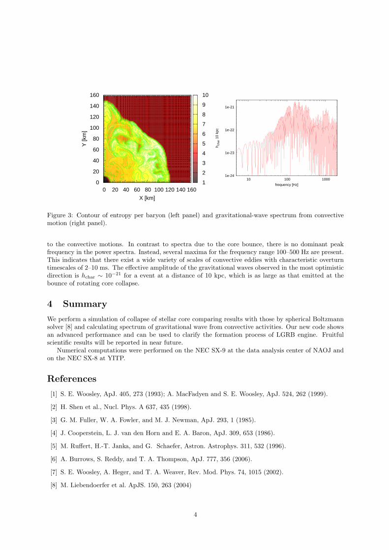
1
2
3
4
5
6
7
8
9
10
0 20 40 60 80 100 120 140 160
X [km]
0
20
40
60
80
100
120
140
160
Y [k
m]
1e-24
1e-23
1e-22
1e-21
10 100 1000
h cha
r 10
kpc
frequency [Hz]
Figure 3: Contour of entropy per baryon (left panel) and gravitational-wave spectrum from convectivemotion (right panel).
to the convective motions. In contrast to spectra due to the core bounce, there is no dominant peakfrequency in the power spectra. Instead, several maxima for the frequency range 100–500 Hz are present.This indicates that there exist a wide variety of scales of convective eddies with characteristic overturntimescales of 2–10 ms. The effective amplitude of the gravitational waves observed in the most optimisticdirection is hchar ∼ 10−21 for a event at a distance of 10 kpc, which is as large as that emitted at thebounce of rotating core collapse.
4 Summary
We perform a simulation of collapse of stellar core comparing results with those by spherical Boltzmannsolver [8] and calculating spectrum of gravitational wave from convective activities. Our new code showsan advanced performance and can be used to clarify the formation process of LGRB engine. Fruitfulscientific results will be reported in near future.
Numerical computations were performed on the NEC SX-9 at the data analysis center of NAOJ andon the NEC SX-8 at YITP.
References
[1] S. E. Woosley, ApJ. 405, 273 (1993); A. MacFadyen and S. E. Woosley, ApJ. 524, 262 (1999).
[2] H. Shen et al., Nucl. Phys. A 637, 435 (1998).
[3] G. M. Fuller, W. A. Fowler, and M. J. Newman, ApJ. 293, 1 (1985).
[4] J. Cooperstein, L. J. van den Horn and E. A. Baron, ApJ. 309, 653 (1986).
[5] M. Ruffert, H.-T. Janka, and G. Schaefer, Astron. Astrophys. 311, 532 (1996).
[6] A. Burrows, S. Reddy, and T. A. Thompson, ApJ. 777, 356 (2006).
[7] S. E. Woosley, A. Heger, and T. A. Weaver, Rev. Mod. Phys. 74, 1015 (2002).
[8] M. Liebendoerfer et al. ApJS. 150, 263 (2004)
4
The scalar field potential and the energy density ofthe super-in ation in Loop Quantum Cosmology
Masahiro SHIMANO1 and Tomohiro HARADA2
Department of Physics, Rikkyo University, Toshima, Tokyo 171-8501, Japan
AbstractIn loop quantum cosmology there may be a super-inflation phase in the very earlyuniverse, in which a single scalar field with a negative power-law potential V = fϕβ
in Planck units plays important roles. Since the effective horizon√
SD/H controlsthe behavior of quantum fluctuation instead of the usual Hubble horizon, we assumethe inflation scenario; the super-inflation starts when the quantum state of the scalarfield emerges into the classical regime and ends when the effective horizon reaches theHubble horizon, and the effective horizon scale never gets shorter than the Plancklength. From consistency with the WMAP 5-year data, we place a constraint on theparameters of the potential (β and f) and the energy density at the end of the super-inflation, depending on the volume correction parameter n, and we also determinethe allowed range for n.
1 Introduction
Loop Quantum Gravity (LQG) is the candidate of the quantum gravity, and which is the canonicalapproach with triad variables instead of the metric. In the end of the previous century, LQG has inspiredloop quantum cosmology (LQC), which is an application of loop quantization to the homogeneous universemodels [5, 6, 7, 8]. This is featured with the avoidance of a big bang singularity and a super-inflation,where the Hubble parameter increases with time. If the loop quantum effects may have been significantin the early universe, quantum fluctuation generated in that phase must be consistent with the currentlyobserved nearly scale-invariant power spectrum. The power spectrum for the LQC super-inflation wascalculated in [11] and scale invariant conditions were obtained in [9] with the volume correction, which isone of the loop quantum effects. The scale invariant conditions are the following: i) the scalar field satisfiesa scaling condition and ii) the scalar field has a negative potential, and iii) the potential is a power-lawform and the index is infinitely large. In this paper we assume i) and ii) conditions and the followinginflation scenario; the super-inflation starts when the scalar field emerges into the classical regime fromthe quantum regime, and since the effective horizon
√SD/H controls the behavior of quantum fluctuation
and its scale decreases with time, the super-inflation ends when the effective horizon reaches the Hubblehorizon. We need to assume that the effective horizon never gets smaller than the order of the Plancklength so that we can calculate quantum fluctuation at semiclassical region. We consider the abovescenario and require consistency with the WMAP 5-year data [10] to place a constraint on the parameters.In this paper we use the units in which c = h = 1.
2 The quantum uctuation in LQC
2.1 Loop Quantization
We first consider the homogeneous and isotropic universe described by the FRW metric
ds2 = −dt2 + a(t)2[dr2 + r2
(dθ2 + sin2 θdϕ2
)], (1)
where a is the scale factor. In LQC the Hamiltonian for the gravitational and the single scalar fieldsis given by H = Hgrav + Hmatter, where[1, 15] : Hgrav = −3/(8πγG)aS(q)a2, Hmatter = D(q)(2a3)p2
ϕ +1E-mail:[email protected]:[email protected]
1
a3V (ϕ). S(q) and D(q) are respectively the loop correction factors for the gravitational Hamiltonian andthe inverse volume in the matter Hamiltonian, and the dot denotes the derivative respect to t. The scalarfield depends only on time, i.e. ϕ = ϕ(t). pϕ is a conjugate momentum of ϕ, defined as pϕ = −a3ϕ/D,and q is defined as [2, 3, 4]: q ≡ (a/a∗)
3, where
a∗ =(
2j
K
) 13
√4πγ
3lpl, K =
2√
2
3√
3√
3, l2pl = G, (2)
j is an SU(2) parameter which is associated with the link of the spin network state in LQG (we assumej is sufficiently large), and γ is the Immirzi parameter which is here assumed γ = ln(2)/(π
√3) by the
black hole entropy argument in LQG [13], but see also [14]. Note that a∗ is the characteristic scale factorin LQC: if the scale factor is smaller than a∗, the LQC effects are remarkable. In the semiclassical region(lpl ≪ a ≪ a∗), S(q) and D(q) take the following forms [12]: S(q) = S∗a
r, and D(q) = D∗an, where,
S∗ = S∗a−r∗ = (3/2)a−r
∗ and D∗ = D∗a−n∗ = (9(9 − n))/(81 − 5n)(n−9)/12
a−n∗ , n = 9(3 − l)/(1 − l)
and r = 3. We assume 0 < l < 1 or 9 < n < ∞ to remove the divergence of the inverse volume factor,while, in the classical region (a ≫ a∗), these are S(q) ∼ 1, and D(q) ∼ 1 so that the classical theory isrecovered.
From the gravitational and scalar field Hamiltonians, we can obtain the following modified Friedmannequation and the scalar field equation:
H2 =8πG
3S(q)
[ϕ2
2D(q)+ V (ϕ)
], (3)
ϕ′′ +(
2 − d lnD
d ln a
)a′
aϕ′ + a2DVϕ = 0, (4)
where Vϕ ≡ dV/dϕ, the prime denotes the derivative with respect to τ (we also use the conformaltime τ where dt = adτ), H ≡ a/a is the Hubble parameter. In the classical regime a ≫ a∗, sinceD(q) = S(q) = 1, these equations reduce to the classical ones. However, in the semiclassical regimelpl ≪ a∗ ≪ a, the second term acts an anti-friction term and the scalar field may climb the potential.
More remarkably, the time derivative of the Hubble parameter
H = −4πGSϕ2
D
[1 −
(16
d lnD
d ln a+
16
d lnS
d ln a
)]+
4πGS
3d lnS
d ln aV, (5)
is positive in the semiclassical regime. The inflation with this feature is called super-inflation.
2.2 The scaling solution and the power spectrum
We review the scaling solution and its stability according to Refs [11, 9]. We write the dynamics of thehomogeneous system in terms of the following three variables,
x =ϕ√2Dρ
, y =
√|V |√
ρ, λ = −
√3D
16πGS
Vϕ
V, (6)
where we use the negative potential, and we also need a constraint x2 − y2 = 1 to satisfy the Friedmannequation Eq. (3). Then we can derive the set of ordinary differential equations, and we can find the stablefixed points in this equations. The one of the stable fixed points correspond to the scaling solutions wherethe ratio of the kinetic term to the potential term is kept constant. For simplicity, we only consider aconstant Γ and then we can determine the potential from the definition of the Γ. For Γ = 1, the potentialis given by V = −f |ϕ|β , where β and f are constants. Moreover, we can calculate the scale factor on thisfixed points as a = A(−τ)p, where
A =
−1p
√8πfS∗
3(x20 − 1)
∣∣∣∣∣∣ 2x0
n − r
√3D∗
4πS∗
∣∣∣∣∣∣β2
p [(2j
K
) 13
√4πγ
3
]p+1
lPl, (7)
p = − 42(r + 2) + (n − 3)β
, (8)
2
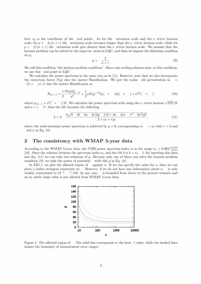
here x0 is the coordinate of the fixed points. As for the fluctuation scale and the effective horizonscale, for p > −2/(n + r) the fluctuation scale becomes longer than the effective horizon scale, while forp < −2/(n + r) the fluctuation scale gets shorter than the effective horizon scale. We assume that thehorizon problem can be solved by the super-inflation in LQC, and then we impose the following conditionon p,
p > − 2n + r
(9)
We call this condition “the horizon problem condition”. Since only scaling solution satisfies this condition,we use this fixed point in LQC.
We calculate the power spectrum in the same way as in [11]. However, note that we also incorporatethe correction factor S(q) into the matter Hamiltonian. We put the scalar field perturbation as ϕ =ϕ(t) + δϕ(x, t) into the matter Hamiltonian as
Hϕ+δϕ =12
D(q)p2ϕ+δϕ
a3+
12aS(q)δab∂a(ϕ + δϕ)∂b(ϕ + δϕ) + a3V (ϕ + δϕ), (10)
where pϕ+δϕ = a3(ϕ+ ˙δϕ)/D. We calculate the power spectrum with using the effective horizon√
SD/Hand a = (−τ)p, then the tilt becomes the following
b = 3 −2√
9 − (6 − 4n − 3r)2p − (12 + 4n − 2nr − r2 − 2n2)p2
2 + (n + r)p, (11)
where the scale-invariant power spectrum is achieved by p = 0, corresponding to β → ∞ with r = 3 andfixed n in Eq. (8).
3 The consistency with WMAP 5-year data
According to the WMAP 5-year data, the CMB power spectrum index is in the range ns = 0.963+0.014−0.015
[10]. Since the relation between the spectrum index ns and the tilt b is b = ns − 1, for inserting this datainto Eq. (11) we can take two solutions of p. Because only one of these can solve the horizon problemcondition (9), we take the power of potential β with this p in Eq. (8).
In FIG.1, we plot the allowed region of β against n. If we can specify the value for n, then we canplace a rather stringent constraint on β. However, if we do not have any information about n, β is onlyweakly constrained to 15 <∼ β <∼ 150. In any case, β is bounded from above in the present scenario andan infinitely large value is not allowed from WMAP 5-year data.
0
20
40
60
80
100
120
140
160
10 100 1000 10000
β
n
0
20
40
60
80
100
120
140
160
10 100 1000 10000
β
n
0
20
40
60
80
100
120
140
160
10 100 1000 10000
β
n
Figure 1: The allowed region of β. The solid line corresponds to the best-fit value, while the dashed linesdenote the boundary of measurement error ranges.
3
Moreover, we can take the constraint on the energy density and the potential constant with thefollowing inflation scenario: the super-inflation starts when the quantum state of the scalar field emergesinto the classical regime and ends when the effective horizon gets equal to the Hubble horizon before theeffective horizon scale gets shorter than the square root of the smallest area element.
4 Conclusion
We have considered a single scalar field with the negative power-law potential V ∝ −fϕβ in LQC, thenwe have determined the allowed region of the potential power β and the energy density at the end ofthe super-inflation, and the potential constant f , and the volume correction parameter n by using theconsistency with the WMAP 5-year data.
First we have reviewed Ref [9]. Using dynamical systems theory we have found a scaling solutionwhich is a stable fixed point and satisfies the horizon problem condition. Second, we have assumedthe super-inflation scenario. By using this inflation scenario and the consistency with the WMAP 5-year data, we have reached the following conclusion. If we can specify the volume correction parametern, we can determine the potential parameters β and f rather stringently. Even if we only know thevolume correction parameter n, then we can determine β and f , and the energy density at the end of thesuper-inflation.
In this paper we have only considered the scalar field perturbation. However, the CMB power spectrumis actually the temperature perturbation on the last scattering surface, so we should derive the curvatureperturbations as well as matter perturbations and their evolution in different scales in LQC. To get morestringent constraint on the super-inflation scenario, we will need to use other independent observations:large scale structure, non-gaussianity, gravitational waves and so on. These problems will be our nextwork.
References
[1] A. Ashtekar, M. Bojowald, and J. Lewandowski Adv. Theor. Math. Phys 7 233-268 (2003)
[2] A. Ashtekar, T. Pawlowski and P. Singh Phys. Rev. D 73 124038 (2006)
[3] A. Ashtekar, T. Pawlowski and P. Singh Phys. Rev. D 73 084003 (2006)
[4] A. Ashtekar, T. Pawlowski and P. Singh, and K. Vandersloot Phys. Rev. D 75 024035 (2007)
[5] M. Bojowald Class. Quant. Grav. 17 1489-1508 (2000)
[6] M. Bojowald Class. Quant. Grav. 17 1509-1526 (2000)
[7] M. Bojowald Class. Quant. Grav. 18 1055-1070 (2001)
[8] M. Bojowald Class. Quant. Grav. 18 1071-1088 (2001)
[9] E. J. Copeland, D. J. Mulryne, N. J. Nunes and M. Shaeri Phys. Rev. D 77 023510 (2008)
[10] E. Komatsu, et al. arXiv:0803.0547v1 [astro-ph]
[11] D. J. Mulryne and N. J. Nunes Phys. Rev. D 74 083507 (2006)
[12] J. Magueijo and P. Singh Phys. Rev. D 74 023510 (2007)
[13] C. Rovelli ”Quantum Gravity ” (Cambridge University Press, Cambridge, 2004)
[14] T. Tamaki and H. Nomura, Phys. Rev. D 72, 107501 (2005).
[15] K. Vandersloot Phys. Rev. D 71 103506 (2005)
4
Non-Gaussianity in the Curvaton Scenario
Tomo Takahashi1
Department of Physics, Saga University, Saga 840-8502, Japan
AbstractWe discuss the signatures of non-Gaussianity in the curvaton model where the poten-tial includes also a non-quadratic term. In such a case the non-linearity parameterfNL can become very small, and we show that non-Gaussianity is then encoded inthe non-reducible non-linearity parameter gNL of the trispectrum, which can be verylarge. Thus the place to look for the non-Gaussianity in the curvaton model may bethe trispectrum rather than the bispectrum. We also show that gNL measures directlythe deviation of the curvaton potential from the purely quadratic form.
1 Introduction
The high precision of cosmological observations such as WMAP [1, 2] and the forthcoming Planck SurveyorMission [3] will soon make it possible to probe the actual physics of the primordial perturbation ratherthan merely describing it. As is well known, the primordial scalar and tensor power spectra, characterizedby spectral indices the and tensor-to-scalar ratio, can be used to test both models of inflation and othermechanisms for the generation of the primordial perturbation such as the curvaton [4, 5, 6]. However,many models can imprint similar features on the primordial power spectrum. Thus a possible deviationfrom Gaussian fluctuations, which may provide invaluable implications on the physics of the early universe,has been the focus of much attention recently.
The simplest inflation models generate an almost Gaussian fluctuation. In contrast, in the curvatonscenario there can arise a large non-Gaussianity. However, in most studies on the curvaton so far, onesimply assumes a quadratic curvaton potential. Since the curvaton cannot be completely non-interacting(it has to decay), it is of interest to consider the implications of the deviations from the exactly quadraticpotential, which represent curvaton self-interactions. Such self-interactions would arise e.g. in curvatonmodels based on the flat directions of the minimally supersymmetric standard model (MSSM). Evensmall deviations could be important for phenomenology, as was pointed out in [7] where it was shownthat the non-Gaussianity predicted by the curvaton model can be sensitive to the shape of the potential.In particular, the nonlinearity parameter fNL which quantifies the bispectrum of primordial fluctuationcan, in contrast to the case of the quadratic curvaton potential, be very small in some cases. However, thesignatures of non-Gaussianity can be probed not only with the bispectrum but also with the trispectrum.In the following, we will show that even when fNL is negligibly small, gNL can be very large, indicatingthat the first signature of the curvaton-induced primordial non-Gaussianity may not come from thebispectrum but rather from the trispectrum.
2 Non-linearity parameters
To discuss non-Gaussianity in the scenario, we make use of the non-linearity parameters fNL and gNL
defined by the expansion
ζ = ζ1 +35fNLζ2
1 +925
gNLζ31 + O(ζ4
1 ), (1)
where ζ is the primordial curvature perturbation. Writing the power spectrum as
⟨ζk1ζk2
⟩ = (2π)3Pζ(k1)δ(k1 + k2), (2)
1E-mail:[email protected]
1
the bispectrum and trispectrum are given by
⟨ζk1ζk2
ζk3⟩ = (2π)3Bζ(k1, k2, k3)δ(k1 + k2 + k3). (3)
⟨ζk1ζk2
ζk3ζk4
⟩ = (2π)3Tζ(k1, k2, k3, k4)δ(k1 + k2 + k3 + k4), (4)
where Bζ and Tζ are products of the power spectra and can be written as
Bζ(k1, k2, k3) =65fNL (Pζ(k1)Pζ(k2) + Pζ(k2)Pζ(k3) + Pζ(k3)Pζ(k1)) , (5)
Tζ(k1, k2, k3, k4) = τNL (Pζ(k13)Pζ(k3)Pζ(k4) + 11 perms.)
+5425
gNL (Pζ(k2)Pζ(k3)Pζ(k4) + 3 perms.) . (6)
Note the appearance of the independent non-linearity parameter τNL. However, in the scenario we areconsidering in the following, τNL is related to fNL by
τNL =3625
f2NL . (7)
To evaluate the primordial curvature fluctuation in the curvaton model, we need to specify a potentialfor the curvaton. Here we go beyond the usual quadratic approximation and consider the followingpotential:
V (σ) =12m2
σσ2 + λm4σ
(σ
mσ
)n
, (8)
which contains a higher polynomial term in addition to the quadratic term. For later discussion, wedefine a parameter s which represents the size of the non-quadratic term relative to the quadratic one:
s ≡ 2λ
(σ∗
mσ
)n−2
. (9)
Thus the larger s is, the larger is the contribution from the non-quadratic term.When the potential is quadratic, the fluctuation evolves exactly as the homogeneous mode. However,
when the curvaton field evolves under a non-quadratic potential, the fluctuation of the curvaton evolvesnon-linearly on large scales. In that case the curvature fluctuation can be written, up to the third order,as [8]
ζ = δN =23rσ′
osc
σoscδσ∗ +
19
[3r
(1 +
σoscσ′′osc
σ′2osc
)− 4r2 − 2r3
](σ′
osc
σosc
)2
(δσ∗)2
+481
[9r
4
(σ2
oscσ′′′osc
σ′3osc
+ 3σoscσ
′′osc
σ′2osc
)− 9r2
(1 +
σoscσ′′osc
σ′2osc
)+
r3
2
(1 − 9
σoscσ′′osc
σ′2osc
)+ 10r4 + 3r5
](σ′
osc
σosc
)3
(δσ∗)3 , (10)
where σosc is the value of the curvaton at the onset of its oscillation and the prime represents the derivativewith respect to σ∗. r roughly represents the ratio of the energy density of the curvaton to the total densityat the time of the curvaton decay. The exact definition is given by
r ≡ 3ρσ
4ρrad + 3ρσ
¯decay
. (11)
Notice that σ′osc/σosc = 1/σ∗ for the case of the quadratic potential. With this expression, we can write
down the non-linearity parameter fNL as
fNL =54r
(1 +
σoscσ′′osc
σ′2osc
)− 5
3− 5r
6. (12)
2
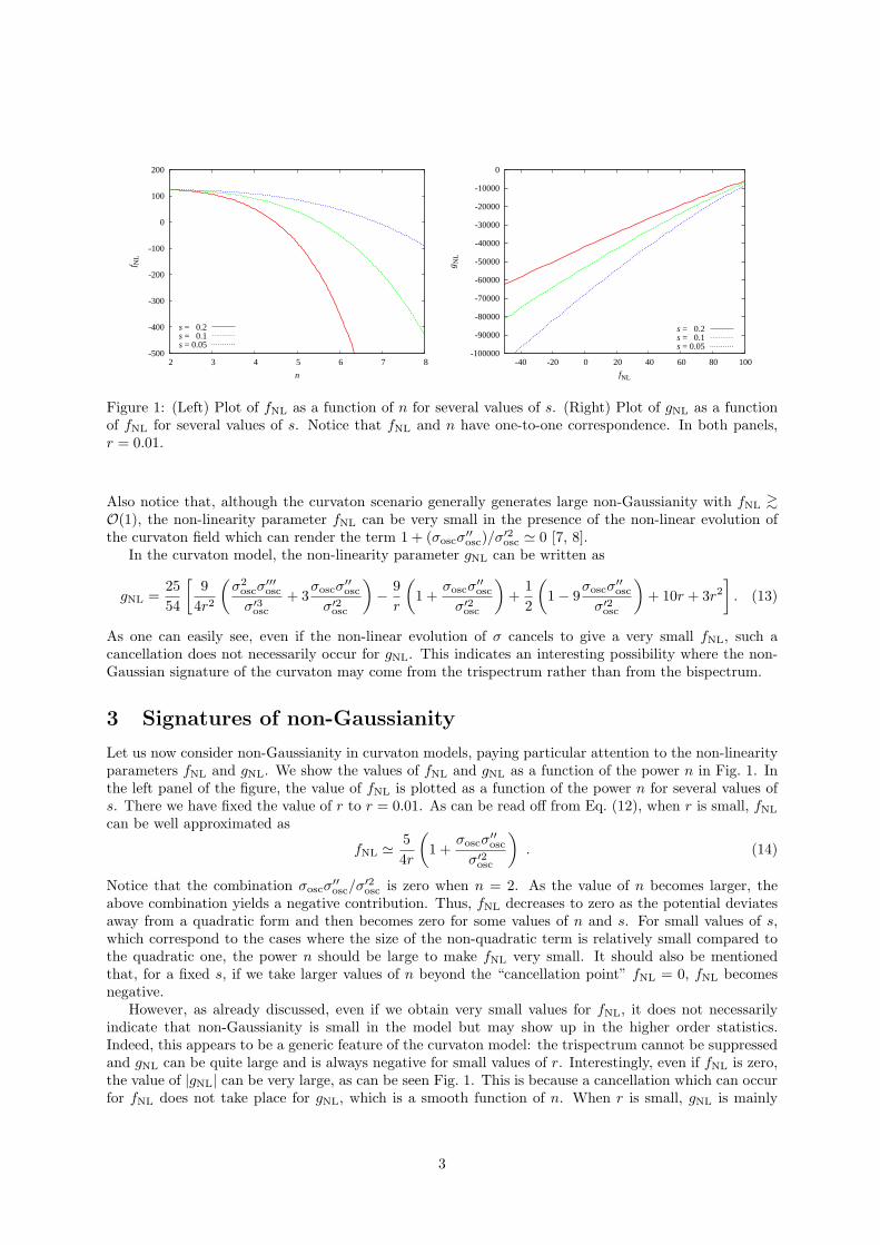
-500
-400
-300
-200
-100
0
100
200
2 3 4 5 6 7 8
f NL
n
s = 0.2s = 0.1s = 0.05
-100000
-90000
-80000
-70000
-60000
-50000
-40000
-30000
-20000
-10000
0
-40 -20 0 20 40 60 80 100
g NL
fNL
s = 0.2s = 0.1s = 0.05
Figure 1: (Left) Plot of fNL as a function of n for several values of s. (Right) Plot of gNL as a functionof fNL for several values of s. Notice that fNL and n have one-to-one correspondence. In both panels,r = 0.01.
Also notice that, although the curvaton scenario generally generates large non-Gaussianity with fNL>∼
O(1), the non-linearity parameter fNL can be very small in the presence of the non-linear evolution ofthe curvaton field which can render the term 1 + (σoscσ
′′osc)/σ′2
osc ≅ 0 [7, 8].In the curvaton model, the non-linearity parameter gNL can be written as
gNL =2554
[9
4r2
(σ2
oscσ′′′osc
σ′3osc
+ 3σoscσ
′′osc
σ′2osc
)− 9
r
(1 +
σoscσ′′osc
σ′2osc
)+
12
(1 − 9
σoscσ′′osc
σ′2osc
)+ 10r + 3r2
]. (13)
As one can easily see, even if the non-linear evolution of σ cancels to give a very small fNL, such acancellation does not necessarily occur for gNL. This indicates an interesting possibility where the non-Gaussian signature of the curvaton may come from the trispectrum rather than from the bispectrum.
3 Signatures of non-Gaussianity
Let us now consider non-Gaussianity in curvaton models, paying particular attention to the non-linearityparameters fNL and gNL. We show the values of fNL and gNL as a function of the power n in Fig. 1. Inthe left panel of the figure, the value of fNL is plotted as a function of the power n for several values ofs. There we have fixed the value of r to r = 0.01. As can be read off from Eq. (12), when r is small, fNL
can be well approximated as
fNL ≅ 54r
(1 +
σoscσ′′osc
σ′2osc
). (14)
Notice that the combination σoscσ′′osc/σ′2
osc is zero when n = 2. As the value of n becomes larger, theabove combination yields a negative contribution. Thus, fNL decreases to zero as the potential deviatesaway from a quadratic form and then becomes zero for some values of n and s. For small values of s,which correspond to the cases where the size of the non-quadratic term is relatively small compared tothe quadratic one, the power n should be large to make fNL very small. It should also be mentionedthat, for a fixed s, if we take larger values of n beyond the “cancellation point” fNL = 0, fNL becomesnegative.
However, as already discussed, even if we obtain very small values for fNL, it does not necessarilyindicate that non-Gaussianity is small in the model but may show up in the higher order statistics.Indeed, this appears to be a generic feature of the curvaton model: the trispectrum cannot be suppressedand gNL can be quite large and is always negative for small values of r. Interestingly, even if fNL is zero,the value of |gNL| can be very large, as can be seen Fig. 1. This is because a cancellation which can occurfor fNL does not take place for gNL, which is a smooth function of n. When r is small, gNL is mainly
3
determined by the first term in Eq. (13):
gNL ≅ 2554
[9
4r2
(σ2
oscσ′′′osc
σ′3osc
+ 3σoscσ
′′osc
σ′2osc
)]. (15)
In fact, one can show that the terms (σoscσ′′osc)/σ′2
osc and (σ2oscσ
′′′osc)/σ′3
osc give negative contributions forthe cases being considered here, which indicates that the cancellation between these terms never occurs[9]. Therefore gNL is always negative for small values of r even when fNL is very small. Thus, it mayturn out that the best place to look for non-Gaussianity in curvaton models is the trispectrum and gNL
in particular.
4 Summary
We have discussed the signatures of non-Gaussianity in the curvaton model with the potential includinga non-quadratic term in addition to the usual quadratic term. When the curvaton potential is not purelyquadratic, fluctuations of the curvaton field evolve nonlinearly on superhorizon scales. This gives riseto predictions for the bispectrum, characterized by the non-linearity parameter fNL, which can deviateconsiderably from the quadratic case. However, by studying the trispectrum which is characterized bygNL along with fNL, we find that even when fNL is negligibly small, the absolute value of gNL can bevery large. Thus the signature of non-Gaussianity in the curvaton model may come from the trispectrumrather than from the bispectrum if its potential deviates from a purely quadratic form, as one wouldexpect in realistic particle physics models.
Here we discussed the case where a non-quadratic term is also taken into account in the curvatonpotential, however the cases where fluctuations from the inflaton can also be responsible for cosmicdensity perturbations today would also be interesting since such a case can arise in general. Such mixedfluctuation scenarios have been investigated in Refs. [10, 11, 12].
References
[1] E. Komatsu et al. [WMAP Collaboration], arXiv:0803.0547 [astro-ph].
[2] J. Dunkley et al. [WMAP Collaboration], arXiv:0803.0586 [astro-ph].
[3] [Planck Collaboration], arXiv:astro-ph/0604069;Planck webpage, http://www.rssd.esa.int/index.php?project=planck
[4] K. Enqvist and M. S. Sloth, Nucl. Phys. B 626, 395 (2002) [arXiv:hep-ph/0109214];
[5] D. H. Lyth and D. Wands, Phys. Lett. B 524, 5 (2002) [arXiv:hep-ph/0110002];
[6] T. Moroi and T. Takahashi, Phys. Lett. B 522, 215 (2001) [Erratum-ibid. B 539, 303 (2002)][arXiv:hep-ph/0110096].
[7] K. Enqvist and S. Nurmi, JCAP 0510, 013 (2005) [arXiv:astro-ph/0508573].
[8] M. Sasaki, J. Valiviita and D. Wands, Phys. Rev. D 74, 103003 (2006) [arXiv:astro-ph/0607627].
[9] K. Enqvist and T. Takahashi, JCAP 0809, 012 (2008) [arXiv:0807.3069 [astro-ph]].
[10] K. Ichikawa, T. Suyama, T. Takahashi and M. Yamaguchi, Phys. Rev. D 78, 023513 (2008)[arXiv:0802.4138 [astro-ph]].
[11] K. Ichikawa, T. Suyama, T. Takahashi and M. Yamaguchi, Phys. Rev. D 78, 063545 (2008)[arXiv:0807.3988 [astro-ph]].
[12] T. Moroi and T. Takahashi, arXiv:0810.0189 [hep-ph].
4
Nonlinear superhorizon perturbations of non-canonical scalarfield
Yu-ichi Takamizu1 and Shinji Mukohyama2
1Department of Physics, Waseda University, Okubo 3-4-1, Shinjuku, Tokyo 169-8555, Japan2Institute for the Physics and Mathematics of the Universe (IPMU), The University of Tokyo, 5-1-5
Kashiwanoha, Kashiwa, Chiba 277-8582, Japan
AbstractWe develop a theory of non-linear cosmological perturbations at superhorizon scalesfor a scalar field with a Lagrangian of the form P (X,φ), where X = −∂µφ∂µφ and φis the scalar field. We employ the ADM formalism and the spatial gradient expansionapproach to obtain general solutions valid up to the second order in the gradientexpansion. This formulation can be applied to, for example, DBI inflation modelsto investigate superhorizon evolution of non-Gaussianities. With slight modification,we also obtain general solutions valid up to the same order for a perfect fluid with ageneral equation of state P = P (ρ).
1 Introduction
Generation of primordial fluctuations during inflation is one of the most interesting predictions of quantumfield theory. Indeed, those quantum fluctuations are considered as seeds of the large scale structure of thepresent universe, and this picture has been accepted by many researchers as a standard scenario. Therecent more accurate observation by WMAP has revealed deviation from exact scale invariance, with aslight red tilt. Moreover, there is a good possibility that deviation from Gaussianity can be detected bythe future experiments such as PLANCK. With those current and future precision observations, deviationfrom the exact scale invariance and Gaussianity can be a powerful tool to discriminate many possibleinflationary models. On the theoretical side, there are at least two known mechanisms to generatelarge non-Gaussianity: isocurvature perturbations and non-canonical kinetic terms. As for the formercase, a typical example is the curvaton scenario is responsible for isocurvature perturbations duringinflation. Now let us consider the later case, where non-canonical kinetic terms are responsible for largenon-Gaussianity. Examples of this type include k-inflation [1] and DBI inflation [2]. In k-inflation andDBI inflation, large non-Gaussianity is expected when the non-linear nature of the non-canonical kineticaction becomes significant. To quantify the non-Gaussianity and clarify its observational signature, it isimportant to develop a theory that can deal with nonlinear cosmological perturbations. There are coupleof methods to tackle this problem. One is a second-order perturbation theory. Another is based on spatialgradient expansion [3]. Closely related to the gradient expansion method, cosmological perturbations onsuperhorizon scales have been studied extensively in the so-called separate universe approach or δNformalism [4]. Actually, these approaches are essentially the leading order approximation to the gradientexpansion. Including these, many of the previous studies were confined to the leading order approximationto the gradient expansion. However, higher order corrections to the leading order results can be importantto get more detailed information about non-Gaussianity. One good example is the case studied by Leachet al [5]. They considered linear perturbations in single-field inflation models and supposed that there is astage at which slow-roll conditions are violated. It has been then shown that, due to the decaying mode,the O(ε2) corrections in spatial derivative expansion do affect the evolution of curvature perturbationson superhorizon scales. However, the linear perturbation theory is not capable for calculation of non-Gaussianity. Thus, it is necessary to develop nonlinear theory of cosmological perturbations valid up toO(ε2) in the spatial gradient expansion. Gradient expansion formalism has been developed and used bymany authors [3, 4, 6, 7]. Formulation valid up to O(ε2) was developed, for example, by Tanaka and
1E-mail:[email protected]:[email protected]
1
Sasaki for a universe dominated by a perfect fluid with a specific equation of state P/ρ = const [6] andthat dominated by a canonical scalar field [7]. However, as far as the authors know, those works have notextended to a perfect fluid with general equation of state P = P (ρ) nor to a scalar field with non-canonicalkinetic action, which is essential for the second type of mechanism of generating non-Gaussianity. Thepurpose of this paper is to fill this gap. Namely, we shall develop a theory of nonlinear superhorizonperturbations valid up to the order O(ε2) for a scalar field with non-canonical kinetic action and a perfectfluid with general equation of state.
2 Formalism
Throughout this paper we consider a minimally-coupled scalar field described by an action of the formI =
∫
d4x√−gP (X,φ) where X = −gµν∂µφ∂νφ, and suppose that −gµν∂νφ is timelike and future-
directed. The following relation among first-order variations of P , ρ and φ will be useful in the analysisbelow. δP = c2sδρ+ ρΓδφ, where
c2s =PX
2PXXX + PX, Γ =
1ρ
(
Pφ − c2sρφ)
, (1)
where the subscripts X and φ represent derivative with respect to X and φ, respectively. Note that cs isthe speed of sound for the gauge invariant scalar perturbation in the linear theory.
We shall develop a theory of nonlinear cosmological perturbations on superhorizon scales. For thispurpose we employ the ADM formalism and the gradient expansion in the uniform Hubble slicing. In the(3+1)-decomposition, the metric is expressed as ds2 = gµνdx
µdxν = −α2dt2 +γij(dxi+βidt)(dxj+βjdt)where α is the lapse function, βi is the shift vector and Latin indices run over 1, 2, 3. Since α andβi represent gauge degrees of freedom for diffeomorphism and appear as Lagrange multipliers in theaction, the corresponding equations of motion leads to constraint equations. Contrary to α and β,components of the spatial metric γij are dynamical variables (subject to the constraint equations) andthe corresponding equations of motion are called dynamical equations. In what follows we shall expressthe dynamical equations as a set of first-order differential equations with respect to the time t. For thispurpose we introduce the extrinsic curvature Kij defined by Kij = − 1
2α (∂tγij −Diβj −Djβi) where Dis the covariant derivative compatible with the spatial metric γij . For the stress-energy tensor in theperfect fluid form, we define the 3-vector vi as vi ≡ ui/u0. Hereafter, we shall use γij and its inverseγij to raise and lower indices of K, D, v, β. In addition to the standard ADM decomposition brieflyreviewed above, we further decompose the spatial metric and the extrinsic curvature as
γij = a2ψ4γij , Kij = a2ψ4
(
13Kγij + Aij
)
, (2)
where a(t) is the scale factor of a fiducial Friedmann background (specified later) and the determinant ofγij is constrained to be unity: det γij = 1. Throughout this paper we adopt the uniform Hubble slicing
K = −3H(t), H(t) ≡ ∂ta
a. (3)
In the gradient expansion approach we introduce a flat FRW universe (a(t), φ0(t)) as a backgroundand suppose that the characteristic length scale L of perturbations is longer than the Hubble length scale1/H of the background, i.e. HL 1. Therefore, we consider ε ≡ 1/(HL) as a small parameter andsystematically expand our equations by ε, considering a spatial derivative acted on perturbations is oforder O(ε). The background flat FRW universe (a(t), φ0(t)) satisfies the Friedmann equation and theequation of motion. Since the FRW background is recovered in the limit ε → 0, we naturally have theassumptions vi = O(ε), βi = O(ε) and ∂tγij = O(ε). Actually, following the arguments in refs. [6, 7], weassume a stronger condition ∂tγij = O(ε2). This assumption significantly simplifies our analysis and, webelieve, still allows many useful applications of the formalism. On the other hand, we consider ψ and γij(without derivatives acted on them) as quantities of order O(1). We can estimate orders of magnitudeof various quantities by using the above assumption and the basic equations. In summary, we have the
2
following estimates (including assumptions):
ψ = O(1), γij = O(1), vi = O(ε), βi = O(ε), χ ≡ α− 1 = O(ε2),
Aij = O(ε2), δ ≡ ρ− ρ0
ρ0= O(ε2), π ≡ φ− φ0 = O(ε2), p ≡ P − P0 = O(ε2),
∂tγij = O(ε2), ∂tψ = O(ε2), vi + βi = O(ε3). (4)
We substitute the order of magnitude shown in (4) into the conservation equations ∇µTµν = 0, the
Hamiltonian and momentum constraint equations, and the evolution equations for the spatial metricand for the extrinsic curvature. By using these equations and the background conservation equation∂tρ0 + 3H(ρ0 + P0) = 0, a single equation for δ is easily obtained, ∂t(a2ρ0δ) = O(ε4). It is intriguing tonote that we have not yet specified the form of p. The form of p for the scalar field system is specifiedby the relation as
p = ρ0(c2s0δ + Γ0π) +O(ε4), (5)
where c2s0 = P0X/(2P0XXX0+P0X) and Γ0 = (P0φ−c2s0ρ0φ)/ρ0. We can obtain another equation relatingp and π, by expanding p as p = P0X(X−X0)+P0φπ+O(ε4), where X−X0 = 2(∂tφ0∂tπ−χX0)+O(ε4).Actually, this equation can be interpreted as a first-order equation for π.
3 General solution
Having written down all relevant equations up to the order O(ε2) in the gradient expansion, we now seeka general solution. First, ψ = O(1) and ∂tψ = O(ε2) imply that ψ = L(0)(xk) + O(ε2) where L(0)(xk) isan arbitrary function of the spatial coordinates xk (k = 1, 2, 3). Hereafter, the superscript (n) indicatesthat the corresponding quantity is of order O(εn). Similarly, γij = O(1) and ∂tγij = O(ε2) imply thatγij = f
(0)ij (xk) + O(ε2) where f
(0)ij (xk) is a (3 × 3)-matrix with unit determinant whose components
depend only on the spatial coordinates. By using these equations and background conservation equation,equations for δ and ui are easily obtained. The traceless part of the extrinsic curvature Aij is solved byusing the leading part of ψ and γij . The ‘constants‘ of integration are not independent but are relatedto each other by the two constraint equations. Indeed, by solving the Hamiltonian and momentumconstraints, the ‘constants‘ are expressed in terms of other integration ‘constants‘. Until now, we havenot used (5). Therefore, the general solutions presented above are valid not only for the scalar fieldsystem but also for radiation, dust or any other sources, provided that the stress-energy tensor is of theperfect fluid form and that p = O(ε2). We now use (5) to proceed further. It is easy to integrate thecorresponding eqs to give the solutions of π and χ.
Solutions obtained so far are correct up to leading order in the gradient expansion. Among them, thespatial metric ψ and γij have been obtained only up to O(1) while all other variables are correct at leastup to O(ε2). In this subsection we seek O(ε2) corrections to ψ and γij . For this purpose it is convenientto specify the shift vector βi more accurately than indicated by (4) as βi = O(ε3). With this gaugechoice, in summary we have obtained the following solutions in the gradient expansion for the scalar field
3
system.
δ =R(0)
2κ2ρ0a2+O(ε4),
ui =1
6κ2(ρ0 + P0)a3∂i
(
R(0)
∫ t
t0
a(t′)dt′ + C(2)
)
+O(ε5),
π = − ∂tφ0
6κ2(ρ0 + P0)a3
(
R(0)
∫ t
t0
a(t′)dt′ + C(2)
)
+O(ε4),
χ = − 16κ2(ρ0 + P0)a2
[(
1 + 3c2s0 −ρ0Γ0∂tφ0
(ρ0 + P0)a
∫ t
t0
a(t′)dt′)
R(0) − ρ0Γ0∂tφ0
(ρ0 + P0)aC(2)
]
+O(ε4),
ψ = L(0)
(
1 +12
∫ t
t0
H(t′)χ(t′)dt′)
+O(ε4),
γij = f(0)ij − 2
(
F(2)ij
∫ t
t0
dt′
a3(t′)
∫ t′
t0
a(t′′)dt′′ + C(2)ij
∫ t
t0
dt′
a3(t′)
)
+O(ε4),
Aij =1a3
(
F(2)ij
∫ t
t0
a(t′)dt′ + C(2)ij
)
+O(ε4), (6)
where R(0) = R[
(L(0))4f (0)]
, C(2) in this expression is related to Π(2), and ‘constants‘ of integrationL(0), f (0)
ij , C(2) and C(2)ij depend only on the spatial coordinates xk (k = 1, 2, 3).
4 Summary and discussion
We have developed a theory of nonlinear cosmological perturbations on superhorizon scales for a scalarfield described by a Lagrangian of the form P (X,φ), whereX = −∂µφ∂µφ and φ is the scalar field, and alsofor a perfect fluid with a general equation of state P = P (ρ). The general solutions valid up to the orderO(ε2) in the spatial gradient expansion have been presented for the scalar field system and in Appendixof [8] for the perfect fluid. This formalism can be applied to many interesting circumstances. Someparticular examples including a scalar with shift symmetry, a canonical scalar and a DBI scalar. Thus,the formalism can be used to investigate superhorizon evolution of nonlinear cosmological perturbations ink-inflation and DBI inflation. If matching subhorizon perturbation with superhorizon perturbation occursin enough large scale (or enough late time), the O(ε0) effect becomes dominant. However, near crossingthe horizon, there is the case where the O(ε2) corrections need to estimate. In order to quantify thenon-Gaussianity, it needs to translate curvature perturbation ψ in our solutions which has been obtainedon the uniform Hubble hypersurface, into ones on the uniform density ζ, which have been discussed inthe first section. Calculating three point correlation function of ζ including the O(ε0) corrections will beaddressed in future publication.
References
[1] C. Armendariz-Picon, T. Damour and V. F. Mukhanov, Phys. Lett. B 458, 209 (1999).
[2] M. Alishahiha, E. Silverstein and D. Tong, Phys. Rev. D 70, 123505 (2004).
[3] D. H. Lyth, K. A. Malik and M. Sasaki, JCAP 0505, 004 (2005).
[4] M. Sasaki and T. Tanaka, Prog. Theor. Phys. 99, 763 (1998).
[5] S. M. Leach, M. Sasaki, D. Wands and A. R. Liddle, Phys. Rev. D 64, 023512 (2001).
[6] Y. Tanaka and M. Sasaki, Prog. Theor. Phys. 117, 633 (2007).
[7] Y. Tanaka and M. Sasaki, Prog. Theor. Phys. 118, 455 (2007).
[8] Y. Takamizu and S. Mukohyama, JCAP 0901, 013 (2009).
4
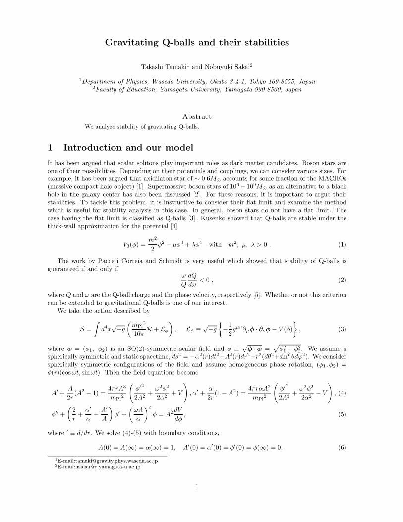
Gravitating Q-balls and their stabilities
Takashi Tamaki1 and Nobuyuki Sakai2
1Department of Physics, Waseda University, Okubo 3-4-1, Tokyo 169-8555, Japan2Faculty of Education, Yamagata University, Yamagata 990-8560, Japan
AbstractWe analyze stability of gravitating Q-balls.
1 Introduction and our model
It has been argued that scalar solitons play important roles as dark matter candidates. Boson stars areone of their possibilities. Depending on their potentials and couplings, we can consider various sizes. Forexample, it has been argued that axidilaton star of ∼ 0.6M accounts for some fraction of the MACHOs(massive compact halo object) [1]. Supermassive boson stars of 106− 109M as an alternative to a blackhole in the galaxy center has also been discussed [2]. For these reasons, it is important to argue theirstabilities. To tackle this problem, it is instructive to consider their flat limit and examine the methodwhich is useful for stability analysis in this case. In general, boson stars do not have a flat limit. Thecase having the flat limit is classified as Q-balls [3]. Kusenko showed that Q-balls are stable under thethick-wall approximation for the potential [4]
V3(φ) =m2
2φ2 − μφ3 + λφ4 with m2, μ, λ > 0 . (1)
The work by Pacceti Correia and Schmidt is very useful which showed that stability of Q-balls isguaranteed if and only if
ω
Q
dQ
dω< 0 , (2)
where Q and ω are the Q-ball charge and the phase velocity, respectively [5]. Whether or not this criterioncan be extended to gravitational Q-balls is one of our interest.
We take the action described by
S =∫
d4x√−g
(
mPl2
16πR + Lφ
)
, Lφ ≡ √−g
−12gμν∂μφ · ∂νφ − V (φ)
, (3)
where φ = (φ1, φ2) is an SO(2)-symmetric scalar field and φ ≡ √φ · φ =
√
φ21 + φ2
2. We assume aspherically symmetric and static spacetime, ds2 = −α2(r)dt2+A2(r)dr2+r2(dθ2+sin2 θdϕ2). We considerspherically symmetric configurations of the field and assume homogeneous phase rotation, (φ1, φ2) =φ(r)(cosωt, sinωt). Then the field equations become
A′ +A
2r(A2 − 1) =
4πrA3
mPl2
(
φ′2
2A2+ω2φ2
2α2+ V
)
, α′ +α
2r(1 −A2) =
4πrαA2
mPl2
(
φ′2
2A2+ω2φ2
2α2− V
)
, (4)
φ′′ +(
2r
+α′
α− A′
A
)
φ′ +(
ωA
α
)2
φ = A2 dV
dφ, (5)
where ′ ≡ d/dr. We solve (4)-(5) with boundary conditions,
A(0) = A(∞) = α(∞) = 1, A′(0) = α′(0) = φ′(0) = φ(∞) = 0. (6)
1E-mail:[email protected]:[email protected]
1
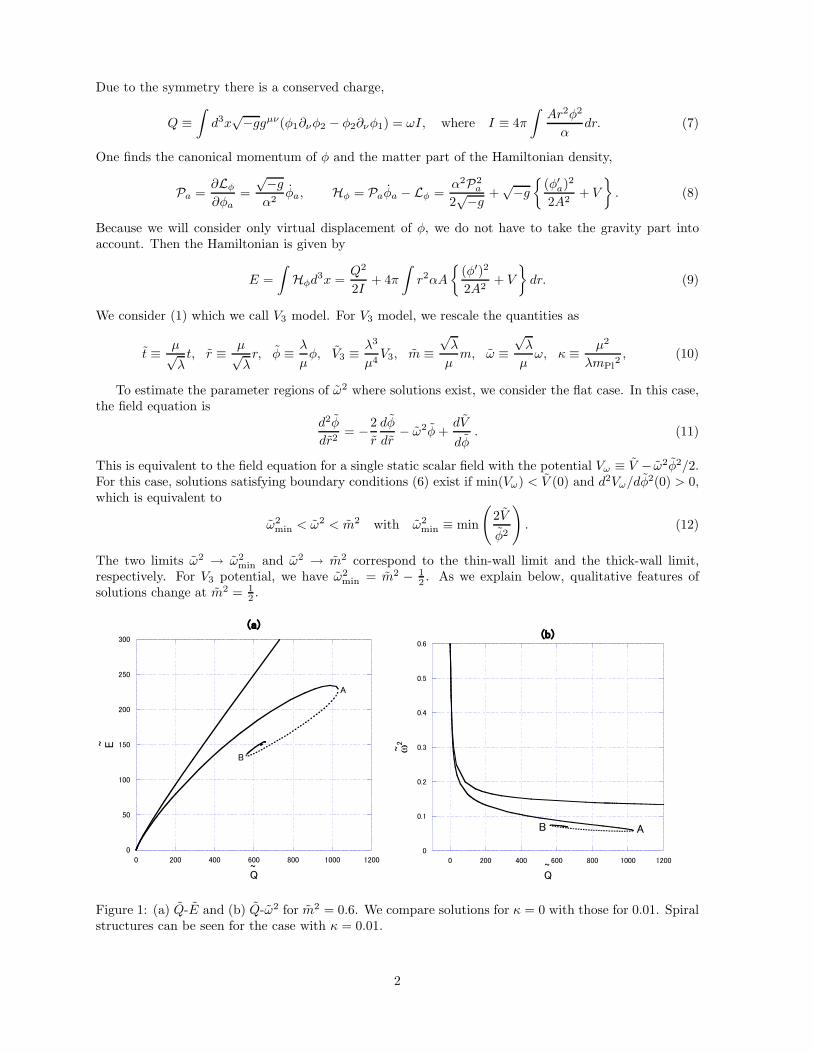
Due to the symmetry there is a conserved charge,
Q ≡∫
d3x√−ggμν(φ1∂νφ2 − φ2∂νφ1) = ωI, where I ≡ 4π
∫
Ar2φ2
αdr. (7)
One finds the canonical momentum of φ and the matter part of the Hamiltonian density,
Pa =∂Lφ∂φa
=√−gα2
φa, Hφ = Paφa − Lφ =α2P2
a
2√−g +
√−g
(φ′a)2
2A2+ V
. (8)
Because we will consider only virtual displacement of φ, we do not have to take the gravity part intoaccount. Then the Hamiltonian is given by
E =∫
Hφd3x =
Q2
2I+ 4π
∫
r2αA
(φ′)2
2A2+ V
dr. (9)
We consider (1) which we call V3 model. For V3 model, we rescale the quantities as
t ≡ μ√λt, r ≡ μ√
λr, φ ≡ λ
μφ, V3 ≡ λ3
μ4V3, m ≡
√λ
μm, ω ≡
√λ
μω, κ ≡ μ2
λmPl2, (10)
To estimate the parameter regions of ω2 where solutions exist, we consider the flat case. In this case,the field equation is
d2φ
dr2= −2
r
dφ
dr− ω2φ+
dV
dφ. (11)
This is equivalent to the field equation for a single static scalar field with the potential Vω ≡ V − ω2φ2/2.For this case, solutions satisfying boundary conditions (6) exist if min(Vω) < V (0) and d2Vω/dφ
2(0) > 0,which is equivalent to
ω2min < ω2 < m2 with ω2
min ≡ min
(
2Vφ2
)
. (12)
The two limits ω2 → ω2min and ω2 → m2 correspond to the thin-wall limit and the thick-wall limit,
respectively. For V3 potential, we have ω2min = m2 − 1
2 . As we explain below, qualitative features ofsolutions change at m2 = 1
2 .
0
50
100
150
200
250
300
0 200 400 600 800 1000 1200
(a)
E
Q~
~
A
B
0
0.1
0.2
0.3
0.4
0.5
0.6
0 200 400 600 800 1000 1200
(b)
ω2
Q
~
~
AB
Figure 1: (a) Q-E and (b) Q-ω2 for m2 = 0.6. We compare solutions for κ = 0 with those for 0.01. Spiralstructures can be seen for the case with κ = 0.01.
2
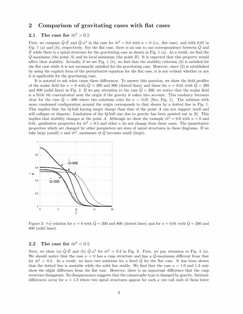
2 Comparison of gravitating cases with flat cases
2.1 The case for m2 > 0.5
First, we compare Q-E and Q-ω2 in the case for m2 = 0.6 with κ = 0 (i.e., flat case), and with 0.01 inFig. 1 (a) and (b), respectively. For the flat case, there is an one to one correspondence between Q andE while there is a spiral structure for the gravitating case as shown in Fig. 1 (a). As a result, we find theQ-maximum (the point A) and its local minimum (the point B). It is expected that this property wouldaffect their stability. Actually, if we see Fig. 1 (b), we find that the stability criterion (2) is satisfied forthe flat case while it is not necessarily satisfied for the gravitating case. However, since (2) is establishedby using the explicit form of the perturbative equation for the flat case, it is not evident whether or notit is applicable for the gravitating case.
It is natural to ask what cause these differences. To answer this question, we show the field profilesof the scalar field for κ = 0 with Q = 200 and 800 (dotted lines) and those for κ = 0.01 with Q = 200and 800 (solid lines) in Fig. 2. If we pay attention to the case Q = 200, we notice that the scalar fieldis a little bit concentrated near the origin if the gravity is taken into account. This tendency becomesclear for the case Q = 800 where two solutions exist for κ = 0.01 (See, Fig. 1). The solution withmore condensed configuration around the origin corresponds to that shown by a dotted line in Fig. 1.This implies that the Q-ball having larger charge than that of the point A can not support itself andwill collapse or disperse. Limitation of the Q-ball size due to gravity has been pointed out in [6]. Thisimplies that stability changes at the point A. Although we show the example m2 = 0.6 with κ = 0 and0.01, qualitative properties for m2 > 0.5 and other κ do not change from these cases. The quantitativeproperties which are changed by other parameters are sizes of spiral structures in these diagrams. If wetake large (small) κ and m2, maximum of Q becomes small (large).
0
0.2
0.4
0.6
0.8
1
0 5 10 15 20
φ
r
Q=800
Q=200
~
~
~
~
Figure 2: r-φ relation for κ = 0 with Q = 200 and 800 (dotted lines) and for κ = 0.01 with Q = 200 and800 (solid lines).
2.2 The case for m2 < 0.5
Next, we show (a) Q-E and (b) Q-ω2 for m2 = 0.2 in Fig. 3. First, we pay attention to Fig. 3 (a).We should notice that the case κ = 0 has a cusp structure and has a Q-maximum different from thatfor m2 > 0.5. As a result, we have two solutions for a fixed Q for the flat case. It has been shownthat the dotted line is unstable while the solid line stable. We find that the case κ = 1.0 and 1.3 onlyshow the slight difference from the flat case. However, there is an important difference that the cuspstructure disappears. Its disappearance suggests that the catastrophe type is changed by gravity. Intrinsicdifferences occur for κ > 1.3 where two spiral structures appear for each κ (we call each of them lower
3
and higher branch corresponding to their energy, respectively). If one considers the analogy with theflat case where the solid (dotted) line is the stable (unstable), one may suppose that the lower (higher)branch is stable (unstable). However, we should suppose that two spiral structures appear for the samereason for the corresponding one for m2 > 0.5 where gravity makes a Q-maximum. Thus, it is naturalto guess that the lower branch shown by a solid (dotted) line is stable (unstable). The stability of thehigher branch is more puzzling. If we compare the case κ = 1.4 with the case κ = 1.3, we may supposethat the interval between B and C is stable. However, the case κ = 1.5 does not have such an interval.Therefore, it is difficult to judge the stability without other criteria.
We also comment on the diagram (b) and the stability criterion (2). The solid (dotted) lines correspondto those in the diagram (a). For the flat case, we can confirm that the solid line satisfies (2) while thedotted line does not. For the gravitating with κ < 1.4, we also confirm it while it is not for κ ≥ 1.4. Inparticular, the solution shown by the solid line and that by the dotted line, both satisfying (2), mergeat the cusp for κ = 1.4. Since the cusp is a typical structure which suggests a stability change via acatastrophe theory, (2) would not be applicable for gravitating Q-balls.
0
0.2
0.4
0.6
0.8
0 0.5 1 1.5 2 2.5 3 3.5
(a)
E
Q
~
~
AC
B
κ=0
1.0 1.3
1.4
1.5
1.5
0
0.05
0.1
0.15
0.2
0 0.5 1 1.5 2 2.5 3 3.5
(b)
ω2
Q
~
~
κ=01.0
1.3
1.41.5
1.5
AC B
1.4
Figure 3: (a) Q-E and (b) Q-ω2 for m2 = 0.2.
3 Conclusion
We have analyzed stability of gravitating Q-balls for a V3 model and revealed their structures.
References
[1] E. W. Mielke and F. E. Schunck, Nucl. Phys. B 564, 185 (2000); ibid., Gen. Rel. Grav. 33, 805(2001).
[2] F. E. Schunck and A. R. Liddle, Phys. Lett. B 404, 25 (1997); E. W. Mielke and F. E. Schunck,Phys. Rev. D 66, 023503 (2002).
[3] S. Coleman, Nucl. Phys. B262, 263 (1985).
[4] A. Kusenko, Phys. Lett. B 404, 285 (1997).
[5] F. Paccetti Correia and M. G. Schmidt, Eur. Phys. J. C21, 181 (2001).
[6] T. Multamaki and I. Vilja, Phys. Lett. B 542, 137 (2002).
4
Kerr black hole and rotating black string by intersectingM-branes
Makoto Tanabe1
1Department of Physics, Waseda University, Tokyo, Japan
AbstractWe find eleven dimensional non-BPS black M-brane solutions from Kerr solution inM-theory by using U-duality. Under the transformation four dimensional Kerr met-ric change to non-BPS rotating intersecting M-brane solutions. To easy applicationfor AdS/CFT correspondence we must need a supersymmetric black brane solution,which limits special configuration of M-branes, e.g., M2-M2-M2 branes in five dimen-sional black brane and M5-M5-M5 brane with pp-wave in four dimensional one. Inthis case we may easily apply the AdS/CFT correspondence for non-BPS black holesolutions.
1 Introduction
AdS/CFT correspondence [1] is the most successful theory to describe strong coupling limit for boundaryconformal field theory. There is a holographic duality between bulk quantum gravity and boundaryquantum field theory. Four dimensional CFT is studied in all aspects because of CFT interests, and itsdual theory is based on five dimensional supergravity black hole solutions. In recent years, Kerr/CFTcorrespondence are found only for the extremal limit case [2]. The paper shows the reason of the finiteentropy of the extremal Kerr black hole, even the Hawking temperature is zero. AdS/CFT correspondenceare very useful to show that reason. However non-extremal case we have no information about AdS/CFTcorrespondence, thus for non-extremal Kerr/CFT correspondence we will give the M-brane configurationabout non-extremal Kerr solution.
Non BPS black ring solutions [3] using the same method we use below, but these solutions relatedto intersecting M2 ⊥ M2 ⊥ M2-brane solution in M-theory, or intersecting F1 ⊥ D2 ⊥ D2-branesolution in type IIA string theory with compactification on one-dimensional torus of M-Theory. Theseconfiguration in string theory is impossible to analysis for AdS/CFT correspondence [1], because we mustchoose typical coordinates for the compact space for near horizon limit, which is the kk-wave direction,but this solution has not any typical direction for compact spaces. Thus we show the NS5 ⊥ D4 ⊥ D4-brane solutions from general axisymmetric four-dimensional vacuum solution with two Killing vector, e.g.,Kerr metric. We also get the general rotating black string solutions, which is rotating four-dimensionalblack hole with extra one dimension, by the M2 ⊥ M2 ⊥ M2-brane solutions from the Kerr metric.
In our previous work [4], black hole solutions with flat extra dimensions in M-theory are only existthe specific configuration of intersecting M-branes. However the earlier study for the micro state of Kerrblack hole [5] using the D0⊥D6 branes, which is impossible to extension to the supersymmetric blackbrane solution in four dimension. The supersymmetric black brane means which have the regular eventhorizon with finite surface area.
Adding the new charge for the solution, we apply the boost for the ordinary metric along the extradimension. Applying T-duality for the boost solution, we find D3-brane given by four-form field D4,which is the self-dual field strength dD4 = ∗(dD4). There are some technical difficulties for the Hodgedual for the stationary spacetime, since the stationary black hole remains the non-diagonal componentafter the boost. Such a component makes problem for integration in order to get the explicit descriptionof the dual field D4.
We will construct the intersecting M-brane solution consistent to the intersecting rule, and avoidingthe difficulties of integration we apply the final boost after the lifting up to the eleven dimension. Thuswe try to find the sequence to get the M5⊥M5⊥M5-brane soltuion, which is related to the D4⊥D4⊥NS5brane solutions in type IIA superstring theory.
1E-mail:[email protected]
1
2 From Kerr metric to Intersecting D-branes
Before charging up the vacuum solution, we introduce the Kerr metric, which is a stationary solution offour-dimensional vacuum Einstein equation. The Kerr metric in spherical coordinate is written in
ds2 = −f (dt + Ω)2 + Σ2
(dr2
∆+ dθ2
)+
∆f
sin2 θdφ2
where the metric functions are defined by
Σ2 = r2 + a2 cos2 θ , ∆ = r2 − 2mr + a2
Ω =2mr
Σ2 − 2mra sin2 θdφ , f = 1 − 2mr
Σ2.
The mass of the black hole is m and a is the specific angular momentum witch bounded for m ≥ a. Inthe Kerr/CFT correspondence, we take the extremal limit m = a and near horizon limit r → r+, wherethe event horizon r+ is determined by ∆ = 0. For simplicity we denote ds2 = −f(dt + Ω)2 + ds2
base inbelow. The base metric ds2
base = γijdxidxj are the orthogonal three-dimensional metric written by thevariables r, θ, φ. The metric has the two Killing vector ξt and ξφ.
Adding the extra six flat dimension, the metric change to ds2 + −f(dt + Ω)2 + ds2base +
∑6i=1 dz2
i .This metric is also a solution of ten dimensional vacuum Einstein equation Rµν = 0. To add first charge(D3-brane), we apply a sequence in below;
Bα2(z1) → T (z1) → S → T (z2) → T (z3) ,
then we find a D3-brane solution in type IIB supergravity. We denote Bα(z1) is boost for zi directionwith boost parameter α, T (zi) is T-dual for zi direction, and S is S-dual. To add second and thirdcharges, we take next sequence in below,
T (z4) → Bα1(z1) → T (z1) → S → T (z5) → T (z6) → T (z2) → B(z6) → T (z6) → S → T (z5) ,
then we find a D2 ⊥ D2 ⊥ D2 intersecting brane solution as
ds2 = −ξ−1/2f(dt + c1c2c3Ω)2 + ξ1/2ds2base + ξ1/2
[h−1
1
2∑i=1
dz2i + h−1
2
4∑i=3
dz2i + h−1
3
6∑i=5
dz2i
],
where ξ = h1h2h3 −β2t , βt = s1s2s3
ma cos θΣ2 . The dilaton field is e−2ϕ = ξ−3/2h1h2h3 and the gauge fields
are
Bzizj = h−1α
cα
sαβt , At = −ξ−1βtf , Aφ = −ξ−1βtfω
Czizjt =23h−1
α sαcα(f − 1) , Czizjφ =23h−1
α fc−1α sαω .
where the pair of indices (i, j) = (1, 2), (3, 4), (5, 6) are corresponding to α = 1, 2, 3, and ω = c1c2c3Ω.For the first example of a black hole solution, we continue to apply the U-duality for the charging up
the four-dimensional Kerr solutions. Next we try to apply another example related to the rotating blackstring, which can be described by the Kerr metric with another one extra dimension, and these solutionsmust possess the Gregory-Laflamme instability [6].
In order to get M5⊥M5⊥M5 brane solution, we must apply the sequence in following as
T (z1) → T (z3) → T (z5) → T (z2) → T (z4) → T (z6) ,
then we find the D4 ⊥ D4 ⊥ D4-brane solutions and we lift up the z7 direction and boost for the samedirection z7, then we find the M5 ⊥ M5 ⊥ M5-brane with pp-wave solutions in M-theory;
ds2 = Ξ1/3
[h−1
1
2∑i=1
dz2i + h−1
2
4∑i=3
dz2i + h−1
3
6∑i=5
dz2i
]
+ Ξ1/3[−ξ−1f(dt + ωdφ)2 + ds2
base
]+ Ξ−2/3ξ
(dz7 + Atdt + Aφdφ
)2
, (1)
2
where the conformal factor can be written by Ξ = h1h2h3 and hi = ξh−1i with hi = −s2
i f + c2i g
−1i . The
function gi is determined by gi = 1 + (h1h2h3)−1h−1i s−2
2 β2t . The three-form fields related to M5-brane
are given by
C(α)7 ≡ Czizjz7 =
23h−1
α s−1α cαβt , C(α)
a ≡ Czizja =83D(α)
a + h−1α s−1
α cαβtAa ,
where the component of M5-brane fields and the metric components are given by
D(1)t = −ξ−1h2s1c2c3Dt , D
(1)φ = s2c2
[Dφ + (1 − ξ−1h2c
21c
23)DtΩφ
]D
(2)t = −ξ−1h1c1s2c3Dt , D
(2)φ = s1c1
[Dφ + (1 − ξ−1h1c
22c
23)DtΩφ
]D
(3)t = −ξ−1h3c1c2s3Dt , D
(3)φ = s3c3
[Dφ + (1 − ξ−1h3c
21c
22)DtΩφ
]At = s1c1s2c2s3c3
ma2 cos2 θ
Σ4
Aφ = −s1s2s3
(c21c
22c
23 +
2rΣ2h1h2h3
r2 − a2 cos2 θ
)ma3 sin2 θ cos2 θ
Σ4.
We note that Kerr metric with flat dimensions has no Chern-Simons term, but there are exist in elevendimension after the charging up sequence, e.g., C
(1)7 ∧dC
(2)t ∧ C
(3)φ or like that combinations. The Chern-
Simons terms gives the non-trivial effect of the topology for BPS black ring solutions, and this effectchange the Laplace equation for the harmonic function hi to the Poisson equation for the non-harmonicfunction hi. Because of non conformally flat base space, supersymmetrie breaks for φ direction, thus inthe ordinary base space configuration we took maximally charge for three.
Finally we apply the boost for the z7 direction, then we find non-BPS four charge solution. Howeverif we took same special value for physical parameters, we find supersymmetric solution with conformallyflat base space. To Compactify extra seven dimensions (z1, · · · , z7) on torus, we find the four dimensionalcharged solution as
ds2 = −Υf(dt + ωdφ)2 + Υ−1ds2base , (2)
where ω and Υ are determined by
ω = c4ω + s4(ωAt − Aφ)
Υ−2 = Ξ(−ξ−1fs2
4 + Ξ−1ξ(c4 + s4At)2)
,
In the Kerr metric case, the regularity condition for the rotating axis are the same as before, thus themetric has no conical singularity at the ordinary event horizon r+ = m +
√m2 − a2.
In the asymptotic region (r → ∞) the metric becomes flat and the ADM mass M = m(1+∑4
i=1 s2i /2),
the conserved charge Q =√
2m∑4
i=1 sici/2 and the angular momentum J = c1c2c3c4a are given in theasymptotic metric form. The surface gravity change as below
κ =1
β2t+(c4 + s4At+)
r2+ − a2
4mr2+
, (3)
where βt+ and At+ are defined by the substitution for r = r+. The surface area of the outer event horizon
A =∫
dθdφ√
Σ2 (Υ−2γφφ − fω2)¯r=r+
= 8πmr+c1c2c3
[c4 −
12a3s4
(π
4− a
r+arctan
r+
a
)],
and we can show the thermodynamics with the physical parameter as the charge and angular momentumand the temperature, but the dilaton fields does not contribute.
3
The extremal solution (κ = 0) is given by m = a, which is as the same as ordinary Kerr metric. Thearea surface is vanishing in the extremal limit of the ordinary Kerr metric, however the area surface inM-theoretical Kerr metric doesn’t vanishing (A = 8πm2c1c2c3c4). Since cα is related to the charge ofM-brane (or D-brane), this non-vanishing area surface gives the microstate of M-brane.
Sen gave the rotating charged black hole solution [7], which metric is given in
ds2 = −h−1α f
(dt + c2
αΩ)2
+ hαds2base , (4)
where hα = −s2αf + c2
α. Sen’s solution is included in our solution with the parameter c1 = c2 = cα andc3 = c4 = 1, and this case the action is changing as φ1 = φ2 and φ3 = φ4 = 0 and ρα = 0 and onlyA(1)
a = A(2)a are exist.
3 Concluding remark
In this paper we have presented the charging up Kerr solution using the U-duality method. Black holesolutions are presented by intersecting M-brane, and we have construct the intersecting M-brane solution,which consistent to the supersymmetrical black hole solution given by our previous work [4]. The four-dimensional black hole solution is given by M5⊥M5⊥M5 brane solution with traveling wave, and thefive-dimensional black string solution is given by M2⊥M2⊥M2 brane solution. Both of the solution existthe non-vanishing Chern-Simons term in M-theory, although the Chern-Simons term in the ordinaryKerr metric with additional flat extra dimensions must be vanishing. The Chern-Simons terms changethe metric function given by Laplece equation to the function given by Poisson equation.
The four-dimensional solution is represented by the charged dilaton black hole. The Maxwell chargeand the dilatons are coupled to each other, and the angular momentum are represented by the charges.Thus we are only possible to take the limit to vanishing the charges with the trivial dilaton, and this limitgives static black brane solution [?]. The black hole has the regular extremal limit to the BPS solutionin four dimension with non-vanishing are surface, and the area surface are represented by the micro stateof M- or D-branes.
Since there are kk-wave mode in the ten-dimensional metric, the D-brane configuration of this metricis suitable to apply the AdS/CFT correspondence. We will show the micro state of these solutions inthe context of AdS/CFT correspondence, and we will also show the regular solutions with the specificphysical parameters in subsequent paper, witch we are writing now. In the limit for the CFT, we comparethe micro state of Kerr black hole by D0 ⊥ D6-brane solutions given by Horowitz et. al., [5].
By the way of this paper we only consider from the vacuum solutions, but adding the extra dimensionwe can extend to the Einstein manifold with the constant gauge field, which satisfy the Einstein andMaxwell equation in lower and higher dimension. In this formalism, including the one rotating black ringcase, we can apply the more interesting case, especially cosmology and black hole dynamics.
References
[1] O. Aharony, S. S. Gubser, J. M. Maldacena, H. Ooguri and Y. Oz, Phys. Rept. 323, 183 (2000)[arXiv:hep-th/9905111].
[2] M. Guica, T. Hartman, W. Song, A. Strominger, [arXiv:0809.4266].
[3] H. Elvang, R Emparan and P. Figueras, JHEP 0502 (2005) 031, [arXiv:hep-th/0412130].
[4] K. Maeda and M Tanabe, Nucl. Phys. B738 (2006) 184, [arXiv:hep-th/0510082].
[5] G. T. horowitz and M. M. Roberts, [arXiv:0708.1346].
[6] R. Gregory and R. Laflamme, Phys. Rev. D 37 (1988) 305.
[7] A. Sen, Phys.Rev.Lett. 69 (1992) 1006, [arXiv:hep-th/9204046].
[8] , G. W. Gibbons and K. Maeda, Nucl. Phys. B 298 (1998) 741.
4
Initial data of black holelocalized on Karch-Randall brane
Norihiro Tanahashi1 and Takahiro Tanaka2
Department of Physics, Kyoto University, Kyoto 606–8502, Japan
AbstractBased on the conjectured duality in the Karch-Randall braneworld models, it is sug-gested that a static brane-localized black hole larger than bulk curvature length doesexist in this model. It is also suggested that the Hawking-Page transition of the four-dimensional black hole may be reproduced as a change in the shape of five-dimensionalblack hole in the bulk. In order to test these suggestions, we try to construct time-symmetric initial data of brane-localized black hole in the Karch-Randall braneworldmodel and study its properties. I will explain the method of the analysis and illustrateexpected results.
1 Introduction
The Randall-Sundrum II (RS-II) model [1] is a brane world model, which provides a way to realize ourfour-dimensional world in a higher-dimensional spacetime. This model is composed of five-dimensionalbulk spacetime with negative cosmological constant and a four-dimensional brane with positive tension.Weak gravitational field on the brane obeys the usual four-dimensional Newton law with a correctionsuppressed at a large distance from the gravitational source [1, 2], though the extra-dimension extendsinfinitely in this model. If we weaken the brane tension a little, a small negative cosmological constantappears in the effective Einstein gravity on the four-dimensional brane, and the spacetime on the branebecomes AdS4. It is known that there is an “almost” massless graviton even in this model, and four-dimensional gravity is realized if length scale of interest is shorter than the curvature scale on the brane.This model with an AdS brane is called the Karch-Randall (KR) model [3]. Since four-dimensionalgravity is realized effectively in these models, it is difficult to distinguish them from ordinary four-dimensional models as long as we investigate only in the weak gravity regime. Essential features of thesemodels will appear in strong gravitation phenomena on them. In order to assess viability of these modelsobservationally, we should study how these models behave when strongly gravitation exists in them.
Now, consider a gravitational collapse on the brane in each of these models for an example of suchstrong gravitation phenomena. Naively thinking, a static black hole (BH) whose horizon is localized nearthe brane will form as a final state of this collapse, since ordinary four-dimensional gravity is realizedon the brane. There are exact static solutions of black objects, which are black strings (BS) in thosemodels [4,5], and they also are candidates of the black object which is formed after the collapse. However,it seems unlikely that a BS is formed as a result of gravitational collapse, since it is singular at the bulkAdS horizon and also unstable due to so-called Gregory-Laflamme instability [6]. Thus, a brane-localizedBH seems to be most likely to form after the collapse on the brane.
Contrary to this expectation of brane-localized BH formation, such an exact static solution has notbeen discovered yet though much effort has been devoted into this issue (e.g. Ref. [7]). Numerical solutionof a static brane-localized BH was constructed when the horizon size is not much larger than the bulkcurvature scale, but the construction becomes harder as the horizon size becomes larger [8, 9]. A workon brane-localized BH issue [10] reports that there are some problems in numerical solution constructioneven when the brane-localized BH is smaller than the bulk curvature scale. These facts do not excludethe possibility that a static solution of brane-localized BH larger than the bulk curvature scale does exist,but we do not have any strong evidence of its existence. As an explanation of the lack of static solution,there is a conjecture that brane-localized static BHs larger than bulk curvature scale do not exist in RS-IImodel based on the AdS/CFT correspondence in this model [11,12].
1E-mail:[email protected]:[email protected]
1
There are several works related to this conjecture (e.g. [13,14]), but no definite conclusion is obtainedyet. It is desirable to investigate the properties of static BH solution directly in order to test the validityof this conjecture, but it is technically difficult to construct a static large BH solution numerically. Thus,we consider time-symmetric initial data which have a brane-localized apparent horizon (AH), expectingthat their properties may give some insight into the brane-localized BH.
We have done this initial data construction and analysis of their properties in [15]. It was confirmed inthis work that there exists an initial data with an arbitrariry large blane-localized BH. We analyzed theirthemodynamic properties by comparing this initial data with a black string solution which have the samefour-dimensional ADM mass. This analysis revealed that such a large brane-localized BH have smallerentopy than than the black string of the same mass has, and thus it seems to be unstable and tend toevolve into some other black object. This tendency changes as we decrease the size of the brane-localizedBH; when it is smaller than the bulk curvature scale, it have more entropy than the black string has.This result is consistent that a static stable brane-localized BH does exists when it is smaller than thebulk curvature scale, and it becomes unstable when it is larger than that scale.
This time, we do a similar analysis on the KR model. One of the differences from the RS-II model isthe behavior of warp factor in the bulk; in the RS-II model, it just decreases down to zero as we moveinto the bulk from the brane; in KR model, it first decreases, but it begins to grow again after we passedover a critical point which is at a distant of the bulk curvature scale. The effective potential for a smallparticle behaves in a similar manner to the warp factor. If we put a small black hole at that minimumpoint of the effective potential, it will stay there stably. At this stage, no black object is visible from anobserver on the brane; radiation field of nonzero temperature is induced on the brane by that BH, andthe brane observer will see only a lump of this thermal radiation.
Now, let us gradually increase the size of that BH which sits at that potential minimum. It willkeep to stay there as long as its size is smaller than the bulk curvature scale. A curious phase transitionoccurs when its size become comparable to the bulk curavature scale: the BH touches the brane, and itbecomes observable from an observer on the brane. By the way, in the four-dimensional AdS spacetime,it is known that such a phase transition occurs between thermal AdS phase and AdS BH phase. Thisphenomenon is known as the Hawking-Page transition [16]. We conjecture that the transition of the bulkBH shape to be a holographic dual of the Hawking-Page transition on the brane [11]. In order to checkthis conjecture, we construct initial data of bulk BHs and brane-localized BHs in the KR model, and testthe thermodynamic property of those BHs.
2 Initial data construction method
In this section, we introduce a construction method of time-symmetric initial data with a BH in the KRmodel. This model is composed of two copies of five-dimensional empty bulk with negative cosmologicalconstant Λ, and they are separated by a Z2-symmetric positive tension brane. The tension of the brane isgiven by λ = 3k(1 + δ)/4πG5 with k =
√−Λ/6, where G5 is the five-dimensional gravitational constant.
The parameter δ describes how a brane tension is detuned from that of the RS-II model; when δ = 0,this model reduce to the RS-II model with a Minkowski brane. Four-dimensional cosmological constantis given by Λ4D = 3k2
(2δ + δ2
), thus a negative cosmological constant appears when δ < 0. In this
work, we assume δ < 0. The initial data we consider have O(3)-symmetry in the spacelike dimension aswell as the symmetry with respect to time reversal. These symmetries are property shared with staticbrane-localized BH solutions. Hence, we think it appropriate to restrict our attention to this class ofinitial data.
The starting point of our construction procedure is to choose an asymptotically AdS vacuum solutionof the Einstein equations with negative cosmological constant Λ. In this study, we use the well-knownAdS-Schwarzschild solution. The metric is given by
ds2 = −U(r)dt2 +dr2
U(r)+ r2
(dχ2 + sin2 χdΩII
), U(r) = 1 + k2r2 − µ
r2, (1)
where dΩII is the line element on a unit S2, and µ is the mass parameter of the AdS-SchwarzschildBH. The spacetime described by this metric is asymptotically AdS, and has an spherical event horizon
2
at r = rg where U(r) vanishes. In the following discussion, we set k to unity by rescaling the unit oflength. In this sense, this background spacetime has only one free parameter µ, which becomes one offree parameters of the initial data.
We put a vacuum brane with Z2-symmetry in this AdS BH bulk. We denote the unit normal ofthe brane by sµ, and take this sµ in the direction toward the bulk from the brane. We introduce theinduced metric γµν ≡ gµν − sµsν on the brane. The extrinsic curvature Kab on the brane is defined byKab = −γ µ
a γ νb ∇µsν . Here Latin indices starting from the beginning of the alphabet (a, b, · · · ) run the
four-dimensional coordinates on the brane. A vacuum brane has the four-dimensional energy-momentumtensor localized on the brane given by Tab = −λγab. Israel’s junction condition [17] on the brane is givenby Kab − Kγab = 1
2 · 8πG5Tab, where we used Z2-symmetry across the brane. At the moment of thetime-reversal symmetry, we only have to solve the Hamiltonian constraint, which is the (t, t)-componentof the junction condition. Using the normal vector sµ, this equation is written as
Disi = −3k (1 + δ) , (2)
where Di is a covariant differenciation with respect to the induced metric γij . Assuming O(3)-symmetryof the brane, we specify the brane trajectory by (r, χ) = (rb(ξ), χb(ξ)), where ξ is the proper radial lengthalong the brane. The spacelike unit normal sµ is given by
sµ =(√
Urbχ′b,− r′b√
Urb
). (3)
Then the Hamiltonian constraint (2) becomes a second order ODE of rb(ξ) and χb(ξ). We solve Eq. (2)numerically to obtain the brane trajectory. In this way, we can construct a system of a brane and a BHwhich floats on it. We can change the brane position with respect to the bulk BH, and also we can changethe mass parameter µ of the bulk BH as well as the detune paramter δ of the brane tension. Namely, wecan construct a three-parameter family of the initial data. We note here that we can construct an initialdata which have a BH localized on the brane, not one floating in the bulk.
3 Analysis method
In order to study thermodynamic properties of these BHs in the KR model, we have to calculate mass andentropy of them. When we studied the system with a flat brane, we calculated four-dimensional ADMmass measured on the brane and five-dimensional BH horizon area, and conducted a thermodynamicanalysis using them. We obtained some pieces of evidence that brane-localized BHs larger than the bulkcurvature scale are unstable. We would like to do a similar analysis using BH initial data on the KRmodel, but there is a difficulty in the calculation of mass. In the RS-II model, the localization of the four-dimensional graviton is perfect, and the four-dimensional ADM mass is expected to be an appropriatequantity to characterize the system. On the other hand, the bulk of the KR model largely opens upto the AdS boundary, and then the localization of the graviton is not perfect; the lowest Kaluza-Kleinmode have very small mass, and since it behaves differently from zero mass graviton when it propagatesa long length. In order to calculate mass in this system with imperfectly localized gravitation, we have tocalculate five-dimensionally defined mass, not the mass which is four-dimensionally defined on the brane.However, there are no definite way to define five-dimensional mass in the KR model.
In [18], a way to define mass in AdS spacetime is proposed. They construct a conserved quantitywhich is expressed as a surface integral of metric perturbation. Our proposal is to use this definition tocalculate mass in the KR model. We regard pure AdS5 spacetime as background spacetime, calculatemetric perturbation which is induced by the brane and the BH, and then calculate mass by integratingthe metric perturbation on some surface which is located near spatial infinity.
When we applied this Abbott-Deser definition of mass to the KR model, we found that the massdefined in this way is conserved only when we keep to take the Gaussian-Normal coordinates. Thus, themass defined in this way is coordinate dependent. It is not so clear that this mass satisfies the laws ofthermodynamics, but we expect that we can obtain some information of the system using mass definedin this way.
3
Consider a family of initial data for a fixed value of mass. There are initial data of two types inthis family: one with a BH floating in the bulk, and one with a BH localized on the brane. In thistwo-parameter family of the initial data for a fixed mass, we can find one which extremizes the entropy.We expect this initial data to be one with a floating BH in the bulk when the temperature on the braneis low, and to be one with a brane-localized BH when the temperature is above a critical temperaturewhich is determined by the curvature scale on the brane.
From this analysis, we will obtain useful information about the holography in RS-II and KR models.Based on this result, we would like to tackle more difficult problems toward proof of the classical evapo-ration conjecture. Especially, we would like to simulate a time-evolving brane-localized black hole usingnumerical relativity technique. This analysis will clarify the behavior of BH solutions on these models,and will provide essential knowledge about the holography on these braneworld models.
References
[1] L. Randall and R. Sundrum, Phys. Rev. Lett. 83, 4690 (1999)
[2] J. Garriga and T. Tanaka, Phys. Rev. Lett. 84, 2778 (2000)
[3] A. Karch and L. Randall, Phys. Rev. Lett. 87, 061601 (2001) [arXiv:hep-th/0105108].
[4] A. Chamblin and A. Karch, Phys. Rev. D 72, 066011 (2005) [arXiv:hep-th/0412017].
[5] A. Chamblin, S. W. Hawking and H. S. Reall, Phys. Rev. D 61, 065007 (2000)
[6] R. Gregory, Class. Quant. Grav. 17, L125 (2000)
[7] D. Karasik, C. Sahabandu, P. Suranyi and L. C. R. Wijewardhana, Phys. Rev. D 69, 064022 (2004)
[8] H. Kudoh, T. Tanaka and T. Nakamura, Phys. Rev. D 68, 024035 (2003)
[9] H. Kudoh, Phys. Rev. D 69, 104019 (2004) [Erratum-ibid. D 70, 029901 (2004)]
[10] H. Yoshino, JHEP 0901, 068 (2009) [arXiv:0812.0465 [gr-qc]].
[11] T. Tanaka, Prog. Theor. Phys. Suppl. 148, 307 (2003)
[12] R. Emparan, A. Fabbri and N. Kaloper, JHEP 0208, 043 (2002)
[13] P. R. Anderson, R. Balbinot and A. Fabbri, Phys. Rev. Lett. 94, 061301 (2005)
[14] T. Tanaka, arXiv:0709.3674 [gr-qc].
[15] N. Tanahashi and T. Tanaka, arXiv:0712.3799 [gr-qc].
[16] S. W. Hawking and D. N. Page, Commun. Math. Phys. 87, 577 (1983).
[17] W. Israel, Nuovo Cim. B 44S10, 1 (1966) [Erratum-ibid. B 48, 463 (1967 NUCIA,B44,1.1966)].
[18] L. F. Abbott and S. Deser, Nucl. Phys. B 195, 76 (1982).
4
Black hole entropy for the general area spectrum
Tomo Tanaka1 and Takashi Tamaki2
1Department of Physics, Waseda University, Okubo 3-4-1, Tokyo 169–8555, Japan2Department of Physics, Waseda University, Okubo 3-4-1, Tokyo 169–8555, Japan and Department of
Physics, Rikkyo University, Toshima, Tokyo 171–8501, Japan
AbstractWe consider the possibility that the horizon area is expressed by the general areaspectrum in loop quantum gravity and calculate the black hole entropy by countingthe degrees of freedom in spin-network states related to its area. Although the generalarea spectrum has a complex expression, we succeeded in obtaining the result that theblack hole entropy is proportional to its area as in previous works where the simplifiedarea formula has been used. This gives new values for the Barbero-Immirzi parameter(γ = 0.5802 · · · or 0.7847 · · · ) which are larger than that of previous works.
1 Introduction
Statistical mechanics in a self-gravitating system is quite different from that without gravity. For example,particles in the box have maximal entropy when they spread out uniformly in the box if gravity is nottaken into account. On the other hand, if particles are self-gravitating, we can suppose that clustersappear as an entropically favorable state. Then, if the pressure of particles can be neglected, it is likelythat a black hole appears as a maximal entropy state. Thus, black hole entropy would be the key forunderstanding statistics in a self-gravitating system.
One of the most mysterious things about black holes is their entropy S which is not proportional toits volume but to its horizon area A. This was first pointed out related to the first law of black holethermodynamics. The famous relation S = A/4 has been established by the discovery of the Hawkingradiation. Recently, its statistical origin has been discussed in the candidate theories of quantum gravity,such as string theory, or loop quantum gravity (LQG) [1], etc. It has been discussed that LQG candescribe its statistical origin independent of black hole species because of its background independentformulation [2]. For this reason, we concentrate on LQG here.
Quantum states in LQG are described by spin-network [3], and basic ingredients of the spin-networkare edges, which are lines labeled by spin j(j = 0, 1/2, 1, 3/2, · · · ) reflecting the SU(2) nature of the gaugegroup, and vertices which are intersections between edges. For three edges having spin j1, j2, and j3 thatmerge at an arbitrary vertex, we have following conditions.
j1 + j2 + j3 ∈ N, (1)ji 5 jj + jk, (i, j, k different from each other.). (2)
These conditions guarantee the gauge invariance of the spin-network.Using this formalism, general expressions for the spectrum of the area and the volume operators can
be derived [4, 5]. For example, the area spectrum Aj is
Aj = 4πγ∑
i
√2ju
i (jui + 1) + 2jd
i (jdi + 1) − jt
i (jti + 1) , (3)
where γ is the Barbero-Immirzi parameter related to an ambiguity in the choice of canonically conjugatevariables. The sum is added up all intersections between a surface and edges. Here, the indices u, d, andt mean edges upper side, down side, and tangential to the surface, respectively (We can determine whichside is upper or down side arbitrarily).
1E-mail:[email protected]:[email protected]
1
In [1], it was proposed that black hole entropy is obtained by counting the number of degrees offreedom about j when we fix the horizon area where a simplified area formula is used. This simplifiedarea formula is obtained by assuming that there are no tangential edges on black hole horizon, that isjti = 0. We obtain ju
i = jdi := ji by using the condition (2). Then, we consider the degrees of freedom
about j satisfying
Aj = 8πγ∑
i
√ji(ji + 1) = A. (4)
The standard procedure is to impose the Bekenstein-Hawking entropy-area law S = A/4 for large blackholes in order to fix the value of γ. Ashtekar et al. in [2] extended this idea using the isolated horizonframework (ABCK framework) [6]. Error in counting in this original work has been corrected in [7, 8].Similar works appear related to how to count the number of freedom in [9, 10].
However, should we restrict to the simplified area spectrum (4) ? Thiemann in [11] used the boundarycondition that there is no other side of the horizon, i.e., jd
i = 0. Then, by using (2), we obtain jui = jt
i := ji
which gives Aj = 4πγ∑
i
√ji(ji + 1). Based on this proposal, the number counting has been performed
in [12] which gives γ = 0.323 · · · .Another interesting possibility is to use (3) motivated by the hypothesis that a black hole is a maximal
entropy state in a self-gravitating system. If we agree that the origin of the black hole entropy is relatedto degrees of freedom in j (or m = −j,−j + 1, · · · , j considered in [2]), it is evident that (3) can gainlarger number of states than (4) for the fixed area. See, also [13] which also discuss using (3) as expressingthe horizon area. Of course, it is speculative and the typical objection to the idea is that since the blackhole evaporates, it is not the maximal entropy state. However, the black hole we consider is the limitA → ∞ where the evaporation process can be negligible. The second objection is that if we require theentropy-area law S = A/4, the black hole entropy does not depend on what types of area formula we use,so it is not relevant to the above hypothesis. This is a delicate question to be answered carefully. Fromthe view point that the Barbero-Immirzi parameter is determined a priori, the formula S = A/4 onlyprovides us the method to know the value of γ. If this is the case, using (3) would enhance the entropy.Therefore, we concentrate on evaluating the number of states using (3) by adopting this view point. Toanswer whether this view point is true or not, we need independent discussion to know the value of γthrough, e.g., cosmology [14] or quasinormal modes of black holes [15, 16, 17].
Our strategy is as follows [18]. Based on the observation that the value of γ in [2] is qualitatively sameas that inferred in [1] which counts the degrees of freedom of j without imposing the horizon conditionsfor the case (4), we restrict counting the corresponding j freedom for (3) as a first step. We can performit by carefully reanalyzing the case (4). This paper is organized as follows. In section 2, we count thedegrees of freedom for (3). In section 3, we mention concluding remarks.
2 Consideration of the general area spectrum
In the case for (4), horizon conditions does not affect entropy formula. Therefore in the case for (3) weconsider only degrees of freedom about area. In this case, we also denote number of states as N(A) whichis defined as
N(A) :=
(ju1 , jd
1 , jt1, · · · , ju
n , jdn, jt
n)|0 = jui , jd
i ∈ N2
, 0 = jti ∈ N, ju
i , jdi , jt
i should satisfy (1) and (2).
∑i
√2ju
i (jui + 1) + 2jd
i (jdi + 1) − jt
i (jti + 1) =
A
4πγ
. (5)
We adopt the condition jt ∈ N motivated by the ABCK framework where the “classical horizon” isdescribed by U(1) connection. This is, of course, not verified in the present situation and should bereconsidered in future.
Then, we perform counting as follows. If we use the condition jt ∈ N, we have ju + jd := n ∈ N by(1). If we fix n, we can classify the possible ju, jd, jt as follows, which is one of the most important partsin this paper. First, we have (ju, jd) = (n
2 ± s2 , n
2 ∓ s2 ) (double-sign corresponds) for 0 5 s 5 n, s ∈ N to
2
satisfy (2). Then, for each s, possible value of jt is jt = s, s + 1, · · · , n to satisfy (2). For any eigenvaluex := 4πγ
√2ju
x (jux + 1) + 2jd
x(jdx + 1) − jt
x(jtx + 1) (0 < x 5 A) of the area operator, we have
(j1, · · · , jn) ∈ N(A − x) ⇒ (j1, · · · , jn, jx) ∈ N(A), (6)
where we used the abbreviation as ji = (jui , jd
i , jti ). We have (j1, · · · , jn, jx) = (j1, · · · , jn, jx′), if jx = jx′ .
Therefore, as for the case in (4), if we consider all 0 < x 5 A and (j1, · · · , jn) ∈ N(A−x), (j1, · · · , jn, jx)form the entire set N(A).
Then, if we use the notation ju = n2 + s
2 , jd = n2−
s2 , jt = t, we have x(n, s, t) = 4πγ
√n2 + 2n + s2 − t(t + 1)
and
N(A) =∞∑
n=1
[n∑
s=1
n∑t=s
2N(A − x(n, s, t)) +n∑
t=0
N(A − x(n, s = 0, t))
], (7)
where the factor 2 in front of N(A − x(n, s, t)) for s = 0 corresponds to the fact that same x(n, s, t)
appears twice for the exchange of ju and jd. For A → ∞, by assuming N(A) = CeAγM4γ , where C is a
constant and substituting to the recursion relation (7), we obtain the beautiful formula as a generalizationof the case (4) as,
1 =∞∑
n=1
[n∑
s=1
n∑t=s
2 exp(−γMx(n, s, t)/4γ) +n∑
t=0
exp(−γMx(n, s = 0, t)/4γ)
]. (8)
If we require S = A/4, we have γ = γM = 0.5802 · · · . This means that even if we use (3) as the horizonspectrum, we can reproduce the entropy formula S = A/4 by adjusting the Barbero-Immirzi parameter.This is nontrivial and is our main result in this paper.
Let us turn back to our assumptions. Although we obtained γ satisfying S = A/4 for the case (3),there may be a criticism that the result is underestimated by only counting j freedom. To answer it, weconsider the following counting. When the simplified area formula was used, there is an proposal thatwe should count not only j but also m = −j,−j + 1, · · · , j freedom based on the ABCK framework [9].Although it is nontrivial whether this framework can be extended to the general area formula, let us countalso the m freedom for each ju to maximize the estimate. Counting only m related to ju is reasonablefrom the point of view of the entanglement entropy or the holography principle.
If we notice that there are (n+ s+1) and (n− s+1) freedoms for m (total 2(n+1)) corresponding to(ju, jd) = (n
2 + s2 , n
2 − s2 ) and (n
2 − s2 , n
2 + s2 ), respectively, the factor 2 in the first term of the right-hand
side of (8) is replaced by 2(n + 1) in this case. For s = 0, the factor 1 in the second term is replaced by(n + 1). Then, we obtain
1 =∞∑
n=1
[n∑
s=1
n∑t=s
2(n + 1) exp(−γMx(n, s, t)/4γ) +n∑
t=0
(n + 1) exp(−γMx(n, s = 0, t)/4γ)
], (9)
which gives γ = γM = 0.7847 · · · . Thus, we confirm that the black hole entropy is proportional to thearea again. Naively speaking, we expect that there is no qualitative deviation from these two values of γeven if we take into account the ABCK framework for (3) appropriately.
3 Conclusion and Discussion
In this paper, we obtained the black hole entropy by considering the general area formula. It is surprisingthat we succeeded in obtaining the black hole entropy proportional to the horizon area even in this case.Then, it is natural to ask what the area formula should be in describing the horizon area. There aremany possibilities examining the area spectrum. For example, we have not yet established the blackhole thermodynamics in LQG which is one of the most important topics to be investigated. There is anidea that black hole evaporation process should also be described by using the general area formula [13].Therefore, whether we can establish the generalized second law of black hole thermodynamics might beone of the criteria in judging which area formula is appropriate. For this purpose, it is desirable to extend
3
the ABCK framework for the general area formula since the exact counting is required. Though we donot take care of the topology of the horizon, discussing the difference caused by the topology is importantas considered for the simplified area formula [19].
Of course, as we mentioned in the introduction, we should check the value of the Barbero-Immirziparameter in several independent discussions. Therefore, we should also take care of cosmology [14] andquasinormal modes of black holes [15, 16, 17] in determining the Barbero-Immirzi parameter. ConfirmingLQG in many independent methods would be the holy grail of the theory.
Acknowledgements
We would like to thank Tomohiro Harada and Kei-ichi Maeda for useful comments and continuousencouragement.
References
[1] C. Rovelli, Phys. Rev. Lett. 77, 3288 (1996).
[2] A. Ashtekar, J. Baez, A. Corichi, and K. Krasnov, Phys. Rev. Lett. 80, 904 (1998); A. Ashtekar, J.Baez, and K. Krasnov, Adv. Theor. Math. Phys. 4, 1 (2000).
[3] C. Rovelli and L. Smolin, Phys. Rev. D 52, 5743 (1995).
[4] C. Rovelli and L. Smolin, Nucl. Phys. B 442, 593 (1995); Erratum, ibid., 456, 753 (1995).
[5] A. Ashtekar and J. Lewandowski, Class. Quantum Grav. 14, A55 (1997).
[6] A. Ashtekar, A. Corichi, and K. Krasnov, Adv. Theor. Math. Phys. 3, 419 (1999).
[7] M. Domagala and J. Lewandowski, Class. Quant. Grav. 21, 5233 (2004).
[8] K. A. Meissner, Class. Quant. Grav. 21, 5245 (2004).
[9] A. Ghosh and P. Mitra, Phys. Lett. B 616, 114 (2005); Int. J. Mod. Phys. 80, 867 (2006); Phys.Rev. D 74, 064026 (2006).
[10] T. Tamaki and H. Nomura, Phys. Rev. D 72, 107501 (2005).
[11] T.Thiemann, gr-qc/0110034, Modern Canonical Quantum General Relativity (Cambridge UniversityPress, Cambridge, 2007).
[12] T. Tamaki, Class. Quant. Grav. 24, 3837 (2007).
[13] M. H. Ansari, Nucl. Phys. B 783, 179 (2007); ibid., 795, 635 (2008).
[14] M. Bojowald, Living. Rev. Rel. 8, 11 (2005); A. Ashtekar, T. Pawlowski, P. Singh, Phys. Rev. D 74,084003, (2006).
[15] For review, see, e.g., J. Natario and R. Schiappa, hep-th/0411267.
[16] O. Dreyer, Phys. Rev. Lett. 90, 081301 (2003).
[17] S. Hod, Phys. Rev. Lett. 81, 4293 (1998).
[18] T. Tanaka and T. Tamaki, arXiv:0808.4056.
[19] S. Kloster, J. Brannlund, and A. DeBenedictis, Class. Quant. Grav. 25, 065008 (2008).
4
Nonlinear supersymmetric general relativity and origin of mass
Kazunari Shima1 and Motomu Tsuda2
Laboratory of Physics, Saitama Institute of TechnologyFukaya, Saitama 369-0293, Japan
AbstractWe explain the relation between the large scale structure (the cosmology) and thelow energy particle physics, e.g. the observed mysterious relation between the (dark)energy density of the universe and the neutrino mass, which gives a new insight intothe origin of mass, based upon nonlinear supersymmetric general relativity towardsthe unity of nature beyond (behind) the standard model.
Nonlinear supersymmetric general relativity (NLSUSY GR) [1], which is based upon the general relativity(GR) principle and the nonlinear (NL) representation [2] of supersymmetry (SUSY) [3, 4], proposes anew paradigm called the SGM (superon-graviton model) scenario [1, 5, 6] for the unified description ofspace-time and matter beyond (behind) the standard model.
The NLSUSY [2] is known as a symmetry which represents a priori spontaneous SUSY breaking (SSB)and the basic NLSUSY action [2] is described in terms of only spin-1/2 Nambu-Goldstone (NG) masslessfermions. Also, the NLSUSY model is recasted (related) rigorously to various linear (L) SUSY theorieswith the SSB (NL/L SUSY relation), which has been shown by many authors in the various cases [7]-[12].
In NLSUSY GR, a new (generalized) space-time, SGM space-time [1], is introduced, where the tangentspace-time has the NLSUSY structure, i.e. it is specified not only by the SO(3, 1) Minkowski coodinatesxa but also by SL(2, C) Grassmann coordinates ψi
α (i = 1, 2, · · · , N) for NLSUSY. The new Grassmanncoordinates in the new (SGM) space-time means the coset parameters of superGL(4R)
GL(4R) which can beinterpreted as the NG fermions (superons) associated with the spontaneous breaking of super-GL(4R)down to GL(4R). The fundamental action in NLSUSY GR is given in the Einstein-Hilbert (EH) formin SGM space-time by extending the geometrical arguments of GR in Riemann space-time, which has apriori promising large symmetries isomorphic to SO(10) (SO(N)) super-Poincare (SP) group [5].
The SSB in NLSUSY GR due to the NLSUSY structure is interpreted as the phase transition of SGMspace-time to Riemann space-time with massless superon (fermionic matter), i.e. Big Decay [6, 11] whichsubsequently ignites the Big Bang and the inflation of the present universe. In the SGM scenario all(observed) particles are assigned uniquely into a single irreducible representation of SO(N) (SO(10)) SPgroup as an on-shell supermultiplet of N LSUSY. And they are considered to be realized as (massless)eigenstates of SO(N) SP composed of N NG fermion-superons through the NL/L SUSY relation afterBig Decay.
Since the cosmological term in NLSUSY GR gives the NLSUSY model [2] in asymptotic Riemann-flat(an ordinary vierbein ea
µ → δaµ) space-time, the scale of the SSB in NLSUSY GR induces (naturally) a
fundamental mass scale depending on the cosmological constant and through the NL/L SUSY relation itgives a simple explanation of the mysterious (observed) numerical relation between the (four dimensional)dark energy density of the universe and the neutrino mass [6] in the vacuum of the N = 2 SUSY QEDtheory (in two-dimensional space-time (d = 2) for simplicity) [13].
In order to explain the above low energy physics in NLSUSY GR, i.e. the relation between the largescale structure and the low energy particle physics, let us begin with the fundamental EH-type action ofNLSUSY GR in SGM space-time given by [1]
LNLSUSYGR(w) =c4
16πG|w|Ω(w)− Λ, (1)
1E-mail:[email protected]:[email protected]
1
where G is the Newton gravitational constant, Λ is a (small) cosmological constant, Ω(w) is the theunified scalar curvature in terms of the unified vierbein wa
µ(x) (and the inverse waµ) defined by
waµ = ea
µ + taµ(ψ), taµ(ψ) =κ2
2i(ψiγa∂µψi − ∂µψiγaψi), (2)
and |w| = det waµ. In Eq.(2), ea
µ is the ordinary vierbein of GR for the local SO(3, 1), taµ(ψ) is thestress-energy-momentum tensor (i.e. the mimic vierbein) of the NG fermion ψi(x) for the local SL(2, C)and κ is an arbitrary constant of NLSUSY with the dimemsion (mass)−2. Note that ea
µ and taµ(ψ)contribute equally to the curvature of space-time, which may be regarded as the Mach’s principle inultimate space-time.
The NLSUSY GR action (1) possesses promissing large symmetries isomorphic to SO(N) (SO(10))SP group [5]; namely, LNLSUSYGR(w) is invariant under
[new NLSUSY] ⊗ [local GL(4,R)] ⊗ [local Lorentz] ⊗ [local spinor translation]⊗ [global SO(N)] ⊗ [local U(1)N ].
Note that the no-go theorem is overcome (circumvented) in a sense that the nontivial N -extended SUSYgravity theory with N > 8 has been constructed in the NLSUSY invariant way.
The SGM (empty) space-time for everything described by the (vacuum) EH-type NLSUSY GR action(1) is unstable due to NLSUSY structure of tangent space-time and decays spontaneously to Riemannspace-time with the NG fermion-superons (matter) described by the ordinary EH action with the cosmo-logical term, the NLSUSY action for the N NG fermions and their gravitational interactions, i.e. by thefollowing SGM action;
LSGM(e, ψ) =c4
16πGe|wVA|R(e)− Λ + T (e, ψ), (3)
where R(e) is the scalar curvature of ordinary EH action, T (e, ψ) represents highly nonlinear gravitationalinteraction terms of ψi, and |wVA| = det wa
b = det(δab + tab) is the determinant in the NLSUSY model
[2]. The second cosmological term in the action (3) reduces to the NLSUSY action [2], LNLSUSY(ψ) =− 1
2κ2 |wVA|, i.e. the arbitrary constant κ of NLSUSY is now fixed to
κ−2 =c4Λ8πG
(4)
in Riemann-flat eaµ(x) → δµ
a space-time. Note that the NLSUSY GR action (1) and the SGM one(3) possess different asymptotic flat space-time, i.e. SGM-flat wa
µ → δµa space-time and Riemann-
flat eaµ → δa
µ space-time, respectively. The scale of the SSB in NLSUSY GR (Big Decay) induces afundamental mass scale depending on the Λ through the relation (4).
It is interesting and important to investigate the low energy physics of NLSUSY GR through theNL/L SUSY relation. In asymptotic Riemann-flat space-time, we focus below on the relation betweenthe NLSUSY model and a LSUSY QED theory for the minimal and realistic N = 2 [10] SUSY (in thed = 2 case for simplicity) [11, 12]; namely,
LN=2SGM(e, ψ)ea
µ→δaµ−→ LN=2NLSUSY(ψ) = LN=2SUSYQED(V, Φ) + [tot. der. terms]. (5)
In the relation (5), the N = 2 NLSUSY action LN=2NLSUSY(ψ) for the two (Majorana) NG-fermionsuperons ψi (i = 1, 2) is written in d = 2 as follows;
LN=2NLSUSY(ψ) = − 12κ2
|wVA| = − 12κ2
1 + taa +
12!
(taatbb − tabtba)
= − 12κ2
1− iκ2ψi6∂ψi − 1
2κ4(ψi6∂ψiψj 6∂ψj − ψiγa∂bψ
iψjγb∂aψj)
, (6)
where κ is a constant with the dimension (mass)−1, which satisfies the relation (4) in the d = 4 case.On the other hand, in Eq.(5), the N = 2 LSUSY QED action LN=2SUSYQED(V, Φ) is constructed
from a N = 2 minimal off-shell vector supermultiplet V and a N = 2 off-shell scalar one Φ. Indeed, the
2
most general LN=2SUSYQED(V, Φ) in d = 2 with a Fayet-Iliopoulos D term and Yukawa interactions, isgiven in the explicit component form as follows for the massless case;
LN=2SUSYQED(V, Φ) = −14(Fab)2 +
i
2λi6∂λi +
12(∂aA)2 +
12(∂aφ)2 +
12D2 − ξ
κD
+i
2χ6∂χ +
12(∂aBi)2 +
i
2ν 6∂ν +
12(F i)2
+f(Aλiλi + εijφλiγ5λj −A2D + φ2D + εabAφFab)
+e
ivaχγaν − εijvaBi∂aBj + λiχBi + εij λiνBj
−12D(Bi)2 +
12A(χχ + νν)− φχγ5ν
+
12e2(va
2 −A2 − φ2)(Bi)2. (7)
where (va, λi, A, φ,D) (Fab = ∂avb − ∂bva) is the V containing va for a U(1) vector field, λi for doublet(Majorana) fermions and A for a scalar field in addition to φ for another scalar field and D for anauxiliary scalar field, while (χ, Bi, ν, F i) is the Φ containing (χ, ν) for two (Majorana) are fermions, Bi
for doublet scalar fields and F i for auxiliary scalar fields. Also ξ is an arbitrary dimensionless parametergiving a magnitude of SUSY breaking mass, and f and e are Yukawa and gauge coupling constants withthe dimension (mass)1 (in d = 2), respectively. The N = 2 LSUSY QED action (7) can be rewrittenas the familiar manifestly invariant form under the local (U(1)) gauge transformation in the superfieldformulation (for further details see Ref.[12]).
In the relation (equivalence) of the two theories (5), the component fields of (V, Φ) in the N = 2LSUSY QED action (7) are expanded as composites of the NG fermions ψi, i.e. as SUSY invariantrelations,
(V, Φ) ∼ ξκn−1(ψi)n|wVA|+ · · · (n = 0, 1, 2), (8)where (ψi)2 = ψiψj , εijψiγ5ψ
j , εijψiγaψj , which are very promissing features for SGM scenario. Theexplicit form [11] of the SUSY invariant relations (8) are obtained systematically in the superfield for-mulation (for example, see Refs.[7, 9, 12]) and the familiar LSUSY transformations on the componentfields of the supermultiplet are reproduced in terms of the NLSUSY transformations on the ψi contained.Note that a four NG-fermion self-interaction term (i.e. the condensation of ψi) appears only in theauxiliary fields F i of the scalar supermultiplet Φ as the origin of the familiar local U(1) gauge symmetryof LSUSY theory [11, 12]. Is the condensation of NG-fermion superons the origin of the local U(1) gaugeinteraction? The relation (5) are shown explicitly (and systematically) by substituting Eq.(8) into theLSUSY QED action (7) [11, 12].
Now we briefly show the (physical) vacuum structure of N = 2 LSUSY QED action (7) related(equivalent) to the N = 2 NLSUSY action (6) [13]. The vacuum is determined by the minimum of thepotential V (A,φ, Bi, D) in the action (7), which is given by using the equation of motion for the auxiliaryfield D as
V (A,φ, Bi) =12f2
A2 − φ2 +
e
2f(Bi)2 +
ξ
fκ
2
+12e2(A2 + φ2)(Bi)2 ≥ 0, (9)
In the potential (9) the configurations of the fields corresponding to vacua in (A,φ,Bi)-space, which areSO(1, 3) or SO(3, 1) invariant, are classified according to the signatures of the parameters e, f, ξ, κ. Theparticle (mass) spectra are obtained by expanding the field (A, φ,Bi) around the vacua. We have foundthat two different vacua appear in the SO(3, 1) isometry [13], one of which are described by means of theresulting (physical) model with
one charged Dirac fermion (ψDc ∼ χ + iν), one neutral (Dirac) fermion (λD
0 ∼ λ1 − iλ2),one massless vector (a photon) (va),one charged scalar (φc ∼ θ + iϕ), one neutral complex scalar (φ0 ∼ ρ + iω),
which are the composites of NG-fermion superons and the vacuum breaks SUSY spontaneously (the localU(1) is not broken) (for further detailes, e.g. mass spectra, · · · etc., see [13]).
As for the cosmological significances of N = 2 SUSY QED in SGM scenario, the (physical) vacuumfor the above model simply explains the observed mysterious (numerical) relation between the (dark)energy density of the universe ρD (∼ c4Λ
8πG ) and the neutrino mass mν ,
3
ρobsD ∼ (10−12GeV )4 ∼ (mν)4 ∼ Λ
G (∼ gsv2),
provided −ξf ∼ O(1) and λi is identified with neutrino (m2λi = −4ξf
κ ), which gives a new insight into theorigin of mass [6, 13]. (gsv is the superon-vacuum coupling constant.) Furthermore, the neutral scalarfield ρ (∼ mν) of the radial mode in the vacuum may be a candidate of the dark matter, provided theN = 2 LSUSY QED structure is preserved in the realistic large N SUSY GUT model. (Note that ω inthe model is a NG boson and disappears provided the corresponding local gauge symmetry is introducedas in the standard model.)
Recently, we have been shown that the magnitude of the bare electromagnetic coupling constant e
(i.e. the fine structure constant α = e2
4π ) is determined in the NL/L SUSY relation (i.e. the over-allcompositness condition) between the N = 2 NLSUSY model and the N = 2 LSUSY QED theory (ind = 2) from the general auxiliary-field structure in the general off-shell vector supermultiplet [14].
The similar investigations in d = 4 are urgent, and the extension to N = 5 is important in SGMscenario and to N = 4 is suggestive for the anomaly free nontrivial d = 4 field theory. Also NLSUSY GRwith extra space-time dimensions equipped with the Big Decay is an interesting problem, which can givethe framework for describing all observed particles as elementary a la Kaluza-Klein. Linearizing the SGMaction (3), LSGM(e, ψ), on curved space-time, which elucidates the topological structure of space-time,is a challenge. The corresponding NL/L SUSY relation will give the supergravity (SUGRA) [15, 16]analogue with the vacuum breaking SUSY spontaneously. The physical and mathematical meanings ofthe black hole as a singularity of space-time and the role of the equivalence principle are to be studied indetail in NLSUSY GR and SGM scenario. Finally we just mention that NLSUSY GR and the subsequentSGM scenario for spin-3/2 NG fermions [5, 17] is in the same scope.
References
[1] K. Shima, European Phys. J. C7 (1999) 341; Phys. Lett. B501 (2001) 237.
[2] D.V. Volkov and V.P. Akulov, JETP Lett. 16 (1972) 438; Phys. Lett. B46 (1973) 109.
[3] J. Wess and B. Zumino, Phys. Lett. B 49 (1974) 52.
[4] Yu. A. Golfand and E.S. Likhtman, JETP Lett. 13 (1971) 323.
[5] K. Shima and M. Tsuda, Phys. Lett. B507 (2001) 260; Class. Quant. Grav. 19 (2002) 5101.
[6] K. Shima and M. Tsuda, PoS HEP2005 (2006) 011.
[7] E.A. Ivanov and A.A. Kapustnikov, J. Phys. A11 (1978) 2375; ibid G8 (1982) 167.
[8] M. Rocek, Phys. Rev. Lett. 41 (1978) 451.
[9] T. Uematsu and C.K. Zachos, Nucl. Phys. B201 (1982) 250.
[10] K. Shima, Y. Tanii and M. Tsuda, Phys. Lett. B525 (2002) 183; ibid B546 (2002) 162.
[11] K. Shima and M. Tsuda, Mod. Phys. Lett. A22 (2007) 1085; ibid A22 (2007) 3027.
[12] K. Shima and M. Tsuda, Phys. Lett. B666 (2008) 410; N = 2 SUSY QED in nonlinear/linear SUSYrelation, Mod. Phys. Lett. A, at press, arXiv:0810.2015 [hep-th].
[13] K. Shima and M. Tsuda, Phys. Lett. B645 (2007) 455; K. Shima, M. Tsuda and W. Lang, ibidB659 (2008) 741, Erratum ibid B660 (2008) 612, ibid, at press, arXiv:0710.1680 [hep-th].
[14] K. Shima and M. Tsuda, Gauge coupling constant, compositeness and supersymmetry,arXiv:0810.5006 [hep-th].
[15] D. Z. Freedman, P. van Nieuwenhuisen and S. Ferrara, Phys. Rev. D 13, 3214 (1976).
[16] S. Deser and B. Zumino, Phys. Lett. B 62, 335 (1976).
[17] N. S. Baaklini, Phys. Lett. B 67, 335 (1977).
4
Solution to IR divergence problem of interacting inflaton field
Yuko Urakawa1 and Takahiro Tanaka2
1Department of Physics, Waseda University, Okubo 3-4-1, Shinjuku, Tokyo 169-8555, Japan2Yukawa Institute for Theoretical Physics, Kyoto University, Kyoto 606–8502, Japan
AbstractIn the direct computation of the fluctuations generated during inflation, we will easilyfind the logarithmic divergence in the infrared(IR) limit. We focus on the fact thatthe usual gauge invariant perturbation theory cannot describe the fluctuations thatwe actually observe. This is because we can observe the fluctuations only within thecausally connected region to us. In this paper, we show that, taking an appropriategauge, we can compute the evolution of fluctuations which better correspond to whatwe actually observe. In this gauge we no longer encounter the IR divergence.
1 Introduction
Inflation has become the leading paradigm to explain the initial condition of the universe as seen in theCosmic Microwave Background (CMB) anisotropies. Despite its attractive aspects, there are still manyunknowns about the inflation theory When we discuss the primordial fluctuations within linear analysis,many inflation models predict almost the same results, which are compatible with the observational data,although the underlying models are quiet di!erent. To discriminate between di!erent inflationary models,it is important to take into account nonlinear e!ects However, it is widely known that we encounter thedivergence coming from the infrared (IR) corrections in computing the non-linear perturbations generatedduring inflation This divergence is due to the massless (or quasi massless) fields including the inflatonwhich gives the almost scale invariant power spectrum, i.e., P(k) ! k!3. In the gauge-invariant treatment,the curvature perturbation in the comoving gauge, !, is often used to describe fluctuations of the inflatonfield. Fluctuations in ! are directly related to the observed CMB anisotropies, and ! is not free from theIR divergence problem, either.
We can easily observe the appearance of the logarithmic divergence in the IR limit from the directcomputation of the loop corrections under the assumption of scale invariant power spectrum. As thesimplest example, let us consider the one loop diagram containing only one four-point vertex, in whichthe end points of the loop are connected to the same four-point vertex. Therefore the factor comingfrom the integral of this loop becomes
!d3kP(k). Substituting the scale invariant power spectrum
into P(k) ! k!3, we find that the integral is logarithmically divergent in the IR limit like!
d3k/k3.As is seen also in this simple example, the IR divergence on the primordial perturbation is typicallylogarithmic To be a little more precise, we also need to care about UV divergence, since the loop integralis also UV divergent in general. However, since the fluctuation modes whose wavelength is well below thehorizon scale (sub-horizon modes) do not feel the cosmic expansion, they are expected to behave as if inMinkowski spacetime. Namely, the quantum state of sub-horizon modes is approximately given by theone in the adiabatic vacuum. Hence, the sub-horizon modes will not give any time-dependent cumulativecontribution to the loop integral after appropriate renormalization. They are therefore irrelevant for thediscussions in this paper.
As a practical way to make the loop corrections finite, we often introduce the IR cut-o! at the co-moving scale corresponding to the Hubble horizon scale at the initial time, aiHi This kind of artificialIR cut-o! is not fully satisfactory because it leads to the logarithmic amplification of the loop correctionsas we push the initial time to the past like
! aHaiH
d3k k!3 ! log(a/ai) where ai is the scale factor at theinitial time and we neglected the time dependence of the Hubble parameter. Due to the non-vanishingIR contribution, the choice of the IR cut-o! a!ects the amplitude of loop corrections. Furthermore, the
1E-mail:[email protected]:[email protected]
1
reason why we select a specific IR cut-o! is not clear. This means that, in order to obtain a reliableestimate for the IR corrections, we need to derive a scheme to make the corrections finite from physicallyreasonable requirements. This is what we wish to discuss in this paper.
To begin with, we point out that the usual gauge invariant perturbation theory cannot describe thefluctuations that we actually observe. This is because we can observe the fluctuations only within thecausally connected region to us. [1] To discuss the so-called observable quantities in the framework ofthe gauge invariant perturbation, in general, it is necessary to fix the gauge in all region of the universe.However, in reality it is impossible for us to make observations imposing the gauge conditions in the regioncausally disconnected from us. We need to be careful in defining what is the observable fluctuation. Weusually define the fluctuation by the deviation from the background value which is the averaged value overthe whole universe. However, since we can observe only a finite volume of the universe, the fluctuationsevaluated in such a way are inevitably influenced by the information contained in the unobservableregion. In general, the deviation from the global average is much larger than the deviation from thelocal average, which leads to the over-estimation of the fluctuations due to the contribution from longwavelength fluctuations. In this paper, we show that, taking an appropriate gauge, we can compute theevolution of fluctuations which better correspond to what we actually observe. It is often the case toadapt the flat gauge or the comoving gauge in computing non-linear quantum e!ects.
2 A Solution to IR problem
2.1 Setup of the problem
We first define the setup that we study in this paper. We consider the single field inflation model withthe conventional kinetic term. The total action is given by S = 1
2
! "#g [R # ($")2 # V (")] . where
m!2pl % 8#G = 1. In order to discuss the non-linearity, it is convenient to use the ADM formalism, where
the line element is expressed in terms of the lapse function N , the shift vector N i, and the purely spatialmetric hij : ds2 = #N2dt2 + hij(dxi + N idt)(dxj + N jdt) . Using this metric ansatz, we can denote theaction as
S =12
" "h#N (3)R# 2NV (") +
1N
(EijEij # E2) +
1N
("#N i$i")2 #Nhij$i"$j"$
(1)
where Eij = N%ij = 12hij # DiNj # DjNi and E = hijEij . In the ADM formalism, we can obtain
the constraint equations easily by varying the action with respect to N and N i, which can be thoughof as Lagrange multipliers. Hereafter, neglecting the vector perturbation, we denote the shift vector asNi = $i&. In this paper, we work in the flat gauge, defined by hij = e2!'ij where a = e! is the backgroundscale factor, and we focused on the scalar perturbation, in which the IR divergence of our interest arises .In this gauge, we find two constraint equations as
2N2%
n=0
1n!
($n"V ("))(n # 6)2 + 4)e!2!$2& + e!4!$i$j&$i$j&# ($&)2
+(" + (# e!2!$i&$i()2 + N2e!2!($()2 = 0 (2)($iN)2)'i
j + e!2!($i$j&# 'ij$
2&)# ($j()N (" + (# e!2!$i&$i() = 0 . (3)
Expanding N and & as N = 1 + 'N1 + 12'N2 + · · · and & = &1 + 1
2&2 + · · · , for instance, we find thatthe first order constraint equations are written as
V"( + 2V 'N1 + 2)e!2!$2&1 + " ( = 0 , $i(2) 'N1 # " () = 0 . (4)
Taking the variation of the action with respect to (, we can derive the equation of motion for (, whichincludes the Lagrange multipliers 'N and &. Solving the constraint equations for the lapse function andshift vector at each order, we can express N and & as functions of (.
To compute n-point functions of ((x), we expand the Heisenberg field ((x) in terms of the interactionpicture field (I(x). Here we shall adopt the expansion in which we take the full advantage of using
2
the retarded Green function GR(x, x"). It is because the retarded Green function has a finite non-vanishing support for fixed t and t", its three dimensional Fourier transform becomes regular in the IRlimit, while the other Green functions behave like k!3. Let us denote the equation of motion for (schematically as ( $2 # m2
e! )( = "int[(] . The left hand side is identical to the linear equation for(. "[(] represents the non-linear interaction terms. Using the retarded Green function GR(x, x") thatsatisfies ( $2 #m2
e! )GR(x, x") = e!3!'(x# x") , we can solve the equation of motion for ( as
((x) = (I(x) +"
d4x" GR(x, x")e3!"int[(](x"). (5)
Substituting this expression for ((x) iteratively into ((x) on the R.H.S., we obtain the Heisenberg field((x) expanded in terms of (I(x) to any order using the retarded Green function GR(x, x").
When we compute the expectation value for n-point functions of the Heisenberg field, the interactionpicture fields (I are contracted to make pairs. Then, when we evaluate the expectation value, the pairs of(I are replaced with Wightman functions, G+(x, x") or G!(x, x"). As these propagators are IR singularin contrast to GR(x, x"), they are the possible origin of IR divergence in momentum integrations.
2.2 Gauge degree of freedom in flat gauge
On the most computation of non-linear quantum e!ects, either the flat gauge or the comoving gauge(in which ( = 0 and hij = e2(!+#)'ij) has been adapted. It is partly because these gauges do not haveany residual gauge degrees of freedom. However, we claim that this statement is not strictly correct.For instance, in the flat gauge we have to solve the constraint equations to determine the lapse functionand the shift vector. As is shown in Eqs. (4), these equations are di!erential equations which are nothyperbolic. The solutions of these equations depend on the boundary conditions when they are solvedwithin a finite volume. At the linear order, these extra degrees of freedom appears as arbitrary time-dependent integration constants. Indeed, we can solve the first order momentum constraint equation as'N1(x) = f1(t) + "
2!(1(x) where an arbitrary function f1(t) was introduced. Substituting this into the
Hamiltonian constraint, we can solve it to obtain &1(x) = # "2
2!2 e2!$!2$t
&!"(1
'# V
6!f1(t)e2!xixi. Thelast term proportional to xixi cannot be expanded in terms of the spatial harmonics (& ei ), we do nothave this residual gauge degree of freedom in the standard cosmological perturbation scheme.
The degree of freedom *(t) introduced above corresponds to scale transformation: xi #' xi =e!$(t)xi . Such a scale transformation is compatible with the perturbative expansion only when ourinterest is concentrated on a finite region of spacetime. Once we consider an infinite volume, thistransformation does not remain to be a small change of coordinates irrespective of the amplitude of*(t). Simultaneously, we apply the temporal coordinate transformation t ' t such that t satis-fies )(t) = )(t) # )*(t) . Under this transformation, (i, j) component of the metric transforms ashij(x) = e!2!$(t) hij(x) = e2!(t)'ij . Thus we find that this scale transformation keeps the flat gaugeconditions that we imposed on the spatial metric unchanged, and therefore it is in fact a residual gaugedegree of freedom. Under the same coordinate transformation with the identification f1 = *# "2
2! * , wecan easily confirm that the first order lapse function and the shift vector transform as given above. Herewe have explained only for the first order lapse function and the shift vector, the corresponding degree offreedom also exists in the higher order. In this paper we focus on the flat gauge, but a similar discussionapplies for the comoving gauge, too.
2.3 Local gauge condition
As is mentioned in Sec. 1, our final goal is to define finite observable quantities in place of the naivelydivergent quantum correlation functions. Here, we propose a minimum necessary regularization schemewhich naturally requires to control the residual gauge degree of freedom discussed in the precedingsubsection as is explained immediately below.
We consider the time evolution for t ( [ti, tf ], where tf represents the observation time. We denotethe region which is causally connected to us by O. On a final time slice #tf , where we evaluate the n-pointfunctions, we evaluate the fluctuation at x ( O ) #tf . We require that the fluctuation at x ( O ) #tf
3
not to be a!ected by the evolution of the field in Oc. Thus, we fix the residual gauge only using theinformation within the observable region O. We impose the gauge condition:
Wt · ((t) % 1L3
t
"d3x Wt(x) ((t, x) = 0 (6)
where Wt(x) is the window function, whose non-vanishing support is limited to the finite region Ot %O ) #t. We assume that Wt(x) is almost a step function except in the region near the boundaryof Ot. Near the boundary Wt(x) is supposed to smoothly continue to zero so as to avoid artificialUV contribution due to sharp cuto!. Lt, an approximate radius of the region Ot, is defined by thenormalization condition Wt · 1 = 1. By construction, ( represents the deviation from the local averagevalue in Ot. By choosing the corresponding function f(t) on each time slice, we can adapt this local gaugecondition. The detailed explanation will be described in [2]. In addition, to be completely determined bythe information in Ot, we define $!2 by $!2F (x) = #(4#)!1
!Ot
d3y/|x # y| F (t,y) where F (x) is anarbitrary function. As the observable fluctuation, inserting the window function, we compute the Fouriermode of ( : (obs(t) =
!d3x W% (x) eik·x((x) .
2.4 IR regularity
In this subsection, we show that once we impose the local gauge condition, the n-point functions for (become IR regular for the most of inflation models. Thanks to the gauge condition Eq.(6), ((x) does notinclude the long wave-length modes such that k < 1/Lt. Indeed, ((x) is rewritten as ((x) = (1#Wt·)((x)The long wave-length modes with k < 1/Lt in ( is also included in WOt · ( and they are canceled witheach other. Here, appealing the intuitive understanding, we briefly describe how the n-point functionfor (obs(t) is regularized. The IR divergence can appear both from the temporal and the spatial(ormomentum) integrals. To assure their regularity, the preservation of the causal evolution is necessary.All the interaction vertexes, mediated by the retarded Green function, are confined within the causalpast O. In addition, thanks to the local gauge condition, the integral region of $!2 in 'N and & is setto the causal past O. Therefore, all the interaction vertexes which contribute to (obs(tf ) are limitedonly within the finite region O. Furthermore, in this gauge the IR modes of (I are removed. Therefore,the momentum integrals no longer give IR divergence. Similarly, since the IR modes of GR · "[(] areremoved, the temporal integrals are also regularized. It is because the logarithmically increasing termsappear from the temporal integrals of these IR corrections. More accurate proof will be given in [2].
3 Conclusion
In this paper, we have showed that adapting the local gauge in which the fluctuation mimics to whatwe actually observe, we can regularize the IR corrections. Nevertheless, since we have only one residualgauge degree of freedom, our argument is not enough to regularize more than one IR divergent fields.
AcknowledgmentsYU would like to thank Kei-ichi Maeda for his continuously encouragement. YU is supported by JSPS.TT is supported by Monbukagakusho Grant-in-Aid for Scientific Research Nos. 17340075 and 19540285.
References
[1] D. H. Lyth, JCAP 0712, 016 (2007) [arXiv:0707.0361 [astro-ph]].
[2] Y. Urakawa and T. Tanaka, in preparation
4
Classification of dynamical intersecting brane solutions
Kunihito Uzawa∗
1Osaka City University Advanced Mathematical Institute Sumiyoshi-ku, Osaka-shi 558-8585, Japan
AbstractWe present general intersecting dynamical brane solutions in higher-dimensional grav-
itational theory coupled to dilaton and several forms. The dynamical solutions give
rise to a static geometry in a certain spacetime region.
1 Introduction
Recently there have been works on dynamical solutions of supergravity which are of cosmological interest.The dynamical solution of supergravity has a number of important applications. In the original version[1], one considers a time-dependent solution with five-form flux and gravity in the ten-dimensional typeIIB supergravity. In the presence of the time dependence in the background metric, one finds, even forthe general black p-brane system, that the structure of warp factor which depends on the time is differentfrom the usual “product type” ansatz.
In addition to time-dependent solutions in higher-dimensional supergravity, there are several analysisof lower-dimensional effective theory after compactifying the internal space [2]. Since the four-dimensionalcosmology can be understood in terms of the dynamics of the original higher-dimensional theory, the sameconsiderations apply to the string theories which are of much interest as an approach to behavior of theearly universe. However, there can be four-dimensional effective theories for warped compactificationof ten-dimensional type IIB supergravity that cannot be obtained from solutions in the original higher-dimensional theories [2]. These remarks can be generalized in various p-brane solutions [3]. Another,equally significant fact is that the dynamical solutions arise if the gravity are coupled not only to singlegauge field but to several combination of the scalar and gauge fields, as intersecting brane solutions inthe supergravity. For instance, in a supergravity theory with several antisymmetric tensor fields, one canobtain the solution to the equations of motion. The intersecting brane solutions were originally foundby Guven in eleven-dimensional supergravity. After that, many authors investigated related solutionssuch as intersecting membranes, and they constructed static new solutions of intersecting branes. At thesame time, the concepts in string theory such as dualities and discovery of D-branes led to the relationbetween several types of superstring theory. Among others, dynamical solutions which depend both ontime and space coordinates have been found in [4], and special intersecting dynamical solutions of D4-D8are given in [3].
In the proceeding, we give general dynamical solutions for intersecting brane systems in D-dimensionaltheory, which may have more general applications to cosmology.
2 Dynamical intersecting p-branes solutions
In this section, we consider dynamical intersecting p-brane systems in D dimensions. We write down theEinstein equations under a certain ansatz on the metric, which is a generalization of that of known staticintersecting p-brane solutions. We then solve the Einstein equations and present the solutions explicitly.
Let us consider a gravitational theory with the metric gMN , dilaton φ, and an anti-symmetric tensorfield of rank (pI + 2), I = 1, · · ·m. The most general action for the pI-brane system is written as
S =1
2κ2
∫
[
R ∗ 1D −1
2dφ ∧ ∗dφ −
∑
I
1
2(pI + 2)!ecIφF(pI+2) ∧ ∗F(pI+2)
]
, (2.1)
∗E-mail:[email protected]
1
where κ2 is the D-dimensional gravitational constant, ∗ is the Hodge dual operator in the D-dimensionalspacetime, cI is a constant given by c2
I = 4− 2(pI + 1)(D − pI − 3)(D − 2)−1. The expectation values offermionic fields are assumed to be zero.
The field equations are given by
RMN =1
2∂Mφ∂Nφ +
1
2
∑
I
1
(pI + 2)!eǫIcIφ
[
(pI + 2)FMA2···ApI+2FN
A2···ApI +2 −pI + 1
D − 2gMNF 2
(pI+2)
]
,
φ =1
2
∑
I
ǫIcI
(pI + 2)!ecIφF 2
(pI+2), d(
ecIφ ∗ F(pI+2)
)
= 0, (2.2)
where is the D-dimensional D’Alambertian.To solve the field equations, we assume the D-dimensional metric of the form
ds2 = −B(t, y)dt2 +
p∑
µ=1
Cµ(t, y)(dxµ)2(X) + A(t, y)uij(Y)dyidyj
= −∏
I
haI (t, y)dt2 +
p∑
µ=1
∏
I
hδ
µI
D−2
I (t, y)(dxµ)2(X) +∏
I
hbI(t, y)uij(Y)dyidyj , (2.3)
where uij is the (D − p − 1)-dimensional metric which depends only on the (D − p − 1)-dimensionalcoordinates yi, which are also written as a vector y. The parameters a, δµ
I and b are given by
a = −D − pI − 3
D − 2, b =
pI + 1
D − 2, δµ
I =
−(D − pI − 3) for µ ‖ IpI + 1 for µ ⊥ I
(2.4)
The metric (2.3) is a straightforward generalization of a static p-brane system with a dilaton coupling.We also assume that the scalar field φ and the gauge field strength F(p+2) are given by
eφ =∏
I
hǫIcI/2I , F(pI+2) = d(h−1
I ) ∧ Ω(XI ), (2.5)
where ǫI is defined by
ǫI =
+ if pI−brane is electric− if pI−brane is magnetic
(2.6)
and Ω(XI) denotes the volume (pI + 1)-form Ω(XI ) = dt ∧ dxp1 ∧ · · · ∧ dxpI . The form (2.5) is writtenfor electric ansatz, but the final results are basically the same for magnetic ansatz. In what follows, wewrite our formulae mainly for electric case with comments on modifications for magnetic case.
Let us assume B1/2(
∑
µ Cµ)1/2
A(D−p−3)/2 = 1, and define VI , V ⊥I as VI = B1/2
(
∏
µ||I Cµ)1/2
,
V ⊥I =
(
∏
µ⊥I Cµ)1/2
. We also make the following ansatz V −2I eǫIcIφ = h2
I , where B, Cµ, A are given by
B =∏
I h−
D−pI−3
D−2
I , Cµ =∏
I hδ
µI
D−2
I , A =∏
I hpI+1
D−2
I . The Einstein equations (2.2) then reduce to
1
2
∑
I,I ′
[
MII ′ − 2δII ′ +2
D − 2(pI + 1) − δII ′(pI ′ + 1)
]
∂t lnhI∂t ln hI ′
+∑
I
(D + pI − 1)
(D − 2)h−1
I ∂2t hI + 2
∏
I
h−1I
∑
I ′
D − pI ′ − 3
D − 2h−1
I ′ YhI ′ = 0, (2.7)
2∑
I
h−1I ∂t∂ihI +
∑
I,I ′
(MII ′ − 2δII ′) ∂t ln hI∂i lnhI ′ = 0, (2.8)
2
δab
∏
J′
hD−p
J′ −3
D−2
J′
∑
µ
∏
J
hδ
µJ
D−2
J
∑
I
[
δµI h−1
I ∂2t hI −
(
δµI ∂t ln hI −
∑
I ′
δµI ′∂t ln hI ′
)
∂t ln hI
]
− δab
∏
J′
h−
pJ′+1
D−2
J′
∑
µ
∏
J
hδ
µJ
D−2
J
∑
I
δµI h−1
I YhI = 0, (2.9)
Rij(Y) +1
2uij
∏
J
hJ
∑
I
[
(pI + 1)h−1I ∂2
t hI +
(pI + 1)∂t ln hI −∑
I ′
(pI ′ + 1)∂t ln hI ′
∂t ln hI
]
−1
2uij
∑
I
h−1I
pI + 1
D − 2YhI −
1
4
∑
I,I ′
(MII ′ − 2δII ′) ∂i ln hI∂j ln hI ′ = 0, (2.10)
and Rij(Y) is the Ricci tensor of the metric uij , MII ′ is given by
MII ′ ≡1
(D − 2)2
[
(D − pI − 3)(D − pI ′ − 3) +∑
µ
δµI δµ
I ′ + (d − 2)(pI + 1)(pI ′ + 1)
]
+1
2ǫIǫI ′cIcI ′.(2.11)
Let us consider Eq. (2.8). We can rewrite this as
∑
I,I ′
[
MII ′ + 2δII ′
∂t∂i ln hI
∂t ln hI∂i ln hI
]
∂t ln hI∂i ln hI ′ = 0. (2.12)
In order to satisfy this equation for arbitrary coordinate values and independent functions hI , the secondterm in the square bracket must be constant
∂t∂i ln hI
∂t ln hI∂i ln hI= c. (2.13)
Then in order for (2.12) to be satisfied identically, we must have MII ′ + 2cδII ′ = 0. Using the expressioncI , (2.4) and (2.11), we get
MII =1
(D − 2)2[(pI + 1)(D − pI − 3)2 + (p − pI)(pI + 1)2 + (d − 2)(pI + 1)2] +
1
2c2I = 2. (2.14)
This means that the constant c in (2.13) is c = −1, namely MII ′ = 2δII ′. It then follows from Eq. (2.13)that ∂i∂t[hI(t, y)] = 0, and hence the warp factor hI must be in the form hI(t, y) = HI(t) + KI(y).
For I 6= I ′, the equation MII ′ = 2δII ′, gives a restriction on the dimension p of the intersection foreach pair of branes I and I ′ (p ≤ pI , pI ′) : 2p = 2(pI + 1)(pI ′ + 1)(D − 2)−1 − 2 − ǫIcIǫI ′cI ′.
Let us next consider the gauge field. Under the ansatz (2.5) for electric background, we find dF(pI+2) =0. Thus, the Bianchi identity is automatically satisfied. Also the equation of motion for the gauge fieldbecomes d
[
e−cI φ ∗ F(pI+2)
]
= 0. Hence we again find the condition hI(t, y) = HI(t) + KI(y), andYhI = 0. We note that the roles of the Bianchi identity and field equations are interchanged formagnetic ansatz but the net result is the same.
Let us finally consider the scalar field equation. Substituting the scalar field, the gauge field (2.5),and the warp factor hI(t, y) = HI (t) + KI(y) into the equation of motion for the scalar field (2.2), weobtain
−∏
J
h(D−pJ−3)/(D−2)J
∑
I,I ′
ǫIcI
[
h−1I ∂2
t HI + (−δII ′δµI + δµ
I ′) ∂t ln hI∂t ln hI ′
]
+∏
J
h−(pJ+1)/(D−2)J
∑
I
h−1I ǫIcIYKI = 0. (2.15)
This equation is satisfied by
∂2t HI = 0, YKI = 0,
∑
I,I ′
ǫIcI (−δµI + δII ′δµ
I ′) ∂t ln hI∂t ln hI ′ = 0. (2.16)
3
Equation (2.16) can be satisfied only if there is only one function hI depending on both yi and t and
other functions depend either on yi or constant. The Einstein equations (2.7)- (2.10) now reduce to
∑
I,I ′
[(pI + 1) − δII ′(pI ′ + 1)]∂t lnhI∂t ln hI ′ = 0,∑
I,I ′
(−δµI + δII ′δµ
I ′) ∂t ln hI∂t ln hI ′ = 0,(2.17)
Rij(Y) = 0, hI(t, y) = HI(t) + KI(y), (2.18)
where Eq. (2.18) is valid only for one I, and other h’s can depend on either on y or constant only andmust satisfy YhI = 0. Obviously the first two sets of equations (2.17) are automatically satisfiedfor our solutions in which there is only one function hI depending on both t and yi. Given the setof solutions to Eq. (2.18), (2.16), and YhI = 0, we have thus derived general intersecting dynamicalbrane solutions (2.3). For static (time-independent) case, our solutions are consistent with the harmonicfunction rule, but are more general with time-dependent functions. Note that the internal space is notwarped [2] if the function KI is trivial.
As a special example, we consider the case uij = δij , where δij is the (D − p − 1)-dimensionalEuclidean metric. In this case, the solution for hI can be obtained explicitly as
hI(t, y) = At + B +∑
α
Mα,I
|y − yα|D−p−3, (2.19)
where A, B and Mα are constant parameters and yα represent the positions of the branes in Y. ForA = 0, the metric describes the known extremal multi-black hole solution with black hole masses Mα,I .
Here let us point out an important fact on the nature of the dynamical solutions described in the above.In general, we consider the (pI +1)-dimensional spacetime to contain our four-dimensional universe whilethe remaining space is assumed to be compact and sufficiently small in size. Then one would expect thatan effective (pI + 1)-dimensional description of the theory should be possible at low energies. However,the dynamical solutions of the above type have the warp factor which is a sum of time-dependent andinternal space parts. This means that they are genuinely D-dimensional so that one can never neglectthe dependence on the internal space Y in hI .
3 Summary
In this proceeding, we have derived general intersecting dynamical brane solutions and discussed thedynamics of the higher-dimensional model. The solutions we have found are the time-dependent solu-tions. These solutions were obtained by replacing a constant A in the warp factor h = A + h1(y) of asupersymmetric solution by a function h0(x) of the coordinates xµ [4, 3]. Our solutions can contain onlyone function depending on both time and transverse space coordinates.
In the viewpoint of higher-dimensional theory, the dynamics of four-dimensional background are givenby the solution of higher-dimensional Einstein equations. For instance, in the black p-brane system, thesolution tells us that the (p+1)-dimensional spacetime X is Ricci flat. The (p+1)-dimensional spacetimeis then similar to the Kasner solution for the (p+1)-dimensional background [3]. Although the examplesconsidered in the present paper do not provide realistic cosmological models, this feature may be utilisedto investigate a cosmological analysis in a realistic higher-dimensional cosmological model.
References
[1] G. W. Gibbons, H. Lu and C. N. Pope, Phys. Rev. Lett. 94 (2005) 131602 [arXiv:hep-th/0501117].
[2] H. Kodama and K. Uzawa, JHEP 0603 (2006) 053 [arXiv:hep-th/0512104].
[3] P. Binetruy, M. Sasaki and K. Uzawa, arXiv:0712.3615 [hep-th].
[4] H. Kodama and K. Uzawa, JHEP 0507 (2005) 061 [arXiv:hep-th/0504193].
4
!"#$%&
! " " #
$ ! # % & % '( % '#
% )* + )'*
)* # )* )* )* )*
% +
,
,-
)-*
% . $ /'0
%(
1 + 1 2 ),*
# % #
%'
-3
+ +2 )3*
2 4
$ ! # / 0 % Æ # # % # 5
+ -32
6) * % . )7*
'
!
6) * %
-
-2
,
2 . 6) * %
-
-2,
2 . )(*
5
6) * %
)*6 ) * )8*
)* 9
$ :
# ; /-0
) *)* % "
-
)*)* )<*
%
Æ +
Æ
)=*
- # #
/ 0 % )'.*
>
/ 0 % / 0 % )Æ + * / 0 % )''*
% . % .#
/ 0 % / 0 % Æ / 0 % . )'-*
? # )3*# #
%'
-3
+ +2 )',*
5 ? )7* ; + + -32
6) * % . )'3*
@ ? ; )<*#
) * 6) * % ) *6) * )'7*
% % % '
- % +
'
- )'(*
-
# 5
+ -32
6) * % . )'8*
6) * % )* :
6) * % 6) + ,*
% )*
% 6) * )'<*
)'8*
+ -32
6) * % . )'=*
6) * %
-
-2
,
2 . 6) * %
-
-2,
2 .
)-.* )'=* ? " )8*
> " > " ? /,0 A 9 @ B )9@B* ! #
/ 0 % &' +
)-'*
# " ! )-'* ? /,0
/ 0 % Æ + Æ
+ - )--*
:# ? )--* ?
% '
,
)-,*
$ )3* 9@B )-,* 5
-
,
+
-
,
+ -32
6) * % . )-3*
% . 5 )(* ! % .# )-3* "# " # B # # # # . )(* )-3*# " . ?
6) * %
-
-2
,
2 . )-7*
6) * %
-
-2,
2 . )-(*
>#
,
0
1
2
3
u-20
0
20
v0
0.0015
2
0
1
2u
01
23
4u
-20
0
20
v0
0.000250.0005
0.000750.001
2
01
23u
0
1
2
3u
-10
-5
0
5
10
v0
2
0
1
2u
C 'D !"
# $
! # # # 5 ! ? ' > ?# 4 % . # 4 ! % .# E CF G # )* # # 4 # 4 C# 9@B ? > ?# # H # 4 5 # # " 9@B # G # 9@B # # # % .# # G # 9@B ?# % . 9@B
/'0 F A# ' )-..8* 8=
/-0 IJ ;# () * )'=3=* ==
/,0 > K# 9 ;# F ;# + 5 )'==7* ''.<
3
Stringent Constraints on Brans-Dicke Parameter using deci-HzGravitational Wave Interferometers
Kent Yagi1, Takahiro Tanaka2 and Naoki Seto3
1,3Department of Physics, Kyoto University, Kyoto, 606–8502, Japan2Yukawa Institute for Theoretical Physics, Kyoto University, Kyoto 606–8502, Japan
AbstractWe calculate how strong one can put constraints on Brans-Dicke parameter ωBD
using 0.1Hz space laser interferometers such as DECIGO and BBO. We considersituations where neutron stars inspiral into small mass black holes whilst radiatinggravitational waves. Compared to General Relativity, gravitational waves in Brans-Dicke theory have dipole radiation. For the amplitudes of the waveforms, we onlytake the leading quadrupole term and for the phases, we take subleading terms up to2PN including spin-spin coupling term. For simplicity, we assume that the orbits arecircular and we neglect the effect of spin precessions. We find that we can put 100times stronger constraints on ωBD than the Cassini bound ωBD > 40000, which is thecurrent greatest constraint found by solar system experiments. This certainly gives abig scientific significance for DECIGO/BBO projects.
1 Introduction
One of the approaches to solve dark energy problem is to modify gravitational thoery from generalrelativity. The simplest modification is to add scalar degree of freedom to gravity. This theory is calledscalar-tensor theory. This theory also appears in inflation problem and superstring theory. A prototypeof scalar-tensor theory is Brans-Dicke theory. This theory is characterised by a parameter ωBD and bytaking the limit ωBD → ∞, it reduces general relativity. The current strongest bound on ωBD is theCassini bound obtained in the solar system experiment [1]; ωBD,Cassini > 40000.
The aim of our work is to investigate how strongly we can constrain ωBD in the strong field regimeby detecting gravitational waves from NS/BH binaries. Berti et al. [2] estimated this by using spaceinterferometer LISA [3] and we estimated this by using deci-Hz interferometer DECIGO [4]. We takespin-spin coupling effect into account which Berti et al. [2] does not include. We find, by using DECIGO,we can put at least 100 times stronger constraint on ωBD than the Cassini bound.
2 Binary Gravitational Waveforms in Brans-Dicke Theory
Gravitational waveforms in general depend on the orientations of the binaries and the orbital angularmomentum, but here, we average over these orientations. We adopt the restricted 2nd post-Newtonian(2PN) waveforms in which the amplitude is expressed to the leading order in a post-Newtonian expansionwhilst the phase is taken up to 2PN order. (Post-Newtonian approximation is an expansion for slow-motion, weak-field systems in powers of binary velocity v.) For point masses, the phase evolution iscalculated up to 3.5PN order but spin terms are known only up to 2PN order. Therefore to be consistent,we take the phase up to 2PN. Under the stationary phase approximation, the Fourier component of thewaveform is [2]
h(f) =√
32Af−7/6eiΨ(f). (1)
Here, f is the frequency of the gravitational waves. The amplitude is given by
1E-mail:[email protected]:[email protected]:[email protected]
1
A =1√
30π2/3
M5/6
D, (2)
where M = η3/5M is the chirp mass, with total mass M = m1 + m2 and dimensionless mass parameterη = m1m2/M
2, and D is the luminosity distance to the source.The phase is given by
Ψ(f) =2πftc − φc +3
128(πMf)−5/3
[1− 5
84S2ωx−1 +
(3715756
+559
η
)x
− 4(4π − β)x3/2 +(
15293365508032
+27145504
η +308572
η2 − 10σ
)x2
],
(3)
where x = v2 = (πMf)2/3 = η−2/5(πMf)2/3. The first two terms are related to the time tc andphase φc of coalescence. The first term (”1”) inside the brackets corresponds to the leading quadrupoleapproximation of general relativity. The second term represents the dipole gravitational radiation inBrans-Dicke theory. ω ≡ ω−1
BD is the inverse of the Brans-Dicke parameter. S = s2− s1 where si is calledthe sensitivity of the i-th body defined as
si ≡(
∂(lnmi)∂(lnGeff)
)
0
. (4)
Here, Geff is the gravitational constant at the location of the body and is proportional to the inverse ofthe Brans-Dicke scalar field there. The subscript 0 denotes that we evaluate si at infinity. This sensitivityroughly equals to the binding energy of the body per unit mass. For example, sWD ∼ 10−3 and sNS ∼ 0.2.Because of No Hair Theorem, black holes cannot have scalar charges and sBH = 0.5. From Eq. (3), largerthe S, greater the contribution of dipole radiation. Binaries with large S are the ones with bodies ofdifferent types. Here, we consider NS/BH binaries. The event rate of NS/BH mergers is still uncertain,but it seems that it is considerably small for LISA, so only a lucky detection can constrain Brans-Dickeparameter. In contrast, for DECIGO, it is said to be around 104 merger events per year so NS/BHbinaries should be the definite sources [5]. The rest of the terms in brackets are usual higher order PNterms in general relativity.
The quantities β and σ represent spin-orbit and spin-spin contributions to the phase respectively,given by
β =112
2∑
i=1
χi
(113
m2i
M2+ 75η
)L · Si, (5)
σ =η
48χ1χ2(−247S1 · S2 + 721(L · S1)(L · S2)), (6)
where L and Si are unit vectors in the direction of the orbital angular momentum and spin angularmomenta respectively. The spin angular momenta are given by Si = χim
2i Si where χi are the dimen-
sionless spin parameters. For black holes, they must be smaller than unity, and for neutron stars, theyare generally much smaller than unity. It follows that |β| . 9.4 and |σ| . 2.5.
3 Parameter Estimation
The detected signal s(t) is the sum of the gravitational wave signal h(t;θ) and the noise n(t). Weuse the matched filtering analysis to estimate the binary parameters θ. We assume that the noise isstationary and Gaussian. Then, the probability that the GW parameters are θ given by [2]
p(θ|s) ∝ p(0)(θ) exp[−1
2Γij∆θi∆θj
], (7)
2
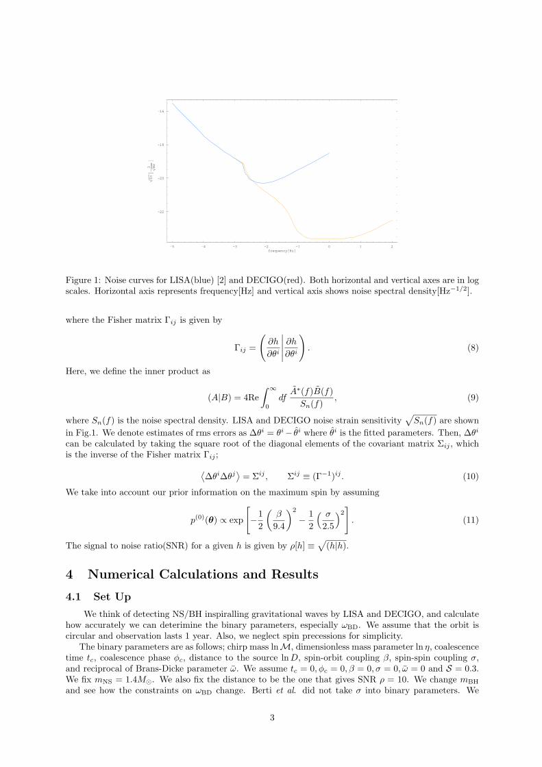
-5 -4 -3 -2 -1 0 1 2frequency@HzD
-22
-20
-18
-16
!!!!!!!
SnA
1
!!!!!!!
HzE
Figure 1: Noise curves for LISA(blue) [2] and DECIGO(red). Both horizontal and vertical axes are in logscales. Horizontal axis represents frequency[Hz] and vertical axis shows noise spectral density[Hz−1/2].
where the Fisher matrix Γij is given by
Γij =
(∂h
∂θi
∣∣∣∣∣∂h
∂θi
). (8)
Here, we define the inner product as
(A|B) = 4Re∫ ∞
0
dfA∗(f)B(f)
Sn(f), (9)
where Sn(f) is the noise spectral density. LISA and DECIGO noise strain sensitivity√
Sn(f) are shownin Fig.1. We denote estimates of rms errors as ∆θi = θi− θi where θi is the fitted parameters. Then, ∆θi
can be calculated by taking the square root of the diagonal elements of the covariant matrix Σij , whichis the inverse of the Fisher matrix Γij ;
⟨∆θi∆θj
⟩= Σij , Σij ≡ (Γ−1)ij . (10)
We take into account our prior information on the maximum spin by assuming
p(0)(θ) ∝ exp
[−1
2
(β
9.4
)2
− 12
( σ
2.5
)2]
. (11)
The signal to noise ratio(SNR) for a given h is given by ρ[h] ≡√
(h|h).
4 Numerical Calculations and Results
4.1 Set Up
We think of detecting NS/BH inspiralling gravitational waves by LISA and DECIGO, and calculatehow accurately we can deterimine the binary parameters, especially ωBD. We assume that the orbit iscircular and observation lasts 1 year. Also, we neglect spin precessions for simplicity.
The binary parameters are as follows; chirp mass lnM, dimensionless mass parameter ln η, coalescencetime tc, coalescence phase φc, distance to the source ln D, spin-orbit coupling β, spin-spin coupling σ,and reciprocal of Brans-Dicke parameter ω. We assume tc = 0, φc = 0, β = 0, σ = 0, ω = 0 and S = 0.3.We fix mNS = 1.4M¯. We also fix the distance to be the one that gives SNR ρ = 10. We change mBH
and see how the constraints on ωBD change. Berti et al. did not take σ into binary parameters. We
3
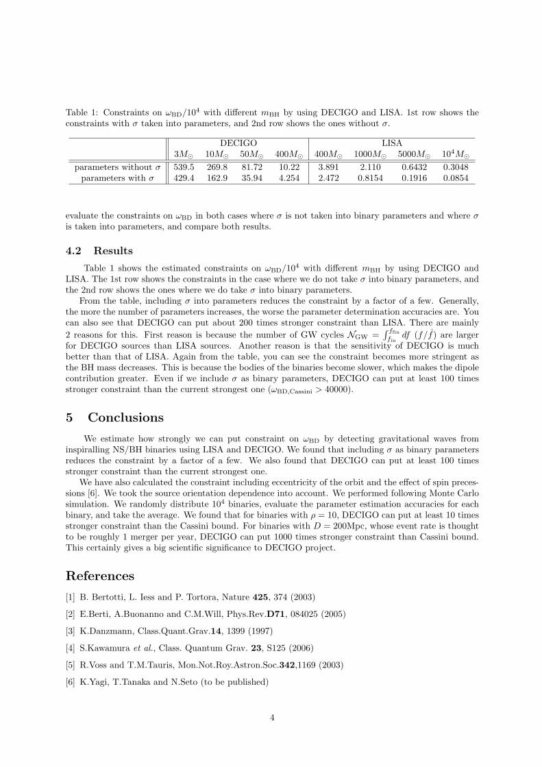
Table 1: Constraints on ωBD/104 with different mBH by using DECIGO and LISA. 1st row shows theconstraints with σ taken into parameters, and 2nd row shows the ones without σ.
DECIGO LISA3M¯ 10M¯ 50M¯ 400M¯ 400M¯ 1000M¯ 5000M¯ 104M¯
parameters without σ 539.5 269.8 81.72 10.22 3.891 2.110 0.6432 0.3048parameters with σ 429.4 162.9 35.94 4.254 2.472 0.8154 0.1916 0.0854
evaluate the constraints on ωBD in both cases where σ is not taken into binary parameters and where σis taken into parameters, and compare both results.
4.2 Results
Table 1 shows the estimated constraints on ωBD/104 with different mBH by using DECIGO andLISA. The 1st row shows the constraints in the case where we do not take σ into binary parameters, andthe 2nd row shows the ones where we do take σ into binary parameters.
From the table, including σ into parameters reduces the constraint by a factor of a few. Generally,the more the number of parameters increases, the worse the parameter determination accuracies are. Youcan also see that DECIGO can put about 200 times stronger constraint than LISA. There are mainly2 reasons for this. First reason is because the number of GW cycles NGW =
∫ ffin
findf (f/f) are larger
for DECIGO sources than LISA sources. Another reason is that the sensitivity of DECIGO is muchbetter than that of LISA. Again from the table, you can see the constraint becomes more stringent asthe BH mass decreases. This is because the bodies of the binaries become slower, which makes the dipolecontribution greater. Even if we include σ as binary parameters, DECIGO can put at least 100 timesstronger constraint than the current strongest one (ωBD,Cassini > 40000).
5 Conclusions
We estimate how strongly we can put constraint on ωBD by detecting gravitational waves frominspiralling NS/BH binaries using LISA and DECIGO. We found that including σ as binary parametersreduces the constraint by a factor of a few. We also found that DECIGO can put at least 100 timesstronger constraint than the current strongest one.
We have also calculated the constraint including eccentricity of the orbit and the effect of spin preces-sions [6]. We took the source orientation dependence into account. We performed following Monte Carlosimulation. We randomly distribute 104 binaries, evaluate the parameter estimation accuracies for eachbinary, and take the average. We found that for binaries with ρ = 10, DECIGO can put at least 10 timesstronger constraint than the Cassini bound. For binaries with D = 200Mpc, whose event rate is thoughtto be roughly 1 merger per year, DECIGO can put 1000 times stronger constraint than Cassini bound.This certainly gives a big scientific significance to DECIGO project.
References
[1] B. Bertotti, L. Iess and P. Tortora, Nature 425, 374 (2003)
[2] E.Berti, A.Buonanno and C.M.Will, Phys.Rev.D71, 084025 (2005)
[3] K.Danzmann, Class.Quant.Grav.14, 1399 (1997)
[4] S.Kawamura et al., Class. Quantum Grav. 23, S125 (2006)
[5] R.Voss and T.M.Tauris, Mon.Not.Roy.Astron.Soc.342,1169 (2003)
[6] K.Yagi, T.Tanaka and N.Seto (to be published)
4
Open Inflation in String Landscape
Daisuke Yamauchi†,1, Andrei Linde††,2, Misao Sasaki†,3, Takahiro Tanaka†,4 and Atsushi Naruko†,5
†Yukawa Institute for Theoretical Physics, Kyoto University, Kyoto 606–8502, Japan††Department of Physics, Stanford University, Stanford, CA 94305-4060, USA
AbstractThe recent observational data indicate that the universe is almost spatially flat. Nev-ertheless, the open inflationary scenario is attracting a renewed interest in the contextof string landscape. Since there are a large number of metastable de Sitter vacua instring landscape, tunneling transitions to lower metastable vacua through the bubblenucleation occur quite naturally, which leads to a natural realization of open infla-tion. Recently, it was argued anthropically that string landscape would lead to anestimate of the density parameter in the range Ω0 ≈ 0.998 ∼ 0.9996. Although thedeviation of Ω0 from unity, the effect of this small deviation on the CMB anisotropiesmight be significant. If their estimate of the value of Ω0 is correct, although yet thereis no consensus about the problem of the probability measure, we might be able todiscriminate the string landscape scenario from others. We argue that although thedeviation of Ω0 from unity may be small, the effect of this small deviation on thelarge angle CMB anisotropies may be significant for large angle mode in tensor-typeperturbation. We found that the large amplification of power spectrum occurs whenthe difference of false and true vacuum potential energy is exponentially large.
1 Introduction
The recent observational data indicate that the universe is almost spatially flat. Nevertheless, the openinflationary scenario is attracting a renewed interest in the context of ”string landscape” [2]. It realizedthat inflation may divide our universe into many exponentially large domains corresponding to differentmetastable vacuum, so-called ”inflationary multiverse”. Since in this context there are a enormous numberof metastable de Sitter vacua in the range of 10100 or 101000 and the global universe is an eternally inflating”megaverse” that is continually producing small pocket universes, the tunneling transitions to a lowermetastable vacuum and the bubble nucleation occurs quite naturally, which leads to a natural realizationof the open inflation scenario.
The basic idea of the one-bubble open inflationary scenario is following. Initially the scalar fieldis trapped in the false vaccum during the sufficiently long period such that it solve the homogeneityproblem and the our universe becomes well-approximated by a pure de Sitter space. Then, bubblenucleation occurs through quantum tunneling. The process is described by a Euclidean O(4)-symmetricbounce solution called Coleman-De Luccia (CDL) instanton [3]. The expanding bubble after nucleationis described by analytic continuation of the bounce solution to Lorentzian regime. The bubble formed byCDL instanton looks from the inside like an infinite open universe [3, 2]. If we assume that the vacuumenergy inside the bubble is nonzero, the second stage of inflation inside the bubble occurs and it solvesentropy problem and is necessary to avoid the curvature dominant universe.
Although the open inflation scenario, by definition, predicts nonzero spatial curvature of the universe,as long as the curvature is sufficiently small, this scenario will not contradict with observations. Recently,string theorists are interested in this kind of scenario [2] in context of string landscape by means ofanthropic argument. The most important cosmological consequence they claimed was that there wasa tunneling event in our past. Especially Freivogel et al. have estimated the present value of densityparameter Ω0 by using their landscape measure and the estimated value is given by Ω0 ≈ 0.998 ∼ 0.9996
1E-mail:[email protected]:[email protected]:[email protected]:[email protected]:[email protected]
1
by means of anthropic argument. Although the deviation of Ω0 from unity, the effect of this smalldeviation on the CMB anisotropies might be significant. If their estimate of the value of Ω0 is correct,although yet there is no consensus about the problem of the probability measure, we might be able todiscriminate the string landscape scenario from others.
We also have to comment the another distinct feature for the string landscape. Almost inflationarymodel inspired by string theory are formulated in the context of type IIB string theory with the Kachru-Kallosh-Linde-Trivedi(KKLT) stabilization mechanism [5]. There exists strong constraints on particlephenomenology and on inflation model and one can expect that the final slow-roll inflation must below-scale inflation. Also, one can naively expect that the shape of the global potential for landscape isdecided only by fundamental scale corresponding to Planck scale. Thus, the distinctive feature for stringlandscape is expected as the large difference of the hight of potential between false and true vacua. In thispaper, we will consider the possibility that ”open inflation scenario” can realize in ”string landscape”.Especially, we will focus on the power spectrum and power spectrum in open inflation scenario under thecondition one can expect that it is satisfied in string landscape [1].
2 Power spectrum for one-bubble open inflation model
We consider the system that consists of a minimally coupled scalar field, φ with the Einstein gravity. Wedenote the potential of the scalar field by V (φ). Let us consider the O(4)-symmetric bubble solution.We are, in particular, interested in the wall fluctuation mode, which will show up a distinctive feature ofopen inflation in the context of string landscape. An O(4)-symmetric bubble nucleation is described bythe Euclidean solution (instanton). The metric is given by
ds2 = dτ2E + a2
E(τE)(dχ2E + sin2 χEdΩ2) , (1)
and the background scalar field is denoted by φ = φ(τ). The Euclidean background equations are(aE
aE
)2
− 1a2
E
=κ
3
(12φ2 − V (φ)
),
(aE
aE
)·
+1
a2E
= −κ
2φ2 , φ + 3
aE
aEφ − V ′(φ) = 0 , (2)
where a dot “ ˙ ” represents differentiation with respect to τE . The background geometry and the fieldconfiguration in the Lorentzian regime are obtained by the analytic continuation of the bounce solution.Sometimes it is convenience to use the coordinate η defined by dτ = a(η)dη. The coordinates in theLorentzian regime are given by ηE = ηC = −ηR − π
2 i = ηL + π2 i , χE = −iχC + π
2 i = −iχR = −iχL , aE =aC = iaR = iaL.
From a gauge-invariant method developed by Garriga, Motes, Sasaki, Tanaka [4] in the one-fieldmodel of one-bubble open inflation, the tensor-type perturbation is conveniently described by a variablew, which is related to the transverse-traceless metric perturbation in the open universe. When we expandthis mode function in terms of the sherical harminics and spatial eigenfunction wp with eigenvalue p2,the equation for wp is given by [
− d2
dη2E
+ UT (ηE) − p2
]wp = 0 , (3)
where ηE denotes Euclidean conformal time defined by ηE =∫
dτE/aE and UT (ηE) = κφ′2/2.In order to compute the power spectrum at the end of inflation, we will define ”tansfer function” given
by In order to compute the power spectrum at the end of inflation, we will define an auxiliary ”transferfunction” given by
T pT = lim
ηR→ηendR
− κ
a2(p2 + 1)d
dηR(awp) , (4)
where ηendR denotes the value of the conformal time ηR for which a → ∞ and wp is the solution of the
equation which analytic continuation of Eq. (3) to region-R which satisfies the appropriate boundary
2
condition, i.e., behaves as wp → eipηR when ηR → −∞. Then, the power spectrum for tensor-typeperturbation can be expressed as [4]⟨¯
Up
¯2⟩ = 2|T p
T |2(p2 + 1) coth πp
κp
[1 − yeff
], (5)
where yeff represents the effects of the bubble wall and the phase factor of the transfer function.
3 CMB anisotropy in string landscape
3.1 Assumption
Before calculating the CMB anisotropy in the string landscape, we take the some assumption: As onecan expect naively, almost all information about the string landscape can be determined only by thefundamental scale (at least this is valid at sufficiently high energy region), i.e. Planck scale and/or stringscale, which leads that the shape and width of the potential for the scalar field are also determinedonly by fundamental scale. Futhermore, we assume that the final tunneling transition occurs throughCDL instanton. Typically, CDL instantons exists only if m2 ≡ V ′′ > H2
L ≡ κVfalse/3 during tunneling.Therefore we have to consider the steep potential after the tunneling. From the approximated equationsof motion, e.g., H2
L ∼ Vfalse/M2pl ,m
2 ∼ Vb/(4φ)2, we have the condition for the CDL instanton as
H2L
m2∼ Vfalse
Vb
(4φ)2
M2pl
<∼ 1 . (6)
In this paper, we will assume this CDL condition Eq. (6).Under these condition, one can show that the thin-wall approximation in region-C is almost valid, i.e.
the effective potential UT of the mode function wp in Eq. (3) has only local and small contribution inregion-C : UT ≈ 4sδ(ηC − ηW ) where 4s =
∫dηCUT (ηC) and ηW denotes the value of the conformal
time at the bubble wall. However, the tunneling transition through CDL instanton in our setup is notapproximated by exact thin wall since one can expect that the energy scale of the final inflation is prettylower than the fundamental scale due to the strong constrants from the particle phenomenology, i.e.there exists very large difference of the potential hight at the nucleation point of the bubble and at truevacuum. Thus, we find that the evolutionary behavior of scalar field inside the bubble is significant dueto the large potential gap.
3.2 Evolutionary behavior of scalar field inside bubble
Since the amplitude for the open inflation Eq. (5) is almost determined by the transfer function Eq. (4).The transfer function becomes constant for p2 +1 ¿ H2 except for the decaying mode. Then the transferfunction is approximated at the froze-in time tfroze(p) s.t. (p2 + 1) ≈ a2H2(tfroze):
T pT ≈ − κ
p2 + 1Hwp
¯t=tfroze(p)
, (7)
If one can neglect the effects of the evolution inside the bubble, mode function becomes the plane wavesolution in the all range and the transfer function is given by T p
T ≈ −κHR/(p2 + 1) where H2R = κVtrue.
However, in general the scale factor in Eq. (7) is no longer exactly de Sitter space and can evolve throughthe evolution of the scalar field. Also the mode function is no longer plane wave solution. Especially whenwe consider the large effects of the evolution or small p mode, i.e. (κφ′)max À p2, the mode function iswell-approximated by WKB solution from Eq. (3). In this case, one can see that the norm of wp can beexponentially enhanced. Reminding the boundary condition and the connection formulas at the turningpoint η = ηcrit(p) such that p2 = UT (ηcrit), one can obtain the WKB solution at η → ηfroze(p) as follow:
ln¯wp(ηfroze(p))
¯= A(small p) ∼
∫ ηfroze(p)
ηcrit(p)
dη′√
UT (η′) − 14
ln
[UT (ηfroze(p))UT (ηcrit(p))
], (8)
Thus, in this case the amplitude becomes exponentially larger than usual ones.
3
3.3 Power spectrum and multipole moment
Under these consideration in Sec. 3.1, 3.2, one can calculate the power spectrum by using the generalformula Eq. (5). In order to investigate the feature of the power spectrum, we assume that the energydensity of the scalar field at the nucleation point is not exponentially smaller than the wall tension. Thiscondition is naturally valid under the assumption in Sec. 3.1. One can see that the power spectrum fortensor-type perturbation is sharply peaked around p ≈ 0 mode, so-called ”wall fluctuation mode”. Notethat the amplitde can be larger than the usual ones in exact thin wall approximation due to the evolutioninside the bubble as we already mentioned in Sec. 3.2. For the large p mode, the amplitude becomes scaleinvariant spectrum : |Up|2p3 → κH2
R.Here we study how severely the revised open inflation scenarios based on the string landscape are
constrained after more detailed comparison with the observed CMB anisotropies. Although the observa-tional date indicate that our universe is almost spatially flat, the deviation of Ω0 from unity might besignificant in string landscape. Expanding all the quantities with respect to |1 − Ω0|, one can calculatethe approximateed multipole moment:
C(T )` ≈ f`
κH2Re2A0
4s(1 − Ω0)` ; f` =
(` + 1)(` + 2)100π
¯¯ Γ(` + 1)Γ(` + 3/2)
¯¯2 ¯¯1 + ` × z
1/2LSS
¯¯2
. (9)
where zLSS ≈ 1100 and A0 denotes the amplification factor due to the evolution of the scalar field insidethe bubble. By a certain fine-tunining of parameters one can obtain Eq. (8) as amplification factor.
4 Summary
In this paper we considered the possibility that ”open inflation scenario” can realize in ”string landscape”.We focused on the power spectrum and power spectrum in open inflation scenario under the conditionone can expect that it is satisfied in string landscape. We find that the multipole moment is in proportionto |1−Ω0|`. This means that the wall fluctuation mode corresponding to small p modes affects only small` mode in CMB fluctuations, especially when Ω is close to unity. An interesting observation is that therecan exist the enhancement factor A(p) due to the evolution inside the bubble. We found that the wallfluctuation mode is significant even in string landscape and the evolutionary behavior of scalar field insidethe bubble is sufficiently important the due to large difference of false and true potential energy. If thepotential energy at the nucleation point becomes pretty higher than the true one, the power spectrumbecomes amplified. The multipole moment for higher ` modes are highly suppressed by the deviationof the density parameter |1 − Ω0|. Thus, the wall fluctuation mode affects only small ` mode in CMBfluctuations. From these interesting oservations, we might be able to discriminate the string landscapescenario from others.
References
[1] D. Yamauchi, A. Linde, M. Sasaki, T. Tanaka, A. Naruko, in preparation
[2] L. Susskind, arXiv:hep-th/0302219 , B. Freivogel and L. Susskind, Phys. Rev. D 70, 126007 (2004)[arXiv:hep-th/0408133] , B. Freivogel, M. Kleban, M. Rodriguez Martinez and L. Susskind, JHEP0603, 039 (2006) [arXiv:hep-th/0505232].
[3] S. R. Coleman, Phys. Rev. D 15, 2929 (1977) [Erratum-ibid. D 16, 1248 (1977)] , S. R. Colemanand F. De Luccia, Phys. Rev. D 21, 3305 (1980).
[4] J. Garriga, X. Montes, M. Sasaki and T. Tanaka, Nucl. Phys. B 551, 317 (1999) [arXiv:astro-ph/9811257] , J. Garriga, X. Montes, M. Sasaki and T. Tanaka, Nucl. Phys. B 513, 343 (1998)[arXiv:astro-ph/9706229].
[5] S. Kachru, R. Kallosh, A. Linde and S. P. Trivedi, Phys. Rev. D 68, 046005 (2003) [arXiv:hep-th/0301240].
4
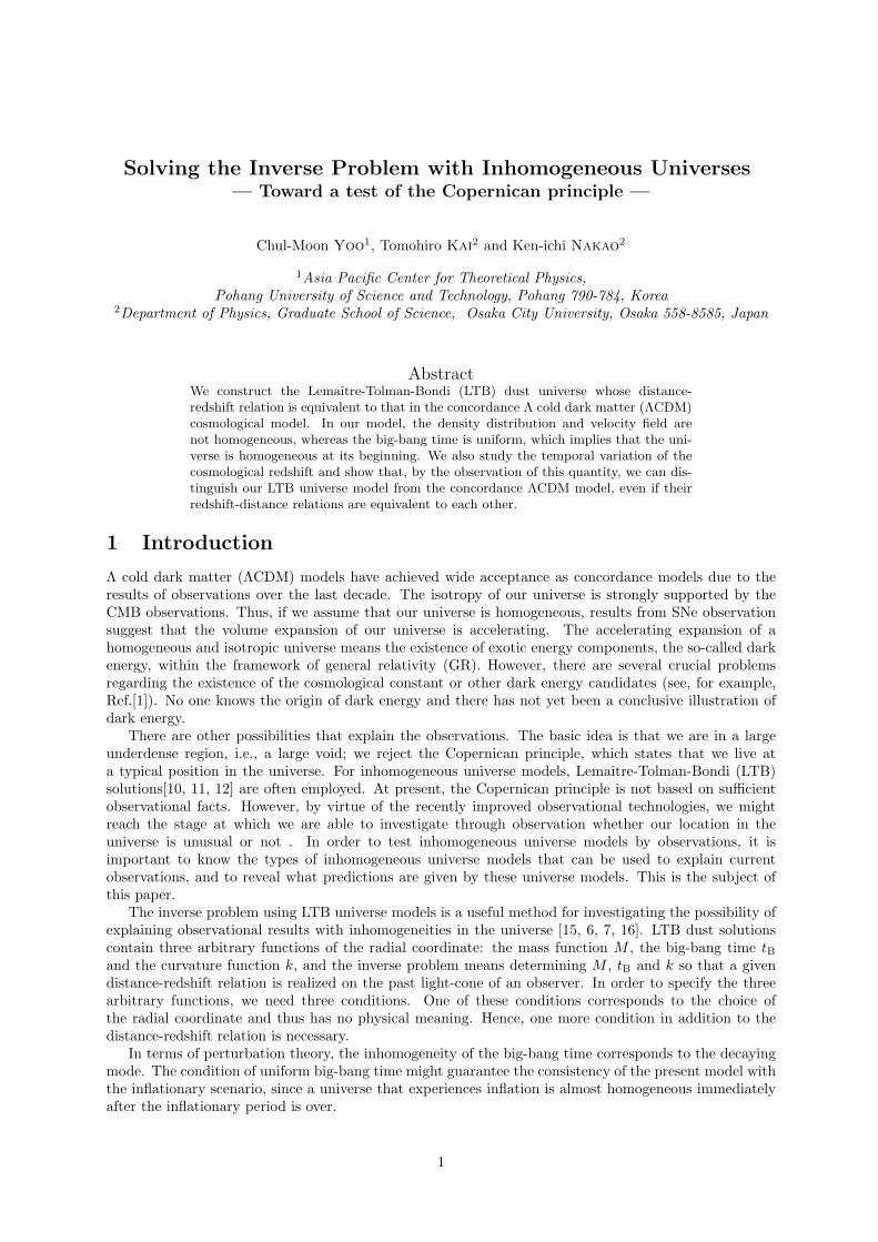
Solving the Inverse Problem with Inhomogeneous Universes— Toward a test of the Copernican principle —
Chul-Moon Yoo1, Tomohiro Kai2 and Ken-ichi Nakao2
1Asia Pacific Center for Theoretical Physics,Pohang University of Science and Technology, Pohang 790-784, Korea
2Department of Physics, Graduate School of Science, Osaka City University, Osaka 558-8585, Japan
AbstractWe construct the Lemaıtre-Tolman-Bondi (LTB) dust universe whose distance-redshift relation is equivalent to that in the concordance Λ cold dark matter (ΛCDM)cosmological model. In our model, the density distribution and velocity field arenot homogeneous, whereas the big-bang time is uniform, which implies that the uni-verse is homogeneous at its beginning. We also study the temporal variation of thecosmological redshift and show that, by the observation of this quantity, we can dis-tinguish our LTB universe model from the concordance ΛCDM model, even if theirredshift-distance relations are equivalent to each other.
1 Introduction
Λ cold dark matter (ΛCDM) models have achieved wide acceptance as concordance models due to theresults of observations over the last decade. The isotropy of our universe is strongly supported by theCMB observations. Thus, if we assume that our universe is homogeneous, results from SNe observationsuggest that the volume expansion of our universe is accelerating. The accelerating expansion of ahomogeneous and isotropic universe means the existence of exotic energy components, the so-called darkenergy, within the framework of general relativity (GR). However, there are several crucial problemsregarding the existence of the cosmological constant or other dark energy candidates (see, for example,Ref.[1]). No one knows the origin of dark energy and there has not yet been a conclusive illustration ofdark energy.
There are other possibilities that explain the observations. The basic idea is that we are in a largeunderdense region, i.e., a large void; we reject the Copernican principle, which states that we live ata typical position in the universe. For inhomogeneous universe models, Lemaıtre-Tolman-Bondi (LTB)solutions[10, 11, 12] are often employed. At present, the Copernican principle is not based on sufficientobservational facts. However, by virtue of the recently improved observational technologies, we mightreach the stage at which we are able to investigate through observation whether our location in theuniverse is unusual or not . In order to test inhomogeneous universe models by observations, it isimportant to know the types of inhomogeneous universe models that can be used to explain currentobservations, and to reveal what predictions are given by these universe models. This is the subject ofthis paper.
The inverse problem using LTB universe models is a useful method for investigating the possibility ofexplaining observational results with inhomogeneities in the universe [15, 6, 7, 16]. LTB dust solutionscontain three arbitrary functions of the radial coordinate: the mass function M , the big-bang time tBand the curvature function k, and the inverse problem means determining M , tB and k so that a givendistance-redshift relation is realized on the past light-cone of an observer. In order to specify the threearbitrary functions, we need three conditions. One of these conditions corresponds to the choice ofthe radial coordinate and thus has no physical meaning. Hence, one more condition in addition to thedistance-redshift relation is necessary.
In terms of perturbation theory, the inhomogeneity of the big-bang time corresponds to the decayingmode. The condition of uniform big-bang time might guarantee the consistency of the present model withthe inflationary scenario, since a universe that experiences inflation is almost homogeneous immediatelyafter the inflationary period is over.
1
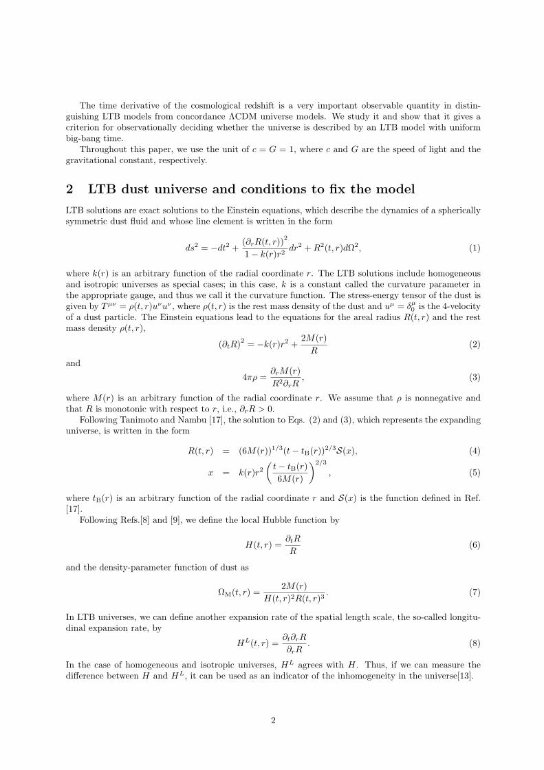
The time derivative of the cosmological redshift is a very important observable quantity in distin-guishing LTB models from concordance ΛCDM universe models. We study it and show that it gives acriterion for observationally deciding whether the universe is described by an LTB model with uniformbig-bang time.
Throughout this paper, we use the unit of c = G = 1, where c and G are the speed of light and thegravitational constant, respectively.
2 LTB dust universe and conditions to fix the model
LTB solutions are exact solutions to the Einstein equations, which describe the dynamics of a sphericallysymmetric dust fluid and whose line element is written in the form
ds2 = −dt2 +(∂rR(t, r))2
1− k(r)r2dr2 + R2(t, r)dΩ2, (1)
where k(r) is an arbitrary function of the radial coordinate r. The LTB solutions include homogeneousand isotropic universes as special cases; in this case, k is a constant called the curvature parameter inthe appropriate gauge, and thus we call it the curvature function. The stress-energy tensor of the dust isgiven by Tµν = ρ(t, r)uνuν , where ρ(t, r) is the rest mass density of the dust and uµ = δµ
0 is the 4-velocityof a dust particle. The Einstein equations lead to the equations for the areal radius R(t, r) and the restmass density ρ(t, r),
(∂tR)2 = −k(r)r2 +2M(r)
R(2)
and
4πρ =∂rM(r)R2∂rR
, (3)
where M(r) is an arbitrary function of the radial coordinate r. We assume that ρ is nonnegative andthat R is monotonic with respect to r, i.e., ∂rR > 0.
Following Tanimoto and Nambu [17], the solution to Eqs. (2) and (3), which represents the expandinguniverse, is written in the form
R(t, r) = (6M(r))1/3(t− tB(r))2/3S(x), (4)
x = k(r)r2
(t− tB(r)6M(r)
)2/3
, (5)
where tB(r) is an arbitrary function of the radial coordinate r and S(x) is the function defined in Ref.[17].
Following Refs.[8] and [9], we define the local Hubble function by
H(t, r) =∂tR
R(6)
and the density-parameter function of dust as
ΩM(t, r) =2M(r)
H(t, r)2R(t, r)3. (7)
In LTB universes, we can define another expansion rate of the spatial length scale, the so-called longitu-dinal expansion rate, by
HL(t, r) =∂t∂rR
∂rR. (8)
In the case of homogeneous and isotropic universes, HL agrees with H. Thus, if we can measure thedifference between H and HL, it can be used as an indicator of the inhomogeneity in the universe[13].
2
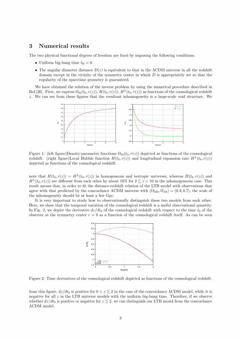
3 Numerical results
The two physical functional degrees of freedom are fixed by imposing the following conditions.
• Uniform big-bang time tB = 0.
• The angular diameter distance D(z) is equivalent to that in the ΛCDM universe in all the redshiftdomain except in the vicinity of the symmetry center in which D is appropriately set so that theregularity of the spacetime geometry is guaranteed.
We have obtained the solution of the inverse problem by using the numerical procedure described inRef.[20]. First, we express ΩM(t0, r(z)), H(t0, r(z)), HL(t0, r(z)) as functions of the cosmological redshiftz. We can see from these figures that the resultant inhomogeneity is a large-scale void structure. We
0
0.1
0.2
0.3
0.4
0.5
0.6
0.7
0.8
0.9
0 2 4 6 8 10
ΩM
Redshift
0.65
0.7
0.75
0.8
0.85
0.9
0.95
1
0 2 4 6 8 10
H/H
0
Redshift
H
HL
Figure 1: (left figure)Density-parameter functions ΩM(t0, r(z)) depicted as functions of the cosmologicalredshift. (right figure)Local Hubble function H(t0, r(z)) and longitudinal expansion rate HL(t0, r(z))depicted as functions of the cosmological redshift.
note that H(t0, r(z)) = HL(t0, r(z)) in homogeneous and isotropic universes, whereas H(t0, r(z)) andHL(t0, r(z)) are different from each other by about 10% for 2 <∼ z < 10 in the inhomogeneous case. Thisresult means that, in order to fit the distance-redshift relation of the LTB model with observations thatagree with that predicted by the concordance ΛCDM universe with (ΩM0,ΩΛ0) = (0.3, 0.7), the scale ofthe inhomogeneity should be at least a few Gpc.
It is very important to study how to observationally distinguish these two models from each other.Here, we show that the temporal variation of the cosmological redshift is a useful observational quantity.In Fig. 2, we depict the derivative dz/dt0 of the cosmological redshift with respect to the time t0 of theobserver at the symmetry center r = 0 as a function of the cosmological redshift itself. As can be seen
-1.2
-1
-0.8
-0.6
-0.4
-0.2
0
0.2
0.4
0 0.5 1 1.5 2
dz/d
t 0
Redshift
LTBΛCDM
Figure 2: Time derivatives of the cosmological redshift depicted as functions of the cosmological redshift.
from this figure, dz/dt0 is positive for 0 < z <∼ 2 in the case of the concordance ΛCDM model, while it isnegative for all z in the LTB universe models with the uniform big-bang time. Therefore, if we observewhether dz/dt0 is positive or negative for z <∼ 2, we can distinguish our LTB model from the concordanceΛCDM model.
3
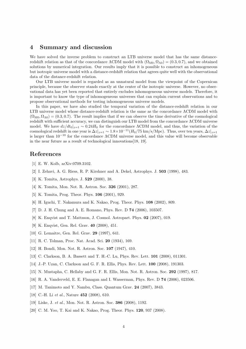
4 Summary and discussion
We have solved the inverse problem to construct an LTB universe model that has the same distance-redshift relation as that of the concordance ΛCDM model with (ΩM0, ΩΛ0) = (0.3, 0.7), and we obtainedsolutions by numerical integration. Our results imply that it is possible to construct an inhomogeneousbut isotropic universe model with a distance-redshift relation that agrees quite well with the observationaldata of the distance-redshift relation.
Our LTB universe model is regarded as an unnatural model from the viewpoint of the Copernicanprinciple, because the observer stands exactly at the center of the isotropic universe. However, no obser-vational data has yet been reported that entirely excludes inhomogeneous universe models. Therefore, itis important to know the type of inhomogeneous universes that can explain current observations and topropose observational methods for testing inhomogeneous universe models.
In this paper, we have also studied the temporal variation of the distance-redshift relation in ourLTB universe model whose distance-redshift relation is the same as the concordance ΛCDM model with(ΩM0, ΩΛ0) = (0.3, 0.7). The result implies that if we can observe the time derivative of the cosmologicalredshift with sufficient accuracy, we can distinguish our LTB model from the concordance ΛCDM universemodel. We have dz/dt0|z=1 ∼ 0.24H0 for the concordance ΛCDM model, and thus, the variation of thecosmological redshift in one year is ∆z|z=1 ∼ 1.8×10⁻¹¹(H0/75 km/s/Mpc). Thus, over ten years, ∆z|z=1
is larger than 10−10 for the concordance ΛCDM universe model, and this value will become observablein the near future as a result of technological innovations[18, 19].
References
[1] E. W. Kolb, arXiv:0709.3102.
[2] I. Zehavi, A. G. Riess, R. P. Kirshner and A. Dekel, Astrophys. J. 503 (1998), 483.
[3] K. Tomita, Astrophys. J. 529 (2000), 38.
[4] K. Tomita, Mon. Not. R. Astron. Soc. 326 (2001), 287.
[5] K. Tomita, Prog. Theor. Phys. 106 (2001), 929.
[6] H. Iguchi, T. Nakamura and K. Nakao, Prog. Theor. Phys. 108 (2002), 809.
[7] D. J. H. Chung and A. E. Romano, Phys. Rev. D 74 (2006), 103507.
[8] K. Enqvist and T. Mattsson, J. Cosmol. Astropart. Phys. 02 (2007), 019.
[9] K. Enqvist, Gen. Rel. Grav. 40 (2008), 451.
[10] G. Lemaitre, Gen. Rel. Grav. 29 (1997), 641.
[11] R. C. Tolman, Proc. Nat. Acad. Sci. 20 (1934), 169.
[12] H. Bondi, Mon. Not. R. Astron. Soc. 107 (1947), 410.
[13] C. Clarkson, B. A. Bassett and T. H.-C. Lu, Phys. Rev. Lett. 101 (2008), 011301.
[14] J.-P. Uzan, C. Clarkson and G. F. R. Ellis, Phys. Rev. Lett. 100 (2008), 191303.
[15] N. Mustapha, C. Hellaby and G. F. R. Ellis, Mon. Not. R. Astron. Soc. 292 (1997), 817.
[16] R. A. Vanderveld, E. E. Flanagan and I. Wasserman, Phys. Rev. D 74 (2006), 023506.
[17] M. Tanimoto and Y. Nambu, Class. Quantum Grav. 24 (2007), 3843.
[18] C.-H. Li et al., Nature 452 (2008), 610.
[19] Liske, J. et al., Mon. Not. R. Astron. Soc. 386 (2008), 1192.
[20] C. M. Yoo, T. Kai and K. Nakao, Prog. Theor. Phys. 120, 937 (2008).
4
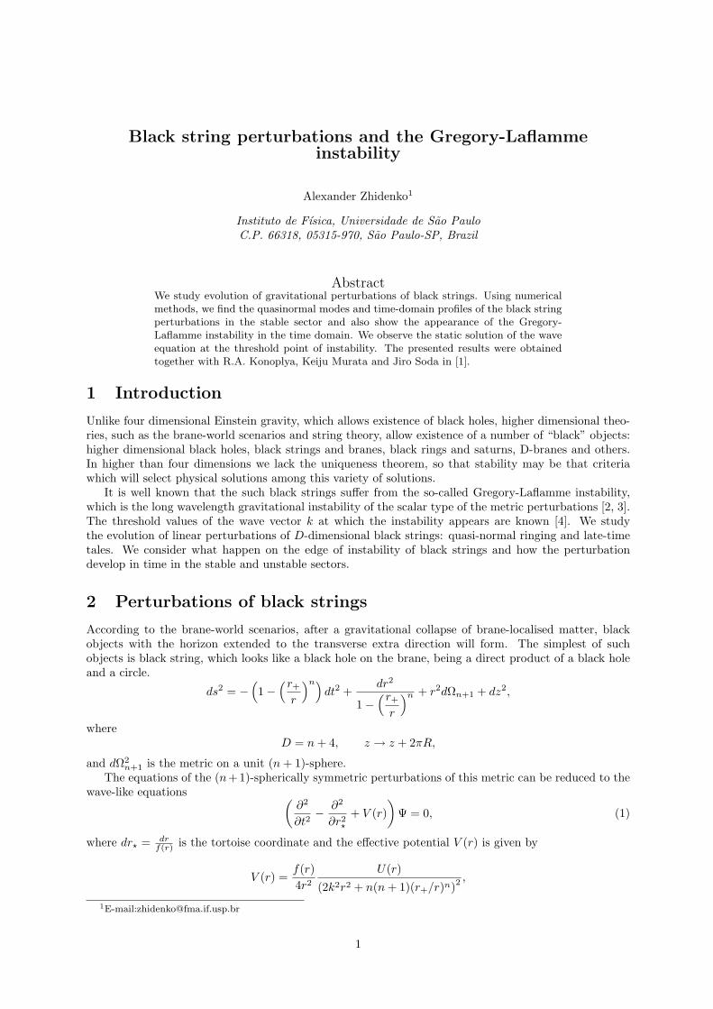
Black string perturbations and the Gregory-Laflammeinstability
Alexander Zhidenko1
Instituto de Fısica, Universidade de Sao PauloC.P. 66318, 05315-970, Sao Paulo-SP, Brazil
AbstractWe study evolution of gravitational perturbations of black strings. Using numericalmethods, we find the quasinormal modes and time-domain profiles of the black stringperturbations in the stable sector and also show the appearance of the Gregory-Laflamme instability in the time domain. We observe the static solution of the waveequation at the threshold point of instability. The presented results were obtainedtogether with R.A. Konoplya, Keiju Murata and Jiro Soda in [1].
1 Introduction
Unlike four dimensional Einstein gravity, which allows existence of black holes, higher dimensional theo-ries, such as the brane-world scenarios and string theory, allow existence of a number of “black” objects:higher dimensional black holes, black strings and branes, black rings and saturns, D-branes and others.In higher than four dimensions we lack the uniqueness theorem, so that stability may be that criteriawhich will select physical solutions among this variety of solutions.
It is well known that the such black strings suffer from the so-called Gregory-Laflamme instability,which is the long wavelength gravitational instability of the scalar type of the metric perturbations [2, 3].The threshold values of the wave vector k at which the instability appears are known [4]. We studythe evolution of linear perturbations of D-dimensional black strings: quasi-normal ringing and late-timetales. We consider what happen on the edge of instability of black strings and how the perturbationdevelop in time in the stable and unstable sectors.
2 Perturbations of black strings
According to the brane-world scenarios, after a gravitational collapse of brane-localised matter, blackobjects with the horizon extended to the transverse extra direction will form. The simplest of suchobjects is black string, which looks like a black hole on the brane, being a direct product of a black holeand a circle.
ds2 = −(1−
(r+
r
)n)dt2 +
dr2
1−(r+
r
)n + r2dΩn+1 + dz2,
whereD = n + 4, z → z + 2πR,
and dΩ2n+1 is the metric on a unit (n + 1)-sphere.
The equations of the (n+1)-spherically symmetric perturbations of this metric can be reduced to thewave-like equations (
∂2
∂t2− ∂2
∂r2?
+ V (r))
Ψ = 0, (1)
where dr? = drf(r) is the tortoise coordinate and the effective potential V (r) is given by
V (r) =f(r)4r2
U(r)(2k2r2 + n(n + 1)(r+/r)n)2
,
1E-mail:[email protected]
1
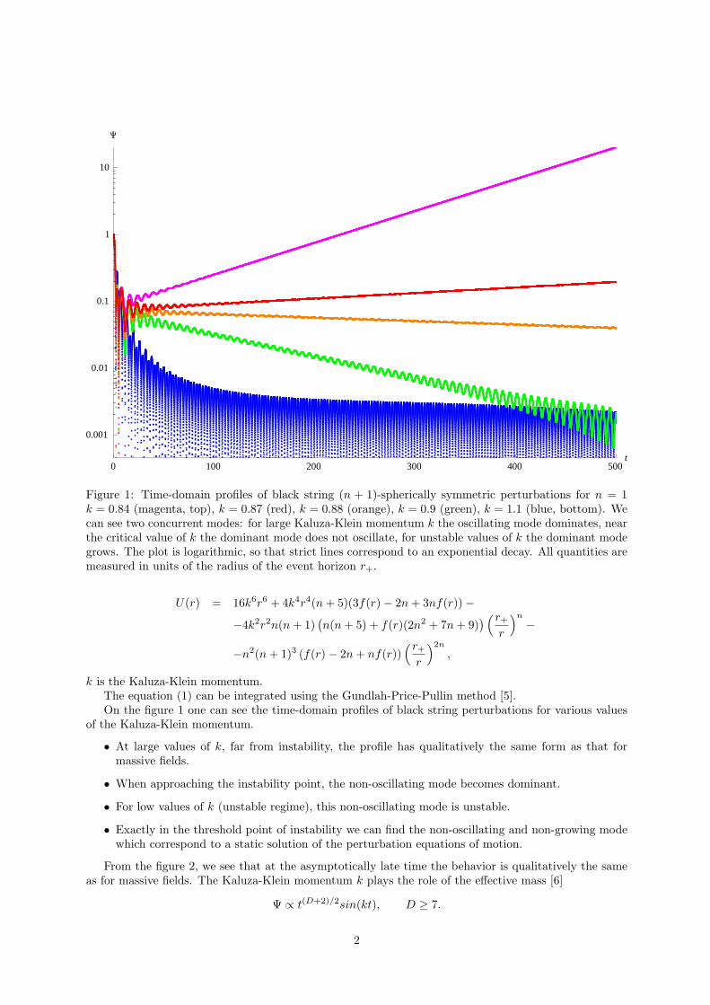
0 100 200 300 400 500t
0.001
0.01
0.1
1
10
Y
Figure 1: Time-domain profiles of black string (n + 1)-spherically symmetric perturbations for n = 1k = 0.84 (magenta, top), k = 0.87 (red), k = 0.88 (orange), k = 0.9 (green), k = 1.1 (blue, bottom). Wecan see two concurrent modes: for large Kaluza-Klein momentum k the oscillating mode dominates, nearthe critical value of k the dominant mode does not oscillate, for unstable values of k the dominant modegrows. The plot is logarithmic, so that strict lines correspond to an exponential decay. All quantities aremeasured in units of the radius of the event horizon r+.
U(r) = 16k6r6 + 4k4r4(n + 5)(3f(r)− 2n + 3nf(r))−−4k2r2n(n + 1)
(n(n + 5) + f(r)(2n2 + 7n + 9)
) (r+
r
)n
−
−n2(n + 1)3 (f(r)− 2n + nf(r))(r+
r
)2n
,
k is the Kaluza-Klein momentum.The equation (1) can be integrated using the Gundlah-Price-Pullin method [5].On the figure 1 one can see the time-domain profiles of black string perturbations for various values
of the Kaluza-Klein momentum.
• At large values of k, far from instability, the profile has qualitatively the same form as that formassive fields.
• When approaching the instability point, the non-oscillating mode becomes dominant.
• For low values of k (unstable regime), this non-oscillating mode is unstable.
• Exactly in the threshold point of instability we can find the non-oscillating and non-growing modewhich correspond to a static solution of the perturbation equations of motion.
From the figure 2, we see that at the asymptotically late time the behavior is qualitatively the sameas for massive fields. The Kaluza-Klein momentum k plays the role of the effective mass [6]
Ψ ∝ t(D+2)/2sin(kt), D ≥ 7.
2
20 50 100 200 500 1000 2000t
10-8
10-6
10-4
0.01
Y
Figure 2: Time-domain profiles of black string (n + 1)-spherically symmetric perturbations for k = 2.5n = 2 (red, top), n = 3 (orange), n = 4 (green), n = 5 (blue, bottom). Late-time decay of perturbationsfor n ≥ 3 is ∝ t−(n+6)/2. All quantities are measured in units of the radius of the event horizon r+.
3
The first overtone’s behavior is qualitatively similar to that of the fundamental mode for massivefields of higher-dimensional Schwarzschild black holes [7, 8]:
• For D = 5, as k grows, the imaginary part of the first overtone quickly decreases and vanishes forsome threshold value of k, while its real part stays smaller than the threshold value of k. After thethreshold value is reached, the first overtone “disappears”.
• For D ≥ 6, the imaginary part of the first overtone becomes small for large k, while the real partasymptotically approaches k.
3 Conclusions
1. We have found the quasinormal modes and late-time tails for scalar type of gravitational pertur-bations of D-dimensional black strings, that is for the type of perturbations where the Gregory-Laflamme instability forms.
2. In the stable sector the behavior of the perturbations evolution is qualitatively similar to thebehavior of the scalar field in the Schwarzschild background.
3. The time domain profiles indicate that the threshold instability value of k corresponds to dominanceof some static solution.
References
[1] R. A. Konoplya, K. Murata, J. Soda and A. Zhidenko, Phys. Rev. D 78, 084012 (2008)[arXiv:0807.1897 [hep-th]].
[2] R. Gregory and R. Laflamme, Phys. Rev. Lett. 70, 2837 (1993) [arXiv:hep-th/9301052].
[3] R. Gregory and R. Laflamme, Nucl. Phys. B 428 (1994) 399 [arXiv:hep-th/9404071].
[4] J. L. Hovdebo and R. C. Myers, Phys. Rev. D 73 (2006) 084013 [arXiv:hep-th/0601079].
[5] C. Gundlach, R. H. Price and J. Pullin, Phys. Rev. D 49, 883 (1994) [arXiv:gr-qc/9307009].
[6] R. A. Konoplya, C. Molina and A. Zhidenko, Phys. Rev. D 75 (2007) 084004 [arXiv:gr-qc/0602047].
[7] A. Zhidenko, Phys. Rev. D 74 (2006) 064017 [arXiv:gr-qc/0607133].
[8] R. A. Konoplya and A. Zhidenko, Phys. Lett. B 609 (2005) 377 [arXiv:gr-qc/0411059].
4
Deparametrized Quantum Cosmology with Phantom Dust
Fumitoshi Amemiya1 and Tatsuhiko Koike2
Faculty of Science and Technology, Keio University3-14-1 Hiyoshi, Kohoku-ku, 223-8522 Yokohama Japan
AbstractWe study a canonical, reduced phase space quantization of the at Friedmann-Robertson-Walker universe which is formulated as a gauge invariant fashion in theclassical theory. We construct a wave packet as the wave function of the universe andcompute the expectation value of the scale factor. As a results, it is shown that theinitial singularity of the universe is avoided in our models.
1 Introduction
The modern cosmolgy is mainly based on General Relativity (GR). However, since GR breaks down atthe singularity, one must construct a quantum theory of gravity in order to understand what is occuringnear the singularity. Because we still do not have a complete quantum theory of gravity, a number ofworks for this purpose have been done by first carrying out a symmetry reduction, e.g. homogeneousand isotropic one, and then quantizing the resulting models. Although various interesting results aresuggested so far, these previous works seem imcomplete at least in the sense that there are not enoughconsiderarions for the problem of time, which is inevitable when one tries to quantize GR canonically.Roughly speaking, the problem of time is that the time evolution of a wave function is lost in canonicalquantum gravity because time has no physical meaning in GR.
Recently Dittrich developed Rovelli’s relational formalism [1] for constructing gauge invariant quan-tities [2, 3]. The application of this formalism to the Friedmann-Robertson-Walker (FRW) universe withdynamical dust [4] provide a possible resolultion to the problem of time. We assume that this dynamicaldust has negative energy in order for the physical Hamiltonian to become positive difinite, and this dustis called Phantom dust [5]. In our study, we canonically quantize this gauge-invariantly reformulatedFRW universe with Phantom dust by using a reduced phase space quantization method [6].
2 Relational formalism for deparametrized theories
In this section we summarize the relational formalism especially for deparametrized theories, which isenough to treat the FRW universe. Here, “deparametrized theory” means that one can find phase spacecoordinates qa, T ; pa, P such that the constraints can be written in the form C = P + h(qa, pa).
We consider the system which contains only one constraint for simplisity. In the relational formalism,the key observation to define gauge invariant quantities is as follows: Take two functions F and T . Thenthe value of F when T = is gauge invariant even if F and T themselves are gauge variant respectively.We can interpret the function T as a clock. The mathematical definition of the gauge invariant quantityOF () is given by
OF () := tC(F )|t
C(T )= . (1)
Here, tC(F ) denotes the action of the gauge transformation generated by C on the function F , which is
defined as
tC(F ) :=
∞∑n=0
tn
n!C,F(n), (2)
C,F(0) := F, C,F(n+1) :=C, C,F(n)
,
1E-mail:[email protected]:[email protected]
1
where t is a gauge parameter. In other words, OF () can be interpreted as the gauge invariant extentionof F along gauge orbits.
In order to reduce the phase space, we consider the map O : F 7→ OF () on the phase spacecoordinates qa, T ; pa, P. The homomorphism property of the map O is used in the calculation below.The gauge invariant quantity associated to T ,
OT () = tC(T )|t
C(T )= = , (3)
becomes simply a constant value . Then the same calculation associated to P on the constraint surfaceyields
OP () = −Oh() = h (Oqa(), Opa()) =: −H. (4)
Thus OP () is expressed in terms of Oqa() and Opa() on the constraint surface. Finally, the Poissonbracket of Oqa() and Opa() is given by
Oqa(), Opa() = Oqa,pb() = Oab() = a
b . (5)
The above discussion shows that the reduced phase space is coordinatized by a conjugate pair (Oqa(), Opa())and the symplectic structure has a simple expression in terms of them. Moreover, it is shown that thefunctionH becomes a true physical Hamiltonian which generates the time evolution of the gauge invariantquantities:
∂OF ()∂
= H,OF () . (6)
Thus we now have the time evolution of the gauge invariant quantity, so that the problem of time hascompletely been resolved in the present case. Since the reduced phase space is characterized by (5) and(6), we can quantize the system by the ordinary quantization method with no constraints.
3 FRW universe with Phantom dust
In order to use the reduced phase space quantization method to the FRW universe, we must first de-parametrize the system. It is known that the system is completely deparametrized by adding the pressurefree dust Lagrangian to the usual Einstein-Hilbert action [4]. We add the dust with negative energy, whichis called Phantom dust as mentioned above.
The action of Phantom dust is given by
Sdust = −12
∫M
d4x√−g(gµνUµUν + 1). (7)
Here, g is the determinant of the metric tensor gµν on the spacetime manifold M , is the energy densityand the 1-form U is defined by U = −dT +WidS
i, where the vector field Uµ = gµνUν is tangent to anaffinely parametrized geodesic, T defines the proper time along each geodesic and Wi and Si are constantsalong geodesics. The variable Si labels the geodesics along the fluid particles. Phantom dust fills thespacetime, so that (T, Si) can be used as coordinates on M .
In the case of the FRW universe, the Einstein-Hilbert action with Phantom dust is written as
S =∫dt
(paa+ PT,t −NCtot
), (8)
Ctot = C + P, (9)
C = −c2 p2a
12a+
Λa3
+ ma
3 − 3ka. (10)
Here, a is the scale factor, pa is its conjugate momentum, c is the speed of light, Λ is the cosmologicalconstant, m is the energy density of the matter except Phantom dust and the constant k = ±1, 0determine the curvature of the three dimensional space. In this work, we consider the k = 0 case which
2
corresponds to the flat universe. In general, since the volume of the three-space and the Hamiltonian willdiverge in the flat case, we must get rid of this divergence. In the present work, we solve this problemby assuming that the topology of the universe is compact. For simplisity, we only consider the case ofthree-dimensional torus where the fiducial cell is a cube. We shall interpret the scale factor as the lengthof an edge of the cube, which in fact represent the physical size of the universe.
The reduced phase space are coordinatized by
A() := Oa(), PA() := Opa() (11)
and the symplectic structure is given by
A(), PA() = 1. (12)
The Hamiltonian which generates time evolution of gauge invariant variables becomes
H : = h′(A,PA)
= −c2 P2A
12A+
ΛA3
+ mA
3. (13)
4 Quantization of the model
In order to quantize the previously derived system, we simply replace the classical Poisson bracket relationand the Hamilton equation,
A,PA = 1 ,dF
d= H,F , F = F (A,PA), (14)
with the quantum commutation relation and the Heisenberg equation,
[A, PA] = i~ ,dF
d=
1i~
[H, F ]. (15)
We choose the Schrodinger representation,
|Ψ⟩ → Ψ(A), A|Ψ⟩ → AΨ(A), PA|Ψ⟩ → −i~ ∂
∂AΨ(A). (16)
Since we would like to restrict the range of the scale factor as A ≥ 0, it is necessary to consider a conditionto ensure the self-adjointness of the Hamiltonian in the space L2(0,∞).
To this end, we choose the operator ordering of the Hamiltonian as
H = −c2 112A
P 2A +
ΛA3
+ m(A)A3 (17)
and define the inner product by
⟨Ψ,Φ⟩ :=∫ ∞
0
Ψ∗(A)Φ(A)AdA. (18)
Then, it can be shown that the following boundary conditions to a wave function ensure the self-adjointness of the Hamiltonian [7]:
(1) (0, t) = 0, or (2)d
dt(0, t) = 0. (19)
The Schrodinger-Wheeler-DeWitt equation (time-dependent Schrodinger equation) is
i~∂Ψ∂
=c2~2
12A∂2Ψ∂A2
+(
ΛA3
+R
A
)Ψ, (20)
3
where R is a constant which corresponds to the total energy of a radiation in the universe.In this proceeding, we consider only the case Λ = R = 0 in which one can analytically solve the
differential equation (20). The energy eigenvalue equation is
14x
d2 (x)dx2
= E (x). (21)
Here, we have introduced the dimensionless variables x := AA0
and t := H0 , where A0 := ~H0c0
, c0 = 3H20
c2
and H0 is the present value of Hubble’s constant. The general solution of this equation takes the form
(x) = C1Ai(−y) + C2Bi(−y)
=√y
[C3J 1
3
(23y
32
)+ C4J− 1
3
(23y
32
)], (22)
where y is given by y := [4(Ωm − E)]13x, Ai and Bi are Airy functions, J± 1
3are Bessel functions and
Cj ’s are arbitrary constants. We can construct the following wave packets by superposing the energyeigenstates,
Ψ(1)(x, t) =x
(2)43e−
x34α−iΩmt, (23)
Ψ(2)(x, t) =1
(2)23e−
x34α−iΩmt, (24)
where := − i 916 t. These wave packets correspond to the two types of boundary conditions (19). The
expectation value of x is given by
⟨x⟩ =
∫ ∞0xΨ∗(x, t)xΨ(x, t)dx∫ ∞
0xΨ∗(x, t)Ψ(x, t)dx
. (25)
The calculation of the right hand side for the wave packets above leads to
⟨x⟩(1) =2Γ
(53
)3Γ
(73
) ( 2 +
(916 t
)2
2
) 13
, (26)
⟨x⟩(2) =4
3 · 2 13 Γ
(53
) ( 2 +
(916 t
)2
2
) 13
. (27)
These solutions represent a bounsing universe with no singularity because the expectation value of xnever goes to zero in both cases.
References
[1] C.Rovelli, Phys.Rev.D 42, 2638 (1990)
[2] B.Dittrich, gr-qc/0411013
[3] B.Dittrich, Class.Quant.Grav. 23, 6155 (2006)
[4] J.D.Brown and K.V.Kuchar, Phys.Rev.D 51, 5600 (1995)
[5] K.Giesel, T.Thiemann, arXiv:0711.0119[gr-qc]
[6] T.Thiemann, Class.Quant.Grav. 23, 1163 (2006)
[7] F.G.Alvarenga and N.A.Lemos, Gen.Rel.Grav. 30, 681 (1998)
4
Influence of Dark Matter on Light Propagationin Solar System Experiment
Hideyoshi Arakida1
School of Education, Waseda University1-6-1, Nishiwaseda, Shinjuku, Tokyo 169-8050 JAPAN
AbstractWe investigated the influence of dark matter on light/signal propagation in the solarsystem. We concentrated on the gravitational time delay and relative frequency shiftand took the effect of solar system-bound dark matter into consideration. As theapplication of results, we considered the secular increasing of the astronomical unitreported by Krasinsky and Brumberg (2004).
1 Introduction
It is considered the dark matter is the essential component of the Universe, then it is worth to investigatethe possibility to detect and estimate its abundance in our Solar System. Especially, recent astronomi-cal/astrophysical measurements in the solar system have been grown drastically. Due to such a context,till now, the gravitational influence of dark matter on the planetary motion, such as the additional peri-helion advance, has aroused interest and studied by several authors. The effect of galactic dark matter onthe planetary dynamics are considered by [6, 12, 14, 15]. On the other hand, the upper limit of density ofdark matter bound in the solar system has been estimated by [3, 8, 11, 9, 17, 10, 7]. Also planet-bounddark matter is evaluated by [1, 2].
While its contribution to the light/signal propagation has hardly been examined in disregard of thefact the current accurate observations are archived by the improvement of observational of light/signaland perhaps this advance will go on. Then from these situations, it is interesting to examine how theexistence of dark matter bound in solar system affects the light/signal propagation and whether we candetect its traces from the observations of light/signal.
We will study the influence of dark matter on the light/signal propagation in the solar system. First,under the spherical symmetry, we derive the approximate solution of Einstein equation which consistsof gravitational field due to the central celestial body as the Sun and the thin distributed dark mattersurrounding to the external region of central body. Then we will concentrate on the light/signal prop-agation and calculate the additional effects due to the dark matter on the gravitational time delay andthe relative frequency shift. As the application of results, we consider the problem of secular increase ofastronomical unit (of length) AU reported by Krasinsky and Brumberg (2004) [13].
2 Approximate Solution of Einstein Equation
We seek the spherically symmetric form of spacetime as,
ds2 = −eµc2dt2 + eνdr2 + r2(dθ2 + sin2 θdφ2), (1)
where µ, ν are the function of time t and radius r, and c is the speed of light in vacuum. As thestress-energy tensor Tα
β , we suppose as,
T 00 = −%(t, r)c2, T 1
0 = σ(t, r)c, T ij = 0. (2)
T 00 is due to the dark matter density %(t, r) and let us choose the form of %(t, r) as,
%(t, r) = ρ(t)(
`
r
)k
, (3)
1E-mail:[email protected]
1
in which ` is the normalizing factor and we put ` ' rE where rE is the orbital radius of Earth, k is theexponent characterising r-dependence of %(t, r), and ρ(t) represents the time variation of dark matterdensity, which is considered as the dark matter density around the Earth since ` ∼ rE. We retaintime-dependence of ρ(t) in order to formulate as general as possible and to apply to secular increaseof astronomical unit discussed in Section 5. Nonetheless for the sake of simplicity, we specify ρ(t) as,presuming the time variation of dark matter density in solar system is much slower,
ρ(t) ' ρ0 +dρ
dt
¯0
(t − t0). (4)
here subscript 0 denotes the initial epoch of ephemerides.From Einstein equation Gµν ≡ Rµν − (1/2)gµνR = (8πG/c4)Tµν , as the approximate solution, we
have,
ds2 = −[1 − 2
c2U(t, r)
]c2dt2 +
[1 +
2c2
V (t, r)]
dr2 + r2dΩ2, (5)
where
U(t, r) =GM
r− 4πGρ(t)`k
(2 − k)(3 − k)r2−k, V (t, r) =
GM
r+
4πGρ(t)`k
3 − kr2−k. (6)
3 Gravitational Time Delay
In this section, we calculate the additional time delay due to the existence of dark matter. To begin with,we transform (5) into rectangular coordinates by the coordinate transformation x = r sin θ sin φ, y =r sin θ cos φ, z = r cos θ. And as the first approximation of light/signal path, we suppose the rectilinearmotion along x-direction, y = b = constant, z = 0, r =
√x2 + b2. Then we have,
ds2 = −(
1 − 2c2
U
)c2dt2 +
(1 +
2c2
Vx2
r2
)dx2. (7)
World line of the light/signal is the null geodesic ds2 = 0, hence we have from (7),
cdt
dx= 1 +
1c2
[GM
r
(1 +
x2
r2
)− 4πG`kρ(t)
(2 − k)(3 − k)r2−k +
4πG`kρ(t)3 − k
x2
rk
]. (8)
As the ρ(t) we adopt (4) and from (8) we reckon the time lapse. We assume the lapse time ∆t is thelinear combination of each effect as,
∆t = ∆tpN + ∆tdm0 + ∆tdmt (9)
here ∆tpN corresponds to the Shapiro time delay in 1st post-Newtonian approximation, ∆tdm0 is due tothe static part of dark matter density (ρ0 of (4)) and ∆tdmt is the contribution of time dependent partof dark matter density (dρ/dt|0t of (4)). The round-trip time in the coordinate time, ∆T is given by,
∆T = 2aE + aR
c+
2GM
c3
[2 ln
(aE +√
a2E + b2)(aR +
√a2R + b2)
b2
−
(aE√
a2E + b2
+aR√
a2R + b2
)]+
2πG
c3
(ρ0 +
dρ
dt
¯0
T
)H(aE, aR; k).
H(aE, aR; k) = H(0, aE; k) + H(0, aR; k) (10)
H(x1, x2; k) =
−2`b2 ln x2+√
x22+b2
x1+√
x21+b2
(k = 1)23
[13 (x3
2 − x31) − b2(x2 − x1)
](k = 0)
− 112`
[3b4 ln x2+
√x22+b2
x1+√
x21+b2
−2(x2
√x2
2 + b23− x1
√x2
1 + b23)
+ 3b2(x2
√x2
2 + b2 − x1
√x2
1 + b2)]
(k = −1)
(11)
2
Let us estimate the extra time delay ∆Tdm. In this estimation, we set ρ0 ' 10−16 [g/cm3] which is thelargest upper limit from the dynamical perturbation on planetary motion. Since the part of dρ/dt|0T isanticipated to be much smaller than the dominant part of ρ0, then we drop the dρ/dt|0T term here andevaluate,
∆Tdm ' 2πGρ0
c3H(aE, aR; k). (12)
∆Tdm is approximately order of 10−20 [s] in the inner planetary region, while in the outer planetaryregion, 10−19 < ∆Tdm < 10−17 [s] for k = 0 and 10−16 < ∆Tdm < 10−14 [s] for k = −1. However, thecurrent observational limit in the solar system is ∼ 10−8[s] or a few 100 [m] for planetary radar, 10−11[s]or a few [m] for spacecraft ranging, and synchronization (internal) error of atomic clocks is ∼ 10−9 [s].Then at this time, it is hard to extract the trace of dark matter from the existing observational data.
4 Relative Frequency Shift
Next using (11), we derive the relative frequency shift of light/signal y which is defined as,
y =δν
ν≡ −d∆T
dt. (13)
When the light/signal passes near the limb of the Sun as the Cassini experiment [5], the conditionsaE, aR À b, daE/dt, daR/dt ¿ db/dt hold, here b =
√b20 + (vt)2. Then the relative frequency shift due to
the gravitational field of the Sun ypN and dark matter ydm are obtained as,
ypN =8GM
c3b
db
dt(14)
ydm =πG
c3
(ρ0 +
dρ
dtT
)K(aE, aR; k) (15)
K(aE, aR; k) =
8b`
(ln 4aEaR
b2 − 1)
dbdt (k = 1)
83b(aE + aR)db
dt (k = 0)2` b
[b2 ln 4aEaR
b2 − (a2E + a2
R)]
dbdt (k = −1)
(16)
Approximately, the order of magnitude of ydm is ∼ 10−25 but current threshold of relative frequency shiftmeasurement is around 10−15 or better. Therefore expected frequency shift due to the dark matter isabout 10 order of magnitude smaller than the present observational limit of relative frequency shift.
5 Application to Secular Increase of Astronomical Unit
In this section, we apply our result to the secular increase of astronomical unit (of length) AU reportedby Krasinsky and Brumberg (2004) [13]. Astronomical unit AU is one of the important and fundamentalastronomical constants which gives the relation of two length unit; 1 [AU] of astronomical system ofunits and 1 [m] of SI ones. Presently the astronomical unit AU is determined by using the planetaryradar and spacecraft ranging data (the round-trip time of light/signal), and the latest value is, 1 [AU] =1.495978706960×10¹¹±0.1 [m] [16]. From the planetary ephemerides (the solution of equation of motionof planet), the theoretical value of round-trip time ttheo is calculated as, ttheo = dtheoAU/c [sA] wheredtheo [AU] is the interplanetary distance calculated from the planetary ephemerides. Then ttheo [s] iscompared with the observed round-trip time tobs [s], and AU is optimized by the least square method.See e.g. Section 5 of [4] for more detail.
However, when Krasinsky and Brumberg set ttheo as,
ttheo =dtheo
c
(AU +
dAUdt
T
), (17)
and fit to observational data, they found non-zero and positive value dAU/dt = 15±4[m/century], where Tis the time interval counted off from some initial epoch. The evaluated value dAU/dt = 15±4 [m/century]
3
is about 100 times larger than the current determination error of AU. Here it is worth to note the observeddAU/dt does not mean the expansion of planetary orbit and/or increase of orbital period of planet. Asa matter of fact, the determination error of the latest planetary ephemerides is much smaller than thereported dAU/dt. The recent orbital determination error of lunar and planetary ephemerides is showne.g. in Table 4. of [16]. Hence, dAU/dt may be caused not by dynamical perturbation on planetarymotion but by the some influences on light/signal propagation.
Then, let us investigate whether the time variation of dark matter density in (11) explains the observeddAU/dt. If we assume dAU/dt is related with dρ/dt|0, it follows,
dtheo
c
dAUdt
T ∼ 2πG
c3
dρ
dt
¯0
TR3, (18)
where approximately we set H(aE, aR; k) ∼ R3 and R is the radius of sphere in which the light/signalpropagates. Taking Earth–Mars ranging into account, we put R ∼ 1.52 [AU] (the orbital radius ofMars). To cause the observed dAU/dt, dρ/dt|0 must be the order of 10−9 [g/(cm3s)] and we havedρ/dt|0T ∼ 1[g/cm3] for T ∼ 100 [y]. But this value corresponds to the density of water, thus thispossibility is made an exception.
Krasinsky and Brumberg (2004) [13], and Arakida (2008) [4] attempted to explain dAU/dt in termsof the cosmological expansion. Further Krasinsky and Brumberg (2004) also considered the effect of solarmass loss and variation of gravitational constant, G. However it is shown that these effect is too smallto give an explanation of observed dAU/dt.
References
[1] Adler, S., 2008, arXiv:0808.0899
[2] Adler, S., 2008, arXiv:0808.2823
[3] Anderson, J. D., Lau, E. L., Taylor, A. H., Dicus, D. A., Teplitz, D. C., Teplitz, V. L., 1989, ApJ,342, 539.
[4] Arakida, H. 2009, New Astron., 14, 264, arXiv:0808.3828
[5] Bertotti, B., Iess, L., and Tortora, P., 2003, Nature, 425, 374.
[6] Braginsky, V. B., Gurevich, A. V., and Zybin, K. P., 1992, Phys. Lett. A, 171, 275.
[7] Frere, J.-M., Ling, F.-S., and Vertongen, G., Phys. Rev. D, 2008, 77, id. 083005.
[8] Grøn, Ø., and Soleng, H, H. 1996, ApJ, 456, 445.
[9] Iorio, L. 2006, J. Cosm. Astr Phys., 05, 2.
[10] Khriplovich, I. B., 2007, Int. J. Mod. Phys. D, 16, 1475.
[11] Khriplovich, I. B. and Pitjeva, E. V., 2006, Int. J. Mod. Phys. D, 15, 616.
[12] Klioner, S. S., and Soffel, M. H., 1993, 184, 41.
[13] Krasinsky, G. A. and Brumberg, V. A., 2004, Celest. Mech. Dyn. Astron., 90, 267.
[14] Nordtvedt, K., 1994, ApJ, 437, 529.
[15] Nordtvedt, K., and Soffel, M. H., 1995, A&A, 293, L73.
[16] Pitjeva, E. V., 2005. Solar Syst. Res., 39, 176.
[17] Sereno, M., and Jetzer, Ph., 2006, MNRAS, 371, 626.
4
Bound geodesics in Kerr space time
Ryuichi Fujita1 and Wataru Hikida2
1Theoretical Physics, Raman Research Institute, Bangalore 560 080, India2Department of Earth and Space Science, Graduate School of Science, Osaka University, Toyonaka,
Osaka 560-0043, Japan
AbstractWe derive the analytical solutions of the bound timelike geodesic orbits in Kerr space-time. The analytical solutions are expressed in terms of the elliptical integrals usingMino time λ. Mino time is useful to understand physical properties of Kerr geodesicssince it decouples radial and polar motion of a particle. Then, we can estimate thefundamental frequencies of the orbits such as radial, polar and azimuthal motion, andthe Fourier series of arbitrary functions of particle’s orbits. In this paper, we derivethe analytical expression of both the fundamental frequencies and the orbits in termsof the elliptical integrals using Mino time. We can use these analytical expressions toinvestigate physical properties of Kerr geodesics and immediately apply them to theestimation of gravitational waves from the extreme mass ration inspirals.
1 Introduction
One of the main subjects to understand the properties of Kerr black hole spacetime is the geodesic motion.A lot of studies of the geodesic motion in black hole spacetime are summarized in the classical text bookof Chandrasekhar[1]. In the weak field regime, the orbits of a particle is almost same as that of Newtongravity. In the strong field regime, however, the orbits show quite complicated trajectories. For thecase of bound geodesics, this can be explained by mismatches between fundamental frequencies of radial,Ωr, polar, Ω and azimuthal-motion, Ωφ. Ωφ Ω shows the precession of orbital plane and Ωφ Ωr
shows the precession of orbital ellipse. These mismatches become larger as the particle goes to stronggravity region around black hole horizon or separatrix, which is the boundary between stable and unstableorbits. These relativistic effects are studied for some cases and some sorts of extreme phenomena, suchas horizon-skimming orbits[2, 3, 4] and zoom-whirl orbits[5], are found.
Therefore the fundamental frequencies play important roles to understand geodesic orbits. However,the coupling of both r and motions in geodesics equation has been preventing us from deriving thefundamental frequencies, Ωr, Ω and Ωφ, for bound geodesic orbits until recently. Using elegant Hamilton-Jacobi formalism, Schmidt[6] derived the fundamental frequencies without discussing the coupling of bothr and motions. Mino[7] decoupled both r and motions introducing a new time parameter λ, which iscalled Mino time. Then Drasco and Hughes[8] rederived the fundamental frequencies using Mino time andshowed how to compute the Fourier components of arbitrary functions of orbits. These facts enable us tocompute gravitational waves from extreme mass ratio inspirals(EMRIs) in the case of bound geodesics.
In this paper, we derive the analytical expression of both the fundamental frequencies and the orbitsin Kerr spacetime. This analytical expressions help us to discuss bound geodesics in Kerr spacetime.Moreover, it enables us to compute gravitational waves from EMRIs more accurately since we can computethe orbits with the arbitrary accuracy in principle. This paper is organized as follows. In Sec. 2, we reviewKerr geodesics in Mino time. In Sec. 3, we briefly show how to derive the analytical expressions of thefundamental frequencies of bound geodesics in terms of the elliptic integrals. And we summarize thispaper in Sec. 4. Throughout this paper, we use units with G = c = 1.
1E-mail:[email protected]:[email protected]
1
2 Geodesic Orbits in Kerr Spacetime
The geodesic equations that describes particle’s orbits in Kerr spacetime are given by(dr
dλ
)2
= R(r),(
d cos
dλ
)2
= Θ(cos ),
dt
dλ= Tr(r) + T(cos ) + aLz,
d
dλ= Φr(r) + Φ(cos ) aE , (1)
where the functions R(r), Θ(cos ),Tr(r), T(cos ), Φr(r) and Φ(cos ) are defined by
R(r) = [P (r)]2 ∆[r2 + (aE Lz)2 + C],Θ(cos ) = C (C + a2(1 E2) + L2
z) cos2 + a2(1 E2) cos4 ,
Tr(r) =r2 + a2
∆P (r), T(cos ) = a2E(1 cos2 ),
Φr(r) =a
∆P (r), Φ(cos ) =
Lz
1 cos2 ,
with P (r) = E(r2 + a2) aLz, Σ = r2 + a2 cos2 and ∆ = r2 2Mr + a2. Here M and a are the massand the angular momentum of the black hole, respectively. λ is Mino time defined by λ =
∫d/Σ, where
is proper time along geodesics. There are three constants of motion, E , Lz and C, which are the energy,the z-component of the angular momentum and the Carter constant per unit mass, respectively.
In Eq. (1), dr/dλ depends only on r and d cos /dλ depends only on cos . Thus, for the bound orbits,r(λ) and cos (λ) become periodic functions which are independent of each other. The fundamentalperiods for the radial and polar motion, Λr and Λ, with respect to λ are given by
Λr = 2∫ rmax
rmin
dr√R(r)
, Λ = 4∫ cos min
0
d cos √Θ(cos )
, (2)
where
rmin =pM
1 + e, rmax =
pM
1 e, inc + (sgnLz) min =
2. (3)
Here rmin and rmax is periapsis and apoapsis for the radial motion respectively, and inc is the inclina-tion angle from the equatorial plane of black hole. Of course, (E ,Lz, C) are described by these orbitalparameters (p, e, inc) and given in Ref.[6, 8].
Then the angular frequencies of the radial and the polar motion become
Υr =2
Λr, Υ =
2
Λ. (4)
Integral forms of t(λ) and (λ) sre given by
t(λ) = Γλ + t(r)(λ) + t()(λ), (λ) = Υφλ + (r)(λ) + ()(λ), (5)
where Γ and Υφ are the frequencies of coordinate time t and with respect to λ respectively, which aregiven by
Γ = Υt(r) + Υt(θ) + aLz, Υφ = Υφ(r) + Υφ(θ) aE , (6)
where
Υt(r) = 2Λr
∫ rmax
rmin
Tr(r)√R(r)
dr, Υt(θ) = 4Λθ
∫ cos min
0Tθ(cos )√
Θ(cos )d cos ,
Υφ(r) = 2Λr
∫ rmax
rmin
r(r)√R(r)
dr, Υφ(θ) = 4Λθ
∫ cos min
0θ(cos )√
Θ(cos )d cos , (7)
and t(r)/() and (r)/() are given by
t(r)(λ) =∫ r[]
rmin
Tr(r) Υt(r)√R(r)
dr, t()(λ) =∫ cos []
0
T(cos ) Υt(θ)√Θ(cos )
d cos ,
2
(r)(λ) =∫ r[]
rmin
Φr(r) Υφ(r)√R(r)
dr, ()(λ) =∫ cos []
0
Φ(cos ) Υφ(θ)√Θ(cos )
d cos . (8)
Eq. (5) shows that both t(λ) and (λ) are decomposed into two parts, in which the first term representsaccumulation over λ-time and the last two terms represent oscillation from it with periods 2/Υr and2/Υ. We note that the frequencies with respect to λ are related to the frequencies with distant observertime as[8]
Ωr =Υr
Γ, Ω =
Υ
Γ, Ωφ =
Υφ
Γ. (9)
3 Analytical solutions of bound geodesics
Since both R(r) and Θ(cos ) are forth order polynomials, Eq. (2) can be expressed in terms of the ellipticintegrals. It is useful if we know the four zero points of both R(r) and Θ(cos ). We rewrite R(r) andΘ(cos ) as[8]
R(r) = (1 E2)(r1 r)(r r2)(r r3)(r r4),Θ(cos ) = L2
z0(z− cos2 )(z+ cos2 ), (10)
where
r1 =pM
1 e, r2 =
pM
1 + e, r3 =
(A + B) +√
(A + B)2 4AB
2, r4 =
AB
r3,
A + B =2M
1 E2 (r1 + r2), AB =
a2C(1 E2) r1r2
, (11)
and where 0 = a2(1 E2)/L2z, z− = cos2 min and z+ = C/(L2
z0z−). We note that two zero points, r1
and r2, of R(r) are apoapsis and periapis respectively and two zero point, z− and z−, of Θ(cos ) aremin and min respectively. These zero points correspond to turning points, defined in Eq. (3), ofradial and polar motion. But the other two zero points of both R(r) and Θ(cos ), r3, r4 and z+, donot correspond to turning points of radial and polar motion, but represent zero points of them.
Using Eq. (10), we can express Eq. (2) in terms of the elliptic integrals as∫ r
r2
dr√R(r)
=2√
(1 E2)(r1 r3)(r2 r4)F (arcsin yr, kr),∫ cos
0
d cos √Θ(cos )
=1
Lz√
0z+F (arcsin y, k), (12)
where
yr =√
r1 r3
r1 r2
r r2
r r3, kr =
√r1 r2
r1 r3
r3 r4
r2 r4,
y =cos √
z−, k =
√z−z+
, (13)
and F (ϕ, k) is the incomplete elliptic integral of the first kind.Therefore orbital frequencies of radial and polar motion with respect to λ are given by
Υr =√
(1 E2)(r1 r3)(r2 r4)2K(kr)
, Υ =Lz
√0z+
2K(k). (14)
Here K(k) is the complete elliptic integral of the first kind defined by K(k) = F (/2, k). Using Eq. (13),it is straightforward to express Γ and Υφ in terms of the complete elliptic integrals. Explicit forms of Γand Υφ will be given in elsewhere. Basically, geodesic orbits are derived by replacing the complete ellipticintegrals of the fundamental frequencies with the elliptic integrals. Again, explicit forms of geodesic orbitswill be given in elsewhere. We compare our analytical results of bound geodesics with that of numericalintegration method as a consistency check in Fig. 1. This figure shows that the analytical solutions ofgeodesic equation in this paper exactly represent the solutions of bound geodesics in Kerr spacetime.
3
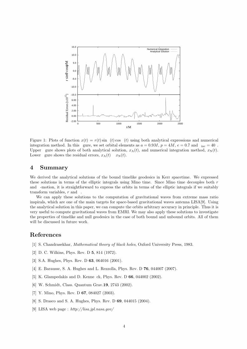
-2.00
0.00
2.00
4.00
6.00
0 500 1000 1500 2000 2500
Res
idua
l Err
ors
[x10
12]
t/M
-15.0
-10.0
-5.0
0.0
5.0
10.0
15.0
r si
nθ c
osφ/
M
Numerical IntegrationAnalytical Solution
Figure 1: Plots of function x(t) = r(t) sin (t) cos (t) using both analytical expressions and numericalintegration method. In this figure, we set orbital elements as a = 0.9M , p = 4M , e = 0.7 and inc = 40.Upper figure shows plots of both analytical solution, xA(t), and numerical integration method, xN(t).Lower figure shows the residual errors, xA(t) xN(t).
4 Summary
We derived the analytical solutions of the bound timelike geodesics in Kerr spacetime. We expressedthese solutions in terms of the elliptic integrals using Mino time. Since Mino time decouples both rand -motion, it is straightforward to express the orbits in terms of the elliptic integrals if we suitablytransform variables, r and .
We can apply these solutions to the computation of gravitational waves from extreme mass ratioinspirals, which are one of the main targets for space-based gravitational waves antenna LISA[9]. Usingthe analytical solution in this paper, we can compute the orbits arbitrary accuracy in principle. Thus it isvery useful to compute gravitational waves from EMRI. We may also apply these solutions to investigatethe properties of timelike and null geodesics in the case of both bound and unbound orbits. All of themwill be discussed in future work.
References
[1] S. Chandrasekhar, Mathematical theory of black holes, Oxford University Press, 1983.
[2] D. C. Wilkins, Phys. Rev. D 5, 814 (1972).
[3] S.A. Hughes, Phys. Rev. D 63, 064016 (2001).
[4] E. Barausse, S. A. Hughes and L. Rezzolla, Phys. Rev. D 76, 044007 (2007).
[5] K. Glampedakis and D. Kennefick, Phys. Rev. D 66, 044002 (2002).
[6] W. Schmidt, Class. Quantum Grav.19, 2743 (2002).
[7] Y. Mino, Phys. Rev. D 67, 084027 (2003).
[8] S. Drasco and S. A. Hughes, Phys. Rev. D 69, 044015 (2004).
[9] LISA web page : http://lisa.jpl.nasa.gov/
4
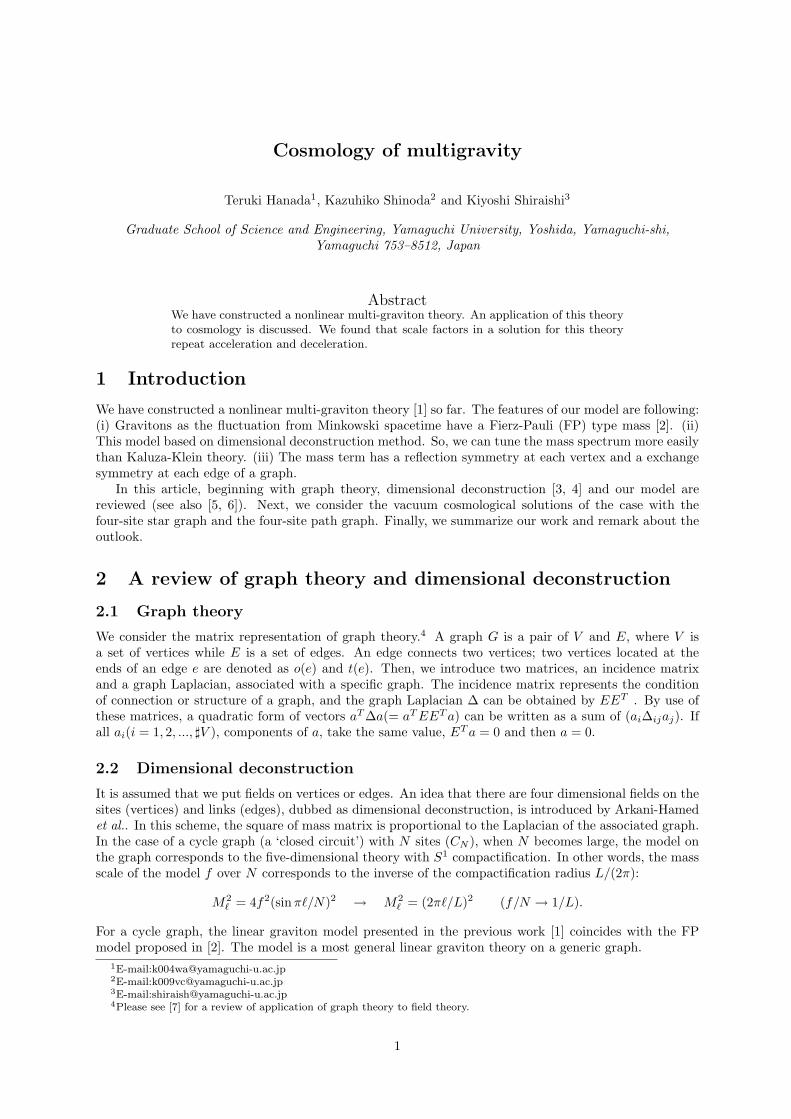
Cosmology of multigravity
Teruki Hanada1, Kazuhiko Shinoda2 and Kiyoshi Shiraishi3
Graduate School of Science and Engineering, Yamaguchi University, Yoshida, Yamaguchi-shi,Yamaguchi 753–8512, Japan
AbstractWe have constructed a nonlinear multi-graviton theory. An application of this theoryto cosmology is discussed. We found that scale factors in a solution for this theoryrepeat acceleration and deceleration.
1 Introduction
We have constructed a nonlinear multi-graviton theory [1] so far. The features of our model are following:(i) Gravitons as the fluctuation from Minkowski spacetime have a Fierz-Pauli (FP) type mass [2]. (ii)This model based on dimensional deconstruction method. So, we can tune the mass spectrum more easilythan Kaluza-Klein theory. (iii) The mass term has a reflection symmetry at each vertex and a exchangesymmetry at each edge of a graph.
In this article, beginning with graph theory, dimensional deconstruction [3, 4] and our model arereviewed (see also [5, 6]). Next, we consider the vacuum cosmological solutions of the case with thefour-site star graph and the four-site path graph. Finally, we summarize our work and remark about theoutlook.
2 A review of graph theory and dimensional deconstruction
2.1 Graph theory
We consider the matrix representation of graph theory.4 A graph G is a pair of V and E, where V isa set of vertices while E is a set of edges. An edge connects two vertices; two vertices located at theends of an edge e are denoted as o(e) and t(e). Then, we introduce two matrices, an incidence matrixand a graph Laplacian, associated with a specific graph. The incidence matrix represents the conditionof connection or structure of a graph, and the graph Laplacian ∆ can be obtained by EET . By use ofthese matrices, a quadratic form of vectors aT ∆a(= aT EET a) can be written as a sum of (ai∆ijaj). Ifall ai(i = 1, 2, ..., ]V ), components of a, take the same value, ET a = 0 and then a = 0.
2.2 Dimensional deconstruction
It is assumed that we put fields on vertices or edges. An idea that there are four dimensional fields on thesites (vertices) and links (edges), dubbed as dimensional deconstruction, is introduced by Arkani-Hamedet al.. In this scheme, the square of mass matrix is proportional to the Laplacian of the associated graph.In the case of a cycle graph (a ‘closed circuit’) with N sites (CN ), when N becomes large, the model onthe graph corresponds to the five-dimensional theory with S1 compactification. In other words, the massscale of the model f over N corresponds to the inverse of the compactification radius L/(2π):
M2` = 4f2(sinπ`/N)2 → M2
` = (2π`/L)2 (f/N → 1/L).
For a cycle graph, the linear graviton model presented in the previous work [1] coincides with the FPmodel proposed in [2]. The model is a most general linear graviton theory on a generic graph.
1E-mail:[email protected]:[email protected]:[email protected] see [7] for a review of application of graph theory to field theory.
1
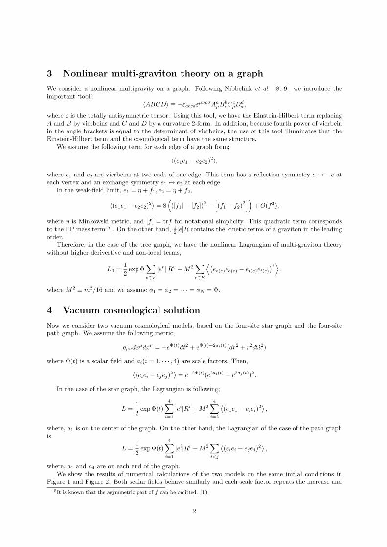
3 Nonlinear multi-graviton theory on a graph
We consider a nonlinear multigravity on a graph. Following Nibbelink et al. [8, 9], we introduce theimportant ‘tool’:
〈ABCD〉 ≡ −εabcdεµνρσAa
µBbνCc
ρDdσ,
where ε is the totally antisymmetric tensor. Using this tool, we have the Einstein-Hilbert term replacingA and B by vierbeins and C and D by a curvature 2-form. In addition, because fourth power of vierbeinin the angle brackets is equal to the determinant of vierbeins, the use of this tool illuminates that theEinstein-Hilbert term and the cosmological term have the same structure.
We assume the following term for each edge of a graph form;
〈(e1e1 − e2e2)2〉,
where e1 and e2 are vierbeins at two ends of one edge. This term has a reflection symmetry e ↔ −e ateach vertex and an exchange symmetry e1 ↔ e2 at each edge.
In the weak-field limit, e1 = η + f1, e2 = η + f2,
〈(e1e1 − e2e2)2〉 = 8(([f1]− [f2])
2 −[(f1 − f2)
2])
+ O(f3),
where η is Minkowski metric, and [f ] = trf for notational simplicity. This quadratic term correspondsto the FP mass term 5 . On the other hand, 1
2 |e|R contains the kinetic terms of a graviton in the leadingorder.
Therefore, in the case of the tree graph, we have the nonlinear Lagrangian of multi-graviton theorywithout higher derivertive and non-local terms,
L0 =12
expΦ∑
v∈V
|ev|Rv + M2∑
e∈E
⟨(eo(e)eo(e) − et(e)et(e)
)2⟩
,
where M2 ≡ m2/16 and we assume φ1 = φ2 = · · · = φN = Φ.
4 Vacuum cosmological solution
Now we consider two vacuum cosmological models, based on the four-site star graph and the four-sitepath graph. We assume the following metric;
gµνdxµdxν = −eΦ(t)dt2 + eΦ(t)+2ai(t)(dr2 + r2dΩ2)
where Φ(t) is a scalar field and ai(i = 1, · · · , 4) are scale factors. Then,⟨(eiei − ejej)2
⟩= e−2Φ(t)(e2ai(t) − e2aj(t))2.
In the case of the star graph, the Lagrangian is following;
L =12
expΦ(t)4∑
i=1
|ei|Ri + M24∑
i=2
⟨(e1e1 − eiei)2
⟩,
where, a1 is on the center of the graph. On the other hand, the Lagrangian of the case of the path graphis
L =12
expΦ(t)4∑
i=1
|ei|Ri + M2∑
i<j
⟨(eiei − ejej)2
⟩,
where, a1 and a4 are on each end of the graph.We show the results of numerical calculations of the two models on the same initial conditions in
Figure 1 and Figure 2. Both scalar fields behave similarly and each scale factor repeats the increase and5It is known that the asymmetric part of f can be omitted. [10]
2
the decrease. However, the scalar field in the star graph case changes slightly slower than the other. Theoscillation of the scale factors in the path graph case include more modes of different frequencies thanthat of the scale factors in the star graph case.
The star graph model has more symmetries than the path graph model. A lot of modes in the stargraph case degenerate. In the path graph case, increase of the number of sites gives the more complicatedbehaviors of the scale factors. On the other hand, in the star graph case, the symmetries are preservedif the number of sites are inceased. Therefore, the behaviors of the scale factors are the same as thefour-site model, essentially.
5 Summary and prospects
We considered the four-site star and path graph model and found that vacuum cosmological solutions withthe scale factors show the repeated accelerating and decelerating expansions. The differences betweenthese two models were discussed from a viewpoint about symmetries.
As the future works, we should investigate the case that the matter fields exist. We also shouldinvestigate the models based on arbitrary tree graphs.
Acknowledgements
The authors would like to thank N. Kan and K. Kobayashi for useful comments, and also the organizersof JGRG18.
20 40 60 80 100t
0.9
1.1
1.2
1.3
1.4
FHtL
20 40 60 80 100t
0.2
0.4
0.6
0.8
1
1.2
1.4
a_1HtL
20 40 60 80 100t
0.2
0.4
0.6
0.8
1
1.2
1.4
a_2HtL
20 40 60 80 100t
0.2
0.4
0.6
0.8
1
1.2
1.4
a_3HtL
20 40 60 80 100t
0.6
0.8
1.2
1.4
a_4HtL
Figure 1: A numerical solutions of the scale factors in the case of the four-site star graph.
References
[1] T. Hanada, K. Shinoda and K. Shiraishi, to appear in Proceedings of the Seventeenth Work-shop on General Relativity and Gravitation (Nagoya University, Nagoya, December 2-6, 2007)arXiv:0801.2641[gr-qc].
[2] M. Fierz and W. Pauli, Proc. Roy. Soc. Lond. A173 (1939) 211.
[3] N. Arkani-Hamed, A. G. Cohen and H. Georgi, Phys. Rev. Lett. 86 (2001) 4757; Phys. Lett. B513(2001) 232.
3
20 40 60 80 100t
0.6
0.8
1.2
1.4FHtL
20 40 60 80 100t
0.8
0.9
1.1
1.2
1.3
1.4
a_1HtL
20 40 60 80 100t
0.2
0.4
0.6
0.8
1
1.2
1.4
a_2HtL
20 40 60 80 100t
0.2
0.4
0.6
0.8
1
1.2
1.4
a_3HtL
20 40 60 80 100t
0.8
1.2
1.4
a_4HtL
Figure 2: A numerical solutions of the scale factors the case of the four-site path graph.
[4] C. T. Hill, S. Pokorski and J. Wang, Phys. Rev. D64 (2001) 1050050.
[5] S. Hamamoto, Prog. Theor. Phys. 97 (1997) 327, hep-th/9611141.
[6] N. Kan and K. Shiraishi, Class. Quant. Grav. 20 (2003) 4965, gr-qc/0212113.
[7] N. Kan and K. Shiraishi, J. Math. Phys. 46 (2005) 112301.
[8] S. G. Nibbelink, M. Peloso and M. Sexton, Eur. Phys. J. C51 (2007) 741, hep-th/0610169.
[9] S. G. Nibbelink and M. Peloso, Class. Quant. Grav. 22 (2005) 1313, hep-th/0411184.
[10] C. Bizdadea et al., JHEP 02 (2005) 016; C. Bizdadea et al., Eur. Phys. J. C48 (2006) 265.
4
The distance-redshift relation for the inhomogeneous andanisotropic universe
Kazuhiro Iwata1, Yasusada Nambu2 and Masayuki Tanimoto3
1,2,3Department of Physics, Graduate School of Science, Nagoya University, Chikusa, Nagoya 464-8602,Japan
AbstractRecently, there have been a indication that the universe is in a state of acceleratedexpansion. This accelerated expansion is supposed to be caused by unidentified darkenergy as a result of fitting the observations of type Ia supernovae to a distance-redshift relation of homogeneous and isotropic universe model. But the universe isnot perfectly homogeneous and isotropic because of structures such as galaxies orgroups of galaxies. In this work, by taking into account effects of such inhomo-geneities and anisotropies of the matter distribution, we explain the distance-redshiftrelation suggested by the observations of type Ia supernovae without dark energy.First, we show that after averaging the optical scalar equation of an inhomogeneousand anisotropic spacetime over the sphere, we can obtain a simplified optical scalarequation, which coincides with that in the Lemaıtre-Tolman-Bondi spacetime witha Dyer-Roeder-like extention. Then, we show that the distance-redshift relation ob-tained from our equation provides better fitting of the observational data than theΛCDM model and the void model.
1 Introduction
Conparisons of reliable distance-redshift relation obtained from Type Ia supernova (SNIa) observa-tions(e.g. [1]) with the predictions from Friedmann-Lemaıtre (FL) homogeneous and isotropic universemodels suggest that the Universe is in a phase of accelerated expansion, and there must exist undefineddark energy that causes the acceleration.
On the other hand, the possibilities have been discussed that the distance-redshift relations providedby the SNIa observations could be reproduced by taking account of the inhomogeneties in the matterdistibution and geometry even without dark energy. One of such models is the so-called void model,in which existence of a large scale underdense region (void). Alnes et al. [2] showed that there exists amodel that provides a good fit to the SNIa observations, assuming that the outside if a spherical regionis homogeneous and isotropic but the inside of it is described by the Lemaıtre-Tolman-Bondi (LTB)spherically symmetric dust solution (e.g. see [2]).
In reality, however, the matter distribution in the Universe is not isotropic, and the distance-redshiftrelation inferred by the observational data should be considered as an average over all the directions ofsight. This point seems to have been mostly ignored in the literature. To take into account the effectcaused by these anisotropies, we start with the optical scalar equation in general inhomogeneous andanisotropic spacetimes, and then take an average of a form of this equation (distance equation) over thespheres on the past light cone. With this averaged distance equation, we numerically investigate a voidmodel.
1E-mail:[email protected]:[email protected]:[email protected]
1
2 The distance equation for inhomogeneous andanisotropic spacetime
2.1 The distance equation in general spacetime
Let us consider a null geodesic congruence which arrive at the observer. We start with the optical scalarequation [3], which determines the variations of the cross sectional area of a null geodesic congruence.For simplicity, let us assume the spacetime which there is no the shear and rotation of the congruence.The optical scalar equation in this case becomes
2√A
d2√
A
dλ2+ Rµνkµkν = 0, (1)
where A is the cross sectional area of the congruence, kµ the null geodesic generator, λ the affine param-eter, and Rµν the Ricci tensor. With the relation DA ∝
√A for the angular diameter distance DA, we
obtain1
DA
d2DA
dλ2+ 4πGTµνkµkν = 0, (2)
from Eq.(1) and Einstein’s equation. The only energy content we consider is dust, so that Tµν = ρuµuν ,where ρ is the energy density for dust, uµ the 4-velocity of dust. The frequency of the light observed bythe comoving observer at a given λ with 4-velocity uµ is given by ω(λ) = −uµkµ.Therefore the secondterm in the left hand side of Eq.(2) yields Tµν = ω(0)(1 + z)2ρ, where we have used the definition ofredshift z, z ≡ ω(λ)/ω(0) − 1. Thus, Eq.(2) can be written as
L2DA + 4πGρDA = 0, (3)
where L2 is the second order linear derivative operator defined by L2 = 1ω2(0)(1+z)2
d2
dλ2 . We stress thatthis equation is valid for any dust universem, as long as the shear and rotation of the congruence can beignored. Note also that solving this equation requires another equation (geodesic equation) to relate λwith z, for a given ρ.
2.2 Averaging of anisotropies
In this subsection, we take a spherical average of Eq.(3).For our purpose, it is most convenient to take a particular coordinate system that is based on a
foliation of spacetime by past light cones of a timelike curve. We employ a spherical null coordinatesystem (t, z, θ, ϕ) such that on each light cone t = constant, that z = 0 corrsponds to the vertex of eachlight cone, that the timelike curve the vertices z = 0 comprise coincides with the orbit of matter flowthere, and that the angular coordinates (θ, ϕ) are constant along every null geodesic that reaches thevertex z = 0. (This choice of angular coordinates is possible each other.) The radial null coordinate z ischosen to give the redshift along each null geodesic labeled by (t, θ, ϕ). Our observation is supposed tobe done at the coordinate center z = 0 at a certain instant t = t0.
Let DA(z; θ, ϕ) be the angular-diameter distance to an object observed in the direction (θ, ϕ) withredshift z. This is a function of z, θ, ϕ, but we will often regard this as a function of z with θ and ϕ beingparameters, since we mostly consider its variations along the null geodesic, in which situation θ and ϕare constant. We will therefore use d/dz instead ∂/∂z when it acts on DA(z; θ, ϕ). The same rule will beapplied to other functions as well.
Let us define the spherical average of function f(z; θ, ϕ) by
f(z) ≡ ⟨f(z; θ, ϕ)⟩ ≡ 14π
∫f(z; θ, ϕ)dΩ, (4)
where dΩ = sin θdθdϕ. Then, then spherical average of Eq.(3) can be written as
⟨L2DA(z; θ, ϕ)⟩ + 4πG⟨ρ(z; θ, ϕ)DA(z; θ, ϕ)⟩ = 0. (5)
2
Here, the derivative operator L2 becomes under our coordinates
L2 =1
ω2(0)(1 + z)2
(d
dλ
)2
= H(z; θ, ϕ)d
dz
[H(z; θ, ϕ)(1 + z)2
d
dz
], (6)
where the function H(z; θ, ϕ) is defined by H(z; θ, ϕ) ≡ 1ω(0)(1+z)2
dzdλ .
Note that in the averaged equation (5), each term in the left hand side depends only on z. Wewish to estimate how much different the averaged distance function DA(z) = ⟨DA(z; θ, ϕ)⟩ is from anspherically symmtetric LTB distance function D
(LTB)A (z). To this, we match an LTB solution with the
given inhomogeneous and anisotropic universe according to the following correspondence: ρ(z) = ρLTB(z),H(z) = HLTB(z). Since the LTB solution possesses two arbitrary physical functions, it is natural to expectthat these two conditions are satisfied for a suitable choice of these functions.
Keeping this correspondence in mind, we formally rewrite Eq.(5) in the form
β(z)L2LTBDA(z) + 4πGα(z)ρLTB(z)DA(z) = 0, (7)
where
α(z) ≡ ⟨ρ(z; θ, ϕ)DA(z; θ, ϕ)⟩ρLTB(z)DA(z)
, β(z) ≡ ⟨L2DA(z; θ, ϕ)⟩L2
LTBDA(z), L2
LTB ≡ HLTB(z)d
dz
[HLTB(z)(1 + z)2
d
dz
].
(8)
To estimate the magnitude of the ratio function α(z) and β(z), let us decompose physical function as
ρ(z; θ, ϕ) = ρLTB(z) + δρ(z; θ, ϕ), (9)H(z; θ, ϕ) = HLTB(z) + δH(z; θ, ϕ), (10)
DA(z; θ, ϕ) = DA(z) + δDA(z; θ, ϕ), (11)
where ⟨δρ⟩ = ⟨δH⟩ = ⟨δDA⟩ = 0. Then α can be calculated as
α(z) = 1 + ⟨δρ(z; θ, ϕ)ρLTB(z)
δDA(z; θ, ϕ)DA(z)
.⟩ (12)
In general, the emptier the region the light we observe travels, the longer the distance, which implies thatδρ and δDA have opposite signs each other. This in turn implies α(z) ≤ 1 with equality being satisfiedonly in the LTB isotropic universe.
For β, we can roughly estimate as
β(z) ∼ 1 + ⟨(
δH(z; θ, ϕ)HLTB(z)
)2
⟩, (13)
where we have used δDA/DA ∼ δH/HLTB because the perturbation of distance is mainly caused by theperturbation of the expansion rate. According to the CMB observation, however, the perturbation of theexpansion rate is about 0.1 on scales of z ∼ 0.1. This implies that ∆β ≡ |β − 1| is much smaller and canbe neglected as compared to ∆α ≡ |α − 1|.
Putting β ∼ 1 in Eq.(7), we finally obtain
L2LTBDA(z) + 4πGα(z)ρLTB(z)DA(z) = 0 (14)
This is the distance equation the averaged distance function DA(z) should satisfy. We obtained thisequation for a given inhomogeneous and anisotropic universe, but in practice, we will use it to determinea matched LTB solution and α(z) so that the solution DA(z) well describes observational data.
3 Numerically Analysis
Using Eq.(14), we numerically seek in a space of control parameters the best confuguration that canexplain observational data of SNIa. For inhomogeneity, we employ the same void model considered by
3
Alnes et al. [2] as the parametrization of the LTB solution. In their model, the arbitrary functions tB(r),M(r), E(r) are chosen to be
tB(r) = 0, M(r) =12H2
0r3
[1 − ∆M
2
(1 − tanh
r − r0
2∆r
)], E(r) =
14H2
0r2∆M
(1 − tanh
r − r0
2∆r
).
(15)
The model represents FL universe near the center, since M(r) ∝ r3, E(r) ∝ r2 there. From this fact, wecan define the following density parameters at the center: Ωk ≡ −E′′(0)
H20
, Ωm ≡ M ′′′(0)3H2
0= 1 − Ωk. These
equation allow us to use observational value Ωm instead of ∆M .For anisotropy, we define the function α(z) as
α(z) = 1 − 1 − α0
2
(1 − tanh
r(z) − rα0
2∆rα
)(16)
Thus, our paramter space consists of (Ωm, r0,∆r, α0, rα0,∆rα). But, for simplicity, we set ∆rα = 0.001.As for the observational data to consider, we use the so-called gold samples of Riess et al. [4].
The best-fit parameters for our model are summarized in Table 1. Our best-fit value χ2 = 174.046is smaller than χ2
ΛCDM = 174.046 in the ΛCDM model [4] and χ2void = 176.5 in the void model of Alnes
et al. [2]. From the value α = 0.42(z < 2), we can estimate the characteristic magnitude of densityfluctuation on the scale z ∼ 1 as δρ/ρ ∼ 5.8, since δH/H is of the magnitude about 0.1 on this scale.Our value Ωm = 0.31 coincides with the galaxy survey. The scale z0 = 0.199 corresponds to large-scalestructure of the Universe.
Table 1: Our best-fit parameters.
(Ωm, r0, ∆r, α0) χ2 z0 zα0(0.31, 0.18, 0.085, 0.42) 174.046 0.199 zα0 > 2
4 Conclusion
Since SNIae are observed in various directions in the sky, the distance-redshift relation inferred by acollective data of them should be considered as an averaged over the solid angle. On the other hand,the distance-redshift relation DA(z) for a given direction of sight can theoretically be determined by adistance equation that is equivalent to the optical scalar equation. To obtain an effective equation forthe spherically averaged distance DA, with which the observed distance-redshift relation can directly becompared, we took an average of the distance equation.
The function α(z) introduced in our effective equation represents the degree to which the Universefluctuates from an isotropic configulation. This newly introduced freedom enabled us to obtain a betterfit to the observation, and our best-fit value of α suggests that the dark matter fluctuation δρ/ρ ∼ 6.Although it is very rough, this is perhaps the first estimation of the fluctuation determined from theobservational data of SNIae.
References
[1] Supernova Search Team, A. G. Riess et al., Astron. J. 116, 1009 (1998), astro-ph/9805201.
[2] H. Alnes, M. Amarzguioui, and O. Grøn, Phys. Rev. D73, 083519 (2006), astro-ph/0512006.
[3] R. K. Sachs, Proc. Roy. Soc. Lond. A264, 309 (1961).
[4] Supernova Search Team, A. G. Riess et al., Astrophys. J. 607, 665 (2004), astro-ph/0402512.
4
! "#$%& '(!)* +,%- , #$ .!$%/ 012134567 8497:; <:==>3>? @:A4BC67? 012134567 DEDFGHIH? 81J19% 012134567 K97L>;C7MN? 012134567BC67? 012134567 DOIFPOGH? 81J19
QRSTUVWTXY YZ[\]^Y _[^_Y``[a]b^ bc `b^def[^dY cbf_Yg ]^ h]^gaY]^ei[ZjY``ek]`[ab^]_ glgaY\mnYoYf[` _b^p]a]b^g bc aqY Yrs]`]tf]s\ bc ajb _q[fdYp \[ggYg ]^ dY^Yf[` fY`[a]o]al ]gcbs^p tl \[^l [saqbfgm uqYgY _b^p]a]b^g [fY [`aYfYp tl a[v]^d [__bs^a bc p]`[ab^]_wY`pm x^pYf aqY ^Yj _b^p]a]b^y jY gqbj _[^_Y``[a]b^ bc z| ~baY^a][` sg]^d Yl^\[^p][df[\gm
'( (! "((( !(, $$( ! ($ $ ,($ !"(, "# ( ( , ( )"(
(!( $ ( ( $ , !( ! ($ !( ((, ( (! ( $$ (( ((! !(# ( $ ( $) ! ( (¡)"!) !(,$$($ $ ), "# ¢£),! , ¤(!) ¥¦ '( $) !(¡)!($ , §¨ ¨'( $ ( $) , $ ), "# .!$ ¥©¦ '( $) $,$ ! ( $( ( " ( , ¨ ¨ ª¨ § «& « (!( ª $ , !( $ !*( ( ( ( !( ! ($ ( ¬$(¢ ( $#$( )$ ®(#,!$ ),(! ( " ( , § «&
¯ ° ±( $! ( ²! ), , ³(, ´
µ §¶ · ¸¹&º»¼ & ©¶½¾¿½´¿¾´ ©
(!( · $ À $ ! ¼½¾ Á½Â¾ Á¾Â½ ¿½´ Á½´ , « $ ( ) $"((( ( , ³(, , (! ³(,$ !,(! ( ! ( (! $ )(, ( ,³(, ( )$( ( $ ! "$ à $ !"( '( ²! ( (Ä!, ³(, $ ¥Å¦
µÆÇ §¶ ¥ ¹º»¶½¾ ȽÃȾà &¸º»Ãæ Å(!( Ƚà Á½Ã É½à ±( ,( $( ( (! ¶½¾ ( Ê " *!), ³(, ˽¾ , (! ³(, ̽¾ ¶½¾ ˽¾ Í̽¾ (!( Í §Å© , ˽¾ ÎÉ«¶ $ ,( $ ( !(,
¶½¾ ˽¾ Í̽¾ Í&̽ÏÌ¾Ï Í-̽ÏÌÏÐÌо Ñ Ñ Ñ ÒÓÔÕÖ×ØÙÚÛ×ÜÝÞ×Ö×ßàáâØÕãáä×áäãåÔÕÖ×ØÙÚÖææçè×ÝÞ×Ö×ßàáâØÕàä×áäãåéÔÕÖ×ØÙÚÛææçè×ÝÞ×Ö×ßàáâØÕàä×áäãåêÔÕÖ×ØÙÚëâØì×ØëâÝÞ×Ö×ßàáâØÕàä×áäãå
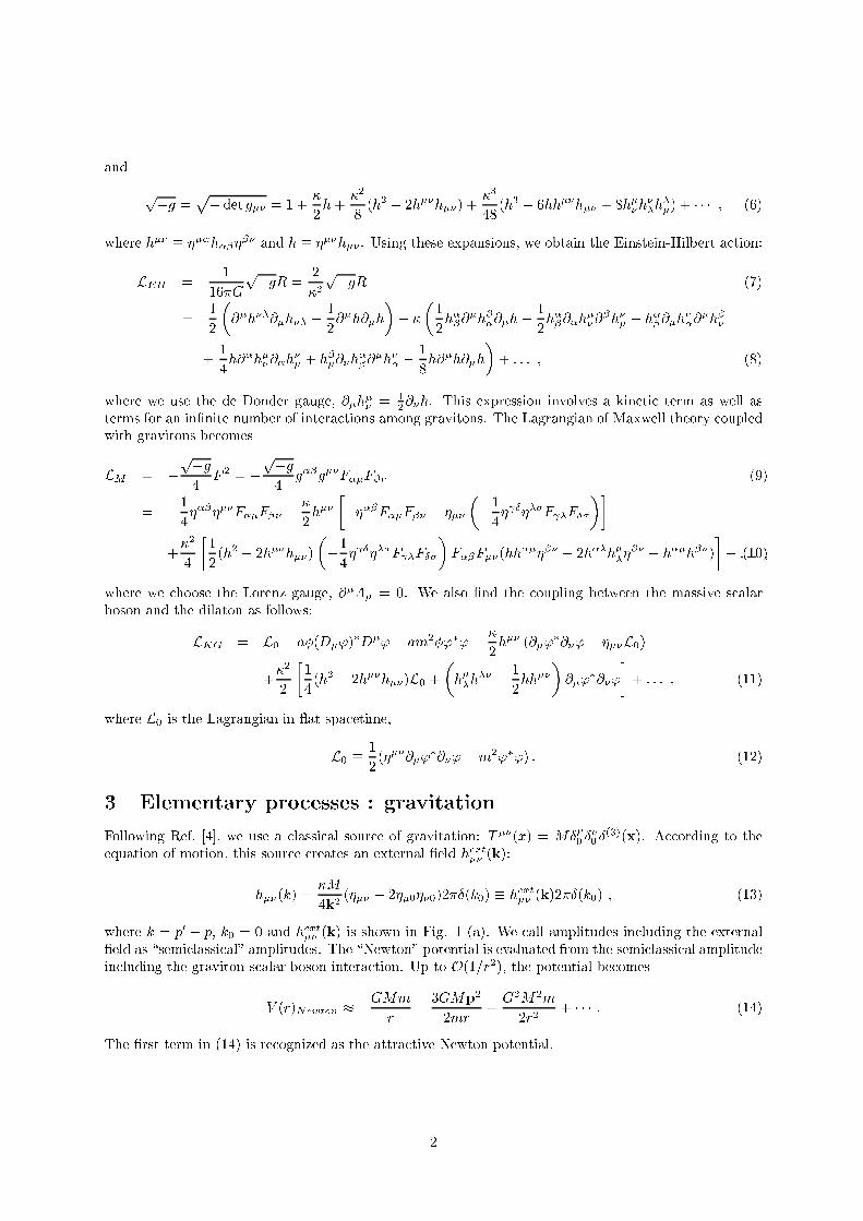
,
§¶ ,( ¶½¾ Í©Ì Í& Ì& ©Ì½¾Ì½¾ Í- Ì- Ì̽¾Ì½¾ ̽¾Ì¾ÏÌϽ Ñ Ñ Ñ (!( ̽¾ ˽ÐÌÐ˾ , Ì Ë½¾Ì½¾ $ ($( ( $$ ( " ( ¬$(+"(!
µ §¶· ©
Í&§¶·
© Á½Ì¾ÏÁ½Ì¾Ï
©Á½ÌÁ½Ì
Í ©ÌÐÁ½ÌÐÁ½Ì
©ÌÐÁÐ̽¾Á̾½ ÌÐÁ½Ì¾ÐÁ½Ì¾
ÌÁÐ̽¾ÁÐ̾½ ̽Á¾ÌÐÁ½Ì¾Ð ÌÁ½ÌÁ½Ì
(!( ( )$( ( ,( ,(! )( Á½Ì½¾ &Á¾Ì '$ ( !($$ ($ *( (! $ ( $(!$ ! ³( )"(! (! $ !$ '( ²! ¢ ( (!# )(, !$ "( ($
µ §¶ ¼& §¶
¶Ð¶½¾¼Ð½¼¾
ËÐ˽¾¼Ð½¼¾ ͩ̽¾ Ëмн¼¾ ˽¾ ËËϼϼ
Í& © Ì& ©Ì½¾Ì½¾ ËËϼϼ¼Ð¼½¾ ÌÌн˾ ©ÌÐÏ̽ÏË
¾ Ìн̾
(!( ( $( ( ²!( )( Á½Â½ ±( $ ³, ( ) "((( ( $$( $ !"$ , ( , $ $
µÆÇ µ «´È½ÃȽà «&´Ãà ͩ̽¾ Á½ÃÁ¾Ã ˽¾µÍ&© Ì& ©Ì½¾Ì½¾µ ̽ÏÌϾ
©Ì̽¾ Á½ÃÁ¾Ã
(!( µ $ ( ²! Ê $ ((µ
© ˽¾Á½ÃÁ¾Ã &Ãà ©
® À( ¥¦ ( )$( $$ $)! ( ! ½¾ ½ ¾ - !, ((¡) $ $)! ( !(($ ( (! ³(, Ì !"½¾ #
̽¾ $ Í#& ˽¾ ©Ë½Ë¾©$ Ì !"½¾ #©$ Å(!( $ %& % $ , Ì !"½¾ # $ $ ® ±( ),($ ), ( ( (!³(, $ '$( $$ ( ),($ '( '(( ( $ ()(, ! ( $( $$ ),( ), ( !$ ! "$ (! )*& ( ( "( ($
+ ,"-. / Å0&©
&&©& Ñ Ñ Ñ '( ³!$ (! $ !( (, $ ( ! ( ( (
©
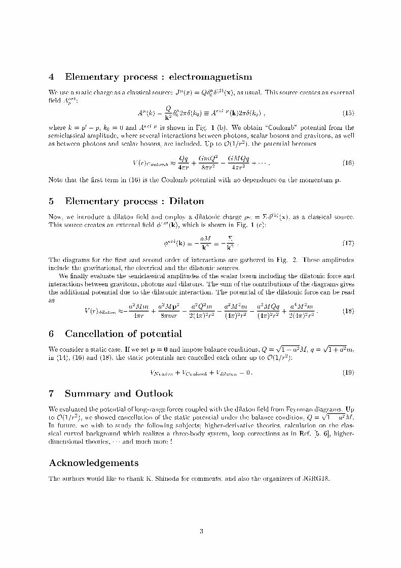
±( )$( $ !( $ $$ $)! ( ½ ½ - $ )$) '$ $)! ( !(($ ( (!³(, Â !"½
½$ #& ½ ©$  !" ½#©$ Ò(!( $ %& % $ ,  !" ½ $ $ ® " ±( " ')"( ( ! ($( $$ ),( (!( $((! (! $ "((( $ $ ! "$$ , !$ $ ($ "((( $ , $ ! "$$ !( ),(, )*& ( ( "( ($
-- /
&& & Ñ Ñ Ñ
( ( ³!$ (! $ ( )" ( ,((,( ( ( () 0
( !,) ( , ³(, , (# , !( ª - $ $$ $)! ('$ $)! ( !(($ ( (! ³(, ´ !" # $ $ ®
´ !" # «#& ª#& '( ,!$ ! ( ³!$ , $( , !,(! (! $ !( (!(, ® © '($( ),($ ),( ( ! ( (( ! , ( , $)! ($±( ³# ()( ( $( $$ ),($ ( $ ! "$ ), ( , ! ( ,(! $ "((( !$ $ , ,$ '( $) ( !")$ ( ,!$ ($( ,, ( ,)( ( , (! '( ( ( , ! ( "( !(,$
¨º"-. /«& «&0& «&&©&& «&&&& «&&& «/&©&&
±( $,(! $ $( ( $( 0 , $( " ( ,$ § «& § «& , ( $ ($ !( ((, ( (! ) )*&
+ ,"-. -- ¨º"-. ±( ()(, ( ( !( ! ($ )(, ( , ³(, ! ®(# ,!$ )*& ( $(, ( ( $ ( ),(! ( " ( , § «& ))!( ( $ $),# ( $)"£( $ (!,(!( (!($ ) ( $$ )!(, " *!), !(($ !((",# $#$( !!( $ $ À( ¥Ò ¦ (!,($ (!($ Ñ Ñ Ñ , ) !(
'( )!$ ), *( * ., ! ($ , $ ( !(!$ ÄÀÄ
Å
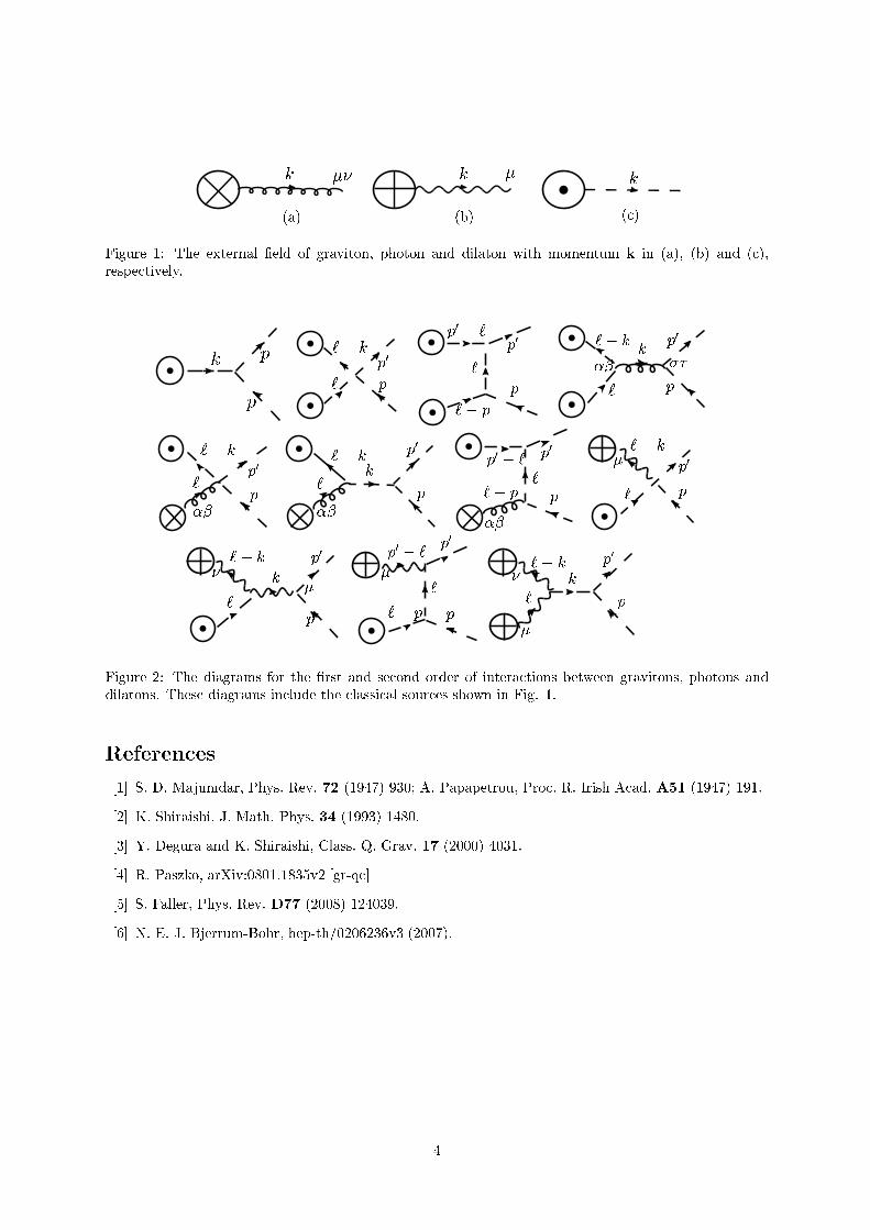
®)!( '( ( (! ³(, ! , , () # " , !($( (#
®)!( © '( ,!$ ! ( ³!$ , $( , !,(! (! $ "((( !$ $ ,,$ '($( ,!$ ),( ( $$ $)! ($ $ ®
¥¦ . ¢£),! ¤#$ À( Å ¤(!) ¤! À !$ , ¥©¦ .!$ ¢ ¤#$ Å ¥Å¦ ()! , .!$ $$ Ä! © Å¥¦ À ¤$* !ÅÒ© ¥!¡ ¦¥Ò¦ . ®(! ¤#$ À( © ©Å ¥¦ ¬ !£(!!)!! ("©©ÅÅ ©
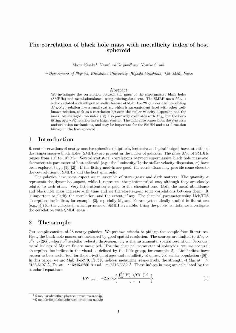
The correlation of black hole mass with metallicity index of hostspheroid
Shota Kisaka1, Yasufumi Kojima2 and Yosuke Otani
1,2Department of Physics, Hiroshima University, Higashi-hiroshima, 739–8526, Japan
AbstractWe investigate the correlation between the mass of the supermassive black holes(SMBHs) and metal abundance, using existing data sets. The SMBH mass Mbh iswell correlated with integrated stellar feature of Mgb. For 28 galaxies, the best-fittingMbh-Mgb relation has a small scatter, which is an equivalent level with other well-known relation, such as a correlation between the stellar velocity dispersion and themass. An averaged iron index 〈Fe〉 also positively correlates with Mbh, but the best-fitting Mbh-〈Fe〉 relation has a larger scatter. The difference comes from the synthesisand evolution mechanisms, and may be important for the SMBH and star formationhistory in the host spheroid.
1 Introduction
Recent observations of nearby massive spheroids (ellipticals, lenticular and spiral bulges) have establishedthat supermassive black holes (SMBHs) are present in the nuclei of galaxies. The mass Mbh of SMBHsranges from 106 to 109 M¯. Several statistical correlations between supermassive black hole mass andcharacteristic parameter of host spheroid (e.g., the luminosity, L; the stellar velocity dispersion, σ) havebeen explored (e.g., [1], [2]). If the fitting models are good, the correlations may provide some clues tothe co-evolution of SMBHs and the host spheroids.
The galaxies have some aspect as an assemble of stars, gases and dark matters. The quantity σrepresents the dynamical aspect, while L represents the photometrical one, although they are closelyrelated to each other. Very little attention is paid to the chemical one. Both the metal abundanceand black hole mass increase with time and we therefore expect some correlations between them. Itis important to clarify the correlation, and the extent, if any. The chemical parameter using Lick/IDSabsorption line indices, for example [3], especially Mg and Fe are systematically studied in literatures(e.g., [4]) for the galaxies in which presence of SMBH is reliable. Using the published data, we investigatethe correlation with SMBH mass.
2 The sample
Our sample consists of 28 neargy galaxies. We put two criteria to pick up the sample from literatures.First, the black hole masses are measured by good spatial resolution. The sources are limited to Mbh >σ2rres/(2G), where σ2 is stellar velocity dispersion, rres is the instrumental spatial resolution. Secondly,metal indices of Mg or Fe are measured. For the chemical parameter of spheroids, we use spectralabsorption line indices in the visual as defined by the Lick group, for example [5]. Lick indices haveproven to be a useful tool for the derivation of ages and metallicity of unresolved stellar population ([6]).In this paper, we use Mgb, Fe5270, Fe5335 indices, measuring, respectively, the strength of MgI at ¸ '5156-5197 A, FeI at ¸ ' 5246-5286 A and ¸ ' 5312-5352 A. These indices in mag are calculated by thestandard equations:
EWmag = −2.5 log∫ λ2
λ1[F (¸)/C(¸)]d¸
¸2 − ¸1
, (1)
1E-mail:[email protected]:[email protected]
1
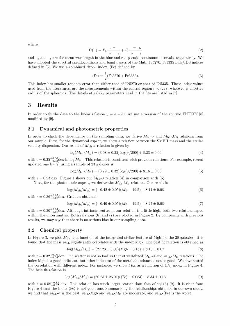
whereC(¸) = Fb
¸r − ¸
¸r − ¸b+ Fr
¸ − ¸b
¸r − ¸b(2)
and ¸b and ¸r are the mean wavelength in the blue and red pseudo-continuum intervals, respectively. Wehave adopted the spectral pseudocontinua and band passes of the Mgb, Fe5270, Fe5335 Lick/IDS indicesdefined in [3]. We use a combined “iron” index, 〈Fe〉 defined by
〈Fe〉 ≡ 12(Fe5270 + Fe5335). (3)
This index has smaller random error than either that of Fe5270 or that of Fe5335. These index valuesused from the literatures, are the measurements within the central region r < re/8, where re is effectiveradius of the spheroids. The details of galaxy parameters uesd in the fits are listed in [7].
3 Results
In order to fit the data to the linear relation y = a + bx, we use a version of the routine FITEXY [8]modified by [9].
3.1 Dynamical and photometric properties
In order to check the dependence on the sampling data, we derive Mbh-σ and Mbh-MB relations fromour sample. First, for the dynamical aspect, we show a relation between the SMBH mass and the stellarvelocity dispersion. Our result of Mbh-σ relation is given by
log(Mbh/M¯) = (3.98 ± 0.35) log(σ/200) + 8.23 ± 0.06 (4)
with ε = 0.25+0.06−0.03dex in log Mbh. This relation is consistent with previous relations. For example, recent
updated one by [2] using a sample of 23 galaxies is
log(Mbh/M¯) = (3.79 ± 0.32) log(σ/200) + 8.16 ± 0.06 (5)
with ε = 0.23 dex. Figure 1 shows our Mbh-σ relation (4) in comparison with (5).Next, for the photometric aspect, we derive the Mbh-MB relation. Our result is
log(Mbh/M¯) = (−0.42 ± 0.05)(MB + 19.5) + 8.14 ± 0.08 (6)
with ε = 0.36+0.07−0.05dex. Graham obtained
log(Mbh/M¯) = (−0.40 ± 0.05)(MB + 19.5) + 8.27 ± 0.08 (7)
with ε = 0.30+0.04−0.05dex. Although intrinsic scatter in our relation is a little high, both two relations agree
within the uncertainties. Both relations (6) and (7) are plotted in Figure 2. By comparing with previousresults, we may say that there is no serious bias in our sampling data.
3.2 Chemical property
In Figure 3, we plot Mbh as a function of the integrated stellar feature of Mgb for the 28 galaxies. It isfound that the mass Mbh significantly correlates with the index Mgb. The best fit relation is obtained as
log(Mbh/M¯) = (27.23 ± 3.00)(Mgb − 0.16) + 8.13 ± 0.07 (8)
with ε = 0.32+0.06−0.04dex. The scatter is not so bad as that of well-fitted Mbh-σ and Mbh-MB relations. The
index Mgb is a good indicator, but other indicator of the metal abundance is not so good. We have testedthe correlation with different index. For instance, we show Mbh as a function of 〈Fe〉 index in Figure 4.The best fit relation is
log(Mbh/M¯) = (60.25 ± 26.01)(〈Fe〉 − 0.083) + 8.34 ± 0.13 (9)
with ε = 0.58+0.12−0.07 dex. This relation has much larger scatter than that of eqs.(5)-(9). It is clear from
Figure 4 that the index 〈Fe〉 is not good one. Summarizing the relationships obtained in our own study,we find that Mbh-σ is the best, Mbh-Mgb and Mbh-MB are moderate, and Mbh-〈Fe〉 is the worst.
2
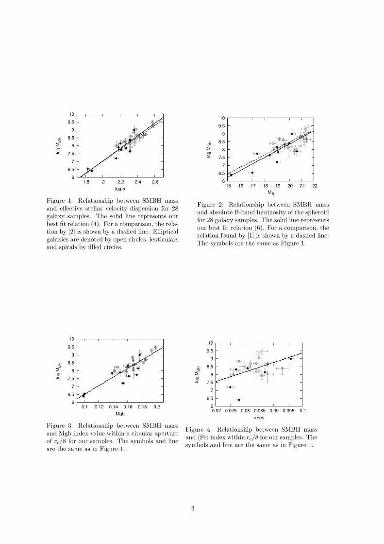
6
6.5
7
7.5
8
8.5
9
9.5
10
1.8 2 2.2 2.4 2.6
log
MB
H
log σ
Figure 1: Relationship between SMBH massand effective stellar velocity dispersion for 28galaxy samples. The solid line represents ourbest fit relation (4). For a comparison, the rela-tion by [2] is shown by a dashed line. Ellipticalgalaxies are denoted by open circles, lenticularsand spirals by filled circles.
6
6.5
7
7.5
8
8.5
9
9.5
10
-22-21-20-19-18-17-16-15
log
MB
H
MB
Figure 2: Relationship between SMBH massand absolute B-band luminosity of the spheroidfor 28 galaxy samples. The solid line representsour best fit relation (6). For a comparison, therelation found by [1] is shown by a dashed line.The symbols are the same as Figure 1.
6
6.5
7
7.5
8
8.5
9
9.5
10
0.1 0.12 0.14 0.16 0.18 0.2
log
MB
H
Mgb
Figure 3: Relationship between SMBH massand Mgb index value within a circular apertureof re/8 for our samples. The symbols and lineare the same as in Figure 1.
6
6.5
7
7.5
8
8.5
9
9.5
10
0.07 0.075 0.08 0.085 0.09 0.095 0.1
log
MB
H
<Fe>
Figure 4: Relationship between SMBH massand 〈Fe〉 index within re/8 for our samples. Thesymbols and line are the same as in Figure 1.
3
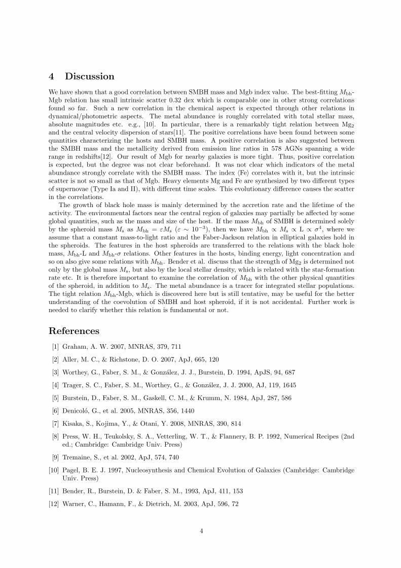
4 Discussion
We have shown that a good correlation between SMBH mass and Mgb index value. The best-fitting Mbh-Mgb relation has small intrinsic scatter 0.32 dex which is comparable one in other strong correlationsfound so far. Such a new correlation in the chemical aspect is expected through other relations indynamical/photometric aspects. The metal abundance is roughly correlated with total stellar mass,absolute magnitudes etc. e.g., [10]. In particular, there is a remarkably tight relation between Mg2
and the central velocity dispersion of stars[11]. The positive correlations have been found between somequantities characterizing the hosts and SMBH mass. A positive correlation is also suggested betweenthe SMBH mass and the metallicity derived from emission line ratios in 578 AGNs spanning a widerange in redshifts[12]. Our result of Mgb for nearby galaxies is more tight. Thus, positive correlationis expected, but the degree was not clear beforehand. It was not clear which indicators of the metalabundance strongly correlate with the SMBH mass. The index 〈Fe〉 correlates with it, but the intrinsicscatter is not so small as that of Mgb. Heavy elements Mg and Fe are synthesized by two different typesof supernovae (Type Ia and II), with different time scales. This evolutionary difference causes the scatterin the correlations.
The growth of black hole mass is mainly determined by the accretion rate and the lifetime of theactivity. The environmental factors near the central region of galaxies may partially be affected by someglobal quantities, such as the mass and size of the host. If the mass Mbh of SMBH is determined solelyby the spheroid mass Ms as Mbh = εMs (ε ∼ 10−3), then we have Mbh ∝ Ms ∝ L ∝ σ4, where weassume that a constant mass-to-light ratio and the Faber-Jackson relation in elliptical galaxies hold inthe spheroids. The features in the host spheroids are transferred to the relations with the black holemass, Mbh-L and Mbh-σ relations. Other features in the hosts, binding energy, light concentration andso on also give some relations with Mbh. Bender et al. discuss that the strength of Mg2 is determined notonly by the global mass Ms, but also by the local stellar density, which is related with the star-formationrate etc. It is therefore important to examine the correlation of Mbh with the other physical quantitiesof the spheroid, in addition to Ms. The metal abundance is a tracer for integrated stellar populations.The tight relation Mbh-Mgb, which is discovered here but is still tentative, may be useful for the betterunderstanding of the coevolution of SMBH and host spheroid, if it is not accidental. Further work isneeded to clarify whether this relation is fundamental or not.
References
[1] Graham, A. W. 2007, MNRAS, 379, 711
[2] Aller, M. C., & Richstone, D. O. 2007, ApJ, 665, 120
[3] Worthey, G., Faber, S. M., & Gonzalez, J. J., Burstein, D. 1994, ApJS, 94, 687
[4] Trager, S. C., Faber, S. M., Worthey, G., & Gonzalez, J. J. 2000, AJ, 119, 1645
[5] Burstein, D., Faber, S. M., Gaskell, C. M., & Krumm, N. 1984, ApJ, 287, 586
[6] Denicolo, G., et al. 2005, MNRAS, 356, 1440
[7] Kisaka, S., Kojima, Y., & Otani, Y. 2008, MNRAS, 390, 814
[8] Press, W. H., Teukolsky, S. A., Vetterling, W. T., & Flannery, B. P. 1992, Numerical Recipes (2nded.; Cambridge: Cambridge Univ. Press)
[9] Tremaine, S., et al. 2002, ApJ, 574, 740
[10] Pagel, B. E. J. 1997, Nucleosynthesis and Chemical Evolution of Galaxies (Cambridge: CambridgeUniv. Press)
[11] Bender, R., Burstein, D. & Faber, S. M., 1993, ApJ, 411, 153
[12] Warner, C., Hamann, F., & Dietrich, M. 2003, ApJ, 596, 72
4
Integrability of strings with a symmetry in the Minkowskispacetime
Hiroshi Kozaki1, Tatsuhiko Koike2 and Hideki Ishihara3
1Department of General Education, Ishikawa National College of Technology, Tsubata, Ishikawa929–0392, Japan
2Department of Physics, Keio University, Yokohama 223–8522, Japan3Department of Mathematics and Physics, Graduate school of Science, Osaka City University, Osaka
558–8585, Japan
AbstractWe investigate the integrability of Nambu-Goto strings with a cohomogeneity-onesymmetry in the Minkowski spacetime. By virtue of the symmetry, the equationsof motion reduce to the geodesic equations in a three dimensional orbit space. Theorbit space inherits the Killing vectors from the Minkowski spacetime, which help usto integrate the geodesic equations. The cohomogeneity-one strings are fallen intoseven families (Type I ∼ VII) in the Minkowski spacetime. We find that the stringsof Type I ∼ VI are integrable due to the existence of two or more inherited Killingvectors. We also find that the strings of Type VII are integrable due to the existenceof an inherited Killing vector and a Killing tensor.
1 Introduction
Recently, cosmic strings gather much attention in the context of the superstring theories, since it waspointed out that the fundamental strings and other string-like solitons such as D-strings could exist inthe universe as cosmic strings [1]. In the brane inflation models, these cosmic superstrings are producedat the end of inflation [2, 3] and stretched by the expansion of the universe. Existence of the cosmicsuperstrings is a strong evidence of the superstring theories.
Jackson et al. showed that the reconnection probability of the cosmic superstrings can be much moresuppressed than that of the gauge theoretic cosmic strings [4]. If the reconnection probability is muchsuppressed, the cosmic superstrings exist stably in the universe. When the cosmic superstrings stay inisolation in effect, they must have gone through some kind of relaxation process such as gravitationalradiations. Then, they are considered to be in stationary motions.
The stationary string has a world surface which is tangent to a timelike Killing vector field. Existenceof the tangential Killing vector reduces the equations of motions of the string to ordinary differentialequations, which are much more tractable than partial differential equations. Stationary strings in variousspacetimes have been studied so far, and many non-trivial solutions were found even in the Minkowskispacetime [5, 6, 7].
The notion of stationary strings is generalized to that of cohomogeneity-one strings. A cohomogeneity-one string is defined as a string whose world surface is tangent to a Killing vector field which is notrestricted to being timelike. The cohomogeneity-one string is characterized by the Killing vector towhich the world surface is tangent. When the spacetime admits multiple independent Killing vectors,there are infinitely various Killing vectors in the form of linear combination of the independent Killingvectors. Hence, correspondingly various cohomogeneity-one strings are possible. However, all of thecohomogeneity-one strings do not have equal importance. For example, two stationary rotating stringswith equal angular velocity but different rotational axis, e.g. x-axis and y-axis, are physically equivalent.This kind of equivalence are generalized as follows: two strings are equivalent if their world surfaces, say
1E-mail:[email protected]:[email protected]:[email protected]
1
Σ1 and Σ2, are mapped by an isometry ϕ : Σ1 → Σ2. In terms of the Killing vectors of the cohomogeneity-one strings, we identify the strings if the tangential Killing vectors, say ξ1 and ξ2, are mapped by theisometry ϕ∗ : ξ1 → ξ2.
In the Minkowski spacetime, the Killing vectors are classified into seven families (Type I ∼ VII) underthe identification by the isometries, and then, the cohomogeneity-one strings are fallen into seven families[8]. The Type I family includes stationary rotating strings. The Nambu-Goto equations of motion for thisclass are exactly solved and various configurations are found. By using the exact solutions, the energymomentum tensors are calculated and the properties of the stationary rotating strings are clarified [7].The gravitational perturbations are also studied in detail and the wave form of the gravitational wavesare obtained [9].
The studies of Type I family show that exact solutions are useful for investigating the gravitationalphenomena such as gravitational lensing and gravitational waves, which are indispensable to verifyingthe existence of cosmic strings. Furthermore, exact solutions provide us a deeper insight to the stringdynamics. In this article, we clarify the integrability of the remaining families (Type II ∼VII). We assumethat the motions of the strings are governed by the Nambu-Goto action.
2 Integrability of the cohomogeneity-one string
A trajectory of the string is a two-dimensional surface, say Σ, embedded in a spacetime (M, g). Wedenote the embedding
ζa → xµ = xµ(ζa), (1)
where ζa(ζ0 = τ, ζ1 = σ) are the coordinate on Σ and xµ (µ = 0, 1, 2, 3) are the coordinate in M. TheNambu-Goto action is written as
S =∫
Σ
√−γd2ζ, (2)
where γ is the determinant of the induced metric γab on Σ which is given by
γab = gµν∂xµ
∂ζa
∂xν
∂ζb. (3)
Let us consider the case that the spacetime M admits a Killing vector field ξ. We denote the one-parameter isometry group generated by ξ as H. The group action on a point in M makes an orbit of H,or an integral curve of ξ. If the string world surface Σ is foliated by the orbits of H, the string is calledcohomogeneity-one associated with the Killing vector ξ. It is obvious that Σ is tangent to ξ. Stationarystrings are examples of cohomogeneity-one strings, where the Killing vectors are timelike.
When we identify all the points in M which are connected by the action of H, we have the orbit spaceO := M/H. Under this identification, the cohomogeneity-one world surface Σ turns out to be a curve inO. This curve is shown to be a spacelike geodesic in O with the norm-weighted metric
hµν = −fhµν , (4)
where f is the norm of ξ and hµν is a naturally induced metric on O:
hµν = gµν − ξµξν/f. (5)
Therefore, the problem of solving the equations of motion for the cohomogeneity-one string is reduced tosolving the geodesic equations in (O, h).
Integrability of the geodesic equations is related to the existence of the Killing vectors. The geodesicequations in (O, h), where dimO = 3 , are integrable if (O, h) admits two or more linearly independentKilling vectors which commute with each other. In the orbit space (O, h), we can investigate suchKilling vectors without solving the Killing equations. Let us consider a Killing vector X in (M, g) which
2
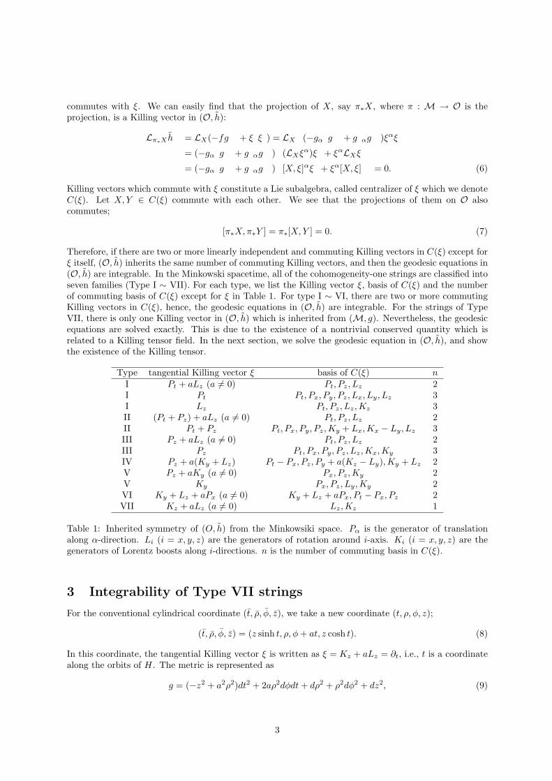
commutes with ξ. We can easily find that the projection of X, say π∗X, where π : M → O is theprojection, is a Killing vector in (O, h):
Lπ∗X hµν = LX(−fgµν + ξµξν) = LX
(−gαβgµν + gµαgνβ)ξαξβ
= (−gαβgµν + gµαgνβ)
(LXξα)ξβ + ξαLXξβ
= (−gαβgµν + gµαgνβ)
[X, ξ]αξβ + ξα[X, ξ]β
= 0. (6)
Killing vectors which commute with ξ constitute a Lie subalgebra, called centralizer of ξ which we denoteC(ξ). Let X,Y ∈ C(ξ) commute with each other. We see that the projections of them on O alsocommutes;
[π∗X,π∗Y ] = π∗[X,Y ] = 0. (7)
Therefore, if there are two or more linearly independent and commuting Killing vectors in C(ξ) except forξ itself, (O, h) inherits the same number of commuting Killing vectors, and then the geodesic equations in(O, h) are integrable. In the Minkowski spacetime, all of the cohomogeneity-one strings are classified intoseven families (Type I ∼ VII). For each type, we list the Killing vector ξ, basis of C(ξ) and the numberof commuting basis of C(ξ) except for ξ in Table 1. For type I ∼ VI, there are two or more commutingKilling vectors in C(ξ), hence, the geodesic equations in (O, h) are integrable. For the strings of TypeVII, there is only one Killing vector in (O, h) which is inherited from (M, g). Nevertheless, the geodesicequations are solved exactly. This is due to the existence of a nontrivial conserved quantity which isrelated to a Killing tensor field. In the next section, we solve the geodesic equation in (O, h), and showthe existence of the Killing tensor.
Type tangential Killing vector ξ basis of C(ξ) nI Pt + aLz (a 6= 0) Pt, Pz, Lz 2I Pt Pt, Px, Py, Pz, Lx, Ly, Lz 3I Lz Pt, Pz, Lz, Kz 3II (Pt + Pz) + aLz (a 6= 0) Pt, Pz, Lz 2II Pt + Pz Pt, Px, Py, Pz,Ky + Lx,Kx − Ly, Lz 3III Pz + aLz (a 6= 0) Pt, Pz, Lz 2III Pz Pt, Px, Py, Pz, Lz,Kx, Ky 3IV Pz + a(Ky + Lz) Pt − Px, Pz, Py + a(Kz − Ly),Ky + Lz 2V Pz + aKy (a 6= 0) Px, Pz,Ky 2V Ky Px, Pz, Ly,Ky 2VI Ky + Lz + aPx (a 6= 0) Ky + Lz + aPx, Pt − Px, Pz 2VII Kz + aLz (a 6= 0) Lz,Kz 1
Table 1: Inherited symmetry of (O, h) from the Minkowsiki space. Pα is the generator of translationalong α-direction. Li (i = x, y, z) are the generators of rotation around i-axis. Ki (i = x, y, z) are thegenerators of Lorentz boosts along i-directions. n is the number of commuting basis in C(ξ).
3 Integrability of Type VII strings
For the conventional cylindrical coordinate (t, ρ, φ, z), we take a new coordinate (t, ρ, φ, z);
(t, ρ, φ, z) = (z sinh t, ρ, φ + at, z cosh t). (8)
In this coordinate, the tangential Killing vector ξ is written as ξ = Kz + aLz = ∂t, i.e., t is a coordinatealong the orbits of H. The metric is represented as
g = (−z2 + a2ρ2)dt2 + 2aρ2dφdt + dρ2 + ρ2dφ2 + dz2, (9)
3
then, the norm weighted metric h is
h = (z2 − a2ρ2)(dρ2 + dz2) + z2ρ2dφ2. (10)
We solve the geodesic equation for this metric. Let σ be a parameter of the geodesic curve; (ρ(σ), φ(σ), z(σ)).The cohomogeneity one string solution, i.e., embedding (τ, σ) → (t, ρ, φ, z), is given as
(τ, σ) → (τ, ρ(σ), φ(σ), z(σ)). (11)
In order to solve the geodesic equation in (O, h), we start from the action
S =∫ [
1N
(z2 − a2ρ2)(ρ′2 + z′2) + z2ρ2φ′2 + N
]dσ, (12)
where the prime represents the differentiation with σ and N is a function of σ. N determines theparameter choice of the geodesic curve. For example, when we set N(σ) = 1, σ becomes an affineparameter. Fixing the re parametrization freedom by taking the function N as N = z2 − a2ρ2, we cansolve the geodesic equations as
z2 = C +√
C2 − a2L2 cosh 2(σ + σ0), (13)
a2ρ2 = C +√
C2 − a2L2 cos 2aσ, (14)
φ = tan−1
C −
√C2 − a2L2
aLtan aσ
− a tanh−1
C −
√C2 − a2L2
aLtanh(σ + σ0)
. (15)
where L, σ0 and C > 0 are constants. The constant L is related to φ-independence of h which is theresult of the inherited Killing. The constant C is related to the Killing tensor
K = a2ρ2(z2 − a2ρ2)dz2 + z2(z2 − a2ρ2)dρ2 + z2ρ2(z2 + a2ρ2)dφ2. (16)
4 Conclusion
We have found that the equation of motion for the cohomogeneity-one Nambu-Goto strings in theMinkowski spacetime are integrable. The equations of motion for the cohomogeneity-one strings arereduce to the geodesic equations in the orbit space. For the Type I ∼ VI, integrability of the geodesicequations comes from two or more inherited Killing vectors. For the Type VII, integrability comes froman inherited Killing vector and a non-trivial Killing tensor.
References
[1] E. J. Copeland, R. C. Myers and J. Polchinski, JHEP 0406, 013 (2004)
[2] S. Sarangi and S. H. H. Tye, Phys. Lett. B 536, 185 (2002)
[3] G. Dvali and A. Vilenkin, JCAP 0403, 010 (2004)
[4] M. G. Jackson, N. T. Jones and J. Polchinski, JHEP 0510, 013 (2005)
[5] C. J. Burden and L. J. Tassie, Austral. J. Phys. 35, 223 (1982).
C. J. Burden and L. J. Tassie, Austral. J. Phys. 37, 1 (1984).
[6] V. P. Frolov, V. Skarzhinsky, A. Zelnikov and O. Heinrich, Phys. Lett. B 224, 255 (1989).
V. P. Frolov, S. Hendy and J. P. De Villiers, Class. Quant. Grav. 14, 1099 (1997)
[7] K. Ogawa, H. Ishihara, H. Kozaki, H. Nakano and S. Saito,
[8] H. Ishihara and H. Kozaki, Phys. Rev. D 72, 061701 (2005)
[9] K. Ogawa, H. Ishihara, H. Kozaki and H. Nakano, arXiv:0811.2846 [gr-qc].
4
Primordial magnetic fields from second-order cosmologicalperturbations: Tight coupling approximation
Satoshi Maeda1, Satoshi Kitagawa2, Tsutomu Kobayashi3 and Tetsuya Shiromizu4
1 Department of Physics, Tokyo Institute of Technology, Tokyo 152-8551, Japan2,3 Department of Physics, Waseda University, Tokyo 169-8555, Japan,
4 Department of Physics, Kyoto University, Kyoto 606–8502, Japan
AbstractWe explore the possibility of generating large-scale magnetic fields from second-ordercosmological perturbations during the pre-recombination era [1]. The key process forthis is Thomson scattering between the photons and the charged particles within thecosmic plasma. To tame the multi-component interacting fluid system, we employthe tight coupling approximation. It is shown that the source term for the magneticfield is given by the vorticity, which signals the intrinsically second-order quantities,and the product of the first order perturbations. The vorticity itself is sourced bythe product of the first-order quantities in the vorticity evolution equation. Themagnetic fields generated by this process are estimated to be ∼ 10−29 Gauss on thehorizon scale.
1 Introduction
Magnetic fields are known to be present on various scales in the universe [2, 3]. For example, magneticfields are observed in galaxies and clusters, with intensity ∼ 1 µGauss. Only an upper limit has beengiven for magnetic fields on cosmological scales, < 10−9 Gauss. Primordial large-scale magnetic fieldsmay be present and serve as seeds for the magnetic fields in galaxies and clusters, which are amplifiedthrough the dynamo mechanism after galaxy formation [4].
A number of models have been proposed for generating large-scale magnetic fields in the early universe.However, they rely more or less on some unknown physics. In the present paper, we discuss magneto-genesis in the pre-recombination era using only the conventional physics that has been established. Thegeneration of magnetic fields in this era has been studied in Refs. [5, 6, 7, 8]. Now it is widely acceptedthat large-scale cosmological perturbations, generated from inflation in the early universe, evolve intoa variety of structures such as the cosmic microwave background anisotropies and galaxies. However,inflation produces only density fluctuations (scalar perturbations) and gravitational waves (tensor per-turbations); vector perturbations, and hence large-scale magnetic fields, are quite unlikely to be generatedin the context of standard inflationary scenarios. Even if they were generated due to some mechanism,they only decays without any sources. This argument is based on linear perturbation theory, and so wewill be studying second-order perturbations to overcome this difficulty. We consider a multi-fluid systemcomposed of photons, electrons, and protons, which are tightly coupled via Thomson and Coulomb scat-tering but slightly deviate from each other [9]. Thomson scattering is important for the generation oflarge-scale magnetic fields in the pre-recombination era, because a rotational current will be produced bythe momentum transfer due to the Thomson interaction. We shall see how this process occurs by doingthe tight coupling expansion.
1E-mail:maeda”at”th.phys.titech.ac.jp2E-mail:satoshi”at”gravity.phys.waseda.ac.jp3E-mail:tsutomu”at”gravity.phys.waseda.ac.jp4E-mail:shiromizu”at”tap.scphys.kyoto-u.ac.jp
1
2 Basic equations in second-order cosmological perturbation the-ory
The background spacetime is given by the spatially flat Friedmann-Lemaitre-Robertson-Walker metric.We write the perturbed metric in the Poisson gauge as
ds2 = a2(η)[−
(1 + 2ϕ(1) + 2ϕ(2)
)dη2 + 2χ
(2)i dηdxi +
(1 − 2R(1) − 2R(2)
)δijdxidxj
], (1)
where a is the scale factor and η is the conformal time We have dropped the first order vector perturbationsχ
(1)i since they are not generated from inflation in the standard scenarios. We also neglect the tensor
perturbations (gravitational waves) for simplicity.We consider a multi-fluid system composed of photons (γ), electrons (e), and protons (p). We assume
that the energy-momentum tensor for each fluid component is given by that of a perfect fluid (i.e., weneglect anisotropic stresses):
T ν(I)µ = (ρI + pI)u(I)µuν
(I) + pIδν
µ (I = γ, p, e), (2)
where pI = wIρI (wp = we = 0, wγ = 1/3) and uµ(I) is the 4-velocity of the fluid satisfying gµνu(I)µu(I)ν =
−1. We define δv(IJ)i ≡ v(I)i − v(J)i, β ≡ me/mp and v(b)i as the center of baryon’s mass velocity.The equations of motion governing the present 3-fluid system are given by
∇νT(γ)iν = κγp
i + κγei , (3)
∇νT(p)iν = enpEi + κpe
i + κpγi , (4)
∇νT(e)iν = −eneEi + κep
i + κeγi , (5)
where we neglected the Lorentz force from the magnetic field because it will give rise to higher ordercontributions and scattering term is
κγei = −κeγ
i = −σT neργ
(u(γ)i − u(e)i
), (6)
κγpi = −κpγ
i = −m2e
m2pσT npργ
(u(γ)i − u(p)i
), (7)
where σT , ργ , ne, np and me, mp are the Thomson cross section, the energy density of photons, thenumber density and mass of electrons and protons [6, 8]. The momentum transfer due to Coulombscattering is written as
κpei = −κep
i = −e2npneηC
(u(p)i − u(e)i
), (8)
where ηC is a electric resistivity which comes from Coulomb scattering.We get “Ohm’s law” from Eq.(4) and Eq.(5):
Ei =1 − β3
1 + β
σT
eaργ(1 − 2R)δv(γb)i. (9)
where we neglect δv(pe)i because δv(pe)i ≪ δv(γb)i in our case [8]. This equation may be regarded as“Ohm’s law” in some sense. In the standard Ohm’s law, the electric field is proportional to the electriccurrent density ∼ eδv(pe)i. It is reminded that the contribution from the electric current gives us thediffusion term in the evolution equation for the magnetic field, and then the source for the magnetic fieldcannot be induced. However, the electric field is proportional to δv(γb)i in the above formula. The currentin our “Ohm’s law”is originated from the velocity difference between protons and electrons through theinteraction with photons. Indeed, if one takes the same mass limit of β → 1 (though it is not realized inthe nature), the electric field cannot be generated.
Maxwell equation, ∇[λFµν] = 0, is(a3Bi
)′= −ϵijk∂j [a (1 + ϕ)Ek] − ϵijk (avjEk)′ . (10)
2
Thus we substitute Eq.(9) into Eq.(10) and get(a3Bi
)′= −1 − β3
1 + β
σT
eϵijka2
[∂j
(ργδv(γb)k
)+ ργ∂j(ϕ − 2R)δv(γb)k +
1a2
(ργvja
2δv(γb)k
)′]. (11)
Our remaining task is to evaluate δv(γb)i. The evolution equation of δv(γb)i is (4ργ/3)−1 × (3) −[mp (1 + β) n]−1 × [(4) + (5)] :
ρ′γργ
(v(γ)i + χi
)− n′
n
(v(b)i + χi
)+
(δv(γb)i
)′ + 4Hδv(γb)i − (ϕ + 2R)[ρ′γργ
v(γ)i −n′
nv(b)i +
(δv(γb)i
)′ + 4Hδv(γb)i
]−5R′δv(γb)i +
14
∂iργ
ργ+ ∂j
(v(γ)iv
j(γ)
)− 1
1 + β∂j
(v(p)iv
j(p) + βv(e)iv
j(e)
)= −α(1 − 2R)δv(γb)i, (12)
where α is defined as
α :=1 + β2
1 + β(1 + R)
aσT ργ
mp
(=
β(1 + β2)1 + β
(1 + R)1τT
)(13)
with R := 3mp (1 + β) n/4ργ and τT is the timescale of Thomson scattering for electrons.
3 Tight coupling approximation
We are to solve Eq. (12) using the tight coupling approximation (TCA) [9]. In this approximationthe time scale of Thomson scattering, τT , is assumed to be much smaller than the wavelengths of theperturbations (k−1). Thus, the small expansion parameter of the TCA is kτT , which is dimensionless.During the pre-recombination era, photons, protons, and electrons are strongly coupled via Thomsonscattering, and hence the TCA will be a good approximation.
At zeroth order in the TCA, all fluid components have the same velocity vi and the density fluctuationsare adiabatic. Following Ref. [8], we define the deviation from the adiabatic distribution for baryons bynb = nb (1 + ∆b) . Then, we expand various quantities such as ∆b and v(I)i in terms of the tight couplingparameter kτT :
∆b = ∆(I)b + ∆(II)
b + · · · , (14)
v(γ)i = vi, v(b)i = vi + v(I)(b)i + v
(II)(b)i + · · · , (15)
δv(γb)i = δv(I)(γb)i + δv
(II)(γb)i + · · · , (16)
where vi is the common velocity of photons and baryons in the tight coupling limit. Our notation is thatRoman and Arabic numerals stand for the order of TCA and that in cosmological perturbation theory,respectively. Here, we adopt the photon frame, so that ∆(I)
γ = ∆(II)γ = 0. In other words, the quantities
associated with photons give the “background” in the TCA. Note that we consider cosmological pertur-bation theory and the TCA simultaneously. The following analysis includes cosmological perturbationsup to second-order and the tight coupling expansion up to TCA(II), where TCA(n) denotes the tightcoupling approximation at n-th order.
4 Generation of magnetic fields
We solve Eq.(12) for δv(γb)i using TCA and substitute the results into Eq.(11). When we consider up toTCA(I), the equation of the magnetic field is
(a3Bi)′ = 21 − β3
1 + β
σT
ea4ρ(0)
γ
Hα(0)
ω(2)i. (17)
where ω(2)i is photon’s vorticity, ωi ≡ − 12εiνρλu(γ)λ∇νu(γ)ρ. The evolution equation of the vorticity is
obtained by taking the curl of the total momentum conservation:(2a2ρ
(0)T ωi(2)
)′+ 8a2Hρ
(0)T ωi(2) = 0. (18)
3
It is important to note here that there is no source for the vorticity at TCA(I). Therefore, the vorticitydecays and the magnetic field is not generated at TCA(I).
Next we consider up to TCA(II). Then the equation of the magnetic field is
(a3Bi)′ =1 − β3
1 + β
σT
ea2ρ(0)
γ
[2a2Hα(0)
ω(2)i + ϵijk R(0)
1 + R(0)∂j∆
(I,1)b δv
(I,1)(γb)k
]. (19)
In the same way the evolution equation of the vorticity is
(a2ω(2)i)′ +HR(0)
1 + R(0)a2ω(2)i =
R(0)
2(1 + R(0))2ϵijk∂j∆
(I,1)b δv
(I,1)(γb)k. (20)
Since the right hand side in Eq. (20) contain the source term for the vorticity at TCA(II), the vorticitycan be generated at this order. Thus the magnetic field is generated. We estimate roughly the valueof the generated magnetic field at the recombination epoch. When we consider the horizon scale, B ∼10−29 Gauss. According to [4], this will be amplified enough to explain the present observed magneticfields.
5 Summary and future works
We have derived an analytic formula for the magnetic fields generated from second-order cosmologicalperturbations in the pre-recombination era. Photons and charged particles are strongly coupled viaThomson scattering within the cosmic plasma, and hence the system behaves almost as a single fluid. Inthis single-fluid description magnetic fields are never generated, and therefore the tiny deviation from thesingle-fluid description is crucial here. Using the tight coupling approximation (TCA) to treat the smalldifference between photons and charged particles, we have seen how magnetic fields are generated fromcosmic inhomogeneities. It was found that magnetic fields are not generated at first order in the TCA.Therefore, we conclude that magnetogenesis requires both the second-order cosmological perturbationsand the second-order TCA. The resultant magnetic fields are expressed in terms of the vorticity andthe product of the first-order perturbations. The latter can be computed by solving the linear Einsteinequations, while the former is governed by the vorticity evolution equation, with the source term givenby the product of the first order terms.
We have not included the effect of anisotropic stresses of photon fluids and the recombination process,though they will be equally important for magnetogenesis on small scales [7]. Taking into account theseeffects and computing the power spectrum of the generated magnetic fields require detailed numericalcalculations, which are left for future works.
References
[1] S. Maeda, S. Kitagawa, T. Kobayashi and T. Shiromizu , arXiv:0805.0169 [astro-ph].
[2] L. M. Widrow, Rev. Mod. Phys. 74, 775 (2002).
[3] D. Grasso and H. R. Rubinstein, Phys. Rep. 348, 163 (2001).
[4] See, e.g., A. C. Davis, M. Lilley and O. Tornkvist, Phys. Rev. D 60, 021301 (1999).
[5] S. Matarrese, S. Mollerach, A. Notari and A. Riotto, Phys. Rev. D 71, 043502 (2005).
[6] T. Kobayashi, R. Maartens, T. Shiromizu and K. Takahashi, Phys. Rev. D 75, 103501 (2007).
[7] K. Ichiki, K. Takahashi, N. Sugiyama, H. Hanayama and H. Ohno, Science 311, 827 (2006).
[8] K. Takahashi, K. Ichiki and N. Sugiyama, Phys. Rev. D 77, 124028 (2008).
[9] P. J. E. Peebles, The Large Scale structure of the Universe (Princeton University Press, Princeton,NJ, 1980).
4
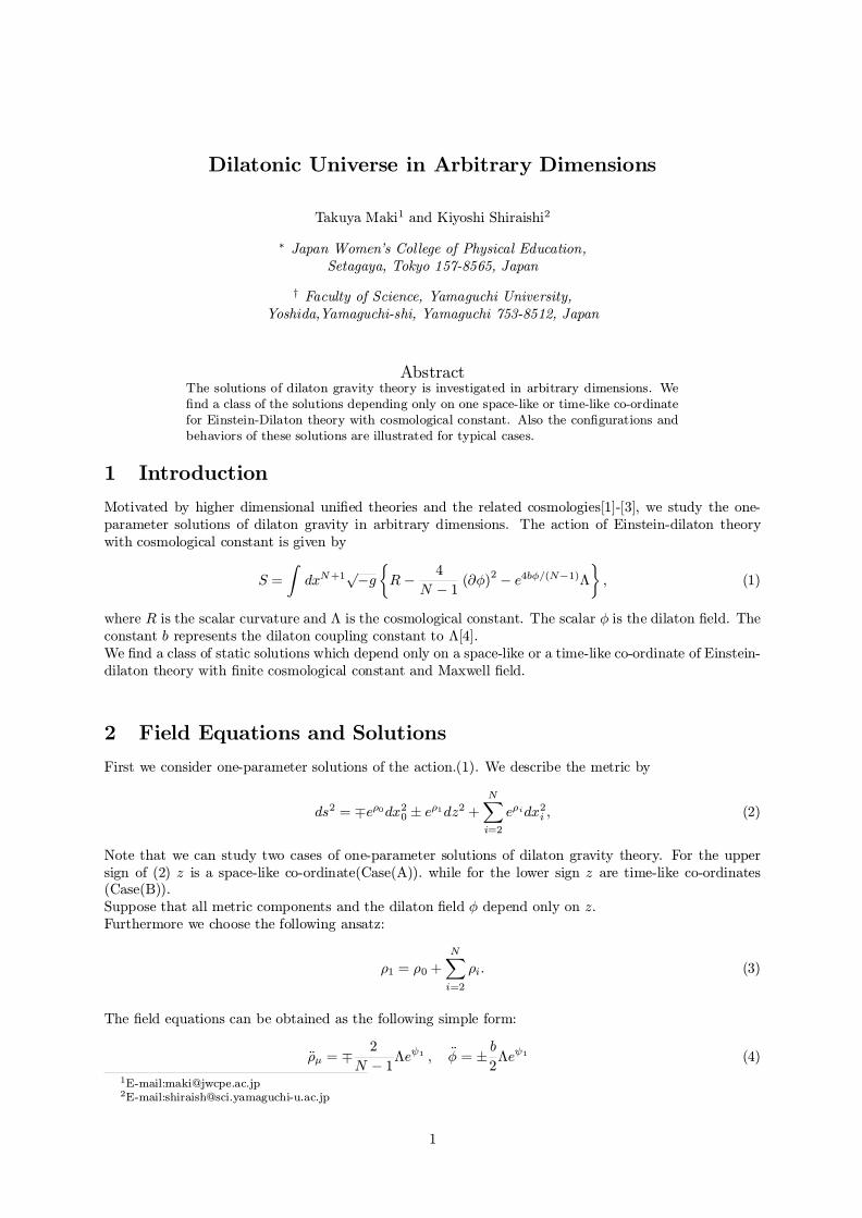
Dilatonic Universe in Arbitrary Dimensions
Takuya Maki1 and Kiyoshi Shiraishi2
¤ Japan Women's College of Physical Education,Setagaya, Tokyo 157-8565, Japan
y Faculty of Science, Yamaguchi University,Yoshida,Yamaguchi-shi, Yamaguchi 753-8512, Japan
AbstractThe solutions of dilaton gravity theory is investigated in arbitrary dimensions. We¯nd a class of the solutions depending only on one space-like or time-like co-ordinatefor Einstein-Dilaton theory with cosmological constant. Also the con¯gurations andbehaviors of these solutions are illustrated for typical cases.
1 Introduction
Motivated by higher dimensional uni¯ed theories and the related cosmologies[1]-[3], we study the one-parameter solutions of dilaton gravity in arbitrary dimensions. The action of Einstein-dilaton theorywith cosmological constant is given by
S =
ZdxN+1
p¡g½R ¡ 4
N ¡ 1 (@Á)2 ¡ e4bÁ=(N¡1)¤
¾; (1)
where R is the scalar curvature and ¤ is the cosmological constant. The scalar Á is the dilaton ¯eld. Theconstant b represents the dilaton coupling constant to ¤[4].We ¯nd a class of static solutions which depend only on a space-like or a time-like co-ordinate of Einstein-dilaton theory with ¯nite cosmological constant and Maxwell ¯eld.
2 Field Equations and Solutions
First we consider one-parameter solutions of the action.(1). We describe the metric by
ds2 = ¨e½0dx20 § e½1dz2 +NX
i=2
e½idx2i ; (2)
Note that we can study two cases of one-parameter solutions of dilaton gravity theory. For the uppersign of (2) z is a space-like co-ordinate(Case(A)). while for the lower sign z are time-like co-ordinates(Case(B)).Suppose that all metric components and the dilaton ¯eld Á depend only on z.Furthermore we choose the following ansatz:
½1 = ½0 +NX
i=2
½i: (3)
The ¯eld equations can be obtained as the following simple form:
Ľ¹ = ¨2
N ¡ 1¤eÃ1 ; ÄÁ = § b
2¤eÃ1 (4)
1E-mail:[email protected]:[email protected]
1
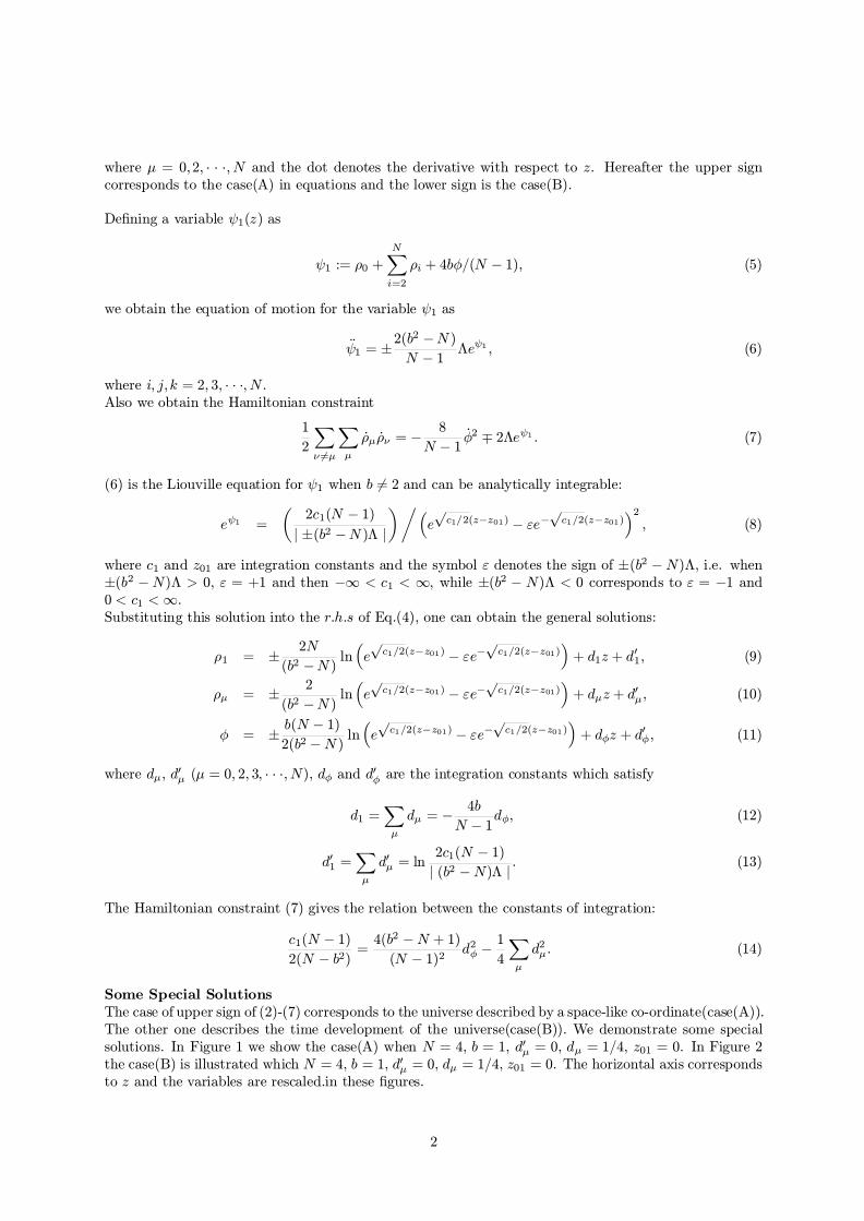
where ¹ = 0;2; ¢ ¢ ¢; N and the dot denotes the derivative with respect to z. Hereafter the upper signcorresponds to the case(A) in equations and the lower sign is the case(B).
De¯ning a variable Ã1(z) as
Ã1 := ½0 +NX
i=2
½i + 4bÁ=(N ¡ 1); (5)
we obtain the equation of motion for the variable Ã1 as
ÄÃ1 = §2(b2 ¡N )N ¡ 1 ¤eÃ1 ; (6)
where i; j;k = 2; 3; ¢ ¢ ¢; N .Also we obtain the Hamiltonian constraint
1
2
X
º 6=¹
X
¹
_½¹ _½º = ¡8
N ¡ 1_Á2 ¨ 2¤eÃ1 : (7)
(6) is the Liouville equation for Ã1 when b 6= 2 and can be analytically integrable:
eÃ1 =
µ2c1(N ¡ 1)j §(b2 ¡N )¤ j
¶Á³epc1=2(z¡z01) ¡ "e¡
pc1=2(z¡z01)
´2; (8)
where c1 and z01 are integration constants and the symbol " denotes the sign of §(b2 ¡N)¤, i.e. when§(b2 ¡N)¤ > 0, " = +1 and then ¡1 < c1 < 1, while §(b2 ¡ N)¤ < 0 corresponds to " = ¡1 and0 < c1 <1.Substituting this solution into the r:h:s of Eq.(4), one can obtain the general solutions:
½1 = § 2N
(b2 ¡N ) ln³epc1=2(z¡z01) ¡ "e¡
pc1=2(z¡z01)
´+ d1z + d01; (9)
½¹ = § 2
(b2 ¡N ) ln³epc1=2(z¡z01) ¡ "e¡
pc1=2(z¡z01)
´+ d¹z + d0¹; (10)
Á = § b(N ¡ 1)2(b2 ¡N ) ln
³epc1=2(z¡z01) ¡ "e¡
pc1=2(z¡z01)
´+ dÁz + d0Á; (11)
where d¹, d0¹ (¹ = 0; 2; 3; ¢ ¢ ¢; N), dÁ and d0Á are the integration constants which satisfy
d1 =X
¹
d¹ = ¡4b
N ¡ 1dÁ; (12)
d01 =X
¹
d0¹ = ln2c1(N ¡ 1)j (b2 ¡N)¤ j : (13)
The Hamiltonian constraint (7) gives the relation between the constants of integration:
c1(N ¡ 1)2(N ¡ b2) =
4(b2 ¡N + 1)
(N ¡ 1)2 d2Á ¡1
4
X
¹
d2¹: (14)
Some Special SolutionsThe case of upper sign of (2)-(7) corresponds to the universe described by a space-like co-ordinate(case(A)).The other one describes the time development of the universe(case(B)). We demonstrate some specialsolutions. In Figure 1 we show the case(A) when N = 4, b = 1, d0¹ = 0, d¹ = 1=4, z01 = 0. In Figure 2the case(B) is illustrated which N = 4, b = 1, d0¹ = 0, d¹ = 1=4, z01 = 0. The horizontal axis correspondsto z and the variables are rescaled.in these ¯gures.
2
Figure 1: case(A) The solid line is dilaton Á,the doted line is g00 = e½0 and the dashedline is g11 = e½1 .
Figure 2: case(A) The solid line is dilaton Á, thedoted line is g00 = e½0 and the dashed line is g11 =e½1.
3 Charged Dilatonic Universe
Next we consider the case of Einstein-Maxwell-Dilaton system given by the action
S =
ZdxN+1
p¡g½R ¡ 4
N ¡ 1 (@Á)2 ¡ e¡4aÁ=(N¡1)F2
¾; (15)
where F is the strength of Maxwell ¯eld, and a = 1 corresponds to the low energy string action in Einsteinframe.
De¯ne a set of the variables ù where ¹ = 0;2; :::N as
ù = ½¹ +4a
N ¡ 1Á: (16)
For the case(A) the ¯eld equations are described by Ã's as
Äù = 4X
®
´¹®q®q¹eù +
4(a2 ¡ 1)N ¡ 1
X
®;¯
´®¯q®q¯eî ; (17)
ÄÁ = aX
¹;º
´¹ºq¹qºeù ; (18)
where ´¹º = diag(¡1;+1;+1; :::;+1) and q¹ = (qe; qmj) are the constants of integration with respect toMaxwell ¯eld:
F1¹ = _A¹ = q¹eù : (19)
The Hamiltonian constraint is
1
2
X
º 6=¹
X
¹
_½¹ _½º =¡8
N ¡ 1_Á2 ¡ 4
X
®;
´®¯q®q¯eî (20)
3
From (¹; º)-components(¹ 6= º) of the Einstein equations
q¹qº = 0; (q¹ 6= qº): (21)
For the case(B) we obtained the equation of motion by exchanging ´¹º to ±¹º in (17)-(20) This resultmeans that only one of q¹ is not zero.
The electric solutions with vanishing cosmological constantIn this case, i.e. q¹ = (qe; 0; 0; ¢ ¢ ¢; 0) and ¤ = 0, the ¯eld equations are
ÄÃ0 = ¨4µ1 +
a2 ¡ 1N ¡ 1
¶q2ee
Ã0 ; ÄÃj = ¨4µa2 ¡ 1N ¡ 1
¶q2ee
Ã0 ; (22)
Ľ0 = ¨4(1§ 1
N ¡ 1)q2eeÃ0 Ľj = §
4
N ¡ 1q2eeÃ0 ; (23)
ÄÁ = ¡aq2eeÃ0 ; (24)
F10 = _A0 = qeeÃ0 : (25)
The Hamiltonian constraint is
1
2
X
º 6=¹
X
¹
_½¹ _½º =¡8
N ¡ 1_Á2 ¨ 4qeeÃ0 (26)
One can integrate these equations and obtain the `electric solutions':
½0 =2(N ¡ 2)N + a2 ¡ 2 ln cosh
rc12(z ¡ z01) + d0z + d00 ; (27)
½1 =2(2N ¡ 3)N + a2 ¡ 2 ln cosh
rc12(z ¡ z01) + d1z + d01 ; (28)
½i =2
N + a2 ¡ 2 ln coshrc12(z ¡ z01) + diz + d0i ; (29)
Á =¡a(N ¡ 1)N + a2 ¡ 2 ln cosh
rc12(z ¡ z01) + dÁ + d0Á ; (30)
F10 = :(c=4qe)(N ¡ 1)N + a2 ¡ 2
1
cosh2p
c12 (z ¡ z01)
: (31)
The con¯gurations of the solution are researching now and will be studied in a separate publication.
4 Summary and Outlook
We have investigated the universe of the dilaton gravity in arbitrary dimensions. The metric given inthis paper describes two type solutions, i.e. the static dilatonic universe depending only on a space-likeco-ordinate and the universe which behaves by a time-like co-ordinate. A class of the solutions have beenfound for ¯nite cosmological constant and Maxwell ¯eld. We have shown some special con¯gurations ofthe solutions.
References
[1] N. Arkani-Hamed, S. Dimpooulos and G. Dvali, Phys.Lett. B429 (1998) 263.
[2] L. Randall and R. Sundrum, Phys.Rev.Lett. 83 (1999) 3370.
[3] C. Charmousis, Class. Quant. Grav. 19 (2002) 83.
[4] M. Cadoni, Phys. Rev. D54, 7378 (1996)
4
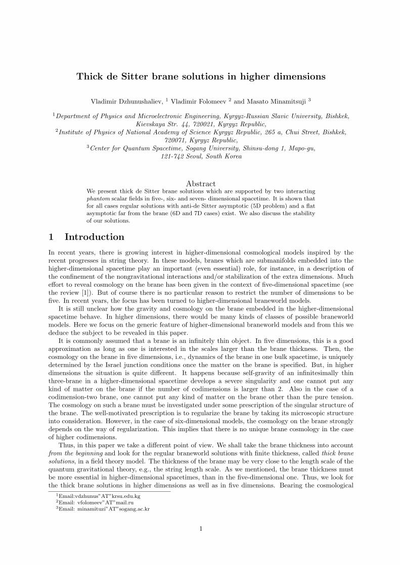
Thick de Sitter brane solutions in higher dimensions
Vladimir Dzhunushaliev, 1 Vladimir Folomeev 2 and Masato Minamitsuji 3
1Department of Physics and Microelectronic Engineering, Kyrgyz-Russian Slavic University, Bishkek,Kievskaya Str. 44, 720021, Kyrgyz Republic,
2Institute of Physics of National Academy of Science Kyrgyz Republic, 265 a, Chui Street, Bishkek,720071, Kyrgyz Republic,
3Center for Quantum Spacetime, Sogang University, Shinsu-dong 1, Mapo-gu,121-742 Seoul, South Korea
AbstractWe present thick de Sitter brane solutions which are supported by two interactingphantom scalar fields in five-, six- and seven- dimensional spacetime. It is shown thatfor all cases regular solutions with anti-de Sitter asymptotic (5D problem) and a flatasymptotic far from the brane (6D and 7D cases) exist. We also discuss the stabilityof our solutions.
1 Introduction
In recent years, there is growing interest in higher-dimensional cosmological models inspired by therecent progresses in string theory. In these models, branes which are submanifolds embedded into thehigher-dimensional spacetime play an important (even essential) role, for instance, in a description ofthe confinement of the nongravitational interactions and/or stabilization of the extra dimensions. Mucheffort to reveal cosmology on the brane has been given in the context of five-dimensional spacetime (seethe review [1]). But of course there is no particular reason to restrict the number of dimensions to befive. In recent years, the focus has been turned to higher-dimensional braneworld models.
It is still unclear how the gravity and cosmology on the brane embedded in the higher-dimensionalspacetime behave. In higher dimensions, there would be many kinds of classes of possible braneworldmodels. Here we focus on the generic feature of higher-dimensional braneworld models and from this wededuce the subject to be revealed in this paper.
It is commonly assumed that a brane is an infinitely thin object. In five dimensions, this is a goodapproximation as long as one is interested in the scales larger than the brane thickness. Then, thecosmology on the brane in five dimensions, i.e., dynamics of the brane in one bulk spacetime, is uniquelydetermined by the Israel junction conditions once the matter on the brane is specified. But, in higherdimensions the situation is quite different. It happens because self-gravity of an infinitesimally thinthree-brane in a higher-dimensional spacetime develops a severe singularity and one cannot put anykind of matter on the brane if the number of codimensions is larger than 2. Also in the case of acodimension-two brane, one cannot put any kind of matter on the brane other than the pure tension.The cosmology on such a brane must be investigated under some prescription of the singular structure ofthe brane. The well-motivated prescription is to regularize the brane by taking its microscopic structureinto consideration. However, in the case of six-dimensional models, the cosmology on the brane stronglydepends on the way of regularization. This implies that there is no unique brane cosmology in the caseof higher codimensions.
Thus, in this paper we take a different point of view. We shall take the brane thickness into accountfrom the beginning and look for the regular braneworld solutions with finite thickness, called thick branesolutions, in a field theory model. The thickness of the brane may be very close to the length scale of thequantum gravitational theory, e.g., the string length scale. As we mentioned, the brane thickness mustbe more essential in higher-dimensional spacetimes, than in the five-dimensional one. Thus, we look forthe thick brane solutions in higher dimensions as well as in five dimensions. Bearing the cosmological
1Email:vdzhunus”AT”krsu.edu.kg2Email: vfolomeev”AT”mail.ru3Email: minamituzi”AT”sogang.ac.kr
1
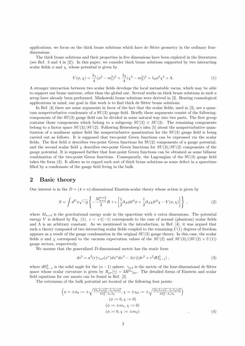
applications, we focus on the thick brane solutions which have de Sitter geometry in the ordinary four-dimensions.
The thick brane solutions and their properties in five dimensions have been explored in the literatures(see Ref. 3 and 4 in [2]). In this paper, we consider thick brane solutions supported by two interactingscalar fields φ and χ, whose potential is given by
V (φ, χ) =λ1
4(φ2 −m2
1)2 +
λ2
4(χ2 −m2
2)2 + λ3φ
2χ2 + Λ. (1)
A stronger interaction between two scalar fields develops the local metastable vacua, which may be ableto support our brane universe, other than the global one. Several works on thick brane solutions in such asetup have already been performed. Minkowski brane solutions were derived in [3]. Bearing cosmologicalapplications in mind, our goal in this work is to find thick de Sitter brane solutions.
In Ref. [4] there are some arguments in favor of the fact that the scalar fields, used in [3], are a quan-tum nonperturbative condensate of a SU(3) gauge field. Briefly these arguments consist of the following:components of the SU(3) gauge field can be divided in some natural way into two parts. The first groupcontains those components which belong to a subgroup SU(2) ∈ SU(3). The remaining componentsbelong to a factor space SU(3)/SU(2). Following Heisenberg’s idea [5] about the nonperturbative quan-tization of a nonlinear spinor field the nonperturbative quantization for the SU(3) gauge field is beingcarried out as follows. It is supposed that two-point Green functions can be expressed via the scalarfields. The first field φ describes two-point Green functions for SU(2) components of a gauge potential,and the second scalar field χ describes two-point Green functions for SU(3)/SU(2) components of thegauge potential. It is supposed further that four-point Green functions can be obtained as some bilinearcombination of the two-point Green functions. Consequently, the Lagrangian of the SU(3) gauge fieldtakes the form (2). It allows us to regard such sort of thick brane solutions as some defect in a spacetimefilled by a condensate of the gauge field living in the bulk.
2 Basic theory
Our interest is in the D = (4 + n)-dimensional Einstein-scalar theory whose action is given by
S =∫
dDx√−g
−Mn+2
n+4
2R + ε
[12∂Aφ∂Aφ +
12∂Aχ∂Aχ− V (φ, χ)
], (2)
where Mn+4 is the gravitational energy scale in the spacetime with n extra dimensions. The potentialenergy V is defined by Eq. (1). ε = +1(−1) corresponds to the case of normal (phantom) scalar fieldsand Λ is an arbitrary constant. As we mentioned in the introduction, in Ref. [4], it was argued thatsuch a theory composed of two interacting scalar fields coupled to the remaining U(1) degrees of freedomappears as a result of the gauge condensation in the original SU(3) gauge theory. In this case, the scalarfields φ and χ correspond to the vacuum expectation values of the SU(2) and SU(3)/(SU(2) × U(1))gauge sectors, respectively.
We assume that the generalized D-dimensional metric has the static form
ds2 = a2(r)γαβ(xν)dxαdxβ − λ(r)(dr2 + r2dΩ2n−1) , (3)
where dΩ2n−1 is the solid angle for the (n− 1) sphere. γαβ is the metric of the four-dimensional de Sitter
space whose scalar curvature is given by Rµν [γ] = 3H2γµν . The detailed forms of Einstein and scalarfield equations for our ansatz can be found in Ref. [2].
The extremum of the bulk potential are located at the following four points(φ = ±φ0 := ±
√2λ3λ2m2
2−λ1λ2m21
4λ23−λ1λ2
, χ = ±χ0 := ±√
2λ3λ1m21−λ1λ2m2
24λ2
3−λ1λ2
)
(φ := 0, χ := 0)(φ := ±m1, χ := 0)(φ := 0, χ := ±m2) . (4)
2
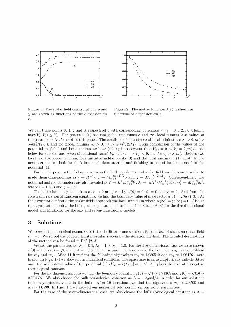
0 2 4 6 8 100,0
0,4
0,8
1,2
1,6
2,0
2,4
5D 6D 7D
r
Figure 1: The scalar field configurations φ andχ are shown as functions of the dimensionlessr.
0 2 4 6 8 100,0
0,2
0,4
0,6
0,8
1,0
6D 7D
r
5D
Figure 2: The metric function λ(r) is shown asfunctions of dimensionless r.
We call these points 0, 1, 2 and 3, respectively, with correspoding potentials Vi (i = 0, 1, 2, 3). Clearly,max(V2, V3) ≤ V1. The potential (1) has two global minimums 3 and two local minima 2 at values ofthe parameters λ1, λ2 used in this paper. The conditions for existence of local minima are λ1 > 0,m2
1 >λ2m
22/(2λ3), and for global minima λ2 > 0,m2
2 > λ1m21/(2λ3). From comparison of the values of the
potential in global and local minima we have (taking into account that Vloc = 0 at V0 = λ2m42/4, see
below for the six- and seven-dimensional cases) Vgl < Vloc =⇒ Vgl < 0, i.e. λ2m42 > λ1m
41. Besides two
local and two global minima, four unstable saddle points (0) and the local maximum (1) exist. In thenext sections, we look for thick brane solutions starting and finishing in one of local minima 2 of thepotential (1).
For our purpose, in the following sections the bulk coordinate and scalar field variables are rescaled tomade them dimensionless as r → H−1r, φ → M
−(n+2)/2n+4 φ and χ → M
−(n+2)/2n+4 χ. Correspondingly, the
potential and its parameters are also rescaled as V → H2Mn+2n+4 V , λi → λiH
2/Mn+2n+4 and m2
j → Mn+2n+4 m2
j ,where i = 1, 2, 3 and j = 1, 2.
Then, the boundary conditions at r → 0 are given by a′(0) = 0, φ′ = 0 and χ′ = 0. And from theconstraint relation of Einstein equations, we find the boundary value of scale factor a(0) =
√6ε/V (0). At
the asymptotic infinity, the scalar fields approach the local minimum where φ′(∞) = χ′(∞) = 0. Also atthe asymptotic infinity, the bulk geometry is assumed to be anti-de Sitter (AdS) for the five-dimensionalmodel and Minkowki for the six- and seven-dimensional models.
3 Solutions
We present the numerical examples of thick de Sitter brane solutions for the case of phantom scalar fieldε = −1. We solved the coupled Einstein-scalar system by the iteration method. The detailed descriptionsof the method can be found in Ref. [2, 3].
We set the parameters as: λ1 = 0.1, λ2 = 1.0, λ3 = 1.0. For the five-dimensional case we have chosenφ(0) = 1.0, χ(0) =
√0.6 and Λ = −3.6. For these parameters we solved the nonlinear eigenvalue problem
for m1 and m2. After 11 iterations the following eigenvalues m1 ≈ 1.989512 and m2 ≈ 1.964764 werefound. In Figs. 1-4 we showed our numerical solutions. The spacetime is an asymptotically anti-de Sitterone: the asymptotic value of the potential (1) εV∞ = ε(λ2m
42/4 + Λ) < 0 plays the role of a negative
cosmological constant.For the six-dimensional case we take the boundary condition φ(0) =
√3 ≈ 1.73205 and χ(0) =
√0.6 ≈
0.774597. We also choose the bulk cosmological constant as Λ = −λ2m42/4, in order for our solutions
to be asymptotically flat in the bulk. After 10 iterations, we find the eigenvalues m1 ≈ 2.3590 andm2 ≈ 3.0599. In Figs. 1-4 we showed our numerical solution for a given set of parameters.
For the case of the seven-dimensional case, we also choose the bulk cosmological constant as Λ =
3
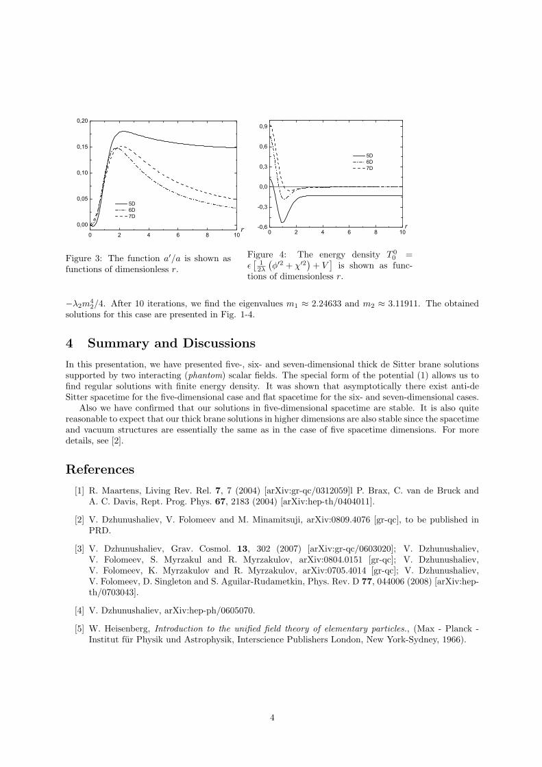
0 2 4 6 8 10
0,00
0,05
0,10
0,15
0,20
5D 6D 7D
r
Figure 3: The function a′/a is shown asfunctions of dimensionless r.
0 2 4 6 8 10-0,6
-0,3
0,0
0,3
0,6
0,9
5D 6D 7D
r
Figure 4: The energy density T 00 =
ε[
12λ
(φ′2 + χ′2
)+ V
]is shown as func-
tions of dimensionless r.
−λ2m42/4. After 10 iterations, we find the eigenvalues m1 ≈ 2.24633 and m2 ≈ 3.11911. The obtained
solutions for this case are presented in Fig. 1-4.
4 Summary and Discussions
In this presentation, we have presented five-, six- and seven-dimensional thick de Sitter brane solutionssupported by two interacting (phantom) scalar fields. The special form of the potential (1) allows us tofind regular solutions with finite energy density. It was shown that asymptotically there exist anti-deSitter spacetime for the five-dimensional case and flat spacetime for the six- and seven-dimensional cases.
Also we have confirmed that our solutions in five-dimensional spacetime are stable. It is also quitereasonable to expect that our thick brane solutions in higher dimensions are also stable since the spacetimeand vacuum structures are essentially the same as in the case of five spacetime dimensions. For moredetails, see [2].
References
[1] R. Maartens, Living Rev. Rel. 7, 7 (2004) [arXiv:gr-qc/0312059]l P. Brax, C. van de Bruck andA. C. Davis, Rept. Prog. Phys. 67, 2183 (2004) [arXiv:hep-th/0404011].
[2] V. Dzhunushaliev, V. Folomeev and M. Minamitsuji, arXiv:0809.4076 [gr-qc], to be published inPRD.
[3] V. Dzhunushaliev, Grav. Cosmol. 13, 302 (2007) [arXiv:gr-qc/0603020]; V. Dzhunushaliev,V. Folomeev, S. Myrzakul and R. Myrzakulov, arXiv:0804.0151 [gr-qc]; V. Dzhunushaliev,V. Folomeev, K. Myrzakulov and R. Myrzakulov, arXiv:0705.4014 [gr-qc]; V. Dzhunushaliev,V. Folomeev, D. Singleton and S. Aguilar-Rudametkin, Phys. Rev. D 77, 044006 (2008) [arXiv:hep-th/0703043].
[4] V. Dzhunushaliev, arXiv:hep-ph/0605070.
[5] W. Heisenberg, Introduction to the unified field theory of elementary particles., (Max - Planck -Institut fur Physik und Astrophysik, Interscience Publishers London, New York-Sydney, 1966).
4
Informational interpretation on volume operator and physicalbound on information
Yoshiyuki Morisawa1
Faculty of General Arts and Sciences, Osaka University of Economics and Law,Gakuonji 6-10, Yao, Osaka, 581–8511, Japan
AbstractFrom informational viewpoint on volume operator in loop quantum gravity, followingconjecture is suggested: a logic gate must occupy finite volume which has the mini-mum value, and number of logic gates contained within a region of space are boundedby the volume of the region.
1 Introduction
Since information is registered and processed by physical system, it is necessarily restricted by physicallaw. Several physical bounds on information are well-known. The most famous example is causality:information cannot travel faster than the speed of light. As for thermodynamics, it must consume freeenergy kT ln 2 to erase a bit [1, 2]. In addition, entropy (or information) that can be contained withina region of a space are bounded by the area of the region as S ≤ A/4, so-called holographic bound (seee.g. [3]). Margolus-Levitin theorem gives the bound on the maximum speed of dynamical evolution (i.e.bound on information processing rates) [4]. This bound depends on the energy of the system. Using this,Lloyd estimated the bound for the total number of elementary operations in the universe [5].
In this article, a new physical bound on information is conjectured: a logic gate must occupy finitevolume and this volume has the minimum value. Then, number of logic gates contained within a regionof a space are bounded by the volume of the region.
2 Informational viewpoint on loop quantum gravity
At the beginning, we review some facts about loop quantum gravity (for detail, see e.g. [6]). Loop quantumgravity is the nonperturbative quantization of the general relativity as a diffeomorphism-invariant gaugetheory. Its quantum states are gauge invariant and diffeo-invariant. The spin network states satisfy suchinvariances, and they span the state space of loop quantum gravity as the ortho-normal bases. A spinnetwork state is labeled by a spin network. A spin network is a graph with edges labeled by half-integerspin and can be interpreted as a linear combination of some loops. As a functional of connection field, aspin network state takes value of the trace of the holonomy along its spin network.
In loop quantum gravity, area and volume are defined as operators. These operators geometricallyoperate on spin network states, and spin network states are eigen states of area and volume operators.Area operator for a surface is constructed from area integral with regularization. Its discrete eigenvalue isthe form of A = 8πγl2Planck
∑Nn=1
√jn(jn + 1). Where n = 1 . . . N labels the edges (of the spin network)
crossing the surface, and each edge has spin jn. The area of the surface is sum over the area of theedges crossing the surface. Volume operator for a region is also constructed from volume integral withregularization. The volume of the region is sum over the volume of vertices within the region. It has alsodiscrete eigenvalues: 3-valent vertex has 0 volume, and 4(or more)-valent vertex has finite volume.
Now, let us see the loop quantum gravity from informational viewpoint. Consider a spin networkstate with spin 1/2 edge. How is this state different from the state without such edge as a functional ofconnection? The difference is (trace of) holonomy along that edge. By existence of the edge, this statecan probe the connection there like as spin 1/2 degree of freedom. It seems there is 1 bit informationalong spin 1/2 edge.
1E-mail:[email protected]
1
Then, consider the situation that the spin 1/2 edge across some surface. There is 1 bit informationalong the spin 1/2 edge and this edge produces area on the surface. It seems that a channel where 1bit information can pass must have the area
√3
4 l20 where l20 = 8πγl2Planck. This is a kind of holographic
bound.Finally, let us reinterpret the volume operator from informational viewpoint. The spin 1/2 edges can
be regarded as 1 bit channels and an invertible logic gate such as controlled-NOT has at least 2 inputsand 2 outputs. Then, can 4-valent vertices be regarded as invertible logic gates? 4-valent vertices producefinite volumes under operation of the volume operator. Thus, the logic gate must occupy finite volume
at least√√
38 l
30.
3 Summary and discussion
A new kind of physical bound on information is conjectured. A logic gate must occupy finite volume andthis volume has the minimum value. Then, number of logic gates contained within a region of a spaceare bounded by the volume of the region.
Roughly estimation shows that computation with only 10183 logic gates can be executed in the uni-verse. Of course this bound is not so severe on present CPUs. They have about 109 gates in about10−6m3 volume. It takes about 600 years to become effective even if “Moore’ s law” is correct.
It should be mentioned that the dynamical feature is not treated here. The spin foam model mightshow the bound for executable operations in a finite spacetime region.
References
[1] R. Landauer, “Irreversibility and Heat Generation in the Computing Process,” IBM Journal ofResearch and Development 5, 183 (1961).
[2] C. H. Bennett, “Logical Reversibility of Computation,” IBM Journal of Research and Development17, 525 (1973).
[3] R. Bousso, “The holographic principle,” Rev. Mod. Phys. 74, 825 (2002) [arXiv:hep-th/0203101].
[4] N. Margolus and L. B. Levitin, “The maximum speed of dynamical evolution,” Physica D 120, 188(1998) [arXiv:quant-ph/9710043].
[5] S. Lloyd, “Computational capacity of the universe,” Phys. Rev. Lett. 88, 237901 (2002) [arXiv:quant-ph/0110141].
[6] C. Rovelli, “Quantum Gravity,” Cambridge University Press, (2004).
2
Consistency relations between the source terms in thesecond-order Einstein equations for cosmological perturbations
Kouji NAKAMURA1,
Department of Astronomical Science, the Graduate University for Advanced Studies,Mitaka, Tokyo 181-8588, Japan.
AbstractIn addition to the second-order Einstein equations on four-dimensional homogeneousisotropic background universe filled with the single perfect fluid, we also derived thesecond-order perturbations of the continuity equation and the Euler equation for aperfect fluid in gauge-invariant manner without ignoring any mode of perturbations.The consistency of all equations of the second-order Einstein equation and the equa-tions of motion for matter fields is confirmed. Due to this consistency check, we maysay that the set of all equations of the second-order are self-consistent and they arecorrect in this sense.
1 Introduction
The general relativistic second-order cosmological perturbation theory is one of topical subjects in therecent cosmology. By the recent observation[1], the first order approximation of the fluctuations of ouruniverse from a homogeneous isotropic one was revealed. The observational results also suggest that thefluctuations of our universe are adiabatic and Gaussian at least in the first order approximation. We arenow on the stage to discuss the deviation from this first order approximation from the observational[2]and the theoretical side[3] through the non-Gaussianity, the non-adiabaticity, and so on. To carry outthis, some analyses beyond linear order are required. The second-order cosmological perturbation theoryis one of such perturbation theories beyond linear order.
In this article, we confirm the consistency of all equations of the second-order Einstein equation andthe equations of motion for matter fields, which are derived in Refs. [4, 5]. Since the Einstein equationsinclude the equation of motion for matter fields, the second-order perturbations of the equations of motionfor matter fields are not independent equations of the second-order perturbation of the Einstein equations.Through this fact, we can check whether the derived equations of the second order are self-consistent ornot. This confirmation implies that the all derived equations of the second order are self-consistent andthese equations are correct in this sense.
2 Metric perturbations
The background spacetime for the cosmological perturbations is a homogeneous isotropic backgroundspacetime. The background metric is given by
gab = a2−(dη)a(dη)b + γij(dxi)a(dxj)b
, (1)
where γab := γij(dxi)a(dxj)b is the metric on the maximally symmetric three-space and the indicesi, j, k, ... for the spatial components run from 1 to 3. On this background spacetime, we consider theperturbative expansion of the metric as gab = gab + λXhab + λ2
2 Xlab + O(λ3), where λ is the infinitesimalparameter for perturbation and hab and lab are the first- and the second-order metric perturbations,respectively. As shown in Ref. [6], the metric perturbations hab and lab are decomposed as
hab =: Hab + £Xgab, lab =: Lab + 2£Xhab +(£Y −£2
X
)gab, (2)
1E-mail:[email protected]
1
where Hab and Lab are the gauge-invariant parts of hab and lab, respectively. The components of Hab
and Lab can be chosen so that
Hab = a2
−2
(1)
Φ (dη)a(dη)b + 2(1)ν i (dη)(a(dxi)b) +
(−2
(1)
Ψ γij+(1)χ ij
)(dxi)a(dxj)b
, (3)
Lab = a2
−2
(2)
Φ (dη)a(dη)b + 2(2)ν i (dη)(a(dxi)b) +
(−2
(2)
Ψ γij+(2)χ ij
)(dxi)a(dxj)b
. (4)
In Eqs. (3) and (4), the vector-mode(p)ν i and the tensor-mode
(p)χij (p = 1, 2) satisfy the properties
Di (p)ν i= γijDp
(p)ν j= 0,
(p)
χii= 0, Di
(p)χ ij= 0, (5)
where γkj is the inverse of the metric γij .
3 Background, First-, and Second-order Einstein equations
The Einstein equations of the background, the first order, and the second order on the above four-dimensional homogeneous isotropic universe are summarized as follows.
The Einstein equations for this background spacetime filled with a perfect fluid are given by
(0)(p)E(1):= H2 + K − 8πG
3a2ε = 0,
(0)(p)E(2):= 2∂ηH+H2 + K + 8πGa2p = 0, (6)
where H = ∂ηa/a, K is the curvature constant of the maximally symmetric three-space, ε and p areenergy density and pressure, respectively.
On the other hand, the second-order perturbations of the Einstein equation are summarized as
(2)(p)E(1) := (−3H∂η + ∆ + 3K)
(2)
Ψ −3H2(2)
Φ −4πGa2(2)
E −Γ0 = 0, (7)(2)
(p)E(2) :=(
∂2η + 2H∂η −K − 1
3∆
)(2)
Ψ +(H∂η + 2∂ηH+H2 +
13∆
)(2)
Φ
−4πGa2(2)
P −16Γ k
k = 0, (8)
(2)(p)E(3) :=
(2)
Ψ −(2)
Φ −32
(∆ + 3K)−1
(∆−1DiDjΓij − 1
3Γ k
k
)= 0, (9)
(2)(p)E(4)i := ∂ηDi
(2)
Ψ +HDi
(2)
Φ −12Di∆−1DkΓk + 4πGa2(ε + p)Di
(2)v = 0, (10)
(2)(p)E(5)i := (∆ + 2K)
(2)νi +2
(Γi −Di∆−1DkΓk
)− 16πGa2(ε + p)(2)
Vi= 0, (11)(2)
(p)E(6)i := ∂η
(a2 (2)
νi
)− 2a2 (∆ + 2K)−1
Di∆−1DkDlΓkl −DkΓik
= 0, (12)
(2)(p)E(7)ij :=
(∂2
η + 2H∂η + 2K −∆) (2)
χij −2Γij +23γijΓ k
k
+3(
DiDj − 13γij∆
)(∆ + 3K)−1
(∆−1DkDlΓkl − 1
3Γ k
k
)
−4(D(i (∆ + 2K)−1
Dj)∆−1DlDkΓlk −D(i (∆ + 2K)−1DkΓj)k
)= 0, (13)
where we denote Γ ji = γjkΓik. In these equations,
(2)
E and(2)
P are the second-order perturbations of the
energy density and the pressure, respectively. Further, Di
(2)v and
(2)
Vi are the scalar- and the vector-parts
2
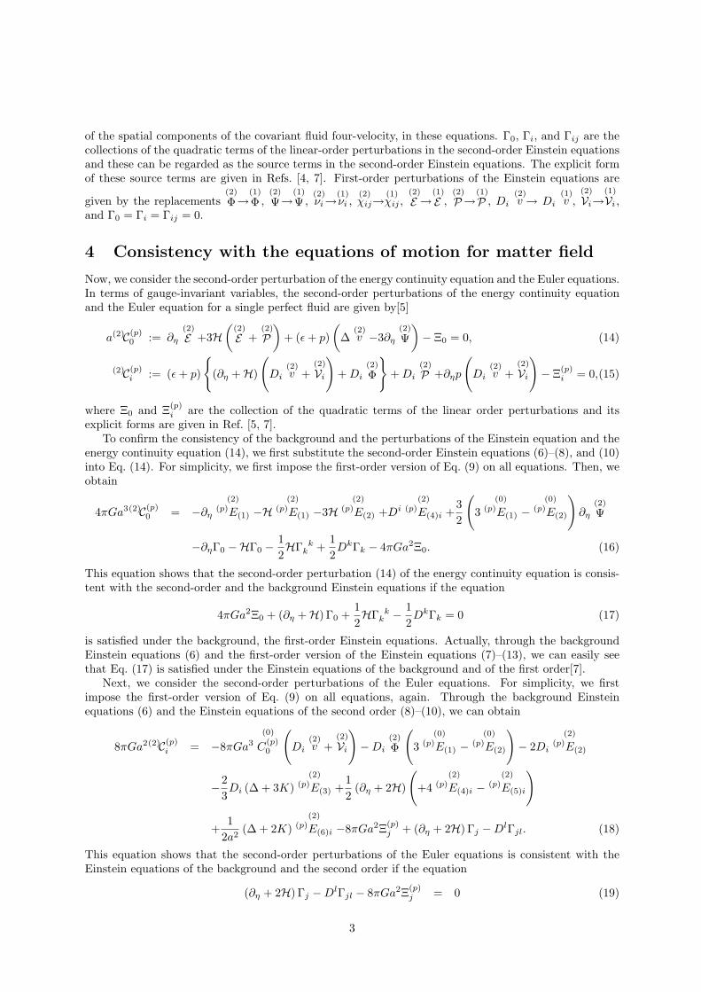
of the spatial components of the covariant fluid four-velocity, in these equations. Γ0, Γi, and Γij are thecollections of the quadratic terms of the linear-order perturbations in the second-order Einstein equationsand these can be regarded as the source terms in the second-order Einstein equations. The explicit formof these source terms are given in Refs. [4, 7]. First-order perturbations of the Einstein equations are
given by the replacements(2)
Φ→(1)
Φ ,(2)
Ψ→(1)
Ψ,(2)νi→
(1)νi ,
(2)χij→
(1)χij ,
(2)
E →(1)
E ,(2)
P→(1)
P , Di
(2)v → Di
(1)v ,
(2)
Vi→(1)
Vi ,and Γ0 = Γi = Γij = 0.
4 Consistency with the equations of motion for matter field
Now, we consider the second-order perturbation of the energy continuity equation and the Euler equations.In terms of gauge-invariant variables, the second-order perturbations of the energy continuity equationand the Euler equation for a single perfect fluid are given by[5]
a(2)C(p)0 := ∂η
(2)
E +3H(
(2)
E +(2)
P)
+ (ε + p)(
∆(2)v −3∂η
(2)
Ψ)− Ξ0 = 0, (14)
(2)C(p)i := (ε + p)
(∂η +H)
(Di
(2)v +
(2)
Vi
)+ Di
(2)
Φ
+ Di
(2)
P +∂ηp
(Di
(2)v +
(2)
Vi
)− Ξ(p)
i = 0,(15)
where Ξ0 and Ξ(p)i are the collection of the quadratic terms of the linear order perturbations and its
explicit forms are given in Ref. [5, 7].To confirm the consistency of the background and the perturbations of the Einstein equation and the
energy continuity equation (14), we first substitute the second-order Einstein equations (6)–(8), and (10)into Eq. (14). For simplicity, we first impose the first-order version of Eq. (9) on all equations. Then, weobtain
4πGa3(2)C(p)0 = −∂η
(2)(p)E(1) −H
(2)(p)E(1) −3H
(2)(p)E(2) +Di
(2)(p)E(4)i +
32
(3
(0)(p)E(1) −
(0)(p)E(2)
)∂η
(2)
Ψ
−∂ηΓ0 −HΓ0 − 12HΓ k
k +12DkΓk − 4πGa2Ξ0. (16)
This equation shows that the second-order perturbation (14) of the energy continuity equation is consis-tent with the second-order and the background Einstein equations if the equation
4πGa2Ξ0 + (∂η +H) Γ0 +12HΓ k
k − 12DkΓk = 0 (17)
is satisfied under the background, the first-order Einstein equations. Actually, through the backgroundEinstein equations (6) and the first-order version of the Einstein equations (7)–(13), we can easily seethat Eq. (17) is satisfied under the Einstein equations of the background and of the first order[7].
Next, we consider the second-order perturbations of the Euler equations. For simplicity, we firstimpose the first-order version of Eq. (9) on all equations, again. Through the background Einsteinequations (6) and the Einstein equations of the second order (8)–(10), we can obtain
8πGa2(2)C(p)i = −8πGa3
(0)
C(p)0
(Di
(2)v +
(2)
Vi
)−Di
(2)
Φ
(3
(0)(p)E(1) −
(0)(p)E(2)
)− 2Di
(2)(p)E(2)
−23Di (∆ + 3K)
(2)(p)E(3) +
12
(∂η + 2H)
(+4
(2)(p)E(4)i −
(2)(p)E(5)i
)
+1
2a2(∆ + 2K)
(2)(p)E(6)i −8πGa2Ξ(p)
j + (∂η + 2H) Γj −DlΓjl. (18)
This equation shows that the second-order perturbations of the Euler equations is consistent with theEinstein equations of the background and the second order if the equation
(∂η + 2H) Γj −DlΓjl − 8πGa2Ξ(p)j = 0 (19)
3
is satisfied under the Einstein equations of the background and the first order. Actually, we can easilyconfirm Eq. (19) due to the background Einstein equations and the first-order perturbations of theEinstein equations[7], and implies that the second-order perturbation of the Euler equation is consistentwith the set of the background, the first-order, and the second-order Einstein equations.
The consistency of equations for perturbations shown here is just a well-known result, i.e., the Einsteinequation includes the equations of motion for matter field due to the Bianchi identity. However, theabove verification of the identities (17) and (19) implies that our derived second-order perturbations ofthe Einstein equation, the equation of continuity, and the Euler equation are consistent. In this sense, wemay say that the derived second-order Einstein equations, especially, the derived formulae for the sourceterms Γ0, Γi, Γij , Ξ0, and Ξi in Ref. [7] are correct.
5 Summary
In summary, we show the all components of the second-order perturbation of the Einstein equationwithout ignoring any modes of perturbation in the case of a perfect fluid. The derivation is based on thegeneral framework of the second-order gauge-invariant perturbation theory developed in Refs. [8]. In thisformulation, any gauge fixing is not necessary and we can obtain any equation in the gauge-invariant formwhich is equivalent to the complete gauge fixing. In other words, our formulation gives complete gaugefixed equations without any gauge fixing. Therefore, equations which are obtained in gauge-invariantmanner cannot be reduced without physical restrictions any more. In this sense, these equations areirreducible. This is one of the advantages of the gauge-invariant perturbation theory.
We have also checked the consistency of the set of equations of the second-order perturbation of theEinstein equations and the evolution equation of the matter field in the cases of a perfect fluid. Therefore,in the case of the single matter field, we may say that we have been ready to clarify the physical behaviorsof the second-order cosmological perturbations. The physical behavior of the second-order perturbationsin the universe filled with a single matter field will be instructive to clarify those of the second-orderperturbations in more realistic cosmological situations. We leave these issues as future works.
References
[1] C.L. Bennett et al., Astrophys. J. Suppl. Ser. 148, (2003), 1.
[2] E. Komatsu et al., arXiv:0803.0547 [astro-ph], (2008).
[3] V. Acquaviva, N. Bartolo, S. Matarrese, and A. Riotto, Nucl. Phys. B 667 (2003), 119; J. Maldacena,JHEP, 0305 (2003), 013; K. A. Malik and D. Wands, Class. Quantum Grav. 21 (2004), L65; N. Bar-tolo, S. Matarrese and A. Riotto, Phys. Rev. D 69 (2004), 043503; N. Bartolo, S. Matarrese andA. Riotto, JHEP 0404 (2004), 006; D.H. Lyth and Y. Rodrıguez, Phys. Rev. D 71 (2005), 123508;F. Vernizzi, Phys. Rev. D 71 (2005), 061301R; N. Bartolo, S. Matarrese and A. Riotto, JCAP 0401(2004), 003; N. Bartolo, S. Matarrese and A. Riotto, Phys. Rev. Lett. 93 (2004), 231301; N. Bartolo,E. Komatsu, S. Matarrese and A. Riotto, Phys. Rept. 402 (2004), 103; N. Bartolo, S. Matarrese,and A. Riotto, [arXiv:astro-ph/0512481].
[4] K. Nakamura, Proceedings of 17th General Relativity and Gravitation in Japan, “Inclusion of thefirst-order vector- and tensor-modes in the second-order gauge-invariant cosmological perturbationtheory”.
[5] K. Nakamura, preprint (arXiv:0804.3840 [gr-qc]).
[6] K. Nakamura, Phys. Rev. D 74 (2006), 101301(R); K. Nakamura, Prog. Theor. Phys. 117 (2007),17.
[7] K. Nakamura, preprint (arXiv:0812.4865 [gr-qc]).
[8] K. Nakamura, Prog. Theor. Phys. 110, (2003), 723; K. Nakamura, Prog. Theor. Phys. 113 (2005),481.
4
Comparison of Post-Newtonian and Numerical Evolutionsof Black-Hole Binaries
Hiroyuki Nakano1, Manuela Campanelli2, Carlos O. Lousto3, and Yosef Zlochower4
Center for Computational Relativity and Gravitation, and School of Mathematical Sciences,Rochester Institute of Technology, Rochester, New York 14623, USA
AbstractIn this paper, we compare the waveforms from the post-Newtonian (PN) approachwith the numerical simulations of generic black-hole binaries which have mass ratioq ∼ 0.8, arbitrarily oriented spins with magnitudes S1/m2
1 ∼ 0.6 and S2/m22 ∼ 0.4,
and orbit 9 times from an initial orbital separation of r ≈ 11M prior to merger. Weobserve a reasonably good agreement between the PN and numerical waveforms, withan overlap of over 98% for the first six cycles of the (` = 2, m = ±2) mode and over90% for the (` = 2, m = 1) and (` = 3, m = 3) modes.
1 Introduction
In 2005, two complementary and independent methods were discovered that allowed numerical relativiststo completely solve the black-hole binary problem in full strong-field gravity [1, 2, 3]. On the other hand,there are currently major experimental and theoretical efforts underway to measure these gravitationalwave signals. Therefore, one of the most important tasks of numerical relativity (NR) is to assist grav-itational wave observatories in detecting gravitational waves and extracting the physical parameters ofthe sources. Given the demanding resources required to generate these black-hole binary simulations,it is necessary to develop various techniques in order to model arbitrary binary configuration basedon numerical simulations in combination with post-Newtonian (PN) and perturbative (e.g. black-holeperturbation) calculations.
In this paper, we compare the NR and PN waveforms for the challenging problem of a generic black-hole binary, i.e., a binary with unequal masses and unequal, non-aligned, and precessing spins. Compar-isons of numerical simulations with post-Newtonian ones have several benefits aside from the theoreticalverification of PN. From a practical point of view, one can directly propose a phenomenological de-scription and thus make predictions in regions of the parameter space still not explored by numericalsimulations. From the theoretical point of view, an important application is to have a calibration of thepost-Newtonian error in the last stages of the binary merger.
The paper is organized as follows. In Sec. II we present our method to derive the PN gravitationalwaveforms from generic black-hole binaries, and in III we compare the NR and PN waveforms. Finally inSec. IV we summarize this paper and discuss remaining problems. The detailed numerical method andPN calculation presented here have been given in [4].
2 Gravitational waveforms in the PN approach
In order to calculate PN gravitational waveforms, we need to calculate the orbital motion of binariesin the post-Newtonian approach. Here we use the ADM-TT gauge, which is the closest to our quasi-isotropic numerical initial data coordinates. In this paper, we use the PN equations of motion (EOM)based on [5, 6, 7]. The Hamiltonian is given in [5], with the additional terms, i.e., the next-to-leading
1E-mail:[email protected]:[email protected]:[email protected]:[email protected]
1
order gravitational spin-orbit and spin-spin couplings provided in [6, 7], and the radiation-reaction forcegiven in [5]. The Hamiltonian which we used here is given by
H = HO,Newt + HO,1PN + HO,2PN + HO,3PN
+HSO,1.5PN + HSO,2.5PN + HSS,2PN + HS1S2,3PN , (1)
where the subscript O, SO and SS denote the pure orbital (non-spinning) part, spin-orbit coupling andspin-spin coupling, respectively, and Newt, 1PN, 1.5PN, etc., refer to the perturbative order in the post-Newtonian approach. From this Hamiltonian, the conservative part of the orbital and spin EOM isderived using the standard techniques of the Hamiltonian formulation. For the dissipative part, we usethe non-spinning radiation reaction results up to 3.5PN (which contributes to the orbital EOM at 6PNorder), as well as the leading spin-orbit and spin-spin coupling to the radiation reaction [5].
The above PN evolution is used both to produce very low eccentricity orbital parameters at r ≈ 11Mfrom an initial orbital separation of 50M , and to evolve the orbit from r ≈ 11M . We use these sameparameters at r ≈ 11M to generate the initial data for our numerical simulations. The initial binaryconfiguration at r = 50M had the mass ratio q = m1/m2 = 0.8, ~S1/m2
1 = (−0.2,−0.14, 0.32), and~S2/m2
2 = (−0.09, 0.48, 0.35).We then construct a hybrid waveform from the orbital motion by using the following procedure. First
we use the 1PN accurate waveforms derived by Wagoner and Will [8] (WW waveforms) for a generic orbit.By using these waveforms, we can introduce effects due to the black-hole spins, including the precessionof the orbital plane. On the other hand, Blanchet et al. [9] recently obtained the 3PN waveforms (Bwaveforms) for non-spinning circular orbits. We combine these two waveforms to produce a hybridwaveform. In order to combine the WW and B waveforms, we need to take into account differences inthe definitions of polarization states and the angular coordinates. The WW waveforms use the standarddefinition of GW polarization states, which are the same as those derived from the Weyl scalar, but theB waveforms use an alternate definition. The angular coordinates in the B waveforms are derived fromcircular orbits in the equatorial (xy) plane. To directly compare the NR and PN waveforms, we mustadd a time dependent inclination to the B waveforms because in the generic case the orbital planes areinclined with respect to the xy plane.
We note that since there is no gauge ambiguity for combining the two waveforms, the combination ofthe WW and B waveforms is unique. Also, it should be noted that we calculate the spin contribution tothe waveforms through its effect on the orbital motion directly in the WW waveforms and indirectly inB waveforms through the inclination of the orbital plane.
For the NR simulations we calculate the Weyl scalar ψ4 and then convert the (`,m) modes of ψ4 into(`,m) modes of h = h+ − ih×.
3 Comparison of the NR and PN waveforms
To compare PN and numerical waveforms, we need to determine the time translation δt between thenumerical time and the corresponding point on the PN trajectory. That is to say, the time it takes forthe signal to reach the extraction sphere (r = 100M in our numerical simulation). We determine this byfinding the time translation near δt = 100M that maximizes the agreement of the early time waveformsin the (` = 2,m = ±2), (` = 2,m = ±1), and (` = 3,m = ±3) simultaneously. We find δt ∼ 112, ingood agreement with the expectation for our observer at r = 100M . Since our PN waveforms are givenuniquely by a binary configuration, i.e., an actual location of the PN particle, we do not have any timeshift or phase modification other than this retardation of the signal. It is noted that other methods whichare not based on the particle locations, have freedom in choosing a phase factor.
In the left panel of Fig. 1, we show the real part of the (` = 2,m = 2) mode of the strain h withthis time translation. (The other modes are shown in [4].) We note that the reasonable agreement of thenumerical and PN waveforms for 700M .
From the analysis of the amplitudes of each mode, we see that the precession and eccentricity of theorbit impart signatures on the modes of the waveform at the orbital frequency. However, the long-timeoscillations in the amplitudes, here apparent only in the (` = 2, m = ±1) modes, seem to be due purely to
2
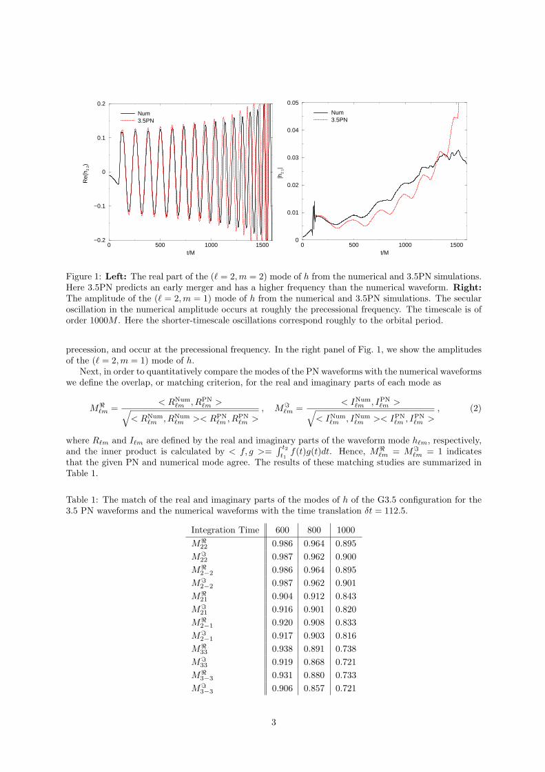
0 500 1000 1500t/M
−0.2
−0.1
0
0.1
0.2
Re(
h 2 2)
Num3.5PN
0 500 1000 1500t/M
0
0.01
0.02
0.03
0.04
0.05
|h2
1|
Num3.5PN
Figure 1: Left: The real part of the (` = 2,m = 2) mode of h from the numerical and 3.5PN simulations.Here 3.5PN predicts an early merger and has a higher frequency than the numerical waveform. Right:The amplitude of the (` = 2,m = 1) mode of h from the numerical and 3.5PN simulations. The secularoscillation in the numerical amplitude occurs at roughly the precessional frequency. The timescale is oforder 1000M . Here the shorter-timescale oscillations correspond roughly to the orbital period.
precession, and occur at the precessional frequency. In the right panel of Fig. 1, we show the amplitudesof the (` = 2,m = 1) mode of h.
Next, in order to quantitatively compare the modes of the PN waveforms with the numerical waveformswe define the overlap, or matching criterion, for the real and imaginary parts of each mode as
M<`m =
< RNum`m , RPN
`m >√< RNum
`m , RNum`m >< RPN
`m , RPN`m >
, M=`m =
< INum`m , IPN
`m >√< INum
`m , INum`m >< IPN
`m , IPN`m >
, (2)
where R`m and I`m are defined by the real and imaginary parts of the waveform mode h`m, respectively,and the inner product is calculated by < f, g >=
∫ t2t1
f(t)g(t)dt. Hence, M<`m = M=
`m = 1 indicatesthat the given PN and numerical mode agree. The results of these matching studies are summarized inTable 1.
Table 1: The match of the real and imaginary parts of the modes of h of the G3.5 configuration for the3.5 PN waveforms and the numerical waveforms with the time translation δt = 112.5.
Integration Time 600 800 1000M<
22 0.986 0.964 0.895M=
22 0.987 0.962 0.900M<
2−2 0.986 0.964 0.895M=
2−2 0.987 0.962 0.901M<
21 0.904 0.912 0.843M=
21 0.916 0.901 0.820M<
2−1 0.920 0.908 0.833M=
2−1 0.917 0.903 0.816M<
33 0.938 0.891 0.738M=
33 0.919 0.868 0.721M<
3−3 0.931 0.880 0.733M=
3−3 0.906 0.857 0.721
3
We also determine an alternate time translation, one wavelength in the (` = 2,m = 2) mode, thatincreases the matching of the (` = 2,m = 2) mode over longer integration periods. On the other hand,this new time translation, δt = 233, causes the (` = 3) modes to be out of phase, leading to negativeoverlaps. Thus by looking at the (` = 2) and (` = 3) modes simultaneously, we can reject this falsematch.
4 Conclusion and discussion
We analyzed the first long-term generic waveform produced by the merger of unequal mass, unequal spins,precessing black holes. It is found that a good initial agreement of waveforms for the first six cycles,with overlaps of over 98% for the (` = 2,m = ±2) modes, over 90% for the (` = 2,m = ±1) modes, andover 90% for the (` = 3, m = ±3) modes. These agreement degrades as we approach the more dynamicalregion of the late merger and plunge.
There are some remaining problems. The PN gravitational waveforms used here do not include directspin effects. We considered the spin contribution to the waveform only through its effect on the orbitalmotion. Recently, the direct spin effects have been discussed in [10]. And also in the PN approach, thewaveforms are derived from binaries whose each body is considered as a point particle. The finite sizeeffects of the bodies is also important in the late-inspiral region. Furthermore, we will need higher-orderpost-Newtonian calculations of both spin-orbit and spin-spin terms, especially for the phase evolution ofgravitational waves.
We also have a important issue. In order to detect the gravitational waves from binaries, it is necessaryto study the data analysis. (For example, the Numerical INJection Analysis (NINJA) project [11].)Here, we must treat a very large parameter space for intrinsic parameters of black-hole binaries, Thedevelopment of effective GW templates for the whole history of binaries, i.e., the inspiral, merger andringdown should be done.
Acknowledgments
We would like to thank H. Tagoshi and R. Fujita for useful discussions.
References
[1] F. Pretorius, Phys. Rev. Lett. 95, 121101 (2005) [arXiv:gr-qc/0507014].
[2] M. Campanelli, C. O. Lousto, P. Marronetti and Y. Zlochower, Phys. Rev. Lett. 96, 111101 (2006)[arXiv:gr-qc/0511048].
[3] J. G. Baker, J. Centrella, D. I. Choi, M. Koppitz and J. van Meter, Phys. Rev. Lett. 96, 111102(2006) [arXiv:gr-qc/0511103].
[4] M. Campanelli, C. O. Lousto, H. Nakano and Y. Zlochower, arXiv:0808.0713 [gr-qc].
[5] A. Buonanno, Y. Chen and T. Damour, Phys. Rev. D 74, 104005 (2006) [arXiv:gr-qc/0508067].
[6] T. Damour, P. Jaranowski and G. Schaefer, Phys. Rev. D 77, 064032 (2008) [arXiv:0711.1048 [gr-qc]].
[7] J. Steinhoff, S. Hergt and G. Schaefer, Phys. Rev. D 77, 081501 (2008) [arXiv:0712.1716 [gr-qc]].
[8] R. V. Wagoner and C. M. Will, Astrophys. J. 210 (1976) 764 [Erratum-ibid. 215 (1977) 984].
[9] L. Blanchet, G. Faye, B. R. Iyer and S. Sinha, arXiv:0802.1249 [gr-qc].
[10] K. G. Arun, A. Buonanno, G. Faye and E. Ochsner, arXiv:0810.5336 [gr-qc].
[11] Numerical INJection Analysis (NINJA) Project Home Page,http://www.gravity.phy.syr.edu/dokuwiki/doku.php?id=ninja:home
4
Damping of the baryon acoustic oscillations in the matter powerspectrum as a probe of the growth factor1
Hidenori Nomura2
Department of Physics, Hiroshima University, Higashi-Hiroshima, 739–8526, Japan
AbstractWe investigate damping of the baryon acoustic oscillations (BAO) in the matter power
spectrum due to quasi-nonlinear clustering of density perturbations. On the basis of
third order perturbation theory, we construct a fitting formula of the damping in
an analytic way. This demonstrates that the damping is closely related with the
growth factor and the amplitude of the matter power spectrum. Then, we investigate
the feasibility of constraining the growth factor through a measurement of the BAO
damping. An extension of our formula based on the Lagrangian perturbation theory
is also discussed.
1 Introduction
The Baryon Acoustic Oscillations (BAO) imprinted in galaxy clustering has recently attracted remarkableattention, as a powerful probe for exploring the nature of mysterious dark energy component commonlybelieved to be responsible for the accelerated expansion of the universe [2]. The usefulness of the BAO toconstrain the dark energy has been demonstrated, and a lot of the BAO survey projects are in progressor planned.
Even though the BAO surveys will precisely measure the galaxy power spectrum, but we also needprecise theoretical templates, in order to obtain a useful cosmological constraint from observational data.In practice, the observed galaxy power spectrum is contaminated by nonlinear evolution of the densityperturbations, redshift-space distortions and galaxy clustering bias. These uncertainties might yieldsome systematic effects on the BAO signature. Therefore the comparison of theoretical templates withobservation is complicated.
We examine one of the above uncertainties about the nonlinear correction due to the gravitationalclustering. This effect cause shift of peaks (troughs) and damping of the amplitude of the BAO signature.In this work, we focus on the BAO damping, and investigate the nonlinear correction in an analytic way.As a result, we construct a fitting formula of the BAO damping in weakly nonlinear regime. We alsodiscuss the feasibility of constraining the growth factor of density fluctuations using a measurement ofthe BAO damping.
2 Damping of the baryon acoustic oscillations
In this section, we examine the BAO damping due to the nonlinear gravitational clustering with employingthe third order perturbation theory. The BAO signature in the matter power spectrum can be extractedas follows:
B(k, z) ≡ P (k, z)
P (k, z)− 1, (1)
where P (k, z) is the matter power spectrum including the BAO, but P (k, z) is the matter power spectrumwithout the BAO, which is calculated using the no-wiggle transfer function in [3]. Hereafter, the quantitywith the ’tilde’ implies the quantity calculated using the no-wiggle transfer function.
1This work is based on a collaboration with Kazuhiro Yamamoto and Takahiro Nishimichi, which is published in Ref.[1].2E-mail:[email protected]
1
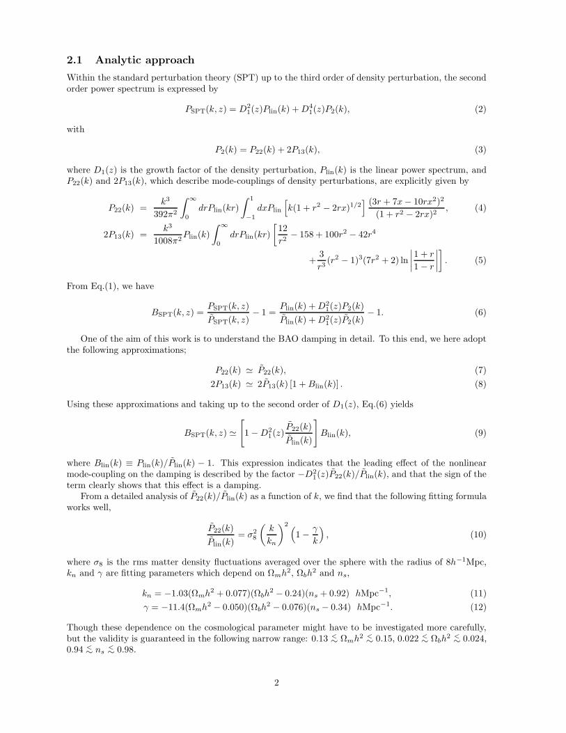
2.1 Analytic approach
Within the standard perturbation theory (SPT) up to the third order of density perturbation, the secondorder power spectrum is expressed by
PSPT(k, z) = D21(z)Plin(k) + D4
1(z)P2(k), (2)
with
P2(k) = P22(k) + 2P13(k), (3)
where D1(z) is the growth factor of the density perturbation, Plin(k) is the linear power spectrum, andP22(k) and 2P13(k), which describe mode-couplings of density perturbations, are explicitly given by
P22(k) =k3
392π2
∫
∞
0
drPlin(kr)
∫ 1
−1
dxPlin
[
k(1 + r2 − 2rx)1/2] (3r + 7x − 10rx2)2
(1 + r2 − 2rx)2, (4)
2P13(k) =k3
1008π2Plin(k)
∫
∞
0
drPlin(kr)
[
12
r2− 158 + 100r2 − 42r4
+3
r3(r2 − 1)3(7r2 + 2) ln
∣
∣
∣
∣
1 + r
1 − r
∣
∣
∣
∣
]
. (5)
From Eq.(1), we have
BSPT(k, z) =PSPT(k, z)
PSPT(k, z)− 1 =
Plin(k) + D21(z)P2(k)
Plin(k) + D21(z)P2(k)
− 1. (6)
One of the aim of this work is to understand the BAO damping in detail. To this end, we here adoptthe following approximations;
P22(k) ' P22(k), (7)
2P13(k) ' 2P13(k) [1 + Blin(k)] . (8)
Using these approximations and taking up to the second order of D1(z), Eq.(6) yields
BSPT(k, z) '[
1 − D21(z)
P22(k)
Plin(k)
]
Blin(k), (9)
where Blin(k) ≡ Plin(k)/Plin(k) − 1. This expression indicates that the leading effect of the nonlinearmode-coupling on the damping is described by the factor −D2
1(z)P22(k)/Plin(k), and that the sign of theterm clearly shows that this effect is a damping.
From a detailed analysis of P22(k)/Plin(k) as a function of k, we find that the following fitting formulaworks well,
P22(k)
Plin(k)= σ2
8
(
k
kn
)2(
1 − γ
k
)
, (10)
where σ8 is the rms matter density fluctuations averaged over the sphere with the radius of 8h−1Mpc,kn and γ are fitting parameters which depend on Ωmh2, Ωbh
2 and ns,
kn = −1.03(Ωmh2 + 0.077)(Ωbh2 − 0.24)(ns + 0.92) hMpc−1, (11)
γ = −11.4(Ωmh2 − 0.050)(Ωbh2 − 0.076)(ns − 0.34) hMpc−1. (12)
Though these dependence on the cosmological parameter might have to be investigated more carefully,but the validity is guaranteed in the following narrow range: 0.13 <∼ Ωmh2 <∼ 0.15, 0.022 <∼ Ωbh
2 <∼ 0.024,0.94 <∼ ns
<∼ 0.98.
2
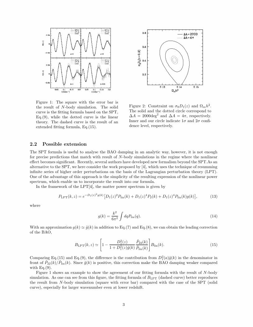
Figure 1: The square with the error bar isthe result of N -body simulation. The solidcurve is the fitting formula based on the SPT,Eq.(9), while the dotted curve is the lineartheory. The dashed curve is the result of anextended fitting formula, Eq.(15).
Figure 2: Constraint on σ8D1(z) and Ωmh2.The solid and the dotted circle correspond to∆A = 2000deg2 and ∆A = 4π, respectively.Inner and our circle indicate 1σ and 2σ confi-dence level, respectively.
2.2 Possible extension
The SPT formula is useful to analyse the BAO damping in an analytic way, however, it is not enoughfor precise predictions that match with result of N -body simulations in the regime where the nonlineareffect becomes significant. Recently, several authors have developed new formalism beyond the SPT.As analternative to the SPT, we here consider the work proposed by [4], which uses the technique of resumminginfinite series of higher order perturbations on the basis of the Lagrangian perturbation theory (LPT).One of the advantage of this approach is the simplicity of the resulting expression of the nonlinear powerspectrum, which enable us to incorporate the result into our formula.
In the framework of the LPT[4], the matter power spectrum is given by
PLPT(k, z) = e−D1(z)2g(k)[
D1(z)2Plin(k) + D1(z)4P2(k) + D1(z)4Plin(k)g(k)]
, (13)
where
g(k) =k2
6π2
∫
dqPlin(q). (14)
With an approximation g(k) ' g(k) in addition to Eq.(7) and Eq.(8), we can obtain the leading correctionof the BAO,
BLPT(k, z) '[
1− D21(z)
1 + D21(z)g(k)
P22(k)
Plin(k)
]
Blin(k). (15)
Comparing Eq.(15) and Eq.(9), the difference is the contribution from D21(a)g(k) in the denominator in
front of P22(k)/Plin(k). Since g(k) is positive, this correction make the BAO damping weaker comparedwith Eq.(9).
Figure 1 shows an example to show the agreement of our fitting formula with the result of N -bodysimulation. As one can see from this figure, the fitting formula of BLPT (dashed curve) better reproducesthe result from N -body simulation (square with error bar) compared with the case of the SPT (solidcurve), especially for larger wavenumber even at lower redshift.
3
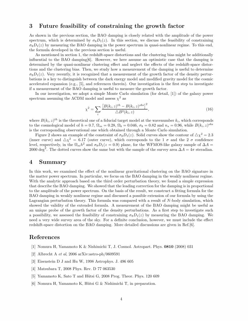
3 Future feasibility of constraining the growth factor
As shown in the previous section, the BAO damping is closely related with the amplitude of the powerspectrum, which is determined by σ8D1(z). In this section, we discuss the feasibility of constrainingσ8D1(z) by measuring the BAO damping in the power spectrum in quasi-nonlinear regime. To this end,the formula developed in the previous section is useful.
As mentioned in section 1, the redshift-space distortions and the clustering bias might be additionallyinfluential to the BAO damping[6]. However, we here assume an optimistic case that the damping isdetermined by the quasi-nonlinear clustering effect and neglect the effects of the redshift-space distor-tions and the clustering bias. Then, we study how a measurement of the damping is useful to determineσ8D1(z). Very recently, it is recognized that a measurement of the growth factor of the density pertur-bations is a key to distinguish between the dark energy model and modified gravity model for the cosmicaccelerated expansion (e.g., [5], and references therein). Our investigation is the first step to investigateif a measurement of the BAO damping is useful to measure the growth factor.
In our investigation, we adopt a simple Monte Carlo simulation (for detail, [1]) of the galaxy powerspectrum assuming the ΛCDM model and assess χ2 as
χ2 =∑
i
[
B(ki, z)th − B(ki, z)obs]2
4B2(ki, z), (16)
where B(ki, z)th is the theoretical one of a fiducial target model at the wavenumber ki, which correspondsto the cosmological model of h = 0.7, Ωm = 0.28, Ωb = 0.046, σ8 = 0.82 and ns = 0.96, while B(ki, z)obs
is the corresponding observational one which obtained through a Monte Carlo simulation.Figure 2 shows an example of the constraint of σ8D1(z). Solid curves show the contour of 4χ2 = 2.3
(inner curve) and 4χ2 = 6.17 (outer curve), which corresponds to the 1 σ and the 2 σ confidencelevel, respectively, in the Ωmh2 and σ8D1(z = 0.9) plane, for the WFMOS-like galaxy sample of ∆A =2000 deg2. The dotted curves show the same but with the sample of the survey area ∆A = 4π steradian.
4 Summary
In this work, we examined the effect of the nonlinear gravitational clustering on the BAO signature inthe matter power spectrum. In particular, we focus on the BAO damping in the weakly nonlinear regime.With the analytic approach based on the third order perturbation theory, we found a simple expressionthat describe the BAO damping. We showed that the leading correction for the damping is in proportionalto the amplitude of the power spectrum. On the basis of the result, we construct a fitting formula for theBAO damping in weakly nonlinear regime and discussed a possible extension of our formula by using theLagrangian perturbation theory. This formula was compared with a result of N -body simulation, whichshowed the validity of the extended formula. A measurement of the BAO damping might be useful asan unique probe of the growth factor of the density perturbations. As a first step to investigate sucha possibility, we assessed the feasibility of constraining σ8D1(z) by measuring the BAO damping. Weneed a very wide survey area of the sky. For a definite conclusion, however, we must include the effectredshift-space distortion on the BAO damping. More detailed discussions are given in Ref.[6].
References
[1] Nomura H, Yamamoto K & Nishimichi T, J. Cosmol. Astropart. Phys. 0810 (2008) 031
[2] Albrecht A et al, 2006 arXiv:astro-ph/0609591
[3] Eisenstein D J and Hu W, 1998 Astrophys. J. 496 605
[4] Matsubara T, 2008 Phys. Rev. D 77 063530
[5] Yamamoto K, Sato T and Hutsi G, 2008 Prog. Theor. Phys. 120 609
[6] Nomura H, Yamamoto K, Hutsi G & Nishimichi T, in preparation.
4
Quasinormal Modes of Black Holes Localized on theRandall-Sundrum 2-brane
Masato Nozawa1 and Tsutomu Kobayashi2
Department of Physics, Waseda University, Okubo 3-4-1, Shinjuku, Tokyo 169-8555, Japan
AbstractWe explore the quasinormal modes of a black hole localized on the Randall-Sundrum2-brane against the test field perturbations [1]. The background metric admits aconformal Killing tensor, which allows us to obtain tractable–indeed separable–fieldequations for the conformally coupled scalar, the massless Dirac and the Maxwellfields. We find that each radial equation obeys the same equation as the correspondingequation in the Schwarzschild background with the same horizon radius. The angularequation reflects the impact of brane tension, resulting in a distinct quasinormal modeprediction.
1 Exact description of a braneworld black hole
The Randall-Sundrum scenario has attracted much attention for intriguing phenomenological predictionin particle physics and cosmological scenario [2]. In order to further validate this model, the stronggravity test is imperative. Black holes are the best experimental fields for this purpose. Despite thata lot of effort has been devoted toward finding an exact solution describing a black hole localized onthe Randall-Sundrum 3-brane, none of them are successful yet. Some authors discussed based on theAdS/CFT correspondence that the static (and large) back holes fail to exist [3, 4]. Under the presentcircumstances, it is very illustrative to look in a bird’s-eye view. We consider a simple toy model andextract useful information. Emparan, Horowitz and Myers succeeded in constructing the desired blackhole solution in a 3+1-dimensional Randall-Sundrum model [5], on which we will focus hereafter.
The Randall-Sundrum braneworld has a negative cosmological constant in the bulk, so as to reproducea Newtonian gravity on the brane. An important point to notice is the fact that the brane undergoes auniform acceleration in the background AdS. So the repelling acceleration is required to obtain a staticblack hole. In 4-spacetime dimensions, the C-metric in AdS is the desired solution. For the Z2-symmetryacross the brane, the metric describing a localized black hole is given by
gabdxadxb =`2
(|x|− y)2
∑F (y)dt2 − dy2
F (y)+
dx2
G(|x|) + G(|x|)dϕ2
∏, (1)
where
F (y) = −y2 − 2µy3, G(x) = 1− x2 − 2µx3. (2)
The metric (1) solves Einstein’s equations with a negative cosmological constant, Rab = −(3/`2)gab, for|x| > 0. The brane locus is x = 0, across which the bulk has a mirror symmetry. Israel’s junctioncondition shows that the brane tension is proportional to 1/`. The x and y-coordinates are the directioncosine x = cos θ and the radial coordinate y = −`/r. x ranges from the brane x = 0 to the axis x = x2–thelargest root of G(x2)–and y from the horizon y = −1/2µ to infinity y = x. Observe that in order to avoidconical singularities on the axis x = x2, the period of ϕ is fixed by ∆ϕ = 2πβ, where β−1 = −G0(x2)/2.
The parameter µ corresponds to the mass of the black hole, hence we take µ ≥ 0. The black holewith small µ mimics the isolated black hole. Indeed, one can confirm easily that the µ → 0 limit withrh = 2µ` fixed recovers the Schwarzschild black hole with the horizon radius rh(ø `). On the other hand,the horizon will become flattened in the µ ¿ 1 limit (see Fig. 1). In the latter case, the brane tensionhas a distinguished effect on the properties of black holes from the isolated ones.
1Email:nozawa“ at”gravity.phys.waseda.ac.jp2Email:tsutomu“ at”gravity.phys.waseda.ac.jp
1
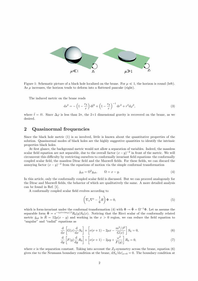
Figure 1: Schematic picture of a black hole localized on the brane. For µø 1, the horizon is round (left).As µ increases, the horizon tends to deform into a flattened pancake (right).
The induced metric on the brane reads
ds2 = −≥1− rh
r
¥dt2 +
≥1− rh
r
¥−1dr2 + r2dϕ2, (3)
where t = `t. Since ∆ϕ is less than 2π, the 2+1 dimensional gravity is recovered on the brane, as wedesired.
2 Quasinormal frequencies
Since the black hole metric (1) is so involved, little is known about the quantitative properties of thesolution. Quasinormal modes of black holes are the highly suggestive quantities to identify the intrinsicproperties black holes.
At first glance, the background metric would not allow a separation of variables. Indeed, the masslessscalar field equation are not separable, due to the overall factor (x− y)−2 in front of the metric. We willcircumvent this difficulty by restricting ourselves to conformally invariant field equations–the conformallycoupled scalar field, the massless Dirac field and the Maxwell fields. For these fields, we can discard theannoying factor (x− y)−2 from the equations of motion via the simple conformal transformation
gab = Ω2gab, Ω = x− y. (4)
In this article, only the conformally coupled scalar field is discussed. But we can proceed analogously forthe Dirac and Maxwell fields, the behavior of which are qualitatively the same. A more detailed analysiscan be found in Ref. [1].
A conformally coupled scalar field evolves according toµ∇a∇a − 1
6R
∂Φ = 0, (5)
which is form-invariant under the conformal transformation (4) with Φ→ Φ = Ω−1Φ. Let us assume theseparable form Φ = e−iωt+imϕ/βR0(y)S0(x). Noticing that the Ricci scalar of the conformally relatedmetric gab is R = 12µ(x − y) and working in the x > 0 region, we can reduce the field equation to“angular” and “radial” equations as
ddx
∑G(x)
ddx
S0
∏+
∑ν(ν + 1)− 2µx− m2/β2
G(x)
∏S0 = 0, (6)
ddy
∑F (y)
ddy
R0
∏+
∑ν(ν + 1)− 2µy +
ω2
F (y)
∏R0 = 0, (7)
where ν is the separation constant. Taking into account the Z2-symmetry across the brane, equation (6)gives rise to the Neumann boundary condition at the brane, dSs/dx|x=0 = 0. The boundary condition at
2
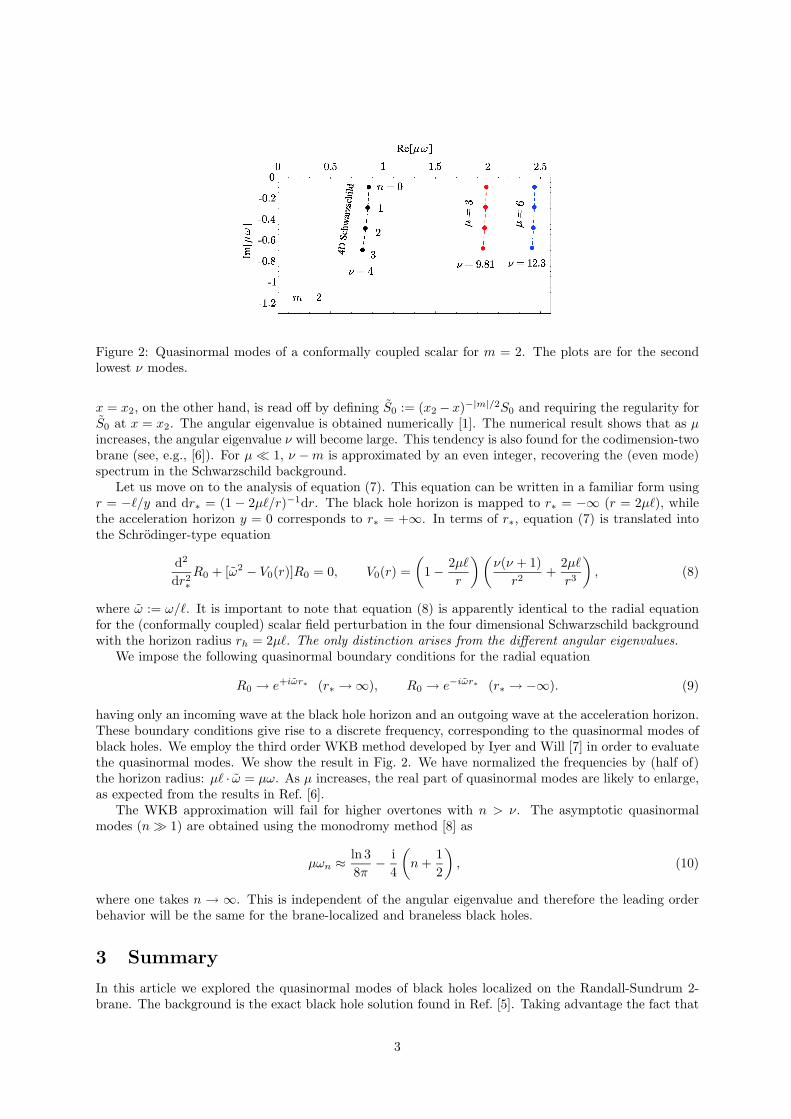
Figure 2: Quasinormal modes of a conformally coupled scalar for m = 2. The plots are for the secondlowest ν modes.
x = x2, on the other hand, is read off by defining S0 := (x2 − x)−|m|/2S0 and requiring the regularity forS0 at x = x2. The angular eigenvalue is obtained numerically [1]. The numerical result shows that as µincreases, the angular eigenvalue ν will become large. This tendency is also found for the codimension-twobrane (see, e.g., [6]). For µø 1, ν −m is approximated by an even integer, recovering the (even mode)spectrum in the Schwarzschild background.
Let us move on to the analysis of equation (7). This equation can be written in a familiar form usingr = −`/y and dr∗ = (1 − 2µ`/r)−1dr. The black hole horizon is mapped to r∗ = −∞ (r = 2µ`), whilethe acceleration horizon y = 0 corresponds to r∗ = +∞. In terms of r∗, equation (7) is translated intothe Schrodinger-type equation
d2
dr2∗R0 + [ω2 − V0(r)]R0 = 0, V0(r) =
µ1− 2µ`
r
∂ µν(ν + 1)
r2+
2µ`
r3
∂, (8)
where ω := ω/`. It is important to note that equation (8) is apparently identical to the radial equationfor the (conformally coupled) scalar field perturbation in the four dimensional Schwarzschild backgroundwith the horizon radius rh = 2µ`. The only distinction arises from the different angular eigenvalues.
We impose the following quasinormal boundary conditions for the radial equation
R0 → e+iωr∗ (r∗ →∞), R0 → e−iωr∗ (r∗ → −∞). (9)
having only an incoming wave at the black hole horizon and an outgoing wave at the acceleration horizon.These boundary conditions give rise to a discrete frequency, corresponding to the quasinormal modes ofblack holes. We employ the third order WKB method developed by Iyer and Will [7] in order to evaluatethe quasinormal modes. We show the result in Fig. 2. We have normalized the frequencies by (half of)the horizon radius: µ` · ω = µω. As µ increases, the real part of quasinormal modes are likely to enlarge,as expected from the results in Ref. [6].
The WKB approximation will fail for higher overtones with n > ν. The asymptotic quasinormalmodes (n¿ 1) are obtained using the monodromy method [8] as
µωn ≈ln 38π− i
4
µn +
12
∂, (10)
where one takes n → ∞. This is independent of the angular eigenvalue and therefore the leading orderbehavior will be the same for the brane-localized and braneless black holes.
3 Summary
In this article we explored the quasinormal modes of black holes localized on the Randall-Sundrum 2-brane. The background is the exact black hole solution found in Ref. [5]. Taking advantage the fact that
3
the background metric allows a conformal Killing tensor, which is a direct consequence of Petrov type D,we have investigated the behavior of conformally invariant field perturbations around the brane-localizedblack hole.
For all types of fields we considered, we found that each radial equation is identical to the correspondingfield equation in the four Schwarzschild background. However, the angular equations differ from theirSchwarzschild counterparts. We have determined the angular eigenfunctions and eigenvalues numerically.In the case of the conformal scalar field, the angular eigenvalues ν are given by ν ' l = 0, 1, 2, ... for asmall black hole (µ ø 1), recovering the Schwarzschild result. As the size of the black hole increases, νbecomes larger (ν > l) and hence become sensitive to the magnetic quantum number m. Accordingly, eachquasinormal modes of the large localized black hole (with the horizon radius 2µ` on the brane) behaveslike the mode having a larger angular mode number in the four dimensional Schwarzschild backgroundwith the same horizon radius rh = 2µ`. The situation is basically the same for electromagnetic andmassless Dirac field perturbations. In particular, we have found no unstable modes for any types of fieldswe investigated.
It has been widely known that the Randall-Sundrum braneworlds have a rich structure concerningthe AdS/CFT correspondence [3, 4]. It would be also interesting to discuss the implications of our resultfrom the viewpoint of the AdS/CFT correspondence.
Acknowledgements. MN and TK are supported by the JSPS under Contract Nos. 19-204 and 19-4199.
References
[1] M. Nozawa and T. Kobayashi, Phys. Rev. D. 78 064006 (2008) [arXiv:0803.3317 [hep-th]].
[2] L. Randall and R. Sundrum, Phys. Rev. Lett. 83, 3370 (1999) [arXiv:hep-ph/9905221]; L. Randalland R. Sundrum, Phys. Rev. Lett. 83, 4690 (1999) [arXiv:hep-th/9906064].
[3] T. Tanaka, Prog. Theor. Phys. Suppl. 148, 307 (2003) [arXiv:gr-qc/0203082].
[4] R. Emparan, A. Fabbri and N. Kaloper, JHEP 0208, 043 (2002) [arXiv:hep-th/0206155].
[5] R. Emparan, G. T. Horowitz and R. C. Myers, JHEP 0001, 007 (2000).
[6] T. Kobayashi, M. Nozawa and Y. i. Takamizu, Phys. Rev. D 77, 044022 (2008) [arXiv:0711.1395[hep-th]].
[7] S. Iyer and C. M. Will, Phys. Rev. D 35, 3621 (1987).
[8] L. Motl, Adv. Theor. Math. Phys. 6, 1135 (2003) [arXiv:gr-qc/0212096].
4
Classicality of the stochastic approach to inflation
Yuji Ohsumi1 and Yasusada Nambu2
Department of Physics, Nagoya University, Nagoya, 464–8602, Japan
AbstractThe stochastic approach to the inflationary universe is the method which treats quan-tum time evolution of long wave length mode of an inflaton field as a stochastic pro-cess. In this presentation, we discuss the conditions for the probability distribution tobehave as classical one by using the bipartite entanglement, or quantum correlationamong two regions.
1 Introduction
The inflationary scenario indicates that the large scale structure in the present universe originated fromthe quantum fluctuation of a field in the early universe. There is a conventional method to calculatethis fluctuation, called stochastic approach [1, 2]. In this approach, by coarse-graining the quantum fieldin the inflationary universe over the super-horizon scale, the quantum stochastic behavior of the field isrepresented by a classical distribution function. Classical distribution means a positive definite normalizedfunction. This method is based on the naive assumption in the inflationary scenario that the quantumfield becomes classical when their wave length exceeds to the super-horizon scale by the inflationaryexpansion. And this is used to calculate various quantities including the non-Gaussian fluctuations.
However, it is in general impossible to describe the quantum mechanical nature by using a classicaldistribution. For example, let us consider two particles with spin half in the follwing state.
|√i =1√2(| ↑↑ i+ | ↓↓ i),
where the first arrow in each term is the state of one spin, and the second is that of the other spin. Notethat the direction of one particle fluctuates and is not fixed. If we observe this direction and obtain theresult “↑”, then that of the other spin also becomes “↑”. In other words, the observation on one degree offreedom affects the other degree of freedom. Such a correlation between two degrees of freedom is calledentanglement, which is known as purely quantum correlation and does not exist in classical mechanics. J.S. Bell showed that the the classical distribution function cannot reproduce the correlations in the systemunder this state [3]. Cavalcanti et al. showed that this theorem is valid for general bipartite systems[4]. Thus general bipartite systems in entangled state do not have the classical distribution function.Therefore, if the coarse-grained region has entanglement with another region, there does not exist theclassical distribution function describing the stochastic nature of the field. Then the stochastic approachis not valid.
Nambu showed that, if the entanglement in the system disappear, the classical distribution for thesystem appears [5]. We investigated the classicality condition for the stochastic approach by applyingNambu’s result to the quantum field in inflaionary universe. In conclusion, we find that the system canbe treat as classical if the coarse-graining scale is sufficiently large.
2 Classicality condition
2.1 The entanglement measure
In this section, we introduce the entanglement measure ∏ which is necessary to represent the classicalitycondition. Let us consider a bipartite system (q, p), (Q, P ) in Gaussian state. We introduce the
1E-mail:[email protected]:[email protected]
1
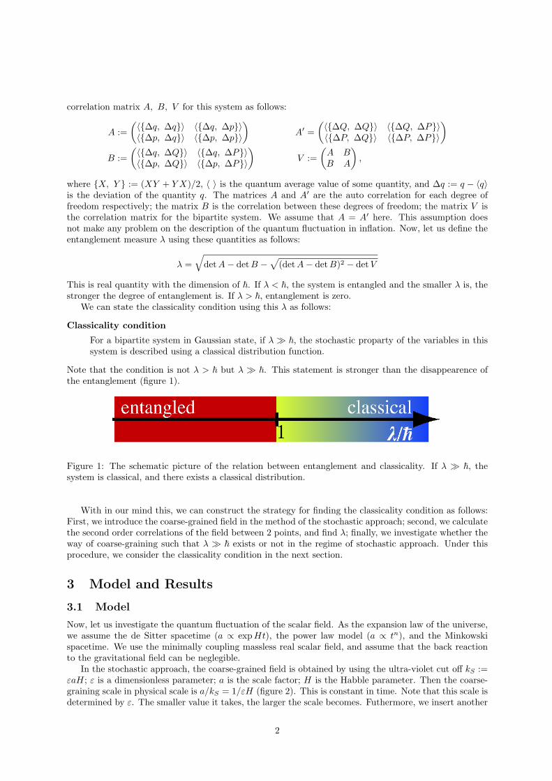
correlation matrix A, B, V for this system as follows:
A :=µh∆q, ∆qi h∆q, ∆pih∆p, ∆qi h∆p, ∆pi
∂A0 =
µh∆Q, ∆Qi h∆Q, ∆Pih∆P, ∆Qi h∆P, ∆Pi
∂
B :=µh∆q, ∆Qi h∆q, ∆Pih∆p, ∆Qi h∆p, ∆Pi
∂V :=
µA BB A
∂,
where X, Y := (XY + Y X)/2, h i is the quantum average value of some quantity, and ∆q := q − hqiis the deviation of the quantity q. The matrices A and A0 are the auto correlation for each degree offreedom respectively; the matrix B is the correlation between these degrees of freedom; the matrix V isthe correlation matrix for the bipartite system. We assume that A = A0 here. This assumption doesnot make any problem on the description of the quantum fluctuation in inflation. Now, let us define theentanglement measure ∏ using these quantities as follows:
∏ =q
det A− det B −p
(det A− det B)2 − det V
This is real quantity with the dimension of ~. If ∏ < ~, the system is entangled and the smaller ∏ is, thestronger the degree of entanglement is. If ∏ > ~, entanglement is zero.
We can state the classicality condition using this ∏ as follows:
Classicality condition For a bipartite system in Gaussian state, if ∏ ¿ ~, the stochastic proparty of the variables in thissystem is described using a classical distribution function.
Note that the condition is not ∏ > ~ but ∏ ¿ ~. This statement is stronger than the disappearence ofthe entanglement (figure 1).
Figure 1: The schematic picture of the relation between entanglement and classicality. If ∏ ¿ ~, thesystem is classical, and there exists a classical distribution.
With in our mind this, we can construct the strategy for finding the classicality condition as follows:First, we introduce the coarse-grained field in the method of the stochastic approach; second, we calculatethe second order correlations of the field between 2 points, and find ∏; finally, we investigate whether theway of coarse-graining such that ∏ ¿ ~ exists or not in the regime of stochastic approach. Under thisprocedure, we consider the classicality condition in the next section.
3 Model and Results
3.1 Model
Now, let us investigate the quantum fluctuation of the scalar field. As the expansion law of the universe,we assume the de Sitter spacetime (a ∝ expHt), the power law model (a ∝ tn), and the Minkowskispacetime. We use the minimally coupling massless real scalar field, and assume that the back reactionto the gravitational field can be neglegible.
In the stochastic approach, the coarse-grained field is obtained by using the ultra-violet cut off kS :=εaH; ε is a dimensionless parameter; a is the scale factor; H is the Habble parameter. Then the coarse-graining scale in physical scale is a/kS = 1/εH (figure 2). This is constant in time. Note that this scale isdetermined by ε. The smaller value it takes, the larger the scale becomes. Futhermore, we insert another
2
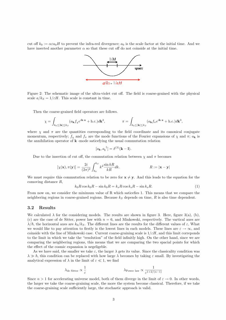
cut off k0 := αεa0H to prevent the infra-red divergence; a0 is the scale factor at the initial time. And wehave inserted another parameter α so that these cut off do not coinside at the initial time.
Figure 2: The schematic image of the ultra-violet cut off. The field is coarse-grained with the physicalscale a/kS = 1/εH. This scale is constant in time.
Then the coarse-grained field operators are follows.
χ =Z
k0≤|k|≤kS
(akfχeik·x + h.c.)dk3, π =Z
k0≤|k|≤kS
(akfπeik·x + h.c.)dk3,
where χ and π are the quantities corresponding to the field coordinate and its canonical conjugatemomentum, respectively; fχ and fπ are the mode functions of the Fourier expansions of χ and π; ak isthe annihilation operator of k -mode saticefying the usual commutation relation
[ak, a †l ] = δ(3)(k− l).
Due to the insertion of cut off, the commutation relation between χ and π becomes
[χ(x),π(y)] =2i
(2π)2
Z kS
k0
k2 sin kR
kRdk. R := |x− y|
We must require this commutation relation to be zero for x 6= y. And this leads to the equation for thecomoving distance R,
k0R cos k0R− sin k0R = ksR cos ksR− sin ksR. (1)
From now on, we consider the minimum value of R which saticefies 1. This means that we compare theneighbering regions in coarse-grained regions. Because kS depends on time, R is also time dependent.
3.2 Results
We calculated ∏ for the considering models. The results are shown in figure 3. Here, figure 3(a), (b),(c) are the case of de Sitter, power law with n = 6, and Minkowski, respectively. The vartical axes are∏/~, the horizontal axes are k0/kS . The different lines are the results for the different values of ε, Whatwe would like to pay attention to firstly is the lowest lines in each models. These lines are ε → 1, andcoinside with the line of Minkowski case. Current coarse-graining scale is 1/εH, and this limit correpondsto the limit in which we take the “resolution” of the field infinitly high. On the other hand, since we arecomparing the neighbering regions, this means that we are comparing the two spacial points for whichthe effect of the cosmic expansion is negeligeble.
As we have said, the smaller we take ε, the larger ∏ gets its value. Since the classicality condition was∏ ¿ ~, this condition can be replaced with how large ∏ becomes by taking ε small. By investigating theanalytical expression of ∏ in the limit of ε ø 1, we find
∏de Sitter ∝1ε
∏Power law ∝1
ε1+2/(n−1)
Since n > 1 for accelerating universe model, both of them diverge in the limit of ε → 0. In other words,the larger we take the coarse-graining scale, the more the system become classical. Therefore, if we takethe coarse-graining scale sufficiently large, the stochastic approach is valid.
3
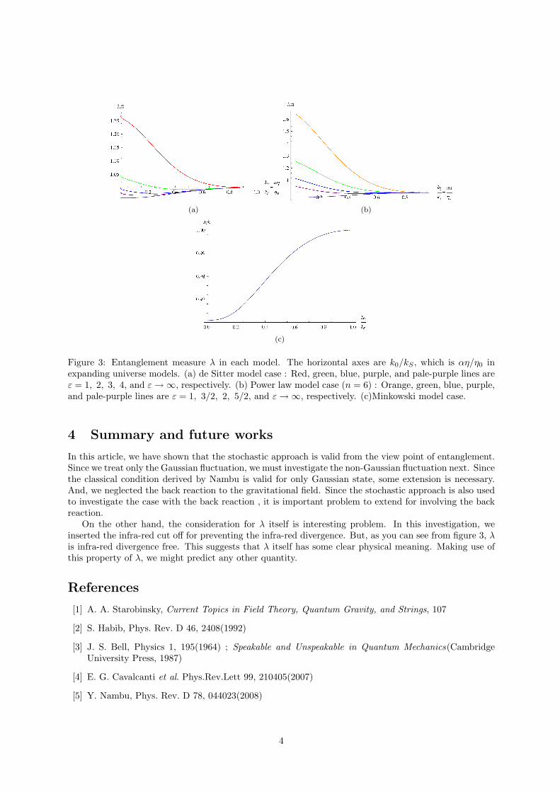
(a) (b)
(c)
Figure 3: Entanglement measure ∏ in each model. The horizontal axes are k0/kS , which is αη/η0 inexpanding universe models. (a) de Sitter model case : Red, green, blue, purple, and pale-purple lines areε = 1, 2, 3, 4, and ε →1, respectively. (b) Power law model case (n = 6) : Orange, green, blue, purple,and pale-purple lines are ε = 1, 3/2, 2, 5/2, and ε →1, respectively. (c)Minkowski model case.
4 Summary and future works
In this article, we have shown that the stochastic approach is valid from the view point of entanglement.Since we treat only the Gaussian fluctuation, we must investigate the non-Gaussian fluctuation next. Sincethe classical condition derived by Nambu is valid for only Gaussian state, some extension is necessary.And, we neglected the back reaction to the gravitational field. Since the stochastic approach is also usedto investigate the case with the back reaction , it is important problem to extend for involving the backreaction.
On the other hand, the consideration for ∏ itself is interesting problem. In this investigation, weinserted the infra-red cut off for preventing the infra-red divergence. But, as you can see from figure 3, ∏is infra-red divergence free. This suggests that ∏ itself has some clear physical meaning. Making use ofthis property of ∏, we might predict any other quantity.
References
[1] A. A. Starobinsky, Current Topics in Field Theory, Quantum Gravity, and Strings, 107
[2] S. Habib, Phys. Rev. D 46, 2408(1992)
[3] J. S. Bell, Physics 1, 195(1964) ; Speakable and Unspeakable in Quantum Mechanics(CambridgeUniversity Press, 1987)
[4] E. G. Cavalcanti et al. Phys.Rev.Lett 99, 210405(2007)
[5] Y. Nambu, Phys. Rev. D 78, 044023(2008)
4
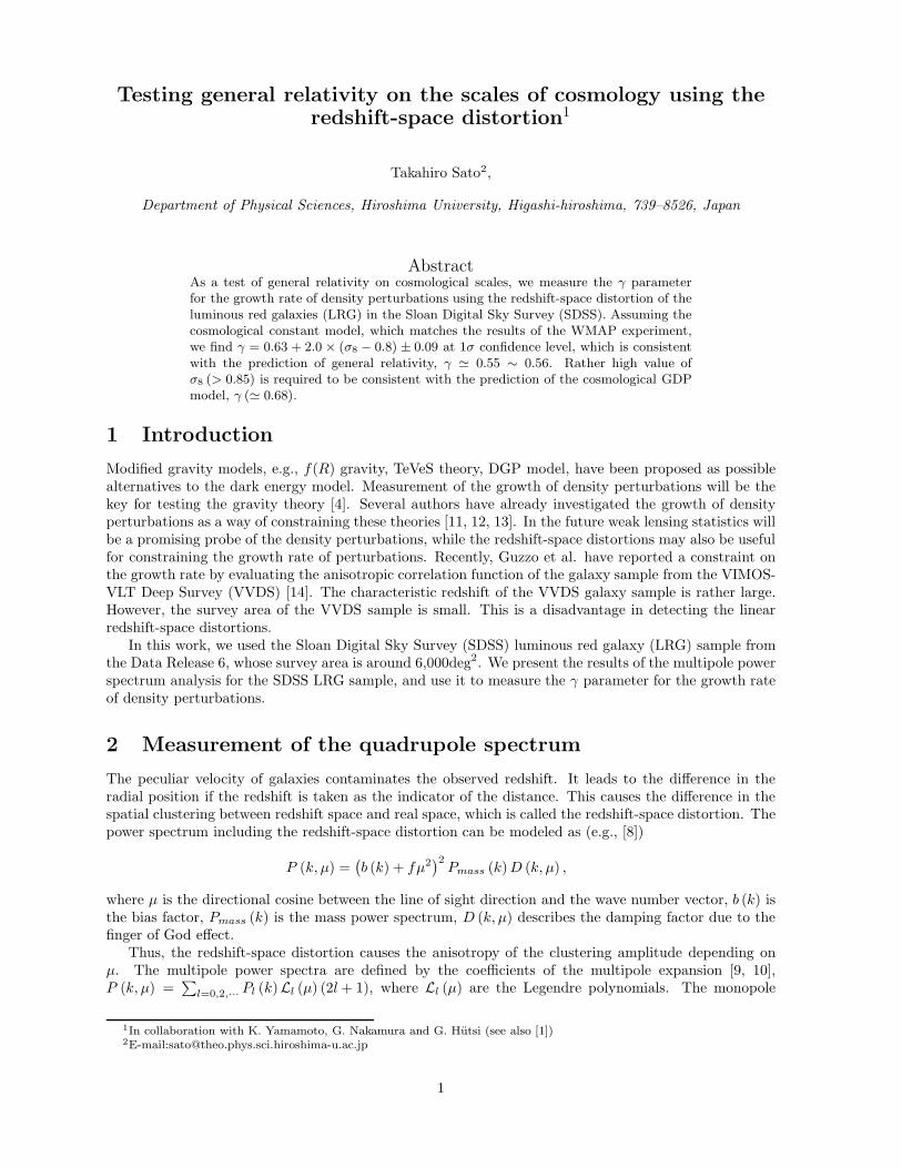
Testing general relativity on the scales of cosmology using theredshift-space distortion1
Takahiro Sato2,
Department of Physical Sciences, Hiroshima University, Higashi-hiroshima, 739–8526, Japan
AbstractAs a test of general relativity on cosmological scales, we measure the γ parameterfor the growth rate of density perturbations using the redshift-space distortion of theluminous red galaxies (LRG) in the Sloan Digital Sky Survey (SDSS). Assuming thecosmological constant model, which matches the results of the WMAP experiment,we find γ = 0.63 + 2.0 × (σ8 − 0.8) ± 0.09 at 1σ confidence level, which is consistentwith the prediction of general relativity, γ 0.55 ∼ 0.56. Rather high value ofσ8 (> 0.85) is required to be consistent with the prediction of the cosmological GDPmodel, γ ( 0.68).
1 Introduction
Modified gravity models, e.g., f(R) gravity, TeVeS theory, DGP model, have been proposed as possiblealternatives to the dark energy model. Measurement of the growth of density perturbations will be thekey for testing the gravity theory [4]. Several authors have already investigated the growth of densityperturbations as a way of constraining these theories [11, 12, 13]. In the future weak lensing statistics willbe a promising probe of the density perturbations, while the redshift-space distortions may also be usefulfor constraining the growth rate of perturbations. Recently, Guzzo et al. have reported a constraint onthe growth rate by evaluating the anisotropic correlation function of the galaxy sample from the VIMOS-VLT Deep Survey (VVDS) [14]. The characteristic redshift of the VVDS galaxy sample is rather large.However, the survey area of the VVDS sample is small. This is a disadvantage in detecting the linearredshift-space distortions.
In this work, we used the Sloan Digital Sky Survey (SDSS) luminous red galaxy (LRG) sample fromthe Data Release 6, whose survey area is around 6,000deg2. We present the results of the multipole powerspectrum analysis for the SDSS LRG sample, and use it to measure the γ parameter for the growth rateof density perturbations.
2 Measurement of the quadrupole spectrum
The peculiar velocity of galaxies contaminates the observed redshift. It leads to the difference in theradial position if the redshift is taken as the indicator of the distance. This causes the difference in thespatial clustering between redshift space and real space, which is called the redshift-space distortion. Thepower spectrum including the redshift-space distortion can be modeled as (e.g., [8])
P (k, μ) =(
b (k) + fμ2)2Pmass (k)D (k, μ) ,
where μ is the directional cosine between the line of sight direction and the wave number vector, b (k) isthe bias factor, Pmass (k) is the mass power spectrum, D (k, μ) describes the damping factor due to thefinger of God effect.
Thus, the redshift-space distortion causes the anisotropy of the clustering amplitude depending onμ. The multipole power spectra are defined by the coefficients of the multipole expansion [9, 10],P (k, μ) =
∑
l=0,2,··· Pl (k)Ll (μ) (2l+ 1), where Ll (μ) are the Legendre polynomials. The monopole
1In collaboration with K. Yamamoto, G. Nakamura and G. Hutsi (see also [1])2E-mail:[email protected]
1
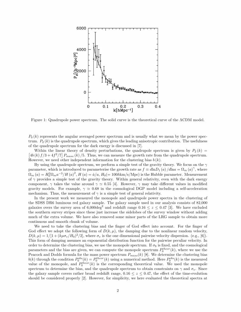
Figure 1: Quadrupole power spectrum. The solid curve is the theoretical curve of the ΛCDM model.
P0 (k) represents the angular averaged power spectrum and is usually what we mean by the power spec-trum. P2 (k) is the quadrupole spectrum, which gives the leading anisotropic contribution. The usefulnessof the quadrupole spectrum for the dark energy is discussed in [7].
Within the linear theory of density perturbations, the quadrupole spectrum is given by P2 (k) =[
4b (k) f/3 + 4f2/7]
Pmass (k) /5. Thus, we can measure the growth rate from the quadrupole spectrum.However, we need other independent information for the clustering bias b (k).
By using the quadrupole spectrum, we perform a simple test of the gravity theory. We focus on the γparameter, which is introduced to parameterise the growth rate as f ≡ dlnD1 (a) /dlna = Ωm (a)γ , whereΩm (a) = H2
0Ωma−3/H (a)2, H (a) = a/a, H0(= 100hkm/s/Mpc) is the Hubble parameter. Measurementof γ provides a simple test of the gravity theory. Within general relativity, even with the dark energycomponent, γ takes the value around γ 0.55 [4]. However, γ may take different values in modifiedgravity models. For example, γ 0.68 in the cosmological DGP model including a self-accelerationmechanism. Thus, the measurement of γ is a simple test of general relativity.
In the present work we measured the monopole and quadrupole power spectra in the clustering ofthe SDSS DR6 luminous red galaxy sample. The galaxy sample used in our analysis consists of 82,000galaxies overs the survey area of 6,000deg2 and redshift range 0.16 ≤ z ≤ 0.47 [3]. We have excludedthe southern survey stripes since these just increase the sidelobes of the survey window without addingmuch of the extra volume. We have also removed some minor parts of the LRG sample to obtain morecontinuous and smooth chunk of volume.
We need to take the clustering bias and the finger of God effect into account. For the finger ofGod effect we adopt the following form of D(k, μ), the damping due to the nonlinear random velocity,D(k, μ) = 1/[1 + (kμσv/H0)2/2], where σv is the one dimensional pairwise velocity dispersion. (e.g., [6]).This form of damping assumes an exponential distribution function for the pairwise peculiar velocity. Inorder to determine the clustering bias, we use the monopole spectrum. If σ8 is fixed, and the cosmologicalparameters and the bias are given, we can compute the monopole spectrum P theor0 (k), where we use thePeacock and Dodds formula for the mass power spectrum Pmass(k) [8]. We determine the clustering biasb(k) through the condition P obs0 (k) = P theor0 (k) using a numerical method. Here P obs0 (k) is the measuredvalue of the monopole, and P theor0 (k) is the corresponding theoretical value. We used the monopolespectrum to determine the bias, and the quadrupole spectrum to obtain constraints on γ and σv. Sincethe galaxy sample covers rather broad redshift range, 0.16 ≤ z ≤ 0.47, the effect of the time-evolutionshould be considered properly [2]. However, for simplicity, we here evaluated the theoretical spectra at
2
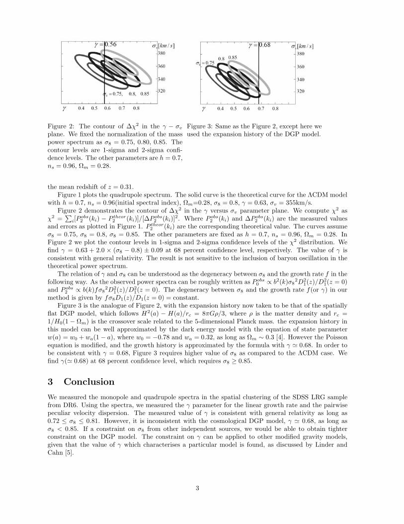
Figure 2: The contour of Δχ2 in the γ − σvplane. We fixed the normalization of the masspower spectrum as σ8 = 0.75, 0.80, 0.85. Thecontour levels are 1-sigma and 2-sigma confi-dence levels. The other parameters are h = 0.7,ns = 0.96, Ωm = 0.28.
Figure 3: Same as the Figure 2, except here weused the expansion history of the DGP model.
the mean redshift of z = 0.31.Figure 1 plots the quadrupole spectrum. The solid curve is the theoretical curve for the ΛCDM model
with h = 0.7, ns = 0.96(initial spectral index), Ωm=0.28, σ8 = 0.8, γ = 0.63, σv = 355km/s.Figure 2 demonstrates the contour of Δχ2 in the γ versus σv parameter plane. We compute χ2 as
χ2 =∑
i[Pobs2 (ki) − P theor2 (ki)]/[ΔP obs2 (ki)]2. Where P obs2 (ki) and ΔP obs2 (ki) are the measured values
and errors as plotted in Figure 1. P theor2 (ki) are the corresponding theoretical value. The curves assumeσ8 = 0.75, σ8 = 0.8, σ8 = 0.85. The other parameters are fixed as h = 0.7, ns = 0.96, Ωm = 0.28. InFigure 2 we plot the contour levels in 1-sigma and 2-sigma confidence levels of the χ2 distribution. Wefind γ = 0.63 + 2.0 × (σ8 − 0.8) ± 0.09 at 68 percent confidence level, respectively. The value of γ isconsistent with general relativity. The result is not sensitive to the inclusion of baryon oscillation in thetheoretical power spectrum.
The relation of γ and σ8 can be understood as the degeneracy between σ8 and the growth rate f in thefollowing way. As the observed power spectra can be roughly written as P obs0 ∝ b2(k)σ8
2D21(z)/D
21(z = 0)
and P obs2 ∝ b(k)fσ82D2
1(z)/D21(z = 0). The degeneracy between σ8 and the growth rate f(or γ) in our
method is given by fσ8D1(z)/D1(z = 0) = constant.Figure 3 is the analogue of Figure 2, with the expansion history now taken to be that of the spatially
flat DGP model, which follows H2(a) − H(a)/rc = 8πGρ/3, where ρ is the matter density and rc =1/H0(1 − Ωm) is the crossover scale related to the 5-dimensional Planck mass. the expansion history inthis model can be well approximated by the dark energy model with the equation of state parameterw(a) = w0 + wa(1 − a), where w0 = −0.78 and wa = 0.32, as long as Ωm ∼ 0.3 [4]. However the Poissonequation is modified, and the growth history is approximated by the formula with γ 0.68. In order tobe consistent with γ = 0.68, Figure 3 requires higher value of σ8 as compared to the ΛCDM case. Wefind γ( 0.68) at 68 percent confidence level, which requires σ8 ≥ 0.85.
3 Conclusion
We measured the monopole and quadrupole spectra in the spatial clustering of the SDSS LRG samplefrom DR6. Using the spectra, we measured the γ parameter for the linear growth rate and the pairwisepeculiar velocity dispersion. The measured value of γ is consistent with general relativity as long as0.72 ≤ σ8 ≤ 0.81. However, it is inconsistent with the cosmological DGP model, γ 0.68, as long asσ8 < 0.85. If a constraint on σ8 from other independent sources, we would be able to obtain tighterconstraint on the DGP model. The constraint on γ can be applied to other modified gravity models,given that the value of γ which characterises a particular model is found, as discussed by Linder andCahn [5].
3
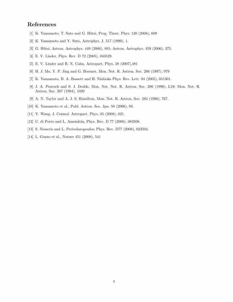
References
[1] K. Yamamoto, T. Sato and G. Hutsi, Prog. Theor. Phys. 120 (2008), 609
[2] K. Yamamoto and Y. Suto, Astrophys. J. 517 (1999), 1.
[3] G. Hutsi, Astron. Astrophys. 449 (2006), 891; Astron. Astrophys. 459 (2006), 375.
[4] E. V. Linder, Phys. Rev. D 72 (2005), 043529.
[5] E. V. Linder and R. N. Cahn, Astropart. Phys. 28 (2007),481
[6] H. J. Mo, Y. P. Jing and G. Boerner, Mon. Not. R. Astron. Soc. 286 (1997), 979
[7] K. Yamamoto, B. A. Bassett and H. Nishioka Phys. Rev. Lett. 94 (2005), 051301.
[8] J. A. Peacock and S. J. Dodds, Mon. Not. Not. R. Astron. Soc. 280 (1996), L19; Mon. Not. R.Astron. Soc. 267 (1994), 1020
[9] A. N. Taylor and A. J. S. Hamilton, Mon. Not. R. Astron. Soc. 282 (1996), 767.
[10] K. Yamamoto et al., Publ. Astron. Soc. Jpn. 58 (2006), 93.
[11] Y. Wang, J. Cosmol. Astropart. Phys. 05 (2008), 021.
[12] C. di Porto and L. Amendola, Phys. Rev. D 77 (2008), 083508.
[13] S. Nesseris and L. Perivolaropoulos, Phys. Rev. D77 (2008), 023504.
[14] L. Guzzo et al., Nature 451 (2008), 541
4
Higher curvature theories of gravityin the ADM canonical formalism
Yuuiti Sendouda1,a, Nathalie Deruelleb, Misao Sasakia and Daisuke Yamauchia
aYukawa Institute for Theoretical Physics, Kyoto University, Kyoto 606–8502, JapanbAPC, UMR 7164 (CNRS, Universite Paris 7, CEA, Observatoire de Paris), 75205 Paris Cedex 13,
France
AbstractWe present a canonical formulation for higher-curvature theories of gravity whoseaction is a generic function of Riemann tensor. The Arnowitt–Deser–Misner canon-ical formalism is employed to identify the extra gravitational dynamical degrees offreedom other than metric. We also nd a surface term that gives Dirichlet boundaryconditions for the dynamical degrees of freedom.
1 Introduction
Quantum theories of gravity, such as string theories, predict the conventional Einstein–Hilbert action,Sg = (2)1
∫M
√−gR, is necessarily supplemented by higher-order terms in curvature, which, even at
the classical level, may come into play in the regime of strong gravity. Studies on higher-order gravitycan open a window to the fundamental theory and it is therefore interesting to investigate its possibleimprints on cosmological and/or astrophysical phenomena.
Our start-up strategy is to abstract essential properties of higher-order gravity and examine whethereach class of theories can qualify basic requirements as viable gravity theory. In order to serve suchphenomenological studies, one should keep as much generality as possible. We treat generic actions onD-dimensional spacetime (M, g) such as
Sg =12
∫M
√−gf(Rabcd, gab), (1)
where f is an arbitrary scalar-valued (non-linear) function of the Riemann tensor.Since the equation of motion stemming from the above action contains fourth-order derivatives, gravity
involves extra dynamical degrees of freedom other than metric. To have a clear view on such aspect, weemploy the Arnowitt–Deser–Misner (ADM) [1] canonical formalism to describe the theory. We will atthe same time nd a relevant surface action by which existence of extra gravitational degrees of freedomis taken into account.
The main body of this article consists of identication of a Dirichlet surface term necessary in con-structing a rst-order action (section 2) and ADM canonical formulation (section 3).
2 Dirichlet surface term
Appearance of higher derivatives is avoided by considering an equivalent theory which is linear in secondderivative of the metric
Sg =12
∫M
√−g[abcd(Rabcd − abcd) + f(abcd, gab)], (2)
where the auxiliary eld abcd and the Lagrange multiplier abcd are independent of gab. The variationof the action reads
Sg =12
∫M
√−g
[−Eabgab + (Rabcd − abcd)abcd +
(∂f
∂abcd− abcd
)abcd
]+
1
∫M
√−g∇d(gab∇c
acbd − acbd∇cgab),(3)
1E-mail:sendouda(a)yukawa.kyoto-u.ac.jp
1
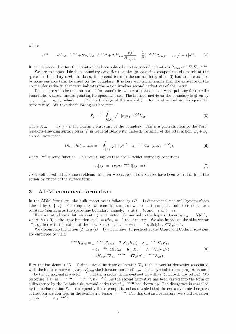
where
Eab ≡ −R(acde
b)cde + 2∇c∇d(a|c|b)d + 2(a
cde∂f
∂b)cde− 1
2[cdef (Rcdef − cdef ) + f ]gab. (4)
It is understood that fourth derivative has been splitted into two second derivatives Rabcd and ∇c∇dacbd.
We are to impose Dirichlet boundary conditions on the (propagating components of) metric at thespacetime boundary ∂M. To do so, the second term in the surface integral in (3) has to be cancelledby some suitable term localised on the boundary. It is here worth mentioning that the existence of thenormal derivative in that term indicates the action involves second derivatives of the metric.
Dene here na to be the unit normal for boundaries whose orientation is outward-pointing for timelikeboundaries whereas inward-pointing for spacelike ones. The induced metric on the boundary is given by ab = gab − nanb, where ≡ nana is the sign of the normal (−1 for timelike and +1 for spacelike,respectively). We take the following surface term
Sg =2
∮∂M
√| |ncndacbdKab, (5)
where Kab ≡ ca∇cnb is the extrinsic curvature of the boundary. This is a generalisation of the York–Gibbons–Hawking surface term [2] in General Relativity. Indeed, variation of the total action, Sg + Sg,on-shell now reads
(Sg + Sg)|on-shell =1
∮∂M
√| |(P ab ab + 2Kab(ncndacbd)), (6)
where P ab is some function. This result implies that the Dirichlet boundary conditions
ab|∂M = (ncndacbd)|∂M = 0 (7)
gives well-posed initial-value problems. In other words, second derivatives have been get rid of from theaction by virtue of the surface term.
3 ADM canonical formalism
In the ADM formalism, the bulk spacetime is foliated by (D − 1)-dimensional non-null hypersurfaceslabeled by t, t. For simplicity, we consider the case where t is compact and there exists twoconstant-t surfaces as the spacetime boundary, namely, 0 at t = t0 and 1 at t = t1.
Here we introduce a ‘future-pointing’ unit vector eld normal to the hypersurfaces by na = N(dt)a,where N (> 0) is the lapse function and = nana = ±1 the signature. We also introduce the shift vectora together with the notion of the ‘ ow’ vector eld ta = Nna + a satisfying ta∇at = 1.
We decompose the action (2) in a (D− 1)+1 manner. In particular, the Gauss and Codazzi relationsare employed to yield
abcdRabcd = ⊥abcd( Rabcd − 2KacKbd) + 8⊥abcn ∇aKbc
+ 4⊥anbn(KKab −KacKbc − N1 ∇a
∇bN)
+ 4Kabnc∇c⊥
anbn − 4∇c(nc⊥anbnKab).
(8)
Here the bar denotes (D − 1)-dimensional intrinsic quantities: ∇a is the covariant derivative associatedwith the induced metric ab and Rabcd the Riemann tensor of ab. The ⊥ symbol denotes projection ontot by the orthogonal projector ab, and the n index means contraction with na (before ⊥-projection). Werecognise, e.g., as ⊥
anbn = acnd benf
cdef . As the second derivative has been casted into the form ofa divergence by the Leibniz rule, normal derivative of ⊥
anbn has shown up. The divergence is cancelledby the surface action Sg. Consequently this decomposition has revealed that the extra dynamical degreesof freedom are conned in the symmetric tensor ⊥
anbn. For this distinctive feature, we shall hereafterdenote ab ≡ 2⊥anbn.
2
Terms in the action are all decomposed in this manner. We may see f as a function of projectedcomponents of abcd and of metric gab. We dene ‘velocities’ of the dynamical variables in terms of Liederivatives as ab ≡ £t ab = 2NKab + 2 ∇(ab) and ab ≡ £t
ab, respectively. Then we arrive at theaction totally represented with the following set of quantities (and their derivatives on t):
ab, ab, ab, ab, N, a,⊥abcd,⊥abcn,⊥anbn,⊥abcd,⊥abcn. (9)
This form of action is suitable for canonical formulation. Canonical momenta conjugate to each variableare dened by
qi ≡(Sg + Sg)
qi. (10)
Then the total action is rewritten in terms of canonical variables qi, qi via Legendre transformation
Sg + Sg =∫ t1
t0
dt[∫
t
(ab ab + ab ab) −Hg
], (11)
where Hg is the Hamiltonian.At this stage, Dirac’s prescription [3] tells how to obtain canonical equations of motion and constraints.
Here we illustrate the procedure and outcomes, the whole of which will be presented in a forthcomingpaper [4]. Each variable whose velocity is missing in the action gives a primary constraint
i ≡ i ≈ 0, (12)
where λi = N, a,⊥abcd,⊥abcn,⊥anbn,⊥abcd,⊥
abcn represents those non-dynamical variables andthe weak equality ≈ means modulo constraints. The total Hamiltonian is constructed as
Ht = Hg +∑i
∫t
uii , (13)
where ui ’s are multipliers. Evolution of the variables is described by Poisson bracket. t-derivative ofeach quantity is determined by Poisson bracket with the total Hamiltonian
Q ≈ −Ht, Q. (14)
The canonical equations of motion for dynamical variables are therefore given as
ab ≈Hg
ab , ab ≈ − Hg
ab, ab ≈ Hg
ab, ab ≈ − Hg
ab. (15)
They correspond to the denitions of velocities and the dynamical part of the Euler–Lagrange equationsof motion, i.e., those two normal components containing second derivatives. On the other hand, asthe constraints must preserve, consistency of the theory demands derivatives of primary constraintsi vanish thereby leading to secondary constraints i ≈ 0. One can check that the rest of Euler–Lagrange equations is indeed recovered by them. Consequently equivalence between the Euler–Lagrangeand Hamilton formulations has been conrmed at the level of equations of motion.
To guarantee that those secondary constraints preserve, we have to pay attention to what i bringsabout. When i ≈ 0 is not automatically satised, i.e., it is independent of known secondary constraints,we have two possibilities; If the equality contains some multiplier ui yet undetermined, then the equationis used to x, or constrain, the multiplier. On the other hand, if the equality does not contain multipliers,then we add it to the set of constraints. In the latter case, we have to continue to take derivatives ofthose new secondary constraints until derivatives will automatically vanish by virtue of other constraints.The number of collected secondary constraints in turn tells how many dynamical degrees of freedom cansurvive and this is where the detailed form of f plays an essential role. This aspect will be discussedelsewhere [4].
Focusing on rather basic properties, derivatives of the momenta of lapse and shift are analogues ofthe Hamiltonian and momentum constraints in General Relativity,
CN ≡ Hg
N≈ 0, Cβa ≡ Hg
a≈ 0. (16)
3
The Hamiltonian can be represented as
Hg =∫
t
(NCN + aCβa ). (17)
up to divergence on t. Derivatives of the Hamiltonian and momentum constraints does not arise furthersecondary constraints leaving corresponding multipliers uN and uaβ undetermined.
4 Conclusion
We presented a basic framework of ADM canonical formulation for higher-curvature theories of gravitywhose Lagrangian is a generic function of Riemann tensor. Two auxiliary elds, abcd and abcd, wereintroduced to make the action linear in second derivative. Further, in order to cast the theory into arst-order form, the action (2) was supplemented by a Dirichlet surface term (5). Then the rst-orderaction was Legendre transformed to the canonical form. We showed all the possible dynamical degreesof freedom other than metric were conned in ab = 2anbn. Emergence of new dynamical degreesof freedom is all due to non-linearity of Ranbn in f , which exclusively contains second derivative of themetric among projected components of the Riemann tensor.
Then Dirac’s procedure was employed to derive canonical equations of motion and constraints. Theequivalence between Euler–Lagrange and Hamilton formulations were seen at the level of equations ofmotion. The resultant number of the extra degrees of freedom is controlled by the detailed form of f viasecondary constraints.
Our results can be applied in various contexts. Surface action will play an inevitable role in gravita-tional systems with boundary (e.g., construction of new braneworld models, AdS/CFT correspondence,and so on). As a theoretical problem, there have long been claims that spin-2 elds coupled to gravitytend to appear ghost [5], which can cause serious inconsistency in quantum theory as well as instabilitiesat the classical level. Possibilities of such pathology should be taken care of in applications.
Acknowledgements
Two of the authors were supported by Grant-in-Aid for JSPS Fellows No. 19-7852 (YS) and No. 20-1117(DY). MS was supported in part by JSPS Grant-in-Aid for Scientic Research (B) No. 17340075 and(A) No. 18204024, and by JSPS Grant-in-Aid for Creative Scientic Research No. 19GS0219. This workwas also supported by Grant-in-Aid for the Global COE Program “The Next Generation of Physics,Spun from Universality and Emergence” from the Ministry of Education, Culture, Sports, Science andTechnology of Japan.
References
[1] R. Arnowitt, S. Deser, and C.W. Misner, in Gravitation: an introduction to current research, ed.L. Witten (John Wiley & Sons, Inc., New York, 1962), pp. 227–265, gr-qc/0405109.
[2] J.W. York, Jr., Phys. Rev. Lett. 28 (1972) 1082–1085; G.W. Gibbons and S.W. Hawking, Phys.Rev. D15 (1977) 2752–2756.
[3] P.A.M. Dirac, Lectures on Quantum Mechanics (Dover Publications, Inc., New York, 2001).
[4] N. Deruelle, M. Sasaki, Y. Sendouda, and D. Yamauchi, in preparation.
[5] K.S. Stelle, Gen. Rel. Grav. 9 (1978) 353–371.
4
Towards the dynamics in Einstein-Gauss-Bonnet gravity:Initial Value Problem1
Takashi Torii2 and Hisa-aki Shinkai3
1General Education of Science, Osaka Institute of Technology, Omiya, Asahi-ku, Osaka 535-85852Dept. of Information Systems, Osaka Institute of Technology, Kitayama, Hirakata, Osaka 573-0196
AbstractTowards the investigation of the full dynamics in higher-dimensional and/or stringygravitational model, we present the basic equations of the Einstein-Gauss-Bonnetgravity theory. We show (N+1)-dimensional version of the Arnowitt-Deser-Misner de-composition including the Gauss-Bonnet term, which shall be the standard approachto treat the space-time as a Cauchy problem. Due to the quasi-linear property ofthe Gauss-Bonnet gravity, we find that the evolution equations can be in a treatableform in numerics. We also show the conformally-transformed constraint equationsfor constructing an initial data. Our equations can be used both for timelike andspacelike foliations.
1 Introduction
General relativity (GR) has been tested with many experiments and observations both in the strong andweak gravitational field regimes, and none of them are contradictory to GR. However, the theory alsopredicts the appearance of the spacetime singularities under natural conditions, which also indicates thatGR is still incomplete as a physics theory that describes whole of the gravity and the spacetime structure.
We expect that the true fundamental theory will resolve these theoretical problems. Up to now,several quantum theories of gravity have been proposed. Among them superstring/M-theory, formulatedin higher dimensional spacetime, is the most promising candidate. The Gauss-Bonnet (GB) term isthe next leading order of the α′-expansion (α′ is the inverse string tension) of type IIB superstringtheory[2, 3], and has nice properties such that it is ghost-free combinations[4] and does not give higherderivative equations but an ordinary set of equations with up to second derivative in spite of the highercurvature combinations.
The models with the GB term and/or other higher curvature terms have been intensively studiedin the high energy physics, in the contexts both in string cosmology and in black hole physics (seereferences in [1]). All the analysis so far are performed on the assumption of highly symmetric spacetimebecause the system is much more complicated than that in GR. To obtain deeper understanding of theearly stage of the universe, singularity, and/or black holes, we should consider less symmetric and/ordynamical spacetime; the analyses require the direct numerical integration of the equations. None of thefully dynamical simulations in GB gravity has been performed.
In this article, we present the basic equations of the Einstein-GB gravity theory. We show (N + 1)-dimensional version of the ADM decomposition, which is the standard approach to treat the spacetimeas a Cauchy problem. The topic was first discussed by Choquet-Bruhat [5], but the full set of equationsand the methodology have not yet been presented. Therefore, as the first step, we in this paper justpresent the fundamental space-time decomposition of the GB equations, focusing on the GB term.
The ADM decomposition is supposed to construct the spacetime with foliations of the constant-time hypersurfaces. This method can be also applied to study the brane-world model. We think theseexpressions are useful for future dynamical investigations.
1Please refer the details in [1].2E-mail: [email protected]: [email protected]
1
2 (N + 1)-decomposition in Einstein-Gauss-Bonnet gravity
We start from the Einstein-Gauss-Bonnet action in (N + 1)-dimensional spacetime (M, gµν) which isdescribed as 4:
S =∫M
dN+1X√−g
[1
2κ2(R− 2Λ + αGBLGB) + Lmatter
], (1)
with LGB = R2−4RµνRµν +RµνρσRµνρσ,where κ2 is the (N +1)-dimensional gravitational constant, R,Rµν , Rµνρσ and Lmatter are the (N+1)-dimensional scalar curvature, Ricci tensor, Riemann curvature andthe matter Lagrangian, respectively. This action reproduces the standard (N + 1)-dimensional Einsteingravity, if we set the coupling constant αGB (≥ 0) equals to zero.
The action (1) gives the gravitational equation as
Gµν + αGBHµν = κ2 Tµν , (2)
where Gµν = Rµν − 12gµνR + gµνΛ, Tµν = −2
δLmatter
δgµν+ gµνLmatter, (3)
Hµν = 2(RRµν − 2RµαRα
ν − 2RαβRµανβ + R αβγµ Rναβγ
)− 1
2gµνLGB . (4)
In order to investigate the space-time structure as the foliations of the N -dimensional (spacelike ortimelike) hypersurface Σ, we introduce the projection operator to Σ as
⊥µν = gµν − εnµnν , (5)
where nµ is the unit-normal vector to Σ with nµnµ = ε, with which we define nµ is timelike (if ε = −1)or spacelike (if ε = 1). Therefore, Σ is spacelike (timelike) if nµ is timelike (spacelike).
The projections of the gravitational equation (2) give the following three equations:(Gµν + αGBHµν
)nµ nν = κ2 Tµν nµ nν = κ2ρ, (6)(
Gµν + αGBHµν
)nµ ⊥ν
ρ = κ2 Tµν nµ ⊥νρ = −κ2Jρ, (7)(
Gµν + αGBHµν
)⊥µ
ρ ⊥νσ = κ2 Tµν ⊥µ
ρ ⊥νσ = κ2Sρσ, (8)
where we defined the components of the energy-momentum tensor as Tµν = ρnµnν + Jµnν + Jνnµ + Sµν ,and we also define T = ερ + Sα
α for later convenience.Following the standard procedure of the ADM formulation, we find that the equations (6)–(8) corre-
spond to (a) the Hamiltonian constraint equation:
M + αGB
(M2 − 4MabM
ab + MabcdMabcd
)= −2εκ2ρH + 2Λ , (9)
(b) the momentum constraint equation:
Ni + 2αGB
(MNi − 2M a
i Na + 2MabNiab − M cabi Nabc
)= κ2Ji , (10)
and (c) the evolution equations for γij :
Mij −12Mγij − ε
(−KiaKa
j + γijKabKab − £nKij + γijγ
ab£nKab
)+ 2αGB
[Hij + ε
(M£nKij − 2M a
i £nKaj − 2M aj £nKai − W ab
ij £nKab
)]= κ2Sij − γijΛ ,(11)
respectively, where
Mijkl = Rijkl − ε(KikKjl − KilKjk), (12)
Nijk = DiKjk − DjKik, (13)4The Greek indices move 0, 1, · · · , N , while the Latin indices move 1, · · · , N .
2
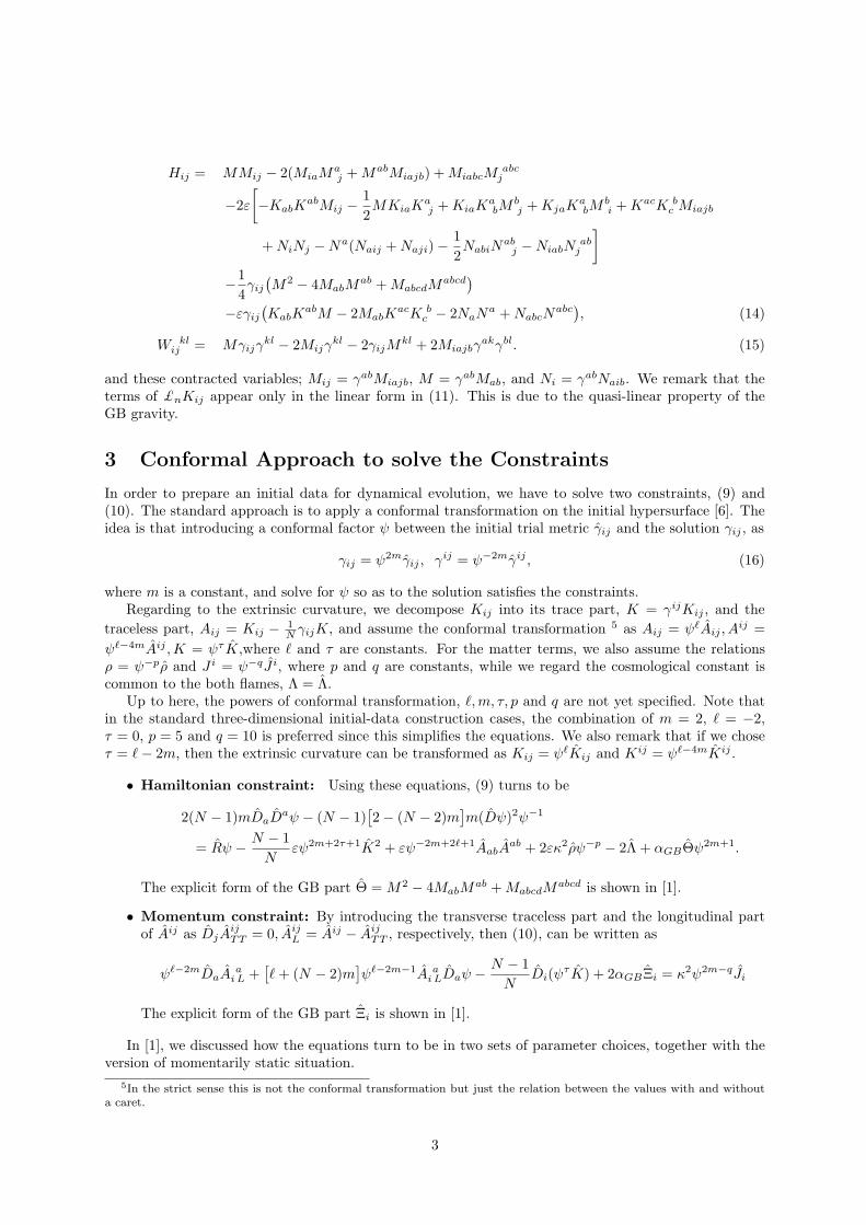
Hij = MMij − 2(MiaMaj + MabMiajb) + MiabcM
abcj
−2ε
[−KabK
abMij −12MKiaKa
j + KiaKabM
bj + KjaKa
bMbi + KacK b
c Miajb
+ NiNj − Na(Naij + Naji) −12NabiN
abj − NiabN
abj
]−1
4γij
(M2 − 4MabM
ab + MabcdMabcd
)−εγij
(KabK
abM − 2MabKacK b
c − 2NaNa + NabcNabc
), (14)
W klij = Mγijγ
kl − 2Mijγkl − 2γijM
kl + 2Miajbγakγbl. (15)
and these contracted variables; Mij = γabMiajb, M = γabMab, and Ni = γabNaib. We remark that theterms of £nKij appear only in the linear form in (11). This is due to the quasi-linear property of theGB gravity.
3 Conformal Approach to solve the Constraints
In order to prepare an initial data for dynamical evolution, we have to solve two constraints, (9) and(10). The standard approach is to apply a conformal transformation on the initial hypersurface [6]. Theidea is that introducing a conformal factor ψ between the initial trial metric γij and the solution γij , as
γij = ψ2mγij , γij = ψ−2mγij , (16)
where m is a constant, and solve for ψ so as to the solution satisfies the constraints.Regarding to the extrinsic curvature, we decompose Kij into its trace part, K = γijKij , and the
traceless part, Aij = Kij − 1N γijK, and assume the conformal transformation 5 as Aij = ψ`Aij , A
ij =ψ`−4mAij ,K = ψτ K,where ` and τ are constants. For the matter terms, we also assume the relationsρ = ψ−pρ and J i = ψ−qJ i, where p and q are constants, while we regard the cosmological constant iscommon to the both flames, Λ = Λ.
Up to here, the powers of conformal transformation, `,m, τ, p and q are not yet specified. Note thatin the standard three-dimensional initial-data construction cases, the combination of m = 2, ` = −2,τ = 0, p = 5 and q = 10 is preferred since this simplifies the equations. We also remark that if we choseτ = ` − 2m, then the extrinsic curvature can be transformed as Kij = ψ`Kij and Kij = ψ`−4mKij .
• Hamiltonian constraint: Using these equations, (9) turns to be
2(N − 1)mDaDaψ − (N − 1)[2 − (N − 2)m
]m(Dψ)2ψ−1
= Rψ − N − 1N
εψ2m+2τ+1K2 + εψ−2m+2`+1AabAab + 2εκ2ρψ−p − 2Λ + αGBΘψ2m+1.
The explicit form of the GB part Θ = M2 − 4MabMab + MabcdM
abcd is shown in [1].
• Momentum constraint: By introducing the transverse traceless part and the longitudinal partof Aij as DjA
ijTT = 0, Aij
L = Aij − AijTT , respectively, then (10), can be written as
ψ`−2mDaA ai L +
[` + (N − 2)m
]ψ`−2m−1A a
i LDaψ − N − 1N
Di(ψτ K) + 2αGBΞi = κ2ψ2m−qJi
The explicit form of the GB part Ξi is shown in [1].
In [1], we discussed how the equations turn to be in two sets of parameter choices, together with theversion of momentarily static situation.
5In the strict sense this is not the conformal transformation but just the relation between the values with and withouta caret.
3
4 Dynamical equations
The Einstein evolution equation in general N -dimensional ADM version is presented in [7]. With theGB terms, the evolution equation (11) cannot be expressed explicitly for each £nKij . That is, (11) isrewritten as
(1 + 2αGBM)£nKij − (γijγab + 2αGBW ab
ij )£nKab − 8αGBM a(i £nK|a|j)
= −ε
(Mij −
12Mγij
)− KiaKa
j + γijKabKab + εκ2Sij − εγijΛ − 2εαGBHij , (17)
and the second and the third terms in r.h.s include the linearly-coupled terms between £nKij . Therefore,in an actual simulation, we have to extract each evolution equation of Kij using a matrix form of Eq. (17)like
k = Ak + b (18)
where k = (£nK11,£nK12, · · · ,£nKNN )T and A, b are appropriate matrix and vector derived fromEq. (17).
The procedure of the inverting the matrix (1 − A) is technically available, but the invertibility ofthe matrix is not generally guaranteed at this moment. In the case of the standard ADM foliation infour-dimensional Einstein equations, the continuity of the time evolutions depends on the models and thechoice of gauge conditions for the lapse function and shift vectors. If the combination is not appropriate,then the foliation hits the singularity which stops the evolution. The similar obstacle may exist also forthe GB gravity. Actually, Deruelle and Madore [8] gave an explicit example in a simple cosmologicalmodel where the equation corresponding to (18) is not invertible. We expect that in the most casesEq. (18) is invertible for Kij but we cannot deny the pathological cases which depend on the models andgauge conditions. Such a study must be done together with actual numerical integrations in the future.
5 Discussion
In summary, we show the (N +1)-dimensional decomposition of the basic equations, in order to treat thespace-time as a Cauchy problem. The equations can be separated to the constraints (the Hamiltonianconstraint and the momentum constraint) and the evolution equations.
Two constraints should be solved for constructing an initial data, and we show how the actual equa-tions turn to be. If we have the GB term, however, the equations still remain in a complicated style.
For the evolution equations, we find that £nKij components are coupled. However, this mixture isonly up to the linear order due to the quasi-linear property of the GB term, so that the equations can bein a treatable form in numerics.
We are now developing our numerical code and hope to present some results elsewhere near future.
References
[1] T. Torii and H. Shinkai, Phys. Rev. D 78, 084037 (2008).
[2] D. J. Gross and E. Witten, Nucl. Phys. B277, 1 (1986);D. J. Gross and J. H. Sloan, Nucl. Phys. B291, 41 (1987).
[3] M. C. Bento and O Bertolami, Phys. Lett. B 368, 198 (1996).
[4] B. Zwiebach, Phys. Lett. B 156, 315 (1985).
[5] Y. Choquet-Bruhat, J. Math. Phys. 29, 1891 (1988).
[6] N. OMurchadha and J. W. York, Jr., Phys. Rev. D 10, 428 (1974).
[7] H. Shinkai and G. Yoneda, Gen. Rel. Grav. 36, 1931 (2004).
[8] N. Deruelle and J. Madore, arXiv:gr-qc/0305004.
4
Revisiting chameleon gravity–thin-shells and no-shellswith appropriate boundary conditions
Takashi Tamaki1 and Shinji Tsujikawa2
1Department of Physics, Waseda University, Okubo 3-4-1, Tokyo 169-8555, Japan2Department of Physics, Faculty of Science, Tokyo University of Science, 1-3, Kagurazaka, Shinjuku-ku,
Tokyo 162-8601, Japan
AbstractWe derive analytic solutions of a chameleon scalar field φ that couples to a non-relativistic matter in the weak gravitational background of a spherically symmetricbody, paying particular attention to a field mass mA inside of the body.
1 Introduction
Recently there have been a lot of efforts to understand the origin of dark energy under the frameworkof modified gravity theories (see Refs. [1] for reviews). In modified gravity models of dark energy, it iscrucially important to appropriately study the compatibility of couplings with local gravity experimentsas well as with a late-time acceleration of the Universe preceded by a standard matter era. Interestingattempt to reconcile large coupling models with local gravity constraints is to use “chameleon” scalarfields whose masses depend on the environment they are in [2, 3]. The analysis in Refs. [2, 3] assumesthat the field is frozen (φ = φA) in the regime 0 < r < r1 without explicitly taking into account the fieldmass mA. Here and [4], we consider mA.
The action we study is given by
S =∫
d4x√−g
[
M2pl
2R− 1
2(∇φ)2 − V (φ)
]
−∫
d4xLm(Ψ(i)m , g(i)
μν) , (1)
where Ψ(i)m are matter fields that couple to a metric g(i)
μν related with the Einstein frame metric gμν viag(i)μν = e2Qiφgμν . Here Qi are the strength of couplings for each matter field. An example is
V (φ) = M4+nφ−n , (2)
where M has a unit of mass and n is a constant. In the context of f(R) gravity, Hu and Sawicki [5] andStarobinsky [6] proposed models that can be consistent with cosmological and local gravity constraints.We consider
V (φ) = V0
[
1 − C(1 − e−2Qφ)p]
, (3)
where V0 > 0, C > 0, 0 < p < 1 as a generalization of the potential in f(R) gravity.
2 Chameleon mechanism
The trace of the i-th matter is given by T (i) ≡ gμν(i)T(i)μν = −ρi for a non-relativistic fluid, where ρi is an
energy density. It is more convenient to introduce the quantity ρi = ρi e3Qiφ, which is conserved in the
Einstein frame. In a spherically symmetric background, we obtain
d2φ
dr2+
2r
dφdr
=dVeff
dφ, (4)
1E-mail:[email protected]:[email protected]
1
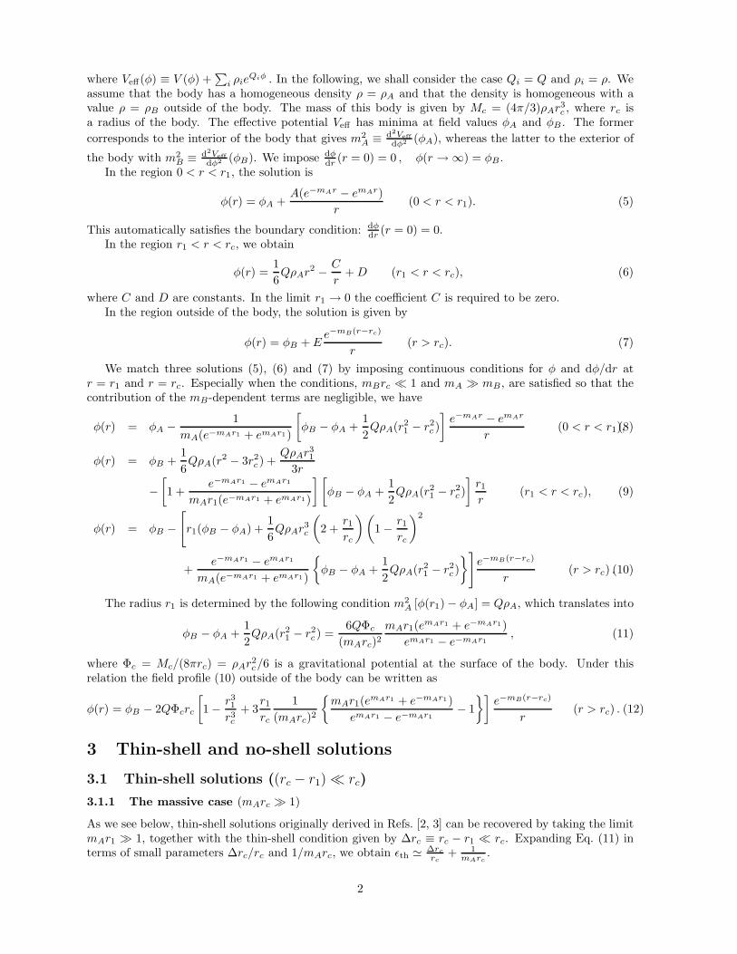
where Veff(φ) ≡ V (φ) +∑
i ρieQiφ . In the following, we shall consider the case Qi = Q and ρi = ρ. We
assume that the body has a homogeneous density ρ = ρA and that the density is homogeneous with avalue ρ = ρB outside of the body. The mass of this body is given by Mc = (4π/3)ρAr3c , where rc isa radius of the body. The effective potential Veff has minima at field values φA and φB . The formercorresponds to the interior of the body that gives m2
A ≡ d2Veffdφ2 (φA), whereas the latter to the exterior of
the body with m2B ≡ d2Veff
dφ2 (φB). We impose dφdr (r = 0) = 0 , φ(r → ∞) = φB.
In the region 0 < r < r1, the solution is
φ(r) = φA +A(e−mAr − emAr)
r(0 < r < r1). (5)
This automatically satisfies the boundary condition: dφdr (r = 0) = 0.
In the region r1 < r < rc, we obtain
φ(r) =16QρAr
2 − C
r+D (r1 < r < rc), (6)
where C and D are constants. In the limit r1 → 0 the coefficient C is required to be zero.In the region outside of the body, the solution is given by
φ(r) = φB + Ee−mB(r−rc)
r(r > rc). (7)
We match three solutions (5), (6) and (7) by imposing continuous conditions for φ and dφ/dr atr = r1 and r = rc. Especially when the conditions, mBrc 1 and mA mB, are satisfied so that thecontribution of the mB-dependent terms are negligible, we have
φ(r) = φA − 1mA(e−mAr1 + emAr1)
[
φB − φA +12QρA(r21 − r2c )
]
e−mAr − emAr
r(0 < r < r1),(8)
φ(r) = φB +16QρA(r2 − 3r2c ) +
QρAr31
3r
−[
1 +e−mAr1 − emAr1
mAr1(e−mAr1 + emAr1)
] [
φB − φA +12QρA(r21 − r2c )
]
r1r
(r1 < r < rc), (9)
φ(r) = φB −[
r1(φB − φA) +16QρAr
3c
(
2 +r1rc
) (
1 − r1rc
)2
+e−mAr1 − emAr1
mA(e−mAr1 + emAr1)
φB − φA +12QρA(r21 − r2c )
]
e−mB(r−rc)
r(r > rc) .(10)
The radius r1 is determined by the following condition m2A [φ(r1) − φA] = QρA, which translates into
φB − φA +12QρA(r21 − r2c ) =
6QΦc(mArc)2
mAr1(emAr1 + e−mAr1)emAr1 − e−mAr1
, (11)
where Φc = Mc/(8πrc) = ρAr2c/6 is a gravitational potential at the surface of the body. Under this
relation the field profile (10) outside of the body can be written as
φ(r) = φB − 2QΦcrc
[
1 − r31r3c
+ 3r1rc
1(mArc)2
mAr1(emAr1 + e−mAr1)emAr1 − e−mAr1
− 1]
e−mB(r−rc)
r(r > rc) . (12)
3 Thin-shell and no-shell solutions
3.1 Thin-shell solutions ((rc − r1) rc)
3.1.1 The massive case (mArc 1)
As we see below, thin-shell solutions originally derived in Refs. [2, 3] can be recovered by taking the limitmAr1 1, together with the thin-shell condition given by Δrc ≡ rc − r1 rc. Expanding Eq. (11) interms of small parameters Δrc/rc and 1/mArc, we obtain εth Δrc
rc+ 1
mArc.
2
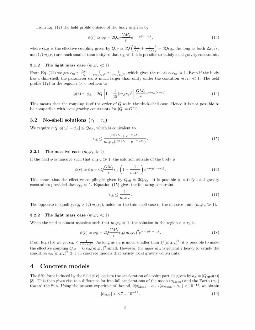
From Eq. (12) the field profile outside of the body is given by
φ(r) φB − 2QeffGMc
re−mB(r−rc) , (13)
where Qeff is the effective coupling given by Qeff 3Q(
Δrc
rc+ 1
mArc
)
= 3Qεth. As long as both Δrc/rcand 1/(mArc) are much smaller than unity so that εth 1, it is possible to satisfy local gravity constraints.
3.1.2 The light mass case (mArc 1)
From Eq. (11) we get εth Δrc
rc+ 1
(mArc)2 1
(mArc)2, which gives the relation εth 1. Even if the body
has a thin-shell, the parameter εth is much larger than unity under the condition mArc 1. The fieldprofile (12) in the region r > rc reduces to
φ(r) φB − 2Q[
1 − 115
(mArc)2]
GMc
re−mB(r−rc) . (14)
This means that the coupling is of the order of Q as in the thick-shell case. Hence it is not possible tobe compatible with local gravity constraints for |Q| = O(1).
3.2 No-shell solutions (r1 = rc)
We require m2A [φ(rc) − φA] ≤ QρA, which is equivalent to
εth ≤ emArc + e−mArc
mArc(emArc − e−mArc). (15)
3.2.1 The massive case (mArc 1)
If the field φ is massive such that mArc 1, the solution outside of the body is
φ(r) φB − 6QGMc
rεth
(
1 − 1mArc
)
e−mB(r−rc) . (16)
This shows that the effective coupling is given by Qeff 3Qεth. It is possible to satisfy local gravityconstraints provided that εth 1. Equation (15) gives the following constraint
εth ≤ 1mArc
. (17)
The opposite inequality, εth > 1/(mArc), holds for the thin-shell case in the massive limit (mArc 1).
3.2.2 The light mass case (mArc 1)
When the field is almost massless such that mArc 1, the solution in the region r > rc is
φ(r) φB − 2QGMc
rεth(mArc)2e−mB(r−rc) . (18)
From Eq. (15) we get εth ≤ 1(mArc)2
. As long as εth is much smaller than 1/(mArc)2, it is possible to makethe effective coupling Qeff = Qεth(mArc)2 small. However, the mass mA is generally heavy to satisfy thecondition εth(mArc)2 1 in concrete models that satisfy local gravity constraints.
4 Concrete models
The fifth force induced by the field φ(r) leads to the acceleration of a point particle given by aφ = |Qeffφ(r)|[3]. This then gives rise to a difference for free-fall accelerations of the moon (aMoon) and the Earth (a⊕)toward the Sun. Using the present experimental bound, 2|aMoon − a⊕|/(aMoon + a⊕) < 10−13, we obtain
|φB,⊕| < 3.7 × 10⁻¹⁵ . (19)
3
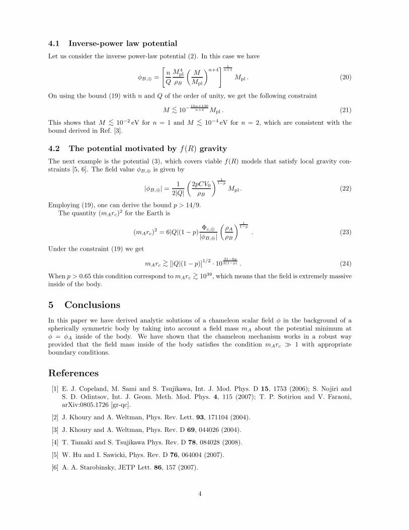
4.1 Inverse-power law potential
Let us consider the inverse power-law potential (2). In this case we have
φB,⊕ =
[
n
Q
M4pl
ρB
(
M
Mpl
)n+4]
1n+1
Mpl . (20)
On using the bound (19) with n and Q of the order of unity, we get the following constraint
M <∼ 10−15n+130
n+4 Mpl . (21)
This shows that M <∼ 10−2 eV for n = 1 and M <∼ 10−4 eV for n = 2, which are consistent with thebound derived in Ref. [3].
4.2 The potential motivated by f(R) gravity
The next example is the potential (3), which covers viable f(R) models that satisfy local gravity con-straints [5, 6]. The field value φB,⊕ is given by
|φB,⊕| =1
2|Q|(
2pCV0
ρB
)1
1−p
Mpl . (22)
Employing (19), one can derive the bound p > 14/9.The quantity (mArc)2 for the Earth is
(mArc)2 = 6|Q|(1 − p)Φc,⊕|φB,⊕|
(
ρAρB
)1
1−p
. (23)
Under the constraint (19) we get
mArc >∼ [|Q|(1 − p)]1/2 · 1031−6p2(1−p) . (24)
When p > 0.65 this condition correspond tomArc >∼ 1039, which means that the field is extremely massiveinside of the body.
5 Conclusions
In this paper we have derived analytic solutions of a chameleon scalar field φ in the background of aspherically symmetric body by taking into account a field mass mA about the potential minimum atφ = φA inside of the body. We have shown that the chameleon mechanism works in a robust wayprovided that the field mass inside of the body satisfies the condition mArc 1 with appropriateboundary conditions.
References
[1] E. J. Copeland, M. Sami and S. Tsujikawa, Int. J. Mod. Phys. D 15, 1753 (2006); S. Nojiri andS. D. Odintsov, Int. J. Geom. Meth. Mod. Phys. 4, 115 (2007); T. P. Sotiriou and V. Faraoni,arXiv:0805.1726 [gr-qc].
[2] J. Khoury and A. Weltman, Phys. Rev. Lett. 93, 171104 (2004).
[3] J. Khoury and A. Weltman, Phys. Rev. D 69, 044026 (2004).
[4] T. Tamaki and S. Tsujikawa Phys. Rev. D 78, 084028 (2008).
[5] W. Hu and I. Sawicki, Phys. Rev. D 76, 064004 (2007).
[6] A. A. Starobinsky, JETP Lett. 86, 157 (2007).
4
Squashed Kerr-Godel Black Holes
Shinya Tomizawa,1 Hideki Ishihara,2 Ken Matsuno3 and Toshiharu Nakagawa4
1Cosmophysics Group, Institute of Particle and Nuclear Studies, KEK, Tsukuba, Ibaraki, 305-0801,Japan
2,3,4Department of Mathematics and Physics, Graduate School of Science, Osaka City University,3-3-138 Sugimoto, Sumiyoshi, Osaka 558-8585, Japan
AbstractApplying squashing transformation to Kerr-Godel black hole solutions, we presenta new type of a rotating Kaluza-Klein black hole solution to the five-dimensionalEinstein-Maxwell theory with a Chern-Simonss term. The new solutions generatedvia the squashing transformation have no closed timelike curve everywhere outsidethe black hole horizons. The spacetime is asymptotically locally flat. One of theremarkable features is that the solution has two independent rotation parametersalong an extra dimension associated with the black hole’s rotation and the Godel’srotation. The space-time also admits the existence of two disconnected ergoregions,an inner ergoregion and an outer ergoregion. These two ergoregions can rotate in theopposite direction as well as in the same direction.
1 Summary
In recent years, some non-BPS black hole solutions have also been found in addition to supersymmetricblack hole solutions. Although no one has found higher-dimensional Kerr-Newman solutions in Einstein-Maxwell theory yet, Cvetic et al [1] found a non-extremal, charged and rotating black hole solution withasymptotic flatness in the five-dimensional Einstein-Maxwell theory with a Chern-Simons term. In theneutral case, the solution reduces to the same angular momenta case of the Myers-Perry black hole solu-tion [2]. Exact solutions of non-BPS Kaluza-Klein black hole solutions are found in neutral case [3, 4] andcharged case [5]. These solutions have a non-trivial asymptotic structure, i.e., the spacetime is asymp-totically locally flat and approaches a twisted S1 metric over a four-dimensional Minkowski spacetime,topologically not a direct product. The horizons are deformed due to this non-trivial asymptotic structureand have a shape of a squashed S3, where S3 is regarded as a S1 bundle over a S2 base space. The ratioof the radius S2 to that of S1 is always larger than one.
As was proposed by Wang, a kind of Kaluza-Klein black hole solutions can be generated by thesquashing transformation from black holes with asymptotic flatness [6]. In fact, he regenerated thefive-dimensional Kaluza-Klein black hole solution found by Dobiasch and Maison [3, 4] from the five-dimensional Myers-Perry black hole solution with two equal angular momentum (The solution generatedby Wang coincides with the solution in Ref.[3, 4].). In the previous work [7], applying the squashingtransformation to the Cvetic et al’s charged rotating black hole solution [1] in vanishing cosmologicalconstant case, we obtain the new Kaluza-Klein black hole solution in the five-dimensional Einstein-Maxwell theory with a Chern-Simons term. This is the generalization of the Kaluza-Klein black holesolutions in Ref. [3, 4, 5]. This solution has four parameters, the mass, the angular momentum in thedirection of an extra dimension, the electric charge and the size of the extra dimension. The solutiondescribes the physical situation such that in general a non-BPS black hole is boosted in the direction ofthe extra dimension. As the interesting feature of the solution, unlike the static solution [5], the horizonadmits a prolate shape in addition to a round S3. The solution has the limits to the supersymmetric blackhole solution and a new extreme non-BPS black hole solutions and a new rotating black hole solutionwith a constant S1 fiber.
1E-mail:[email protected]:[email protected]:[email protected]:[email protected]
1
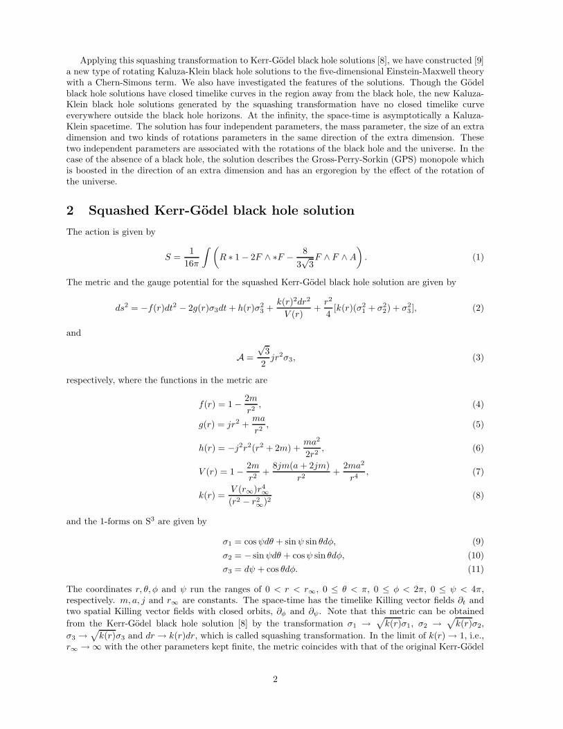
Applying this squashing transformation to Kerr-Godel black hole solutions [8], we have constructed [9]a new type of rotating Kaluza-Klein black hole solutions to the five-dimensional Einstein-Maxwell theorywith a Chern-Simons term. We also have investigated the features of the solutions. Though the Godelblack hole solutions have closed timelike curves in the region away from the black hole, the new Kaluza-Klein black hole solutions generated by the squashing transformation have no closed timelike curveeverywhere outside the black hole horizons. At the infinity, the space-time is asymptotically a Kaluza-Klein spacetime. The solution has four independent parameters, the mass parameter, the size of an extradimension and two kinds of rotations parameters in the same direction of the extra dimension. Thesetwo independent parameters are associated with the rotations of the black hole and the universe. In thecase of the absence of a black hole, the solution describes the Gross-Perry-Sorkin (GPS) monopole whichis boosted in the direction of an extra dimension and has an ergoregion by the effect of the rotation ofthe universe.
2 Squashed Kerr-Godel black hole solution
The action is given by
S =1
16π
∫(
R ∗ 1 − 2F ∧ ∗F − 83√
3F ∧ F ∧A
)
. (1)
The metric and the gauge potential for the squashed Kerr-Godel black hole solution are given by
ds2 = −f(r)dt2 − 2g(r)σ3dt+ h(r)σ23 +
k(r)2dr2
V (r)+r2
4[k(r)(σ2
1 + σ22) + σ2
3 ], (2)
and
A =√
32jr2σ3, (3)
respectively, where the functions in the metric are
f(r) = 1 − 2mr2, (4)
g(r) = jr2 +ma
r2, (5)
h(r) = −j2r2(r2 + 2m) +ma2
2r2, (6)
V (r) = 1 − 2mr2
+8jm(a+ 2jm)
r2+
2ma2
r4, (7)
k(r) =V (r∞)r4∞(r2 − r2∞)2
(8)
and the 1-forms on S3 are given by
σ1 = cosψdθ + sinψ sin θdφ, (9)σ2 = − sinψdθ + cosψ sin θdφ, (10)σ3 = dψ + cos θdφ. (11)
The coordinates r, θ, φ and ψ run the ranges of 0 < r < r∞, 0 ≤ θ < π, 0 ≤ φ < 2π, 0 ≤ ψ < 4π,respectively. m, a, j and r∞ are constants. The space-time has the timelike Killing vector fields ∂t andtwo spatial Killing vector fields with closed orbits, ∂φ and ∂ψ. Note that this metric can be obtainedfrom the Kerr-Godel black hole solution [8] by the transformation σ1 → √
k(r)σ1, σ2 → √
k(r)σ2,σ3 → √
k(r)σ3 and dr → k(r)dr, which is called squashing transformation. In the limit of k(r) → 1, i.e.,r∞ → ∞ with the other parameters kept finite, the metric coincides with that of the original Kerr-Godel
2
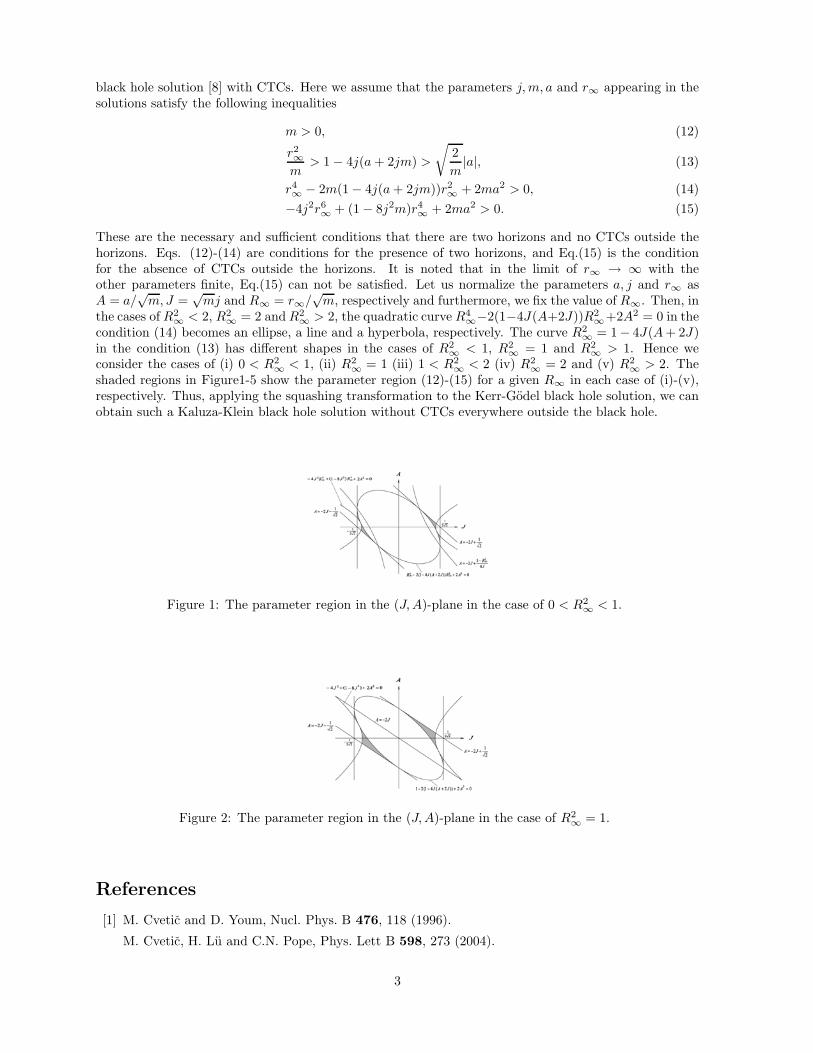
black hole solution [8] with CTCs. Here we assume that the parameters j,m, a and r∞ appearing in thesolutions satisfy the following inequalities
m > 0, (12)
r2∞m
> 1 − 4j(a+ 2jm) >
√
2m|a|, (13)
r4∞ − 2m(1 − 4j(a+ 2jm))r2∞ + 2ma2 > 0, (14)−4j2r6∞ + (1 − 8j2m)r4∞ + 2ma2 > 0. (15)
These are the necessary and sufficient conditions that there are two horizons and no CTCs outside thehorizons. Eqs. (12)-(14) are conditions for the presence of two horizons, and Eq.(15) is the conditionfor the absence of CTCs outside the horizons. It is noted that in the limit of r∞ → ∞ with theother parameters finite, Eq.(15) can not be satisfied. Let us normalize the parameters a, j and r∞ asA = a/
√m,J =
√mj and R∞ = r∞/
√m, respectively and furthermore, we fix the value of R∞. Then, in
the cases of R2∞ < 2, R2∞ = 2 andR2∞ > 2, the quadratic curve R4∞−2(1−4J(A+2J))R2∞+2A2 = 0 in thecondition (14) becomes an ellipse, a line and a hyperbola, respectively. The curve R2∞ = 1− 4J(A+ 2J)in the condition (13) has different shapes in the cases of R2∞ < 1, R2∞ = 1 and R2∞ > 1. Hence weconsider the cases of (i) 0 < R2
∞ < 1, (ii) R2∞ = 1 (iii) 1 < R2
∞ < 2 (iv) R2∞ = 2 and (v) R2
∞ > 2. Theshaded regions in Figure1-5 show the parameter region (12)-(15) for a given R∞ in each case of (i)-(v),respectively. Thus, applying the squashing transformation to the Kerr-Godel black hole solution, we canobtain such a Kaluza-Klein black hole solution without CTCs everywhere outside the black hole.
Figure 1: The parameter region in the (J, A)-plane in the case of 0 < R2∞ < 1.
Figure 2: The parameter region in the (J, A)-plane in the case of R2∞ = 1.
References
[1] M. Cvetic and D. Youm, Nucl. Phys. B 476, 118 (1996).
M. Cvetic, H. Lu and C.N. Pope, Phys. Lett B 598, 273 (2004).
3
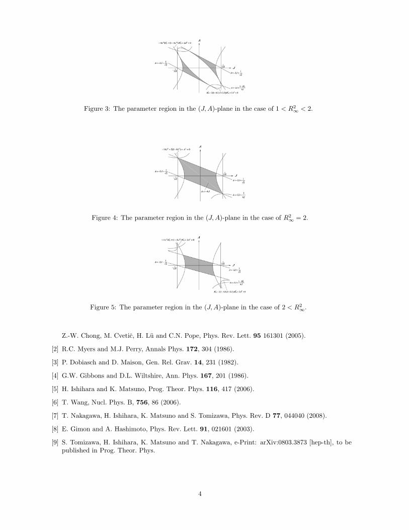
Figure 3: The parameter region in the (J, A)-plane in the case of 1 < R2∞ < 2.
Figure 4: The parameter region in the (J, A)-plane in the case of R2∞ = 2.
Figure 5: The parameter region in the (J, A)-plane in the case of 2 < R2∞.
Z.-W. Chong, M. Cvetic, H. Lu and C.N. Pope, Phys. Rev. Lett. 95 161301 (2005).
[2] R.C. Myers and M.J. Perry, Annals Phys. 172, 304 (1986).
[3] P. Dobiasch and D. Maison, Gen. Rel. Grav. 14, 231 (1982).
[4] G.W. Gibbons and D.L. Wiltshire, Ann. Phys. 167, 201 (1986).
[5] H. Ishihara and K. Matsuno, Prog. Theor. Phys. 116, 417 (2006).
[6] T. Wang, Nucl. Phys. B, 756, 86 (2006).
[7] T. Nakagawa, H. Ishihara, K. Matsuno and S. Tomizawa, Phys. Rev. D 77, 044040 (2008).
[8] E. Gimon and A. Hashimoto, Phys. Rev. Lett. 91, 021601 (2003).
[9] S. Tomizawa, H. Ishihara, K. Matsuno and T. Nakagawa, e-Print: arXiv:0803.3873 [hep-th], to bepublished in Prog. Theor. Phys.
4
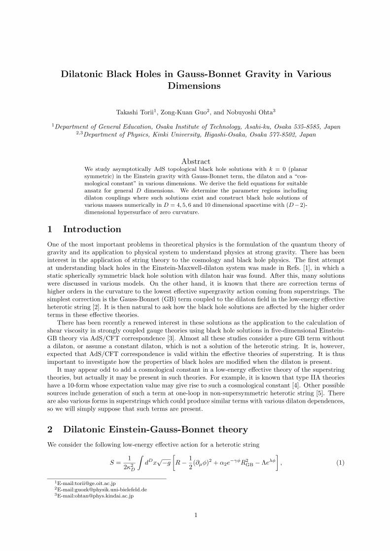
Dilatonic Black Holes in Gauss-Bonnet Gravity in VariousDimensions
Takashi Torii1, Zong-Kuan Guo2, and Nobuyoshi Ohta3
1Department of General Education, Osaka Institute of Technology, Asahi-ku, Osaka 535-8585, Japan2,3Department of Physics, Kinki University, Higashi-Osaka, Osaka 577-8502, Japan
AbstractWe study asymptotically AdS topological black hole solutions with k = 0 (planarsymmetric) in the Einstein gravity with Gauss-Bonnet term, the dilaton and a “cos-mological constant” in various dimensions. We derive the field equations for suitableansatz for general D dimensions. We determine the parameter regions includingdilaton couplings where such solutions exist and construct black hole solutions ofvarious masses numerically in D = 4, 5, 6 and 10 dimensional spacetime with (D−2)-dimensional hypersurface of zero curvature.
1 Introduction
One of the most important problems in theoretical physics is the formulation of the quantum theory ofgravity and its application to physical system to understand physics at strong gravity. There has beeninterest in the application of string theory to the cosmology and black hole physics. The first attemptat understanding black holes in the Einstein-Maxwell-dilaton system was made in Refs. [1], in which astatic spherically symmetric black hole solution with dilaton hair was found. After this, many solutionswere discussed in various models. On the other hand, it is known that there are correction terms ofhigher orders in the curvature to the lowest effective supergravity action coming from superstrings. Thesimplest correction is the Gauss-Bonnet (GB) term coupled to the dilaton field in the low-energy effectiveheterotic string [2]. It is then natural to ask how the black hole solutions are affected by the higher orderterms in these effective theories.
There has been recently a renewed interest in these solutions as the application to the calculation ofshear viscosity in strongly coupled gauge theories using black hole solutions in five-dimensional Einstein-GB theory via AdS/CFT correspondence [3]. Almost all these studies consider a pure GB term withouta dilaton, or assume a constant dilaton, which is not a solution of the heterotic string. It is, however,expected that AdS/CFT correspondence is valid within the effective theories of superstring. It is thusimportant to investigate how the properties of black holes are modified when the dilaton is present.
It may appear odd to add a cosmological constant in a low-energy effective theory of the superstringtheories, but actually it may be present in such theories. For example, it is known that type IIA theorieshave a 10-form whose expectation value may give rise to such a cosmological constant [4]. Other possiblesources include generation of such a term at one-loop in non-supersymmetric heterotic string [5]. Thereare also various forms in superstrings which could produce similar terms with various dilaton dependences,so we will simply suppose that such terms are present.
2 Dilatonic Einstein-Gauss-Bonnet theory
We consider the following low-energy effective action for a heterotic string
S =1
2κ2D
∫dDx
√−g
[R− 1
2(∂µφ)2 + α2e
−γφR2GB − Λeλφ
], (1)
1E-mail:[email protected]:[email protected]:[email protected]
1
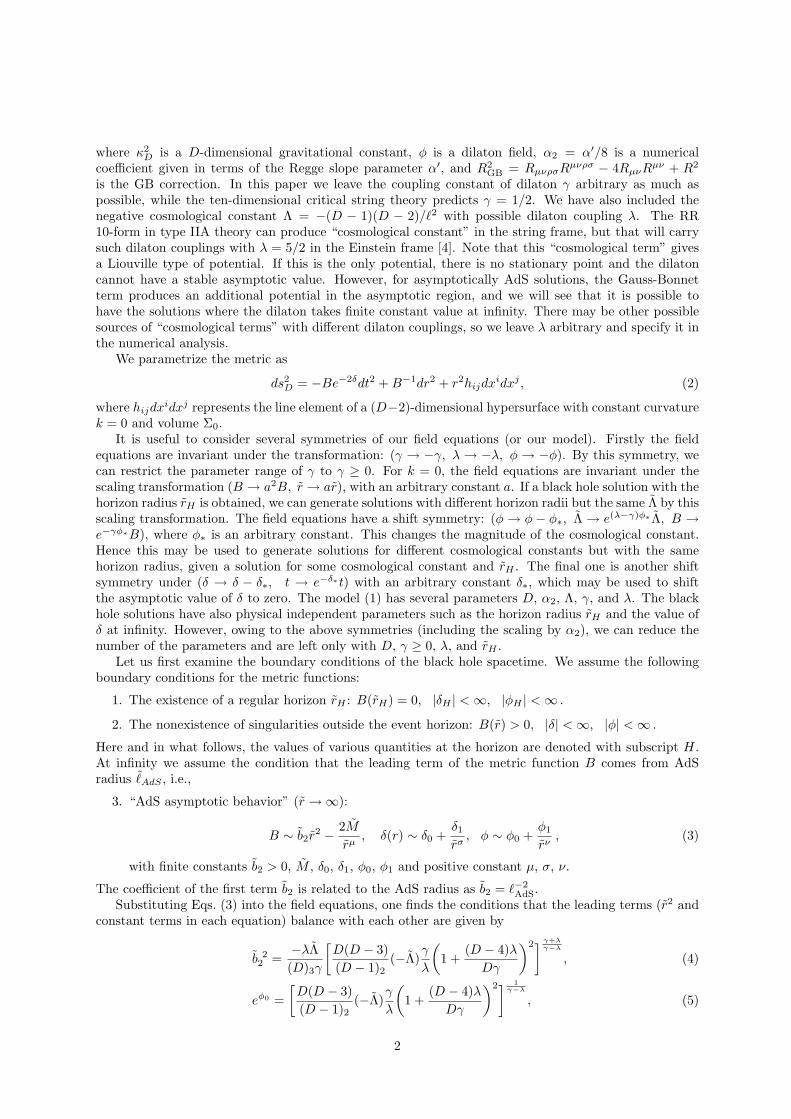
where κ2D is a D-dimensional gravitational constant, φ is a dilaton field, α2 = α′/8 is a numerical
coefficient given in terms of the Regge slope parameter α′, and R2GB = RµνρσRµνρσ − 4RµνRµν + R2
is the GB correction. In this paper we leave the coupling constant of dilaton γ arbitrary as much aspossible, while the ten-dimensional critical string theory predicts γ = 1/2. We have also included thenegative cosmological constant Λ = −(D − 1)(D − 2)/`2 with possible dilaton coupling λ. The RR10-form in type IIA theory can produce “cosmological constant” in the string frame, but that will carrysuch dilaton couplings with λ = 5/2 in the Einstein frame [4]. Note that this “cosmological term” givesa Liouville type of potential. If this is the only potential, there is no stationary point and the dilatoncannot have a stable asymptotic value. However, for asymptotically AdS solutions, the Gauss-Bonnetterm produces an additional potential in the asymptotic region, and we will see that it is possible tohave the solutions where the dilaton takes finite constant value at infinity. There may be other possiblesources of “cosmological terms” with different dilaton couplings, so we leave λ arbitrary and specify it inthe numerical analysis.
We parametrize the metric as
ds2D = −Be−2δdt2 + B−1dr2 + r2hijdxidxj , (2)
where hijdxidxj represents the line element of a (D−2)-dimensional hypersurface with constant curvaturek = 0 and volume Σ0.
It is useful to consider several symmetries of our field equations (or our model). Firstly the fieldequations are invariant under the transformation: (γ → −γ, λ → −λ, φ → −φ). By this symmetry, wecan restrict the parameter range of γ to γ ≥ 0. For k = 0, the field equations are invariant under thescaling transformation (B → a2B, r → ar), with an arbitrary constant a. If a black hole solution with thehorizon radius rH is obtained, we can generate solutions with different horizon radii but the same Λ by thisscaling transformation. The field equations have a shift symmetry: (φ → φ− φ∗, Λ → e(λ−γ)φ∗Λ, B →e−γφ∗B), where φ∗ is an arbitrary constant. This changes the magnitude of the cosmological constant.Hence this may be used to generate solutions for different cosmological constants but with the samehorizon radius, given a solution for some cosmological constant and rH . The final one is another shiftsymmetry under (δ → δ − δ∗, t → e−δ∗t) with an arbitrary constant δ∗, which may be used to shiftthe asymptotic value of δ to zero. The model (1) has several parameters D, α2, Λ, γ, and λ. The blackhole solutions have also physical independent parameters such as the horizon radius rH and the value ofδ at infinity. However, owing to the above symmetries (including the scaling by α2), we can reduce thenumber of the parameters and are left only with D, γ ≥ 0, λ, and rH .
Let us first examine the boundary conditions of the black hole spacetime. We assume the followingboundary conditions for the metric functions:
1. The existence of a regular horizon rH : B(rH) = 0, |δH | < ∞, |φH | < ∞ .
2. The nonexistence of singularities outside the event horizon: B(r) > 0, |δ| < ∞, |φ| < ∞ .
Here and in what follows, the values of various quantities at the horizon are denoted with subscript H.At infinity we assume the condition that the leading term of the metric function B comes from AdSradius ˜
AdS , i.e.,
3. “AdS asymptotic behavior” (r →∞):
B ∼ b2r2 − 2M
rµ, δ(r) ∼ δ0 +
δ1
rσ, φ ∼ φ0 +
φ1
rν, (3)
with finite constants b2 > 0, M , δ0, δ1, φ0, φ1 and positive constant µ, σ, ν.
The coefficient of the first term b2 is related to the AdS radius as b2 = `−2AdS.
Substituting Eqs. (3) into the field equations, one finds the conditions that the leading terms (r2 andconstant terms in each equation) balance with each other are given by
b 22 =
−λΛ(D)3γ
[D(D − 3)(D − 1)2
(−Λ)γ
λ
(1 +
(D − 4)λDγ
)2] γ+λγ−λ
, (4)
eφ0 =[D(D − 3)(D − 1)2
(−Λ)γ
λ
(1 +
(D − 4)λDγ
)2] 1γ−λ
, (5)
2
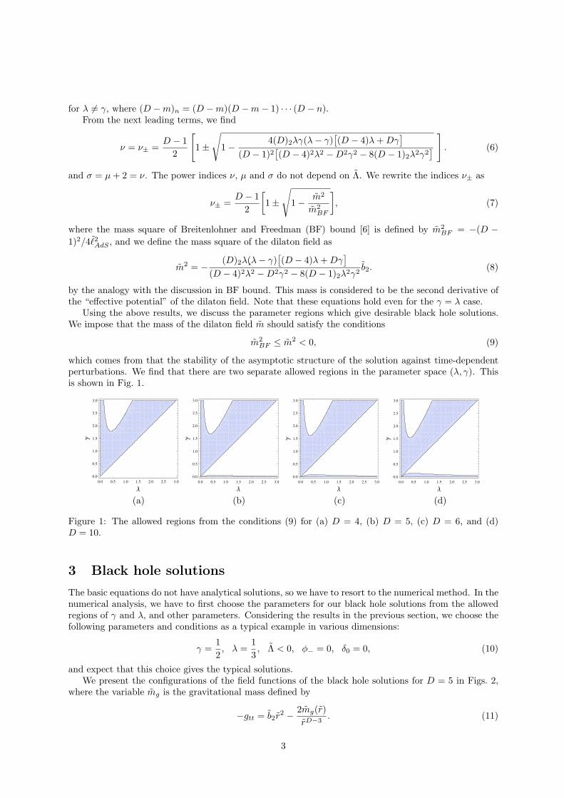
for λ 6= γ, where (D −m)n = (D −m)(D −m− 1) · · · (D − n).From the next leading terms, we find
ν = ν± =D − 1
2
[1±
√1− 4(D)2λγ(λ− γ)
[(D − 4)λ + Dγ
]
(D − 1)2[(D − 4)2λ2 −D2γ2 − 8(D − 1)2λ2γ2
]]
. (6)
and σ = µ + 2 = ν. The power indices ν, µ and σ do not depend on Λ. We rewrite the indices ν± as
ν± =D − 1
2
[1±
√1− m2
m2BF
], (7)
where the mass square of Breitenlohner and Freedman (BF) bound [6] is defined by m2BF = −(D −
1)2/4˜2AdS , and we define the mass square of the dilaton field as
m2 = − (D)2λ(λ− γ)[(D − 4)λ + Dγ
]
(D − 4)2λ2 −D2γ2 − 8(D − 1)2λ2γ2b2. (8)
by the analogy with the discussion in BF bound. This mass is considered to be the second derivative ofthe “effective potential” of the dilaton field. Note that these equations hold even for the γ = λ case.
Using the above results, we discuss the parameter regions which give desirable black hole solutions.We impose that the mass of the dilaton field m should satisfy the conditions
m2BF ≤ m2 < 0, (9)
which comes from that the stability of the asymptotic structure of the solution against time-dependentperturbations. We find that there are two separate allowed regions in the parameter space (λ, γ). Thisis shown in Fig. 1.
0.0 0.5 1.0 1.5 2.0 2.5 3.00.0
0.5
1.0
1.5
2.0
2.5
3.0
Λ
Γ
0.0 0.5 1.0 1.5 2.0 2.5 3.00.0
0.5
1.0
1.5
2.0
2.5
3.0
Λ
Γ
0.0 0.5 1.0 1.5 2.0 2.5 3.00.0
0.5
1.0
1.5
2.0
2.5
3.0
Λ
Γ
0.0 0.5 1.0 1.5 2.0 2.5 3.00.0
0.5
1.0
1.5
2.0
2.5
3.0
Λ
Γ
(a) (b) (c) (d)
Figure 1: The allowed regions from the conditions (9) for (a) D = 4, (b) D = 5, (c) D = 6, and (d)D = 10.
3 Black hole solutions
The basic equations do not have analytical solutions, so we have to resort to the numerical method. In thenumerical analysis, we have to first choose the parameters for our black hole solutions from the allowedregions of γ and λ, and other parameters. Considering the results in the previous section, we choose thefollowing parameters and conditions as a typical example in various dimensions:
γ =12, λ =
13, Λ < 0, φ− = 0, δ0 = 0, (10)
and expect that this choice gives the typical solutions.We present the configurations of the field functions of the black hole solutions for D = 5 in Figs. 2,
where the variable mg is the gravitational mass defined by
−gtt = b2r2 − 2mg(r)
rD−3. (11)
3
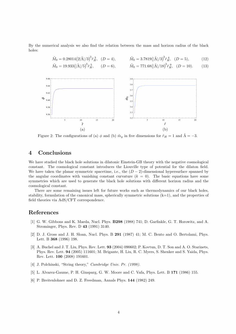
By the numerical analysis we also find the relation between the mass and horizon radius of the blackholes:
M0 = 0.28014(2|Λ|/3
)3r 3H , (D = 4), M0 = 3.7819
(|Λ|/3)3
r 4H , (D = 5), (12)
M0 = 19.933(|Λ|/5
)3r 5H , (D = 6), M0 = 771.68
(|Λ|/18)3
r 9H , (D = 10). (13)
5 10 15 20
9.36
9.38
9.40
9.42
9.44
9.46
r
Φ
5 10 15 203.2
3.3
3.4
3.5
3.6
3.7
3.8
3.9
(a) (b)
Figure 2: The configurations of (a) φ and (b) mg in five dimensions for rH = 1 and Λ = −3.
4 Conclusions
We have studied the black hole solutions in dilatonic Einstein-GB theory with the negative cosmologicalconstant. The cosmological constant introduces the Liouville type of potential for the dilaton field.We have taken the planar symmetric spacetime, i.e., the (D − 2)-dimensional hypersurface spanned bythe angular coordinates with vanishing constant curvature (k = 0). The basic equations have somesymmetries which are used to generate the black hole solutions with different horizon radius and thecosmological constant.
There are some remaining issues left for future works such as thermodynamics of our black holes,stability, formulation of the canonical mass, spherically symmetric solutions (k=1), and the properties offield theories via AdS/CFT correspondence.
References
[1] G. W. Gibbons and K. Maeda, Nucl. Phys. B298 (1988) 741; D. Garfinkle, G. T. Horowitz, and A.Strominger, Phys. Rev. D 43 (1991) 3140.
[2] D. J. Gross and J. H. Sloan, Nucl. Phys. B 291 (1987) 41; M. C. Bento and O. Bertolami, Phys.Lett. B 368 (1996) 198.
[3] A. Buchel and J. T. Liu, Phys. Rev. Lett. 93 (2004) 090602; P. Kovtun, D. T. Son and A. O. Starinets,Phys. Rev. Lett. 94 (2005) 111601; M. Brigante, H. Liu, R. C. Myers, S. Shenker and S. Yaida, Phys.Rev. Lett. 100 (2008) 191601.
[4] J. Polchinski, “String theory,” Cambridge Univ. Pr. (1998).
[5] L. Alvarez-Gaume, P. H. Ginsparg, G. W. Moore and C. Vafa, Phys. Lett. B 171 (1986) 155.
[6] P. Breitenlohner and D. Z. Freedman, Annals Phys. 144 (1982) 249.
4
Apparent Horizon Formation in Five-dimensional Spacetime
Yuta Yamada1 and Hisa-aki Shinkai2
Dept. of Information Science and Technology,Osaka Institute of Technology, Hirakata, Osaka 573-0196
AbstractWe numerically investigated the formation of an apparent horizon in ve-dimensionalspacetime in the context of the cosmic censorship hypothesis. We modeled the matterby distributing collisionless particles both in spheroidal and toroidal congurationsunder the momentarily static assumption, and obtained the sequence of initial data bysolving the Hamiltonian constraint equation. We found both S3 and S2S1 horizons,only when the matter conguration is not steep. By monitoring the location of themaximum Kretchmann invariant, we guess an appearance of ‘naked singularity’ or‘naked ring’ under the special situations.
1 Introduction
In general relativity, there are two famous conjectures concerning the gravitational collapse. One is thecosmic censorship hypothesis which states collapse driven singularities will always be clothed by eventhorizon and hence can never be visible from the outside. The other is the hoop conjecture [1] whichstates that black holes will form when and only when a mass M gets compacted into a region whosecircumference in every direction is C ≤ 4M . These two conjectures have been extensively searched invarious methods, among them we believe the numerical works by Shapiro and Teukolsky [2] showed themost exciting results; (a tendency of) the appearance of a naked singularity. This was reported from thefully relativistic time evolution of collisionless particles in a highly prolate initial shape; and the resultsof time evolutions are agree with those of the sequence of their initial data [3].
In recent years, on the other hand, gravitation in higher-dimensional spacetime is much getting a lot ofattention. This is from an attempt to unify fundamental forces including gravity at TeV scale, and if so,it is suggested that small black-holes might be produced at the CERN Large Hadron Collider (LHC). Thefour-dimensional black-holes are known to be S1 from the topological theorem, while in higher-dimensionalspacetime quite rich structures are available including a torus black-hole (“black ring”).
We, therefore, plan to reproduce the earlier numerical works in higher-dimensional spacetime, andthis report shows our rst trials to obtain the sequence of the initial data. As for the hoop conjecture,the modied version called hyper-hoop was proposed by Ida and Nakao [4] for the higher-dimensionalspacetime, which was consistent with semi-analytic works [5]. We used the results of [5] as our codechecks, and developed the code as we can investigate in more general situations.
2 Basic Equations
2.1 The Hamiltonian constraint equation
We consider the initial data sequence on a four-dimensional space-like hypersurface. A solution of theEinstein equations is obtained by solving the Hamiltonian constraint equation if we assume the momentof time symmetry. Applying a conformal transformation,
ij = 2 ij , (1)
from conformally- at base metric ij , the Hamiltonian constraint equation becomes
= −42G5, (2)1E-mail:[email protected]:[email protected]
1
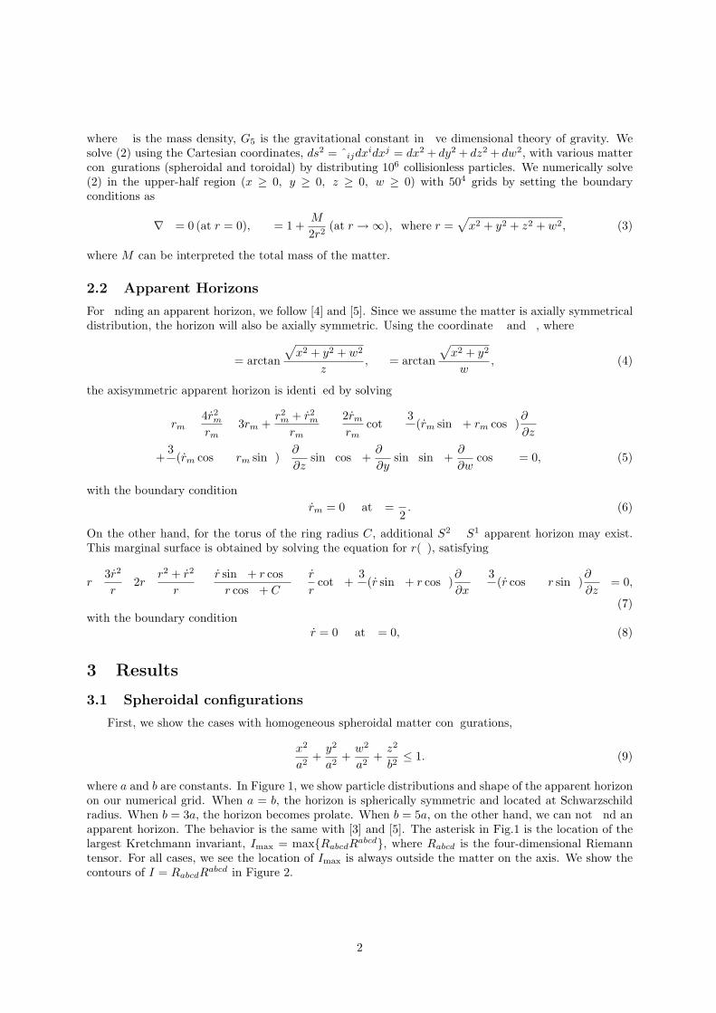
where is the mass density, G5 is the gravitational constant in ve dimensional theory of gravity. Wesolve (2) using the Cartesian coordinates, ds2 = ijdx
idxj = dx2 + dy2 + dz2 + dw2, with various mattercongurations (spheroidal and toroidal) by distributing 106 collisionless particles. We numerically solve(2) in the upper-half region (x ≥ 0, y ≥ 0, z ≥ 0, w ≥ 0) with 504 grids by setting the boundaryconditions as
∇ = 0 (at r = 0), = 1 +M
2r2(at r → ∞), where r =
√x2 + y2 + z2 + w2, (3)
where M can be interpreted the total mass of the matter.
2.2 Apparent Horizons
For nding an apparent horizon, we follow [4] and [5]. Since we assume the matter is axially symmetricaldistribution, the horizon will also be axially symmetric. Using the coordinate and , where
= arctan
√x2 + y2 + w2
z, = arctan
√x2 + y2
w, (4)
the axisymmetric apparent horizon is identied by solving
rm − 4r2mrm
− 3rm +r2m + r2mrm
×[2rmrm
cot − 3
(rm sin + rm cos )∂
∂z
+3
(rm cos − rm sin )(∂
∂zsin cos +
∂
∂ysin sin +
∂
∂wcos
)]= 0, (5)
with the boundary conditionrm = 0 at =
2. (6)
On the other hand, for the torus of the ring radius C, additional S2 × S1 apparent horizon may exist.This marginal surface is obtained by solving the equation for r(), satisfying
r− 3r2
r−2r− r2 + r2
r×
[r sin + r cos r cos + C
− r
rcot +
3
(r sin + r cos )∂
∂x− 3
(r cos − r sin )∂
∂z
]= 0,
(7)with the boundary condition
r = 0 at = 0, (8)
3 Results
3.1 Spheroidal configurations
First, we show the cases with homogeneous spheroidal matter congurations,
x2
a2+y2
a2+w2
a2+z2
b2≤ 1. (9)
where a and b are constants. In Figure 1, we show particle distributions and shape of the apparent horizonon our numerical grid. When a = b, the horizon is spherically symmetric and located at Schwarzschildradius. When b = 3a, the horizon becomes prolate. When b = 5a, on the other hand, we can not nd anapparent horizon. The behavior is the same with [3] and [5]. The asterisk in Fig.1 is the location of thelargest Kretchmann invariant, Imax = maxRabcdR
abcd, where Rabcd is the four-dimensional Riemanntensor. For all cases, we see the location of Imax is always outside the matter on the axis. We show thecontours of I = RabcdR
abcd in Figure 2.
2
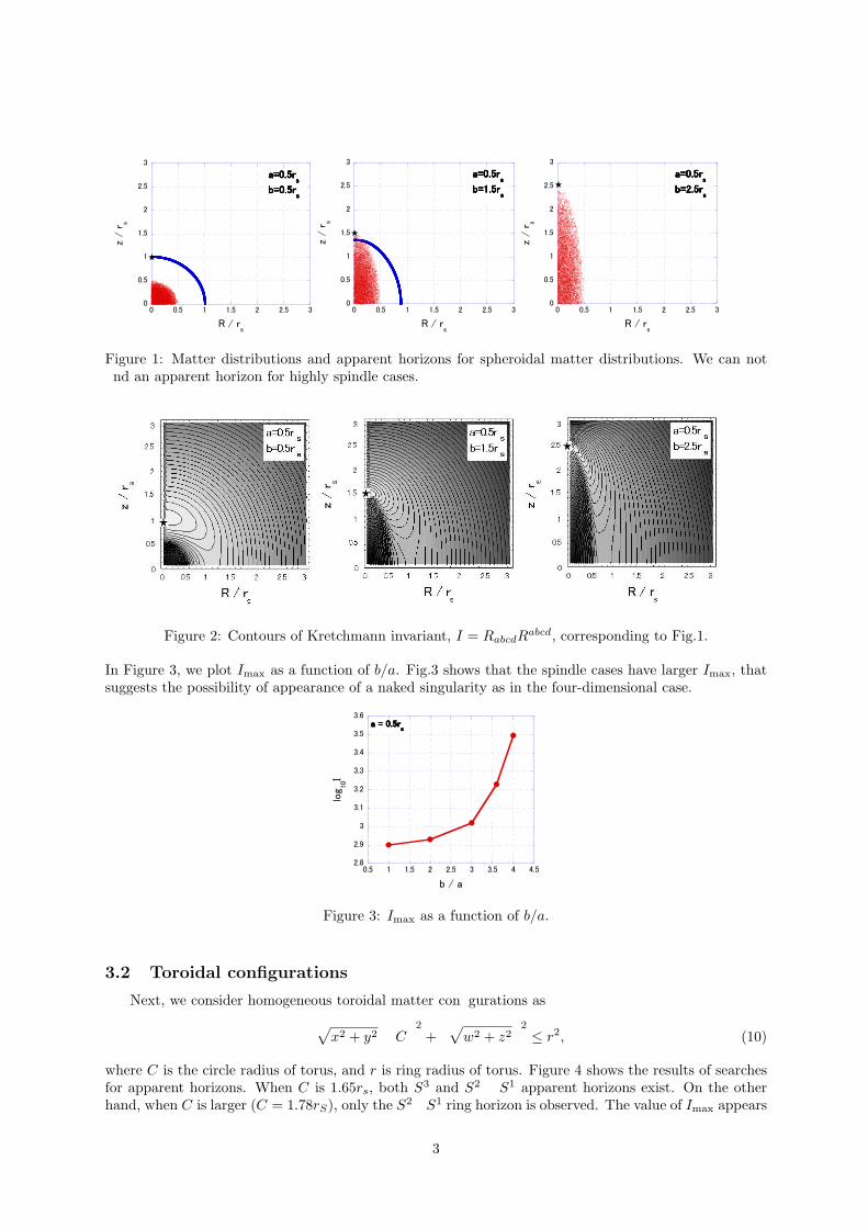
Figure 1: Matter distributions and apparent horizons for spheroidal matter distributions. We can notnd an apparent horizon for highly spindle cases.
Figure 2: Contours of Kretchmann invariant, I = RabcdRabcd, corresponding to Fig.1.
In Figure 3, we plot Imax as a function of b/a. Fig.3 shows that the spindle cases have larger Imax, thatsuggests the possibility of appearance of a naked singularity as in the four-dimensional case.
Figure 3: Imax as a function of b/a.
3.2 Toroidal configurations
Next, we consider homogeneous toroidal matter congurations as(√x2 + y2 − C
)2
+(√
w2 + z2)2
≤ r2, (10)
where C is the circle radius of torus, and r is ring radius of torus. Figure 4 shows the results of searchesfor apparent horizons. When C is 1.65rs, both S3 and S2 × S1 apparent horizons exist. On the otherhand, when C is larger (C = 1.78rS), only the S2×S1 ring horizon is observed. The value of Imax appears
3
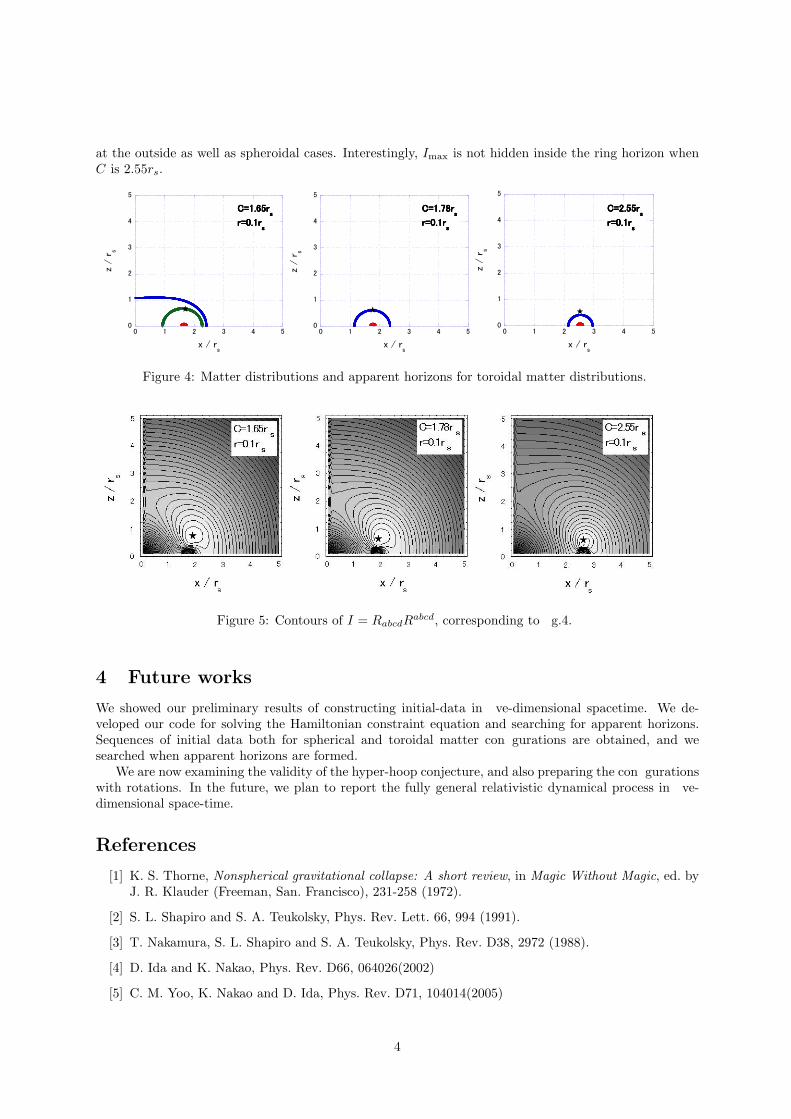
at the outside as well as spheroidal cases. Interestingly, Imax is not hidden inside the ring horizon whenC is 2.55rs.
Figure 4: Matter distributions and apparent horizons for toroidal matter distributions.
Figure 5: Contours of I = RabcdRabcd, corresponding to g.4.
4 Future works
We showed our preliminary results of constructing initial-data in ve-dimensional spacetime. We de-veloped our code for solving the Hamiltonian constraint equation and searching for apparent horizons.Sequences of initial data both for spherical and toroidal matter congurations are obtained, and wesearched when apparent horizons are formed.
We are now examining the validity of the hyper-hoop conjecture, and also preparing the congurationswith rotations. In the future, we plan to report the fully general relativistic dynamical process in ve-dimensional space-time.
References
[1] K. S. Thorne, Nonspherical gravitational collapse: A short review, in Magic Without Magic, ed. byJ. R. Klauder (Freeman, San. Francisco), 231-258 (1972).
[2] S. L. Shapiro and S. A. Teukolsky, Phys. Rev. Lett. 66, 994 (1991).
[3] T. Nakamura, S. L. Shapiro and S. A. Teukolsky, Phys. Rev. D38, 2972 (1988).
[4] D. Ida and K. Nakao, Phys. Rev. D66, 064026(2002)
[5] C. M. Yoo, K. Nakao and D. Ida, Phys. Rev. D71, 104014(2005)
4