Decentralized Harmonic Active Vibration Control of a Flexible

Plate using Piezoelectric Actuator - Sensor Pairs.

Matthieu Baudry, Philippe Micheau and Alain Berry

G.A.U.S, Mechanical Engineering Department

Universite de Sherbrooke, Sherbrooke, Quebec, Canada J1K 2R1

Number of pages : 36

Number of figures : 10

Running title : Decentralized Control of Flexible Plate

Received :

August 19, 2005

Abstract

We have investigated decentralized active control of periodic panel vibration using multiple

pairs combining PZT actuators and PVDF sensors distributed on the panel. By contrast with

centralized MIMO controllers used to actively control the vibrations or the sound radiation

of extended structures, decentralized control using independent local control loops does only

require identification of the diagonal terms in the plant matrix. However, it is difficult to a priori

predict the global stability of such decentralized control. In this study, the general situation of

non-collocated actuator-sensor pairs was considered. Frequency domain gradient and Newton-

Raphson adaptation of decentralized control were analyzed, both in terms of performance and

stability conditions. The stability conditions are especially derived in terms of the adaptation

coefficient and a control effort weighting coefficient. Simulations and experimental results are

presented in the case of a simply-supported panel with 4 PZT-PVDF pairs distributed on it.

Decentralized vibration control is shown to be highly dependent of the frequency, but can be as

effective as a fully centralized control even when the plant matrix is not diagonal-dominant or

is not strictly positive real (not dissipative).

Keywords : active control, vibration, decentralized control, piezoelectric materials, complex

envelope, closed-loop stability, dissipative systems

M. Baudry, P. Micheau and A. Berry Decentralized Control of Flexible Plate 3

1 Introduction

Active control is an efficient tool for attenuating low frequency vibrations in structures whose

vibration response or sound radiation needs to be globally reduced. This technique has been

applied to control lumped and distributed parameter structures [9]. Usually, the vibration

response is sensed at a number of locations on the structure and modified by a number of local

actuators using a centralized controller. The sensors and the actuators must be located in order

to have sufficient authority to respectively, sense and control structural vibrations. In simple

situations, such as the active damping of a limited number of weakly damped structural modes,

this approach is very effective. However, its application to more complicated situations involving

forced response of a large number of structural modes, is more challenging: in such a case, a

centralized control strategy involves modelling a large number of secondary transfer functions,

requires cumbersome wiring and is prone to instability due to plant uncertainty or individual

actuator or sensor failure.

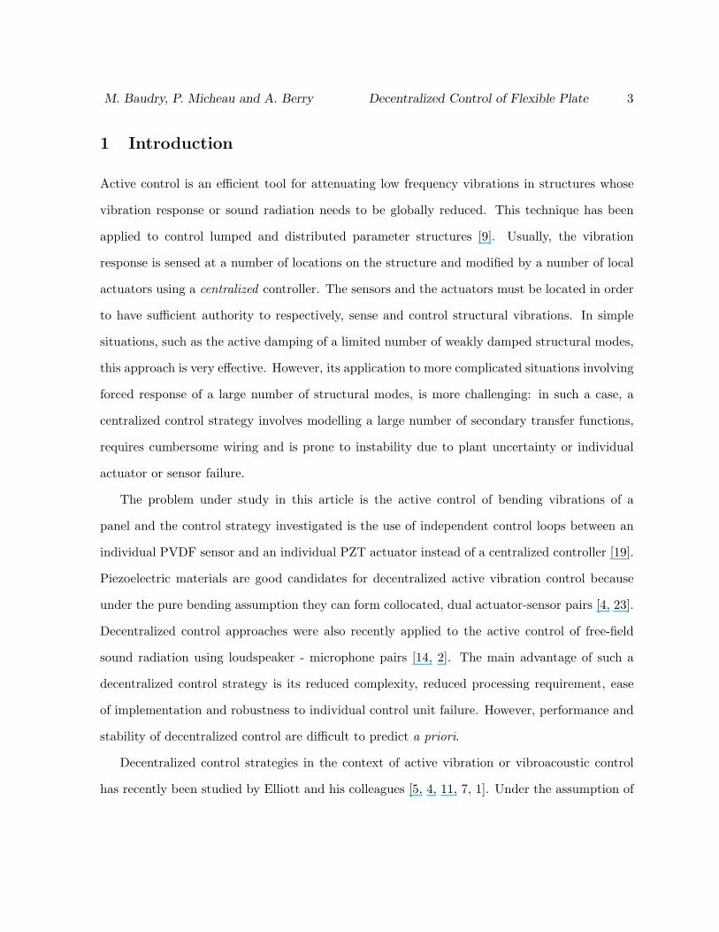
The problem under study in this article is the active control of bending vibrations of a

panel and the control strategy investigated is the use of independent control loops between an

individual PVDF sensor and an individual PZT actuator instead of a centralized controller [19].

Piezoelectric materials are good candidates for decentralized active vibration control because

under the pure bending assumption they can form collocated, dual actuator-sensor pairs [4, 23].

Decentralized control approaches were also recently applied to the active control of free-field

sound radiation using loudspeaker - microphone pairs [14, 2]. The main advantage of such a

decentralized control strategy is its reduced complexity, reduced processing requirement, ease

of implementation and robustness to individual control unit failure. However, performance and

stability of decentralized control are difficult to predict a priori.

Decentralized control strategies in the context of active vibration or vibroacoustic control

has recently been studied by Elliott and his colleagues [5, 4, 11, 7, 1]. Under the assumption of

M. Baudry, P. Micheau and A. Berry Decentralized Control of Flexible Plate 4

collocated and dual actuator-sensor pairs, decentralized control has the very attractive property

that each local feedback loop (with the other feedback loops being active) is stable regardless

of the local feedback gains applied [4], leading to a globally stable and robust implementation.

When applied to globally reducing the vibration response of - or sound transmission through

panels, decentralized control leads to control performance very similar to a fully centralized

control structure [11, 10, 7, 1]. However, piezoelectric strain actuators (PZT) and strain

sensors (PVDF) cannot, strictly speaking, be collocated and dual because of coupling through

extensional excitation [6]. Hence, the main objective of this article is to analyze performance

and stability of decentralized vibration control using the general situation of non-collocated

actuator-sensor PZT-PVDF pairs.

The specific situation investigated here is the active control of a reverberant system (a

weakly damped bending plate) under a periodic excitation. For such disturbance, the feedback

controller and the x-LMS MIMO feedforward controller can both be seen as an equivalent

resonant controller [21]. The similarity between feedback and feedforward comes from the

fact that the equivalent compensator has 1 undamped mode at the disturbance frequency to

provide the high loop gain necessary for the rejection of the disturbance frequency. Hence,

without loss of generality, the control problem can be addressed with an harmonic controller

which adjusts complex gains (amplitude and the phase of the sinusoidal control inputs with

respect to the amplitude and phase of the sensor signals). The feedback law, can be tuned with

two parameters: the adaptation coefficient which specifies the convergence rate, and the control

effort weighting which limits the amplitude of the control input. Decentralized control is the

special case where the gain matrix is diagonal, in contrast with a fully centralized control where

the gain matrix is fully populated.

The problem of decentralized controller is to ensure the stability of the whole system [18].

Decentralized control was studied in the context of large structures, and it was established that

a solution to the decentralized problem exists if and only if a solution exists to the centralized

M. Baudry, P. Micheau and A. Berry Decentralized Control of Flexible Plate 5

problem [24]. For x-lms feedforward, the Gershgorin theorem is useful to derive a sufficient

condition of stabilization [5]: the diagonal dominance of the matrix gain. The same condition

can be derived from the Small Gain theorem for feedback controllers. However, this diagonal

dominance condition proves to be too conservative to be applied in practice. More adequate

necessary and sufficient stability conditions were derived in the active free-field sound control

problem [14]. The objective of this article is to extend this previous analysis by providing a

set of simple analytical tools to a priori predict closed loop stability of active vibration control

using piezoelectric actuators and sensors.

Section 2 introduces the problem, and section 3 details the plant modelling. The controller

synthesis in term of minimization of a quadratic criterion is presented in section 4, together with

the conditions of stability related to the requirement of a positive definite plant matrix at the

disturbance frequency. Section 5 presents the implementation of the harmonic controller using

a complex envelope controller [16]. Finally, experimental results presented in section 6 illustrate

the effectiveness of the proposed analytical tools.

2 The Problem

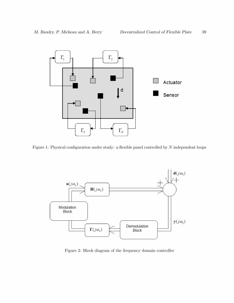
The physical system under study is a flexible panel under forced harmonic oscillation, whose

vibration response or sound radiation needs to be globally reduced. To this end, the vibration

response is sensed at a number of locations on the structure, and modified by a number of local

actuators on it (figure 1). The control strategy investigated here is the use of N independent

control loops Γi between an individual sensor and an individual actuator instead of a N × N

centralized controller. The controller is implemented in the frequency domain. A general

block-diagram form of the controller is shown on figure 2 (ω0 is the angular frequency of the

disturbance, d is the disturbance vector measured by the N sensors, y is the error signal at

the sensors, u is the control inputs at the N actuators, and H is the N × N transfer function

M. Baudry, P. Micheau and A. Berry Decentralized Control of Flexible Plate 6

matrix between actuators and sensors). In order to reject the frequency ω0, the controller Γ

restricts to a matrix of complex gains at ω0. In the general case of a central controller, the

control matrix has off-diagonal components Γij . In the case of decentralized control, the control

matrix is diagonal, Γ = diag(Γii). In the following, the controller Γ is iteratively adapted in

order to minimize a given error criterion. Since it is assumed that the disturbance has a fixed

frequency and that the error is slowly varying in time (slow convergence), the time variations of

the error phasor are slow, and it is therefore possible to implement the controller adaptation at

a much slower rate than the disturbance frequency. The demodulation and modulation blocks

shown on figure 2 are used to respectively extract the phasor of the error y, and synthesize the

oscillatory control input u at the disturbance frequency. Since the error and control phasors

have slow time variations (compared to the disturbance period), the adaptation of the controller

Γ can be done at a much slower rate than the disturbance frequency. The demodulation and

modulation blocks are described in more details in section 5.

3 Plant Modelling

3.1 A model of the transfer functions between PZT actuators and PVDF

sensors

We consider a rectangular, simply-supported panel equipped with N surface-mounted, identical

actuator-sensor pairs. Each pair consists of a rectangular piezoceramic (PZT) actuator and

a rectangular polyvinylidene fluoride (PVDF) sensor, which are not necessarily collocated on

the panel. In the following analysis, pure bending response is assumed, therefore, the effect of

extensional deformation of the panel on the actuator-sensor transfer functions is not considered.

Applying an oscillatory voltage (of angular frequency ω0) on an individual PZT actuator

generates forced bending vibrations of the panel which are sensed by all PVDF films. The

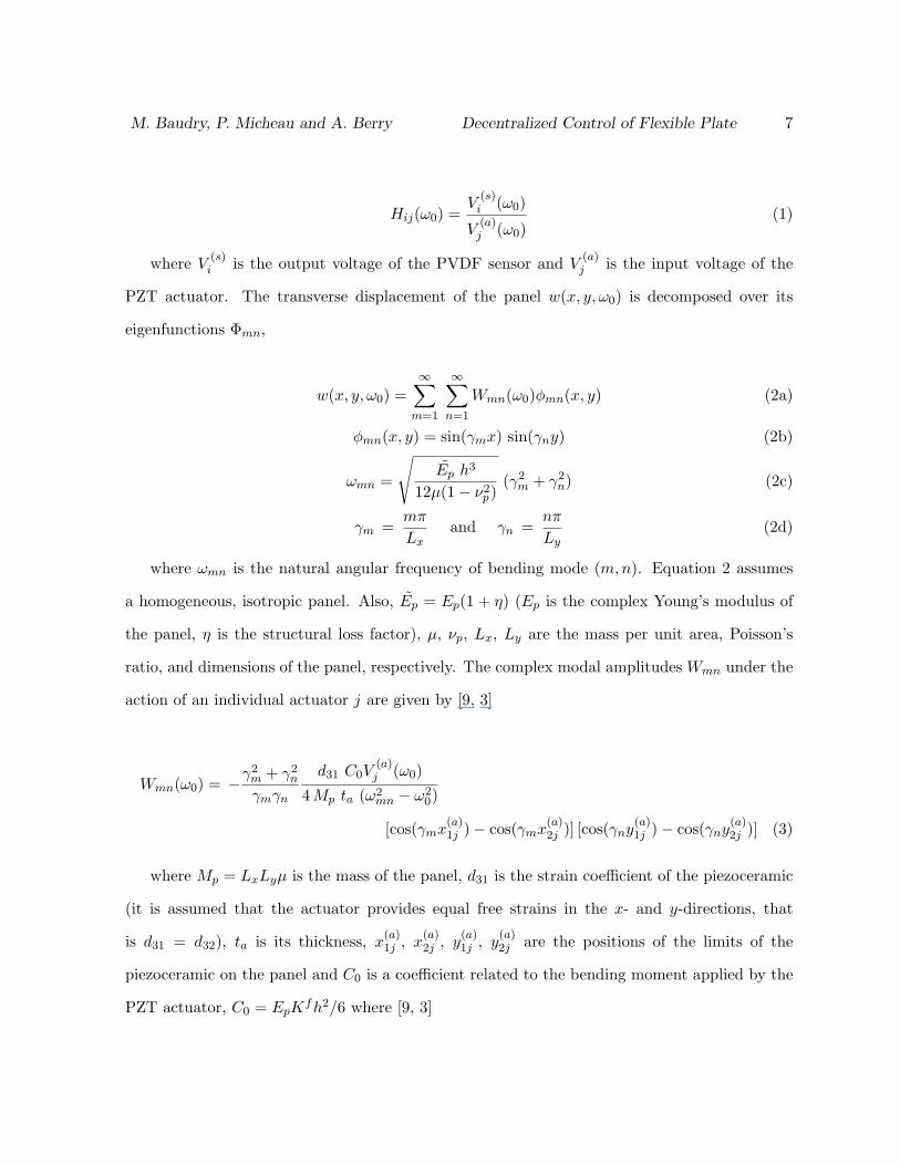
transfer function between actuator j and sensor i is defined by

M. Baudry, P. Micheau and A. Berry Decentralized Control of Flexible Plate 7

Hij(ω0) =V

(s)i (ω0)

V(a)j (ω0)

(1)

where V(s)i is the output voltage of the PVDF sensor and V

(a)j is the input voltage of the

PZT actuator. The transverse displacement of the panel w(x, y, ω0) is decomposed over its

eigenfunctions Φmn,

w(x, y, ω0) =∞∑

m=1

∞∑

n=1

Wmn(ω0)φmn(x, y) (2a)

φmn(x, y) = sin(γmx) sin(γny) (2b)

ωmn =

√Ep h3

12µ(1− ν2p)

(γ2m + γ2

n) (2c)

γm =mπ

Lxand γn =

nπ

Ly(2d)

where ωmn is the natural angular frequency of bending mode (m,n). Equation 2 assumes

a homogeneous, isotropic panel. Also, Ep = Ep(1 + η) (Ep is the complex Young’s modulus of

the panel, η is the structural loss factor), µ, νp, Lx, Ly are the mass per unit area, Poisson’s

ratio, and dimensions of the panel, respectively. The complex modal amplitudes Wmn under the

action of an individual actuator j are given by [9, 3]

Wmn(ω0) = −γ2m + γ2

n

γmγn

d31 C0V(a)j (ω0)

4Mp ta (ω2mn − ω2

0)

[cos(γmx(a)1j )− cos(γmx

(a)2j )] [cos(γny

(a)1j )− cos(γny

(a)2j )] (3)

where Mp = LxLyµ is the mass of the panel, d31 is the strain coefficient of the piezoceramic

(it is assumed that the actuator provides equal free strains in the x- and y-directions, that

is d31 = d32), ta is its thickness, x(a)1j , x

(a)2j , y

(a)1j , y

(a)2j are the positions of the limits of the

piezoceramic on the panel and C0 is a coefficient related to the bending moment applied by the

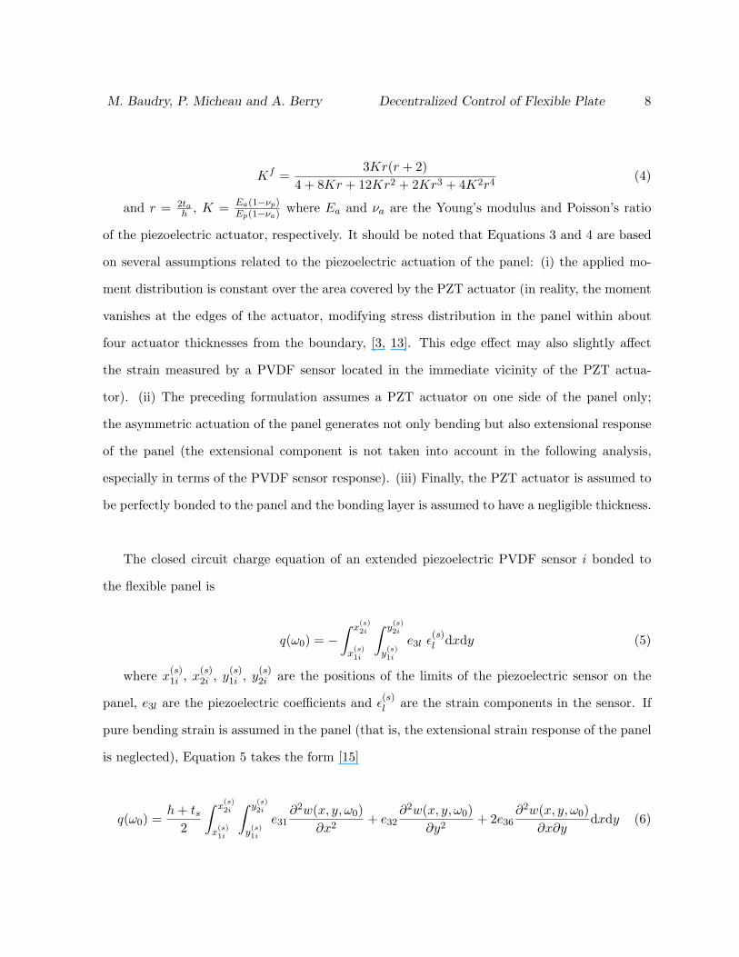
PZT actuator, C0 = EpKfh2/6 where [9, 3]

M. Baudry, P. Micheau and A. Berry Decentralized Control of Flexible Plate 8

Kf =3Kr(r + 2)

4 + 8Kr + 12Kr2 + 2Kr3 + 4K2r4(4)

and r = 2tah , K = Ea(1−νp)

Ep(1−νa) where Ea and νa are the Young’s modulus and Poisson’s ratio

of the piezoelectric actuator, respectively. It should be noted that Equations 3 and 4 are based

on several assumptions related to the piezoelectric actuation of the panel: (i) the applied mo-

ment distribution is constant over the area covered by the PZT actuator (in reality, the moment

vanishes at the edges of the actuator, modifying stress distribution in the panel within about

four actuator thicknesses from the boundary, [3, 13]. This edge effect may also slightly affect

the strain measured by a PVDF sensor located in the immediate vicinity of the PZT actua-

tor). (ii) The preceding formulation assumes a PZT actuator on one side of the panel only;

the asymmetric actuation of the panel generates not only bending but also extensional response

of the panel (the extensional component is not taken into account in the following analysis,

especially in terms of the PVDF sensor response). (iii) Finally, the PZT actuator is assumed to

be perfectly bonded to the panel and the bonding layer is assumed to have a negligible thickness.

The closed circuit charge equation of an extended piezoelectric PVDF sensor i bonded to

the flexible panel is

q(ω0) = −∫ x

(s)2i

x(s)1i

∫ y(s)2i

y(s)1i

e3l ε(s)l dxdy (5)

where x(s)1i , x

(s)2i , y

(s)1i , y

(s)2i are the positions of the limits of the piezoelectric sensor on the

panel, e3l are the piezoelectric coefficients and ε(s)l are the strain components in the sensor. If

pure bending strain is assumed in the panel (that is, the extensional strain response of the panel

is neglected), Equation 5 takes the form [15]

q(ω0) =h + ts

2

∫ x(s)2i

x(s)1i

∫ y(s)2i

y(s)1i

e31∂2w(x, y, ω0)

∂x2+ e32

∂2w(x, y, ω0)∂y2

+ 2e36∂2w(x, y, ω0)

∂x∂ydxdy (6)

M. Baudry, P. Micheau and A. Berry Decentralized Control of Flexible Plate 9

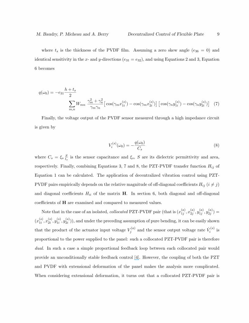
where ts is the thickness of the PVDF film. Assuming a zero skew angle (e36 = 0) and

identical sensitivity in the x- and y-directions (e31 = e32), and using Equations 2 and 3, Equation

6 becomes

q(ω0) = −e31h + ts

2∑m,n

Wmnγ2

m + γ2n

γmγn

[cos(γmx

(s)1i )− cos(γmx

(s)2i )

] [cos(γny

(s)1i )− cos(γny

(s)2i )

](7)

Finally, the voltage output of the PVDF sensor measured through a high impedance circuit

is given by

V(s)i (ω0) = −q(ω0)

Cs(8)

where Cs = ξsSts

is the sensor capacitance and ξs, S are its dielectric permittivity and area,

respectively. Finally, combining Equations 3, 7 and 8, the PZT-PVDF transfer function Hij of

Equation 1 can be calculated. The application of decentralized vibration control using PZT-

PVDF pairs empirically depends on the relative magnitude of off-diagonal coefficients Hij (i 6= j)

and diagonal coefficients Hii of the matrix H. In section 6, both diagonal and off-diagonal

coefficients of H are examined and compared to measured values.

Note that in the case of an isolated, collocated PZT-PVDF pair (that is (x(a)1j , x

(a)2j , y

(a)1j , y

(a)2j ) =

(x(s)1i , x

(s)2i , y

(s)1i , y

(s)2i )), and under the preceding assumption of pure bending, it can be easily shown

that the product of the actuator input voltage V(a)j and the sensor output voltage rate V

(s)i is

proportional to the power supplied to the panel: such a collocated PZT-PVDF pair is therefore

dual. In such a case a simple proportional feedback loop between each collocated pair would

provide an unconditionally stable feedback control [4]. However, the coupling of both the PZT

and PVDF with extensional deformation of the panel makes the analysis more complicated.

When considering extensional deformation, it turns out that a collocated PZT-PVDF pair is

M. Baudry, P. Micheau and A. Berry Decentralized Control of Flexible Plate 10

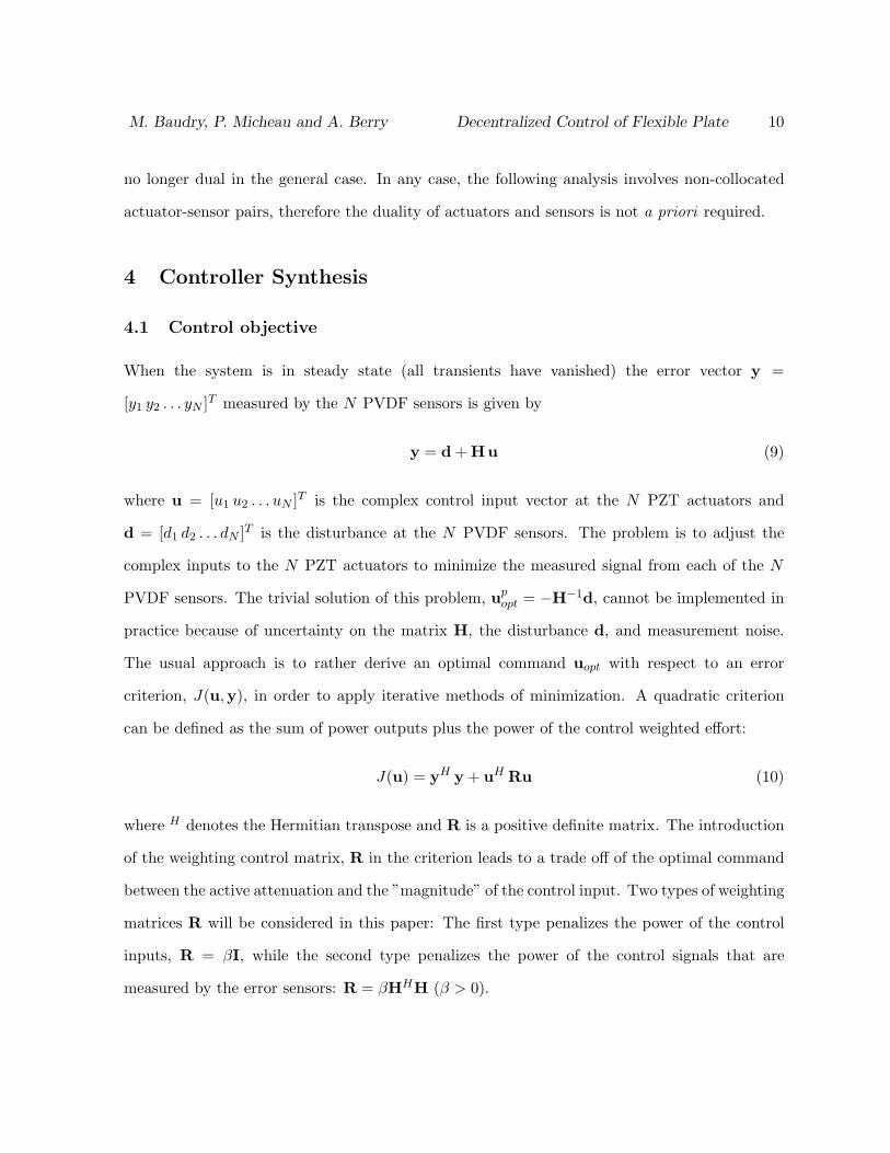
no longer dual in the general case. In any case, the following analysis involves non-collocated

actuator-sensor pairs, therefore the duality of actuators and sensors is not a priori required.

4 Controller Synthesis

4.1 Control objective

When the system is in steady state (all transients have vanished) the error vector y =

[y1 y2 . . . yN ]T measured by the N PVDF sensors is given by

y = d + Hu (9)

where u = [u1 u2 . . . uN ]T is the complex control input vector at the N PZT actuators and

d = [d1 d2 . . . dN ]T is the disturbance at the N PVDF sensors. The problem is to adjust the

complex inputs to the N PZT actuators to minimize the measured signal from each of the N

PVDF sensors. The trivial solution of this problem, upopt = −H−1d, cannot be implemented in

practice because of uncertainty on the matrix H, the disturbance d, and measurement noise.

The usual approach is to rather derive an optimal command uopt with respect to an error

criterion, J(u,y), in order to apply iterative methods of minimization. A quadratic criterion

can be defined as the sum of power outputs plus the power of the control weighted effort:

J(u) = yH y + uH Ru (10)

where H denotes the Hermitian transpose and R is a positive definite matrix. The introduction

of the weighting control matrix, R in the criterion leads to a trade off of the optimal command

between the active attenuation and the ”magnitude” of the control input. Two types of weighting

matrices R will be considered in this paper: The first type penalizes the power of the control

inputs, R = βI, while the second type penalizes the power of the control signals that are

measured by the error sensors: R = βHHH (β > 0).

M. Baudry, P. Micheau and A. Berry Decentralized Control of Flexible Plate 11

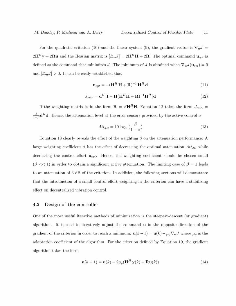
For the quadratic criterion (10) and the linear system (9), the gradient vector is ∇uJ =

2HHy + 2Ru and the Hessian matrix is [4uJ ] = 2HHH + 2R. The optimal command uopt is

defined as the command that minimizes J . The minimum of J is obtained when ∇uJ(uopt) = 0

and [4uJ ] > 0. It can be easily established that

uopt = −(HH H + R)−1 HH d (11)

Jmin = dH[I−H(HHH + R)−1HH

]d (12)

If the weighting matrix is in the form R = βHHH, Equation 12 takes the form Jmin =

β1+βdHd. Hence, the attenuation level at the error sensors provided by the active control is

AttdB = 10 log10(β

1 + β) (13)

Equation 13 clearly reveals the effect of the weighting β on the attenuation performance: A

large weighting coefficient β has the effect of decreasing the optimal attenuation AttdB while

decreasing the control effort uopt. Hence, the weighting coefficient should be chosen small

(β << 1) in order to obtain a significant active attenuation. The limiting case of β = 1 leads

to an attenuation of 3 dB of the criterion. In addition, the following sections will demonstrate

that the introduction of a small control effort weighting in the criterion can have a stabilizing

effect on decentralized vibration control.

4.2 Design of the controller

One of the most useful iterative methods of minimization is the steepest-descent (or gradient)

algorithm. It is used to iteratively adjust the command u in the opposite direction of the

gradient of the criterion in order to reach a minimum: u(k +1) = u(k)−µg∇uJ where µg is the

adaptation coefficient of the algorithm. For the criterion defined by Equation 10, the gradient

algorithm takes the form

u(k + 1) = u(k)− 2µg(HH y(k) + Ru(k)) (14)

M. Baudry, P. Micheau and A. Berry Decentralized Control of Flexible Plate 12

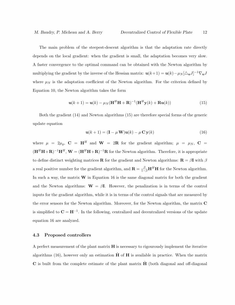
The main problem of the steepest-descent algorithm is that the adaptation rate directly

depends on the local gradient: when the gradient is small, the adaptation becomes very slow.

A faster convergence to the optimal command can be obtained with the Newton algorithm by

multiplying the gradient by the inverse of the Hessian matrix: u(k+1) = u(k)−µN [4uJ ]−1∇uJ

where µN is the adaptation coefficient of the Newton algorithm. For the criterion defined by

Equation 10, the Newton algorithm takes the form

u(k + 1) = u(k)− µN (HHH + R)−1(HHy(k) + Ru(k)) (15)

Both the gradient (14) and Newton algorithms (15) are therefore special forms of the generic

update equation

u(k + 1) = (I− µW)u(k)− µCy(k) (16)

where µ = 2µg, C = HH and W = 2R for the gradient algorithm; µ = µN , C =

(HHH+R)−1HH , W = (HHH+R)−1R for the Newton algorithm. Therefore, it is appropriate

to define distinct weighting matrices R for the gradient and Newton algorithms: R = βI with β

a real positive number for the gradient algorithm, and R = β1−βHHH for the Newton algorithm.

In such a way, the matrix W in Equation 16 is the same diagonal matrix for both the gradient

and the Newton algorithms: W = βI. However, the penalization is in terms of the control

inputs for the gradient algorithm, while it is in terms of the control signals that are measured by

the error sensors for the Newton algorithm. Moreover, for the Newton algorithm, the matrix C

is simplified to C = H−1. In the following, centralized and decentralized versions of the update

equation 16 are analyzed.

4.3 Proposed controllers

A perfect measurement of the plant matrix H is necessary to rigourously implement the iterative

algorithms (16), however only an estimation H of H is available in practice. When the matrix

C is built from the complete estimate of the plant matrix H (both diagonal and off-diagonal

M. Baudry, P. Micheau and A. Berry Decentralized Control of Flexible Plate 13

coefficients), then Equation 16 provides the update of a centralized controller. In what follows,

it is assumed that for centralized control, both the diagonal and off-diagonal coefficients of H

are perfectly estimated, therefore H = H for centralized control.

The case of a decentralized controller corresponds to N independent update equations that

take into account only the diagonal coefficients of the plant matrix. This is formally equivalent

to a biased estimation of the complete matrix H, H = diag(Hii) for all i = 1, .., N ; in other

words, the off-diagonal coefficients are forced to 0 and the diagonal coefficients are assumed to

be perfectly estimated. Therefore, decentralized control derived from the gradient algorithm

corresponds to C = diag(H∗ii), where H∗

ii denotes the complex conjugate of Hii. On the other

hand, decentralized control derived from the Newton algorithm corresponds to C = diag(1/Hii).

Note that decentralized control derived from the Newton algorithm does not need the inversion

of the complete plant matrix, but only the inverse of its diagonal elements.

In summary, Equation 16 is the general update equation that applies to the four cases

investigated in this article: the control matrix is C = HH for the gradient algorithm, C = H−1

for the Newton algorithm, H = H for centralized control and H = diag(Hii) for decentralized

control. For the four cases, the weighting matrix is W = βI.

The main limitation of decentralized control is that both the Hessian and the gradient of

the criterion are approximated from only the diagonal elements of the plant matrix. Hence,

the estimated gradient computes a biased direction for searching the optimal command. In the

worst case, the controller may search the minimum of the criterion in its opposite direction and

never reach it: the system is unstable. The following sections address the conditions of stability

of the controlled system.

4.4 Conditions of stability

It is possible to establish the condition of asymptotic stability of the closed loop system described

by Equations 16 and 9. If we consider that the closed loop system is stable, then the command

M. Baudry, P. Micheau and A. Berry Decentralized Control of Flexible Plate 14

u(k) converges to u∞ = −(CH+W)−1 Cd (obtained by imposing u(k +1) = u(k) in equation

16). It is then possible to re-express Equations 16 and 9 as an autonomous linear discrete-time

system:

x(k + 1) = Ax(k) (17)

where x(k) = u(k)−u∞ (or x(k) = y(k)−y∞) and A = I−µ(CH+W). Such a discrete-time

dynamic system is called stable when x(k) tends exponentially to zero when k → ∞ for any

initial condition such that x(0) 6= 0. The necessary and sufficient condition of stability of the

closed loop system is that the matrix A is Schur stable: all its eigenvalues lie within the interior

of the unit circle in the complex plane: |λi(A)| < 1 for all i.

In the special case of A = I − µB with B = CH + W and µ > 0, the condition of Schur

stability becomes |1−µλi(B)| < 1 for all i = 1, ..., N . Hence, the Schur stability condition leads

to the necessary and sufficient condition of stability

µ <2<(λi(B))|λi(B)|2 , ∀ i = 1, ..., N (18)

where <(λi) designates the real part of the complex eigenvalue λi. An important interpretation

of the above condition is that it introduces an upper bound for the adaptation coefficient in

the iterative algorithm, µmax = 2<(λi(B))|λi(B)|2 . The main implication of Equation 18 is that the real

part of all eigenvalues of B must necessarily be positive, <(Λi) > 0 for all i. In the following,

and in the context of this paper, the term ”µ-stabilization” refers to the necessary condition of

stability: if <(λi(B)) > 0 for all i then it is possible to obtain stable control with an appropriate

tuning of the adaptation coefficient µ. When all eigenvalues of B are located in the open right

complex half plane, the matrix theory literature often refers to the concept of positive stability. In

control theory literature, the matrix −B is said to be Hurwitz stable: the associated autonomous

continuous time system x(t) = −Bx(t) is stable.

An alternative and simpler method of analyzing the ”µ-stabilization” of the closed loop

system is derived from the following theorem [12] (p. 88): If B ∈ CN×N with n0(B) = 0

M. Baudry, P. Micheau and A. Berry Decentralized Control of Flexible Plate 15

and if the Hermitian nonsingular matrix P ∈ CN×N satisfies the condition PB + BHP = −Q

with Q ≥ 0 then InB = InP. The inertia of a matrix B, denoted InB is defined by the

triple (n+(B), n0(B), n−(B)) where n+(B) is the number of eigenvalues of B in the open right

complex half-plane, n0(B) is the number of purely imaginary eigenvalues of B, n−(B) is the

number of eigenvalues of B in the open left complex half-plane. According to the theorem,

choosing P = I and assuming that BH + B is positive definite, then InB = (N, 0, 0) (meaning

that <(λi(B)) > 0). Consequently, if B is a ”strictly positive-real” (SPR) matrix (that is,

BH +B is positive definite) it is possible to find a µ which achieves stable control of the overall

closed-loop system. Moreover, when B is a SPR matrix, this implies that V (x) = xHx is a

quadratic Liapunov function for the system x(t) = −Bx(t). Therefore dV/dt ≤ 0, the matrix

−B is said to be Hurwitz diagonally stable (this is also referred to as Volterra stability, Voltera-

Liapunov stability or VL-stability, or dissipativity) [12]. Hence, the necessary condition of B

SPR means that in the limiting case of µ → 0, −B must be Hurwitz diagonally stable. The

diagonal stability is a stronger requirement than just stability; in our case diagonal stability

means that the sum of power outputs measured by the PVDF sensors monotonously decreases

with time when µ is very small.

From a purely mathematical point of view, the concept of strictly positive-real matrix B

has the advantage of simplifying the stability analysis and of providing some physical insight.

For example, we consider the case of centralized control, a perfectly estimated plant matrix

and no effort weighting (R = 0). In the case of the centralized Newton algorithm, C = H−1,

then CH = I is SPR (its eigenvalues are 1). In the case of the centralized gradient algorithm,

C = HH , then CH = HHH is a SPR matrix (because HHH is a hermitian positive definite

matrix). Consequently, centralized control with perfect system estimation will always be stable.

The case of decentralized control is more interesting. The consideration of only the diagonal

coefficients of the plant matrix H is formally equivalent to a biased estimation of the complete

matrix H. In the case of imperfect plant estimation, the eigenvalues of CH are not necessarily

M. Baudry, P. Micheau and A. Berry Decentralized Control of Flexible Plate 16

real and positive, therefore the condition <(λi(B)) > 0 suggests that control effort weighting W

may be necessary to stabilize the control. The following sections investigate the effect of effort

weighting on the stability of decentralized control.

4.5 Decentralized control without effort weighting, W = 0

When W = 0, the disturbance rejection is theoretically perfect but ”µ-stabilization” of the

closed loop system is possible if and only if <(λi(CH)) > 0, this condition is verified if CH

is a strictly positive-real (SPR) matrix. In order to illustrate the role of the decentralized

compensator C, 2 cases are considered in this section for the plant matrix: H is a SPR matrix

and H is not SPR.

• When H is a SPR matrix, the ”µ-stabilization” in decentralized or centralized is guaran-

teed. Disturbance rejection is possible without any estimation of the plant matrix H: with

C = I, the matrix CH = H is SPR, therefore a sufficiently small adaptation coefficient

µ will necessarily ensure closed loop stability. A SPR plant matrix H for all frequencies

physically corresponds to a dissipative plant [22]. The SPR condition is obtained in a

linear undamped flexible structure with dual-collocated actuator-sensor pairs (passive op-

erator), without poles on the imaginary axis (strictly stable linear system) and without

null eigenvalues (dissipativity condition) [20]. In other words, the collocation of actuators

and sensors and the intrinsic damping in the plant imply the SPR condition at any fre-

quency. In contrast, the configuration of distributed and non-collocated actuator-sensor

pairs results in a non PR plant matrix H (and consequently to a non SPR H), leading to

more difficult control situations.

• When H is not SPR, the role of the diagonal compensator matrix C can be to ensure a

SPR matrix CH. A necessary (but not sufficient) condition for CH to be SPR is that

the real part of diagonal elements of CH are strictly positive: <(CiHii) > 0. With the

M. Baudry, P. Micheau and A. Berry Decentralized Control of Flexible Plate 17

assumption of perfect estimation of the diagonal coefficients of the plant matrix, Hii = Hii,

this necessary condition is always verified in decentralized control because CiHii = |hii|2

for the gradient algorithm and CiHii = 1 for the Newton algorithm. However, in the

case of a biased estimation of the diagonal coefficients of the plant matrix, this condition

may be not verified. For example, if we consider the Newton algorithm with a phase-shift

error φ of the diagonal coefficient, Hii = Hii expjφ, then the diagonal coefficients of CH

have a real part <(Hii/Hii) = cos(φ) which is negative when the phase error is such that

π/2 > φ > 3π/2 (mod 2π): therefore, an individual control unit can be unstable (with the

other units being inactive). In this case, since the corresponding diagonal coefficient CiHii

is not strictly positive, the whole system is not SPR (it may still be stable, though).

To summarize, the main role of the diagonal compensator C in decentralized control is to

compensate the phase of the diagonal coefficients of the plant matrix H in order to ensure

a SPR matrix diag(CiHii). Along these lines, we can conclude that any compensator of the

form C = KHH with H = diag(Hii), and K a diagonal positive matrix is a candidate

for decentralized control. For example, Ki = 1 corresponds to the gradient algorithm and

Ki = 1/|Hii|2 corresponds to the Newton algorithm.

4.6 Decentralized control with effort weighting, W 6= 0

In situations where it exists at least one negative eigenvalue <(λi(CH)) < 0, then, according

to Equation 18, the weighting matrix W = βI must be included in the criterion to ensure a

stable closed loop. The weighting coefficient β that ensures theoretical µ-stabilization of the

convergence process should satisfy:

β > −< (λi(CH)) ∀ i (19)

Therefore, the minimum value of β is β = max(−< (λi(CH))). The main drawback of weighting

the control effort is to decrease the active attenuation. For example, Equation 13 shows that

M. Baudry, P. Micheau and A. Berry Decentralized Control of Flexible Plate 18

β = 1 leads to a 3 dB attenuation of the criterion after control. In practical situations, values of

β should be kept much lower than unity in order to maintain satisfactory control performance.

4.7 Positive definite and diagonal dominance

In case of a perfect estimation of the diagonal coefficients of the plant matrix, the Gershgorin

theorem can be applied to derive a sufficient condition of µ-stabilization. The Gershgorin

theorem states that ”the eigenvalues of a complex matrix B are within disks in the complex

plane whose centers are the diagonal coefficients Bii of B and whose radii are the sums of the

modulus of off-diagonal coefficients Bij with i 6= j”. When Bii is a real positive number and∑m

j=1,j 6=i|Bij | < Bii, then all these disks lie within the right-hand side of the complex plane,

therefore all eigenvalues of B have a positive real part: <(λi(B)) > 0; therefore, the system is

µ-stabilizable. A matrix such that∑m

j=1,j 6=i|Bij | < Bii for all i is called diagonal dominant.

Consequently, a sufficient condition of µ-stabilization is that the matrix B = CH + W is

diagonal dominant and diag(Bii) > 0.

It can be easily established that the condition CH diagonal dominant is equivalent to the

condition H diagonal dominant for the gradient and Newton algorithms, |Hii| >∑m

j=1,j 6=i|Hij |for all i. Therefore, if H is diagonal dominant then CH is SPR and the decentralized control

is µ-stabilizable without control effort weighting. The condition that H is diagonal dominant is

easy to test in practice. However this condition is fairly restrictive because the phase of transfer

functions between actuators and sensors is not considered. For example, in the case where the

number of actuator-sensor pairs N →∞, the diagonal dominant condition will be never satisfied

even if the matrix CH is SPR or the system is dissipative. The plant H does not necessarily

need to be diagonal dominant in order to make decentralized control effective.

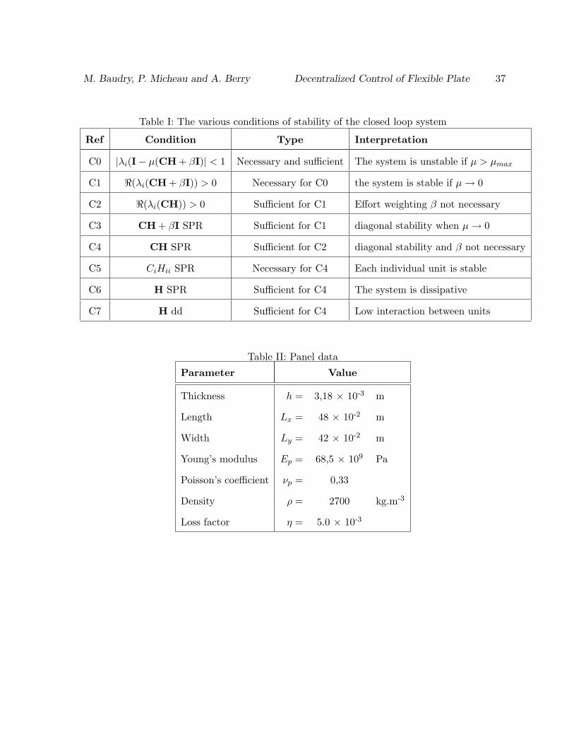
To summarize, the various conditions of µ-stabilization (to obtain A = I − µ(CH + W)

Schur stable by tuning µ) are presented in Table I as a function of the plant matrix H, the

control matrix C, the effort weighting coefficient β and the adaptation coefficient µ.

M. Baudry, P. Micheau and A. Berry Decentralized Control of Flexible Plate 19

5 Control Implementation

5.1 Implemented harmonic controller

In the preceding sections, the inherent delay of the control system in processing the error signal

y and generating the next control input u has not been taken into account. In practice, the

implementation of a frequency-domain control used demodulation and modulation blocks that

extract the phasor of the error y and generate the oscillatory control input, respectively (figure

2). This section presents the practical signal processing to implement the decentralized harmonic

controllers.

In order to extract the phasor Yi from the real oscillatory signal yi(t) provided by sensor i, a

complex demodulation is applied. The method involves translating the signal yi in the frequency

domain, from the harmonic frequency ω0, to 0 (rad/s), by multiplication with the complex sine

wave of frequency ω0. A low-pass filter f , is applied to this complex signal in order to extract

the phasor of interest:

Yi(t) = f(t) ? (yi(t) exp(−iω0t)) (20)

where ? denotes the convolution operator. The cut-off frequency of the low-pass filter is set

equal to ωc << ω0 and its static gain is set to 1, |f(0)| = 1. Because of the low-pass filtering,

the complex signal Yi(t), called the complex envelope, is localized in the low frequency domain.

Hence, according to the Shannon criterion, Yi(t) can be sampled without aliasing at a rate

ωe < 2ω0. The discrete down-sampled output of the complex envelope is Yi[k] = Yi(kTe) with

Te = 2π/ωe the sampling period and k the discrete time.

In order to generate each command signal ui(t) from each phasor Ui (figure 2), a complex

modulation is used. First, the causal low-pass filtering f is applied to generate Ui(t) from the

down-sampled dicrete-time signal Ui[k]. Then, the signal is translated in the frequency domain

from 0 (rad/s) to the harmonic frequency, ω0, and the real part is extracted to generate the

M. Baudry, P. Micheau and A. Berry Decentralized Control of Flexible Plate 20

command signal:

ui(t) = 2<(Ui(t) exp(iω0t)) (21)

In order to provide insight in the controller implementation, its equivalent form is developed.

In the continuous time domain, Equation 16 can be written by considering the finite difference

approximation with Te → 0 and µ → 0:

U(k + 1)−U(k)Te

≈ dU(t)dt

= −aU(k)− bCY(k) (22)

where b = µTe

and a = bβ. The Laplace Transform of Equation 22, gives the equivalent

compensator in terms of the complex envelopes U and Y:

U(s) = − b

s + aCY(s) (23)

By introducing Laplace Transforms of Equations 20 and 21 in Equation 23, the equivalent

decentralized compensator is obtained in terms of the real oscillatory signals ui and yi:

ui(s)yi(s)

= − bN(s)(s + a)2 + ω2

0

(24)

with N(s) = Cf2(s− jω0)(s + a + jω0) + C∗f2(s + jω0)(s + a− jω0).

The numerator N(s) includes bandpass filtering f , centered at ω0; the denominator includes

two weakly damped poles close to the harmonic frequency ω0: s0 = −a+jω0 and s∗0 = −a−jω0.

The feedback loop gain at the disturbance frequency, ω0, is approximately bCii/a. It is tuned

with the µ parameter: with µ = 0 there is no feedback loop (b = 0) and no control. The maximal

adaptation coefficient, µmax defined by Equation 18, is equivalent to the critical feedback gain:

the stability is marginal for this value. When β = 0, Equation 24 is the expression of a resonant

controller because the added pole is undamped: the compensator is characterized by an infinite

gain at ω0. According to the Wohan’s Principle [8], this allows perfect rejection of the harmonic

disturbance because the compensator includes a model of the harmonic generator: it is able to

generate a sinusoidal waveform at the disturbance frequency even when the error is null. When

M. Baudry, P. Micheau and A. Berry Decentralized Control of Flexible Plate 21

it exists at least one negative eigenvalue <(λi(CH)) < 0, the compensator poles should be

damped for the purpose of adding stability robustness: the increase of β in Equation 24 moves

the compensator poles from the imaginary axis to the left-side of the complex plane. According to

Siever [21], the equivalent controller is independent of the methodology chosen (analog, adaptive,

classical, modern method); for example a MIMO adaptive feedforward algorithm (usually called

x-lms) will also present complex poles centered at the disturbance frequency [14].

5.2 Stability analysis of the implemented controller

When the controller slowly adapts the control inputs (µ → 0) in comparison to the dynamics

of the low-pass filters, the influence of modulation and demodulation blocks is negligible and

closed loop stability can be analyzed using Equation 9. However, in the general case, the low-

pass filtering operations induce transients in the modulation and demodulation processes and

they must be taken into account by modifying Equation 9 as follows:

y(k) = d + Hφ(q−1)u(k) (25)

where φ(q−1) = φ0+φ1q−1+ ...+φdq

−d is the impulse response of the filters and q−1 is the delay

operator. The impulse response coefficients are computed from the down-sampled discrete-time

impulse response of the two lowpass filters in series: φn = (f ? f)(nTe) for n = 0, 1, 2..., d. In

other words, the impulse response of the combined modulation and demodulation blocks are

represented by a Finite Impulse Response (FIR) filter with d+1 coefficients. This FIR filter has

an unitary static gain, φ(1) = φ0 +φ1 + ...+φd = 1, because |f(ω)| ≈ 1 for ω ≈ 0. Consequently,

the steady state version of Equation 25 is Equation 9. In other words, Equation 25 describes

the transients due to the signal processing operations (modulation and demodulation), but not

the transients due to the physical system.

Similar to Equation 17, Equation 25 can be re-expressed as a discrete time autonomous

M. Baudry, P. Micheau and A. Berry Decentralized Control of Flexible Plate 22

system of state variable x(k):

x(k + 1) = (1− µβ)x(k)− µCHφ(q−1)x(k) (26)

where x(k) = u(k)− u∞. By introducing the expression of φ(q−1), Equation 26 takes the form

of a difference equation

x(k + 1) = [(1− µβ)I− µφ0 CH]x(k)− µ

d∑

i=1

φi CHx(k − i) (27)

The condition for which x converges to x∞ is more difficult to establish in the case of

Equation 27 than in the case of Equation 17. It is necessary to re-express Equation 27 in an

augmented state space form

z(k + 1) = Ad z(k) (28)

where z(k) = [x(k)x(k − 1) ...x(k − d)]t is the new state vector, and the evolution matrix is:

Ad =

(I− µW)− µF0 −µF1 ... −µFd−1 −µFd

I O ... O O...

. . . . . ....

...

O O ... I O

with Fi = φi CH.

The necessary and sufficient condition of stability is that the matrix Ad is Schur stable: all

its eigenvalues are inside the unit circle in the complex plane.

When the weighting coefficient β is fixed, the stability condition consists of finding

the maximum adaptation coefficient µmax such that ∀ µ < µmax : sup |λi(Ad(µ))| <

1 and |λi(Ad(µmax))| = 1. Considering the complexity of the matrix Ad, this search was

done numerically.

M. Baudry, P. Micheau and A. Berry Decentralized Control of Flexible Plate 23

6 Simulation and experimental results

6.1 Comparison of plant model with measured data

The prediction of H, presented in section 3 was first compared to experimental data in the case

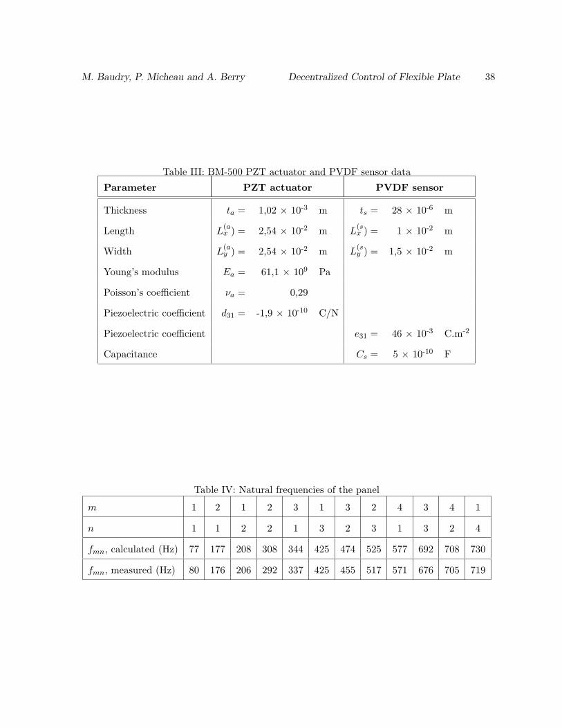
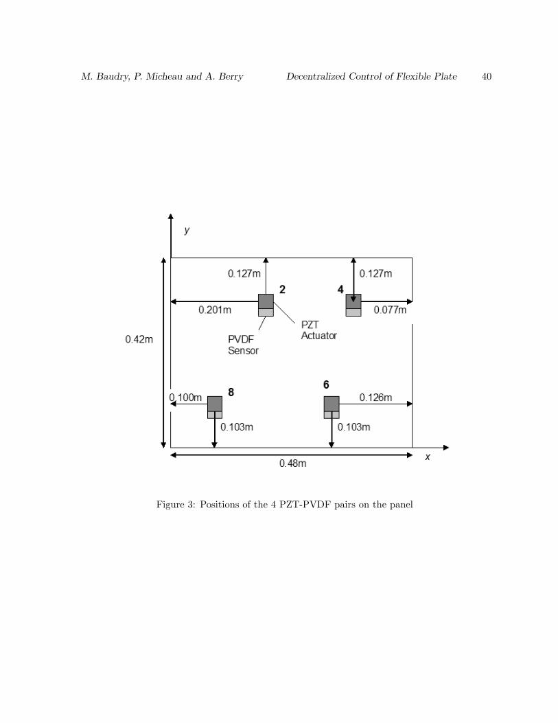
of a simply-supported 48cm × 42cm aluminium panel instrumented with 4 BM-500 2.54cm ×2.54cm, 1mm thick PZT actuators and 4 1.5cm × 1cm, 28 µ m thick PVDF sensors. Tables II

and III list the panel, actuator and sensor data. Table IV shows the calculated and measured

natural frequencies of the panel in the[0− 800Hz

]range. The positions of actuator and sensor

pairs on the panel (subsequently referred to as positions 2, 4, 6 and 8) are shown on figure

3. The actuator positions were selected randomly in order to excite as many panel modes as

possible in the[0 − 800Hz

]frequency range. Note however that in this configuration, PZT

2 and 4 do not effectively excite the panel modes n = 3, and PZT 6 and 8 are not effective

for panel modes n = 4. A PVDF sensor was bonded close to each PZT to form a pair (their

separation was of the order of 1mm). The PZT-PVDF transfer functions were measured us-

ing a[0 − 800Hz

]white noise input signal sequentially driving the PZT actuators; the charge

response of the PVDF sensors was amplified and converted to a voltage output through high

input impedance Frequency Device filters. The following transfer functions do not include the

input gain of the high voltage PZT amplifier and the output gain of the PVDF filters. On

the other hand, a structural loss factor of the panel of 5 × 10−3 was considered in the simula-

tions; this value was adjusted to fit the measured response on resonance of selected panel modes.

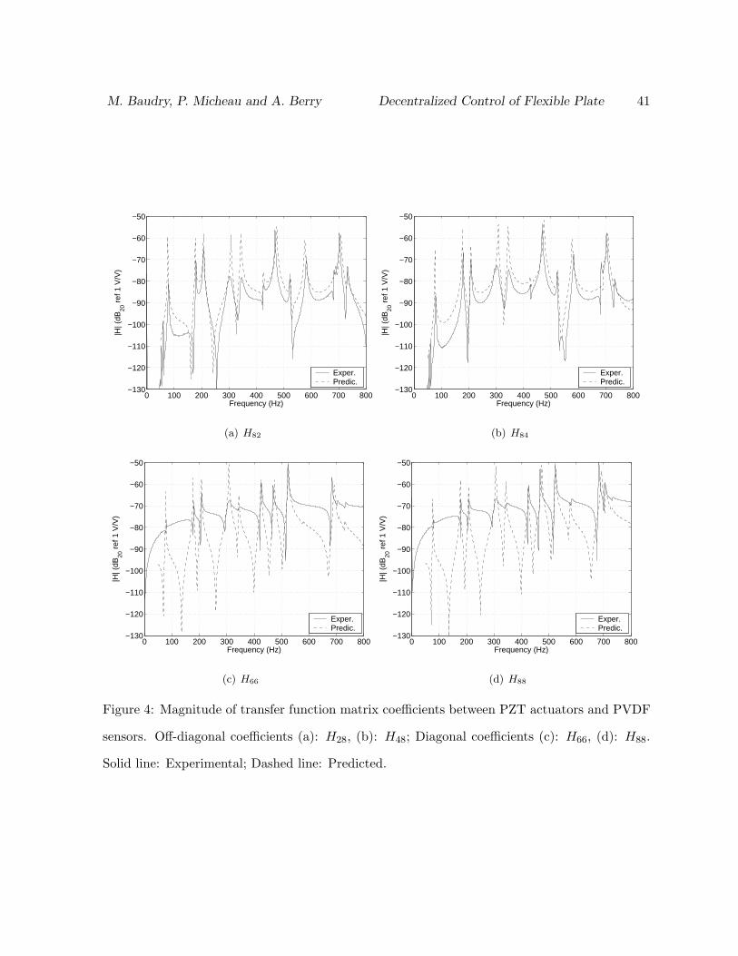
Figure 4 shows examples of measured and predicted transfer functions H28, H48, H66, H88.

The agreement is generally good for the off-diagonal terms H28, H48 (with the prediction slightly

overestimating the measured values), but much less satisfactory for the diagonal terms H66, H88.

In this case the prediction largely underestimates the magnitude of the transfer function off-

resonance. This leads to a measured H which is more diagonally-dominant than the calculated

M. Baudry, P. Micheau and A. Berry Decentralized Control of Flexible Plate 24

H, and therefore an a-priori more viable implementation of decentralized control. Possible

explanations for the underestimation of direct transfer by the theory are bending near-field

effects of the PZT actuators and the effect of extensional excitation of the panel by the PZT

actuators, which were not accounted for in the model.

6.2 Predicted stability indicators for decentralized control

For the physical configuration with 4 control units shown on figure 3, the various stability

conditions listed in Table I were tested for decentralized control. The stability conditions are

derived from the theoretical plant matrix or the measured plant matrix H. In this case, the plant

matrix was measured by driving the PZT actuators with a pure sine in the frequency range from

500Hz to 800 Hz, with a 10 Hz step. The amplitude of the actuator signal was automatically

adjusted in order to obtain the largest possible output signal from the PVDF sensors without

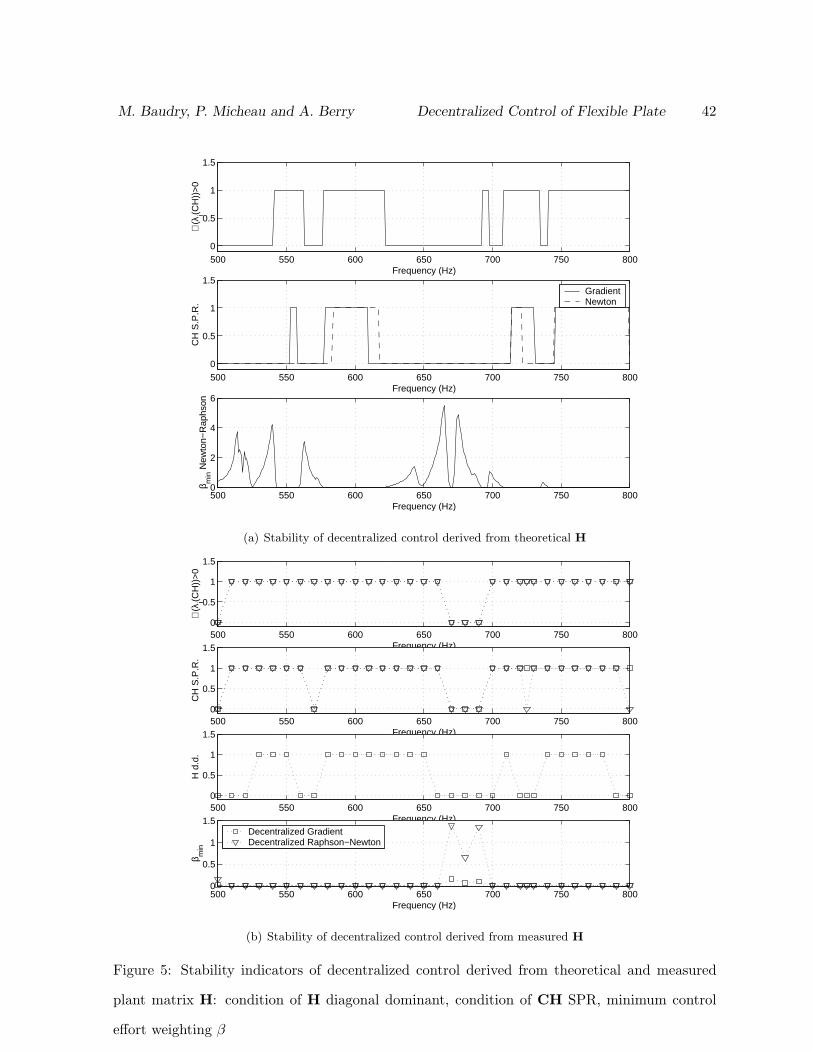
saturation. Figure 5 presents predicted stability of decentralized control derived from either the

theoretical or measured plant matrix H in the frequency range 500 Hz - 800 Hz. The presented

stability indicators are the diagonal dominant property of H, the condition of <(λi(CH)) > 0,

the condition CH strictly positive real (SPR) and the minimum control effort weighting β

according to Equation 19.

In the case of stability derived from the theoretical plant matrix, the sufficient condition of

H being diagonal dominant is never verified in the frequency range investigated: the interaction

between PZT-PVDF pairs is large at all frequencies. In the case of stability derived from the

measured plant matrix, the diagonal dominant condition is verified in some frequency intervals.

This is consistent with the observations derived from the plant matrix components Hij in Figure

4. The measured plant matrix tends to be not diagonal dominant close to resonances of panel

modes.

The condition that the matrix CH is SPR guarantees that µ-stabilization of the closed loop

system is possible without requiring control effort weighting (β = 0). This condition is presented

M. Baudry, P. Micheau and A. Berry Decentralized Control of Flexible Plate 25

on Figure 5 for decentralized Newton, for which C = diag(1/Hii). In the case of stability derived

from the theoretical plant matrix and for the Newton algorithm, the CH matrix is SPR only

in some frequency intervals included in those of the condition <(λi(CH)) > 0; accordingly, the

minimum value of β is predicted to be larger than 0 only when <(λi(CH)) < 0. Note that for

the gradient algorithm, the condition <(λi(CH)) > 0 is verified at all frequencies, therefore the

minimal value of β is predicted to be null (not shown on the figure). Stability derived from

the measured H is less stringent: for decentralized Newton, CH always verifies <(λi(CH)) > 0

except at 500Hz and in the frequency range 670 Hz - 690 Hz. At these frequencies, control

effort weighting is necessary in order to stabilize the closed-loop system, βmin > 0 for both the

gradient and Newton algorithms. Note that at frequencies for which βmin > 0, H is not diagonal

dominant, but the inverse is not true: for example, at 800Hz, the experimental and theoretical

matrices H are not diagonal dominant but the associated CH matrix is SPR for the gradient

algorithm, and both gradient and Newton algorithms are µ-stable because <(λi(CH)) > 0. The

hierarchy between the conditions is verified: the diagonal dominance of H or the SPR of CH

are sufficient, but not necessary conditions of closed-loop stability.

Note also that the minimum value of the effort weighting coefficient β required to stabilize

the Newton algorithm is large, and usually larger than for the gradient algorithm (a value of

β = 1 reduces the attenuation at the error sensors to 3 dB). Hence, the control performance

obtained with the weighted Newton is expected to be smaller than the performance of the

weighted gradient.

6.3 Predicted and measured stability limits

The decentralized and centralized controllers were implemented in a rapid prototyping dSPace

system. The sampling frequency was set to 5kHz. For the analysis and synthesis of the

complex envelopes, the low-pass FIR filters were implemented with 4 Butterworth second order

filters in order to ensure an attenuation of 40dB outside ±7.5 Hz. Consequently, the complex

M. Baudry, P. Micheau and A. Berry Decentralized Control of Flexible Plate 26

envelopes were under-sampled at 25Hz without aliasing. The identification of the plant matrix

was performed for each frequency with an harmonic input of the PZT actuators (with the

disturbance off) and under steady-state response of the system. The identified plant matrix was

used to perform the active centralized/decentralized control of the plate. Steady- state harmonic

response of the system can be assumed for the control due to the slow dynamics of the FIR filters

(and the slow dynamics of the controller - low value of µ) against the dynamics of a low damped

mode in the considered narrow frequency band [17]. This point is experimentally verified with

the results presented in Figure 6 where the dynamics of the filters limit the maximum value of

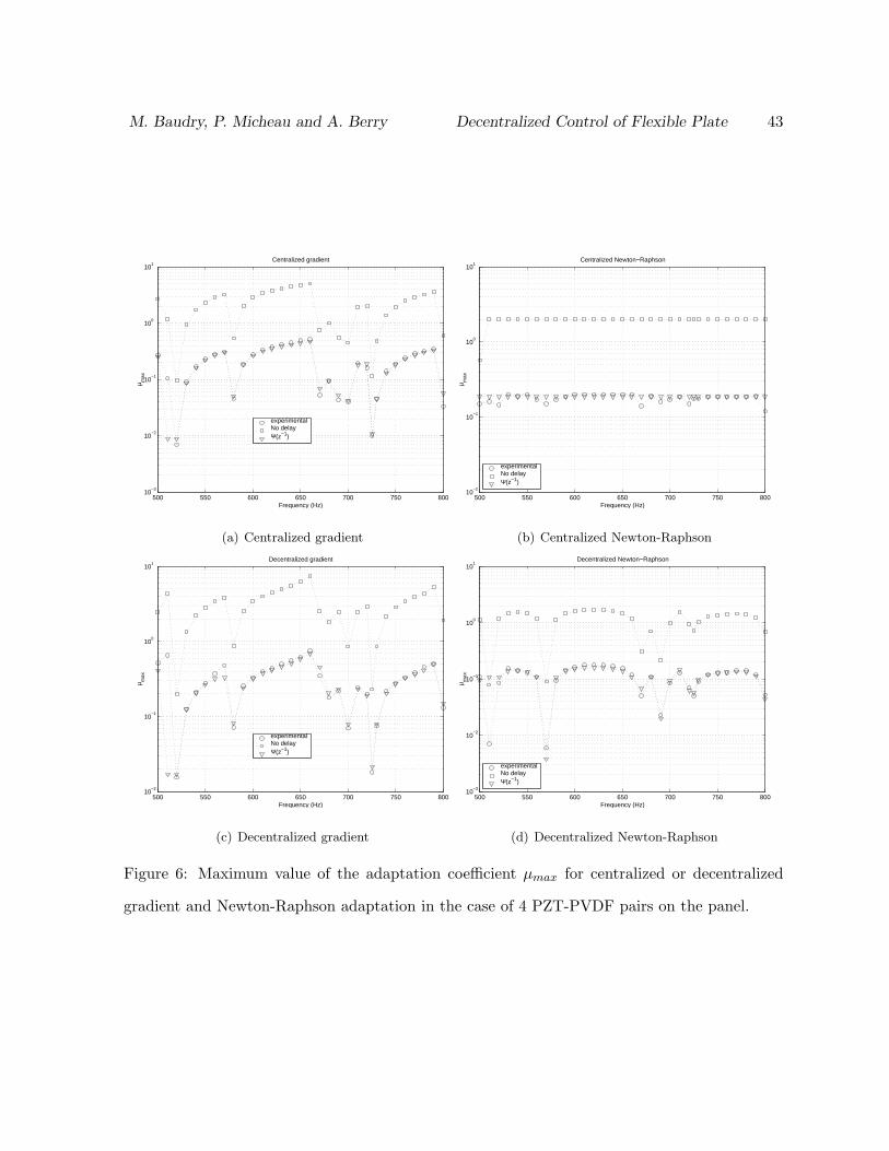
the adaptation coefficient.

Figure 6 shows the predicted and measured stability limits of the centralized and decentral-

ized controllers in the case of the 4 PZT-PVDF control pairs shown on figure 3, in the frequency

range [500Hz − 800Hz]. Note that the predicted stability limit was obtained from the measured

plant matrix H. The maximum adaptation coefficient, µmax, observed experimentally for the

various controllers is also reported. Two cases of low-pass filter dynamic response were examined

in the prediction: (i) a unitary frequency response, φ0 = 1 and φi = 0 for i > 0 (in this case, no

filter delay is assumed, and the stability limit was obtained from Equation 18); (ii) the measured

impulse response of the low-pass filters φ(q−1) (in this case, the stability limit was derived from

the eigenvalues of the matrix Ad in Equation 28).

In the case of the centralized gradient and Newton algorithms, the CH matrix is always

SPR, therefore the control effort weighting was set to zero: β = 0. The maximum adaptation

coefficient µmax turns to be frequency-independent for the centralized Newton, its predicted

value being 2 in the case of a zero loop delay and close to 0.02 in the case of the loop delay

induced by the low-pass filters. The negative impact of the time-delay, or filtering, is clearly

apparent in this computation. The value of µmax = 2 in the case of a zero loop delay is consistent

with convergence analysis derived from Equation 16. As expected, when loop delay is increased,

the critical feedback gain is reduced. The experimental values of µmax are close to the values

M. Baudry, P. Micheau and A. Berry Decentralized Control of Flexible Plate 27

predicted when the measured impulse response of low-pass filters is included in the loop. It is

clear that µmax is largely overestimated if no loop delay is included. In the case of centralized

gradient, the values of µmax are frequency-dependent: when C = HH , Equation 18 becomes

µmax < 2/σ2max, where σ2

max is the largest eigenvalue of HHH. Therefore, at resonance of panel

modes, the system presents a high gain and the adaptation coefficient must be reduced. The

time-delay induced by low-pass filters still decreases the critical value of µ. The agreement

between experimental and predicted values of µmax when the measured impulse response of

low-pass filters is included in the loop, is again very good.

In the case of decentralized control, the matrix CH is not SPR for all frequencies in the

[500Hz − 800Hz] range, therefore a strictly positive control effort weighting coefficient β has to

be introduced at certain frequencies. The same value of β was used in the experiments and the

prediction (1.5 time the minimum value computed with Equation 18). It appears that in this

case µmax if frequency-dependent for both the gradient and Newton algorithms.

The following sections detail the control results obtained at frequencies where: (i) H is

diagonal dominant, (ii) <(λi(CH)) > 0, the closed loop is µ-stable without effort weighting;

(iii) <(λi(CH)) < 0, control effort weighting is necessary. In all cases, the primary disturbance

is a transverse point force provided by an electrodynamic shaker at location x = 35 cm, y = 17

cm in the coordinate system of Figure 3.

6.4 Experimental results for a case H diagonal dominant

At the disturbance frequency of 550 Hz, the measured plant matrix H is diagonal dominant

(see figure 5), and SPR. The diagonal dominant condition of H is a sufficient condition to

guarantee that the matrix CH is positive definite, and that the system is µ-stable without

control effort weighting, β = 0. Consequently, the eigenvalues associated to the decentralized

gradient algorithm, λi(diag(H)HH) = {0.70, 0.41, 0.27, 0.10}, are close to the eigenvalues of the

centralized gradient λi(HHH) = {0.85, 0.41, 0.29, 0.06}. Similarly, the eigenvalues associated

M. Baudry, P. Micheau and A. Berry Decentralized Control of Flexible Plate 28

to the decentralized Newton algorithm, <(λi(CH)) = {1.36, 1.26, 0.78, 0.59}, are close to the

eigenvalues of the centralized Newton (equal to unity).

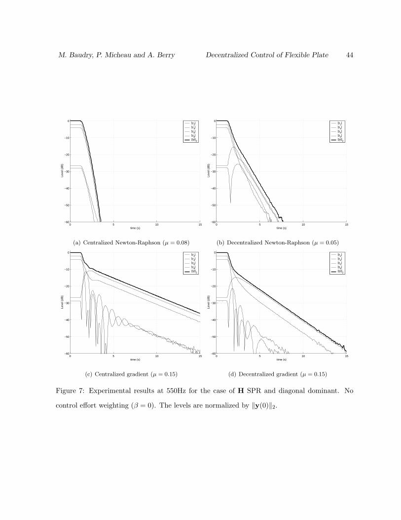
Figure 7 shows the measured convergence of the error measured by each of the PVDF sensors,

for centralized Newton, decentralized Newton and decentralized gradient. In this case, β = 0

since the closed-loop system is µ-stable without control effort weighting. For equal adaptation

coefficients, the decentralized Newton algorithm converges at a rate similar to the centralized

Newton, because the associated eigenvalues are similar. Moreover, the convergence rate is

similar for of all PVDF sensors in the case of the centralized and decentralized Newton. For the

decentralized gradient, the convergence rate varies from one PVDF sensor to another: the largest

eigenvalue of CH is associated in this case to the fastest convergence mode and the smallest

eigenvalue of CH corresponds to the slowest convergence mode. The ratio of the largest to the

smallest eigenvalue defines the condition number of CH, and is representative of the convergence

rate of the algorithm. It was experimentally verified that in this case, decentralized Newton

converges faster (cond(CH) = 2.43) than decentralized gradient (cond(CH) = 7.23) for equal

adaptation coefficients µ.

6.5 Experimental results for a case CH is SPR

At the frequency of 520 Hz, the disturbance is close to the natural frequency of the (2,3) plate

mode. The plant matrix H measured at this frequency is not diagonal dominant: the interaction

between control units is significant. The transverse velocity field of the panel due to the primary

point force driving the panel at 520 Hz is presented on the right-hand side of figure 9. It appears

that at this frequency, PZT actuator 2 is close to a vibration node and leads to a low response

of PVDF sensor 2 (|H22| = 0.36), but PZT actuator 8, close to an antinode, leads to a high

response of PVDF sensor 2: |H82| = 0.63. Consequently, the diagonal dominant condition can

not be respected. Moreover, the plant matrix is not SPR, λi(HH+H) = {5.41, 0.97, 0.51,−0.67},the system is not dissipative: it is necessary to introduce the diagonal compensator matrix C.

M. Baudry, P. Micheau and A. Berry Decentralized Control of Flexible Plate 29

Consequently, it is not possible to conclude on the closed-loop stability without investigation

of the positiveness of CH. The matrices CH associated to the decentralized gradient and

newton algorithms are both SPR; consequently, the stability can be diagonal for µ → 0: the

decentralized algorithms are predicted µ-stable.

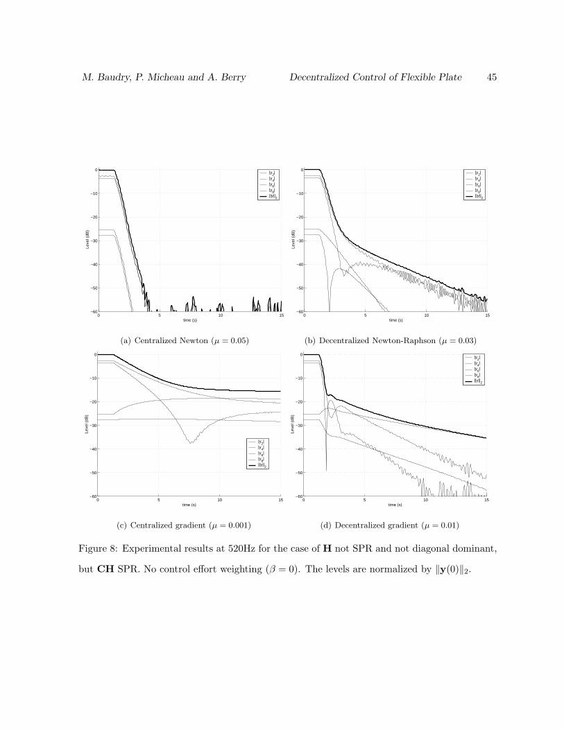
Figure 8 shows the measured convergence of the error measured by each of the PVDF sensors,

for centralized Newton, decentralized Newton and decentralized gradient. β is set to 0 since

the closed-loop system is µ-stable without control effort weighting. The centralized gradient

algorithm converges less rapidly than the decentralized gradient because the condition number

of HHH is large in comparison to the condition number of diag(H)HH. In other words, the

panel resonance leads to a ill-conditioned matrix, which implies that the centralized gradient

(cond(CH) = 97) is slower than the decentralized gradient (cond(CH) = 45). On the other

hand, the Newton algorithm is seen to have the largest convergence rates, cond(CH) = 6 for

the decentralized algorithm and cond(CH) = 1 for the centralized algorithm.

Figure 9 shows the transverse vibration filed of the panel at 520 Hz with the control off and

after convergence of the decentralized gradient algorithm. A significant decrease of the panel

response is observed not only at the sensor locations, but also over the whole panel area.

6.6 Experimental results for a case with effort weighting β

At the frequency of 680 Hz, the measured plant matrix H, is not diagonal dominant (for

example, |H11| = 0.26 but |H14| = 0.59)), H is not SPR, and the matrices CH corresponding

to decentralized gradient and decentralized Newton are not SPR: there exists eigenvalues such

that <(λi(CH)) = −0.05 for the gradient algorithm, and <(λi(CH)) = −0.5 for the Newton

algorithm. In order to guarantee that the matrix B = CH+βI is SPR, a control effort weighting

coefficient must be introduced: a value of β = 0.3 was chosen for the gradient algorithm and

β = 0.7 for the Newton algorithm. Figure 10 shows the measured convergence of the error

measured by each of the PVDF sensors, for various control algorithms. Decentralized gradient

M. Baudry, P. Micheau and A. Berry Decentralized Control of Flexible Plate 30

is seen to diverge when β = 0 and when a relatively small value µ = 0.02 of the adaptation

coefficient is chosen. On the other hand, applying an effort weighting β = 0.3 has the effect of

stabilizing the decentralized gradient when µ = 0.05. This is done however at the detriment

of a smaller attenuation of the error signals (of the order of 10 dB). On the other hand, the

performance of decentralized Newton is marginal in this case, because of the relatively large

effort weighting applied.

7 Conclusions

We have analyzed the performance and stability of decentralized active control of panel

vibration using multiple pairs combining PZT actuators and PVDF sensors distributed (and

not necessarily collocated) on the panel. The stabilization condition of the closed loop by

adjusting the convergence coefficient were especially investigated through an adjustable control

effort term in the quadratic cost function. Various necessary or sufficient conditions derived

from the plant matrix have been obtained to analyze the stability of decentralized gradient and

decentralized Newton-Raphson algorithms; these conditions, were summarized in Table I from

the most restrictive to the less restrictive condition. Figure 11 illustrates the hierarchy between

the three cases investigated in the experiments: at 550 Hz the plant matrix is diagonal dominant,

hence the stability is ensured by the low interaction between units; at 520 Hz the plant matrix

is not SPR, hence the stability is ensured by the diagonal compensator; at 680 Hz the stability

requires a control effort weighting term, consequently perfect rejection can not be reached.

While the diagonal dominance of the plant matrix H provides a sufficient condition for closed

loop µ-stability, it is not a necessary condition. Therefore, decentralized vibration control is

achievable even in the presence of strong interaction between control units. Also, the collocation

of dual actuator-sensor pairs has the very attractive property to theoretically provide a SPR plant

matrix H, but this is also a sufficient condition of µ-stability. Finally, the necessary condition

M. Baudry, P. Micheau and A. Berry Decentralized Control of Flexible Plate 31

of µ-stability (the real part of the eigenvalues of CH being positive), can be interpreted as a

tolerance on the collocation of dual actuator-sensor pairs.

M. Baudry, P. Micheau and A. Berry Decentralized Control of Flexible Plate 32

References

[1] O.N. Baumann, W.P. Engels, and S.J. Elliott. A comparison of centralised and decentralised

control for the reduction of kinetic energy and radiated sound power. In Proceedings of

ACTIVE04, Williamsburg, VA, USA, 2004.

[2] C. Bordier. Controle actif de sources inaccessibles. PhD thesis, Universite Aix-Marseille,

2003.

[3] E.K. Dimitriadis, C.R. Fuller, and C.A Rogers. Piezoelectric actuators for distributed

vibration excitation of thin plates. Journal of Vibration and Acoustics, 113(1):100–107,

Janvier 1991.

[4] S.J. Elliott. Distributed control of sound and vibration. In Proceedings of ACTIVE04,

Williamsburg, VA, USA, 2004.

[5] S.J. Elliott and C. Boucher. Interaction between multiple feedforward active control

systems. IEEE Trans. Speech and Audio Processing, 2(2):521–530, 1994.

[6] S.J. Elliott, P. Gardonio, T.C. Sors, and M.J. Brennan. Active viboacoustic control with

multiple local feedback loops. Journal of Acoustical Society of America, 111(2):908–915,

2002.

[7] O.N. Engels, W.P.and Baumann and S.J. Elliott. Centralised and decentralised feedback

control of kinetic energy. In Proceedings of ACTIVE04, Williamsburg, VA, USA, 2004.

[8] B.A. Francis and W. Wonham. The internal model principle of control theory. Automatica,

12:457–465, 1976.

[9] C.R. Fuller, S.J. Elliot, and P.A. Nelson. Active control of vibration. Academic Press,

London, 1996.

M. Baudry, P. Micheau and A. Berry Decentralized Control of Flexible Plate 33

[10] P. Gardonio, E. Bianchi, and S.J. Elliott. Smart panel with multiple decentralised units

for the control of sound transmission. part i theoretical predictions, part ii design of the

decentralised control units, part iii control system implementation. Journal of Sound and

Vibration, 274:163–232, 1996.

[11] P. Gardonio, E. Bianchi, and S.J. Elliott. Smart panel with multiple decentralised units for

the control of sound transmission. Proceeding of Active 2002, 2002.

[12] E. Kaszkurewicz and A. Bhaya. Matrix diagonal stability in systems and computation.

Birkhauser, 1999.

[13] J.H. Kim, S.B. Choi, C.C. Cheong, S.S. Han, and J.K. Lee. hinf control of structure-borne

noise of a plate featuring piezoceramic actuators. ASME Smart Material Structures, 8:1–12,

1999.

[14] E. Leboucher, P. Micheau, A. Berry, and A. L’Esperance. A stability analysis of a

decentralized adaptive feedback active control system of sinusoidal sound in free space.

JASA, 111(1):189–199, January 2002.

[15] C.K. Lee and F.C. Moon. Modal sensors/actuators. Journal of Applied Mechanics, 57:434–

441, 1990.

[16] P. Micheau and P. Coirault. Adaptive controller using filter banks to reject multi-sinusoidal

disturbance. Automatica, 36:1659–1664, 2000.

[17] P. Micheau and S. Renault. Active control of the complex envelope associated with a low

damped mode. Mechanical Systems and Signal Processing, accepted, 2005.

[18] M. Morari and E. Zafiriou. Robust Process Control. Prentice Hall, 1989.

[19] B. Petitjean and I. Legrain. Feedback controllers for active vibration suppression. J. Struct.

Control, 3:111–127, 1996.

M. Baudry, P. Micheau and A. Berry Decentralized Control of Flexible Plate 34

[20] K.B. Scribner, L.A. Sievers, and A.H. Flotow. Active narrow-band vibration isolation of

machinery noise from resonant substructures. Journal of Acoustical Society of America,

167(1):17–24, 1993.

[21] L.A. Sievers and A.H. Flotow. Comparison and extensions of control methods for narrow-

band disturbance rejection. IEEE Transactions on signal processing, 40(10):2377–2391,

October 1992.

[22] J.-J. Slotine and W. Li. Applied nonlinear control. Prentice Hall, 1991.

[23] J.Q. Sun. Some observations on physical duality and collocation of structural control sensors

and actuators. Journal of Sound and Vibration, 194:765–770, 1996.

[24] G. West-Vukovich and E.J Davison. The decentralized control of large flexible space

structures. IEEE Transactions on Automatic Control, 29(10):866–879, October 1984.

M. Baudry, P. Micheau and A. Berry Decentralized Control of Flexible Plate 35

List of Tables

I The various conditions of stability of the closed loop system . . . . . . . . . . . . 37

II Panel data . . . . . . . . . . . . . . . . . . . . . . . . . . . . . . . . . . . . . . . . 37

III BM-500 PZT actuator and PVDF sensor data . . . . . . . . . . . . . . . . . . . . 38

IV Natural frequencies of the panel . . . . . . . . . . . . . . . . . . . . . . . . . . . . 38

List of Figures

1 Physical configuration under study: a flexible panel controlled by N independent

loops . . . . . . . . . . . . . . . . . . . . . . . . . . . . . . . . . . . . . . . . . . . 39

2 Block diagram of the frequency domain controller . . . . . . . . . . . . . . . . . . 39

3 Positions of the 4 PZT-PVDF pairs on the panel . . . . . . . . . . . . . . . . . . 40

4 Magnitude of transfer function matrix coefficients between PZT actuators and

PVDF sensors. Off-diagonal coefficients (a): H28, (b): H48; Diagonal coefficients

(c): H66, (d): H88. Solid line: Experimental; Dashed line: Predicted. . . . . . . . 41

5 Stability indicators of decentralized control derived from theoretical and measured

plant matrix H: condition of H diagonal dominant, condition of CH SPR,

minimum control effort weighting β . . . . . . . . . . . . . . . . . . . . . . . . . . 42

6 Maximum value of the adaptation coefficient µmax for centralized or decentralized

gradient and Newton-Raphson adaptation in the case of 4 PZT-PVDF pairs on

the panel. . . . . . . . . . . . . . . . . . . . . . . . . . . . . . . . . . . . . . . . . 43

7 Experimental results at 550Hz for the case of H SPR and diagonal dominant. No

control effort weighting (β = 0). The levels are normalized by ‖y(0)‖2. . . . . . . 44

8 Experimental results at 520Hz for the case of H not SPR and not diagonal

dominant, but CH SPR. No control effort weighting (β = 0). The levels are

normalized by ‖y(0)‖2. . . . . . . . . . . . . . . . . . . . . . . . . . . . . . . . . . 45

M. Baudry, P. Micheau and A. Berry Decentralized Control of Flexible Plate 36

9 transverse velocity field of the panel measured by Doppler Laser Vibrometry at

520 Hz. Note that the amplitude scale is increased by a factor about 3 on the

right-hand side. . . . . . . . . . . . . . . . . . . . . . . . . . . . . . . . . . . . . . 46

10 Experimental results at 680Hz for the case of CH not SPR and not diagonal

dominant. The levels are normalized by ‖y(0)‖2. . . . . . . . . . . . . . . . . . . 47

11 The hierarchy of stability conditions shows that at 550 Hz the system is diagonal

dominant and SPR (in C6 and C7). At 520 Hz H is not SPR and not dd but

CH is SPR (in C4 but not in C6 nor C7). At 680 Hz only C3 is satisfied, control

effort weighting is necessary to stabilize the closed loop. . . . . . . . . . . . . . . 48

M. Baudry, P. Micheau and A. Berry Decentralized Control of Flexible Plate 37

Table I: The various conditions of stability of the closed loop system

Ref Condition Type Interpretation

C0 |λi(I− µ(CH + βI)| < 1 Necessary and sufficient The system is unstable if µ > µmax

C1 <(λi(CH + βI)) > 0 Necessary for C0 the system is stable if µ → 0

C2 <(λi(CH)) > 0 Sufficient for C1 Effort weighting β not necessary

C3 CH + βI SPR Sufficient for C1 diagonal stability when µ → 0

C4 CH SPR Sufficient for C2 diagonal stability and β not necessary

C5 CiHii SPR Necessary for C4 Each individual unit is stable

C6 H SPR Sufficient for C4 The system is dissipative

C7 H dd Sufficient for C4 Low interaction between units

Table II: Panel data

Parameter Value

Thickness h = 3,18 × 10-3 m

Length Lx = 48 × 10-2 m

Width Ly = 42 × 10-2 m

Young’s modulus Ep = 68,5 × 109 Pa

Poisson’s coefficient νp = 0,33

Density ρ = 2700 kg.m-3

Loss factor η = 5.0 × 10-3

M. Baudry, P. Micheau and A. Berry Decentralized Control of Flexible Plate 38

Table III: BM-500 PZT actuator and PVDF sensor data

Parameter PZT actuator PVDF sensor

Thickness ta = 1,02 × 10-3 m ts = 28 × 10-6 m

Length L(ax ) = 2,54 × 10-2 m L

(sx ) = 1 × 10-2 m

Width L(ay ) = 2,54 × 10-2 m L

(sy ) = 1,5 × 10-2 m

Young’s modulus Ea = 61,1 × 109 Pa

Poisson’s coefficient νa = 0,29

Piezoelectric coefficient d31 = -1,9 × 10-10 C/N

Piezoelectric coefficient e31 = 46 × 10-3 C.m-2

Capacitance Cs = 5 × 10-10 F

Table IV: Natural frequencies of the panel

m 1 2 1 2 3 1 3 2 4 3 4 1

n 1 1 2 2 1 3 2 3 1 3 2 4

fmn, calculated (Hz) 77 177 208 308 344 425 474 525 577 692 708 730

fmn, measured (Hz) 80 176 206 292 337 425 455 517 571 676 705 719

M. Baudry, P. Micheau and A. Berry Decentralized Control of Flexible Plate 39

Figure 1: Physical configuration under study: a flexible panel controlled by N independent loops

Figure 2: Block diagram of the frequency domain controller

M. Baudry, P. Micheau and A. Berry Decentralized Control of Flexible Plate 40

Figure 3: Positions of the 4 PZT-PVDF pairs on the panel

M. Baudry, P. Micheau and A. Berry Decentralized Control of Flexible Plate 41

0 100 200 300 400 500 600 700 800−130

−120

−110

−100

−90

−80

−70

−60

−50

Frequency (Hz)

|H| (

dB20

ref

1 V

/V)

Exper.Predic.

(a) H82

0 100 200 300 400 500 600 700 800−130

−120

−110

−100

−90

−80

−70

−60

−50

Frequency (Hz)

|H| (

dB20

ref

1 V

/V)

Exper.Predic.

(b) H84

0 100 200 300 400 500 600 700 800−130

−120

−110

−100

−90

−80

−70

−60

−50

Frequency (Hz)

|H| (

dB20

ref

1 V

/V)

Exper.Predic.

(c) H66

0 100 200 300 400 500 600 700 800−130

−120

−110

−100

−90

−80

−70

−60

−50

Frequency (Hz)

|H| (

dB20

ref

1 V

/V)

Exper.Predic.

(d) H88

Figure 4: Magnitude of transfer function matrix coefficients between PZT actuators and PVDF

sensors. Off-diagonal coefficients (a): H28, (b): H48; Diagonal coefficients (c): H66, (d): H88.

Solid line: Experimental; Dashed line: Predicted.

M. Baudry, P. Micheau and A. Berry Decentralized Control of Flexible Plate 42

500 550 600 650 700 750 800

0

0.5

1

1.5

Frequency (Hz)

ℜ(λ

i(CH

))>

0

500 550 600 650 700 750 800

0

0.5

1

1.5

Frequency (Hz)

CH

S.P

.R.

GradientNewton

500 550 600 650 700 750 8000

2

4

6

Frequency (Hz)

β min

New

ton−

Rap

hson

(a) Stability of decentralized control derived from theoretical H

500 550 600 650 700 750 8000

0.5

1

1.5

Frequency (Hz)

ℜ(λ

i(CH

))>

0

500 550 600 650 700 750 8000

0.5

1

1.5

Frequency (Hz)

CH

S.P

.R.

500 550 600 650 700 750 8000

0.5

1

1.5

Frequency (Hz)

H d

.d.

500 550 600 650 700 750 8000

0.5

1

1.5

Frequency (Hz)

β min

Decentralized GradientDecentralized Raphson−Newton

(b) Stability of decentralized control derived from measured H

Figure 5: Stability indicators of decentralized control derived from theoretical and measured

plant matrix H: condition of H diagonal dominant, condition of CH SPR, minimum control

effort weighting β

M. Baudry, P. Micheau and A. Berry Decentralized Control of Flexible Plate 43

500 550 600 650 700 750 80010

−3

10−2

10−1

100

101

Frequency (Hz)

µ max

Centralized gradient

experimentalNo delayΨ(z−1)

(a) Centralized gradient

500 550 600 650 700 750 80010

−2

10−1

100

101

Frequency (Hz)

µ max

Centralized Newton−Raphson

experimentalNo delayΨ(z−1)

(b) Centralized Newton-Raphson

500 550 600 650 700 750 80010

−2

10−1

100

101

Frequency (Hz)

µ max

Decentralized gradient

experimentalNo delayΨ(z−1)

(c) Decentralized gradient

500 550 600 650 700 750 80010

−3

10−2

10−1

100

101

Frequency (Hz)

µ max

Decentralized Newton−Raphson

experimentalNo delayΨ(z−1)

(d) Decentralized Newton-Raphson

Figure 6: Maximum value of the adaptation coefficient µmax for centralized or decentralized

gradient and Newton-Raphson adaptation in the case of 4 PZT-PVDF pairs on the panel.

M. Baudry, P. Micheau and A. Berry Decentralized Control of Flexible Plate 44

0 5 10 15−60

−50

−40

−30

−20

−10

0

time (s)

Leve

l (dB

)

|y2|

|y4|

|y6|

|y8|

||y||2

(a) Centralized Newton-Raphson (µ = 0.08)

0 5 10 15−60

−50

−40

−30

−20

−10

0

time (s)

Leve

l (dB

)

|y2|

|y4|

|y6|

|y8|

||y||2

(b) Decentralized Newton-Raphson (µ = 0.05)

0 5 10 15−60

−50

−40

−30

−20

−10

0

time (s)

Leve

l (dB

)

|y2|

|y4|

|y6|

|y8|

||y||2

(c) Centralized gradient (µ = 0.15)

0 5 10 15−60

−50

−40

−30

−20

−10

0

time (s)

Leve

l (dB

)

|y2|

|y4|

|y6|

|y8|

||y||2

(d) Decentralized gradient (µ = 0.15)

Figure 7: Experimental results at 550Hz for the case of H SPR and diagonal dominant. No

control effort weighting (β = 0). The levels are normalized by ‖y(0)‖2.

M. Baudry, P. Micheau and A. Berry Decentralized Control of Flexible Plate 45

0 5 10 15−60

−50

−40

−30

−20

−10

0

time (s)

Leve

l (dB

)

|y2|

|y4|

|y6|

|y8|

||y||2

(a) Centralized Newton (µ = 0.05)

0 5 10 15−60

−50

−40

−30

−20

−10

0

time (s)

Leve

l (dB

)

|y2|

|y4|

|y6|

|y8|

||y||2

(b) Decentralized Newton-Raphson (µ = 0.03)

0 5 10 15−60

−50

−40

−30

−20

−10

0

time (s)

Leve

l (dB

)

|y2|

|y4|

|y6|

|y8|

||y||2

(c) Centralized gradient (µ = 0.001)

0 5 10 15−60

−50

−40

−30

−20

−10

0

time (s)

Leve

l (dB

)

|y2|

|y4|

|y6|

|y8|

||y||2

(d) Decentralized gradient (µ = 0.01)

Figure 8: Experimental results at 520Hz for the case of H not SPR and not diagonal dominant,

but CH SPR. No control effort weighting (β = 0). The levels are normalized by ‖y(0)‖2.

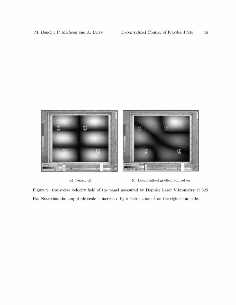
M. Baudry, P. Micheau and A. Berry Decentralized Control of Flexible Plate 46

(a) Control off (b) Decentralized gradient control on

Figure 9: transverse velocity field of the panel measured by Doppler Laser Vibrometry at 520

Hz. Note that the amplitude scale is increased by a factor about 3 on the right-hand side.

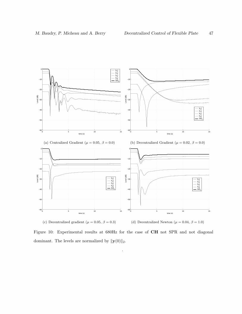
M. Baudry, P. Micheau and A. Berry Decentralized Control of Flexible Plate 47

0 5 10 15−60

−50

−40

−30

−20

−10

0

time (s)

Leve

l (dB

)

|y2|

|y4|

|y6|

|y8|

||y||2

(a) Centralized Gradient (µ = 0.05, β = 0.0)

0 5 10 15−60

−50

−40

−30

−20

−10

0

time (s)

Leve

l (dB

)

|y2|

|y4|

|y6|

|y8|

||y||2

(b) Decentralized Gradient (µ = 0.02, β = 0.0)

0 5 10 15−60

−50

−40

−30

−20

−10

0

time (s)

Leve

l (dB

)

|y2|

|y4|

|y6|

|y8|

||y||2

(c) Decentralized gradient (µ = 0.05, β = 0.3)

0 5 10 15−60

−50

−40

−30

−20

−10

0

time (s)

Leve

l (dB

)

|y2|

|y4|

|y6|

|y8|

||y||2

(d) Decentralized Newton (µ = 0.04, β = 1.0)

Figure 10: Experimental results at 680Hz for the case of CH not SPR and not diagonal

dominant. The levels are normalized by ‖y(0)‖2.

.

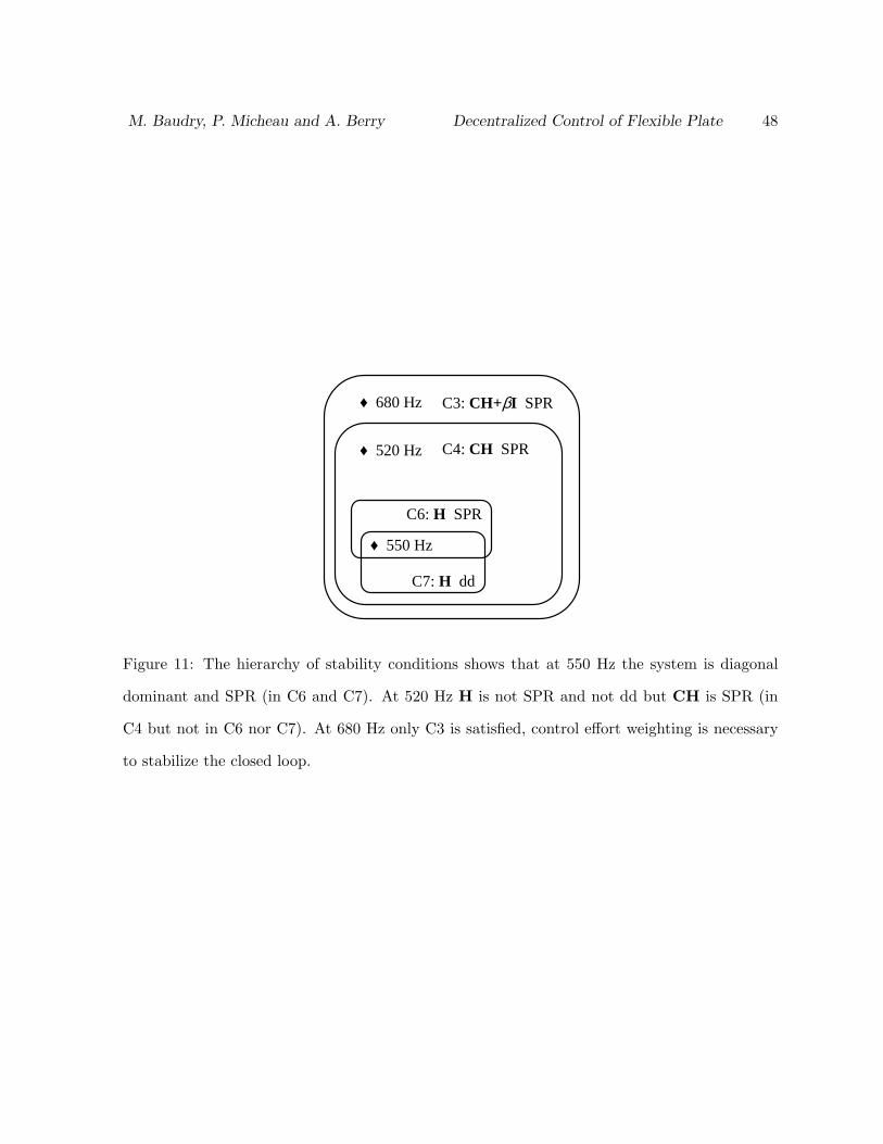
M. Baudry, P. Micheau and A. Berry Decentralized Control of Flexible Plate 48

C6: H SPR

C7: H dd

♦ 550 Hz Hz

♦ 520 Hz Hz

♦ 680 Hz C3: CH+βI SPR

C4: CH SPR

Figure 11: The hierarchy of stability conditions shows that at 550 Hz the system is diagonal

dominant and SPR (in C6 and C7). At 520 Hz H is not SPR and not dd but CH is SPR (in

C4 but not in C6 nor C7). At 680 Hz only C3 is satisfied, control effort weighting is necessary

to stabilize the closed loop.