Decentralized Matching:The Role of Commitment

Effrosyni Diamantoudi∗CIREQ and Concordia University

Eiichi Miyagawa†

Columbia University

Licun Xue‡

CIREQ and McGill University

April 16, 2007

AbstractGale and Shapley’s matching model has a “stable matching,” where no

pair of a firm and a worker prefer each other. The main application has been aone-time matching with a centralized matchmaking mechanism. However, notmany job markets are centralized, and participants may remain active in themarket even after they are matched. This paper studies an infinite-horizongame where matching takes place every period in a decentralized fashion.Every period, firms with vacant positions make offers to workers, who thendecide which offer to accept. The game depends on whether agents committo their relationships. With no commitment, a worker can leave the currentemployer but may also be dismissed. With two-sided commitment, matchedpairs withdraw from the market. With one-sided commitment, workers areprotected from dismissal but remain active in the market, as in the case oftenured professors. We characterize stationary equilibria for each commit-ment structure. Without commitment, equilibrium outcomes coincide withstable matchings; neither side of the market is favored and the set of unem-ployed workers is equilibrium-invariant. With commitment, either one-sidedor two-sided, an equilibrium may reach an unstable matching even if thereis no initial commitment. With one-sided commitment, an equilibrium mayeven yield an unstable matching where all workers are worse off than in everystable matching. In this case, the workers are better off if job protections areremoved.

JEL Classification: C72, C73, C78, D85, J44, J63.Keywords: Matching, job protection.

∗Department of Economics, Concordia University, 1455 de Maisonneuve Blvd. West, Montreal,Quebec, H3G 1M8, Canada; ediamant@alcor.concordia.ca

†Department of Economics, Columbia University, 420 West 118th Street, New York, NY 10027,U.S.A.; em437@columbia.edu

‡Department of Economics, McGill University, Leacock Building, Room 433, 855 SherbrookeStreet West, Montreal, Quebec, H3A 2T7, Canada; licun.xue@mcgill.ca

1 Introduction

The basic idea of matching theory is that a matching between agents is not stable ifthere exists a pair of agents who prefer each other to their current partners. Such apair is called a “blocking pair,” and matchings with no blocking pair are called “sta-ble matchings.” For the standard matching problem, a stable matching exists forany number of agents and any profile of preferences, as shown by Gale and Shapley(1962). Gale and Shapley also give an algorithm that finds a stable matching. Thealgorithm has been used since early 1950s by a centralized matchmaking mecha-nism to assign new American physicians to hospitals (Roth, 1984). The hypothesisof Roth (1991) is that the success of a centralized labor market depends on whetherthe matchmaking mechanism generates a stable matching.

The focus of the literature has been matching markets that are centralized, whereparticipants submit preferences to the center and a matching is determined by an al-gorithm. On the other hand, many markets—including the market for economists—are decentralized, where a matching is determined by a series of offers and replieschosen strategically by the agents. How does a decentralized market compare witha centralized one? Does a decentralized market generate a stable matching? Is theanswer sensitive to the way in which the decentralized market operates?

To address these questions, this paper studies equilibria in a dynamic game ofmatching. We extend the original Gale–Shapley model to a dynamic and nonco-operative setting where firms and workers interact repeatedly in a decentralizedmanner. In every period, firms with vacant positions make offers to workers, whothen choose individually which offer to accept. To raise realism, we assume thateach worker observes only the offers made to her. The market takes place everyperiod—for example, once a year—and all agents derive utility from their matchingin each period. We focus on stationary equilibria, where actions vary only with thepayoff-relevant state of the game.

Our dynamic matching model makes it possible to analyze the role of commit-ment, in particular, how equilibrium matching depends on whether agents committhemselves to their employment relationships. In our stylized model, three interest-ing possibilities can be considered. The first possibility is that, once a pair of agentsare matched, they withdraw from the market and stay together permanently. Thesecond possibility is that agents make no commitment beyond one period. That is,employees can accept new job offers but may also be dismissed. The third possibil-ity is that firms make commitments while workers do not. That is, workers remainactive in the job market but are protected from dismissal, as in the case of tenuredprofessors and government employees.

In the absence of commitment, we show that every stationary equilibrium yieldsa stable matching. An implication is that if a worker is unemployed in one equi-librium, he is unemployed in every equilibrium. We also show that, in the absenceof commitment, stationary equilibria can yield any stable matching: no bias to-ward a subset of stable matchings exists. By Gale and Shapley, there exists a stable

1

matching that is unambiguously best for one side of the market. The so-called “firm-optimal stable matching” is a stable matching that is best for all firms and worst forall workers. There also exists a “worker-optimal” stable matching. Each of thesematchings can be supported by an equilibrium. It should be noted that there existsan asymmetry between firms and workers in the game: only firms can make offers,and workers can only accept or reject offers. Despite the asymmetry and withoutjob security laws, the market need not be unfavorable to workers.

On the other hand, if at least one side of the market makes commitment, a sta-tionary equilibrium need not yield a stable matching. Of course, the result is trivialif the game starts with many committed firms and workers and no stable matchingis reachable. However, the result obtains even if agents start with no commitment.Without any initial commitment and without any random shock or mistake, it ispossible that agents knowingly and willingly reach an unstable matching and staythere. A blocking pair exists in the equilibrium matching but does not get together.For the one-sided commitment case, the reason is that, if the firm in the blockingpair makes an offer to the blocking partner, the action triggers a chain reaction inwhich a firm that lost a worker takes another worker from another firm. The chainreturns to the firm who started the process and the firm ends up losing the blockingpartner. Anticipating this, the firm in the blocking pair does not make an offer tothe blocking partner.

For the one-sided commitment case, it is even possible that the equilibrium out-come is an unstable matching where all workers are worse off than in any stablematching. This is interesting since job protections are intended to protect workers.As the model predicts, if job protections are lifted, every equilibrium yields a stablematching. Therefore, in the example, all workers are better off if job protections areremoved.

An example of workers who are protected from dismissal is public school teach-ers in the US. In most states, teachers in public schools are strongly protected bystate law and the collective bargaining agreement between the district and the teach-ers’ union. Dismissing a teacher is known to be difficult and hence rare becausethe principal has to go through a lengthy legal procedure (Bridges, 1992; Ballou,1999). Weakening job protections for public school teachers has been a major po-litical issue but met a strong resistance from teachers’ unions. For example, in 2005,Governor Schwarzenegger of California proposed a measure, called Proposition 74,to make it easier to dismiss teachers. According to the press, California TeachersAssociation spent more than $7 million to defeat the measure. The measure wasindeed rejected by the public in a special election.

The results of this study suggest that job protections need not be good for teach-ers. The result for the no-commitment case shows that, without job protections, themarket reaches a stable matching and has no systematic bias against either side ofthe market. With job protections, unstable matchings are possible but teachers maynot gain from it. It is theoretically possible that job protections make all teachersworse off.

2

There are a few papers that also study decentralized matching markets.Haeringer and Wooders (2006) study a similar game but there are a few criticaldifferences. They assume that once a pair forms a partnership, it is the end of thegame for the pair, as in our two-sided commitment case. Furthermore, they assumethat the payoff realizes only once and depends only on the identity of the partner.There is no time preferences. Their model therefore can be thought of as describinga job market for a single year. Our model, on the other hand, describes the dynamicsof a job market over years where agents collect payoffs as they go along. Techni-cally, their model is similar to a bargaining model while ours is similar to a repeatedgame.

Blum, Roth, and Rothblum (1997) consider an algorithm that finds a stablematching when some of the agents are initially matched. Toward the end of thepaper, the authors study a game similar to ours with one-sided commitment. How-ever, the payoff realizes only once and depends only on the final matching. Thepaper characterizes Nash equilibria in “preference strategies,” where each agentuses a single (possibly false) preference ordering for the decision at every node [seealso Pais (2005) for an extension].

Alcalde and Romero-Medina (2000), in the context of mechanism design theory,study a game where only one round of offers and replies takes place. That is, firmsmake offers, workers reply, and the game ends. They show that this game achieves(or implements) stable matchings [see also Alcalde, Perez-Castrillo, and Romero-Medina (1998)].

Konishi and Sapozhnikov (2005) consider a model where firms make job offerswith a variable salary level. They consider a multi-period model where firms canchoose when to make their offer. But, as in Haeringer and Wooders, agents who getmatched exit the game.

There is also a strand of literature that studies, within the original static model,whether a myopic adjustment process based on the blocking notion converges toa stable matching. Knuth (1976) gives an example showing that a sequence ofsuccessive myopic blockings may form a cycle and never reach a stable matching.Roth and Vande Vate (1990) show that, if a blocking pair is chosen randomly ateach step of the process, the process reaches a stable matching with probability one.The sequential blocking process implicity assumes that no commitment is made bythe agents. The critical feature of the process is that the agents are myopic: in eachstep, the acting blocking pair behaves as if the process terminates in their turn.

Our dynamic matching game also brings some insights from the literature ofdynamic coalition-formation games [see, e.g., Chatterjee, Dutta, Ray, and Sengupta(1993), Bloch (1996), Ray and Vohra (1999)] to the study of decentralized matchingmarket. With a dynamic game of coalition formation, in each period a proposer isselected among the set of active players using a protocol (often exogenously given)to make a proposal of forming a coalition and prospective members respond sequen-tially to such a proposal. This coalition is formed if all prospective members acceptthe proposal. Therefore, in each period, at most one coalition can form. In contrast,

3

in our dynamic matching game, all active firms can simultaneously make offers andseveral firm-worker pairs can form in a single period. Another feature of our gameis the different commitment structures that naturally arise in a labor market.

In the next section, we introduce a standard static model of matching. Section 3defines our dynamic game of matching. Sections 4–6 study respectively the threeaforementioned commitment structures. A short conclusion follows. The appendixcontains proofs of several results.

2 Static Matching Problem

In a static matching problem, introduced by Gale and Shapley (1962), there are twodisjoint finite sets F and W of firms and workers. An agent refers to either a firm ora worker. Each agent i has a utility function ui such that

u f : W ∪{ f}→ R for all f ∈ F ,

uw : F ∪{w}→ R for all w ∈W .

Here, ui( j) denotes agent i’s utility of being matched with agent j. The number ui(i)is the agent’s utility of being unmatched. We normalize utilities so that ui(i) = 0 forall i. If ui( j) ≥ 0, we say j is acceptable to i. We assume that preferences have noindifference: ui( j) = ui(k) only if j = k.

For simplicity, we assume that each firm has only one position. A matching isthen a function µ : F ∪W → F ∪W such that (i) for all f ∈ F , µ( f ) ∈W ∪{ f},(ii) for all w ∈W , µ(w) ∈ F ∪{w}, and (iii) for all i, j ∈ F ∪W , if µ(i) = j thenµ( j) = i. Here, µ(i) denotes the agent with whom i is matched. If µ(i) = i, then i isnot matched with anyone. Let µ /0 denote the matching in which no one is matched.

A matching µ is individually rational if, for all i ∈ F ∪W , µ(i) is acceptable toi. A matching µ is blocked by a pair ( f ,w) ∈ F×W if

u f (w) > u f (µ( f )),uw( f ) > uw(µ(w)).

That is, f and w both prefer each other to their partner under µ . A matching µ isstable if it is individually rational and has no blocking pair. By Gale and Shapley(1962), a stable matching exists for any matching problem.

3 Dynamic Matching Game

We consider a situation where agents are matched every period in a de-centralized fashion. A dynamic matching game, parameterized by a list(F,W,(ui,δi)i∈F∪W ,Fc,Wc), is defined as follows.

4

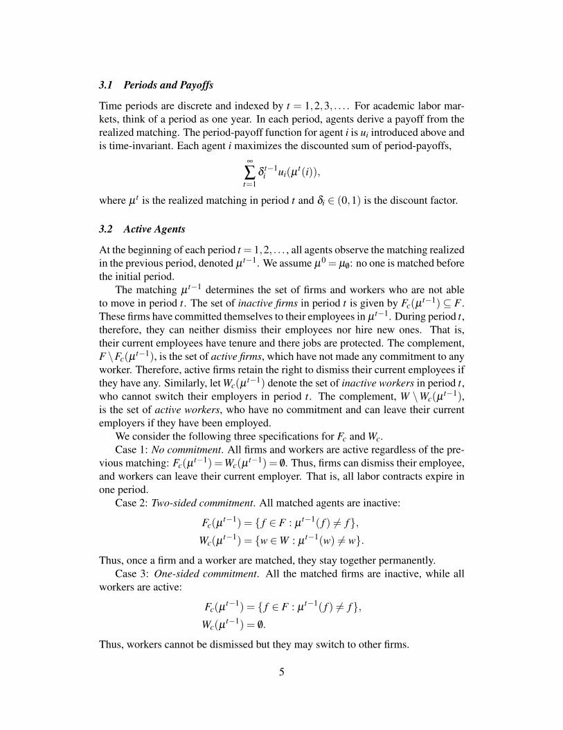
3.1 Periods and Payoffs

Time periods are discrete and indexed by t = 1,2,3, . . . . For academic labor mar-kets, think of a period as one year. In each period, agents derive a payoff from therealized matching. The period-payoff function for agent i is ui introduced above andis time-invariant. Each agent i maximizes the discounted sum of period-payoffs,

∞

∑t=1

δ t−1i ui(µ t(i)),

where µ t is the realized matching in period t and δi ∈ (0,1) is the discount factor.

3.2 Active Agents

At the beginning of each period t = 1,2, . . . , all agents observe the matching realizedin the previous period, denoted µ t−1. We assume µ0 = µ /0: no one is matched beforethe initial period.

The matching µ t−1 determines the set of firms and workers who are not ableto move in period t. The set of inactive firms in period t is given by Fc(µ t−1)⊆ F .These firms have committed themselves to their employees in µ t−1. During period t,therefore, they can neither dismiss their employees nor hire new ones. That is,their current employees have tenure and there jobs are protected. The complement,F \Fc(µ t−1), is the set of active firms, which have not made any commitment to anyworker. Therefore, active firms retain the right to dismiss their current employees ifthey have any. Similarly, let Wc(µ t−1) denote the set of inactive workers in period t,who cannot switch their employers in period t. The complement, W \Wc(µ t−1),is the set of active workers, who have no commitment and can leave their currentemployers if they have been employed.

We consider the following three specifications for Fc and Wc.Case 1: No commitment. All firms and workers are active regardless of the pre-

vious matching: Fc(µ t−1) =Wc(µ t−1) = /0. Thus, firms can dismiss their employee,and workers can leave their current employer. That is, all labor contracts expire inone period.

Case 2: Two-sided commitment. All matched agents are inactive:

Fc(µ t−1) = { f ∈ F : µ t−1( f ) 6= f},Wc(µ t−1) = {w ∈W : µ t−1(w) 6= w}.

Thus, once a firm and a worker are matched, they stay together permanently.Case 3: One-sided commitment. All the matched firms are inactive, while all

workers are active:

Fc(µ t−1) = { f ∈ F : µ t−1( f ) 6= f},Wc(µ t−1) = /0.

Thus, workers cannot be dismissed but they may switch to other firms.

5

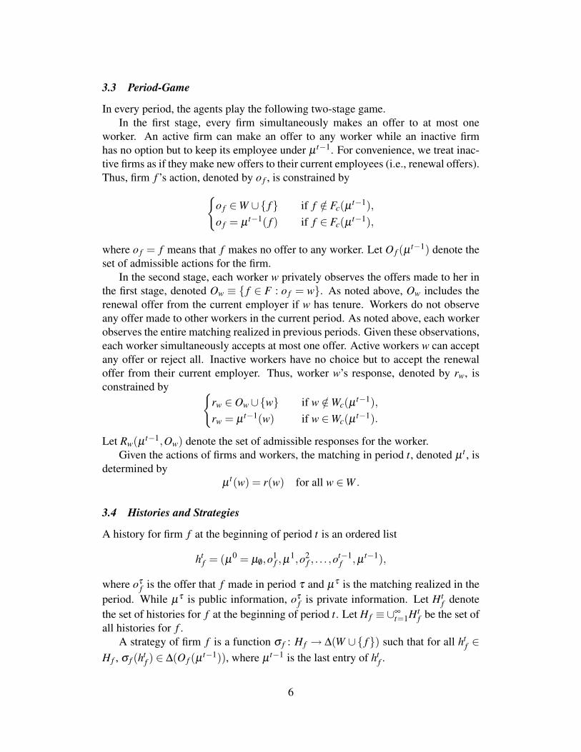
3.3 Period-Game

In every period, the agents play the following two-stage game.In the first stage, every firm simultaneously makes an offer to at most one

worker. An active firm can make an offer to any worker while an inactive firmhas no option but to keep its employee under µ t−1. For convenience, we treat inac-tive firms as if they make new offers to their current employees (i.e., renewal offers).Thus, firm f ’s action, denoted by o f , is constrained by

{o f ∈W ∪{ f} if f /∈ Fc(µ t−1),o f = µ t−1( f ) if f ∈ Fc(µ t−1),

where o f = f means that f makes no offer to any worker. Let O f (µ t−1) denote theset of admissible actions for the firm.

In the second stage, each worker w privately observes the offers made to her inthe first stage, denoted Ow ≡ { f ∈ F : o f = w}. As noted above, Ow includes therenewal offer from the current employer if w has tenure. Workers do not observeany offer made to other workers in the current period. As noted above, each workerobserves the entire matching realized in previous periods. Given these observations,each worker simultaneously accepts at most one offer. Active workers w can acceptany offer or reject all. Inactive workers have no choice but to accept the renewaloffer from their current employer. Thus, worker w’s response, denoted by rw, isconstrained by {

rw ∈ Ow∪{w} if w /∈Wc(µ t−1),rw = µ t−1(w) if w ∈Wc(µ t−1).

Let Rw(µ t−1,Ow) denote the set of admissible responses for the worker.Given the actions of firms and workers, the matching in period t, denoted µ t , is

determined byµ t(w) = r(w) for all w ∈W .

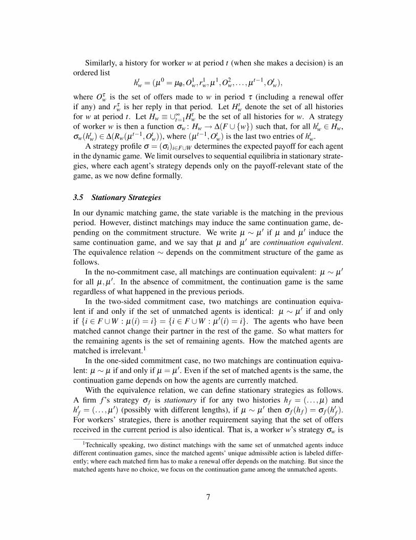
3.4 Histories and Strategies

A history for firm f at the beginning of period t is an ordered list

htf = (µ0 = µ /0,o1

f ,µ1,o2f , . . . ,o

t−1f ,µ t−1),

where oτf is the offer that f made in period τ and µτ is the matching realized in the

period. While µτ is public information, oτf is private information. Let Ht

f denotethe set of histories for f at the beginning of period t. Let H f ≡∪∞

t=1Htf be the set of

all histories for f .A strategy of firm f is a function σ f : H f → ∆(W ∪{ f}) such that for all ht

f ∈H f , σ f (ht

f ) ∈ ∆(O f (µ t−1)), where µ t−1 is the last entry of htf .

6

Similarly, a history for worker w at period t (when she makes a decision) is anordered list

htw = (µ0 = µ /0,O1

w,r1w,µ1,O2

w, . . . ,µ t−1,Otw),

where Oτw is the set of offers made to w in period τ (including a renewal offer

if any) and rτw is her reply in that period. Let Ht

w denote the set of all historiesfor w at period t. Let Hw ≡ ∪∞

t=1Htw be the set of all histories for w. A strategy

of worker w is then a function σw : Hw → ∆(F ∪{w}) such that, for all htw ∈ Hw,

σw(htw) ∈ ∆(Rw(µ t−1,Ot

w)), where (µ t−1,Otw) is the last two entries of ht

w.A strategy profile σ = (σi)i∈F∪W determines the expected payoff for each agent

in the dynamic game. We limit ourselves to sequential equilibria in stationary strate-gies, where each agent’s strategy depends only on the payoff-relevant state of thegame, as we now define formally.

3.5 Stationary Strategies

In our dynamic matching game, the state variable is the matching in the previousperiod. However, distinct matchings may induce the same continuation game, de-pending on the commitment structure. We write µ ∼ µ ′ if µ and µ ′ induce thesame continuation game, and we say that µ and µ ′ are continuation equivalent.The equivalence relation ∼ depends on the commitment structure of the game asfollows.

In the no-commitment case, all matchings are continuation equivalent: µ ∼ µ ′for all µ,µ ′. In the absence of commitment, the continuation game is the sameregardless of what happened in the previous periods.

In the two-sided commitment case, two matchings are continuation equiva-lent if and only if the set of unmatched agents is identical: µ ∼ µ ′ if and onlyif {i ∈ F ∪W : µ(i) = i} = {i ∈ F ∪W : µ ′(i) = i}. The agents who have beenmatched cannot change their partner in the rest of the game. So what matters forthe remaining agents is the set of remaining agents. How the matched agents arematched is irrelevant.1

In the one-sided commitment case, no two matchings are continuation equiva-lent: µ ∼ µ if and only if µ = µ ′. Even if the set of matched agents is the same, thecontinuation game depends on how the agents are currently matched.

With the equivalence relation, we can define stationary strategies as follows.A firm f ’s strategy σ f is stationary if for any two histories h f = (. . . ,µ) andh′f = (. . . ,µ ′) (possibly with different lengths), if µ ∼ µ ′ then σ f (h f ) = σ f (h′f ).For workers’ strategies, there is another requirement saying that the set of offersreceived in the current period is also identical. That is, a worker w’s strategy σw is

1Technically speaking, two distinct matchings with the same set of unmatched agents inducedifferent continuation games, since the matched agents’ unique admissible action is labeled differ-ently; where each matched firm has to make a renewal offer depends on the matching. But since thematched agents have no choice, we focus on the continuation game among the unmatched agents.

7

stationary if for any two histories hw = (. . . ,µ ,Ow) and h′w = (. . . ,µ ′,O′w), if µ ∼ µ ′

and Ow = O′w then σw(hw) = σw(h′w). A stationary equilibrium is a sequential equi-

librium in which everyone’s strategy is stationary.

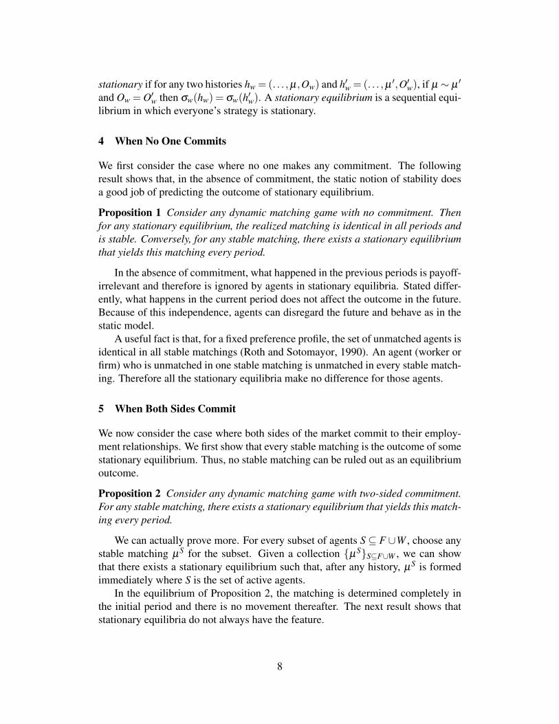
4 When No One Commits

We first consider the case where no one makes any commitment. The followingresult shows that, in the absence of commitment, the static notion of stability doesa good job of predicting the outcome of stationary equilibrium.

Proposition 1 Consider any dynamic matching game with no commitment. Thenfor any stationary equilibrium, the realized matching is identical in all periods andis stable. Conversely, for any stable matching, there exists a stationary equilibriumthat yields this matching every period.

In the absence of commitment, what happened in the previous periods is payoff-irrelevant and therefore is ignored by agents in stationary equilibria. Stated differ-ently, what happens in the current period does not affect the outcome in the future.Because of this independence, agents can disregard the future and behave as in thestatic model.

A useful fact is that, for a fixed preference profile, the set of unmatched agents isidentical in all stable matchings (Roth and Sotomayor, 1990). An agent (worker orfirm) who is unmatched in one stable matching is unmatched in every stable match-ing. Therefore all the stationary equilibria make no difference for those agents.

5 When Both Sides Commit

We now consider the case where both sides of the market commit to their employ-ment relationships. We first show that every stable matching is the outcome of somestationary equilibrium. Thus, no stable matching can be ruled out as an equilibriumoutcome.

Proposition 2 Consider any dynamic matching game with two-sided commitment.For any stable matching, there exists a stationary equilibrium that yields this match-ing every period.

We can actually prove more. For every subset of agents S⊆ F ∪W , choose anystable matching µS for the subset. Given a collection {µS}S⊆F∪W , we can showthat there exists a stationary equilibrium such that, after any history, µS is formedimmediately where S is the set of active agents.

In the equilibrium of Proposition 2, the matching is determined completely inthe initial period and there is no movement thereafter. The next result shows thatstationary equilibria do not always have the feature.

8

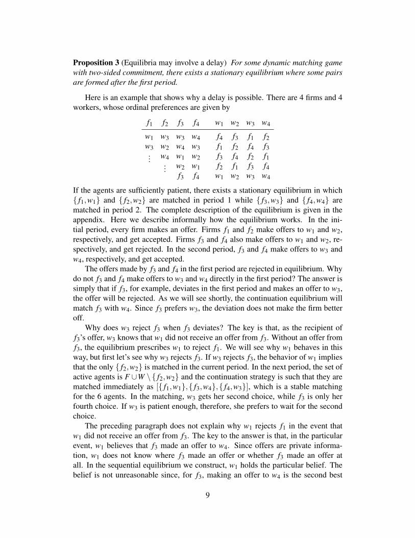
Proposition 3 (Equilibria may involve a delay) For some dynamic matching gamewith two-sided commitment, there exists a stationary equilibrium where some pairsare formed after the first period.

Here is an example that shows why a delay is possible. There are 4 firms and 4workers, whose ordinal preferences are given by

f1 f2 f3 f4 w1 w2 w3 w4

w1 w3 w3 w4 f4 f3 f1 f2w3 w2 w4 w3 f1 f2 f4 f3... w4 w1 w2 f3 f4 f2 f1

... w2 w1 f2 f1 f3 f4f3 f4 w1 w2 w3 w4

If the agents are sufficiently patient, there exists a stationary equilibrium in which{ f1,w1} and { f2,w2} are matched in period 1 while { f3,w3} and { f4,w4} arematched in period 2. The complete description of the equilibrium is given in theappendix. Here we describe informally how the equilibrium works. In the ini-tial period, every firm makes an offer. Firms f1 and f2 make offers to w1 and w2,respectively, and get accepted. Firms f3 and f4 also make offers to w1 and w2, re-spectively, and get rejected. In the second period, f3 and f4 make offers to w3 andw4, respectively, and get accepted.

The offers made by f3 and f4 in the first period are rejected in equilibrium. Whydo not f3 and f4 make offers to w3 and w4 directly in the first period? The answer issimply that if f3, for example, deviates in the first period and makes an offer to w3,the offer will be rejected. As we will see shortly, the continuation equilibrium willmatch f3 with w4. Since f3 prefers w3, the deviation does not make the firm betteroff.

Why does w3 reject f3 when f3 deviates? The key is that, as the recipient off3’s offer, w3 knows that w1 did not receive an offer from f3. Without an offer fromf3, the equilibrium prescribes w1 to reject f1. We will see why w1 behaves in thisway, but first let’s see why w3 rejects f3. If w3 rejects f3, the behavior of w1 impliesthat the only { f2,w2} is matched in the current period. In the next period, the set ofactive agents is F ∪W \{ f2,w2} and the continuation strategy is such that they arematched immediately as [{ f1,w1},{ f3,w4},{ f4,w3}], which is a stable matchingfor the 6 agents. In the matching, w3 gets her second choice, while f3 is only herfourth choice. If w3 is patient enough, therefore, she prefers to wait for the secondchoice.

The preceding paragraph does not explain why w1 rejects f1 in the event thatw1 did not receive an offer from f3. The key to the answer is that, in the particularevent, w1 believes that f3 made an offer to w4. Since offers are private informa-tion, w1 does not know where f3 made an offer or whether f3 made an offer atall. In the sequential equilibrium we construct, w1 holds the particular belief. Thebelief is not unreasonable since, for f3, making an offer to w4 is the second best

9

response. The action is actually the best response if f3 is sufficiently impatient.If f3 indeed made an offer to w4, the equilibrium prescribes w4 to accept the offer.Therefore w1 believes that if she rejects f1, the set of active agents in the next periodwill be { f1, f4,w1,w3} and the continuation strategy will prescribe the agents to bematched immediately as [{ f1,w3},{ f4,w1}]. The outcome is a stable matching forthe 4 agents, where both workers get their first choice. Thus, by rejecting f1 in theinitial period, w1 can get the first choice in the next period. If w1 is patient enough,therefore, she prefers to wait for the first choice.

The equilibrium outcome, where { fi,wi} is matched for all i, is not a stablematching, being blocked by f2 and w3. Therefore,

Proposition 4 (An equilibrium matching may be unstable) For some dynamicmatching game with two-sided commitment, there exists a stationary equilibriumwhose final matching is not stable.

The question is why the blocking pair does not get together. Why does not f2make an offer to w3 in the first period? They prefer each other, and once they arematched, they commit to each other. The answer is that, if f2 makes an offer tow3, the offer will be rejected. In the continuation equilibrium, f2 will be matchedwith w2. Thus the deviation only delays the matching with the same worker. Thequestion is then: why does w3 reject f2? The answer is that if w3 rejects f2, the setof active agents in the next period is F ∪W \{ f1,w1} and the continuation strategyprescribes them to be matched as [{ f2,w2},{ f3,w4},{ f4,w3}], which is a stablematching for the 6 agents. In the matching, w3 gets her second choice, while herblocking partner, f2, is only her third choice. If w3 is patient enough, therefore, sherejects the blocking partner in order to be matched with an even more desirable firmin the next period.

The above description shows that the incentives that support delay and insta-bility in the equilibrium have a similar structure. Delay and instability prevail inequilibrium because a firm’s attempt to deviate from the equilibrium to either getthe same worker earlier or get together with the blocking partner is thwarted by arejection from the worker. The worker rejects the firm since doing so affects thecontinuation play in the worker’s favor. This is the case even though offers are ob-served privately and the rejected offer is a deviation from an equilibrium. Rejectinga private out-of-equilibrium offer can change the continuation play since the devia-tion by the firm also affects the behavior of the worker who did not receive an offerfrom the firm.

The result relies on the standard assumption that the continuation equilibriumcan vary with the state in any way. There is no a priori restriction on the relation-ship between the current state and equilibrium selection for the continuation game.Although the treatment is standard, it makes one wonder whether there might be areasonable restriction on how the continuation equilibrium relates to the state. In theremainder of the section, we suggest one natural restriction and see its implications.

10

To motivate the restriction, suppose that, after a history, 3 firms and 3 work-ers are active, and the continuation equilibrium prescribes them to be matched as[{ f1,w1},{ f2,w2},{ f3,w3}]. Suppose further that, for whatever reason, only thepair { f1,w1} was formed in the current period. Stationarity alone does not putany restriction on how the remaining four agents will be matched in the continua-tion game. However, one natural expectation is that the remaining agents will bematched as [{ f2,w2},{ f3,w3}] since it was the initial expectation. It appears to bea strong focal point. Why does anyone expect [{ f2,w3},{ f3,w2}]?

The formalize the idea, let us limit ourselves to pure strategies. For any pure-strategy stationary strategy profile σ and any subset S ⊆ F ∪W , let m(σ ,S) denotethe matching within S that realizes as the final result under σ in the continuationgame where S is the initial set of active agents.

Definition A pure-strategy stationary equilibrium is consistent if for any subsetS⊆ F∪W and any subset T ⊆ S, if T is obtained from S by removing some matchedpairs in µ ≡ m(σ ,S) (i.e., for any firm f ∈ S \T , µ( f ) is a worker in S \T ), thenm(σ ,T ) = µ|T .

Thus, if µ is the final matching in a continuation game, then after some of thepairs in µ are formed, the remaining agents are matched according to µ .

Proposition 5 For any dynamic matching game with two-sided commitment andfor any pure-strategy consistent stationary equilibrium, the final matching is stable.

Proof. Let µ be the final matching (namely, µ = m(σ ,F ∪W )) and suppose thatit is unstable. Let ( f ,w) be a blocking pair in µ . We choose a pair so that f isthe most preferred firm that forms a blocking pair with w.2 Then consider a subsetT = { f ,µ( f ),w,µ(w)}∪ {i ∈ F ∪W : µ(i) = i}. Within the subset, f is w’s firstchoice among the firms for which w is acceptable. Therefore, if T is the set of activeagents and f makes an offer to w, w will accept. So, in the continuation game, fgets w or someone better. However, consistency requires f to be matched with µ( f )in the continuation game. This is a contradiction since f prefers w to µ( f ). ¤

Proposition 6 There exists a dynamic matching game with two-sided commitmentwhere every pure-strategy stationary equilibrium is inconsistent.

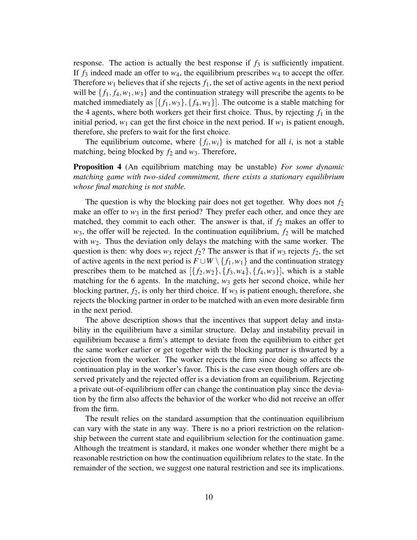
Proof. Consider a 5×5 matching problem with the following ordinal preferences:

f1 f2 f3 f4 f5 w1 w2 w3 w4 w5

w1 w2 w3 w4 w5 f2 f1 f1 f4 f3w3 w1 w5 ...

... f3 f2 f3 f3 f5w2 ... w1 f1 ...

......

...... w4 ...f3

2That is, if ( f ′,w) is a blocking pair and f ′ 6= f , then uw( f ′) < uw( f ).

11

The unique stable matching is where { fi,wi} is formed for all i. Denote the match-ing by µ1. Suppose, toward a contradiction, that there exists a pure-strategy consis-tent stationary equilibrium. Then, by Proposition 5, the final result of the equilib-rium is µ1. Consider a subset S ≡ { f1, f2, f3,w1,w2,w4}. Within the subset, thereis a unique stable matching, which is µ2 ≡ [{ f1,w2},{ f2,w1},{ f3,w4}]. Considerthe continuation game where S is the initial set of active agents. Observe that thecontinuation equilibrium remains stationary and consistent. Therefore, by Propo-sition 5, the final result of the continuation equilibrium is µ2 (i.e., m(σ ,S) = µ2).Now, consider a subset T ≡ { f1, f2,w1,w2}. Since T is obtained from S by remov-ing a matched pair in µ2, consistency implies that in the continuation game whereT is the initial set of active agents, the final result is µ2|T = [{ f1,w2},{ f2,w1}]. Onthe other hand, T is also obtained from the entire set of F ∪W by removing threematched pairs in µ1. Therefore, consistency also implies that the same continuationgame for T results in µ1|T = [{ f1,w1},{ f2,w2}]. ¤

6 When Only Firms Commit

We now turn to the one-sided commitment case. As in academic job markets forseniors, workers are protected but do not commit themselves to their employers. Instationary equilibria, the payoff-relevant state is the matching in the previous period.

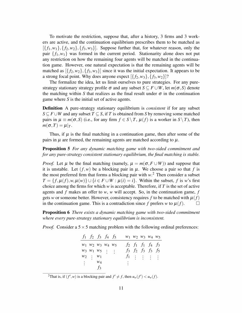
Proposition 7 For some dynamic matching game with one-sided commitment, thereexists a stationary equilibrium in which, at every period, the realized matchingis unstable and such that every stable matching is a Pareto improvement for theworkers.

Proof. Here is an example that proves the result. There are 3 firms and 3 workers,whose ordinal preferences are given by

f1 f2 f3 w1 w2 w3

w1 w3 w3 f3 f2 f1w3 w2 w1 f1 f3 f2w2 w1 w2 f2 f1 f3f1 f2 f3 w1 w2 w3

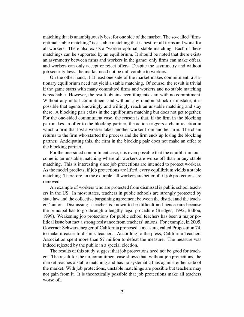
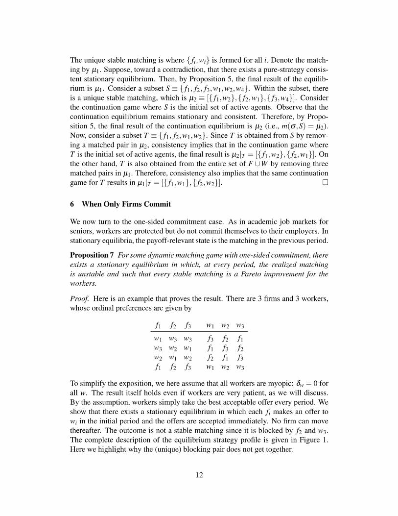
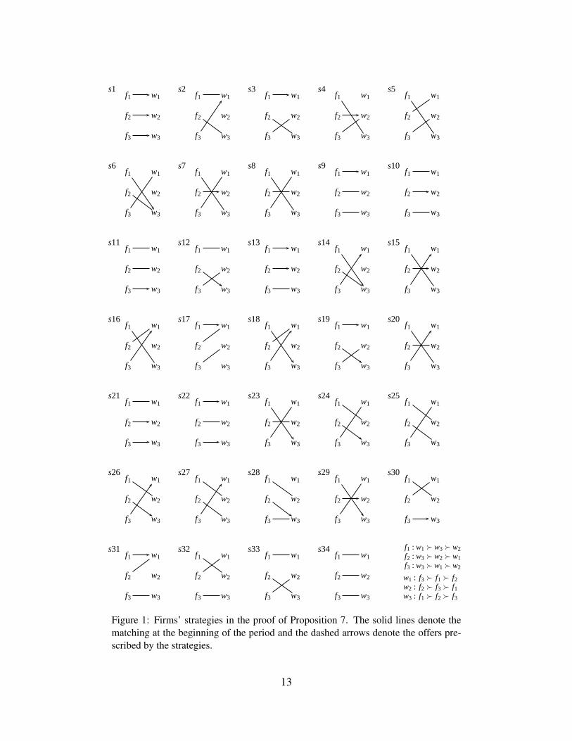
To simplify the exposition, we here assume that all workers are myopic: δw = 0 forall w. The result itself holds even if workers are very patient, as we will discuss.By the assumption, workers simply take the best acceptable offer every period. Weshow that there exists a stationary equilibrium in which each fi makes an offer towi in the initial period and the offers are accepted immediately. No firm can movethereafter. The outcome is not a stable matching since it is blocked by f2 and w3.The complete description of the equilibrium strategy profile is given in Figure 1.Here we highlight why the (unique) blocking pair does not get together.

12

f1 w1

f2 w2

f3 w3

s1f1 w1

f2 w2

f3 w3

s2f1 w1

f2 w2

f3 w3

s3f1 w1

f2 w2

f3 w3

s4f1 w1

f2 w2

f3 w3

s5

f1 w1

f2 w2

f3 w3

s6f1 w1

f2 w2

f3 w3

s7f1 w1

f2 w2

f3 w3

s8f1 w1

f2 w2

f3 w3

s9f1 w1

f2 w2

f3 w3

s10

f1 w1

f2 w2

f3 w3

s11f1 w1

f2 w2

f3 w3

s12f1 w1

f2 w2

f3 w3

s13f1 w1

f2 w2

f3 w3

s14f1 w1

f2 w2

f3 w3

s15

f1 w1

f2 w2

f3 w3

s16f1 w1

f2 w2

f3 w3

s17f1 w1

f2 w2

f3 w3

s18f1 w1

f2 w2

f3 w3

s19f1 w1

f2 w2

f3 w3

s20

f1 w1

f2 w2

f3 w3

s21f1 w1

f2 w2

f3 w3

s22f1 w1

f2 w2

f3 w3

s23f1 w1

f2 w2

f3 w3

s24f1 w1

f2 w2

f3 w3

s25

f1 w1

f2 w2

f3 w3

s26f1 w1

f2 w2

f3 w3

s27f1 w1

f2 w2

f3 w3

s28f1 w1

f2 w2

f3 w3

s29f1 w1

f2 w2

f3 w3

s30

f1 w1

f2 w2

f3 w3

s31f1 w1

f2 w2

f3 w3

s32f1 w1

f2 w2

f3 w3

s33f1 w1

f2 w2

f3 w3

s34 f1 : w1 � w3 � w2f2 : w3 � w2 � w1f3 : w3 � w1 � w2

w1 : f3 � f1 � f2w2 : f2 � f3 � f1w3 : f1 � f2 � f3

Figure 1: Firms’ strategies in the proof of Proposition 7. The solid lines denote thematching at the beginning of the period and the dashed arrows denote the offers pre-scribed by the strategies.

13

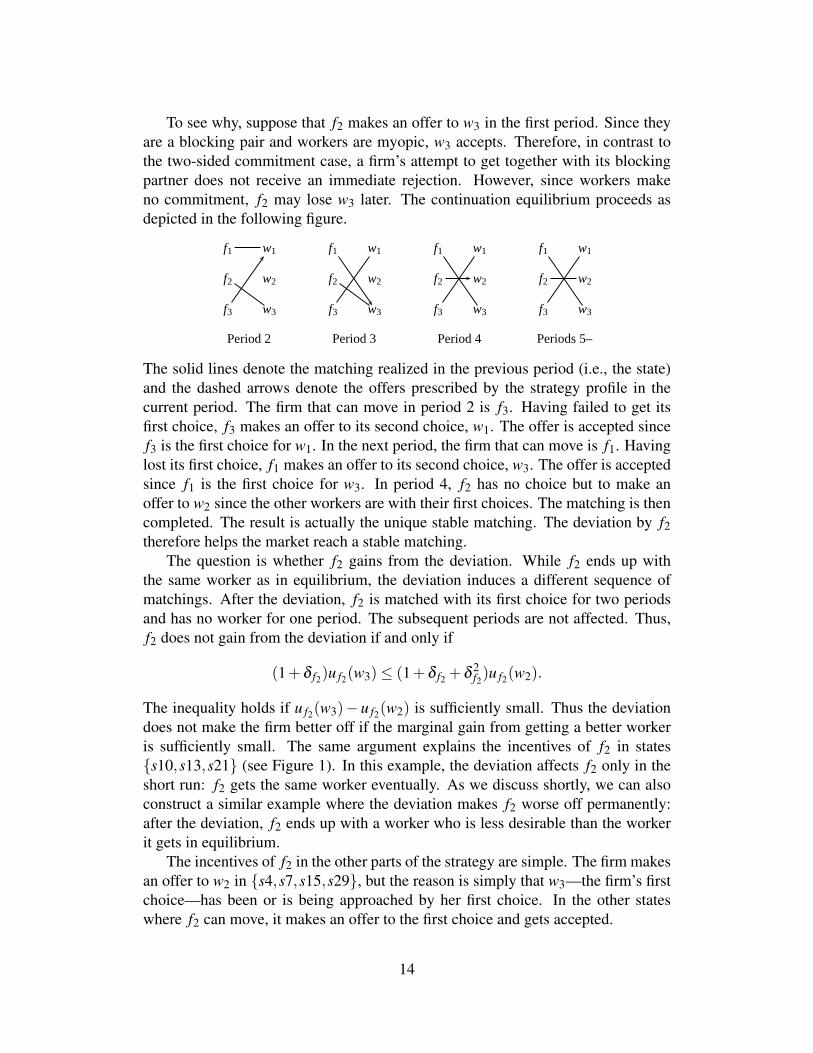
To see why, suppose that f2 makes an offer to w3 in the first period. Since theyare a blocking pair and workers are myopic, w3 accepts. Therefore, in contrast tothe two-sided commitment case, a firm’s attempt to get together with its blockingpartner does not receive an immediate rejection. However, since workers makeno commitment, f2 may lose w3 later. The continuation equilibrium proceeds asdepicted in the following figure.

f1 w1

f2 w2

f3 w3

Period 2

f1 w1

f2 w2

f3 w3

Period 3

f1 w1

f2 w2

f3 w3

Period 4

f1 w1

f2 w2

f3 w3

Periods 5–

The solid lines denote the matching realized in the previous period (i.e., the state)and the dashed arrows denote the offers prescribed by the strategy profile in thecurrent period. The firm that can move in period 2 is f3. Having failed to get itsfirst choice, f3 makes an offer to its second choice, w1. The offer is accepted sincef3 is the first choice for w1. In the next period, the firm that can move is f1. Havinglost its first choice, f1 makes an offer to its second choice, w3. The offer is acceptedsince f1 is the first choice for w3. In period 4, f2 has no choice but to make anoffer to w2 since the other workers are with their first choices. The matching is thencompleted. The result is actually the unique stable matching. The deviation by f2therefore helps the market reach a stable matching.

The question is whether f2 gains from the deviation. While f2 ends up withthe same worker as in equilibrium, the deviation induces a different sequence ofmatchings. After the deviation, f2 is matched with its first choice for two periodsand has no worker for one period. The subsequent periods are not affected. Thus,f2 does not gain from the deviation if and only if

(1+δ f2)u f2(w3)≤ (1+δ f2 +δ 2f2)u f2(w2).

The inequality holds if u f2(w3)− u f2(w2) is sufficiently small. Thus the deviationdoes not make the firm better off if the marginal gain from getting a better workeris sufficiently small. The same argument explains the incentives of f2 in states{s10,s13,s21} (see Figure 1). In this example, the deviation affects f2 only in theshort run: f2 gets the same worker eventually. As we discuss shortly, we can alsoconstruct a similar example where the deviation makes f2 worse off permanently:after the deviation, f2 ends up with a worker who is less desirable than the workerit gets in equilibrium.

The incentives of f2 in the other parts of the strategy are simple. The firm makesan offer to w2 in {s4,s7,s15,s29}, but the reason is simply that w3—the firm’s firstchoice—has been or is being approached by her first choice. In the other stateswhere f2 can move, it makes an offer to the first choice and gets accepted.

14

The incentives of f1 and f3 are straightforward and no condition is necessaryfor their patience or payoff function. First, f1 can always secure its second choice(w3) since the firm is the first choice for the worker. In the equilibrium, f1 does notmake an offer to the first choice (w1) only when the worker has been or is beingapproached by the worker’s first choice (s6, s14, s18, s23, and s29). Similarly, f3can always secure its second choice (w1), but the firm is not liked by its first choice(w3). In the equilibrium, f3 does not make an offer to its first choice only when thefirst choice has been or is being approached by other firms (s2, s14–s16, s18, s20,s26, and s27). ¤

Intuitively, the unstable matching is sustained as equilibrium outcome since anyattempt by f2 to get the blocking partner succeeds only temporarily and backfires inthe long run. The temporal success for f2 in getting w3 intensifies the competitionamong the firms. At the end, f2 loses w3 to f1. If the loss from having no worker islarge relative to the marginal gain from the better worker, the net effect of initiatinga recruiting war is negative.

A comparison between the equilibrium and the unique stable matching (s8) re-veals that none of the workers prefers the equilibrium outcome. While w2 is in-different, the other workers prefer the stable matching. This is interesting sinceworkers are the ones who are protected by tenure. Without job protections, the sta-ble matching is the unique equilibrium outcome. In this example, the workers arebetter off if job protections are removed.

The conclusion of Proposition 7 does not change if workers and firms are verypatient. In the Appendix, we construct an example showing that the propositionholds when δi → 1 for all i ∈ F ∪W . However, the construction is considerablymore involved since we need to specify each worker’s action contingent on everypossible set of offers. Even with the small number of agents, constructing an equi-librium strategy profile is not easy since there are 34 states. The example is thereforerelegated to Appendix A.4. In the example, if a firm deviates by making an offer tothe blocking partner, it gets the worker only temporarily and ends up with a workerwho is strictly less desirable than the permanent employee in the equilibrium.

If workers are myopic, we can also show that every stable matching can besupported as a permanent equilibrium outcome. Whether the result extends to non-myopic workers is open at this point.

Proposition 8 Consider any dynamic matching game with one-sided commitmentwhere workers are myopic (δw = 0 for all w). Then for any stable matching, thereexists a stationary equilibrium that yields this matching every period.

7 Conclusion

We considered a dynamic matching game in which firms and workers interact re-peatedly in a decentralized job market. The main question was whether a decentral-

15

ized matching market generates a stable matching of Gale and Shapley (1962) andhow the answer varies with the commitment structure of the market. Without com-mitment, we show that every stationary equilibrium matching is stable and everystable matching can be sustained by a stationary equilibrium. Once commitmentis possible, this equivalence breaks down. It is possible for an equilibrium match-ing to be unstable. When only firms commit (i.e., there is job security), it is evenpossible that an equilibrium matching makes every worker worse off than any sta-ble matching, illustrating the adverse effect job protection may have on workers’welfare.

To simply our analysis, our dynamic matching game builds on the classical one-to-one matching model without monetary transfers (i.e., salary negotiations). Ex-tending a many-to-one matching model with monetary transfers such as the one inCrawford and Knoer (1981) and Kelso and Crawford (1982) would certainly bringus closer to modeling real labor market dynamics. Recently, salary competitionin matching model has been brought into focus by, for example, Bulow and Levin(2006) and Crawford (2006, forthcoming). It would be also interesting to make thecommitment structure endogenous.

16

Acknowledgments

We are grateful to Vincent Crawford, Tatsuhiro Shichijo, Fernando Vega-Redondo,and participants of SAET 2005 and the seminar at Osaka Prefecture University forhelpful comments. We also thank SSHRC and FQRSC for financial support.

A Appendix: Proofs

A.1 Proof of Proposition 1

To prove the first statement, consider any stationary equilibrium. First, suppose,by way of contradiction, that the equilibrium yields an unstable matching µ t insome period t. Let { f ,w} be a blocking pair for µ t . Since the firms’ strategiesare stationary, w’s action in period t does not affect the offers she will receive in thesubsequent periods. This implies that, in period t, worker w’s best action is to acceptthe most preferred acceptable offer. Since w prefers f to µ t(w), it follows that wdoes not receive an offer from f in this period. Suppose then that, in period t, firm fdeviates from the equilibrium and makes an offer to w. By the observation above,w will accept the offer and this has no influence over the other agents’ strategy inthe continuation game. Therefore, f gains from the deviation, a contradiction.

The above paragraph shows that the realized matching is stable in every period.Since firms’ strategies are stationary, the realized matching is the same in everyperiod.

To prove the converse, choose any stable matching µ and consider the followingstrategy profile: in every period, each firm f makes an offer to µ( f ) and eachworker w accepts the most preferred acceptable offer. The workers’ strategies areoptimal given that the firms’ strategies are stationary. The firms’ strategies are alsooptimal since making an offer to a preferred worker will be rejected since µ isstable, and making an offer to a less preferred worker will have no influence overthe subsequent periods.

A.2 Proof of Proposition 2

For any subset S ⊆ F ∪W , let µS be any stable matching among S. Let σ be thestrategy profile defined as follows. Consider any period and let S be the set of activeagents. Each active firm f makes an offer to µS( f ). Each active worker w whoreceived an offer from µS(w) (and possibly others) accepts the most preferred offer.For each active worker w who did not receive an offer from µS(w), let T be definedby

T ≡ {w,µS(w)}∪Ow∪{i ∈ S : µS(i) ∈ Ow∪{i}}. (1)

Then w accepts the most preferred offer if

maxi∈Ow

uw(i) > δwuw(µT (w)). (2)

17

Otherwise, w rejects all offers.Let β be the belief system derived from the strategy profile above, with the

following additional rule: at any period, if the set of active agents is S and an activeworker w did not receive an offer from µS(w), then w believes that µS(w) did notmake an offer to any worker.

We claim that (σ ,β ) is a sequential equilibrium. To see this, take any periodand let S be the set of active agents.

We first examine firms’ incentives. Let f be an active firm. If the firm followsthe equilibrium strategy, it will be matched with w ≡ µS( f ) in the current period(where w = f is a possibility). If f makes an offer to any worker w′ that f prefers tow, then since µS is a stable matching, the offer will be rejected. In the next period,therefore, the set of active agents will be { f ,w}∪{i ∈ S : µS(i) = i} and the bestoutcome for f is to get w. Since f gets w earlier in equilibrium, the firm does notgain from the deviation. Similarly, the firm does not gain by not making any offer.

Now, consider workers’ incentives. Let w be an active worker. There are twocases. First, suppose that w receives an offer from µS(w), i.e., µS(w) ∈ Ow. In thisevent, if w rejects all offers, the set of active firms in the next period will be

Ow∪{ f ∈ F : µS( f ) = f}.

Since µS is stable, w prefers µS(w) to any f such that µS( f ) = f and for which wis acceptable. Therefore, if µS(w) ∈ Ow, worker w gains nothing by waiting.

Suppose µS(w) /∈ Ow. By the definition of β , worker w believes that µS(w) didnot make an offer to any worker. According to the belief, if w rejects all offers,the set of active agents in the next period will be T in (1) and hence the expected(average) utility is the right-hand side of (2). On the other hand, the maximumutility from accepting an offer in the current period is given by the left-hand side.

A.3 Proof of Propositions 3 and 4

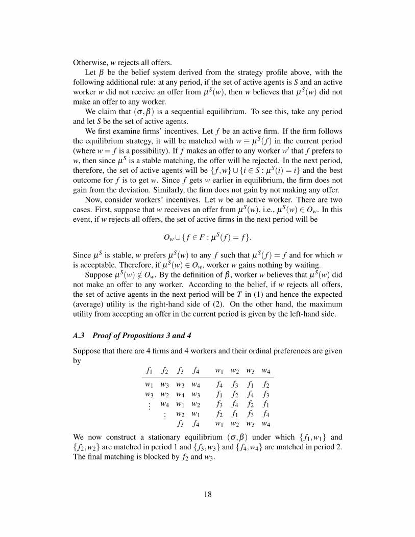
Suppose that there are 4 firms and 4 workers and their ordinal preferences are givenby

f1 f2 f3 f4 w1 w2 w3 w4

w1 w3 w3 w4 f4 f3 f1 f2w3 w2 w4 w3 f1 f2 f4 f3... w4 w1 w2 f3 f4 f2 f1

... w2 w1 f2 f1 f3 f4f3 f4 w1 w2 w3 w4

We now construct a stationary equilibrium (σ ,β ) under which { f1,w1} and{ f2,w2} are matched in period 1 and { f3,w3} and { f4,w4} are matched in period 2.The final matching is blocked by f2 and w3.

18

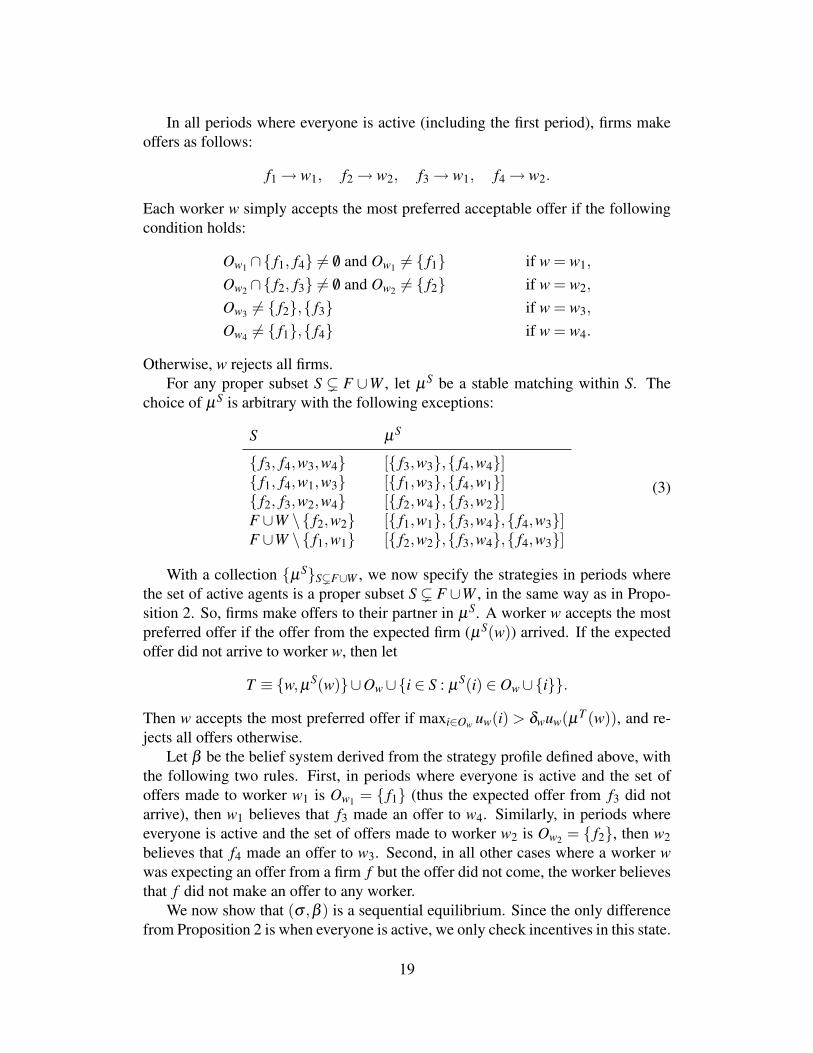
In all periods where everyone is active (including the first period), firms makeoffers as follows:

f1 → w1, f2 → w2, f3 → w1, f4 → w2.

Each worker w simply accepts the most preferred acceptable offer if the followingcondition holds:

Ow1 ∩{ f1, f4} 6= /0 and Ow1 6= { f1} if w = w1,

Ow2 ∩{ f2, f3} 6= /0 and Ow2 6= { f2} if w = w2,

Ow3 6= { f2},{ f3} if w = w3,

Ow4 6= { f1},{ f4} if w = w4.

Otherwise, w rejects all firms.For any proper subset S ( F ∪W , let µS be a stable matching within S. The

choice of µS is arbitrary with the following exceptions:

S µS

{ f3, f4,w3,w4} [{ f3,w3},{ f4,w4}]{ f1, f4,w1,w3} [{ f1,w3},{ f4,w1}]{ f2, f3,w2,w4} [{ f2,w4},{ f3,w2}]F ∪W \{ f2,w2} [{ f1,w1},{ f3,w4},{ f4,w3}]F ∪W \{ f1,w1} [{ f2,w2},{ f3,w4},{ f4,w3}]

(3)

With a collection {µS}S(F∪W , we now specify the strategies in periods wherethe set of active agents is a proper subset S ( F ∪W , in the same way as in Propo-sition 2. So, firms make offers to their partner in µS. A worker w accepts the mostpreferred offer if the offer from the expected firm (µS(w)) arrived. If the expectedoffer did not arrive to worker w, then let

T ≡ {w,µS(w)}∪Ow∪{i ∈ S : µS(i) ∈ Ow∪{i}}.Then w accepts the most preferred offer if maxi∈Ow uw(i) > δwuw(µT (w)), and re-jects all offers otherwise.

Let β be the belief system derived from the strategy profile defined above, withthe following two rules. First, in periods where everyone is active and the set ofoffers made to worker w1 is Ow1 = { f1} (thus the expected offer from f3 did notarrive), then w1 believes that f3 made an offer to w4. Similarly, in periods whereeveryone is active and the set of offers made to worker w2 is Ow2 = { f2}, then w2believes that f4 made an offer to w3. Second, in all other cases where a worker wwas expecting an offer from a firm f but the offer did not come, the worker believesthat f did not make an offer to any worker.

We now show that (σ ,β ) is a sequential equilibrium. Since the only differencefrom Proposition 2 is when everyone is active, we only check incentives in this state.

19

Firm f1 has no incentive to deviate since it gets its first choice in equilibrium.Firm f2 gets only its second choice (w2) but does not gain by deviating. Indeed, iff2 makes an offer to w3 or w1, the offer will be rejected and the firm will be matchedwith w2 in the next period.3 Similarly, by not making any offer, f2 only delays itsmatching with w2. Finally, if f2 makes an offer to w4, the offer will be accepted,which is not good for f2 since it prefers w2.

Firm f3, on the other hand, gets his first choice (w3) only in the next period. Ifthe firm is patient enough (i.e., δ f3 > u f3(w4)/u f3(w3)), therefore, the only possiblereason to deviate is to get the first choice in the current period. However, if f3 makesan offer to w3, then Ow3 = { f3} and hence the offer will be rejected. A symmetricargument applies to f4.

For workers’ incentives, we start with w1 and w2. Since they are symmetric, weneed only to consider w1. If she received an offer from f4, her optimal action is toaccept the offer since f4 is her top choice. So, in what follows, suppose that w1 didnot receive an offer from f4. We divide the remaining case into two.

Suppose Ow1 6= { f1}. Then it can be checked that w1 believes that if she rejectsall offers, she will get the second choice ( f1) in the next period.4 So, the optimalchoice for w1 depends on whether f1 ∈ Ow1 . If f1 ∈ Ow1 , then w1 should accept f1in the current period since it is the best offer at hand and rejecting all offers willonly delay the matching with the same firm. If f1 /∈ Ow1 , on the other hand, theoptimal reply depends on the firm’s patience. If the firm is sufficiently patient (i.e.,δ f1 > uw1( f3)/uw1( f1)), the optimal reply is to reject all offers now and get f1 in thenext period.

Now, suppose Ow1 = { f1}. By the construction of β , w1 believes that f3 madean offer to w4 and the offer will be accepted. Thus, w1 believes that if she rejectsf1, the set of active agents in the next period will be { f1, f4,w1,w3} and hence shewill get f4, which is her first choice. If w1 is patient enough, therefore, she prefersto wait for the first choice.

Finally, consider w3 and w4. Since they are symmetric, we only discuss w3. Ifshe received an offer from her top choice ( f1), she obviously accepts it. So, supposethat she did not receive an offer from f1. If Ow3 = { f2} and w3 rejects the offer,the set of active agents in the next period will be F ∪W \ { f1,w1} and w3 will gether second choice ( f4). Since the offer at hand is her third choice, if w3 is patientenough, she prefers to wait for her second choice. Similarly, if Ow3 = { f3} (whichis the fourth choice for w3) and w3 rejects the offer, the set of active agents in thenext period will be F ∪W \{ f2,w2} and so w3 will get her second choice ( f4).5 Soif w3 is patient enough, she prefers to wait. If f4 ∈ Ow3 , it can be checked that ifw3 rejects all offers, she will get either f4 in the next period or f3 in the following

3The set of active players in the next period will be F ∪W \{ f1,w1}.4For example, suppose Ow1 = { f1, f2}. Then w1 believes that f3 did not make any offer and f4

made an offer to w2. According to w2’s strategy, w2 will reject the offer from f4. So if w1 rejects alloffers, she believes that, in the next period, everyone will be active and she will get f1.

5Note that w1 will reject f1.

20

period. Since she prefers f4 to f3, she prefers to accept f4 in the current period.Similarly, if Ow3 = { f2, f3}, rejecting all offers will give her f3 in two periods, soshe should accept f3 in the current period.

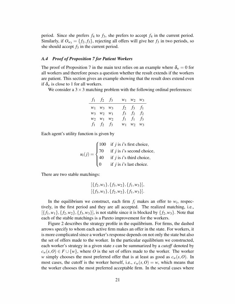
A.4 Proof of Proposition 7 for Patient Workers

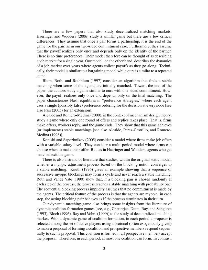
The proof of Proposition 7 in the main text relies on an example where δw = 0 forall workers and therefore poses a question whether the result extends if the workersare patient. This section gives an example showing that the result does extend evenif δw is close to 1 for all workers.

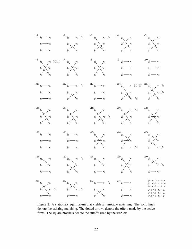
We consider a 3×3 matching problem with the following ordinal preferences:

f1 f2 f3 w1 w2 w3

w1 w3 w3 f2 f3 f1w3 w2 w1 f3 f2 f2w2 w1 w2 f1 f1 f3f1 f2 f3 w1 w2 w3

Each agent’s utility function is given by

ui( j) =

100 if j is i’s first choice,70 if j is i’s second choice,40 if j is i’s third choice,0 if j is i’s last choice.

There are two stable matchings:

[{ f2,w1},{ f3,w2},{ f1,w3}],[{ f3,w1},{ f2,w2},{ f1,w3}].

In the equilibrium we construct, each firm fi makes an offer to wi, respec-tively, in the first period and they are all accepted. The realized matching, i.e.,[{ f1,w1},{ f2,w2},{ f3,w3}], is not stable since it is blocked by { f2,w3}. Note thateach of the stable matchings is a Pareto improvement for the workers.

Figure 2 describes the strategy profile in the equilibrium. For firms, the dashedarrows specify to whom each active firm makes an offer in the state. For workers, itis more complicated since a worker’s response depends on not only the state but alsothe set of offers made to the worker. In the particular equilibrium we constructed,each worker’s strategy in a given state s can be summarized by a cutoff denoted bycw(s,O) ∈ F ∪{w}, where O is the set of offers made to the worker. The workerw simply chooses the most preferred offer that is at least as good as cw(s,O). Inmost cases, the cutoff is the worker herself, i.e., cw(s,O) = w, which means thatthe worker chooses the most preferred acceptable firm. In the several cases where

21

f1 w1

f2 w2

f3 w3

s1f1 w1

f2 w2

f3 w3

[ f3]s2

f1 w1

f2 w2

f3 w3

[ f3]s3

f1 w1

f2 w2

f3 w3

s4f1 w1

f2 w2

f3 w3

s5

f1 w1

f2 w2

f3 w3

[ f3] if |O|≥2[ f2] if |O|=1

s6f1 w1

f2 w2

f3 w3

s7f1 w1

f2 w2

f3 w3

s8f1 w1

f2 w2

f3 w3

s9f1 w1

f2 w2

f3 w3

s10

f1 w1

f2 w2

f3 w3

s11f1 w1

f2 w2

f3 w3

[ f2]s12

f1 w1

f2 w2

f3 w3

s13f1 w1

f2 w2

f3 w3

[ f3] if |O|≥2[ f2] if |O|=1

[ f2]

s14f1 w1

f2 w2

f3 w3

[ f2]

[ f3]

s15

f1 w1

f2 w2

f3 w3

s16f1 w1

f2 w2

f3 w3

s17f1 w1

f2 w2

f3 w3

[ f3]

s18f1 w1

f2 w2

f3 w3

[ f2]s19

f1 w1

f2 w2

f3 w3

s20

f1 w1

f2 w2

f3 w3

s21f1 w1

f2 w2

f3 w3

s22f1 w1

f2 w2

f3 w3

s23f1 w1

f2 w2

f3 w3 [ f1]

s24f1 w1

f2 w2

f3 w3 [ f1]

s25

f1 w1

f2 w2

f3 w3

s26f1 w1

f2 w2

f3 w3

[ f2]s27

f1 w1

f2 w2

f3 w3

s28f1 w1

f2 w2

f3 w3

s29f1 w1

f2 w2

f3 w3

[ f3]

s30

f1 w1

f2 w2

f3 w3

[ f2]

s31f1 w1

f2 w2

f3 w3

[ f2]

s32f1 w1

f2 w2

f3 w3

[ f3]s33

f1 w1

f2 w2

f3 w3

s34 f1 : w1 � w3 � w2f2 : w3 � w2 � w1f3 : w3 � w1 � w2

w1 : f2 � f3 � f1w2 : f3 � f2 � f1w3 : f1 � f2 � f3

Figure 2: A stationary equilibrium that yields an unstable matching. The solid linesdenote the existing matching. The dotted arrows denote the offers made by the activefirms. The square brackets denote the cutoffs used by the workers.

22

cw(s,O) 6= w, the cutoffs are specified in Figure 2 in square brackets attached to theworker (e.g., [ f2]). Nothing is attached if the cutoff is oneself.

If the worker is currently employed, her current job is included in the offer set.Therefore, if the current job is less preferred to the cutoff, the worker resigns fromthe current job. For example, w3 in s25 resigns from f2 since f2 is less preferred tof1.

Except for worker 1 in states 6 and 14, the cutoffs are independent of the setof offers. In states 6 and 14, worker 1’s cutoff depends on the number of offers(including the renewal offer).

To complete the description of the equilibrium, we need to specify workers’ out-of-equilibrium beliefs since offers are private information. If a firm is prescribed tomake an offer to a worker but deviates, the worker observes only the fact that thefirm makes no offer to her. She does not observe where the firm makes an offer. Inthe particular equilibrium we construct, the worker in this situation is assumed tobelieve that the firm does not make any offer to any worker. The particular beliefwas chosen to simplify our construction of an equilibrium.

The strategy profile together with the belief system is a sequential equilibriumif the agents are sufficiently patient. A sufficient condition is that δi ≥ 3

√0.7≈ 0.89

for all agents. Verifying sequential rationality is extremely tedious. We thereforeprovide a computer program (a MATLAB code) that verifies sequential rational-ity when δi = 0.9 for all i. The program is available from our personal web sites(e.g., http://www.columbia.edu/∼em437/). Below we informally discuss why theblocking pair does not form.

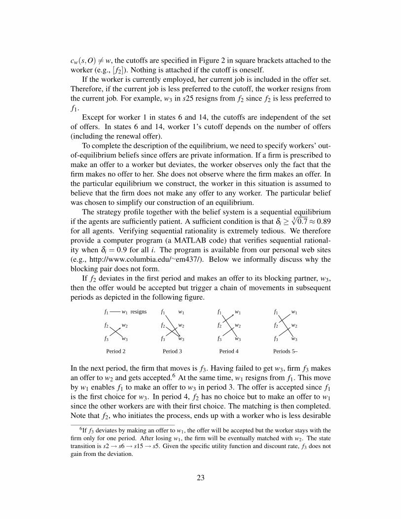
If f2 deviates in the first period and makes an offer to its blocking partner, w3,then the offer would be accepted but trigger a chain of movements in subsequentperiods as depicted in the following figure.

f1 w1

f2 w2

f3 w3

resigns

Period 2

f1 w1

f2 w2

f3 w3

Period 3

f1 w1

f2 w2

f3 w3

Period 4

f1 w1

f2 w2

f3 w3

Periods 5–

In the next period, the firm that moves is f3. Having failed to get w3, firm f3 makesan offer to w2 and gets accepted.6 At the same time, w1 resigns from f1. This moveby w1 enables f1 to make an offer to w3 in period 3. The offer is accepted since f1is the first choice for w3. In period 4, f2 has no choice but to make an offer to w1since the other workers are with their first choice. The matching is then completed.Note that f2, who initiates the process, ends up with a worker who is less desirable

6If f3 deviates by making an offer to w1, the offer will be accepted but the worker stays with thefirm only for one period. After losing w1, the firm will be eventually matched with w2. The statetransition is s2→ s6→ s15→ s5. Given the specific utility function and discount rate, f3 does notgain from the deviation.

23

than the one the firm gets in equilibrium. Therefore, if f2 is sufficiently patient, thedeviation makes the firm worse off.

A.5 Proof of Proposition 8

As before, since workers are myopic and make no commitment, they simply acceptthe best acceptable offer every period. Since the state space and the action setsare finite, there exists a stationary equilibrium σ .7 But the equilibrium outcomeis unknown. Let µ be any stable matching. To support µ , we construct anotherstrategy profile σ ′ as follows. If all agents are active, each firm f makes an offerto µ( f ). If not all agents are active, follow σ . Thus, σ ′ differs from σ only whenall agents are active. We shall show that σ ′ is a stationary equilibrium. By theconstruction of σ ′, it suffices to consider the state in which everyone is active. So,suppose that in period τ , everyone is active and a firm f deviates from σ . Since theoutcome induced by the deviation may be stochastic, consider any path of play thatoccurs with a positive probability after the deviation. Let {wt}∞

t=τ be the sequenceof workers that f is matched with along the path (where wt ∈W ∪{ f}). For anyt ≥ τ , if wt /∈ {µ( f ), f}, then wt prefers f to µ(wt) since wt receives an offer fromµ(wt) in period τ and a worker’s period-payoff is non-decreasing over time. Sinceµ is a stable matching, it follows that f prefers µ( f ) to wt . That is, along the path,f is never matched with a worker better than µ( f ). Since this is the case for anypossible path, f does not benefit from the deviation.

7See, e.g., Mertens (2002).

24

References

Alcalde, J., D. Perez-Castrillo, and A. Romero-Medina (1998): “Hiring Proceduresto Implement Stable Allocations,” Journal of Economic Theory, 82, 469–480.

Alcalde, J., and A. Romero-Medina (2000): “Simple Mechanisms to Implementthe Core of College Admissions Problems,” Games and Economic Behavior, 31,294–302.

Ballou, D. (1999): “The New York City Teachers’ Union Contract: Shackling Prin-cipals’ Leadership,” Civic Report 6, Center for Civic Innovation at the ManhattanInstitution.

Bloch, F. (1996): “Sequential Formation of Coalitions in Games with Externalitiesand Fixed Payoff Division,” Games and Economic Behavior, 14, 90–123.

Blum, Y., A. E. Roth, and U. G. Rothblum (1997): “Vacancy chains and equilibra-tion in senior-level labor markets,” Journal of Economic Theory, 76, 362–411.

Bridges, E. M. (1992): The Incompetent Teacher: Managerial Responses. FalmerPress, Washington, D.C.

Bulow, J., and J. Levin (2006): “Matching and Price Competition,” American Eco-nomic Review, 96, 652–668.

Chatterjee, K., B. Dutta, D. Ray, and K. Sengupta (1993): “A Noncooperative The-ory of Coalitional Bargaining,” Review of Economic Studies, 60, 463–477.

Crawford, V. P. (2006, forthcoming): “The Flexible-Salary Match: A Proposal toIncrease the Salary Flexibility of the National Resident Matching Program,” Jour-nal of Economic Behavior and Organization.

Crawford, V. P., and E. M. Knoer (1981): “Job Matching with Heterogeneous Firmsand Workers,” Econometrica, 49, 437–450.

Gale, D., and L. Shapley (1962): “College admissions and the stability of marriage,”American Mathematical Monthly, 69, 9–15.

Haeringer, G., and M. Wooders (2006): “Decentralized Job Matching,” Discussionpaper, Universitat Autonoma de Barcelona.

Kelso, A. S., and V. P. Crawford (1982): “Job Matching, Coalition Formation, andGross Substitutes,” Econometrica, 50, 1483–1504.

Knuth, D. E. (1976): Mariages Stables et leurs relations avec d’autres problemescombinatoires. Les Presses de l’Universite de Montreal, Montreal.

25

Konishi, H., and M. Sapozhnikov (2005): “Decentralized Matching Markets withEndogeneous Salaries,” Discussion paper, Boston College.

Mertens, J.-F. (2002): “Stochastic games,” in Handbook of Game Theory with Eco-nomic Applications, ed. by R. Aumann, and S. Hart, vol. 3, chap. 47, pp. 1809–1832. North-Holland, Amsterdam.

Pais, J. (2005): “Incentives in Random Matching Markets,” Ph.D. thesis, UniversitatAutonoma de Barcelona.

Ray, D., and R. Vohra (1999): “A Theory of Endogenous Coalition Structures,”Games and Economic Behavior, 26, 286–336.

Roth, A. E. (1984): “The evolution of the labor market for medical interns andresidents: A case study in game theory,” Journal of Political Economy, 92, 991–1016.

(1991): “A natural experiment in the organization of entry-level labor mar-kets: Regional markets for new physicians and surgeons in the United Kingdom,”American Economic Review, 81, 415–440.

Roth, A. E., and M. A. O. Sotomayor (1990): Two-Sided Matching: A Study inGame-Theoretic Modelling and Analysis. Cambridge University Press.

Roth, A. E., and J. H. Vande Vate (1990): “Random paths to stability in two-sidedmatching,” Econometrica, 58, 1475–80.

26