[COASTAL GROUNDWATER INFILTRATION]CVEN2002/2702 Numerics Assignment Report

2014

University of NewSouth WalesDonald LeeZ3378780

IntroductionIn engineering modelling, it is important to assess and evaluate thegroundwater system and their vulnerability to contamination withinan estuary or even in larger scale, the ocean. Since high seepageflows within a boundary my cause backward erosion and piping, whichin turn can lead to embankment dam failures. Thus it is important toapply numerical methods throughout practical engineering systems toassess and calculate these flows and determine the volume flux andmaximum velocities associated within the boundary.

In this assignment, we are required to create a program to predictthe head value and flow velocity throughout the foundation below theembankment dam, an aquitard is located somewhere within thisboundary and has no significant foundation capacity issues for theembankment. However, due to the differences in hydraulicconductivity of the materials, it has the potential to changeseepage flowswithin thefoundation.Boundary conditionsare given and the head values are governed by the Laplace equation.

Problem(214)

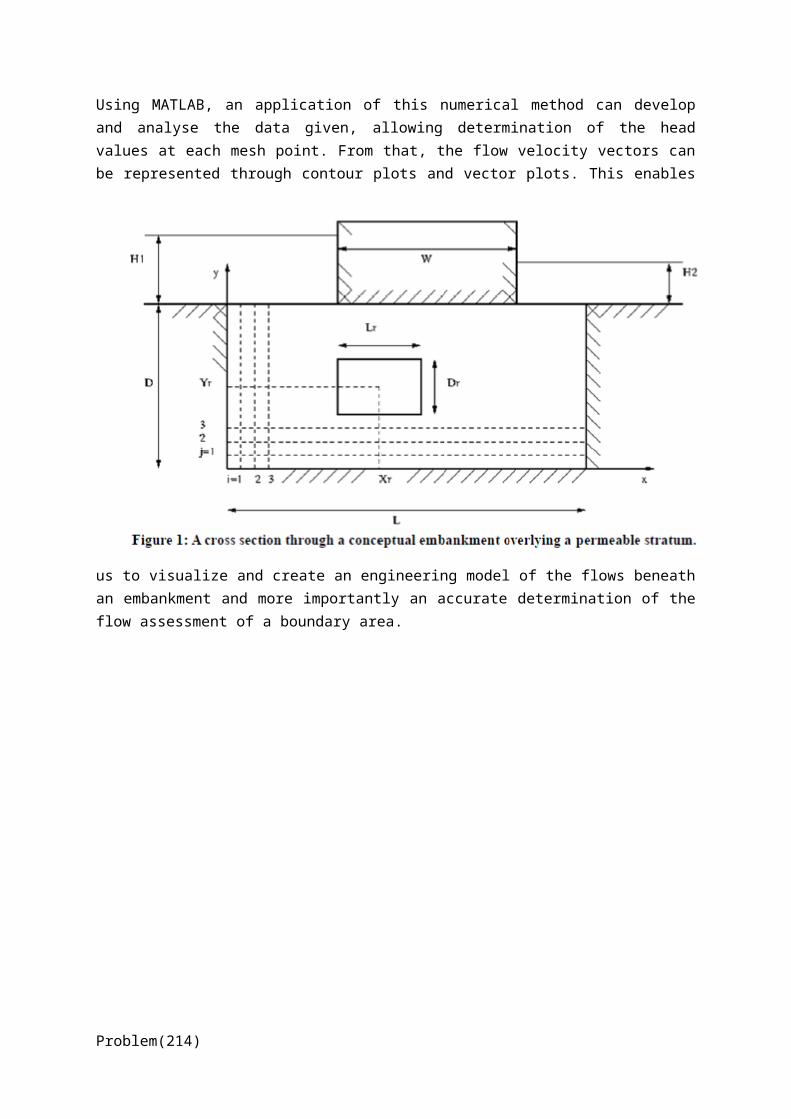
Using MATLAB, an application of this numerical method can developand analyse the data given, allowing determination of the headvalues at each mesh point. From that, the flow velocity vectors canbe represented through contour plots and vector plots. This enables

us to visualize and create an engineering model of the flows beneathan embankment and more importantly an accurate determination of theflow assessment of a boundary area.

Problem(214)

Numerical Method

DiscretisationBefore a numerical evaluation of the embankment model can becreated, discretisation of the continuous models and equations intodiscrete counterparts must be done. Whenever continuous data isdiscretized, there is always some amount of discretisation error.The goal is to reduce the amount to a level considered negligiblefor the modeling purposes at hand.

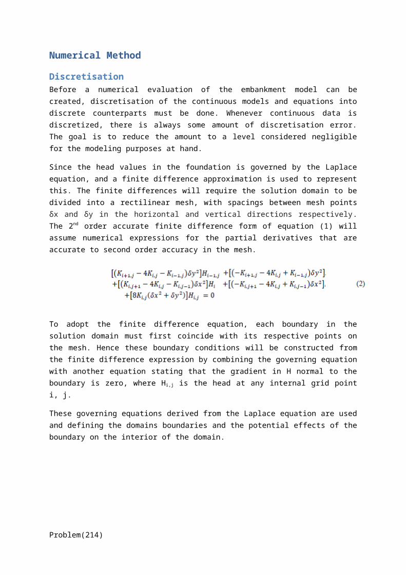
Since the head values in the foundation is governed by the Laplaceequation, and a finite difference approximation is used to representthis. The finite differences will require the solution domain to bedivided into a rectilinear mesh, with spacings between mesh pointsδx and δy in the horizontal and vertical directions respectively.The 2nd order accurate finite difference form of equation (1) willassume numerical expressions for the partial derivatives that areaccurate to second order accuracy in the mesh.

To adopt the finite difference equation, each boundary in thesolution domain must first coincide with its respective points onthe mesh. Hence these boundary conditions will be constructed fromthe finite difference expression by combining the governing equationwith another equation stating that the gradient in H normal to theboundary is zero, where Hi,j is the head at any internal grid pointi, j.

These governing equations derived from the Laplace equation are usedand defining the domains boundaries and the potential effects of theboundary on the interior of the domain.

Problem(214)

Boundary ConditionsTo solve this numerical model, the mesh must be constructed so thatall boundary points coincide with the boundary of the mesh. Separateequations are used to specify different points of the boundary.Hence,a large

matrix,” matrix A”, is used to define the domain of the embankment.These expressions are listed below:

The four expressions listed above represents the left, right, upper(that is, beneath the embankment) and lower boundaries. There aretwospecialboundarycondition points for the matrix:

Equations (8) and (9), represents the bottom left grid point and thebottom right grid point. All these equations listed defines theboundary area, which are almost the same with the representation ofthe governing equations.

Problem(214)

From field investigations, the presence of an aquitard was foundwithin the foundation. The aquitard has no significant foundationcapacity issues for the embankment, but it has the potential tochange the seepage flows through the foundation due to its reducedhydraulic conductivity. Hence defining the difference in thehydraulic conductivity “Kr” of the aquitard within the embankmentarea is required.

To do this, we are given information that the aquitard isapproximately rectangular with its centre located at (Xr, Yr),(55,10) and dimensions (Lr, Dr), (10,5) with a characteristichydraulic conductivity of 0.0025.

Numerical RepresentationSince Matrix A is the coefficient matrix for finding the Head valuesof each mesh point on the foundation cross-section:

For creating matrix A, the boundary conditions are needed. H, ourunknown column vector of the head values at each grid point, can becalculated by creating a column vector, b, containing constantvalues from each grid point. This is done by using MATLAB to formthe two loops and using “if” and “elseif” statements, where thefinite difference expressions are tested until it satisfies theconditions. This would be almost impossible to do by hand for such alarge domain, as each point is affected by adjacent nodes; henceiterations are done until the governing equations are satisfied.

Solution MethodAfter the head values are computed, we can determine the flow velocity components using a finite difference representation again:

After the values of the velocities are obtained in the horizontal

and vertical direction, velocity at each point can be calculated

using, v = (u2+w2)1/2, and a maximum velocity can be determined.

Problem(214)

Once we know the horizontal and vertical flow velocities at

each mesh point, we can determine the maximum mesh velocity

and the total volume flux

per unit length along the crest of the embankment q as:

However since the defined surface can be located beneath the centre of the embankment, q is reduced to:

Results and Discussion

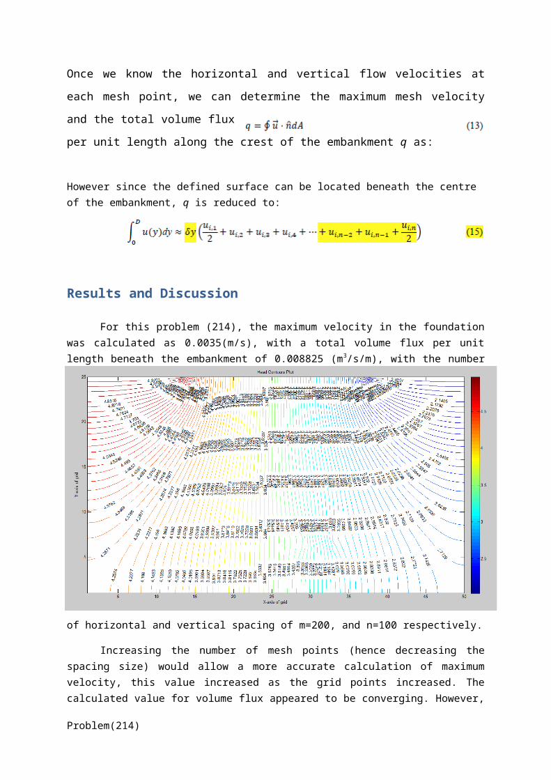
For this problem (214), the maximum velocity in the foundationwas calculated as 0.0035(m/s), with a total volume flux per unitlength beneath the embankment of 0.008825 (m3/s/m), with the number

of horizontal and vertical spacing of m=200, and n=100 respectively.

Increasing the number of mesh points (hence decreasing thespacing size) would allow a more accurate calculation of maximumvelocity, this value increased as the grid points increased. Thecalculated value for volume flux appeared to be converging. However,

Problem(214)

for a more accurate solution, it would also require the program tomake more iteration, in turn require more run time. Therefore, themaximum resolution achievable was tested considering the givenresources.

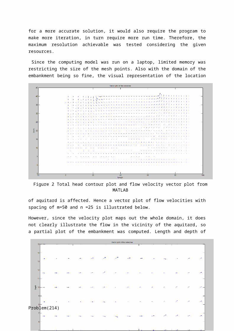
Since the computing model was run on a laptop, limited memory wasrestricting the size of the mesh points. Also with the domain of theembankment being so fine, the visual representation of the location

of aquitard is affected. Hence a vector plot of flow velocities withspacing of m=50 and n =25 is illustrated below.

However, since the velocity plot maps out the whole domain, it doesnot clearly illustrate the flow in the vicinity of the aquitard, soa partial plot of the embankment was computed. Length and depth of

Problem(214)

Figure 2 Total head contour plot and flow velocity vector plot from MATLAB

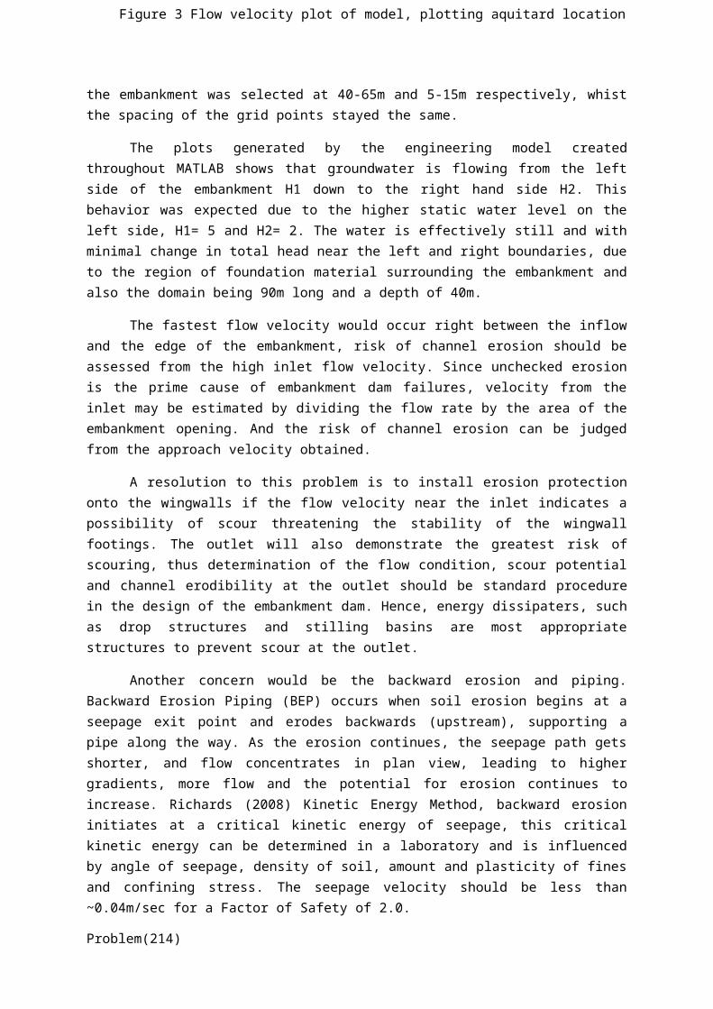
Figure 3 Flow velocity plot of model, plotting aquitard location

the embankment was selected at 40-65m and 5-15m respectively, whistthe spacing of the grid points stayed the same.

The plots generated by the engineering model createdthroughout MATLAB shows that groundwater is flowing from the leftside of the embankment H1 down to the right hand side H2. Thisbehavior was expected due to the higher static water level on theleft side, H1= 5 and H2= 2. The water is effectively still and withminimal change in total head near the left and right boundaries, dueto the region of foundation material surrounding the embankment andalso the domain being 90m long and a depth of 40m.

The fastest flow velocity would occur right between the inflowand the edge of the embankment, risk of channel erosion should beassessed from the high inlet flow velocity. Since unchecked erosionis the prime cause of embankment dam failures, velocity from theinlet may be estimated by dividing the flow rate by the area of theembankment opening. And the risk of channel erosion can be judgedfrom the approach velocity obtained.

A resolution to this problem is to install erosion protectiononto the wingwalls if the flow velocity near the inlet indicates apossibility of scour threatening the stability of the wingwallfootings. The outlet will also demonstrate the greatest risk ofscouring, thus determination of the flow condition, scour potentialand channel erodibility at the outlet should be standard procedurein the design of the embankment dam. Hence, energy dissipaters, suchas drop structures and stilling basins are most appropriatestructures to prevent scour at the outlet.

Another concern would be the backward erosion and piping.Backward Erosion Piping (BEP) occurs when soil erosion begins at aseepage exit point and erodes backwards (upstream), supporting apipe along the way. As the erosion continues, the seepage path getsshorter, and flow concentrates in plan view, leading to highergradients, more flow and the potential for erosion continues toincrease. Richards (2008) Kinetic Energy Method, backward erosioninitiates at a critical kinetic energy of seepage, this criticalkinetic energy can be determined in a laboratory and is influencedby angle of seepage, density of soil, amount and plasticity of finesand confining stress. The seepage velocity should be less than~0.04m/sec for a Factor of Safety of 2.0.

Problem(214)

Conclusions and RecommendationsOverall, the methods and calculations were all used correctly; thisis validated by using a base model with the resultant A matrix setup in comparison with our written model throughout MATLAB. From theuse of the base model, we were able to compare the derived boundaryconditions set up in the loops and verify that the conditions wereset-up correctly.

The errors incurred from the numerical representation were small andalso anticipated, since discretisation breaks the model down into aset of representative points, the accuracy was dependent on thepreciseness of the mesh points. This was restricted by our computerscapabilities, as the more grid points set up, the more accurate thecalculations, however it would also make the program run a fairwhile longer and also take up a lot more memory. This is because theprogram contains various loops, which loops over every point in themesh and needs to store various matrices like the coefficient matrixA which is (m*n)x(m*n) in size.

To allow a more representative engineering model of the embankment,if a more efficient code was written, the loop for thediscretisation process will allow bigger mesh points, as less memorywill be stored. Hence will achieve a higher maximum resolution

Through our physical model, it can be seen that higher flow velocityoccurs at inflow and outflow of the embankment. Due to that, thecentre of the embankment is prone to backward erosion. It isimportant to keep maintaining of the middle of the foundation, or aresolution would be to strengthen the area under the embankmentduring construction, or use of a more impervious material will allowless volume flux to be experienced by the embankment material, thisis crucial to our engineering modelling since erosion of thefoundation material could lead to failure of the embankment dam.

ReferencesA method for assessing the relative likelihood of failure of embankment dams by piping Foster, M., Fell, R., Spannagle, M. (2000) Canadian Geotech. J., 37(5),1025-1061. (accessed from UNSW library)

Internal Erosion- Potential Failure Modes.

Problem(214)

Kevin S. Richardsm Ph.D. Federal Energy Regulatory Commission, Februrary 22,2012 (accessed online)http://www.damsafety.org/media/Documents/FEMA/TS19_FiltersDrainsGeotex_EMI2012feb/Richards_InternalErosion.pdf

Problem(214)